RECENT COMMON ANCESTORS OF ALL PRESENT-DAY INDIVIDUALS Joseph T. Chang Department of Statistics, Yale University Abstract Previous study of the time to a common ancestor of all present-day indi- viduals has focused on models in which each individual has just one parent in the previous generation. For example, “mitochondrial Eve” is the most recent common ancestor (MRCA) when ancestry is defined only through maternal lines. In the standard Wright-Fisher model with population size n, the expected number of generations to the MRCA is about 2n, and the standard deviation of this time is also of order n. Here we study a two-parent analog of the Wright-Fisher model that defines ancestry using both parents. In this model, if the population size n is large, the number of generations, Tn, back to a MRCA has a distribution that is concen- trated around lg n (where lg denotes base-2 logarithm), in the sense that the ratio Tn/(lg n) converges in probability to 1 as n →∞. Also, con- tinuing to trace back further into the past, at about 1.77 lg n generations before the present, all partial ancestry of the current population ends, in the following sense: with high probability for large n, in each generation at least 1.77 lg n generations before the present, all individuals who have any descendants among the present-day individuals are actually ancestors of all present-day individuals. COALESCENT, WRIGHT-FISHER MODEL, GALTON-WATSON PROCESS, GENEALOGICAL MODELS, POPULATION GENETICS AMS 1991 SUBJECT CLASSIFICATION: PRIMARY 92D25 SECONDARY 60J85 Running head: Recent common ancestors Postal address: Yale University Statistics Department Box 208290 Yale Station New Haven, CT 06520–8290 Phone: 203-432-0642 Fax: 203-432-0633 Email: [email protected]Version: June 12, 1998
Transcript
RECENT COMMON ANCESTORS OF ALL
PRESENT-DAY INDIVIDUALS
Joseph T. Chang
Department of Statistics, Yale University
Abstract
Previous study of the time to a common ancestor of all present-day indi-viduals has focused on models in which each individual has just one parentin the previous generation. For example, “mitochondrial Eve” is the mostrecent common ancestor (MRCA) when ancestry is defined only throughmaternal lines. In the standard Wright-Fisher model with population sizen, the expected number of generations to the MRCA is about 2n, andthe standard deviation of this time is also of order n. Here we study atwo-parent analog of the Wright-Fisher model that defines ancestry usingboth parents. In this model, if the population size n is large, the numberof generations, Tn, back to a MRCA has a distribution that is concen-trated around lgn (where lg denotes base-2 logarithm), in the sense thatthe ratio Tn/(lgn) converges in probability to 1 as n → ∞. Also, con-tinuing to trace back further into the past, at about 1.77 lgn generationsbefore the present, all partial ancestry of the current population ends, inthe following sense: with high probability for large n, in each generationat least 1.77 lgn generations before the present, all individuals who haveany descendants among the present-day individuals are actually ancestorsof all present-day individuals.
COALESCENT, WRIGHT-FISHER MODEL, GALTON-WATSON PROCESS,GENEALOGICAL MODELS, POPULATION GENETICS
Starting with the set of all of us present-day humans, imagine tracing back in time through ourmothers, our mothers’ mothers, and so on. This is the maternal family tree of mankind, andwe are at its leaves. Recent research has suggested that the woman at the root of this treelived roughly 100,000 or 200,000 years ago, perhaps in Africa (Cann et al., 1987; Vigilant etal., 1991). This woman has been dubbed “mitochondrial Eve,” since all present-day humanmitochondrial DNA descended from hers. Mitochondrial Eve was undoubtedly not the onlywoman alive at her time, so the name “Eve” is misleading, as has been pointed out by anumber of authors; see, e.g., Ayala (1995). However, this misunderstanding aside, questions ofthe origins of mankind and the nature of our relationships to each other are still of keeninterest, and the research on mitochondrial Eve has received a great deal of publicity,generating headlines in the popular press as well as in scientific publications. Svante Paabo(1995) explains:
...the recent date of our mitochondrial ancestor is in a sense the really controversialconclusion from these studies. Everyone agrees that we trace our ancestry to Homoerectus, who emerged in Africa and from there colonized most of Eurasia about amillion years ago or even earlier. What the mitochondrial data seem to show,however, is that we have a much more recent ancestor, one who lived some 100,000or 200,000 years ago.
What captures the imagination is not the particular choice to trace back through thematernal line, but rather it is the idea that all of present-day humanity may have a commonancestor who lived as little as 100,000 years ago, a time that seems to many to be surprisinglyrecent. If we retain this idea while removing the restriction to the maternal line, the questionbecomes: How far back in time do we need to trace the full genealogy of mankind in order tofind any individual who is a common ancestor of all present-day individuals? In this paper weaddress this sort of question in a simple mathematical model.
The coalescent model of Kingman (1982) forms the basis of many of the calculations,formal and informal, used in recent treatments of questions about mitochondrial Eve andrelated topics. The coalescent is a large-population limit of a number of the fundamentalmodels of population genetics, including the Wright-Fisher process. These models are haploid,with each individual in a given generation having a single parent in the previous generation.The Wright-Fisher model assumes “random mating,” in the sense that the parent of a givenindividual is equally likely to be any of the individuals in the previous generation. Thestandard model also postulates a constant population size, which may be an “effectivepopulation size” when modeling more general situations. A number of important properties ofthe coalescent model are used in applications. For example, the model implies a relationshipbetween coalescence times and population size: the expected coalescence time (measured ingenerations) of a large sample is about twice the population size. Hudson (1990) gives a surveyof the theory and applications of the coalescent.
Here we study a natural two-parent analog of the Wright-Fisher process. (This process waspreviously considered by Kammerle (1991) and Mohle (1994); see the end of this section for adiscussion of related work.) We assume the population size is constant at n. Generations arediscrete and nonoverlapping. The genealogy is formed by this random process: in eachgeneration, each individual chooses two parents at random from the previous generation. The
2
J. Chang Recent common ancestors
choices are made just as in the standard Wright-Fisher model — randomly and equally likelyover the n possibilities — the only difference being that here each individual chooses twiceinstead of once. All choices are made independently. Thus, for example, it is possible thatwhen an individual chooses his two parents, he chooses the same individual twice, so that infact he ends up with just one parent; this happens with probability 1/n.
This model is designed only as a simple starting point for thought; of course it is not meantto be particularly realistic. Still, one might worry that this simple model ignoresconsiderations of sex and allows impossible genealogies. If this seems bothersome, analternative interpretation of the same process is that each “individual” is actually a couple,and that the population consists of n monogamous couples. Then the random choices cause nocontradictions: the husband and wife each were born to a couple from the previous generation.They could even come from the same couple in the previous generation.
Our interest here is in finding individuals who are common ancestors of all present-dayindividuals. For convenience, we use the abbreviation “CA” to refer to a common ancestor ofall present-day individuals, and “MRCA” stands for “most recent common ancestor.”
It turns out that mixing occurs extremely rapidly in the two-parent model, so that CA’smay be found within a number of generations that depends logarithmically on the populationsize. In particular, our first main result says that the number of generations back to a MRCAis about lgn, where lg denotes logarithm to base 2.
Theorem 1. Let Tn denote the number of generations, counting back in time from thepresent, to a MRCA of all present-day individuals, in a population of size n. Then
Tnlg n
P−→ 1 as n→ ∞.
This contrasts dramatically with the one-parent situation. For example if n is 1 million,then the one-parent MRCA (“Eve”) is expected to occur about 2 million generations ago,whereas a two-parent MRCA occurs with high probability within the last 20 generations or so.Also, the variability in the one-parent situation is such that the actual time to the MRCA mayeasily be as small as half the expected time or as large as double the expected time, say, evenin arbitrarily large populations. In contrast, the time to a MRCA for the two-parent model ismuch less variable. For example, if the population is large enough, it is very unlikely that arandom realization of the two-parent MRCA time will differ from lgn by even one percent.
This paper also addresses a second related question. Imagine tracing back through thetwo-parent genealogy. According to Theorem 1, after about lgn generations, we will reach themost recent generation that contains a CA. That generation might contain just one CA, or itmight contain more than one. In any case, if we continue tracing back further throughsuccessive generations, then the title of “CA” becomes much less of a prestigious distinction.For example, both parents of a CA will be CA’s, and all grandparents of a CA will be CA’s,and so on. Eventually, in a given generation, many (and in fact most) of the individuals will beCA’s. At some point we reach a generation in which some individuals are CA’s (having allpresent-day individuals as descendants) and some are “extinct” (having no present-dayindividuals as descendants), but no individual is intermediate (having some but not allpresent-day individuals as descendants). That is, at this point, everyone who is not extinct is aCA. This condition persists forever as we trace back in time: every individual is a CA or
3
J. Chang Recent common ancestors
1 32 4 5
{3,5}{2,3} {4} {5} {1,2,4}
{4,5}{1,2,3,4} {2,3}
S 0/
SS {4,5} {1,2,3,4}0/
{4,5} S 0/ SS
SS
S0/ 0/
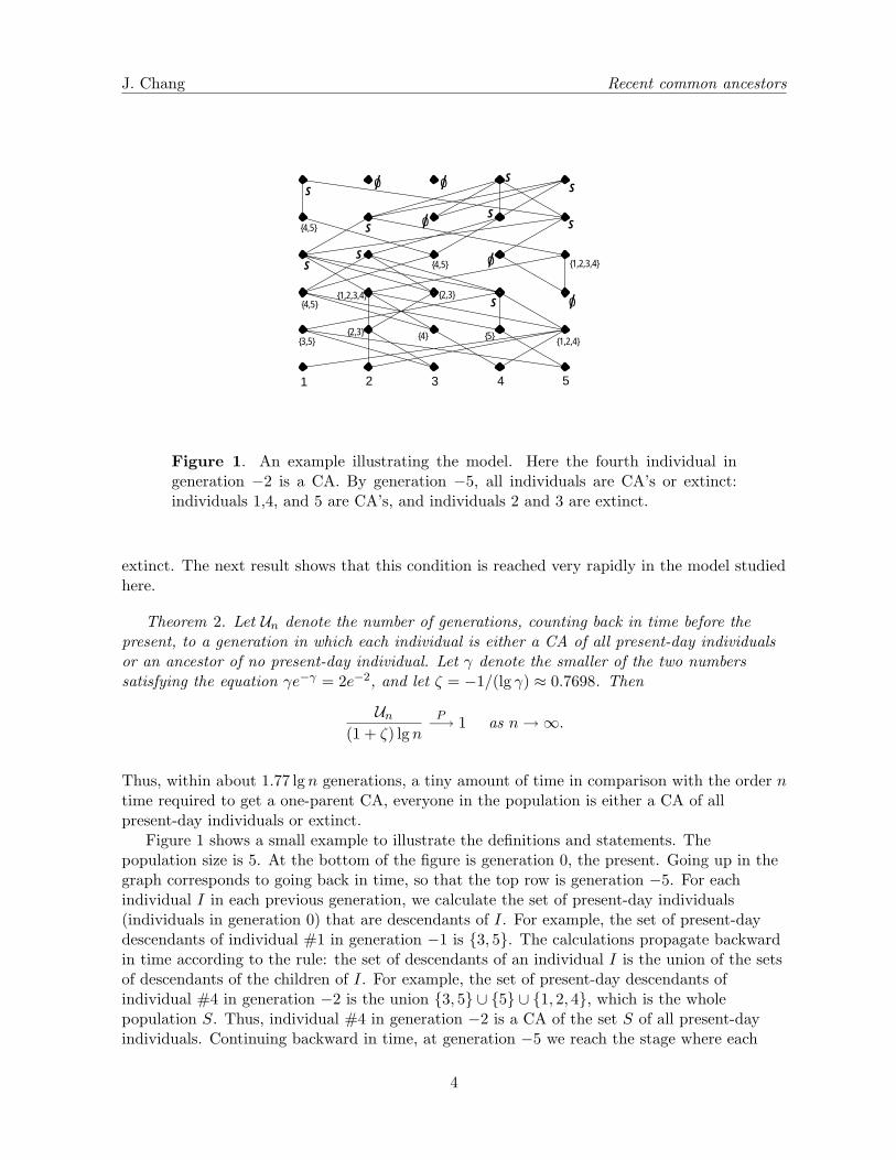
Figure 1. An example illustrating the model. Here the fourth individual ingeneration −2 is a CA. By generation −5, all individuals are CA’s or extinct:individuals 1,4, and 5 are CA’s, and individuals 2 and 3 are extinct.
extinct. The next result shows that this condition is reached very rapidly in the model studiedhere.
Theorem 2. Let Un denote the number of generations, counting back in time before thepresent, to a generation in which each individual is either a CA of all present-day individualsor an ancestor of no present-day individual. Let γ denote the smaller of the two numberssatisfying the equation γe−γ = 2e−2, and let ζ = −1/(lg γ) ≈ 0.7698. Then
Un
(1 + ζ) lg nP−→ 1 as n→ ∞.
Thus, within about 1.77 lg n generations, a tiny amount of time in comparison with the order ntime required to get a one-parent CA, everyone in the population is either a CA of allpresent-day individuals or extinct.
Figure 1 shows a small example to illustrate the definitions and statements. Thepopulation size is 5. At the bottom of the figure is generation 0, the present. Going up in thegraph corresponds to going back in time, so that the top row is generation −5. For eachindividual I in each previous generation, we calculate the set of present-day individuals(individuals in generation 0) that are descendants of I. For example, the set of present-daydescendants of individual #1 in generation −1 is {3, 5}. The calculations propagate backwardin time according to the rule: the set of descendants of an individual I is the union of the setsof descendants of the children of I. For example, the set of present-day descendants ofindividual #4 in generation −2 is the union {3, 5} ∪ {5} ∪ {1, 2, 4}, which is the wholepopulation S. Thus, individual #4 in generation −2 is a CA of the set S of all present-dayindividuals. Continuing backward in time, at generation −5 we reach the stage where each
4
J. Chang Recent common ancestors
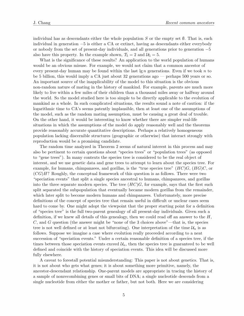
individual has as descendants either the whole population S or the empty set ∅. That is, eachindividual in generation −5 is either a CA or extinct, having as descendants either everybodyor nobody from the set of present-day individuals, and all generations prior to generation −5also have this property. In the example shown, T5 = 2 and U5 = 5.
What is the significance of these results? An application to the world population of humanswould be an obvious misuse. For example, we would not claim that a common ancestor ofevery present-day human may be found within the last lgn generations. Even if we took n tobe 5 billion, this would imply a CA just about 32 generations ago — perhaps 500 years or so.An important source of the inapplicability of the model to this situation is the obviousnon-random nature of mating in the history of mankind. For example, parents are much morelikely to live within a few miles of their children than a thousand miles away or halfway aroundthe world. So the model studied here is too simple to be directly applicable to the evolution ofmankind as a whole. In such complicated situations, the results sound a note of caution: if thelogarithmic time to CA’s seems patently implausible, then at least one of the assumptions ofthe model, such as the random mating assumption, must be causing a great deal of trouble.On the other hand, it would be interesting to know whether there are simpler real-lifesituations in which the assumptions of the model do apply reasonably well and the theoremsprovide reasonably accurate quantitative descriptions. Perhaps a relatively homogeneouspopulation lacking discernible structures (geographic or otherwise) that interact strongly withreproduction would be a promising candidate.
The random time analyzed in Theorem 2 seems of natural interest in this process and mayalso be pertinent to certain questions about “species trees” or “population trees” (as opposedto “gene trees”). In many contexts the species tree is considered to be the real object ofinterest, and we use genetic data and gene trees to attempt to learn about the species tree. Forexample, for humans, chimpanzees, and gorillas, is the “true species tree” (HC)G, (HG)C, or(CG)H? Roughly, the conceptual framework of this question is as follows. There were two“speciation events” that split a single species ancestral to humans, chimpanzees, and gorillasinto the three separate modern species. The tree (HC)G, for example, says that the first suchsplit separated the subpopulation that eventually became modern gorillas from the remainder,which later split to become modern humans and chimpanzees. Unfortunately, more precisedefinitions of the concept of species tree that remain useful in difficult or unclear cases seemhard to come by. One might adopt the viewpoint that the proper starting point for a definitionof “species tree” is the full two-parent genealogy of all present-day individuals. Given such adefinition, if we knew all details of this genealogy, then we could read off an answer to the H,C, and G question (the answer might be “none of the 3 choices above”—that is, the speciestree is not well defined or at least not bifurcating). One interpretation of the time Un is asfollows. Suppose we imagine a case where evolution really proceeded according to a neatsuccession of “speciation events.” Under a certain reasonable definition of a species tree, if thetimes between those speciation events exceed Un, then the species tree is guaranteed to be welldefined and coincide with the history of speciation events. This idea will be discussed morefully elsewhere.
A caveat to forestall potential misunderstanding: This paper is not about genetics. That is,it is not about who gets what genes; it is about something more primitive, namely, theancestor-descendant relationship. One-parent models are appropriate in tracing the history ofa sample of nonrecombining genes or small bits of DNA; a single nucleotide descends from asingle nucleotide from either the mother or father, but not both. Here we are considering
5
J. Chang Recent common ancestors
ancestry in the more common, demographic sense of the word, as applied to people, forexample, rather than genes.
Previous genetics research that is somewhat related, although still very different from thepresent study, considers models incorporating recombination. This type of model has beeninvestigated in a number of papers, including those of Hudson (1983) and Griffiths andMarjoram (1997). The history of a sample of DNA sequences may be described by a collectionof genealogies, with each nucleotide position in the DNA having its own one-parent genealogy.The genealogies for two positions that experience no recombination between them will becongruent, with the paths of the two genealogies going back through the same individuals,whereas a recombination between two positions causes the genealogies of those positions todiffer. Each of the genealogies in the collection will have its own MRCA (the nucleotide at itsroot), which may occur in different individuals. Each of these individuals will be a CA in thesense considered in this paper, but the most recent of these individuals is generally not aMRCA in our sense. Our MRCA is more recent, since the paths from ancestors to descendantsconsist of all potential paths for genes to be transmitted, and may include paths that did nothappen to be taken by any genes. No previous results about these genetic models have beensimilar to the results here, for example, in getting times of order logn. This is not surprising,since the asymptotics would require an assumption that the sequence lengths and the numberof recombinations tend to infinity. This is another manifestation of the statement that thequestions we are investigating here are not fundamentally genetics questions.
There is some previous work on the process we study here and related processes. Twopapers of Kammerle (1989, 1991) introduce a general class of two-parent (called “bisexual” inthose papers) versions of the Wright-Fisher and other processes. These papers focus on twomain questions. First, they analyze the probability of extinction of a set of individuals in thepresent generation, that is, the probability that the set of individuals eventually has nodescendants in some future generation. Second, in a two-parent version of the Moran model,they study the number Rn(t) of individuals t generations ago who have at least one descendantin the present generation. Kammerle (1989) finds that the Markov chain {Rn(t) : t = 0, 1, . . .},suitably normalized and suitably initialized (with the initialization essentially requiring thatthe chain is started in steady state), converges weakly as n→ ∞ to a discrete-timeOrnstein-Uhlenbeck process.
Mohle (1994) both generalizes and refines the results of Kammerle. In particular, Mohleprovides a detailed analysis of the extinction probabilities in a two-parent Wright-Fisher modelthat approximates the probabilities up to o(1/n). He also establishes weak convergence in ageneral class of two-parent models, including an Ornstein-Uhlenbeck limit for the two-parentWright-Fisher process. Mohle also has a number of other papers in press, including one thatrelaxes the assumption of constant population size.
These previous results are complementary to the results in this paper. The previous papersconsidered individuals who have at least 1 descendant in a given future generation. Here weconsider CA’s, who have as descendants all members of the future generation. The previousresults about the process {Rn(t)} apply to large t, that is, to the behavior the process manygenerations before the present, with the process in steady state. Here we focus on the behaviorof a related process at small (i.e. recent) times, starting far away from steady state. We showthat at about t = 1.77 lg n generations before the present, with high probability the Rn(t)individuals who have at least 1 present-day descendant are all in fact CA’s.
6
J. Chang Recent common ancestors
2 Simulations
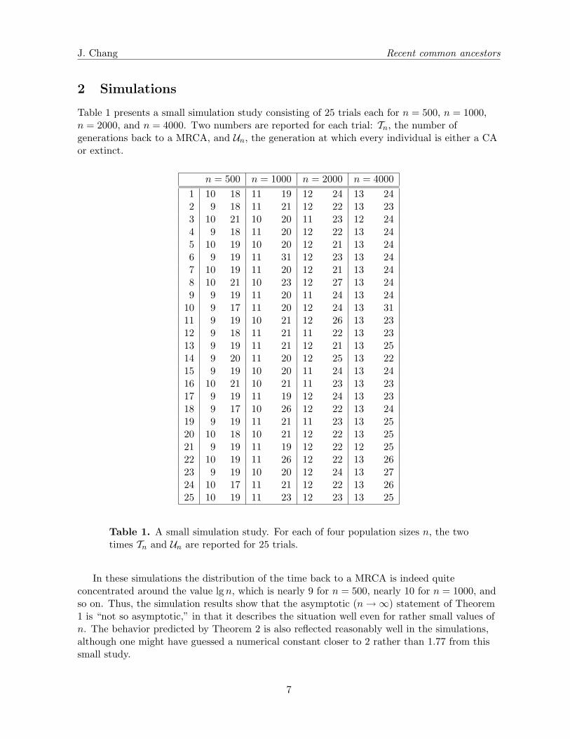
Table 1 presents a small simulation study consisting of 25 trials each for n = 500, n = 1000,n = 2000, and n = 4000. Two numbers are reported for each trial: Tn, the number ofgenerations back to a MRCA, and Un, the generation at which every individual is either a CAor extinct.
Table 1. A small simulation study. For each of four population sizes n, the twotimes Tn and Un are reported for 25 trials.
In these simulations the distribution of the time back to a MRCA is indeed quiteconcentrated around the value lgn, which is nearly 9 for n = 500, nearly 10 for n = 1000, andso on. Thus, the simulation results show that the asymptotic (n→ ∞) statement of Theorem1 is “not so asymptotic,” in that it describes the situation well even for rather small values ofn. The behavior predicted by Theorem 2 is also reflected reasonably well in the simulations,although one might have guessed a numerical constant closer to 2 rather than 1.77 from thissmall study.
7
J. Chang Recent common ancestors
3 Proofs
3.1 General ideas and tools
We start with the observation that although Theorems 1 and 2 are phrased in terms ofcounting generations back in time from the present until some condition obtains, these resultsmay be proved by counting forward in time from a fixed generation. For example, the event{Tn ≤ m} requires that a CA of all individuals in generation 0 may be found amonggenerations −1,−2, . . . ,−m. This is equivalent to requiring that if we start with generation−m and trace forward in time, then some individual in generation −m becomes a CA of allindividuals in some generation t ∈ {−m+ 1,−m+ 2, . . . , 0}.
So we will count generations forward in time, and for convenience let us renumbergenerations so that the initial generation is “generation 0.” The population at generation t ≥ 0consists of n individuals denoted by It,1, It,2, . . . , It,n. We can picture It,1, It,2, . . . , It,n as dotsin an array as in Figure 1, with It,j being the jth dot in row t. The association of a number jto individual It,j is an arbitrary labeling of the individuals within generation t. Assigned onlyas a means of referring to individuals, the labels have no significance in the model, which doesnot order the individuals within a generation. Let µt,1, νt,1, µt,2, νt,2, . . . , µt,n, νt,n beindependent and uniformly distributed on the set {1, . . . , n}. We interpret µt,j and νt,j aslabels of the parents of individual It,j ; that is, the parents of It,j are It−1,µt,j and It−1,νt,j .Defining a sequence of random sets Gi
0,Gi1, . . . recursively by Gi
0 = {i} and
Git = {j ≤ n : µt,j ∈ Gi
t−1 or νt,j ∈ Git−1},
Git is the set of labels of the descendants of I0,i in generation t. Let Gi
t denote the cardinality ofGit . The conditional probability that individual It+1,j has at least one parent among the Gi
t
members of Git is
P ({µt+1,j ∈ Git} ∪ {νt+1,j ∈ Gi
t} | Git) = (Gi
t/n) + (Git/n)− (Gi
t/n)(Git/n).
The process {Git : t = 0, 1, . . .} is a Markov chain with transition probabilities
(Git+1 | Gi
t) ∼ Bin
n, 2Gi
t
n−
(Gi
t
n
)2 , (1)
where Bin(n, p) denotes the binomial distribution for the number of successes in n independenttrials each having success probability p.
Throughout the proof, {Gt} will denote a Markov chain with transition probabilities as in(1), although in different parts of the proof we will consider different possible initial values G0.For example, taking G0 = 1 corresponds to following the descendants of a particular individualin generation 0. In the early stages of the process, while Gt remains small relative to n, in viewof (1) the conditional distribution of Gt+1 given Gt is nearly Poisson(2Gt), that is, the Poissondistribution with mean 2Gt. In other words, while {Gt} remains small, it evolves nearly as aGalton-Watson branching process {Yt} with offspring distribution Poisson(2). Kammerle(1991) gave a formal statement of a result of this nature. A special case of his result says thatfor fixed u, the joint distribution of (G0, G1, . . . , Gu) converges to that of (Y0, Y1, . . . , Yu) asn→ ∞. For our purposes, we will use the following result that allows us to approximate
8
J. Chang Recent common ancestors
probabilities for the G process by those for the Y process up to a higher order of accuracy andover longer intervals of time that may have random lengths.
Lemma 3. Let Y0, Y1, . . . denote a Galton-Watson branching process with offspringdistribution Poisson(2). Suppose that Y0 = G0 = 1. Define τYb = inf{t : Yt ≥ b} andτY0b = inf{t : Yt = 0 or Yt ≥ b}, with corresponding definitions for τGb and τG0b. As n→ ∞, if mand b satisfy mb2 = o(n), then
P{τGb > m} = P{τYb > m}(1 + o(1)) (2)
andP{τG0b > m} = P{τY0b > m}(1 + o(1)). (3)
Proof. A straightforward calculation bounds the likelihood ratio
L(y | x) := P{Gt+1 = y | Gt = x}P{Yt+1 = y | Yt = x} =
P{Bin
(n, 2xn − x2
n2
)= y
}P{Poisson(2x) = y} ≤ e2x
(1− 2x
n+x2
n2
)n−y
,
so that
logL(y | x) ≤ 2x+ (n− y)(−2xn
+x2
n2
)≤ (x2 + 2xy)/n.
This holds whenever the denominator P{Yt+1 = y | Yt = x} is positive, that is, for all x > 0and y ≥ 0, and also for x = y = 0. Thus, for all such pairs of x and y satisfying x < b andy < b, we have
logL(y | x) ≤ 3b2/n.
A similar calculation gives the lower bound
logL(y | x) ≥ −5b2/(2n)[1 +O(b/n)],
so that logL(y | x) ≥ −3b2/n for sufficiently large n. So if x1, . . . , xm are all less than b, then
and, similarly, P{τGb > m} ≥ P{τYb > m}e−3mb2/n, so that, by the assumption thatmb2 = o(n), we obtain P{τGb > m} = P{τYb > m}(1 + o(1)). This proves (2). The proof of (3)uses the same reasoning, with the summations in (4) ranging over 0 < xt < b rather than0 ≤ xt < b.
The previous result will be useful because the Poisson Galton-Watson process is simple andwell understood. The next lemma records a few well known items for future reference.
Lemma 4. Let Y0, Y1, . . . denote a Galton-Watson process with offspring distributionPoisson(2). Define the moment generating function ψ(z) = E(zY1) = e−2+2z. The extinctionprobability ρ = P{Yt = 0 for some t} ≈ 0.20319 is the smaller of the two solutions of ψ(ρ) = ρ,and ρ = γ/2, where γ is as defined in Theorem 2. The t-fold composition ψt = ψ ◦ · · · ◦ ψsatisfies ψt(z) ↑ ρ for all 0 ≤ z ≤ ρ.
The relation ρ = γ/2 is confirmed by comparing the definitions of ρ and γ. Despite the simplerelationship, we will keep the two different letters in our notation for conceptual clarity.
Defining gt = Gt/n, we have
E(gt+1 | gt) = 2gt − g2t = gt(2− gt). (5)
That is, if the fraction of descendants of a given individual is currently gt, it is expected tomultiply by a factor of 2− gt in the next generation. For example, in the early stages of theprocess when the fraction gt is small, it nearly doubles in expectation in the next generation.For very small gt (of the order 1/n, for example) the random variability is large; for example,the process could easily go extinct. This is when it is most useful to approximate the Gprocess by the Poisson(2) Galton-Watson process.
On the other hand, for larger values of gt, the multiplication factor gt+1/gt, althoughexpected to be somewhat smaller, has much less variability. The deviations of this factor fromits expected value are bounded probabilistically by large deviations inequalities for thebinomial distribution. We will use the following inequality of Bernstein (1946) as a basic tool.
Lemma 5.[Bernstein’s inequality] If X ∼ Bin(n, p) and r > 0, then
P{X ≥ np+ r} ≤ exp
{−r2
2np(1− p) + (2/3)r
}. (6)
Since n−X ∼ Bin(n, 1− p), the right side of (6) is also an upper bound for the probabilityP{X ≤ np− r}.
3.2 Proof of Theorem 1
Outline. The proof will be divided into several parts. We start from generation 0 and traceforward in time.
Stage 1: By the end of stage 1, we identify an individual I in generation 0 who has anumber of descendants that is small compared to n, but large enough so that I is unlikely everto become extinct. In particular, we look for a generation t such that some individual I in
10
J. Chang Recent common ancestors
generation 0 has at least lg2(n) descendants in generation t. With probability approaching 1,this happens in time o(lg n), negligible compared with lgn; this is shown by using Lemma 3 toapproximate our process by a Poisson Galton-Watson process. The rest of the proof will showthat with probability approaching 1, individual I becomes a CA within (1 + ε)(lg n)generations, where ε is an arbitrary positive number.
Stage 2: Let β ∈ (0, 1). Stage 2 follows the descendants of I until reaching a generationcontaining at least nβ descendants. In view of (5), since nβ is a small fraction of n for large n,throughout Stage 2 the number of descendants in a generation is expected to be nearly doublethe number of descendants in the previous generation. And lg2(n) is large enough so that themultiplication factor will be very close to its expected value, with high probability. So stage 2should not take much more than about lg(nβ) = β lg(n) generations.
Stage 3: This stage brings the count of descendants of I up from nβ to (1/2)n. Since thefraction of descendants during stage 3 stays below 1/2, the expected multiplication factor is atleast 2− 1/2 = 3/2. Again, this multiplication factor is very reliable, so that with highprobability stage 3 takes no more than about log3/2{(n/2)/(nβ)} generations. We can makethis an arbitrarily small fraction of lgn by choosing β close enough to 1.
Stage 4: Now we switch to looking at the fraction Bt of individuals in a generation who arenot descendants of individual I. This fraction is expected to square each generation. Thiscauses Bt to decrease very quickly. Fixing α ∈ (1/2, 2/3), we show that stage 4, which takesthe fraction Bt from 1/2 down to n−α, takes only order lg lgn time.
Stage 5: This completes the process, ending when the B process hits 0, and individual Ihas become a CA. We show that this takes just one generation with high probability.
Upper bound: Combining the results of Stages 1 through 5 gives the probabilistic upperbound limn→∞ P{Tn ≤ (1 + ε) lg n} = 1.
Lower bound: Here we show that limn→∞ P{Tn ≥ (1− ε) lg n} = 1. This is done by usingBernstein’s inequality to prove an assertion of the following form: For positive r and δ, oncethe process of descendants of any given individual reaches a power nr of n, it is very unlikelyto increase by a factor of more than 2 + δ in a generation, whereas it would have to do so inorder to have Tn < (1− ε) lg n.
Stage 1. Here we will show that with high probability, within a number of generationsnegligible compared to lgn, we can find a generation with at least lg2 n individuals who sharea common ancestor. For simplicity we give a crude argument that circumvents the need toconsider any dependence among the processes {Gi
t : t ≥ 0} starting from different individualsI0,i. This could also be done along the lines of the argument in Lemma 19 below, where weneed to confront this dependence.
Proof. Let b and m denote lg2 n and �3 lg lg n�, respectively. Let {Yt} be a Galton-Watsonprocess with offspring distribution Poisson(2), and define Mt = Yt2−t. The process {Mt} is anonnegative martingale that converges almost surely to a limit M∞, say, with
11
J. Chang Recent common ancestors
P{M∞ = 0} = ρ < 1. Note that P{τYb > m} ≤ P{Ym < b} = P{Mm < b2−m}. Therefore,using Fatou’s lemma and the assumption that b2−m → 0,
By Lemma 3, P{τb > m} = P{τYb > m}(1 + o(1)) as n→ ∞. Therefore,
lim supP{τb > m} ≤ lim supP{τYb > m} ≤ ρ < 1.
So lim inf P{τb ≤ m} ≥ 1− ρ > 0.
Proposition 7. Let Git denote the number of descendants in generation t of individual I0,i
(the ith individual in generation 0), and let G∗t = max1≤i≤n{Gi
t}. DefineτG
∗b = inf{t : G∗
t ≥ b}. Then τG∗
lg2 n= oP (lg n).
Proof. We use a geometric trials argument. Let mn = �3 lg lg n�, and choose a sequence{kn} with kn → ∞ and knmn = o(lg n). Perform a sequence of kn trials as follows. For the firsttrial, start with individual I0,1, and follow his progeny for mn generations. We say the trial is asuccess if I0,1 has at least lg2 n descendants in generation mn; by Lemma 6 this happens withprobability at least c, say, where c > 0. If the trial is a failure, start a new trial, following theprogeny of individual Imn,1 for mn more generations. And so on. We stop at the first success,having found an individual with at least lg2 n descendants. The probability that this sequenceof trials fails to terminate by generation knmn is at most (1− c)kn , which tends to 0.
Thus, with probability tending to 1, there is a κ ∈ {0, . . . , kn − 1} such that individualIκmn,1 has at least lg
2 n descendants in generation (κ+ 1)mn. Let I denote any ancestor ofIκmn,1 in generation 0. We will show in the remainder of the proof that for each ε > 0, withprobability tending to 1 as n→ ∞, individual I becomes a CA within (1 + ε) lg n generations.
Stage 2. The following simple consequence of Bernstein’s inequality will be a convenient tool.
Lemma 8. If δ ≤ 3/4 and Gt ≤ δn/20, thenP{Gt+1 ≤ (2− δ)Gt | Gt} ≤ exp(−δ2Gt/5).
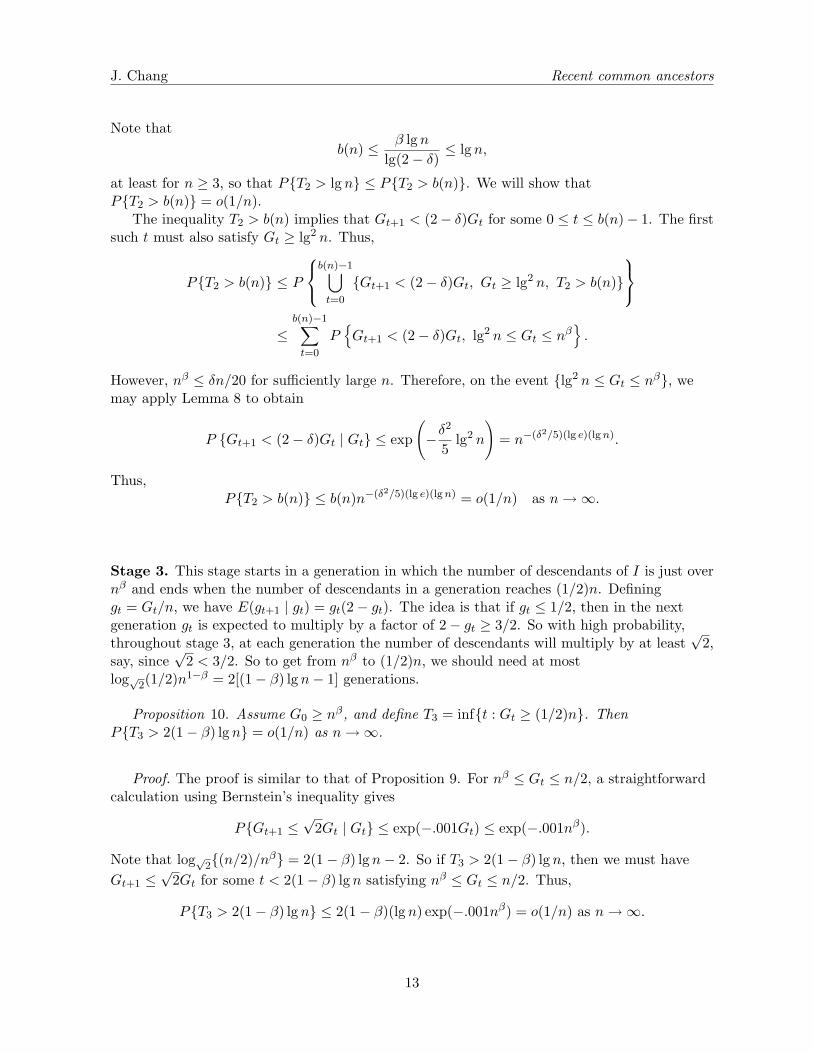
The next result shows that the probability that Stage 2 takes more than lgn generationsapproaches 0 as n→ ∞. In fact, we show that this probability is o(1/n); this will be used inthe proof of Theorem 2.
Proposition 9. Assume that G0 ≥ lg2 n, and let 0 < β < 1. Define T2 = inf{t : Gt ≥ nβ}.Then P{T2 > lg n} = o(1/n) as n→ ∞.
Proof. Take 0 < δ < 3/4 such that lg(2− δ) > β, and define
b(n) =
⌈log2−δ
(nβ
lg2 n
)⌉.
12
J. Chang Recent common ancestors
Note thatb(n) ≤ β lg n
lg(2− δ) ≤ lg n,
at least for n ≥ 3, so that P{T2 > lg n} ≤ P{T2 > b(n)}. We will show thatP{T2 > b(n)} = o(1/n).
The inequality T2 > b(n) implies that Gt+1 < (2− δ)Gt for some 0 ≤ t ≤ b(n)− 1. The firstsuch t must also satisfy Gt ≥ lg2 n. Thus,
P{T2 > b(n)} ≤ P
b(n)−1⋃t=0
{Gt+1 < (2− δ)Gt, Gt ≥ lg2 n, T2 > b(n)}
≤b(n)−1∑t=0
P{Gt+1 < (2− δ)Gt, lg2 n ≤ Gt ≤ nβ
}.
However, nβ ≤ δn/20 for sufficiently large n. Therefore, on the event {lg2 n ≤ Gt ≤ nβ}, wemay apply Lemma 8 to obtain
Stage 3. This stage starts in a generation in which the number of descendants of I is just overnβ and ends when the number of descendants in a generation reaches (1/2)n. Defininggt = Gt/n, we have E(gt+1 | gt) = gt(2− gt). The idea is that if gt ≤ 1/2, then in the nextgeneration gt is expected to multiply by a factor of 2− gt ≥ 3/2. So with high probability,throughout stage 3, at each generation the number of descendants will multiply by at least
√2,
say, since√2 < 3/2. So to get from nβ to (1/2)n, we should need at most
log√2(1/2)n1−β = 2[(1− β) lg n− 1] generations.
Proposition 10. Assume G0 ≥ nβ, and define T3 = inf{t : Gt ≥ (1/2)n}. ThenP{T3 > 2(1− β) lg n} = o(1/n) as n→ ∞.
Proof. The proof is similar to that of Proposition 9. For nβ ≤ Gt ≤ n/2, a straightforwardcalculation using Bernstein’s inequality gives
P{Gt+1 ≤√2Gt | Gt} ≤ exp(−.001Gt) ≤ exp(−.001nβ).
Note that log√2{(n/2)/nβ} = 2(1− β) lg n− 2. So if T3 > 2(1− β) lg n, then we must haveGt+1 ≤
√2Gt for some t < 2(1− β) lg n satisfying nβ ≤ Gt ≤ n/2. Thus,P{T3 > 2(1− β) lg n} ≤ 2(1− β)(lg n) exp(−.001nβ) = o(1/n) as n→ ∞.
13
J. Chang Recent common ancestors
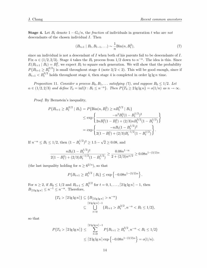
Stage 4. Let Bt denote 1−Gt/n, the fraction of individuals in generation t who are notdescendants of the chosen individual I. Then
(Bt+1 | Bt, Bt−1, . . .) ∼ 1nBin(n,B2t ), (7)
since an individual is not a descendant of I when both of his parents fail to be descendants of I.Fix α ∈ (1/2, 2/3). Stage 4 takes the Bt process from 1/2 down to n−α. The idea is this. SinceE(Bt+1 | Bt) = B2t , we expect Bt to square each generation. We will show that the probabilityP{Bt+1 ≥ B3/2t } is small throughout stage 4 (note 3/2 < 2). This will be good enough, since ifBt+1 < B
3/2t holds throughout stage 4, then stage 4 is completed in order lg lgn time.
Proposition 11. Consider a process B0, B1, . . . satisfying (7), and suppose B0 ≤ 1/2. Letα ∈ (1/2, 2/3) and define T4 = inf{t : Bt ≤ n−α}. Then P{T4 ≥ 2 lg lg n} = o(1/n) as n→ ∞.
If n−α ≤ Bt ≤ 1/2, then (1−B1/2t )2 ≥ 1.5−√2 ≥ 0.08, and
nBt(1−B1/2t )2
2(1−B2t ) + (2/3)B−1/2t (1−B1/2t )
≥ 0.08n1−α
2 + (2/3)nα/2≥ 0.08n1−(3/2)α
(the last inequality holding for n ≥ 62/α), so that
P{Bt+1 ≥ B3/2t | Bt} ≤ exp{−0.08n1−(3/2)α
}.
For n ≥ 2, if B0 ≤ 1/2 and Bt+1 ≤ B3/2t for t = 0, 1, . . . , �2 lg lg n� − 1, thenB�2 lg lgn� ≤ n−1 ≤ n−α. Therefore,
{T4 > �2 lg lg n�} ⊆ {B�2 lg lgn� > n−α}
⊆�2 lg lgn�−1⋃
t=0
{Bt+1 > B3/2t , n−α < Bt ≤ 1/2},
so that
P{T4 > �2 lg lg n�} ≤�2 lg lgn�−1∑
t=0
P{Bt+1 ≥ B3/2t , n−α < Bt ≤ 1/2}
≤ �2 lg lg n� exp{−0.08n1−(3/2)α
}= o(1/n).
14
J. Chang Recent common ancestors
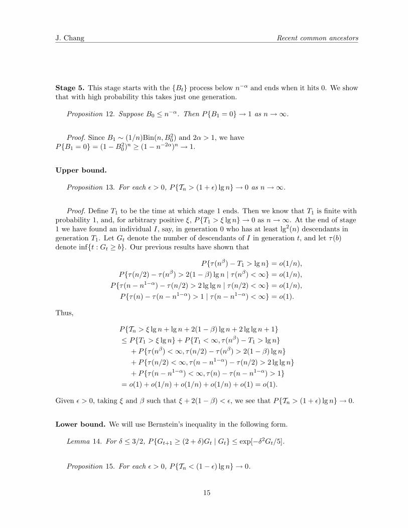
Stage 5. This stage starts with the {Bt} process below n−α and ends when it hits 0. We showthat with high probability this takes just one generation.
Proposition 12. Suppose B0 ≤ n−α. Then P{B1 = 0} → 1 as n→ ∞.
Proof. Since B1 ∼ (1/n)Bin(n,B20) and 2α > 1, we haveP{B1 = 0} = (1−B20)n ≥ (1− n−2α)n → 1.
Upper bound.
Proposition 13. For each ε > 0, P{Tn > (1 + ε) lg n} → 0 as n→ ∞.
Proof. Define T1 to be the time at which stage 1 ends. Then we know that T1 is finite withprobability 1, and, for arbitrary positive ξ, P{T1 > ξ lg n} → 0 as n→ ∞. At the end of stage1 we have found an individual I, say, in generation 0 who has at least lg2(n) descendants ingeneration T1. Let Gt denote the number of descendants of I in generation t, and let τ(b)denote inf{t : Gt ≥ b}. Our previous results have shown that
P{τ(nβ)− T1 > lg n} = o(1/n),P{τ(n/2)− τ(nβ) > 2(1− β) lg n | τ(nβ) <∞} = o(1/n),
P{τ(n− n1−α)− τ(n/2) > 2 lg lg n | τ(n/2) <∞} = o(1/n),P{τ(n)− τ(n− n1−α) > 1 | τ(n− n1−α) <∞} = o(1).
Thus,
P{Tn > ξ lg n+ lg n+ 2(1− β) lg n+ 2 lg lgn+ 1}≤ P{T1 > ξ lg n}+ P{T1 <∞, τ(nβ)− T1 > lg n}
+ P{τ(nβ) <∞, τ(n/2)− τ(nβ) > 2(1− β) lg n}+ P{τ(n/2) <∞, τ(n− n1−α)− τ(n/2) > 2 lg lg n}+ P{τ(n− n1−α) <∞, τ(n)− τ(n− n1−α) > 1}
= o(1) + o(1/n) + o(1/n) + o(1/n) + o(1) = o(1).
Given ε > 0, taking ξ and β such that ξ + 2(1− β) < ε, we see that P{Tn > (1 + ε) lg n} → 0.
Lower bound. We will use Bernstein’s inequality in the following form.
Proposition 15. For each ε > 0, P{Tn < (1− ε) lg n} → 0.
15
J. Chang Recent common ancestors
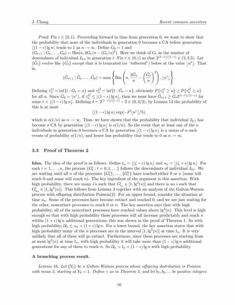
Proof. Fix ε ∈ (0, 1). Proceeding forward in time from generation 0, we want to show thatthe probability that none of the individuals in generation 0 becomes a CA before generation�(1− ε) lg n� tends to 1 as n→ ∞. Define G0 = 1 and(Gt+1 | Gt, . . . , G0) ∼ Bin(n, 2Gt/n− (Gt/n)2). Here we think of Gt as the number ofdescendants of individual I0,1 in generation t. Fix r ∈ (0, ε) so that 2(1−r)/(1−ε) ∈ (2, 3.5). Let{Gt} evolve like {Gt} except that it is truncated (or “reflected”) below at the value �nr�. Thatis,
(Gt+1 | Gt, . . . , G0) ∼ max
Bin
n, 2Gt
n−
(Gt
n
)2 , �nr� .
Defining τGn = inf{t : Gt = n} and τ Gn = inf{t : Gt = n}, obviously P{τGn ≥ u} ≥ P{τ Gn ≥ u}for all u. Since G0 = �nr�, if τ Gn ≤ �(1− ε) lg n�, then we must have Gt+1 ≥ Gt2(1−r)/(1−ε) forsome t < �(1− ε) lg n�. Defining δ = 2(1−r)/(1−ε) − 2 ∈ (0, 3/2), by Lemma 14 the probability ofthis is at most
�(1− ε) lg n� exp(−δ2�nr�/5),which is o(1/n) as n→ ∞. Thus, we have shown that the probability that individual I0,1 hasbecome a CA by generation �(1− ε) lg n� is o(1/n). So the event that at least one of the nindividuals in generation 0 becomes a CA by generation �(1− ε) lg n� is a union of n suchevents of probability o(1/n), and hence has probability that tends to 0 as n→ ∞.
3.3 Proof of Theorem 2
Idea. The idea of the proof is as follows. Define tn = �(ζ − ε) lg n� and un = �(ζ + ε) lg n�. Foreach i = 1, . . . , n, the process {Gi
t : t = 0, 1, . . .} follows the descendants of individual I0,i. Weare waiting until all n of the processes {G1t }, . . . , {Gn
t } have reached either 0 or n (some willreach 0 and some will reach n). The key ingredient of the argument is this assertion: Withhigh probability, there are many i’s such that Gi
tn ∈ [1, lg2(n)] and there is no i such thatGi
un∈ [1, lg2(n)]. This follows from Lemma 3 together with an analysis of the Galton-Watson
process with offspring distribution Poisson(2). For an upper bound, consider the situation attime un. Some of the processes have become extinct and reached 0, and we are just waiting forthe other, nonextinct processes to reach 0 or n. The key assertion says that with highprobability, all of the nonextinct processes have reached values above lg2(n). This level is highenough so that with high probability these processes will all increase predictably and reach nwithin (1 + ε) lg n additional generations; this was shown in the proof of Theorem 1. So withhigh probability, Un ≤ un + (1 + ε) lg n. For a lower bound, the key assertion states that withhigh probability many of the n processes are in the interval [1, lg2(n)] at time tn. It is veryunlikely that all of these will go extinct. Furthermore, since these processes are starting fromat most lg2(n) at time tn, with high probability it will take more than (1− ε) lg n additionalgenerations for any of them to reach n. So Un > tn + (1− ε) lg n with high probability.
A branching process result.
Lemma 16. Let {Yt} be a Galton-Watson process whose offspring distribution is Poissonwith mean 2, starting at Y0 = 1. Define γ as in Theorem 2, and let b1, b2, ... be positive integers
16
J. Chang Recent common ancestors
satisfying lg(bt) = o(t) as t→ ∞. Then
limt→∞
1tlgP{1 ≤ Yt ≤ bt} = lg(γ) ≈ −1.29911.
Proof. We use a number of results from chapter 1 of Athreya and Ney (1972). First, theMonotone Ratio Lemma says that for each k there is a λk <∞ such that
P{Yt = k}P{Yt = 1} ↑ λk as t→ ∞.
Also,
Λ(s) :=∞∑k=1
λksk <∞ for all s ∈ (0, 1).
Finally, using the notation and facts collected in Lemma 4, we have
P{Yt = 1} = ψ′t(0) = ψ
′[ψt−1(0)]ψ′t−1(0) = ψ
′[ψt−1(0)]P{Yt−1 = 1},so that
P{Yt = 1}P{Yt−1 = 1} ↑ ψ′(ρ) = 2ρ = γ.
In particular, (1/t) lgP{Yt = 1} ↑ lg γ.For s ∈ (0, 1),
bt∑k=1
P{Yt = k} ≤ P{Yt = 1}bt∑
k=1
λk
≤ P{Yt = 1}s−bt
bt∑k=1
λksk
≤ P{Yt = 1}s−btΛ(s). (8)
If we take s close to 1 (e.g. s = 1− b−1t , say), then the term s−bt will remain bounded andpresent no difficulty. So we would like to know how Λ(s) grows as s ↑ 1.
Define ϕ to be the inverse function ψ−1, and ϕk to be the k-fold composition ϕ ◦ · · · ◦ϕ. Byequation (6) on page 12 of Athreya and Ney (1972), for each s ∈ (ρ, 1),
However, since ψ′(1) = 2, we may choose a number Φ so that
ϕk(1/2) ≥ 1− (1.9)−kΦ
and, therefore,Λ(1− (1.9)−kΦ) ≤ γ−kΛ(1/2)
17
J. Chang Recent common ancestors
hold for all sufficiently large k. From this, it follows that
Λ(1− y) ≤ Λ(1/2)(y/Φ)(lgγ)/(lg1.9) ≤ y2lgγ
holds for all sufficiently small positive y.Now substituting s = 1− b−1t in (8), there is a finite constant C such that
bt∑k=1
P{Yt = k} ≤ CγtΛ(1− b−1t ) ≤ Cγtb2lg(1/γ)t .
Thus, as long as bt grows subgeometrically, that is, lg(bt) = o(t), we have
lim t→∞(1/t) lgP{1 ≤ Yt ≤ bt} ≤ lg(γ).
Combining this with the fact that limt→∞(1/t) lgP{Yt = 1} = lg(γ) completes the proof.
Upper bound.
Lemma 17. Let I0,i denote individual i in generation 0. Define Git to be the number
descendants of I0,i in generation t; in particular, Gi0 = 1 for all i = 1, . . . , n. Also define
τ i0,b = inf{t : Git = 0 or Gi
t ≥ b},
and let
An =n⋃
i=1
{τ i0,lg2 n
> (ζ + ε) lg n}. (9)
Then P (An) → 0 as n→ ∞.
Proof. Define τY0b = inf{t : Yt = 0 or Yt ≥ b}. Since {τY0b > t} ⊆ {1 ≤ Yt < b}, Lemma 16 and(3) give
lim (1/t) lgP{τ i0b > t} ≤ lg(γ) if lg(b) = o(t) and tb2 = o(n). (10)
Letting ε > 0 and applying (10) to t = (ζ + ε)(lg n) and b = lg2(n) gives
lgP{τ i0,lg2(n)
> (ζ + ε)(lg n)} ≤ (lg(γ) + δ)(ζ + ε)(lg n)
for all δ and all sufficiently large n. Taking δ sufficiently small, from the definition of ζ we seethat
P{τ i0,lg2(n)
> (ζ + ε)(lg n)} = o(1/n) as n→ ∞,so that P (An) = o(1).
We have shown that, with high probability, all individuals in generation 0 have either nodescendants or more than lg2(n) descendants in generation �(ζ + ε) lg n� for ε > 0. Next wewill show that for any given ε > 0, with high probability, each individual having more thanlg2(n) descendants in generation �(ζ + ε) lg n� becomes a CA within (1 + ε) lg n additionalgenerations. Most of the work required to prove this has already been done in the proof of
18
J. Chang Recent common ancestors
Theorem 1; the extra ingredient is the following lemma, which takes a closer look at “stage 5.”We retain the definition Bt = 1− (Gt/n) from above.
Lemma 18. Let α ∈ (1/2, 2/3) and take k(α) > 1/(2α− 1). Suppose that B0 ≤ n−α anddefine T5 = inf{t : Bt = 0}. Then P{T5 > k(α)} = o(1/n) as n→ ∞.
where the first inequality holds for sufficiently large n (since α > 1/2 implies that nB2t isarbitrarily small for sufficiently large n). In particular,
P{0 < Bt+1 ≤ n−α | 0 < Bt ≤ n−α} ≤ 2n1−2α for sufficiently large n. (11)
Next, by Bernstein’s inequality, on the event {Bt ≤ n−α},
P{Bt+1 > n−α | Bt} = P{ 1
nBin(n,B2t ) > B
2t + (n−α −B2t ) | Bt}
≤ exp
[−n2(n−α −B2t )2
2nB2t (1−B2t ) + 23n(n
−α −B2t )
]
≤ exp
[−n2−2α
2n1−2α + 23n1−α
].
Since the exponent is asymptotic to −(3/2)n1−α, clearly
P{Bt+1 > n−α | Bt} ≤ exp[−n1−α] on {Bt ≤ n−α}
for sufficiently large n. Assuming that B0 ≤ n−α,
k⋃t=0
{Bt > n−α} ⊆
k−1⋃t=0
{Bt ≤ n−α, Bt+1 > n−α}.
Therefore, since
P{Bt ≤ n−α, Bt+1 > n−α} = E
[{Bt ≤ n−α}P{Bt+1 > n−α | Bt}
] ≤ exp[−n1−α],
we obtain
P
[k⋃
t=0
{Bt > n−α}
]≤ k exp[−n1−α]. (12)
Thus, using (11) and (12),
P{T5 > k} ≤ P
(k⋃
t=0
{Bt > n−α}
)+ P
(k⋂
t=0
{0 < Bt ≤ n−α})
≤ k exp[−n1−α] + (2n1−2α)k.
19
J. Chang Recent common ancestors
Applying this to k = k(α) > 1/(2α− 1) gives the desired result.
Proof of the upper bound in Theorem 2. Let Un denote the time at which everyone fromgeneration 0 has become a CA or extinct. Recall the definition of An from (9), and letτ i(b) = inf{t : Gi
t ≥ b}. Since{Un > (1 + ζ + 2ε) lg n} ⊆ An ∪ [Ac
n ∩ {Un > (1 + ζ + 2ε) lg n}]
⊆ An ∪n⋃
i=1
{τ i(lg2 n) ≤ (ζ + ε) lg n, τ i(n) > (1 + ζ + 2ε) lg n},
to show that P{Un > (1 + ζ + 2ε) lg n} = o(1), by Lemma 17 it suffices to show that
P{τ1(lg2 n) ≤ (ζ + ε) lg n, τ1(n) > (1 + ζ + 2ε) lg n} = o(1/n).
To see this, observe that the results of Stages 2 through 4 from the proof of Theorem 1 showthat
P{τ1(nβ)− τ1(lg2 n) > lg n | τ1(lg2 n) <∞} = o(1/n),P{τ1(n/2)− τ1(nβ) > 2(1− β) lg n | τ1(nβ) <∞} = o(1/n),
P{τ1(n− n1−α)− τ1(n/2) > 2 lg lg n | τ1(n/2) <∞} = o(1/n),
P{τ1(n)− τ1(lg2 n) > lg n+ 2(1− β) lg n+ 2 lg lgn+ k(α) | τ1(lg2 n) <∞} = o(1/n).
Choosing β sufficiently close to 1, we see that for any given ε > 0,
P{τ1(n)− τ1(lg2 n) > (1 + ε) lg n | τ1(lg2 n) <∞} = o(1/n).
Thus,
P{τ1(lg2 n) ≤ (ζ + ε) lg n, τ1(n) > (1 + ζ + 2ε) lg n}≤ P{τ1(lg2 n) <∞, τ1(n)− τ1(lg2 n) > (1 + ε) lg n} = o(1/n),
as desired.
Lower bound.The proof goes as follows. First we show that at time tn = �(ζ − ε) lg n�, there are many
individuals i who have Gitn ∈ [1, lg2 n]. The probability that all of these individuals eventually
become extinct is negligibly small. In the probable event that not all of these individualsbecome extinct, the time Un must wait for at least one of them to become a CA. From theprevious results we know that this will take an additional (1− ε) lg n generations.
Here is some notation that will be used throughout the proof. Let tn denote �(ζ − ε) lg n�.For 1 ≤ i ≤ n, define Ji to be the event {Gi
t ∈ [1, lg2 n] for all t ≤ tn}; we will also denote by Ji
20
J. Chang Recent common ancestors
the indicator random variable corresponding to this event. Thus, Ji = 1 means that individuali in generation 0 does not become extinct by time tn and that the number of descendants ofthis individual also remains relatively small (no more than lg2(n)) up to time tn. At time tnthese individuals still have a chance to become CA’s, but they have not yet made muchprogress toward doing so. The number of such individuals is Nn =
∑ni=1 Ji.
The next lemma shows that there is little dependence between the numbers of descendantsof different individuals in the early stages of the process. The lemma gives an upper bound ona probability; a similar lower bound may be obtained, but it is not needed in the remainder ofthe proof.
Lemma 19. P (J1J2) ≤ [P (J1)]2(1 + o(1)) as n→ ∞.
Proof. Consider individuals I0,1 and I0,2, that is, individuals 1 and 2 in generation 0. LetAt denote the number of individuals in generation t who are descendants of I0,1 but not of I0,2.Let Ct denote the number of individuals in generation t who are descendants of I0,2 but not ofI0,1. Let Bt denote the number of individuals in generation t who are descendants of both I0,1and I0,2. This notation is local to this proof; in particular, Bt has a different meaning herethan it did in the proof of Theorem 1. So G1t = At +Bt and G2t = Ct +Bt. LettingHt = (At, Bt, Ct), the process {Ht} is a Markov chain. For convenience we use the notationPH(at, bt, ct) for P{At = at, Bt = bt, Ct = ct}, PH(at+1, bt+1, ct+1 | at, bt, ct) forP{At+1 = at+1, Bt+1 = bt+1, Ct+1 = ct+1 | At = at, Bt = bt, Ct = ct}, and so on.
We begin by observing that
P (J1J2) ∼ P (J1J2{Bt = 0 for all t ≤ tn}). (13)
This is easy to see intuitively: If At and Ct are both bounded by lg2(n) and Bt = 0, then theconditional probability that Bt+1 > 0 is at most 2AtCt/n = O(lg4(n)/n). This suggests thatfor each s ≤ tn, given the event J1J2, the conditional probability that Bt is positive for thefirst time at t = s is O(lg4(n)/n). Adding these probabilities over all s ≤ tn = O(lg n) wouldthen give
P (Bt > 0 for some t ≤ tn | J1J2) = O(lg5(n)/n).This is correct, and the relation
P (J1J2) = P (J1J2{Bt = 0 for all t ≤ tn})[1 +O
(lg5(n)n
)]
follows from a rather tedious calculation whose details we omit. The calculation bounds ratiosof binomial probabilities in similar way to an argument that is given later in this proof.
Letting Ln denote the interval [1, lg2 n], we want an upper bound on the probability
Proof. We will show that the mean and standard deviation of Nn satisfy ENn → ∞ andSD(Nn) = o(E(Nn)). To see that ENn = nPJ1 → ∞, begin with (3), which gives
P (J1) ∼ P{Yt ∈ [1, lg2(n)] for all t ≤ tn}.This last probability is very close to P{Ytn ∈ [1, lg2(n)]}. Indeed, the difference
P{Ytn ∈ [1, lg2(n)]} − P{Yt ∈ [1, lg2(n)] for all t ≤ tn}= P{Ytn ∈ [1, lg2(n)], Yt > lg2(n) for some t < tn}, (18)
is the probability that the Y process exceeds lg2(n) some time before tn but then decreases tobe below lg2(n) at time tn. Since the Bernstein inequality applied to the Poisson distributiongives
P{Yt+1 ≤ Yt | Yt} ≤ exp[−(3/14)Yt] ≤ exp[−(3/14) lg2(n)] on {Yt > lg2(n)},the difference (18) is bounded by tn exp[−(3/14) lg2(n)] = o(1/n). By Lemma 16,
lgP{Ytn ∈ [1, lg2(n)]}(ζ − ε) lg n ∼ 1
tnlgP{Ytn ∈ [1, lg2(n)]} → lg γ =
−1ζ.
23
J. Chang Recent common ancestors
which implies that nP{Ytn ∈ [1, lg2(n)]} → ∞. Thus,
nP (J1) ∼ nP{Yt ∈ [1, lg2(n)] for all t ≤ tn} = n[P{Ytn ∈ [1, lg2(n)]}+ o(1/n)] → ∞.Finally, to see that SD(Nn) = o(E(Nn)), we apply Lemma 19 to obtain
Proof of the lower bound in Theorem 2. Defining Wn = {i : Gitn ∈ [1, lg2(n)]}, we have
P{Un ≤ tn + (1− ε) lg(n)}≤ P{Wn = ∅}+ P{eventual extinction for all i ∈Wn}
+P{Gi�tn+(1−ε) lg(n) = n for some i ∈Wn}. (19)
The cardinality of the set Wn is Nn. Since NnP−→ ∞, clearly the probability that all
individuals {I0,i : i ∈Wn} eventually become extinct converges to 0; this is an easyconsequence of results about extinction probabilities of Kammerle (1991) or Mohle (1994). Soit remains to show that the last probability in (19) tends to 0. To see this, taking i ∈Wn,observe that for the event {Gi
�tn+(1−ε) lg(n) = n} to occur the {Git} process must go from below
lg2(n) at time tn to n at time �tn + (1− ε) lg(n)�. That is, the process must go from belowlg2(n) to n within a time span of at most (1− ε) lg(n) generations. However, by the proof ofProposition 15, we know that this has probability o(1/n), so that, taking the union overi ∈Wn gives a total probability of o(1).
4 Discussion
A motivation behind this study was the interest surrounding the idea of all of mankind havinga recent common ancestor. In thinking about a mathematical treatment of that idea, it seemednatural to remove the restriction to the maternal line and consider a two-parent model.
We have seen that CA’s occur very recently in the two-parent model studied here. Themost recent CA occurs, with high probability, about lgn generations ago. Within 1.77 lg ngenerations, with high probability, all individuals who are not extinct are CA’s. These resultsdescribe the behavior of populations satisfying certain assumptions of random mating and soon. If our world really satisfied such assumptions, the anthropological excitement about therecentness of mitochondrial Eve would be misplaced: In only a tiny fraction of the time backto mitochondrial Eve, common ancestors of mankind would abound, and in fact a randomlychosen individual would be a CA with probability about 0.8.
If we wish to understand analogous questions in more complicated models that could betteraddress phenomena such as the evolution of mankind, further study is required. For example,the absence of geographic structure is a key feature limiting the applicability of the modelstudied here to such situations.
24
J. Chang Recent common ancestors
Conclusions based on analyses of simple models that ignore geographic considerations arecommonly seen in the scientific discourse about the evolution of mankind. As a typicalexample, the abstract of Ayala’s (1995) paper states
The theory of gene coalescence suggests that, throughout the last 60 million years,human ancestral populations have had an effective size of 100,000 individuals orgreater.
The investigation of “Y -chromosome Adam” by Dorit et al. (1995) is another interestingexample. Such analyses rely strongly on the basic predictions of standard coalescent theory: ngenerations for the expected coalescence time of a pair of genes among a population of n genes,and 2n generations for the expected coalescence of the whole population.
On the other hand, it is doubtful that anyone would seriously entertain the two-parentanswer of lg n for a CA in the context of the evolution of mankind. This raises conceptualquestions. On what basis do we draw insight from the analysis of a one-parent model, whenanalysis of an analogous two-parent model leads to results we find implausible? Whereas theanswer 2n given by a haploid model for the “Eve” coalescence time may not be so obviouslyinapplicable in a given situation, the two-parent model’s CA time of lgn may well be.
A possible source of comfort when confronting doubts about the realism of the assumptionsunderlying the standard coalescent model is the body of results about “robustness” of thecoalescent. Kingman (1982) showed that the coalescent arises as a limiting genealogy in awhole class of models that includes Wright-Fisher and other classical models. However, thisclass of models assumes symmetries (related to exchangeability) that are typically violated inmodels incorporating population subdivision or geographic structure.
The two-parent results highlight the strong consequences that can follow from assumingmodels of the Wright-Fisher type, and in particular from assumptions of random mating. Themathematical conclusions of these models may not be as robust as one might hope, and modelsthat ignore violations of assumptions such as random mating can easily lead to absurdestimates. Such unrealistically simple assumptions form a natural starting point for this firstinvestigation of MRCA’s in two-parent models, as it seems appropriate to begin with a directanalog of a classical model that lies at the foundation of the one-parent theory. But there ismuch that could be done to generalize this work.
In the context of one-parent models, a substantial literature investigates departures fromthe simplest assumptions of the classical models. In particular, models allowing population sizeto vary over time and models incorporating various forms of population subdivision andgeographic structure are all under continuing investigation. See, for example, the recentcollection of papers edited by Donnelly and Tavare (1997), which gives a fine overview ofrecent work.
Mohle (1997) has considered the effect of varying population size in some genetic modelsdistinguishing males and females. Mohle’s focus is on the genetic question of ultimate fixationof an allele, so that the two-sex, diploid aspect of the models does not fundamentally affect thenature of the results, although it complicates the proofs; the results match earlier results ofDonnelly (1986) about variable population size versions of the standard one-parent models.Aside from this work, generalizations of the standard assumptions remain to be investigated intwo-parent models.
25
J. Chang Recent common ancestors
Acknowledgments. I am grateful to Russell Lyons, Robin Pemantle, Yuval Peres, and PeterWinkler for helpful discussions about this work. Some of these discussions took place at thefirst summer workshop of the Institute for Elementary Studies in Pinecrest, California; I wouldlike to thank Robin Pemantle for inviting me and for hosting a wonderful meeting.
References
[1] Athreya, K. B. and Ney, P. (1972) Branching Processes. Springer, New York.
[2] Ayala, F. J. (1995) The myth of Eve: molecular biology and human origins. Science270, 1930–1936.
[3] Bernstein, S. (1946) The Theory of Probabilities. Gastehizdat Publishing House,Moscow.
[4] Cann, R. L., Stoneking, M., and Wilson, A. C. (1987) Mitochondrial DNA andhuman evolution. Nature 325, 31–36.
[5] Donnelly, P. (1986) Genealogical approach to variable-population-size models inpopulation genetics. J. Appl. Prob. 23, 283–296.
[6] Donnelly, P. and Tavare, S., Eds. (1997) Progress in Population Genetics andHuman Evolution. Springer, New York.
[7] Dorit, R. L., Akashi, H., and Gilbert, W. (1995) Absence of polymorphism at theZFY locus on the human Y chromosome. Science 268, 1183–1185.
[8] Griffiths, R. and Marjoram, P. (1997) An ancestral recombination graph. Pp.257–270 in Progress in Population Genetics and Human Evolution, S. Tavare andP. Donnelly, Eds., Springer, New York.
[9] Hudson, R. R. (1983) Properties of a neutral allele model with intragenic recombination.Theoret. Popn. Biol. 23, 183–201.
[10] Hudson, R. R. (1990) Gene genealogies and the coalescent process. Oxford Surveys inEvolutionary Biology 7, 1–44.
[11] Kammerle, K. (1989) Looking forwards and backwards in a bisexual model. J. Appl.Prob. 27, 880–885.
[12] Kammerle, K. (1991) The extinction probability of descendants in bisexual models offixed population size. J. Appl. Prob. 28, 489–502.
[13] Kingman, J. F. C. (1982) Exchangeability and the evolution of large populations.Pp. 97–112 in Exchangeability in Probability and Statistics, G. Koch and F. Spizzichino,Eds., North-Holland Publishing Co., New York.
[14] Kingman, J. F. C. (1982) On the genealogy of large populations. J. Appl. Prob. 19,27–43.
26
J. Chang Recent common ancestors
[15] Mohle, M. (1994) Forward and backward processes in bisexual models with fixedpopulation sizes. J. Appl. Prob. 31, 309–332.
[16] Mohle, M. (1997) Fixation in bisexual models with variable population sizes. Preprint.
[17] Paabo, S. (1995) The Y chromosome and the origin of all of us (men). Science 268,1141–1142.
[18] Vigilant, L., Stoneking, M., Harpending, H., Hawkes, K., and Wilson, A. C.(1991) African populations and the evolution of human mitochondrial DNA. Science 253,1503–1507.