Recent developments in exponential random graph(p*) models for social networks
Garry Robins a,∗, Tom Snijders b, Peng Wang a,Mark Handcock c, Philippa Pattison a
a Department of Psychology, School of Behavioural Science, University of Melbourne, Vic., 3010, Australiab Faculty of Behavioral and Social Sciences, University of Groningen, The Netherlands
c Department of Statistics, University of Washington, Seattle, USA
Keywords: Exponential random graph models; p* models; Statistical models for social networks
In recent years, there has been growing interest in exponential random graph models forsocial networks (Frank and Strauss, 1986; Frank, 1991; Wasserman and Pattison, 1996; see alsoPattison and Wasserman, 1999; Robins et al., 1999). The class of exponential random graph
∗ Corresponding author.E-mail address: [email protected] (G. Robins).
G. Robins et al. / Social Networks 29 (2007) 192–215 193
models includes edge and dyadic independence models, the Markov random graphs of Frank andStrauss (1986), and many other graph distributions.
Markov random graphs are defined by a particular dependence structure between network ties,and have seemed a natural way to generalize the demonstrably limited dyad-independent modelsthat preceded them. Although they have been the most widely explored form of these models todate, they have deficiencies that are now well-recognized (e.g. Snijders, 2002; Handcock, 2003b)and that are discussed further below. Models with higher order dependence assumptions havealso been proposed (Pattison and Robins, 2002). In this article, we summarize new versions ofexponential random graph models that generalize Markov random graphs. These new modelsincorporate the higher order specifications for exponential random graph models proposed bySnijders et al. (2006).
The motivation for the new specifications is the failure of Markov random graph modelsto fit observed social networks. These deficiencies had been masked previously by the use ofapproximate pseudo-likelihood estimation techniques. When we use more principled maximumlikelihood estimation, it is often impossible to find satisfactory Markov graph parameter estimates(technically, the Markov Chain Monte Carlo (MCMC) estimation procedure does not converge). Inthese cases, Markov models cannot fit the data at all. The models are said to be near degenerate,a term we define and illustrate below. In this article, we show that, in terms of avoiding neardegeneracy and the ability to obtain satisfactory parameter estimates, the new models performdramatically better than Markov random graphs.1
In summary, the results we describe below include the following: for 20 well-known data setsincluded with the UCINET program (Borgatti et al., 1999), Markov graph parameter estimates canbe obtained for a little more than half, but estimation of the newly specified models is successfulin every case. These UCINET networks are all relatively small. Our experience has indicated thatit is increasingly difficult to obtain Markov model parameter estimates as observed networks getlarger, whereas the newly specified models can still be estimated. An example of fitting the newspecifications to a network with over a thousand nodes is given by Goodreau (this issue), a laterpaper in this special edition.
This is not to say that the new specifications provide satisfactory models in all cases. Rather,they are more successful than Markov models and offer the prospect of further ways forwardto model complex networks. Moreover, just because the new specifications can be fit to givenempirical network data, it is not necessarily the case that the resulting model is successful inreproducing all of the features of the observed network (although sometimes they do very wellindeed). But with convergent parameter estimates for a particular model, a researcher is then in aposition to add further effects to improve fit, as we illustrate below.
The structure of this article is as follows. We begin by presenting the general form of expo-nential random graph models. We then briefly describe Markov random graph models and theproblem of near degeneracy to which they give rise. We then provide a simplified introductionto the new specifications of Snijders et al. (2006). We briefly outline estimation techniques andreview currently available programs for maximum likelihood estimation. We then present theresults of fitting both Markov and newly specified models to the UCINET networks, includ-ing a more detailed analysis for two of the data sets, and comparing maximum likelihood andpseudo-likelihood estimates for these cases. The paper concludes with remarks on further work.
1 In what follows, we use the expressions, “non-convergent” and “near degenerate” (and, indeed, “degenerate”), some-what interchangeably. The point is that, when a model is near degenerate, the parameter estimates will not converge, asdescribed below.
194 G. Robins et al. / Social Networks 29 (2007) 192–215
1. Exponential random graph models
We use the notation and terminology described in Robins et al. (2007). For each pair i and j ofa set N of n actors, Yij is a network tie variable with Yij = 1 if there is a network tie from i to j, andYij = 0 otherwise. We specify yij as the observed value of Yij with Y the matrix of all variables andy the matrix of observed ties, the network. Y may be directed or non-directed. A configuration isa set of nodes (usually small) and a subset of ties among them. For example, a 2-star is a subsetof three nodes in which one node is connected by a tie to each of the other two, and a triangle isa subset of three mutually connected nodes. Configurations are defined hierarchically, so that atriangle also includes three 2-stars.
The general form of the class of (homogeneous) exponential random graph models is as follows:
Pr(Y = y) = 1
κexp{ΣAηAgA(y)} (1)
where:
(i) the summation is over configuration types A; different sets of configuration types representdifferent models (e.g. dyadic independence or Markov random graph);
(ii) ηA is the parameter corresponding to configuration of type A;(iii) gA(y) is the network statistic corresponding to configuration A (for homogeneous Markov
graph models this is the number of configurations of type A observed in the network: forexample, the number of triangles);
(iv) κ is a normalizing quantity to ensure that (1) is a proper probability distribution.2
The model represents a probability distribution of graphs on a fixed node set, where the probabilityof observing a graph is dependent on the presence of the various configurations expressed by themodel. One can interpret the structure of a typical graph in this distribution as the result of acumulation of these particular local configurations. With suitable constraints on the number ofparameters, it is possible to estimate parameters for a given observed network. The parametersthen provide information about the presence of structural effects observed in the network data.
2. Markov random graphs
The Markov random graphs of Frank and Strauss (1986) are a particular sub-class of exponen-tial random graph models in which a possible tie from i to j is assumed conditionally dependent3
only on other possible ties involving i and/or j. An example of a Markov random graph model fornon-directed networks, with edge (or density), 2-star, 3-star and triangle parameters, is given in
2 The above formulation of the model is specifically based on subgraph counts gA because of a derivation from theHammersley–Clifford theorem. This derivation is explicit in Frank and Strauss (1986) and is reflected in several recenttreatments (e.g. Wasserman and Robins, 2005). An alternative approach is to assert various network statistics g as thebasis for the model, whether they are subgraph counts or not. This was the approach taken by Wasserman and Pattison(1996) but has become less common. The advantage of the approach we follow here is that the dependence assumptionsunderpinning the model are thereby made explicit, so that the theoretical basis of the model is clear.
3 i.e. conditioning on the rest of the graph.
G. Robins et al. / Social Networks 29 (2007) 192–215 195
Eq. (2):
Pr(Y = y) = 1
κexp{θL(y) + σ2S2(y) + σ3S3(y) + τT (y)} (2)
In Eq. (2), θ is the density or edge parameter and L(y) refers to the number of edges in the graphy; σk and Sk(y) refer to the parameter associated with k-star effects and the number of k-stars iny; while τ and T(y) refer to the parameter for triangles and the number of triangles, respectively(Robins et al., 2007, describe this model and the edge, star and triangle effects). For a givenobserved network y, parameter estimates indicate the strength of effects in the data. For instance,a large and positive estimate for τ suggests that, given the observed number of edges and stars,networks with more triangles are more likely; that is, there is a strong transitivity effect in thenetwork. One of the strengths of these models is the explicit inclusion of transitivity effects, whichare of course widely observed in social networks, but seldom successfully modeled (Snijders etal., 2006).
When the star and triangle effects are set to zero, so that the edge parameter θ is the onlynon-zero effect in the model, the result is a Bernoulli random graph distribution, often called thesimple random graph or Erdos–Renyi graph distribution. For graphs in this distribution, edgesoccur independently of each other with a constant probability across the graph. Bernoulli randomgraphs are poor models for social networks, in part because they tend to have low levels oftriangulation.
It is, in principle at least, relatively straightforward to simulate the distribution of graphsexpressed in (2) for a given set of parameter values (and a fixed number of nodes), using for instancethe Metropolis–Hastings algorithm. Strauss (1986) was the first to simulate Markov randomgraph distributions; more recent simulation results and additional descriptions of algorithms forsimulation are in Snijders (2002), Handcock (2003a,b), Hunter and Handcock (2006) and Robinset al. (2005).
2.1. Near degeneracy
Simulation studies have revealed that for certain parameter values, models such as (2) haveproperties that lead us to question their value for data analysis. A graph distribution is termed neardegenerate if it implies only a very few (possibly only one or two) distinct graphs with substantialnon-zero probabilities (Handcock, 2003a,b). For certain parameter values, Markov random graphdistributions exhibit this property, with only nearly empty or complete graphs likely under thedistribution. These distributions cannot then be reasonable models for observed networks (whichof course are usually neither empty nor complete).
Another problematic property may be a bimodal shape to the distribution, concentrated ontwo separate subsets of graphs, one of low density and one of density close to 1, with negligibleprobability for intermediate density graphs. This may be regarded as a softened version of near-degeneracy, the distribution being practically concentrated on two separated subsets rather than ononly two outcomes. Unfortunately, degeneracy and bimodality are often observed when attemptingto fit Markov models to networks where, for instance, transitivity is in the medium to high range,as is usual for social networks. This result calls into question whether Markov random graphmodels are plausible models for many empirically observed networks.
For more technical treatments, we refer readers to Handcock (2003a,b), Robins et al. (2005),Snijders (2002), Snijders et al. (2006) and Wasserman and Robins (2005). To illustrate the problembriefly, we present a simple example for graphs of 20 nodes (although the results generalize to
196 G. Robins et al. / Social Networks 29 (2007) 192–215
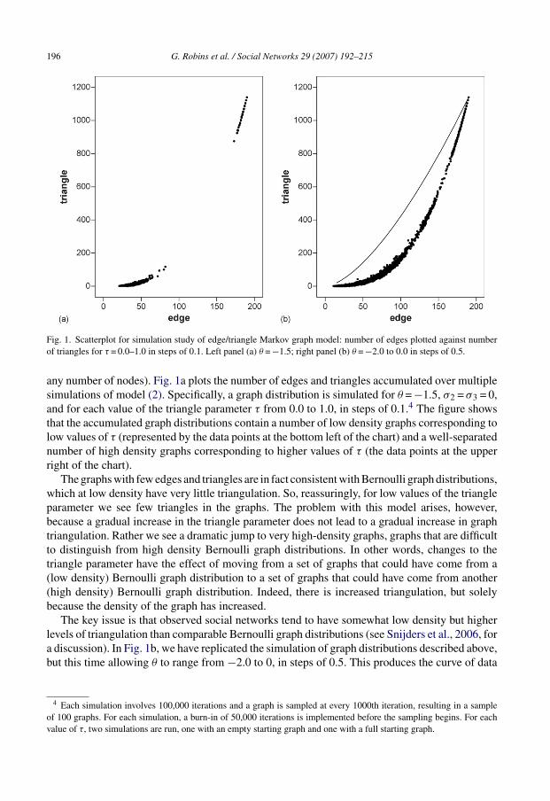
Fig. 1. Scatterplot for simulation study of edge/triangle Markov graph model: number of edges plotted against numberof triangles for τ = 0.0–1.0 in steps of 0.1. Left panel (a) θ = −1.5; right panel (b) θ = −2.0 to 0.0 in steps of 0.5.
any number of nodes). Fig. 1a plots the number of edges and triangles accumulated over multiplesimulations of model (2). Specifically, a graph distribution is simulated for θ = −1.5, σ2 = σ3 = 0,and for each value of the triangle parameter τ from 0.0 to 1.0, in steps of 0.1.4 The figure showsthat the accumulated graph distributions contain a number of low density graphs corresponding tolow values of τ (represented by the data points at the bottom left of the chart) and a well-separatednumber of high density graphs corresponding to higher values of τ (the data points at the upperright of the chart).
The graphs with few edges and triangles are in fact consistent with Bernoulli graph distributions,which at low density have very little triangulation. So, reassuringly, for low values of the triangleparameter we see few triangles in the graphs. The problem with this model arises, however,because a gradual increase in the triangle parameter does not lead to a gradual increase in graphtriangulation. Rather we see a dramatic jump to very high-density graphs, graphs that are difficultto distinguish from high density Bernoulli graph distributions. In other words, changes to thetriangle parameter have the effect of moving from a set of graphs that could have come from a(low density) Bernoulli graph distribution to a set of graphs that could have come from another(high density) Bernoulli graph distribution. Indeed, there is increased triangulation, but solelybecause the density of the graph has increased.
The key issue is that observed social networks tend to have somewhat low density but higherlevels of triangulation than comparable Bernoulli graph distributions (see Snijders et al., 2006, fora discussion). In Fig. 1b, we have replicated the simulation of graph distributions described above,but this time allowing θ to range from −2.0 to 0, in steps of 0.5. This produces the curve of data
4 Each simulation involves 100,000 iterations and a graph is sampled at every 1000th iteration, resulting in a sampleof 100 graphs. For each simulation, a burn-in of 50,000 iterations is implemented before the sampling begins. For eachvalue of τ, two simulations are run, one with an empty starting graph and one with a full starting graph.
G. Robins et al. / Social Networks 29 (2007) 192–215 197
points at the bottom of the chart. This curve, however, is also difficult to distinguish with a rangeof Bernoulli graph distributions.5 The upper curve on the chart, on the other hand, indicates themaximum number of triangles in the graph possible for the given number of edges, so networkscan have substantially more triangles than suggested by the lower curve of data points. (Somerather extreme combinations of θ and τ, when starting the simulations from a complete graph,have a non-negligible probability of leading to a simulated graph on the upper curve.) Becauseobserved social networks so frequently have triangulation much greater than Bernoulli graphs,we expect most networks of interest to lie above the lower curve. Yet it is the lower curve thatrepresents possible outcomes of the edge/triangle models we have simulated. This illustrates thata model with only edge and triangle effects is almost certainly inadequate for most observed socialnetworks.
The problem may not be quite as bad as Fig. 1 suggests. For many observed networks, Markovgraph distributions with non-zero 2- and 3-star parameters (and with the 3-star parameter negative)can produce reasonable models (see Robins et al., 2005; Snijders et al., 2006). Nevertheless, whennetworks have high concentrations of triangles (i.e. suggesting large positive τ), inclusion of starparameters is likely to be inadequate to prevent degeneracy or bimodality.
These problems do not apply only to the triangle parameter: there are degenerate regions ofthe parameter space also for the edge and 2-star model (Handcock, 2003b; Park and Newman,2004).
3. New specifications
Snijders et al. (2006) proposed three new statistics that can be included in specifications forexponential random graph models: alternating k-stars, alternating k-triangles and alternatingindependent two-paths. For this article we concentrate on the first two. We particularly emphasizethe utility of the new concept of alternating k-triangles as a higher order measure of transitivity.We typically refer to these parameters, and their associated models, as higher order because theyinclude configurations with more than three nodes. In this section, we focus on higher orderparameters for non-directed graphs, with some comments about directed versions at the end ofthe section.
3.1. Alternating k-stars
Technically, a model with an alternating k-star parameter alone remains within the class ofMarkov random graph models. The motivation for the new parameter comes from our experienceof fitting models. In fitting models with star parameters to network data sets for which successfullyconvergent estimates could be obtained, we often observed that a higher order star parameterestimate was the opposite sign to, and smaller than, a lower order star parameter. For instance,it would be common in a Markov model such as (2) to see parameter estimates where σ3 wasapproximately equal to −σ2/λ for some λ greater than 1.
In the Markov model of (2), the star parameters are deliberately limited to a maximum of3-stars. More generally, however, the Markov dependence assumption permits higher order stars,up to stars of the maximum possible order (n − 1). In (2) there is an assumption that parameters
5 We know this because simulations with τ set to zero seem to cover the range of graphs produced by simulations withnon-zero τ.
198 G. Robins et al. / Social Networks 29 (2007) 192–215
for these higher order stars are 0, the motivation being to limit the number of parameters and toachieve an identifiable model for which parameters can be estimated.6
The alternating k-star assumption proposes that, rather than setting higher order star parametersto equal 0, all star parameters be retained in the model but with a linear constraint among parametervalues such that, for all k ≥ 2, σ(k+1) = −σk/λ for some λ greater than 1. Then in (1) there is oneparameter σ2 that takes into account all star effects simultaneously, with an associated statistic:
u =n−1∑
k=2
(−1)kSk
λk−2 (3)
In the context of the assumption that σ(k+1) = −σk/λ for k ≥ 2, we refer to the parameter σ2 as thealternating k-star parameter.
The statistic (3) includes stars of all orders but, for λ greater than 1, the impact of higher orderstars is reduced for higher k (that is, for higher order stars) and they have alternating signs. In thatsense, this assumption is rather more general than simply forcing higher order star parameters tohave value 0, the assumption implicit in (2).7
An obvious question is what value to give to λ? We have used λ = 2 in many cases, and thisseems a reasonable starting point for many investigations. But of course it would be desirable toestimate an optimal value of λ. Hunter (2007), also in this special edition, shows how this can bedone (see also Hunter and Handcock, 2006). For the purposes of this article, we set λ = 2.
What is important is how to interpret this parameter in terms of its implications for graphstructure. Of course, the estimate of a parameter for a given local structure is usually indicativeof the extent to which that structure is empirically observed (as long as there are no issues ofdegeneracy or bimodality). But the cumulation of these structures will produce particular globalnetwork patterns as well, so when a network exhibits such patterns, we might expect estimates ofthe relevant parameter to be large and significant.
If the alternating k-star parameter is positive, then highly probable networks are likely to containsome higher degree nodes (“hubs”), whereas a negative parameter suggests that networks with highdegree nodes are improbable, so that nodes tend not to be hubs, with a smaller variance betweenthe degrees. More particularly, Snijders et al. (2006) argued that a positive alternating k-starparameter (together with a negative density parameter) implied graphs that exhibit preference forconnections between a larger number of low degree nodes and a smaller number of higher degreenodes, akin to a core–periphery structure. But once a node reaches a certain degree, the attainmentof additional degrees adds little to its “popularity”.8 So for λ = 2, there is little difference betweena node of degree 5, 6 or higher in “popularity”. Loosely, a node finds its way into the core once ithas achieved a certain degree, with no particularly strong pressure for much higher degrees. At thesame time, other nodes of lower degree remain outside the core. So the global implication is fora “loose” core–periphery structure, with few or any core nodes having particularly high degrees.This core–periphery structure is attained by (dampened) popularity processes. Changing the value
6 This assumption can be seen as analogous to ignoring higher order interactions in, for instance, a standard regression.7 Note that in contrast to standard Markov graphs the statistic is no longer a direct count of configurations in the observed
network, but rather a function of several configurations counts, in this case of counts of the various star configurations. Inother words, we have utilized a Markov dependence assumption, but have imposed a particular form of constraint acrossstar parameters, not the standard homogeneity constraint first used by Frank and Strauss (1986).
8 Here, what we are loosely terming as “popularity” of a node i can be considered more technically as the conditionallog odds under the model of an additional node j forming a tie with i.
G. Robins et al. / Social Networks 29 (2007) 192–215 199
of λ changes the level of dampening, with higher λ implying increased chances for higher degreenodes. Later we show how core–periphery structures may also be attained by strong overlappingtransitivity effects.
An important point is that the parameter assists in modeling the degree distribution. The Markovparameters in model (2) give some leverage over the first three moments of the degree distribution(via the edge, 2- and 3-star parameters), but these are not always sufficient when, for instance,degree distributions exhibit some outliers (high degree nodes). The new parameter, which does notexclude the higher order stars, provides leeway in dealing with such skewed degree distributions.This is not to say, of course, that all possibilities are accommodated, and when networks are highlycentralized with a small number of very high degree nodes (hubs), a model with the new parameteralone is unlikely to provide a good fit to the data (we provide an example below). Nevertheless,our experience to date suggests that the alternating k-star parameter is more useful in model-fittingthan a smaller number of individual Markov star parameters. Sometimes, as shown below, good fitof the degree distribution may be achieved with a combination of an alternating k-star parameterand a standard Markov 2-star parameter.
Why might the alternating k-stars assumption help with degeneracy? Snijders et al. (2006)argued that a model needs a balance between positive and negative star parameters to preventthe resulting graph distribution from being forced towards containing largely complete or largelyempty graphs. The presence of alternating signs in the summation in (3) addresses this balance.
3.2. Alternating k-triangles
The alternating k-triangle assumption moves beyond the dependence assumptions underlyingMarkov random graph models, utilizing instead the partial dependence concept proposed byPattison and Robins (2002). The underlying dependence assumption is presented by Snijders etal. (2006). In short, two possible edges in a graph, Yrs and Yuv, for distinct nodes, r, s, u, v, areassumed to be conditionally dependent if Ysu = Yuv = 1. In other words, if the two possible edgesin the graph were actually observed, they would create a 4-cycle. Substantively, it is not difficultto imagine situations where such social circuit dependence might be plausible. For instance, in anorganization, suppose Steve typically worked with Ursula and Robyn with Victor. Then if Robynand Steve commenced work on a new project, the chances of Ursula and Victor also workingtogether might increase. In other words, the chances of Ursula and Victor working together areincreased by Robyn and Steve working together, but only when Robyn already works with Victorand Steve with Ursula.
Snijders et al. (2006) invoke this dependence assumption in addition to Markov dependence,so in the above case, Yrs and Ysv (and so on) are also assumed to be dependent. It is not difficultto see intuitively that, with both social circuit and Markov dependence, configurations that aremore complex than simple triangles are relevant to the model.
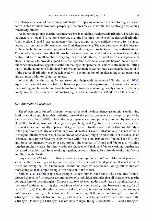
Snijders et al. (2006) proposed k-triangles as new higher order transitivity structures for non-directed graphs. A k-triangle is a combination of k individual triangles that all share one edge (thecommon base of the k triangles). Suppose that two adjacent nodes r and s are also both adjacent tothe same k nodes t1, t2, . . ., tk (i.e. there is an edge between r and tm, and between s and tm, for allm = 1, 2, . . ., k). Then the edge between r and s (the base) is common to the k individual triangleswith nodes r, s and tm. The entire structure comprising all the individual triangles is termed ak-triangle. The edges between r and tm, and between s and tm, are referred to as the sides of thek-triangle. Obviously a 1-triangle is an ordinary triangle. In Fig. 2, we depict 2-, 3- and 4-triangles.
200 G. Robins et al. / Social Networks 29 (2007) 192–215
Fig. 2. 2-, 3- and 4-triangles.
As Snijders et al. (2006) showed, the inclusion of k-triangles in the model leads to a probabilitydistribution where two edge variables are conditionally dependent only if either the Markov con-figuration (a common node) or the social circuit configuration (creation of a 4-cycle) applies. Thisis of some importance since it shows that the model remains strongly constrained by conditionalindependence assumptions.
Let Tk be the count of k-triangles in a graph. Then the k-triangles can be combined into onestatistic in precisely the same way as for the alternating k-stars, that is:
v =n−1∑
k=2
(−1)kTk
λk−2 (4)
This is the alternating k-triangle statistic. The corresponding k-triangle parameter τ = τ1 corre-sponds to a (1-)triangle configuration, with the additional constraint that τk+1 = −τk/λ, where τkis the parameter corresponding to a k-triangle. This statistic and its associated parameter are thenincluded in models of the form (1).
The alternating k-triangle statistic does not simply represent triangulation in the network butadditionally is a measure of the extent to which triangles themselves group together in largerhigher order “clumps” in the network. Near degeneracy for Markov models often occurs whennetworks include larger clique-like structures that contain many triangles, rather than when manytriangles are simply scattered rather homogeneously and individually throughout the network. Inother words, networks that contain dense areas of clumping with many triangles are difficult toreproduce using for Markov random graphs. The detection and examination of such denser areas(e.g. the identification of cohesive subsets of nodes) has had an extensive history and remains amajor theme in network analysis more generally. The transitivity parameter in Markov randomgraphs was a first attempt to model these denser structures because the triangle is the smallestclique among three nodes.
Yet, as Snijders et al. (2006) argued, a transitivity-based parameter incorporating subsets ofnodes larger than three is needed to avoid degeneracy in modeling these agglomerations oftriangles. Such parameters need to strike a balance between a tendency to have rather manycohesive subsets of three or more nodes, but a limitation of the total number of triangles, nec-essary to avoid a complete graph. As well, this parameter requires a statistic that is not linearin the triangle count inside the exponential, in contrast to (2). This linearity in the exponent isa major source of the degeneracy problem when graphs have many triangles. The alternatingk-triangle statistic addresses these needs, with the alternating sign and decreasing weights for
G. Robins et al. / Social Networks 29 (2007) 192–215 201
higher order k-triangles serving the same purposes in limiting degeneracy problems as for alter-nating k-stars.
Broadly, a positive k-triangle parameter can be interpreted as evidence for transitivity effectsin the network. More particularly, a positive k-triangle parameter suggests elements of acore–periphery structure (dependent on other effects in the model), but in this case due to tri-angulation effects rather than to popularity (degree) effects, as was the case for the alternatingk-star effects. We might think of the star-based core–periphery structure as arising from the degreedistribution, a natural outcome of a process whereby a subset of actors are more popular; whereasfor the triangle-based core–periphery process, the degree distribution is itself one of the out-comes of the process, in which a core is built from overlapping triangulations. Below we alsoshow how certain combinations of these star-based and triangle-based processes lead to networksegmentation.
3.3. Alternating k-two-paths
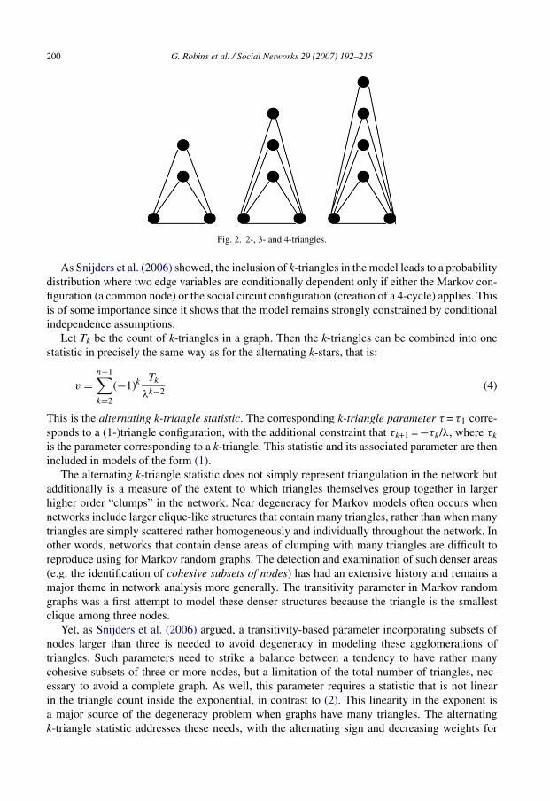
Snijders et al. (2006) also proposed a parameter that is a lower order configuration for ak-triangle, namely a k-two-path. These configurations represent the number of distinct two-pathsbetween a pair of nodes. They can be thought of as k-triangles without the base. The motivation isto introduce a parameter that, when used in conjunction with k-triangles, will enable researchersto distinguish between tendencies to form edges at the base, or at the sides of a k-triangle. Notethat the sides of a k-triangle in the absence of the base represent a type of edge clustering that isonly the precondition to transitivity, while the presence of the base edge reflects transitive closure.So this combination of parameters can provide evidence for pressures to transitive closure (butpressures that do not increasing linearly with k in the exponent). Fig. 3 depicts 2-, 3- and 4-twopath structures. Counts of these structures are then incorporated into one statistic analogously to(4). In this article, we do not concentrate on alternating k-two-path parameters. For some data,we have found it important to include them in models but further work is needed to understandbetter their effect when included with other parameters.
3.4. Alternative equivalent parameterizations
There are equivalent parameterizations to the alternating k-star, alternating k-triangle and alter-nating k-two-path specifications for the model that have mathematical elegance and enhanceinterpretation.
Fig. 3. 2-, 3- and 4-independent two-paths.
202 G. Robins et al. / Social Networks 29 (2007) 192–215
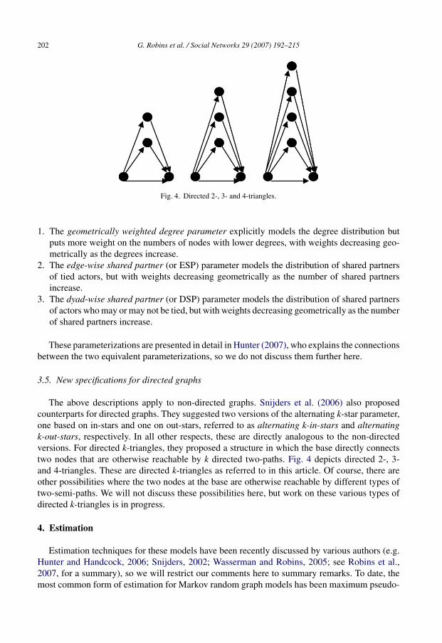
Fig. 4. Directed 2-, 3- and 4-triangles.
1. The geometrically weighted degree parameter explicitly models the degree distribution butputs more weight on the numbers of nodes with lower degrees, with weights decreasing geo-metrically as the degrees increase.
2. The edge-wise shared partner (or ESP) parameter models the distribution of shared partnersof tied actors, but with weights decreasing geometrically as the number of shared partnersincrease.
3. The dyad-wise shared partner (or DSP) parameter models the distribution of shared partnersof actors who may or may not be tied, but with weights decreasing geometrically as the numberof shared partners increase.
These parameterizations are presented in detail in Hunter (2007), who explains the connectionsbetween the two equivalent parameterizations, so we do not discuss them further here.
3.5. New specifications for directed graphs
The above descriptions apply to non-directed graphs. Snijders et al. (2006) also proposedcounterparts for directed graphs. They suggested two versions of the alternating k-star parameter,one based on in-stars and one on out-stars, referred to as alternating k-in-stars and alternatingk-out-stars, respectively. In all other respects, these are directly analogous to the non-directedversions. For directed k-triangles, they proposed a structure in which the base directly connectstwo nodes that are otherwise reachable by k directed two-paths. Fig. 4 depicts directed 2-, 3-and 4-triangles. These are directed k-triangles as referred to in this article. Of course, there areother possibilities where the two nodes at the base are otherwise reachable by different types oftwo-semi-paths. We will not discuss these possibilities here, but work on these various types ofdirected k-triangles is in progress.
4. Estimation
Estimation techniques for these models have been recently discussed by various authors (e.g.Hunter and Handcock, 2006; Snijders, 2002; Wasserman and Robins, 2005; see Robins et al.,2007, for a summary), so we will restrict our comments here to summary remarks. To date, themost common form of estimation for Markov random graph models has been maximum pseudo-
G. Robins et al. / Social Networks 29 (2007) 192–215 203
likelihood (Strauss and Ikeda, 1990). The properties of the pseudo-likelihood estimator are notwell understood, the pseudo-likelihood estimates can at best be thought of as approximate, andit is not clear from existing research as to when pseudo-likelihood estimates may be acceptable.We shall shed some light on this for actual data below.
Monte Carlo Markov chain maximum (MCMC) likelihood estimation, when available, is thepreferred estimation procedure.9 The different Monte Carlo techniques of Snijders (2002) andHunter and Handcock (2006) are both based on refining approximate parameter estimates bycomparing the observed graphs against a distribution of random graphs generated by a stochasticsimulation using the approximate parameter values. If the parameter estimates never stabilize(converge), the model is likely to be degenerate. When convergent estimates are obtained, thensimulation from the estimates will produce distributions of graphs in which the observed graph istypical for all of the effects in the model. One of the advantages over maximum pseudo-likelihoodestimates is that one can also obtain reliable standard errors for the estimates.
Snijders et al. (2006) conditioned on the number of edges when estimating parameters, thatis, they fixed the number of edges in Monte Carlo estimation procedures (see Snijders and vanDuijn, 2002; also Frank and Strauss, 1986, who proposed fixing parameters for estimation ofMarkov graphs). In such models there are no density parameters. Fixing the number of edgesis designed to diminish the risk of degeneracy problems and will have minor effects on otherparameter estimates (except perhaps for star parameters). Our experience has been that, at leastwith smaller networks, conditioning on edges may not be necessary, and estimation proceduresmay successfully converge for the new specifications with density parameters included. This isthe case for all of the examples of convergence that we present in this article.10
4.1. Programs for Monte Carlo maximum likelihood estimation
There are currently three programs available for Monte Carlo maximum likelihood estimation.SIENA and pnet were used to obtain the results in this article. Both use the same algorithm asdescribed below. The program statnet is used in other articles in this special edition (Goodreau,2007; Hunter, 2007).
4.1.1. SIENA (and pnet)The first generally available software to implement Monte Carlo maximum likelihood estima-
tion for exponential random graph models was SIENA (in its 2002 release; the current versionis Snijders et al., 2005) in the StOCNET suite of programs (Boer et al., 2006). The SIENA pro-cedure implements the stochastic approximation algorithm described in Snijders (2002). Morerecently, the pnet program (Wang et al., 2006) has also been developed, implementing the samealgorithm. The estimates from the two programs have been checked against each other, ensuringthey produce the same results (except for differences caused by the stochastic nature of the algo-rithm). In addition to estimates and standard errors, output includes a convergence t-ratio for eachestimate. This ratio indicates how well that estimate has converged, with a small value close to
9 At the time of writing, Monte Carlo estimation was not available, for instance, for some of the more complicatedexponential random graph models in the literature, e.g. for valued networks, for multiple network models involving morethan two networks, and for tripartite graphs. Work is progressing in developing the programs to estimate more complicatedmodels.10 But this may not be universally so. For larger networks, especially directed networks, in some instances conditioning
on edges may be required for convergence. Arguably, this is an indication that model specification is not exactly right.
204 G. Robins et al. / Social Networks 29 (2007) 192–215
zero suggesting good convergence. Estimation may be conditional on edges, or unconditional. Ifany of the t-ratios are too large, this may indicate either that convergence is not yet satisfactory orthat the model is degenerate and incapable of fitting the data. For non-degenerate models, goodconvergence is indicated by t-ratios for all parameter estimates being less than (or close to) 0.1 inabsolute value. (The convergence t-ratio should be distinguished from the usual t-statistic definedas estimate divided by standard error, and used for testing whether the coefficient is 0.)
Efficiency has been improved in the pnet program to the point where on a standard laptopcomputer convergent estimates for models with higher order parameters can be obtained in minutesfor networks of, for instance, 150 nodes. For very large graphs of one thousand or more nodes,estimation will be slow (and statnet might be the preferred option).
Both SIENA and pnet contain some diagnostics that in addition to the convergence t-ratioswill assist judgments about convergence. For instance, SIENA includes the hysteresis analysisdescribed in Snijders et al. (2006). Another good diagnostic is to simulate from the parameterestimates to check that the observed graph is not extreme in the model statistics derived from thesimulated distribution. Sometimes the simulation shows two regions of possible graphs (e.g. highdensity and low density as in Fig. 1a), indicating degeneracy.
Additional information is available from the SIENA website (http://stat.gamma.rug.nl/siena.html) and the StOCNET homepage (http://stat.gamma.rug.nl/stocnet/). Material on pnetis available from the Melnet website (http://www.sna.unimelb.edu.au/).
Statnet is an integrated set of software tools for the representation, visualization, simulationand analysis of network data. The package allows maximum likelihood estimates of exponen-tial random graph models to be calculated using Markov Chain Monte Carlo. The primarymethod is MCMC Newton–Raphson as described in Geyer and Thompson (1992). The stat-net algorithm is different from the stochastic approximation algorithm of Snijders (2002) andis intended to optimize computational efficiency in estimation. For instance, rather than havingmany simulation runs within the program, as is the case for SIENA and pnet, it implementsvery few simulation runs (possibly only one) but then weights the graphs within the simula-tions in ways that optimizes estimation (see Handcock, 2003b; Hunter and Handcock, 2006,for details). This means that the program is able to estimate models for large graphs in areasonably short time frame. The computational procedures in statnet are sophisticated, incor-porating recent advances in Metropolis–Hastings algorithms and multiple proposal types thatprovide flexibility for fitting many kinds of models. The software is written for computing envi-ronment R, a GNU-licensed freeware statistical computing package that runs on a variety ofplatforms, including Windows, Linux and Macintosh based systems. This program uses the Rstatistical language as an interface and so enables a researcher to employ the extensive fea-tures of R in an analysis. If, on the other hand, a researcher wishes simply to estimate models,the R commands to do this are not difficult to learn. The statnet package does much morethan provide parameter estimates. It provides a framework for the analysis of network data.It uses the network package to store network data (Butts, 2005). The bundle also provides sim-ple tools for plotting networks, simulating networks and assessing model goodness of fit (seeGoodreau, 2007). The performance of the MCMC algorithms can be monitored graphically andnumerically. The summary of model results includes the usual estimates and standard errors,as well as estimates of the error attributable to the MCMC algorithm and an analysis of thestatistical deviance (akin to GLM models). In addition, many of the traditional methods andtools of social network analysis are available via the sna package (Butts, 2002). Additionalmaterial is on the statnet webpage http://csde.washington.edu/statnet and in Handcock et al.(2004).
G. Robins et al. / Social Networks 29 (2007) 192–215 205
5. Models with combinations of parameters
There is no impediment to using Markov parameters and the newly specified parameterstogether in one model (we give an example below) although the precise interpretation of anyparameter depends on the other effects in the model. For this article, we wish to compare theperformance of each, so for the most part we keep Markov and the new parameters in separatemodels.
As with any modeling endeavor, the application of one model to the data may not be the end ofthe story. Often it is desirable to fit several different models, either to explore different parametercombinations if it happens that convergence is difficult to achieve, or to find the model that bestrepresents the data. For the purposes of this article, for non-directed graphs we included 2- and 3-star and triangle parameters in Markov models, and alternating k-stars and alternating k-trianglesin higher order models. If these models did not converge we tried either simpler or more complexmodels (e.g. with additional or fewer star parameters). We often found, for instance, that fornon-directed networks very simple models with only edge and alternating k-triangles parameterssuccessfully converged. For Markov models for directed networks, we began by including density,reciprocity, 2- and 3-in- and out-star parameters, and 2-mixed-star, and triangle parameters; and forhigher order models for directed networks, we included density, reciprocity, alternating k-in-stars,alternating k-out-stars and directed alternating k-triangles.
Many of these statistics may exhibit quite high levels of collinearity. Indeed the alternatingk-star and alternating k-triangle statistics can be shown to include the number of edges as oneof the terms in a closed form expression for the statistic (Snijders et al., 2006; see also Hunter,2007). As the alternative weighted degree parameterization does not include the number of edges(Hunter, 2007), this might be a reason to prefer it. In practice, however, collinearity is not usuallya problem for estimating these models, as long as appropriate Monte Carlo estimation techniquesare used.
5.1. Model interpretation and “goodness of fit”
We have already discussed some aspects of parameter interpretation. In brief, a positive alter-nating k-star parameter estimate suggests a degree distribution containing some higher degreenodes, and a resulting “loose” core–periphery structure; whereas a negative parameter suggests atruncated degree distribution with a tendency against particularly high degree nodes. A positivek-triangle parameter estimate suggests a tendency for triangulation in the graph, with the triangletending to form together into “clumps”.
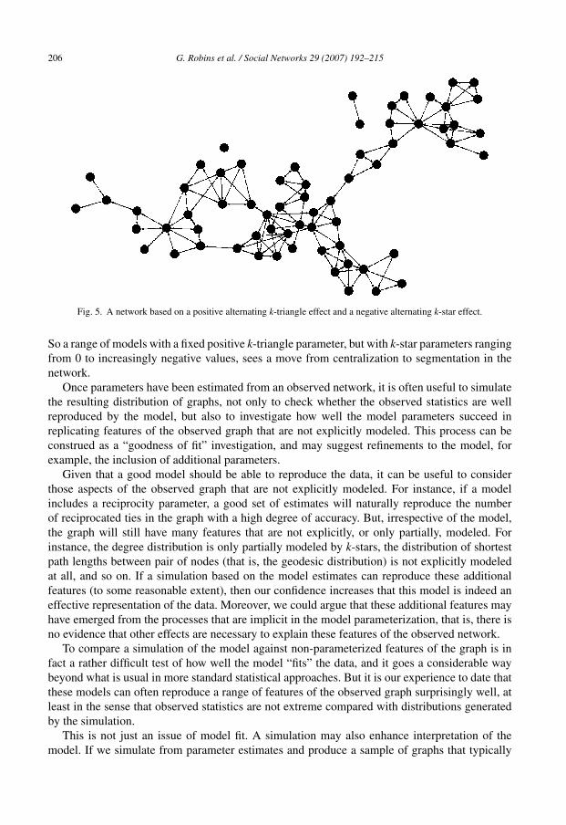
For the higher order models, it is important to interpret the combination in the one model ofalternating k-stars and alternating k-triangle parameters. A pattern of negative k-star and positivek-triangle estimates is not uncommon. Here there are two countervailing tendencies: one towardsa triangulated core–periphery structure, and one against a degree-based core–periphery structure.The global outcome is not a single core of one internally densely connected set of nodes, but several(often connected) smaller regions of overlapping triangles. An example is provided in Fig. 5. Asingle core–periphery structure implied by the positive k-triangle effect has been segmented bythe inclusion of negative k-star parameter into a chain of smaller dense regions of the network.11
11 This graph is from a simulation of non-directed graphs on 65 nodes with parameter values: edge = −0.5, alternatingk-star = −1.5, alternating k-triangle = 2.0.
206 G. Robins et al. / Social Networks 29 (2007) 192–215
Fig. 5. A network based on a positive alternating k-triangle effect and a negative alternating k-star effect.
So a range of models with a fixed positive k-triangle parameter, but with k-star parameters rangingfrom 0 to increasingly negative values, sees a move from centralization to segmentation in thenetwork.
Once parameters have been estimated from an observed network, it is often useful to simulatethe resulting distribution of graphs, not only to check whether the observed statistics are wellreproduced by the model, but also to investigate how well the model parameters succeed inreplicating features of the observed graph that are not explicitly modeled. This process can beconstrued as a “goodness of fit” investigation, and may suggest refinements to the model, forexample, the inclusion of additional parameters.
Given that a good model should be able to reproduce the data, it can be useful to considerthose aspects of the observed graph that are not explicitly modeled. For instance, if a modelincludes a reciprocity parameter, a good set of estimates will naturally reproduce the numberof reciprocated ties in the graph with a high degree of accuracy. But, irrespective of the model,the graph will still have many features that are not explicitly, or only partially, modeled. Forinstance, the degree distribution is only partially modeled by k-stars, the distribution of shortestpath lengths between pair of nodes (that is, the geodesic distribution) is not explicitly modeledat all, and so on. If a simulation based on the model estimates can reproduce these additionalfeatures (to some reasonable extent), then our confidence increases that this model is indeed aneffective representation of the data. Moreover, we could argue that these additional features mayhave emerged from the processes that are implicit in the model parameterization, that is, there isno evidence that other effects are necessary to explain these features of the observed network.
To compare a simulation of the model against non-parameterized features of the graph is infact a rather difficult test of how well the model “fits” the data, and it goes a considerable waybeyond what is usual in more standard statistical approaches. But it is our experience to date thatthese models can often reproduce a range of features of the observed graph surprisingly well, atleast in the sense that observed statistics are not extreme compared with distributions generatedby the simulation.
This is not just an issue of model fit. A simulation may also enhance interpretation of themodel. If we simulate from parameter estimates and produce a sample of graphs that typically
G. Robins et al. / Social Networks 29 (2007) 192–215 207
have a long tailed degree distribution, or a high clustering coefficient, we can infer that this isan expected outcome of the model. Goodreau (2007) provides an example of the effectiveness ofpost hoc simulations in assessing and interpreting a fitted model.
6. Fitting the new specifications to UCINET data sets
We fitted Markov models and models with the new specifications to 20 well-known data setsavailable with the UCINET V network analysis program (Borgatti et al., 1999). The networkswe examined were one-mode (not bipartite), binary (not rankings) and positive relationships (notantagonistic). The data sets comprised: the Kapferer mine data (kapfmm and kapfmu, both of 16nodes and non-directed); the Kapferer tailor shop data (all of 39 nodes, with two non-directednetworks – kapfts1 and kapfts2 – and two directed networks – kapfti1 and kapfti2); the Wolfprimate networks (one directed network, wolfk, on 20 nodes); the Padgett Florentine families data(two non-directed networks on 16 nodes, padgm and padgb); the Krackhardt hi-tech managersdata (two directed networks on 21 nodes, friendship and advice); the Read Highland tribes network(one non-directed network on 16 nodes, Gamapos); the Zachary karate club network (one non-directed network on 34 nodes, Zache); the Roethlisberger and Dickson bank wiring room data(all on 14 nodes, with two non-directed networks – rdpos and rdgam – and one directed network,rdhlp); the Taro exchange network (one non-directed network on 22 nodes); the Thurman officenetwork (one non-directed network on 15 nodes); and the Knoke bureaucracies data (two directednetworks on 10 nodes, knokm and knoki).12 In summary, we have 12 non-directed networks and8 directed networks, with numbers of nodes ranging from 10 to 39.
Models were fitted to all data sets using pnet and checked with SIENA. Without going throughthe details of all the results, Markov models could not be estimated for 5 of 12 non-directednetworks (kapfts1, kapfts2, gamapos, zache, taro), and for 3 of 8 directed networks (kapfti1,kapfti2, wolfk). Models incorporating the new specifications, on the other hand, were estimablefor all of the data sets. All of these higher order models included parameters for k-triangles, withthe exception of the wolfk network which included parameters for alternating in- and out-starsbut was degenerate when an alternating k-triangle parameter was included.13
6.1. Some particular examples: estimates and goodness of fit
Rather than including details of parameter estimates of all models, we provide two illustrativeexamples: one for a non-directed network where Markov models converge (padgb), and one whereMarkov models are degenerate (kapfts1) (Table 1).
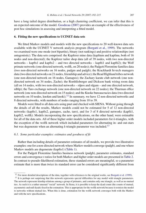
For the Padgett Florentine families business network (padgb), parameter estimates, standarderrors and convergence t-ratios for both Markov and higher order models are presented in Table 2.In contrast to pseudo-likelihood estimation, these standard errors are meaningful, so a parameterestimate that is more than twice its standard error can be considered significantly different from
12 For more detailed descriptions of the data, together with references to the original works, see Borgatti et al. (1999).13 It is perhaps not surprising that this network represents special difficulties for any model with triangle parameters.
The network represents kinship relations among a group of primates, and contains only one triangle, as well as no mutualties. As such it is a rather unusual “social” network. In Siena, it is possible to keep the dyad count (the counts of mutual,asymmetric and null dyads) fixed in the estimation. This is appropriate for the wolfk network because it restricts the modelto networks without mutual ties. When this is done, estimation for the wolfk network converges both with the Markovand with the new specifications.
208 G. Robins et al. / Social Networks 29 (2007) 192–215
Table 1Models for the padgb network: parameter estimates, standard errors and convergence statistics
Parameter Estimate Standard error Convergence-Statistic
zero. For the triangle and alternating k-triangle parameters, a one-sided test is appropriate in mostapplications, so estimates exceeding 1.65 times the standard error can be regarded as significantat the 5% level.
In each model, the edge (or density) parameter is significant, as is the triangle parameter inthe Markov model and the alternating k-triangle parameter in the higher order model. It would beparticularly naıve simply to exclude non-significant parameters from the model without a littleforethought. If we did so, for instance, in the Markov model, we would revert to the edge/trianglemodel which is never likely to be an adequate representation of the data (see Fig. 1).
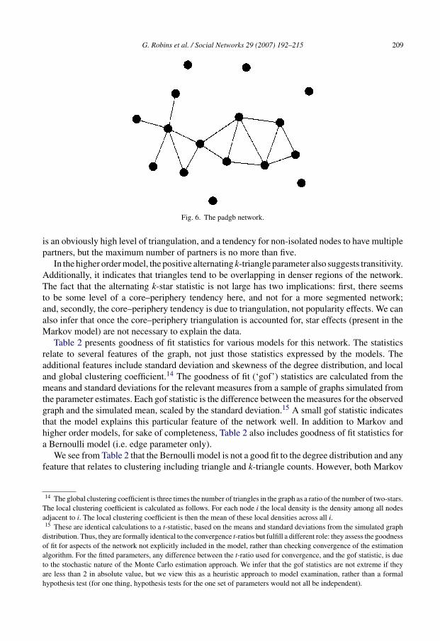
Our interpretation of the parameters is as follows. For the Markov model, the large negativeedge parameter indicates a low baseline propensity (net of other effects) to form ties. The positive2-star and negative 3-star parameters in combination indicates a tendency for multiple networkpartners but with a ceiling on this effect, so that while most nodes will have 2, 3, or possibly morepartners, and the variance of the degrees may be higher than expected for a random graph, thenumber of very high degree nodes is limited. The positive triangle parameter suggests tendenciesfor transitivity in this network. We can see these effects in the network as depicted in Fig. 6. There
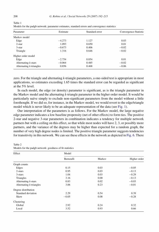
Table 2Models for the padgb network: goodness of fit statistics
G. Robins et al. / Social Networks 29 (2007) 192–215 209
Fig. 6. The padgb network.
is an obviously high level of triangulation, and a tendency for non-isolated nodes to have multiplepartners, but the maximum number of partners is no more than five.
In the higher order model, the positive alternating k-triangle parameter also suggests transitivity.Additionally, it indicates that triangles tend to be overlapping in denser regions of the network.The fact that the alternating k-star statistic is not large has two implications: first, there seemsto be some level of a core–periphery tendency here, and not for a more segmented network;and, secondly, the core–periphery tendency is due to triangulation, not popularity effects. We canalso infer that once the core–periphery triangulation is accounted for, star effects (present in theMarkov model) are not necessary to explain the data.
Table 2 presents goodness of fit statistics for various models for this network. The statisticsrelate to several features of the graph, not just those statistics expressed by the models. Theadditional features include standard deviation and skewness of the degree distribution, and localand global clustering coefficient.14 The goodness of fit (‘gof’) statistics are calculated from themeans and standard deviations for the relevant measures from a sample of graphs simulated fromthe parameter estimates. Each gof statistic is the difference between the measures for the observedgraph and the simulated mean, scaled by the standard deviation.15 A small gof statistic indicatesthat the model explains this particular feature of the network well. In addition to Markov andhigher order models, for sake of completeness, Table 2 also includes goodness of fit statistics fora Bernoulli model (i.e. edge parameter only).
We see from Table 2 that the Bernoulli model is not a good fit to the degree distribution and anyfeature that relates to clustering including triangle and k-triangle counts. However, both Markov
14 The global clustering coefficient is three times the number of triangles in the graph as a ratio of the number of two-stars.The local clustering coefficient is calculated as follows. For each node i the local density is the density among all nodesadjacent to i. The local clustering coefficient is then the mean of these local densities across all i.15 These are identical calculations to a t-statistic, based on the means and standard deviations from the simulated graph
distribution. Thus, they are formally identical to the convergence t-ratios but fulfill a different role: they assess the goodnessof fit for aspects of the network not explicitly included in the model, rather than checking convergence of the estimationalgorithm. For the fitted parameters, any difference between the t-ratio used for convergence, and the gof statistic, is dueto the stochastic nature of the Monte Carlo estimation approach. We infer that the gof statistics are not extreme if theyare less than 2 in absolute value, but we view this as a heuristic approach to model examination, rather than a formalhypothesis test (for one thing, hypothesis tests for the one set of parameters would not all be independent).
210 G. Robins et al. / Social Networks 29 (2007) 192–215
Fig. 7. The kapfts1 network.
and higher order models seem to fit well on all of the features. In addition, we have examined thequartiles of geodesic distributions: both Markov and higher order models produce graphs withgeodesic quartiles that are consistent with the observed network. This is a case where a Markovmodel seems quite adequate and where the higher order model does not provide any marked gainsin terms of fitting the data, although as discussed above consideration of both models providessome interesting points on interpretation.
Next, we turn to the example of the Kapferer tailor shop data, kapfts1, for which the estimationprocedure did not converge in the Markov model case. The network is depicted in Fig. 7. Thefirst point that becomes clear is that because of the larger number of nodes compared with theprevious example, it is not simple to make inferences based solely on visual inspection.
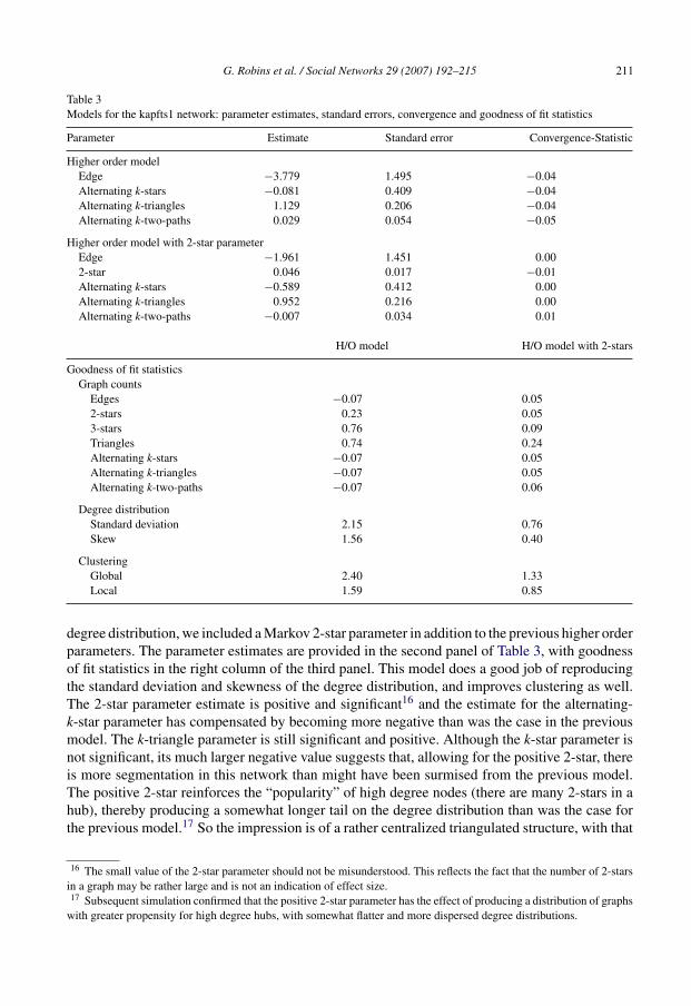
The top panel of Table 3 provides parameter estimates for the higher order model for this data:goodness of fit statistics are provided in the left column of the third panel. In this example we haveincluded the k-two-path parameter in the models but as can be seen this effect is not substantial.
This simple four-parameter model indicates significant clustering among the nodes into denseregions of overlapping triangles. The fact that the alternating k-star parameter, although negative,is small and not significant, suggests a triangulated core–periphery structure. These features areapparent from Fig. 7. But what is also clear from the goodness of fit is that this model does notdo a particularly good job of explaining the degree distribution. The observed graph has a moredispersed and skewed degree distribution than the model would suggest. As well, the level ofclustering in the observed graph is even higher than that predicted by the model. So, for this data,while we can determine nothing from a Markov model, we do learn something from the higherorder specifications, but there are additional features of the network that are not captured.
In some cases it is possible to incorporate further additional effects in the model to improve fit(e.g. Snijders et al., 2006). For the kapfts1 network, given the failure to provide a good fit to the
G. Robins et al. / Social Networks 29 (2007) 192–215 211
Table 3Models for the kapfts1 network: parameter estimates, standard errors, convergence and goodness of fit statistics
Parameter Estimate Standard error Convergence-Statistic
degree distribution, we included a Markov 2-star parameter in addition to the previous higher orderparameters. The parameter estimates are provided in the second panel of Table 3, with goodnessof fit statistics in the right column of the third panel. This model does a good job of reproducingthe standard deviation and skewness of the degree distribution, and improves clustering as well.The 2-star parameter estimate is positive and significant16 and the estimate for the alternating-k-star parameter has compensated by becoming more negative than was the case in the previousmodel. The k-triangle parameter is still significant and positive. Although the k-star parameter isnot significant, its much larger negative value suggests that, allowing for the positive 2-star, thereis more segmentation in this network than might have been surmised from the previous model.The positive 2-star reinforces the “popularity” of high degree nodes (there are many 2-stars in ahub), thereby producing a somewhat longer tail on the degree distribution than was the case forthe previous model.17 So the impression is of a rather centralized triangulated structure, with that
16 The small value of the 2-star parameter should not be misunderstood. This reflects the fact that the number of 2-starsin a graph may be rather large and is not an indication of effect size.17 Subsequent simulation confirmed that the positive 2-star parameter has the effect of producing a distribution of graphs
with greater propensity for high degree hubs, with somewhat flatter and more dispersed degree distributions.
212 G. Robins et al. / Social Networks 29 (2007) 192–215
centralization in part due to some high degree nodes (the 2-star effect), but nevertheless with thepossibility of some segmentation (the negative – but not significant – alternating k-star effect).18
6.2. Comparisons of maximum likelihood and pseudo-likelihood estimates
The UCINET data enable a comparison of the Monte Carlo maximum likelihood (ML) esti-mates with the approximate pseudo-likelihood (PL) estimation procedure. There has been a limitedcomparison of the two estimators in previous studies (see Wasserman and Robins, 2005, for asummary).
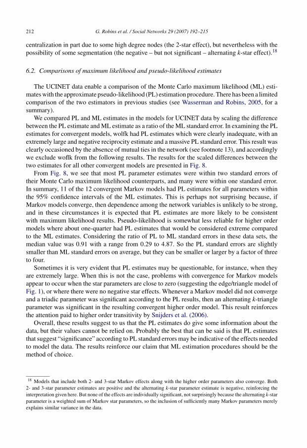
We compared PL and ML estimates in the models for UCINET data by scaling the differencebetween the PL estimate and ML estimate as a ratio of the ML standard error. In examining the PLestimates for convergent models, wolfk had PL estimates which were clearly inadequate, with anextremely large and negative reciprocity estimate and a massive PL standard error. This result wasclearly occasioned by the absence of mutual ties in the network (see footnote 13), and accordinglywe exclude woflk from the following results. The results for the scaled differences between thetwo estimates for all other convergent models are presented in Fig. 8.
From Fig. 8, we see that most PL parameter estimates were within two standard errors oftheir Monte Carlo maximum likelihood counterparts, and many were within one standard error.In summary, 11 of the 12 convergent Markov models had PL estimates for all parameters withinthe 95% confidence intervals of the ML estimates. This is perhaps not surprising because, ifMarkov models converge, then dependence among the network variables is unlikely to be strong,and in these circumstances it is expected that PL estimates are more likely to be consistentwith maximum likelihood results. Pseudo-likelihood is somewhat less reliable for higher ordermodels where about one-quarter had PL estimates that would be considered extreme comparedto the ML estimates. Considering the ratio of PL to ML standard errors in these data sets, themedian value was 0.91 with a range from 0.29 to 4.87. So the PL standard errors are slightlysmaller than ML standard errors on average, but they can be smaller or larger by a factor of threeto four.
Sometimes it is very evident that PL estimates may be questionable, for instance, when theyare extremely large. When this is not the case, problems with convergence for Markov modelsappear to occur when the star parameters are close to zero (suggesting the edge/triangle model ofFig. 1), or where there were no negative star effects. Whenever a Markov model did not convergeand a triadic parameter was significant according to the PL results, then an alternating k-triangleparameter was significant in the resulting convergent higher order model. This result reinforcesthe attention paid to higher order transitivity by Snijders et al. (2006).
Overall, these results suggest to us that the PL estimates do give some information about thedata, but their values cannot be relied on. Probably the best that can be said is that PL estimatesthat suggest “significance” according to PL standard errors may be indicative of the effects neededto model the data. The results reinforce our claim that ML estimation procedures should be themethod of choice.
18 Models that include both 2- and 3-star Markov effects along with the higher order parameters also converge. Both2- and 3-star parameter estimates are positive and the alternating k-star parameter estimate is negative, reinforcing theinterpretation given here. But none of the effects are individually significant, not surprisingly because the alternating k-starparameter is a weighted sum of Markov star parameters, so the inclusion of sufficiently many Markov parameters merelyexplains similar variance in the data.
G. Robins et al. / Social Networks 29 (2007) 192–215 213
Fig. 8. Scaled deviation of pseudo-likelihood estimates.
7. Conclusions
In this article, we have reviewed the new specifications for exponential random graph modelsproposed by Snijders et al. (2006). We demonstrated by empirical example how these may be moreeffective than Markov random graph models. This is not to suggest that Markov random graphmodels are necessarily inappropriate. The point, rather, is that the new specifications offer waysforward in the quite frequent cases when Markov graph models fail because of near-degeneracy.We have illustrated how Markov parameters may still be used effectively alongside the new spec-ifications, and indeed Markov dependence is still an important component in the new models. Wedo not claim that these models will be effective for all networks. But the new models do illustratehow different parameterizations may be developed to address particular modeling purposes.
So there is further work to be done. The focus in this article (and to a lesser extent in Snijderset al., 2006) has been on non-directed graphs. The recommendations by Snijders et al. for newparameterizations of models for directed graphs have already shown their value in achievingconvergence in the case of models for directed graphs in the UCINET data sets. But these recom-mendations can be elaborated further in interesting ways. This is a matter for ongoing work.
Moreover, there are still many gaps in a full representation of network structure. This isevidenced by some of our goodness of fit examples, where a convergent model still does notadequately capture all of the features of the observed network. In addition, the contribution of
214 G. Robins et al. / Social Networks 29 (2007) 192–215
the k-two-path statistic needs to be better understood. We have also not discussed the inclusionof nodal attributes in these models. It is not difficult to incorporate node-level social selectioneffects into the higher order models (Snijders et al., 2006, provide examples).
The new parameters involve higher order constructs than Markov graph configurations. Theyimplement the partial conditional dependence approach of Pattison and Robins (2002) whichemphasizes longer-range connectivity rather than direct adjacency. That such a higher orderapproach is often necessary for successful modeling of empirical networks may tell us some-thing of the emergent properties of certain social systems. It seems clear that sometimes Markovconfigurations do not simply accumulate homogeneously across a network; rather, they agglom-erate heterogeneously within regions of the network. This fact emphasizes the connectedness andoverlapping nature of the basic structures (such as triads) that we use to analyze observed net-works. Through such approaches, then, we may begin to appreciate the interpolation from local toglobal structures, and may seek further understanding of the emergence of higher order structuralfeatures.
Acknowledgements
This work was supported by grants from the Australian Research Council. We are grateful forcomments from the social network groups at the University of Groningen and the University ofMelbourne, and for the helpful suggestions of an anonymous reviewer.
References
Boer, P., Huisman, M., Snijders, T.A.B., Wichers, L.H.Y., Zeggelink, E., 2006. StOCNET: an open software system forthe advanced analysis of social networks. Version 1.7. ICS/Science Plus, Groningen.
Borgatti, S., Everett, M., Freeman, L., 1999. UCINET 5 for Windows: Software for Social Network Analysis. AnalyticTechnologies, Harvard, MA.
Butts, C.T., 2002. Memory Structures for Relational Data in R: Classes and Interfaces Working Paper. Department ofSociology, UC-Irvine.
Butts, C.T., 2005. The Network Package. Manual. Department of Sociology, UC-Irvine (URL:http://erzuli.ss.uci.edu/R.stuff).
Frank, O., 1991. Statistical analysis of change in networks. Statistica Neerlandica 45, 283–293.Frank, O., Strauss, D., 1986. Markov graphs. Journal of the American Statistical Association 81, 832–842.Geyer, C.J., Thompson, E.A., 1992. Constrained Monte Carlo maximum likelihood calculations (with discussion). Journal
of the Royal Statistical Society, Series C 54, 657–699.Goodreau, S., 2007. Applying advances in exponential random graph (p*) models to a large social network. Social
Networks 29, 231–248.Handcock, M.S., 2003a. Statistical models for social networks: degeneracy and inference. In: Breiger, R., Carley, K.,
Pattison, P. (Eds.), Dynamic Social Network Modeling and Analysis. National Academies Press, Washington, DC,pp. 229–240.
Handcock, M.S., 2003b. Assessing degeneracy in statistical models of social networks. Center for Statistics and the SocialSciences. Working Paper No. 39.
Handcock, M., Hunter, D., Butts, C., Goodreau, S., Morris, M., 2004. Statnet: An R Package for the Statistical Modelingof Social Networks. Manual, University of Washington (URL: http://www.csde.washington.edu/statnet).
Hunter, D., 2007. Curved exponential family models for social networks. Social Networks 29, 216–230.Hunter, D., Handcock, M., 2006. Inference in curved exponential family models for networks. Journal of Computational
and Graphical Statistics 15, 565–583.Park, J., Newman, M., 2004. Solution of the 2-star model of a network. Physical Review E 70, 066146.Pattison, P.E., Robins, G.L., 2002. Neighbourhood-based models for social networks. Sociological Methodology 32,
G. Robins et al. / Social Networks 29 (2007) 192–215 215
Pattison, P.E., Wasserman, S., 1999. Logit models and logistic regressions for social networks: II. Multivariate relations.British Journal of Mathematical and Statistical Psychology 52, 169–194.
Robins, G.L., Pattison, P.E., Kalish, Y., Lusher, D., 2007. An introduction to exponential random graph (p*) models forsocial networks. Social Networks 29, 173–191.
Robins, G.L., Pattison, P.E., Wasserman, S., 1999. Logit models and logistic regressions for social networks, III. Valuedrelations. Psychometrika 64, 371–394.
Robins, G.L., Pattison, P.E., Woolcock, J., 2005. Social networks and small worlds. American Journal of Sociology 110,894–936.
Snijders, T.A.B., 2002. Markov chain Monte Carlo estimation of exponential random graph models. Journal of SocialStructure 3, 2.
Snijders, T.A.B., van Duijn, M.A.J., 2002. Conditional maximum likelihood estimation under various specifications ofexponential random graph models. In: Jan Hagberg (Ed.), Contributions to Social Network Analysis, InformationTheory, and Other Topics: A Festschrift in Honour of Ove Frank. Department of Statistics, University of Stockholm,pp. 117–134.
Snijders, T.A.B., Pattison, P., Robins, G.L., Handcock, M., 2006. New specifications for exponential random graph models.Sociological Methodology.
Snijders, T.A.B., Steglich, C.E.G., Schweinberger, M., Huisman, M., 2005. Manual of SIENA Version 2.1. ICS, Universityof Groningen, Groningen.
Strauss, D., 1986. On a general class of models for interaction. SIAM Review 28, 513–527.Strauss, D., Ikeda, M., 1990. Pseudo-likelihood estimation for social networks. Journal of the American Statistical Asso-
ciation 85, 204–212.Wang, P., Robins, G., Pattison, P., 2006. Pnet: A Program for the Simulation and Estimation of Exponential Random
Graph Models. University of Melbourne.Wasserman, S., Pattison, P.E., 1996. Logit models and logistic regressions for social networks: I. An introduction to
Markov graphs and p*. Psychometrika 61, 401–425.Wasserman, S., Robins, G.L., 2005. An introduction to random graphs, dependence graphs, and p*. In: Carrington, P.,
Scott, J., Wasserman, S. (Eds.), Models and Methods in Social Network Analysis. Cambridge University Press, NewYork, pp. 148–161.


![Some statistical approaches in random graph modelingmath.univ-lille1.fr/~tran/Exposesgraphesaleatoires/Matias.pdf · I Exponential random graph model (ERGM) [Frank & Strauss 86].](https://static.documents.pub/doc/80x56/5fcf53907e447967c1590ae8/some-statistical-approaches-in-random-graph-tranexposesgraphesaleatoiresmatiaspdf.jpg)


