522

Recent Progress in Conformal Geometry

Imperial College Press Advanced Texts in Mathematics
Series Editor: Dennis Barden (Univ. of Cambridge, UK)
Vol. 1 Recent Progress in Conformal Geometryby Abbas Bahri (Rutgers Univ. USA) & YongZhong Xu(Courant Inst. for the Mathematical Sciences, USA)
ZhangJi - Recent Progress.pmd 1/12/2007, 5:09 PM2

ICP Imperial College Press
Recent Progress in Conformal Geometry
ICP Advanced Texts in Mathematics – Vol. 1
Abbas Bahri Rutgers University, USA
Yongzhong Xu Courant Institute for the Mathematical Sciences, USA

British Library Cataloguing-in-Publication DataA catalogue record for this book is available from the British Library.
Published by
Imperial College Press57 Shelton StreetCovent GardenLondon WC2H 9HE
Distributed by
World Scientific Publishing Co. Pte. Ltd.
5 Toh Tuck Link, Singapore 596224
USA office: 27 Warren Street, Suite 401-402, Hackensack, NJ 07601
UK office: 57 Shelton Street, Covent Garden, London WC2H 9HE
Printed in Singapore.
For photocopying of material in this volume, please pay a copying fee through the CopyrightClearance Center, Inc., 222 Rosewood Drive, Danvers, MA 01923, USA. In this case permission tophotocopy is not required from the publisher.
ISBN-13 978-1-86094-772-8ISBN-10 1-86094-772-7
All rights reserved. This book, or parts thereof, may not be reproduced in any form or by any means,electronic or mechanical, including photocopying, recording or any information storage and retrievalsystem now known or to be invented, without written permission from the Publisher.
Copyright © 2007 by Imperial College Press
RECENT PROGRESS IN CONFORMAL GEOMETRY
ZhangJi - Recent Progress.pmd 1/12/2007, 5:09 PM1

January 17, 2007 11:55 WSPC/Book Trim Size for 9in x 6in finalBB
Preface
This book is divided into two parts. The first part is about Sign-ChangingYamabe-type problems. A Morse Lemma at infinity, under reasonable basicconjectures, is proved for such problems. This work is an attempt to definea new area of research for nonlinear analysts. We have tried in it to providea family of estimates and techniques with the help of which the problem offinding infinitely many solutions to these equations on domains of R3 canbe studied.
Our estimates and our work is a “cas d’ecole” in that we work on R3
or S3, a framework where solutions are known to exist, in fact in infinitenumber; and we have chosen to study the asymptots generated by thesesolutions and their combinations under the action of the Conformal Group.This work could also be useful for other variational problems such as Ein-stein or Yang-Mills equations.
The second part of this book is about Contact Form Geometry viaLegendrian curves. Given a three-dimensional compact orientable manifoldM3 and a contact form α on it, we have assumed in earlier works theexistence of a “dual” contact form β, β = dα(v, ·), with the same orientationthan α and we have introduced the variational problem
∫ 1
0αx(x)dt on Cβ =
x ∈ H1(S1, M)|βx(x) ≡ 0. We have defined a homology related to theperiodic orbits of the Reeb vector-field ξ of α on Cβ .
We prove in this framework two main results. First, we establish thatthe hypothesis that β is a contact form with the same orientation than α isnot essential. The techniques involved in order to prove such a result (on atypical example) have the definite advantage that they are quantitative: aswe allow regions where β is no longer a contact form with the same orien-tation than α, we track down the modifications of the variational problemand we provide bounds on a key quantity (denoted τ) as we introduce a
v
January 17, 2007 11:55 WSPC/Book Trim Size for 9in x 6in finalBB
vi Recent Progress in Conformal Geometry
large amount of rotation for kerα along the orbits of v near these areas.We then move to prove a compactness result about the flow-lines of
this variational problem which originate at a periodic orbit of ξ. This —still slightly imperfect — compactness result indicates that all flow-linesoriginating at periodic orbits go to periodic orbits (at least if the differenceof Morse indexes is 1), unless the number of zeros of the v-component of x,the tangent vector to the curves under deformation, drops.
No critical point at infinity (asymptot)interferes with this homology. Westrongly suspect that this homology is, in the case of the standard contactstructure of S3, the homology of PC∞. We expect that we will be able tocompute this homology in some easy cases at least.
We had been searching for a long time for such a result. This workentitled “Compactness” will be published independently by the first au-thor and dedicated to his long time friend and collaborator Haim Brezisfor his sixtieth birthday. Both directions of research i.e. Conformal Geom-etry, Einstein equations, Yang-Mills equations on one hand, Contact FormGeometry on the other hand, are also studied by other techniques due to“hard-chore” Geometry and Symplectic Geometry.
In fact, Geometers have always been our “co-area researchers”. Weview these areas which we have contributed to define — for Contact FormGeometry — in a different way and with different techniques.
This book is a book of collaboration and research. It also defines newgoals and presents a new understanding. It is not (yet) a textbook forgraduate students. It rather informs our collaborators about a definiteprogress in the two above mentioned areas.
This research has been long; and at times hard and difficult. It hasbeen a strain on our friends and companions. Thanks are due: AbbasBahri wishes to thank Haim Brezis, his long-time collaborator and friend,not only for his obvious support but more so for his friendship. Having afriend — and of such a quality — is a rare blessing in life.
Abbas Bahri wishes also to thank Diana Nunziante, his wife, for herpatience, her understanding and her love as this book was being written.
Lines and equations are written, but only with the overwhelming intel-ligence and love of those closest to us.
Both of us extend our warmest thanks to Barbara Mastrian for herwonderful work as well as her wit and life. It has been a pleasure to workwith her all these years.
Finally, we would like to thank H. Brezis, S. Chanillo, R. Nussbaumand Z. Han for giving up so much of their time and patiently listen to our

January 17, 2007 11:55 WSPC/Book Trim Size for 9in x 6in finalBB
Preface vii
arguments as they developed.We also thank them, as well as our friends and colleagues of the Math-
ematics Department at Rutgers, for their thoughtful remarks and observa-tions.

January 17, 2007 11:55 WSPC/Book Trim Size for 9in x 6in finalBB
This page intentionally left blankThis page intentionally left blank
January 17, 2007 11:55 WSPC/Book Trim Size for 9in x 6in finalBB
Contents
Preface v
A. Bahri and Y. Xu
1. Sign-Changing Yamabe-Type Problems 1
1.1 General Introduction . . . . . . . . . . . . . . . . . . . . . . 11.2 Results and Conditions . . . . . . . . . . . . . . . . . . . . . 21.3 Conjecture 2 and Sketch of the Proof of Theorem 1; Outline 71.4 The Difference of Topology . . . . . . . . . . . . . . . . . . 111.5 Open Problems . . . . . . . . . . . . . . . . . . . . . . . . . 14
1.5.1 Understand the difference of topology . . . . . . . . 141.5.2 Non critical asymptots . . . . . . . . . . . . . . . . . 151.5.3 The exit set from infinity . . . . . . . . . . . . . . . . 151.5.4 Establishing Conjecture 2 and continuous forms of the
discrete inequality . . . . . . . . . . . . . . . . . . . 161.5.5 The Morse Lemma at infinity, Part I, II, III . . . . . 161.5.6 Notations v, vi, hi . . . . . . . . . . . . . . . . . . . . 16
1.6 Preliminary Estimates and Expansions, the Principal Terms 171.7 Preliminary Estimates . . . . . . . . . . . . . . . . . . . . . 18
1.7.1 The equation satisfied by v . . . . . . . . . . . . . . 191.7.2 First estimates on vi and hi . . . . . . . . . . . . . . 231.7.3 The matrix A . . . . . . . . . . . . . . . . . . . . . . 251.7.4 Towards an H1
0 -estimate on vi and an L∞-estimateon hi . . . . . . . . . . . . . . . . . . . . . . . . . . . 26
1.7.5 The formal estimate on hi . . . . . . . . . . . . . . . 311.7.6 Remarks about the basic estimates . . . . . . . . . . 35
ix
January 17, 2007 11:55 WSPC/Book Trim Size for 9in x 6in finalBB
x Recent Progress in Conformal Geometry
1.7.7 Estimating the right hand side of Lemma 12 . . . . . 351.7.8 Ri and the estimate on |vi|H1
0. . . . . . . . . . . . . 45
1.8 Proof of the Morse Lemma at Infinity When theConcentrations are Comparable . . . . . . . . . . . . . . . . 54
1.9 Redirecting the Estimates, Estimates on |vi|H10
+ |h0i |∞ +∑
λs>λi
εsi |hs
i |∞ . . . . . . . . . . . . . . . . . . . . . . . . . . 66
1.9.1 Content of Part II . . . . . . . . . . . . . . . . . . . 661.9.2 Redirecting the estimates . . . . . . . . . . . . . . . 68
1.10 Proof of the Morse Lemma at Infinity . . . . . . . . . . . . 1081.10.1 Decomposition in groups, gradient and
L∞-estimates on v, proof of the Morse Lemmaat infinity . . . . . . . . . . . . . . . . . . . . . . . . 108
1.10.2 Content of Part III . . . . . . . . . . . . . . . . . . . 1081.10.3 Basic conformally invariant estimates . . . . . . . . . 1091.10.4 Estimates on v − (vI + vII) . . . . . . . . . . . . . . 1211.10.5 The expansion . . . . . . . . . . . . . . . . . . . . . . 1291.10.6 The coefficient in front of εkδ . . . . . . . . . . . . 1541.10.7 The σi-equation, the estimate on
∑ |γji | . . . . . . . 159
1.10.8 The system of equations corresponding to thevariations of the points ai . . . . . . . . . . . . . . . 174
1.10.9 Rule about the variation of the points ofconcentrations of the various groups . . . . . . . . . 182
1.10.10The basic parameters and the end of the expansion . 1851.10.11Remarks on the basic parameters . . . . . . . . . . . 1851.10.12The end of the expansion and the concluding
remarks . . . . . . . . . . . . . . . . . . . . . . . . . 189
Bibliography 199
2. Contact Form Geometry 201
2.1 General Introduction . . . . . . . . . . . . . . . . . . . . . . 2012.2 On the Dynamics of a Contact Structure along a Vector Field
of its Kernel . . . . . . . . . . . . . . . . . . . . . . . . . . . 2052.2.1 Introduction . . . . . . . . . . . . . . . . . . . . . . . 2052.2.2 Introducing a large rotation . . . . . . . . . . . . . . 2102.2.3 How γ is built . . . . . . . . . . . . . . . . . . . . . . 2142.2.4 Modification of α into αN . . . . . . . . . . . . . . . 2262.2.5 Computation of ξN . . . . . . . . . . . . . . . . . . . 227
January 17, 2007 11:55 WSPC/Book Trim Size for 9in x 6in finalBB
Contents xi
2.2.6 Conformal deformation . . . . . . . . . . . . . . . . . 2352.2.7 Choice of λ . . . . . . . . . . . . . . . . . . . . . . . 2402.2.8 First step in the construction of λ . . . . . . . . . . . 241
2.3 Appendix 1 . . . . . . . . . . . . . . . . . . . . . . . . . . . 2752.3.1 The normal form for (α, v) when α does not turn well 275
2.4 The Normal Form of (α, v) Near an Attractive Periodic Orbitof v . . . . . . . . . . . . . . . . . . . . . . . . . . . . . . . 276
2.5 Compactness . . . . . . . . . . . . . . . . . . . . . . . . . . 2792.5.1 Some basic facts . . . . . . . . . . . . . . . . . . . . 2802.5.2 A model for Wu(xm), the unstable manifold in Cβ of
a periodic orbit of index m . . . . . . . . . . . . . . . 2822.5.3 Hypothesis (A), Hypothesis (B), Statement of the
result . . . . . . . . . . . . . . . . . . . . . . . . . . . 2882.5.4 The hole flow . . . . . . . . . . . . . . . . . . . . . . 291
2.5.4.1 Combinatorics . . . . . . . . . . . . . . . . 2912.5.4.2 Normals . . . . . . . . . . . . . . . . . . . . 2942.5.4.3 Hole flow and Normal (II)-flow on curves of
Γ4k near x∞ . . . . . . . . . . . . . . . . . . 2962.5.4.4 Forced repetition . . . . . . . . . . . . . . . 2992.5.4.5 The Global picture, the degree is zero . . . . 301
2.5.5 Companions . . . . . . . . . . . . . . . . . . . . . . . 3042.5.5.1 Their definition, births and deaths . . . . . 3042.5.5.2 Families and nodes . . . . . . . . . . . . . . 305
2.5.6 Flow-lines for x2k+1 to x∞2k . . . . . . . . . . . . . . . 323
2.5.7 The S1-classifying map . . . . . . . . . . . . . . . . . 3322.5.8 Small and high oscillation, consecutive characteristic
pieces . . . . . . . . . . . . . . . . . . . . . . . . . . 3342.5.9 Iterates of critical points at infinity . . . . . . . . . . 3542.5.10 The Fredholm aspect . . . . . . . . . . . . . . . . . . 3592.5.11 Transversality and the compactness argument . . . . 364
2.6 Transmutations . . . . . . . . . . . . . . . . . . . . . . . . . 3842.6.1 Study of the Poincare-return maps . . . . . . . . . . 4022.6.2 Definition of a basis of Tx∞Γ2s for the reduction of
d2J(x∞) . . . . . . . . . . . . . . . . . . . . . . . . 4132.6.3 Compatibility . . . . . . . . . . . . . . . . . . . . . . 417
2.7 On the Morse Index of a Functional Arising in Contact FormGeometry . . . . . . . . . . . . . . . . . . . . . . . . . . . . 4202.7.1 Introduction . . . . . . . . . . . . . . . . . . . . . . 4202.7.2 The Case of Γ2 . . . . . . . . . . . . . . . . . . . . . 424
January 17, 2007 11:55 WSPC/Book Trim Size for 9in x 6in finalBB
xii Recent Progress in Conformal Geometry
2.7.3 Darboux Coordinates . . . . . . . . . . . . . . . . . . 4252.7.4 The v-transport maps . . . . . . . . . . . . . . . . . 4302.7.5 The equations of the characteristic manifold near x∞;
the equations of a critical point . . . . . . . . . . . . 4342.7.5.1 The characteristic manifold for the unper-
turbed problem . . . . . . . . . . . . . . . . 4342.7.6 Critical points, vanishing of the determinant . . . . . 4362.7.7 Introducing the perturbation . . . . . . . . . . . . . 4372.7.8 The characteristic manifold for the perturbed
problem; the determinant equations . . . . . . . . . . 4412.7.9 Reduction to the Case k = 1 . . . . . . . . . . . . . . 4472.7.10 Modification of d2Jτ
∞(x∞) |spanu2,···,uk−1 . . . . . . 4542.7.11 Calculation of ∂2J∞(x∞).u2.u3 . . . . . . . . . . . . 459
2.8 Calculation of ∂2J∞(x∞).u2.u2 . . . . . . . . . . . . . . . . 4652.9 Calculation of ∂2J∞(x∞).u2.u4 . . . . . . . . . . . . . . . . 4712.10 Other Second Order Derivatives . . . . . . . . . . . . . . . . 4742.11 Appendix . . . . . . . . . . . . . . . . . . . . . . . . . . . . 476
2.11.1 The Proof of Lemma 42 . . . . . . . . . . . . . . . . 4762.11.2 The proof of Lemma 47 . . . . . . . . . . . . . . . . 4802.11.3 Proof of the Lemmas in 2.7.11 . . . . . . . . . . . . . 4832.11.4 Proof of Lemma 48 . . . . . . . . . . . . . . . . . . . 4832.11.5 The Proof of Lemma 49 . . . . . . . . . . . . . . . . 4842.11.6 The proof of Lemma 50 . . . . . . . . . . . . . . . . 4852.11.7 Proof of Claim 1 . . . . . . . . . . . . . . . . . . . . 4872.11.8 Proof of Claim 3 . . . . . . . . . . . . . . . . . . . . 4892.11.9 The Final Details of the Calculation of
∂2J(x∞).u2.u3 . . . . . . . . . . . . . . . . . . . . 4922.11.10Details involved in 2.8 . . . . . . . . . . . . . . . . . 4942.11.11Proof of Lemma 52 . . . . . . . . . . . . . . . . . . . 4942.11.12Proof of Lemma 53 . . . . . . . . . . . . . . . . . . . 4952.11.13Proof of Claim 3 . . . . . . . . . . . . . . . . . . . . 4962.11.14Proof of Claim 4 . . . . . . . . . . . . . . . . . . . . 4972.11.15Details of the Calculation of ∂2J.u2.u2 . . . . . . . . 503
Bibliography 509

January 17, 2007 11:55 WSPC/Book Trim Size for 9in x 6in finalBB
Chapter 1
Sign-Changing Yamabe-TypeProblems
1.1 General Introduction
Let us consider a very simple (and classical) model in Nonlinear Analysisand Riemannian Geometry, namely the Yamabe problem on S3, with thestandard metric:
−3∆S3u + 4u = u5 u > 0. (1.1)
Equivalently, we might consider
∆R3u + u5 = 0 u > 0. (1.2)
This problem has received a lot of attention in the 1980’s and the 1990’sbecause of the Yamabe conjecture and the scalar-curvature problem. Twoor three main techniques have been devised to solve such problems: mini-mizing techniques combined with geometric results (positive mass conjec-ture etc.), variational techniques combined with topological techniques andstudy of critical points at infinity, maximum principle techniques to derivea priori estimates. We are interested here in the variational techniques andthe study of the critical points at infinity.
In order to describe this technique, we recall that (1.1) or (1.2) are vari-ational problems with defects. The defect relies in the “non-compactness”or failure of the Palais-Smale condition. Indeed, the set of solutions of (1.1)or (1.2) is non-compact because the conformal group of S3 (which leaves(1.1) or (1.2) invariant) is non-compact. All the (for (1.2)) functions
δ(a, λ) =c√
λ
(1 + λ2|x − a|2)1/2
are solutions of (1.2). Combinations∑p
i=1 δ(ai, λi) of such functions (λi →+∞) are almost solutions. These problems have asymptots.
1

January 17, 2007 11:55 WSPC/Book Trim Size for 9in x 6in finalBB
2 Recent Progress in Conformal Geometry
Our aim is to complete for them a Morse Lemma at infinity (see [Bahri1989], [Bahri 2001], [Bahri and Coron (1988)]) from which formulae for thedifference of topology in the level sets of the associated functional and (quiteinvolved sometimes, see [Aubin (1976)]) mechanisms of existence could bederived. All the techniques — including the geometric techniques used byAubin [Aubin (1976)], Schoen [Schoen (1988)], Schoen and Yau [Schoen andYau (1988)] etc.— use heavily the assumption that the function u which issought for should be positive. This further requirement, which should makethe problem more difficult, makes it easier in some regard, since the varia-tions (this is a variational problem) can be restricted (because of the specialstructure of (1.1)) to the set of positive functions. The non-compactnessis then less stringent (limited to the δ(a, λ)’s and their combiniations) andmore controlled. The maximum principle can be used as well as Alexandrovreflection techniques. The positivity helps also considerably in the proof ofthe Morse Lemmas at infinity.
However, (1.1) and (1.2) are well-posed problems without the assump-tion u > 0 and it makes perfect sense to study these questions, as wellas equations of this type on domains or with other metrics or manifoldswithout the positivity assumption.
There are several motivations to study (1.1) or (1.2) without the pos-itivity assumption, besides the main ones, namely that it displays newphenomena, and a new and interesting direction of research.
One of the main mathematical motivations is that (1.1) or (1.2) hasinfinite many changing-sign solutions which are not explicitly known. Thus,understanding the non compactness in such problems is closer to the (twodimensional) harmonic map problem or the Yang-Mills equations (awayfrom minima).
The Yamabe problem, without the positivity assumption, is a sim-pler model of less explicit non-compactness phenomena. (1.2) is “un casd’ecole”.
1.2 Results and Conditions
We state now the result which we wish to prove, then the result which wehave established and the conditions under which we have completed thiswork. We then discuss these conditions.
The functional is
J(u) =1∫
R3 u6dx
for u ∈∑ = w;∫ |∇w|2 +
∫w6 < +∞;
∫ |∇w|2 = 1.
January 17, 2007 11:55 WSPC/Book Trim Size for 9in x 6in finalBB
Sign-Changing Yamabe-Type Problems 3
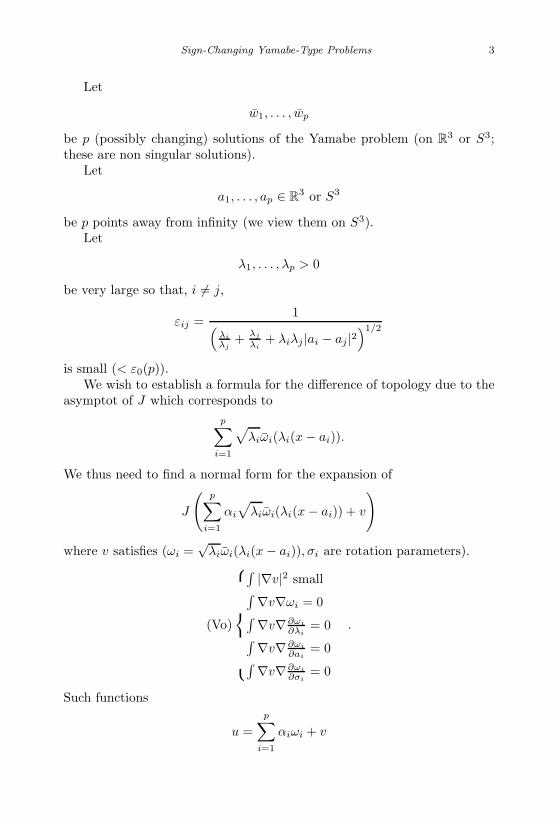
Let
w1, . . . , wp
be p (possibly changing) solutions of the Yamabe problem (on R3 or S3;these are non singular solutions).
Let
a1, . . . , ap ∈ R3 or S3
be p points away from infinity (we view them on S3).Let
λ1, . . . , λp > 0
be very large so that, i = j,
εij =1(
λi
λj+ λj
λi+ λiλj |ai − aj |2
)1/2
is small (< ε0(p)).We wish to establish a formula for the difference of topology due to the
asymptot of J which corresponds top∑
i=1
√λiωi(λi(x − ai)).
We thus need to find a normal form for the expansion of
J
(p∑
i=1
αi
√λiωi(λi(x − ai)) + v
)
where v satisfies (ωi =√
λiωi(λi(x − ai)), σi are rotation parameters).
(Vo)
∫ |∇v|2 small∫ ∇v∇ωi = 0∫ ∇v∇∂ωi
∂λi= 0∫ ∇v∇∂ωi
∂ai= 0∫ ∇v∇∂ωi
∂σi= 0
.
Such functions
u =p∑
i=1
αiωi + v

January 17, 2007 11:55 WSPC/Book Trim Size for 9in x 6in finalBB
4 Recent Progress in Conformal Geometry
where v satisfies (Vo) can be seen to span neighborhoods of the asymptot(neighborhoods of the critical points at infinity).
The conjecture is then:
Conjecture 1 There is a change of variables in the (αi, λi, ai, v)-spacesuch that
J
(p∑
i=1
αiωi + v
)=
(p∑
i=1
α2i
∫ |∇ωi|2)3
p∑i=1
α6i
∫ω6
i
×1 − c
∑i=j
ωi(˜aj)ω∞j εij −
∑i=j
cij(ωi, ωj)ε3ij + Q(V, V )
(αi, ai, λi, V ) are the new variables. Q is a nondegenerate quadratic formin V . V is in a small neighborhood of zero in a Hilbert space.
The expression ωi(˜aj)ω∞j requires some explanations. ω∞
j is the value ofωj(x) at the north pole when ωj is concentrated at the south pole. When ωi
is totally deconcentrated, ωi(˜aj) is the value of ω (ωi after deconcentration)at ˜aj the concentration point of ωj (see [Bahri 2001]). Index Q is the sum ofthe strict indexes of each ωi. We assume that each of them is nondegeneratetransversally to the conformal group.
The result which we prove here is close to Conjecture 1. Its proof relieson two additional assumptions which we conjecture to hold and which read:
Conjecture 2 There exists a constant c(p) > 0 such that, for any(a1, . . . ap) ∈ R3p and (u1, . . . , up) ∈ Rp,
|Au|2 + supi,j
|tu ∂A
∂aji
u| ≥ c(p)∑i=j
u2i
|ai − aj |2
A is the matrix 0 1|ai−aj |
. . .1
|ai−aj | 0
.
Conjecture 3 Let σi be the compact (rotation-related) parameters of theconformal group acting on ωi. Assume that, for each i and for a smallconstant c:

January 17, 2007 11:55 WSPC/Book Trim Size for 9in x 6in finalBB
Sign-Changing Yamabe-Type Problems 5
If
−c∂ω∞
i
∂σi
(∑j =i
ω∞j εij
)=∑i=j
∂cij
∂σiε3
ij
∑i
∣∣∣∣ ∑j =i
(ω∞
i (ω∞j +
Dω∞j (
ai−aj|ai−aj | )
λj |ai−aj | + 3 cij
c ε2ij
)εij
∣∣∣∣≤ c
(∑i=j
ε3ij +
∑ω∞2
i εij
).
then,
∑i
∣∣∣∣∑j =i
ω∞i ω∞
j
∂εij
∂ai+∑j =i
εijω∞j
∂
∂ai
(Dω∞
j |( ai−aj
|ai−aj | )
λj |ai − aj |
)
+3c
∑j =i
cijε2ij
∂εij
∂ai
∣∣∣∣ ≥ c
∑j =i
ω∞2
i
λi|ai − aj | +∑ ε3
ij
|ai − aj |
Observation.Replacing εij by 1√
λiλj |ai−aj |, we can see that, if Conjecture 3 does not
hold, we have more conditions than variables.There are variants of Conjecture 2 and Conjecture 3 which we need also
to introduce:
Conjecture 2′ Let ϕ and ϕ′ be two different charts of S3−pt where the
South and North poles are “far” from the points ai. Let u =
...ω∞
i /√
λi
...
,
in the first chart and u′ =
...ω∞
i /√
λ′i
...
, in the second chart be the corre-
sponding vector associated to∑
αiωi. Let A′ be the matrix A at the pointsa′
i in the second chart.There exists c(p) > 0 such that, for any (a1, . . . ap) ∈ R3p and
(ω1, . . . , ωp) solutions of the Yamabe problem on S3:
sup(i,j)
|tu ∂A
∂aji
u| + sup(i,j)
|tu′ ∂A′
∂a′ji
u′| ≥ c(p)∑i=j
ω∞2i
λi|ai − aj |2 .

January 17, 2007 11:55 WSPC/Book Trim Size for 9in x 6in finalBB
6 Recent Progress in Conformal Geometry
Conjecture 3′ Let σi be the compact rotation parameters correspondingto rotations preserving the polar axis (hence ∂ω∞
i
∂σi= 0).
Assume that, for each i,∑i=j
∂cij
∂σiε3
ij = 0.
The ai-equations∑i
∣∣∣∣ ∑j =i
(ω∞
i ω∞j + 3 cij
c ε2ij
) ∂εij
∂ai+∑j =i
εijω∞j
∂∂ai
(Dω∞
j (ai−aj|ai−aj | )
λi|ai−aj |
)∣∣∣∣ = 0
hold in both charts
.
Then,
∑i
∣∣∑j =i
(ω∞
i
(ω∞
j +Dω∞
j ( ai−aj
|ai−aj | )
λj |ai − aj |
)+ 3
cij
cε2
ij
)εij
∣∣∣∣≥ c
∑i=j
ε3ij +
∑ω∞2
i εij
.
We also define a well-distributed packing in groups of a configuration∑αiωi + v to be a packing of the concentration points ai of the ωi’s into
groups G1, . . . , G such that
i) d(ai, aj) = o(d(ai, ak)) if i, j ∈ Gm and k ∈ Gs, s = m.
ii) If, for (i, j, m) pairwise distinct, d(Gi, Gj) ≤ d(Gi, Gm), then∑s=t
s∈Git∈Gj
εst ≥ c∑s=t
s∈Git∈Gm
εst.
We prove in this work the two following results:
Theorem 1 Assume that Conjectures 2 and 3 hold and that
εij ∼ 1√λiλj |ai − aj |
for each i = j. (1.3)

January 17, 2007 11:55 WSPC/Book Trim Size for 9in x 6in finalBB
Sign-Changing Yamabe-Type Problems 7
Then Conjecture 1 holds for a well-distributed packing of a configu-ration such that, for each i,
∑s∈Git∈Gj
i=j
εst ≥ c∑s=t
εst.
Theorem 1′ Assume that Conjectures 2, 2′, 3, 3′ hold and that (1.3)hold. Then Conjecture 1 holds for every configuration
∑αiωi + v.
These results open the gate to the finding of an existence mechanismfor the solutions of (1.1) or (1.2). Such a mechanism has been found forpositive solutions [Bahri 1989], [Bahri 2001], via variational techniques. Theexistence of solutions has been tied directly to the existence and behaviorof the asymptots.
This project is however more difficult for changing-sign Yamabe-typeproblem since now once a solution u is found, an infinite number of genuineasymptots arise out of combinations u +
∑ωi, while for positive solutions
u+∑
δi never forms an asymptot. Nevertheless, despite this complication,interesting “structures” emerge from our analysis, in particular we find a
nice extension of the use of the symmetric matrix A =
0 1|xi−xj |
. . .0
already appearing for the study of positive solutions. It turns out thatthere is a way (see below) to combine the asymptots so that the p × pmatrix A appears, acting on Rp − 0.
1.3 Conjecture 2 and Sketch of the Proof of Theorem 1;Outline
Conjecture 2 is a very interesting direction for research, which is easy toestablish in the case of two masses i.e. p = 2. Much trickier is the followingresults due to Y. Xu [Xu].
Theorem A (Y. Xu [Xu]) Conjecture 2 holds for p = 3 i.e. for thecase of three masses.
Sketch of the proof of Theorem 1We now sketch the proof of Theorem 1. The proof is divided in three
steps which correspond to the subdivision of this work in three parts. Part Iand Part III are basic and are required for the proof. Part II provides anintermediate result, a partial progress with respect to Part I. Part III goesmuch beyond Part II. However the results of Part II provide a naturalinsight in the problem. It is only after the work of Part II that we findout what should be done to overcome the problem of clusters of ωi’s having

January 17, 2007 11:55 WSPC/Book Trim Size for 9in x 6in finalBB
8 Recent Progress in Conformal Geometry
little interaction among themselves.Part I
The main new ingredient in the proof of Theorem 1 with respect tothe study of the same equation with u > 0 is, under (1.3), to think of
equation (1.2) in a matrix way as u readsp∑
i=1
αiωi + v. v is the optimal v
under (Vo).We define, for each i a domain of influence of ωi, after setting:
Ωi = x such that λi|x− ai| ≤ Minj =i
18εij
and λj |x− aj | ≥ 1εij
for λj ≥ λi.
We then split v in Ωi into two parts:
v∣∣Ωi
= vi + hi
where v ∈ H10 (Ωi), hi is harmonic and we prove the estimate:
Theorem B |vi|H10
+ |hi|∞√λi
≤ C
(∑j
|ωi(˜ai)|εij + ε3ij
).
This theorem does not assume (1.3). All the estimates, for every i, aretied to each other by (1.2) and the related equation satisfied by v. Aftercarefully splitting v in
∑vi + hi and a remainder portion in (UΩi)c, we
estimate each part separately. The estimate involves for i the other indexesj. We derive a matrix and bootstrap our arguments.
Theorem B is quite essential for the following reason: when we wereworking with positive functions, the ωi’s were δi’s and the ω∞
j ’s were pos-itive quantities. Then, we used to combine ([Bahri 1989], [Bahri 2001],[Bahri and Coron (1988)]) estimates using λi-dervatives (along λi
∂∂λi
) andestimates along 1
λi
∂∂ai
of the normal form
P =∑(
ω∞i ω∞
j εij +cij
cε3
ij
).
The positivity of ω∞i , ω∞
j played a very strong role and allowed us to derivevery good lowerbounds on J ′(u) = gradJ(u).
Once the positivity is removed, these lowerbounds disappear. We cannotuse 1
λi
∂∂ai
anymore because the derivatives of the remainder terms can belarge when compared to the derivatives of P which do not work togetheranymore.
We have to work with ∂∂ai
instead of 1λi
∂∂ai
and we have to track downthe contribution of the remainder in a much better manner. Thus, theestimates of Part I set up the general framework and lead to the proof of
January 17, 2007 11:55 WSPC/Book Trim Size for 9in x 6in finalBB
Sign-Changing Yamabe-Type Problems 9
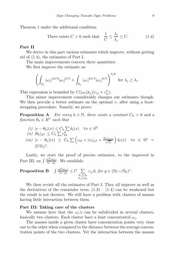
Theorem 1 under the additional condition:
There exists C > 0 such that1C
≤ λi
λj≤ C. (1.4)
Part IIWe derive in this part various estimates which improve, without getting
rid of (1.4), the estimates of Part I.The main improvements concern three quantities:We first improve the estimate on(∫
Ωj
|ωj |24/5|ωi|6/5 +∫
Ωj
|ωi|24/5|ωj |6/5
)5/6
for λj ≥ λi.
This expression is bounded by C(|ωi(aj)|εij + ε3ij).
This minor improvement considerably changes our estimates though.We then provide a better estimate on the optimal v, after using a boot-strapping procedure. Namely, we prove:
Proposition A For every h ∈ N, there exists a constant Ch > 0 and afunction θh ∈ H1 such that
(i) |v − θh|(x) ≤ Ch
∑δ(x) ∀x ∈ S3
(ii) |θh|H1 ≤ Ch
∑εh
k
(iii) |v − θh|(x) ≤ Ch
∑(εk + |v|L6 + |h|L∞√
λ
)δ(x) ∀x ∈ Ωc =
(UΩi)c.
Lastly, we start the proof of precise estimates, to the improved inPart III, on
∫ w4 |wk||x−y| . We establish:
Proposition B∫ w4
|wk||x−y| ≤ C
∑λi≥λλi≥λk
εijδi for y ∈ (Ω ∪ Ωk)c.
We then revisit all the estimates of Part I. They all improve as well asthe derivatives of the remainder term. (1.3) – (1.4) can be weakened butthe result is not decisive. We still have a problem with clusters of masseshaving little interaction between them.
Part III: Taking care of the clustersWe assume here that the ωj ’s can be subdivided in several clusters,
basically two clusters. Each cluster have a least concentrated ωj .The masses inside a given cluster have concentration points very close
one to the other when compared to the distance between the average concen-tration points of the two clusters. Yet the interaction between the masses

January 17, 2007 11:55 WSPC/Book Trim Size for 9in x 6in finalBB
10 Recent Progress in Conformal Geometry
inside a cluster is small with respect to the interaction between the twobasic masses of each cluster. This is the difficulty which we are facing inour expansions. We then rewrite
∑αiωi + v under the form(∑
i∈I
αiωi + vI
)+
(∑i∈II
αiωi + vII
)+ (v − (vI + vII))
where vI and vII are the optimal v’s for each cluster. v is optimal for∑αiωi. In this part, we think of each cluster as a single mass and we thus
move them together and we think of them as combined. Accordingly R3 isnow derived in three regions ΩI , ΩII and R3 − (ΩI ∪ ΩII). ΩI and ΩII aresmaller versions of ΩI and ΩII . The distance between ΩI and ΩII is |a|.We then prove the three following basic estimates.
Proposition C
(i) |v(x)| ≤ C∑
(|ω∞k | +∑ |ωk(a)|
√λk|ak − a| + εk)εkδ(x)
(ii) |vI(x)| ≤ C∑
k,∈I
(|ω∞k | +∑ |ωk(a)|
√λk|ak − a| + εk)εkδ
(iii) |vII(x)| ≤ C∑
k,∈II
(|ω∞k | +∑ |ωk(a)|
√λk|ak − a| + εk)εkδ
(iv) |v−(vI +vII)| ≤∑
(k,)∈(I,II)
[[(|∑ω∞
k | + εk) εk + |∑ ωk(a)|√λ
]δ+
(|∑ω∞ | + εk) εk + |∑ ωk(ak)|√
λkδk
]+
∑(i,j)∈(I,II)
or (II,I)
O(∑
εm)εijδi.
Proposition D (Gradient estimates)
(i) Assume that y is in ΩII a smaller version of ΩII such thatd(ΩI , ΩII) ≥ c|a|.Then, for y ∈ ΩII,
|∇vI(y)| ≤ C
|a|
∑(k,j)∈I
k =j
(|ω∞j | + |ωj(ak)|√λj |aj − ak| + εkj)εkjδk
(ii) ∀y ∈ S3, |∇vI | ≤ C
∑i∈II
√λiδ
2i .
Similar estimates hold for vII .
January 17, 2007 11:55 WSPC/Book Trim Size for 9in x 6in finalBB
Sign-Changing Yamabe-Type Problems 11
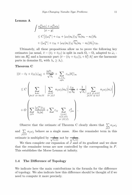
Lemma A ∫ω4
k|ω| + ω4 |ωk|
|x − y|≤ C
[(|ω∞
| + εk + |ω(ak)|√
λ|ak − a|)δk
+ (|ω∞k | + εk + |ωk(a)|
√λk|ak − a|)δ
]εk.
Ultimately, all these propositions allow us to prove the following keyestimates (as usual, v − (vI + vII) is split in each Ωi − Ωi adapted to ωi -into an H1
0 and a harmonic part (v − (vI + vII))i + h0i ; h
si are the harmonic
parts in domains Ωs with λs ≥ λi).
Theorem C
|(v − vI + vII)i|H10
+|h0
i |∞√λi
+∑
λs≥λi
s=i
εis|hsi |∞
≤ C
∑k =i
k∈I or k∈II
∣∣∣∣ ∑j∈IIor j∈I
αjωj(ak)∣∣∣∣ εik√
λk
+1√λi
∣∣∣∣ ∑j∈I if i∈IIj∈II if i∈I
αjωj(ai)∣∣∣∣
+ O
∑j =i
|ω∞j |εij
λi|a| +∑
εij
∑(j,m)
∈(I,II)or (II,I)
ε2jm
.
Observe that the estimate of Theorem C clearly shows that∑j∈I
αjωj
and∑
j∈II
αjωj behave as a single mass. Also the remainder term in this
estimate is multiplied by 1√λi|a|
not by 1√λj |a|
.
We then complete our expansion of J and of its gradient and we showthat the remainder terms are now controlled by the corresponding in P .This establishes the Morse Lemma at infinity.
1.4 The Difference of Topology
We indicate here the main contributions in the formula for the differenceof topology. We also indicate how this difference should be thought of if weneed to compute it more precisely.
January 17, 2007 11:55 WSPC/Book Trim Size for 9in x 6in finalBB
12 Recent Progress in Conformal Geometry
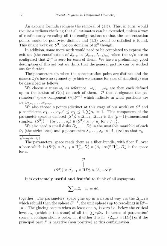
An explicit formula requires the removal of (1.3). This, in turn, wouldrequire a tedious checking that all estimates can be extended, unless a wayof continuously rescaling all the configurations so that the concentrationpoints would be pointwise distinct and (1.3) would be satisfied is found.This might work on S3, not on domains of R3 though.
In addition, some more work would need to be completed to express theexit set (the contribution of Jc−ε in (Jc+ε, Jc−ε)∞) when the ωj ’s are soconfigured that ω∞
i is zero for each of them. We have a preliminary gooddescription of this set but we think that the general picture can be workedout far further.
The parameters set when the concentration point are distinct and themasses ωj ’s have no symmetry (which we assume for sake of simplicity) canbe described as follows:
We choose a mass ω1 as reference. ω2, . . . , ωp are then each definedup to the action of O(4) on each of them. P thus designates the pa-rameters’ space component O(4)p−1 which indicate in what positions areω1, ω2,σ2 , . . . , ωp,σp .
We also choose p points (distinct at this stage of our work) on S3 andp coefficients α1, . . . , αp, 0 ≤ α1 ≤ 1,
∑αi = 1. This component of the
parameter space is denoted (S3)p∗ ×∆p−1. ∆p−1 is the (p− 1)-dimensional
simplex. (S3)p∗ = (a1, . . . , ap) ∈ (S3)p; ai = aj for i = j.
We also need p small disks D′u, . . . , Dp
u in the unstable manifold of eachωj (the strict ones) and p parameters λ1, . . . , λp in [A, +∞) so that εij ∼
1√λiλj |ai−aj |
.
The parameters’ space reads them as a fiber bundle, with fiber P , overa base which is (S3)p
∗ × ∆p−1 × ΠPj=1D
ju × (A, +∞)p.ΠP
j=1Dju is the space
for v.
P∣∣(S3)p
∗ × ∆p−1 × ΠDju × [A, +∞)p.
It is extremely useful and fruitful to think of all asymptots∑εiωi εi = ±1
together. The parameters’ space glue up in a natural way via the ∆p−1’swhich rebuild then the sphere Sp−1, the unit sphere (up to rescaling) in Rp−o. The glueing occurs when at least one αi is zero i.e. below the criticallevel c∞ (which is the same) of all the
∑εiωi. In terms of parameters’
space, a configuration is below c∞ if either it is in ∂(∆p−1 ×ΠDju) or if the
principal part P is negative (non positive) at this configuration.

January 17, 2007 11:55 WSPC/Book Trim Size for 9in x 6in finalBB
Sign-Changing Yamabe-Type Problems 13
P is made of two pieces, one usually of higher order than the other one.The first one is
−c∑ εiεjω
∞i ω∞
j√λiλj |ai − aj |
.
We are thus naturally led to the set where∑ εiεjω∞
i ω∞j√
λiλj |ai−aj |≥ 0. Since∑
εiαiωi is below c∞ if αi/αjis not 1 + o(1), we can expand this set into
∑ εiαiεjαjω∞i ω∞
j√λiλj |ai − aj|
≥ 0.
The εiαi√λi
ω∞i ’s for those ω∞
i ’s which are non zero form then a system ofcoordinates and this set becomes, with ≤ p,
N− = u ∈ R − 0 such thattuAu ≥ 0
A is the × matrix
0 1|ai−aj |
. . .1
|ai−aj | 0
corresponding to those indexes
i such that ω∞i is non zero.
In the description of the parameters’ space, we have left a part largelynot explicit; it is the part P corresponding to the relative positions of ωi,σi ,with respect to ω1. We can think of P as follows: we choose a point ai onS3. We rotate ωi around ai and we identify ai and ai. Then ωi is changedinto ωi,σi through the rotation σi around ai and ω∞
i becomes ωi(ai). Wethen rescale around ai the function ωi,σi . In this way, the concentrationpoint ai is thought of as made of two points: ai itself on S3 and anotherpoint on S3, with the standard ωi attached to it, which will be the pointai. We identify ai and ai through the action of an element of O(4). Wealso rotate ωi around ai and we rescale the function which we obtain (onthe original S3) in this way.
We thus derive a stratified Sp which can be described using the ai’s.There is a natural map:
Π :Sp → (S3)p × (S3)p∗
s → (a1, . . . , ap) × (a1, . . . , ap)
F = Π−1((a1, . . . , ap), (a1, . . . , ap)) is a set very similar to N− i.e. there are
indexes i1, . . . , i such that ω∞j = ωj(aj) is now zero. F can be identified
as N− (i1, . . . , i), where N−
(i1, . . . , i) is defined as N− above, with the
indexes i1, . . . , i.

January 17, 2007 11:55 WSPC/Book Trim Size for 9in x 6in finalBB
14 Recent Progress in Conformal Geometry
Accordingly, the topology of Sp can be computed using the distributionof the signatures of A over (S3)p
∗ and the zero sets of the ωi’s.We will discuss this more elsewhere.The last piece of information about the difference of topology which we
need to study comes in when all the ω∞i ’s are zero.
Indeed, under the hypothesis:(H) For every p, the function f(u, a1, . . . , ap) = tuAu defined on Sp−1×
(S3)p∗ does not have 0 as a critical value,
the principal part P of the expansion should reduce to
−c∑ ω∞
i ω∞j√
λiλj |aj − aj |if the ω∞
i ’s are not all o(1).If all ω∞
i ’s are zero then the second piece of P,−∑ cijε3ij enters into
play. We know [Bahri and Coron (1988)] that cij = c∇ω∞i · ∇ω∞
i .Thus, we derive a set of the type
−c∑
∇ω∞i · ∇ω∞
i ε3ij ≤ 0
which should provide a condition on the relative positions of the ωi’s in-volved in the configuration.
The ai’s are subject to the requirement ωi(ai) = 0.This gives a qualitative account of what we expect for the difference of
topology. We think that this program is within reach.
1.5 Open Problems
1.5.1 Understand the difference of topology
As we explore the normal form in our expansion:
P = −c∑
ωi(˜aj)ω∞j εij −
∑cijε
3ij
a quantity very close to P , which we denote P∞, appears:
P∞ = −c∑
ω∞i ω∞
j εij −∑
cijε3ij .
Thinking of εij as 1√λiλj |ai−aj |
, we find
P∞ = −c
(. . .
ω∞j√λj
. . .
)A
...ω∞
i /√
λi
...
−∑
cijε3ij .

January 17, 2007 11:55 WSPC/Book Trim Size for 9in x 6in finalBB
Sign-Changing Yamabe-Type Problems 15
Thus an important piece of information comes from the behavior of
S = u ∈ Rp − 0s.t.(Au, u) ≥ 0.
This does not seem to be quite true at first glance since the u which appears
in the definition of S is equal in our context to
...ω∞
i /√
λi
...
, so that the sign
of ui = ω∞i√λi
is prescribed. However if all asymptots∑±ωi are combined,
the various pieces combine and S is naturally found.Another piece of information is provided by the zero sets of the ωi’s and
a last piece is less explicit, more related to the relative position of ∇ω∞i
with respect to ∇ω∞j .
1.5.2 Non critical asymptots
Assume that we have only “masses” ωi such that ω∞i is positive.
It is then fairly obvious that such combinations of ωi do not build agenuine asymptot since tuAu is negative on them. The same observationholds if the ω∞
i ’s are all negative. The result holds as well when thereare many more negative (or positive) contributions than contributions ofthe opposite sign. One would like to understand the behavior of the crit-ical configurations as p tends to ± and relate them to discrete as well ascontinuous geometric problems on S3.
1.5.3 The exit set from infinity
The expansion shows the use of the quadratic form tuAu, with u = ...ω∞
i /√
λi
...
. It is a quite striking fact that the expression of the nor-
mal form depends so little on the actual functions themselves. The maindependence is via the vector u i.e. via the signs of the ω∞
i ’s. If we exceptthe case when one ω∞
i is zero, we could think of a model where the asymp-tot
∑ωi would be replaced by
∑ω∞
i δi. The critical levels, the indexesat infinity etc. would not match; but the value of tuAu which indicateswhether with the preassigned concentrations λ1, . . . , λp and with the pre-assigned values ω∞
1 , . . . , ω∞p , the asymptot is genuine or not genuine would
match. So would a decreasing flow defined at infinity.We thus see that the exit set from infinity is independent of the actual
asymptot. The simplest model i.e. the model involving∑±δi intervenes

January 17, 2007 11:55 WSPC/Book Trim Size for 9in x 6in finalBB
16 Recent Progress in Conformal Geometry
as a basic factor in the understanding of the functional J at infinity.
1.5.4 Establishing Conjecture 2 and continuous forms of
the discrete inequality
Conjecture 2 is a key hypothesis in the proof of Theorem 1. The proofprovided in the case p = 3 [Xu] is quite involved. Y. Xu has also providedin [Xu] heuristic reasons why this result should hold in general.
A continuous form of this inequality should also be derived as the num-ber p of points tends to ±∞.
1.5.5 The Morse Lemma at infinity, Part I, II, III
The proof of the Morse Lemma at infinity is divided in three distinct parts.Part I and Part III provide the proof. Part II is an intermediate stepwhich on one hand provides insight in what should be completed to removethe restrictions involved in Part I (where the Morse Lemma at infinity isestablished when the concentration are comparable) and on the other handprovides a key estimate (Theorem 1).
1.5.6 Notations v, vi, hi
The ωi’s are solutions of the Yamabe problem on R3. They are rescaledversion of ωi’s which all have concentration equal to O(1).
For each ωi, a domain of influence
Ωi = x ∈ R3s.t.λi|x − xi| ≤ Min1
8εij∀j,
λj |x − xj | ≥ 1εij
if λj ≥ λi.
Any u is defined close top∑
i=1
ωi
(∫ |∇(u −∑ωi)|2 is small)
can be uniquely
written as u =p∑
i=1
αiωi + v where v satisfies a family of orthogonality
conditions which read
(Vo)
∫ ∇ωi∇v = 0∫ ∇∂ωi
∂ai∇v = 0∫ ∇∂ωi
∂λi∇v = 0∫ ∇∂ωi
∂σi∇v = 0 (σi is in O(4))
. (Vo)

January 17, 2007 11:55 WSPC/Book Trim Size for 9in x 6in finalBB
Sign-Changing Yamabe-Type Problems 17
The functional J(∑i=1
αiωi + v) can be max-minimized with respect to the
variation of v (under (Vo)) if we assume that each ωi is a non degeneratecritical point of J transversally to the parameters of the conformalgroup. We will work under this assumption. Then, following the results of[Bahri and Coron (1988)], the expansion of J in v reads as (f, v)+Q(v, v)+
o((|∇v|2)3/2), where Q is non degenerate of index equal to p−1+p∑
i=1
index
J′′(ωi). Such an expression can be max-minimized. We derive an optimal
v.This v can be decomposed in each Ωi into vi + hi, where hi is harmonic
and vi is in H10 (Ωi).
1.6 Preliminary Estimates and Expansions, the PrincipalTerms
The Content of Part I.Part I provides the framework for the completion of the Morse Lemma
at infinity. After two preliminary estimates (to be improved later), theequation satisfied by v is extracted and it is decomposed accordingly tothe Ωi’s. v is split in
∑(vi + hi). Due to the constraints (V 0) on v,
this equation involves projection terms which are global by nature (theyexpress orthogonality conditions). Thus, the various vi’s, hi’s etc. are tiedalthough their supports are disjoint. The main quantity tying them is thematrix A of the H1
0 -scalar product in
Spanpi=1
ωi,
1λi
∂ωi
∂ai, λi
∂ωi
∂λi,∂ωi
∂σi
.
We thus need to estimate A and also vi, hi.In a first step (Lemmas 3-11), the estimate on |vi|H1
0is shown to depend
on an estimate on |hi|∞.Next, using the Green’s function of an annulus-type domain, a pointwise
estimate is derived on hi(Lemma 12).The estimate is complex because it involves (via the right hand side of
the equation satisfied by v) an enormous amount of terms and expressionsrelated to Ωi but also Ωj , for j = i, (UΩi)c. It ties vi, hi with vj , hj etc.
We need to estimate carefully all of these expressions. This is what wecomplete in Lemmas 13—30.
We then are in position to derive an estimate (not yet optimal) on |vi|H10
and |hi|∞ (Lemmas 31—34).

January 17, 2007 11:55 WSPC/Book Trim Size for 9in x 6in finalBB
18 Recent Progress in Conformal Geometry
Using this estimate, we derive in the last section of Part I, after estab-lishing two further estimates (Lemmas 35—36) on the contribution of v inJ ′(∑
αjωj + v). ∂ωi, our Morse Lemma at infinity under (1.3)—(1.4).
1.7 Preliminary Estimates
We will denote in what follows
∂ωi
any of ωi,1λi
∂ωi
∂ai, λi
∂ωi
∂λiand by ψi the Laplacian of any of those functions.
We will work on R3 or S3. ∆R3 transforms into the Yamabe operator L onS3. We differenciate (V0) to get∫
∇∂ωi∇ ∂v
∂ai= −
∫∇∂2ωi
∂ai∂∇v.
We decompose v into∑
vj +h, where each vj has support into Ωj ; the Ω′js
are disjoint and h is harmonic in ∪Ωj .We thus need to estimate
αij =∫
∇∂2ωi
∂ai∂∇vj i = j
αii =∫
∇∂2ωi
∂ai∂∇vi
βi =∫
∇∂2ωi
∂ai∂∇h.
Observe that
∂2ωi
∂ai∂= 0(λiδi), ∆
∂2ωi
∂ai∂= 0(λiδ
5i ).
It is difficult to estimate αij if λj ≥ λi, in particular αii. We need moreinsight into the equations satisfied by the vk’s and h.
We start with the following preliminary estimates:
Lemma A(∫
Ωci|∂ωi|6
)5/6
+
(∫ |∂ωi|6/5∑ =i
|∂ω|24/5
)5/6
≤
C(∑
(|ω∞i | + |ω∞
j |)εij + ε5/2ij ).
Proof. The estimate on (∫Ωc
i|∂ωi|6)5/6 will follow from 1. of Lemma
13 below and from the definition of Ωi. In order to upperbound
January 17, 2007 11:55 WSPC/Book Trim Size for 9in x 6in finalBB
Sign-Changing Yamabe-Type Problems 19
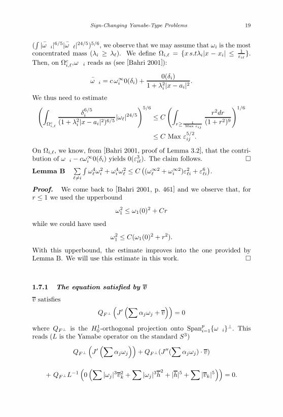
(∫ |∂ωi|6/5|∂ω|24/5)5/6, we observe that we may assume that ωi is the most
concentrated mass (λi ≥ λ). We define Ωi, = x s.tλi|x − xi| ≤ 1εi
.Then, on Ωc
i,, ∂ωi reads as (see [Bahri 2001]):
∂ωi = c ω∞i 0(δi) +
0(δi)1 + λ2
i |x − ai|2 .
We thus need to estimate(∫Ωc
i,
δ6/5i
(1 + λ2i |x − ai|2)6/5
|ω|24/5
)5/6
≤ C
(∫r≥ 1
Max εij
r2dr
(1 + r2)9
)1/6
≤ C Max ε5/2ij .
On Ωi,, we know, from [Bahri 2001, proof of Lemma 3.2], that the contri-bution of ∂ωi − cω∞
i 0(δi) yields 0(ε3i). The claim follows.
Lemma B∑ =i
∫ω4
ω2i + ω4
i ω2 ≤ C
((ω∞2
+ ω∞2i )ε2
i + ε6i
).
Proof. We come back to [Bahri 2001, p. 461] and we observe that, forr ≤ 1 we used the upperbound
ω21 ≤ ω1(0)2 + Cr
while we could have used
ω21 ≤ C(ω1(0)2 + r2).
With this upperbound, the estimate improves into the one provided byLemma B. We will use this estimate in this work.
1.7.1 The equation satisfied by v
v satisfies
QF⊥
(J ′(∑
αjωj + v))
= 0
where QF⊥ is the H10 -orthogonal projection onto Spanp
i=1∂ωi⊥. Thisreads (L is the Yamabe operator on the standard S3)
QF⊥
(J ′(∑
αjωj
))+ QF⊥(J ′′(
∑αjωj) · v)
+ QF⊥L−1(0(∑
|ωj |3v2k +
∑|ωj |3h2
+ |h|5 +∑
|vk|5))
= 0.
January 17, 2007 11:55 WSPC/Book Trim Size for 9in x 6in finalBB
20 Recent Progress in Conformal Geometry
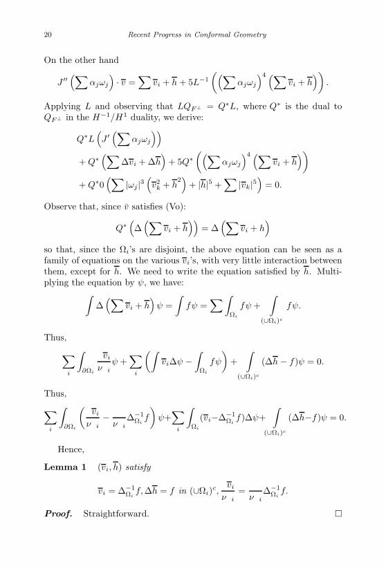
On the other hand
J ′′(∑
αjωj
)· v =
∑vi + h + 5L−1
((∑αjωj
)4 (∑vi + h
)).
Applying L and observing that LQF⊥ = Q∗L, where Q∗ is the dual toQF⊥ in the H−1/H1 duality, we derive:
Q∗L(J ′(∑
αjωj
))+ Q∗
(∑∆vi + ∆h
)+ 5Q∗
((∑αjωj
)4 (∑vi + h
))+ Q∗0
(∑|ωj |3
(v2
k + h2)
+ |h|5 +∑
|vk|5)
= 0.
Observe that, since v satisfies (Vo):
Q∗(∆(∑
vi + h))
= ∆(∑
vi + h)
so that, since the Ωi’s are disjoint, the above equation can be seen as afamily of equations on the various vi’s, with very little interaction betweenthem, except for h. We need to write the equation satisfied by h. Multi-plying the equation by ψ, we have:∫
∆(∑
vi + h)
ψ =∫
fψ =∑∫
Ωi
fψ +∫
(∪Ωi)c
fψ.
Thus,∑i
∫∂Ωi
∂vi
∂νiψ +
∑i
(∫vi∆ψ −
∫Ωi
fψ
)+
∫(∪Ωi)c
(∆h − f)ψ = 0.
Thus,∑i
∫∂Ωi
(∂vi
∂νi− ∂
∂νi∆−1
Ωif
)ψ+∑
i
∫Ωi
(vi−∆−1Ωi
f)∆ψ+∫
(∪Ωi)c
(∆h−f)ψ = 0.
Hence,
Lemma 1 (vi, h) satisfy
vi = ∆−1Ωi
f, ∆h = f in (∪Ωi)c,∂vi
∂νi=
∂
∂νi∆−1
Ωif.
Proof. Straightforward.
January 17, 2007 11:55 WSPC/Book Trim Size for 9in x 6in finalBB
Sign-Changing Yamabe-Type Problems 21
On the other hand,∑
vi + h is smooth, so that
∂vi
∂νi+
∂h
∂νi= − ∂h
∂ν−i
where ∂∂νi
is the outwards normal derivative of Ωi and ∂∂ν−
i
is the inwardsone.
f reads as
f = −Q∗(∆J ′(∑
αjωj
)+ 5
(∑αjωj
)4 (∑vi + h
)+ O
(∑|ωj |3
(v2
k + h2)
+ |h|5 +∑
|vk|5) (1.5)
so that the equation on vi reads:∆vi + Q∗(5(
∑αjωj)4vi + 0(
∑j
|ωj|3v2i + |vi|5)) = −Q∗(∆J ′(
∑αjωj)
+5(∑
αjωj)4(∑j =i
vj + h) + O(∑k =i
|ωj|3(v2k + h
2) + |h|5 +
∑k =i
|vk|5))vi = 0|∂Ωi
.
(1.6)Let
ei = L∂ωi ; A =
. . . − ∫ ejL
−1ei
. . .. . .
. (1.7)
Then
Q∗(g) = g −∑A−1
...
− ∫ gL−1ei
...
j
ej. (1.8)
We write h as
h =∑
hi + k∗ (1.9)
when hi = hχΩi then rereads:
January 17, 2007 11:55 WSPC/Book Trim Size for 9in x 6in finalBB
22 Recent Progress in Conformal Geometry
∆vi + Q∗(5(∑
αjωj)4vi + O(∑j
|ωj|3v2i + |vi|5)) = −Q∗(∆J ′(
∑αjωj)
−Q∗(5(∑
αjωj)4hi + O(∑ |ωj |3(h2
i + |hi|5))
+∑
A−1
...− ∫ (
∑j =i
5(∑
αsωs)4(vj + hj + k∗) + O(∑k =i
|ωj|3v2k+
+h2
k + k∗2) +∑k =i
(|vk|5 + |hk|5 + |k∗|5))L−1em
...
e
vi = 0|∂Ωi .
(1.10)In addition, we have
∂h
∂νi+
∂h
∂ν−i
= − ∂
∂νi
(∆−1
Ωifi
) ∣∣∂Ωi
. (1.11)
with
fi = − Q∗(∆J ′(
∑αjωj) − 5(
∑αjωj)4(vi + hi)
+ O(∑
|ωj|3(v2i + h
2
i ) + |hi|5 + |vi|5))
+∑
A−1
...− ∫ [5(
∑αω)4(
∑j =i
vj + hj + k∗)
+O(∑k =i
|ωj |3(v2k + h
2
k + k∗2) +∑k =i
(|hk|5
+|vk|5 + |k∗|5))]L−1em
...
e
.
(1.12)
Our aim is to find a good estimate on each vi in H10 and an estimate
on |hi|∞. The two estimates turn out to be tied. The estimates for twodifferent indexes i = j are also tied. We will derive these estimates aftera careful analysis of the contribution of each term of fi in (1.12). Theseterms are either projection terms due to Q∗ or other terms involving theinteraction of the ωj ’s between each other or the vk’s, hk’s.
We need to estimate each of them carefully. This is what we completebelow:

January 17, 2007 11:55 WSPC/Book Trim Size for 9in x 6in finalBB
Sign-Changing Yamabe-Type Problems 23
1.7.2 First estimates on vi and hi
A key step in the estimate about vi is to obtain a good estimate on themean value of hi. This will lead us to a good estimate on hi in a sizableball around xi. We start with
Lemma 2 Let ψi = ∆∂ωi.∫viψi = −
∫hiψi + Max ε
5/2im 0
(∑εk
).
Proof. ∫viψi =
∫vψi −
∫hiψi −
∫(v − vi − hi)ψi∫
vψi is zero and since v − vi −∑
hj is zero on Ωi,∣∣∣∣ ∫ (v − vi − hi)ψi
∣∣∣∣ ≤ C
(∫|∇v|2
)1/2(∫
Ωci
|ψi|6/5
)5/6
≤ C
(∫|∇v|2
)1/2
Max ε5/2im
from which Lemma 2 follows. The above estimate on (
∫Ωc
i|ψi|6/5)5/6 will be established later. (1. of
Lemma 13)A weaker estimate can be seen to hold as follows: Ωc
i is made of anexterior partx s.t λi|x − xi| ≥ Min 1
εij where the estimate is straightforward and
interior partsx s.t λj |x − xj | ≤ c
εij, for j = i, λj ≥ λi.
On such parts, |ψi| ≤ Cδ5i and because λj ≥ λi, λj |x − xj | ≤ c
εij, by
[Bahri 1989, (3.64)],
δi ≤ Cδj
for such values of x.Thus ∫
λj |x−xj|≤ cεij
|ψi|6/5
5/6
≤ C
(∫δ3i δ3
j
)5/6
≤ Cε5/2ij log5/6 ε−1
ij
using [Bahri 1989].
January 17, 2007 11:55 WSPC/Book Trim Size for 9in x 6in finalBB
24 Recent Progress in Conformal Geometry
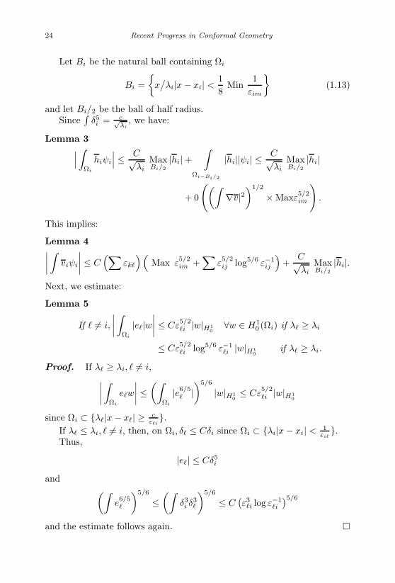
Let Bi be the natural ball containing Ωi
Bi =
x/λi|x − xi| <
18
Min1
εim
(1.13)
and let Bi/2 be the ball of half radius.Since
∫δ5i = c√
λi, we have:
Lemma 3∣∣∣ ∫Ωi
hiψi
∣∣∣ ≤ C√λi
MaxBi/2
|hi| +∫
Ωi−Bi/2
|hi||ψi| ≤ C√λi
MaxBi/2
|hi|
+ 0
((∫∇v|2
)1/2
× Maxε5/2im
).
This implies:
Lemma 4∣∣∣∣ ∫ viψi
∣∣∣∣ ≤ C(∑
εk
)(Max ε
5/2im +
∑ε5/2ij log5/6 ε−1
ij
)+
C√λi
MaxBi/2
|hi|.
Next, we estimate:
Lemma 5
If = i,
∣∣∣∣ ∫Ωi
|e|w∣∣∣∣ ≤ Cε
5/2i |w|H1
0∀w ∈ H1
0 (Ωi) if λ ≥ λi
≤ Cε5/2i log5/6 ε−1
i |w|H10
if λ ≥ λi.
Proof. If λ ≥ λi, = i,∣∣∣∣ ∫Ωi
ew
∣∣∣∣ ≤ (∫Ωi
|e6/5 |
)5/6
|w|H10≤ Cε
5/2i |w|H1
0
since Ωi ⊂ λ|x − x| ≥ cεi
.If λ ≤ λi, = i, then, on Ωi, δ ≤ Cδi since Ωi ⊂ λi|x − xi| < 1
εi.
Thus,
|e| ≤ Cδ5i
and (∫e6/5
)5/6
≤(∫
δ3i δ3
)5/6
≤ C(ε3
i log ε−1i
)5/6
and the estimate follows again.

January 17, 2007 11:55 WSPC/Book Trim Size for 9in x 6in finalBB
Sign-Changing Yamabe-Type Problems 25
We then have:
Lemma 6∫Ωi
Q∗(∆J ′(
∑αjωj)
)w
≤ C(∑(|ω∞
j |εij + |ω∞i |εij
)+∑
ε5/2ij log5/6 ε−1
ij
)|w|H1
0.
Proof. The operator Q∗ removes from ∆J ′(∑
αjωj) the contribution ofω5
i . We are left with ω5 for = i or ω4
ωk or the like. Q∗ of such termsinvolve first these terms themselves. Their contribution is given for andk = i by the previous lemma and for or k = i by [Bahri 2001, Lemma3.2]. In addition, there are the projection terms related to A−1. Thosecorresponding to e, with = i, are again controlled by the previous lemma.The term corresponding to ei is typically:A−1
...
− ∫ ω4 ωkL−1em
...
i
ei.
Here, we need to understand more the matrix A and its inverse.
1.7.3 The matrix A
A can be written as
B + C
where C is an almost diagonal matrix which separates the block i from theblock j:
B =
() 0 00 () 00 0 ()
.
Each block is nearly the identity matrix and, in fact, after a change of basiswhich does not affect our estimates, can be considered to be the identitymatrix; so that B = Id.
C corresponds to the interactions between these various blocks. Typi-cally, it involves terms such as
−∫
ejL−1ei

January 17, 2007 11:55 WSPC/Book Trim Size for 9in x 6in finalBB
26 Recent Progress in Conformal Geometry
which, by [Bahri 2001, Lemma 5 and Lemma 3.2], after splitting the con-tribution onto Ωc
i and Ωi, is
O((|ω∞
i | + |ω∞j |) εij + ε
5/2ij log5/6 ε−1
ij
)A−1 is (Id + C)−1 = Id − C − C2 . . . .
We then claim:
Lemma 7 The coefficients of A−1 at the line i, bim, for m in a differentblock than i, areO(∑
(|ω∞i | + |ω∞
m |)εim +∑
ε5/2im log5/6 ε−1
im).
Proof of Lemma 6 completed. In view of Lemma 7, we need to under-stand only
∫ω4
ωkL−1ei. Either or k = i and [Bahri 2001, Lemma 3.2]provides the result. Or , k = i. We then split the integral between itscontribution on Ωi and on Ωc
i and use Lemma A and Lemma 5. Proof of Lemma 7. First observe that the coefficients bim of Id − C −C2 . . . build convergent series as each multiplication adds p terms, butwhich are all multiplied by an additional o(1). These series are, in absolutevalues, bounded above by a geometric series.
Furthermore, the coefficient of the line i of Cr are obtained after mul-tiplication of the line i of C with the columns of Cr−1. The estimate on− ∫ ejL
−1ei provided above yields then the result.
1.7.4 Towards an H10 -estimate on vi and an L∞-estimate
on hi
We would like to derive an H10 -estimate on vi and an L∞-estimate on hi.
We thus need to estimate all projection terms in (1.10)–(1.12) and we alsoneed to estimate each term in
∫fiw, where w ∈ H1
0 (Ωi). We start with:
Lemma 8∣∣∣∣ ∫ O
∑k =i
|ω|4(|vk| + |hk| + |k∗|) + |vk|5 + |hk|5 + |k∗|5 ∂ωi
∣∣∣∣ ≤
C(∑
ε5kε
1/2ij +
∑εkmε
5/2ij +
∑εkm
(∑(|ω∞
i | + |ω∞j |)εij + ε
5/2ij
)).
Proof. vk, hk, k∗ have all supports in Ωci .

January 17, 2007 11:55 WSPC/Book Trim Size for 9in x 6in finalBB
Sign-Changing Yamabe-Type Problems 27
Thus, denoting
s = O
∑k =i
|ω|4(|vk| + |hk| + |k∗|) + |vk|5 + |hk|5 + |k∗|5
we have:∣∣∣∣∫ s∂ωi
∣∣∣∣ ≤ C
∫Ωc
i
|∂ωi|∑
k =i
|ω|4(|vk| + |hk| + |k∗|) + |vk|5 + |hk|5 + |k∗|5
≤ C
(∫ |∇v|2)5/2
(∫Ωc
i
|ϕi|6)1/6
+
(∫Ωc
i
|∂ωi|6/5∑
|ω|24/5
)5/6 (∫|∇v|2
)1/2 .
It is then clear that (∫Ωc
i
|ϕi|6)1/6
≤ C Max ε1/2ij
and, by Lemma A, that(∫Ωc
i
|∂ωi|6/5∑
|ω|24/5
)5/6
≤ C(∑
(|ω∞i | + |ω∞
j |)εij + ε5/2ij
).
The result follows.We move now to estimate the contribution of hi. We observe that
5(∑
αjωj
)4
hi + O(∑
|ωj |3h2
i + |hi|5)
= O(∑
|ωj |4|hi| + |hi|5)
and we then have:
Lemma 9 ∀w ∈ H10 (Ωi),∑∫
Ωi
(|ωj |4|hi| + |hi|5)|w| ≤ C
(∫|∇w|2
)1/2
×(∑
ε5k +
|hi|∞√λi
Bi/2 +(∑
εkm
)(∑ε2
i log2/3 ε−1i
)).
Observation. |hi|∞,Bi/2 = Supx∈Bi/2|hi(x)|.
Proof. The contribution of∫Ωi
|w||hi|5 is clear.
January 17, 2007 11:55 WSPC/Book Trim Size for 9in x 6in finalBB
28 Recent Progress in Conformal Geometry
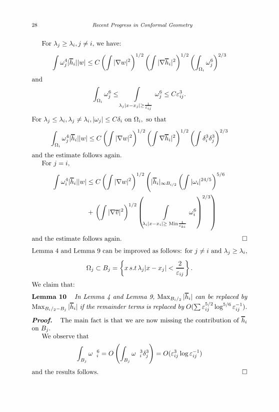
For λj ≥ λi, j = i, we have:∫ω4
j |hi||w| ≤ C
(∫|∇w|2
)1/2(∫|∇hi|2
)1/2(∫Ωi
ω6j
)2/3
and ∫Ωi
ω6j ≤
∫λj |x−xj|≥ 1
εij
ω6j ≤ Cε3
ij .
For λj ≤ λi, λj = λi, |ωj | ≤ Cδi on Ωi, so that∫Ωi
ω4j |hi||w| ≤ C
(∫|∇w|2
)1/2(∫∇hi|2
)1/2(∫δ3i δ3
j
)2/3
and the estimate follows again.For j = i,∫
ω4i |hi||w| ≤ C
(∫|∇w|2
)1/2(|hi|∞Bi/2
(∫|ωi|24/5
)5/6
+(∫
|∇v|2)1/2
∫λi|x−xi|≥ Min 1
εki
ω6i
2/3
and the estimate follows again. Lemma 4 and Lemma 9 can be improved as follows: for j = i and λj ≥ λi,
Ωj ⊂ Bj =
x s.t λj |x − xj | <2
εij
.
We claim that:
Lemma 10 In Lemma 4 and Lemma 9, MaxBi/2 |hi| can be replaced byMaxBi/2−Bj
|hi| if the remainder terms is replaced by O(∑
ε5/2ij log5/6 ε−1
ij ).
Proof. The main fact is that we are now missing the contribution of hi
on Bj .We observe that∫
Bj
∂ω6i = O
(∫Bj
∂ω3i δ3
j
)= O(ε3
ij log ε−1ij )
and the results follows.
January 17, 2007 11:55 WSPC/Book Trim Size for 9in x 6in finalBB
Sign-Changing Yamabe-Type Problems 29
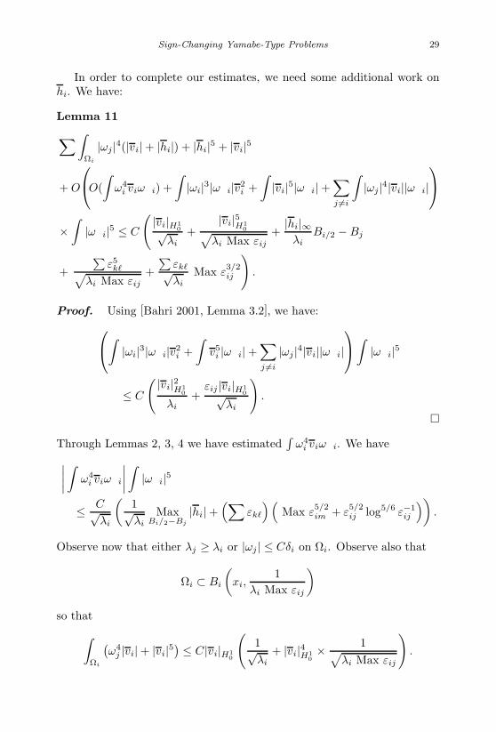
In order to complete our estimates, we need some additional work onhi. We have:
Lemma 11∑∫Ωi
|ωj |4(|vi| + |hi|) + |hi|5 + |vi|5
+ O
O(∫
ω4i vi∂ωi) +
∫|ωi|3|∂ωi|v2
i +∫|vi|5|∂ωi| +
∑j =i
∫|ωj|4|vi||∂ωi|
×∫
|∂ωi|5 ≤ C
(|vi|H1
0√λi
+|vi|5H1
0√λi Max εij
+|hi|∞
λiBi/2 − Bj
+∑
ε5k√
λi Max εij
+∑
εk√λi
Max ε3/2ij
).
Proof. Using [Bahri 2001, Lemma 3.2], we have:∫ |ωi|3|∂ωi|v2i +
∫v5
i |∂ωi| +∑j =i
|ωj |4|vi||∂ωi|∫ |∂ωi|5
≤ C
( |vi|2H10
λi+
εij |vi|H10√
λi
).
Through Lemmas 2, 3, 4 we have estimated∫
ω4i vi∂ωi. We have∣∣∣∣ ∫ ω4
i vi∂ωi
∣∣∣∣ ∫ |∂ωi|5
≤ C√λi
(1√λi
MaxBi/2−Bj
|hi| +(∑
εk
)(Max ε
5/2im + ε
5/2ij log5/6 ε−1
ij
)).
Observe now that either λj ≥ λi or |ωj | ≤ Cδi on Ωi. Observe also that
Ωi ⊂ Bi
(xi,
1λi Max εij
)so that∫
Ωi
(ω4
j |vi| + |vi|5) ≤ C|vi|H1
0
(1√λi
+ |vi|4H10× 1√
λi Max εij
).

January 17, 2007 11:55 WSPC/Book Trim Size for 9in x 6in finalBB
30 Recent Progress in Conformal Geometry
On the other hand,
∫Ωi
ω4j |hi| + |hi|5 ≤ C
( |hi|∞λi
Bi/2 − B
+∑
εk
∑j
∫Ωi−(Bi/2−B)
ω24/5j
5/6
+∑
ε5k√
λi Max εij
.
Either λj ≥ λi, j = i. Then,
∫Ωi−(Bi/2−B)
ω24/5j
5/6
≤
∫λj |x−xj|≥ 1
εij
ω24/5j
5/6
≤ 1√λi
O(ε3/2ij ).
Or λj ≤ λi, |ωj | ≤ Cδi on Ωi and
(∫Ωi−(Bi/2−B)
ω24/5j
)5/6
≤ C
(∫Ωi−(Bi/2−B)
δ24/5j
)5/6
≤ C
(1√λi
Max ε3/2im +
(∫B∩Ωi
δ24/5i
)5/6)
.
On B(λ ≥ λi, = i),
δi ≤ Cδ
and
(∫Ωi∩B
δ24/5i
)5/6
≤(∫
λ|x−x|≥ 1εi
δ24/5
)5/6
≤ 1√λi
O(ε3/2i ).
Next, we assume for sake of simplicity that Ωi is:
Bi = B(xi, ρi)

January 17, 2007 11:55 WSPC/Book Trim Size for 9in x 6in finalBB
Sign-Changing Yamabe-Type Problems 31
1.7.5 The formal estimate on hi
Using the Green function on annuli-type domains, we derive in what followsa preliminary estimate on hi (Lemma 12).
This estimate involves the contribution of f i.e. of the fj ’s on Ωi butalso on Ωc
i ; it is an intermediate result which displays the expressions whichwe need to estimate in order to upperbound |hi|∞ and |vi|H1
0.
We give an estimate for hi in Ωi.
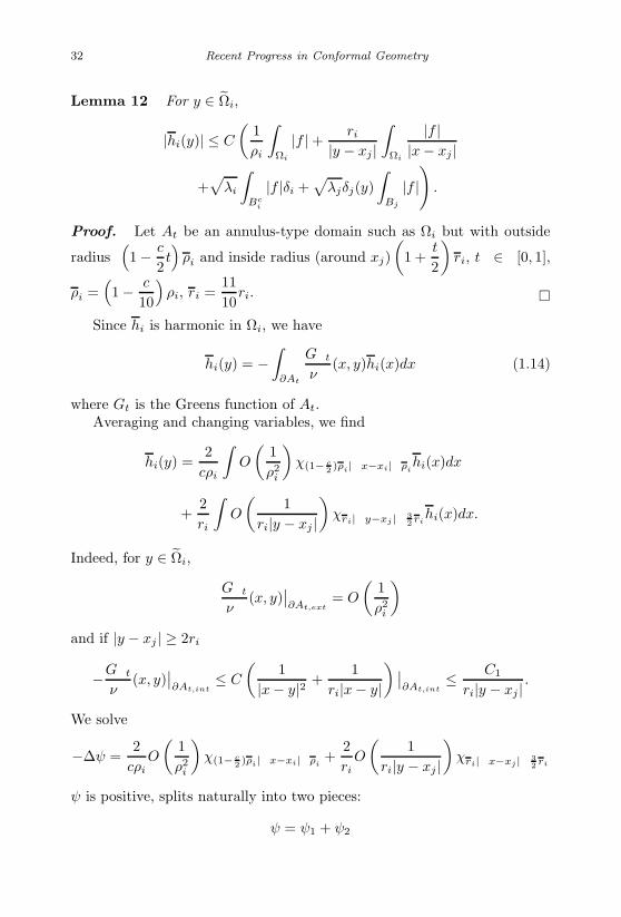
January 17, 2007 11:55 WSPC/Book Trim Size for 9in x 6in finalBB
32 Recent Progress in Conformal Geometry
Lemma 12 For y ∈ Ωi,
|hi(y)| ≤ C
(1ρi
∫Ωi
|f | + ri
|y − xj |∫
Ωi
|f ||x − xj |
+√
λi
∫Bc
i
|f |δi +√
λjδj(y)∫
Bj
|f |)
.
Proof. Let At be an annulus-type domain such as Ωi but with outside
radius(1 − c
2t)
ρi and inside radius (around xj)(
1 +t
2
)ri, t ∈ [0, 1],
ρi =(1 − c
10
)ρi, ri =
1110
ri.
Since hi is harmonic in Ωi, we have
hi(y) = −∫
∂At
∂Gt
∂ν(x, y)hi(x)dx (1.14)
where Gt is the Greens function of At.Averaging and changing variables, we find
hi(y) =2
cρi
∫O
(1ρ2
i
)χ(1− c
2 )ρi≤|x−xi|≤ρihi(x)dx
+2ri
∫O
(1
ri|y − xj |)
χri≤|y−xj|≤ 32 ri
hi(x)dx.
Indeed, for y ∈ Ωi,
∂Gt
∂ν(x, y)
∣∣∂At,ext
= O
(1ρ2
i
)and if |y − xj | ≥ 2ri
−∂Gt
∂ν(x, y)
∣∣∂At,int
≤ C
(1
|x − y|2 +1
ri|x − y|) ∣∣
∂At,int≤ C1
ri|y − xj | .
We solve
−∆ψ =2
cρiO
(1ρ2
i
)χ(1− c
2 )ρi≤|x−xi|≤ρi+
2ri
O
(1
ri|y − xj |)
χri≤|x−xj|≤ 32 ri
ψ is positive, splits naturally into two pieces:
ψ = ψ1 + ψ2

January 17, 2007 11:55 WSPC/Book Trim Size for 9in x 6in finalBB
Sign-Changing Yamabe-Type Problems 33
and it is easy to check that
ρiψ1 and riψ2 are L∞ − bounded independently of i for y ∈ Ωi. (1.15)
Thus, using (1.14)
hi(y) = −∫
R3∆ψh = −
∫(∪Ω)c
ψ∆h +∑∫
∂Ω
(∂h
∂ν+
∂h
∂ν−
)ψ
= −∫
(∪Ω)c
ψ∆h −∑
∫∂Ω
∂
∂ν(∆−1
Ωf)ψ = −
∫(∪Ω)c
ψ∆h −∑
∫Ω
fψ
where ψ is the harmonic extension of ψ∣∣∂Ω
.Using (1.5), we find
hi(y) = −∫
(∪Ω)c
ψf −∑
∫Ω
fψ
ψ∣∣(∪Ω)c and the ψ are harmonic positive. They are all upperbounded by
the original ψ. Thus,
|hi(y)| ≤∫
(∪Ω)c
ψ|f | +∑
∫Ω
ψ|f|
ψ reads as
ψ(z) =∫
R3
c1
|x − z|
×
2cρi
O
(1ρ2
i
)χ(1− c
2 ρi≤|x−xi|≤ρi+
2ri
O
(1
ri|y − xj |)
χri≤x−xj|≤ 32 ri
= I + II.
If z ∈ Ωi, then
I ≤ C
ρi.
If z ∈ Bj , I ≤ Cρi
χz∈Bj ≤ Cδj(y)√
λjχz∈Bj .
If z ∈ Bci , then by choice of ρi,
1|x − z|χ(1− c
2 )ρi≤|x−xi|≤ρi≤ C
|z − xi| .

January 17, 2007 11:55 WSPC/Book Trim Size for 9in x 6in finalBB
34 Recent Progress in Conformal Geometry
Since λi|z − xi| ≥ λiρi is large, this is upperbounded by C√
λiδi(z) sothat
I ≤ C√
λiδi(z).
Thus, the contribution of I to the upperbound on |hi(y)| is
C
ρi
∫Ωi
|f | + C√
λi
∫Bc
i
|f |δi + Cδj(y)√
λj
∫Bj
|f |.
If z ∈ Bci , the contribution of (II) is upperbounded as for I since |y −
xj | ≥ 2ri.If z ∈ Bj
1|x − z|χri≤|x−xj|≤ 3
2 ri≤ C
riχri≤|x−xj|≤ 3
2 ri
and
1|y − xj | ≤ Cδj(y)
√λj since |y − xj | ≥ 2ri.
Thus, if z ∈ Bj , the contribution of II is upperbounded byC√
λjδj(y)∫
Bj|f |.
Finally, if z ∈ Ωi, either |z − xj | ≥ 2ri. Then,
1|x − z|χri≤|x−xj|≤ 3
2 ri≤ C
|z − xj |χri≤|x−xj|≤ 32 ri
.
This contribution of II is bounded by
Cri
|y − xj |∫
Ωi
|f ||z − xj |χ|z−xj|≥2ri
.
Or |z − xj | ≤ 2ri and |x − z| ≤ 4ri if χri≤|x−xj|≤ 32 ri
is non zero.So that ∫
|z−xj|≤2ri
1|x − z|χri≤|x−xj|≤ 3
2 ri≤ Cr2
i
and this contribution of II is bounded by
C
|y − xj |∫
ri≤|z−xj |≤2ri
|f | ≤ C1ri
|y − xj |∫
Ωi
|f ||z − xj | .
Lemma 12 follows.
January 17, 2007 11:55 WSPC/Book Trim Size for 9in x 6in finalBB
Sign-Changing Yamabe-Type Problems 35
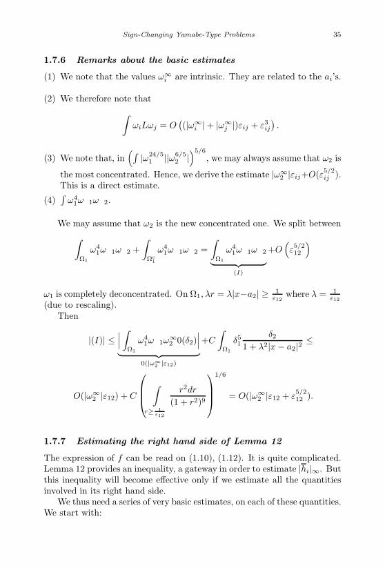
1.7.6 Remarks about the basic estimates
(1) We note that the values ω∞i are intrinsic. They are related to the ai’s.
(2) We therefore note that∫ωiLωj = O
((|ω∞
i | + |ω∞j |)εij + ε3
ij
).
(3) We note that, in(∫ |ω24/5
1 ||ω6/52 |
)5/6
, we may always assume that ω2 is
the most concentrated. Hence, we derive the estimate |ω∞2 |εij+O(ε5/2
ij ).This is a direct estimate.
(4)∫
ω41∂ω1∂ω2.
We may assume that ω2 is the new concentrated one. We split between∫Ω1
ω41∂ω1∂ω2 +
∫Ωc
1
ω41∂ω1∂ω2 =
∫Ω1
ω41∂ω1∂ω2︸ ︷︷ ︸(I)
+O(ε5/212
)
ω1 is completely deconcentrated. On Ω1, λr = λ|x−a2| ≥ 1ε12
where λ = 1ε12
(due to rescaling).Then
|(I)| ≤∣∣∣ ∫
Ω1
ω41∂ω1ω
∞2 0(δ2)
∣∣∣︸ ︷︷ ︸0(|ω∞
2 |ε12)
+C
∫Ω1
δ51
δ2
1 + λ2|x − a2|2 ≤
O(|ω∞2 |ε12) + C
∫r≥ 1
ε12
r2dr
(1 + r2)9
1/6
= O(|ω∞2 |ε12 + ε
5/212 ).
1.7.7 Estimating the right hand side of Lemma 12
The expression of f can be read on (1.10), (1.12). It is quite complicated.Lemma 12 provides an inequality, a gateway in order to estimate |hi|∞. Butthis inequality will become effective only if we estimate all the quantitiesinvolved in its right hand side.
We thus need a series of very basic estimates, on each of these quantities.We start with:
January 17, 2007 11:55 WSPC/Book Trim Size for 9in x 6in finalBB
36 Recent Progress in Conformal Geometry
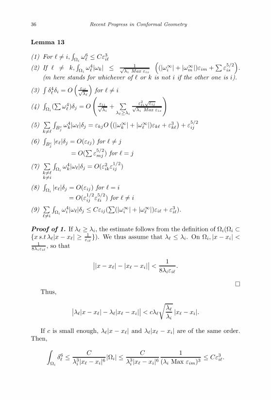
Lemma 13
(1) For = i,∫Ωi
ω6 ≤ Cε3
i
(2) If = k,∫Ωi
ω4 |ωk| ≤ 1√
λi Max εis
((|ω∞
i | + |ω∞m |)εim +
∑ε5/2is
).
(m here stands for whichever of or k is not i if the other one is i).
(3)∫
δ4 δi = O
(εi√λ
)for = i
(4)∫Ωi
(∑
ω4 )δj = O
(εij√λi
+∑
λ≥λi
ε2i√
εij√λi Max εis
)(5)
∑k =
∫Bc
jω4
k|ω|δj = εkjO((|ω∞
k | + |ω∞ |)εk + ε3
k
)+ ε
5/2ij
(6)∫
Bcj|e|δj = O(εj) for = j
= O(∑
ε5/2mj ) for = j
(7)∑k =k =i
∫Ωi
ω4k|ω|δj = O(ε2
ikε1/2ij )
(8)∫Ωi
|e|δj = O(εij) for = i
= O(ε1/2ij ε
5/2i ) for = i
(9)∑ =i
∫Ωi
ω4i |ω|δj ≤ Cεij(
∑(|ω∞
i | + |ω∞ |)εi + ε3
i).
Proof of 1. If λ ≥ λi, the estimate follows from the definition of Ωi(Ωi ⊂x s.t λ|x − x| ≥ 1
εi). We thus assume that λ ≤ λi. On Ωi, |x − xi| <
18λiεi
, so that
∣∣|x − x| − |x − xi|∣∣ <
18λiεi
.
Thus,
∣∣λ|x − x| − λ|x − xi|∣∣ < cλ
√λ
λi|x − xi|.
If c is small enough, λ|x − x| and λ|x − xi| are of the same order.Then,∫
Ωi
δ6 ≤ C
λ3i |x − xi|6 |Ωi| ≤ C
λ3i |x − xi|6
1(λi Max εim)3
≤ Cε3i.
January 17, 2007 11:55 WSPC/Book Trim Size for 9in x 6in finalBB
Sign-Changing Yamabe-Type Problems 37
Proof of 2. Observe that∫Ωi
ω4 |ωk| ≤ |Ωi|1/6
(∫Ωi
ω24/5 |ωk|6/5
)5/6
≤ C√λiMax εis
(∫Ωi
|ω|24/5|ωk|6/5)5/6
. Assume first that or k = i. The claim then follows from [Bahri 2001,
Lemma 3.2]. Next, if and k are different from i, we use 1. and Holder toconclude.
Proof of 3. Either |x − xi| ≥ 110 |x − xi|. Then, δi(x) ≤ c
√λεi and∫
Dδ4 δi = 0
(εi√λ
)where D is the domain where |x − xi| ≥ |x−xi|
10 .
Or |x−x| ≥ 12 |x−xi| and |x−xi| ≤ 1
10 |x−xi|. Then, δ(x) ≤ C√
λiεi
and ∫Dc
δ4 δi ≤ Cλ2
i ε4i
∫|x−xi|≤ 1
10 |x−xi|
√λi
(1 + λ2i |x − xi|2)1/2
= Cλ2
i
√λi
λ3i
ε4i
∫r≤λi|x−xi|
10
r2dr
(1 + r2)1/2
≤ C1ε4i√
λi
λ2i |x − xi|2 =
C1√λiλ|x − xi|
· 1
λ3/2 |x − xi|
= o
(εi√λ
).
Proof of 4. Either λ ≤ λi. Then |ω| ≤ Cδi on Ωi and the estimatefollows from 3. Or λ > λi and the estimate follows, after the use of theHolder inequality, from the definition of Ωi.
Proof of 5. Either k = j and the estimate follows from the fact thatBc
j ⊂ λj |x − xj | ≥ 1εij
. Or k = j. Then∫ω4
k|ω|δj ≤(∫
ω4kω2
)1/2 (∫ω4
kδ2j
)1/2
.
The estimate then follows from Lemma B.
Proof of 6. Straightforward. Proof of 7 and 8. Follows from 1, after the use of the Holder inequality(for = i in the case of 8.) The estimate on
∫Ωi
|ei|δj is straightforward.
Proof of 9. Use Holder and [Bahri 2001, Lemma 3.2].
January 17, 2007 11:55 WSPC/Book Trim Size for 9in x 6in finalBB
38 Recent Progress in Conformal Geometry
2. can be modified as follows if λ ≤ λi, = i or if λ > λj :
Lemma 14 • If = k and λ ≤ λi, = i,∫Bj
ω4 |ωk| ≤ Cε2
i√λjεij
• If = k and λ ≥ λj,
∫Bj
ω4 |ωk| ≤ C√
λ
(∑(|ω∞
| + |ω∞k |)εk + ε3
k
).
Proof. If = k and λ ≤ λi, = i, we use 1. of Lemma 13 and Holder.If = k and λ ≥ λj ,
∫Bj
ω4 |ωk| ≤
(∫Bj
ω4 ω2
k
)1/2(∫ω4
)1/2
.
Lemma 15∑∫Ωc
i
ω4 |ωk|δi +
∫Ωi
ω4 |ωk|δj +
√λjO(εij)
∫Bj
ω4 |ωk|
≤∑s=i
εsiO
(∑k
(|ω∞k | + |ω∞
s |)εks + ε3ks
)+ ε
5/2ij +
∑k
O(ε2ikεij)
+0(εij)√Max εjs
(∑
(|ω∞j | + |ω∞
m |)εjm + ε5/2jm ).
Proof. We use 5 of Lemma 13 for the first term, 7 and 9 of Lemma 13for the second term and 2 of Lemma 13 for the third term.
Lemma 16∫Ωc
i|v|5δi +
∫Ωi
|v|5δj + O(εij
√λj)
∫Bj
|v|5 = O(√
εij
(∫ |∇v|2)5/2)
.
Proof. Straightforward, via Holder.

January 17, 2007 11:55 WSPC/Book Trim Size for 9in x 6in finalBB
Sign-Changing Yamabe-Type Problems 39
Lemma 17 For O = δi or δj,∫(∪Ωm)c
(∑αω
)4
|k∗|O +√
λjO(εij) ×∫
(∪Ωm)c∩Bj
(∑αω
)4
|k∗|
≤ C
(∫|∇v|2
)1/2∑ε2
s
(∑t
√εti +
∑t
√εtj
).
Proof. Observe that∫Ωc
ω6
= O(∑
ε3s
)and that |Bj |1/6 ≤ C√
λj Max εjs
.
The proof follows in a straightforward way from these estimates.
Lemma 18 Let s be bounded in L6. If m = ,
∣∣∣∣∣A−1
...∫
sL−1em
...
∣∣∣∣∣(∫
Ωci
|e|δi +∫
Ωi
|e|δj + 0(εij)√
λj
∫Bj
|e|)
≤ C
∑ =i
εi
(∑(|ω∞
| + |ω∞m |)εm + ε
5/2m log5/6 ε−1
m
)+(∑
ε5/2j
√εij + ε3
is
)((ω∞
| + |ω∞m |)εm + ε
5/2m log5/6 ε−1
m
)
+εij
∑m =i
(|ω∞i | + |ω∞
m |)εim + ε5/2im log5/6 ε−1
im
.
Proof. Observe that∫Ωc
i|e|δi = O(εi) for = i, O
(∑ε3
is
)for = i;
that∫Ωi
|e|δj = O(εi) if = i since either λ ≤ λi and δ ≤ cδi on
Ωi,∫Ωi
|e|δj ≤ c∫Ωi
δ4 δiδj ≤ C
(∫Ωi
δ24/5 δ
6/5i
)5/6
≤ Cεi; or λ ≥ λi, = i
and the estimate follows from the definition of Ωi after the use of Holder.Observe that
∫Ωi
|ei|δj = O(εij). Observe finally that
O(εij)√
λj
∫Bj
|e| = O(εij) if = j
= O(ε5/2j
√εij) after the use of Holder if = j.
January 17, 2007 11:55 WSPC/Book Trim Size for 9in x 6in finalBB
40 Recent Progress in Conformal Geometry
We also know that, for = m, the coefficient of the matrix A is
0(√
(ω∞2m + ω∞2
)εm + ε5/2m log5/6 ε−1
m).
Lemma 18 follows.A corollary of the proof of the above lemma is the following estimate:
Lemma 19∫Ωc
i
|e|δi +∫
Ωi
|e|δj +√
λjO(εij)∫
Bj
|e| = O(εi +√
εij
∑ε5/2m ) if = i
= O(εij +∑
ε3im) if = i.
We then have:
Lemma 20∫ω4
k|ωs||L−1e|= O((|ω∞
k | + |ω∞ |)εk + ε
5/2k )((|ω∞
k | + |ω∞s |)εks + ε3
ks) if k =
= O((|ω∞ | + |ω∞
s |)εs + ε3s) if k = .
Proof. If k = = s, the estimate follows from [Bahri 2001, Lemma 3.2].If k = , we have:∫
ω4k|ωs||L−1e| ≤
(∫ω4
k(L−1e)2)1/2(∫
ω4kω2
s
)1/2
.
L−1e expands as ∂ω does. We may assume that ωk is less concentratedthan ω after the use of the conformal group on S3. Lemma 20 follows fromthe estimate on
∫ω4
1ω22 in [Bahri 2001] verbatim. The precise expression of
ω2 is never used in this proof, only expansions, which L−1e satisfies, areused. Lemma 21 ∫
|v|5|L−1e| = O
((∫|∇v|2
)5/2)
.
Proof. Straightforward. Lemma 22∫ (∑
αsωs
)4
|k∗||L−1e| ≤ C∑
ε5/2st
(∫|∇v|2
)1/2
.
Proof. Straightforward.

January 17, 2007 11:55 WSPC/Book Trim Size for 9in x 6in finalBB
Sign-Changing Yamabe-Type Problems 41
Lemma 23∣∣∣ ∫ ω4 L−1e(v + h)
∣∣∣ ≤ C
(∫|∇v|2
)1/2 (∑ε5/2m +
∑ε5/2m log5/6 ε−1
m
).
Proof. Follows from Lemmas 2, 3, 4 after gathering the contribution ofv and h.
We then have:
Lemma 24 If = t∫|ω|3|ωt||vm+hm||L−1e| ≤ C
(∫|∇v|2
)1/2(∫(ω3
L−1e)6/5|ωt|6/5
)5/6
≤ C
(∫|∇v|2
)1/2 ((|ω∞
t | + |ω∞ |)εt + ε
5/2t log5/6 ε−1
t
).
Proof. A small variant of the proof of Lemma A.
Lemma 25 If = t∫|ω||ωt|3|vm + hm||L−1e|
≤ C
(∫(|ωt|6/5(|ω|3|L−1e)6/5 + |ωt|24/5|L−1e|6/5
)5/6(∫|∇v|2
)1/2
≤ C
(∫|∇v|2
)1/2 ((|ω∞
t | + |ω∞ |)εt + ε
5/2t log5/6 ε−1
t
).
Proof. We split between the case when |ω(x)| ≤ |ωt(x)| and the casewhen |ωt(x)| ≤ |ω(x)| at a given x and we use Holder.
Lemma 26 If k = ,∫ω4
k|vm + hm||L−1e|
≤ C
(∫|∇v|2
)1/2 (∑(|ω∞
k | + |ω∞ |)εk + ε
5/2k log5/6 ε−1
k
).
Proof. Straightforward.
Next, we have the following key Lemma which displays the quantitiesthat we need to estimate:
January 17, 2007 11:55 WSPC/Book Trim Size for 9in x 6in finalBB
42 Recent Progress in Conformal Geometry
Lemma 27∫|ω|3|v + h|2|L−1e|
≤ C
|v|2H10
+1
λρ2
(∫Ω
|f |)2
+ λkε2k
(∫Bk
|f |)2
+
(∫Bc
|f |δ
)2
+(∫
B
|f |δf
)2)
+ C
∫|∇v|2
∑ε2
m.
Proof. Using Lemma 12, we have:∫|ω|3|v + h|2|L−1e| ≤ C|v|2H1
0+∫
|ω|3|L−1e|(
1ρ
∫Ω
|f |
+√
λkδk
∫Bk
|f | + δk
Max εs
∫B
|f |δk +√
λ
∫Bc
|f |δ
)2
+ C
∫|∇v|2
∑ε2
m (for the contribution in Ω − Ω; observe that∫
D
|ω|6
≤ Cε3k on the inner radius of Ω − Ω. This follows from 1 of Lemma 13).
Since∫ |ω|3|L−1e| = 0
(1λ
)and
∫ |ω|3|L−1e|δ2k = O(ε2
k), Lemma 23follows.
Observe that the above proof implies the estimate:(∫ω4
(v + h)2)1/2
≤ C
(1√λρ
∫Ω
|f | +√
λk εk
∫Bk
|f |
+∫
Bc
|f |δ +∫
B
|f |δk + |v| +(∫
|∇v|2)1/2
×(∑
εm
))= Cγ.
(1.16)We then have:
Lemma 28∫Ωi
ω4i |vi + hi|δj +
∫Ω
ω4 |v + h|δi +
√λj O(εij)
∫Bj
ω4j |vj + hj |
≤ O(εij)(γi + γj) + O(εiγ).

January 17, 2007 11:55 WSPC/Book Trim Size for 9in x 6in finalBB
Sign-Changing Yamabe-Type Problems 43
Proof. we observe that∫ω4
j |vj + hj | ≤(∫
ω4j
)1/2 (∫ω4
j |vj + hj |2)1/2
≤ C√λj
γj
∫ω4
j |v + h|δi ≤(∫
ω4 δ2
i
)1/2(∫ω4
|v + h|2)1/2
≤ Cγεi
∫ω4
i |vi + hi|δj ≤(∫
ω4i δ2
j
)1/2(∫ω4
i |vi + hi|2)1/2
≤ Cεijγi.
Lemma 28 follows.
Lemma 29 ∫Ωj
ω4 |ωm| ≤ C
|ω∞m |εm√
λ
+O(ε2
m)√λm
(a)
∫Ωj
ω4 |ωm| ≤ c√
λj Max εjs
∑ε5/2jt if , m = j. (b)
Proof. (b) follows in a straightforward way from 1. of Lemma 13 andHolder. To prove (a), we expand
ωm = cω∞m δm +
O(δ2m)√
λm
so that∫Ωj
ω4 |ωm| ≤ c|ω∞
m |∫
Ωj
ω4 δm+
1√λm
∫Ωj
ω4 δ2
m ≤ Cε2
m√λm
+c|ω∞m |∫
Ωj
ω4 δm.
We split∫Ωj
ω4 δm into two pieces A and B. A is the portion on x s.t |x −
am| ≤ 14 |a − am|. On B, |x−am|
|a−am| ≥ 14 . We then have
c|ω∞m |∫
Ωj
ω4 δm ≤ c|ω∞
m |λ2
|a − am|4 · 1
λ5/2m
∫r≤λm
4 |a−am|
r2dr√1 + r2
+c|ω∞
m |√λm|a − am|
∫Ωj
ω4 ≤ c|ω∞
m |εm√λλ|a − am|
+c|ω∞
m |√λm|a − am| inf
(1λj
,1λ
).
January 17, 2007 11:55 WSPC/Book Trim Size for 9in x 6in finalBB
44 Recent Progress in Conformal Geometry
(Observe that if λ ≤ λj , = j, |ω| ≤ Cδj on Ωj).
The claim follows.Lemma 15 is modified accordingly. Indeed, in this estimate of this
lemma, we have used 2 of Lemma 13 to estimate√
λjO(εij)∫
Bjω4
|ωk|.For , k = j, we use (b) of Lemma 29. For or m = j, we use (a) of
Lemma 29 or 2 of Lemma 13. We observe that if = j, by (a) of Lemma 29:
√λj O(εij)
∫Bj
ω4j |ωk| ≤ C|ω∞
k |εjkεij +√
λj
0(ε2kj)√λk
εij .
This works for λk ≥ λj since we then derive:√λj 0(εij)
∫Bj
ω4j |ωk| ≤ C|ω∞
k |εjkεij + 0(ε2kjεij).
If λk ≤ λj , we come back to 2 of Lemma 13 and we derive:√λj O(εij)
∫Bj
ω4j |ωk| ≤ O(εij)√
Max εjs
((|ω∞
j | + |ω∞k |)εjk +
∑ε5/2js
).
This provides the estimate if k = i. We thus assume now that k = i.Since |ai − ak| ≤ |ai − aj | + |aj − ak|,
1|ai − ak| ≥
12|ai − aj | or
1|ai − ak| ≥
12|aj − ak|
so that either (λk ≤ λj)
εijεjk ≤ c
λj
√λk
√λi |ai − ak||aj − ak|
≤ Cεikεjk
or
εijεjk ≤ c
λj
√λk
√λi |ai − aj ||ai − ak|
≤ Cεikεij since λj ≥ λi
(Bj ⊂ Bi, k = i).At any rate,
εijεjk√Max εjs
≤ Cεik√
εjk.
Thus,√λj O(εij)
∫Bj
ω4j |ωk| ≤ C
((|ω∞
j |εij + |ω∞k |εik)
√εjk + εij
∑ε2
js
).
January 17, 2007 11:55 WSPC/Book Trim Size for 9in x 6in finalBB
Sign-Changing Yamabe-Type Problems 45
Lastly, if k = j, we have after using (a) of Lemma 29:
√λj O(εij)
∫Bj
ω4 |ωj | ≤ C|ω∞
j |√
λj εjεij√λ
+ O(εij)ε2j
≤ C|ω∞j |εij
λ|aj − a| + O(εij)ε2j.
Summarizing, we have:
Lemma 30√λj O(εij)
∫Bj
ω4 |ωk| ≤ o(|ω∞
|εi + |ω∞k |εki) + Cεij
∑ε2
js.
1.7.8 Ri and the estimate on |vi|H10
We are now ready to derive an estimate on |vi|H10
+ |hi|∞√λi
.We denote
Ri =∫
Ωi
|f |δj +∫
Bci
|f |δi +√
λj εij
∫Bj
|f |
Γs =∑
(|ω∞t | + |ω∞
s |)εts +∑
ε5/2tm log5/6 ε−1
tm.
We then have:
Lemma 31
Ri ≤ o (Γi) + O
(1
ρi
√λi
∫Ωi
|f | +∑
εi
(1
ρ
√λ
∫Ω
|f | + |v|H10
)+(∑
εij
)|vi|H1
0
)+ O
(εij
∑ε3/2st +
√εit
∑ε5/2st
).
Proof of Lemma 31. The expression of f is provided in (1.5).By Lemma 15 improved by Lemma 29, the contribution of ω4
ωk isbounded by∑
s=i
εsiΓs + ε5/2ij +
∑k
O(εikεij) + o (Γi) + Cεij
∑ε2
js.
Since εsiεst = o(εit), this can be replaced by
o (Γi) + O(εij
∑ε3/2st
).

January 17, 2007 11:55 WSPC/Book Trim Size for 9in x 6in finalBB
46 Recent Progress in Conformal Geometry
The contribution of |v|5 by Lemma 16 is 0(√
εij
(∫ |∇v|2)5/2). The con-
tribution of (∑
αω)4|k∗| is, by Lemma 17,
O
((∫|∇v|2
)1/2∑ε2
s
(∑t
√εti +
∑t
√εtj
)).
The contribution of∑
(∑
αω)4(vm + hm) and the like (the direct contri-bution, not the one due to Q∗) splits between the terms where = m andthe terms where one of the indexes is not m. We may upperbound thistotal direct contribution with
C
ω4m|vm + hm| +
∑k =m
ω4k|vm + hm|
.
The contribution to Ri of ω4m|vm + hm| is provided by Lemma 28: it is
0(εij)
(Ri + Rj +
1ρi
√λi
∫Ωi
|f | + 1ρj
√λj
∫Ωj
|f | + |vj |H10
+(∫
|∇v|2)1/2∑
εs
)
+ 0(εi)
(R +
1ρ
√λ
∫Ω
|f | + |v| +(∫
|∇v|2)1/2∑
εts
).
The contribution of∑
k =m
ω4k|vm + hm| is
∫Ωi
ω4k|vi + hi|δj +
∫Ω
ω4t |v + h|δi +
√λj 0(εij)
∫Bj
ω4s |vj + hj |
with k = i, t = , s = j, j = i, = i.The first two terms are easily upperbounded using 1 of Lemma 13 by
Cε2ki
√εij
(∫|∇v|2
)1/2
+ C√
εi ε2t
(∫|∇v|2
)1/2
.
The third term is upperbounded by
C√
λjεijε2sj
(∫|∇v|2
)1/2 1√λj Max εjn
= O(εijε
3/2sj
∑εk
).

January 17, 2007 11:55 WSPC/Book Trim Size for 9in x 6in finalBB
Sign-Changing Yamabe-Type Problems 47
The direct contribution of (∑
αω)3(vm + hm)2 and the like is upper-bounded by the contribution of
C
((∑αω
)4
|vm + hm| + |v|5)
.
We are left with the contribution of the projection terms. For m = , thecontribution of these terms to Ri is provided in Lemma 18. It is
O(∑
εiΓ
)+(ε3
is +√
εij
∑ε5/2j
)Γ.
For m = , Lemmas 23, 26, 27, 28 provide the contribution to Ri. It is
if = i O(εij +
∑ε3
im
)× C0,
if = i O(εi +
√εij
∑ε5/2m
)× C0.
with
C0 ≤ C
(Γ +
(∫|∇v|2
)5/2
+∑
ε5/2st
(∫|∇v|2
)1/2
log5/6 ε−1st + |v|2H1
0
+ R2 +
1λρ2
(∫Ω
|f |)2
+∫
|∇v|2∑
ε2m
).
Observe that
Ri = o(1), Γi = o(1),1√λiρi
∫Ωi
|f | = o(1), εiΓ = o(Γi).
Thus, our estimates read:1 0(εij). . .
1
R1
...Rp
=
o(Γi) × 1ρi
√λi
∫Ωi
|f | +∑i=
|v|H10εi
+∑j =i
εij |v|H10
+ O(εij
∑ε3/2st
√εit
∑ε5/2st
.
An equation goes here
January 17, 2007 11:55 WSPC/Book Trim Size for 9in x 6in finalBB
48 Recent Progress in Conformal Geometry
It is not difficult to see thatId +
0 0(εij). . .
0
−1
= Id +
0 0(εij). . .
0
because εitεtm = o(εim).
Since εiΓ = o(Γi), the claim follows.
Lemma 32
1√λiρi
∫Ωi
|f | = o(Γi + |vi|H1
0
)+ O
(∑εi|v|H1
0
).
Proof. Using 2 of Lemma 13 as well as Lemma 14 and Lemma 29 (for =i), using the fact that
∫Ωi
e ≤ C√λi Max εis
ε5/2i (for = i) = C
√ρi ε
5/2i , we
find that the contribution of Q∗(∆J ′(∑
αjωj)) is o(Γi).Using then Lemma 14 and Lemma 12, which we revisit after Lemma 31,
we find that the remainder of the contribution of f is:
o(|vi|H1
0+ Γi + Ri
)+ O
(1
λ3/2i ρ2
i
∫Ωi
|f |)
= o(|vi|H1
0+ Γi
)+ o
(1
ρi
√λi
∫Ωi
|f | +∑
εi|v|H10
)+ o
(∑εi
1ρ
√λ
∫Ω
|f |)
.
Inverting our matrix as usual, we derive the estimate (use εiΓ = o(Γi)).
Finally, we have:
Lemma 33
|vi|H10
= O(Γi) + o(Γi).
Proof.
We multiply (1.2) by w where w ∈ H10 (Ωi) and w is H1
0 -orthogonal tothe small eigenvalues-eigenspace of −∆ − 5ω4
i on H10 (Ωi).
We derive ∫Ωi
(∆vi + 5ω4i vi)w =
∫Ωi
gw

January 17, 2007 11:55 WSPC/Book Trim Size for 9in x 6in finalBB
Sign-Changing Yamabe-Type Problems 49
g is made of several terms. The first contribution comes fromQ∗(∆J ′(
∑αjωj)). It is estimated in Lemma 6. We have:∫
Q∗(∆J ′
(∑αjωj
))w = O(Γi)|w|H1
0.
Next, we have the contribution of
O
∑k =i
ω4 (|vk| + |hk| + |k∗|) + |vk|5 + |hk|5 + |k∗|5
which, by Lemma 8, is
o(Γi)|w|H10.
Next, we have the contribution of hi which we trace back to Lemmas 9–10 and Lemma 11. It is o(Γi)|w|H1
0except for
∫ω4
i |hi||w| which yielded acontribution equal to
|w|H10o(Γi) + |w|H1
00(
1√λi
MaxBi/2−Bj
|hi|)
.
We revisit this estimate using Lemma 12. We obtain:(o(Γi) + O
(1√λiρi
∫Ωi
|f | +∫
Bci
|f |δi
))|w|H1
0+
O
((∫Ωi
|f |δj
)1
Max εis+√
λj
∫Bj
|f |)
×∫
Ωi
ω4i δj |w| =(
o(Γi) + O
(1√λiρi
∫Ωi
|f | +∫
Bci
|f |δi +∫
Ωi
|f |δj +√
λj εij
∫Bj
|f |))
|w|H10.
Using Lemmas 31 and 32, we find that it is(o(Γi + |vi|H1
0)+
o(∑
εi|v|H10
))|w|H1
0.
We are left with the projection terms associated to vi, hi and with thecontribution of vi to g.
The contribution of vi to g comes from
(∑j =i
αjωj
)4
− α4i ω
4i
vi +
0(|vi|2) and thus yields
o(|vi|H10)|w|H1
0.
January 17, 2007 11:55 WSPC/Book Trim Size for 9in x 6in finalBB
50 Recent Progress in Conformal Geometry
For the projection terms, the contribution of vi and hi is gathered. For = i, ∣∣∣ ∫
Ωi
ew∣∣∣ ≤ Cε
5/2i |w|H1
0.
For = i, we use Lemmas 20–24 and derive that these projection termscontribute (use also Lemmas 25–27)(
O(∑
εi|v|H10
+ o(|vi|H10
+ Γi))|w|H1
0
).
We thus have:∫Ωi
(∆vi + 5ω4i vi)w =
(O(Γi) + o(Γi + |vi|H1
0))|w|H1
0∀w ∈ H1
0 (Ω).
(1.17)On the other hand, revisiting the proof of Lemma 12 after Lemmas 31–32,we find ∫
hiψi =(o(Γi + |vi|H1
0) + O
(∑εi|v|H1
0
)).
Thus ∫viψi = o
(Γi + |vi|H1
0
)+ O
(∑εi|v|H1
0
). (1.18)
Let ∂ωi be the H10 -orthogonal projection of ∂ωi onto H1
0 (Ωi). We have:∫∇vi∇∂ωi =
(o(Γi + |vi|H1
0) + O
(∑εi|v|H1
0
))|w|H1
0. (1.19)
We assume as in [Bahri 2001] that the operator
−∆ − 5ω4i
is not degenerate on Span ∂ωi⊥ = W.Let w ∈ W . Let w be the orthogonal projection of w on H1
0 (Ωi). Using[Bahri 1989, Lemma 3.2]:∫
∇wi∇w − 5∫
ω4i viw =
∫∇vi∇w − 5
∫ω4
i viw
+ o
((∫|∇vi|2
)1/2(∫|∇w|2
)1/2)
=(O(Γi) + o(Γi + |vi|H1
0) + O
(∑εi|v|H1
0
))|w|H1
0.

January 17, 2007 11:55 WSPC/Book Trim Size for 9in x 6in finalBB
Sign-Changing Yamabe-Type Problems 51
Adding up the norm of the projection vi of vi onto Span∂ωi, which weknow by (1.18) to be of the same order we find, after inverting the matrix:
|vi|H10
= O(Γi) + o(Γi).
Lemma 34 Given εo > 0, there exists a constant Cεo such that
|vi|2H10≤ Cεo
∑k =i
ω∞k εik
2
+ εo
(∑(ω∞2
k + ω∞2
i
)ε2
ki +∑
ε4stεki log5/3 ε−1
st
)+ Om
(∑ε5/2i
).
Proof. Let ψ be an eigenfunction on R3 for the linearized operator witheigenvalue θi = 5, θi = 1
−Li = −∆ − 5ω4i .
Thus ψi satisfies
−θi∆ψi − 5w4i ψi = o , θi = 5, θi = 1.
We estimate ∑k =i
∫ω4
i ωkψi.
We pick up a special value of k. We rescale ωk so that
γεo ≤ λi
λk≤ γ2
εo
where γεo is a fixed and large constant. We also assume, changing stereo-graphic projection if needed, that |ai − ak| is bounded.
Let
Ak = x/λi|x − ai| <1
εik.
Since γεo is large,
|x − ak| = |ai − ak|(1 + oεo(1)) for x ∈ Ak

January 17, 2007 11:55 WSPC/Book Trim Size for 9in x 6in finalBB
52 Recent Progress in Conformal Geometry
ωk expands on Ak into (L is a bounded linear form)
ωk(x) = ω∞k
√λk
(1 + λ2k|x − ak|2)1/2
+√
λk L(λk(x − ak))(1 + λ2
k|x − ak|2)3/2
+O(
√λk)
(1 + λ2k|x − ak|2)3/2
=ω∞
k√λk|ak − ai|
(1 + o(1)) +O(γ2
εo)
λiλ3/2k |ai − ak|3
+√
λk L(λk(x − ak)) ×(
1(1 + λ2
k|x − xk|2)3/2− 1
(1 + λ2k|ai − ak|2)3/2
)
+√
λk L(λk(x − ak))(1 + λ2
k|ai − ak|2)3/2=
ω∞k (1 + o(1))√λk |ak − ai|
+O(γ2
εo)
λiλ3/2k |ai − ak|3
+ λk
√λk
O(|x − ai|)(1 + λ2
k|ai − ak|)3/2+
√λk L(λk(x − ak))
(1 + λ2k|ai − ak|2)3/2
.
Calculating ∫Ak
ω4i ωkψi = −θi
5
∫Ak
∆ψiωk,
observing that ψi expands as an ωi does at infinity,
−θi
∫Ak
∆ψi =ci√λi
− θi
∫Ac
k
∆ψi =ci√λi
+1√λi
O(ε2ki)
and that
− θi
∫Ak
∆ψi L(x − ak) = −θi
∫R3
∆ψiL(x − ak) + θi
∫Ac
k
∆ψiL(x − ai)
+ θiL(ai − ak)∫
Ack
∆ψi = O
(1
λ3/2i
)εik +
1√λi
O(ε2ik),
we derive ∫Ak
ω4i ωkψi = ciω
∞k εik(1 + o(1)) + O(ε3
ik).
Observe now that∫Ac
k
ω4i ωkψi = O
(∫Ac
k
δ6i
)5/6
= O(ε5/2ik
).

January 17, 2007 11:55 WSPC/Book Trim Size for 9in x 6in finalBB
Sign-Changing Yamabe-Type Problems 53
We thus derive that∑k =i
∫ω4
i ωkψi = ci
∑k =i
ω∞k εik(1 + o(1)) + O(ε5/2
ik ).
Observe also that for every ei, ∫eiψi = o,
since L−1ei is an eigenvalue of −∆ − 5ω4i with eigenvalue 5 or 1. We thus
see that ∑k =1
∫Q∗(ω4
i ωk)ψi = ci
∑k =i
ω∞k εik(1 + o(1)) + O(ε5/2
ik ).
This holds for every single eigenfunction ψ1i , . . . , ψm
i , with θj = 5, θj = 1.As m tends to +∞, θm tends to zero. We split
H1 = Em ⊕ E⊥m
where
Em = Span ψ1i , . . . , ψm
i , L−1eiand E⊥
m is its orthogonal for the scalar - product∫ ∇h∇k as well as
∫ω4
i hk.Let p⊥m : H → E⊥
m be the orthogonal projection.For w ∈ E⊥
m , we have:
O(∑
ε5/2i
)+∫
Q∗(ω4i ωk)w =
∫ω4
i ωkw ≤(∫
ω4i ω2
k
)1/2(∫ω4
i w2
)1/2
≤ θm
(∫ω4
i ω2k
)1/2(∫|∇w|2
)1/2
.
This implies that (|ϕ|H1 =(− ∫ |L|ϕϕ
)1/2 for ϕ satisfying (Vo)
|L−1i p⊥m(Q∗(ω4
i ωk))|H1 = o ((|ω∞i | + |ω∞
k |) εik + ε3ik)
and thus,
|L−1i (Q∗(ω4
i ωk))|H1
≤ Cm
∣∣∣∑k =i
ω∞k εik
∣∣∣+ o((|ω∞
i | + |ω∞k |)εik + ε3
ik
)+ Om
(∑ε5/2i
).
January 17, 2007 11:55 WSPC/Book Trim Size for 9in x 6in finalBB
54 Recent Progress in Conformal Geometry
If we consider other terms in Q∗(∆J ′(∑
αjωj)), we can drop Q∗ in view ofLemma 18, the observations on the coefficients of A and Lemma 20.
We are left estimating∫Ωi
(|ωi|3w2k + ω4
k|wi|)|w|.
We have:∫Ωi
|ω3i |w2
k|w| ≤(∫
Ωi
ω4i w2
k
)1/2(∫Ωi
ω2i w2
kw2
)1/2
≤ C
(∫Ωi
ω4i w2
k
)1/2(∫Ωi
|ωi|3|wk|3)1/3 (∫
|∇w|2)1/2
= o((|ω∞i | + |ω∞
k |)εki + ε2ki)∫
Ωi
ω4k|ωi||w| ≤
(∫Ωi
ω4kω2
i
)1/2(∫Ωi
ω4kw2
)1/2
≤ C
(∫Ωi
ω4kω2
i
)1/2(∫Ωi
ω6k
)1/3(∫|∇w|2
)1/2
= o((|ω∞
i | + |ω∞k |)εki + ε3
ki
).
We thus see (Li is Li acting on H10 (Ωi)).
|L−1i Q∗(∆J ′(
∑αjωj))|H1
0≤ Cm|
∑ω∞
k εik|
+ o(∑
(|ω∞k | + |ω∞
i |)εki +∑
ε2st
√εki log5/6 ε−1
st
)+ Om
(∑ε5/2i
).
This combined with Lemma 31, Lemma 32 and Lemma 33 yields the result.
1.8 Proof of the Morse Lemma at Infinity When theConcentrations are Comparable
After estimating the contribution of v in J ′(∑
αjωj + v). ∂ωi, we establishthe Morse Lemma at infinity under (1.3) (which we always assume) and(1.4) which we will eventually suppress. (1.4) states that the concentrationsof all masses are comparable.

January 17, 2007 11:55 WSPC/Book Trim Size for 9in x 6in finalBB
Sign-Changing Yamabe-Type Problems 55
In what follows, we will denote
S2i = Cε0
∑k =i
ω∞k εik
2
+ εo
(∑(ω∞2
k + ω∞2
i
)ε2
ki +∑
ε4stεki log5/3 ε−1
st
)+ Om
(∑ε5
i
).
(1.20)
In the sequel, ∂ωi is ∂ωi
∂ai.
Lemma 35 ∑ =i
∫Ωc
i
ω4 |∂ωi||v| ≤ o
(∑λmΓ2
m
).
Proof. For a given , we decompose the above integral into two pieces,one on Ω ∩ Ωc
i and the other one on (Ω ∪ Ωi)c. Ω and Ωi are the subdo-mains of Ω and Ωi where the estimate of Lemma 12 holds.
We first take care of ∫Ω∩Ωc
i
ω4 |∂ωi||v + h|.
We start with∫Ω∩Ωc
iω4
|∂ωi||v| which we split into two pieces A + B.
A =∫
Ω∩Ωci∩|x−ai|≤ 1
4 |ai−a|ω4
|∂ωi||v|
B =∫
Ω∩Ωci∩|x−ai|≥ 1
4 |ai−a|ω4
|∂ωi||v|.
Since |x − ai||∂ωi| ≤ C|ωi|, where ωi behaves just as ωi does:
B ≤(∫
Ω∩Ωci
ω4 |ωi||v|
)1
|a − ai| ≤1
|a − ai|S×((|ω∞
| + |ω∞i |)εi + ε3
i
)
≤∑
m =
|ω∞m εm|
((|ω∞ | + |ω∞
i |)εi + ε3i
)+
o(∑
(|ω∞m | + |ω∞
|)εm +∑
ε4stεm log5/6 ε−1
st +∑
0(ε5/2s )
)

January 17, 2007 11:55 WSPC/Book Trim Size for 9in x 6in finalBB
56 Recent Progress in Conformal Geometry
×((|ω∞ | + |ω∞
i |)εi + ε3i))
1|a − ai| =
∑m
Bm.
Either
|a − ai| ≥ 110
|a − am|.
Then
Bm ≤ C((|ω∞
|2 + |ω∞i |2)ε2
i + ε6i
) 1|a − ai|
+C
|a − am|((|ω∞
m |2 + |ω∞ |2)ε2
m + O(ε2mε
6st + ε5
s)).
Or |a − ai| ≤ 110 |a − am| so that
910
≤ |a − am||ai − am| ≤
1110
.
Then,
εm · εi ≤ 109
εim · 1λ|ai − a|
and
Bm ≤ Cλi
((|ω∞
|2 + |ω∞i |2 +
∑|ω∞
m |(|ω∞ | + |ω∞
i |))
εimε2i
)+
1|a − ai|
∑ε5/2st (|ω∞
| + |ω∞i )εi +
ε3i
∑ε5/2st
|a − ai|
+√
λλi
(∑(|ω∞
| + |ω∞m |)εm
)ε5
i.
Thus
Bm ≤ o((λi + λ)(|ω∞
|2 + |ω∞i |2)ε2
i
)+o(λi
∑|ω∞
m |2ε2im
)+C
√λλi
∑ε5
st.
This settles B for v.Now considering A, we have:
34|ai − a| ≤ |x − a| ≤ 5
4|ai − a|.
Thus,
A ≤ C
λ2 |ai − a|4 |v|H1
0
(∫Ωc
i∩|x−ai|≤ 14 |ai−a|
|∂ωi|6/5
)5/6
.
January 17, 2007 11:55 WSPC/Book Trim Size for 9in x 6in finalBB
Sign-Changing Yamabe-Type Problems 57
∂ωi expands (see [Bahri 2001]) as follows:
∂ωi = λi
(ω∞
i ∂δi +O(δi)
1 + λ2i |x − ai|2
)= λiω
∞i ∂δi + O(δ3
i )
where ∂δi is the derivative of δi with respect to rescaled variables 1λi
∂
∂aji
·Ωci
is made of two parts Ei ∪ Ii, where
Ei = x /∈ Ωi, λi|x − xi| ≥ c Min(
1εij
)
Ii = x; λm|x − xm| ≤ c
εimfor some λm ≥ λi, λi, = λm = λi
and we have accordingly:
A ≤ C|v|H1o
λ2 |ai − a|4 × 1
λi
|ω∞i |(∫
r≤ 14 λi|ai−a|
r2dr
(1 + r2)6/5
)5/6
+
(∫r≥ c
Max εij
r2dr
(1 + r2)12/5
)5/6
+C|v|H1
0
λ|ai − a|2(∫
Ii
ω12/5 δ
18/5i
)5/6
≤ Cλi|v|H10
ε4
i
(|ω∞
i |√
λi|ai − a| + Maxε3/2ij
)
+ ε2i
∑λm≥λi
λm =λi
ε5/2mi log5/6 ε−1
mi +∑
λm≥λi
λm =λi
εmε3/2im
≤ C√
λiεi|v|H10· √λi |ω∞
i |ε2i
λ1/2 |ai − a|1/2
+ o(λi
(ε2
i|v|2H10
+∑
ε5im
))≤ o
(λiε
2i|v|2H1
0+ λiω
∞i ε4
i
)+ Cλi
∑ε5
im.
We now take care of the contribution of h. δk is the notation for the genericmass (with λk ≥ λ) contained in B = x s.t λ|x − x| ≤ c Min 1
εs.
We are studying∫Ω∩Ωc
i
ω4 |h||∂ωi| ≤ θ
∫Ω∩Ωc
i
ω4 δk|∂ϕi| + β
∫Ω∩Ωc
i
ω4 |∂ωi|
with
θεk +β√λ
= o(∑
(|ω∞m | + |ω∞
|)εm + ε5/2m log5/6 ε−1
m
).

January 17, 2007 11:55 WSPC/Book Trim Size for 9in x 6in finalBB
58 Recent Progress in Conformal Geometry
We start with
θ
∫Ω∩Ωc
i
ω4 δk|∂ωi| ≤ λiθ
(∫Ω∩Ωc
i
ω4 |δ2
k
)1/2
×(∫
Ω∩Ωci
ω4 |∂ωi|2
)1/2
≤ λiθεk
(∫Ω∩Ωc
i
ω4 |∂ωi|2
)1/2
.
We split the integral into two pieces A and B as above; Ωci is made of two
pieces Ei and Ii; Ω is connected, hence contained in one of them.Then,
A ≤ C
λiλ|ai − a|2∫
Ei
(ω∞2
i
(1 + λ2i |x − ai|2)2 +
1(1 + λ2
i |x − ai|2)3)
λ3i r
2dr
+∫
Ω∩Ii
δ6i
1/2
≤ Cε2i
|ω∞
i |ε1/2is + ε
3/2is + ε
3/2i
and
λiθεkA ≤ C√
λi (θεk)εi
√λi |ω∞
i |εiε1/2is +
√λi εiε
3/2is
≤ o(λi(θεk)2ε2
i + λiω∞2
i ε2i) + Cλiε
2iε
3is.
We now have(for B, |x−ai|
|ai−a| ≥ c > o; λi|∂ωi||x − ai| ≤C(|ω∞
i |δi + δi
(1+λ2i |ai−a|2)1/2
))
B ≤ C√λi |ai − a|
ω∞2
i
1 + λ2i |ai − a|2 +
1(1 + λ2
i |ai − a|2)21/2 (∫
ω4
)1/2
≤ C
λi|ai − a|(|ω∞
i |εi +εi
λi|ai − a|)
and
λiθεkB ≤ C
(θεk|ω∞
i |εi
|ai − a| +θεkεi
λi|ai − a|2)
≤ C(√
λ θεk
√λi |ω∞
i |ε2i +
√λ θεk ·
√λ ε3
i
)≤ O
(λ(θεk)2 + λiω
∞2
i ε2i + λε
5i
).
January 17, 2007 11:55 WSPC/Book Trim Size for 9in x 6in finalBB
Sign-Changing Yamabe-Type Problems 59
We study now
β
∫Ω∩Ωc
i
ω4 |∂ωi|.
We split again∫Ω∩Ωc
iω4
|∂ωi| into two pieces A and B.We have:
A ≤ Cλi
λ5/2i λ2
i |ai − a|4|ω∞
i |∫≤cλi|ai−a|
r2dr
1 + r2+
C√λ |ai − a|
∫Ω
ω3 δ
3i
≤ C|ω∞i |εi
λ3/2 |ai − a|2
+ C√
λi εi(ε3i log ε−1
i ).
Thus,
βA ≤ C
(√λ
(β√λ
) √λ |ω∞
i |εi
λ2 |ai − a|2 +
√λ
(β√λ
)√λiε
4i log ε−1
i
)
≤ O
(λ
(β2
λ
)+ λω
∞2
i ε2i + λiε
7i
).
We study now B: (|x − ai| ≥ c|ai − a|)
B ≤ C
|ai − a|(∫
Ω
ω4
)( |ω∞i |√λi
(1 + λ2i |ai − a|2)1/2
+√
λi
1 + λ2i |ai − a|2
)≤ C√
λ
( |ω∞i |εi
|ai − a| +εi
λi|ai − a|2)
βB ≤ C
(β√λ
|ω∞i |εi
|ai − a| + C√
λ
(β√λ
)·√
λε3i
)
≤ C
(β2
λ
1|ai − a| + O
(ω∞2
i ε2i
|ai − a|
)+ λ
(β2
λ
)+ λε
6i
).
To complete the proof of Lemma 35, we need to estimate∫(Ω∪Ωi)c
ω4 |∂ωi||v|.
In (Ω ∪ Ωi)c, there are three portions: the first one is exterior to the twoballs B and Bi. We denote it A. We then have B and C which are theportions in B ∩ Ωc
and in Bi ∩ Ωci .

January 17, 2007 11:55 WSPC/Book Trim Size for 9in x 6in finalBB
60 Recent Progress in Conformal Geometry
We first estimate ∫A
ω4 |∂ωi||v|
which we upperbound as follows:∫A
ω4 |∂ωi||v| ≤ Cω∞4
∫A
δ4 |∂ωi||v| + C
∫A
δ4
(1 + λ2 |x − a|2)2 |∂ωi||v|
≤ Cω∞4
λiε2s
(∫|∇v|2
)1/2(∫A
δ6i
(1 + λ2i |x − ai|2)3
)1/6
· |ω∞i |
+ Cλi
(∫A
δ6
(1 + λ2 |x − a|2)2
)2/3(∫|∇v|2
)1/2 (∫A
δ6i
)1/6
.
Observe that
A ⊂
λi|x − ai| ≥ c
Max εis
A ⊂
λ|x − a| ≥ c
Max εs
so that∫
A
ω4 |∂ωi||v| ≤ C|ω∞
i ||ω∞i |4λiε
2s
(∫|∇v|2
)1/2
· ε3/2is
+ Cλiε6s
(∫|∇v|2
)1/2
ε1/2is ≤ o(λi|ω∞
i |2ε2is)
+ Cλiε1/2is ε4
s
(∫|∇v|2
)1/2
.
This settles A.B is typically made of balls ∪Bk corresponding to “masses” ωk whose
center ak lies in B ∩ Ωc with λ ≥ λ.
On such balls,
λk|x − ak| ≤ 14εk
∼√
λkλ|a − ak|
4
so that on such balls,
34|a − ak| ≤ |x − a| ≤ 5
4|a − ak|
January 17, 2007 11:55 WSPC/Book Trim Size for 9in x 6in finalBB
Sign-Changing Yamabe-Type Problems 61
and, therefore,∫Bk
ω4 |∂ωi||v| ≤ C
( |ω∞ |4
λ2 |a − ak|4 +
1λ6
|a − ak|8)∫
Bk
|∂ωi||v|
≤ Cλi
( |ω∞ |4
λ2 |a − ak|4 +
1λ6
|a − ak|8)(∫
|∇v|2)1/2(∫
Bk
|∂ωi|6/5
)5/6
≤ Cλi
( |ω∞ |4
λ2 |a − ak|4 +
1λ5
|a − ak|8)(∫
|∇v|2)1/2
× 1√λi
×(∫
Bk
(√
λi)12/5
(1 + λ2i |x − ai|2)6/5
)5/6
≤ Cλi
( |ω∞ |4
λ2 |a − ak|4 +
1λ6
|a − ak|8)
×(∫
|∇v|2)1/2 1√
λi
(∫Bk
δ6i
)1/3
|Bk|3/5.
Thus, with εkt = Max εkm∫Bk
ω4 |∂ωi||v|
≤ C√
λi
( |ω∞ |4
λ2 |a − ak|4 +
1λ6
|a − ak|8)(∫
|∇v|2)1/2
εikλ
1/5k ε
1/5kt
λ2kε2
kt
≤ C√
λiλ1/5k
ε4k
ε2kt
(∫|∇v|2
)1/2
εikε1/5kt = o
(λiε
2ik
∑ε3
st + λkε2k
∑ε3
st
).
This settles B.
Arguing in the same way on C, we have:∫Ck
ω4 |∂ωi||v| ≤ Cλi
( |ω∞ |√λi
(1 + λ2i |ai − ak|2) +
√λi
(1 + λ2i |ai − ak|2)3/2
)×(∫
|∇v|2)1/2(∫
Ck
ω6
)2/3
· 1√λkMax εkt
≤ C|ω∞
i |εik
|ai − ak|ε2k
(∫ |∇v|2)1/2
√Max εkt
+(∫ |∇v|2)1/2ε2
k√Max εkt
εik
λi|ai − ak|2
≤ C√
λi |ω∞i |εik ·
√λkε
3/2k εik
(∫|∇v|2
)1/2
+ λk
(∫|∇v|2
)1/2
ε3/2k ε3
ik
≤ o
(λiω
∞2
i ε2ik + λkε3
kε2ik
∫|∇v|2
).
This settles C.

January 17, 2007 11:55 WSPC/Book Trim Size for 9in x 6in finalBB
62 Recent Progress in Conformal Geometry
Lemma 36∑ =i
∫Ωi
ω4 |v||∂ωi| ≤ CλiS
2i .
Proof. In view of Lemma 35, we just need to estimate
∑ =i
∫Ωi
ω4 |vi + hi||∂ωi| ≤ C
∑ =i
|vi|H10
(∫Ωi
ω24/5 |∂ωi|6/5
)5/6
+∑ =i
(1ρi
∫Ωi
|f | +√
λi
∫Bc
i
|f |δi
)∫Ωi
ω4 |∂ωi|
+∑ =i
(1
Max εis
∫Ωi
|f |δj +√
λi
∫Bj
|f |)∫
Ωi
ω4 |∂ωi|δj
.
Observe that |∂ωi| ≤ C(√
λi|ω∞i |δ2
i + δ3i
)so that∫
Ωi
ω4 |∂ωi| ≤ C
√λi|ω∞
i |ε2i + C
√λ
∫Ωi
ω3 δ
3i
≤ C√
λi |ω∞i |ε2
i + C√
λ ε3i log ε−1
i
while ∫Ωi
ω4 |∂ωi|δj ≤ λi
(∫Ωi
ω4 δ2
j
)1/2 (∫ω4
|∂ωi|2)1/2
≤ λiεj
((|ω∞
| + |ω∞i |)εi + ε4
i
).
Hence,
∑ =i
∫Ωi
ω4 |vi + hi||∂ωi| ≤ C
∑ =i
λi|vi|H10((|ω∞
| + |ω∞i |)εi + ε3
i)
+∑ =i
√λi
(1
ρi
√λi
∫Ωi
|f | +∫
Bci
|f |δi
)(√λi|ω∞
i |ε2i +
√λ ε3
i log ε−1i
)
+∑ =i
√λi
(√λj εj
∫Bj
|f |)
·√
λi
((|ω∞
| + |ω∞i |)εi + ε4
i
)+∑ =i
λi
Max εis
∫Ωi
|f |δj
(∫Ωi
ω4 δ
2j
)1/2
× ((|ω∞ | + |ω∞
i |)εi + ε4i)).

January 17, 2007 11:55 WSPC/Book Trim Size for 9in x 6in finalBB
Sign-Changing Yamabe-Type Problems 63
Either λ ≤ λi. Then |ω| ≤ Cδi on Ωi and(∫
Ωiω4
δ2j
)1/2
≤
C(∫
Ωiδ4i δ2
j
)1/2
≤ Cεij .Or λ ≥ λi( = i). Then,(∫
Ωi
ω4 δ2
j
)1/2
= O(εi√
εij).
Thus
λi
Max εis
∫Ωi
|f |δj
(∫Ωi
ω4 δ2
j
)1/2 ((|ω∞
| + |ω∞i )εi + ε4
i
)≤ C
(√λi
∫Ωi
|f |δj
)√λi
((|ω∞
| + |ω∞i |)εi + ε4
i
)and the estimate follows.
Lemma 37∑ =i
∫Ωi
|ω|3v2|∂ωi| ≤ CλiS2i .
Proof. If = i, either |ω(x)| ≤ |v(x)| or |v(x)| ≤ |ω(x)| so that∫Ωi
|ω|3v2|∂ωi| ≤∫
Ωi
ω4 |v||∂ωi| + λi
(∫|∇v|2
)5/2
and the estimate follows from the previous lemma.
Lastly, we have:
Lemma 38∫ |ωi|3|v|2|∂ωi| ≤ CλiS
2i .
Proof. We split the integral in∫Ωi
|ωi|3v2|∂ωi| and∫Ωc
i|ωi|3v2|∂ωi|.
For the first part, we have∫Ωi
|ωi|3v2|∂ωi| ≤ C
∫Ωi
|ωi|3v2i |∂ωi| + C
∫Ωi
|ωi|3h2
i |∂ωi|
≤ Cλi|vi|2H10
+ C
(1ρi
∫Ωi
|f | +√
λi
∫Bc
i
|f |δi
)2
+ C
(√λj
∫Bj
|f | + 1Max εit
∫Ωi
|f |δj
)2
×∫
Ωi
|ωi|3δ2j |∂ωi|

January 17, 2007 11:55 WSPC/Book Trim Size for 9in x 6in finalBB
64 Recent Progress in Conformal Geometry
≤ Cλi
|vi|2H10
+
(1√λiρi
∫Ωi
|f | +∫
Bci
|f |δi
)2
+ C
(√λjεij
∫Bj
|f | +∫
Ωi
|f |δj
)2 .
The first part is thus settled.Next, we estimate ∫
Ωci
|ωi|3|∂ωi||v|2
|∂ωi| is bounded by λi
(|ω∞
i |δi + δi
(1+λ2i |x−ai|2)1/2
).
Thus,∫Ωc
i
|ωi|3|∂ωi|v2 ≤ Cλi|ω∞i |∫
Ωci
δ4i v2 + Cλi
∫Ωc
i
δ4i
(1 + λ2i |x − ai|2)2 |v|
2
≤ Cλi|ω∞i |(∫
|∇v|2)∑
ε2i + Cλi
∫|∇v|2
(∫Ωc
i
δ6i
(1 + λ2i |x − ai|2)3
)2/3
.
The first term is easily upperbounded by
Cλi|ω∞i |2
∑ε2
i + Cλi
(∫|∇v|2
)2∑ε2
i.
For the second term, we split the integral over Ωci into two pieces.
The first one is
Cλi
∫|∇v|2
(∫λi|x−ai|≥ 1
Maxεit
δ6i
(1 + λ2i |x − ai|2)3
)2/3
≤ Cλi
∫|∇v|2 Max ε6
it.
The second one involves integration over subdomains Bk of Bi which cor-responds to masses “ωk” having λk ≥ λi.
On Bk
λi|x − ai| ≥ 12λi|ak − ai|
January 17, 2007 11:55 WSPC/Book Trim Size for 9in x 6in finalBB
Sign-Changing Yamabe-Type Problems 65
and we have:
Cλi
∫|∇v|2
(∫Bk
δ6i
(1 + λ2i |x − ai|2)
3)2/3
≤ Cλi
∫|∇v|2 · 1
λ4i |ak − ai|4 ε2
ik
≤ C√
λiλk
λ3i |ak − ai|3
∫|∇v|2ε3
ik = o(λi
∫|∇v|2ε3
ik + λk
∫|∇v|2ε3
ik).
Lemma 38 follows.Next we observe that:
Lemma 39∑ =i
∫|ωi|3|ω||∂ωi||v| + |ω|3|ωi||v||∂ωi|
≤ C
∫ |ωi|3|∂ωi||v|3 +∑ =i
∫|ωi|3|∂ωi|ω2
+∑ =i
∫ω4
|∂ωi||v| .
Proof. Observe that∫|ωi|≥|ω|
|ω|3|ωi||∂ωi||v| ≤∫
|ωi|≥|ω||v|≥|ω| |ωi|3|∂ωi||v|2 +
∫|ωi|≥|ω|
ω4 |ωi||∂ωi|
≤∫
|ωi|3|∂ωi|v2 +∫
|ωi|3|∂ωi|ω2 .
Lemma 40 follows. The estimate of Lemma 8 on∫ |ωi|4ω2
extends of courseto 1
λi
∫ |ωi|3|∂ωi|ω2 .
We expand
J ′(∑
αjωj + v)· ∂ωi = J ′
(∑αjωj
)· ∂ωi + J ′′
(∑αjωj
)· v · ∂ωi
+ O
(∑∫ω4
j v2|∂ϕi| +∫
|v|5|∂ϕi|)
.
The expansion of J ′(∑
αjωj)∂ωi
∂aiis straightforward and yields as prin-
cipal terms
∑i=j
ω∞j
∂
∂ai
((ω∞
i +Dωi(
ai−aj
|ai−aj | )
λi|ai − aj |
)εij
)−∑
cij
∂ε3ij
∂ai
ωi is the rescaled version of ωi. There are additional terms which areo(∑ ω∞2
i
λi|ai−aj |2 + ε3ij
|ai−aj | + · · ·)
.

January 17, 2007 11:55 WSPC/Book Trim Size for 9in x 6in finalBB
66 Recent Progress in Conformal Geometry
We split the various integrals involving v, after the use of (Vo) to getrid of all
∫ω4
i∂ωi
∂aiv etc. between the various contributions over each do-
mains Ωi and the contribution over (UΩi)c. We use Lemmas 32 to39 and we find that these contributions can be thrown into a remain-der. However, the remainder does not behave as a small o of the princi-pal terms for two main reasons: first we find, because our estimates over|vi|H1
0are not suitable, contributions of the type o
(λiω
∞2i εij
), which are
o(
ω∞2i
λj |ai−aj |2)
, not o(
ω∞2i
λi|ai−aj |2)
.
Second, because the remainders in these estimates (and in the estimateson |ho
i |∞√λi
+∑
λs≥λi
εis|his|∞) are only O(εij
∑ε2
st) at best, we find terms such
as o(
εij
∑ε2
st
|ai−aj |)
which are not o(
ε3ij
|ai−aj |).
Nevertheless, if the λi’s are comparable as well as the εij ’s, these re-mainder terms are all
o
(∑ ω∞2i
λi|ai − aj |2 +∑ ε3
ij
|ai − aj |
).
Using then Conjecture 2 and the σi-equation (see Proposition 8 in the thirdpart of the book), we can establish the Morse Lemma at infinity.
The details about this proof and this expansion are provided at theend of the third part of the first half of the book. We refer the reader to“Basic Conformal Estimates” and more precisely to Lemmas 62–67 and tothe sections “The system of equations corresponding to the variations ofthe points ai’s” and the following sections for all details on the expansionsand proof of the Morse Lemma at infinity.
If the λi’s are comparable as well as the εij ’s, the estimates providedabove are sufficient. But these are strong hypotheses which we remove, stepby step, over the remainder of this work.
1.9 Redirecting the Estimates, Estimates on |vi|H10
+|h0
i |∞ +∑
λs>λi
εsi |hs
i |∞
1.9.1 Content of Part II
Part II contains three new estimates:First, a simple observation allows to improve the estimate on(∫
Ωj
|ωj |24/5|ωi|6/5 + |ωi|24/5|ωj |6/5
)3/2
for λj ≥ λi.

January 17, 2007 11:55 WSPC/Book Trim Size for 9in x 6in finalBB
Sign-Changing Yamabe-Type Problems 67
Instead of C((|ω∞
i | + |ω∞j |)εij + ε3
ij
), we find
C(|ωi(aj)|εij + ε3
ij
)i.e. basically C(|ω∞
i |εij + ε3ij).
Second, we derive an L∞-estimate on v after bootstrapping in the equa-tion that v satisfies (derived in Part I). This L∞-estimate reads
|v − θh|(x) ≤ Ch
∑δ(x) ∀x ∈ S3
with
|θh|H1(S3) ≤ Ch
∑εh
k
h is an arbitrary exponent. This pointwise estimate can be improved in(UΩi)c.
Third, we derive a better estimate on∫ω4
|ωk||x − y| .
We prove (Lemma 40) that:∫ω4
|ωk||x − y| ≤ C
∑λi≥λ
orλ≥λk
εijδi for y ∈ (Ω ∪ Ωk)c .
After these three estimates, we revisit all the estimates of Part I, Lemmas 13to 30 in particular, which we improve considerably. (Lemmas 41–56)
The remainder terms in our expression, on each Ωi involve now a powerof |vi|H1
0+ |hi|∞√
λi; this power is however too weak to allow us to prove the
Morse Lemma at infinity without (1.3). (See Lemma 57).After Lemma 41–56, we derive the main improvement of Part II which
is provided in Theorem 1: we establish that a much better estimate on|vi|H1
0+ |hi|∞√
λiwhen compared to the ones provided in Lemmas 33–34 holds,
up to a remainder term equal to Ch
∑εh
st (due to bootstrapping; we willget rid of it in Part III).
If we remove the remainder term, the estimate on |vi|H10
is optimal
because the remainder is then (essentially) O
(∑
ε3ik
).
Lemma 57 of Part II can be skipped if one wants to go directly to theproof of the Morse Lemma at infinity.

January 17, 2007 11:55 WSPC/Book Trim Size for 9in x 6in finalBB
68 Recent Progress in Conformal Geometry
1.9.2 Redirecting the estimates
In the previous sections, we have devised a method and a number of esti-mates. We have thought of S3 as subdivided in various regions Ωi, Ωc =(UΩi)c adapted to our family of solutions ωi and we have thought of v asdecomposed in
∑(vi + hi) + k∗. We have estimated the various vi, hi, k
∗,thinking of them at single entries related by “a matrix of interaction”.However, these estimates are not enough to cover the general case of anypossible configuration. So far, we can complete our Morse Lemma at infin-ity only if the concentrations λi are of the same order and the points arenot “too close”.
Here we redirect our estimates, keeping the same general framework andwork out in this way improvements in the estimates. Eventually, we willwork out the general case.
We start with an observation. Namely,
Proposition 1 Assume that λj ≥ λi. Then,(∫Ωj
|ωj |24/5|ωi|6/5 +∫
Ωj
|ωi|24/5|ωj |6/5
)5/6
≤ C(∣∣ωi(aj)
∣∣εij + ε3ij
)where wi(aj) is the value of ωi set in its standard form (with concentration0(1)) at aj , the (then new) concentration point (on S3, after dilation) ofωj.
Proof. We revisit [Bahri 2001, proof of Lemma 3.2].
For(∫
Ωj|ωj|24/5|ωi|6/5
)5/6
, there is nothing to change.
For(∫
Ωj|ωi|24/5|ωj|6/5
)5/6
, we notice that
Ωj ⊂
λj |x − aj | ≤ C
εij
.
All our domains in fact are defined on the sphere, using the geodesic dis-tance. When needed, we complete a stereographic projection with respectto a North Pole which keeps all points of concentration in a given compactset and all concentrations roughly of the same size than they were on thesphere if needed.
Thinking of aj as being the South Pole (we are here only estimating∫Ωj
|ωi|24/5|ωj |6/5, not considering all the mases together, our observationswhich we just stated do not apply) after rescaling so that ωi has concen-tration 1, performing a stereographic projection, Ωj becomes:

January 17, 2007 11:55 WSPC/Book Trim Size for 9in x 6in finalBB
Sign-Changing Yamabe-Type Problems 69
Ωj =
λj |x| ≤ C
εij
.
Now, εij is of the size of λ−1/2j , hence Ωj is a very small ball of radius
0(
1
λ1/2j
)around the origin.
ωi expands as ωi(0) + 0(|x|) and we derive that
(∫Ωj
|ωi|24/5|ωj |6/5
)5/6
≤ Cωi(0)4
∫
r≤ 1√λj
√
λj
(1 + λ2jr
2)1/2
6/5
5/6
+ C
∫
r≤ 1√λj
r24/5
√
λj
(1 + λ2jr
2)1/2
6/5
5/6
≤ C
|ωi(0)|√λj
+1
λ3/2j
.
We now move to prove a much finer estimate on v, namely:
Proposition 2 ∀h ∈ N, there exists a constant Ch > 0 and a functionθh ∈ H1 such that
(i) |v − θh|(x) ≤ Ch
∑δ(x) ∀x ∈ S3
(ii) |θh|H1 ≤ Ch
∑εh
k
(iii) |v − θh|(x) ≤ Ch
∑(εk + |v|L6 + |h|∞/√λ
)δ(x) ∀x ∈ Ωc =
(UΩi)c.
Proof.Proof of (i) and (ii). v satisfies
− ∆v −((∑
αjωj + v)5
−(∑
αjωj
)5
− 5(∑
αjωj
)4
v
)= f + 5
(∑αjωj
)4
v
which we rewrite as
−∆v − b(x, v) = f + 5(∑
αjωj
)4
v.
January 17, 2007 11:55 WSPC/Book Trim Size for 9in x 6in finalBB
70 Recent Progress in Conformal Geometry
Let
ϕ = −∆−1
(f + 5
(∑αjωj
)4
v
).
It is easy to see that, with a suitable constant C:
|f(x)| ≤ C(∑
δ5
).
We consider ∫ω4
i |v||x − y| .
Either |y − xi| ≥ Cλi
. Then∫ω4
i |v||x − y| ≤
∫|x−y|≤ c
2λi
ω4i |v|
|x − y| + C1
√λi
∫|x−y|≥ c
2λi
ω4i δi(y, λi)(x)|v|.
Clearly, if |x − y| ≤ c2λi
,
ω4i ≤ Cδ4
i (xi, λi)(y)
and ∫|x−y|≤ c
2λi
|v||x − y| ≤
C|v|L6
λ3/2i
.
Thus, ∫|x−y|≤ c
2λi
ω4i |v|
|x − y| ≤ Cδ4i (xi, λi)(y)|v|L6
λ3/2i
≤ Cδi(xi, λi)(y)|v|L6 .
On the other hand,∫ω4
i δi(y, λi)(x)|v| ≤ C|v|L6
(∫δ24/5i (xi, λi)δ
6/5i (y, λi)(x)
)5/6
≤ C|v|L6
λi|y − xi| .
Thus, ∫ω4
i |v||x − y| ≤ C2|v|L6δi(xi, λi)(y) if λi|y − xi| ≥ C.
January 17, 2007 11:55 WSPC/Book Trim Size for 9in x 6in finalBB
Sign-Changing Yamabe-Type Problems 71
If |y − xi| ≤ Cλi
, then (observe that |x − xi| ≥ 2Cλi
⇒ |x − y| ≥ |x−xi|2 )∫
ω4i |v|
|x − y| ≤∫
|x−xi|≤ 2Cλi
ω4i |v|
|x − y| + C√
λi
∫δ5i |v|
≤ C1δ4i (xi, λi)(y)
∫|x−y|≤ 3C
λi
|v||x − y| + C1δi(xi, λi)(y)|v|L6
≤ C2δ4i |v|L6
λ3/2i
+ C2δi(xi, λi)(y)|v|L6 ≤ C3δi|v|L6 .
Combining these estimates and the one of f , we derive that
|ϕ(x)| = O(∑
δ
).
Then,
−∆(v − ϕ) − (b(x, v) − b(x, ϕ)) = b(x, ϕ).
Since b is of second order in the second variable,
|b(x, v) − b(x, ϕ)|L6/5 = o(|v − ϕ|L6)
and∫|∇(v−ϕ)|2 ≤ C
∫b(x, ϕ)(v−ϕ) ≤ C|v−ϕ|L6 |b(x, y)|L6/5 ≤ C1|v−ϕ|L6 |ϕ|2L6 .
Thus, (∫|∇(v − ϕ)|2
)1/2
≤ C2|ϕ|2L6 .
Set
ϕ1 = −∆−1 (b(x, ϕ)) .
Clearly,
|ϕ1|L6 ≤ C3|ϕ|2L6 .
Then,
−∆ (v − (ϕ + ϕ1)) − (b(x, v) − b(x, ϕ + ϕ1)) = b(x, ϕ + ϕ1) − b(x, ϕ)
|b(x, v) − b(x, ϕ + ϕ1)|L6/5 = o (|v − (ϕ + ϕ1)|L6)

January 17, 2007 11:55 WSPC/Book Trim Size for 9in x 6in finalBB
72 Recent Progress in Conformal Geometry
and
|b(x, ϕ + ϕ1) − b(x, ϕ)|L6/5 ≤ C|ϕ1|L6(|ϕ|L6 + |ϕ1|L6) ≤ C4|ϕ|3L6
so that (∫ ∣∣∇(v − (ϕ + ϕ1))∣∣2)1/2
≤ C5|ϕ|3L6
and
|ϕ1(x)| = | − ∆−1(b(x, ϕ))| ≤ C∑
δ(x).
Bootstrapping and observing that
f =(∑
αjωj
)5
−(∑
αjωj + v)5
− Q∗((∑
αjωj + v)5
−(∑
αjωj
)5)
− Q∗((∑
αjωj
)5)
.
So that, since |v|H1 ≤ C∑
εij and since |Q ∗ ((∑αjωj)5) |L6/5 ≤ C
∑εij ,
|f |L6/5 ≤ C∑
εij ,
we derive that
|ϕ|L6 ≤ C∑
εij .
(i) and (ii) of Proposition 2 follow. Proof of (iii). v satisfies
−∆v − Q∗((∑
αjωj + v)5)
= 0
which we rewrite:
−∆v − Q∗((∑
αjωj
)5
+ γ(x)v)
= 0.
Using (i) and (ii), we can estimate γ as follows:|γ − γh|(x) ≤ Ch
∑δ4
|γh|L3/2 ≤ Ch
∑εh
k.

January 17, 2007 11:55 WSPC/Book Trim Size for 9in x 6in finalBB
Sign-Changing Yamabe-Type Problems 73
Thus,
−∆v − Q∗((∑
αjωj
)5
+ Oh
(∑δ4
)v + γhv
)= 0
and
v =∫ Q∗
((∑
αjωj)5 + Oh
(∑δ4
)v + γhv
)|x − y| .
We now prove the following:
Lemma 40 ∫ω4
|ωk||x − y| ≤ C
∑λi≥λ
orλi≥λk
εijδi for y ∈ (Ω ∪ Ωk)c.
Observation. The dependence on δi for i also different from and k isdue to the definition of Ω′
, Ω′k which involves other δ′i’s.
Proof. We first establish the lemma with λ ≥ λk, λ|y−xk|, λk|y−xk| ≥1, with only the two masses δ and δk involved in the definition of Ω, Ωk.
We reduce, after the use of some arguments which include the action ofthe conformal group, the general case to this one.
We first claim that (Ω′, Ω
′k are two smaller versions of Ω, Ωk):∫
Ω′
ω4 |ωk|
|x − y| ≤C
|y − x|∫
Ω
ω4 |ωk|.
Indeed, in Ω′,
λ|x − x| ≤ 118εk
while
λ|y − x| ≥ 18εk
so that, if x ∈ Ω′, |y − x| and |x − y| are of the same order while |x − xk|
is of the order of |xk − x|.Thus,

January 17, 2007 11:55 WSPC/Book Trim Size for 9in x 6in finalBB
74 Recent Progress in Conformal Geometry
∫Ω′
ω4 |ωk|
|x − y| ≤C
|y − x|∫
Ω′
ω4 |ωk| ≤ C1
|y − x|√
λk|xk − x|∫
Ω′
ω4
≤ C2√λ|y − x|
εk ∼ C′2εkδ.
In Ω′k, λ|x − x| ≥ 1
18εkand λk|x − xk| < c
2εks, while λk|y − xk| >
18εks
or λk|y − xk| < 18εks
and λ|y − x| < cεk
.
Thus, either |x − y| is of the order of |y − xk| or |x − x| is large whencompared to |y − x| so that
|y − x| ≥ c|y − x|.In all, ∫
Ω′k
ω4 |ωk|
|x − y| ≤ C
(1
|y − x| +1
|y − xk|)∫
Ω′k
ω4 |ωk|
≤ C
(ε2
kδk +1
|y − x|ε2
k√λk
)≤ Cεk(δk + δ).
For x ∈ (Ω′ ∪ Ω′
k)c,∫
(Ω′k∪Ω′
)c
ω4 |ωk|
|x − y| ≤∫
|x−y|≤14 inf(|y−xk|,|y−x|)(Ω′
k∪Ω′)
c
ω4 |ωk|
|x − y|
+ C
(1
|y − xk| +1
|y − x|) ∫
(Ω′k∪Ω′
)c
ω4 |ωk|.
Since |x − y| is small when compared to |y − xk| and |y − x| for the firstintegral, we have:
ω4 (x) ≤ Cδ4
(y)
|ωk(x)| ≤ Cδk(y)
and ∫(Ω′
k∪Ω′)
c
ω4 |ωk|
|x − y| ≤ Cδ4 (y)δk(y) inf(|y − xk|2, |y − x|2)
+ C
(1
|y − xk| +1
|y − x|)
1√λk
ε2k

January 17, 2007 11:55 WSPC/Book Trim Size for 9in x 6in finalBB
Sign-Changing Yamabe-Type Problems 75
≤ Cεk(δk + δ) +C
λ2 |y − x|4
√λk|y − xk|
inf(|y − xk|2, |y − x|2)
≤ Cεk(δk + δ) +Cδk
λ2 |y − x|2 · inf
( |y − xk||y − x| , 1
).
|y − x| or |y − xk| is lowerbounded by c|xk − x|. Thus,
δk
λ2 |y − x|2 ≤ 1
C
(δk
λ2 |y − x||x − xk| ×
|y − xk||y − x| +
εk
λ3/2 |y − x|2
)
≤ 1cεkδ.
This provides the estimate.Suppose now that the definition of Ω, Ωk involves a third mass ωi.
Then, y could also be in the domain Ω1i of this mass and we have to prove
the estimate on∫ ω4
|ωk||x−y| for y in Ωc
i ∩ Ω1i .
We rename Ω, Ωk the domains related to ω and ωk when there is noadditional mass. Our estimate is established for y ∈
(Ω ∪ Ωk
)c
. We need
to do some more work if Ω1i has some intersection with Ω ∪ Ωk. Then,
λi ≥ λk
and
|ωk|(x) ≤ Cδi(x) on Ω1i ⊃ Ωi ⊃ Ω′
i.
Thus,∫ω4
|ωk||x − y| ≤
∫Ω1
i
ω4 |ωk|
|x − y| +∫
Ω1ci
ω4 |ωk|
|x − y| ≤ C
∫Ω1
i
ω4 δi
|x − y| +∫
Ω1ci
ω4 |ωk|
|x − y|∫ ω4 δi
|x−y| can now be estimated as above, since y ∈ (Ω ∪ Ωi)c.
We need to consider ∫Ω1c
i
ω4 |ωk|
|x − y| .
Assume for sake of simplicity that Ωi reduces to a ball x|λi|x − xi| <18 Min 1
εij around xi which does not interest Ω and is entirely contained in
Ωk. The general case is only a variation of this one. We might shrink some

January 17, 2007 11:55 WSPC/Book Trim Size for 9in x 6in finalBB
76 Recent Progress in Conformal Geometry
domains, enlarge others when there is some intersection, but the argumentsremain the same.
Then, y is in an annular region Ωci ∩ Ωk around xi included in Ω1
i , (inthe remainder of (Ω ∪ Ωk ∪ Ωi)c, the estimate is already established) andx is outside an even larger ball
Thus,
1cλi|x − xi| ≥ λi|x − y| ≥ cλi|x − xi|
and ∫Ω1c
i
ω4 |ωk|
|x − y| ≤ c−1√
λi
∫Ω1c
i
ω4 |ωk|δi(x) ≤ C
√λiεiεk.
Observe that:
|x − xi| ≥ c|x − y|since x /∈ Ω1
i .Thus, √
λiεi ≤ Cδ(y)
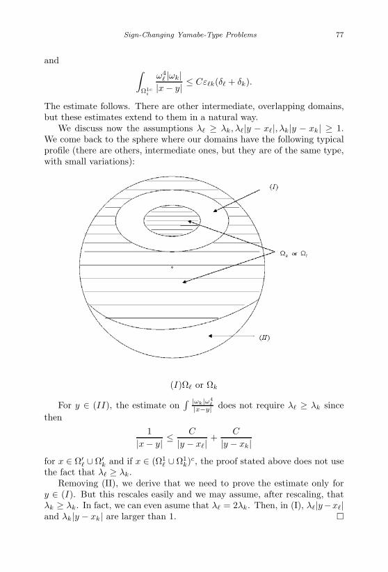
January 17, 2007 11:55 WSPC/Book Trim Size for 9in x 6in finalBB
Sign-Changing Yamabe-Type Problems 77
and ∫Ω1c
i
ω4 |ωk|
|x − y| ≤ Cεk(δ + δk).
The estimate follows. There are other intermediate, overlapping domains,but these estimates extend to them in a natural way.
We discuss now the assumptions λ ≥ λk, λ|y − x|, λk|y − xk| ≥ 1.We come back to the sphere where our domains have the following typicalprofile (there are others, intermediate ones, but they are of the same type,with small variations):
(I)Ω or Ωk
For y ∈ (II), the estimate on∫ |ωk|ω4
|x−y| does not require λ ≥ λk sincethen
1|x − y| ≤
C
|y − x| +C
|y − xk|for x ∈ Ω′
∪ Ω′k and if x ∈ (Ω1
∪ Ω1k)c, the proof stated above does not use
the fact that λ ≥ λk.Removing (II), we derive that we need to prove the estimate only for
y ∈ (I). But this rescales easily and we may assume, after rescaling, thatλk ≥ λk. In fact, we can even asume that λ = 2λk. Then, in (I), λ|y−x|and λk|y − xk| are larger than 1.

January 17, 2007 11:55 WSPC/Book Trim Size for 9in x 6in finalBB
78 Recent Progress in Conformal Geometry
Next, we have the estimate:
Lemma 41 ∫δ4i |vi + hi||x − y| ≤ C
(|vi|L6 +
|hi|∞√λi
)δi.
Proof. The estimate on∫ δ4
i
|x−y| has been completed in the proof of Propo-sition 2.
For hi, we split between the casea. |y − xi| ≥ C
λi. Then,∫
δ4i
|x − y| ≤∫
|x−y|≤c|y−xi|
δ4i
|x − y| +∫
|x−y|≥c|y−xi|
δ4i
|x − y| ≤ Cδ4i (y)|y − xi|2
+1
c|y − xi|∫
δ4i ≤ C
λ2i |y − xi|2 +
Cδi√λi
≤ C1δi√λi
b. |y − xi| ≤ Cλi
.Then,∫
δ4i
|x − y| ≤∫
|x−y|≥c|y−xi|
δ4i
|x − y| +∫
|x−y|≤c|y−xi|≤Ccλi
δ4i
|x − y|
≤∫
|x−y|≥c|y−xi|
δ4i
|x − y| + Cδ4i (y)|y − xi|2
≤∫
|x−y|≥c|y−xi||x−y|≥ C
λi
δ4i
|x − y| +∫
|x−y|≥c|y−x|i||x−y|≤ C
λi
δ4i
|x − y| + Cδ4i (y)|y − xi|2
≤ Cλi
(1 + λ2i |y − xi|2)1/2
× 1λi
+Cδ4
i (y)λ2
i
+ Cδ4i (y)|y − xi|2 ≤ Cδi√
λi
.
Lemma 41 follows.
Next, we have
Lemma 42∣∣∣∣∣θh − O
(∫Ω
′ci
δ4i |v|
|x − y| +∫
Ω′ci
δ5i
|x − y|
) ∣∣∣∣∣ ≤ Ch
∑εjδj
with |θh|H1 ≤ Ch(∑
εhk) for Y ∈ Ωc = (UΩ)c.

January 17, 2007 11:55 WSPC/Book Trim Size for 9in x 6in finalBB
Sign-Changing Yamabe-Type Problems 79
Proof. We use (i) of Proposition 2 and replace |v| by∑
δ. The price topay is the introduction of the function θh.
We thus need to take care of∫Ω
′ci
δ4i δ
|x − y| .
For = i, since y ∈ Ωc = (UΩk)c, Lemma 40 provides the estimate.For = i, we notice that Ω
′ci is made of two parts; one where λi|x−xi| ≥
18εis
and another one where λj |x − xj | with λj ≥ λi. On the latter sets,
δi ≤ Cδj .
Thus, ∫Ω
′ci
δ5i
|x − y| ≤ C
∫δ4j δi
|x − y|and the estimate follows from Lemma 40.
We thus assume that x ∈ Ω∗ci = x such that λi|x − xi| ≥ 1
8εis.
We then have∫Ω∗
i
δ5i
|x − y| ≤∫
Ω∗ci ∩|x−y|≥ 1
8 |y−xi|
δ5i
|x − y|
+ Cδ5i (y)
∫Ω∗c
i ∩|x−y|≤18 |y−xi|
1|x − y| = (1) + (2).
Let
A = Ω∗ci ∩ |x − y| ≥ 1
8|y − xi|.
Then,
(1) ≤(∫
A
δ5i
)√λiδi(y) = O(εiδi) if |y − xi| ≥ C
λi
(1) ≤ C√
λi
∫Ω∗c
i
δ6i ≤ Cε3
i
√λi = O(εiδi) if |y − xi| ≤ C
λi
since, on Ω∗ci ,
|x − y| ≥ |x − xi| − |y − xi| ≥ 1λi
(1
εis− C
)≥ 1
2λiεis.
On the other hand,
(2) ≤ Cδ5i (y)|y − xi|2 ≤ C1δi
λ2i |y − xi|2
(1 + λ2i |y − xi|2)2 ≤ C′
1δiεis
January 17, 2007 11:55 WSPC/Book Trim Size for 9in x 6in finalBB
80 Recent Progress in Conformal Geometry
since, if
|x − y| ≤ 18|y − xi|
then,
98|y − xi| ≥ |x − xi|
and
λi|y − xi| ≥ 89λi|x − xi| ≥ 8
9εis.
In the sequel, we introduce on Ωi the two quantities:
|h0i |∞ = C
(1ρi
∫Ωi
|f | +√
λi
∫Bc
i
|f |δi
). (1.21)
|h1i,j |∞ = C
(√λj
∫Bj
|f | + 1εij
∫Ωi
|f |δj
)(1.22)
so that, according to Lemma 12, we have
|hi(y)| ≤ |hi|∞ +∑
λj≥λi
λj =i
|h1ij |∞δj(y) for y ∈ Ωi. (1.23)
We then improve (iii) of Proposition 2 into:
Proposition 2′
|v − θh|(x) ≤ Ch
∑ εk + |v|L6 +|h0
|∞√λ
+∑
λs≥λs=
εs|h1s|∞
δ(x)
∀x ∈ Ωc = (UΩi)c (iii′)
The proof of (iii) requires a slight modification for (iii′).We now have a new term to estimate:
|h1is|∞
∫Ωi
δ4 δs
|x − y| .

January 17, 2007 11:55 WSPC/Book Trim Size for 9in x 6in finalBB
Sign-Changing Yamabe-Type Problems 81
We will see later (Lemma 68, below) that δ ≤ Cδi on Ωi so that ourestimate becomes an estimate on
|h1is|∞
∫Ωi
δ4i δs
|x − y|which we split as usual between the various cases λi|y − xi| ≥ C,λi|y − xi| ≤ C etc. For λi|y − x| ≥ 1, this becomes an estimate
on√
λi|h1is|∞
∫Ωi
δ4i δy,λi(x)δs ≤ √
λi|h1is|∞
(∫δ4i δ2
y,λi
)1/2 (∫δ4i δ2
s
)1/2 ≤C|h1
is|∞εisδi(y).If λi|y − x| ≤ 1, the estimate is straightforward.We now establish the following sequence of Lemmas and directly im-
prove of the estimates of Section 1.1. The Morse Lemma at infinity doesnot follow from these improvements, but this will bring us a step closer.
We will prove:
Lemma 43 Let Ωc be the complement of UiΩi. then,∫Ωc
δ5 δi ≤ C
∑λj≥λ
εijε2js.
We will then prove:
Lemma 44 For = i,
∫Ω
δi|v|5 ≤ Cεi
|v|H10
+|h0
|∞√λ
+∑
λs≥λs=
εs|h1,s|∞
+ C
∑λk≥λ
k =
εikε2k + C
∑εiε
2k + Ch
(∑εst
)h
.
Lemma 45 Assume λk ≥ λ, λk = λ. Then∫Ω∩Ωc
i
δiδ5k ≤ C(εiε
2k + εikε2
k) ≤ C1εiεk.
Lemma 46 Let λk ≥ λ. Then,∫Ω
δiδ4k ≤ Cεi√
λ
.
We turn them to our previous estimates of Section 1 and derive thefollowing intermediate improvements:
January 17, 2007 11:55 WSPC/Book Trim Size for 9in x 6in finalBB
82 Recent Progress in Conformal Geometry
Lemma 47
(i)√
λjεij
∫Bj
|vj + hj|5 ≤ Cεij
|vj |H10
+|h0
j |∞√λj
+∑
λs≥λj
εsj |h1j,s|∞
+ Cεij
∑λk≥λj
ε5/2kj + ε
5/2jt
+ Ch
(∑εst
)h √εij
(ii)1
ρi
√λi
∫Ωi
|vi + hi|5 ≤ Cεiq
(|vi|H1
0+
|h0i |∞√λi
+ εij |h1ij |∞
)+ Cεij
∑λk≥λj
ε5/2kj + Ch(
∑εst)h√εij .
Lemma 48∫|v|5|L−1e| ≤ C(|v|2H1
0+ o
( |h0i |∞√λ
)+ o
(∑εs|h1
,s|∞)
+ C∑
ε3k +
∑εm
|vn|H10
+|h0
m|∞√λm
+∑
λm≥λ
εm|h1,m|∞
+ C
∑εkε2
ks + Ch
(∑εst
)h
.
Lemma 49 ∫ω4
s |k∗||L−1e| ≤ C∑
εkεks +(∑
εst
)h
.
Lemma 50
∫|ω|3|v + h|2|L−1e| ≤ C
(|v|2H1
0+
1λρ2
(∫Ω
|f |)2)
+∑
λk≥λk =
λkε2k
(∫Bk
|f |)2
+
(∫Bc
|f |δ
)2
+(∫
B
|f |δk
)2
+ C∑
ε2mεk + Ch
(∑εst
)h
εm
).

January 17, 2007 11:55 WSPC/Book Trim Size for 9in x 6in finalBB
Sign-Changing Yamabe-Type Problems 83
Lemma 51∫Ωc
i
|v|5δi +∫
Ωi
|v|5δj + 0(εij
√λj
)∫Bj
|v|5
≤ C∑ =i
εi
|v|H10
+|h0
|∞√λ
+∑
λs≥λs=
εs|h1,s|∞
+ Cεij
|vi|H10
+|h0
i |∞√λi
+∑
λs≥λi
s=i
εsi|h1i,s|∞
+ C
(∑(εjkε2
ks + εiε2k
))+ Ch
∑εh
st.
Lemma 52 For θ = δi or δj :∫(UΩm)c
(∑αω
)4
|k∗|θ +√
λj0(εij)∫
(UΩm)c∩Bj
(∑αω
)4
|k∗|
≤ C(∑
εiε2s +
∑εjε
2s
)+ Ch
(∑εst
)h
.
We then improve Lemmas 8, 9, 11:
Lemma 53
∑∫Ωi
ω4j |hi| + |hi|5 ≤ C√
λi
|h0i |∞√λi
+∑
λs≥λis=i
εis|h1i,s|∞
+ C
∑ ε2si√λi
+ Ch(∑
εst)h
√λiεim
.
Lemma 54∫(ω4
j |hi| + |hi|5)|w|
≤ C|w|H10
|h0i |∞√λi
+∑
λs≥λis=i
εis|h1i,s|∞ + ε
5/2it + Ch
(∑εst
)h
.

January 17, 2007 11:55 WSPC/Book Trim Size for 9in x 6in finalBB
84 Recent Progress in Conformal Geometry
Lemma 55∫Ωc
i
ω4 (|vk| + |hk| + |k∗| + |vk|5 + |hk| + |k∗|5)|∂ωi|
≤ C
|ω∞i | + εit +
∑λj≥λi
j =i
1λi|ai − aj |
∑ εiε2s + Ch
(∑εst
)h
.
In view of all these new estimates, we revisit the proof of Lemmas 31–34of Section 1.1. Observe that now we can use Proposition 1 which yields (forλi ≥ λj)(∫
Ωi
|ωj |24/5|ωi|6/5 + |ωi|24/5|ωj |6/5
)5/6
≤ C(|ωj(ai)|εij + ε3ij)
while for , k = i,(∫Ωi
|ω|24/5|ωk|6/5 + |ωk|24/5|ω|6/5
)5/6
= 0(ε2ki + ε2
i).
Observe also that if λk ≥ λ:
•√
λiεi(|ωk(ω)| + |ω(ak)|)εk = o(√
λ|ωk(a)|εk +√
λk|ω(ak)|εk
).
For λk ≤ λ, Proposition 1 yields an improvement thoughout our esti-mates since (|ωk(a)| + |ω(ak)|)εk is replaced by |ωk(a)|εk for the con-tribution on Ω and this yields for
•√
λiεiωk(a)|εk = o(√
λ|ωk(a)εk
).
Next, we have:
Lemma 56 Assume k = s,∫
ω4k|ωs||ω| = 0(ε2
s) if one of k or s is . Ifboth are different from , then∫
ω4k|ωs||ω| ≤ Cεs(|ωk(as)|εks + ε2
ks) + Cεk(|ωs(ak)|εks + ε2ks)
+ C(|ωk(a)|εk +ε3k)( if λk ≤ λ)+C((|ωk(a)|+ |ω(ak)|)εk +ε3
k)( if λ ≤ λk)
+ Cεs
((|ωs(ak)| + |ωk(as)|)εsk + ε2
sk
)( if λk ≥ λs)
+ C∑
λj≥λk
εjε2jm+C
∑λj≥λs
εjε2j+Cεk((|ωs(ak)|+|ωk(as)|)εsk+ε2
jk)( if λk ≤ λs).

January 17, 2007 11:55 WSPC/Book Trim Size for 9in x 6in finalBB
Sign-Changing Yamabe-Type Problems 85
This allows us to derive the better estimate:
Theorem 1
|vi|H10
+1
ρi
√λi
∫Ωi
|f | +∫
Ωi
|f |δj +∫
Bci
|f |δ1 +√
λjεij
∫Bj
|f | ≤
C
(∑
(|ω(ai)|εi + ε3i) +
∑
εiε2s
)+ Ch(
∑εst)h.
We move now to control better the remainder terms in the expansionof ∂J(
∑αiω1 + v) · ∂ϕi · ∂ϕi is ωi = ∂ωi
∂ai. We establish:
Lemma 57 For = i:
(1)∫Ω
|∂ϕi|δ4 (|v| + |h|)
≤ C√
λ
(|v|L6 + |h0
|∞√λ
+∑
⊂λs≥λs=
εs|hs |∞
)√
λiε2i + C
λ|a−as|(|ω∞
i |2λi|ai−as|2 +
∑⊂λs≥λs=
λε2s|h1
,s|2∞ + λiε4i
)
+C∑
λk
(|vk|2H1
0+ |h0
k|2∞λk
+∑
⊂λs≥λks=k
|h1k,s|2∞ε2
ks
)
+ C
(∑k =i
λi|ωk(ai)|2ε2ki + ε2
kiε4k +
∑k =
λ|ωk(a)|2ε2k + ε2
kε4kt
)+ Cλ
(∑εm(
∑εkt)2 +
∑ε2
kε4kt
)+ Cλi
(∑ε2
kiε4k +
∑ε4
im(∑
εst)2)
+ Cλk(∑
ε2mkε4
kt +∑
ε4mkε2
st).
(2) For s = ,∫Ω
|∂ϕi|δ4s(|v| + |h|) ≤ C
√λsε
2s
√λiεi(|v|H1
0+ |h0
|L∞√λ
+∑
λs≥λ
εs|hs |∞) + C
λ|a−as|
|ω∞i |2
λi|ai−as|2 +∑
λs≥λs=
λε2s|h1
,s|2∞ + λiε4i
+ C
∑λk
|vk|2H10
+ |h0k|2∞λk
+∑
λs≥λks=k
|h1k,s|2∞ε2
ks
+ C
(∑k =i
λi|ωk(ai)|2ε2ki + ε2
kiε4k +
∑k =
λ|ωk(a)|2ε2k + ε2
kε4kt
)+ Cλ
(∑εm(
∑εkt)2 +
∑ε2
kε4kt
)+ Cλi
(∑ε2
kiε4k +
∑ε4
im(∑
εst)2)
+ Cλk(∑
ε2mkε4
kt +∑
ε4mkε2
st).

January 17, 2007 11:55 WSPC/Book Trim Size for 9in x 6in finalBB
86 Recent Progress in Conformal Geometry
(3) εks
∫Ωc |∂ϕi|δ4
δs ≤ C(εks(√
λsεst
√λiε
2i) +
√λiλsε
2imεmt( for λm ≥
λs) + λ1/4s
√λiε
2iλ
1/4 εt + λ
1/4s (λiεit)3 + (λ1/4
i εit)5/2(λ1/4s εsq)3/2)
(4) εks
∫Ωc |∂ϕi|δ4
i δs ≤ εks
√λi
∫Ωc δ6
i δs ≤ εks
√λiλsε
3it( for λs ≤ λs) +
εksλi(∑
λs≥λi
εsjε2js)( for λs ≥ λi)
Observation. All inequalities can be transformed into o(upperbound) i.e.an ε can be inserted as a coefficient of the upperbound. For 1 and 2 thereare at various spots in the upperbound an ε1−δ
it , δ > 0 as small as we wishwhich can be inserted.
Proof. We start with 3. We split Ωc into two pieces, Ω1c and Ω2c adaptedto δs. In Ω1c, λs|x− xs| ≥ c
εstfor some t = s. In Ω2c, for some m = s with
λm ≥ Cλs(λm λs), λs|x − xs| ≤ cεms
and λm|x − xm| ≤ 18εms
so that, inΩ2c,
δs ≤ δm
|x − xm| = o(|xs − sm|)|x − xs|′′ ∼′′ |xm − xs|.
We have
εks
∫Ω1c
|∂ϕi|δ4 δs ≤ C
√λiεks
√λsεst
∫Ω1c
δ2i δ4
≤ C(√
λsεksεst
)(√λiε
2i
).
In Ω2c, since λm λs,
1cεmt
≤ λm|x − xm| ≤ c
εmsfor some t = m.
We claim and we will prove later that:
∫Ωc∩|x−xi|≥c|xi−x
δ2i δ4
≤ Cε2iε
2t(or Cε2
ijε2jt with λj ≥ λ)
and ∫Ωc∩|x−xi|≤c|xi−x|
δ2i δ4
≤ Cε2i
λ|xi − x| .
In order to estimate εks
√λi
∫Ω2
cδ2i δ4
δs, we will distinguish between twocases: either λ ≤ λm and δ ≤ δm.

January 17, 2007 11:55 WSPC/Book Trim Size for 9in x 6in finalBB
Sign-Changing Yamabe-Type Problems 87
Then,
εks
√λi
∫Ω2
c∩|x−xi|≥c|xi−xm|
δ2i δ4
mδs ≤ Cεks
√λiλsε
2imε2
mt
εks
√λi
∫Ω2
c|x−xi|≤c|xi−xm|
δ2i δ4
mδs ≤ Cεks
√λiλsε
2im
λm|xi − xm| .
In Ω2c ∩ |x − xi| ≤ c|xi − xm|,
|x − xm|“ ∼′′ |xi − xm|so that
λm|xi − xm| ≥ λm|x − xm| ≥ 1cεmt
and
εks
√λi
∫Ω2
c∩|x−xi|≤c|xi−xm|
δ2i δ4
mδs ≤ Cεks
√λiλsε
2imεmt.
Or λ ≥ λm ≥ λs
εks
√λi
∫Ω2
c∩|x−xi|≥c|xi−x|
δ2i δ4
δs ≤ Cεks
√λiλsε
2iε
2t
εks
√λi
∫Ω2
c∩|x−xi|≤c|xi−x|
δ2i δ4
δs ≤ Cεksλ1/4s
√λiε
2iλ
1/4m
1λ|xi − x| .
We then observe that, in Ω2c ∩ |x − xi| ≤ c|xi − x|,|xi − x|“ ∼′′ |x − x|
so that
λ|xi − x| ≥ cλ|x − x|.Then, either
λ|x − x| ≥ c
εt

January 17, 2007 11:55 WSPC/Book Trim Size for 9in x 6in finalBB
88 Recent Progress in Conformal Geometry
and
εks
√λi
∫Ω2
c∩|x−xi|≤c|xi−x|
δ2i δ4
δs ≤ Cεksλ1/4s
√λiε
2iλ
1/4m εt
or
λj |x − xj | ≤ 18εj
for some λj > λ.
We may then replace δ by δj and proceed as above.Lastly, assume that λ ≤ λm and δm ≤ δ in a part of Ω2c.Then,
δs ≤ δm ≤ δ.
εks
√λiδ
2i δ4
δs ≤ εksλ1/4s
√λiλ
1/4 δ2
i δ4
so that
εks
√λi
∫Ω2
c∩|x−xi|≥c|xi−x|
δ2i δ4
δs
≤ εksλ1/4s
√λiλ
1/4
∫Ω2
c∩|x−xi|≥c|xi−x|
δ2i δ4
≤ Cεksλ1/4s
√λiε
2iλ
1/4 ε2
t
and
εks
√λi
∫Ω2
c∩|x−xi|
δ2i δ4
δs ≤ Cεksλ1/4s
√λiλ
1/4
ε2i
λ|xi − x| .
In Ω2c = |x − xi| ≤ c|xi − x|, |x − x| and |xi − x| are of the same
order so that
λ|xi − x| ≥ cλ|x − x|.Again, either
λ|x − x| ≥ c
εt
and we upperbound with Cεksλ1/4s
√λiεiλ
1/4 εt or there exist some j, with
λj ≥ λ, j = and
λj |x − xj | ≤ c
εj.

January 17, 2007 11:55 WSPC/Book Trim Size for 9in x 6in finalBB
Sign-Changing Yamabe-Type Problems 89
Then,
δ ≤ δj
and the induction proceeds.If, at any point, we end up with = i, then either λs ≤ λi and√
λiεks
∫Ωc
δ6i δs ≤ C
√λi
√λsεksε
3it ≤ C
(λ
1/4i εit
)3
λ1/4s εks
and if λs ≥ λi,√λiεks
∫Ωc
δ6i δs ≤ λiεks
∫Ωc
δ5i δs ≤ Cλiε
5/2it εksε
1/2sq
≤ C(λ
1/4i εit
)5/2 (λ1/4
s εsq
)3/2
.
We now prove our claim about∫Ωc
δ2i δ4
.If |x − xi| ≥ c|xi − x|, then∫
Ωc∩|x−xi|≥c|xi−x|
δ2i δ4
≤ C
λi|xi − x|2∫
λ|x−x|≥ cεt
δ4 ≤ Cε2
iε2t
unless δ ≤ δj for a part of the domain of integration, with λj ≥ λ, j = and λj |x − xj | ≤ 1
8εin which case we start an induction.
Or, we integrate on Ωc ∩ |x − xi| ≤ c|xi − x|. Then,∫Ωc∩|x−xi|≤c|xi−x|
δ2i δ4
≤ 1λ2
|xi − x|4∫
|x−xi|≤c|xi−x|
δ2i
≤ 1λ2
|xi − x|4 · 1λ2
i
· λi|xi − x| ≤ C
λiλ2 |xi − x|3
≤ Cε2i
λ|xi − x| .
as claimed.Proof of 1.
∫Ω
|∂ϕi|δ4 |v| ≤ C
√λi
∫Ω
δ2i δ4
|v| ≤ C√
λi|v|L6
(∫Ω
δ12/5i δ
24/5
)5/6
January 17, 2007 11:55 WSPC/Book Trim Size for 9in x 6in finalBB
90 Recent Progress in Conformal Geometry
≤ C√
λi|v|L6
∫
Ω∩|x−xi|≤c|xi−x|δ12/5i δ
24/5
5/6
+1
λi|xi − x|2(∫
δ24/5
)5/6
= (1) + (2).
Clearly,
≤ c√
λi|v|L6
λλi|xi − x|2√
λ ≤ C√
λ|v|L6
√λiε
2i (1.24)
and
≤ C√
λi|v|L6
λ2 |xi − x|4
∫|xi−x|≤c|xi−xρ
δ12/5i
5/6
=C1
√λi|v|L6
λ2 |xi − x|4 · 1
λ3/2i
(λi|x − xi|)(3− 125 )· 56 (1.25)
=C1
√λi|v|L6
λ2 |xi − x|4 · 1
λ3/2i
(λi|x − xi|)1/2 =C1
√λi
√λ|v|L6
λiλ|xi − x|2λ3/2 |xi − x|3/2
=C1
√λiε
2i
√λ|v|L6
λ3/2 |xi − x|3/2
.
On the other hand,∫Ω
|∂ϕi|δ4 |h| ≤ C|h0
|∞√
λi
∫Ω
δ2i δ4
+ C∑
λs≥λs=
∫Ω
|∂ϕi|δ4 |h1
,s|∞δs
≤ c√
λ
( |h0 |∞√λ
)√λiε
2i + C
∑λs≥λs=
(∫Ω
|∂ϕi|δ4 δs
)|h1
,s|∞.
We estimate C
∑λs≥λs=
(∫ |∂ϕi|δ4 δs
) |h1,s|∞ below, after starting the
proof of 2. of Lemma 57.
Proof of 2. For s = , λs ≥ λ∫Ω
|∂ϕi|δ4s |v| ≤ C
√λiλsεs
∫Ω
δ2i δ3
s |v| ≤ C√
λiλsεiε3/2+1s |v|H1
≤ C(√
λiεi|v|H1
)√λsε
5/2s .
January 17, 2007 11:55 WSPC/Book Trim Size for 9in x 6in finalBB
Sign-Changing Yamabe-Type Problems 91
On the other hand,∫Ω
|∂ϕi|δ4s |h| ≤ C
√λiλsεs|h0
|∞∫
Ω
δ2i δ3
s+C∑
λt≥λt=
(∫Ω
|∂ϕi|δ4sδt
)|h1
,t|∞
≤ C√
λiλsεs|h0 |∞
(∫Ω
δ6i
)1/3
×(∫
Ω
δ9/2s
)2/3
+ C∑
λt≥λt=
(∫Ω
|∂ϕi|δ4sδt
)|h1
,t|∞
≤ C√
λiλsεi|h0
|∞√λ
ε2s + C
∑λt≥λt=
(∫Ω
|∂ϕi|δ4sδt
)|h1
,t|∞
≤ C
(√λiεi
|h0 |∞√λ
)√λsε
2s + C
∑λt≥λt=
(∫Ω
|∂ϕi|δ4sδt
)|h1
,t|∞.
The two terms C
∑λs≥λs=
|h1,s|∞
∫Ω
|∂ϕi|δ4 δs and C
∑λt≥λt=
|h1,t|∞
× ∫Ω
|∂ϕi|δ4sδt are estimated now. Recall that |∂ϕi| ≤ C
(λi|ω∞
i |δi + δ3
i
).
We estimate first √λi
∫Ω
δ2i δ4
δs,√
λi
∫Ω
δ2i δ4
sδt.
Since we know that δs ≤ Cδ on Ω (Lemma 68 below), we need only toestimate
√λi
∫Ω
δ2i δ4
δs. We divide Ω into three subdomains, one where|x − as| ≥ c|as − a|. On the domain, labeled Ω1
we have√λi
∫Ω1
δ2i δ4
δs ≤ C√
λI√λs|as − a|
∫Ω1
δ2i δ4
≤ C√
λiε2i
√λ εs.
On Ω2 , we have |x − as| ≤ c|as − a|, c small, so that |x − a| and |a − as|
are of the same order and |x − ai| ≥ c|ai − a|. We then have, using 3 ofLemma 13:√
λi
∫Ω2
δ2i δ4
δs ≤ C√
λi
λi|ai − a|2 · εs√λ
≤ C√
λiε2i
√λ εs.
On Ω3 , |x− a| and |a − as| are of the same order and |x− a| and |ai − a|
are of the same order, |x − ai| ≤ c(ai − a). We then upperbound√λi
∫Ω3
δ2i δ4
δs ≤ C√
λi
λ2 |ai − a|3|a − as|
∫δ2i δs.

January 17, 2007 11:55 WSPC/Book Trim Size for 9in x 6in finalBB
92 Recent Progress in Conformal Geometry
Assuming that i = s, we have∫Ω3
δ2i δs ≤ C
λi|ai − as|2∫
|x−as|≤ 110 |ai−as|∩Ω3
δs
+C√
λs|ai − as|∫
|x−ai|≤ 110 |ai−as|
δ2i +
C
λi
√λs
∫3|a−as|≥r≥10|ai−as|
r2dr
r3
+C
λi
√λs|ai − as|3
∫r≤10|ai−as|
r2dr ≤ C
λi
√λs
(1 + Log
|a − as||ai − as|
).
and, since |a − as| and |a − ai| are of the same order:√λi
∫Ω3
δ2i δ4
δs ≤ C√
λi
λiλ2 |ai − a|3
√λεs
(1 + Log
|ai − a||ai − as|
)≤ C√
λi|ai − as|· 1λ2
|ai − a|2|ai − as||ai − a|
(1 + Log
|ai − a||ai − as|
)·√
λεs.
Since we may assume that |ai−as||ai−a| ≤ C (otherwise the estimate is straight-
forward), we find√λi
∫Ω3
δ2i δ4
δs ≤ C√λi|ai − as|
· 1λ2
|ai − a|2 ·√
λεs.
Thus,
|ω∞i |√
λi
∫Ω3
δ2i δ2
4δs|h1,s|∞ ≤ C|ω∞
i√λi|ai − as|
·√
λεs|h1,s|∞ · 1
λ2 |ai − a|2 .
On the other hand, observing that δ3i ≤ √
λiδ2i and using some estimates
from above,
∫Ω3
δ3i δ4
4δs ≤ C
λ2 |a − as|4
1√λsλi
+1√
λsλ3/2i
∫10|ai−as|≤r≤3|a−as|
r2dr
r4
≤ C
λ2 |a − as|4
( √λi√
λsλi
+1
λ3/2i
√λs
Logλi|a − ai|λi|ai − as|
)
≤ C√λiλ2
|a − ai|3√
λεs
(1 +
1√λi
Log λi|a − ai|)
.

January 17, 2007 11:55 WSPC/Book Trim Size for 9in x 6in finalBB
Sign-Changing Yamabe-Type Problems 93
We may assume that |a − ai| ≤ 1, using the proper chart. Thus, since|∂ϕi| ≤ C(|ω∞
i |√λiδ2i + δ3
i ), for i = s∫|∂ϕi|δ4
δs ≤ C
(√λiε
2i
√λεs +
|ω∞i |√
λi|ai − as|√
λεs
)and
|h1,s|∞
∫∂ϕiδ
4 δs ≤ C
λ|a − as|( |ω∞
i |2λi|ai − as|2 + λε
2s|h1
,s|2∞ + λiε4i
).
For s = i, the estimate is more involved. We have
|h1,i|∞
∫Ω3
|∂ϕi||ω4 |δi ≤ C
λ2 |ai − a|4 |h
1,i|∞
(|ω∞
i |√
λi
∫Ω3
δ3i +
∫Ω3
δ4i
)C|h1
,i|∞λ2
|ai−a|4∫Ω3
δ4i is easy to handle and provides the same contribution than
before.On the other hand (we assume that λi λ, otherwise the estimate is
straightforward)
C|h1,i|∞
λ2 |ai − a|4 |ω
∞i |√
λi
∫Ω3
δ3i ≤ C|ω∞
i ||h1,i|∞
λiλ2 |ai − a|4
∫1
λiεi≤r≤c|ai−a|
r2dr
r3
≤ C|ω∞i ||h1
,i|∞λiλ2
|ai − a|4 Log√
λi
λ≤ C1
( |ω∞i√λi
εi|h1,i|∞ Log
λi
λ
)1
λ3/2 |ai − a|3
≤(
C1|ω∞i |εi · εi|h1
,i|∞ Log(
λi
λ
))1
λ|ai − a|2 .
We consider
εi,|h1,i|∞ =
√λiεi
∫Bi
|f | +∫
Ω
|f |δi
and we try to estimate directly√
λiεi
∫Bi
|f | + ∫Ω
|f |δi.f is made of three types of terms:
1 - terms which are O
(∑k =j
|ωk|4|ωj |)
2 - terms involving v = vi + hi in Bi, v = v + h in Ω.
3 - projection terms

January 17, 2007 11:55 WSPC/Book Trim Size for 9in x 6in finalBB
94 Recent Progress in Conformal Geometry
We denote f1 the contribution of f of the terms of type 1 and 2. Thus,f reads
f = f1 +∑
Akek
where ek could be ωk, λk∂ωk
∂λk, ∂ωk
∂σk, 1
λk
∂ωk
∂ak. Ak is somewhat complicated be-
cause it involves the inverse of the matrix of the scalar-product in the basesωi, . . . but it is essentially
∫fek.
We know that∫Bi
|ei| ≤ C√λi
,
∫Bi
|ek| ≤ Cε2
ik√λi
for k = i.
Thus,√λiεi
∫Bi
|f | +∫
Ω
|f |δi ≤ C
(√λiεi
∫Bi
|f1| +∫
Ω
|f1|δi
+εi
|Ai| +∑k =i
ε2ik|Ak|
+∑
k
|Ak|∫
Ω
|ek|δi
≤ C
√εi
(∫Bi
|f1|6/5
)5/6
+∫
Ω
|f1|δi + εi
|Ai| +∑k =i
ε2ik|Ak|
+∑
k
|Ak|∫
Ω
|ek|δi
).
In fact, |Ai| stands for several terms which correspond to the various ei’s(ωi,
∂ωi
λi∂aietc.
)with the same index i.
We use then the fact that |v − θh| ≤ Ch
∑δk and the fact (see Lemma
68 below) that δk ≤ Cδm on Ωm to derive
√εi
(∫Bi
|f1|6/5
)5/6
+∫
Ω
|f1|δi
≤ C∑k =m
(√
εi
(∫Bi
|ωk|24/5|ωm|6/5
)5/6
+∫
Ω
|ωk|4|ωm|δi
)

January 17, 2007 11:55 WSPC/Book Trim Size for 9in x 6in finalBB
Sign-Changing Yamabe-Type Problems 95
+C√
εi
(∫Bi
δ24/5i (|vi| + |hi|)6/5
)5/6
+C
∫Ω
δ4 (|v|+|h|)δi+Ch(
∑εst)h.
Considering also∫
ω|ek|δi, either k = and this is O(εi) or k = i and
this is O(ε3i) or k = i, k = , then δk ≤ Cδ in Ω (Lemma 68 below) and∫
Ω
|ek|δi ≤∫
Ω
δ4kδδi ≤ Cεikεk.
Thus,
√λiεi
∫Bi
|f | +∫
Ω
|f |δi ≤ C
εi
|Ai| +∑k =i
ε2ik|Ak| + |A|
+
∑k =ik =
εikεk|Ak| +∑k =m
(√
εi
(∫Bi
|ωk|24/5|ωm|6/5
)5/6
+∫
Ω
|ωk|4|ωm|δi
)
+√
εi
(∫Bi
δ24/5i (|vi| + |hi|)6/5
)5/6
+∫
Ω
δ4 (|v| + |h|)δi + Ch
(∑εh
st
).
= B.
We thus have
C|h1,i|∞|ω∞
i |λ2
|ai − a4
√λi
∫Ω3
δ3i ≤ (C1|ω∞
i |εiB) Logλi
λ× 1
λ|ai − a|2 .
The main issue is to see that Logλi
λ, which is less that C Log ε−1
i can beabsorbed into B while enough room is left to provide an upperbound of theusual type.
We track down the terms and find (λ ≤ λi)
C|h1,i|∞
λ2 |ai − a|4 |ω
∞i |√
λi
∫Ω3
δ3i ≤ C1
λ2 |ai − a|2
(√λ|ω∞
i |εi
)
×(
εi Log ε−1i
√λ|v|H1
0+
√λ√λi
√εi Log ε−1
i
[√λi|vi|H1
0+√
λi
( |h0i |∞√λi

January 17, 2007 11:55 WSPC/Book Trim Size for 9in x 6in finalBB
96 Recent Progress in Conformal Geometry
+∑
λs≥λi
s=i
|h1i,s|∞εis + ε2
im
∑εst
]
+εi Log ε−1i
√λ
|h0 |∞√λ
+∑
⊂λs≥λis=i
εs|h1,s|∞ + ε2
m
∑εst
+√
εi Log ε−1i
√λ
λi
√λi
∑k =i
|ωk(ai)|εki + εkiε2i
+εi Log ε−1i
√λ
∑k =
|ωk(a)|εk + εkε2kt
+εi Log ε−1i
εk
√λ√λi
√λi|Ai| +
∑k =i
εik
√λiεik|Ak|
√λ√λi
+√
λ|A|
+∑k =ik =
λ≤λk
Log ε−1i εikεk
√λ
λk
√λk|Ak| +
∑k =ik =
λk≤λ
(εik Log
√λi√λ
)√λεk|Ak|
.
Observe that
εikεk ≤ Cεi.
Hence
Log ε−1i εiεk
√λ
λk≤ Cεi Log ε−1
i if λk ≥ λ.
If λk ≤ λ,
εik Log√
λi√λ
≤ εik Log√
λi√λk
≤ Cεik Logε−1
ik
λk|ai − ak| ≤ C1εik Log ε−1ik .
Observe also that
|Am| ≤ C
(∫Ωm
|f1|δm +∑
εms
∫Ωs
|f1|δs
).

January 17, 2007 11:55 WSPC/Book Trim Size for 9in x 6in finalBB
Sign-Changing Yamabe-Type Problems 97
The estimate on∫Ωm
|f1|δm follows in the same way the estimates of The-orem 1 were derived.
Our estimate follows.
Proof of Lemma 43.Considering
∫Ωc
δ5 δi, either we are on the part of Ωc where |x − xi| ≥
c|x − xi|. We call this part Ω1c . Then,∫
Ω1c
δ5 δi ≤ C√
λi|x − xi|∫
Ωc
δ5 ≤ Cεiε
2s.
On the remainder Ω2c of Ωc,
|x − xi| ≤ c|x − xi|and
|x − x| ≥ (1 − c)|x − xi|.Thus, ∫
Ω2c
δ5 δi ≤ C
λ5/2 |x − xi|5
1√λi
∫r≤c|x−xi|
rdr ≤ Cεi
λ2 |xi − x|2 .
Since Ω2c is non empty and Ω2
c ⊂ Ωc, either at a given x ∈ Ω2
c
λ|x − x| ≥ c1
εs
or
λ|x − xj | ≤ c2
εjfor some λj > λ.
In the second case,
δ ≤ Cδj
at such an x and we can replace their contribution to∫
δ5 δi by
∫δ5j δi.
Since λj > λi, the induction will eventually stabilize.Thus, we may assume that we are in the domain where
λ|x − x| ≥ c1
εs.
On the other hand,
|x − x| ≤ |x − xi| + |xi − x| ≤ (1 + c)|xi − x| in Ω2c .

January 17, 2007 11:55 WSPC/Book Trim Size for 9in x 6in finalBB
98 Recent Progress in Conformal Geometry
Hence,
λ|xi − x| ≥ c3
εs
and ∫Ω2
c
δ5 δi ≤ Cεiε
2s.
Proof of Lemma 44.
We split, according to the estimate of Lemma 12 and according to (1.21)and (1.22), h into h0
and h1 . We split Ω in two parts, Ω1
and Ω2 .
In Ω1 ,
|x − xi| ≥ c|xi − x| and
∫Ω1
δi|v|5 ≤ C√λi|xi − x|
∫Ω1
|v|5 ≤ Cεi√εt
(∫Ω
|v|6)5/6
+C√
λi|xi − x|
(∑k
∫Ω1
δ4k|h0
| +∫
Ω−Ω
δi|h|5 +∫
Ω1
δih4 inf(|h|, |h1
|))
+Ch
∑εh
st ≤Cεi√
εt|v|5H1
0+ C
√λεi
∑λk≥λ
∫Ω1
δ4k|h0
|
+∫
Ω1
δih4 inf(|h|, |h1
|) +∫
Ω−Ω
δi|h|5 + Ch
(∑εst
)h
.
Observe now that, using Lemma 68 and which we prove below (δk ≤Cδ in Ω).
√λεi
∫Ω
δ4k|h0
| +∫
Ω
δih4 inf(|h|, |h1
|) +∫
Ω−Ω
δi|h|5
≤ Cεi|h0
|∞√λ
+∑
λs≥λs=
|h1,s|∞
∫Ω
δiδ4 δs + C
∫Ω−Ω
δi
∑λk≥λ
k =
δ5k

January 17, 2007 11:55 WSPC/Book Trim Size for 9in x 6in finalBB
Sign-Changing Yamabe-Type Problems 99
+C
∫Ω−Ω
δiδ5 + Ch
(∑εh
st
)≤ Cεi
|h0 |∞√λ
+
∑λs≥λ
s=
εs|h1,s|∞
εi
+C
∑λk≥λ
k =
εikε2k +
∑εiε
2s
+ Ch(∑
εst)h.
Indeed, the function |h| up to a function θ with |θ|H1 ≤ Ch(∑
εst)h
is using Proposition 2, either bounded by Cδ or by C∑
λk≥λk =
δk.
In Ω2 ,
|x − xi| ≤ c|xi − x|.Then, ∫
Ω2
δi|v|5 ≤ C∑
k
∫Ω2
δiδ4k|v| + C
∫Ω
δi|h|5 + Cεhst
≤ C∑
λk≥λ
∫Ω2
δiδ4k|v| + C
∫Ω
δi|h|5 + C∑
εhst
∫Ω
δi|h|5 has been estimated above.Considering now
∫Ω2
δiδ
4k|v| with λk ≥ λ, either λk > λi. Then,∫
Ω2
δiδ4k|v| ≤
(∫δ2i δ4
k
)1/2(∫Ω
δ4kv2
)1/2
≤ Cεikεk|v|H10≤ C1εi|v|H1
0.
If k = , we derive the same upperbound (in both cases, it iso(εi|v|H1
0)).
If λ ≤ λk ≤ λi, then either
|xi − xk| ≥ c|xi − x|and ∫
Ω
δiδ4k|v| ≤ Cεik|v|H1
0≤ C1εi|v|H1
0
or
|xi − xk| ≤ c|xi − x|.
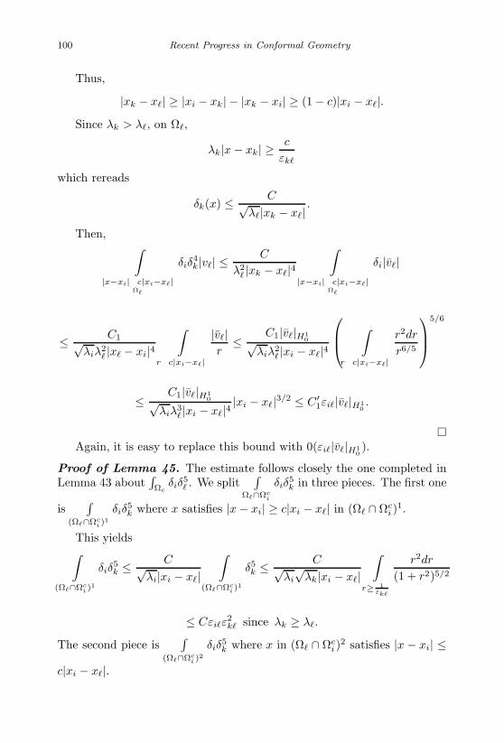
January 17, 2007 11:55 WSPC/Book Trim Size for 9in x 6in finalBB
100 Recent Progress in Conformal Geometry
Thus,
|xk − x| ≥ |xi − xk| − |xk − xi| ≥ (1 − c)|xi − x|.Since λk > λ, on Ω,
λk|x − xk| ≥ c
εk
which rereads
δk(x) ≤ C√λ|xk − x|
.
Then, ∫|x−xi|≤c|xi−x|
Ω
δiδ4k|v| ≤ C
λ2 |xk − x|4
∫|x−xi|≤c|xi−x|
Ω
δi|v|
≤ C1√λiλ2
|x − xi|4∫
r≤c|xi−x|
|v|r
≤ C1|v|H10√
λiλ2 |xi − x|4
∫r≤c|xi−x|
r2dr
r6/5
5/6
≤ C1|v|H10√
λiλ3 |xi − x|4
|xi − x|3/2 ≤ C′1εi|v|H1
0.
Again, it is easy to replace this bound with 0(εi|v|H1
0).
Proof of Lemma 45. The estimate follows closely the one completed inLemma 43 about
∫Ωc
δiδ5 . We split
∫Ω∩Ωc
i
δiδ5k in three pieces. The first one
is∫
(Ω∩Ωci )
1
δiδ5k where x satisfies |x − xi| ≥ c|xi − x| in (Ω ∩ Ωc
i )1.
This yields∫(Ω∩Ωc
i )1
δiδ5k ≤ C√
λi|xi − x|∫
(Ω∩Ωci )
1
δ5k ≤ C√
λi
√λk|xi − x|
∫r≥ 1
εk
r2dr
(1 + r2)5/2
≤ Cεiε2k since λk ≥ λ.
The second piece is∫
(Ω∩Ωci )2
δiδ5k where x in (Ω ∩ Ωc
i )2 satisfies |x − xi| ≤
c|xi − x|.

January 17, 2007 11:55 WSPC/Book Trim Size for 9in x 6in finalBB
Sign-Changing Yamabe-Type Problems 101
We split it into two pieces: a first contribution on (Ω ∩ Ωci )
21 where
|x − xi| ≥ c|xi − x|. For this contribution, we derive as above:∫(Ω∩Ωc
i )21
δiδ5k ≤ Cεikε2
k ≤ C1εiεk.
The remainder is∫
(Ω∩Ωci )22
δiδ5k.
On (Ω ∩ Ωci )
22, |x − xi| ≤ |xi − xk|; so that
(1 − c)|xi − xk| ≤ |x − xk| ≤ (1 + c)|xi − xk|.
Since x is in Ω with λk ≥ λ, k = :
λk|x − xk| ≥ 18εk
.
Hence
cλk|xi − xk| ≥√
λkλ|xk − x|
and
c√λk|x − xk|
≤ 1√λk|xi − xk|
≤ c√λ|xk − x|
so that
δk(xk, λk)(x) ≤ C√λk|xi − xk|
and ∫(Ω∩Ωc
i )22
δiδ5k ≤ C
λ5/2k |xi − xk|5
∫|x−xi|≤c|xi−xk|
δi ≤ C√λiλ
5/2k |xi − xk|5
×∫
r≤c|xi−xk|
rdr ≤ C1√λi
√λk
· 1λ2
k|xi − xk|2 ≤ Cεik
λkλ|xk − x|2 ≤ C3εikε2k.
Proof of Lemma 46. The estimate is straightforward for k = , so weassume that k = .

January 17, 2007 11:55 WSPC/Book Trim Size for 9in x 6in finalBB
102 Recent Progress in Conformal Geometry
Let
Ω1 = Ω ∩ |x − xi| ≥ c|xi − x|
Ω2 = Ω ∩ |x − xi| ≥ c|xi − xk|
Ω3 = Ω ∩ |x − xi| ≤ c|xi − xk|⊂ Ω ∩ (1 − c)|xi − xk| ≤ |x − xk| ≤ (1 + c)|xi − x|.
If Ω3 is not empty, then since λk ≥ λ, k = ,
λk|x − xk| ≥ c
εkfor some x ∈ Ω3
and therefore
λk|xi − xk| ≥ c1
εk,
an estimate which we will use on Ω3 .
We compute: ∫Ω1
δiδ4k ≤ C√
λi|xi − x|× 1
λk≤ C1εi√
λ
∫Ω2
δiδ4k ≤ C√
λi|xi − xk|∫
λkr≥ cεk
λ2kr2dr
(1 + λ2kr2)2
≤ Cεk
λk
√λi|xi − xk|
≤ C1εikεk√λk
≤ Cεi√λ∫
Ω3
δiδ4k ≤ C
λ2k|xi − xk|4
∫r≤c|xi−xk|
r2dr√λir
≤ C|xi − xk|2√λiλ2
k|xi − xk|4
≤ Cεik√λkλk|xi − xk|
≤ Cεikεk√λk
≤ cεi√λ
.
Proof of Lemma 47. The proof of (ii) follows closely the proof of (i).
First we have, using Proposition 2√λiεij
∫Bj
|vj |5 ≤ C√
λjεij
∫Bj
∑λk≥λj
δ4k|vj | + Ch
(∑εst
)h √εij
≤ Cεij |vj |H10
+ Ch
(∑εst
)h √εij .

January 17, 2007 11:55 WSPC/Book Trim Size for 9in x 6in finalBB
Sign-Changing Yamabe-Type Problems 103
Then,
√λjεij
∫Bj
|hj|5 ≤ C√
λjεij
∫Bj
∑λk≥λj
δ4k|h0
j | + C√
λjεij
×
∫Bj
∑λk≥λj
λs≥λj
δ4kδs
|h1j,s|∞ + Ch
(∑εst
)h √εij +
√λjεij
∫Bj−Bj
∑λk≥λj
δ5k
≤ Cεij
|h0j |∞√λj
+ Cεij
∑εsj |h1
j,s|∞ + Ch
(∑εst
)h √εij
+ Cεij
∑λj≥λj
ε5/2kj + ε
5/2jt
.
The claim follows. The proof of (ii) is identical. Proof of Lemma 48. We split the integral between an integral on Ω
and an integral on Ωc. We have using Proposition 2
∫Ωc
|v|5|L−1e| ≤ C∑k =mm =
∫Ωc
∩Ωm
δ5kδ + Ch
(∑εst
)h √εq
+ C∑m =
∫Ωc
∩Ωm
δ|v|5 ≤ C∑
εkε2ks + Ch
(∑εst
)h √εq
+∑
εm
|vm|H10
+|h0
m|∞√λm
+∑
λs≥λms=m
εsm|h1m,s|∞
+ C(∑
εkε2ks
).
On the other hand,
∫Ω
|v + h|5|L−1e| ≤ C|v|2H10
+ C
∫Ω
∑λk≥λ
δ3k|L−1e||h|
|h0 |∞
+ C
∫Ω
∑λk≥λλs≥λ
s=
δ4kδs|L−1e||h1
,s|∞ + Ch
(∑εst
)h
+ C∑
ε3k

January 17, 2007 11:55 WSPC/Book Trim Size for 9in x 6in finalBB
104 Recent Progress in Conformal Geometry
≤ C
|v|2H10
+|h0
|∞√λ
|h|L6 + |h1,s|∞
∑λk≥λλs≥λ
s=
(∫δ4kδ2
s
)1/2 (∫δ4kδ2
)1/2
+ Ch
(∑εst
)h
+∑
ε3k
≤ C
(|v|2H1
0+ o
( |ho |∞√λ
)
+∑(
εkεks|h1,s|∞ + ε,s|h1
,s|∞)
+ C∑
ε3k + Ch
(∑εst
)h)
.
Proof of Lemma 49. Using Lemma 43, we have:∫
ω4s |k∗||L−1e| ≤ C
∑∫Ωc
δ5kδ + Ch
∑εh
st ≤∑
εkε2ks + Ch
∑εh
st.
Proof of Lemma 50. This is a modification of Lemma 49, using the factthat |v + h − θ| ≤ C
∑δk with |θ|H1
0≤ Ch (
∑εst)
h.
This allows to upperbound∫Ω−Ω
|ω|3|v + h|2|L−1e|
by
Cε2mεk + Ch
(∑εst
)h
.
Proof of Lemma 51. We first estimate O
(√λjεij
∫Bj
|v|5). Using Lem-
mas 12, and Proposition 2, we upperbound this quantity with:
O(εij
√λj
)∫Bj
∑δ4k
(|v| + |ho
j | +∑
s
|h1j,s|δs
)
+ O(εij
√λj
) ∫Bj−Bj
∑δ5k + O
(εij
√λj
)Ch
(∑εst
)h
|Bj |1/6.
We may retain among the δk’s only those with λk ≥ Cλj .

January 17, 2007 11:55 WSPC/Book Trim Size for 9in x 6in finalBB
Sign-Changing Yamabe-Type Problems 105
We then derive
O(εij
√λj
)∫Bj
|v|5 ≤ O(εij)|vj |H10
+ O(εij
√λj
)∫Bj
∑λk≥λj
δ4k
(|hoj | + |h1
j,s|δs
)+ O
(εij
√λj
)∫Bj−Bj
∑λk≥λj
δ5k + O
(√εij
)Ch
(∑εst
)h
≤ O(εij)
|vj |H10
+|ho
j |∞√λj
+∑
λs≥λj
s=j
εjs|h1j,s|∞
+ εijO
(∑ε2
j
)+ O
(√εij
)Ch
(∑εst
)h
.
Proof of Lemma 52. The first term has been estimated in Lemma 43,after the use of Proposition 2.
For the second term, we use again Proposition 2. Up to a term of orderCh (
∑εst)
h, this term is then upperbounded by (on Ωj , λk|x− xk| ≥ cεkj
ifλk ≥ Cλj , k = j):∑
k
√λjO(εij)
∫(Bj−Bj)∩Ωc
k
δ5k
≤ C∑
λk≥λj
√λjO(εij)
∫(Bj−Bj)∩Ωc
k
δ5k ≤ C
∑εijε
2js.
Proof of Lemma 53. Using our observations, we derive the followingupperbounds:∫
Ω
ω4k|ωs||∂ω| ≤ (|ωk(a)| + |ω(ak)|)εk + ε3
k if λ ≤ λk
≤ |ωk(a)|εk + ε3k if λk ≤ λ.
If λ ≤ λk, we upperbound∫Ωk
ω4k|ωs||∂ω| ≤
(∫Ωk
|ωk|24/5|∂ω|6/5
)5/6
≤ C((|ωk(a)| + |ω(ak)|)εk + ε3
k
).
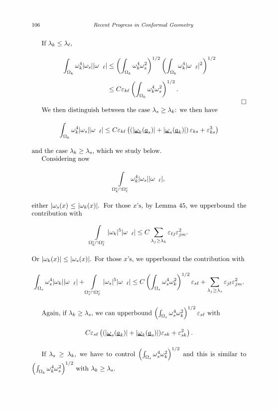
January 17, 2007 11:55 WSPC/Book Trim Size for 9in x 6in finalBB
106 Recent Progress in Conformal Geometry
If λk ≤ λ,
∫Ωk
ω4k|ωs||∂ω| ≤
(∫Ωk
ω4kω2
s
)1/2(∫Ωk
ω4k|∂ω|2
)1/2
≤ Cεk
(∫Ωk
ω4kω2
s
)1/2
.
We then distinguish between the case λs ≥ λk: we then have∫
Ωk
ω4k|ωs||∂ω| ≤ Cεk
((|ωk(as)| + |ωs(ak)|) εks + ε3
ks
)and the case λk ≥ λs, which we study below.
Considering now ∫Ωc
k∩Ωc
ω4k|ωs||∂ω|,
either |ωs(x) ≤ |ωk(x)|. For those x’s, by Lemma 45, we upperbound thecontribution with ∫
Ωck∩Ωc
|ωk|5|∂ω| ≤ C∑
λj≥λk
εjε2jm.
Or |ωk(x)| ≤ |ωs(x)|. For those x’s, we upperbound the contribution with
∫Ωs
ω4s |ωk||∂ω| +
∫Ωc
s∩Ωc
|ωs|5|∂ω| ≤ C
(∫Ωs
ω4sω2
k
)1/2
εs +∑
λj≥λs
εjε2jm.
Again, if λk ≥ λs, we can upperbound(∫
Ωsω4
sω2k
)1/2
εs with
Cεs
((|ωs(ak)| + |ωk(as)|)εsk + ε2
sk
).
If λs ≥ λk, we have to control(∫
Ωsω4
sω2k
)1/2
and this is similar to(∫Ωk
ω4kω2
s
)1/2
with λk ≥ λs.

January 17, 2007 11:55 WSPC/Book Trim Size for 9in x 6in finalBB
Sign-Changing Yamabe-Type Problems 107
We thus consider∫Ωk
ω4kω2
s with λk ≥ λs. Since such quantities areconformally invariant, we deconcentrate ωs so that λs = 1, ωs becomesωs, λk becomes λk with λk ∼ cε−2
ks . ωk is concentrated at ak(= 0) and wewrite: ∫
Ωk
ω4kω2
s ≤ ω2s(ak)
∫|x|≤1
ω4k + C
∫|x|≤1
r2ω4k +
∫|x|≥1
ω4kω2
s.
We can think of all this decomposition as occuring on the sphere S3 andwe then have, since |ωk| ≤ C√
λk
for |x| ≥ 1,
∫|x|≥1
ω4kω2
s ≤ C
λ2k
= O(ε4ks)
∫|x|≤1
ω4k = O
(1λk
)= O
(ε2
ks
)
∫|x|≤1
r2ω4k ≤ C
∫r≤1
r2λ2kr2dr(
1 + λ2kr2)2 ≤ Cλk
λ3k
=C
λ2k
= O(ε4ks)
so that (∫Ωk
ω4kω2
s
)1/2
≤ C(|ωs|(ak)εks + ε2
ks
)and, if λk ≥ λs, ∫
Ωk
ω4k|ωs||∂ω| ≤ Cεk
(ωs|(ak)εks + ε2
ks
)while, if λs ≥ λk,∫
Ωs
ω4s |ωk||∂ω| ≤ Cεs
(|ωk|(as)εks + ε2ks
).

January 17, 2007 11:55 WSPC/Book Trim Size for 9in x 6in finalBB
108 Recent Progress in Conformal Geometry
1.10 Proof of the Morse Lemma at Infinity
1.10.1 Decomposition in groups, gradient and
L∞-estimates on v, proof of the Morse Lemma
at infinity
1.10.2 Content of Part III
Parts I and II have clearly indicated that the main obstacle to the derivationof a general Morse Lemma at infinity relies on the fact that some masses,which interact very little, could be concentrated at points very close to oneanother. The remainder terms are then impossible to control.
If this occurs,∑
αiωi can be split in several clusters, denoted for sim-plicity as I and II. The masses in each cluster are very close to one anothercompared to the masses of I with respect to the masses of II (the distanceof the cluster I to the cluster II is of the order of |a|). We then have twoclusters and their optimal v’s:∑
i∈I
αiωi + vI ,∑i∈II
αiωi + vII
and a remainder v − (vI + vII).In Part III we complete major improvements of the estimates of Part
II.On one hand, using the uniqueness feature of the implicit function theo-
rem applied to v, we get rid of all the remainder terms Ch(∑
εst)h involvedin the pointwise estimates on v in Part II.
On the other hand, we derive a much better estimate, for every x of R3,of∫ ω4
k|ω|+|ω|4|ωk||x−y| of the type C((|ω∞
| + |ω(ak)|√λ|ak − a| + εk)δk +(|ω∞
k | + |ωk(a)|√
λk|ak − a| + εk)δ)εk.We also show that |v − (vI + vII)| is pointwise estimated by such an
expression but with ∈ I and k ∈ II (Proposition 3).Another meaningful estimate is derived on ∇vI in
ΩII( and ∇vII in ΩI) in terms of
C
|a|
∑(k,j)∈I
k =j
(|ω∞
j | + |ωj(ak)|√λj |ak − aj| + εkj
)εkjδk
.
All these improvements concur and yield a better estimate on |(v − (vI +vII))|H1
0than the one provided in Theorem 1 of Part II. The new estimate
has the definite advantage that instead of splitting the contribution in theupperbound of the ωj ’s of each cluster (C
∑ |ω∞j | etc.), it combines them in
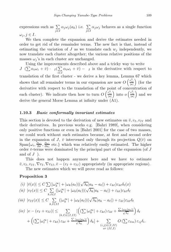
January 17, 2007 11:55 WSPC/Book Trim Size for 9in x 6in finalBB
Sign-Changing Yamabe-Type Problems 109
expressions such as∑j∈I
αjωj(ak) i.e.∑j∈I
αjωj behaves as a single function
ωj , j ∈ I.We then complete the expansion and derive the estimates needed in
order to get rid of the remainder terms. The new fact is that, instead ofestimating the variation of J as we translate each wj independently, wenow translate each cluster altogether; the various relative positions of themasses ωj’s in each cluster are unchanged.
Using the improvements described above and a tricky way to write∂J(
∑αiωi + v) · ∂I(
∑i∈I
αiωi + v) − ∂I is the derivative with respect to
translation of the first cluster - we derive a key lemma, Lemma 67 which
shows that all remainder terms in our expansion are now O(
ε3ij
|a|)
(for thederivative with respect to the translation of the point of concentration of
each cluster). We indicate then how to turn O(
ε3ij
|a|)
into o(
ε3ij
|a|)
and wederive the general Morse Lemma at infinity under (A1).
1.10.3 Basic conformally invariant estimates
This section is devoted to the derivation of new estimates on v, vI , vII andtheir derivatives. In previous works e.g. [Bahri 1989], when consideringonly positive functions or even in [Bahri 2001] for the case of two masses,we could work without such estimates because, at first and second orderin the expansion of J , v intervened only through its projection Q(v) onSpanωi,
∂ωi
∂σ , ∂ωi
∂aietc. which was relatively easily estimated. The higher
order v-terms were dominated by the principal part of the expansion (of Jand of ∂J).
This does not happen anymore here and we have to estimatev, vI , vII ,∇vI ,∇vII , v − (vI + vII) appropriately (in appropriate regions).
The new estimates which we will prove read as follows:
Proposition 3
(i) |v(x)| ≤ C∑
(|ω∞k | + |ωk(a)|(
√λk|ak − a|) + εk)εkδ(x)
(ii) |vI(x)| ≤ C∑
k,∈I
(|ω∞k | + |ωk(a)|(
√λk|ak − a|) + εk)εkδ
(iii) |vII(x)| ≤ C∑
k,∈II
(|ω∞k | + |ωk(a)|(
√λk|ak − a|) + εk)εkδ
(iv) |v − (vI + vII)| ≤∑
(k,)∈(I,II)
[((∑ |ω∞
k | + εk) εk +∑ |ωk(a)|√
λ
)δ
+((∑ |ω∞
| + εk) εk +∑ |ω(ak)|√
λk
)δk] +
∑(i,j)∈(I,II)
or (II,I)
O (∑
εm) εijδi.
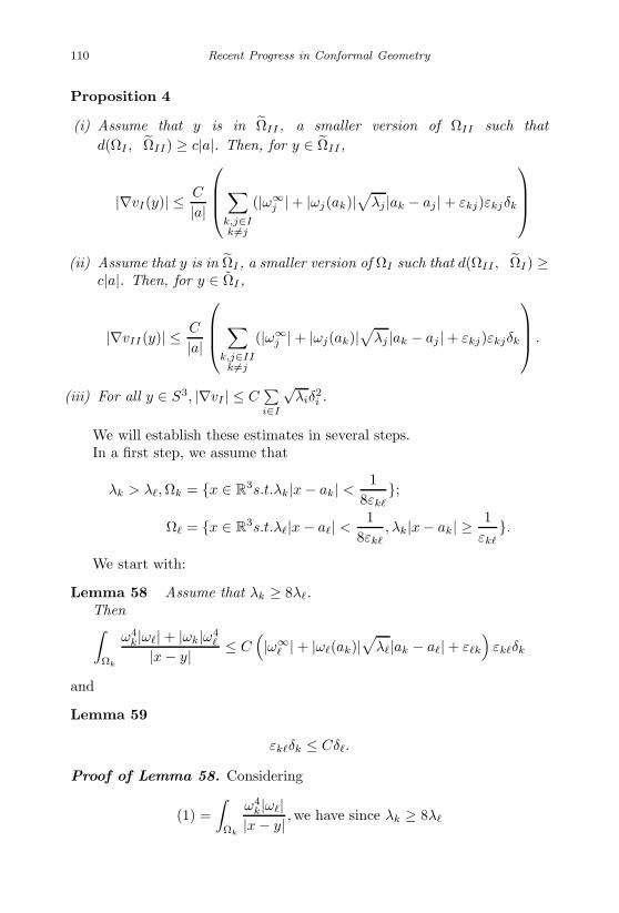
January 17, 2007 11:55 WSPC/Book Trim Size for 9in x 6in finalBB
110 Recent Progress in Conformal Geometry
Proposition 4
(i) Assume that y is in ΩII , a smaller version of ΩII such thatd(ΩI , ∂ΩII) ≥ c|a|. Then, for y ∈ ΩII ,
|∇vI(y)| ≤ C
|a|
∑k,j∈Ik =j
(|ω∞j | + |ωj(ak)|√λj |ak − aj | + εkj)εkjδk
(ii) Assume that y is in ΩI , a smaller version of ΩI such that d(ΩII , ∂ΩI) ≥
c|a|. Then, for y ∈ ΩI ,
|∇vII(y)| ≤ C
|a|
∑k,j∈II
k =j
(|ω∞j | + |ωj(ak)|√λj |ak − aj | + εkj)εkjδk
.
(iii) For all y ∈ S3, |∇vI | ≤ C∑i∈I
√λiδ
2i .
We will establish these estimates in several steps.In a first step, we assume that
λk > λ, Ωk = x ∈ R3s.t.λk|x − ak| <1
8εk;
Ω = x ∈ R3s.t.λ|x − a| <1
8εk, λk|x − ak| ≥ 1
εk.
We start with:
Lemma 58 Assume that λk ≥ 8λ.Then∫
Ωk
ω4k|ω| + |ωk|ω4
|x − y| ≤ C(|ω∞
| + |ω(ak)|√
λ|ak − a| + εk
)εkδk
and
Lemma 59
εkδk ≤ Cδ.
Proof of Lemma 58. Considering
(1) =∫
Ωk
ω4k|ω|
|x − y| , we have since λk ≥ 8λ

January 17, 2007 11:55 WSPC/Book Trim Size for 9in x 6in finalBB
Sign-Changing Yamabe-Type Problems 111
|ω(x)| ≤ C
(|ω(ak)|
√λ|ak − a| +
( |ω∞ |
|ak − a| +1
λ|ak − a|2)|x − ak|
)× 1√
λ|ak − a|for x ∈ Ωk
so that since |x − ak| ≤ C/λkεk
(1) ≤ C(|ω(ak)|
√λ|ak − a| + |ω∞
| + εk
) 1√λ|ak − a|
∫Ωk
ω4k
|x − y| .
Observe now that∫
Ωk
ω4k
|x − y| ≤√
λk
∫Ωk∩λk|x−y|≥1
ω4kδk(y)
+∫
Ωk∩|x−y|≤ 1λk
ω4k
|x − y| if λk|y − ak| is large
≤ Cδk√λk
+C
λ2k|ak − y|4 × 1
λ2k
≤ C
λk|y − ak| .
Thus,
(1) ≤ C(|ω∞
| + |ω(ak)|√
λ|ak − a| + εk
)εkδk if λk|y − ak| is large.
If λk|y − ak| is bounded by C, then∫Ωk
ω4k
|x − y| ≤ C√
λk
∫λk|x−y|≥100C
ω4kδk(y)
+∫
λk|x−y|≤100C
ω4k
|x − y| ≤Cδk√
λk
+ C ≤ Cδk(y)√
λk
and the estimate above extends.We now consider
(2) =∫
Ωk
|ωk|ω4
|x − y|
≤ C
(ω∞4
λ2 |ak − a|4 + (|ω(ak)|
√λ|ak − a|)4 + ε4
k
)∫Ωk
|ωk||x − y|
and we subdivide between the case
a. λk|y − ak| ≤ C.
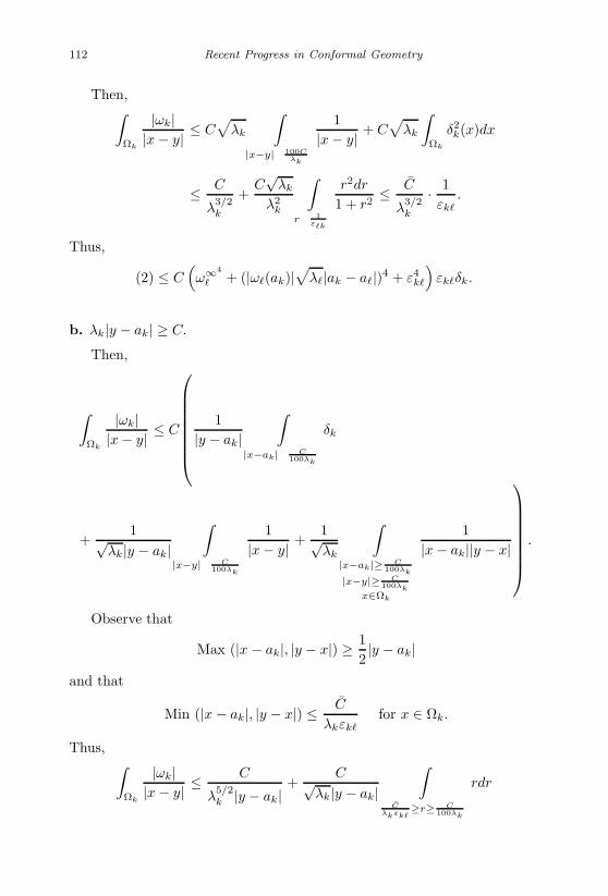
January 17, 2007 11:55 WSPC/Book Trim Size for 9in x 6in finalBB
112 Recent Progress in Conformal Geometry
Then,∫Ωk
|ωk||x − y| ≤ C
√λk
∫|x−y|≤ 100C
λk
1|x − y| + C
√λk
∫Ωk
δ2k(x)dx
≤ C
λ3/2k
+C√
λk
λ2k
∫r≤ 1
εk
r2dr
1 + r2≤ C
λ3/2k
· 1εk
.
Thus,
(2) ≤ C(ω∞4
+ (|ω(ak)|√
λ|ak − a|)4 + ε4k
)εkδk.
b. λk|y − ak| ≥ C.
Then,
∫Ωk
|ωk||x − y| ≤ C
1
|y − ak|∫
|x−ak|≤ C100λk
δk
+1√
λk|y − ak|∫
|x−y|≤ C100λk
1|x − y| +
1√λk
∫|x−ak|≥ C
100λk
|x−y|≥ C100λk
x∈Ωk
1|x − ak||y − x|
.
Observe that
Max (|x − ak|, |y − x|) ≥ 12|y − ak|
and that
Min (|x − ak|, |y − x|) ≤ C
λkεkfor x ∈ Ωk.
Thus, ∫Ωk
|ωk||x − y| ≤
C
λ5/2k |y − ak|
+C√
λk|y − ak|∫
Cλkεk
≥r≥ C100λk
rdr
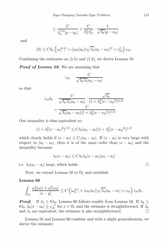
January 17, 2007 11:55 WSPC/Book Trim Size for 9in x 6in finalBB
Sign-Changing Yamabe-Type Problems 113
≤ C
λ5/2k |y − ak|
+C
λ2kε2
k
· 1√λk|y − ak|
and
(2) ≤ Cδk
(|ω∞
|4 + (|ω(ak)|√
λ|ak − a|)4 + ε4k
)εk.
Combining the estimates on (1.5) and (1.2), we derive Lemma 58.
Proof of Lemma 59. We are assuming that
εk ∼ C√λkλ|ak − a|
so that
εkδk ∼ C√λkλ|ak − a|
·√
λk
(1 + λ2k|x − ak|2)1/2
=C√
λ|ak − a|(1 + λ2k|x − ak|2)1/2
.
Our inequality is thus equivalent to:
(1 + λ2 |x − a|2)1/2 ≤ Cλ|ak − a|(1 + λ2
k|x − ak|2)1/2
which clearly holds if |x − a| ≤ C1|ak − a|. If |x − a| is very large withrespect to |ak − a|, then it is of the same order than |x − ak| and theinequality becomes
λ|x − ak| ≤ Cλλk|x − ak||ak − a|i.e. λ|ak − a| large, which holds.
Next, we extend Lemma 58 to Ω and establish:
Lemma 60∫Ω
ω4k|ω| + ω4
|ωk||x − y| ≤ C
(|ω∞
k | + |ωk(a)|√
λk|ak − a| + εk
)εkδ.
Proof. If λ ≥ 8λk, Lemma 60 follows readily from Lemma 58. If λk ≥8λ, λk|x − ak| ≥ ε−1
k for x ∈ Ω and the estimate is straightforward. If λk
and λ are equivalent, the estimate is also straightforward.
Lemma 58 and Lemma 60 combine and with a slight generalization, wederive the estimate:

January 17, 2007 11:55 WSPC/Book Trim Size for 9in x 6in finalBB
114 Recent Progress in Conformal Geometry
Lemma 61∫ω4
k|ω| + ω4 |ωk|
|x − y| ≤ C((|ω|∞ + |ω(ak)|
√λ|ak − a| + εk
)δk
+(|ω∞
k | + |ωk(a)|√
λk|ak − a| + εk
)δ)εk.
We now establish (i), (ii), (iii) of Proposition 3. The proof of (iv)requires a few further remarks and we will be completing later, in a sectiondevoted to v − (vI + vII).
Proof of (i), (ii), (iii) of Proposition 3. v satisfies
QF⊥
(J ′(∑
αjωj + v))
= 0. (1.26)
Picking up a large constant C1 (much larger than C∑ |ω∞
j |), we modify(1.26) as follows; we write it as
Q∗L(J ′(∑
αjωj
))+ ∆v + Q∗
(5(∑
αjωj
)4
v +5∑
m=2
fmvm
)= 0
(1.27)which we transform into
−∆v = Q∗L(J ′(∑
αjωj
))− Q∗
(5(∑
αjωj
)4
vχUΩi
+5∑
m=2
fm inf(C1
∑εijδi, |v|
)m−1
sgn(vm−1)v
+ 5(∑
αjωj
)4
χ(UΩi)c × sgnv × inf(|v|, C1
∑εijδi
))= f
(1.28)
(1.28) is only a slight modification of (1.27) and one can easily see that theinversion theorem applies to it yielding a unique solution v in F⊥.
If we are able to prove on v the estimate
|v(x)| ≤ C1
∑εijδi (1.29)
then v = v and v satisfies (1.28). In order to prove (1.29), we derive from(1.28)
v = c
∫f
|x − y| (1.30)
v splits also in pieces vi, hi just as v did. Theorem 1 will extend readilywith an improvement: there is no contribution of Ch (
∑εst)
h because we

January 17, 2007 11:55 WSPC/Book Trim Size for 9in x 6in finalBB
Sign-Changing Yamabe-Type Problems 115
can use (1.29) in(U Ωi
)c
. The constant C1 is then multiplied by o(1) wederive the estimate
|vi|H10
+|h0
i |√λi
+∑
λs≥λi
s=i
εis|h1is| ≤ C
∑εij (1.31)
where C does not depend on C1 because
inf(|v|, C1
∑εijδi
)≤ |v|. (1.32)
In order to prove (1.31) - (1.32), we first prove that v satisfies (i) ofProposition 2, page 72 with θh = 0. Indeed, using (1.30) in (1.28) andforgetting a first step the projection operator Q∗, we find
|v| ≤ C
∫ ∑k =j
ω4j |ωk| + ω4
k|ωj ||x − y|
+∑
i
|vi|H10
∫Ωi
∑j
δ5j
|x − y| + |h0i |∞
∫Ωi
∑k
δ4k
|x − y|
+∑
sλs≥λi
s=i
|hsi |∞
∫Ωi
∑k
δ4kδs
|x − y|
+5∑2
Cm−11 εm−1
ik
|vi|H10
∫Ωi
δ5k
|x − y|
+ |h0i |∞
∫Ωi
δ4k
|x − y| +∑
sλs≥λi
s=i
|hsi |∞
∫Ωi
δ4kδs
|x − y|
+∑
j
∫(UΩ)c
C1δ4j
∑εikδk + C5
1
∑ε5
ikδ5k
|x − y|(1.33)
C is independent of C1.We will prove later that∫
Ωi
δ4j
|x − y| ≤cδi√λi
,
∫Ωi
δ5j
|x − y| ≤ Cδi (1.34)

January 17, 2007 11:55 WSPC/Book Trim Size for 9in x 6in finalBB
116 Recent Progress in Conformal Geometry
∫(UΩ)c
δ5i
|x − y| = o(δi),∫
Ωi
δ4j δs
|x − y| = O(εis)δi for λs ≥ λis=i
(1.35)
(i) of Proposition 2 follows. Theorem 1 thereby follows for v, (iii) ofProposition 2 is not needed because (1.28) is a modified version of (1.26)and the nonlinearity involve inf(v|, C1
∑εkδ) in (∪Ωj)c.
Then, after tracking down the contribution of Q∗, (1.33) implies that
|v(x)| ≤ C∑
εijδi + o(C1
∑εijδi
)(1.36)
(1.29) follows and v = v.
Plugging then in (1.28) the estimates on |v|H10
and |hi|∞√λi
provided byTheorem 1 (without Ch(
∑εst)h, we got rid of this contribution), using the
estimates on∫Ωi
δ4k
|x−y| ,∫(UΩ)c
δ5j
|x−y| and using also the estimate (Lemma 59)
εikδk ≤ Cδi
we derive that
|v(x)| = |v(x)| ≤
C
∑(|ω∞k | + |ωk(a)|
√λk|ak − a| + εk)εkδ(x) +
∑i=
εkiεkδ
.
(1.37)
The extra-term∑
εikεkδ is due to∫(UΩ)c
δ4j
∑εikδk
|x−y| (see Lemma 40 k = j).Bootstrapping (1.37) into (1.28), we get a better estimate with∑
i=
εkiεkδ replaced by εikεkεk11δ1with i = , i = 1, k, = 1, k1 =
k or (otherwise we are done). Thus εij and εk belong to different pairs,εij and εk11 belong to different pairs as well as εk and εk11 . Since thereis a finite number of pairs, we end up with a term of the type ε2
kδ and weare done.
(i), (ii), (iii) of Proposition 3 follow.
We now establish (i) and (ii) of Proposition 4.
Proof of Proposition 4. We write
vI(y) =∫
fI
|x − y| .

January 17, 2007 11:55 WSPC/Book Trim Size for 9in x 6in finalBB
Sign-Changing Yamabe-Type Problems 117
We assume that y ∈ ΩII and split
∇vI(y) =∫
fIO
(1
|x − y|2)
=∫
|x−y|≥c|a|
fIO
(1
|x − y|2)
+∫
|x−y|≤c|a|
fIO
(1
|x − y|2)
.
We can easily estimate the first term and we derive∣∣∣∣∣∣∣∫
|x−y|≥c|a|
fIO
(1
|x − y|2)∣∣∣∣∣∣∣ = O
(1|a|)∫ |fI |
|x − y| .
The second term yields∣∣∣∣∣∣∣∫
|x−y|≤c|a|
fIO
(1
|x − y|2)∣∣∣∣∣∣∣ ≤ C|a| Sup
|x−y|≤c|a||fI(x)|.
In fI , all terms are explicit except those involving vI .For those, we can use (ii) of Proposition 3. Thus, since y ∈ ΩII ,
|a| Sup|x−y|≤c|a|
|fI(x)| ≤ C
|a| · |a|2
∑k,∈I
(|ω∞
k | + 1λk|a| + εk
)4
×(|ω∞
| + 1λ|a| + εk
)(εk
1√λk|a|
+1
λ2k
√λ|a|5
))
≤ C
|a|
∑k,∈I
(|ω∞
k | + 1λk|a| + εk
)4
×(|ω∞
| + 1λ|a| + εk
)×(
εk√λk|a|
+1√
λk
√λ|a|
· 1λk|a| ·
1√λk|a|
)).
Combining the two estimates, using (1.28) and (1.31) to estimate∫ |fI |
|x−y|as already done above, using Lemma 61, we derive the estimate on ∇vI ,hence also on ∇vII .
We prove now (1.34), (1.35).
We start with∫Ωi
δ4j
|x−y| . In Lemma 68, we establish that δj ≤ Cδi onΩi, ∀j.

January 17, 2007 11:55 WSPC/Book Trim Size for 9in x 6in finalBB
118 Recent Progress in Conformal Geometry
Thus,
∫Ωi
δ4j
|x − y| ≤ C
∫Ωi
δ4i
|x − y| ≤Cδi√
λi
. (1.38)
We now consider(Ωj are smaller versions of Ωj).∫(UΩ)c
δ5j
|x − y| ≤ C√
λj
∑λ<λj
∫(UΩ)c
δ4j
|x − y| + C∑
λ>λj
∫Ωc
j
δ4j δ
|x − y|
≤ C∑
εjδj .
(1.39)Finally, considering
∫Ωi
δ4kδs
|x−y| and using Lemma 68, we upperbound it
by∫Ωi
δ4i δs
|x−y| . We have, if λi|y − xi| is large
∫Ωi
δ4i δs
|x − y| ≤√
λi
∫Ωi
δ4i δsδy,λi +
∫Ωi∩|x−y|≤ 1
λi
δ4i δs
|x − y| (1.40)
≤ c√λi|y − x|εis +
∫Ωi∩|x−y|≤ 1
λi
δ4i δs
|x − y| ≤ Cεisδi +∫
Ωi∩|x−y|≤ 1λi
δ4i δs
|x − y| .
If λi|y − xi| is bounded, then∫Ωi
δ4i δs
|x − y| ≤ C√
λi
∫Ωi
δ5i δs +
∫Ωi∩|x−y|≤ C
λi
δ4i δs
|x − y|
≤ Cεisδi +∫
Ωi∩|x−y|≤ Cλi
δ4i δs
|x − y| .
If |y − xs| ≥ c|xs − xi|, we write∫Ωi∩|x−y|≤ 1
λi
δ4i δs
|x − y| ≤Cδ4
i (y)√λs
∫|x−y|≤ C
λi
1|x − xs||x − y|
≤ Cδ4i (y)√
λs|y − xs|λ2i
≤ C1εsiδi.
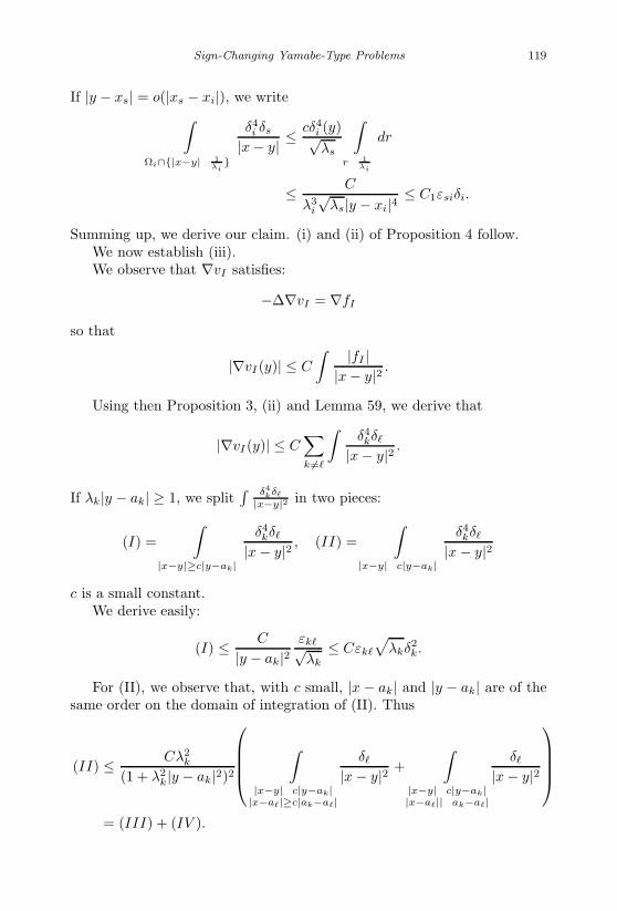
January 17, 2007 11:55 WSPC/Book Trim Size for 9in x 6in finalBB
Sign-Changing Yamabe-Type Problems 119
If |y − xs| = o(|xs − xi|), we write∫Ωi∩|x−y|≤ 1
λi
δ4i δs
|x − y| ≤cδ4
i (y)√λs
∫r≤ 1
λi
dr
≤ C
λ3i
√λs|y − xi|4
≤ C1εsiδi.
Summing up, we derive our claim. (i) and (ii) of Proposition 4 follow.We now establish (iii).We observe that ∇vI satisfies:
−∆∇vI = ∇fI
so that
|∇vI(y)| ≤ C
∫ |fI ||x − y|2 .
Using then Proposition 3, (ii) and Lemma 59, we derive that
|∇vI(y)| ≤ C∑k =
∫δ4kδ
|x − y|2 .
If λk|y − ak| ≥ 1, we split∫ δ4
kδ
|x−y|2 in two pieces:
(I) =∫
|x−y|≥c|y−ak|
δ4kδ
|x − y|2 , (II) =∫
|x−y|≤c|y−ak|
δ4kδ
|x − y|2
c is a small constant.We derive easily:
(I) ≤ C
|y − ak|2εk√λk
≤ Cεk
√λkδ2
k.
For (II), we observe that, with c small, |x − ak| and |y − ak| are of thesame order on the domain of integration of (II). Thus
(II) ≤ Cλ2k
(1 + λ2k|y − ak|2)2
∫
|x−y|≤c|y−ak||x−a|≥c|ak−a|
δ
|x − y|2 +∫
|x−y|≤c|y−ak||x−a|≤|ak−a|
δ
|x − y|2
= (III) + (IV ).
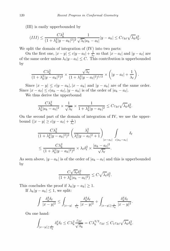
January 17, 2007 11:55 WSPC/Book Trim Size for 9in x 6in finalBB
120 Recent Progress in Conformal Geometry
(III) is easily upperbounded by
(III) ≤ Cλ2k
(1 + λ2k|y − ak|2)2
1√λ|ak − a|
|y − ak| ≤ Cεk
√λkδ2
k.
We split the domain of integration of (IV) into two parts:On the first one, |x− y| ≤ c|y− a|+ 1
λso that |x− a| and |y − a| are
of the same order unless λ|y−a| ≤ C. This contribution is upperboundedby
Cλ2k
(1 + λ2k|y − ak|2)2 ×
√λ
(1 + λ2 |y − a|2)1/2
×(|y − a| + 1
λ
).
Since |x − y| ≤ c|y − ak|, |x − ak| and |y − ak| are of the same order.Since |x − a| ≤ c|ak − a|, |y − ak| is of the order of |ak − a|.
We thus derive the upperbound
Cλ2k
λ2k|ak − a|2 × 1√
λ
× 11 + λ2
k|y − ak|2 ≤ Cεk
√λkδ2
k.
On the second part of the domain of integration of IV, we use the upper-bound (|x − y| ≥ c|y − a| + 1
λ)
Cλ2k
(1 + λ2k|y − ak|2)2
(λ2
λ2 |y − a|2 + 1
) ∫|x−a|≤c|ak−a|
δ
≤ Cλ2k
(1 + λ2k|y − ak|2)2 × λδ
2 × |ak − a|2√
λ
.
As seen above, |y−ak| is of the order of |ak −a| and this is upperboundedby
C√
λδ2
(1 + λ2k|ak − a|2) ≤ C
√λδ
2 .
This concludes the proof if λk|y − ak| ≥ 1.If λk|y − ak| ≤ 1, we split:∫
δ4kδ
|x − y|2 ≤∫|x−y|≤ 1
λk
δ4kδ
|x − y|2 +∫|x−y|≥ 1
λk
δ4kδ
|x − y|2 .
On one hand:∫|x−y|≥ 1
λk
δ4kδ ≤ Cλ2
k
εk√λk
= Cλ3/2k εk ≤ C1εk
√λkδ2
k.
January 17, 2007 11:55 WSPC/Book Trim Size for 9in x 6in finalBB
Sign-Changing Yamabe-Type Problems 121
On the other hand, if |x − y| ≤ 1λk
, then
∣∣|x − a| − |ak − a|∣∣ ≤ |x − ak| = O
(1λk
).
Thus, since λk|ak − a| is very large, |x− a| is of the order of |ak − a| and
∫|x−y|≤ 1
λk
δ4kδ
|x − y|2 ≤ Cλ2k√
λ|ak − a|× 1
λk≤ Cεkδ
2k ·√
λk
(iii) follows.
1.10.4 Estimates on v − (vI + vII)
We want in this section to show how our estimates on v, vI , vII extend tov − (vI + vII). The equation satisfied by v − (vI + vII) is basically thesame than the one satisfied by the other quantities but it has an additionalsplitting between group I and group II which makes it more specific. Wewant to use this splitting to derive better estimates. This requires somecare.
The equation satisfied by v is
−∆v = Q∗((∑
αiωi + v)5)
while vI and vII satisfy
−∆vI = Q∗I
(∑i∈I
αiωi + vI
)5
−∆vII = Q∗II
(∑i∈I
αiωi + vII
)5 .
Let us forget in a first step the presence of Q∗, Q∗I , Q
∗II and have a look at
the equation satisfied by v − (vI + vII). Since we are not taking care ofQ∗, Q∗
I , Q∗II , we will leave an additional term U for this contribution. We

January 17, 2007 11:55 WSPC/Book Trim Size for 9in x 6in finalBB
122 Recent Progress in Conformal Geometry
thus have
− ∆(v − (vI + vII)) =(∑αiωi + v
)5
−(∑
i∈I
αiωi + vI
)5
−(∑
i∈II
αiωi + vII
)5
+ U
= O
(∣∣∣∣∑i∈II
αiωi
∣∣∣∣∣∣∣∣∑i∈I
αiωi
∣∣∣∣4 +∣∣∑
i∈I
αiωi
∣∣∣∣∣∣∣∣ ∑i∈II
αiωi
∣∣∣∣4)
+ 5(∑
αiωi
)4
(v − (vI + vII))
+3∑
µ=1
O
(∣∣∣∣∑i∈II
αiωi
∣∣∣∣∣∣∣∣∑i∈I
αiωi
∣∣∣∣µ−1
+∣∣∣∣∑
i∈II
αiωi
∣∣∣∣µ)|vI |4−µ
+3∑
µ=1
O
(∣∣∣∣∑i∈II
αiωi
∣∣∣∣µ−1∣∣∣∣∑i∈I
αiωi
∣∣∣∣+ ∣∣∣∣∑i∈I
αiωi
∣∣∣∣µ)|vII |4−µ
+5∑
θ=2
fθ (v − (vI + vII))θ + U.
We view it as
−∆(v−(vI +vII))−5(∑
αiωi
)4
(v−(vI +vII))−5∑
θ=2
fθ(v−(vI +vII))θ =
O
(∣∣∑i∈II
αiωi
∣∣∣∣∑i∈I
αiωi
∣∣4 +∣∣∑
i∈I
αiωi
∣∣∣∣ ∑i∈II
αiωi
∣∣4)
+3∑
µ=1
O
((∣∣∑i∈II
αiωi
∣∣∣∣∑i∈I
αiωi
∣∣µ−1 +∣∣∑
i∈II
αiωi
∣∣µ) |vI |4−µ
+
(∣∣∑i∈II
αiωi
∣∣µ−1∣∣∑i∈I
αiωi
∣∣+ ∣∣∑i∈I
αiωi
∣∣µ) |vII |4−µ
)+ U.
We split R3 or S3 as usual in its different pieces Ωi, adjusted to the ωi’sand Ωc = (UΩi)c.
Accordingly, v − (vI + vII) is split in each Ω into an H10 -piece
(v − (vI + vII)) and a harmonic piece h. The non-linear operator −∆u−5(∑
αiωi)4u−5∑
θ=2
fθuθ is the same than the one used for v and the splitting
January 17, 2007 11:55 WSPC/Book Trim Size for 9in x 6in finalBB
Sign-Changing Yamabe-Type Problems 123
gives rise to a matrix relating |(v−(vi +vII))|H10,|h0
|∞√λ
,∑
λs≥λss=
εs|hs
|∞√λ
just
as for v. We thus need only to keep track of the terms which do not involve(v − (vI + vII)), h. These terms all come either from
g = O
(∣∣∑i∈II
αiωi
∣∣∣∣∑i∈I
αiωi
∣∣4 +∣∣∑
i∈I
αiωi
∣∣∣∣ ∑i∈II
αiωi
∣∣4)
+3∑
µ=1
O
((∣∣∑i∈II
αiωi
∣∣∣∣∑i∈I
αiωi
∣∣µ−1 +∣∣ ∑
i∈II
αiωi
∣∣µ) |vI |4−µ+
(∣∣∑i∈II
αiωi
∣∣µ−1∣∣∑i∈I
αiωi
∣∣+ ∣∣∑i∈I
αiωi
∣∣µ) |vII |4−µ
)
and its projections or from the contribution on v − (vI + vII) in Ωc. Thecontribution of g is controlled by:
∫Ωc
i
gδi +1√λiρi
∫Ωi
g +∫
Ωi
gδj +√
λjεij
∫Bj
g.
Indeed, if we replace g by f of (1.1) in Section 1.1, the above quantity isrelated to hi (see Lemma 12) and upperbounds what we denoted |h0
i |∞√λi
+∑λs≥λi
s=i
εis|hsi |∞. These quantities, in turn, are involved in the upperbound
of |vi|H10, together with
(∫Ωi
g6/5)5/6
. |vi|H10( or |(v− (vI +vII))i|H1
0here )
is involved, together with a bound on v( or v− (vI +vII) here) in Ωc in thederivation of the bound on
∫Ωc
i
|f |δi +1√λiρi
∫Ωi
|f | +∫
Ωi
|f |δj +√
λjεij
∫Bj
|f |.
Due to the form of the matrix involved in this estimate, see (3), estimateson |(v − (vI + vII))|H1
0on |ho
|∞√λ
+∑
λs≥λs=
εs|hs |∞ are easily derived from
the following:

January 17, 2007 11:55 WSPC/Book Trim Size for 9in x 6in finalBB
124 Recent Progress in Conformal Geometry
Proposition 5
(i)∫Ωc
igδi + 1√
λiρi
∫Ωi
g +∫Ωi
gδj ≤
C
∑k =ik∈I
or k∈II
∣∣∣∣ ∑j∈IIor
j∈I
αjωj(ak)∣∣∣∣ εik√
λk
+∣∣∣∣ ∑
j∈I if i∈IIj∈II if i∈I
αjωj(ai)∣∣∣∣∑ εim√
λi
+ O
∑j =i
|ω∞j |εij
λi|a| +∑
εij
∑(j,m)∈
(I,II) or (II,I)
ε2jm
.
(ii)
(∫Ωi
g6/5
)5/6
≤ C√λi
∣∣∣∣ ∑j∈I if i∈IIj∈II if i∈I
αjωj(ai)∣∣∣∣
+ O
∑j =i
|ω∞j |εij
λi|a| +∑
εij
∑(j,m)∈
(I,II) or (II,I)
ε2jm
.
(iii)
|v − (vI + vII)|(x) ≤ C∑
(i,j)∈(I,II) or (II,I)
(|ω∞
j | + εij +1
λj |a|)
εijδi.
We will derive from Proposition 5 the following theorem.
Theorem 2 |(v − (vI + vII))i|H10
+ |h0i |∞√λi
+∑
λs≥λi
s=i
εis|hsi |∞
≤ C
[ ∑k =ik∈I
or k∈II
∣∣∣∣ ∑j∈IIor
j∈I
αjωj(ak)∣∣∣∣ εik√
λk
+1√λi
∣∣∣∣ ∑j∈I if i∈IIj∈II if i∈I
αjωj(ai)∣∣∣∣]

January 17, 2007 11:55 WSPC/Book Trim Size for 9in x 6in finalBB
Sign-Changing Yamabe-Type Problems 125
+ O
∑j =i
|ω∞j |εij
λi|a| +∑
εij
∑(j,m)∈
(I,II) or (II,I)
ε2jm
.
Proof of Proposition 5.Proof of (i). The only contribution which is not related to an Ω (moreaccurately to a smaller version of Ω, Ω, since we need to leave some roomin the estimate of the harmonic part h) comes from
∫Ωc
igδi and is of the
type∫Ωc gδi.
g contains products of δk’s with k ∈ I with δm’s with m ∈ II. Bothterms are present. Assume i is in II for example. Consider∑∫
Ωc
δi(δ4kδm + δ4
mδk).
We can always upperbound one of δk or δm by C√λk|a| or C√
λm|a| , or δi byC√λi|a| .
Thus, using Lemma 69,∫Ωc
δiδ4mδk ≤ C
∑(s,t)∈
(I,II) or (II,I)
εisε2st.
We now estimate, for k = i,∫Ωk
gδi. Assume k ∈ I for example. Then,since δj ≤ δk on Ωk,∫
Ωk
gδi ≤ C
∣∣∣∣∑αjωj(ak)∣∣∣∣ ∫
Ωk
δ4kδi + C
∑j∈II
∫Ωk
|x − ak|√λj |a|2
δ4kδi
+ C∑
(,m)∈(I,I)
εm
∫Ωk
δmδiδ3k
∑s∈II
δs + C∑
(,m)∈(II,II)
εm
∫Ωk
δ3kδiδm
∑s∈II
δs
≤ C
∣∣∣∣ ∑j∈II
αjωj(ak)∣∣∣∣ εki√
λk
+ C∑j∈II
1√λj
√λk|a|2
∫Ωk
δ3kδi
+ C∑
(,m)∈(I,I)
εm
∑s∈II
1√λs|a|
∫Ωk
δmδ3kδi+C
∑(,m)∈(II,II)
εm
∑s∈II
1√λs|a|
∫Ωk
δ3kδiδm.

January 17, 2007 11:55 WSPC/Book Trim Size for 9in x 6in finalBB
126 Recent Progress in Conformal Geometry
Observe that ∫Ωk
δmδiδ3k ≤ C
∫Ωk
δ4kδi ≤ C
εki√λk
and ∫Ωk
δ3kδi ≤
∫Ωk∩|x−ai|≥10|ai−ak|
+∫
Ωk∩c|ai−ak|≤|x−ai|≤10|ai−ak|
+∫
Ωk∩|x−ai|≤c|ai−ak|≤ C√
λiλ3/2k
1|ai − ak| +
C√λi|ai − ak|
× 1
λ3/2k
Log (|ai − ak|λk) +C
λ3/2k |ai − ak|3
1√λi
|ai − ak|2
≤ Cεik
λk(1 + Log (λk|ai − ak|)).
Thus, ∫Ωk
gδi ≤ C
∣∣∣∣ ∑j∈II
αjωj(ak)∣∣∣∣ εik√
λk
+ C∑j∈II
1√λj
√λk|a|
· εik
λk|a| (1 + Log (λk|ai − ak|))
+ C∑
εm
∑s∈II
1√λs
√λk|a|
εki.
This estimate adapts easily if k ∈ II. Let us now estimate 1ρi
√λi
∫Ωi
g =√λi Max εi
∫Ωi
g.Assume that i ∈ II for example. We then have (again δs ≤ Cδi in Ωi).√
λiεim
∫Ωi
g ≤ C√
λiεim
∣∣∣∣∑j∈I
αjωj(ai)∣∣∣∣ ∫
Ωi
δ4i
+ C√
λiεim
∑j∈I
1√λj |a|
∫Ωi
|x−ai|δ4i +C
√λiεim
(∑εts
)∑j∈I
1√λj |a|
∫Ωi
δ4i
January 17, 2007 11:55 WSPC/Book Trim Size for 9in x 6in finalBB
Sign-Changing Yamabe-Type Problems 127
≤ εim√λi
∣∣∣∣∑j∈I
αjωj(ai)∣∣∣∣+ Cεim
∑j∈I
1√λi
√λj |a|
∫Ωi
δ3i
+ Cεim
∑εts
∑j∈I
1√λi
√λj |a|
+ Cεim
∑εts
∑j∈I
1√λi
√λj |a|
≤ εim√λi
∣∣∣∣∑j∈I
αjωj(ai)∣∣∣∣+ Cεim
∑j∈I
1√λi
√λj |a|
1
λ3/2i
Log(λi|a|)
+ Cεim
∑εts
∑j∈I
1√λi
√λj |a|
.
For√
λjεij
∫Bj
g, the estimate is identical to the one completed above.As we multiply by
√λi, the upperbound takes away this multiplicative
factor which cancels in a natural way with√
λj in the denominator (λj ≥λi). We estimate now
∫Ωi
gδj and(∫
Ωig6/5
)5/6
.
Recalling that we are assuming that i ∈ II, we upperbound∫Ωi
gδj asfollows∫
Ωi
gδj ≤ C
∣∣∣∣ ∑m∈I
αmωm(ai)∣∣∣∣ ∫
Ωi
δ4i δj + C
∑m∈I
1√λm|a|
∫Ωi
|x − ai|δ4i δj
+ C(∑
εs
)∑m∈I
1√λm|a|
∫Ωi
δ4i δj
≤ C
(∣∣∣∣ ∑m∈I
αmωm(ai)∣∣∣∣+ (∑ εs
)∑m∈I
1√λm|a|
)
× εij√λi
+ C∑m∈I
1√λm
√λi|a|
∫Ωi
δ3i δj
≤ C
(∣∣∣∣∑m∈I
αmωm(ai)∣∣∣∣+ (∑ εs
)∑m∈I
1√λm|a|
)εij√λi
+ C∑m∈I
1√λm
√λi|a|
εij
λiLog (λi|ai − aj |).
January 17, 2007 11:55 WSPC/Book Trim Size for 9in x 6in finalBB
128 Recent Progress in Conformal Geometry
We finally estimate(∫
Ωig6/5
)5/6
which we upperbound as follows usingthe finer structure of g:(∫
Ωi
g6/5
)5/6
≤ C√λi
∣∣∣∣∑j∈I
αjωj(ai)∣∣∣∣
+ C∑j∈I
1√λj |a|2
(∫Ωi
|x − ai|6/5δ24/5i
)5/6
+ C(∑
εs
)∑j∈I
1√λj |a|
(∫Ωi
δ24/5i
)5/6
≤ C√λi
∣∣∣∣∑j∈I
αjωj(ai)∣∣∣∣
+ C∑j∈I
1√λi
√λjλi|a|2
+ C(∑
εs
)∑j∈I
1√λiλj |a|
U contains two type of terms: on one hand it contains terms whichwe are expecting, that is Q∗ of the nonlinearly involved in the equa-tion satisfied by v − (vI + vII). On the other hand it contains (Q∗ −Q∗
I)
((∑i∈I
αiωi + vI
)5)
, (Q∗ − Q∗II)(
∑i∈II
αiωi + vII)5. Without changing
the equation much we may apply the operator Q∗ to it again. U thencontains
Q∗(∆vI), Q∗(∆vII), Q∗(Q∗ − Q∗I)
((∑i∈I
αiωi + vI
))5
etc.
We claim that all these terms are∑(i,j)∈(I,II)
or (II,I)
O(∑
εm
)εijδi.
Indeed,
Q∗ = Q∗Q∗II = Q∗Q∗
I
so that
Q∗(∆vI) = Q∗Q∗II(∆vI), Q∗(∆vII) = Q∗Q∗
II(∆vI)
Q∗
(Q∗ − Q∗I)
(∑i∈I
αiωi + vI
)5 = Q∗(Q∗−Q∗I)Q
∗I
(∑I∈I
αiωi + vI
)5
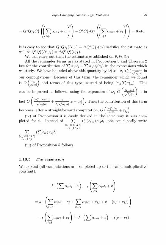
January 17, 2007 11:55 WSPC/Book Trim Size for 9in x 6in finalBB
Sign-Changing Yamabe-Type Problems 129
= Q∗Q∗IIQ
∗I
(∑i∈I
αiωi + vI
)5−Q∗Q∗IIQ
∗I
(∑i∈I
αiωi + vI
)5 = 0 etc.
It is easy to see that Q∗Q∗II(∆vI) = ∆Q∗Q∗
II(vI) satisfies the estimate aswell as Q∗Q∗
I(∆vII) = ∆Q∗Q∗I(vII).
We can carry out then the estimates established on v, vI , vII .All the remainder terms are as stated in Proposition 5 and Theorem 2
but for the contribution of∑
αjωj −∑
αjωj(ai) in the expressions whichwe study. We have bounded above this quantity by O(|x− ai|)
∑1√
λj |a|in
our computations. Because of this term, the remainder which we foundis O
(εij
λi|a|)
and terms of this type instead of being (εij
∑ε2
m). This
can be improved as follows: using the expansion of ωj , O
(|x−ai|√
λj |a|
)is in
fact O
(|ω∞
j ||x−ai|√λj |a|
+ 1
λj
√λj |a|
|x − ai|)
. Then the contribution of this term
becomes, after a straightforward computation, O( |ω∞
j |εij
λi|a| + ε3ij
).
(iv) of Proposition 3 is easily derived in the same way it was com-pleted for v. Instead of
∑(i,j)∈(I,II)
or (II,I)
(∑
εm) εijδi, one could easily write
∑(i,j)∈(I,II)
or (II,I)
(∑
εi) εijδi.
(iii) of Proposition 5 follows.
1.10.5 The expansion
We expand (all computations are completed up to the same multiplicativeconstant).
∂J(∑
αiωi + v)· ∂I
(∑i∈I
αiωi + v
)
= ∂J
(∑i∈I
αiωi + vI +∑i∈II
αiωi + vII + v − (vI + vII)
)
· ∂I
(∑i∈I
αiωi + vI
)+ ∂J
(∑αiωi + v
)· ∂I(v − vI)
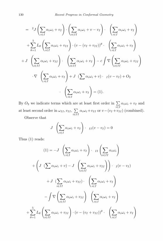
January 17, 2007 11:55 WSPC/Book Trim Size for 9in x 6in finalBB
130 Recent Progress in Conformal Geometry
= ∂2J
(∑i∈I
αiωi + vI
)·(∑
i∈II
αiωi + v − vI
)· ∂(∑
i∈I
αiωi + vI
)
+5∑
θ=1
Lθ
(∑i∈I
αiωi + vII
)· (v − (vI + vII))θ · ∂
(∑i∈I
αiωi + vI
)
+ ∂J
(∑i∈II
αiωi + vII
)· ∂(∑
i∈II
αiωi + vI
)− c
∫∇(∑
i∈II
αiωi + vII
)
· ∇∂
(∑i∈I
αiωi + vI
)+ ∂J(
∑αiωi + v) · ∂I(v − vI) + O2
· ∂(∑
i∈I
αiωi + vI
)= (1).
By O2 we indicate terms which are at least first order in∑i∈I
αiωi + vI and
at least second order in ωII , vII ,∑
i∈II
αiωi +vII or v−(vI +vII) (combined).
Observe that
∂J
(∑i∈I
αiωi + vI
)· ∂II(v − vI) = 0
Thus (1) reads:
(1) = −∂J
(∑i∈I
αiωi + vI
)· ∂II
(∑i∈II
αiωi
)
+
(∂J(
∑αiωi + v) − ∂J
(∑i∈II
αiωi + vII
))· ∂I(v − vI)
+ ∂J(∑i∈II
αiωi + vII) · ∂(∑
i∈I
αiωi + vI
)
−∫
∇(∑
i∈II
αiωi + vII
)∂
(∑i∈I
αiωi + vI
)
+5∑
θ=1
Lθ
(∑i∈II
αiωi + vII
)· (v − (vI + vII))θ · ∂
(∑i∈I
αiωi + vI
)
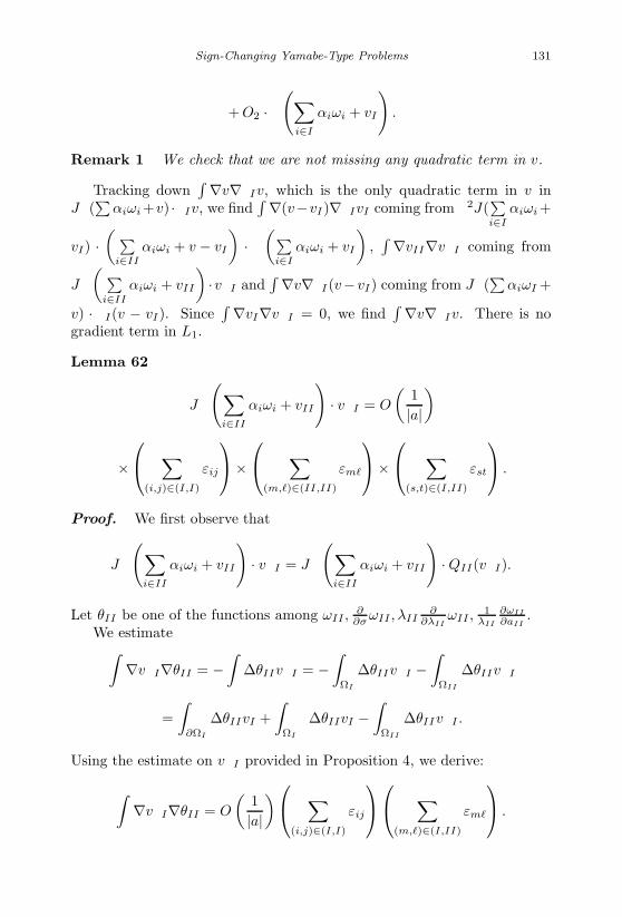
January 17, 2007 11:55 WSPC/Book Trim Size for 9in x 6in finalBB
Sign-Changing Yamabe-Type Problems 131
+ O2 · ∂(∑
i∈I
αiωi + vI
).
Remark 1 We check that we are not missing any quadratic term in v.
Tracking down∫ ∇v∇∂Iv, which is the only quadratic term in v in
∂J(∑
αiωi +v) ·∂Iv, we find∫ ∇(v−vI)∇∂IvI coming from ∂2J(
∑i∈I
αiωi +
vI) ·( ∑
i∈II
αiωi + v − vI
)· ∂
(∑i∈I
αiωi + vI
),∫ ∇vII∇∂vI coming from
∂J
( ∑i∈II
αiωi + vII
)·∂vI and
∫ ∇v∇∂I(v−vI) coming from ∂J(∑
αiωI +
v) · ∂I(v − vI). Since∫ ∇vI∇∂vI = 0, we find
∫ ∇v∇∂Iv. There is nogradient term in L1.
Lemma 62
∂J
(∑i∈II
αiωi + vII
)· ∂vI = O
(1|a|)
× ∑
(i,j)∈(I,I)
εij
× ∑
(m,)∈(II,II)
εm
× ∑
(s,t)∈(I,II)
εst
.
Proof. We first observe that
∂J
(∑i∈II
αiωi + vII
)· ∂vI = ∂J
(∑i∈II
αiωi + vII
)· QII(∂vI).
Let θII be one of the functions among ωII ,∂
∂σ ωII , λII∂
∂λIIωII ,
1λII
∂ωII
∂aII.
We estimate∫∇∂vI∇θII = −
∫∆θII∂vI = −
∫ΩI
∆θII∂vI −∫
ΩII
∆θII∂vI
=∫
∂ΩI
∆θIIvI +∫
ΩI
∂∆θIIvI −∫
ΩII
∆θII∂vI .
Using the estimate on ∂vI provided in Proposition 4, we derive:
∫∇∂vI∇θII = O
(1|a|) ∑
(i,j)∈(I,I)
εij
∑(m,)∈(I,II)
εm
.
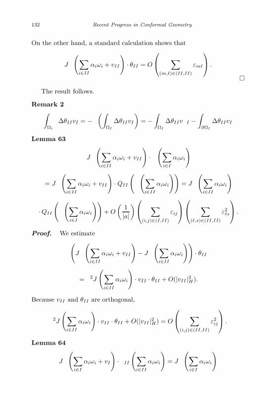
January 17, 2007 11:55 WSPC/Book Trim Size for 9in x 6in finalBB
132 Recent Progress in Conformal Geometry
On the other hand, a standard calculation shows that
∂J
(∑i∈II
αiωi + vII
)· θII = O
∑(m,)∈(II,II)
εm
.
The result follows.
Remark 2∫Ωi
∂∆θIIvI = −∂
(∫ΩI
∆θIIvI
)= −
∫ΩI
∆θII∂vI −∫
∂ΩI
∆θIIvI
Lemma 63
∂J
(∑i∈II
αiωi + vII
)· ∂(∑
i∈I
αiωi
)
= ∂J
(∑i∈II
αiωi + vII
)· QII
(∂
(∑i∈II
αiωi
))= ∂J
(∑i∈II
αiωi
)
·QII
(∂
(∑i∈I
αiωi
))+ O
(1|a|) ∑
(i,j)∈(I,II)
εij
∑(,s)∈(II,II)
ε2s
.
Proof. We estimate(∂J
(∑i∈II
αiωi + vII
)− ∂J
(∑i∈II
αiωi
))· θII
= ∂2J
(∑i∈II
αiωi
)· vII · θII + O(|vII |2H).
Because vII and θII are orthogonal,
∂2J
(∑i∈II
αiωi
)· vII · θII + O(|vII |2H) = O
∑(i,j)∈(II,II)
ε2ij
.
Lemma 64
∂J
(∑i∈I
αiωi + vI
)· ∂II
(∑i∈II
αiωi
)= ∂J
(∑i∈I
αiωi
)

January 17, 2007 11:55 WSPC/Book Trim Size for 9in x 6in finalBB
Sign-Changing Yamabe-Type Problems 133
·QI
(∂II
(∑i∈II
αiωi
))+ O
(1|a|) ∑
(i,j)∈(I,II)
εij
∑(,s)∈(I,I)
ε2s
.
Proof. same than above Lemma 65 Let θ ≥ 2, µ + µ1 ≥ 2, µ1 ≥ 1, θ + µ + µ1 = 6. Then
∣∣∣∣ ∫ ∂
(∑i∈I
αiωi + vI
)θ
ωµIIv
µ1II
∣∣∣∣ ≤ C
|a|
∑(k,)∈(I,II)
or (I,I)
εk
∑
(s,t)∈(I,II)
ε2st
.
Proof. We split∫
∂
(∑i∈I
αiωi + vI
)θ
ωµIIv
µ1II into
∫ΩI
∂
(∑i∈I
αiωi + vI
)θ
ωµIIv
µ1II +
∫ΩII
∂
(∑i∈I
αiωi + vI
)θ
ωµIIv
µ1II .
The second integrand is easily upperbounded using Proposition 4 by
C1|a|
∑(k,)
∈(II,II)
εk
∫ΩII
δθI δµ+µ1
II ≤ C
|a|
∑(k,)
∈(II,II)
εk
∑(s,t)∈(I,II)
ε2st.
For the first integrand we complete an integration by parts and the resultfollows. Lemma 66 Let i0 ∈ I, ∂ϕI0 = ∂ϕI0
∂ai0= −∇ϕi0 .∣∣∣∣ ∫ ∇(v − (vI + vII))∇∂ϕi0
∣∣∣∣≤ C
√λi0
(√λi0 (|(v − (vI + vII))i0 |H1
0+
|h0i0|∞√
λi0
+∑
λs≥λi0s=i0
εi0s|hsi0 |∞ +
∑j
√λi0
∑ ε3i0s +
∑λt≥λi0
εiotε2ts
.
Proof. Integrating by parts, we find∫∇(v − (vI + vII))∇∂ϕi0 = −
∫(v − (vI + vII))∆∂ϕi0 .
January 17, 2007 11:55 WSPC/Book Trim Size for 9in x 6in finalBB
134 Recent Progress in Conformal Geometry
Clearly ∣∣∣∣ ∫Ωi0
(v − (vI + vII))∆∂ϕi0
∣∣∣∣≤ Cλi0
|(v − (vI + vII))i0 |H10
+|hi0 |∞√
λi0
+∑
λs≥λi0s=i0
εi0s|hsi0 |∞
.
On the other hand, ∣∣∣∣ ∫Ωc
i0
(v − (vI + vII))∆∂ϕi0
∣∣∣∣≤ Cλi0
∑⊂(i,j)∈(I,II) or (II,I)
(|ω∞
j | + 1λj |a|
)εij
∫Ωc
i0
(δ5i0δi + δ5
i0δj)
Observe now that∫Ωc
i0
δsi0δi ≤ Cε3
i0s if i = i0,≤∫
Ωci0
∩Ωci
δ5i0δi +
∫Ωc
i0∩Ωi
δ5i0δi
≤ C∑
λt≥λi0
εitε2ts + Cε3
i0s.
Thus∣∣∣∣ ∫Ωc
i0
(v− (vI + vII))∆∂ϕi0
∣∣∣∣ ≤ C√
λi0 (√
λi0εijε3i0s + εij
√λi0
∑λj≥λi0
εitε2ts).
Observe that
QI(v − vI) = 0.
Thus
(∂IQI)(v − vI) = −QI(∂I(v − vI)).
We then have
Lemma 66′
∂J(∑i∈II
αiωi + vII) · QI∂I(v − vI − vII)

January 17, 2007 11:55 WSPC/Book Trim Size for 9in x 6in finalBB
Sign-Changing Yamabe-Type Problems 135
= −∂J
(∑i∈II
αiωi + vII
)· QII ((∂IQI)(v − vI − vII))
−∂J
(∑i∈II
αiωi + vII
)· QII(∂IQI(vII))
= O
(1|a|) ∑
(i,j)∈(I,II)
εij
∑(s,t)∈(II,II)
ε2st
+∑i0∈I
λi0
|(v − (vI + vII))i0 |2H10
+|h0
i0|2∞
λi0
+∑
λs≥λi0s=io
ε2i0s|hs
i0 |2∞
.
Proof. Observe that
∂J
(∑i∈II
αiωi + vII
)· θII = O
∑(s,t)∈(II,II)
εst
.
On the other hand, for i0 ∈ I;
∫∇θII∇θio = O
∑j∈II
εi0j
,
∫∇θII∇∂θi0 = O
1|a|
∑j∈II
εi0j
.
Using Lemma 66 and extensions of it
−∫
∆∂θi0(v − vI − vII)
≤ C√
λi0
(√λio
(|(v − (vI + vII))i0 |H1
0+
|h0i0 |∞√λi0
+∑
λs≥λi0s=i0
εi0s|hsi0 |∞ +
∑j
√λi0
ε3i0s +
∑λt≥λi0
εitε2ts
εi0s
.

January 17, 2007 11:55 WSPC/Book Trim Size for 9in x 6in finalBB
136 Recent Progress in Conformal Geometry
On the other hand,
−∫
∆∂θIvII = O
∑(i,j)∈(I,II)
ε2ij
|a|
.
Observe that each − ∫ ∆∂θi0(v − (vI + vII)) is multiplied by∫ ∇θII∇θi0
and by ∂J
( ∑i∈II
αiωi + vII
)· θII . The result follows
Lemma 67(1) ∫ (∣∣∣∣∑
i∈I
αiωi + vI
∣∣∣∣+ ∣∣∣∣ ∑i∈II
αiωi + vII
∣∣∣∣+ |v − (vI + vII |)2
(∣∣∣∣∑i∈II
αiωi + vII
∣∣∣∣+ |v − (vI + vII)|)·
· |v − (vI + vII)| ·∣∣∣∣∂(∑
i∈I
αiωi + vI
)2 ∣∣∣∣≤ C
∑(i,j)∈(I,II)
ε3ij
|a| +∑∈I
λ
(|(v − (vI + vII))|2H1
0+
|h0 |2∞λ
+∑
λs≥λs=
ε2s|hs
|2∞
+∑∈I
(∑i∈II
αiωi(a)
)2
+∑i∈II∈I
ω∞2
i ε2i
λ|ai − a|2
.
(2) ∫ (∣∣∣∣∑i∈I
αiωi + vI
∣∣∣∣+ ∣∣∣∣ ∑i∈II
αiωi + vII
∣∣∣∣+ |v − (vI + vII |)2
(∣∣∣∣∑i∈II
αiωi + vII
∣∣∣∣+ |v − (vI + vII)|)2
· |v − (vI + vII)| ·∣∣∣∣∂(∑
i∈I
αiωi + vI
) ∣∣∣∣
January 17, 2007 11:55 WSPC/Book Trim Size for 9in x 6in finalBB
Sign-Changing Yamabe-Type Problems 137
≤ C
∑(i,j)∈(I,II)
ε3ij
|a| +∑∈I
λ
|(v − (vI + vII))|2H10
+|h0
|2∞λ
+∑
λs≥λs=
ε2s|hs
|2∞
+∑∈I
(∑i∈II
αiωi(a)
)2
+∑i∈II∈I
ω∞2
i ε2i
λ|ai − a|2
.
(3) (∂ωI is either
1λi0
∂ωi0
∂ai0
or λi0
∂ωi0
∂λi0
or∂ωi0
∂σi0
with i0 ∈ I
)∫ (∑
i∈I
αiωi + vI
)4 ∣∣∣∣ ∑i∈II
αiωi + vII
∣∣∣∣
+
(∑i∈II
αiωi + vII
)4 ∣∣∣∣∑i∈I
αiωi + vI
∣∣∣∣+
(∑i∈I
αiωi + vI
)4
|v − (vI + vII)| + |v − (vI + vII)|4∣∣∣∣∑
i∈I
αiωi + vI
∣∣∣∣+ |v − (vI + vII)|5
) |∂ωI |
≤ C1√λi0
∑∈I =i0
√λ
λ|a − ai0 |[|(v − (vI + vII))|H1
0
+∑
λs≥λs=
|hs |∞εs +
|h0 |∞√λ
+| ∑i∈II
αiωi(a)|√
λ
+∑
(i,j)∈(II,II)
εijεi +√
εi
λ|a|
+∑∈II
ε3/2i√λ|a|
+1|a|∑ ε2
ij√λi

January 17, 2007 11:55 WSPC/Book Trim Size for 9in x 6in finalBB
138 Recent Progress in Conformal Geometry
+C∑ εi0iεis√
λiλj |a|+ C
∣∣∣∣∑
i∈II
αiωi(ai0 )√λi0
∣∣∣∣+ |(v − (I+vII))|H10
+∑
λs≥λi0s=i0
εi0s|hsi0 |∞ +
|h0i0|∞√
λi0
+∑i∈II
ε2ii0
.
Proof. Proof of (1). The contribution on ΩII of the integral is easily upper-bounded by
1|a|
∑(i,j)∈(I,II)
ε3ij .
Indeed, in ΩII ,
|∂(∑
i∈I
αiωi + vI
)| ≤ C
1|a|∑i∈I
δi
and
|v − (vI − vII)| ≤ C∑
(i,j)∈(I,II)
εij(δi + δj).
The claim then follows from the standard estimate∑(i,j)∈(I,II)
(∫δ4j δ2
i +∫
ΩII
δ6i
)≤ C
∑(i,j)∈(I,II)
ε2ij .
We turn now to the contribution on ΩI which we split between the contri-bution on each Ω
I and the contribution on (UΩI)
c ∩ ΩI :Let us first consider the contribution on (UΩ
I)c ∩ ΩI . We observe that
in ΩI :
|v−(vI+vII)|(x)+|∑i∈II
αiωi+vII |(x) ≤ C∑
(i,j)∈(I,II)
(|ω∞
j | + 1λj |a| + εij
)εij
√λi.
Indeed, for j ∈ II, in ΩI
|δj(x)| ≤ C√λj |a|
≤ Cεij
√λi if i ∈ I.

January 17, 2007 11:55 WSPC/Book Trim Size for 9in x 6in finalBB
Sign-Changing Yamabe-Type Problems 139
Also,
|∂ωi| ≤ Cδ3i (λi|x − ai|).
Let us first estimate the contribution of ∂ωi, i ∈ I, ignoring the contri-bution of ∂vI .
Thus, ∫(UΩ
I )c∩ΩI
≤ C∑
(i,j)∈(I,II)
(|ω∞
j |2 +1
λ2j |a|2
+ ε2ij
)λiε
2ij
×∫
(UΩI )c∩ΩI
∑i,j,∈Im∈II
δ3i (λi|x − ai|)δj(δ2
+ δ2m).
Observe that ∫(UΩ
I )c∩ΩI
δ6i (λir)2r2dr
1/2
≤ C
∫r≥ c
εis
r4dr
(1 + r2)3+∑k =i
λk>λi
∫Ωc
k∩Ωci
δ6kλ2
i (|ai − ak|2 + |x − ak|2)
1/2
.
Indeed, in (UΩI)
c, either
λi|x − ai| ≥ c
εis,
or, for some k such that λk > λi,
c
εkm≤ λk|x − ak| ≤ 1
εki.
Then,
|x − ai| ≤ |ai − ak| + |x − ak|
and
δi ≤ Cδk.
January 17, 2007 11:55 WSPC/Book Trim Size for 9in x 6in finalBB
140 Recent Progress in Conformal Geometry
Thus, (∫(UΩ
I )c∩ΩI
δ6i (λir)2r2dr
)1/2
≤ C∑
λk≥λi
√εks.
Summing, the contribution on (UΩI)
c ∩ ΩI is bounded by
∫(UΩ
I )c∩ΩI
≤ C
|a|
∑j∈II
1λj |a|
(ω∞2
j +1
λ2j |a|2
+ ε2ij
)∑ ε2ks.
since (∫(UΩ
I )c∩ΩI
δ2j (δ2
+ δ2m)2
)1/2
≤ C∑
ε3/2ks .
This does not quite fit into the expression of the remainder as we areseeking it. We need to improve this estimate. We observe that there is afactor equal to v−(vI +vII) in the expression which we want to upperbound.Above, we replaced it by |v − (vI + vII)|(x) + | ∑
i∈II
αiωi + vII |(x).
|v − (vI + vII)| is less in ΩI than Cεij
(1√
λj |a|+ δi
), i, j ∈ I, II. For
εij√λj |a|
, the estimate is straightforward since this factor comes out of the
integral entirely. The factor λiε2ij is then recomposed, but the expression
under the integral has one power of δ less. The estimate follows for thispart of v − (vI + vII).
For εijδi, we repeat our initial argument, only that now a factor equalto
√λi is missing. In the end, we derive an extra δ2
i in(∫(UΩ
I )c∩ΩI
δ2i δ2
j (δ2 + δ2
m)2)1/2
·
(∫Ωc δδ
i
)1/2 is less than C√
λiε5/2it . Our upperbound becomes:√
λiε2ij
(√λkε
5/2kt
)√εmt, i, j belong to I, II.
These two groups have a large interaction. Discussing various cases accord-ing to the fact that λj is the smallest concentration in its group or not andusing the fact that the interaction of I and II is largest or equivalent tothe largest, we derive the result.
January 17, 2007 11:55 WSPC/Book Trim Size for 9in x 6in finalBB
Sign-Changing Yamabe-Type Problems 141
We now consider the contribution on each ΩI (or a smaller version Ω
I).We expand(∑
i∈II
αiωi + vII
)(x) =
∑i∈II
αiωi(a) +∑i∈II
αi(ωi(x) − ωi(a)) + vII(x)
=∑i∈II
αiωi(a) + O
(1|a|∑i∈II
δi|x − a|)
+ O
∑(i,j)∈(II,II)
εijδi
.
(1.41)We then have, with j ∈ I, j1, k1 ∈ I, 1 ∈ II∫
ΩI
|∂ωj||v− (vI +vII)|(|v − (vI + vII)| + |
∑i∈II
αiωi + vII |)
δj1(δ2k1
+ δ21)
≤ C
∫Ω
I
√λjδ
2j |v − (vI + vII)|
(|v − (vI + vII)| + |
∑i∈II
αiωi + vII |)
× δj1(δ2k1
+ δ21)
≤ C
∫Ω
I
√λjδ
2j |v − (vI + vII)|
(|v − (vI + vII)| + |
∑i∈II
αiωi + vII |)
× (δ3j1 + δ3
k1+ δ3
1).
We have already used the claim (which we reestablish below) that on ΩI
δm ≤ Cδ ∀m.
Thus,∫Ω
I
≤ C
∫Ω
I
√λjδ
2j |v − (vI + vII)|(|v − (vI + vII)| + |
∑i∈II
αiωi + vII |)δ3 .
We first consider∫Ω
I
√λjδ
2j |v − (vI + vII)|2δ3
.
We split v− (vI + vII) in ΩI into (v− (vI + vII)) +h0
+∑
λs≥λs=
hsδs and
we have∫Ω
I
≤ C√
λj
∫Ω
I
δ2j |(v − (vI + vII))|2δ3
+ C√
λj |h0 |2∞
∫Ω
I
δ2j δ3
+∑
s
C√
λj |hs |2∞
∫Ω
j
δ2j δ2
sδ3 .

January 17, 2007 11:55 WSPC/Book Trim Size for 9in x 6in finalBB
142 Recent Progress in Conformal Geometry
Observe that
C√
λj
∫Ω
I
δ2j |(v − (vI + vII))|2δ3
≤ C√
λj
(∫Ω
I
δ6j
)1/3
|(v − (vI + vII))|2H10×√
λ.
For j = , this yields
C√
λjεj
√λ|(v − (vI + vII))|2H1
0≤ λ|v − (vI + vII)|2H1
0.
For j = , the same estimate holds readily.Observe also that (δj ≤ Cδ on Ω
I)√λj
∫Ω
I
δ2j δ3
≤ C√
λj
∫Ω
I
δjδ4 ≤ C
√λjεj√λ
≤ C1. (See Lemma 70)
This also works for j = .By Lemma 70 (below),√
λj
∫Ω
I
δ2j δ2
sδ3 = o(λε
2s)
(O(λε
2s) if j =
).
Thus∫Ω
I
≤ C(λ|(v − (vI + vII))|2H10
+ |h0 |2∞ + λ
∑⊂λs≥λs=
ε2s|h2
|2∞).
We now consider∫Ω
I
√λjδ
2j |v − (vI + vII)|
∣∣∣∣ ∑i∈II
αiωi + vII
∣∣∣∣δ3 ,
which we upperbound using (1.41) by
C
∑(i,m)∈(II,II)
(|ω∞
m | + 1λm|am − ai|
)εim√λi|a|
+∣∣∣∣∑
i∈II
αiωi(a)∣∣∣∣
×∫
ΩI
√λjδ
2j |v − (vI + vII)|δ3
+∑i∈II
√λj
(C
|ω∞i |√
λi|a|2+
C
λ3/2i |a|2
)
×∫
ΩI
δ2j |v − (vI + vII)||x − a|δ3
= (I) + (II).
January 17, 2007 11:55 WSPC/Book Trim Size for 9in x 6in finalBB
Sign-Changing Yamabe-Type Problems 143
Observe that √λ|x − a|δ ≤ C
so that
(II) ≤ C∑i∈II
√λj√λ
(C
|ω∞i |√
λi|a|2+
C
λ3/2i |a|2
)∫Ω
I
δ2j |v − (vI + vII)|δ2
≤ C∑i∈II
√λj
( |ω∞i |εi
|a| +Cεi
λi|a|2)|h0
|∞∫
ΩI
δ2j δ2
+∑
λs≥λs=
|hs |∞
∫Ω
δ2j δsδ
2
+ |(v − (vI + vII))|H10
(∫Ω
I
δ12/5j δ
12/5
)5/6 .
For j = , we have
∫Ω
I
δ2j δsδ
2 ≤
(∫Ω
I
δ2sδ4
)1/2(∫Ω
I
δ4j
)1/2
≤ Cεs
1λj
∫r≥ 1
εj
r2dr
(1 + r2)2
1/2
≤ Cεs
√εj
λjif λj ≥ λ,≤ Cεs
(∫Ω
I
δ6j
)1/3
× |ΩI |1/6 ≤ Cεsεj√
λ Max εm
≤ Cεs
√εj
λif λj ≤ λ.
For j = , we have ∫Ω
I
δ4 δs ≤ C
εs√λ
.
Combining, we derive that√λjεi
|a| |hs |∞
∫Ω
I
δ2j δsδ
2 ≤ C
√λεs|hs
|∞ × εi
|a|(√
εj√λ
+1√λ
).
We estimate now, using the above computations,∫Ω
I
δ2j δ2
≤(∫
ΩI
δ4j
)1/2(∫Ω
I
δ4
)1/2
≤ C
√εj
λj× 1√
λ
for j =
≤ C
λfor j = .

January 17, 2007 11:55 WSPC/Book Trim Size for 9in x 6in finalBB
144 Recent Progress in Conformal Geometry
Thus, √λjεi
|a| |h0 |∞
∫Ω
I
δ2j δ2
≤ C|h0 |∞ · εi
|a|(√
εj√λ
+1√λ
).
We then consider(∫Ω
I
δ12/5j δ
12/5
)5/6
≤(∫
ΩI
δ3j δ3
)2/3
|ΩI |1/6 ≤ C
ε2j log2/3 ε−1
j√λjεj
for j =
(∫Ω
I
δ24/5
)5/6
≤ C√λ
for j = .
We thus derive√λjεi
|a| |(v−(vI +vII))|H10
(∫Ω
I
δ12/5j δ
12/5
)5/6
≤ C√
λ|(v−(vI +vII))|H10
× εi√λ|a|
(√εj log2/3 ε−1
j + 1)
.
This, using the factor |ω∞i |+ C
λi|a| , i ∈ II, takes care of (II). We now estimate(I).
We split√λj
∫Ω
I
δ2j |v − (vI + vII)|δ3
≤ C√
λj
|h0 |∞
∫Ω
I
δ2j δ3
+∑
λs≥λs=
|hs |∞
∫Ω
I
δ2j δsδ
3
+ |(v − (vI + vII))|H10
(∫Ω
I
δ12/5j δ
18/5
)5/6 .
Observe that (δj ≤ cδ)√λj
∫Ω
I
δ2j δ3
≤√λj
∫Ω
I
δ4 δj ≤ C
√λjεj√λ
≤ C1
√λj
∫Ω
I
δ2j δsδ
3 ≤√λj
(∫Ω
I
δ6j
)1/3(∫Ω
I
δ3/2s δ
9/2
)
January 17, 2007 11:55 WSPC/Book Trim Size for 9in x 6in finalBB
Sign-Changing Yamabe-Type Problems 145
≤ C√
λjεj
(∫Ω
I
(δ2sδ4
)3/4δ3/2
)2/3
≤ C√
λjεj
(∫ω
I
δ2sδ4
)1/2
≤ C√
λjεjεs ≤ C√
λεs ( it works also for j = )
√λj
(∫Ω
I
δ12/5j δ
18/5
)5/6
≤ C√
λj
(∫Ω
I
δ2j δ4
)5/6
≤ C√
λjε5/3j ≤ C
√λ.
Combining, we derive that
C
∑(i,m)
∈(II,II)
(|ω∞
m | + 1λm|ai − am|
)εim√λi|a|
+∣∣∣∣∑
i∈II
αiωi(a)∣∣∣∣) ∫
ΩI
√λjδ
2j |v − (vI + vII)|δ3
≤ C
∑(i,m)
∈(II,II)
(|ω∞
m | + 1λm|ai − am|
)εim√λi|a|
+∣∣∣∣∑
i∈II
αiωi(a)∣∣∣∣
×
|h0 |∞ +
∑λs≥λ
s=
√λεs|hs
|∞ +√
λ|(v − (vI + vII))|H10
.
1) follows for ∂ωi.The above proof extends almost verbatim to ∂vI using (iii) of Propo-
sition 4 since the main estimate we have used in the proof of 1) for ∂ωI
was
|∂ωI | ≤ C∑i∈I
√λiδ
2i
and ∂vI satisfies the same estimate.However, in the beginning of the proof of 1) when estimating the con-
tribution on (UΩI)
c ∩ ΩI , we have used
|∂ωi| ≤ Cδ3i (λi|x − ai|).
January 17, 2007 11:55 WSPC/Book Trim Size for 9in x 6in finalBB
146 Recent Progress in Conformal Geometry
This estimate is not verified by ∂vI and we have to modify the argument.In the worst case, using Proposition 2 and 4, we have to estimate
(1) =∑
s
∑i∈I
√λi
∫Ωc
,I∩ΩI
δ2i
∑j∈II
(k,m)∈(I,II)
δjεkmδk
δ3s
≤ C∑
s
∑i∈I
∑j∈II
(k,m)∈(I,II)
√λiεkm√λj |a|
∫Ωc
,I∩ΩI
δ2i δkδ3
s
≤ C∑
s
∑i∈I
∑j∈II
(k,m)∈(I,II)
√λiεkm√λj |a|
ε3/2s
(∫Ωc
,I∩ΩI
δ4i δ2
k
)1/2
.
We now distinguish two cases:
(1) λi ≤ λk.We then upperbound by
C√λj
√λm|a|2 ε
3/2s εik = o
(∑ ε3st
|a|)
.
(2) λi ≥ λk.
We then have, after splitting the domain of integration between |x−ai| ≥c|ai − ak|, c small, and its complement:∫
Ωc,I
δ4i δ2
k ≤ C
λk|ai − ak|2∫
Ωc,I
δ4i +
C
λ2i |ai − ak|4 × λk|ai − ak|
λ2k
≤ C
λk|ai − ak|2∑
λm≥λi
εms
λm+
C
λ2i λk|ai − ak|3 .
This yields on (1) the upperbound:
(1) ≤ C∑
s
∑i∈I
∑j∈II
(k,m)∈(I,II)
ε3/2s√
λm
√λj |a|2
(εnt
λiλk|ai − ak|2 +1
λkλ2i |ai − ak|3
)
= o
(∑ε3
st
|a|)
.
(1.42)

January 17, 2007 11:55 WSPC/Book Trim Size for 9in x 6in finalBB
Sign-Changing Yamabe-Type Problems 147
Proof of 3). We now turn to estimate∫ (∑i∈I
αiωi + vI
)4(∣∣∣∣∑i∈II
αiωi + vII | + |v − (vI + vII)|)
+
(∑i∈II
αiωi + vII
)4
+ |v − (vI + vII)|4×
∣∣∣∣∑i∈I
αiωi + vI
∣∣∣∣ |∂ωi0 |.
Here ∂ωi0 is either ωi0 or λi0∂ωi0∂ai0
or 1λi0
∂ωi0∂ai0
or ∂ωi0∂σi0
. If a derivative istaken on ωi0 , it is tamed.
We have ∫(UΩ)c∩ΩII
≤ C√λi0 |a|
∑ ε2ij√λi
.
∫(UΩ)c∩ΩI
≤ C
∑j∈II
1√λj |a|
∑∫Ωc
δ4i δi0 .
We now claim that∑∫Ωc
δ4i δi0 ≤ C
(∑ εi0iεis√λi
+∑ ε2
is√λi0
).
We will establish this claim later. Thus,∫(UΩ)c∩ΩI)
≤ C
∑j∈II
1√λj |a|
(∑ εi0iεis√λi
+∑ ε2
is
λi0
).
We are left with the contribution in UΩ.The contribution on (UΩ) ∩ ΩII is upperbounded as follows
∫(UΩ)∩ΩII
≤ C√λi0 |a|
∑∈II
(∑
i∈I
1√λi|a|
)4∑ ∫
Ω∩ΩII
δ6j
1/6
× 1(λ maxεm)5/2
+∑i∈I
1√λi|a|
1λ
≤∑∈II
C√λi0
√λ|a|
(∑i∈I
ε4i
max ε5/2m
)
≤ C∑∈II
C√λi0
√λ|a|
· ε3/2i
January 17, 2007 11:55 WSPC/Book Trim Size for 9in x 6in finalBB
148 Recent Progress in Conformal Geometry
Using the fact that δj ≤ Cδ on Ω, we upperbound the contribution onΩ ∩ ΩI( ∈ I) as follows∫Ω∩ΩI
≤ C
∫Ω∩ΩI
δ4 |∂ωi0
(∣∣∣∣∑i∈II
αiωi + vII
∣∣∣∣+ |v − (vI + vII)|)
≤ C
(∫δ4 δ2
i0
)1/2 ∫
Ω∩ΩI
δ4
(∣∣∣∣∑i∈II
αiωi + vII
∣∣∣∣2 + |v − (vI + vII)|2)1/2
≤ Cεi0
∫Ω∩ΩI
δ4
(∣∣∣∣∑i∈II
αiωi + vII
∣∣∣∣2 + |v − (vI + vII)|2)1/2
≤ C1
λ|a − ai0 |√
λ√λi0
|(v − (vI + vII))|H10
+∑
λs≥λs=
|hs |∞εs +
|h0 |∞√λ
+| ∑i∈II
αiωi(a)|√
λ
+∑
(i,j)∈(II,II)
εijεi +1|a|∑i∈II
∫Ω∩ΩI
δ4 δ2
i |x − a|21/2
.
Observe now that ∫Ω∩ΩI
δ4 δ2
i |x − a|21/2
≤ 1√λ
∫Ω∩ΩI
δ2 δ2
i
1/2
≤ C√λ
√λi|a|
(∫Ω
δ2
)1/2
≤ Cεi
λ× 1√
Max εm
≤ C
√εi
λ
for i ∈ II.Thus,
∫Ω∩ΩI
≤ C
√λ
λi0
× 1λ|a − ai0 |
|(v − (vI + vII))|H10
+∑
λs≥λs=
|hs |∞εs
+|h0
|∞√λ
+| ∑i∈II
αiωi(a)|√
λ
+∑
(i,j)∈(II,II)
εijεi +√
εi
λ|a|
.

January 17, 2007 11:55 WSPC/Book Trim Size for 9in x 6in finalBB
Sign-Changing Yamabe-Type Problems 149
We also have an additional term which comes from the integration overΩi0 ∩ ΩI .
∫Ωi0∩ΩI
≤ C
| ∑i∈II
αiωi(ai0 )|√λi0
+∑i∈II
ε2ii0 + |(v − (vI + vII))i0 |H1
0
+∑
λs≥λi0s=i0
εi0s|hsi0 |∞ +
|h0i0 |∞√λi0
.
Proof of 2). In ΩI , 2) follows from 1). In ΩII , 2) is either immediate orfollows closely 3) in ΩII because, in ΩII ,
|∂ωi0 | ≤C
|a|δi0 for i0 ∈ I.
Thus, we obtain an extra factor 1|a| with respect to the estimate in 3).
Observation. Let us remove from the expression in 3) the term
∫ (∑i∈I
αiωi + vI
)4 ∣∣∣∣ ∑i∈II
αiωi + vII
∣∣∣∣|∂ωI | and replace it by
∫ ∣∣∣∣∑i∈I
αiωi + vI
∣∣∣∣3∣∣∣∣∑i∈II
αiωi + vII
∣∣∣∣2|∂ωI |.
The estimate then improves because| ∑i∈II
αiωi(ai0)|√
λi0is replaced by its square.
The term contributing
C
(|(v − (vI + vII))i0 |H1
0+∑
εi0s|hsi0 |∞ +
|h0s|∞√λi0
)
in 3) of Lemma 67 comes from
∫Ωi0
(∑i∈I
αiωi
)4
(v − (vI + vII))∂ωi0 ,
January 17, 2007 11:55 WSPC/Book Trim Size for 9in x 6in finalBB
150 Recent Progress in Conformal Geometry
more precisely from ∫Ωi0
ω4i0(v − (vI + vII))∂ωi0 .
All the other terms will yield a contribution which is small o of the samequantity. Up to an additional small o term, we find∫
R3ω4
i0(v − (vI + vII))∂ωi0 .
Using our orthogonality conditions,∫
ω4i0
∂ωi0(v−vI) = 0 so that the abovequantity reduces to
−∫
R3ω4
i0vII ∂ωi0 = 0
∑(,j)∈(II,II)
(|ω∞
j | + 1λj |a − aj | + εj
) εjεi0
=1√λi0
o
(|ω∞
j |√λj |ai0 − a|
+∑ ε3
ij√λj |ai − aj |
).
Lemma 68 Let j = . There exists C such that δj ≤ Cδ on Ω.
Proof. This is already established if λj ≤ λ.Assume λj ≥ λ. Then,
λj |x − aj | ≥ 1εj
∼√λjλ|aj − a| on Ω
i.e.
1√λ|aj − a|
≥ 1√λj |x − aj |
.
This yields the result if |x − aj | ≤ 10|aj − a|. Otherwise, |x − aj | and|x − a| are of the same order and the inequality is immediate.
We now establish our claim.
Lemma 69
∑∫Ωc
δ4i δi0 ≤ C
(∑ εi0iεis√λi
+∑ ε2
is√λi0
).

January 17, 2007 11:55 WSPC/Book Trim Size for 9in x 6in finalBB
Sign-Changing Yamabe-Type Problems 151
Proof. We split the integral into two pieces∫Ωc∩|x−ai0 |≥c|ai−ai0 |
≤ C√λi0 |ai − ai0 |
∫Ωc
δ4i ≤ Cε2
is
λi
√λi0 |ai − ai0 |
≤ Cε2is√
λi0
and ∫Ωc∩|x−ai|≥c1|ai−ai0 |∩|x−ai0 |≤c|ai−ai0 |
≤ C
λ2i |ai − ai0 |4
∫Ωc∩|x−ai0 |≤c|ai−ai0 |
δi0
≤ C
λ2i |ai − ai0 |4
× 1
λ5/2i0
× λ2i0 |ai − ai0 |2 ≤ Cεi0i√
λiλi|ai − ai0 |.
Observe now that if the domain of integration is not empty,
c1|ai − ai0 | ≤ |x − ai| ≤ 1c1|ai − ai0 |
for every x in this domain. Thus
λi|ai − ai0 | ≥ c1λi|x − ai| ≥ 18εis
for some s, unless x is in (an extended version) of an Ωm ∩ Ωc for some msuch that λm ≥ λi, m = i. On such a domain
δi ≤ Cδm
and we can start an induction where∫Ωc δ4
i δi0 is replaced by∫Ωc δ4
mδi0 .
Lemma 70 i) Assume that λs ≥ λ, s = . Assume that j = , λj ≥ λ.Then, √
λj
∫Ω
δ2j δ2
sδ3 ≤ C
√λjεj
√λε
2s = o(λε
2s).
ii) If j = , then √λ
∫Ω
δ5 δ2
s ≤ Cλε2s.
This estimate extends to j = , λj ≤ λ,√
λj
∫Ω
δ2j δ3
δ2s .
January 17, 2007 11:55 WSPC/Book Trim Size for 9in x 6in finalBB
152 Recent Progress in Conformal Geometry
Proof of i). We first estimate the contribution on Ω1 = Ω ∩ |x − as| ≥
1100 |a − as|.
We find √λj
∫Ω1
δ2j δ3
sδ3 ≤ C
√λj
λs|as − a|2∫
Ω1
δ2j δ3
.
We split Ω1 into
Ω0 = Ω1
∩ |x − a| ≤ 10|aj − a|, Ω1 ∩ |x − a| ≥ 10|aj − a| = Ω1
.
In Ω1 ,
12≤ |x − aj |
|x − a| ≤ 2
and
δ2j δ2
≤ C
λλj
1|x − aj |4
so that ∫Ω1
δ2j δ3
≤√
λ
∫Ω
δ2j δ2
≤ C√
λ
λλj
∫Ω1
1|x − aj|4
≤ C√
λ
λMaxΩ
1λj |x − aj | ≤
C√
λ
λεj .
So that
C√
λj
λs|as − a|2∫
Ω
δ2j δ3
≤ C√
λ
√λjεjε
2s = o
(λε
2s
).
Considering now∫Ω0
, we have
∫Ω0
≤ C√
λj
λs|as − a|2
1λj |aj − a|2
∫|x−a|≤10|aj−a|
δ3 +
1
λ3/2 |aj − a|3
×∫
|x−aj|≤11|aj−a|
δ2j +
∫Ω1
δ3 δ2
j
.
Indeed, if |x − aj | ≥ 11|aj − a|, then |x − a| ≥ 10|aj − a| and we are inΩ1
.
January 17, 2007 11:55 WSPC/Book Trim Size for 9in x 6in finalBB
Sign-Changing Yamabe-Type Problems 153
The contribution on Ω1 has been estimated.
We obtain∫Ω0
≤ C√
λj
λs|as − a|2(
1λj |aj − a|2 × 1
λ3/2
× Log (λ|aj − a|)
+1
λ3/2 |aj − a|3
· 1λj
|aj − a|)
o(λε2s) ≤ o(λε
2s).
Next, we consider
Ω2 = Ω ∩ |x − as| ≤ 1
100|a − as| ⊂ Ω ∩ |x − a| ≥ 1
2|a − as|.
We have √λj
∫Ω2
δ2j δ2
sδ3 ≤ C
√λj
λ3/2 |a − as|3
∫Ω2
δ2j δ2
s .
We then distinguish two cases1.λj |aj − as| ≥ cε−1
j
Arguing as above∫δ2j δ2
s ≤ C
λs|as − aj |2∫
|x−aj |≤10|as−aj |
δ2j +
C
λs|as − aj|2∫
|x−as|≤10|as−aj |
+C
λjλs
∫Ω
1|x − aj |4 ≤ C1
λsλj |as − aj | +C
λjλsMaxΩ
1|x − aj | .
In Ω,
λj |x − aj | ≥ cε−1j
so that √λj
∫Ω2
δ2j δ2
sδ3 ≤ C
√λj
λ3/2 |a − as|3
(1
λsλj |as − aj | +εj
λs
)≤ C
√λjεj
√λε
2s = o(λε
2s).
2.λj |aj − as| = o(ε−1j ); then |aj − as| = o(|a − aj |).
For any x in Ω, λj |x − aj | ≥ cε−1j so that |x − aj | ≥ 100|aj − as| and
|x − as| ≥ 99|aj − as|. Thus,
12≤ |x − aj |
|x − as| ≤ 2.
January 17, 2007 11:55 WSPC/Book Trim Size for 9in x 6in finalBB
154 Recent Progress in Conformal Geometry
Then,
√λj
∫Ω2
δ2j δ2
sδ3 ≤ C
√λj
λ3/2 |a − as|3
∫Ω2
δ2j δ2
s
≤ C√
λj
λ3/2 |a − as|3
× 1λjλs
∫Ω2
1|x − aj |4
≤ C√
λj
λ3/2 |a − as|3
× 1λs
MaxΩ
1λj |x − aj | ≤
C√
λj
λ3/2 |a − as|3
× 1λs
εj ≤ o(λε2s)
(i) follows. Proof of (ii). √
λ
∫Ω
δ4 δ2
s ≤ λ
∫Ω
δ4 δ2
s ≤ Cλε2s.
If λj ≤ λ, δj ≤ Cδ in Ω and the estimate follows readily.
1.10.6 The coefficient in front of εkδ
In all the estimates derived on v, vI , vII , v − (vI + vII), we use a coefficientin front of the main term of the estimate which varies greatly. In Theorem1, this coefficient is ω∞
k and the estimate reads:
|v|H10
+|h0
|∞√λ
+∑
λs≥λ
εs|hs |∞ ≤
∑(ω∞
k |εk + . . . .
In Proposition 3, this coefficient changes into.
|v(x)| ≤ C∑
(|ω∞k | + |ωk(ak)(
√λk|ak − a|) + εk)εkδ(x)
etc. (see Theorem 2 in particular).This coefficient is obviously close to ω∞
k but we want to make it moreprecise here as it has a direct effect on our Morse Lemma at infinity as wellas an effect on the remainder terms found in all estimates of Theorem 1,Propositions 3, 4, Theorem 2 etc. The value of this coefficient involves twomasses ωk and ω. We rescale ωk into ωk which has concentration 1 i.e.is in its standard form. ω then, after this rescaling, is concentrated at apoint which we denote ak
and we have:
Proposition 6(|ω∞
k | + |ωk(a)(√
λk|ak − a|)|)εk can be replaced in
Theorem 1, Proposition 3, Theorem 2 by |αkωk(ak )|
√λk√λ
.
January 17, 2007 11:55 WSPC/Book Trim Size for 9in x 6in finalBB
Sign-Changing Yamabe-Type Problems 155
In Proposition 5 and Theorem 2, the combinations∑
αjωj(ak) can bereplaced with
∑αjωj(a
jk)√
λj .The remainder terms in Theorem 2 becomes third order in
∑ε3
ks.
Proof. The proof for the L∞-estimates is similar to the proof in the othercases i.e. to the proof for results such as Theorems 1 and 2.
Let us show how to estimate expressions such as∫Ωi
(∑j =i
αjωj
)ω4
i vi
or, setting:
ft = ωtω3j ∂ωi, ∂ =
∂
∂σior
1λi
∂
∂aior λi
∂
∂λi
how to estimate∫Ωj
ωsft. We will see in each case how the expressionωs(as
j)√
λs emerges and we will estimate the remainder term.We start with
∫Ωj
ωsft. We rescale ωs to a concentration 1. ωj thenconcentrates around a new point as
j and we have:∫Ωj
ωsft =∫
Ωsj
ωsft = ωs(asj)ft + O
(∫Ωs
j
|x − asj ||ft|
)
= ωs(asj)√
λs
∫Ωj
ft + O
(∫Ωj
|x − asj ||ft|
).
For t = j, ∫Ωs
j
|x − asj ||ft| = o
(∫Ωs
j
|x − asj |δ4
j δi
)
= o
εij
(∫Ωs
j
|x − asj |2δ4
j
)1/2 .
Let λj be the new concentration of δj . Then 1√λj
∼ cεjs and
(∫Ωs
j
|x − asj |2δ4
j
)1/2
≤ C
λ3/2j
(∫λj Ωs
j
dr
)1/2
≤ C
λ3/2j
× 1√Max εjm
≤ Cε5/2js .
Thus, ∫Ωs
j
|x − asj ||ft| = 0(εijε
5/2js ).

January 17, 2007 11:55 WSPC/Book Trim Size for 9in x 6in finalBB
156 Recent Progress in Conformal Geometry
On the other hand,
∫Ωj
|ft| ≤ C
∫Ωj
δtδ3j δi ≤ Cεij
(∫Ωj
δ2t δ2
j
)1/2
≤ Cεij√λj
.
Thus,
∫Ωj
∑s=j
αsωs
2
ω3j ∂ωi = O(εij)
∣∣∣∣∣∣∑s=j
αs
ωs(asj)√
λs√λj
∣∣∣∣∣∣+ O(ε5/2js
.
This estimate extends readily, for j = i, to (δs ≤ cδj in Ωj)
∫Ωj
∑s=j
αsωs
γ
ω5−γj ∂ωi for γ ≥ 3.
We can also estimate directly the contribution on Ωcj since∫
Ωcj
δ5j δi = O(εij
∑ε2
jt).
We consider now the case when j = t and estimate, for j = i:
∫Ωj
∑s=j
αsωs
ω4j ∂ωi.
Arguing as above, this is:
0
∣∣∣∣∣∣∑s=j
αsωs(asj)
√λs√λj
∣∣∣∣∣∣ εij
+ O
(∑s
∫Ωs
j
|x − asj ||g|
)
with g = ω4j ∂ωi. This remainder yields as above 0(
∑εijε
5/2js ).
For j = i, we consider
∫Ωj
∑s=i
αsωs
2
ω3i ∂ωi = O
(|∑αjωj(a
ji )√
λj |√λi
εit +∫
Ωji
|x − aji |δ4
i δt)
)
= O
(∑ |∑αjωj(aji )√
λj |√λi
εit + εit
∑ε5/2is
).

January 17, 2007 11:55 WSPC/Book Trim Size for 9in x 6in finalBB
Sign-Changing Yamabe-Type Problems 157
This estimate extends to
∑γ≥3
∫Ωj
∣∣∣∣∣∣∑
s=j
αsωs
γ
ω5−γj
∂ωi
∂σi
∣∣∣∣∣∣ .We also consider∫Ωi
∑s=i
αsωs
ω4i ∂ωi
=∑s=i
αsωs(asi )√
λs
∫Ωi
ω4i ∂ωi + O
(∫Ωs
i
|x − asi |δ5
i
)
=
∑s=i
αsωs(asi )√
λs
∫R3
ω4i ∂ωi + 0
∑λs≥λi
εisε2st
+ O
(1
λ3/2j
)
= c∑s=i
αsωs(asi )√
λs√λi
∂ω∞i + O
∑λs≥λi
εisε2st
.
We used again the fact that 1√λj
∼ cεij .
For∫Ωi
(∑j =i
αjωj
)ω4
i vi , we rescale again and derive
∑j =i
αjωj(aji )√
λj
∫Ωi
ω4i vi + O
(∑∫Ωj
i
|x − aji |ω4
i |˜vi|)
which we upperbound by
C∣∣∑
j =i
αjωj(aji )√
λj√λi
∣∣|vi|H10
+ |vi|H10
∑O
(∫Ωj
i
|x − aji |6/5|ωi|24/5
)5/6
≤ C
∣∣∑j =i
αjωj(aji )√
λj√λi
∣∣+∑j
1
λ3/2i
|vi|H10
≤ C
∣∣∑j =i
αj
ωj(aji )√
λj√λi
∣∣+∑ ε3ij
|vi|H10.

January 17, 2007 11:55 WSPC/Book Trim Size for 9in x 6in finalBB
158 Recent Progress in Conformal Geometry
These arguments repeat and repeat again. They can also be adaptedto derive the L∞-estimates of Proposition 3, 4, 5 etc. We need only touse the precise expressions which we have rather than bounds such as∫ | ∑
i=j
αiωi|ω4j +| ∑
i=j
αiωi|4|ωj||x−y| since our rescaling are completed for each ωi.
Though tedious, the checking of these estimates is straightforward. The next question which arises is to compare ωj(a
ji ) with ω∞
j and withωj(ai) which are the expressions used previously.
As we use (instead of rescaling) the expansion of ωj arounf ai in theabove estimate, we typically derive expressions such as
ωj(ai)∫
Ωi
ft +∫
Ωi
L(x, ωj)(x − ai)ft
where L(x, ωj) is some nonlinear operator depending on ωj .ωj expands as:
ωj =cω∞
j
√λj
(1 + λ2j |x − aj |2)1/2
+ c
√λjλjT (x − aj)
(1 + λ2j |x − aj |2)3/2
+ h.o (1.43)
Let
γij = ωj(ai) −
cω∞j
√λj
(1 + λ2j |ai − aj|2)1/2
. (1.44)
Clearly
γji = O
(1
λ3/2j |ai − aj |2
). (1.45)
On the other hand, L(x, ωj) is obtained through the differential of ωj . Thus,
L(x, ωj) = O
(|ω∞
j |√λj |ai − aj|2
)+ O
(1
λ3/2j |ai − aj |3
)for x ∈ Ωi if λi ≥ δλj(|x− aj| ∼ c|ai − aj| in Ωi) or if |x− aj | ≥ c|ai − aj |,
L(x, ωj) = O
(|ω∞
j |√λj |ai − aj|2
)+ O
(1
λ3/2j |ai − aj |2
)otherwise.
Observe that ∫Ωi
|x − ai|ft =1√λi
∫Ωi
δ4i = O
(1
λ3/2i
)

January 17, 2007 11:55 WSPC/Book Trim Size for 9in x 6in finalBB
Sign-Changing Yamabe-Type Problems 159
∫Ωi
1√λj |x − aj |
|x − ai||ft| = O
(∫Ωi
δj |x − ai|δ5i
)
= O
(1√λi
∫Ωi
δjδ4i
)= O
(εij
λi
)∫
Ωi
1λj |x − aj |2 |x − ai||ft| = O
(∫Ωi
δ2j δ4
i√λi
)= O
(ε2
ij√λi
).
Thus,
Proposition 7
ωj(ai)∫
Ωi
ft +∫
Ωi
L(x, ωj)(x − ai)ft =
O
(|ω∞
j |εij +|γj
i |√λi
)+ O
(ε3
ij
).
Observation.The conclusion is that there are two ways to obtain in all our estimates
in Theorems 1, 2, Proposition 3, 5, a remainder equal O(ε3ij) after the
|ω∞j |εij term: either we rescale at each step and we get a linear expression∣∣∣∣∣∣
∑j =i
αjωj(aji )
√λj√λi
∣∣∣∣∣∣+ O(ε3ij).
Or we do not rescale, we just expand around ai as we did in most of thispaper. We also can then regain some linearity with
∑αjω
∞j but we have
an additional term which is O(∑ |ω∞
j |εij
)and another additional term
which comes from|γi
j |√λi
.
The next section has two aims: derive an equation for ∂∂σi
on one hand,establish an estimate on
∑ |γji | on the other hand.
1.10.7 The σi-equation, the estimate on∑ |γj
i |Proposition 8 We may assume that, for each i

January 17, 2007 11:55 WSPC/Book Trim Size for 9in x 6in finalBB
160 Recent Progress in Conformal Geometry
(1)
ui =∑j =i
αjωj(aji )
√λj√λi
= εiO
∑j =
|ω∞j |εj
λ|aj − a| + εj
∑ε2
mt
+ O
∑λs≥λi
εisε2st
.
(2)
ui∂σiω∞i = c
∑j =i
ω∞j εij(1 + o(1))∂σiω
∞i + O
(∑ ε3/2ij√
λi|ai − aj |1/2
)
= εi0
∑j =
|ω∞j |εj
λ|aj − a| + εj
∑ε2
mt
+ O
∑λs≥λi
εisε2st
.
Observation.The second equation is a linear dependency equation between vectors
of R3. If σi is a rotation which does not change ω∞i (a rotation around the
polar axis of S3), we still have an equation. We will use this fact later.
Proof. We expand
J ′(∑
αjωj + v)· ∂ωi
∂σi
= J ′(∑
αjωj + v)· ∂ωi
∂σi= J ′
(∑αjωj
)· ∂ωi
∂σi
+ J ′′(∑
αjωj
)· v · ∂ωi
∂σi+ O
(∫ ∣∣∣∑αjωj
∣∣∣3 v2 ×∣∣∣∣∂ωi
∂σi
∣∣∣∣+ |v|5 ×∣∣∣∣∂ωi
∂σi
∣∣∣∣) .
Observe that, because of the orthogonality conditions satisfied by v,
J ′′(∑
αjωj
)· v · ∂ωi
∂σi= O
4∑γ=1
∫ ∑j =i
αjωj
γ
ω4−γi × v × ∂ωi
∂σi
.
Let
f = O
4∑γ=1
∫ ∑j =i
αjωj
γ
ω4−γi × v × ∂ωi
∂σi+ O
(∣∣∣∑αjωj
∣∣∣ v2)
+ O(|v|5)
= f1 + f2 f3.

January 17, 2007 11:55 WSPC/Book Trim Size for 9in x 6in finalBB
Sign-Changing Yamabe-Type Problems 161
We decompose∫
f ∂ωi
∂σiinto
∑∫Ω
f ∂ωi
∂σi+∫(UΩ)c f ∂ωi
∂σi. In each Ω, we think
of∑
αjωj as made of two pieces, αω and∑j =
αjωj. There are optimal
v’s, v, and v′ related to this decomposition into groups just as we have vI
and vII in the case of two combinations. v is related to ω and is thereforeequal to zero since ω is a solution of the Yamabe problem. v′ satisfies theestimate (after our remarks above).
|v′| ≤∑
j,k =j =k
(|ω∞
k | + 1λk|ak − aj | + εjk
)εjkδj
and (Theorem 2)
|(v − (v + v′))|H10
+|h0
|∞√λ
+∑
λs>λ
εs|hs |∞
≤ C
∣∣∣∣∣∣∑j =
√λj√λ
αjωj(aij)
∣∣∣∣∣∣+∑k =
∣∣∣∣∣∣∑j =
√λjαjωj(a
jk)
∣∣∣∣∣∣ εk√λk
+∑j =
∣∣√λω(aj)∣∣ εj√
λj
+O
(∑ |ω∞j |εj
λj |aj − a|)
+ O(∑
εj
∑ε2
mt
)).
We then derive that (we show below how to estimate∫Ωi
(∑j =i
αjωj
)· ω4
i v
and expressions of the same type)
∣∣∣∣∫ f∂ωi
∂σi
∣∣∣∣ ≤ C
∑i=
εi
∣∣∣∣∣∣∑j =
√λj
αjωj(aj)√
λ
∣∣∣∣∣∣+
C∑m =i
∣∣∣∣∣∣∑j =i
√λj√λi
αjωj(aji )
∣∣∣∣∣∣ εim +∑
εi
( |ω∞j |εj
λ|aj − a| +∑
εj
(∑ε2
mt
)).
This estimate is transparent for γ ≥ 2.On the other hand,
J ′(∑
αjωj
)· ∂ωi
∂σi= −c
∫ ((∑αjωj
)5
−∑
α5jω
5j
)∂ωi
∂σi

January 17, 2007 11:55 WSPC/Book Trim Size for 9in x 6in finalBB
162 Recent Progress in Conformal Geometry
= −c∑
j
∫Ωj
((∑αsωs
)5
− αjω5j
)∂ωi
∂σi+ O
(∑∫Ωc
j
δ5j δi
)
=∑
j
∑γ≥3
∫Ωj
O
∣∣∣∣∑
s=j
αsωs
γ
ω5−γj
∂ωi
∂σi
∣∣∣∣+ O
(∑∫Ωc
j
δ5j δi
)
− c∑
j
15α2j
∫Ωj
∑s=j
αsωs
2
ω3j
∂ωi
∂σi− 5c
∑j
αj
∫Ωj
∑s=j
αsωs
ω4j
∂ωi
∂σi.
Our estimates from here are a repetition of the remarks made in the previous
section.∫Ωj
(∑s=j
αsωs
)2
ω3j
∂ωi
∂σiis estimated for j = i as follows:
∫Ωj
∑s=j
αsωs
2
ω3j
∂ωi
∂σi=∑t=j
αt
∫Ωj
ωtω3j
∂ωi
∂σi.
Let
ft = ωtω3j
∂ωi
∂σi.
We consider∫
ωsft and rescale ωs to a concentration 1.ωj then concentrates around a new part as
j and we have:
∫Ωj
ωsft =∫
Ωj
ωsft = ωs(asj)∫
Ωj
ft + O
(∫Ωj
|x − asj ||ft|
).
Thus,
∫Ωj
∑s=j
αsωs
2
ω3j
∂ωi
∂σi=
∑s=j
αsωs(asj)√
λs
O
(∫Ωj
|ft|)
+ O
(∫Ωs
j
|x − asj ||ft|
).

January 17, 2007 11:55 WSPC/Book Trim Size for 9in x 6in finalBB
Sign-Changing Yamabe-Type Problems 163
Clearly, because t = j.
∫Ωs
j
|x − asj ||ft| = o
(∫Ωs
j
|x − asj |ω4
j δi
)= o
εij
(∫Ωs
j
|x − asj |2ω4
j
)1/2 .
Let λj be the new concentration of ωj . Then, 1√λj
∼ cεjs and:
(∫Ωs
j
|x − asj |2ω4
j
)1/2
≤ C
λ3/2j
(∫λjΩs
j
dr
)1/2
≤ C
λ3/2j
× 1√Max εjm
≤ Cε5/2js .
Thus, ∣∣∣∣ ∫Ωs
j
|x − asj |ft
∣∣∣∣ = o(εijε
5/2js
).
On the other hand,
∫Ωj
|ft| ≤ C
∫Ωj
δtδ3j δi ≤ Cεij
(∫Ωj
δ2t δ2
j
)1/2
≤ Cεij√λj
.
Thus, for j = i:
∫Ωj
∑s=j
αsωs
2
ω3j
∂ωi
∂σi= O(εij)
∣∣∣∣∑s=j
αs
ωs(asj)√
λs√λj
∣∣∣∣+ O(ε5/2js
) .
The estimate extends readily, for j = i, to (δs ≤ Cδj in Ωj).
∫Ωj
∑s=j
αsωs
γ
ω5−γj
∂ωi
∂σifor γ ≥ 3.
A direct estimate shows that:∫Ωc
j
δ5j δi = O
(εij
∑ε2
jt
).
In order to finish the study of our expansion for j = i, we consider
∫Ωj
∑s=j
αsωs
ω4j
∂ωi
∂σi= O
∣∣∣∣∑s=j
αs
ωs(asj)√
λs√λj
∣∣∣∣εij
January 17, 2007 11:55 WSPC/Book Trim Size for 9in x 6in finalBB
164 Recent Progress in Conformal Geometry
+ O
(∑s
∫Ωs
j
|x − asj ||g|
).
|g| is equal to ω4j
∂ωi
∂σi. We have estimated such quantities above.
We find∫Ωj
∑s=j
αsωs
ω4j
∂ωi
∂σi= O
∣∣∣∣∑s=j
αsωs(asj)√
λs√λj
∣∣∣∣εij
+ O(∑
εijε5/2js
).
For j = i, the estimates change.We have since |∂ωi
∂σi| ≤ Cδi
∫Ωj
∑s=i
αsωs
2
ω3i
∂ωi
∂σi= O
(|∑αjωj(a
ji )√
λj |√λi
εit +∫
Ωji
|x − aji |δ4
i δt
)
= O
(∑∣∣∣∣∑αjωj(aji )√
λj√λi
∣∣∣∣εit + εit
∑ε5/2is
).
This estimate extends to∑γ≥3
∫Ωj
O
(∣∣∣∣∣(∑
s=j
αsωs
)γ
ω5−γj
∂ωi
∂σi
∣∣∣∣∣)
.
We are left with∫Ωi
(∑s=i
αsωs
)ω4
i∂ωi
∂σi=
∫R3
(∑s=i
αsωs
)ω4
i∂ωi
∂σi+
O(εis
∑ε2
it
).
We split∫
R3
(∑s=i
αsωs
)ω4
i∂ωi
∂σiinto two pieces. The first piece is
(I) =∑
λs>λi
αs
∫ωsω
4i
∂ωi
∂σi
and the second one is
(II) =∑
λs≤λis=i
αs
∫ωsω
4i
∂ωi
∂σi.
We rewrite (II) as
(II) =∑
λs≤λi
s=i
αs
5∂
∂σi
∫ωiω
5s .

January 17, 2007 11:55 WSPC/Book Trim Size for 9in x 6in finalBB
Sign-Changing Yamabe-Type Problems 165
We expand (I) as
∑λs>λi
αs
∫ωsω
4i
∂ωi
∂σi=∑
λs>λi
αsωs(asi )√
λs
∫R3
ω4i
∂ωi
∂σi
+ O
(∫R3
|x − asi |δ5
i
)=∑
λs>λi
αsωs(asi )√
λs√λi
∂σiω∞i
+ O
(1
λ3/2i
)=∑
λs>λi
αsωs(asi )√
λs
λi
∂σiω∞i
5+ 0
(∑ε3
is
)
=∑
λs>λi
(αsωsεis(1 + o(1)) + O
(1
λ3/2s
√λi
1|ai − as|2
))∂σiω
∞i
5+O
(∑ε3
is
)
=∑
λs>λi
(αsω
∞s
5√
λs|ai − as|(1 + o(1))
∂ω∞i
∂σi+ O
(ε3/2is
|ai − as|1/2
))× 1√
λi
.
On the other hand, using the expansion of ωi:
(II)
=∑
λs≤λis=i
αs
5∂
∂σi
cω∞i
∫δiω
5s + O
(1
λ3/2i |as − ai|2
)1√λs
+ O
∑λs≤λi
s=i
ε3is
.
We can—a simple argument shows this—differentiate with respect to σi
and we derive:
(II)
=∑
λs≤λi
s=i
cαs
5(ω∞
s εis + O(ε3is)) ∂ω∞
i
∂σi+ O
1√λsλ
3/2i |as − ai|2
+∑
λs≤λi
s=i
ε3is
= c∑
λs≤λis=i
(αs
5ω∞
s√λs|ai − as|
(1 + o(1))
∂ω∞i
∂σi+ O
(ε3/2is
|ai − as|1/2
)× 1√
λi
.

January 17, 2007 11:55 WSPC/Book Trim Size for 9in x 6in finalBB
166 Recent Progress in Conformal Geometry
We thus have established that∫Ωi
∑s=i
αsωs
ω4i
∂ωi
∂σi
=c√λi
∑s=i
ω∞s√
λs|ai − as|(1 + o(1))
∂ω∞i
∂σi+ O
(∑ ε3/2is
|ai − as|1/2
) .
On the other hand, we may write:
∫Ωi
∑s=i
αsωs
ω4i
∂ωi
∂σi
=∑s=i
αsωs(asi )√
λs
∫Ωi
ω4i
∂ωi
∂σi+ O
(∫Ωj
i
|x − asi |δ5
i
)
=
∑s=i
αsωs(asi )√
λs
∫R3
ω4i
∂ωi
∂σi+ O
∑λs≥λi
ε2st√λs
+ O
(1
λ3/2i
)
= c∑s=i
αsωs(asi )√
λs
λi∂σiω
∞i + O
∑λs≥λi
ε2stεis
.
We used again above the fact that
1√λj
∼ cεij .
The techniques used above apply as well to∫Ωi
(∑j =i
αjωj
)ω4
i v after split-
ting v into vi + h0i +
∑λs≥λi
δshsi , rescaling etc.
Summing up and denoting
ui =∑s=i
αjωj(aji )
√λj√λi
,
our equation reads
J ′(∑
αjωj + v)· ∂ωi
∂σi= c
(1 + O
(∑εit
))ui∂σiω
∞i +
∑O(εijuj)

January 17, 2007 11:55 WSPC/Book Trim Size for 9in x 6in finalBB
Sign-Changing Yamabe-Type Problems 167
+ εiO
(∑ |ω∞j |εj
λ|aj − a| +∑
εj
∑ε2
mt
)+ O
∑λs≥λi
ε3st
= c
∑s=i
ω∞s εis(1 + o(1))∂σiω
∞i + O
(∑ ε3/2is√
λi|ai − as|1/2
).
On the other hand, since the σi are compact variables, we may assume that
J ′(∑
αjωj + v)·(
αi∂ωi
∂σi+
∂v
∂σi
)= o(ε3
ij).
Thus
J ′(∑
αjωj + v)· ∂ωi
∂σi= −J ′
(∑αjωj + v
) ∂v
∂σi+ o(ε3
ij).
Using the fact that J ′(u + v) is orthogonal to the v-space, we can write
J ′(u + v) · ∂v
∂σi=∑
Aji
(J ′(u + v) · ∂ωi
∂σji
)+ Bi
(J ′(u + v) · λi
∂ωi
∂λi
)
+∑
Cji J ′(u + v) · 1
λi
∂ωi
∂aji
.
Thus, (1 +
Ai
αi
)J ′(u + v) · ∂v
∂σi=
Ai
αi
(J ′(u + v) · (αi
∂ωi
∂σi+
∂v
∂σi
)
+ BiJ′(u + v) · λi
∂ωi
∂λi+∑
Cji J ′(u + v) · 1
λi
∂ωi
∂aji
.
It is easy to see that
|Ai| + |Bi| +∑
|Cji | ≤ C
∫|v|δ5
i ≤ C
∫Ωi
|v|δ5i +
∑j
∫Ωc
i
δ5i δj
.
As above, we decompose v into v − v′i where v′i is the optimal v related tothe decomposition
∑j =i
αjωj . We know that:
|v′i| ≤∑j,k =ij =k
εjkδj

January 17, 2007 11:55 WSPC/Book Trim Size for 9in x 6in finalBB
168 Recent Progress in Conformal Geometry
so that ∫|v′i|δ5
i = O(εijεjk)
= o(εijεjk) when the ω∞k = o(1)
and we know that (Theorem 2)∣∣(v − v′i)i
∣∣H1
0+
|h0i |∞√λi
+∑
λs≥λi
εsi|hsi |∞
≤ C
|ui| +∑k =
εikuk + O
(∑|ω∞
j | εij
λi|ai − aj | + O(∑
εij
(∑ε2
mt
))) .
Thus,∫Ωc
i
|v|δ5i +∫
Ωi
|v|δ5i = O
|ui| +∑k =
εik|uk| +∑ |ω∞
j |λi|ai − aj |εij +
∑ε2
mt
.
On the other hand, since∣∣∣∣λi∂ωi
∂λi
∣∣∣∣+ 1λi
∣∣∣∣∂ωi
∂aji
∣∣∣∣ ≤ C
(|ω∞
i |δi +δ2i√λi
),
∣∣∣∣J ′(u + v) · λi∂ωi
∂λi
∣∣∣∣+ ∣∣∣∣J ′(u + v) · 1λi
∂ωi
∂aji
∣∣∣∣≤ C
∑
|ω∞i |εi +
∑ =is=
∫δ4 δs
δ2i√λi
+∑ =i
∫ (δ4 + δ3
i |ω|) |v| δ2
i√λi
+∫
|v|5 δ2i√λi
.
We know that∫δ4 δs
δ2i√λi
≤∫
δ4 δ2
i +∫
δ4sδ2
i ≤ C(ε2i + ε2
si) if λ or λs ≤ λi
∫δ4 δs
δ2i√λi
≤∫
δ4 δsδi ≤ Cεsεi if λs and λ ≥ λi

January 17, 2007 11:55 WSPC/Book Trim Size for 9in x 6in finalBB
Sign-Changing Yamabe-Type Problems 169
∑ =i
∫δ4 |v|
δ2i√λi
≤ C
∑ =is=
∫δ4 δs
δ2i√λi
∫
δ3i |ω| δ2
i√λi
|v| ≤ C
∫Ωi
δ4i δ|v| + C
∫Ωc
i
δ4i δ|v|
≤ C
(εi(|vi|H1
0+
|h0i |∞√λi
+∑
λs>λi
εis|hsi |∞) +
∑ε2
im
)for = i
∫|v|5 δ2
i√λi
≤ C
∑ ε5ki +
∑ =i
δ4 |v|
δ2i√λi
|v|H1
0+ |h0
i |∞√λi
+∑
λs>λi
εis|hsi |∞ is bounded above by εit.
Combining, we derive that:
c(1 + O
(∑εit
))ui∂σiω
∞i + O
(∑εiuj
)
= εiO
(∑ |ω∞j |εj
λ|aj − a| +∑
εj
∑ε2
mt
)+∑
λs≥λi
O(ε2stεis).
If ω∞i = o(1),∇ω∞
i is non zero (an assumption) and there exists σi suchthat ∂σiω
∞i is away from zero (we complete a rigid rotation of ωi, then
reconcentrate it around the same point ai, with the same concentrationλi). These equations take a matrical form. We derive that:
ui = εiO
(∑ ω∞j εj
λ|aj − a| +∑
εj
∑ε2
mt
)+ O
∑λs≥λi
εisε2st
and
ui∂σiω∞i = εiO
(∑ |ω∞j |εj
λ|aj − a| +∑
εj
∑ε2
mt
)+ O
∑λs≥λi
εisε2st
.
January 17, 2007 11:55 WSPC/Book Trim Size for 9in x 6in finalBB
170 Recent Progress in Conformal Geometry
We now easily derive from Proposition 8 and similar computations thefollowing identity:
√λi(1 + o(1))ω∞
j εij + γγi = ωj(a
ji )√
λj + O
√λi
∑λs≥λi
εisε2st
.
Using (1) of Proposition 8, we derive:
∑j =i
αjγji = −
∑ αjω∞j√
λj |ai − aj |(1 + o(1)) + O
√λi
∑λs≥λi
εisε2st
. (1.46)
We then have the following Lemma:Let
|A| =∣∣γj
i γki
∣∣ for j = k.
Lemma 71 (a) If |ai − aj | and |ai − ak| are comparable,
|A| ≤ Cε3
jk
|aj − ak|(b) If λi ≤ C Sup (λj , λk) e.g. λi ≤ Cλi ≤ Cλk, then
|A| ≤ o(γj2i ) + C
ε3ik
|ai − ak|(c) If |ai − aj| = o(|ai − ak|) and λk ≥ Cλj,
|A| ≤ o(γj2i ) + C
ε3jk
|aj − ak|(d) If |ai − aj | = o(|ai − ak|), λk + λj = o(λi), λk = o(λj),
|A| ≤ C|γji γk
j | + Cε3
jk
|ai − aj |Proof.
Proof of (a) Since |ai − aj | and |ai − ak| are comparable,
|aj − ak| ≤ C|ai − aj |
|aj − ak| ≤ C|ai − ak|

January 17, 2007 11:55 WSPC/Book Trim Size for 9in x 6in finalBB
Sign-Changing Yamabe-Type Problems 171
so that
|A| = |γji γk
i | ≤ C × 1
λ3/2j λ
3/2k
× 1|ak − aj |4 ≤ C′ ε3
jk
|ak − aj | .
Proof of (b) Assume λi ≤ Cλk. Then,
|A| ≤ Cγji × 1
λ3/4i λ
3/4k |ai − ak|2
≤ o(γj2i ) + C
ε3ik
|ai − ak| .
Proof of (c) If |ai − aj | = o(|ai − ak|), then |aj − ak| and |ai − ak| aresome of the same order. Thus, if λk ≥ Cλj ,
|A| ≤ Cγji × ε
3/2jk
|aj − ak|1/2≤ o(γj2
i ) + Cε3
jk
|aj − ak| .
Proof of (d) By definition,
γki = ωk(ai) − c ω∞
k
√λk
(1 + λ2k|ai − ak|2)1/2
= ωk(aj) − cω∞
k
√λk
(1 + λ2k|aj − ak|2)1/2
+ O
(1
λ3/2k |aj − ak|3
)|ai − aj | = γk
j + O
(1
λ3/2k |aj − ak|3
)|ai − aj |.
Thus,
|A| = |γji γk
i | ≤ |γkj γj
i | +C
λ3/2k λ
3/2j |aj − ak|3
× |ai − aj||ai − aj |2
≤ |γkj γj
i | + Cε3
jk
|ai − aj | .
We now introduce a definition:
Definition 1 A configuration∑
αiωi + v is well-distributed if ∀i, j, kpairwise distinct, with λk + λj = o(λi), λk = o(λj),then εkj ≤ Cεij if|ai − aj | = o(|ai − ak|)
January 17, 2007 11:55 WSPC/Book Trim Size for 9in x 6in finalBB
172 Recent Progress in Conformal Geometry
and we have
Proposition 9 If a configuration∑
αiωi + v is well-distributed, then
|γki | ≤ C
∑k
λk≤λi
∣∣∣∣∑ ω∞j√
λj |ak − aj |(1 + o(1))
∣∣∣∣+ C∑
λj≤Cλi
ε3/2jk
|aj − ak|1/2
for each i and .
Proof. If a configuration is well distributed, we may replace in (d) of
Lemma 71ε3
jk
|ai−aj | byε3
ij
|ai−aj | .We consider then all the relations (1.46) for i ≤ i where i is a fixed index.
We square all these relations and we add them in a weighted combination,with much larger weights on lower i, these weights decreasing as i increasesto i. (b) of Lemma 71 allows us to replace all products for a given i withλi ≤ C Sup (λj , λk) by o(γj2
i ) + Cε3
ik
|ai−ak| · o(γj2i ) is of course absorbed into
α2jγ
j2i . We are left with j, k such that Sup (λj , λk) = o(λi).We then use (c) and also (d) since Cγj
i γkj = o(γj2
i )+O(γk2j ) and O(γk2
j )can be aborbed into Mγk2
j provided by the same relation for i = j now,squared and weighted appropriately. Finally, if |ai − aj | and |ai − ak| arecomparable, we use (a).
Assuming now that we have a general configuration which is not neces-sarily well-distributed, we prove:
Lemma 72 |γji |√λi
≤ Cε2ij .
Proof.γj
i√λi
is invariant by all conformal deformations which do not
change ω∞i and ai because γj
i√λi
can be identified as c∫(δj − δj(ai))ω5
i fromthe expansion of ωj and of
∫ωjω
5i .
We thus dilate ωi around ai, on S3, until λi and λj are about of thesame order. With the new ai, aj , λi, λj (computed in any chart we please,as long as |ai − aj | ≤ 10 for example), we have:
γji√λi
= O
(1√
λiλ3/2j |ai − aj|2
)= O(ε2
ij).
Both sides are conformally invariant. Lemma 72 follows.

January 17, 2007 11:55 WSPC/Book Trim Size for 9in x 6in finalBB
Sign-Changing Yamabe-Type Problems 173
Corollary 1 In the estimate of |(v − (vI + vII))|H10
+ |h0i |∞√λi
+∑
λs≥λi
εis
|hsi |∞ carried out in Theorem 2,
∑k =i
k∈I or k∈II
∣∣ ∑j∈IIor
j∈I
αjωj(ak)∣∣ εik√
λk
can be replaced by∑k =i
k∈I or k∈II
∣∣ ∑j∈IIor
j∈I
αjω∞j | + O(
∑εik
∑ε2
jk).
We introduce now a new definition:
Definition 2 A partition of a configuration in groups is the data of apacking of the various masses into at least two distinct groups, G1, . . . , Gs
such that |ai − aj | = o(|ai − as|) if i, j belong to the same group and s isin a different group.
Given a partition, each group Gm has a lowest concentration λim . Theinteraction of Gm and Gs, m = s, is εimis .
A partition of a configuration is groups is well-distributed if thereexists C1, C2 > 0 such that for every m, j, k pairwise distinct
d(Gm, Gj) ≤ 1C1
d(Gm, Gk) ⇒ εimik≤ C2εimij .
Observation. If a configuration is well-distributed, then it is obviouslywell-distributed as a partition, with groups reduced to single masses.
We then have:
Lemma 73 Let p ∈ Gm, j and k ∈ G, Gq with , q = m.If |ap − aj | = o(|ap − ak|) , is different from q.If in addition, λj + λk = o(λp), λk = o(λj), then
|γjpγ
kp | ≤ C|γj
pγkj | + C
ε3imi
|aim − ai| .
Proof. If j and k are in the same group, then |ap − aj | and |ap − ak| areof the same order. If in addition λj + λk = o(λp), λk = o(λj) then, using(d) of Lemma 71:
|γjpγk
p | ≤ Cγjpγk
j | + Cε3
jk
|ap − aj | .
Since |ap − aj| = o(|ap − ak|), |ap − aj | = o(|aj − ak|) and
d(G, Gm) ≤ 1C1
d(G, Gq)

January 17, 2007 11:55 WSPC/Book Trim Size for 9in x 6in finalBB
174 Recent Progress in Conformal Geometry
so that
εjk ≤ Cεiiq ≤ CC2εiim
while
|ap − aj | ∼ |aim − ai|.
We also observe that:
Lemma 74 If j, k,∈ Gm with λj ≤ λk, then
|γki | = o
(ε3/2jk
|aj − ak|1/2
)for i ∈ G, = m.
Proof.
|γki | ≤
C
λ3/2k |ai − ak|2
≤ C′
(λjλk)3/4|ai − ak|2 = o
(ε3/2jk
|aj − ak|1/2
).
And
Lemma 75 If i, j,∈ Gm and λj ≥ λi, then
|γji | ≤ C
ε3/2ij
|ai − aj |1/2.
Proof. Straightforward.
1.10.8 The system of equations corresponding to the
variations of the points ai
We turn now to the system of equations corresponding to the variation ofthe points ai. We move all the points of the same group together. Weassume that
(H)∑
i under motionj not moving
|γij | = O
(∑ ε3mt
|am − at| +∑ ω∞2
k
λk|ak − a|2)
(H) is satisfied, without any restriction on i and j, for well-distributedconfiguration by Proposition 9.
Under (H), we use Lemmas 62, 63, 64, 65, and Lemma 67 (1) and (2).

January 17, 2007 11:55 WSPC/Book Trim Size for 9in x 6in finalBB
Sign-Changing Yamabe-Type Problems 175
The remainder is then controlled, after Lemmas 62–67 and is, when allω∞
i ’s are o(1), which we are assuming since this is the most difficult case,
o
(∑ ε3mt
|am − at| +∑ ω∞2
k
λk|ak − a|2)
.
In fact, the remainder is
o
∑
(i,j)∈differentgroups
ε3ij
|ai − aj |
+ R
where R are all remainders in (1) and (2) of Lemma 67.We find (we take for simplicity the case of two groups):
−∂J
(∑i∈I
αiωi + vI
)· ∂II
(∑i∈II
αiωi
)
+ ∂J
(∑i∈II
αiωi + vII
)· ∂I
(∑i∈I
αiωi + vI
)
−∫
∇(∑
i∈I
αiωi + vII
)∇∂I
(∑i∈I
αiωi + vI
)
= o
(∑ ε3mt
|am − at| +∑ ω∞2
k
λk|ak − a|2)
.
We estimate ∫∇(∑
i∈II
αiωi + vII
)∇∂
(∑i∈I
αiωi + vI
)which we split into∫
∇(∑
i∈II
αiωi
)∇∂
(∑i∈I
αiωi
)+∫ (∑
i∈II
αiω5i
)∂vI
+ 5∫ (∑
i∈I
αiω4i
)∂ωivII +
∫∇vII∇∂vI =
∫ (∑i∈II
αiω5i
)∂
(∑i∈I
αiωi
)
+∫ (∑
i∈II
αiω5i
)∂vI −
∫ (∑i∈I
αiω5i
)∂vII +
∫∇vII∇∂vI .

January 17, 2007 11:55 WSPC/Book Trim Size for 9in x 6in finalBB
176 Recent Progress in Conformal Geometry
The term∫ ( ∑
i∈II
αiω5i
)∂
(∑i∈I
αiωi
)is the main term of the expansion.∫ ∇vII∇∂vI reads as − ∫ ∆vII∂vI . Using the estimates of Proposition 4
on ∂vI , the equation satisfied by −∆vII and the estimate on vII , it is easy
to see that this expression is o(
ε3ij
|aj−aj |)
in fact o(∑ ε3
ij
|a|)
when all theω∞
i ’s are small.The terms
∫ω5
i ∂vI , i ∈ II, and∫
ω5i ∂vII , i ∈ I, are of the same type.
We focus on∫
ω5i ∂vI for i ∈ II.
We split it as follows:∫ω5
i ∂vI =∫
ΩII
ω5i ∂vI +
∫Ωc
II
ω5i ∂vI .
We rewrite ∫Ωc
II
ω5i ∂vI =
∫∂Ωc
II
ω5i vI − 5
∫Ωc
II
ω4i ∂ωivI .
On the other hand,∫ΩII
ω5i ∂vI = ∂vI(ai)
∫ΩII
ω5i + O
(Sup
x∈ΩII
|∇ (∇(vI)|))∫
ΩII
|ωi|5|x − ai|.
We have in ΩII an estimate on ∇vI and we can derive a similar estimateon |∇(∇vI)|: each time we take an additional derivative, we divide by 1
|a| .Thus,∣∣∂vI(ai)
∫ΩII
ω5i
∣∣≤ C
|a|∑
(,m)∈(I,I)
(|ω∞
| + εm +1
λ|a − am|)
εm1√
λm|am − ai|
×∣∣∣∣ ∫
R3ω5
i + O
(1√λi
∑ε2
ij
) ∣∣∣∣ ≤ O
(∑ |ω∞i |√
λi|am − ai|
×( |ω∞
|εm√λm|a| +
ε2m
|a|√λm
+ε2
m
|a|√λ
))+ o
(∑ ε3j
|a|
)
= o
(∑ ω∞2j
λj |am − aj |2 +∑ ε3
j
|a − aj |
).
A similar estimate is readily available for∫
∂ΩcII
ω5i vI − 5
∫Ωc
IIω4
i ∂ωivI .

January 17, 2007 11:55 WSPC/Book Trim Size for 9in x 6in finalBB
Sign-Changing Yamabe-Type Problems 177
Considering∫ΩII
|ωi|5|x − ai|, we have:∫ΩII
|ωi|5|x − ai| ≤ C
λ3/2i
so that
Supx∈ΩII
|∇(∇vI)|∫
ΩII
|ωi|5|x − ai|
≤ C
|a|2 · 1
λ3/2i
∑(,m)∈(I,I)
(|ω∞
| + εm +1
λ|am − a|)× εm × 1√
λm|am − ai|.
Observe that since we may assume that |am − aj | is of the order of |a|(when there are more than two groups, we improve easily the estimate onvI ,∇vi,∇(∇vI)):
|ω∞ |εm
λ3/2i |a|2√λm|am − ai|
≤ C|ω∞√
λ|a − ai|× 1
λm|am − a| ×1
λ3/2i |a|2
.
Observe that i ∈ II which has a basic concentration larger than the basicconcentration of I. Thus, this expression can be upper bounded by
|ω∞ |ε3
oi × εm
|a| = o
∑(i,j)∈
different groups
ε3ij
|a|
if ω∞
is o(1).We also have
ε2m
λ3/2i |a|2√λm|am − ai
≤ o
(∑ ε3jt
|a|
)εm
λ3/2i |a|2λ|am − a|
× 1√λm|am − ai|
≤ Cε2m
λi|a|2√
λ
√λi|am − ai|
≤ C1ε2m
λi|a|2√
λ
√λi|a − ai|
= o
(∑ ε3jt
|a|
).
Combining, we derive that

January 17, 2007 11:55 WSPC/Book Trim Size for 9in x 6in finalBB
178 Recent Progress in Conformal Geometry
Supx∈ΩII
|∇(∇vI)|∫
ΩII
|ωi|5|x − ai| ≤ o
(∑ ε3jt
|aj − at| +∑ ω∞2
λ|a − am|2)
and thus that ∫∇(∑
i∈II
αiωi + vII
)∇∂
(∑i∈I
αiωi + vI
)
=∫ (∑
i∈II
αiω5i
)∂
(∑i∈I
αiωi
)+ o
(∑ ε3jt
|aj − at| +∑ ω∞2
λ|a − am|2)
.
The above estimates extend to the study of
∂J
(∑i∈I
αiωi
)· QI
(∂II
(∑i∈II
αiωi
)).
Indeed, denoting ϕI one of ωi,1λi
∂ωi
∂ai, ∂ωi
∂σifor i ∈ I, the above quantity is
essentially controlled by∣∣∣∣∂J
(∑i∈I
αiωi
)· ϕI
∣∣∣∣∣∣∣∣ ∫ ∇ϕI∇∂II
(∑i∈II
αiωi
) ∣∣∣∣.The projection operator is slightly more complicated, but these are theessential terms.
Thus, we have:
∑i∈IIj∈I
αiαj
∫ω5
i ∂Iωj = o
(∑ ε3mt
|am − at| +∑ ω∞2
k
λk|ak − a|2)
.
We know that (see [Bahri 2001])∫ω5
i ωj = cωj(ai)ω∞
i√λi
− cijε3ij + o
(∑ε3
ij + (ω∞2i + ωj(ai)2λj |ai − aj |2)ε2
ij
)= cωi(aj)
ω∞j√λj
− cijε3ij + o
(∑ε3
ij + (ω∞2j + ωi(aj)2λi|ai − aj |2)ε2
ij
)and we can establish as well that (λi0 is the smallest concentration ofgroup I)

January 17, 2007 11:55 WSPC/Book Trim Size for 9in x 6in finalBB
Sign-Changing Yamabe-Type Problems 179
∫ω5
i ∂Iωj = −cω∞
i√λi
∂
∂aiωj(ai) − ∂
∂ai(cijε
3ij)
+ o
∑ ε3t
|a| +∑ ω∞2
λ|a − at|2 +∑i∈I
j∈II
λi0
λiγj2
i
.
Thus using Lemmas 71–75:∫ω5
i ∂Iωj = −cω∞
i√λi
∂
∂aiωj(ai)− ∂
∂ai(cijε
3ij)+o
(∑ ε3t
|a| +∑ ω∞2
λ|a − at|2)
or using the other expression.∫ω5
j ∂IIωi = cω∞
j√λj
∂
∂ajωi(aj)− ∂
∂aj(cijε
3ij)+o
(∑ ε3t
|a| +∑ ω∞2
λ|a − at|2)
.
If λj ≥ λi we use the first expression and if λi > λj we use the secondexpression.
ωj(ai) reads as:
ωj(ai) =ω∞
j√λj |ai − aj |
+ O
∣∣Dωj
(ai−aj
|ai−aj |) ∣∣
λ3/2j |ai − aj |2
.
∂
∂aiωj(ai) = − ω∞
j (ai − aj)√λj |ai − aj |3
+ O
(1
λ3/2j |ai − aj |3
).
Observe that for λj ≥ λi
|ω∞i |√
λiλ3/2j |ai − aj |3
= O
(ω∞2
i
λi|ai − aj |2 +1
λ3j |ai − aj |4
)
= O
(ω∞2
i
λi|ai − aj |2 +ε3
ij
|ai − aj|
).
We want to transform this large O into a small o.We observe that since |ai − ai0 | = o(|ai − aj |) if i, io belong to the same
group while i and j are not in the same group:
∂
∂aiωj(ai) =
∂
∂aiωj(ai)
∣∣ai=ai0
+ o
(|ω∞
j |√λj |ai − aj |2
+1
λ3/2j |ai − aj |3
)

January 17, 2007 11:55 WSPC/Book Trim Size for 9in x 6in finalBB
180 Recent Progress in Conformal Geometry
so that ∑λi<λj
αi
(ω∞
i
∂
∂aiωj(ai)
)1√λi
= −∑
λi<λj
αi
ω∞i ω∞
j (ai − aj)√λi
√λj |a − aj |3
+∑
λi<λj
αiω∞
i√λi
∂
∂ai
(ωj(ai) −
ω∞j√
λj |ai − aj|
)∣∣ai=ai0
+ o
(∑ ω∞2k
λk|ak − ai|2 +∑ ε3
mt
|am − at|)
.
Observe that now for λi < cλj(i ∈ I, j ∈ II)
∑λi<cλj
αiω∞
i√λi
∂
∂ai
(ωj(ai) −
ω∞j√
λj |ai − aj |
)
= o
(∑ ω∞2i
λi|ai − aj |2 +ε3
ij
|ai − aj |
).
We thus find∑i∈IIj∈I
αiαj
∫ω5
i ∂Iωj = −∑i∈IIj∈I
αiαj
ω∞i ω∞
j√λi
√λj
ai − aj
|ai − aj |3
+∑
cλj<λi<1c λj
αj
αjω∞j√
λj
∂
∂aj
(ωi(aj) − ω∞
i√λi|ai − aj |
) ∣∣aj=aj0
−∑
λi≤λj
αiαj∂
∂ai(cijε
3ij) −
∑λi>λj
αiαj∂
∂aj(cijε
3ij)
+o
(∑ ω∞2i
λi|ai − aj|2 +ε3
ij
|ai − aj |
).
We know that
ωi(aj) =ω∞
i√λi|ai − aj |
+ ∇ω∞i
(ai − aj
λ3/2i |ai − aj |3
)+ h.o.
Thus,
∂
∂aj
(ωi(aj) − ω∞
i√λi|ai − aj |
)

January 17, 2007 11:55 WSPC/Book Trim Size for 9in x 6in finalBB
Sign-Changing Yamabe-Type Problems 181
= − 1
λ3/2i
∇ω∞i
|ai − aj |3 − 3(ai − aj)
λ3/2i |ai − aj |4
∇ω∞i
(ai − aj
|ai − aj|)
+ h.o
and
∑i∈II
αiαj
∫ω3
i ∂Iωj = −∑i∈IIj∈I
αiαj
ω∞i ω∞
j√λiλj
ai − aj
|ai − aj |3 −∑
λi≤λj
αiαj∂
∂ai(cijε
3ij)
−∑
λi>λj
αiαj∂
∂aj(cijε
3ij) +
∑cλj<λi<
λjc
3αiαj
ω∞j√
λj |ai − aj |ai − aj
|ai − aj |
×∇ω∞
i
(ai−aj
|ai−aj |)
λ3/2i |ai − aj |2
+∇ω∞
i
λ3/2i
∑cλj<λi<
λjc
αiαjω∞j√
λj |ai − aj |× 1
|ai − aj |2
+ o
(∑ ω∞2j
λj |ai − aj |2 +∑ ε3
ij
|ai − aj|
)
= o
(∑ ω∞2j
λj |ai − aj|2 +∑ ε3
ij
|ai − aj |
).
(1.47)
Observation. The remainder are in fact o
∑(i,j)∈
different groups
ε3ij
|ai−aj |
or are
found among the remainders in the estimates of Lemma 67.(1.47) has been derived for the motion of groups relative one to the
other under (H).We need, in order to derive our Morse Lemma at infinity, a complete
and coherent set of equations. (1.47) provides part of these equations,the remainder being given by Proposition 8. Our argument for the MorseLemma at infinity is based on Conjectures 3, 3′ (see the Introduction) andrequires therefore that we pass to the limit, getting rid of the remainders.This process is tricky because the vectorial equations of Proposition 8 areabout single masses, while (1.47) is about groups, furthermore it holds onlyunder (H).
We thus have to pause briefly in our computations, to show how toderive equations similar to (1.47) for single masses and explain how theseequations, using Conjectures 3, 3′, provide us with bounds after a contra-diction argument.
These bounds read:
January 17, 2007 11:55 WSPC/Book Trim Size for 9in x 6in finalBB
182 Recent Progress in Conformal Geometry
∑ ω∞2i
λi|ai − aj | ≤ C∑
(i,j)∈differentgroups
ε3ij
|ai − aj | . (K)
We start with:
Definition 3 (basic concentration): We define the basic concentrationλm0 of a group Gm to be the smallest among the concentrations of thegroup Gm.
We introduce the following rule which we follow as we deform the con-centrations of the points ai:
1.10.9 Rule about the variation of the points of
concentrations of the various groups
Given a number A, we will be moving, in a single movement, all groupshaving a basic concentration smaller than a given number A.
We now introduce five basic observations about Lemma 67, its remain-ders and our expansion above.
Five observations.
Observation 1. Coming back to the estimates of Lemma 67, we see that
these estimates involve∑∈I
( ∑j∈II
αjωj(a)
)2
. These quantities involve γj2
for j ∈ II (the non-moving group) and ∈ I, the moving group. Since
γj = O
(1
λ3/2j |aj−a|2
)= O
(1
λ3/2j0
|aj0−a0 |
)and since λj0 ≥ λi0 , we can
claim that
γj2 = O
∑i∈I
m∈II
ε3im
|ai − am|
.
Observation 2. The remainder terms in Lemma 67 also contain∑∈I
λ(|(v − (vI + vII))|2H10
+ . . . ). Coming back to Theorem 2,
with i, such quantities have been estimated. The estimate involves( ∑j∈II
αjωj(a)
)2
(see Theorem 2, after squaring the estimate and mul-

January 17, 2007 11:55 WSPC/Book Trim Size for 9in x 6in finalBB
Sign-Changing Yamabe-Type Problems 183
tiplying by λ). Observation 1 holds for this quantity. But we also find
λ
∑k =k∈I
∑j∈IIor
j∈I
αjωj(ak)
2
ε2k
λkwhich contains λ
λkε2
kγj2k .
belongs to the moving group, while j and k alternate. If k does notbelong to the moving group, then, using basic concentrations:
λε2k ≤ Cλ0ε
20k.
Using Lemma 72,
λεj2k
γj2k
λk≤ Cλ0ε
2okε4
kj ≤ Cλ0
(ε6
ok + ε6kj
) ≤ C∑m∈In∈II
o
(ε3
mm
|am − an|)
since λ0 ≤ Cλk.If, on the other hand, k belongs to the moving group, then j does not.
Then,
λε2k
γj2k
λk≤ Cλε
2kε4
kj ≤ Cλkε4kj ≤ C′λk0ε
4k0j .
Since λk0 ≤ Cλj ,
λk0ε4k0j ≤ C
√λk0λjε
4k0j ≤ C
ε3k0j
|ak0 − aj | .
We thus see that, if we split our masses at each step, into two larger groups,each made of our basic groups Gm and if the first large group has basicconcentrations smaller than the ones of the second large group, then wehave a good control on λ
λkε2
kγj2k as we move, in a single movement, the
concentration points of the first large group.Observation 3. We consider here the remainder O(
∑εij
∑ε2
jm) in The-orem 2. This remainder comes from
∫Ωc δiδ
4kδm, with k and m belong-
ing to different groups. Assume for simplicity that i = k. This expres-sion, when squared and multiplied by λi, becomes O(λiε
2ikε2
kmε2kt) · ωi
is in the group which moves. If ωk is in the other group, Observa-tion 2 extends: λiε
2ik reads O(λi0ε
2i0k) with λi0 ≤ CA. Our expression
becomes, with obvious notations and after some work, O(λIIε6I,II) and
we are done. If ωk is in the same group, i.e. the moving group, thenour remainder becomes o(λkε2
kmε2kt) = o(λk0ε
2k0mε2
kt) = o(λk0ε2k0m0
ε2kt) =

January 17, 2007 11:55 WSPC/Book Trim Size for 9in x 6in finalBB
184 Recent Progress in Conformal Geometry
o(
εk0m0|ak0−am0 |εkt
)= o
εk0m0|ak0−am0 |
∑(,j)
∈ different groups
ε2j
. This latter expres-
sion becomes, if we assume that the packing in groups is well-
distributed, o
∑(,j)
∈ different groups
ε3j
|a−aj |
. This last part of Observation
3 can be used for all remainders O(
ε3ij
|a|)
which we stated in Lemma 67 in
order to see them as O
∑(,j)
∈ different groups
ε3j
|a−aj |
.
Observation 4. We have an additional term which we cannot con-trol by
∑i∈I,j∈II
ε3ij
|ai−aj | in Lemma 67, in the remainder. This term reads∑i∈II∈I
ω∞2i ε2
i
λ|ai−a|2 .
It can be traced back to three terms in the proof of Proposition 5.These terms are all of the same type; as we expand
∑j∈G
αjωj around ak,
we find first∑
j∈G
αjωj(ak), then∑
j∈G
αjω∞j (δj(x) − δj(ai)) which provides
this term (after integration and squaring). Finally, we find a third term
which is O
∑i∈I
j∈II
ε3ij
|ai−aj |
. With our present techniques, we cannot claim
that the second term is O
∑i∈I
j∈II
ε3ij
|ai−aj | +∑,m
∈ differentgroups
( ∑j∈G
ω∞j√
λj |aj−am|
)2
.
Observe however that if λ is not λ0 , this term is readily
O
∑i∈I
j∈II
ε3ij
|ai − aj |
, even o
∑i∈I
j∈II
ε3ij
|ai − aj |
.
When the configuration is well-distributed, the groups are reduced to sin-
gletons and this second term is right away o
(∑i=j
ω∞2i
λi|ai−aj |2
). The estimate
on this term holds on all configurations, well-distributed or not. i and j
January 17, 2007 11:55 WSPC/Book Trim Size for 9in x 6in finalBB
Sign-Changing Yamabe-Type Problems 185
can be taken in different groups.Observation 5.
In the expansion completed above for ∂J(∑
αiωi + v)·∂I
(∑i∈I
αiωi + v
), we have found as we were trying to estimate
∂vI(ai)∫ΩII
ω5i a term which was O
(∑ |ω∞i |√
λi|am−ai| ×|ω∞
|εm√λm|a|
). This is a
term similar, to a large extent, to the expression discussed in Observation 4.One would like, for this term, to gather the contribution for all i’s ∈ II,thinking of this expression as(∑
O
(εm√λm|a|
))∑i∈II
ω∞i√
λi|am − ai|.
This would suit more our estimates (m ∈ I). We cannot derive such an esti-
mate at this point. However, this expression is again o
∑i,j∈
differentgroups
ω∞2i
λi|ai−aj |2
1.10.10 The basic parameters and the end of the expansion
1.10.11 Remarks on the basic parameters
Our basic parameters are αi, λi and ai and σi.σi are parameters of rigid motions, motions on the basic rescaled ωi.
This includes rotation around an axis but also global rotation. The globalrotations, i.e. the rotations which do not preserve the polar axis of S3
may be viewed in fact as the composition of a rotation around the polaraxis and of a translation of ai. Only that this translation occurs in thebasic parameter i.e. is scaled by 1
λiand that it must be viewed, because
it involves a change of the point at infinity, as a translation in a differentchart than the one where the points ai are read. Accordingly, we canexpress our basic equations in the following way: αi and λi equations (easyto derive and yield
∑i
∣∣ ∂J∂αi
∣∣+λi
∣∣ ∂J∂λi
∣∣ = o(∑ ω∞2
i
λi|ai−aj |2 +∑
ε3ij
); they can
be completed uniformly on groups the estimate becoming then an estimatefor (i, j) ∈ different groups), ai - equations derived in two distinct chartsi.e. a chart and the chart derived after a Kelvin transform and then σi-equations. However, for the σi-equations, we can then think in terms ofrotations which preserve the polar axis.
We should be able to pass to the limit in the σi-equations when we
January 17, 2007 11:55 WSPC/Book Trim Size for 9in x 6in finalBB
186 Recent Progress in Conformal Geometry
consider a packing in groups each one of which have a large interaction.These more restricted equations might also, if suitably read, pass to
the limit even as groups or single masses involved do not have a largeinteraction.
For the first conclusion, we come back to (1.47) to have a second lookat the equation involved:
This expression reads
c∑i∈IIj∈I
αiαj
ω∞i ω∞
j√λiλj
ai − aj
|ai − aj |3 −∑
λi≤λj
αiαj∂
∂ai(cijε
3ij)
−∑
λi>λj
αiαj∂
∂aj(cijε
3ij)
−c∑
cλj≤λi≤λjc
i∈I,j∈II
αiαjω∞j√
λj |ai − aj |
(∇ω∞
i
λ3/2i |ai − aj|2
+ 3ai − aj
|ai − aj |∇ω∞
i
λ3/2i |ai − aj |2
· ai − aj
|ai − aj|
).
The sum for cλi ≤ λi ≤ λj
c can be replaced by
+∑i∈I
j∈II
αiαjω∞j√
λj |ai − aj |(1 + o(1))
×(
∇ω∞i
λ3/2i |ai0 − aj0 |2
+ 3ai0 − aj0
|ai0 − aj0 |∇ω∞
i
λ3/2i |ai0 − aj0 |2
· ai0 − aj0
|ai0 − aj0 |
)
and this sum might be restricted to i = i0. 1
λ3/2i0
|ai0−aj0 |2is larger than
c∑i∈I
j∈II
ε3/2ij
|ai−aj |1/2 and we thus see that, indeed, (1.47) rewritten in this way
provides us with an estimate on∑
j∈II
αjω∞j√
λj |ai0−aj? |similar to the one of
Proposition 8 provided that
−∑i∈IIj∈I
αiαj
ω∞i ω∞
j√λiλj
ai − aj
|ai − aj |3 = O
∑i∈IIj∈I
ε3ij
|ai − aj |
.

January 17, 2007 11:55 WSPC/Book Trim Size for 9in x 6in finalBB
Sign-Changing Yamabe-Type Problems 187
Coming back to (1.47) under the earlier form, we find that once i ∈I, j ∈ II and λi and λj are of the same order∑
i∈II,j∈I
αiαj
ω∞i ω∞
j√λiλj
ai − aj
|ai − aj |2
= O
∑i∈I,j∈II
ε3ij
|ai − aj|
+ o
∑i∈I,j∈II
ω∞2
i
λi|ai − aj|2
which is nearly the required estimate. We thus see that, indeed, the ai
equations, viewed in various charts should contain the estimates of Propo-sition 8. Accordingly, instead of Conjecture 2, we introduce:
Conjecture 2′ Let C1 and C2 be two symmetric charts of S3, with ai
far from the poles
supCi
supak
l
∣∣∣∣ (. . .ω∞
m√λm
. . .
)(∂A
∂akl
)...
ω∞m√λm
...
∣∣∣∣ ≥ c
∑ ω∞2
i
λi|ai − aj |2 .
The ω∞i√λi
’s should be taken in each chart to be equal to their respective values.
For the second conclusion, we use the expansion of ωi. Under a variationδσi which preserves the polar axis, ω∞
i is unchanged, as well as ai. Thus,
∂ωi
∂σi=
c( ∂∂σi
Dωi)(x − ai)λi
√λi
(1 + λ2i |x − ai|2)3/2
+ h.o.
When λi|x − ai| is large, we find:
∂ωi
∂σi= O
(1
λi
√λi|x − ai|2
)+ h.o.
We have derived in (1.2) of Proposition 8, the σi-equations for groups.We derive these equations here in another way which makes clear that afactor equal to 1
λ3/2i
is present in all the terms involved in these equations.
This, when applied to single masses, offers a way to pass to the limit whenthe concentration tend to +∞ even though the total interaction of a givensingle mass is o(
∑εij).
When we are considering a group G, we may perform on all the massesof the group the same variation δσi so that their relative positions areunchanged and their specific contribution to the functional J is untouched.
January 17, 2007 11:55 WSPC/Book Trim Size for 9in x 6in finalBB
188 Recent Progress in Conformal Geometry
So are ω∞i , ω∞
j for each i and j. We follow for these σi’s the rule set forthe points ai, so that the masses of the configuation
∑αiωi + v are split
into two groups. The first group undergoes the variation δσi while thesecond one does not. If we expand ∂J
∂σi, we find that the main terms of the
expansion are i
∑(i,j)∈(I,II)
− ω∞i√
λi|ai − aj |∂σi((Dωj + o(1))( ai−aj
|ai−aj | ))
λj
√λj |ai − aj |
−∑
(i,j)∈(I,II)
(∂σicij)ε3ij .
The remainder is easily controlled (The |∂ωi
∂σi| are bounded by Cδi, in fact
by a much better estimate.) and we can pass to the limit after dividing by∑i∈I,j∈II
( |ω∞i |εij
λj |ai−aj | + ε3ij). This provides us with a set of σi-equations in the
limit, in this framework. As explained above, when we have to come backto single mass ωi for which the εij ’s could be very small, the system whichwe find at the limit might not contain the mass ωi because the remainderinvolves o(εij
∑ε2
js), thus might overwhelm the principal term as we passto the limit. There is however another way to pass to the limit under suchconditions: in view of the expansion of ∂ωi
∂σicarried out above and of the
principal terms of the expansion, we can multiply the whole equation byλ
3/2i . If we carry our expansion so that we have ω∞
j ωi(ai)εij as leadingterms in the expansion of J , instead of the symmetric expression with(j, i), (which we may assume), we can see easily that there is a factor 1
λ3/2i
in all our expansions. This factor is easy to trace back: As we compute∫gω4
i∂ωi
∂σi= g(ai)
∫ω4
i∂ωi
∂σi+ |∇g|L∞
∫O(|x−ai|)δ5
i , we recognize this factorimmediately. This works for g = δ or ωl or −1w4
kωl etc. We thus seethat this factor should be present everywhere, including in the remainder.This remainder includes ∂J.∂σiv which reads∑
∂J.ϕ
∫∇∂σiv∇ϕ
with ϕ = ωi,1λi
∂ωi
∂ai, ∂ωi
∂σietc. Observe that∫
∇∂σiv∇ϕ = −∫
∇v∇∂σiϕ =∫
v∂σiϕ.
We now have L∞ estimates on v and also on ∇vI , ∇vII etc which we canuse. The factor 1
λ3/2i
can be expected here too. Multiplying by λ3/2i , we
find that our σi-equation take another form which allows under suitableconditions to pass to the limit even though some of the masses might havea very small total interaction.

January 17, 2007 11:55 WSPC/Book Trim Size for 9in x 6in finalBB
Sign-Changing Yamabe-Type Problems 189
At the end of the next section, we justify this claim.
1.10.12 The end of the expansion and the concluding
remarks
Combining Proposition 8 and (1.47), we can conclude if we have a well-distributed configuration of masses such that for each single mass θi =∑j =i
εij ≥ c∑k =t
εkt, since we may then warrant (H) for each motion if we
follow the rule which we set above for the motion of the points. Lookingin the end to the complete set of equations, we can rebuild an equation forthe motion of each ai. Combining with the σi-equation of Proposition 8,we conclude.
At the end of this section, we show how to pass to the limit in theσi-equation even though θi =
∑j =i
εij = o (∑
εkt).
We can also, in view of our five observations which we made in the lastsection, conclude in the case of a well-distributed packing in groups underthe additional condition that
(K)∑
(i,j)∈different groups
ω∞2
i
λi|ai − aj |2 ≤ C∑
(i,j)∈ different groups
ε3ij
|ai − aj | .
We could even multiply the left hand side in (K) by 1λl|am−al| , the require-
ment would be sufficient in order to conclude. If the basic concentrations ofall groups are comparable, we can absorb all the terms covered by Oberser-vation 4. We are left only with the term covered by Observation 5, i.e. weneed:
(K ′)∑
l∈I,i∈II,m∈I
|ω∞i ω∞
j |εlm√λm
√λi|a||am − ai|
≤ C∑
(i,j)∈different group
ε3ij
|ai − aj | .
The conclusions stated above require us to transform all O’s inLemma 67 into o’s. This can be completed when the ω∞
l ’s are o(1). Weneed also for this to use the v−(vI +vII) factor in these estimates, splittingthis expression on low and high modes, using Progsition 8 on low modesand eigenvalues for large modes. We assume now that (K) and (K’) do nothold.
We want a bound on∑ ω∞2
i
λi|ai−aj |2 in terms of∑
(i,j)∈different groups
ε3ij
|ai−aj | .
This depends on the derivation of σi-equations for single masses. We startby showing how and why we can move each single mass with a reasonablecontrol on the remainders:

January 17, 2007 11:55 WSPC/Book Trim Size for 9in x 6in finalBB
190 Recent Progress in Conformal Geometry
Lemma 76 Assume that λi < sup λj, we may then assume that ourconfiguration satisfies the estimate:
λ2i ∂J
(∑αjωj + v
).∂ωi
∂λi= o
∑j =i
ω∞2
j
λj |aj − ai|2 +∑j =i
ε3ij
|ai − aj |
.
Proof. Since λi < sup λj , we are free to move λi and thus we may as-sume, unless our proof of the Morse Lemma at infinity is complete for theconfiguration, that
λ2i ∂J
(∑αjωj + v
)· (αi
∂ωi
∂λi+
∂v
∂λi) = 0.
We compute, with Q the usual projection operator, λiQ( ∂v∂λi
). We havefor ϕ = 1
λi
∂ωi
∂λi, λi
∂ωi
∂λi, ∂ωi
∂σji
,∫∇λi
∂v
∂λi∇ϕ = −
∫∇v∇λi
∂ϕ
∂λi.
Thus,
λ2i ∂J
(∑αjωj + v
)· ∂v
∂λi= Ai∂J
(∑αjωj + v
)· ∂ωi
∂ai
+ Bi∂J(∑
αjωj + v)
.λ2i
∂ωi
∂λi+∑
k
Cki ∂J
(∑αjωj + v
)· λi
∂ωi
∂σji
.
Thus,(1 +
Bi
αi
)λ2
i ∂J(∑
αjωj + v)· αi
∂ωi
∂λi= −Ai∂J
(∑αjωj + v
)· ∂ωi
∂ai
−∑
k
Cki ∂J
(∑αjωj + v
).λi
∂ωi
∂σji
.
The same computation can be carried out for
∂J(∑
αjωj + v)· λi(
∂ωi
∂σji
+∂v
∂σji
).
We find (after inverting a matrix)
λi∂J(∑
αjωj + v).∂ωi
∂σji
= −Ai∂J(∑
αjωj + v).∂ωi
∂ai
− Bi∂J(∑
αjωj + v).λ2i
∂ωi
∂λi.
January 17, 2007 11:55 WSPC/Book Trim Size for 9in x 6in finalBB
Sign-Changing Yamabe-Type Problems 191
Combining, we derive:
λ2i ∂J(
∑αjωj + v).αi
∂ωi
∂λi= O(|Ai| + |Bi| + |Ck
i | + |Ai| + |Bi| + |Cki |)
× ∂J(∑
αjωj + v).∂ωi
∂ai.
Next, we have:
Lemma 77 Let ω1 be a mass in a group G1 which is not the most concen-trated mass among all masses. In a chart where a1 is a compact variable,we may assume that
∂J(∑
αjωj + v)
.(∂a1ω1 +∂a1v) = o
∑j =1
ω∞2
j
λj |aj − a1|2 +∑j =1
ε31j
|aj − a1| .
(1.48)Furthermore, the above estimate rereads:
∂J(∑
αjωj + v)
.∂a1ω1 = o
∑j =1
ω∞2
j
λj |aj − a1|2 +∑j =1
ε31j
|aj − a1|
. (1.49)
Proof. We start with the proof of (1.48). If (1.48) does not hold, we maydecrease J by moving the point a1. If for every j = 1, |aj − a1| does nottend to zero along the deformation, the only hinderance in this decreasewould come from the fact that a1 would move away to infinity.
However, this would not happen without a decrease in J which we canestimate easily and which suffices in order to carry out the Morse Lemmaat infinity.
If |aj − a1| tends to zero for a certain j, then we use the factthat some control on the concentrations—they cannot increase beyondtwice their initial value along the global deformation—is built in our de-
formation.∑j =1
(ω∞2
j
λj |aj−a1|2 +∑j =1
ε31j
|aj−a1|
)comes eventually to dominate
∑k =s
ω∞2j
λk|ak−as| +∑ ε3
1j
|ak−as| (assuming that a1 and aj are the only points
colliding, otherwise the argument can be modified and generalized).
Thus, before the collision occurs, J has decreased enough so that theMorse Lemma at infinity can be carried out.

January 17, 2007 11:55 WSPC/Book Trim Size for 9in x 6in finalBB
192 Recent Progress in Conformal Geometry
We now expand ∂J(∑
αjωj + v).(∂a1ω1 + ∂a1v). Considering∂J(
∑αjωj + v).∂a1v, we use the projection operator Q and we derive that
∂J(∑
αjωj + v)
.∂a1v = A1∂J.∂a1ω1 +∑
j
Bj1∂J.λ1
∂ω1
∂σj1
+ C1∂J.λ21
∂ω1
∂λ1.
Since ω1 is not the most concentrated of its group, we may use Lemma 76.∂J.λ2
1∂ω1∂λ1
is as small as we please depending on ∂a1ω1. The same conclusioncan be derived for ∂J.∂ω1
∂σj1. A1, Bj
1, C1 are all o(1), in fact much smaller.
Therefore, the estimate on ∂J(∑
αjωj + v).(∂a1ω1 + ∂a1v) is in fact anestimate on ∂J(
∑αjωj + v).∂a1ω1.
We thus have a good control on the size of ∂J(∂a1ω1 + ∂a1v). But weneed now to complete an expansion. As we already know, this expansionprovides additional remainders and these remainders cannot be controlledif a condition of type (H) does not hold along the deformation. We thusneed to move together, in a single movement, all the groups having abasic concentration of the same order than G1 and all the masses of G1
having a concentration at most λ1. Then, (H), restricted to the appropriateindexes, hold. We still need the expansion, this expansion is not providedby Lemma 67 right away since we are also moving certain masses of G1
relative to the other ones.We sketch here how the estimates of Lemma 67 extend to this new
framework, observe that ∂J(∂a1ω1 + ∂a1v).∂v has disappeared from the es-timates. We need only to estimate∑jmoving
∂J(∂a1ω1 + ∂a1v).(αj∂ωj). The expansion is then easier and com-
pleted as follows:We decompose the configuration into a group I made of groups Gl where
all masses (some for G1) move and a group II where all the masses of allgroup do not move:
∑αiωi + v =
(∑i∈I
αiωi + vI
)+
(∑i∈II
αiωi + vII
)+ (v − (vI + vII))
= U1 + U2 + v12.
We expand (ω1 stands for all moving masses in I):
∂J(U1 + U2 + v12).∂ω1 = ∂J(U1).∂ω1 + ∂2J(U1).U2.∂ω1 + ∂2J(U1).v12.∂ω1
− c
∫U5
2 ∂ω1 +∑
2≤µ1≤4,µ+µ1=5
cµµ1
∫Uµ
1 Uµ12 ∂ω1 + R.

January 17, 2007 11:55 WSPC/Book Trim Size for 9in x 6in finalBB
Sign-Changing Yamabe-Type Problems 193
cµµ1 are constants bounded independently of λi, ai, etc. R has beenestimated throught Lemma 62 untill Lemma 68, only that ∂ω1 was∂(∑i∈I
αiωi +vI) in these lemmas. However, the exact expression of ∂ω1 was
∂(∑i∈I
αiωi +vI) was never used in the proofs of these lemmas. ∂2J(ω1).∂ω1
is zero so that
∂2J(U1).v12.∂ω1 = O
∑j∈I,j =1
∫ω4
j |v12||∂ω1| +∫
v4I |v12||∂ω1|
.
We split the domain of integration between the various Ωj , j ∈ I and theircomplement.
For j = 1,∫Ω1
ω4k|v12||∂ω1| behaves as R. For j = 1, we upperbound∫
Ωj
ω4k|v12||∂ω1| ≤
∫Ωj
ω4k|v12|(|ω∞
1 |√
λ1δ21 + δ3
1)
≤ C
∫Ωj
ω4j |v12|(|ω∞
1 |√
λ1δ21 + δ3
1).
|ω∞1 | ∫
Ωjω4
k|v12|√
λ1δ21 behaves like R. For λ1 ≤ λj ,∫
Ωj
ω4j |v12|
√λ1δ
31 ≤ C
λ3/21 |ai − aj|3
≤∫
Ωj
ω4j |v12| ≤ C|(v0
12)j |∞
× ε21j√
λ1|a1 − aj |+ C
∑λs≥λj
√λjεjs|(vs
12)j |∞ε21j√
λ1|a1 − aj |
+ C√
λj |(vo12)j |H1
0
ε21j√
λ1|a1 − aj |.
For λ1 ≥ λj , |∂ω1 ≤ C(|ω∞1 | + ε1j)
√λ1δ
21 and the estimate is straight
forward. For∫Ωj
v4I |v12||∂ω1|, we use Proposition 3. We can upperbound
this quantity by ∑(m,n)∈(I,II),(q,k)∈(I,I)
√λ1ε
4qkεmn
∫Ωj
δ4q(δm + δn)δ2
1
≤∑√
λ1
√λqε
4qkεmn
∫Ωj
δ3q (δm + δn)δ2
1 ≤ C√
λ1
√λqε
5qk.

January 17, 2007 11:55 WSPC/Book Trim Size for 9in x 6in finalBB
194 Recent Progress in Conformal Geometry
This upperbound works for λ1 ≤ λq. If λ1 ≥ λq , we upperbound by
λqε4qkεmn
∫δ2q(δm + δn)δ2
1 ≤ Cλqε5qk.
∑2≤µ1≤4,µ+µ1=5
∫ |U1|µ|U2|µ1 |∂ω1| can be treated in a similar way. We then
conclude that (all bounds in Lemma 67 can be transformed into small o’srather than large O’s when the ω∞
i ’s are small as explained above):
|∂J(∑
αiωi + v)· (∂a1 ω1 + ∂a1v)| ≥ |∂J(UI)(∂aI ω1 + ∂a1v)|
+ o
(∑ ω∞2
j
λj |ai − aj |2 +∑ ε3
ij
|ai − aj |
)
−C∑
(i,j)∈Gl×Gm,l =m
ε3ij
|ai − aj | .
ω1 stands for all moving masses. The set of these moving masses dependson the choice of a single mass ω1. Summing up on all the masses ω1 whichare not the most concentrated in their groups, with appropriate scales Mi
so the concentrations increase, we find∑ωinot the most concentrated
of their group
Mi|∂J(∑
αjωj + v)· (∂ai ωi + v)|
≥∑
l
|∂J(U)(∂a1ωi + ∂a1vl)|
+ o
(∑ ω∞2
j
λj |ai − aj |2 +∑ ε3
ij
|ai − aj |
)− C
∑(i,j)∈Gl×Gm,l =m
ε3ij
|ai − aj | .
U stands for the configuration∑
i∈Gl
αiωi + vl of the group Gl. There is
no restriction on i in the right hand side since the following identity holds(translation invariance of J):
∂J(U)
(∑i∈Gl
(∂aiωj + ∂aivl
)= 0.
Assuming that the Ul’s are well distributed and that we can derive limitσi-equations for each ωi relative to U i.e. if we knew how to pass to
January 17, 2007 11:55 WSPC/Book Trim Size for 9in x 6in finalBB
Sign-Changing Yamabe-Type Problems 195
the limit for each mass ωi in these equations (only for U’s such that (K)does not hold; σi is a rotation preserving the polar axis), we would find
(K ′′)∑
l
∑(i,j)∈Gl×Gl
(ω∞2
i
λi|ai − aj |2 +ε3
ij
|ai − aj |
)≤ C
∑(i,j)∈Gl×Gl,l =m
ε3ij
|ai − aj |
if ∑|∂J
(∑αjωj + v
)· (∂aiωi + v)| ≤ C
∑(i,j)∈Gl×Gm,l =m
ε3ij
|ai − aj |
+ o
∑(i,j)∈Gl×Gm,l =m
(ω∞2
i
λi|ai − aj|2 +ε3
ij
|ai − aj |
) .
Observe that (1.47) combined with Proposition 8 and Conjecture 3 providesan estimate of the type
∑m
∑j∈Gm,m =s
αjω∞j√
λi|ajm − ajs |
2
= o
(∑ ω∞2
i
λj |ai − aj | +∑ ε3
ij
|ai − aj |
).
ajm and ajs are the concentration points of the least concentrated mass inGm and Gs respectively. The above relation is useful for groups reduced toa single mass. Combined with (K ′′), they provide (K).
We turn now to Proposition 8 and the σi-equations which we want toderive when σi is a rotation preserving the polar axis for each mass ωi. Theissue is to show that these equations, for each mass ωi, yield a relation withcoefficients equal to O(
∑j =i
ε3ij) and not O(
∑k =t
ε3kt) as Proposition 8 displays
(observe that for the rotations preserving the polar axis ∇ω∞i = 0). Five
terms need to be estimated for this purpose:∑k =j,k,j =i
∫ω4
k|ωj ||∂ωi
∂σi|,∫
|ωk|3|ωi|2|∂ωi
∂σi|,∫
ω4kωi
∂ωi
∂σi,
∫ ∑k =i
αkωk
2
ω3i
∂ωi
∂σi, and
∫∇v∇∂ωi
∂σi,
more generally,∫ ∇v∇∂ωi
∂σifor ϕ = 1
λi
∂ωi
∂ai, λi
∂ωi
∂λi, ∂ωi
∂σji
.
Let us start with the last term and observe that, for a rotation pre-serving the polar axis, | ∂ϕ
∂σi| ≤ Cδ2
i√λi
. Thus,∫ ∇v∇∂ϕi
∂σi= − ∫ ∆v ∂ϕi
∂σi=
January 17, 2007 11:55 WSPC/Book Trim Size for 9in x 6in finalBB
196 Recent Progress in Conformal Geometry
O(∫
∆vO( δ2i√λi
)). Using the equation satisfied by v and the L∞ bounds on
v, this is O(ε2ij): the only term to fear is
∫ω4
i ωj∂ϕ∂σi
which is easily seen afterrescaling etc to be O(
∑j =i
ε3ij). The other terms would contain either a δ2
k,
k = i, to the least or a v. If an L∞-estimate on v produces a δi, a coefficientεik multiplies it and yields our claim. Thus
∫ ∇v∇∂ϕi
∂σi= O(
∑j =i
ε2ij). This
term is multiplied by ∂J(u) ·ϕ which is O(∑j =i
εij). We thus find O(∑j =i
ε3ij).
Considering now∫
ωkωω3i
∂ωi
∂σi, k, l = i, we rescale first ωk to ωk and derive
∫ωkωlω
3i
∂ωi
∂σi= ωk(ai)
∫ ˜ωlω3
i
∂ωi
∂σi+ O
(∫|x − ai|
˜ωlω3
i
∂ωi
∂σi
)
= ωk(ai)ωk( ˜ai)∫
˜ω3
i
∂ ˜ωi
∂σi+ ωk(ai)
∫O(|x − ˜ai|)| ˜
ω3i
∂ ˜ωi
∂σi|
+ O
(∫|x − ai|δl
δi5√λi
)= ωk(ai)
∫O
∫ |x − ˜ai|˜δ5i√˜λi
+ O
(∫|x − ai|δl
δi5√λi
)
=ωk(ai)
˜λ2
i
+1√λi
O
((∫δ2l δ4
i
)1/2(∫|x − ai|2δi
6)1/2
)
= O(ε4il + ε4
ik).
Next, we consider∫ω4
kωj∂ωi
∂σi= ωj(ai)
∫|ω4
k||∂ωi
∂σi| + O
(∫|x − ai|ω4
k
δi2√λi
)
=ωj(ai)√
λi
∫ω4
kδi2
+1λi
O
(∫ω4
k δi
)
= O
(ε2
ikεij + ε2ij
εki√λi
)= O
(∑ε3
it
).

January 17, 2007 11:55 WSPC/Book Trim Size for 9in x 6in finalBB
Sign-Changing Yamabe-Type Problems 197
Similarly, we find that∫|ωk|3|∂ωi
∂σi|ω2
i = O
(∫|ωk|3 δ4
i√λi
)= O
(∫δi
4√λi
)
= O
(1
λi
√λi
)= O(ε3
ik).
Finally, we consider ∫ω4
kωj∂ωi
∂σi
= ωj(ai)∫
B
ωi∂ωi
∂σiω3
k + O
(∫B
|x − ai| δi3√λi
|ωk|3)
+ O
(∫BC
ω4k
δi2√λi
).
Observe that using the expansion of ωi and oddness argument,∫B
ωi∂ωi
∂σi= O(
1
λi3/2
) = O(ε3ik),
∫B
|x − ai| δi3|ωk|3√
λi
= o
(1
λi
√λi
),
∫BC
ω4k
δi2√λi
= O(1
λi
√λi
), so that∫
ω4kωi
∂ωi
∂σi= O(
∑ε3
ik).
In all, we see that we find a σi-relation for ωi which has only ε3ij , j = i,
as coefficients. This relation does not disappear as we divide by∑j =i
ε3ij . A
limit relation exists. The conclusion follows. A similar proof can be builtunder Conjecture 2′, Conjecture 3′.

January 17, 2007 11:55 WSPC/Book Trim Size for 9in x 6in finalBB
This page intentionally left blankThis page intentionally left blank

January 17, 2007 11:55 WSPC/Book Trim Size for 9in x 6in finalBB
Bibliography
Bahri, A., Critical Points at infinity in some variational problems, Pitman Re-search Notes in Mathematics Series No. 182 Longman Scientific and Tech-nical, Longman, London (1989).
Bahri, A.- Chanillo S., The difference of topology at infinity in changing signYamabe problems on S3 (the case of two masses) Comm. Pure Appl. Math.54:450–478, (2001).
Bahri, A. and Coron, J.M., On a non-linear elliptic equation involving the criticalSobolev exponent: The effect of the topology of the domain, Comm. PureAppl. Math., 41:253–284, (1988).
Aubin, T., Equations differentielles non lineaires et probleme de Yamabe concer-nant la courbure scalaire, J. Math. Pures appl., 55:269–296, (1976).
Schoen, R., The existence of weak solutions with prescribed singular behavior fora conformally invariant scalar equation, Comm. Pure and Appl. Math XLI,317–392, (1988).
Schoen, R., S. T. Yau, Conformally flat manifolds, Kleinian groups and scalarcurvature, Invent. Math. 92:47–71, (1988).
Xu, Y., A note on an Inequality with applications to Sign-Changing-Yamabe typeproblems, Annales I.H.P., Paris, France, to appear.
199

January 17, 2007 11:55 WSPC/Book Trim Size for 9in x 6in finalBB
This page intentionally left blankThis page intentionally left blank
January 17, 2007 11:55 WSPC/Book Trim Size for 9in x 6in finalBB
Chapter 2
Contact Form Geometry
2.1 General Introduction
The second part of this book is about Contact Form Geometry via Leg-endrian curves. This is a direction of work which we have started earlyon [Bahri 1988]. We have published a number of results in this direction[Bahri 1988], [Bahri 1998], [Bahri-1 2003].
The main outcome of this previous work is the definition of a homologyin the variational framework which we study. This variational frameworkis as follows:
Given (M3, α) a three dimensional compact orientable manifold and αa contact form on M3, we choose a vector-field v in kerα which we assume(an assumption which we study in this work) to be non singular.
We introduce the form β dual to α, β = dα(v, ·) and the space ofLegendrian curves of β:
Lβ = x ∈ H1(S1, M)∣∣x = aξ + bv.
More specifically, we will be considering
Cβ = x ∈ Lβ
∣∣αx(x) = C > 0.Let also
C+β = x ∈ Lβ
∣∣αx(x) ≥ 0.On Cβ , we consider the variational problem
J(x) =∫ 1
0
αx(x)dt.
Assuming (an assumption which is also discussed in this work) that β isalso a contact form with the same orientation than α, we have established
201

January 17, 2007 11:55 WSPC/Book Trim Size for 9in x 6in finalBB
202 Recent Progress in Conformal Geometry
in our earlier work that the critical points of J on Cβ were the periodicorbits of the Reeb vector-field of α which we denote ξ.
We have also established that this variational problem has asymptots(critical points at infinity). Asymptots in a variational problem depend onthe definition of a pseudo-gradient.
There is a special pseudo-gradient Z0 for J on Cβ which we have builtin [Bahri 1998]. The main feature of Z0 is that the number of zeros of b,the v-component of x (x is the curve under deformation) does not increasealong a decreasing flow-line.
Z0 has some flavour of the curve-shortening flow (viewed in three dimen-sions. Legendrian curves, in a restricted framework, may be viewed as liftsof two dimensional immersed curves). In fact, there is a pseudo-gradientZ1 for J which behaves just as the curve-shortening flow does. We have tomodify it because it has too many asymptots.
Z0 has the additional property that the L1-norm of b (the v-componentof x) is bounded on any given flow-line. Furthermore, if blow-up occurs at atime T , then b(s, t) converges to
∑mi=1 ciδti as s tends to T i.e. b converges
to a finite combination of Dirac masses.Accordingly, the curve x(s, t) converges (in graph) to a curve made of ξ
and ±v-pieces. Among these curves, there are more specific curves whichare the critical points at infinity of Z0. There is a vast zoology for themwhich we have described in [Bahri-1 2003].
We have also explained in [Bahri-1 2003] how the geometric curve as-sociated to one of them could support several critical points at infinity ofvarious indexes. We have defined for these critical points at infinity x∞’sa stable and unstable manifold, a Morse index (made of two parts i0 + i∞)and a maximal number of zeros of b, θ(x∞), on their unstable manifolds.
We also have explored the flow-lines from the periodic orbits of ξ to theseasymptots and the flow-lines from the asymptots to the periodic orbits of ξ.
Accordingly, we have defined a homology using the periodic orbits of ξand some of the aymptots. We have not computed this homology. Severalproblems stand in the way of making of this homology a practical tool inthe study of contact structures.
We address some of these problems in this work.The first issue is the generality of this method. It has been suggested
that the two basic hypotheses which we introduced for the sake of simplicity,namely that v is non singular and that β is a contact form with the sameorientation than α, were severe limitations to our method which wouldthereby be confined to the framework of unit sphere cotangent bundles.
We address this issue in the first part of this work in a simplified frame-work.
Namely, we first recognize that the hypothesis that β is a contact form

January 17, 2007 11:55 WSPC/Book Trim Size for 9in x 6in finalBB
Contact Form Geometry 203
is tied to the amount of rotation of kerα along the flow-lines of v. Typically,around some hyperbolic periodic orbits of v (we provide a normal form for(α, v)), kerα has a finite amount of rotation. Then β cannot be a contactform, at least a contact form with the same orientation than α.
We focus on such a framework, assume that v is a Morse-Smale flowhaving an attractive and a repulsive orbit and a family of hyperbolic orbits,some of them of the type described above.
We then prove that we can modify the contact form using the largeamount of rotation around the attractive and repulsive orbits of v andbuild “mountains” around the “bad” hyperbolic orbits keeping the flow-lines of our variational problem away from these neighborhoods where βmight not exist.
The method is interesting because it relies on a quantitative argument;the introduction of a large amount of rotation is completed via a secondorder differential equation of the form:
[v, [v, ξ]] = −ξ + γ(s)[ξ, v] + θv
s is the time along the flow-line of v.As a large amount of rotation is introduced, the quantity τ =
dα([ξ, v], [ξ, [ξ, v]]) remains bounded above. This in turn keeps∫ 1
0|b|
bounded on a given flow-line, even as this large rotation is introduced. Thisresult generalizes to include the case when v might have attractive, repul-sive or hyperbolic circles of zeros (the natural framework for vector-fields vin kerα).
We believe that we have in this way partially answered the questionsabout the limitations of our techniques.
The second part of this work is devoted to a compactness result aboutthe flow-lines of our variational problem. This is the first result of thistype for this technique. It is at this stage slightly imperfect: we establishhere that there are no flow-lines going from a periodic orbit of Morse index2k (for J on Cβ) to a critical point at infinity of index 2k − 1; there is atechnical restriction at this point on this critical point at infinity, namelythat it has no characteristic ξ-piece (see [Bahri-1 2003] for the definition ofa characteristic piece, also the introduction of Part V of the present book)of strict index less than or equal to 1.
The same result holds for flow-lines from periodic orbits of Morse in-dex 2k + 1 to critical points at infinity of index 2k. This result is only ageneralization, with some more specific arguments, of the result about theflow-lines from x2k to x∞
2k−1.The result established here is thus far-reaching because it indicates that
there is a homology, invariant under deformation of contact forms,which involves only the periodic orbits of ξ.

January 17, 2007 11:55 WSPC/Book Trim Size for 9in x 6in finalBB
204 Recent Progress in Conformal Geometry
We provide, at the end of this work—entitled compactness—the classi-fying map σ for the S1-action on C∗
β = Cβ − periodic orbits of ξ. Thismap should be helpful for the computation of the homology.
The third part of this work is devoted to two basic technical resultsrelated to a phenomenon which we have discovered in [Bahri-1 2003] andwhich we are coming, step by step, to understand better and more.
We use in our technique a procedure which we call transmutation.With this procedure, we change, given a critical point at infinity x∞, themaximal number θ(x∞) of zeros of the v-component of x, b, on Wu(x∞),while keeping x∞ isolated in its “species” i.e. among the critical points atinfinity which have the same number of characteristic ξ-pieces (see [Bahri-12003]) than x∞.
However, along this process, we create another critical point at infinityy∞ having an additional ξ-piece when compared to x∞.
In order to track down the changes through the collapse of x∞ and y∞,we build a suitable basis for J
′′(x∞) made of three parts: one is related to
the H10 -index i0 i.e. the index of x∞ along variations where the v-orbits
which are part of the graph of x∞ are unchanged while the ξ-pieces areperturbed among the curves x having x = aξ + bv, a > 0 (thinking ofgeodesics, this would the index of a geodesic with fixed end points).
A second part is related to the characteristic pieces of x∞; one vec-tor vi is defined for each of them. It is built using the degeneracy of acharacteristic piece (its end points are in the “cut-locus” one of the other).
A third part is related to the ±v-orbits and the non-degenerate ξ-piecesof x∞.
It turns out that the two last parts of this basis are J′′(x∞)-orthogonal
and that, after a perturbation of the contact form near x∞, we may assumethat the index of J
′′(x∞) is distributed as we please among these two parts
(given the dimension restrictions on each part). There is therefore a largeflexibility in the interpretation of the Morse index at infinity i∞ which maybe read as i1∞ + i2∞; i1∞ is related to the characteristic pieces, i2∞ to the±v-jumps and the non-degenerate ξ-pieces of x∞. The values of i1∞ and i2∞can be changed as long as i1∞ + i2∞ remains unchanged and that each ij∞ isless than the dimension of the related space where it lives.
This technical result allows us to track very precisely the changes ofindexes between x∞ and y∞ through a collapse and transmutation. Weunderstand thereby what part changed in which part (i.e. among i0 andi∞, what piece has increased by 1 and what piece has decreased by 1, foreach of x∞ and y∞).
For the full compactness argument, as we are writing it in [Bahri-22003], we need to complete such transmutations and understand how atransmutation occurs technically.

January 17, 2007 11:55 WSPC/Book Trim Size for 9in x 6in finalBB
Contact Form Geometry 205
To conclude, we simply will say that we have uncovered here new phe-nomena related to the rotation of kerα along v and we have also started toestablish compactness results in order to compute our homology see Propo-sition 25 Section 2.6 of the second part of this book and its generalizations.
These new results are to us a clear indication that we are progressingin a meaningful direction.
Significant improvements in the understanding of the behavior of con-tact structures can now be expected via these techniques, after due progressis made and our present results are pushed to their natural ends.
2.2 On the Dynamics of a Contact Structure along a VectorField of its Kernel
2.2.1 Introduction
Let M3 be a three dimensional manifold and α be a contact form on M .Let v be a vector-field in kerα which we assume throughout this work tohave a finite number of non degenerate periodic orbits and also a finitenumber of circles of zeros.
Let us consider near a point x0 of M a frame (v, e1, e2) transported byv. kerα defines a trace in Span (e1, e2) generated by u = α(e2)e1−α(e1)e2.The fact that α is a contact form translates into a property of monotonerotation of u along v-transport, see [Bahri 1988, Proposition 9 p. 24] formore details. Thus, given a point y0 ∈ M and the v-orbit through y0, thereis a definite amount of rotation of kerα on the positive v-orbit and on thenegative v-orbit.
It is natural to ask whether these amounts are infinite and the answer tothis question is negative since one can produce (see [Bahri 1988, Section 12])non singular codimension 1 foliation transverse to contact structures. If vgenerates the intersection of the tangent plane to the foliation with thekernel of the contact structure, the amount of rotation has to be less thanπ on any positive or negative v-orbit.
On the other hand, having an infinite amount of rotation for all halfv-orbits can be quite useful: introducing the dual form β = dα(v, ·), α andβ are transverse, both have v in their respective kernels. If kerα rotatesinfinitely along v, so does kerβ. kerβ could have some reverse rotationsbut it must essentially be a contact form with the same rotation than α.
When β is a contact form with the same rotation than α, a very inter-esting framework sets in: we introduce the space Lβ = x ∈ H1(S1, M) s.t.βx(x) ≡ 0 of Legendrian curves of β and also the more constrained spaceCβ = x ∈ Lβ s.t. α(x) = a positive constant.
January 17, 2007 11:55 WSPC/Book Trim Size for 9in x 6in finalBB
206 Recent Progress in Conformal Geometry
On Cβ , the action functional J(x) =∫ 1
0 αx(x)dt has the periodic orbitsof ξ, the Reeb vector-field of α, as critical points (of finite Morse index).
The variational problem is not compact (there are asymptots) but onecan nevertheless, after the construction of a special flow [Bahri-1 2003],define a homology related to the periodic orbits of ξ [Bahri-1 2003]. Itis therefore interesting to establish, given a contact structure α, that onecan find a vector-field v in kerα such that the amount of rotation on eachhalf-orbit is infinite.
We consider hence vector-fields v in kerα which have an ω-limit setreduced to their periodic orbits and their circles of zeros i.e. essentiallyMorse-Smale-type vector-fields (with lines of zeros allowed). Near the at-tractive orbit of v, after possibly perturbing slightly, v, an infinite amountof rotation is warranted on all half v-orbits attracted by this periodic orbitof v. There is a similar statement for the repulsive periodic orbit.
On the other hand, one can produce models of hyperbolic periodic orbitsfor v and models of contact forms having v in their kernel such that theamount of rotation of kerα along these hyperbolic orbits is finite.
This type of orbits is called in this paper “bad hyperbolic orbits”. Theydo not allow to set the variational problem J on Cβ properly. Ideally, wewould like to get rid of them or to the least to be able to consider the vari-ational problem J on Cβ away from these bad regions. In order to achievethis goal, a natural idea which comes to mind is to use the large rotationsavailable (after perturbation possibly) near the attractive or near the repul-sive periodic orbits. A diffeomorphism would then redistribute this largerotation over other regions of M , for example around the bad hyperbolicorbit. In this way, the bad hyperbolic orbit could be “surrounded” by alarge rotation of kerα along v, either coming from the attractive orbit orfrom the repulsive orbit.
This approach has a defect: it does not keep bounds. The price topay for redistributing the rotation from the attractive or repulsive orbitbecomes exponentially high with the amount of rotation.
The bounds carefully built [Bahri 1998] on the L1-length of b as wedeform curves of Cβ along a pseudo-gradient for J (one of them is “curveshortening flow” which we do not use because of its “bad” behavior at blow-up) and which rely on a bound from above on τ = −dα([ξ, v], [ξ, [ξ, v]])collapse.
We need therefore to find another way to introduce a large rotation. Weconsider two nested tori surrounding the attractive orbit for example. Weintroduce a second order differential equation which takes the form:
[v, [v, ξ]] = −ξ + γ(s)[ξ, v] − γ′(s)ds(ξ)v.
January 17, 2007 11:55 WSPC/Book Trim Size for 9in x 6in finalBB
Contact Form Geometry 207
The unknown is ξ and the solution provides us with an extension of α.This differential equation has a unique solution under the condition thatwe should match α (up to a multiplicative constant) on the boundary of eachtorus. This differential equation, with v properly rescaled, generates a largeamount of rotation. We may introduce this rotation and keep the existingperiodic orbits of ξ unperturbed. Some new ones may appear but they areprecisely localized and they appear in cancelling pairs. Furthermore, thebounds on all relevant quantities to the variation problem J on Cβ (on|µ|, |dµ| see [Bahri 1998] or τ from above) hold, unchanged.
This is the first part of this work.We then move, in the second part of this work, to set the variational
problem J on Cβ using this large rotation.We introduce a “Hamiltonian” λ = e
∑θiδisi . si is a measure of the
rotation of kerα completed at a given point on a v-orbit originating atthe boundary of one of the tori. λ is localized near the stable and unsta-ble manifold of the bad hyperbolic orbit. Replacing α by λα, we build“mountains” around the bad hyperbolic orbit, i.e. regions where the Reebvector-field of λα is extremely small while the action is large. We provethat the bound from above still holds on τ , independently of λ and thatthe variational problem J on Cβλ
can be defined. Furthermore, we considercompact subsets of Cβλ
enjoying bounds independent of λ. Under decreas-ing deformation along the flow-lines of the pseudo-gradient, these compactsets never enter small pre-assigned neighborhoods of the bad orbits.
This holds in particular for all the flow-lines which start at the (unper-turbed) periodic orbits of ξ. The definition of our homology follows and isindependent of λ.
These results indicate that the assumption that β = dα(v, ·) is a contactform with the same orientation than α all over M is not needed in order todefine the homology of [Bahri-1 2003].
One may question the generality of this method. We consider in thisbook only the simpler case of a single bad hyperbolic orbit and we assumethat its stable and unstable manifolds are caught by the attractive andrepulsive orbits, in short that there is no flow-line connecting hyperbolicorbits.
However, such connecting flow-lines can easily be added, as well as cir-cles of zero as long as they are attractive, repulsive or hyperbolic not ofmixed behavior.
The only constraint lies with the hypothesis that the ω-limit set of v ismade of periodic orbits and circles of zeros.
Some thought shows that this hypothesis is not needed, but it makes ourstudy much easier. This hypothesis can be weakened and a more generalbehavior allowed; we expect that there is always, given a contact structure,

January 17, 2007 11:55 WSPC/Book Trim Size for 9in x 6in finalBB
208 Recent Progress in Conformal Geometry
a vector-field v in its kernel with this behavior.We proceed now with the statement of our results and their proofs.
Let us consider the differential equation:
[v, [v, ξ]] = −ξ + γ(s)[ξ, v] − γ′(s)ds(ξ)v
where s is, in this first step, the time along v.More generally, for ϕ = ϕ(s) > 0, we consider the differential equation:
[ϕv, [ϕv, ξ]] = −ξ + γ(s)[ξ, ϕv] − γ′(s)ds(ξ)ϕv (*)
γ(s) could be replaced by a function γ(x0, s) where x0 is an initial data forthe flow-line of v and s is a monotone increasing function on this flow-line.Observe that γ′(s)ds(ξ) = ξ · γ.
Let us define α by
α(v) = 0; α([ξ, ϕv]) = 0; α(ξ) = 1.
This is possible if v, [ξ, ϕv] and ξ are independent. Writing (*) in a ϕv-transported frame, with ϕv = ∂
∂s1, ξ = A ∂
∂x + B ∂∂y + C ∂
∂s1, we derive:
∂2A
∂s21
+ A + γ∂A
∂s1= 0
∂2B
∂s1+ B + γ
∂B
∂s1= 0.
Thus,
∂
∂s1
(A
∂B
∂s1− B
∂A
∂s1
)= −γ
(A
∂B
∂s1− B
∂A
∂s1
).
Thus, if ϕv, [ξ, ϕv] and ξ are independent at time zero (which we will as-sume) they are independent thereafter.
We then have:
Lemma 1
(i) dα(ϕv, [ξ, ϕv]) = −1(ii) dα(ϕv, [ϕv, [ξ, ϕv]]) = γ (denoted µ usually)(iii) [ϕv, [ξ, [ξ, ϕv]]] = −γ[ξ, [ξ, ϕv]] + hϕv.
Corollary 1
(i) If [ξ, [ξ, ϕv]](0) is collinear to v, then so is [ξ, [ξ, ϕv]](s) and ξ is thecontact vector-field of α.
(ii) If γ = 0 on an open set, then dτ(v) = τv is zero on this set([ξ, [ξ, ϕv]] = −τϕv).
Proof. Since α(v) = α([ξ, ϕv]) = 0, dα(ϕv, [ξ, ϕv]) = −α ([ϕv, [ξ, ϕv]]) =α(−ξ + γ[ξ, ϕv] − ξ · γϕv) = −1
January 17, 2007 11:55 WSPC/Book Trim Size for 9in x 6in finalBB
Contact Form Geometry 209
(i) follows.Next, we observe that α is a contact form since
α ∧ dα(ϕv, [ξ, ϕv], ξ) = −1.
Let ξr be its Reeb vector-field. Since dα(ϕv, ξ) = −α([ϕv, ξ]) = 0 anddα(ξ, ξ) = 0,
ξr = ξ + νϕv
and using [Bahri 1998],
µ = dα(ϕv, [ϕv, [ξr , ϕv]]) = dα(ϕv, [ϕv, [ξ, ϕv]])
= dα(ϕv, ξ − γ[ξ, ϕv] + zϕv) = −dα(ϕv, [ξ, ϕv]) · γ = γ
(ii) follows.Next, we compute:
[ξ, [ϕv, [ϕv, ξ]]].
Using (*), it is equal to:
γ[ξ, [ξ, ϕv]] + ξ · γ[ξ, ϕv] − ξ · γ[ξ, ϕv] + hϕv
= γ[ξ, [ξ, ϕv]] + hϕv.
Using the Jacobi identity, it is equal to:
−[[ϕv, ξ], [ξ, ϕv]] + [ϕv, [ξ, [ϕv, ξ]]]
= −[ϕv, [ξ, [ξ, ϕv]]].
Thus,
−[ϕv, [ξ, [ξ, ϕv]]] = γ[ξ, [ξ, ϕv]] + hϕv.
(iii) follows.
Proof. [Proof of Corollary 1] Set ϕv = ∂∂s1
(iii) reads
∂U
∂s1= −γU + h
∂
∂s1
January 17, 2007 11:55 WSPC/Book Trim Size for 9in x 6in finalBB
210 Recent Progress in Conformal Geometry
i.e.
∂
∂s1
(e∫ s1γ0 U
)= k
∂
∂s1
∂
∂s1
(e∫ s1γ0 U +
∫ s1
0
k∂
∂s1
)= 0.
The claim follows.Observe that
α([ξ, ξ, ϕv]]) = −dα(ξ, [ξ, ϕv]).
Set
ξr = ξ + νϕv.
Then,
−dα(ξ, [ξ, ϕv]) = −dα(ξr − νϕv, [ξr − νϕv, ϕv])
= νdα(ϕv, [ξr , ϕv]) = −ν.
Thus, if [ξ, [ξ, ϕv]] is collinear to v, ν is zero and ξ = ξr
2.2.2 Introducing a large rotation
We consider now α0 and v near the repelling (or attracting) periodic orbitof v. Their normal form, see Appendix 1, is:
(α0) α0 = dx +120
(y + γx)dθ (γ > 0)
(v) v =(
20∂
∂θ− (y + γx)
∂
∂x+ (x − γy)
∂
∂y
)1√
1 + γ2.
Then,
ξ =∂
∂x− γ
∂
∂y
and
[ξ, v] =√
1 + γ2∂
∂yso that dα0(v, [ξ, v]) = −1.

January 17, 2007 11:55 WSPC/Book Trim Size for 9in x 6in finalBB
Contact Form Geometry 211
Observe that [ξ, [ξ, v]] = 0 while
[v, [v, ξ]] = −[20
∂
∂θ− (y + γx)
∂
∂x+ (x − γy)
∂
∂y,
∂
∂y
]
= − ∂
∂x− γ
∂
∂y= −
(∂
∂x− γ
∂
∂y
)− 2γ
∂
∂y= −ξ − 2γ√
1 + γ2[ξ, v].
Thus,
[v, [v, ξ]] = −ξ +2γ√
1 + γ2[v, ξ] (**)
(**) is the same form than (*).Indeed, if we set
γ(s) =−2γ√1 + γ2
,
then γ′ = 0 and (**) is a special case of (*).We are going to modify (**), keeping the framework of (*) but intro-
ducing a function γ(s) which has a flat piece where it is equal to zero. Welater will use this flat piece in order to introduce a large rotation of γ. How-ever, ξ and [ξ, v] are modified once γ is modified and we need to completethis modification so that the modified data for ξ, [ξ, v] will glue up after acertain time s with the former data.
Observe that ξ for α0 is in Span ∂∂x , ∂
∂y. Observe also thatSpan ∂
∂x , ∂∂y is invariant by the one-parameter group of v. It is easy to
construct two vector-fields in Span ∂∂x , ∂
∂y which commute to v. Theyneed to satisfy:[
20∂
∂θ− (y + γx)
∂
∂x+ (x − γy)
∂
∂y, A0
∂
∂x+ B0
∂
∂y
]= 0.
This yields
∂A0
∂s1+ γA0 + B0 = 0
∂B0
∂s1+ A0 + γB0 = 0.
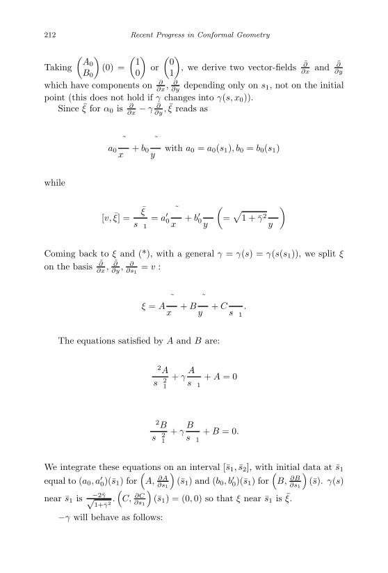
January 17, 2007 11:55 WSPC/Book Trim Size for 9in x 6in finalBB
212 Recent Progress in Conformal Geometry
Taking(
A0
B0
)(0) =
(10
)or(
01
), we derive two vector-fields ∂
∂x and ∂∂y
which have components on ∂∂x , ∂
∂y depending only on s1, not on the initialpoint (this does not hold if γ changes into γ(s, x0)).
Since ξ for α0 is ∂∂x − γ ∂
∂y , ξ reads as
a0∂
∂x+ b0
∂
∂ywith a0 = a0(s1), b0 = b0(s1)
while
[v, ξ] =∂ξ
∂s1= a′
0
∂
∂x+ b′0
∂
∂y
(=√
1 + γ2∂
∂y
)
Coming back to ξ and (*), with a general γ = γ(s) = γ(s(s1)), we split ξ
on the basis ∂∂x , ∂
∂y , ∂∂s1
= v :
ξ = A∂
∂x+ B
∂
∂y+ C
∂
∂s1.
The equations satisfied by A and B are:
∂2A
∂s21
+ γ∂A
∂s1+ A = 0
∂2B
∂s21
+ γ∂B
∂s1+ B = 0.
We integrate these equations on an interval [s1, s2], with initial data at s1
equal to (a0, a′0)(s1) for
(A, ∂A
∂s1
)(s1) and (b0, b
′0)(s1) for
(B, ∂B
∂s1
)(s). γ(s)
near s1 is −2γ√1+γ2
.(C, ∂C
∂s1
)(s1) = (0, 0) so that ξ near s1 is ξ.
−γ will behave as follows:
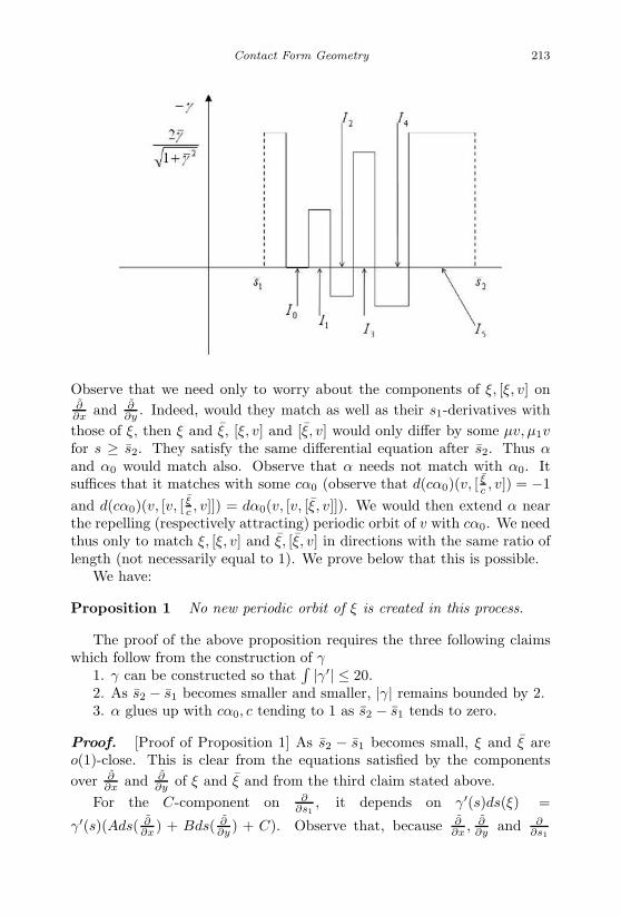
January 17, 2007 11:55 WSPC/Book Trim Size for 9in x 6in finalBB
Contact Form Geometry 213
Observe that we need only to worry about the components of ξ, [ξ, v] on∂∂x and ∂
∂y . Indeed, would they match as well as their s1-derivatives withthose of ξ, then ξ and ξ, [ξ, v] and [ξ, v] would only differ by some µv, µ1vfor s ≥ s2. They satisfy the same differential equation after s2. Thus αand α0 would match also. Observe that α needs not match with α0. Itsuffices that it matches with some cα0 (observe that d(cα0)(v, [ ξ
c , v]) = −1and d(cα0)(v, [v, [ ξ
c , v]]) = dα0(v, [v, [ξ, v]]). We would then extend α nearthe repelling (respectively attracting) periodic orbit of v with cα0. We needthus only to match ξ, [ξ, v] and ξ, [ξ, v] in directions with the same ratio oflength (not necessarily equal to 1). We prove below that this is possible.
We have:
Proposition 1 No new periodic orbit of ξ is created in this process.
The proof of the above proposition requires the three following claimswhich follow from the construction of γ
1. γ can be constructed so that∫ |γ′| ≤ 20.
2. As s2 − s1 becomes smaller and smaller, |γ| remains bounded by 2.3. α glues up with cα0, c tending to 1 as s2 − s1 tends to zero.
Proof. [Proof of Proposition 1] As s2 − s1 becomes small, ξ and ξ areo(1)-close. This is clear from the equations satisfied by the componentsover ∂
∂x and ∂∂y of ξ and ξ and from the third claim stated above.
For the C-component on ∂∂s1
, it depends on γ′(s)ds(ξ) =
γ′(s)(Ads( ∂∂x ) + Bds( ∂
∂y ) + C). Observe that, because ∂∂x , ∂
∂y and ∂∂s1

January 17, 2007 11:55 WSPC/Book Trim Size for 9in x 6in finalBB
214 Recent Progress in Conformal Geometry
commute, ds( ∂∂y ) and ds( ∂
∂y ) are independent of s1. They are boundeduniformly. So are A and B.
Since∫ |γ′| is bounded by 20, then∫ s1
s1
∫ τ
s1
|γ′| ≤ 20
s∑j=0
|Ij | = o(1).
After some work, this implies that the v-components of ξ and ξ are closeup to o(1). Indeed, C (the v-component of ξ) satisfies:
∂2C
∂s21
+ C + γ∂C
∂s1= γ′(s)ds(ξ) = γ′(s)
(Ads
(∂
∂x
)+ Bds
(∂
∂y
)+ C
)while C, the v-component of ξ satisfies
∂2C
∂s21
+ C + γ∂C
∂s1= 0
with C(s1) = C(s1), ∂C∂s1
(s1) = ∂C∂s1
(s1). The claim follows.
2.2.3 How γ is built
We start with the differential equation with a constant γ0
∂2u
∂s21
+ γ0∂u
∂s1+ u = 0.
We set it in a matricial form with v = −∂u∂s .
Then,
∂
∂s
(uv
)=(
0 −11 −γ0
)(uv
).
We claim that:
Lemma 2 Consider with |γ0| < 2,
et
0 −11 −γ0
.
For t small, it reads up to a multiplicative factor as
1cosϕ
(cos(βt + ϕ) − sin(βt)
sin(βt) cos(βt − ϕ)
)

January 17, 2007 11:55 WSPC/Book Trim Size for 9in x 6in finalBB
Contact Form Geometry 215
with |β| < 1, β = cosϕ.
Proof. Since γ0 is small (|γ0| < 2),(
0 −11 −γ0
)reduces to a matrix of ro-
tation(
α −ββ α
)with α2 + β2 = 1.
(0 −11 −γ0
)= Q−1
(α −ββ α
)Q
with
Q =(
1 α0 β
), Q−1 =
1β
(β −α0 1
), 2α = −γ0.
Then,
et
0 −11 −γ0
= Q−1e
t
α −ββ α
Q = etαQ−1e
t
0 −ββ 0
Q
= etαQ−1
(cosβt − sinβtsinβt cosβt
)Q
=etα
β
(β −α0 1
)(cosβt α cosβt − β sin βtsin βt α sin βt + β cosβt
)=
etα
β
(β cosβt − α sin βt − sin βt
sin βt α sinβt + β cosβt
).
Set β = cosϕ, α = sin ϕ. We find:
et
0 −11 −γ0
=
etα
β
(cos(βt + ϕ) − sinβt
sinβt cos(βt − ϕ)
).
Observe that the multiplicative factor tends to 1 as γ0 tends to zero. Let now A be an arbitrary 2 by 2 matrix close to
(1 00 1
)which reads
A =(
a −c2
c2 b
),
has complex eigenvalues and determinant equal to 1.
Lemma 3 There exists then β1 = cosϕ1 > 0 such that
January 17, 2007 11:55 WSPC/Book Trim Size for 9in x 6in finalBB
216 Recent Progress in Conformal Geometry
A =1
cosϕ1
(cos(β1t1 + ϕ1) − sinβ1t1
sin β1t1 cos(β1t1 − ϕ1)
)= e−t1 sin ϕ1e
t1
0 −11 2 sin ϕ1
.
Proof. We identify
a cosϕ1 = cos(β1t1 + ϕ1) b cosϕ1 = cos(β1t1 − ϕ1).
Thus,
cos(β1t1) =a + b
2
sin(β1t1) =(b − a)2 tanϕ1
.
The first equation can be solved since A has complex eigenvalues and|trA| < 2.
The second equation yields then:
tan ϕ1 =b − a
2√
1 − (a+b)2
4
=b − a√
4 − (a + b)2.
We also have
c2 =sin β1t1cosϕ1
i.e.
c2 cosϕ1 =(b − a) cosϕ1
2 sinϕ1
b − a
2= c2 sin ϕ1.
Since detA = ab + c4 = 1, c2 is equal to√
1 − ab.Thus,
sin ϕ1 =b − a
2√
1 − ab, cos ϕ1 =
√1 − (b − a)2
4(1 − ab)
tan ϕ1 =b − a√
4(1 − ab) − (b − a)2=
b − a√4 − (a + b)2
.
The compatibility follows.
Observation 1. 1 − ab > (b+a)2
4 − ab = (b−a)2
4 .

January 17, 2007 11:55 WSPC/Book Trim Size for 9in x 6in finalBB
Contact Form Geometry 217
Observation 2. β1 = cosϕ1 can tend to zero here. Then since β1t1can be chosen close to zero (cos β1t1 = a+b
2 ), sinβ1t1 is of the order ofβ1t1 = (cosϕ1)t1. Thus,
(cos ϕ1)t1 ∼ b − a
2cosϕ1
sinϕ1.
i.e. t1 ∼ b−a2 sin ϕ1
=√
1 − ab. a and b have both to tend to 1 so that t1 tends
to zero. On the other hand, coming back to et1
0 −11 −γ0
, we have
2α1 = −γ0
and |α1| tends to 1 so that |γ0| is at most 2.
Observation 3. t1 is positive and tends to zero as c2 tends to zero. (Thisfollows readily if β1 does not tend to zero. If β1 tends to zero, the claimfollows from Observation 2).
Next, we prove:
Lemma 4 Let A =(
a −γδ b
), with a + b < 2, ab < 1, a, b close to 1,
0 < δ < γ, ab+γδ = 1, δ(γ− δ) small enough. Then, there exists a, b, c witha + b < 2, a, b close to 1, ab < 1, ab + c4 = 1 and α, β, β1, α < 1, α close to1, α2 + β2β2
1 = 1 such that(a −γδ b
)=(
a −c2
c2 b
)(α −β2
1
β2 α
).
Proof. We have
a = aα − c2β2 b = bα − c2β21
α2 + β2β21 = 1
δ = c2α + bβ2 γ = aβ21 + c2α
.
We may replace the condition δ = c2α + bβ2 with ab + c4 = 1.We then have
b = b+c2β21
α , aβ21 = γ − c2α
α2 + β2β21 = 1
a = aα − c2 (1−α2)β21
ab + c4 = 1
which rereads
January 17, 2007 11:55 WSPC/Book Trim Size for 9in x 6in finalBB
218 Recent Progress in Conformal Geometry
β21 =
α(γ − c2α) − c2(1 − α2)a
=αγ − c2
a
b =b + c2β2
1
α
a =a(γ − c2α)αγ − c2
α2 + β2β21 = 1
(b + c2β21)(γ − c2α) = αβ2
1(1 − c4).
The last equation yields
β21(α − γc2) = b(γ − c2α). (***)
Combining this equation with the first equation, we find
(α − γc2)(αγ − c2) = ab(γ − c2α). (****)
This equation ties α and c.If we can solve (****) with c small, α close to 1(α2 < 1), then (***)
gives us β21 > 0 (provided c2 < γ). We can then find a and b. As α tends
to 1, with γ − c2 bounded away from zero, aa tends to 1. If γc2 is small
enough, b will be very close to b. β can be computed from
β2 =1 − α2
β21
(****) rereads
γc4 − c2(αγ2 + α − abα) + γ(α2 − ab) = 0 i.e.
c4 − c2α(γ + δ) + (α2 − 1 + γδ) = 0.
The discriminant is
(αγ2 + α − abα)2 − 4γ2(α2 − ab) ≥ α2((γ2 + 1 − ab)2 − 4γ2(1 − ab)).
Observe that
(γ2+1−ab)2−4γ2(1−ab) = (γ2+γδ)2−4γ2·γδ = (γ2−γδ)2 = γ2(γ−δ)2 > 0.
Hence (****) has two positive roots as |α| tends to 1(ab < 1). For α = 1,the equation becomes
c4 − c2(γ + δ) + δγ = 0.
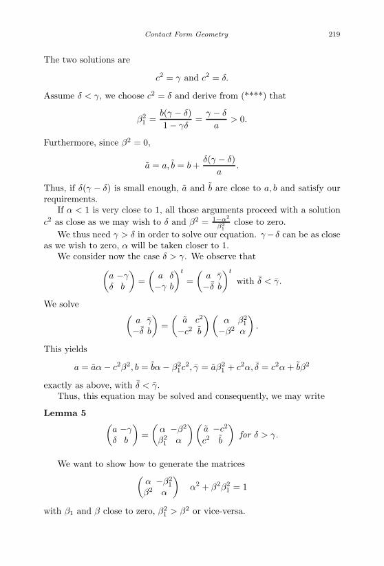
January 17, 2007 11:55 WSPC/Book Trim Size for 9in x 6in finalBB
Contact Form Geometry 219
The two solutions are
c2 = γ and c2 = δ.
Assume δ < γ, we choose c2 = δ and derive from (****) that
β21 =
b(γ − δ)1 − γδ
=γ − δ
a> 0.
Furthermore, since β2 = 0,
a = a, b = b +δ(γ − δ)
a.
Thus, if δ(γ − δ) is small enough, a and b are close to a, b and satisfy ourrequirements.
If α < 1 is very close to 1, all those arguments proceed with a solutionc2 as close as we may wish to δ and β2 = 1−α2
β21
close to zero.We thus need γ > δ in order to solve our equation. γ− δ can be as close
as we wish to zero, α will be taken closer to 1.We consider now the case δ > γ. We observe that(
a −γδ b
)=(
a δ−γ b
)t
=(
a γ−δ b
)t
with δ < γ.
We solve (a γ−δ b
)=(
a c2
−c2 b
)(α β2
1
−β2 α
).
This yields
a = aα − c2β2, b = bα − β21c2, γ = aβ2
1 + c2α, δ = c2α + bβ2
exactly as above, with δ < γ.Thus, this equation may be solved and consequently, we may write
Lemma 5 (a −γδ b
)=(
α −β2
β21 α
)(a −c2
c2 b
)for δ > γ.
We want to show how to generate the matrices(α −β2
1
β2 α
)α2 + β2β2
1 = 1
with β1 and β close to zero, β21 > β2 or vice-versa.

January 17, 2007 11:55 WSPC/Book Trim Size for 9in x 6in finalBB
220 Recent Progress in Conformal Geometry
We compute the product of two matrices A, A1
A =(
a −√1 − ab√
1 − ab b
)and A1 =
(a1 −√
1 − a1b1√1 − a1b1 b1
).
We find
AA1 =(
aa1 −√
1 − ab√
1 − a1b1 −a√
1 − a1b1 − b1
√1 − ab
a1
√1 − ab + b
√1 − a1b1 bb1 −
√1 − ab
√1 − a1b1
).
If a = b1 and b = a1, we find
AA1 =(
2ab− 1 −2a√
1 − ab
2b√
1 − ab 2ab − 1
).
Clearly if aa1 = bb1 then
AA1 =(
α −β21
β2 α
)with α2 + β2β2
1 = 1.Furthermore, if a is close to b1 and b is close to a1, then α is close to
2ab− 1, which is close to 1 if ab is close to 1. We thus need to worry about
β21 > β2 or β2 > β2
1 .
We then observe that, since aa1 = bb1,
β21 = a
√1 − a1b1 + b1
√1 − ab = a
√1 − a1b1 +
aa1
b
√1 − ab
=a
b
(a1
√1 − ab + b
√1 − a1b1
)=
a
bβ2.
Taking a > b or b > a, we achieve the two occurrences.Consider now a matrix
A =(
a −c2
c2 b
)with ab + c4 = 1
0 < a + b < 2.
a, b close to 1, fixed.Consider a small angle t2 > 0 and the product
At2 =(
a −c2
c2 b
)(cos t2 sin t2− sin t2 cos t2
)=(
a cos t2 + c2 sin t2 a sin t2 − c2 cos t2c2 cos t2 − b sin t2 b cos t2 + c2 sin t2
).
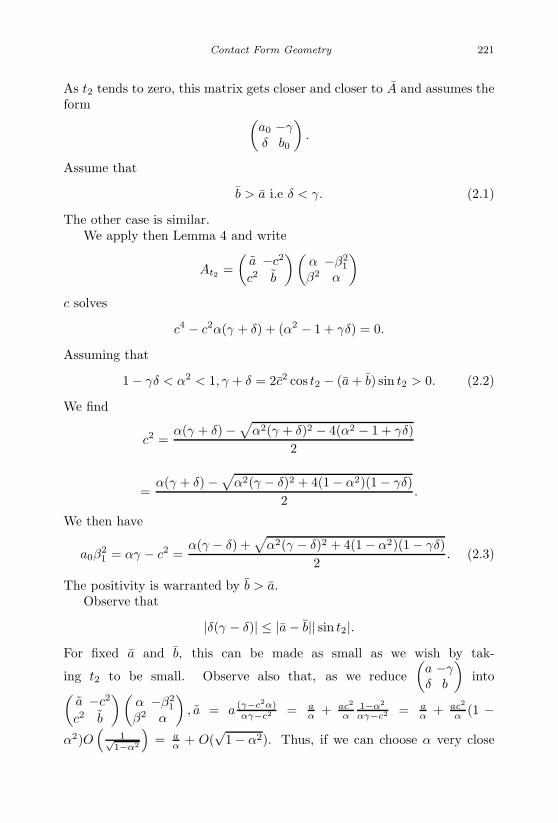
January 17, 2007 11:55 WSPC/Book Trim Size for 9in x 6in finalBB
Contact Form Geometry 221
As t2 tends to zero, this matrix gets closer and closer to A and assumes theform (
a0 −γδ b0
).
Assume that
b > a i.e δ < γ. (2.1)
The other case is similar.We apply then Lemma 4 and write
At2 =(
a −c2
c2 b
)(α −β2
1
β2 α
)c solves
c4 − c2α(γ + δ) + (α2 − 1 + γδ) = 0.
Assuming that
1 − γδ < α2 < 1, γ + δ = 2c2 cos t2 − (a + b) sin t2 > 0. (2.2)
We find
c2 =α(γ + δ) −√α2(γ + δ)2 − 4(α2 − 1 + γδ)
2
=α(γ + δ) −√α2(γ − δ)2 + 4(1 − α2)(1 − γδ)
2.
We then have
a0β21 = αγ − c2 =
α(γ − δ) +√
α2(γ − δ)2 + 4(1 − α2)(1 − γδ)2
. (2.3)
The positivity is warranted by b > a.Observe that
|δ(γ − δ)| ≤ |a − b|| sin t2|.For fixed a and b, this can be made as small as we wish by tak-
ing t2 to be small. Observe also that, as we reduce(
a −γδ b
)into(
a −c2
c2 b
)(α −β2
1
β2 α
), a = a (γ−c2α)
αγ−c2 = aα + ac2
α1−α2
αγ−c2 = aα + ac2
α (1 −
α2)O(
1√1−α2
)= a
α + O(√
1 − α2). Thus, if we can choose α very close
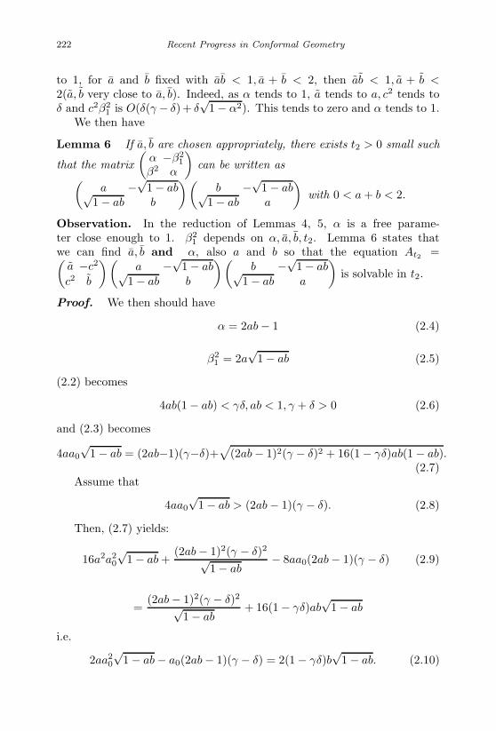
January 17, 2007 11:55 WSPC/Book Trim Size for 9in x 6in finalBB
222 Recent Progress in Conformal Geometry
to 1, for a and b fixed with ab < 1, a + b < 2, then ab < 1, a + b <2(a, b very close to a, b). Indeed, as α tends to 1, a tends to a, c2 tends toδ and c2β2
1 is O(δ(γ − δ)+ δ√
1 − α2). This tends to zero and α tends to 1.We then have
Lemma 6 If a, b are chosen appropriately, there exists t2 > 0 small such
that the matrix(
α −β21
β2 α
)can be written as(
a −√1 − ab√
1 − ab b
)(b −√
1 − ab√1 − ab a
)with 0 < a + b < 2.
Observation. In the reduction of Lemmas 4, 5, α is a free parame-ter close enough to 1. β2
1 depends on α, a, b, t2. Lemma 6 states thatwe can find a, b and α, also a and b so that the equation At2 =(
a −c2
c2 b
)(a −√
1 − ab√1 − ab b
)(b −√
1 − ab√1 − ab a
)is solvable in t2.
Proof. We then should have
α = 2ab − 1 (2.4)
β21 = 2a
√1 − ab (2.5)
(2.2) becomes
4ab(1 − ab) < γδ, ab < 1, γ + δ > 0 (2.6)
and (2.3) becomes
4aa0
√1 − ab = (2ab−1)(γ−δ)+
√(2ab − 1)2(γ − δ)2 + 16(1 − γδ)ab(1 − ab).
(2.7)Assume that
4aa0
√1 − ab > (2ab − 1)(γ − δ). (2.8)
Then, (2.7) yields:
16a2a20
√1 − ab +
(2ab − 1)2(γ − δ)2√1 − ab
− 8aa0(2ab − 1)(γ − δ) (2.9)
=(2ab − 1)2(γ − δ)2√
1 − ab+ 16(1 − γδ)ab
√1 − ab
i.e.
2aa20
√1 − ab − a0(2ab − 1)(γ − δ) = 2(1 − γδ)b
√1 − ab. (2.10)

January 17, 2007 11:55 WSPC/Book Trim Size for 9in x 6in finalBB
Contact Form Geometry 223
Thus,
2√
1 − ab(aa20 − b(1 − γδ)) = a0(2ab − 1)(γ − δ). (2.11)
Observe that
a0 = a cos t2 + c2 sin t2, γ = c2 cos t2 − a sin t2, δ = c2 cos t2 − b sin t2 (2.12)
t2 should be positive and small.Replacing in (2.11) and using ab = 1 − c4, we derive
2√
1 − aba(aa − bb) = (a cos t2 + c2 sin t2)(2ab − 1)(b − a) sin t2 (2.13)
+ 2 sin t2√
1 − ab(sin t2(c4(b − a) + a(aa − bb))
+ cos t2c2(a(b − a) + bb − aa)
).
Observe that
b − a =a
b(a − b) +
bb − aa
b. (2.14)
Thus,
2√
1 − aba(aa − bb) = (b − a) sin t2((a cos t2 + c2 sin t2)(2ab − 1) (2.15)
−2a
b
√1 − abc4 sin t2 − 2
aa
b
√1 − abc2 cos t2
)+ 2(aa − bb)
√1 − ab × sin t2
×(
a sin t2 − sin t2c4
b− cos t2c
2( a
b+ 1
)).
Assume now that
b > a, aa > bb, aa − bb = O((b − a)2). (2.16)
ab < 1, a + b < 2, a, b close to 1. (2.17)
Since 1 — ab is small and 2ab — 1 is close to 1 while aa− bb > 0, aa− bb =O((b−a)2), we can solve (2.15) by implicit function theorem and find t2 > 0small. Indeed (2.15) rewrites under (2.16):
2√
1 − aba(aa − bb)
b − a= sin t2(a(2ab − 1) + o(1)). (2.18)
We need therefore to fulfill (2.16) and (2.17), also (2.8).

January 17, 2007 11:55 WSPC/Book Trim Size for 9in x 6in finalBB
224 Recent Progress in Conformal Geometry
Consider
1 > b > a. (2.19)
Let c be such that c4 = 1 − ab.Take
a =bb
a+ ε, ε > 0 tending to zero , b < 1. (2.20)
For ε small enough, if ba is close enough to 1 (in function of b)
ab =b2b
a+ εb < 1. (2.21)
Also
a + b =bb
a+ ε + b = b
(b
a+ 1
)+ ε < 2. (2.22)
We then need
aa − bb = O((b − a)2) (2.23)
i.e.
ε = O((b − a)2) = O((b
a− 1)2)
and this is easy to satisfy.The proximity of a and b to 1 depends only on the proximity of b and
ba to 1.
Finally, we need (2.6) i.e.
4ab(1 − ab) < (c2 cos t2 − a sin t2)(c2 cos t2 − b sin t2) (2.24)
2c2 cos t2 − (b + a) sin t2 > 0 (2.25)
(2.25) follows from the fact that t2 is small.For (2.24), we observe that as b
a tends to 1 and 1 − ab to zero, ab canbe kept away from 1 so that c2 is far from zero and t2 tends to zero. (2.24)follows.
We also assumed (2.8) i.e.
(2ab − 1)(b − a) sin t2 < 4a(a cos t2 + c2 sin t2)√
1 − ab. (2.25′)
Using (2.18), this rereads:
2√
1 − ab (aa − bb)(1 + o(1)) < 4aa√
1 − ab(1 + o(1)) (2.26)

January 17, 2007 11:55 WSPC/Book Trim Size for 9in x 6in finalBB
Contact Form Geometry 225
which follows readily.
We now build γ:We pick up a small interval J and we consider the v-transport over J
which is given in Span(
∂∂x , ∂
∂y
)by
e
t
0 −11 −2γ√
1+γ2
.
Assume −γ > 0 for example; γ will be assumed — there is, after a simpleargument, no restriction in this assumption — to be as small as we please.Use Lemma 2 to read this matrix up to a multiplicative factor under theform (
a −c2
c2 b
)with a + b < 2, a, b close to 1, ab + c4 = 1.
Choose β = cosϕ > 0. Since −γ > 0, α = sinϕ is positive and since t issmall,
b =cos(βt − ϕ)
cosϕ>
cos(βt + ϕ)cosϕ
= a.
Also
ab =1
cos2 ϕ(cos2 βt cos2 ϕ − sin2 βt sin2 ϕ) < 1 (2.27)
b
atends to 1 as γ tends to zero since sin ϕ =
|γ|2
.
Pick up b < 1. Set a = bba +
(ba − 1
)3
. Adjust |γ| so small that ba − 1 is as
small as we please with b, a away from 1 (t is given, small, positive). a, b, absatisfy (2.16) and (2.17). (2.6) and (2.8) follow if t2 is small positive, see(2.24), (2.25), (2.25′), (2.26).
Using Lemma 6, we rewrite(a −c2
c2 b
)=(
a −c2
c2 b
)(a −√
1 − ab√1 − ab b
)(b −√
1 − ab√1 − ab a
)(cos t2 − sin t2sin t2 cos t2
)with t2 positive small, 0 < a + b < 2, 0 < a + b < 2, ab < 1, ab < 1.

January 17, 2007 11:55 WSPC/Book Trim Size for 9in x 6in finalBB
226 Recent Progress in Conformal Geometry
Using then Lemma 3, we may write
(a −c2
c2 b
)= θe
t5
0 −11 2 sinϕ1
e
t4
0 −11 2 sinϕ2
e
t3
0 −11 2 sinϕ3
e
t2
0 −11 0
with θ, t2, t3, t4, t5 > 0.All multiplicative factors tend to 1 as t1 tends to zero.
∫ |γ′| is clearlybounded.
2.2.4 Modification of α into αN
We focus on the interval I0 and we pick up ε > 0 and N large, withε = o
(|I0|N
). We pick up a real
|I0|2π(N + 1)
< θN <|I0|2πN
in a way which will become clear in a moment.We build a fucntion on I0 as follows:
θN is chosen so that∫ s4
s3
ds1(s1) = 2πN + |I0|.

January 17, 2007 11:55 WSPC/Book Trim Size for 9in x 6in finalBB
Contact Form Geometry 227
Setting
s2 =∫ s1
s3
dτ
(τ)i.e.
ds2 =ds1
(s1),
∂
∂s2= (s1)
∂
∂s1
we consider the differential equation
(s1)∂
∂s1
((s1)
∂
∂s1
)u + u = 0 on I0
which rereads
∂2u
∂s22
+ u = 0 on an interval of length 2πN + |I0|
starting at s3 i.e. on [s3, s4 + 2πN ].Thus, the solutions of
[v, [v, ξ]] = −ξ on I0
and of
[v, [v, ξ]] = −ξ on I0
with the same initial data ξ, [v, ξ] match at s4.
2.2.5 Computation of ξN
We compute ξN .ξN satisfies the differential equation:
[ϕv, [ϕv, ξN ]] = −ξN ϕ = .
We know that ξN (s3) = ξ.We need to compute [−ϕv, ξN ](s3) = [−v, ξN ](s3).
Lemma 7 −[v, ξN ](s3) = −2 (x−γy)(0)√1+γ2(x2+y2)(0)
v +√
1 + γ2 ∂∂y .
Proof. ξ satisfies
[−v, [−v, ξ]] = ξ + γ[ξ, v] − (ξ · γ)v
and γ incurs a jump at s3 from −2γ√1+γ2
= −2γ1 to 0. γ is a function of s,
which is a function of τ , the time along −v. We are here taking s = x2 +y2

January 17, 2007 11:55 WSPC/Book Trim Size for 9in x 6in finalBB
228 Recent Progress in Conformal Geometry
and thinking of γ′ds(ξ) as dγ(ξ). We have
dγ
dτ= +
dγ
ds· ds
dτ
so that
γ′ = +dγ
dτ· dτ
ds=
dγ
dτ× 1
2γ(x2 + y2).
Thus,
(s+3 ) − [−v, ξ](s−3 ) = − 2γ√
1 + γ2× 1
2γ(x2 + y2)ds(ξ)(s3)v
= − 2(x − γy)(0)√1 + γ2(x2 + y2)(0)
· v.
On the other hand
[−v, ξ](s−3 ) =[−20
∂
∂θ+ (y + γx)
∂
∂x− (x − γy)
∂
∂y,
∂
∂x− γ
∂
∂y
]
· 1√1 + γ2
=√
1 + γ2∂
∂y.
Thus, ξN satisfies[−ϕv, [−ϕv, ξN ]] = −ξN
ξN (s3) = ξ
[−ϕv, ξN ](s3) =√
1 + γ2 ∂∂y − 2 (x−γy)(0)√
1+γ2(x2+y2)(0)v.
(2.28)
Let
e1 = 20∂
∂θ, e2 = y
∂
∂x− x
∂
∂y, e3 = ϕv
ϕ is a function of s = x2 + y2. Thus,
ds(e1) = ds(e2) = 0
and
[e1, v] = [e2, v] = [e1, ϕv] = [e2, ϕv] = 0

January 17, 2007 11:55 WSPC/Book Trim Size for 9in x 6in finalBB
Contact Form Geometry 229
since [x
∂
∂x+ y
∂
∂y, y
∂
∂x− x
∂
∂y
]= 0.
Observe that
x∂
∂x+y
∂
∂y= −v − 20 ∂
∂θ + (y ∂∂x − x ∂
∂y )
γ·√
1 + γ2 =e1 − e2 − ϕv
γ
√1 + γ2.
Observe also that
∂
∂x=
x(x ∂∂x + y ∂
∂y ) + y( ∂∂x − x ∂
∂y )
x2 + y2=
x
x2 + y2
√1 + γ2
e1 − e2 − ϕv
γ
+y
x2 + y2e2
∂
∂y=
y
x2 + y2· e1 − e2 − ϕv
γ·√
1 + γ2 − xe2
x2 + y2.
Thus,ξ = ∂
∂x − γ ∂∂y = x−γy
x2+y2
√1 + γ2 (e1−e2−ϕv)
γ + (y+γx)e2x2+y2
[−ϕv, ξN ](s3) =√
1 + γ2 yx2+y2
(e1−e2−ϕv)γ −
√1+γ2xe2
x2+y2 − 2 (x−γy)x2+y2
ϕv√1+γ2
.
Here, x, y are taken at s3 and we will label them x(0), y(0).We solve then (2.28). We derive:
Proposition 2 Let s2 be the time parameter along −ϕv
ξN =
((x − γy)(0)(x2 + y2)(0)
1√1 + γ2
(e1 − e2 − ϕv
γ
)+
(y + γx)(0)(x2 + y2)(0)
e2
)cos2
+
(√1 + γ2
y(0)(x2 + y2)(0)
e1 − e2 − ϕv
γ−√
1 + γ2x(0)e2
(x2 + y2)(0)
− 2(x − γy)(0)(x2 + y2)(0)
ϕv√1 + γ2
)sin s2.
Corollary 2 Given a fixed connection on M , ξN · ξN , ξN · [ϕv, ξN ],[ϕv, ξN ]·ξN and [ϕv, ξN ]·[ϕv, ξN ] are bounded independently on M transver-sally to v.
Proof. Observe that ds2(ϕv) = −1 and ds2(e1) = ds2(e2) = 0. Theonly unbounded terms could come from a derivative taken on ϕ. But ϕ ismultiplied by v. Hence the claim.

January 17, 2007 11:55 WSPC/Book Trim Size for 9in x 6in finalBB
230 Recent Progress in Conformal Geometry
Observe that
[ϕv, e1] = [ϕv, e2] = 0.
Thus, denoting γs2 the one-parameter group of −ϕv
Dγs2(e1) = e1 Dγs2(e2) = e2
(x, y, θ)(s2) is derived from (x, y, θ)(0) through the use of γs2 .We can use this fact and reread the differential equation
˙(x, y, θ) = ξN (x, y, θ).
Indeed, we then have
Dγs2
( ˙(x, y, θ)(0))− s2ϕv = Aϕv
+ cos2
((x − γy)(0)(x2 + y2)(0)
× 1√1 + γ2
Dγs2
(e1 − e2
γ
)+
(y + γx)(0)(x2 + y2)(0)
Dγs2(e2)
)
+
(√1 + γ2
y
x2 + y2(0)Dγs2
(e1 − e2
γ
)−√
1 + γ2x(0)(x2 + y2)(0)
Dγs2(e2)
)sin s2.
Set
x(0) = ρ cosψ
y(0) = ρ sinψ.
Then,
e2 = y(0)∂
∂x− x(0)
∂
∂y= −ρ
∂
∂ψ.
and
˙(x, y, θ)(0) =cos s2
ρ
(cosψ − γ sin ψ
γ√
1 + γ2
(20
∂
∂θ+ ρ
∂
∂ψ
)− (sin ψ + γ cosψ)ρ
∂
∂ψ
)
+sin s2
ρ
(√1 + γ2
sin ψ
γ
(20
∂
∂θ+ ρ
∂
∂ψ
)+√
1 + γ2 cosψρ∂
∂ψ
).
Observe now that
˙(x, y, θ)(0) = θ∂
∂θ+ ρψ
∂
∂ψ

January 17, 2007 11:55 WSPC/Book Trim Size for 9in x 6in finalBB
Contact Form Geometry 231
since ρ2 = (x2 + y2)(0) is a constant.We thus derive:
Proposition 3 The differential equation ˙(x, y, θ) = ξN (x, y, θ) rereads
ρψ = cos s2
(cosψ − γ sin ψ
γ√
1 + γ2− (sin ψ + γ cosψ)
)
+ sin s2
(√1 + γ2
sin ψ
γ+√
1 + γ2 cosψ
)ρθ = 20
(cos s2 · cosψ − γ sin ψ
γ√
1 + γ2+
sin s2
√1 + γ2 sin ψ
γ
)
ρs2 = cos s2
(cosψ − γ sin ψ
γ√
1 + γ2
)+
(√1 + γ2
sin ψ
γ+ 2
cosψ − γ sinψ√1 + γ2
)sin s2.
If we set ∂∂τ = ργ ∂
∂t , this becomes
∂ψ
∂τ= cos s2
(cosψ − γ sin ψ√
1 + γ2− γ(sin ψ + γ cosψ)
)+ sin s2
(√1 + γ2 sin ψ + γ
√1 + γ2 cosψ
)∂θ
∂τ= 20
(cos s2
cosψ − γ sin ψ√1 + γ2
+√
1 + γ2 sin s2 sin ψ
)∂s2
∂τ=
cosψ − γ sin ψ√1 + γ2
cos s2 +
(√1 + γ2 sin ψ + 2γ
(cos ψ − γ sinψ)√1 + γ2
)sin s2.
The first and the last equation define an autonomous differential equation.We conjecture that, generically on γ, this differential equation will have atmost a countable number of nondegenerate periodic orbits.
In order to have periodic orbits in (ψ, θ, s1), we need the additionalcondition2kπ = 20
∫ T
0
(cos s2
cos ψ−γ sin ψ√1+γ2
+√
1 + γ2 sin s2 sinψ
)dτ
k ∈ Z
.
We conjecture that, generically on γ, this condition is not satisfied, hencethat there are no periodic orbits in (ψ, θ, s2).
We cannot rule out other periodic orbits which would be partly madeof orbits of ξN continued by orbits of ξ.
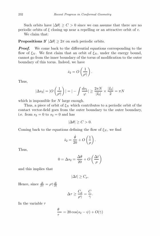
January 17, 2007 11:55 WSPC/Book Trim Size for 9in x 6in finalBB
232 Recent Progress in Conformal Geometry
Such orbits have |∆θ| ≥ C > 0 since we can assume that there are noperiodic orbits of ξ closing up near a repelling or an attractive orbit of v.
We claim that:
Propositions 3′ |∆θ| ≥ 2π on such periodic orbits.
Proof. We come back to the differential equations corresponding to theflow of ξN . We first claim that an orbit of ξN , under the energy bound,cannot go from the inner boundary of the torus of modification to the outerboundary of this torus. Indeed, we have
s2 = O
(1ργ
).
Thus,
|∆s2| = |O(
1ργ
)| = | −
∫ds1
ϕ| ≥ 2πN
|I0| × |I0|2
= πN
which is impossible for N large enough.Thus, a piece of orbit of ξN which contributes to a periodic orbit of the
contact vector-field goes from the outer boundary to the outer boundary,i.e. from s2 = 0 to s2 = 0 and has
|∆θ| ≥ C > 0.
Coming back to the equations defining the flow of ξN , we find
s2 =θ
20+ O
(1ρ
).
Thus,
0 = ∆s2 =∆θ
20+ O
(∆t
ρ
)and this implies that
|∆t| ≥ Cρ.
Hence, since ∂∂τ = ργ ∂
∂t
∆τ ≥ Cρ
ργ=
C
γ.
In the variable τ
∂θ
∂τ= 20 cos(s2 − ψ) + O(γ)

January 17, 2007 11:55 WSPC/Book Trim Size for 9in x 6in finalBB
Contact Form Geometry 233
∂
∂τ(s2 − ψ) = γ sin(ψ + s2) + O(γ2).
We start at s2 = 0 and we have an interval of time at least equal to Cγ
ahead of us. Either | cos(s2 −ψ)| or | sin(ψ + s2)| is therefore larger than 12
as we start.Assume first that | cos(s2 − ψ)| ≥ 1
2 as we start. Since ∂∂τ (s2 − ψ) =
O(γ), | cos(s2 − ψ)| will remain larger than 14 for a time interval I of length
larger than c1γ .
Thus, taking I of length c1/γ,
|∆θ| = 2θ∣∣ ∫
I
cos(s2 − ψ) + O(γ)|I|∣∣ ≥ c1
4γ− C
and the conclusion follows.The argument extends to the case where, at any time τ ,
| cos(s2 − ψ)| ≥ c > 0
with c any prescribed positive constant (γ small in relation to c).Thus, we may assume that
| cos(s2 − ψ)| ≤ c small
on the entire piece of ξN -orbit.Then, we have
∂
∂τ
(ψ − θ
20
)= γ sin(s2 − ψ) + O(γ2)
and (ψ − θ
20
)(τ) =
(ψ − θ
20
)(0) ± γτ(1 + 0(1)).
Also
∂
∂τ(s2 − ψ) = γ sin(ψ + s1) + O(γ2)
= γ(sin 2ψ cos(s2 − ψ) + cos 2ψ sin(s2 − ψ)) + O(γ2)= ±γ cos 2ψ + O(γ).
Observe that the constraint | cos(s2 − ψ)| ≤ c forces
|s2 − ψ +(2k + 1)π
2| ≤ c.
January 17, 2007 11:55 WSPC/Book Trim Size for 9in x 6in finalBB
234 Recent Progress in Conformal Geometry
Thus, at the entry and at the exit point,
ψ =(2k + 1)π
2± c
and
x = ρ cos(
(2k + 1)π2
± c
)y = ρ sin
((2k + 1)π
2± c
).
After integration, we derive∫I
∂
∂τ(s2 − ψ) = ±γ
∫I
cos 2ψ + o(γ)|I|.
Since ∆(s2 − ψ) = o(1), we must have∫I
cos 2ψ = o(|I|)
for any I such that
|I| ≥ c
γ.
Otherwise, there will be an I, with |I| ≥ Cγ , such that∣∣∣∣± γ
∫I
cos 2ψ + o(γ)|I|∣∣∣∣ ≥ c1γ|I| ≥ c1C
yielding a contradiction.Hence, on any such interval I, there exists an integer q and a certain
time τ1 if I such that
2ψ +(2q + 1)π
2= o(1).
Thus,
ψ +(2q + 1)π
4= o(1).
Comparing, we derive that
|ψ(0) − ψ(τ1)| ≥ π
4(1 + o(1)).
January 17, 2007 11:55 WSPC/Book Trim Size for 9in x 6in finalBB
Contact Form Geometry 235
Thus,
| θ
20(τ1) − θ
20(0) ± γτ1(1 + o(1)| ≥ π
4(1 + o(1)).
If τ is the entire time spent on this ξN -piece of orbit, either
|γτ | ≥ π
8(1 + o(1))
which forces
|θ(τ) − θ(0)| ≥ 20 · π
8(1 + o(1)) ≥ 2π
since
ψ(τ) − ψ(0) = o(1).
Or
|γτ | ≤ π
8(1 + o(1)).
Thus,
|γτ1| ≤ π
8(1 + o(1)).
Thus,
|θ(τ1) − θ(0)| ≥ 20π
8(1 + o(1)) ≥ 2π again.
2.2.6 Conformal deformation
Let λ be a positive function on M . We consider the contact form λαN
where αN is α modified by the construction of this large rotation.We assume that
dαN (vN , [ξ, vN ]) = −1 with vN = ϕNv
in the region of M where we will carry out our constructions and compu-tations. For simplicity and generality, we come back here to the followingnotations
v instead of vN
ξ0 instead of ξN
α0 instead of αN .

January 17, 2007 11:55 WSPC/Book Trim Size for 9in x 6in finalBB
236 Recent Progress in Conformal Geometry
It must though be kept clear to the mind that in the application below —which is our main purpose — v = ϕNv, ξN = ξ0, αN = α0. Later, we willhave vN and v, ξN and ξ0, αN and α0. This is why we want to avoid anyconfusion.
α is λα0 (it will be λαN thereafter).We thus assume that
dα0(v, [ξ0, v]) = −1
in the region of M where we will carry out out constructions and compu-tations.
We start with
Lemma 8 ξ = ξ0λ + dλ(v)
λ2 [ξ0, v] − dλ([ξ0,v])λ2 v.
Proof. We compute
(dλ ∧ α0 + λdα0)(ξ, v) = (dλ ∧ α0)(ξ, v) + λdα0(ξ, v)
= −dλ(v)λ
+dλ(v)
λdα0([ξ0, v], v) = 0
(dλ ∧ α0 + λdα0)(ξ, [ξ0, v]) = (dλ ∧ α0)(ξ, [ξ0, v]) + λdα0(ξ, [ξ0, v])
= −dλ([ξ0, v])λ
− dλ([ξ0, v])λ
dα0(v, [ξ0, v]) = 0.
We now compute
dα(v, [ξ, v]) = λdα0(v, [ξ, v]).
Lemma 9
−γ = dα(v, [ξ, v]) = −λ
(1λ
+(
1λ
)vv
+(
1λ
)v
dα0(v, [[ξ0, v], v]))
.
Proof.
λdα0(v, [ξ, v]) = λdα0
(v,
[ξ0
λ+
dλ(v)λ2
[ξ0, v] − dλ([ξ0, v])λ2
v, v
])
= dα0(v, [ξ0, v]) − λ
(dλ(v)
λ2
)v
dα0(v, [ξ0, v]) +dλ(v)
λdα0(v, [[ξ0, v], v])
= −λ
(1λ
+(
1λ
)vv
+(
1λ
)v
dα0(v, [[ξ0, v], v]))
.
January 17, 2007 11:55 WSPC/Book Trim Size for 9in x 6in finalBB
Contact Form Geometry 237
Corollary 3 Set λt = 1t+ 1−t
λ
. If dα(v, [ξ, v])(x) < 0, then so is
dαt(v, [ξt, v])(x) for αt = λtα0.
Proof.dαt(v, [ξt, v])(x) = −λt
(1−tλ + t +
(1−tλ
)vv
+(
1−tλ
)vdα0(v, [[ξ0, v], v])
)and
the result follows. Assume now that
λ
(1λ
)v
, λ
(1λ
)vv
are o(1).
Recall that
γ(x) = 1 + λ
(1λ
)vv
+ λ
(1λ
)v
dα0(v, [[ξ0, v], v])
and
v =v√γ(x)
so that
dα(v, [ξ, v]) =1
γ(x)dα(v, [ξ, v]) = −1.
We compute in the sequel
˜µ = dα(v, [v, [ξ, v]])˜µξ = d ˜µ(ξ)˜µv = d ˜µ(v)
and also τ , where [ξ, [ξ, v]] = −τ v.
Lemma 10 ˜µ = 1γ(x)3/2 (dα0(v, [v, [ξ0, v]])(
1 + 2λ(
1λ
)vv
+ dλ(v)λ (2 + γ(x)) − λ
(1λ
)vvv
+ λv
λ dα0(v, [v, [[ξ0, v], v]])
.
Proof. Clearly,
˜µ =1
γ(x)3/2dα(v, [v, [ξ, v]]).
We have
dα(v, [v, [ξ, v]]) = (dλ ∧ α0 + λdα0)(v, [v, [ξ, v]]) = dλ(v)α0([v, [ξ, v]])
+ λdα0(v, [v, [ξ, v]]) = γ(x)dλ(v)
λ+ λdα0
(v,
[v,
[ξ0
λ, v
]])

January 17, 2007 11:55 WSPC/Book Trim Size for 9in x 6in finalBB
238 Recent Progress in Conformal Geometry
+ λdα0
(v,
[v,
[dλ(v)
λ2[ξ0, v], v
]])
= γ(x)dλ(v)
λ− λ
(1λ
)v
dα0(v, [v, ξ0]) + λdα0
(v,
[v,
1λ
[ξ0, v]])
+ λdα0
(v,
[v,
[dλ(v)
λ2[ξ0, v], v
]])= dα0(v, [v, [ξ0, v]])−2λ
(1λ
)v
dα0(v, [v, ξ0])
+γ(x)dλ(v)
λ+ λdα0
(v,
[v,
(1λ
)vv
[ξ0, v]])
+λv
λdα0(v, [v, [[ξ0, v], v]])
−λ
(1λ
)vv
dα0(v, [[ξ0, v], v]) = dα0(v, [v, [ξ0, v]])(
1 + 2λ
(1λ
)vv
)−λ
(1λ
)vvv
−2λ
(1λ
)v
+ γ(x)dλ(v)
λ+
λv
λdα0(v, [v, [[ξ0, v], v]]).
Observe that
λ
(dλ(v)
λ2
)v
=λvv
λ− 2
λ2v
λ2
λ
(dλ(v)
λ2
)vv
=λvvv
λ− 5
λvλvv
λ2+ 4
λ3v
λ3.
Next, we compute τ . We know that −τ is the collinearity coefficient of[ξ, [ξ, v]] on v.
We will therefore compute [ξ, [ξ, v]] in the (ξ0, v, [ξ0, v]) basis and we willtrack down the component on v, throwing away the other components.
We have:
Lemma 11 Let ν(x) =√
γ(x). Then,
τ = − 1ν(x)
[dA(ξ0)
λ− Bτ
λ+
dλ(v)λ2
dA([ξ0, v]) − Aµξ0
dλ(v)λ2
− dλ([ξ0, v])λ2
dA(v)
+A
(dλ([ξ0, v])
λ2
)v
− Bdλ([ξ0, v])
λ2µξ0 + B
(dλ([ξ0, v])
λ2
)[ξ0,v]
]with
A = dν(ξ) − µξ0νdλ(v)
λ2+ ν
(dλ([ξ0, v])
λ2
)v
, B = ν
(1λ
+ µdλ(v)
λ2+(
1λ2
)vv
).

January 17, 2007 11:55 WSPC/Book Trim Size for 9in x 6in finalBB
Contact Form Geometry 239
Proof.
[ξ, [ξ, v]] =[ξ0
λ+
λv
λ2[ξ0, v] − dλ([ξ0, v])
λ2v,
[ξ0
λ+
λv
λ2[ξ0, v] − dλ([ξ0, v])
λ2v, v
]]with v = ν(x)v. Observe that
[v, [ξ0, v]] = ξ0 − µ[ξ0, v] + µξ0v.
Indeed,
α0([v, [ξ0, v]]) = 1dα0([v, [ξ0, v]], v) = −µ
dα0([ξ0, v], [v, [ξ0, v]]) = µξ0 = dµ(ξ0).
We then compute
[ξ, v] = dν(ξ)v + ν
(−((
1λ
)v
+λv
λ2
)ξ0 + [ξ0, v]
(1λ
+(
1λ
)vv
+ µλv
λ2
)
+ v
(µξ0
(1λ
)v
+(
dλ([ξ0, v])λ2
)v
))
= v
(dν(ξ) + µξ0
(1λ
)v
+ ν
(dλ([ξ0, v])
λ2
)v
)
+ [ξ0, v]ν(
1λ
+(
1λ
)vv
+ µdλ(v)
λ2
)= Av + B[ξ0, v].
Set [ξ0, [ξ0, v]] = −τv
[ξ, [ξ, v]] =[ξ0
λ+
λv
λ2[ξ0, v] − dλ([ξ0, v])
λ2v, Av + B[ξ0, v]
]
= v
(dA(ξ0)
λ− Bτ
λ+
λv
λ2dA([ξ0, v]) − dλ([ξ0, v])
λ2dA(v) − µξ0A
λv
λ2
+ A
(dλ([ξ0, v])
λ2
)v
+ +B
(dλ([ξ0, v])
λ2
)[ξ0,v]
−Bµξ0
dλ([ξ0, v])λ2
).
Thus,
τ = −1ν
(dA(ξ0)
λ− Bτ
λ+
dλ(v)λ2
dA([ξ0, v])

January 17, 2007 11:55 WSPC/Book Trim Size for 9in x 6in finalBB
240 Recent Progress in Conformal Geometry
−Aµξ0
dλ(v)λ2
− dλ([ξ0, v])λ2
dA(v) + A
(dλ([ξ0, v])
λ2
)v
+B
(dλ([ξ0, v])
λ2
)[ξ0,v]
− Bµξ0
dλ([ξ0, v])λ2
).
Coming back to αN , ξN , vN , we observe that µN is bounded as well asits derivative since µN is identically zero wherever we introduce the large,2πN rotation and µN equals µ0 outside of the set where this modificationoccurs. Similarly, τN is bounded as well as its derivatives independently ofN by construction.
Proposition 4 |µN |+ |dµN |+ |τN | ≤ C, where C does not depend on N .
Next, we show how to build λ so that τ remains bounded and “moun-tains” are built around the hyperbolic orbit. These “mountains” keep thevariations away from this hyperbolic orbit. Since this is a quite surprisingresult, we complete our construction carefully.
2.2.7 Choice of λ
The construction of ξN,λ, αN,λ = λαN involves the definition of the functionλ. We would like to choose this function carefully with respect to v(vN ) sothat λdαN (vN , [ξN,λ, vN ]), ˜µN , ˜µN,v = d ˜µN (vN ), ˜µN,ξN,λ
= d ˜µN (ξN,λ), τN
enjoy appropriate bounds.To avoid unnecessary complicated notations, we again use ξ, α, ξ0, α0
etc. The main issue is that we cannot hope that β = dα(v, ·) is a contactform (with the same orientation than α).
Assuming that v is nonsingular, it is reasonable to first consider the casewhen the ω-limit set of v is made of periodic orbits only. Around “elliptic”(attractive or repelling) periodic orbits, kerα “turns well” (see [Bahri 1988,p. 26]) so that the existence of such a β (with appropriate choices of λ)follows.
Around hyperbolic periodic orbits, kerα “turns well” in most of thecases, except for one case which yields a precise (local) normal form ofα and v (see Appendix 2.3). Then, locally, kerα0 behaves (nearly) as afoliation. There is no hope for such a λ and such a β to exist near suchorbits, with this behavior of α0 and v.
We thus need to keep our homology away from such neighborhoods orto extend it using the ideas of [Bahri-1 2003, Chapter V.1]. These ideascan be pushed and worked out. They still require a certain amount ofwork to become practical. We explore here another direction: we aim at

January 17, 2007 11:55 WSPC/Book Trim Size for 9in x 6in finalBB
Contact Form Geometry 241
keeping the unstable manifolds of the periodic orbits of ξ0 away from suchneighborhoods by creating “mountains” around them. These “mountains”are built by increasing to a high value the Hamiltonian λ around them sothat the curves on the unstable manifolds of the periodic orbits of ξ0 areunable to penetrate them.
We need for this a lot of rotation of kerα around v. This will allow us tokeep control of ˜µ, τ , dα(v, [ξ, v]) and derivatives with respect to v, [ξ0, v]...We cannot get such a rotation from the neighborhood of a “bad” hyperbolicorbit since kerα0 turns very little around v in such a neighborhood. Wehave to seek for it in the neighborhood of attractive or repelling orbits and“bring it back” to our neighborhoods.
For the sake of simplicity, we will assume in a first step that the stableand unstable manifolds of our “bad” hyperbolic orbit θ do not intersect theunstable and stable manifolds of another hyberbolic orbit. We will discussthe case later.
Thus, (H1) the stable (respectively unstable) manifold of O is partof the unstable manifold of the repelling (respectively attracting) periodicorbit.
We will assume — a very natural hypothesis which we will see to holdafter a minor modification of kerα0 and v if needed — that (H2) α0, vhave the normal forms provided in (α0), (v) above near the repelling andattracting orbit.
The construction of the function λ is ultimately quite involved. How-ever, in order to describe a basic step in this direction, we first take thefollowing example. The construction is refined later.
2.2.8 First step in the construction of λ
Let Wu(O) be unstable manifold of O and let ∂V be the boundary of asmall basin for the attractive orbit. ∂V is a section to v. We considerWu(O) ∩ ∂V = Γ and a small neighborhood L of it in ∂V . Let L′ be aneven smaller neighborhood, θ = θ(x0), x0 ∈ L be a C∞- function valued in[0,1], equal to 1 on L′ and to zero outside of L.
We set:
λ(x) = eδθ(x0)s(τ),
for all x of Ws(L) i.e. for all the x′s of the flow-lines of v abutting in L.Such x′s are parametrized by a base point x0 in L and a time τ on the
(reverse) flow-line of v abuting at x0. δ is a small number which we willchoose later.

January 17, 2007 11:55 WSPC/Book Trim Size for 9in x 6in finalBB
242 Recent Progress in Conformal Geometry
More generally,
λ(x) = eδ(∑
θi(xi)si(τi))
where the (xi, τi) are various sets of parameters traking a point x of Mthrough its reference point xi in a section to v and a time τi on the flow-line of v abuting at xi.
Clearly
λv
λ= δ
(∑θi
∂si
∂τi
),λvv
λ= δ
∑θi
∂2si
∂τ2i
+ δ2
(∑θi
∂si
∂τi
)2
λ
(1λ
)vvv
=(
λ
(1λ
)vv
)v
− λv
(1λ
)vv
=(
λ
(1λ
)vv
)v
− λv
λλ
(1λ
)vv
=((
λ
(1λ
)v
)v
− λv
λλ
(1λ
)v
)v
− λv
λλ
(1λ
)vv
= δO
(∑θi
(∣∣∣∣∂3si
∂τ3i
∣∣∣∣+ ∣∣∣∣∂si
∂τi
∣∣∣∣∣∣∣∣∂2si
∂τ2i
∣∣∣∣∣∣∣∣∂2si
∂τ2i
∣∣∣∣+ ∣∣∣∣∂si
∂τi
∣∣∣∣3))
.
(2.29)We assume that ∣∣∣∣∂si
∂τi
∣∣∣∣+ ∣∣∣∣∂2si
∂τ2i
∣∣∣∣+ ∣∣∣∣∂3si
∂τ3i
∣∣∣∣ = O(1). (2.30)
Then,
λv
λ, λ
(1λ
)vv
, λ
(1λ
)vvv
are O(δ).
In this way, γ(x) and ˜µ are under control. We need to worry about d ˜µ andτ . Coming back to the formula of τ in Lemma 11, to A and B as well a theformulae for ν and ξ, we see that these formulae involve derivatives of 1
λ .According to our choice of λ above, λ is larger than or equal to 1, mighttend to +∞. Because we are only considering negative powers of λ andderivatives of such quantities, we do not fear the increase of λ to infinity.
The derivative of δ∑
θi(xi)si(τi) yield more problems because si maybe very large and derivatives of θ may also be very large. Since we wantλ to be very large when θi = 1 and we are at the “end” of the (reverse)flow-lines, we require
δsi(τi) = Log λ
where λ is some large number. The flow-lines are defined on [o, τi]. Thus δcannot tame si(τi).

January 17, 2007 11:55 WSPC/Book Trim Size for 9in x 6in finalBB
Contact Form Geometry 243
We observe that, as we modify α0 into αN and ξ0 in ξN , see Propo-sition 2, µN = dαN (vN , [vN , [ξN , vN ]]) is zero in the domain where themodification takes place.
Also, since in this domain [vN , [vN , ξN ]] = −ξN ,
dαN (vN , [vN , [[ξN , vN ], vN ]]) = −dαN (vN , [vN , ξN ]) = −1.
Thus, in the domain where ξ0 is modified into ξNµN = 0dαN (vN , [vN , [[ξN , vN ], vN ]] = −1γN (x) = 1 + λ
(1λ
)vN vN
˜µN = 1
γ3/2N
(dλ(vN )
λ (2 + γN(x)) − λ(
1λ
)vN vN vN
− λvN
λ
).
(2.31)
We then have:
Proposition 5 Assume si is only a function of τi, the time along vN .Then, there exists C independent of N, δ, λ such that, given N and λ,
| ˜µN | + |d ˜µN (ξN )| + |d ˜µN (vN )| + |d ˜µN ([ξN , vN ])| + |d ˜µN (ξN,λ)|+ d ˜µN ([ξN,λ, vN ]) + |d(d ˜µN (ξN,λ))(ξN,λ)| ≤ C.
Proof. Recall that λ = eδ(∑
θisi).
Either x is in the domain where ξ0 has been modified into ξN .Then, ξN · ξN , ξN · [ξN , vN ], [ξN , vN ] · ξN , [ξN , vN ] · [ξN , vN ] split over
e1, e2 with bounded coefficients, the bounds being C1 and independent ofN .
We do not claim any control on the vN -components of these vectors.˜µN is expressed using λ
(1λ
)vN
, λ(
1λ
)vN vN
and λ(
1λ
)vN vN vN
. Since the θi’shave a zero derivative along vN , all these expressions read as products
δ
(∑θi
∂msi
∂τmi
)m = 1, 2, 3.
By construction dsi(e1) = dsi(e2) = 0 since dτi(e1) = dτi(e2) = 0while dτi(ϕNv) = 1. ξN , vN , [ξN , vN ] split on e1, e2 and ϕNv with boundedcoefficients. Thus dθi(ξN ), dθi(vN ), dθi ([ξN , vN ]) are clearly bounded and| ˜µN | + |d ˜µ(ξN )| + |d ˜µN (vN )| + |d ˜µN ([ξN , vN ]) | is bounded and even 0(δ)in such a region.
For d(d ˜µN (ξN,λ))(ξN,λ) we come back to the expression of ξN,λ
ξN,λ =ξN
λ+
dλ(vN )λ2
[ξN , vN ] − dλ([ξN , vN ])λ2
vN .

January 17, 2007 11:55 WSPC/Book Trim Size for 9in x 6in finalBB
244 Recent Progress in Conformal Geometry
We thus have to take derivatives which are typically expressions such as
δ
λ
(∑θi
∂msi
∂τmi
)ξN
+δdλ(vN )
λ2
(∑θi
∂msi
∂τmi
)[ξN ,vN ]
− δdλ([ξN , vN ])
λ2
(∑θi
∂msi
∂τmi
)vN
and then take again a derivative of such expressions along ξN,λ. On ∂msi
∂τmi
,the e1 and e2 components of each derivative do not give any contribution. Itis only the ϕNv-components which give a contribution. These are boundedand have a bounded derivative along ξN , [ξN , vN ], vN . The problems comeonly after taking a first derivative of θi and then going on with a secondderivative of this expression. Typically, we need to estimate
(dθi(ξN ))ξN, (dθi([ξN , vN ]))ξN
, (dθi([ξN , vN ]))vN,
(dθi([ξN , vN ]))[ξN ,vN ] , (dθi(ξN ))[ξN ,vN ] etc.
We recall now that
ξN · ξN , [ξN , vN ] · [ξN , vN ], ξN · [ξN , vN ], [ξN , vN ] · ξN
are bounded transversally to vN . Furthermore, dθi(vN ) = 0. Thus,
(dθi(ξN ))ξN, (dθi([ξN , vN ]))ξN
etc.
are bounded independently of N .For dθi([ξN , vN ])vN and the like, we observe that
dθi([ξN , vN ])vN = dθi([vN , [ξN , vN ]])
since dθi(vN ) = 0 and the conclusion follows again.Thus,
|d(d ˜µN (ξN,λ)(ξN,λ)| = O(δm+1∑
τmi ) = δO( Logmλ).
We can bound d ˜µN (ξN,λ) in a similar way.For d ˜µN ([ξN,λ, vN ]), we observe that
[ξN,λ, vN ] =[ξN , vN ]
λ+
dλ(vN )λ2
ξN +λvN
λ[[ξN , vN ], vN ]
−(
λvN
λ
)vN
[ξN , vN ] +(
dλ([ξN , vN ])λ2
)vN
vN .
The condition follows again since we have an additional δ coming from theexpression of ˜µN .
January 17, 2007 11:55 WSPC/Book Trim Size for 9in x 6in finalBB
Contact Form Geometry 245
Finally, if x is not in the domain where ξ0 has been modified intoξN , then dα0(v, [v, [ξ0, v]]), dα0(v, [v, [ξ0, v], v]]) are C∞-functions and eventhough ˜µ is not expressed only with the use of λ
(1λ
)v
and other terms of thesame type, ˜µ is a product of these terms with these C∞-functions, whichare independent of N . The above argument extends verbatim.
Before proceeding with the estimate on τ , we make the following fourobservations:
Observation 1. As we take a derivative of si along ξN , [ξN , vN ] or vN
(which we see as split on the basis (e1, e2, vN )), ϕNv = vN is absorbed in∂si
∂τior other derivatives of the same type, but higher order (dθi(v) = 0).
vN gone, we are left with the coefficient of vN which is C1-bounded inde-pendently of N . We can take safely another derivative along ξN , [ξN , vN ]or vN . We will not hit ϕN with a derivative.
Observation 2. Since dθi(v) = 0, vN · dθi(w) = dθi([vN , w]). We maythen take one more derivative along a direction such as ξN , [ξN , vN ]. Weknow that ξN · ξN , ξN · [ξN , vN ], [ξN , vN ] · ξN , [ξN , vN ] · [ξN , vN ] are boundedtransversally to v and that dθi(v) = 0. We get then bounds on such ex-pressions which depend on |θi|C2 and are independent of N .
Observation 3. If we take a derivative of si along vN , ξN or [ξN , vN ], wefree a δ. Furthermore, in all our computations, we never take a vN -deriativeafter taking two derivatives along ξN or [ξN , vN ]. Otherwise, we might endup with terms such as dθi(dϕN (vN ) · (ξN · v)). This never happens.
Observation 4. Thus, if a derivative is taken along vN , either it goes ontosi and frees a δ, or it goes onto dθi(ξN ) or dθi([ξN , vN ]). Since dθi(vN ) = 0,we end up with dθi of a Lie bracket ([vN , ξN ] or [vN , [ξN , vN ]] = ξN ), hencewith an expression of the same type.
Taking more derivatives along vN will not change this pattern. We canthen always take one more derivative along ξN or [ξN , vN ] and use Observa-tion 1 if the expression which we have contains a dθi(ξN ) or dθi([ξN , vN ]);or this expression contains only θi and we can then take two derivativesalong ξN and/or [ξN , vN ]. The result is bounded independently of N .
Using the four observations above, we turn to τ and estimate it, firstlyin the domain where ξ0 has been replaced by ξN .
Then, in Lemma 11, A and B reduce to
A = dν(ξ) + ν
(dλ([ξ0, v])
λ2
)v
B = ν
(1λ
+(
1λ
)vv
)
January 17, 2007 11:55 WSPC/Book Trim Size for 9in x 6in finalBB
246 Recent Progress in Conformal Geometry
and τ reads
τ = − 1ν(x)
[dA(ξ0)
λ− Bτ
λ+
dλ(v)λ
dA([ξ0, v]) − dλ([ξ0, v])λ2
dA(v)
+ A
(dλ([ξ0, v])
λ2
)v
+ B
(dλ([ξ0, v])
λ2
)[ξ0,v]
]ξ0 is in fact ξN and v = vN . Recall that µN is zero. Thus, since µN,ξNξN +τN µN = −dτN (vN ) [Bahri 1998], dτN (v) = 0 and τN is constant on a flow-line of v. They all abut to a point where ϕN = 1 and τN is the original τof α0. Thus, τ in the expression of τ above is τN and is bounded.
dν(ξ) is equal to
1λ
dν(ξ0) +dλ(v)
λ2dν([ξ0, v]) − dλ([ξ0, v])
λ2dν(v).
All of this involves derivatives of λ(
1λ
)vv
along ξ0, [ξ0, v], v. In comput-ing τ , we take one further derivative along ξ0 of dν(ξ).
Taking into account our four observations, we derive that
(dν(ξ))ξ0 = O(δ Logmλ)
since the initial derivative λ(
1λ
)vv
frees a δ. This O depends on dθi, d2θi.
The same estimate holds for the contribution of the ν(
1λ
)vv
part of B.
Also, taking ν-derivatives in ν(
dλ([ξ0,v])λ2
)v
(the second part of A) or in νλ
(this first part of B) yields the same estimate since ν = 1+0(δ). The sameholds true of dλ(v)
λ dA([ξ0, v]).Thus,
τ = O(δ Logmλ + 1)
− 1
λ
((dλ([ξN , vN ])
λ2
)vN
)ξN
+dλ([ξN , vN ])
λ2
(dλ([ξN , vN ])
λ2
)vN vN
−(
dλ([ξN , vN ])λ2
)2
vN
− 1λ
(dλ([ξN , vN ])
λ2
)[ξN ,vN ]
).
As we compute(
dλ([ξN ,vN ])λ2
)vN
or(
dλ([ξN ,vN ])λ2
)vN vN
, all vN− derivatives
have to be taken on dθi([ξN , vN ]). Otherwise, a δ is freed either because vN
has been absorbed in si, yielding ∂si
∂τi= O(1), or because [ξN , vN ] has been
applied to si in the first place, with the same conclusion. Such contributionscan be included into O(δ Logmλ). Observe also that vN cannot be appliedto a simple θi since dθi(vN ) = 0.
January 17, 2007 11:55 WSPC/Book Trim Size for 9in x 6in finalBB
Contact Form Geometry 247
Thus, since dθi(vN ) = 0(dλ([ξN , vN ])
λ2
)vN
=(dλ([ξN , vN ]))vN
λ2+ O(δ Logmλ)
and since vN · dθ([ξN , vN ]) = dθi([vN , [ξN , vN ]]) = dθi(ξN ),(dλ([ξN , vN ])
λ2
)vN
=dλ(ξN )
λ2+ O(δ Logmλ).
(In dλ(ξN ), either the ξN -derivative is taken on θi or, if not, a δ is freed.The additional contribution is thrown into O(δ Logmλ)).
Similarly,(dλ([ξN , vN ])
λ2
)vN vN
=dλ([vN , ξN ])
λ2+ O(δ Logmλ).
Thus,
τ = −(
1λ
(dλ(ξN )
λ2
)ξN
+1λ
(dλ([ξN , vN ])
λ2
)[ξN ,vN ]
−(
dλ(ξN )λ2
)2
−(
dλ([ξN , vN ])λ2
)2)
+ O(δ Logmλ + 1).
Observe now that
− 1λ
(dλ(ξN )
λ2
)ξN
= − 1λ2
(dλ(ξN )
λ
)ξN
+(
dλ(ξN )λ2
)2
− 1λ
(dλ([ξN , vN ])
λ2
)[ξN ,vN ]
= − 1λ2
(dλ([ξN , vN ])
λ
)[ξN ,vN ]
+(
dλ([ξN , vN ]λ2
)2
.
Thus, using the identities above and the form observations stated earlier
τ = O(δ Logmλ + 1) − 1λ2
((dλ(ξN )
λ
)ξN
+(
dλ([ξN , vN ])λ
)[ξN ,vN ]
)= O(δ Logmλ + 1) − e−2δ
∑θisi
∑i
δsi
(∑(dθi([ξN , vN ]))[ξN ,vN ]
+ (dθi(ξN ))ξN
).
Let π be the pull back map from x towards the torus T2 − T1 (outsideT1, inside of T2) where the modification takes place (the introduction of the
January 17, 2007 11:55 WSPC/Book Trim Size for 9in x 6in finalBB
248 Recent Progress in Conformal Geometry
large rotation) onto ∂T2 · θi is in fact defined on ∂T2 and should be thoughtof as θi π. Thus,
τ = O(δ Logmλ + 1) − e−2δ∑
θisi
∑i
δsi ([ξN , vN ] · (dθi dπ)([ξN , vN ])
+ ξN · (dθi dπ)(ξN )) .
We then split
[ξN , vN ] = dπ([ξN , vN ]) + αNvN
ξN = dπ(ξN ) + βNvN
αN and βN are easily seen to be bounded and independent of N .Thus, since dθi dπ(vN ) = 0,
αNvN · dθi dπ([ξN , vN ]) = αNdθi dπ([vN , [ξN , vN ]]) = αNdθi dπ(ξN )βNvN · dθi dπ(ξN ) = βNdθi dπ([vN , ξN ])
and
τ = O(δ Logmλ + 1) − e2δ∑
θisi
∑i
δsi (dπ([ξN , vN ])· dθi dπ([ξN , vN ])
+ dπ(ξN ) · dθi dπ(ξN ) + O(|dθi dπ|) )
= O(δ Logmλ + 1) − e−2δ∑
θisi
∑δsi
(d2θi (dπ([ξN , vN ]), dπ([ξN , vN ]))
+ d2θ (dπ(ξN ), dπ(ξN )) + dθi (dπ([ξN , vN ]) · dπ([ξN , vN ])
+ dπ(ξN ) · dπ(ξN )) + O(|dθi dπ|) ) .
It is easy to see that dπ([ξN , vN ]) · dπ([ξN , vN ]) and dπ(ξN ) · dπ(ξN ) arebounded independently of N so that
τ = O(δ Logmλ + 1) − e−2δ∑
θisi
∑i
δsi
(d2θi (dπ([ξN , vN ]), dπ([ξN , vN ]))
+ d2θi(dπ(ξN , dπ(ξN ))) + O(|dθi dπ|) ) .
From the formula for ξN , see Proposition 2, it is clear that dπ([ξN , vN ])and dπ(ξN ) have bounded lengths and lengths bounded away from zero

January 17, 2007 11:55 WSPC/Book Trim Size for 9in x 6in finalBB
Contact Form Geometry 249
and their determinant is bounded away from zero (γ is small). Indeed
(x2 + y2)(0)γdπ(ξN ) =((x − γy)(0)√
1 + γ2cos s2 +
√1 + γ2y(0) sin s2
)(e1 − e2)
+ γ((y + γx)(0) cos s2 −
√1 + γ2x(0) sin s2
)e2
(x2 + y2)(0)γdπ([vN , ξN ]) =(− (x − γy)(0)√
1 + γ2sin s2 +
√1 + γ2y(0) cos s2
)(e1 − e2)
− γ((y + γx)(0) sin s2 +
√1 + γ2x(0) cos s2
)e2.
On the basis ((e1 − e2), e2), the determinant is:
− γ((
(y + γx)(0) sin s2 +√
1 + γ2x(0) cos s2
)(
(x − γy)(0)√1 + γ2
cos s2 +√
1 + γ2y(0) sin s2
)
+((y + γx)(0) cos s2 −
√1 + γ2x(0) sin s2
)(− (x − γy)(0)√
1 + γ2sin s2 +
√1 + γ2y(0) cos s2
))= −γ
((y(0) sin s2 + x(0) cos s2)2 + (y(0) cos s2 − x(0) sin s2)2
+γO((x2 + y2)(0)
))= −γ(x2 + y2)(0) (1 + O(γ)) .
On the other hand, setting (X = A(e1 − e2) + Be2)‖X‖2 = A2 + 1γ2 B2,
we have:((x − γy)(0) cos s2√
1 + γ2+√
1 + γ2y(0) sin2
)
+((y + γx)(0) cos s2 −
√1 + γ2x(0) sin s2
)2
= (x(0)2 + y(0)2)(1 + O(γ)) = (x2 + y2)2(0)γ2‖dπ(ξN )‖2.
The claim follows.We are ready to prove:
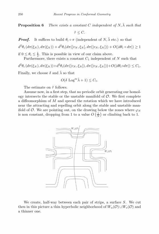
January 17, 2007 11:55 WSPC/Book Trim Size for 9in x 6in finalBB
250 Recent Progress in Conformal Geometry
Proposition 6 There exists a constant C independent of N, λ such that
τ ≤ C.
Proof. It suffices to build θi π (independent of N, λ etc.) so that
d2θi (dπ(ξN ), dπ(ξN )) + d2θi(dπ([vN , ξN ], dπ([vN , ξN ])) + O(|dθi dπ|) ≥ 1
if 0 ≤ θi ≤ 12 . This is possible in view of our claim above.
Furthermore, there exists a constant C1 independent of N such that
d2θi (dπ(ξN ), dπ(ξN ))+d2θi(dπ([vN , ξN ]), dπ([vN , ξN ]))+O(|dθidπ|) ≤ C1.
Finally, we choose δ and λ so that
O(δ Logmλ + 1) ≤ C1.
The estimate on τ follows.Assume now, in a first step, that no periodic orbit generating our homol-
ogy intersects the stable or the unstable manifold of O. We first completea diffeomorphism of M and spread the rotation which we have introducednear the attracting and repelling orbit along the stable and unstable man-ifold of O. We are pointing out, on the drawing below the zones where ϕN
is non constant, dropping from 1 to a value O(
1N
)or climbing back to 1.
We create, half-way between each pair of strips, a surface S. We cutthen in this picture a thin hyperbolic neighborhood of Wu(O)∪Ws(O) anda thinner one.
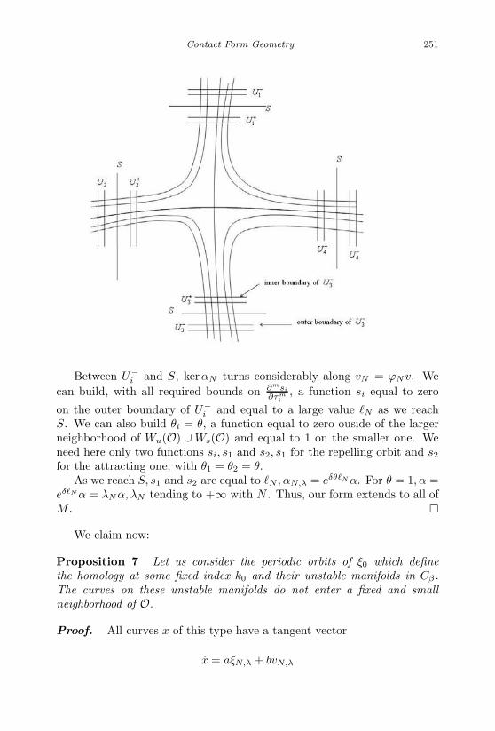
January 17, 2007 11:55 WSPC/Book Trim Size for 9in x 6in finalBB
Contact Form Geometry 251
Between U−i and S, kerαN turns considerably along vN = ϕNv. We
can build, with all required bounds on ∂msi
∂τmi
, a function si equal to zero
on the outer boundary of U−i and equal to a large value N as we reach
S. We can also build θi = θ, a function equal to zero ouside of the largerneighborhood of Wu(O) ∪ Ws(O) and equal to 1 on the smaller one. Weneed here only two functions si, s1 and s2, s1 for the repelling orbit and s2
for the attracting one, with θ1 = θ2 = θ.As we reach S, s1 and s2 are equal to N , αN,λ = eδθN α. For θ = 1, α =
eδN α = λNα, λN tending to +∞ with N . Thus, our form extends to all ofM .
We claim now:
Proposition 7 Let us consider the periodic orbits of ξ0 which definethe homology at some fixed index k0 and their unstable manifolds in Cβ .The curves on these unstable manifolds do not enter a fixed and smallneighborhood of O.
Proof. All curves x of this type have a tangent vector
x = aξN,λ + bvN,λ
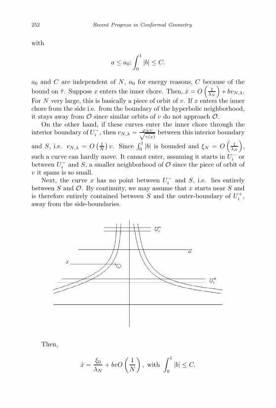
January 17, 2007 11:55 WSPC/Book Trim Size for 9in x 6in finalBB
252 Recent Progress in Conformal Geometry
with
a ≤ a0;∫ 1
0
|b| ≤ C.
a0 and C are independent of N , a0 for energy reasons, C because of thebound on τ . Suppose x enters the inner chore. Then, x = O
(1
λN
)+ bvN,λ.
For N very large, this is basically a piece of orbit of v. If x enters the innerchore from the side i.e. from the boundary of the hyperbolic neighborhood,it stays away from O since similar orbits of v do not approach O.
On the other hand, if these curves enter the inner chore through theinterior boundary of U−
i , then vN,λ = ϕN v√γ(x)
between this interior boundary
and S, i.e. vN,λ = O(
1N
)v. Since
∫ 1
0 |b| is bounded and ξN = O(
1λN
),
such a curve can hardly move. It cannot enter, assuming it starts in U−i or
between U−i and S, a smaller neighborhood of O since the piece of orbit of
v it spans is so small.Next, the curve x has no point between U−
i and S, i.e. lies entirelybetween S and O. By continuity, we may assume that x starts near S andis therefore entirely contained between S and the outer-boundary of U+
i ,away from the side-boundaries.
Then,
x =ξ0
λN+ bvO
(1N
), with
∫ 1
0
|b| ≤ C.
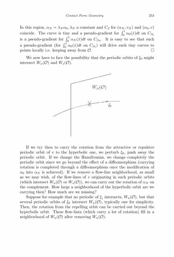
January 17, 2007 11:55 WSPC/Book Trim Size for 9in x 6in finalBB
Contact Form Geometry 253
In this region, αN = λNα0, λN a constant and Cβ for (αN , vN ) and (α0, v)coincide. The curve is tiny and a pseudo-gradient for
∫ 1
0 α0(x)dt on Cβ0
is a pseudo-gradient for∫ 1
0αN (x)dt on CβN . It is easy to see that such
a pseudo-gradient (for∫ 1
0α0(x)dt on Cβ0) will drive such tiny curves to
points locally i.e. keeping away from O. We now have to face the possibility that the periodic orbits of ξ0 might
intersect Wu(O) and Ws(O).
If we try then to carry the rotation from the attractive or repulsiveperiodic orbit of v to the hyperbolic one, we perturb ξ0, push away theperiodic orbit. If we change the Hamiltonian, we change completely theperiodic orbit since we go beyond the effect of a diffeomorphism (carryingrotation is completed through a diffeomorphism once the modification ofα0 into αN is achieved). If we remove a flow-line neighborhood, as smallas we may wish, of the flow-lines of v originating in such periodic orbits(which intersect Wu(O) or Ws(O)), we can carry out the rotation of αN onthe complement. How large a neighborhood of the hyperbolic orbit are wecarrying then? How much are we missing?
Suppose for example that no periodic of ξ) intersects, Wu(O), but thatseveral periodic orbits of ξ0 intersect Wu(O), typically one for simplicity.Then, the rotation from the repelling orbit can be carried out beyond thehyperbolic orbit. These flow-lines (which carry a lot of rotation) fill in aneighborhood of Wu(O) after removing Wu(O).

January 17, 2007 11:55 WSPC/Book Trim Size for 9in x 6in finalBB
254 Recent Progress in Conformal Geometry
Using a view from top, we have:
On the other hand, our periodic orbit intersects Wu(O):
Thus, if we remove a neighborhood of the flow-line of v through P , wecan safely bring rotation from the attracting orbit as well.

January 17, 2007 11:55 WSPC/Book Trim Size for 9in x 6in finalBB
Contact Form Geometry 255
Using a view from top
Thus, below P , we can build a lot of rotation after combining the rota-tion which we can safely bring from the attractive orbit with the rotationfrom the repelling orbit:
The piece which is left is as small as we wish, we can think of it as atiny neighborhood of the (downwards) flow-line of v through P . We thusonly need to fill this hole. On the boundaries of this hole, we have a lot ofrotation distributed as follows
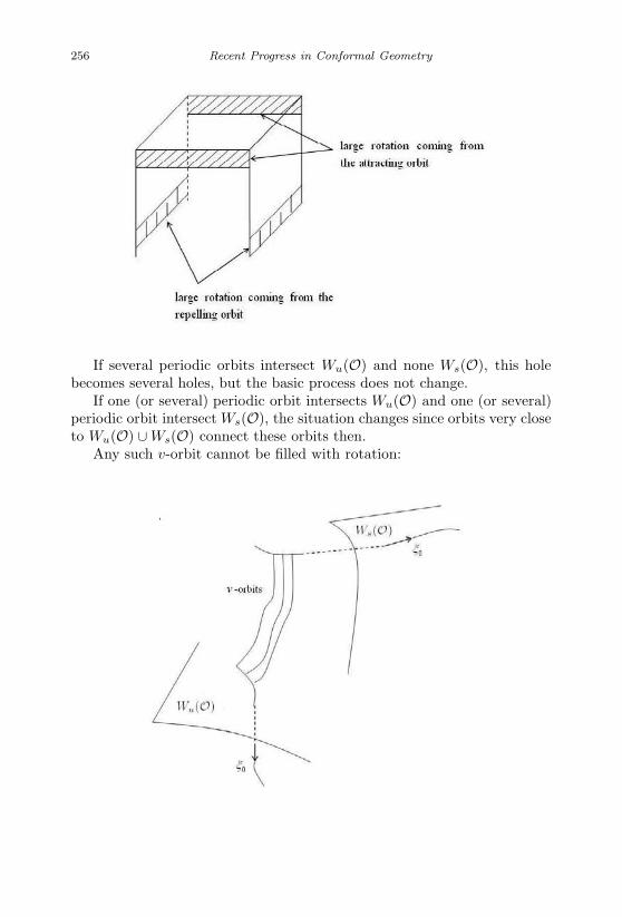
January 17, 2007 11:55 WSPC/Book Trim Size for 9in x 6in finalBB
256 Recent Progress in Conformal Geometry
If several periodic orbits intersect Wu(O) and none Ws(O), this holebecomes several holes, but the basic process does not change.
If one (or several) periodic orbit intersects Wu(O) and one (or several)periodic orbit intersect Ws(O), the situation changes since orbits very closeto Wu(O) ∪ Ws(O) connect these orbits then.
Any such v-orbit cannot be filled with rotation:

January 17, 2007 11:55 WSPC/Book Trim Size for 9in x 6in finalBB
Contact Form Geometry 257
If we remove these flow-lines, we can fill in every remaining flow-linewith rotation.
Combining, we can certainly fill with rotation near the intersection pointof a periodic orbit with Ws(O) or Wu(O) the following (shaded) set of flow-lines:
The ξ0-orbit is above this picture and intersects Wu(O) at a point onthe v-flow-line through T .
The periodic orbit lies above this picture. We cannot fill the hole morebecause some v-flow-lines of the hole connect this periodic orbit (whichintersects Wu(O) here) with another periodic orbit (intersecting Ws(O)then). We can take this hole to be as small as we wish though after takingthinner neighborhood of the allowed set of flow-lines.
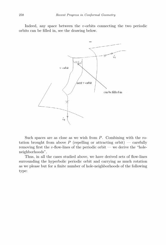
January 17, 2007 11:55 WSPC/Book Trim Size for 9in x 6in finalBB
258 Recent Progress in Conformal Geometry
Indeed, any space between the v-orbits connecting the two periodicorbits can be filled in, see the drawing below.
Such spaces are as close as we wish from P . Combining with the ro-tation brought from above P (repelling or attracting orbit) — carefullyremoving first the v-flow-lines of the periodic orbit — we derive the “hole-neighborhoods”.
Thus, in all the cases studied above, we have derived sets of flow-linessurrounding the hyperbolic periodic orbit and carrying as much rotationas we please but for a finite number of hole-neighborhoods of the followingtype:
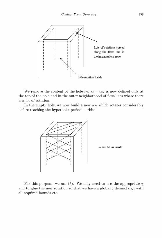
January 17, 2007 11:55 WSPC/Book Trim Size for 9in x 6in finalBB
Contact Form Geometry 259
We remove the content of the hole i.e. α = αN is now defined only atthe top of the hole and in the outer neighborhood of flow-lines where thereis a lot of rotation.
In the empty hole, we now build a new αN which rotates considerablybefore reaching the hyperbolic periodic orbit:
For this purpose, we use (*). We only need to use the appropriate γand to glue the new rotation so that we have a globally defined αN , withall required bounds etc.

January 17, 2007 11:55 WSPC/Book Trim Size for 9in x 6in finalBB
260 Recent Progress in Conformal Geometry
The first step is to get µ = 0 on the boundaries of smaller holes, in-cluding the top boundary. Next, we need to rescale the large rotation thatwe have on each lateral wall so that it stays large but becomes the sameall around instead of being split between the top part and the bottom part(see Figure (A)) according to the wall which we are considering.
These two steps are completed in the space between an inner hole andan outer hole (which is smaller than the initial hole, (see Figure (B) below).Then, we can fill the inner hole with a uniform, large rotation.
We first observe that the boundary ∂S, in the flow-box, of the setS = x ∈ flow-box, ϕ(x) = 1 is independent of N . It depends only on v,which remains unchanged with N , on the intervals I0 and on how we carrythe rotation below the periodic orbit (coming from the attractive as well asrepulsive orbits).
Second, v is transverse to ∂S since v is transverse to the boundaries ofthe tori where the insertion of a large rotation has taken place.
Third, on each flow-line of v in the box, there are at most three intervals;one where ϕ is not 1, then one where ϕ is 1 and a last one where ϕ is not1 again.
Figure (A)
The only interval which is always present is the one where ϕ is 1, the“intermediate” one since the large rotations take place in the vicinity ofthe top and of the bottom of the box. The flow-lines run from top tobottom near (only near) the lateral sides of the box. Each of these flow-lines carries a large rotation which is borrowed either from its top portionor from its bottom one, or from both. Using the large rotations coming

January 17, 2007 11:55 WSPC/Book Trim Size for 9in x 6in finalBB
Contact Form Geometry 261
from the attractive v-orbit and the repelling v-orbit, we can construct abox around the hole where a lot of rotation is carried around its boundary(all of it):
We draw then the following two layers:
which cut into the upwards rotation, go down to the downwards one andthen come back to the upwards one. The top one stays some more upstairsas the lower one speeds up to the lower level to collect rotation from there.If we cut then the central piece and flatten it, we find a thin box:

January 17, 2007 11:55 WSPC/Book Trim Size for 9in x 6in finalBB
262 Recent Progress in Conformal Geometry
Figure (B)
This carries rotation all around its boundary.Our arguments apply to this box.If there is a flow-line (and then several) running from a periodic orbit
of ξ cutting Wu(O) to a peridic orbit of ξ cutting Ws(O), there are twoconstructions as the one carried out above, one for the top with the peri-odic orbit cutting Wu(O), the other one for the bottom with the periodicorbit cutting Ws(O). We can match the parts containing a lot of rotationfrom the top and from the bottom (the boundaries parts). We then fill inpartially inside (without matching, leaving a hole which is a neighborhoodof the flow-line which connects the two periodic orbits) as if we had only atop or only a bottom.
The basic double picture for top and bottom together (not thickened,just flat) is:
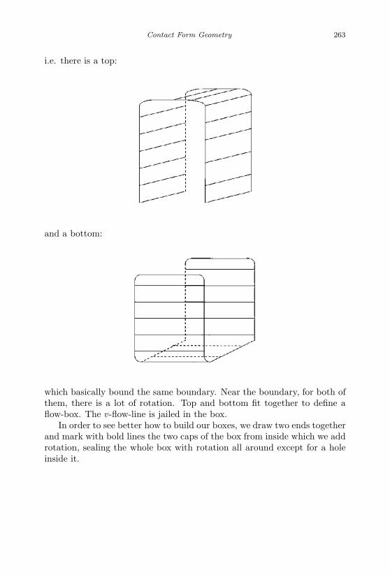
January 17, 2007 11:55 WSPC/Book Trim Size for 9in x 6in finalBB
Contact Form Geometry 263
i.e. there is a top:
and a bottom:
which basically bound the same boundary. Near the boundary, for both ofthem, there is a lot of rotation. Top and bottom fit together to define aflow-box. The v-flow-line is jailed in the box.
In order to see better how to build our boxes, we draw two ends togetherand mark with bold lines the two caps of the box from inside which we addrotation, sealing the whole box with rotation all around except for a holeinside it.

January 17, 2007 11:55 WSPC/Book Trim Size for 9in x 6in finalBB
264 Recent Progress in Conformal Geometry
Observation. Between the two bold lines defining either of the top orthe bottom caps, the v-flow-lines carry a lot of rotation near the boundary.This fact is used to extend the rotation inside the box, sealing it off; a holeis left inside.
We now have our initial flow-box and an inner, smaller one withoutbottom. α is defined in the space between the two boxes and or the topside.
The only space where ξ and α are not defined is a parallelepiped witha top and with a bottom. We build another yet smaller parallelepiped:
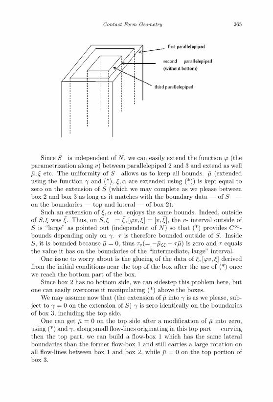
January 17, 2007 11:55 WSPC/Book Trim Size for 9in x 6in finalBB
Contact Form Geometry 265
Since ∂S is independent of N , we can easily extend the function ϕ (theparametrization along v) between parallelepiped 2 and 3 and extend as wellµ, ξ etc. The uniformity of ∂S allows us to keep all bounds. µ (extendedusing the function γ and (*), ξ, α are extended using (*)) is kept equal tozero on the extension of S (which we may complete as we please betweenbox 2 and box 3 as long as it matches with the boundary data — of ∂S —on the boundaries — top and lateral — of box 2).
Such an extension of ξ, α etc. enjoys the same bounds. Indeed, outsideof S, ξ was ξ. Thus, on ∂S, ξ = ξ, [ϕv, ξ] = [v, ξ], the v- interval outside ofS is “large” as pointed out (independent of N) so that (*) provides C∞-bounds depending only on γ. τ is therefore bounded outside of S. InsideS, it is bounded because µ = 0, thus τv(= −µξξ − τµ) is zero and τ equalsthe value it has on the boundaries of the “intermediate, large” interval.
One issue to worry about is the glueing of the data of ξ, [ϕv, ξ] derivedfrom the initial conditions near the top of the box after the use of (*) oncewe reach the bottom part of the box.
Since box 2 has no bottom side, we can sidestep this problem here, butone can easily overcome it manipulating (*) above the boxes.
We may assume now that (the extension of µ into γ is as we please, sub-ject to γ = 0 on the extension of S) γ is zero identically on the boundariesof box 3, including the top side.
One can get µ = 0 on the top side after a modification of µ into zero,using (*) and γ, along small flow-lines originating in this top part — curvingthen the top part, we can build a flow-box 1 which has the same lateralboundaries than the former flow-box 1 and still carries a large rotation onall flow-lines between box 1 and box 2, while µ = 0 on the top portion ofbox 3.
January 17, 2007 11:55 WSPC/Book Trim Size for 9in x 6in finalBB
266 Recent Progress in Conformal Geometry
We then observe that the rotation of γ on the lateral boundaries of box 3is large, either on the top portion or on the bottom one. This is embedded inthe construction and is due to the fact that
∫dx
ϕ(x) (ϕ is the parametrizationalong v) is large on each of these flow-lines. We then extend ϕ so that itbecomes constant (small obviously) on all the lateral sides of a yet smallerparallelepiped box 4. From there, the extension inside box 4 is immediate.
We need to check that this last modification, the spreading of the ro-tation so that it becomes uniform, keeps all bounds holding true. Thisrescaling is typically derived through the diffeomorphism of [0,1].
[0, 1] −→ [0, 1]
x −→t∫ x
0ds
ϕ(s) + (1 − t)x∫ 1
0ds
ϕ(s)
[0,1] is the time along the v-flow-line from bottom to top, ϕ is the functionbuilt with the rotations, as such it depends on the base point z of the flow-line. t = t(z) depends also on the base point of the flow-line z, which is onthe top of the box. t is zero on the lateral boundary of box 2 and 1 on thelateral boundary of box 3.
This gives rise to a diffeomorphism γs(y)(y) of the space between box 2and box 3. γs is the one-parameter of v.
Dγs is of course bounded. ds is the differential of
t(z)∫ x
0ds
ϕ(s) + (1 − t(z))x∫ 1
0ds
ϕ(s)
− x.
Observe that 1ϕ is at most CN, hence is upperbounded by C1
∫ 1
0ds
ϕ(s) , sincewe may assume that the total rotation of these flow-lines, between box 2and box 3, is at least c0N .
We also claim that ∣∣∣∣ ∫ x
0
∂ϕ
∂z
ds
ϕ2
∣∣∣∣ ≤ C1
∫ 1
0
ds
ϕ(s).
Indeed, the top of the flow-box is transverse to v. ϕ is a function of s andas such, between the two tori, does not depend on the flow-lines. The de-pendency on the flow-lines is due to the transformation (given, independentof N) which brings the rotation to the flow-box. Thus,∣∣∣∣∂ϕ
∂z
∣∣∣∣ ≤ C|ϕ′(s)|

January 17, 2007 11:55 WSPC/Book Trim Size for 9in x 6in finalBB
Contact Form Geometry 267
and ∣∣∣∣ ∫ x
0
∂ϕ
∂z
ds
ϕ2
∣∣∣∣ ≤ C
∫ x
0
|ϕ′|ϕ2
ds ≤ C′ Max1ϕ
.
Thus, again, ∣∣∣∣ ∫ x
0∂ϕ∂z
dsϕ2
∣∣∣∣∫ 1
0ds
ϕ(s)
≤ C1
dt is also bounded independently of N . Thus, ds is bounded independentlyof N .
We thus have (ϕ is the parametrization which we built).
Proposition 8 ξ, [ϕv, ξ], µ, τ are bounded. Furthermore,
ξ · ξ, [ϕv, ξ] · [ϕv, ξ], ξ · [ϕv, ξ], [ϕv, ξ] · ξare bounded independently of N transversally to v.
Proof. Since Dγs(y) + ds(·)v is bounded, ξ, [ϕv, ξ] are bounded. µ and τare bounded by construction.
ξ ·ξ etc are initially bounded but γs(y)(y) could have an effect. However,denoting ξ the initial ξ,
ξ = Dγs(y)(ξ) + ds(ξ)v = D(γs(y))(ξ).
Any further derivative taken on ξ through a vector-field which reads
Dγs(y)(X) + ds(X)v = D(γs(y))(X)
would yield derivatives of ξ along X which are bounded transversally tov (and v is mapped onto θv by D(γs(y))) if X splits on ξ, [ϕv, ξ], i.e. ifDγs(y)(X)+ds(X)v splits on ξ, [ϕv, ξ], derivatives of v, which are boundedand would yield derivatives of D(γs(y)) which might be unbounded.
But
D(γs(y)) = Dγs(y) + dsv.
Derivatives fo Dγs(y) are bounded as well as derivatives of v. Derivativesof ds might be unbounded; but these are multiplied by v and our estimateis transversal to v.
Our construction of the functions s1, s2 etc proceeds then as in the casewhen no periodic orbit of the contact vector-field intersected Wu(O) andWs(O). Proposition 8 holds.
January 17, 2007 11:55 WSPC/Book Trim Size for 9in x 6in finalBB
268 Recent Progress in Conformal Geometry
Lemma 12 The function x2+y2 has no local maximum near the repellingor attracting orbits along the trajectories of ξ.
Proof. We recall that ξ = ∂∂x = γ ∂
∂y so that
ξ · ξ · (x2 + y2) = 2ξ · (x − γy) = 2(1 + γ2) > 0.
Corollary 4 There is no “small” ξ-trajectory exiting from T2 and comingback after a short time.
Next, we establish the following qualitive result:
Lemma 13 For γ small enough, τN is negative in T2 − T1.
Proof. We write
ξN = (A cos s1 + B sin s1)e2 + (A1 cos s1 + B1 sin s1)ϕv + De1
ϕv is ∂∂s1
, e2 = y ∂∂x − x ∂
∂y , e1 = 20 ∂∂θ .
We know that
[ξN , [ϕv, ξN ]] = τNϕv
i.e.
[ξN ,∂ξN
∂s1] = τN
∂
∂s1.
Also
∂e1
∂s1=
∂e2
∂s1= 0.
Since ds1(e1) = ds1(e2) = 0 and since ∂∂θ A1 = ∂
∂θB1 = 0, e1 has no contri-bution in [ξN , ∂ξN
∂s1] and
[ξN ,∂ξN
∂s1] =
[(A cos s1 + B sin s1)e2 + (A1 cos s1 + B1 sin s1)
∂
∂s1,
(−A sin s1 + B cos s1)e2 + (−A1 sin s1 + B1 cos s1)∂
∂s1
]=
∂
∂s1
(−(A1 cos s1 + B1 sin s1)2 − (B1 cos s1 − A1 sin s1)2
+(A cos s1 + B sin1)(−e2 · A1 sin s1 + e2 · B1 cos s1)
−(−A sin s1 + B cos s1)(e2 · A1 cos1 +e2 · B1 sin s1))
January 17, 2007 11:55 WSPC/Book Trim Size for 9in x 6in finalBB
Contact Form Geometry 269
=(−(A2
1 + B21) + Ae2 · B1 − Be2 · A1
) ∂
∂s1.
Thus,
τN = −(A21 + B2
1) + Ae2 · B1 − Be2 · A1.
From Proposition 2, we derive
A =−(x − γy)
γ(x2 + y2)√
1 + γ2(0) +
(y + γx)(0)(x2 + y2)(0)
B =−y(0)
√1 + γ2
γ(x2 + y2)(0)−√
1 + γ2x(0)(x2 + y2)(0)
.
A1 = − (x − γy)(0)
γ(x2 + y2)(0)√
1 + γ2
B1 = − y(0)√
1 + γ2
γ(x2 + y2)(0)− 2
(x − γy)(0)(x2 + y2)(0)
√1 + γ2
.
Observe that
e2 · (x2 + y2)(0) = 0
γ(x2 + y2)(0)A = −x(0) + O(γ)(|x| + |y|)
γ(x2 + y2)(0)B = −y(0) + O(γ)(|x| + |y|)
γ(x2 + y2)(0)A1 = −x(0) + O(γ)(|x| + |y|)
γ(x2 + y2)(0)B1 = −y(0) + O(γ)(|x| + |y|)
e2 · (γ(x2 + y2)(0)A1) = −y(0) + O(γ)(|x| + |y|)
e2 · (γ(x2 + y2)(0)B1) = x(0) + O(γ)(|x| + |y|).Thus,
τN =1
γ(x2 + y2)(0)2(−2(x(0)2+y(0)2)(1+O(γ2))) = −2
(1 + O(γ2))γ2(x2 + y2)(0)
< 0.

January 17, 2007 11:55 WSPC/Book Trim Size for 9in x 6in finalBB
270 Recent Progress in Conformal Geometry
Lemma 14 If all the θi’s involved in the construction of τ are small ata point x of M (θi ≤ c, c independent of N), then
τ ≤ −2γ2(x2 + y2)(0)
(1 + O(γ2))e−δ∑
θisi + O(δ Logmλ).
Proof. Coming back to τ , we recognize that the term O(1) in its expres-sion comes from Bτ
ν(x)λ and that, for θi small,
[ξN , vN ] · (dθi dπ)([ξN , vN ]) + ξN · (dθi dπ)(ξN )
is positive. The claim follows.
Ws(O) and Wu(O) are tangent to v. Let us for example focus here onWu(O). Along v, as we move away from O to go to the attracting orbit ofv, ξ, ξN rotate as well as [ξ, v] and [ξN , vN ]. This builds a sequence of lines(closed lines) of tangency of ξ(ξN ), [ξ, v]([ξN , vN ]) to Wu(O):
These lines are sizably spaced along v for ξ, [ξ, v], along vN forξN , [ξN , vN ].
⊗ designates the region where ξ (or ξN ) points into the paper acrossWu(O) while designates the region where ξ (or ξN ) points towards us.
Let us consider the vector-field
−sδdθ([ξ, v])v
where ξ = ξN,λ and v = vN,λ. θ here is zero above the piece of paper andbuilds up to 1 as we approach it:

January 17, 2007 11:55 WSPC/Book Trim Size for 9in x 6in finalBB
Contact Form Geometry 271
Lemma 15 Between 1 and 2 , −sδdθ([ξ, v])v points downwards from2 and 1 . Below 1 until the next ξ-tangency line, −sδdθ([ξ, v])v pointsupwards towards 1 .
Proof. Observe that, since dθ(v) = 0,
v · dθ(ξ) = dθ([v, ξ]).
From 1 to 2 along a v-flow-line, dθ(ξ) decreases (it is positive near 1 ,negative near 2 ) so that
dθ([v, ξ]) < 0, dθ([ξ, v]) > 0 between 1 and 2 .
The claim follows.We now have:
Lemma 16 Assume that δs ≥ M . There exists c(M) > 0, c(M) tendingto zero with 1
M and δ, such that any piece of ξN,λ-orbit entering and exitingthe region of modification between 1 and 2 stays in a c(M)-neighborhoodof the ξ(ξN ) line of tangency.
Proof. We take local coordinates between 1 and 2 where Wu(O) isy = 0, v is ∂
∂z
(vN = ∂
∂z
)and ∂
∂x is tangent to the ξ or ξN tangency line.ξN,λ reads up to the factor 1
λ as
ξ − sδdθ([ξ, v])v + O(δθ)[ξ, v]

January 17, 2007 11:55 WSPC/Book Trim Size for 9in x 6in finalBB
272 Recent Progress in Conformal Geometry
ξ has near the tangency line a non-zero component on ∂∂x . It thus reads as
θ0 + a1(x − x0) + b1y + c1z + higher order−zγ(x, y, z) , with θ0 = 0, γ(x0, 0, 0) = 0, positiveµ0 + a2(x − x0) + b2y + c2z + higher order.
near (x0, 0, 0). The y-axis goes from left to right through Wu(O). ThusξN,λ reads after setting θ = M(y + η)+4 for example
O(M (y+η)+4δ)+
θ0 + a1(x − x0) + b1y + c1z + higher order−zγ(x, y, z)µ0 + a2(x − x0) + b2y + c2z − δs4M(y + η)+3c(x, y, z)
+ higher order.
with c(x0, 0, 0) > 0 and M = M(x, y, z) very-large.This provides the general form (up to meaningless details) of ξN,λ near
the line of tangency of ξ. The size of the neighborhood where this formholds does not depend on M, M . The higher terms are independent onM, M .
Observe that if (c0 ≤ c)
4MM(y + η)3c0 ≥ C1,
C1 a fixed constant, then
z < 0.
Thus, if at such point z < O(M (y+η)+4δ), y = −zγ+O(M(y+η)+4δ) > 0.4MM(y + η)3c0 is larger than C1 thereafter, z remains less than O(M(y +η)+4δ), the ξN,λ piece of orbit cannot exit without crossing the chore.
Thus, we need
4MM(y + η)3c0 ≤ C1 as long as z < −c2Mδ(y + η)+4.
Assume now that
z(0) ≤ −c(M), y + η(0) ≥ 0.
Then,
z(t) ≤ −c(M) + c∆t , c independent of M, M.
Thus,
z
(c(M)
2c
)≤ −c(M)
2
January 17, 2007 11:55 WSPC/Book Trim Size for 9in x 6in finalBB
Contact Form Geometry 273
and for 0 ≤ t ≤ c(M)2c , taking Mδ < 1:
y + η(t) ≥ c(M)4
γt.
Thus, (y + η)(
c(M)2c
)≥ c(M)2γ
8c
z(
c(M)2c
)≤ − c(M)
2 .
It suffices then to take c(M) > 2c2Mδ
4MMc0c(M)6γ3
γ3c3 = 2C1
and we have a contradiction.We thus need to have
0 ≥ z(0) ≥ −c(M)
at the time of entry.We now follow the piece of orbit of ξN,λ. As z reaches the value c(M)
2 −if it does; if it does not, we are done — either z < 0 and z becomes lessthan c(M)
2 or z is nonnegative. This forces (sδ = δ so that sδ = sδ +0(δ) =sδ(1 + o(1)))
(y + η)+ ≤(
C1
4sδM c0
)1/3
.
As long as z remains larger than c(M)4 ,
˙(y + η)+ ≤ − c(M)8
and
0 ≤ (y + η)+ ≤ − c(M)8
∆t +(
C1
4sδM c0
)1/3
. (2.32)
This forces
∆t <8
c(M)
(C1
4sδM c0
)1/3
= ∆t max.
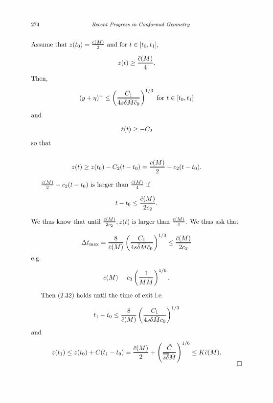
January 17, 2007 11:55 WSPC/Book Trim Size for 9in x 6in finalBB
274 Recent Progress in Conformal Geometry
Assume that z(t0) = c(M)2 and for t ∈ [t0, t1],
z(t) ≥ c(M)4
.
Then,
(y + η)+ ≤(
C1
4sδM c0
)1/3
for t ∈ [t0, t1]
and
z(t) ≥ −C2
so that
z(t) ≥ z(t0) − C2(t − t0) =c(M)
2− c2(t − t0).
c(M)2 − c2(t − t0) is larger than c(M)
4 if
t − t0 ≤ c(M)2c2
.
We thus know that until c(M)2c2
, z(t) is larger than c(M)4 . We thus ask that
∆tmax =8
c(M)
(C1
4sδM c0
)1/3
≤ c(M)2c2
e.g.
c(M) ∼ c3
(1
MM
)1/6
.
Then (2.32) holds until the time of exit i.e.
t1 − t0 ≤ 8c(M)
(C1
4sδM c0
)1/3
and
z(t1) ≤ z(t0) + C(t1 − t0) =c(M)
2+
(C
sδM
)1/6
≤ Kc(M).

January 17, 2007 11:55 WSPC/Book Trim Size for 9in x 6in finalBB
Contact Form Geometry 275
2.3 Appendix 1
2.3.1 The normal form for (α, v) when α does not turn well
We consider a hyperbolic orbit O of v. We establish:
Proposition 9 There is, up to diffeomorphism, a unique local model for(α, v) around O such that α does not turn well.
Proof. Let σ be a section to v at x0 ∈ O. Since O is hyperbolic, it has astable and an unstable manifold; they can be seen as two foliations Fu,Fs
with traces Au, As in σ.Since α does not turn well along v, kerα along O is never tangent to
Fu, neither is it tangent to Fs. Otherwise the mononicity of the rotation ofkerα would imply an infinite amount of rotation. Thus, kerα is containedbetween TFu and TFs, it lies in exactly one of the sectors defined by thetangent spaces along O to Fu and Fs.
This property extends, by continuity, to a small neighborhod of O. Letσ be a small section to v at x0 and let be the Poincare return map. Alongthe v-orbit from x ∈ σ to (x), kerαy rotates monotonically with respectto the tangent spaces to the foliations TyFu and TyFs, since these tangentspaces are transported by v. If we declare TxFu and TxFs to be orthogonalto each other, we have
0 < θ(x) <π
2

January 17, 2007 11:55 WSPC/Book Trim Size for 9in x 6in finalBB
276 Recent Progress in Conformal Geometry
θ(x) designates the amount of rotation of kerαy from x to (x). Giventwo distinct contact structures, both having v in their kernel and both notturning well along v, we have two functions θ1(x), θ2(x), both between 0and π
2 .We complete around O a rotation which maps kerα1 to kerα2 at x0.
Along the rotation, kerα1 remains in the same quadrant for all x in a smallneighborhood ofO. It is then easy to scale the speed of the rotation of kerα1
so that it coincides along O with kerα2. This rescaling is a diffeomorphismof a neighborhood of O which may be achieved through a reparametrizationof the v-orbits.
kerα1 and kerα2 are now close in a whole neighborhood of O and theyboth have v in their kernel.
Since both planes rotate monotonicaly, are very close and have the samelimits at infinity (due to the hyperbolic behavior of v), it is possible to bringone onto the other through a reparametrization of each v-orbit.
2.4 The Normal Form of (α, v) Near an Attractive PeriodicOrbit of v
Let O be a periodic orbit of v. We establish:
Proposition 10 There are suitable coordinates (θ1, x, y), θ1 being anangular coordinate along O such that α reads λ(θ1, x, y)(xdθ1 + dy).
Proof. kerα is tangent to O and there is an additional direction alongO defining kerα. v and this additional direction define an orientable framein kerα. If we add to these two vectors the contact vector-field ξ of α, webuild a frame for M3 along O. We thus can take, along O, this additionaldirection to be ∂
∂x and ξ to be ∂∂y , v = ∂
∂θ .α then takes the form:(
a(θ)x + b(θ)y + O(x2 + y2))dθ +
(1 + a2(θ)x + b2(θ)y + O(x2 + y2)
)dy
+(a1(θ)x + b1(θ)y + O(x2 + y2)
)dx.
Using Gray’s theorem, its use leaves O unchanged as can be checked, wecan get rid of all second order terms after the introduction of a relateddiffeomorphism.
Rescaling, α reads (up to a multificative factor):(a(θ)x + b(θ)y
)dθ +
(a1(θ)x + b1(θ)y)dx + dy.
Since α ∧ dα is a volume form, a(θ) is non-zero for every θ ∈ [0, 2π].

January 17, 2007 11:55 WSPC/Book Trim Size for 9in x 6in finalBB
Contact Form Geometry 277
We rewrite α (rescaled) as:(a(θ)x + b(θ)y
)dθ +
(1 − b1(θ)x
)dy + d
(a1(θ)
x2
2+ b1(θ)xy
)− x2
2a′1(θ)dθ − b′1(θ)xydθ.
We remove as above x2
2 a′1(θ)dθ − b′1(θ)xy dθ since it is second order.
d(a1(θ)x2
2 + b1(θ)xy) is closed and o(1). We may also remove it usingagain Gray’s theorem.
We are left, after rescaling with:(a(θ)x + b(θ)y
)dθ + dy with a(θ) = 0.
Setting
dθ1 = a(θ)dθ,
we find (x + b1(θ)y
)dθ1 + dy.
The family (x + tb1(ϑ)y
)dϑ1 dy
is a one-parameter family of contact forms. For all of them, there is avector-field vt in their kernel having O as a periodic orbit,. The family isconstant equal to dy on O.
We thus can use Gray’s theorem and reduce up to rescaling, α to
xdθ1 + dy
as claimed.Let us consider two vector-fields v1, v2 having O as a periodic orbit. Up
to reparameterization, they read:
∂
∂θ1− x
∂
∂y+ δxi
∂
∂x.
Assuming that O is attractive for both of them, we can find functionsa1(θ), a2(θ), b1(θ), b2(θ), c1(θ), c2(θ) such that ai > 0, b2
i − 4aici < 0 andd(ai(θ)x2 + bi(θ)xy + c1(θ)2)(vi) < 0 for x2 + y2 > 0, small.
This reads:
(a′i − bi)x2 + (b′i − 2ci)xy + c′iy
2 + 2ai(θ)(
x +bi
2ai
)δxi < 0.

January 17, 2007 11:55 WSPC/Book Trim Size for 9in x 6in finalBB
278 Recent Progress in Conformal Geometry
Set
X = x +bi
2aiy Y = y
so that
x = X − bi
2aiY.
The above equation rereads:
(a′i − bi)(X − bi
2aiY )2 + (b′i − 2ci)(X − bi
2aiY )Y + c′iY
2 + 2ai(θ)Xδxi < 0.
Setting
δxi = Ai(θ)X + Bi(θ)Y + higher order,
we find
(a′i − bi + 2aiAi)X2 + (b′i − 2ci + 2aiBi − bi
ai(a′
i − bi))XY < 0
(b2i
4a2i
(a′i − bi) + c′i −
bi
2ai(b′i − 2ci))Y 2 < 0,
i.e.(b′i − 2ci + 2aiBi − bi
ai(a′
i − bi))2 − 4(c′i − bi
2ai(b′i − 2ci) + ( i
2ai)2(a′
i − bi))(a′
i − bi + 2aiAi) < 02aiAi + a′
i − bi < 0.
This implies: (bi
2ai
)2
(a′i − bi) + c′i <
bi
2ai(b′i − 2ci).
Furthermore,
2aiAi + a′i − bi must be sufficiently negative,
once Bi is given.This last condition is easy to satisfy as we build a convex-combination
of v1 and v2 in kerα. O should be an attractive orbit for the convex-combination. We thus consider the condition:(
bi
2ai
)2
(a′i − bi) + c′i <
bi
2ai(b′i − 2ci)
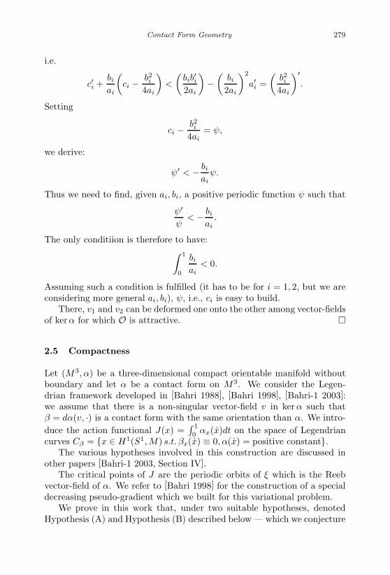
January 17, 2007 11:55 WSPC/Book Trim Size for 9in x 6in finalBB
Contact Form Geometry 279
i.e.
c′i +bi
ai
(ci − b2
i
4ai
)<
(bib
′i
2ai
)−(
bi
2ai
)2
a′i =
(b2i
4ai
)′.
Setting
ci − b2i
4ai= ψ,
we derive:
ψ′ < − bi
aiψ.
Thus we need to find, given ai, bi, a positive periodic function ψ such that
ψ′
ψ< − bi
ai.
The only conditiion is therefore to have:∫ 1
0
bi
ai< 0.
Assuming such a condition is fulfilled (it has to be for i = 1, 2, but we areconsidering more general ai, bi), ψ, i.e., ci is easy to build.
There, v1 and v2 can be deformed one onto the other among vector-fieldsof kerα for which O is attractive.
2.5 Compactness
Let (M3, α) be a three-dimensional compact orientable manifold withoutboundary and let α be a contact form on M3. We consider the Legen-drian framework developed in [Bahri 1988], [Bahri 1998], [Bahri-1 2003]:we assume that there is a non-singular vector-field v in kerα such thatβ = dα(v, ·) is a contact form with the same orientation than α. We intro-duce the action functional J(x) =
∫ 1
0 αx(x)dt on the space of Legendriancurves Cβ = x ∈ H1(S1, M) s.t. βx(x) ≡ 0, α(x) = positive constant.
The various hypotheses involved in this construction are discussed inother papers [Bahri-1 2003, Section IV].
The critical points of J are the periodic orbits of ξ which is the Reebvector-field of α. We refer to [Bahri 1998] for the construction of a specialdecreasing pseudo-gradient which we built for this variational problem.
We prove in this work that, under two suitable hypotheses, denotedHypothesis (A) and Hypothesis (B) described below — which we conjecture

January 17, 2007 11:55 WSPC/Book Trim Size for 9in x 6in finalBB
280 Recent Progress in Conformal Geometry
to be always satisfied — compactness holds for some flow-lines (all in fact,see [Bahri]) on the unstable manifold of a periodic orbit.
This result is far reaching because it indicates the existence of an in-variant sub-Morse complex made of flow-lines connecting periodic orbits,with no additional asymptots involved.
We have defined in [Bahri-1 2003] a homology related to the periodicorbits using J or Cβ . The existence of this invariant sub-Morse complexcan be equivalently rephrased into the more technical statement that thishomology has only periodic orbits as intermediate critical points (at infin-ity).
We believe that this homology is equal to the homology of PC∞ forthe standard contact form on S3. Some of the tools required in order tocompute this homology in this particular case extend to the general case.We provide a brief account of one of these tools in Section 2.5.7.
This work is organized as follows:
In Section 2.5.1, we recall (without proof) some basic facts about α, v, Jand Cβ . Our proof uses little of the analytical framework. In Section 2.5.2we consider a periodic orbit of index m in Cβ and we build a model forits unstable manifold. In Section 2.5.3, we introduce Hypothesis (A), Hy-pothesis (B), and we state our results. In Sections 2.5.4 and 2.5.5, weproceed with the proofs. In Section 2.5.6, we extend the result to flow-lines from x2k+1 to x∞
2k (In Sections 2.5.4, 2.5.5 we had only considered thecase x2k − x∞
2k−1). In Section 2.5.7, we provide the classifying map for theS1-action on the space Cβ . This should be an essential tool in the compu-tation of this homology. In Section 2.5.8, we discuss oscillations and howto enlarge them or tame them whenever possible, if they are “high”. InSection 2.5.9, we discuss iterates (of critical points at infinity, not iteratesof periodic orbits). In Sections 2.5.10 and 2.5.11 we overcome the Fred-holm and transversality difficulties which we had set aside in the previoussections.
2.5.1 Some basic facts
α is a contact form, v is a vector-field in ker α. We are assuming thatβ = dα(v, ·) is a contact form with the same orientation than α. We rescalev so that
β ∧ dβ = α ∧ dα.
The following results are established in [Bahri 1998], [Bahri-1 2003].
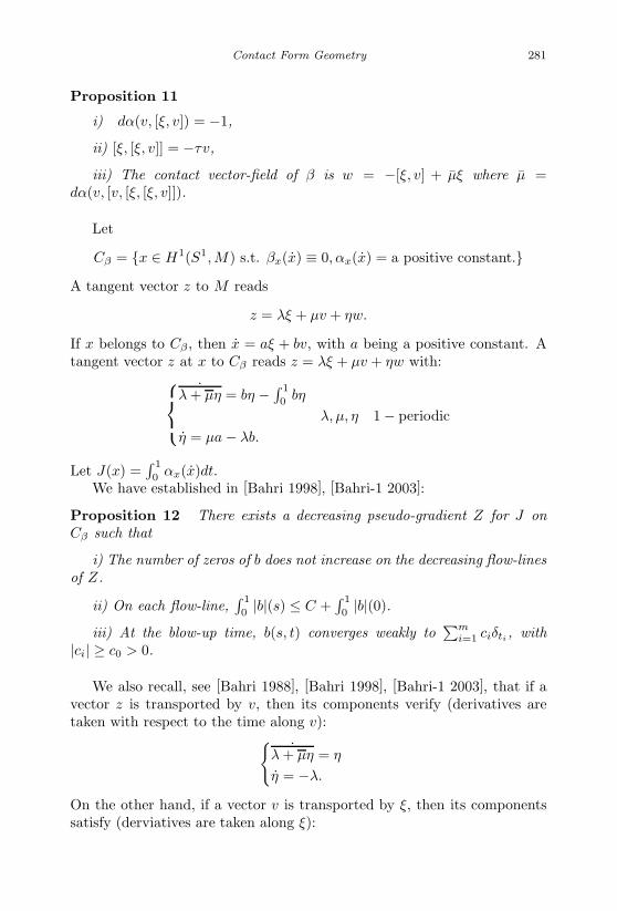
January 17, 2007 11:55 WSPC/Book Trim Size for 9in x 6in finalBB
Contact Form Geometry 281
Proposition 11
i) dα(v, [ξ, v]) = −1,
ii) [ξ, [ξ, v]] = −τv,
iii) The contact vector-field of β is w = −[ξ, v] + µξ where µ =dα(v, [v, [ξ, [ξ, v]]).
Let
Cβ = x ∈ H1(S1, M) s.t. βx(x) ≡ 0, αx(x) = a positive constant.A tangent vector z to M reads
z = λξ + µv + ηw.
If x belongs to Cβ , then x = aξ + bv, with a being a positive constant. Atangent vector z at x to Cβ reads z = λξ + µv + ηw with:
˙λ + µη = bη − ∫ 1
0 bη
λ, µ, η 1 − periodicη = µa − λb.
Let J(x) =∫ 1
0 αx(x)dt.We have established in [Bahri 1998], [Bahri-1 2003]:
Proposition 12 There exists a decreasing pseudo-gradient Z for J onCβ such that
i) The number of zeros of b does not increase on the decreasing flow-linesof Z.
ii) On each flow-line,∫ 1
0|b|(s) ≤ C +
∫ 1
0|b|(0).
iii) At the blow-up time, b(s, t) converges weakly to∑m
i=1 ciδti , with|ci| ≥ c0 > 0.
We also recall, see [Bahri 1988], [Bahri 1998], [Bahri-1 2003], that if avector z is transported by v, then its components verify (derivatives aretaken with respect to the time along v):
˙λ + µη = η
η = −λ.
On the other hand, if a vector v is transported by ξ, then its componentssatisfy (derviatives are taken along ξ):

January 17, 2007 11:55 WSPC/Book Trim Size for 9in x 6in finalBB
282 Recent Progress in Conformal Geometry
µ + η τ = 0η = µ.
2.5.2 A model for Wu(xm), the unstable manifold in Cβ of
a periodic orbit of index m
Let xm be a periodic orbit of index m. We provide in what follows a modelfor its unstable manifold in Cβ .
Proposition 13 The unstable manifold of xm can be achieved in Γ2m form ≥ m0(m0 ≥ 4).
Proof. Let us assume in a first step that xm is a simple periodic orbit.We indicate at the end of the proof how to extend the result to iterates.We start with the case where m = 2k +1. xm can be elliptic or hyperbolic.Assume that it is hyperbolic to start with. Then, if is the Poincare-returnmap of the periodic orbit and u is a real eigenvector of d in kerα, u istransported by ξ while v rotates (considerably: m ≥ m0).
Setting xm(0) at a point where v and u coincide, setting η to be the−[ξ, v]-component of u, we have
η(0) = η(1) = 0
η can easily be seen to have at least 2k genuine zeros, also η(1)η(0) < 0because the periodic orbit is hyperbolic of odd Morse index. The zeros ofη are t1 = 0, t2, . . . , t2k+1, t2k+2 = 1.
Setting η = ηi|[ti,ti+1], i = 1, . . . , 2k+1 we derive 2k+1-functions whichare pairwise orthogonal and are orthogonal to themselves. Each ηi definesa tangent vector zi with
ηi + a2ηiτ = ciδti + ci+1δti+1 .
Thus, Span z1, . . . , z2k+1 is achieved in Γ2m.If x2k+1 is of odd Morse index 2k + 1 but elliptic, the [ξ, v]- component
η of any transported vector u has always 2k, 2k + 1 or 2k + 2 zeros exactly.Indeed, it needs to have at least 2k, at most 2k+2, zeros and if the numberof zeros were to change, there would be a point where u(v) would be mappedonto γu(γv) with γ < 0, yielding 2k + 1 zeros, 2k of which are genuine i.e.a hyperbolic orbit.
Taking the base point at one of the nodes of the most oscillating eigen-function, η must have 2k + 1 zeros to the least. This yields 2k function

January 17, 2007 11:55 WSPC/Book Trim Size for 9in x 6in finalBB
Contact Form Geometry 283
η1, . . . , η2k which are zero at
t1 = 0, t2, . . . , t2k+1
and yield 2k vectors z1, . . . , z2k which are pairwise orthogonal and orthog-onal to themselves. For each of these vectors, we have
ηi + a2ηiτ = ciδti + ci+1δti+1
so that Spanz1, . . . , z2k is achieved in Γ4k+2.We still need an additional vector z2k+1. At xm(0), we introduce the
solution of
d(u) − u = v.
This yields a new vector z2k+1. η of z2k+1, which we denote η2k+1, is notzero at x(0) or at t1 = 0 since the orbit is not hyperbolic. If we computethe second derivative J
′′(xm) · z2k+1 · z (the −[ξ, v]- component of z is η),
we find
J′′(xm) · z2k+1 · z = −
∫ 1
0
(¨η2k+1 + a2η2k+1τ)η = η(0).
Thus, z2k+1 is J′′(xm)-orthogonal to z1, . . . , z2k.
We claim that we can take, after deformation of the contact form,η2k+1(0) to be negative and z2k+1 in the negative eigenspace of J
′′(xm).
Then, J′′(xm) is non positive on Spanz1, . . . , z2k, z2k+1 which is again
achieved in Γ4k+2.In order to prove our claim, we complete a deformation of the contact
form so that xm, without degenerating, changes from elliptic to hyperbolicwith eigenvalues equal to −1 and back to elliptic i.e. xm iterated twicedegenerates but not xm which stays of odd Morse index. At the switch,d|ker α is -Id and we can set x(t1) = x(0) at any point. We may solvecontinuously, through the degeneracy, the equation d(u) − u = v.
η2k+1(0) is zero at the switch and changes sign through it. We considerthe side of the switch where it is negative. z1, . . . , z2k still exist but z2k+1
might have disappeared (when the Poincare-return map has an eigenvalueequal to -1 and 0 is at the node, z2k+1 exists). The negativity of η2k+1(0)means that J
′′(xm) · z2k+1 · z2k+1 < 0. We thus will have produced a space
of dimension 2k+1, Span z1, . . . , z2k, z2k+1 where J′′(xm) is non positive.
If xm = x2k is of Morse index 2k, the most negative eigenfunction of−(η + a2ητ) has 2k zeros. An elliptic orbit is, as we will see, of odd Morseindex. Thus x2k is hyberbolic. We pick an eigenvector u. Since m ≥ 4, ucoincides with v at some points on the periodic orbit. We set x(0) at such atime. We transport v along the periodic orbit. This yields an η-component

January 17, 2007 11:55 WSPC/Book Trim Size for 9in x 6in finalBB
284 Recent Progress in Conformal Geometry
of the transported vector. Using Sturm-Liouville arguments, η vanishes at2k + 1 times, t1 = 0, t1, . . . , t2k+1 = 0. This yields 2k functions η1, . . . , η2k
with
ηi + a2ηiτ = ciδti + ci+1δti+1
and 2k vectors z1, . . . , z2k which are pairwise J′′(xm)-orthogonal and or-
thogonal to themselves.Again,
Span z1, . . . , z2k is achieved in Γ2m.
In each occurence, J′′(xm) is non positive on the vector-space which we
build and we therefore can take these directions to achieve the unstablemanifold of xm.
Let us enter into some more details and check that our representationof Wu(xm) in Γ2m works. We will consider for simplicity first the case of ahyperbolic orbit of index 2k.
We then have 2k nodes t1, t2, · · · , t2k where we locate the v-jumps. Thebasic equation is
η + a2ητ =2k∑i=1
ciδti,
η reads as∑2k
i=1 ciηi where each ηi solves
−( ¨ηi + a2ηiτ) = δti
ηi1 − periodic.
We may consider the above equation when the ti’s are in the vicin-ity of the ti. We find in this way 2k functions η1, η2, . . . , η2k. Thesecond derivative
∫ 1
0 η2 − a2η2τ in Spanη1, . . . , η2k reads as ctAc =∑i=j cicj (ηi(tj) + ηj(ti)) +
∑c2i ηi(ti). Clearly after integration by parts,
ηi(tj) = ηj(ti).When all the ti’s are located at the ti’s, this quadratic form is identically
zero. We claim that
∑i
∣∣∣∣∣∣ci
2∑j =i
cj∂
∂tiηj(ti) + ci
∂
∂tiηi(ti)
|(t1,...,t2k)
∣∣∣∣∣∣ ≥ c∑
c2i
when c is a fixed positive constant. Thus, by moving slightly for eachdirection (c1, . . . , c2k) the location of the Dirac masses, we may achievethat J
′′(x2k) is negative in this space.

January 17, 2007 11:55 WSPC/Book Trim Size for 9in x 6in finalBB
Contact Form Geometry 285
Assume that the above inequality does not hold. Then, for each i suchthat |ci| ≥ c1
√∑c2k, where c1 is a small constant( c1 =
√c for example),
ci∂
∂tiηi(ti) + 2
∑j =i
cj∂
∂tiηj(ti) |(t1,...,t2k)= o
((∑c2k
)1/2)
.
In the remainder getting rid of the other c′is ( ∂∂ti
ηj(ti) is bounded as wewill see) we derive that the matrix (off diagonal terms should be multipliedby 2) (
∂
∂tiηj(ti)
)|(t1,...,t2k)
or some nontrivial sub-matrix of the above one should have a zero eigen-value. For the sake of simplicity, we will assume that the number of points(t1, . . . , t2k) has not been reduced in the above process. We can computethis matrix as follows: we set a section to ξ at t1, tangent to kerα at x2k(t1).Let ψ be the Poincare-return map. η1 is obtained by solving the equation
Dψ(z) − z = v,
z is in kerαx2k(t1) and reads z = µ1v − η1[ξ, v].Let ψ0 be the Poincare-return map at t1. x2k is hyperbolic so that
Dψ0(v) = γv.Dψ read as σ Dψ0 σ−1 and our equation above becomes
Dψ0 σ−1(z) − σ−1(z) = σ−1(v).
Let ∆t = −t1+t1 which we can assume to be small,. We then have, usingthe transport equations (µ = −ητ, η = µ) : σ−1(z) = (µ1 + O(η1∆t))v −(η1 + µ1∆t)[ξ, v] + o(∆t). Observe that η1(t1) = 0 so that η1(t1) = o(1)and σ−1(z) = µ1v − (η1 + µ1∆t)[ξ, v] + o(∆t).
The matrix of Dψ0 on kerα reads(
γ α0 1
γ
)in the (v,−[ξ, v]) basis so that
Dψ0 − Id =(
γ − 1 α0 1
γ − 1
).
Our equations on z then re-read:
(γ − 1)µ1 + αη1 = 1 + o(∆t)
1 − γ
γ(η1 + µ1∆t) = ∆t(1 + o(1)).

January 17, 2007 11:55 WSPC/Book Trim Size for 9in x 6in finalBB
286 Recent Progress in Conformal Geometry
Thus, since ∆t = −t1 + t1 and η1(t1) = 0, we find:
∂
∂t1η1(t1) |t1= −γ + 1
1 − γ=
γ + 1γ − 1
,
and this extends to give
∂
∂tiηi(ti) |ti
=γ + 1γ − 1
.
If we want to compute now ∂∂ti
ηj(ti) |tifor i = j, we use that fact that
ηj = µj so that ∂∂ti
ηj(ti) |ti= µj(ti). Between tj and ti, along ξ, v is
mapped onto θijv so that
µj(ti) = θijµj(tj) =
θij
γ − 1.
Our matrix thus reads
1γ − 1
γ + 1 2θ1
2 · · · · · · 2θ12k
2θ21 γ + 1 2θ2
3 · · · 2θ22k
· · · · · · · · · · · · · · ·· · · · · · · · · · · · · · ·2θ2k
1 2θ2k2 · · · · · · γ + 1
.
The θji satisfy the relations (we go from x(tj) to x(ti) along +ξ): θj
i θij =
γ; θji θ
j = θ
i if x2k(tj) is in between x2k(ti) and x2k(t), θji θ
j = γθ
i other-wise.
We have to compute the determinant of this matrix. We multiply thematrix by γ − 1 and each line i by θ1
i ( θ11 = 1). We find then the follow-
ing determinant (after a manipulation and a transposition with the abovenotations): ∣∣∣∣∣∣∣∣∣∣
γ + 1 2θ12 · · · · · · 2θ1
2k
2γ (γ + 1)θ12 2θ1
3 · · · 2θ12k
2γ 2θ12γ (γ + 1)θ1
3 · · · 2θ12k
· · · · · · · · · · · · · · ·2γ 2θ1
2γ 2θ13γ · · · (γ + 1)θ1
2k
∣∣∣∣∣∣∣∣∣∣= θ1
2 · · · θ12k
∣∣∣∣∣∣∣∣∣∣γ + 1 2 2 2 22γ (γ + 1) 2 · · · 22γ 2γ γ + 1 · · · 2· · · · · · · · · · · · · · ·2γ 2γ 2γ · · · γ + 1
∣∣∣∣∣∣∣∣∣∣.
which is not zero for γ = 1 and γ = −1.
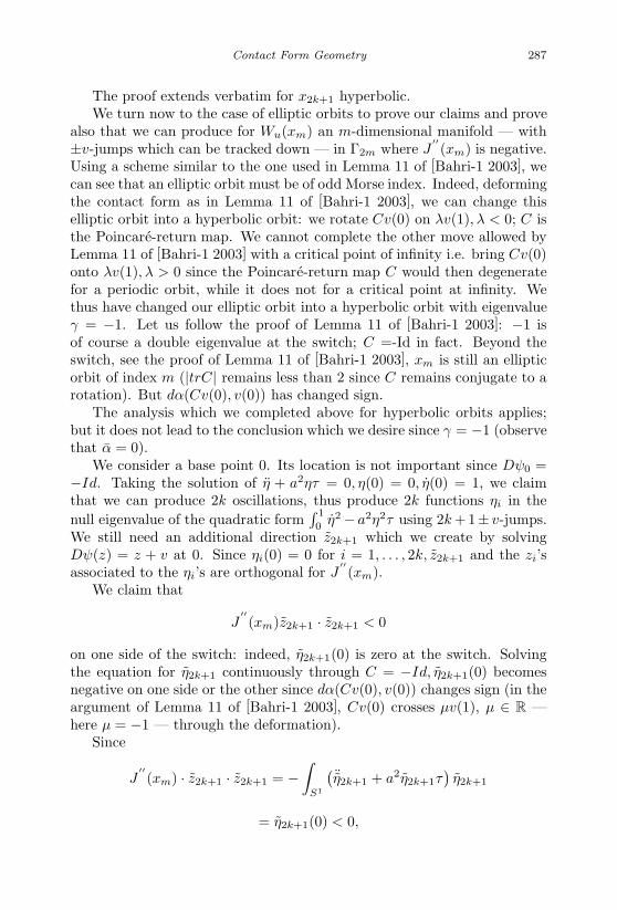
January 17, 2007 11:55 WSPC/Book Trim Size for 9in x 6in finalBB
Contact Form Geometry 287
The proof extends verbatim for x2k+1 hyperbolic.We turn now to the case of elliptic orbits to prove our claims and prove
also that we can produce for Wu(xm) an m-dimensional manifold — with±v-jumps which can be tracked down — in Γ2m where J
′′(xm) is negative.
Using a scheme similar to the one used in Lemma 11 of [Bahri-1 2003], wecan see that an elliptic orbit must be of odd Morse index. Indeed, deformingthe contact form as in Lemma 11 of [Bahri-1 2003], we can change thiselliptic orbit into a hyperbolic orbit: we rotate Cv(0) on λv(1), λ < 0; C isthe Poincare-return map. We cannot complete the other move allowed byLemma 11 of [Bahri-1 2003] with a critical point of infinity i.e. bring Cv(0)onto λv(1), λ > 0 since the Poincare-return map C would then degeneratefor a periodic orbit, while it does not for a critical point at infinity. Wethus have changed our elliptic orbit into a hyperbolic orbit with eigenvalueγ = −1. Let us follow the proof of Lemma 11 of [Bahri-1 2003]: −1 isof course a double eigenvalue at the switch; C =-Id in fact. Beyond theswitch, see the proof of Lemma 11 of [Bahri-1 2003], xm is still an ellipticorbit of index m (|trC| remains less than 2 since C remains conjugate to arotation). But dα(Cv(0), v(0)) has changed sign.
The analysis which we completed above for hyperbolic orbits applies;but it does not lead to the conclusion which we desire since γ = −1 (observethat α = 0).
We consider a base point 0. Its location is not important since Dψ0 =−Id. Taking the solution of η + a2ητ = 0, η(0) = 0, η(0) = 1, we claimthat we can produce 2k oscillations, thus produce 2k functions ηi in thenull eigenvalue of the quadratic form
∫ 1
0η2 − a2η2τ using 2k +1± v-jumps.
We still need an additional direction z2k+1 which we create by solvingDψ(z) = z + v at 0. Since ηi(0) = 0 for i = 1, . . . , 2k, z2k+1 and the zi’sassociated to the ηi’s are orthogonal for J
′′(xm).
We claim that
J′′(xm)z2k+1 · z2k+1 < 0
on one side of the switch: indeed, η2k+1(0) is zero at the switch. Solvingthe equation for η2k+1 continuously through C = −Id, η2k+1(0) becomesnegative on one side or the other since dα(Cv(0), v(0)) changes sign (in theargument of Lemma 11 of [Bahri-1 2003], Cv(0) crosses µv(1), µ ∈ R —here µ = −1 — through the deformation).
Since
J′′(xm) · z2k+1 · z2k+1 = −
∫S1
(¨η2k+1 + a2η2k+1τ)η2k+1
= η2k+1(0) < 0,
January 17, 2007 11:55 WSPC/Book Trim Size for 9in x 6in finalBB
288 Recent Progress in Conformal Geometry
our claim is established.We now claim — this will conclude the proof of Proposition 1 after a
perturbation argument bringing us back to the elliptic case — that, at theswitch,
∑i
∣∣2 ∂
∂ti
∑ =j
ccj η(tj)
+∂
∂tic2i ηi(ti)
∣∣ ≥ c∑
c2j
for z ∈ Span z1, . . . , z2k. zi is built using ηi. The ηj ’s are not here theηj ’s of the zj’s. They are the ηj ’s corresponding to the various solutions ofDψ(z) − z = v at the various nodes.
Computing as in the case when xm was hyperbolic (here xm is ellipticturned to hyperbolic with γ = −1), we find that such an inequality holdsfor all vectors (c1, . . . , c2k) which are not in the vicinity of unit vectors suchthat an odd number of ci’s are non zero. In fact, the zero eigenvectors ofthe matrices A — these matrices may be p × p, for any p ≤ m if someci’s are o(
√∑c2) — are equal to (1,−1, 1,−1, . . . ) with an odd number of
components (some intermediate ci’s might be zero).The η-component of all these eigenvectors read
∑cj ηj . Since the ηj are
equal to∑j+2k
j (−1)i−jηi with ηi > 0, such a combination∑
cj ηj with thecj ’s as above (an odd number of them is non zero and equal to 1 in absolutevalue) is far from Span z1, . . . , z2k: a vector in Spanz1, . . . , z2k has nocomponent on η2k+1.
The conclusion follows.Another line of proof uses Proposition 29, page 198 of [Bahri 1998]:
once C = −Id, we can perturb slightly C and bring C to have real eigen-values very close to −1 but different from −1. xm has become hyperbolicand the framework developed for hyperbolic orbits applies. This methodhas the definite advantage that the representation of Wu(xm) extend toiterates since the Morse index of iterates grows then linearly. Turning allsimple periodic orbits into hyperbolic orbits might be the best choice forthis homology.
Observe that the unstable manifold of xm, as we start near xm, is pro-vided by m ± v-jumps which have a location than can be tracked down.
* will designate below the location of such a ±v-jump
2.5.3 Hypothesis (A), Hypothesis (B), Statement of the
result
J on Cβ has critical points at infinity which are curves of UkΓ2k. Each Γ2k
is the space of curves made of k pieces of ξ-orbits alternated with k pieces
January 17, 2007 11:55 WSPC/Book Trim Size for 9in x 6in finalBB
Contact Form Geometry 289
of ±v-orbits. Denoting ai the time spent along ξ on the i-th ξ-piece of acurve of Γ2k, we introduce the functional J∞ equal to
∑ai.
The critical points at infinity of J on Cβ are the critical points of J∞ onUkΓ2k. They are described in [Bahri-1 2003], there is a vast zoology amongthem.
Let us recall the two following definitions:
Definition 1 A v-jump between two points x0 and x1 = xs1 is a v-jumpbetween conjugate points if, denoting ϕs, the one-parameter group of v, wehave: (
ϕ∗s1
α)x1
= αx1 .
Such points live generically on a hypersurface∑
of M .
Definition 2 A ξ-piece [y0, y1] of orbit is characteristic if v has completedexactly k (k ∈ Z) half revolutions from y0 to y1.
The description of the critical points at infinity x∞ of J goes as follows[Bahri-1 2003]:
• If x∞ has no characteristic ξ-piece, all its v-jumps are v-jumps be-tween conjugate points.
• If x∞ has some characteristic ξ-pieces, some additional conditionshave to be satisfied, see [Bahri-1 2003]. Any v-jump between non charac-teristic pieces is a v-jump between conjugate points.
To each x∞ is associated a suitable Poincare-return map C (see [Bahri-12003]) which preserves area.
We have shown in [Bahri-1 2003], Proposition 28 and Lemma 11, how,without modifying C, we can redistribute the v-rotation from a non-characteristic ξ-piece of orbit to another one at the expense of creatingadditional critical points at infinity with more characteristic ξ-pieces thanx∞. We may thus redistribute all the v-rotation from all the characteristicξ-pieces on a single one (up to ε > 0; a small amount of rotation is to beleft on each ξ-piece).
We then introduce:Hypothesis (A)
Assume that x∞ has at most one characteristic ξ-piece. As the numberof ξ-pieces of x∞ tends to infinity, the amount of rotation of v derived afterrescaling the rotation from all the non-characteristic ξ-pieces onto a singleone of them is at least 2π (the ξ-piece where the rotation is relocated is ofour choice).
Hypothesis (A) is not needed in the study of the flow-lines from a peri-odic orbit xm to a critical point at infinity having at least one characteristic

January 17, 2007 11:55 WSPC/Book Trim Size for 9in x 6in finalBB
290 Recent Progress in Conformal Geometry
piece x∞m−1 with m odd, i.e. in the Sections 2.5.4 and 2.5.5 of the present
work. It is needed later as we study flow-lines from xm to x∞m−1, with m
even or with x∞m−1 having only non degenerate ξ-pieces, see Section 2.5.6.
We also need to state our results another hypothesis, Hypothesis (B) as“companions” develop. The concept of “companions” is explained belowin 2.5.5.2, it is related to the existence of “false critical points at infinity”which we bypass by introducing small ±v-jumps near one of the edges ofone of their characteristic pieces, see [Bahri 1998], [Bahri-1 2003] for moredetails. “Companions” have all the same orientation and build “families”.The ±v-jumps of two distinct families do not overlap, see 2.5.5.2. Somethought shows that it is reasonable to expect that, as we decrease J andwe deform our curves in the Γ′
2ss and if the curves under deformation arenot in the vicinity of a critical point at infinity, the relative sizes of thevarious ±v-jumps should be bounded above and below by constants C and1C , unless the ξ-distance between two of them becomes very small (then,one of them might disappear if it has been created as a companion of theother one). As we approach a critical point at infinity, we cannot expectsuch estimates to hold uniformly since some of the ±v-jumps become largeand contribute to the edges while other ones live on the ξ-pieces and aresmall. However, we may assume that,
Hypothesis (B)On a given characteristic piece, all the ±v-jumps belonging to the same
family and which are a little bit inside(counting using v-rotation) the char-acteristic piece are of comparable relative sizes
The statement of Hypothesis (B) is very natural as long as some of the±v-jumps of a family do not concur to build an edge as the associatedconfigurations approach the critical point at infinity. However, if a givencompanion is part of one of the edges, therefore might be large and entersa characteristic ξ-piece, we may “tame” it as it enters so that it becomescomparable to the other companions or members of the other families inthe second case which are already inside. This can be done with the use ofa decreasing normal see Section 2.5.4.2 below or see [Bahri-1 2003], if thecritical point at infinity is true. If it is false, this issue does not arise sincea decrease can then be engineered with the introduction of a companion.
Under Hypothesis (A) and Hypothesis (B), we prove the following result:
Theorem 1 Let y∞m−1 be a critical point at infinity of index m−1 having
at least one characteristic piece. Assume that the maximal number of zerosof b on its unstable manifold is 2[m
2 ]. Assume that,if m is odd, m is largeand that all ξ-pieces are of (strict if degenerate)H1
0 -index at least 1. Letym be a periodic orbit of ξ of index m. Then, the intersection numberi(ym, y∞
m−1) for the flow of [Bahri-1 2003] is zero.

January 17, 2007 11:55 WSPC/Book Trim Size for 9in x 6in finalBB
Contact Form Geometry 291
Observation: The proof of Theorem 1 which we present here does notrequire any restriction on the H1
0 -index of the ξ-pieces if the flow-linesfrom ym to a neighborhood of y∞
m−1 do not involve companions, see 2.5.5.2for the definition of this notion. The case of zero H1
0 -index is discussed inAppendix 1. Hypothesis (A) and Hypothesis (B) are discussed in [6]. Flow-lines from ym to y∞
m−1 with y∞m−1 having only non characteristic ξ-pieces
have already been studied and ruled out for m large under Hypothesis (A),in [Bahri-1 2003].
2.5.4 The hole flow
2.5.4.1 Combinatorics
We start with an abstract result which may be viewed as an (elementary)observation in combinatorics.
We consider a sequence of 2k points each bearing a sign, + or −. Sucha sequence, together with the assigned distribution of signs, is called in thesequel a configuration.
A configuration contains at most 2k sign changes. A configuration with2k sign changes is called maximal.
Given a configuration, we consider two consecutive points. We assumek ≥ 2. We are given a sign of rotation (the same for all configurations,which are placed on a curve). Then, one of these points is the first one(using the positive rotation) and the other one is the second one. Let usassume that the sign + is assigned to the first one:
+· · ·1 2 3
.
The hole flow assigns signs to the intervals between the points as fol-lows:
Starting from the + assigned to 1 and independently of the configu-ration which we are facing, we assign signs to the remaining 2k − 1 pointsso that there is an alternance each shift between the + and − signs. Thus,we have
+ + − +· · · ·1 2 3 4
signs of the configuration

January 17, 2007 11:55 WSPC/Book Trim Size for 9in x 6in finalBB
292 Recent Progress in Conformal Geometry
1 2 3 4· · · ·+ − + −
alternating distribution
We then introduce on each interval[i, i + 1
]the sign of i in the alter-
nating distribution.
We claim:
Proposition 14 The original configuration of signs with the additionalintermediate signs has at most 2k sign changes.
Proof. We reverse the process and start with the alternating configura-tion. We add in between its jump the signs of the original configuration,inserting between 1 and 2, the sign of 2 for the original configuration andso forth. The result is the same. Viewed in this way, the claim of theProposition 14 is obvious.
Next, we discuss the choice of the starting point 1. We assume thatwe have some freedom of choice on 1 but the sign assigned to the choiceshould be + (i.e. the same, it could also be -) for all possible choices in theconfiguration. We then claim:
Proposition 15 Let us consider two distinct choices 1 and 1′ for 1 ex-tracted from the same configuration. Then either the configuration has asign repetition between 1 and 1′ or the two hole flows, the one correspondingto 1 and the one corresponding to 1′, coincide.
Proof. The alternating distributions for 1 and 1′ coincide if and only ifthere is an odd number of points between 1 and 1′. Then (and only then),the hole flows coincide.
If there is an even number of points between 1 and 1′, then there is aforced sign repetition in the configuration since 1 and 1′ bear the same sign.
An obvious observation which we will be using below states:
Observation 1. Given a configuration, assume that between two identicalsigns points there is an even number of points or that between two reversesigns points there is an odd number of points, then the configuration isforced to contain a sign repetition.
Next, we define:

January 17, 2007 11:55 WSPC/Book Trim Size for 9in x 6in finalBB
Contact Form Geometry 293
Definition 3 Given a configuration, an elementary operation on thisconfiguration is the reversal of the sign of one and only one point in theconfiguration.
Proposition 16 Given a configuration with a choice of 1 and the addi-tion of the intermediate signs of the hole flow, any elementary operationcompleted on a point of the configuration distinct from 1 does not increasethe number of sign changes of the configuration beyond 2k.
Proof. The hole flow is unperturbed. We are simply modifying the orig-inal configuration outside of 1.
Let us assume that we are considering several configurations σ which allhave the sign + on point j and have a forced repetition between positivesigns in
[i, j], i < j. Assume that two distinct alternating distributions
starting from a + can be defined on σ. We then have
Proposition 17 Choose a hole flow using one of the alternating dis-tributions. Introduce the corresponding intermediate signs in all intervals[k, k + 1] except those contained in [i, j]. Introduce furthermore a sign −between j and j + 1. The distribution of signs derived in this way has atmost 2k sign changes.
Another more obvious Proposition states:
Proposition 18 Given all configurations σ which have a sign repetition,we can introduce once an arbitrary additional sign on the interval of ourchoice without increasing the number of sign changes beyond 2k.
Observation 2. For Proposition 18, since we are not assuming that weproceed as for Proposition 14, we need to be careful and not use the holeflow as we are introducing the additional sign. We may use, however,elementary operations on the configurations σ as long as these elementaryoperations do not destroy one sign repetition at least.
Proof. [Proof of Proposition 17] In the case where the hole flow used is not the one provided by the use
of j as initial point, then this hole flow gives a − between j and j +1 (sincethe one of j gives a + in this interval). Thus this hole flow is compatiblewith the additional introduction of a − between j and j+1 and the numberof sign changes does not increase beyond 2k.
We consider now the hole flow provided by the use of j as initial point.We introduce a − between j and j + 1. This might increase the number ofzeros beyond 2k.
From i to j, we then have one sign repetition to the least. The full useof the hole flow associated to j (before the introduction of the − between

January 17, 2007 11:55 WSPC/Book Trim Size for 9in x 6in finalBB
294 Recent Progress in Conformal Geometry
j and j + 1) will result in an additional sign change between i and j withrespect to σ. This is obvious if this sign repetition occurs between j andj − 1. Then the hole flow would introduce a − between j − 1 and j whichare both positive.
Otherwise, starting from the + sign introduced by the hole flow betweenj and j +1, we evolve left towards i, alternating the signs. Before hitting arepetition of sign, the sign introduced by the hole flow agrees with the signof the left edge of the interval [k, k + 1] considered; otherwise an additionalsign change occurs and the claim follows:
+ + − − + +· · · ·
j − 2 j − 1 j j + 1←−etc.
Accordingly, the sign introduced has to disagree with the sign of the rightedge of the interval. But then, we arrive at the repetition, a sign changehas to occur.
We thus see that if we had used the hole flow between i and j, we wouldhave introduced a sign change, i.e. two additional zeros. The total numberof sign changes would be 2k. However, we have not used this hole flowbetween i and j. The introduction of the sign − between j and j +1 wouldonly provide for one sign change. Proposition 17 follows.
Observation 3. We could have introduced the + of the hole flow of j or[j, j + 1], only we would need to complete it close to j and introduce the− after it is the interval. With this provision, the statement of Proposition5 can be modified into “Introduce the corresponding intermediate signs —except those contained in [i, j].”
2.5.4.2 Normals
Given a critical point as infinity x∞, with a ξ-piece [x−0 , x+
0 ] which is char-acteristic, i.e. along which v has completed exactly a certain number m ofhalf-revolutions in the ξ-transport, we may define m + 1 nodes,
y0 = x−0 < y1 < · · · < ym = x+
0 .
These nodes are the points yi along the characteristic ξ-piece at which v,starting from y0 = x+
0 , has completed exactly i half-revolutions. To eachinterval (yi, yi+1), are associated a decreasing normal to the right and

January 17, 2007 11:55 WSPC/Book Trim Size for 9in x 6in finalBB
Contact Form Geometry 295
a decreasing normal to the left, in fact continuously varying families ofthese as follows.
We choose a point z in (yi, yi+1). We consider the vector v at z and wetransport it to y0 = x−
0 for the normal to the right and to ym = x+0 for the
normal to the left. We derive vectors which have components on [ξ, v] sincez is not a node. On the other hand, this characteristic ξ-piece is precededand is followed by ξ-pieces:
We take ξ at x′−0 , x
′+0 and we transport along v to y0, ym. We derive
vectors at y0, ym, equal respectively to (1 + A−1 )ξ + B−
1 [ξ, v] + µ−v, (1 +A+
1 )ξ + B+1 [ξ, v] + µ+v. We scale these vectors so that they compensate
exactly the [ξ, v]-component of the transport of v(z) at y0, ym:
We adjust the ξ and v-components by modifying the lengths of the ξand v-pieces. We derive in this way a normal to the right and a normal tothe left, ±N−
i (z),±N+i (z).

January 17, 2007 11:55 WSPC/Book Trim Size for 9in x 6in finalBB
296 Recent Progress in Conformal Geometry
We assign to each of them the orientation which corresponds to decreaseJ . Indeed, A−
1 , A+1 are not zero and∣∣J ′(x∞)N±(z)
∣∣ = ε±A±1 (A+
1 for A+1 ).
We derive our normals N±i (z).
To each of them is associated on orientation of the ± v-jump which isintroduced at z. Observe that there is a way to combine ±N−
i (z) with∓N+
i (z) in order to build a tangent vector into x∞; we simply assign thesame orientation to the v-jump at z. Because x∞ is critical in its stratifi-cation,
J ′(x∞) · u = 0.
Thus, if u is chosen with N−i on the left side, it was −N+
i on the rightside. N−
i and N+i corresponding to ± v-jumps having reverse orientations.
Accordingly, if we think of the curves x∞ + εN−i , x∞ + εN+
i , ε > 0, thesetwo curves will contain at z a ± v-jump with the same orientation. Thisorientation is the same throughout (yi, ui+1). We will refer to it in theremainder of this work as the preferred orientation of the normals in(yi, yi+1).
Definition 4 x∞ will be labeled false if the preferred orientation in(y0, y1) (or (ym−1, ym)) corresponds to the orientation of the left edge ofthe ξ-piece (respectively the orientation of the right edge of this ξ-piece).Otherwise, x∞ is sign-true.
We then have:
Proposition 19 If x∞ is sign-true, then the edge orientations are re-versed; otherwise, if m is odd, they agree.
Proof. Assume the left edge is positively oriented. Since x∞ is sign true,N−
0 (z) has − as preferred orientation. The preferred orientation switchesfrom a nodal zone to the next nodal zone. If m is even, N−
m−1(z) has + aspreferred orientation. Since x∞ is sign-true, the right edge has the negativeorientation. Proposition 19 follows.
2.5.4.3 Hole flow and Normal (II)-flow on curves of Γ4k near x∞
Γ4k is the space of curves made of 2k ξ-pieces alternating with 2k ± v-pieces. The 2k ± v-pieces build a configuration. Some of these ±v-jumpsmight be zero. We are assuming throughout section 2.5.4 that we cankeep track of all the 2k± v-pieces on our deformation classes. Letus consider such curves near x∞. Since they are close in graph to x∞, they

January 17, 2007 11:55 WSPC/Book Trim Size for 9in x 6in finalBB
Contact Form Geometry 297
must have a nearly ξ-piece (a “ξ-piece” broken maybe with ±v-jumps)close to the characteristic piece of x∞ and they must have nearly ±v-jumpscorresponding to the two edges of this characteristic piece.
Let us assume, in a first step, that we can associate without ambiguity a±v-jump on our curves which corresponds to the left edge. We will discussthis point later. We have “nodes” also, x0, . . . , xm which correspond toy0, . . . , ym and can be roughly defined using the v-rotation in the transportalong the nearly ξ-piece, up to o(1). We thus have preferred orientations oneach (xi, xi+1) and also normals N±
i defined on our curves (the definitionof preferred orientation, normals on x∞ extends easily).
Let us consider such a curve and the sequence of its ± v-jumps on thenearby ξ-piece. We denote the nodes (up to o(1)) by vertical lines, thesequences of ± v-jumps by ∗’s. We will also have a line indicating thepreferred orientation of each nodal zone, which will be labelled “Area of+” or “Area of −”. We will assume for the sake of simplicity that the leftedge is positively oriented and we will introduce the hole flow associated tothis left edge. Its distribution of signs will be indicated at the bottom ofour drawings:
Preferred orientation
(Area of ) Hole flow Observe that there is a ∗ with the positive orientation at x0 or nearby,
corresponding to the left edge. These should be also another one at xm ornearby (up to ambiguity) corresponding to the right edge.
We then have:

January 17, 2007 11:55 WSPC/Book Trim Size for 9in x 6in finalBB
298 Recent Progress in Conformal Geometry
Proposition 20 If at any point between two consecutive ∗’s, not closeo(1) to the nodes, there is agreement between the sign of the hole flow andthe preferred orientation, a decreasing normal can be defined which willbring the curve below the level of J(x∞) without increasing the number ofsign changes beyond 2k.
If there are several points of this type, these decreasing normals can beconvex-combined and the claims remain unchanged.
Proof. The point lies between two nodes (xi, xi+1). It is not close o(1)to the edges of this interval. We may use N±
i (ξ). This use decreases J at anegative rate bounded away from zero. Along this displacement, the nodesmay move. We need to decrease J only by an amount equal to o(1) so thatthe ± v-jump introduced by the normal is small and the nodes move little.The points when N−
i was introduced was not o(1) close to the nodes sothat the argument proceeds above J(x∞) − ε.
Since the sign(s) introduced by this (these) normals agree with thesign(s) of the hole flow associated to the left edge, the number of signchanges does not increase beyond 2k.
Corollary 5 If there is a node with no ∗ close to it, such a normal canbe introduced.
Proof. Indeed, there are then two consecutive ∗’s with points inbetweenthem not close o(1) to nodes and having reversed preferred orientations.One of them agrees with the sign of the hole flow on the interval.
Proposition 21 Assume that a ∗ is in between nodes, not close o(1)to any of them. Then, a normal can be introduced at the location of this∗ with the associated preferred orientation. This normal will decrease thecurve below J(x∞)−ε without increasing the number of sign changes beyond2k.
The use of several such normals together, also combined with the holeflow, has the same properties.
Proof. This corresponds to elementary operations on a configuration.Since the ∗ corresponding to the the left edge is not in between nodes,
we are not perturbing it. The conclusion then follows from Proposition 16above.
Definition of the ∗ of an edgeWe consider the case of the left edge and an approaching configuration
σ. We can define an “average left edge” θ which varies continuously with σ.We consider a fixed small number δ > 0 and all the ± v-jumps of σ whichare contained in a δ-neighborhood of θ,Vδ. δ is fixed as σ approaches x∞.

January 17, 2007 11:55 WSPC/Book Trim Size for 9in x 6in finalBB
Contact Form Geometry 299
δ is as small as we may wish. These ± v-jumps are ordered according to thetime-parameter on the corresponding curve. c0 is a fixed small parameter.We consider the last of the ± v-jumps in Vδ of size at least 2c0 having theorientation of the left edge. If this last ± v-jump is defined unambiguously,the corresponding ∗ is the ∗ of the left edge. As this ± v-jump becomesof size 2c0 or starts to move out of Vδ, we may have an overlap of variouschoices for this ± v-jump and therefore of various choices for the ∗ definingthe left edge. A problem of definition for our deformation arises whenthese various ∗’s define different hole flows; we will address this issue in ourarguments. As we point out below, in the proof of Proposition 24, whenthe last of these large ± v-jumps becomes small (of size c0
2 < c < c0), wecan move it away from this Vδ-neighborhood while decreasing J . This usesProposition 30 (below).
2.5.4.4 Forced repetition
The construction completed in 2.5.4.3 rests upon the definition of the holeflow which, in turn, rests upon the choice of a representative for the left edgeIf there is a clear representative for this left edge—as when the left edge ofthe curve neighboring x∞ is large and isolated from the other ± v-jumps—this hole flow is well defined. But if there is an ambiguity—as when the left“edge” of the neighboring curve is made of several ± v-jumps having thesame orientation—then the hole flow might not be well defined. In view ofthe proof of Proposition 17, the configuration has then to contain a forcedrepetition corresponding to the orientation of the left edge (positive). Thus,
Proposition 22 If the construction of 2.5.4.3 cannot be carried out at acurve x near x∞, then the configuration σ of x contains a forced repetition(with the positive orientation) near the left edge of x∞. Outside of thecurves x having such configurations, the constructions of 2.5.4.3 can becarried out continuously. Furthermore,
Proposition 23 Let x be a curve neighboring x∞ with a configurationσ for which the hole flow of the left edge is defined without ambiguity. Ifthe construction of 2.5.4.3 cannot be carried on a whole neighborhood of x,then σ contains a forced repetition between the representatives of the leftedge and the right edge of x∞.
Proof. In view of 2.5.4.3, we must then have at least a ∗ at each nodey1, . . . , ym−1. Two very close ∗’s can be separated, see Proposition 30,below. Thus, there is exactly one ∗ at each node (close o(1)). In view of2.5.4.3 again, we cannot have then a ∗ between nodes. Finally, before thefamily of ∗’s at x1, . . . , xm−1, there must be a ∗ at x0 (close o(1))) with the
January 17, 2007 11:55 WSPC/Book Trim Size for 9in x 6in finalBB
300 Recent Progress in Conformal Geometry
orientation of the left edge. A similar statement can be made for the rightedge.
We are assuming that x∞ is sign true. Thus, if m is odd, the edgeorientations agree and we have a sign repetition in between. The argumentrepeats for m even since the edge orientations are then reversed.
We continue our study of such configurations and observe:
Proposition 24 A neighborhood U of such configurations may be chosenso that the construction of 2.5.4.3 on ∂U reduces to the use of the normal(II) flow on ∗’s which do not represent the left edge, while all configurationsin U contain a forced repetition.
Proof. If U is taken small enough, all the configurations will have exactlyone ∗ in a neighborhood of a node. On ∂U , one of these ∗’s has to be “away”from its corresponding node and the normal (II) flow can then be appliedto this ∗. Since this ∗ might represent the left edge, we have to modify U .We observe that if any of the ∗’s which are located near x1, . . . , xm−1 movesmore than o(1) from the related node, the configuration has crossed in aregion where the use of the normal (II) flow on a ∗ which does not representthe left edge is available. We then consider the first ∗(∗o) before the ∗ atx1 having the same orientation than the left edge and the first ∗(∗m) afterthe ∗ at xm−1 having the same orientation than the right edge. If one ofthese ∗’s advances (for x1) or recedes (for xm) towards the neighboring ∗on the characteristic piece, then this ∗ has to move out of the node and theconfiguration crosses into a region with a good normal (II) flow.
One of these ∗’s could also exit the characteristic piece and reverse signor become small after leaving the edge (forcing thereby all preceding ∗’s onthe left, all following ∗’s for the right to leave also). But since we need arepresentative for the edge, a ∗ at the node x1 of xm−1 has to move out ofthe node, with the same conclusion.
Finally, one of these ∗’s, ∗o or xm, could become smaller and smaller,reaching a size c, c0
2 < c < c0, c0 small and fixed. Since all our configura-tions are near x∞, one or several large ± v-jumps build the edges and noneof them is then ∗0 or ∗m, whichever has become small. We are assuming,for example, that ∗0 is becoming small. There is a ∗, denoted ∗1, withino(1) of x1 and no ∗ between ∗0 and ∗1.
Using Proposition 30 (see below) on such configurations, we can move∗0 away from the large ± v-jumps of the edge towards x0, while decreasingJ . Once ∗0 is a little bit away from the edge, since it does not representit anymore (it is small and slightly away from the “average edge”), thenormal (II) flow can be used on it in order to decrease below x∞. Thiscovers in particular the situation, near ∂U , when the jump ∗0 defining the

January 17, 2007 11:55 WSPC/Book Trim Size for 9in x 6in finalBB
Contact Form Geometry 301
left edge (or ∗m for the right edge) is becoming small and is being replacedby another jump, another ∗ for the left edge. In the transition, the initial∗0 can be moved inside the characteristic piece. As the definition of the ∗associated to the left edge changes, the normal (II) flow can be used on thisinitial ∗0 to decrease below x∞. We thus see that we can track down allthese configurations and that they contain, throughout, a forced repetitioninside the characteristic piece, i.e. between ∗0 and ∗m and that the exitset is through the frontier ∂U of a domain U where a normal (II) flow isavailable. This includes the case when the jump at ∗0 or ∗m becomes of asize c, c0
2 < c < c0. Then we are changing the definition of ∗0 or ∗m forthe left or right edge (respectively). In the transition region, the normal(II) flow (without any use of another hole flow on the introduction of anadditional± v-jump) can be used on the jump ∗0 or ∗m which has becomesmall.
Observation 4. Some further thinking shows that the above reasoningon ∗0 and ∗m is not needed. The basic argument runs as follows: U isdefined to be the set on Wu(x2k) near x∞
2k−1 where there is a * near eachnode x1, . . . , xm. Would there be other ∗’s in between nodes, the normal IIflow can be used on them. This is in particular the case on ∂U . Assumingthat there is a * near each node and none in between, in U1 ⊂ U1 ⊂ U ,we can introduce in each zone a decreasing normal corresponding to thepreferred orientation. This corresponds to a distribution of signs which be-haves exactly as a hole flow, only that the initial 1 is not defined for thisdistribution of signs. However, since we are introducing this alternatingdistribution once, we do not increase the number of signs changes beyond2k. The definition of this alternating distribution is clear and unique. Theuse of this distribution is limited to U1, shielded from U c. It convex - com-bines naturally with the normal II flow-. The advantage of this argumentis that it bypasses the use of Proposition 23 and the forced repetition in U ,thus the definition of ∗0 and ∗m as well as of the ∗’s of the edges as thispoint.
2.5.4.5 The Global picture, the degree is zero
Two or more ∗’s can be assumed not to be too close. Otherwise, usingProposition 30 below we can bring them apart (in a global deformation)while decreasing J .
We have now four regions and the transition between them; there is firstU and U1 ⊂ U , a smaller version of U . On U1 we use the normal N−
0 (z)and extensions of it (alternating sign distribution starting with N−
0 (z) be-tween nodes) related to (x0, x1) and we convex-combine it with the normal(II) flow as above on U − U1. Using Proposition 18 and Observation 2,

January 17, 2007 11:55 WSPC/Book Trim Size for 9in x 6in finalBB
302 Recent Progress in Conformal Geometry
we have not raised the number of zeros beyond 2k. Outside of U , we usethe construction 3. when available. It provides with combinations of holeflow and normal (II) flows in the region where the representative of theleft edge is defined properly. In the remainder, we have several possiblerepresentatives. We may assume that the hole flows corresponding to theserepresentatives do not coincide. Otherwise, we find no problem in orderto define our decreasing deformation. We then must have a forced repeti-tion. In order to decrease J in this region, we introduce again a normalN−
0 (z) related to (x0, x1). This is completed as follows: we may assumethat there is no * “between nodes” (i.e. not in the immediate vicinity ofnodes). Otherwise, we use the normal (II) flow maybe on several nodesat the same time. This flow can easily be seen, after the construction ofN−
0 (z), convex-combined through “sliding” with N−0 (z) (we can use sev-
eral consecutive copies of N−0 (z) in the same interval between two ∗’s to
complete the convex-combination). Under this assumption, there is a last∗ “before the node at x1”(i.e. before x1 and not in the vicinity of x1). Thislast ∗(∗0) is close to the left edge.
N−0 (z) is introduced betweeen this * and x1. It is introduced in the
“middle” of the first nodal zone. The representatives for the left edge arechosen among the v-jumps of size ≥ c0 having the orientation of the leftedge and close to the average left edge. Thus N−
0 (z) is introduced after anyof these representatives. It is also introduced before (on the characteristicpiece) the ±v-jump corresponding to the hole flow (whatever it is) in theinterval starting with ∗0. In fact, since the only ±v-jumps needed for thehole flow can be located in the vicinity of the nodes and the other onestaken to be zero, we may assume that N−
0 (z) is introduced before any±v-jumps used by any of the hole flows on the configuration. Thus we donot introduce v-jumps “in the edge” i.e. before ∗0. Since the competing ∗’sfor the definition of our hole flows are before ∗0 (∗0 possibly included), wedo not introduce ±v-jumps between the starting 1’s of our hole flows.
We have to worry about the convex-combination of N−0 (z) and one of
the competing hole-flows, namely the one such that the ±v-jump introducedbetween ∗0 and ∗1 (the next ∗, to the right of ∗0) is not negative. If ∗1 isnot beyond x1, no positive v-jump is introduced before ∗1 since this v-jumpwould not decrease J . We need to worry only if ∗0 is a positive v-jump.Otherwise if ∗0 is negative or zero, N−
0 (z) and ∗0 are compatible (includingif ∗0 is zero).
If ∗0 is positive, it generates a hole flow which may be viewed as one ofthe competing hole flows.
We thus may view ∗0 as a positive j generating one hole flow and wehave another i, i < j, with a ∗ at i, positive again, in the left edge, defin-ing the competing hole flow. We thus have replaced our two competing

January 17, 2007 11:55 WSPC/Book Trim Size for 9in x 6in finalBB
Contact Form Geometry 303
∗’s with the ∗ at i and ∗0. We then invoke Proposition 17: the use ofN−
0 (z) is allowed without increase of the number of sign changes beyond2k. Along the decreasing deformation, ∗0 is untouched and therefore itssign unchanged, unless it moves inside the characteristic piece. But, then,N−
0 (z) locates precisely at ∗0 and becomes the normal II flow which is com-patible with all hole flows. At the boundary of the region where there isa hole but not a well-defined representative for the left edge, N−
0 (z) willconvex-combine with each of the hole flows (used on disjoint closed regions)and by Proposition 17, this combination will not raise the number of zerosbeyond 2k.
With the support of a drawing:
Using now a standard deformation lemma, we may assert that a givencompact K in Jc∞+ε, with c∞ = J(x∞), can be deformed into Jc∞−ε′ ∪V ,where V is contained in a neighborhood, as small as we please, of x∞. In thisneighborhood, the nodes are defined up to o(1). If K is in Γ4k and if its ± v-jumps can be tracked down, as is the case fo K’s contained in Wu(x∞
2k), x2k
a periodic orbit of index 2k, then after the use of the deformation lemma,we may apply our construction to the part of the deformed set in V . Theresult is that all of K is moved below c∞. Thus—and this is the form underwhich we will use this conclusion:
Proposition 25 Let x∞2k−1 be a true critical point at infinity of index
2k − 1 (x∞2k−1 could be a cycle at infinity) with at least one characteristic

January 17, 2007 11:55 WSPC/Book Trim Size for 9in x 6in finalBB
304 Recent Progress in Conformal Geometry
piece. Assume that all the oscillations on Wu(x2k) near x2k−1 are small(i.e. no Fredholm issue). Then, the intersection number of Wu(x2k) withWs(x∞
2k−1) is zero if there is no intermediate false critical point at infinitybetween x2k and x∞
2k−1.
2.5.5 Companions
2.5.5.1 Their definition, births and deaths
When we defined normals, we defined also what a “preferred orientation”was. If the preferred orientation on (y0, y1) or (ym−1, ym) coincides withthe orientation of the closest edge, x∞ is labelled false.
False x∞’s can be bypassed downwards, without increase in the numberof sign changes but at the expense of introducing a normal, i.e. a new ± v-jump which is the immediate neighbor of an edge ± v-jump bearing thesame orientation. Bypassing such x∞’s modifies our configurations in oneregard: individual jumps are replaced by families of companions arounda single original jump. If we wish to extend Proposition 25 to this newsituation, we find out very soon that the reasoning has to be different sincea family can control several nodes through its various companions.
Let us observe though that as long as there are two companions ormore in a family, the original companion is among them and it survivestheir death, with the same orientation, i.e. as an added companion goesaway, its original companion survives its death, with the same orientation.Elsewhere, this original jump might switch signs, but it then has no com-panion.
This observation is important as can be seen when we try to understandhow a true critical point at infinity y∞ dominates another true critical pointat infinity x∞. If x∞ has several characteristic pieces, then x∞ is in fact acluster of several critical points x∞
s , x∞s−1, . . . , x
∞s−. x∞
s− is the critical pointat infinity which has the same graph as x∞ but its associated cycle doesnot use any full (half)-unstable manifold associated to a characteristic ξ-piece. x∞
s−+1 builds a cycle through a combination of various characteristicξ-pieces, one at a time, as pieces of a puzzle. x∞
s−+2 using two of them at atime, etc. As soon as y∞ dominates x∞
s , it has to dominate x∞s−1, . . . , x
∞s−
and if we try to cancel Wu(y∞)∩Ws(x∞s ), it is in fact Wu(y∞) ∩ Ws(x∞
s−),a stratified space of top dimension which we need to move down past thelevel of x∞. Along this stratified space, configurations vary, companionsare given birth to, then die, etc. It is a full story which we are facing.
The following Proposition which we will prove later reduces considerablythis otherwise quite complicated scenery:

January 17, 2007 11:55 WSPC/Book Trim Size for 9in x 6in finalBB
Contact Form Geometry 305
Proposition 26 When a companion in a family which is not a family ofan edge, and such that the v-rotation between its extreme companions, onthe left and on the right, is less than π − δ, δ > c, becomes extremely small,it can be brought back close to its closest surviving companion (towards theoriginal companion).
We will prove this Proposition later. Its proof involves slight modifica-tions of the flow which we will indicate later. It is of relevant importancein that no companion can appear suddenly or disappear somewhere. Allthese births and deaths are within the family.
2.5.5.2 Families and nodes
a. Critical Configurations of families
The basic observation which we make here is that a family of two compan-ions or more cannot overlap a node which is not x0 or xm, i.e. an edgenode; or if it does, the associated configuration, in fact all the configura-tions containing such an overlap, can be moved continuously down, pastJ(x∞).
Indeed, the family covers then at least two distinct preferred orienta-tions; one of them coincides with the orientation of the ± v-jumps of thefamily or by creating a new companion (obviously with the same orienta-tion) in between existing companions, we can move all these configurationsdown.
Each time a deformation (obviously a J-downwards deformation) is de-fined, we study the configurations which are “at the boundary” of sucha deformation, i.e. the transitions to other configurations where such adeformation cannot be defined.
For the deformations defined above, their definition is directly relatedto the overlap. As the overlap fades away and the family recedes (up too(1)) on one side of the node, this deformation cannot be defined anymore.Thus, we have to find another way of decreasing these configurations oncethe overlap on a node is one-sided up to a small constant c. We will thenscale the growth of the companion which we grew or introduced, putting itto a smaller and smaller growth. It does not suffice anymore to move theconfiguration down. We have to find other, compatible ways to decrease Jover such configurations (by deforming them).
The configurations which we consider below are therefore configurationssuch that any family is within o(1) of at most two consecutive nodes. In-deed, otherwise, there is a definite overlap. On the other hand, we willassume that the hole flow of the left edge is well defined, which amountsto say that the family associated to the left edge is defined without am-
January 17, 2007 11:55 WSPC/Book Trim Size for 9in x 6in finalBB
306 Recent Progress in Conformal Geometry
biguity, then its hole flow can be used in between families, which impliesthat continuously defined and decreasing deformations can be defined onconfigurations such that one node among x1, . . . , xm−1 is not within o(1)reach of a family. The hole flow convex-combines in a natural way with theprevious flow related to the overlaps. They coexist without increasing thenumber of sign changes in the configuration beyond 2k.
Lastly, we observe that if a family lies between two consecutive nodes,within c > 0, c small and fixed, of each node, then we can think of thewhole family as reduced to its original companion.
Such a family is obviously not associated to an edge of the character-istic piece and the use of the normal (II) flow, increasing or decreasingall members of the family at once, whatever suitable, even reversing, alltogether, their orientation, is available for it. Again this portion of theflow convex-combines with the other portions defined above and there is nofamilly which cannot have at least a node with o(1) reach.
We thus define:
Definition 5 A critical configuration on a characteristic ξ-piece of x∞ isa configuration such that every node x1, . . . , xm−1 is within o(1)-reach ofone family, every family with support on the characteristic piece is withino(1)-reach of a node at least and every such family is within o(1)-reach ofat most two consecutive nodes.
We then have:
Proposition 27 Consider all critical configurations such that one familyis within o(1)-reach of two consecutive non-edge nodes. Assume that thehole flow of the left edge is well defined. Then all these configurations canbe deformed below J(x∞) using the hole flow of the left edge.
Proof. On each side of the area where the family sits (up to o(1)), thepreferred orientations agree. There is one side where the preferred orien-tation agrees with the sign of the ± v-jump introduced by the hole flow aswe use it.
We extend Proposition 27 as follows:
Proposition 28 Assume that a critical configuration σ does not containa forced sign repetition, with the sign of the left edge, between the familydefining this left edge and x0+c, c > 0 small. Then, Proposition 27 extendsto all such σ’s which contain a family within o(1) of x0 and x1.

January 17, 2007 11:55 WSPC/Book Trim Size for 9in x 6in finalBB
Contact Form Geometry 307
Remark 1 x0 + c stands for a point close to x0 inside the characteristicpiece.
Proof. This family has to have the orientation of the edge, otherwise wecould separate it away from the edge (a family with the wrong orientationcannot leave the characteristic piece through the left edge unless it is fol-lowed by a family having the orientation of the edge which will take theplace of the family of the edge. Such a family would be after x1 and wewould have ample room to separate the edge and the family with the wrongorientation.)
The hole flow starting at this family has to agree, under our assumption(no sign repetition near the left edge, with the sign of the left edge), withthe hole flow defined by the family of the edge. This hole flow provides asign + after x1 and this agrees with the preferred orientation of (x1, x2).
Corollary 6 If a critical configuration σ contains two or more familieswithin o(1)-reach of two consecutive nodes, then either σ can be decreasedbelow J(x∞) in a continuously defined deformation or σ contains a forcedsign repetition, with the sign of the left edge, between the family definingthis left edge and x0 + c, c > 0 small.
Proof. At least one of the families does not control the nodes xm−1, xm
but controls another pair of nodes.
b. Critical configurations with one family within o(1)-reach of(xm−1, xm)
We thus see that the only critical configurations which we have not beenable to decrease below J(x∞) are those such a family is within o(1)-reach of(xm−1, xm). If an additional family is within o(1)-reach of two other nodes,we have defined such a deformation. However, once we define a decreasingdeformation for the configurations with only one family within o(1)-reach of(xm−1, xm), we need to check that the flows convex-combine and generatea global decrease below J(x∞), without increase of the number of zerosbeyond 2k.
Let us consider such a configuration:

January 17, 2007 11:55 WSPC/Book Trim Size for 9in x 6in finalBB
308 Recent Progress in Conformal Geometry
We use in the sequel the hole flow of the right edge, between xm−3 andxm−1. It is well defined if there is no repetition in the configuration relatedto this edge. We make this assumption in a first step. Since we are usingthe hole flow of the left edge in other parts, we need to convex-combine insome regions and this needs careful checking. This is the reason why weare not starting from a critical configuration and we are simply assumingthat a family controls xm−1 and xm.
The normal (II) flow on intermediate families is compatible with bothflows. Thus, we assume that every family has to be within o(1)-reach of anode and that it does not overlap over a node. We cannot yet assert thatevery node is controlled by a family.
We focus on xm−2.
Proposition 29 If no family is within o(1)-reach of xm−2, then the twohole flows can be convex-combined near the configuration on the intervalpreceding (xm−1, xm).
Proof. Since x∞ is sign-true, the preferred orientation of (xm−2, xm−1)is + and the preferred orientation of (xm−1, xm−2) is −. If the two holeflows disagree, then one requires the use of + between the family controllingxm−1, xm and the previous family, while the other one requires the use of−. The introduction of + follows the introduction of − and is compatiblewith the orientation of the family controlling (xm−1, xm). The convex-combination can proceed. It makes use of a single interval in the transitionbut, on each side, the use of the full hole flow is warranted.
Thus a family must be within o(1)-reach of xm−2, on one side or on theother side, with no overlap.

January 17, 2007 11:55 WSPC/Book Trim Size for 9in x 6in finalBB
Contact Form Geometry 309
Let U0 be a small neighborhood of the set of all configurations containingsuch a behavior, with no repetitions related to the right as well as to theleft edges.
Let F1 be the family within o(1)-reach of (xm−1, xm) and F2 be thefamily within o(1)-reach of xm−2
We claim:We consider in what follows three distinct consecutive families of com-
panions F1, F2, F3. F2 follows F3 and F1 follows F2. The support of F2
is inside a characteristic piece. We define the thickness T of F2 to bethe ξ-length between the first and the last companion of F2. We assumethroughout this part that the maximal size of a companion of F2 is o(T )and that T ≤ π
2 .
We then claim:
Proposition 30 We can rearrange F1, F2, F3 along a J-decreasing de-formatiion so that
i) The v-rotation between the right edge of F2 and the left edge of F1
is at least π − δ, where δ is a fixed positive number.

January 17, 2007 11:55 WSPC/Book Trim Size for 9in x 6in finalBB
310 Recent Progress in Conformal Geometry
ii) If T > 0, the v-rotation between the left edge of F2 and the rightedge of F3 is also at least π − δ. It is also at least π − δ if the v-rotationbetween F1 and F2 is more than π + δ. The first part of ii) has to beunderstood as a statement involving T after the deformation.
iii) Assume that F2 had initially a thickness T ≥ c, a fixed positivenumber c ≤ π
2 . Assume that F2 can be separated in two distinct families ofconsecutive ± v-jumps F−
2 , F+2 and that the maximum size of the jumps of
F+2 , s+ is small o of the maximum size of the jump of F−
2 , s−. Then, afterdecreasing deformation, all of F+
2 is at a ξ-distance equal to c100 at most of
F−2 . Furthermore, s+ changes into s1
+, with 1cs+ ≤ s1
+ ≤ cs+ and s− intos−(1 + o(1)).
Proof.
Proof of i) See Section 2.5.8, Proposition 32. Given two consecutive ± v-jumps, the ξ-piece between them has H1
0 -index zero (is minimal) if thev-rotation along this ξ-piece is at most π − δ. If it is less than π − δ,then we can “widen” the intermediate ξ-piece between them by insertingv-verticals to the left of left jump or to the right of the right jump. We takethe side which corresponds to the smallest jump. In this way, no v-jumpdisappears. We need to take this cautionary step only if the jumps haveopposite orientations. This widening process never stops as long as thev-rotation is less than π. There are indeed no “small” rectangles made oftwo small ± v-jumps and two large ξ-pieces as long as the v-rotation alongthese ξ-pieces is less than π − δ. See Section 2.5.8 for further details.
Proof of ii) Once the distance between F1 and F2 is π− δ or more, we turnto F2 and F3 and complete the same process. If the thickness of F2 does notfade away in this process, then it goes to the end and the distance betweenF2 and F3 is at least π − δ. It can also happen that the thickness of F2 iszero or becomes very close to zero while the distance between F1 and F2 ismore than π.
At the end of the process, if either T > 0 or the v-rotation between F1
and F2 is more than π, the v-rotation between F2 and F3 is at least π − δ.
Proof of iii) The claim can be derived from the case when F−2 is reduced
to a single ± v-jump of size c− and F+2 is reduced to a single ± v-jump of
size c+, with c+ = o(c−) assume that both ± v-jumps have the positiveorientation for example.

January 17, 2007 11:55 WSPC/Book Trim Size for 9in x 6in finalBB
Contact Form Geometry 311
Our deformation is the composition of two deformations. The first oneinvolves a recession of the right v-jump towards the left. This one might notbe (in fact is not) J-decreasing. We thus have to compose this deformationwith a second one which decreases J . To define the first deformation, weconsider the ξ-orbit through x+ and we consider a distance T+ along thisξ-orbit before x+; we find a point x−:
We introduce the v-vertical at x−. There is a unique piece of ξ-orbitbetween the v-vertical corresponding to the v-jump of size c− and the v-vertical at x−:
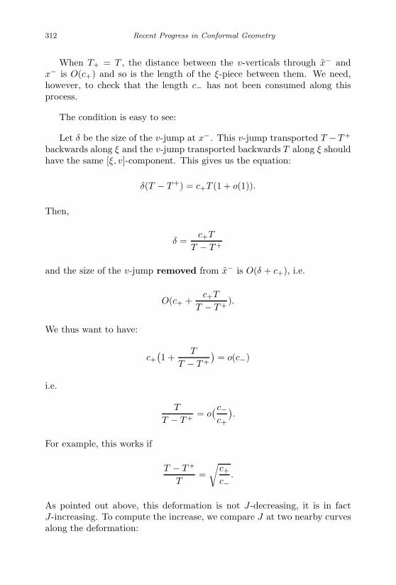
January 17, 2007 11:55 WSPC/Book Trim Size for 9in x 6in finalBB
312 Recent Progress in Conformal Geometry
When T+ = T , the distance between the v-verticals through x− andx− is O(c+) and so is the length of the ξ-piece between them. We need,however, to check that the length c− has not been consumed along thisprocess.
The condition is easy to see:
Let δ be the size of the v-jump at x−. This v-jump transported T −T +
backwards along ξ and the v-jump transported backwards T along ξ shouldhave the same [ξ, v]-component. This gives us the equation:
δ(T − T+) = c+T (1 + o(1)).
Then,
δ =c+T
T − T+
and the size of the v-jump removed from x− is O(δ + c+), i.e.
O(c+ +c+T
T − T+).
We thus want to have:
c+
(1 +
T
T − T +
)= o(c−)
i.e.
T
T − T += o
(c−c+
).
For example, this works if
T − T+
T=√
c+
c−.
As pointed out above, this deformation is not J-decreasing, it is in factJ-increasing. To compute the increase, we compare J at two nearby curvesalong the deformation:

January 17, 2007 11:55 WSPC/Book Trim Size for 9in x 6in finalBB
Contact Form Geometry 313
The change in J is ε − ∫∆ α.∆ is obtained from εξ by v-transport during a time c. Thus, since
˙λ + µη = η
η = −λ
ε − ∫∆ α = O(δ2).The size δ of the v-jump has been computed above. It is c+T
T−T+ (1+o(1)).Thus,
dJ
dT +=
O(c2+T 2)
(T − T +)2
and
∆J = O(c2+T )
√c−c+
= O(c3/2+
√c−T ).
In order to define a decreasing deformation, we need to find another de-formation of the same curves which would be decreasing and which wouldconvex-combine with the previous one.
We recall for this that F2 has support in a characteristic piece and thatits thickness T is less than π
2 and larger than c > 0. Thus, one of thesev-jumps (we are assuming for the sake of simplicity that F2 is made of twojumps. There is no loss of generality in this assumption) is c/2 to the leastaway from a node. A decreasing normal can be defined at such a jump andit will warrant a decrease of J at a rate ≥ Ac, A > 0 fixed. Consuming asize c+/100 of the related v-jump (this is possible since c+ = o(c−)) whichwe set aside and do not touch during the first deformation if the normal

January 17, 2007 11:55 WSPC/Book Trim Size for 9in x 6in finalBB
314 Recent Progress in Conformal Geometry
has to be taken at x+, we warrant a constant decrease of J . This works ifthe normal at x+ or x− decreases the size of the v-jump.
It also works in the other case at x−. If the normal at x+ increases thesize of the v-jump, then we engineer the decrease of J by increasing the sizeof the v-jump as it travels along the first deformation. We then stop — toavoid entering into technical difficulties — when the right v-jump is at c
100of the left v-jump since then the distance to a node might have shrinked to
c200 . We could of course have used other smaller fractions of c.
The statement about s+ and s− follows from the estimate on ∆J andon δ with T − T + ≥ c
100 . This proof contains the proof of Proposition 26as well.
Proposition 31 If xm−2 is not x0, all such configurations in U0 can bedeformed below J(x∞) and the deformation can be convex-combined, withglobal decrease and no increase in the number of sign changes beyond 2k,with the hole flow of the left edge.
Proof. The proof of Proposition 31 uses Hypothesis (B). On all the con-figurations which we are considering, there are three consecutive families.F1 and F2 are as above. F3 is the first family before F2. We pick up asmall constant δ = c3
200 and we reorder these families, along a J-decreasingdeformation as described in Proposition 32, Section 2.5.8 below.
F1 and F2 are now away by π − c3
200 to the least. If they are away bymore than π + c or if F2 has some thickness, then F2 and F3 are also awayby π− c3
200 to the least. Finally, the two-edge jumps of F2 are of comparablesize. Otherwise, the thickness of F2 is less than c
100 . We assume in a firststep that xm−3 is not x0. We distinguish five distinct situations accordingto the behaviour of the right and left edge of F2, denoted L.E.F2 andR.E.F2 with respect to xm−2.
1st Case: The distance (all distances are along ξ) of R.E.F2 to xm−2 ismore than c. Since the v-rotation between R.E.F2 and L.E.F1 is at leastπ − c
2 , there is a hole at xm−1. We use the hole flow of the left edge in thishole to decrease J . Observe that we need to prove Proposition 31 if thehole flows of the right edge and hole flow of the left edge do not coincide.This implies at once that the hole flow of the left edge should yield a −between F1 and F2. If it yields a +, Proposition 31 is a straightforwardstatement since this + coincides with the orientation of F1, and is providedby the hole flow which we are using outside of U0.2nd Case: The distance of R.E.F2 to xm−2 is less than c but more thanc2 and the distance of L.E.F2 to xm−2 is less than c3
100 .F2 has then a thickness larger than c
100 . This implies that its right edgejump and its left edge jump (we may assume that there are only two of
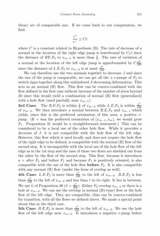
January 17, 2007 11:55 WSPC/Book Trim Size for 9in x 6in finalBB
Contact Form Geometry 315
them) are of comparable size. If we come back to our computation, wefind:
c+
c−≥ Cc
where C is a constant related to Hypothesis (B). The rate of decrease of anormal at the location of the right edge jump is lowerbound by C1c sincethe distance of RE.F2 to xm−2 is more than c
2 . The rate of variation ofa normal at the location of the left edge jump is upperbounded by C c3
100
since the distance of L.E.F2 to xm−2 is at most c3
100 .We can therefore use the two normals together to decrease J and since
the size of the jump is comparable, we can get all the ± v-jumps of F2 toswitch signs together along this unhindered J-decreasing deformation. Thisacts as an normal (II) flow. This flow can be convex-combined with theflow defined in the first case without increase of the number of zeros beyond2k since this would yield a combination of normal (II) flow (generalized)with a hole flow (used partially near xm−1).3rd Case: The R.E.F2 is within c
2 of xm−2 while L.E.F2 is within c3
100of xm−2. We then introduce a normal between R.E.F2 and xm−1 whichyields, since this is the preferred orientation of this area, a positive v-jump. (If + was the preferred orientation of (xm−1, xm), we would growF1. Proposition 31 would be a straightforward statement.) This can beconsidered to be a local use of the other hole flow. While it provides adecrease of J , it is not compatible with the hole flow of the left edge.However, this flow which is used locally and does not require the hole flowof the right edge to be defined, is compatible with the normal (II) flow of thesecond step. It is incompatible with the local use of the hole flow of the leftedge as in the 1st step and the uses of these two flows are shielded one fromthe other by the flow of the second step. This flow, because it introducesa + after F2 and before F1 and because F1 is positively oriented, is alsocompatible with the use of the hole flow before F2. It is also compatiblewith any normal (II) flow (under the form of overlap as well).4th Case: L.E.F2 is more than c3
100 to the left of xm−2. R.E.F2 is lessthan c3
100 to the left of xm−2 and less than c to its right. It lies in between.We use i) of Proposition 30 (δ = c3
200 ). Either F2 overlap xm−3 or there is ahole at xm−3. We can use the overlap (a normal (II)-type) flow or the holeflow of the left edge. They are compatible, thus can be convex-combinedfor transition, with all the flows we defined above. We made a special pointabout this in the third case.5th Case: R.E.F2 is more than c3
100 to the left of xm−2. We use the holeflow of the left edge near xm−2. It introduces a negative v-jump before

January 17, 2007 11:55 WSPC/Book Trim Size for 9in x 6in finalBB
316 Recent Progress in Conformal Geometry
xm−2 and is compatible with all previous flows.The above argument requires some additional work in the second case.
Indeed, in order to create a hole at xm−2 or at xm−3, that is in order toset up the framework of the discussion above, we need to use the wideningprocess developed above.This process has a disadvantage: if two familiessuch as F2 and F3 have the same orientation, then as the v-rotation betweenthem approaches π, the size of the members of these families facing eachother increases considerably. This can destroy Hypothesis(B). If they havean opposite orientation , we push away F3 from F2; then the v-jumps ofF2 are decreased, we can scatter the decrease over the family and keepHypothesis (B) satisfied. The argument used above thus works perfectlyif F3 has the positive orientation since when we use Hypothesis (B), seeabove in the second case, F2 is negatively oriented. The orientation of thefamilies is not relevant in the other cases.
We thus can use this widening process and the above discussion only ifF3 is positively oriented or if it is tiny, reduced to a single negative v-jump.Again in this latter case, the widening process will not increase the size ofthe left edge of F2 considerably.
We need to adjust our contact form now so that this argument will alsoproceed in the case when two families F3 and F2 having the same negativeorientation face each other.
In order to solve this problem, we provide the following constructionwhich allows the use of the Normal (II)-flow while decreasing J on recedingfamilies.
Let us consider a piece of ξ-orbit, of length π4 . We can modify ξ into ξ,
in Darboux coordinates, α into α = (1 + o(1))α near this piece of ξ-orbitso that, in these coordinates , the transport map of ξ from one edge to theother edge of the ξ-orbit becomes(
1C 00 C
)
C is a positive constant. The transport matrix is provided in a basis ofkerα = kerα transported by ξ. Details for this construction are providedin Appendix 1.
We use the above construction twice on the characteristic piece: we useit once just after the right edge, on a v-rotation interval of length π
2 . Themodification takes place a bit away from the boundaries of this interval.The first vector of the basis is parallel to v at the right edge and is ξ-transported, the second vector of the basis is parallel to [ξ, v] + γv at theright edge and is ξ-transported also. C is a large constant. In this way, thetransport matrix of ξ to the left(in the direction of −ξ)will yield a large

January 17, 2007 11:55 WSPC/Book Trim Size for 9in x 6in finalBB
Contact Form Geometry 317
contraction along the [ξ, v].We “undo” this modification but on another piece of ξ-orbit carrying
also a v-rotation equal to π2 . This piece of ξ-orbit is the first half of the
nodal zone (xm−2, xm−1). On this latter piece of ξ-orbit, Cis replaced by1C . The two vectors of the basis are equal to v, [ξ, v] at xm−2. In this waythe total transport matrix along the characteristic piece is unchanged. It isquite obvious from the details of the construction which are carried out inAppendix 2 that we do not create in this way new critical points at infinity.However, we modify greatly the rates of decrease or increase of J alongnormals between the middle of the first nodal zone, starting from left, untilxm−2, which are tamed in this way: the [ξ, v]-component of a transportedvector to the left edge is divided by 1
C , while the rate of decrease of a normalafter the first half of the nodal zone (xm−2, xm−1) is kept unchanged. Theuse of the Normal(II)-flow on F2 as it recedes follows.
These modifications affect v, see Appendix 2 and also the transportmatrices of ξ. We prove in Appendix 2 that we can keep the same v in thenodal zone (xm−2, xm−1). v is modified in the first half of the first nodalzone, but this has no impact on our deformation.
We discuss this deformation in details:In the interval which immediately follows the left edge, we observe that
the modification affects the flow very little. Assuming that left edge ispositively oriented, small positive v-jumps can be destroyed in this region,this decreases J before and after the modification. Small negative v-jumpscan be slid to the right in this first half of the first nodal zone without changein their sizes, J decreases in this way. This follows from the constructionof a new type of “Normals” of which ample use is made in the sequel:
Given any±v-jump inside the characteristic piece, of a given size c, wecan transport ±ξ from the base of this ±v-jump to its top, creating thereforea small vector at its top with an η-component equal to ±c(1 + o(1)). Theξ-component has changed by O(c2). The v-component is also O(c2) andtherefore, the size of our ±v-jump is not really affected. We then transportthis vector back to the left edge. Assume for simplicity that this ±v-jumpwas the first one after the left edge. The vector at the left edge has thena component equal to Cc. C is far from zero if the ±v-jump is far fromspecial positions where [ξ, v] is transported from the v-jump to the left edgeonto ±v (up to a multiplicative constant). Transporting ±ξ from the baseof the left edge to its top as if we were building our left normals, we finda variation of our curve which decreases it by C1c where C1 is non zerounless C is zero. But then, the v-jump is in between nodes and using ourusual normals, we can decrease and slide over these special positions so thatwe do not encounter them until the next critical one or until the processis hindered by another ±v-jump, of this family or of another one. Direct
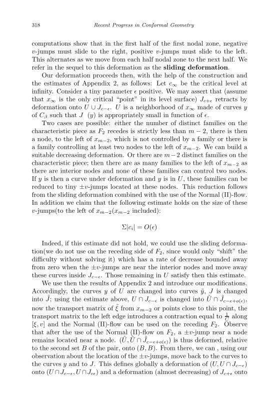
January 17, 2007 11:55 WSPC/Book Trim Size for 9in x 6in finalBB
318 Recent Progress in Conformal Geometry
computations show that in the first half of the first nodal zone, negativev-jumps must slide to the right, positive v-jumps must slide to the left.This alternates as we move from each half nodal zone to the next half. Werefer in the sequel to this deformation as the sliding deformation.
Our deformation proceeds then, with the help of the construction andthe estimates of Appendix 2, as follows: Let c∞ be the critical level atinfinity. Consider a tiny parameter ε positive. We may assert that (assumethat x∞ is the only critical “point” in its level surface) Jc+ε retracts bydeformation onto U ∪ Jc−ε. U is a neighborhood of x∞ made of curves yof Cβ such that ∂J(y) is appropriately small in function of ε.
Two cases are possible: either the number of distinct families on thecharacteristic piece as F2 recedes is strictly less than m − 2, there is thena node, to the left of xm−2, which is not controlled by a family or there isa family controlling at least two nodes to the left of xm−2. We can build asuitable decreasing deformation. Or there are m−2 distinct families on thecharacteristic piece; then there are as many families to the left of xm−2 asthere are interior nodes and none of these families can control two nodes.If y is then a curve under deformation and y is in U , these families can bereduced to tiny ±v-jumps located at these nodes. This reduction followsfrom the sliding deformation combined with the use of the Normal (II)-flow.In addition we claim that the following estimate holds on the size of thesev-jumps(to the left of xm−2(xm−2 included):
Σ|ci| = O(ε)
Indeed, if this estimate did not hold, we could use the sliding deforma-tion(we do not use on the receding side of F2, since would only “shift” thedifficulty without solving it) which has a rate of decrease bounded awayfrom zero when the ±v-jumps are near the interior nodes and move awaythese curves inside Jc−ε. Those remaining in U satisfy then this estimate.
We use then the results of Appendix 2 and introduce our modifications.Accordingly, the curves y of U are changed into curves y, J is changedinto J ; using the estimate above, U ∩ Jc−ε is changed into U ∩ Jc−ε+o(ε),now the transport matrix of ξ from xm−2 or points close to this point, thetransport matrix to the left edge introduces a contraction equal to 1
C along[ξ, v] and the Normal (II)-flow can be used on the receding F2. Observethat after the use of the Normal (II)-flow on F2, a ±v-jump near a noderemains located near a node. (U , U ∩ Jc−ε+o(ε)) is thus deformed, relativeto the second set B of the pair, onto (B, B). From there, we can , using ourobservation about the location of the ±v-jumps, move back to the curves tothe curves y and to J . This defines globally a deformation of (U, U ∩ Jc−ε)onto (U ∩Jc−ε, U ∩Jcε) and a deformation (almost decreasing) of Jc+ε onto
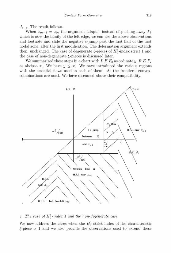
January 17, 2007 11:55 WSPC/Book Trim Size for 9in x 6in finalBB
Contact Form Geometry 319
Jc−ε. The result follows.When xm−3 = x0, the argument adapts: instead of pushing away F3
which is now the family of the left edge, we can use the above observationsand footnote and slide the negative v-jump past the first half of the firstnodal zone, after the first modification. The deformation argument extendsthen, unchanged. The case of degenerate ξ-pieces of H1
0 -index strict 1 andthe case of non-degenerate ξ-pieces is discussed later.
We summarized these steps in a chart with L.E.F2 as ordinate y, R.E.F2
as abcissa x. We have y ≤ x. We have introduced the various regionswith the essential flows used in each of them. At the frontiers, convex-combinations are used. We have discussed above their compatibility.
c. The case of H10 -index 1 and the non-degenerate case
We now address the cases when the H10 -strict index of the characteristic
ξ-piece is 1 and we also provide the observations used to extend these

January 17, 2007 11:55 WSPC/Book Trim Size for 9in x 6in finalBB
320 Recent Progress in Conformal Geometry
arguments to non-characteristic pieces. This is needed in order to establishthat transversality holds.
When a characteristic piece is of H10 -index 1, the two edges facing each
other may each have one or more companions living on this ξ-piece. If thereis no additional family is in between, there is a problem of transversality. Ifone of the families is confined to the interior of the half of the ξ-piece definedby the edge within a family, it is easy to define a decreasing deformation viathe introduction of an additional companion for the other family in betweenthe middle of the ξ-piece and the confined family. However, if this does nothappen, the downwards deformation becomes very difficult to define. Wehave been able, along the lines of the argument developed in the previoussection, to find such a deformation. The idea of this deformation is thefollowing: if we could, using one of the families, engineer a decrease of Jwhich would not change the orientation of the companions of this familybut would cancel the companions of the other edge which are living on thecharacteristic ξ-piece, we could then complete the deformation downwardssince we would then have after only one family on the ξ-piece. This has theflavor of the argument used for the Normal(II)-flow on F2 in the previoussection: we use the strength of a ±v-jump to cancel another one.
The modifications of the last section, those of Appendix 2 become useful,but only after we can identify the ±v-jumps and where they are localized.
The ±v-jump used to cancel the other one must survive the other oneall over the configurations under deformation. This is the result of thefollowing construction:
We can always, using the “widening” process between the right edgeand the family of the left edge-this is a technical improvement of the clas-sical widening process defined above, which bypasses intermediate smallcompanions of the right edge-assume that the companions of the left edgeenter little in the second half of the characteristic piece. We could then useagain the widening process, now between the family of the left edge andthe companions of the right edge and bring these companions to be at leastπ4 away from the family of the left edge.
As long as a small companion for the left edge survives now, we canengineer a decrease of J combining the sliding deformation with the use ofdecreasing normals on this companion. We can use this decrease to buildup a sizable companion for the right edge on the ξ-piece, evolve therefore toconfigurations where a(n) “artificial” companion of the right edge is presentas long as a companion for the left edge is present. This deformation canbe assumed to be J-decreasing. The sliding process might have broughtthis companion of the left edge a little too much inside the second half ofthe ξ-piece, we can make use again of the widening processes and bring thiscompanion only a little bit inside this second half, with the companion of
January 17, 2007 11:55 WSPC/Book Trim Size for 9in x 6in finalBB
Contact Form Geometry 321
the right edge at least π4 away. The relative sizes can be assumed to be
comparable as the size of the companion of the left edge tends to zero. Thiscompanion might recede towards the left edge, the decrease which we canthen create is small, but we do not need it then: the middle nodal positionand a neighborhood of it are free.
Let us rethink about our deformation process. Again we can deformJc+εonto U ∪ Jc−ε. The y′s of U have their small ±v-jumps on the char-acteristic piece close to the middle node. Therefore, U can be naturallydivided in two distinct connected components or more: those such thatthis ±v-jump belongs to the family of the left edge, those such that it be-longs to the right edge, and in fact also those such there is no such v-jump.These connected components are connected one to the other through Jc−ε
and we need to define a coherent decreasing deformation on all of them.For the two last ones, we can choose to introduce a negative v-jump(with
the orientation of the right edge) in the first half of the characteristic ξ-piece. For the first, we want to do the same thing, but we need first to getrid of the positive companion of the left edge near the middle nodal point.This is completed using our modifications, as in the previous section and inAppendix 2. The case of characteristic ξ-pieces of non-zero index is therebycompletely solved.
In the case of non-characteristic pieces of non-zero H10 -index, the de-
formation uses the representation of Proposition 13 of the ±v-jumps asDirac masses that give rise(here)toH1
0 (there periodic)functions η betweenthe edges of the non-characteristic piece. These functions η are used in thesecond derivative of J . This representation has already been introducedand used in [Bahri-1 2003], the H1
0 -problem has been studied in details.Once a sequence of small ±v-jumps has been represented in this way, we
can use the H10 -diffusion flow of the second derivative (η + ητ), projected
on the L2 -spheres (L2 in η) to engineer a decrease of J and once this isaccomplished, we can turn back to the representation involving ±v-jumps.The number of sign changes never increases along this process. Furthermoreif the initial datum is non zero, it remains so.
The number of sign changes, counted locally, between the v-edges of thenon-characteristic piece indicates the(minimal) number of families neededto describe this configuration. This number does not increase. Thus theminimal number of families (which might differ by 1 from the number ofsign-changes) needed to describe the configurations which we consider anddeform never increases. We might have a gap with respect to the actualnumber of families because there might be sign repetitions between thesefamilies. But coming from a number which is less than or equal than thisactual number, we can certainly relabel, reorder, create twins and rebuildour original local set of families.

January 17, 2007 11:55 WSPC/Book Trim Size for 9in x 6in finalBB
322 Recent Progress in Conformal Geometry
Assuming that the H10 -index of our non degenerate ξ-piece is initially
non zero, we can use the results of [Bahri-1 2003], manipulate the rotationof v on this ξ-piece so that the maximal number of sign changes on theH1
0 -unstable manifold of this ξ-piece is ij0 + 1. ij0 is the H10 -index of the
ξ-piece (after manipulation of the rotation).Then, if the number of sign changes between the families in this ξ-
piece, with the edges added, is less than ij0 + 1, the flow will deform ourconfigurations below the critical level corresponding to this ξ-piece for indexreasons. From there, we end up in Jc−ε. This implies transversality as faras non-characteristic pieces are involved.
If the maximal number of sign changes on the H10 -unstable manifold of
a non degenerate ξ-piece is ij0, then we can assert that the flow deforms ourconfigurations below the critical level only if the number of sign changesbetween the families is less than ij0. We can generate ij0 sign changes in thisframework with ij0−1 distinct families. Thus transversality does not followoutright from this argument in such a case. We have to use the Appendix 2(adapted) again, as in Section 2.5.5.2c: we need to show that we can adjustthe value(s) of the Green’s function of the operator η + ητ under Dirichletboundary conditions on the non degenerate ξ-piece. We elaborate somemore about this at the end of Section 2.5.9, but the main arguments areessentially the same than in 2.5.5.2c and Appendix 2.
d. An additional rule
After this full discussion, there is still an additional rule to introduce inorder to build a global flow as some ∗′s turn to families or vice-versa. Thisrule reads as follows:
If there is a hole at the last node xm−1 and no family is “advancing”towards this node from the left, we introduce, in order to engineer a decreaseof J , before this last node a ±v-jump with the orientation of the right edgerather than using the hole flow near this node
This is of course impossible if another family advances on this last node,but we can then use the construction of Section 2.5.5.2b and switch to theother flow if the strict H1
0 -index of the characteristic is not 1 and the con-struction of 2.5.5.2c otherwise, while if we used the hole flow and this holeflow would have directed us to introduce a ±v-jump with the orientationopposite to the one of the right edge in the last nodal zone, then unless afamily advances from the left, this switch is impossible. Thus, as a familyfor the right edge advances towards this node, we are less and less able toengineer a decrease and a switch is not available. This issue does not arisewith the left edge, because the hole flow provides always for this edge a±v-jump with the orientation that this edge has.
January 17, 2007 11:55 WSPC/Book Trim Size for 9in x 6in finalBB
Contact Form Geometry 323
Using this rule, Proposition 31 follows under the assumption that thehole flow of the left edge is well defined.
If there is a repetition barring the use of the left edge hole flow, we needto introduce a decreasing normal and we are allowed to introduce it with anadditional sign change if the repetition is not already exhausted by the useof one of the non-compatible hole flows We have gone over this argumentbefore:
The repetition occurs “in the left edge” in that, in our construction,we may require that the family of the left edge should be at a distanceo(1) from the average left edge (which can be defined easily). It followsthat no normal is used in between the repetition. In the interval where itis used, this normal identifies then with the orientation of one of the holeflows. With the other one, it might induce an additional sign change butthis would correspond exactly to the single additional sign change allowed.
2.5.6 Flow-lines for x2k+1 to x∞2k
The extension of the results to the odd case is long and delicate. We provideit here.
We are assuming that we have at least two characteristic pieces. Let usassume for simplicity-the arguments are unchanged in the other cases-thatthe two left edges of the two characteristic pieces are positively oriented. Weobserve first that the hole flow extended into an alternating sequence doesnot provide more than 2k sign changes even in the case of 2k+1±v-jumps.Indeed ,starting from the first v-jump which we assume for simplicity to bepositive ,the alternating sequence ends with the positive sign on the otherside of this initial v-jump, we then have a positive v-jump on both sides ofthe first positive v-jump and we may as well think that this v-jump is notthere. The conclusion follows.
Next we have two characteristic pieces, we assume in the sequel that,after the use of the Normal (II)-flow, there is a hole on each of them. Webuild a decreasing deformation on such configurations that do not raise thenumber of zeros beyond 2k. We pick a hole flow on each characteristicpiece. We overextend this hole flow as an alternating sequence all around.Either it coincides with the other hole flow and their combination does notprovide more than 2k sign changes. Or it does not. Then the alternatingsequence starts with a − to the right of the positive (for simplicity) startingv-jump of the other hole flow (which starts with a +). Considering thesetwo sequences between the edges of the second characteristic piece-startingfrom the v-jump of this other hole flow-we see that the sequence of signchanges of this other hole flow gives at most as many changes of sign as

January 17, 2007 11:55 WSPC/Book Trim Size for 9in x 6in finalBB
324 Recent Progress in Conformal Geometry
the alternating sequence. Thus, the two hole flows (restricted to theirrespective characteristic pieces) can be convex-combined with a number ofsign changes at most equal to 2k.
Third, we consider one of the characteristic pieces and ∗0, the first ∗before (not in the vicinity) of the first node. We know how to build adecreasing normal N−
0 (z): we introduce a negative v-jump after ∗0, wehave discussed this matter above; since we are discussing hole flows, wemay assume that the ∗’s are not in between nodes. N−
0 (z) is in a naturalway part of an alternating sequence on this characteristic piece. Let usassume that there are competing hole flows on this characteristic piece -because there are several possible representatives for the left edge - and letus assume that N−
0 (z) is not part of the hole flow which introduces a-signafter the representative most to the right of the left edge (baptized “first”representative). Thus, there is an even number of ∗’s between ∗0 and thisfirst representative of the left edge. We assume that no sign changes areused for decreasing normals to the left of ∗0. We then claim that N−
0 (z)is compatible with both hole flows. This is a local argument which can beused as we please. Indeed, it is compatible with the hole flow which includesit. The other hole flow can be identified as the hole flow starting with a -sign at the first representative and has a + sign immediately after ∗0. Theremight be a problem with the simultaneous use of N−
0 (z) and this other holeflow if N−
0 (z) and the orientation of ∗0 do not agree i.e if ∗0 is a positivev-jump. Then this other hole flow, the distribution of signs of this otherhole flow introduces a sign change between this first representative and ∗0
since there is an even number of ∗’s in between. This sign change is notactually being used according to our rules and we thus have the freedom touse N−
0 (z) and induce thereby a decreasing deformation. This works alsoif there is more than one repetition in the left edge. Again this argumentis of local type, N−
0 (z) is free, available under such circumstances and canbe inserted in any other flow.
Thus so far, we have seen that, if there are holes on one of the twocharacteristic pieces, we can define a decreasing deformation if the holeflow is well defined on at least one of the characteristic pieces and also ifthis hole flow is not well defined on both, but there is an even number of ∗’sin between ∗0 and the first representative of the left edge of any of them.This works in case of multiple repetitions in the edge, the local argumentalso works with the right edge.
Let us now consider the case when there are competing hole flows oneach characteristic piece and there each N−
i (z) is part of the alternatingsequence starting with a − at the first representative of each characteristicpiece. We may also assume for simplicity that the competing representa-tives for the left edges on each characteristic piece are consecutive ∗’s. We

January 17, 2007 11:55 WSPC/Book Trim Size for 9in x 6in finalBB
Contact Form Geometry 325
thus have two pairs of consecutive representatives for the left edges of thesetwo characteristic pieces. These two pairs define on the circle two timeintervals. On one of them, there is an even number of ∗’s. This interval isunique since the total number of ∗’s is odd. Let us assume that it starts forexample with the left edges of the first characteristic piece. We then claimthat the hole flow starting with a + at the first representative of the firstcharacteristic piece, when combined with any other hole flow on the secondcharacteristic piece yields at most 2k − 2 zeros. Indeed, since the numberof intermediate ∗’s is even, this hole flow ends also with a + at the secondrepresentative of the left edge of the second characteristic piece. Let usextend, as an alternating sequence all around, the sequence starting with a− at the first representative of the first characteristic piece after identifyingthe two representatives of the first characteristic piece. We then have 2ksign changes. We compare: the hole flow starting with a + ends also with a+ before the second representative of the second characteristic piece, whilethe alternating sequence starts and ends with a − at both (positive) ends.We thus have two less zeros for the hole flow starting with a +. On thesecond characteristic piece, the alternating sequence starts with a − sign,opposite to the sign + of the first representative of the second character-istic piece (there are two representatives of the second characteristic pieceto bypass, starting with a − sign on one side. We reach the other sidewith a − sign also. The two representatives of the first characteristic piecehave been identified). Hence this alternating sequence introduces at least asmany changes on this second interval (running from the first representativeof the second characteristic piece to the second representative of the firstcharacteristic piece) as any other alternating sequence restricted to this in-terval with the given boundary (positive) v-jumps. The claim follows. Wethus have a freedom of two zeros with the use of the hole flow starting witha + on the first characteristic piece when combined with any hole flow onthe second one. N−
1 (z) is included in all combinations containing the holeflow starting with a sign - on the first characteristic piece. The addition ofN−
1 (z) to the hole flow starting with a +, when combined with any otherhole flow on the second piece does not raise the number of zeros beyond2k. Thus, as competing hole flows- with the presence of holes on both char-acteristic pieces-develop, we reduce our flow to the use of one of the twoN−
i (z)’s depending on the configuration. We may then use both of themsince, once the other v-jumps of the hole flows are removed, their jointuse becomes possible. Along the convex-combination, the number of signchanges does not raise above 2k. We may assume in the sequel, workingon pairs of characteristic pieces one after the other, that there are holes onone characteristic piece at most.
Assume now that, on this characteristic piece, there are two holes or
January 17, 2007 11:55 WSPC/Book Trim Size for 9in x 6in finalBB
326 Recent Progress in Conformal Geometry
a hole covering two nodes. We then claim that if a repetition develops inthe left edge of this characteristic piece and we are forced to switch holeflows, this switch can be completed without increase in the number of signchanges beyond 2k. Indeed, assume for example that we have two holes,each jumping over exactly one node, each with a starting ∗. We can attacha sign to each ∗, starting from the representative most to the right of theleft edge which gets assigned the sign defined by its own orientation, andalternating to the right. Then for a given ∗, either the orientation of this∗ and the attached orientation agree, or there is an additional repetition;we can use it to introduce two zeros. We have two hole flows. One agreeson the interval immediately after any ∗ with the attached sign, the otherone disagrees (signs for hole flows also alternate). Let us consider the holeflow which agrees with the attached orientation of the starting ∗ for eachgiven interval. On the other hand, we have defined a preferred orientationfor each nodal region and there is one which is associated to the nodalregion immediately following a given ∗. If the attached orientation andthis preferred orientation disagree at a hole, they will agree at the (nextor previous) hole since there is one more change at a node for a preferredorientation and not for the attached sequence of ∗’s. At the hole where thepreassigned orientation of the nodal zone to the right of the ∗ agrees with theattached sign on this ∗, we know that this preferred orientation correspondsto a hole flow- the one of the attached sign- while the preferred orientationof the next nodal zone corresponds to the other hole flow. Typically, wefind for example:
Attached sign +∗ + −
HF1 HF2.
Now eliminate the normals and hole flows in all other intervals andobserve the following: If the actual orientation of the ∗ agrees with theattached orientation, HF1 does not introduce any sign change. We canuse jointly HF2 on this interval. Otherwise, they disagree and there is anadditional repetition and we have a freedom of two zeros which we use tointroduce HF1 together with HF2 (HF2 by itself did not then add zeros).We thus can use such a node to switch from a hole flow to another one.Summarizing, if there are two holes on two distinct characteristic pieces,we have built a decreasing deformation. Any change in a configuration ismonitored by the Normal(II)-flow. Also if all the characteristic pieces arefilled but one and if on the remaining one there are two holes, or a hole overmore than one nodal zone, we also have a decreasing deformation since wecan switch hole flows. This also holds if there is no repetition in the leftedge of the piece with a hole. Finally, if on one of the characteristic besides

January 17, 2007 11:55 WSPC/Book Trim Size for 9in x 6in finalBB
Contact Form Geometry 327
the one bearing a hole there is a repetition-as when the number of ∗’s inthe characteristic piece from ∗0 till ∗m equals, mod2,the total number of ∗’scarried by this characteristic piece- then we can also switch at the hole thetwo hole flows. Thus a decreasing deformation is impeded (when there areholes) if all characteristic pieces but one are filled up and do not jail a forcedrepetition (∗0 and ∗m are different from their associated edges, on one sidethe number of ∗’s in between is even, on the other side it is odd), there isexactly one hole at exactly one node on this last characteristic piece, there isa repetition in its left edge. It is also impeded if all characteristic pieces havebeen filled up and, singling out a characteristic piece, characteristic piecenumber 1, there is no admissible extension (i.e. not raising the number ofzeros beyond 2k) for its basic set of decreasing normals (such as its N−
0 (z)).We are going to discuss this below. In all the other cases, after numberingthe characteristic pieces, we can start to reduce holes for pieces 1 and 2.Once only one with a hole is left, we move to reduce holes for 1, 2, 3 (onlya pair is involved after the first stage), then 1, 2, 3, 4 etc. At the endof this continuous process, at most one with holes is left. If the holes aremore than one or contain more than one node, we can build a decreasingdeformation , this is in fact part of a global deformation.
The transition between all these situations involving a change in theholes or a change in the number of holes is monitored by the Normal (II)-flow which is compatible with all hole flows. The only issue related to theuse of the Normal (II) flow is that it might change the orientation of ∗0,∗m. This becomes important now because we are tracking sign-repetitions.We address this issue: In order to stabilize the repetitions associated to acharacteristic piece which has been “filled up” or is being “filled up”, weintroduce representatives L for its left edge and R for its right edge. Letassume that there is dissymmetry i.e that the number of ∗’s in between ∗0
and L, for example is odd, while the number of ∗’s in between ∗m and Ris even. ∗m and R have the same orientation before any use of the Normal(II)-flow since the characteristic piece is almost filled up, if not filled upand therefore there must be a repetition between ∗m and R. We thus maydefine an alternating sequence which will start with the sign opposite tothe orientation of R immediately to the left of ∗m and move backwardsalong the characteristic piece, alternating at each crossing of a ∗. Sincethe characteristic piece is sign-true, we derive for this sequence the signopposite to the orientation of ∗0 or L immediately to the right of ∗0. Westop here the alternating sequence and we use it in order to define decreasingnormals. Since we have not used one repetition to the least, it is extendableinto an admissible alternating sequence .The argument and the repetitionsbeing local, we can use these flows on these dissymmetric pieces together.Furthermore, immediately to the right of ∗0 and to the left of ∗m, we have

January 17, 2007 11:55 WSPC/Book Trim Size for 9in x 6in finalBB
328 Recent Progress in Conformal Geometry
decreasing Normals which have the orientations of the Normal (II)-flow.Thus, we may extend the use of this flow after sliding the position of itsaction on the v-jumps over ∗0, ∗m to the position of the decreasing normals.The sliding starts on both sides simultaneously and preserves therefore therepetition between ∗0 and ∗m (no v-jump is introduced before ∗m, therepetition is to the right of ∗m). We could also, since we have two repetitionson this characteristic piece, reverse the position of the normals and exhaustthe repetition in the middle, leaving the one to the side unperturbed. Again,we can convex-combine all the flows on these dissymmetric pieces. TheNormal (II)-flow finds a natural extension on these pieces.
Along the other characteristic pieces, we can either continue the full useof the Normal (II)-flow, a repetition is anyway jailed in there or ∗0 and ∗m
confound with the edges; there is no use of the Normal (II)-flow on themand nothing to extend.
In the sequel, [L, R] designates the characteristic piece with a singlehole at a single node in it and the left edge repetition; or [L, R] designates,when all characteristic pieces have been filled up the first one in an a priorichosen order.
In the second case, on [L, R] we pick up the flow defined by the basicset of normals and we need to extend it only on dissymmetric critical con-figurations, which is easy to accomplish as explained above. We could evenswitch, if needed, the use of - between the two repetitions and incorporatethe flow inside such pieces into the alternating sequence generated by thisbasic set of normals. We do not need to extend it over symmetric config-urations. This works as long as there is one symmetric configuration on acharacteristic piece distinct from [L, R] which we can use in order to turnour sequence into an admissible sequence. A similar argument can be madein the first case, with the same basic set of normals, as we already have arepetition in the left edge of [L, R] and we need another one, distinct from[L, R], in order to switch hole flows. We develop a counting argument whichis the same in both cases: Let n be the number of characteristic pieces, letic0 be the total strict index on the characteristic pieces, if0 be the index onthe non-degenerate ξ-pieces. Let γ1 be the number of free ξ-pieces havingeither even H1
0 -index and reverse edge orientations or odd H10 -index and
identical edge orientations, see Definition 4, page 78 of [Bahri-1 2003] forthe use of this notion. Let γ be the number of non degenerate ξ-piecesbearing a sign change between their edge orientations. Let be the num-ber of full (with their full half-unstable manifold) characteristic pieces usedonce at a time in the definition of x∞
m . We then have, see [Bahri-1 2003,pp. 139] also page 78 to gather the full information:
ic0 + if0 + γ1 + 2 + 1 = 2k + 1.

January 17, 2007 11:55 WSPC/Book Trim Size for 9in x 6in finalBB
Contact Form Geometry 329
Using the results of [Bahri-1 2003], [Bahri-2 2003], we can modify α in thevicinity of x∞ and set if0 = 0. Thus,
ic0 + 2 + γ + 1 = 2k + 1.
On the other hand, assuming that all characteristic pieces have been filledup, if as [L, R] is becoming symmetric and we need to extend its basicset of normals into an admissible sequence, there is no other symmetricconfiguration on any other characteristic piece, then on each characteristicpiece, including [L, R], there are ij0 + 2∗’s. ij0 is the strict H1
0 index of thejth characteristic piece, a 1 is added for the dissymmetry (∗0 or ∗m) andanother 1 for the incoming edge. Summing up, we find∑
j
(ij0 + 2) = ic0 + 2n
v-jumps to which we have to add 1 for each non degenerate ξ-piece with achange in the edge orientations. Since the edges could be part of the samefamily, we do not consider the other non-degenerate ξ-pieces. In all, we findic0 + 2n + γ ± v-jumps. The count has to be slightly modified when thereis a single hole and a repetition in [L, R]. The formula is decreased by one.Thus, in all cases,
ic0 + 2n + γ − 1 ≤ ic0 + 2 + γ + 1
and
≥ n − 1.
If is strictly less then n−1, we find in the second case that, even when[L, R] has turned symmetric, there is an extra symmetric configuration, thebasic set of normals can be extended. The same conclusion holds in thefirst case. This leaves with = n − 1 as the only possible case. In fact, wemust have:
ic0 + 2n − 2 + γ = 2k. (**)
otherwise, this is not possible.Continuing our analysis, we look into more details at what happens as
we try to extend our alternating sequence outside of [L, R] assuming thatthere is no outside symmetric configuration. Since there are more than onecharacteristic piece, there are outside dissymmetric configurations. Let usassume for simplicity that the edges of one such dissymmetric configura-tion are positively oriented. We extend using the ξ-orientation i.e. we gofrom characteristic piece to characteristic piece along ξ. If we reach theleft edge of our dissymmetric configuration, after extending the basic set of
January 17, 2007 11:55 WSPC/Book Trim Size for 9in x 6in finalBB
330 Recent Progress in Conformal Geometry
normals of [L, R], with a +, then we will be able in a natural way to jumpover an inside repetition in this configuration, and still include a decreas-ing normal, in our alternating sequence. The alternating sequence wouldbecome admissible. Otherwise, we have to alternate signs inside the fulldissymmetric configuration, thereby exhausting the two inside repetitionsin order to build an extension to the Normal (II)-flow inside (which we needto do). We then exit on the other side with the + sign, i.e with the orienta-tion of the edge. This repeats starting from R until the next characteristicpiece etc. Each occurrence, we reach , if the alternating sequence is notadmissible, the left edge with an orientation opposite to this edge and leavethe right edge with the orientation of the edge, the only exception being Litself. Thus, on each such interval between two characteristic pieces, theremust be a free ξ-piece with a switch in the orientation of the edges:
γ ≥ n − 1.
The argument goes now as follows. Assume that n is large. Choose a char-acteristic piece with γj = 0, ij0 = 0 (H1
0 -index 0, reverse edge orientation).We had previously turned ij0 to be 0 on this critical point at infinity, see[Bahri-1 2003], [Bahri-2 2003] for the argument used to derive this result.In doing this, we could have kept, since we have a large amount of non-degenerate ξ-pieces, the amount of v-rotation on several of these pieces tobe less than π, but only by a tiny bit; so that we can easily rebuild a largerotation on a given ξ-piece. This last part of the argument uses Hypothesis(A). We pile up v-rotation on this ξ-piece which has ij0 = 0, γj = 0. Pilingup, we cross ij0 = 1, creating only false critical points at infinity since theyhave a characteristic piece of strict H1
0 -index 0 and with the orientation ofits edges reversed. There is still our critical point at infinity which has nowa non degenerate ξ-piece with ij0 = 1. Counting the maximal number ofzeros of b on the unstable manifold of this critical point at infinity, we findthat we should have if it interacts in our homology (page 78, pp 137-139 of[Bahri-1 2003]:
ic0 + 1 + γ − 12′ = ic0 + γ2.
Thus,
′ = .
We continue our filling on the same characteristic piece. We cross the H10 -
index 2 and the maximal number of zeros of b on the unstable manifoldof our critical point at infinity (with the same number of characteristicpieces) changes by 2. This critical point at infinity do not interfere with ourhomology anymore. We still have the new critical points at infinity which
January 17, 2007 11:55 WSPC/Book Trim Size for 9in x 6in finalBB
Contact Form Geometry 331
we have created. They have i0 = 0 again because the only new phenomenonis taking place on the new characteristic piece. Again, counting see [Bahri-12003, pp. 139], also page 78, we should have
ic0 + 1 + γ − 1 + 2′ = ic0 + 2 + γ.
Thus, ′ = , which is n−1 while the number of characteristic pieces is nown + 1. A contradiction.
n is bounded and so is the number of non degenerate ξ-pieces of x∞.Otherwise, using Hypothesis (A), we would reach the same conclusion. As ktends to infinity, this forces the H1
0 -strict index of some characteristic pieceto tend to infinity. Considering Wu(x2k+1) ∩ Wu(x∞
2k), we observe that is bounded above independently of k. Let n0 be this upperbound. ThenWu(x2k+1)∩Wu(x∞
2k) is of dimension n0 at most. Tracking this intersectionnear x2k+1, using the construction of Proposition 1, we may assume afterperturbing the location of the v-jumps in Proposition 1 if needed, thateach given configuration has at most n0 v-jumps which are zero. Thiscould change after the use of the Normal (II)- flow . However, this doesnot change under the use of the flow at infinity i.e the flow on the Γ2s’s.This flow is the one driving our curves to x∞. The other flows are usedto bypass x∞ downwards. In this circumstance, we are not going to usethe Normal(II)- flow because we want to keep the orientation of the non-zero v-jumps unchanged. We go to the characteristic piece with a largerH1
0 -index. There are several triplets of v-jumps on this characteristic piecehaving non-zero alternating orientations. Otherwise there are too manyrepetitions and we may use a basic normal. We pick such a triplet; in factwe may choose a large number of triplets which are “far away” one from theother. On a given configuration, there will be among those triplets, underour assumption that there are few repetitions, a non-zero alternating triplet.Our construction below can then be convex-combined; as the configurationschange, we change our triplet and the construction of the normals which wecomplete below can be in the transition zones carried out on several triplets,the fading and the emerging ones at the same time. We can “widen” thefirst oscillation of these triplets, using the procedure of Proposition 30 andif along this procedure we find some other v-jumps, we continue the processwith the agglomerate v-jump but keeping track of the sign changes allowed.In the end, going left and going right around such a triplet, we can assumethat we cover more than one nodal zone. We choose to construct onlypositive Normals in between. Since we are covering more than one nodalzone, we are always sure that one of them will be decreasing. That is theone that we choose to expand. Our proof is complete in this case.
We are left with the case when x∞ has only one characteristic piece.Then = 0 and Wu(x2k+1) ∩ Ws(x∞
2k) is made of isolated flow-lines. We
January 17, 2007 11:55 WSPC/Book Trim Size for 9in x 6in finalBB
332 Recent Progress in Conformal Geometry
may assume, perturbing the locations of the v-jumps near x2k+1, that noneof them is zero on these flow-lines at the beginning. The flow on the Γ2s’swill preserve this property. Thus no ±v-jump is zero on our single charac-teristic piece, which is of strict index at least 2. The flow-line is isolated,we are facing a single configuration and we can grow a companion to theappropriate ∗, closest to the first node. If there are two such ∗’s,one to theright, one to the left, we choose the one to the left.
In order to complete our proof, we have to remove the assumption thatthe characteristic pieces are isolated one from the other. Assuming nowthat we have sequences of characteristic pieces, we use Proposition 33 be-low which involves a special construction of a decreasing deformation onconsecutive ξ-pieces as an additional ∗ travels along a common edge. Af-ter completing this construction, we resume the proof of Theorem 1 inour present framework and finish it, see Section 2.5.8, after the proof ofProposition 33 below.
2.5.7 The S1-classifying map
Consider C∗β = Cβ - periodic orbits of ξ. Assume that the curves x which
we consider are H1 (this follows, continuously, from a simple regularizationprocedure).
We then have a map
C∗β
σ→ −→H1(S1, R) − ox −→ b
where b is the v-component of x.Let
C∗∗β = x ∈ C∗
βsuch that b =∫ 1
0
b.
We compose σ with the orthogonal projection q on E+⊕E− where E+⊕E−
is the L2-orthogonal of the constants in H1(S1, R). q σ maps C∗∗β into
E+ ⊕ E− − 0. S1 acts effectively on E+ ⊕ E− − 0. Therefore q σ isthe classifying map for the S1-action on C∗∗
β . The use of this observationis deferred to a forthcoming work. We now study the Faddell-Rabinowitzindex γFR of some subsets of Cβ .
We have:
Lemma 17 Let A = x s.t b has at most 2r zeros and at least two genuinezeros.

January 17, 2007 11:55 WSPC/Book Trim Size for 9in x 6in finalBB
Contact Form Geometry 333
Then γFR(A) ≤ r − 1; the classifying map for A is provided bypr(−b−
∫ 1
0 b+ + b+∫ 1
0 b−) where pr is the L2-orthogonal projector onSpancos 2πit, sin 2πit, i = 1, . . . , r.Proof. Let b = b+
∫ 1
0b−−b−
∫ 1
0b+. b has also at most 2r zeros and
∫ 1
0b =
0. Assume that pr(b) = 0. Then, b =∑
l≥2r+1
ak sin 2πkx + bk cos 2πkx.
Rescaling, we may assume that∫ 1
0b2 = 1. We then solve
∂u
∂s= u +
(∫ 1
0
u2
)u/
∫ 1
0
u2 u(0, t) = b(t).
Observe that the number of zeros of u does not increase with s, that∫ 1
0u2 =∫ 1
0 b2 and that
12
∂
∂s
∫ 1
0
u2 = −∫ 1
0
u2 +(∫ 1
0u2)2∫ 1
0 u2≤ 0.
Thus u(s, ·) converges strongly in L2 to a rest-point (∫ 1
0 u2/∫ 10 u2 is a Lya-
punov function) which is a solution of ϕ = λϕ.Observe that
∂
∂s
∫ 1
0
u = c(s)∫ 1
0
u.
Since∫ 1
0b = 0,
∫ 1
0u = 0 and thus this solution verifies
∫ 1
0ϕ = 0.
Thus,
ϕ = A cos 2πkt + B sin 2πkt with k ≥ 2r + 1
ϕ has more than 2r zeros, a contradiction.
Lemma 18 Let Bε = x s.t x = aξ+bv with∫ 1
0b+∫ 1
0b− = 0; a ≥ ε. Let
B1 = Bε ∩(
Uz periodicorbit
Wu(z))
. Then B1 cannot dominate any periodic
orbit of ξ of non zero index and B1 cannot dominate any critical point atinfinity of J of non zero H1
0 -index. Furthermore, γFR(B1) = 0.
Proof. The first claim follows from the fact that the curves of B1, haveb ≥ 0 or b ≤ 0. This extends to B1. For the second claim, we argue asfollows:
The curves x of Bε have either b ≥ 0, b = 0 or b ≤ 0, b = 0 or b ≡ 0. Neareach z, the curves of Bε can be equivariantly (S1-equivariantly) pushed,
January 17, 2007 11:55 WSPC/Book Trim Size for 9in x 6in finalBB
334 Recent Progress in Conformal Geometry
with a unchanged, into a neighborhood as small as we may wish of z and itsfirst unstable direction. Thus, B1 retracts by deformation, S1-equivariantly,into an S1-invariant set, which is stratified and which is of dimension 1transversally to the S1-action.
There are no fixed point for the S1-action on B1, in fact the S1-actionon B1 is free since the curves are immersed.
Thus, γFR(B1) can be directly computed on B1/S1 . Since this set isstratified of top dimension 1, it cannot carry any Chern class of positiveeven degree and γFR(B1) = 0.
These are the initial steps towards computing on homology in a moregeneral framework.
2.5.8 Small and high oscillation, consecutive characteristic
pieces
We study in this section curves x of Cβ or C+β = x ∈ H1(S1, M) such that
x = aξ + bv, a ≥ 0 supporting “oscillations” i.e. sequences of consecutive±v-jumps which are either small and close — we then “widen” them i.e.bring the two consecutive ±v-jump further apart — or are large and close(high oscillations).
For high oscillations, we prove that these — which are due to the non-Fredholm character of the variational problem — either can be enlargedwhile J is decreasing somewhere above x∞, or they can all be thinneddown and brought back to be small oscillations.
In the next section, we will use this technical result in order to includehigh oscillations in our compactness result.
We also study in this section critical points at infinity containing se-quences of consecutive characteristic ξ-pieces.
We start with:
Proposition 32 There exists c0 > 0 small such that for every c > 0and 0 < δ < c, considering all curves x of C+
β bearing two consecutive±v-jumps of size less than c0 separated by a ξ-piece supporting a v-rotationless than π−c, a J-decreasing deformation (generated by a vector-field) canbe defined in their neighborhood. This deformation sepatates further these±v-jumps, without cancelling them or reversing their orientation, until thev-rotation on the ξ-piece between them is less than π − δ.
Proposition 33 Let x∞ or x have two consecutive characteristic piecesc1, c2 with strict H1
0 -index zero. Let c1 be the full unstable manifold associ-ated to c1 and c2 be the full unstable manifold associated to c2. Any cycle

January 17, 2007 11:55 WSPC/Book Trim Size for 9in x 6in finalBB
Contact Form Geometry 335
σ× c1 ∪σ× c2 in Jc, c = J∞(x∞) or J∞(x), bounds with no increase in themaximal number of zeros of b.
Observation 5. Proposition 33 extends to x∞ having more than twoconsecutive characteristic pieces, see the end of the proof of Proposition 33.The construction of Proposition 33 allows to cover the case of sequencesof consecutive characteristic pieces left open in Section 2.5.6. The case ofcharacteristic pieces of H1
0 -index zero is discussed in Appendix 1.
Proof. [Proof of Propsition 32]We have to take care of curves bearing “small and rapid oscillations”.Let us draw such an oscillation with its incoming ξ-piece and let us
introduce a v-vertical through A, A close to Ao on the incoming ξ-piece:
The curve A−Ao−Co−Do is a curve whose tangent vector x = aξ+bvsplits on ξ and ±v; it goes from the v-vertical through A to the v-verticalthrough Bo
Since these two verticals are close, since CoDo is a piece of ξ-orbit (a“geodesic”) from the v-vertical through Ao to the v-vertical through Do,there is also a ξ-orbit joining these two verticals and its length is less thanthe addition of the ξ-length of AAo with that of CoDo:

January 17, 2007 11:55 WSPC/Book Trim Size for 9in x 6in finalBB
336 Recent Progress in Conformal Geometry
Thus, replacing A−Ao −Co −Do −Bo with A−A′ −D′ −Bo shortensthe ξ-length of the curve, keeps the sign distribution for A close to Ao andincreases the size of CoDo into A′D′. The fact that the ξ-piece A′D′ islarger than CoDo can be seen as follows: we consider the case where A isvery close to Ao. AoA is then a small ξ-piece which we think of as a tangentvector z at Ao. v-transporting it during the time −ε from Ao to Co, we geta vector zε going from Co to the v-orbit through A. We write at first orderthat
−→CoA
′ = zε + δv.
On the other hand, the variation of the ξ-length is at first order equalto
α(−→
DoD′) − α(
−→CoA
′) = −α(zε), which is positive.
This enlargement can be completed without cancelling the base ±v-jumpsof the oscillation.
The v-jump which is on the side of the oscillation which we extend doesnot cancel; this is easy to see.
Thus if we alternate, extending always on the side which correspondsto the smaller v-jump, both v-jumps would cancel together.
This cannot happen because if we then superpose the initial and thefinal pictures, we get a small rectangle as follows:

January 17, 2007 11:55 WSPC/Book Trim Size for 9in x 6in finalBB
Contact Form Geometry 337
Such rectangles do no exist if the ξ-piece are small, less than character-istic of H1
0 -index zero.Indeed, we choose Darboux coordinates at xo (which depend on xo in a
differentiable way) so that v ·v(xo) = 0. v then reads up to a multiplicativefactor as ∂
∂y −x ∂∂z +(az+bx) ∂
∂x +0(x2+z2+xy+yz+g(y)) ∂∂x . Completing
the Darboux change of coordinates:
z′ = z + h(y)x′ = x − h′(y)y′ = y
this vector-field becomes:
∂
∂y′ − x′ ∂
∂z′+ (az′ + bx′ + g(y′) − ah(y′) + bh′(y′) − h′′(y′)
+ 0(x′2 + z′2 + x′y′ + y′z′)
+ 0(y′h(y′) + y′h′(y′) + 0(h2(y′) + h′2(y′))∂
∂x′ .
We set h′′(y′) − bh′(y′) + ah(y′) + 0(y′h(y′))
+ 0(y′h′(y′) + 0(h2(y′) + h′2(y′)) = g(y′)
h′(0) = h(0) = 0.
We derive a function h in this way, which depends differentially on x0 =(0, 0, 0) in our coordinates.
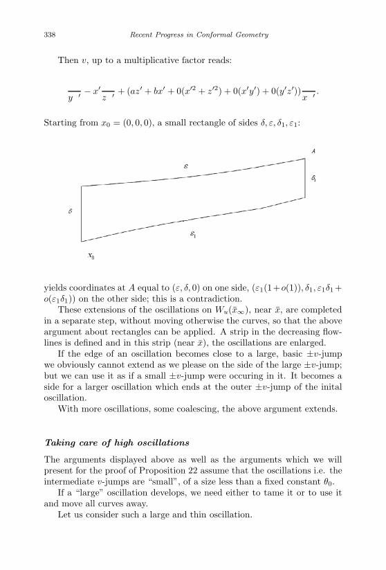
January 17, 2007 11:55 WSPC/Book Trim Size for 9in x 6in finalBB
338 Recent Progress in Conformal Geometry
Then v, up to a multiplicative factor reads:
∂
∂y′ − x′ ∂
∂z′+ (az′ + bx′ + 0(x′2 + z′2) + 0(x′y′) + 0(y′z′))
∂
∂x′ .
Starting from x0 = (0, 0, 0), a small rectangle of sides δ, ε, δ1, ε1:
yields coordinates at A equal to (ε, δ, 0) on one side, (ε1(1+o(1)), δ1, ε1δ1 +o(ε1δ1)) on the other side; this is a contradiction.
These extensions of the oscillations on Wu(x∞), near x, are completedin a separate step, without moving otherwise the curves, so that the aboveargument about rectangles can be applied. A strip in the decreasing flow-lines is defined and in this strip (near x), the oscillations are enlarged.
If the edge of an oscillation becomes close to a large, basic ±v-jumpwe obviously cannot extend as we please on the side of the large ±v-jump;but we can use it as if a small ±v-jump were occuring in it. It becomes aside for a larger oscillation which ends at the outer ±v-jump of the initaloscillation.
With more oscillations, some coalescing, the above argument extends.
Taking care of high oscillations
The arguments displayed above as well as the arguments which we willpresent for the proof of Proposition 22 assume that the oscillations i.e. theintermediate v-jumps are “small”, of a size less than a fixed constant θ0.
If a “large” oscillation develops, we need either to tame it or to use itand move all curves away.
Let us consider such a large and thin oscillation.

January 17, 2007 11:55 WSPC/Book Trim Size for 9in x 6in finalBB
Contact Form Geometry 339
On such curves which support an oscillation of a height larger than θ0,we can define a decreasing pseudo-gradient z1 as follows:
We pick up a small ξ-piece of size ε at the edge of the ξ-piece preceedingthe almost characteristic piece where this high oscillation takes place andwe transport it to y(0):

January 17, 2007 11:55 WSPC/Book Trim Size for 9in x 6in finalBB
340 Recent Progress in Conformal Geometry
On the other hand, we pick up δξ at y′(0) and we pull it down toy(0). We obtain two small displacements at y(0), εz1 and δz2. If the[ξ, v]-component of εz1 is not zero, we can use it to compensate the [ξ, v]-component of δz2. This will adjust, for a given δ, the value of ε. Adjustingthe v and ξ displacement at y(0), we define a tangent vector z. If J ′ · z isnon zero, we have a decreasing direction using z or −z.
It might happen though that εz1 has no [ξ, v]-component for specialpositions of y(0); or that for special values of s (the height of the oscillation),J ′ · z is zero even though εz1 has a [ξ, v]-component.
The first problem is easy to take care of: instead of transporting εξ, wecan transport εv from x+ to y(0), yielding an εz′1 at y(0). It cannot happenthat both of εz1 and εz′1 have no [ξ, v]-component.
If s is special and the z-directions defined above both satisfy J ′ · z = 0or if one of them cannot be defined while the other one satisfies J ′ · z = 0,we build yet another direction by pulling back εξ from y(0) to y′(0) andwe use the small top ξ-piece, transport δv from y′(0) to y(0). We can thenglue the [ξ, v]-components of the two-displacements after adjusting δ to ε.This new z′ satisfies
J ′ · z′ = 0.
If θ0 is not too large and if |s| ≤ 2θ0, the first z will always work andthe decreasing direction will always remove a portion of the small ξ-piece[y′(0), y′(0)] and decrease its height, thereby decreasing and thinning outthe oscillation.
The process might however be different for higher oscillations and al-though there is always a decreasing direction, we might end up with verythin back and forth v-runs without any ξ-piece between them.
We also have to glue our deformation, which we built for “small” oscil-lations (of size θ0 at most) with these new deformations (not yet completelyspecified). For this latter purpose, we slightly modify z and z′ to incorpo-rate in them a small “widening” of the base of the oscillation so that itbecomes, after the use of z or z′ even for a small time, into:
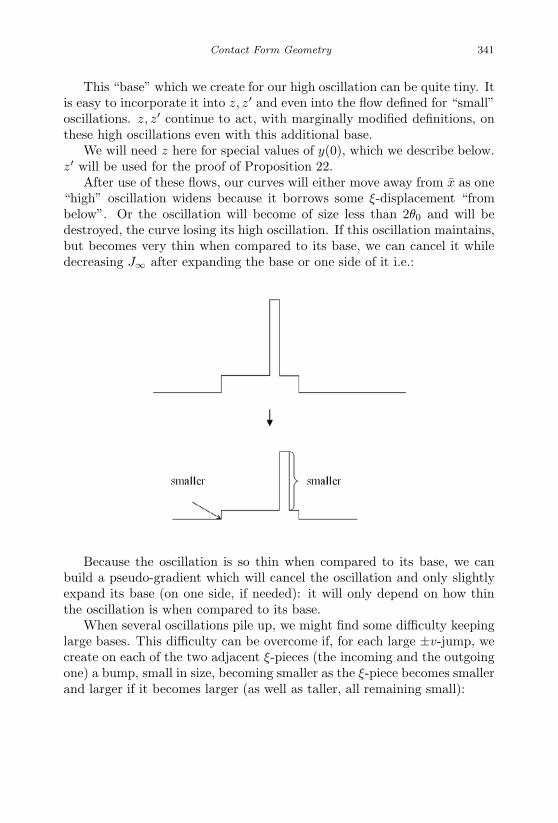
January 17, 2007 11:55 WSPC/Book Trim Size for 9in x 6in finalBB
Contact Form Geometry 341
This “base” which we create for our high oscillation can be quite tiny. Itis easy to incorporate it into z, z′ and even into the flow defined for “small”oscillations. z, z′ continue to act, with marginally modified definitions, onthese high oscillations even with this additional base.
We will need z here for special values of y(0), which we describe below.z′ will be used for the proof of Proposition 22.
After use of these flows, our curves will either move away from x as one“high” oscillation widens because it borrows some ξ-displacement “frombelow”. Or the oscillation will become of size less than 2θ0 and will bedestroyed, the curve losing its high oscillation. If this oscillation maintains,but becomes very thin when compared to its base, we can cancel it whiledecreasing J∞ after expanding the base or one side of it i.e.:
Because the oscillation is so thin when compared to its base, we canbuild a pseudo-gradient which will cancel the oscillation and only slightlyexpand its base (on one side, if needed): it will only depend on how thinthe oscillation is when compared to its base.
When several oscillations pile up, we might find some difficulty keepinglarge bases. This difficulty can be overcome if, for each large ±v-jump, wecreate on each of the two adjacent ξ-pieces (the incoming and the outgoingone) a bump, small in size, becoming smaller as the ξ-piece becomes smallerand larger if it becomes larger (as well as taller, all remaining small):

January 17, 2007 11:55 WSPC/Book Trim Size for 9in x 6in finalBB
342 Recent Progress in Conformal Geometry
As several high and thin, oscillations pile up (this number is a prioribounded), the first and the last one have “sizable” small bumps, on the leftfor the first, on the right for the last, and we can use them to cancel all thethin oscillations in between.
We now show how to use z1 or z (the first decreasing direction whichwe have built) in order to get rid of high oscillations along a characteris-tic piece with H1
0 -index non zero. It is easy to convex-combine the flowwhich is defined for small oscillations with the flow on high oscillations;we need to take care of these only when they develop in the vicinity of asubcharacteristic piece.
since then the v-jumps of such an oscillation can be used to define thedecreasing normal associated to this characteristic piece when one of themis far from x1, x2, x3 etc.
We revisit now the definition of z:We transport ξ from x0 to x1 along v, then from x1 to x2 along ξ. We
derive at x2 a vector θ(ξ) = a1ξ + b1[ξ, v] + c1v.

January 17, 2007 11:55 WSPC/Book Trim Size for 9in x 6in finalBB
Contact Form Geometry 343
We pull back ξ from a height s along v above x2. We derive a vector atx2: Dφ−s(ξ) = A1ξ + B1[ξ, v] + C1v. Dφ−s(ξ)− B1
b1θ(ξ) has no component
along [ξ, v].Using the ξ-piece abuting at x2 and the v-jump starting at x2, we can
adjust these other components.If the high oscillation at x2 is not high enough, we can increase it (if
the deformation which we are going to define is decreasing) and if it is toohigh, we can introduce a tiny, flat ξ-piece at the right level.
We compute the variation of J along this direction. We find
ϕ(s) = 1 − A1 +B1
b1(a1 − 1) = 1 − αx2(Dφ−s(ξ)) − βx2(Dφ−s(ξ))
b1(a1 − 1).
If this expression is negative at any s, we can introduce a decreasing defor-mation which expands the tiny high ξ-piece and moves these curves awayfrom the critical one. This deformation convex-combines with the otherones which take place when the base of the high oscillation or the oscilla-tion is far from x2, x3 etc.
If it is positive for every s, we can thin down any high oscillation andtame it down to be a small one. The argument preceeds.
If ϕ(s0) = 0 above x2, x3, . . . , which are extremities of a subcharacter-istic piece, ϕ′(s0) is non zero generically and the argument proceeds.
Proof. [Proof of Propsition 33] Assume that the first characteristic piecec1, lies between two positive edge v-pieces. Assume that its full unstablemanifold is used in order to define the dominated cycle. Since its unstablemanifolds bounds, there must be another characteristic piece involved, withits full unstable manifold, in the definition of this cycle.
A dominating flow-line must contain, as it spans the full unstable mani-fold of c1, a negative small v-jump in addition to all the v-jumps of the basecurve; otherwise the full unstable manifold of c1 cannot be covered. Thesame argument holds for c2, with a positive or negative v-jump dependingon the signs of the edge v-jumps of c2, and in fact holds for every ci as itsfull unstable manifold is used.
If these additional v-jumps do not travel, they would allow to movedown, past x; they can be used either with the decreasing normals associ-ated to each characteristic piece, or in a direct construction of a decreasingdeformation.
Thus, they must travel from a characteristic piece c1 to another char-acteristic piece, for example c2. Assume that c1 and c2 follow each other,so that both of them have positive v-edges in particular.
This happens in the following process.
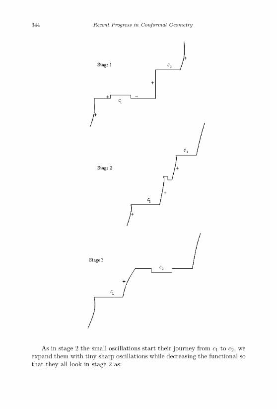
January 17, 2007 11:55 WSPC/Book Trim Size for 9in x 6in finalBB
344 Recent Progress in Conformal Geometry
As in stage 2 the small oscillations start their journey from c1 to c2, weexpand them with tiny sharp oscillations while decreasing the functional sothat they all look in stage 2 as:

January 17, 2007 11:55 WSPC/Book Trim Size for 9in x 6in finalBB
Contact Form Geometry 345
(*)
Transporting ξ from x1 to x2 and using the tiny ξ-piece [x2, x3], we canbuild a decreasing direction z2 (reversing this direction if needed).
This ability to decrease might fade away very fast as either the ξ-piece[x2, x3] disappears or the sharp oscillation x1−x2−x3−x4 changes sharplyits height.
It is easy to stabilize and even to increase the length of the ξ-piece[x2, x3]. Indeed, there is a tangent direction z on the base curve
formed by transporting ξ from y1 to x1, pulling down ξ from x2 to x1
and matching, after scaling and adding v and ξ-components at x1 the two

January 17, 2007 11:55 WSPC/Book Trim Size for 9in x 6in finalBB
346 Recent Progress in Conformal Geometry
vectors thus derived at x1. Since the base curve is critical,
J ′ · z = 0
z or −z will increase the length of c2.We can use z on (*) so that the ξ-length of [x2, x3] increases. Since
J ′ · ˜z = o(1) while our other direction z2 has J ′ · z2 ≤ −γ2 < 0, thecombination still decreases J and increases [x2, x3].
The v-jumps around [x2, x3] are considerably perturbed in this way.We need to make sure that as, for example, the oscillation correspondingto [x2, x3] (upwards) increases somewhat, we can tame it and bring it down.
If at any height h above c1 we can decrease J by expanding [x2, x3] aftertransporting ±ξ from [x2, x3] down to c1 or to any other part of the basecurve, we can infer that we could have scaled (expanded) our oscillationsor have introduced, if they went above h a tiny flat ξ-piece at the level h,and from there on use this decreasing direction which expands the ξ-pieceat the level h.
This deformation, unlike z2, does not hinder itself since it expands[x2, x3] and does not involve great perturbations of the v-size of the os-cillation.
If on the contrary no such h exists, we are able to thin down any suchoscillation while decreasing J . Hence, would our oscillation greatly perturbafter the use of z2, ˜z, we would be able to tame it, reintroduce an [x2, x3]-piece of a similar size or larger at the level of c2 and proceed with thisdownwards deformation.
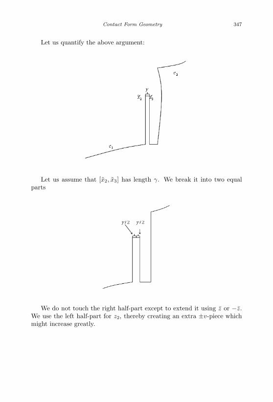
January 17, 2007 11:55 WSPC/Book Trim Size for 9in x 6in finalBB
Contact Form Geometry 347
Let us quantify the above argument:
Let us assume that [x2, x3] has length γ. We break it into two equalparts
We do not touch the right half-part except to extend it using z or −z.We use the left half-part for z2, thereby creating an extra ±v-piece whichmight increase greatly.

January 17, 2007 11:55 WSPC/Book Trim Size for 9in x 6in finalBB
348 Recent Progress in Conformal Geometry
Let us estimate the size µ of the v-jump created versus the size ∆ ofthe right half-piece.
After time t if we use ±Mz, ∆ is at least
γ
2+ Mt.
During the same time, the left half-piece length has become γ2 −O(ct), due
to the use of z2, c a priori-bounded and the size µ of the v-piece created isO(
tγ
)as long as ct ≤ γ
4 .We thus need
ct ≤ γ4
tγ ≤ c0.
Thus, t ≤ Cγ. After the time Cγ, the right half-piece has length
γ
2+ MCγ.
If MC > 12 , which we may assume since M can be chosen large, we have
rebuilt a top ξ-piece of size γ. The direction of the new ±v-jump whichwe will create as we iterate the construction described above is the samethen the one found in the first step because z2 in each stage is built aftertransporting ξ along nearly the same large ±v-jump, with maybe small (intotal) ξ-pieces inserted in between and back and forth runs along v.

January 17, 2007 11:55 WSPC/Book Trim Size for 9in x 6in finalBB
Contact Form Geometry 349
The decreasing deformation described above is thus self sustained andcan be used to glue the decreasing deformation along c1 with the decreasingdeformation along c2.
Another issue has to be addressed though in the above process: comingback to stage 1 of this process, we observe the need along c1 to have twov-jumps, one positive, the other one negative in order to complete the travelprocess in stage 2 and after. While the negative v-jump among these twois naturally provided by Span of c1, the positive one may be thought asa companion of the positive left edge of c1 and might have to be created.This can be achieved using the “small room” for decrease provided by theexistence of the negative v-jump , exhausting half of it if needed in orderto create the positive one close to the left edge as it is created, moving tothe negative one as it becomes larger. The whole process of creation of thisv-jump can be embedded in a decreasing flow-line along which on one handHypothesis (B) is locally satisfied, on the other hand the flow-line createsthe initial conditions of stage 1 and stage 2, i.e a small positive v-jumpclose to a small negative v-jump, see the figures above.
The first statement of Proposition 33 follows for two characteristicpieces. Observe that the above deformation requires only the existenceof an intermediate positive v-jump followed by a negative v-jump, thus theexistence on this pair of characteristic pieces of three distinct families, oneof each extreme edge and one for the intermediate negative v-jump. Thisobservation will be generalized (with a slight variation) below for morecharacteristic pieces.
We now establish that the topological statement of Proposition 33 ex-tends for more than two characteristic pieces of strict H1
0 -index zero:Given two consecutive characteristic pieces and their associated full
(half) unstable manifolds c1 and c2, we just proved that
∂(c1 ⊗ c2) = ∂σ
where σ carries 2 zeros at most for b. We also have established that c1 ⊗ c2
and σ are homologous relative to their common boundary, without increasein the number of zeros of b relative to c1 ⊗ c2. Assume that we have k + 1consecutive characteristic ξ-pieces. Let ci be their full (half) - unstablemanifold. We write:
∂(c1 ⊗ · · · ⊗ ck+1) = ∂σ ⊗ c3 ⊗ · · · ⊗ ck+1 + c1 ⊗ c2 ⊗ ∂(c3 ⊗ · · · ⊗ ck+1)
= ∂(σ ⊗ c3 · · · ⊗ ck+1) + (c1 ⊗ c2 − σ) ⊗ ∂(c3 ⊗ · · · ⊗ ck+1)
= ∂(σ ⊗ c3 · · · ⊗ ck+1 + u ⊗ ∂(c3 ⊗ · · · ⊗ ck+1)).
January 17, 2007 11:55 WSPC/Book Trim Size for 9in x 6in finalBB
350 Recent Progress in Conformal Geometry
Observe that
σ ⊗ c3 · · · ⊗ ck+1 + u ⊗ ∂(c3 ⊗ · · · ⊗ ck+1)
carries two less zero than c1 ⊗ · · · ⊗ ck+1.The conclusion follows for more than two characteristic consecutive ξ-
pieces. We could even multiply by other homology classes (due to the indexat infinity or other characteristic ξ-pieces of non zero index) the argumentwould go through for all classes containing ∂(c1 ⊗ · · · ⊗ ck+1) as a factor.The argument goes also through for characteristic pieces of non zero H1
0
strict index without substantial modifications. The idea is the following:each cj , j = 1, 2 may be represented using ij0 + 1 ± v-jumps which havesizes varying independently and an additional large ±v-jump in order torepresent the left edge. ij0 of them are located at interior nodes, theyprovide a representation of the strict H1
0 -unstable manifold, the additional±v-jump is used to represent the full unstable manifold of the characteristicpiece. We can insert this additional ±v-jump in the last nodal zone for c1
and in the first nodal zone for c2. Assuming that the common edge ispositive, this additional v-jump is negative. Again, we may view ∂(c1 ⊗ c2)as the boundary of another chain where this additional negative v-jumpwill travel along the common edge. As in the case of the zero H1
0 -index,this travel requires the use of a positive v-jump which would progressively,as this additional v-jump moves to the next characteristic piece, build upthe common edge. If the ±vjump at the last interior node of the firstcharacteristic piece is positive, we can build a companion of it to playthis role. Otherwise, we have to introduce it after the ij0 internal ∗′s.Because the critical point at infinity is not false, ij0 is even (the two edgesare positively oriented) and the introduction of this positive v-jump doesnot increase the number of sign changes between the left edge and the rightedge beyond ij0 +2 which is the maximal number of sign changes allowed byc1. The additional negative v-jump can travel now and once it has reachedthe second characteristic piece, then it can be used to generate c2. ∂(c1⊗c2)is generated in this way as the boundary of a chain supporting two zerosless than c1 ⊗ c2.
Proof of the results of Section 2.5.6 and Theorem 1 completed We con-sider now a maximal sequence of consecutive characteristic pieces whichwe assume to be derived after the constructions of Section 2.5.6. Then, allinterior nodes of all characteristic pieces but one node possibly, on a singlecharacteristic piece, are controlled by a ∗. This feature of the configura-tions which we study is stable. This means that as this feature is about tochange, the Normal (II)-flow can be used on one of the ∗′s which are not

January 17, 2007 11:55 WSPC/Book Trim Size for 9in x 6in finalBB
Contact Form Geometry 351
∗’s of an edge, in fact is an interior ∗, in the transition zone. On these con-figurations, each edge must have a ∗ associated to it. Otherwise, the edgewould be a companion of a neighboring interior ∗ and we could engineera decrease through a use of a decreasing normal to the immediate right ofthe ∗ for a right edge, to the immediate left of the ∗ for the left edge. Thisnormal would be an additional companion for this ∗. This holds under theassumption that the H1
0 -strict index of these ξ-pieces is non zero. This ar-gument is adjusted for characteristic pieces of H1
0 -index zero in Appendix1.
Furthermore, we can state that on these configurations, all ∗′s are eitherin the vicinity of the interior nodes or in the vicinity of the edges.
Let us assume in a first step that there is no hole on the sequence ofcharacteristic pieces. The count of Section 2.5.6 is tight and implies thenthat on each characteristic piece but one, there are ij0 + 1∗’s, besides the∗’s of the edges. On the remaining characteristic piece, there are ij0∗’s anda ∗ for each edge. We refer to this characteristic piece in the sequel as the“(I)ξ-piece”. Let us assume that (I) is in between characteristic pieces. Theadditional ∗ on each other characteristic piece is in the vicinity of an edge.Thus, on the characteristic piece with only ij0∗’s, there is an edge whichdoes not have an additional ∗ in its vicinity, neither on this nor on the nextcharacteristic piece. No additional ∗ will ever come close to this edge, unlesswe can use the Normal (II) flow on it prior to its motion close to this edge.Let us consider the other edge of the same characteristic piece. This otheredge has an additional ∗ in its neighborhood, on the next characteristicξ-piece. There are then two possibilities: either this other edge also doesnot have an additional ∗ in its vicinity. Then, no additional ∗ will come toits vicinity unless we can use the Normal (II) flow on an interior node todecrease. The (I)ξ-piece jails a repetition which is stable. We can introduceon the next characteristic piece to the right a fixed decreasing Normal N−,it will be extendable into an admissible alternating sequence because of thestable repetition. These configurations can be decreasing. Or this otheredge does have an additional ∗ in its vicinity, not on the (I)ξ-piece, butthis could change after a travel of this ∗ along this edge. We then chooseto introduce a decreasing Normal N− in the nodal zone of the (I)ξ-pieceneighboring this edge. This requires some justification:
The additional ∗ which we are considering remains in the vicinity of thisedge, otherwise we could use the Normal (II) flow on it and decrease theconfiguration. It can however travel along the edge, from the (I) ξ-piece tothe next characteristic piece. When it is in the (I) ξ-piece, the use of N−
is justified, we have used this argument several times before. When the∗ travels along the edge, it has the orientation of the edge because thereare only then two neighboring ∗’s. There is then a repetition and this N−
January 17, 2007 11:55 WSPC/Book Trim Size for 9in x 6in finalBB
352 Recent Progress in Conformal Geometry
can be made part of an admissible alternating sequence. However whenthis ∗ has traveled to the next characteristic piece, it is disconnected fromthe use of N−. This ∗ could change sign and the repetition with the ∗ ofthe edge would disappear and N− would not be justified anymore. So weneed then to make N− travel to the next characteristic piece to becomenext to this additional ∗ and to the other ∗ of the edge, along the processdescribed in the proof of Proposition 33. This requires the introduction of a±v-jump with the orientation of the edge along which the travel takes placeon the other side of N− than the edge. This ±v-jump can be introducedas a simple counting argument on the (I)ξ-piece after the introduction ofN− shows: the various ∗’s, including those of the edges, build with N− asequence which admits an alternating representative. One can then checkthat the introduction of such a ±v-jump in the second nodal zone closestto the edge never increases the total number of families after reordering,relabeling etc. Furthermore, it decreases J . Using the widening process,we can then assume that the node closest to the edge is occupied by this±v-jump. The next ±v-jump in the direction of the edge either has theorientation of N− and can be confounded with it(this includes the casewhen it is zero) . A ±v-jump can now be introduced prior to N−(the edgebeing after) with the orientation of the edge.
Or this next ±v-jump has already the orientation of the edge. There isno need to introduce an additional ±v-jump.
The process of Proposition 33 can now begin. It will decrease J andbring N− to the next characteristic piece as the repetition between the ∗ ofthe edge and the additional ∗ still holds. Once on the other side, our large±v-jumps can be assumed to be small, but the new edge. The two ∗’s arenow on the other side, follow each other and have the same orientation, weconfound them, bring them into the new N− after the travel which theycross to reappear on the other side close to the edge. This crossing can beaccomplished as J is decreasing using the “negative” decreasing Normal.We now relabel ∗ and ∗ the two ∗’s which follow each other and have theorientation of the edge. The new N− is next to it. The decreasing processgoes on, continuity has been achieved.
A similar argument, with some modifications, can be made in the case ofa single hole at a single node. There is a repetition in the left edge betweenexactly two ∗’s, of course this can evolve; but each other characteristicpiece has an additional ∗, as above only that it can travel along the edge itneighbors. Let us assume that the ξ-piece next to the characteristic piecewith a hole(after it)is also characteristic. An additional ∗ neighbors it.There are exactly ij0∗’s strictly between the representative most to the leftof the left edge and the right edge when the additional ∗ is either travelingalong the edge or on the next characteristic piece to the right. We are in
January 17, 2007 11:55 WSPC/Book Trim Size for 9in x 6in finalBB
Contact Form Geometry 353
the same situation than above. We can make an N− decreasing Normaltravel and follow the additional ∗.
The N− decreasing Normal is part of the Hole flow corresponding tothe representative most to the right of the left edge because of the singlehole. Thus, there is no need to make N− travel as this representative is“large”. We can declare it then to be left edge and use its Hole flow. N−
can be used then, without travel. As the other representative develops, arepetition occurs as long as the additional ∗ is either traveling or on the nextcharacteristic piece as discussed above and the travel becomes possible. Inall, the location of N− can be adjusted in a continuous way.
If the next ξ-piece to the right is not characteristic, then the right edgeof (I) is isolated and can be used to define a Hole flow. This constructionworks as long as another ∗ does not reach this edge obviously through itsnon degenerate end, a case which is discussed below.
The conclusion follows in such cases.The argument works for a (I)ξ-piece which is at the end of a sequence
if the extreme edge of the sequence does not “receive” other ∗’s from itsnon degenerate end. In case of “stable” repetition, we should choose tointroduce N− on the nearest characteristic ξ-piece, to the right or to theleft, depending on the configuration. It also works for an isolated ξ-piece,under the condition that both edges do not receive additional ∗’s. For a“stable” repetition and an isolated ξ-piece, we insert N− on a characteristicpiece which is interior to a sequence ξ-piece and does not neighbor (I) (whichis here an extreme or isolated characteristic piece). We are assuming thatthere are sequences with more than three characteristic pieces.
Such a (I)ξ-piece may receive other ∗’s from its non degenerate end(s).Either they come from a non degenerate ξ-piece which is then, at an inter-mediate time, pierced with a hole; J decreases below the critical level atthat intermediate time, the cycle splits. Or they come from other charac-teristic sequences which are neighbors to (I), from their edge characteristicpieces through the removal of the additional ∗. After this removal, eitherwe have a “stable” repetition on another characteristic ξ-piece or the con-struction of Proposition 33 can be carried out on this new characteristicξ-piece which we label (I)’. There might two possible choices for (I)’, but(I) was unique and we declare (I)’ to be the first one to the right of (I).
Observe that in the case of the “stable” repetition, the traveling ∗ willnot reach the interior of (I)if a second repetition does not develop in an edge.This allows to switch between the decreasing flow(use of one decreasingNormal N− for each of them, or of a Hole flow outside of the support ofthe two repetitions) due to (I) and the decreasing flow due to (I)’: eachone can be thought as due to alternating sequences with disjoint supports(observe that N− was always introduced either in the same sequence or
January 17, 2007 11:55 WSPC/Book Trim Size for 9in x 6in finalBB
354 Recent Progress in Conformal Geometry
interior to a sequence, see the construction above, which we slightly modifyfor (I)’ so that the supports of the constructions for (I) and (I)’ are disjoint);none of them includes a Normal in the repetitions which we just pointedout. We can extend one of them, not crossing the support of the other oneuntil it reaches one of the repetition. Extending it inside the repetitionif needed, we can make its orientation and the orientation of one of the±v-jumps of the repetition coincide. It behaves then as a Hole flow. Wethen overextend the other partial alternating sequence jumping over theother repetition. We derive an admissible alternating sequence. Howeversince the other alternating sequence behaves as a Hole flow, we can removethe corresponding part of the first sequence and insert the second one in it.The switch is possible.
On the other hand, the construction of Proposition 33 finds its justi-fication locally and therefore can be used in (I)’ in conjunction with thedeformation induced on (I). Indeed, typically when there is an additional ∗on a characteristic ξ-piece, either this ∗ and the related edge do not havethe same orientation and the use of N− is allowed as well as the switch; orthey have the same orientation, then the ξ-piece (I)’ jails exactly two rep-etitions. On the side of (I), either we have a stable repetition and we thenintroduced somewhere else, not on (I)’, an N−. We are also introducingan N− on (I)’. Two repetitions are spared sometimes over the transitionbetween (I) and (I)’, we can switch. Or we are using a Hole flow on (I),it can be inserted in an alternating sequence defined by the N− on (I)’and jumping over one of the repetitions of (I)’, again the switch is possible.The transition, in case of a hole, from this Hole flow to the construction ofProposition 33 on (I) is a reduction to the use of N− on (I), no justificationfor the switch is required. If we are using directly this construction on (I)(typically when there is no hole on (I)), either the additional ∗ has theorientation opposite to the edge on (I) or the next piece(after the travelis completed), there is nothing to prove. Or there are two repetitions, inaddition to the two repetitions related to (I)’. Two of them will be usedby the two N−’s and two are left, they warrant the compatibility and theymake the switch possible. Our proof is complete.
We study in this section the behavior of the Morse index at infinity i∞of x∞ along iterates.
2.5.9 Iterates of critical points at infinity
Lemma 19 Let x∞ or x be a hyperbolic critical point at infinity withat least one non characteristic ξ-piece, with H1
0 -index i0 and with index atinfinity i∞. Let xk∞ be the kth iterate of x∞ (or x).
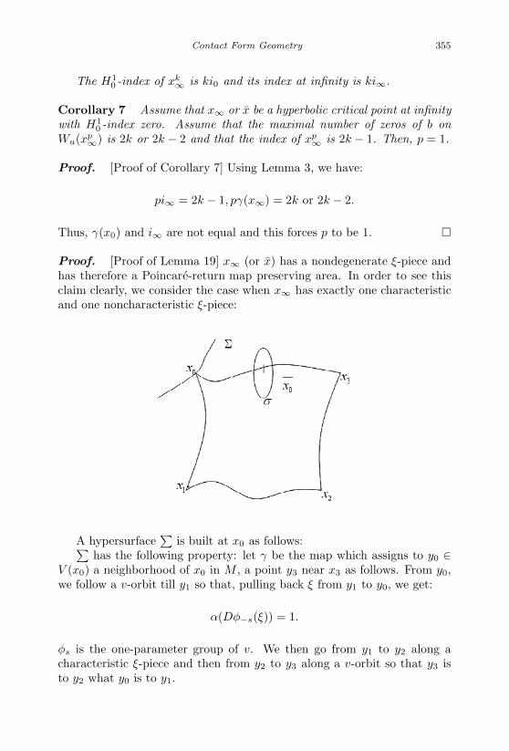
January 17, 2007 11:55 WSPC/Book Trim Size for 9in x 6in finalBB
Contact Form Geometry 355
The H10 -index of xk
∞ is ki0 and its index at infinity is ki∞.
Corollary 7 Assume that x∞ or x be a hyperbolic critical point at infinitywith H1
0 -index zero. Assume that the maximal number of zeros of b onWu(xp
∞) is 2k or 2k − 2 and that the index of xp∞ is 2k − 1. Then, p = 1.
Proof. [Proof of Corollary 7] Using Lemma 3, we have:
pi∞ = 2k − 1, pγ(x∞) = 2k or 2k − 2.
Thus, γ(x0) and i∞ are not equal and this forces p to be 1.
Proof. [Proof of Lemma 19] x∞ (or x) has a nondegenerate ξ-piece andhas therefore a Poincare-return map preserving area. In order to see thisclaim clearly, we consider the case when x∞ has exactly one characteristicand one noncharacteristic ξ-piece:
A hypersurface∑
is built at x0 as follows:∑has the following property: let γ be the map which assigns to y0 ∈
V (x0) a neighborhood of x0 in M , a point y3 near x3 as follows. From y0,we follow a v-orbit till y1 so that, pulling back ξ from y1 to y0, we get:
α(Dφ−s(ξ)) = 1.
φs is the one-parameter group of v. We then go from y1 to y2 along acharacteristic ξ-piece and then from y2 to y3 along a v-orbit so that y3 isto y2 what y0 is to y1.

January 17, 2007 11:55 WSPC/Book Trim Size for 9in x 6in finalBB
356 Recent Progress in Conformal Geometry
γ being defined , we pull back ξ from y0 to y1 and from y3 to y2. Wederive two vectors z1 and z2.
z1 splits into:
z1 = (1 + A1)ξ + B1[ξ, v] + C1v
z2 splits into
z2 = (1 + A1)ξ + B1[ξ, v] + C1v.
Along the characteristic ξ-piece from y1 to y2, v is mapped onto θv and[ξ, v] maps onto 1
θ [ξ, v] + νv.So that z1 and B1
θB1z2 have, after ξ-transport from y1 to y2, the same
[ξ, v]-component.∑is then defined to be y0 such that A1B1θ = B1A1.
If y0 ∈ σ, we then define a Poincare-return map C as follows: we followξ backwards starting from y0 until we hit
∑, then proceed with γ until y3
and from y3 to σ following ξ. It is easy to verify that
C∗α = α + df,
C∗dα|σ = dα|σfrom which our claim is derived.
It therefore makes sense to speak about hyperbolic or elliptic criticalpoint (at infinity). We are assuming here that x∞ is hyperbolic. Then,DCx0 has two eigenvalues, λ and 1
λ , both real and different from 1 (and−1, generically).
After multiplication by C, the tangent space has a natural complexifica-tion and the quadratic form d2J∞(x∞) becomes a Hermitian form of index2i∞. Considering now the iterate xp
∞ of order p of x∞, we introduce thepth-roots of 1:
1, ω1, . . . , ωp−1.
The tangent space to xp∞ splits in a natural way into a direct summand:
⊕pi=1Ti
xp∞ is parametrized over [0, p]. If z ∈ Ti, then z|[j,j+1] = ωiz|[j−1,j], with
j = 1, . . . , p.It is easy to see that, for i = j, Ti and Tj are d2J∞(xp∞)-orthogonal.The equation of Ti can be written using C, the initial variation in σ, z(0)
and then various increments in ξ and v (when compared to C) on the variousbranches transported to σ.
dCx0(z(0)) + X = ωiz(0).

January 17, 2007 11:55 WSPC/Book Trim Size for 9in x 6in finalBB
Contact Form Geometry 357
Then, z(1) = ωiz(0).If z1 and z2 ∈ Ti, then
z1(0) · α(z2(0) + z1(0) · α(z1(0)) − z1(1) · α(z1(1)) − z2(1) · α(z2(1)) = 0
since ωiωi = 1.
This computation extends to vectors in T (µ) where µ ∈ C, |µ| = 1 definedby the equation: dCx0(z(0)) + X = µz(0).
d2J∞ is defined on Ti and this definition extends to T (µ) as we will seelater.
We consider a path µ(t) on the unit circle, from 1 to ωi. T (µ) evolvesthen from Tx∞ , the tangent space to x∞, where d2J∞(x∞) has index 2i∞,to Ti. If we can prove that the quadratic form does not degenerate, weare done. Assume, arguing by contradiction, that the quadratic form d2J∞degenerates at T (µ0), with a simple degeneracy. Perturbing a little bit C(as in Proposition 15 of [Bahri-1 2003], for example) and using a genericityargument, we can move µo continuously, filling a tiny open interval, wherea root of unity ω, with ωq = 1, can be found.
Thus, we may assume that µ0 = ω. Then, d2J∞ degnerates on T (ω) ifand only if d2J∞(xq
∞), on Txq∞ , degenerates with the direction of degeneracy
satisfying:
z|[j+1,j] = ωz|[j,j−1]
xq∞ is a closed curve, with Poincare-return map Cq ·d2J∞(xq∞) degenerates ifand only if Cq degenerates and this is impossible because the eigenvalues ofC are real and different from 1 in absolute value. Thus, no such degeneracymay occur and d2J∞(x∞)|Ti has index 2i∞. Lemma 3 follows.
The extension of d2J∞ to T (µ) is quite simple: there is a formula ford2J∞ · z · z involving only the values of a tangent vector z at the edgepoints xj(j = 0, 1, 2, 3 in the example shown above). This formula extendsnaturally on T (µ). When µ = ω, with ωq = 1, we find (up to multiplicationby q) d2J∞(xq∞) · z · z on the tangent space to xq∞.
We now have:
Lemma 20 Let x∞ (or x) be of H10 -index zero and have a non-degenerate
ξ-piece. Assume x∞ ( or x) is elliptic. Then, all iterates of x∞ (or x) oforder p ≥ 2 can be discarded from our homology for k ≥ 4.
Proof. If x∞ or x is elliptic, we can complete deformations of α near x∞so that xp
∞ degenerates and xr∞ does not for 1 ≤ r < p. Then the index
of xp∞ changes (xp∞ maintains since x∞ maintains) and xp∞ is replaced
January 17, 2007 11:55 WSPC/Book Trim Size for 9in x 6in finalBB
358 Recent Progress in Conformal Geometry
by a very close y∞ which is not an iterate but has as many ξ and ±v-
pieces as xp∞. Indeed, then C is conjugate to a rotation(
cos θ0 − sin θ0
sin θ0 cos θ0
)and Cp degenerates after the introduction (as in Propostion 15 of [Bahri-12003]) of a perturbation of α into λα which changes C into R−θ0/p
C or intoR2π−θ0/p
C. We would like β to remain a contact from so that we requirethat θ0/p < γ, where γ is the v-rotation on this non-degenerate ξ-piece. Inthe second case, we would like i0 to remain zero, so that we require that
2π − θ0/p < π − γ.
Clearly, since 0 < θ0 < 2π, one of θ0/γ or 2π−θ0π−γ is less than 2 so that this
yields p ≥ 2.If xp
∞ hinders our deformation downwards, then assuming tht x∞ hasH1
0 -index zero, we have:pγ(x∞) = 2k or 2k − 2
index (xp∞) = 2k − 1
. (*)
This equation might be satisfied for more than one index of iteration p; butsince γ(x∞) is at least 2 (k ≥ 2), if this occurs for more than one indexof iteration, then these indexes will be consecutive indexes p and p − 1.Working as above, with R−θ0/p−1 or R2π−θ0/p−1, C
p and Cp−1 degenerate(p will be ≥ 3 if k ≥ 4) and xp
∞, xp−1∞ do not have the Morse index 2k − 1
anymore.
Lemma 21 Assume that x∞ (or x) is a critical point (at infinity) havinga non degenerate ξ-piece with H1
0 -index ij0.If using the procedure of Proposition 15 of [Bahri-1 2003], we can in-
crease ij0 to ij0 + 1, then x∞ (or x), prior to any perturbation, has an indexat infinity i∞ ≥ 1 and the index at infinity of its iterates xp∞ is at least p.
Proof. If ij0 can be increased to ij0 + 1, then i∞ ≥ 1 since the total in-dex is unchanged. Thus, when the H1
0 -index on the non-degenerate ξ-pieceis ij0, x∞ has a negative direction at infinity, which is derived after bifur-cation from the v associated to the non-degenerate ξ-piece as it becomesdegenerate at the transition between ij0 and ij+1
0 .Very near to this degeneracy position, when the H1
0 -index on this branchis ij0, we may view the new negative direction at infinity as obtained from v-tranport from one edge to the next one of this ξ-piece, the [ξ, v]-componentbeing compensated by v-transport of ξ from the next ξ-piece back to theξ-piece which we are considering:

January 17, 2007 11:55 WSPC/Book Trim Size for 9in x 6in finalBB
Contact Form Geometry 359
This negative direction at infinity ¯v has compact support in [0,1].Lemma 5 follows.
2.5.10 The Fredholm aspect
We know that our variational problem is not Fredholm [Bahri 1998], [Bahri-1 2003]. This translates into the fact that the “oscillations” i.e. a sequenceof two consecutive v-jumps of opposite orientation can be large :
Indeed, as explained in [Bahri 1998], [Bahri-1 2003], some variationswhich are not L∞-small can decrease J .
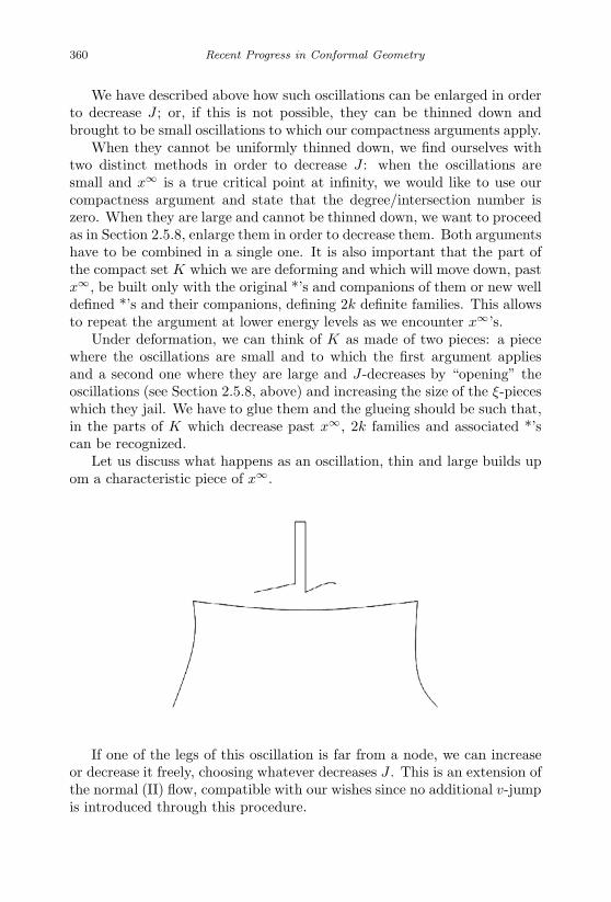
January 17, 2007 11:55 WSPC/Book Trim Size for 9in x 6in finalBB
360 Recent Progress in Conformal Geometry
We have described above how such oscillations can be enlarged in orderto decrease J ; or, if this is not possible, they can be thinned down andbrought to be small oscillations to which our compactness arguments apply.
When they cannot be uniformly thinned down, we find ourselves withtwo distinct methods in order to decrease J : when the oscillations aresmall and x∞ is a true critical point at infinity, we would like to use ourcompactness argument and state that the degree/intersection number iszero. When they are large and cannot be thinned down, we want to proceedas in Section 2.5.8, enlarge them in order to decrease them. Both argumentshave to be combined in a single one. It is also important that the part ofthe compact set K which we are deforming and which will move down, pastx∞, be built only with the original *’s and companions of them or new welldefined *’s and their companions, defining 2k definite families. This allowsto repeat the argument at lower energy levels as we encounter x∞’s.
Under deformation, we can think of K as made of two pieces: a piecewhere the oscillations are small and to which the first argument appliesand a second one where they are large and J-decreases by “opening” theoscillations (see Section 2.5.8, above) and increasing the size of the ξ-pieceswhich they jail. We have to glue them and the glueing should be such that,in the parts of K which decrease past x∞, 2k families and associated *’scan be recognized.
Let us discuss what happens as an oscillation, thin and large builds upom a characteristic piece of x∞.
If one of the legs of this oscillation is far from a node, we can increaseor decrease it freely, choosing whatever decreases J . This is an extension ofthe normal (II) flow, compatible with our wishes since no additional v-jumpis introduced through this procedure.

January 17, 2007 11:55 WSPC/Book Trim Size for 9in x 6in finalBB
Contact Form Geometry 361
If, anywhere along the characteristic piece, there is an interval alongwhich all large oscillations can be thinned down while decreasing (a regionwhere the Fredholm hypothesis is satisfied, this can be quantified geomet-rically see [Bahri 1998], [Bahri-1 2003]), we can redistribute the rotationalong this ξ-piece and assume that all the nodes are in this region. Thus,all large oscillations near the nodes can be brought down to be small.
Our compactness arguments proceed.We consider now the case when every thin oscillation of the right size
(with the orientation of the oscillations which we have) can be enlargedalong a decreasing deformation of J in the vicinity of a given node.
Thus, if an oscillation is of the right size or more, we can enlarge it:
and decrease J .
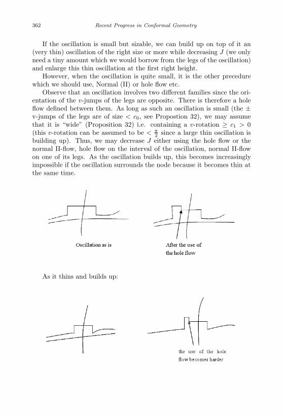
January 17, 2007 11:55 WSPC/Book Trim Size for 9in x 6in finalBB
362 Recent Progress in Conformal Geometry
If the oscillation is small but sizable, we can build up on top of it an(very thin) oscillation of the right size or more while decreasing J (we onlyneed a tiny amount which we would borrow from the legs of the oscillation)and enlarge this thin oscillation at the first right height.
However, when the oscillation is quite small, it is the other precedurewhich we should use, Normal (II) or hole flow etc.
Observe that an oscillation involves two different families since the ori-entation of the v-jumps of the legs are opposite. There is therefore a holeflow defined between them. As long as such an oscillation is small (the ±v-jumps of the legs are of size < c0, see Propostion 32), we may assumethat it is “wide” (Proposition 32) i.e. containing a v-rotation ≥ c1 > 0(this v-rotation can be assumed to be < π
2 since a large thin oscillation isbuilding up). Thus, we may decrease J either using the hole flow or thenormal II-flow, hole flow on the interval of the oscillation, normal II-flowon one of its legs. As the oscillation builds up, this becomes increasinglyimpossible if the oscillation surrounds the node because it becomes thin atthe same time.
As it thins and builds up:

January 17, 2007 11:55 WSPC/Book Trim Size for 9in x 6in finalBB
Contact Form Geometry 363
Thus, as the oscillation is still “wide” and small and is building up, weintroduce, at the same point where we introduce the ±v-jump correspond-ing to the hole flow, a thin oscillation, which we build up.
and progressively cancel the use of the hole flow. We find
All these oscillations in the vicinity, wherever the hole flow has beenused, can be brought back to one single wide oscillation or family of wideoscillations, before, after or surrounding the node:
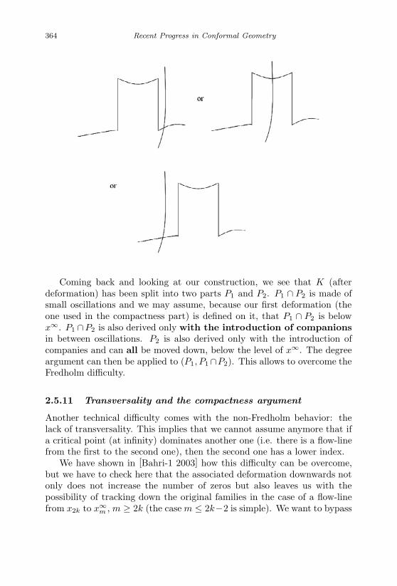
January 17, 2007 11:55 WSPC/Book Trim Size for 9in x 6in finalBB
364 Recent Progress in Conformal Geometry
Coming back and looking at our construction, we see that K (afterdeformation) has been split into two parts P1 and P2. P1 ∩ P2 is made ofsmall oscillations and we may assume, because our first deformation (theone used in the compactness part) is defined on it, that P1 ∩ P2 is belowx∞. P1 ∩P2 is also derived only with the introduction of companionsin between oscillations. P2 is also derived only with the introduction ofcompanies and can all be moved down, below the level of x∞. The degreeargument can then be applied to (P1, P1∩P2). This allows to overcome theFredholm difficulty.
2.5.11 Transversality and the compactness argument
Another technical difficulty comes with the non-Fredholm behavior: thelack of transversality. This implies that we cannot assume anymore that ifa critical point (at infinity) dominates another one (i.e. there is a flow-linefrom the first to the second one), then the second one has a lower index.
We have shown in [Bahri-1 2003] how this difficulty can be overcome,but we have to check here that the associated deformation downwards notonly does not increase the number of zeros but also leaves us with thepossibility of tracking down the original families in the case of a flow-linefrom x2k to x∞
m , m ≥ 2k (the case m ≤ 2k−2 is simple). We want to bypass
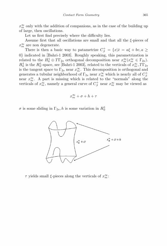
January 17, 2007 11:55 WSPC/Book Trim Size for 9in x 6in finalBB
Contact Form Geometry 365
x∞m only with the addition of companions, as in the case of the building up
of large, then oscillations.Let us first find precisely where the difficulty lies.Assume first that all oscillations are small and that all the ξ-pieces of
x∞m are non degenerate.
There is then a basic way to patametrize C+β = x|x = aξ + bv, a ≥
0 indicated in [Bahri-1 2003]. Roughly speaking, this parametrization isrelated to the H1
0 ⊕ TΓ2s orthogonal decomposition near x∞m (x∞
m ∈ Γ2s).H1
0 is the H10 -space, see [Bahri-1 2003], related to the verticals of x∞
m , TΓ2s
is the tangent space to Γ2s near x∞m . This decomposition is orthogonal and
generates a tubular neighborhood of Γ2s near x∞m which is nearly all of C+
β
near x∞m . A part is missing which is related to the “normals” along the
verticals of x∞m , namely a general curve of C+
β near x∞m may be viewed as
x∞m + σ + h + τ
σ is some sliding in Γ2s, h is some variation in H10
τ yields small ξ-pieces along the verticals of x∞m :
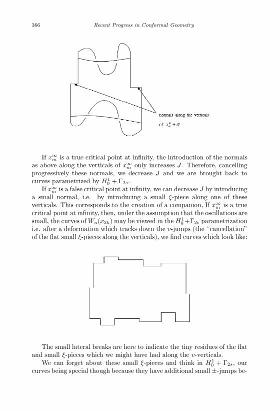
January 17, 2007 11:55 WSPC/Book Trim Size for 9in x 6in finalBB
366 Recent Progress in Conformal Geometry
If x∞m is a true critical point at infinity, the introduction of the normals
as above along the verticals of x∞m only increases J . Therefore, cancelling
progressively these normals, we decrease J and we are brought back tocurves parametrized by H1
0 + Γ2s.If x∞
m is a false critical point at infinity, we can decrease J by introducinga small normal, i.e. by introducing a small ξ-piece along one of theseverticals. This corresponds to the creation of a companion, If x∞
m is a truecritical point at infinity, then, under the assumption that the oscillations aresmall, the curves of Wu(x2k) may be viewed in the H1
0 +Γ2s parametrizationi.e. after a deformation which tracks down the v-jumps (the “cancellation”of the flat small ξ-pieces along the verticals), we find curves which look like:
The small lateral breaks are here to indicate the tiny residues of the flatand small ξ-pieces which we might have had along the v-verticals.
We can forget about these small ξ-pieces and think in H10 + Γ2s, our
curves being special though because they have additional small ±-jumps be-
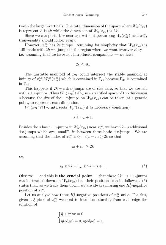
January 17, 2007 11:55 WSPC/Book Trim Size for 9in x 6in finalBB
Contact Form Geometry 367
tween the large v-verticals. The total dimension of the space where Wu(x2k)is represented is 4k while the dimension of Wu(x2k) is 2k.
Since we can perturb v near x2k without perturbing Ws(x∞m ) near x∞
m ,tranversality should follow easily.
However, x∞m has 2s jumps. Assuming for simplicity that Wu(x2k) is
still made with 2k± v-jumps in the region where we want transversality —i.e. assuming that we have not introduced companions — we have:
2s ≤ 4k.
The unstable manifold of x2k could intersect the stable manifold atinfinity of x∞
m , W∞s (x∞
m ) which is contained in Γ2s because Γ2s is containedin Γ4k.
This happens if 2k − s ± v-jumps are of size zero, so that we are leftwith s±v-jumps. Thus Wu(x2k)∩Γ2s is a stratified space of top dimensions because the size of the ±v-jumps on Wu(x2k) can be taken, at a genericpoint, to represent each dimension.
Wu(x2k) ∩ Γ2s intersects W∞s (x2k) if (a neccesary condition)
s ≥ i∞ + 1.
Besides the s basic ±v-jumps in Wu(x2k) near x∞m , we have 2k−s additional
±v-jumps which are “small”, in between these basic ±v-jumps. We areassuming that the index of x∞
m is i0 + i∞ = m ≥ 2k so that
i0 + i∞ ≥ 2k
i.e.
i0 ≥ 2k − i∞ ≥ 2k − s + 1. (*)
Observe — and this is the crucial point — that these 2k − s ± v-jumpscan be tracked down on Wu(x2k) i.e. their positions can be followed. (*)states that, as we track them down, we are always missing one H1
0 -negativeposition of x∞
m .Let us analyze how these H1
0 -negative positions of x∞m arise. For this,
given a ξ-piece of x∞m we need to introduce starting from each edge the
solution of η + a2ητ = 0
η(edge) = 0, η(edge) = 1.
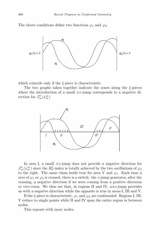
January 17, 2007 11:55 WSPC/Book Trim Size for 9in x 6in finalBB
368 Recent Progress in Conformal Geometry
The above conditions define two functions ϕ1 and ϕ2:
which coincide only if the ξ-piece is characteristic.The two graphs taken together indicate the zones along the ξ-pieces
where the introduction of a small ±v-jump corresponds to a negative di-rection for J ′′∞(x∞
m )
In area I, a small ±v-jump does not provide a negative direction forJ ′′∞(x∞
m ) since the H10 -index is totally achieved by the two oscillations of ϕ2
to the right. The same claim holds true for area V and ϕ1. Each time azero of ϕ1 or ϕ2 is crossed, there is a switch: the v-jump generates, after thecrossing, a negative direction if we were coming from a positive directionor vice-versa. We thus see that, in regions II and IV, a±v-jump providesus with a negative direction while the opposite is true in areas I, III and V.
If the ξ-piece is characteristic, ϕ1 and ϕ2 are confounded. Regions I, III,V reduce to single points while II and IV span the entire region in betweennodes.
This repeats with more nodes.

January 17, 2007 11:55 WSPC/Book Trim Size for 9in x 6in finalBB
Contact Form Geometry 369
Coming back to the 2k − s ± v-jumps whose positions can be trackeddown, we assert that, in every occurrence, there will be a ξ-piece wherethe number of ±v-jumps among these 2k − s which live on this ξ-piece isstrictly less than the trict H1
0 -index of this ξ-piece.The positions of these ±v-jumps can be tracked down. We can then -
it is a technical lemma — slide them so that each of them is in a “negativearea”, two of them not being in the same negative area (we know how toseparate ±v-jumps when they are small while decreasing J).
There is then, in every occurence, one negative area where no ±v-jumplives. If this negative area is the first one after the left edge, we can intro-duce in it a ±v-jump which has the orientation of this left edge.
This will decrease J and this decrease is completed through the intro-duction of a companion (to the edge).
If this (there could be several of them) negative area is not the first one,then we can deform our ±v-jump progressively, with the introduction ofcompanions, and make it to be the first negative area.
Indeed, we can fill every empty negative area with a ±v-jump havingthe same orientation and the same weight than the next existing ±v-jumpto the right of this empty negative area. As we create these ±v-jumps(which might be zero if the next — tracked — ±v-jump existing to theright is zero), we can cancel its next companion to the right. Working stepby step, we free the first negative area and proceed as above, introducing a±v-jump in it with the orientation of the right edge. J decreases then andtransversality follows.
The definition of companions is slightly extended in this way to include“twin” ±v-jumps because the ±v-jumps which we are replacing may bezero.
The argument as described above assumes that Wu(x2k) is constantlyachieved through Γ4k, which is of course wrong because companions andtwins can be introduced along the way. This builds families of ±v-jumps.Revisiting our argument above, we may reduce a whole family to a single±v-jump in a negative area and proceed as above. This requires only theaddition of a few technical details allowing to slide the ±v-jumps of a familyin negative areas and reduce them to a single one. Observe that alongthese slidings, the ±v-jumps can change orientation. However, families willchange orientation together as can be engineered easily.
The transversality argument in this simplified framework thus holds,when x∞
m does not have characteristic pieces.If x∞
m has some characteristic pieces, but the oscillations are still as-sumed to be small, the above argument extends. Indeed, the curve sup-porting x∞
m , x∞, supports in fact a cluster of critical points of variousindices x∞ = x∞
0 , x∞1 , . . . , x∞
m etc. corresponding to the various “puzzles”

January 17, 2007 11:55 WSPC/Book Trim Size for 9in x 6in finalBB
370 Recent Progress in Conformal Geometry
which we can build using the full (half)-unstable manifolds associated tothe characteristic pieces of x∞. x∞ itself has an index equal to i0 + i∞. Ifi0 + i∞ ≤ 2k − 1, then some xi’s have index 2k − 1 (see [Bahri-1 2003], theindex increases by 1 at most at each step) and the arguments developed forcompactness above work. The covering degree of these xi’s by x2k is zero.
If i0 + i∞ ≥ 2k, then x∞ has already an index too large for x2k andwe would like to establish that Wu(x2k) and Ws(x∞) do not intersect.x∞ does not use any full (half)-unstable manifold of any characteristicpiece included in it. Its index is made of i∞, the index of x∞ in Γ2s
and i0, the strict H10 -index. The arguments used for x∞
m when it did notinclude any characteristic piece then apply, after being suitably adapted(they require some modifications and extensions though which we do notstate here for the sake of conciseness).1 The case of families which mightcontrol several nodes or fill several negative areas at some point over theconfiguration requires a different approach: the case of H1
0 -index equal to1 has been solved in 2.5.5.2d. There is nothing to prove for the index 0. Inthe remaining cases, there is more “room” to move inside whenever thereis a hole.We have to use iii) of Proposition 30 and Proposition 31 and wemust verify that we can use them and engineer a decrease and we must beable along this decrease to track the families as they evolve. To this aim,we view Proposition 31 differently: instead of switching the orientation ofF2, see Propositions 30 and 31, when its left edge is very near the nodexm−2 and its right edge is in the middle of the next nodal zone, we use ourdeformation differently and create a hole at xm−2.This can be done easilythrough the same deformation which we used in the proof of Proposition 31,only that instead of switching the orientation of F2, we stop it once a holehas been created at xm−2, before any orientation switch. Some membersof F2 are then canceled, others survive.
1In the framework of families which can be reduced to a single ±v-jump, the argumentgoes as follows: a free node allows to build, given a family, a twin family through anon-increasing deformation. In this way, a “twin” — switching is completed family byfamily, freeing progressively the left extreme node with the use of an inside free node.This process is hindered as a family exits the characteristic piece through the left edge.This can happen if the family is “large” with the same orientation than the left edge.When it is small, we may assume that it is well inside the characteristic piece, past thefirst node — using the switching described above — As it gets larger, we can make ittravel — we are manipulating the original configurations — from inside the characteristicpiece through the left extreme node so that it can exit through the left edge. When itis still inside the characteristic piece, after the first node — which is then free — wecreate a companion to the left edge near the node (past it) so that J decreases. As thefamily travels and approaches this node, we switch this companion and create it afterthe family. Only details are now left aside.
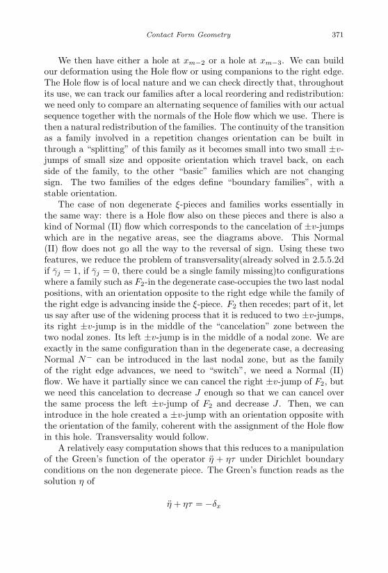
January 17, 2007 11:55 WSPC/Book Trim Size for 9in x 6in finalBB
Contact Form Geometry 371
We then have either a hole at xm−2 or a hole at xm−3. We can buildour deformation using the Hole flow or using companions to the right edge.The Hole flow is of local nature and we can check directly that, throughoutits use, we can track our families after a local reordering and redistribution:we need only to compare an alternating sequence of families with our actualsequence together with the normals of the Hole flow which we use. There isthen a natural redistribution of the families. The continuity of the transitionas a family involved in a repetition changes orientation can be built inthrough a “splitting” of this family as it becomes small into two small ±v-jumps of small size and opposite orientation which travel back, on eachside of the family, to the other “basic” families which are not changingsign. The two families of the edges define “boundary families”, with astable orientation.
The case of non degenerate ξ-pieces and families works essentially inthe same way: there is a Hole flow also on these pieces and there is also akind of Normal (II) flow which corresponds to the cancelation of ±v-jumpswhich are in the negative areas, see the diagrams above. This Normal(II) flow does not go all the way to the reversal of sign. Using these twofeatures, we reduce the problem of transversality(already solved in 2.5.5.2dif γj = 1, if γj = 0, there could be a single family missing)to configurationswhere a family such as F2-in the degenerate case-occupies the two last nodalpositions, with an orientation opposite to the right edge while the family ofthe right edge is advancing inside the ξ-piece. F2 then recedes; part of it, letus say after use of the widening process that it is reduced to two ±v-jumps,its right ±v-jump is in the middle of the “cancelation” zone between thetwo nodal zones. Its left ±v-jump is in the middle of a nodal zone. We areexactly in the same configuration than in the degenerate case, a decreasingNormal N− can be introduced in the last nodal zone, but as the familyof the right edge advances, we need to “switch”, we need a Normal (II)flow. We have it partially since we can cancel the right ±v-jump of F2, butwe need this cancelation to decrease J enough so that we can cancel overthe same process the left ±v-jump of F2 and decrease J . Then, we canintroduce in the hole created a ±v-jump with an orientation opposite withthe orientation of the family, coherent with the assignment of the Hole flowin this hole. Transversality would follow.
A relatively easy computation shows that this reduces to a manipulationof the Green’s function of the operator η + ητ under Dirichlet boundaryconditions on the non degenerate piece. The Green’s function reads as thesolution η of
η + ητ = −δx

January 17, 2007 11:55 WSPC/Book Trim Size for 9in x 6in finalBB
372 Recent Progress in Conformal Geometry
under Dirichlet boundary conditions on the appropriate time interval. Thisis tantamount to manipulate the transport equation between the right edgeand the left edge of F2 when the right is in the “cancelation” position andthe left edge is in the second last nodal zone (counting from the right), itis totally equivalent to the construction of Appendix 2, which is carriedout in great detail, together with its application to degenerate ξ-pieces(part of the application is carried out before hand in 2.5.5.2c, 2.5.5.2d).The extension to the present framework requires exactly the same resultthan Appendix 2, with some modifications from the point of view of theapplication, computations of the second derivative on ±v-jumps locatedat various times on the ξ-piece have to be carried; one finds out that thisquadratic form is controlled by the Green’s functions taken at couple ofpoints among these times. Using the results of Appendix 2, one can checkon this quadratic form that the Green’s function can be manipulated sothat the deformation associated to the Normal (II) flow is J-decreasing.The details are left to the reader
The above arguments all assume that all oscillations are small. However,some oscillations can be large and, as explained in [Bahri 1998], [Bahri-12003], they might yield decreasing deformation after widening.
We now have two deformations: one, due to transversality, applies whenthe oscillations are small and moves the curves downwards, past x∞
m . Theother one, due to the non Fredholm character, applies when the oscillationsare large and thin and J decreases after “opening and widening” them. Weneed to glue them together.
The following basic phenomenon shows that this is possible: let us con-sider some point on x∞ where a thin, large oscillation can be built, thenwidened so as to decrease J . Once this construction can be carried outfor x∞, it can be carried for all nearby curves, the situation being similar(the opening of these oscillations and then widening obey precise equationsrelated to the geometry of α on the v-orbits through the points of x∞ see[Bahri-1 2003], hence extends naturally nearby).
Thus, such a thin large oscillation can be built on all the flow-lines outof the curves of Wu(x2k) which are in the vicinity of x∞ and which arerepresented with small oscillations. Once, it is built, it can be opened andwidened and this decreases J all along the curves of such flow-lines. Wethus have the following diagram:
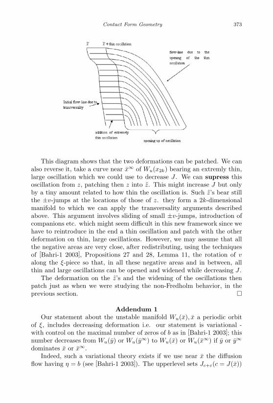
January 17, 2007 11:55 WSPC/Book Trim Size for 9in x 6in finalBB
Contact Form Geometry 373
This diagram shows that the two deformations can be patched. We canalso reverse it, take a curve near x∞ of Wu(x2k) bearing an extremly thin,large oscillation which we could use to decrease J . We can supress thisoscillation from z, patching then z into z. This might increase J but onlyby a tiny amount related to how thin the oscillation is. Such z’s bear stillthe ±v-jumps at the locations of those of z. they form a 2k-dimensionalmanifold to which we can apply the transversality arguments describedabove. This argument involves sliding of small ±v-jumps, introduction ofcompanions etc. which might seem difficult in this new framework since wehave to reintroduce in the end a thin oscillation and patch with the otherdeformation on thin, large oscillations. However, we may assume that allthe negative areas are very close, after redistributing, using the techniquesof [Bahri-1 2003], Propositions 27 and 28, Lemma 11, the rotation of valong the ξ-piece so that, in all these negative areas and in between, allthin and large oscillations can be opened and widened while decreasing J .
The deformation on the z’s and the widening of the oscillations thenpatch just as when we were studying the non-Fredholm behavior, in theprevious section.
Addendum 1Our statement about the unstable manifold Wu(x), x a periodic orbit
of ξ, includes decreasing deformation i.e. our statement is variational -with control on the maximal number of zeros of b as in [Bahri-1 2003]; thisnumber decreases from Wu(y) or Wu(y∞) to Wu(x) or Wu(x∞) if y or y∞
dominates x or x∞.Indeed, such a variational theory exists if we use near x the diffusion
flow having η = b (see [Bahri-1 2003]). The upperlevel sets Jc+ε(c = J(x))

January 17, 2007 11:55 WSPC/Book Trim Size for 9in x 6in finalBB
374 Recent Progress in Conformal Geometry
deform then on D−(x)∪ Jc−ε where D−(x) is a small unstable disk in E−.E− is the negative eigenspace of the linearized operator −(η + a2ητ).
We have defined functions η(c1,−, c2k) for Wu(x) (when the Morse indexof x is 2k; there is a similar formula for 2k +1) such that J
′′(x) is negative
along these directions. Such functions η(c1,−, c2k) split on E− ⊕ E+ intoη−(c1,−, c2k) and η+(c1,−, c2k). It is easy to see that η−(c1,−, c2k) is nonzero. We can define, using the diffusion flow (η = b) a decreasing flow-linefrom η(c1,−, c2k) to η−(c1,−, c2k) ∈ E−. η−(c1,−, c2k) is non zero: theproof of this fact is equivalent to the statement that η−(c1,−, c2k) is nonzero. The map from D−(x) to a neighborhood of x in Wu(x) is one to oneand onto. The number of zeros of b on such flow lines is at most 2k.
We thus can define “cylinders” running from disks in our unstable man-ifold to disks in E− and the maximal numbers of zeros of b along these“cylinders” (after removal of x) is 2k.
There is on the other hand a natural “dilation” on our unstable manifoldand J decreases along this dilation. Combining this “dilation” and the flow-lines defined above, we can create reverse cylinders, starting from disks inE− and ending in (non-standard) disks around x in Wu(x). This family offlow-lines when combined with this dilation allows to define a decreasingdeformation of D−(x)∪Jc−ε on D(x)∪Jc−ε′ where D(x) is a “disk” in ourunstable manifold. Because we use flow-lines along which b has at most2k zeros and because the “dilation” is only a progressive transversal shiftin the flow-lines, the maximal numbers of zero of b does not go beyond2k (including multiplicity). This extends to a small C∞-neighborhood ofthese flow-lines. The fibrations of Wu(y) or Wu(y∞) (above Wu(x)) canbe assumed to be defined using the C∞-topology (or Cm for m very large)since we basically use the diffusion flow (+ dilation).
The claim follows.The deformation result of “Compactness” is variational. It goes beyond
properties of flow-lines connecting periodic orbits.
Addendum 2Considering the first ∗ before the first node on a characteristic piece,
we claim that there is a small constant c > 0 such that if the associated±v-jump does not have the orientation of the left edge (there is a similarstatement for the right edge) or is of size less than c, then we may movethis ∗ to the middle of the first nodal zone while decreasing J . Thereafter,we can use the normal II-flow on it. No use of the hole flow is needed onsuch configurations.
The size of the associated ±v-jump might change then. But this de-formation can be extended to a global decreasing deformation where theorientation of the ±v-jump associated to this ∗ does not change at least if

January 17, 2007 11:55 WSPC/Book Trim Size for 9in x 6in finalBB
Contact Form Geometry 375
it was initially of size c2 or more. In addition, the ±v-jumps among thesewhich have the orientation of the left edge and which are of size ≥ 2c areleft untouched and those of size between 5c
4 and 2c might be translated andchanged but they remain of size c
4 to the least.Finally, picking c1 small, positive but very large with respect to c (the
choice of c follows the choice of c1), all ±v-jumps associated to this ∗ ornot, of size ≥ c1 having the orientation of the left edge are only very littleperturbed through this process if the ±v-jumps associated to this ∗ havethe orientation of the left edge (or are tiny, less than 2c in size with thereverse orientation).
This last piece of our claims allows us to stabilize through this process -the aim of which is to push “in the middle” such a ∗ which has an orientationopposite to the left edge or has the same orientation, but is small - thevarious possible representatives of the left edge for the hole flow.
Indeed, in order to engineer a decrease, if the left edge is positivelyoriented for example, it suffices to decrease an existing positive v-jump orto increase in size a negative v-jump, see below for the proof of this fact ingeneral.
As we engineer this decrease, we may translate the position of ∗, theposition of this ±v-jump. If this v-jump is zero, we may translate it with-out changing its size. Similarly, we can move a tiny v-jump inside thecharacteristic piece, inside the first nodal zone while decreasing its size anddecreasing the functional. We proceed as follows to achieve this goal: ifthis tiny v-jump is the first one after the left edge, it is straightforward tomove it away from this edge while decreasing the functional. If it is not thefirst one, we can “widen”, as in Proposition 30, the oscillations where it isinvolved, being careful though to move this v-jump always more inside thecharacteristic piece. This procedure contrasts in some ways with the one ofProposition 30 because we do not complete the widening of the oscillationnecessarily on this side of this oscillation where the ±v-jump is smallest.Since we are basically - we will see that we cannot always do that - wideningalways on the side of our v-jump, we might cancel in this process ±v-jumpswhich are intermediate between this v-jump and the left edge. The processcan be continued though with the next ±v-jump in the direction of theleft edge and it can be made into a continuous process if, when a ±v-jumpbecomes tiny, we move progressively the position of the left vertical of theoscillation towards the next ±v-jump in the direction of the left edge. Thislast move might affect the orientation of the ±v-jump associated to our ∗.However, we observe that initially we were deforming a compact subset Kof Wu(xm) in J−1(c∞ + ε), ε > 0 a fixed number, c∞ = J(x∞). The ±v-jumps of K are separated by a ξ-distance δ(ε) > 0 to the least. Thus, as wewiden the oscillations, the ±v-jumps associated to our ∗ of size (absolute
January 17, 2007 11:55 WSPC/Book Trim Size for 9in x 6in finalBB
376 Recent Progress in Conformal Geometry
size) c2 or more will remain of an absolute size lowerbounded by δ1(ε) > 0.As we move the left side of the oscillation (whose right side is our ∗) tomake our process continuous, this left side is tiny as we please. We mayimpose that it is less than δ1(ε)2. Then, the orientation of our ±v-jumps(those associated to this ∗, also the other v-jumps of size ≥ δ1(ε)) is notaffected; they remain of size δ1(ε)/2 to the least.
In the end, the ±v-jump which we are pushing inside will have to go tothe transition zone and beyond; this process cannot stop since the left edgeis “large”. We can then adjust this process to the size of this ±v-jump beforedeformation. As the size of this v-jump increases (once it is positive), wemove it less and less inside the first nodal zone. We can scale the changesso that once these v-jumps are positive of size more than 2c, they areuntouched and if they are of size 5c
4 or more, they are of size c4 to the least
in the end. All other v-jumps, positively oriented, of size c1 very large withrespect to c will remain - it is easy to see - of size ≥ c1 −Cc = c1(1 + o(1))through this process provided the ±v-jumps associated to the ∗ are eitherpositively oriented or are of negative size c to the most, i.e. representativesof the left edge are stabilized in this process if a hole flow needs to be used.
Let us prove now, a fact that we already know if there is only one ±v-jump after the left edge which we decrease (algebraically) in size, that if wedecrease (algebraically) a ±v-jump on an almost characteristic ξ-piece (the±v-jump being in the first nodal zone, “away” from the node) J decreases.
The addition at the ±v-jump is µ0v, µ0 < 0, which we transport backto the left edge following the history of the curve. We are going to showthat the transported vector z at the left edge reads:
z = o(η0)ξ − η0(1 + o(1))[ξ, v] + (µ0 + o(η0))v
where η0 = −µ0∆t, ∆t being the ξ-length between the left edge and the±v-jump which we are considering. It is then easy, using z, to constructa decreasing normal N− as in 4.2. Let us prove the above formula; thetransport equations read
µ + aητ − bηµξ = 0η = µa − λb t ∈ [0, t0]
˙λ + µη = bη
0 is the time of our ±v-jump; t0 is the (negative) time of the left edge. b isequal to a sum of Dirac masses
∑mi=1 ciδti with
∑ |ci| = o(1), t0 = −∆t.Integrating we find:
η +∫ t
0
b(∫ s
0
bη − µη) = −µ0at − a
∫ t
0
∫ s
0
(aητ − bηµξ).
January 17, 2007 11:55 WSPC/Book Trim Size for 9in x 6in finalBB
Contact Form Geometry 377
A simple argument shows then that
η = −µ0at(1 + o(1))
Addendum 3Curves nearby x∞ can be split between nearly v-verticals (see [Bahri-1
2003] for the definition of v-verticals) and nearly ξ-pieces. The nearly v-verticals can be modelized ([Bahri 1988], [Bahri 1998], [Bahri-1 2003]) bylarge pieces of ± v-orbits alternated with small ξ-pieces.
Because x∞ is assumed not to be false (see [Bahri-1 2003]; false criticalpoints at infinity can be bypassed through the introduction of companions,see 2.5.1 above for the definition of companion), the small ξ-pieces can beabsorbed through a J-decreasing deformation into the nearly ξ-pieces.
Thus, any deformation class can be represented near x∞ by curves madeof large ± v-verticals joined by nearly ξ-pieces. The analysis of [Bahri-12003, pp. 113–141] tells us then that any chain of (Jc∞ + ε, Jc∞ − ε) inV(§∞ ) − V(§∞ ) is a neighborhood of x∞
m in C+β = x; x = aξ + bv, a ≥
0, c∞ = J(x∞) - can be represented as a product of the unstable manifoldinfinity of x∞ (of dimension i∞) with the H1
0 -unstable manifold of the nondegenerate ξ-pieces of x∞ and with the H1
0 -unstable manifold (strict or full;the full one is half of the usual unstable manifold because it corresponds toa degenerate critical point) of the characteristic pieces (each piece in thisproduct is taken a number of times). In our situation - i.e. in 2.5.4.5; thestatement has to be adapted for 6.- the maximal number of zeros of b onWu(x∞
m−1) is 2k and m− 1 = 2k− 1. The number of characteristic ξ-piecesneeded to define the cycle(s) of x∞
m−1 is then imposed; this is the numberof characteristic ξ-pieces whose full unstable H1
0 -manifolds are used in thedefinition of the cycles of x∞
m−1 see [Bahri-1 2003, p. 126].Furthermore this is a consequence of the above representation, denoting
C+,2kβ = x, x = aξ + bv, a ≥ 0, b has at most 2k zeros , the group
W = H2k(Jc∞+ε ∩ C+,2kβ ∩ V(§∞−∞),J∞−ε ∩ C+,∈‖
β ∩ V(§∞−∞), Z)
is a free group. Let ϕ1,−, ϕs be a basis of this group. Wu(x2k) generatesnear x∞
m−1 an element ψ of W which therefore reads
ψ =∑
niϕi, ni ∈ Z.
Since Wu(xm) ∩ V(§∞−∞) can be moved in C+,2kβ below x∞
m−1, each ni iszero.
January 17, 2007 11:55 WSPC/Book Trim Size for 9in x 6in finalBB
378 Recent Progress in Conformal Geometry
Appendix 1
We now take care of the ξ-pieces of zero H10 -index.Those which are non
degenerate do not interfere with our argument, therefore we will not discussthem. For the degenerate ones, the key point relies again into the fact thatwe are able to track the ∗′s of the families as they travel.
Our cycles are all taken modulo Jc∞−ε, we are going to prove that wecan rewrite any given cycle into a sum of cycles such that for any given cycletaken from this sum, the number of ∗′s associated to a given degenerateξ-piece of H1
0 -index 0 is constant equal either to 0 or to 2 all over thecycle. In the former case, the full (half) unstable manifold of the associatedξ-piece is not part of the definition of the cycle while in the latter case, it ispart of this definition, (see Section 2.5.6) is increased by 1, but n also inthe argument of Section 2.5.6 can be increased by 1 since we do have two∗′s associated to this ξ-piece which thus behaves as if it were of non zeroH1
0 -index.Assume that for a given configuration in our cycle, three ∗′s are living
on a given degenerate ξ-piece of index zero, two for each edge and one inbetween. Let us track these three ∗′s as the configuration changes in our cy-cle. We obviously can follow them as their respective locations change overthe basic curve x which is close to the critical point at infinity x∞. As theytravel outside of the characteristic piece of index zero and go inside its edges,their orientations might change but we can still relate two of them to thischaracteristic piece in our global count and the counting argument of Sec-tion 2.5.6 can proceed at least as far as this characteristic piece is involved.As a ∗ travels away, it can enter non-characteristic pieces, engineering thena reordering of the ±v-jumps generating their H1
0 -unstable manifolds, a ∗,maybe modified, can be still tracked and attributed to our initial charac-teristic ξ-piece of index zero, so there is no meaningful modification in thiscase. If we use the results of [Bahri-2 2003], modify the rotation of v onnon-degenerate ξ-pieces until either a ξ-piece becomes characteristic, or itbecomes of H1
0 -index zero, so that if0 of Section 2.5.6 becomes zero, then wecan even assume that this ∗ , after decreasing deformation, has the sameorientation all over these transitions.
The count could change only as such a ∗ enters another characteristicpiece. If it is a single v-jump as it enters, then the Normal(II)-flow canbe applied upon it and a related splitting of the cycle occurs. If it entersas a family, a problem might arise if it is a family of an edge, typically ofthe right edge. We have discussed configurations such as these in 2.5.5.2b,2.5.5.2c, 2.5.5.2d, in Propositions 30 and 31 although these configurationswere more specific in 2.5.5.2. Forgetting about the use of the hole flow inthe last nodal zone which we introduced in 2.5.5.2 (in our present configu-

January 17, 2007 11:55 WSPC/Book Trim Size for 9in x 6in finalBB
Contact Form Geometry 379
ration, flows are provided by Normal(II)-flows or the use of an appropriatealternating sequence), we can, once the family of our ∗ has penetrated alittle bit inside the last nodal zone and there is a hole in the vicinity ofxm−1, engineer a decrease through the introduction of a companion to theright edge, also repeating the construction of 2.5.5.2c, 2.5.5.2d and usingif needed (for a transition with the use of the alternating sequence) theNormal (II)-flow on the family preceding the family of our incoming ∗, orif this family (with an orientation opposite to the orientation of the rightedge) starts overextending, use the previous node xm−3. At this xm−3,the use of the Hole flow of the left edge (which we assume to provide anorientation opposite to the one of the right edge just before the incoming ∗)and the introduction of a companion of this family are compatible becausethe companion to this family near xm−3 comes after the ±v-jump due tothe Hole flow, nearest to the family itself. We thus can use the Normaldue to this Hole flow(recall that Hole flows can be inserted in alternatingsequences)in combination with the Normal (II)-flow and thereafter, oncewe are not using the Normal (II)-flow anymore, introduce the companionto the family, cancel the use of the Normal associated to the Hole flowand keep the use of this companion as the family overextends, past xm−3.In all, our cycle splits into two pieces at such a transition and there is anatural way to extend the flow on each piece of the cycle because of thiscompatibility at xm−3.
We are thus left with maximal sequences of characteristic pieces of H10 -
index zero. We count the number of ∗′s associated to them, which are allthe ∗′s between the ∗ associated to the right edge of the first characteristicpiece preceding the sequence (included) and the ∗ associated to the leftedge of the first characteristic piece following the sequence (not included).If there are repetitions in these edges, we include the ∗′s involved in theserepetitions in the count except for the last ∗ for the left edge of the firstcharacteristic piece following the sequence . Again, we can split the cycle insub-cycles along which this number does not change for each given sequence.It can be even equal to 2s or odd equal to 2s + 1. In both cases, thesequence contributes at most s to the number of Section 2.5.6, but thesequence contributes also at least 2s to the number of ∗′s. The argument ofSection 2.5.6 can therefore proceed for each of these sub-cycles. Would thenumber of characteristic pieces of index zero which contribute to a givencycle through their full(half)-unstable manifold change over the span of thecycle (very close to the top level c∞)without a corresponding change forthe number of ∗′s , we could not derive the same conclusion. Observe thatnear this top level we can assume after Section 2.5.6 that all characteristicpieces of non zero H1
0 are “filled” up, but maybe for one of them whichbears a single simple hole, together with a repetition in its left edge.

January 17, 2007 11:55 WSPC/Book Trim Size for 9in x 6in finalBB
380 Recent Progress in Conformal Geometry
We can conclude now along the lines of the arguments used in Sec-tion 2.5.6. Either , see Section 2.5.6, tends to infinity with k; we useHypothesis (A) , argue as in Section 2.5.6 (with variants) and conclude.Or is bounded , then n, the number of characteristic pieces of non zeroH1
0 -index≥ 1, is bounded (using the arguments of Section 2.5.6). If theH1
0 -index of anyone of these pieces tends infinity or if the number or theH1
0 -index of the non degenerate ξ-pieces tends to infinity, we can argue againas in section 6. Otherwise, the total H1
0 -index is bounded , is boundedand so is γ1. Then k is also bounded since if0 + γ1 + 2 = 2k

January 17, 2007 11:55 WSPC/Book Trim Size for 9in x 6in finalBB
Contact Form Geometry 381
Appendix 2
Let us consider a piece of ξ orbit of length π4 . We modify ξ into ξ, α
into α = (1 + o(1))α near the piece of ξ-orbit as follows.α is xdy + dz, ξ = ∂
∂z . We replace α by
(1 + 2νω(x2 + y2
ε1)ω2(z)C1xy)−1α
The piece of v-orbit is provided by x = 0, y = 0, z belongs to [0, γ], γsmall. ε1 is a small parameter, ω′
1(t)t and ω′′1 (t)t2 are small; ω1 is 1 near
zero and is zero for t ≥ M, ω1 = ω1(t). ω2 is 1 on a small z-interval insidethe ξ-piece, close to its starting point and is zero outside an interval twiceas large. The first and second derivatives of ω2 are bounded in functionof the size of these intervals. This size is large when compared to ε1. ν isan appropriate constant, the value of which is provided below. We use theformulae for ξ available in [Bahri-1 2003, p. 83] and we find that
ξ = ξ − 2νω1ω2C1x∂
∂x+ 2νω1ω2C1y
∂
∂y+ o(|x| + |y|)
o(|x|+ |y|) is small in the C1-sense if ε1 is chosen small enough once ω1
and ω2 are chosen.Differentiating, we find for the ξ-transport matrix:
δx = −2νω1ω2C1δx + o(|δx| + |δy|)
δy = 2νω1ω2C1δy + o(|δx| + |δy|)with ω1 = 1 on the piece of ξ or ξ-orbit.We thus see that the transport matrix of ξ has been modified into the
transport matrix of ξ which is:
A =(
C 00 1
C
)C can be chosen as we please after an appropriate choice of C1 and ν
in function of ω2 and C.With this new ξ, β = dα(v, .) is not necessarily a contact form anymore.
It is easy however to modify v into hv so that β = dα(v, .) is a contactform with the same orientation than α. Indeed, the transport map of ξ isessentially a contraction or dilation along ∂
∂x and a dilation or contractionalong ∂
∂y .We first, before any modification of α into α, unwind v along the piece
of ξ-orbit where we introduce the modification, redistributing the rotation

January 17, 2007 11:55 WSPC/Book Trim Size for 9in x 6in finalBB
382 Recent Progress in Conformal Geometry
of v so that v builds with ξ on the piece of ξ-orbit a foliation. We take vto be ∂
∂x . The transport map of ξ maps ∂∂x onto γ ∂
∂x , γ positive. We thuscan reintroduce some missing rotation and turn β into β a contact form.
In the case when C ≥ 1, i.e the modification has introduced a dilationalong ∂
∂x = ”v” (this is v at the beginning of the ξ-piece), we can take v = vi.e keep v unchanged. Indeed, we compute:
dα(v, [ξ, v]) = dα(v, [∂
∂z− 2νω1ω2C1x
∂
∂x+ 2νω1ω2C1y
∂
∂y, v]) + o(1)
v reads as
v =∂
∂x− zb(x, y)(
∂
∂y− x
∂
∂z)
if we set z = 0 at the beginning of the ξ-piece where v equals ∂∂x . b(x, y) is
a positive smooth function of y and x. The above formula is obtained usingthe equation dα(v, [ξ, v]) = −1; the Darboux coordinates are built so thatv = ∂
∂x on a section to ∂∂z at the starting point of the ξ-piece. We find:
[ξ, v] = o(1) + [∂
∂z− 2νω1ω2C1(x
∂
∂x),
∂
∂x− zb(x, y)(
∂
∂y− x
∂
∂z)]
= o(1) − b(x, y)∂
∂y+ 2νω1ω2C1 × (
∂
∂x+ b(x, y)
∂
∂y)
and
dα(∂
∂x− b(x, y)z
∂
∂y,−b(x, y)
∂
∂y+ 2νω1ω2C1(
∂
∂x+ b(x, y)z
∂
∂y))
= −b(x, y) + 2νω1ω2zC1(1 + b).
Since C1 is negative when C ≥ 1, β = dα(v, .) is indeed a contact formas claimed.
Modifications of the above type, the first one with 1C and the second
one with C, are introduced on the first nodal zone, in the vicinity of theleft edge, and on the second last nodal zone (xm−2, xm−1), in the vicinityof xm−2., see Sections 2.5.4 and 2.5.5 for the related uses and notations. vis mapped onto θv from xm−2 to the left edge. We can use a first couple ofmodifications of this type and modify θ into 1. It is easy to see that we donot create new critical points at infinity over this process. Thus we assumein what follows that θ = 1. Then, ∂
∂x can be viewed as a ξ-transportedvector from the left edge until xm−2 that coincides with v at the left edgeand at xm−2. The x, y, z-Darboux coordinates extend also from the left
January 17, 2007 11:55 WSPC/Book Trim Size for 9in x 6in finalBB
Contact Form Geometry 383
edge until xm−1. The two modifications are thus written in the same setof coordinates. For x2 + y2 small with respect to ε1, using the formulae of[Bahri-1 2003, p. 83], we find that z for ξ is equal to 1 and that the mapsof ξ on each interval are linear given by matrices such as A, see above. Theerror in this approximation is precisely O(|x|3 + |y|3). It is simple then toarrange the values of the constants such as C1, ν and the functions suchas ω2 on each interval modification so that the total ξ − ξ-transport mapfrom the middle of the nodal zone (xm−2, xm−1) , or points close to thismiddle point on curves close to the critical point at infinity, to the left edgeof these curves is the identity map in the (x, y)-coordinates, i.e is simplyz-translation, of the same amount than the ξ-translation on the originalcurve, up to an error of size O(|x|3 + |y|3). This holds of course under theassumption that there are no ±v-jump on the way.
Assuming now that there are ±v-jumps on the way, but that they areall located in the vicinity of nodes and of total size Σci, assuming alsofor simplicity that we have completed a family of previous modificationsso that all the related coefficients θi from all nodes to the left of xm−2,xm−2 included, are equal to 1, these ±v-jumps are then translations inthe x-direction of ci at the nodes which we can define on each ξ-piececorresponding to the characteristic piece, up to o(ci). We are assuming thatthere are no ±v-jumps in the areas where the modifications are completed.The matrices of type A “commute” with such translations, i.e the totaltransport map is then the ξ-transport map composed with a translationalong v at the left edge of size CΣθi, up to o(Σ|θi|).
We can also, instead of replacing the ξ-piece of curve, with the ±v-jumpsinserted in it, by a −ξ-piece of curve, with all ±v-jumps gathered at theleft edge (up to o(σci)), insert back ±v-jumps at the similar locations onthe piece of ξ − ξ-curve. A ±v-jump of size c should then be replaced by a±v-jump of size 1
C . We can also complete the process in the reverse way,starting with a ξ − ξ-piece of curve.
In all, a curve x, close to x∞ is replaced by a curve x. x might not beclosed, up to o(Σci), but we can close it, using the left edge for examplewhere we have the freedom of using variations along v, variations along ξand also variations along the transport of ξ from the bottom to the top ofthe left edge.
There are two functionals involved, J and J , corresponding respectivelyto α and ξ on one hand and α and ξ on the other hand. As we change fromx to x , our estimates above indicate that:
J(x) = J(x) + o(Σci)
The c′is involved are the sizes of the ±v-jumps to the left of the middle

January 17, 2007 11:55 WSPC/Book Trim Size for 9in x 6in finalBB
384 Recent Progress in Conformal Geometry
of the nodal zone (xm−2, xm−1), they are all supposed to be close to thelocation of the “nodal” points in our estimate above.
2.6 Transmutations
In this section we study in more details transmutations of critical points atinfinity and the related changes of the indexes at infinity.
Transmutations of a critical point at infinity x∞ have been introducedin [Bahri-1 2003] following two distinct procedures. They correspond tothe following basic fact: given a critical point at infinity x∞, of indexi0 + i∞ = m (i0 is the H1
0 -index, i∞ is the index at infinity), the maximalnumber of zeros of b on the unstable manifold of x∞ is i0 + γ see [Bahri-12003]. i0 + γ and i0 + i∞ are different. Therefore, one can hope to changei0 + γ through a modification of α into λα near x∞
m while i0 + i∞ remainsunchanged i.e. x∞
m remains isolated in its species.This has been carried out in [Bahri-1 2003] either by introducing a suit-
able “Hamiltonian” λ in the neighborhood of a non-degenerate ξ-piece ofx∞
m or by redistributing the v-rotation along the non-degenerate ξ-pieceswithout changing the Poincare-return map of x∞
m , C. The phenomenon issubtle because as explained in [Bahri-1 2003], as this transmutation occurs,x∞
m remains isolated in its species but an additional critical point at infinityy∞ (in fact a couple or more) is created which has an additional charac-teristic ξ-piece with respect to x∞
m (corresponding to the non degenerateξ-piece where the transmutation is occuring).
We will be particularly interested in this section to x∞2k’s i.e. critical
points at infinity of index 2k having an index i∞ = k as these are, see [Bahri-1 2003], the critical points at infinity which interfere with the homologydefined in [Bahri-1 2003].
Assuming hypothesis (A), either x∞m has no characteristic piece. If the
number of its ξ-pieces is large, we can redistribute the v-rotation on oneof them. We change i∞ to something different as we will see. Whenm = 2k, x∞
2k does not interfere with our homology anymore. We havecreated through this process other critical points at infinity y∞’s, but theyall have at least one characteristic ξ-piece and we may apply to them ourcompactness results (after full generalization, we are providing here ourprogram of work).
If x∞m has a characteristic piece, then the compactness results can be
directly applied to it.Our compactness results, as they stand, require that one of the charac-
teristic pieces of x∞m or y∞ be of strict index different from 1. We believe
that they hold in fact in full generality ([Bahri-2 2003]).

January 17, 2007 11:55 WSPC/Book Trim Size for 9in x 6in finalBB
Contact Form Geometry 385
Our focus in this section is to understand in details the changes ofindexes as a transmutation takes place. We will assume, for the sake of theprecision in the details, that m = 2k, i∞ = k; however the results which weestablish hold in full generality, for all generic transmutations.
We consider such a transmutation which necessarily involves the collapse(see [Bahri-1 2003]) of x∞
2k with y∞ another critical point at infinity havingthe same number of ξ and ±v-pieces than x∞
2k.We start with:
Proposition 34 As x∞2k and y∞ collapse, we may assume that dac(v) = 0
on the ξ-piece where the change of H10 -index takes place. dθ(ξ), the differ-
ential along ξ of the collinearity coefficient θ of dϕac(v) on v, can also beperturbed as we please at the time of the collapse at x−
0 , while θ(x−0 ) = θ is
kept unchanged.
Observation 6. As we pile up rotation on a ξ-piece, bringing it from otherfree ξ-pieces see [Bahri-1 2003] pp 96-102, the full Poincare-return map doesnot change. Let a be the length of the ξ-piece. dφa(v) and −v are closer andcloser in direction as we pile up rotation (keeping it less than π). Recallingnow the other way of transmuting x∞
2k i.e. of changing the H10 -index of this
ξ-piece from 0 to 1, we may complete this transmutation once the rotationis almost π through a change of the Hamiltonian see [Bahri-1 2003] pp. 81-102. Since C has not changed in the first step, since dφa(v) and −v are thenvery close, we may assume by genericity that the forbidden direction(s), see[Bahri-1 2003] pp 85-90, do not lie between dφa(v) and −v. Thus, we mayassume that, at the time of the collapse, α is unchanged outside of a smallneighborhood of the ξ-piece which changes H1
0 -index. We assume in thesequel that the transmutation takes place in this way.
Corollary 8 Either i∞ ≥ k + 1 or the direction vk on the characteristicpiece of y∞ corresponding to the ξ-piece of x∞
2k which changes H10 -index is
in the negative eigenspace of J′′∞(y∞) after the collapse while the index of
J′′∞(y∞) on the J
′′∞(y∞)-orthogonal of vk does not change.
Observation 7. As the collapse, J′′∞(y∞) · vk · vk = 0 as we will see. Thus,
vk is orthogonal to itself. However, we will prove that vk has a codimensionone orthogonal (for J
′′∞(y∞)) which can be followed continuously through
the collapse.
Proof. [Proof Corollary 8 and of Proposition 34] As we add rotation, theindex of y∞ will change from i∞ − 1 to i∞ through the collapse, at leastif y∞ remains isolated in its type. This will follow from the behavior ofJ
′′∞(y∞) transversally to vk.
If we are able to define continuously an orthogonal G to vk, through thecollapse, transversally to vk, and if J
′′(y∞)|G does not degenerate, then
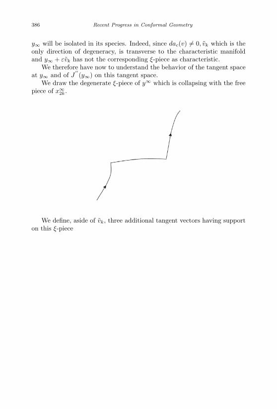
January 17, 2007 11:55 WSPC/Book Trim Size for 9in x 6in finalBB
386 Recent Progress in Conformal Geometry
y∞ will be isolated in its species. Indeed, since dac(v) = 0, vk which is theonly direction of degeneracy, is transverse to the characteristic manifoldand y∞ + εvk has not the corresponding ξ-piece as characteristic.
We therefore have now to understand the behavior of the tangent spaceat y∞ and of J
′′(y∞) on this tangent space.
We draw the degenerate ξ-piece of y∞ which is collapsing with the freepiece of x∞
2k.
We define, aside of vk, three additional tangent vectors having supporton this ξ-piece

January 17, 2007 11:55 WSPC/Book Trim Size for 9in x 6in finalBB
Contact Form Geometry 387
We continue building up tangent vectors using each ξ-piece and itsneighboring ξ-pieces. If it is characteristic, it has a vector such as u+
k , u−k
and a v. If it is free, the upperside of a vector such as u+k and the lower

January 17, 2007 11:55 WSPC/Book Trim Size for 9in x 6in finalBB
388 Recent Progress in Conformal Geometry
side of a vector such as u−k can be removed and we derive two vectors
u+, u−. This builds a base of Ty∞(Γ2s)(y∞ ∈ Γ2s). Clearly, vk interactswith wk, u+
k , u−k . The other vectors do not have support on the character-
istic piece of y∞. Orthogonality for J′′∞(y∞) follows. Let us draw curves of
Γ2s nearby y∞:
θ1 and θ−12 are the v-transport maps corresponding to the edge v-jumps
of the curve. We write:
dθ1(ξ) = (1 + A1)ξ + B1[ξ, v] + µ1v
dφa(v) = −θv + c(x−)(a − ac(x−1)[ξ, v]
with c(x−) bounded away from zero.
dθ−12 (ξ) = (1 + A2)ξ + B2[ξ, v] + µ2v dφac(v(x−
0 )) = −θv(x+0 ).
Accordingly, vk, wk, u+k , u−
k find natural extensions to nearby curves. Inorder to extend vk, we take v at x−, transport it via ξ into −θv+c(x−)(a−ac(x−))[ξ, v] at x+ and we compensate the component on [ξ, v] of dϕa(v)by dθ−1
2
(c(x−)(a−ac(x
−))B2
ξ). We thus have at a nearby curve x(vk is also
the notation for the extension of vk):
J ′∞(x) · vk =
A2
B2c(x−)(a − ac(x−)).
Observation 8. At the collapse, A2 = A1 = 0 on y∞ because x∞2k which
is then confounded with y∞ has this ξ-piece free.

January 17, 2007 11:55 WSPC/Book Trim Size for 9in x 6in finalBB
Contact Form Geometry 389
On y∞, a = ac. Therefore, any tangent vector ϕ ∈ Ty∞Γ2s
J′′∞(y∞) · vk · ϕ =
A2
B2c(x−
0 )(δa − δac)(ϕ)
and the formula holds through the collapse.We thus may define the J
′′∞(y∞) - orthogonal of vk to be:
G = ker(δa − δac).
Observe that
(δa − δac)(vk) = −dac(v) = 0.
It is therefore easy to project wk, u+k , u−
k orthogonally on G; we use theformula:
ϕ +(δa(ϕ) − δac(ϕ))vk
dac(v).
We denote these vectors wk, u+k , u−
k . they are independent and we add tothem vk, we find the same span for this family of vectors.
J′′∞(y∞) takes then the simple form through the collapse:
vkck 0 . . . 00... B0
ck is equal to −A2
B2c(x−
0 )dac(v).Since vk is orthogonal to itself at the collapse, we might as well compute
B using wk, u+k , u−
k and the other vectors having no support on the ξ-piecewhere the tranmutation takes place.
B reads:J
′′∞(y∞) · wk · wk J
′′∞(y∞) · wk · u+
k J′′∞(y∞) · wk · u−
k
J′′∞(y∞) · wk · u+
k J′′∞(y∞) · u+
k · u+k J
′′∞(y∞) · u+
k · u−k C
J′′∞(y∞) · wk · u−
k J′′∞(y∞) · u+
k · u−k J
′′∞(y∞) · u−
k · u−k
C B1
.
We may compute B at the collapse, when y∞ = x∞2k. Outside of the ξ-
piece where the transmutation takes place, y∞ and x∞2k and their partial
Poincare-return maps (those not involving this ξ-piece) coincide.
January 17, 2007 11:55 WSPC/Book Trim Size for 9in x 6in finalBB
390 Recent Progress in Conformal Geometry
The second step of the transmutation can be assumed to take place awayfrom the edges of the ξ-piece of x∞
2k. Thus, if we think of all the tangentvectors, outside of wk, as defined for x∞
2k at the collapse and also slightlybefore and after the collapse, we derive that B1, C and also J
′′∞(x∞
2k)·u±k ·u±
k
and J′′∞(x∞
2k) · u+k · u−
k are constant through the collapse. At the collapse,they identify with the corresponding part of J
′′∞(y∞). We are going to
compute J′′∞(y∞) · wk · ϕ and show that we can stabilize J
′′∞(y∞) · wk · wk
and J′′∞(y∞) ·wk · u±
k near the collapse. The entire matrix B will thereforechange very little through the collapse. Because we can perturb a little bitθ at the collapse, we will see that we may assume that det B = 0 at thecollapse and nearby, which is our claim.
We compute now J′′∞(y∞) · wk · ϕ:
We need to know the value of dφac([ξ, v])(x−). We have:
dφa(v) = −θv + c(x−)(a − ac(x−))[ξ, v]
which we differentiate along ξ to get:
dφa([ξ, v]) = −dθ(ξ)v + γ[ξ, v] + (a − ac)A.
Thus,
dφac([ξ, v]) = −dθ(ξ)v + γ[ξ, v].
Since
dα(dφa(v), dφa([ξ, v]) = −dα(v, [ξ, v]),
γ is equal to − 1θ and
dφac([ξ, v]) = −1θ[ξ, v] − dθ(ξ)v.
We use the following figure.

January 17, 2007 11:55 WSPC/Book Trim Size for 9in x 6in finalBB
Contact Form Geometry 391
to support our construction.In order to build wk, we transport ξ using dθ1 from the lower ξ-piece.
At x− we derive:
(1 + A1)ξ + B1[ξ, v] + µv.
We use dφa to transport this vector to x+. We derive at x+ a vector equalto:
(1 + A1)ξ − B1
(1θ[ξ, v] + dθ(ξ)v
)− µ1θv.
We pull back − B1B2θ ξ from the upper ξ-branch using dθ−1
2 . We derive at x+
the vector:
− B1
B2θ(1 + A2)ξ − B1
B2θ[ξ, v] − µ2B1
B2θv.
The [ξ, v]- components of the above two vectors match. Using v-transport,we can adjust the v-component of dθ−1
2
(− B1
B2θ ξ)
to be −µ1θ. Using ξ-
transport, we can adjust the ξ-component of dφadθ1(ξ) to be − B1B2θ (1+A2).
We then have (wk is the tangent vector which we have built):
J ′∞(x) · wk = A1 − A2B1
B2θ.

January 17, 2007 11:55 WSPC/Book Trim Size for 9in x 6in finalBB
392 Recent Progress in Conformal Geometry
Since A1 = A2 = 0 when y∞ = x2k∞ , we have:
J′′∞(y∞) · wk · ϕ = dA1(ϕ(x−
0 )) − B1
B2θdA2(ϕ(x+
0 )).
If we take ϕ to be u±k , ϕ(x±
0 ) is independent of the transmutation processand so is therefore J
′′∞(x∞
2k) · wk · u±k because dA1 and dA2 are given on
x∞2k. Since J
′′∞(y∞) ·wk ·u±
k equals J′′∞(x∞
2k) ·wk · u±k at the collapse, we see
that the only term in B which depends on the transmutation (i.e. cannotbe computed on x∞
2k also nearby the transmutation) is J′′∞(y∞) · wk · wk,
which is equal to:
dA1(wk(x−0 )) − B1
B2θdA2(wk(x+
0 ))
wk(x−0 ) is independent of the transmutation process. But wk(x+
0 ) is equal,according to our computations above, to:
− B1
B2θξ − B1
θ[ξ, v] − v
(B1dθ(ξ) + µ, θ
)which depends on the transmutation process via the two quantities θ anddθ(ξ). dA1 and dA2 are independent of the transmutation process. Com-puting detB, we find that it reads:
det B = A0dθ(ξ) +B0
θ+ C0θ + D0,
where A0, B0, C0, D0 are independent of the transmutation process nearthe collapse i.e. can be computed on x∞
2k at the collapse and nearby. Theyare equal to the corresponding quantities for y∞ at the collapse. Using theresults of Part 6 below, which provide us with a large set of free parameters,at least 2(s − 1) if x∞
2k and y∞ are in Γ2s, we may assume that A0, B0, C0
and D0 are non zero.Let us prove that we can change sθ(ξ) while θ stays unchanged. θ
depends on the ξ-transport and of the values v(x±0 ). If these values are
unchanged, θ is unchanged if dα(v, [ξ, v]) remains equal to −1. To trackthe parameters which we can modify, we follow the framework introducedin Part 6 (below). We pick up Darboux coordinates near x+
0 where α readsydz + dx and we transport them along−ξ to x−
0 at the time of the collapse.ξ is therefore ∂
∂x .We can use at x+
0 special Darboux coordinates where v reads:
v = λ
(∂
∂z− y
∂
∂x+ (a1x + b1y + p2)
∂
∂y
)

January 17, 2007 11:55 WSPC/Book Trim Size for 9in x 6in finalBB
Contact Form Geometry 393
p2 being of order 2 or more in (x, y, z) v near x−0 then reads:
v = µ
(∂
∂z− y
∂
∂x+ (ax + bycz + q2)
∂
∂y
).
Again, q2 is of order 2 or more in (x, y, z).It is easy to see that
dac(v)(x−0 ) =
c
a1
a1 is certainly non zero because
−1 = dα(v, [ξ, v])
= λ2dy ∧ dz
(∂
∂z− y
∂
∂x+ (a1x + b2y + p2)
∂
∂y,
(a1 +
∂p2
∂x
)∂
∂y
)= −λ2
(a1 +
∂p2
∂x
).
Also
−1 = −µ2
(a +
∂q2
∂x
).
We may clearly assume, after a C1-small perturbation of v, with no changein v(x±
0 ) that c = 0. Thus, we may assume as claimed in the statement ofProposition 34 that dac(v)(x−
0 ) is non zero at the collapse.We need to compute θ(x, 0, 0) at first order, with θ(0, 0, 0, ) = θ(x−
0 ) = θ.At (δx, 0, 0), v is collinear to:
∂
∂z+ (aδx + c2δx
2)∂
∂y.
We transport it along ∂∂x near x+
0 = (0, 0, 0). It is collinear to v(δx′, 0, 0) if
a1δx′ + c2δx
′2 = aδx + c2δx2.
Thus,
δx′ =a
a1δx(1 + O(δx))
and
θ(δx, 0, 0) =λ(δx, 0, 0)µ(δx′, 0, 0)
=λ + ∂λ
∂x (0, 0, 0)δx + O(δx2)
µ + ∂µ∂x (0, 0, 0) a
a1δx + O(δx2))
.

January 17, 2007 11:55 WSPC/Book Trim Size for 9in x 6in finalBB
394 Recent Progress in Conformal Geometry
Thus,
θ(δx, 0, 0) = θ(1 +(
1λ
∂λ
∂x(0) − 1
µ
∂µ
∂x(0))
δx + O(δx2).
It follows that
dθ(ξ)(0)θ
=1λ
dλ
∂x(0) − 1
µ
∂µ
∂x(0).
Since λ = 1√a1+
∂p2∂x
and µ = 1√a+
∂q2∂x
,
dθ(ξ)θ
(0) = − 12a1
∂2p3
∂x2(0, 0, 0) +
12a
∂2q2
∂x2(0, 0, 0).
Changing ∂2p2∂x2 (0, 0, 0) or ∂2q2
∂x2 (0, 0, 0) is a C1-small perturbation of v whichdoes not affect v(x±
0 ). Proposition 34 and Corollary 8 follow.
Let us now consider x∞2k made of a cycle which uses k (half)-full unstable
of characteristic pieces in its definition.Using the results of Part 6, we may assume since i∞ = k and since x∞
2k
has at least k + 1 characteristic pieces ( = k), that v1, . . . , vk−1 are in thenegative eigenspace of J
′′∞(x∞
2k). At the collapse, v1, . . . , vk−1 are thereforein the negative eigenspace of J
′′∞(y∞) and after the collapse, vk is also in
this negative eigenspace for y∞, see Proposition 35, below. We then have:
Corollary 9 Assume that hypothesis (A) holds on y∞. Then i∞ ≥ k+1.
Proof. If hypothesis (A) holds on y∞, we can carry rotation on an addi-tional free piece (of y∞, this time) and change the H1
0 -index by 1. We createthen another critical point at infinity z∞, of index i∞ · z∞ has v1, ..., vk inits negative eigenspace (because it collapses with y∞) and also, by Propo-sition 35 below, after the collapse, an additional vk+1. The result follows.
We now establish that, as we pile up rotation, the index at infinity ofy∞ increases. We prove this result under the assumption that the H1
0 -index of the ξ piece of x∞
2k to which v-rotation is added is initially zero.This assumption can be easily removed.
Proposition 35 If the H10 -index on a non degenerate ξ-piece of x∞
2k
changes from zero to 1, then x∞2k collapses with another critical point at
infinity y∞ having the corresponding piece as a degenerate ξ-piece of indexzero. The index at infinity of x∞
2k changes from i∞ to i∞ − 1 and the indexat infinity of y∞ changes from i∞ − 1 to i∞.

January 17, 2007 11:55 WSPC/Book Trim Size for 9in x 6in finalBB
Contact Form Geometry 395
Proof. The phenomenon has been described and discussed in [Bahri-12003] pp 129—130 and pp 133—136.
Our proof here sets the description of [Bahri-1 2003] on a rigorous stand-ing. The isolation of x∞
2k has been proved in [Bahri-1 2003, Proposition 16].The existence of at least one y∞ follows. We need however to show thatthe index at infinity of x∞
2k changes from i∞ to i∞ − 1, that y∞ is unique(collapsing with x∞
2k) and that its index at infinity changes from i∞ − 1 toi∞.
We are going to define a space W2s+1, a manifold of dimension 2s+1 towhich x∞ belongs because Γ2s near x∞ is embedded in W2s+1 in a naturalway.
In W2s+1,x∞ which is the critical point at infinity with an additional
degenerate ξ-piece collapsing with x∞, will be degenerate.x∞ has index i∞ before the collapse. Through the collapse, all other
critical points at infinity created in the process are degenerate in Cβ andwill be so in W2s+1. Since an H1
0 -index equal to 1 has been created on x∞,one of the negative directions of x∞ is tranverse to Γ2s. Thus, the index ofx∞ in Γ2s is i∞ − 1 after the collapse.
The space W2s+1 is defined as follows: x∞ belongs to Γ2s, hence hass±v-verticals. Two consecutive v-verticals are special here because it is onthe ξ-piece lying between them that the deformation of α will be completed.As it stands i.e. before this process is started, the ξ-piece between thesetwo verticals is non degenerate, of H1
0 -index zero. Let us denote O1, O2
these two verticals and let us consider all neighboring v-verticals O1, O2. Ifthese are close enough to O1, O2, there is a unique ξ-piece joining them inthe neighborhood of the ξ-piece of x∞. Let us denote y(t, O1, O2) = y(t)this ξ-piece. Assume that y(t) is parametrized by [0,1], pick up a time t0,for example t0 = 1
2 . Consider the orbit zs, s ∈ (−ε, ε), ε uniform and small,of the vector-field w through y(t0). For each s, we can consider the v-orbitthrough zs, which we denote Os
3.We then have 2s + 1 verticals which are the 2s former v-verticals close
to the v-orbits of x∞, to which Os3 has been added.
Os3 is not as free to move as are O1 and O2 since it is constrained to
move along the prescribed orbit of w.We then join all these v-verticals by ξ-pieces close to those of x∞.If we remove Os
3, we get a neighborhood of x∞ in Γ2s. If we now replace,for s given, the ξ-piece between O1 and O2 with a ξ-piece between O1 andO2, we derive a manifold of dimension 2s. If s varies now, we find a manifoldof dimension 2s + 1.
Indeed, the ξ-piece between O1 and O2 is unique. Thus, the dimensionof the space of curves made of ξ and v-pieces between the assigned verticalseven after the ξ-piece between O1 and O2 is removed is 2s. O1, O2 being

January 17, 2007 11:55 WSPC/Book Trim Size for 9in x 6in finalBB
396 Recent Progress in Conformal Geometry
given, zs is unique because the ξ-piece between O1 and O2 is unique, thusthe family Os
3 is given and we have an additional dimension.The space thus defined is a manifold of dimension 2s + 1.Along our process, ξ and α change into ξτ , ατ , τ ∈ [0, 1]. The construc-
tion of zs, Os3 does not change: it is performed for ξ0, α0, w0. However
W2s+1 is in fact Wτ2s+1 i.e. is built using ξτ . Since the ξτ -piece of x∞ has,
all along the process, an index at most equal to 1, with a rotation of vonly slightly larger than π at most, there are always two unique ξτ -piecesjoining O1 and Os
3 on one hand and Os3 and O2 on the other hand. Thus,
Wτ∈∫+∞ is a manifold near x∞, of dimension 2s + 1, all along the process.
We remove in the sequel the index τ for convenience.All the critical points of J∞ in W2s+1 are in fact in Γ2s. Indeed, suppose
that we have a small v-jump along Os03 on a critical point z∞ of J∞ near
x∞:
Let us consider variations s near s0 and let us consider all curves ywhich have the same graph than z∞ outside of O1 and O2 and are builtbetween O1 and O2 by moving Os
3.

January 17, 2007 11:55 WSPC/Book Trim Size for 9in x 6in finalBB
Contact Form Geometry 397
xs2 is derived from xs
1 by v-transport since both curves join the v-orbitsOs0
3 and Os3 as s varies continuously near s0.
Clearly,
J∞(y) − J∞(z∞) =∫
xs2
α −∫
xs1
α
using Stokes formula (as s varies, we span surfaces to which ξ is tangentand which are bounded by the ξ-pieces of y and z∞, v-pieces along O1 andO2, and xs
1, xs2. x3
1 is derived after ξ-transport from a piece of v-orbit alongO1). We may assume that α is not changed on the first portion of theξ-piece of x∞ so that xs
1 has a non-zero component along w. The transportequations along v then read:
˙λ + µη = η.
Since xs2 is derived from xs
1 by v-transport and η is non zero along xs1(s−s0
is very small) initially, since the v-jump s genuine, J∞(y)− J∞(z∞) is nonzero and our claim follows.
We thus can follow the critical points of J∞ near x∞ in W2s+1 in re-striction to Γ2s. We know that x∞ survives the collapse and that any othercritical point y∞ has a characteristic piece bewteen its O1, O2 verticals.
We now prove that the index of x∞ along the additional direction ofW2s+1 transverse to Γ2s changes from 0 to 1 and that y∞ is degenerate inW2s+1.
Since W2s+1 is a manifold, it follows that x∞ is the only critical pointof J∞ which induces a difference of topology in its level sets, the index of

January 17, 2007 11:55 WSPC/Book Trim Size for 9in x 6in finalBB
398 Recent Progress in Conformal Geometry
x∞ has to remain unchanged, equal to i∞. Since its normal index changesfrom 0 to 1, its index along Γ2s has to change from i∞ to i∞ − 1.
We will later prove our claim about y∞. Let us prove for the momentthat the normal index of i∞ changes from 0 to 1. We draw a normaldirection near x∞:
Let η1 be the first eigenfunction of the linearized operator under Dirich-let boundary conditions. η1 satisfies:
−(η1 + a2η1τ) = λ1η1
η1(0) = η1(1) = 0.
We will follow this equation along the deformation process, as λ1 crossesthe value zero (being positive and becoming negative).
A little bit before and a little bit after this crossing, the operator −(η +a2ητ) is invertible. Therefore, it is easy to take the limit of (y − x∞)(t),for t ∈ [0, 1]. We find, point by point, a vector z(t) tangent to M . Its w -component η satisfies:
−(η + a2ητ) = δt0
η(0) = η(1) = 0,
where δt0 is the Dirac mass at t0, the time of the v-jump. η1 is the firsteigenfunction, with
∫ 1
0 η21 = 1. We then have:
η =η1(t0)
λ1η1 + U
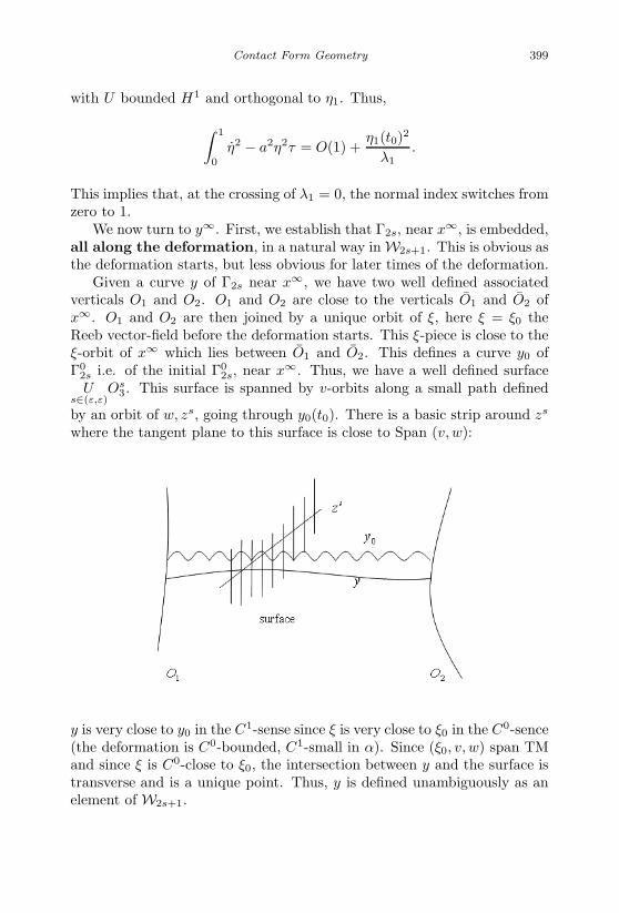
January 17, 2007 11:55 WSPC/Book Trim Size for 9in x 6in finalBB
Contact Form Geometry 399
with U bounded H1 and orthogonal to η1. Thus,
∫ 1
0
η2 − a2η2τ = O(1) +η1(t0)2
λ1.
This implies that, at the crossing of λ1 = 0, the normal index switches fromzero to 1.
We now turn to y∞. First, we establish that Γ2s, near x∞, is embedded,all along the deformation, in a natural way in W2s+1. This is obvious asthe deformation starts, but less obvious for later times of the deformation.
Given a curve y of Γ2s near x∞, we have two well defined associatedverticals O1 and O2. O1 and O2 are close to the verticals O1 and O2 ofx∞. O1 and O2 are then joined by a unique orbit of ξ, here ξ = ξ0 theReeb vector-field before the deformation starts. This ξ-piece is close to theξ-orbit of x∞ which lies between O1 and O2. This defines a curve y0 ofΓ0
2s i.e. of the initial Γ02s, near x∞. Thus, we have a well defined surface
Us∈(ε,ε)
Os3. This surface is spanned by v-orbits along a small path defined
by an orbit of w, zs, going through y0(t0). There is a basic strip around zs
where the tangent plane to this surface is close to Span (v, w):
y is very close to y0 in the C1-sense since ξ is very close to ξ0 in the C0-sence(the deformation is C0-bounded, C1-small in α). Since (ξ0, v, w) span TMand since ξ is C0-close to ξ0, the intersection between y and the surface istransverse and is a unique point. Thus, y is defined unambiguously as anelement of W2s+1.
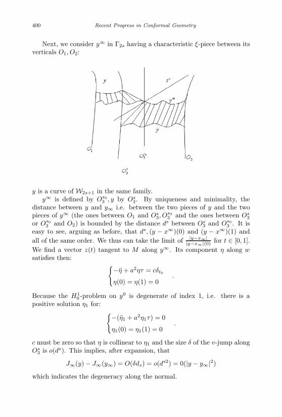
January 17, 2007 11:55 WSPC/Book Trim Size for 9in x 6in finalBB
400 Recent Progress in Conformal Geometry
Next, we consider y∞ in Γ2s having a characteristic ξ-piece between itsverticals O1, O2:
y is a curve of W2s+1 in the same family.y∞ is defined by Os0
3 , y by Os3. By uniqueness and minimality, the
distance between y and y∞ i.e. between the two pieces of y and the twopieces of y∞ (the ones between O1 and Os
3, Os03 and the ones between Os
3
or Os03 and O2) is bounded by the distance ds between Os
3 and Os03 . It is
easy to see, arguing as before, that ds, (y − x∞)(0) and (y − x∞)(1) andall of the same order. We thus can take the limit of |y−x∞|
|y−x∞|(0) for t ∈ [0, 1].We find a vector z(t) tangent to M along y∞. Its component η along wsatisfies then:
−η + a2ητ = cδt0
η(0) = η(1) = 0.
Because the H10 -problem on y0 is degenerate of index 1, i.e. there is a
positive solution η1 for: −(η1 + a2η1τ) = 0
η1(0) = η1(1) = 0.
c must be zero so that η is collinear to η1 and the size δ of the v-jump alongOs
3 is o(ds). This implies, after expansion, that
J∞(y) − J∞(y∞) = O(δds) = o(ds2) = 0(|y − y∞|2)which indicates the degeneracy along the normal.

January 17, 2007 11:55 WSPC/Book Trim Size for 9in x 6in finalBB
Contact Form Geometry 401
We now prove that δ = O(ds2) = O(|y − y∞|2), which implies that
J∞(y) − J∞(y∞) = O(d3s).
Indeed, coming back to our drawing, we label:
J∞(y) − J∞(y∞) =∫
[B,C]
α −∫
[A,B]
α
since the surfaces S1, S2 are spanned by ξ.[A, C] has size δ, [A, B] has size O(ds), has a component along w at first
order equal to c1ds, c1 = 0 and [B, C] is derived from [A, B] by v-transport
during a time O(δ) so that
J∞(y) − J∞(y∞) = O(δds) = O(ds3).
If we establish that δ ∼ cd2s, c = 0, then
J∞(y) − J∞(y∞) = c1ds3 + o(ds3)
and our statement about y∞ and its unstable manifold follows.In order to prove that δ ∼ cds2, let us follow the ξ-trajectory from A0
past A until it arrives near A1 at a point A2. The ξ-length [A0, A2] equalsthe ξ-length [B0, B]. Since the ξ-piece [B0, B1] is characteristic and [A0, B0]is a piece of v-orbit of length s ∼ c1d
s, this ξ-trajectory reaches a point A2
with d(A2, O2) ∼ c2ds2, c2 = 0, because [A2, B1] is at first order tangent to

January 17, 2007 11:55 WSPC/Book Trim Size for 9in x 6in finalBB
402 Recent Progress in Conformal Geometry
v ([B0, B1] is characteristic) and the situation is generic (no vanishing atthird order):
Thus, there is a minimal ξ-orbit from Os3 to O1
2 from A to A2 and [C, A1]is a minimal ξ-orbit from Os
3 to O2 with d(O2, O′2) ∼ c2d
s2. The conclusionfollows for ds small enough, since the distance from A to C is of the sameorder than the distance between the two curves [A0, A] and [C, A1]. Thisdistance is equivalent past any given positive time along [C, A1], to any ofthe distances between the two v-verticals at two corresponding points, onetaken on [C, A1] and the other along [A, A2].
2.6.1 Study of the Poincare-return maps
We prove in this section that the Poincare-return map of a general criticalpoint at infinity preserve dα. This generalizes the result of [Bahri-1 2003]IIIb.9
Lemma 22 Assume that (a part of) the Poincare-return map g : σ1 →σ2, where σ1 and σ2 are sections to ξ, satisfies g∗α = α + df .
We can then find a section σ3 to ξ as close as we please to σ1 so thatthe Poincare-return map g: σ3 → σ2 satisfies g∗α = α.
Proof. Let o be the center of σ1 and σ2 so that g(o) = 0. Let f1(x) =f(x) − f(o) = dfo(x) + O(|x|2).
January 17, 2007 11:55 WSPC/Book Trim Size for 9in x 6in finalBB
Contact Form Geometry 403
Observe that
(g−1)∗(α + df) = α.
Let ψs be the one parameter group of ξ. Define
γ :σ1 → σ3
x → ψf1(x)(x).
Then,
γ∗α = α(dψf1(x) + df1ξ) = α + df.
Thus,
(g−1)∗oγ∗α = α i.e.(γog−1)∗α = α.
Let
g = goγ−1.
The conclusion follows.
The next Lemma generalizes [Bahri-1 2003, III B.9, pp 134–136]. Aswe carry out rotation from (non characteristic) pieces of x∞ to other (noncharacteristic) pieces, we can view this transport as a composition of maps.Each map bypasses a sequence of consecutive characteristic pieces, fromone side of the family to the other side.
When the family is reduced to one characteristic piece, we have provedin [Bahri-1 2003] that there are sections σ1 and σ2 which can be definedin a natural way such that the (partial) Poincare-return map g : σ1 → σ2
satisfies g∗α = α + df . Using the previous lemma, we may assume thatdf = 0. We may then use Proposition 16 of [Bahri-1 2003] and transportthe v-rotation from one to the other side of the characteristic piece.
We extend III B. 9 of [Bahri-1 2003] as follows:Consider a (full) sequence of characteristic ξ-piece of x∞.

January 17, 2007 11:55 WSPC/Book Trim Size for 9in x 6in finalBB
404 Recent Progress in Conformal Geometry
We define σ0 and σ1 as follows:Given a characteristic piece and the two edge v-orbits,
condition (*) of [Bahri-1 2003] is satisfied between x− and x+ if the vectorh defined by transport of ξ-appropriately scaled, with different scales ε, ε′
on each side - from x− to y−, x+ to y+ respectively and by matching thetwo transported vectors along the ξ-piece satisfies:

January 17, 2007 11:55 WSPC/Book Trim Size for 9in x 6in finalBB
Contact Form Geometry 405
ε′ − α(h+) + (h−) − ε = 0 (*)
x+ is defined by (*) as a function of x−.σ0 and σ1 are then defined by the following property that they should
satisfy:From z ∈ σ0, we move along v a time s0 until we reach a point y− such
that −γs is the one parameter group of v-αz(Dγ−s0(ξ(y))) = 1. We thenmove along ξ from y− to y+ a characteristic length (of strict H1
0 - indexzero) and from y+ we move along −v until we reach a point z′ so that (*)holds between z and z′. From z′, we move a characteristic ξ-length to z
′′
and from z′′
we move along −v a time s2 until we reach a point z′′
so that(*) holds between y+ and z
′′′; and so on until we reach the last v-jump of
the family. Then, in addition to (*), we require that, with sm denoting thetime along the last v-jump:
α(Dγ−sm(ξ)) = 1.
This imposes a extra-condition and provides a restriction which defines σ0
and σ1.
g : σ0 → σ1
is defined accordingly and we claim that:
Lemma 23
g∗α = α + df.
Proof. Observe that (*) allow us to define a variation u (a tangent vector)along each characteristic ξ-piece with edge v-pieces so that x+ is derivedfrom x− through the use of (*):
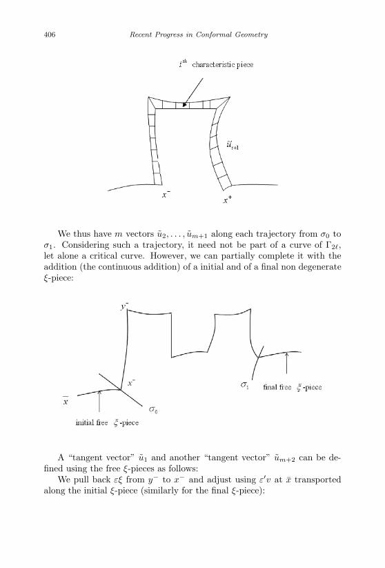
January 17, 2007 11:55 WSPC/Book Trim Size for 9in x 6in finalBB
406 Recent Progress in Conformal Geometry
We thus have m vectors u2, . . . , um+1 along each trajectory from σ0 toσ1. Considering such a trajectory, it need not be part of a curve of Γ2,let alone a critical curve. However, we can partially complete it with theaddition (the continuous addition) of a initial and of a final non degenerateξ-piece:
A “tangent vector” u1 and another “tangent vector” um+2 can be de-fined using the free ξ-pieces as follows:
We pull back εξ from y− to x− and adjust using ε′v at x transportedalong the initial ξ-piece (similarly for the final ξ-piece):
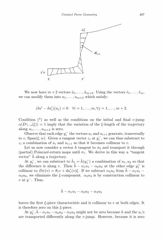
January 17, 2007 11:55 WSPC/Book Trim Size for 9in x 6in finalBB
Contact Form Geometry 407
We now have m +2 vectors u1, . . . , um+2. Using the vectors v1, . . . , vm,we can modify them into u1, . . . , um+2 which satisfy:
(δai − δaic)(uj) = 0 ∀i = 1, . . . , m,∀j = 1, . . . , m + 2.
Condition (*) as well as the conditions on the initial and final v-jumpα(Dγ−s(ξ)) = 1 imply that the variation of the ξ-length of the trajectoryalong u1, . . . , um+2 is zero.
Observe that each edge y−i the vectors ui and ui+1 generate, tranversally
to v, Span(ξ, w). Given a tangent vector zi at y−i , we can thus substract to
zi a combination of ui and ui+1 so that it becomes collinear to v.Let us now consider a vector h tangent to σ0 and transport it through
(partial) Poincare-return maps until σ1. We derive in this way a “tangentvector” h along a trajectory.
At y−1 , we can substract to h1 = h(y−
1 ) a combination of u1, u2 so thatthe difference is along v. Then h − α1u1 − α2u2 at the other edge y+
1 iscollinear to Dψ(v) = θ1v + da′
c(v)ξ. If we subtract α3u3 from h − α1u1 −α2u2, we eliminate the ξ-component. α3u3 is by construction collinear tov at y−. Thus,
h − α1u1 − α2u2 − α3u3
leaves the first ξ-piece characteristic and is collinear to v at both edges. Itis therefore zero on this ξ-piece.
At y−2 , h−α1u1−α2u2−α3u3 might not be zero because h and the ui’s
are transported differently along the v-jump. However, because it is zero
January 17, 2007 11:55 WSPC/Book Trim Size for 9in x 6in finalBB
408 Recent Progress in Conformal Geometry
at y+1 , it is collinear to v at y−
2 , thus collinear to dψ(x) = θ2v + da2c(v)ξ at
y+2 . Subtracting α4u4, h−α1u1−α2u2−α3u3−α4u4 is zero on the second
ξ-piece as well.Iterating, we find that
h =m+2∑i=1
αiui
between σ and σ1. Observe that the ui’s are parallel to v at the edges of theinitial and final non degenerate ξ-pieces. Since the variation of the ξ-lengthalong each ui is zero, we can write:
α(h(x1)) − α(h(x0)) =m+2∑i=1
αi
m∑j=1
(α(ui(y+
j )) − α(ui(y−j )))
=m∑
j=1
(α(h(y+
j )) − α(h(y−j )))
=m∑
j=1
(α(Dψ(h(y−
j )) − α(h(y−j )))
=m∑
j=1
dajc(h(y−
j ))
h(y−j ) is the image of h(x0) through the (partial) Poincare-return map dgj
so that
α
dg(h(x0)) − α(h(x0)) =m∑
j=1
dajc(dgj(h(x0)))
hence
g∗α = α + df on σ0.
We now state a result (Lemma 8) which may be useful in the verificationof hypothesis (A):
Let z be a critical point at infinity with all its v-jumps having the sameorientation, for example positive and having all its ξ-pieces of H1
0 -indexzero. Assume that z has index at infinity i∞ = k. Assume that z supportsa critical point at infinity x∞
2k which corresponds to a non trivial cycleof dimension 2k. Assume that this cycle has a non zero component on∂(w1 ⊗ . . . wk+1 ⊗W i∞). W i∞ is the unstable manifold of z and each wi isthe (half) — full unstable manifold of a degenerate ξ-piece of z (they are

January 17, 2007 11:55 WSPC/Book Trim Size for 9in x 6in finalBB
Contact Form Geometry 409
of H10 -index zero). We label the wi’s in the order in which they follow each
other on z, as we describe the full circle of time.There might be sequences of other degenerate ξ-piece spaced with free
ξ-pieces between wi and wi+1. We still label them wi, wi+1 for the sakeof simplicity. From Proposition 33, we know that each wi belongs to adifferent sequence of degenerate ξ-pieces. We then claim:
Lemma 24 For each i, there are times t−i < ti, z(ti) and z(ti) belong-ing to non degenerate ξ-pieces between wi and wi+1 such that z(ti) belongto some characteristic surface
∑−j of α and z(ti) belongs to some other
characteristic surface∑
of α i.e. z(ti) has a conjugate point after 2πjrevolutions of kerα along −v and z(ti) has a conjugate point after 2πrevolutions of kerα along +v.
Proof. We consider one edge of a sequence of degenerate ξ-pieces, theend one for example:
We know that
αx−0(Dγsf
(ξ(x+f )) = 1
and that (by genericity) x+f and x−
0 are not conjugate. Thus,
a(sf ) =∂
∂sαx−
0(Dγs(ξ(γ−s(x−
0 ))))∣∣s=sf
= 0.
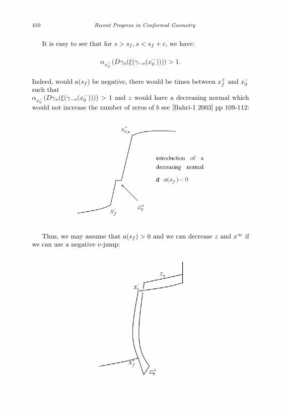
January 17, 2007 11:55 WSPC/Book Trim Size for 9in x 6in finalBB
410 Recent Progress in Conformal Geometry
It is easy to see that for s > sf , s < sf + c, we have:
αx−0(Dγs(ξ(γ−s(x−
0 )))) > 1.
Indeed, would a(sf ) be negative, there would be times between x+f and x−
0
such thatαx−
0(Dγs(ξ(γ−s(x−
0 )))) > 1 and z would have a decreasing normal whichwould not increase the number of zeros of b see [Bahri-1 2003] pp 109-112:
Thus, we may assume that a(sf ) > 0 and we can decrease z and x∞ ifwe can use a negative v-jump:

January 17, 2007 11:55 WSPC/Book Trim Size for 9in x 6in finalBB
Contact Form Geometry 411
This can be viewed as part of
or part of
We use here a small negative v-jump on the degenerate ξ-piece as adirection of decrease.
The two decreasing deformations can be made part of the same globaldecreasing deformation, just as in the proof of Proposition 33.
When is this deformation hindered after x−0 ? : We may define such a
deformation at z(t) as long as we can find s > 0 such that
αz(t)(Dγs(ξ)) > 1.
If we cross a v-jump between conjugate points after x−0 :
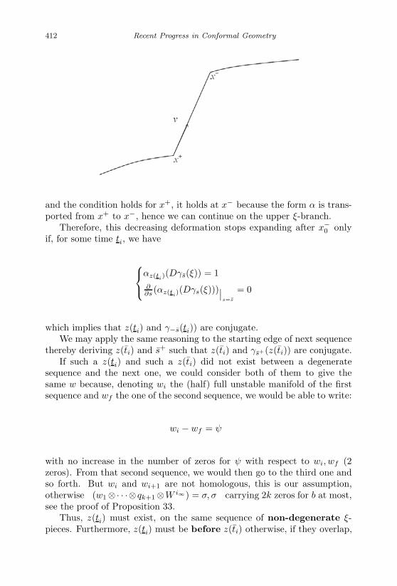
January 17, 2007 11:55 WSPC/Book Trim Size for 9in x 6in finalBB
412 Recent Progress in Conformal Geometry
and the condition holds for x+, it holds at x− because the form α is trans-ported from x+ to x−, hence we can continue on the upper ξ-branch.
Therefore, this decreasing deformation stops expanding after x−0 only
if, for some time ti, we have
αz(ti)(Dγs(ξ)) = 1
∂∂s(αz(ti)
(Dγs(ξ)))∣∣s=s
= 0
which implies that z(ti) and γ−s(ti)) are conjugate.We may apply the same reasoning to the starting edge of next sequence
thereby deriving z(ti) and s+ such that z(ti) and γs+(z(ti)) are conjugate.If such a z(ti) and such a z(ti) did not exist between a degenerate
sequence and the next one, we could consider both of them to give thesame w because, denoting wi the (half) full unstable manifold of the firstsequence and wf the one of the second sequence, we would be able to write:
wi − wf = ∂ψ
with no increase in the number of zeros for ψ with respect to wi, wf (2zeros). From that second sequence, we would then go to the third one andso forth. But wi and wi+1 are not homologous, this is our assumption,otherwise ∂(w1⊗· · ·⊗qk+1⊗W i∞) = ∂σ, σ carrying 2k zeros for b at most,see the proof of Proposition 33.
Thus, z(ti) must exist, on the same sequence of non-degenerate ξ-pieces. Furthermore, z(ti) must be before z(ti) otherwise, if they overlap,

January 17, 2007 11:55 WSPC/Book Trim Size for 9in x 6in finalBB
Contact Form Geometry 413
we can build in the overlap upon a transition between the two decreasingdeformations using:
As we combine the two oscillations, the functional is still decreasing andthe number of zeros is still only increased by 2(as allowed by the use of wi).
We can thin down and cancel one of these oscillations as we evolve toone or to the other edge.
Before ending Part V, we define a suitable basis at x∞ ∈ Γ2s of Tx∞Γ2k
for the reduction of d2J(x∞) and we also establish that β remains a contactform through all our perturbations above (and below in Part VI).
2.6.2 Definition of a basis of Tx∞Γ2s for the reduction of
d2J(x∞)
We define, for a general x∞ belonging to Γ2s a basis of Tx∞Γ2s suitable forthe reading of d2J(x∞). This basis will be redefined in section VI whenwe will be studying more specifically critical points at infinity having onlycharacteristic ξ-pieces.
We need first to define, given a ξ-piece, free or characteristic, what is theassociated vector vi. We draw this ξ-piece and the next one. We assumein a first step that both are free ξ-pieces.
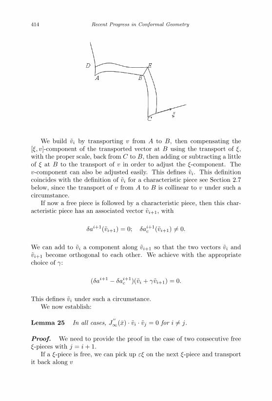
January 17, 2007 11:55 WSPC/Book Trim Size for 9in x 6in finalBB
414 Recent Progress in Conformal Geometry
We build vi by transporting v from A to B, then compensating the[ξ, v]-component of the transported vector at B using the transport of ξ,with the proper scale, back from C to B, then adding or subtracting a littleof ξ at B to the transport of v in order to adjust the ξ-component. Thev-component can also be adjusted easily. This defines vi. This definitioncoincides with the definition of vi for a characteristic piece see Section 2.7below, since the transport of v from A to B is collinear to v under such acircumstance.
If now a free piece is followed by a characteristic piece, then this char-acteristic piece has an associated vector vi+1, with
δai+1(vi+1) = 0; δai+1c (vi+1) = 0.
We can add to vi a component along vi+1 so that the two vectors vi andvi+1 become orthogonal to each other. We achieve with the appropriatechoice of γ:
(δai+1 − δai+1c )(vi + γvi+1) = 0.
This defines vi under such a circumstance.We now establish:
Lemma 25 In all cases, J′′∞(x) · vi · vj = 0 for i = j.
Proof. We need to provide the proof in the case of two consecutive freeξ-pieces with j = i + 1.
If a ξ-piece is free, we can pick up εξ on the next ξ-piece and transportit back along v

January 17, 2007 11:55 WSPC/Book Trim Size for 9in x 6in finalBB
Contact Form Geometry 415
Then,
−→BD = ε(1 + A1)ξ + B1[ξ, v] + θv.
At a critical curve, A1 = 0.This fact is not changed on the second ξ-piece after x∞ has been dis-
placed along vi since vi has no support near the second edge of the secondfree ξ-piece:

January 17, 2007 11:55 WSPC/Book Trim Size for 9in x 6in finalBB
416 Recent Progress in Conformal Geometry
Thus, the natural extension of vi+1 along x∞ + εvi still satisfies J ′∞ ·
vi+1 = 0 and we must have:
J′′∞(x∞) · vi · vi+1 = 0.
We now extend to a free piece the definition of the vectors ui providedabove (in the proof of Proposition 34):
We take v at A, we transport it along ξ at B, then along v to C, thenalong ξ to D, then again along v to E and finally along ξ to F and weexpect that it glues up with µv at F .
The free parameters are δa1, δs1, δa2, δs2, δa3 since we are free to changeslightly the length of the ξ- and of the v-pieces along our transports.
At F , we have two equations to satisfy since we need ui at F to be equalto µv.

January 17, 2007 11:55 WSPC/Book Trim Size for 9in x 6in finalBB
Contact Form Geometry 417
Furthermore, we want ui to be orthogonal to vi−1, vi and vi+1. This re-quirement introduces three additional conditions. We have five parametersfor five conditions. We will see later that the system is compatible.
We now have a basis for Tx∞Γ2s made of v1, . . . , vs, u1, . . . , us whereJ
′′∞(x∞) takes the form:
c1 0. . .
0 cs 0
0 A
.
Inspecting A, we find that as in [Bahri-1 2003], also Section 2.7 below,A is as follows:
. . . . . . 0
. . .. . .
. . .
0. . . . . .
2.6.3 Compatibility
We now prove that the C2-bounded perturbations of v which we have in-troduced do not destroy the requirement on β to be a contact form. Sincethe arguments establishing that i∞ ≥ k + 1 (Corollary 9) are of local type(local near x∞
2k), we will not worry about establishing global statementsabout the perturbed α, v, β etc, we will worry only about local propertiesnear x∞
2k. Our v-jump is between x− and x−0 :
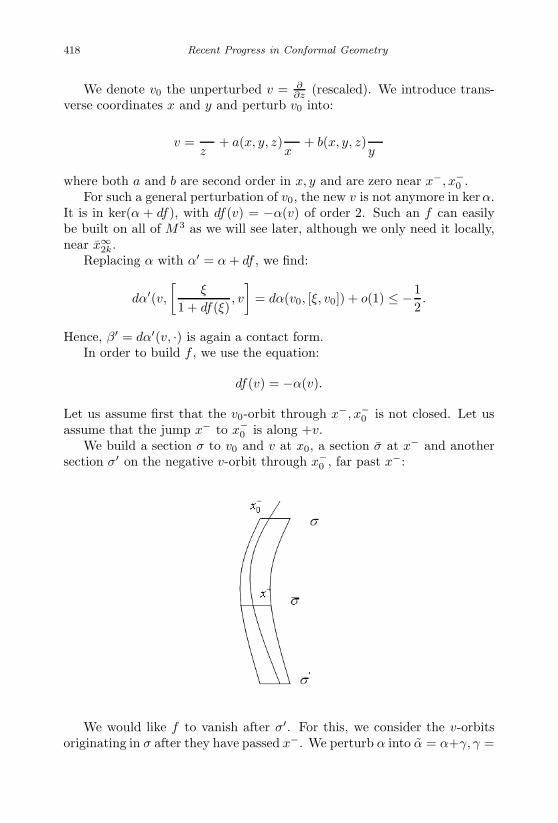
January 17, 2007 11:55 WSPC/Book Trim Size for 9in x 6in finalBB
418 Recent Progress in Conformal Geometry
We denote v0 the unperturbed v = ∂∂z (rescaled). We introduce trans-
verse coordinates x and y and perturb v0 into:
v =∂
∂z+ a(x, y, z)
∂
∂x+ b(x, y, z)
∂
∂y
where both a and b are second order in x, y and are zero near x−, x−0 .
For such a general perturbation of v0, the new v is not anymore in kerα.It is in ker(α + df), with df(v) = −α(v) of order 2. Such an f can easilybe built on all of M3 as we will see later, although we only need it locally,near x∞
2k.Replacing α with α′ = α + df , we find:
dα′(v,
[ξ
1 + df(ξ), v
]= dα(v0, [ξ, v0]) + o(1) ≤ −1
2.
Hence, β′ = dα′(v, ·) is again a contact form.In order to build f , we use the equation:
df(v) = −α(v).
Let us assume first that the v0-orbit through x−, x−0 is not closed. Let us
assume that the jump x− to x−0 is along +v.
We build a section σ to v0 and v at x0, a section σ at x− and anothersection σ′ on the negative v-orbit through x−
0 , far past x−:
We would like f to vanish after σ′. For this, we consider the v-orbitsoriginating in σ after they have passed x−. We perturb α into α = α+γ, γ =
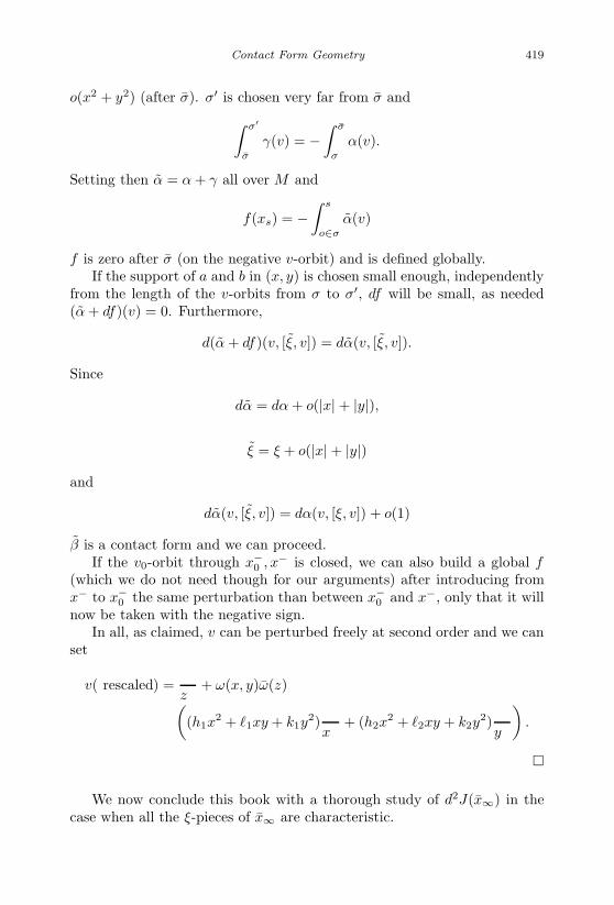
January 17, 2007 11:55 WSPC/Book Trim Size for 9in x 6in finalBB
Contact Form Geometry 419
o(x2 + y2) (after σ). σ′ is chosen very far from σ and∫ σ′
σ
γ(v) = −∫ σ
σ
α(v).
Setting then α = α + γ all over M and
f(xs) = −∫ s
o∈σ
α(v)
f is zero after σ (on the negative v-orbit) and is defined globally.If the support of a and b in (x, y) is chosen small enough, independently
from the length of the v-orbits from σ to σ′, df will be small, as needed(α + df)(v) = 0. Furthermore,
d(α + df)(v, [ξ, v]) = dα(v, [ξ, v]).
Since
dα = dα + o(|x| + |y|),
ξ = ξ + o(|x| + |y|)and
dα(v, [ξ, v]) = dα(v, [ξ, v]) + o(1)
β is a contact form and we can proceed.If the v0-orbit through x−
0 , x− is closed, we can also build a global f(which we do not need though for our arguments) after introducing fromx− to x−
0 the same perturbation than between x−0 and x−, only that it will
now be taken with the negative sign.In all, as claimed, v can be perturbed freely at second order and we can
set
v( rescaled) =∂
∂z+ ω(x, y)ω(z)(
(h1x2 + 1xy + k1y
2)∂
∂x+ (h2x
2 + 2xy + k2y2)
∂
∂y
).
We now conclude this book with a thorough study of d2J(x∞) in thecase when all the ξ-pieces of x∞ are characteristic.

January 17, 2007 11:55 WSPC/Book Trim Size for 9in x 6in finalBB
420 Recent Progress in Conformal Geometry
2.7 On the Morse Index of a Functional Arising in ContactForm Geometry
2.7.1 Introduction
Let (M3, α) be a three dimensional compact manifold without boundary.Let α be the contact form on M . Let ξ be the contact vector field of α,and let v be a non-singular vector field in kerα such that
β = dα(v, ·)is also a contact form with the same orientation than α.
The existence of such v and β is discussed in other papers [Bahri 1998]and [Bahri-1 2003]. It is not needed for our results here but is used for thesake of simplicity.
Let k ∈ N∗ be a non-zero integer and let Γ2k be the space of closedcurves on M made of k pieces of ξ-orbits alternated by k-pieces of ±v-orbits. The orientation εi of the ith v-orbit is pre-assigned so that weshould rigorously work with Γ2k(ε1, · · ·, εk), but we work with Γ2k for thesake of simplicity.
Γ2k is, under a generic perturbation on v if needed [Bahri 1998], a 2kdimensional manifold. It is natural to ask, a question which we will notaddress here, whether Γ2k is a symplectic or complex manifold.
A curve of Γ2k x is typically drawn as follows:
And there is a natural functional defined on Γ2k,
J∞(x) =k∑
i=1
ai,
where ai is the length of the ith ξ-piece.
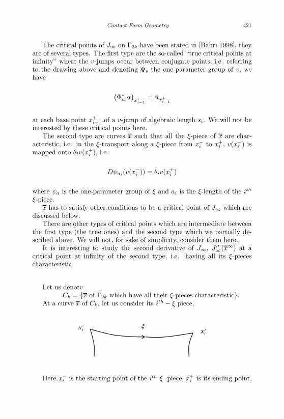
January 17, 2007 11:55 WSPC/Book Trim Size for 9in x 6in finalBB
Contact Form Geometry 421
The critical points of J∞ on Γ2k have been stated in [Bahri 1998], theyare of several types. The first type are the so-called “true critical points atinfinity” where the v-jumps occur between conjugate points, i.e. referringto the drawing above and denoting Φs the one-parameter group of v, wehave
(Φ∗
siα)x+
i−1= αx+
i−1
at each base point x+i−1 of a v-jump of algebraic length si. We will not be
interested by these critical points here.The second type are curves x such that all the ξ-piece of x are char-
acteristic, i.e. in the ξ-transport along a ξ-piece from x−i to x+
i , v(x−i ) is
mapped onto θiv(x+i ), i.e.
Dψai(v(x−i )) = θiv(x+
i )
where ψa is the one-parameter group of ξ and ai is the ξ-length of the ith
ξ-piece.x has to satisfy other conditions to be a critical point of J∞ which are
discussed below.There are other types of critical points which are intermediate between
the first type (the true ones) and the second type which we partially de-scribed above. We will not, for sake of simplicity, consider them here.
It is interesting to study the second derivative of J∞, J ′′∞(x∞) at a
critical point at infinity of the second type, i.e. having all its ξ-piecescharacteristic.
Let us denoteCk = x of Γ2k which have all their ξ-pieces characteristic.
At a curve x of Ck, let us consider its ith − ξ piece,
Here x−i is the starting point of the ith ξ -piece, x+
i is its ending point.

January 17, 2007 11:55 WSPC/Book Trim Size for 9in x 6in finalBB
422 Recent Progress in Conformal Geometry
We can define along this piece a tangent vector to Γ2k (not to Ck) whichwe denote vi. It is generated by the transport of v along ξ from x−
i to x+i .
At a generic point of Ck, in particular at x∞, we have
TxΓ2k = TxCk ⊕(→i=1
k→ ⊕Rvi
).
This decomposition might not be a direct sum along a k−1 dimensionalsub-manifold of Ck. At a critical point at infinity x∞, it will be genericallya direct sum.
J ′′∞(x∞) reads in the decomposition as follows:
c1 0 0
0 ... 00 0 ck
0
0 A
here,
ci = J ′′∞(x∞)·vi·vi,
J ′′∞(x∞)·vi·vj = 0 for i = j.
Thus, the index i∞ of J ′′∞(x∞) splits into
i∞ = i1∞ + i2∞
with i1∞ = number of negative c′is and i2∞=index A. i1∞ is what we call thenormal index.
Usually, at a non-degenerate critical point y0 of a function f(x), anegative direction can be adjusted to be any prescribed direction throughrotation.
January 17, 2007 11:55 WSPC/Book Trim Size for 9in x 6in finalBB
Contact Form Geometry 423
We prove in this paper that we can adjust these negative directions aswe please between i1∞ and i2∞, switching them from one side to the otherand vice-versa, not through rotations in the parameter spaces but throughlocal deformation of α and v around x∞.
Namely, we prove,
Theorem 2 (Main Theorem) Given i1∞ and i2∞ and another way ofwriting i1∞+i2∞ as j1∞+j2∞, j1∞ ≤ k, j2∞ ≤ k, as long as i2∞ ≥ 2 and j2∞ ≥ 1,there is a C2−bounded and C1-small deformation of α and v keeping x∞
isolated and non-degenerate such that, for the new α and v, J ′′∞(x∞) has
normal index j1∞ and j2∞ as index along Ck.
Corollary 10 Assume i1∞ < k and i2∞ ≥ 2, let i be such that ci =J ′′∞(x∞)·vi·vi > 0, we can complete a C2−bounded and C1-small deforma-
tion of α and v which keeps x∞ isolated and non-degenerate and changesci from ci > 0 to ci < 0.
Results of this kind are directly related to the homology defined in[Bahri-1 2003] and which we studied more thoroughly in [Bahri-2 2003].They give us some freedom in the definition of this homology as decreasingflow-lines which go to x∞’s as above can be assumed to leave later neighbor-hoods of such x∞’s using decreasing directions corresponding to the normal( i1∞) or the tangential (i2∞) as we please.
The Γ2k’s and J∞ arise in the variational problem at infinity associatedwith the variational problem
J(x) =∫ 1
0
αx(x)dt
on loops x = x(t) of Cβ = x ∈ H1(S1, M) s.t. βx(x) = 0, αx(·) = const >0.
Such curves have a tangent vector which reads x = aξ + bv. Thereare decreasing flow trajectories for a suitable pseudo-gradient which do notconverge to the periodic orbits of ξ and end up in the Γ2k’s, more preciselyat the x∞’s. Hence, the usual ∂−operator of Morse theory when related tothe critical points only (periodic orbits of ξ) does not work and we have toinclude the x∞’s. The x∞’s have two indices, an H1
0 - index i0 and an indexat infinity i∞, see [Bahri-1 2003]. i0, if we use an outstretched analogy withpiece-wise geodesics between prescribed points, is the index of the piece-wise geodesics between the prescribed points once these prescribed pointsare fixed. i∞ is the index when the curves between the prescribed pointsare geodesics and the preassigned points are free to move.

January 17, 2007 11:55 WSPC/Book Trim Size for 9in x 6in finalBB
424 Recent Progress in Conformal Geometry
Studying flow lines more closely out of or reaching periodic orbits, wederive that we may assume for the x∞’s which interfere with the homologythat i0 = 0, see [Bahri-2 2003].
This implies that the total index of such x∞’s can be computed inrestriction to the slice of Γ2k to which these x∞’s belong.
Understanding their unstable manifold is useful and our theorem pro-vides some preliminary information on this index. A more thorough studyof the Ck’s and of their injection in the Γ2k’s should provide some insightabout this index. Other related questions may be asked such as, are theCk’s for example real sub-manifolds in Γ2k? Are they lagrangian?
Another interesting question is to study the part of Γ2k where i0 = 0,see [Bahri-2 2003]. This part corresponds to curves such that their ξ- pieces,if thought as geodesics (this can always be done locally), are minima in avariational problem J(x) =
∫ 1
0αx(x)dt defined on curves whose ends are not
completely prescribed but constrained to move along prescribed v-orbits.Such a part of Γ2k can be thought of as a covering of the configuration
space of pieces of surfaces transverse to v (S2 in the case of Hopf fibrationS3 → S2 and the standard contact structure). A natural question whicharises then is the question of understanding the relationship between i1∞,i2∞ and the topology of the configuration spaces which are underlying theset of curves having i0 = 0.
We proceed now with the proof of the theorem as follows.
2.7.2 The Case of Γ2
Theorem 3 Let x∞ be a false critical point at infinity in Γ2, with itscharacteristic ξ-piece. Assume that the index at infinity of x∞ is 1. Wecan then modify the vector field v in the vicinity of x∞ so that the vector fieldv at x∞ defines the negative direction of the second derivative at infinity.After this modification, β remains a contact form and no new critical pointat infinity is created.
The proof starts with the choice of suitable coordinates in order todescribe Γ2 near x∞. Once these coordinates are found and the equationsfor Γ2 become explicit, the vector-field will be modified so that v becomesthe negative direction for J ′′∞.
x∞ has a base point x0. The characteristic ξ-piece of x∞ starts at x0
and ends at x1:
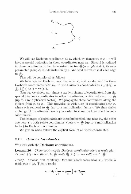
January 17, 2007 11:55 WSPC/Book Trim Size for 9in x 6in finalBB
Contact Form Geometry 425
We will use Darboux coordinates at x0 which we transport at x1. v willhave a special reduction in these coordinates near x1. Since ξ is reducedin these coordinates to be the constant vector ∂
∂x (α = ydz + dx), its one-parameter group φs is x-translation by s. We need to reduce v at each edgeto ∂
∂z .This will be completed as follows:We have special Darboux coordinates at x1 and we derive from these
Darboux coordinates near x0. In the Darboux coordinates at x1, v(x1) =∂∂z ,(
∂∂z v
)(x1) = γv(x1).
Near x1, we choose an (almost) explicit change of coordinates, from thespecial Darboux coordinates to other coordinates, which reduces v to ∂
∂z(up to a multiplication factor). We propagate these coordinates along thev-piece from x1 to x0. This provides us with a set of coordinates near x0
where v is reduced to ∂∂z (up to a multiplication factor). We thus derive
a change of coordinates near x0 in order to come back to the Darbouxcoordinates.
Two changes of coordinates are therefore needed, one near x0, the otherone near x1; both relate coordinates where v = ∂
∂z (up to a multiplicationfactor) to Darboux coordinates.
We give in what follows the explicit form of all these coordinates.
2.7.3 Darboux Coordinates
We start with the Darboux coordinates.
Lemma 26 There exist near x1 Darboux coordinates where α reads ydz+dx and v(x1) is collinear to ∂
∂z while ∂v∂z (x1) is also collinear to ∂
∂z .
Proof. Choose first arbitrary Darboux coordinates near x1, where αreads ydz + dx. Then v reads:
v = A0
(∂
∂z− y
∂
∂x
)+ B0
∂
∂y.

January 17, 2007 11:55 WSPC/Book Trim Size for 9in x 6in finalBB
426 Recent Progress in Conformal Geometry
Let
x′ = x − θz2/2
y′ = y + θz
z′ = z.
This provides new Darboux coordinates where
v(0, 0, 0) = A0∂
∂z+ B0
∂
∂y
= A0
(∂
∂z′+ θ
∂
∂y′
)+ B0
∂
∂y′
= A0∂
∂z′+ (A0θ + B0)
∂
∂y′ .
A0 can be assumed not to be zero since we can use if needed the new setof Darboux coordinates:
x′ = x − y2
2y′ = y
z′ = z + y
where ∂∂y = ∂
∂y′ + ∂∂z′ at (0, 0, 0).
Choosing θ = −B0A0
, v reads as:
v = µ1
(∂
∂z− y
∂
∂x+ (a1x + b1y + g(z) + O(x2 + y2 + xz + yz))
∂
∂y
)a1 is not zero since dα(v, ∂v
∂x) = 0 at x1.
We need to get rid of g(z) ∂∂y . We set:
x′ = x + h(z)y′ = y − h′(z)z′ = z.
Then,
ydz + dx = (y − h′(z′))dz′ + dx + h′(z′)dz′ = y′dz′ + dx′.

January 17, 2007 11:55 WSPC/Book Trim Size for 9in x 6in finalBB
Contact Form Geometry 427
In these new coordinates,
∂
∂z=
∂
∂z′− h′′(z′)
∂
∂y′ + h′(z′)∂
∂x′
∂
∂x′ =∂
∂x∂
∂y′ =∂
∂y.
So that,
∂
∂z− y
∂
∂x+ (a1x + b1y + g(z) + O(x2 + y2 + xz + yz))
∂
∂y
=∂
∂z′− y′ ∂
∂x′ + a1x′ + b1y
′ + g(z′) − a1h(z′) + b1h′(z′) − h′′(z′)
+ O(x′2 + y′2 + x′z′ + +y′z′ + |z′h(z′)| + |z′h′(z′)| + h2(z′) + h′2(z′)
) ∂
∂y′ .
We choose h so that
b1h′ − h′′ = g(z) with h = O(z3), h′ = O(z2).
The claim follows.
Next, we reduce v to ∂∂z (up to collinearly) at each edge x0, x1. Near
x0 and x1, v is now collinear to ∂∂z − y ∂
∂x +(ax + by + cz + q2(x, y, z)
)∂∂y ,
where q2 stands for a function which is O(x2 + y2 + z2) at the origin. q2 isits second order term.
Let ψ1 be a local diffeomorphism such that D0ψ1 = Id, which maps theabove vector-field onto ∂
∂z . Writing:
ψ1(x, y, z) = (x+P 12 +P 1
3 +R)∂
∂x′+(y+P 22 +P 2
3 +S)∂
∂y′+(z+P 32 +P 3
3 +T )∂
∂z′
where P i2 and P i
3 are of degree 2 and 3 respectively and where R, S and Tare remainders of order four or more, we seek that
Dψ1
(∂
∂z− y
∂
∂x+ (ax + by + cz + q2(x, y, z))
∂
∂y
)=
∂
∂z′.

January 17, 2007 11:55 WSPC/Book Trim Size for 9in x 6in finalBB
428 Recent Progress in Conformal Geometry
This yields:
∂P 12
∂z= y
∂P 22
∂z+ ax + by + cz = 0
∂P 32
∂z= 0
∂P 13
∂z= y
∂P 12
∂x− (ax + by + cz)
∂P 12
∂y
∂P 23
∂z= y
∂P 22
∂x− (ax + by + cz)
∂P 22
∂y− q2(x, y, z)
∂P 33
∂z= y
∂P 32
∂x− (ax + by + cz)
∂P 32
∂y
R, S, T satisfy other equations. We thus have:
Proposition 36 If ψ1 satisfies the above system, thenDψ1( ∂
∂z − y ∂∂x + (ax + by + cz + q2(x, y, z)) ∂
∂y ) = ∂∂z′ + O3, where O3 is of
order 3 at (0, 0, 0).
A particular solution to the above system is (set q3 =∫ z
0q2(x, y, τ)dτ) :
P 12 = yz P 2
2 = −(ax + by +cz
2)z P 3
2 = 0
P 13 = − axz2
2− byz2
2− cz3
3
P 23 = − ayz2
2+ (ax + by)
bz2
2+ c
bz3
3− q3(x, y, z)
P 33 = 0.
Let now ψ(x, y, z) = A ∂∂x + B ∂
∂y + C ∂∂z be a diffeomorphism achieving
Dψ
(∂
∂z
)=
∂
∂z− B
∂
∂x+ (aA + bB + cC + p2)
∂
∂y(collinear to v)
with A = x + A, B = y + B, C = z + C, A, B, C of order 2 and higher. Inour framework, the image ∂
∂x , ∂∂y , ∂
∂z will be the Darboux coordinates for αnear x0. We then have:
∂A
∂z= −B,
∂B
∂z= aA + bB + cC + p2,
∂C
∂z= 1.
Thus, C = z + h(x, y), with h of order 2 and higher and
∂A
∂z= −B
∂B
∂z= aA + bB + c(z + h(x, y)) + p2(x, y, z) + O3.
January 17, 2007 11:55 WSPC/Book Trim Size for 9in x 6in finalBB
Contact Form Geometry 429
Hence,
(A
B
)(x, y, z)
= e
0 −1a b
z(A
B
)(x, y, 0) +
(0
ch(x, y)z +∫ 3
0p2(x, y, τ)dτ
)
+ c e
0 −1a b
z ∫ z
0
(τ
(01
)− τ2
(0 −1a b
)(01
))dτ + O4
= e
0 −1a b
z(x + A(x, y, 0)y + B(x, y, 0)
)+( − cz3
6
czh +∫ z
0p2(x, y, τ)dτ + cz2
2 + z3
6 + cb
)+ O4
=(
Id +(
0 −1a b
)z +
(−a −bab b2 − a
)z2
2
)(x
y
)+(
Id +(
0 −1a b
)z
)(A(x, y, 0)B(x, y, 0)
)+( − cz3
6
czh +∫ z
0p2(x, y, τ)dτ + cz2
2 + cbz3
6
)+ O4.
We thus have:
Lemma 27
ψ(x, y, z) =(
x − yz + A(x, y, 0) − (ax + by)z2
2− zB(x, y, 0) − cz3
6
)∂
∂x
+
(y + (ax + by)z + cz
22 + B(x, y, 0) + (abx + (b2 − a)y) z2
2
+(aA(x, y, 0) + bB(x, y, 0))z + czh +∫ z
0p2(x, y, τ)dτ + cb z3
6
)∂
∂y
+ (z + h2(x, y))∂
∂z+ O4.
We now compute the differential of ψ with respect to a variation(δx, δy, 0).
Differentiating, we find:

January 17, 2007 11:55 WSPC/Book Trim Size for 9in x 6in finalBB
430 Recent Progress in Conformal Geometry
Lemma 28
Dψ
(δx
∂
∂x+ δy
∂
∂y
)
=
δx − δyz − (aδx + bδy) z2
2 + ∂A∂x (x, y, 0)δx + ∂A
∂y (x, y, 0)δy
−z ∂B∂x (x, y, 0)δx − z ∂B
∂y (x, y, 0)δy + y(
∂h2∂x δx + ∂h2
∂y δy) ∂
∂x
+(
δy + (aδx + bδy)z +∂B
∂x(x, y, 0)δx +
∂B
∂y(x, y, 0)δy
+ (abδx + (b2 − a)δy)z2
2
+ a
(∂A
∂x(x, y, 0)δx +
∂A
∂y(x, y, 0)δy
)
+ b
(∂B
∂x(x, y, 0)δx +
∂B
∂y(x, y, 0)δyz
)
+ c
(∂h2
∂xδx +
∂h2
∂yδy
)z +
∫ z
0
(∂p2
∂xδx +
∂p2
∂yδy
)(x, y, τ)dτ
−(
∂h2
∂xδx +
∂h2
∂yδy
)(ax + by + cz)
))∂
∂y+ γ1v + h.o.
Proof. Differentiating in restriction to δz = 0 and observing that:(∂h2
∂xδx +
∂h2
∂y
)∂
∂z
=(
∂h2
∂xδx +
∂h2
∂yδy
)(∂
∂z−(y + B(x, y, z)
) ∂
∂x
+(aA + bB + cC + p2)∂
∂y
)+ (y + B(x, y, z))
(∂h2
∂xδx +
∂h2
∂y
)∂
∂x
−(
∂h2
∂xδx +
∂h2
∂yδy
)(ax + by + cz + aA + bB + cC + p2)
∂
∂y+ h.o.
We derive the claim.
ψ will be used to reduce v near x0. Near x1, we use ψ1 given by (P), toreduce v. Then, ψ1|z=0 and Dψ1|z=0,δz=0 are identity maps.
2.7.4 The v-transport maps
We now study the map along the v-side of x∞.
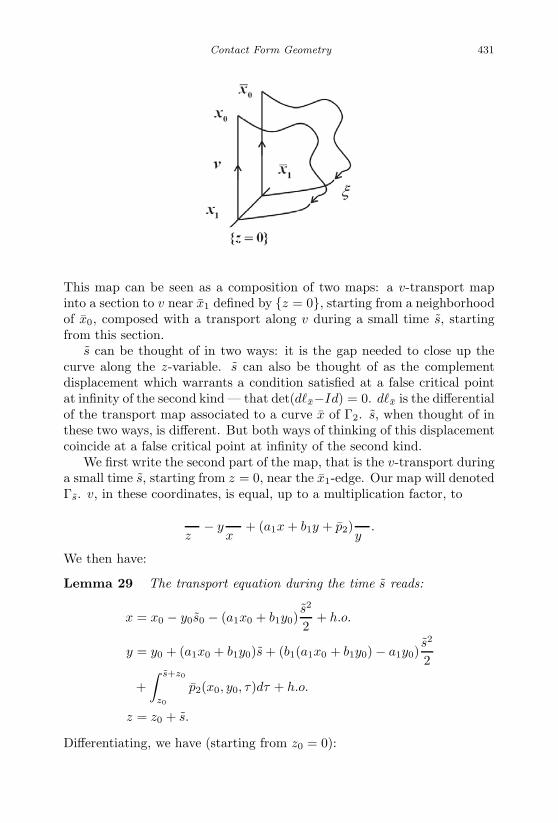
January 17, 2007 11:55 WSPC/Book Trim Size for 9in x 6in finalBB
Contact Form Geometry 431
This map can be seen as a composition of two maps: a v-transport mapinto a section to v near x1 defined by z = 0, starting from a neighborhoodof x0, composed with a transport along v during a small time s, startingfrom this section.
s can be thought of in two ways: it is the gap needed to close up thecurve along the z-variable. s can also be thought of as the complementdisplacement which warrants a condition satisfied at a false critical pointat infinity of the second kind — that det(dx−Id) = 0. dx is the differentialof the transport map associated to a curve x of Γ2. s, when thought of inthese two ways, is different. But both ways of thinking of this displacementcoincide at a false critical point at infinity of the second kind.
We first write the second part of the map, that is the v-transport duringa small time s, starting from z = 0, near the x1-edge. Our map will denotedΓs. v, in these coordinates, is equal, up to a multiplication factor, to
∂
∂z− y
∂
∂x+ (a1x + b1y + p2)
∂
∂y.
We then have:
Lemma 29 The transport equation during the time s reads:
x = x0 − y0s0 − (a1x0 + b1y0)s2
2+ h.o.
y = y0 + (a1x0 + b1y0)s + (b1(a1x0 + b1y0) − a1y0)s2
2
+∫ s+z0
z0
p2(x0, y0, τ)dτ + h.o.
z = z0 + s.
Differentiating, we have (starting from z0 = 0):

January 17, 2007 11:55 WSPC/Book Trim Size for 9in x 6in finalBB
432 Recent Progress in Conformal Geometry
Lemma 30
δx = δx0 − δy0s − (a1δx0 + b1δy0)s2
2+ h.o.
δy = δy0(1 + b1s + (b21 − a1)
s2
2) + δx0(a1s + a1b1
s2
2) +
∫ s
0
δp2 + h.o.
δz = δz0 = 0.
Proof. The transport equations read:
x = −y
y = a1x + b1y + p2
z = 1
from which the two lemmas follow.
Next, we write the v-map into z = 0. In z = 0, near the end-pointx1, we pick up commuting vector-fields ∂
∂x′ and ∂∂y′ , with ∂
∂x′ = ξ(x′, y′, 0).We pull them back along v and we obtain in this way three commutingvector-fields ∂
∂x , ∂∂y and v collinear to ∂
∂z .We can arrange so that ∂
∂x (0), ∂∂y (0) and ∂
∂z are the Darboux coordinatesat x0 and that ∂
∂x′ ,∂
∂y′ , v(x1) are the Darboux coordinates at x1. We can
also arrange so that(
∂∂x , ∂
∂y
)is derived from
(∂
∂x′ ,∂
∂y′
)using a constant
matrix. This involves a reparametrization of v (for the transport equationsonly) so that z = 0 at x1 is mapped into z = 0 at x0. Then, thetransport along v from (x, y) to (x′, y′) and cutting into the v-section z =0 reads through a constant matrix D which satisfies det(D − Id) = 0 andthus reads:
D = Id +(
A1 λA1
B1 λB1
).
Therefore, the map on the v-side reads as:
Γz
(Id +
(A1 λA1
B1 λB1
))(x
y
)= Γz
(x + A1(x + λy)y + B1(x + λy)
).
Composing, we find:

January 17, 2007 11:55 WSPC/Book Trim Size for 9in x 6in finalBB
Contact Form Geometry 433
Lemma 31
Γz
(x + A1(x + λy)y + B1(x + λy)
)
=
x + A1(x + λy) − (y + B1(x + λy))z + O(|X |3)
y + B1(x + λy) + (a1(x + A1(x + λy)) + b1(y + B1(x + λy)))z+O(|X |3)
z
.
Differentiating, we introduce new variables:
δx(0) = δx(0) + A1(δx(0) + λδy(0))
δy(0) = δy(0) + B1(δx(0) + λδy(0))
and we have:
Lemma 32
δx = δx(0)(1 − a1z2
2) − δy(0)(z + b1
z2
2) + h.o
δy = δy(0)(1 + b1z + (b21 − a1)
z2
2) + a1δx(0)(z + b1
z2
2)
+∫ z
0
(∂p2
∂xδx(0) +
∂p2
∂yδy(0)
)dτ + h.o.
Ultimately, z is a function of (x, y, z), but no differentiation with respectto z is involved in the computation of det(dx − Id).
Using the above lemmas, with ψ as in Lemma 27 and φs being theone-parameter group of ξ, ac the characteristic length (ac = ac(x, y, z)), wederive:
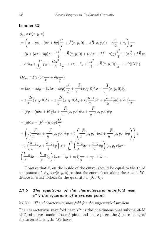
January 17, 2007 11:55 WSPC/Book Trim Size for 9in x 6in finalBB
434 Recent Progress in Conformal Geometry
Lemma 33
φac ψ(x, y, z)
=(
x − yz − (ax + by)z2
2+ A(x, y, 0) − zB(x, y, 0) − c
z3
6+ ac
)∂
∂x
+ (y + (ax + by)z +cz2
2+ B(x, y, 0) + (abx + (b2 − a)y)
z2
2+ (aA + bB)z
+ czh2 +∫ z
0
p2 +cbz3
6)
∂
∂y+ (z + h2 +
cz2
2+ B(x, y, 0))
∂
∂z+ O(|X |3)
Dφac Dψ(δx∂
∂x+ δy
∂
∂y)
= (δx − zδy − (aδx + bδy)z2
2+
∂A
∂x(x, y, 0)δx +
∂A
∂y(x, y, 0)δy
− z∂B
∂x(x, y, 0)δx − z
∂B
∂y(x, y, 0)δy + (y
∂h2
∂xδx + y
∂h2
∂yδy) + h.o)
∂
∂x
+ (δy + (aδx + bδy)z +∂B
∂x(x, y, 0)δx +
∂B
∂y(x, y, 0)δy
+ (abδx + (b2 − a)δy)z2
2
+
(a(
∂A
∂xδx +
∂A
∂y(x, y, 0)δy + b
(∂B
∂x(x, y, 0)δx +
∂B
∂y(x, y, 0)δy
))z
+ c
(∂h2
∂xδx +
∂h2
∂yδy
)z +
∫ z
0
(∂p2
∂xδx +
∂p2
∂yδy
)(x, y, τ)dτ−(
∂h2
∂xδx +
∂h2
∂yδy
)(ax + by + cz))
∂
∂y+ γ2v + h.o.
Observe that z, on the v-side of the curve, should be equal to the thirdcomponent of φac ψ(x, y, z) so that the curve closes along the z-axis. Wedenote in what follows a0 the quantity ac(0, 0, 0).
2.7.5 The equations of the characteristic manifold near
x∞; the equations of a critical point
2.7.5.1 The characteristic manifold for the unperturbed problem
The characteristic manifold near x∞ is the one-dimensional sub-manifoldof Γ2 of curves made of one ξ-piece and one v-piece, the ξ-piece being ofcharacteristic length. We have:
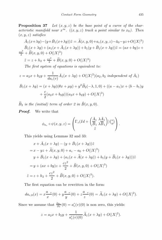
January 17, 2007 11:55 WSPC/Book Trim Size for 9in x 6in finalBB
Contact Form Geometry 435
Proposition 37 Let (x, y, z) be the base point of a curve of the char-acteristic manifold near x∞. ((x, y, z) track a point similar to x0). Then(x, y, z) satisfies
A1(x+λy)−(y+B1(x+λy))z = A(x, y, 0)+ac(x, y, z)−a0−yz+O(|X |3)B1(x + λy) + (a1(x + A1(x + λy)) + b1(y + B1(x + λy))z = (ax + by)z +
cz2
2 + B(x, y, 0) + O(|X |3)z = z + h2 + cz2
2 + B(x, y, 0) + O(|X |3)The first system of equations is equivalent to:
z = a2x + b2y +1
dac(v)A1(x + λy) + O(|X |2)(a2, b2 independent of A1)
B1(x + λy) = (x + λy)(θx + µy) + y2B2(−λ, 1, 0) + ((a − a1)x + (b − b1)y
+c
2(a2x + b2y))(a2x + b2y) + O(|X |3)
B2 is the (initial) term of order 2 in B(x, y, 0).
Proof. We write that
φac ψ(x, y, z) =
Γz(Id +(
A1 λA1
B1 λB1
))(xy
)z
.
This yields using Lemmas 32 and 33:
x + A1(x + λy) − (y + B1(x + λy))z
=x − yz + A(x, y, 0) + ac − a0 + O(|X |3)y + B1(x + λy) + (a1(x + A(x + λy)) + b1(y + B1(x + λy)))z
= y + (ax + by)z +cz2
2+ B(x, y, 0) + O(|X |3)
z = z + h2 +cz2
2+ B(x, y, 0) + O(|X |3).
The first equation can be rewritten in the form:
dac,0(x) = x∂ac
∂x(0) + y
∂ac
∂y(0) + z
∂ac
∂z(0) = A1(x + λy) + O(|X |2).
Since we assume that ∂ac
∂z (0) = a′c(v)(0) is non zero, this yields:
z = a2x + b2y +1
a′c(v)(0)
A1(x + λy) + O(|X |2).

January 17, 2007 11:55 WSPC/Book Trim Size for 9in x 6in finalBB
436 Recent Progress in Conformal Geometry
The second equation then yields:
B1(x + λy) = (x + λy)(θx + µy) + y2B2(−λ, 1, 0) + (a2x + b2y)((a − a1)x
+ (b − b1)y +c
2(a2x + b2y)) + 0(|x|3)
as stated.
2.7.6 Critical points, vanishing of the determinant
Let γs be the one-parameter group of v, x be a curve of Γ2 near x∞, withbase point x0 and v-length s0.
x is a critical point of the functional a = length along ξ near x∞ if thelength of the ξ-piece of x∞ is characteristic and if det(Dφac Dψ−Dγs0) =0.
Dγs0 is taken here from the coordinates which reduce v near x0 to theDarboux coordinates near x1. Since ac is characteristic,
Dφac Dψ
(∂
∂z
)= θ1v.
Also,
Dγs0
(∂
∂z
)= θ2v with θ1 = θ2 generically.
Thus, denoting
π2 : Span(
∂
∂x,
∂
∂y, v
)−→ Span
(∂
∂x,
∂
∂y
)the projection onto the space generated by the two first vectors of theDarboux reduction near x1, parallel to v, we must have:
π2 Dφac Dψ
δxδy0
= Dγs0
δxδy0
=(
δx
δy
)for some non zero (δx, δy).
We then have:
Lemma 34 The coordinates (x, y, z) of the base point x0 of the criticalcurve x satisfy:
A1
(b1z − ∂B(x, y, 0)
∂y− bz + λ
(∂B
∂x(x, y, 0) + az − a1z
))

January 17, 2007 11:55 WSPC/Book Trim Size for 9in x 6in finalBB
Contact Form Geometry 437
+ B1
(∂A
∂y(x, y, 0) + z − z − λ
∂A
∂x(x, y, 0)
)+ O(|X |2) = 0.
Proof. Using Lemma 32, the condition on the vanishing of the determi-nant reads:
O(|X|2)
=
∣∣∣∣∣∣∣∣∣A1 − ∂A
∂x− B1z z − ∂A
∂y+ λA1 − λB1z − z
b1B1z + B1 − ∂B
∂x− az + a1z + a1A1z b1(1 + λB1)z + λB1 − ∂B
∂y− bz + λa1A1z
∣∣∣∣∣∣∣∣∣ .
This yields: A1(b1(1 + λB1)z − ∂B∂y − bz + λa1A1z) − λB1
(∂A∂x + B1z
)−
λA1(b1B1z− ∂B∂x −az+a1z+a1A1z)−B1(z− ∂A
∂y −λB1z− z)+O(|X |2) = 0.
Lemma 35 follows.
2.7.7 Introducing the perturbation
To start with, we observe that the formulae for the characteristic manifold,for γ2 and for the false critical points at infinity involve p2, but only at ahigher order. ac involves p2 at second order but we have:
Lemma 35 Using a cut-off function ω near x0, we may suppress p2 fromv. This does not create new critical points at infinity.
Lemma 35 will follow from the same arguments (easier form) than theones used in order to prove that the sign of a′
c(v) = dac(v) can be changedwithout creating new critical points at infinity.
Assuming that p2 is zero, v is, in the Darboux coordinates near x0,equal up to a collinearity coefficient to ∂
∂z − y ∂∂x + (x + by + cz) ∂
∂y . Wewant to replace c with cτ (x, y, z), τ ∈ [0, 1], a modification which will takeplace on a small neighborhood of x0 with c0 = c and c1(0, 0, 0) · c negative.
cτ will be of the form:
c + τω(x, y, z)(c(z) − c)
c(z) is equal to c for |z| ≥ z0, where z0 is small. ω(x, y, z) is a cut-offfunction which is constructed in a non-standard way. In fact, the modifiedv is defined in a first stage as a non-autonomous modification of v which weprove later to be autonomous. For this, we consider the plane z = 0 at

January 17, 2007 11:55 WSPC/Book Trim Size for 9in x 6in finalBB
438 Recent Progress in Conformal Geometry
x0. The plane is a section to v. The flow of the modified v can be writtenup to re-parametrization (|z| ≤ z0):
z = 1y = ax + by + cτ (x, y, z)zx = − y.
We want to define cτ (x, y, z) and for this purpose, we start with the sectionz = 0. On this section, cτ (x, y, 0) is defined to be
cτ (x, y, 0) = c + τω(x, y)(c(0) − c)
ω(x, y) is a cut-off function equal to 1 on a small disk of radius η and equalto zero outside of the disk of radius 2η. c will be defined later. At each(x0, y0, 0),
We define a differential equation:
x = − y x(0) = x0, y(0) = y0
y = ax + by + (c + τω(x0, y0)(c(s) − c))s. (*)
This defines (x(s), y(s)) which we view in three dimensions:
(x(s), y(s), s)
which satisfies:
x = −y
y = ax + by + (c + ω(x0, y0) · τ(c(s) − c))s
x(0) = x0, y(0) = y0, z(0) = 0 (*)z = 1
and we have:
Lemma 36 For each s, (*) defines a diffemorphism from z = 0 toz = s. Thus, (*) defines a vector-field v in kerα.
We differentiate (*) and we find:
˙δx = − δy
δy = aδx + bδy + τδωs(c(s) − c)
δω is taken with respect to variations (δx0, δy0) in the initial conditions.

January 17, 2007 11:55 WSPC/Book Trim Size for 9in x 6in finalBB
Contact Form Geometry 439
Denoting A the matrix(
0 −1a b
), we have,
(δxδy
)·= A
(δxδy
)+ O
(z
η
)(δx0
δy0
).
Thus, (δxδy
)= esA
[(δx0
δy0
)+∫ s
0
e−ξAO
(z
η
)(δx0
δy0
)]
= esA
(Id + O
(z2
η
))(δx0
δy0
)= esA
(Id + O
(inf(z, z0)2
η
))(δx0
δy0
).
Next, we have:
Lemma 37 c(z) can be chosen so that:
(i) c(0) = −c and for the time 1 of the homotopy, a′c(v)(x0) has changed
sign
(ii) The time z0-map of v, starting from z = 0 to z = z0, does notchange along the homotopy.
(iii) x∞ has the same transport map in a section to v such as z = 0at x0.
(iv) det(dx0 − Id|z=0
)= 0 and x∞ remains a false critical point at
infinity of the same nature along the homotopy.
Proof. We use (*) the time z0-map:
(x
y
)(z0) = ez0A
(
x0
y0
)+(c∫ z0
0e−sAsds
)(01
)+ω(x0, y0)τ
∫ z0
0e−sAs(c(s) − c)ds
(01
) .
We thus want to have:∫ z0
0
e−sAs(c(s) − c)ds01 =(
00
). (**)
We also ask that c(s) = c after 3z04 so that our new vector-field glues up
smoothly with the original v. We prove later that (**) can be satisfied,with c(0) = −c, c(s) = c for |s| ≥ 3z0
4 . Lemma 37 follows.We then have:
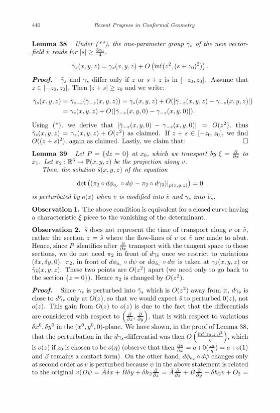
January 17, 2007 11:55 WSPC/Book Trim Size for 9in x 6in finalBB
440 Recent Progress in Conformal Geometry
Lemma 38 Under (**), the one-parameter group γs of the new vector-field v reads for |s| ≥ 3z0
4 .
γs(x, y, z) = γs(x, y, z) + O(inf(z2, (s + z0)2)
).
Proof. γs and γs differ only if z or s + z is in [−z0, z0]. Assume thatz ∈ [−z0, z0]. Then |z + s| ≥ z0 and we write:
γs(x, y, z) = γz+s(γ−z(x, y, z)) = γs(x, y, z) + O(|γ−z(x, y, z) − γ−z(x, y, z)|)= γs(x, y, z) + O(|γ−z(x, y, 0) − γ−z(x, y, 0)|).
Using (*), we derive that |γ−z(x, y, 0) − γ−z(x, y, 0)| = O(z2), thusγs(x, y, z) = γs(x, y, z) + O(z2) as claimed. If z + s ∈ [−z0, z0], we findO((z + s)2), again as claimed. Lastly, we claim that:
Lemma 39 Let P = dz = 0 at x0, which we transport by ξ = ∂∂x to
x1. Let π2 : R3 → P(x, y, z) be the projection along v.Then, the solution s(x, y, z) of the equation
det((π2 dφac dψ − π2 dγs)|p(x,y,z)
)= 0
is perturbated by o(z) when v is modified into v and γs into vs.
Observation 1. The above condition is equivalent for a closed curve havinga characteristic ξ-piece to the vanishing of the determinant.
Observation 2. s does not represent the time of transport along v or v,rather the section z = s where the flow-lines of v or v are made to abut.Hence, since P identifies after ∂
∂x transport with the tangent space to thosesections, we do not need π2 in front of dγs once we restrict to variations(δx, δy, 0). π2, in front of dφac dψ or dφac dψ is taken at γs(x, y, z) orγs(x, y, z). These two points are O(z2) apart (we need only to go back tothe section z = 0). Hence π2 is changed by O(z2).
Proof. Since γs is perturbed into γs which is O(z2) away from it, dγs isclose to dγs only at O(z), so that we would expect s to perturbed 0(z), noto(z). This gain from O(z) to o(z) is due to the fact that the differentialsare considered with respect to
(∂∂x , ∂
∂y
), that is with respect to variations
δx0, δy0 in the (x0, y0, 0)-plane. We have shown, in the proof of Lemma 38,that the perturbation in the dγs-differential was then O
(inf(z0,z0)
2
η
), which
is o(z) if z0 is chosen to be o(η) (observe that then ∂v∂x = a+0( z0
η ) = a+o(1)and β remains a contact form). On the other hand, dφac dψ changes onlyat second order as v is perturbed because ψ in the above statement is relatedto the original v(Dψ = Aδx + Bδy + δh2
∂∂z = A ∂
∂x + B ∂∂y + δh2v + O2 =

January 17, 2007 11:55 WSPC/Book Trim Size for 9in x 6in finalBB
Contact Form Geometry 441
A ∂∂x + B ∂
∂y + δh2v + O2) and dφac is not sensitive to the modification inac. Lemma 2.14 follows.
2.7.8 The characteristic manifold for the perturbed
problem; the determinant equations
As we perturb v to change the sign of dac(v)(x0), we modify the one-parameter group of v. We have estimated this perturbation previously. Wefound that, for s ≥ 2z0
γs(x, y, z) = γs(x, y, z) + Dγz+s(γ−z(x, y, z) − γ−z(x, y, z) + 0(z4).
On the other hand,·
γ−s(x, y, z) − γ−s(x, y, z)
=
X
Y0
= B→
︷ ︸︸ ︷ A00
0 0 0
XY0
− τω(c(z − s) − c)(z − s)
010
.
Thus,
γ−z(x, y, z) − γ−z(x, y, z) = −ezBτω
∫ z
0
e−sB(c(z − s) − c)(z − s)ds
010
= −τω
∫ z
0
esB(c(s) − c)sds
010
.
Since Dx0ψ = Id, the map on the v-side is changed into (observe thatDγz+s = Id in coordinates where v = ∂
∂z ): Set X = (x, y, z)
Γz
(Id +
(A1 λA1
B1 λB1
))(x
y
)− τω
∫ z
0
(c(s) − c)sds
(0
1
)+ O(|X |3)
=
(x + A1(x + λy) − (y + B1(x + λy))z + O(|X |2)
y + B1(x + λy) + (a1(x + A1(x + A1(x + λy)) + b1(x + λy)))z + O(|X |2)
).
On the other side, that is the side of ξ, we have:
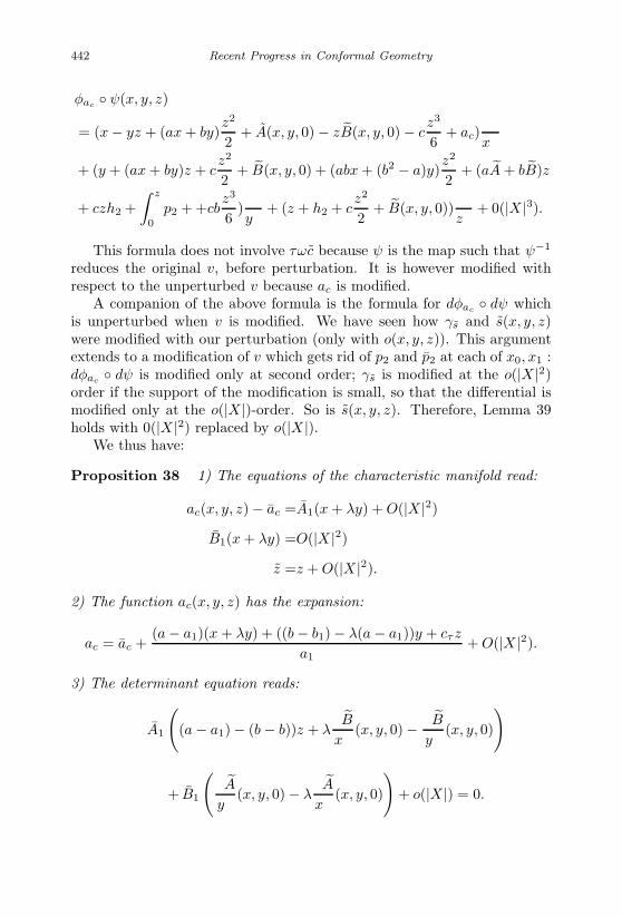
January 17, 2007 11:55 WSPC/Book Trim Size for 9in x 6in finalBB
442 Recent Progress in Conformal Geometry
φac ψ(x, y, z)
= (x − yz + (ax + by)z2
2+ A(x, y, 0) − zB(x, y, 0) − c
z3
6+ ac)
∂
∂x
+ (y + (ax + by)z + cz2
2+ B(x, y, 0) + (abx + (b2 − a)y)
z2
2+ (aA + bB)z
+ czh2 +∫ z
0
p2 + +cbz3
6)
∂
∂y+ (z + h2 + c
z2
2+ B(x, y, 0))
∂
∂z+ 0(|X |3).
This formula does not involve τωc because ψ is the map such that ψ−1
reduces the original v, before perturbation. It is however modified withrespect to the unperturbed v because ac is modified.
A companion of the above formula is the formula for dφac dψ whichis unperturbed when v is modified. We have seen how γs and s(x, y, z)were modified with our perturbation (only with o(x, y, z)). This argumentextends to a modification of v which gets rid of p2 and p2 at each of x0, x1 :dφac dψ is modified only at second order; γs is modified at the o(|X |2)order if the support of the modification is small, so that the differential ismodified only at the o(|X |)-order. So is s(x, y, z). Therefore, Lemma 39holds with 0(|X |2) replaced by o(|X |).
We thus have:
Proposition 38 1) The equations of the characteristic manifold read:
ac(x, y, z) − ac =A1(x + λy) + O(|X |2)B1(x + λy) =O(|X |2)
z =z + O(|X |2).
2) The function ac(x, y, z) has the expansion:
ac = ac +(a − a1)(x + λy) + ((b − b1) − λ(a − a1))y + cτz
a1+ O(|X |2).
3) The determinant equation reads:
A1
((a − a1) − (b − b))z + λ
∂B
∂x(x, y, 0) − ∂B
∂y(x, y, 0)
)
+ B1
(∂A
∂y(x, y, 0) − λ
∂A
∂x(x, y, 0)
)+ o(|X |) = 0.

January 17, 2007 11:55 WSPC/Book Trim Size for 9in x 6in finalBB
Contact Form Geometry 443
Proof. The proof of 3) follows readily from Lemma 34 and our remarksabove. The proof of 2) follows from the definition of ac. Observe that∂∂y , ∂
∂x and ξ = ∂∂x are ξ-transported. For v to come back collinear to itself
in the ξ-transport, we need:
a1(x + s − ac)b1y + ˜p2(x + s − ac, y, z) = ax + by + cτz + p2(x, y, z).
This happens for s = ac(x, y, z) and yields 2) immediately.
The proof of 1) is straightforward using the expansions provided above.We proceed now with the the proof of the theorem.Combining 1) and 2), we derive that:
((b − b1) − λ(a − a1)) y + cτz = O(y2 + z2).
Let A2(x, y, 0), B2(x, y, o) the first terms (of order 2) of A(x, y, 0),B(x, y, 0). After using the fact that x + λy = O(|X |2), the determinantequation yields:
A1 ((b − b1) − λ(a − a1)) z + 2(A1B2(−λ, 1, 0) − B1A2(−λ, 1, 0)
)y
= o(|y| + |z|).We thus have at a critical point:
((b − b1) − λ(a − a1)) y + cτz
= o(|y| + |z|)A1 ((b − b1) − λ(a − a1)) z + 2(A1B2(−λ, 1, 0) − B1A2(−λ, 1, 0)y
= o(|y| + |z|).This yields y = z = 0 if the determinant is far from zero. Since cτ = cwhen we want to rid of p2, p2, we see that such a homotopy will not createnew critical points at infinity. This proves Lemma 28.
The determinant of the above “linear” system is:
∆ = A1 ((b − b1) − λ(a − a1))2 − 2cτ
(A1B2(−λ, 1, 0) − B1A2(−λ, 1, 0)
).
We now claim that:
Lemma 40 x∞ is of index 1 at infinity if and only if
2A1c(A1B2(−λ, 1, 0) − B1A2(−λ, 1, 0)
)< A2
1 ((b − b1) − λ(a1 − a))2 .

January 17, 2007 11:55 WSPC/Book Trim Size for 9in x 6in finalBB
444 Recent Progress in Conformal Geometry
Assuming this lemma, we see that we can modify the sign of c, i.e. introducecτ and keep ∆ away from zero. cτ must satisfy (**) above, i.e.∫ z
0
e−sAs(c(s) − c)ds
(01
)=(
00
)for z0 > 0 and z0 < 0 (∗∗)
with A =(
0 −1a b
).
c, assuming that c is positive, behaves as in the drawing on next page.Clearly, for ε small enough, ∆ will be away from zero on
[−z0,−γ1], [γ1, z0]. On [−γ0, γ0], the statement follows from Lemma 39above. We need now to show that we can choose γ0, γ1, z0 so that (**)holds. We expand (**) at first order i.e. replace e−sA by 1 − sA. Wederive: ∫ z
0
(c − c)s(
1 s−sa 1 − sb
)(01
)ds = O(z4
0)
that is ∫ z0
0
(c − c)s2ds =O(z40)
∫ z0
0
(c − c)s(1 − sb) =O(z40).
Take γ0 = O(e−1/z0). Impose c as above, on the graph, on [−γ0, γ0].The above conditions then reread:

January 17, 2007 11:55 WSPC/Book Trim Size for 9in x 6in finalBB
Contact Form Geometry 445
∫ z0
γ1
(c − c)s2ds = O(z40) (also on [−z0,−γ1])∫ z0
γ1
(c − c)s(1 − sb)ds = O(z40).
Choose γ1 = 12z0. This rereads:
∫ 1
1/2
(c − c)x2dx = O(z0)
∫ 1
1/2
(c − c)xdx = O(z20)
c − c are re-scaled. The above conditions are easy to fulfill with smallperturbations of zero. The argument clearly extends to the full e−sA.
Proof. [Proof of Lemma 40]First, let us observe that, since v = γ
(∂∂z − y ∂
∂x + (ax + by + cz) ∂∂y ,)
where a, b, c are constants (we are looking here at the unperturbed problemafter suppressing p2, p2), we derive from the normalization dα(v, [ξ, v]) =−1 that γ = ± 1√
a.
Assuming γ = 1√a
near x0 (the other case is similar), then since therotation of v along the ξ-piece of x∞ is 1, γ = − 1√
a1near x1. Observe that
[ξ, v](x0) =√
a ∂∂y and [ξ, v](x1) = −√
a1∂∂y .
Using the notations of [Bahri-1 2003], let θ1 be the transport map fromx1 to x0 along v.
Then,
dθ−11 (ξ) − ξ = A1ξ + B1
∂
∂y= A1ξ − B1√
a1[ξ, v](x1).
According to [Bahri-1 2003], the vector-field v generates then an eigenvaluefor J ′′
∞(x∞) equal to A1B1
× ca .(dac(v)(x0) = 1√
a× c
a1
).
Since a is positive (dα(v, [ξ, v]) < 0), this has the sign of A1B1
× c.We use the equation of the characteristic manifold to find the other
eigenvalue. By Proposition 38, along the characteristic manifold:

January 17, 2007 11:55 WSPC/Book Trim Size for 9in x 6in finalBB
446 Recent Progress in Conformal Geometry
ac − a0
= −A(x, y, 0) +A1
B1
(B(x, y, 0) + c
z2
2+ ((b − b1) − λ(a − a1)) yz
)+ O(|X |3) =
(A1
B1B2(−λ, 1, 0) − A2(−λ, 1, 0)
)y2
+A1
B1
(cz2
2+ ((b − b1) − λ(a − a1)) yz
)+ O(|X |3).
On the other hand, a direct expansion shows that:
ac − a0 =∂ac
∂xx +
∂ac
∂yy +
∂ac
∂zz + O(|X |2) = O(|X |2)
(= O(|X |2) by the expansion above).Thus, since x + λy = O(|X |2),
∂ac
∂z(0)z =
(−∂ac
∂y(0) + λ
∂ac
∂x(0))
y + O(|X |2).
By Proposition 38,
∂ac
∂x(0) =
a − a1
a1;
∂ac
∂y=
b − b1
a1;
∂ac
∂z=
c
a1
so that
z =y
c(b1 − b − λ(a1 − a)) + O(y2).
and
ac − a0
=(
A1
B1B2(−λ, 1, 0) − A2(−λ, 1, 0) − A1
2B1c((b1 − b) − λ(a1 − a))2
)y2
+ O(y3).
Since the other eigenvalue is A1B1
× ca with a positive, x∞ is of index 1 if
A1c
(A1B2(−λ, 1, 0) − A2(−λ, 1, 0)B1 − A1
2c((b1 − b) − λ(a1 − a))2
)< 0.
i.e.
2A1c(A1B2(−λ, 1, 0) − B1A2(−λ, 1, 0)
)< A2
1 ((b1 − b) − λ(a1 − a))2 .

January 17, 2007 11:55 WSPC/Book Trim Size for 9in x 6in finalBB
Contact Form Geometry 447
2.7.9 Reduction to the Case k = 1
We show in this section how to reduce the general case to the case of Γ2
with minor changes after a result of Y.Xu about the deformation, usingthe deformation of the Hamiltonians, of the second derivative J ′′
∞(x∞) orx∞ of Γ2k. x∞ is a critical point of J∞ and has k (all) of its ξ- piecescharacteristic.
We need to think of the criticality conditions in a non-standard way sincefor Γ2, they are expressed (see above) in the vanishing of a determinant andthe fact that the ξ-piece is characteristic.
Since here the variations are many more, we cannot expect to have sucha simple situation. We will then need the following definition:
Definition 6 A ξ-piece of an orbit of ξ is characteristic if it transportsthe v-vector onto itself, i.e. Dψa(v(x−)) = θv(x+), here ψa is the one-parameter group of ξ, and a is the length of this ξ-piece.
We then denote ac = akc (x−) the characteristic length, i.e. the length
along ξ of a piece of ξ-orbit starting at x− which is characteristic with arotation kπ for v.
Definition 7 We define the characteristic manifold Ck(x∞) to be themanifold of the curves of Γ2k having all their ξ-pieces characteristic.
It is easy to see that Ck(x∞) is a manifold after a generic assumptionof v [Bahri-2 2003]. Ck(x∞) has codimension k in Γ2k and a complementsubspace to the tangent space at a curve x near x∞ is generated by thevectors v1, · · ·, vk which are defined by transport of v along ξ, along eachξ- piece, from one edge of the ξ piece to the other one ( from x−
i to x+i for
vi).This holds for each curve x of Ck(x∞) such that the differential
daic(v(x−
i )) = 0, for i = 1, · · ·, k.aic is the characteristic length of the point
xi.
Considering a curve x of Γ2k, we may relate to this curve k ξ-lengths,a1, · · ·, ak, and k characteristic lengths a1
c(x−1 ), · · ·, ak
c (x−k ). Accordingly,
δa1, · · ·, δak are the differentials of the ai′s on TxΓ2k and δa1c , · · ·, δak
c arethe differentials of the characteristic lengths ai′
c s on TxΓ2k.
At x∞, we have,
Proposition 39 There exists a constant ci = 0 such that J ′′∞(x∞).vi.z =
ci(δai − δaic)(z) for any zεTx∞Γ2k where δai(z) is the variation along z of
the ith ξ-piece of x∞.
See [Bahri-1 2003], [Bahri-2 2003].
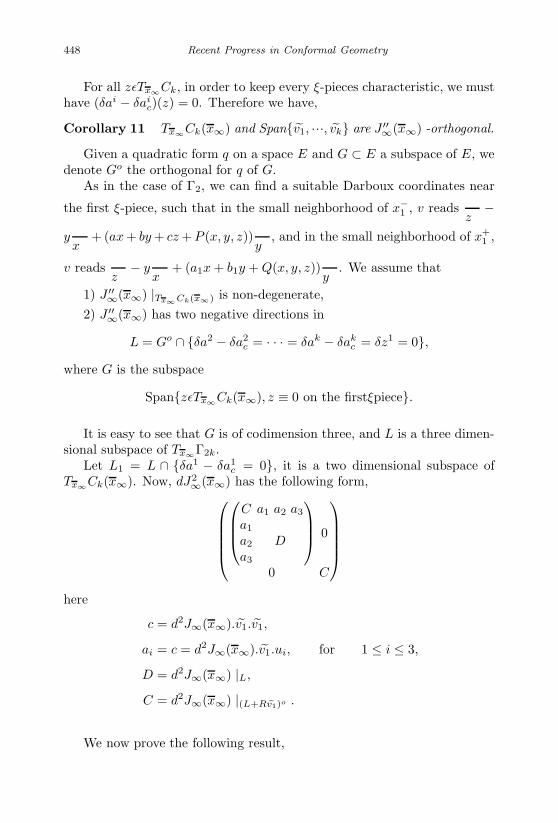
January 17, 2007 11:55 WSPC/Book Trim Size for 9in x 6in finalBB
448 Recent Progress in Conformal Geometry
For all zεTx∞Ck, in order to keep every ξ-pieces characteristic, we musthave (δai − δai
c)(z) = 0. Therefore we have,
Corollary 11 Tx∞Ck(x∞) and Spanv1, ···, vk are J ′′∞(x∞) -orthogonal.
Given a quadratic form q on a space E and G ⊂ E a subspace of E, wedenote Go the orthogonal for q of G.
As in the case of Γ2, we can find a suitable Darboux coordinates near
the first ξ-piece, such that in the small neighborhood of x−1 , v reads
∂
∂z−
y∂
∂x+ (ax + by + cz + P (x, y, z))
∂
∂y, and in the small neighborhood of x+
1 ,
v reads∂
∂z− y
∂
∂x+ (a1x + b1y + Q(x, y, z))
∂
∂y. We assume that
1) J ′′∞(x∞) |Tx∞Ck(x∞) is non-degenerate,2) J ′′
∞(x∞) has two negative directions in
L = Go ∩ δa2 − δa2c = · · · = δak − δak
c = δz1 = 0,where G is the subspace
SpanzεTx∞Ck(x∞), z ≡ 0 on the firstξpiece.
It is easy to see that G is of codimension three, and L is a three dimen-sional subspace of Tx∞Γ2k.
Let L1 = L ∩ δa1 − δa1c = 0, it is a two dimensional subspace of
Tx∞Ck(x∞). Now, dJ2∞(x∞) has the following form,
C a1 a2 a3
a1
a2
a3
D
0
0 C
here
c = d2J∞(x∞).v1.v1,
ai = c = d2J∞(x∞).v1.ui, for 1 ≤ i ≤ 3,
D = d2J∞(x∞) |L,
C = d2J∞(x∞) |(L+Rv1)o .
We now prove the following result,
January 17, 2007 11:55 WSPC/Book Trim Size for 9in x 6in finalBB
Contact Form Geometry 449
Lemma 41 There is a deformation of Lτ , such that either c changes signor D changes index.
Proof. [Proof of Lemma 41] We are going to use the following lemma inthe proof.
Lemma 42 In a suitable fixed connection in Γ2k, and after havingextended v1 to a neighborhood of x∞, for x near x∞, while modifyinga, a1, b, b1 and c of v near x−
1 and x+1 along aτ , a1τ , bτ , b1τ and cτ , we have
d2Jτ∞(x).v1.h = d2J0
∞(x).v1.h + o(|h|),d2Jτ
∞(x).h.k = d2J0∞(x).h.k + o(|h| + |k|)
and d2Jτ∞(x).v1.v1 = cτ + o(1)
for all h, k ∈ Tx∞Ck(x∞) such that dz1(h) = dz1(k) = 0.
The proof the Lemma 42 is deferred to the appendix.
Assume c = d2J∞(x).v1.v1 is positive. We know how to change c ( seethe proof of Γ2). This does not change C. Using Lemma42, a1, a2, a3 and Dchange very little in a neighborhood. The determinant of L is a linear formin c. Either we can decrease c and make it cross zero while detL remainsnon zero, we are done or we cannot do that. But then we can increase c toa very large value without ever crossing the value 0 for detL.
If we change index of C while the total matrix does not degenerate, thenthe upper matrix changes index. Clearly if |c| is large enough with respectto a1,a2, a3, this implies that D changes index.
We will establish the following theorem in Section 2.7.10, which states,
Theorem 4 Under the assumption i∞ ≥ 2, there is a deformation of αand v such that
1) d2Jτ∞(x) does not degenerate.
2) Index of C changes by 2.
A corollary of this theorem is that either we can modify c =d2J∞(x).v1.v1 from positive to negative or we can adjust α and v nearx∞ such that there are two negative directions in
L = Go ∩ δa2 − δa2c = · · · = δak − δak
c = δz1 = 0
since we can create two more positive directions in spanu3, . . . , uk−1.Thus we established Lemma 41.

January 17, 2007 11:55 WSPC/Book Trim Size for 9in x 6in finalBB
450 Recent Progress in Conformal Geometry
Using the notation in the proof of Section 2.7.2 (the case of Γ2), weclaim that,
Lemma 43 a and b of v at x+1 and a1, b1of v at x−
1 can be adjusted sothat there is a negative direction u for J ′′∞(x∞) in the J ′′∞(x∞)-orthogonalof L1 in L.
Proof. [Proof of Lemma 43]A tangent vector on the first ξ piece has at x−
1 components δx1, δy1, δz1
and we denote δx′1 the variation δa + δx′
1 along this vector.
We are asserting that we have two negative directions in
L = Go ∩ δz1 = δa2 − δa2c = · · · = δak − δak
c = 0.
We want to create a negative direction in L ∩ δz1 = δa1 − δa1c = 0.
We work in the sequel in L.On δz1 = 0, δa1 − δa1
c reduces to
δx′1 − δx1 − (
a − a1
a1)δx1 − (
b − b1
a1)δy1 = δx′
1 −a
a1δx1 − (
b − b1
a1)δy1.
δx′1, δx1, δy1 are independent linear forms since δx1, δy1, δa1 are linearly
independent , we have to restrict the value ofa
a1. Thus
a
a1,b − b1
a1are free
to choose in a half plane (see [Bahri-2 2003]), because − a
a1needs to remain
negative if β has to remain a contact form.According to Lemma 42, d2J∞(x).h.k does not change as we change
a, a1, b, b1 if δz1(h) = δz1(k) = 0.Since c1 is so large, d2J∞ does not change sign and x∞ remains isolated.
Actually, the proof of Lemma 42 implies that we do not create any newcritical point at infinity.
Let now
A = dJ2∞(x∞) |δz1=0 in L.
Let P be a generic plane which is negative for A−1. We may assumethat (0, 1, 0) (for (δx1, δy1, δx
′1)) is not in AP . AP has then the equation
aδx1 + cδy1 + bδx′1 = 0 with c = 0.

January 17, 2007 11:55 WSPC/Book Trim Size for 9in x 6in finalBB
Contact Form Geometry 451
Let u in AP be such that δx1(u) < 0, δx′1(u) > 0. Choose u with
δx′1(u) = 1, we set a, a1, b, b1 so that
δx1(u) = − a
a1
δy1(u) = −b − b1
a1
δx′1(u) = 1
then
A−1u ∈ P.
If x is in δz1 = δa1−δa1c = 0, then txA(A−1u) =t xu = δx′
1−a
a1δx1−(
b − b1
a1
)δy1 = 0.
Thus A−1u is d2J∞(x)- orthogonal to δz1 = δa1 − δa1c = 0 in L.
Furthermore,tuA−1AA−1u =t uA−1u < 0, thus A−1u satisfies our purpose.
After this lemma, Tx∞Ck(x∞) reads
G ⊕ L1 ⊕ Ru = G ⊕ L1 ⊕ R(u − J ′′∞(x∞).v1.u
J ′′∞(x∞).v1.v1)v1).
Since L1 and v1 are J ′′∞(x∞)-orthogonal and u − J ′′
∞(x∞).v1.u
J ′′∞(x∞).v1.v1v1 is
independent of v1(δz1(u) = 0) and satisfies δai − δaic = 0 for every i ≥
1, we can pick up a co-dimensional one sub-manifold Ck−1 of Ck(x∞)which is tangent to G ⊕ L1 at x∞. We then have Rv1 ⊕
(k→ →
i=2⊕Rvi
)=
J ′′∞(x∞)oTx∞Ck.
We foliate Ck(x∞) by manifolds Csk−1 with C0
k−1 = Ck−1, here Csk−1
are the co-dimensional 1 sub-manifolds of Ck which are tangent to G ⊕ L1
at some base points xs∞. xs∞, s ∈ (−ε, ε) is a curve tangent to u, withx0∞ = x∞. We prove below that the Cs
k−1’s are basically unchanged alongthe homotopy which we complete.
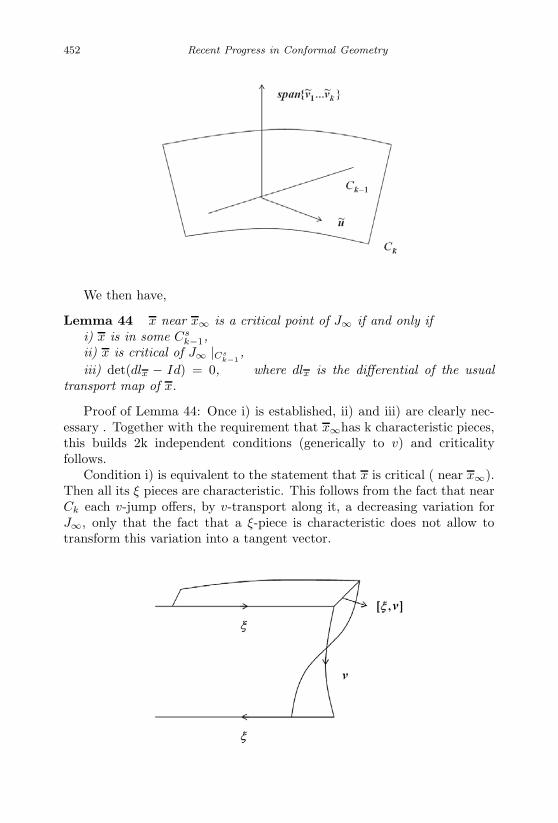
January 17, 2007 11:55 WSPC/Book Trim Size for 9in x 6in finalBB
452 Recent Progress in Conformal Geometry
We then have,
Lemma 44 x near x∞ is a critical point of J∞ if and only ifi) x is in some Cs
k−1,ii) x is critical of J∞ |Cs
k−1,
iii) det(dlx − Id) = 0, where dlx is the differential of the usualtransport map of x.
Proof of Lemma 44: Once i) is established, ii) and iii) are clearly nec-essary . Together with the requirement that x∞has k characteristic pieces,this builds 2k independent conditions (generically to v) and criticalityfollows.
Condition i) is equivalent to the statement that x is critical ( near x∞).Then all its ξ pieces are characteristic. This follows from the fact that nearCk each v-jump offers, by v-transport along it, a decreasing variation forJ∞, only that the fact that a ξ-piece is characteristic does not allow totransform this variation into a tangent vector.

January 17, 2007 11:55 WSPC/Book Trim Size for 9in x 6in finalBB
Contact Form Geometry 453
If ξ is non-characteristic, the variation can be closed and is J∞-decreasing.
Hence, if x is in the neighborhood of Ck and has a non-characteristicξ-piece, it is not critical for J∞. i) follows, as well as ii) and iii) and thelemma.
We now establish that the proof of theorem 2 follows from the proof ofΓ2.
We will think of Spanv1, u as the extension of Tx∞Γ2 and completeour modification of v1 so that,
(i) Spanv1, u=Span v1, uis basically unperturbed.(ii) L1, G and the Cs′
k−1s is basically unperturbed.(iii) The orthogonality relations of Spanv1, u and L1 and the matrix
J ′′∞(x∞) |L1 are unperturbed.
(iv) J ′′∞(x∞) |Spanv1,u does not degenerate.
(v) Along the deformation, J ′′∞(x∞).v1.v1 changes sign.
We think of the whole Poincare-return map as the composition of threemaps, the transport along u, the transport along v1 and the remaining partof the Poincare-return map. According to Lemma 30, the remaining partis basically unperturbed.
Now, dJ2∞(x∞) has the following form,c d
d a0
0 B
with
E1 = Spanv1, uE2 = Tx∞Ck−1 ⊕ Spanv2, . . . , vk ⊂ δz1 = 0.
We also know that
a = dJ2∞(x∞).u.u < 0, c = dJ2
∞(x∞).v1.v1 > 0.
Hence,
ca − d2
< 0.
According to Lemma 41, we have,
Lemma 45 As we change c along cτ , τε[0, 1] from positive to negative,B, a, d do not change.

January 17, 2007 11:55 WSPC/Book Trim Size for 9in x 6in finalBB
454 Recent Progress in Conformal Geometry
Then, the isolation of x∞ reduces to the condition
cτa − d2
< 0
(i.e. does not change sign).This is equivalent to our determinant condition in the case of Γ2 and
the proof are completely parallel. The vanishing of the determinant in thecase of Γ2 being equivalent to ca − d
2= 0. The two are linear forms on cτ
which vanish when the other one vanishes.Obviously, since a is positive, unchanged and ca is negative, we can
change cτ , make it cross zero, using the same construction than the one forΓ2 and never have cτa − d
2= 0.
We now prove that i), ii), iii), iv) and v) stated above hold.iv) and v) are clear. iii) follows from Lemma 31. Along G and L1, δz1
equals 0. The base vectors at x−1 have no component on v(x−
1 ). This alsoholds for u, since u ∈ L. The proof of theorem 6 implies then that theirnatural extension to a neighborhood of x∞ in Γ2k changes very little.
2.7.10 Modification of d2Jτ∞(x∞) |spanu2,···,uk−1
In this section, we will prove Theorem 4, which states as,
Theorem 4 There is a deformation of α and v such that1) d2Jτ
∞(x∞) does not degenerate.2) Index of d2Jτ
∞(x∞) |spanu2,···,uk−1) changes by 2
First we need to describe a basis for the tangent space at x. Given threeconsecutive characteristic ξ-pieces:

January 17, 2007 11:55 WSPC/Book Trim Size for 9in x 6in finalBB
Contact Form Geometry 455
We create a tangent vector at x∞ after picking up at x−1 a vector δs1v,
transporting it a characteristic length to x+1 , then along v from x2 to x3 with
an addition of δs2v, transporting it then a characteristic length again fromx−
2 to x+2 and along v from x+
2 to x−3 , with an addition of δs3v, transporting
it finally a characteristic length from x−3 to x+
3 . Using the freedom of δs2
and δs3, we may arrange so that the vector obtained at x+3 is parallel to v.
The vector will be denoted u2, where 2 is the index of the middle char-acteristic piece. In this way, we build k vectors u1, . . . , uk. It is clearthat ∂2J(x∞).ui.uj is zero when |i − j| > 2.
As in the case of Γ2, we work with Darboux coordinates α = dx + ydz,so we can follow the curves in a small neighborhood of the base curveexplicitly. We will perturb all the ξ−pieces and all the v− pieces, so we canchange ∂2J∞(x∞).ui.ui and ∂2J∞(x∞).ui.ui+1 freely and independently,for 1 ≤ i ≤ k, without changing dai
c(v).After the modification, in a small neighborhood of the ith v-piece, v
becomes (up to a multiplication factor)
∂
∂z+ ω3i(z)ω4i(x, y)(h1ix
2 + l1ixy)∂
∂x+ ω3i(z)ω4i(x, y)(h2ix
2 + l2ixy)∂
∂y.
Integrating along the v-pieces, the modification occurs only at the sec-ond order and higher. Here, ω3i(z) and ω4i(x, y) are the cut-off functionsin a small neighborhood of the v-pieces.
And α on the ith ξ−piece becomes λα, where1λ
= 1 +
ω1i(x)ω2i(y, z)diy2z, here, ω1i(x) and ω2i(y, z) are the cut-off functions in
a small neighborhood of the ξ−pieces. The corresponding Reeb vector fieldbecomes
ξ =1λ
(∂
∂x+
λz − yλx
λ2
∂
∂y− λy
λ2
(∂
∂z− y
∂
∂x
)).
We will prove,
Lemma 46 Using the perturbation we described above, we can modify thesecond derivatives
∂2J∞(x∞).ui.ui, ∂2J∞(x∞).ui.ui+1
for 1 ≤ i ≤ k freely and independently, i.e. we can prescribe any set of 2kreal values for
∂2J∞(x∞).ui.ui, ∂2J∞(x∞).ui.ui+1, 1 ≤ i ≤ k.

January 17, 2007 11:55 WSPC/Book Trim Size for 9in x 6in finalBB
456 Recent Progress in Conformal Geometry
A corollary of Lemma 46 is,
Corollary 12 With a C1-small, and C2-bounded modification, we canchange the index of J ′′∞(x∞) |G by 2 while keeping J ′′∞(x∞) |TCk(x∞) non-degenerate.
Proof of Corollary 12: We reorder A so that the first coefficient is uk becausethe supplement of G in the space Spanui is Spanu1, u2, uk. A reads
∂2J∞(x∞).uk.uk · · 0 0 · ∂2J∞(x∞).uk.uk−1
∂2J∞(x∞).u1.uk · · · 0 0 ∂2J∞(x∞).u1.uk−1
∂2J∞(x∞).u2.uk · · · · 0 00 · · · · · 00 0 · · · · ·
∂2J∞(x∞).u1.uk−1 0 0 · · · ∂2J∞(x∞).uk−2.uk−1
∂2J∞(x∞).uk−1.uk · 0 0 · · ∂2J∞(x∞).uk−1.uk−1
.
If we look at the matrix A, it has on each line 5 non zero terms at most.For all lines besides the first two ones and the two last ones, these termsare the diagonal term and the two next terms on each side. For the firstline, we have the diagonal, two terms on the immediate right and two otherterms on the extreme right of the matrix. For the second line, we have fourterms, one to the left of the diagonal, two to the immediate right and oneat the extreme right. The situation is similar but with right replaced by leftfor the two last lines. Our lemma above establishes that the diagonal of Aand the two next “diagonals” on the right and on the left are made of freeparameters which we can choose as we please. The next two diagonals onthe right and on the left are untouched through these changes. The extremetop coefficients on the right and its symmetric on the left are free to choose.The two remaining coefficients are untouched through these changes.
detA is linear in the diagonal terms. We can therefore send the diagonalcoefficients to +∞ or −∞ so that detA is never zero. The other terms areuntouched. Now A has a very large diagonal, all other terms are bounded.Let us take the other coefficients which are free to choose and make themvery large (still small with respect to the absolute value of the diagonalterms).
Setting the untouched coefficients to be zero, including the top rightand the bottom left coefficients, we derive a matrix A0 whose coefficientsare totally free to choose. A0 reads
January 17, 2007 11:55 WSPC/Book Trim Size for 9in x 6in finalBB
Contact Form Geometry 457
· · 0 0 0 0 ·· · · 0 0 0 00 · · · 0 0 00 0 · · · 0 00 0 0 · · · 00 0 0 0 · · ·· 0 0 0 0 · ·
.
In this form our claim becomes a simple algebraic statement involvingpathes and connectedness of the set of non degenerate matrices of the abovetype as long as they have the same index. We do not include the proof here.
Now we proceed with the proof of Lemma 46. Since the proof is somehowlong and technical, we will only outline the main steps here and leave thedetails in the appendix.
First, let us look at what happens if we modify only the third ξ-piece andthe second v-piece, the result extends to the general case. For the sake ofsimplicity, we drop the subscript i in the proof. After the modification, in asmall neighborhood of the second v-piece, v becomes (up to a multiplicationfactor)
∂
∂z+ ω3(z)ω4(x, y)(h1x
2 + l1xy)∂
∂x+ ω3(z)ω4(x, y)(h2x
2 + l2xy)∂
∂y.
Here, ω3(z) and ω4(x, y) are the cut-off functions in a small neighborhoodof the second v-piece.
And α on the third ξ−piece becomes λα, where
1λ
= 1 + ω1(x)ω2(y, z)dy2z.
Here, ω1(x) and ω2(y, z) are the cut-off functions in a small neighborhoodof the third ξ-piece.
Let v be the new vector field introduced. We build a function ψ usingthe orbits of v such that
dψ(v) = −α(v).
Setting then
α = α − dψ,
we find
α(v) = 0.
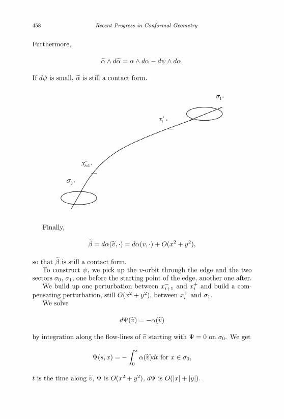
January 17, 2007 11:55 WSPC/Book Trim Size for 9in x 6in finalBB
458 Recent Progress in Conformal Geometry
Furthermore,
α ∧ dα = α ∧ dα − dψ ∧ dα.
If dψ is small, α is still a contact form.
Finally,
β = dα(v, ·) = dα(v, ·) + O(x2 + y2),
so that β is still a contact form.To construct ψ, we pick up the v-orbit through the edge and the two
sectors σ0, σ1, one before the starting point of the edge, another one after.We build up one perturbation between x−
i+1 and x+i and build a com-
pensating perturbation, still O(x2 + y2), between x+i and σ1.
We solve
dΨ(v) = −α(v)
by integration along the flow-lines of v starting with Ψ = 0 on σ0. We get
Ψ(s, x) = −∫ s
0
α(v)dt for x ∈ σ0,
t is the time along v, Ψ is O(x2 + y2), dΨ is O(|x| + |y|).

January 17, 2007 11:55 WSPC/Book Trim Size for 9in x 6in finalBB
Contact Form Geometry 459
Following the notation in the case of Γ2, in a small neighborhood of
point x+i , the v−vector after re-normalization reads
∂
∂z− y
∂
∂x+ (a+
i x +
b+i y + Qi(x, y, z))
∂
∂y, and in the small neighborhood of x−
i , the v− vector
after re-normalization reads∂
∂z− y
∂
∂x+ (a−
i x + b−i y + cz + Pi(x, y, z))∂
∂y.
As we modify the third ξ-piece, δa3c changes. For the sake of simplicity,
we omit the superscript below. We will need the following lemma:
Lemma 47 After performing the modification on the third ξ-piece, δac
becomes
δac =(a−
3 − a+3 )x0 + (b−3 − b+
3 )y0 + c3z0 − a2dy0
a+3
− (a−3 − a+
3 )x0 + (b−3 − b+3 )y0 + c3z0 − a2dy0
a+3
· 2dy0 + Q2,x(x0,y0, z0)a+3
+ P 32 (x0, y0, z0) − Q3
2(x0, y0, z0) + ab+3 2dy0z0
− a2dz0(a−3 x0 + b−3 y0 + c3z0) − a22dz0(a−
3 x0 + b−3 y0 + c3z0)/a+3 .
Here, the first line is the first order terms, and the rest are the secondorder terms.
The proof of Lemma 47 is deferred to the Appendix.
We proceed with the calculation of ∂2J∞(x∞).u2.u2, ∂2J∞(x∞).u2.u3,∂2J∞(x∞).u2.u4 now.
2.7.11 Calculation of ∂2J∞(x∞).u2.u3
First let us focus on the u3-piece, the bottom variation. We start at x1
with a small variation δs1 along v, we transport this small variation alongthe second ξ-piece a characteristic length to x2. From x2 we transport italong the second v-piece to x3, then from x3 with a small variation δs2
along v, we transport it along the third ξ-piece a characteristic length tox4. From x4 we transport it along the third v-piece to x5, then from x5
with a small variation δs3 along v, we transport it along the fourth ξ-piecea characteristic length to x6 . The z-coordinates of the 1st, 2nd and 3rdξ−piece of u2 are respectively δs1, δs2, δs3. δs1 and δs3 are constant alongthe first and third ξ-pieces of u2. Because the third ξ−piece is perturbed,

January 17, 2007 11:55 WSPC/Book Trim Size for 9in x 6in finalBB
460 Recent Progress in Conformal Geometry
δs2 varies at the second order (refer to Lemma 47) along this piece, but itstays the same at x∞. We have:
Lemma 48 δs1, δs2, δs3 satisfy the following relation,
δs2 = p2δs1 + O(δs2
1
), δs3 = q2δs1 + O
(δs2
1
)where
p2 = − c2
a+2
a+3
c3(a−3 B1 + (∆b3 − 2da)B2
a+3
+B2
C2C4),
q2 =c2
a+2
a−4
c4
B2
C2detC
and A =(
A1 A3
A2 A4
), B =
(B1 B3
B2 B4
)and C =
(C1 C3
C2 C4
)
are respectively the transport matrices of the 1st, 2nd, and 3rd v-pieces.
The proof of this lemma is deferred to the Appendix.On top of u3, now we construct u2(u3), assume that the z-coordinates of
the 1st, 2nd and 3rd ξ−pieces of u2(u2) are respectively δs1, δs2 + δs1andδs2 + δs3. We start at x7 with a small variation δs1 along v, then wetransport this small variation along the third ξ-piece a characteristic lengthto x0. From x0 we transport along the first v-piece to x′
1, then from x′1
with a small variation δs1 + δs2 along v, we transport it along the secondξ-piece a characteristic length to x′
2. From x′2 we transport it along the
second v-piece to x′3, then from x′
3 with a small variation δs2 + δs3 alongv, we transport it along the third ξ-piece a characteristic length to x′
4.
Lemma 49 The x, y coordinates of point x′4 reads
( − c2
a+2
B2
C2C4δs1 − c2
a+2
B2δs1δs3
c2
a+2
B2δs1 +c2
a+2
(b+3 B2 − a+
3
B2
C2C4)δs1δs3
)+Uδs2
1+V δs12+O(δs3
1+δs13),
here U and and V are constants which we will not track.
The proof of Lemma 49 is in the Appendix.

January 17, 2007 11:55 WSPC/Book Trim Size for 9in x 6in finalBB
Contact Form Geometry 461
Assume
δs2 = pδs1 + Rδs1δs1 + Uδs12
+ V δs21 + O(δs1
3+ δs3
1),
δs3 = qδs1 + Tδs1δs1 + U1δs12
+ V1δs21 + O(δs1
3+ δs3
1).
Here, we will track only R and T , and we will not track U , V , U1 and V1.
First, we track only first order terms along u2(u3) , we get
Lemma 50 δs1, δs2 and δs3 satisfy the following relation at the firstorder,
δs2 = p1δs1 + O(δs2
1, δs12, δs1δs1
),
δs3 = q1δs1 + O(δs2
1, δs12, δs1δs1
),
where
p1 = − c1
a+1
· a+2
c2·(
a−2 A1 + ∆b2A2
a+3
+A2
B2B4
),
q1 =c1
a+1
a−3
c3
A2
B2detB.
Hence we know how u3 and u2(u3) constitute at the first order.The proof of the Lemma 50 is in the Appendix.
January 17, 2007 11:55 WSPC/Book Trim Size for 9in x 6in finalBB
462 Recent Progress in Conformal Geometry
Let us look at
J(x∞ + δs1u2(u3) + δs1u3) − J(x∞ + δs1u3)
= δs1∂J(x∞ + δs1u3).u2(u3) + O(δs12)
= δs1δs1∂2J(x∞).u2.u3 + O(δs2
1, δs12) .
Since x∞ is critical, ∂J(x∞).(·) is 0. If we take δs1 very small comparedwith δs1, then we can ignore the δs2
1 terms. Similarly if we take δs1 verysmall compared with δs1, then we can ignore the δs1
2terms. Since our aim
is to compute ∂2J.u2.u3 we need only to concentrate on the δs1δs1 terms,so from now on in all our computation, we keep only the δs1δs1 terms, anddrop the δs2
1, δs12
terms and terms with order higher than 2.
Claim 1 Along u2(u3), the transport matrix in x, y- coordinates alongthe first v-piece is(
Id + (δs2 + δs1)(
0 − 1a−2 b−2
))A
(Id − δs1
(0 − 1a+1 b+
1
))· x0
+(
0c2
)δs2δs1 + O
(δs2
1, δs12)
+ O3.
As before, the proof of the claim is deferred to the Appendix.Therefore we can write the x, y-coordinates of x′
1 as(Id + (δs2 + δs1)
(0 − 1
a−2 b−2
))A
(Id − δs1
(0 − 1
a+1 b+
1
))( c1
a+1
0
)δs1+
(0
c2
)δs2δs1
= A
( c1
a+1
0
)δs1 +
(0 − 1
a−2 b−2
)A
( c1
a+1
0
)δs1δs1 +
(0
c2p1
)δs1δs1.
So the x, y-coordinates of x′2 read
(a−2
a+2
∆b2
a+2
0 1
)· x′
1 +( c2
a+2
0
)(δs2 + δs1) +
(N2
0
)
=(a−
2
a+2
∆b2
a+2
0 1
)A
( c1
a+1
0
)δs1 +
( c2
a+2
0
)(δs1 + p1δs1) + R
( c2
a+2
0
)δs1δs1
+(a−
2
a+2
∆b2
a+2
0 1
)(0 − 1a−2 b−2
)A
( c1
a+1
0
)+(
0c2p1
) δs1δs1 +(
N2
0
)

January 17, 2007 11:55 WSPC/Book Trim Size for 9in x 6in finalBB
Contact Form Geometry 463
here N2 is the second order term of dac(x′1).
Claim 2 The transport matrix along the second v- piece is(Id + (δs3 + δs2)
(0 − 1a−3 b−3
))B
(Id − (δs2 + δs1)
(0 − 1a+2 b+
2
))· x′
2
+(
0c3
)δs3δs2 + Uδs2
1 + V δs12+ O(δs3
1 + δs13).
Here, the values of U and V has changed. However, we will not trackthese values. The proof of Claim 2 is similar with the proof of the Claim 1,so we omit it here.
The first order term of x′2 is
(a−2
a+2
∆b2
a+2
0 1
)· point1′ +
( c2
a+2
0
)(δs2 + δs1)
=c1
a+1
(−A2
B2B4
A2
)δs1 +
( c2
a+2
0
)δs1.
Integrating along the second v−piece, we geth1(− c1
a+1
A2
B2B4δs1 +
c2
a+2
δs1)2 + l1(− c1
a+1
A2
B2B4δs1 +
c2
a+2
δs1)c1
a+1
A2δs1
h2(− c1
a+1
A2
B2B4δs1 +
c2
a+2
δs1)2 + l2(− c1
a+1
A2
B2B4δs1 +
c2
a+2
δs1)c1
a+1
A2δs1
=c1
a+1
c2
a+2
A2
−2h1B4
B2+ l1
−2h2B4
B2+ l2
δs1δs1 + O(δs21, δs1
2).
We are able to write the crossing terms of x′3 now.
Thus x′3 can be written as(
Id + (δs3 + δs2)(
0 − 1a−3 b−3
))B
(Id − (δs2 + δs1)
(0 −1
a+2 b+
2
))· x′
2
+(
0c3
)δs3δs2 + O(δs2
1, δs12) +
c1
a+1
c2
a+2
A2
−2h1B4
B2+ l1
−2h2B4
B2+ l2
δs1δs1 + O3.

January 17, 2007 11:55 WSPC/Book Trim Size for 9in x 6in finalBB
464 Recent Progress in Conformal Geometry
Then we transport it along third ξ-piece, we are able then to get anexpression of x′
4. Comparing the crossing terms, i.e. δs1δs1 terms of pointx′
4 with the expression in Lemma 49, we get
Claim 3 R satisfies the following relation,
− c1
a+1
A2B2
(a−2 − a+
2
a+2
+∆b2
a+2
(a+2
B4
B2− b+
2
))− c3p2q1 − c2p1B4
−2dac2
a+2
q1B2 +c2
a+2
RB2 + NB2 +c1
a+1
c2
a+2
A2
(−2h2
B4
B2+ l2
)= 0.
We leave the details of the proof of this claim in the Appendix.It is clear that there is no δs1δs1 term which is contributed by the
first and the fourth ξ−pieces. So in order to calculate the δs1δs1 terms inJ∞(x∞ + δs1u1(u2)+ δs1u2)−J∞(x∞ + δs1u2), we need only to count theδs1δs1 terms contributed by the second and the third ξ-pieces.
For the second ξ−piece, the δs1δs1 terms come from three sources. Sinceδs2 = p1δs1 + Rδs1δs1, so R is one of the sources. Also the second orderterms of dac(x′
1) , N2 contributes δs1δs1 terms, and all the other δs1δs1
terms come from the v-transport.For the third ξ-piece, the δs1δs1 terms also come from three sources.
Since δs3 = q1δs1 + Tδs1δs1, so T is one of the sources. Also the secondorder terms of dac(x′
3) N3 contributes δs1δs1 terms, and all the other δs1δs1
terms come from the v-transport.Summing them up, we get,
∂2J∞(x∞).u2.u3 = q1a−3 B1 + (∆b3−4dac)B2 + a+
3
B2
C2C4︸ ︷︷ ︸
(I)
+ c2p1B4
B2− c2p1
det B
B2c2p1
detB
B2︸ ︷︷ ︸(II)
+c1
a+1
c2
a+2
A2((2h1B1
B2− 2h2)
B4
B2+ l2 − l1)︸ ︷︷ ︸
(III)
.
(I) involves the perturbation parameter d.
(II) involves no perturbation parameter, since p1 = − c1
a+1
· a+2
c2·(
a−2 A1 + ∆b2A2
a+3
+A2
B2B4
)involves no perturbation parameter.
And since (III) involves parameters h1, l1.h2, l2 , we know∂2J∞(x∞).u1.u2 involves perturbation parameters h1, l1.h2, l2 and d. As wemodify the contact form, we can change it freely without changing dac(v).
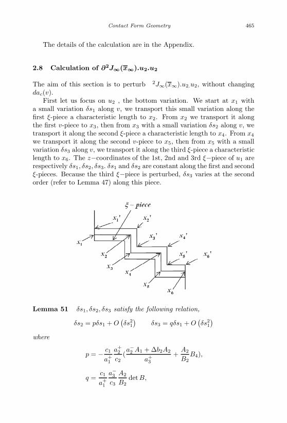
January 17, 2007 11:55 WSPC/Book Trim Size for 9in x 6in finalBB
Contact Form Geometry 465
The details of the calculation are in the Appendix.
2.8 Calculation of ∂2J∞(x∞).u2.u2
The aim of this section is to perturb ∂2J∞(x∞).u2.u2, without changingdac(v).
First let us focus on u2 , the bottom variation. We start at x1 witha small variation δs1 along v, we transport this small variation along thefirst ξ-piece a characteristic length to x2. From x2 we transport it alongthe first v-piece to x3, then from x3 with a small variation δs2 along v, wetransport it along the second ξ-piece a characteristic length to x4. From x4
we transport it along the second v-piece to x5, then from x5 with a smallvariation δs3 along v, we transport it along the third ξ-piece a characteristiclength to x6. The z−coordinates of the 1st, 2nd and 3rd ξ−piece of u1 arerespectively δs1, δs2, δs3. δs1 and δs2 are constant along the first and secondξ-pieces. Because the third ξ−piece is perturbed, δs3 varies at the secondorder (refer to Lemma 47) along this piece.
Lemma 51 δs1, δs2, δs3 satisfy the following relation,
δs2 = pδs1 + O(δs2
1
)δs3 = qδs1 + O
(δs2
1
)where
p = − c1
a+1
a+2
c2(a−2 A1 + ∆b2A2
a+3
+A2
B2B4),
q =c1
a+1
a−3
c3
A2
B2detB,

January 17, 2007 11:55 WSPC/Book Trim Size for 9in x 6in finalBB
466 Recent Progress in Conformal Geometry
and
A =(
A1 A3
A2 A4
), B =
(B1 B3
B2 B4
)are the transport matrices of the 1st and 2nd v−pieces.
The proof of this lemma is similar to the proof of Lemma 48, so we omitit here.
Lemma 52 The x, y coordinates of x′6 reads
(00
)+Uδs2
1+V δs12+O(δs3
1+
δs13), and the z coordinate is δs3 + δs3, here U and V are constants which
we will not track.
The proof is similar with the proof of Lemma 49 which we defer to theAppendix.
Now on top of u2, we construct u2(u2). We start at x1 with a smallvariation δs1 + δs1 along v, we transport this small variation along thefirst ξ-piece a characteristic length to x2. From x2 we transport it alongthe first v-piece to x3, then from x3 with a small variation δs2 + δs2 alongv, we transport it along the second ξ-piece a characteristic length to x4.From x4 we transport it along the second v-piece to x5, then from x5 witha small variation δs3 + δs3 along v, we transport it along the third ξ-piecea characteristic length to x6. The z−coordinates of the 1st, 2nd and 3rdξ−pieces of u1(u2) are respectively δs1 + δs1 , δs2 + δs2 and δs3 + δs3 ,
since v has a constant component equal to 1 on∂
∂z. As before, first we
concentrate only on the first order terms, then we go to the δs1δs1 terms.Considering only the first order terms, we get:
Lemma 53 δs1, δs2 and δs3 satisfy the following relation at the firstorder,
δs2 = pδs1 + O(δs2
1, δs12, δs1δs1
),
δs3 = qδs1 + O(δs2
1, δs12, δs1δs1
),
where
p = − c1
a+1
a+2
c2
(a−2 A1 + ∆b2A2
a+2
+A2
B2B4
),
q =c1
a+1
a−3
c3
A2
B2detB.
January 17, 2007 11:55 WSPC/Book Trim Size for 9in x 6in finalBB
Contact Form Geometry 467
The proof of this lemma is along the same line with the proof ofLemma 50, we defer it to the Appendix.
As before, since our goal is to compute ∂2J∞(x∞).u2.u2, we need onlyto concentrate on the δs1δs1 terms, so from now on in all our computation,we keep only the δs1δs1 terms, and drop the δs2
1, δs12
terms and terms withorder higher than 2.
Assume
δs2 = pδs1 + Rδs1δs1 + Uδs12
+ V δs21 + O(δs1
3+ δs3
1),
δs3 = qδs1 + Tδs1δs1 + U1δs12
+ V1δs21 + O(δs1
3+ δs3
1).
Now let us track the δs1δs1 terms along u1(u1).
Claim 4 x′1 reads
0cδs1δs1
δs1 + δs1
+ V δs21 + O(δs1
3+ δs3
1)
The proof is deferred to the Appendix.
x′2 reads
( c1
a+10
)(δs1 + δs1) +
a−1
a+1
b−1 − b+1
a+1
01
( 0c1
)δs1δs1 +
(N1
0
)δs1 + δs1
,
where N1 is the second order term of ac(x′1) − ac(x
′2).
As in Section 2.7.11, we can prove that the transport matrix for x, y−coordinates along the first v-piece is(
Id + (δs2 + δs2)(
0 −1a−2 b−2
))A
(Id − (δs1 + δs1)
(0 −1
a+1 b+
1
))· x′
2
+(
0c2
)δs2δs2 + Uδs1
2+ V δs2
1 + O(δs13
+ δs31),
here U and V are changed than before, which we will not track exactly.
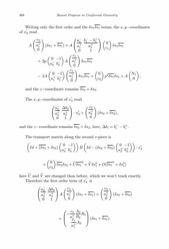
January 17, 2007 11:55 WSPC/Book Trim Size for 9in x 6in finalBB
468 Recent Progress in Conformal Geometry
Writing only the first order and the δs1δs1 terms, the x, y−coordinatesof x
′3 read
A
( c1
a+10
)(δs1 + δs1) + A
a−1
a+1
b−1 − b+1
a+1
0 1
( 0c1
)δs1δs1
+ 2p
(0 −1
a−2 b−2
)A
( c1
a+10
)δs1δs1
− 2A
(0 −1
a+1 b+
1
)( c1
a+10
)δs1δs1 +
(0c2
)p2δs1δs1 + A
(N1
0
),
and the z−coordinate remains δs2 + δs2.
The x, y−coordinates of x′4 reada−
2
a+2
∆b2
a+2
0 1
· x′3 +
( c2
a+20
)(δs2 + δs2),
and the z−coordinate remains δs2 + δs2, here, ∆bi = b−i − b+i .
The transport matrix along the second v-piece is(Id + (δs3 + δs3)
(0 −1
a−3 b−3
))B
(Id − (δs2 + δs2)
(0 −1
a+2 b+
2
))· x′
4
+(
0c3
)δs3δs3 + Uδs1
2+ V δs2
1 + O(δs13
+ δs31)
here U and V are changed than before, which we won’t track exactly.Therefore the first order term of x
′4 isa−
2
a+2
∆b2
a+2
0 1
A
( c1
a+10
)(δs1 + δs1) +
( c2
a+20
)(δs2 + δs2)
=
− c1
a+1
A2
B2B4
c1
a+1
A2
(δs1 + δs1).
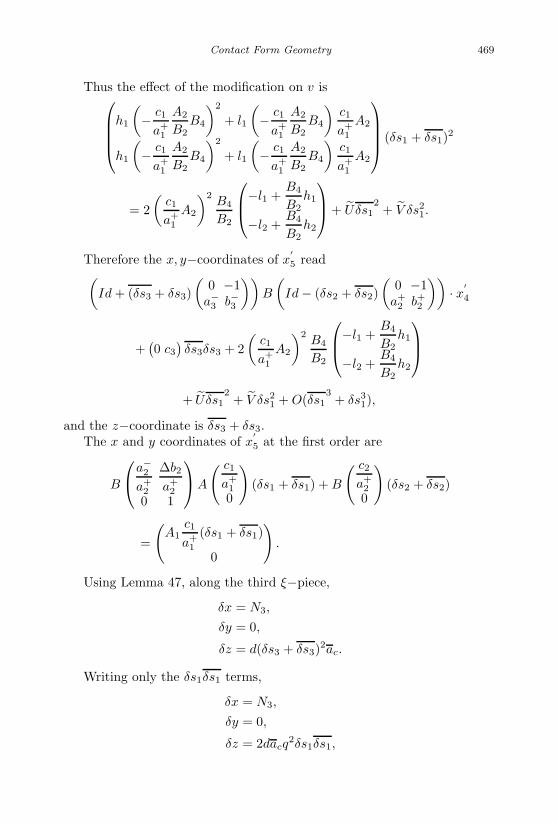
January 17, 2007 11:55 WSPC/Book Trim Size for 9in x 6in finalBB
Contact Form Geometry 469
Thus the effect of the modification on v ish1
(− c1
a+1
A2
B2B4
)2
+ l1
(− c1
a+1
A2
B2B4
)c1
a+1
A2
h1
(− c1
a+1
A2
B2B4
)2
+ l1
(− c1
a+1
A2
B2B4
)c1
a+1
A2
(δs1 + δs1)2
= 2(
c1
a+1
A2
)2B4
B2
−l1 +B4
B2h1
−l2 +B4
B2h2
+ Uδs12
+ V δs21.
Therefore the x, y−coordinates of x′5 read(
Id + (δs3 + δs3)(
0 −1a−3 b−3
))B
(Id − (δs2 + δs2)
(0 −1
a+2 b+
2
))· x′
4
+(0 c3
)δs3δs3 + 2
(c1
a+1
A2
)2B4
B2
−l1 +B4
B2h1
−l2 +B4
B2h2
+ Uδs1
2+ V δs2
1 + O(δs13+ δs3
1),
and the z−coordinate is δs3 + δs3.The x and y coordinates of x
′5 at the first order are
B
a−2
a+2
∆b2
a+2
0 1
A
( c1
a+10
)(δs1 + δs1) + B
( c2
a+20
)(δs2 + δs2)
=
(A1
c1
a+1
(δs1 + δs1)
0
).
Using Lemma 47, along the third ξ−piece,
δx = N3,
δy = 0,
δz = d(δs3 + δs3)2ac.
Writing only the δs1δs1 terms,
δx = N3,
δy = 0,
δz = 2dacq2δs1δs1,
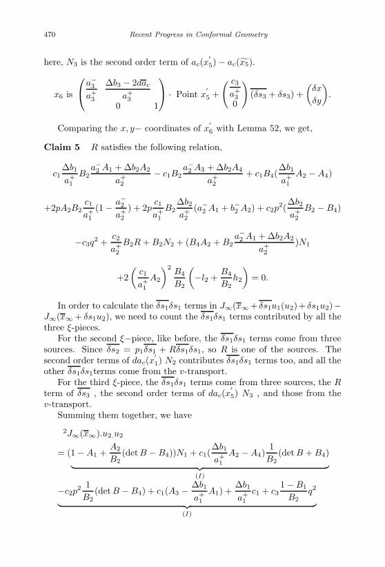
January 17, 2007 11:55 WSPC/Book Trim Size for 9in x 6in finalBB
470 Recent Progress in Conformal Geometry
here, N3 is the second order term of ac(x′5) − ac(x5).
x6 is
a−3
a+3
∆b3 − 2dac
a+3
0 1
· Point x′5 +
( c3
a+30
)(δs3 + δs3) +
(δx
δy
).
Comparing the x, y− coordinates of x′6 with Lemma 52, we get,
Claim 5 R satisfies the following relation,
c1∆b1
a+1
B2a−2 A1 + ∆b2A2
a+2
− c1B2a−2 A3 + ∆b2A4
a+2
+ c1B4(∆b1
a+1
A2 − A4)
+2pA2B2c1
a+1
(1 − a−2
a+2
) + 2pc1
a+1
B2∆b2
a+2
(a−2 A1 + b−2 A2) + c2p
2(∆b2
a+2
B2 − B4)
−c3q2 +
c2
a+2
B2R + B2N2 + (B4A2 + B2a−2 A1 + ∆b2A2
a+2
)N1
+2(
c1
a+1
A2
)2B4
B2
(−l2 +
B4
B2h2
)= 0.
In order to calculate the δs1δs1 terms in J∞(x∞ + δs1u1(u2)+ δs1u2)−J∞(x∞ + δs1u2), we need to count the δs1δs1 terms contributed by all thethree ξ-pieces.
For the second ξ−piece, like before, the δs1δs1 terms come from threesources. Since δs2 = p1δs1 + Rδs1δs1, so R is one of the sources. Thesecond order terms of dac(x
′1) N2 contributes δs1δs1 terms too, and all the
other δs1δs1terms come from the v-transport.For the third ξ-piece, the δs1δs1 terms come from three sources, the R
term of δs3 , the second order terms of dac(x′5) N3 , and those from the
v-transport.Summing them together, we have
∂2J∞(x∞).u2.u2
= (1 − A1 +A2
B2(detB − B4))N1 + c1(
∆b1
a+1
A2 − A4)1
B2(det B + B4)︸ ︷︷ ︸
(I)
−c2p2 1B2
(det B − B4) + c1(A3 − ∆b1
a+1
A1) +∆b1
a+1
c1 + c31 − B1
B2q2︸ ︷︷ ︸
(I)
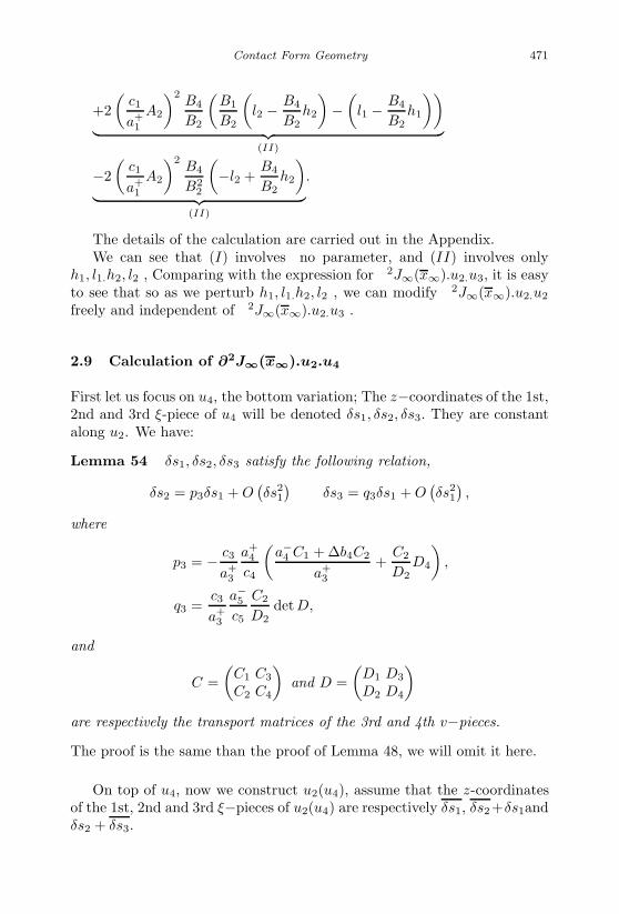
January 17, 2007 11:55 WSPC/Book Trim Size for 9in x 6in finalBB
Contact Form Geometry 471
+2(
c1
a+1
A2
)2B4
B2
(B1
B2
(l2 − B4
B2h2
)−(
l1 − B4
B2h1
))︸ ︷︷ ︸
(II)
−2(
c1
a+1
A2
)2B4
B22
(−l2 +
B4
B2h2
)︸ ︷︷ ︸
(II)
.
The details of the calculation are carried out in the Appendix.We can see that (I) involves no parameter, and (II) involves only
h1, l1.h2, l2 , Comparing with the expression for ∂2J∞(x∞).u2.u3, it is easyto see that so as we perturb h1, l1.h2, l2 , we can modify ∂2J∞(x∞).u2.u2
freely and independent of ∂2J∞(x∞).u2.u3 .
2.9 Calculation of ∂2J∞(x∞).u2.u4
First let us focus on u4, the bottom variation; The z−coordinates of the 1st,2nd and 3rd ξ-piece of u4 will be denoted δs1, δs2, δs3. They are constantalong u2. We have:
Lemma 54 δs1, δs2, δs3 satisfy the following relation,
δs2 = p3δs1 + O(δs2
1
)δs3 = q3δs1 + O
(δs2
1
),
where
p3 = − c3
a+3
a+4
c4
(a−4 C1 + ∆b4C2
a+3
+C2
D2D4
),
q3 =c3
a+3
a−5
c5
C2
D2detD,
and
C =(
C1 C3
C2 C4
)and D =
(D1 D3
D2 D4
)are respectively the transport matrices of the 3rd and 4th v−pieces.
The proof is the same than the proof of Lemma 48, we will omit it here.
On top of u4, now we construct u2(u4), assume that the z-coordinatesof the 1st, 2nd and 3rd ξ−pieces of u2(u4) are respectively δs1, δs2+δs1andδs2 + δs3.

January 17, 2007 11:55 WSPC/Book Trim Size for 9in x 6in finalBB
472 Recent Progress in Conformal Geometry
Lemma 55 The x, y coordinates of x6 read c3
a+3
δs1
c3δs1δs3
+ Uδs21 + V δs2
1 + O(δs31 + δs1
3),
here U and and V are constants which we will not track.
The proof is similar with Lemma 49Assume
δs2 = pδs1 + Rδs1δs1 + Uδs12
+ V δs21 + O(δs1
3+ δs3
1),
δs3 = qδs1 + Tδs1δs1 + U1δs12
+ V1δs21 + O(δs1
3+ δs3
1).
Here, we will track only R and T , and we will not track U , V , U1 and V1.
First, we track only the first order terms along u2(u4); we find:
Lemma 56 δs1, δs2 and δs3 satisfy the following relation at the firstorder,
δs2 = p1δs1 + O(δs2
1, δs12, δs1δs1
),
δs3 = q1δs1 + O(δs2
1, δs12, δs1δs1
),

January 17, 2007 11:55 WSPC/Book Trim Size for 9in x 6in finalBB
Contact Form Geometry 473
where
p1 = − c1
a+1
· a+2
c2·(
a−2 A1 + ∆b2A2
a+3
+A2
B2B4
),
q1 =c1
a+1
a−3
c3
A2
B2detB.
Hence we know how u4 and u2(u4) are built at the first order.As before, since our aim is to compute ∂2J∞(x∞).u2.u4 we need only to
concentrate on the δs1δs1 terms, so from now on in all our computations,we keep only the δs1δs1 terms, and drop the δs2
1, δs12
terms and terms withorder higher than 2.
Let us track u2(u4), the x, y coordinates of x1 is(
00
), transport them
to the point x2, we get
( c1
a+1
δs1
0
); the z-coordinate along the first ξ-piece
is constant δs1.
The x, y coordinates of x3 read A
( c1
a+10
)δs1, the transport along the
second ξ-piece reads
a−2
a+2
∆b2
a+2
0 1
· point x3 +
( c2
a+20
)δs2.
The first order term of x4 isa−2
a+2
∆b2
a+2
0 1
· point x3 +
( c2
a+20
)δs2 =
c1
a+1
−A2
B2B4
A2
δs1.
Integrating along the second v−piece, we get only δs12
terms. Theseterms would not influence the second derivative we are calculating.
We are able to write the crossing terms of x5 now, they read,
B
a−2
a+2
∆b2
a+2
0 1
A
( c1
a+10
)δs1 + B
( c2
a+20
)δs2 +
(0c3
)δs3δs1.
January 17, 2007 11:55 WSPC/Book Trim Size for 9in x 6in finalBB
474 Recent Progress in Conformal Geometry
The first order terms are
B
a−2
a+2
∆b2
a+2
0 1
A
( c1
a+10
)δs1 + B
( c2
a+20
)δs2 =
−a−3
c3q1
0
δs1.
According to Lemma 47, along the third ξ-piece,(δx, δy
)=(
N3
0
).
Then transporting along the third ξ-piece, we are able to derive anexpression of x6. Comparing the crossing terms, i.e. δs1δs1 terms of x′
4
with the expression in Lemma 55, we get
c2
a+2
B2R = c3q1.
It is clear the only ξ-pieces that contribute δs1δs1 terms are the secondand the third one, so we need only to count the δs1δs1 terms contributedby them. The second ξ-piece contributes R
c2
a+2
δs1δs1. The third ξ-piece
contributes
(1, 0)
a−3
a+3
∆b3 − 2da
a+3
0 1
B
( c2
a+20
)R +
c3
a+3
T + N3.
Summing them up, we get
∂2J∞(x∞).u2.u4 =1 − B1
B2c3q1.
Since q1 contains no perturbation parameters, we know the modificationwhich we built does not change the value of ∂2J(x∞).u2.u4.
2.10 Other Second Order Derivatives
The modification which we performed on the third ξ-piece and the secondv-piece will also change the following second derivatives: ∂2J∞(x∞).u3.u3,∂2J∞(x∞).u4.u4, ∂2J∞(x∞).u3.u4. Since the computation of these sec-ond derivatives is very similar to the one which we carried out for∂2J∞(x∞).u2.u2, ∂2J∞(x∞).u2.u3, ∂
2J∞(x∞).u2.u4 in Sections 2.7.11, 2.8and 2.9, we will only give the results without going into the details of thecalculation here.
January 17, 2007 11:55 WSPC/Book Trim Size for 9in x 6in finalBB
Contact Form Geometry 475
∂2J∞(x∞).u3.u3
= (1 − B1 +B2
C2(det C − C4))N1 + c2
(∆b2
a+2
B2 − B4
)1
C2(det C + C4) +
∆b2
a+2
c2︸ ︷︷ ︸(I)
−c3p2 1
C2(det C − C4) + c2
(B3 − ∆b2
a+2
B1
)+ c4
1 − C1
C2q2 + 4d
c2
a+2
B2p1
C2(det C + C4)︸ ︷︷ ︸
(I)
− c2
a+2
h2
(C4 +
C4
C2(1 − C1)
)︸ ︷︷ ︸
(II)
,
here,
p = − c2
a+2
a+3
c3
(a−3 B1 + (∆b3 − 2dac)B2
a+3
+B2
C2C4
),
q =c2
a+2
a−4
c4
B2
C2detC.
∂2J∞(x∞).u4.u4 =(1 − C1 +
C2
D2(det D − D4)
)N1 + c3
(∆b3 − 2bac
a+3
C2 − C4
)1
D2(det D + D4)︸ ︷︷ ︸
(I)
−c4p2 1
D2(det D − D4) + c3
(C3 − ∆b3 − 2bac
a+3
C1
)+
∆b3 − 2bac
a+3
c3 + c51 − D1
D2q2
︸ ︷︷ ︸(I)
,
here
p = − c3
a+3
a+4
c4
(a−4 C1 + ∆b4C2
a+4
+C2
D2D4
),
q =c3
a+3
a−5
c5
C2
D2detD.
And we also have,
January 17, 2007 11:55 WSPC/Book Trim Size for 9in x 6in finalBB
476 Recent Progress in Conformal Geometry
∂2J∞(x∞).u3.u4
= − c2
a+2
(a−3 B1 + b−3 B2) +
c2
a+2
B2
a+3
+ 2c4q2p31
C2− c4q2
C4
C2
+ p2
(c3
a+3
a+4
C4 − detC
C2− 2dB2
c2
a+2
C4 + detC
C2
),
here,
p2 = − c2
a+2
a+3
c3
(a−3 B1 + (∆b3 − 2dac)B2
a+3
+B2
C2C4
),
q2 =c2
a+2
a−4
c4
B2
C2detC,
and
p3 = − c3
a+3
a+4
c4
(a−4 C1 + ∆b4C2
a+4
+C2
D2D4
),
q3 =c3
a+3
a−5
c5
C2
D2detD.
Comparing the expressions for ∂2J∞(x∞).u2.u2, ∂2J∞(x∞).u2.u3,∂2J∞(x∞).u2.u4, ∂2J∞(x∞).u3.u3, ∂2J∞(x∞).u4.u4 and ∂2J∞(x∞).u3.u4,we can see that, if we let d = 0, then only ∂2J∞(x∞).u2.u3,∂2J∞(x∞).u3.u3, ∂2J∞(x∞).u4.u4 are modified, and they change in-dependently. Therefore, we can prescribe any three real values for∂2J∞(x∞).u2.u3, ∂2J∞(x∞).u3.u3, ∂2J∞(x∞).u4.u4. In this way, we canprescribe any set of 2k real values for ∂2J∞(x∞).ui.ui, ∂2J∞(x∞).ui.ui+1
for 1 ≤ i ≤ k. Thus we proved Lemma 46.
2.11 Appendix
2.11.1 The Proof of Lemma 42
Let us consider first two directions h and k in Tx∞Γ2k such that δz1(h) =δz1(k) = 0. We study dJ t
x∞(h, k) along the homotopy of v into vt.As we change c into ct, a, b into at, bt, we have to study the change in
the vt transport matrix. If the second derivative of this vt transport along(h, k) varies little, then dJ t
x∞(h, k) varies also very little.Writing the equation of the tangent space, we obtain,
w = dltx(w) +∑
δaiξti +
∑δsiv
ti .
January 17, 2007 11:55 WSPC/Book Trim Size for 9in x 6in finalBB
Contact Form Geometry 477
Observe that,
dz1(w) = 0 for both h and k.
Now we compute the variation of the equation defining h along k,
δhw = (δhdltx)(w) +∑
δaiδhξti +
∑δsiδhvt
i
+ dltx(δhw) +∑
δh(δai)ξti +
∑δh(δsi)vt
i .
Once (δhdltx)(w)+∑
δaiδhξti +∑
δsiδhvti is computed, δhw, δh(δai) and
δh(δsi) can be found since Span(Id−dlx)+Spanki=1(ξ
ti , v
ti) = R3 since Γ2k
is a manifold.(δhdltx)(w) +
∑δaiδhξt
i +∑
δsiδhvti can be computed as we modify
a, b, c into at, bt, ct. Each involves the transport of a vector (w, ξi, vi) whichis (w, ξ, v) after suitable transport along part of the curve. These vectorsdo not change until the last v jump where
v =∂
∂z− y
∂
∂x+ (ax + by + cz + h.o.)
∂
∂y.
The tangent equation along v reads,
z = 1,
y = ax + by + cz + h.o.,
x = −y.
Its differential reads
˙δz = 0,
˙δy = aδx + bδy + cδz + δax + δby + δcz + δ(h.o.),
˙δx = −δy.
The modification which we introduce occurs along ∂∂y . We make the
modification explicit.The space of variation h such that δz1(h) = 0 can be seen as the tangent
space to the sub-manifold of curves x near x∞ such that x1 has its z1-coordinate equal to zero if x1
−∞ has its z1coordinate equal to zero. h can
be seen as a variation of µ.

January 17, 2007 11:55 WSPC/Book Trim Size for 9in x 6in finalBB
478 Recent Progress in Conformal Geometry
The tangent equation along v takes then the form
R = A(t, µ)R R(0, µ) = Id
˙∂R
∂µ=
∂A
∂µR + A
∂R
∂µ.
Here A comes from the differential of the differential equation
X = v(X),
which reads
˙δX = Dv(δX),
A corresponds to Dv, i.e. to the linearization of v along the v-orbit.We compute this linearization in the region where
v =∂
∂z− y
∂
∂x+ (ax + by + cz + h.o.)
∂
∂y.
Therefore, A(x, y, z) is explicit, and
A =
0 −1 0a + xax + ybx + zcx b + xay + yby + zcy c + xaz + ybz + zcz
0 0 0
.
The variation map of the transport map dlt as we move along εh readsas dA(h)(δx).
We then have to study
Q =∫
I
d2(xa + yb + cz)(h, dltx(w) +∑
δaiξti +
∑δsiv
ti),
where I is the z-interval of modification and this second derivative (d2(xa+yb + cz) ) is taken along the value of h and the value of dltx(w)+
∑δaiξ
ti +∑
δsivti at the precise points of the interval I.
We observe that
δz1(h) = 0 ( at x1).

January 17, 2007 11:55 WSPC/Book Trim Size for 9in x 6in finalBB
Contact Form Geometry 479
But also, since
dltx(w) +∑
δaiξti +
∑δsiv
ti = w(k) at x1,
δz1(dltx(w) +∑
δaiξti +
∑δsiv
ti) = 0 at x1,
if δz(x1) = 0, δz is zero throughout and if the interval of integration over zalong which a, b, c are modified is small with respect to the x and y intervalof modification, the Poincare-return map is very little changed.
We look now at dltx(δhw) +∑
δh(δai)ξti +
∑δh(δsi)vt
i , with δz1(h) =δz1(k) = 0 through out I.
Computing, we find terms of the order of
|I| (|x|∣∣∣∇2
(x,y)a∣∣∣+|y|
∣∣∣∇2(x,y)b
∣∣∣+|z|∣∣∣∇2
(x,y)c∣∣∣+∣∣∇(x,y)a
∣∣+∣∣∇(x,y)b∣∣+∣∣∇(x,y)c
∣∣).Assuming |I| is small with respect to the size of the (x, y) domain of
the variations, we obtain that Q is small.Hence, the contribution of the term
(δhdltx)(w) +∑
δaiδhξti +
∑δsiδhvt
i
over the interval I of the modification is o(|h| , |k|).The remainder corresponds to the computation of the second derivative
before perturbation.This shows that
d2J tx∞(h, k) = d2Jx∞(h, k) + o(|h| , |k|),
if δz1(h) = δz1(k) = 0.
Computing d2Jx∞(v1, k), we find as usual
c(δa − δa1c)(h).
If δz1(h) = 0 and we are modifying only c along ct, this does not changemuch.
Lastly, we compute
d2Jx∞(v1, v1) = δa1c(v1) = cτ
as usual, which changes as much as cτ changes.
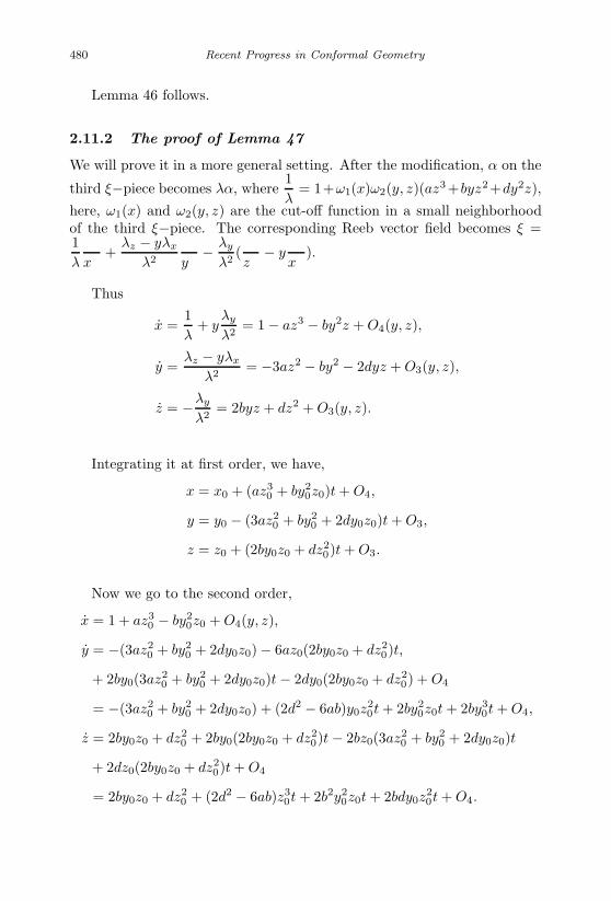
January 17, 2007 11:55 WSPC/Book Trim Size for 9in x 6in finalBB
480 Recent Progress in Conformal Geometry
Lemma 46 follows.
2.11.2 The proof of Lemma 47
We will prove it in a more general setting. After the modification, α on the
third ξ−piece becomes λα, where1λ
= 1+ω1(x)ω2(y, z)(az3+byz2+dy2z),
here, ω1(x) and ω2(y, z) are the cut-off function in a small neighborhoodof the third ξ−piece. The corresponding Reeb vector field becomes ξ =1λ
∂
∂x+
λz − yλx
λ2
∂
∂y− λy
λ2(
∂
∂z− y
∂
∂x).
Thus
x =1λ
+ yλy
λ2= 1 − az3 − by2z + O4(y, z),
y =λz − yλx
λ2= −3az2 − by2 − 2dyz + O3(y, z),
z = −λy
λ2= 2byz + dz2 + O3(y, z).
Integrating it at first order, we have,
x = x0 + (az30 + by2
0z0)t + O4,
y = y0 − (3az20 + by2
0 + 2dy0z0)t + O3,
z = z0 + (2by0z0 + dz20)t + O3.
Now we go to the second order,
x = 1 + az30 − by2
0z0 + O4(y, z),
y = −(3az20 + by2
0 + 2dy0z0) − 6az0(2by0z0 + dz20)t,
+ 2by0(3az20 + by2
0 + 2dy0z0)t − 2dy0(2by0z0 + dz20) + O4
= −(3az20 + by2
0 + 2dy0z0) + (2d2 − 6ab)y0z20t + 2by2
0z0t + 2by30t + O4,
z = 2by0z0 + dz20 + 2by0(2by0z0 + dz2
0)t − 2bz0(3az20 + by2
0 + 2dy0z0)t
+ 2dz0(2by0z0 + dz20)t + O4
= 2by0z0 + dz20 + (2d2 − 6ab)z3
0t + 2b2y20z0t + 2bdy0z
20t + O4.

January 17, 2007 11:55 WSPC/Book Trim Size for 9in x 6in finalBB
Contact Form Geometry 481
Integrating it, we get
x = x0 + (az30 − by2
0z0)ac + O4(y0, z0),
y = y0 − (3az20 + by2
0 + 2dy0z0)ac
+((2d2 − 6ab)y0z
20 + 2bdy2
0z0 + 2b2y30
) a2c
2+ O4,
z = z0 +(2by0z0 + dz2
0
)ac +
((2d2 − 6ab)z3
0 + 2b2y20z0 + 2bdy0z
20
) a2c
2+ O4.
On one hand, we can find Darboux coordinates such that around x−3 ,
the vector v reads∂
∂z− y
∂
∂x+ (a−
3 x + b−3 y + c3z + P 32 (x, y, z))
∂
∂y, and
around x+3 , the vector v reads
∂
∂z− y
∂
∂x+ (a+
3 x+ b+3 y + Q3
2(x0, y0, z0))∂
∂y.
So
dl(vinitial) =(−y0 + ac
(3az2
0 − by20 − 2by0z0(a−
3 x0 + b−3 y0 + c3z0))) ∂
∂x
+ a−3 x0 + b−3 y0 + c3z0 + P 3
2 (x0, y0, z0)
− ac(6az0 + by0(a−3 x0 + b−3 y0 + c3z0) + 2dy0
+ 2dz0(a−3 x0 + b−3 y0 + c3z0)) + a2
c((2d2 − 6ab)y0z0 + bdy20
+ 3b2y20(a
−3 x0 + b−3 y0 + c3z0) + (2d2 − 6ab)z2
0(a−3 x0 + b−3 y0 + c3z0)
+ 2bdy0z0(a−3 x0 + b−3 y0 + c3z0)) ∂
∂y
+ 1 + ac(2bz0(a−3 x0 + b−3 y0 + c3z0) + 2dz0 + 2by0)
+ a2c((3d2 − 9ab)z2
0 + b2y20 + 2bdy0z0 + b2y0z0(a−
3 x0 + b−3 y0 + c3z0)
+ bdz20(a
−3 x0 + b−3 y0 + c3z0)) ∂
∂z.
But on the other hand, around x+3 , the vector v reads
∂
∂z− y
∂
∂x+ (a+
3 x + b+3 y + Q3
2(x0, y0, z0))∂
∂y.

January 17, 2007 11:55 WSPC/Book Trim Size for 9in x 6in finalBB
482 Recent Progress in Conformal Geometry
Therefore,
vfinal
=∂
∂z− (y0 − (3az2
0 + by20 + 2dy0z0)ac + ((2d2 − 6ab)y0z
20 + 2bdy2
0z0
+ 2b2y30)
a2c
2)
∂
∂x+ (a+
3 (x0 + (az30 − by2
0z0)ac)
+ b+3 (y0 − (3az2
0 + by20 + 2dy0z0)ac
+((2d2 − 6ab)y0z
20 + 2bdy2
0z0 + 2b2y30
) a2c
2)
+ c3(z0 +(2by0z0 + dz2
0
)ac +
((2d2 − 6ab)z3
0 + 2b2y20z0 + 2bdy0z
20
) a2c
2)
+ Q32(x0 + ac − a, y0, z0))
∂
∂y.
Comparing vfinal and dl(vinitial) up to second order, we have,
a+3 (x0 + ac − a) + b+
3 y0 − acb+3 (3az2
0 + by20 + 2dy0z0)
+ Q32(x0 + ac − a, y0, z0)
a−3 x0 + b−3 y0 + c3z0 + P 3
2 (x0, y0, z0) − ac(6az0 + by0(a−3 x0 + b−3 y0 + c3z0)
+ 2dy0 =+2dz0(a−
3 x0 + b−3 y0 + c3z0)) + a2c((2d2 − 6ab)y0z0 + bdy2
0)1 + 2ac(2by0 + 2dz0)
.
Therefore,
δac =(a−
3 − a+3 )x0 + (b−3 − b+
3 )y0 + c3z0 − a(6az0 + 2dy0)a+3
− (a−3 − a+
3 )x0 + (b−3 − b+3 )y0 + c3z0 − a(6az0 + 2dy0)
a+3
· 6az0 + 2dy0 + Q2,x(x0,y0, z0)a+3
+ P 32 (x0, y0, z0) − Q3
2(x0, y0, z0) + ab+3 (3az2
0 + by20 + 2dy0z0)
− a(2by0 + 2dz0)(a−3 x0 + b−3 y0 + c3z0)
+ a(bdy20 + (2d2 − 6ab)y0z0 − a(2by0 + 2dz0)(a−
3 x0 + b−3 y0 + c3z0)/a+3 .

January 17, 2007 11:55 WSPC/Book Trim Size for 9in x 6in finalBB
Contact Form Geometry 483
In order to keep dac(v) unchanged, we take1λ
= 1+1(x)2(y, z)dy2z,therefore,
δac =(a−
3 − a+3 )x0 + (b−3 − b+
3 )y0 + c3z0 − a2dy0
a+3
− (a−3 − a+
3 )x0 + (b−3 − b+3 )y0 + c3z0 − a2dy0
a+3
· 2dy0 + Q2,x(x0,y0, z0)a+3
+ P 32 (x0, y0, z0) − Q3
2(x0, y0, z0) + ab+3 2dy0z0 − a2dz0(a−
3 x0 + b−3 y0 + c3z0)
− a22dz0(a−3 x0 + b−3 y0 + c3z0)/a+
3 .
2.11.3 Proof of the Lemmas in 2.7.11
2.11.4 Proof of Lemma 48
Following u2, in Darboux coordinates in the small neighborhood of the base
curve, the x, y coordinates of x1 read(
00
), x2 reads
( c2
a+20
)δs1, and the z
coordinates of both x1 and x2 is δs1; x3 reads
B
( c2
a+20
)δs1
δs2
, here B is
the transport matrix along the second v-piece.Since the third ξ−piece is modified, the transport matrix in x, y- coor-
dinates along this piece is
a−3 − a+
3
a+3
b−3 − b+3 − 2da
a+3
0 0
+ Id, and there is
a small increment
c3 − 6a · aa+30
δs2 due to the effect of the z−component
(refer to Lemma 47)
Therefore, the x, y−coordinates of x4 read
a−3
a+3
∆b3 − 2da
a+3
0 1
B
( c2
a+20
)δs1 +
( c3
a+30
)δs2, here ∆b3 = b−3 − b+
3 , and the z−coordinate
of x4 is δs2.

January 17, 2007 11:55 WSPC/Book Trim Size for 9in x 6in finalBB
484 Recent Progress in Conformal Geometry
The x, y−coordinates of x5 are
C
a−3
a+3
∆b3 − 2da
a+3
01
B
( c2
a+20
)δs1 + C
c3 − 6a · aa+30
δs2,
and the z−coordinate of x5 is δs3.Therefore the x, y−coordinates of x6 reada−
4
a+4
b−4 − b+4
a+4
0 1
C
a−3
a+3
∆b3 − 2da
a+3
0 1
B
( c2
a+20
)δs1
+
a−4
a+4
b−4 − b+4
a+4
01
C
c3 − 6a · aa+30
δs2 +
( c4
a+40
)δs3,
and the z−coordinate of x6 is δs3.On the other hand, u3 is parallel with v at x6.Thus we havea−
4
a+4
b−4 − b+4
a+4
0 1
C
a−3
a+3
∆b3 − 2da
a+3
0 1
B
( c2
a+20
)δs1.
+
a−4
a+4
b−4 − b+4
a+4
0 1
C
c3 − 6a · aa+30
δs2 +
( c4
a+40
)δs3 =
(00
).
Solving it for δs2, δs3, we get
δs2 = − c2
a+2
a+3
c3 − 6a · a(
a−3 B1 + (∆b3 − 2dac)B2
a+3
+B2
C2C4
)δs1,
δs3 =c2
a+2
a−4
c4
B2
B4detCδs1.
2.11.5 The Proof of Lemma 49
Along u3,
00
δs1
−→
c2
a+201
−→
B
( c2
a+20
)δs1
δs2

January 17, 2007 11:55 WSPC/Book Trim Size for 9in x 6in finalBB
Contact Form Geometry 485
−→
a−
3 − a+3
a+4
∆b3 − 2da
a+4
0 1
B
( c2
a+20
)δs1 +
c3 − 6a · aa+30
δs2
δs2
,
so point x4 reads
c2
a+2
δs1
−B2
C2C4
B2
δs2
.
And since in the small neighborhood of x6, the vector v reads
∂
∂z− y
∂
∂x+ (a+
3 x + b+3 y + Q3
2(x, y, z))∂
∂y.
So the vector v at x6 is parallel with− c2
a+2
B2δs1
c2
a+2
(b+3 B2 − a+
3
B2
C2C4)δs1
1
+ O(δs21).
Thus the x, y coordinates of x′4 are
c2
a+2
δs1
(−B2
C2C4B2
)
+
− c2
a+2
B2δs1
c2
a+2
(b+3 B2 − a+
3
B2
C2C4
)δs1
δs3 + Uδs21 + O(δs3
1 + δs13).
2.11.6 The proof of Lemma 50
We track only the first order terms of the base points along u2(u3). The
x, y coordinates of point x7 are(
00
), and the x, y coordinates of x0 read( c1
a+10
)δs1, both of their z coordinates are δs1; Thus x′
1 reads
A
( c1
a+10
)δs1
δs2 + δs1
.
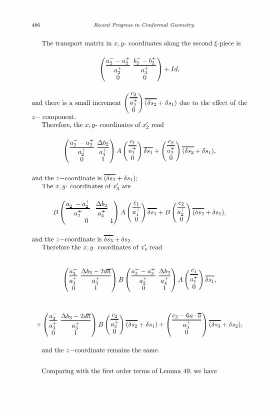
January 17, 2007 11:55 WSPC/Book Trim Size for 9in x 6in finalBB
486 Recent Progress in Conformal Geometry
The transport matrix in x, y- coordinates along the second ξ-piece is
a−2 − a+
2
a+2
b−2 − b+2
a+4
0 0
+ Id,
and there is a small increment
( c2
a+20
)(δs2 + δs1) due to the effect of the
z− component.Therefore, the x, y- coordinates of x′
2 read
a−2 − a+
2
a+2
∆b2
a+4
0 1
A
( c1
a+10
)δs1 +
( c2
a+20
)(δs2 + δs1),
and the z−coordinate is (δs2 + δs1);The x, y- coordinates of x′
3 are
B
a−2 − a+
2
a+2
∆b2
a+4
0 1
A
( c1
a+10
)δs1 + B
( c2
a+20
)(δs2 + δs1),
and the z−coordinate is δs3 + δs2.Therefore the x, y- coordinates of x′
4 read
a−3
a+3
∆b3 − 2da
a+3
0 1
B
a−2 − a+
2
a+2
∆b2
a+4
0 1
A
( c1
a+10
)δs1,
+
a−3
a+3
∆b3 − 2da
a+3
0 1
B
( c2
a+20
)(δs2 + δs1) +
c3 − 6a · aa+30
(δs3 + δs2),
and the z−coordinate remains the same.
Comparing with the first order terms of Lemma 49, we have

January 17, 2007 11:55 WSPC/Book Trim Size for 9in x 6in finalBB
Contact Form Geometry 487
a−3
a+3
∆b3 − 2da
a+3
0 1
B
a−2 − a+
2
a+2
∆b2
a+4
0 1
A
( c1
a+10
)δs1+
a−3
a+3
∆b3 − 2da
a+3
0 1
B
( c2
a+20
)(δs2 + δs1) +
c3 − 6a · aa+30
(δs3 + δs2)
=c2
a+2
δs1
−B2
C2C4
B2
.
Solving it for δs2, δs3, we know that δs1, δs2 and δs3 satisfy the follow-ing relation at the first order,
δs2 = p1δs1 + O(δs2
1, δs12, δs1δs1
),
δs3 = q1δs1 + O(δs2
1, δs12, δs1δs1
),
with
p1 = − c1
a+1
· a+2
c2·(
a−2 A1 + ∆b2A2
a+3
+A2
B2B4
),
q1 =c1
a+1
a−3
c3
A2
B2detB.
2.11.7 Proof of Claim 1
In a neighborhood of x0, the vector v reads up to a multiplicative factor∂
∂z− y
∂
∂x+ (a+
1 x + b+1 y + Q1
2(x, y, z))∂
∂y, so the v trajectory satisfies
x = −y,
y = a+1 x + b+
1 y + Q12(x, y, z),
z = 1.
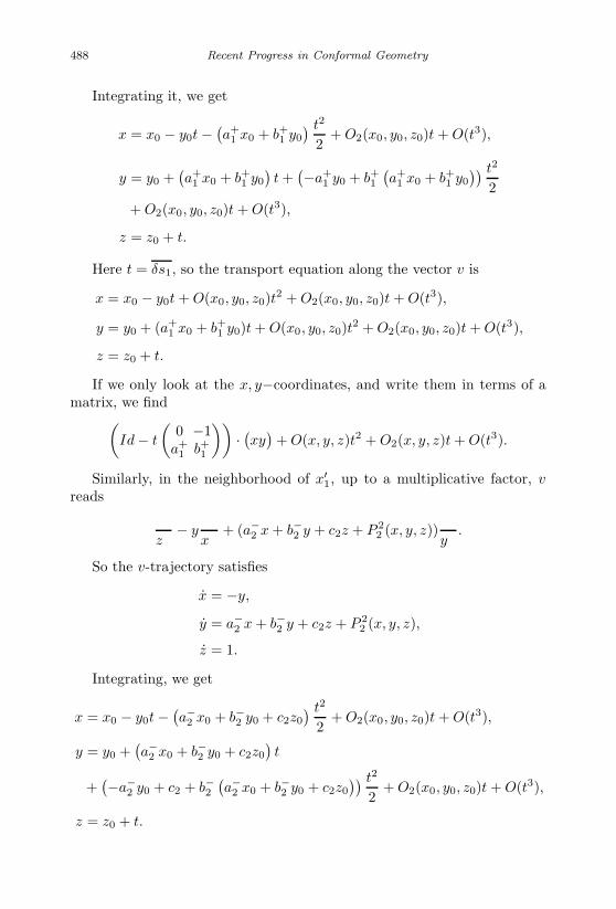
January 17, 2007 11:55 WSPC/Book Trim Size for 9in x 6in finalBB
488 Recent Progress in Conformal Geometry
Integrating it, we get
x = x0 − y0t −(a+1 x0 + b+
1 y0
) t2
2+ O2(x0, y0, z0)t + O(t3),
y = y0 +(a+1 x0 + b+
1 y0
)t +
(−a+1 y0 + b+
1
(a+1 x0 + b+
1 y0
)) t2
2+ O2(x0, y0, z0)t + O(t3),
z = z0 + t.
Here t = δs1, so the transport equation along the vector v is
x = x0 − y0t + O(x0, y0, z0)t2 + O2(x0, y0, z0)t + O(t3),
y = y0 + (a+1 x0 + b+
1 y0)t + O(x0, y0, z0)t2 + O2(x0, y0, z0)t + O(t3),
z = z0 + t.
If we only look at the x, y−coordinates, and write them in terms of amatrix, we find(
Id − t
(0 −1
a+1 b+
1
))· (xy
)+ O(x, y, z)t2 + O2(x, y, z)t + O(t3).
Similarly, in the neighborhood of x′1, up to a multiplicative factor, v
reads
∂
∂z− y
∂
∂x+ (a−
2 x + b−2 y + c2z + P 22 (x, y, z))
∂
∂y.
So the v-trajectory satisfies
x = −y,
y = a−2 x + b−2 y + c2z + P 2
2 (x, y, z),
z = 1.
Integrating, we get
x = x0 − y0t −(a−2 x0 + b−2 y0 + c2z0
) t2
2+ O2(x0, y0, z0)t + O(t3),
y = y0 +(a−2 x0 + b−2 y0 + c2z0
)t
+(−a−
2 y0 + c2 + b−2(a−2 x0 + b−2 y0 + c2z0
)) t2
2+ O2(x0, y0, z0)t + O(t3),
z = z0 + t.
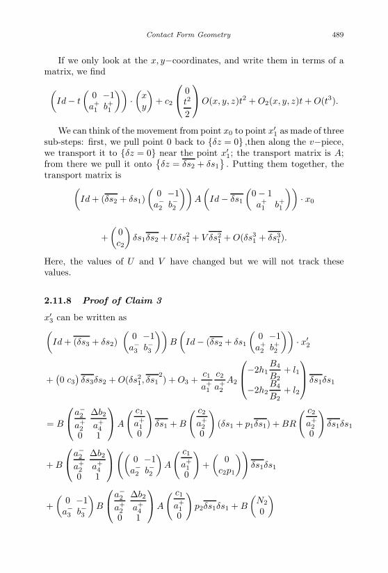
January 17, 2007 11:55 WSPC/Book Trim Size for 9in x 6in finalBB
Contact Form Geometry 489
If we only look at the x, y−coordinates, and write them in terms of amatrix, we find(
Id − t
(0 −1
a+1 b+
1
))·(
xy
)+ c2
0t2
2
O(x, y, z)t2 + O2(x, y, z)t + O(t3).
We can think of the movement from point x0 to point x′1 as made of three
sub-steps: first, we pull point 0 back to δz = 0 ,then along the v−piece,we transport it to δz = 0 near the point x′
1; the transport matrix is A;from there we pull it onto
δz = δs2 + δs1
. Putting them together, the
transport matrix is(Id + (δs2 + δs1)
(0 −1
a−2 b−2
))A
(Id − δs1
(0 − 1a+1 b+
1
))· x0
+(
0c2
)δs1δs2 + Uδs2
1 + V δs21 + O(δs3
1 + δs31).
Here, the values of U and V have changed but we will not track thesevalues.
2.11.8 Proof of Claim 3
x′3 can be written as(Id + (δs3 + δs2)
(0 −1
a−3 b−3
))B
(Id − (δs2 + δs1
(0 −1
a+2 b+
2
))· x′
2
+(0 c3
)δs3δs2 + O(δs2
1, δs12) + O3 +
c1
a+1
c2
a+2
A2
−2h1B4
B2+ l1
−2h2B4
B2+ l2
δs1δs1
= B
a−2
a+2
∆b2
a+4
0 1
A
( c1
a+10
)δs1 + B
( c2
a+20
)(δs1 + p1δs1) + BR
( c2
a+20
)δs1δs1
+ B
a−2
a+2
∆b2
a+4
0 1
(( 0 −1a−2 b−2
)A
( c1
a+10
)+(
0c2p1
))δs1δs1
+(
0 −1a−3 b−3
)B
a−2
a+2
∆b2
a+4
0 1
A
( c1
a+10
)p2δs1δs1 + B
(N2
0
)
January 17, 2007 11:55 WSPC/Book Trim Size for 9in x 6in finalBB
490 Recent Progress in Conformal Geometry
− B
(0 −1
a+2 b+
2
)a−2
a+2
∆b2
a+4
0 1
A
( c1
a+10
)δs1δs1 +
(0c3
)p2q1δs1δs1
+(
0 −1a−3 b−3
)B
( c2
a+20
)(q1 + p1p2)δs1δs1 − B
(0 −1
a+2 b+
2
)2p1δs1δs1
+c1
a+1
c2
a+2
A2
−2h1B4
B2+ l1
−2h2B4
B2+ l2
δs1δs1.
Therefore, the first order terms of x′3 are
B
a−2
a+2
∆b2
a+4
0 1
A
( c1
a+10
)δs1 + B
( c2
a+20
)p1δs1
=
(− c3
a−3
q1
0
)δs1 +
c2
a+2
(B1
B2
)δs1.
Using Lemma 47, along the 3rd ξ−piece of u2(u3), the second orderterms of the displacement in x, y and z are
δx = N3(δs1,δs1) = ac(x′3) − ac(x2),
δy = −2dc2
a+2
B2δs1(δs3 + δs2)a,
δz = d(δs3 + δs2)2a.
As we explained before, drop the δs21, δs1
2terms, we have,
δx = N3(δs1,δs1),
δy = −2dc2
a+2
B2q1aδs1δs1,
δz = 2dp2q1aδs1δs1.
Thus the x, y−coordinates of x′4 area−
3
a+3
∆b3 − 2da
a+3
0 1
· x′3 +
( c3
a+30
)(δs3 + δs2) +
(δxδy.
)
January 17, 2007 11:55 WSPC/Book Trim Size for 9in x 6in finalBB
Contact Form Geometry 491
Comparing the δs1δs1 terms of point x′4 with Lemma 49, we get
a−3
a+3
∆b3 − 2da
a+3
0 1
(BR
( c2
a+20
)δs1δs1 + B
(N2
0
)+(
0c3
)p2q1δs1δs1
)
+
N3(δs1δs1)−2d
c2
a+2
B2q1aδs1δs1
+
a−3
a+3
∆b3 − 2da
a+3
0 1
B
a−2
a+2
∆b2
a+2
0 1
(( 0 −1a−2 b−2
)A
( c1
a+10
)+(
0c2p1
))δs1δs1
+
a−3
a+3
∆b3 − 2da
a+3
0 1
(
0 −1a−3 b−3
)B
a−2
a+2
∆b2
a+2
0 1
A
( c1
a+10
)p2
+(
0 −1a−3 b−3
)B
( c2
a+20
)(q1 + p1p2)
δs1δs1
−a−
3
a+3
∆b3 − 2da
a+3
0 1
B
(0 −1
a+2 b+
2
)a−2
a+2
∆b2
a+2
0 1
A
( c1
a+10
)
+B
(0 −1
a+2 b+
2
)( c2
a+20
)2p1
δs1δs1
+ T
( c3
a+30
)δs1δs1
+c1
a+1
c2
a+2
A2
a−3 − a+
3
a+3
∆b3 − 2da
a+3
0 1
−2h1
B4
B2+ l1
−2h2B4
B2+ l2
δs1δs1
=
− c2
a+2
B2
c2
a+2
(b+3 B2 − a+
3
B2
C2C4
) q1δs1δs1. (∗)
Computing the y−coordinate, we get
− c1
a+1
A2B2
(a−2 − a+
2
a+2
+∆b2
a+2
(a+2
B4
B2− b+
2 ))− c3p2q1 − c2p1B4

January 17, 2007 11:55 WSPC/Book Trim Size for 9in x 6in finalBB
492 Recent Progress in Conformal Geometry
−2dac2
a+2
q1B2 +c2
a+2
RB2 + NB2 +c1
a+1
c2
a+2
A2(−2h2B4
B2+ l2) = 0.
2.11.9 The Final Details of the Calculation of
∂2J(x∞).u2.u3
For the second ξ−piece, the δs1δs1 terms come from three sources. Sinceδs2 = p1δs1+Rδs1δs1, R is one of the sources. Also the second order termsof dac(x′
1), N2 contribute δs1δs1 terms too, and all the other δs1δs1termscome from the v-transport. Now we write it explicitly,
(1, 0) ·
R
( c2
a+20
)δs1δs1 +
(N2
0
)+(
0c2p1
)
+
a−2 − a+
2
a+2
∆b2
a+2
0 1
(( 0 −1a−2 b−2
)A
( c1
a+10
))
=(
c3
B2p2q1 + c2p1
B4
B2+ 2da
c2
a+2
q1
)δs1δs1.
For the third ξ−piece, the δs1δs1 terms also come from three sources.Since δs3 = q1δs1 +Tδs1δs1, T is one of the sources. Also the second orderterms of dac(point3
′), N3 contributes to the δs1δs1 terms too. All the other
δs1δs1terms come from the v-transport. Computing, we find:
(1, 0) ·a−
3 − a+3
a+3
∆b3 − 2da
a+3
0 1
×(
BR
( c2
a+20
)δs1δs1 + B
(N2
0
)+(
0c3
)p2q1δs1δs1
)
+(1, 0) ·a−
3 − a+3
a+3
∆b3 − 2da
a+3
0 1
B
a−2
a+2
∆b2
a+2
0 1
×((
0 −1a−2 b−2
)A
( c1
a+10
)+(
0c2p1
))δs1δs1

January 17, 2007 11:55 WSPC/Book Trim Size for 9in x 6in finalBB
Contact Form Geometry 493
+(1, 0) ·a−
3 − a+3
a+3
∆b3 − 2da
a+3
0 1
×
(
0 −1a−3 b−3
)B
a−2
a+2
∆b2
a+2
0 1
A
( c1
a+10
)p2
+(
0 −1a−3 b−3
)B
( c2
a+20
)(2q1 + p1p2)
δs1δs1
−(1, 0)·a−
3 − a+3
a+3
∆b3 − 2da
a+3
0 1
B
(0 −1
a+2 b+
2
)a−2
a+2
∆b2
a+2
0 1
A
( c1
a+10
)
+B
(0 −1
a+2 b+
2
)( c2
a+20
)2p1
δs1δs1
+T (1, 0) ·( c3
a+30
)δs1δs1 + N3(δs1,δs1)
+(1, 0)c1
a+1
c2
a+2
A2
a−3 − a+
3
a+3
∆b3 − 2da
a+3
0 1
−2h1
B4
B2+ l1
2h2B4
B2+ l2
δs1δs1.
Comparing with (∗), we find that this is equal to:
−(1, 0) ·(
BR
( c2
a+20
)δs1δs1 + B
(N2
0
)+(
0c3
)p2q1δs1δs1
)
−(1, 0) · Ba−
2
a+2
∆b2
a+2
0 1
(( 0 −1a−2 b−2
)A
( c1
a+10
)+(
0c2p1
))δs1δs1
−(1, 0) ·
(
0 −1a−3 b−3
)a−2
a+2
∆b2
a+4
0 1
A
( c1
a+10
)p2+
(0 −1
a−3 b−3
)B
( c2
a+20
)(2q1 + p1p2)
δs1δs1
January 17, 2007 11:55 WSPC/Book Trim Size for 9in x 6in finalBB
494 Recent Progress in Conformal Geometry
+(1, 0)·B
(0 −1
a+2 b+
2
)a−2
a+2
∆b2
a+4
0 1
A
( c1
a+10
)− B
(0 −1
a+2 b+
2
)( c2
a+20
)2p1
δs1δs1
−(1, 0)c1
a+1
c2
a+2
A2
−2h1B4
B2+ l1
2h2B4
B2+ l2
δs1δs1
=(−c3
B1
B2p2q1 − c2p1
detB
B2− 2da
c2
a+2
q1B1
)δs1δs1
+c1
a+1
c2
a+2
A2
((2h1
B1
B2− 2h2)
B4
B2+ l2 − l1
)δs1δs1.
Summing them up, we find
∂2J.u2.u3
=c3
B2p2q1 + c2p1
B4
B2+ 2da
c2
a+2
q1 − c3B1
B2p2q1 − c2p1
detB
B2− 2da
c2
a+2
q1B1
+c1
a+1
c2
a+2
A2
((2h1 − 2h2)
B4
B2+ l2 − l1
)
= q1
(c3
B2p2 + 2da
c2
a+2
− 2dac2
a+2
B1 − c3B1
B2p2
)︸ ︷︷ ︸
(I)
+ c2p1B4
B2− c2p1
detB
B2c2p1
detB
B2︸ ︷︷ ︸(II)
+c1
a+1
c2
a+2
A2((2h1B1
B2− 2h2)
B4
B2+ l2 − l1)︸ ︷︷ ︸
(III)
.
2.11.10 Details involved in 2.8
2.11.11 Proof of Lemma 52
It is clear that the x, y coordinates of x6 read(
00
), and the z coordinate is
δs3. And in the neighborhood of point x6, the vector v reads∂
∂z− y
∂
∂x+

January 17, 2007 11:55 WSPC/Book Trim Size for 9in x 6in finalBB
Contact Form Geometry 495
(a+3 x + b+
3 y + Q32(x, y, z))
∂
∂y, so at x6, v is parallel with
0Q3
2(0, 0, δs3)1
,
so x′6 is
00
δs3
+ δs3
0Q3
2(0, 0, δs3)1
=
00
δs3 + δs3
+ Uδs21 + V δs1
2+
O(δs31 + δs1
3).
2.11.12 Proof of Lemma 53
Following u2(u2), we write only the first order terms in a first step,
x′1 is
00
δs1 + δs1
; the transport matrix along the first ξ-piece isa−1
a+1
b−1 − b+1
a+1
0 1
and there is a small increment
( c1
a+10
)(δs1 + δs1) due to
the effect of the z−coordinate, therefore x′2 reads
c1
a+101
(δs1 + δs1); now
we go to point x′3, it reads
A
( c1
a+10
)(δs1 + δs1)
δs2 + δs2
; x′4 is , using the same
argument
a−
2
a+2
b−2 − b+2
a+2
0 1
A
( c1
a+10
)(δs1 + δs1) +
( c2
a+20
)(δs2 + δs2)
δs2 + δs2
.
Therefore x′5 reads
B
a−2
a+2
b−2 − b+2
a+2
0 1
A
( c1
a+10
)(δs1 + δs1) + B
( c2
a+20
)(δs2 + δs2)
δs3 + δs3
.
January 17, 2007 11:55 WSPC/Book Trim Size for 9in x 6in finalBB
496 Recent Progress in Conformal Geometry
The transport matrix along the third ξ-piece is
a−3
a+3
∆b3 − 2dac
a+3
0 1
and
there is a small increment( c3
a+30
)(δs3 + δs3), so the x, y- coordinates of x6 read
a−3
a+3
∆b3 − 2dac
a+3
0 1
B
a−2
a+2
b−2 − b+2
a+2
0 1
A
( c1
a+10
)(δs1 + δs1)
+
a−3
a+3
∆b3 − 2dac
a+3
0 1
B
( c2
a+20
)(δs2 + δs2) +
( c3
a+30
)(δs2 + δs3),
and the z−coordinate remains the same δs3 + δs3.Using Lemma 52, we havea−
3
a+3
∆b3 − 2dac
a+3
0 1
B
a−2
a+2
b−2 − b+2
a+2
0 1
A
( c1
a+10
)(δs1 + δs1)
+
a−3
a+3
∆b3 − 2dac
a+3
0 1
B
( c2
a+20
)(δs2 + δs2) +
( c3
a+30
)(δs3 + δs3) =
(00
).
Observe that these are exactly the equations satisfied by δs1, δs2 relativeto δs3. At first order, there is no difference. Solving it for δs2 and δs3, wederive the lemma.
2.11.13 Proof of Claim 3
Since x1 is
00
δs1
, and the vector v reads, up to a multiplicative factor,
∂
∂z− y
∂
∂x+ (a+
1 x + b+1 y + c1z + P 1
2 (x, y, z))∂
∂yaround x1, along the v

January 17, 2007 11:55 WSPC/Book Trim Size for 9in x 6in finalBB
Contact Form Geometry 497
trajectory, it satisfies
x = −y,
y = a+1 x + b+
1 y + c1z + P 12 (x, y, z),
z = 1.
Integrating it, we get
x = x0 − y0t −(a+1 x0 + b+
1 y0 + c1z0
) t2
2+ O2(x, y, z)t + O(t3),
y = y0 +(a+1 x0 + b+
1 y0 + c1z0
)t +
(−a+1 y0 + b+
1
(a+1 x0 + b+
1 y0 + c1z0
)+c1)
t2
2+ O2(x, y, z)t + O(t3),
z = z0 + t.
Here t = δs1 + δs1, therefore
x = O(δs13+ δs3
1),
y = c1δs1δs1 + O(δs13+ δs3
1) + c1δs1
2+ δs2
1
2,
z = δs1 + δs1.
2.11.14 Proof of Claim 4
We write only the first order and δs1δs1 terms. The x, y−coordinates of x′3
read:
A
( c1
a+10
)(δs1 + δs1) + A
a−1
a+1
b−1 − b+1
a+1
0 1
0c1δs1δs1
+ 2p
(0 − 1a−2 b−2
)A
( c1
a+1
0
)δs1δs1
− 2A
(0 −1
a+1 b+
1
)( c1
a+10
)δs1δs1 +
(0c2
)p2δs1δs1 + A
(N1
0
),
and the z−coordinate remains δs2 + δs2.

January 17, 2007 11:55 WSPC/Book Trim Size for 9in x 6in finalBB
498 Recent Progress in Conformal Geometry
The x, y−coordinates of x′4 read
a−2
a+2
∆b2
a+2
0 1
A
( c1
a+10
)(δs1 + δs1) +
( c2
a+20
)(δs2 + δs2)
+
a−2
a+2
∆b2
a+2
0 1
A
(N1
0
)+(
N2
0
)+
a−2
a+2
∆b2
a+2
0 1
A
a−1
a+1
∆b1
a+1
0 1
(0c1
)δs1δs1
+
a−2
a+2
∆b2
a+2
0 1
2p
(0 −1
a−2 b−2
)A
( c1
a+10
)δs1δs1
−2
a−2
a+2
∆b2
a+2
0 1
A
(0 −1
a+1 b+
1
)( c1
a+10
)δs1δs1
+
a−2
a+2
∆b2
a+2
0 1
( 0c2
)p2δs1δs1 +
a−2
a+2
∆b2
a+2
0 1
A
(N1
0
)
and the z−coordinate remains the same δs2 + δs2. Here, ∆bi = b−i − b+i
and N2 is the second order term of ac(x′3) − ac(x3).
The modification of the v transport contributes,
2(
c1
a+1
A2
)2B4
B2
−l1 +B4
B2h1
−l2 +B4
B2h2
δs1δs1
if we only count δs1δs1 terms.Therefore, writing only the first order and δs1δs1 terms, the
x, y−coordinates of x′5 read
B
a−2
a+2
∆b2
a+2
0 1
A
( c1
a+1
0
)(δs1 + δs1) + B
( c2
a+2
0
)(δs2 + δs2)
+B
a−2
a+2
∆b2
a+2
0 1
A
(N1
0
)+B
(N2
0
)+B
a−2
a+2
∆b2
a+2
0 1
A
a−1
a+1
∆b1
a+1
0 1
( 0c1
)δs1δs1
January 17, 2007 11:55 WSPC/Book Trim Size for 9in x 6in finalBB
Contact Form Geometry 499
+B
a−2
a+2
∆b2
a+2
0 1
2p
(0 −1
a−2 b−2
)A
( c1
a+1
0
)δs1δs1
−2B
a−2
a+2
∆b2
a+2
0 1
A
(0 −1
a+1 b+
1
)( c1
a+1
0
)δs1δs1B
a−2
a+2
∆b2
a+2
0 1
( 0c2
)p2δs1δs1
+
(0 −1
a−2 b−2
)B
2q
a−2
a+2
∆b2
a+2
0 1
A
( c1
a+1
0
)+ 2pq
( c2
a+2
0
) δs1δs1
−B
(0 −1
a+1 b+
1
)2p
a−2
a+2
∆b2
a+2
0 1
A
( c1
a+1
0
)+ 2p2
( c2
a+2
0
) δs1δs1 +
(0c3
)q2δs1δs1
+2
(c1
a+1
A2
)2B4
B2
−l1 +B4
B2h1
−l2 +B4
B2h2
δs1δs1,
and the z−coordinate is δs3 + δs3.
The x and y coordinates of x′5 at the first order are,
B
a−2
a+2
∆b2
a+2
0 1
A
( c1
a+10
)(δs1 + δs1) + B
( c2
a+20
)(δs2 + δs2)
=
(A1
c1
a+1
(δs1 + δs1)
0
).
Using the Lemma 47, along the third ξ-piece,
δx = N3,
δy = 0,
δz = d(δs3 + δs3)2ac.
Writing only δs1δs1 terms,
δx = N3,
δy = 0,
δz = 2dacq2δs1δs1,

January 17, 2007 11:55 WSPC/Book Trim Size for 9in x 6in finalBB
500 Recent Progress in Conformal Geometry
here, N3 is the second order term of ac(x′5) − ac(x5).
x6 is
a−3
a+3
∆b3 − 2dac
a+3
0 1
· x′5 +
( c3
a+30
)(δs3 + δs3) +
(δxδy
)so the x, y− coordinates of x′
6 are
a−3
a+3
∆b3 − 2dac
a+3
0 1
B
a−2
a+2
∆b2
a+2
0 1
A
( c1
a+10
)(δs1 + δs1)
+
a−3
a+3
∆b3 − 2dac
a+3
0 1
B
( c2
a+20
)(δs2 + δs2) +
( c3
a+30
)(δs3 + δs3)
+
a−3
a+3
∆b3 − 2dac
a+3
0 1
B
a−2
a+2
∆b2
a+2
0 1
A
(N1
0
)
+
a−3
a+3
∆b3 − 2dac
a+3
0 1
B
(N2
0
)+(
N3
−6aq2δs1δs1
)
+
a−3
a+3
∆b3 − 2dac
a+3
0 1
( 0c3
)q2δs1δs1
+
a−3
a+3
∆b 3
− 2daca+3
0 1
B
a−2
a+2
∆b2
a+2
0 1
A
(a−1
a+1
∆b1
a+1
0 1)(
0c1
)δs1δs1
+
a−3
a+3
∆b3 − 2dac
a+3
0 1
B
a−2
a+2
∆b2
a+2
0 1
2p
(0 −1
a−2 b−2
)A
( c1
a+10
)
−2A
(0 −1
a+1 b+
1
)( c1
a+10
) δs1δs1

January 17, 2007 11:55 WSPC/Book Trim Size for 9in x 6in finalBB
Contact Form Geometry 501
+
a−3
a+3
∆b3 − 2dac
a+3
0 1
B
a−2
a+2
∆b2
a+2
0 1
( 0c2
)p2δs1δs1
+
a−3
a+3
∆b3 − 2dac
a+3
0 1
( 0 −1a−3 b−3
)B
2q
a−2
a+2
∆b2
a+2
0 1
A
( c1
a+10
)
+2pq
( c2
a+20
))δs1δs1
−a−
3
a+3
∆b3 − 2dac
a+3
0 1
B
(0 −1
a+2 b+
2
)2p
a−2
a+2
∆b2
a+2
0 1
A
( c1
a+10
)
+2p2
( c2
a+20
))δs1δs1
+2(
c1
a+1
A2
)2B4
B2
a−3
a+3
∆b3 − 2dac
a+3
0 1
−l1 +
B4
B2h1
−l2 +B4
B2h2
Comparing this with Lemma 52, we derive the equation
R
a−3
a+3
∆b3 − 2dac
a+3
0 1
B
( c2
a+20
)δs1δs1 + T
( c3
a+30
)δs1δs1
+
a−3
a+3
∆b3 − 2dac
a+3
0 1
B
a−2
a+2
∆b2
a+2
0 1
A
(N1
0
)+(
N3
−6aq2δs1δs1
)
+
a−3
a+3
∆b3 − 2dac
a+3
0 1
B
(N2
0
)+
a−3
a+3
∆b3 − 2dac
a+3
0 1
( 0c3
)q2δs1δs1

January 17, 2007 11:55 WSPC/Book Trim Size for 9in x 6in finalBB
502 Recent Progress in Conformal Geometry
+
a−3
a+3
∆b3 − 2dac
a+3
0 1
B
a−2
a+2
∆b2
a+2
0 1
A
a−1
a+1
∆b1
a+1
0 1
( 0c1
)δs1δs1
+
a−3
a+3
∆b3 − 2dac
a+3
0 1
B
a−2
a+2
∆b2
a+2
0 1
2p
(0 −1
a−2 b−2
)A
( c1
a+10
)
−2A
(0 −1
a+1 b+
1
)( c1
a+10
) δs1δs1
+
a−3
a+3
∆b3 − 2dac
a+3
0 1
B
a−2
a+2
∆b2
a+2
0 1
( 0c2
)p2δs1δs1
+
a−3
a+3
∆b3 − 2dac
a+3
0 1
( 0 −1a−3 b−3
)B
2q
a−2
a+2
∆b2
a+2
0 1
A
( c1
a+10
)+ 2pq
( c2
a+20
)
× δs1δs1
−a−
3
a+3
∆b3 − 2dac
a+3
0 1
B
(0 −1
a+2 b+
2
)2p
a−2
a+2
∆b2
a+2
0 1
A
( c1
a+10
)+ 2p2
( c2
a+20
)
× δs1δs1
+2(
c1
a+1
A2
)2B4
B2
a−3
a+3
∆b3 − 2dac
a+3
0 1
−l1 +
B4
B2h1
−l2 +B4
B2h2
=(
00
). (**)
Comparing the y-coordinates, we get

January 17, 2007 11:55 WSPC/Book Trim Size for 9in x 6in finalBB
Contact Form Geometry 503
c1∆b1
a+1
B2a−2 A1 + ∆b2A2
a+2
− c1B2a−2 A3 + ∆b2A4
a+2
+ c1B4
(∆b1
a+1
A2 − A4
)
+2pA2B2c1
a+1
(1 − a−
2
a+2
)+ 2p
c1
a+1
B2∆b2
a+2
(a−2 A1 + b−2 A2
)
+c2p2
(∆b2
a+2
B2 − B4
)− c3q
2 +c2
a+2
B2R + B2N2
+(
B4A2 + B2a−2 A1 + ∆b2A2
a+2
)N1
+2(
c1
a+1
A2
)2B4
B2
(−l2 +
B4
B2h2
)= 0.
2.11.15 Details of the Calculation of ∂2J.u2.u2
In order to calculate the δs1δs1 terms in J(x + δs1u2(u2) + δs1u2)− J(x +δs1u2), we need to count the δs1δs1 terms contributed by all the ξ-pieces.
Computing the first ξ-piece contributes
N1 + (1, 0) ·a−
1 − a+1
a+1
b−1 − b+1
a+1
0 1
( 0c1
)δs1δs1 = N1 +
∆b1
a+1
c1δs1δs1.
For the second ξ-piece, as before, the δs1δs1 terms come from threesources. Since δs2 = p1δs1 + Rδs1δs1, so R is one of the three sources.Also the second order terms of dac(x′
3), N2 contribute to the δs1δs1 termstoo. All the other δs1δs1terms come from the v-transport. Computing, wefind:
R(1, 0)
( c2
a+2
0
)δs1δs1 + (1, 0)
a−2 − a+
2
a+2
∆b2
a+2
0 1
A
(N1
0
)+ N2
+(1, 0) ·a−
2 − a+2
a+2
∆b2
a+2
0 1
A
a−1
a+1
∆b1
a+1
0 1
( 0c1
)δs1δs1

January 17, 2007 11:55 WSPC/Book Trim Size for 9in x 6in finalBB
504 Recent Progress in Conformal Geometry
+(1, 0) ·a−
2 − a+2
a+2
∆b2
a+2
0 1
2p
(0 −1
a−2 b−2
)A
( c1
a+1
0
)δs1δs1
−2(1, 0) ·a−
2 − a+2
a+2
∆b2
a+2
0 1
A
(0 −1
a+1 b+
1
)( c1
a+1
0
)δs1δs1
+(1, 0) · a−
2 − a+2
a+2
∆b2
a+2
0 1
( 0c2
)p2δs1δs1
=
c1(A3 − ∆b1
a+1
A1) − c1B4
B2
(∆b1
a+1
A2 − A4
)+ c2p
2 B4
B2−(
A1 +B4A2
B2
)N1
+c31
B2q2 − 2
(c1
a+1
A2
)2B4
B22
(−l2 +
B4
B2h2
)
×δs1δs1.
For the third ξ−piece, the δs1δs1 terms come from three sources, the Rterm of δs3, the second order terms of dac(x′
5) i.e.N3 , and those from thev-transport. Computing, we find
R(1, 0) ·a−
3
a+3
∆b3 − 2dac
a+3
0 1
B
( c2
a+20
)δs1δs1 + T (1, 0) ·
( c3
a+30
)δs1δs1
+(1, 0) ·a−
3
a+3
∆b3 − 2dac
a+3
0 1
B
a−2
a+2
∆b2
a+2
0 1
A
(N1
0
)+ N3
+(1, 0) ·a−
3
a+3
∆b3 − 2dac
a+3
0 1
B
(N2
0
)
+(1, 0) ·a−
3
a+3
∆b3 − 2dac
a+3
0 1
( 0c3
)q2δs1δs1

January 17, 2007 11:55 WSPC/Book Trim Size for 9in x 6in finalBB
Contact Form Geometry 505
+(1, 0) ·a−
3
a+3
∆b3 − 2dac
a+3
0 1
B
a−2
a+2
∆b2
a+2
0 1
a−1
a+1
∆b1
a+1
0 1
( 0c1
)δs1δs1
+(1, 0)·a−
3
a+3
∆b3 − 2dac
a+3
0 1
B
a−2
a+2
∆b2
a+2
0 1
2p
(0 −1
a−2 b−2
)A
( c1
a+10
)
+A
(0 −1
a+1 b+
1
)( c1
a+10
) δs1δs1
+(1, 0) ·a−
3
a+3
∆b3 − 2dac
a+3
0 1
B
a−2
a+2
∆b2
a+2
0 1
( 0c2
)p2δs1δs1
+(1, 0) ·a−
3
a+3
∆b3 − 2dac
a+3
0 1
( 0 −1a−3 b−3
)B
2q
a−2
a+2
∆b2
a+2
0 1
A
( c1
a+10
)
+2pq
( c2
a+20
))δs1δs1
−(1, 0) ·a−
3
a+3
∆b3 − 2dac
a+3
0 1
B
(0 1
a+2 b+
2
)2p
a−2
a+2
∆b2
a+2
0 1
A
( c1
a+10
)
+2p2
( c2
a+20
))δs1δs1
+(1, 0) · 2(
c1
a+1
A2
)2B2
B4
a−3
a+3
∆b3 − 2dac
a+3
0 1
l1 − B2
B4h1
l2 − B2
B4h2
δs1δs1.
Comparing with (∗∗), we find
January 17, 2007 11:55 WSPC/Book Trim Size for 9in x 6in finalBB
506 Recent Progress in Conformal Geometry
−(1, 0) ·RB
( c2
a+20
)s1δs1 + B
a−2
a+2
∆b2
a+2
0 1
A
(N1
0
)+ B
(N2
0
)
−(1, 0) · Ba−
2
a+2
∆b2
a+2
0 1
A
a−1
a+1
∆b1
a+1
0 1
( 0c1
)δs1δs1
+2p
(0 −1
a−2 b−2
)A
( c1
a+10
)− 2A
(0 −1
a+1 b+
1
)( c1
a+10
)
×δs1δs1
−(1, 0) · Ba−
2
a+2
∆b2
a+2
0 1
( 0c2
)p2δs1δs1
−(1, 0) ·(
0 −1a−3 b−3
)B
2q
a−2
a+2
∆b2
a+2
0 1
A
( c1
a+10
)+ 2pq
( c2
a+20
) δs1δs1
+(1, 0) · B(
0 −1a+2 b+
2
)2p
a−2
a+2
∆b2
a+2
0 1
A
( c1
a+10
)+ 2p2
( c2
a+20
) δs1δs1
−(1, 0) · 2(
c1
a+1
A2
)2B4
B2
l1 − B4
B2h1
l2 − B4
B2h2
=
c1(∆b1
a+1
A2 − A4)(
B4B1
B2− B3
)+ c2p
2
(B3 − B4B1
B2
)+A2N1
(B4B1
B2− B3
)− c3
B1
B2q2
δs1δs1
+2(
c1
a+1
A2
)2B4
B2
(B1
B2
(−l2 +
B4
B2h2
)−(−l1 +
B4
B2h1
))δs1δs1.
January 17, 2007 11:55 WSPC/Book Trim Size for 9in x 6in finalBB
Contact Form Geometry 507
Summing them together, we have
∂2J.u1.u1 = N1 +∆b1
a+1
c1 + c1(A3 − ∆b1
a+1
A1) − c1B4
B2(∆b1
a+1
A2 − A4)
+ c2p2 B4
B2− (A1 +
B4A2
B2)N1 + c3
1B2
q2 + c1(∆b1
a+1
A2 − A4)(
B4B1
B2− B3
)+ c2p
2
(B3 − B4B1
B2
)+ A2N1
(B4B1
B2− B3
)
− 2(
c1
a+1
A2
)2B4
B22
(−l2 +
B4
B2h2
)− c3
B1
B2q2
+ 2(
c1
a+1
A2
)2B4
B2
(B1
B2
(−l2 +
B4
B2h2
)+(
l1 − B4
B2h1
))δs1δs1
= (1 − A1 +A2
B2(detB − B4))N1 + c1(
∆b1
a+1
A2 − A4)1
B2(detB + B4)︸ ︷︷ ︸
(I)
−c2p2 1B2
(detB − B4) + c1(A3 − ∆b1
a+1
A1) +∆b1
a+1
c1 + c31 − B1
B2q2︸ ︷︷ ︸
(I)
− 2(
c1
a+1
A2
)2B4
B22
(−l2 +
B4
B2h2
)+ 2
(c1
a+1
A2
)2B4
B2
(B1
B2
(l2 − B4
B2h2
)−(
l1 − B4
B2h1
))︸ ︷︷ ︸
(II)
.

January 17, 2007 11:55 WSPC/Book Trim Size for 9in x 6in finalBB
This page intentionally left blankThis page intentionally left blank

January 17, 2007 11:55 WSPC/Book Trim Size for 9in x 6in finalBB
Bibliography
Bahri, A., Pseudo-Orbits of Contact Forms, Pitman Research Notes in Mathe-matics Series No. 173 Longman Scientific and Technical, Longman, London(1988)
Bahri, A., Classical and Quantic periodic motions of multiply polarized spin-manifolds, Pitman Research Notes in Mathematics Series No. 378 Longmanand Addison - Wesley, London and Reading, MA (1998)
Bahri, A., Flow-lines and Algebraic invariants in Contact Form GeometryPNLDE, 53 (2003), Birkhauser, Boston
Bahri, A., Recent Progress in Conformal Geometry, Adv. Nonlinear Stud. 3(2003), no. 1, 65–150.
Bahri, A., (to appear)
509


