Recent Progress in Fermion Quantum Monte Carlo Simulations The FFLO Phase in 1D Imbalanced Fermion Systems AntiFerromagnetic Order Parameter of 2D Half-Filled Hubbard Model Orbitally Selective Mott Transitions Conclusions G.G. Batrouni, K. Bouadim (INLN); M.H. Huntley (MIT); V.G. Rousseau (Leiden) Z.J. Bai, S. Chiesa, C.N. Varney, R.T. Scalettar (UC Davis) C.R. Lee (NTHU Taiwan); M. Jarrell (LSU); T. Maier, E. D’Azevedo (ORNL) Funding: ARO Award W911NF0710576 with funds from the DARPA OLE Program DOE SciDAC Program DOE-DE-FC0206ER25793 0-0
Transcript
Recent Progress in Fermion Quantum Monte Carlo Simulations
The FFLO Phase in 1D Imbalanced Fermion Systems
AntiFerromagnetic Order Parameter of 2D Half-Filled Hubbard Model
Orbitally Selective Mott Transitions
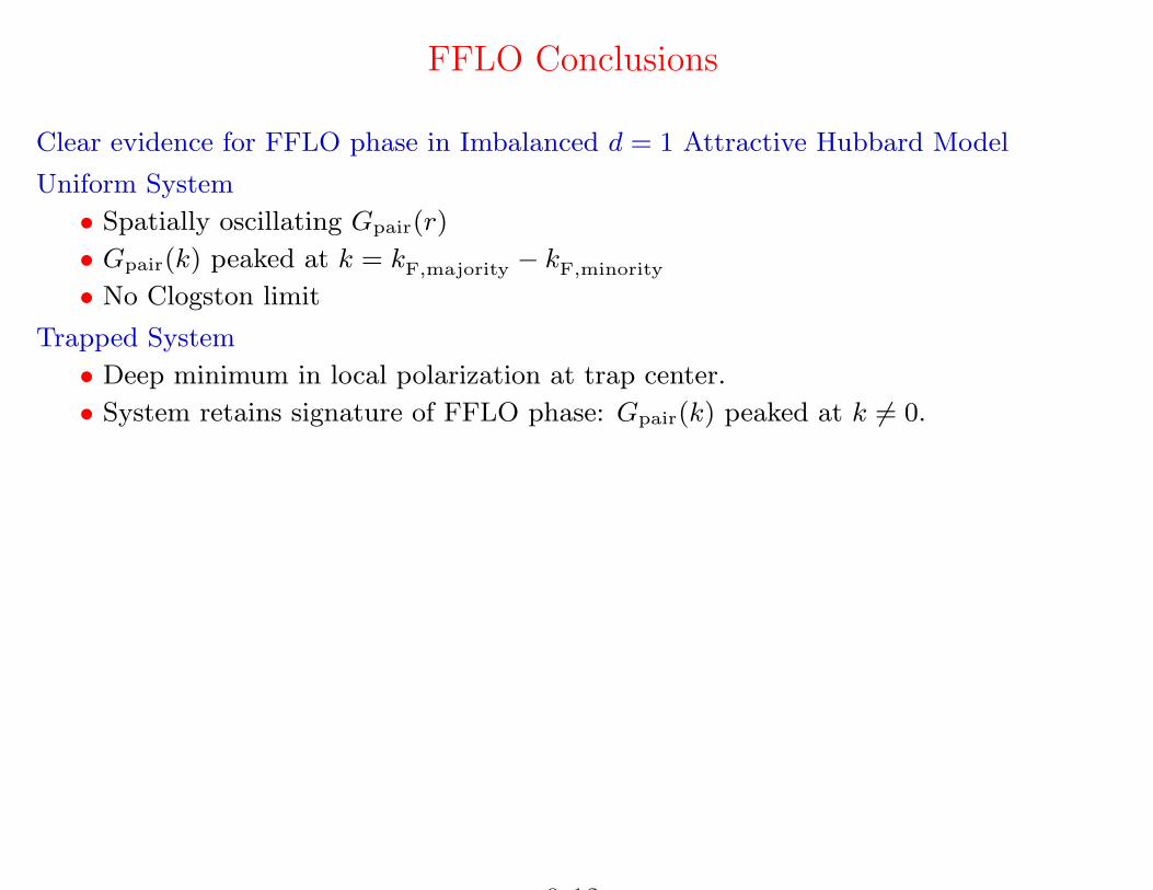
Conclusions
G.G. Batrouni, K. Bouadim (INLN); M.H. Huntley (MIT); V.G. Rousseau (Leiden)Z.J. Bai, S. Chiesa, C.N. Varney, R.T. Scalettar (UC Davis)C.R. Lee (NTHU Taiwan); M. Jarrell (LSU); T. Maier, E. D’Azevedo (ORNL)
Funding:ARO Award W911NF0710576 with funds from the DARPA OLE ProgramDOE SciDAC Program DOE-DE-FC0206ER25793
• Superfluid of Cooper pairs ( k ↑ , −k ↓ ) for k < kF, minority.coexists with normal fluid (of excess species).
• Pairs have zero momentum.
• Translationally invariant.
Fulde-Ferrell-Larkin-Ovchinnikov
• Pairs have non-zero momentum kF, majority − kF, minority.
• Spatially inhomogeneous.
• Hard to see in CM systems.
Cold Atom Systems
• Two hyperfine states play role of spin up and down.
• One complication is role of trapping potential.
0-1
FFLO Experimental Motivation - Solid State
Forty years after its theoretical discussion, FFLO phase observed.Heavy fermion system CeCoIn5.Requires very pure and strongly anisotropic single crystals.Apply large field parallel to conducting planes.
H.A. Radovan et al., Nature 425, 51 (2003).
0-2
FFLO Experimental Motivation - Cold Atoms
Fermion 6Li in hyperfine states F = 12, mF = ± 1
2.
Three dimensional, but highly elongated, traps.Tunable interaction strength via Feschbach resonance.Tunable relative mF = ± 1
2populations.
Core of system has uniform pairing (n1 − n2 = 0). Excess atoms sit at edge.G.B. Partridge et al., Science 311, 503 (2006).Also: M.W. Zwierlein et al., Science 311, 492 (2006); Nature 422, 54 (2006).
0-3
The Attractive Fermion Hubbard Hamiltonian
H = −tX
j,σ
(c†jσcj+1σ + c†j+1σcjσ) − |U |X
j
nj↑nj↓ + VT
X
j
j2(nj↑ + nj↓)
Operators c†iσ (ciσ) create (destroy) an electron of spin σ on site i.
Electron kinetic energy t; interaction energy U ; Quadratic confining potential VT .
Ut
Condensed matter: Two spin species σ =↑, ↓.Optically Trapped Atoms: Two hyperfine states “σ” = 1, 2.
Observables
Gσ(l) = 〈c†j+l σcj σ〉 Fourier transform : nσ(k)
Gpair(l) = 〈∆j+l∆†j〉 Fourier transform : npair(k)
∆j = cj2cj1
0-4
Algorithm
Continuous time canonical ‘worm’ algorithm (Rombouts, Van Houcke, Pollet).
No discretization of imaginary time (no ‘Trotter’ errors).
Constant particle number.
Broken world lines (‘worms’) are propagated.
Large moves through configuration space (short correlation times).
Can measure non-local Greens functions.
0-5
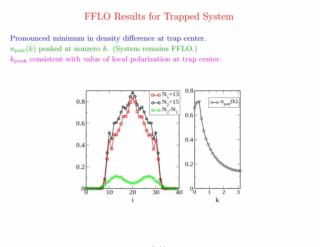
FFLO Results for Uniform System
Gσ(l) = 〈c†j+l σcj σ〉 Fourier transform : nσ(k)
Gpair(l) = 〈∆j+l∆†j〉 Fourier transform : npair(k)
∆j = cj2cj1
0 10 20 30|i-j|
0
0.1
Gpa
ir(|i-j|
) =
<∆i∆+ j>
N1=15, N2=15N1=15, N2=19N1=15, N2=23N1=15, N2=27
U = −8Gpair(l) oscillates as cos(qr) with q = kmajority − kminority consistent with LO.
0-6
Begin analysis of nσ(k) and npair(k) by examining unpolarized case
• Weak coupling: n1(k) = n2(k) is sharp.
• Strong coupling: n1(k) = n2(k) rounded.
• npair(k) peaked at k = 0. Peak sharpens with |U |.
0 1 2 3k
0
0.5
1
1.5
2
2.5
n1(k), U=-2npair(k), U=-2
n1(k), U=-4npair(k), U=-4
n1(k), U=-8npair(k), U=-8
L=32, N1= N2=15
0-7
Polarized case
npair(k) peaked at kmajority − kminority for all |U |.
Left panel: U = −4
Right panel: U = −10
Symbols: N1 = 7, N2 = 9, L = 32 sites, β = 64.
Lines: N1 = 21, N2 = 27, L = 96 sites, β = 192.
0 1k
0
0.2
0.4
0.6
0.8
1
1.2
0 1k
n1(k)n2(k)npair(k)
U=-4 U=-10
0-8
FFLO pairing no matter how large the polarization is made.
Have not seen “Clogston Limit”.Inset: Peak in npair(k) scales precisely as kF, majority − kF, minority.
dim(Mσ) is the number of spatial sites. For multi-band models
dimension is (number of spatial sites)x(number of orbitals per site).
0-16
• Sample HS field stochastically.
Si0τ0→ −Si0τ0
detMσ({Siτ}) → detMσ({Siτ}′)
Computation of new determinant is o(N3). Algorithm is order o(N4L) since NL HSvariables. Local nature of change in HS field: evaluate ratio of determinants in order N2
(“Sherman-Morrison” formula).
Algorithm is order N3L .N ∼ a hundred lattice sites/electronsL = β/∆τ ∼ a hundred imaginary time slices (low temperatures).
• Measurements
〈ciσc†jσ〉 ↔ 〈[M−1σ ]ij〉 = 〈[Gσ]ij〉
• Sign Problem
0-17
We have modernized our legacy DQMC codes
• Optimized linear algebra kernals
• “Delayed Updating” (Jarrell-Maier-D’Azevedo)
• N ∼ five hundred lattice sites/electrons (on a small cluster of workstations)
DOE SciDAC Program
0-18
Updated DQMC codes: Large lattices (N =24x24) allow for good momentum resolution.
U = 2 Fermi function:
ρ = 0.2
-π -π/2 0 π/2 π-π
-π/2
0
π/2
πρ = 0.4
-π/2 0 π/2 π
ρ = 0.6
-π/2 0 π/2 π
ρ = 0.8
-π/2 0 π/2 π 0
0.2
0.4
0.6
0.8
1
n(k)
ρ = 1.0
-π/2 0 π/2 π
U = 2 Gradient of Fermi function:
-π -π/2 0 π/2 π-π
-π/2
0
π/2
π
-π/2 0 π/2 π -π/2 0 π/2 π -π/2 0 π/2 π 0
0.5
1
1.5
2
2.5
∇ n
(k)
-π/2 0 π/2 π
0-19
Fermi surface is smeared further by increasing interaction strength.
U = 4 Fermi function:
ρ = 0.2 β = 8
-π -π/2 0 π/2 π-π
-π/2
0
π/2
πρ = 0.4 β = 8
-π/2 0 π/2 π
ρ = 0.6 β = 6
-π/2 0 π/2 π
ρ = 0.8 β = 4
-π/2 0 π/2 π 0
0.2
0.4
0.6
0.8
1
n(k)
ρ = 1.0 β = 8
-π/2 0 π/2 π
U = 4 Gradient of Fermi function:
-π -π/2 0 π/2 π-π
-π/2
0
π/2
π
-π/2 0 π/2 π -π/2 0 π/2 π -π/2 0 π/2 π 0
0.5
1
1.5
∇ n
(k)
-π/2 0 π/2 π
0-20
Optical Lattice Imaging of Fermi Surface
M. Kohl etal. Phys. Rev. Lett. 94, 080403 (2005).Fermionic 40K atoms
0-21
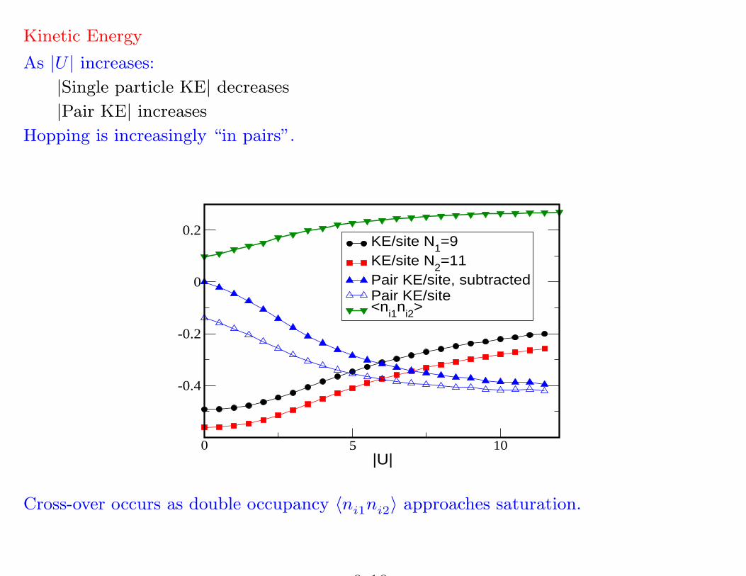
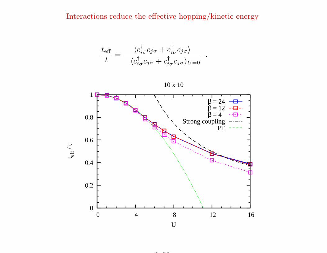
Interactions reduce the effective hopping/kinetic energy
tefft
=〈c†iσcjσ + c†iσcjσ〉
〈c†iσcjσ + c†iσcjσ〉U=0
.
0
0.2
0.4
0.6
0.8
1
0 4 8 12 16
t eff
/ t
U
10 x 10
β = 24β = 12β = 4
Strong couplingPT
0-22
Local moments form as U increases.
0.5
0.6
0.7
0.8
0.9
1
0 4 8 12 16
C(0
,0)
U
10 x 10
β = 24β = 12β = 4
0-23
Antiferromagnetic spin correlations form at low temperature.
βt = 20 → T = t/20 = W/160 (bandwidth W = 8t)
-0.15
-0.1
-0.05
0
0.05
0.1
(0,0) (10,0) (10,10) (0,0)
C(l
x,ly
)
20 x 20 U = 2.00
(0,0) (10,0)
(10,10)
(a)
β = 32β = 20β = 12
0-24
Antiferromagnetic correlations are well converged for N =20x20 lattices.
-0.2
-0.15
-0.1
-0.05
0
0.05
0.1
(0,0) (L/2,0) (L/2, L/2) (0,0)
C(l
x,ly
)
U = 2.00 β = 32
(0,0) (L/2,0)
(L/2, L/2)
24 x 2420 x 2016 x 1612 x 12
8 x 8
0-25
Increasing U enhances antiferromagnetic correlations
reaches asymptotic ground state value as β increases. Lower T is required for largerspatial lattices. Correlation length ξ(T ) must exceed linear size.
• In ordered phase S(π, π) grows with N .
0
2
4
6
8
10
12
14
4 8 12 16 20 24 28 32
S
b
U = 2.00
4 x 4 6 x 6 8 x 8
10 x 1012 x 1214 x 1416 x 1618 x 1820 x 20
0-27
Finite size scaling of AF structure factor
0
0.02
0.04
0.06
0.08
0.1
0.12
0.14
0 0.05 0.1
1 / L
U = 4.00 β = 24
(b)
(c)
S(π,π) / L2
C(L/2,L/2)
0-28
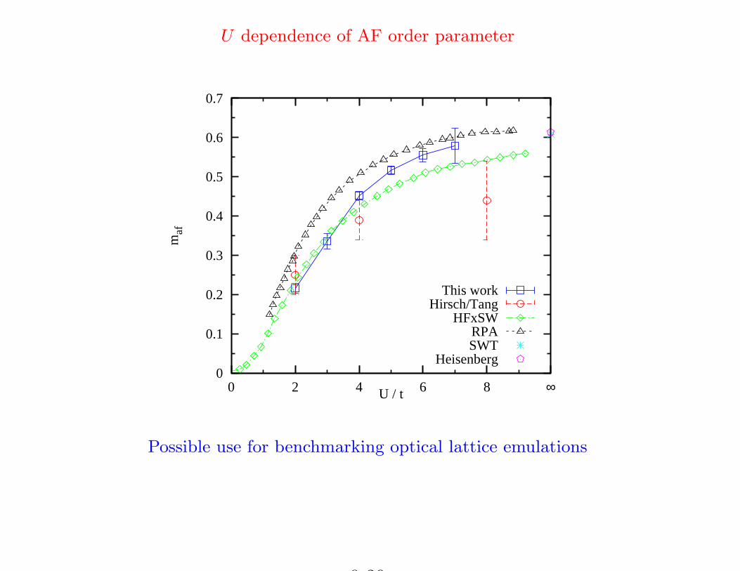
U dependence of AF order parameter
0
0.1
0.2
0.3
0.4
0.5
0.6
0.7
0 2 4 6 8 ∞
maf
U / t
This workHirsch/Tang
HFxSWRPASWT
Heisenberg
Possible use for benchmarking optical lattice emulations
0-29
III. Orbitally selective Mott Transitions
Multiple bands with different degree of electronic correlation, e.g.
• One band with U > UcMott
• Another with U > UcMott
What happens with interband hybridization or interactions?
H = −tX
〈ij〉σ
( c†iσcjσ + c†jσciσ ) − µX
i
(ni↑ + ni↓)
+X
i
h
JzSzi (ni↑ − ni↓) + J⊥( S+
i c†i↓ci↑ + S−i c†i↑ci↓ )
i
+ UX
i
(ni↑ −1
2)(ni↓ −
1
2)
Itinerant band (adjustable U) and a fully localized orbital (spin- 12
degrees of freedom)
OSMT: Is band metallic or localized?
0-30
Local Moment
DMFT (Costi) shows first order OSMT at Uc
Signaled by discontinuous jump in 〈S2z 〉
DQMC Results:
0 0.5 1 1.5 U
0.5
0.6
0.7
Sz2
β=10β=12β=14
0 0.5 1 1.5 U
J/U=0.1J/U=0.2J/U=0.4
J/U=0.2 β=14
0-31
Spectral Function
In same range of U values
• Temperature dependence of A(ω = 0) changes sign
• Gap opens in A(ω)
0 0.5 1 U
0
0.2
0.4
0.6
0.8
1
A(0
)
β=10β=12β=14
-4 -2 0 2 4 ω
0
0.2
0.4
U=0.50U=0.75U=1.00
J/U=0.2
J/U=0.2 β=14
0-32
Conductivity
Change in sign of dσ(T )/dT provides additional signal of MIT.
0 0.5 1 1.5 U
0
5
10
15
20
σ
β=10β=12β=14
0 0.5 1 1.5U
β=10β=12β=14
0 0.5 1 1.5U
β=10β=12β=14
J/U= 0.1 J/U= 0.2 J/U= 0.4
0-33
Scaling of AF Order Parameter
Change in transport at OSMT accompanied by a paramagnet-antiferromagnet transition.
0 0.05 0.1 0.15 0.2
N-1/2
0
0.05
0.1
0.15
0.2
Szz
(π,π
) / N
U=0.55U=0.5U=0.45U=0.4
0 0.05 0.1 0.15 0.2
N-1/2
0.05
0.1
0.15
0.2U=0.2U=0.25U=0.3U=0.35
J/U=0.2
J/U=0.4
β=20
0-34
Phase Diagram
Different measurements provide numerically consistent picture of OSMT
0 0.2 0.4 0.6 0.8J/U
0
0.5
1
1.5
2U
σdcA(ω=0)Szz(π,π)
Paramagnetic Metal
AFzz Insulator
0-35
CONCLUSIONS
• Observe FFLO Phase in Spin Polarized Attractive Hubbard Hamiltonian
• Large lattice (N ∼ 24x24) of half-filled Repulsive Hubbard Hamiltonian
→ Antiferromagnetic Order Parameter 〈m2af(U)〉
• Observation of OSMT in Two Orbital Repulsive Hubbard Hamiltonian
G.G. Batrouni, K. Bouadim (INLN)M.H. Huntley (MIT)V.G. Rousseau (Leiden)Z.J. Bai, S. Chiesa, C.N. Varney, R.T. Scalettar (UC Davis)C.R. Lee (NTHU Taiwan), M. Jarrell (LSU)T. Maier, E. D’Azevedo (ORNL)
Funding:ARO Award W911NF0710576 with funds from the DARPA OLE ProgramDOE SciDAC Program DOE-DE-FC0206ER25793