254
Recharge Estimation in the Surat Basin FINAL REPORT

Recharge Estimation
in the Surat Basin
FINAL REPORT

Recharge Estimation in the Surat Basin Page 1
Research Team
Lucy Reading1, Neil McIntyre1, Josh Larsen2, Nevenka Bulovic1, Abdollah Jarihani2, Long
Dinh1, Warren Finch1
1 Centre for Water in the Minerals Industry, Sustainable Minerals Institute, The University of
Queensland 2 School of Geography, Planning and Environmental Management, The University of
Queensland
Acknowledgements
This research was performed by the Centre for Water in the Minerals Industry (part of
Sustainable Minerals Institute) in collaboration with the School of Geography, Planning and
Environmental Management, on behalf of the Centre for Coal Seam Gas, The University of
Queensland.
The research team would like to acknowledge the kind assistance of the Project Industry
Partner Contacts: St.John Herbert (Arrow Energy Pty Ltd), Andrew Moser and Peter Evans
(APLNG), Lindsey Campbell and Patrick McKelvey (QGC), Dave Gornall (Santos), Linda
Foster and Mark Silburn (DNRM), and Sanjeev Pandey (formerly DNRM).
The research team would also like to acknowledge the following for their kind assistance and
helpful input in no particular order: Allison Hortle (CSIRO), Elad Dafny (USQ), Adrian Butler
(Imperial College London), Andrew Ireson (University of Saskatchewan), Ofer Dahan (Ben-
Gurion University of the Negev) and Jim Underschultz (CCSG).
Centre for Water in the Minerals Industry
Sustainable Minerals Institute
The University of Queensland, Australia
www.cwimi.uq.edu.au
Centre for Coal Seam Gas
Sustainable Minerals Institute
The University of Queensland, Australia

Recharge Estimation in the Surat Basin Page 2
www.ccsg.uq.edu.au
Centre for Coal Seam Gas
Disclosure
1. The UQ, Centre of Coal Seam Gas is currently funded by the University of Queensland 25%
($5 million) and the Industry members 75% ($15 million) over 5 years.
2. For more information about the Centre’s activities and governance see:
http://www.ccsg.uq.edu.au/AboutCCSG/FAQs
Disclaimer
The information, opinions and views expressed in this report do not necessarily represent those of the
University of Queensland, the UQ, Centre for Coal Seam Gas or its constituent members or
associated companies.
Researchers within or working with the Centre for Coal Seam Gas are bound by the same policies
and procedures as other researchers within The University of Queensland, which are designed to
ensure the integrity of research. You can view these policies at:
http://ppl.app.uq.edu.au/content/4.-research-and-research-training
The Australian Code for the Responsible Conduct of Research outlines expectations and
responsibilities of researchers to further ensure independent and rigorous investigations.
This report has not yet been independently peer reviewed.
ISBN: 978 1 74272 139 2

Recharge Estimation in the Surat Basin Page 3
Document Control Sheet
Project number: CLX 148323
Version # Reviewed by Revision Date Brief description of changes
1.0 Lucy Reading
Neil McIntyre
Jim Underschultz
2.0 Lucy Reading
Neil McIntyre
28.11.14 Incorporate feedback on version
1.0 from the project technical
group

Recharge Estimation in the Surat Basin Page 4
Executive Summary
The Recharge Estimation project aims to improve our understanding of spatial and temporal
distributions of groundwater recharge in the Surat Basin. Phase 1 of this project has brought
together existing relevant data sets and knowledge, developed new recharge estimates
particularly for the Surat Basin, provided a short-list of possible experimental sites and
conceptual models, and produced an outline of designs for potential field experiments at those
sites. These outcomes have been guided by industry partners and external experts at a series
of six project workshops and numerous separate meetings.
The outcomes of the project are presented in two separate reports. This report covers the
review and recharge estimation. The second report covers the field experiment design.
The objectives of this report are to provide:
1. A review of recharge estimation methods used globally
2. A review of previous recharge studies in the Surat
3. New recharge estimates based on analysis of existing data
4. Recommendations for further research based on identified knowledge gaps
A literature review of current techniques used globally was conducted to determine which
recharge estimation methods might be suitable for recharge estimation in the Surat Basin. Key
findings from the literature review were: 1. multiple methods should ideally be applied because
of the considerable uncertainty in any one approach, and 2. individual approaches are tailored
to a particular range of time and space scales. The review also concludes that extensive field
measurements are an essential part of developing models and achieving useful levels of
reliability in recharge estimates.
Recharge Estimation:
A number of recharge estimation methods have been applied in the Surat Basin prior to this
study, e.g. groundwater hydrograph analyses, groundwater chloride mass balance,
unsaturated zone chloride mass balance and soil water balance modelling. These previous
recharge estimates included a range of spatial scales but were typically limited to long term
averages with limited information about temporal variation.

Recharge Estimation in the Surat Basin Page 5
Analysis and interpretation of available data provided here examines this gap and has resulted
in new estimates of the spatial and temporal distribution of groundwater recharge in the Surat
Basin.
The regional groundwater flow directions in different aquifers were plotted by fitting
potentiometric surfaces to available borehole data. However due to various data limitations,
the potentiometric surfaces are only broadly indicative of regional groundwater flow paths and
require improvement. Higher quality and quantity of water level data is necessary with better
characterisation of source aquifers and borehole location.
The water table fluctuation method was applied to selected groundwater hydrographs
producing new estimates of groundwater recharge. Calculated annual average recharge rates
varied between 4 and 37 mm/year depending on location, but were restricted to a limited
number of bores with sufficient data and where aquifers are unconfined, water tables are
shallow, and pumping impacts are limited. If suitable locations are targeted for additional
groundwater monitoring, this method could easily be used to extend recharge rate estimation
further throughout the unconfined Main Range Volcanics and Walloon Coal Measures.
Analysis of surface water data was also used to quantify groundwater recharge. This is a
powerful method because it only requires streamflow records; however it has important
assumptions, including the need to assume that recharge appears as stream baseflow at the
outlet of the surface catchment. Annual average recharge rates using this method varied
between 0 and 3.2 mm/year.
There are a number of potential ways forward for the surface water analyses including
extending it to other parts of the Surat Basin, examining recharge on larger time scales such
as annual or seasonal, and applying alternative baseflow separation and recession analysis
methods.
Deep Drainage Estimation:
The combined remote sensing and modelling product from CSIRO, the Australian Water
Availability Project (http://www.csiro.au/awap/) gives regional deep drainage estimates at a 5
km grid resolution at monthly and annual timescales. The CSIRO data, supplemented with
additional remote sensed soil moisture data, were used to investigate the spatial and temporal
variability of recharge throughout the whole Surat and for separate geological units. For
Recharge Estimation in the Surat Basin Page 6
example, over the Walloon-Injune units, the annual average deep drainage rate ranged
between 2 and 34 mm/year; while across the Main Range Volcanics the rate varied between
1 and 105 mm/year. Averaging deep drainage over the whole of the Surat, the range changed
from 3 to 64 mm/year when moving from a particularly dry to a particularly wet year. Although
they provide the sought spatial and temporal resolutions, the CSIRO deep drainage estimates
are based on national scale water balance generalisations, only partially use the available
remote sensed data, and provide deep drainage rather than actual recharge rates. Hence
these data should not yet be assumed to be suitable for groundwater impacts assessment in
the Surat Basin, and further analysis and development is recommended.
Deep drainage within the Surat Basin as a whole was found to exhibit a high degree of spatial
variability, and areas of higher deep drainage are driven by a combination of higher
precipitation and /or soil and landscape properties.
The temporal distribution of deep drainage shows large variability around the long term mean
values. These results show the potential importance of including recharge as a time varying
input (at least annually varying) to groundwater models.
Summary:
Phase 1 of the Recharge Estimation project demonstrated some of the approaches that can
be used to generate improved estimates of recharge and deep drainage; and has developed
local and regional scale estimates using the most easily accessible existing data. However, to
date the local scale data analysed represent only small parts of the recharge areas, and do
not provide the process understanding needed to extrapolate these estimates across the key
Surat Basin recharge areas. Furthermore, Phase 1 has not included merging of local scale
and regional scale data. We therefore recommend that the project moves into Phases 2 and
3, which will develop new process understanding through field experiments that can be used
to calibrate local scale recharge estimates and finally extrapolate to regional scale products.

Recharge Estimation in the Surat Basin Page 7
Table of Contents
Table of Contents 7
List of Figures 11
List of Tables 14
1 Introduction 17
2 Literature Review 18
2.1 Recharge Estimation Methods 18
2.1.1 Empirical Approaches and Remote Sensing .................................................. 19
2.1.2 Groundwater Tracers ..................................................................................... 20
2.1.3 Surface Water Analysis Based Methods ........................................................ 20
2.1.4 Field and Point Scale Methods ...................................................................... 21
2.1.5 Water Balance Measurements ....................................................................... 23
2.1.6 Modelling Approaches ................................................................................... 24
2.1.7 Comparing Recharge Estimates .................................................................... 24
2.2 Recharge in the Surat Basin 28
2.2.1 Recharge Pathways and Mechanisms ........................................................... 33
2.2.2 Groundwater Recharge in the Surat – previous estimates ............................. 38
3 Recharge Estimation Using Analysis of Available Data - Introduction 48
4 Re-Analysis of Previous Deep Drainage Results 49
4.1 Assumptions 50
4.2 Methodology 50
4.3 Results 53
5 Analysis of Groundwater Potentiometric Surfaces 60
5.1 Introduction 60
5.2 Current Understanding of Groundwater Surfaces and Water Movement in the Great
Artesian and Surat Basins 60

Recharge Estimation in the Surat Basin Page 8
5.3 Data Availability and Data Processing Methods 66
5.3.1 Introduction to Data Sources .......................................................................... 66
5.3.2 Processing and Quality Control of Groundwater Database and Water
Monitoring Data Portal ........................................................................................................ 66
5.3.3 Gathering, Processing and Quality Control of Springs Data ........................... 68
5.3.4 Petroleum and CSG Well Completion Reports Data ...................................... 69
5.4 Water Level Dataset and Single Reading Pipes 74
5.4.1 Single Reading Pipes ..................................................................................... 77
5.4.2 Temporal Distribution of Data ........................................................................ 78
5.5 Groundwater Surfaces and Potential Movement of Groundwater 85
5.5.1 Groundwater Surface Interpolation Methods .................................................. 85
5.5.2 Groundwater Surface Models and Aquifer Flow Patterns ............................... 88
5.5.3 Uncertainties, Limitations and Difficulties ..................................................... 128
5.6 Conclusions and Recommendations 131
6 Analysis of Groundwater Hydrographs 132
6.1 Limitations and Assumptions 133
6.2 Methodology 134
6.3 Results 138
6.4 Discussion 141
6.5 Conclusions 142
7 Analysis of Remote Sensing Data 142
7.1 Introduction 142
7.2 Methods 143
7.3 Spatial Recharge Estimates 144
7.3.1 Whole Surat: Spatial average, wet and dry years ......................................... 144
7.3.2 Walloon Coal Measures & Injune Creek Group: Average, wet and dry years 151
7.3.3 Main Range Volcanics: Average, wet and dry years .................................... 158

Recharge Estimation in the Surat Basin Page 9
7.4 Temporal Recharge Estimates 164
7.5 Uncertainty 169
7.6 Soil Moisture Comparisons 169
7.7 Summary 171
7.7.1 Spatial variability .......................................................................................... 172
7.7.2 Temporal variability ...................................................................................... 172
7.7.3 Further investigation .................................................................................... 172
8 Analysis of Surface Water Hydrographs 173
8.1 Introduction 173
8.2 Estimating Groundwater Recharge – Study Area, Data and Methods 173
8.2.1 Storage – Discharge Theory and Method Formulation ................................. 174
8.2.2 Streamflow and Precipitation Data and Quality Control ................................ 175
8.2.3 Recession Plots and Storage – Discharge Relationships ............................. 181
8.2.4 Quantifying Annual Groundwater Recharge ................................................. 190
8.2.5 Sensitivity Analysis ...................................................................................... 191
8.3 Results 191
8.3.1 Storage – Discharge Relationships .............................................................. 191
8.3.2 Recharge Estimates ..................................................................................... 198
8.3.3 Sensitivity Analysis ...................................................................................... 204
8.4 Limitations, Future Research and Recommendations 207
9 Conclusions 209
10 Recommendations for further work on Recharge Estimation in the Surat Basin 213
References 214
Glossary 226
Appendices 227
Appendix 1 – Summary of available Research Outputs from Phase 1 228
Appendix 2 – Deep Drainage Results 231

Recharge Estimation in the Surat Basin Page 10
Appendix 3 – Water Table Fluctuation Analyses 246

Recharge Estimation in the Surat Basin Page 11
List of Figures
Figure 1 – Indicative scales for commonly applied recharge estimation methods (where UZ =
unsaturated zone). .............................................................................................................. 19
Figure 2 - Location of the Surat Basin, the "GAB intake beds" and the "primary recharge
areas" ................................................................................................................................. 32
Figure 3 - Surface water / groundwater interactions: Condamine and Balonne Rivers
(Parsons, Evans et al. 2008) ............................................................................................... 37
Figure 4 - Fitzroy Basin Modelled Deep Drainage ............................................................... 40
Figure 5 - Previous Deep Drainage Estimates (mm/yr) ....................................................... 41
Figure 6 - Recharge estimates using the chloride mass balance method (Ransley and
Smerdon, 2012) .................................................................................................................. 44
Figure 7 - Location of bores with water level data ............................................................... 49
Figure 8 - Atlas of Australian Soils ...................................................................................... 54
Figure 9 - Land Use Classifications in the QMDB ................................................................ 55
Figure 10 – Modelled Locations and Deep Drainage Zones ................................................ 57
Figure 11 - Deep Drainage Results (mm/year) .................................................................... 60
Figure 12 - Groundwater flow directions in the Cadna-owie Formation - Hooray Sandstone
aquifers (from Habermehl (2002)) ....................................................................................... 61
Figure 13 - Groundwater flow directions of the a) Mooga Sandstone, b) Gubberamunda
Sandstone, and c) Hutton Sandstone (after Quarantotto, 1989) .......................................... 61
Figure 14 – Groundwater contours and flow directions for the Hutton Sandstone from 1960
to 1970 (from Hodgkinson et al. (2010)) .............................................................................. 62
Figure 15 - Potentiometric surface of the Walloon Coal Measures (Source: Australia Pacific
LNG 2014) .......................................................................................................................... 63
Figure 16 - Groundwater surface of the Condamine River Alluvium in 2011 (from Dafny and
Silburn 2014) ...................................................................................................................... 65
Figure 17 - Map of all Queensland petroleum wells (QLD DNRM, 2014b), southern Qld
petroleum wells with data contained in PressurePlot, and lastly petroleum wells with no
pressure data reported in the WCRs. QLD DNRM material is licensed under a Creative
Commons - Attribution 3.0 Australia licence ........................................................................ 71
Figure 18 - Map of Queensland CSG exploration wells (QLD DNRM, 2014a). QLD DNRM
material is licensed under a Creative Commons - Attribution 3.0 Australia licence. ............. 73
Figure 19 - Project study area and location of all data points .............................................. 77
Figure 20 - Number of bores with water level readings for each geologic formation in annual
increments, between 1920 and 2014 .................................................................................. 81

Recharge Estimation in the Surat Basin Page 12
Figure 21 - Number of bores with water level readings in 10 year increments for each
geologic formation ............................................................................................................... 83
Figure 22 - Number of bores of each category for each geological formation with water level
data over different time periods relative to 2014 .................................................................. 85
Figure 23 - Scatterplot and correlation of mean water level elevation against elevation,
easting and northing for each geologic formation ................................................................ 92
Figure 24 - Groundwater surface contours (10 m) of the Condamine River Alluvium (1995 -
2014) by IDW interpolation, with yellow arrows indicating general flow directions. .............. 94
Figure 25 - Groundwater surface contours (10 m) of the Condamine River Alluvium (1995 -
2014) by universal kriging, with yellow arrows indicating general flow directions. ................ 96
Figure 26 - Groundwater surface contours (20 m) of the Gubberamunda Sandstone (1995 -
2014) by IDW interpolation, with yellow arrows indicating general flow directions. .............. 99
Figure 27 - Groundwater surface contours (20 m) of the Gubberamunda Sandstone (1995 -
2014) by ordinary kriging, with yellow arrows indicating general flow directions. ............... 101
Figure 28 - Groundwater surface contours (20 m) of the Hutton Sandstone (1995 - 2014) by
IDW interpolation, with yellow arrows indicating general flow directions. ........................... 104
Figure 29 - Groundwater surface contours (20 m) of the Hutton Sandstone (1995 - 2014) by
ordinary kriging, with yellow arrows indicating general flow directions ............................... 106
Figure 30 - Groundwater surface contours (20 m) of the Kumbarilla Beds (1995 - 2014) by
IDW interpolation, with yellow arrows indicating general flow directions. ........................... 109
Figure 31 - Groundwater surface contours (20 m) of the Kumbarilla Beds (1995 - 2014) by
ordinary kriging, with yellow arrows indicating general flow directions. .............................. 111
Figure 32 - Groundwater surface contours (40 m) of the Main Range Volcanics (1995 - 2014)
by IDW Interpolation, with yellow arrows indicating general flow directions. ...................... 114
Figure 33 - Groundwater surface contours (40 m) of the Main Range Volcanics (1995 - 2014)
by ordinary kriging, with yellow arrows indicating general flow directions. ......................... 116
Figure 34 - Groundwater surface contours (20 m) of the Mooga Sandstone (1995 - 2014) by
IDW Interpolation, with yellow arrows indicating general flow directions. ........................... 119
Figure 35 - - Groundwater surface contours (20 m) of the Mooga Sandstone (1995 - 2014)
by ordinary kriging, with yellow arrows indicating general flow directions. ......................... 121
Figure 36 - Groundwater surface contours (20 m) of the Walloon Coal Measures (1995 -
2014) by IDW Interpolation, with yellow arrows indicating general flow directions. ............ 125
Figure 37 - Groundwater surface contours (20 m) of the Walloon Coal Measures (1995 -
2014) by universal kriging, with yellow arrows indicating general flow directions. .............. 127
Figure 38. Water table fluctuation method (USGS, 2013) .................................................. 132
Figure 39 - Location of WTF bores close to Toowoomba .................................................. 137
Figure 40 - Average annual deep drainage estimates for the whole Surat CMA between
1900 – 2013 (data source: CSIRO AWAP 2014). .............................................................. 146

Recharge Estimation in the Surat Basin Page 13
Figure 41 - Average annual deep drainage estimates for the whole Surat CMA in an example
wet year – 2011 (data source: CSIRO AWAP 2014). ........................................................ 148
Figure 42 - Average annual deep drainage estimates for the whole Surat CMA in an example
dry year – 2006 (data source: CSIRO AWAP 2014). ......................................................... 150
Figure 43 - Average annual deep drainage estimates for the Walloon Coal Measures and
Injune Creek Group geologic units between 1900 – 2013 (data source: CSIRO AWAP 2014).
......................................................................................................................................... 153
Figure 44 - Average annual deep drainage estimates for the Walloon Coal Measures and
Injune Creek Group geologic units in an example wet year – 2011 (data source: CSIRO
AWAP 2014). .................................................................................................................... 155
Figure 45 - Average annual deep drainage estimates for the Walloon Coal Measures and
Injune Creek Group geologic units in an example dry year – 2006 (data source: CSIRO
AWAP 2014). .................................................................................................................... 157
Figure 46 - Average annual deep drainage estimates for the Main Range Volcanics (Basalts)
between 1900 – 2013 (data source: CSIRO AWAP 2014). ............................................... 160
Figure 47 - Average annual deep drainage estimates for the Main Range Volcanics (Basalts)
in an example wet year – 2011 (data source: CSIRO AWAP 2014). ................................. 162
Figure 48 - Average annual deep drainage estimates for the Main Range Volcanics (Basalts)
in an example dry year – 2006 (data source: CSIRO AWAP 2014). .................................. 164
Figure 49 - Time series of annual precipitation and deep drainage for the whole Surat CMA
as a spatial average for 1900 – 2014. ............................................................................... 165
Figure 50 - Time series of monthly precipitation and deep drainage for the whole Surat CMA
as a spatial average for 1900 – 2014. ............................................................................... 166
Figure 51 - Time series of monthly precipitation and deep drainage for the Walloon Coal
Measures – Injune Creek Group geological units as a spatial average for 1900 – 2014. ... 167
Figure 52 - Time series of monthly precipitation and deep drainage for the Main Range
Volcanics (Basalts) geological unit as a spatial average for 1900 – 2014. ......................... 168
Figure 53 - Monthly rainfall time series for the whole Surat CMA between 1995 – 2013,
highlighting the importance of ENSO induced wet and drought periods. ........................... 168
Figure 54 - Cumulative distribution of deep drainage in the Main Range Volcanics (Basalts)
and Walloon Coal Measures – Injune Creek Group geological units. ................................ 169
Figure 55 - Remote sensing soil moisture vs AWAP soil moisture, where soil moisture is
expressed as a percentage. .............................................................................................. 171
Figure 56 - Time series results for remote sensing soil moisture vs AWAP soil moisture,
where soil moisture is expressed as a percentage. ........................................................... 171
Figure 57 - Location of stream gauging stations used in storage-discharge analysis and
respective rainfall gauges. The location of all open and historical stream gauging stations
(QLD DNRM, 2014e, 2014f), and all rain gauges (BOM, 2014) is indicated. ..................... 178

Recharge Estimation in the Surat Basin Page 14
Figure 58 - Flow duration curves, normalised by catchment area, of the five stream gauging
stations ............................................................................................................................. 180
Figure 59 - Temporal distribution of stream flow and rainfall data for each stream gauging
station, with distribution of missing data also indicated (BOM, 2014; QLD DNRM, 2014f) . 183
Figure 60 - Daily streamflow (black line) and rainfall (grey bars) data from January 2010 to
August 2014 for Spring Creek (GS 422321B), with rainless periods used in recession
analysis highlighted in green and respective local flow peaks indicated by triangles.
Downwards facing rainfall data represent rainfall less than 1mm in magnitude, as all the data
are plotted on a lognormal scale. ...................................................................................... 188
Figure 61 - Schematic of how representative discharge values are extracted from
hydrograph to determine event-based recharge. A representative discharge is obtained
before (Qt) and after (Qt+1) each recharge event (Figure after Ajami et al. (2011)). ............ 190
Figure 62 - Recession plots for Spring Creek (GS 422321B) based on daily rainless stream
flow data. Black dots are binned data, error bars indicate standard error of each bin where
the standard error was less than half the mean of –dQ/dt for each bin. Both the equal interval
(left) and quantile (right) binning method were applied. ..................................................... 193
Figure 63 - Spring Creek quadratic regression models fitted to binned data (top) for both
equal interval (left) and quantile (right) binning methods, with model residuals depicted
below. ............................................................................................................................... 194
Figure 64 - Recession plots and model residuals of a) Swan Creek (GS 422306A), b) Emu
Creek (GS 422313B), and c) Condamine River (GS 422341A) ......................................... 197
Figure 65 - Time series of groundwater recharge estimates for each of the four streams.
Recharge is provided per water year (July - June), from July 1999 to June 2014. ............. 201
Figure 66 - Time series of percentage of rainfall resulting in groundwater recharge for each
of the four streams. Percentages are provided per water year (July - June), from July 1999 to
June 2014. ........................................................................................................................ 203
Figure 67 - Rainfall to water level rise method (Sy) ........................................................... 247
Figure 68 - All data bore RN 42220061 ............................................................................. 248
Figure 69 - 2005/2006 water year ..................................................................................... 249
Figure 70 - WTF method applied to 2005/2006 water year ................................................ 250
Figure 71 - 2004/2005 water year ..................................................................................... 251
Figure 72 - WTF method applied to 2004/2005 ................................................................. 252
List of Tables
Table 1 - Recharge estimation methods .............................................................................. 25
Table 2 - Previous Deep Drainage Studies ......................................................................... 42

Recharge Estimation in the Surat Basin Page 15
Table 3 - Previous recharge estimates ................................................................................ 45
Table 4 - Summary of Qualitative land use data reformatting .............................................. 51
Table 5 - Summary of available dataset for each geologic formation ................................... 74
Table 6 - Summary of available dataset for each geologic formation if the first water level
reading is removed. The final three columns indicate what proportion this dataset makes up
of the entire data (refer to Table 4). ..................................................................................... 77
Table 7 - Summary statistics of the water level elevation and water level depth of the
Condamine River Alluvium .................................................................................................. 89
Table 8 - Summary statistics of the water level elevation and water level depth of the
Gubberamunda Sandstone ................................................................................................. 96
Table 9 - Summary statistics of the water level elevation and water level depth of the Hutton
Sandstone ......................................................................................................................... 101
Table 10 - Summary statistics of the water level elevation and water level depth of the
Kumbarilla Beds ................................................................................................................ 107
Table 11 - Summary statistics of the water level elevation and water level depth of the Main
Range Volcanics ............................................................................................................... 112
Table 12 - Summary statistics of the water level elevation and water level depth of the
Mooga Sandstone ............................................................................................................. 117
Table 13 - Summary statistics of the water level elevation and water level depth of the
Walloon Coal Measures .................................................................................................... 122
Table 14 - Cross validation errors for each geologic formation for all kriged surfaces ....... 128
Table 15 - Specific Yield Values (Morris and Johnson, 1967) ............................................ 135
Table 16 - Specific yield values (Heath, 1983) .................................................................. 136
Table 17 - Groundwater bore information .......................................................................... 138
Table 18 - Annual recharge values .................................................................................... 139
Table 19 – General stream and gauging station information (QLD DNRM, 2014f) ............ 176
Table 20 - Stream gauging station data distribution, quantity and quality (QLD DNRM, 2014f)
......................................................................................................................................... 179
Table 21 - Information on rainfall gauge used for each stream gauging station (BOM, 2014)
......................................................................................................................................... 180
Table 22 - Peak discharge filter (cutoff) used in recession data extraction, and the number of
bins used in determining storage-discharge relationships. ................................................ 184
Table 23 - Assessment of the number of recession points lost due to missing rainfall data 191
Table 24 - Comparison of Spring Creek regression models for both equal interval and
quantile binning methods .................................................................................................. 193
Table 25 - Summary of the final storage – discharge functions used in estimating recharge
for each catchment ........................................................................................................... 198

Recharge Estimation in the Surat Basin Page 16
Table 26 - Summary statistics of annual recharge (mm/year) for each of the four streams.
Respective water year indicated in brackets where relevant. ............................................ 200
Table 27 - Summary statistics of the percentage of annual rainfall that results in recharge, for
each of the four streams. Respective water year indicated in brackets where relevant. .... 201
Table 28 - Summary of the different storage – discharge functions used in the sensitivity
analysis, and respective estimates of mean annual recharge over the last 15 years. Four
storage – discharge functions were derived for each stream for the sensitivity analysis. The
influence of different regression functions (linear/quadratic) and binning techniques (equal
interval/quantile) was investigated. Model 4 (quadratic regression function and quantile
binning method) was used to estimate final recharge within each stream catchment. ....... 205
Table 29 - Previous recharge estimates ............................................................................ 210
Table 30 - Recharge estimates from analysis of water table fluctuations, surface water
hydrographs, and the CSIRO Australian Water Availability Project data............................ 212
Table 31 - Drainage (mm/yr) matrix for Woodland ............................................................. 231
Table 32 - Drainage (mm/yr) for Buffel Grass Pasture ....................................................... 234
Table 33 - Drainage (mm/yr) for Summer Cropping .......................................................... 237
Table 34 - Average Drainage (mm/yr) for Woodlands ....................................................... 240
Table 35 - Average Drainage (mm/yr) for Buffel Grass Pasture ........................................ 242
Table 36 - Average Drainage (mm/yr) for Summer Cropping ............................................ 244

Recharge Estimation in the Surat Basin Page 17
Introduction
Groundwater modelling studies and aquifer water balances rely on an accurate determination
of recharge rates so that sustainable yields, potential impacts of extraction, and susceptibility
to change can be properly quantified. However, accurate determination of recharge is often
elusive because of complex flow paths and a lack of data available to inform processes or
constrain uncertainty.
Where there are potential aquifer impacts from activities such as CSG development, an
accurate knowledge of recharge rates in both space and time is critical for a reliable
assessment of this impact likelihood and an understanding of risk. Within the context of the
Surat Basin specifically, there is a need to develop improved knowledge about groundwater
recharge mechanisms and improved estimates of groundwater recharge rates because: 1)
The quantity and distribution of recharge across the basin are expected to influence
groundwater levels during CSG production as well as during the post-production recovery
period; 2) The quantity and distribution of recharge may influence the attribution of
groundwater pressure changes; 3) The current gaps in scientific knowledge limit the
robustness of current recharge models and estimates; and 4) Representation of recharge
varies widely between groundwater impacts assessment models.
The Recharge Estimation project aims to improve our understanding of spatial and temporal
distributions of groundwater recharge in the Surat Basin. Phase 1 of this project has brought
together existing relevant data sets and knowledge, developed new recharge estimates,
compiled a short-list of experimental sites and conceptual models, and designed field
experiments. Two reports have been produced from Phase 1. While this report focuses on the
literature review and development of new recharge estimates, the “Field Experimental Design”
report focuses on the short-listed experimental sites and proposed field measurements.
The objectives of this report are to provide:
1. A review of recharge estimation methods
2. A review of previous recharge studies in the Surat
3. A summary of testing of different recharge estimation methods based on analysis of
existing data
4. Recommendations for further research based on identified knowledge gaps

Recharge Estimation in the Surat Basin Page 18
Literature Review
Recharge Estimation Methods
Groundwater recharge is the flux of water that reaches the groundwater table (Bond, 1998).
This differs from “deep drainage” which is the downwards movement of water across the
bottom of the root zone.
Recharge can reach groundwater tables through a number of pathways. These pathways can
generally be categorised into “diffuse” recharge and “focussed” recharge. Whilst “diffuse”
recharge can potentially occur across the landscape, “focussed” recharge only occurs through
streams, cracks and other preferential flow pathways. Preferential flow encompasses a range
of hydrological processes such as macropore flow, funnelling and unstable flow fingering and
means that recharge can reach to deeper depths at greater speeds than would occur via
diffuse recharge alone (Cuthbert and Tindimugaya, 2010). Diffuse recharge is strongly
influenced by local vegetation and climate characteristics, which are largely dependent on
climate types (Barron et al., 2012).
In general, the most suitable approach to estimating groundwater recharge is to derive a
conceptual model for recharge processes first, then determine groundwater recharge using
one or more of several suitable methods (Scanlon et al., 2002). A suitable conceptual model
may include aspects of location, timing and likely unsaturated flow pathways. As part of the
development of a conceptual model, available hydrologic data including precipitation records,
stream-flow records and groundwater level records should be evaluated (Scanlon et al., 2002).
There are limitations to the well-established recharge estimation methods, most of which yield
results that are method and scale dependent (de Vries and Simmers, 2002). In cases where
recharge estimation is required for large, complex groundwater basins, it is therefore
appropriate to apply multiple estimation techniques including techniques that are applicable at
different scales (Delin et al., 2007). Complex processes such as preferential flow, which exert
a strong control on recharge are often not simulated in regional scale studies (Ordens et al.,
2014). Comparison of estimates from multiple methods can also provide information to test
hypotheses.

Recharge Estimation in the Surat Basin Page 19
The different scales at which recharge may be estimated range from point scale to regional
scale. Figure 1 lists approaches to recharge estimation methods and illustrates the scales over
which they are commonly applied.
Figure 1 – Indicative scales for commonly applied recharge estimation methods (where UZ =
unsaturated zone).
A brief description of the available recharge estimation methods is provided in Sections 0 to
0. Detailed descriptions of the applied recharge estimation methods are provided at the start
of Sections 6, 7 and 8.
Empirical Approaches and Remote Sensing
Commonly applied regional scale estimation approaches include empirical approaches and
remote-sensing based approaches. Empirical approaches involve taking local estimates of
recharge (using one of the other methods) and relating these estimates to easily observable
properties such as soil type and vegetation indices. These approaches have previously been
applied at the national scale (Crosbie et al., 2010), who developed empirical relationships for
use across Australia based on a dataset of field scale recharge estimates. . For global scale
estimation of recharge, a simple equation has been used to relate physical factors such as
hydrogeology, soil texture, precipitation intensity and relief to diffuse recharge rates (Doll and
Fiedler, 2008).

Recharge Estimation in the Surat Basin Page 20
Remote sensing has been a widely applied measurement tool within hydrology. Remote
sensing cannot directly measure groundwater recharge; instead the data must be able to
account for the other major elements in the water balance (evapotranspiration, surface runoff,
soil water storage, surface storage and precipitation) and recharge inferred from this (Becker
2006).
Groundwater Tracers
The chloride mass balance (CMB) approach is the most widely used technique for estimating
recharge (Scanlon et al., 2006). This approach has previously been applied for recharge
estimation at the regional scale using groundwater chloride and rainfall chloride data (Wood
and Sanford, 1995) but care needs to be taken with regards to interpolating between sparse
groundwater chloride measurements and combining groundwater chloride data from multiple
different aquifers. Some key assumptions of the chloride mass balance method are that: the
chloride in the groundwater originates only from precipitation and that there is no recycling or
concentration of chloride within the aquifer (Wood, 1999). As the groundwater chloride
concentrations represent chloride that may have accumulated over many years, the method
is typically used to give long-term average recharge rates rather than time distributions.
Remotely sensed data can be used to estimate the space and time distributions of recharge
(Brunner, 2004). These estimates can then be adjusted by calibration to more accurate but
lower resolution values of recharge, e.g. derived from the chloride method (Brunner, 2004).
In addition to the CMB method, there are a number of other groundwater chemical tracer
techniques (including isotopic techniques) that can be applied to estimate recharge rates.
Groundwater chemical methods for quantifying recharge can be divided into two broad
categories: methods which rely on mass balance of solutes to deduce information about the
magnitudes of recharge to the aquifer; and methods which seek to estimate the age or
residence time of the groundwater (Cook and Herczeg, 1998). All of these methods produce
long-term average estimates of recharge rates.
Surface Water Analysis Based Methods
There are also a number of recharge estimation methods that rely on surface water data and
are applied at either the river reach scale or the sub-catchment scale (Shanafield and Cook,

Recharge Estimation in the Surat Basin Page 21
2014). Streamflow differencing can be used to estimate transmission losses in perennial
streams (by measuring the difference between upstream and downstream flow while taking
into account other flow sources and sinks, including evaporation) (Shanafield and Cook,
2014).
Quantification of “mountain block recharge” has recently been achieved using recession flow
analysis (Ajami et al., 2011). The method relies on the application of catchment storage-
discharge relationships proposed by Kirchner (2009) and is based on certain assumptions,
such as low evapotranspiration (ET) rates during dry periods and perennial flow conditions at
the gauge, and that interflow and other catchment losses are negligible (Ajami et al., 2011).
Field and Point Scale Methods
Finally, there are a plethora of recharge estimation methods that can be applied at the field
scale to the point scale. These include lysimeters, unsaturated zone soil moisture
measurements, unsaturated zone tracers, groundwater hydrograph analyses and water
balance measurements and modelling.
Lysimetry can be used to make direct measurements of drainage and evapotranspiration
(Allison et al., 1994). Some of the problems associated with using lysimeters to determine
recharge are the expense of construction and maintenance, soil and vegetation disturbance,
modification of the bottom boundary condition relative to that prevailing in the open field and
the localized nature of the data obtained (Gee and Hillel, 1988). Recent studies have found
that passive wick lysimeters (where a wetted fibreglass wick acts as a hanging water column
that develops suction in the soil water depending on the flux) are capable of achieving minimal
disturbance to the native flow regime (Louie et al., 2000).
Unsaturated zone moisture monitoring traditionally involves the use of water content sensors,
such as time-domain reflectometry (TDR) probes and tensiometers for water-pressure
measurements (Dahan et al., 2009). Measurement of percolation of both water and
contaminants through deep unsaturated zones can be achieved by installing FTDR (flexible
time-domain reflectometry) probes and VSP (vadose zone sampling ports) into the upper
sidewall of an uncased small-diameter slanted borehole (Dahan et al., 2009). Downward flux
rates of water can then be determined by combining the calculated wetting-front propagation
velocity with the measured change in water content (Dahan et al., 2009).

Recharge Estimation in the Surat Basin Page 22
The natural tracers most commonly for unsaturated zone based recharge estimates are 3H,
14C, 36Cl, 15N, 18O, 2H, 13C and Cl (Allison et al., 1994). The mechanisms of infiltration will affect
the interpretation of results (so multiple tracers are required) (Allison et al., 1994).
The most common assumption applied in unsaturated zone tracer methods is that piston flow
is occurring, but there is mounting evidence that water movement along preferred pathways
is the rule rather than the exception (Allison et al., 1994). In cases where bypass flow occurs,
deep drainage rates are underestimated when using unsaturated zone tracer methods
(Ringrose-Voase and Nadelko, 2011).
In arid and semi-arid environments, desiccation cracks can make up a substantial proportion
of the soil’s volume, especially near the surface (Baram et al., 2012b). While it was previously
though that plowing and irrigation would prevent the development of crack networks and
promote matrix percolation through clay soils (Kurtzman and Scanlon, 2011), recent research
has found that naturally formed desiccation cracks can remain open year-round, even at high
sediment water contents (Baram et al., 2012b).
Evidence of preferred pathway flow has been presented recently through a vadose zone
monitoring study where major differences were detected in the solute concentrations between
the mobile flowing phase and the sediment profile (Rimon et al., 2011). Comparison of
recharge estimates from different methods can be used to help determine whether preferential
flow is occurring. For example, discrepancies between vadose zone based methods and
groundwater based methods can indicate the occurrence of preferential flow (Kurtzman and
Scanlon, 2011).
Analysis of groundwater hydrographs can be used to calculate recharge rates at the
groundwater table. A commonly applied method is the water-table fluctuation (WTF) method.
This method requires knowledge of specific yield and changes in water levels over time (Healy
and Cook, 2002). Advantages of this approach include its simplicity and an insensitivity to the
mechanism by which water moves through the unsaturated zone (Healy and Cook, 2002).
Recharge estimates derived using the WTF method can be assumed to represent an area of
at least several square meters around an observation bore (Healy and Cook, 2002).
Uncertainty in estimates generated by this method relate to the limited accuracy with which

Recharge Estimation in the Surat Basin Page 23
specific yield can be determined and to the extent to which assumptions inherent in the method
are valid (Healy and Cook, 2002).
There can be considerable variation in rates of recharge over the scale of a few meters (Allison
et al., 1994). For this reason, when point scale recharge estimation methods are applied,
multiple sampling locations are often required to capture the variability in groundwater
recharge.
Water Balance Measurements
Water balance measurements are implicit to some of the methods previously described, which
use various forms of measurement (remote sensing, groundwater levels, etc) to help close the
water balance and to determine the space and time distribution of the water balance. At
smaller scales, field experiments are often used to estimate recharge by directly measuring
all other components of the water balance. This direct approach reduces the chance of over-
or under-estimation (Lerner et al., 1990).
Mdaghri-Alaoui and Eugster (2001) measured the components of the water balance at an
experimental site to quantify recharge through a highly heterogeneous unsaturated zone.
Numerous other examples exist of field scale water balance measurements (Freeze and
Banner, 1970; Ireson et al., 2006; Lerner et al., 1990; Marshall et al., 2009; Rutter et al., 2014).
Any errors associated with estimating or measuring the individual components of the water
balance may reduce the accuracy of recharge estimates based on water balance
measurements (Herczeg and Love, 2007). The water balance approaches are therefore
ideally coupled with deep vadose zone percolation measurements and/or groundwater
hydrograph monitoring.
Field based water balance measurements can also be readily combined with recharge process
modelling. Rockhold et al. (2009) used field monitoring of the water balance at a waste
disposal field site to refine and improve recharge estimates from numerical simulations. The
approach used in this study encompassed lysimetry, water flux measurements (Gee et al.,
2002) and measurements of unsaturated zone water content and matric potential.
Recharge Estimation in the Surat Basin Page 24
The combination of field based measurements and process based modelling has recently
been applied for regional scale recharge estimation in China (Lu, Jin et al. 2011) and Denmark
(Andreasen et al., 2013). Lu et al. (2011) calibrated a 1D unsaturated flow model (HYDRUS-
1D) at five representative sites using field data of climate, soil moisture and groundwater
levels. While Andreasen et al. (2013) calibrated the 1D soil-vegetation-atmosphere transfer
model Daisy against soil moisture measurements from 30 stations and three depths.
Modelling Approaches
Unsaturated zone process models simulate the stores and fluxes of water at different levels
in the soil (and in some cases surface and interception stores and fluxes), driven by rainfall
inputs and evapotranspiration demands. The deep drainage estimates are the downward
fluxes from the bottom store.
Model types range from relatively simple soil moisture accounting models such as PERFECT
(Littleboy et al., 1989) and APSIM-SoilWat (McCown et al., 1996), where drainage is based
on simplistic storage-drainage approximations; to more complex physics-based models such
as HYDRUS (Simunek and van Genuchten, 2008), where pore water pressure is simulated
using soil water-pressure characteristic curves, and drainage rates are based on pressure
gradients.
The use of these models to estimate recharge requires an assumption about the pressure
gradient or the storage-discharge equation at the interface of the unsaturated and saturated
zone. Typically, it is assumed that there is no interaction and a ‘free drainage’ boundary
condition applies. An alternative method is the use of models which fully couple unsaturated
zone and saturated zone processes. This approach has been illustrated using several models
including HYDRUS-2D (Reading et al., 2010) and MIKESHE (Christiaens and Feyen, 2001).
Regional groundwater recharge can also be estimated using inverse numerical groundwater
modelling. However, during inverse modelling, recharge and hydraulic conductivity are
typically estimated (calibrated) simultaneously (Sanford, 2002). Independent measurements
of recharge rates are therefore required in order to constrain model calibration (Sanford,
2002).
Comparing Recharge Estimates

Recharge Estimation in the Surat Basin Page 25
There is value in directly comparing recharge estimates derived using different recharge
estimation methods. However, the assumptions and the relevant temporal and spatial scale
need to be kept in mind when comparing estimates derived from different recharge estimation
techniques. A brief summary of some of the limitations of different techniques (included those
related to scale) is provided in Table 1.
Inconsistencies in estimates derived from different recharge estimation methods may provide
insight into measurement errors or the validity of assumptions underlying a method and thus
may provide direction for revising the conceptual model (Healy and Scanlon, 2010). However,
many methods are applicable for estimating recharge that occurs via multiple recharge
mechanisms e.g. both diffuse and focussed recharge. One reason for inconsistencies in
estimates is that the quantity measured is different i.e. methods that estimate potential
recharge (or deep drainage) may give different recharge estimates from those methods that
estimate actual recharge (Crosbie et al., 2010).
Table 1 - Recharge estimation methods
Method
Description
Parameters required Main advantages Main limitations
Groundwater
hydrograph
analyses (“water
table fluctuation”
method)
Groundwater levels,
specific yield, rainfall and
groundwater pumping.
Can make use of
available groundwater
level data.
Additional monitoring is
cheap.
Recharge estimation at
the water table.
Requires knowledge of specific
yield and good water level
records.
Works at small scales but is
difficult to extend to larger
areas without extensive
monitoring systems.
Restricted by assumptions
regarding other influences on
groundwater levels.
Discharge-storage
relationships
Stream-flow time-series. Can make use of
available streamflow
data.
Provides a “lower bound”
recharge estimate /
estimates “net recharge”.
Assumes that baseflow
volumes equal recharge
volumes.
Limited to water sheds where
lateral fluxes, pumping, leakage
and water storage changes are
minimal.

Recharge Estimation in the Surat Basin Page 26
Lysimetry Deep drainage is directly
measured but data on
rainfall, irrigation and soil
hydraulic properties may
be useful in interpreting
lysimetry results.
Can provide accurate
data on deep drainage
and crop water use.
Lysimeters are expensive to
construct and are not
transportable.
Only provide point estimates of
deep drainage.
Soil hydraulic properties will be
disturbed during installation of
the lysimeter.
Unsaturated zone
moisture
measurements
Soil moisture content and
soil hydraulic properties.
Relatively simple
measurement techniques
can be used (unless
deep profiles are
monitored).
Requires data on both water
content and water pressure.
Only provides point estimates
of deep drainage (unless
monitoring extends to the water
table in which case, provides
point estimates of recharge).
Unsaturated zone
process models
Rainfall, irrigation, runoff,
climate variables for
calculating
evapotranspiration. Ideally
soil moisture and pressure.
For simple models, soil
“bucket” parameters need
to be calibrated or
estimated using
regionalisation.
For Richards’ equation
models, hydraulic
properties need to be
calibrated, estimated using
regionalisation or
laboratory or in-situ
experiments.
Can be applied
regionally when simple
(bucket-type) models are
used.
Where more complex
(e.g. Richards’ equation)
models are used, the
modelling may be too
computationally
demanding to use
regionally; but can be
used for local recharge
and to improve our
understanding of
recharge processes.
Can provide high
resolution recharge
estimates.
Requires knowledge of other
components of water balance
(some of these components
can have high uncertainty).
Limited by how well the chosen
model represents the physical
system.
Model parameter uncertainty
can be high.
Typically used to provide
estimates of deep drainage (but
can be used to provide
estimates of groundwater
recharge if the entire
unsaturated zone is simulated).
Water Balance
calculation using
remotely sensed
data
Remote sensing data can
be used to estimate:
Precipitation; near-surface
soil moisture;
evapotranspiration; land
cover; in some cases large
river flows and
groundwater levels.
Reasonable spatial and
temporal resolution;
near-global coverage.
Unknown uncertainty in
conversion of raw remote
sensing signals to hydrological
data.
Generally does not account for
deep unsaturated zone
changes in storage.

Recharge Estimation in the Surat Basin Page 27
Independent estimates of
surface flow are usually
needed.
Groundwater
modelling -
Calibration of
recharge
Geological model, aquifer
and aquitard hydraulic
properties, groundwater
levels, groundwater
pumping etc.
Can make use of existing
groundwater models.
Recharge is controlled by
hydraulic properties and
boundary conditions (therefore
non-unique).
Darcy’s Law (i.e.
relating the
groundwater flow
rate through a
cross-sectional
area of the aquifer
to the surface
area that
contributes to
recharge)
Hydraulic conductivity,
hydraulic gradient and
surface area for geological
formations of interest.
Potential to integrate
over large spatial scales.
This method suffers
significantly from reliable
estimates of hydraulic
conductivity.
Considering the natural
variation in hydraulic
conductivity and the difficulty in
scaling up regional values of
hydraulic conductivity, the
method at best would provide
order of magnitude estimates of
recharge.
Groundwater
chloride mass
balance
Chloride concentrations in
groundwater and rainfall.
Can make use of readily
available data (therefore
there is potential for
regional recharge
estimation using this
method).
Based on long term average
precipitation and chloride
concentrations in rain and
groundwater or soil water.
Assumes steady state
conditions (provides long term
average estimates of
recharge).
Groundwater age
dating
Tracer concentrations in
groundwater.
Not a direct measure of flux
(bounding fluxes must be
determined indirectly).
Assumptions relating to GW
flow paths and solute
sources/sinks.
Unsaturated zone
solute tracers
Solutes in rainfall, solutes
in the unsaturated zone.
Relatively cheap
(therefore it is possible to
make measurements at
multiple locations).
Only provide point estimates of
deep drainage.
Piston flow reduces the value
of this method.

Recharge Estimation in the Surat Basin Page 28
Water balance
measurements
As many components of
the water balance are
measured as possible (e.g.
rainfall, potential
evaporation, soil moisture,
groundwater levels,
surface water levels,
plant/tree water uptake).
Reduced reliance on
models and indirect
measurements.
The recharge rates are site
specific i.e. controlled by the
physical characteristics of the
site.
Recharge in the Surat Basin
The Great Artesian Basin is the largest confined groundwater basin within Australia, covering
the majority of Queensland and extending into New South Wales, South Australia and the
Northern Territory. The basin is made up of multiple layers of aquifers, predominantly
comprised of sandstone, which are interbedded by layers of mudstone and siltstone that
commonly act as aquitards (Habermehl, 1980). The basin is of a synclinal shape, with a
general tilt towards the southwest (Habermehl, 1980).
The Surat Basin is a structural sub-basin within the GAB. Due to the vast area of the Surat
Basin, covering an area of approximately 270,000 km2, many of the hydrological
characteristics are highly variable across the basin.
The Surat Basin sits within the “subtropical” climate zone. Average annual rainfall ranges from
500 mm/year in the west to 800 mm/year in the east. Potential evaporation rates greatly
exceed average annual rainfall (average annual open pan evaporation is greater than
1200mm/year). Rainfall is highly variable and seasonal within the basin with occasional
periods of high intensity rain and runoff alternating with extended periods of severe drought
and low stream flow (Preston et al., 2007).
The basin is roughly bounded to the north and east by the Great Dividing Range; however the
surface water catchments within the Surat Basin do not line up with the groundwater basin
boundaries. In fact, multiple surface water basins coincide with the Surat geological basin
(including the Fitzroy River Basin, the Condamine-Balonne River Basin, the Moonie River
Basin and the Border Rivers Basin). As a result, there are several surface water divides within
the Surat Basin.

Recharge Estimation in the Surat Basin Page 29
Due to the vast scale of the Surat Basin, multiple recharge mechanisms pathways may be
present. However, the majority of the recharge flux probably occurs within a small area along
the basin boundaries (Kellett et al., 2003). Within this broad context, groundwater recharge
processes in the Basin can be separated into 1) recharge to the shallow, unconfined alluvial
aquifers associated with the surface hydrology, and 2) the direct recharge to the aquifers of
the Great Artesian Basin (GAB).
Recharge pathways for 1) will occur as a direct hydraulic connection (permanent or temporary)
with river channels (Winter et al., 1998) and via the unsaturated zone of the wide expanse of
floodplain soils (diffuse recharge). Recharge pathways for 2) include preferential flow, diffuse
recharge and recharge via surface channels. The latter recharge pathways have traditionally
been considered to occur primarily within the extent of “GAB intake beds” (Figure 2), or
locations where the GAB aquifers outcrop and thus become exposed to the surface and
atmosphere. These intake beds are located at the margins of the GAB (Radke et al., 2000)
comprise a layered sequence of sandstone aquifers and interbedded mudstone confining
beds (Kellett et al., 2003) and have been mapped previously using a combination of
geological, geophysical and remote sensing methods (Bierwirth and Welsh, 2000).
The majority of the recharge in the GAB intake beds occurs following high intensity, short
duration rainfall events and is therefore likely to be associated with localised preferential flow
pathways (Habermehl, 2002; Kellett et al., 2003). However, a robust conceptual model
incorporating these pathways and surface interactions is yet to be developed.
Recent assessments by CSIRO (Herczeg and Love, 2007; Smerdon et al., 2012a) suggest
that there is also potential for recharge to occur to GAB aquifers outside of the GAB intake
beds. The Office for Groundwater Impact Assessment (OGIA) model also assumes that
recharge occurs outside of the GAB intake beds (to the “Primary Recharge Areas as shown
in Figure 2). There is therefore a clear research need to more conclusively demonstrate the
recharge processes and pathways to GAB aquifers, which will in turn allow a better
assessment of the relative contributions of recharge via the “GAB intake beds” versus
recharge outside of these beds.
There are very little data available to confirm whether “indirect” recharge to the GAB
formations is occurring via other geologic units. In addition to the uncertainty surrounding

Recharge Estimation in the Surat Basin Page 30
recharge locations and pathways, there is only limited information about the recharge rates
and the spatial variability of these rates.

Recharge Estimation in the Surat Basin Page 31

Recharge Estimation in the Surat Basin Page 32
Figure 2 - Location of the Surat Basin, the "GAB intake beds" and the "primary recharge
areas"

Recharge Estimation in the Surat Basin Page 33
Recharge Pathways and Mechanisms
Three separate pathways have been suggested for recharge to the GAB formations. These
are: recharge exclusively through the “GAB intake beds”, recharge through the Main Range
Volcanics and recharge through the unconfined alluvial aquifers.
Recharge through the “GAB intake beds”
The “GAB intake beds” coincide with the locations where the GAB formations outcrop. There
is some disagreement on which formations contribute significant recharge to the GAB. While
some definitions for the “intake beds” encompass both aquifers and aquitards e.g. Kellett et
al. (2003), others define the “intake beds” as consisting exclusively of GAB aquifers (Smerdon
and Ransley, 2012).
The “intake beds” were originally defined based on available geological mapping (Kellett et
al., 2003). It was hoped that delineation of the recharge beds could be improved using
remotely sensed data sets. In particular, it was hoped that differentiation could be made
between the low permeability materials and the higher permeability materials. However, data
from gamma-radiometrics surveys of the GAB “intake beds” did not appear to discriminate
between low permeability units and higher permeability units such as sandstones. It was
hypothesized that this may be due to weathering effects causing the potassium values to be
low for all units; alternatively, there may be errors within the geological mapping.
According to the Kellett et al. (2003) recharge estimation study, the formations included in the
intake beds within Queensland are: Bungil, Mooga, Gubberamunda, Hooray, Kumbarilla,
Ronlow, Gilbert, Southlands, Springbok, Adori, Hutton, Marburg, Boxvale, Precipice, Clematis
and Warang. The majority of these formations consist of fine to coarse quartzose sandstones
with limited information available about the presence or absence of fractures. Many of these
formations contain either interbedded mudstone and siltstone or kaolinitic clays infilling pore
spaces. The permeabilities of sandstone formations in the outcrop zones are expected to be
controlled in part by the presence of clays and carbonate minerals existing in certain horizons
(Arditto, 1983).
The hydraulic properties of the soils that overlie the outcrops may limit groundwater recharge
volumes or contribute to significant time lags between rainfall events and the occurrence of
recharge. The dominant soil types mapped within the intake beds are: Chromosol (loam),

Recharge Estimation in the Surat Basin Page 34
Sodosol (sandy loam), Tenosol and Rudosol (sand) with lessor amounts of Vertosol (clay),
Kandasol and Ferrosol. The range of clay percentages in the A horizon is approximately 5 to
60. Based on this information, the soils that overlie geological outcrops within the intake beds
would be expected to display wide ranging hydraulic properties.
Land use may also play a role in controlling groundwater recharge potential by altering
infiltration capacity and runoff occurrence and/or by consuming water that may otherwise have
been available for deep percolation and eventually groundwater recharge. Land uses that are
present within the GAB recharge beds include livestock grazing, semi-intensive agriculture,
production forestry and national parks (Kellett et al., 2003).
There is evidence that both diffuse recharge and preferential flow occur throughout the GAB
intake beds (Kellett et al., 2003). Preferential flow is likely to be the dominant recharge process
in the GAB intake beds (Kellett et al., 2003). Preferential flow pathways within the GAB intake
beds include creeks, cracks in clay soils and fractures in geological formations. There is
evidence from international studies that preferential flow can be responsible for up to 75% of
total recharge in fractured rock environments (Sukhija et al., 2003), however, the information
about the location and density of fractures within the GAB intake beds is very limited.
Rainfall of greater than 200 mm during a one month period was found to be necessary to
generate preferential flow as it was hypothesized that the unsaturated zone typically needs to
be saturated before preferential flow can occur (Kellett et al., 2003). Yet, recent studies have
shown that the unsaturated zone typically does not need to be saturated in order for
preferential flow to occur through cracking clay soils (Greve et al., 2010).
Desiccation cracks can serve as water conduits and preferentially transport water and solutes
into deep sections of the vadose zone during high rainfall events (Baram et al., 2012a).
However, preferential flow may also occur in between these high rainfall events as soil cracks
can remain pathways for preferential flow even when they are closed at the soil surface (Greve
et al., 2010).
Habermehl (2002) introduced the idea of “induced recharge” through GAB intake beds. He
claimed that: “abstraction by waterbores has caused a large scale lowering of the
potentiometric surface and a steepening of the hydraulic gradient, which allowed more
recharge water to enter the system.” There is currently some speculation regarding the

Recharge Estimation in the Surat Basin Page 35
possibility of this occurring in response to coal seam dewatering but the theory has not yet
undergone further investigation. The conditions that would be required in order for
depressurisation of the coal measures to induce increased recharge rates include: shallow,
highly permeable unsaturated zones or direct connection of groundwater with surface water.
These conditions are important because they could lead to a situation where recharge
processes are driven by the hydraulic gradient in the groundwater as well as unsaturated zone
properties and processes.
Recharge to GAB formations through the Main Range Volcanics
When developing a regional groundwater flow model for the Surat “Cumulative Management
Area”, the Office for Groundwater Impact Assessment (OGIA) identified the potential for
recharge to occur to the east of the previously mapped intake beds, through the Main Range
Volcanics. This is contrary to an assumption in Kellett (2003) that the basalt areas are unlikely
to contribute significantly to recharge due to associations between the basalts and “relatively
impermeable soils”. Yet, within the area underlain by the Main Range Volcanics, there are
actually a range of soil types present and even the least permeable of these soils have
previously been found to drain readily (Silburn et al., 2006).
The entire sequence of basalts within the Main Range Volcanics is intensely jointed with very
well developed vertical joints (Armstrong, 1974). The joints and weathered zones are of great
significance in the groundwater cycle since the basalt itself is extremely compact and
impervious (Armstrong, 1974). Beneath the hills there is a thick cover of soil and weathered
mantle below which vertical joints in the basalt form a network of narrow channels through
which recharge reaches the water table and makes a limited contribution to the storage
capacity (Armstrong, 1974). There is evidence that groundwater flow to the west within the
Main Range Volcanics is considerable (Armstrong, 1974).
There remains some debate, however, about the potential for recharge to the Main Range
Volcanics to flow into the GAB formations such as the Walloon Coal Measures. The Walloon
Coal Measures directly underlie the Main Range Volcanics and are exposed as fine grained
sandstone and shale, sometimes masked by shallow soils (Free, 1989). The Walloon Coal
Measures consist of grey mudstone, siltstone, fine-grained labile sandstone, coal seams and
minor limestone (Free, 1989).

Recharge Estimation in the Surat Basin Page 36
If the basalts hold groundwater directly above the Walloon Coal Measures and some hydraulic
connectivity exists, it is expected that groundwater would flow to the Walloon Coal Measures
if they are depressurised. Available groundwater level data suggest that there is potential for
groundwater flow from the basalts to the Walloon Coal Measures (see section 5 of this report).
In addition, there is geochemical evidence that groundwater recharge is occurring through the
basalts into the Walloon Coal Measures. While there is some variability in groundwater
composition within the Walloon Coal Measures, there is an area within the Walloon Coal
Measures that is geographically close to the Main Range Volcanics where the groundwater
composition is geochemically similar to groundwater in the Main Range Volcanics.
Recharge to GAB formations via unconfined alluvial aquifers
A recent study by Herczeg and Love (2007) into conceptual models of recharge in the GAB
concluded that recharge can occur where the GAB intake beds are exposed or are close to
the land surface, or anywhere in the unconfined parts of the GAB. Recharge to GAB
formations in central part of the Surat could only occur via vertical leakage in locations where
the predominant vertical hydraulic gradient is downwards rather than upwards. There is still
some debate about whether diffuse recharge through unconfined formations such as the
Condamine alluvium has the potential to be transmitted downwards to the GAB formations
(Hillier, 2010).
In order to assess the potential for focussed recharge to occur through stream beds (both
within the Condamine alluvium and throughout the Surat Basin), it is important to consider
previous studies into possible surface water – groundwater interactions in the Surat Basin.
Ransley et al. (2007) developed a new method to map potential hydraulic connection between
groundwater and river systems and evaluated this mapping method in the Border Rivers
catchment. This mapping method uses depth to water table as the basis for distinguishing
connected and disconnected streams and combines this information with information about
the hydraulic conductance of the geological material beneath the base of a river.
Parsons et al. (2008) conducted an assessment of surface-groundwater connectivity
throughout the Murray Darling Basin. The connectivity mapping involved determining the
direction and magnitude of groundwater flux to or from major rivers for a given point in time.
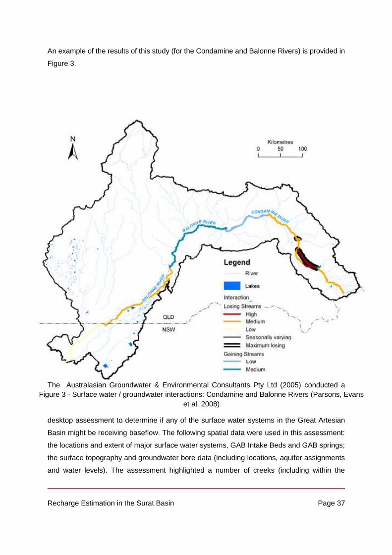
Recharge Estimation in the Surat Basin Page 37
An example of the results of this study (for the Condamine and Balonne Rivers) is provided in
Figure 3.
The Australasian Groundwater & Environmental Consultants Pty Ltd (2005) conducted a
desktop assessment to determine if any of the surface water systems in the Great Artesian
Basin might be receiving baseflow. The following spatial data were used in this assessment:
the locations and extent of major surface water systems, GAB Intake Beds and GAB springs;
the surface topography and groundwater bore data (including locations, aquifer assignments
and water levels). The assessment highlighted a number of creeks (including within the
Figure 3 - Surface water / groundwater interactions: Condamine and Balonne Rivers (Parsons, Evans
et al. 2008)

Recharge Estimation in the Surat Basin Page 38
Kumbarilla Beds, Hutton Sandstone and Hooray Sandstone outcrops) that may potentially be
receiving baseflow.
Groundwater Recharge in the Surat – previous estimates
Some of the recharge estimation methods identified in Section 2.1 have already been applied
in the Surat Basin. These methods have included groundwater hydrograph analyses,
groundwater chloride mass balance, unsaturated zone chloride mass balance and soil water
balance modelling. A summary of the relevant studies is provided below and a summary of
the recharge estimates produced is provided in Table 3 at the end of Section 2.
Groundwater Recharge in the GAB Intake Beds (Kellett, Ransley et al. 2003)
Kellett et al. (2003) calculated recharge rates within GAB intake beds along the eastern margin
of the GAB, with the exception of the intake beds in far north Queensland. Measurements
were focussed on the shallowest GAB aquifers that are intercepted by water bores, namely
the Hooray and Hutton Sandstones (Kellett et al., 2003). Groundwater recharge was assessed
using several methods including hydrograph analyses, chloride mass balance calculations,
radiocarbon dating of groundwater and stable isotope analyses.
Based on the hydrograph for a shallow observation bore in one of the sandstone formations,
the Mooga Sandstone, a recharge rate of 4-7 mm/year was calculated. The dynamic nature
of hydrographs for some of the bores within the GAB intake beds indicated that streambed
leakage to the underlying aquifers is an important recharge process (Kellett et al., 2003).
The chloride mass balance technique was used to determine the spatial distribution of long
term average recharge rates within the GAB intake beds. The recharge rates ranged from
<0.5 mm/year to >10 mm/year. The results of radiocarbon age dating of groundwater generally
supported the chloride mass balance results as older waters were detected in locations with
lower estimated recharge rates. From the results of stable isotope analyses for groundwater,
it was determined that significant recharge only occurs following high rainfall events, i.e. >200
mm within a one month period. Kellett et al. (2003) also identified a number of locations where
streams flow across GAB intake beds
Soil water balance modelling, soil chloride mass balance and lysimeter studies

Recharge Estimation in the Surat Basin Page 39
Outside of the GAB intake beds, deep drainage estimates have been made using the
PERFECT soil water balance model for the Queensland Murray Darling Basin (Yee Yet and
Silburn, 2003) and the Fitzroy Basin (Owens et al., 2007). These two surface water basins
cover more than 90% of the Surat and Bowen basins. In the Murray Darling Basin study, deep
drainage estimates were summarised using look-up tables of drainage for a range of soil, land
use and climate combinations. Estimates of average annual deep drainage for the Murray
Darling Basin study ranged from 1 mm/year to 455 mm/year (Yee Yet and Silburn, 2003). The
modelled deep drainage results for the Fitzroy Basin are shown in Figure 4. The estimates
that fall within the recharge estimation project “study area” ranged from close to 0 mm/year to
139 mm/year.
Chloride mass balance estimates of deep drainage were also conducted in the Murray Darling
Basin (Owens et al., 2004) and the Fitzroy Basin (Radford et al., 2009) to complement the
modelling studies.
Researchers working in the Murray Darling Basin have found compelling evidence (based on
transient chloride mass balance calculations) that deep drainage occurred despite heavy clay
soils and a semi-arid climate (Silburn et al., 2011). Deep drainage since clearing was
determined to be greater under cropping (mean 10 mm/year) than under pasture (mean 3
mm/year) or native vegetation (0.1-0.3 mm/year) (Silburn et al., 2011).
Starting in 2002, 27 non-weighing drainage barrel lysimeters were installed across nine
irrigated cropping sites in the Northing Darling Basin of QLD and NSW to monitor deep
drainage (Silburn and Montgomery, 2004). Deep drainage was measured under a range of
cotton and grain crops. Sites in Queensland included St. George, Macalister and Dalby.
The deep drainage estimates from a range of studies conducted between 2004 and 2011
(including soil Cl mass balance, lysimetry and soil water balance studies) have been compiled
in Figure 5. Details of the previous studies with their corresponding legends are in Table 2.

Recharge Estimation in the Surat Basin Page 40
Figure 4 - Fitzroy Basin Modelled Deep Drainage

Recharge Estimation in the Surat Basin Page 41
Figure 5 - Previous Deep Drainage Estimates (mm/yr)

Recharge Estimation in the Surat Basin Page 42
Table 2 - Previous Deep Drainage Studies
Literature Reference Method used
Corresponding legend
The Brigalow Catchment Study revisited: Effects of
land development on deep drainage determined
from non-steady chloride profiles (2009)
D.M. Silburn, B.A. Cowie, C.M. Thornton
Research station. Three
permanent monitoring sites (soil
profile used for deep drainage
and chloride mass analysis)
Soil monitoring JHYDROL
2009_Brigalow
Validating modelled deep drainage estimates for
the Queensland Murray-darling basin (2004)
J.S. Owens, P.E. Tolmie and D.M. Silburn
Water balance modelling at
Greenmount. Runoff and soil
erosion from previous model +
use of PERFECT
Water balance modelling
Greenmount ISCO2004
Soil chloride and deep drainage responses to land
clearing for cropping at seven sites in central
Queensland, northern Australia (2009)
B.J. Radford, D.M. Silburn, B.A. Forster
Soil sampling. Sites previously
used in the project ‘‘Sustainable
Farming Systems for Central
Queensland” in which data on soil
characteristics was collected.
Soil Samples
JHDROL2009_DeepDrainage
Deep drainage and soil salt loads in the
Queensland Murray–Darling Basin using soil
chloride: comparison of land uses (2011)
P. E. Tolmie, D. M. Silburn, and A. J. W. Biggs
Composited or averaged Cl
profiles were collected
Previous Cl, pH and EC data. Use
of past runoff studies and
cropping-tillage studies.
Soil Samples
SR2011_DeepDrainage_Tol
mie
Deep drainage rates of Grey Vertosols depend on
land use in semi-arid subtropical regions of
Queensland, Australia (2011)
D. M. Silburn,F, P. E. Tolmie, A. J. W. Biggs, J. P. M.
Whish, and V. French
Hydraulic soil coring rig was used.
Soil samples for chemical
analysis and soil water content
Soil Samples
SR2011_DeepDrainage_Silb
urn
Deep drainage through Vertosols in irrigated fields
measured with drainage lysimeters (2011)
T. A. Gunawardena, D. McGarry, J. B. Robinson, and
D. M. Silburn
Three drainage lysimeters per
site. One near each of the head
and tail ditches, and one at the
mid-point. All irrigated sites.
Lysimeters still there but no
longer monitored.
Lysimeter
SR2011_DD_irrigation

Recharge Estimation in the Surat Basin Page 43
Hodgson Creek, QMDB—salinity and recharge
studies and 2CSalt modelling (2006)
D.M. Silburn, J.S. Owens, S. Dutta, R.G. Cresswell, V.
McNeil
Recharge modelling. NRMW
bores and salinity study bores.
Measure of stream flow, salinity
and ionic chemistry.
Recharge modelling
QMDB_HodgsonCreek
CSIRO – groundwater chloride mass balance
The chloride mass balance method has been used recently to estimate recharge across the
intake beds as shown in Figure 6 (Ransley and Smerdon, 2012). This method was selected
as it allows recharge to be estimated over larger spatial scales and provides a smoothing
effect that dampens the annual variations in rainfall and chloride. Chloride concentrations in
rainfall were obtained from a recently constructed map of chloride deposition for Australia
(Davies and Crosbie, 2011) and chloride concentrations in groundwater were obtained from
the recharge studies by Kellett et al. (2003) and Habermehl et al. (2009). There may be
potential to apply this method to other geological formations, such as the Walloon Coal
Measures. However, our ability to apply this method to specific areas is limited by the
availability of groundwater chloride data and rainfall chloride data.
OGIA groundwater model
In the OGIA groundwater model, recharge was allowed to vary on a zonal basis during model
calibration i.e. different recharge rates were applied to different formation outcrops throughout
the Surat Basin (GHD, 2012). In most zones, recharge was allowed to vary between 1 and 30
mm/yr, based on maximum and minimum long-term average estimates reported by Kellett et
al. (2003) and an initial value of 15 mm/year was assumed. The assumed recharge rates for
aquifers were typically the same as for the aquitards.
However, it was expected that a significant proportion of the “recharge” assigned to aquitard
units would be rejected due to the limited capacity of these units to transmit water, hence the
“net recharge” is close to zero. The “net recharge” for each geological formation is equal to
water table recharge plus inflow from adjacent formations minus discharge to local shallow
groundwater systems (GHD, 2012). The total “net recharge” was estimated to be 125,267
ML/year (GHD, 2012). To provide some context to this figure, groundwater extractions for
agriculture, industry, urban, stock and domestic uses were estimated to be 215,000 ML/year
and over the life of the CSG industry, water extraction was predicted to average approximately
95,000 ML/year (QWC, 2012b).

Recharge Estimation in the Surat Basin Page 44
Figure 6 - Recharge estimates using the chloride mass balance method (Ransley and Smerdon,
2012)

Recharge Estimation in the Surat Basin Page 45
Table 3 - Previous recharge estimates
Method Used Spatial Scale Time
Period
Estimated
Recharge
Rate
(mm/year)
Reference
Groundwater
Hydrograph Analysis
Single bore in the
Mooga Sandstone
1993-
2001 4-7 (Kellett et al., 2003)
Groundwater Chloride
Mass Balance GAB intake beds N/A <0.5 - >10 (Kellett et al., 2003)
PERFECT Model Queensland Murray
Darling Basin
1900-
2001 1-455
(Yee Yet and
Silburn, 2003)
PERFECT Model Fitzroy Basin 1900-
2005 0-139*
(Owens et al.,
2007)
PERFECT Model Greenmount Site 1977-
1996 12
(Owens et al.,
2004)
Soil Chloride Mass
Balance Greenmount Site
1977-
1996 14 (Tolmie et al., 2004)
Soil Chloride Mass
Balance
13 cropped sites in the
Queensland Murray
Darling Basin
1985-
2001 2-16 (Tolmie et al., 2004)
Soil Chloride Mass
Balance
5 paired sites
(pasture/annual
cropping) in southern
Queensland
N/A 0.1-25 (Silburn et al.,
2011)
Lysimeters
7 irrigated sites in the
Queensland Murray
Darling Basin
2002-
2009 0-235
(Gunawardena et
al., 2011)
Groundwater Chloride
Mass Balance GAB intake beds N/A 0-79
(Ransley and
Smerdon, 2012)

Recharge Estimation in the Surat Basin Page 46
OGIA groundwater
model – calibrated “net
recharge”
Surat CMA N/A 0-5.2 (GHD, 2012)
*only recharge estimates for the portion of the Fitzroy Basin that coincides with the “Recharge Estimation Project Study Area” are reported here

Recharge Estimation in the Surat Basin Page 47

Recharge Estimation in the Surat Basin Page 48
Recharge Estimation Using Analysis of Available Data - Introduction
The boundary for the recharge estimation project was derived by extending the Surat
“Cumulative Management Area” boundary to include the “primary recharge areas” identified
by OGIA in their underground water impact report (QWC, 2012b) . The extended boundary is
shown in Figure 7. The data analyses that are described within the remainder of this report
include only data from within this “study area” boundary. Analysis of existing data was used to
improve our understanding of recharge processes and develop refined recharge estimates.
The methods used were:
1. Re-analysis of previous deep drainage results
2. Analysis of groundwater potentiometric surfaces
3. Analysis of groundwater hydrographs
4. Analysis of remote sensing data, principally the outputs of CSIRO’s Australian Water
Availability Project
5. Analysis of surface water hydrographs

Recharge Estimation in the Surat Basin Page 49
Figure 7 - Location of bores with water level data
Re-Analysis of Previous Deep Drainage Results

Recharge Estimation in the Surat Basin Page 50
Deep drainage estimates under a range of land uses in the Queensland Murray-Darling Basin
(QMDB) using water balance modelling, (Yee Yet and Silburn, 2003) is a study providing
estimates of drainage for a range of land uses, soils and locations in the QMDB (which QMDB
covers a large proportion of the recharge estimation study). Using soil moisture accounting
models GRASP and PERFECT, the study produced tables of deep drainage estimates but did
not map these results. Developing recharge maps using the tabulated data will act as a
baseline to compare alternative estimates.
Two types of pastures were modelled using GRASP: native pastures and improved pastures
(Yee Yet and Silburn, 2003). The PERFECT model was used to simulate the following
cropping systems (Yee Yet and Silburn, 2003):
1. “winter cropping” (wheat-fallow-wheat rotation)
2. “summer cropping” (sorghum-fallow-sorghum rotation)
3. “opportunity cropping” (automatic planting dates for wheat and sorghum rotations)
4. “irrigated cropping” (irrigated cotton, where ‘perfect irrigation’ i.e. no drainage during
irrigation is assumed).
Assumptions
During the development of the maps, the following assumptions were made:
1. Simplifications were used to translate available qualitative land use descriptions to the
land use categories used in the look-up tables (see Table 4)
1. Due to the lack of detailed soils mapping, an average value of deep drainage per land
use category, soil type and location was deemed adequate
2. As data were location specific, “drainage zones” were produced using modelled
locations and climate data.
Methodology
The three data sets used to translate the tables to maps were:
1. The Atlas of Australian Soils by CSIRO’s Australian Soil Resource Information System
(ASRIS) (Figure 8)
2. Land use mapping – Queensland 1999 by the Department of Natural Resources and
Mines (DNRM) (Figure 9) and

Recharge Estimation in the Surat Basin Page 51
3. The results from “Deep drainage estimates under a range of land uses in the QMDB
using water balance modelling” (Yee Yet and Silburn, 2003) (Appendix 2).
Several land use and soils descriptions available from the above sources were not consistent
with the descriptions used in the deep drainage look-up tables. The DNRM land use data were
reformatted into three of the land use categories used by Yee Yet and Silburn (2003). These
were: Woodlands, Buffel Grass Pasture and Irrigated Summer Cropping. Table 4 shows the
qualitative data conversion between DNRM land use mapping and land use categories used
by Yee Yet and Silburn (2003).
Table 4 - Summary of Qualitative land use data reformatting
Original categories used by Yee Yet and Silburn
(2003)
Corresponding categories on the DNRM
maps
Channel/aqueduct <void>*
Cropping Irrigated Summer Cropping
Grazing natural vegetation Buffel Grass Pasture
Intensive animal production Buffel Grass Pasture
Intensive horticulture Irrigated Summer Cropping
Irrigated cropping Irrigated Summer Cropping
Irrigated perennial horticulture Irrigated Summer Cropping
Irrigated plantation forestry Woodlands
Irrigated seasonal horticulture Irrigated Summer Cropping
Lake <void>
Manufacturing and industrial <void>
Marsh/wetland <void>
Mining <void>
Nature conservation Woodlands
Other minimal Use <void>

Recharge Estimation in the Surat Basin Page 52
Perennial horticulture Irrigated Summer Cropping
Plantation forestry Woodlands
Production forestry Woodlands
Reservoir/dam <void>
Residential <void>
River <void>
Seasonal horticulture Irrigated Summer Cropping
*<void> represents areas of the land use map which were excluded when assigning deep
drainage results spatially.
For soils, the CSIRO data allow for identification of general soil types using the Australian Soil
Classification (ASC) but the level of soil classification did not include soil colour. In contrast,
Yee Yet and Silburn (2003) simulated deep drainage for a specific soil type including colour
e.g. ‘black Dermosol’. Because of the lack of detail in the CSIRO soils maps, the Yee Yet and
Silburn (2003) data were averaged using general ASC soil types, e.g. the deep drainage rates
for black, brown and red Dermosols were averaged to estimate the deep drainage rate for
Dermosols. The tables provided in Appendix 2 are the deep drainage values reported by Yee
Yet and Silburn (2003) for specific locations, land use types and soil types.
Lastly, to assign the deep drainage value to a specific area, the 35 locations modelled by Yee
Yet and Silburn (2003) were used to produce “drainage zones”. The PERFECT modelling
generally relied on local climate data for each modelled location so the “drainage zones” were
designed to represent an area around each modelled location while taking into account spatial
trends in climate. The sizes of these “drainage zones” were therefore driven by the spacing
between modelled locations and information on the spatial variability of rainfall throughout the
QMDB. The zones can be seen in Figure 10. It is noted that the creation of these “drainage
zones” was based on judgement regarding the translation shown in Table 3 so a degree of
error is likely to be introduced using this approach. In particular, to improve the conversion
between the look-up tables and the new maps, it is recommended that maps of more specific
soil types are developed.

Recharge Estimation in the Surat Basin Page 53
Finally, these drainage zones, combined with land use and soils mapping were used to assign
the estimated deep drainage rates spatially.
Results
Figure 11 shows the long-term average deep drainage estimates in the QMDB part of the
Surat Cumulative study area derived from the Yee Yet and Silburn (2003) look-up tables. The
range of long-term average drainage values varies from 0 mm/yr to 455 mm/yr.

Recharge Estimation in the Surat Basin Page 54
Figure 8 - Atlas of Australian Soils

Recharge Estimation in the Surat Basin Page 55
Figure 9 - Land Use Classifications in the QMDB

Recharge Estimation in the Surat Basin Page 56

Recharge Estimation in the Surat Basin Page 57
Figure 10 – Modelled Locations and Deep Drainage Zones

Recharge Estimation in the Surat Basin Page 58

Recharge Estimation in the Surat Basin Page 59

Recharge Estimation in the Surat Basin Page 60
Figure 11 - Deep Drainage Results (mm/year)
Analysis of Groundwater Potentiometric Surfaces
Introduction
Groundwater potentiometric surfaces provide information on regional flow patterns within
hydrogeologic systems, and can be used to identify potential recharge areas. Comparison of
different groundwater surfaces can also provide information on the potential for groundwater
flow between aquifers if they are vertically connected. This chapter investigates regional
groundwater flow patterns of a number of younger geologic formations within the Surat CMA.
Due to the major limitations of currently available datasets identified during this study, this
chapter primarily demonstrates an approach for mapping regional groundwater flow patterns.
It also provides a critical analysis of the quantity and quality of available water level data and
its limitations. Preliminary results on groundwater flow patterns are presented, however these
potentiometric surfaces have low reliability primarily due to data quality.
This chapter is made up of five further sections. A literature review on the current
understanding of regional flow patterns within the Great Artesian Basin and Surat Basin is
provided in Section 0. Section 0 and Section 0 discuss the various data sources that were
used in producing groundwater potentiometric surfaces, the applied data processing
techniques and data availability. Section 0 provides information on how groundwater surfaces
were developed for the different geologic formations of the Surat Basin, the actual
groundwater surfaces and also a discussion on the assumptions and limitations of the data
and applied methods. Lastly, a conclusion and future recommendations are provided in
Section 0.
Current Understanding of Groundwater Surfaces and Water Movement in the Great Artesian
and Surat Basins
At the scale of the Great Artesian Basin, the dominant directions of groundwater flow are
towards the southern, southwestern, western and northern margins (Habermehl (2002),
Figure 12). Habermehl (1980) found potentiometric water levels in the confined portions of the
Lower Cretaceous-Jurassic aquifers varied from approximately 40 m AHD in the southwest up
to 400 m AHD in the east in the 1970s. Similar work has been carried out on the same aquifer

Recharge Estimation in the Surat Basin Page 61
(e.g. Audibert, 1976; Habermehl, 1980; Radke et al., 2000; Welsh, 2000) with a thorough
review available in Smerdon et al. (2012b). Most recently groundwater
Figure 12 - Groundwater flow directions in the Cadna-owie Formation - Hooray Sandstone
aquifers (from Habermehl (2002))
Figure 13 - Groundwater flow directions of the a) Mooga Sandstone, b) Gubberamunda Sandstone,
and c) Hutton Sandstone (after Quarantotto, 1989)
!.
!.
!.
!.
!.
!.!.
!.
!. !.
!.
!.
!.
!.
!.
ROMA
DALBYSURAT
MILES
MOURA
MOONIE
INJUNE
TAROOM
WANDOAN
THEODORE
ST GEORGE
ROLLESTON
CHINCHILLA
GOONDIWINDI
250
275
325
300
200
225
325
!.
!.
!.
!.
!.
!.!.
!.
!. !.
!.
!.
!.
!.
!.
ROMA
DALBYSURAT
MILES
MOURA
MOONIE
INJUNE
TAROOM
WANDOAN
THEODORE
ST GEORGE
ROLLESTON
CHINCHILLA
GOONDIWINDI
250
300
350
200
400
300
!.
!.
!.
!.
!.
!.!.
!.
!. !.
!.
!.
!.
!.
!.
ROMA
DALBYSURAT
MILES
MOURA
MOONIE
INJUNE
TAROOM
WANDOAN
THEODORE
ST GEORGE
ROLLESTON
CHINCHILLA
GOONDIWINDI
300
350
250
400
450
50
0
200
300
a) b) c)

Recharge Estimation in the Surat Basin Page 62
surfaces of the Cadna-owie Formation – Hooray Sandstone have been produced at 20 year
intervals, from 1900 to 2010, by Smerdon et al. (2012b).
Within the Surat Basin, located in the southeastern part of the Great Artesian Basin, the
dominant flow directions in the Cadna-owie Hooray Sandstone are south and west (Smerdon
et al., 2012b). Quarantotto (1989) investigated the groundwater surfaces of similar aquifers,
however interpreted them as discrete units rather than investigating them as a single lumped
system. Groundwater flow within the Gubberamunda Sandstone was found to be centripetal
from the northwestern and eastern margins, while flow in the Mooga Sandstone was
predominantly southerly (Figure 13). Flow directions within the Hutton Sandstone exhibited
more similarity to the flow lines of the Cadna-owie Hooray Sandstone (Figure 12; Figure 13),
with groundwater flow predominantly from northwest to south and east, with a secondary
northerly component also evident. A similar trend was reported by Hodgkinson et al. (2010)
and Australia Pacific LNG (2014) that further highlighted the significant components of flow in
the north and eastern directions (Figure 14).
Figure 14 – Groundwater contours and flow directions for the Hutton Sandstone from 1960
to 1970 (from Hodgkinson et al. (2010))

Recharge Estimation in the Surat Basin Page 63
Information on the groundwater surfaces of the other formations of interest from the
Cretaceous and Jurassic age is limited to the reports by Golder Associates (2009),
Schlumberger Water Services (2011), WorleyParsons (2012) and most recently Australia
Pacific LNG (2014). Groundwater flow in the Kumbarilla Beds is predominantly westwards,
radiating from a central highpoint of approximately 425 m (Schlumberger Water Services,
2011).
In the Walloon Coal Measures a general trend of water flowing westwards is present in both
the Golder Associates (2009) and Schlumberger Water Services (2011) reports, however
there is substantial dissimilarity between the two surfaces at a finer scale. Conversely,
WorleyParsons (2012) and Australia Pacific LNG (2014) reported an easterly and northerly
trend in groundwater flow in the northern parts of the basin around Taroom and Injune (Figure
15). Groundwater flows from the northwest to the south, southeast and east in the Springbok
Sandstone, with groundwater levels varying from approximately 200 to 450 m AHD (Australia
Pacific LNG, 2014; Golder Associates, 2009; Schlumberger Water Services, 2011).
Figure 15 - Potentiometric surface of the Walloon Coal Measures (Source: Australia Pacific
LNG 2014)
Recharge Estimation in the Surat Basin Page 64
No information on the groundwater surface of the Main Range Volcanics was found. However,
some further information on groundwater surfaces of other geologic formations in the Surat
Basin was available. This predominantly focused on the Precipice Sandstone (Hitchon and
Hays, 1971; Hodgkinson et al., 2010; Quarantotto, 1989) with less information available on
the Evergreen Formation (Hodgkinson et al., 2010). However, this information was not
included in this report as it did not address the target geologic formations.
Groundwater in the Condamine River Alluvium flows in a predominantly SE to NW direction,
following the same general direction of the Condamine River (Dafny and Silburn, 2014). A
secondary trend is present in a NE to SW direction, with water flowing from the neighbouring
aquifers to the east. Hydraulic sinks are present in the central-southerly portions of the
alluvium (east of the river), as a result of heavy development of the alluvium for agricultural
purposes. A generally similar trend of groundwater flow in a SE to NW direction with hydraulic
sinks was found by Schlumberger Water Services (2011). It should be noted that even though
the alluvium is generally conceptualised as one continuous aquifer, in some localised areas
there is evidence of perched aquifers where vertical hydraulic gradients are present (Dafny
and Silburn, 2014). However, the alluvium does act as a single system on the whole (QWC,
2012b) .

Recharge Estimation in the Surat Basin Page 65
Figure 16 - Groundwater surface of the Condamine River Alluvium in 2011 (from Dafny and
Silburn 2014)

Recharge Estimation in the Surat Basin Page 66
Data Availability and Data Processing Methods
Introduction to Data Sources
This Section presents a detailed description of the data that were used to develop the
groundwater level dataset into groundwater surfaces, and it also details the data processing
and quality control methods that were implemented.
All groundwater level data were obtained from:
1. Queensland Groundwater Database (up to 16 June 2014) (QLD DNRM, 2014b)
2. Queensland Water Monitoring Data Portal (up to 16 June 2014) (QLD DNRM, 2014d)
3. Variety of references on the springs of the Great Artesian Basin and Surat Basin
Processing and Quality Control of Groundwater Database and Water Monitoring Data Portal
Preliminary Bore Selection Technique
The Queensland Groundwater Database (GWDB) was interrogated and a preliminary subset
of data was identified based on the following:
1. Spatial extent – did the groundwater bore fall within the general vicinity of the study
area?
2. Did the groundwater bore have any water level readings recorded within the
‘WATER_LEVELS’ attribute table?
3. Did the groundwater bore have any aquifer/stratigraphy record with the ‘AQUIFER’ and
‘STRATIGRAPHY’ attribute tables?
4. Did the groundwater bore have casing attributes which were indicative of where
water would be entering the pipe? Only groundwater bores with a Material
Description of ‘OPEN’, ‘PERF’, ‘ENDD’ and ‘SCRN’ in the ‘CASING’ attribute table
were retained. This information would be used with aquifer and stratigraphy
information to associate source aquifer(s) to the bores with larger confidence.
Aquifer and Stratigraphy Pipe Association
A source aquifer was associated to a groundwater pipe primarily based on the GWDB
‘AQUIFER’ attribute table. Data from the ‘STRATIGRAPHY’ table were used to supplement
information on the rare occasions when a bore had no entry in the AQUIFER table. The

Recharge Estimation in the Surat Basin Page 67
following procedure was applied in associating a source aquifer to each of the groundwater
pipes:
1. A pipe was automatically associated to a source aquifer if only a single aquifer was
listed in the AQUIFER table for that RN;
2. If multiple aquifers were listed in the AQUIFER table for a specific RN, depth
information of the aquifer layers and pipe casing were cross-checked to identify the
accurate source aquifer(s);
3. A pipe was included in the final dataset if it only had a single aquifer as a water
source.
Once a final dataset of source aquifers to pipes was established, a quality control procedure
was implemented to check and correct the source aquifer nomenclature. This was necessary
to allow easy interrogation of the dataset, as there were general errors in data entry and also
discrepancies in the naming of aquifers.
Water Level Calculation
The majority of the water level data was obtained from the GWDB and this was supplemented
with additional and generally more recent data obtained from the Queensland Water
Monitoring Portal. Water level depth data from these databases were converted to water level
elevations with elevation data obtained from the ELEVATION table in the GWDB and also
from a 9 Second Digitial Elevation Model (DEM) of Australia (AUSLIG, 2001). Elevation data
were used from the ELEVATION table only in circumstances where there was confidence in
the data quality, namely the ‘Datum’ attribute had to be AHD (Australian Height Datum) and
the ‘Precision’ attribute was SVY (Surveyed). In all other circumstances elevations were
extracted from a DEM. On occasion, the reference ‘Measurement Point’ between water level
depths and elevations did not match. Accordingly, this reference was corrected by 0.5 m – the
‘common’ distance separating the top of a pipe from the natural elevation point. Lastly, a
subset of the data was made that only included the target geologic formations in this study,
namely the Condamine River Alluvium, Main Range Volcanics, Walloon Coal Measures,
Kumbarilla Beds, Hutton, Springbok, Mooga and Gubberamunda Sandstones. Aquifers
attributed as ‘Basalts’ that fell within the extent of the Main Range Volcanics were also taken
as a part of the Main Range Volcanics.
Hydrograph Quality Control

Recharge Estimation in the Surat Basin Page 68
All water level data taken for the geologic formations targeted in this study went through a
quality control process. First, water level data classified as ‘dry’ in the GWDB were removed
from the record. In addition, time series of the data records were visually inspected for each
pipe, and portions that had clear errors in data logging were discarded (e.g. portions of time
series where all readings were identical). The time series were also assessed for clear outliers
which were discarded. Some of the data obtained from the Qld Water Monitoring Portal that
were used to supplement the GWDB differed substantially from the rest of the time series for
that pipe. In all cases this data had no quality assurance from the Queensland Water
Monitoring Portal and as a result they were removed from the dataset.
In a limited number of circumstances, data were corrected where clear manual errors were
made in data entry and these could be adjusted with confidence. For example, one pipe had
some data entered without a ‘negative’. In another example, five pipes were identified in the
Main Range Volcanics with a similar time series pattern. Values of the hydraulic heads had
increased by approximately 400 m in less than a year across all pipes. Here an error with the
reference measurement point was identified and had to be manually corrected.
Gathering, Processing and Quality Control of Springs Data
A database of springs within the Surat Basin was compiled based off three principal sources:
QWC (2012b), QWC (2012a) and Wolhuter et al. (In review). Even though data from four
spring supergroups were considered, in the end only data on springs from the Springsure
Supergroup were included. Springs from the other three supergroups were either not within
the area of this study or had a source from a localised water system rather than being a
discharge spring of a basin scale aquifer (Fensham and Fairfax, 2003).
Only five springs sourced by the Hutton Sandstone were incorporated into the final water level
elevation dataset. Even though the size of the original database was substantially larger, the
majority of the springs were sourced from deeper formations such as the Precipice Sandstone,
had multiple aquifers attributed as potential sources, or were ‘recharge’ rather than ‘discharge’
springs. The water level elevations of the springs were also compared to the rest of the dataset
to identify discrepancies and potential presence of regolith rather than regional aquifer springs.
All data points that appeared to be outliers were removed. The final springs were assumed to
have a water level depth of 0 m, or a water level elevation equal to the natural elevation at that
point which was obtained from the 9 Second DEM of Australia (AUSLIG, 2001).

Recharge Estimation in the Surat Basin Page 69
Petroleum and CSG Well Completion Reports Data
Data obtained from petroleum well completion reports (WCR) within the Surat Basin were also
considered as a means of supplementing the GWDB and springs datasets. Hodgkinson et al.
(2010) used petroleum well pressure data to investigate groundwater flow patterns within
geologic formations after converting pressure data into equivalent hydraulic head values.
A repository in excess of 3000 Queensland petroleum well completion reports is available
through the Queensland Digital Exploration Reports system (QDEX) managed by the
Geological Survey of Queensland (Figure 17, QLD DNRM (2014c)), of which some has been
integrated into the PressurePlot database (CSIRO, 2007). The CSIRO has also compiled
information on WCRs not containing pressure data (Figure 17). Similar data are becoming
available with QDEX for CSG WCRs (Figure 18, QLD DNRM (2014a)). Data already compiled
into the PressurePlot database were interrogated and only 41 wells (predominantly in the
Hutton Sandstone) contained any relevant pressure data. Petroleum well pressure data were
not incorporated in this study due to limited data availability and the complexity of converting
and correcting pressure data to equivalent hydraulic heads. However, there is future potential
to expand the database, with the support of the CSIRO, and incorporate such data.

Recharge Estimation in the Surat Basin Page 70

Recharge Estimation in the Surat Basin Page 71
Figure 17 - Map of all Queensland petroleum wells (QLD DNRM, 2014b), southern Qld
petroleum wells with data contained in PressurePlot, and lastly petroleum wells with no
pressure data reported in the WCRs. QLD DNRM material is licensed under a Creative
Commons - Attribution 3.0 Australia licence

Recharge Estimation in the Surat Basin Page 72

Recharge Estimation in the Surat Basin Page 73
Figure 18 - Map of Queensland CSG exploration wells (QLD DNRM, 2014a). QLD DNRM
material is licensed under a Creative Commons - Attribution 3.0 Australia licence.

Recharge Estimation in the Surat Basin Page 74
Water Level Dataset and Single Reading Pipes
Initially, a general rudimentary analysis of the water level datasets for each geologic formation
was carried out. A summary of the data is presented in Table 5, which contains information
on the number of bores, pipes, springs and water level readings for each geologic formation,
and the dates the first and last water level readings were taken. The Main Range Volcanics
and Condamine River Alluvium have the largest datasets with over 1000 bores each (Table
5). Other than the Springbok Sandstone with a meagre 31 bores, the other geologic formations
have a reasonable number of bores, varying between 183 for the Gubberamunda Sandstone
and 469 for the Walloon Coal Measures. Springs data were only used to supplement the
Hutton Sandstone dataset.
The locations of these datasets are depicted in Figure 19. The Condamine River Alluvium and
Main Range Volcanics bores are all generally closely located on the eastern margins of the
basin. The Walloon Coal Measures bores are located in the same general area, however
appear to occur in two distinct spatial groups – west and east of the Great Dividing Range.
These are most likely associated with the Walloons of the Surat and Clarence-Morton Basins.
The bores of the Hutton, Mooga and Gubberamunda Sandstone are found further to the west
and north. These bores are also more sparsely distributed over larger areas of the Surat Basin,
with very few data points available in the southern and western sections of the basin.
Table 5 - Summary of available dataset for each geologic formation
Geologic Formation No. Bore No. Pipe No. WL No.
Sprgs Start Date End Date
Condamine River Alluvium 1 123 1 244 70 926 0 1/01/1932 15/06/2014
Gubberamunda Sandstone 183 185 6 486 0 10/04/1919 15/06/2014
Hutton Sandstone 328 330 28 416 5 16/05/1897 15/06/2014
Kumbarilla Beds 269 278 464 0 1/01/1927 6/02/2014
Main Range Volcanics 1 698 1 822 44 905 0 01/07/1946 15/06/2014
Mooga Sandstone 293 296 7 020 0 27/05/1918 15/06/2014
Springbok Sandstone 31 31 31 0 1/10/1948 11/08/2011
Walloon Coal Measures 469 478 4 370 0 1/05/1936 26/02/2014
Total 4 394 4 664 162 618 5

Recharge Estimation in the Surat Basin Page 75

Recharge Estimation in the Surat Basin Page 76

Recharge Estimation in the Surat Basin Page 77
Figure 19 - Project study area and location of all data points
Single Reading Pipes
The first value taken at a pipe is not always an accurate representation of water
levels/pressure of the geologic formation at that point. Depending on the physical attributes of
the geologic formation, it can take a longer time to reach hydrodynamic equilibrium, which
may not be captured by the first reading taken immediately after drilling. As a result, the
possibility of removing the first value for each pipe was investigated.
From the quality control process undertaken on water level data, it was found that the first
value was a clear outlier only on 11 occasions (equivalent to 1.9 percent out of a possible 569
pipes which had at least 3 water level readings each). Furthermore, the dataset is dominated
by single reading pipes. Removing the first value would result in the loss of more than 85
percent of all pipes (Table 6), with only the Condamine River Alluvium (255 bores) and Main
Range Volcanics (213 bores) geologic formation groups having adequately large datasets to
attempt groundwater surface modelling. The Walloon Coal Measures have the next largest
dataset of only 49 bores, while the Gubberamunda Sandstone has a meagre 14 bores.
Consequently, only first water level readings identified in the quality control process were
removed from the dataset. Pipes were categorised based on whether they are single
(Category 2) or multiple (Category 1) water level reading pipes.
Table 6 - Summary of available dataset for each geologic formation if the first water level
reading is removed. The final three columns indicate what proportion this dataset makes up
of the entire data (refer to Table 4).
Geologic
Formation
No. of
Bores
No. of
Pipes
No. of
Water L Start Date End Date % Bore % Pipe % WL
Condamine River
Alluvium 255 286 69 682 29/08/1962 15/06/2014 22.71 22.99 98.25
Gubberamunda
Sandstone 14 14 6 301 23/03/1928 15/06/2014 7.65 7.57 97.15
Hutton Sandstone 26 26 28 086 10/03/1960 15/06/2014 7.93 7.88 98.84
Kumbarilla Beds 31 31 186 21/01/1976 6/02/2014 11.52 11.15 40.09

Recharge Estimation in the Surat Basin Page 78
Main Range
Volcanics 213 242 43 083 29/09/1959 15/06/2014 12.54 13.28 95.94
Mooga Sandstone 32 32 6 724 10/02/1958 15/06/2014 10.92 10.81 95.78
Springbok
Sandstone 0 0 0 NA NA 0.00 0.00 0.00
Walloon Coal
Measures 49 49 3 892 22/08/1963 26/02/2014 10.45 10.25 89.06
Total 620 680 157 954 14.11 14.58 97.13
Temporal Distribution of Data
Due to the importance of temporal variability in water levels, the temporal distribution of data
was examined to gain a better general understanding of the data collection periods of
individual geologic formations, and identify suitable time periods for which groundwater
surfaces of the various geologic formations could be modelled. The numbers of bores with
water level data were calculated for a number of different time periods and temporal ‘windows’.
Figure 20 and Figure 21 show the temporal distribution of the number of bores with water level
readings for one year and ten year periods, starting from 1920.
The dominant data collection periods for the Kumbarilla Beds, Gubberamunda, Hutton and
Mooga Sandstones were between 1950 and 1980, with the number of bores being monitored
greatly reduced in the more recent decades. However, even through the more intensive
monitoring periods, the number of bores being monitored is still rather limited. Generally less
than ten bores were monitored in a year per formation, with the maximum number of 22 bores
monitored in a year in the Hutton Sandstone (Figure 20). The Condamine River Alluvium, Main
Range Volcanics and Walloon Coal Measures had the largest numbers of bores monitored in
the 1970s (Figure 21). Currently, these are the formations with the largest number of
monitored bores, of which majority are Category 1. The Condamine River Alluvium is the best
monitored of all the aquifers, with between 100 and 150 bores monitored yearly over the last
few decades (Figure 20). Approximately 75 Category 1 bores are monitored annually in the
Main Range Volcanics, while in the last decade this number has varied between 20 to 40
bores in the Walloon Coal Measures.
In selecting a representative time period for the groundwater surface modelling of the various
geologic formations, a number of factors were taken into account:

Recharge Estimation in the Surat Basin Page 79
1. Using recent groundwater level data to have groundwater surfaces that are currently
representative
2. Finding a balance between reducing temporal variability in data to prevent false trends
(short temporal periods), and the need for larger datasets with greater spatial coverage
(longer temporal periods)
3. Selecting the same temporal period for all the geologic formations to provide a
consistent basis for comparison.
To account for the three points listed above, a moving window analysis was performed where
the numbers of bores with water level data were calculated for different time periods (Figure
22). The time period calculations were carried out for 1, 2, 5 and then in five-year

Recharge Estimation in the Surat Basin Page 80

Recharge Estimation in the Surat Basin Page 81
Figure 20 - Number of bores with water level readings for each geologic formation in annual
increments, between 1920 and 2014

Recharge Estimation in the Surat Basin Page 82

Recharge Estimation in the Surat Basin Page 83
Figure 21 - Number of bores with water level readings in 10 year increments for each
geologic formation

Recharge Estimation in the Surat Basin Page 84
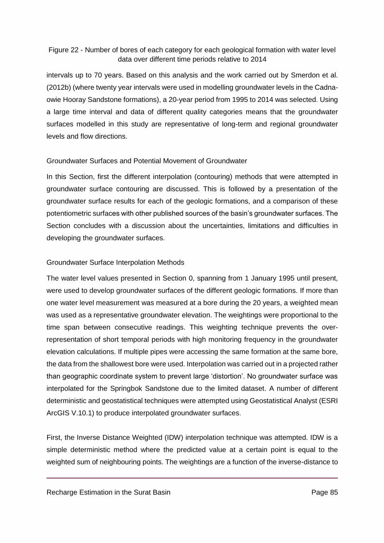
Recharge Estimation in the Surat Basin Page 85
Figure 22 - Number of bores of each category for each geological formation with water level
data over different time periods relative to 2014
intervals up to 70 years. Based on this analysis and the work carried out by Smerdon et al.
(2012b) (where twenty year intervals were used in modelling groundwater levels in the Cadna-
owie Hooray Sandstone formations), a 20-year period from 1995 to 2014 was selected. Using
a large time interval and data of different quality categories means that the groundwater
surfaces modelled in this study are representative of long-term and regional groundwater
levels and flow directions.
Groundwater Surfaces and Potential Movement of Groundwater
In this Section, first the different interpolation (contouring) methods that were attempted in
groundwater surface contouring are discussed. This is followed by a presentation of the
groundwater surface results for each of the geologic formations, and a comparison of these
potentiometric surfaces with other published sources of the basin’s groundwater surfaces. The
Section concludes with a discussion about the uncertainties, limitations and difficulties in
developing the groundwater surfaces.
Groundwater Surface Interpolation Methods
The water level values presented in Section 0, spanning from 1 January 1995 until present,
were used to develop groundwater surfaces of the different geologic formations. If more than
one water level measurement was measured at a bore during the 20 years, a weighted mean
was used as a representative groundwater elevation. The weightings were proportional to the
time span between consecutive readings. This weighting technique prevents the over-
representation of short temporal periods with high monitoring frequency in the groundwater
elevation calculations. If multiple pipes were accessing the same formation at the same bore,
the data from the shallowest bore were used. Interpolation was carried out in a projected rather
than geographic coordinate system to prevent large ‘distortion’. No groundwater surface was
interpolated for the Springbok Sandstone due to the limited dataset. A number of different
deterministic and geostatistical techniques were attempted using Geostatistical Analyst (ESRI
ArcGIS V.10.1) to produce interpolated groundwater surfaces.
First, the Inverse Distance Weighted (IDW) interpolation technique was attempted. IDW is a
simple deterministic method where the predicted value at a certain point is equal to the
weighted sum of neighbouring points. The weightings are a function of the inverse-distance to

Recharge Estimation in the Surat Basin Page 86
a defined power between the target and known point, where the higher the power the larger
the weighting to nearby points. The same power value is assumed within a sampling
neighbourhood. The IDW interpolation technique is an exact interpolator, and all interpolated
values are in the range of the dataset, i.e. no interpolated values can be smaller than the
smallest data point or larger than the largest. A distinction of IDW interpolated surfaces is the
presence of cone-like features (or bulls-eyes) at data locations due to the large weighting
towards these points.
The Geostatistical Analyst tab (ESRI ArcGIS) was used. This tool allows the influence of the
power value and neighbourhood assumptions to be evaluated both graphically and
quantitatively. Neighbourhood characteristics (number, direction of points or search radius)
can be adjusted so that unique subsets of the population meeting these parameters are used
in interpolation. Using a subset of the data points instead of the entire population can result in
improved interpolation because of increased similarity between spatially closer points. The
‘Optimise’ tool identifies the optimal power value for that sampling neighbourhood. Various
neighbourhood sizes and neighbourhood directions were tested to identify the best-fitting
groundwater surface model.
The second interpolation technique that was implemented was kriging - a commonly used
geostatistical interpolation method essentially based on least-squares regression. Kriging
interpolation methods are commonly described as ‘best linear unbiased estimator’ (BLUE)
(Isaacs and Srivastava 1989), because they are linear interpolators that minimise the error
variances of the predicted variable. Kriging interpolation methods not only produce a surface
of predictions of the variable, but also a surface of standard errors of each prediction point.
There are several variations of kriging (e.g. Goovaerts, 1997; Isaaks and Srivastava, 1989;
Wackernagel, 2003).
Kriging estimates unknown values at specific locations in a similar manner to IDW. However,
a major difference between the two methods is in the way that weightings to neighbouring
points are determined. Unlike IDW methods, which determine weightings purely based on the
inverse distance between points, kriging applies statistical methods that incorporate the spatial
autocorrelation between sample points, which is usually estimated as a function of the
distance between points and the direction of the line joining the points in the case of
anisotropy. Weightings are determined in such a way to ensure minimum error variances of
the predicted values are achieved. The modelling of the semivariogram (spatial
Recharge Estimation in the Surat Basin Page 87
autocorrelation model) is the most difficult aspect of kriging, with Kitanidis (1997) describing it
as more of an art than a science. Furthermore, kriging methods are better suited to normally
distributed data. They can still be applied to other data distributions for predictions but with
less meaning attached to predicted quantiles.
In this study, two main approaches were implemented depending on the geologic formation,
namely ordinary and universal kriging. A requirement of ordinary kriging is second order
stationarity, which is not met by data that exhibit strong spatial trends. In the instance of the
Condamine River Alluvium and Walloon Coal Measures, strong spatial trends were evident
both in a northerly and easterly direction (Figure 23) and as such universal kriging was applied,
which incorporates a spatial trend model. Ordinary kriging was used on the other geologic
formations where no evident spatial trend in groundwater elevation data was present (Figure
23). The Geostatistical Analyst tab (ESRI ArcGIS) was also utilised for kriging interpolations.
Various semivariogram models, semivariogram parameters and prediction search
neighbourhoods were tested to find a suitable semivariogram model that produced reasonable
groundwater surfaces.
A commonly used model validation technique, known as cross-validation, was used to assess
the accuracy/suitability of the different groundwater surfaces obtained. The cross-validation
process involves removing a known data point and using all other data points to predict the
value. This is repeated for all data points, and the cross-validation residuals provide
information on the quality of the kriging model. A number of different measures of the accuracy
of predictions, obtained from cross-validation were used. These were:
1. Mean of Prediction Errors – this should be approximately zero, and is an indicator of
unbiasedness in predictions
2. Root Mean Square of Prediction Errors – this value should be as small as possible,
and indicates how accurately points during cross-validation were estimated
3. Squared Standardised Error – this should be approximately equal to one; it is a
measure of how similar the estimation errors are to the errors predicted by the model,
and thus the ‘quality’ of the selected model (Wackernagel, 2003)
The groundwater surface rasters of each of the geologic formations were automatically
contoured in ArcGIS and inspected. In some circumstances the groundwater surface contours
were manually edited and smoothed. This was especially necessary with universal kriging
surfaces where erroneous results were obtained away from the sample points due to the
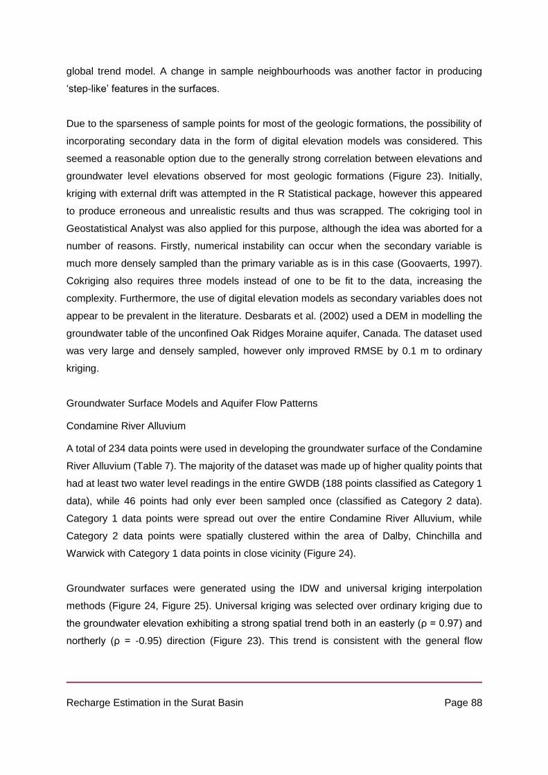
Recharge Estimation in the Surat Basin Page 88
global trend model. A change in sample neighbourhoods was another factor in producing
‘step-like’ features in the surfaces.
Due to the sparseness of sample points for most of the geologic formations, the possibility of
incorporating secondary data in the form of digital elevation models was considered. This
seemed a reasonable option due to the generally strong correlation between elevations and
groundwater level elevations observed for most geologic formations (Figure 23). Initially,
kriging with external drift was attempted in the R Statistical package, however this appeared
to produce erroneous and unrealistic results and thus was scrapped. The cokriging tool in
Geostatistical Analyst was also applied for this purpose, although the idea was aborted for a
number of reasons. Firstly, numerical instability can occur when the secondary variable is
much more densely sampled than the primary variable as is in this case (Goovaerts, 1997).
Cokriging also requires three models instead of one to be fit to the data, increasing the
complexity. Furthermore, the use of digital elevation models as secondary variables does not
appear to be prevalent in the literature. Desbarats et al. (2002) used a DEM in modelling the
groundwater table of the unconfined Oak Ridges Moraine aquifer, Canada. The dataset used
was very large and densely sampled, however only improved RMSE by 0.1 m to ordinary
kriging.
Groundwater Surface Models and Aquifer Flow Patterns
Condamine River Alluvium
A total of 234 data points were used in developing the groundwater surface of the Condamine
River Alluvium (Table 7). The majority of the dataset was made up of higher quality points that
had at least two water level readings in the entire GWDB (188 points classified as Category 1
data), while 46 points had only ever been sampled once (classified as Category 2 data).
Category 1 data points were spread out over the entire Condamine River Alluvium, while
Category 2 data points were spatially clustered within the area of Dalby, Chinchilla and
Warwick with Category 1 data points in close vicinity (Figure 24).
Groundwater surfaces were generated using the IDW and universal kriging interpolation
methods (Figure 24, Figure 25). Universal kriging was selected over ordinary kriging due to
the groundwater elevation exhibiting a strong spatial trend both in an easterly (ρ = 0.97) and
northerly (ρ = -0.95) direction (Figure 23). This trend is consistent with the general flow

Recharge Estimation in the Surat Basin Page 89
direction of the Condamine River from the headwaters in the south-east flowing towards the
north-west, represented in the kriging by a first-order trend model.
Groundwater surface elevations ranged from a maximum of approximately 480 m AHD in the
Condamine River headwaters to approximately 290 m AHD in the North West of the alluvium
(Table 7, Figure 24, and Figure 25). Groundwater surfaces produced by both IDW and
universal kriging interpolation methods showed similar general trends in data. The primary
trend that is evident in both figures is of groundwater flow in a north-westerly direction,
consistent with the flow direction of the Condamine River. In addition, a major groundwater
sink is present west of Oakey and extends north up to the region of Dalby, where water levels
are up to 50 m below the surface. This is most likely due to the high level of water use and
extraction from the alluvium for agricultural purposes (Dafny and Silburn, 2014). The universal
kriging surface also infers a secondary flow trend from the east as observed by Dafny and
Silburn (2014) to a greater degree, indicating lateral flow into the alluvium from neighbouring
aquifers.
The groundwater surfaces presented here of the Condamine River Alluvium for the period
1995 to 2014 generally concur with the groundwater surface for 2011 reported by Dafny and
Silburn (2014). The most noticeable difference present between surfaces is on the eastern
boundary of the alluvium, where the Dafny and Silburn (2014) surface exhibits steeper and
more prominent groundwater contours towards the west. This could be a result of the different
number and distribution of groundwater bores used, but could also be indicative of larger
lateral flow from the east during the wet periods of 2011.
Table 7 - Summary statistics of the water level elevation and water level depth of the
Condamine River Alluvium
Elevation
(mAHD)
Depth
(m)
Mean 357.03 -17.11
Median 339.9 -15
StdDev 48.10 9.93
Count 234 234

Recharge Estimation in the Surat Basin Page 90

Recharge Estimation in the Surat Basin Page 91
𝜌 = 0.98
𝜌 = 0.59
𝜌 = 0.17
𝜌 = −0.73
𝜌 = 0.58
𝜌 = −0.44
𝜌 = 0.51
𝜌 = 0.94
𝜌 = 0.95
𝜌 = 0.77
𝜌 = −0.95 𝜌 = 0.97
𝜌 = 0.21
𝜌 = −0.40 𝜌 = 0.47
𝜌 = 0.97
𝜌 = 0.29
𝜌 = −0.06
𝜌 = 0.99
𝜌 = −0.19 𝜌 = −0.26

Recharge Estimation in the Surat Basin Page 92
Figure 23 - Scatterplot and correlation of mean water level elevation against elevation,
easting and northing for each geologic formation

Recharge Estimation in the Surat Basin Page 93

Recharge Estimation in the Surat Basin Page 94
Figure 24 - Groundwater surface contours (10 m) of the Condamine River Alluvium (1995 -
2014) by IDW interpolation, with yellow arrows indicating general flow directions.

Recharge Estimation in the Surat Basin Page 95
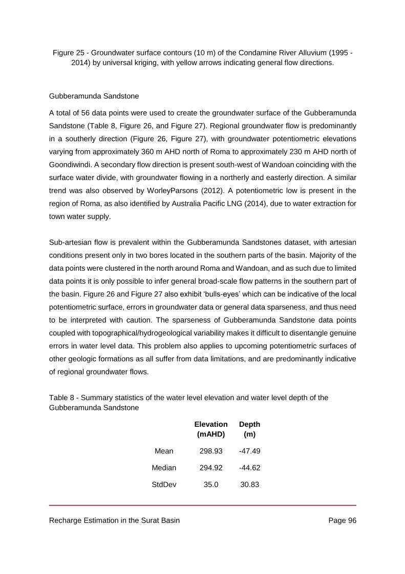
Recharge Estimation in the Surat Basin Page 96
Figure 25 - Groundwater surface contours (10 m) of the Condamine River Alluvium (1995 -
2014) by universal kriging, with yellow arrows indicating general flow directions.
Gubberamunda Sandstone
A total of 56 data points were used to create the groundwater surface of the Gubberamunda
Sandstone (Table 8, Figure 26, and Figure 27). Regional groundwater flow is predominantly
in a southerly direction (Figure 26, Figure 27), with groundwater potentiometric elevations
varying from approximately 360 m AHD north of Roma to approximately 230 m AHD north of
Goondiwindi. A secondary flow direction is present south-west of Wandoan coinciding with the
surface water divide, with groundwater flowing in a northerly and easterly direction. A similar
trend was also observed by WorleyParsons (2012). A potentiometric low is present in the
region of Roma, as also identified by Australia Pacific LNG (2014), due to water extraction for
town water supply.
Sub-artesian flow is prevalent within the Gubberamunda Sandstones dataset, with artesian
conditions present only in two bores located in the southern parts of the basin. Majority of the
data points were clustered in the north around Roma and Wandoan, and as such due to limited
data points it is only possible to infer general broad-scale flow patterns in the southern part of
the basin. Figure 26 and Figure 27 also exhibit ‘bulls-eyes’ which can be indicative of the local
potentiometric surface, errors in groundwater data or general data sparseness, and thus need
to be interpreted with caution. The sparseness of Gubberamunda Sandstone data points
coupled with topographical/hydrogeological variability makes it difficult to disentangle genuine
errors in water level data. This problem also applies to upcoming potentiometric surfaces of
other geologic formations as all suffer from data limitations, and are predominantly indicative
of regional groundwater flows.
Table 8 - Summary statistics of the water level elevation and water level depth of the
Gubberamunda Sandstone
Elevation
(mAHD)
Depth
(m)
Mean 298.93 -47.49
Median 294.92 -44.62
StdDev 35.0 30.83

Recharge Estimation in the Surat Basin Page 97
Count 56 56
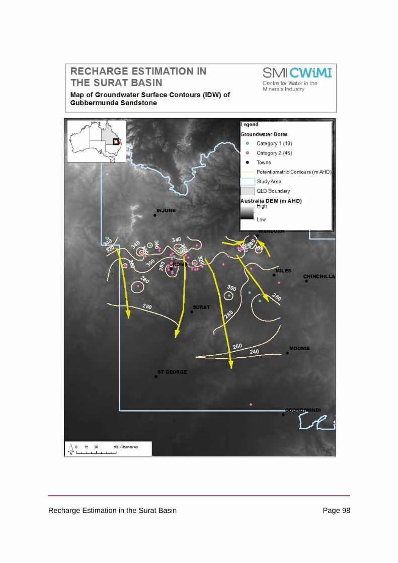
Recharge Estimation in the Surat Basin Page 98

Recharge Estimation in the Surat Basin Page 99
Figure 26 - Groundwater surface contours (20 m) of the Gubberamunda Sandstone (1995 -
2014) by IDW interpolation, with yellow arrows indicating general flow directions.

Recharge Estimation in the Surat Basin Page 100

Recharge Estimation in the Surat Basin Page 101
Figure 27 - Groundwater surface contours (20 m) of the Gubberamunda Sandstone (1995 -
2014) by ordinary kriging, with yellow arrows indicating general flow directions.
Hutton Sandstone
The groundwater potentiometric surface of the Hutton Sandstone was created using 53 data
points, five of which were obtained from springs and 48 from groundwater wells. The majority
of the points were Category 2 (Figure 28, and Figure 29). The data points are spread out over
several hundred kilometres in a northerly and easterly direction. Most of the data are clustered
west of Injune spreading south towards Roma, with a second cluster of data points located
around Taroom and Wandoan. Similar to the Gubberamunda Sandstone, more southerly data
points are scarce.
Groundwater potentiometric elevations varied from approximately 490 m AHD in the north-
west to below 200 m in the north-east around Taroom. The regional groundwater flow within
the Hutton Sandstone is complex and multi-directional. An easterly flow from west of Injune
towards Taroom is prevalent. There is also evidence of flow from the elevated recharge zones
southwards towards Surat, northerly groundwater flow from around Wandoan towards
Taroom, and radiating groundwater flow from the eastern margins, which could be indicative
of a recharge zone. There is also some evidence of westerly flow towards the Eromanga Basin
from the high elevation zones (Orange lines, Figure 12), although sparse data points prevent
better interpretation. The Nebine Ridge divides the Surat and Eromanga Basins, but
stratigraphic data provides evidence of continuity in the younger and shallower stratigraphic
formations, including the Hutton Sandstone (Hodgkinson et al., 2009).
Sub-artesian conditions were prevalent throughout the entire Hutton Sandstone. This is
indicative of the clustering of data points in the northern outcropping areas. Artesian bores
have been reported in the Hutton Sandstone primarily in the southern zone (Hodgkinson et
al., 2010). The groundwater potentiometric surface of the Hutton Sandstone reinforces the
findings of regional groundwater flow patterns in the northern region described by Quarantotto
(1989) and Hodgkinson et al. (2010).
Table 9 - Summary statistics of the water level elevation and water level depth of the Hutton
Sandstone
Elevation
(mAHD)
Depth
(m)

Recharge Estimation in the Surat Basin Page 102
Mean 328.90 -50.12
Median 353.14 -43
StdDev 80.90 37.38
Count 53 53

Recharge Estimation in the Surat Basin Page 103

Recharge Estimation in the Surat Basin Page 104
Figure 28 - Groundwater surface contours (20 m) of the Hutton Sandstone (1995 - 2014) by
IDW interpolation, with yellow arrows indicating general flow directions.

Recharge Estimation in the Surat Basin Page 105

Recharge Estimation in the Surat Basin Page 106
Figure 29 - Groundwater surface contours (20 m) of the Hutton Sandstone (1995 - 2014) by
ordinary kriging, with yellow arrows indicating general flow directions

Recharge Estimation in the Surat Basin Page 107
Kumbarilla Beds
The groundwater potentiometric surface of the Kumbarilla Beds was constructed from a mere
35 data points (Table 10), with data points clustered around Miles (Figure 30, Figure 31).
Groundwater potentiometric elevations varied from approximately 400 m AHD on the eastern
margins, to 200 m AHD by Goondiwindi. Groundwater flow is predominantly radial from the
eastern higher elevation margins of the geologic formations. A secondary trend is present with
groundwater flows also occurring southwards in the region of Miles. These groundwater flow
patterns follow the general topographic trends in the region (Figure 31), however groundwater
flow interpretations are severely restricted due to sparseness of data and clustering.
Table 10 - Summary statistics of the water level elevation and water level depth of the
Kumbarilla Beds
Elevation
(mAHD) Depth (m)
Mean 288.65 -28.15
Median 289.17 -24.48
StdDev 47.01 20.90
Count 35 35

Recharge Estimation in the Surat Basin Page 108

Recharge Estimation in the Surat Basin Page 109
Figure 30 - Groundwater surface contours (20 m) of the Kumbarilla Beds (1995 - 2014) by
IDW interpolation, with yellow arrows indicating general flow directions.

Recharge Estimation in the Surat Basin Page 110

Recharge Estimation in the Surat Basin Page 111
Figure 31 - Groundwater surface contours (20 m) of the Kumbarilla Beds (1995 - 2014) by
ordinary kriging, with yellow arrows indicating general flow directions.

Recharge Estimation in the Surat Basin Page 112
Main Range Volcanics
The groundwater surface of the Main Range Volcanics was interpolated from 373 points, the
largest dataset available for any single geologic formation in the Surat Basin (Table 11). The
majority of the data were located between Oakey and Warwick, and west of Toowoomba
(Figure 32, Figure 33). Additional data points were found slightly north generally close to the
Great Dividing Range.
Groundwater elevations varied substantially from more than 700 m AHD to less than 200 m
AHD on the eastern edge of the Great Dividing Range. This variability is indicative of the
topographical variability of the region, with topographical highs and steeply incised valleys in
close proximity. Groundwater flow within the Main Range Volcanics exhibits a radial pattern
outwards from the divide, indicating that the basalts are a potential recharge source to
neighbouring aquifers. The groundwater surface contours exhibit a very similar pattern to the
regional topography (Figure 33).
During the groundwater surface interpolation, anisotropic rather than isotropic behaviour of
the semivariogram was identified and supported by improved cross-validation results. This
anisotropic behaviour was incorporated into the kriging model, providing an explanation of the
similarity between the groundwater contours and respective topography.
Table 11 - Summary statistics of the water level elevation and water level depth of the Main
Range Volcanics
Elevation
(mAHD) Depth (m)
Mean 492.73 -22.22
Median 476.34 -15
StdDev 80.20 20.46
Count 373 373

Recharge Estimation in the Surat Basin Page 113

Recharge Estimation in the Surat Basin Page 114
Figure 32 - Groundwater surface contours (40 m) of the Main Range Volcanics (1995 - 2014)
by IDW Interpolation, with yellow arrows indicating general flow directions.

Recharge Estimation in the Surat Basin Page 115

Recharge Estimation in the Surat Basin Page 116
Figure 33 - Groundwater surface contours (40 m) of the Main Range Volcanics (1995 - 2014)
by ordinary kriging, with yellow arrows indicating general flow directions.

Recharge Estimation in the Surat Basin Page 117
Mooga Sandstone
The groundwater surface of the Mooga Sandstone was interpolated from 54 data points (Table
12), predominantly located around Roma and spread out eastwards towards Miles and Moonie
(Figure 34, Figure 35). The Mooga Sandstone had the smallest variation in groundwater
elevations of the all the geologic formations, with groundwater elevations varying from around
270 m AHD in the south-west to around 340 m AHD in the north. Groundwater flow is
predominantly in a southerly direction for the entire Mooga Sandstone, as indicated by
Quarantotto (1989). The groundwater surface interpolated by kriging does infer the possibility
of westerly groundwater flow from the eastern margins (Figure 35). The limited number of data
points does prevent further exploration of this trend.
Sub-artesian conditions are prevalent in the higher northern and western areas of the Mooga
Sandstone. Four artesian bores are located in the lower lying central area of the geologic
formation associated with the flatter valley-type landscape, as is observed in other confined
aquifers such as the Gubberamunda Sandstone.
Table 12 - Summary statistics of the water level elevation and water level depth of the
Mooga Sandstone
Elevation
(mAHD) Depth (m)
Mean 292.28 -38.39
Median 288.05 -36.2
StdDev 16.62 25.37
Count 54 54

Recharge Estimation in the Surat Basin Page 118

Recharge Estimation in the Surat Basin Page 119
Figure 34 - Groundwater surface contours (20 m) of the Mooga Sandstone (1995 - 2014) by
IDW Interpolation, with yellow arrows indicating general flow directions.

Recharge Estimation in the Surat Basin Page 120

Recharge Estimation in the Surat Basin Page 121
Figure 35 - Groundwater surface contours (20 m) of the Mooga Sandstone (1995 - 2014) by
ordinary kriging, with yellow arrows indicating general flow directions.

Recharge Estimation in the Surat Basin Page 122
Walloon Coal Measures
A total of 162 bores make up the Walloon Coal Measures 1995 to 2014 groundwater elevation
dataset (Table 13). These bores are distributed between two geologic basins, both the Surat
Basin to the west and Clarence-Moreton Basin to the east of the Great Dividing Range (Figure
36, Figure 37). The largest cluster of groundwater bores is located in the vicinity of Warwick,
with groundwater bores extending all the way out to Wandoan in a somewhat sparse and
linear arrangement. A second cluster of groundwater bores is located in the Clarence-Moreton
Basin, east of the Great Dividing Range.
Table 13 - Summary statistics of the water level elevation and water level depth of the
Walloon Coal Measures
Elevation
(mAHD) Depth (m)
Mean 332.96 -22.69
Median 344.51 -16.15
StdDev 146.66 19.46
Count 162 162
The entire dataset was used to interpolate a groundwater surface of the Walloon Coal
Measures using the IDW technique. However, groundwater bores located in the Clarence-
Moreton Basin were excluded when interpolating groundwater elevations by kriging. The two
subsets of groundwater bores have two distinct spatial structures associated with the two
geologic basins, which is highlighted in the scatterplots of groundwater elevation vs. eastings
and northings (refer to Figure 23). These distinct spatial structures made it difficult to model
the spatial trend and a representative semivariogram. Considering the uncertainty on the
continuity of hydrogeologic formations between the Surat and Clarence-Moreton Basins
(Hodgkinson et al., 2009) and the focus of this study being the Surat Basin, the data set was
split and interpolations were carried out only on the bores that were west of the divide. This
reduced the dataset down from 162 to 112 data points (Category 1 with 33 points, Category 2
with 79 data points). The dataset had a strong spatial trend from south-east to north-west,
best represented by a second order polynomial (ρ = 0.94 (Eastings), ρ = -0.90 (Northings)).
As a result, universal kriging rather than ordinary kriging was applied, to account for the spatial
trend in data.

Recharge Estimation in the Surat Basin Page 123
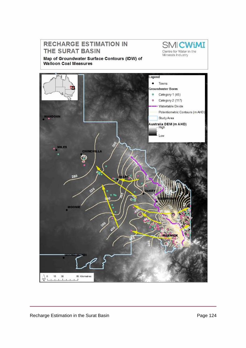
Recharge Estimation in the Surat Basin Page 124

Recharge Estimation in the Surat Basin Page 125
Figure 36 - Groundwater surface contours (20 m) of the Walloon Coal Measures (1995 -
2014) by IDW Interpolation, with yellow arrows indicating general flow directions.

Recharge Estimation in the Surat Basin Page 126

Recharge Estimation in the Surat Basin Page 127
Figure 37 - Groundwater surface contours (20 m) of the Walloon Coal Measures (1995 -
2014) by universal kriging, with yellow arrows indicating general flow directions.

Recharge Estimation in the Surat Basin Page 128
Groundwater potentiometric elevations varied between 260 m AHD in close proximity to Miles
to approximately 590 m AHD east of Warwick in the high elevation zones. The dominant
direction of groundwater flow in the Surat part of the Walloon Coal Measures was north-
westerly (Figure 37). The groundwater flow directions showed similar trends to the regional
topography, with westerly groundwater flows present around Dalby and Warwick. Sub-
artesian conditions were prevalent throughout the entire Walloon Coal Measures.
Uncertainties, Limitations and Difficulties
Table 14 presents the cross-validation results of the kriged groundwater surfaces presented
in the previous section. The quality of the geostatistical model predictions vary, with RMSEs
for the Condamine River Alluvium being the best of the different geologic formations and
reasonably low (RMSE = 6.1 m), followed by the Mooga Sandstone. The Main Range
Volcanics have the largest prediction error (RMSE = 31.0 m) even with the largest dataset. A
mean error of 1.27 m also indicates that values are being over-predicted on average. The
RMSE of the other formations are around 20 m.
Table 14 - Cross validation errors for each geologic formation for all kriged surfaces
Geologic Formation Kriging Technique Mean Error
(m) RMSE (m)
Condamine River Alluvium Universal -0.014 6.1110
Gubberamunda Sandstone Ordinary -0.0836 22.626
Hutton Sandstone Ordinary 0.3068 23.368
Kumbarilla Beds Ordinary 0.0077 16.84
Main Range Volcanics Ordinary 1.265 31.04
Mooga Sandstone Ordinary -0.0414 10.5442
Walloon Coal Measures Universal -0.2398 21.517
Currently, limited information is available on the success/difficulties of other attempts at
interpolating groundwater surface elevations within the Surat and Great Artesian Basins, even
though groundwater surface interpolation is not uncommon, especially with the recent CSG
activity (e.g. Dafny and Silburn, 2014; Hodgkinson et al., 2010; Quarantotto, 1989; Smerdon
Recharge Estimation in the Surat Basin Page 129
et al., 2012b; WorleyParsons, 2012). In addition, generally the implemented technique is either
not identified or only identified in name with minimal description on the interpolation process.
This limits our ability to compare the quality of the kriged groundwater surfaces in this report
relative to others. Hodgkinson et al. (2010) did attempt both kriging and radial basis functions
before settling for minimum curvature interpolation (i.e. spline functions), which produced
better results with some manual tuning. However, minimum curvature interpolation has its
own limitations, including inability for cross-validation to be performed and weak performance
for closely spaced data.
Geostatistical techniques have been implemented successfully in interpolating groundwater
and other environmental systems (e.g. climate) in the literature (e.g. Bohling and Wilson, 2006,
2012; Goovaerts, 2000; Hofstra et al., 2008; Kumar, 2007). For example, the Kansas
Geological Survey (KGS) has been interpolating groundwater surface elevations and changes
in water level of the High Plains aquifer on an annual basis for years (Bohling and Wilson,
2006, 2012). Desbarats et al. (2002) and Kumar (2007) also used kriging techniques to
interpolate groundwater surface elevations, while Ahmadi and Sedghamiz (2007) used kriging
to interpolate changes in groundwater levels and for time series interpolation. The studies
reported RMSE values up to approximately 10 m. These values are generally smaller than
those reported in this study (Table 14). However, there are substantial differences in the
datasets (not all of these apply to all of the studies):
1. Higher quality data values, with groundwater levels surveyed during certain periods to
allow for aquifer replenishment and over short time spans to capture the same ‘event’
(e.g. Bohling and Wilson (2006) surveyed 1266 wells over the winter months)
2. Larger number of data points that are more evenly distributed
3. Substantially smaller study areas
4. Higher density of data points
5. Interpolating water table levels in unconfined aquifers
6. Limited topographical variability.
There were a number of limitations, uncertainties and difficulties encountered in interpolating
groundwater surfaces for the various geologic formations within the Surat Basin. These were
associated with the quality of the available data, the complexity of the groundwater systems
and the complexity of the interpolation techniques employed. These could explain some of the
larger prediction errors. The main limitations and difficulties encountered were:
Recharge Estimation in the Surat Basin Page 130
1. Temporal range of data
The data incorporated were sampled over a long period of time (20 years), with different points
sampled during different events. Thus some data might reflect the average state of the aquifer
over 20 years, other bores might be indicative of a flood or drought, and some might be
indicative of a localised impact such as pumping. For example, some of the major outliers that
were identified in the Main Range Volcanics during cross-validation were very closely spaced
(less than a kilometre apart) but had groundwater elevations that differed by approximately
100m.
2. Inaccuracy in bores with only single readings taken at time of construction.
Sometimes there can be large discrepancies between these bores and neighbouring bores.
Most of the datasets other than the Condamine River Alluvium were made up of single reading
bores, where Category 2 data made up between 50 and 80 % of the datasets of each geologic
formation.
3. Small datasets
Datasets for most of the geologic formations were generally either clustered or sparse (this
was a major limitation also pointed out by WorleyParsons (2012)). Furthermore, the
interpolated areas were large with variable topography, but generally a very low data point
density. For example, most of the data points for the Gubberamunda Sandstone were located
close to Roma, while there was only one data point in the southern parts of the Basin. This
explains the peculiar groundwater surface contours in that region (Figure 27).
4. Uncertainty about the source aquifer
The aquifer assignments of all bores were wholly based on the GWDB logs and could not be
checked with a Geological Model. There is doubt to the accuracy of the aquifer and
stratigraphy logs of the GWDB. In some instances, the GWDB incorporates a number of
different geologic formations that could not be individually identified in a single entry. The
Kumbarilla Beds geologic formation is a good example of this.
5. Hydrogeologic complexity of geologic formations
The groundwater surfaces developed in this report are a simple representation of groundwater
surfaces in the various geologic formations. Some of the challenges experienced in
interpolation could be associated with the complexity of the geologic formation systems. For
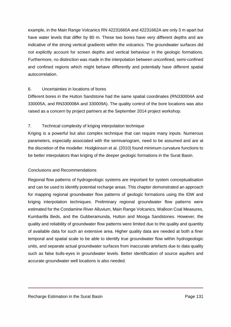
Recharge Estimation in the Surat Basin Page 131
example, in the Main Range Volcanics RN 42231660A and 42231662A are only 3 m apart but
have water levels that differ by 80 m. These two bores have very different depths and are
indicative of the strong vertical gradients within the volcanics. The groundwater surfaces did
not explicitly account for screen depths and vertical behaviour in the geologic formations.
Furthermore, no distinction was made in the interpolation between unconfined, semi-confined
and confined regions which might behave differently and potentially have different spatial
autocorrelation.
6. Uncertainties in locations of bores
Different bores in the Hutton Sandstone had the same spatial coordinates (RN330004A and
330005A, and RN330008A and 330009A). The quality control of the bore locations was also
raised as a concern by project partners at the September 2014 project workshop.
7. Technical complexity of kriging interpolation technique
Kriging is a powerful but also complex technique that can require many inputs. Numerous
parameters, especially associated with the semivariogram, need to be assumed and are at
the discretion of the modeller. Hodgkinson et al. (2010) found minimum curvature functions to
be better interpolators than kriging of the deeper geologic formations in the Surat Basin.
Conclusions and Recommendations
Regional flow patterns of hydrogeologic systems are important for system conceptualisation
and can be used to identify potential recharge areas. This chapter demonstrated an approach
for mapping regional groundwater flow patterns of geologic formations using the IDW and
kriging interpolation techniques. Preliminary regional groundwater flow patterns were
estimated for the Condamine River Alluvium, Main Range Volcanics, Walloon Coal Measures,
Kumbarilla Beds, and the Gubberamunda, Hutton and Mooga Sandstones. However, the
quality and reliability of groundwater flow patterns were limited due to the quality and quantity
of available data for such an extensive area. Higher quality data are needed at both a finer
temporal and spatial scale to be able to identify true groundwater flow within hydrogeologic
units, and separate actual groundwater surfaces from inaccurate artefacts due to data quality
such as false bulls-eyes in groundwater levels. Better identification of source aquifers and
accurate groundwater well locations is also needed.

Recharge Estimation in the Surat Basin Page 132
Analysis of Groundwater Hydrographs
Groundwater hydrographs can be used to estimate groundwater recharge by applying the
Water Table Fluctuation (WTF) method (Healy and Cook, 2002). The attraction of this method
is that it is comparatively easy to use and makes no assumptions about the mechanisms by
which water travels through the unsaturated zone (Healy and Cook, 2002). Therefore the
presence of preferential flow paths within the unsaturated zone in no way restricts its
application. The WTF method aims to be representative of recharge over several square
meters around the borehole (Healy and Cook, 2002).
The rise in the water table due to rainfall (Figure 38) can be used to determine the recharge
into the system. The standard equation is shown below.
𝑅 = 𝑆𝑦
𝑑ℎ
𝑑𝑡= 𝑆𝑦
∆ℎ
∆𝑡
Where R is equal to recharge, Sy is the specific yield and dh/dt is the rise in water level after
a rainfall event.
Figure 38. Water table fluctuation method (USGS, 2013)
It is important to ensure when using this method that any rise in the water table is due to a
rainfall event as water tables can fluctuate due to other factors including evapotranspiration,
atmospheric pressure, pumping and irrigation as well as the movement of entrapped air within
the unsaturated zone (Healy and Cook, 2002) . It is recommended that any wells chosen for

Recharge Estimation in the Surat Basin Page 133
analysis be located a sufficient distance away from pumping wells to ensure that water levels
are not significantly lowered by pumping (Cuthbert, 2010). The circumstances under which
the effect of pumping can be considered negligible are case dependent (Cuthbert, 2010).
Recharge rates are also substantially variable across the basin of interest due to differences
in elevation, geology, land surface slope, vegetation and other factors (Cuthbert, 2010; Healy
and Cook, 2002). Therefore the wells chosen with this method should ideally be representative
of the basin as a whole (Healy and Cook, 2002) .
Limitations and Assumptions
The WTF method is best applied to shallow water tables that display sharp water level rises
and declines. In some cases this method can be applied to deeper aquifers if they display
seasonal water level fluctuation trends (Healy and Cook, 2002). The main assumptions in
using the WTF method are:
1. Recharge rates can be calculated using water table fluctuations if it is assumed that
water arriving at the water table goes immediately into storage and that all other
fluxes e.g. evapotranspiration and pumping, are zero during the period of estimation
(Healy and Cook, 2002).
2. Depth to water table should be low to reduce the amount of attenuation and lag that
can occur after recharge events (Cuthbert, 2010).
3. Wells used for WTF should be representative of the catchment; if not, a number of
wells should be used to get an average for the effects of spatial and temporal
variability (Cuthbert, 2010; Healy and Cook, 2002).
4. The method is only applicable to unconfined aquifers (Healy and Cook, 2002).
5. No considerations are made for preferential flow or other flow mechanisms (Healy
and Cook, 2002).
6. Specific yield values need to be determined in order for the method to be applied
(Healy and Cook, 2002).
The main uncertainty with the WTF method is the specific yield value, which defines how high
the water table will rise as a function of the net amount of water infiltrating the system. Its value
can change between different sites within close proximity and at different depths.

Recharge Estimation in the Surat Basin Page 134
There are many different methods to estimate specific yield ranging from pumping tests (Moon
et al., 2004) to a simplified water balance. Due to the inherent uncertainty of this value it is
recommended that several methods be utilised and that the chosen result should be
representative of the in-situ conditions (Timlin et al., 2003). If there is insufficient data to
complete multiple analyses a proxy method can be used to acquire a representative value.
This proxy method is applied in conditions where it may be assumed that recharge is equal to
rainfall. It uses the ratio of rainfall to water level rise to determine the specific yield (Gerla,
1992; Heliotis, 1989; Loheide et al., 2005; Rosenberry and Winter, 1997; Schilling and Kiniry,
2007).
𝑆𝑦 =𝑟𝑎𝑖𝑛𝑓𝑎𝑙𝑙
𝑤𝑎𝑡𝑒𝑟 𝑙𝑒𝑣𝑒𝑙 𝑟𝑖𝑠𝑒
The ratio method takes into account the following assumptions and recommendations:
1. Vertical infiltration (Gerla, 1992).
2. Negligible overland flow (Loheide et al., 2005; Timlin et al., 2003).
3. No change in unsaturated one storage (Loheide et al., 2005).
4. No evapotranspiration (Timlin et al., 2003).
Due to actual losses of water, this ratio generally provides an upper bound estimate of specific
yield and is best calculated for a number of rainfall events to get an average specific yield
value for each borehole (Timlin et al., 2003).
Methodology
As the method for calculating specific yield and groundwater recharge with WTF are highly
interchangeable, many of bore selection criteria will apply to both methods and the following
considerations need to be made:
1. There needs to be continuous daily readings of bore level over a significant period of
time.
2. Aquifers must be unconfined. The depth to water table should be less than 20m or
there should be significant evidence to prove that there is no confining layer. This will
reduce the errors due totime lags, storage effects and lateral movement of water.
3. There needs to be a rainfall monitoring station in close proximity to collect rainfall
rates as well as monitoring if the rise in water level is due to rainfall or other factors.
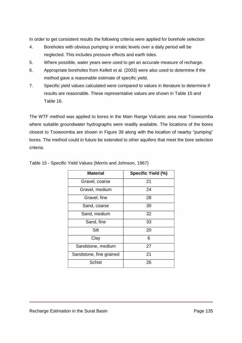
Recharge Estimation in the Surat Basin Page 135
In order to get consistent results the following criteria were applied for borehole selection
4. Boreholes with obvious pumping or erratic levels over a daily period will be
neglected. This includes pressure effects and earth tides.
5. Where possible, water years were used to get an accurate measure of recharge.
6. Appropriate boreholes from Kellett et al. (2003) were also used to determine if the
method gave a reasonable estimate of specific yield.
7. Specific yield values calculated were compared to values in literature to determine if
results are reasonable. These representative values are shown in Table 15 and
Table 16.
The WTF method was applied to bores in the Main Range Volcanic area near Toowoomba
where suitable groundwater hydrographs were readily available. The locations of the bores
closest to Toowoomba are shown in Figure 39 along with the location of nearby “pumping”
bores. The method could in future be extended to other aquifers that meet the bore selection
criteria.
Table 15 - Specific Yield Values (Morris and Johnson, 1967)
Material Specific Yield (%)
Gravel, coarse 21
Gravel, medium 24
Gravel, fine 28
Sand, coarse 30
Sand, medium 32
Sand, fine 33
Silt 20
Clay 6
Sandstone, medium
grained
27
Sandstone, fine grained 21
Schist 26

Recharge Estimation in the Surat Basin Page 136
Table 16 - Specific yield values (Heath, 1983)
Material Specific Yield
(%)
Soil 40
Clay 2
Sand 22
Gravel 19
Limestone 18
Sandstone (unconsolidated) 6
Granite 0.09
Basalt (young) 8

Recharge Estimation in the Surat Basin Page 137
Figure 39 - Location of WTF bores close to Toowoomba
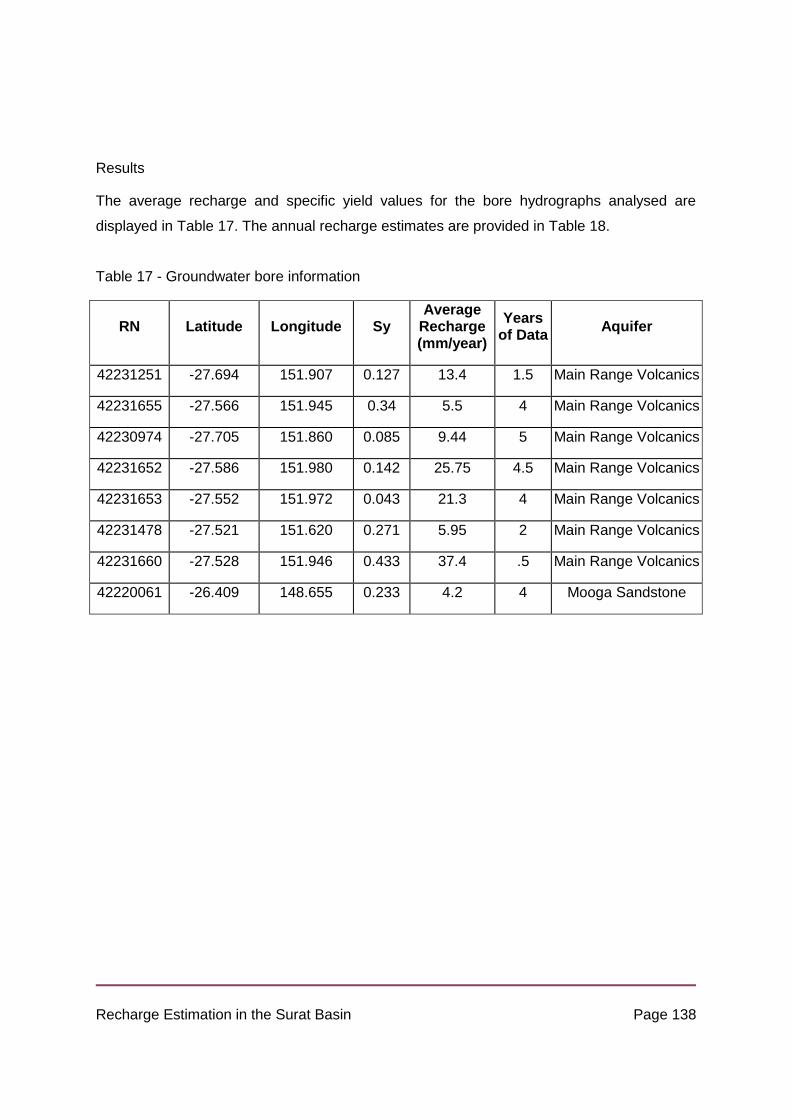
Recharge Estimation in the Surat Basin Page 138
Results
The average recharge and specific yield values for the bore hydrographs analysed are
displayed in Table 17. The annual recharge estimates are provided in Table 18.
Table 17 - Groundwater bore information
RN Latitude Longitude Sy Average
Recharge (mm/year)
Years of Data
Aquifer
42231251 -27.694 151.907 0.127 13.4 1.5 Main Range Volcanics
42231655 -27.566 151.945 0.34 5.5 4 Main Range Volcanics
42230974 -27.705 151.860 0.085 9.44 5 Main Range Volcanics
42231652 -27.586 151.980 0.142 25.75 4.5 Main Range Volcanics
42231653 -27.552 151.972 0.043 21.3 4 Main Range Volcanics
42231478 -27.521 151.620 0.271 5.95 2 Main Range Volcanics
42231660 -27.528 151.946 0.433 37.4 .5 Main Range Volcanics
42220061 -26.409 148.655 0.233 4.2 4 Mooga Sandstone

Recharge Estimation in the Surat Basin Page 139
Table 18 - Annual recharge values
RN Year Type of Data Recharge (mm)
42231251 2011-2012 All daily readings 13.4
42231655
2009-2010 Water year 5.3
2010-2011 Partial water year 7.3
2011-2012 Water year 3.5
2012-2013 Water year 5.8
42230974
2008-2009 Water year 4
2009-2010 Water year 11.5
2010-2011 Water year 11.4
2011-2012 Water year 6.5
2012-2013 Water year 13.8
42231652
2009 Partial year 10.7
2010 Partial year 25.5
2010-2011 Partial water year 19.1
2011-2012 Water year 12.4
2012-2013 Water year 46
42231653
2009-2010 Water year 28.2
2010-2011 Partial water year 11.3
2011-2012 Water year Pumping?
2012-2013 Water year 24.5
42231478 1993-1994 Initial data + water year 7.5
1994-1995 Water year 4.4
42220061
2005-2006 Water year 2.1
2008-2009 Water year 4
2009-2010 Water year 4.1
2010-2011 Water year 27.5
42231660 2009 Partial Year 37.4

Recharge Estimation in the Surat Basin Page 140

Recharge Estimation in the Surat Basin Page 141
Discussion
In determining if the ratio method was giving reasonable results a comparison was taken from
borehole RN42220061 which is a shallow unconfined aquifer within the Mooga Sandstone.
RN42220061 has an automated water level recorder as well as a rainfall data collector so
measurements can be taken daily. This data can either be accessed from the Ground Water
Database (GWDB) or the Department of Natural Resources and Mines (DNRM) Water
Monitoring Portal. RN42220061 was used in the Kellett et al. (2003) report and was assumed
to have a specific yield of 0.2. The value calculated from the ratio method of 0.23 corresponds
closely to the Kellett et al. (2003) report. WTF recharge estimates were also compared and it
was found that the Kellett et al. (2003) report gave recharge rates between 2.6 and 4.7 mm/yr
which are comparable with the average found by applying the specific yield proxy method of
4.2 mm/yr.
Another bore from the Kellett et al. (2003) report was also considered (bore RN42220058) but
there were too many fluctuations in the data for it to be properly assessed. Bore RN13030613
appears to be a confined or very deep aquifer so it was also dismissed even though it has
continuous monitoring. Of the Kellett et al. (2003) report only these 3 boreholes are within the
area of interest for this project.
The large specific yield value for RN42231655 of 0.34 was unexpected when compared with
the specific yield for other bores nearby. This value is similar to values expected for soils or
sand (Table 15 and Table 16). Analysis of the bore log enabled the identification of
“honeycombed basalt” which explains the higher specific yield for this bore.
Most of the bores that were analysed are located in urban areas and this could lead to
uncertainties in results. The recharge rates in urban areas can be much larger than expected
even with the increased runoff and reduced surface area due to impermeable buildings
(Lerner, 1990). Water can be introduced into the system through leaking service networks
(mains or septic) as well as over-irrigation of gardens for aesthetic reasons (Lerner, 1990) .
This could be problematic as the WTF method computes both infiltration from rainwater and
domestic wastewater and it is recommended that geochemical analysis and interpretation can
be used as a means to separate the two sources (Diouf et al., 2012). Upper and lower bound
recharge estimation is also recommended due to the possibility of large uncertainties that can
occur from leaking services in urban areas (Lerner, 1990) .

Recharge Estimation in the Surat Basin Page 142
Evapotranspiration has not been considered in our hydrograph analysis approach and further
testing is recommended. As most of the rainfall seems to occur within the summer months it
would be hard to find events that occur within the minimal evapotranspiration periods, which
has been suggested in some of the literature. As evapotranspiration and runoff have not been
considered it may mean that the recharge estimates are upper bounds and it would be
advisable to cross check these results with other methods.
Some water years included major flood events. Most of the partial water years are because of
the halt in readings due to flooding. This is another potential source of bias when estimating
time-averaged recharge using this approach.
Conclusions
The Water Table Fluctuation (WTF) method was applied based on the specific yield proxy
method and an estimate of recharge was found for the Toowoomba and surrounding basalts.
The method gave recharge estimates comparable to the independent estimates of Kellett et
al. (2003). There are many assumptions in this method, which means that ideally results would
be part of a multi-method approach to recharge estimation.
Even though the specific yield proxy method has many drawbacks and makes many
assumptions it is still the most viable option to get representative in-situ values of specific
yields. Other methods can then be applied to validate these values such as laboratory
drainage testing of aquifer material or pump testing as mentioned previously.
Analysis of Remote Sensing Data
Introduction
Remote sensing has been a widely applied measurement tool within hydrology. Remote
sensing cannot directly measure groundwater recharge; instead the data must be able to
account for the other major elements in the water balance (evapotranspiration, surface runoff,
soil water storage, surface storage and precipitation) and recharge inferred from this (Becker,
2006). Given that these elements are poorly constrained (especially runoff and soil water
storage), remote sensing data are often combined with a simple water and energy balance
modelling framework in order to derive recharge estimates (e.g. Bastiaanssen et al. (1998)).

Recharge Estimation in the Surat Basin Page 143
This section investigates the spatial and temporal variability of recharge throughout the whole
Surat, and for separate geological units (Walloon – Injune units, and Main Range Volcanics).
Since the data available from remote sensing only allow a water balance in the top ~2 meters
of soil, groundwater recharge here is more precisely called ”deep drainage”.
Methods
The combined remote sensing and model product from CSIRO, the Australian Water
Availability Project (http://www.csiro.au/awap/) is utilised here. This dataset provides the past
and present soil moisture and all water fluxes contributing to changes in soil moisture
(precipitation, transpiration, soil evaporation, surface runoff and deep drainage), across the
entire Australian continent at a spatial resolution of 5 km. The timescales of output availability
are monthly and annually, 1900 – present. The data – model fusion methods, calibration, and
uncertainties are described in detail within Raupach et al. (2009).
Briefly, the WaterDyn25M (version August 2008) is constructed as the mass balance
interaction between two soil depths (M1 and M2):
M1 is the shallow soil layer, typically between 0 and 0.2m depth, and M2 is the deeper soil
layer, typically 0.2 to 1.5m depth. The variable of interest here is deep drainage, which in this
model is the residual drainage from the M2 mass balance.
Soil properties defining the soil moisture balance and deep drainage rates are derived from
the digital Atlas of Australian Soils (McKenzie and Hook, 1992; McKenzie et al., 2000). This
atlas classifies Australian soils into ~700 soil types, and is translated into soil physical
properties using pedotransfer functions. Vegetation is also a critical component of the deep

Recharge Estimation in the Surat Basin Page 144
drainage estimates, with the fractional vegetation cover typically derived from the Fraction of
Absorbed Photosynthetically Active Radiation (FAPAR) from the SeaWiFS satellite.
Spatial deep drainage estimates are produced as whole record (~100 year) averages, as well
as example ‘wet’ (2011) and ‘dry’ (2006) years to illustrate the influence of climatic variability
on deep drainage for: 1. The entire Surat Basin, 2. the Walloon – Injune outcrop areas, and 3.
the Main Range Volcanics Basalt outcrop areas.
Spatial Recharge Estimates
The deep drainage estimates presented in this section have been produced by CSIRO as
part of the Australian Water Availability Project (http://www.csiro.au/awap/). This data set
can be requested directly from CSIRO.
Whole Surat: Spatial average, wet and dry years
Taking the Surat as a whole, on average (1900 – 2014) high deep drainage estimates occur
within the SE Main Range Volcanics as well as those NW of Toowoomba (near Oakey), the
upper Condamine, within channel segments to the north of the Basin and across the surface
catchment divides (Fitzroy catchment), and in the far NW of the Basin. Figure 40 shows the
spatial variation of annual average deep drainage estimates across the Surat. The mean value
over the whole Surat is 11 ± 7.9 mm/year (where the latter value is the standard deviation
representing the spatial variation of the annual average value), although the distribution is
highly skewed towards lower values. For the above average precipitation year (2011), mean
deep drainage increased to 64.1 ± 39.7 mm/yr, and the distribution becomes more distinctly
bimodal (Figure 41). In this example, high deep drainage values expanded across the whole
length of the Main Range Volcanics, the upper Condamine, and much of the NW of the basin.
Looking at 2006 as an example of a very dry year, the distribution of deep drainage values is
even more positively skewed, and the mean deep drainage drops to 2.6 ± 3.1 mm/yr (Figure
42). Higher deep drainage values (~10 – 20 mm/yr) in this case are restricted to isolated
pockets around the main river channels, Oakey and the northern Main Range Volcanics, and
a small area west of Chinchilla. The maximum annual average over the Surat at this 5 km2
scale was 105 mm/year (in the Main Range Volcanics), compared to the mean of 11 mm/year
and minimum of 0.5 mm/year; confirming the importance of considering spatial variations.

Recharge Estimation in the Surat Basin Page 145

Recharge Estimation in the Surat Basin Page 146
Figure 40 - Average annual deep drainage estimates for the whole Surat CMA between
1900 – 2013 (data source: CSIRO AWAP 2014).
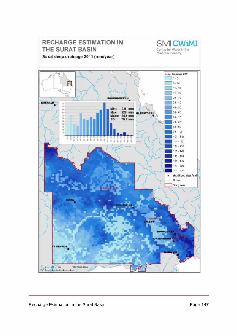
Recharge Estimation in the Surat Basin Page 147

Recharge Estimation in the Surat Basin Page 148
Figure 41 - Average annual deep drainage estimates for the whole Surat CMA in an example
wet year – 2011 (data source: CSIRO AWAP 2014).

Recharge Estimation in the Surat Basin Page 149

Recharge Estimation in the Surat Basin Page 150
Figure 42 - Average annual deep drainage estimates for the whole Surat CMA in an example
dry year – 2006 (data source: CSIRO AWAP 2014).

Recharge Estimation in the Surat Basin Page 151
Walloon Coal Measures & Injune Creek Group: Average, wet and dry years
The combined Walloon and Injune beds deep drainage averages are difficult to evaluate
spatially given the limited and patchy outcrop, especially in the SE of the basin, although here
the deep drainage appears to be higher towards the east in association with the Main Range
Volcanics (Figure 43). Within the north, higher deep drainage areas are quite discrete along
channel networks, and become less discrete towards the west. The long term mean deep
drainage exclusively for the Walloon – Injune units is 11.4 ± 10 mm/yr, with the distribution
strongly positively skewed towards lower deep drainage estimates, although the higher deep
drainage tail is slightly bimodal. During the wet example year there is a clear response towards
increased deep drainage within the NW of the basin outcrop, and this is reflected in the shift
towards a slightly negatively skewed (i.e. towards higher deep drainage), albeit bimodal
distribution (Figure 44). This response is also clear from the very large shift in the mean
outcrop deep drainage to 73.5 ± 32.1 mm/yr. In contrast, during the dry example year, the
mean deep drainage is greatly reduced to 3.9 ± 3 mm/yr, and the resulting distribution of deep
drainage is extremely positively skewed (Figure 45).

Recharge Estimation in the Surat Basin Page 152

Recharge Estimation in the Surat Basin Page 153
Figure 43 - Average annual deep drainage estimates for the Walloon Coal Measures and
Injune Creek Group geologic units between 1900 – 2013 (data source: CSIRO AWAP 2014).

Recharge Estimation in the Surat Basin Page 154

Recharge Estimation in the Surat Basin Page 155
Figure 44 - Average annual deep drainage estimates for the Walloon Coal Measures and
Injune Creek Group geologic units in an example wet year – 2011 (data source: CSIRO
AWAP 2014).

Recharge Estimation in the Surat Basin Page 156

Recharge Estimation in the Surat Basin Page 157
Figure 45 - Average annual deep drainage estimates for the Walloon Coal Measures and
Injune Creek Group geologic units in an example dry year – 2006 (data source: CSIRO
AWAP 2014).

Recharge Estimation in the Surat Basin Page 158
Main Range Volcanics: Average, wet and dry years
The spatial variation in the long term (1900 – 2014) mean deep drainage highlights higher
values in the SE of the Main Range Volcanics, as well as NW of Toowoomba (near Oakey,
Figure 46). The mean long term deep drainage for the Main Range Volcanics is 15.8 ± 13.8
mm/yr, higher than the Walloon – Injune and whole basin averages, and the distribution of
deep drainage throughout the basalts is more Gaussian than the previous distributions. In the
example wet year the spatial distribution is more uniform, although declining deep drainage to
the west is still evident. The spatial mean deep drainage increases to 99 ± 42 mm/yr and the
distribution becomes more bimodal (Figure 47). In the dry year example the spatial contrast
becomes more apparent, with the areas in the very SE and just NW of Toowoomba dominating
deep drainage, albeit at much lower rates (Figure 48). The spatial mean in this case drops to
3.9 ± 3.9 mm/yr, but the distribution returns to close to Gaussian.

Recharge Estimation in the Surat Basin Page 159

Recharge Estimation in the Surat Basin Page 160
Figure 46 - Average annual deep drainage estimates for the Main Range Volcanics (Basalts)
between 1900 – 2013 (data source: CSIRO AWAP 2014).
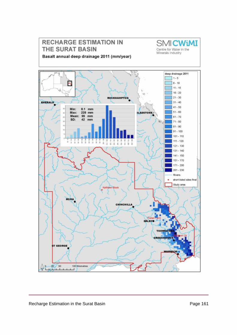
Recharge Estimation in the Surat Basin Page 161

Recharge Estimation in the Surat Basin Page 162
Figure 47 - Average annual deep drainage estimates for the Main Range Volcanics (Basalts)
in an example wet year – 2011 (data source: CSIRO AWAP 2014).

Recharge Estimation in the Surat Basin Page 163

Recharge Estimation in the Surat Basin Page 164
Figure 48 - Average annual deep drainage estimates for the Main Range Volcanics (Basalts)
in an example dry year – 2006 (data source: CSIRO AWAP 2014).
Temporal Recharge Estimates
The annual time series of deep drainage shows a mean of 11 ± 11 mm/yr for the whole Surat
(Figure 49) (where the latter value is the standard deviation representing the time variability of
the spatial mean annual values). As a percentage of precipitation, the long term mean is just
below 2% precipitation, although the role of sporadic high intensity wet periods is discernible
(Figure 50).
Dividing the Surat into the Main Range Volcanic (Basalts) (Figure 13) and Walloon – Injune
(Figure 51) geological units, the time variability of deep drainage in the Walloon – Injune is
similar to that for the whole Surat, although the variability in the Main Range Volcanics is
higher. This implies that during wet periods the Surat experiences more spatially widespread
increases in deep drainage, and may explain the bimodal distribution (i.e. high deep drainage
peak) in Figure 41.
Although these average values are useful, for further interpretation and any possible use as
model inputs it is critical to better honour the large degree of climatic variability driving deep
drainage within the Surat. Periods of above average precipitation clearly have an impact on
the monthly deep drainage estimates for the Surat as a whole. As an example, above average
precipitation occurred from 1995 – 1999, a prolonged drought period for 2000 – 2009, and a
very above average precipitation period again 2010 – 2013. Despite the annual mean deep
drainage of ~11 mm/yr, the period 1995 – 2000 experienced ~22.2 mm/yr, 2000 – 2009 only
~4.9 mm/yr, and 2010 – 2013 a much higher ~45.7 mm/yr (Figure 53). These large contrasts
over ENSO timescales highlight that from dry to wet period’s deep drainage rates can change
tenfold.
Interestingly, comparing the Main Range Volcanic and Walloon – Injune geological units
indicates that despite the similar average deep drainage values the rate is generally greater
for the Main Range Volcanics, whereas the Walloon – Injune units have a proportionally
greater response during very wet phases. This slight disparity explains the different trends in
the cumulative distribution (Figure 54) which estimates that the Main Range Volcanics have
transported ~500 mm additional deep drainage over the last ~100 years.

Recharge Estimation in the Surat Basin Page 165
Figure 49 - Time series of annual precipitation and deep drainage for the whole Surat CMA
as a spatial average for 1900 – 2014.
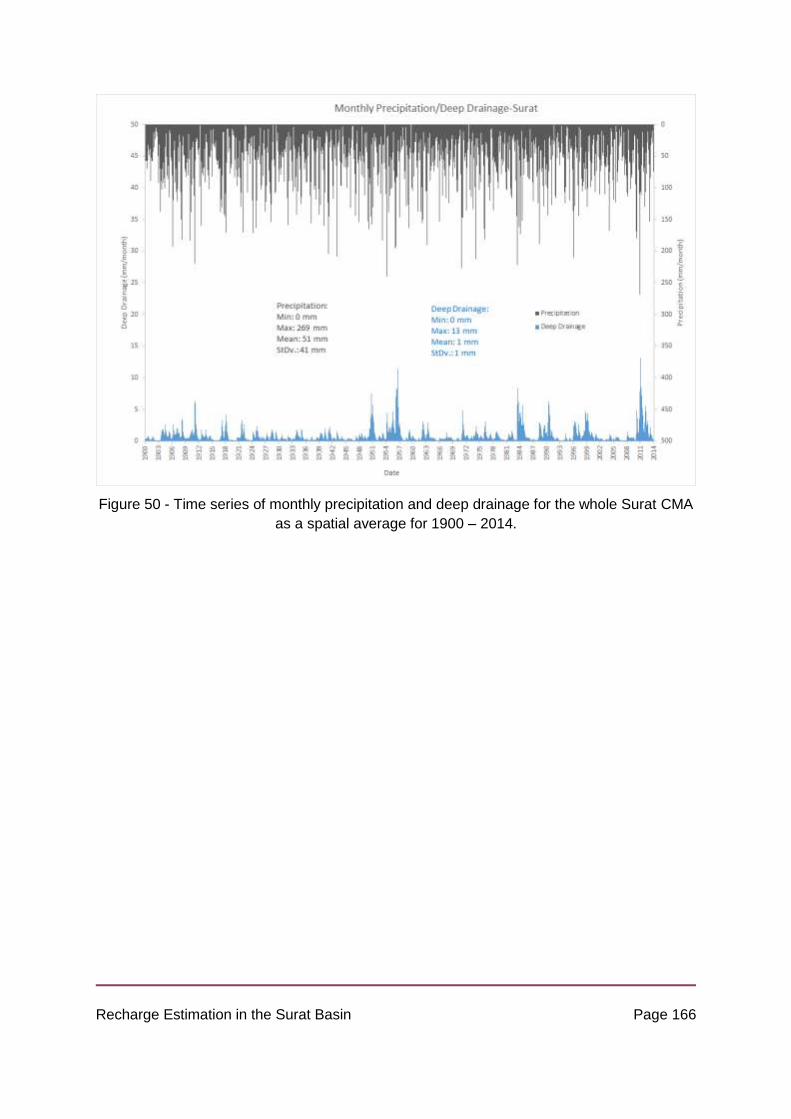
Recharge Estimation in the Surat Basin Page 166
Figure 50 - Time series of monthly precipitation and deep drainage for the whole Surat CMA
as a spatial average for 1900 – 2014.
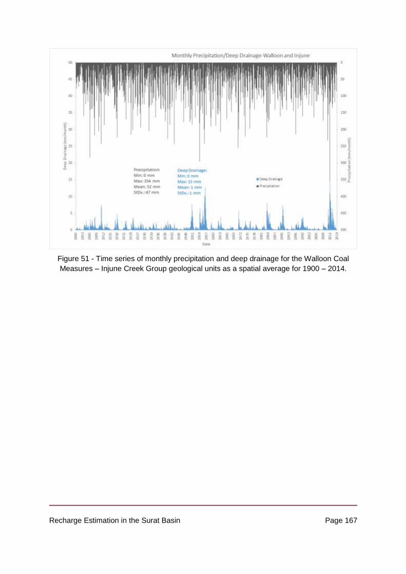
Recharge Estimation in the Surat Basin Page 167
Figure 51 - Time series of monthly precipitation and deep drainage for the Walloon Coal
Measures – Injune Creek Group geological units as a spatial average for 1900 – 2014.

Recharge Estimation in the Surat Basin Page 168
Figure 52 - Time series of monthly precipitation and deep drainage for the Main Range
Volcanics (Basalts) geological unit as a spatial average for 1900 – 2014.
Figure 53 - Monthly rainfall time series for the whole Surat CMA between 1995 – 2013,
highlighting the importance of ENSO induced wet and drought periods.

Recharge Estimation in the Surat Basin Page 169
Figure 54 - Cumulative distribution of deep drainage in the Main Range Volcanics (Basalts)
and Walloon Coal Measures – Injune Creek Group geological units.
Uncertainty
It is important to recognise the potentially high uncertainty in deep drainage estimates based
on remote sensed and modelled data. Uncertainties in parameter estimation for WaterDyn25M
followed a 3-step procedure (Raupach et al., 2009): 1. Reference parameter set was
determined and then applied to a limited set of training data, 2. Sensitivities of key water fluxes
to parameter values were determined. In terms of deep drainage fluxes, the greatest sensitivity
was from the Priestly – Taylor co-efficient (within the evapotranspiration equation), the
multiplier used for the deeper soil layer (M2) water saturation, and finally multipliers for
emissivity and albedo. 3. The reference parameter set was subjected to several tests against
a set of observations (e.g. actual soil moisture, measured runoff) over the national scale, with
inevitable uncertainty arising about local accuracy. There would also be significant additional
uncertainty in converting the deep drainage estimates to recharge.
Soil Moisture Comparisons
Another potentially signficant uncertainty is derived from the reliance on soil moisture data
from the AWAP model. As a preliminary exploration of the accuracy of modelled soil moisture
data, they were compared with the LANDSAT derived soil moisture (Figure 55 and Figure 56).

Recharge Estimation in the Surat Basin Page 170
The Surface Soil Moisture data (SSM) were retrieved from the Metop ASCAT 25 km soil
moisture images product of the Research Group Remote Sensing, Department for Geodesy
and Geoinformation (GEO), Vienna University of Technology (TU-Wien). The product is
provided as daily gridded images. These data were produced by using radar backscattering
coefficients measured by the Advanced Scatterometer (ASCAT) onboard the Metop satellite.
The relative soil moisture data ranging between 0% and 100% are derived by scaling the
normalized backscattering coefficients between the lowest/highest values corresponding to
the driest/wettest soil conditions. The derived soil moisture product represents the content in
the first 5 cm of the soil in relative units between totally dry conditions (0%) and total water
capacity (100%). The unit is degree of saturation, but can be converted into volumetric units
with the help of soil porosity information. The Metop ASCAT data also is composed of some
useful information such as error/noise of daily soil moisture and land surface conditions (i.e.,
unknown, unfrozen, frozen, temporary melting/water on the surface or permanent ice). The
overlapping daily soil moisture data from (2006-2014) was extracted from Metop ASCAT data
and compared with CSIRO AWAP daily soil moisture data.
The remote sensing soil moisture percentage is based on range between highest and lowest
pixel values, whereas the AWAP soil moisture is based on a pedotransfer function (soil class)
porosity and the shallow soil water balance equation. Also, the AWAP output is exactly
monthly, where as remote sensing is much more haphazard, therefore the remote sensing is
only crudely date adjusted so they can be compared (the AWAP data is a monthly average,
whereas the remote sensing data is a monthly snapshot). Interpretation of the errors is
challenging due to this timing issue, and due to the numerous potential sources of error in
both the AWAP and LANDSAT-derived data. Nevertheless, we recommend further exploration
of the spatial and temporal patterns of error over the Surat aiming to infer biases in these deep
drainage estimates.

Recharge Estimation in the Surat Basin Page 171
Figure 55 - Remote sensing soil moisture vs AWAP soil moisture, where soil moisture is
expressed as a percentage.
Figure 56 - Time series results for remote sensing soil moisture vs AWAP soil moisture,
where soil moisture is expressed as a percentage.
Summary

Recharge Estimation in the Surat Basin Page 172
Spatial variability
The analysis of the deep drainage estimates from the CSIRO Australian Water Availability
Project (AWAP) illustrates that deep drainage within the Surat Basin as a whole has high
spatial variability, and areas of higher deep drainage are driven by a combination of higher
precipitation and /or soil and landscape properties. This spatial variability was also evident
after separating the Surat into areas where the Walloon - Injune and Basalts are likely to be
unconfined (i.e. outcrop areas of these units and the Main Range Volcanics which over-lie the
Walloon Coal Measures). While caution is required due to the various modelling assumptions
used to produce these estimates, the AWAP data can be used to illustrate the degree of
variability. The long term (1900 – 2014) spatial range in deep drainage across the Surat is ~0
– 63 mm/yr, identical to the long term range for the Main Range Volcanics, although the long
term range for the Walloon – Injune beds is much lower (~0 – 30 mm/yr). The data indicate
that the Main Range Volcanics show the largest spatial sensitivity to variability from wet and
dry phases, although the Walloon – Injune outcrop areas are also quite dynamic, and are
certainly more sensitive to changes than the basin average.
Temporal variability
The temporal distribution of AWAP deep drainage data shows large variability around the long
term means, strongly influenced by ENSO driven dry and wet phases. Although the Main
Range Volcanics are again the most sensitive to this variability, the Surat as a whole can
experience order of magnitude deep drainage changes between dry and wet periods. The
results show the potential importance of including recharge as a time varying input (at least
annually varying) to groundwater models.
Further investigation
Within the temporal distribution, the role of climatic variability as well as antecedent conditions
and event intensity in driving deep drainage should be evaluated more explicitly.
Within the spatial distribution, the cause of variation in deep drainage distributions can be
investigated further, specifically targeting potential hotspot recharge areas, as well as priority
CSG impact areas.

Recharge Estimation in the Surat Basin Page 173
For both the spatial and temporal distributions, more localised verification of the AWAP model
using independent estimates of surface water and soil moisture from key recharge zones is
required; and resolution of significant biases that may be uncovered.
Furthermore, relating the deep drainage estimates to actual recharge rates requires
comparison with borehole hydrographs that have been interpreted as containing clear
recharge signals. This would allow the soil moisture balance based deep drainage to be
constrained by actual unconfined water table responses.
This would allow better estimation of a final recharge rate product for implementation within
groundwater models for the Surat Basin. However, this also requires better propagation of
uncertainty regarding deep drainage and recharge than is currently employed.
Analysis of Surface Water Hydrographs
Introduction
In this chapter, groundwater recharge on the eastern boundary of the Surat CMA is estimated
with the use of streamflow data. Annual groundwater recharge is quantified in four stream
catchments on the south-western extents of the Main Range Volcanics. The storage-
discharge method developed by Kirchner (2009) was used to quantify groundwater recharge
in the Surat CMA. This method has recently been applied to quantify seasonal mountain block
recharge in semi-arid Arizona (Ajami et al., 2011). A very similar approach was implemented
in this study to obtain a time series of annual recharge estimates from 1999 to 2014 for each
catchment. The estimates are a lower bound as only changes in storage due to stream
discharge are accounted for. Furthermore, a preliminary sensitivity analysis was carried out to
investigate the impact of storage-discharge functions on recharge estimates.
This chapter is made up of three sections in addition to this introduction. The following section
discusses the study area, the data and the methods applied in quantifying groundwater
recharge and testing the sensitivity of these estimates to the main assumptions used. Section
3 presents the results of this study. The chapter concludes with a section discussing the
limitations of the study, and putting forward recommendations for further work to improve and
build upon these findings.
Estimating Groundwater Recharge – Study Area, Data and Methods

Recharge Estimation in the Surat Basin Page 174
Storage – Discharge Theory and Method Formulation
The storage-discharge method developed by Kirchner (2009) is a catchment-based approach,
where the change in catchment (aquifer) storage is described by the conservation of mass
equation:
𝑑𝑆
𝑑𝑡= 𝑃 − 𝐸 − 𝑄 (1)
Where S is the volume of water in storage, P is the rate of precipitation, and E and Q are the
rates of evapotranspiration and discharge. Furthermore, the storage-discharge method is
based on the assumption that discharge (Q) is dependent on the amount of water in catchment
storage (S). This relationship is quantifiable by the storage – discharge function:
𝑄 = 𝑓(𝑆) (2)
This relationship is also invertible, so that the magnitude of discharge provides a measure of
the amount of water in catchment storage:
𝑆 = 𝑓−1(𝑄) (3)
If it is assumed that the storage represents groundwater storage, which discharges only to
surface streams, and the groundwater storage catchment area is known, increases in
measured stream baseflow can be interpreted as changes in S and thus as changes in
groundwater recharge. These are quantified as follows:
𝐺𝑊𝑅𝑡 = 𝑆𝑡+1 − 𝑆𝑡 = 𝑓−1(𝑄𝑡+1) − 𝑓−1(𝑄𝑡) (4)
Where GWR is groundwater recharge, S is catchment storage, Q is discharge, and t and t +
1 refer to the time periods before and after a precipitation event that results in groundwater
recharge. The first step in the method is therefore to define the inverse function f-1.
The inverse function f-1 is defined through analysis of the shape of recession curves. The
derivative of the storage-discharge function, also known as the sensitivity function, can be
determined directly from streamflow data when the catchment water balance (Equation 1) is
dominated by discharge (Q >> P, Q >> E) (Kirchner, 2009):
𝑔(𝑄) = 𝑑𝑄
𝑑𝑆≈
−𝑑𝑄𝑑𝑡⁄
𝑄|
𝑃≪𝑄,𝐸𝑇≪𝑄
(5)
The sensitivity function is derived by applying the recession plot method of Brutsaert and
Nieber (1977). The recession plot data are binned and a least squares regression model is
Recharge Estimation in the Surat Basin Page 175
fitted, defining the rate of change of discharge (-dQ/dt) as a function of discharge (Q). From
this relationship, the inverse storage-discharge function can be derived as follows:
𝑓−1(𝑄) = ∫ 𝑑𝑆 = ∫1
𝑔(𝑄)𝑑𝑄 (6)
The remainder of this section will provide further details on how this method was applied in
quantifying groundwater recharge in this study. This information is provided in four
subsections. First, general information is provided on the streamflow and precipitation data
used in the study. Second, the details of the methods applied in the recession plot analysis
and deriving storage-discharge functions are provided for each catchment. Third, the manner
in which recharge events were defined and respective discharge data extracted is explained.
Last, the sensitivity analysis carried out on recharge estimates is described.
Streamflow and Precipitation Data and Quality Control
Daily streamflow data used to carry out storage-discharge analysis were obtained from
Queensland’s Department of Natural Resources and Mines (QLD DNRM, 2014e, 2014f). For
a stream to be suitable for this method, the catchment had to have an identifiable storage –
discharge relationship and closure of the mass balance was also necessary. As such, this
restricts the method to small headwater catchments where the surface catchments can be
assumed the same as the groundwater catchment, with no groundwater recharge bypassing
the stream. This assumes that depletion of groundwater storage is only due to stream
discharge, and that all groundwater recharge returns as stream baseflow. However, some
components of groundwater recharge feed regional groundwater systems and not all recharge
flow paths in the catchment are accounted for. Thus the answer may be considered as a lower
bound estimate of groundwater recharge.
Five suitable gauging stations, with stream catchment areas varying between 35 and 148 km2,
were identified to provide initial estimates of recharge (Figure 57, Table 19). The streams are
located on the western side of the Great Dividing Range from Toowoomba southwards
towards the New South Wales border. The catchments of all the streams were predominantly
located in the Main Range Volcanics geologic formation, which is likely to be the dominant
source of groundwater to the streams. As such, the groundwater recharge estimates obtained
from this study are believed to be indicative of recharge within the Main Range Volcanics.

Recharge Estimation in the Surat Basin Page 176
Table 19 – General stream and gauging station information (QLD DNRM, 2014f)
Stream Basin Stream Gauging
Station Number
Catchment
Area (km2)
Elevation
(mAHD)
Swan Creek Balonne - Condamine 422306A 83 536
Emu Creek Balonne - Condamine 422313B 148 491
Spring Creek Balonne - Condamine 422321B 35 552
Gowrie Creek Balonne - Condamine 422326A 47 538
Condamine River Balonne - Condamine 422341A 92 515
General quantity and quality analyses were carried out on the daily streamflow data. The
possibility of using hourly streamflow data was explored. However, this was abandoned due
to the increased levels of noise in the data at smaller discharges. In addition, hourly data were
not available for the entire time series. For the majority of the streams the data record extended
to the early 1970s, with the exception of Swan Creek which had a data record in

Recharge Estimation in the Surat Basin Page 177

Recharge Estimation in the Surat Basin Page 178
Figure 57 - Location of stream gauging stations used in storage-discharge analysis and
respective rainfall gauges. The location of all open and historical stream gauging stations
(QLD DNRM, 2014e, 2014f), and all rain gauges (BOM, 2014) is indicated.

Recharge Estimation in the Surat Basin Page 179
excess of 90 years (Figure 59, Table 20). Swan Creek also had the largest number of missing
data points, approximately 4.5 % of the total time series. Zero flow days made up less than 7
% of the remaining flow record for all the catchments (Table 20), with Swan and Emu Creek
characterised by lower flows in comparison to Spring and Gowrie Creek (Figure 58). One
assumption of the recession plot analysis is that the streams are perennial (Ajami et al., 2011).
Even though the streams were not truly perennial, this limited number of zero flow days was
assumed not to disqualify the approach.
Table 20 - Stream gauging station data distribution, quantity and quality (QLD DNRM, 2014f)
Stream
Stream
Gauging
Station
Period of
Record -
Start
Period of
Record -
End
Total
Number of
Data
Points
% of Total
Time
Series
% of Net
Time
Series
Swan Creek 422306A 03/09/1920 21/08/2014 34 321 4.4 6.8
Emu Creek 422313B 24/01/1973 21/08/2014 15 185 0.3 6.1
Spring Creek 422321B 24/01/1973 20/08/2014 15 184 0.2 0.1
Gowrie Creek 422326A 20/11/1969 21/08/2014 16 346 2.7 0
Condamine River 422341A 27/05/1976 21/08/2014 13 966 2.3 4.2

Recharge Estimation in the Surat Basin Page 180
Figure 58 - Flow duration curves, normalised by catchment area, of the five stream gauging
stations
Precipitation fluxes to the catchment had to be known for selecting baseflow recession
periods. Rainfall data were obtained from the Bureau of Meteorology (BOM, 2014). Rainfall
gauges were selected based on both the proximity of the gauge to the gauging station and the
temporal overlaps in record with the stream gauging station (Figure 57, Figure 59, Table 21).
In some circumstances one rain gauge was the optimal choice with respect to both criteria,
while in other situations this was not the case. Generally, the length and quality of rainfall
record was prioritised over the proximity as long as the rain gauge was within the vicinity (less
than 10 km) of the stream gauging station and representative of rainfall in the catchment.
Table 21 - Information on rainfall gauge used for each stream gauging station (BOM, 2014)
Stream
Stream
Gauging
Station
Rainfall
Gauge
Distance
(km)
Period of
Record - Start
Period of
Record – End
Swan Creek 422306A 041120 8 01/01/1912 31/07/2014
Emu Creek 422313B 041120 4.1 01/01/1912 31/07/2014
Recharge Estimation in the Surat Basin Page 181
Spring Creek 422321B 041208 0.7 01/02/1959 31/07/2014
Gowrie Creek 422326A 041369 5.9 01/05/1972 31/03/2014
Condamine River 422341A 041056 1.9 01/09/1903 31/08/2014
After further data interrogation and quality control, Gowrie Creek catchment (GS 422326A)
was not included in the analysis. Gowrie Creek is on the northern outskirts of Toowoomba with
the creek flowing through Toowoomba upstream. It appears that Toowoomba covers the
majority of the stream catchment. Thus, streamflow would be heavily influenced by large areas
of impermeable surfaces and stormwater diversions. This was evident from the Gowrie Creek
hydrograph, which was highly responsive to rainfall but had a generally constant baseflow
component indicating low groundwater recharge; however calculation of the sensitivity
function is highly uncertain due to low values of dQ/dt and thus recharge was not quantified
for this catchment.
Recession Plots and Storage – Discharge Relationships
Recession plots, as originally developed by Brutsaert and Nieber (1977), were used to
estimate the catchment sensitivity function and thus the catchment storage-discharge
relationship. To obtain recession plots of each of the four catchments, streamflow data were
first normalised by surface water catchment area (assumed equal to the groundwater
catchment) so that all water fluxes were in the same depth based units (mm/day).

Recharge Estimation in the Surat Basin Page 182

Recharge Estimation in the Surat Basin Page 183
Figure 59 - Temporal distribution of stream flow and rainfall data for each stream gauging station, with distribution of missing data also
indicated (BOM, 2014; QLD DNRM, 2014f)

Recharge Estimation in the Surat Basin Page 184
A model was developed to automate recession curve extraction. A large variety of methods
with different recession parameters have been applied in extracting baseflow recession data
(e.g. Oyarzún et al., 2014; Stoelzle et al., 2013; Tallaksen, 1995; Wittenberg, 1999; WMO,
2008). In this study, recessions were defined as the component of the hydrograph where dQ/dt
was negative, from two days after a peak until a day before a trough in discharge (or when
missing data or constant discharge was encountered). This reduced the chance of including
the effects of storm runoff and interflow on recessions. Only recessions that had a peak
discharge higher than a specified cut-off value (Table 22) and lasted for a minimum of four
consecutive days were used. This was done to increase the likelihood of extracting actual
recessions rather than small fluxes in discharge that are especially evident at low flows, where
data noise and gauging errors are more prevalent.
Table 22 - Peak discharge filter (cutoff) used in recession data extraction, and the number of
bins used in determining storage-discharge relationships.
Stream Stream Gauging
Station
Cutoff Discharge
(mm/day)
Number of
Bins
Swan Creek 422306A 0.06 30
Emu Creek 422313B 0.06 50
Spring Creek 422321B 0.35 30
Condamine River 422341A 0.1 40
Rainy days and days with missing rainfall data were removed from the recession data, while
the effects of evapotranspiration on recessions were assumed to be negligible as stream
discharge was fed from groundwater storage (Ajami et al., 2011). The validity of this
assumption varies between catchments, with groundwater storage losses to
evapotranspiration (and thus recession behaviour) being more important in some catchments
than others (Wittenberg, 1999). Kirchner (2009) indicated that precipitation and
evapotranspiration fluxes did not need to be wholly absent, just relatively small compared to
discharge. However, this could not be investigated due to a lack of adequate daily
evapotranspiration data. A five year sample of the automatically extracted recession data for
Spring Creek (GS 422321B) is depicted in Figure 60for the period January 2010 to August
2014.

Recharge Estimation in the Surat Basin Page 185
Recession plots were generated from the filtered recession dataset. The rate of change of
discharge (-dQ/dt) was plotted as a function of discharge (Q) in natural log space. These
variables were calculated between all successive streamflow recession data points. The rate

Recharge Estimation in the Surat Basin Page 186

Recharge Estimation in the Surat Basin Page 187
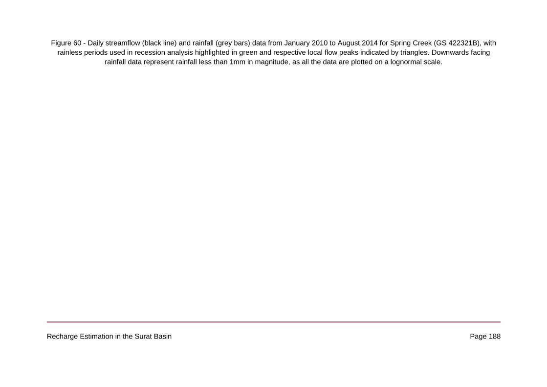
Recharge Estimation in the Surat Basin Page 188
Figure 60 - Daily streamflow (black line) and rainfall (grey bars) data from January 2010 to August 2014 for Spring Creek (GS 422321B), with
rainless periods used in recession analysis highlighted in green and respective local flow peaks indicated by triangles. Downwards facing
rainfall data represent rainfall less than 1mm in magnitude, as all the data are plotted on a lognormal scale.

Recharge Estimation in the Surat Basin Page 189
of change of discharge and the corresponding discharge were estimated as follows (Brutsaert
and Nieber, 1977):
−𝑑𝑄
𝑑𝑡≈
𝑄𝑡−∆𝑡 − 𝑄𝑡
∆𝑡 (7)
𝑄 ≈𝑄𝑡−∆𝑡 + 𝑄𝑡
2 (8)
where Δt = 1 day. To determine the functional relationship between –dQ/dt and Q, recession
plot data were binned based on the Q value (independent variable), and a least squares
regression model was fitted to the binned values. The primary reason that recession plots
were binned was to properly define recession behaviour at low discharges where scatter in
data points is high (Kirchner, 2009). Two different binning techniques were employed as per
Ajami et al. (2011), namely the quantile and equal interval binning techniques. The quantile
binning technique bins data so that each bin contains approximately the same number of data
points. On the other hand, the equal interval method bins data so that all bins span an equal
width of log-transformed streamflows, resulting in bins with vastly different numbers of data
points. The binned data undergo a quality control process, so that only bins where the
standard error (-dQ/dt) is less than half mean (-dQ/dt) are kept (Kirchner, 2009). The number
of bins was determined such that the relationship between Q and –dQ/dt was well defined
(Table 22). Both linear and quadratic regression functions were fitted to the binned data. The
most suitable of the four models that best represented the functional relationship between –
dQ/dt and Q was selected for each catchment.
Storage-discharge relationships were derived from these regression functions by the methods
outlined in Section 0 (Equation 5 and 6), where analytical solutions to the regression functions
were already available (Ajami et al., 2011; Kirchner, 2009). The storage-discharge function of
a linear regression equation of the form:
ln (−𝑑𝑄
𝑑𝑡) = ln(𝑎) + 𝑏. ln (𝑄) (9)
was defined as:
𝑆 − 𝑆0 =1
𝑎
1
2 − 𝑏𝑄2−𝑏 (10)
where ln(a) is the y-intercept , b is the slope and S0 is a constant of integration. Similarly, the
storage-discharge function of a quadratic polynomial regression equation of the form:
ln (−𝑑𝑄
𝑑𝑡) = 𝑐1 + 𝑐2 ln(𝑄) + 𝑐3[ln (𝑄)]2 (11)

Recharge Estimation in the Surat Basin Page 190
where the quadratic coefficient (c3) is positive, was defined as:
𝑆 − 𝑆0 =1
2√
𝜋
𝑐3exp (
(𝑐2 − 2)2 − 4𝑐3𝑐1
4𝑐3) erf (√𝑐3𝑙𝑛𝑄 +
𝑐2 − 22
√𝑐3
) (12)
where erf is the error function.
Quantifying Annual Groundwater Recharge
Groundwater recharge was quantified on an event by event basis for the last 15 years (July
1999 to June 2014). This time period was selected for two primary reasons. First, high quality
streamflow data with limited missing data were available across all catchments. Second,
recharge estimates could be obtained for periods of both flood and drought, thus providing
information over a range of climatic conditions. Groundwater recharge due to a precipitation
event was estimated by calculating the change in catchment storage (i.e. recharge) before
and after the event, using either Equation 10 or 12. The representative stream discharge
values for each event were manually identified as depicted in Figure 61, which captures
changes in catchment baseflow due to recharge. The values of groundwater recharge
obtained are minimum estimates for three reasons: 1) only events that could be identified with
confidence were incorporated; 2) any depletion of groundwater storage during the event was
not considered, and 3) only groundwater recharge and respective changes in storage that
returned as stream discharge was accounted for.
Figure 61 - Schematic of how representative discharge values are extracted from
hydrograph to determine event-based recharge. A representative discharge is obtained
before (Qt) and after (Qt+1) each recharge event (Figure after Ajami et al. (2011)).

Recharge Estimation in the Surat Basin Page 191
Groundwater recharge estimates were aggregated into water years (July to June), where
recharge events were assigned to the water year in which the event started. Aggregating the
data allowed recharge estimates to be compared to the other estimates in this report. Total
annual precipitation was quantified for the same time periods, and the percentage of rainfall
resulting in recharge was evaluated.
Sensitivity Analysis
A sensitivity analysis was carried out to investigate the influence of the binning technique
(quantile and equal interval) and the form of the regression equation (linear and quadratic) on
predicted groundwater recharge values. Storage-discharge functions were derived for each of
the four scenarios, and groundwater recharge values were estimated for each recharge event
across all catchments. Annual groundwater recharge estimates for each scenario were
quantified as discussed in Section 0. Groundwater recharge values were also compared to
recharge data obtained for each catchment from the remote sensing analysis carried out in
Chapter 0.
Results
Storage – Discharge Relationships
Simple quality control showed that only a limited number of recession points were lost due to
missing rainfall record (Table 23). This was important as recession data were removed from
the dataset if either rain was recorded on that day or if no rainfall data were available. Thus
such a check ensured that large amounts of data were not being lost because of an incomplete
rainfall dataset. The number of days lost due to incomplete rainfall record was calculated for
the final dataset once recession data had been extracted from the stream flow time series,
rather than for the entire rainfall record. A maximum of 1.4 % of recession points were lost
across all four catchments (Table 23), which was considered satisfactory.
Table 23 - Assessment of the number of recession points lost due to missing rainfall data
Stream
Stream
Gauging
Station
Rainfall
Gauge
No. of
Recession
Points
No. of NA
Rainfalls % of Total
Swan Creek 422306A 041120 6 112 6 0.10

Recharge Estimation in the Surat Basin Page 192
Emu Creek 422313B 041120 3 758 3 0.08
Spring Creek 422321B 041208 2 736 20 0.73
Condamine River 422341A 041056 4 267 58 1.36
The recession behaviour of Spring Creek catchment (GS 422321B) was characterised by a
cloud of recession points (Figure 62). The scatter in the recession plot, especially at lower
discharge values, might be attributed to any of a number of factors, including: data
measurement noise, gauging equipment limitations, impacts of evapotranspiration and
precipitation on recession behaviour, and model simplification of real catchment (Kirchner,
2009).
After the recession data were binned, streamflow recession behaviour of Spring Creek
catchment exhibited an upward curving, positive quadratic relationship for both the equal
interval and quantile binning methods (Figure 62). In both instances, the relationship between
rate of change of discharge (-dQ/dt) and discharge (Q) during streamflow recession was better
defined by a quadratic rather than linear equation (Figure 63, Table 24). The quantile binning
technique was selected because it defined catchment recession behaviour well with a suitable
regression model (Figure 63, Table 25).

Recharge Estimation in the Surat Basin Page 193
Figure 62 - Recession plots for Spring Creek (GS 422321B) based on daily rainless stream
flow data. Black dots are binned data, error bars indicate standard error of each bin where
the standard error was less than half the mean of –dQ/dt for each bin. Both the equal interval
(left) and quantile (right) binning method were applied.
Quantile binning was also selected over the equal interval binning technique because all bin
sizes were equal, thus preventing bins with very few data points having a large influence on
the relationship. The storage-discharge function was derived from Equation 12, because the
regression model had a positive quadratic coefficient and thus this analytical solution was
suitable:
𝑆 − 𝑆0 = 32.1 erf (0.51𝑙𝑛𝑄 − 0.88)
Table 24 - Comparison of Spring Creek regression models for both equal interval and
quantile binning methods
Equal Interval Binning Quantile Binning
Linear
Model
Quadratic
Model
Linear
Model
Quadratic
Model
lnQ 0.956 1.01 0.907 1.1
(lnQ)2 NA 0.19 NA 0.26
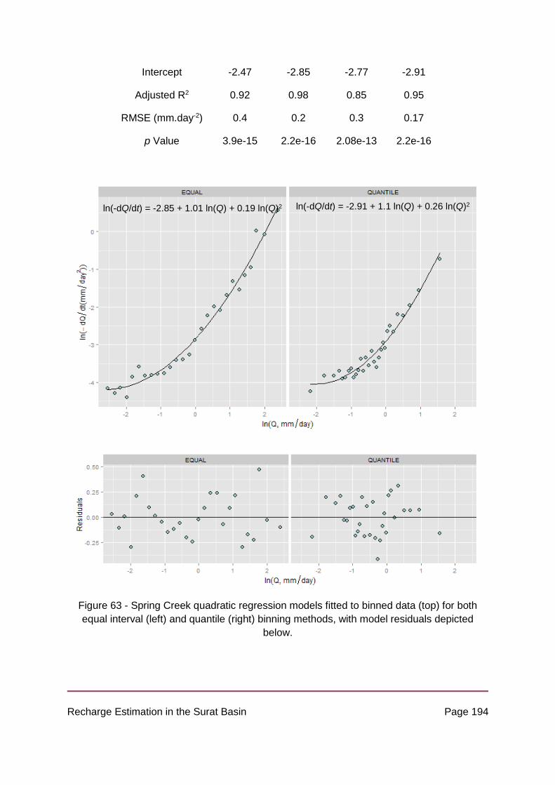
Recharge Estimation in the Surat Basin Page 194
Intercept -2.47 -2.85 -2.77 -2.91
Adjusted R2 0.92 0.98 0.85 0.95
RMSE (mm.day-2) 0.4 0.2 0.3 0.17
p Value 3.9e-15 2.2e-16 2.08e-13 2.2e-16
Figure 63 - Spring Creek quadratic regression models fitted to binned data (top) for both
equal interval (left) and quantile (right) binning methods, with model residuals depicted
below.
ln(-dQ/dt) = -2.85 + 1.01 ln(Q) + 0.19 ln(Q)2
ln(-dQ/dt) = -2.91 + 1.1 ln(Q) + 0.26 ln(Q)2

Recharge Estimation in the Surat Basin Page 195
The other three catchments (Swan Creek, Emu Creek and Condamine River) all exhibited
similar streamflow recession behaviour to Spring Creek (Figure 62, Figure 64). In each
instance, the quantile binning technique and a quadratic regression function were found to be
most suitable for defining the relationship between –dQ/dt and Q. The least squares
regression model was a good fit to the binned data with R2 values varying between 0.97 and
0.99, while RMSE values were between 0.1 and 0.17 mm.day-2 (Table 25). As with Spring
Creek, the storage-discharge function of each catchment was derived from Equation 12.
ln(-dQ/dt) = -1.14 + 1.48 ln(Q) + 0.08 ln(Q)2
a). Swan Creek (GS 422306A)

Recharge Estimation in the Surat Basin Page 196
ln(-dQ/dt) = -1.33 + 1.36 ln(Q) + 0.07 ln(Q)2
b). Emu Creek (GS 422313B)
ln(-dQ/dt) = -1.97 + 1.36 ln(Q) + 0.13 ln(Q)2
c). Condamine River (GS 422341A)
Recharge Estimation in the Surat Basin Page 197
Figure 64 - Recession plots and model residuals of a) Swan Creek (GS 422306A), b) Emu Creek (GS 422313B), and c) Condamine River (GS
422341A)

Recharge Estimation in the Surat Basin Page 198
Table 25 - Summary of the final storage – discharge functions used in estimating recharge
for each catchment
Stream Gauging
Station S – Q Function
Regression
Type
Binning
Technique
Adjusted
R2
RMSE
(mm.day-2)
Swan Creek 422306A 𝑆 − 𝑆0 = 19.7 erf (0.29𝑙𝑛𝑄
− 0.91) Quadratic Quantile 0.99 0.11
Emu Creek 422313B 𝑆 − 𝑆0 = 19.40 𝑒𝑟𝑓 (0.27𝑙𝑛𝑄
− 1.17) Quadratic Quantile 0.99 0.10
Spring Creek 422321B 𝑆 − 𝑆0 = 32.1 𝑒𝑟𝑓 (0.51𝑙𝑛𝑄
− 0.88) Quadratic Quantile 0.95 0.17
Condamine
River 422341A
𝑆 − 𝑆0 = 23.21 erf (0.35𝑙𝑛𝑄
− 0.90) Quadratic Quantile 0.97 0.17
Recharge Estimates
Groundwater recharge estimates varied among the four catchments (Figure 65, Table 26)
even though all gauging stations were within a 22 km range as the crow flies. Groundwater
recharge for the period 1999 to 2014 was on average the largest at Spring Creek (13.0
mm/year), followed by the Condamine River (10.2 mm/year), Swan Creek (3.1 mm/year) and
lastly Emu Creek (2.1 mm/year). The Condamine River (GS 422341A) streamflow dataset had
some missing data during 2002, 2003 and 2005 and thus recharge during this time period is
potentially underestimated. It appeared that only a small percentage of annual rainfall resulted
in recharge in these catchments, with the Condamine River exhibiting the largest mean
percentage turnover (1.3 %) while Emu Creek had the smallest with a meagre 0.3 % (Figure
66, Table 27).
This spatial variation in recharge estimates might be a result of a number of factors. The
recharge rates are (unsurprisingly) correlated to the general streamflows in the catchments,
with Emu and Swan Creek having the lowest area-normalised streamflows (Figure 58) and
largest number of no-flow days (Table 20). There also appears to be a general north-south
trend in groundwater recharge, with larger recharge rates occurring in the southerly (Spring
Creek and Condamine River) as to the northerly (Swan and Emu Creek) catchments (Figure
57). Furthermore, Spring Creek has the smallest catchment area (35 km2) and highest
elevation (552 mAHD), while Emu Creek has the largest catchment area (148 km2), lowest
elevation (491 mAHD) and the gauging station might already be in alluvial deposits. These
differences might be indicative of shallower recharge flow paths at higher elevations within the

Recharge Estimation in the Surat Basin Page 199
Main Range Volcanics; while recharge might be deeper and more regional further from the
outcrops, with less water returning to rivers as baseflow.

Recharge Estimation in the Surat Basin Page 200
Table 26 - Summary statistics of annual recharge (mm/year) for each of the four streams.
Respective water year indicated in brackets where relevant.
Swan Creek
(GS 422306A)
Emu Creek
(GS 422313B)
Spring Creek
(GS 422321B)
Condamine River
(GS 422341A)
Mean 3.12 2.05 13.01 10.16
Median 1.87 1.89 8.56 7.79
Minimum 0
(2006 - 2007)
0.00
(2006 - 2007)
0.01
(2006 - 2007)
0.72
(2006 - 2007)
Maximum 10.18
(2010 - 2011)
7.84
(2010 - 2011)
49.82
(2010 - 2011)
27.30
(2010 - 2011)
Standard Dev. 3.15 2.13 14.48 8.04
Count 15 15 15 15

Recharge Estimation in the Surat Basin Page 201
Figure 65 - Time series of groundwater recharge estimates for each of the four streams.
Recharge is provided per water year (July - June), from July 1999 to June 2014.
Table 27 - Summary statistics of the percentage of annual rainfall that results in recharge, for
each of the four streams. Respective water year indicated in brackets where relevant.
Swan Creek
(GS 422306A)
Emu Creek
(GS 422313B)
Spring Creek
(GS 422321B)
Condamine River
(GS 422341A)
Mean 0.42 0.27 1.27 1.31
Median 0.30 0.25 1.02 1.33

Recharge Estimation in the Surat Basin Page 202
Minimum 0
(2006 - 2007)
0.00
(2006 - 2007)
0.00
(2006 - 2007)
0.13
(2006 - 2007)
Maximum 1.37
(2012 - 2013)
0.80
(2012 - 2013)
3.17
(2012 - 2013)
2.32
(2012 - 2013)
Standard Dev. 0.40 0.24 1.14 0.82
Count 15 15 15 15

Recharge Estimation in the Surat Basin Page 203
Figure 66 - Time series of percentage of rainfall resulting in groundwater recharge for each
of the four streams. Percentages are provided per water year (July - June), from July 1999 to
June 2014.

Recharge Estimation in the Surat Basin Page 204
Groundwater recharge not only varied spatially but also substantial temporal variability was
evident within each catchment (Figure 65, Table 26). During drought periods (e.g. 2006 -
2007), groundwater recharge was approximately zero for Swan, Emu and Spring Creek, while
0.7 mm of recharge occurred in the Condamine River catchment. On the other hand during
flood periods (e.g. 2010 - 2011), recharge increased by many orders of magnitude with Spring
Creek experiencing 50 mm. This variability in recharge rates is highlighted by the large
standard deviations, with only the Condamine River catchment having a higher mean recharge
rate than the respective standard deviation (Table 26). Similar trends were present in the
amount of rainfall resulting in groundwater recharge (Figure 66, Table 27).
Sensitivity Analysis
Groundwater recharge estimates did vary depending on which storage-discharge function was
used (Table 28). Generally, recharge estimates were the largest for storage-discharge
functions derived from the linear recession behaviour regression models. Similarly, storage-
discharge functions derived from data binned by the quantile technique resulted in larger
estimates than from data binned into equal intervals. Recharge estimates derived from the
quadratic regression model and equal interval binning technique were consistently the
smallest. For three of the four catchments (Swan Creek, Emu Creek and Condamine River)
predicted recharge estimates were substantially smaller than the recharge estimates that were
derived from the other three storage-discharge functions (Table 28).
With the exception of the quadratic regression model fitted to equal interval binned data,
recharge estimates were of the same order of magnitude giving confidence in the estimated
values. Spring Creek had the largest range in mean recharge estimates (13.0 to 30.8
mm/year), while Swan Creek recharge estimates were very close between all models (3.0 to
3.7 mm/year). The groundwater recharge values used in this study (Model 4 - quadratic
regression model fitted to quantile binned data) were consistently in the lower range of
predicted values. Model 4 had the smallest RMSE across all catchments and also very high
Adjusted R2 (Table 28).

Recharge Estimation in the Surat Basin Page 205
Table 28 - Summary of the different storage – discharge functions used in the sensitivity analysis, and respective estimates of mean annual
recharge over the last 15 years. Four storage – discharge functions were derived for each stream for the sensitivity analysis. The influence of
different regression functions (linear/quadratic) and binning techniques (equal interval/quantile) was investigated. Model 4 (quadratic regression
function and quantile binning method) was used to estimate final recharge within each stream catchment.
Stream and
Gauging Station
Number
Model S-Q Function (mm) Regression Type Binning
Technique Adjusted R2
RMSE
(mm.day-2)
Mean Annual
Recharge
(mm/yr)
Swan Creek
(GS 422306A)
1 𝑆 − 𝑆0 = 3.76 𝑄0.84 Linear Equal Interval 0.98 0.37 3.03
2 𝑆 − 𝑆0 = 4.73 𝑄0.90 Linear Quantile 0.97 0.23 3.68
3 𝑆 − 𝑆0 = 105 erf (0.09𝑙𝑛𝑄 − 4.45) Quadratic Equal Interval 0.98 0.36 2.5e-8
4 𝑺 − 𝑺𝟎 = 𝟏𝟗. 𝟕 𝒆𝒓𝒇 (𝟎. 𝟐𝟗𝒍𝒏𝑸 − 𝟎. 𝟗𝟏) Quadratic Quantile 0.99 0.11 3.12
Emu Creek
(GS 422313B)
1 𝑆 − 𝑆0 = 3.95 𝑄1.07 Linear Equal Interval 0.96 0.54 3.81
2 𝑆 − 𝑆0 = 5.12 𝑄0.99 Linear Quantile 0.97 0.23 5.17
3 𝑆 − 𝑆0 = 20.31 𝑒𝑟𝑓 (0.25𝑙𝑛𝑄 − 1.45) Quadratic Equal Interval 0.995 0.18 0.873
4 𝑺 − 𝑺𝟎 = 𝟏𝟗. 𝟒𝟎 𝒆𝒓𝒇 (𝟎. 𝟐𝟕𝒍𝒏𝑸 − 𝟏. 𝟏𝟕) Quadratic Quantile 0.99 0.10 2.05
Spring Creek
(GS 422321B)
1 𝑆 − 𝑆0 = 11.30 𝑄1.04 Linear Equal Interval 0.92 0.4 22.54
2 𝑆 − 𝑆0 = 14.66 𝑄1.09 Linear Quantile 0.85 0.3 30.85
3 𝑆 − 𝑆0 = 35.03 𝑒𝑟𝑓 (0.44𝑙𝑛𝑄 − 1.13) Quadratic Equal Interval 0.98 0.2 7.75
4 𝑺 − 𝑺𝟎 = 𝟑𝟐. 𝟏 𝒆𝒓𝒇 (𝟎. 𝟓𝟏𝒍𝒏𝑸 − 𝟎. 𝟖𝟖) Quadratic Quantile 0.95 0.17 13.01

Recharge Estimation in the Surat Basin Page 206
Condamine River
(GS 422341A)
1 𝑆 − 𝑆0 = 5.74 𝑄1.10 Linear Equal Interval 0.95 0.55 13.72
2 𝑆 − 𝑆0 = 8.4 𝑄1.10 Linear Quantile 0.91 0.31 20.09
3 𝑆 − 𝑆0 = 28.43 erf (0.22𝑙𝑛𝑄 − 1.93) Quadratic Equal Interval 0.96 0.45 0.40
4 𝑺 − 𝑺𝟎 = 𝟐𝟑. 𝟐𝟏 𝒆𝒓𝒇 (𝟎. 𝟑𝟓𝒍𝒏𝑸 − 𝟎. 𝟗𝟎) Quadratic Quantile 0.97 0.17 10.16

Recharge Estimation in the Surat Basin Page 207
Limitations, Future Research and Recommendations
A limitation of this study is that it estimates recharge that subsequently discharges into the
surface water system at the outlet of headwater catchments, rather than recharge that directly
recharges to the Surat Basin groundwater system. Nevertheless, the estimates provide
constraints on how much recharge may be directly entering the groundwater system from
these headwaters and other areas of the Surat Basin with similar hydrological properties; and
builds understanding of the surface flows.
The results presented in this report are only over a limited spatial and temporal scale, and can
be expanded to get a fuller understanding of groundwater recharge in the Surat CMA. The
catchments analysed in this study are located on the western side of the Main Range
Volcanics from Toowoomba southwards towards the New South Wales border. There are
other open gauging stations that can be analysed on the eastern extent of the Main Range
Volcanics, and further historic stations both west and east of the divide. A handful of potential
gauges have also been identified further west and north in the Surat Basin, however
catchment areas at the gauging station locations might be too large to make these methods
applicable. The time period of recharge estimates can also be expanded beyond the 15 years
investigated in this report. There is potential for aggregating and expanding datasets from
open and historical gauges in some circumstances.
The recharge estimates obtained here may be considered as a lower limit of groundwater
recharge in the catchment. The methods account for groundwater flow paths from the aquifer
to the stream, however this might not capture other recharge flow paths and inter-aquifer flows
in the catchment (Ajami et al., 2011). The recession plot analysis of Brutsaert and Nieber
(1977) is also based on the assumption that the investigated streams are perennial. Even
though the streams investigated were only dry for less than seven percent of their flow record,
this does result in underestimation of recharge events when pre-event discharge is zero as
the actual level of catchment storage is unknown. There will also be some recharge that exits
the catchment as streamflow during the events and therefore is not captured in the measured
storage difference; and some recharge during the recession periods that the method assumes
to be negligible
A preliminary sensitivity analysis was carried out on the impact of regression model and
binning technique on recharge estimates. The methods applied in estimating groundwater

Recharge Estimation in the Surat Basin Page 208
recharge have other assumptions whose impacts should also be further investigated. An
automated technique was developed to extract recession data for this study that employed
specific assumptions on recession length, start of recession, rate of recession and flow event
magnitude. A recent study carried out on mesoscale catchments in Germany found that
recession characteristics varied substantially depending on what method was applied, and
recommended a multiple-methods approach to be implemented when possible (Stoelzle et al.,
2013). Rupp and Selker (2006) developed a method to account for the scatter and noise in
recession data at low discharges that might be valuable.
Further improvements in recession plot quality and quantifying recession behaviour can also
be made by better identifying low precipitation and evapotranspiration days. The impacts of
evapotranspiration on streamflow recession were not accounted for in the recession plots in
this study. However, evapotranspiration can have substantial effects on baseflow recession in
some systems and result in inaccurate interpretation of recession behaviour (Kirchner, 2009).
Even though accurate daily evapotranspiration data are not available for these catchments,
recession data can be selected for time periods of generally lower evapotranspiration rates.
Improvements can be made in selecting rain free days by using spatially interpolated rainfall
data or multiple rain gauges.
Recharge events and respective discharge values for quantifying groundwater recharge were
manually identified in this study. Implementing such a manual hydrograph separation
technique decreases objectivity, results are often not reproducible and separating the
influence of multiple recharge events in close succession is difficult (Healy and Scanlon,
2010). The objectivity of results could be improved by looking at recharge on a larger time
scale such as annual or seasonal, rather than on an event basis where errors can accumulate
(Kirchner, 2009). Automated baseflow filters might also be valuable in reducing subjectivity in
selecting recharge events and representative discharge values (Arnold et al., 1995; Chapman,
1999; Sloto and Crouse, 1996).
Furthermore, a number of different methods utilising streamflow data, such as the recession
curve displacement method (Rorabaugh, 1964; Rutledge, 1998), have been applied in
different studies to estimate groundwater recharge (Arnold and Allen, 1999; Arnold et al.,
2000; Healy and Scanlon, 2010; Wittenberg, 1999). Applying different estimation techniques
based on the same streamflow data might be fruitful in investigating the range in recharge
estimates that are obtained by different streamflow recession methods and comparing to

Recharge Estimation in the Surat Basin Page 209
values obtained from other recharge estimation approaches (e.g. water balance methods,
water table fluctuation, etc.).
Conclusions
This section presents the main conclusions covering our literature review and analysis of
existing data for the Surat Basin, including summary tables of previous and new recharge
estimates. Recommendations follow in the next section.
A literature review was conducted to determine which recharge estimation methods used
globally might be suitable for recharge estimation in the Surat Basin. Key findings from the
literature review were: that multiple methods should be applied, and it is important to keep in
mind the assumptions and limitations of each method. There is evidence that modelling
methods can be readily combined with field measurements and that this combination of
approaches may be suitable in the Surat Basin.
A number of recharge estimation methods have been applied in the Surat Basin prior to our
study, e.g. groundwater hydrograph analyses, groundwater chloride mass balance,
unsaturated zone chloride mass balance and soil water balance modelling. Of these methods,
the soil water balance modelling resulted in the greatest range of recharge estimates (0 – 455
mm/year). Several methods resulted in estimated groundwater recharge rates that were
higher than the groundwater recharge rates currently included in the OGIA model (see Table
29).
The previous recharge estimates included a range of spatial scales but the temporal scales
were typically quite limited (see Table 29). Many of the previous studies reported long term
average recharge rates but did not provide the finer detail of time-variable recharge estimates.
Our analysis and interpretation of available data has resulted in an improved understanding
of the spatial and temporal distribution of groundwater recharge in the Surat Basin.
Re-analysis of the deep drainage results produced using the PERFECT model for the
Queensland Murray Darling Basin resulted in a map of deep drainage for this region. However,
the spatial distribution of these results is dependant on how the soil and land use
classifications used by PERFECT are translated into available soil and land use maps.

Recharge Estimation in the Surat Basin Page 210
Table 29 - Previous recharge estimates
Method Used Spatial Scale Time
Period
Estimated
Recharge
Rate
(mm/year)
Reference
Groundwater
Hydrograph Analysis
Single bore in the
Mooga Sandstone
1993-
2001 4-7 (Kellett et al., 2003)
Groundwater Chloride
Mass Balance GAB intake beds N/A <0.5 - >10 (Kellett et al., 2003)
PERFECT Model Queensland Murray
Darling Basin
1900-
2001 1-455
(Yee Yet and
Silburn, 2003)
PERFECT Model Fitzroy Basin 1900-
2005 0-139*
(Owens et al.,
2007)
PERFECT Model Greenmount Site 1977-
1996 12
(Owens et al.,
2004)
Soil Chloride Mass
Balance Greenmount Site
1977-
1996 14 (Tolmie et al., 2004)
Soil Chloride Mass
Balance
13 cropped sites in the
Queensland Murray
Darling Basin
1985-
2001 2-16 (Tolmie et al., 2004)
Soil Chloride Mass
Balance
5 paired sites
(pasture/annual
cropping) in southern
Queensland
N/A 0.1-25 (Silburn et al.,
2011)
Lysimeters
7 irrigated sites in the
Queensland Murray
Darling Basin
2002-
2009 0-235
(Gunawardena et
al., 2011)
Groundwater Chloride
Mass Balance GAB intake beds N/A 0-79
(Ransley and
Smerdon, 2012)

Recharge Estimation in the Surat Basin Page 211
OGIA groundwater
model – calibrated “net
recharge”
Surat CMA N/A 0-5.2 (GHD, 2012)
*only recharge estimates for the portion of the Fitzroy Basin that coincides with the “Recharge Estimation Project Study Area” are reported here
The regional groundwater flow directions in different aquifers were plotted by fitting
potentiometric surfaces to available borehole data. However due to various data limitations,
the potentiometric surfaces are only broadly indicative of regional groundwater flow paths and
require improvement. Higher quality and quantity of water level data is necessary with better
characterisation of source aquifers and borehole location.
The water table fluctuation method was applied to available groundwater hydrographs to
produce estimates of groundwater recharge. New recharge data were produced for the Main
Range Volcanics, with rates varying between 6 and 37 mm/year (see Table 30). Yet the
locations were restricted to bores with sufficient data where aquifers are unconfined,
preferably where water tables are shallow, and pumping impacts are limited. If suitable
locations are targeted for additional groundwater monitoring, this method could be extended
to easily estimate recharge rates at further locations of interest.
Analysis of surface water data was also used to quantify groundwater recharge. This is a
powerful method because it relies mainly on streamflow records; however it has important
assumptions, including the assumption that a component of recharge (due to changes in
storage) appears as stream baseflow at the outlet of the surface catchment. New recharge
data were produced for the Main Range Volcanics area, with rates varying between 0 and 3.2
mm/year (see Table 30).
There are a number of potential ways forward for the surface water analyses including:
extending it to other parts of the Surat Basin, looking at recharge on a larger time scale such
as annual or seasonal basis, or applying alternative baseflow separation and recession
analysis methods.
Data from the combined remote sensing and model product from CSIRO, the Australian Water
Availability Project (http://www.csiro.au/awap/), were utilised to to investigate the spatial and
temporal variability of deep drainage throughout the whole Surat Basin and for separate

Recharge Estimation in the Surat Basin Page 212
geological units (Walloon – Injune units, and Main Range Volcanics) (summarised in Table
30).
Since the data available from remote sensing only allow a water balance in the top ~2 meters
of soil, the term ”deep drainage” is used here in preference to “recharge”. Deep drainage within
the Surat Basin as a whole was found to exhibit a high degree of spatial variability, and areas
of higher deep drainage correlate to areas with a combination of higher precipitation and /or
certain soil and landscape properties.
The temporal distribution of deep drainage shows large variability around the long term means.
These results show the potential importance of including recharge as a time varying input (at
least annually varying) to groundwater models.
Further work is required to improve the local and regional recharge estimates developed in
Phase 1 of the Recharge Estimation project. This work includes: comparing the deep drainage
estimates to recharge rates determined using borehole hydrographs; converting deep
drainage into groundwater recharge; verification and adjustment of the CSIRO regional
estimates and refinement by improved use of local data and remote sensed data; development
of process knowledge to understand the causes for temporal and spatial variations in
groundwater recharge; and merging local scale estimates and process knowledge with the
regional scale data to produce spatial-temporal recharge data sets suitable for use in
groundwater impacts assessment.
Table 30 - Recharge estimates from analysis of water table fluctuations, surface water
hydrographs, and the CSIRO Australian Water Availability Project data.
Method Used Locations Spatial
Resolution Time Period
Estimated
Recharge Rate
(mm/year)
Groundwater
Hydrograph Analyses1
Main Range
Volcanics A few metres 1993-2011 6-37
Surface Water
Hydrograph Analyses
(Storage/Discharge
Relationships)1
Swan Creek
Small
catchments
1999-2014 0-10.2
Emu Creek 1999-2014 0-7.8
Spring Creek 1999-2014 0-49.8

Recharge Estimation in the Surat Basin Page 213
Condamine River 1999-2014 0.7-27.3
Remote Sensing
Based Water Balance
(AWAP)2
Regional (Recharge
Estimation Project
Study Area)
5 km x 5 km
2006 0-28
2011 1- 64
1900-2013 1 - 105
Walloon-Injune
Outcrop Areas
2006 0 - 15.7
2011 12 - 191.5
1900-2013 1.8 - 34
Main Range
Volcanics
2006 0 - 28
2011 8.1 - 228
1900-2013 1.3 - 105
1Recharge, and 2Deep drainage
Recommendations for further work on Recharge Estimation in the Surat Basin
The overall objectives of the groundwater recharge project, including the completed Phase 1
presented here and the future Phases 2 and 3, were:
1. To review existing recharge estimates and knowledge about recharge processes the
Surat Basin (Phase 1)
2. To use existing data sets to develop new recharge estimates (Phase 1)
3. To identify priority experimental sites and experimental approaches (Phase 1)
4. To provide new evidence about recharge processes and rates at these selected priority
recharge sites (Phase 2-3)
5. To regionalise this information to similar sites in the Surat (Phase 2-3)
6. To produce new broad-scale recharge estimates by merging estimation methods
including remote sensing based methods (Phase 2-3)
7. To make recommendations for refinements to the recharge inputs used in the OGIA
groundwater impacts assessment model (Phase 2-3)
Phase 1 of the project has met its objectives, with the overall conclusion that there is
substantial scope to use local scale experiments and recharge estimation methods, merged

Recharge Estimation in the Surat Basin Page 214
with improved remote-sensing based regional estimates, to produce more credible, time-
variable inputs to the Surat CMA groundwater impacts assessment.
We recommend that Phase 2-3 addresses this conclusion and proceed according to the
objectives outlined above and with the following approach:
1. Refinement of the CSIRO Australian Water Availability Project remote-sensing
approach to include additional remote-sensed data (soil moisture, surface storage and
additional climate variables), to use surface water data that is more relevant for the
Surat, and to look at the value of including time-lags that convert deep drainage into
groundwater recharge.
2. Extension of the groundwater hydrograph and surface water hydrograph methods to
other key areas of the Surat Basin.
3. Implementation of the proposed field experiment program, details of which are
included in the accompanying Field Experiment report.
4. Application of methods for merging the small scale data and process knowledge with
the annual regional scale estimates to produce the best practicable accuracy and
resolution for groundwater impacts assessment.
These recommendations are expanded upon in the Phase 2-3 proposal document.
References
Ahmadi, S. H., and Sedghamiz, A. (2007). Geostatistical Analysis of Spatial and Temporal
Variations of Groundwater Level. Environmental Monitoring and Assessment, 129(1-
3), 277-294. doi: 10.1007/s10661-006-9361-z
Ajami, H., Troch, P. A., Maddock, T., Meixner, T., and Eastoe, C. (2011). Quantifying
mountain block recharge by means of catchment-scale storage-discharge
relationships. Water Resources Research, 47.
Allison, G. B., Gee, G. W., and Tyler, S. W. (1994). Vadose-Zone Techniques for Estimating
Groundwater Recharge in Arid and Semiarid Regions. Soil Science Society of
America Journal, 58(1), 6-14.
Recharge Estimation in the Surat Basin Page 215
Andreasen, M., Andreasen, L. A., Jensen, K., Sonnenborg, T. O., and Bircher, S. (2013).
Estimation of Regional Groundwater Recharge Using Data from a Distributed Soil
Moisture Network. Vadose Zone Journal, 18. doi: 10.2136/vzj2013.01.0035
Arditto, P. A. (1983). Mineral-Groundwater Interactions and the Formatin of Authigenic
Kaolinite within the Southeastern Intake Beds of the Great Australian (Artesian)
Basin, New South Wales, Australia. Sedimentary Geology, 35, 249-261.
Armstrong, D. (1974). Recharge and the Groundwater Regime of the Toowoomba City
Catchment (pp. 25).
Arnold, J. G., and Allen, P. M. (1999). Automated methods for estimating baseflow and
ground water recharge from streamflow records. Journal of the American Water
Resources Association, 35(2), 411-424.
Arnold, J. G., Allen, P. M., Muttiah, R., and Bernhardt, G. (1995). Automated Base-Flow
Separation and Recession Analysis Techniques. Ground Water, 33(6), 1010-1018.
Arnold, J. G., Muttiah, R. S., Srinivasan, R., and Allen, P. M. (2000). Regional estimation of
base flow and groundwater recharge in the Upper Mississippi river basin. Journal of
Hydrology, 227(1-4), 21-40.
Audibert, M. (1976). Progress report of the Great Artesian Basin hydrogeological study, 1972
- 1974. Record 1976/5. Canberra: Bureau of Mineral Resources, Geology and
Geophysics.
AUSLIG. (2001). AUSLIG 9 Second DEM (Version 2).
Australasian Groundwater & Environmental Consultants Pty Ltd. (2005). Great Artesian
Basin Water Resource Plan - Potential River Baseflow From Aquifers of the GAB (pp.
19): Prepared for the Department of Natural Resources and Mines.
Australia Pacific LNG. (2014). 2013 - 2014 Groundwater Assessment Report (Q-LNG01-75-
RP-0001).
Baram, S., Arnon, S., Ronen, Z., Kurtzman, D., and Dahan, O. (2012a). Infiltration
Mechanism Controls Nitrification and Denitrification Processes under Dairy Waste
Lagoon. Journal of Environmental Quality, 41, 1623-1632.
Baram, S., Kurtzman, D., and Dahan, O. (2012b). Water percolation through a clayey
vadose zone. Journal of Hydrology, 424-425, 165-171.
Barron, O. V., Crosbie, R. S., Dawes, W. R., Charles, S. P., Pickett, T., and Donn, M. J.
(2012). Climatic controls on diffuse groundwater recharge across Australia.
Hydrological and Earth System Sciences, 16, 4557-4570.

Recharge Estimation in the Surat Basin Page 216
Bastiaanssen, W. G. M., Merenti, M., Feddes, R. A., and Holtslag, A. A. M. (1998). A remote
sensing surface energy balance algorithm for land (SEBAL). 1. Formulation. Journal
of Hydrology, 212-213, 198-212.
Becker, M. W. (2006). Potential for Remote Sensing of Ground Water. Ground Water, 44(2),
1745-6584.
Bierwirth, P. N., and Welsh, W. D. (2000). Delination of recharge beds in the Great Artesian
Basin using airborne gamma-radiometrics and satellite remote sensing (F. a. F.
Department of Agriculture, Trans.) (pp. 34). Canberra: Bureau of Rural Sciences.
Bohling, G., and Wilson, B. (2006). Statistical and Geostatistical Analysis of the Kansas High
Plains Water-Table Elevations, 2006 Measurement Campaign: Kansas Geological
Survey.
Bohling, G., and Wilson, B. (2012). Statistical and geostatistical analysis of the Kansas High
Plains Water-Table Elevations, 2012 Measurement Campaign: Kansas Geological
Survey.
BOM. (2014). Climate Data Online - Rainfall. Retrieved 22 August 2014, from
Commonwealth of Australia, Bureau of Metereology (BOM)
http://www.bom.gov.au/climate/data/
Bond, W. (1998). Soil Physical Methods for Estimating Recharge. In L. Zhang (Ed.), The
Basics of Recharge and Discharge. Collingwood, VIC: CSIRO.
Brunner, P. (2004). Using remote sensing to regionalize local precipitation recharge rates
obtained from the Chloride Method. Journal of Hydrology, 294, 241-250.
Brutsaert, W., and Nieber, J. L. (1977). Regionalized drought flow hydrographs from a
mature glaciated plateau. Water Resources Research, 13(3), 637-643. doi:
10.1029/WR013i003p00637
Chapman, T. (1999). A comparison of algorithms for stream flow recession and baseflow
separation. Hydrological Processes, 13(5), 701-714. doi: 10.1002/(SICI)1099-
1085(19990415)13:5<701::AID-HYP774>3.0.CO;2-2
Christiaens, K., and Feyen, J. (2001). Analysis of uncertainties associated with different
methods to determine soil hydraulic properties and their propagation in the
distributed hydrological MIKE SHE model. Journal of Hydrology, 246, 63-81.
Cook, P. G., and Herczeg, A. (1998). Groundwater chemical methods for recharge studies.
Part 2 of 2. In L. Zhang (Ed.), The Basics of Recharge and Discharge: CSIRO.
Crosbie, R. S., Jolly, I. D., Leaney, F. W., and Petheram, C. (2010). Can the dataset of field
based recharge estimates in Australia be used to predict recharge in data-poor
areas? Hydrology and Earth System Sciences, 14, 2023-2038.

Recharge Estimation in the Surat Basin Page 217
CSIRO. (2007). PressurePlot v2.0. Retrieved from http://www.pressureplot.com/
Cuthbert, M., and Tindimugaya, C. (2010). The importance of preferential flow in controlling
groundwater recharge in tropical Africa and implications for modelling the impact of
climate change on groundwater resources. Journal of Water and Climate Change
Vol, 1(4), 234-245.
Cuthbert, M. O. (2010). An improved time series approach for estimating groundwater
recharge from groundwater level fluctuations. Water Resources Research, 46(9).
Dafny, E., and Silburn, D. M. (2014). The hydrogeology of the Condamine River Alluvial
Aquifer, Australia: a critical assessment. Hydrogeology Journal, 22, 705-727. doi:
10.1007/s10040-013-1075-z
Dahan, O., Talby, R., Yechieli, Y., Adar, E., Lazarovitch, N., and Enzel, Y. (2009). In Situ
Monitoring of Water Percolation and Solute Tranport Using a Vadose Zone
Monitoring System. Vadose Zone Journal, 8(4), 916-925. doi: 10.2136/vzj2008.0134
Davies, P. J., and Crosbie, R. S. (2011). Australian 0.05 degree gridded chloride deposition.
Retrieved from: http://www.ga.gov.au/metadata-gateway/metadata/record/71620/
de Vries, J. J., and Simmers, I. (2002). Groundwater recharge: an overview of processes
and challenges. Hydrogeology Journal, 10(1), 5-17.
Delin, G. N., Healy, R. W., Lorenz, D. L., and Nimmo, J. R. (2007). Comparison of local- to
regional-scale estimates of ground-water recharge in Minnesota, USA. Journal of
Hydrology, 334(1-2), 231-249.
Desbarats, A. J., Logan, C. E., Hinton, M. J., and Sharpe, D. R. (2002). On the kriging of
water table elevations using collateral information from a digital elevation model.
Journal of Hydrology, 255(1–4), 25-38. doi: http://dx.doi.org/10.1016/S0022-
1694(01)00504-2
Diouf, O. C., Faye, S. C., Diedhiou, M., Kaba, M., Faye, S., Gaye, C. B., Faye, A., Englert,
A., and Wohnlich, S. (2012). Combined uses of water-table fluctuation (WTF),
chloride mass balance (CMB) and environmental isotopes methods to investigate
groundwater recharge in the Thiaroye sandy aquifer (Dakar, Senegal). African
Journal of Environmental Science and Technology, 6, 425-437.
Doll, P., and Fiedler, K. (2008). Global-scale modeling of groundwater recharge. Hydrology
and Earth System Sciences, 12, 863-885.
Fensham, R. J., and Fairfax, R. J. (2003). Spring wetlands of the Great Artesian Basin,
Queensland, Australia. Wetlands Ecology and Management, 11(5), 343-362. doi:
10.1023/B:WETL.0000005532.95598.e4

Recharge Estimation in the Surat Basin Page 218
Free, D. (1989). Geology of the Main Range Volcanics and Hydrogeological Implications,
Toowoomba District, South East Queensland (pp. 64).
Freeze, R. A., and Banner, J. (1970). The Mechanism of Natural Ground-Water Recharge
and Discharge 2. Laboratory Column Experiments and Field Measurements. Water
Resources Research, 6(1), 138-155.
Gee, G. W., and Hillel, D. (1988). Groundwater Recharge in Arid Regions - Review and
Critique of Estimation Methods. Hydrological Processes, 2(3), 255-266.
Gee, G. W., Ward, A. L., Cadwell, L. L., and Ritter, J. C. (2002). A Vadose Zone Water
Fluxmeter with Divergence Control. Water Resources Research, 38(8). doi:
10.1029/2001WR000816
Gerla, P. J. (1992). The relationship of water-table changes to the capillary fringe,
evapotranspiration, and precipitation in intermittent wetlands. Wetlands, 12(2), 91-98.
GHD. (2012). Surat Cumulative Management Area Groundwater Model Report (pp. 290).
Golder Associates. (2009). QGC Groundwater Study Surat Basin, Queensland: Coal seam
gas field component for environmental impact statement.
Goovaerts, P. (1997). Geostatistics for natural resources evaluation. New York: Oxford
University Press.
Goovaerts, P. (2000). Geostatistical approaches for incorporating elevation into the spatial
interpolation of rainfall. Journal of Hydrology, 228(1–2), 113-129. doi:
http://dx.doi.org/10.1016/S0022-1694(00)00144-X
Greve, A., Andersen, M. S., and Acworth, R. I. (2010). Investigations of soil cracking and
preferential flow in a weighing lysimeter filled with cracking clay soil. Journal of
Hydrology, 393, 105-113.
Gunawardena, T. A., McGarry, D., Robinson, J. B., and Silburn, D. M. (2011). Deep
drainage through Vertosols in irrigated fields measured with drainage lysimeters Soil
Research, 49, 343-354.
Habermehl, M. (1980). The Great Artesian Basin, Australia. BMR Journal of Australian
Geology & Geophysics, 5, 9-38.
Habermehl, M. (2002). Hydrogeology, Hydrochemistry and isotope hydrology of the Great
Artesian Basin. GAB FEST 2002: A resource under pressure.
Habermehl, M., Devenshire, J., and Magee, J. (2009). Sustainable groundwater allocations
in the intake beds of the Great Artesian Basin in New South Wales (recharge to the
New South Wales part of the Great Artesian Basin). Final report for the National
Water Commission. Canberra: Bureau of Rural Science.
Recharge Estimation in the Surat Basin Page 219
Healy, R. W., and Cook, P. G. (2002). Using groundwater levels to estimate recharge.
Hydrogeology Journal, 10(1), 91-109.
Healy, R. W., and Scanlon, B. R. (2010). Estimating Groundwater Recharge. Cambridge,
New York: Cambridge University Press.
Heath, R. C. (1983). Basic ground-water hydrology. (2220). U.S. Govt. Print. Off.,.
Heliotis, F. D. (1989). Water storage capacity of wetland used for wastewater treatment.
Journal of Environmental Engineering, 115(4), 822-834.
Herczeg, A., and Love, A. (2007). Review of Recharge Mechanisms for the Great Artesian
Basin Water for a Healthy Country Glen Osmond, SA: CSIRO.
Hillier, J. R. (2010). Groundwater connections between the Walloon Coal Measures and the
Alluvium of the Condamine River (pp. 24): A report for the Central Downs Irrigators
Limited.
Hitchon, B., and Hays, J. (1971). Hydrodynamics and Hydrocarbon Occurrences, Surat
Basin, Queensland, Australia. Water Resources Research, 7(3), 658-676. doi:
10.1029/WR007i003p00658
Hodgkinson, J., Hortle, A., and McKillop, M. (2010). The application of hydrodynamic
analysis in the assessment of regional aquifers for carbon geostorage: preliminary
results for the Surat Basin, Queensland. APPEA Journal, 50th Anniversary Issue,
445-462.
Hodgkinson, J., Preda, M., Hortle, A., McKillop, M., Dixon, O., and Foster, L. M. (2009). The
Potential Impact of Carbon Dioxide Injection on Freshwater Aquifers: The Surat and
Eromanga Basins in Queensland. In J. Draper (Ed.). Brisbane: QLD Department of
Employment, Economic Development and Innovation.
Hofstra, N., Haylock, M., New, M., Jones, P., and Frei, C. (2008). Comparison of six
methods for the interpolation of daily, European climate data. Journal of Geophysical
Research: Atmospheres, 113(D21), D21110. doi: 10.1029/2008JD010100
Ireson, A. M., Wheater, H. S., Butler, A. P., Mathias, S. A., Finch, J., and Cooper, J. D.
(2006). Hydrological processes in the Chalk unsaturated zone - Insights from an
intensive field monitoring programme. Journal of Hydrology, 330, 29-43.
Isaaks, E. H., and Srivastava, R. M. (1989). An introduction to applied geostatistics. New
York: Oxford University Press.
Kellett, J. R., Ransley, T. R., Coram, J., Laycock, J., Barclay, D. F., McMahon, G. A., Foster,
L. M., and Hillier, J. R. (2003). Groundwater Recharge in the Great Artesian Basin
Intake Beds, Queensland. Brisbane: Bureau of Rural Sciences and the Queensland
Department of Natural Resources and Mines.
Recharge Estimation in the Surat Basin Page 220
Kirchner, J. W. (2009). Catchments as simple dynamical systems: Catchment
characterization, rainfall-runoff modeling, and doing hydrology backward. Water
Resources Research, 45(2), W02429. doi: 10.1029/2008WR006912
Kitanidis, P. K. (1997). Introduction to Geostatistics: applications to hydrogeology.
Cambridge: Cambridge University Press.
Kumar, V. (2007). Optimal contour mapping of groundwater levels using universal kriging—a
case study. Hydrological Sciences Journal, 52(5), 1038-1050. doi:
10.1623/hysj.52.5.1038
Kurtzman, D., and Scanlon, B. R. (2011). Groundwater Recharge through Vertisols: Irrigated
Cropland vs. Natural Land, Israel. Vadose Zone Journal, 10, 662-674.
Lerner, D. N. (1990). Groundwater recharge in urban areas. Atmospheric Environment. Part
B. Urban Atmosphere, 24(1), 29-33. doi: http://dx.doi.org/10.1016/0957-
1272(90)90006-G
Lerner, D. N., Issar, A. S., and Simmers, I. (1990). Groundwater Recharge: A Guide to
Understanding and Estimating Natural Recharge (Vol. 8, pp. 372): International
Association of Hydrogeologists.
Littleboy, M., Silburn, D. M., Freebairn, D. M., Woodruff, D. R., and Hammer, G. L. (1989).
PERFECT, A computer simulation model of Productivity, Erosion, Runoff Functions
to Evaluate Conservation Techniques (pp. 119): Queensland Department of Primary
Industries.
Loheide, S. P. l., Butler Jr, J. J., and Gorelick, S. M. (2005). Estimation of groundwater
consumption by phreatophytes using diurnal water table fluctuations: A saturated-
unsaturated flow assessment. Water Resources Research, 41(7), 1-14.
Louie, M. J., Shelby, P. M., Smesrud, J. S., Gatchell, L. O., and Selker, J. S. (2000). Field
evaluation of passive capillary samplers for estimating groundwater recharge. Water
Resources Research, 36(9), 2407-2416.
Lu, X., Jin, M.-g., van Genuchten, M. T., and Wang, B.-g. (2011). Groundwater Recharge at
Five Representative Sites in the Hebei Plain, China. Ground Water, 49(2), 286-294.
Marshall, M. R., Francis, O. J., Frogbrook, Z. L., Jackson, B. M., McIntyre, N., Reynolds, B.,
Solloway, I., Wheater, H. S., and Chell, J. (2009). The impact of upland land
management on flooding: results from an improved pasture hillslope. Hydrological
Processes, 23, 464-475. doi: 10.1002/hyp
McCown, R. L., Hammer, G. L., Hargreaves, J. N. G., Holzworth, D. P., and Freebairn, D. M.
(1996). APSIM: A novel software system for model development, model testing and
simulation in agricultural research. Agricultural Systems 50, 255-271 Agricultural
Systems, 50(255-271).

Recharge Estimation in the Surat Basin Page 221
McKenzie, N., and Hook, J. (1992). Interpretations of the Atlas of Australian Soils:
Consulting report to the Environmental Resources Information Network (ERIN) (pp.
7). Canberra: CSIRO Division of Soils.
McKenzie, N., Jacquier, D. W., Ashton, L. J., and Cresswell, H. P. (2000). Estimation of soil
properties using the Atlas of Australian Soils (pp. 24). Canberra: CSIRO Land and
Water.
Mdaghri-Alaoui, A., and Eugster, W. (2001). Field determination of the water balance of the
Areuse River delta, Switzerland. Hydrological Sciences Journal, 46(5), 747-760.
Moon, S.-K., Woo, N. C., and Lee, K. S. (2004). Statistical analysis of hydrographs and
water-table fluctuation to estimate groundwater recharge. Journal of Hydrology,
292(1–4), 198-209. doi: http://dx.doi.org/10.1016/j.jhydrol.2003.12.030
Morris, D. A., and Johnson, A. I. (1967). Summary of hydrologic and physical properties of
rock and soil materials, as analyzed by the hydrologic laboratory of the U.S.
Geological Survey, 1948-60. U.S. Govt. Print. Off.,.
Ordens, C. M., Post, V. E. A., Werner, A. B., and Hutson, J. L. (2014). Influence of model
conceptualisation on one-dimensional recharge quantification: Uley South, South
Australia. Hydrogeology Journal, 22, 795-805.
Owens, J. S., Silburn, D. M., Forster, B. A., Chamberlain, T., and Wearing, C. (2007). Deep
drainage estimates under a range of land uses and soils in the Fitzroy Basin.
Brisbane: Department of Natural Resources and Water.
Owens, J. S., Tolmie, P. E., and Silburn, D. M. (2004). Validating Modelled Deep Drainage
Estimates for the Queensland Murray-Darling Basin. ISCO 2004 - 13th International
Soil Conservation Organisation Conference, Brisbane. July 2004, 6.
Oyarzún, R., Godoy, R., Núñez, J., Fairley, J. P., Oyarzún, J., Maturana, H., and Freixas, G.
(2014). Recession flow analysis as a suitable tool for hydrogeological parameter
determination in steep, arid basins. Journal of Arid Environments, 105(0), 1-11. doi:
http://dx.doi.org/10.1016/j.jaridenv.2014.02.012
Parsons, S., Evans, R., and Hoban, M. (2008). Surface-groundwater connectivity
assessment: A report to the Australian Government from the CSIRO Murray-Darling
Basin Sustainable Yields Project (pp. 40): CSIRO.
Preston, R., Lawson, P., and Darbas, T. (2007). Landholder Practices, Attitudes, Constraints
and Opportunities for Change in the Condamine Alliance Region. Brisbane:
Condamine Alliance and the Department of Natural Resources and Water.
QLD DNRM. (2014a). Coal seam gas well locations - Queensland. Retrieved 15 August
2014, from QLD Department of Natural Resources and Mines (QLD DNRM)
http://dds.information.qld.gov.au/dds/

Recharge Estimation in the Surat Basin Page 222
QLD DNRM. (2014b). Groundwater Database - Queensland. Retrieved 16 June 2014, from
QLD Department of Natural Resources and Mines (QLD DNRM)
http://dds.information.qld.gov.au/dds/
QLD DNRM. (2014c). Petroleum well locations - Queensland. Retrieved 15 August 2014,
from QLD Department of Natural Resources and Mines (QLD DNRM)
http://dds.information.qld.gov.au/dds/
QLD DNRM. (2014d). Water Monitoring Data Portal. Retrieved 16 June 2014, from QLD
Department of Natural Resources and Mines (DNRM)
http://watermonitoring.derm.qld.gov.au/host.htm
QLD DNRM. (2014e). Water Monitoring Data Portal - Historical Streamflow Data. Retrieved
22 August 2014, from QLD Department of Natural Resources and Mines (DNRM)
http://watermonitoring.derm.qld.gov.au/host.htm
QLD DNRM. (2014f). Water Monitoring Data Portal - Streamflow Data. Retrieved 22 August
2014, from QLD Department of Natural Resources and Mines (DNRM)
http://watermonitoring.derm.qld.gov.au/host.htm
Quarantotto, P. (1989). Hydrogeology of the Surat Basin, Queensland. Record 1989/26.
Brisbane: Queensland Department of Mines.
QWC. (2012a). Hydrogeological Attributes Associated with Springs in the Surat Cumulative
Management Area (Vol. M09744A01). Brisbane: Queensland Water Commission
(QWC).
QWC. (2012b). Underground Water Impact Report for the Surat Cumulative Management
Area. Brisbane: Queensland Water Commission (QWC).
Radford, B. J., Silburn, D. M., and Forster, B. A. (2009). Soil chloride and deep drainage
responses to land clearing for cropping at seven sites in central Queensland,
northern Australia. Journal of Hydrology, 379, 20-29.
Radke, B. M., Ferguson, J., Cresswell, R. G., Ransley, T. R., and Habermehl, M. (2000).
Hydrochemistry and implied hydrodynamics of the Cadna-owie - Hooray Aquifer,
Great Artesian Basin, Australia (pp. 248). Canberra: Bureau of Rural Sciences.
Ransley, T. R., and Smerdon, B. D. (2012). Hydrostratigraphy, hydrogeology and system
conceptualisation of the Great Artesian Basin (pp. 324): Australian Government,
Department of Sustainability, Environment, Water, Population and Communties.
Ransley, T. R., Tottenham, R., Sundaram, B., and Brodie, R. (2007). Development of
Method to Map Potential Stream-Aquifer Connectivity: a case study in the Border
Rivers Catchment: Australian Government, Department of Agriculture, Fisheries and
Forestry.

Recharge Estimation in the Surat Basin Page 223
Raupach, M. R., Briggs, P. R., Haverd, V., King, E. A., Paget, M., and Trudinger, C. M.
(2009). Australian Water Availability Project (AWAP): CSIRO Marine and
Atmospheric Research Component: Final Report for Phase 3. Canberra: CSIRO and
the Bureau of Meteolology.
Reading, L. P., Lockington, D. A., Bristow, K. L., and Baumgartl, T. (2010). An analysis of
the impacts of sodic soil hydraulic conductivity on deep drainage and groundwater
recharge using the HYDRUS model. American Geophysical Union (AGU) National
Meetings, San Francisco, USA.
Rimon, Y., Nativ, R., and Dahan, O. (2011). Physical and Chemical Evidence for Pore-Scale
Dual-Domain Flow in the Vadose Zone. Vadose Zone Journal, 10. doi:
10.2136/vzj2009.0113
Ringrose-Voase, A. J., and Nadelko, A. J. (2011). Quantifying deep drainage in an irrigated
cotton landscape. Canberra: CSIRO.
Rockhold, M. L., Waichler, S. R., Saunders, D. L., Clayton, R. E., and Strickland, C. E.
(2009). Soil Water Balance and Recharge Monitoring at the Hanford Site - FY09
Status Report (pp. 87): U.S. Department of Energy.
Rorabaugh, M. I. (1964). Estimating changes in bank storage and groundwater contribution
to streamflow. Inter. Assoc. Sci. Hydrol. Pub., 63, 432-441.
Rosenberry, D. O., and Winter, T. C. (1997). Dynamics of water-table fluctuations in an
upland between two prairie-pothole wetlands in North Dakota. Journal of Hydrology,
191(1-4), 266-289.
Rupp, D. E., and Selker, J. S. (2006). Information, artifacts, and noise in dQ/dt-Q recession
analysis. Advances in Water Resources, 29(2), 154-160. doi:
http://dx.doi.org/10.1016/j.advwatres.2005.03.019
Rutledge, A. T. (1998). Computer programs for describing the recession of ground-water
discharge and for estimating mean ground-water recharge and discharge from
streamflow records: update.: US Geological Survey Water-Resources Investigations
Report 98-4148.
Rutter, H. K., Cooper, J. D., Pope, D., and Smith, M. (2014). New understanding of deep
unsaturated zone controls on recharge in the Chalk: a case study near Patcham, SE
England. Quaterly Journal of Engineering Geology and Hydrogeology, 45, 487-495.
doi: 10.1144/qjegh2011-010
Sanford, W. (2002). Recharge and groundwater models: an overview. Hydrogeology
Journal, 10(1), 110-120.
Scanlon, B. R., Healy, R. W., and Cook, P. G. (2002). Choosing appropriate techniques for
quantifying groundwater recharge. Hydrogeology Journal, 10(1), 18-39.

Recharge Estimation in the Surat Basin Page 224
Scanlon, B. R., Keese, K. E., Flint, A. L., Flint, L. E., Gaye, C. B., Edmunds, W. M., and
Simmers, I. (2006). Global synthesis of groundwater recharge in semiarid and arid
regions. Hydrological Processes, 20, 3335-3370. doi: 10.1002/hyp.6335
Schilling, K. E., and Kiniry, J. R. (2007). Estimation of evapotranspiration by reed
canarygrass using field observations and model simulations. Journal of Hydrology,
337(3-4), 356-363.
Schlumberger Water Services. (2011). Groundwater Modelling of the Surat Basin: Prepared
for Arrow Energy Limited.
Shanafield, M., and Cook, P. G. (2014). Transmission losses, infiltration and groundwater
recharge through ephemeral and intermittent streambeds: A review of applied
methods. Journal of Hydrology, 511, 518-529.
Silburn, D. M., and Montgomery, J. (2004). Deep drainage under irrigated cotton in Australia
- A review WATERpak: a guide for irrigation management in cotton (pp. 29-40).
Narrabri, NSW: Cotton Research and Development Corporation.
Silburn, D. M., Owens, J. S., Dutta, S., Cresswell, R. G., and McNeil, V. (2006). Hodgson
Creek, QMDB - salinity and recharge studies and 2CSalt modelling. 10th Murray-
Darling Basin Groundwater Workshop, Canberra, Australia. September, 2006.
Silburn, D. M., Tolmie, P. E., Biggs, A. J. W., Whish, J. P. M., and French, V. (2011). Deep
drainage rates of Grey Vertosols depend on land use in semi-arid subtropical regions
of Queensland, Australia. Soil Research, 49, 424-438.
Simunek, J., and van Genuchten, M. T. (2008). Modeling nonequilibrium flow and transport
with HYDRUS. Vadose Zone Journal, 7(2), 782-797.
Sloto, R. A., and Crouse, M. Y. (1996). HYSEP: A computer program for streamflow
hydrograph separation and analysis (pp. 46): U.S. Geological Survey Water-
Resources Investigations Report 96-4040.
Smerdon, B. D., and Ransley, T. R. (2012). Water resource assessment for the Surat region:
A report to the Australian Government from the CSIRO Great Artesian Basin Water
Resource Assessment (pp. 142): Australian Government, Department of
Sustainability, Environment, Water, Population and Communities.
Smerdon, B. D., Ransley, T. R., Radke, B. M., and Kellett, J. R. (2012a). Water Resource
Assessment for the Great Artesian Basin (pp. 56): CSIRO.
Smerdon, B. D., Rousseay-Gueutin, P., Love, A., Taylor, A. R., Davies, P. J., and
Habermehl, M. (2012b). Chapter 7: Regional hydrodynamics. In T. R. Ransley & B.
D. Smerdon (Eds.), Hydrostratigraphy, hydrogeology and system conceptualisation
of the Great Artesian Basin. A technical report to the Australian Government from the
CSIRO Great Artesian Basin Water Resource Assessment. Australia.

Recharge Estimation in the Surat Basin Page 225
Stoelzle, M., Stahl, K., and Weiler, M. (2013). Are streamflow recession characteristics really
characteristic? Hydrology and Earth System Sciences, 17, 817-828.
Sukhija, B. S., Reddy, D. V., Nagabhushanam, P., and Hussain, S. (2003). Recharge
processes: piston flow vs preferential flow in semi-arid aquifers of India.
Hydrogeology Journal, 11, 387-395.
Tallaksen, L. M. (1995). A review of baseflow recession analysis. Journal of Hydrology,
165(1–4), 349-370. doi: http://dx.doi.org/10.1016/0022-1694(94)02540-R
Timlin, D., Starr, J., Cady, R., and Nicholson, T. (2003). Comparing Ground-Water Recharge
Estimates Using Advanced Monitoring Techniques and Models. U.S. Department of
Agriculture Agricultural Research Service Beltsville Agricultural Research Center.
Tolmie, P. E., Silburn, D. M., and Biggs, A. J. W. (2004). Estimating deep drainage in the
Queensland Murray-Darling Basin using soil chloride. Toowoomba: Department of
Natural Resources and Mines.
USGS. (2013). Water Table Fluctuation (WTF) Method. Groundwater Resources Program.
Retrieved 14/08, 2014, from http://water.usgs.gov/ogw/gwrp/methods/wtf/
Wackernagel, H. (2003). Multivariate Geostatistics: an introduction with applications (3rd
Edition ed.). Berlin: Springer-Verlag.
Welsh, W. D. (2000). GABFLOW: A steady state groundwater flow model of the Great
Artesian Basin (pp. 75). Canberra: Bureau of Rural Sciences.
Winter, T. C., Harvey, J. W., Franke, O., and Alley, W. (1998). Ground water and surface
water: a single resource. Denver, Colorado.: US Geological Survey.
Wittenberg, H. (1999). Baseflow recession and recharge as nonlinear storage processes.
Hydrological Processes, 13, 715-726.
WMO. (2008). Manual on Low-flow Estimation and Prediction Operational Hydrology Report
No. 50 (pp. 136): World Meteorological Organization (WMO).
Wolhuter, A., Hines, K., Robbins, S., Vink, S., and Esterle, J. (In review). Final Report
Volume 2 – Hydrogeological profiles of Great Artesian Basin springs; Springsure,
Eulo, Bourke and Bogan River supergroups.
Wood, W. W. (1999). Use and Misuse of the Chloride-Mass Balance Method in Estimating
Groundwater Recharge. Ground Water, 37(1).
Wood, W. W., and Sanford, W. E. (1995). Chemical and Isotopic Methods for Quantifying
Groundwater Recharge in a Regional, Semiarid Environment. Ground Water, 33(3),
458-468.

Recharge Estimation in the Surat Basin Page 226
WorleyParsons. (2012). Activity 1.2: Spatial Analysis of Coal Seam Gas Water Chemistry
Healthy HeadWaters: Coal Seam Gas Water Feasibility Study: Prepared for the
Department of Environment and Resource Management.
Yee Yet, J. S., and Silburn, D. M. (2003). Deep drainage estimates under a range of land
uses in the Queensland Murray-Darling Basin using water balance modelling (pp.
76). Toowoomba: Queensland Department of Natural Resources and Mines.
Glossary
Aquifer: A saturated underground geological formation that can store water and transmit it
to a bore or spring.
Aquitard: A geological formation that restricts the flow of water.
Baseflow Separation: Baseflow separation is often used to determine what portion of a
streamflow hydrograph originates from baseflow and what portion originates from overland
flow.
Confined Aquifer: A saturated aquifer bounded between low permeability materials like clay
or dense rock.
Deep Drainage: Downwards movement of water across the bottom of the root zone.
Diffuse Recharge: Diffuse recharge is recharge that is distributed over large areas in
response to precipitation infiltrating the soil surface and percolating through the unsaturated
zone to the water table.
Focussed Recharge: Focussed recharge is the movement of water from surface-water
bodies, such as streams to an underlying aquifer.
Piston Flow: The assumption that soil water moves vertically in a layered form.
Potentiometric Surface: A hypothetical surface representing the level to which groundwater
would rise if not trapped in a confined aquifer. The potentiometric surface is equivalent to the
water table in an unconfined aquifer.
Preferred Pathway Flow: Water flow through high permeability zones or cracks.
Process-Based Modelling: A modelling approach which focusses on simulating detailed
physical processes that explicitly describe system behaviour.
Recharge: Groundwater recharge is the flux of water that reaches the groundwater table.

Recharge Estimation in the Surat Basin Page 227
Unconfined Aquifer: A groundwater aquifer is said to be unconfined when its upper surface
(water table) is open to the atmosphere through permeable material.
Appendices
Appendix 1 – Summary of available Research Outputs from Phase 1
Appendix 2– Deep Drainage Data
Appendix 3 – Water Table Fluctuation Analyses

Recharge Estimation in the Surat Basin Page 228
Appendix 1 – Summary of available Research Outputs from Phase 1
Chapter 0: Deep Drainage Results, Surat CMA
Data ID
Number
Data Description/
Location Product
Spatial Data
Resolution Time Period
Temporal
Data
Resolution
1A Surat Basin Deep drainage estimates Regional NA NA
Chapter 0: Groundwater Potentiometric Surfaces
Data ID
Number
Data Description/
Location Product
Spatial Data
Resolution Time Period
Temporal
Data
Resolution
2A Condamine River
Alluvium
Groundwater
potentiometric surface –
IDW Method
Regional
scale aquifer 1995 - 2014
20 year
interval
2B Condamine River
Alluvium
Groundwater
potentiometric surface –
Kriging Method
Regional
scale aquifer 1995 - 2014
20 year
interval
2C Gubberamunda
Sandstone
Groundwater
potentiometric surface –
IDW Method
Regional
scale aquifer 1995 - 2014
20 year
interval
2D Gubberamunda
Sandstone
Groundwater
potentiometric surface –
Kriging Method
Regional
scale aquifer 1995 - 2014
20 year
interval
2E Hutton Sandstone
Groundwater
potentiometric surface –
IDW Method
Regional
scale aquifer 1995 - 2014
20 year
interval
2F Hutton Sandstone
Groundwater
potentiometric surface –
Kriging Method
Regional
scale aquifer 1995 - 2014
20 year
interval
2G Kumbarilla Beds
Groundwater
potentiometric surface –
IDW Method
Regional
scale aquifer 1995 - 2014
20 year
interval
2H Kumbarilla Beds
Groundwater
potentiometric surface –
Kriging Method
Regional
scale aquifer 1995 - 2014
20 year
interval

Recharge Estimation in the Surat Basin Page 229
2I Main Range Volcanics
Groundwater
potentiometric surface –
IDW Method
Regional
scale aquifer 1995 - 2014
20 year
interval
2J Main Range Volcanics
Groundwater
potentiometric surface –
Kriging Method
Regional
scale aquifer 1995 - 2014
20 year
interval
2K Mooga Sandstone
Groundwater
potentiometric surface –
IDW Method
Regional
scale aquifer 1995 - 2014
20 year
interval
2L Mooga Sandstone
Groundwater
potentiometric surface –
Kriging Method
Regional
scale aquifer 1995 - 2014
20 year
interval
2M Walloon Coal
Measures
Groundwater
potentiometric surface –
IDW Method
Regional
scale aquifer 1995 - 2014
20 year
interval
2N Walloon Coal
Measures
Groundwater
potentiometric surface –
Kriging Method
Regional
scale aquifer 1995 - 2014
20 year
interval
Chapter 0: Groundwater Hydrograph Recharge Estimates
Data ID
Number
Data Description/
Location Product
Spatial Data
Resolution Time Period
Temporal
Data
Resolution
3A RN 42231251 (Main
Range Volcanics)
Groundwater recharge
estimates
Point
estimate 2011 – 2012 Water Year
3B RN 42231655 (Main
Range Volcanics)
Groundwater recharge
estimates
Point
estimate 2009 – 2013 Water Year
3C RN 42230974 (Main
Range Volcanics)
Groundwater recharge
estimates
Point
estimate 2008 – 2013 Water Year
3D RN 42231652 (Main
Range Volcanics)
Groundwater recharge
estimates
Point
estimate 2009 – 2013 Water Year
3E RN 42231653 (Main
Range Volcanics)
Groundwater recharge
estimates
Point
estimate 2009 – 2013 Water Year
3F RN 42231478 (Main
Range Volcanics)
Groundwater recharge
estimates
Point
estimate 1993 – 1995 Water Year
3G RN 42231660 (Main
Range Volcanics)
Groundwater recharge
estimates
Point
estimate 2005 – 2011 Water Year

Recharge Estimation in the Surat Basin Page 230
3H RN 42220061 (Mooga
Sandstone)
Groundwater recharge
estimates
Point
estimate 2009 Water Year
Chapter 0: Remote Sensing Recharge Estimates (available from the CSIRO
http://www.csiro.au/awap/)
Data ID
Number
Data Description/
Location Product
Spatial Data
Resolution Time Period
Temporal
Data
Resolution
4A Surat Basin Deep drainage estimates Regional 1900 - 2014 Yearly
4B Surat Basin Deep drainage estimates Regional 1900 - 2014 Monthly
Chapter 0: Surface Water Hydrograph Recharge Estimates
Data ID
Number
Data Description/
Location Product
Spatial Data
Resolution Time Period
Temporal
Data
Resolution
5A Swan Creek
(GS 422306A)
Groundwater
recharge estimates
Headwater
catchment
July 1999 –
June 2014 Water Year
5B Emu Creek
(GS 422313B)
Groundwater
recharge estimates
Headwater
catchment
July 1999 –
June 2014 Water Year
5C Spring Creek
(GS 422321B)
Groundwater
recharge estimates
Headwater
catchment
July 1999 –
June 2014 Water Year
5D Condamine River
(GS 422341A)
Groundwater
recharge estimates
Headwater
catchment
July 1999 –
June 2014 Water Year

Recharge Estimation in the Surat Basin Page 231
Appendix 2 – Deep Drainage Results
Table 31 - Drainage (mm/yr) matrix for Woodland
SOIL TYPE
Vertosols Dermosols Kandosol Tendosol
Sodosols Rudosol
Chromosol Ferrosol
gre bla bro red bla bro red red yel gre bla bro red red red
Augathella 0 0 0 0 20 0 3 1 9 2 35 0 0 3 73 0 2
Bollon 0 0 0 0 12 0 1 1 4 1 22 0 0 1 53 0 1
Brigalow RS 0 0 0 0 32 0 5 3 14 3 59 0 0 7 100 0 5
Charleville 0 0 0 0 15 0 1 0 6 1 26 0 0 1 57 0 1
Chinchilla 0 0 0 0 23 0 3 1 8 2 48 0 0 3 94 0 3
Condamine 0 0 0 0 15 0 0 0 3 0 31 0 0 0 67 0 0
Cunnamulla 0 0 0 0 12 0 2 1 4 1 19 0 0 2 41 0 2
Dalby 0 0 0 0 19 0 1 0 4 0 37 0 0 1 82 0 1
Dirranbandi 0 0 0 0 12 0 1 1 5 1 21 0 0 2 53 0 1
Goondiwindi 0 0 0 0 19 0 2 1 7 1 36 0 0 2 74 0 2
Greenmount 0 0 0 0 20 0 1 1 6 0 43 0 0 2 89 0 1

Recharge Estimation in the Surat Basin Page 232
Hungerford 0 0 0 0 10 0 1 1 3 1 16 0 0 1 33 0 1
Inglewood 0 0 0 0 17 0 2 1 7 1 34 0 0 3 77 0 2
Injune 0 0 0 0 22 0 2 1 9 1 43 0 0 3 80 0 2
Killarney 0 0 0 0 19 0 1 0 5 0 43 0 0 1 84 0 0
Meandarra 0 0 0 0 14 0 0 0 2 0 29 0 0 0 64 0 0
Miles 0 0 0 0 24 0 2 1 8 1 46 0 0 2 89 0 2
Mitchell 0 0 0 0 23 0 3 2 11 2 42 0 0 4 78 0 3
Moonie 0 0 0 0 10 0 0 0 2 0 22 0 0 0 54 0 0
Morven 0 0 0 0 22 0 3 1 10 2 38 0 0 3 76 0 2
Mungindi 0 0 0 0 15 0 1 0 4 1 27 0 0 1 60 0 1
Narayen 0 0 0 0 22 0 2 1 8 1 44 0 0 3 89 0 2
Nindigully 0 0 0 0 17 0 2 1 7 1 29 0 0 3 65 0 2
Oakey 0 0 0 0 12 0 1 0 3 0 25 0 0 1 58 0 1
Quilpie 0 0 0 0 10 0 1 0 3 1 16 0 0 1 36 0 1
Roma 0 0 0 0 23 0 1 0 6 1 40 0 0 2 81 0 1
St George 0 0 0 0 15 0 2 1 6 2 27 0 0 2 61 0 2
Surat 0 0 0 0 22 0 2 0 6 1 38 0 0 2 79 0 1

Recharge Estimation in the Surat Basin Page 233
Talwood 0 0 0 1 21 0 2 1 7 2 36 0 0 3 78 0 2
Tambo 0 0 0 0 17 0 2 0 6 1 30 0 0 2 69 0 1
Tara 0 0 0 0 17 0 2 1 5 1 36 0 0 2 74 0 1
Taroom 0 0 0 0 33 0 3 2 13 2 60 0 0 4 105 0 3
Texas 0 0 0 0 15 0 2 1 6 1 32 0 0 2 72 0 2
Thargomindah 0 0 0 0 9 0 1 0 3 1 13 0 0 1 29 0 1
Toowoomba 0 0 0 1 56 0 11 8 36 6 108 1 0 15 168 0 11
Wandoan 0 0 0 0 22 0 1 0 6 1 44 0 0 2 88 0 1
Warwick 0 0 0 0 16 0 1 0 3 0 34 0 0 1 74 0 1
Wyandra 0 0 0 0 12 0 2 1 4 1 20 0 0 2 47 0 2
Average 0 0 0 0 19 0 2 1 7 1 36 0 0 2 72 0 2
Note: bla = black, gre = grey, bro = brown, yel =yellow

Recharge Estimation in the Surat Basin Page 234
Table 32 - Drainage (mm/yr) for Buffel Grass Pasture
SOIL TYPE
Vertosols Dermosols Kandosol Tenosol
Sodosols Rudosol
Chromosol Ferrosol
gre bla bro red bla bro red red yel gre bla bro red red red
Augathella 0 0 0 1 29 0 8 21 46 4 69 2 0 14 102 0 14
Bollon 0 0 0 1 19 0 4 12 31 2 50 1 0 8 77 0 8
Brigalow RS 4 1 5 8 52 5 21 41 79 12 108 8 2 32 139 5 31
Charleville 0 0 0 0 21 0 5 14 33 2 53 0 0 10 82 0 11
Chinchilla 2 0 2 4 45 2 14 37 77 7 101 5 1 24 137 3 23
Condamine 0 0 0 0 29 0 6 20 50 2 72 0 0 12 103 0 12
Cunnamulla 0 0 0 1 15 0 4 9 24 3 39 1 0 7 57 0 7
Dalby 0 0 0 1 37 0 10 28 64 4 90 2 0 19 127 0 19
Dirranbandi 0 0 0 0 20 0 4 10 28 2 49 1 0 7 77 0 8
Goondiwindi 1 0 0 1 33 0 9 25 58 4 76 2 0 16 110 1 15
Greenmount 1 0 2 2 48 0 13 40 83 6 112 2 0 26 147 0 26
Hungerford 0 0 0 0 12 0 2 6 18 1 30 0 0 4 44 0 5
Inglewood 2 0 2 3 38 2 12 30 65 6 87 4 1 20 123 2 20

Recharge Estimation in the Surat Basin Page 235
Injune 1 0 0 2 36 0 10 26 59 4 85 2 0 18 117 1 17
Killarney 1 0 1 3 44 1 14 39 85 5 110 3 0 26 138 1 26
Meandarra 0 0 0 0 28 0 4 17 45 1 68 0 0 10 97 0 10
Miles 2 0 2 4 43 2 13 36 77 7 98 4 1 24 132 2 23
Mitchell 1 0 1 2 34 1 9 23 55 5 78 2 0 17 106 1 17
Moonie 0 0 0 1 23 0 5 14 36 2 59 1 0 10 86 0 10
Morven 0 0 0 1 31 0 9 21 49 5 74 1 0 16 105 0 16
Mungindi 0 0 0 0 24 0 4 11 33 1 58 0 0 7 86 0 8
Narayen 1 0 1 2 41 1 10 28 65 4 94 2 0 19 128 1 19
Nindigully 0 0 0 1 28 0 6 17 39 3 64 0 0 12 91 0 12
Oakey 0 0 0 1 25 0 5 16 41 2 68 1 0 9 99 0 10
Quilpie 0 0 0 1 13 0 4 9 22 3 34 1 0 6 50 0 7
Roma 0 0 0 1 37 0 10 27 59 4 83 1 0 19 115 0 19
St George 0 0 0 0 23 0 6 14 35 3 57 0 0 10 88 0 10
Surat 0 0 0 1 34 0 9 23 53 3 77 1 0 16 110 0 17
Talwood 1 0 1 1 33 1 7 21 49 3 74 1 0 14 108 1 15
Tambo 0 0 0 1 27 0 6 18 42 3 65 1 0 12 95 0 12

Recharge Estimation in the Surat Basin Page 236
Tara 0 0 0 1 36 0 8 25 58 3 80 1 0 16 111 0 17
Taroom 1 0 1 3 51 1 15 36 78 7 107 3 0 26 143 1 25
Texas 1 0 1 3 36 1 12 33 67 6 85 3 0 21 122 2 21
Thargomindah 0 0 0 0 9 0 2 5 15 2 24 0 0 3 37 0 4
Toowoomba 10 1 11 19 103 11 52 99 180 25 209 22 4 79 235 11 74
Wandoan 1 0 1 1 39 1 10 29 66 4 92 2 0 19 128 1 19
Warwick 0 0 1 1 35 1 9 30 68 4 92 2 0 18 123 1 19
Wyandra 0 0 1 1 16 1 4 9 24 2 41 1 0 6 66 1 7
Average 1 0 1 2 33 1 9 24 54 4 77 2 0 17 106 1 17
Note: bla = black, gre = grey, bro = brown, yel =yellow

Recharge Estimation in the Surat Basin Page 237
Table 33 - Drainage (mm/yr) for Summer Cropping
SOIL TYPES
Vertosols Dermosols Kandosol Tenosol
Sodosols Rudosol
Chromosol Ferrosol
gre bla bro red bla bro red red yel gre bla bro red red red
Augathella 28 31 26 27 42 26 60 96 168 22 32 18 26 43 98 62 115
Bollon 26 28 19 22 43 19 47 79 136 19 28 15 24 35 81 50 96
Brigalow RS 44 47 39 39 55 39 90 149 233 32 46+ 27 40 61 143 98 166
Charleville 23 23 20 21 37 20 46 80 143 16 29 15 19 37 81 48 97
Chinchilla 43 45 34 38 61 34 81 136 227 30 43 25 40 54 134 89 157
Condamine 42 44 33 34 58 33 68 113 178 30 39 25 39 48 111 77 127
Cunnamulla 16 44 13 14 30 13 34 55 101 12 18 10 15 24 57 35 69
Dalby 38 41 31 34 58 31 75 128 215 25 42 24 36 52 124 79 147
Dirranbandi 29 30 24 26 47 24 53 78 136 23 31 18 27 38 80 57 95
Goondiwindi 48 51 37 42 67 37 81 123 196 37 46 30 47 59 125 92 142
Greenmount 78 83 60 66 88 60 125 174 248 65 62 51 79 79 183 164 207
Hungerford 10 10 9 9 22 9 23 38 77 7 13 6 8 16 41 25 49
Inglewood 48 50 36 40 64 36 81 125 203 33 47 28 45 57 127 87 148

Recharge Estimation in the Surat Basin Page 238
Injune 35 37 28 31 48 28 69 119 193 27 38 22 32 49 117 72 138
Killarney 144 148 123 131 124 123 193 222 289 141 118 111 133 154 251 233 270
Meandarra 40 42 30 33 55 30 66 107 169 30 39 24 38 48 110 77 124
Miles 46 47 35 40 60 35 82 138 222 31 44 27 42 57 133 90 154
Mitchell 34 36 28 30 52 28 64 110 183 24 35 19 31 45 110 73 131
Moonie 43 45 34 35 57 34 63 96 150 30 39 25 39 46 98 72 111
Morven 30 30 24 26 45 24 57 98 170 22 31 17 26 39 100 62 120
Mungindi 32 35 26 27 53 26 56 92 154 24 33 19 31 40 93 63 108
Narayen 42 45 34 38 58 34 82 139 221 28 43 25 39 55 134 89 157
Nindigully 31 33 26 27 49 26 59 92 155 24 33 19 29 40 94 64 109
Oakey 30 31 23 26 47 23 59 103 167 19 35 18 27 39 104 61 122
Quilpie 12 13 10 12 23 10 30 49 92 9 17 8 11 24 52 30 59
Roma 36 39 28 31 53 28 71 117 194 27 38 22 34 52 117 78 135
St George 34 36 26 29 53 26 61 95 159 25 36 20 31 46 97 67 114
Surat 37 40 29 32 56 29 69 113 188 27 39 22 36 50 112 77 132
Talwood 41 42 32 33 57 32 71 111 185 28 41 24 38 52 112 79 132
Tambo 25 28 22 21 39 22 50 90 157 18 28 14 24 36 89 54 108
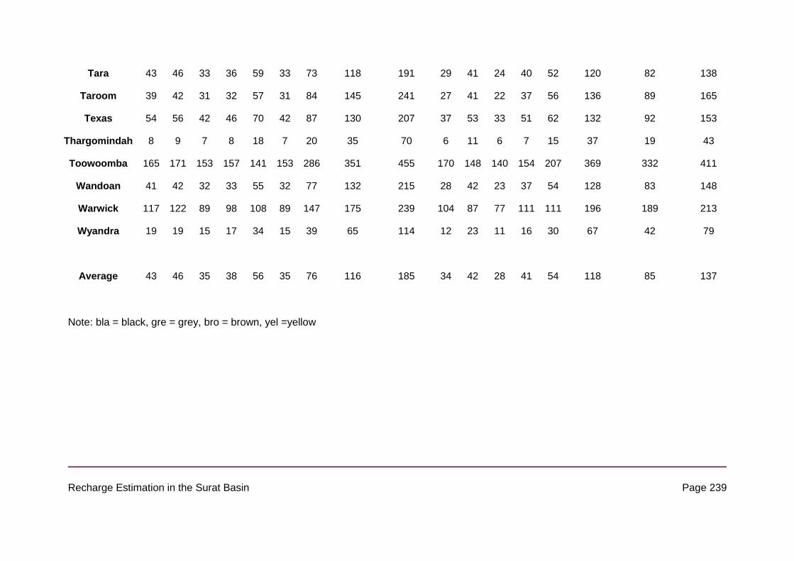
Recharge Estimation in the Surat Basin Page 239
Tara 43 46 33 36 59 33 73 118 191 29 41 24 40 52 120 82 138
Taroom 39 42 31 32 57 31 84 145 241 27 41 22 37 56 136 89 165
Texas 54 56 42 46 70 42 87 130 207 37 53 33 51 62 132 92 153
Thargomindah 8 9 7 8 18 7 20 35 70 6 11 6 7 15 37 19 43
Toowoomba 165 171 153 157 141 153 286 351 455 170 148 140 154 207 369 332 411
Wandoan 41 42 32 33 55 32 77 132 215 28 42 23 37 54 128 83 148
Warwick 117 122 89 98 108 89 147 175 239 104 87 77 111 111 196 189 213
Wyandra 19 19 15 17 34 15 39 65 114 12 23 11 16 30 67 42 79
Average 43 46 35 38 56 35 76 116 185 34 42 28 41 54 118 85 137
Note: bla = black, gre = grey, bro = brown, yel =yellow

Recharge Estimation in the Surat Basin Page 240
Table 34 - Average Drainage (mm/yr) for Woodlands
SOIL TYPES
Vert Derm Kan Ten Sod Rud Chr Fer
Augathella 0 7.7 1 9 8 73 0 2
Bollon 0 4.3 1 4 4.8 53 0 1
Charleville 0 5.3 0 6 5.6 57 0 1
Chinchilla 0 8.7 1 8 10.6 94 0 3
Condamine 0 5 0 3 6.2 67 0 0
Cunnamulla 0 4.7 1 4 4.4 41 0 2
Dalby 0 6.7 0 4 7.6 82 0 1
Dirranbandi 0 4.3 1 5 4.8 53 0 1
Goondiwindi 0 7 1 7 7.8 74 0 2
Greenmount 0 7 1 6 9 89 0 1
Hungerford 0 3.7 1 3 3.6 33 0 1
Inglewood 0 6.3 1 7 7.6 77 0 2
Injune 0 8 1 9 9.4 80 0 2
Killarney 0 6.7 0 5 8.8 84 0 0
Meandarra 0 4.7 0 2 5.8 64 0 0
Miles 0 8.7 1 8 9.8 89 0 2
Mitchell 0 8.7 2 11 9.6 78 0 3
Moonie 0 3.3 0 2 4.4 54 0 0
Morven 0 8.3 1 10 8.6 76 0 2
Mungindi 0 5.3 0 4 5.8 60 0 1
Nindigully 0 6.3 1 7 6.6 65 0 2
Oakey 0 4.3 0 3 5.2 58 0 1
Quilpie 0 3.7 0 3 3.6 36 0 1

Recharge Estimation in the Surat Basin Page 241
Roma 0 8 0 6 8.6 81 0 1
St George 0 5.7 1 6 6.2 61 0 2
Surat 0 8 0 6 8.2 79 0 1
Talwood 0.3 7.7 1 7 8.2 78 0 2
Tambo 0 6.3 0 6 6.6 69 0 1
Tara 0 6.3 1 5 7.8 74 0 1
Texas 0 5.7 1 6 7 72 0 2
Thargomindah 0 3.3 0 3 3 29 0 1
Toowoomba 0.3 22.3 8 36 26 168 0 11
Wandoan 0 7.7 0 6 9.4 88 0 1
Warwick 0 5.7 0 3 7 74 0 1
Wyandra 0 4.7 1 4 4.6 47 0 2
Note: Vert = Vertosol, Derm = Dermosol, Kan = Kandosol, Ten = Tenosol, Sod = Sodosol,
Rud = Rudosol, Chr = Chromosol, Fer = Ferrosol

Recharge Estimation in the Surat Basin Page 242
Table 35 - Average Drainage (mm/yr) for Buffel Grass Pasture
SOIL TYPES
Vert Derm Kan Ten Sod Rud Chr Fer
Augathella 0.3 12.3 21 46 17.8 102 0 14
Bollon 0.3 7.7 12 31 12.2 77 0 8
Charleville 0 8.7 14 33 13 82 0 11
Chinchilla 2.0 20.3 37 77 27.6 137 3 23
Condamine 0 11.7 20 50 17.2 103 0 12
Cunnamulla 0.3 6.3 9 24 10 57 0 7
Dalby 0.3 15.7 28 64 23 127 0 19
Dirranbandi 0 8 10 28 11.8 77 0 8
Goondiwindi 0.5 14.0 25 58 19.6 110 1 15
Greenmount 1.3 20.3 40 83 29.2 147 0 26
Hungerford 0 4.7 6 18 7 44 0 5
Inglewood 1.8 17.3 30 65 23.6 123 2 20
Injune 0.8 15.3 26 59 21.8 117 1 17
Killarney 1.3 19.7 39 85 28.8 138 1 26
Meandarra 0 10.7 17 45 15.8 97 0 10
Miles 2.0 19.3 36 77 26.8 132 2 23
Mitchell 1.0 14.7 23 55 20.4 106 1 17
Moonie 0.3 9.3 14 36 14.4 86 0 10
Morven 0.3 13.3 21 49 19.2 105 0 16
Mungindi 0 9.3 11 33 13.2 86 0 8
Nindigully 0.3 11.3 17 39 15.8 91 0 12
Oakey 0.3 10 16 41 16 99 0 10
Quilpie 0.3 5.7 9 22 8.8 50 0 7

Recharge Estimation in the Surat Basin Page 243
Roma 0.3 15.7 27 59 21.4 115 0 19
St George 0 9.7 14 35 14 88 0 10
Surat 0.3 14.3 23 53 19.4 110 0 17
Talwood 0.8 13.7 21 49 18.4 108 1 15
Tambo 0.3 11 18 42 16.2 95 0 12
Tara 0.3 14.7 25 58 20 111 0 17
Texas 1.3 16.3 33 67 23 122 2 21
Thargomindah 0 3.7 5 15 5.8 37 0 4
Toowoomba 10.3 55.3 99 180 67.8 235 11 74
Wandoan 0.8 16.7 29 66 23.4 128 1 19
Warwick 0.5 15 30 68 23.2 123 1 19
Wyandra 0.5 7 9 24 10 66 1 7
Note: Vert = Vertosol, Derm = Dermosol, Kan = Kandosol, Ten = Tenosol, Sod = Sodosol,
Rud = Rudosol, Chr = Chromosol, Fer = Ferrosol

Recharge Estimation in the Surat Basin Page 244
Table 36 - Average Drainage (mm/yr) for Summer Cropping
SOIL TYPES
Vert Derm Kan Ten Sod Rud Chr Fer
Augathella 28 42.7 96 168 28.2 98 62 115
Bollon 23.8 36.3 79 136 24.2 81 50 96
Brigalow RS 42.3 61.3 149 233 40 143 98 166
Charleville 21.8 34.3 80 143 23.2 81 48 97
Chinchilla 40 58.7 136 227 38.4 134 89 157
Condamine 38.3 53 113 178 36.2 111 77 127
Cunnamulla 21.8 25.7 55 101 15.8 57 35 69
Dalby 36 54.7 128 215 35.8 124 79 147
Dirranbandi 27.3 41.3 78 136 27.4 80 57 95
Goondiwindi 44.5 61.7 123 196 43.8 125 92 142
Greenmount 71.8 91 174 248 67.2 183 164 207
Hungerford 9.5 18 38 77 10 41 25 49
Inglewood 43.5 60.3 125 203 42 127 87 148
Injune 32.8 48.3 119 193 33.6 117 72 138
Killarney 136.5 146.7 222 289 131.4 251 233 270
Meandarra 36.3 50.3 107 169 35.8 110 77 124
Miles 42 59 138 222 40.2 133 90 154
Mitchell 32 48 110 183 30.8 110 73 131
Moonie 39.3 51.3 96 150 35.8 98 72 111
Morven 27.5 42 98 170 27 100 62 120
Mungindi 30 45 92 154 29.4 93 63 108
Narayen 39.8 58 139 221 38 134 89 157
Nindigully 29.3 44.7 92 155 29 94 64 109

Recharge Estimation in the Surat Basin Page 245
oakey 27.5 43 103 167 27.6 104 61 122
Quilpie 11.8 21 49 92 13.8 52 30 59
Roma 33.5 50.7 117 194 34.6 117 78 135
St George 31.3 46.7 95 159 31.6 97 67 114
Surat 34.5 51.3 113 188 34.8 112 77 132
Talwood 37 53.3 111 185 36.6 112 79 132
Tambo 24 37 90 157 24 89 54 108
Tara 39.5 55 118 191 37.2 120 82 138
Taroom 36 57.3 145 241 36.6 136 89 165
Texas 49.5 66.3 130 207 47.2 132 92 153
Thargomindah 8 15 35 70 9 37 19 43
Toowoomba 161.5 193.3 351 455 163.8 369 332 411
Wandoan 37 54.7 132 215 36.8 128 83 148
Warwick 106.5 114.7 175 239 98 196 189 213
Wyandra 17.5 29.3 65 114 18.4 67 42 79
Note: Vert = Vertosol, Derm = Dermosol, Kan = Kandosol, Ten = Tenosol, Sod = Sodosol,
Rud = Rudosol, Chr = Chromosol, Fer = Ferrosol

Recharge Estimation in the Surat Basin Page 246
Appendix 3 – Water Table Fluctuation Analyses

Recharge Estimation in the Surat Basin Page 247
Figure 67 - Rainfall to water level rise method (Sy)

Recharge Estimation in the Surat Basin Page 248
Figure 68 - All data bore RN 42220061

Recharge Estimation in the Surat Basin Page 249
Figure 69 - 2005/2006 water year

Recharge Estimation in the Surat Basin Page 250
Figure 70 - WTF method applied to 2005/2006 water year

Recharge Estimation in the Surat Basin Page 251
Figure 71 - 2004/2005 water year
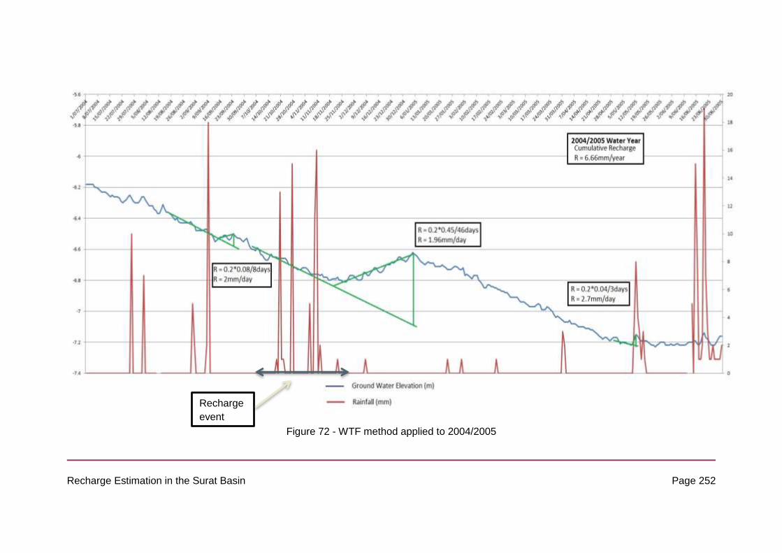
Recharge Estimation in the Surat Basin Page 252
Figure 72 - WTF method applied to 2004/2005
Recharge
event

Recharge Estimation in the Surat Basin Page 253


