ESSLINGER AND VOGELGESANG VOL. 6 ’ NO. 9 ’ 8173–8182 ’ 2012 www.acsnano.org 8173 August 17, 2012 C 2012 American Chemical Society Reciprocity Theory of Apertureless Scanning Near-Field Optical Microscopy with Point-Dipole Probes Moritz Esslinger * and Ralf Vogelgesang Max Planck Institute for Solid State Research, Stuttgart, Germany S ince the advent of nanotechnology, the exploration of nanoscopic structures continues to spur new developments in all areas of the natural sciences, ranging from research on their fundamental properties to ultrasensitive detectors, subwavelength light management, biomedical diagnostics and therapeutics, etc. 110 Especially, where this concerns optical phenomena, a key role is played by microscopy techniques capable of spatial resolution at the nanometer scale. This appears to be an unreachable goal with conventional di ffraction-limited imaging tech- niques, which offer hardly better than half a wavelength resolution. However, a variety of significant technological advances in both electronic and optical near-field microscopies now offer routine discrimination of optical features smaller than 10 nm. 11 Unfortunately, this high-resolution con- trast does not necessarily come with easy, faithful interpretation of recorded images. To beat the diffraction limit, the evanescent near-fields must be accessed by some kind of (scanning) probe. 12 The intricate interac- tion between an unknown sample under study and the probe is all but fully under- stood. A detailed model for recorded signals would also be very beneficial in inverse scat- tering problems. 13,14 Here we concentrate on scanning near-field optical microscopy. For a handful of special cases, successful models are available, which represent the signal measured in terms of easily understood quantities. 1517 A general theory for SNOM, based on the Max- well equations, is also available. 18 In this frame- work, the measured signal can be calculated by integrating over an infinite plane, separat- ing tip and sample. The current situation in SNOM is somewhat reminiscent of scanning tunneling microscopy (STM) in the early 1980s. Ab initio theories were available but cumbersome to use, and simpli fied models based on ad hoc assump- tions often led to paradoxical interpretations. This changed when Tersoff and Hamann pro- vided their celebrated interpretation frame- work, 19,20 which allowed scanning tunneling microscopy images to be easily interpreted with certainty and largely without a priori knowledge or further simulations. In STM, the interpretation of recorded sig- nals is based on Bardeen's formula for the current across a tunneling barrier. 21 It presumes weak coupling between the two electrodes referred to as “sample” and “tip”. Weak coupling is appropriate for electronic states that decay evanescently into the gap between the electrodes. Tersoff and Hamann proceeded by introducing the sim- plest conceivable model for a tip, namely, a point-like s-wave emitter. Their elegant * Address correspondence to [email protected]. Received for review June 27, 2012 and accepted August 16, 2012. Published online 10.1021/nn302864d ABSTRACT Near-field microscopy offers the opportunity to reveal optical contrast at deep subwavelength scales. In scanning near-field optical microscopy (SNOM), the diffraction limit is overcome by a nanoscopic probe in close proximity to the sample. The interaction of the probe with the sample fields necessarily perturbs the bare sample response, and a critical issue is the interpretation of recorded signals. For a few specific SNOM configurations, individual descriptions have been modeled, but a general and intuitive framework is still lacking. Here, we give an exact formulation of the measurable signals in SNOM which is easily applicable to experimental configurations. Our results are in close analogy with the description Tersoff and Hamann have derived for the tunneling currents in scanning tunneling microscopy. For point-like scattering probe tips, such as used in apertureless SNOM, the theory simplifies dramatically to a single scalar relation. We find that the measured signal is directly proportional to the field of the coupled tipsample system at the position of the tip. For weakly interacting probes, the model thus veri fies the empirical findings that the recorded signal is proportional to the unperturbed field of the bare sample. In the more general case, it provides guidance to an intuitive and faithful interpretation of recorded images, facilitating the characterization of tip-related distortions and the evaluation of novel SNOM configurations, both for aperture-based and apertureless SNOM. KEYWORDS: imaging theory . reciprocity theorem . Born series interaction . apertureless near-field microscopy . SNOM ARTICLE
Reciprocity Theory of AperturelessScanning Near-Field OpticalMicroscopy with Point-Dipole ProbesMoritz Esslinger* and Ralf Vogelgesang
Max Planck Institute for Solid State Research, Stuttgart, Germany
Since the advent of nanotechnology, theexploration of nanoscopic structurescontinues to spur new developments
in all areas of the natural sciences, rangingfromresearchon their fundamental propertiesto ultrasensitive detectors, subwavelengthlight management, biomedical diagnosticsand therapeutics, etc.1�10 Especially, wherethis concerns optical phenomena, a key roleis played by microscopy techniques capableof spatial resolution at the nanometer scale.This appears to be an unreachable goal withconventional diffraction-limited imaging tech-niques, which offer hardly better than half awavelength resolution. However, a varietyof significant technological advances in bothelectronic andoptical near-fieldmicroscopiesnow offer routine discrimination of opticalfeatures smaller than 10 nm.11
Unfortunately, this high-resolution con-trast does not necessarily come with easy,faithful interpretation of recorded images.To beat the diffraction limit, the evanescentnear-fields must be accessed by some kindof (scanning) probe.12 The intricate interac-tion between an unknown sample understudy and the probe is all but fully under-stood. A detailed model for recorded signalswould also be very beneficial in inverse scat-tering problems.13,14 Here we concentrate onscanning near-field optical microscopy. For ahandful of special cases, successful models areavailable,which represent the signalmeasuredin termsof easily understoodquantities.15�17Ageneral theory for SNOM, based on the Max-well equations, is also available.18 In this frame-work, the measured signal can be calculatedby integrating over an infinite plane, separat-ing tip and sample.The current situation in SNOM is somewhat
reminiscentof scanning tunnelingmicroscopy(STM) in the early 1980s. Ab initio theorieswere available but cumbersome to use, andsimplified models based on ad hoc assump-tions often led to paradoxical interpretations.
This changed when Tersoff and Hamann pro-
vided their celebrated interpretation frame-
work,19,20 which allowed scanning tunneling
microscopy images to be easily interpreted
with certainty and largely without a priori
knowledge or further simulations.In STM, the interpretation of recorded sig-
nals is based on Bardeen's formula forthe current across a tunneling barrier.21 Itpresumes weak coupling between the twoelectrodes referred to as “sample” and “tip”.Weak coupling is appropriate for electronicstates that decay evanescently into thegap between the electrodes. Tersoff andHamann proceeded by introducing the sim-plest conceivable model for a tip, namely,a point-like s-wave emitter. Their elegant
analytical expression for the tunneling current showedit is simply proportional to the wave function of thebare sample at the location of the point-like tip.Some of the earliest results in SNOM were inspired
by the successes of STM, emulating the evanescentcoupling character. Possibly the closest equivalent,albeit somewhat exotic, is the observation of photontunneling through a gap filled with liquid metal.22
Illumination by total internal reflection and pick upby a near-field probe that frustrates the evansecentfields shares similar evanescent field features with theSTM.23,24 In the late 1990s, a number of general and exactdescriptions of SNOM were proposed, which arrive atformulas that closely resemble that of Bardeen.25 Re-markably, no explicit assumption of weak coupling be-tween sample and tip is necessary in their derivation. Inprinciple, therefore, these formulas do also describe theoperation of SNOMs;aperture-based or apertureless;that do not operate in the weak coupling regime.26
In the present report, we outline an approach to ananalytic theory for recordable SNOM signals. The cor-relation between the general expressions for the elec-tronic tunneling matrix elements and the optical rec-iprocity relations is rooted in the intimate relationsbetween the Schrödinger equation and the Maxwell�Helmholtz equation,27,28 which are the respective waveequations for theelectron andphoton. This suggests thepossibility of picking up the idea of Tersoff and Hamannof a point-like probe tip for SNOM, aswell. We show thatit is possible to express recordable signals as an integralof the probing tip volume. Consequently, for aperture-less or scattering-type SNOM;which are indeed point-like at the wavelength scale;an analytical, closed-formexpression is obtained for the measured signals inSNOM that is analogous to the Tersoff�Hamann results.We demonstrate the utility of this framework in discuss-ing how different forms of apertureless SNOM may beused to map local electric field components and howwell thesemaybe related to thebare samplenear-fields.
RESULTS AND DISCUSSION
Bardeen's formulaMμν�RdS 3 (ψuh3ψν�ψν3ψuh) de-
scribes the flow of charge (or equivalently probabilitydensity) across a fictitious plane inserted in the gapbetween probe tip and sample. An analogon for SNOMhas been derived earlier by Carminati, Greffet, and co-workers,whoused reciprocity theory in their approach.29
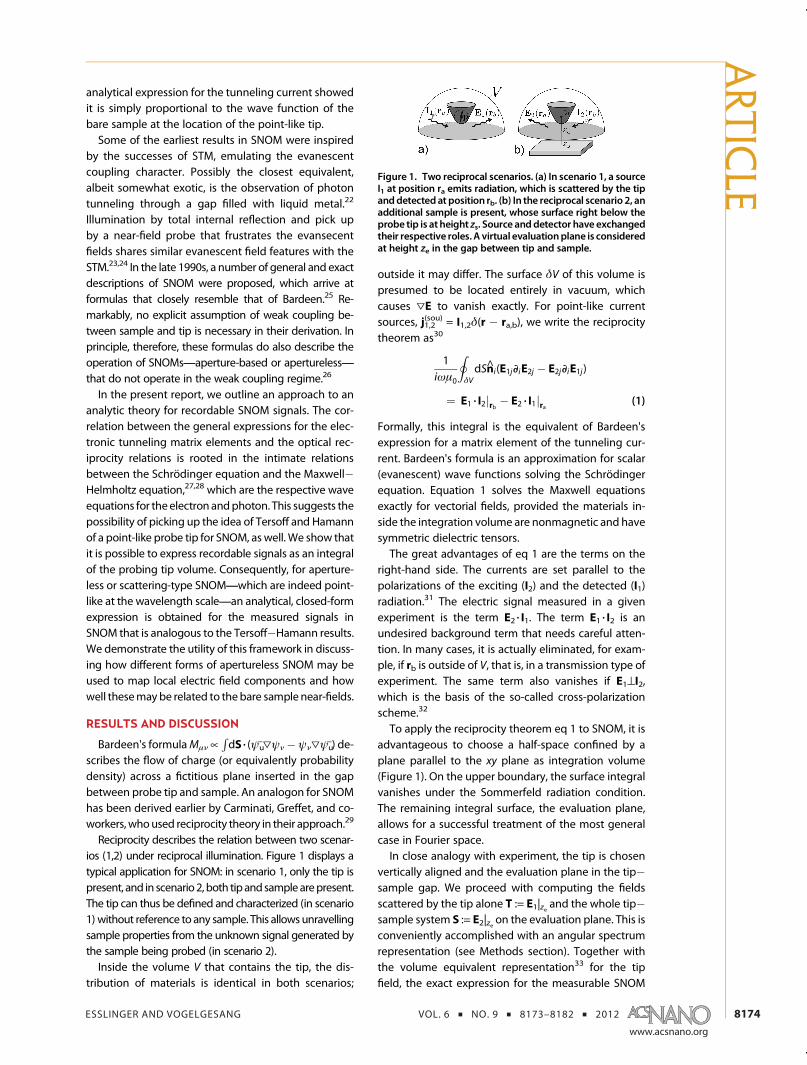
Reciprocity describes the relation between two scenar-ios (1,2) under reciprocal illumination. Figure 1 displays atypical application for SNOM: in scenario 1, only the tip ispresent, and in scenario2, both tipandsamplearepresent.The tip can thus be defined and characterized (in scenario1) without reference to any sample. This allowsunravellingsample properties from the unknown signal generated bythe sample being probed (in scenario 2).Inside the volume V that contains the tip, the dis-
tribution of materials is identical in both scenarios;
outside it may differ. The surface δV of this volume ispresumed to be located entirely in vacuum, whichcauses 3E to vanish exactly. For point-like currentsources, j1,2
(sou) = I1,2δ(r � ra,b), we write the reciprocitytheorem as30
1iωμ0
IδVdSn̂i(E1jDiE2j � E2jDiE1j)
¼ E1 3 I2jrb � E2 3 I1jra (1)
Formally, this integral is the equivalent of Bardeen'sexpression for a matrix element of the tunneling cur-rent. Bardeen's formula is an approximation for scalar(evanescent) wave functions solving the Schrödingerequation. Equation 1 solves the Maxwell equationsexactly for vectorial fields, provided the materials in-side the integration volume are nonmagnetic and havesymmetric dielectric tensors.The great advantages of eq 1 are the terms on the
right-hand side. The currents are set parallel to thepolarizations of the exciting (I2) and the detected (I1)radiation.31 The electric signal measured in a givenexperiment is the term E2 3 I1. The term E1 3 I2 is anundesired background term that needs careful atten-tion. In many cases, it is actually eliminated, for exam-ple, if rb is outside of V, that is, in a transmission type ofexperiment. The same term also vanishes if E1^I2,which is the basis of the so-called cross-polarizationscheme.32
To apply the reciprocity theorem eq 1 to SNOM, it isadvantageous to choose a half-space confined by aplane parallel to the xy plane as integration volume(Figure 1). On the upper boundary, the surface integralvanishes under the Sommerfeld radiation condition.The remaining integral surface, the evaluation plane,allows for a successful treatment of the most generalcase in Fourier space.In close analogy with experiment, the tip is chosen
vertically aligned and the evaluation plane in the tip�sample gap. We proceed with computing the fieldsscattered by the tip alone T := E1|ze and the whole tip�sample system S := E2|ze on the evaluation plane. This isconveniently accomplished with an angular spectrumrepresentation (see Methods section). Together withthe volume equivalent representation33 for the tipfield, the exact expression for the measurable SNOM
Figure 1. Two reciprocal scenarios. (a) In scenario 1, a sourceI1 at position ra emits radiation, which is scattered by the tipanddetected at position rb. (b) In the reciprocal scenario 2, anadditional sample is present, whose surface right below theprobe tip is at height zs. Source anddetector have exchangedtheir respective roles. A virtual evaluationplane is consideredat height ze in the gap between tip and sample.
signal (eq 1) becomes a comparatively simple term asan integral over the scattering tip volume
E2 3 I1jra ¼ E1 3 I2jrb � iω
Zd3rT(r)Δε (r)Sþ(r) (2)
Such integrals over small tip volumes are easily manage-able with modern numerical Maxwell solvers. One mayconsider eq 2 as a fall-back option for delicate cases, or ifspecifically crafted probe tips deviated significantly fromthe point-like dipole model, which is considered next.Sþ(rt) should not be confused with the actual field
S(rt) of the tip�sample system at the location of the tipin scenario 1. Instead, it denotes those field compo-nents that exist in the evaluation plane and travel uptoward the tip, as displayed in angular spectrumrepresentation.
Point-like Tip Model. In the form of eq 2, reciprocitytheory is fully general, applicable to both aperture-based and apertureless versions of SNOM. We now askwhat algebraic simplification and intuitive understandingcan be gained if we restrict ourselves to point-like tips inthe apertureless case? Nanoscopic probe tips, in the spiritof the dipole tipmodel,34 are often treated as a point-likedipolar moment p(rt) = VtT(rt)Δε (rt). This replacementturns eq 2 into the central result of this report, the simplescalar relation for the measured signal
E2 3 I1jra ¼ E1 3 I2jrb � iωp(rt) 3 Sþ(rt) (3)
It is the equivalent of the Tersoff�Hamann formula I �Dt(EF)|ψν(rt)|
2 for the tunneling current in STM. There, themeasured signal is proportional to the squaremodulus ofthe sample wave function |ψν(rt)|
2 at the location of thetip, multiplied with the density of states Dt of the tip. Inclose analogy, the detected electric field is proportionalto the field Sþ(rt) at the tip position, projected by theinner product on the dipole moment p of the tip. Onedifference between STM and aSNOM is noteworthy:whereas |ψν(rt)|
2 is a property of the bare sample, Sþ
describes the fully coupled tip�sample system. There-fore, in the following, we discuss how the field Sþmay berelated to the unperturbed sample near-field S(unp) in theabsence of any probe tip.
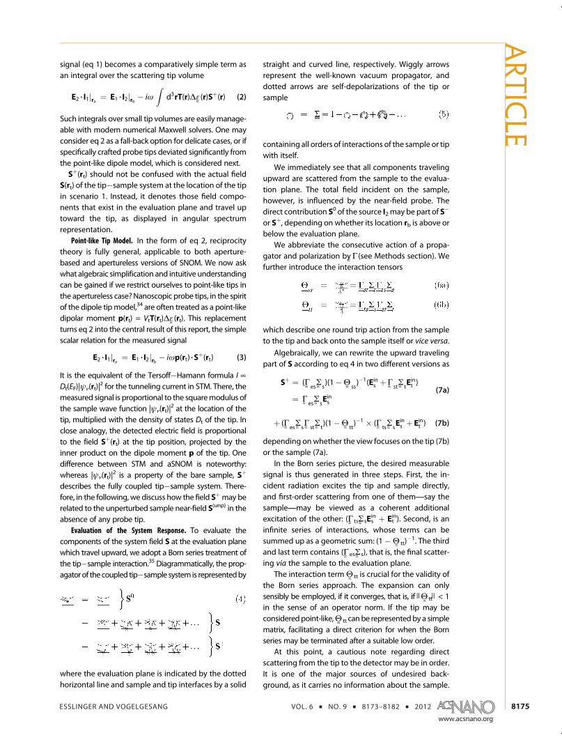
Evaluation of the System Response. To evaluate thecomponents of the system field S at the evaluation planewhich travel upward, we adopt a Born series treatment ofthe tip�sample interaction.35 Diagrammatically, the prop-agatorof thecoupled tip�samplesystemis representedby
where the evaluation plane is indicated by the dottedhorizontal line and sample and tip interfaces by a solid
straight and curved line, respectively. Wiggly arrowsrepresent the well-known vacuum propagator, anddotted arrows are self-depolarizations of the tip orsample
containing all orders of interactions of the sample or tipwith itself.
We immediately see that all components travelingupward are scattered from the sample to the evalua-tion plane. The total field incident on the sample,however, is influenced by the near-field probe. Thedirect contribution S0 of the source I2may be part of S�
or Sþ, depending on whether its location rb is above orbelow the evaluation plane.
We abbreviate the consecutive action of a propa-gator and polarization byΓ (see Methods section). Wefurther introduce the interaction tensors
which describe one round trip action from the sampleto the tip and back onto the sample itself or vice versa.
Algebraically, we can rewrite the upward travelingpart of S according to eq 4 in two different versions as
Sþ ¼ (ΓesΣ
s)(1�Θ
ss)�1(Eins þΓ
stΣ
tEint )
¼ ΓesΣ
sEins
(7a)
þ (ΓesΣ
sΓ
stΣ
t)(1�Θ
tt)�1 � (Γ
tsΣ
sEins þ Eint ) (7b)
depending onwhether the view focuses on the tip (7b)or the sample (7a).
In the Born series picture, the desired measurablesignal is thus generated in three steps. First, the in-cident radiation excites the tip and sample directly,and first-order scattering from one of them;say thesample;may be viewed as a coherent additionalexcitation of the other: (Γ tsΣ sEs
in þ Etin). Second, is an
infinite series of interactions, whose terms can besummed up as a geometric sum: (1�Θ tt)
�1. The thirdand last term contains (ΓesΣ s), that is, the final scatter-ing via the sample to the evaluation plane.
The interaction termΘ tt is crucial for the validity ofthe Born series approach. The expansion can onlysensibly be employed, if it converges, that is, if )Θ tt ) < 1in the sense of an operator norm. If the tip may beconsideredpoint-like,Θ tt canbe representedby a simplematrix, facilitating a direct criterion for when the Bornseries may be terminated after a suitable low order.
At this point, a cautious note regarding directscattering from the tip to the detector may be in order.It is one of the major sources of undesired back-ground, as it carries no information about the sample.
Any measurable signal that stems directly from the tipis due either to S0 ∈ Sþ, if the source I2 at rb is locatedbelow the evaluation plane, or due to the term (E1 3 I2),if rb is above the evaluation plane, inside the integra-tion volume. Thus, this parasitic background signalcannot generally be assumed to vanish, unless specialcare is taken to ensure exactly normal field vectors,E1^I2,36 or this signal is suppressed by modulation/demodulation techniques to a level below the detectornoise floor.
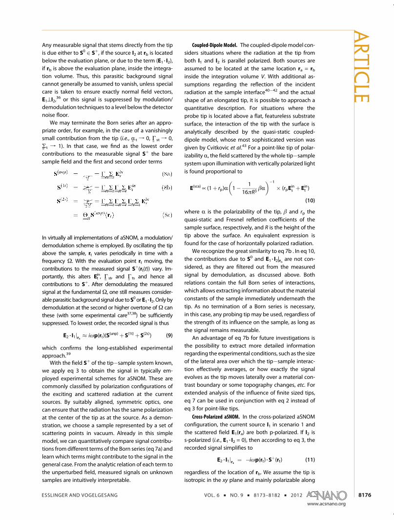
We may terminate the Born series after an appro-priate order, for example, in the case of a vanishinglysmall contribution from the tip (i.e., R t f 0, Γ st f 0,Σ t f 1). In that case, we find as the lowest ordercontributions to the measurable signal Sþ the baresample field and the first and second order terms
In virtually all implementations of aSNOM, a modulation/demodulation scheme is employed. By oscillating the tipabove the sample, rt varies periodically in time with afrequency Ω. With the evaluation point rt moving, thecontributions to the measured signal Sþ(rt(t)) vary. Im-portantly, this alters Et
in, Γ st, and Γ ts and hence allcontributions to Sþ. After demodulating the measuredsignal at the fundamentalΩ, one still measures consider-ableparasitic backgroundsignaldue toS0 orE1 3 I2.Onlybydemodulation at the second or higher overtone ofΩ canthese (with some experimental care37,38) be sufficientlysuppressed. To lowest order, the recorded signal is thus
E2 3 I1jra � iωp(rt)(S(unp) þ S(1t) þ S(2s)) (9)
which confirms the long-established experimentalapproach.39
With the field Sþ of the tip�sample system known,we apply eq 3 to obtain the signal in typically em-ployed experimental schemes for aSNOM. These arecommonly classified by polarization configurations ofthe exciting and scattered radiation at the currentsources. By suitably aligned, symmetric optics, onecan ensure that the radiation has the same polarizationat the center of the tip as at the source. As a demon-stration, we choose a sample represented by a set ofscattering points in vacuum. Already in this simplemodel, we can quantitatively compare signal contribu-tions fromdifferent terms of the Born series (eq 7a) andlearn which terms might contribute to the signal in thegeneral case. From the analytic relation of each term tothe unperturbed field, measured signals on unknownsamples are intuitively interpretable.
Coupled-Dipole Model. The coupled-dipolemodel con-siders situations where the radiation at the tip fromboth I1 and I2 is parallel polarized. Both sources areassumed to be located at the same location ra = rbinside the integration volume V. With additional as-sumptions regarding the reflection of the incidentradiation at the sample interface40�42 and the actualshape of an elongated tip, it is possible to approach aquantitative description. For situations where theprobe tip is located above a flat, featureless substratesurface, the interaction of the tip with the surface isanalytically described by the quasi-static coupled-dipole model, whose most sophisticated version wasgiven by Cvitkovic et al.43 For a point-like tip of polar-izability R, the field scattered by the whole tip�samplesystem upon illuminationwith vertically polarized lightis found proportional to
E(sca) � (1þ rp)R 1� 116πR3
βR� ��1
� (rpEins þ Eint )
(10)
where R is the polarizability of the tip, β and rp thequasi-static and Fresnel refletion coefficients of thesample surface, respectively, and R is the height of thetip above the surface. An equivalent expression isfound for the case of horizontally polarized radiation.
We recognize the great similarity to eq 7b . In eq 10,the contributions due to S0 and E1 3 I2|rb are not con-sidered, as they are filtered out from the measuredsignal by demodulation, as discussed above. Bothrelations contain the full Born series of interactions,which allows extracting information about thematerialconstants of the sample immediately underneath thetip. As no termination of a Born series is necessary,in this case, any probing tip may be used, regardless ofthe strength of its influence on the sample, as long asthe signal remains measurable.
An advantage of eq 7b for future investigations isthe possibility to extract more detailed informationregarding the experimental conditions, such as the sizeof the lateral area over which the tip�sample interac-tion effectively averages, or how exactly the signalevolves as the tip moves laterally over a material con-trast boundary or some topography changes, etc. Forextended analysis of the influence of finite sized tips,eq 7 can be used in conjunction with eq 2 instead ofeq 3 for point-like tips.
Cross-Polarized aSNOM. In the cross-polarized aSNOMconfiguration, the current source I1 in scenario 1 andthe scattered field E1(ra) are both p-polarized. If I2 iss-polarized (i.e., E1 3 I2 = 0), then according to eq 3, therecorded signal simplifies to
E2 3 I1jra ¼ �iωp(rt) 3 Sþ(rt) (11)
regardless of the location of rb. We assume the tip isisotropic in the xy plane and mainly polarizable along
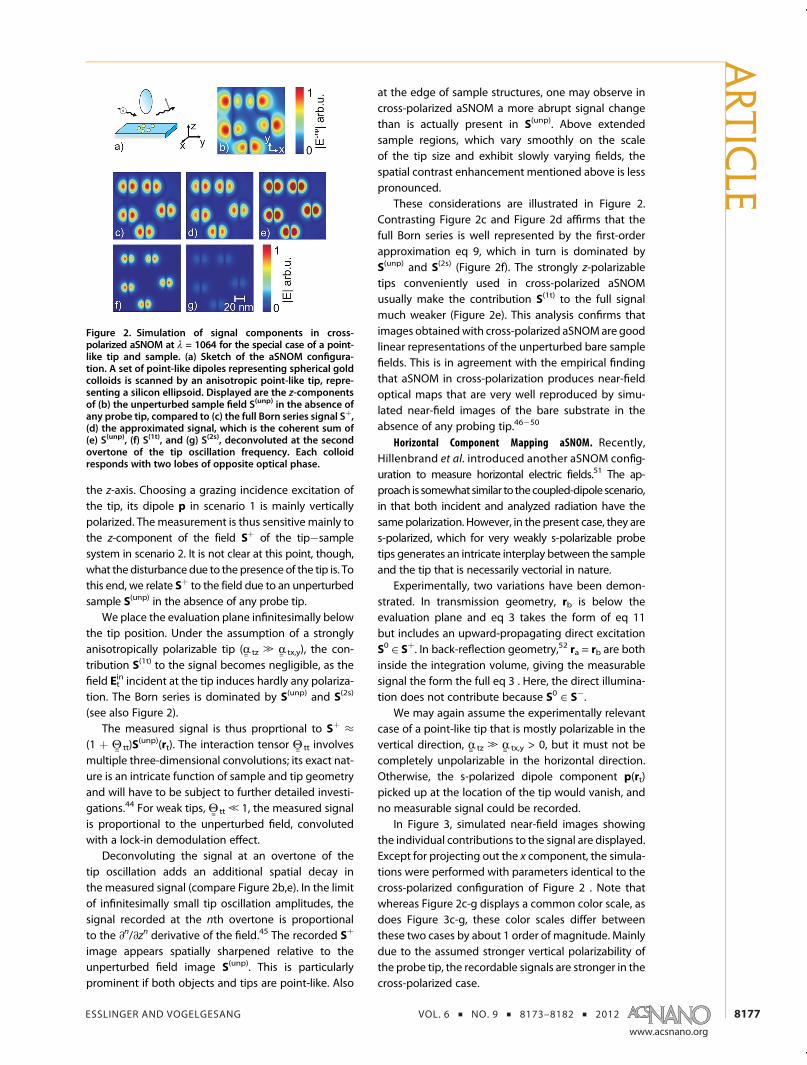
the z-axis. Choosing a grazing incidence excitation ofthe tip, its dipole p in scenario 1 is mainly verticallypolarized. Themeasurement is thus sensitive mainly tothe z-component of the field Sþ of the tip�samplesystem in scenario 2. It is not clear at this point, though,what the disturbance due to the presence of the tip is. Tothis end, we relate Sþ to the field due to an unperturbedsample S(unp) in the absence of any probe tip.
We place the evaluation plane infinitesimally belowthe tip position. Under the assumption of a stronglyanisotropically polarizable tip (R tz . R tx,y), the con-tribution S(1t) to the signal becomes negligible, as thefield Et
in incident at the tip induces hardly any polariza-tion. The Born series is dominated by S(unp) and S(2s)
(see also Figure 2).The measured signal is thus proprtional to Sþ ≈
(1 þ Θ tt)S(unp)(rt). The interaction tensor Θ tt involves
multiple three-dimensional convolutions; its exact nat-ure is an intricate function of sample and tip geometryand will have to be subject to further detailed investi-gations.44 For weak tips, Θ tt , 1, the measured signalis proportional to the unperturbed field, convolutedwith a lock-in demodulation effect.
Deconvoluting the signal at an overtone of thetip oscillation adds an additional spatial decay inthe measured signal (compare Figure 2b,e). In the limitof infinitesimally small tip oscillation amplitudes, thesignal recorded at the nth overtone is proportionalto the ∂
n/∂zn derivative of the field.45 The recorded Sþ
image appears spatially sharpened relative to theunperturbed field image S(unp). This is particularlyprominent if both objects and tips are point-like. Also
at the edge of sample structures, one may observe incross-polarized aSNOM a more abrupt signal changethan is actually present in S(unp). Above extendedsample regions, which vary smoothly on the scaleof the tip size and exhibit slowly varying fields, thespatial contrast enhancement mentioned above is lesspronounced.
These considerations are illustrated in Figure 2.Contrasting Figure 2c and Figure 2d affirms that thefull Born series is well represented by the first-orderapproximation eq 9, which in turn is dominated byS(unp) and S(2s) (Figure 2f). The strongly z-polarizabletips conveniently used in cross-polarized aSNOMusually make the contribution S(1t) to the full signalmuch weaker (Figure 2e). This analysis confirms thatimages obtainedwith cross-polarized aSNOMare goodlinear representations of the unperturbed bare samplefields. This is in agreement with the empirical findingthat aSNOM in cross-polarization produces near-fieldoptical maps that are very well reproduced by simu-lated near-field images of the bare substrate in theabsence of any probing tip.46�50
Horizontal Component Mapping aSNOM. Recently,Hillenbrand et al. introduced another aSNOM config-uration to measure horizontal electric fields.51 The ap-proach is somewhat similar to thecoupled-dipole scenario,in that both incident and analyzed radiation have thesamepolarization. However, in the present case, they ares-polarized, which for very weakly s-polarizable probetips generates an intricate interplay between the sampleand the tip that is necessarily vectorial in nature.
Experimentally, two variations have been demon-strated. In transmission geometry, rb is below theevaluation plane and eq 3 takes the form of eq 11but includes an upward-propagating direct excitationS0 ∈ Sþ. In back-reflection geometry,52 ra = rb are bothinside the integration volume, giving the measurablesignal the form the full eq 3 . Here, the direct illumina-tion does not contribute because S0 ∈ S�.
We may again assume the experimentally relevantcase of a point-like tip that is mostly polarizable in thevertical direction, R tz . R tx,y > 0, but it must not becompletely unpolarizable in the horizontal direction.Otherwise, the s-polarized dipole component p(rt)picked up at the location of the tip would vanish, andno measurable signal could be recorded.
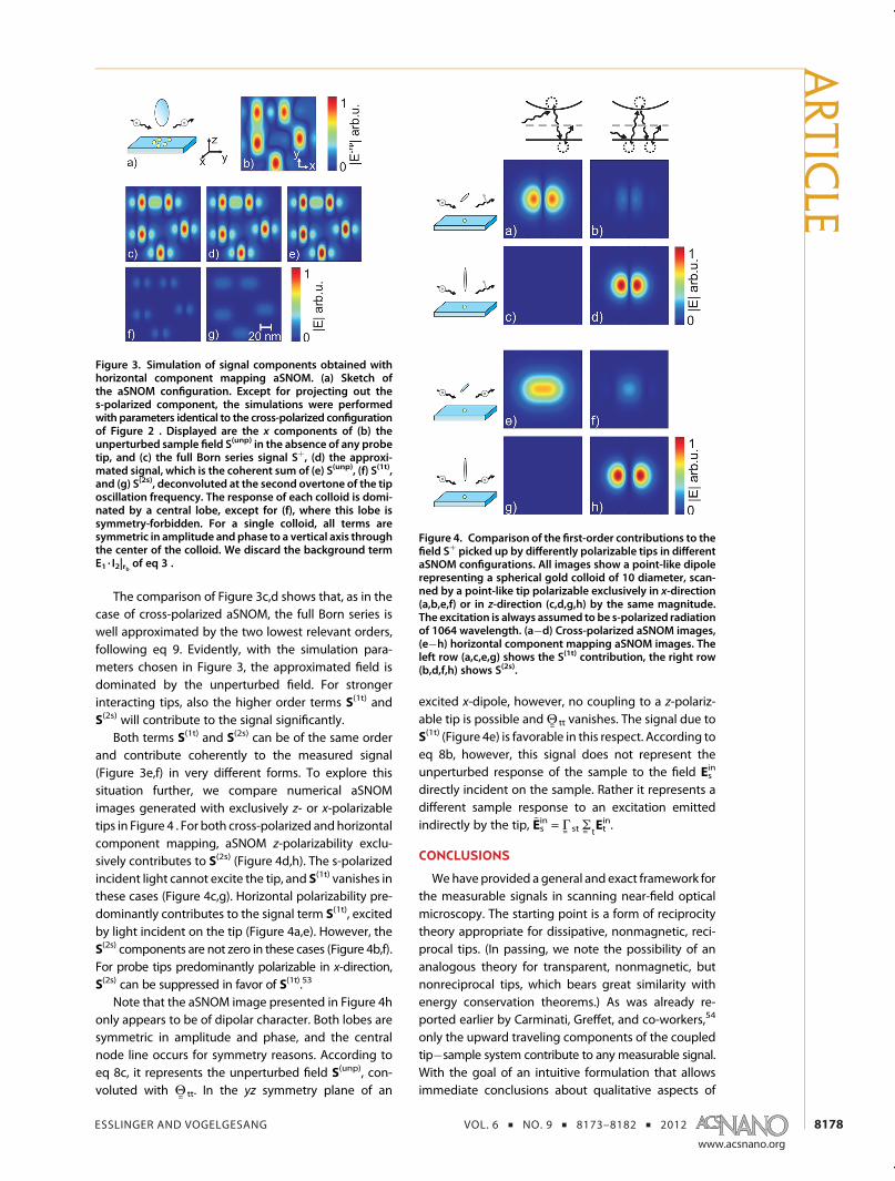
In Figure 3, simulated near-field images showingthe individual contributions to the signal are displayed.Except for projecting out the x component, the simula-tions were performed with parameters identical to thecross-polarized configuration of Figure 2 . Note thatwhereas Figure 2c-g displays a common color scale, asdoes Figure 3c-g, these color scales differ betweenthese two cases by about 1 order of magnitude. Mainlydue to the assumed stronger vertical polarizability ofthe probe tip, the recordable signals are stronger in thecross-polarized case.
Figure 2. Simulation of signal components in cross-polarized aSNOM at λ = 1064 for the special case of a point-like tip and sample. (a) Sketch of the aSNOM configura-tion. A set of point-like dipoles representing spherical goldcolloids is scanned by an anisotropic point-like tip, repre-senting a silicon ellipsoid. Displayed are the z-componentsof (b) the unperturbed sample field S(unp) in the absence ofany probe tip, compared to (c) the full Born series signal Sþ,(d) the approximated signal, which is the coherent sum of(e) S(unp), (f) S(1t), and (g) S(2s), deconvoluted at the secondovertone of the tip oscillation frequency. Each colloidresponds with two lobes of opposite optical phase.
The comparison of Figure 3c,d shows that, as in thecase of cross-polarized aSNOM, the full Born series iswell approximated by the two lowest relevant orders,following eq 9. Evidently, with the simulation para-meters chosen in Figure 3, the approximated field isdominated by the unperturbed field. For strongerinteracting tips, also the higher order terms S(1t) andS(2s) will contribute to the signal significantly.
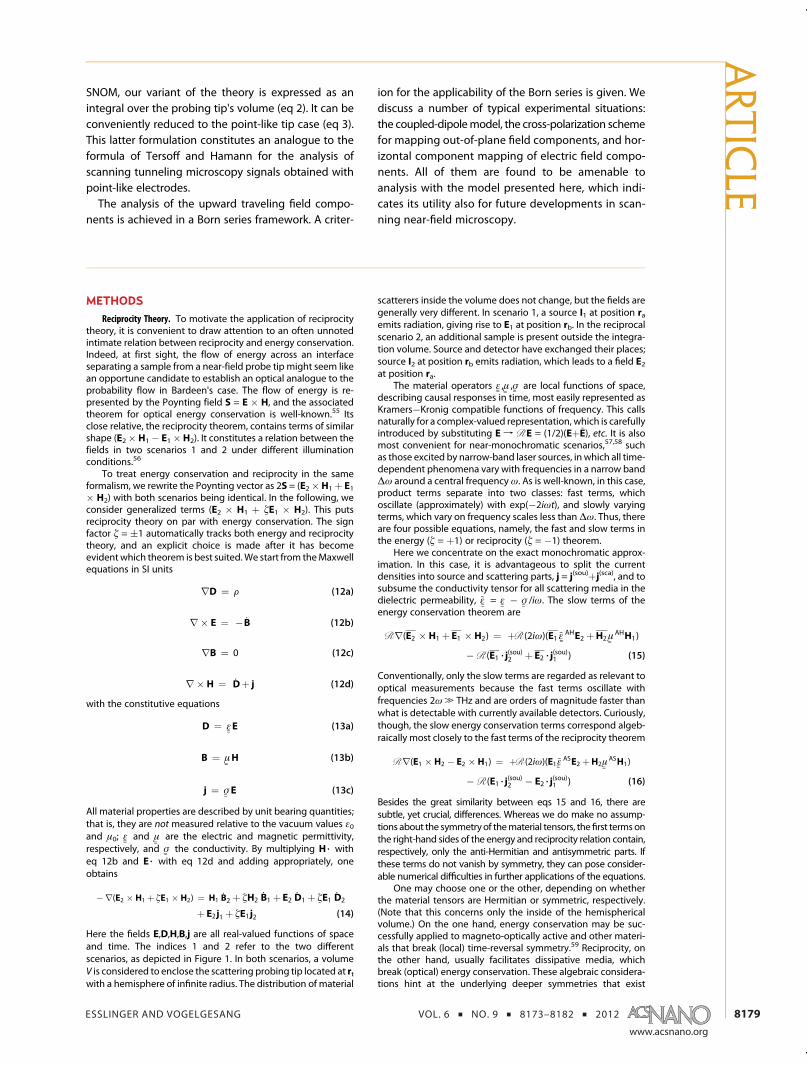
Both terms S(1t) and S(2s) can be of the same orderand contribute coherently to the measured signal(Figure 3e,f) in very different forms. To explore thissituation further, we compare numerical aSNOMimages generated with exclusively z- or x-polarizabletips in Figure 4 . For both cross-polarized andhorizontalcomponent mapping, aSNOM z-polarizability exclu-sively contributes to S(2s) (Figure 4d,h). The s-polarizedincident light cannot excite the tip, and S(1t) vanishes inthese cases (Figure 4c,g). Horizontal polarizability pre-dominantly contributes to the signal term S(1t), excitedby light incident on the tip (Figure 4a,e). However, theS(2s) components are not zero in these cases (Figure 4b,f).For probe tips predominantly polarizable in x-direction,S(2s) can be suppressed in favor of S(1t).53
Note that the aSNOM image presented in Figure 4honly appears to be of dipolar character. Both lobes aresymmetric in amplitude and phase, and the centralnode line occurs for symmetry reasons. According toeq 8c, it represents the unperturbed field S(unp), con-voluted with Θ tt. In the yz symmetry plane of an
excited x-dipole, however, no coupling to a z-polariz-able tip is possible andΘ tt vanishes. The signal due toS(1t) (Figure 4e) is favorable in this respect. According toeq 8b, however, this signal does not represent theunperturbed response of the sample to the field Es
in
directly incident on the sample. Rather it represents adifferent sample response to an excitation emittedindirectly by the tip, ~Es
in = Γ st Σ tEtin.
CONCLUSIONS
Wehave provided a general and exact framework forthe measurable signals in scanning near-field opticalmicroscopy. The starting point is a form of reciprocitytheory appropriate for dissipative, nonmagnetic, reci-procal tips. (In passing, we note the possibility of ananalogous theory for transparent, nonmagnetic, butnonreciprocal tips, which bears great similarity withenergy conservation theorems.) As was already re-ported earlier by Carminati, Greffet, and co-workers,54
only the upward traveling components of the coupledtip�sample system contribute to any measurable signal.With the goal of an intuitive formulation that allowsimmediate conclusions about qualitative aspects of
Figure 3. Simulation of signal components obtained withhorizontal component mapping aSNOM. (a) Sketch ofthe aSNOM configuration. Except for projecting out thes-polarized component, the simulations were performedwith parameters identical to the cross-polarized configurationof Figure 2 . Displayed are the x components of (b) theunperturbed sample field S(unp) in the absence of any probetip, and (c) the full Born series signal Sþ, (d) the approxi-mated signal, which is the coherent sum of (e) S(unp), (f) S(1t),and (g) S(2s), deconvoluted at the second overtone of the tiposcillation frequency. The response of each colloid is domi-nated by a central lobe, except for (f), where this lobe issymmetry-forbidden. For a single colloid, all terms aresymmetric in amplitude and phase to a vertical axis throughthe center of the colloid. We discard the background termE1 3 I2|rb of eq 3 .
Figure 4. Comparison of the first-order contributions to thefield Sþ picked up by differently polarizable tips in differentaSNOM configurations. All images show a point-like dipolerepresenting a spherical gold colloid of 10 diameter, scan-ned by a point-like tip polarizable exclusively in x-direction(a,b,e,f) or in z-direction (c,d,g,h) by the same magnitude.The excitation is always assumed to be s-polarized radiationof 1064 wavelength. (a�d) Cross-polarized aSNOM images,(e�h) horizontal component mapping aSNOM images. Theleft row (a,c,e,g) shows the S(1t) contribution, the right row(b,d,f,h) shows S(2s).
SNOM, our variant of the theory is expressed as anintegral over the probing tip's volume (eq 2). It can beconveniently reduced to the point-like tip case (eq 3).This latter formulation constitutes an analogue to theformula of Tersoff and Hamann for the analysis ofscanning tunneling microscopy signals obtained withpoint-like electrodes.The analysis of the upward traveling field compo-
nents is achieved in a Born series framework. A criter-
ion for the applicability of the Born series is given. Wediscuss a number of typical experimental situations:the coupled-dipolemodel, the cross-polarization schemefor mapping out-of-plane field components, and hor-izontal component mapping of electric field compo-nents. All of them are found to be amenable toanalysis with the model presented here, which indi-cates its utility also for future developments in scan-ning near-field microscopy.
METHODS
Reciprocity Theory. To motivate the application of reciprocitytheory, it is convenient to draw attention to an often unnotedintimate relation between reciprocity and energy conservation.Indeed, at first sight, the flow of energy across an interfaceseparating a sample from a near-field probe tip might seem likean opportune candidate to establish an optical analogue to theprobability flow in Bardeen's case. The flow of energy is re-presented by the Poynting field S = E � H, and the associatedtheorem for optical energy conservation is well-known.55 Itsclose relative, the reciprocity theorem, contains terms of similarshape (E2� H1� E1� H2). It constitutes a relation between thefields in two scenarios 1 and 2 under different illuminationconditions.56
To treat energy conservation and reciprocity in the sameformalism, we rewrite the Poynting vector as 2S = (E2�H1þ E1� H2) with both scenarios being identical. In the following, weconsider generalized terms (E2 � H1 þ ζE1 � H2). This putsreciprocity theory on par with energy conservation. The signfactor ζ = (1 automatically tracks both energy and reciprocitytheory, and an explicit choice is made after it has becomeevident which theorem is best suited.We start from theMaxwellequations in SI units
rD ¼ F (12a)
r� E ¼ � :B (12b)
rB ¼ 0 (12c)
r� H ¼ :Dþ j (12d)
with the constitutive equations
D ¼ εE (13a)
B ¼ μH (13b)
j ¼ σE (13c)
All material properties are described by unit bearing quantities;that is, they are not measured relative to the vacuum values ε0and μ0; ε and μ are the electric and magnetic permittivity,respectively, and σ the conductivity. By multiplying H 3 witheq 12b and E 3 with eq 12d and adding appropriately, oneobtains
�r(E2 � H1 þ ζE1 � H2) ¼ H1:B2 þ ζH2
:B1 þ E2
:D1 þ ζE1
:D2
þ E2j1 þ ζE1j2 (14)
Here the fields E,D,H,B,j are all real-valued functions of spaceand time. The indices 1 and 2 refer to the two differentscenarios, as depicted in Figure 1. In both scenarios, a volumeV is considered to enclose the scattering probing tip located at rtwith a hemisphere of infinite radius. The distribution of material
scatterers inside the volume does not change, but the fields aregenerally very different. In scenario 1, a source I1 at position raemits radiation, giving rise to E1 at position rb. In the reciprocalscenario 2, an additional sample is present outside the integra-tion volume. Source and detector have exchanged their places;source I2 at position rb emits radiation, which leads to a field E2at position ra.
The material operators ε ,μ ,σ are local functions of space,describing causal responses in time, most easily represented asKramers�Kronig compatible functions of frequency. This callsnaturally for a complex-valued representation, which is carefullyintroduced by substituting E f RE = (1/2)(EþE), etc. It is alsomost convenient for near-monochromatic scenarios,57,58 suchas those excited by narrow-band laser sources, in which all time-dependent phenomena vary with frequencies in a narrow bandΔω around a central frequencyω. As is well-known, in this case,product terms separate into two classes: fast terms, whichoscillate (approximately) with exp(�2iωt), and slowly varyingterms, which vary on frequency scales less thanΔω. Thus, thereare four possible equations, namely, the fast and slow terms inthe energy (ζ = þ1) or reciprocity (ζ = �1) theorem.
Here we concentrate on the exact monochromatic approx-imation. In this case, it is advantageous to split the currentdensities into source and scattering parts, j = j(sou)þj(sca), and tosubsume the conductivity tensor for all scattering media in thedielectric permeability, ~ε = ε � σ /iω. The slow terms of theenergy conservation theorem are
Rr(E2 � H1 þ E1 � H2) ¼ þR (2iω)(E1~εAHE2 þH2μ
AHH1)
�R (E1 3 j(sou)2 þ E2 3 j
(sou)1 ) (15)
Conventionally, only the slow terms are regarded as relevant tooptical measurements because the fast terms oscillate withfrequencies 2ω. THz and are orders of magnitude faster thanwhat is detectable with currently available detectors. Curiously,though, the slow energy conservation terms correspond algeb-raically most closely to the fast terms of the reciprocity theorem
Besides the great similarity between eqs 15 and 16, there aresubtle, yet crucial, differences. Whereas we do make no assump-tions about the symmetryof thematerial tensors, thefirst termsonthe right-hand sides of the energy and reciprocity relation contain,respectively, only the anti-Hermitian and antisymmetric parts. Ifthese terms do not vanish by symmetry, they can pose consider-able numerical difficulties in further applications of the equations.
One may choose one or the other, depending on whetherthe material tensors are Hermitian or symmetric, respectively.(Note that this concerns only the inside of the hemisphericalvolume.) On the one hand, energy conservation may be suc-cessfully applied to magneto-optically active and other materi-als that break (local) time-reversal symmetry.59 Reciprocity, onthe other hand, usually facilitates dissipative media, whichbreak (optical) energy conservation. These algebraic considera-tions hint at the underlying deeper symmetries that exist
between energy conservation, time-reversal symmetry, andreciprocity.
We assume a symmetric dielectric function ~ε AS = 0 andnonmagnetic materials. We integrate eq 16 over a volumecontaining the tip and use the Gauss theorem to transform itinto the surface integral eq 1.
Angular Spectrum Representation. For evaluating eq 1, we re-present both fields scattered by the tip and the whole system inthe evaluation plane using angular spectrum representation.Angular spectrum representation is based on a two-dimen-sional Fourier transform of electric fields. The Helmholtz equa-tion constitutes the out-of plane propagation constant k0
2 =ω2/c2. We distinguish between components traveling upward(ξ = þ1) and downward (ξ = �1).
The upward and downward traveling field components ξ = (1can be separated in Fourier space
E(k ) , z) ¼12π
ZZd2k )E(r)exp(�ik )r )) (18)
through the use of a projection operator
Eξ(k ), z) ¼kz � iξDz
2kzE(k ) , z) (19)
Notice that this requires, besides the field in the evaluationplane, also its normal derivative. An alternative scheme mightbe more convenient for certain numerical implementations. Ifthe derivative of the field in the transformation plane is notavailable, but the fields are known in two parallel planes close toeach other, the projections can also be obtained as
Once the fields are distinguished into their upward and down-ward traveling components, one can propagate them veryeasily from one plane to another:
Eξ(k ) , z) ¼ Eξ(k ) , z0)exp(ξikz (z� z0)) (21)
Note that this propagation may only be applied inside ofhomogeneous media. In our case, fields are propagatedthrough the gap between tip and sample.
Integration over the Evaluation Plane. In order to derive eq 2, weuse the self-consistent scattered field expression for the tip field
Ti(r) ¼ k20ε0
Zd3r0Tm(r0)Δεmj
(r0)� 1þrjri
k20
!eik0 jr � r0 j
jr� r0j (22)
Here, Δε is the difference between the scatterer permittivity andthe background medium. The integration volume covers only thefinite tip volume, whereΔε is nonzero. With the angular spectrumrepresentation of the scalar Green function60�62
eik0 jrj
jrj ¼ � i
8π2
ZZd2 ~k
)
1~kze�i~kz rze
i ~k
)r ) (23)
one can substitute eq 22 for T and eq 17 for S in eq 1. After a fewalgebraic manipulations, eq 2 is obtained.
Green Functions. As is well-known, a single scattering event ismediated by the vacuum Green dyadic of the Helmholtzequation
G 0ij(r, r0) ¼ � 1þrjri
k20
!exp(ik0jr� r0j)
4πjr� r0j (24)
We introduce the tensor Γ = (k02/ε0)G
0R to describe the con-secutive action of polarizing a scatterer and propagating thescattered field to the target location. The polarizability is R =RdVΔε .We abbreviate the fields after a single scattering event by
Esca(r) ¼ �Zd3r0G 0(r, r0)Δε (r0)Ein(r0) (25a)
¼ ΓEin (25b)
In this sense, the self-interaction of tip and sample (eq 5) can bewritten as
Σ ¼ ∑¥
n¼ 0Γ n ¼ (1� Γ)�1 (26)
We write the upward traveling part of the sample-field accord-ing to eq 4 as
Sþ ¼ (ΓesΣ
s)� (1þΘ
ssþΘ 2
ssþ :::)� (Eins þΓ
stΣ
tEint ) (27)
which we abbreviate as eq 7a.Numerical Evaluation for Point-like Samples. In a typical experi-
ment, one considers an excitation source at a certain location,which gives rise to a scattered field. At another location, oneplaces a detector, which then measures the effect communi-cated from the source to the detector. In numerical simulations,this signal can be calculated straightforwardly with any variantof rigorous Maxwell equation solving method. Essentially, onecomputes in a single scenario the transmission of energy fromthe source to the detector.
Reciprocity theory uses a different approach to obtain thissignal, which considers two reciprocal scenarios. It establishesrelations between oscillating currents and resulting electricfields if one interchanges the locations where the currentsare placed and where the fields are measured. For computingoptical scattering signals, one considers in the first scenario thesource currents that generate the exciting radiation as in anactual experiment. The resulting fields are evaluated at thelocation of the detector. In the second scenario, their places areinterchanged. In this case, one considers currents in the place of thedetector to excite scattered response fields at the location of thesource. This may at first seem somewhat counterintuitive. By com-bining the two scenarios, however, it is possible to establish arelation thatdirectly represents theexperimentallymeasured signal.
To motivate further the application of reciprocity theory, weapply the field of the tip�sample system to the case of a sampleconsisting of point-like scatterers in vacuum. The scattererpolarizabilities represent spherical gold colloids of 10 nm dia-meter. The refractive index of gold at 1064 nm wavelength istaken from Johnson and Christy.63 The tip�sample distance is25 nm. The polarizability of the tip is assumed to be the same asa 10 nmdiameter sphere of silicon for the in-plane components.We chose that value according to the data sheet of typicalsilicon tips employed in our experimental setup (ATEC-NC, Nanoand More). In Figures 2 and 3, we chose the out-of planecomponent of the tip polarizability 10 times as large as the in-plane components. In Figure 4, the magnitude of dipolarmoment is equal between individual tips pxa,b = pzc,d. The pointsources I1,2 are collimated by optics inside the integrationvolume. The exact geometry of illumination and detection pathis represented by the tensorial connection between sourcecurrent I1,2 and incident field on tip and sample. In the simula-tion, we assume the illumination field to be a plane wave ofsame polarization as the sources, making this tensor a multiple ofthe unit operator. The angle of illumination is 70� from the surfacenormal. The (complex valued) measured signal at the secondovertone of the tip oscillation frequency is proportional to
E2 3 I1j2Ω �Z 2π=Ω
0dtp(rt(t)) 3 S
þ(rt(t)) 3 exp(2iΩt) (28)
Weplot theabsolutevalueof the signal. Thefield incidenton the tipin scenario 1 changes with the oscillating tip position. The dipolar
moment p changes with time, and also portions of S changinglinearly with tip�sample distance contribute to the signal. Thisincludes far-field scattering of a substrate�air interface.
The images are a demonstration of the Green functionansatz for discrete sample dipoles to show the Born seriesmay be terminated after few orders. More sophisticatedmodelsfor sample and tip can be easily applied using eq 2.
Conflict of Interest: The authors declare no competingfinancial interest.
REFERENCES AND NOTES1. Lieber, C. M. Nanoscale Science and Technology: Building
a Big Future from Small Things.MRS Bull. 2003, 28, 486–491.2. Kelly, K. L.; Coronado, E.; Zhao, L. L.; Schatz, G. C. The
Optical Properties of Metal Nanoparticles: The Influence ofSize, Shape, and Dielectric Environment. J. Phys. Chem. B2003, 107, 668–677.
3. Barnes, W. L.; Dereux, A.; Ebbesen, T. W. Surface PlasmonSubwavelength Optics. Nature 2003, 424, 824–830.
4. Rosi, N. L.; Mirkin, C. A. Nanostructures in Biodiagnostics.Chem. Rev. 2005, 105, 1547–1562.
5. Maier, S. A.; Atwater, H. A. Plasmonics: Localization andGuiding of Electromagnetic Energy in Metal/DielectricStructures. J. Appl. Phys. 2005, 98, 011101.
6. Ozbay, E. Plasmonics: Merging Photonics and Electronicsat Nanoscale Dimensions. Science 2006, 311, 189–193.
7. Jain, P. K.; Huang, X.; El-Sayed, I. H.; El-Sayed, M. A. NobleMetals on the Nanoscale: Optical and Photothermal Prop-erties and SomeApplications in Imaging, Sensing, Biology,and Medicine. Acc. Chem. Res. 2008, 41, 1578–1586.
8. Yoshida, M.; Lahann, J. Smart Nanomaterials. ACS Nano2008, 2, 1101–1107.
9. Anker, J. N.; Hall, W. P.; Lyandres, O.; Shah, N. C.; Zhao, J.;Van Duyne, R. P. Biosensing with Plasmonic Nanosensors.Nat. Mater. 2008, 7, 442–453.
10. Halas, N. J. Plasmonics: An Emerging Field Fostered byNano Letters. Nano Lett. 2010, 10, 3816–3822.
11. Vogelgesang, R.; Dmitriev, A. Real-Space Imaging of Na-noplasmonic Resonances. Analyst 2010, 135, 1175–1181.
12. Méndez, E.; Greffet, J.-J.; Carminati, R. On the Equivalencebetween the Illumination and Collection Modes of theScanning Near-Field Optical Microscope. Opt. Commun.1997, 142, 7–13.
13. Carney, P. S.; Schotland, J. C. Inverse Scattering for Near-Field Microscopy. Appl. Phys. Lett. 2000, 77, 2798–2800.
14. Carney, P. S.; Frazin, R. A.; Bozhevolnyi, S. I.; Volkov, V. S.;Boltasseva, A.; Schotland, J. C. Computational Lens for theNear Field. Phys. Rev. Lett. 2004, 92, 163903.
15. Kosobukin, V. Theory of Scanning Near-Field Magnetoop-tical Microscopy. Tech. Phys. 1998, 43, 824–829.
16. Taminiau, T. H.; Moerland, R. J.; Segerink, F. B.; Kuipers, L. K.;van Hulst, N. F. λ/4 Resonance of an Optical MonopoleAntenna Probed by Single Molecule Fluorescence. NanoLett. 2007, 7, 28–33.
Aussenegg, F.; et al. Squeezing the Optical Near-FieldZone by Plasmon Coupling ofMetallic Nanoparticles. Phys.Rev. Lett. 1999, 82, 2590–2593.
25. Carminati, R.; Sáenz, J. J. Scattering Theory of Bardeen'sFormalism for Tunneling: New Approach to Near-FieldMicroscopy. Phys. Rev. Lett. 2000, 84, 5156–5159.
27. De Raedt, H.; Lagendijk, A.; de Vries, P. Transverse Localiza-tion of Light. Phys. Rev. Lett. 1989, 62, 47–50.
28. Steuernagel, O. Equivalence between Focused ParaxialBeams and the Quantum Harmonic Oscillator. Am. J. Phys.2005, 73, 625–629.
29. Carminati, R.; Sáenz, J. J.; Greffet, J.-J.; Nieto-Vesperinas, M.Reciprocity, Unitarity, and Time-Reversal Symmetry of theS Matrix of Fields Containing Evanescent Components.Phys. Rev. A 2000, 62, 012712.
30. Porto, J. A.; Carminati, R.; Greffet, J.-J. Theory of Electro-magnetic Field Imaging and Spectroscopy in ScanningNear-Field Optical Microscopy. J. Appl. Phys. 2000, 88,4845–4850.
31. Monteath, G. D. Applications of the Electromagnetic Reci-procity Principle; Pergamon Press: New York, 1973.
32. Esteban, R.; Vogelgesang, R.; Dorfmüller, J.; Dmitriev, A.;Rockstuhl, C.; Etrich, C.; Kern, K. Direct Near-Field OpticalImaging of Higher Order Plasmonic Resonances. NanoLett. 2008, 8, 3155–3159.
33. Balanis, C. A. Advanced Engineering Electromagnetics;Wiley: New York, 1989.
34. Koglin, J.; Fischer, U. C.; Fuchs, H. Material Contrast inScanning Near-Field Optical Microscopy at 1�10 nm Re-solution. Phys. Rev. B 1997, 55, 7977–7984.
35. Sun, J.; Carney, P. S. Strong Tip Effects in Near-FieldScanning Optical Tomography. J. Appl. Phys. 2007, 102,103103.
36. Esslinger, M.; Dorfmüller, J.; Khunsin, W.; Vogelgesang, R.;Kern, K. Background-Free Imaging of Plasmonic Structureswith Cross-Polarized Apertureless Scanning Near-FieldOptical Microscopy. Rev. Sci. Instrum. 2012, 83, 033704.
37. Vogelgesang, R.; Esteban, R.; Kern, K. Beyond Lock-inAnalysis for Volumetric Imaging in Apertureless ScanningNear-Field Optical Microscopy. J. Microsc. 2008, 229, 365–370.
38. Esteban, R.; Vogelgesang, R.; Kern, K. Simulation of OpticalNear and Far Fields of Dielectric Apertureless ScanningProbes. Nanotechnology 2006, 17, 475–482.
39. Hillenbrand, R.; Keilmann, F. Complex Optical Constantson a Subwavelength Scale. Phys. Rev. Lett. 2000, 85, 3029–3032.
40. Raschke, M. B.; Lienau, C. Apertureless Near-Field OpticalMicroscopy: Tip�Sample Coupling in Elastic Light Scatter-ing. Appl. Phys. Lett. 2003, 83, 5089–5091.
41. Bek, A. Apertureless SNOM: A New Tool for Nano-Optics.Ph.D. Thesis, EPFL, 2004.
42. Renger, J.; Grafström, S.; Eng, L. M.; Hillenbrand, R. Reso-nant Light Scattering by Near-Field-Induced Phonon Po-laritons. Phys. Rev. B 2005, 71, 075410.
43. Cvitkovic, A.; Ocelic, N.; Hillenbrand, R. Analytical Model forQuantitative Prediction ofMaterial Contrasts in Scattering-Type Near-Field Optical Microscopy.Opt. Express 2007, 15,8550–8565.
44. Deutsch, B.; Hillenbrand, R.; Novotny, L. Visualizing theOptical Interaction Tensor of a Gold Nanoparticle Pair.Nano Lett. 2010, 10, 652–656.
45. Walford, J. N.; Porto, J. A.; Carminati, R.; Greffet, J.-J.; Adam,P. M.; Hudlet, S.; Bijeon, J.-L.; Stashkevich, A.; Royer, P.Influence of Tip Modulation on Image Formation in Scan-ning Near-Field Optical Microscopy. J. Appl. Phys. 2001, 89,5159–5169.
51. Schnell, M.; Garcia-Etxarri, A.; Huber, A. J.; Crozier, K. B.;Borisov, A.; Aizpurua, J.; Hillenbrand, R. Amplitude- andPhase-Resolved Near-Field Mapping of Infrared AntennaModes by Transmission-Mode Scattering-Type Near-FieldMicroscopy. J. Phys. Chem. C 2010, 114, 7341–7345.
52. Alonso-González, P.; Albella, P.; Schnell, M.; Chen, J.; Huth,F.; García-Etxarri, A.; Casanova, F.; Golmar, F.; Arzubiaga, L.;Hueso, L.; et al. Resolving the Electromagnetic Mechanismof Surface-Enhanced Light Scattering at Single Hot Spots.Nat. Commun. 2012, 3, 684.
53. McLeod, A.; Weber-Bargioni, A.; Zhang, Z.; Dhuey, S.;Harteneck, B.; Neaton, J. B.; Cabrini, S.; Schuck, P. J. Non-perturbative Visualization of Nanoscale Plasmonic FieldDistributions via Photon Localization Microscopy. Phys.Rev. Lett. 2011, 106, 037402.
54. Carminati, R.; Nieto-Vesperinas, M.; Greffet, J.-J. Reciprocityof Evanescent Electromagnetic Waves. J. Opt. Soc. Am. A1998, 15, 706–712.
55. Jackson, J. D. Classical Electrodynamics, 3rd ed.; Wiley: NewYork, 1998.
56. Collin, R. E. Field Theory of GuidedWaves; Oxford UniversityPress: New York, 1990.
57. Landau, L. D.; Lifshitz, E. M. Electrodynamics of ContinuousMedia; Pergamon Press: New York, 1963.
59. Nye, J. Physical Properties of Crystals: Their Representationby Tensors and Matrices; Oxford University Press: NewYork, 1957.
60. Marathay, A. S. Fourier Transform of the Green's Functionfor the Helmholtz Equation. J. Opt. Soc. Am. 1975, 65, 964–965.
61. Devaney, A. J.; Wolf, E. Multipole Expansions and PlaneWave Representations of the Electromagnetic Field.J. Math. Phys. 1974, 15, 234–244.
62. Kvien, K. Angular Spectrum Representation of Fields Dif-fracted by Spherical Objects: Physical Properties andImplementations of Image Field Models. J. Opt. Soc. Am.A 1998, 15, 636–651.
63. Johnson, P. B.; Christy, R. W. Optical-Constants of Noble-Metals. Phys. Rev. B 1972, 6, 4370–4379.