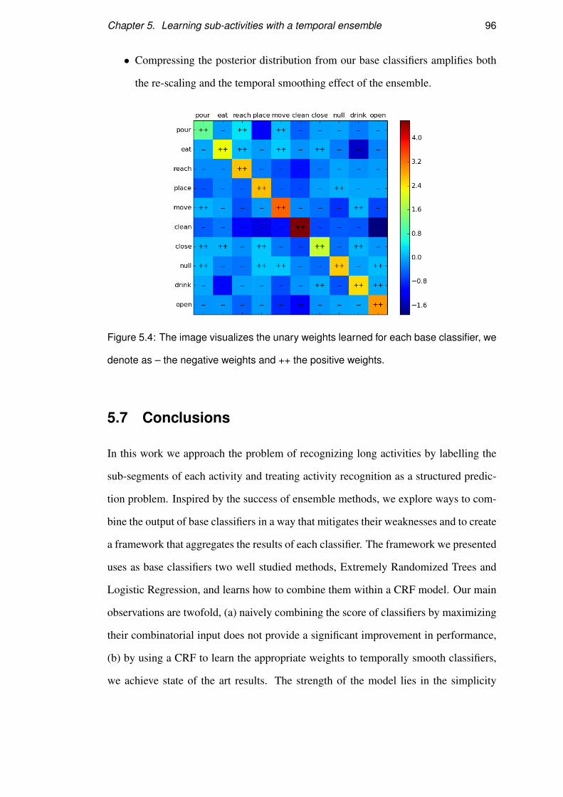
Recognising activities by jointly modelling

This thesis has been submitted in fulfilment of the requirements for a postgraduate degree

(e.g. PhD, MPhil, DClinPsychol) at the University of Edinburgh. Please note the following

terms and conditions of use:

This work is protected by copyright and other intellectual property rights, which are

retained by the thesis author, unless otherwise stated.

A copy can be downloaded for personal non-commercial research or study, without

prior permission or charge.

This thesis cannot be reproduced or quoted extensively from without first obtaining

permission in writing from the author.

The content must not be changed in any way or sold commercially in any format or

medium without the formal permission of the author.

When referring to this work, full bibliographic details including the author, title,

awarding institution and date of the thesis must be given.

Recognising activities by jointly modelling

actions and their effects

Efstathios Vafeias

TH

E

U N I V E RS

IT

Y

OF

ED I N B U

RG

H

Doctor of Philosophy

Institute of Perception, Action and Behaviour

School of Informatics

University of Edinburgh

2015

Abstract

With the rapid increase in adoption of consumer technologies, including inexpensive

but powerful hardware, robotics appears poised at the cusp of widespread deployment

in human environments. A key barrier that still prevents this is the machine under-

standing and interpretation of human activity, through a perceptual medium such as

computer vision, or RBG-D sensing such as with the Microsoft Kinect sensor.

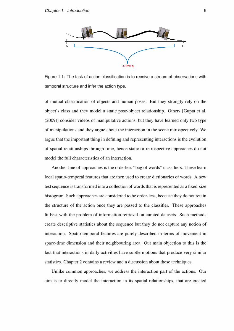
This thesis contributes novel video-based methods for activity recognition. Specif-

ically, the focus is on activities that involve interactions between the human user and

objects in the environment. Based on streams of poses and object tracking, machine

learning models are provided to recognize various of these interactions. The the-

sis main contributions are (1) a new model for interactions that explicitly learns the

human-object relationships through a latent distributed representation, (2) a practical

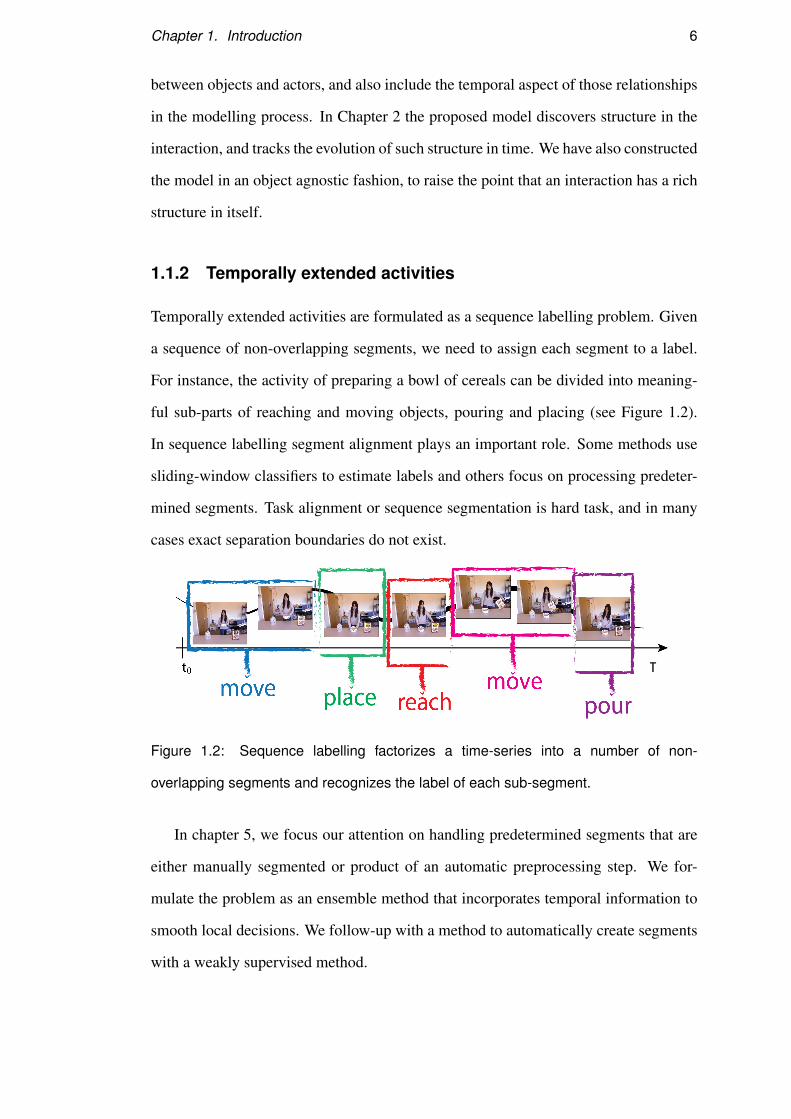
framework for labeling chains of manipulation actions in temporally extended activi-

ties and (3) an unsupervised sequence segmentation technique that relies on slow fea-

ture analysis and spectral clustering.

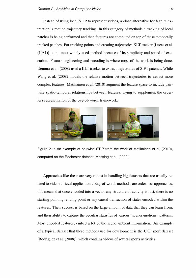
These techniques are validated by experiments with publicly available data sets,

such as the Cornell CAD-120 activity corpus which is one of the most extensive pub-

licly available such data sets that is also annotated with ground truth information. Our

experiments demonstrate the advantages of the proposed methods, over and above state

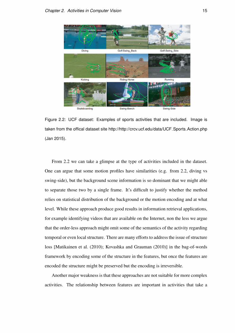
of the art alternatives from the recent literature on sequence classifiers.

i

Acknowledgements

I would like to thank my supervisor Subramanian Ramamoorthy for his guidance and

support. I would also like to thank Aris, Yiannis, Benji, Majd, Alejandro, Stavros

and the rest of the people in the RAD group and the IPAB for the constructive dis-

cussions we had during our weekly meetings. Thanks to my colleagues Ioan, Benny,

Kostantinos, Michael and many more for our daily conversions. I would also like to

thank everyone in the Informatics Forum for making it a stimulating and creative place

to work. Special thanks to my close friends who continuously motivated through my

thesis. Most of all, I would like to thank my parents for their love and support.

ii

Declaration

I declare that this thesis was composed by myself, that the work contained herein is

my own except where explicitly stated otherwise in the text, and that this work has not

been submitted for any other degree or professional qualification except as specified.

(Efstathios Vafeias)

iii

Table of Contents

1 Introduction 1

1.1 Research Problem . . . . . . . . . . . . . . . . . . . . . . . . . . . . 3

1.1.1 Interactions . . . . . . . . . . . . . . . . . . . . . . . . . . . 4

1.1.2 Temporally extended activities . . . . . . . . . . . . . . . . . 6

1.1.3 Activity Segmentation . . . . . . . . . . . . . . . . . . . . . 7

1.2 Contributions . . . . . . . . . . . . . . . . . . . . . . . . . . . . . . 8

2 Activities in Computer Vision 10

2.1 Taxonomy of Activities . . . . . . . . . . . . . . . . . . . . . . . . . 10

2.2 Approaches . . . . . . . . . . . . . . . . . . . . . . . . . . . . . . . 12

2.2.1 Space-Time Approaches . . . . . . . . . . . . . . . . . . . . 13

2.2.2 Sequential Modeling . . . . . . . . . . . . . . . . . . . . . . 16

2.2.3 Discriminative Models . . . . . . . . . . . . . . . . . . . . . 19

2.2.4 Hierarchical . . . . . . . . . . . . . . . . . . . . . . . . . . . 20

2.2.5 Template Matching . . . . . . . . . . . . . . . . . . . . . . . 21

3 Machine Learning Background 23

3.1 Supervised Learning . . . . . . . . . . . . . . . . . . . . . . . . . . 23

3.2 Graphical Models . . . . . . . . . . . . . . . . . . . . . . . . . . . . 24

3.3 Conditional Random Fields . . . . . . . . . . . . . . . . . . . . . . . 28

3.3.1 Chain Structured CRF . . . . . . . . . . . . . . . . . . . . . 29

3.3.2 Inference . . . . . . . . . . . . . . . . . . . . . . . . . . . . 31

iv

3.3.3 Parameter Learning . . . . . . . . . . . . . . . . . . . . . . . 32

3.3.4 Large Margin Learning . . . . . . . . . . . . . . . . . . . . . 34

3.4 Decision Trees and Random Forests . . . . . . . . . . . . . . . . . . 38

3.4.1 Decision Trees . . . . . . . . . . . . . . . . . . . . . . . . . 38

4 Modelling Interactions with a Latent CRF 41

4.1 Introduction . . . . . . . . . . . . . . . . . . . . . . . . . . . . . . . 41

4.1.1 Contributions . . . . . . . . . . . . . . . . . . . . . . . . . . 43

4.2 Related Work . . . . . . . . . . . . . . . . . . . . . . . . . . . . . . 44

4.3 Spatio-temporal Relationships . . . . . . . . . . . . . . . . . . . . . 46

4.4 Model Formulation . . . . . . . . . . . . . . . . . . . . . . . . . . . 48

4.4.1 Hidden State CRF . . . . . . . . . . . . . . . . . . . . . . . 48

4.4.2 Parameter Learning . . . . . . . . . . . . . . . . . . . . . . . 55

4.4.3 Computational Complexity . . . . . . . . . . . . . . . . . . . 57

4.5 Implementation . . . . . . . . . . . . . . . . . . . . . . . . . . . . . 58

4.5.1 Viewpoint Invariance . . . . . . . . . . . . . . . . . . . . . . 60

4.5.2 Managing trajectories . . . . . . . . . . . . . . . . . . . . . . 62

4.5.3 Pose features . . . . . . . . . . . . . . . . . . . . . . . . . . 63

4.5.4 Hand features . . . . . . . . . . . . . . . . . . . . . . . . . . 65

4.5.5 Object features . . . . . . . . . . . . . . . . . . . . . . . . . 65

4.6 Experiments . . . . . . . . . . . . . . . . . . . . . . . . . . . . . . . 65

4.6.1 Dataset . . . . . . . . . . . . . . . . . . . . . . . . . . . . . 67

4.6.2 Models and implementation details . . . . . . . . . . . . . . 69

4.6.3 Results . . . . . . . . . . . . . . . . . . . . . . . . . . . . . 70

4.7 Conclusions . . . . . . . . . . . . . . . . . . . . . . . . . . . . . . . 74

5 Learning sub-activities with a temporal ensemble 76

5.1 Introduction . . . . . . . . . . . . . . . . . . . . . . . . . . . . . . . 76

5.1.1 Contributions . . . . . . . . . . . . . . . . . . . . . . . . . . 78

v

5.2 Related work . . . . . . . . . . . . . . . . . . . . . . . . . . . . . . 79

5.3 Model . . . . . . . . . . . . . . . . . . . . . . . . . . . . . . . . . . 80

5.3.1 Overview . . . . . . . . . . . . . . . . . . . . . . . . . . . . 80

5.3.2 Model Structure . . . . . . . . . . . . . . . . . . . . . . . . 81

5.3.3 Potential Functions . . . . . . . . . . . . . . . . . . . . . . . 83

5.4 Learning . . . . . . . . . . . . . . . . . . . . . . . . . . . . . . . . . 84

5.4.1 Feature Learning . . . . . . . . . . . . . . . . . . . . . . . . 85

5.4.2 CRF Training & Inference . . . . . . . . . . . . . . . . . . . 86

5.5 Implementation . . . . . . . . . . . . . . . . . . . . . . . . . . . . . 87

5.5.1 Data . . . . . . . . . . . . . . . . . . . . . . . . . . . . . . . 87

5.5.2 Features . . . . . . . . . . . . . . . . . . . . . . . . . . . . . 87

5.5.3 Training Details . . . . . . . . . . . . . . . . . . . . . . . . . 88

5.6 Experiments . . . . . . . . . . . . . . . . . . . . . . . . . . . . . . . 91

5.6.1 Evaluation . . . . . . . . . . . . . . . . . . . . . . . . . . . 91

5.6.2 Results . . . . . . . . . . . . . . . . . . . . . . . . . . . . . 93

5.7 Conclusions . . . . . . . . . . . . . . . . . . . . . . . . . . . . . . . 96

6 Sequence segmentation with Spectral clustering in Slow Feature space 98

6.1 Overview . . . . . . . . . . . . . . . . . . . . . . . . . . . . . . . . 98

6.2 Method . . . . . . . . . . . . . . . . . . . . . . . . . . . . . . . . . 100

6.2.1 Slow Feature Analysis . . . . . . . . . . . . . . . . . . . . . 101

6.2.2 Clustering . . . . . . . . . . . . . . . . . . . . . . . . . . . . 104

6.3 Experimental Analysis . . . . . . . . . . . . . . . . . . . . . . . . . 109

6.3.1 Evaluation . . . . . . . . . . . . . . . . . . . . . . . . . . . 110

6.4 Conclusions . . . . . . . . . . . . . . . . . . . . . . . . . . . . . . . 115

7 Conclusions and Future Directions 117

7.1 Interactions . . . . . . . . . . . . . . . . . . . . . . . . . . . . . . . 117

7.2 Temporal Ensemble . . . . . . . . . . . . . . . . . . . . . . . . . . . 118

vi

7.3 Segmentation . . . . . . . . . . . . . . . . . . . . . . . . . . . . . . 119

Bibliography 120

vii

Chapter 1

Introduction

Humans hold an exceptional visual cognition system that enables them to acquire and

process knowledge. Our ability to interpret visual cues not only informs us about

the external environment but also helps shape our thoughts. We have the ability to

generalize complex concepts of entities or interactions. Being able to generalize in

this way is a powerful tool for interpreting new situations, quickly and reliably.

For humans, vision is a core component in perceiving the world. Robots that op-

erate in the physical world have a range of sensors available but, among the many

perceptual modalities available to a modern robotic system, vision is the pinnacle of

sensing. In robotic systems, the term “vision” often refers to various types of range

data, could be plain 2D images or depth information. Vision is perhaps the richest

modality in terms of the amount of information it captures about the physical world.

This very richness also makes interpretation highly ambiguous and often brittle. The

amount of variation and complexity in visual information makes the task of visual

understanding a tough problem, but a rewarding one nonetheless.

Given the aspirations of the robotics community to introduce robots into human

environments, they should be competent in interacting with people. Equipping robots

with a powerful perception system would, therefore, make their interaction with hu-

mans seem more natural and effortless. Robots should be able to understand human

1

Chapter 1. Introduction 2

actions and interpret them correctly in order to make this happen. The goal of robotic

perception is to create meaningful representations of the world, in order to aid the agent

in reasoning and decision making. Reasoning is the complicated task of making sense

of the world; being able to form concepts, create beliefs and applying logic rules on

them is a crucial part of it. To reason in the physical world, is a mandatory requirement

for intelligent robots, hence being able to form crisp representations of a dynamic en-

vironment has a direct impact on the quality of the reasoning. A robotic perception

module has the responsibility of creating context of the decision, and establishing the

beliefs about the world. This makes robotic perception an integral part of reasoning in

robots.

While such perception abilities for living entities has been developed over thou-

sands of years, through evolution, to create such perception module in machine vision

we need to build representations for every level of understanding. Starting from the

lowest levels of visual cues -such as textures and edges- moving to mid layer rep-

resentations -like objects and scenes- to higher level of understanding like activities

and behaviors. In low and mid level understanding computer vision techniques show

remarkable results. Such results are demonstrated in ImageNet challenge1 , where

object recognition is performed in hundreds of classes with thousands of examples.

Challenges on datasets, like ImageNet, push the state of the art techniques in terms

of image understanding, however they model the question as an information-retrieval

problem.

Interpreting visual cues to identify objects is already a hard task but it does not tell

the full story of a scene. An object belongs to a class but it can also be categorized

according to the way it is used, Gibson (1978) introduced the term “affordance” to

describe the idea of a relation between an object or an environment and an agent. So

a scene cannot be described purely by the inventory of detected objects. A human,

or any living organism, in any environment, dynamically changes the relations of the

1//www.image-net.org/challenges/LSVRC/2014/


scene and takes part in interactions that produce as much context, if not more, as the

entities in the scene itself. It is these interactions that are more meaningful, in order to

create new technologies where robots will be able to understand human behaviour, and

assist them in cooperative scenarios. Robotic perception requires more than building

an object inventory of the scene. Essentially it requires understanding the events and

interactions in a scene.

The goal of the thesis is to tackle the entry level problems of high level understand-

ing, and provide a stepping stone for human behaviour analysis. We refer to this field

as that of interactive activities between a human and objects in daily home scenarios.

Selecting daily interactions, not only aligns with the goal of enabling robots to operate

along with humans, but is a problem with some very interesting characteristics. A ma-

jor aspect is the redundancy of objects in daily household scenes, meaning that most

object types may be used in a wide variety of actions. In such cases plain object recog-

nition will not provide all the information needed to classify the interaction. Hence,

providing a solution for such class of problems, one needs to create models that encap-

sulate the characteristics of the problem. Models often represent how we think about,

and how we understand, a process. Following the guideline that models represent the

ideas we have about processes, the first model that is proposed captures our intuition

of how interactions are formed, while the second part of the thesis provides a practical

framework for labelling the sequential actions that form high-level activity. The last

part introduces an unsupervised method for time-series segmentation that enables our

framework to be applied in real scenarios.

1.1 Research Problem

The analysis of activities has been extensively studied in the context of computer vision

[Aggarwal and Ryoo (2011)]. Creating an exact taxonomy of activities can be a fairly

complicated task, since the notion of activity is very broad and extends from single


actions to complicated group interactions with complex dynamics. Activities also vary

in the temporal aspect; activities extend from being a few seconds to long periods;

depending on the task. Some actions are repetitive while others are formed from short

snap movements. Much of the ambiguity about activities is handled by defining a

specific domain of analysis.

The motivation of the thesis is to explore graphical models that are able to capture

the rich spatio-temporal relationships of interactions which enable robots to create

adequate representations of activities for reasoning in the physical world. The general

problems are tackled by being divided into manageable sub-problems. There are two

sub-problems identified here; (a) classifying single interactions, and (b) classifying

temporally extended activities that are formed by a sequence of actions.

1.1.1 Interactions

Sequence classification is the most restrictive case of activity analysis. In this case,

each input sequence is assigned to a label; thus we assume that the sequence is a sin-

gle action. This setting looks similar to the common pattern recognition task where,

given a multidimensional input, xi one needs to compute the class of the instance

yi ∈ {1,2, ...,C} (Figure 1.1). The difference from pattern recognition is that input

xi, has a temporal structure and can be of arbitrary length. Being a well constrained

problem, such types of applications have drawn much attention in the computer vision

community. The first model proposed here is formulated as a sequence classification

problem, of variable length interactions.

Interactions are a class of actions that involve actors and entities that share a causal

effect relationship. To analyse such actions one needs to consider the human part of the

action in relationship with environment and the object of manipulation. There are not

many approaches that explicitly model interaction, meaning they do not directly model

that causal relationship of actors and objects in its fully spatio-temporal aspect. In the

still image domain, Yao and Fei-Fei (2010) and others, have addressed the problem


Figure 1.1: The task of action classification is to receive a stream of observations with

temporal structure and infer the action type.

of mutual classification of objects and human poses. But they strongly rely on the

object’s class and they model a static pose-object relationship. Others [Gupta et al.

(2009)] consider videos of manipulative actions, but they have learned only two type

of manipulations and they argue about the interaction in the scene retrospectively. We

argue that the important thing in defining and representing interactions is the evolution

of spatial relationships through time, hence static or retrospective approaches do not

model the full characteristics of an interaction.

Another line of approaches is the orderless “bag of words” classifiers. These learn

local spatio-temporal features that are then used to create dictionaries of words. A new

test sequence is transformed into a collection of words that is represented as a fixed-size

histogram. Such approaches are considered to be order-less, because they do not retain

the structure of the action once they are passed to the classifier. These approaches

fit best with the problem of information retrieval on curated datasets. Such methods

create descriptive statistics about the sequence but they do not capture any notion of

interaction. Spatio-temporal features are purely described in terms of movement in

space-time dimension and their neighbouring area. Our main objection to this is the

fact that interactions in daily activities have subtle motions that produce very similar

statistics. Chapter 2 contains a review and a discussion about these techniques.

Unlike common approaches, we address the interaction part of the actions. Our

aim is to directly model the interaction in its spatial relationships, that are created


between objects and actors, and also include the temporal aspect of those relationships

in the modelling process. In Chapter 2 the proposed model discovers structure in the

interaction, and tracks the evolution of such structure in time. We have also constructed

the model in an object agnostic fashion, to raise the point that an interaction has a rich

structure in itself.

1.1.2 Temporally extended activities

Temporally extended activities are formulated as a sequence labelling problem. Given

a sequence of non-overlapping segments, we need to assign each segment to a label.

For instance, the activity of preparing a bowl of cereals can be divided into meaning-

ful sub-parts of reaching and moving objects, pouring and placing (see Figure 1.2).

In sequence labelling segment alignment plays an important role. Some methods use

sliding-window classifiers to estimate labels and others focus on processing predeter-

mined segments. Task alignment or sequence segmentation is hard task, and in many

cases exact separation boundaries do not exist.

Figure 1.2: Sequence labelling factorizes a time-series into a number of non-

overlapping segments and recognizes the label of each sub-segment.

In chapter 5, we focus our attention on handling predetermined segments that are

either manually segmented or product of an automatic preprocessing step. We for-

mulate the problem as an ensemble method that incorporates temporal information to

smooth local decisions. We follow-up with a method to automatically create segments

with a weakly supervised method.


1.1.3 Activity Segmentation

Activity segmentation is the task of creating a set of segments S = {s1,s2, ...,sn} that

are not overlapping. In traditional statistics this is known as the change point detection

problem [Basseville et al. (1993)]. The task is to define change points in time series,

by the computing of changes in the cumulative statistics of the signal. Many of these

methods focus on low dimensional signals, like the ones encountered in economics and

biological systems. Capturing statistics in high dimensional, highly interdependent,

non-linear signals like videos is not trivial. Defining such complex distributions over

signals is difficult, but creating statistical comparisons between segment hypotheses

is even harder. The reason is that the boundaries between separate states are unclear,

and approximating such a boundary in high dimensional spaces is an NP-hard problem

[Gionis et al. (2004)]. In machine learning and computer vision applications, various

HMM based models have been applied to segment activities. Brand and Kettnaker

(2000) used an HMM model to discover and segment activities in office. Willsky et al.

(2009) used non-parametric learning of switching linear dynamic systems to model

changes in sequences of synthetic data and bee motions.

This thesis presents a novel hybrid approach that deals with sequence segmenta-

tion in the hard daily activity setting. This setting has a very soft boundary between

segments, that makes the task even more difficult to handle. The method combines

change point analysis with spectral clustering of slow varying features in a two layer

hierarchy model. In the first layer change point analysis has been used to capture major

changes in the sequence. At the second layer, each segment produced at the previous

layer has been subdivided with an spectral clustering algorithm. The segmentation is

performed in an unsupervised manner, and no other data is required, apart from the test

sequence. The procedure is followed by segmentation refinement. Chapter 6 contains

a full description of the method.


1.2 Contributions

The thesis’ main contributions come in the form of novel models of learning and repre-

senting activities. The first contribution is a new way of modelling primitive interaction

patterns, where the human actions and scene (or objects in the scene) state changes are

highly correlated in a “cause and effect” manner. Driven by our goal to create robots

that work alongside humans, we need to solve the task of identifying subtle actions;

actions that have a large degree of intra-class variation and have similar motion pro-

files across classes: Manipulation actions, for example, where the motions are very

fine and they are defined more by their correlation with the manipulatable objects than

their own motion profile. To understand the difference between a common activity,

such as running, and a manipulation action, think of the example of how pushing an

object and picking up an object might have a very similar motion profile but a different

outcome. An attempt has been made here to fill the gap between classifying motions

and interactions, by trying to learn the structure of interactions in sequential data. The

thesis contributes a novel approach to modelling the aforementioned type of actions;

one aim in the approach presented here is to learn the underlying structure of activities,

in terms of cause and effect, and model the causal relationships of the actor and the

manipulatable object.

Our model is a latent CRF, that learns a hidden layer for each factor (i.e. human,

objects) in the scene and brings the structure of the activity into an abstract layer where

interactions are learned through the weighted connections of each latent variable. The

latent layers, that intertwine through time, are able to learn the non-linear relationships

of the interaction and enable us to comprehend the nature of these activities directly

from data. Current experiments have demonstrated that thinking of actions in terms of

cause and effect yields a significant classification improvement.

The second major contribution is a framework for temporally extended activities,

these are defined as being a sequence of sub-actions. The problem is to label each

separate sub-action, as well as to identify high-level activity. A sub-activity on its own


contains enough information to be classified, but incorporating estimations of previ-

ous observations can dramatically improve the overall classification. A framework has

been built that brings together a number of well-studied machine learning classification

techniques, to form a temporal ensemble model for activity learning. Ensembles train a

number of different classifiers and combine their results to provide a unified, and more

accurate, solution. Typically, ensemble models aggregate the information of different

classifiers about a single prediction and, by weighting its output, the ensemble decides

on the best hypothesis. When it comes to structured prediction (i.e. sequences), the

sequence of predictions at each time-step highly depends on the past. In our approach

we propose a consensus function in the form of an energy minimization problem that

learns the weights of each classifier according to its temporal neighbourhood. The

strength of the method comes from its ability to combine robust non-parametric mod-

els, in our case Random Forests, in a structured prediction scheme. We show that

our ensemble method gives state-of-the-art results, while remaining computationally

efficient for fast training and inference.

The third contribution is a novel hybrid method for segmenting activities. We com-

bine knowledge from statistical analysis and machine learning to create method that is

able to capture the tenuous changes that happen between actions.

Chapter 2

Activities in Computer Vision

2.1 Taxonomy of Activities

For robots computer vision is a way to perceive the outside environment. The goal of

robotic perception is to supply a semantic understanding of the environment in order

to provide enough information to the agent to act accordingly. Particularly image and

video understanding is the ability to label objects, people and their events in a scene.

Semantic understanding through video is a big leap towards advancing the field of Ar-

tificial Intelligence. Currently there is focus on three major fields of applications smart

environments - robotics, health care and surveillance. Each field of application has its

own peculiar setting. Surveillance systems lean more towards prediction of abnormal

behaviors or motion pattern analysis with distant stationary cameras. Smart environ-

ments and robotics aim towards improving the Human Computer Interaction (HCI)

abilities of a smart environment, this can extend to the field of robotics where the robot

needs to interact with people. The health care applications use activity recognition to

help elder, or to help the rehabilitation of patience through a system that will provide

feedback in their physio therapies. A number of report of such applications e.g. abnor-

mal activity home activity [Duong et al. (2005)], sports [Lu et al. (2004)], healthcare

[Li et al. (2011);Kuo et al. (2010)] are just a few examples.

10

Chapter 2. Activities in Computer Vision 11

Video understanding is a hard problem, and can be divided into various aspects,

but the most general distinctive categories are object and human segmentation, feature

extraction and representation, activity detection and classification algorithms. Each of

these topics has been approached separately as to improve the core technologies, how-

ever to create an activity understanding application, a combination of such approaches

is required since it is a complex matter. In order to comprehend what it takes to detect

and classify actions, we need to determine what is important in terms of context. In

an high level analysis about machine understanding of human behaviour, Pantic et al.

(2007) defines the context of the scene with respect to humans in six questions:

• Who? General Computer Vision classification problem (includes objects).

• Where? Scene recognition.

• What? Activity recognition.

• How? Activity recognition with some causal relationships.

• When? Activity detection.

• Why? High level plan recognition.

Some of these questions are easier to answer, like addressing the problems of “who”

and “where” which boil down to detecting objects [Everingham et al. (2010)], people

[Andriluka et al. (2008)] and classification of the scene [Li et al. (2009)]. The question

of “what”, “how” and “when” is what characterizes the goals of activity recognition

mostly, but it is largely based on answering the “Who” and “Where” of the scene.

Creating a taxonomy of activities can be a fairly complicated task, since the field

has a broad definition, from minor single actions to complicated group activities of

high complex dynamics. However in recent literature one can divide most of the meth-

ods developed into one of the following categories: gestures, actions, interactions and

group activities. These categories often change context according to the application


that they are addressing. Gestures are basic movements that a person can perform,

they are components that describe the motion of a person, an example of gestures is

lifting your leg, or extending your hand. These gestures are not necessarily mean-

ingful if viewed separately and out of context, but they are good describing motions.

Actions are performed from a single person and they have a meaningful interpretation,

for example walking, kicking, standing etc. Interactions are the activities that involve

multiple actors and/or entities at the same time. A simple interaction can be lifting a

cup, while a more complicated interaction is the case of someone who is trying to deal

with a cashier. Group activities are defined by a group of people and/or objects that

act in the same context of achieving some goals, it is not limited to a single one, each

one can have its own goal. Group activities can have complex dynamics that are not

bounded to the physical world, but interact at a conceptual and behavioral level.

2.2 Approaches

There are various approaches on the problem of modeling and classifying activities,

some vary in the descriptions of motions some and vary on the classifier level. A

high level separation is between single layer and hierarchical approaches. Single layer

approaches represent actions directly from the sequences of frames. These methods

preprocess the video and extract a set of features that are used to encode parts of the

sequence. These features are then aggregated to a classifier that implements a decision

function. Hierarchical approaches represent activities in a layered matter, the higher

level activity is modeled from simpler building blocks that describe lower level and

more specific events. In this work we explore both types of architectures. In our

ensemble model we combine single layer classifiers to build a layered representation,

while our interaction model is two-layer approach that tries to discover sub-events in

interactions in an unsupervised manner. For the rest of the chapter we will briefly

describe various methodologies used to classify activities.


2.2.1 Space-Time Approaches

Single layer approaches usually define one action in a sequence of images, they clas-

sify the whole sequence as one and they make no distinctions between various parts

of the action. The common pipeline is (a) feature detection and (b) description, some

sort of (c) encoding or pooling and then (d) train a strong classifier in fully super-

vised manner. For every part of the scheme there are many alternatives each with its

own strength. A popular approach to implement (a) and (b) is through space-time de-

scription. The video is decomposed in local regions (volumes) defined in the XY-T,

spatial and temporal dimensions. These volumes can be directly compared between

them, but its not efficient since it requires the length to be very similar in appearance

and tempo. The most sophisticated is to create local definition of volumes, these are

mentioned as Spatio-Temporal Interest Points (STIP). STIP detector methods are usu-

ally derived from their 2D counterparts from image analysis and are extended to the

temporal frame. Common detectors include, hessian detectors [Willems et al. (2008)],

Harris 3D [Laptev (2005)], cuboid detector [Dollar et al. (2005)]. These methods pro-

vide the points in the 3D space that contain some statistical variation that might be an

interest point. Then descriptors are used to create capture the statistics of the specific

points. Popular descriptors are HOGHOF [Laptev et al. (2008)], HOG3D [Klaser and

Marszalek (2008)], extended SURF [Willems et al. (2008)].

The STIP methods, describe the motion as trajectories of points within the se-

quence. The number of points is arbitrary and depends on the structure of the sequence.

In order to deal with variation the number of points being detected, pooling and en-

coding methods are applied. An encoding method captures the statistical variation of

features by learning clusters of similar features and assigning them as ”visual words”.

These bag-of-words approaches [Wang et al. (2011); Luo and Shah (2009)] use some

form of unsupervised methods to form a vocabulary that is then used to represent a

sequence. A vocabulary takes the form of a histogram, so each video is represented by

n-dimensional vector regardless of its temporal scale.


Instead of using local STIP to represent videos, a close alternative for feature ex-

traction is motion trajectory tracking. In this category of methods a tracking of local

patches is being performed and then features are computed on top of these temporally

tracked patches. For tracking points and creating trajectories KLT tracker [Lucas et al.

(1981)] is the most widely used method because of its simplicity and speed of exe-

cution. Feature engineering and encoding is where most of the work is being done.

Uemura et al. (2008) used a KLT tracker to extract trajectories of SIFT patches. While

Wang et al. (2008) models the relative motion between trajectories to extract more

complex features. Matikainen et al. (2010) augment the feature space to include pair-

wise spatio-temporal relationships between features, trying to supplement the order-

less representation of the bag-of-words framework.

Figure 2.1: An example of pairwise STIP from the work of Matikainen et al. (2010),

computed on the Rochester dataset [Messing et al. (2009)].

Approaches like these are very robust in handling big datasets that are usually re-

lated to video retrieval applications. Bag-of-words methods, are order-less approaches,

this means that once encoded into a vector any structure of activity is lost, there is no

starting pointing, ending point or any causal transaction of states encoded within the

features. Their success is based on the large amount of data that they can learn from,

and their ability to capture the peculiar statistics of various “scenes-motions” patterns.

Most encoded features, embed a lot of the scene ambient information. An example

of a typical dataset that these methods use for development is the UCF sport dataset

[Rodriguez et al. (2008)], which contains videos of several sports activities.


Figure 2.2: UCF dataset: Examples of sports activities that are included. Image is

taken from the offical dataset site http://http://crcv.ucf.edu/data/UCF Sports Action.php

(Jan 2015).

From 2.2 we can take a glimpse at the type of activities included in the dataset.

One can argue that some motion profiles have similarities (e.g. from 2.2, diving vs

swing-side), but the background scene information is so dominant that we might able

to separate those two by a single frame. It’s difficult to justify whether the method

relies on statistical distribution of the background or the motion encoding and at what

level. While these approach produce good results in information retrieval applications,

for example identifying videos that are available on the Internet, non the less we argue

that the order-less approach might omit some of the semantics of the activity regarding

temporal or even local structure. There are many efforts to address the issue of structure

loss [Matikainen et al. (2010); Kovashka and Grauman (2010)] in the bag-of-words

framework by encoding some of the structure in the features, but once the features are

encoded the structure might be preserved but the encoding is irreversible.

Another major weakness is that these approaches are not suitable for more complex

activities. The relationship between features are important in activities that take a


certain amount of time, outside this scope there are not very effective. Also view-point

variance is a very important aspect of the problem, and space-time feature approaches

find it difficult to generalize across various view-points and distances.

In applications like robotic perception, where context plays an important role in

interpreting the activities we argue that losing temporal structure makes it difficult to

represent causal relationships of the actions. Also the un-ordered arbitrary points of

interest mark no distinction between actors and objects, rendering the method unable

to capture the important semantics of an interaction beyond the cross-correlated statis-

tics. Hence scenarios like pushing a box in a tropical environment will create different

statistics than pushing a sledge in the Arctic circle, but the concept of the interaction

between the two scenes remains the same. In our proposed model for interactions in

chapter 4, we present a way to deal with variable length sequences while preserving

temporal structure and object-actor relationships.

2.2.2 Sequential Modeling

Sequential models treat activities as a sequence of events, or specific observations.

They rely strongly on modelling the relationships between consecutive events. The

common scheme is to recognize patterns of sub-events and search for such sequences

in a new video. Essentially the methods try to measure how likely it is for a specific

sequence to occur give the observation features. Such approaches build a state-model,

where each time-step in the sequence is assigned to a state. Then a maximum a poste-

rior(MAP) or maximum likelihood estimator (MLE) classifier is built to recognize the

activities. hidden Markov models (HMMs) and their generalization Dynamic Bayesian

Networks (DBNs) are common state-model methods.

In its simplest (Fig. 2.3) form the HMM’s general concept is to represent the state

of each sequence as a hidden (unobserved) variable that changes through time and the

state of the variable governs the generation process of the observations. Therefore the

observed sequences are directly dependant on the hidden variables. HMMs hold a key


property, that is clear from the Figure 2.3, that the conditional distribution of the hidden

state yi given the current observations xi depends on only on the previous hidden state

yi−1 and values before that (e.g xi−1,xi−2) have no influence on the variable, this is

called the Markov property. The model parameters build a state observation model,

and a transition model. These parameters are learned via a supervised manner through

labelled training set. Once the parameters are estimated the system solves a problem

of dynamic programming trying to compute the most likely sequence of hidden states,

the viterbi algorithm is the most common.

Figure 2.3: A temporal HMM in its simplest form.

The first use of HMMs for recognizing activities dates back to Yamato et al. (1992),

in their original work they segment the silhouette of the foreground into meshes, and

these meshes are encoded into features and each feature vector is encoded into a sym-

bol. The algorithm learns the model of the symbols and the transition between sym-

bols within a specific action class. Separate HMMs are trained for each class and to

infer the class of a new sequence every HMM is evaluated, while the one with the

highest likelihood. Their success lead researchers to further pursue these type of mod-

els. Starner and Pentland (1996) used HMMs successfully to classify words of the

American Signed Language, their method tracked the colored gloves of the users, and

encoded their shape and position. They managed to model a 40 word vocabulary with

a high success rate. Similar HMM frameworks for activities have been developed by

others [Bobick and Wilson (1997)], where the basic state model is an HMM but the

features and the state probability calculation is done in different manner to fit the ap-

plication.


Expansions of the HMMs were made to overcome their limitations. One of the

limitations of the simple HMM is the inability to model two different entities inter-

acting with each other. An HMM describes one state at a time, so in order to track

motion from two different agents one need to augment the state space with the product

of each entity state space. Augmenting the space creates the needs for more powerful

observation models; but in some cases the distinction boundary between interaction in

a common space does not exist. To overcome this problem Oliver et al. (2000) created

a Coupled HMM (CHMM) to model the interaction of two entities. In the CHMM,

basically there are two parallel Markov chains that are coupled and each one is mod-

eling the state of one entity. The resulting system was able to capture interactions of

people walking in space, some of the interactions that were able to model was “moving

together”, “meeting”.

Natarajan and Nevatia (2007) extended the interaction model of Coupled HMM to

be able to handle semi-markov chains. The new Coupled Hidden Semi-Markov Model

(CHSMM) was able to model the temporal length of an activity creating a more ro-

bust model against sub-events of various lengths. In the original HMM formulation,

the probability of staying in the same state decays over time, contrary to the CHSMM

where each hidden state has its own duration according the sub-event it represents. In

their work they presented efficient algorithms to learn and do inference on CHSMM

structures and demonstrated improved classification accuracy. Semi-HMM for activ-

ities has also explored in earlier works like Hongeng and Nevatia (2003) and Duong

et al. (2005).

DBNs are a more a general case of HMM, they consist of a Bayesian network that

copies the same structure along the time-axis. Every local structure encapsulates the

process of the specific time window with temporal dependencies on the previous time

step. Luo et al. (2003) used a DBN to form a semantic event modeling of objects

in sports videos. An example of a more advanced structure is the Coupled Hierar-

chical Duration-State DBN (CHDS-DBN) introduced by Du et al. (2007) to model


interactions as a multiple stochastic process. They address the mulitscale aspect of an

activity, and they consider multiple scales of a motion at each time. One of the major

DBN problems is the complexity of training, and the time required to do so.

2.2.3 Discriminative Models

The HMM create a generative model of the sequence and model the joint probability

of P(X ,Y ). In discriminative models we can learn only the conditional probability of

a sequence P(Y |X) given some input. For pure classification tasks, where the goal

is to identify an action/activity they joint probability is not required. The Conditional

random field (CRF) [Lafferty et al. (2001)] is a discriminative model that has been used

to represent the sequential nature of activities. CRFs originally were used to model

language problems but given the similar structure of the problem it was later used to

model activities successfully. In its simple form, the linear chain CRF, it is considered

the discriminative counterpart of the HMM, in Chapter 3 we formally present the CRF

framework and discuss some of the merits of using conditional distributions on the

data to model the problem, rather than the joint probability of the sequence.

Sminchisescu et al. (2005) used a CRF to model activities, the conditional structure

of the model could accommodate arbitrary features of long-term dependencies among

observations among observations of different time steps. This is impossible to impose

in HMM since strict dependencies assumptions are made to ensure the tractability of

the model. A factorial CRF (FCRF) was proposed by Wang and Suter (2007) to infer

both pose and action labels as correlated output. Wang et al. (2006) introduced a

hidden variable CRF (HCRF) model for recognizing human gestures, they incorporate

a layer of hidden variables in the structure that enabled them to predict the label of the

entire sequence rather than the parts of sequence. Morency et al. (2007) introduced a

latent-dynamic conditional random field (LDCRF) for action recognition, there model

had long term relationships of a regular CRF, but could also model the sub-structure of

each action class and the dynamics between different class labels. More recently Wang


Wang and Mori (2011) learned the parameters of an HCRF with max-margin approach

showing improved results over the likelihood optimization learning approach, Chapter

3 has more information on this matter.

2.2.4 Hierarchical

In hierarchical settings the main motivation is to describe each action as a compos-

ite of sub-events, for example drinking can be described by sub-events like ’approach

cup’, ’pick cup’, ’move cup to mouth’, ’drink’. Hierarchical settings implement dif-

ferent layers of abstractions to deal with different classifications. A 2-layer model will

use the first layer to identify sub-events and small actions while the second layer will

infer activities taking as input the classification results of the previous layer. An ad-

vantage of the hierarchical systems is that they have conceptual understandable and

they are computationally tractable since they manage to reduce redundancy by reusing

recognized sub-events.

A layered HMM (LHMM) was presented by Oliver et al. (2002), which is one of

the most fundamental forms of a hierarchical style of modeling. The bottom layer used

a number of HMMs that were used to identify each sub-event, the result of each HMM

in the bottom layer was fed into the upper layer HMM that treats the recognized actions

as observations. At the upper layer the activity is recognized as a complete sequence.

An advantage of this method is that it is designed to be trained separately enabling

flexible retraining. Other multilayered HMMs have been explored like the one by

Nguyen et al. (2005) used it to classify complex activities. Zhang et al. (2006) used

a multilayer hmm to classify activities in meeting groups, the lower level classified

atomic activities like ’writing’ and ’talking’ while the upper layer was used to classify

the group activities like ’presentation’ and ’discussion’.

The HCRF models described in the previous section are also a form of hierarchical

models, but their main difference is that the structure is expected to be discovered by

the data. Unlike the two-layer model of HMM the, HCRF implements the first layer of


abstraction as latent variables. This type of modeling implies that we expect a under-

lying structure of the activities, but we do not want to explicitly declare it, we expect

to capture it in the training phase. Hence such a hidden CRF model can capture sub-

structure and classify activities according to the intermediate level of representation.

2.2.5 Template Matching

Template matching approaches maintain a set of examples or templates of actions

and they represent the activities according to those templates. When a new input is

given the algorithm extracts the needed features and tries to find the template that best

matches those set of features. Because humans perform actions differently it is crucial

that the features are somehow invariant to motion perturbation or temporal differences.

A popular method to find non-linear matching algorithm, that handles differences on

speed and time is the dynamic time warping (DTW) method. Dynamic time warping

matches the two time series by warping the non-linearly in the in the time dimension.

The warped sequences maximize a given similarity measure by aligning the similar

parts of the sequence. Aligning the sequences makes the template matching process

easier to perform.

Darrell and Pentland (1993) presented a DTW based method for gesture recogni-

tion, they used it to detect gestures for ”hello” or ”goodbye”. Their method stores

various views of an object (e.g. hand) at different conditions. Given a video each

frame extracts a score for every available view in the database as a function of time.

The statistics of this function are used to form a template from a training video. A new

video is aligned with the DTW algorithm and then the statics are compared with the

template database to identify the video label. Gavrila et al. (1995) followed a similar

approach of template matching. Their model used a multi-camera body part tracking

system to create a stick-figure representation. The sequences were represented as an-

gles between joints developed in time. Then the model used DTW to compare the new

sequences with the pre-trained templates.


Efros et al. (2003) used a template matching methodology to detect distant activi-

ties, roughly 30 pixel height for each tracked person. The person is tracked through-out

the video and they create a spatio-temporal motion descriptor based on the optical flow

of the image. The video is translated to a sequence of frame by frame motion de-

scriptors. To classify the actions they use a nearest neighbour approach from a dataset

of stored annotated videos. Their method was trained to classify tennis plays, soccer

plays and ballet movements.

While the aforementioned methods are matching templates through direct compar-

ison of the reference and the query sequence, all methods that use the support vector

machine that uses the kernel trick can be considered template matching methods. In

SVMs the kernel trick expresses an observation as a vector of similarities between the

given observation and all other observations in the training set transforming the origi-

nal space into a new one that is based on the similarities metric. Then the max-margin

separation boundary is calculated in the new space, defined by support vectors which

are observations that define the hyperplane boundaries of the decision function. These

support vectors can be thought as templates, but instead of comparing to a single tem-

plate we define a set of templates that separate the new high dimensional space. We

can interpret this procedure as an advanced method for template matching with nice

mathematical properties. Loosely we can say that the methods we described in the

beginning of the chapter, that vectorize the sequence and use SVMs as classifiers, can

also be considered template matching methods.

Chapter 3

Machine Learning Background

”History is moving statistics and statistics is frozen history.”August Ludwig von Schlozer

This chapter provides some background material on supervised learning. A de-

scription is given of the basic concepts and methods that were built upon to create the

current models for activity understanding. Section 3.2 gives an overview of the graph-

ical models. Section 3.3 describes a special case of graphical models; conditional

random fields. In the last section, 3.4, the decision trees framework is presented.

3.1 Supervised Learning

In literature, learning is divided into three major fields; supervised learning, unsuper-

vised learning and reinforcement learning. Problems where a set of input-targets is

provided for training are referred to as supervised learning. This is different from the

unsupervised learning scenario, where no training signal is provided, and the objec-

tive is to discover the structure of the data. Reinforcement learning replaces the target

value for a given input with a reward process, in the training phase negative or positive

rewards are given for each input.

In a standard supervised learning scenario, a learning task consists of a training set

D of pairs xi,yi, where xi is the input and yi is the desired target value in the target

23

Chapter 3. Machine Learning Background 24

space Y , and a disjoint set D′ that has not been observed yet and defines the test set

that is used to define and validate the performance of the task. Usually there is a model

function g(x;θ), that is parametrized through some vector θ and provides an output y.

Learning is often defined as an optimization problem, where the objective function is

to minimize the difference of the error E of the function f (x;θ). In a simple binary

classification task, Y = {0,1}, the error can be defined as

E(g,D) = ∑(x,yi)∈D

yi−g(xi)

the total number of misclassified instances in a given set. This is the simplest

form of objective function. In the literature, more complex objective functions can be

found, according to the task requirements. While many algorithms are successful in

optimizing the objective function, a more important aspect is the ability of the model to

transfer it successfully in the training set to a new test set. This ability is referred to as

the generalization power of the model. Bishop (2006) provides an extensive overview

of the problem of pattern recognition and supervised learning.

3.2 Graphical Models

Many of the problems in A.I. involve predicting multiple variables that depend on each

other. In such problems, the goal is to predict an output vector of random variables,

y = {y0,y1, ...,yn}, given an input vector of observations x. One way to represent the

dependencies between the output variables is provided by means of graphical models.

Probabilistic graphical models are a framework that allows for representation of com-

plex processes in a compact way. The key attributes of graphical models are that they

allow for combination of logical structure and uncertainty in processes. Uncertainty is

handled via probability theory, while graph theory is used to deal with the complex-

ity of the structure. Graphical models come in to two major categories: (a) Bayesian

networks and (b) Markov networks. Bayesian networks have a directed acyclic graph


x1

x2

x3

x4

Figure 3.1: Simple undirected graph.

structure, while Markov networks (also known as Markov Random Fields) are an undi-

rected graphical model. Models such as hidden Markov models and neural networks

are considered to be special cases of Bayesian networks (also known as Belief Net-

works). While belief nets have their success, current focus is placed on the undirected

graphical models as the prime analysis tool. Throughout this thesis, the problem is

modelled as a Markov Random Field (MRF), particularly using a special case of the

MRF, the Conditional Random Field, as introduced by Lafferty et al. (2001).

An undirected graph (G) consists of (V ) nodes that represent the variables and (E)

edges that describe the dependences between the variables. The graph structure de-

pends on the problem and it is used to incorporate any prior knowledge concerning the

relationship of the variables. Figure 3.1 shows a simple graphical model of four vari-

ables, the variables X = {x1,x2,x3,x4} are represented as nodes and connected nodes

are dependent on each other. The graph structure represents the qualitative properties

of the distribution. One way to parametrize the graph is through factors.

An MRF holds the local independence assumptions (referred to as local Markov

property), which propose that a node is independent, given all its neighbours:

∀i ∈ V ,Xi ⊥ XV−{ j}|XNi(3.1)

Ni denotes the neighbours of node i in the graph(G), and Xi ⊥ X j|Xk states that Xi


and X j are independent, given Xk.

Let a set of random variables be Z , then a factor is defined as a function that maps

Val(Z) to a non-negative real number, ℜ+. To parametrize a distribution such as the

one shown in 3.1, where one wants to define the distribution P(x1,x2,x3,x4) in terms

of factors, such that

P(x1,x2,x3,x4) =1Z

P′(x1,x2,x3,x4) (3.2)

where Z is the normalization constant, also called partition function

Z = ∑X

P′(x1,x2,x3,x4) (3.3)

the unnormalized factored distribution is defined by

P′(x1,x2,x3,x4) = φ(x1,x2)×φ(x1,x4)×φ(x2,x3)×φ(x3,x4) (3.4)

A distribution, P, that factorizes the graph G(fig 3.1) is also called a Gibbs distri-

bution. The connected variables, (x1,x2),(x1,x4),(x2,x3),(x3,x4) are cliques in G . A

clique is a subset of of the vertex set C ⊆ G , such that for every two vertices in C, an

edge exists connecting them. The distribution is parametrized using a set of factors

φ(C1),φ(C2), ...,φ(CN) also called clique potentials. These potentials do not have a

probabilistic interpretation but can be interpreted as compatibility between variables;

a higher potential value is a more probable configuration.

The probability of a graph can be expressed as a product of factors

P(x) =1Z ∏

c∈Cφc(xc) (3.5)

A common representation of potential functions can be made through a logarithmic

transformation.

φc(xc) = exp(−E(xc)) (3.6)


where E(xc) > 0 is the energy of the clique c. Models that use these types of

potentials, called energy based models, are also known as Gibbs distribution and are

widely used in physics, biochemistry and machine learning. The Gibbs distribution

model can be written as

P(x) =1Z

exp(−∑c∈C

E(xc)) (3.7)

Every distribution with a factorized form, like Equation 3.7, satisfies the local

Markov property of Equation 3.1.

The global Markov property refers to all the conditional independences implied by

the graph structure. The conditional independence is defined as: ∀V1,V2,V3 ⊆ V , if

any path from node V1 to V2 includes at least V3 then V1,V2 are independent, given the

V3. In graph theory, this is described as the reachability problem and can be solved

using standard algorithms, such as the breadth first search [Cormen et al. (2009)].

MRFs have gained a lot of popularity in the image processing community, due

to their ability to impose contextual constraints in a principled probabilistic model

[Blake et al. (2011)]. A scene is analysed by its internal dependencies and interactions,

pixel sets that belong to the same object usually have spatial consistency and objects

within the scene can be modelled through their interactions with other objects. All this

information can be encoded as potentials in a graph and be dealt with in a principled

manner.

Inference in MRFs is finding the configuration of variables that maximize the prob-

ability of the network and can be calculated via Maximum a posteriori estimation

(MAP):

x∗ = argmaxx∈X P(x) (3.8)

replacing the P(x) with the Gibbs distribution, we have the equivalent minimization

problem. The log transformation is a monotonic function and can be ignored.

x∗ = argminx∈X E(x) (3.9)


A very popular case of modelling MRFs can be observed when X is a set of discrete

variables. There is a large corpus referring to the problem of discrete optimization

[Boykov et al. (2001a)], Kolmogorov and Zabin (2004a) analyse the types of graphs

can be minimized using these approaches. Applications such as image segmentation

[Boykov and Funka-Lea (2006)], image registration [Glocker et al. (2008)] and others

have been very successful when applying MRFs.

3.3 Conditional Random Fields

A special case of the MRF is the Conditional Random Field, where the random vari-

ables are conditioned on the input features. Redefining the notation that is given as

y = {y1,y2, ...,yn} as the variables we want to predict and x = {x1, x2, ..., xn} is the

input, divided into feature vectors. On the contrary to MRF, here the conditional dis-

tribution is modelled p(y|x) directly, with respect to the parameter vector θ

p(y|x;θ) =1

Z(y|x;θ) ∏clique∈C

ψ(y,x;θ) (3.10)

and similar to the MRF energy based models, the potentials assume a log-linear

representation of the factors

ψ(y,x;θ) = exp(θTc φ(x,yc)) (3.11)

the φ(x,yc) is extracted from the input x, according to the local clique yc that it

refers to. CRFs are often thought to be analogous to the logistic regression for struc-

tured prediction and combine the discriminative power of such models with the mod-

elling abilities of graphical models. Applying conditional relationships to the labels of

interest grants some advantages to the CRF model over the MRF; that is, modelling

the distribution of labels given only the data which improve the accuracy of the predic-

tions, by just modelling the differences that are observed.


One important aspect of discriminative models, and thus CRFs, is their ability to

handle pre-processed data, meaning the data x can be passed through a pre-processing

function φ(x). It is difficult to define generative models for such cases, since the new

features are correlated in a complex manner. An extension to this is that data dependant

potentials can be constructed for the models. A simple example to understand the

power of such potentials is to consider a sequence where neighbouring nodes are to

be modelled; the smoothing from node yi to yi+1 can be “turned off” if a discontinuity

in the corresponding φ(x,yi),φ(x,yi+1) input features is observed. Likewise, global

potentials can be defined that draw information from the complete sequence. This is

something very hard to incorporate in generative models like the MRF.

3.3.1 Chain Structured CRF

As mentioned earlier, graph structure is dependant on the application, since the aim

is to incorporate prior knowledge through graph formation. For example, vision tasks

implement grid-like CRFs because they want to manage the spatial consistency and

can represent the natural image structure of pixels. Similar to grid structured graphs for

image analysis, a natural way to model sequences is by means of chain-like structures

(an example of a chain model fig. 3.2). In such chain models, each step corresponds to

a variable that connects to the previous and the next in the chain, in order to replicate

the sequential correlation of a sequence.

Figure 3.2 shows part of a linear chain, at point i with its connected neighbours

{i−1, i+1}. (a) is a Hidden Markov Model modelling of a linear chain, while (b) is

a linear chain CRF. In the HMM the marginal distribution p(y,x) is considered and it

is assumed that 1) each state depends on its immediate predecessor and 2) that each

observation xt depends only on the current variable yt . In (b) the linear chain CRF

explicit consideration of only the current observation is not needed. A dependence is

imposed between the yi−1,yi,yi+1 nodes through their connection edges. Such a linear

structure is described as:


[t]

(a) HMM (b) Linear Chain CRF

Figure 3.2: An HMM model and a CRF model with analogous structure, that tries to

model a sequence of observations. Note that in Linear Chain CRF each variable is

connected with the complete sequence of observations x.

p(y|x;θ) =1

Z(x;θ)

T

∏t=1

ψ(yt |x;θ)︸︷︷︸unary

T

∏t=1

ψ(yt ,yt+1|x;θ)︸︷︷︸pairwise

(3.12)

The first term is the unary term - which considers how each label is affected by

the data. It expresses a score function between the data with the local area, and the

given label. While the second term is the pairwise potential which measures the com-

patibility of - or how likely- the configuration of two sequential nodes. For example,

consider how likely it would be to drink after picking up a cup. Since measurements of

compatibility between data and labels are being taken, this term can be provided by an

external classifier, and a key role in the model of Chapter 5. One thing to note is that

conditional models, like the CRF, make assumptions about dependencies among y and

between y and the data x but make no assumptions about the conditional dependencies

among x. Because of the condition on p(y|x), any dependencies on x vanish from the

general graph. This allows use of unary terms that can draw data from the entire se-

quence without the need to explicitly model their dependencies; something that would

hinder the tractability of the problem.


3.3.2 Inference

Inference in undirected graph models is the task of finding the configuration of vari-

ables that maximizes the probability distribution of the graph, known as the maximum

a posteriori estimate. An alternative way to model the MAP problem, is to reformulate

as an energy minimization problem. In this context, the assumption is that a graph

G = {V ,E} has variables that take values from a discrete set of labels L . Given the

graph and a set of parameters, the task is to assign a label lp at each variable in order

to minimize the graph energy:

E(x) = ∑c∈C

φc(x)

For the Gibbs distribution (see Equation 3.7) the minimization of E(x) finds the

labeling of the MAP solution. Factor models and energy minimization has gained a lot

of ground; the reason is that factor graphs represent the structure of the problem in a

more precise way [Koller and Friedman (2009)].

There are two prominent approaches [Szeliski et al. (2008)] to the energy min-

imization problem in the context of undirected graphs: (a) the graph cut based ap-

proaches [Boykov et al. (2001b)], (b) message passing approaches. The latter includes

approaches like tree-reweighted message passing (TRW) algorithms [Wainwright et al.

(2005)] and the more popular belief propagation [Pearl (1988)]. Message passing ap-

proaches like BP provide a solution for a large variety of graphs. Although this al-

gorithm provides exact inference in tree structured graphs, there is no convergence

guarantee for cyclic graphs. However, even without convergence guarantees the loopy

belief propagation, variation of the belief propagation algorithm, performs reasonably

well.

Recently a new class of polyhedral methods has been explored, these approaches

solve an underlying integer linear programming formulation (LP/ILP). Furthermore

these methods are applicable to models with higher order factors and more complex

graph structures. The topic of inference has been extensively studied in the past two


decades, and going in depth is not in the scope of this thesis. A good reference guide

on inference methods is the recent work of Kappes et al. (2013). In their work, they

provide an extensive comparison of 24 popular methods. The presented results give a

valuable insight about the strengths of each method, and the class of problems that is

more suitable.

3.3.3 Parameter Learning

Learning in CRFs is formed as a problem of estimating the best set of parameters θ

that fit the training data. This current work considers the case of supervised learning,

where one is provided with labelled, independent samples. Provision of a training

set is assumed D = {xi,yi}, and an estimate of the parameters that explain the given

distribution of samples needs to be determined. Depending on the data and the power

of the model, it is possible to generalize with new, unseen samples.

One way to describe this problem of setting and learning the CRF parameters is

through maximum likelihood. Maximum likelihood estimation (MLE) for a given train-

ing set of samples tries to find the parameters of the given model that maximize the

probability of the data. A common strategy, and an approach that is used for the model

presented in Chapter 4, is to use a general purpose optimizer (e.g. L-BFGS) that has

as an objective the minimization of the likelihood function and will be paired with an

inference method (3.3.2) that provides the marginal probabilities and the likelihood

derivatives.

Because CRF is a discriminative model, the conditional distribution is considered

and, hence, the conditional likelihood of the data. Let us consider the set D = {xi,yi}

where xi is the input sequence and yi is the target labels of the sequence. A usual sce-

nario is to work on the log-domain of the likelihood function because it is more con-

venient and preserves the maximum points. So, the conditional log-likelihood given to

the data takes the form:


l(θ) =N

∑i=1

logp(y(i)|x(i);θ) (3.13)

It is the summation of the log-likelihood of each example pair x(i),y(i). If we plug-

in Equation 3.12 with the exponential factor of Equation 3.11 the log-likelihood for

chain model is formed as

l(θ) =N

∑i=1

T

∑t=1

K

∑k=1

θkφk(y(i)t ,y(i)t+1,x

(i))−N

∑i=1

logZ(y,x(i)) (3.14)

Equation. 3.14 is the objective function that should be maximized to estimate the

set of optimal parameters θ∗. Because it has been learned on a given training, with

the goal of generalizing on new unseen samples, that over-fitting the parameters to

the training set should be avoided. Regularization is the way to prevent overfitting

of models while training. In particular, regularization forces the optimizer to avoid

overfitting by penalizing the models with extreme parameter values. Regularization is

added as an extra term to the objective function and usually takes the form of the norm

of the parameters θ. The L1 norm and the L2 norm are the most common penalty terms

used.

l(θ) =N

∑i=1

T

∑t=1

K

∑k=1

θkφk(y(i)t ,y(i)t+1,x

(i))−N

∑i=1

logZ(y,x(i))−λ

K

∑k=1‖ θk ‖p

p (3.15)

the parameter p = 1,2 defines regularization as L1 or L2 respectively, while λ is

a hyper-parameter that needs tuning, according to the training set. Determining the

parameter is a hyper-parameter optimization problem, and usually requires a sweep in

the parameter space while using cross-validation to define the best value.

In principle, adding a regularization term to the objective function will force the

model to find smoother solutions. The optimizer tries to find a good trade-off between

fitting the training set and finding a ”smooth” solution that generalizes well on new

examples.


Maximizing 3.15 is conducted through numerical optimization, since it doesn’t

have a closed-form solution. The objective function l(θ) is of the form f (x)= log∑e(x);

which is a convex function. Convexity is a very desirable attribute when optimizing

functions, since it guarantees that a local minima is also the global minima of the func-

tion. There is a large body of work about function optimization that involves various

techniques. What have been shown to be particularly effective are techniques that use

second-order information, such as quasi-newton methods.

In particular, L-BFGS is a very popular likelihood optimization method since it

can handle large number of parameters and has been reported to achieve good results

(papers needed). Because in CRF it is not practical to obtain second order information,

L-BFGS is particularly useful since it approximates the curvature numerically from

previously computed gradients and updates. As such it avoids computing the exact

Hessian from the objective function derivatives. Multiple studies have successfully

used L-BFGS to train CRFs with a large number of parameters(cite). Optimization

techniques is a large topic and a complete discussion is beyond the scope of this thesis,

Nocedal and Wright (2006) present a more detailed description of the L-BFGS and

other optimization methods. Stochastic gradient decent is also considered to be a good

optimization approach for parameter learning, with some desirable properties. For

example, in their work, Vishwanathan et al. (2006) applied a Stochastic Meta-Decent

(SMD) and showed that it achieves same quality results but on an order of magnitude

that is faster than L-BFGS.

3.3.4 Large Margin Learning

An alternative method to the MLE approach for parameter learning is the max-margin

learning approach. Max-margin learning for structured output is an efficient, general

purpose learning framework that is based on the the well-studied notion of separa-

tion margins, as introduced by Support Vector Machines [Cortes and Vapnik (1995)].

Taskar et al. (2004), introduced a max margin approach for Markov Networks and later


on Tsochantaridis et al. (2005) introduced the more general framework of SVMstruct.

Szummer et al. (2008) showed the full power of max-margin learning for MRF and

CRF models when they combined it with fast inference techniques, such as graph cuts,

to learn the parameters of the model.

Let us assume the same task of learning the parameters θ of a CRF model from

a dataset D = x(i),y(i) where y(i) is a structured output. The conditional distribution

expressed in an energy form

P(y|x;θ) =1Z

exp(−E(y,x)) (3.16)

During training our goal is to learn a vector θ such that y(i) has an equal or greater

probability than any other label ordering of y of the i-th instance. Unlike maximum

likelihood estimation, the objective is not to define the θ that maximizes the probability

of the example, but find a vector θ such that every other configuration of variables

generates a lower probability estimate. Hence maximize the separation ability of the

model. This results in a more flexible objective that can be expressed as

P(y(i)|x(i);θ)≥ P(y|x(i);θ),∀y 6= y(i),∀i (3.17)

Replacing Equation 3.17 and canceling the normalization constant, we express the the

inequality in terms of energies

E(y(i),x(i);θ)≤ E(y,x(i);θ),∀y 6= y(i),∀i (3.18)

This inequality might have multiple solutions or no solutions at all. To resolve this

issue the framework defines a margin γ, and searches for parameters that satisfy the

inequality with the largest possible margin. This large margin approach is where the

framework draws it’s generalization power. Also the margin might be negative in the

case that the inequality has no solution.

The problem can be expressed in form of maximization of the margin with con-

straints:


maxθ:‖θ‖=1γ (3.19)

s.t. costraints:

E(y,x(i);θ)−E(y(i),x(i);θ)≥ γ,∀y 6= y(i),∀i (3.20)The norm of the weights ‖ θ ‖ is constrained to 1 to prevent the weights from

growing out of bounds.

The problem of optimizing 3.19 is the exponential number of constraints, one for

each possible configuration of variables, for each data point in the training set. The

large number of constraints make it infeasible to optimize directly. Szummer et al.

(2008) give a basic algorithm for solving the problem, by performing optimization

in only a small set of labellings. They started with a minimal set of labellings, then

performed an optimization and finally perform MAP through graph-cuts. If the new

labelling didn’t achieve the desired margin, they added it to the set and performed the

optimization again. The algorithm iterates until the weights stop changing (within a

tolerance threshold). Algorithm 1. shows a high-level description of the algorithm.

A key observation is that step 1 (MAP) turns into a graph optimization problem

that can be effectively solved with graph-cuts. Graph-cuts perform very well when

applied to sub-modular type of energies [Kolmogorov and Zabin (2004b)] and are

guaranteed to find the global optima. In non sub-modular energies one can apply

message passing algorithms to find approximate solutions. Algorithms like TRW(tree

reweighted message passing) also give a lower bound of the energy which can be used

as indicator of how close the solution is to the global minimum.

Overall the ability to express the inference in the model as discrete optimization

and neglect the normalization constant of the model is significant. MRFs and CRFs

for many problems are not tractable to train exactly with MLE, but large-margin ap-

proaches combined with graph-cuts give a practical solution to this problem.


Algorithm 1 Basic learning algorithm for Random Fields1: Input: D,θ0

2: labelled training set D = {(x1,y1), ...,(xn,yn)}

3: initial parameters θ0

4: Repeat until θ is unchanged (with tolerance e)

5: Empty set of constraints S

6: Loop in training examples

7: Step 1:

8: Find MAP labelling of the i-th instance (using graph cuts).

9: y∗← argminE(y,x(i);θ)

10: Step 2:

11: if E(y∗,x(i))< E(y(i),x(i)) then

12: add it to constraint set S

13: Step 3:

14: Solve 3.19 for the instance i and the constraint set S

15: Update the parameters θ so that ground truth y(i) has the lowest energy


3.4 Decision Trees and Random Forests

3.4.1 Decision Trees

Decision Trees is a model of sequential decisions and their consequences. The model is

described as a binary-tree graph that defines parent-child relationships between nodes.

The tree is traversed from the root node and, at each, a decision rule was evaluated

that led to one of the two children nodes; left or right. The procedure was repeated

until the algorithm reached a terminal node; a leaf. At the terminal node a result was

stored. The result could be a member of a discrete set (classification tree) or a real

value (regression tree). While the use of decision trees goes back to the 50’s and

60’s, Breiman et al. (1984) unified much of the previous work using this approach to a

consistent framework under the term CART (Classification and Regression Trees).

Figure 3.3: A binary decision tree that solves a classification problem of X = {X1,X2}→

Y = {A,B,C,D,E,F}

As an example, Fig. 3.3 shows a decision tree of a two dimensional variable X =

{X1,X2} mapping to a class set of Y = {A,B,C,D,E,F}. The algorithm starts and

queries the value of X1. If the value is less than threshold it moves left - else it moves

right. At the next node it repeats the process with a different variable (although it’s not


bounded to pick another variable) with a different threshold. The terminal node holds

the value of y that classifies the input. In brief, at each node the tree partitions the input

space, by making a split decision, until it reaches the sub-area where a specific class

lays. By consecutively splitting the input space a very strong predictor can be created,

that is capable of handling non-linearities and complex arbitrary relationships between

the input. While the descriptive power of the tree grows with the depth of the tree, the

real challenge is to find the best decision at each node.

3.4.1.1 Mathematical Notation

Let us describe the notation used for decision trees. A vector x = {x1,x2, ...,xd} ∈ℜd

is the input vector, where each xi is some scalar feature. The feature space might be

very large, or even infinite since in decision trees only a subset is used at each node.

More formally, a sampling function at node j φ j : ℜd −→ ℜd′ , with d � d′, is used

to define the variables of interest. Each node j is described with a binary splitting

function h

h(x j,θ j) ∈ {0,1} (3.21)

the function h is often described as being a weak learner model [cite RTs msr].

The model is characterized by its parameters θ = (φ,ψ,τ), φ is the variable sampling

function, ψ is the geometric boundary description (e.g. axis aligned hyperplane or a

general surface etc.). The parameter τ is used by the geometric descriptor ψ to set the

inequality boundaries for the binary split.

3.4.1.2 Learning

During training, a Decision Tree creates nodes by optimizing the information gain of

each split. At split j the following objective function is optimized:

θ∗ = argmaxθ jI j (3.22)


I j corresponds to the information gain for the specific split

I = H(S)− ∑i∈{1,2}

|S i||S |

H(|S i|) (3.23)

with H(S) being the Shannon entropy defined as H(S) = −∑c∈C p(c)log(p(c)) with

c ∈ C being the class set.

While optimizing the splits it learns the rules to traverse the tree and the informa-

tion about the predictions is learned in the leaf nodes. For the classification task (the

focus of this thesis), each leaf stores an empirical class distribution of the subset of the

training data that reached that specific leaf.

3.4.1.3 Randomness and Ensembles

In his seminal work about random forests, Breiman (2001) presents the idea of ran-

domness in an ensemble of trees. Each tree in the ensemble is randomly different from

the others. This leads to de-correlated predictions between trees, which in turn im-

proves the ensemble’s generalization ability and achieves robustness with respect to

noise. The way that randomness is implemented in the training process is through ran-

domly sampling the data and training each tree in a random subset. In these methods, a

random subset of data points xi or a random sub space of the features [Ho (1998)], are

not mutually exclusive, so they can both be applied at the same time. After every tree

is trained, the ensemble aggregates the decisions into a single prediction by a weighted

mean:

p(c|x) = 1T

T

∑t

pt(c|x) (3.24)

The ensemble returns a probabilistic output since in each leaf a complete class

distribution is stored, rather than just a single decision.

Chapter 4

Modelling Interactions with a Latent

CRF

This work has appeared in ICRA 2014 under the name “Joint classification of actions

and object state changes with a latent variable discriminative model”, Vafeias and Ra-

mamoorthy (2014).

4.1 Introduction

The first computer vision methods for action classification were primarily concerned

with finding distinct patterns in motion. While these approaches have enjoyed success

in applications that require distinctions between sequences of poses, they have often

succeeded by ignoring interactions with the environment that change the context of

the action, or focusing on datasets that included only motion-based actions. But, if

we want to create meaningful representations of humans in the environment, there is

a need to account for human interactions since they encapsulate much of the scene

context. We define interactions as a special category of actions/activities that occur

between an actor and at least one object, while they share a causal effect. An actor

is changing the state of the object but simultaneously the motion pattern of the actor

41

Chapter 4. Modelling Interactions with a Latent CRF 42

changes to account for the object shape, weight, and functionality. The idea is that

every object might have a two-way causal effect.

The focus of this chapter is to present a model that encapsulates the notion of

interaction, when dealing with actors and objects. The goal is to demonstrate that such

a model uses the context of the interaction to create a more complete description of

these actions and that boosts classification performance over regular approaches. Other

lines of research [Yao and Fei-Fei (2012)] have been developed in computer vision,

where models use detected objects jointly with human poses in still images. They

have shown that the scene context provided by the objects improve the classification

of actions, since the correlation of object categories with specific poses can be a strong

predictor. For example, a service pose with a racket can be easily distinguished as a

tennis playing activity rather than volleyball. Intuitively we can say that, in the real

world, entities form relationships which are rich in contextual information.

This chapter moves beyond still images to videos, and addresses contextual rela-

tionships based on coordinate motion of objects and humans. Unlike methods that are

based, for example, on features of single frames within the activity, this current work

models spatio-temporal interactions with objects that define the classification outcome

of an action. This makes the method suitable for the understanding of activities which

are best defined by the joint evolution of the state of an object in the environment

and the changes in body poses that cause that state to change. A technique is pre-

sented that learns to classify such interactions, from video data, and performs better

than alternate baselines due to its use of the joint information in the recognition pro-

cess. Work is based on object information, without explicitly identifying the object,

showing that spatio-temporal relationships are sufficient to improve the performance of

activity recognition. This is believed to be better suited to the needs of incremental and

lifelong learning because the notion of tracking the motion of a not-yet-fully-modelled

object conceptually precedes the more sophisticated task of identifying and making

inferences about the detailed properties of the object in question.


In order to explain the concept intuitively before jumping into detail, consider the

fact that two actions - picking up and slightly pushing an object - can appear highly

aliased and difficult to disambiguate unless one also considers what happened to the

object: did it leave the hand and roll away or did it move with the hand away from

the surface of a table? The disambiguating signal is neither the pose of the hand nor

the identity of the object. Instead, it is the joint hand-object movement. Incorporating

such structure into our models is key to learning “symbolic” relational concepts.

In this chapter, previous work on action classification, based on state of the art

statistical learning techniques, is built upon. Given the intention to work with sequen-

tial data, a discriminative sequential classifier, Conditional Random Field, has been

adopted. This model is a variation of the hidden state CRF [Quattoni et al. (2007)],

which allows consideration of the object-action spatio-temporal dependencies upon

action classifications.

4.1.1 Contributions

This chapter introduces a supervised method for learning spatio-temporal interactions

of human and objects in the environment. It demonstrates the merits of constructing a

model for interactions. The approach taken separates the information extracted by the

human motion and the information about the object state. We show that our latent vari-

able approach can extract structure from each information channel, while creating an

abstract representation of the interaction. We also use a heuristic algorithm for splitting

a sequence in segments of similar motion profiles, in order to make the model com-

putationally efficient. Our results show that this formulation is better at incorporating

object information and merging this information with the human motion.


4.2 Related Work

The idea that objects and actions are intertwined and highly dependant was originally

proposed by the psychologist Gibson (1978), who coined the term affordance. Af-

fordance refers to a quality of an object or the environment that allows an agent to

perform an action. In the field of robotics, the idea of affordances has been explored

from various viewpoints. One popular approach is to apply known motor actions to

either segment objects or learn about the affordance possibilities [Fitzpatrick et al.

(2003);Montesano et al. (2008)]. Other approaches consider the role of objects in im-

itation learning and use them to support motor experiences [Lopes and Santos-Victor

(2005)]. Kruger et al. (2010) introduced a framework that describes how object state

changes can help to form action primitives. In other cases human demonstration is

used to visually infer object affordances [Kjellstrom et al. (2011)]. Furthermore, Ak-

soy et al. (2011) represent relations between objects to interpret human actions in the

context of learning by demonstration.

Approaches such as those presented in [Yang et al. (2010);Yao and Fei-Fei (2010)]

combine pose estimation and object information for single frame inference, to learn the

mutual context of actions and objects. These methods have been tested on databases

where objects provide enough information, but almost no temporal dependencies are

required to classify the image, e.g. holding a racket and taking the serving pose is very

likely to be assigned with playing tennis. Modelling interactions from still images has

a potential value in information retrieval cases, but it can be a less complete representa-

tion in human robot interaction scenarios. In our work, we are interested in recognizing

more subtle actions that differ at a lower level, where object recognition itself is not

enough to generally characterize the activity. The same action can be performed with

multiple objects, thus we focus especially on temporal dependencies.

Kjellstrom et al. (2011) use a Factorial CRF to simultaneously classify human ac-

tions and object affordances from videos. The difference from our work is that they

use object detection that assumes known object instances and accurate hand pose seg-


mentation. This is a valid setting for imitation learning, yet difficult to achieve in other

activity recognition scenarios, especially when we do not yet have detailed object la-

bels. While the FCRF and our proposed HCRF structure are similar in the way they

split object and action information, Kjellstrom et al. (2011) consider factorization sep-

arately and predict object-action combinations, however we embed a factorization of

object and motion hidden states to jointly classify them in a latent representation space.

Additionally we use hidden states to explore structure from raw input.

Unlike other previous work from Gupta et al. (2009) on classification without an

explicit notion of time scale, we also want to model temporal relationships of the ac-

tions. Gupta et al. (2009) is using the temporal dimension indirectly, given a video a

motion is first classified as a reaching or a manipulation motion and the likelihood of

each motion is aggregated to the system. The system builds a Bayesian network that

gathers information about the object appearance, the start and end state of the motion

and then inference is performed. This type of model doesn’t explicitly models the state

of the object in time. It also has the problems of any generative model that inference is

performed on the marginal probability of network. This assumes that we have a prob-

ability distribution over the data, which is not always the case in non-experimental

scenarios.

Close to our proposed model for interactions is the work of Oliver et al. (2000)

where they make use of a coupled HMM to model interactions in pedestrian motion.

The main idea of coupled HMMs matches the model we present here. Instead of a

single hidden state representing all entities, a separate hidden state is dedicated for

every entity in the scene. Then each hidden state is coupled with the other hidden

states forming a transition matrix that depends on both the previous state of the same

state but also the previous state of coupled entity. Most of their experiments though

are carried out in pedestrian tracking scenarios and some synthetic data. There hasn’t

been any work in manipulative actions. Such actions have a higher dimensionality and

much more complex input space compared to pedestrian motion trajectories. CHMM


like regular HMM models face problems like vanishing probabilities in transitions at

low probability states. The transition model can also be problematic given that you can

only do state transitions that have been seen through training.

Our proposed discriminative model holds the merits of considering the conditional

probabilities p(y|x) of sequence. We do not explicitly define a P(X) distribution over

the observations like generative models and thus make it more tractable at training.

We also optimize towards maximizing discriminative power of the model, while in

generative models optimize for the marginal distribution of p(Y,X). We also present a

full temporal modelling of and not retrospective analysis of events.

4.3 Spatio-temporal Relationships

Techniques that have been developed for still images, e.g. [Yang et al. (2010)], contain

spatial relationships of objects and human poses. Most of these methods are evaluated

and developed around datasets with activities/actions that are easily recognized by the

co-occurrence of a pose and an object. For example, the UFC dataset [Kovashka and

Grauman (2010)], where the context is very powerful. Recognizing special equipment,

such as musical instruments, tennis rackets etc., can limit the prediction space signif-

icantly. Much of the stability of these methods rely on the strong object classification

techniques used in the first layer.

Another group of methods for action recognition is the bag of words. These de-

tect features and create descriptors over them; clustering these descriptors and creating

code-words which are then used to describe the sequences as histograms of those code

words (bag of words). The descriptors that are used encode some form of short-term

temporal relationship and some local spatial structure but, beyond that, they are con-

sidered order-less. A way to consider these methods is as a statistical distribution of

micro-events in the video, but without having the ability to tell when each one has

happened or which micro-event preceded another. The success of these approaches


lies in capturing the statistical diversity of videos such as those in the Olympic dataset

[Niebles et al. (2010)]. These micro-events appear to be very distinct, since they cap-

ture both appearance information and motion information. It is unsure if this approach

is useful in robotic application scenarios where the daily-scenes are less distinct in ap-

pearance and the motions are subtle. Empirical results concerning these assumptions

have been shown in recent work of Karpathy et al. (2014). Karpathy et al. (2014) de-

veloped a Convolution Neural Network, to recognize actions in a large video dataset.

They tested their algorithm on a new dataset (Sports 1-M 1) of 1 million Youtube sports

videos that contained 487 classes where state of the art performance was demonstrated.

From their results they noted that the single frame architecture accuracy differed very

little from the spatio-temporal architectures; the reported increase in performance was

from 59.3% to 60.9%. Such results expose the structure of the dataset; if single frame

approaches produce comparable results it means that the amount of information in

appearance dominates the temporal relations.

The line of work presented here tackles the problem of action recognition from a

different angle. It is primarily focused on robotic applications of action recognition

and the current model is driven with human-robot interactions in mind. Therefore,

an object-actor interaction model, that is object-agnostic, is introduced. The model

discovers spatial relationships of the entities and evaluates how they cross-correlate

through time.

1https://code.google.com/p/sports-1m-dataset/


4.4 Model Formulation

A hidden state CRF, which is a discriminative probabilistic model that defines a con-

ditional distribution over sequence labels, given the observations, has been used in this

current study. An explanation is given of how an object - action pair can be jointly

modelled under a framework that considers both temporal and causal relationship be-

tween the action and the object’s change in the physical world. A description is also

given of the features that have been devised to create a robust representation of body

posture that is viewpoint invariant and has sufficient descriptive power for the task.

Furthermore, the processing of sequences, in order to shorten their length and reduce

the model complexity, is explained; thus achieving gains in speed and accuracy.

4.4.1 Hidden State CRF

Hidden state Conditional Random Fields (HCRF) are random fields that include latent

variables in their structure, and have been shown to perform well in a wide range of

problems. Quattoni et al. (2007) extended the CRF framework to incorporate hidden

variables, in order to capture the spatial relationships of object parts in images, while

Wang et al. (2006) used an HCRF for sequential data segmentation. In Chapter 3 the

basic formulation of a CRF was presented. The same notation is used in this current

chapter to describe the extension of the framework to include latent variables. Like any

undirected graphical model, variables are represented as nodes(V ) and edges(E) ac-

counting for variable correlation, forming a graph G = (V ,E). The graph is factorized

and represented as a conditional probability distribution.

Let us consider the problem of classifying a sequence, for each sequence of ob-

servations x = {x1,x2, ...,xT}, we have a label y that classifies the sequence. To

extend the model to include latent variables, we create a sub-structure of variables

h= {h1,h2, ...,hT}, that are the latent variables we include to the graph. For each time-

step t we add a latent variable ht and these latent variables h create a ”sub-structure”


that is between the class node and the observation nodes. Fig. 4.1 shows the layout of

such a graph in comparison with a simple CRF.

x1 x2 xt

y1 y2 yt

CRF

x1 xt

h1 h2 ht

y

x2

HCRF

Figure 4.1: Structure comparison between a linear chain CRF and an HCRF.

Each latent variable is connected to the observations and then the class y is de-

pendent on the configuration of the latent variables. The latent variables are assigned

labels from a disjoint set of Hc ∈ H , so for each class there is a number of different

labels that the latent variable can be assigned to. Essential the latent chain of vari-

ables tries to discover structure in the input space. This can be loosely interpreted as

a phase detector within the action. A pickup action can have an approaching phase, a

grab phase and a moving phase, for example. For such an HCRF structure with latent

variables the conditional probability is expressed as

p(y|x;θ) = ∑h

P(h|x;θ)P(y|h,x;θ) (4.1)

The set of latent variables form disjoint sets for each class, i.e. H is the union

of Hc,c∀C and Hci ∪Hc j = /0, i, j∀C . This restriction keeps the model tractable since

the probability P(y, |h,x;θ) = 0 for every other class except the conditioned one. The

latent variables h take values from the empty set, hence they have no probability mass.


While the probability mass of ∑h P(y, |h,x;θ) is always equal to 1, since it sums the

whole set of probable configurations. The conditional probability of equation 4.1 takes

the form

P(y|x;θ) = ∑h:∀h j∈Hc=y

P(h|x;θ) (4.2)

The probability of the above equation is modeled as a sum of factors

P(y|x;θ) = ∑h:∀h j∈Hc=y

P(h|x;θ) =1Z ∑

h:∀h j∈Hc=y

eΨ(y,h,x;θ) (4.3)

Z is the partitioning function, and sums up the unnormalized score of every possible

configuration of the latent variables h for every class y

Z = ∑y∈Y,h

eΨ(y,h,x;θ) (4.4)

As mentioned in Chapter 3, because the graph only shows model conditional de-

pendencies, it has the flexibility to create arbitrary dependencies between the observa-

tion variables, the latent variables and the input variables. The hidden variables at each

time t have the potential to select arbitrary subsets of observations, hence they can be

dependent on observations from any frame of the sequence (see Figure 4.2). Selecting

subsets of the full observation set is commonly used in image processing as a way to

express spatial relationships. In sequences this means that long-term temporal, spatial

or contextual dependencies can be captured.


x1 xt

h1 h2 ht

y

x2

Figure 4.2: Latent variables ht are connected to a window of observations of length ω.

In this figure they are connected to the complete sequence. The window of observations

determines if the latent variable models short or long term relationships in the sequence

and it is problem dependent.

These dependencies encapsulate prior knowledge concerning the structure of the

problem. For the purpose of modelling interactions between objects and actors, two

chains of latent variables were created for each modality; one for the actor state and

one for the object state. The main idea is to represent the action as a factorization of

intermediate layer of latent factors that will capture the lower level structure within

the sequence. These latent factors try to encode a product of local functions that each

depend on only a small number of variables. Abstracting the input into meaningful

higher levels increases the expressive power of the model. A structure such as the one

proposed here is able to cluster phases in the object’s state and the actor’s motion; then

consider their combination to infer the action class. The utility of this structure is that

it solves sub-problems more efficiently.

We choose to separate object-related features and body based features connected to

different latent variables at each time step t. We create nodes that depend on the f ob jt

object observations, and nodes that depend on f skelt , the skeleton tracking observations.


The observation sequence is represented as X = [x1,x2, ...,xT ], and each observation xt

is an object-action pattern represented by 2 feature vectors, f skelt ∈ℜ18, f ob j

t ∈ℜ6. The

model has two sets of latent variables, hob j = [ho1,h

o2, ...,h

oT ], and hskel = [hs

1,hs2, ...,h

sT ],

each node having zero and first order dependencies2. The connectivity of the model

is represented in Figure 4.3. Each pair of nodes is assigned to a different set of hid-

den states according to its type. Latent variables referring to skeleton hsi are assigned

hidden state values from the set hsi ∈ H s, and object variables ho

i , are assigned from

a different set hoi ∈ H o. We denote as h = [{ho

1,hs1},{ho

2,hs2}, ...,{ho

T ,hsT}] a chain of

pair nodes(object - skeleton) and their states from their corresponding sets.

From the probability Equation 4.3 we can see that the model is factorized through

the potential function Ψ(y,s;θ) ∈ℜ. The potential function is parametrized by θ, and

its purpose is to measure the compatibility between the observation sequence X , the

hidden state configuration, and a label y. The parameter vector θ has 3 components

θ = [θv,θe,θy]. Each of the three vector components is used to model a different fac-

tor of the graph. The first component θv models the dependencies between the raw

features f skelt , f ob j

t and the hidden states hi ∈ Hs , hi ∈ Ho. The length of the vector

θv is (ds× |Hs|)+ (do× |Ho|). The component θe models the connectivity between

the hidden states, which, for a fully connected graph like the one we use, has length

(|Y |×|Hs|×|Hs|) + (|Y |×|Ho|×|Ho|) + 2× (|Y |×|Hs|×|Ho|). The θy vector corre-

sponds to the links between the hidden states and the label node y, and is of length

(|Y |×|Hs|+|Y |×|Ho|). We define Ψ(y,h,x;θ) as a summation along the chain

Ψ(y,h,x;θ) =T

∑j=1

ϕ( f sj ,θ

v[h j|s])+T

∑j

θy[y,h j|s]

+T

∑k=1

ϕ( f ok ,θ

v[hk|o])+T

∑k=1

θy[y,hk|o]

+T

∑j=2

( ∑k=s,o

θe[y,h j|k,h j−1|k])+θ

e[y,h j|o,h j|s])

In the above definition of Ψ(y,h,x;θ), the function ϕ is the inner product of the

2In the HCRF framework, zero order dependencies denote the dependency between the variablenodes and the data, while first order dependencies are defined in variable pairs.


features at time step j and the θv parameters of the corresponding hidden state. The

θy[y,h j] term stands for the weight of connection between the latent state and the class

y, whereas θe[y,h j,h′] measures the dependency of state h j to state h′ for the given class

y. For simplicity reasons the formula does not include the case of various observation

windows. In cases were the observation window is ω > 0, then the feature function

ft is the concatenation of all xt− j∀ j = [−ω,+ω], so as to include all the raw observa-

tions of the time window ω. The observation window is a way to capture long term

relationships within the sequence. The observation window can be of arbitrary length

but usually we define it through a cross validation process, after certain length we see

no performance gains and we have to consider the additional training cost through the

increase of the model parameters.


y

Skeleton Tracking Information

Object informationAction information

hs

hs

hs

hs

ho

ho

ho

ho

time time

Object tracking information

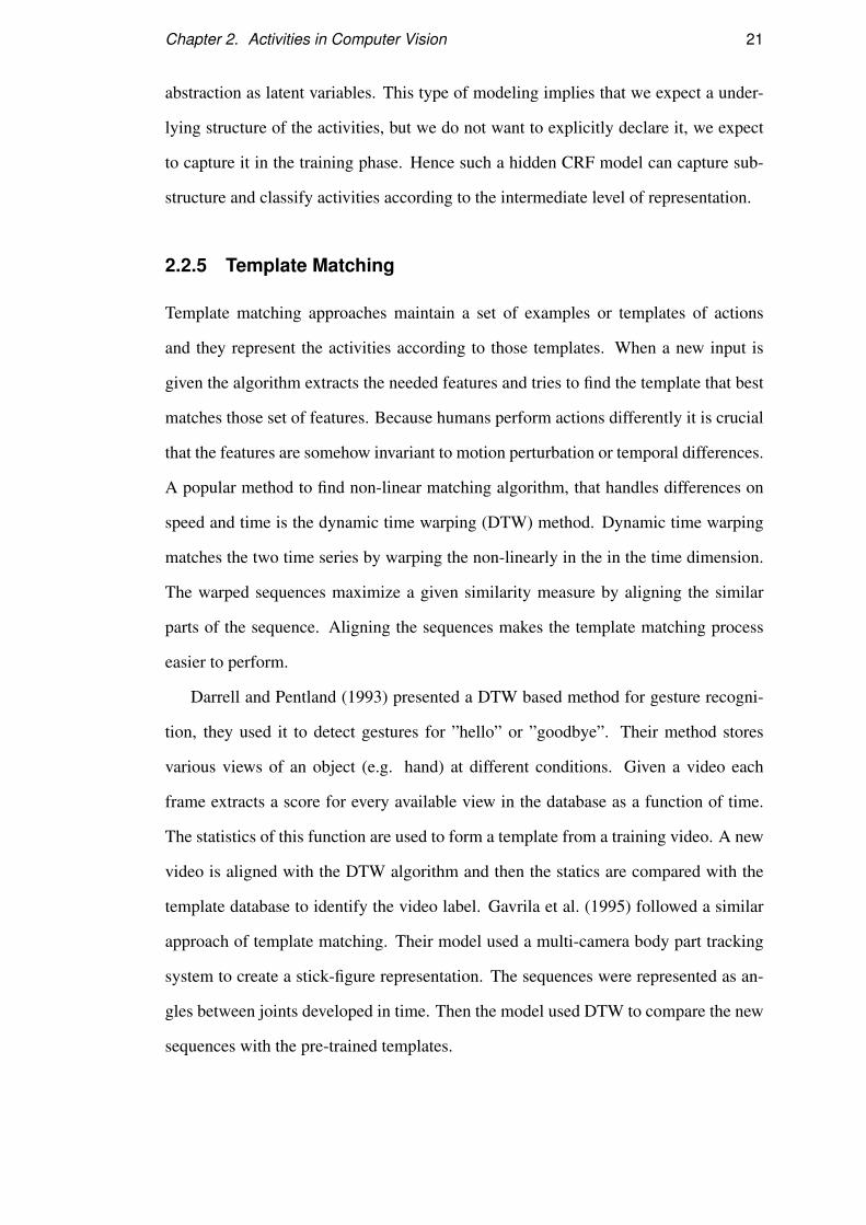
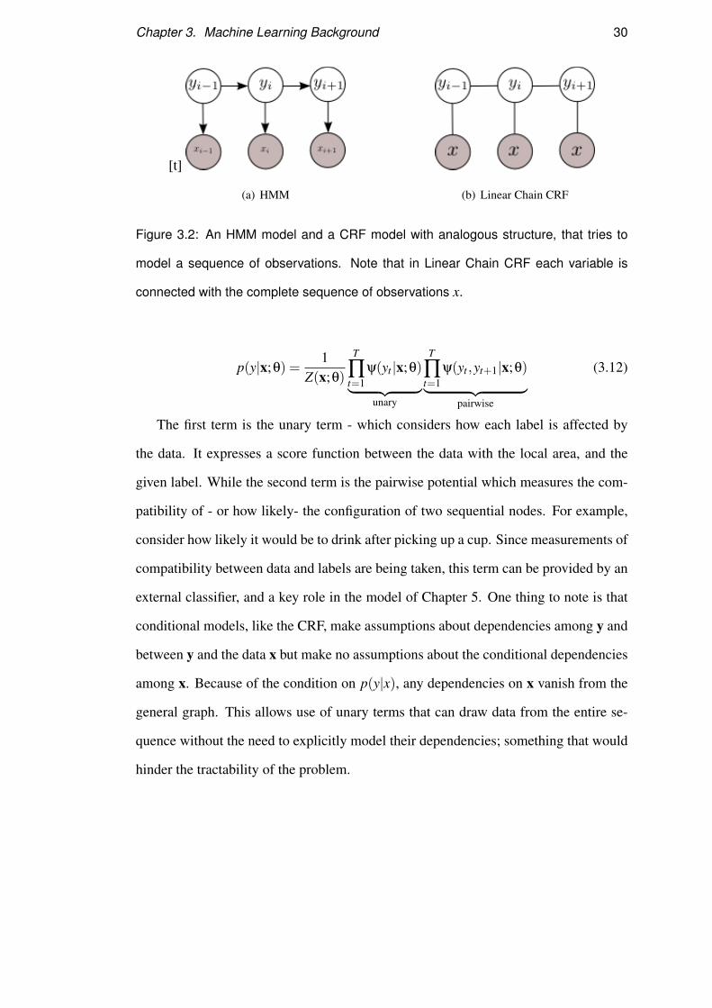
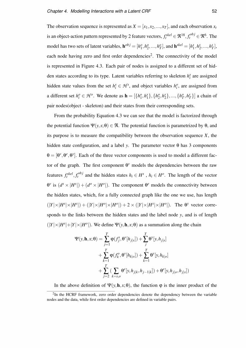
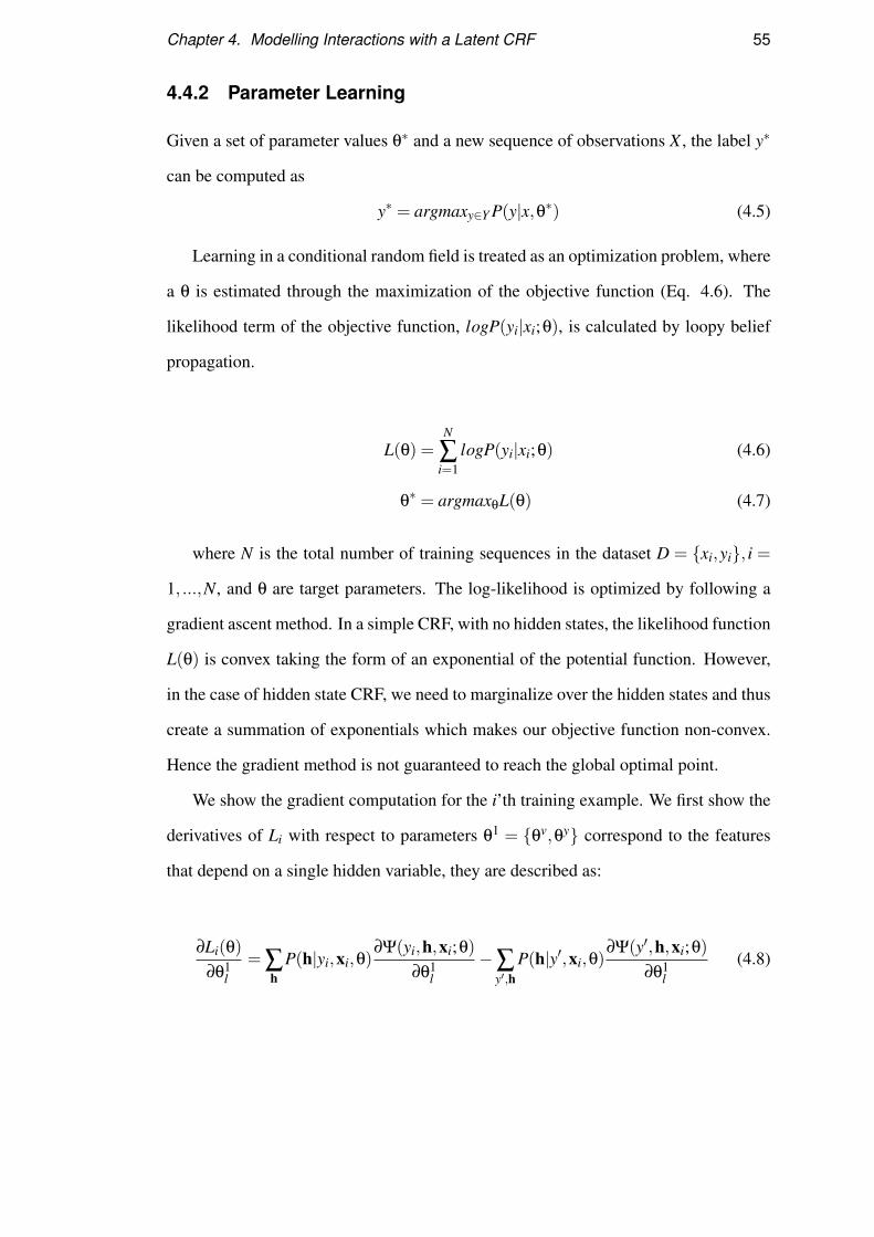
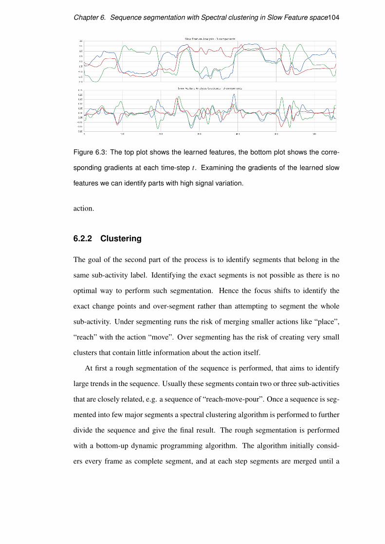
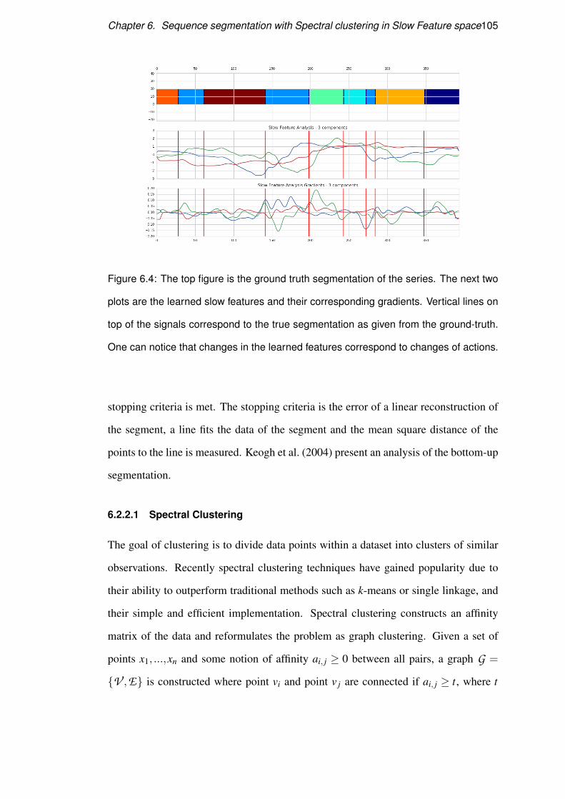
Figure 4.3: A segmented sequence is shown at the bottom of the figure. White nodes

represent latent variables of the model, blue lines represent object-related factors, while

red lines are used to represent action-related factors. This allows our model to explicitly

distinguish between action and the outcome of an action on the manipulted object. In

Conditional Random Fields, the latent variable models the dependence between each

state and the entire observation sequence in order to deal with the variable length of

observations each state is dependent on a window of observations, [xt−ω,xt+ω].


4.4.2 Parameter Learning

Given a set of parameter values θ∗ and a new sequence of observations X , the label y∗

can be computed as

y∗ = argmaxy∈Y P(y|x,θ∗) (4.5)

Learning in a conditional random field is treated as an optimization problem, where

a θ is estimated through the maximization of the objective function (Eq. 4.6). The

likelihood term of the objective function, logP(yi|xi;θ), is calculated by loopy belief

propagation.

L(θ) =N

∑i=1

logP(yi|xi;θ) (4.6)

θ∗ = argmaxθL(θ) (4.7)

where N is the total number of training sequences in the dataset D = {xi,yi}, i =

1, ...,N, and θ are target parameters. The log-likelihood is optimized by following a

gradient ascent method. In a simple CRF, with no hidden states, the likelihood function

L(θ) is convex taking the form of an exponential of the potential function. However,

in the case of hidden state CRF, we need to marginalize over the hidden states and thus

create a summation of exponentials which makes our objective function non-convex.

Hence the gradient method is not guaranteed to reach the global optimal point.

We show the gradient computation for the i’th training example. We first show the

derivatives of Li with respect to parameters θ1 = {θv,θy} correspond to the features

that depend on a single hidden variable, they are described as:

∂Li(θ)

∂θ1l

= ∑h

P(h|yi,xi,θ)∂Ψ(yi,h,xi;θ)

∂θ1l

−∑y′,h

P(h|y′,xi,θ)∂Ψ(y′,h,xi;θ)

∂θ1l

(4.8)


∂Li(θ)

∂θ1l

= ∑h

P(h|yi,xi,θ) ∑g=s,o

T

∑j=1

(ϕ( f sj ,θ

v[h j|g])+θy[yi,h j|g])

−∑y′,h

P(h,y′|,xi,θ) ∑g=s,o

T

∑j=1,y′∈Y

(ϕ( f sj ,θ

v[h j|g])+θy[yi,h j|g])

Similarly we show the derivatives of the parameters θ2 = {θe} that correspond to

pairwise features, G is the graph and the indexes j,k denote every node in the graph G.

We denote as a,b

∂Li(θ)

∂θ2l

= ∑j,k∈G,a,b

P(h j = a,hk = b|yi,xi,θ)∑θe[h j = a,hk = b]

− ∑y′∈Y, j,k∈G,a,b

P(h j = a,hk = b,y′|,xi,θ)∑θe[h j = a,hk = b]

The gradients∂Li(θ)

∂θ1l

,∂Li(θ)

∂θ2l

depend on components like P(h|yi,xi,θ) which we

calculate through the loopy belief propagation (LBP) algorithm. The fact that the graph

is loopy gives no theoretical guarantees in terms of convergence, but practically the

results are close to the real probability values. LBP is a message passing algorithm

that solves inference problems and has been extensively studied and applied in various

inference scenarios. Yedidia et al. (2003) provides a detailed description of the method

and an analysis about the success of belief propagation algorithms.

In order to avoid over-fitting the training data we add a regularization term in our

objective function. We use an L2 regularization− ||θ||2

2σ2 and the log-likelihood (Eq. 4.6)

the form:

L(θ) =N

∑i=1

logP(yi|xi;θ)− ||θ||2

2σ2 (4.9)

the them − 1σ2 controls how relaxed is the penalty over the parameters.

The optimization of the objective function is being performed by a conjugate-

gradient method, specifically we use the L-BFGS [Zhu et al. (1997)] optimizer which

is shown to perform well with a large number of parameters. Initially we randomize


our weights, and we repeat the process in order to perform gradient ascent from various

starting points in search for better local maxima.

4.4.3 Computational Complexity

Computational complexity can be defined as the asymptotic difficulty in computing the

output of the algorithm relative to the size of the input. The computational complexity

of the model is the number of operations required in order to compute the P(y|x). Due

to the fact that the graph is cyclic, we use the iterative approximation method loopy

Belief Propagation. Loopy Belief Propagation requires messages to be passed over all

edges of the graph, where each message summarizes the effect over all labellings of

the source sub-graph and the target node state. Given that our model’s graph is cyclic,

messages are passed continuously until convergence criteria is met.

Since convergence is approximate and not guaranteed, computing the upper bound

of the number of operations needed is not possible. However we can consider the effect

of the hidden states and the length of the sequence on a single pass of the algorithm.

A pass from the graph depends on the total number of nodes and their plausible states

each. For each segment in the sequence we create two nodes(hot ,h

st ) and each node has

|Ho| or |Hs| states depending on the node types. Given a sequence of length T > 1 we

have 2×T +1 nodes, as the hidden state nodes increase with the time-steps and there is

one extra node for the sequence label. Between nodes i, j each message has complexity

O(|Si|×|S j|), where |Si| denotes the number of states of node i. Considering the fact

that every message passing iteration requires to compute every node/factor, we can say

that increasing the time-steps increases linearly the number of nodes, while increasing

the number of classes or hidden states will incur into a quadratic penalty.

Overall a crucial factor is the number of message passes the algorithm will perform

to achieve convergence, and this depends on the data. An empirical evaluation of our

implementation sets the time for inference at a fraction of a second since we keep the

time-steps T to small numbers. This renders the application capable of doing real-time


inference.

4.5 Implementation

This framework focuses on robotic recognizing interactions for a robotic perception

system. Robots nowadays have access to cheap RGB-Depth sensors, such as Kinect or

Asus Xtion. The RGB-Depth sensors have gained popularity in the robotics commu-

nity because of their ability to provide good quality depth detail concerning the scene.

Depth information is valuable for understanding the scale of the scene; a very common

problem when dealing with images. Depth information has been used to produce high

quality descriptive features; being able to calculate distances between the actor and the

objects in the scene. A second advantage of using RGB-Depth cameras is access to

state of the art real-time pose classification. Here, the skeleton tracking [Shotton et al.

(2013)] algorithm, that is provided with the OpenNi SDK3, is used. The tracker pro-

vides 18 joint positions, ji = {xi,yi,zi}. At each given time step, a set of features, that

correspond to the body posture of the person and the object that is being manipulated,

are tracked.

Since the aim of this study is interaction learning, a model of the objects available

in the scene is required. A two-step process has been followed, in order to handle

objects. At step 1 an object-detection, based on 3D information is performed. The

Ransac plane fitting algorithm is run, to detect the largest co-planar clusters. Once

a set of clusters has been obtained, the largest horizontal clusters are selected and

considered as support planes. The assumption is that objects lay on horizontal flat

surfaces. Once these surfaces have been found, a region growing algorithm is used

on the remaining points and the Euclidean clusters that their projection falls within

on the flat surface’s convex hull. Once small clusters, and clusters that are not on top

of our support planes, are filtered a few object candidates remain and are moved onto

3The OpenNI framework is an open source SDK, more info: http://www.openni.org


the tracking part. Each cluster is treated as a potential object, and only objects that

fall within close distance to the user’s hands are considered for tracking. For object

pose tracking, an off-the-shelf Monte Carlo algorithm, created by Ryohei Ueda and

implemented as part of the Point Cloud Library [Rusu and Cousins (2011)] is used.

The tracker is a particle filter based tracker, with particles spread at the points of each

candidate cluster. The particle probabilities are updated according to their RGB values,

the XYZ location and some local structure, like the normal information of the local

patch. The object that is closer to the actor’s moving hand is set as the active object.

This is then set as the main tracking object and its pose is tracked. The object pose

information at each time step t is represented as a 6D vector, containing position and

rotation vectors, ot = {x,y,z,roll, pitch,yaw}.

While the combination of depth and intensity images can provide a rich set of

features, our strategy is to classify the actions with a minimal set. This decision al-

lows us to stress the importance of learning the structure of interaction between object

and body motion. The temporal relationships between the state distribution of human

actions and the object’s spatial changes affect the classification of a sequence. We

represent a sequence of length T as X = [x1,x2, ...,xT ], and each observation at time t

is composed of f skelt , f ob j

t , which are the features extracted from the skeleton tracking

and features from object tracking respectively.


y

Skeleton Tracking Information

Object informationAction information

hs

hs

hs

hs

ho

ho

ho

ho

time time

Object tracking information

Sequence

01.Segment Objects

02.Normalize Skeleton

03.Segment Sequence

04.Extract Features

05.Build CRF

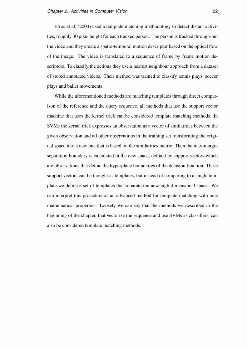
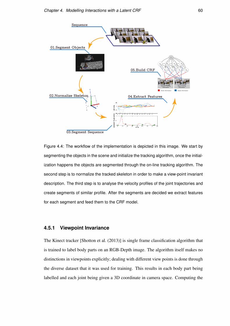
Figure 4.4: The workflow of the implementation is depicted in this image. We start by

segmenting the objects in the scene and initialize the tracking algorithm, once the initial-

ization happens the objects are segmented through the on-line tracking algorithm. The

second step is to normalize the tracked skeleton in order to make a view-point invariant

description. The third step is to analyse the velocity profiles of the joint trajectories and

create segments of similar profile. After the segments are decided we extract features

for each segment and feed them to the CRF model.

4.5.1 Viewpoint Invariance

The Kinect tracker [Shotton et al. (2013)] is single frame classification algorithm that

is trained to label body parts on an RGB-Depth image. The algorithm itself makes no

distinctions in viewpoints explicitly; dealing with different view points is done through

the diverse dataset that it was used for training. This results in each body part being

labelled and each joint being given a 3D coordinate in camera space. Computing the


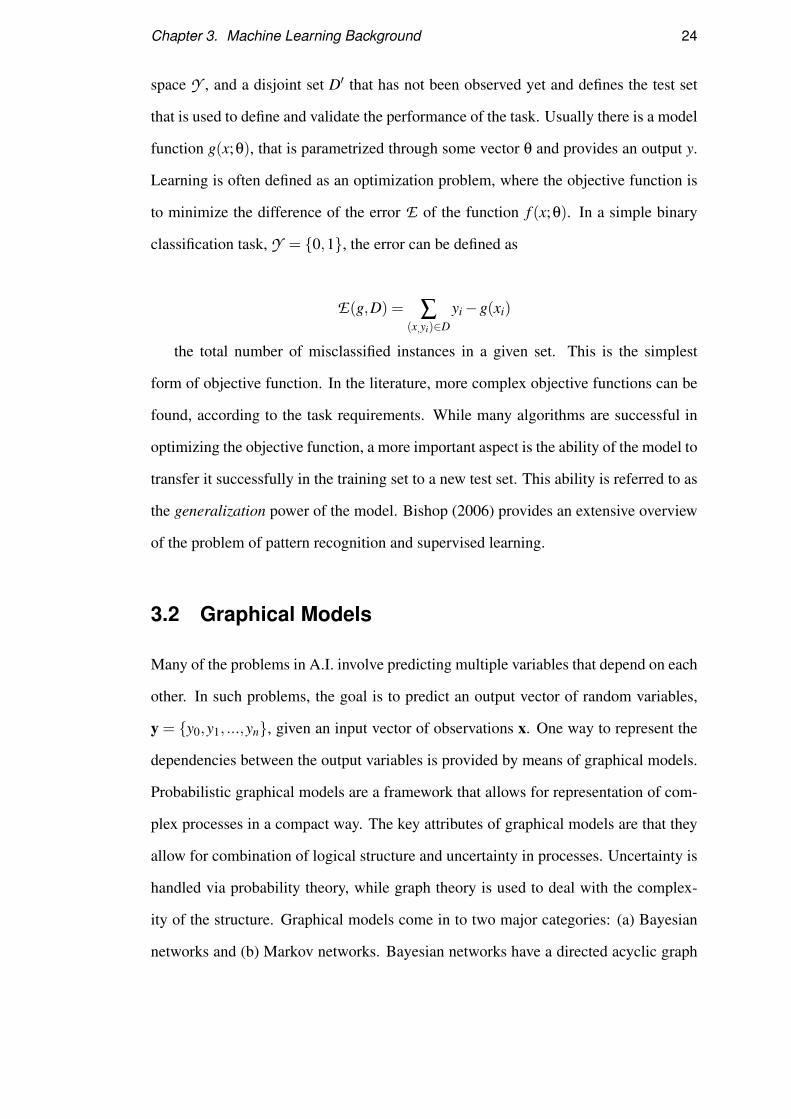
Figure 4.5: Joint positions are transformed to a new coordinate system with x-axis

aligned to the mid point of the hips and the left hip, y-axis defined by the mid point of

hips and the shoulder center, while z-axis is the normal defined by x-y plane.

features on the 3D coordinates would require the algorithm to be trained at all possible

view points in order to capture the differences in motion in absolute space. The other

option is to create view-point invariant representation; where the values of each joint

do not rely on the relative camera position.

The representation in this current study transforms the points of the skeleton into

a new coordinate system that is defined through the detected joints. The x-axis is

co-linear with the left hip joint and the right hip joint. The y-axis is defined by the

mid point of the left - right hip segment and the neck joint. The z-axis is defined by

the normal of the x-y plane. Such a coordinate system is skeleton-centric and only

measures in-between joint translations. Any change in the camera point will not affect

the coordinates of the joints.

Another aspect to be considered is the difference in actor size, since the variation of

limb length can be a potential problem. To remove limb length relationships from the


representation, the coordinates of the joints are transformed from the Cartesian system

into spherical coordinates. Each joint ji = {xi,yi,zi} is represented with its correspond-

ing spherical coordinates ji = {φi,θi,radiusi}, then the radius dimension is dropped.

A skeleton in the same pose but double the size will have the same angles but different

radio. Therefore, by omitting the radius dimension it is possible to keep the relative

joint position regardless of scale. Of course, this representation does not consider all of

the skeletal variation that exists, but it proved to sufficient for the experimental setting

presented here.

4.5.2 Managing trajectories

The model described in this work takes the form of a dynamic template; meaning that,

for each time-step, there is a template of parameters that dictate the connecting weights.

For every new time-step, the same parameters are used with the corresponding input.

This allows for training and testing using sequences of variable length. The label of the

sequence is estimated by summing the potentials of each frame belonging to a specific

class. If a frame-by-frame classification is applied, two problems have to be faced:

a) increased complexity of the model, since the number of nodes needed to be dealt

with are equal to the number of frames; b) not all frames are informative, some are

corrupted by misclassifications in the tracking system and others just repeat the same

signal without adding extra information to the previous state. Such an approach would

increase the complexity without providing any advantage to the performance. During

experiments it was noticed that long sequences tended to result in error accumulation

over time; which has an adverse effect on classification.

As we discussed in Section 4.4.3 the number of nodes increase the computational

complexity of the model. To alleviate this problem trajectories are split, using a heuris-

tic procedure that detects similar moving patterns, and merged into a single block. The

features are then computed on the entire segment. For each block of frames only two

latent variable nodes are added to the graph.


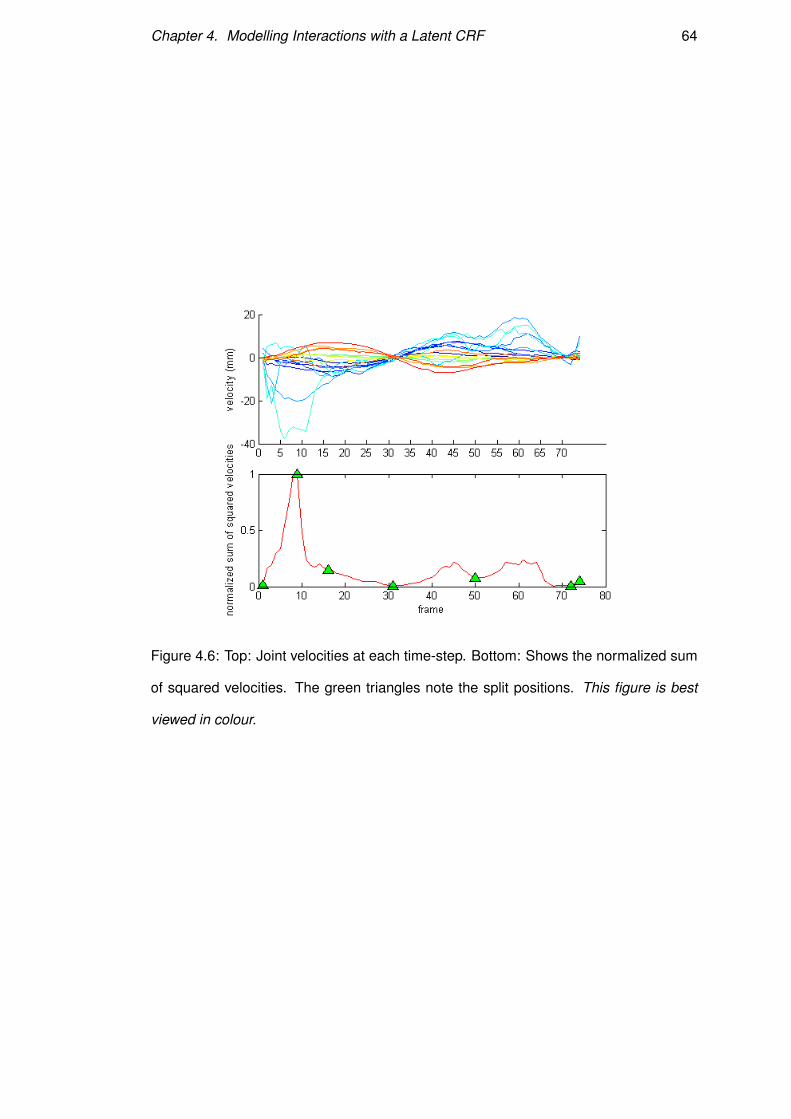
The simple assumption has been made that joint speed profiles consist of an ac-

celerating motion segment, a maximum speed segment, and a decelerating segment.

This is considered to be advantageous for creating segments that fall roughly into any

of these three categories. The heuristic sums the squared speed of all joints and then

finds the peaks and valleys in the new signal; as in Fig.4.6, subject to some constraints,

e.g. minimum thresholds for peaks and valleys and a length of 5 frames for a seg-

ment to be valid. The mean velocity of each joint is the new feature set for a segment.

Merging similar frames into a single observation variable has the advantage of creat-

ing shorter sequences and, thus, smaller latent variable chains. While this particular

trajectory segmentation method is a simple heuristic, it does manage to capture motion

changes and to segment homogeneous parts of the motion. Thus, it exploits the full

power of this current model, which relies on capturing temporal correlations between

varying states. Alternate trajectory segmentation methods could be used as drop-in

replacements without altering the overall arguments.

4.5.3 Pose features

Using RGB-Depth cameras has significant advantages: as previously mentioned it is

possible to easily deal with scale variation and view point invariance. However, in

monocular videos this still poses a problem. The efficiency of tracking in RGB-Depth

is also significantly better and, while many methods have been created to track poses

from 2D videos, they still lack performance compared to the Kinect-based tracking.

Recent success have been further built on and a low dimensional vector has been cre-

ated that accurately describes a pose. Because the focus here has mainly been on daily

activity interactions, movements are considered that are performed by the upper body,

since it is often expected that the lower body is occluded by tables, chairs and other

objects in the scene. Hence, the poses with 6 joints: L/R shoulder, L/R elbow and

L/R hand have been described. Once the joints are transformed into spherical coordi-

nates, each one is represented by a tuple jit = (ϕi

t ,θit). The resulting viewpoint invariant


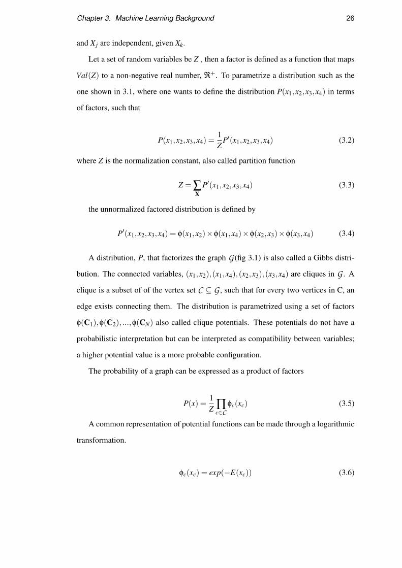
Figure 4.6: Top: Joint velocities at each time-step. Bottom: Shows the normalized sum

of squared velocities. The green triangles note the split positions. This figure is best

viewed in colour.


feature vector has length d = 6×2 = 12.

4.5.4 Hand features

While pose features capture the static joint configuration, dynamic information about

the motion performed at each time step should also be included. In order to incorporate

motion patterns into this feature set, joint velocities were computed in the spherical

coordinate system (v(i)t = {(φ(i)t −φ(i)t+1)

130sec,(θ(i)t −θ

(i)t+1)

130sec}) of the L/R hand for

each frame, then averaged across all frames of the segments.

4.5.5 Object features

Tracking the object gives a real-time update of its position in the scene. Since interest is

focused on modelling the interaction itself, the aim is to create an object agnostic inter-

action model. With respect to object agnostic implementation of the model presented

here, the aim is to create object features that only capture spatio-temporal correlations.

Two simple types of features have been implemented a) the object’s velocity relative

to the skeleton coordinate system, and b) the absolute distance between the L/R hand

joint and the head. The velocity features try to capture the motion patterns of the ob-

ject, is it moving away from the actor, is it coming closer or is it stationary? The object

to hands/head distances are used to determine the relationship of the actor with the

object. A human manipulation action is mainly described by the motion of the hands.

Hence, the definition of an object state dependant upon the hands is key to successful

interaction modelling.

4.6 Experiments

To evaluate how our system deals with actions that result in object state changes, we

have created a new dataset of people using various objects. Our dataset consists of

actions with substantial motion similarities, making it hard to naively distinguish be-


tween them without knowing the effect on the objects of the environment. Our baseline

comparison is against two different implementations of the HCRF [Wang et al. (2006)].

We report on experiments with the following models:

• B model: a simple HCRF model with a single chain of latent variables trained

on action features only.

• B-O model: a HCRF model with a single chain of latent variables and trained on

action and object features that are modelled through a single observation vari-

able.

• Full Model: Our model as explained in Section 4.4.

These models have been selected to bring out the importance of object interactions

in activity and behaviour understanding. HCRF models perform reasonably in clas-

sifying sequential data, however we show that altering the basic model to explicitly

consider the interaction boosts the overall recognition performance.

Hidden Markov Models comparison

Hidden Markov Models (HMM) are a ubiquitous tool for modelling sequential data

like time-series, speech or gestures. HMMs have at core a probability distribution over

the input space, P(X), and they model how that input evolves through time. They can

be viewed as the temporal extension of the mixture models, with the most common

mixture model being the Gaussian Mixture Model (GMM). In order to fit a model such

as the HMM, a generative model of the input needs to created. This is feasible for

simple trajectories signals and generally cases where a GMM is sufficient to model the

input. In our application, the use of GMMs to model the input was unsuccessful. The

GMM model was unable to handle the mix of features (skeleton - object) due to two

reasons a) the input has high complexity and b) the Gaussian distributions are not very

effective at handling mixed signals from different sources.


As such creating an HMM baseline is not a trivial task and all freely available

method, that we know of, do not deal with a high dimensional mixed signal input

space like the one presented here. For this reason, we are unable to compare against

alternatives such as HMM variants.

4.6.1 Dataset

Our overall goal is to model human activity that involves object manipulation. In or-

der to do that we had to create a dataset that is suited to our needs. We recorded 918

sequences from 12 different people. We selected 5 different actions that have similar

appearance and statistics if seen out of context (i.e., without the object information).

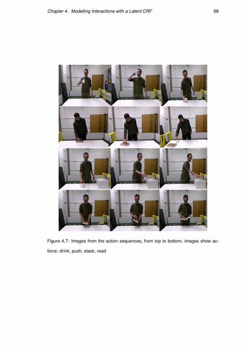
The action set we recorded is based on the categories A={drink, push, pickup, stack

objects, read}, as in Figure 4.7. The actions were not thoroughly scripted, as each per-

son was given simple oral instructions about each action and was not given an explicit

instruction regarding preferred or typical trajectories to follow. This is how we expect

regular people to behave in a natural setting. On each repetition, users freely choose

how to perform the action, which hand to use, what the starting position of the object

should be, speed of execution, etc. Most subjects did not repeat the same motion, so

the majority of the recorded sequences have a wide range of motion variations. The

actions were recorded with a Kinect camera at a rate of 30Hz, and the time length of

each sequence were from 50 frames to 250 frames depending on the action class.

All the sequences were recorded in our lab in a fairly generic setting (Figure 4.7).

Users stood in front of a table on which the objects of interest were placed, at distance

of 2∼ 2.5 meters away from the Kinect camera. The difficulties in recognizing motions

in the dataset are primarily related to motion similarity and occlusions. Occlusions

seriously affect the performance of the skeleton tracking algorithm, which is really

designed to work best in an occlusion free environment. In order to strengthen our

hypothesis and test our model, we chose highly similar (i.e., aliased) motions to be

part of the dataset. For example, reaching to pick an object produces a similar body


Figure 4.7: Images from the action sequences, from top to bottom, images show ac-

tions: drink, push, stack, read


posture sequence as pushing an object on the table. Similarity in motion can be found

in picking and stacking objects, the reaching part of the motion and the withdrawing

of the person are very similar.

4.6.2 Models and implementation details

The full model is expected to learn the spatio-temporal action - object state transitions

and be able to outperform its simple counterpart where no information fusion is per-

formed. To optimize performance, we search for parameter configurations, keeping

the one with the best score on the cross validation set. The free model parameters

that need to be determined are the number of hidden states in the sets, H s,H o, the

observation window length, the standard deviation (σ) of the L2 regularization factor

and the starting values of θ for the gradient search. For hidden states, we experimented

with a number of different state sets, varying from 3 to 8 for the object latent variables

and from 4 to 12 for the latent variables that depend on skeleton nodes. Based on the

average sequence length we experimented with window sizes of ω = 0,1,2. After de-

termining the best parameters for the number of hidden states, we keep them constant

and then tune the L2 standard deviation parameter. The σ of the regularization term

was set to σ = 1k where k=-3,...,3.

To investigate how information fusion affects the classification performance we

implemented two alternative hidden state CRF models as comparison methods. Both

models contain a single layer of latent variables, meaning we use one latent variable

per time-step to form single a chain for each sequence. The first model is trained only

with body motion information (noted as B model), the object features are neglected,

while in the second HCRF (noted as B-O model) the object features and body motion

are modelled through a single observation variable XT . Our aim is to show that we

can gain accuracy compared to a model that does not consider object context, but

also showing that modelling the action and the object information through different

observation and latent variables can further improve the performance of the model.


Both models have the same free parameters, number of hidden states, regularization

factor and the length of the observation window. Parameters are tuned via the same

grid search technique as mentioned before.

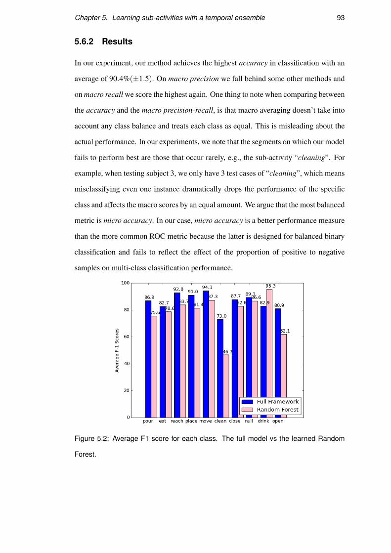
4.6.3 Results

To evaluate the performance of the different models we report the F1 score which is

a measure of accuracy that considers both the precision and recall. The F1 score is

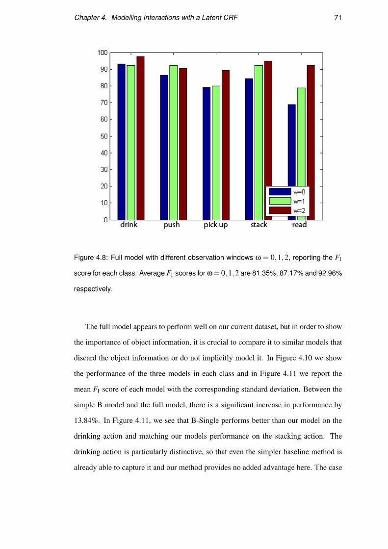
defined as F1 = 2× precision×recallprecision+recall . In Figure 4.8, we summarize the F1 score of our

approach for each class with 3 different observation window lengths( ω = 0,1,2). For

each window parameter we report the best configuration of hidden states and regular-

ization term, which differs for each model. The bar graph shows performance is cor-

related to the temporal relationships between the hidden states and the observations.

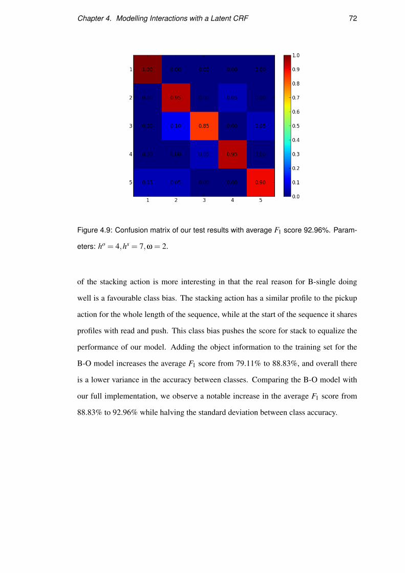
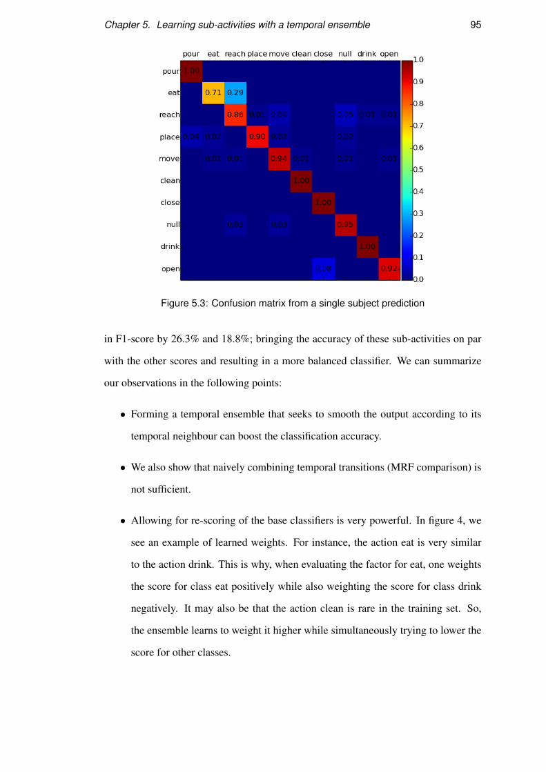
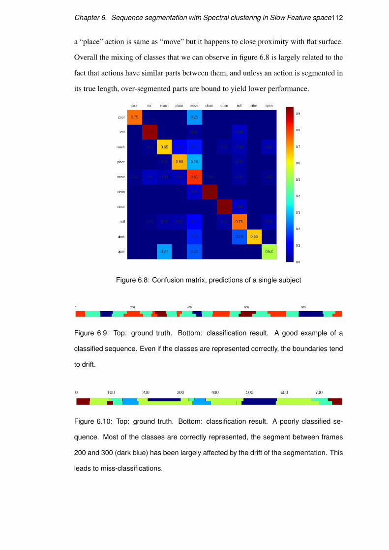
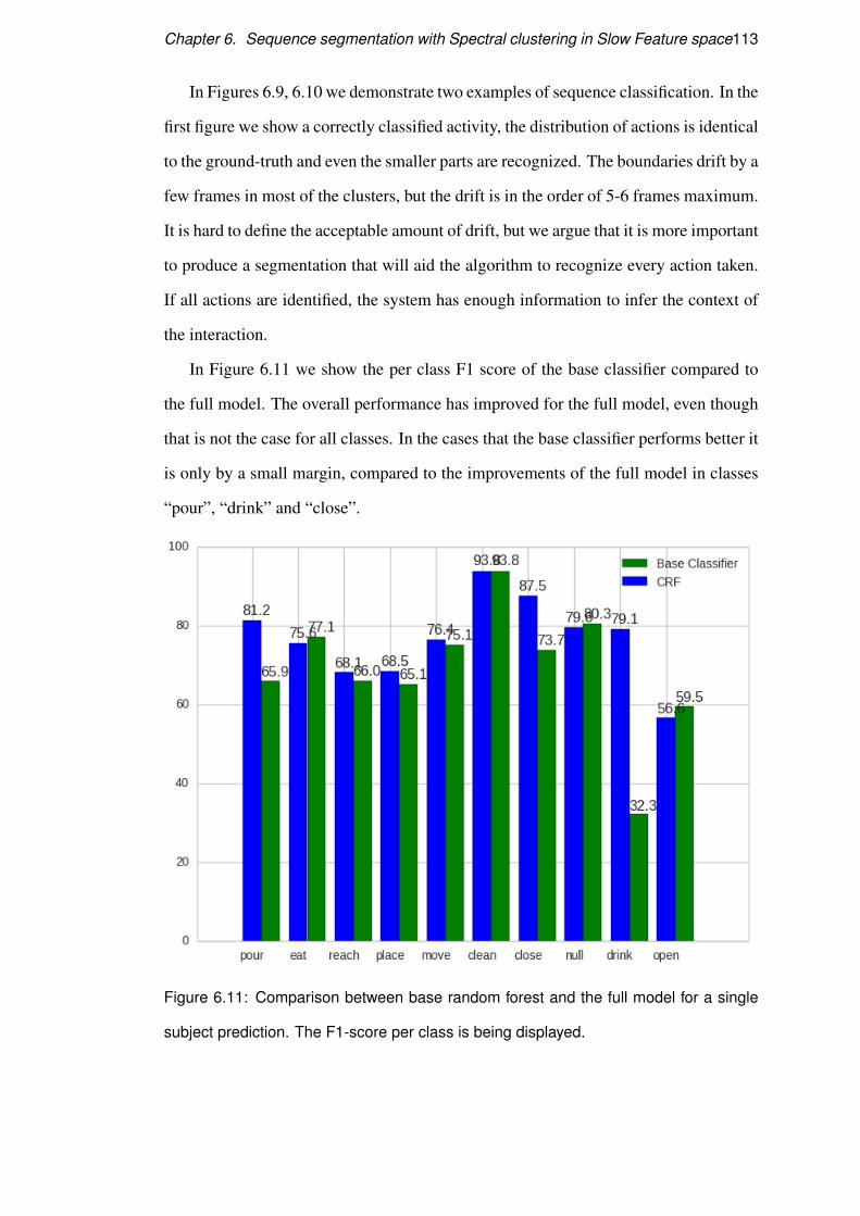
Figure 4.9 shows the confusion matrix of our best results on this dataset with average

F1 score for all the classes of 92.96%. From the confusion matrix, we can see that the

lowest classification rate corresponds to the pick class. Picking is a sub-event occur-

ring in every action of the dataset, so in noisy sequences or sequences which have been

mistreated during the trajectory splitting, this can cause misclassification. Intuitively

when we consider spatio-temporal process we think of them in terms of past state,

present state, and future state and the change of state, encoding the past-present-future

information in each hidden state and not only through latent state transitions creates a

more powerful representation of the action.


Figure 4.8: Full model with different observation windows ω = 0,1,2, reporting the F1

score for each class. Average F1 scores for ω= 0,1,2 are 81.35%, 87.17% and 92.96%

respectively.

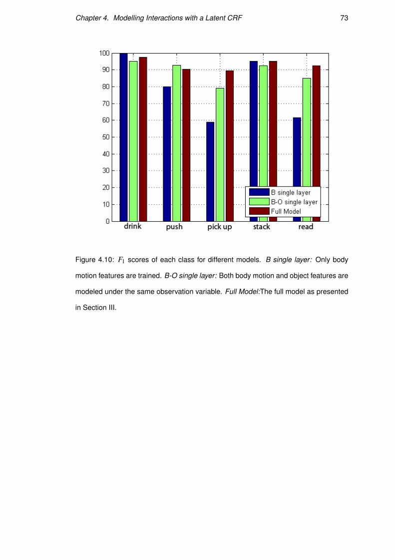
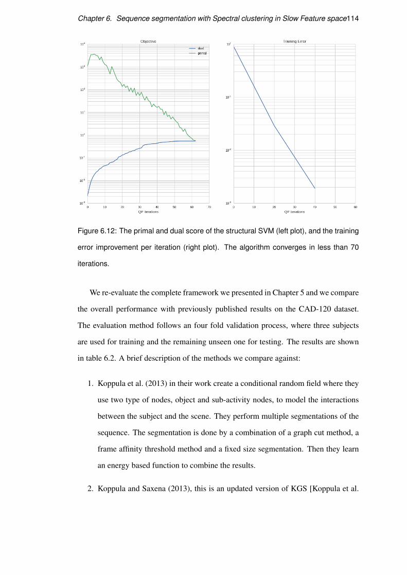
The full model appears to perform well on our current dataset, but in order to show

the importance of object information, it is crucial to compare it to similar models that

discard the object information or do not implicitly model it. In Figure 4.10 we show

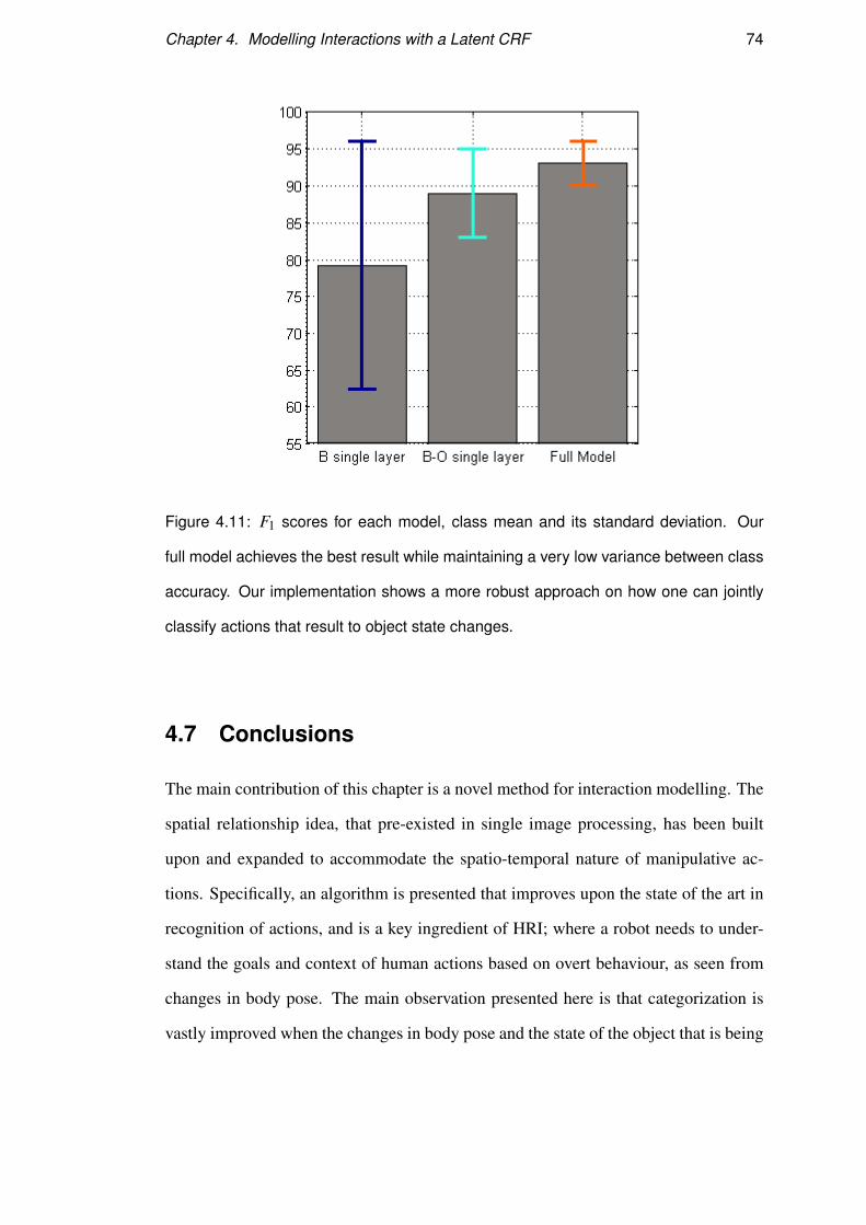
the performance of the three models in each class and in Figure 4.11 we report the

mean F1 score of each model with the corresponding standard deviation. Between the

simple B model and the full model, there is a significant increase in performance by

13.84%. In Figure 4.11, we see that B-Single performs better than our model on the

drinking action and matching our models performance on the stacking action. The

drinking action is particularly distinctive, so that even the simpler baseline method is

already able to capture it and our method provides no added advantage here. The case


Figure 4.9: Confusion matrix of our test results with average F1 score 92.96%. Param-

eters: ho = 4,hs = 7,ω = 2.

of the stacking action is more interesting in that the real reason for B-single doing

well is a favourable class bias. The stacking action has a similar profile to the pickup

action for the whole length of the sequence, while at the start of the sequence it shares

profiles with read and push. This class bias pushes the score for stack to equalize the

performance of our model. Adding the object information to the training set for the

B-O model increases the average F1 score from 79.11% to 88.83%, and overall there

is a lower variance in the accuracy between classes. Comparing the B-O model with

our full implementation, we observe a notable increase in the average F1 score from

88.83% to 92.96% while halving the standard deviation between class accuracy.


Figure 4.10: F1 scores of each class for different models. B single layer: Only body

motion features are trained. B-O single layer: Both body motion and object features are

modeled under the same observation variable. Full Model:The full model as presented

in Section III.


Figure 4.11: F1 scores for each model, class mean and its standard deviation. Our

full model achieves the best result while maintaining a very low variance between class

accuracy. Our implementation shows a more robust approach on how one can jointly

classify actions that result to object state changes.

4.7 Conclusions

The main contribution of this chapter is a novel method for interaction modelling. The

spatial relationship idea, that pre-existed in single image processing, has been built

upon and expanded to accommodate the spatio-temporal nature of manipulative ac-

tions. Specifically, an algorithm is presented that improves upon the state of the art in

recognition of actions, and is a key ingredient of HRI; where a robot needs to under-

stand the goals and context of human actions based on overt behaviour, as seen from

changes in body pose. The main observation presented here is that categorization is

vastly improved when the changes in body pose and the state of the object that is being


acted upon are modelled jointly, i.e., the effects on the environment of the person’s

movement. This has been done in the setting of a state-of-the-art statistical learning

algorithm for discriminative classification; the HCRF. Experiments have demonstrated

that thinking of actions in terms of motion and outcome yields significant overall im-

provement. This work is viewed as a first step towards understanding how to devise

the ability to decode human activity at finer levels, which lead to improved human -

robot interactions and learning, by demonstration capabilities.

Chapter 5

Learning sub-activities with a

temporal ensemble

5.1 Introduction

Chapter 4 presents a model for learning manipulation actions from videos. These

actions were short and self contained within the video. In this chapter we construct a

framework that deals with temporally extended activities. The assumption is that these

temporally extended activities are chains of actions, where each action is self-defined,

examples of such actions are “move”, “pour”, “drink” etc. In such cases, one can learn

sub-parts of the problem by training classifiers to recognize the actions while a high

level module will be responsible for the temporal smoothing of the decisions. The

proposed framework gathers the decision of base classifiers and merges them into a

temporal ensemble.

We aim at learning long sequences of interactions, and specifically we target the

estimation of labels for each sub-segment of the activity by aggregating temporal in-

formation from the rest of the sequence. We present an ensemble method that tackles

the challenging problem of classifying activities in a domestic environment, activities

like preparing meal, cleaning tables, arranging objects etc. The large intra class vari-

76

Chapter 5. Learning sub-activities with a temporal ensemble 77

ability, number of objects and scene set-up variations make the task very challenging.

Our proposed framework forms a set of decisions on each sub-segment by assigning

a score for each possible outcome; then these decisions are re-weighted according to

the temporal structure of the data in order to decide on the optimal estimated sequence

of sub-activities. Essentially, the model works on a local level to create a first set of

classifications; then information is aggregated through-out the sequence to smooth the

decisions according to their temporal correlations.

In the previous chapter, we introduced a model creates an intermediate latent layer

to represent an action as a hierarchical model. Carrying out this idea to this chapter

we would have to create a similar structure, as the one in Chapter 4, for every action

sub-segment in our long activity chain. While this configuration is possible, an end-

to-end training is difficult to achieve with the amount of latent variables that we need

to introduce to the graph. This part of the thesis, aims at longer and more complex

sequences, hence we picked an evaluation dataset (CAD-120) that contains multiple

objects being used simultaneously. For every object that we add in our HCRF we

increase the complexity of the graph through adding more edges and more latent states

that need to be computed. A non-convex object of such complexity needs careful

initialization a lot more data than what we have available.

Given the increased complexity of a combined model, we decided to separate the

two models by addressing only the top-level problem that considers the decisions of

arbitrary action classifiers in order to label the sub-segments of an activity. Our HCRF

can fit the role of the base classifier in the model that is presented in this chapter.

The reason it was not preferred as a base classifier is the difficulty of training it with

the number of actions that were available to us. We set the integration of the two

models as one of the main future goals of this thesis. An interesting aspect of such

expansion would be the comparison of end-to-end training with the current model of

independently training the base classifiers and top level module.


5.1.1 Contributions

In this chapter we present a practical framework for sub-activity learning. We struc-

ture an ensemble of classifiers that combines their decisions with respect to the local

temporal relationships. Our core insight is that a decision of a classifier provides the

class with the maximum score but also gives information about the remaining classes.

The proposed method is able to extract knowledge from the complete distribution of

the classes and significantly improve the performance compared to our baseline tem-

poral ensemble. The experimental results also suggest that this method outperforms

previously published methods on the same dataset.


5.2 Related work

There is large body of work on computer vision that robotic perception can benefit

from. A notable recent contribution is the use of RGB-Depth cameras combined with

a robust classifier for real-time human pose estimation from depth images [Shotton

et al. (2013)]. RGB-Depth cameras have also boosted object recognition1 for robots

by giving access to cheap, fast and reliable depth perception in scenes. In the field of

human activity recognition there is a large variety of work that expands from still 2D

images to video and RGB-Depth videos. A relatively recent review in activity recog-

nition is by Aggarwal and Ryoo (2011). Gupta et al. (2009) suggest a Bayesian model

combining actions, objects and scene context to improve the classification of each of

the elements. Similar ideas of jointly modelling objects and actions in 2D images are

explored by Yao et al. (2011), who combine human poses with object attributes to

improve results in 2D image classification.

The first attempt to use CRFs for actions classification is in Sminchisescu et al.

(2006) who show the merits of using CRF over an HMM to classify actions. Wang et al.

(2006) present a latent variable CRF for action classification. Their model was used to

classify arm and head gestures. Closer to our problem of annotating sub-parts of larger

sequence is Tang et al. (2012), who tackle temporal structure understanding and try to

detect events in segments. However, this only goes as far as recognizing a single event,

whereas we are interested in labeling a sequence of (sub)events simultaneously. Sung

et al. (2012) train a 2-layered maximum entropy Markov model to classify activities

but this is based only on human pose features. As this model does not incorporate scene

information, their overall performance with unseen persons is significantly lower.

Koppula et al. (2013) built a CRF where they represent both sub-activities and

object affordances. At each segment, nodes are fully connected and transitions happen

1The Washington Univ. RGB-D Object dataset is popular in the robotics community asit provides a test bed for object recognition. In all published results (see: http://rgbd-dataset.cs.washington.edu/results.html ), combining RGB with Depth information improves the per-formance of each method.


over time between nodes of the same type. A cyclical graph like the one in [Koppula

et al. (2013)] needs an approximate inference solution which is not as accurate as

exact approximations. Hu et al. (2014) express a latent CRF model as an augmented

linear chain CRF to take advantage of exact inference properties and achieve very good

classification scores.

Our temporal ensemble method relies on the strength of its base classifiers, based

on Random Forests - a strong non-parametric model exploiting nonlinear relationships

better than log-linear factors typically used in CRFs. The ability of random forests to

robustly model nonlinearities in data, combined with our proposed structured output

scheme represents an effective framework for sub-activity labelling. In the results

section we show that the proposed method outperforms the current state of the art.

5.3 Model

5.3.1 Overview

Consider a high-level activity sequence X = x1, ...,xT , that is composed of segments

xi, where each segment is a sub-activity and has a “meaning” of its own. Our objective

is to recognize every sub-segment xi in the sequence and give it a label yi. An example

of such high level activity label is drinking, which can be separated into steps: reach

for mug, pick mug, move mug to mouth and finally drink. To label each separate sub-

activity in a video sequence we formulate a structured prediction problem, in which

the output domain is the set of all possible sequences of sub-activities. Our work

is inspired by ensemble methods [Breiman (2001);Dzeroski and Zenko (2004)] and

especially [Wolpert (1992)]. The idea is to train k classifiers, and each classifier will

give an output G j that will be used as meta-features in a combinatorial model. Then

the meta-classifier has the form:

h(x) = f (G1(x),G2(x), ...,Gk(x))


Many ensemble methods like bagging, boosting, Bayesian averaging are designed

for single label prediction. Our structured prediction need is for a meta-classifier that

combines predictions in such a way that it enforces temporal consistency on the se-

quence. So, we formulate our ensemble as a Random Field, where each node repre-

sents a sub-activity and the link between nodes models the temporal transitions be-

tween sub-activities.

Given a sequence, each sub-segment is classified with an extremely randomized

tree classifier Geurts et al. (2006). The pairwise meta-features are learned from two

logistic regressions that predict the distribution of segment xt and xt+1 separately. In

our experiments, we also explored a greedy strategy of picking MAP solutions for each

node/transition and optimizing the graph as an MRF. While this does achieve reason-

able results, our proposed method significantly outperforms such a greedy approach.

We discovered that by allowing the ensemble to learn how to weight the probability

distribution given by the base classifier, we can achieve a superior performance. Our

aim is for each decision to take into account the complete distribution and its temporal

connections. Forming the ensemble as a Conditional Random Field, we take advan-

tage of its ability to combine the base classifier’s posterior distribution with different

weights for each sub-activity label. Such a method allows the model to consider the

negative decisions of a classifier combined with the pairwise meta-features to make

more informed decisions, since it will aggregate information from other nearby nodes.

To amplify the CRF’s ability to re-score each output we compress the base posteriors

through a sigmoid function.

5.3.2 Model Structure

At the top level of our model sits a Linear Chain CRF, like the one described in sec-

tion 3.3.1, that performs the information aggregation of our base classifiers. Figure

5.1 shows how the information of the base classifiers is fed into the CRF. Given a se-

quence of features X =< x1, ...,xT > will try to infer a set of labels Y =< y1, ..,yT > by


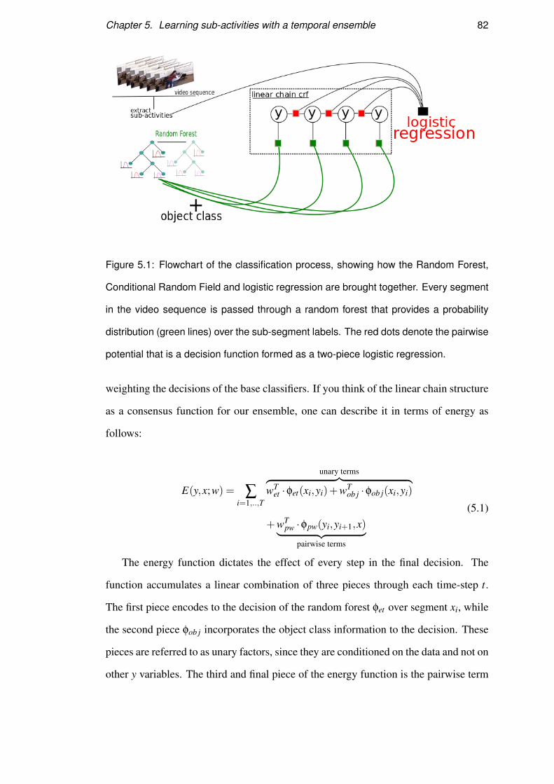
Figure 5.1: Flowchart of the classification process, showing how the Random Forest,

Conditional Random Field and logistic regression are brought together. Every segment

in the video sequence is passed through a random forest that provides a probability

distribution (green lines) over the sub-segment labels. The red dots denote the pairwise

potential that is a decision function formed as a two-piece logistic regression.

weighting the decisions of the base classifiers. If you think of the linear chain structure

as a consensus function for our ensemble, one can describe it in terms of energy as

follows:

E(y,x;w) = ∑i=1,..,T

unary terms︷︸︸︷wT

et ·φet(xi,yi)+wTob j ·φob j(xi,yi)

+wTpw ·φpw(yi,yi+1,x)︸︷︷︸

pairwise terms

(5.1)

The energy function dictates the effect of every step in the final decision. The

function accumulates a linear combination of three pieces through each time-step t.

The first piece encodes to the decision of the random forest φet over segment xi, while

the second piece φob j incorporates the object class information to the decision. These

pieces are referred to as unary factors, since they are conditioned on the data and not on

other y variables. The third and final piece of the energy function is the pairwise term


that provides a decision(φpw) for each transition, yi to yi+1. This decision is formed as

two-piece logistic regression.

Each decision function is trained separately and the weight assigned to each deci-

sion is learned afterwards. The following section presents the way we structure and

create each decision problem. Section 5.4 describes the learning process of the poten-

tial functions (φet ,φpw) and their assigned weights in the consensus energy function

(Eq. 5.1).

5.3.3 Potential Functions

5.3.3.1 Unary Potentials

The first unary potential is defined as

φet(xi,yi) =1

1+ e−1.5p(yi|xi)

where p(yi|xi) is the posterior probability distribution of node yi computed by the ran-

dom forest classifier. The classifier models the probability of a segment xi being as-

signed to a sub-activity label yi. The vector φet is a concatenation of the probability

of every class c passed through a sigmoid function. With a different weight for each

class, we perform a re-scoring operation that is based on the sequence context. To

give an intuitive explanation, when factoring the output of the classifier we do not only

consider the most probable class, but also take into account how well the other classes

scored. This makes smoothing more efficient and achieves better temporal consistency

of the sequence.

The second unary potential, φob j(xi,yi) , is a binary vector that encodes the object

in use. Its purpose is to strengthen the co-occurrence of an object and action, e.g. a

segment that has as a primary object of use the cup, strengthening the score of classes

like drinking and moving while assigning a lower score to cleaning.


5.3.3.2 Pairwise Potentials

For our pairwise potentials we follow a similar approach, where the φpw function pro-

vides the concatenated output of two multi-class logistic regression classifiers. The first

classifier models the distribution p(yi = a|xi,xi+1) while the second classifier models

p(yi+1 = a|xi,xi+1). Given A , the set of sub-activities, the transition space is defined

by A ×A and this creates a dim(A)2 feature vector φ. We choose to work with fewer

features, (2× dim(A)), by solving a relaxed version of the problem, where we sepa-

rately model the probability of yi and yi+1. From a complexity perspective, the sim-

plified version of the state transition classification needs to compute less parameters,

2× dim(A)× dim([xi,xi+1]) versus dim(A)2× dim([xi,xi+1]). The parameters in the

relaxed problem are linear to the number of classes, while they are cubic on the full

version of the problem.

Apart from the computational benefits of solving for two separate probability dis-

tributions of smaller prediction space, there are some implementation difficulties as

well. We use a dataset based on four subjects, and we train and evaluate in an 4-fold

scheme. For instance, some transitions appearing in the data for subject 1 do not appear

in that for subject 3. The lack of a such complete set of transitions in all training splits

forbid us to form an elaborate empirical evaluation of how much the simplification of

the problem improves the accuracy of the model. Hence the relaxation of our classifi-

cation is the only way we choose to model the state transitions. In such conditions we

implement two separate distributions and create a joint feature vector. As in the first

unary potential we also compress our feature vector through the sigmoid function.

5.4 Learning

Learning the model consists of two steps: A) we learn the unary and pairwise features

through the base classifiers, B) we train our linear-chain CRF on learned meta-features.


5.4.1 Feature Learning

To learn the classifier that provides the φet feature vector we use an ensemble of ex-

tremely randomized trees (ET)[Geurts et al. (2006)], which are shown to be very ef-

ficient and robust in classification tasks. The ET classifier has various merits, the

most important if which is that decision trees do not make assumptions about the input

space. Decision trees operate equally well when features come from different sources,

or involve different input space or different scale without having to worry about pre-

processing or needing smart feature engineering. As we describe in Section 5.5.2, we

make use of a mix of features. In such cases, it is difficult to define distance functions

between vectors since we mix various input spaces. Given this inability to define a

meaningful distance function, alternate classifiers such as SVMs are also ineffective.

In order to train the tree ensemble, we sample segments from our training set and

try to learn the sub-activity label of each segment given the local information. In ET

we use a set of decision trees; each tree is trained on a subset of the data, and the

training process strongly randomizes both the feature subset and the cut-point choices.

Growing the trees follows a greedy strategy where at each node we pick the random

cut that maximizes the information gain. At each leaf we store a distribution of all

the classes that reached that end node during training, we denote ϕki (yi,xi;θ) as the

histogram of the distribution. The outcome of the K trees is computed by averaging

these distributions:

φet(yi,xi) =1K

K

∑k=1

ϕki (yi,xi;θ)

The parameters of the tree that need to be specified are the number of trees K, the

minimum number of samples to perform a split and number of features d used in

each node to perform a split. The parameters were chosen empirically through a cross

validation process. In the implementation (Section 5.5) we give more details about the

training process, parameter choice and the features that are extracted.

For the pairwise case, the features are produced through two logistic regressions.

Logistic regression is a probabilistic linear classifier that models the conditional proba-


bility of a class as P(y = i|x) = exp(−wix)∑ j exp(−w jx)

, where y is the class label, x is the data and

w the model parameters. The training algorithm [Fan et al. (2008)] uses a one vs all

approach for each of the classes, and the model is regularized with a L2 penalty term.

The input of the classifier are two consecutive segments, xi,xi+1 but each classifier

evaluates a different target label, yi and yi+1. We sample the sequences of the training

set for pairs of adjacent segments to create training examples. In the implementation

section, we show the type of features we extract from each pair of segments.

5.4.2 CRF Training & Inference

A popular approach to training structured linear classifiers is based on max-margin

learning. The basic idea of max-margin learning is to find weights such that the energy

of the training sequence y(i) is better than all the alternatives y∀y 6= y(i) by a margin γ.

Using the energy defined in equation 1, we can express the max-margin condition as:

E(y,x(i))−E(y(i),x(i))≥ γ,∀y 6= y(i). Given a training set of N activity sequences and

given the ground truth sequence yn we solve the following optimization problem:

minW,ξ≥0

θT

θ+C∑n

ξn(y)

s.t. : ξn(y) = maxy(H(y;yn)+E(yn|θ)−E(y|θ))

(5.2)

C balances the cost between the regularization term and the sum of violated terms

∑ξ. The H(y;yn) function is the Hamming loss for the given sequence n. The Ham-

ming loss is the equivalent of Hinge loss for structure output spaces. Hamming loss

is computing the Hamming distance between the predicted sequence and the ground

truth. Such distance metric promotes larger cost for bigger differences in the sequences

yn,y. Essentially it measures the minimum number of errors that could have trans-

formed one sequence into the other. To solve Equation 5.2 we use a structured SVM

method as described by Tsochantaridis et al. (2005).

In this chapter we use a max-margin learning approach in contrast with the model


presented Chapter 4, where we implemented a MLE solution to our model. The major

difference is the lack of latent variables in the model presented in this chapter. Apply-

ing max-margin learning in chain CRF is more straight forward compared to the more

complicated latent structure that we present in Chapter 4.

Inference is performed as a discrete minimization problem on the energy function

E(y;θ) where we try to find the optimal sequence of y that minimizes the energy given

a set of weights θ.

5.5 Implementation

5.5.1 Data

Our data consists of a sequence of RGB-Depth images from a Kinect type sensor. This

gives us access to both RGB and depth information about the scene simultaneously.

The sensor is capable of producing images at a rate of 30Hz. The sensor is accom-

panied by an SDK that has human tracking capabilities. The OpenNi tracker provides

information about the joint locations of the human skeleton, however these joint values

are not very accurate especially in cluttered scenes and situations where body parts are

occluded by objects. We experiment on a dataset that involves people manipulating

multiple objects. At any given point there 1-5 objects in the scene and a human subject

is interacting with them in various ways.

5.5.2 Features

Features are dependent on the input channel to a great extent. We make use of the 3D

information provided by the RGB-Depth sensor to create a rich set of features. Given

that our aim is to capture the interactions of each temporal segment we extract features

that not only capture the variety of human motion, but we also enable the algorithm

to capture human-object and object-object relationships. We create a separate set of


features to train the unary extremely randomized trees (ET) classifier and the pairwise

logistic regression classifiers. For each segment of n-frames we create a number of

equal splits on which we compute our features. Some segment features are defined

on their own while others describe the difference between consecutive splits. In order

to create a view invariant feature set we define a skeleton oriented coordinate system

while we transform the Cartesian coordinates into spherical coordinates. All of our fea-

tures are defined on the upper part of the skeleton since the legs are usually occluded.

Table 5.1 describes the features for the unary ET classifier.

For our implementation, we limit our scene description to use the three most rele-

vant objects of each segment. We pick the first object by identifying which object has

the largest variation in its x,y,z location. If all objects have variance lower than a small

threshold td we assume they are stationary and we pick the object that is closer to the

hand that moved the most within the segment. The other two objects are selected by

computing their distance to the main object and picking the closest two. We also detect

the largest supporting plane in the scene by iteratively fitting planes to the scene point

cloud and picking the one that fits the most points. The distance to plane turns out to

be particularly useful in classification.

The pairwise features describe the transitions between each segment and they are

shared between both classifiers. The features are created by concatenation of the unary

features of each segment and some additional features as described in table 5.2.

5.5.3 Training Details

The local classifiers are the basic building block of the framework, and their perfor-

mance is tied with the total performance of the model. Testing and evaluating such

a framework on a dataset such as CAD-120 [Koppula et al. (2013)], where only 4

subjects are available, can be challenging. The challenge is to avoid over-fitting the

base classifiers to the training set. Since we use the output of the base classifiers as

meta-features in the CRF, over-fitting causes a peculiar problem. Once we move to


Table 5.1: Unary Classifier Features

Skeleton Features # Features

Mean sub-segment angles be-

tween all possible 3 arm joint

configurations.

8 × Num. splits

Difference of mean angles be-

tween consecutive sub-segments

8 × (Num. splits-1)

Spherical coordinates of the up-

per body joints

18 × Num. splits

Hand and elbow velocities 12 × Num. splits

Distance covered by each hand 2

Min-Max vertical position of

each hand

4

Object-Object Features # Features

Relative position between ob-

jects.

6 × Num. splits

Vertical distance between object

and largest support plane in the

scene

3 × Num. splits

Num. of pixels of the bounding

box

3

Min-Max vertical position of

each object

12 × Num. splits

Distance travelled by each object 6

Object-Skeleton Features # Features

Distance to head and left/right

hand

9 × Num. splits

Difference of object distances

between sub-segments

9 × (Num. splits-1)


Table 5.2: Pairwise Classifier Features

Pairwise features # Features

ET features of segment xt−1 -

ET features of segment xt -

Difference in object distance travelled 3

Difference in hands distance travelled 2

Mean displacement of hands 6

Standard Deviation of displacement 6

the second stage of training the CRF parameters we essentially use the base classifiers

to do estimates on the same 3 subjects that we used to train them. This could limit

the diversity of the meta-features since the base classifiers will make more confident

decision on previously seen segments. This could be easily mitigated by using a very

large dataset that has sufficient examples to create sub-sets of people within the train-

ing set. In our implementation we overcome this problem by sampling a percentage

of the training set to use in the base classifier training step. Specifically, we use a

stratification sampling process where we cluster the training samples into class groups

and sample proportionally from each group to create our training subset. Because the

sub-activity class distribution is unbalanced we weight each training example by the

inverse sum for the class instances, wc =1

∑i δ(i,c) .

By sub-dividing the training and performing an n-fold cross validation routine we

choose the best set of parameters. The number of random trees we used was 300, the

number of features we randomly choose to select a split is 40 and we set the minimum

number of samples that are needed to create a cut to 5. The most crucial parameter is

the number of trees - above 300, we see little gain in accuracy. For logistic regression

we train the model with an L2 penalty and the coefficient C set to 0.1.

The rescaling logistic function that we apply on the output of the base classifiers


plays an important role. It compresses the range of the probabilities and smooths the

difference between classes. This signal compression allows the re-scoring aspect of

the framework to be more effective. In the results section we show how the re-scoring

concept improves the overall classification compared to a winner takes all approach.

5.6 Experiments

We evaluate our framework on a publicly available dataset provided by Cornell Uni-

versity, the Cornell Activity Dataset-120 (CAD-120). The dataset contains 120 se-

quences of activity performed by four different subjects. Each subject performs ten

high-level activities, each time with different objects. Each of the high-level activities

is composed of ten different sub-activities that vary in length, order, objects in use

and motion trajectories. The high-level activities are: making cereal, taking medicine,

stacking objects, unstacking objects, microwaving food, picking objects, cleaning ob-

jects, taking food, arranging objects, having a meal. The sub-activities are: reaching,

moving, pouring, eating, drinking, opening, placing, closing, cleaning, null.

The CAD-120 dataset comes with annotated sequences. We use the ground truth

segmentation to form the segments that we feed our model. All the methods we com-

pare against also use the ground truth segmentation of each segment.

5.6.1 Evaluation

To evaluate the results we replicate the leave-one out scheme, which uses three subjects

for training while performing the test on the fourth subject. As mentioned before,

we cross-validate and train our base classifiers and framework only on the 3 training

subjects, leaving the fourth one completely unseen. We report our results by averaging

across a 4-fold validation, and we report on the overall micro accuracy, as well as

macro precision and macro recall. Accuracy or micro precision is the percentage of

correctly classified samples. Macro precision and macro recall take the average of the


precision and recall for each class but without considering the class balance.

We seek to compare the viability of the framework against various methods for

classifying long activities and sub-activities. Table 5.3 accumulates results from sev-

eral previously published methods that are evaluated on the CAD-120 dataset. Here is

a brief description of the methods we compare against:

1. Koppula et al. (2013) create a conditional random field where they use two type

of nodes, object and sub-activity nodes, to model the interactions between the

subject and the scene.

2. Koppula and Saxena (2013), is an updated version of the KGS that includes new

type of additive features that improve performance.

3. Hu et al. (2014) implement a latent conditional random field to represent struc-

ture within sub-activities.

4. MRF Baseline. In this case we use the outputs of our base classifiers, to form a

graph and treat it as a discrete optimization problem just like in a MRF.

Comparison against HMM

Implementing an HMM on the CAD-120 dataset is not trivial, and has many potential

problems. Firstly, creating an observation model of such a high-dimensional complex

input space is a difficult task(Section 4.6). Secondly, HMMs build a transition model

that assigns probabilities to jump from state A to state B, but that makes the assumption

that in your training set you will actually see all such transitions. This assumption

does not hold in our n-fold separations of the dataset. We would also have to deal with

problems like vanishing probabilities when we make jumps at low probability states.

For these reasons we did not attempt to create an HMM baseline, nor were we aware

of previously published HMM-based models using a similar extensive dataset.


5.6.2 Results

In our experiment, our method achieves the highest accuracy in classification with an

average of 90.4%(±1.5). On macro precision we fall behind some other methods and

on macro recall we score the highest again. One thing to note when comparing between

the accuracy and the macro precision-recall, is that macro averaging doesn’t take into

account any class balance and treats each class as equal. This is misleading about the

actual performance. In our experiments, we note that the segments on which our model

fails to perform best are those that occur rarely, e.g., the sub-activity “cleaning”. For

example, when testing subject 3, we only have 3 test cases of “cleaning”, which means

misclassifying even one instance dramatically drops the performance of the specific

class and affects the macro scores by an equal amount. We argue that the most balanced

metric is micro accuracy. In our case, micro accuracy is a better performance measure

than the more common ROC metric because the latter is designed for balanced binary

classification and fails to reflect the effect of the proportion of positive to negative

samples on multi-class classification performance.

Figure 5.2: Average F1 score for each class. The full model vs the learned Random

Forest.


In Figure 5.2 the base classifier’s performance on the test set is compared against

our CRF framework. We gain performance in all class but one, but the precision of

the RF for those classes is already very high (95.3%). Tree ensembles are proven to

achieve state of the art results on a variety of applications and they thrive on large

datasets with a variety of dense features. An important point to note about the dataset

is that it is highly imbalanced, which is a major obstacle to training our base classifiers.

Specifically, we try to learn “cleaning” sub-activity from 9 instances and then test on

2. Our intuition is that our method is only going to improve with a larger dataset, and

has the potential to achieve better results at larger scale of data. After all, ensemble

methods are highly parallel systems and a very good choice for large datasets, e.g.

Shotton et al. (2013). Unfortunately there is a lack of large datasets of RGB-Depth

sequences of activities.

Sub-Activities

Method Micro Accuracy Macro Prec. Macro Recall

KGS 86.0(0.9) 84.2(1.3) 76.9(2.6)

Kopula et al., 89.3(0.9) 87.9(1.8) 84.9(1.5)

Hu et al. 87.0(1.9) 89.2(4.6) 83.1(2.4)

Our MRF 83.7(1.3) 89.8(1.8) 73.6(4.3)

Our Model 90.4(1.5) 83.1(2.6) 92.5(1.6)

Table 5.3: Reported accuracy and macro precision-recall for the sub-activities. The

measurements are the average of a 4-fold validation process, in the parenthesis we

report the variance of the score.

Examining the per class F1-score, in figure 2, with the ET and with our full model,

we show a significant increase in performance - on average, an 8.1% gain. It is im-

portant to note that in sub-activities like “cleaning” and “opening” where our base

classifier has very low F1-score (46.7% and 62.1% respectively), we record a boost


Figure 5.3: Confusion matrix from a single subject prediction

in F1-score by 26.3% and 18.8%; bringing the accuracy of these sub-activities on par

with the other scores and resulting in a more balanced classifier. We can summarize

our observations in the following points:

• Forming a temporal ensemble that seeks to smooth the output according to its

temporal neighbour can boost the classification accuracy.

• We also show that naively combining temporal transitions (MRF comparison) is

not sufficient.

• Allowing for re-scoring of the base classifiers is very powerful. In figure 4, we

see an example of learned weights. For instance, the action eat is very similar

to the action drink. This is why, when evaluating the factor for eat, one weights

the score for class eat positively while also weighting the score for class drink

negatively. It may also be that the action clean is rare in the training set. So,

the ensemble learns to weight it higher while simultaneously trying to lower the

score for other classes.


• Compressing the posterior distribution from our base classifiers amplifies both

the re-scaling and the temporal smoothing effect of the ensemble.

Figure 5.4: The image visualizes the unary weights learned for each base classifier, we

denote as – the negative weights and ++ the positive weights.

5.7 Conclusions

In this work we approach the problem of recognizing long activities by labelling the

sub-segments of each activity and treating activity recognition as a structured predic-

tion problem. Inspired by the success of ensemble methods, we explore ways to com-

bine the output of base classifiers in a way that mitigates their weaknesses and to create

a framework that aggregates the results of each classifier. The framework we presented

uses as base classifiers two well studied methods, Extremely Randomized Trees and

Logistic Regression, and learns how to combine them within a CRF model. Our main

observations are twofold, (a) naively combining the score of classifiers by maximizing

their combinatorial input does not provide a significant improvement in performance,

(b) by using a CRF to learn the appropriate weights to temporally smooth classifiers,

we achieve state of the art results. The strength of the model lies in the simplicity


and power of the base classifiers that are combined with the smoothing abilities of the

linear chain CRF.

Looking forward, recognizing high level activities as well as identifying the indi-

vidual segments that form sub activities is an important part of robotic perception. To

move towards assistive systems such as personal robots, we need to enable them to

seamlessly interact with humans by understanding their activity context in a flexible

and generalizable way. Action recognition is a key element of what must be a pipeline

of related tools addressed at such problems of Human-Robot Interaction. This work is

a step towards developing a complete, robust human-robot interaction system.

Chapter 6

Sequence segmentation with Spectral

clustering in Slow Feature space

6.1 Overview

In Chapter 5 we presented a model for classifying temporally extended activities.

These activities are assumed to be a sequence of non-overlapping segments and that

each segment is an observation of a single sub-activity. This chapter presents a novel

method for sequence segmentation, specifically we aim to create a method that is able

to pick up smooth transitions between sub-segments, such as in human daily activities.

The process of dividing a time-series into segments is an old problem and has been

addressed in various scenarios. The original question was formulated in statistical anal-

ysis of time-series, where the problem was to identify abrupt changes in the generative

parameters of sequential data. This is known as the change point detection problem.

Such an analysis tool has proven to be valuable in applications like EEG analysis [Bar-

low et al. (1981)], DNA segmentation [Braun et al. (2000)], econometrics [Koop and

Potter (2004)] and control problems. A common approach is to create segments of

uniform statistical attributes, significant changes in these statistics denote the change

points.

98

Chapter 6. Sequence segmentation with Spectral clustering in Slow Feature space 99

In computer vision the problem has been addressed in a different way since the

nature of data is different. The videos have a high dimensional input with complex

probability distribution. Identifying changes in high dimensional space is not a trivial

task. In addition to the signal complexity, human activities tend to be continuous and

fluent, so defining exact boundaries is extremely hard in many cases. Because of these

obstacles, the change point analysis is approached indirectly in two scenarios:

Event detection

Given a video, the task is to identify the location -temporal and spatial- of a

specific query action. In this type of problems, the change points are defined

as boundaries to the detected action. Usually the video is queried for a specific

event and then the algorithm tries to localize in time and space [Yao et al. (2010)].

Sequence Labeling

For the purposes of per-frame classification, change points are produced as byprod-

uct of the labelling process. Often the classification is being performed as a slid-

ing window scheme, at each frame a window of observations are used to estimate

the frame label.

For the case of event detection, identifying accurately the change points is not very

crucial. An action is expected to fall within the boundaries but discrepancy will not

have a strong effect on future predictions. It is often the case that an action of inter-

est is being performed between unimportant or easy to identify events, for instance

in surveillance scenarios where someone is walking and suddenly stops to do a hand-

shake. The walking part of such sequence and the exact moment of stopping is easy

to identify, they also have little effect on the identification of the following events.

The second case where a frame by frame classification is being performed, the change

point detection is a byproduct of the label estimates. Changes in the labels denote the

boundaries of each actions.

We choose not to apply sliding window approaches or fixed step size segmenta-

Chapter 6. Sequence segmentation with Spectral clustering in Slow Feature space100

tion. Sliding window approaches are computationally more expensive, while fixed

size segments tend to miss short sub-activities(e.g. “reaching”, “placing”) and cause

large displacement of the actual boundaries. Having segments of similar frames, and

ideally belong to the same sub-action, fits both our feature extraction and structure of

the proposed temporal ensemble. We aim to create a segmentation method that is able

to handle daily activities, like those presented in Chapter 5. Such activities have very

similar motion profiles and transitions between actions are very smooth. This renders

the task of change point detection non-trivial, even to human annotators.

6.2 Method

The proposed method is an unsupervised two fold process that estimates the boundaries

of sub-activities by relying on the principle of slowly varying features. The method

is based on the technique of Slow Feature Analysis (SFA) [Wiskott and Sejnowski

(2002)] and inspired by previous work of Nater et al. (2011). Nater et al. (2011), in

their work, use SFA to transform a sequence of features ft ∈ RD into a lower dimen-

sional space zt ∈ Rd where d� D. In the low dimensional space they perform Gaus-

sian Mixture Model (GMM) clustering to identify different sub-activities. Directly

applying this approach in our problem yielded poor result. The reason is the type of

actions that this thesis is dealing with, which are subtle actions of similar pose and

motion. Boundaries are not distinct even in the low dimensional embedding of SFA.

Nater et al. (2011) apply their method in scenarios of traffic surveillance, where change

of direction in cars is a very distinct event, and in an human action dataset where they

concatenate different actions to create a new sequence. Concatenating sub-activities is

not the same as recording the fluent motion of a daily activity.

To adapt the SFA to this thesis context, a two fold process is developed. The first

part, SFA transforms the high dimensional input signal into a new space that captures

the temporal variation of the signal. The new signal is oriented towards describing


the changes of the higher space into a low dimensional manifold. In such a space,

changes in the statistics of the signal denote probable change points in the original

sequence. The second part of process, takes advantage of the attributes of the new

space to estimate a sequence segmentation. The segmentation step is a combination of

dynamic programming and Spectral clustering [Luxburg (2007)]. Figure 6.1 presents

a description of the proposed segmentation process. The choice of spectral clustering

is based on the ability of the method to identify non-compact clusters in a single data

set (e.g. time series).

Figure 6.1: Sequence segmentation pipeline is a four steps process, two non-linear

transformation gates and two layers of clustering.

6.2.1 Slow Feature Analysis

Slow feature analysis is a technique that extracts slowly varying features from rapidly

changing time-series. The technique attempts to learn invariant or slow varying fea-

tures from vectorial input signal. The process is based on a non-linear expansion of the


input signal x(t) and the application of principal component analysis to the expanded

signal and its time derivative. Essentially, given a multidimensional signal x(t) the

method learns a number of non-linear functions g(x) that transform the original input x

into a slowly-varying signal y(t) = g(x(t)). This technique is biologically inspired and

was first developed by Wiskott (1999) as model of unsupervised learning of invariant

features in the visual system of vertebrates. A brief description of the method follows,

a more detailed one can be found in the work of Wiskott and Sejnowski (2002).

Consider a high dimensional input x(t), where t denotes the time step and x =

[x1,x2, ...,xd] is vector of each feature in the input signal. Slow features analysis learns

a transformation:

y(t) := g(x(t))

The transformation function g j has J components j = {1,2, ...,J}. The aim is to min-

imize the temporal variance of the time derivative of the components. The objective

can be expressed as:

ming j∀ j ∑〈g2j(x(t)〉 (6.1)

subject to constraints:

〈g j〉= 0 (6.2)

〈g2j〉= 1 (6.3)

〈g jgi〉= 0 (6.4)

Constraints 6.2 & 6.3 avoid the trivial solution of a constant value, they also nor-

malize the output signal to a common scale which makes the it directly comparable

between different non-linear functions g j. Constraint 6.4 guarantees that all functions

gi,g j are decorrelated from each other, such that each functions encodes different in-

formation about the input. Equation 6.1 has a closed form solution if g j is a linear

transformation of x(t), e.g. g j(x(t)) = wTj x(t). As such the minimization turns out to

solve a generalized eigenvalue problem:


E[x(t)x(t)T ]W = E[x(t)x(t)T ]WD (6.5)

W are the generalized eigenvectors, and D is a diagonal matrix with the generalized

eigenvalues. The most slowly varying signal has the lowest index in the diagonal

matrix. More details on this can be found in Wiskott and Sejnowski (2002).

Figure 6.2: An example of the learned features, the input signal is the relative posi-

tions of the upper body joints. The output is the product of slow feature analysis with

components 1-2-3 ordered from the slowest to the fastest varying feature. X-axis is

time.

In this implementation the input signal is the tracked joint positions of the upper

body. The joints are translated into body oriented frame of reference and then pro-

cessed through slow feature analysis. Figure 6.3 shows an example of learned features

and their gradients. Similar patterns in the signal belong to the same actions in the

activity sequence. In Figure 6.4 the slow-features are segmented with the ground-truth

to help us visualize the change points. Identifying the changes in the trend of the signal

will assist us split the sequence into sub-segments that belong to the same action. The

nature of the problem is hard, for example a placing action lasts for 8-15 frames but it

is difficult to identify the exact point that an stops being a “move” action and becomes

an “place” one. A slight delay in identifying the changing point will split a “place”

action in half and produce segments with less valuable information about the type of


Figure 6.3: The top plot shows the learned features, the bottom plot shows the corre-

sponding gradients at each time-step t. Examining the gradients of the learned slow

features we can identify parts with high signal variation.

action.

6.2.2 Clustering

The goal of the second part of the process is to identify segments that belong in the

same sub-activity label. Identifying the exact segments is not possible as there is no

optimal way to perform such segmentation. Hence the focus shifts to identify the

exact change points and over-segment rather than attempting to segment the whole

sub-activity. Under segmenting runs the risk of merging smaller actions like “place”,

“reach” with the action “move”. Over segmenting has the risk of creating very small

clusters that contain little information about the action itself.

At first a rough segmentation of the sequence is performed, that aims to identify

large trends in the sequence. Usually these segments contain two or three sub-activities

that are closely related, e.g. a sequence of “reach-move-pour”. Once a sequence is seg-

mented into few major segments a spectral clustering algorithm is performed to further

divide the sequence and give the final result. The rough segmentation is performed

with a bottom-up dynamic programming algorithm. The algorithm initially consid-

ers every frame as complete segment, and at each step segments are merged until a


Figure 6.4: The top figure is the ground truth segmentation of the series. The next two

plots are the learned slow features and their corresponding gradients. Vertical lines on

top of the signals correspond to the true segmentation as given from the ground-truth.

One can notice that changes in the learned features correspond to changes of actions.

stopping criteria is met. The stopping criteria is the error of a linear reconstruction of

the segment, a line fits the data of the segment and the mean square distance of the

points to the line is measured. Keogh et al. (2004) present an analysis of the bottom-up

segmentation.

6.2.2.1 Spectral Clustering

The goal of clustering is to divide data points within a dataset into clusters of similar

observations. Recently spectral clustering techniques have gained popularity due to

their ability to outperform traditional methods such as k-means or single linkage, and

their simple and efficient implementation. Spectral clustering constructs an affinity

matrix of the data and reformulates the problem as graph clustering. Given a set of

points x1, ...,xn and some notion of affinity ai, j ≥ 0 between all pairs, a graph G =

{V ,E} is constructed where point vi and point v j are connected if ai, j ≥ t, where t


is a threshold. The problem of clustering is define graph cuts that partition the graph

in groups, these groups should maximize the in-group similarity and at the same time

the between group similarity should be minimized. This problem is NP-hard. Spectral

clustering uses the eigenvectors of the affinity matrix to solve a relaxed version of the

problem.

The two main variations of the spectral clustering algorithm can be found in works

[Shi and Malik (2000); Ng et al. (2002)]. We makes use of the algorithm proposed

by Shi and Malik (2000). The algorithm assumes a dataset D with n points and their

given affinity matrix A. It creates the corresponding Laplacian matrix L and then solves

the generalized eigenvalue problem to define a k dimensional subspace that is used to

perform k-means (see Algorithm 2).

The affinity is a metric that defines how close, or how similar to points are. The

similarity matrix is largely defined by the application and the nature of the data. A

very common similarity metric is the Gaussian kernel Ai, j = exp(−γ‖xi−x j‖2)). Other

application define A as a sparsely connected matrix, computed by k-nearest neighbours

where points are connected in their k neighbourhood, or the extension of it the mutual

k-nearest neighbours, where the k-neighbours of neighbours are also connected.

There is a whole theory about defining Laplacian matrices, it is called spectral

graph theory. An extensive analysis on spectral graph theory can be found in the work

of Chung (1997). The unnormalized Laplacian L is defined as:

L =W −D

Normalized version of the Laplacian is:

LN = D−1/2LD−1/2

Where W is the graph weight matrix and D is the degree matrix that measures the

degree at each node, and it is defined as:

Di, j =n

∑j

ai, j


Algorithm 2 Spectral clustering algorithm

1: Input: Affinity matrix A ∈ Rn×m, k number of clusters

2: Construct graph G according to A.

3: Compute the Normalized Laplacian LN .

4: Solve the generalized eigenvalue problem Lu = λDu

5: Let U ∈ Rn×K be the matrix that has the k largest eigenvectors u1, ...,uk as

columns.

6: Let yi ∈ Rk, for i = 1, ...,n, correspond to the i-th row of U

7: Cluster the yi points with the k-means algorithm into C1, ...,Ck clusters

8: Output: C1, ...,Ck

6.2.2.2 Implementation

The proposed implementation tries to take advantage of the powerful slow feature rep-

resentation. Describing the whole sequence as a series of slow varying variables en-

ables us to do segmentation in a lower dimensional space where changes in signal

trends identify change points for actions. Figure 6.4 demonstrates such relationship

between signal trend changes and change of actions. The clustering is build upon the

hypothesis, that the segments that have the same trend (vector of direction) belong

to the same action, and changes in that direction are candidate positions for change

points. We enforce such hypothesis by constructing an affinity matrix that will con-

sider the orientation of the feature vector.

Given a signal Z = {z1, ...zn} that is a result of slow feature transform, we compute

the gradient, ∇Z(t), at each time step. The gradients shows the direction of the signal.

To apply spectral clustering on the gradients ∇Z(t) an adjacency matrix is created,

the adjacency is defined by the orientation of the gradients. To create such matrix,

the cosine similarity is being used. The cosine metric measures the orientation of

two vectors; vectors with the same orientation have a similarity of 1. An affinity Ai, j

matrix is created that computes the pairwise distances of frames according to the cosine


metric. The cosine similarity of two vectors is defined as:

sim(~xi,~x j) =~xi~x j

‖~xi‖‖~x j‖

with a temporal hard cut:

Ai, j = 0,(i, j)∀|i− j|> t

The hard cut is there to satisfy the need for temporal consistency between the clus-

ters. Cluster formation should mostly consider frames in their immediate temporal

neighbourhood. Parameter t controls the size of the neighbourhood and is set through

empirical evaluation. The clustering process is not very sensitive to this parameter,

when it is in a reasonable scale (e.g. 20-40 frames).

From the “cosine” affinity matrix a k-nearest neighbour graph W is computed. The

W is a connectivity matrix connecting every point with its k-nearest neighbours and

forming a graph G = {V ,E}. Spectral clustering is applied on the normalized Lapla-

cian of W . Such clustering is expected to form groups that are temporally close (see

temporal cut) and represent similar trends in the transformed signal Z(t).

Figure 6.5: The affinity matrix of the computed slow features. X-Y axis denote the frame

position in the sequence.


The number of the clusters for each segment is picked by a simple heuristic, that

follows two rules: (a) if a segment from the layer 1 is smaller than a threshold ts the

segment remains as is. (b) if a segment is then k is set to k = lengthl1

. The parameters ts

and l1 are chosen empirically.

6.3 Experimental Analysis

The proposed segmentation approach is a complementary method to the classification

framework that was presented in Chapter 5. Thus the analysis of the clustering is done

from the classification perspective. As mentioned in the introduction the goal is to

produce a segmentation that identifies the boundaries of each sub-activity. Figure 6.6

helps us understand the nature of the problem. In the figure the pairwise affinity of

the frames is displayed, along with horizontal lines that identify the true change points

of the sequence. For some transitions between actions a clear boundary is formed in

the affinity matrix, but this depends on the type of movement. Some movements have

subtle differences between them, and their corresponding poses have high similarity.

Such result is not surprising, since human motion in daily activities is smooth in nature.

The proposed adjacency graph based on k-neighbours and cosine similarity pro-

duces crisp boundaries between the transitions. Boundaries, even for subtle move-

ments, fall within a few frames of distance. Figure 6.7 shows a complete segmentation

of a sequence; the segmentation process managed to pick-up the small segment at

frame 459 (noted with dark blue color). The length of the segment is only 8 frames,

but working with the cosine similarity of the gradients enables the algorithm to identify

and cluster those frames.


(a) (b)

Figure 6.6: The figure shows the affinities of each frame computed with a Gaussian

kernel. The horizontal lines show the ground truth segmentation. (a) is the affinity

matrix of the poses. (b) shows the affinity of the slow feature space.

Figure 6.7: A visualization of the sequence “having a meal”. The top row is the ground

truth segmentation, bottom row visualizes the closest computed boundaries. All ap-

proximated change points are close to the real boundaries within a few frames.

6.3.1 Evaluation

Since the segmentation is tailored to supplement the classification framework, exper-

iments are carried on the CAD-120 dataset and we evaluate them by examining the

effect of segmentation on the classification accuracy compared to the use of the ground

truth segments of Chapter 5. The feature extraction, classification and training process

is the same as in Chapter 5. The difference in this series of experiments is the choice of

segments and the training data for the base classifiers. To create the training set, each

sequence is processed and the segments are assigned to labels by the majority of the

frames they include. A necessary condition is that the majority of the frames belong to


the same sub-action and correspond to at least 50% of the sequence length. Additional

data is added to the training set, these segments are of fixed length w = 20 frames and

are sampled from random positions within ground truth segments. The new augmented

training set contains parts from the clustering algorithm but also parts from the ground

truth. Because the segmentation has a small drift on the boundaries, augmenting the

dataset helps the base classifier produce a better distribution of the action probability.

Table 6.1 shows the difference in the results when the system uses the ground-truth

segments and the segments that are produced by the proposed segmentation method.

The features that we use are designed to capture the motion and the relative state of

objects. The segments produced by the clustering have smaller length, since the algo-

rithm is designed to over-segment the sequence on purpose. Smaller segments of sub-

activities have high similarity across different type of actions. In fact, base classifiers

produce significantly lower accuracy when trained in the smaller segments, compared

the base classifiers that were trained in the ground truth segments. On average the base

classifier trained on ground truth have an F1 score of 83.4%, on the other hand when

trained on the inferred segments the average F1 score is 69.3%.

Sub-Activities


With GT segmentation 90.4 83.1 92.5

With our segmentation 72.4 74.6 68.3

Table 6.1: Reported accuracy and macro precision-recall for the sub-activities.

The confusion matrix in Figure 6.8 can provide some insight about the effect of

over segmentation of the actions. It shows a mix-up between actions “pour” and

“move” or the “place” and “move”. There is no clear distinction of where an action

stops being a “move” and becomes “pour”, hence the algorithm classifies early parts

of “pour” as “move”. Similar case is between actions “place” and “move”, technically


a “place” action is same as “move” but it happens to close proximity with flat surface.

Overall the mixing of classes that we can observe in figure 6.8 is largely related to the

fact that actions have similar parts between them, and unless an action is segmented in

its true length, over-segmented parts are bound to yield lower performance.

Figure 6.8: Confusion matrix, predictions of a single subject

Figure 6.9: Top: ground truth. Bottom: classification result. A good example of a

classified sequence. Even if the classes are represented correctly, the boundaries tend

to drift.

Figure 6.10: Top: ground truth. Bottom: classification result. A poorly classified se-

quence. Most of the classes are correctly represented, the segment between frames

200 and 300 (dark blue) has been largely affected by the drift of the segmentation. This

leads to miss-classifications.


In Figures 6.9, 6.10 we demonstrate two examples of sequence classification. In the

first figure we show a correctly classified activity, the distribution of actions is identical

to the ground-truth and even the smaller parts are recognized. The boundaries drift by a

few frames in most of the clusters, but the drift is in the order of 5-6 frames maximum.

It is hard to define the acceptable amount of drift, but we argue that it is more important

to produce a segmentation that will aid the algorithm to recognize every action taken.

If all actions are identified, the system has enough information to infer the context of

the interaction.

In Figure 6.11 we show the per class F1 score of the base classifier compared to

the full model. The overall performance has improved for the full model, even though

that is not the case for all classes. In the cases that the base classifier performs better it

is only by a small margin, compared to the improvements of the full model in classes

“pour”, “drink” and “close”.

Figure 6.11: Comparison between base random forest and the full model for a single

subject prediction. The F1-score per class is being displayed.


Figure 6.12: The primal and dual score of the structural SVM (left plot), and the training

error improvement per iteration (right plot). The algorithm converges in less than 70

iterations.

We re-evaluate the complete framework we presented in Chapter 5 and we compare

the overall performance with previously published results on the CAD-120 dataset.

The evaluation method follows an four fold validation process, where three subjects

are used for training and the remaining unseen one for testing. The results are shown

in table 6.2. A brief description of the methods we compare against:

1. Koppula et al. (2013) in their work create a conditional random field where they

use two type of nodes, object and sub-activity nodes, to model the interactions

between the subject and the scene. They perform multiple segmentations of the

sequence. The segmentation is done by a combination of a graph cut method, a

frame affinity threshold method and a fixed size segmentation. Then they learn

an energy based function to combine the results.

2. Koppula and Saxena (2013), this is an updated version of KGS [Koppula et al.


(2013)] that includes new type of additive features that improve performance.

The method for segmentation is the same as Koppula et al. (2013).

Sub-Activities


KGS 68.2 71.1 62.2

Kopula et al., 70.3 74.8 66.2

Our Model 72.4 74.6 68.3

Table 6.2: Results without ground truth segmentation. Reported accuracy and macro

precision-recall for the sub-activities.

Overall the combination of the proposed segmentation and the framework pre-

sented in chapter 5, outperforms the previously published methods on the same dataset.

The strength of the proposed approach is that the segmentation is performed in an un-

supervised way and yields equally good results. A second point is that the results

reported in [Koppula and Saxena (2013); Koppula et al. (2013)] are a product of a

weighted average over multiple segmentation and classification iterations. Essentially

we provide a simpler model that allows our framework to achieve better results. The

performance is not a result of solely the segmentation results, it is a combined result

of the classification and the segmentation. The main point of the comparison is that

the segmentation allows the classification framework of Chapter 5 to remain compet-

itive in its performance even if it doesn’t achieve the same results as the ground-truth

segmentation.

6.4 Conclusions

In this chapter we provide a practical algorithm for the task of sequence segmentation.

The proposed technique is created to supplement the sequence classification frame-


work of Chapter 5. The algorithm uses slow feature analysis to transform the input

sequence into a low dimensional space that reflects the velocity of variation in the

original feature space. Such space proves to be useful in tracking changes in actions

and displays great potential for segmentation techniques. Using spectral clustering on

the cosine affinity of the slow feature gradients manages to identify the change points

of actions with success.

A notable point of the experimental analysis is the definition of sub-activities. The

coarseness of actions largely affects the segmentation and classification outcome. The

question arises of how much detail is needed when recognizing actions, and it greatly

depends on the level of planning the agent is designed to do.

A second point is that features in sequence classification scenarios with unknown

segmentation, have a better behaviour when they possess additive characteristics. By

additive characteristics we mean the ability to add features per frame into a single

representation. A good example of that is bag of words, where each frame added to the

bag alters the overall description. Our approach of treating each segment as a complete

entity has the drawback of not describing accurately small sub-parts of an action.

Chapter 7

Conclusions and Future Directions

The aim of this thesis is to provide machine learning models for activity recognition. In

particular it is focused on robotic applications and scenarios of humans manipulating

multiple objects in daily activities. Through-out the thesis we tried to tackle three main

aspects of problem. We presented a latent variable CRF that is designed specifically

to capture the evolution of spatial relationships during the human-object interactions.

We introduced a temporal ensemble, that makes use of local classifiers, to recognize

actions as a part of temporally extended activities. Furthermore, a novel method for

unsupervised activity segmentation is developed in order to supplement the proposed

models.

7.1 Interactions

The main point we address in this thesis is the motion-object relationships that are

formed during an interaction. In the scenarios we addressed, the challenge is that

semantically similar poses may not necessarily be close in the feature space. Similar

effects are observed with objects; in daily activities objects are used in multiple actions.

Hence, static representations that consider a pose and an object class might not be

adequate to disambiguate between the wide range of actions in daily activities. We

suggested a model that discovers a latent structure of human-object relationships and

117

Chapter 7. Conclusions and Future Directions 118

how it evolves through time. Additionally we show that our distributed representation

of the activity yields improved performance over flat incorporation of features.

Such a principled approach does not have to be constrained to object-human in-

teractions. Different factors can be considered according to the application. In the

future we would like to investigate an expanded set of dynamic interactions such as

agent-human/human-human, and explore the ability of the model to infer plans and

behaviours. Another direction that we would like to pursue is the use of higher order

potentials [Rother et al. (2009)]. Higher order potentials can describe situations where

there are multiple entities in an interaction and their combined states have a specific

semantic meaning. For more than two entities, pairwise relationships might not fully

describe the activity, but this is a topic worthy of further research.

7.2 Temporal Ensemble

The practical framework is an ensemble that aggregates decisions of local classifiers

to improve the overall performance. The model strength is not solely based on the

averaging of decisions, but as we demonstrate in the experiments it is improved signif-

icantly through the re-scaling operation that we implement. The idea behind re-scaling

is to extract the hidden knowledge in the posterior distributions of the base classifiers.

Essentially the proposed meta-classifier can integrate any type of base decisions,

including models such as the interaction model we presented in chapter 4. In the future

we would like to incorporate the two models into a single framework that will be jointly

trained. To produce such a solution, we need to modify the interaction model to cope

with multiple objects.

Chapter 7. Conclusions and Future Directions 119

7.3 Segmentation

Having a segmentation process is crucial in the implementation of the temporal en-

semble. The segmentation problem is NP-hard, but we provide a practical approxi-

mate solution to it by applying clustering in a lower dimensional domain. Slow feature

analysis has been proven to be a powerful tool for activity segmentation.

A major point that needs to be noted is that every real world application that deals

with sequential data can benefit from a segmentation process that identifies similar sub-

parts. We discovered that the type of features we engineered do not perform as well

with arbitrary length of clusters, specifically in short segments the type of information

they capture is insufficient. In the future we would like to explore different type of

features that are less affected by the length of the segment.

A secondary point is that the way we define actions in a problem affects the both

the structure of the model and it’s performance. Coarser actions are easier to segment

and describe, hence one needs to define how coarse an action needs to be. Fine seg-

mentation of actions, that have a length of a few frames, do not always provide valuable

information to a robotic agent.

Bibliography

Aggarwal, J. and Ryoo, M. S. (2011). Human activity analysis: A review. ACM

Computing Surveys (CSUR), 43(3):16.

Aksoy, E. E., Abramov, A., Dorr, J., Ning, K., Dellen, B., and Worgotter, F. (2011).

Learning the semantics of object–action relations by observation. The International

Journal of Robotics Research, 30(10):1229–1249.

Andriluka, M., Roth, S., and Schiele, B. (2008). People-tracking-by-detection and

people-detection-by-tracking. In Computer Vision and Pattern Recognition, 2008.

CVPR 2008. IEEE Conference on, pages 1–8. IEEE.

Barlow, J. S., Creutzfeldt, O. D., Michael, D., Houchin, J., and Epelbaum, H. (1981).

Automatic adaptive segmentation of clinical EEGs. Electroencephalogr Clin Neu-

rophysiol, 51(5):512–525.

Basseville, M., Nikiforov, I. V., et al. (1993). Detection of abrupt changes: theory and

application, volume 104. Prentice Hall Englewood Cliffs.

Bishop, C. M. (2006). Pattern Recognition and Machine Learning. Springer-Verlag

New York, Inc., Secaucus, NJ, USA.

Blake, A., Kohli, P., and Rother, C. (2011). Markov Random Fields for Vision and

Image Processing. MIT Press.

Bobick, A. and Wilson, A. (1997). A state-based approach to the representation and

120

Bibliography 121

recognition of gesture. Pattern Analysis and Machine Intelligence, IEEE Transac-

tions on, 19(12):1325–1337.

Boykov, Y. and Funka-Lea, G. (2006). Graph cuts and efficient n-d image segmenta-

tion. International Journal of Computer Vision, 70(2):109–131.

Boykov, Y., Veksler, O., and Zabih, R. (2001a). Fast approximate energy minimization

via graph cuts. IEEE Transactions on Pattern Analysis and Machine Intelligence,

23:2001.

Boykov, Y., Veksler, O., and Zabih, R. (2001b). Fast approximate energy minimization

via graph cuts. Pattern Analysis and Machine Intelligence, IEEE Transactions on,

23(11):1222–1239.

Brand, M. and Kettnaker, V. (2000). Discovery and segmentation of activities in video.

Pattern Analysis and Machine Intelligence, IEEE Transactions on, 22(8):844–851.

Braun, J. V., Braun, R., and Muller, H.-G. (2000). Multiple changepoint fitting

via quasilikelihood, with application to dna sequence segmentation. Biometrika,

87(2):301–314.

Breiman, L. (2001). Random forests. Machine learning, 45(1):5–32.

Breiman, L., Friedman, J., Olshen, R., and Stone, C. (1984). Classification and Re-

gression Trees. Wadsworth and Brooks, Monterey, CA.

Chung, F. R. (1997). Spectral graph theory, volume 92. American Mathematical Soc.

Cormen, T. H., Leiserson, C. E., Rivest, R. L., and Stein, C. (2009). Introduction to

Algorithms, Third Edition. The MIT Press, 3rd edition.

Cortes, C. and Vapnik, V. (1995). Support-vector networks. Machine Learning,

20(3):273–297.

Bibliography 122

Darrell, T. and Pentland, A. (1993). Space-time gestures. In Computer Vision and

Pattern Recognition, 1993. Proceedings CVPR’93., 1993 IEEE Computer Society

Conference on, pages 335–340. IEEE.

Dollar, P., Rabaud, V., Cottrell, G., and Belongie, S. (2005). Behavior recognition via

sparse spatio-temporal features. In Visual Surveillance and Performance Evaluation

of Tracking and Surveillance, 2005. 2nd Joint IEEE International Workshop on,

pages 65–72.

Du, Y., Chen, F., and Xu, W. (2007). Human interaction representation and recognition

through motion decomposition. Signal Processing Letters, IEEE, 14(12):952–955.

Duong, T., Bui, H., Phung, D., and Venkatesh, S. (2005). Activity recognition and

abnormality detection with the switching hidden semi-markov model. In Computer

Vision and Pattern Recognition, 2005. CVPR 2005. IEEE Computer Society Confer-

ence on, volume 1, pages 838–845 vol. 1.

Dzeroski, S. and Zenko, B. (2004). Is combining classifiers better than selecting the

best one? In MACHINE LEARNING, pages 255–273. Morgan Kaufmann.

Efros, A., Berg, A., Mori, G., and Malik, J. (2003). Recognizing action at a distance.

In Computer Vision, 2003. Proceedings. Ninth IEEE International Conference on,

pages 726–733 vol.2.

Everingham, M., Gool, L., Williams, C. K., Winn, J., and Zisserman, A. (2010). The

pascal visual object classes (voc) challenge. Int. J. Comput. Vision, 88(2):303–338.

Fan, R.-E., Chang, K.-W., Hsieh, C.-J., Wang, X.-R., and Lin, C.-J. (2008). LIB-

LINEAR: A library for large linear classification. Journal of Machine Learning

Research, 9:1871–1874.

Fitzpatrick, P., Metta, G., Natale, L., Rao, S., and Sandini, G. (2003). Learning about

objects through action-initial steps towards artificial cognition. In Robotics and

Bibliography 123

Automation, 2003. Proceedings. ICRA’03. IEEE International Conference on, vol-

ume 3, pages 3140–3145. IEEE.

Gavrila, D., Davis, L., et al. (1995). Towards 3-d model-based tracking and recog-

nition of human movement: a multi-view approach. In International workshop on

automatic face-and gesture-recognition, pages 272–277. Citeseer.

Geurts, P., Ernst, D., and Wehenkel, L. (2006). Extremely randomized trees. Machine

learning, 63(1):3–42.

Gibson, J. J. (1978). The ecological approach to the visual perception of pictures.

Leonardo, 11(3):227–235.

Gionis, A., Mannila, H., and Terzi, E. (2004). Clustered segmentations. In In Work-

shop on Mining Temporal and Sequential Data, 10th ACM SIGKDD International

Conference on Knowledge Discovery and Data Mining (KDD04. ACM Press.

Glocker, B., Komodakis, N., Tziritas, G., Navab, N., and Paragios, N. (2008). Dense

image registration through {MRFs} and efficient linear programming. Medical Im-

age Analysis, 12(6):731 – 741.

Gupta, A., Kembhavi, A., and Davis, L. (2009). Observing human-object interactions:

Using spatial and functional compatibility for recognition. Pattern Analysis and

Machine Intelligence, IEEE Transactions on, 31(10):1775–1789.

Ho, T. K. (1998). The random subspace method for constructing decision forests.

Pattern Analysis and Machine Intelligence, IEEE Transactions on, 20(8):832–844.

Hongeng, S. and Nevatia, R. (2003). Large-scale event detection using semi-hidden

markov models. In Computer Vision, 2003. Proceedings. Ninth IEEE International

Conference on, pages 1455–1462 vol.2.

Hu, N., Englebienne, G., Lou, Z., and Krose, B. (2014). Learning latent structure

Bibliography 124

for activity recognition. In Proceedings of the IEEE International Conference on

Robotics and Automation (ICRA).

Kappes, J., Andres, B., Hamprecht, F., Schnorr, C., Nowozin, S., Batra, D., Kim, S.,

Kausler, B., Lellmann, J., Komodakis, N., and Rother, C. (2013). A comparative

study of modern inference techniques for discrete energy minimization problems.

In Computer Vision and Pattern Recognition (CVPR), 2013 IEEE Conference on,

pages 1328–1335.

Karpathy, A., Toderici, G., Shetty, S., Leung, T., Sukthankar, R., and Fei-Fei, L.

(2014). Large-scale video classification with convolutional neural networks. In

CVPR.

Keogh, E., Chu, S., Hart, D., and Pazzani, M. (2004). Segmenting time series: A

survey and novel approach. Data mining in time series databases, 57:1–22.

Kjellstrom, H., Romero, J., and Kragic, D. (2011). Visual object-action recognition:

Inferring object affordances from human demonstration. Computer Vision and Im-

age Understanding, 115(1):81–90.

Klaser, A. and Marszalek, M. (2008). A spatio-temporal descriptor based on 3d-

gradients.

Koller, D. and Friedman, N. (2009). Probabilistic Graphical Models: Principles and

Techniques - Adaptive Computation and Machine Learning. The MIT Press.

Kolmogorov, V. and Zabin, R. (2004a). What energy functions can be minimized via

graph cuts? Pattern Analysis and Machine Intelligence, IEEE Transactions on,

26(2):147–159.

Kolmogorov, V. and Zabin, R. (2004b). What energy functions can be minimized via

graph cuts? Pattern Analysis and Machine Intelligence, IEEE Transactions on,

26(2):147–159.

Bibliography 125

Koop, G. M. and Potter, S. (2004). Forecasting and estimating multiple change-point

models with an unknown number of change points.

Koppula, H. and Saxena, A. (2013). Learning spatio-temporal structure from rgb-d

videos for human activity detection and anticipation. In Proceedings of the 30th

International Conference on Machine Learning (ICML-13), pages 792–800.

Koppula, H. S., Gupta, R., and Saxena, A. (2013). Learning human activities and object

affordances from rgb-d videos. The International Journal of Robotics Research,

32(8):951–970.

Kovashka, A. and Grauman, K. (2010). Learning a hierarchy of discriminative space-

time neighborhood features for human action recognition. In Computer Vision and

Pattern Recognition (CVPR), 2010 IEEE Conference on, pages 2046–2053.

Kruger, V., Herzog, D., Baby, S., Ude, A., and Kragic, D. (2010). Learning actions

from observations. Robotics & Automation Magazine, IEEE, 17(2):30–43.

Kuo, Y.-M., Lee, J.-S., and Chung, P.-C. (2010). A visual context-awareness-based

sleeping-respiration measurement system. Information Technology in Biomedicine,

IEEE Transactions on, 14(2):255–265.

Lafferty, J., McCallum, A., and Pereira, F. C. (2001). Conditional random fields:

Probabilistic models for segmenting and labeling sequence data.

Laptev, I. (2005). On space-time interest points. Int. J. Comput. Vision, 64(2-3):107–

123.

Laptev, I., Marszaek, M., Schmid, C., Rozenfeld, B., Rennes, I., Grenoble, I. I., and

Ljk, L. (2008). B.: Learning realistic human actions from movies. In In: CVPR.

(2008.

Li, L.-J., Socher, R., and Fei-Fei, L. (2009). Towards total scene understanding: Clas-

sification, annotation and segmentation in an automatic framework. In Computer

Bibliography 126

Vision and Pattern Recognition, 2009. CVPR 2009. IEEE Conference on, pages

2036–2043.

Li, Y.-R., Miaou, S.-G., Hung, C., and Sese, J. (2011). A gait analysis system us-

ing two cameras with orthogonal view. In Multimedia Technology (ICMT), 2011

International Conference on, pages 2841–2844.

Lopes, M. and Santos-Victor, J. (2005). Visual learning by imitation with motor repre-

sentations. Systems, Man, and Cybernetics, Part B: Cybernetics, IEEE Transactions

on, 35(3):438–449.

Lu, X., Liu, Q., and Oe, S. (2004). Recognizing non-rigid human actions using joints

tracking in space-time. In Information Technology: Coding and Computing, 2004.

Proceedings. ITCC 2004. International Conference on, volume 1, pages 620–624

Vol.1.

Lucas, B. D., Kanade, T., et al. (1981). An iterative image registration technique with

an application to stereo vision. In IJCAI, volume 81, pages 674–679.

Luo, J. and Shah, M. (2009). Recognizing realistic actions from videos in the wild. In

Computer Vision and Pattern Recognition, pages 1996–2003.

Luo, Y., Wu, T.-D., and Hwang, J.-N. (2003). Object-based analysis and interpretation

of human motion in sports video sequences by dynamic bayesian networks. Comput.

Vis. Image Underst., 92(2-3):196–216.

Luxburg, U. V. (2007). A tutorial on spectral clustering.

Matikainen, P. K., Hebert, M., and Sukthankar, R. (2010). Representing pairwise

spatial and temporal relations for action recognition. In K. Daniilidis, P. Maragos,

N. P., editor, European Conference on Computer Vision 2010 (ECCV 2010).

Messing, R., Pal, C., and Kautz, H. (2009). Activity recognition using the velocity

Bibliography 127

histories of tracked keypoints. In Computer Vision, 2009 IEEE 12th International

Conference on, pages 104–111.

Montesano, L., Lopes, M., Bernardino, A., and Santos-Victor, J. (2008). Learning

object affordances: From sensory–motor coordination to imitation. Robotics, IEEE

Transactions on, 24(1):15–26.

Morency, L., Quattoni, A., and Darrell, T. (2007). Latent-dynamic discriminative mod-

els for continuous gesture recognition. In Computer Vision and Pattern Recognition,

2007. CVPR ’07. IEEE Conference on, pages 1–8.

Natarajan, P. and Nevatia, R. (2007). Coupled hidden semi markov models for activity

recognition. In In WMVC.

Nater, F., Grabner, H., and Van Gool, L. J. (2011). Temporal relations in videos for

unsupervised activity analysis. In BMVC, pages 1–11.

Ng, A. Y., Jordan, M. I., Weiss, Y., et al. (2002). On spectral clustering: Analysis and

an algorithm. Advances in neural information processing systems, 2:849–856.

Nguyen, N., Phung, D., Venkatesh, S., and Bui, H. (2005). Learning and detecting

activities from movement trajectories using the hierarchical hidden markov model.

In Computer Vision and Pattern Recognition, 2005. CVPR 2005. IEEE Computer

Society Conference on, volume 2, pages 955–960 vol. 2.

Niebles, J. C., Chen, C.-W., and Fei-Fei, L. (2010). Modeling temporal structure

of decomposable motion segments for activity classification. In Computer Vision–

ECCV 2010, pages 392–405. Springer.

Nocedal, J. and Wright, S. J. (2006). Numerical Optimization. Springer, New York,

2nd edition.

Bibliography 128

Oliver, N., Horvitz, E., and Garg, A. (2002). Layered representations for human activ-

ity recognition. In Multimodal Interfaces, 2002. Proceedings. Fourth IEEE Interna-

tional Conference on, pages 3–8.

Oliver, N., Rosario, B., and Pentland, A. (2000). A bayesian computer vision system

for modeling human interactions. Pattern Analysis and Machine Intelligence, IEEE


Pantic, M., Pentland, A., Nijholt, A., and Huang, T. S. (2007). Human computing and

machine understanding of human behavior: a survey. In Artifical Intelligence for

Human Computing, pages 47–71. Springer.

Pearl, J. (1988). Probabilistic Reasoning in Intelligent Systems: Networks of Plausible

Inference. Morgan Kaufmann Publishers Inc., San Francisco, CA, USA.

Quattoni, A., Wang, S., Morency, L.-P., Collins, M., and Darrell, T. (2007). Hidden

conditional random fields. Pattern Analysis and Machine Intelligence, IEEE Trans-

actions on, 29(10):1848–1852.

Rodriguez, M., Ahmed, J., and Shah, M. (2008). Action mach a spatio-temporal max-

imum average correlation height filter for action recognition. In Computer Vision

and Pattern Recognition, 2008. CVPR 2008. IEEE Conference on, pages 1–8.

Rother, C., Kohli, P., Feng, W., and Jia, J. (2009). Minimizing sparse higher order

energy functions of discrete variables. In Computer Vision and Pattern Recognition,

2009. CVPR 2009. IEEE Conference on, pages 1382–1389. IEEE.

Rusu, R. B. and Cousins, S. (2011). 3D is here: Point Cloud Library (PCL). In IEEE

International Conference on Robotics and Automation (ICRA), Shanghai, China.

Shi, J. and Malik, J. (2000). Normalized cuts and image segmentation. IEEE Trans.

Pattern Anal. Mach. Intell., 22(8):888–905.

Bibliography 129

Shotton, J., Sharp, T., Kipman, A., Fitzgibbon, A., Finocchio, M., Blake, A., Cook,

M., and Moore, R. (2013). Real-time human pose recognition in parts from single

depth images. Commun. ACM, 56(1):116–124.

Sminchisescu, C., Kanaujia, A., Li, Z., and Metaxas, D. (2005). Conditional models

for contextual human motion recognition. In Computer Vision, 2005. ICCV 2005.

Tenth IEEE International Conference on, volume 2, pages 1808–1815 Vol. 2.

Sminchisescu, C., Kanaujia, A., and Metaxas, D. (2006). Conditional models for

contextual human motion recognition. Computer Vision and Image Understanding,

104(2):210–220.

Starner, T. and Pentland, A. (1996). Real-time american sign language recognition

from video using hidden markov models.

Sung, J., Ponce, C., Selman, B., and Saxena, A. (2012). Unstructured human activ-

ity detection from rgbd images. In Robotics and Automation (ICRA), 2012 IEEE

International Conference on, pages 842–849. IEEE.

Szeliski, R., Zabih, R., Scharstein, D., Veksler, O., Kolmogorov, V., Agarwala, A.,

Tappen, M., and Rother, C. (2008). A comparative study of energy minimization

methods for markov random fields with smoothness-based priors. Pattern Analysis

and Machine Intelligence, IEEE Transactions on, 30(6):1068–1080.

Szummer, M., Kohli, P., and Hoiem, D. (2008). Learning crfs using graph cuts. In

Computer Vision–ECCV 2008, pages 582–595. Springer.

Tang, K., Fei-Fei, L., and Koller, D. (2012). Learning latent temporal structure for

complex event detection. In Computer Vision and Pattern Recognition (CVPR),

2012 IEEE Conference on, pages 1250–1257. IEEE.

Taskar, B., Guestrin, C., and Koller, D. (2004). Max-margin markov networks. In

Bibliography 130

Thrun, S., Saul, L., and Scholkopf, B., editors, Advances in Neural Information

Processing Systems 16, pages 25–32. MIT Press.

Tsochantaridis, I., Joachims, T., Hofmann, T., and Altun, Y. (2005). Large margin

methods for structured and interdependent output variables. In Journal of Machine

Learning Research, pages 1453–1484.

Uemura, H., Ishikawa, S., and Mikolajczyk, K. (2008). Feature tracking and motion

compensation for action recognition. In BMVC, pages 1–10.

Vafeias, E. and Ramamoorthy, S. (2014). Joint classification of actions and object

state changes with a latent variable discriminative model. In Proceedings of the

IEEE International Conference on Robotics and Automation (ICRA).

Vishwanathan, S., Schraudolph, N. N., Schmidt, M. W., and Murphy, K. P. (2006).

Accelerated training of conditional random fields with stochastic gradient methods.

In Proceedings of the 23rd international conference on Machine learning, pages

969–976. ACM.

Wainwright, M., Jaakkola, T., and Willsky, A. (2005). Map estimation via agree-

ment on trees: message-passing and linear programming. Information Theory, IEEE


Wang, F., Jiang, Y.-G., and Ngo, C.-W. (2008). Video event detection using motion

relativity and visual relatedness. In Proceedings of the 16th ACM International

Conference on Multimedia, MM ’08, pages 239–248, New York, NY, USA. ACM.

Wang, H., Klaser, A., Schmid, C., and Liu, C.-L. (2011). Action recognition by dense

trajectories. In Proceedings of the 2011 IEEE Conference on Computer Vision and

Pattern Recognition, CVPR ’11, pages 3169–3176, Washington, DC, USA. IEEE

Computer Society.

Bibliography 131

Wang, L. and Suter, D. (2007). Recognizing human activities from silhouettes: Motion

subspace and factorial discriminative graphical model. In Computer Vision and

Pattern Recognition, 2007. CVPR ’07. IEEE Conference on, pages 1–8.

Wang, S. B., Quattoni, A., Morency, L.-P., Demirdjian, D., and Darrell, T. (2006).

Hidden conditional random fields for gesture recognition. In Computer Vision and

Pattern Recognition, 2006 IEEE Computer Society Conference on, volume 2, pages

1521–1527. IEEE.

Wang, Y. and Mori, G. (2011). Hidden part models for human action recognition:

Probabilistic versus max margin. Pattern Analysis and Machine Intelligence, IEEE


Willems, G., Tuytelaars, T., and Van Gool, L. (2008). An efficient dense and scale-

invariant spatio-temporal interest point detector. In Forsyth, D., Torr, P., and Zisser-

man, A., editors, Computer Vision ECCV 2008, volume 5303 of Lecture Notes in

Computer Science, pages 650–663. Springer Berlin Heidelberg.

Willsky, A. S., Sudderth, E. B., Jordan, M. I., and Fox, E. B. (2009). Nonparametric

bayesian learning of switching linear dynamical systems. In Advances in Neural

Information Processing Systems, pages 457–464.

Wiskott, L. (1999). Learning invariance manifolds. Neurocomputing, 26:925–932.

Wiskott, L. and Sejnowski, T. J. (2002). Slow feature analysis: Unsupervised learning

of invariances. Neural computation, 14(4):715–770.

Wolpert, D. H. (1992). Stacked generalization. Neural networks, 5(2):241–259.

Yamato, J., Ohya, J., and Ishii, K. (1992). Recognizing human action in time-

sequential images using hidden markov model. In Computer Vision and Pattern

Recognition, 1992. Proceedings CVPR ’92., 1992 IEEE Computer Society Confer-

ence on, pages 379–385.

Bibliography 132

Yang, W., Wang, Y., and Mori, G. (2010). Recognizing human actions from still images

with latent poses. In Computer Vision and Pattern Recognition (CVPR), 2010 IEEE

Conference on, pages 2030–2037. IEEE.

Yao, A., Gall, J., and Van Gool, L. (2010). A hough transform-based voting framework

for action recognition. In Computer Vision and Pattern Recognition (CVPR), 2010

IEEE Conference on, pages 2061–2068. IEEE.

Yao, B. and Fei-Fei, L. (2010). Modeling mutual context of object and human pose

in human-object interaction activities. In Computer Vision and Pattern Recognition

(CVPR), 2010 IEEE Conference on, pages 17–24. IEEE.

Yao, B. and Fei-Fei, L. (2012). Recognizing human-object interactions in still images

by modeling the mutual context of objects and human poses. IEEE Transactions on

Pattern Analysis and Machine Intelligence, 34(9):1691–1703.

Yao, B., Jiang, X., Khosla, A., Lin, A. L., Guibas, L., and Fei-Fei, L. (2011). Human

action recognition by learning bases of action attributes and parts. In Computer

Vision (ICCV), 2011 IEEE International Conference on, pages 1331–1338. IEEE.

Yedidia, J. S., Freeman, W. T., and Weiss, Y. (2003). Exploring artificial intelligence

in the new millennium. chapter Understanding Belief Propagation and Its Gener-

alizations, pages 239–269. Morgan Kaufmann Publishers Inc., San Francisco, CA,

USA.

Zhang, D., Gatica-Perez, D., Bengio, S., and McCowan, I. (2006). Modeling individual

and group actions in meetings with layered hmms. Multimedia, IEEE Transactions

on, 8(3):509–520.

Zhu, C., Byrd, R. H., Lu, P., and Nocedal, J. (1997). Algorithm 778: L-bfgs-b: For-

tran subroutines for large-scale bound-constrained optimization. ACM Trans. Math.

Softw., 23(4):550–560.

Date post:	06-Apr-2022
Category:	Documents
Upload:	others
View:	3 times
Download:	0 times

Recognising activities by jointly modelling

Documents