Recognizing bird species in audio recordings using deep convolutional neural networks Karol J. Piczak Institute of Electronic Systems, Warsaw University of Technology [email protected]Abstract. This paper summarizes a method for purely audio-based bird species recognition through the application of convolutional neural networks. The approach is evaluated in the context of the LifeCLEF 2016 bird identification task - an open challenge conducted on a dataset containing 34 128 audio recordings representing 999 bird species from South America. Three different network architectures and a simple en- semble model are considered for this task, with the ensemble submission achieving a mean average precision of 41.2% (official score) and 52.9% for foreground species. Keywords: bird species identification, convolutional neural networks, audio classification, BirdCLEF 2016 1 Introduction Reliable systems that would allow for large-scale bird species recognition from audio recordings could become a very valuable tool for researchers and govern- mental agencies interested in ecosystem monitoring and biodiversity preservation. In contrast to field observations made by expert and hobbyist ornithologists, automated networks of acoustic sensors [1–4] are not limited by environmental and physiological factors, tirelessly delivering vast amounts of data far surpassing human resources available for manual analysis. Over the years, there have been numerous efforts to develop and evaluate methods of automatic bird species recognition based on auditory data [5]. Un- fortunately, with more than 500 species in the EU itself [6] and over 10 000 worldwide [7], most experiments and competitions in this area seemed rather limited when compared to the scope of real-world problems. The NIPS 2013 multi-label bird species classification challenge [8] encompassed 87 sound classes, whereas the ICML 2013 [9] and MLSP 2013 [10] counterparts were even more constrained (35 and 19 species respectively). The annual BirdCLEF challenge [11], part of the LifeCLEF lab [12] organized by the Conference and Labs of the Evaluation Forum, vastly expanded on this topic by evaluating competing approaches on a real-world sized dataset comprising audio recordings of 501 (BirdCLEF 2014 ) and 999 bird species from South America (BirdCLEF 2015-2016 ). The richness of this dataset, built from field
Transcript
Recognizing bird species in audio recordingsusing deep convolutional neural networks
Karol J. Piczak
Institute of Electronic Systems, Warsaw University of [email protected]
Abstract. This paper summarizes a method for purely audio-basedbird species recognition through the application of convolutional neuralnetworks. The approach is evaluated in the context of the LifeCLEF2016 bird identification task - an open challenge conducted on a datasetcontaining 34 128 audio recordings representing 999 bird species fromSouth America. Three different network architectures and a simple en-semble model are considered for this task, with the ensemble submissionachieving a mean average precision of 41.2% (official score) and 52.9%for foreground species.
Keywords: bird species identification, convolutional neural networks,audio classification, BirdCLEF 2016
1 Introduction
Reliable systems that would allow for large-scale bird species recognition fromaudio recordings could become a very valuable tool for researchers and govern-mental agencies interested in ecosystem monitoring and biodiversity preservation.In contrast to field observations made by expert and hobbyist ornithologists,automated networks of acoustic sensors [1–4] are not limited by environmentaland physiological factors, tirelessly delivering vast amounts of data far surpassinghuman resources available for manual analysis.
Over the years, there have been numerous efforts to develop and evaluatemethods of automatic bird species recognition based on auditory data [5]. Un-fortunately, with more than 500 species in the EU itself [6] and over 10 000worldwide [7], most experiments and competitions in this area seemed ratherlimited when compared to the scope of real-world problems. The NIPS 2013multi-label bird species classification challenge [8] encompassed 87 sound classes,whereas the ICML 2013 [9] and MLSP 2013 [10] counterparts were even moreconstrained (35 and 19 species respectively).
The annual BirdCLEF challenge [11], part of the LifeCLEF lab [12] organizedby the Conference and Labs of the Evaluation Forum, vastly expanded on this topicby evaluating competing approaches on a real-world sized dataset comprisingaudio recordings of 501 (BirdCLEF 2014 ) and 999 bird species from SouthAmerica (BirdCLEF 2015-2016 ). The richness of this dataset, built from field
recordings gathered through the Xeno-canto project [13], provides a benchmarkwhich is much closer to actual practical applications.
Past BirdCLEF submissions have evaluated a plethora of techniques basedon statistical features and template matching [14, 15], mel-frequency cepstralcoefficients (MFCC ) [16, 17] and spectral features [18], unsupervised featurelearning [19–21], as well as deep neural networks with MFCC features [22]. How-ever, to the best of the author’s knowledge, neural networks with convolutionalarchitectures have not yet been applied in the context of bird species identifica-tion, apart from visual recognition tasks [23]. Therefore, the goal of this work isto verify whether an approach utilizing deep convolutional neural networks forclassification could be suitable for analyzing audio recordings of singing birds.
2 Bird identification with deep convolutional neuralnetworks
2.1 Data pre-processing
The BirdCLEF 2016 dataset consists of three parts. In the training set, there are24 607 audio recordings with a duration varying between less than a second andup to 45 minutes. The training set was annotated with a single encoded labelfor the main species and potentially with a less uniform list of additional specieswhich are most prominently present in the background. The main part of theevaluation set has been left unchanged when compared to BirdCLEF 2015 - 8 596test recordings (1 second to 11 minutes each) of a dominant species with othersin the background. The new part of the 2016 challenge comprises 925 soundscaperecordings (MP3 files, mostly 10 minutes long) that are not targeting a specificdominant species and may contain an arbitrary number of singing birds.
The approach presented in this paper concentrated solely on evaluating single-label classifiers suitable for recognition of the foreground (main) species present inthe recording. At the beginning, all recordings were converted to a unified WAVformat (44 100 Hz, 16 bit, mono) from which mel-scaled power spectrograms werecomputed using the librosa [24] package with FFT window length of 2048 frames,hop length of 512, 200 mel bands (HTK formula) with a max frequency cap at16 kHz. Perceptual weighting using peak power as reference was performed on allspectrograms. Subsequently, all spectrograms were processed and normalized withsome simple scaling and thresholding to enhance foreground elements. 25 lowestand 5 highest bands were discarded. Additionally, total variation denoising wasapplied with a weight of 0.1 to achieve further smoothing of the spectrograms(the implementation of Chambolle’s algorithm [25] provided by scikit-image [26]was used for this purpose). An example of the results of this processing pipelinecan be seen in Figure 1.
80% of training recordings were randomly chosen for network learning, while20% of the dataset was set aside for local validation purposes. Each recording wasthen split into shorter segments with percentile thresholding in order to discardsilent parts. As a final outcome of this process, 85 712 segments of varying length
were created for training - each labeled with a single target species. In order toaccommodate a fixed input size expectation of most network architectures, all thesegments were adjusted on-the-fly during training by either trimming or paddingso as to achieve a desired segment length of 430 frames (5 seconds). This alsoallowed for some significant data augmentation - shorter segments being insertedwith a random offset and padded with -1 values, while longer segments trimmedat random points to get a 5-second-long excerpt. Finally, the input vectors werestandardized.
2.2 Network architectures
Numerous convolutional architectures loosely based on the author’s previouswork in environmental sound classification [27] were evaluated, with 3 modelsbeing chosen for final submissions (schematically compared in Table 1). All themodels were implemented using the Keras Deep Learning library [28]. Eacharchitecture processed input segments of spectrograms (170 bands × 430 frames)into a softmax output of 999 units (one-hot encoding all the target species in thedataset) providing a probability prediction of the dominant species present inthe analyzed segment. Final prediction for a given audio recording was computedby averaging the decisions made across all segments of a single file. The multi-label character of the evaluation data was simplistically addressed in the finalsubmission by providing a ranked list of the most probable dominant speciesencountered for each file, thresholded at a probability of 1%.
DROP - dropout, CONV-N - convolutional layer with N filters of given size, LReLU -Leaky Rectified Linear Units, M-P - max-pooling with pooling size (and stride size),FC - fully connected layer, PReLU - Parametric Rectified Linear Units, SOFTMAX -output softmax layer
Run 1 - Submission-14.txt
This model was inspired by recent work of Phan et al. [29] which consideredshallow architectures with 1-Max pooling. The main idea here is to use a singleconvolutional layer with numerous filters that would allow learning specializedtemplates of sound events, and then to use their maximum activation valuethroughout the whole time span of the recording.
The actual model consists of a single convolutional layer of 600 rectangularfilters (170 × 5) with LeakyReLUs (rectifier activation with a small non-activegradient, α = 0.3) and dropout probability of 5%. The activation values are then1-max pooled (pooling size of 1 × 426) into a chain of 600 single scalar values
representing the maximum activation of each learned filter over the entire inputsegment. Further processing is achieved through a fully connected layer of 3 000units with dropout probability of 30% and Parametric ReLU [30] activations. Theoutput softmax layer (999 fully connected units) also has a dropout probabilityof 30%. All layer weights are initialized with a uniform scaled distribution [30](denoted in Keras by he uniform) with biases of the initial layer set to 1.
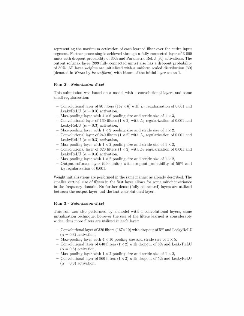
Run 2 - Submission-6.txt
This submission was based on a model with 4 convolutional layers and somesmall regularization:
– Convolutional layer of 80 filters (167× 6) with L1 regularization of 0.001 andLeakyReLU (α = 0.3) activation,
– Max-pooling layer with 4 × 6 pooling size and stride size of 1 × 3,– Convolutional layer of 160 filters (1 × 2) with L2 regularization of 0.001 and
LeakyReLU (α = 0.3) activation,– Max-pooling layer with 1 × 2 pooling size and stride size of 1 × 2,– Convolutional layer of 240 filters (1 × 2) with L2 regularization of 0.001 and
LeakyReLU (α = 0.3) activation,– Max-pooling layer with 1 × 2 pooling size and stride size of 1 × 2,– Convolutional layer of 320 filters (1 × 2) with L2 regularization of 0.001 and
LeakyReLU (α = 0.3) activation,– Max-pooling layer with 1 × 2 pooling size and stride size of 1 × 2,– Output softmax layer (999 units) with dropout probability of 50% andL2 regularization of 0.001.
Weight initializations are performed in the same manner as already described. Thesmaller vertical size of filters in the first layer allows for some minor invariancein the frequency domain. No further dense (fully connected) layers are utilizedbetween the output layer and the last convolutional layer.
Run 3 - Submission-9.txt
This run was also performed by a model with 4 convolutional layers, sameinitialization technique, however the size of the filters learned is considerablywider, thus more filters are utilized in each layer:
– Convolutional layer of 320 filters (167×10) with dropout of 5% and LeakyReLU(α = 0.3) activation,
– Max-pooling layer with 4 × 10 pooling size and stride size of 1 × 5,– Convolutional layer of 640 filters (1× 2) with dropout of 5% and LeakyReLU
(α = 0.3) activation,– Max-pooling layer with 1 × 2 pooling size and stride size of 1 × 2,– Convolutional layer of 960 filters (1× 2) with dropout of 5% and LeakyReLU
(α = 0.3) activation,
– Max-pooling layer with 1 × 2 pooling size and stride size of 1 × 2,– Convolutional layer of 1280 filters (1×2) with dropout of 5% and LeakyReLU
(α = 0.3) activation,– Max-pooling layer with 1 × 2 pooling size and stride size of 1 × 2,– Output softmax layer (999 units) with dropout probability of 25%.
Run 4 - Submission-ensemble.txt
The final run consisted of a simple meta-model averaging the predictions of theaforementioned submissions.
2.3 Training procedure
All network models were trained using a categorical cross-entropy loss functionwith a stochastic gradient descent optimizer (learning rate of 0.001, Nesterovmomentum of 0.9). Training batches contained 100 segments each. Validation wasperformed locally on the hold-out set (20% of the original training data available)by selecting a random subset on each epoch (approximately 2 500 files each time)and calculating the model’s prediction accuracy. This metric was assumed asa proxy for the expected mean average precision without background species -category which was reported as MAP2 in BirdCLEF 2015 results.
Each model was trained for a number of epochs (30–102). The training timefor a single model on a single GTX 980 Ti card was in the range of 30–60 hours.The results of final validation for each of the trained models are presented inTable 2, whereas Figure 2 depicts a small selection of filters learned by one ofthe models.
Table 2: Local validation results for each run
Run 1 Run 2 Run 3
MAP2 proxy 45.1% 50.0% 49.5%
Fig. 2: Example of filters learned in the first convolutional layer
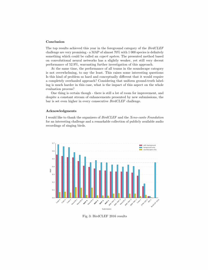
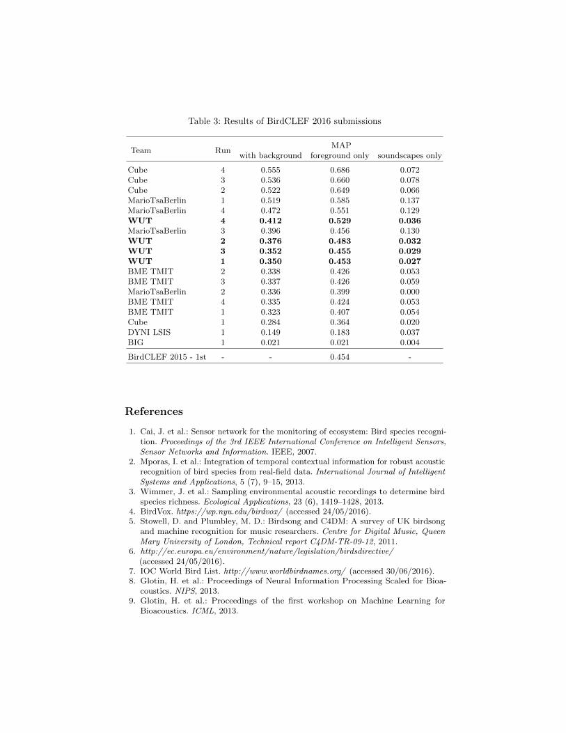
3 Submission results & discussion
The official results of the BirdCLEF 2016 challenge are presented in Table 3and Figure 3. There were 6 participating groups which submitted 18 runs intotal. The submission described in this work resulted in a 3rd place amongparticipating teams with individual runs achieving 6th, 8th, 9th and 10th officialscore (1st column - MAP with background species and soundscape files). Theanalysis of these results and the experience gathered during the BirdCLEF 2016challenge allows for the following remarks:
– With almost 1 000 bird species, the BirdCLEF dataset creates a demandingchallenge for any machine audition system. In this context, an approachbased on convolutional neural networks seems to be valid and promisingfor the analysis of bioacoustical data. Looking at comparable results fromthe very last year, surpassing a foreground only MAP of 50% is definitelya success. However, this year’s top performing submission was still able toremarkably improve on this evaluation metric.
– The performance of the described networks is quite consistent between models.It seems that a decent convolutional architecture with proper training andinitialization regime should be able to learn a reasonable approximation ofthe classifying function based on the provided data, and minor architecturaldecisions may not be of the utmost importance in this case.
– Very poor performance in the soundscape category confirms that the presentedapproach has a strong bias against multi-label scenarios - a thing which is notsurprising when considering the applied learning scheme, which was ratherforcefully extended to the multi-label case. Not only does learning on a singletarget label for each recording impose some constraints in this process, butthe whole pre-processing step may also be detrimental in this situation. Thusit seems that further work should concentrate more on what is learned (datasegmentation and pre-processing, labeling, input/output layers) than how(internal network architecture).
– A promising feature of the dataset lies in the good correspondence betweenresults obtained through local validation and evaluation of the private groundtruth by the organizers. This means that the dataset is both rich and uniformenough for such estimations to be of value - an aspect which should help infurther efforts in improving the described solution.
– A very simple ensembling method was quite beneficial in the case of theevaluated models. This shows that more sophisticated approaches could yieldsome additional gains - both when it comes to meta-model blending andin-model averaging. A progressive increase of the dropout rate was one of thefacets which was actually considered during the experiments. Unfortunately,these attempts had to be preemptively stopped due to the time constraintsencountered in the final stage of the competition.
Conclusion
The top results achieved this year in the foreground category of the BirdCLEFchallenge are very promising - a MAP of almost 70% with 1 000 species is definitelysomething which could be called an expert system. The presented method basedon convolutional neural networks has a slightly weaker, yet still very decentperformance of 52.9%, warranting further investigation of this approach.
At the same time, the performance of all teams in the soundscape categoryis not overwhelming, to say the least. This raises some interesting questions:Is this kind of problem so hard and conceptually different that it would requirea completely overhauled approach? Considering that uniform ground-truth label-ing is much harder in this case, what is the impact of this aspect on the wholeevaluation process?
One thing is certain though - there is still a lot of room for improvement, anddespite a constant stream of enhancements presented by new submissions, thebar is set even higher in every consecutive BirdCLEF challenge.
Acknowledgments
I would like to thank the organizers of BirdCLEF and the Xeno-canto Foundationfor an interesting challenge and a remarkable collection of publicly available audiorecordings of singing birds.
1. Cai, J. et al.: Sensor network for the monitoring of ecosystem: Bird species recogni-tion. Proceedings of the 3rd IEEE International Conference on Intelligent Sensors,Sensor Networks and Information. IEEE, 2007.
2. Mporas, I. et al.: Integration of temporal contextual information for robust acousticrecognition of bird species from real-field data. International Journal of IntelligentSystems and Applications, 5 (7), 9–15, 2013.
3. Wimmer, J. et al.: Sampling environmental acoustic recordings to determine birdspecies richness. Ecological Applications, 23 (6), 1419–1428, 2013.
4. BirdVox. https://wp.nyu.edu/birdvox/ (accessed 24/05/2016).5. Stowell, D. and Plumbley, M. D.: Birdsong and C4DM: A survey of UK birdsong
and machine recognition for music researchers. Centre for Digital Music, QueenMary University of London, Technical report C4DM-TR-09-12, 2011.
7. IOC World Bird List. http://www.worldbirdnames.org/ (accessed 30/06/2016).8. Glotin, H. et al.: Proceedings of Neural Information Processing Scaled for Bioa-
coustics. NIPS, 2013.9. Glotin, H. et al.: Proceedings of the first workshop on Machine Learning for
Bioacoustics. ICML, 2013.
10. Briggs, F. et al.: The 9th annual MLSP competition: New methods for acoustic clas-sification of multiple simultaneous bird species in a noisy environment. Proceedingsof the IEEE International Workshop on Machine Learning for Signal Processing(MLSP), IEEE, 2013.
11. Goeau, H. et al.: LifeCLEF bird identification task 2016. CLEF working notes 2016.12. Joly, A. et al.: LifeCLEF 2016: multimedia life species identification challenges.
Proceedings of CLEF 2016.13. Xeno-canto project. http://www.xeno-canto.org (accessed 24/05/2016).14. Lasseck, M.: Improved automatic bird identification through decision tree based
feature selection and bagging. CLEF working notes 2015.15. Lasseck, M.: Large-scale identification of birds in audio recordings. CLEF working
notes 2014.16. Joly, A., Leveau, V., Champ, J. and Buisson, O.: Shared nearest neighbors match kernel
for bird songs identification - LifeCLEF 2015 challenge. CLEF working notes 2015.17. Joly, A., Champ, J. and Buisson, O.: Instance-based bird species identification with
undiscriminant features pruning. CLEF working notes 2014.18. Ren, L. Y., Dennis, J. W. and Dat, T. H.: Bird classification using ensemble
classifiers. CLEF working notes 2014.19. Stowell, D.: BirdCLEF 2015 submission: Unsupervised feature learning from audio.
CLEF working notes 2015.20. Stowell, D. and Plumbley, M. D.: Audio-only bird classification using unsupervised
feature learning. CLEF working notes 2014.21. Stowell, D. and Plumbley, M. D.: Automatic large-scale classification of bird sounds
is strongly improved by unsupervised feature learning. PeerJ 2:e488, 2014.22. Koops, H. V., Van Balen, J. and Wiering, F.: A deep neural network approach to
the LifeCLEF 2014 bird task. CLEF working notes 2014.23. Branson, S., Van Horn, G., Belongie, S. and Perona, P.: Bird species categorization
using pose normalized deep convolutional nets. arXiv preprint arXiv:1406.2952, 2014.24. McFee, B. et al.: librosa: 0.4.1. Zenodo. 10.5281/zenodo.32193, 2015.25. Chambolle, A.: An algorithm for total variation minimization and applications.
Journal of Mathematical Imaging and Vision, 20 (1-2), 89–97, 2004.26. van der Walt, S. et al.: scikit-image: Image processing in Python. PeerJ 2:e453, 2014.27. Piczak, K. J.: Environmental sound classification with convolutional neural networks.
Proceedings of the IEEE International Workshop on Machine Learning for SignalProcessing (MLSP), IEEE, 2015.
28. Chollet, F.: Keras. https://github.com/fchollet/keras (accessed 24/05/2016).29. Phan, H., Hertel, L., Maass, M. and Mertins, A.: Robust audio event recognition with
1-Max pooling convolutional neural networks. arXiv preprint arXiv:1604.06338, 2016.30. He, K., Zhang, X., Ren, S. and Sun, J.: Delving deep into rectifiers: Surpassing
human-level performance on ImageNet classification. Proceedings of the IEEEInternational Conference on Computer Vision, IEEE, 2015.


![BBC VOICES RECORDINGS€¦ · BBC Voices Recordings) ) ) ) ‘’ -”) ” (‘)) ) ) *) , , , , ] , ,](https://static.documents.pub/doc/80x56/5f8978dc43c248099e03dd05/bbc-voices-recordings-bbc-voices-recordings-aa-a-a-a-.jpg)