Aggregate analyst recommendation ratings and international stock market returns Ari Yezegel Assistant Professor of Accounting Bentley University 175 Forest Street Waltham, Massachusetts 02452 [email protected]Tel: +1.781.891.2264 Fax: +1.781.891.2896 Current Draft: March 18th, 2015 Abstract This study investigates the determinants of aggregate analyst recommendation ratings and tests whether aggregate recommendations predict future market returns. Based on a sample of 59 countries for the period 1993-2013, U.S. macroeconomic conditions, prior market returns and the average aggregate recommendation in the world are found to be significantly associated with aggregate analyst recommendations in individual countries. The results also suggest that aggregate analyst recommendations possess predictive power of future returns in developed markets while they contain no such predictive information in emerging and frontier markets. Interestingly, the U.S. aggregate analyst recommendations have predictive information content for future returns in emerging countries. These results demonstrate the predictive power of aggregate recommendations in the U.S. do not extend beyond that of developed markets.
Transcript
Aggregate analyst recommendation ratings and international
This study investigates the determinants of aggregate analyst recommendation ratings and tests whether aggregate recommendations predict future market returns. Based on a sample of 59 countries for the period 1993-2013, U.S. macroeconomic conditions, prior market returns and the average aggregate recommendation in the world are found to be significantly associated with aggregate analyst recommendations in individual countries. The results also suggest that aggregate analyst recommendations possess predictive power of future returns in developed markets while they contain no such predictive information in emerging and frontier markets. Interestingly, the U.S. aggregate analyst recommendations have predictive information content for future returns in emerging countries. These results demonstrate the predictive power of aggregate recommendations in the U.S. do not extend beyond that of developed markets.
1
1. Introduction
Sell-side analysts regularly analyze companies and issue recommendations to provide useful investment
advice to their clients. The prior literature finds that analysts’ stock recommendations at a firm-level
contain predictive information concerning future price changes and are informative to investors. For
example, Stickel (1995) and Womack (1996) analyze the value of analysts’ individual recommendations
and find that the market reaction following upgrades exceeds that of downgrades. Further, Barber et al.
(2001), Jegadeesh et al. (2004) and Green (2006) find that firms with more favorable recommendation
ratings outperform those with less favorable ratings. In addition, recent research by Howe, Unlu and Yan
(2009) shows that aggregate analyst recommendations are successful in predicting future U.S. market
returns. In contrast, a number of studies show that analysts provide limited information concerning
future stock price fluctuations (Bradshaw 2004; Altinkilic and Hansen 2009; Drake, Rees and Swanson
2011).
While there is extensive research on the informativeness and value of recommendations in the
U.S., there is limited information on how well analysts’ recommendations perform outside of the U.S.
The U.S. finance industry employs a large number of highly qualified individuals who acquire
information, analyze securities and provide investment advice to their clients. Further, their employers
invest significant sums to support analysts’ research and valuation activities. It is also common for
financial analysts in the U.S. to consult, through expert networks, with experts in the field to identify and
take advantage of incremental pieces of information that may not be fully reflected in the market prices.
In contrast, anecdotal evidence suggests that banks outside the U.S. provide less resources and support
to help their analysts issue useful trading advice to their clients. However, there may be more
opportunities for informed market participants (e.g. analysts) to identify mispricings in non-U.S.
countries which presumably have less mature and efficient markets. Therefore, in comparison to foreign
2
analysts, U.S. analysts may find it more challenging to identify under- or over-valuations when analyzing
domestic securities whereas foreign analysts have more opportunities but lack the needed resources.
Further, the accelerating rate of globalization has created an expansion in the number of
companies that operate at a global scale. The impact of globalization is clearly evident in the U.S. capital
markets which house a large number of multinational corporations. The global nature of the operations
of these companies requires U.S. analysts to not only investigate and understand the macro-economic
environment in the U.S. but also around the world. For instance, an analyst analyzing Coca-Cola is
expected to assess the business environment in the U.S. as well as abroad to make meaningful sales
projections. To the extent that U.S. analysts have more resources and are superior in analyzing
corporate information, their global focus opens up the possibility of U.S. analysts’ recommendations
also containing predictive value for non-U.S. markets incremental to the value of recommendations of
their colleagues abroad.
In summary, it is unclear whether recommendations of U.S. sell-side analysts are more or less
informative than the recommendations of non-U.S. based analysts. This remains an empirical question
which requires the analysis of analysts’ recommendations at a global scale. Further, the role that U.S.
analysts play in the predictability of international markets is unexplored. On the one hand, U.S. analysts
may be waiting to receive information from their colleagues abroad to incorporate it into their
valuations of multinational companies. On the other hand, analysts abroad may be taking cues from U.S.
analysts that are analyzing the performance of companies who operate in a large number of countries.
Hence, information flow can flow both ways and understanding the dominant direction requires an
empirical investigation.
This study takes a different approach compared to prior studies and focuses on the
determinants and value of analysts’ recommendations at a global level using aggregate level
3
recommendation and return data. In order to accomplish this, I measure the aggregate
recommendation rating each month for 59 countries in the world. I then explore the potential valuation,
macroeconomic, market and fundamental factors that contribute to the variation in aggregate
recommendations. In addition, I examine whether recommendation ratings contain predictive
information content concerning future stock market returns.
The analysis conducted in this paper intends to contribute to the literature in several ways. First,
the findings of this study extend the recent work by Howe, Unlu and Yan (2009) which shows that
aggregate recommendation ratings have predictive power of future returns in the U.S. market. The
results in this study show that the findings in Howe, Unlu and Yan (2009) extend to other developed
markets but interestingly not to emerging or frontier markets. Second, this paper extends Bradshaw's
(2004) work on the determinants of analysts’ recommendation ratings at a firm-level for the U.S. stock
market. I use data on a large number of international markets to provide insights on the determinants of
analysts’ recommendations that can be generalized to other financial markets. Finally, this study
contributes to the literature concerned with the predictability of international stock market returns.
Rapach, Strauss and Zhou (2013) find that the U.S. monthly returns contain predictive content of the
future returns of numerous other countries. The findings in this study propose financial analysts as one
possible channel through which information in the U.S. is transferred to other markets across the world.
The remainder of this paper is organized as follows. The next section reviews the relevant
literature and develops the hypotheses. The following two sections describe the data and methodology.
Section four discusses the empirical findings and the final section concludes.
2. Hypotheses Development
The literature on financial analysts’ stock recommendations primarily focuses on the value and
performance of recommendations in the U.S. capital markets. Despite the U.S. centered focus in the
4
literature there are a number of studies that examine the performance of analysts in other countries
and compare them to the performance of analysts based in the U.S.
Most notably, Jegadeesh and Kim (2006) study the value of analyst recommendations in the Group
of Seven (G7) industrialized countries. Among the sample of countries that they examine, they find that
analysts covering U.S. listed firms provide the most informative recommendations. Further, they
examine a sub-sample of companies with American Depository Receipts (ADRs) which tend to have both
U.S. and foreign analysts and find that U.S. analysts add more value to the price discovery process
relative to their peers in foreign countries. Similarly, Moshirian, Ng and Wu (2009) examine the
performance of analysts’ recommendations in thirteen emerging countries over a ten year period. They
show that subsequent share price movements are positively associated with analysts’ recommendations
and revisions. Further, Farooq and Ali (2014) study the performance of analysts’ recommendations in
the Middle East and North Africa region. Interestingly, they find that while analysts’ buy
recommendations are associated with future returns their sell recommendations are not. Finally, a
number of papers examine the performance of analysts in individual countries. For example, Azzi and
Bird (2005) and He, Grant and Fabre (2013) analyze the performance of analysts in Australia. Pereira da
Silva (2013), Erdogan, Palmon and Yezegel (2011) and Lonkani, Khanthavit and Chunahachinda (2010)
study the value of recommendations in Portugal, Turkey, and Thailand, respectively. The results of these
studies based on firm-specific recommendations report mixed results on the value of analysts’
recommendations.
In a recent study, Howe, Unlu and Yan (2009) follow an innovative approach and examine the
predictive content of aggregate recommendations. They begin with a sample of 350,000
recommendations issued for U.S. companies during the period between January 1994 and August 2006.
They then aggregate the firm-level recommendations to the market level and find that changes in
5
aggregate analyst recommendations predict future market excess returns. Based on these results, Howe
et al. (2009) conclude that analyst recommendations contain market-level information about future
returns.
The Howe et al. (2009) study opens up new avenues for research in several dimensions. First, what
are the key determinants of aggregate analyst recommendation ratings? Bradshaw (2004) examine
determinants of analyst recommendations at a firm-level and conclude that analysts frequently rely on
valuation heuristics (e.g. P/E and derivatives) while developing their recommendations. It is unclear
whether these results are generalizable to aggregate analyst recommendations or to non-U.S. markets.
Further, at an aggregate level, other factors (e.g. macro-economic) that were not relevant at a firm-level
may begin to contribute to variation in analyst recommendation ratings. In order to shed light on this
issue, this paper examines the following research question:
Research Question 1: What are the key determinants of aggregate analyst recommendations?
A related question is whether aggregate analyst recommendations are informative in countries
other than the U.S. The U.S. is considered by many to host the most efficient and largest equity markets
(e.g., NYSE, NASDAQ) in the world. On the one hand, the higher level of efficiency present in the U.S. is
likely to eliminate opportunities for analysts to detect mispricings and make it more challenging for
analysts to provide informative recommendations to their clients. On the other hand, the increased
demand for research is likely to incentivize analysts to invest greater effort and resources to produce
informative equity research. Ex ante, it is unclear whether the predictive content attributed to
recommendations issued by U.S. analysts can be generalized to other markets. Therefore, I first
empirically examine the predictive content of aggregate analyst recommendations in the U.S. and use
this as a base-line measure to examine the value of aggregate recommendations in other developed
markets and emerging and frontier markets.
6
H1: Aggregate analyst recommendations in non-U.S. markets are not associated with future market
excess returns.
Finally, prior research conducted by Rapach, Strauss and Zhou (2013) suggests that lagged U.S.
stock market returns significantly predict returns in numerous non-U.S. countries. Rapach et al. (2013)
suggest that information shocks are gradually diffused into equity prices outside of the U.S., leading to a
lead-lag relationship between non-U.S. and U.S. returns. One potential mechanism through which
information is diffused to non-U.S. markets is via analysts’ recommendations. To provide insights on this
issue I test the following hypothesis:
H2: Aggregate U.S. analyst recommendations significantly predict non-U.S. market returns.
3. Sample
The Thomson Reuters Institutional Brokers’ Estimate System (I/B/E/S) collects earnings estimates and
recommendation ratings issued by analysts who are employed by institutions worldwide. The
recommendation ratings in I/B/E/S are in decreasing order where one indicates “Strong Buy” and five
indicates “Strong Sell”. Consistent with the prior literature, I reverse the ratings to provide an easier
interpretation of the estimation results. In the revised organization, one represents “Strong Sell”, five
represents “Strong Buy” and the values between correspond to “Sell”, “Hold”, “Buy” in increasing order.
Using the country codes available on the I/B/E/S database, I identify recommendation ratings
issued for companies listed in 59 countries for which there is MSCI index return data available for the
period 1994-2013.1 MSCI categorizes 23 of these countries as developed, 20 as emerging and 16 as
frontier markets. When computing consensus recommendations, I consider each recommendation
rating as outstanding until it is revised or six-months have elapsed without a revision (whichever comes
1 Eight countries were eliminated from the initial sample because of limited historical data (less than five years).
These countries are: Bangladesh, Botswana, Bulgaria, Lebanon, Lithuania, Ghana, Tunisia and Zimbabwe.
7
first). I then compute the consensus recommendation rating for each firm and month based on the
outstanding recommendations. Finally, I compute the consensus recommendation rating for each
country and month by calculating the equal-weighted average consensus recommendation rating for all
firms listed in each country. By first computing the consensus recommendation for each firm and then
calculating the average recommendation rating for the country, I aim to prevent large firms with greater
analyst coverage from unduly influencing aggregate analyst recommendations.
I obtain monthly return data for the countries from the Morgan Stanley Capital International
(MSCI) website. I then merge return data with fundamental accounting and valuation data (e.g., B/M,
E/P, S/P) compiled from Bloomberg and macroeconomic data obtained from the Federal Reserve
Economic Data (FRED) system and from the Fama French & Liquidity Factors file available on Wharton
Research Data Services (WRDS).
Table 1 presents descriptive statistics for the country-level MSCI dollar denominated index
returns used in this study. The table is organized based on the market segment. Panel A reports statistics
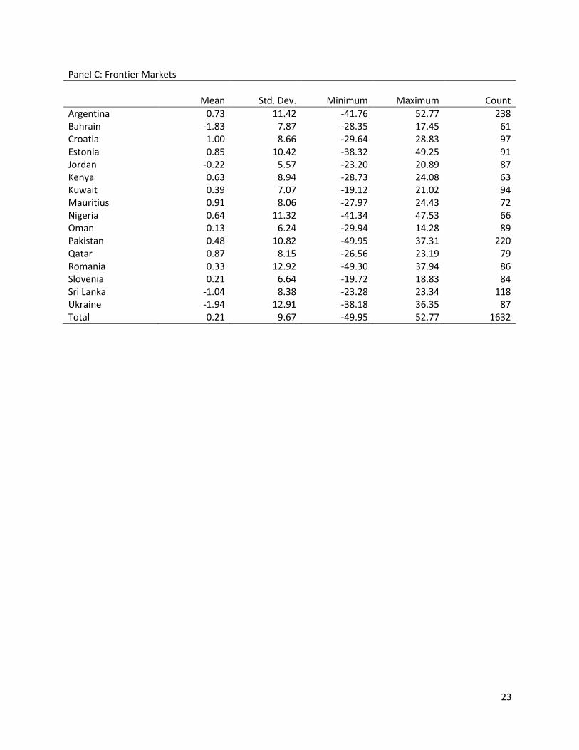
for developed markets, Panel B for emerging markets and Panel C presents statistics for frontier
markets.
For developed and emerging markets, the MSCI country-level index database contains data for
most of the sample period. In contrast, the return data for frontier markets is scarce. This is potentially
due to the maturity and significance of frontier markets. As countries in this group mature and MSCI
begins to track them, we are likely to observe an expansion in this market segment.
Table 1 also reports mean, standard deviation, minimum and maximum values for excess
monthly index returns. There is significant variation both within and between market groups. The
average excess monthly return in the developed market is 0.63 percent whereas in the emerging market
group it is 0.78 which is 15 basis points higher. The higher mean excess monthly return is consistent with
8
the larger risk that is associated with investing in emerging markets. However, at odds with the notion of
a positive relation between risk and returns, the mean return associated with frontier markets is
considerably lower. Specifically, the average excess monthly return in the frontier markets group is 0.21.
These statistics indicate that, at least in the limited sample available for frontier markets, risk and return
are not positively associated.
Finally, within each market group, we observe significant variation in average returns. For
instance, in the developed countries group, Finland ranks first with an average excess monthly return of
1.23 percent. The lowest average monthly return is computed to be 0.02 percent for Japan. In the
emerging markets category, Egypt (1.72%) and China (0.16%) have the highest and lowest average
excess monthly returns, respectively. Finally, the frontier market category has the greatest dispersion in
returns. In this group, Croatia has the lead with an average excess monthly return of one percent and
Ukraine ranks last with an average of -1.94 percent. The unusually low average return computed for
Ukraine is potentially due to the relative short sample period for this country (87 months) and possibly
due to the recent conflict with Russia.
Table 2 reports descriptive statistics for the variables employed in the regression analysis. The
final sample consists of 11,846 monthly observations. However, certain variables are not available for
some of the countries or months. Therefore, the number of observations used in estimations varies
depending on the variables employed in the analysis. Table 2 reports that the mean recommendation
rating is 3.49. This corresponds to a point between a “Hold” and a “Buy” recommendation. Further 75
percent of the consensus recommendations are greater than 3.30. The statistics for the REC variable are
consistent with the optimistic bias documented in the prior literature. The ΔREC variable which is the
change in consensus recommendation rating has a mean and median of zero. Compared to the REC, an
optimistic bias in changes in consensus recommendations is not evident. However, this does not rule out
9
the possibility of another type of bias whereby analysts delay downgrading their recommendations but
immediately incorporate increases. Finally, the descriptive data for REC_SEGMENT and REC_WORLD
closely mirror descriptive statistics for REC.
In terms of macro-economic factors, the mean default spread (DEF) is computed to be 2.48
percent for the sample period. The average term spread (TERM) is 1.73 percent and the mean three-
month Treasury bill rate (TB3M) is 2.66 percent.
The following two variables reported in Table 2 measure dividends distributed in relation to the
market value of the company (DIVYIELD) and the profitability of the company in relation to equity (ROE).
The mean dividend yield for the period is 2.92 and the mean ROE is reported to be 13.21.
The next four variables represent various valuation ratios that are commonly used in the
financial community. Consistent with the prior literature, I use the reciprocal of these ratios to reduce
the influence of outliers in regression analysis. For instance, instead of the commonly used market-to-
book ratio in the profession, I compute and use the book-to-market ratio in my regression analysis. The
mean book-to-market (B/M) and earnings-to-price (E/P) ratios are 0.60 and 0.07, respectively. Further
the mean cash-flow-to-price (C/P) and sales-to-price (S/P) ratios are 0.13 and 0.89, respectively. The
descriptive statistics concerning these variables are in line with the statistics reported for these variables
in prior studies.
Finally, the last two variables (RET3M and RET12M) measure the performance of the country-
level index during the past three- and twelve-month periods. The average past three-month market
excess return is 2.05 percent and the average past twelve-month market return is 9.06 percent. These
statistics are in line with the country-specific statistics reported in Table 1.
10
Table 3 presents the correlation matrix for the variables used in the regression analysis. The
correlations between REC_SEGMENT and REC_WORLD (0.79), among DEF, TERM and TB3M, and among
C/P, S/P and B/M are in excess of 0.50 which raises concern for the influence of multicolinearity on the
estimation results. I investigate this issue further in the regression analysis by examining variance
inflation factors and excluding certain variables when necessary.
4. Methodology
The research design centers on the examination of two interrelated aspects of analysts’
recommendations. In the first analysis, I examine the potential determinants of analysts’ aggregate
recommendation levels and changes. In the second analysis I test whether aggregate recommendation
ratings have predictive information content concerning future market returns.
In the first analysis, I explore factors that contribute to the time-series and cross-sectional variation
in recommendation rating levels and changes. The first set of variables that I examine, measure the
aggregate recommendation rating in the previous month (RECit-1), the average recommendation rating
for other countries in the same market segment (REC_SEGMENTit-1) and the rest of the world
(REC_WORLDit-1). I consider these three measures as potential factors to test whether analysts take into
account the recommendation levels in other countries. Finally, the recommendation level in the prior
month is likely to serve as an important factor because it is the starting point for the recommendation
ratings this month.
As the second set of variables influencing the level of recommendation ratings, I explore macro-
economic factors concerning the U.S. I focus on the U.S. because the indices are denominated in U.S.
dollars and also the macroeconomic condition in the U.S. tends to have a profound impact in financial
markets across the world. I examine the effect of the default spread, the term spread and the three-
month Treasury bill rate.
11
As the third set of variables, I test whether dividend yield and return on equity are significantly
associated with consensus recommendations. In addition, I examine a host of valuation metrics (B/M,
E/P, C/P and S/P) to test whether analysts take into account these ratios in reaching their
recommendation ratings. Finally, using the last set of variables (RET3M and RET12M), I assess the
influence of price momentum on aggregate analyst recommendations.
I conduct the determinants analysis both for levels and changes in aggregate recommendation
ratings to shed light on analysts’ decision making process. In the levels analysis, all variables with the
exception of the return measures (RET3M and RET12M) are based on levels whereas in the changes in
analysis all variables are differenced. In both analyses RET3M and RET12M represent the cumulative
returns over the preceding three- and twelve- month periods.
In this sub-section, I explore various determinants of aggregate analyst recommendations to provide
insights on the mechanism through which analysts make recommendation decisions. Table 4 reports the
estimation results of Equation (1) which involves the regression of the aggregate recommendation levels
on market, macro- economic, valuation and past return variables.
I begin the analysis by first examining whether aggregate analyst recommendations are
associated with the aggregate recommendations for other countries in the same market segment and in
the rest of the world. Table 4 Model 1 reports the estimation results of the regression of REC on prior
month’s REC, REC_SEGMENT and REC_WORLD. The coefficient on REC is estimated to be positive and
statistically significant, suggesting that aggregate recommendations are sticky and the prior month’s
recommendation levels is an important determinant of the recommendation level this month. Further,
the coefficient on REC_SEGMENT and REC_WORLD are reported to be 0.137 and 0.392, respectively.
Both coefficients are statistically significant at the five-percent significance level. The positive
coefficients on REC_SEGMENT and REC_WORLD indicate that analysts’ aggregate recommendation
ratings are highly integrated across countries. In order to ensure that the results are not plagued by a
13
potential multicolinearity problem arising from the correlation between REC_SEGMENT and
REC_WORLD, I inspect the variance inflation factors (VIF) and include each variable separately in the
model. The average VIF in Model 1 is 1.88 and the highest factor is 2.28, raising no concern for
multicolinearity. However, when I include REC_SEGMENT without REC_WORLD, the coefficient on
REC_SEGMENT is estimated to be 0.018 and statistically insignificant. In contrast, the coefficient on
REC_WORLD remains positive and statistically significant when REC_SEGMENT is excluded from the
model.
In Model 2, I examine the relation between aggregate analyst recommendations and macro-
economic factors including the default and term spreads in the U.S (DEF and TERM) as well as the three-
month Treasury bill yield (TB3M). The coefficients on DEF, TERM and TB3M are estimated to be -0.019,
0.022, and 0.019, respectively. The three coefficients are estimated to be statistically significant.
Economically, a one percentage point increase in the default spread is associated with a 0.019 decline in
the aggregate recommendation. Similarly a one percentage point increase in the term spread is
associated with a 0.019 increase in the aggregate recommendation. In terms of economic significance, a
one percentage point change in one of the independent variables corresponds to a change in REC that is
equivalent to a change that is nearly five percent of the standard deviation of the aggregate analyst
recommendation rating.
Table 4 Model 3 additionally includes the dividend yield (DIVYIELD) and return on equity (ROE)
measures to examine whether these two factors explain variation in the aggregate recommendation
levels. The estimation results indicate that neither variable is statistically significant. Model 4 includes
four valuation ratios: book-to-market (B/M), earnings-to-price (E/P), cash-flow-to-price (C/P), and sales-
to-price (S/P) ratios. With the exception of C/P, the valuation ratios are not found to be statistically
significant. The coefficient on C/P is estimated to be -0.025 and suggests that as the average cash-flow-
14
to-price ratio for a country increases the mean aggregate analyst recommendation rating tends to
decline. The negative relation between REC and C/P indicates that analysts favor countries with more
growth opportunities. In model 4, after including the four valuation ratios, the coefficient on ROE is
estimated to be 0.003 and statistically significant. The positive coefficient indicates that the aggregate
recommendation level is higher for countries with more profitable firms.
Finally, in Model 5 of Table 4, I include two prior return measures to examine the influence of
momentum on aggregate analyst recommendations. While REC is not found to be significantly
associated with the most recent three month period market excess returns, there is a positive
association between REC and RET12M which is the market excess return during the preceding twelve
month period.
Table 5 repeats the determinants analysis conducted in Table 4 by estimating equation (2) which
is based on changes in aggregate analyst recommendations. The coefficients on lagged recommendation
change (ΔREC), default (ΔDEF), return on equity (ROE), cash-flow-to-price (C/P) and past three-month
market excess return (RET3M) are estimated to be statistically significant and in the same direction
found in the prior analysis. In contrast, the coefficients on the changes in average aggregate
recommendation for the other countries in the same market segment (REC_SEGMENT) and the rest of
the world (REC_WORLD), changes in dividend yield (DIVYIELD) and three-month treasury bill rates
(TB3M) are not found to be statistically significant. The changes analysis highlights that past changes in
recommendations positively predict future changes. This is consistent with analysts gradually
incorporating new information into their recommendations thereby inducing a positive serial correlation
in aggregate recommendation ratings.
15
5.2 Aggregate recommendation ratings and future market returns
In this sub-section, I examine whether aggregate recommendation ratings are useful in predicting future
market excess returns. In order to examine this issue I estimate Equation (3). Table 6 reports the
estimation results for various sub-samples and for the full sample.
The results reported in Table 6 under the column labeled “Developed Markets” present the
estimation results for the developed market sample. In this model excess market returns are regressed
on the lagged excess U.S. market returns, recommendation levels, changes in the recommendation level
in the same country and in the U.S., dividend yield, ROE, three-month treasury bill rate and the default
and term spreads.
The coefficient on prior month’s U.S. excess return (RETit-1) is estimated to be 0.107 (p<0.01).
This indicates a positive relation between returns where past U.S. returns are positively associated with
future returns. Surprisingly, the coefficient on the aggregate recommendation level (REC) is estimated to
be -1.196. The estimated REC parameter suggests that expected returns are lower for countries with
higher aggregate recommendation levels. The negative REC coefficient also indicates that returns
behave in the opposite direction suggested by the recommendation levels. In contrast, the coefficient
on ΔRECit-1 is estimated to be 3.264 and statistically significant. The positive coefficient on ΔRECit-1
depicts a positive relation between future returns and lagged changes in recommendation ratings. These
results are consistent with aggregate analyst recommendations containing predictive information
concerning future market returns. Further, the coefficient on ΔREC_USit is estimated to be 7.808
(p<0.01). The positive coefficient suggests that the changes in aggregate U.S. recommendations have
predictive information concerning future market returns in developed markets. However, this may be
driven by the presence of U.S. market data in the market segment. Therefore, in the second model, I
exclude U.S. data and re-estimate Equation (3). The results are largely similar.
16
In the third column, Table 6 reports the estimation results of Equation (3) using data from
emerging markets. In this model, the coefficient on lagged recommendation levels (RECit-1) is not
statistically significant indicating that the change in aggregate analyst recommendation does not
significantly predict future returns excess returns in emerging markets. In contrast, the lagged changes
in the U.S aggregate recommendations (REC_US) contains significant predictive information content.
Specifically, the coefficient on ΔREC_USit-1 is estimated to be 13.354 and is statistically significant. The
coefficient on ΔREC_USit-1 indicates that a 0.1 increase in lagged U.S. aggregate recommendation is
associated with a 1.3 percent increase in future market excess returns. The following column reports
results for the frontier markets sample. Interestingly, the reported results indicate that the aggregate
recommendation level, changes in aggregate recommendations and changes in U.S. aggregate
recommendations are not significantly associated with future excess market returns. These results are in
stark contrast with the results reported for developed and emerging markets and indicate that
aggregate analyst recommendations do not significantly predict future excess returns in frontier
markets.
The final column in Table 6 reports the estimation results based on the full sample. Lagged U.S.
returns and lagged changes in the U.S. aggregate recommendations are found to be statistically
significant.
5.3 Trading strategy analysis
This section examines whether the predictive information content of lagged aggregate
recommendations that was documented in the prior section can be exploited by investors. Table 7
reports the estimation results of a portfolio analysis separately for developed (Panel A), emerging and
frontier (Panel B) and all markets (Panel C). The results in Panel A show that the country indices that fall
in the Bottom portfolio experience an average monthly return of -0.129 percent in the following month
17
whereas countries ranked into the Top portfolio exhibit an average monthly return of 0.108. Finally, the
Hedge portfolio earns an average monthly abnormal return of 24 basis points within the Developed
market sample. This corresponds to an annualized abnormal return of 2.844 and is not found to be
statistically significant. These results indicate that while a statistically significant association is evident
between lagged recommendation changes and future market returns, the predictive content of
aggregate recommendations is not at a level to warrant a profitable trading strategy.
In Table 7 Panel B, the estimation results of the trading strategy analysis within the Emerging and
Frontier markets sample is reported. The Hedge portfolio earns an average monthly abnormal return of
6 basis points and is both statistically and economically insignificant. These results indicate that the
trading strategy based on recommendation changes fares considerably worse outside of Developed
markets and is nearly non-existent.
Finally, in Panel C of Table 7 the results for the entire sample are reported. These results are very
similar to those reported in Panel B and indicate that the trading strategy appears unprofitable in a
sample consisting of all 59 countries analyzed in this study. Collectively, the inferences reached from the
trading strategy analyses echo the findings from the cross-sectional analysis which relate to emerging
and frontier markets and depict a muted economic relation between lagged aggregate
recommendations and future returns.
6. Conclusions
In conclusion, several insights emerge from the exploration of the determinants of aggregate
recommendations. First, the estimation results indicate that aggregate analyst recommendation levels
are strongly interconnected across countries and that this extends beyond the market group. Analysts
appear to be influenced by the aggregate recommendation levels in other countries in the same market
segment and the world. Second, key U.S. macro-economic factors play an instrumental role in the
18
determination of aggregate analyst recommendations not just in the U.S. but across the entire world.
Further, average return on equity, cash-flow-to-price and past market returns are significantly
associated with aggregate recommendation levels and changes.
Finally, the analysis of the predictive content of aggregate recommendations corroborates the
results reported in Howe et al. (2009) and suggests that the findings therein largely apply to other
developed markets. However, the results in this study demonstrate that the documented relation may
not be strong enough to warrant an economically profitable trading strategy. Further, the aggregate
analyst recommendations are not found to significantly predict future excess market returns in
emerging or frontier markets. In contrast, changes in U.S. aggregate analyst recommendations are
estimated to significantly predict future returns in emerging markets. Overall, the results suggest that
Howe et al.’s (2009) findings are generalizable to other developed markets but not to emerging or
frontier markets.
19
References
Altinkilic O., Hansen R.S., 2009. On the information role of stock recommendation revisions. Journal of Accounting & Economics 48, 17-36.
Azzi S., Bird R., 2005. Prophets during boom and gloom downunder. Global Finance Journal 15, 337-367.
Barber B., Lehavy R., McNichols M., Trueman B., 2001. Can investors profit from the prophets? Security analyst recommendations and stock returns. Journal of Finance 56, 531-563.
Bradshaw M.T. , 2004. How do analysts use their earnings forecasts in generating stock recommendations? The Accounting Review 79, 25-50.
Drake M.S., Rees L., Swanson E.P., 2011. Should investors follow the prophets of the bears? Evidence on the use of public information by analysts and short sellers. The Accounting Review 86, 101-130.
Erdogan O., Palmon D., Yezegel A., 2011. Performance of analyst recommendations in the Istanbul Stock Exchange. International Review of Applied Financial Issues and Economics 3, 504-512.
Farooq O., Ali L.I., 2014. Value of analyst recommendations: Evidence from the MENA region. International Journal of Islamic and Middle Eastern Finance and Management 7, 258-276.
Green T.C. , 2006. The value of client access to analyst recommendations. Journal of Financial and Quantitative Analysis 41, 1-24.
He P.W., Grant A., Fabre J., 2013. Economic value of analyst recommendations in Australia: an application of the Black–Litterman asset allocation model. Accounting & Finance 53, 441-470.
Howe J.S., Unlu E., Yan A.X., 2009. The predictive content of aggregate analyst recommendations. Journal of Accounting Research 47, 799-821.
Jegadeesh N., Kim J., Krische S.D., Lee C.M.C., 2004. Analyzing the Analysts: When Do Recommendations Add Value? Journal of Finance 59, 1083-1124.
Jegadeesh N., Kim W., 2006. Value of analyst recommendations: International evidence. Journal of Financial Markets 9, 274-309.
Lonkani R., Khanthavit A., Chunahachinda P., 2010. The value of analysts' recommendations in the Thai stock market. International Research Journal of Finance and Economics 36, 96-120.
Moshirian F., Ng D., Wu E., 2009. The value of stock analysts' recommendations: Evidence from emerging markets. International Review of Financial Analysis 18, 74-83.
Pereira da Silva P. , 2013. The information content of analyst’s price targets and recommendations on stocks prices: Evidence for the Portuguese market. Portuguese Security Exchange Commission Working Paper. http://www.researchgate.net/publication/234035907_The_information_content_of_analyst's_price_tar
Rapach D.E., Strauss J.K., Zhou G., 2013. International stock return predictability: What is the role of the United States? Journal of Finance 68, 1633-1662.
Stickel S.E. , 1995. The anatomy of the performance of buy and sell recommendations. Financial Analysts Journal 51, 25-39.
Womack K.L. , 1996. Do brokerage analysts' recommendations have investment value? Journal of Finance 51, 137-167.
This table reports descriptive statistics on the excess monthly returns for dollar-denominated MSCI indices. Excess returns are computed by subtracting the U.S. risk-free rate (One-month Treasury bill yield) from the equity index return. The first column presents the country name. The following four columns report mean, standard deviation, minimum and maximum statistics of monthly returns for MSCI indices for each country. The last column reports the number of non-missing monthly returns in the sample for the period 1994-2013. The table is organized with respect to the market type. Panel A reports descriptive statistics for developed markets and Panels B and C report statistics for emerging and frontier markets, respectively.
Panel A: Developed Markets Mean Std. Dev. Minimum Maximum Count
This table reports descriptive statistics (mean, 25th, 50th, 75th percentiles and std. dev.) for the variables employed in the panel data analysis. REC equals the equal-weighted average recommendation rating for each country. ΔREC is the change in REC over the last month. REC_SEGMENT, equals the average recommendation rating for all other countries in the same market segment (i.e. developed, emerging and frontier). Similarly, REC_WORLD is computed as the average recommendation rating for all the other countries in the world (excluding the rating for the country that it is being calculated for). DEF corresponds to the default spread calculated as Moody’s seasoned Baa corporate bond yield minus the ten-year bond yield. TERM represents the term spread which equals the yield difference between the ten-year bond and the three-month Treasury bill. TB3M is the three-month Treasury bill yield. DIVYIELD indicates the average dividend yield. ROE is the return on equity. B/M, E/P, C/P and S/P represent the book-to-market, earnings-to-price, cash flow-to-price and sales-to-price valuation ratios. RET3M and RET12M correspond to the cumulative market returns for the past three- and twelve-month periods.
Mean Median Std. Dev. 1st Quartile 3rd Quartile
REC 3.494 3.500 0.308 3.297 3.692
ΔREC 0.000 0.000 0.122 -0.048 0.048
REC_SEGMENT 3.495 3.498 0.135 3.406 3.586
REC_WORLD 3.527 3.531 0.110 3.437 3.614
DEF 2.482 2.480 0.863 1.710 2.930
TERM 1.731 1.710 1.180 0.710 2.740
TB3M 2.660 2.640 2.159 0.160 4.920
DIVYIELD 2.918 2.631 1.688 1.795 3.594
ROE 13.211 13.190 7.330 9.100 17.350
B/M 0.605 0.520 0.581 0.404 0.676
E/P 0.070 0.065 0.037 0.050 0.082
C/P 0.128 0.092 0.215 0.063 0.143
S/P 0.891 0.734 0.706 0.526 1.073
RET3M 2.047 2.271 15.161 -6.197 10.337
RET12M 9.064 8.600 33.984 -12.731 28.058
N 11846
25
Table 3 Correlation Matrix
This table represents the correlation matrix for the variables employed in the regression analysis. Variable definitions are as provided in Table 2.
The first column indicates the variable name the remaining columns report the coefficients and t-statistics. t-statistics are reported in parentheses and coefficients are reported immediately above the t-statistics. The t-statistics are based on country clustered standard errors. The variables are as defined in Table 2. *, **, and *** indicate significant at ten, five, and one-percent levels. Model 1 Model 2 Model 3 Model 4 Model 5
The first column indicates the variable name the remaining columns report the coefficients and t-statistics. t-statistics are reported in parentheses and coefficients are reported immediately above the t-statistics. The t-statistics are based on country clustered standard errors. The variables are as defined in Table 2. *, **, and *** indicate significant at ten, five, and one-percent levels. Model 1 Model 2 Model 3 Model 4 Model 5
This table reports the estimation results of the following fixed-effects model. RETXit= α + β1RETUSit-1 + β2RECit-1 + β3ΔRECit-1 + β4ΔREC_USit-1 + β5DIVYIELDit-1 + β6TB3Mit-1 + β7TERMit-1
+ β8DEFit-1+ εit
The first column indicates the variable name the remaining columns report the coefficients and t-statistics. t-statistics are reported in parentheses and coefficients are reported immediately above the t-statistics. The t-statistics are based on country clustered standard errors. The variables are as defined in Table 2. *, **, and *** indicate significant at ten, five, and one-percent levels. Developed
N 5132 4906 4198 970 10300 Within R-squared 0.02 0.02 0.02 0.04 0.02 Between R-squared 0.17 0.18 0.01 0.06 0.01 Overall R-squared 0.02 0.02 0.02 0.04 0.02
29
Table 7 Trading Strategy Analysis
This table reports the estimation results of the regression of trading strategy portfolio returns on the equal-weighted return of the market returns in the respective sample (MKTRF), the U.S. size (SMB), book-to-market (HML) and momentum factor returns (UMD). The intercept (Jensen’s alpha) represents the abnormal returns associated with each portfolio (bottom, mid, top, hedge). The Bottom (Top) portfolio consists of countries with the least (most) favorable recommendation changes and the Mid portfolio is comprised of the remaining countries. The hedge portfolio represents the returns to a portfolio that is long on the Top and short on the Bottom portfolio. Panel A, B and C present the results for the developed markets, emerging and frontier markets and all markets, respectively.


![Photo-Taking Locations using Virtual Ratings...• Photo composition recommendation, e.g ClickSmart [5] • Photo-taking location recommendation, Phan et al. [1] • (latitude,longitude)](https://static.documents.pub/doc/80x56/603ba1bb9e9fe350a6423487/photo-taking-locations-using-virtual-a-photo-composition-recommendation-eg.jpg)


