Page 1
Recommendation Systems for IT Recruitment
João Filipe Miranda de Almeida
Thesis to obtain the Master of Science Degree in
Electrical and Computer Engineering
Supervisor: Prof. Luís Manuel Marques Custódio
Examination Committee
Chairperson: Prof. João Fernando Cardoso Silva SequeiraSupervisor: Prof. Luís Manuel Marques Custódio
Members of the Committee: Prof. Cláudia Martins Antunes
May 2017
Page 3
Acknowledgments
I would like to thank my Supervisor Professor Luís Custódio for all the help and patience with
this thesis. All his comments and advice were fundamental throughout the development of this work.
Everyone at Landing.jobs, but specially Tiago Moreiras, Pedro Oliveira and the operations team, have
my gratitude for providing the resources and expert knowledge needed to develop this work. My
sincere thanks to my colleagues from Técnico who have accompanied me since the beginning of this
great journey. To Lídia, who gave me advice, help and sacrificed her free time to allow me to work on
this project, I am forever grateful. And finally to my family, specially my parents and sisters, who gave
me their unconditional support and advice throughout the years.
i
Page 5
Abstract
Recruitment processes have increasingly become dependent on the internet. Companies post job
opportunities on their websites or on online job boards and candidates search and apply online. There
are inefficiencies in the process: candidates are overloaded with opportunities and companies have
trouble reaching interesting candidates. The viability of applying Recommender Systems to Online IT
Recruitment is the focus of this work. The IT field is a particularly good candidate for this research
due to a shortage of talent and because most of IT recruitment processes already have an online
component. Six different Recommender Systems were tested, using the available data: a binary
rating of applications, job descriptions, and candidate profiles. The implemented models use a wide
range of strategies: Collaborative Filtering, Content Based Filtering, Item-to-Item and User-to-User
neighborhood models, Matrix Factorization, and a graph based approach. Based on the results of six
different base models an hybrid model was built to combine their strengths and fight their limitations.
The resulting system generates valuable recommendations to 60% of the tested users. While the
system is not ready to be used autonomously it is useful as a supporting tool. These results pave the
way for further studies in this area, showing that Recommender Systems can bring value to Online IT
Recruitment.
Keywords
Recommender Systems, Collaborative Filtering, IT Recruitment, Content Based filtering, Hybrid
Recommender System
iii
Page 7
Resumo
Os processos de recrutamento têm ficado cada vez mais dependentes da internet. As empresas
publicam ofertas de emprego nos seus websites ou em job boards online e os cadidatos procuram
e candidatam-se online. Existem ineficiências neste processo: os candidatos são soterrados em
oportunidades as empresas têm dificuldade em alcançar candidatos interessantes. A viabilidade da
aplicação de Sistemas de Recommendação ao recrutamento TI online é o foco deste trabalho. A
área das TI é particularmente interessante para esta investigação devido à falta de talento e porque
a maior pare dos processos de recrutamento nas TI já ocorrem parcialmente online. Foram testados
seis diferentes Sistemas de Recomendação, utilizando os dados disponíveis: uma avaliação binária
das candidaturas, as descrições das ofertas e os perfis dos utilizadores. Os modelos estudados
baseiam-se em estratégicas variadas: Collaborative Filtering, Content Based Filtering, Item-to-Item
e User-to-User neighborhood models, factorização de matrizes e um modelo basedo num grafo.
Com base na performance dos modelos, um model híbrido foi desenhado para combinar as suas
forças e combater as suas fraquezas. Este modelo gera recomendações de qualidade a 60% dos
utilizadores onde foi testado. Apesar do sistema não estar pronto para ser utilizado autonomamente,
é útil enquanto ferramenta de suporte. Estes resultados abrem o caminho para mais estudos na área,
mostrando que os Sistemas de Recomendação podem ser úteis para o recrutamento nas TI online.
Palavras Chave
Sistemas de Recomendação, Filtragem Colaborativa, Recrutamento TI, Filtragem Baseada em
Conteúdo, Sistema de Recomendação Híbrido
v
Page 9
Contents
1 Introduction 1
1.1 Motivation . . . . . . . . . . . . . . . . . . . . . . . . . . . . . . . . . . . . . . . . . . . . 3
1.2 Applying Recommendation Systems to Online IT Recruitment . . . . . . . . . . . . . . . 4
1.3 Contributions . . . . . . . . . . . . . . . . . . . . . . . . . . . . . . . . . . . . . . . . . . 6
1.4 Thesis Outline . . . . . . . . . . . . . . . . . . . . . . . . . . . . . . . . . . . . . . . . . 7
2 Recommender Systems 9
2.1 What are Recommender Systems? . . . . . . . . . . . . . . . . . . . . . . . . . . . . . . 10
2.1.1 Non-personalized recommendations . . . . . . . . . . . . . . . . . . . . . . . . . 10
2.1.2 Personalized Approaches . . . . . . . . . . . . . . . . . . . . . . . . . . . . . . . 10
2.1.3 Recommender Systems classification . . . . . . . . . . . . . . . . . . . . . . . . 11
2.2 Content Based Filtering Recommender Systems . . . . . . . . . . . . . . . . . . . . . . 12
2.2.1 Text Processing . . . . . . . . . . . . . . . . . . . . . . . . . . . . . . . . . . . . 12
2.2.1.A Dimensionality Reduction . . . . . . . . . . . . . . . . . . . . . . . . . . 13
2.2.2 Strengths . . . . . . . . . . . . . . . . . . . . . . . . . . . . . . . . . . . . . . . . 15
2.2.3 Limitations . . . . . . . . . . . . . . . . . . . . . . . . . . . . . . . . . . . . . . . 15
2.3 Collaborative Filtering Recommender Systems . . . . . . . . . . . . . . . . . . . . . . . 16
2.3.1 Memory-Based . . . . . . . . . . . . . . . . . . . . . . . . . . . . . . . . . . . . . 16
2.3.1.A Similarities . . . . . . . . . . . . . . . . . . . . . . . . . . . . . . . . . . 16
2.3.1.B Predicting Ratings . . . . . . . . . . . . . . . . . . . . . . . . . . . . . . 17
2.3.1.C Item-Item Collaborative Filtering . . . . . . . . . . . . . . . . . . . . . . 17
2.3.2 Model-Based . . . . . . . . . . . . . . . . . . . . . . . . . . . . . . . . . . . . . . 17
2.3.2.A Finding the Low-Rank Matrices . . . . . . . . . . . . . . . . . . . . . . . 18
2.3.3 Cold-Start . . . . . . . . . . . . . . . . . . . . . . . . . . . . . . . . . . . . . . . . 19
2.4 Other classes of Recommender Systems . . . . . . . . . . . . . . . . . . . . . . . . . . 20
2.4.1 Graph Based . . . . . . . . . . . . . . . . . . . . . . . . . . . . . . . . . . . . . . 20
2.4.2 Association Rules . . . . . . . . . . . . . . . . . . . . . . . . . . . . . . . . . . . 21
2.4.3 Knowledge Based Systems . . . . . . . . . . . . . . . . . . . . . . . . . . . . . . 21
2.4.4 Demographic Systems . . . . . . . . . . . . . . . . . . . . . . . . . . . . . . . . . 22
2.4.5 Machine Learning Models . . . . . . . . . . . . . . . . . . . . . . . . . . . . . . . 22
2.5 Hybrid Recommender Systems . . . . . . . . . . . . . . . . . . . . . . . . . . . . . . . . 22
vii
Page 10
2.6 Evaluation of Recommender Systems . . . . . . . . . . . . . . . . . . . . . . . . . . . . 23
2.7 Recommender Systems for Recruitment . . . . . . . . . . . . . . . . . . . . . . . . . . . 25
2.7.1 Collaborative Filtering for online Recruitment . . . . . . . . . . . . . . . . . . . . 25
2.7.2 Recruitment Data as a Graph . . . . . . . . . . . . . . . . . . . . . . . . . . . . . 26
2.7.3 Predicting job transitions . . . . . . . . . . . . . . . . . . . . . . . . . . . . . . . . 28
2.7.4 Recruitment as a Classification Problem . . . . . . . . . . . . . . . . . . . . . . . 28
2.7.5 Recruitment with a Content Based Filtering Approach . . . . . . . . . . . . . . . 29
2.7.6 Other Recruitment Approaches . . . . . . . . . . . . . . . . . . . . . . . . . . . . 29
3 Methods 31
3.1 The Data . . . . . . . . . . . . . . . . . . . . . . . . . . . . . . . . . . . . . . . . . . . . 32
3.1.1 Available Data . . . . . . . . . . . . . . . . . . . . . . . . . . . . . . . . . . . . . 32
3.1.2 Data Pre-processing . . . . . . . . . . . . . . . . . . . . . . . . . . . . . . . . . . 35
3.1.2.A Text processing . . . . . . . . . . . . . . . . . . . . . . . . . . . . . . . 35
3.1.3 Similarity and Match Functions . . . . . . . . . . . . . . . . . . . . . . . . . . . . 39
3.1.3.A User to User Similarity . . . . . . . . . . . . . . . . . . . . . . . . . . . 39
3.1.3.B Job to Job Similarity . . . . . . . . . . . . . . . . . . . . . . . . . . . . . 40
3.1.3.C Job to User Match . . . . . . . . . . . . . . . . . . . . . . . . . . . . . . 41
3.2 Implemented Models . . . . . . . . . . . . . . . . . . . . . . . . . . . . . . . . . . . . . . 42
3.2.1 Collaborative Filtering Neighborhood Models . . . . . . . . . . . . . . . . . . . . 42
3.2.1.A User to User Model . . . . . . . . . . . . . . . . . . . . . . . . . . . . . 43
3.2.1.B Item to item Model . . . . . . . . . . . . . . . . . . . . . . . . . . . . . . 43
3.2.2 Content Based Filtering Neighborhood Models . . . . . . . . . . . . . . . . . . . 44
3.2.3 Funk’s SVD Model . . . . . . . . . . . . . . . . . . . . . . . . . . . . . . . . . . . 44
3.2.4 3A Algorithm . . . . . . . . . . . . . . . . . . . . . . . . . . . . . . . . . . . . . . 45
3.3 Performance Evaluation . . . . . . . . . . . . . . . . . . . . . . . . . . . . . . . . . . . . 47
3.3.1 Evaluating the models with Cross Validation . . . . . . . . . . . . . . . . . . . . . 47
3.3.2 Parameter Optimization with Genetic Algorithms (GAs) . . . . . . . . . . . . . . 48
3.3.3 Parameter Optimization for the 3A model . . . . . . . . . . . . . . . . . . . . . . 49
3.3.4 Manual Evaluation . . . . . . . . . . . . . . . . . . . . . . . . . . . . . . . . . . . 49
4 Results and Analysis 51
4.1 Parameter Optimization . . . . . . . . . . . . . . . . . . . . . . . . . . . . . . . . . . . . 52
4.1.1 Neighborhood Based Models . . . . . . . . . . . . . . . . . . . . . . . . . . . . . 52
4.1.1.A User-to-User Collaborative Filtering Model . . . . . . . . . . . . . . . . 52
4.1.1.B Item-to-Item Collaborative Filtering Model . . . . . . . . . . . . . . . . . 53
4.1.1.C Item-to-Item Content Based Filtering Model . . . . . . . . . . . . . . . . 53
4.1.1.D User-to-User Content Based Filtering Model . . . . . . . . . . . . . . . 53
4.1.1.E Parameter Values Analysis . . . . . . . . . . . . . . . . . . . . . . . . . 53
4.1.2 Simon Funk SVD Model . . . . . . . . . . . . . . . . . . . . . . . . . . . . . . . . 54
viii
Page 11
4.1.2.A Parameter Values Analysis . . . . . . . . . . . . . . . . . . . . . . . . . 54
4.1.3 3A Model . . . . . . . . . . . . . . . . . . . . . . . . . . . . . . . . . . . . . . . . 55
4.2 Automated Evaluation Results . . . . . . . . . . . . . . . . . . . . . . . . . . . . . . . . 55
4.2.1 Results . . . . . . . . . . . . . . . . . . . . . . . . . . . . . . . . . . . . . . . . . 56
4.2.2 Analysis . . . . . . . . . . . . . . . . . . . . . . . . . . . . . . . . . . . . . . . . . 56
4.2.3 Influence of the Dataset characteristics . . . . . . . . . . . . . . . . . . . . . . . 57
4.3 Manual Evaluation Results . . . . . . . . . . . . . . . . . . . . . . . . . . . . . . . . . . 60
4.3.1 Base Models Results . . . . . . . . . . . . . . . . . . . . . . . . . . . . . . . . . 60
4.3.2 Analysis . . . . . . . . . . . . . . . . . . . . . . . . . . . . . . . . . . . . . . . . . 61
4.3.2.A Funk’s SVD performance discrepancy . . . . . . . . . . . . . . . . . . . 62
4.3.2.B Neighborhood Models performance . . . . . . . . . . . . . . . . . . . . 62
4.3.2.C 3A Model performance . . . . . . . . . . . . . . . . . . . . . . . . . . . 62
4.3.2.D Satisfied user Analysis . . . . . . . . . . . . . . . . . . . . . . . . . . . 63
5 Hybrid Model and Discussion 65
5.1 Hybrid Model . . . . . . . . . . . . . . . . . . . . . . . . . . . . . . . . . . . . . . . . . . 66
5.2 Hybrid Model Results . . . . . . . . . . . . . . . . . . . . . . . . . . . . . . . . . . . . . 67
5.2.1 Results Analysis . . . . . . . . . . . . . . . . . . . . . . . . . . . . . . . . . . . . 67
5.3 No applications simulation . . . . . . . . . . . . . . . . . . . . . . . . . . . . . . . . . . . 67
5.3.1 Results Analysis . . . . . . . . . . . . . . . . . . . . . . . . . . . . . . . . . . . . 68
5.4 Discussion . . . . . . . . . . . . . . . . . . . . . . . . . . . . . . . . . . . . . . . . . . . 68
6 Conclusions and Future Work 71
6.1 Conclusions and Implications of this Work . . . . . . . . . . . . . . . . . . . . . . . . . . 72
6.2 Future Work . . . . . . . . . . . . . . . . . . . . . . . . . . . . . . . . . . . . . . . . . . . 72
6.2.1 Performance . . . . . . . . . . . . . . . . . . . . . . . . . . . . . . . . . . . . . . 73
6.2.2 Evaluation . . . . . . . . . . . . . . . . . . . . . . . . . . . . . . . . . . . . . . . . 73
6.2.3 Models . . . . . . . . . . . . . . . . . . . . . . . . . . . . . . . . . . . . . . . . . 73
Bibliography 75
ix
Page 13
List of Figures
2.1 SVD equation in the form: XV = UΣ, Source: [1] . . . . . . . . . . . . . . . . . . . . . . 13
2.2 Graphical representation of LDA, Source: [2] . . . . . . . . . . . . . . . . . . . . . . . . 15
3.1 Elbow method applied to job titles . . . . . . . . . . . . . . . . . . . . . . . . . . . . . . 38
3.2 Elbow method applied to job role_descriptions . . . . . . . . . . . . . . . . . . . . . . . 38
3.3 Elbow method applied to job main_requirements . . . . . . . . . . . . . . . . . . . . . . 38
3.4 Elbow method applied to job nice_to_have . . . . . . . . . . . . . . . . . . . . . . . . . . 38
3.5 Elbow method applied to job perks . . . . . . . . . . . . . . . . . . . . . . . . . . . . . . 38
3.6 Elbow method applied to user titles . . . . . . . . . . . . . . . . . . . . . . . . . . . . . . 38
3.7 Elbow method applied to user bios . . . . . . . . . . . . . . . . . . . . . . . . . . . . . . 39
xi
Page 15
List of Tables
2.1 Confusion matrix of a binary classification task . . . . . . . . . . . . . . . . . . . . . . . 24
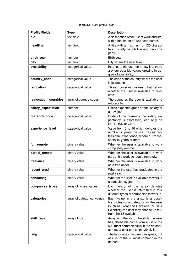
3.1 User profile fields . . . . . . . . . . . . . . . . . . . . . . . . . . . . . . . . . . . . . . . . 33
3.2 Job Descriptions fields . . . . . . . . . . . . . . . . . . . . . . . . . . . . . . . . . . . . . 34
3.3 Parameters for the text vectorizers . . . . . . . . . . . . . . . . . . . . . . . . . . . . . . 37
3.4 Number of Singular values used on LSA and maintained variance . . . . . . . . . . . . 37
3.5 User to User similarity weights and measures . . . . . . . . . . . . . . . . . . . . . . . . 40
3.6 Job to Job similarity weights and measures . . . . . . . . . . . . . . . . . . . . . . . . . 41
3.7 Job experience level similarity matrix . . . . . . . . . . . . . . . . . . . . . . . . . . . . . 41
3.8 User to Job match weights and measures . . . . . . . . . . . . . . . . . . . . . . . . . . 42
3.9 Job to user experience level similarity matrix . . . . . . . . . . . . . . . . . . . . . . . . 42
4.1 Parameter space for U2U CF . . . . . . . . . . . . . . . . . . . . . . . . . . . . . . . . . 53
4.2 Parameter space for I2I CF . . . . . . . . . . . . . . . . . . . . . . . . . . . . . . . . . . 53
4.3 Parameter space for I2I CBF . . . . . . . . . . . . . . . . . . . . . . . . . . . . . . . . . 53
4.4 Parameter space for U2U CBF . . . . . . . . . . . . . . . . . . . . . . . . . . . . . . . . 53
4.5 Parameter space for Funk’s SVD . . . . . . . . . . . . . . . . . . . . . . . . . . . . . . . 54
4.6 Relationships on the 3A data graph . . . . . . . . . . . . . . . . . . . . . . . . . . . . . . 55
4.7 RMSE scores after parameter optimization . . . . . . . . . . . . . . . . . . . . . . . . . 56
4.8 Influence of number of applications restrictions on the dataset sizes . . . . . . . . . . . 58
4.9 RMSE of I2I CBF with different dataset requirements . . . . . . . . . . . . . . . . . . . . 58
4.10 RMSE of I2I CF with different dataset requirements . . . . . . . . . . . . . . . . . . . . . 58
4.11 RMSE of U2U CBF with different dataset requirements . . . . . . . . . . . . . . . . . . . 59
4.12 RMSE of U2U CF with different dataset requirements . . . . . . . . . . . . . . . . . . . 59
4.13 RMSE of Funk’s SVD with different dataset requirements . . . . . . . . . . . . . . . . . 59
4.14 Precision @ 3 score for the 6 models manually obtained . . . . . . . . . . . . . . . . . . 60
4.15 Data about each of the recruiters responsible for the manual evaluation . . . . . . . . . 61
4.16 Fraction of satisfied users by each model . . . . . . . . . . . . . . . . . . . . . . . . . . 61
5.1 Precision @ 3 score for the Hybrid Model . . . . . . . . . . . . . . . . . . . . . . . . . . 67
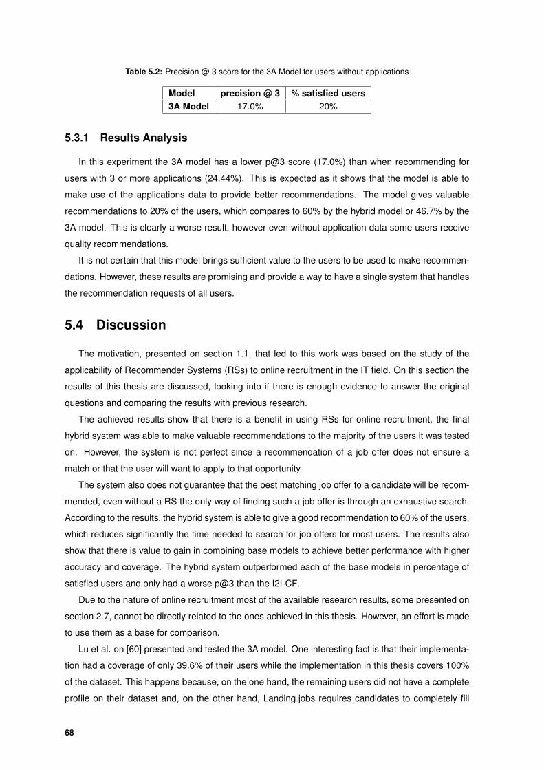
5.2 Precision @ 3 score for the 3A Model for users without applications . . . . . . . . . . . 68
xiii
Page 17
Abbreviations
RS Recommender System
IT Information Technology
CF Collaborative Filtering
CBF Content Based Filtering
I2I Item-to-Item
U2U User-to-User
MSE Mean Square Error
RMSE Root Mean Square Error
NRMSE Normalized Root Mean Square Error
MAE Mean Absolute Error
TF-IDF Term Frequency - Inverse Document Frequency
BoW Bag of Words
SVD Singular Value Decomposition
SVM Support Vector Machines
SGD Stochastic Gradient Descent
ALS-WR Alternating Least Squares with Weighted - λ - Regularization
LSA Latent Semantic Analysis
LSI Latent Semantic Indexing
PCA Principal Component Analysis
LDA Latent Dirichlet Allocation
EM Expectation Maximization
SALSA Stochastic Approach for Link-Structure Analysis
xv
Page 18
CBR Case Based Reasoning
GA Genetic Algorithm
CV Curriculum Vitae
p@n Precision @ n
p@3 Precision @ 3
xvi
Page 19
1Introduction
Contents1.1 Motivation . . . . . . . . . . . . . . . . . . . . . . . . . . . . . . . . . . . . . . . . . 31.2 Applying Recommendation Systems to Online IT Recruitment . . . . . . . . . . . 41.3 Contributions . . . . . . . . . . . . . . . . . . . . . . . . . . . . . . . . . . . . . . . 61.4 Thesis Outline . . . . . . . . . . . . . . . . . . . . . . . . . . . . . . . . . . . . . . . 7
1
Page 20
Recruitment processes consist of the series of events that occur since a company opens a job
position and that result in a candidate receiving an answer to an application. In the first step, called
sourcing, the company searches for potential candidates, active or passively. Then some candi-
dates apply to the position and the screening step starts, with the company reviewing the candidates’
profiles, rejecting the unfit candidate. The final step happens when the company finds a suitable
candidate and hires him.
With the growth of the internet, recruitment processes that were traditionally made through the
physical world have become increasingly web based. Companies use their websites and online job
boards, sites that aggregate job offers for different companies, to advertise their vacancies and can-
didates use the internet to search and apply to interesting opportunities.
A recruitment process has two main actors, the candidate searching for a job opportunity that fits
his skills and expectations and the company that is looking for someone to perform a role in their
organization.
The recruitment process occurring online has benefits, but also raises problems. On one hand
the candidates and companies have many more possibilities and can search much faster, but on the
other hand, there is a risk of information overload, having too many job opportunities or candidates.
Due to the amount of available job offers and candidates online, strategies are needed to help both
parties. This can be done with some filtering of the jobs or candidates or through recommendations.
In the recruitment context, a recommendation given to a candidate consists of a suggestion of a job
offer that matches his interests and characteristics. One given to a company is a suggestion of a
candidate that matches the company’s needs and expectations.
Despite these tools there are still downsides and inefficiencies to the recruitment process occurring
online. Most job boards are not able to provide personalized recommendations to the candidates,
with the filtering of opportunities being mostly based on the binary presence of keywords or search
terms on job descriptions. This leads job seekers to miss potential opportunities and companies
to have lower quantity and quality applications. This problem is more significant on the Information
Technology (IT) field, where a lack of talent is preventing companies from growing and is increasing
hiring costs. According to [3] this problem is the second biggest threat to IT company goals.
In 1992 the first Recommender System (RS), an algorithm that generates recommendations au-
tomatically, was proposed to help match users with their items of interest [4]. This was a system that
recommended emails to users so that they did not need to scan all available emails to see which
were interesting to them. Since then RSs have been in fast development and have been mainly used
on e-commerce systems, such as amazon.com or ebay.com, or online services such as pandora.com
or Netflix.com. There have been some attempts to apply them in the context of online recruiting.
However, a match between job offers and candidates depends on underlying aspects that are hard to
quantify, such as company culture, benefits, economic expectations of both parties, etc. This makes
the application of RSs harder to this area, which leads to a reduced research. This work analyses
the performance of some of the most common RSs techniques and one recent method with some
interesting properties. Based on these models an ensemble system is created to further improve
2
Page 21
performance on the test dataset.
This chapter gives an overview of this Thesis, starting by laying out the motivation and the context
behind the problem being analyzed on section 1.1. On section 1.2 a description of the most important
aspects of online IT recruitment is presented. The contributions of this work are presented on section
1.3. Finally section 1.4 outlines the rest of this Thesis.
1.1 Motivation
The internet has changed different aspects of our lives, job seeking is one of them. A process that
used to involve physically visiting companies and searching in newspapers has been revolutionized
[5]. Now the fastest way for someone to find job opportunities is to use search engines or online job
boards, such as monster.com or netempregos.pt [6]. There users can search with a set of terms that
describes what they are looking for and receive in return hundreds of offers [7] [8].
On some job platforms, such as linkedin.com or stackoverflow.com, there is even the possibil-
ity for candidates to create profiles and automatically subscribe to job opportunities that fit a set of
criteria. With these subscriptions and profiles, users receive a message every time a new job offer
that matches their interests appears.
These processes generate information about both the users and the companies. Users upload
their Curriculum Vitaes (CVs) and preferences and companies post job opportunity descriptions.
While interacting with the online systems the users generate data that implicitly conveys their prefer-
ences. This leads to the availability of large amounts of data that can be used to improve parts of the
recruitment process [9].
Online recruitment processes have inefficiencies and steps that could be improved:
1. Candidates have difficulties formulating what characteristics they want in a job and sometimes
have expectations that do not match their skills and experience [8];
2. Candidates end up being matched to hundreds of different opportunities and have to filter and
analyze all those to find the job offers they should apply to;
3. When using online job boards there is even a chance a user will not be shown the best fitting
job opportunities [8], due to their queries or profiles being improperly formulated;
4. On most current systems candidates are given generic recommendations and recommenda-
tions do not improve with the history of applications and previous actions of the users on the
system. The algorithms used are static, meaning that they do not learn from past data. For
instance, if a user searches for job opportunities that require django (a python framework for
web development) he/she might not be matched to a job offer on web development in python as
there is no explicit match. An algorithm with a learning component might be able to understand
that these two types of offers are related and that both should be suggested to the user [7];
On this thesis, the use of RSs as a solution to all of these problems is explored. RSs are a
subset of information systems that can be applied to domains where there exists a set of users and
3
Page 22
a set of items and where these users consume/buy/rate the items. Typical applications include movie
recommendations, book recommendations or product recommendations on e-commerce websites
and some attempts have been made in the field of online dating and online recruitment but with
limited success [9].
Improving on the online recruitment process through high quality recommendations would bring
varied benefits to candidates, companies and online recruiting websites. For online job boards or
recruitment websites, there is also a need to improve the user experience by being able to serve good
job recommendations [7] [9].
The goal of this work is a RS that brings value to both candidates and companies through useful
recommendations. These can be served to both candidates and companies, serving job recommen-
dations to the former and candidates to the latter. The usefulness of these will be measured according
to whether the candidate would be a good fit to the recommended position. The expected conse-
quences of such a system would be the saving of candidates, recruiters and companies time. The
recommendations would also increase user applications, improve user experience and consequently
revenue for online job boards and recruiting websites.
1.2 Applying Recommendation Systems to Online IT Recruitment
Although this work applies to all of online based recruitment it is specially focused on the IT field.
Due of its inherent nature the recruitment in this area tends to be much more online based, which
in turn makes it a great candidate for experimentation. On this particular field there is also a large
gap between the number of job opportunities and the amount of available talent, which means that
systems that help close this gap and make the recruitment process more efficient are highly valuable
[10].
RSs are a subset of Information systems, an area of research that focus on techniques to process
and manage data. Researchers have already attempted to apply these techniques to the online re-
cruitment field, strategies such as keyword search, text vectorization or topic models [7] [6]. However,
the fact that the best fit between job and candidates depends on underlying aspects that are hard
to measure [9] has deterred extensive research on the application of RSs to the area of personnel
selection.
The characteristics that influence choices of candidates when looking for a job have objective and
subjective components. Some examples of concrete characteristics where there is a straightforward
way of evaluating the fitness are:
Geography - When someone looks for a job, they do it for a specific geographical location or with
some geographic restrictions, due to family relations, visa restrictions, etc.
Skills - For jobs in IT there needs to be a match between the skills desired and the candidate’s profile.
Salary - The candidate’s expected salary needs to be in the ballpark of the company’s offering.
4
Page 23
Even these characteristics are not totally objective, a company might settle for a candidate that does
not fill all their requirements or a candidate might accept a very interesting offer that did not match is
previous expectations. The more subjective and underlying aspects of matching candidates and job
offers comprise:
Company culture - People perform differently in the same environment, for instance some prefer
more autonomy others less. Companies also vary in organizational structure, formality, man-
agement style, etc. However, it is not easy to define the culture of a given company or the
candidate’s preferences.
Candidate goals - Job seekers take into account their future goals, which in many cases are not
concrete and might change with the company/job offer they are evaluating.
Family and friends influence - When modeling a candidate’s preferences we have to take into ac-
count his family and friends influence. A spouse might have almost as much importance in
choosing a job as the candidate. The candidate’s feelings towards a company are also influ-
enced by his friends’ opinions and people who work there that he might know.
Online recruitment is not a traditional area of application of RSs, so it is important to compare it
to other areas, for instance movie recommendations is one of the most researched areas. The most
well known project in the area is the Netflix prize, a competition that occurred between 2006 and 2009
to improve Netflix’s own movie RS [11]. Another very influential project is the MovieLens benchmark
Dataset, that is almost 20 years old and already has more than 20 million movie ratings [12]. These
projects led movie recommendations to become one of the most common areas of research in RS.
When comparing it with online recruiting we notice clear distinctions:
Number of ratings - While a person might watch hundreds if not thousands of movies throughout
the years, he/she will usually only apply to a few job opportunities. This makes the application
of RSs much harder as they depend deeply on past data to generate recommendations.
Size of datasets - As a consequence of the previous point and as there are fewer people applying to
job offers online than rating movies the size of the recruitment datasets are orders of magnitude
smaller, instead of tens of millions of ratings we have tens of thousands.
Importance and thought given to ratings - When evaluating a movie a user is much more careless
than when choosing the company to apply to. This difference in the thinking process that lead
to the action might have an influence in the intrinsic data characteristics.
Size of the Item space - The movie ratings datasets usually contain a small percentage of movies
that aggregate the majority of user ratings. This does not happen on online recruitment as job
offers are temporary and as there are many more different job offers than movies. Also, while
a movie can be watched an infinite amount of times a job offer can only be filled by a single
candidate.
5
Page 24
An area of RSs research that is more similar to online recruitment is online dating [13]. It has also
not been the focus of researchers in the area, but some of its typical characteristics have an equivalent
in online recruiting. Despite existing some objective aspects when matching two people, such as age,
geographical location or even financial or educational level, the more determining characteristics are
subjective and vary greatly from person to person. For instance each person’s concept of beauty,
their goals for a relationship, their friends and family influence are individual preferences that relate to
the ones presented for online recruitment. Another significant aspect is the fact that the system has
to satisfy both parties in the recommendation, similarly to what happens in online recruitment.
These two distinct areas of application of RSs show the versatility of these techniques, that have
been in fast development in the past 20 years. On this thesis the focus will be on online recruitment,
but importing ideas, concepts and the experience of applying RSs in different areas.
To study the application of RSs to this area a real world dataset is used. It was provided by
Landing.jobs, an online recruitment platform focused on IT opportunities. It consists of 35485 user
profiles, 1532 job offers that belong to 502 companies. Between these entities a set of different
relationships are available, 20179 applications from candidates to job offers, 5240 bookmarks by
users of job offers, users following 1470 companies, 171 users that were hired for a given job offer.
Every application created by a user on Landing.jobs is reviewed by a recruiter that evaluates the
fitness of the match between candidate and the job offer. As a result the application can be sent to
the company that posted the job opportunity or it can be rejected. This filtering process guarantees a
match between the candidate and the job offer with the finer matching factors being evaluated by the
company, through interviews. The binary evaluation of the applications will be used as the training
data for the models tested on this thesis.
The goal of the models implemented based on this dataset is to make recommendations to both
the users and the companies on Landing.jobs. To be considered successful the system would have
to recommend matches that would pass the review process that happens on every application.
On this work different RSs models will be tested, with the goal of finding which models are most
appropriate to this dataset and as a consequence, to online IT recruitment.
1.3 Contributions
This work attempts to solve the shortcomings of the current systems used on online recruitment.
The goal is to find a model that can make use of the available data and to generate recommenda-
tions to both job seekers and companies. These recommendations can then be used to change what
job opportunities a user sees when using a job board or an online recruitment platform to improve
their experience.
The context explained on section 1.1 and on section 1.2 presents an opportunity to go deeper in
the exploration of the use of RSs on this problem.
The main contributions of this work can be summarized as:
1. Investigate the performance of five common RS models on a real world online recruiting envi-
6
Page 25
ronment;
2. Study of the application of graph based RSs to this problem, through the study of the 3A model,
in the regular environment and in a situation without interaction data;
3. Evaluate the performance of an hybrid model combining the knowledge gathered through the
study of the base models. Although the use of hybrid models in the field of RSs is not new, this
particular one is.
Besides these aspects, that were the main focus of this thesis, other efforts were also made on
related problems:
1. Study of different data processing techniques to apply on the job and candidate data;
2. Implementation of similarity and matching functions between candidates and job opportunities
based on both structured and unstructured data;
3. Analysis of the influence of dataset characteristics on the performance of the different models;
4. Analysis of the impact of ratings sparsity in the performance of RSs;
5. Application of a Genetic Algorithm (GA) to the parameter tuning of the RS models;
1.4 Thesis Outline
Chapter 2 of this thesis consists of a review of Recommender Systems and associated techniques,
as well as applications of Recommender Systems to recruitment. Additionally some support tools
needed for this work are covered, such as common text processing techniques. On chapter 3 the
methods implemented and tested for this work are presented and analyzed. Chapter 4 covers the
process of evaluating the models and the obtained results. Chapter 5 presents the method used to
combine the results of the base models and its performance evaluation. It also analyzes the thesis
results putting them into context with other research. Chapter 6 draws conclusions from this work,
analyzes what could be improved on every step of the processes in the models and analyzes which
areas and methods should be further investigated.
7
Page 27
2Recommender Systems
Contents2.1 What are Recommender Systems? . . . . . . . . . . . . . . . . . . . . . . . . . . . 102.2 Content Based Filtering Recommender Systems . . . . . . . . . . . . . . . . . . . 122.3 Collaborative Filtering Recommender Systems . . . . . . . . . . . . . . . . . . . . 162.4 Other classes of Recommender Systems . . . . . . . . . . . . . . . . . . . . . . . 202.5 Hybrid Recommender Systems . . . . . . . . . . . . . . . . . . . . . . . . . . . . . 222.6 Evaluation of Recommender Systems . . . . . . . . . . . . . . . . . . . . . . . . . 232.7 Recommender Systems for Recruitment . . . . . . . . . . . . . . . . . . . . . . . . 25
9
Page 28
This chapter gives a general overview of RSs and covers academic and industry solutions. The
main algorithms are explained and compared (sections 2.2, 2.3 and 2.4) as well as methods to inte-
grate the different approaches (section 2.5). The most important aspects to take into account when
evaluating RSs are covered on section 2.6. Finally on section 2.7 the specific case of recruitment is
analyzed.
2.1 What are Recommender Systems?
RSs are a set of techniques, algorithms and processes that can be applied to problems where
items have to be recommended to users. RSs select the most relevant subset of items for a given
user, usually in order to improve user experience and to increase revenue to the platform.
RSs work by filtering or ranking the available items. These systems take advantage of data about
the user to model user preferences and item characteristics to determine which items would be the
best matches. This data can be explicitly given by the user or extracted from its behavior. The most
common form is user-items rating pairs, where a given user rates an item on a predefined scale. An
implicit feedback example would be view counts of an item by a user.
Two good examples of recommender systems are:
• Recommending users new books to read based on the users past ratings of other books;
• Recommending users products to buy based on the products that they have on their virtual
basket;
2.1.1 Non-personalized recommendations
The most simple form of recommender systems uses only generic item ratings to create recom-
mendations. These are not specific for each user and in most RSs there is no information about the
user or its preferences.
The mean rating or difference between positive and negative votes are the most common base
formulas for non personalized systems. For instance IMDb [14] uses a weighted mean of their user
ratings to calculate each movie rating; Amazon [15] also uses the arithmetic mean to define the
rating of each product; ebay [16] lists a seller feedback performance based on the difference between
positive and negative reviews, with the goal of creating trust between buyers and sellers.
More complex formulas take into account the time of the rating or use a logarithmic scale to count
the votes/ratings among other metrics. A good example of such system is the one used on Hacker
News [17]. The most popular online forum Reddit [18] follows a more mathematical approach by
using the lower bound of the Wilson score confidence [19] to choose which comments it should rank
higher.
2.1.2 Personalized Approaches
The real power of RSs arises with the use of item and user data to generate specific recommenda-
tions. This allows users to find items with characteristics tailored to their needs and enables items that
10
Page 29
are not popular (not many users are interested in them) to get recommended, increasing the diversity
of consumed items.
2.1.3 Recommender Systems classification
There are many forms of classifying and characterizing RSs. This thesis follows the classification
presented on Mining Massive Datasets [20] and The Recommender Systems Handbook [21] with
small adaptations.
Some of the classes presented next overlap with each other, for instance a RS can be both Content
Based and Memory Based. This classification describes the main components in RSs.
Content Based Filtering (CBF) methods analyze user and item characteristics. They generate the
recommendations using the information they have about the user profiles and the items descrip-
tions and ignore the user actions. For this reason the generated recommendations tend to be
stable and only change on new items or new users.
Collaborative Filtering (CF) systems, in contrast, ignore the features of users and items, focusing
only on their relations. When a user rates or reviews an item the data is called explicit, whereas
implicit data is created from the actions of the user towards the items, such as buying or con-
suming an item. The idea behind the process is that users with a similar history of interactions
have similar preferences.
Knowledge Based Systems take advantage of domain knowledge to predict the recommendations,
usually through a manually defined score function that takes as input the features of the user
and the item, and outputs a match score.
Content Based, Collaborative Filtering and Knowledge Based Systems present different method-
ologies for creating a RS differing on which data to use in the models.
Memory Based methods generate recommendations based on similarities to past data, as in Neigh-
borhood based approaches. On these kind of models the computation is done at prediction
time.
Model Based systems create a model that describes the user preferences and item characteristics
and use that model to generate the recommendations. These models are created and trained
by analyzing the available data.
Memory and Model based methods establish two different approaches on how to process the data
to create the model and then generate the recommendations.
Hybrid Systems combine these different approaches to improve upon the individual performance
of each method, for instance a combination of a Content-Based and a Collaborative Filtering
approach may be able to overcome the shortcomings of each strategy.
11
Page 30
Association Rules try to predict co-occurrence of items in a transaction by analyzing the data. The
rules are derived from frequent patterns in the transaction data and represent items that are
frequently considered together of interest by the user.
Graph Based Methods model the available data as a graph and use graph properties to generate
the recommendations.
Machine Learning Methods such as decision trees, linear classifiers or linear regressors, can be
applied to create a RS based on items and users characteristics. These methods are usually a
subset of Content-Based methods.
In the following sections some examples of these model classes are presented and discussed in
more detail.
2.2 Content Based Filtering Recommender Systems
Content Based Filtering RSs use the available data to characterize items and user preferences
as a set of features. Given the most common features of the items that a user has demonstrated
preference, the system will suggest items with similar features.
This class of system descends from the Information Retrieval and the Document Classification
fields. For instance, on [22] is described a system that recommends interesting websites for its users.
The system uses a Bag of Words (BoW) approach to represent the websites text, weighting each
word with the Term Frequency - Inverse Document Frequency (TF-IDF) method and then a Naive
Bayes Classifier is trained to predict whether a website is of interested to a user.
2.2.1 Text Processing
A great part of the work behind building a Content Based Filtering RS is on processing the available
data into a usable format. When there is unstructured text data this work grows significantly. This
subsection does an overview of the most common techniques for text processing.
The BoW representation takes a collection of documents and represents each one as vector. First
a vocabulary of relevant words are selected from all the distinct words in the document collection.
There are various strategies to do this word filtering, usually the most common words in the language,
the words that appear in all documents and some words that do not convey any information are
removed. The vector will then be a representation of the document based on this set, each entry
representing the count / presence of a word in the document.
The goal of TF-IDF weighting is to highlight the most informative words in the documents, words
that appear in a document but are rare in the collection will have a high weight. This value is calculated
as the product of the term frequency (tf) (word count or binary presence) of a word and the inverse
document frequency (idf), defined as:
idf(t) = log(1 +N
nt) (2.1)
12
Page 31
where t is the word, N is the number of documents in the corpus, the document collection, and nt
the number of documents where term t appears at least once.
As each document is represented as a vector, each entry being the count or the TF-IDF score, the
corpus can be represented as a matrix where each row is a document and each column represents a
term in the vocabulary.
2.2.1.A Dimensionality Reduction
Applying the BoW results in a high dimensionality data representation which often leads to a very
sparse matrix representing the documents. The sparseness and the dimensionality affect negatively
the performance of the system that is built on top of this data.
The high dimensionality of the dataset leads to problems when training predictive models. The
number of parameters in the model usually grows with the dimensionality of the data. This makes the
model harder and slower to train and to use. A large number of parameters in a model also makes it
more probable to overfit the training data. That is the model stops learning the underlying information
in the data and starts memorizing all the noise in the data set, which leads to poor performance on
new examples. This problem is often called the Curse of Dimensionality [23].
Two common dimensionality reduction techniques for text data, Principal Component Analysis
(PCA) and Latent Semantic Analysis (LSA), are based on the Singular Value Decomposition (SVD),
and are applied to the matrix representation of the textual data [1].
Finding the SVD of a matrix X (n×m) means finding the matrices U (n× n), V (m×m) and Σ, a
diagonal matrix where its values are called the singular values of X, that satisfy:
X = UΣV T (2.2)
Figure 2.1: SVD equation in the form: XV = UΣ,Source: [1]
With PCA [1] the SVD is applied on the covariance matrix of X (n ×m) which can be calculated
by:
CX =1
mXXT (2.3)
The result is:
CX = UΣV T (2.4)
Where V are the principal components of X and T = UΣ is the transformation from the original space
to the basis V. The dimensionality is reduced by using only the k principal components with the larger
13
Page 32
singular values, with the transformation becoming:
Tk = UkΣk (2.5)
PCA makes three assumptions:
Linearity - it is possible to find a linear combination of the original basis that re-expresses the data;
Large variances have important structure - the components that present the largest variance rep-
resent useful information, while small variance components are mostly noise, small data varia-
tions with no significance;
The principal components are orthogonal - the algorithm finds the orthogonal basis vectors that
are ordered in terms of importance by the variance of the data along that direction. These
correspond to the eigenvectors of the covariance matrix of the data.
LSA (chapter 18 of [24]), also called Latent Semantic Indexing (LSI), applies SVD directly to the
term frequency matrix X and selects the k largest singular values to get a transformation as equation
2.5.
After applying these methods the transformed data is represented in a lower dimensional space
where each dimension is not a word anymore, but a linear combination of words and is uninter-
pretable.
A topic modeling approach, such as Latent Dirichlet Allocation (LDA) [2], can also be applied to
reduce the dimensionality of textual data. The LDA is a generative topic model, where the M docu-
ments in a corpus are modeled as a mixture of k topics and the topics as a probability distribution over
words. The model assumes that each document is generated by the following method, represented
on Figure 2.2 :
1. Choose the number N of words from a Poisson distribution;
2. Choose a topic mixture θ from a Dirichlet distribution of parameter α;
3. For each word w :
(a) Pick a topic z from θ;
(b) Choose the word conditioned on the topic z and on β;
α and β are corpus level parameters, they are a characteristic of the corpus and are set at the
beginning of the generating process.
For a given corpus and a fixed k, there are many methods to find the LDA model parameters, one of
them is by maximizing the Log Likelihood of the data using an iterative Expectation Maximization (EM)
algorithm [2].
Content based approaches are not limited to textual features, other data types such as categorical
or numerical information can be integrated into these systems.
14
Page 33
Figure 2.2: Graphical representation of LDA,Source: [2]
2.2.2 Strengths
Although Content Based Filtering methods usually have poorer performance than other methods,
they have some strengths. In this section some of them are discussed.
One characteristic of Content Based Filtering methods is that for a new user or item that has no
ratings these systems are able to generate recommendations, solving the Cold-Start problem (see
section 2.3.3).
Transparency is also characteristic of these methods, as the system is able to explain its rec-
ommendations. The explanation is based on the user and item features considered to make the
recommendation.
2.2.3 Limitations
There is a consensus in the literature about the shortcomings of Content Based Filtering RSs [25]
[26], this section discusses what are its main problems and how some authors try to overcome them.
For RSs of text based documents, such as web pages, there is a clear way for characterizing the
items, however for other domains such as movie or audio recommendations this is not straightforward.
On many systems only a very limited characterization of the items is available, which in turn limits
severely the quality of Content Based Filtering Recommendations.
One limitation of this representation of items is that it is not able to express the intrinsic quality
of the item. For instance the features of a movie, such as genre, length, year, etc, do not reflect the
quality of the movie.
The main problem with Content Based Filtering methods is their overspecialization, since these
types of RSs are usually unable to come up with interesting suggestions for users that are not similar
to previous ones.
There are not many academic RSs purely content-based ([27] and [28] are two examples) as the
problems of this approach soon became clear and researchers started to focus on pure CF Methods
(see section 2.3) and on hybrid systems (see section 2.5).
15
Page 34
2.3 Collaborative Filtering Recommender Systems
Collaborative Filtering (CF) algorithms attempt to explore the information present in the interac-
tions between users and items, using it to find users with similar preferences and items that may
appeal to the same type of user. Given two users with similar taste, A and B, and an item k that user
A demonstrated preference, a CF model will assume that item k will also be of interest to user B.
When using CF models it is assumed that user preferences and item characteristics are relatively
stable. If it was differently it would not be possible to extrapolate from the past ratings. In fact, there
are systems that account for some preference drift with time.
On CF algorithms there are two main approaches: Memory Based and Model Based.
2.3.1 Memory-Based
Neighborhood or Memory-Based Models rely on comparing the user with other users in the sys-
tem, trying to find the K most similar ones, the ones that are in its neighborhood. With these users
selected the RS combines their ratings to predict the user’s preferences.
2.3.1.A Similarities
The foundation of these models is a similarity metric that relates the users. There are various
approaches for this problem. For users a and b, the most common measures are:
Pearson correlation coefficient or simply correlation (present in [29] [30] [31] [32]):
r(a, b) =
∑j (va,j − va)(vb,j − vb)√∑
j (va,j − va)2∑
j (vb,j − vb)2(2.6)
where va,j is the rating given by user a to item j, va is the average rating given by user a and the sum
is made over all items.
Cosine Similarity (present in [29] [32] [33] [34]):
cossim(a, b) =Va·Vb‖Va‖‖Vb‖
(2.7)
where Va is the vector with all ratings given by user a.
Jaccard Similarity (present in [35] [34]) can be used when the ratings are binary values:
Jaccardsim(a, b) =|Ca ∩ Cb||Ca ∪ Cb|
(2.8)
where Ca is the set of items consumed by user a.
For all of these measures the time complexity is O(m) to compute the similarity between two users
and O(n2m) between all users, where m is the number of items and n is the number of users. This
clearly shows the severe scalability problem of memory based CF algorithms.
16
Page 35
2.3.1.B Predicting Ratings
Having the user a and its K nearest (most similar) neighbors the next step is to predict what would
be the ratings by a to items.
For item j the most intuitive way would just be to take the average rating given by the K users
to predict the rating user a would give. This method gives the same importance to ratings of all
neighbors, regardless of their actual similarity to user a.
The next logical step is to use a weighted average of the ratings [36], where the weights are the
similarity between user a and the K neighbors.
A different approach is to use a voting classifier to make the predictions when the possible
outcomes are discrete (e.g. 1 to 5 or binary), as suggested in [37]. The prediction is determined by
having each neighbor do a weighted vote and then selecting the outcome with the largest summed
votes, where the weights are again the similarities.
For all these approaches predicting a rating is a O(K) operation, where the number of similar
neighbors K is a constant.
2.3.1.C Item-Item Collaborative Filtering
Usually in a RS there are many more users than items and this difference tends to accentuate
itself as the system grows, as the set of available items is mostly stable. To overcome the scalability
problem an Item based collaborative filtering RS was proposed by Sarwar, et. al. [36].
The main difference between item based CF and user based is that the similarities are computed
between the items and then the predictions for a given user and item are based on the ratings of that
user to the similar items.
With this algorithm the time complexity becomes O(n) to compute the similarity between two
items and O(m2n) between all items, where m is the number of items and n is the number of users.
However, this does not solve the problem for systems where the number of items is large or is growing.
This approach was adopted in many large scale systems, for instance on Amazon.com [33], and
became a standard approach on the following years [38] [37].
2.3.2 Model-Based
Model-Based or Latent factor models comprehend a set of algorithms that try to characterize users
and items with latent factors that are inferred from the ratings data [39] [40].
Latent Factor CF models appeared under the spotlight on the Netflix Prize, a contest to beat by
10% the Mean Square Error (MSE) score of Netflix’s algorithm [11]. The contest involved thousands
of teams competing for three years to win a 1 million dollars prize. It was not just the prize that
attracted researchers from all over the world, for the first time a high-volume and high-quality dataset
was available. The dataset consisted of more than 100 million ratings of 18.000 movies by 500.000
users.
17
Page 36
It was in this competition that Simon Funk adapted the SVD algorithm (see section 2.2.1.A) to
factorize sparse matrices and then to generate predictions from the decomposed matrices [41].
The general idea behind matrix factorization methods is to try to find the low-rank matrices P of
size k × n and Q of size k ×m that approximate the ratings matrix R of size n ×m, where n is the
number of users, m the number of items, k is the number of factors for each user and item and k � m.
R ≈ PT ·Q (2.9)
What equation 2.9 means is that the rating of item i by user u, ru,i becomes:
ru,i ≈ pTu · qi (2.10)
where pu ∈ Rk is the vector with the user factors and qi ∈ Rk is the vector with the item factors. These
factors do not necessarily represent interpretable dimensions, however, we can think of the item
factors as characteristics (for instance a gender for a movie) and the user factors as the preference of
the user to those characteristics (whether a user likes a certain movie gender).
On [42] the authors define a baseline predictor bu,i to evaluate matrix factorization methods, which
is based on the average rating µ, the user bias bu and item bias bi defined as the average deviation
from the mean of the user ratings and item ratings.
bu,i = µ+ bi + bu (2.11)
Both bias can be estimated simultaneously by solving a least squares problem or by decoupling their
computations with, [42]:
bi =
∑u ru,i − µλ2 + li
(2.12)
where li is the number of ratings of item i, the sum is over all u that rated item i and λ2 is a regular-
ization parameter, and
bu =
∑i ru,i − µ− biλ3 + lu
(2.13)
where lu is the number of ratings of user u, the sum is over all i that have ratings by user u and λ3 is
a regularization parameter.
To remove the biases and mean from the responsibility of latent factors, qi and pu, equation 2.10
becomes:
ru,i ≈ µ+ bi + bu + pTu · qi (2.14)
As mentioned the user preferences can drift with time and to account for this the user biases
bu and the user factors pu can be consider dynamic and be modeled as functions of time. Some
examples of this approach can be found in [42].
2.3.2.A Finding the Low-Rank Matrices
With the prediction model defined the next step is to estimate the best values for the factors. The
first thing to note is that this can only be done using the known ratings, so in this process the unknown
values of ru,i are ignored and the MSE is minimized on the rest.
18
Page 37
There are two main approaches to this, the simpler one is to use Stochastic Gradient Descent
(SGD) as Simon Funk did in his first SVD model [41]. This iterative method estimates the gradient of
the error for each rating and for each parameter to update the values of each parameter. Usually, a
regularization term is added to avoid overfitting the data [42].
For a given training case ru,i, the parameters are updated by following the opposite direction of
the gradient of the error eu,i = ru,i − ˆru,i, where ˆru,i is the estimated value of ru,i, yielding:
bu(k + 1) = bu(k) + γ ∗ (eu,i(k)− λ1 ∗ bu(k)) (2.15)
bi(k + 1) = bi(k) + γ ∗ (eu,i(k)− λ1 ∗ bi(k)) (2.16)
qi(k + 1) = qi(k) + γ ∗ (eu,i(k) ∗ qi(k)− λ1 ∗ qi(k)) (2.17)
pu(k + 1) = pu(k) + γ ∗ (eu,i(k) ∗ pu(k)− λ1 ∗ pu(k)) (2.18)
where λ1 is the regularization term, γ is the learning rate that controls the speed of SGD and k
denotes the kth iteration of the SGD algorithm.
The computational cost of one iteration of SGD grows with the number of ratings, which means
this approach does not scale well when the ratings matrix, R, is not sparse.
The other approach is to use Alternating Least Squares with Weighted - λ - Regularization
(ALS-WR) method presented on [43]. The proposed solution alternates between fixing one of P or
Q and solving the least squares problem with regularization to find the other matrix. Fixing either
matrix turns the problem into a quadratic problem. This approach has two advantages: it is easily
parallelized and scales better with the number of ratings, which mean it can be used when is not
sparse.
2.3.3 Cold-Start
When analyzing CF methods one major problem has been purposely ignored with these algo-
rithms. What happens when we do not have ratings for a user or for an item? Simple, we cannot
make a prediction using a pure CF model. Both Memory-based and Model-based algorithms need
ratings from user u and item i to make prediction for the rating ru,i.
There are many approaches to try to deal with this problem, but essentially the best ideas are to
incorporate content information about item and users or to use implicit feedback. Some approaches
use an hybrid RS with a Content-Based model and a CF model, others use Association Rules or
User/Item clustering [44] [45].
Incorporating content information mitigates the cold-start problem as this information is available
from the moment the user or item are introduced in the system, allowing recommendations to be
made even when there are no ratings for that user or item.
Association Rules and clustering techniques can make recommendations to users and items with-
out ratings by relating them to other users and items that do have ratings.
19
Page 38
2.4 Other classes of Recommender Systems
Although Content-Based and CF are the most used techniques in RSs there are other important
methods that are used to complement these traditional approaches.
2.4.1 Graph Based
Some authors have tried to model the RS data as a graph [46] [47]. One simple way of doing
it is as a bipartite graph, where there are two types of nodes and the edges only connect nodes of
different types. On RSs usually one type of nodes are the users, the other the items and the edges
of the graph are the ratings/feedbacks between users and items. The graph representation allows for
new ways to explore the data and to integrate other types of information into the system.
In [48] the authors propose a new similarity measure that can be used in the CF framework pre-
sented in section 2.3, instead of the measures analyzed on section 2.3.1.A. The proposed similarity
measure, recommendation power, simulates multiple runs of a two-step random walk on the bipar-
tite graph. The two step random walk finds similar users or items based on their shared neighbors. It
is is calculated between users with:
rp(u, v) =∑i∈I
ru,iRu
rv,iRi
(2.19)
where I is the set of all items, Ru is the sum of all ratings given by user u, Ri is the sum of all
ratings received by item i and ru,i is the rating given by u to item i. Equation 2.19 calculates the
recommendation power between two users, however this can be easily altered to calculate between
two items:
rp(i, j) =∑u∈U
ru,iRu
ru,jRj
(2.20)
where U is the set of all users, Ru is the sum of all ratings given by user u, Rj is the sum of all
ratings received by item j and ru,i is the rating given by u to item i.
There are three interesting properties to the recommendation power measure:
1. It is not necessarily symmetric as it can happen that rp(u, v) 6= rp(v, u);
2. The values are normalized, a sum of the recommendation powers of a user sums to 1;
3. The recommendation power decreases with the sum of the ratings a user made;
This measure tries to capture the similarity between users and between items based on the com-
mon ratings. The idea behind this measure is that a user is given a quantity called "power" that he
distributes between the items he rates and the users that rate those items. This way pairs of users
have high recommendation power if they rate the similar sets of items with similar ratings.
On 2013 [49], Gupta et al. presented the "Who to Follow" system used at Twitter. This is a graph
based RS that uses the Stochastic Approach for Link-Structure Analysis (SALSA) algorithm [50]
to recommend which users to follow on Twitter. On the same work other algorithms are analyzed,
however SALSA achieves the best performance. All the system is implemented to work with the
20
Page 39
graph in memory, which restricted some solutions. The goal of the paper was to obtain a working
system in a short amount of time that could be used in production.
The problem studied on [49] is different from the typical RS setup because there is not a clear
distinction between users and items, the user is recommended other users he should follow. To over-
come this the authors define a bipartite graph where "hubs" left side of the graph is the user’s "circle of
trust" and the "authorities" right side are the users that the "hubs" follow. Then the SALSA algorithm
performs 2 step random walks starting from both sides and this way creating recommendations from
both groups. The "authorities" as the interests of the users and the "hubs" as the similar users.
2.4.2 Association Rules
Association rules are mined from the data and try to predict which products are bought or con-
sumed together based on the other items in that purchase or transaction, also called "basket analysis"
as they first appeared in e-commerce systems. For instance, in a supermarket data the rule:
{onions, potatoes} => {burger}
could be used to describe that usually when a costumer buys onions and potatoes also buys burgers.
These rules are generated from the co-occurrence counts of items and are selected with the goal
of explaining the maximum amount of data.
There are many different algorithms to find association rules, but they are not covered in this thesis.
One example is the algorithm AprioriHybrid [51] presented by Agrawal and Srikant that is linear on
the number of transactions.
Association rules are effective in finding relations between items, however they have not become
mainstream in the RSs field due to their similarity, with less flexibility, to item-based CF. This approach
is however used to fight the problem of cold-start in hybrid RSs [44] [45].
2.4.3 Knowledge Based Systems
Knowledge Based Systems exploit domain specific knowledge to create an automatic method of
generating the recommendations for each user. These systems are usually case specific and do not
have a learning component, which leads to a good performance at first, but a tendency to lag behind
Content-Based or CF approaches on the long term.
Critiquing Based RSs are an example of Knowledge Based Systems and are based on a con-
versional style interaction between the user and the system [52]. The system asks the user feedback
on its recommendations to improve the quality of the next recommendation.
Case Based Reasoning (CBR) a paradigm of problem solving that uses specific knowledge from
previous experiences in solving concrete problems [53]. The solving process of CBR systems for a
new problem can be described in five steps:
1. Retrieve - Find in the past solved problems the set of cases that are similar to current problem;
2. Reuse - Use the retrieved cases to generate a solution for the current problem;
21
Page 40
3. Revise - Adapt the solution given the constrains of the situation;
4. Review - Evaluate the quality of the presented solution, if needed go back and generate a new
one;
5. Retain - Add the new problem and solution to the case database for future use;
This process clearly shows that CBR models are highly dependent on similarity measures between
cases, in the RSs field this can lead to a lack of diversity in the recommendations [54].
2.4.4 Demographic Systems
One of the most simple types of RSs are Demographic Systems which only recommend items to
users based on their demographic profile. One simple example is users being redirected to websites
based on their location or language [21]. The most common demographic characteristics used to
make recommendations are location, language and age.
Due to their simplicity and despite the wide use this type of systems have not been widely re-
searched in the RS field.
2.4.5 Machine Learning Models
More traditional Machine Learning algorithms or related techniques can be used in the RSs prob-
lem [55], techniques like dimensionality reduction, clustering or classification are common [21]. These
models are usually a part of Content Based Filtering approaches [27] [28]. Decision Trees, Support
Vector Machines (SVM) and Neural Networks are some of the most common learning algorithms.
Decision trees have been commonly combined with association rules to create RSs [21]. On [56]
the authors present a RS for online purchases where a combination of decision trees and association
rules have been used. The decision tree is used to filter which users should receive recommendations.
In terms of performance, Linear classifiers on the CF framework have presented similar results as
Memory Based approaches with the advantages of being faster on prediction time [57].
Bayesian Classifiers are also commonly used to build RSs [21]. On [58], for instance, the authors
implement a Naive Bayes classifier on a content-based model.
These techniques are also commonly used to combine the results of different models in Hybrid
RSs [29].
2.5 Hybrid Recommender Systems
As each different approach to RSs has its own disadvantages, researchers started trying to com-
bine different models. Combining different methods leads to gains in performance and to fewer of the
drawbacks of each individual method. This section gives an overview of the most used techniques to
create an hybrid RS.
22
Page 41
On 1997 the Fab system was presented [26] as a hybrid approach to recommending webpages
to users, with the goal of overcoming both the weaknesses of Content Based Filtering and CF ap-
proaches. This was one of the first RS that served as a basis for the ones that followed and showed
results beating previous non-hybrid systems.
In [29] Burke classifies the different approaches to hybrid RSs into the following categories:
Weighted RSs combine multiple recommendations coming from different models, which have a given
weight, to select the final recommendation.
Switching RSs serve recommendations from different models according to the context, for instance
a system could use a Content Based Filtering model to generate recommendations for new
users and a CF model for users with more ratings.
Mixed RSs provide recommendations from different models at the same time. This is only possible
as in many cases a user is given more than one recommendation simultaneously.
Feature Combination is the method of integrating the output of some models with item or user fea-
tures and then train the final RS on top of that.
Cascade methods combine RSs models in sequence where each model only selects items to rec-
ommend from the set of items recommended by the previous model.
Feature Augmentation methods use a first RS to generate pseudo-ratings that are then fed has data
for the final algorithm.
Meta-level RSs generate a model of the users and the items with one algorithm and then use that
model as input for another RSs method. This allows the last model to work with compressed
representations of the user and item’s characteristics.
2.6 Evaluation of Recommender Systems
Evaluating RSs is not a straightforward task, since there are many distinct and even contradictory
characteristics to bear in mind. On chapter 8 of the Recommender Systems Handbook [21] the
authors present some of the most commonly desired properties of RSs:
User Preference - Or User Satisfaction is an important measure of RSs quality, however it agglom-
erates many of the system characteristics and does not give insight into how to improve it.
Prediction Accuracy - The first characteristic analyzed when evaluating RSs, usually comparing the
predicted rating with the actual value or whether each recommendation is relevant to the user.
The most common metrics are the Root Mean Square Error (RMSE), the Mean Absolute
Error (MAE) for non binary values, for instance when trying to predict an item rating on a 5 point
scale.
RMSE =
√∑(x− x)2
N(2.21)
23
Page 42
MAE =
∑|x− x|N
(2.22)
where x is the real value and x the predicted value. For classification tasks such as a prediction
of binary values there are three important measures to understand: accuracy, precision and
recall. To understand the measures it helps to look at the confusion matrix on table 2.1.
Table 2.1: Confusion matrix of a binary classification task
Reality1 0
Prediction 1 true positves (tp) false positives (fp)0 false negatives (fn) true negatives (tn)
With this knowledge we can define the measures:
Accuracy - The percentage of examples that the system predicts the value correctly:
Accuracy =|tp + tn|
|tp + tn + fp + fn|(2.23)
Precision - The percentage of examples that were correctly predicted as positive out of all that
were selected as positive:
Precision =|tp|
|tp|+ fp|(2.24)
When making recommendations the measure Precision @ n (p@n) can be used to evalu-
ate the percentage of correct recommendations out of all that were made, where n is the
number of recommendations made for each user.
Recall - The percentage of examples that were correctly predict as positive out of all that should
have been selected as positive:
Recall =|tp|
|tp + fn|(2.25)
F1-score - To evaluate both the precision and recall at the same time the harmonic mean of
both can be used:
F1-score = 2 · Precision · RecallPrecision + Recall
(2.26)
Coverage - Some RSs algorithms are not able to generate recommendations to all users or to all
items due to lack of information or to the Cold-Start problem. So the percentage of users and
items covered by each system are essential performance indicators.
Confidence - The confidence the system has in each of its recommendations, for models that have
it.
Trust - If users trust the system’s recommendations that increases user usage.It is even sometimes
worth recommending items that the user already knows and values to increase this trust.
Novelty - A recommendation is considered novel if the user has not been in contact with the item.
This is important if a RS is to add value to the user.
24
Page 43
Serendipity - Measuring how surprised the user is by the recommendations, not only it was a novel
item but also it was unexpected.
Diversity - If the recommendations cover different item categories and have differences between
each other then the system is considered to be diverse.
Utility - The utility of a RS can be evaluated from two perspectives, the user and the owner of the
system. There is utility for the user if the recommendations bring him value. For the owner the
utility comes from increased revenue, increased user engagement or other business metric.
Robustness - Since malicious user might try to game the system, it is desirable that a RS is able to
ignore false information and maintain recommendation quality in that situation.
Privacy - As users trust the RS with their information and with their preferences, it is the system’s
designer responsibility to ensure no one else has access to it.
Adaptivity - A measure of how the system adapts to changes in the users preferences, the items
characteristics, to new items, etc.
Risk - Some recommendations can have a certain amount of risk to it’s users associated with the
outcome of following the recommendation. Therefore evaluating not only the expected value of
the recommendation utility but also its variance might make sense for some systems.
Scalability - The ability of the system to keep serving recommendations while the user and item
number grows.
The balance between these properties is problem dependent. In the case being studied the fo-
cus will be on prediction accuracy, coverage and utility. The accuracy will be evaluated using the
RMSE and Precision @ 3 (p@3) metrics. The coverage will be based on the percentage of users
that will be able to receive recommendations from the implemented systems. And the utility will be
estimated from the user perspective with the average number of users that receive at least one good
recommendation.
2.7 Recommender Systems for Recruitment
Recruitment and more specifically IT recruitment is not one of the most common areas of research
on the RSs field, as explained on section 1.3. However, some approaches have been proposed, in [9]
a survey of those methods is made with a very careful analysis of each approach.
This section covers some of the most effective and interesting approaches, presenting their strengths
and weaknesses as well as their applicability to the given problem and data.
2.7.1 Collaborative Filtering for online Recruitment
In [59] Rafter, et. al. made one of the first attempts of applying CF to the online recruitment
problem. Two approaches were tested, the traditional user to user neighborhood based method
25
Page 44
presented on section 2.3.1 and an altered version that first clustered users with single link clustering
and then used the clusters of each user as the neighborhoods. The goal was to overcome the problem
of small data overlap between the users and not to be dependent of direct relationships between
users. There is a disadvantage with this approach, because there is no link from the user to some
users in its cluster, there is no way to rank the neighbors influence and all of them have the same
importance when generating the recommendations.
There is a significant difference between the data used on [59] and the data used on this thesis.
The authors use only the visits of job offers by the users as a source of information, only the number
of visits and the read time are considered. In this thesis the focus is on applications and their success.
The evaluation of the work on [59] was done manually. Ten random users were selected each from
a different community (cluster) and both methods were used to generate 10 recommendations. These
recommendations were then graded on ternary scale (1, 2 or 3) and the score of each method was
obtained by normalizing the sum by the maximum score of 30. One important detail of the evaluation
is that the recommendations were graded based on the similarities to the jobs on the user profile, not
based on whether the user is fit for that job.
2.7.2 Recruitment Data as a Graph
In [60] the data from a recruitment website is modeled as a directed, weighted graph. On that
graph an altered version of the Page Rank algorithm [61], the 3A algorithm introduced by Helou et
al. on [62], is used to determine which entities (graph nodes) are more important to other entities.
The weighted graph consists of three different types of entities: users, companies and job offers.
There are also many different types of possible relationships between the entities:
Apply - bidirectional relationship, when a user applies to a job offer ;
Posted - bidirectional relationship, when a company posts a job offer ;
Favorite - unidirectional relationship, when a company favorites a user ;
Like - unidirectional relationship, when a user likes a job offer ;
Visit - unidirectional relationship, when a user visits a job offer ;
Similar - bidirectional relationship that can exist between any two entities of the same type and that
is computed with a content based strategy;
Each of the relationships has a transition matrix T e of shape N × N , where N is the number of
nodes and e is the relationship. The entries of the matrix follow
T ei,j =
{1/outdegree(j), if i points to j0, otherwise
(2.27)
where the i and j are nodes and the outdegree(j) is the number of nodes that j points to.
Accompanying the transition matrix the dangling node matrix De also of shape N ×N is created.
This matrix guarantees the correct behavior of the 3A algorithm by complementing the transition
26
Page 45
matrix by making sure that the random walker can leave nodes that have no neighbors. Each entry
follows:
Dei,j =
{1/N, if outdegree(j) = 0
0, otherwise(2.28)
With these two matrices the 3A algorithm creates the matrix M that represents the random walk
starting at node i:
M =λ
NI + d
∑e∈E
we(Te +De) + puU (2.29)
where λ is the random jump factor, I is a N ×N all ones matrix, E is the set of all relationships, d
is the damping factor, we is the weight of relationship e, pu is the personalization factor and U is a all
zeros matrix except on row i. Consequently there is a different M matrix for each user, with only U
changing. This allows the M matrix without U to be calculated only once and then updated for each
user. The parameters are also subject to: ∑we = 1 (2.30)
λ, d, pu > 0 (2.31)
λ+ d+ pu = 1 (2.32)
Each entry Ml,j represents the probability of jumping from node l to node j during the random
walk. From this the rank vector R containing the importance of each entity to i can be estimated
iteratively by:
Rk+1 = MRk (2.33)
There are three components of the jump probability from one entity to another: the random jump
factor that guarantees that any node is reachable from every other node, the damping factor that leads
the random walk through the structure of the graph and the personalization factor which makes the
random walk more probable to jump to a neighbor of the origin node.
The final system is able to give recommendations to 39.6% of the users and it is evaluated man-
ually for the recommendations of 9 different entities where it usually outperforms a content based
approach and a CF system [60].
Due to the evaluation process used on [60] it is not clear the effectiveness of this approach. The
authors only manually evaluate the system on a very small sample, only 12 examples. However, there
are some interesting aspects to this method and further analysis is desirable. This method presents
a simple way of integrating different kinds of information into a single model, which helps to overcome
the cold-start problem as it is able to integrate content information. It is also based on the PageRank
algorithm, which means it can be computed incrementally and that allows its online computation and
update.
The data used by the authors is a close match to the available data for this thesis, despite being a
smaller amount. This makes this technique a good candidate to be adapted and tested on this work.
27
Page 46
2.7.3 Predicting job transitions
On [63] the authors approach the recruitment context differently. Instead of evaluating the fitness
of a candidate for a job offer or trying to rank the job offers based on the interest for the candidates, the
authors attempt to predict the next company a user will be working at based on the previous company
and its characteristics. The dataset used by the authors was mined from the internet and consisted
of about 5 million user profiles and about 1.5 million institutions (companies and universities). From
this data a job transition graph was created for each user, where each node is an institution the user
belonged to and each edge represents a transition from one institution to another.
The authors trained different machine learning algorithms to predict the next institution for a given
user based on its current institution and the user characteristics. They only present the results for the
best performing model, a decision table / naive bayes classifier hybrid algorithm from [64]. A baseline
predictor was implemented that labels all examples with the most common class in the training data.
The authors restricted the data used to only the 25 most frequent companies as labels. Three different
setups were created using different data samples, one with users coming from the 100 most common
companies and 100 most common universities, the second with users coming from the 100 most
common companies and the last with users coming from the 25 most common companies, the same
present in the label classes. The accuracy of the model was of 66.78%, 78.26% and 86.09% for each
of the three setups with the baseline predictor achieving about 15%.
This is an interesting approach that achieves impressive results, however it is limited in its utility
and being only valid for less than 0.013% of the institutions in the data renders this approach almost
void of business utility.
2.7.4 Recruitment as a Classification Problem
In [7] the authors have access to a private dataset from jobandtalent.com. This is a 80.000
users, 30.000 job offers and 1 million matches dataset. With a test set of 126 users with 1 to 5 best
job offers hand picked for them. The authors cluster (using LDA and K-means) the job offers and then
use ML classifiers (SVM) to match the users to a job offer cluster. They used Chi-squared feature
selection to reduce the 80.000 feature dimensionality to between 2.000 and 3.000 features.
To evaluate the system the authors use a test dataset consisting of 389 users and 126 job offers.
For each user the best job offers were selected which created 658 matches. The authors selected
the p@10 metric as the most important measure of system performance. The p@10 is the precision
of the system when generating a list of 10 ranked recommendations for a given user. The best
performing algorithm is the LDA clustering with Naive Bayes ranking that achieved a 70.44 % p@10.
To further evaluate the results the authors manually evaluated a ranked list of the 10 top recom-
mendations for 20 users. The authors found that on average more than half the recommendations
were considered useful for the users.
28
Page 47
2.7.5 Recruitment with a Content Based Filtering Approach
In [34] the authors present a framework to generate job recommendations using content based
approaches. One of the most interesting aspects of this work is that the proposed methods are
evaluated on a dataset that is available online, which was used on a Kaggle (kaggle.com) competition
in 2012.
The authors studied different approaches of representing the job offers data. They test a BoW
with TF-IDF representation and try adding social tags, generated from the content by a third party
software, to the jobs. Two different strategies of weighting the features are also tested and analyzed
using histograms.
On this work the evaluation and use of the data were different from the competition, so the results
are not comparable (on the competition the maximum precision was of 18% and the authors only
reach about 7%). However, the presented performance is low in the RS context even if this is one of
the few works that does large scale evaluation of a RS for the recruitment problem. Another flaw of
this work is not comparing the system with a CF approach.
2.7.6 Other Recruitment Approaches
In [65] job recommendations are generated by a simple linear combination of vectors representing
the candidates and the offers. These vectors are directly extracted from questionnaires and there is
no learning component in that system. The authors also do not present concrete results which makes
this approach even less attractive for further investigation.
In [6] a bilateral approach to RSs for recruitment is presented. The authors propose a system
capable of recommending job offers to users and users for job offers. The idea behind is that recruit-
ment is a bilateral process and both user and companies preferences have to be taken into account.
The system models users and job offers with a latent aspect model estimated with the EM algorithm,
described in detail on [66]. The authors evaluate the system with the MAE and manually, achieving
good results.
29
Page 49
3Methods
Contents3.1 The Data . . . . . . . . . . . . . . . . . . . . . . . . . . . . . . . . . . . . . . . . . . 323.2 Implemented Models . . . . . . . . . . . . . . . . . . . . . . . . . . . . . . . . . . . 423.3 Performance Evaluation . . . . . . . . . . . . . . . . . . . . . . . . . . . . . . . . . 47
31
Page 50
The goal of this thesis is to evaluate the use of the RSs on the context of IT Recruitment. The
models are used to facilitate both the work of recruiters and job seekers by generating recommenda-
tions of matches between users and job offers. For this work a dataset from Landing.jobs was used
to test hypotheses and evaluate the different approaches.
This chapter covers the chosen methods used to pursue this goal, from the analysis of the avail-
able data to the evaluation process of the implemented models. The available data has particular
characteristics that are explained and analyzed on section 3.1.1. To use the data to train and con-
struct the models it has to be processed, that transformation is explained on section 3.1.2. For the
memory based models similarity metrics are needed to establish the neighborhoods of both users and
job offers, these are described on section 3.1.3. The six different implemented models are described
in detail on section 3.2. These models need to be evaluated and optimized, this process is covered
on section 3.3.
3.1 The Data
The dataset used on this work consists of both the profiles of 35485 users and the descriptions
of 1532 job offers and the relational information between them. This data, provided by Landing.jobs,
contains not only information about user interactions with their system but also content data that
describes the users and the job offers. Its main components are the user profiles, the job descriptions,
the applications information between user and job offers and some extra relational information such
as the companies the job offers belong to and which companies and job offers the candidates are
following / bookmarking for later.
3.1.1 Available Data
The user profiles contain information about the user’s career, professional goals and skills. This
is the information that recruiters use to evaluate if the candidate is a good match for a job opportunity.
On top of this information the recruiters have access to the user’s CV, however the user’s CVs are
not available for this work. The most relevant fields of the user profile are detailed on table 3.1, these
fields have been slightly processed to make them easier to be further manipulated.
32
Page 51
Table 3.1: User profile fields
Profile Fields Type Descriptionbio text field A description of the users work and life,
with a maximum of 1200 characters.headline text field A title with a maximum of 120 charac-
ters, usually his job title and the com-pany.
birth_year number Birth year.city text field City where the user lives.availability categorical value Interest of the user on a new job, there
are four possible values growing in de-gree of availability.
country_code categorical value The code of the country where the useris located in.
relocation categorical value Three possible values that showwhether the user is available to relo-cate.
realocation_countries array of country codes The countries the user is available torelocate to.
salary_expectation number User’s expected gross annual salary ata new job.
currency_code categorical value Code of the currency the salary ex-pectancy is expressed, can only beEUR, USD or GBP.
experience_level categorical value Value from 0 to 10 which denotes thenumber of years the user has as pro-fessional experience, where 10 repre-sents 10 years or more.
full_remote binary value Whether the user is available to workcompletely remote.
partial_remote binary value Whether the user is available to workpart of his work schedule remotely.
freelance binary value Whether the user is available to workas a freelancer.
recent_grad binary value Whether the user has graduated in thepast year.
consulting binary value Whether the user is available to work ina consultancy job.
companies_types array of binary values Each entry of the array denoteswhether the user is interested in fourdifferent types of companies to work in.
categories array of categorical values Each value in the array is a possi-ble professional category for the user(such as Front-end Developer or DataScientist), the user may choose up to 3from the 15 available.
skill_tags array of ids Array with the ids of the skills the userhas, these ids come from a list of the500 most common skills in the dataset,at most a user can select 20 skills.
lang categorical value The languages the user can speak, outof a list of the 20 most common in thedataset.
33
Page 52
The job descriptions contain the descriptions of the desired candidates for the position. The job
requirements tend to be flexible and fit different types of candidates, for instance an opportunity might
ask for someone who knows Python or Java, while candidates skills are rigid and do not change with
the job opportunity. Because of this job descriptions tend to be more text based and because of that
harder to process automatically. On table 3.2 the most important fields of the job descriptions are
presented.
Table 3.2: Job Descriptions fields
Job Description Fields Type Descriptiontitle text field Job offer title, in a maximum of 120 characters.city text field City where the job offer is based.role_description text field Description of the opportunity, the company cul-
ture and what is expected from the candidates.main_requirements text field List of the main requirements for the job opportu-
nity, these are mandatory requirements that thecandidates must fill in order to be considered forthe position.
nice_to_have text field Requirements that are not mandatory, but thatthe company would like the new candidate to fill.
perks text field Benefits that the candidate can expect fromworking at the company.
country_code categorical value The code of the country where the offer is lo-cated in.
company_id number id The internal id of the company that owns the op-portunity.
experience_level categorical value One of the 4 possible levels of experience for ajob offer: junior, intermediate, senior and lead.
gross_salary_high number The maximum gross annual salary the companyis willing to pay for this position.
gross_salary_low number The lowest gross annual salary the company isexpecting to pay for this position.
currency_code categorical value The currency of the previous two fields.visa_support binary value Whether the company supports a visa request
for the candidate.relocation_paid binary value Whether the company will financially support the
candidates relocation.full_remote binary value Whether the job offer is full remote.full_remote_commute binary value Whether the job offer is full remote, but within
commuting distance.partial_remote binary value Whether the job offer is partially remote.work_from_home binary value Whether the candidate is allowed to work from
home on some days.citizenship binary value Whether it is required that the candidate has a
citizenship that allows him to work in that countrywithout requiring a visa.
staffing binary value Whether the job offer is for a staffing opportunity.consultancy binary value Whether the job offer is for a consultancy com-
pany.
Besides the user profiles and the job offer descriptions, the dataset contains more information that
34
Page 53
can be explored. There is a list of companies, which only have a name and an internal identifier. Be-
tween these three entity types, users, job offers and companies, there are in the dataset relationships
between them, some of them with attributes of their own. The relationships are:
Application - When a user applies to a job offer, it can have three macro states: rejected, reviewed or
hired. These states reveal if the application was considered unfit (rejected), if it was considered
good enough by the recruiter, but not by the company (reviewed) or if the candidate was hired
for the job offer, after having the approval of both the recruiter and the company (hired).
Follow - A user can follow a company to be notified of new job opportunities from the company.
Bookmark - A user can bookmark a job opportunity to save it for later.
3.1.2 Data Pre-processing
As presented on the previous section, a large part of the data is not well fit to be used directly with
the RSs algorithms. Because of that some pre-processing steps were taken, this section describes
them.
3.1.2.A Text processing
The text fields in the user profiles and job descriptions present the biggest data pre-processing
challenge since these fields have important and valuable information in a format that is not directly
usable by the available algorithms. The techniques introduced in section 2.2.1 were adapted and
applied.
These techniques are applied in the beginning of the system pipeline and taking into account the
goal of having a single data processing algorithm for the different models. It is not feasible to evaluate
the performance of the models with all the different text processing approaches. The search space for
all the possible choices is too large and this is not the focus of this work. As such, the text processing
step of the systems was defined without a direct feedback from the models performance. The design
of this methodology was based on other research and on the expectation of their influence on the
performance of the models. Moreover, the best design choices could be severely distinct between
models which would lead to different data processing for each model, which was not desired.
Many of the tested approaches ended up not being integrated in the final text processing solution
due to various reasons such as their poor performance on this data, their time or memory complexity
or even due to implementation limitations.
One of these studied techniques was LDA which was abandoned due to:
1. Being hard to estimate its performance, using log perplexity allows to determine how well the
model explains the data, but does not give a strong indication of the performance of the model;
2. Being a very complex model which needs a large amount of data to perform satisfyingly. This
is problematic specifically in the case of the job and user title where the usual text is only a few
words long.
35
Page 54
The final text processing pipeline consisted of:
1. Applying BoW to the text data;
2. Using Stemming and removing unwanted tokens to reduce the dimensionality;
3. Applying TF-IDF to weight the importance of each token;
4. Applying LSA to further reduce the dimensionality of the data.
This process is explained with more detail in the remainder of this section.
The fields where these techniques were applied are the user title and bio, and the job title,
role_description, main_requirements, nice_to_have and perks.
The first step of the process is to a apply a BoW approach to the fields. For this a tokenizer
function was created, this function receives the string with the text and its output is an array with one
word length strings. With the tokenizer the vectorization of the fields can be done by counting the
number of times each different token appears in a document. This creates for each document an
array of fixed length where each entry is the count for each token. To achieve this for a given text field
the steps are:
1. For each entry (document):
(a) Remove all HTML and URL’s from the text (using Beautiful Soup[67]);
(b) Remove all digits and punctuation characters;
(c) Use NLTK [68] word_tokenize to generate list of tokens;
(d) Remove from the list of tokens the NLTK stop words;
(e) Use the NLTK Porter Stemmer to retrieve the word stems;
(f) Return the word stems.
2. Add all different tokens to a vocabulary V ;
3. For each token in V :
(a) If the token appears in more than S % of the documents remove it from the vocabulary;
(b) If the token appears in less than R different documents remove it from the vocabulary.
4. For each document generate the array with the counts for each word in the vocabulary.
For each different field the parameters S and R need to be tuned, their values were selected by
hand maintaining a balance between the sparseness of the resulting matrix, the size of the vocabulary
and the information loss in this process. The values for each field are presented on table 3.3.
36
Page 55
Table 3.3: Parameters for the text vectorizers
Field Max Doc Frequency (S) Min Doc Frequency (R)
User title 60 % 30bio 60 % 30
Job Offer
title 60 % 4role_description 60 % 5main_requirements 60 % 5nice_to_have 60 % 10perks 60 % 8
On this processed representation of the text fields the TF-IDF method is applied, as described
on section 2.2.1. The TF-IDF weighting highlights the most informative terms of each document and
helps avoiding the use of the raw term frequencies.
The resulting TF-IDF weighted vector representations of the documents are of high dimensionality,
this would lead to overfitting and poor performance when using this data. To counter this problem the
LSA technique presented on section 2.2.1 was applied.
The first step is to normalize each vector representation with the L2 norm, defined in equation 3.1,
where x is a vector representation of a document.
||x|| =√x21 + x22 + x23 + ...+ x2n (3.1)
Then the matrix X, formed by the document vectors, is decomposed using SVD. Using the k
largest singular values the matrix is transformed into a lower dimensionality space of size k.
This transformation maintains only a part of the variance of X, but the amount of variance kept
grows with k. To find the most appropriate values of k for each different field an empirical technique
called "elbow method" or gap statistic was used [69]. The idea behind this approach is to observe the
plot of the percentage of variance maintained over k. This plot is monotonically increasing and usually
there is an "elbow", a value of k for which the variance stops increasing significantly. This "elbow"
value is chosen as the best value for k, a value that maintains a significant part of the variance without
having a too large dimensionality.
For each of the text fields the "elbow method" was applied and the values for k chosen are on
table 3.4. The figures 3.1, 3.2, 3.3, 3.4, 3.5, 3.6 and 3.7 show the application of the method to each
of the text fields.
Table 3.4: Number of Singular values used on LSA and maintained variance
Field Number of Components (k ) Maintained Variance
User title 60 56.29 %bio 400 60.59 %
Job Offer
title 20 61.22 %role_description 250 66.23 %main_requirements 200 62.63 %nice_to_have 60 56.67 %perks 125 79.53 %
37
Page 56
Figure 3.1: Elbow method applied to job titles Figure 3.2: Elbow method applied to jobrole_descriptions
Figure 3.3: Elbow method applied to jobmain_requirements
Figure 3.4: Elbow method applied to job nice_to_have
Figure 3.5: Elbow method applied to job perks Figure 3.6: Elbow method applied to user titles
38
Page 57
Figure 3.7: Elbow method applied to user bios
On some of these plots there is not a clear value of k that should be chosen (for example figure
3.6) as the "elbow" is not steep. In those cases one of the possible values was chosen so that it would
maintain the maximum variance, without having a too large dimensionality.
3.1.3 Similarity and Match Functions
For the content based methods a similarity measure between users and between job offers is
needed to establish the neighborhoods. These measures were created using the expert knowledge
of recruiters who helped define the most important characteristics to consider two users or two job
offers similar.
Besides the similarity measures a matching function, that scores the fitness between a user and
a job offer, was created, also based on expert knowledge.
On the next sections these three functions are presented.
3.1.3.A User to User Similarity
The similarity between two users reflects how close are their profiles professionally, it evaluates
their professional experience, skills and goals. This function was implemented as a weighted score of
the similarity of each field.
Table 3.5 describes how the measure is calculated. The feature weights were chosen based on
those that reflected more the professional profile of the user. The weights sum to 1, so if two users
have all fields equal they would achieve a perfect similarity score.
The similarity of each field has different ways of being estimated. For fields where there are a
finite number of possible values, the similarity is one if they are the same, the equality measure.
For fields that contain sets of values the Jaccard similarity, presented on section 2.3.1.A, is used.
The text fields that are represented in the LSA compressed vector representation have their similarity
estimated with the cosine similarity, also mentioned on section 2.3.1.A.
Finally there are two fields that needed specific similarity functions. The salary expectation
similarity between two users needed to meet the following properties:
39
Page 58
Table 3.5: User to User similarity weights and measures
User Profile Fields Weight Similarity functionbio 0.075 Cosine similarityheadline 0.15 Cosine similarityrelocation 0.025 Equalitysalary_expectation 0.05 Hand defined functionexperience_level 0.25 Hand defined functionfull_remote 0.025 Equalityfull_remote_commute 0.025 Equalitypartial_remote 0.025 Equalityrecent_grad 0.025 Equalityconsulting 0.025 Equalitycompanies_types 0.025 Jaccard similaritycategories 0.15 Jaccard similarityskill_tags 0.15 Jaccard similarity
1. Should range between 0 and 1, where 1 is a perfect score;
2. The score should be influenced not only by the difference in salary but also by the relative value
of the salary. That is a 60000 AC and 62000 AC salary pair should be considered more similar
than a 25000AC and 27000AC.
This was achieved with the following formulas:
salary_sim(S1, S2) = 1− clip(∣∣∣ln(S1
S2
)∣∣∣) (3.2)
clip(x) =
0, if x ≤ 0
1, if x ≥ 1
x, otherwise
(3.3)
For the experience level similarity the formula demanded similar properties, also in this case the
more years someone has of experience the less it makes a difference to have one more or one less.
The formula adopted was:
experience_sim(E1, E2) =
0.5− 0.05× E1− 0.05× E2, if (E1 = 0 or E2 = 0) and E1 6= E2
1−∣∣∣log10(E1
E2
)∣∣∣, otherwise(3.4)
3.1.3.B Job to Job Similarity
For the similarity measure between job offers the process was the same. A weighted score func-
tion defines which jobs are more similar and the help of recruiters was also valuable in defining the
important fields and weights. Table 3.6 compiles the calculation of the similarity measure.
The salary similarity function used was the same as in the user similarity. The experience level in
the job profiles is not measured in years, but in three levels so a new function needed to be defined.
For this purpose a similarity matrix between the four experience levels was used, table 3.7 contains
that matrix.
40
Page 59
Table 3.6: Job to Job similarity weights and measures
User Profile Fields Weight Similarity functiontitle 0.075 Cosine similarityrole_description 0.075 Cosine similaritymain_requirements 0.05 Cosine similaritynice_to_have 0.025 Cosine similarityperks 0.025 Cosine similaritycountry_code 0.025 Equalitypreferred_language 0.025 Equalitycity 0.02 Equalitycategory 0.075 Equalityrelocation_paid 0.02 Equalitywork_from_home 0.02 Equalityvisa_support 0.02 Equalityfull_remote 0.02 Equalitypartial_remote 0.02 Equalityfull_remote_commute 0.02 Equalitycitizenship 0.02 Equalityconsultancy 0.02 Equalitystaffing 0.02 Equalityskill_tags 0.20 Jaccard similaritysalary_low 0.025 Hand defined functionsalary_high 0.025 Hand defined functionexperience_level 0.175 Hand defined function
Table 3.7: Job experience level similarity matrix
Job experience levels junior intermediate senior leadjunior 1 0.4 0 0intermediate 0.4 1 0.4 0senior 0 0.4 1 0.7lead 0 0 0.7 1
3.1.3.C Job to User Match
Although trying to estimate the fitness of a match has deeper problems than finding similar users
and job offers the approach to creating the match function was the same. The goal is not that this
function is a RS by itself, but that it supports more complex RSs by providing an indication of whether
the user meets the requirements of the job opportunities.
Table 3.8 depicts the selected fields from both entities, the weight and the measure for each field.
The categories field is different for the user and for the job, as the user can choose up to three
categories, but the job only has one. The measure used gives maximum score if one of the user’s
selected categories is the same as the job offer.
The salary score between the candidate and the job offer takes into account both the salary_low
and salary_high field from the job. The similarity measure is calculated by the average of the salary
similarity, computed using equation 3.2, between the user’s salary_expectation and the job offer’s
41
Page 60
Table 3.8: User to Job match weights and measures
User Profile Field Job fields Weight Measure
salary_expectancy salary_high 0.15 Hand defined functionsalary_low
experience_level experience_level 0.25 Hand defined functionskill_tags skill_tags 0.25 Jaccard similarityfull_remote full_remote 0.025 Equalitypartial_remote partial_remote 0.025 Equalityfull_remote_commute full_remote_commute 0.025 Equalityconsulting consulting 0.025 Equalitycategories category 0.25 Presence
salary_low and salary_high.
The experience level match follows the same strategy from section 3.1.3.B, with a manually de-
fined matrix being used to get the scores, this matrix is depicted on table 3.9.
Table 3.9: Job to user experience level similarity matrix
User experience level0 1 2 3 4 5 6 7 8 9 10+
Job experience level
Junior 1 1 0.9 0.7 0.5 0.2 0 0 0 0 0Intermediate 0 0 0.2 0.5 0.9 1 1 0.9 0.5 0.2 0Senior 0 0 0 0 0 0.2 0.5 0.9 1 1 1Lead 0 0 0 0 0 0.2 0.5 0.7 0.9 1 1
3.2 Implemented Models
On this section the solutions that were explored are presented. The objective of the work here
described is to compare different RSs techniques on the dataset.
The data used for these models consists of the 14265 applications made by 2159 users to 1358
job offers, only users with three or more applications were considered. It is important to note that
this restriction led to only about 6% of the users being considered. Each application is given a binary
classification, 0 if it was rejected and 1 if it was reviewed and considered a good fit. Of the 14265
applications 8093 were rejected and 6172 were reviewed. No distinction was made between applica-
tions that led to a candidate being hired and that led to a reviewed application due to the small number
of hires (171) in relation to the number of applications. The goal of the RS to be created is also that
the recommendations would lead to the users applying and being reviewed.
3.2.1 Collaborative Filtering Neighborhood Models
To take advantage of the data from past user applications two memory based collaborative filtering
models were implemented, an User-to-User (U2U) and an Item-to-Item (I2I), see section 2.3.1.
To implement these models the first step is to define the similarity metric between users and
between job offers that will determine the neighborhoods. In the CF framework users, in this situation
42
Page 61
the candidates, are characterized by the interaction they have with the items, here the application to
a job offer. Users and items are then represented by their sets of applications, candidates by the job
offers they have applied to and job opportunities by the candidates that have applied to them.
This set based representation led to the use of the Jaccard Similarity defined on equation 2.8.
With this measure a user to user and a job offer to job offer similarity matrix was created.
3.2.1.A User to User Model
On the user to user model, when generating a recommendation for a given user the RS looks
for at most K similar users and based on the job opportunities that those users have applied to, it
generates the recommendation.
To generate recommendations for a user u the model predicts a rating ˆru,i between u and all job
offers available. The prediction for a given job offer i is computed by finding in the neighbors of u
users that also applied to i and doing an weighted average of the rating of those users. The process
is described by equation 3.5:
ˆru,i =
∑Kv su,v × rv,i∑Kv su,v + λ
(3.5)
where su,v is the Jaccard similarity between user u and user v, rv,i the rating of the application of user
v to job offer i and λ is a regularization factor to give lower scores when the similarity between u and
its neighbors is low.
There are two important details in this process:
1. To make sure only valuable information is added by the neighbors, only users that have an
higher similarity than the threshold parameter σ are considered neighbors;
2. The output of equation 3.5 is continuous in the interval [0, 1], but the possible values for each
application rating are 0 if it is rejected and 1 if it is reviewed. So the output is rounded to 0
(values below 0.4), 0.5 (values between 0.4 and 0.6) or 1 (values larger than 0.6), where 0.5
represents the situations where the RS is undecided.
This model has three parameters, the number of neighbors K, the similarity threshold σ and the
regularization factor λ. The process of choosing the values for these parameters is detailed in chapter
4.
3.2.1.B Item to item Model
The item to item neighborhood model searches for similar job offers that the user u has applied to
when predicting ˆru,i. Equation 3.5 becomes:
ˆru,i =
∑Kj si,j × ru,j∑Kj si,j + λ
(3.6)
where si,j is the Jaccard similarity between job offer i and job offer j
The remainder of the model details are equal to the user to user model, with the item to item model
having also the three parameters K, σ and λ.
43
Page 62
For both of these models, a recommendation can be done when the system predicts a rating of 1,
when the system predicts 0.5 it is not sure about the rating and so it does not make a recommenda-
tion.
3.2.2 Content Based Filtering Neighborhood Models
The memory based approach can also be used to take advantage of the user profiles and job
descriptions. Many RS only have access to the ratings data but in this work we have both the ratings
and the content data. The neighborhood model with a content based approach is very similar to the
collaborative filtering model.
Here the predictions are made based on the K most similar neighbors, but using content based
similarity matrices. These matrices are computed with the content similarity measures defined on
section 3.1.3. There is one matrix between all users with three or more applications and another one
between all job offers.
The U2U CBF model uses exactly the same process as the collaborative filtering user to user
model, with equation 3.5 being used to make the predictions where the difference is that su,v is
calculated differently, using the similarity measures from section 3.1.3.
The I2I CBF model is similar, using equation 3.6 with the content based similarity measure to
calculate si,j .
3.2.3 Funk’s SVD Model
Matrix factorization models have been outperforming other RS algorithms in the last few years,
so it makes sense to try one of these approaches. Simon Funk’s SVD algorithm was chosen and
implemented with the adaptations presented on [42] and as described on section 2.3.2.
Equation 2.14 reflects how the ratings ru,i between a user u and an item i are estimated with this
model. It used the baseline predictor defined on equation 2.11 and the dot product of the user factors
pu with the item factors qi.
To estimate these factors the SGD algorithm was used, following equations 2.15 to 2.18. To speed
up conversion on the biases bi and bu, they were initialized with equations 2.12 and 2.13. The user
and item factors pu and qi were initialized to 0.1 on all entries. This fixed value does not influence the
results because there is a global minimum that SGD is able to find with enough iterations, it serves
only to guarantee that the number of iterations needed doesn’t change between runs of the algorithm.
Two stop criteria were defined:
1. When reaching 50 iterations;
2. When after one iteration all updated values differed less than ε (set to 0.001) comparatively to
the previous iteration.
The learning rate γ was set initially and at each iteration of the model it was reduced to 90% of its
value. This simple update method for the learning rate allowed the model to converge faster on the
initial iterations and to take smaller steps when reaching the optimum.
44
Page 63
There are 4 parameters that control the behavior of this model:
1. The number of factors K that determines the length of the user factors pu and the item factors
qi;
2. The regularization parameter γ used on the SGD updates;
3. The regularization parameter of the job bias λ1;
4. The regularization parameter of the user bias λ2.
This RS model outputs a continuous prediction in the interval [0, 1] which is then used to rank the
items for recommendation. The system recommends the items with the highest predicted rating.
3.2.4 3A Algorithm
Besides the more common RSs approaches, the use of graph analysis techniques was also ex-
plored in this work. Following the methods presented on section 2.7.2 the 3A algorithm was also
implemented and tested on this data.
There are advantages to this approach, as it can combine all different types of available data. The
data was modeled with three entities, the candidates, the job offers and the companies. Between
these a set of relationships was established, some directly from the data others using the content
based metrics mentioned on section 3.1.3.
One clear advantage of this model is that it is not only dependent on the application data, so it can
generate recommendations for users or job opportunities that do not have applications yet. It uses
the content of profiles and the other relationships to make these recommendations. This led to much
more data being available for this model, for instance instead of just using 2159 users as in the other
models all 35485 were used.
The relationships have different weights and capture different characteristics of the entities they
connect. These can also be either bidirectional or unidirectional, which means that an entity can
influence another without being influenced back. The relationships are represented by weighted di-
rectional edges on the graph and the different types are:
Similar - Two entities are considered similar based on their content data, this relationship only exists
between users and between job offers as there is no content data for the companies. This
bidirectional relationship was determined by the metric presented on section 3.1.3, with only the
0.1 % more similar entities having the connection.
Match - Using the match function described on section 3.1.3 a match relationship was created to
reveal users that fit job requirements. This bidirectional relationship only exists between users
and jobs and only the pairs that have the highest 0.5 % score have the edge on the graph.
Follow / Bookmark - Users can specify companies they are interested on and receive notifications
of all their new job offers. Users can also bookmark interesting job offers to consider them again
45
Page 64
in the future. This information is transcribed to the graph as a single unidirectional relationship
from users to companies and to job offers.
Application - The bidirectional application relationship reflects only reviewed applications done by
users to job opportunities, applications that were considered to match the job offer require-
ments. This justifies the bidirectional property of this relationship as it reflects also the job offers
requirements.
Hire - This bidirectional relationship describes a successful application, when the user is hired for
the job. This is the most important relationship as it reflects the best possible outcome for an
application.
Own - Each job offer is owned by one company, this is reflected as a bidirectional relationship be-
tween job offers and companies. This helps relate different job offers from the same company.
With the available data the graph has:
• 37519 nodes (the entities), of which 35485 are users, 1532 are job offers and 502 are compa-
nies;
• 1261532 similarity relationships, of which 1259185 are between users and 2347 between job
offers;
• 274572 match relationships between users and job offers;
• 1470 follows by users to companies and 5240 bookmarks by users to job offers;
• 1478 owns between companies and job offers;
• 20179 reviewed applications between users and job offers;
• 171 hires between users and job offers.
Equation 2.29 and 2.33 denote the two main components of the algorithm: how the graph data
is used to create a matrix that represents the relationships between the entities and how from that
matrix an importance vector is computed for a given user.
As equation 2.29 shows there are three main parameters in the model, the random jump factor
λ, the damping factor d and the personalization factor pu. The remaining parameters are the weights
associated with each relationship. These are restricted by equations 2.31 and 2.32 and reflect the
relative importance of each relationship. The process of choosing the values for all these parameters
is detailed in section 4.1.3.
To find the importance vector for a given user equation 2.29 is used. Then a vector is initialized
with 1’s on all entries and the power method is performed according to the iterative equation 2.33, the
iterations stop when the difference between two iterations is smaller than ε for all entries.
46
Page 65
3.3 Performance Evaluation
This section describes the performance evaluation of the implemented models. First the approach
to evaluating and optimizing the models and choosing their parameters is detailed in sections 3.3.1
and 3.3.2. Then section 3.3.4 describes an experiment that simulates the evaluation of the recom-
mendations by users seeking a job offer.
The ideal evaluation environment for these models would be a real world scenario with users
receiving recommendations and applying to job offers. By measuring the interactions of users with
the models’ recommendations we would have an evaluation metric. As this is not possible, another
good option would be to serve recommendations to random users and then have recruiter experts
evaluate them, simulating the users behavior. However, this is too expensive and can not be done in
large numbers. So a preliminary automated evaluation was designed to select the best parameters
for the models and to estimate their performance. Then, with the models tuned, a manual evaluation
was done only for a small number of random users to have a more reliable evaluation.
The Neighborhood models and the Funk’s SVD model use the applications data to generate rec-
ommendations. As the goal of these systems is to generate recommendations that will turn into
reviewed applications this problem can be framed as the prediction of which pairs of user and job
offer will result in a reviewed application. With this in mind, cross validation was used to train and
evaluate these models.
3.3.1 Evaluating the models with Cross Validation
Cross Validation is a way to avoid evaluating a model using the data it has been trained on and at
the same time, a way to train it in the largest amount of data possible. There are many cross validation
strategies with different advantages and disadvantages. One of the most widely used and accepted
strategies is the K-fold cross validation which is used in this thesis.
The most simple training and testing procedure of a machine learning algorithm consists in splitting
the data into two sets. One used to train the model and the other to evaluate it. This method has two
significant problems:
1. Negative bias, the model will not perform as good as possible as it is not trained on all the
available data;
2. Bias for that specific split, the results only reflect the performance on a subset of the data which
will most likely not be similar to the whole dataset.
The bias leads to a lack of confidence on the performance of the model as it might be much better or
worse in the rest of the data and on unseen data.
To try to overcome these problems K-fold cross validation partitions the data randomly into K sets
of equal size and uses one as test set and the others as the training set. This process is then repeated
K times so that all K sets are used as test set and the performance is estimated as the average of
the K scores. This mitigates the bias because it allows all of the data to be used for training and
47
Page 66
testing. However, it is still not a perfect solution as the results are sensitive to the dataset partitioning
and might exhibit a large variance between the performance for each subset. Also there is still some
negative bias due to each evaluation only training in a subset of the dataset. More complex cross
validations strategies could have been used to mitigate these bias and variance problems further
such as repeated cross validation, stratified cross validation or bootstrap. For further reading see
[70].
As this automated result evaluation requires significant computer resources only a 5-fold cross
validation was made instead of the usual 10-fold or more complex approaches.
The measure chosen to evaluate the results was the RMSE, as some models had continuous
outputs and others discrete, despite the possible values for each recommendation being only 0 or 1.
For each run of the 5-fold cross validation of a single model and a set of parameters a RMSE was
obtained. The goal was to find the best parameters for each model, the ones that achieve the lowest
RMSE.
3.3.2 Parameter Optimization with Genetic Algorithms (GAs)
The parameter space is infinite and even if it is discretized into a finite space it is not feasible to
try every parameter combination. As such a simple GA was implemented to speed up and automate
the search following the ideas on An Introduction to Genetic Algorithms [71]. This does not guarantee
that the best parameter combination is found, but it allows to find a good one in a reasonable amount
of time. No other optimization technique was tested as the goal was not to evaluate the optimization
techniques, but to find a good set of parameters for each model. GAs were chosen for their flexibility
and easiness of implementation.
A GA is an optimization method inspired in the biological evolutionary process. The GA starts by
creating a population, a set of individuals each representing a solution (a parameter combination),
and then evaluates each individual, finding its fitness. This population is then evolved iteratively with
each new iteration results in a new generation of the population.
The main component of a GA is the evolutionary process that is responsible for generating the next
generation from the current one. The goal is that at each iteration the average fitness of the population
increases. For the algorithm to be successful a balance has to be reached between diversity in the
population and maintaining the best individuals. There are many ways to implement the update
process, for this work in concrete the process was chosen with some experimentation and based on
the most common methods.
The update process consisted of 3 mechanisms each responsible for a subset of the new popula-
tion:
1. 30% Elitists - The best performing individuals of the previous generation;
2. 50% Crossed individuals - Individuals generated by crossover of the elitists, taking half the
parameters from each of the elitists;
3. 20% Random new individuals - Generated by randomly sampling the parameter space.
48
Page 67
On top of the update process there is the mutation process that adds extra diversity to the population,
each individual in the population has a probability m of randomly having one of their genes (one the
parameters) changed. After this update there might be repeated individuals in the population, those
need to be removed and replaced by new random individuals.
The GA was used to try to minimize the RMSE of the Neighborhood and the Funk’s SVD models
over the discretized parameter space of each model.
3.3.3 Parameter Optimization for the 3A model
With the 3A model there is no clear way of evaluating the performance. It differs in how it is used
to generate recommendations. While in the other models the result is a prediction of a rating in the
interval [0, 1] for each pair of user and job offers, the 3A gives for each user a ranked list of the most
"important" job offers for the user. This list cannot be used to say whether a user would apply or not to
a job offer. Besides the fact that the model uses the applications to create the graph it is not possible
to apply the process of hiding some applications and asking the model to predict them based on the
remaining data.
The parameter for the 3A model were chosen with a variety of strategies: with some experimen-
tation following the process presented on the original paper [60], based on the domain knowledge of
recruiters and on some intuition.
The resulting parameters of these approaches for all models are presented on section 4.1.3.
3.3.4 Manual Evaluation
The automated evaluation serves as an estimation of the quality of the implemented models,
however it is just an estimation and not the reality. It focus only in a specific metric and that can
be misleading. In order to have a clear notion of the performance of the models an experimental
environment was set up by simulating a real world scenario of use of these models. The goal of
the models is to suggest job offers to the users to which they would apply and be considered good
candidates for the position.
To test the models performance in this task, 15 users with at least 3 applications (to maintain the
same environment where the models were trained) were randomly selected. Each of the models gen-
erated 3 job offer recommendations for each user. For the Funk SVD and the 3A models these were
the 3 job offers with highest predicted rating. For the Neighborhood models these were selected ran-
domly from the set of job offers that the model predicted would fit the user. These recommendations
were then evaluated by recruiters from Landing.Jobs, with indications to evaluate the fitness between
the user and the job offer as if the user had applied to the job position. As these evaluations are sub-
jective, because of a lack of information on the user and the job offer, two recruiters might evaluate
the same recommendation differently. Usually there would be an interview to assess the fitness of a
candidate for a job. To average out some of the subjectiveness of this process all recommendations
were evaluated by 3 different recruiters.
49
Page 68
As for some users the Neighborhood models do not predict any job offer as a good fit for the user,
the amount of recommendations they produce in this experiment might be lower than the 3 offers for
each of the 15 users that would be expected.
The measure used to evaluate the models is the Precision @ 3 (p@3), see section 2.6, which
represents the percentage of recommendations that were correct of the 3 made for each user. Each
recommendation pair is evaluated by 3 recruiters which either classified as a good or poor recommen-
dation. The resulting scores is one of 0, 1/3, 2/3, 1 depending on how many recruiters classified the
recommendation as good. The precision of a model being calculated as the average of these scores
for all recommendations of that model.
p@3(model) =
∑r∈R scorer
n(3.7)
where n is the number of recommendations the model did.
Another experimental setup was created to test the models for users that had not applied to any
job offer. The only model able to produce recommendations in this situation is the 3A model and was
the only one tested. Another 15 users were randomly chosen, all without any applications. For each
of them 3 job offers were recommended with the 3A model and evaluated by 3 recruiters to obtain the
p@3 for the model in this situation.
50
Page 69
4Results and Analysis
Contents4.1 Parameter Optimization . . . . . . . . . . . . . . . . . . . . . . . . . . . . . . . . . . 524.2 Automated Evaluation Results . . . . . . . . . . . . . . . . . . . . . . . . . . . . . . 554.3 Manual Evaluation Results . . . . . . . . . . . . . . . . . . . . . . . . . . . . . . . . 60
51
Page 70
This chapter presents and analyzes the experimental results obtained during the work on this
thesis. On section 4.1, the parameters obtained to optimize the models are presented as well as a
simple explanation of their meaning. Section 4.2 covers the main results for the automated evaluation
of the models, takes a look into their meaning and implications. Also on that section, the description
and results of small experiments done to explore the importance of different factors in the results are
presented Section 4.3 presents and analyzes the results of the manual evaluation for all the base
methods. The main metric considered is the p@3, however other metrics are included to paint a
clearer picture of the models performance.
The hybrid model which was constructed based on these results is presented and analyzed on
chapter 5.
4.1 Parameter Optimization
The process described in section 3.3.2 optimizes the parameters of the different models to min-
imize the RMSE. On this section the resulting parameter values are presented and analyzed. The
influence of each parameter is explained in order to understand the logic behind the chosen value.
This section covers first the neighborhood based models and then the Simon Funk SVD model. Their
parameters were chosen with the genetic algorithm and their cross validation scores. Then, the pro-
cess of choosing the parameters for the 3A model is described on section 4.1.3. The parameter
space for each model was chosen by trial and error, after each run of the GA the space was updated
by adding new possible values near the current best.
4.1.1 Neighborhood Based Models
The four implementations of neighborhood based models have three parameters that control their
operation.
1. The number of neighbors considered for each prediction;
2. The regularization weight that prevents too much importance being given when there are few
similar neighbors;
3. The similarity threshold, that determines which items or users are considered similar.
The number of neighbors for all models was capped at 100, due to the increased computational
cost.
4.1.1.A User-to-User Collaborative Filtering Model
The explored parameter space for the User-to-User (U2U) Collaborative Filtering (CF) model is
presented on table 4.1, with the parameters chosen by the genetic algorithm in bold. The resulting
RMSE score was of 0.4935 and the chosen parameters: (70, 0.15, 0.05).
52
Page 71
Table 4.1: Parameter space for U2U CF
Parameter Possible ValuesNumber of neighbors 10, 15, 20, 30, 40, 50, 70, 85, 100Regularization weight 0.0, 0.01, 0.02, 0.05, 0.07, 0.1, 0.15, 0.2, 0.3, 0.5, 0.8, 1Similarity threshold 0, 0.01, 0.025, 0.05, 0.07, 0.1, 0.15, 0.2, 0.25, 0.3
4.1.1.B Item-to-Item Collaborative Filtering Model
The explored parameter space for the Item-to-Item (I2I) Collaborative Filtering (CF) model is pre-
sented on table 4.2, with the parameters chosen by the genetic algorithm in bold. The resulting RMSE
score was of 0.4780 and the chosen parameters: (85, 0.1 0.01).
Table 4.2: Parameter space for I2I CF
Parameter Possible ValuesNumber of neighbors 10, 20, 30, 40, 50, 70, 85, 100Regularization weight 0.0, 0.05, 0.1, 0.15, 0.2, 0.3, 0.5, 0.8Similarity threshold 0, 0.01, 0.05, 0.1, 0.15, 0.2, 0.3, 0.5
4.1.1.C Item-to-Item Content Based Filtering Model
The explored parameter space for the I2I CBF model is presented on table 4.3, with the parameters
chosen by the genetic algorithm in bold. The resulting RMSE score was of 0.4879 and the chosen
parameters: (100, 0.5, 0.05).
Table 4.3: Parameter space for I2I CBF
Parameter Possible ValuesNumber of neighbors 10, 20, 30, 40, 50, 70, 85, 100Regularization weight 0.0, 0.01, 0.02, 0.05, 0.07, 0.1, 0.15, 0.2, 0.3, 0.5, 0.8, 1Similarity threshold 0, 0.01, 0.025, 0.05, 0.07, 0.1, 0.15, 0.2, 0.3, 0.5
4.1.1.D User-to-User Content Based Filtering Model
The explored parameter space for the U2U CBF model is presented on table 4.4, with the pa-
rameters chosen by the genetic algorithm in bold. The resulting RMSE score was of 0.5064 and the
chosen parameters: (100, 0.5, 0.3).
Table 4.4: Parameter space for U2U CBF
Parameter Possible ValuesNumber of neighbors 10, 20, 30, 40, 50, 60, 70, 85, 100Regularization weight 0.0, 0.01, 0.02, 0.05, 0.07, 0.1, 0.15, 0.2, 0.3, 0.4, 0.5, 0.6, 0.7, 0.8, 0.9, 1Similarity threshold 0, 0.01, 0.025, 0.05, 0.07, 0.1, 0.15, 0.2, 0.3, 0.4, 0.5, 0.6
4.1.1.E Parameter Values Analysis
When looking at the values for the number of neighbors in the models, one thing is notorious:
the two CBF models gained more value by considering more neighbors (100 and 100 vs 70 and 85).
53
Page 72
This suggests that the CBF models can find more relevant neighbors than the collaborative filtering
approach. This is expected as the dataset contains a much smaller amount of data on applications
(the information used by CF) than it has on user profiles and job descriptions (used by CBF methods).
The regularization weight values are a consequence of the number of neighbors, a low number
means the optimal value will be lower as with the CF models (0.15 and 0.1) in comparison with
CBF models (0.5). The larger number of neighbors means there is a larger probability of finding
neighbors that have ratings that can be used to make a prediction which leads to an higher need for
regularization.
The similarity threshold is a parameter that depends on the similarity data, which is different for
each of the 4 models, so there is no clear relation between the values of each model.
4.1.2 Simon Funk SVD Model
Simon Funk’s SVD model is controlled by four parameters, introduced in section 3.2.3:
1. The number of hidden factors (K) that represent each user and item;
2. The regularization weight (λ1) used in the SGD updates;
3. The regularization weight of the job bias (λ2);
4. The regularization weight of the user bias (λ3);
Table 4.5: Parameter space for Funk’s SVD
Parameter Possible ValuesK 20, 30, 40, 50, 80λ1 0, 0.05, 0.1, 0.2, 0.5, 1, 3, 5, 7.5λ2 0.1, 1, 5, 10, 15, 20, 50, 100, 200, 350, 500, 600, 750, 900λ3 0.1, 1, 5, 10, 15, 20, 50, 100, 200, 350, 500, 600, 750, 900
The explored parameter space for Funk’s SVD model is presented on table 4.5, with the param-
eters chosen by the genetic algorithm in bold. The resulting RMSE score was of 0.4093 and the
chosen parameters were: (30, 1, 0.1, 750).
4.1.2.A Parameter Values Analysis
The number of factors, K, controls how much information the model should extract and store for
each user and item. Not having enough would lead to an ineffective model and having too many would
lead to overfitting of the training data. λ1 is the parameter that controls the operation of SGD and its
optimal value depends on the dataset. The regularization parameters λ2 and λ3 that control the user
and the job bias present very different values. The very high value for λ3 means that in practice it is
ignored by the model. The user bias in contrast has a very small regularization value (λ2) leading to
a great importance when making predictions.
54
Page 73
4.1.3 3A Model
As explained in section 3.3.2, the parameters for the 3A model were not chosen in an automated
way, but with some experimentation, following the original papers and with domain knowledge.
There are two groups of parameters in the 3A model, the first group controls the random walk and
the other the importance of each edge type. The three parameters that define how the random walker
travels through the graph are:
1. The random jump factor (λ) which is the probability of jumping to a random node;
2. The damping factor (d) which is the probability of following the edges of the graph during the
walk;
3. The personalization factor (pu) which is the probability of the random walker jumping to the
original user u;
These parameters are restricted according to equations 2.31 and 2.32. For λ the value chosen
was 0.01 to make sure the model did not take into account too many nodes that were not connected
to the user u. To guarantee a large importance given to the past interaction data of u a large pu (0.69)
was selected, even larger than in [60]. To respect equations 2.31 and 2.32 d was set to 0.3.
The second set of parameters are the importance weights given to each of the different possible
relationships between two nodes. The relationships were described in section 3.2.4 and the chosen
weights are presented in table 4.6, these were then normalized to sum to 1, to respect equation 2.30.
Table 4.6: Relationships on the 3A data graph
Relationship WeightSimilar 3Match 3Follow / Bookmark 2Application 5Hire 5Own 3
The ratio between the weights is what determines their relative importance. The values were
chosen to reflect the significance that each information type has in terms of predicting which users,
job offers and companies match. The highest weight was naturally given to the hire and the reviewed
application relationship as these demonstrate a matching between users and job offers. The follow /
bookmark relationships was given a small importance as it demonstrates some interest of the user,
but no real match. The similar, match and own relationships were given an average importance.
4.2 Automated Evaluation Results
This section presents the RMSE scores for the different optimized models with the parameters
presented on section 4.1. Without changing those parameters other experiments were made varying
the characteristics of the dataset, section 4.2.3.
55
Page 74
4.2.1 Results
The results of the automated evaluation of the different methods are presented on table 4.7.
Table 4.7: RMSE scores after parameter optimization
Model RMSEUser to User Collaborative Filtering 0.4935Item to Item Collaborative Filtering 0.4780User to User Content Based Filtering Model 0.5064Item to Item Content Based Filtering Model 0.4879Funk’s SVD Model 0.4093
4.2.2 Analysis
The results for all the models are situated between 0.40 and 0.51 RMSE. These are high values
for the RMSE, for comparison the maximum RMSE for these experiments would be 1 in the case the
model predicted exactly 0 when the real value was 1 and 1 when it was 0.
Although the RMSE is useful to compare different models on the same dataset, comparisons with
works on different datasets are not straightforward due to the difference in scales. It is then reasonable
to rescale the scores, one possible way is to use the Normalized Root Mean Square Error (NRMSE)
defined as:
NRMSE =RMSE
ymax − ymin(4.1)
where ymax is the maximum output of the model and ymin the minimum. With the dataset used on
this thesis the NRMSE is equal to the RMSE as the scale is already between 0 and 1. However the
dataset used in the Netflix challenge is not normalized as the rating scale varies between 1 and 5.
The RMSE of the original Netflix model was of 0.9514 which corresponds to a NRMSE of 0.23785 and
the competition was won with a RMSE of 0.8567 corresponding to 0.214175 [11]. This clearly shows
that the performance obtained on the Landing.jobs dataset is much worse than that of the models of
the Netflix prize, the NRMSE is approximately double.
There are various factors that contribute for this discrepancy between the results on these two
datasets. The size of the dataset and the amount of ratings each user and item have is probably the
most important reason. The Netflix prize dataset consists of more than 100 million ratings of 18000
movies by almost 500000 users [11], by contrast the Landing.jobs dataset has about 0.02% of those
ratings. There is also the density of each dataset, Netflix’s is about 1.1 % dense while Landing.jobs’
is about 0.038 %.
It is noticeable that the four Neighborhood based models have a similar performance and that
Funk’s SVD Model has a significantly lower RMSE. Funk’s SVD outperforms clearly the other models
and I2I and CF have a slight advantage over U2U and CBF strategies.
The advantage of Funk’s SVD model can be easily understood by its ability to take into account
the entire dataset when making a prediction in contrast with Neighborhood models who just consider
a fixed number of similar items or users.
56
Page 75
The reason behind the higher performance of I2I and CF models is not so clear and the difference
is also not so accentuated. CF models use past data to define which users and items are similar,
which is a more flexible measure than the similarity metric implemented on CBF strategies. It learns
the similarity based on the user actions and is able to understand characteristics that might not be
reflected on the user profiles or on the job descriptions. I2I models focus on comparing similar job
offers, this might be advantageous because each job has on average more applications, which will
allow more neighbors to be found and from which the predictions can be based on.
4.2.3 Influence of the Dataset characteristics
When creating the dataset for training of the models it was imposed that all users and all job offers
should have at least 3 applications. This was done with the intention of guaranteeing a minimum
amount of data so that each algorithm could function properly. It is a traditional approach when
evaluating RSs to exclude users and items that do not have enough information. Where this thesis
diverges is in the amount of data required for each user and item, the usual value is between 15 and
20 interactions for each user and item [72] [73]. The difference in values is due to the amount of data
and the characteristics of online recruiting, stricter restrictions would lead to much smaller datasets.
This difference raised two questions:
1. Are the results obtained valid with different dataset characteristics?
2. Would the performance of the models improve significantly on less sparse datasets?
To investigate the influence of these conditions an experiment was created. Taking the models with
the same parameters, the dataset restrictions were varied and the RMSE measured. The limit was
varied from a minimum of 3 applications per user and job offer up to 15 applications. Consequently
the dataset density varied significantly, from 0.04% up to 7.67%. The density of the dataset, which is
a matrix, is calculated as:
density =number of ratings
number of users× number of items
This measure gives an indication of how much of the dataset is known, the empty entries represent a
possible pair of user and item which has no rating.
Due to amount of data available the restrictions could not have been stricter because there would
not have been enough data. The characteristics of the different resulting datasets are presented on
table 4.8. The first row of the table represents all the available data. It is clear a sharp decrease in the
number of users, job offers and applications with the increase of the restrictions. Going from 14265
applications when requiring 3 applications per user and job offer to 2179 when requiring 10 per user
and 5 per job offer.
57
Page 76
Table 4.8: Influence of number of applications restrictions on the dataset sizes
Minimum number of applications Resulting Datasetper user per job offer # Users # Job offers # Applications Density
0 0 35485 1532 20179 0.04%3 3 2159 1358 14265 0.49%3 4 2021 903 13160 0.72%3 5 1966 815 12701 0.79%3 10 1489 413 9047 1.47%3 15 1022 221 5889 2.61%4 3 1391 950 11427 0.86%4 4 1332 831 10896 0.98%4 5 1270 725 10295 1.12%4 10 210 402 6258 7.41%4 15 327 90 2257 7.67%5 3 967 892 9627 1.12%5 4 912 763 9026 1.30%5 5 860 636 8322 1.52%5 10 392 187 3508 4.79%
10 3 271 594 4608 2.86%10 4 210 402 3531 4.18%10 5 133 224 2179 7.31%
The resulting RMSE of applying the models to the different datasets are presented on tables 4.9,
4.10, 4.11, 4.12 and 4.13.
Table 4.9: RMSE of I2I CBF with different dataset requirements
Job offer RequirementsI2I-CBF 3 4 5 10 15
User Requirements
3 0.4879 0.4766 0.4745 0.4535 0.45454 0.4797 0.4703 0.4738 0.4259 0.42745 0.4611 0.4595 0.4493 0.4178
10 0.4359 0.4203 0.3827
Table 4.10: RMSE of I2I CF with different dataset requirements
Job offer RequirementsI2I-CF 3 4 5 10 15
User Requirements
3 0.4780 0.4710 0.4710 0.4502 0.44464 0.4598 0.4589 0.4536 0.4147 0.42675 0.4515 0.4488 0.4397 0.4128
10 0.4181 0.4130 0.3691
58
Page 77
Table 4.11: RMSE of U2U CBF with different dataset requirements
Job offer RequirementsU2U-CBF 3 4 5 10 15
User Requirements
3 0.5064 0.4880 0.4859 0.4656 0.45164 0.4840 0.4779 0.4638 0.4331 0.43545 0.4769 0.4684 0.4633 0.4202
10 0.4463 0.4358 0.3890
Table 4.12: RMSE of U2U CF with different dataset requirements
Job offer RequirementsU2U-CF 3 4 5 10 15
User Requirements
3 0.4935 0.4742 0.4705 0.4540 0.44004 0.4712 0.4671 0.4627 0.4360 0.42795 0.4686 0.4592 0.4551 0.4203
10 0.4411 0.4366 0.3904
Table 4.13: RMSE of Funk’s SVD with different dataset requirements
Job offer RequirementsFunk’s SVD 3 4 5 10 15
User Requirements
3 0.4093 0.4065 0.4052 0.3947 0.39174 0.4005 0.3983 0.3941 0.3701 0.37975 0.3916 0.3899 0.3844 0.3632
10 0.3771 0.3700 0.3393
As we can see all models improve their RMSE significantly on datasets with more restrictive re-
quirements. With the largest improvements ranging from about 0.06 up to 0.09 in RMSE. An impres-
sive detail is that the models show performance improvements even with less data to be trained on,
as we can see by the number of applications of each dataset shown in table 4.8.
One interesting thing to note regarding the RMSE scores is that the order between the scores of
the different models is the same for almost all datasets. Which demonstrates that, although there is a
change in the performance of the models, the conditions do not invalidate the results, at least in the
range of dataset restrictions tested.
There is also a correlation between the density of the dataset and the model’s performance, how-
ever it is not monotonous as the influence of the data restrictions. Performance tends to improve with
dense datasets, but not always as it can be seen by the fact that the best performance is not achieved
on the most dense dataset. For comparison Malinowski et al. [6] also analyzed the impact of dataset
density on performance and reached similar results with the performance improving with more dense
datasets.
By analyzing the tables 4.9 to 4.13 one can conclude that the number of applications per user is
the requirement that has the largest influence on performance. This is due to the characteristics of the
dataset, on average a job offer has more applications than a user. For instance while there are about
40% job offers with more than 10 users applying, there are less than 1% of users with more than 10
59
Page 78
applications. Raising the required minimum number of applications for a user leads to a significant
increase in the average number of applications per user.
4.3 Manual Evaluation Results
On this section the results from the manual evaluation are presented, as well as some interesting
data related with the experiments.
4.3.1 Base Models Results
On table 4.14 the p@3 scores for each of the 6 models are presented. As it was explained in
section 3.3.4 the neighborhood models were not able to generate recommendations for all sampled
users. For instance the U2U-CBF made 44 recommendations for the 15 users while I2I-CBF made
only 12.
Table 4.14: Precision @ 3 score for the 6 models manually obtained
Model precision @ 3 # EvaluationsUser to User Collaborative Filtering 21.93% 38Item to Item Collaborative Filtering 39.22% 17User to User content based model 22.73% 44Item to Item content based model 33.33% 12Funk’s SVD Model 12.59% 453A Model 24.44% 45
The results presented in table 4.14 are an aggregate of the evaluations made by different re-
cruiters. The recruiters were randomly matched with the users recommendations they would evaluate
and the number of evaluations was determined by their availability. To have some insight into whether
the recruiters might have influenced the results, the data on table 4.15 was compiled. There are large
discrepancies in the number of recommendations evaluated by each recruiter and in their acceptance
rate, the percentage of recommendations considered good. The acceptance rate discrepancy can
be explained by the fact that the recruiters did not evaluate the same recommendations, some might
have recommendations from a better model and other from a worse one. The criteria used by each
recruiter might have also influenced despite their instructions being the same.
60
Page 79
Table 4.15: Data about each of the recruiters responsible for the manual evaluation
Recruiter Acceptance rate % # EvaluationsCristina 38.89 18Filipe 18.75 64Fred 13.79 87Fátima 22.06 68Giovanna 34.43 61Gonçalo 14.94 87Joan 10.34 29Kathryn 15.63 64Ricardo 26.73 202Rita 6.25 64
The analysis of the p@3 scores, calculated according to equation 3.7, can be complemented
with the addition of other evaluation metrics. Two new measures were analyzed, the percentage of
satisfied users and the percentage of satisfied served users. The percentage of satisfied users is
the ratio between the number of users that received at least one good recommendation and all that
were selected to receive recommendations. The percentage of satisfied served users is the ratio
between the number of users that received at least one good recommendation and the users that
received recommendations, essentially we exclude the users for which the models were unable to
generate recommendations. These two metrics are presented in table 4.16.
Table 4.16: Fraction of satisfied users by each model
Model % satisfied users % satisfied served usersUser to User Collaborative Filtering 46.7% 50.0%Item to Item Collaborative Filtering 33.3% 71.4%User to User content based model 40.0% 40.0%Item to Item content based model 26.7% 80.0%Funk’s SVD Model 26.7% 26.7%3A Model 46.7% 46.7%
4.3.2 Analysis
There are several notes that can be taken at a first look into the results on table 4.14:
• The p@3 scores are comprised between 12.59% and 39.22%;
• The best performing model on the automated evaluation results, the Funk’s SVD model, has the
worst performance on this experiment;
• The performance ordering between the neighborhood models is the same as in the automated
evaluation;
• There is a significant difference between the performance of the user based and the item based
neighborhood models;
61
Page 80
• The 3A model which was not evaluated on the automated evaluation has a performance slightly
better than the U2U models.
4.3.2.A Funk’s SVD performance discrepancy
The first topic that deserves a deeper analysis is the Funk’s SVD performance, which was much
lower than what was expected from the automated evaluation results.
After inspecting the recommendations generated by this model, the problem was clear. The model
recommended always the same 3 job offers for every user regardless of the user data. The reason
behind this was that the model was predicting for those 3 job offers that any candidate would be
considered a good candidate, while this was false. This happened due to the fact that these did not
have many applications (maximum 4 applications) and that all of those had been accepted. Leading
the model to believe that all users would be accepted for that job offer. This is essentially a form
of overfitting, that happens due to lack of data and that affects only a small subset of job offers.
The problem was not visible in the automated evaluation because there the model was evaluated
globally on all job offers and on all users using metrics based on the global error such as the RMSE
or the MAE. There is a possible solution for this problem, which would be to exclude from being
recommended all job offers with very high acceptance rate (let’s say more than 75%). This, however,
was not attempted due to a lack of time.
4.3.2.B Neighborhood Models performance
The neighborhood models have p@3 scores in a wide range. The same happens to the number of
recommendations that they are capable of generating. The ordering between the models is the same
as in the automated evaluation experiment and the differences in performance can be attributed to
the same reasons presented on section 4.2.2. The U2U models have a lower performance with the
p@3 score surrounding 22% and are able to generate 3 recommendations for almost all users. The
I2I models on the other hand have an higher performance (33.33% and 39.22%) but are only able to
generate about one third of the expected number of recommendations.
U2U models are able to generate recommendations to a larger number of users and in larger
quantity compared with I2I models due to the fact that there are more users than items. When gen-
erating a recommendation there are usually more similar users than similar items from where to base
the prediction.
4.3.2.C 3A Model performance
The 3A model was not evaluated on the previous experiment, so this is the first data point collected
on its performance. The p@3 score of 24.44% is higher than U2U models, but lower than the I2I. Its
main advantage comes from the fact that it is able to generate any amount of recommendations for all
users as it works differently than the other models, it ranks all possible job offers instead of predicting
which ones would result in a reviewed application. This makes this model a perfect candidate for a
62
Page 81
fallback model, that is, to be used when the other more performant models are not able to generate
recommendations.
4.3.2.D Satisfied user Analysis
A more thorough analysis of these models performance can be made taking into account the
data presented on table 4.16. These metrics evaluate the percentage of users that benefit from the
recommendations of the model. Instead of focusing on how many recommendations the model gave
correctly it focuses on how many users were given a valuable recommendation. Similar models in
terms of precision might have very different user satisfaction scores. For instance, take two models
that give 2 out of 6 correct recommendations to 2 users, if the good recommendations are given to
the same user the percentage of satisfied users will be 50% while if they were given one to each user
it would be a 100%. This second model would be more valuable as more users would benefit from it.
Through this perspective the best performing models are the U2U-CF and the 3A model. They
benefit from being able to generate recommendations to all users, while I2I models that had the
highest p@3 scores were harmed by only serving a small number.
When looking at the percentage of satisfied users we see that the I2I methods are again the top
performers. Where the performance ordering difference is on the the U2U-CF model that overtakes
the 3A model even if by a narrow margin. As expected the percentages of satisfied users do not
change when considering only the served users for Funk’s SVD, the U2U-CBF and the 3A model
because these models recommended job offers to all users.
While investigating the results of the neighborhood based models it became clear that users that
did not have any reviewed application (despite having at least 3 applications) were specially problem-
atic for I2I models. These make recommendations based on finding similar job offers to the ones the
user has a reviewed application, if there are none, these models aren’t able to produce recommen-
dations. Out of the 15 sampled users used in this experiment there are 3 users without any reviewed
application, this means that I2I models could never get more than 80% satisfied users.
63
Page 83
5Hybrid Model and Discussion
Contents5.1 Hybrid Model . . . . . . . . . . . . . . . . . . . . . . . . . . . . . . . . . . . . . . . . 665.2 Hybrid Model Results . . . . . . . . . . . . . . . . . . . . . . . . . . . . . . . . . . . 675.3 No applications simulation . . . . . . . . . . . . . . . . . . . . . . . . . . . . . . . . 675.4 Discussion . . . . . . . . . . . . . . . . . . . . . . . . . . . . . . . . . . . . . . . . . 68
65
Page 84
With the knowledge gained by the analysis of the results presented on chapter 4 a new model is
proposed which takes the strengths of the different studied models to accomplish a better performing
model. On this chapter the reasoning behind this new hybrid model is described, on section 5.1, and
also its performance evaluation results are presented and analyzed, on section 5.2. On section 5.3
an experiment covering the evaluation of the 3A model when predicting recommendations for users
without any applications, is presented and analyzed.
With the full results of this work presented and analyzed the accomplishments and limitations of
this research are discussed on section 5.4.
5.1 Hybrid Model
The evaluation of multiple models was done with the goal of ascertaining which models could
contribute positively for an ensembled model. The different models are supported by taking advantage
of data in different ways. This allows the models to be combined in a way that might take their
strengths and mitigate each others weaknesses. With this in mind the results of the manual evaluation
were analyzed with the goal of constructing a model out of combining the evaluated models.
In this section the reasoning that led to the creation of the hybrid model is present as well as the
final model.
When looking at the manual evaluation we see that the two best performing methods (I2I CF
and I2I CBF) presented a very low coverage of the user space being able to generate only 1/3 of
the necessary recommendations for the sampled users. While the 3rd best performing model (3A)
achieved a significantly lower precision, from more than 30% to less than 25%, however it is able to
generate all the requested recommendations for the users as it does not depend on having enough
data to make the recommendations. It is even able to recommend job offers to users that have not
made any application.
Based on this information a model was created that combined the two item based neighborhood
models and used the 3A as the fallback model. This model generates the recommendations for a
given user with the following procedure:
1. Each of the two item based models generates its set of recommendations for the user, not only
the job offers that it predicts are good matches but also the ones it is not sure. With each
recommended job offer having an associated score that varies between 0.4 and 1;
2. From the average of the scores of the job offers of the intersection of the two sets the top 3 are
selected;
3. If there are not 3 in the intersection then the remaining are chosen from the sets of each model,
first from the I2I CF model then from I2I CBF;
4. If even then there are not enough job offers, three recommended per user, the remaining are
generated by the 3A model;
66
Page 85
The resulting hybrid model would be classified as Weighted Switching model, as it averages the
results of two models and switches to a different model in certain circumstances.
To evaluate this new model a new experimental setup was created with 15 new random users with
at least 3 applications, excluding the ones from the previous evaluations. For each user 3 recommen-
dations were made and were evaluated by 3 recruiters to get the p@3 of the hybrid model.
5.2 Hybrid Model Results
The hybrid model, which was built based on the results presented on the previous section, was
also evaluated with the help of recruiters. The resulting p@3 score and percentage of satisfied users
are presented on table 5.1. The hybrid model is able to generate recommendations for all users,
so there is no need to measure the number of evaluations or to evaluate the percentage of satisfied
served users.
Table 5.1: Precision @ 3 score for the Hybrid Model
Model precision @ 3 % satisfied usersHybrid Model 33.3% 60%
5.2.1 Results Analysis
The hybrid model has the same p@3 score as the I2I-CBF model, but a lower score than the
highest performing model, the I2I-CF. It might seem that the hybrid model is not more useful than any
of these two base models, however its main advantage is that it is able to generate recommendations
to all users, having 100% coverage. This results in a higher % of satisfied users than any of the
base models, but when comparing with the % of satisfied served users it performs worse than both of
the I2I models. The hybrid model accomplishes a recommender system that is able to give valuable
recommendations to the majority of the users.
This experiment shows there is value to gain in combining the base models. However, as only one
possible hybrid model is studied there is no guarantee that this is the best strategy or even a good
one.
5.3 No applications simulation
Both the base models and the hybrid model were evaluated on users that have more than 3
applications. However, the 3A model is able to generate recommendations for users that do not have
any application. This allows this model to be used in conjunction with the hybrid model to serve all
users regardless of how many applications they have. To study the quality of the 3A recommendations
to users without applications, another experiment with manual evaluation was created. 15 users
without applications were served 3 recommendations each and these were evaluated by 3 recruiters.
The result is presented on table 5.2.
67
Page 86
Table 5.2: Precision @ 3 score for the 3A Model for users without applications
Model precision @ 3 % satisfied users3A Model 17.0% 20%
5.3.1 Results Analysis
In this experiment the 3A model has a lower p@3 score (17.0%) than when recommending for
users with 3 or more applications (24.44%). This is expected as it shows that the model is able to
make use of the applications data to provide better recommendations. The model gives valuable
recommendations to 20% of the users, which compares to 60% by the hybrid model or 46.7% by the
3A model. This is clearly a worse result, however even without application data some users receive
quality recommendations.
It is not certain that this model brings sufficient value to the users to be used to make recommen-
dations. However, these results are promising and provide a way to have a single system that handles
the recommendation requests of all users.
5.4 Discussion
The motivation, presented on section 1.1, that led to this work was based on the study of the
applicability of Recommender Systems (RSs) to online recruitment in the IT field. On this section the
results of this thesis are discussed, looking into if there is enough evidence to answer the original
questions and comparing the results with previous research.
The achieved results show that there is a benefit in using RSs for online recruitment, the final
hybrid system was able to make valuable recommendations to the majority of the users it was tested
on. However, the system is not perfect since a recommendation of a job offer does not ensure a
match or that the user will want to apply to that opportunity.
The system also does not guarantee that the best matching job offer to a candidate will be recom-
mended, even without a RS the only way of finding such a job offer is through an exhaustive search.
According to the results, the hybrid system is able to give a good recommendation to 60% of the users,
which reduces significantly the time needed to search for job offers for most users. The results also
show that there is value to gain in combining base models to achieve better performance with higher
accuracy and coverage. The hybrid system outperformed each of the base models in percentage of
satisfied users and only had a worse p@3 than the I2I-CF.
Due to the nature of online recruitment most of the available research results, some presented on
section 2.7, cannot be directly related to the ones achieved in this thesis. However, an effort is made
to use them as a base for comparison.
Lu et al. on [60] presented and tested the 3A model. One interesting fact is that their implementa-
tion had a coverage of only 39.6% of their users while the implementation in this thesis covers 100%
of the dataset. This happens because, on the one hand, the remaining users did not have a complete
profile on their dataset and, on the other hand, Landing.jobs requires candidates to completely fill
68
Page 87
their profile.
On [34] one of the few large scale evaluations of RSs for recruitment achieved a 7% precision. On
[63], to contrast, when predicting the next company for a candidate, the authors achieved a precision
of 86.09%. This shows the wide range of results achieved on current research in this area.
One of the major drawbacks of this thesis results is the evaluation method. The manual evaluation
is subjective, depending on the different criteria each recruiter has and applies, and is based on a
small sample of users. However, it gives good insigths of the models and sets a clear path for future
research. With an online implementation of this system a reliable evaluation could be done through
the measurement of the user’s interaction with the recommendations.
69
Page 89
6Conclusions and Future Work
Contents6.1 Conclusions and Implications of this Work . . . . . . . . . . . . . . . . . . . . . . 726.2 Future Work . . . . . . . . . . . . . . . . . . . . . . . . . . . . . . . . . . . . . . . . 72
71
Page 90
This final chapter of the thesis focus on discussing and presenting the conclusions drawn from
results and experiments of this work, this is done on section 6.1. On section 6.2 some suggestions
for future research are presented with the rationale that led to those ideas.
6.1 Conclusions and Implications of this Work
This thesis started as an investigation into whether Recommender Systems (RSs) are a viable
strategy for online recruitment on the IT field.
The results show that the final system provides a gain in utility for the three parties involved in
online recruitment when compared to most current systems that rely on the candidate to search for
job opportunities. The candidates get suggestions of job offers, that have a high chance of matching
their characteristics, and that they would have to spend time searching for. The companies get their
job offers shown to the candidates that matter to them, saving on sourcing costs, the act of actively
searching for candidates. Online recruitment platforms and job boards gain another tool to push their
job opportunities to the user and to improve his experience when using their platforms.
This thesis resulted in a valuable introductory study of the use of RSs to online IT recruitment. Six
different models were evaluated, covering some of the most studied RS strategies, but also including
a distinct graph based model, the 3A algorithm. The evaluation of the models was done in to steps
and measuring slightly different model characteristics to give a better picture of the strengths and
weaknesses of each algorithm. In result it became clear that the I2I-CF strategy is better fitted for this
situation with datasets such as the one studied.
To complete the investigation of the models, an hybrid model was created. As a proof that this was
a valid intuition the resulting hybrid model outperformed the studied base models. This investigation
opens the door to further research into ways of combining the base models to improve performance.
Further research was also done on the capacity of the 3A model of recommending job offers to users
without any application data. The model was able to serve satisfying recommendations to one fifth of
the users, giving good indications on its use as a fallback model.
To support this work and better understand its details, other techniques were developed and used.
For instance the data processing techniques, the similarity metrics created and the use of GAs to
optimize the models can serve as base for future work. Besides these supporting tools, an investiga-
tion was done to determine the influence of the dataset’s characteristics on the model performance.
These confirmed the belief that the amount of applications per user and job offer has a significant
influence on the performances.
6.2 Future Work
The work presented on this thesis opens up many possibilities for future research. Some of the
questions that served as motivation are still unanswered. On this section some ideas and suggestions,
that were not pursued either due to lack of time or resources, are presented for future investigation.
72
Page 91
6.2.1 Performance
During the development of this thesis the computing performance of the recommender system was
not a focus. Mainly due to the fact that most models and experiments ran in less than one hour and
that all the needed data fitted in memory. However, with the growth of the available data and model
complexity this becomes a more determinant factor into which models are feasible. Further study is
needed on this aspect for the presented models. For instance for the Neighborhood based models
instead of calculating the similarities between all users and all job offers an improvement would be to
estimate the most similar with Locality Sensitive Hashing [20].
6.2.2 Evaluation
The evaluation of the proposed RSs was significantly impacted by limited resources and the cost
of following more exhaustive evaluation strategies. With more time and in order to have a clearer
picture of the model’s real world performance some options for future work could be:
• Integrate the hybrid model with the Landing.jobs platform and evaluate it based on user feed-
back;
• Run the experiment described on section 4.2.3, but maintaining the number of users with each
restriction;
• Adapt the proposed algorithms and test them on online dating datasets to understand the rela-
tion between these two fields;
• Compare the 3A model performance on users without applications with a system that generated
recommendations randomly, this would determine whether using the 3A model in this situation
brings value to the users;
• Evaluate and analyze the model’s performance when generating recommendations for job offers
and for companies.
6.2.3 Models
This work focused on some of the most traditional and simple RSs techniques, only the 3A model
could be considered a recent model. This gives a lot of margin to investigate different models and
modifications to the presented implementations on future research. For instance, with data spanning
a larger period of time, the study of models which take into account the temporal evolution of the
user’s preferences might also be worth pursuing, for instance adapting Funk’s SVD as suggested in
[42].
73
Page 93
Bibliography
[1] J. Shlens, “A tutorial on principal component analysis,” arXiv preprint arXiv:1404.1100, 2014.
[2] D. M. Blei, A. Y. Ng, and M. I. Jordan, “Latent dirichlet allocation,” the Journal of machine Learning
research, vol. 3, pp. 993–1022, 2003.
[3] R. USA, “Information technology workplace trends guide,” 2016.
[4] D. Goldberg, D. Nichols, B. M. Oki, and D. Terry, “Using collaborative filtering to weave an infor-
mation tapestry,” Communications of the ACM, vol. 35, no. 12, pp. 61–70, 1992.
[5] “Jobvite social recruiting survey,” http://web.jobvite.com/rs/jobvite/images/Jobvite-SRP-2011.pdf,
2011, accessed: 2016-08-25.
[6] J. Malinowski, T. Keim, O. Wendt, and T. Weitzel, “Matching people and jobs: A bilateral rec-
ommendation approach,” in System Sciences, 2006. HICSS’06. Proceedings of the 39th Annual
Hawaii International Conference on, vol. 6. IEEE, 2006, pp. 137c–137c.
[7] M. Poch, N. Bel, and S. Espeja, “Ranking job offers for candidates: learning hidden knowledge
from big data.” 2014.
[8] R. Rafter, K. Bradley, and B. Smyth, “Personalised retrieval for online recruitment services,” in
The BCS/IRSG 22nd Annual Colloquium on Information Retrieval (IRSG 2000), Cambridge, UK,
5-7 April, 2000, 2000.
[9] S. T. Al-Otaibi and M. Ykhlef, “A survey of job recommender systems,” International Journal of
the Physical Sciences, vol. 7, no. 29, pp. 5127–5142, 2012.
[10] R. Milne, “Alarm over skills shortage in europe,” http://www.ft.com/cms/s/0/
51dc6cca-c145-11e2-b93b-00144feab7de.html#axzz4ILH4Yv6G, 2013, accessed: 2016-
08-25.
[11] R. M. Bell, Y. Koren, and C. Volinsky, “All together now: A perspective on the netflix prize,”
Chance, vol. 23, no. 1, pp. 24–29, 2010.
[12] F. M. Harper and J. A. Konstan, “The movielens datasets: History and context,” ACM Transactions
on Interactive Intelligent Systems (TiiS), vol. 5, no. 4, p. 19, 2016.
75
Page 94
[13] J. Kunegis, G. Gröner, and T. Gottron, “Online dating recommender systems: The split-complex
number approach,” in Proceedings of the 4th ACM RecSys workshop on Recommender systems
and the social web. ACM, 2012, pp. 37–44.
[14] “Imdb: Votes/ranking faq,” http://www.imdb.com/help/show_leaf?votestopfaq, accessed: 2016-
04-28.
[15] J. Leino and K.-J. Räihä, “Case amazon: ratings and reviews as part of recommendations,” in
Proceedings of the 2007 ACM conference on Recommender systems. ACM, 2007, pp. 137–
140.
[16] “ebay: How feedback works,” http://pages.ebay.com/help/feedback/howitworks.html, accessed:
2016-04-28.
[17] A. Salihefendic, “How hacker news ranking algorithm works,” medium.com/hacking-and-gonzo/
how-hacker-news-ranking-algorithm-works-1d9b0cf2c08d, 2015, accessed: 2016-04-28.
[18] ——, “How reddit ranking algorithms work,” medium.com/hacking-and-gonzo/
how-reddit-ranking-algorithms-work-ef111e33d0d9, 2015, accessed: 2016-04-28.
[19] E. B. Wilson, “Probable inference, the law of succession, and statistical inference,” Journal of the
American Statistical Association, vol. 22, no. 158, pp. 209–212, 1927.
[20] A. Rajaraman, J. D. Ullman, J. D. Ullman, and J. D. Ullman, Mining of massive datasets. Cam-
bridge University Press Cambridge, 2012, vol. 1.
[21] P. B. Kantor, L. Rokach, F. Ricci, and B. Shapira, Recommender systems handbook. Springer,
2011.
[22] M. Pazzani and D. Billsus, “Learning and revising user profiles: The identification of interesting
web sites,” Machine learning, vol. 27, no. 3, pp. 313–331, 1997.
[23] J. Friedman, T. Hastie, and R. Tibshirani, The elements of statistical learning. Springer series
in statistics Springer, Berlin, 2001, vol. 1.
[24] C. D. Manning, P. Raghavan, H. Schütze et al., Introduction to information retrieval. Cambridge
university press Cambridge, 2008, vol. 1, no. 1.
[25] M. de Gemmis, P. Lops, C. Musto, F. Narducci, and G. Semeraro, “Semantics-aware content-
based recommender systems,” in Recommender Systems Handbook. Springer, 2015, pp. 119–
159.
[26] M. Balabanovic and Y. Shoham, “Fab: content-based, collaborative recommendation,” Commu-
nications of the ACM, vol. 40, no. 3, pp. 66–72, 1997.
[27] B. Krulwich and C. Burkey, “Learning user information interests through extraction of semanti-
cally significant phrases,” in Proceedings of the AAAI spring symposium on machine learning in
information access. AAAI Press Menlo Park, 1996, pp. 100–112.
76
Page 95
[28] K. Lang, “Newsweeder: Learning to filter netnews,” in Proceedings of the 12th international
conference on machine learning, 1995, pp. 331–339.
[29] R. Burke, “Hybrid web recommender systems,” in The adaptive web. Springer, 2007, pp. 377–
408.
[30] J. L. Herlocker, J. A. Konstan, A. Borchers, and J. Riedl, “An algorithmic framework for performing
collaborative filtering,” in Proceedings of the 22nd annual international ACM SIGIR conference
on Research and development in information retrieval. ACM, 1999, pp. 230–237.
[31] Y. Hu, Y. Koren, and C. Volinsky, “Collaborative filtering for implicit feedback datasets,” in Data
Mining, 2008. ICDM’08. Eighth IEEE International Conference on. Ieee, 2008, pp. 263–272.
[32] J. S. Breese, D. Heckerman, and C. Kadie, “Empirical analysis of predictive algorithms for col-
laborative filtering,” in Proceedings of the Fourteenth conference on Uncertainty in artificial intel-
ligence. Morgan Kaufmann Publishers Inc., 1998, pp. 43–52.
[33] G. Linden, B. Smith, and J. York, “Amazon. com recommendations: Item-to-item collaborative
filtering,” Internet Computing, IEEE, vol. 7, no. 1, pp. 76–80, 2003.
[34] X. Guo, H. Jerbi, and M. P. O’Mahony, “An analysis framework for content-based job recommen-
dation,” in 22nd International Conference on Case-Based Reasoning (ICCBR), Cork, Ireland, 29
September-01 October 2014, 2014.
[35] A. S. Das, M. Datar, A. Garg, and S. Rajaram, “Google news personalization: scalable online
collaborative filtering,” in Proceedings of the 16th international conference on World Wide Web.
ACM, 2007, pp. 271–280.
[36] B. Sarwar, G. Karypis, J. Konstan, and J. Riedl, “Item-based collaborative filtering recommenda-
tion algorithms,” in Proceedings of the 10th international conference on World Wide Web. ACM,
2001, pp. 285–295.
[37] X. Ning, C. Desrosiers, and G. Karypis, “A comprehensive survey of neighborhood-based rec-
ommendation methods,” in Recommender Systems Handbook. Springer, 2015, pp. 37–76.
[38] M. Deshpande and G. Karypis, “Item-based top-n recommendation algorithms,” ACM Transac-
tions on Information Systems (TOIS), vol. 22, no. 1, pp. 143–177, 2004.
[39] Y. Koren, R. Bell, and C. Volinsky, “Matrix factorization techniques for recommender systems,”
Computer, no. 8, pp. 30–37, 2009.
[40] S. Girase, D. Mukhopadhyay et al., “Role of matrix factorization model in collaborative filtering
algorithm: A survey,” arXiv preprint arXiv:1503.07475, 2015.
[41] S. Funk, “Netflix update: Try this at home,” http://sifter.org/~simon/journal/20061211.html, 2006,
accessed: 2016-05-05.
77
Page 96
[42] Y. Koren and R. Bell, “Advances in collaborative filtering,” in Recommender systems handbook.
Springer, 2011, pp. 145–186.
[43] Y. Zhou, D. Wilkinson, R. Schreiber, and R. Pan, “Large-scale parallel collaborative filtering for
the netflix prize,” in Algorithmic Aspects in Information and Management. Springer, 2008, pp.
337–348.
[44] H. Sobhanam and A. Mariappan, “Addressing cold start problem in recommender systems us-
ing association rules and clustering technique,” in Computer Communication and Informatics
(ICCCI), 2013 International Conference on. IEEE, 2013, pp. 1–5.
[45] G. Shaw, Y. Xu, and S. Geva, “Using association rules to solve the cold-start problem in recom-
mender systems,” in Advances in Knowledge Discovery and Data Mining. Springer, 2010, pp.
340–347.
[46] T. Zhou, J. Ren, M. Medo, and Y.-C. Zhang, “Bipartite network projection and personal recom-
mendation,” Physical Review E, vol. 76, no. 4, p. 046115, 2007.
[47] H. Chen, M. Gan, and M. Song, “A graph model for recommender systems,” in Proceedings of
the 2nd International Conference on Computer Science and Electronics Engineering. Atlantis
Press, 2013.
[48] S. Sawant, “Collaborative filtering using weighted bipartite graph projection: a recommendation
system for yelp,” in Proceedings of the CS224W: Social and Information Network Analysis Con-
ference, 2013.
[49] P. Gupta, A. Goel, J. Lin, A. Sharma, D. Wang, and R. Zadeh, “Wtf: The who to follow service at
twitter,” in Proceedings of the 22nd international conference on World Wide Web. ACM, 2013,
pp. 505–514.
[50] R. Lempel and S. Moran, “Salsa: the stochastic approach for link-structure analysis,” ACM Trans-
actions on Information Systems (TOIS), vol. 19, no. 2, pp. 131–160, 2001.
[51] R. Agrawal, R. Srikant et al., “Fast algorithms for mining association rules.”
[52] L. Chen and P. Pu, “Critiquing-based recommenders: survey and emerging trends,” User Model-
ing and User-Adapted Interaction, vol. 22, no. 1-2, pp. 125–150, 2012.
[53] F. Ricci, D. Cavada, N. Mirzadeh, and A. Venturini, “Case-based travel recommendations,” Desti-
nation Recommendation Systems: Behavioural Foundations and Applications, pp. 67–93, 2006.
[54] D. Bridge, M. H. Göker, L. McGinty, and B. Smyth, “Case-based recommender systems,” The
Knowledge Engineering Review, vol. 20, no. 03, pp. 315–320, 2005.
[55] B. Marlin, “Collaborative filtering: A machine learning perspective,” Ph.D. dissertation, University
of Toronto, 2004.
78
Page 97
[56] Y. H. Cho, J. K. Kim, and S. H. Kim, “A personalized recommender system based on web usage
mining and decision tree induction,” Expert systems with Applications, vol. 23, no. 3, pp. 329–
342, 2002.
[57] T. Zhang and V. S. Iyengar, “Recommender systems using linear classifiers,” The Journal of
Machine Learning Research, vol. 2, pp. 313–334, 2002.
[58] R. Ghani and A. Fano, “Building recommender systems using a knowledge base of product
semantics,” in Proceedings of the Workshop on Recommendation and Personalization in ECom-
merce at the 2nd International Conference on Adaptive Hypermedia and Adaptive Web based
Systems. Citeseer, 2002, pp. 27–29.
[59] R. Rafter, K. Bradley, and B. Smyth, “Automated collaborative filtering applications for online
recruitment services,” in Adaptive Hypermedia and Adaptive Web-Based Systems. Springer,
2000, pp. 363–368.
[60] Y. Lu, S. El Helou, and D. Gillet, “A recommender system for job seeking and recruiting website,”
in Proceedings of the 22nd international conference on World Wide Web companion. Interna-
tional World Wide Web Conferences Steering Committee, 2013, pp. 963–966.
[61] L. Page, S. Brin, R. Motwani, and T. Winograd, “The pagerank citation ranking: bringing order to
the web.” 1999.
[62] S. El Helou, C. Salzmann, and D. Gillet, “The 3a personalized, contextual and relation-based
recommender system.” J. UCS, vol. 16, no. 16, pp. 2179–2195, 2010.
[63] I. Paparrizos, B. B. Cambazoglu, and A. Gionis, “Machine learned job recommendation,” in Pro-
ceedings of the fifth ACM Conference on Recommender Systems. ACM, 2011, pp. 325–328.
[64] M. A. Hall and E. Frank, “Combining naive bayes and decision tables.” in FLAIRS Conference,
vol. 2118, 2008, pp. 318–319.
[65] S. Buschner, R. Schirru, H. Zieschang, and P. Junker, “Providing recommendations for horizontal
career change,” in Proceedings of the 14th International Conference on Knowledge Technologies
and Data-driven Business. ACM, 2014, p. 33.
[66] F. Färber, T. Weitzel, and T. Keim, “An automated recommendation approach to selection in
personnel recruitment,” AMCIS 2003 Proceedings, p. 302, 2003.
[67] L. Richardson, “Beautiful soup,” https://www.crummy.com/software/BeautifulSoup/, 2004, ac-
cessed: 2016-08-25.
[68] S. Bird, “Nltk: the natural language toolkit,” in Proceedings of the COLING/ACL on Interactive
presentation sessions. Association for Computational Linguistics, 2006, pp. 69–72.
79
Page 98
[69] R. Tibshirani, G. Walther, and T. Hastie, “Estimating the number of clusters in a data set via the
gap statistic,” Journal of the Royal Statistical Society: Series B (Statistical Methodology), vol. 63,
no. 2, pp. 411–423, 2001.
[70] R. Kohavi et al., “A study of cross-validation and bootstrap for accuracy estimation and model
selection,” in Ijcai, vol. 14, no. 2. Stanford, CA, 1995, pp. 1137–1145.
[71] M. Mitchell, An introduction to genetic algorithms. MIT press, 1998.
[72] A. M. Rashid, G. Karypis, and J. Riedl, “Learning preferences of new users in recommender
systems: an information theoretic approach,” ACM SIGKDD Explorations Newsletter, vol. 10,
no. 2, pp. 90–100, 2008.
[73] C. Desrosiers and G. Karypis, “A novel approach to compute similarities and its application
to item recommendation,” in Pacific Rim International Conference on Artificial Intelligence.
Springer, 2010, pp. 39–51.
80