Reconnaissance (1:20,000) Fish and Fish Habitat …...FHAT20 User’s Guide May 2000 1 1.0...

Reconnaissance (1:20,000) Fish andFish Habitat Inventory: User’s Guide tothe Fish and Fish Habitat AssessmentTool (FHAT20)

Prepared by

BC FisheriesInformation Services Branch

for the

Resources Inventory Committee

May 2000

Version 1.0

© The Province of British ColumbiaPublished by theResources Inventory Committee

Canadian Cataloguing in Publication DataMain entry under title:Reconnaissance (1:20,000) fish and fish habitat

inventory [computer file] : user’s guide to thefish and fish habitat assessment tool (FHAT20)

Available on the Internet.Issued also in printed format on demand.Includes bibliographical references.ISBN 0-7726-4305-9

1. Fish stock assessment – British Columbia – Dataprocessing – Handbooks, manuals, etc. 2. Fishes –Habitat – British Columbia – Data processing –Handbooks, manuals, etc. I. BC Fisheries.Information Services Branch. II. ResourcesInventory Committee (Canada)

QL626.5.B7R424 2000 333.95'611'09711 C00-960244-5

Additional Copies of this publication can be purchased from:Government Publications CentrePhone: (250) 387-3309 orToll free: 1-800-663-6105Fax: (250) 387-0388www.publications.gov.bc.ca

Digital Copies are available on the Internet at:http://www.for.gov.bc.ca/ric

FHAT20 User’s Guide

May 2000 iii

Disclaimer

Approval by the Ministry of any deliverable created by this model means only that thedeliverables were provided in accordance with standards and specifications of this procedure tothe acceptance levels implicit in Ministry quality assurance procedures. Users are cautioned thatinterpreted information on this product developed for the purposes of the Forest Practices CodeAct and Regulations, for example stream classifications, is subject to review by a statutorydecision maker for the purposes of determining whether or not to approve an operational plan.(The statutory decision maker is typically the Ministry of Forests District Manager except in areasof joint approval where it is the Ministry of Forests District Manager and the DesignatedEnvironment Official).


iv May 2000

Abstract

The Reconnaissance Fish and Fish Habitat Inventory is a sampled-based survey covering wholewatersheds as defined from 1:20,000 scale maps and air photos. This inventory is intended toprovide information regarding fish distribution and relative abundance as well as stream reachand lake biophysical data for interpretation of habitat sensitivity and capability for fishproduction. While the reconnaissance inventory is intended to cover whole watersheds, time,money, and personnel are not available to survey every stream reach and lake in the watershed;therefore only a subset of reaches and lakes in the watershed is sampled. However, forestryplanning processes require the development of products showing the extent of fish distribution orstream channel widths for the entire planning area, not just their distribution in sampled reachesand lakes. These products must be interpreted from the sampled-based inventory. The Fish andFish Habitat Assessment Tool (FHAT20) is a computer program designed to analyzereconnaissance-level inventory data to produce a set of standardized interpretive products.

FHAT20 is an extrapolation program used to estimate fish habitat characteristics, fish presenceand capability in unsampled reaches based on their remote-sensed characteristics and modelsrelating these characteristics to field-based observations in the sampled reaches. FHAT20 usesdata stored in the Field Data Information System (FDIS), the standard reconnaissance inventoryproject database. The end product from FHAT20 is a set of predictions of channel width andprobability of fish presence for all reaches. These predictions are used to estimate the most likelyForest Practices Code (FPC) stream class (S1–S6) for each reach and the level of certaintyassociated with each prediction.

This user’s guide documents the background theory and installation and operating instructions forthe FHAT20 program. There are seven basic modelling steps that must be followed:

1. Define stratification groups used to make physical predictions;2. Predict channel width, wetted width, bankfull depth and the probability of non-visible

channels for all unsampled reaches, possibly using a stratified analysis;3. Define fish groupings;

For each fish grouping:

4. Edit feature data to define whether a feature is an obstruction to each fish group;5. Model the fish group’s range within the watershed;6. Model the fish group’s habitat capability which is combined with the predicted range to

estimate probability of fish presence; and7. Model FPC stream classification based on the predicted probability of fish presence and

predicted channel widths.


May 2000 v

Acknowledgements

This project was funded by contracts from BC Fisheries to Ecometric Research Inc. David Tredgerand Tony Cheong, scientific authorities on the project, provided significant input into the designrequirements of FHAT20. We thank Geographic Data B.C. for providing digital TRIM maps andStu Hawthorn at BC Fisheries for providing a digital TRIM watershed atlas for one of the testwatersheds. Thanks to Dr. Carl Walters at University of British Columbia for providing thebayesian sampling-importance-resampling algorithm.


vi May 2000

Table of Contents

DISCLAIMER ............................................................................................................................................III

ABSTRACT.................................................................................................................................................IV

ACKNOWLEDGEMENTS ........................................................................................................................ V

1.0 INTRODUCTION.............................................................................................................................. 1

2.0 INSTALLATION AND GENERAL OPERATING GUIDELINES.............................................. 3

2.1 INSTALLATION ............................................................................................................................... 32.2 FIRST TIME USE OF FHAT20: IMPORTING A FDIS DATABASE INTO FHAT20............................... 3

2.2.1 Error Checking Procedure................................................................................................. 52.2.2 Error Correction ................................................................................................................ 62.2.3 FHAT20 Maps: Stick Diagrams or the Digital TRIM Atlas ............................................. 11

2.3 CONTROLLING THE MAP DISPLAY ............................................................................................... 122.4 GENERAL MODELLING PROCEDURE ............................................................................................ 192.5 EXPORTING RESULTS, SAVING MAPS, PRINTING MAPS............................................................... 21

3.0 PHYSICAL PREDICTIONS .......................................................................................................... 23

3.1 CHANNEL WIDTH, WETTED WIDTH, AND BANKFULL DEPTH PREDICTIONS ................................ 233.2 STRATIFICATION OF PHYSICAL PREDICTIONS............................................................................... 273.3 NON-VISIBLE CHANNEL PREDICTIONS......................................................................................... 293.4 ADDING PHYSICAL SITE DATA TO THE MODEL DATABASE ......................................................... 30

4.0 FISH GROUPS................................................................................................................................. 31

4.1 ADDING FISH SITE DATA ............................................................................................................. 33

5.0 OBSTRUCTIONS............................................................................................................................ 34

6.0 MODELLING FISH RANGE IN THE WATERSHED ............................................................... 37

7.0 MODELLING FISH HABITAT CAPABILITY........................................................................... 40

7.1 OVERVIEW OF METHOD USED TO PREDICT FISH CAPABILITY ..................................................... 407.1.2 Prediction of Capability Classes based on a PDF........................................................... 42

7.2 USING THE FISH HABITAT CAPABILITY DIALOGUE BOX.............................................................. 437.3 OUTPUT INDICATORS FROM HABITAT CAPABILITY MODELLING ................................................. 45

8.0 FPC STREAM CLASSIFICATION............................................................................................... 49

9.0 EDITING MODEL RESULTS ....................................................................................................... 53

9.1 AUTOMATED EDITING AND THE EDIT RULE................................................................................. 53

10.0 CONTROLLING FHAT20 BY MANIPULATING TABLES AND FILES ............................... 55

10.1ADDING VARIABLES TO INCLUDE IN MODELLING........................................................................ 5510.2CONTROLLING DATA CHECKING ................................................................................................. 5510.3ADDING VARIABLES TO DISPLAY ON THE MAP............................................................................ 56

11.0 REFERENCES................................................................................................................................. 57

APPENDIX I: THEORETICAL BACKGROUND OF MULTIVARIATEKERNEL ESTIMATION................................................................................................................ 58


May 2000 vii

List of Figures

1. THE RELATIONSHIP BETWEEN FDIS DATA, VARIOUS MODELLING STEPS PERFORMED BY THE USER IN

FHAT20, AND THE MAJORITY OF THE FHAT20 MODEL DATABASE (MODEL.MDB) WHERE MODEL

DATA, RULES, AND RESULTS ARE SAVED................................................................................................ 42. SCHEMATIC SHOWING THE PROCEDURE TO IMPORT DATA FROM FDIS INTO FHAT20 ........................... 53. THE ERROR REPORTING DIALOGUE BOX DISPLAYS A RECORD OF ERRORS AND CORRECTIONS MADE TO

THE FHAT20 MODEL DATABASE ........................................................................................................... 74. THE MAIN FHAT20 DIALOGUE BOX USED TO DISPLAY AND QUERY REACH-SPECIFIC DATA AND

MODEL RESULTS................................................................................................................................... 125. THE SEARCH RESULTS DIALOGUE BOX DISPLAYS DATA AND RESULTS FOR REACHES SELECTED

ON THE MAP ......................................................................................................................................... 136. THE LEGEND EDITOR DIALOGUE BOX IS USED TO EDIT THE MAP DISPLAY OF DATA AND

PREDICTED VARIABLES......................................................................................................................... 187. SCHEMATIC SHOWING THE RELATIONSHIP AMONG MODELLING STEPS IN FHAT20.............................. 208. THE OPERATIONAL TRACKING DIALOGUE BOX DISPLAYS THE STATUS OF MODELLING PROCEDURES

AND THE DATE/TIME THE PROCEDURES WERE RUN ............................................................................... 219. THE CHANNEL MORPHOLOGY DIALOGUE BOX IS USED TO MAKE REACH-SPECIFIC PHYSICAL

PREDICTIONS, SUCH AS CHANNEL AND WETTED WIDTHS ...................................................................... 2410. THE OUTLIER DIALOGUE BOX IS USED TO DISPLAY SITE-SPECIFIC PHYSICAL DATA USED IN

CHANNEL MORPHOLOGY MODELLING, ALLOWING USERS TO EXCLUDE SPECIFIC DATA FROM THE

MODELLING PROCEDURES .................................................................................................................... 2511. THE STRATIFICATION DIALOGUE BOX IS USED TO REVIEW AND CREATE RULES THAT STRATIFY DATA

USED TO DEVELOP PHYSICAL PREDICTION MODELS .............................................................................. 2812. THE NON-VISIBLE CHANNEL DIALOGUE BOX IS USED TO PREDICT THE PROBABILITY THAT

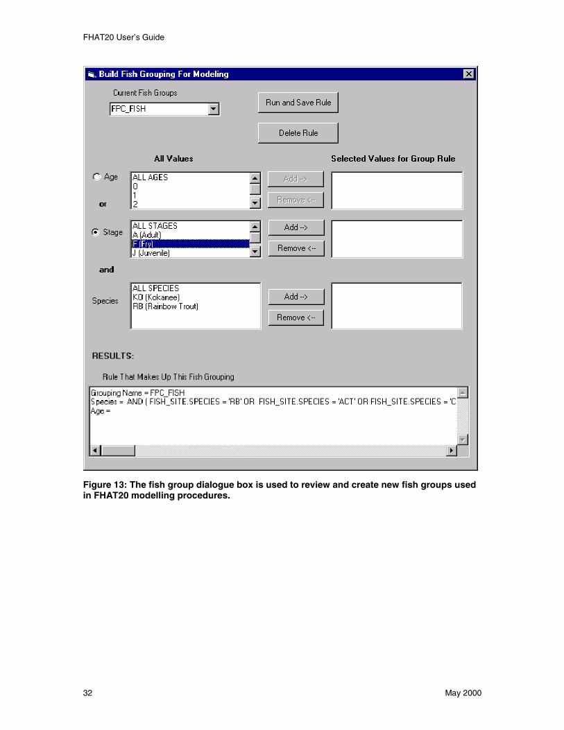
UNSAMPLED REACHES WILL BE NOT BE VISIBLE CHANNELS.................................................................. 2913. THE FISH GROUP DIALOGUE BOX IS USED TO REVIEW AND CREATE NEW FISH GROUPS USED IN

FHAT20 MODELLING PROCEDURES ..................................................................................................... 3214. THE OBSTRUCTION EDITOR DIALOGUE BOX IS USED TO DISPLAY, EDIT, AND ADD

MIGRATION BARRIERS TO THE FHAT20 MODEL DATABASE ................................................................. 3415. THE FISH RANGE DIALOGUE BOX IS USED TO REVIEW AND EDIT RULES THAT PREDICT FISH GROUP

RANGE IN THE MODELLED WATERSHED ................................................................................................ 3916. RELATIONSHIP BETWEEN HABITAT AND FISH ABUNDANCE................................................................... 4217. THE FISH HABITAT CAPABILITY DIALOGUE BOX IS USED TO PREDICT REACH-SPECIFIC HABITAT

CAPABILITY AND PROBABILITY OF FISH PRESENCE ............................................................................... 4518. SCHEMATIC SHOWING HOW THE PROBABILITY OF FISH PRESENCE (POP) IS COMPUTED FOR

EACH REACH AS A FUNCTION OF MODELLED UPSTREAM DISTRIBUTION LIMITS PREDICTED BY

FISH DISTRIBUTION RULES AND OBSERVED FISH OCCURRENCES ........................................................... 4719. SCHEMATIC SHOWING HOW THE PROBABILITY OF FISH PRESENCE (POP) AND FISH DISTRIBUTION IS

COMPUTED FOR STREAM AND LAKE REACHES IN RELATION TO FISH BEARING LAKES ........................... 4820. THE STREAM CLASSIFICATION DIALOGUE BOX IS USED TO CLASSIFY REACHES INTO S1–S6

FPC STREAM CLASSES ......................................................................................................................... 4921. SCHEMATIC SHOWING HOW STREAM CLASSIFICATION PREDICTIONS ARE COMPUTED IN FHAT20 ....... 5122. SCHEMATIC SHOWING HOW CONTINUOUS PROBABILITY OF FISH PRESENCEIS COMPUTED FROM THE

PROBABILITY OF FISH PRESENCE VARIABLE CALCULATED IN FISH HABITAT CAPABILITY MODEL ......... 5223. THE EDIT RESULTS DIALOGUE BOX IS USED TO MODIFY FHAT20 PREDICTIONS BASED ON A SET OF

USER-DEFINED RULES........................................................................................................................... 54


viii May 2000

List of Tables

1. DESCRIPTION OF SOME OF THE FIELDS IN THE WSCODE_LOOKUP TABLE.......................................... 62. DESCRIPTION OF ERROR CODES REPORTED IN WSCODE_LOOKUP ..................................................... 83. ORGANISATION OF VARIABLES (DATA AND MODEL RESULTS) THAT CAN BE DISPLAYED IN THE

FHAT20 MAP INTERFACE ................................................................................................................... 14


May 2000 1

1.0 Introduction

The Reconnaissance Fish and Fish Habitat Inventory is a sampled-based survey covering wholewatersheds, i.e., all lakes, stream reaches and connected wetlands within the watershed, asdefined from 1:20,000 scale maps and air photos. This inventory is intended to provideinformation regarding fish distribution and relative abundance as well as stream reach and lakebiophysical data for interpretation of habitat sensitivity and capability for fish production (Anon.1998a). While the reconnaissance inventory is intended to cover whole watersheds, time, money,and personnel are not available to survey every stream reach and lake in the watershed; thereforeonly a subset of reaches and lakes in the watershed is sampled. However, forestry planningprocesses require the development of products showing the extent of fish distribution or streamchannel widths for the entire planning area, not just their distribution in sampled reaches andlakes. These products must be interpreted from the sampled-based inventory. The Fish and FishHabitat Assessment Tool (FHAT20) is a computer program designed to analyze reconnaissance-level inventory data to produce a set of standardized interpretive products.

FHAT20 is an extrapolation program used to estimate fish habitat characteristics, fish presenceand capability in non-sampled reaches based on their remote-sensed characteristics (derived from1–20,000 scale maps and air photos) and models relating these characteristics to field-basedobservations in the sampled reaches. FHAT20 uses data stored in the Field Data InformationSystem (FDIS), the standard reconnaissance inventory project database. The end product fromFHAT20 is a set of predictions of channel width and probability of fish presence for all reaches.These predictions are used to estimate the most likely Forest Practices Code (FPC) stream class(S1–S6) for each reach and the level of certainty associated with each prediction.

This user’s guide describes how to use FHAT20 and the assumptions and methods of itsmodelling approaches. Section 2.0 describes how to install FHAT20 and provides an overview ofthe steps that you must follow to develop standard interpretive products of fish habitat,distribution, and capability. A critical step in using FHAT20 is importing data from FDIS.Section 2.0 describes how this importing procedure works and what to do when errors in theFDIS database are detected.

The remaining sections provide details on the following FHAT20 modules:

1. A physical habitat module which predicts channel width, wetted width, bank full depth, andthe probability of non-visible channels in all non-sampled reaches (Section 3.0);

2. A fish grouping module which allows users to summarize species/life-stage specific presenceand abundance data collected from the reconnaissance survey into management relevant fish‘groupings’ (Section 4.0). These groupings are then used in all subsequent fish distributionand capability modelling. An example of a fish grouping would be all species identified underthe Forest Practices Code (FPC) that are used to classify a stream as fish bearing.

3. An obstruction module that allows users to visualize and edit fish obstruction informationcollected during the reconnaissance survey and from other surveys. These obstructions areused to restrict the range of the fish grouping within the watershed (Section 5.0).


2 May 2000

4. A fish range module that allows users to predict a fish group’s range in the watershed basedon observed fish occurrences, obstruction data, and rules that use predicted or remote-sensedinformation (Section 6.0).

5. A fish habitat capability module that uses remote-sensed reach characteristics and estimatesof relative abundance from the sampled reaches to estimate capability in unsampled reaches(Section 7.0). Fish range and capability predictions for Forest Practices Code fish arecombined with channel width predictions to estimate the Forest Practices Code (FPC) streamclassification (S1–S6) for each reach.


May 2000 3

2.0 Installation and General OperatingGuidelines

The FHAT20 computer program consists of: 1) a relational database management system toretrieve data from FDIS and save modelling (extrapolation) results; 2) a series of dialogue boxesand graphics to develop and examine various models predicting physical habitat characteristics,fish range, and habitat capability; and 3) a series of computer algorithms that perform statisticaland other extrapolation operations used in the modelling. FHAT20 is a 32-bit application that willoperate under Windows95, Windows98, or Windows NT and must be used in conjunction withFDIS version 6.5 or higher.

2.1 Installation

FHAT20 can be downloaded from the INTERNET via the BC Fisheries FTP site. To obtain theinstallation program go to the FTP site FSHFTP.ENV.GOV.BC.CA. You can do this through aninternet browser by using FTP://FSHFTP.ENV.GOV.BC.CA/pub/outgoing/FHAT20 as theaddress to get into the FHAT directory. Click on FHAT20 ver1.0 May 11 2000.ZIP and you canthen download it to your hard disk (e.g. C:\TEMP). Unzip the files into the temporary directory.One of these files is named SETUP.EXE. Run SETUP.EXE to initiate the FHAT20 installationprogram. There is a file available for download suitable for creating a disk setup version forcomputers not hooked up to the internet – see the README.TXT file for directions to this andany updates.

When the installation process is complete, you will need to create at least one sub-directory belowthe directory where you installed the program (e.g., C:\FHAT20\WSHD1). The FDIS databasethat you want to use to develop an interpretive product using FHAT20 should be copied or movedto this sub-directory. There should be one sub-directory for each FDIS dataset that you wish toanalyze. A typical directory structure would be as follows:

DIRECTORY CONTENTS SOURCE OF CONTENTSC:\FHAT20 FHAT20 program Installation programC:\FHAT20\WSHD1 FDISDAT.MDB

of WSHD1 projectCopy from WSH1 FDIS directory

C:\FHAT20\WSHD2 FDISDAT.MDBof WSHD2 project

Copy from WSHD2 FDIS directory

2.2 First Time Use of FHAT20: Importing a FDIS database into FHAT20

To start FHAT20, double click on FHAT20.EXE from the Windows Explorer. Select the“File/Open Database” menu item, move to the directory that you copied/moved the FDISdatabase to (e.g., C:\FHAT20\WSHD1) and load FDISDAT.MDB. The first time you runFHAT20 on an FDIS dataset, a set of procedures will be initiated to read the data, check it forerrors and omissions, and create a new Access database, MODEL.MDB, which will be used forall future modelling sessions. In subsequent sessions you will still have to move to theappropriate subdirectory and load FDISDAT.MDB, but if you had previously createdMODEL.MDB successfully, FHAT20 will actually open MODEL.MDB. MODEL.MDBcontains imported FDIS data as well as modelling rules and results that you develop.


4 May 2000

FHAT20 uses 7 tables from FDISDAT.MDB to create the MODEL.MDB database:REACH_CARDS; S_SITE_CARDS; FEATURE; FISH_FORM; FISH_GEAR_SPECS;FISH_NET_SPECS; and FISH_EF_SPECS (Fig. 1).

MODEL.MDB contains:• a subset of information from FDIS used for modelling;• new variables computed from information in FDIS (e.g., total stream length upstream of

each reach);• a set of default ‘rules’ used to define fish groupings and model fish range in the watersheds;• predicted results of channel width, wetted width, bankfull depth, probability of non-visible

channels, fish range, and capability computed from previous modelling sessions.

Figure 1: The relationship between FDIS data, various modelling steps performed by theuser in FHAT20, and the majority of the FHAT20 model database (MODEL.MDB) wheremodel data, rules, and results are saved.


May 2000 5

2.2.1 Error Checking Procedure

When you first load FDISDAT.MDB, FHAT20 automatically checks FDIS data forinconsistencies in the watershed codes and reach ids. These inconsistencies must be correctedbecause the watershed code and reach id fields are critical to determine the ‘connectivity’ ofreaches and streams within the watershed (the upstream and downstream neighbours of eachreach). ‘Connectivity’ is used to compute a number of variables in the MODEL.MDB database,for example, the total stream length upstream of each reach (used to predict channel width) orwhether the reach is upstream of an obstruction or downstream of an observed fish occurrence.The error checking procedure also detects missing values for any FDIS variables that canpotentially be used in FHAT20 modelling procedures.

The first step that the FHAT20 import procedure completes is the combination of theReach_Cards and Lake_Cards tables from FDIS (Fig. 2) into a table called REACH_CARDS inMODEL.MDB. The importing procedure then loops through all reaches in this new table andchecks for errors in watershed code and reach_id fields. Errors are reported in the MODEL.MDBtable WSCODE_LOOKUP (Table 1). When errors are found, FHAT20 continues with the importprocedure, but only includes ‘clean’ reaches where no errors were detected. Following the importprocedure, a dialogue box will appear reporting on the numbers of different types of errors thatwere encountered. Although it is possible to continue with various modelling steps (describedbelow) to develop interpretive products based on only the ‘clean’ reaches, it is recommended thatthe user correct the errors following the procedures outlined below.

Figure 2: Schematic showing the procedure to import data from FDIS into FHAT20.


6 May 2000

Table 1: Description of some of the fields in the WSCODE_LOOKUP table (Fields not listedbelow are self-explanatory).

Field Name Field DescriptionRECID An original FDIS identifierFDIS_WS_CODE The original watershed code from the FDIS databaseFDIS_REACH_ID The original reach_id from the FDIS databaseMODEL_WS_CODE The corrected watershed code used in the MODEL database

(you must enter the corrected code in the table)MODEL_REACH_ID The corrected reach_id used in the MODEL database (you must

enter the corrected id in the table)ILP Interim locator point number from FDISILP_MAP Map sheet number associated with interim locator pointCOMMENTS User defined comments concerning errors and changesFIXED True/False denoting that the corrected watershed code and reach

id that you entered was accepted during the last import processIsLake True/False denoting that the record is a lake (and has a

corresponding record in the MODEL Lakes table and the FDISLake_Cards table

TABLE_TYPE If a reach in WSCODE_LOOKUP has corresponding site data(physical, fish, lake, or obstruction), the table name(s) isspecified. Users should check that the records in these tables docorrespond with the modified watershed code and/or reach_idspecified in WSCODE_LOOKUP

ERRORDESCRIPTION String denoting the type of error and which tables are potentiallyaffected

ERROR_TYPE An internal code (an integer value, see Table 2) used forerror/correction computations in FHAT20 during the importingprocess. This field only needs to be set by the user to change awatershed code or reach_id of MODEL.MDB site data (to assignit to another reach in the REACH_CARDS record set).

2.2.2 Error Correction

To correct watershed code/reach_id errors, open WSCODE_LOOKUP in Access, fill in theMODEL_WS_CODE and MODEL_REACH_ID fields with the correct values, and save thetable. Since WSCODE_LOOKUP will always retain the original FDIS (FDIS_WS_CODE,FDIS_REACH_ID) and corrected (MODEL_WS_CODE, MODEL_REACH_ID) values, youwill always be able to link the model results (interpretive products) back to the original FDISdatabase should the need arise. When the corrections have been made to WSCODE_LOOKUP,close Access and select the “Rebuild Database” choice from the “Utilities” main menu item to re-initiate the import process. Rebuilding the database incorporates all the changes made inWSCODE_LOOKUP into the new MODEL.MDB database. Hopefully all errors will becorrected during the MODEL.MDB rebuilding process. If errors are still reported, repeat thesequence just described, but this time only correcting records in WSCODE_LOOKUP where theFIXED field = FALSE. Records where the FIXED field = TRUE were corrected during previousrebuilding events. This cycle can be repeated as many times as required. The error reporting formdisplayed at the end of each import process always provides a summary of the current state of thedata in terms of how many errors were originally detected and how many have been corrected.


May 2000 7

You can view the error report at any time by selecting the “Error Reporting” option from the“Utilities” main menu item (Fig. 3).

Figure 3: The error reporting dialogue box displays a record of errors and correctionsmade to the FHAT20 model database.

Correcting errors in watershed codes and reach ids for each record in the WSCODE_LOOKUPtable in MODEL.MDB requires an understanding of the types of errors that can be trapped andhandled by the importing procedure. These errors are distinguished based on text in theCOMMENTS field of WSCODE_LOOKUP (Table 2).

It is important to note that in MODEL.MDB, the watershed code and reach id fields link recordsin REACH_CARDS with records in the other tables containing site data (PHYS_SITE,FISH_SITE, USER_BARR, LAKES). Making a change to a watershed code or reach id inREACH_CARDS (via modification of WSCODE_LOOKUP) may result in two situations:

a) A record in a site’ table may no longer have a corresponding record inREACH_CARDS (in which case error Types 4–7 will be reported inWSCODE_LOOKUP) or;

b) A record in a site table may match a record in the corrected REACH_CARDS table,but the site data does not belong to that REACH_CARDS record and instead isactually associated with another reach.


8 May 2000

Table 2: Description of error codes reported in WSCODE_LOOKUP.

Code Error Description0 Invalid Watershed Code: Watershed code is invalid (e.g., 000-…., 999-, NA)1 Duplicate Reach ID: Two records in the FDIS table Reach_Cards have the same watershed

code and reach_id. This likely resulted from: a duplication resulting from the importing ofwatershed codes into FDISa; or an incorrect specification of reach_id or watershed code whendata were entered in FDIS.

1 Duplicate Reach ID (reach is a Lake): A record in the FDIS Reach_Cards table matches(same watershed code and reach_id) a record in the FDIS Lake_Cards table. In this case, the“isLake” field in WSCODE_LOOKUP will be “TRUE.” This error type is distinguished fromthe previous error type only because it may be helpful to know which record is the lake whenattempting to determine the correct reach_id (or watershed code) for one of the records.

2 No Parent stream from FDIS (‘orphan’): With the exception of the mainstem, every stream(watershed code) in the FDIS database must have a stream that it flows into (hereafter referredto as its ‘parent’ stream). This error code denotes that a record (a unique watershed code andreach id) does not have a parent stream and that it is not the mainstem; it is therefore an‘orphan’ reach.

3 Stream eventually flows into a stream with no parent (‘incomplete lineage’). The currentstream flows into a parent stream (it is not an ‘orphan’ or the mainstem), but there is a break inthe network (a “non-parent” situation) somewhere between its parent and mainstem.

4 Record in PHYS_SITE with no matching record in Reach_Cards: The PHYS_SITE table inMODEL.MDB is populated based on records in the FDIS table S_SITE_CARDS. When youcorrect a watershed code or reach id in REACH_CARDS (MODEL version) by makingchanges in WSCODE_LOOKUP and re-running the import procedure, you can create asituation where some records in PHYS_SITE have no match in REACH_CARDS in theMODEL database. This error can also arise from incorrect entry of watershed codes or reachids when entering site data in FDIS.

5 Record in FISH_SITE with no matching record in Reach_Cards: The FISH_SITE table inMODEL.MDB is populated based on watershed codes and reach ids in the FDIS tableFish_Form. When you correct a watershed code or reach id in REACH_CARDS (in MODELversion) by making changes in WSCODE_LOOKUP and re-running the import procedure,you can create a situation where some records in FISH_SITE have no match inREACH_CARDS in the MODEL database. This error can also arise from incorrect entry ofwatershed codes or reach ids when entering fish data in FDIS.

6 Record in LAKES with no matching record in Reach_Cards: The LAKES table inMODEL.MDB is initially populated based on watershed codes and reach ids in the FDIS tableLake_Cards and these records are merged into the MODEL.MDB Reach_Cards table. Whenyou correct a watershed code or reach id in REACH_CARDS (in MODEL version) by makingchanges in WSCODE_LOOKUP and re-running the import procedure, you can create asituation where some records in LAKES now have no match in REACH_CARDS in theMODEL database.

7 Record in USER_BARR with no matching record in Reach_Cards: The USER_BARR tablein MODEL.MDB is initially populated based on watershed codes and reach ids in the FDIStable FEATURE (linked to S_Site_Cards). When you correct a watershed code or reach id inREACH_CARDS (in MODEL version) by making changes in WSCODE_LOOKUP and re-running the import procedure, you can create a situation where some records in USER_BARRhave no match in REACH_CARDS in the MODEL database. This error can also arise fromincorrect entry of watershed codes or reach ids when entering obstruction data in FDIS.

a Errors in watershed codes are generally associated with the process of importing the watershed codes inthe ILP table back into FDIS. In some instances, in headwater forks, when the mainstem and tributarygets assigned a code which is opposite to what was identified, this results in both a missing watershedcode and a duplicate watershed code and reach number. Newer versions of FDIS will check for thisproblem.


May 2000 9

Correction of situation b) errors cannot be done automatically. If a match between a correctedrecord in REACH_CARDS and a record in a site table occurs, the import procedure has no wayof knowing whether the identifiers were originally entered correctly in the site table via FDIS(and should therefore now be linked to the record in REACH_CARDS with the originalidentifiers) or whether the site identifiers were entered incorrectly from FDIS (and shouldtherefore be updated based on the corrected values specified in WSCODE_LOOKUP). Thus,when situation b) occurs during the import procedure, the TABLE_TYPE field inWSCODE_LOOKUP is set to the name(s) of the site table(s) where a record corresponding to themodified REACH_CARDS record exists. It is up to the user to then manually check these cases(using original maps, UTMs, etc.) to make sure that the records do correspond. If they do not,additional records must be added to WSCODE_LOOKUP by the user so that the records in theMODEL.MDB site tables are updated. These new records should contain the original watershedcode, reach id, and RecID identifiers (the FDIS_ values, just copy their values) and the newidentifiers (MODEL_ values) that are used to link it to the correct REACH_CARDS record. Inaddition, the ERROR_TYPE field should be set to the appropriate code (e.g., 4 if you areupdating a record in the PHYS_SITE table in MODEL.MDB).

Correction of stream network errors detected by FHAT20 may require a significant amount ofeffort and depends completely on the consistency in the FDIS database. The correction procedurecan be streamlined by realizing the hierarchical nature of some of the errors. You may observe alarge number of records with ‘incomplete lineage’ errors (type 3) all resulting due to a smallnumber of ‘orphans’ (error type 2). If you correct type ‘orphan’ errors first, all ‘incompletelineage’ errors will automatically be corrected by the import procedure. The most efficient way tocorrect the data is to:

• Correct all ‘orphan’ type errors (type 2) and known problems with watershed codes (type 0)first;

• then correct duplicate reach id errors (type 1) which may involve changing watershed codes(i.e., the reach id may be correct and the error resulted from an error in the watershed code);

• correct error types 4–7; and finally,• check and make sure that records in PHYS_SITE, FISH_SITE, USER_BARR, and LAKES

are correctly assigned to the new watershed codes or reach ids in REACH_CARDS (check allrecords with values in the TABLE_TYPE field in WSCODE_LOOKUP). If there are errors,follow the procedure specified in the previous paragraph (add new records toWSCODE_LOOKUP).

Never correct ‘incomplete lineage’ errors, they can only be eliminated by correcting ‘orphan’errors and are only provided in WSCODE_LOOKUP in case you run the modelling procedureswithout completing all corrections (thereby providing a catalogue of reaches missing from theanalysis).

Note it is possible to run the modelling procedures with errors in the watershed codes and reachids, however none of these reaches will be included in the model analysis. At the very least, youhave a record of these reaches in the WSCODE_LOOKUP table (all records with the FIXEDfield = “FALSE”). However, predictions for other reaches still included in the analysis may beeffected by the deletion of the problem reaches due to network connectivity aspects of themodelling. Thus, running the model with missing reaches is not recommended, especially ifthey are ‘parents’ and have reaches flowing into them (i.e., not first order, headwater reaches).


10 May 2000

Errors in the watershed code that do not result in ‘orphan’ streams are not detected during theFHAT20 import procedure. There are two types of such errors that could affect modelling results:

Watershed Code Does Not Reflect Position of Confluence Along the Parent Stream

A tributary of a parent stream may have a code specifying that its confluence is mid-way up theparent (e.g., 120-907500-63000-50000, located 50% of the way up its parent stream 120-907500-63000). However, during inspection of the FHAT20 electronic map (plotting variablesdetermining which tributaries are not accessible to fish because of obstructions) you may noticethat the confluence of the child stream is actually further upstream that specified by the watershedcode. Assuming the map is correct, such an error could result in erroneous predictions. Forexample, an obstruction in the parent stream located 60% of the way up its total length (on themap) would not limit access to the tributary, because electronically, the obstruction is upstream ofthe tributary confluence, which is only 50% of the way up the parents total length. To correct thistype of error, you need to estimate the correct watershed code for the tributary in question basedon the actual proportional distance of its confluence relative to the parents total length (e.g.,75%). A new record in WSCODE_LOOKUP must be added containing the original FDIS andmodified (MODEL) watershed codes (e.g., 120-907500-63000-50000 and 120-907500-63000-75000, respectively).

Watershed Code Does Not Reflect Stream Hierarchy

A stream may appear electronically to be a tributary of a particular parent stream based on itswatershed code, when in reality it is not a tributary of that parent stream (or vice-versa). Forexample, 120-907500-63000-50000-0123 would electronically be treated as a tributary of 120-907500-63000-50000. However, on inspection of the map, the stream in question may actually bea tributary of 120-907500-63000. Its watershed code needs to be modified inWSCODE_LOOKUP to reflect its actual position in the stream hierarchy and its proportionalconfluence distance relative to its parent stream (120-907500-63000-57000).

During the importing routine, FHAT20 catalogues records with missing values for variables thatcan be used in the modelling process. There will be a unique record in the BadData table ofMODEL.MDB for each field with a missing value for a given reach (i.e., there can be multiplerecords per reach). If you want to enter valid values for the records with missing values identifiedin BadData, you must enter them in FDIS and then re-import the data using the “RebuildDatabase” option from the “Utilities” main menu item (Fig. 2). Note that it is possible to continuemodelling with missing values, however FHAT20 cannot make predictions for reaches withmissing values for a variable if that variable was included in one of the model(s). The tableDataCheck in MODEL.MDB contains the list of variables in FDIS that will be screened by the‘data checking’ procedure during the import process. You can add variables to this list, ordeactivate variables (by unchecking the IsActive field) so they are no longer screened for missingvalues. DataCheck allows the user to modify the range of legal values that a field can have, andwhat to do if a particular record does not meet these criteria. Records that fail the data screeningprocedure for a given field are either deleted, or the missing value is replaced with a missingvalue flag (-9999 for numeric fields or ‘NS’ for text fields). The is Dropped field in the BadDatatable specifies which of these two actions will be taken.


May 2000 11

2.2.3 FHAT20 Maps: Stick Diagrams or the Digital TRIM Atlas

A key component of FHAT20 is the ability to view some FDIS data and all model predictions ona digital map of the study area. Two types of maps can be used by FHAT20: 1) a ‘stick diagram’where each reach is a straight line between the upstream and downstream reach coordinates; and2) a TRIM atlas which is a digital version of the hardcopy TRIM maps with watershed codes andreach measures (the distance of each reach break from the confluence of each stream) for eachreach in the FDISDAT database.

Stick Map

The ‘stick’ map represents each reach in the study area as a single, straight line. Such diagramsdo not contain bends, lake boundaries, and other features that will be shown on the TRIM atlasmaps. Stream reaches are shown as straight lines while reaches classified as lakes (i.e., withrecords in the FDIS Lake_Cards table) are shown as fatter lines or filled circles (if the lake lengthcould not be computed). FHAT20 uses the UTM coordinates from the REACH_CARDS table tocreate this ‘stick’ diagram during the import process and saves this information to the fileMODEL.MIF in the project sub-directory. The stick map is actually a MAPINFO file that can beviewed in FHAT20 or MAPINFO. When you view this map for the first time in FHAT20 afterthe import procedure, you will note that the first reach of each stream ‘hangs’ in the sense that itdoes not connect with its parent stream. Such reaches will be represented by open circles at theirupstream boundaries. This occurs because FDISDAT.MDB does not store the UTM coordinatesfor the downstream end for the first reach of each stream. Some of these coordinates can beobtained from the 1:50,000 Watershed Atlas (although coordinates may differ significantly fromthose on a 1:20,000 map) and others may have been created by the ILP/watershed code process. Ifyou have some or all of these ‘first node’ coordinates, create a comma-delimited file with 3fields: watershed code (45 digits – can contain hyphens or not) and UTM easting and northingcoordinates in the following format:

WS_CODE,EASTING,NORTHING120907500000000000000000000000000000000000000,674071,5621503120907500045320000000000000000000000000000000,674810,5622958120907500045325767200000000000000000000000000,674344,5623477

From the “Utilities” main menu item, select the “Import First Nodes File” option. This will readin the .CSV file you created and add these records to the FIRSTNODE table in MODEL.MDB.This process will add the new coordinates to the ‘stick’ map eliminating some of the ‘hanging’tributaries and making the map more readable.

TRIM Watershed Atlas Map

If a digital TRIM Watershed Atlas is available for the study area (with watershed codes thatcorrespond to those in FDISDAT.MDB), a method exists to bring TRIM linework into the model.However, as the TRIM Watershed Atlas is not available provincially, and this procedure is underdevelopment, it has not been included in this manual. The ‘Load Map File’ and ‘Load Lakes File’under the ‘Edit Legend’ selection in “Utilities” are used in this process.1

1 For information on the status of the TRIM Watershed Atlas and the procedure to import TRIM lineworkinto the model, please email the BC Fisheries Information Services Branch at [email protected].


12 May 2000

2.3 Controlling the Map Display

The main FHAT20 form (window) consists of a digital map of the watershed that is used todisplay reach specific data or model results using a color-code system (Fig. 4). Also shown is alegend depicting what the color codes represent, and a set of combo boxes that are used to selectvarious data/model results to display. Data/results are organized into four functional variablegroupings shown in the upper combo box. Within each grouping there are a series of variableswhich are shown in the combo box labeled “Variables” (each variable generally corresponds to aunique field in tables within MODEL.MDB). Table 3 provides a listing of the functional datagroupings and their fields, and what each field represents. To view results for any field, simplyselect the appropriate grouping and field from the combo boxes.

Figure 4: The main FHAT20 dialogue box used to display and query reach-specific dataand model results.


May 2000 13

The mapping display has a number of features to facilitate data review and analysis.

Point-and-Click to get Reach Attribute Information

Double-click on any reach with the left mouse button to bring up the “Search Results” dialoguebox (Fig. 5). A table shows the watershed code and reach id for the reach you selected and thevalue for the current layer on the map. You can then find the value for other reach attributes byselecting the variable group from the combo list box in the dialogue box and double-clicking onthe variable. Click on the watershed code in the table to highlight the stream reach on the map(the selected reach will be displayed as a thick white line).

Figure 5: The search results dialogue box displays data and results for reaches selectedon the map.

‘Zooming-In’ on a Selected Area on the Map

The zoom feature allows you to view a smaller area within the full study watershed shown on themap. Simply click on the check box labeled ‘zoom’, click on the map with the left mouse button,and hold the button down while dragging the mouse over the portion of the map that you want toselect. When you release the mouse button the map will be redrawn showing only the selectedarea. You can repeat this process to select an even smaller area to view, or restore the map to itsfull size by clicking on the button labeled “Draw Full Map.” You can view the reach breaks byclicking on the check box labeled “Show Reach Breaks.”

Overlay Second Layer - Looking at Two Map Variables at One Time

The overlay feature is very useful for comparing predicted results with observed sample data.This feature allows you to look at two different variables on the map at one time. First select avariable and display it on the map, click on the check box labeled “Overlay Second Layer,” andthen select the second variable you want to display. The second variable will be displayed ascolor-coded squares shown in the center of each reach on top of the first variable. Click on the“Show Overlay Legend” check box to bring up legends for both layers simultaneously.

Table 3: Organisation of variables (data and model results) that can be displayed in the FHAT20 Map Interface. The Group andVariable Name columns correspond to the items shown in the combo boxes labelled “Group” and “Variable” on the FHAT20main window. The Table/Field column gives the table and field name where the data/results are stored in MODEL.MDB. ‘Group’in the table is used to designate a fish grouping name (e.g., FPC_FISH); there will be multiple occurrences of fields precededwith ‘Group’, one set of each fish group modelled.

Group Name Variable Name Description Table/FieldPhysical Predictions Order Strahler stream order Reach_Cards / Order_20

Magnitude Magnitude of reach (# of 1st order streams upstreamof reach)

Reach_Cards / Magnitude_20

Gradient Reach gradient Reach_Cards / Gradient_20Downstream Elevation Elevation (metres above MSL) of downstream node

of reachReach_Cards /Downstream_Elevation

Confinement Code Confinement of reach Reach_Cards / Conf_codeChannel Pattern Channel pattern of reach Reach_Cards / Cptn_CodeFeatures Location of Features (from FDIS Features table or

user-defined)User_Barr

Reach is a Wetland Denotes whether reach is a wetland Reach_Cards / WetlandReach is U/S of a Wetland Denotes which reaches are upstream of wetlands Reach_Cards / USofWetlandReach is a Lake Denotes whether the reach has a corresponding

record in the Lakes tableReach_Cards / IsLake

Reach is Lake-headed Denotes whether a reach has a lake upstream Network / IsLakeHeadedReach flows into Lake Denotes whether a reach is an inflow stream to a

lakeNetwork / ReachFlowsIntoLake

Upstream Length Length (km) of stream upstream from thedownstream end of each reach

Network / Uplen

Maximum Downstream Gradient The maximum gradient between the reach and thefirst reach at the most downstream end of thewatershed

Network / Maxdsgrade

Parent Order The Strahler order of the parent stream of the firstreach of its tributary

Network / Parent_order

Sampled for Physical/Fish Data Was the reach sampled for physical parameters orfish (True/False)

Network / Sampled_PhysNetwork / Sampled_Fish

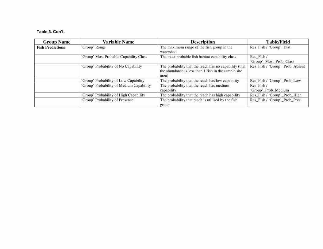
Table 3. Con’t.

Group Name Variable Name Description Table/FieldPhysical Predictions Predicted Channel Width Predicted Channel Width (m) if the reach is not

sampled, Average measured channel width if thereach has been sampled

Res_Phys / Chan_width

Distance to Bottom of System (km) Distance of reach (km) to the most downstreamreach in the project area

Network / Dist_To_Bottom

Sinuosity Ratio of reach length to the straight line distancebetween the bottom and top of the reach

Reach_Cards / Sinuosity

Predicted Wetted Width Same as above but for wetted width Res_Phys / Wet_widthPredicted Bankfull Depth Same as above but for bankfull depth Res_Phys / Bank_Full_DepthProbability of No Visible Channel The predicted probability that the reach is classified

as a non-visible channelRes_Phys / Novis_prob

Observed Non-Visible Channel Denotes whether a sampled reach was a non-visiblechannel

Phys_Site / No_Channel_Vis

‘Group’ Upstream of Obstructions Reaches upstream of obstructions for the fish group(False-fish group is not upstream of an obstructionspecific to that group)

Network / ‘Group’_Dsbarr’

‘Group’ Downstream of Occurrence All reaches downstream of an observed occurrenceof the fish group

Network / ’Group’_Ds_Fish_Pres

‘Group’ Dist U/S of Fish Occurrence Distance upstream (km) from nearest fishoccurrence

Network /’Group’_Dist_US_Fish_Pres

‘Group’ Not Present Upstream All reaches upstream of sampled reach where fishgroup was not found (as long as there is not a fishoccurrence for group upstream of this point)

Network / ‘Group’_US_Fish_Abs

‘Group’ Parent D/S of Fish Occurrence Reach is a tributary of a reach that is downstream ofa known fish occurrence

Network /’Group’_Parent_DS_Fish_Pres

Observed Fish Data ‘Group’ Reach Presence/Abundance Denotes fish presence if the site was notelectrofished, and density (#/100 m2) if the site waselectrofished

Based on a combination ofvariables in Model_Fish_Data /(Meth, TotalNo & Cpue)

Table 3. Con’t.

Group Name Variable Name Description Table/FieldFish Predictions ‘Group’ Range The maximum range of the fish group in the

watershedRes_Fish / ‘Group’_Dist

‘Group’ Most Probable Capability Class The most probable fish habitat capability class Res_Fish /‘Group’_Most_Prob_Class

‘Group’ Probability of No Capability The probability that the reach has no capability (thatthe abundance is less than 1 fish in the sample sitearea)

Res_Fish / ‘Group’_Prob_Absent

‘Group’ Probability of Low Capability The probability that the reach has low capability Res_Fish / ‘Group’_Prob_Low‘Group’ Probability of Medium Capability The probability that the reach has medium

capabilityRes_Fish /‘Group’_Prob_Medium

‘Group’ Probability of High Capability The probability that the reach has high capability Res_Fish / ‘Group’_Prob_High‘Group’ Probability of Presence The probability that reach is utilised by the fish

groupRes_Fish / ‘Group’_Prob_Pres

Table 3. Con’t.

Group Name Variable Name Description Table/FieldStream Classification Most Probable Stream Class The most probable stream classification based on

the combined probability of different stream widthsand discontinuous fish presence (a reach may havea lower probability of fish presence compared to anupstream reach)

Res_Fish / Most_Prob_S

Uncertainty in S Class A relative index of uncertainty associated with theMost Probable Stream Class. A value of ‘0’ denotesthe minimum uncertainty; 100% probability for oneof the S Classes. A value of ‘100’ denotesmaximum uncertainty; all S Classes have an equalprobability (16.67% because there are 6 classes).

Res_Fish / S_Uncert

Sx Probability (x=1 – 6) The probability that the reach is an Sx stream class(e.g., S1) based on combined probabilities

Res_Fish / Sx

FPC Stream Class The stream class based on the most likely width,with fish presence determined fromFPC_Fish_Present

Res_Fish / ConSClass

FPC Fish Present Presence/absence determined from continuousprobability of presence values combined with aminimum probability of presence limit defined bythe user

Res_Fish / ConFishPres

Continuous Probability of Presence Probability of fish presence defined on a continuousbasis (downstream reaches cannot haveprobabilities less than upstream reaches)

Res_Fish / ConPop


18 May 2000

Controlling the Map Legend

Each variable that can be mapped has a unique legend that controls how the data will bedisplayed on the map. If you double-click the mouse on the colored boxes in the legend, the“Legend” dialogue box will be displayed (Fig. 6). Alternatively, select the “Edit Map Legend”choice from the “Utilities” main menu item. There are a number of parameters that you canchange to adjust the legend. To display a variable via color codes on a map, a set of bins must beestablished for specific ranges of the variable (e.g., bin 1 = gradient 0–3%, bin 2 = gradient 3%–7%, bin 3 = …). There is a corresponding color for each bin.

• You can alter the number of bins (labeled number of strata in the dialogue box) and manuallyset the lower and upper end of the range for the variable.

• Alternatively, you can click on the button labelled “Set Upper and Lower Ranges” to have theprogram determine the minimum and maximum value for the variable.

• After you have made any of these edits click on the button labelled “Ramp Breaks” to rampthe breakpoints between the lower and upper range values.

• To change the colour associated with any bin, click on a colour in the colour palette and thenclick on the coloured box adjacent to the bin.

• You can manually edit the bin breakpoints by editing the values in the breakpoint text boxes.

If you wish to edit the legend for another variable simply select it from the list. If you are editingthe legend for a variable currently displayed on the map, you must click on the button labelled“Apply Legend” to see the changes. Note that any changes you make to the legend are saved to afile called MODEL.MDE and effect the display in all subsequent sessions.

Figure 6: The legend editor dialogue box is used to edit the map display of data andpredicted variables.


May 2000 19

2.4 General Modelling Procedure

A series of specific steps must be followed to develop standard interpretative products of fishhabitat, distribution, and capability using FHAT20. As you develop models and apply them,modelling rules and results are saved to various tables in the FHAT20 database (MODEL.MDB).The relationship between FDIS data, various modelling steps, and the FHAT20 database is shownin Figure 1. There are seven basic modelling steps that must be performed in a specific order(Fig. 7):

1. Define stratification groups used to make physical predictions (Section 3.2);2. Predict channel width, wetted width, bankfull depth (optional) and the probability of non-

visible channels for all unsampled reaches, possibly using a stratified analysis (Section 3.0);3. Define fish groupings (Section 4.0);

For each fish grouping:

4. Edit obstruction data to define whether a feature is an obstruction to each fish group(Section 5.0);

5. Model the fish group’s range within the watershed (Section 6.0);6. Model the fish group’s habitat capability (Section 7.0) which is combined with the predicted

range to estimate probability of fish presence; and7. Model FPC stream classification (Section 8.0) based on the predicted probability of fish

presence and predicted channel widths.

A change in data or modelling assumptions in any step requires that all steps following that pointare reprocessed. For example:• if you modify the relationships predicting channel width, and have fish range rules that

depend on channel width, you will need to rerun these rules (i.e., repeat step 5).• If you modify channel width or wetted with predictions you must rerun the habitat capability

calculations.• If you modify channel width you must rerun the habitat capability and stream classification

procedures.• If you add or edit an obstruction that affects the range of a fish group, you will need to rerun

its range rule, and since the habitat capability calculations are dependent on the fish range,you will also have to rerun the capability calculations.

• If you rerun habitat capability for a fish group, you will need to rerun the stream classificationif it was run using the same fish group. The habitat capability modelling contributes to thecalculation of the probability of fish presence variable, which is used in the streamclassification procedure.

• If you define a new fish grouping, you must complete steps 4–6 (and possibly 7) forthis group.

• If you modify the original data in FDIS, you must re-import the data and reprocess allthe results.


20 May 2000

Figure 7: Schematic showing the relationship among modelling steps in FHAT20. Solidlines denote fixed relationships (e.g., channel width is used to predict stream class), whiledashed lines show relationships that depend on whether particular variables are used inlater modelling steps (channel width depth may be used in predicting fish range, but it isnot mandatory).

To assist you in following the correct order in the modelling procedures, FHAT20 keeps track ofthe sequence and time stamps of all modelling operations performed. A dialogue box, accessedfrom the “Show Operational Tracking” choice below the “Utilities” main menu item displays thisinformation (Fig. 8) The dialogue box consists of a grid with rows for each modelling step andcolumns for each of the currently defined fish group. When the data is first imported, all the cellsin the grid will be purple, denoting that none of the operations have been performed. As youbegin to perform various modelling tasks, the appropriate cells on the grid turn green and thedate/time stamp that the task was performed is shown. If you redo a particular model step(e.g., predict channel width), all modelling procedures that depend on that operation will be out ofdate. These steps will need to be redone, and are depicted as red cells on the grid.


May 2000 21

Figure 8: The operational tracking dialogue box displays the status of modellingprocedures and the date/time the procedures were run.

You can easily navigate from one modelling procedure to another by double clicking onindividual cells in the grid. If you attempt to perform a task out of sequence, that is, perform atask that depends on a previous model step that has not been run (purple cell) or is out of date (redcell), FHAT20 will warn you and stop you from performing the operation. If you want to disablethis, toggle the “Operation Tracking” check box off (or deselect the “Operational Tracking”choice below the “Utilities” main menu item).

Due to the structure of the grid, some operations appear fish group specific but are not. Note thatthere are physical prediction rows (channel width, wetted with, probability of non-visiblechannel, bank full depth) for each fish group depicted on the grid, but these events are not fishgroup specific. When you compute one of these variables you will see that the appropriate cell inthe grid is changed for all fish groups. If you edited a model result (section 9.0) and laterrecalculate that result, the “Results Edited” cell will show that the edit rule is out of date. The editrule itself is not out of date, however this tells you that you had previously edited the results froma particular operation, have since recomputed the operation, but have not re-edited the result. Thegrid alerts you to this fact, but does not block you from performing additional operations thatdepend on the result. This is logical as you may not need to edit the new result.

2.5 Exporting Results, Saving Maps, Printing Maps

Model results can be saved to the EXPORT table in MODEL.MDB for analysis in otherapplications and display in FDIS Map. To export results, select the “Export Results” option fromthe “File” main menu item. The EXPORT table contains a number of identifier fields to facilitatelinkage back to FDIS and other BC Fisheries Inventory applications including:

• FDIS watershed code and reach_id• MODEL.MDB watershed code and reach_id (equivalent to FDIS values unless the values

were corrected in WSCODE_LOOKUP)• NID, NID_MAP


22 May 2000

• ILP, ILP_MAP• Easting and Northing UTM

When you export the model results, a table called CUREXPORTLOG is updated. This tablecontains the rules (SQL statements), results, and time stamps associated with the variousmodelling operations you completed. This allows a third party to verify that model results inthe EXPORT table were based on modelling steps completed in the correct sequence.

Maps displayed in FHAT20 can be exported as bitmap files. Select the “Dump Map/Legend toBitmap” option form the “File” main menu item. You will be prompted for a filename to save themap to and a separate filename to save the legend to. You can import both of these files intoanother application, and because the map and legend images are saved in different files, you haveflexibility in terms of where the legend is located on the final graphic. You can also print the mapand legend to the default printer by selecting the “Print Map/Legend” option from the “File” mainmenu item.


May 2000 23

3.0 Physical Predictions

FHAT20 predicts channel width, wetted width, and bankfull depth for all unsampled reaches andthe probability that these reaches are non-visible channels.

3.1 Channel Width, Wetted Width, and Bankfull Depth Predictions

FHAT20 predicts channel and wetted width and bankfull depth in unsampled reaches as afunction of their upstream drainage area and empirical relationships developed from sampledreaches. When FDISDAT.MDB is first imported into FHAT20, the total length of streamupstream for each reach is computed by summing the LENGTH field in REACH_CARDS. Totalupstream length is strongly correlated with drainage area, which is a good predictor of somechannel characteristics in areas of similar unit discharge (m3/sec/km2). The ratio of stream lengthto drainage area (km stream/km2 drainage area) should be relatively consistent within aninventory area and will be a function of rainfall, surficial geology, and the detail that was used torepresent stream lines on the TRIM maps.

Parameters of the power function predicting channel width, wetted width, or bankfull depth (Y)as a function of upstream length (UPLEN),

Y = a * UPLEN ^ b

are estimated from the sample data (where widths and depths have been measured in the field)and applied to unsampled reaches. The model(s) is fit by a least squares procedure on logtransformed variables.

Rather than estimate a single relationship for each variable (channel width or wetted width, etc.),FHAT20 allows the user to develop separate functions for different sets of reaches. For example,while channel width will be correlated positively with upstream length, we would expectunconfined reaches to be wider for a given upstream length than confined reaches. Hence it islogical to develop different relationships for subsets of the entire dataset, which we refer to asstrata (because you are stratifying the data into different sets). Stratification can improve theaccuracy and precision of the physical predictions assuming that there is a sufficient sample sizeto develop the empirical relationships within each strata. FHAT20 provides a mechanism to:

• define these strata based on attributes in the REACH_CARDS table of FDIS (remote-sensedattributes which are available for all reaches);

• build and evaluate models for each of these strata;• estimate uncertainty in the predictions; and• save the predictions to MODEL.MDB for display and use in fish range, habitat capability,

and stream classification modelling.

To predict widths and bankfull depths, open the “Channel Morphology” dialogue box via the“Modelling” main menu item (Fig. 9). Select a variable to model (Channel Width = CW_avg, orWetted Width = WW_avg, Bankfull Depth =BFD_avg) from the combo box at the top of thedialogue box labeled “y-axis.” The relationship between this variable and upstream length for thesampled reaches will be shown in the adjacent x–y scatterplot as blue x’s. Below the scatterplot isa white box containing a list of strata for the currently loaded stratification rule. If you click on astring in the white list box, the x–y scatterplot will display the data for the strata you selected. The


24 May 2000

first item in the list box (0 / Unstratified) always shows the entire sampled dataset. If you want toload a different set of strata that had previously been defined, select one from the combo boxlabeled “Stratification.” If you want to define a new set of strata, select the “Define StratificationGroups” choice below the “Modelling” main menu item (Section 3.2 below).

Figure 9: The channel morphology dialogue box is used to make reach-specific physicalpredictions, such as channel and wetted widths.

To fit power functions to the x–y data for each strata, click on the button labeled “Run Models.”When you do this, model fit statistics will be displayed in the table at the bottom of the dialoguebox and the fitted line (the model) will be shown as a green set of triangles in the x–y scatterplot.Fit statistics include sample size (N), constant (A) and slope (B) parameters of the powerfunction, the unexplained mean square error (MSE), the correlation coefficient (R2, the percent ofthe variance explained by the model), and the probability that the slope of the power function isnot significantly different from zero (Prob.). Low MSE, high R2, and low Prob. values denotegood model fits to the data. You should evaluate these statistics across a range of stratificationschemes to develop the most predictive models possible.

When examining how well the model fit a particular data set, you may notice outliers to themodel, that is, blue points that are noticeably more distant from the fitted green line representingthe model. These outliers may be normal sites that represent the extreme end of the uncertaintyaround the predictive relationship. Alternatively, you may know something about these siteswhich would motivate you to drop them from the model fitting because they do not reflect the


May 2000 25

population of reaches you are trying to model. For example, there could be a problem with themeasurements at a particular site (difficult to determine the top of the bank), or the site could bealtered by human activity (e.g., a rip-rapped bank beside a road would not have a representativechannel width). You would want to exclude these types of sites from the model fitting exercise asthey could bias your predictions and levels of certainty. To exclude outliers, click on the checkbox labeled “Select Site Data to Include in Model.” A grid will appear with the list of sites thatare used in the model fitting (Fig. 10). Green cells denote sites that are included in the modelling,while red cells denote cells that have not been included. To include/exclude data from a site in themodel fitting, toggle the color of the cell by clicking on it with the mouse. When you toggle a cellits corresponding reach will be highlighted on the map. Sites included in the modelling arerecorded in the “UseFor__” (“_CW,””_WW,””_BFD”) fields in the RES_PHYS table.

Figure 10: The outlier dialogue box is used to display site-specific physical data used inchannel morphology modelling, allowing users to exclude specific data from the modellingprocedures.

Channel width is used in conjunction with fish presence to determine the FPC streamclassification (S1–S6). Even with stratification, the empirical power functions you have fitted tothe data will no doubt show substantial scatter. This means that there can be substantialuncertainty in the channel width predictions, and it would be unwise to only use the most likely(best-fit) width prediction in the decision making process. FHAT20 uses a bayesian algorithm(Walters and Ludwig, 1994; McAllister et al., 1994) to estimate the uncertainty in channel widthfor each unsampled reach. When you compute this uncertainty, the bayesian procedure essentiallyfits 1000 different power functions (different parameter values for A and B) to each data set (eachstrata). The relative likelihood of the data given each of these models (combinations of the A andB parameters) is computed and stored in memory. Once these 1000 models and their likelihoodshave been computed, the procedure works its way through each unsampled reach and enters thetotal upstream length into each of these 1000 models to predict its channel width. A frequencydistribution of predicted channel widths, generated by weighting each predicted width by the


26 May 2000

likelihood of each of the 1000 models that was used to generate it, is computed for each reach.This distribution is then used to estimate the probability of each reach being in particular widthclasses (e.g., 1.5–5 m) as explained below.

To implement the bayesian algorithm, click on the check box labeled “Compute Uncertainty” andthen click on the button labeled “Run Models” (Fig. 9). When the computations have finished, anexample frequency histogram of widths will appear in the graphic adjacent to the x–y plot. Thisshows the uncertainty in channel widths for a theoretical reach with a known total upstreamlength. You can adjust the parameters effecting the display of the frequency distribution (e.g., thetotal upstream length, maximum of x-axis, bin size) in the frame labeled “Visualize BayesianEstimates of Uncertainty in Width Predictions.” If you change any of the parameters you mustclick on the button labeled “Plot Test Reach” to update the frequency distribution. Note that therewill be different distributions for each model (strata) that was fit. The distributions will berelatively narrow (low uncertainty) for strata that have precise models (not much scatter), but willbe relatively wide (high uncertainty) for imprecise models.

Below the frequency display parameters are a series of yellow boxes labeled S1–S6 (Fig. 9).When you have computed the uncertainty for a set of models, the values shown in these boxesdisplay the probability that the test reach falls within each of the width classes associated with the6 FPC stream riparian classification groups. This probability is simply the area under thefrequency distribution within a specific width range (e.g., S2= 5–20 m). When you havecomputed the uncertainty for a set of models and save results to the RES_FISH table, a frequencydistribution will be generated for each reach (it will not be displayed to save on computationaltime, but is generated internally), and the probability of the reach being in each of the six channelwidth classes will be computed. Eventually, when you compute stream classification, theprobability of fish presence for each reach will be combined with its probability of being in eachof the width classes to determine its FPC stream class designation. See section 8 for more detailson stream class computations.

A few simple rules to remember when using the “Channel Morphology” dialogue box:• If you want to save channel width predictions, you must first run the model(s) with the

“Compute Uncertainty” box checked. When the computations have finished, click on thebutton labeled “Save Model Results to Res_Phys Table.”

• If you want to save wetted width or bankfull depth predictions, you do not have to run themodels with the uncertainty box checked (only the best-fit predictions for reach are saved tothe database). Once the best- fit models predicting wetted width or bankfull depth have beencomputed for each strata, click on the button labeled “Save Model Results to Res_PhysTable.”

• In cases where some of the stratified models have low sample sizes you might want to basepredictions on the unstratified model for these reaches. Set the minimum sample size in thetext box labeled ‘Minimum Sample Size for Stratified Model’ to define this limit.

• In some situations, the model may predict a wetted width that exceeds a channel width (basedon stratified rules with few data points, or incorrect data, etc.). In such situations you maywant to check the “Ensure wetted width ≤ channel width box prior to saving the results. Thewetted width prediction for each reach will be compared to its predicted channel width andset to the channel latter value if wetted width exceeds channel width.

Note that you must predict channel and wetted widths for unsampled reaches as they aremandatory variables to perform the stream classification and habitat capability modelling steps,respectively (Fig. 7).


May 2000 27

3.2 Stratification of Physical Predictions

Stratification groups are used to improve the precision of models predicting channel width,wetted width, bankfull depth, and the probability that a channel will be non-visible for reachesthat were not sampled. A strata consists of a subset of reaches from the entire dataset defined by aset of remote-sensed characteristics. One or more variables can be used to define strata. Forexample, stream order could be used to define two strata, those reaches with stream order ≤2 andthose with order >2. A more complicated stratification scheme or rule (also termed a stratificationgroup) would be based on two or more variables, for example stream order and gradient. Theprevious stream order classes could be subdivided into 3 additional classes with gradients 0–2%,2–5%, and >5% for a total of 6 strata. In the physical modelling, separate functions (predictingwidth and depth, probability of non-visible channels) will be fit for each strata. When savingmodel results, FHAT20 cycles through each unsampled reach in the dataset, determines its stratabased on the variables you included in the stratification group, and then applies the appropriatemodel to predict its physical characteristics.

To define stratification groups, select the “Define Stratification Groups” choice from the“Modelling” main menu item (Fig. 11). Previously saved stratification schemes will be displayedin the dropdown box in the upper left corner of the dialogue box. When you select a scheme fromthis list, the strata groups will be displayed in the list box in the upper right hand corner.

To create a new stratification scheme, first click on the “Remove” button to remove any variablesfrom the list box at the bottom left hand corner of the dialogue box (these were variables includedin the currently selected stratification group). Then click on a variable from the list of availablevariables. A histogram will be displayed to the right of the list showing the distribution of valuesfor the selected variable and the number of reaches from the total dataset with non-missingvalues. You do not want to select a variable to be included in the stratification scheme if there aremany missing values. You can use the histogram to determine appropriate breakpoints for eachstrata class for this variable. To include a variable, select it and click on the “Add button.” Thevariable will now appear in the list box at the bottom of the dialogue box. If you then select thisvariable again (from the lower list box) a list of unique values in the entire dataset will bepresented to the right. You then need to define the number of bins (classes or breakpoints) for thisvariable. Click on a unique value and then on the text box for a particular breakpoint to populatethat text box. You can also enter values manually. Note for string variables you can have multiplevalues for a single breakpoint. For example, if you used stream confinement code, you mightdefine confined and unconfined classes. The former would consist of entrenched, confined,frequently confined, and occasionally confined reaches while the latter would consist only ofunconfined reaches only. Repeat this procedure for other variables to include in the stratificationscheme by adding additional variables to the lower-left list box. To save the new stratificationscheme, type its name in the dropdown list box in the upper left of the dialogue box and click onthe “Save Strata Group to Database” button. The stratification schemes will be saved to theChanMorphStrata table in MODEL.MDB.


28 May 2000

Figure 11: The stratification dialogue box is used to review and create rules that stratifydata used to develop physical prediction models.

Keep in mind that there will be a strata class for all unique combinations of each variable-classthat you define. For example, if you defined 3 stream order classes, two gradient classes, and twoconfinement classes, there would be 3*2*2=12 unique strata. These 12 strata will be used todevelop separate predictive relationships for the physical modelling which has a sample sizelimited to the number of reaches that were sampled for physical data. If 36 sites were sampled,you would on average have only 3 sites per strata. More likely you would have some strata with5–10 sites, and a number of strata with no or few sites. When you click on the combo boxdisplaying existing strata groups, the number of sites in each strata class will be shown in the bargraph. You must trade-off possible increased precision obtained by more detailed stratificationagainst the danger of fitting models with limited degrees of freedom (e.g., a linear regressionbased on two data points is fairly meaningless, even though its R2 value will be 1). The modelwill default to using the unstratified predictive relationship for any reach that falls in astratification class that has a relationship based on less than 3 data points (sites) or a larger valueif you specify it in the Channel Morphology dialogue box. The stratification class for eachunsampled reach for the last variable you saved in the physical predictions form (e.g., channelwidth) is saved with the predictions in the “WIDTH_STRATA” field in the RES_PHYS table.


May 2000 29

3.3 Non-Visible Channel Predictions

Site assessment of some sampled reaches may reveal that the channel is not visible. This couldsignify that: 1) the mapping was incorrect and there was no channel where the map identified one;or 2) the channel may flow subsurface. In some watersheds, a substantial number of reachescould be non-visible channels. FHAT20 predicts the probability of each unsampled reach being anon-visible channel by stratifying the sampled reaches into different subsets (based on remote-sensed attributes that are available for all reaches – Section 3.2), and computing the percentage ofsampled reaches in each strata that are non-visible. These probabilities are then applied tounsampled reaches in the same strata.

The “Non-Visible Channel” dialogue box, accessed via the “No Visible Channel” option from the“Modelling” main menu item is very straightforward to use (Fig. 12). A list box at the top of thedialogue box shows different stratification groups. When you select one, the total number ofsampled reaches in each strata are displayed, along with the percentage of sampled reaches in thisstrata which were non-visible channels. You should examine these probabilities across differentstratification schemes. The most predictive stratification is the one which provides the mostcontrast in probabilities among strata (i.e., some strata will have very high probabilities of a reachbeing a non-visible channel, while other strata will have low probabilities) while still maintainingsufficient degrees of freedom in each strata class. The model will default to using the unstratifiedpredictive relationship for any reach that falls in a stratification class that has a relationship basedon less than 3 data points. If an unsampled reach cannot be placed in one of the strata because ithas a remote-sensed value that is outside the ranges of the stratification classes, the default(unstratified) relationship will be used to predict its probability of being a non-visible channel.The strata class for each unsampled reach is saved in the “NOVIS_STRATA” field in theRES_PHYS table.

Figure 12: The non-visible channel dialogue box is used to predict the probability thatunsampled reaches will be not be visible channels.

If you need to define a new stratification scheme, access the “Stratification” dialogue box fromthe “Define Stratification Groups” option from the “Modelling” main menu item (Section 3.2).


30 May 2000

When you decide on the best stratification scheme, click on the button labeled “Save Results toRES_PHYS Table” to apply the model to the unsampled reaches and to save the results to theRES_PHYS table in MODEL.MDB.

3.4 Adding Physical Site Data to the Model Database

Additional physical data not contained in FDIS can easily be included in the FHAT20 modeldatabase to improve the precision and accuracy of predicted channel and wetted widths, bankfulldepths, and the probability of non-visible channels. Open the USER_PHYS_SITE table in Accessand enter the watershed code and reach ids for the new sites, as well as identifiers for the Site_ID.The latter field can be any numeric value (make one up if a Site_ID doesn’t exist), and make sureto enter unique values for different sites in the same reach.

Enter any of the following information currently used in FHAT20 for physical modelling:

CW_avg = average channel width in mWW_avg = average wetted width in mBFD_avg = average bankfull depth in mNo_Channel_Vis = is the channel visible (Yes/No)

You can enter values for other data fields in USER_PHYS_SITE for completeness, but these datawill not be used in any calculations in the current version of FHAT20. Since you presumablywant to use these new data in the physical modelling, make sure the UseForCW, UseForWW, andUseForBFD fields are checked. The only circumstance when one of these fields should not bechecked is if there are missing values for some of the measures (i.e., a channel and wetted widthwere measured, but no estimate of bankfull depth was taken).

You want to confirm that the KeepOnRebuild field is checked (default condition). This flag willensure that the new data you enter will not be lost if you rebuild the database at a later date.Ensure that the FDIS_REC field is not checked (default condition). When user defined data isimported to the PHYS_SITE table, this field distinguishes FDIS data from user entered data.

After entering the data, close the USER_PHYS_SITE table and select the “Process Physical SiteData” sub-menu choice below the “Utilities” main menu item. This will initiate a procedure toensure that there are corresponding records in the Reach_Cards table in MODEL.MDB for eachrecord in USER_PHYS_SITE. If a user defined record has been successfully transferred to thePHYS_SITE table, the ValidSite field in USER_PHYS_SITE will be checked. If this field is notchecked after you have “Processed the Physical Site Data,” then the watershed code and reach_idfor the site in question does not exist in the MODEL.MDB version of Reach_Cards, andValidSite will not be checked. Edit the watershed code and reach_id in USER_PHYS_SITE sothat it corresponds to a record in Reach_Cards and rerun the “Process Physical Site Data”procedure.

Note you will need to rerun the physical modelling procedures for these new data to have aneffect on physical predictions.


May 2000 31

4.0 Fish Groups

Fish groups are the basic unit used for modelling fish distribution and capability in FHAT20. Afish group is the sum total of all species and life-stages that make up that group. For example, theONCORHYNCHUS fish group consists of all salmonids of the Oncorhynchus genus. Any reachwhere at least one fish belonging to this genus was caught or observed would be classified aspresent in status for the ONCORHYNCHUS group. The relative abundance ofONCORHYNCHUS In any reach, used for capability modelling, would be the sum of all fishbelonging to this genus caught by electrofishing, divided by the site sample area. When an FDISdataset is successfully imported into FHAT20, three fish groups are automatically created:

ALL_FISH: All fish species and age classes found in the watershed.FPC_FISH: All species of fish found in the watershed used by the Forest Practices

Code to identify a stream as fish bearing (Anon. 1998c).ONCORHYNCHUS: All fish species and life-stages belonging to the Oncorhynchus genus.

You can create additional fish groupings via the Fish Grouping dialogue box. Note that a fishgrouping can consist of a single species/life stage or a combination of different species and/orlife-stages. This provides a very flexible framework for modelling specific species/life-stagecombinations (e.g., 0+ rainbow trout) through to broad management groupings (e.g., all FPCspecies). At the minimum, you must model the range and capability of at least one fish group inorder to predict FPC stream classes. When you create a new fish grouping you need to definewhich obstructions are barriers to migration and model its range and capability.

To define a new fish group, or examine what an existing fish group consists of, open the “FishGroups” dialogue box accessed from the “Fish Groups” option below the “Modelling” mainmenu item (Fig. 13). If you click on any fish group in the dropdown list box labelled “CurrentFish Groups” a text box at the bottom of the dialogue box will show the ‘rule’ (a SQL statement)that defines what species and life stages are included in the group.• If you want to delete an existing fish group, select the group from the list box and click on the

button labelled “Delete Selected Group.”• If you want to create a new fish group, type in the new fish group name in the dropdown list

box, then:− Select the ages or life-stages to be included in the fish group. To add a particular

age, life-stage, or species, select an entry from the one of the lists on the left sideof the dialogue box and then click on the “Add” button and they will appear in thecorresponding list box on the right side of the dialogue box;

− If you want to remove one of the entries (an age, life-stage or species), select theentry from one of the right-side list boxes and then click on the button labelled“Remove;”

− When you have defined the fish group, click on the button labelled “ProcessRecords.” Rules defining a fish group are saved in the GROUP_RULES table inMODEL.MDB.

• It is important to remember that if you add a new fish group you must go to the “Obstruction”dialogue box (section 5.0) and determine which entries in the obstruction table are migrationbarriers for this fish group before you can run fish range and capability models.


32 May 2000

Figure 13: The fish group dialogue box is used to review and create new fish groups usedin FHAT20 modelling procedures.


May 2000 33

4.1 Adding Fish Site Data

Additional fish data not contained in FDIS can easily be included in the FHAT20 model databaseto improve the fish range, capability, and stream classification predictions. Open theUSER_FISH_SITE table in Access and enter the watershed code and reach ids for the new sites,as well as identifiers for the Site_ID. The latter field can be any numeric value (make one up if aSite_ID doesn’t exist), but make sure to enter unique values for different sites in the same reach.

The following fields must be populated:

Species: Use FDIS codes.Stage or Age: Populate one or both of these fields using FDIS codes.TOTALNO: Total number of fish caught.METH: Type of gear employed, Use FDIS codes.EFFORT: # of seconds of electrofishing. Populate with missing value (-9999) if

other gear type is employed.AREA: m2 of area electrofished. Set to missing value for gear types other than

electrofishing.METHOD_NUMBER: # of times a particular type of gear was deployed.

With the exception of the EFFORT and AREA fields, all other fields correspond to FDISstandards. Regarding METHOD_NUMBER, if 10 minnow traps were deployed at a site and onlyone species/age/stage was caught, there should be 10 records with METH=’MT’ with separaterecords for METHOD_NUMBER = 1–10. If two electrofishing locations were fished at a site,each location would be distinguished by a different METHOD_NUMBER. If more than oneelectrofishing pass was completed on a particular date, only enter data from the first pass (do notenter the average or the total across passes). If the site was resampled on a different date, enterseparate records for each date (the data will be averaged when it is processed).

You want to ensure that the KeepOnRebuild field is checked. This flag will ensure that the newdata you enter will not be lost if you rebuild the database at a later date. Enter a date in the Datefield. Enter any comments describing the site or data source in the Comments field.Ensure that the FDIS_REC field is not checked (default condition). When user defined data isimported to the FISH_SITE table, this field distinguishes FDIS data from user entered data.

After entering the data, close the USER_FISH_SITE table and select the “Process Fish Site Data”sub-menu choice below the “Utilities” main menu item. This will initiate a procedure to ensurethat there are corresponding records in the Reach_Cards table in MODEL.MDB for each recordin USER_FISH_SITE. The FHAT20 table summarizing the fish data by fish group (theMODEL_FISH_DATA table in MODEL.MDB) will then be rebuilt, and ‘Network’ typevariables related to known fish occurrences will also be recalculated. Note you will need to rerunfish range, capability, and stream classification models after the new fish data have beenprocessed. If a user defined record has been successfully transferred to the FISH_SITE table, theValidSite field in USER_FISH_SITE will be checked. If this field is not checked after you have“Processed the Fish Site Data,” then the watershed code and reach_id for the site(s) in questiondoes not exist in the MODEL.MDB version of Reach_Cards. Edit the watershed code andreach_id in USER_FISH_SITE so that it corresponds to a record in Reach_Cards and rerun the“Process Fish Site Data” procedure.


34 May 2000

5.0 Obstructions

Obstructions are used by FHAT20 to limit the distribution of a fish group in the watershed throughthe process of running a fish range rule (Section 6.0). All obstructions used in FHAT20 are storedin a table called USER_BARR in MODEL.MDB. When FDIS data are first imported into FHAT20,USER_BARR is populated with all the records from the FEATURE table in FDISDAT.MDB (thusit will contain features that are not obstructions, and you can delete these from the table if youwish). You can examine these records (i.e., the contents of USER_BARR) by opening the“Obstruction Editor” dialogue box accessed from the “Obstructions” option under the “Modelling”main menu item (Fig. 14). A table will show each feature, whose location is identified by awatershed code, reach_id. The feature ‘measure’ (distance upstream from the confluence) is alsocomputed by assuming that the feature is located at the top of the reach it resides in (the measurevalue can be adjusted to reflect its actual position in the reach as described below).

Figure 14: The obstruction editor dialogue box is used to display, edit, and add migrationbarriers to the FHAT20 model database.

Any characteristics of the feature, such as its type, height, length, and any comments that wereentered in the FEATURE table will also be displayed. To view a map of the features listed in thetable, select the “Features” theme from the “Physical Characteristics” table on the main form.

In the Obstructions table, the column labeled “ACTIVE” determines whether an obstruction hashe potential to be a migration barrier for at least one fish group. The remaining columns on theright side of the table are labeled after the fish groups. TRUE/FALSE (-1/0) values denote


May 2000 35

whether the feature is a migration barrier for that group. You must set these values for all fishgroups for any obstruction that is active (“ACTIVE”=-1). To navigate in the grid, click on theappropriate record and move to specific columns by using the left and right arrow keys.Note the following conventions:

• If the ACTIVE field is set to 0 then the obstruction cannot be a migration barrier for any ofthe fish groups (e.g., FPC_FISH = FALSE).

• If the obstruction is a migration barrier for any of the fish groups, then the ACTIVE fieldmust be set to –1.

• The ALL_FISH group represents all fish species. This fish group must therefore have thewidest range in the watershed compared to any other fish group and would therefore beaffected by the smallest number of obstructions relative to other groups. In other words, theALL_FISH obstruction field should only be set to –1 if it is an obstruction to all species andlife-stages found in the watershed.

There will be at least two circumstances in which you will want to add additional obstructionsbeyond those imported from FDIS:

1. You wish to include additional information on obstructions obtained from sources other thanthe reconnaissance survey (e.g., FISS information); and

2. A known upstream limit for a fish group that was not caused by an obstruction(e.g., temperature, channel morphology) cannot be modelled by the remote-sensed reachcharacteristics (gradient, order, width,…) used in the fish range rules. Assuming you haveconfirmed that there are no fish in this stream or reach by sampling, you can simulate thisrange limit by adding an ‘obstruction’, and then using the obstruction variable as part of thedistribution rule (See Section 6.0). This allows you to exactly reproduce the known upstreamlimit of a fish groups range in a particular stream.

There are two ways of entering a new obstruction. The first is to click on a stream in thewatershed code list above the obstruction table. When you do this you will be prompted as towhether you want to add this new record to the obstruction table. Once it has been added, youmust specify the location of the obstruction in the stream. If only the reach_id is specified and themeasure field (distance in km from the obstruction to the most downstream end of the stream(i.e., its confluence) is blank, the model will assume that the obstruction is located at the upstreamend of the reach you specify and the ‘measure’ will be computed accordingly. Alternatively, youcan enter the measure and the model will use this value as the barrier location. After processingthe obstruction table, the reach_id corresponding to the measure will be shown in the table. Setthe measure value to zero and the reach_id value to a legal entry if you want the model to use theupstream location of the specified reach as the obstruction position.

The second way of adding a new obstruction is to double-click on the desired obstruction locationon the map (from any theme) in the main window. When you do this a “Search Results” dialoguebox will appear with a list of reach attributes. If you have selected the correct reach to add theobstruction to, click on the button labeled “Add Obstruction to Selected Reach.” The obstructionwill then appear as a new entry at the top of the table and the reach_id column will automaticallybe populated. You then have the option of specifying a specific ‘measure’ for the obstruction, orto allow the model to assume that the obstruction is located at the upstream end of the reach. Ifyou double click on a reach with an obstruction when viewing existing obstructions on the map(when viewing the “Features” theme), you can move directly to the appropriate row in theobstructions table by clicking on the “Select Record in Obstruction Grid” button on the “SearchResults” dialogue box.


36 May 2000

Once you have added a new record(s) to the obstruction table and defined the obstruction locationvia its measure or reach_id, you will need to fill out the other columns in the table. You can addnotes about the obstruction, and the source of the information in the “Comments” column. Notethat obstructions imported from the FEATURE table in FDIS are identified by the string ‘FDIS’preceding the rest of the text in the COMMENT field in the obstructions table. Set theKeepOnRebuild field to True (-1) to ensure that the obstruction(s) you have entered will not belost if you rebuild the model database at a later date.

Set the values for the “ACTIVE” column for new records to -1 (if you have added an obstruction,presumably it is an obstruction to at least one fish group). You must then set the values for all fishgroup columns. If you want to delete a feature, select if from the obstruction table and click onthe button labeled “Delete the Selected Obstructions.” When you are done editing the obstructiontable click on the button labeled “Process Obstructions.” This will calculate a field called“Group_DSBarr” (where Group = fish group name) in the NETWORK table in MODEL.MDB.This field is set to TRUE for all reaches upstream of any obstructions for this fish group (i.e., theobstruction is downstream of the reach in question), and FALSE for any reaches downstream ofthe obstructions. This new field can be viewed on the map by selecting a variable called “‘Group’Downstream of Obstructions” from the Physical Variable Grouping. As a safeguard, you shouldalways view a map of the obstruction results after you have edited and re-processed theobstruction table. It is very important that you include the “Upstream of Obstruction” variablewhen you build a fish range rule (Section 6.0) or the modelled distribution limits will likely betoo widely distributed in the watershed.

In some cases, imprecision in the watershed codes may result in a tributary appearing to beupstream of a barrier in terms of how the model computes accessibility (when viewing the“Upstream of Obstructions” theme), even though on the hardcopy map the tributary is actuallydownstream of the barrier (and should therefore be accessible). If you are confident in the UTMvalue which determines the confluence location on the map for the stream in question, or knowfrom fish sampling that the confluence is downstream of the barrier, then the barrier should bemoved upstream by increasing its measure until it exceeds the confluence distance of thetributary(s) in question. This can easily be accomplished in a few iterations. Increase the value ofthe measure for the obstruction in question by x km, reprocess the obstructions, and view the“Upstream of Obstructions” field on the main form for the appropriate fish group. If the‘problem’ tributary is still inaccessible, increase the measure again and repeat the process untilthe desired results are achieved (the tributary becomes accessible).


May 2000 37

6.0 Modelling Fish Range in the Watershed

FHAT20 uses fish range rules based on remote-sensed reach attributes and obstruction data tomodel the potential range of a fish group within a watershed. Fish range represents the maximumpotential distribution of the fish group in the watershed. This should not be confused with thecomputation of probability of presence in each reach, which combines information on knownranges, predicted potential ranges, and habitat capability. See Section 7.0 for details on howprobability of presence is calculated.

A typical fish range rule might look something like the following:

MAXDSGRADE<20 AND ORDER>=3 AND FPC_FISH_DSBARR=FALSE,

that states that the range of the FPC_FISH fish group will only be in reaches that: 1) have amaximum downstream grade less than 20% (the maximum gradient of any reach below it is lessthan 20%); 2) have a stream order greater or equal to 3; and 3) do not have any obstructionsdownstream (specific to the fish group, as defined in the “Obstruction” dialogue box). Becausethe range rules must be applied to all reaches in the watershed, only remote-sensed characteristics(from the REACH_CARDS table in FDIS) and predictions made for each reach in the watershed(excluding lakes, e.g., channel width) can be used as independent variables.

Note that range rules do not automatically produce a ‘continuous’ fish range within a watershed.Depending on what variables you use in the model, there can be reaches downstream of theupstream limit that are not included in the range. For example, the following rule,

FPC_FISH_DSBARR=FALSE AND GRADIENT_20<15,

states that the FPC fish group must not have a barrier downstream specific to this group andcannot be present in reaches with gradients ≥15%. If there is a reach of gradient ≥15%downstream of a reach with gradient <15%, there will be a ‘hole’ in the fish range when viewingthe results on the map (fish will be distributed upstream and downstream of a reach which is notincluded in the range). In the final computations of stream classification, probability of presenceis adjusted so that a continuous fish range is used to classify the stream (Section 8.0).

Fish range in reaches classified as lakes in FDIS is predicted based on the predicted range valuefor the closest fluvial reach downstream of the lake. If fish are determined present in the firstreach downstream of the lake, then the fish range is assumed to extend upstream into the lake (aslong as the lake is within the modelled range limits). Alternatively, if the first fluvial reachdownstream of a lake is predicted to be outside of the fish group’s range, then the lake upstreamis also assumed to be outside of this range. If you want to model the range of fish in lakes usingthis approach you must check the box labelled ‘Predict range in lakes based on predicted rangevalue in nearest downstream fluvial reach’. If you do not check this box, your range rule mustinclude a component for lakes (e.g., OR isLake=TRUE), or be based on variables that areavailable for both fluvial reaches and lakes (e.g., MaxDSGrade, DSBarr, etc., but not channelwidth).

FHAT20 users can build a series of such range rules for any fish group, view the resulting rangeson the map, compare the predicted ranges with known distribution limits from the reconnaissancesurvey and other information sources (e.g., FISS), and modify the rules until the desired range is


38 May 2000

achieved. If we knew, via sampling, the upstream range limits for a fish group throughout thewatershed, there would be no need to go through such a modelling process. However, due tolimitations on time and resources, this method is the only way to estimate or ‘interpret’ the rangein parts of the watershed that have not been sampled. Note that by combining range rules withobstruction information, as in the examples given above, it is possible to perfectly replicate therange limits that are known while at the same time estimating the range limits in parts of thewatershed that have not be sampled. The key to matching known range limits is entering them as‘obstructions’ in the “Obstruction” dialogue box, regardless as to whether these observed limitsare caused by actual migration barriers or other factors that cannot be modelled by the remote-sensed characteristics available in the reconnaissance dataset (e.g., temperature). One could alsouse obstructions to restrict the downstream range of a headwater-type fish groups or species. Forexample, a range rule with, ‘Group’_DSBARR=TRUE would restrict the range of the fish groupto reaches upstream of barriers for this group.

Review of existing fish range rules or entering new ones is done through the “Fish Range”dialogue box accessed via the “Fish Range” option under the “Modelling” main menu item(Fig. 15). Select the fish group to review or develop a range rule for from the combo box at thetop of the dialogue box. If you have previously saved rules for this fish group, a list of them willappear in the combo box labeled “Rule Name.” If you want to view one of these rules, simplyclick on the name and the rule will appear in the white text box at the bottom of the dialogue box.If you want to delete the rule click on the button labeled “Delete Rule.” If you want to create anew rule, enter a new rule name in the combo box labeled “Rule Name.” Delete the contents ofthe text box showing the last rule displayed. Then select a variable from the list box on the rightside of the dialogue box. If you single-click on a variable in this list, the adjacent list boxes willbe populated with:

1. unique values for all reaches in the dataset; and2. unique values for reaches where the fish group was observed to be present.

The latter list will provide some guidance on maximum or minimum attribute values to use aspart of the rule. Double-click on the variable to add it to the rule. The variable name(as it appears in the model database MODEL.MDB) will now appear in the lower-left text box.Select an operator (e.g., <, >, =,…) and a value from the list box of unique values(e.g., NETWORK.MAXDSGRADE < 20). Your rule will often contain more than one variable,so you will have to combine them with the ‘OR’ or ‘AND’ operators (see the example ruleabove). The ‘LIKE’ and ‘NOT LIKE’ operators are used to evaluate text variables such asconfinement code (e.g., REACH_CARDS.CONF_CODE LIKE ‘FC’). All rules should containthe statement ‘Group’_DSBARR=FALSE if there are known barriers for the fish groupbeing modelled, otherwise the modelled distribution could extend upstream of these obstructions.

After a fish range rule has been developed, it must be applied to all reaches in the dataset byclicking on the button labeled “Run Rule.” As FHAT20 cycles through all the reaches in thedataset, it inputs the remote-sensed or predicted attributes for each reach into the model anddetermines whether the fish group is potentially present in the reach. This populates a field called‘Group’_DIST in the RES_FISH table in MODEL.MDB. If your rule is overly restrictive, thepredicted range may not extend to reaches where the fish group was observed (false negatives). Ifyour range rule is too liberal, the predicted fish range will extend into reaches that were sampledbut where the fish group was not found (false positive). If you are confident that the fish samplingwas accurate, that failure to find fish really meant that no fish ever use this reach, you may makethe rule more restrictive. A list of false positive and false negative reaches will be shown in thedialogue box after a rule has been run. If you want to review the physical characteristics of these


May 2000 39

reaches, simply double-click on them in the grids to highlight their location on the map. You thenhave the option of double-clicking on the actual reach on the map to see the attributes of interest.

Figure 15: The fish range dialogue box is used to review and edit rules that predict fishgroup range in the modelled watershed.

Fish range results are automatically saved to the RES_FISH table in MODEL.MDB under thefield name ‘Group_DIST’ (where Group represents the name of the fish group). Presence isdenoted by a value of ‘1’, absence by ‘0’, and ‘-9999’ denotes that a prediction could not be madebecause there was a missing value for at least one of the variables used in the fish range model.To save the rule itself to the RULES table in MODEL.MDB (the results are automatically savedwhen you run the rule), click on the button labeled “Save Rule.” To view the results from a rangerule, go to the main window and select the “Fish Predictions” variable group and the “‘FISHRange” variable. To compare the modelled range with observed occurrences of the fish group,select the “‘FISH Reach Presence/Abundance” variable from the “Observed Fish Data” variablegroup. Then click on the “Overlay Second Layer” check box on the main window and display thepredicted fish range. The predicted range will appear as dots on top of the observed range. Youwill want to modify the range rules and possibly edit the obstruction table until: 1) the modelledrange limits do not exceed the limits of observed occurrences if those occurrences are known tobe upstream range limits; and 2) the modelled range limits extend, at a minimum, to all knownoccurrences. Remember that you can double-click on any reach on the map to look at itsattributes. This will allow you to determine what variable in the rule has caused the range to stopat a particular reach. This information is helpful to modify the rule if required.


40 May 2000

7.0 Modelling Fish Habitat Capability

Fish habitat capability is an index that measures the capability of stream reach to support fish.Capability can be assessed for a single species and life stage, or it can be an aggregate measurefor all fish within the reach. Capability can rarely be measured in an absolute sense unless all fishwithin the reach can be caught. More likely, a consistent sampling approach is used to provide arelative index of fish abundance in various reaches and the relative ‘capability’ among reaches isthen be compared. Estimation of absolute capability implicitly assumes that the reaches are ‘fullyseeded’, i.e. abundance is not limited by juvenile recruitment to the reach. More realistically, arelative comparison of capability among reaches must assume that all such reaches are seeded tothe same extent.

The Fish Habitat Capability component of FHAT20 uses fish density estimates (# fish/100 m2 ofsampled habitat) estimated by one pass-electrofishing as an index of fish habitat capability insampled reaches. This assumes that catchability is the same in all reaches. The user builds variousnon-parametric models that relate remote-sensed reach attribute information such as streamwidth, order, and gradient to fish abundance estimates in reaches sampled by electrofishing.These models are then applied to unsampled reaches to predict their fish habitat capability usingremote-sensed reach attribute information as input.

7.1 Overview of Method Used to Predict Fish Capability

The traditional approach to developing habitat capability models has been to rely on parametric,multivariate statistical tools, e.g. linear regressions that relate habitat attributes to an index of fishabundance. The use of these tools require that certain assumptions be met regarding the form ofthe habitat capability function and the distribution of errors among habitat attributes and acrossthe range of abundance measurements. These assumptions however are rarely met (James andMcCulloch, 1990; Rice, 1993) and as a consequence, tend to have weak predictive ability. Ofeven greater concern are the estimates of certainty about these predictions (Rice, 1993).Confidence interval calculations require even stronger adherence to modeling assumptions.

Consider the distribution of fish densities obtained by electrofishing across a number of sites with arange of habitat qualities (Fig. 16a) where in this example, habitat quality is indexed by watersurface gradient (data from R. Ptolemy, BC Fisheries). It is clear from Figure 16a that habitatfactors do not directly control the abundance of animals but rather, provide limits on maximumcapability. In low gradient reaches, the majority of sites have low densities but a few sites arecapable of high densities. As gradient increases, variability in densities is reduced and the highdensities seen in reaches of low gradient are not attained. Gradient does not have much effect on themean density but does limit the ability of a site to produce moderate to very high densities. If two‘slices’ are taken through the bivariate distribution shown in Figure 16a this pattern can be seenmore clearly (Fig. 16b). Note how the proportion of sites in the medium and high density classes(denoted by the vertical dashed lines) declines as reach gradient increases from <1% to 5–7%.


May 2000 41

The functional forms of habitat-abundance data are certainly not simple. To paraphrase Rice(1993);

Although ecological theories can yield predictions of how animals should usehabitats, theory predicts in only general ways the shape of specific abundance-habitat functions. When abundance and habitat data are plotted, the relationshipscommonly show combinations of thresholds, floor and ceiling effects, asymmetricascending and descending limbs, marked skewness or kurtosis, differing variability inabundance at different positions along a habitat gradient and other diverse statisticalproblems. Curvilinear models may fit the data better than linear models, but they donot necessarily fit the data well.

To overcome these problems, Rice (1993) suggested that a non-parametric density approach beused to predict abundance from habitat data. In particular, Rice (1993) advocates the use of kerneldensity estimation to predict or forecast probability distribution functions (pdf) of fish abundancefor a given set of habitat attributes. A probability density function is simply a frequency histo-gram showing the probability (y-axis) of different fish densities classes (x-axis). The solid linesshown in Figure 16b are pdfs of fish abundance in high (gradient <1%) and low (gradient 5–7%)quality habitat. Perhaps the biggest advantage of the use of a pdf to estimate habitat capability inthis application is that it does a good job of capturing the uncertainty in capability predictions.

FHAT20 uses multivariate kernel density estimation to compute the pdf of fish capability forevery unsampled reach in the FDIS dataset based on a comparison of their attributes(e.g., gradient, order, width, elevation) relative to those in the sampled reaches where fishabundance estimates were measured. The simplest way of constructing a pdf for an unsampledreach would be to assemble density estimates from all sampled sites within the fish groupswatershed range and plot this as a histogram. The kernel estimation method would simply draw asmoothed curve through this histogram (e.g., Fig. 16b) and we could compute various statistics ofinterest (e.g., median value, 95% confidence limits) from this distribution. If we employed thisapproach we are essentially saying that the capability of all reaches in the watershed are identical.Clearly, we can do better than this. We know intuitively for example, that abundance in a lowergradient stream tributary to a mainstem will tend to be higher for many species than abundance ina steep gradient stream in the headwaters of the watershed. So, if we were estimating a pdf for alow gradient reach, fish abundance data collected from reaches of similar characteristics shouldbe given greater weight when estimating the pdf. Visualizing this graphically, the multivariatekernel estimation essentially constructs a surface predicting probability as a function of fishabundance and the habitat variable (Fig. 16a) based on all fish site abundance estimates (thereference data set), and then takes a vertical slice through this surface at the location of thereaches habitat value (Fig. 16b). This approach can be extended using multiple habitat variablesbut cannot be visualized graphically since we are limited to viewing results in three dimensions.See section 7.4 for computational and theoretical details of multivariate kernel density estimation.


42 May 2000

Figure 16: Relationship between habitat and fish abundance. Graph a) shows the bivariatedistribution of total salmonids and stream gradient based on data from 77 coastal streamsin British Columbia (data from R. Ptolemy, BC Fisheries). Graph b) shows probabilitydensity functions of total salmonid fitted to distributions taken from two habitat qualityclasses as indexed by stream gradient. Dashed lines denote low, medium, and highabundance classes.

The pdf estimation approach is ideally suited for data intensive situations such as theReconnaissance (1–20,000) Fish and Fish Habitat inventory. Predictions and uncertainty aretotally dependent on the input data. If there are strong relationships between habitat attributes andfish capability in the sample data, the kernel estimation will produce tighter (narrower) pdfs thatare noticeably different between reaches with different habitat attributes. If the relationshipbetween fish capability and habitat attributes is weak (often the case), then this will be reflectedby wide pdfs (high uncertainty in capability) which look more or less the same in all reaches.

7.1.1 Prediction of Capability Classes based on a PDF

A probability density function is really just a plot of the probabilities of a range of fish densitiesfor a particular reach (e.g., 0–600 fish/100 m2 in Fig. 16b). This pdf must be summarized intosimpler terms so that results for all reaches can be examined spatially on a map and summarizedin tabular/statistical formats. One way of summarizing a pdf is to break the distribution intobroader fish abundance classes and then estimate the probability for each of these broader classes.In FHAT20 we divide each pdf into low (<5 fish/100 m2), medium (5–20 fish/100 m2), and high(>20 fish/100 m2) capability classes (classes can be redefined by the user). We essentially draw


May 2000 43

such limits on top of the pdf (e.g., as vertical lines like in Fig. 16b) and then compute theirprobabilities as the integral of the area under the pdf curve within each class.

A pdf can also be used to compute the probability of fish absence, but this requires that a “not-present density limit” be defined. Intuitively, one would expect this density to be 0 fish/m2, i.e., ifthe density is greater than this value, the site should be considered “Present” in status. This wouldindeed be the case if the entire area of the reach were sampled. In practice, sample site size is lessthan the entire reach area and in the case of a reconnaissance level inventory, sampled area is theproduct of the wetted width and 10 times the channel width or 100 m in length, whichever isgreater. The minimum number of fish that can be caught within the site area to negate an “Not-Present” class status is obviously one (you can’t physically catch less than one fish), thus the not-present density class limit must be 1 fish/site area. The ‘not-present density’ limit thereforedecreases proportionally with the size of the site. Given two reaches with equal densities, one in anarrow channel (small sample site) and one in a wider channel (larger sample site), the “not-present density limit” (=1/site area) will be higher in the small site compared to the larger one.Assuming equal pdfs (densities) in these two sites for arguments sake, the probability of fish not-present will be therefore be lower in the larger site because we are sampling a larger area relativeto the small site. FHAT20 accounts for this dynamic when computing the probability of not-present for each reach. Sample site size for each unsampled reach is estimated based on thepredicted channel and wetted widths of the reach. The minimum density below which the reachcan be declared to be ‘Not-Present’ of fish is 1 fish divided by this estimated site area. Large siteswill have lower ‘Not-Present’ density limits than smaller sites.

A numerical example may help clarify these notions. Say you have two sites in two differentreaches with equal densities of 1 fish/100 m2 in both sites. One site is 100 m2 and the other is500m2. Thus one site contains only one fish while the other has five. You classify a site as‘present’ in status if one fish or more is caught, regardless of its size. Thus, under equal densities(1 fish/100 m2 in this example), the probability of classifying the 500 m2 site as not-present is5 times less than the probability of classifying the 100 m2 site as not-present. Thinking about itanother way, assuming you sample both sites with the same degree of effort per unit area, you arefive times more likely to catch a fish in the larger site since there are five times as many fish inyour sampled area, even though the densities are the same. The bottom line is, that under equaldensities, the probability of not-present is inversely proportional to the size of the sample site.

7.2 Using the Fish Habitat Capability Dialogue Box

The Fish Habitat Capability Dialogue box can be accessed from Fish Habitat Capability sub-menu choice below the “Modelling” main menu (Fig. 17). To compute pdfs of fish capabilityfollow these steps:

1. Select a fish group from the combo box at the top of the dialogue box. By default, when thedialogue box loads, the currently active fish group is displayed. Note that before you canselect a fish group to compute capability pdfs, you must first predict the fish group’s rangewithin the watershed via the “Fish Range” dialogue box. When you select a fish group, areference data set (used to compute the pdf) is populated based on all sites sampled for fishwithin the fish group’s watershed range. The number of sites included in this reference set isshown in a yellow box labeled “# of reference sample sites.”


44 May 2000

2. Select habitat variables to include in the multivariate kernel estimation variables fromthe table immediately below the fish group combo box. You can choose multiple habitatvariables. To select the variable, click on the “In Model?” column to toggle the ‘X’ on(variable selected) or off. For each habitat variable, the table shows the habitat value for thereach that you will estimate the pdf for (see step 3 below), and the average, minimum,maximum, and standard deviation of values in the reference data set (sites that have beensampled for fish within the watershed range of the fish group). When you click on a row inthe table, the graphic to the right of the table shows the relationship between this habitatvariable and fish abundance in the reference data set (a two dimensional version of Fig. 16a).Each cell in the graphic shows the percentage of sample sites in a particular fish abundance –habitat value combination. The cells are color-coded (red = high percentage, light gray = lowpercentage) based on the legend shown at the top of the graphic labeled “% of sampled sites.”The white text box to the right of the legend can be edited (followed by hitting the return orenter key) to rescale the legend. To determine which variables to include in the model, clickon each row in the table and examine the values of cells in the adjacent graphic. Habitatvariables that show strong patterns between abundance and the habitat attribute should beincluded in the pdf model.

3. Select the reach to compute the pdf for. The frame labeled “Process PDF for Single Reach”on the right side of the dialogue box contains a unique list of watershed codes. When youclick on a watershed code in this list, the Reach_ID combo box below the list will be updatedshowing all reaches for this stream. Select the reach from this combo box to compute its pdf.An alternate way to select a reach is to close the “Capability” dialogue box to expose the mapon the main window. Double-click on the desired reach. This will bring up a dialogue boxshowing the reaches attributes. If you close this dialogue box and open the “Capability” boxagain, you will note that the reach that you selected on the map will now be the currentlyselected reach in the “Capability” dialogue box. Its pdf will be displayed as well as its pdfstatistics.

4. The pdf computed for a selected reach will be shown in the graphic in the lower left portionof the dialogue box. The pdf graphic shows the probability (0–100%) of different fishabundance classes for a continuous range of fish abundance classes (#/100 m2). You canadjust the y- and x-axis maxima of the graph by editing the values in the text boxes below thegraphic followed by the hitting the return key. The program automatically computes theprobability of different fish abundance classes based on the pdf (i.e., it computes the areaunder the pdf curve within fixed ranges on the x-axis as in Fig. 16b). The fish densities thatdefine each abundance class and their probabilities are shown in a frame immediately abovethe pdf graphic labelled “Fish Abundance Classes.” If you want to alter the abundance classbreakpoints (e.g., >20 fish/100 m2 is the breakpoint for the ‘High Abundance’ class), simplyedit the values in the appropriate text boxes and click on the button labelled “RecomputeAbundance Classes.” When you select a reach to process a pdf for, the estimated sample sitesize will be shown in the text box (labelled “Area of Sample Site”) immediately above thisbutton. This site area is the product of the estimated wetted width for the reach and 10 timesthe estimated channel width or 100 m in length, whichever is greater. Note that the densitylimit defining the “Not Present” abundance class is simply 1 fish/ Site Area (/100 m2). Assample site area increases, the “Not Present” density limit decreases and so does theprobability of fish absence.

5. Once you have examined the pdfs for a representative set of reaches and are comfortable withthe model results, you are ready to process all reaches in the data set and save these results tothe RES_FISH table in the model database. To do this, click on the button labeled “Process


May 2000 45

PDFs for All Reaches” in the lower right hand corner of the dialogue box. This may take afew minutes depending on the number of reaches to process.

Figure 17: The fish habitat capability dialogue box is used to predict reach-specific habitatcapability and probability of fish presence.

7.3 Output Indicators from Habitat Capability Modelling

There are seven output indicators that are produced by FHAT20 for each fish group that ismodelled. All predictions are saved to the RES_FISH table by reach in the model database. Thissection describes what each of these fields represents. Results can be viewed spatially by loadingthe appropriate field from the “Fish Predictions” table in the main FHAT20 map window. Eachfield name is preceded by the fish group name (e.g., FPC_FISH, ALL_FISH), generically referredto as “Group” in the field descriptions below (See Table 3 to find the text descriptions shown inthe main window which correspond to these field names).

Group_DIST: The maximum distribution (range) of the species within the watershed based onobstructions and user-defined distribution rules. ‘1’ = potentially present, ‘0’= Not Present,‘-9999’= could not be predicted because of missing data for input variable.

Group_Prob_Not Present, Low, Medium, High: The probability that fish will be not present ina reach or in low, medium, or high abundance classes based on habitat capability results.


46 May 2000

Predictions are based on the pdf for unsampled reaches and sampled ones where fish were notfound by electrofishing (or where electrofishing was not conducted). Note that the abundanceclasses represent habitat capability; if a site is above an obstruction it may still be given a highcapability value (and low Prob_NotPresent value) even though it is currently not accessible (butcould be if the obstruction was removed) and does not contain fish (see the Group_Prob_Presencefield description). For sample sites where the fish group was found by electrofishing, themeasured density is used to determine the appropriate capability class (set to 100%, all otherclasses set to 0%). For sampled sites were the fish group was found, but not by electrofishing, thepdf is used to estimate the probability of abundance classes but, the _Prob_Low class is the sumof the _Prob_Low value and whatever probability was estimated for the Not Present class(_Prob_NotPresent) and the Prob_NotPresent class is then set to zero (since fish were sampled inthis reach, we know Prob_NotPresent must equal zero).

Group_Most_Probable_Class: The most likely capability class. This is computed by finding themaximum probability across the not present, low, medium, and high categories.

Group_Prob_Presence: Probability of fish group presence. This prediction combines habitatcapability and fish range results. Probability of presence is used in conjunction with channelwidth to predict FPC stream class (as described in Section 8.0 below). If the reach is beyondthe fish groups range in the watershed (Group_DIST=0) then this value is 0%. This applies toboth stream and lake reaches. If the reach is within the group’s range and downstream of asampled reach where this fish group was found, then the value is 100%. If the reach is upstreamof such a point, but within the fish group distribution range, then the value = 100 –Group_Prob_NotPresent as predicted by the pdf (Figs. 18 and 19). The only exceptions to thisrule are for:

• Fluvial reaches that are inlets or outlets to lakes within the fish groups range. In this case, theprobability of presence for the inlet/outlet reaches will be set to 100%.

• The first reach of a tributary flowing into a reach that is downstream of a known fishoccurrence. In this case, the probability of presence for the tributary reach will be set to 100%.

Since a pdf is not computed for reaches classified as lakes, probability of presence is assumed tobe 100% if the lake is within the fish group’s distribution range, otherwise it is set to 0%.


May 2000 47

Figure 18: Schematic showing how the probability of fish presence (PoP) is computed foreach reach as a function of modelled upstream distribution limits predicted by fishdistribution rules and observed fish occurrences. If the reach is upstream of the modelleddistribution limit then the probability of presence is set to 0%. If the reach is downstreamof a known occurrence then the probability of presence is set to 100%. If the reach isupstream of a known occurrence but within the distribution limits of the fish group theprobability of presence is generally 100 – X, where ‘X’ is the predicted probability that thecapability in the reach is less than 1 fish over the typical sample site area for that reach(probability of not-present).


48 May 2000

Figure 19: Schematic showing how the probability of fish presence (PoP) and fishdistribution is computed for stream and lake reaches in relation to fish bearing lakes. ‘X’ isthe predicted probability that the capability in the reach is less than 1 fish over the typicalsample site area for that reach (probability of not-present).


May 2000 49

8.0 FPC Stream Classification

All fluvial reaches in the model database can be classified according to the FPC streamclassification system (Anon. 1998c). To perform a FPC stream classification, open the FPCStream Classification dialogue box from the Stream Classification sub-menu choice under theModelling main menu item (Fig. 20). Classification will depend on predicted and observedaverage channel widths combined with predicted and observed estimates of probability of fishpresence. Thus the first step in classifying the reaches is to select a fish group to be used as thebasis for determining fish bearing status. Since FHAT20 computes the fish group-specificprobability of fish presence (PoP) for each reach on a continuous scale (0–100%, Section 7.3,Figs. 18–19), you must also specify a minimum probability of presence below which a reach willbe classified as being non-fish bearing in status. Note that specifying a value of 0% (defaultcondition) provides the most conservative predictions in that any PoP value >0% will lead to afish-bearing classification for the reach. Once the minimum PoP value has been specified in thedialogue box, click on the “Compute Stream Classification” button to perform the calculations.Click on the “Save statistics…” button to copy the summary statistics from the streamclassification (the table in the dialogue box) to the SclassStats table in MODEL.MDB.

Figure 20: The stream classification dialogue box is used to classify reaches into S1–S6FPC stream classes.

Results for the stream classification are presented in probabilistic and deterministic formats(Fig. 21). The probabilistic approach computes the probability of each FPC stream class(Probability of S1–6) occurring in any reach, rather than generating a single most likely class.


50 May 2000

This probability is generated by multiply the fish group probability of presence (PoP) for a reachby the probability of the appropriate width class for S1–S4 reaches, and 1-PoP times theprobability of the appropriate width class for S5–S6 reaches. In all cases S1–S6 probabilities sumto 100%. The highest probability across the six stream classes is found and saved to the MostProbable Stream Class variable for each reach. For sampled reaches, the observed channelwidth is used to set one of the S1–S4, and S5–S6 width class probabilities to 100%, and all otherprobabilities are set to zero.

Uncertainty in stream class predictions for each reach is summarized in the Uncertainty in SClass variable. The variable compares differences in the probability of FPC stream classes (S1–6)within a reach. If there are fairly even probabilities across some or all of the classes, theuncertainty is high. The most uncertain situation is where all stream classes have the sameprobability (16.67% since there are 6 classes and the probabilities must sum to 100%); in thiscase the uncertainty in S Class variable will equal 100%. If one stream class contains a largeprobability (and others therefore have low probabilities), then the uncertainty is low. The mostcertain situation is where the probability for one stream class is 100%, and therefore 0% for theother classes; in this case the uncertainty value will be 0%. The formula for computinguncertainty is:

1100 1

11

−

−−

∑∑=

+=

n

SSn

iii

n

i

where n=6 (6 FPC stream classes).

The deterministic estimate of stream class follows the FPC guideline that reaches cannot bedeclared non-fish bearing in status if they are downstream of fish-bearing ones. To reproduce thisin the model, the stream classification procedure generates a ‘Continuous’ Probability ofPresence variable where PoP values remain constant or increase as one moves in a downstreamdirection (Fig. 22). A user-defined minimum probability of presence value is then overlaid on the‘Continuous’ PoP map to generate a deterministic map of continuous fish presence, termed FPCFish Present. The final stream classification, termed the FPC Stream Class is computed aseither the most likely width class among S1–S4 ranges if the reach is fish-bearing in status (FPCFish Present = True), or the most likely width class among S5–S6 ranges if the reach is not fish-bearing in status (FPC Fish Present = False). All results are saved to the RES_PHYS table,copied to the EXPORT table when results are exported, and can be viewed on the map.

Figure 21: Schematic showing how stream classification predictions (highlighted in bold) are computed in FHAT20.


52 May 2000

Figure 22: Schematic showing how continuous probability of fish presence (% values notenclosed in boxes) is computed from the probability of fish presence variable (% valuesenclosed in boxes) calculated in fish habitat capability model (Section 7.3, Figs. 18–19).


May 2000 53

9.0 Editing Model Results

You may want to modify model predictions after closer inspection of the results. In some cases,this can be accomplished by simply re-running model rules for physical predictions, fish range, orfish habitat capability using different model variables and/or conditions. However, there may becases where you are comfortable with the overall model(s) and only want to modify specificrecords where model predictions seem inappropriate. This can be accomplished by openingMODEL.MDB in Access and manually changing the values of specific records. Such ‘manual’editing may be adequate when only a few records need be modified and when the database isrelatively small. In other cases, an automated editing procedure, based on a series of user-defined‘editing rules’, is required. For example, you may develop a fish range rule that limits fish toreaches with maximum downstream gradients<20% and to reaches with predicted channel widths> 3 m. However, from field sampling or experience in other systems, you may want your resultsto reflect the fact that many species can utilize the lowest reaches of small steep tributaries tolarger mainstems where fish are present (i.e., confluence areas). You could edit the results using arule that predicts potential fish presence if the reach is less than 3 m but is a tributary to a largermainstem reach where fish were predicted to be present.

9.1 Automated Editing and the Edit Rule

Automated editing of model results can be accomplished via the “Edit Modelling Results”dialogue box accessed from the “Edit Results” option below the “Utilities” main menu item(Fig. 23). To edit a variable, select the variable from the list box on the left side of the dialoguebox. If you want to edit a variable that is fish group-specific, you also need to select theappropriate fish group from the dropdown combo box where the fish groups are listed. When youclick on the variable you want to edit, unique values will appear in the list box immediately to theright. You then need to select the independent variables you want to use in your editing rule.Select these from the right most list box. When you single-click on a variable in this list box itsunique values will be shown in the middle list box. To include the variable in the ‘editing rule’double click on it and it will appear in the text box at the bottom of the dialogue box. Set theappropriate conditions for that variable (e.g., Parent Order > 2) by typing the condition in the textbox or by clicking on the math operators and double-clicking on the unique variable values in themiddle list box. Finally, set the new value that you want to change the predictions to in the smalltext box above the large text box where you are creating the rule.

To run the edit rule, click on the “Run Edit Rule” button. Running the rule automatically overwritesany model results that meet the conditions of your rule. The number of records that are modifiedbased on your rule will be reported. To save the rule to the model database, type a name for the rulein the combo box at the top of the dialogue box (labeled “Existing Edit Rules”) and click on the“Save Edit Rule” button. To delete an existing rule, click on the “Delete Edit Rule” button.


54 May 2000

Figure 23: The edit results dialogue box is used to modify FHAT20 predictions based on aset of user-defined rules.


May 2000 55

10.0 Controlling FHAT20 by ManipulatingTables and Files

Certain aspects of FHAT20 operation can be controlled by modification of tables inMODEL.MDB as well as the legend file MODEL.MDE.

10.1 Adding Variables to Include in Modelling

The DISTLOOKUP table controls what variables are available to use in various modellingprocedures. The FieldName and TableName fields denote the name of the variable (used in thedatabase) and the table that it resides in. The DisplayName field provides the descriptive string ofthe variable that appears in the various dialogue boxes used for modelling. The isGroup andisText fields denote whether the variable is tied to a fish group (e.g., FishGrp_DIST) and whetherthe variable is text or numeric, respectively. The remaining fields determine whether the variablewill be available for use in various modelling procedures:

ForFishDist: variables can be used in fish distribution modelling (Section 6.0)ForMKDE: variables can be used in fish habitat capability modelling (Section 7.0)ForStrat: variables can be used in stratification for physical modelling (Section 3.2)ForEdit: variables can be used for editing rules (Section 9.0)EditableVars: variables can be edited (Section 9.0)

10.2 Controlling Data Checking

The DATACHECK table allows users to control how variables are screened for missing valuesduring the importing process (see Section 2.2). The FieldName and TableName fields denote thename of the variable that will be checked and the table it resides in. The isText field denoteswhether this variable is text or numeric in format. The remaining variables determine how thevariable is screened and what happens when missing values are found:

MinLegalVal: the minimum value the variable can have (e.g., gradient ≥0%)MaxLegalVal: the maximum value the variable can haveDefaultVal: the value that the variable will be set to in MODEL.MDB if it is outside

of the range specified by MinLegalVal and MaxLegalValDeleteRecIfBad: determines whether a record with a missing value will be deleted if it is

outside of the range specified by MinLegalVal and MaxLegalValIsActive: determines if the variable will be screened during the import process. This

variable allows you to maintain the checking parameters in the DataChecktable but to not screen the variable (by setting isActive to false).


56 May 2000

10.3 Adding Variables to Display on the Map

The ASCII text file MODEL.MDE, located in the project data sub-directory, controls whatvariables can be displayed on the map and how they are displayed (i.e., the legend). Modifyingthe legend (e.g., what colours are used, how many categories) for variables that can already bedisplayed is best accomplished through the FHAT20 Legend Editor (Section 2.3). However, ifyou want to display an additional variable from MODEL.MDB, you must make a new entry inMODEL.MDE for this variable. The easiest way to do this is to copy an entry for a similar typeof variable (i.e., string, boolean, numeric) from MODEL.MDE to the bottom of the file, and thenmodify it. A typical entry would look like the following:

"Display Name","Order""Table Name","REACH_CARDS""Field Name","ORDER_20""Group Id",15,1,1,5 16777215,1 65535,2 16711935,3 255,4 16776960,5

The first 3 rows of the entry are self-explanatory. The Group Id row determines which of the fourmapping subsets (the uppermost combo box on the main FHAT20 form) the variable is associatedwith (Physical=1, Observed Fish Data,=2 Fish Predictions=3, Stream Classification=4). The nextline has four fields: the number of categories in the display (e.g., 5), the type of variable(1=numeric, 0=text, -1=boolean), the lowest possible value in the dataset (e.g., 1), and the highestpossible value (e.g., 5). The remaining entries specify the color for each category and thecategory number. Since the colors are represented by long integers, it is probably easier to modifythe entry (what variable, number of bins, etc.) and then edit the colors from the Legend Editor inFHAT20 once you have made the changes.

Note to reload the legend file (MODEL.MDE) in FHAT20, you must close the program and re-open it. Also note that if you re-import the FDIS data any changes that have been made toMODEL.MDE will be overwritten, so it is probably a good idea to keep a copy of themodifications you make to MODEL.MDE in a separate file.


May 2000 57

11.0 References

Anon. 1998a. Reconnaissance (1:20,000) fish and fish habitat inventory: Standards andprocedures. B.C. Ministry of Fisheries, Fisheries Inventory Section for the ResourceInventory Committee.

Anon. 1998b. Reconnaissance (1:20,000) fish and fish habitat inventory: Data Forms and UserNotes. B.C. Ministry of Fisheries, Fisheries Inventory Section for the Resource InventoryCommittee.

Anon. 1998c. Forest Practices Code Fish-stream Identification Guidebook. Forest Practices Codeof British Columbia Act, Operational Planning Regulation.

James, F.C., and C.E. McCulloch. 1990. Multivariate analysis in ecology and systematics:panacea or Pandora’s box? Annu. Rev. Ecol. Syst. 21:129–166.

McAllister, M.K., Pikitch, E.K., A.E. Punt, and R. Hilborn. 1994. A bayesian approach to stockassessment and harvest decisions using the sampling/importance resampling algorithm.Can. J. Fish. Aquat. Sci. 51: 2673–2687.

Rice, J.C. 1993. Forecasting abundance from habitat measures using nonparametric densityestimation methods. Can. J. Fish. Aquat. Sci. 50: 1690–1698.

Silverman, B.W. 1986. Density estimation for statistics and data analysis. Chapman and Hall,New York, N.Y.

Walters, C.J. and D. Ludwig. 1994. Calculation of bayes posterior probability distributions forkey population parameters. Can. J. Fish. Aquat. Sci. 51: 713–722.


58 May 2000

Appendix I: Theoretical Background ofMultivariate Kernel Estimation

Kernel density estimation is analogous to constructing a frequency histogram. However, ratherthan assign counts to a set of predefined bins, a count is assigned to each observation in a data setthat falls within a specified range (analogous to a bin) defined by a window width (x - h, x + h)and centred about the observation:

The scalar (2hn) is used to transform the counts to estimates of probability such that the sum ofall weights equals to one. Silverman (1982) refers to Equation (1) as a naïve estimator and is thesimplest form of kernel density estimation. Kernel density estimation can be more formallydefined as:

where K represents the functional form of the kernel. In the case of the naïve estimator, the kernelfunction K is a simply a ‘box’ defined as:

where,

and x = the observation of interest, Xi = all other observations in the data set. The naïve kernelestimator results in a pdf that is a discontinuous step function that does not meet thedifferentiability criteria of a true pdf. A much smoother pdf estimate can be obtained byconsidering other functional forms of the kernel. The most common and intensively studiedkernel is the Gaussian (normal) distribution function where,

This is the kernel function used in the present algorithm. The resulting pdf estimate is continuousand integrates to one, thus meeting all the criteria of a true pdf.

One of the advantages of kernel density estimation over simple frequency histograms is that onlyone parameter must be set to construct a pdf. To construct frequency histograms, two parametersare required, the bin width and origin. Both parameters can have dramatic effects on the shape of

(2) h

X -x K

1)(ˆ

1

i∑=

=

n

inhxf

(4)

−

=h

Xxt i

(5) 2

1)(

25.0 tetK −=π

( )[ ] (1) ,.........,.2

1)(ˆ

1 hxhxinfallingXXofnohn

xf n +−=

(3) 0

15.0)(

<

=tif

tK


May 2000 59

the resulting pdf estimate. Kernel estimates require only one parameter, the window width h, andwill therefore always be a more robust estimate of the underlying pdf. The choice of windowwidth h can be done subjectively through graphical assessments, based on a reference to astandard distribution, or done more objectively through cross-validation techniques. Variablewindow widths are also possible where h is varied depending on the local density of data. The useof variable window widths is a class of density estimation techniques that are referred to asadaptive kernels. To maximize computational speed, window widths in the present algorithm arecalculated based on a reference Gaussian distribution. Window width in this case is analogous tothe standard deviation of a normal distribution function and theory dictates that an optimumwindow width can be determined by a simple formula that considers the variance of the data set.

The discussion so far has been restricted to a univariate context where the objective of theestimation technique is to estimate the underlying pdf of a single variable. The kernel estimationtechniques described above can be extended to include multiple variables with very littlemodification. The key difference is that each observation in the data set is viewed as a vector ofvariables rather than a single data point, where x and Xi are vectors of dimension d(corresponding to the number of variables). The multivariate Gaussian kernel function is asfollows:

Conditional probability functions can be obtained by considering only the dimension of interestwhen calculating the pdf (in this case abundance). For example, in a two dimensional case(e.g., Fig. 16) where abundance and a single habitat variable form the vectors x and Xi, Equation.6 can be used to construct a 3-D graph showing the probability (z axis) of a given abundancevalue (y axis) in relation to the habitat variable (x axis). A conditional pdf P(abundance|habitatvalue) can be obtained by taking a ‘slice’ through the 3-D relationship at the habitat value ofinterest (e.g., Fig. 16b). This is similar to calculating a univariate pdf, but using the multivariatekernel function (Eq. 6) with the habitat variable set to the value of interest. This rational can beextended to multiple habitat variables.

The use of conditional probability functions to develop estimates of abundance from habitat datais analogous to a non-parametric form of multiple regression analysis (Rice 1993). No a prioriassumptions are made with respect to data distributions and functional form, thus avoiding thestatistical difficulties of regression techniques in general. Further, predictive equations are notdeveloped. Rather abundance predictions are in the form of pdfs that are constructed from thedata itself.

The computational algorithms follow that described by Silverman (1982). All abundance andhabitat variables are checked for symmetry using the g statistic for that describes the level ofskewness. Variables that have g values greater than 1 are log10 transformed to restore a level ofsymmetry. The variables are then standardized to have an average of 0 and a standard deviationof 1. Transforming the variables in this way allows the window width to be calculated using a

(6) h

- K

1)(ˆ

1∑

=

=

n

idnh

f iXxx

(8)

−

=h

iXxt

(7) )5.0exp()2()( 2/ ttt T−= −dK π


60 May 2000

simple relationship that has proven to be robust under a wide range of data conditions. Windowwidth is calculated as follows:

A computational grid, on to which the pdf is mapped, is then created using the abundance data.Minimum and maximum values of the transformed abundance data are used to define a range ofpossible abundance values. The observed data range is then expanded by 4 times the windowwidth to accommodate extrapolated values, and then divided into 150 equally spaced intervals.The result is a new grid variable that is used to map the pdf. A small scalar value is thencomputed and added to each grid point to ensure that at one of the grid points is equal to zero. Acorresponding variable is also created to store the probability values that will be associated witheach of the grid points as the kernel function is calculated.

The grid variable is then used to create a matrix of data consisting of the grid points and thehabitat variables used as the predictor of abundance. The habitat variable values are identical forall of the grid point data. This matrix forms the set of x vectors used in Eq. 6. The transformedobservations form the set of Xi vectors. To improve computational efficiency, all scalarcalculations in the kernel function are moved outside the summation step. The resulting kerneldensity estimation function is as follows;

To improve computational speed, the summation component of Eq. 10 is done only for those gridpoints that lie within a ±5h range about the Xi of interest rather than the enter grid network. Thisresults in a small loss in accuracy, but given the course resolution of the fish abundancecategories, this loss is negligible. The scalar calculations only need to be calculated once.

Because the probability values will be extremely small numbers (10–16 – 10 –32), there is a highrisk of numerical error when scaling the pdf using the appropriate scalar function. Another erroris introduced because of the limited range of the grid, which cut off the very extreme ends of thetails. The cut off tails are not significant in practical terms as they tend to be extremely smallvalues (< 10–32), but they never the less affect the numerical integration of the pdf at thecomputational level. Another problem is that the scalar formula applies to the full multivariatepdf, and not the conditional pdf of interest. To avoid these complications, the scalar is estimatedby integrating the pdf estimate as calculated in Eq. 9 and then dividing the probability of eachgrid point by the integrand. The result is a pdf that integrates fully to one with a 10–10 order ofmagnitude for accuracy.

Because the gaussian kernel is not bounded in any way, negative abundance values will bepossible. There are two ways to deal with these negative abundance data. The first is to simplyaccept the negative values and include their integrand as part of Fish Absence probabilityestimate. From a numerical perspective, the disadvantage of this approach is that the pdf on thepositive line will not integrate to one and therefore will not be considered a true pdf. Further, theresulting pdf may not reflect reality. The fact that no fish are caught at a site does not eliminatethe possibility that there may indeed be fish in the reach (at a location or time other than thesample site and date) and reflects a limitation in the sampling procedure. If one were absolutely

(10) )5.0exp()2(

1)(ˆ

12/ ∑

=

−=n

idd nh

f ttx T

π

{ } (9) )12/(4 )4/(1)4/(1 +−++= dd ndWidthWindowOptimum


May 2000 61

certain that fish were absent from a reach, then this approach may be appropriate. But thiscertainty is not possible given the sampling procedure. A more conservative approach thataccounts for this sampling bias is to ‘reflect’ the probability values associated with negativeabundance values onto the positive line and then ignore all negative abundance values. Thisapproach is the preferred option suggested by the Silverman (1982) and is the default optionadopted in the present algorithm. In the Fish Capability dialogue box, you have the choice toreflect –‘ve values by checking the box labelled “Reflect?. The main drawback of this approachhowever, is that the probability of fish absence may be underestimated if, in sampling, we areindeed certain that fish are absent from a given site. It will be useful to empirically evaluate bothapproaches by comparing their respective predictive capabilities.

Once the data are reflected, the grid points are back transformed and the associated probabilitiesare integrated (summed) across each of the abundance categories as noted above. The result is aprobability value that one of the four abundance categories is appropriate for a given site.

Date post:	31-Jan-2020
Category:	Documents
Upload:	others
View:	2 times
Download:	0 times

Reconnaissance (1:20,000) Fish and Fish Habitat …...FHAT20 User’s Guide May 2000 1 1.0...

Documents