3456 J. Opt. Soc. Am. A/Vol. 24, No. 11 /November 2007 González-Rodríguez et al.
Reconstructing a thin absorbing obstacle in ahalf-space of tissue
Pedro González-Rodríguez,1 Arnold D. Kim,1,* and Miguel Moscoso2
1School of Natural Sciences, P.O. Box 2039, University of California, Merced, Merced, California 95344, USA2Grupo de Modelización y Simulación Numérica, Universidad Carlos III de Madrid, Leganés 28911, Spain
. INTRODUCTIONptical technologies offer a means to obtain quantitative
nformation about tissue health noninvasively. By deter-ining the optical properties of tissues from scatteredeasurements, one may infer physiological properties
hereby allowing for early diagnosis and preventive treat-ent. Specific biomedical applications using optics in-
lude hematoma detection and location [1,2], brain bloodxygenation for functional imaging [3–7], breast canceretection [8–10], and fluorescence imaging [11–13],mong others.Small-animal macroscopic imaging is an emerging ap-
lication because small animals are important model sys-ems in biology. They allow for in vivo investigation ofomplex biological proccess. In most cases small-animalmaging is being carried out by means of photographic
ethods [14]. These methods are technologically andethodologically easy to implement. However, they are
imited due to strong multiple scattering that causes blur-ing. In addition, these methods are unable to quantify lo-al optical parameters, especially as a function of depth.onsequently, there is much interest in mathematicalodels for light propagation in biological tissues that, in
ombination with novel image-reconstruction algorithms,mprove our visualization capability. These mathematical
odels must account for the multiple scattering of light inissues accurately. Moreover, the visualization proccessequires the solution of an inverse problem in which oneeeks to recover details of the tissue interior from mea-urements at the boundary. The inverse problem corre-ponding to light propagating in tissues is severely ill-osed.Light propagation in tissues is governed by the theory
f radiative transport [15]. This theory takes into account
bsorption and scattering due to inhomogeneities. The ra-iative transport equation is an integral–differentialquation for the specific intensity. It is difficult to solveumerically, especially when the medium is opticallyhick or scatters with a sharp peak in the forward direc-ion, both of which are relevant in tissue optics. The sharporward-scattering peak requires restrictively large com-utational resources to approximate the integral operatorn the transport equation accurately. However, it is justor forward-peaked scattering that the Fokker–Planckquation provides a good approximation. This Fokker–lanck approximation takes forward-peaked scattering
nto account analytically by replacing the integral opera-or in the transport equation by a simpler differential op-rator [16].
To reach the full potential of using optics for biomedicalpplications, one must understand how information isontained in scattered light measurements. According tohe theory of radiative transport, there is a diversity ofata available, e.g. spatial, angular, temporal, frequency,tc. In fact, recent technological advances have led to thecquisition of diverse data sets [17]. However, using theiversity inherent in scattered light measurements to re-over optical properties of tissues remains underexplored.here has been some recent progress in using the radia-
ive transport equation for diffuse optical tomographyroblems [18,19]. Nevertheless, the information con-ained in the angular variation of scattered light remainsnder-used. The angular dependence in scattered lighteasurements may contain useful information about tis-
ue properties, especially for applications in small-animalmaging and investigation of epithelial tissue layershere penetration depths are relatively small with re-
pect to the transport mean free path.
007 Optical Society of America
stestdaatpasm[
sasBwpSnsd
kitti
tapftt
iediibp
oHttamafidaclsi
wficwtsttdot
2AATtspi
Taae
ITs�a
ppoaa
wipLGa
w
a
González-Rodríguez et al. Vol. 24, No. 11 /November 2007 /J. Opt. Soc. Am. A 3457
The information contained in the angular variation ofcattered light is not well understood most likely becausehe diffusion approximation of the radiative transportquation is often used to model light propagation in tis-ues. The diffusion approximation applies for opticallyhick tissues [15]. It assumes that light is nearly isotropicue to multiple scattering. It does not contain informationbout the angular distribution of the light that has inter-cted with the tissue inhomogeneities. For this reason,he diffusion equation does not describe accurately lightropagation in optically thin media nor light near sourcesnd boundaries. Because of these limitations, the diffu-ion approximation is not adequate for imaging small ani-als [20,21] and investigating epithelial tissue layers
22], for example.In this paper, we study direct and inverse obstacle-
cattering problems in a half-space composed of a uniformbsorbing and scattering medium. The obstacle is an ab-orbing inhomogeneity that is thin with respect to depth.ecause scattering in tissues is sharply peaked in the for-ard direction, we use the modified Fokker–Planck ap-roximation to the radiative transport equation [16,23].ince we consider relatively weakly absorbing inhomoge-eities, we use the Born approximation to solve the directcattering problem. We use this solution as simulatedata for the inverse obstacle-scattering problem.For the inverse obstacle-scattering problem, we recover
ey characteristics (e.g., depth and shape) of the absorb-ng obstacle. Rather than seeking a complete reconstruc-ion of the obstacle, we seek only those key characteris-ics. By doing so, we reduce the dimensionality of thenverse problem and regularize it, also.
Because this method seeks only a few characteristics ofhe absorbing obstacle, we are able to use it when datare very limited. Here, we show that we recover these keyroperties well with plane-wave illumination at two dif-erent incidence angles. The detector measures the reflec-ance with a fixed numerical aperture. Moreover, we showhat this method is robust even with measurement noise.
Wang and Jacques [24] proposed the use of an obliquencident beam for determining the reduced scattering co-fficient of a turbid medium. This method has been vali-ated experimentally [25] and applied to several studiesn detecting skin cancer [26–28]. Here, we use differentncidence angles to leverage diversity in the data that cane exploited to determine an absorbing obstacle’s keyroperties.Kim and Moscoso [21] used a procedure similar to the
ne used here for the inverse fluorescent source problem.owever, they assumed that the angular dependence of
he backscattered specific intensity was available. Usinghat angle data, they pre-processed the data and derivedreduced problem from which they computed explicit for-ulas. In this study, this angle information is not avail-
ble. The detector measures scattered light through axed numerical aperture. As a result, we are not able toerive explicit formulas at every step. Nonetheless, thenalysis that follows reduces the problem to a sequenceomposed of a simple nonlinear least-squares problem fol-owed by a deconvolution problem with a known point-pread function. We solve these two problems readily us-ng standard numerical methods.
The remainder of this paper is as follows. In Section 2,e discuss the radiative transport equation and the modi-ed Fokker–Planck approximation. In Section 3, we dis-uss the direct obstacle-scattering problem. In Section 4,e describe the inverse obstacle-scattering problem and
he method used to recover the depth and shape of the ab-orbing obstacle under the assumption that it is thin. Sec-ion 5 gives numerical results showing the utility of thisheory. Section 6 contains the conclusions. Appendix Aiscusses plane-wave solutions used extensively through-ut this paper. Appendix B discusses Green’s function forhe half-space.
. RADIATIVE TRANSPORT EQUATIONND THE MODIFIED FOKKER–PLANCKPPROXIMATION
he theory of radiative transport governs light propaga-ion in tissues [15]. It takes into account absorption andcattering due to inhomogeneities. Continuous lightropagation in tissues is governed by the time-ndependent radiative transport equation
� · �I + �aI − �sLI = 0. �2.1�
he specific intensity I is the power flowing in direction �t position r. The absorption and scattering coefficientsre denoted by �a and �s, respectively. The scattering op-rator L is defined as
LI = − I +�S2
f�� · ���I���,r�d��. �2.2�
n Eq. (2.2) integration is taken over the unit sphere S2.he scattering phase function f gives the fraction of lightcattered in direction � due to light incident in direction�. We assume here that scattering is rotationally invari-
nt so that f depends only on � ·��.Tissues scatter light typically with a sharp forward
eak [16]. For that case, the scattering phase function iseaked about � ·���1. Through an asymptotic analysisf the scattering operator L when f is peaked sharplybout � ·���1, we obtain the modified Fokker–Planckpproximation [16]:
LI � ����I − ����−1I, �2.3�
ith �� denoting the spherical Laplacian, I denoting thedentity operator, and � and � denoting constants that de-end on the first three terms of f expanded as a series ofegendre polynomials. For example, for the Henyey–reenstein phase function with asymmetry parameter gnd
f�� · ��� =1
4�
1 − g2
�1 + g2 − 2g� · ���3/2 , �2.4�
e set
� =2 − 3g + g2
6g�1 − g�, �2.5�
nd
� = 1 �1 − g��1 + 2��. �2.6�
2
3PFlphc
WfH
scctc
S
Md
wwdwd
fi
svsttf
st
I
Ts
w
s
WB
I
TtIs
t
I
M�
w
a
tssf
3458 J. Opt. Soc. Am. A/Vol. 24, No. 11 /November 2007 González-Rodríguez et al.
. DIRECT OBSTACLE-SCATTERINGROBLEMor the direct obstacle-scattering problem, we seek the so-
ution of Eq. (2.1) with Eq. (2.3) in the half-space z�0. Alane wave with flux F is incident on the boundary of thisalf-space at z=0 in direction �0, so that the boundaryondition is
�I�z=0 = F��� − �0�, � · z � 0. �3.1�
e have assumed in boundary condition (3.1) that the re-ractive index is matched across the boundary at z=0.ence, there are no reflections at the boundary.The half-space is composed of a uniform absorbing and
cattering medium except for an absorbing obstacle. Theonstant background absorption and scattering coeffi-ients are denoted by �a and �s, respectively. We modelhe absorbing obstacle as a perturbation to the absorptionoefficient of the form
�a��,z� = �a + ��a��,z�. �3.2�
ubstituting Eq. (3.2) into Eq. (2.1), we obtain
� · �I + �aI − �sLI = − ��aI, z � 0. �3.3�
easurements are given by the reflectance R, which isefined as
R��;�0� = −�NA
I��,�,0��zd�, �3.4�
ith �z=� · z. Here, integration is taken over ��NAith NA denoting the numerical aperture. For clarity inistinguishing solutions for different incidence directions,e include the parametric dependence on the incidenceirection �0 in the notation throughout.We introduce the unperturbed solution I0 which satis-
es
� · �I0 + �aI0 − �sLI0 = 0, z � 0, �3.5�
ubject to boundary condition (3.1). Because there is noariation in this problem with respect to the transversepatial variables, I0 does not depend on �. The unper-urbed solution can be written in terms of the Fourierransform of the half-space Green’s function G at spatialrequency q=0 (see Appendix B) as
I0��,z;�0� = �0zG��,z;�0,0,q = 0�. �3.6�
Using the general representation formula and the half-pace Green’s function (see Appendix B), the solution tohe direct obstacle-scattering problem is given as
��,�,z;�0� = I0��,z;�0�
−�0
�R2�
S2G��,�,z;��,��,z��
I���,��,z�;�0���a���,z��d��d��dz�. �3.7�
he solution of Eq. (3.7) can be written as the Neumanneries
I = I0 + �n=1
In, �3.8�
ith In satisfying
� · �In + �aIn − �sLIn = − ��aIn−1, z � 0, n � 0,
�3.9�
ubject to the boundary condition
�In�z=0 = 0, � · z � 0, n � 0. �3.10�
e obtain the first Born approximation by truncating theorn series after two terms, yielding
��,�,z;�0� � I0��,z;�0�
−�0
�R2�
S2G��,�,z;��,��,z��
I0���,z�;�0���a���,z��d��d��dz�. �3.11�
he Born approximation is valid when multiple interac-ions between the obstacle and the medium are negligible.n other words, Eq. (3.11) is valid when the size andtrength of the inhomogeneity are relatively small.
By taking the limit of Eq. (3.11) as z→0+ (from withinhe half-space), we obtain
��,�,0;�0� � I0��,0;�0�
−�0
�R2�
S2G��,�,0;��,��,z��
I0���,z�;�0���a���,z��d��d��dz�. �3.12�
ultiplying Eq. (3.12) by −�z and integrating over �NA, we determine that
�R��;�0� � −�0
�R2
K�� − ��,z�;�0���a���,z��d��dz�,
�3.13�
ith
�R��;�0� = −�NA
�I��,�,0;�0� − I0��,0;�0��zd�,
�3.14�
nd
K�� − ��,z�;�0�
= −�NA�
S2G��,�,0;��,��,z��I0���,z�;�0�d���zd�.
�3.15�
Because G is translationally invariant with respect tohe transverse spatial variables (see Appendix B), wehow explicitly in Eq. (3.13) that the integration with re-pect to �� is a Fourier convolution. Hence, Fourier trans-orming Eq. (3.13) with respect to � yields
U(
w
a
Ip
t
s
K
e
t
TF
fiwbttcpu[tp[
4PFrmt
pcctrs
lw
gt
op
sa
T
piT�wdtctf
s
watpt
FlmtwRttc
González-Rodríguez et al. Vol. 24, No. 11 /November 2007 /J. Opt. Soc. Am. A 3459
�R�q;�0� � −�0
K�z�;q,�0���a�z�;q�dz�, �3.16�
sing the plane-wave solution expansions for G and I0see Appendix B), we determine that
K�z�;q,�0� = �j�0
vj�q�exp�− �j�q�z��k�0
Ajk�q�
exp��k�0�z�ck��0� − �j�0
vj�q��k�0
Yjk�q�
exp�− �k�q�z��l�0
Akl�q�
exp��l�0�z�cl��0�, �3.17�
ith
vj�q� = −�NA
Vj��;q��zd�, �3.18�
nd
Ajk�q� =�S2
Vj��;q�Vk��;0�d�. �3.19�
n Eqs. (3.17)–(3.19), �j�q� and Vj�� ;q� correspond to thelane-wave solutions described in Appendix A.We now outline the procedure to compute the solution
o the direct obstacle-scattering problem:
1. Compute the Fourier transform of ��a�� ,z� with re-pect to � to obtain ��a�z ;q�.
2. With the plane-wave solutions calculated, computeˆ �z� ;q ,�0� through evaluation of Eq. (3.17).
3. Integrate K�z� ;q ,�0���a�z� ;q� with respect to z� forach q to obtain �R�q ;�0�.
4. Compute the inverse Fourier transform of �R�q ;�0�o obtain �R�� ;�0�.
o compute this solution numerically, we use discreteourier transforms with appropriate grids for � and q.In the procedure we have described above, we use the
rst Born approximation. This approximation is validhen the absorbing obstacle is a relatively weak pertur-ation in size and/or strength. Hence, we work only inhis regime. Although this approximation may be subjecto objection, it provides a substantial simplification toomputing the solution of the direct obstacle-scatteringroblem. Moreover, the Born approximation has beensed for several tissue optics problems with success22,30,31]. In applications where the contrast betweenhe obstacle and the background is stronger other ap-roaches, such as shape-based reconstruction methods32,33], are more appropriate.
. INVERSE OBSTACLE-SCATTERINGROBLEMor the inverse obstacle-scattering problem, we seek toecover the absorbing inhomogeneity ��a from reflectanceeasurements at the boundary. In particular, we have
wo sets of measurements denoted by R�� ;� � due to
1,2
lane waves incident on the half-space at two different in-idence directions denoted by �1,2. Rather than seeking aomplete reconstruction of ��a, we seek only key charac-eristics of it, (e.g., its depth and shape). By doing so, weeduce the dimensionality of the inverse obstacle-cattering problem. We summarize the method below:
1. Using the Born approximation, we derive an ana-ytical solution for the direct obstacle-scattering problemhen the obstacle has negligible thickness.2. We evaluate the analytical solution at q=0 which
ives an equation from which we can recover the depth ofhe obstacle through its least-squares solution.
3. With the recovered depth known, we compute theptical transfer function from which we compute theoint-spread function.4. Using that point-spread function, we determine the
hape of the obstacle using a standard deconvolutionlgorithm.
his procedure is shown graphically in Fig. 1.The data comprise measurements from two sets of ex-
eriments. First a plane wave illuminates the half-spacen direction �1 and the reflectance R�� ;�1� is measured.hen a plane wave illuminates the half-space in direction2 and the reflectance R�� ;�2� is measured. Henceforth,e work as if the data have continuous trasverse spatialependence for notational clarity. In doing so, we assumehat the detector samples the � dependence of R suffi-iently well, and where we write continuous Fourierransforms we replace them with discrete Fourier trans-orms.
We now make the assumption that the absorbing ob-tacle is negligibly thin so that
��a��,z� = a�����z − z0�, �4.1�
ith z0 denoting the depth of the absorbing obstacle. Byssuming the obstacle is negligibly thin, we have reducedhe model space, which helps to regularize the inverseroblem. Note that the real object can, in fact, have finitehickness. Substituting Eq. (4.1) into Eq. (3.13), we deter-
ig. 1. Procedure to solve the inverse obstacle-scattering prob-em: (a) Two separate plane waves in directions �1 and �2 illu-
inate a half-space composed of a uniformly absorbing and scat-ering medium except for an absorbing obstacle. (b) Detectorsith a fixed numerical aperture (NA) collect the reflectances�� ;�1,2� corresponding to each plane wave from which we de-
ermine the depth z0 assuming that the obstacle is negligiblyhin. (c) Using the recovered value for z0, we reconstruct theross-sectional shape of the absorbing obstacle.
mg
Imd
a(
TE
Etpl
t�
Bpc�
wm(
taeimiwnodvhn
a
tHtntr
5F=dusfs
AiGlf5
et
Wpurnm
t(
Ftg
3460 J. Opt. Soc. Am. A/Vol. 24, No. 11 /November 2007 González-Rodríguez et al.
ine that the data function �R defined by Eq. (3.14) isiven by
�R��;�1,2� � −�R2
K�� − ��,z0;�1,2�a����d��. �4.2�
n what follows, we analyze Eq. (4.2) thereby leading to aethod to determine the depth z0. Using that result, we
escribe a method to determine a���.Equation (4.2) shows that the data function is given asFourier convolution. Hence, Fourier transforming Eq.
4.2) with respect to � yields
�R�q;�1,2� � − K�z0;q,�1,2�a�q�. �4.3�
o determine the depth z0, we substitute Eq. (3.17) intoq. (4.3) and evaluate that result at q=0 to obtain
�R�0;�1,2� � − a�0��j�0
vj�0�exp�− �j�0�z0
�k�0
Ajk�0�exp��k�0�z0ck��1,2�
− �j�0
vj�0��k�0
Yjk�0�exp�− �k�0�z0
�l�0
Akl�0�exp��l�0�z0cl��1,2�. �4.4�
quation (4.4) gives two explicit equations correspondingo �1,2 for the two unknown values a�0� and z0. We com-ute numerically the least-squares solution of this prob-em to obtain estimates for a�0� and z0.
Once the value of z0 is known, we compute the opticalransfer function OTF�q� using only incident direction
1:
OTF�q� = K�z0,q;�1�. �4.5�
y inverse Fourier transforming OTF�q�, we obtain theoint-spread function PSF���. With PSF��� known, wean represent the data function for the incident direction
1 in terms of the unknown function a��� as
�R��;�1� = PSF�a���, �4.6�
ith � denoting a Fourier convolution. We compute nu-erically a��� using a standard deconvolution algorithm
see Section 5 for details).The utility of this method relies on a good estimation of
he value of z0. One advantage of the method describedbove is that through the analysis, we obtain an explicitquation that isolates the role of the depth of the obstaclen data function. Moreover, because we evaluate the
odel given by Eq. (4.4) at q=0, we are removing implic-tly high spatial frequencies from the data in a naturalay. Hence, this procedure may maintain its fidelity withoisy data. This method for determining the depth reliesn the data functions associated with the different inci-ence directions being sufficiently diverse. This data di-ersity is lost when the obstacle is too deep within thealf-space. We show this reliance on data diversity in ourumerical results.Once the depth z0 is determined, the process reduces todeconvolution problem with a known point-spread func-
ion. There are many methods to treat this problem.ence, one can consider several options in this procedure
hat take into account better a priori information such asoise estimates, for example. The key point here is thathis analysis leads to this reduction that allows for a va-iety of methods for its solution.
. NUMERICAL RESULTSor the numerical results that follow, we have set �a0.01 cm−1, �s=1.00 cm−1, and g=0.95. Therefore, the re-uced scattering coefficient is �s�= �s�1−g�=0.05 cm−1. Wesed the modified Fokker–Planck approximation corre-ponding to the Henyey–Greenstein scattering phaseunction. According to Eqs. (2.5) and (2.6) with g=0.95, weet �=0.1842 and �=0.0342.
We computed the plane-wave solutions (see Appendix) for these optical properties corresponding to a 128128 grid sampling a 5l*5l* area with l*=1/ �s� denot-
ng the transport mean free path. We used a 16-pointauss–Legendre quadrature rule for the cosine of the po-
ar angle variable and a 32-point extended trapezoid ruleor the azimuthal angle variable. Hence, we solved a12512 matrix eigenvalue problem for each q= �qx ,qy�.For the direct obstacle-scattering problem, we consid-
red the perturbation to the absorption coefficient to havehe form
��a��,z� = A���, z0 − �z/2 � z � z0 + �z/2,
0, otherwise � .
�5.1�
e have set =0.001 and �z=0.05l*. The function A��� isiecewise constant (A=0 or 1) and is shown in Fig. 2. Wese the procedure described in Section 3 to solve the di-ect obstacle-scattering problem with �1 corresponding toormal incidence and �2 corresponding to 30° from nor-al.For the data functions, the numerical aperture was set
o NA= �� · z�0 . Hence, integration in Eqs. (3.14), (3.15),3.18), and (3.19) with respect to �� are taken over the en-
ig. 2. Contour plot of the function A��� given in Eq. (5.1). Inhis plot, the black regions correspond to A=0 and the white re-ions correspond to A=1.
tsf
ASTwpaElctitre�tl
ci
aptp
�eh�tm
lopwttTsaigtthHwt
F(
González-Rodríguez et al. Vol. 24, No. 11 /November 2007 /J. Opt. Soc. Am. A 3461
ire hemisphere of directions pointing out of the half-pace. Changing the NA does not result in substantial dif-erences in the qualitative results that follow.
. Recovering of the Depth and Reconstructing thehape with No Noiseo test the utility of the procedure described in Section 4,e first consider the case when no noise is present. We re-ort first on results obtained in solving Eq. (4.4) for a�0�nd z0. To compute the nonlinear least-squares solution ofq. (4.4), we used the Levenberg–Marquardt method with
ine search implemented in the MATLAB 7 (Mathworks, In-orporated, Natick, Massachusetts) function lsqnonlin inhe Optimization Toolbox. For all cases, we have set thenitial values a�0��0�=0.010 and z0
�0�=0.05l* for computinghe nonlinear least-squares solution. Table 1 shows theseesults. The data in Table 1 show that the method recov-rs very well the strength a�0� and the depth z0 when z02l*. As z0 increases beyond 2l*, we find that the method
ends to determine an absorbing obstacle that is shal-ower and weaker than the true obstacle.
This increase in error as the depth of the obstacle in-reases corresponds to the loss of data diversity inherentn the two experiments. Recall that the eigenvalues �j�q�
Table 1. Results of Solving the NonlinearLeast-Squares Problem Given by Eq. (4.4) for z0
ig. 3. (Color online) Direct (a)–(c) and reconstructed (d)–(f) imd) z =0.5l*; (b) and (e) z =1.0l*; and (c) and (f) z =2.0l*.
0 0 0
re ordered by their real parts as given in Eq. (A6) in Ap-endix A. As z0 increases, we can neglect the majority ofhe terms given in Eq. (4.4) to obtain the leading order ex-ression
According to Eq. (5.2), any differences betweenR�0 ;�1� and �R�0 ;�2� are due solely to c−1��1,2�. How-ver, the exponentially decaying term dominates the be-avior of Eq. (5.2) for z0�1/�1�0�. Consequently, �1�0�l* [16], so the diversity in the data is lost when z0 is of
he order of a few l*. This loss in data diversity is theain cause of the errors seen in Table 1 when z0�2l*.Using the depth recovered from solving the nonlinear
east-squares problem, we compute the correspondingptical-transfer function from which we compute theoint-spread function. Using that point-spread function,e compute the reconstructed image using the deconvolu-
ion algorithm with a regularized filter implemented inhe MATLAB 7 function deconvreg in the Image Processingoolbox. The direct images and the corresponding recon-tructed images are shown in Fig. 3 for z0=0.5l*, 1.0l*,nd 2.0l*. These images show that the absorbing obstacles reconstructed well for z0=0.5l* and 1.0l*, but is de-raded for z0=2.0l*. Because the medium multiply scat-ers light, the point-spread function acts as a low pass fil-er. When the obstacle is deep inside the medium, we loseigh frequency information that we cannot recover.ence, the resulting image becomes blurred even whene have a good estimate for the value of the depth. We see
his degradation of the reconstructed image in Fig. 3.
the shape of the absorbing obstacle at different depths: (a) and
ages of
BIfroetst−ttd2rtwits
esmpswsrseofissdr
fiaifw5a
Fo
3462 J. Opt. Soc. Am. A/Vol. 24, No. 11 /November 2007 González-Rodríguez et al.
. Influence of Measurement Noise at the Detectornstrument noise is unavoidable. Hence, it is necessaryor any method designed to solve an inverse problem to beobust enough to give good results with a certain amountf noise. To evaluate our method’s robustness in the pres-nce of instrument noise, we have added Gaussian noiseo the data to determine how noise affects the results. Thetrength of this noise has been measured with respect tohe variation of the data defined as �max��R���min��R����. Because our method consists of two parts
hat behave differently when dealing with noise, we studyhem separately. First, we recover the strength and theepth of the absorber with various noise levels. In Table, we show the results of the values of a�0� and z0 that areecovered by computing the nonlinear least-squares solu-ion of Eq. (4.4). These results show that the methodorks well even with high levels of noise. This robustness
s very important, because the second step of the method,he shape reconstruction, depends strongly on the preci-ion of the results for z0.
To test the second part of our method, the shape recov-ry, we increase the amount of noise and use the corre-ponding depths recovered from the first part of ourethod to compute the point-spread function. We use that
oint-spread function to reconstruct the shape of the ab-orbing obstacle using the same deconvolution algorithmith a regularized filter as above. The results from this
tudy at different noise levels are shown in Fig. 4. Theseesults show that the second part of our method is moreensitive to noise. The reason for this is that in the recov-ry of the depth and the absorber strength, we are usingnly the first Fourier mode of the data �q=0�. Hence, welter all Fourier components of the noise except for q=0,o the noise is attenuated considerably. However, recon-tructing the shape requires all the Fourier modes of theata, so the noise is not attenuated and fully affects theesults.
This drawback can be avoided partially using standardlters in the deconvolution algorithm to denoise the im-ge. As an example, we show the results using a regular-zed and a Wiener filter (implemented in the MATLAB 7
unction deconvwnr in the Image Processing Toolbox)ith 1% noise in Fig. 5 and with 2% noise in Fig. 6. In Fig.we can see that with 1.0% noise, we can recover the im-
ge fairly well. For the case of 2% noise in Fig. 6, the re-
Table 2. Recovered Values for the Strength andDepth of the Absorber with Measurement
González-Rodríguez et al. Vol. 24, No. 11 /November 2007 /J. Opt. Soc. Am. A 3463
overy without filter gives nothing but noise. However, wean also recover the shape of the absorber, although inhis case it is blurred.
. CONCLUSIONSe have discussed the direct and inverse obstacle-
cattering problems in a half-space of biological tissue.he half-space is composed of a uniform absorbing andcattering medium. The obstacle is an absorbing inhomo-
ig. 5. (Color online) Reconstructed images with 1% noise usinga) no denoising with a regularized filter, (b) denoising with aegularized filter, and (c) denoising with a Wiener filter.
eneity that is thin with respect to depth. We model lightropagation in tissues using the modified Fokker–Planckpproximation to the radiative transport equation.For the direct obstacle-scattering problem, we have
sed the first Born approximation. This approximationssumes that there are only first-order interactions ofight with the obstacle and medium. Hence, this approxi-
ation applies when the obstacle is relatively small. Un-er this approximation, we compute explicitly the solu-ion to the direct obstacle-scattering problem.
ig. 6. (Color online) Reconstructed images with 2% noise usinga) no denoising with a regularized filter, (b) denoising with aegularized filter, and (c) denoising with a Wiener filter.
daoUepspof
stdimm
tpmtttmttPeFtdtmg
APg
t
S
w
e�−t
i
ra
wGwfiuiae
do
T�
ATG
s
pg
w
Nvfi
3464 J. Opt. Soc. Am. A/Vol. 24, No. 11 /November 2007 González-Rodríguez et al.
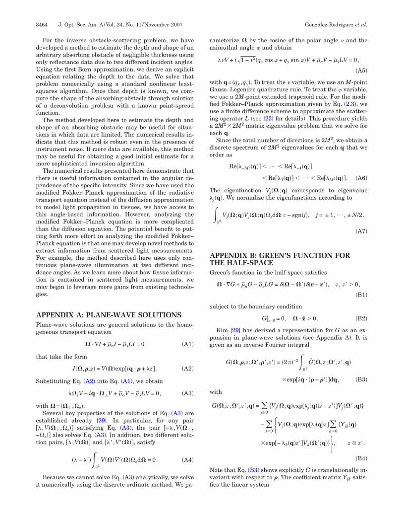
For the inverse obstacle-scattering problem, we haveeveloped a method to estimate the depth and shape of anrbitrary absorbing obstacle of negligible thickness usingnly reflectance data due to two different incident angles.sing the first Born approximation, we derive an explicit
quation relating the depth to the data. We solve thatroblem numerically using a standard nonlinear least-quares algorithm. Once that depth is known, we com-ute the shape of the absorbing obstacle through solutionf a deconvolution problem with a known point-spreadunction.
The method developed here to estimate the depth andhape of an absorbing obstacle may be useful for situa-ions in which data are limited. The numerical results in-icate that this method is robust even in the presence ofnstrument noise. If more data are available, this method
ay be useful for obtaining a good initial estimate for aore sophisticated inversion algorithm.The numerical results presented here demonstrate that
here is useful information contained in the angular de-endence of the specific intensity. Since we have used theodified Fokker–Planck approximation of the radiative
ransport equation instead of the diffusion approximationo model light propagation in tissues, we have access tohis angle-based information. However, analyzing theodified Fokker–Planck equation is more complicated
han the diffusion equation. The potential benefit to put-ing forth more effort in analyzing the modified Fokker–lanck equation is that one may develop novel methods toxtract information from scattered light measurements.or example, the method described here uses only con-inuous plane-wave illumination at two different inci-ence angles. As we learn more about how tissue informa-ion is contained in scattered light measurements, weay begin to leverage more gains from existing technolo-
ies.
PPENDIX A: PLANE-WAVE SOLUTIONSlane-wave solutions are general solutions to the homo-eneous transport equation
� · �I + �aI − �sLI = 0 �A1�
hat take the form
I��,�,z� = V���exp�iq · � + �z. �A2�
ubstituting Eq. (A2) into Eq. (A1), we obtain
��zV + iq · ��V + �aV − �sLV = 0, �A3�
ith �= ��� ,�z�.Several key properties of the solutions of Eq. (A3) are
stablished already [29]. In particular, for any pair� ,V��� ,�z� satisfying Eq. (A3), the pair �−� ,V��� ,�z� also solves Eq. (A3). In addition, two different solu-ion pairs, �� ,V��� and ��� ,V����, satisfy
�� − ����S2
V���V�����zd� = 0. �A4�
Because we cannot solve Eq. (A3) analytically, we solvet numerically using the discrete ordinate method. We pa-
ameterize � by the cosine of the polar angle � and thezimuthal angle � and obtain
��V + i�1 − �2�qx cos � + qy sin ��V + �aV − �sLV = 0,
�A5�
ith q= �qx ,qy�. To treat the � variable, we use an M-pointauss–Legendre quadrature rule. To treat the � variable,e use a 2M-point extended trapezoid rule. For the modi-ed Fokker–Planck approximation given by Eq. (2.3), wese a finite difference scheme to approximate the scatter-
ng operator L (see [23] for details). This procedure yields2M22M2 matrix eigenvalue problem that we solve for
ach q.Since the total number of directions is 2M2, we obtain a
iscrete spectrum of 2M2 eigenvalues for each q that werder as
Re��−M2�q� � ¯ � Re��−1�q�
� Re��1�q� � ¯ � Re��M2�q�. �A6�
he eigenfunction Vj�� ;q� corresponds to eigenvaluej�q�. We normalize the eigenfunctions according to
Kim [29] has derived a representation for G as an ex-ansion in plane-wave solutions (see Appendix A). It isiven as an inverse Fourier integral
G��,�,z;��,��,z�� = �2��−2�R2
G��,z;��,z�,q�
exp�iq · �� − ���dq, �B3�
ith
G��,z;��,z�,q� = �j�0
�Vj��;q�exp��j�q��z − z��Vj���;q�
− �j�0
Vj��;q�exp��j�q�z�k�0
�Yjk�q�
exp�− �k�q�z�Vk���;q� �, z � z�.
�B4�
ote that Eq. (B3) shows explicitly G is translationally in-ariant with respect to �. The coefficient matrix Yjk satis-es the linear system
s
Htm
I
FE�
w
APpDCseU
R
1
1
1
1
1
1
1
1
1
1
2
2
2
2
2
2
González-Rodríguez et al. Vol. 24, No. 11 /November 2007 /J. Opt. Soc. Am. A 3465
�j�0
Vj��;q�Yjk�q� = Vk��;q�, � · z � 0, k � 0.
�B5�
Consider
� · �I + �aI − �sLI = Q, z � 0, �B6�
ubject to the boundary condition
I��,�,0� = b��,��, � · z � 0. �B7�
ere Q denotes a source. The solution to Eq. (B6) subjecto Eq. (B7) is given by the generalized representation for-ula
��,�,z�
=�0
�R2�
S2G��,�,z;��,��,z��Q���,��,z��d��d��dz�
+�R2�
�·z�0
�� · zG��,�,z;��,��,0�b���,���d��d��.
�B8�
or the case in which Q=0 and the boundary conditionq. (B7) corresponds to a plane wave incident in direction0 so that �I�z=0=���−�0�, Eq. (B8) reduces to
I��,�,z� =�R2
�0 · zG��,�,z;�0,��,0�d��, �B9�
=�0zG��,z;�0,0,q = 0�, �B10�
=�j�0
Vj��;0�exp��j�0�zcj��0�, �B11�
ith
cj��0� = �0z�Vj��0;0� − �k�0
Yjk�0�Vk��0;0�� . �B12�
CKNOWLEDGMENTS. González-Rodríguez and A. D. Kim acknowledge sup-ort from the National Science Foundation and the U.S.epartment of Energy through the UC Merced Center foromputational Biology. Miguel Moscoso acknowledgesupport from the Spanish Ministery of Education and Sci-nce (grant FIS2004-03767) and from the Europeannion (contract LSHG-CT-2003-503259).
EFERENCES1. J. P. Van Hounten, D. A. Benaron, S. Spilman, and D. K.
2. S. R. Hintz, W. F. Cheong, J. P. Van Hounten, D. K.Stevenson, and D. A. Benaron, “Bedside imaging ofintracranial hemorrhage in the neonate using light:comparison with ultrasound, computed tomography, andmagnetic resonance imaging,” Pediatr. Res. 45, 54–59(1999).
3. S. R. Arridge, “Optical tomography in medical imaging,”Inverse Probl. 15, R41–93 (1999).
4. X. F. Cheng and D. A. Boas, “Systematic diffuse opticalimage errors resulting from uncertainty in the backgroundoptical properties,” Opt. Express 4, 299–307 (1999).
5. D. A. Benaron, S. R. Hintz, A. Villringer, D. A. Boas, A.Klein-Schmidt, J. Frahm, C. Hirth, H. Obrig, J. P. VanHounten, E. L. Kermit, W. Cheong, and D. K. Stevenson,“Noninvasive functional imaging of human brain usinglight,” J. Cereb. Blood Flow Metab. 20, 469–477 (2000).
6. A. Y. Bluestone, G. Abdoulaev, C. H. Schmitz, R. L.Barbour, and A. H. Hielscher, “Three-dimensional opticaltomography of hemodynamics in the human head,” Opt.Express 9, 272–286 (2001).
7. J. C. Hebden, A. Gibson, T. Austin, R. M. Yusof, N.Everdell, D. T. Delpy, S. R. Arridge, J. H. Meek, and J. S.Wyatt, “Imaging changes in blood volume and oxygenationin the newborn infant brain using three-dimensionaloptical tomography,” Phys. Med. Biol. 49, 1117–1130(2004).
8. B. Monsees, J. M. Destouet, and W. G. Totty, “Lightscanning versus mammography in breast-cancerdetection,” Radiology 163, 463–465 (1987).
9. D. Grosenick, H. Wabnitz, H. H. Rinneberg, K. T. Moesta,and P. M. Schlaq, “Development of a time-domain opticalmammograph and first in vivo applications,” Appl. Opt. 38,2927–2943 (1999).
0. J. C. Hebden, H. Veenstra, H. Dehghani, E. M. C. Hillman,M. Scweinger, S. R. Arridge and D. T. Delpy, “Three-dimensional time-resolved optical tomography of a conicalbreast phantom,” Appl. Opt. 40, 3278–3287 (2001).
1. J. E. Bugaj, S. Achilefu, R. B. Dorshow, and R.Rajagopalan, “Novel fluorescent contrast agents for opticalimaging of in vivo tumors based on a receptor-targeteddye-peptide conjugate platform,” J. Biomed. Opt. 6,122–133 (2001).
2. V. Ntziachristos, C. Bremer, E. E. Graves, J. Ripoll, and R.Weissleder, “In-vivo tomographic imaging of near infraredfluorescent probes,” Mol. Imaging 1, 82–88 (2002).
3. E. E. Graves, J. Ripoll, R. Weissleder, and V. Ntziachristos,“A submillimeiter resolution fluorescence molecularimaging system for small animal imaging,” Med. Phys. 30,901–911 (2003).
4. R. Weissleder and U. Mahmood, “Molecular Imaging,”Radiology 219, 316–333 (2001).
5. A. Ishimaru, Wave Propagation and Scattering in RandomMedia (IEEE Press, 1997).
6. A. D. Kim and J. B. Keller, “Light propagation in biologicaltissue,” J. Opt. Soc. Am. A 20, 92–98 (2003).
7. Y. L. Kim, Y. Liu, R. K. Wali, H. K. Roy, M. J. Goldberg, A.K. Kromin, K. Chen, and V. Backman, “Simultaneousmeasurement of angular and spectral properties of lightscattering for characterization of tissue microarchitectureand its alteration in early precancer,” IEEE J. Sel. Top.Quantum Electron. 9, 243–257 (2003).
8. O. Dorn, “A transport-backtransport method for opticaltomography,” Inverse Probl. 14, 1107–1130 (1998).
9. O. Dorn, “Shape reconstruction in scattering media withvoids using a transport model and level sets,” Can. Appl.Math. Quart. 10, 239–275 (2002).
0. A. D. Klose, V. Ntziachristos, and A. H. Hielscher, “Theinverse source problem based on the radiative transferequation in optical molecular imaging,” J. Comput. Phys.202, 323–345 (2005).
1. A. D. Kim and M. Moscoso, “Radiative transport theory foroptical molecular imaging,” Inverse Probl. 22, 23–42(2006).
2. A. D. Kim, C. Hayakawa, and V. Venugopalan, “Estimatingtissue optical properties using the Born approximation ofthe transport equation,” Opt. Lett. 31, 1088–1090 (2006).
3. A. D. Kim and M. Moscoso, “Beam propagation in sharplypeaked forward scattering media,” J. Opt. Soc. Am. A 21,797–803 (2004).
4. L.-H. Wang and S. L. Jacques, “Use of a laser beam with anoblique angle of incidence to measure the reducedscattering coefficient of a turbid medium,” Appl. Opt. 34,2362–2366 (1995).
5. S.-P. Lin, L.-H. Wang, S. L. Jacques, and F. K. Tittel,
2
2
2
2
3
3
3
3
3466 J. Opt. Soc. Am. A/Vol. 24, No. 11 /November 2007 González-Rodríguez et al.
“Measurement of tissue optical properties using obliqueincidence optical fiber reflectometry,” Appl. Opt. 36,136–143 (1997).
6. G. Marquez and L.-H. Wang, “White light oblique incidencereflectometer for measuring absorption and reducedscattering spectra of tissue-like turbid media,” Opt.Express 1, 454–460 (1997).
7. M. Mehrubeoglu, N. Kehtarnavaz, G. Marquez, M. Duvic,and L.-H. Wang, “Skin lesion classification using diffusereflectance spectroscopic imaging with oblique incidence,”Appl. Opt. 41, 182–192 (2002).
8. A. Garcia-Uribe, N. Kehtarnavaz, G. Marquez, V. Prieto, M.Duvic, and L.-H. Wang, “Skin cancer detection usingspectroscopic oblique-incidence reflectometry: classificationand physiological origins,” Appl. Opt. 43, 2643–2650(2004).
9. A. D. Kim, “Transport theory for light propagation inbiological tissue,” J. Opt. Soc. Am. A 21, 820–827 (2004).
0. A. K. Dunn and D. A. Boas, “Transport-based imagereconstruction in turbid media with small source–detectorseparations,” Opt. Lett. 25, 1777–1779 (2000).
1. E. M. C. Hillman, D. A. Boas, A. M. Dale and A. K. Dunn,“Laminar optical tomography: demonstration of millimeter-scale depth-resolved imaging in turbid media,” Opt. Lett.29, 1650–1652 (2004).
2. M. Schweiger, S. R. Arridge, O. Dorn, A. Zacharopoulos,and V. Kolehmainen, “Reconstructing absorption anddiffusion shape profiles in optical tomography using a levelset technique,” Opt. Lett. 31, 471–473 (2006).
3. S. R. Arridge, O. Dorn, J. P. Kaipio, V. Kolehmainen, M.Schweiger, T. Tarvainen, M. Vauhkonen, and A.Zacharopoulos, “Reconstruction of subdomain boundaries ofpiecewise constant coefficients of the radiative transferequation from optical tomography data,” Inverse Probl. 22,2175–2196 (2006).