Reconstructing compressed photo and video data - The Computer

Technical ReportNumber 813

Computer Laboratory

UCAM-CL-TR-813ISSN 1476-2986

Reconstructing compressedphoto and video data

Andrew B. Lewis

February 2012

15 JJ Thomson AvenueCambridge CB3 0FDUnited Kingdomphone +44 1223 763500

http://www.cl.cam.ac.uk/

c© 2012 Andrew B. Lewis

This technical report is based on a dissertation submittedJune 2011 by the author for the degree of Doctor ofPhilosophy to the University of Cambridge, Trinity College.

Some figures in this document are best viewed in colour. Ifyou received a black-and-white copy, please consult theonline version if necessary.

Technical reports published by the University of CambridgeComputer Laboratory are freely available via the Internet:

http://www.cl.cam.ac.uk/techreports/

ISSN 1476-2986

Summary

Forensic investigators sometimes need to verify the integrity and processing history of digital

photos and videos. The multitude of storage formats and devices they need to access also

presents a challenge for evidence recovery. This thesis explores how visual data files can be

recovered and analysed in scenarios where they have been stored in the JPEG or H.264

(MPEG-4 AVC) compression formats.

My techniques make use of low-level details of lossy compression algorithms in order to tell

whether a file under consideration might have been tampered with. I also show that limitations

of entropy coding sometimes allow us to recover intact files from storage devices, even in the

absence of filesystem and container metadata.

I first show that it is possible to embed an imperceptible message within a uniform region of

a JPEG image such that the message becomes clearly visible when the image is recompressed

at a particular quality factor, providing a visual warning that recompression has taken place.

I then use a precise model of the computations involved in JPEG decompression to build

a specialised compressor, designed to invert the computations of the decompressor. This re-

compressor recovers the compressed bitstreams that produce a given decompression result,

and, as a side-effect, indicates any regions of the input which are inconsistent with JPEG

decompression. I demonstrate the algorithm on a large database of images, and show that it

can detect modifications to decompressed image regions.

Finally, I show how to rebuild fragmented compressed bitstreams, given a syntax description

that includes information about syntax errors, and demonstrate its applicability to H.264/AVC

Baseline profile video data in memory dumps with randomly shuffled blocks.

Acknowledgments

Firstly, I would like to thank my supervisor, Markus Kuhn, for his invaluable insights, advice

and support.

Being a member of the Security Group has allowed me to learn about a huge variety of interest-

ing and important topics, some of which have inspired my work. I am grateful to Markus Kuhn

and Ross Anderson for creating this environment. I owe a debt of gratitude to my colleagues

in the Security Group, especially Joseph Bonneau, Robert Watson, Saar Drimer, Mike Bond,

Jonathan Anderson and Steven Murdoch, for their expertise and suggestions, and to my other

friends at the Computer Laboratory, especially Ramsey Khalaf and Richard Russell.

I would like to thank Claire Summers and her colleagues at the London Metropolitan Police

Service for motivating my work on video reconstruction, and providing information about

real-world evidence reconstruction. I am grateful to the Computer Laboratory’s technical staff,

especially Piete Brooks, who provided assistance with running experiments on a distributed

computing cluster. I am also grateful to Trinity College and the Computer Laboratory for

funding my work and attendance at conferences.

Finally, I am very grateful to my parents and brothers, who have been a constant source of

support and encouragement.

Contents

1 Introduction 9

1.1 Outline . . . . . . . . . . . . . . . . . . . . . . . . . . . . . . . . . . . . . . . . 10

1.2 Notation . . . . . . . . . . . . . . . . . . . . . . . . . . . . . . . . . . . . . . . . 10

1.2.1 JPEG algorithm variables reference . . . . . . . . . . . . . . . . . . . . 12

2 Compression algorithms for photo and video data 13

2.1 Overview of data compression concepts . . . . . . . . . . . . . . . . . . . . . . . 13

2.1.1 Bitstream syntax and entropy coding . . . . . . . . . . . . . . . . . . . . 15

2.2 Image compression . . . . . . . . . . . . . . . . . . . . . . . . . . . . . . . . . . 16

2.2.1 The JPEG still-image compression standard . . . . . . . . . . . . . . . . 17

2.2.2 The JPEG algorithm . . . . . . . . . . . . . . . . . . . . . . . . . . . . . 18

2.3 Video compression . . . . . . . . . . . . . . . . . . . . . . . . . . . . . . . . . . 26

2.3.1 The H.264/AVC video compression standard . . . . . . . . . . . . . . . 27

3 Copy-evidence in digital media 28

3.1 Prior work . . . . . . . . . . . . . . . . . . . . . . . . . . . . . . . . . . . . . . . 29

3.1.1 Digital content protection schemes . . . . . . . . . . . . . . . . . . . . . 29

3.1.2 Security printing . . . . . . . . . . . . . . . . . . . . . . . . . . . . . . . 29

3.2 Digital copy-evidence . . . . . . . . . . . . . . . . . . . . . . . . . . . . . . . . . 31

3.3 Quantisation in JPEG recompression . . . . . . . . . . . . . . . . . . . . . . . . 32

3.4 Marking method . . . . . . . . . . . . . . . . . . . . . . . . . . . . . . . . . . . 33

3.4.1 Maximising distortion . . . . . . . . . . . . . . . . . . . . . . . . . . . . 33

3.4.2 Embedding . . . . . . . . . . . . . . . . . . . . . . . . . . . . . . . . . . 34

3.4.3 Clipping of IDCT output . . . . . . . . . . . . . . . . . . . . . . . . . . 35

3.5 Marking algorithm . . . . . . . . . . . . . . . . . . . . . . . . . . . . . . . . . . 35

3.5.1 Termination conditions and unmarkable blocks . . . . . . . . . . . . . . 36

3.5.2 Gamma-correct marking . . . . . . . . . . . . . . . . . . . . . . . . . . . 37

3.5.3 Untargeted marks . . . . . . . . . . . . . . . . . . . . . . . . . . . . . . 38

3.5.4 Results . . . . . . . . . . . . . . . . . . . . . . . . . . . . . . . . . . . . 39

3.6 Analysis . . . . . . . . . . . . . . . . . . . . . . . . . . . . . . . . . . . . . . . . 41

3.6.1 Possible extensions to the algorithm . . . . . . . . . . . . . . . . . . . . 42

3.7 Conclusion . . . . . . . . . . . . . . . . . . . . . . . . . . . . . . . . . . . . . . 43

4 Exact JPEG recompression 44

4.1 Introduction . . . . . . . . . . . . . . . . . . . . . . . . . . . . . . . . . . . . . . 44

4.1.1 Exact recompression . . . . . . . . . . . . . . . . . . . . . . . . . . . . . 45

4.1.2 Comparison with naıve recompression . . . . . . . . . . . . . . . . . . . 46

4.1.3 Decompressor implementations . . . . . . . . . . . . . . . . . . . . . . . 46

4.2 Applications . . . . . . . . . . . . . . . . . . . . . . . . . . . . . . . . . . . . . . 47

4.2.1 Avoiding quality loss . . . . . . . . . . . . . . . . . . . . . . . . . . . . . 47

4.2.2 Compressor and parameter identification . . . . . . . . . . . . . . . . . . 47

4.2.3 Tampering detection . . . . . . . . . . . . . . . . . . . . . . . . . . . . . 48

4.3 Prior work . . . . . . . . . . . . . . . . . . . . . . . . . . . . . . . . . . . . . . . 48

4.3.1 Maintaining image quality during recompression . . . . . . . . . . . . . 48

4.3.2 Acquisition forensics . . . . . . . . . . . . . . . . . . . . . . . . . . . . . 49

4.3.3 Tampering detection . . . . . . . . . . . . . . . . . . . . . . . . . . . . . 52

4.3.4 Residual information in JPEG artefacts . . . . . . . . . . . . . . . . . . 55

4.4 Exact recompression of JPEG images . . . . . . . . . . . . . . . . . . . . . . . . 55

4.4.1 Colour-space conversion . . . . . . . . . . . . . . . . . . . . . . . . . . . 56

4.4.2 Chroma down-sampling . . . . . . . . . . . . . . . . . . . . . . . . . . . 57

4.4.3 Discrete cosine transform . . . . . . . . . . . . . . . . . . . . . . . . . . 59

4.4.4 Determining possible quality factors . . . . . . . . . . . . . . . . . . . . 60

4.4.5 Quantisation and exhaustive search . . . . . . . . . . . . . . . . . . . . . 61

4.4.6 YCbCr set refinement . . . . . . . . . . . . . . . . . . . . . . . . . . . . 63

4.5 Overall algorithm summary . . . . . . . . . . . . . . . . . . . . . . . . . . . . . 63

4.6 Results . . . . . . . . . . . . . . . . . . . . . . . . . . . . . . . . . . . . . . . . . 64

4.6.1 Detecting in-painting . . . . . . . . . . . . . . . . . . . . . . . . . . . . . 67

4.7 Analysis . . . . . . . . . . . . . . . . . . . . . . . . . . . . . . . . . . . . . . . . 68


4.8 Conclusion . . . . . . . . . . . . . . . . . . . . . . . . . . . . . . . . . . . . . . 70

5 Reconstruction of fragmented compressed data 71

5.1 Overview . . . . . . . . . . . . . . . . . . . . . . . . . . . . . . . . . . . . . . . 71

5.1.1 Terminology . . . . . . . . . . . . . . . . . . . . . . . . . . . . . . . . . 73

5.2 Background and prior work . . . . . . . . . . . . . . . . . . . . . . . . . . . . . 74

5.2.1 Data acquisition, fragmentation and filesystems . . . . . . . . . . . . . . 74

5.2.2 Unfragmented file carving . . . . . . . . . . . . . . . . . . . . . . . . . . 76

5.2.3 Fragmented file carving . . . . . . . . . . . . . . . . . . . . . . . . . . . 77

5.2.4 H.264/AVC error detection . . . . . . . . . . . . . . . . . . . . . . . . . 80

5.3 The defragmentation problem . . . . . . . . . . . . . . . . . . . . . . . . . . . . 81

5.3.1 Syntax checkers . . . . . . . . . . . . . . . . . . . . . . . . . . . . . . . . 81

5.3.2 Decoding contexts . . . . . . . . . . . . . . . . . . . . . . . . . . . . . . 81

5.3.3 Finding valid bitstreams and defragmentation . . . . . . . . . . . . . . . 83

5.3.4 False positives . . . . . . . . . . . . . . . . . . . . . . . . . . . . . . . . 83

5.4 Bitstream syntax description . . . . . . . . . . . . . . . . . . . . . . . . . . . . 83

5.4.1 The bitstream syntax flowgraph . . . . . . . . . . . . . . . . . . . . . . 85

5.4.2 Textual representation of bitstream syntax . . . . . . . . . . . . . . . . 87

5.5 H.264/AVC bitstream syntax checking . . . . . . . . . . . . . . . . . . . . . . . 88

5.5.1 Assumptions about the video . . . . . . . . . . . . . . . . . . . . . . . . 88

5.5.2 Coding modes . . . . . . . . . . . . . . . . . . . . . . . . . . . . . . . . 91

5.5.3 NAL unit syntax . . . . . . . . . . . . . . . . . . . . . . . . . . . . . . . 94

5.5.4 Error detection performance . . . . . . . . . . . . . . . . . . . . . . . . . 97

5.6 Fragmented bitstream recovery algorithm . . . . . . . . . . . . . . . . . . . . . 104

5.6.1 Algorithm notation and objects . . . . . . . . . . . . . . . . . . . . . . . 106

5.6.2 Configuration bitstream parsing and data bitstream offset search . . . . 107

5.6.3 Data bitstream filtering . . . . . . . . . . . . . . . . . . . . . . . . . . . 107

5.6.4 Data bitstream mapping (optional) . . . . . . . . . . . . . . . . . . . . . 109

5.6.5 Data bitstream block search algorithm . . . . . . . . . . . . . . . . . . . 111

5.7 Results . . . . . . . . . . . . . . . . . . . . . . . . . . . . . . . . . . . . . . . . . 113

5.7.1 Input data . . . . . . . . . . . . . . . . . . . . . . . . . . . . . . . . . . 113

5.7.2 Data bitstreams . . . . . . . . . . . . . . . . . . . . . . . . . . . . . . . 114

5.7.3 Proportion of data recovered successfully . . . . . . . . . . . . . . . . . 116

5.8 Analysis . . . . . . . . . . . . . . . . . . . . . . . . . . . . . . . . . . . . . . . . 116


5.9 Conclusion . . . . . . . . . . . . . . . . . . . . . . . . . . . . . . . . . . . . . . 117

6 Conclusions 121

A JPEG encoder quality selection 124

A.1 IJG encoder . . . . . . . . . . . . . . . . . . . . . . . . . . . . . . . . . . . . . . 124

A.2 Adobe Photoshop CS2 . . . . . . . . . . . . . . . . . . . . . . . . . . . . . . . . 124

B H.264/AVC bitstream syntax 127

Chapter 1

Introduction

Compressed photo and video data files present both opportunities and challenges to forensic

investigators dealing with digital evidence. Huge quantities of compressed data are generated

every day by consumer digital cameras and commercial image/video recording systems. This

motivates the development of algorithms which recover evidence from devices and detect tam-

pering on visual data that has undergone lossy compression. The algorithms are of particular

use to law enforcement agencies and journalists, who must routinely deal with compressed

data with uncertain processing history.

A central challenge in digital forensics is the extraction of information from devices where

details of storage formats or filesystem layouts is unavailable, due to a lack of documentation.

Metadata might have been deleted deliberately, or might be invalid due to data corruption.

The multitude of different devices storing video, some using proprietary container formats and

filesystems, is a problem for forensics labs that receive evidence from many sources. Manual

procedures for evidence recovery are time-consuming and require skilled investigators with

knowledge of the characteristics of hardware, software, file formats and compression standards.

Therefore, automatic, general-purpose algorithms that do not rely on detailed knowledge of

the devices will be increasingly important as the volume of digital evidence to process becomes

greater.

The widespread use of digital photo manipulation software provides an opportunity for forensic

investigators. Alterations can affect hidden statistical correlations in photos and videos, which

may expose an attempt to deceive the viewer. Investigators can exploit the disruption of the

patterns introduced by compression algorithms early in a document’s processing history as

an indication that tampering has taken place.

9

1. Introduction

1.1 Outline

In this thesis, I show that it is possible to exploit the low-level details of compression schemes

and their implementations to develop automatic tampering detection and data recovery algo-

rithms that are applicable in scenarios involving compressed data.

Chapter 2 begins with a description of the JPEG compression scheme and the calculations

performed by one decompressor implementation. Chapter 3 describes one approach to achiev-

ing copy-evidence properties in a JPEG image, taking advantage of the effects of a JPEG

compression/decompression cycle. I show that it is possible to embed a low-resolution bi-level

image within a homogeneous area of a cover image, which is imperceptible to viewers of the

original document, but which becomes visible when the image is recompressed using particular

quality settings.

Chapter 4 describes a specialised JPEG compressor which recovers compressed image data

bitstreams given a decompression result as input. As a side-effect, the algorithm determines

whether any regions of the decompression result were modified. It has applications in content

protection system circumvention and tampering detection, and can be used to maintain image

quality in processing pipelines that use compressed data.

Chapter 5 describes an automatic data recovery tool that locates and reconstructs frag-

mented compressed bitstreams, and demonstrates its applicability on memory dumps con-

taining H.264/AVC Baseline profile video data. The tool uses a description of the compressed

bitstream syntax, but does not rely on detailed knowledge of the video container or filesystem

allocation unit ordering.

Finally, chapter 6 draws some conclusions and gives suggestions for future work.

1.2 Notation

This section describes the notational conventions I use throughout this thesis.

For a matrix a (with h rows and w columns), the element in row i and column j is denoted

by ai,j = (a)i,j (0 ≤ i < h, 0 ≤ j < w). I sometimes write a[j, i] for the same value, where the

indexing order is swapped.

The matrix transpose b = aT has elements bi,j = aTi,j = aj,i.

aj (or a[j]) is the column vector (a0,j , . . . , ah−1,j)T and (aT)j denotes the column vector

(aj,0, . . . , aj,w−1)T. The value at index i in aj is aj [i] = ai,j . I also use the notation aj [s : e] to

denote the vector (as,j , . . . , ae−1,j)T.

When indexing two-dimensional signals represented as vectors in raster-scan order, I use the

10

1.2. Notation

following notation:

〈x, y〉w = x+ w · y (1.1)

〈x, y〉w,h = 〈min(x,w − 1),min(y, h− 1)〉w (1.2)

〈i〉−1w = (i mod w, bi/wc) (1.3)

I use the following functions, defined similarly over sets:

max(x, y) =

x x ≥ yy x < y

(1.4)

min(x, y) =

x x ≤ yy x > y

(1.5)

and sgn(x) = x/|x| for non-zero x, and 0 otherwise.

Matrices containing sets of integers are written like s. I make use of integer intervals x =

[x⊥, x>], which contains integers from x⊥ to x> inclusive, and matrices containing intervals

over the integers are denoted by x. y ∈ x⇔ x⊥ ≤ y ≤ x> ∧ y ∈ Z. “Union” and intersection

on such intervals are defined as

x ∪ y := [min(x⊥, y⊥),max(x>, y>)]

x ∩ y :=

empty if x⊥ > y> ∨ y⊥ > x>,

[ max(x⊥, y⊥),

min(x>, y>)]otherwise.

bxc denotes the largest integer less than or equal to x, and dxe denotes the smallest integer

greater than or equal to x (for real x). For scalar division I define

divround(x, q) = sgn(x) · b(|x|+ bq/2c)/qc,div(x, q) = sgn(x) · b|x|/qc for non-zero q.

Multiplying a tuple by a scalar multiplies each element by the scalar: α · (x1, . . . , xN ) =

(α·x1, . . . , α·xN ). Addition is element-wise for two tuples of the same length N : (x1, . . . , xN )+

(y1, . . . , yN ) = (x1 + y1, . . . , xN + yN ).

11

1. Introduction

1.2.1 JPEG algorithm variables reference

Matrix Rows × Columns Interpretation

u 3× w · h w × h pixel image in the RGB colour space

v 3× w · h u in the YCbCr colour space

v− 3× dw/2e · dh/2e down-sampled v

vT

0 w · h× 1 full-resolution luma

v−T1 dw/2e · dh/2e × 1 down-sampled chroma

v−T2 dw/2e · dh/2e × 1 down-sampled chroma

xb 8× 8 bth MCU in one component

Xb 8× 8 xb in the DCT domain

QY 8× 8 quantisation coefficients for luma

QC 8× 8 quantisation coefficients for chroma

Xb 8× 8 DCT coefficients Xb after quantisation

X′b 8× 8 reconstructed DCT coefficients

x′b 8× 8 bth reconstructed MCU in one component

v′−T1 dw/2e · dh/2e × 1 reconstructed down-sampled chroma

v′−T2 dw/2e · dh/2e × 1 reconstructed down-sampled chroma

v′T0 w · h× 1 reconstructed full-resolution luma

v′T1 w · h× 1 up-sampled chroma

v′T2 w · h× 1 up-sampled chroma

v′ 3× w · h reconstructed image in the YCbCr colour space

u′ 3× w · h reconstructed image in the RGB colour space

12

Chapter 2

Compression algorithms for photo

and video data

This chapter introduces visual data compression algorithms and describes the JPEG algo-

rithm, used in chapters 3 and 4.

The development of efficient image and video compression algorithms for content distribution

was originally driven by the telecommunications and entertainment industries, but a diverse

range of consumer devices, including mobile telephones, cameras and mobile computers, now

include software and hardware compressors for visual data. Since the majority of image and

video files on electronic devices and Internet servers are stored in compressed form, forensic

investigators must mostly deal with files that have previously been compressed.

The reconstruction algorithms in this thesis make use of the JPEG still image compression

standard [38] and the H.264/AVC video compression standard [45], which are freely available.

We generally rely on features of the relevant compression schemes that are likely to be shared

by other standards.

2.1 Overview of data compression concepts

Practical compression system implementations (for standards such as MPEG-1/2/4, JPEG,

PNG, . . . ) include two programs: an encoder and a decoder.

The encoder program, or compressor, takes uncompressed source data as input (for example,

pixel values), removes redundant/irrelevant information, and returns a binary file called a

bitstream, which represents the remaining data along with any requisite metadata for decom-

pression.

The decoder program, or decompressor, takes a bitstream produced by an encoder as input

and returns an uncompressed file in the same format as the original source; this file is either

13

2. Compression algorithms for photo and video data

identical to the source file, in the case of lossless compression, or is perceptually similar to it,

in the case of lossy compression.

Because lossless compression systems must define a bijection between source and compressed

data files, some files will in practice expand when they are encoded.

Source domain

Compressed domain

uncompressed source

compressed bitstream

compression

decompression

Figure 2.1: Lossless compression algorithms take source data and produce bitstreams which decom-

press to produce a file identical to the source data.

Lossy compression systems aim to remove both redundant and irrelevant data, normally mak-

ing it impossible to reconstruct the exact file which was input. These compressors should keep

perceptually important information and discard information which is not important to the

observer of the decompression result. Audio/visual compression systems, for example, typi-

cally include a psychophysical model of the limitations of the human auditory/visual systems,

so that information is discarded only when it cannot be heard or seen by the observer (due

to variations in sensitivity to different inputs, masking and filtering inherent in human hear-

ing/vision).

Source domain

Compressed domain

uncompressed source ≈ decompressed file

compressed bitstream

compression

decompression

Figure 2.2: Lossy compression algorithms take source data and produce bitstreams which decompress

to produce a file similar to the source data.

Designers of general-purpose compression algorithms optimise jointly for file size, computa-

tional complexity and, in the case of lossy algorithms, to minimise the distortion introduced

by a compression/decompression cycle. More flexible compressor implementations present an

interface where the user can specify a target bitrate, which can be calculated from the duration

of the input (if known) and a target output file size.

Some lossy encoders allow the user to choose between constant or variable bitrate modes.

Constant bitrate (CBR) encoding tries to keep a consistent rate throughout the document

14

2.1. Overview of data compression concepts

(measured over a particular window size in the signal, such as per frame of a video), while vari-

able bitrate (VBR) encoding can distribute bits in the output bitstream unevenly, allocating

fewer bits to more predictable parts of the signal.

Two-pass compression algorithms are often used in conjunction with the VBR strategy. They

first measure the relative complexity of different parts of the signal (for example, scenes in a

video), then write the output bitstream during a second pass over the input, taking advantage

of information about the entire signal. The overall aim is to achieve constant perceived quality.

Lossy compressors often have to choose between several options, each one making a different

trade-off between bit cost and perceived distortion. These choices arise when coding values

for quantised transform coefficients, motion vectors, and so on. Rate-distortion optimisation

(RDO) is the action of choosing between several options, trying to minimise distortion whilst

keeping within a bit-budget. To perform this minimisation, encoders try to avoid situations

where it is possible to reallocate bits between independently coded features whilst reducing

overall perceived distortion1.

Useful compression schemes will map nearly all typical inputs onto smaller encoded bitstreams,

whilst making good RDO decisions for a particular rate/distortion trade-off.

Salomon gives an overview of many lossy and lossless compression schemes [89].

2.1.1 Bitstream syntax and entropy coding

The overall structure of encoders varies significantly with the type of information processed.

However, most encoders have a final lossless coding step, which maps the calculated, reduced

redundancy data onto a binary stream for output. The data are normally integer values, each

associated with a named syntax element, which denotes the meaning of the value (a sample

from an image, a flag indicating presence of another value, etc.). A syntax element may have

multiple, ordered values, which are associated with different decoding positions (transform

coefficient indices, picture regions, frame numbers, etc.).

The standardisation document for the compression scheme describes a bitstream syntax, which

is a graph specifying the order and coding mode of syntax element values which appear in

valid bitstreams. Compliant encoders output bitstreams that a decoder can parse by referring

to this syntax flowgraph.

There are two categories of coding modes. Symbol coding modes map syntax element values

onto separate bitstrings, which are concatenated to produce the final bitstream. Stream coding

modes map a sequence of syntax element values onto a single long bitstring, where each syntax

element value may affect a non-integer number of bits. The overall process of turning the

1In practice, this is usually achieved by selecting for each coding decision the option that has its local rate

vs. distortion gradient closest to a known value λ. This parameter is chosen based on the desired bitrate or

quality.

15


sequence of syntax element values into a bitstream based on their coding modes as specified

in the bitstream syntax is called entropy coding.

If a symbol to be coded is associated with a random variable Si with probability distribution

P (Si), it should be coded so that the length of the codeword is as close as possible to the

amount of information communicated by the observation of the symbol, H(Si) = − log2 P (Si)

bits. The probability distribution may be estimated based on prior knowledge of the source,

shared by both the encoder and decoder, and can be updated at runtime after observing other

syntax element values.

Huffman symbol coding maps each symbol onto an integer number of bits. It has two main

limitations: firstly, the scheme is only optimal when each probability, P (Si) = 2−k for some

k, so that the rate of the code is equal to the entropy of the probability distribution. If any

symbol has probability P (Si) >12 , variable-length coding must still output at least one bit,

wasting between 0 and 1 bits per symbol. Secondly, Huffman codes cannot adapt elegantly

to changes in symbol probabilities. Arithmetic coding remedies these problems, outputting a

fractional number of bits per input symbol [71, Section 5.6: Disadvantages of the Huffman

Code, page 101].

2.2 Image compression

In natural images, neighbouring pixels’ intensities are normally highly correlated. Some de-

pendency in audio/visual data is due to correlation, and correlation is more practical to tackle

than dependency. Therefore, all algorithms for natural image compression work by removing

redundancy due to correlation.

The most general source coding algorithms predict a value (such as a pixel intensity) based on

its neighbourhood, and entropy-code the prediction error signal using probabilities which are

based on the neighbourhood (see for example [10]). For this technique to work well in natural

images, large neighbourhoods must be considered, using a lot of memory and requiring a large

corpus of training images, as well as slowing down adaptation to changing image content.

Most compression algorithms for natural images instead use less expensive transform coding

algorithms [32], where spatial domain information is linearly, reversibly transformed into a new

representation that decorrelates pixel values. Ideally, the input to the final entropy coding step

should be a sequence of independent random variables with known probability distributions,

so that each output bit communicates close to one bit of information (on average).

16

2.2. Image compression

2.2.1 The JPEG still-image compression standard

The lossy compression method described in the JPEG standard (ITU-T recommendations

T.81 and T.83, ISO/IEC 10918-1/2 [38, 39]) has emerged as the most widely-used algorithm2

for encoding continuous-tone still images for transmission and storage since its first publication

in 1992. It affords compression ratios of 0.05–0.10 with almost no perceived loss in quality [89,

Section 4.8 JPEG, page 337].

The first part of the JPEG standard (Digital compression and coding of continuous-tone

still images: Requirements and guidelines, ITU-T recommendation T.81 (September 1992),

ISO/IEC 10918-1:1994 [38]) specifies the compressed bitstream format normatively, and de-

scribes some elements of the compressor and decompressor informatively. Without additional

metadata, the interchange format it specifies is known as JPEG Interchange Format (JIF).

This format lacks information about the resolution (in dots per inch, for example), colour

space and sampling pattern of the image. However, it includes fields for extension information

(‘application markers’).

Digital cameras use the Exchangeable image file format [47] (Exif). It embeds useful metadata

relevant to digital photographs, such as the location and date/time of capture, camera model

and manufacturer, exposure duration and f-number, colour information and so on, within

JIF’s extension fields. The older JPEG File Interchange Format [44] (JFIF) is sometimes used

as an alternative.

The second part of the JPEG standard [39] (Digital compression and coding of continuous-tone

still images: Compliance testing, ITU-T recommendation T.83 (November 1994), ISO/IEC

10918-2:1995) places restrictions on decompressor outputs. Because the first part of the stan-

dard does not give exact formulae for some calculations, implementations may use any algo-

rithm which produces results within the specified tolerances.

The lossy, non-hierarchical compression algorithm described in the JPEG standard has several

options for coding images: pixel values may be represented either to 8-bit (baseline) or 12-bit

precision; the colour space used to represent pixel values may be chosen; the monochrome

plane (rectangular array of integer samples) corresponding to each colour channel may be

down-sampled horizontally, vertically or in both directions; two entropy coding schemes are

specified (Huffman (variable-length) and arithmetic coding); and the order of coding may be

sequential or progressive, where a reduced-quality version of the image is gradually refined dur-

ing decoding. Though the colour space conversion and down-sampling steps are not described

in the JPEG standard itself, all practical implementations must support these operations.

The most common choice of options encodes an 8 bits per sample red/green/blue (RGB) image

using a luma/chroma (YCbCr) colour space with horizontally and vertically down-sampled

2The hierarchical and lossless coding techniques describe in the standard are less commonly used, and we

do not consider them here.

17


chroma channels (also known as 4 : 2 : 0 down-sampling3) to a sequentially-ordered Huffman

coded bitstream. Unless otherwise specified, I will assume these options are chosen when I

refer to the JPEG algorithm.

2.2.2 The JPEG algorithm

High performance JPEG codecs use limited precision machine integer arithmetic to represent

intermediate results in fixed-point, making a trade-off between accuracy and speed, while

meeting the requirements of the compliance testing part of the standard [39].

The following description of the encoder uses formulae which are equivalent to the operations

described in the standard, while the subsequent description includes the integer arithmetic

(fixed-point) calculations performed by the Independent JPEG Group (IJG) decoder imple-

mentation (version 6b) [57].

Compression

1. An input bitmap in the RGB colour space is first converted to the YCbCr colour space.

In natural images, this reduces the inter-component correlations in pixel values, and

allows the colour and brightness information to be processed independently.

We represent a w × h pixel uncompressed bitmap image with 3 × 8-bit samples per

pixel (red, green, blue) as a matrix u with w · h columns and 3 rows. The tuple (ui)T ∈

0, . . . , 2553 (0 ≤ i < w · h) contains the (red, green, blue) samples for the pixel at

location (x, y) = (i mod w, bi/wc) = 〈i〉−1w .

A YCbCr representation v of this RGB image u is given by the per-pixel calculation

vi =

0.299 0.587 0.114

−0.169 −0.331 0.500

0.500 −0.419 −0.081

ui +

0

128

128

. (2.1)

The transformed samples can be recovered in a decompressor by multiplication with the

inverse matrix 1.000 0.000 1.402

1.000 −0.344 −0.714

1.000 1.772 0.000

(2.2)

where all values are rounded to four significant figures.

3This notation for chroma down-sampling schemes is decoded as follows: w : a : b indicates that in two rows

of w luma samples, the first row contributes a chroma samples and the second row contributes b additional

chroma samples. (w is known as the luma sampling reference, originally relative to a sampling rate of 3.375 MHz

in broadcast television.)

18


Figure 2.3 shows the RGB axes from three different viewpoints in the tri-chromatic

colour space, and the YCbCr axes which contain the RGB cube. We plot pixels from a

16 × 16 neighbourhood in the ‘Lena’ sample image as circles filled in with the respective

pixel’s colour. The luma (Y) axis distribution has higher variance than the chroma axis

distributions, indicating that the colour space transform has some decorrelating effect

in this example.

B

G

50100150

200250

Cb

R

50

100

150

200

250

Y50

100

150

200

250

Cr

Figure 2.3: The RGB to YCbCr colour space conversion as a coordinate transform

If an encoder implementation uses integer arithmetic to perform the colour space con-

version, information may be lost due to rounding.

2. The Y, Cb and Cr components resulting from colour space conversion are processed

independently. The two chroma components are each down-sampled horizontally and

vertically by a factor of two, while the luma component is left at its original resolution.

The human visual system (HVS) has better acuity for brightness than colour, because

the central part of the retina (the fovea) has a lower density of short-wavelength adapted

photoreceptors than medium- and long-wavelength adapted photoreceptors. The latter

two types of receptor exhibit large amounts of overlap in spectral sensitivity (their peak

responses lie only 30 nm apart) [17, Section 4.3.4, page 221]. The brain has more cells

dedicated to addition of the medium/long wavelength receptors’ signals than to their

subtraction. This makes the HVS more sensitive to errors in luma (the additive signal)

than colour. The encoder can therefore store colour information with less precision and

resolution than the luma channel without seriously affecting the perceived image quality.

19


The YCbCr image v is padded by repetition so that its width and height are both

multiples of two. The down-sampling operation averages non-overlapping squares of 2

× 2 pixels, giving v−.

The down-sampling operation (with input padding where necessary) can be implemented

as

v−i =1

4

∑δ∈0,12

v[〈2 · 〈i〉−1dw/2e + δ〉

w,h], (2.3)

for 0 ≤ i < dw/2e · dh/2e.

If both chroma components are down-sampled horizontally and vertically by a factor of

two, the total number of samples is halved.

3. The full-resolution luma component and down-sampled chroma components are each

divided up into non-overlapping 8 × 8 sample blocks, known as minimum coded units

(MCUs), which are processed independently.

After down-sampling of the chroma components, the YCbCr component tuple (vT

0,

v−T1, v−T2), with dimensions ((w, h), (dw/2e, dh/2e), (dw/2e, dh/2e)), represents the

image content. The following processing steps are applied to each component c ∈vT

0,v−T

1,v−T

2 separately; we denote the width and height of c by n and m re-

spectively.

The right and bottom edges of the component must be padded if its width or height

are not multiples of 8. The standard does not specify what values should be used for

padding data. In this example, we pad by repeating the right and bottom edge sam-

ple values. A decoder decompresses the padded component and crops it based on size

metadata in the bitstream. The compressor can subtract 128 from each sample, which

reduces the dynamic range requirements on the following transform step. (Mathemati-

cally, this is equivalent to subtracting 1024 from the lowest frequency component after

the transform.) The bth MCU of c, the 8 × 8 matrix xb, is given by

(xb)[j, i] = c[〈8 · 〈b〉−1dn/8e + (i, j)〉

n,m]− 128 (2.4)

for 0 ≤ i, j < 8 and 0 ≤ b < dn/8e · dm/8e.

An 8 × 8 forward discrete cosine transform (DCT)4 is applied to each MCU in each

component. The 2-D DCT is a linear, separable transform which represents a block of

sample values as the weights of sampled cosine functions at various frequencies. Fig-

ure 2.4 shows one of the transform’s basis vectors along with the 1-D horizontally and

vertically orientated cosine functions which are multiplied to give the 2-D function. The

4Specifically, the type two DCT is used, which interprets its input vector as being even around the point

half-way between its first sample and the previous sample in the periodic extension.

20


Figure 2.4: Cosines with 3/16 cycles per sample (horizontal) and 2/16 cycles per sample (vertical),

and the 2-D DCT basis vector formed by their product.

representation of an MCU xb in the DCT basis is given by

(Xb)u,v =C(u)√N/2

C(v)√N/2

N−1∑i=0

N−1∑j=0

(xb)i,j cos

((2i+ 1)uπ

2N

)cos

((2j + 1)vπ

2N

), (2.5)

where 0 ≤ u, v < 8 and

C(u) =

1√2

u = 0

1 u > 0.

An example decomposition of an 8 × 8 matrix of samples (from the ‘Lena’ sample image)

into a weighted sum of the DCT basis vectors can be visualised as follows:

= 1203 · + 123 · − 26 · + 9 · + 6 · + 4 · − 4 · − 1 ·− 25 · + 9 · + 8 · + 9 · − 8 · + 5 · + 2 · + 1 ·+ 18 · − 10 · − 1 · − 3 · + 0 · + 5 · + 0 · + 2 ·− 12 · + 8 · + 7 · − 4 · + 3 · − 6 · − 1 · + 3 ·+ 12 · − 3 · − 4 · + 6 · − 2 · + 3 · + 1 · − 3 ·− 6 · + 4 · + 4 · − 3 · + 5 · − 4 · − 4 · + 2 ·+ 0 · − 1 · − 4 · + 4 · − 4 · − 1 · + 0 · + 0 ·− 1 · + 3 · + 1 · − 3 · + 6 · + 1 · − 2 · + 2 · (2.6)

The scalar coefficients are known as the DCT coefficients for the transformed block. In

this example, the DCT coefficients are rounded to integers.

In an encoder implementation which uses integer arithmetic, some information may be

lost due to rounding of DCT coefficients, intermediate results and basis function samples.

4. In photographic images, the DCT coefficients are much less correlated than the spatial-

domain samples. The JPEG algorithm now discards information by uniformly quantising

each DCT coefficient in each MCU. The quantisation factor depends on the coefficient’s

21


associated spatial frequency, the component plane being processed (luma/chroma) and,

usually, a user-specified quality parameter. The quantisation factors are kept in two

8 × 8 quantisation tables (one for the luma component and one for the two chroma

components), stored in the header of the bitstream.

The user of the encoder normally controls the choice of quantisation tables indirectly,

via a scalar quality factor which multiplies the standardised, default quantisation ta-

bles. Other schemes are also possible; appendix A describes how quantisation factors

are chosen in two popular encoder implementations (IJG [57] and Adobe Photoshop

CS2 [37]).

As noted earlier, the HVS has higher acuity in brightness compared to colour vision.

We are also more sensitive to errors in the amplitude of lower frequency signals. The

default quantisation tables [38, Tables K.1, K.2] specify (a) more aggressive quantisation

for DCT coefficients corresponding to higher spatial frequencies and (b) more aggres-

sive quantisation for DCT coefficients in chroma blocks. Information deemed to be less

perceptually important will be discarded.

The quantisation factor for a given spatial frequency, (u, v) ∈ 0, . . . , 72 half-cycles per

block, is drawn from the relevant quantisation table for the component being processed,

QY for luma blocks and QC for chroma blocks.

Each DCT coefficient (Xb)u,v in each block in each component is quantised using the

appropriate entry from the quantisation table, Qu,v, by the following calculation:

(Xb)u,v = divround ((Xb)u,v, Qu,v) = sgn ((Xb)u,v) ·⌊ |(Xb)u,v|+ bQu,v/2c

Qu,v

⌋. (2.7)

5. All further coding is lossless, using a Huffman code table shared between the encoder

and decoder. The standard specifies general purpose tables, but also specifies a syntax

which allows encoders to include their own tables in the bitstream.

The majority of the data in the JPEG bitstream for a typical compressed image will

consist of Huffman codewords representing quantised DCT coefficients, (Xb)u,v. To code

blocks of quantised DCT coefficients compactly, the entropy coding step (1) re-orders

quantised DCT coefficients in a zig-zag pattern (figure 2.6), (2) encodes (run, level)

pairs, indicating a run of zeros followed by the value level, (3) uses a short codeword for

the ‘end of block’ (EOB) symbol, which indicates that all further coefficients in the re-

ordered sequence are zero and (4) encodes the top-left (0, 0) cycles per block coefficient

(the DC coefficient) as a difference from the equivalent value in the previous block, as

they will normally be correlated in nearby blocks.

22


0 25−25 50−50

0: 16

1: 11

2: 12

3: 14

4: 12

5: 10

6: 16

7: 14

8: 13

9: 14

10: 18

11: 17

12: 16

13: 19

14: 24

15: 40

16: 26

17: 24

18: 22

19: 22

20: 24

21: 49

22: 35

23: 37

24: 29

25: 40

26: 58

27: 51

28: 61

29: 60

30: 57

31: 51

32: 56

33: 55

zig-z

ag

scan

ind

ex:

qu

anti

sati

on

fact

or

unquantised coefficient value

Figure 2.5: Each row of this chart is associated with a particular DCT coefficient position in zig-

zag scan order (see figure 2.6). The alternately shaded rectangles in each row cover groups of DCT

coefficient values that are mapped onto the same quantised coefficient; the corresponding dequantised

coefficient value is indicated by a circle at the centre of the group. The quantisation table is [38, Table

K.1, page 143].

Figure 2.6: The encoder re-orders quantised

DCT coefficients so that later coefficients in the

bitstream correspond to higher spatial frequencies.

Decompression

1. The IJG decoder is structured to use memory sparingly, so that it can run on embedded

devices which have little storage available. The decoder performs lossless decoding of

Huffman codewords in the stream as they are required, sequentially loading each MCU

row into a buffer for processing. Each MCU in each row contains 64 quantised DCT

coefficients.

2. Each quantised DCT coefficient in each MCU is dequantised. This operation maps the

coefficient onto an integer multiple of the relevant quantisation factor. The quantisa-

23


tion tables, QY for luma blocks and QC for chroma blocks, are encoded in the input

bitstream’s header.

Each quantised DCT coefficient (Xb)u,v in each MCU is dequantised as

(X′b)u,v = (Xb)u,v ·Qu,v. (2.8)

Figure 2.5 shows what ranges of coefficients are mapped to the same value after a

quantisation/dequantisation cycle for several block indices in zig-zag scan order, and

the associated values for the dequantised DCT coefficient.

3. At this stage, the decoder has reconstructed an estimate X′b of the block which was

present after the DCT in the encoder, Xb. The next stage is to perform an inverse DCT

on each block, which transforms the frequency representation of the block back into

the spatial domain. The calculations involved in the IJG codec’s default inverse DCT

algorithm, defined in jidctint.c (implementing the Loeffler/Ligtenberg/Moschytz fast

IDCT [67]), are equivalent to the following calculation, performed on each block X′b:

x′b = max

(0,min

(255,

⌊1

218

(⌊1

211

(TX′b + 210

)⌋TT + 217

)⌋))(2.9)

with element-wise rounding, scalar multiplication and application of min and max, and

the transform matrix T is

8192 11363 10703 9633 8192 6437 4433 2260

8192 9633 4433 −2259 −8192 −11362 −10704 −6436

8192 6437 −4433 −11362 −8192 2261 10704 9633

8192 2260 −10703 −6436 8192 9633 −4433 −11363

8192 −2260 −10703 6436 8192 −9633 −4433 11363

8192 −6437 −4433 11362 −8192 −2261 10704 −9633

8192 −9633 4433 2259 −8192 11362 −10704 6436

8192 −11363 10703 −9633 8192 −6437 4433 −2260

. (2.10)

Note that the final step of the inverse DCT clips the resulting values to lie in the range

0, . . . , 255, which ensures that they fit in an 8-bit unsigned integer representation.

The inverse DCT outputs are mapped back into scan order, resulting in three scan-order

components.

Each block of reconstructed sample values belongs to one of three components c′ ∈v′T0,v

′−T1,v′−T

2. The particular component which contains a given block is dictated

by its position in the bitstream.

The dimensions of the image in pixels (w, h) are encoded in the file’s header. The

luma component (which is not down-sampled) has 8 · dw/8e samples horizontally and

8·dh/8e samples vertically; the down-sampled chroma components have 16·ddw/2e/8e =

16 · dw/16e samples horizontally and 16 · dh/16e samples vertically.

24


We map the blocks x′b of a component c′ with dimensions (n,m) back to scan order:

c′i = c′[〈x, y〉n] = (x′[〈bx/8c, by/8c〉n/8])y mod 8, x mod 8 (2.11)

4. Each down-sampled component is up-sampled using a 2-D four-tap separable smoothing

filter.

×3 ×1

×9 ×3 ×3

×1

×9

×3

×3×1

×9×3 ×3

×1

×9

×3

Figure 2.7: The chroma up-sampling filter in the IJG decompressor weights contributions from neigh-

bouring samples by 116 (1, 3, 3, 9) in order of increasing proximity.

The IJG decoder uses fixed-point arithmetic to calculate the outputs of the filtering

operation (for down-sampled component indices c ∈ 1, 2):

(v′Tc)[〈x, y〉2n] =⌊

116

(α · v′−[〈i− 1, j − 1〉n, c] +

β · v′−[〈i, j − 1〉n, c] +

γ · v′−[〈i− 1, j〉n, c] +

δ · v′−[〈i, j〉n, c] + 8)⌋

,

(2.12)

with weights

(α, β, γ, δ) =

(1, 3, 3, 9) if x = 2i, y = 2j,

(3, 1, 9, 3) if x = 2i− 1, y = 2j,

(3, 9, 1, 3) if x = 2i, y = 2j − 1,

(9, 3, 3, 1) if x = 2i− 1, y = 2j − 1.

(2.13)

Each input sample is located at the centre of 2 × 2 output samples. Each output sample

is a function of the four closest inputs (with padding by repetition at the boundaries of

the image).

5. The decoder converts the YCbCr image v′ to the RGB colour space and outputs it as a

bitmap.

The first step of the colour space conversion calculates the chroma contributions in

fixed-point arithmetic:

w′ =

0 0 b1.40200× 216 + 0.5c0 −b0.34414× 216 + 0.5c −b0.71414× 216 + 0.5c0 b1.77200× 216 + 0.5c 0

v′. (2.14)

25


To calculate the RGB representation u′ of the YCbCr image v′ we then undo the fixed-

point arithmetic scaling and add the luma component. Finally, we clip the outputs so

that they are in the range 0, . . . , 255.

u′i[j] = min(255,max

(0,divround

(w′i[j], 2

16)

+ v′i[0]))

. (2.15)

2.3 Video compression

This section introduces video compression, some relevant terminology and the H.264/AVC

standard.

Video compression algorithms operate on sequences of images. The input image sequence

can typically be partitioned into scenes that exhibit a high degree of temporal redundancy

between their constituent pictures. Most video compression techniques use (1) a compression

algorithm optimised for still images, which is applied to those pictures that have mostly new

(unpredictable) content, to produce key frames, (2) a way to produce a prediction based

on previously decoded pictures which takes into account motion, and (3) an additional image

compression algorithm optimised to operate on the residual data resulting from the subtraction

of a prediction from a decoded key frame, producing a predicted frame.

Entropy coding produces a sequence of bitstreams, storing data from key and residual frames

along with signalling metadata. Beyond the most basic requirements imposed by prediction,

the choice of whether to encode a particular picture as key or predicted data is left up to the

encoder; making this choice to satisfying bandwidth requirements is known as rate control.

Each picture is partitioned into one or more regions called slices5, and each slice is further

subdivided into a sequence of equally sized units called macroblocks. Macroblocks are square,

non-overlapping regions in the slice, and may be split up further into sub-macroblocks or

macroblock partitions. Each macroblock is indexed by a macroblock address, uniquely iden-

tifying it within the picture. Macroblock addresses increase in raster-scan order throughout

each picture, starting from zero.

Video compression standards normally specify how to generate a sequence of bitstreams,

one per slice (for example), that must then be assembled along with some other structured

signalling data to produce a playable video file, according to some separately-standardised

container format.

Chapter 5 processes H.264/AVC Baseline streams where each picture has a single slice con-

taining a grid of 16 × 16 pixel macroblocks.

5The H.264/AVC standard allows encoders to use arbitrarily shaped slices, while some older codecs mandate

that slices form contiguous runs in raster-scan order.

26

2.3. Video compression

2.3.1 The H.264/AVC video compression standard

The H.264/AVC standard (Advanced video coding for generic audiovisual services, ITU-T

recommendation H.264, ISO/IEC 14496-10 Advanced Video Coding [45]) is a widely-used

lossy compression scheme for digital video, first standardised in 2003 by the Joint Video Team

(JVT), a collective partnership formed from members of the ITU-T Video Coding Experts

Group (VCEG) and the ISO/IEC Moving Pictures Experts Group (MPEG). The ISO and

ITU-T standards have identical content.

A large and increasing number of devices include H.264/AVC encoding/decoding capability,

as the standard can be used to communicate high quality video at relatively low bitrates

(compared with older video compression standards such as H.263 and MPEG-2). The 3GPP

standard suggests that mobile telephones should be compatible with the H.264/AVC Baseline

profile [18]. Many closed-circuit television recorders and consumer video cameras also store

video in the H.264/AVC Baseline profile.

27

Chapter 3

Copy-evidence in digital media

This chapter presents a new type of content marking algorithm which adds a high-frequency

pattern to JPEG images that is imperceptible to the unaided eye, but turns into a clearly

readable, large-letter warning if the image is recompressed with some different quality factor.

Our technique aims to achieve a goal similar to copy-evident security-printing techniques

for paper documents, namely to have an easily recognisable message appear in lower-quality

copies, while leaving the appearance of the original unharmed. We exploit non-linearities in

the JPEG process, including the clipping of the result of the inverse discrete cosine transform.

The demonstration images in this chapter should ideally be viewed on a digital display without

scaling, as they rely on carefully adjusted patterns which can be altered by filtering and other

processing steps. To view a web-based demonstration of the effect, see [58].

The work in this chapter was published in [59]: Andrew B. Lewis, Markus G. Kuhn: Towards

copy-evident JPEG images. Digitale Multimedia-Forensik, 39. Jahrestagung der Gesellschaft

fur Informatik 2009, Lubeck, Germany, GI-Edition: in Lecture Notes in Informatics, Volume

P154, pages 1582–1591.

(a) (b)

Figure 3.1: The marking process adds an imper-

ceptible high-frequency checkerboard pattern to a

uniformly grey image, resulting in (a). Recompres-

sion with a lower quality factor, giving (b), reveals

the embedded bi-level message (c).

(c)

28

3.1. Prior work

Richard Clayton originally suggested the project on copy-evidence, motivated by the idea of

trying to warn website users when they receive degraded versions of images from their Internet

service provider. I came up with the idea of using the interaction between dequantisation and

post-IDCT clipping to differentiate separate image blocks, though Markus and I discussed

some other possible techniques. He helped me to improve a first draft of the paper, and drew

my attention to the issue of gamma correction.

3.1 Prior work

This section describes prior work on digital content protection and security printing tech-

niques that achieve physical copy-protection properties using an approach analogous to ours.

Section 4.3 describes prior work on forensic analysis of JPEG images, and requantisation/re-

compression.

3.1.1 Digital content protection schemes

Content producers sometimes wish to control the distribution of their digital media. This is

difficult because the right to view a file generally allows viewers to make and transmit binary-

identical copies of its contents, in the absence of specialist hardware or mandatory access

control systems. One alternative option is to identify the origin of copies, by embedding

unique tracing information.

Watermarking schemes embed an invisible digital signal which allows the content producer to

trace which ‘genuine’ version of a file was copied and distributed (see for example [14, 78, 80]).

Attacks which try to remove the watermark while minimising distortion to the content have

also been studied ([79, 82]).

When the distribution channel cooperates with content producers, perceptual hashing can be

used to detect and discard copied material, even if it has undergone minor modifications. The

distributor produces for each incoming document a content-dependent summary string, called

a perceptual hash; new files are compared against this summary to see whether they may be

unauthorised copies [34].

This chapter discusses a new approach to content protection, which embeds an invisible signal

in a high-quality document that turns into a visible warning message after recompression.

3.1.2 Security printing

Some security documents (for example, banknotes, tickets, academic transcripts and cheques)

are printed with a carefully adjusted copy-evident background pattern that looks uniform to

the unaided eye, but will show a clearly visible large-letter warning, like “COPY” or “VOID”,

29

3. Copy-evidence in digital media

original note digital scan

Figure 3.2: The top-right corner of the EUR 10 note is printed with a scan-trap, which causes aliasing

when captured at low resolutions with a digital scanner (right).

after having been photocopied (Figure 3.3). This differs from some other security-printing

techniques, which rely on tools to decode the hidden message.

Screen-trap and scan-trap printing techniques use periodic screens of arbitrarily shaped image

elements (such as dots and lines) as a carrier, into which an invisible message is modulated [99].

Screen traps cause interference with colour separation screens in the printing process, and scan

traps cause aliasing when sampled by a digital scanner. Various types of modulation may be

used: the phase, angle, size, frequency, shape or colour of screen elements may be altered to

encode the cover and covert message in the security printed image.

One such technique is screen-angle modulation (SAM) [92, 93]. The screen elements for this

technique are very fine lines, whose orientation is locally modulated with a covert image. The

chosen image becomes visible after copying. It is also possible to hide a covert image within a

cover image, rather than in a uniform region, by modulating the width of the screen elements

with the cover image.

Further information on such security-printing techniques is available in [99, 100]. In general,

they cause nearly invisible high-frequency differences in the image signal to turn into clearly

visible low-frequency components.

30

3.2. Digital copy-evidence

3.2 Digital copy-evidence

Digital files in memory can be copied exactly (and without any degradation), unless the user is

prevented from reading the files by hardware or operating system access control mechanisms.

However, it is quite common for visual data to be recompressed before redistribution, in order

to reduce file sizes. For example, movies distributed on Blu-ray discs may be recompressed

to lower bitrates, before being placed on a server for distribution. Some web proxies can also

recompress images and videos, to save bandwidth. Recompression introduces distortion in the

new version of the file, as the compression algorithm must throw away information.

By adding a suitably crafted pattern to digital images, videos or sound files before distribution,

that is imperceptible in the original output of the marking process but likely to become visible

(or audible) after application of standard lossy processing techniques (such as requantisation

or resampling), we may be able to achieve properties analogous to those of security-printed

documents. This would be useful for (1) warning users that they are viewing a degraded

version of a document and (2) deliberately introducing objectionable distortions, spoiling

recompressed versions. For example, the first case is relevant to digital photographers who

would like to warn viewers when an Internet service provider has recompressed their images

to a lower quality factor to make the HTTP connection appear faster.

Commonly used encoding and processing algorithms have been designed specifically to min-

imise perceptible distortion, yet marking algorithms need to maximise distortion in derivative

copies. One possible approach is to add signals to the marked copy that are carefully balanced

to cancel out each other’s distortions, hoping that any further processing will destroy that

balance. This might involve generating a compressed representation that, even though it de-

compresses correctly, could never have been generated by a normal compression step. It might

also involve exploiting non-linearities (quantisation, clipping, gamma correction) or artefacts

(aliasing, blocking) that compression algorithms sometimes introduce.

Ideally, we would even like to have control over the conditions under which the embedded

mark becomes visible. In some applications we prefer a targeted mark, which only becomes

original document photocopy

Figure 3.3: The background pattern of this academic transcript was printed using two different dot

sizes, adjusted to result in the same halftone (left). The photocopier fails to reproduce the smaller

dots, leaving the regions printed with larger dots to form a visible warning (right).

31


visible when one particular a priori known processing step is applied. For example, imagine a

video that shows a warning if it has been uploaded to a particular website where all material

is recompressed with fixed settings. In other applications, we might prefer an untargeted mark,

which becomes visible with high probability as soon as any of a number of possible processing

parameters are applied.

This chapter describes the result of our exploration of this area, namely the generation of a

JPEG image of uniform colour, which on recompression with a particular quantisation table

will result in a message appearing.

3.3 Quantisation in JPEG recompression

To produce suitable marks for JPEG images, we need to take into account the processing

steps which produce JPEG bitstreams and decompress them, described in section 2.2.2. This

section summarises the most relevant features of the compression algorithm.

Recall that the compressor calculates the discrete cosine transform of all non-overlapping

8 × 8 blocks in the image’s luma channel and two down-sampled chroma channels, to repre-

sent each block as a sum of scaled, sampled two-dimensional cosines. For each spatial frequency

in a block, the associated coefficient (Xb)u,v is then linearly quantised by a factor Qu,v pro-

vided in a quantisation table, which determines with what precision the amplitude of that

frequency component is represented. Information is intentionally discarded during chroma

down-sampling (if enabled) and quantisation of DCT coefficients. Subsequent steps code the

latter without further loss of information. Decompression inverts each step in turn, performing

dequantisation, inverse DCT, chroma up-sampling (if required) and conversion back to the

RGB colour space.

Appendix A describes how the quantisation table Q is derived from a scalar quality factor

(from 1–100) in the IJG encoder [57]. Q is encoded in the header of the JPEG file so that the

decompressor has it available for dequantisation. For any block index b, let Xu,v = (Xb)u,v

with (u, v) ∈ 0, . . . , 72. The frequency domain coefficient is quantised by a factor Qu,v to

give

Xu,v = divround (Xu,v, Qu,v) (3.1)

The corresponding dequantisation operation in the decompressor multiplies the quantised

coefficient by the quantisation factor (read from a table in the JPEG header):

X ′u,v = Qu,v · Xu,v (3.2)

Blocks with Xu,v = 0 for high values of u and v (the perceptually less important higher

frequencies) are coded very compactly in the final lossless stage. Therefore, in practice, most

quantisation tables have high valuesQu,v for high values of u and v. For example, the IJG codec

32

3.4. Marking method

implementation’s default quantisation table for luma (quality factor 75, the same table as that

recommended by the JPEG standard for providing a ‘nearly indistinguishable’ reconstruction

of the original [38, Annex K.1]) is

Q =

8 6 5 8 12 20 26 31

6 6 7 10 13 29 30 28

7 7 8 12 20 29 35 28

7 9 11 15 26 44 40 31

9 11 19 28 34 55 52 39

12 18 28 32 41 52 57 46

25 32 39 44 52 61 60 51

36 46 48 49 56 50 52 50

. (3.3)

3.4 Marking method

We now describe our method for creating a JPEG file with an embedded targeted mark,

which will become visible after recompression with a known quantisation table Q′. We embed

a single pixel (one bit, foreground or background) of the marking message in each 8 × 8 luma

DCT block (Figure 3.1). We replace each such block with a visually equivalent block that

contains an added high-frequency checkerboard dither pattern. We choose the amplitude of

that dither pattern such that half its pixel values end up close to a clipping limit (0 or 255).

The exact amplitude chosen differs depending on whether the block represents a foreground

or background pixel of the marking message. We choose this pair of amplitudes such that

their values are (a) as close together as possible, (b) rounded in opposite directions after

requantisation with Q′, and (c) such that up to half of the pixels in a requantised foreground

block will exceed the clipping limits after the inverse DCT in the decoder (Figure 3.4). As a

result, the clipping operation in the decoder will affect the average pixel value in foreground

blocks, but not in background blocks, leading to a visible difference.

3.4.1 Maximising distortion

In a JPEG encoder, each quantisation decision boundary

Bu,v(n) =1

2(n ·Qu,v + (n− sgn(n)) ·Qu,v) = Qu,v · (n− sgn(n)/2) (3.4)

lies centred between two adjacent multiples of the quantisation factor Qu,v, where n ∈ Z\0.The pair of consecutive integers |X>u,v(n)−X⊥u,v(n)| = 1 on either side of this boundary map

33


quantisation with q0

0

5 · q0

10 · q0

requantisation with q1

0

q1

2 · q1

(a)

(b)

255

0

(a) (b)

Figure 3.4: The quantisation of two values (a) and (b) for a 7/2 cycles per block frequency component,

first with quantisation factor q0, then at a lower quality with quantisation factor q1. The results of the

inverse transform when the block is combined with a DC component equivalent to 192 are shown one

dimensionally. Note that the higher amplitude signal (a) will be clipped after recompression, which

reduces its mean.

to adjacent integers n and n− sgn(n), respectively, when quantised:

X>u,v(n) = n ·Qu,v − sgn(n) · bQu,v/2c

= Bu,v(n) + (Qu,v mod 2) · sgn(n)/2,

X⊥u,v(n) = n ·Qu,v − sgn(n) · (bQu,v/2c+ 1)

= X>u,v(n)− sgn(n).

(3.5)

A DCT coefficient taking on one of these values will incur the maximum quantisation error

when compressed. For a particular DCT coefficient position (u, v), if we compress two blocks,

one using X>u,v(n) and the other using X⊥u,v(n), these will each experience maximum quanti-

sation error, but in opposite directions, despite the fact that the uncompressed appearance of

the two blocks is very similar. Figure 3.4 shows this effect where the first compression uses a

low quantisation factor Qu,v = q0 and the second uses a high quantisation factor Q′u,v = q1

(harsher quantisation).

3.4.2 Embedding

To embed a binary message (such as a bitmap showing the text “COPY”) in the cover image,

we map each pixel in the message to an 8 × 8 block in the cover, and set the amplitude of

34

3.5. Marking algorithm

a particular DCT coefficient position (u, v) to X>u,v(n) in foreground blocks and X⊥u,v(n) in

background blocks when quantised in the marked original with q0. To make this effect as

noticeable as possible, we choose the coefficient (u, v) so that the associated recompression

quantisation factor q1 = Q′u,v is large. X7,7 is the highest spatial frequency component and

normally uses a large quantisation factor. This coefficient’s frequency component corresponds

in the spatial domain to a windowed checkerboard pattern ; the associated 1-D sampled

cosine basis vector is .

A 2-D checkerboard pattern will be perceived with a brightness approximately equal to its

mean value (subject to gamma correction), and two checkerboard patterns with the same

mean but different amplitudes will be almost indistinguishable.

3.4.3 Clipping of IDCT output

However, we wish to introduce contrast between blocks in a perceptually more important low

frequency. The results of the inverse DCT are clipped so that they lie in the range 0, . . . , 255.If we arrange, by suitable choice of n, for some of the spatial domain image samples in

foreground message blocks to exceed 255 after recompression with Q′, these values will be

clipped, while the lower values in the checkerboard pattern will not be clipped. Similarly,

sample values less than 0 will be clipped after recompression. The perceived brightness of the

foreground block will, therefore, be reduced (or increased) compared to a block corresponding

to a background pixel in the message, where no clipping will occur: the balance of high and low

samples in the checkerboard pattern will be destroyed in the recompression step. Figure 3.5

demonstrates this effect.

This results in a low-frequency contrast between foreground and background blocks, leading

to a visible message in the recompressed version. In the marked original, we set q0 = Q7,7 as

small as possible while still providing a slight difference in the amplitude of the checkerboard

pattern between foreground blocks and background blocks in the spatial domain, and make

sure that the amplitudes are on either side of a quantisation boundary (using the amplitudes

X>u,v(n) and X⊥u,v(n), from (3.5)). Writing the bitstream directly, rather than using a JPEG

compressor, allows for exact control over coefficient values and the quantisation table required.

3.5 Marking algorithm

Some combinations of block values and target quantisation tables lead to unmarkable blocks,

for example, if addition of a checkerboard pattern of amplitude X>7,7(n) to the original block

causes it to clip already (i.e. the smallest value for |X7,7| that would just cause clipping lies

between a multiple of the requantisation factor and the next higher quantisation decision

boundary), then this will cause unbalanced distortion in the marked original.

35


0 1 2 3 4 5 6 7 01234567

no clipping

0 1 2 3 4 5 6 7 01234567

clipping

Figure 3.5: The results of the inverse DCT are clipped to the range 0, . . . , 255. The left plot shows

a high-frequency DCT basis function at a particular amplitude and DC offset, where no clipping takes

place. The right plot shows the same function but with a higher amplitude. The function is clipped,

lowering the perceived average intensity of the block in the spatial domain.

Because the X7,7 component corresponds to a windowed checkerboard pattern (sampling the

cosine basis function introduces a low beat frequency), the block will not appear as a uniform

checkerboard pattern after recompression.

Our marking process is shown in Algorithm 1. Given an 8 × 8 block of DCT coefficients B

from the original image, the binary value of the message m and the target quantisation table

Q′, MarkBlock(B,m,Q′) searches through the possible amplitudes x for the checkerboard

pattern and returns either FAIL (for unmarkable blocks), or a replacement image block with an

added checkerboard pattern at the amplitude necessary to cause clipping after recompression

with Q′. One value for the pattern’s amplitude is tested on each iteration, with the current

higher amplitude candidate marked block stored in H[x] (returned when m = 1), and the

previous iteration’s marked block stored in H[x− 1] (returned when m = 0).

If it terminates successfully, the algorithm provides a block of DCT coefficients as output. This

block should be written directly to a JPEG bitstream, to avoid the rounding which might be

caused by JPEG compression.

3.5.1 Termination conditions and unmarkable blocks

As the algorithm searches over increasing checkerboard pattern amplitudes, three error condi-

tions can arise, indicating that a block is unmarkable. The algorithm returns the successfully

marked block in all other cases. The algorithm returns FAIL1 if the added checkerboard pat-

tern causes clipping even before compression, FAIL2 if addition of the pattern causes clipping

36


Algorithm 1 Marking algorithm for JPEG image blocks

DCT(b) returns the discrete cosine transform of block b.

IDCT(B) returns the inverse discrete cosine transform of block B without clipping.

Clips(b) returns true if any sample in b exceeds 255 or is less than 0.

Quantise(B,Q) quantises B using table Q according to Equation (3.1).

Dequantise(B,Q) dequantises B using table Q according to Equation (3.2).

Checkerboard(x) returns an 8× 8 checkerboard pattern with elements +x and −x.

H[x] stores the candidate DCT coefficient block, with spatial domain representation h[x].

H[x] and h[x] are those same blocks after requantisation with Q′.

function MarkBlock(B ∈ Z8×8, m ∈ 0, 1, Q′ ∈ N8×8)

for x← 1 to 128 do . For each amplitude value x

h[x]← IDCT(B) + Checkerboard(x)

if Clips(h[x]) then

return FAIL1 . The checkerboard signal is out of range

H[x]← DCT(h[x])

if Clips(IDCT(H[x])) then

return FAIL2 . The original marked block must not clip

H[x]← Dequantise(Quantise(H[x],Q′),Q′)

h[x]← IDCT(H[x])

if Clips(h[x]) and x > 1 then

if H[x]7,7 6= H[x− 1]7,7 then

if m = 1 then return H[x] else return H[x− 1]

else

return FAIL3 . Clipping occurs on recompression, but H[x] and H[x−1]

are not either side of the quantisation boundary of the

highest frequency coefficient: @n : X>7,7(n) = H[x]7,7

before recompression in h = IDCT(H) (where no quantization has taken place) and FAIL3

if clipping occurs after recompression but the highest frequency coefficient (which contributes

the windowed checkerboard pattern) has not changed.

The algorithm must terminate after any of these error conditions, because successful ter-

mination at a given amplitude requires that no clipping took place at the previous (lower)

amplitude.

3.5.2 Gamma-correct marking

To minimise the perceptual impact of marking, we should add checkerboard patterns which do

not alter the perceived brightness of input blocks. However, pixel values from 0, . . . , 255 are

37


µ− x µ µ+ x

mγ − δ

mγ

mγ + δ

sγ

s

Figure 3.6: The mean value of the added checkerboard pattern µ should be chosen based on its

amplitude x so that the perceived brightness of the marked block is the same as that of the original

block, mγ , taking into account gamma correction.

not proportional to actual display brightness (photons per second), but instead are related by

a power law (gamma correction): a pixel value of s results in a pixel brightness proportional

to sγ , where the constant γ is the exponent for the display device (typically γ ≈ 2.2).

To find the checkerboard pattern’s mean pixel value µ for a given amplitude x (in the image

sample domain) such that its brightness matches that of the original block mγ , we solve

Equation (3.8) to find the brightness amplitude δ given x and m, then substitute this back

into Equation (3.7) to find µ [56, pp. 57–60]:

µ± x = (mγ ± δ)1γ (3.6)

µ =1

2

((mγ + δ)

1γ + (mγ − δ)

1γ

)(3.7)

x =1

2

((mγ + δ)

1γ − (mγ − δ)

1γ

)(3.8)

Figure 3.6 illustrates the relationship between these variables.

If this is implemented in a function GammaCorrect(m,x), which returns µ, it can be used

to alter the additive checkerboard pattern in Algorithm 1, making the replacement blocks

perceptually similar to the original blocks.

3.5.3 Untargeted marks

This marking algorithm produces a targeted mark, which requires that the recompression

quantisation factor is known. When a range of quantisation factors might be used, and the

image is sufficiently large, we can embed several targeted marks so that a message appears

under recompression with any of the factors.

38


If it is acceptable for the hidden message to appear at one of several non-overlapping regions

in the image, the algorithm can be applied as described to each region separately, marking

each one with a different target quantisation factor.

Otherwise, multiple targeted mark blocks can be interleaved. We partition the marking region

into equally-sized, non-overlapping rectangles, each containing n DCT blocks. In the targeted

mark, a single DCT block contributed one bi-level pixel of the message, while in this scheme

each partition contributes one pixel. If we must target k different quality factors, each partition

should contain k blocks.

If there are fewer than k blocks in each partition, marking may still be possible. Some quality

factors share the same quantisation factors for the highest frequency coefficient1. Also, blocks

sometimes requantise correctly under multiple distinct quantisation factors q1, . . . , qM. This

occurs when (1) the marking algorithm chooses a quantisation decision boundary b that is

applicable for all the quantisation factors, that is, for each q ∈ q1, . . . , qM, there exists some

k such that B7,7(k) = q · (k − sgn(k)/2) = b, and (2) the candidate block’s DC component is

such that clipping occurs in marked foreground blocks at all those quantisation factors.

In the IJG implementation, the quantisation boundaries which are available for marking at

the highest number of distinct quantisation factors (and quality factors) are 495 and 693,

which both have eight possibilities. Respectively, these are quality factors [99, 97, 95, 91, 89,

85, 45, 25], with associated quantisation factors [2, 6, 10, 18, 22, 30, 110, 198], and [99, 97,

93, 91, 89, 79, 32, 25], with associated quantisation factors [2, 6, 14, 18, 22, 42, 154, 198].

If the untargeted mark is likely to cause multiple blocks in a partition to clip (rather than just

one block), the marker can achieve a uniform appearance by placing blocks which clip at the

same time as far away from each other as possible, for example, using an ordered dithering

pattern [3].

3.5.4 Results

To test the marking on all possible uniform blocks, we marked a 512 × 512 pixel test image

consisting of a grid of 64 × 64 non-overlapping 8 × 8 pixel blocks with a black to white

gradient in raster-scan order. The test image contains two horizontally adjacent blocks at

each DCT domain brightness value, to allow comparison of the cases m = 0 and m = 1

(Figure 3.7 (a)): the pixel at (x, y) is within a block X〈i,j〉64, where (i, j) = (bx/8c , by/8c),

which has one non-zero DCT coefficient taking the value (X[〈i, j〉64])0,0 = bi/2c+32 ·v−1024.

Figure 3.7 shows the results of applying MarkBlock(X[〈i, j〉64], i mod 2,Q′), where Q′ is

the quantisation table for IJG quality factor 50, to each block in this test image (b) before

and (c) after recompression. Unmarkable blocks have been replaced with a digit indicating

the type of failure (as described in subsection 3.5.1).

1Quality factors 1–19 in the IJG implementation share a quantisation factor of 255

39


(a) original (b) marked

(c) recompressed at quality factor 50

Figure 3.7: Marking and recompression of an image with each DCT domain brightness value (a)

and a repeating message (0, 1). Unmarked blocks in the marked image (b) are replaced with a digit

corresponding to the type of error in Algorithm 1. (c) shows the result of recompression.

40

3.6. Analysis

Figure 3.8: The relative contrast difference achieved by each pair of horizontally adjacent blocks in

figure 3.7, where black denotes no contrast and white denotes the maximum contrast of any block pair

Figure 3.8 gives a crude guide to the mark’s visibility after recompression. Each horizontally

adjacent pair of blocks in figure 3.7 (with message (0, 1)) maps onto a pair of co-located

blocks in figure 3.8. For each pair of blocks, we calculate the difference between their average

intensities, and use this as an estimate of the perceived contrast between foreground and

background blocks after recompression. Black denotes that the blocks have the same mean

values (no contrast), while white blocks have the highest contrast achieved between any block

pair.

3.6 Analysis

Based on figure 3.7, it is clear that marking is not possible at a significant proportion of

brightness values in the gradient. However, markable brightness values are distributed over

the range, so a similar brightness may be markable. This is useful if an alteration to the original

block’s content is acceptable. The most clear contrast is achieved at markable brightness values

near black and white, as shown in figure 3.8.

41


Figures 3.7 and 3.8 show that our algorithm would be unsuitable for marking full-colour

photographic images, because it requires brightness level adjustments that distort the original

marked image, even in relatively uniform regions.

Although the visibility of the mark in a high-quality original image is independent of the

target recompression quality factor, as the amplitudes of foreground and background message

checkerboard patterns can always be close, the message’s visibility in recompressed copies

is dependent on the target quality factor: lower-quality copies exhibit a higher maximum

attainable brightness difference between foreground and background message blocks after

clipping.

If the marking technique is used by content distributors, the requirement of knowing the target

recompression quality factor may be too stringent. Furthermore, multiplexing several target-

ted marks is impractical in small images. Recompression to a quality factor that is slightly

different to the target adversely affects the mark’s visibility. Unpredictable recompression

quality factors are therefore a simple countermeasure.

The mark is sensitive to filtering and resampling operations, such as the scaling operations

performed by digital monitors at non-native resolutions, and browser image resizing. The

message tends to remain invisible in the original image, although aliasing can cause Moire

patterns in marked regions.

If a display device rounds sample values (to display 8 bits per sample data on a 6 bits per

sample monitor, for example), some spatial domain amplitudes can create a barely visible

discrepancy in the original image. In this case, it may be possible to select a different pair

of amplitudes which the display rounds in the same way. In the absence of temporal dither-

ing, this has the advantage of making the high-quality original’s foreground and background

message blocks identical.

Subsequent low-pass filtering of recompressed copies must remove the high-frequency checker-

board pattern, leaving the contrast between foreground and background message blocks intact.

3.6.1 Possible extensions to the algorithm

Our algorithm is able to embed a visible message because DCT blocks are processed inde-

pendently in the JPEG compression/decompression algorithms. For other codecs, where the

lossy processing of a given region may be affected by the rest of the image, techniques may

still exist that maximise distortion due to recompression, even if it is not possible to display

a message.

Using the same technique on video content is likely to be impossible because compressors’ rate

control algorithms are not standardised, and their state normally depends on prior input. It

is therefore hard to predict what quantisation factors will be chosen by adaptive rate control

during the course of recompression.

42

3.7. Conclusion

As an initial exploration of the feasibility of digital copy-evidence, our mark is practically

useful for producing warnings that image recompression has taken place, without relying

on special tools. If it is possible to develop more powerful, resilient copy-evident marking

algorithms, they may make use of the same characteristics of compressors, especially non-

linearities. However, compressors and compression schemes are designed to minimise distor-

tion, so copy-evident marks working against this goal will always be difficult to develop.

3.7 Conclusion

Our marking algorithm shows that it is possible to produce a copy-evident multimedia file,

in which a human-readable message becomes visible after recompressing a marked image, by

taking advantage of non-linear processing in the JPEG algorithm.

The challenge remains to extend our approach to mark non-uniform still images, where the

distortion added during embedding must be minimised, and video data, where rate control

and adaptive quantisation make the copied document’s properties less predictable. The result

would be a digital video that would be severely degraded by recompression to a lower quality,

making the algorithm useful for digital content protection.

43

Chapter 4

Exact JPEG recompression

This chapter describes a new type of compressor designed to recover the bitstreams associated

with a given decompression result. As a side-effect, our algorithm also finds the compression

parameters and outputs whether any regions of the input image cannot be the result of

decompression, which may be useful as an indication of tampering.

4.1 Introduction

Lossy perceptual coding algorithms (JPEG, MPEG, etc.) were designed to compress raw

audio-visual data captured by sensors. Ideally, such data should only ever go through a single

lossy compression/decompression cycle. In practice, however, an image is often compressed

already at the beginning of its editing history, such as in a digital camera, and repeatedly

compressed later, after decompression and editing. Only very limited manipulation is practical

without first decompressing (for example, cropping and copying along certain boundaries,

rotation by 90, mirroring, scaling by certain factors [88]).

This chapter describes a variant of the JPEG baseline image compression algorithm, designed

to compress images that were generated by a JPEG decompressor. The algorithm inverts

the computational steps of one particular JPEG decompressor implementation (Independent

JPEG Group, IJG), and uses interval arithmetic and an iterative process to infer the possible

values of intermediate results during the decompression, which are not directly evident from

the decompressor output due to rounding.

The work in this chapter was originally published in [60]: Andrew B. Lewis, Markus G. Kuhn:

Exact JPEG recompression. IS&T/SPIE Electronic Imaging, 17–21 January 2010, San Jose,

California, USA.

Markus Kuhn originally suggested the project on exact JPEG recompression. We came up

with the idea of using interval arithmetic when he suggested a way to invert an operation

44

4.1. Introduction

which involved information loss. I applied this idea to each stage of JPEG decompression, and

developed the algorithms for iterative recovery of down-sampled image components, colour

space conversion, discrete cosine transform and quantisation table reconstruction. Markus

helped me to improve the writing in a first draft of the paper, and was especially helpful with

developing a notation to describe the procedure precisely.

4.1.1 Exact recompression

A decompressor maps compressed bitstreams onto uncompressed data, or a special value

Error in the case of a bitstream syntax error. Decompressors associated with useful lossy

compression schemes output a relatively small subset of all possible uncompressed files, in

normal usage.

An exact recompressor maps an uncompressed input document I1 onto a set of bitstreams,

such that the decompressor maps any of these bitstreams onto I2 = I1 (figure 4.1). The set of

output bitstreams may be empty, in which case the input I1 was not produced by a process

equivalent to the decompressor.

Source domain

Compressed domain

uncompressed

image I0

decompressed

image I1

=decompressed

image I2

JPEG data ∈ recompressed

JPEG data

compression

decompression

recompression

decompression

Figure 4.1: Exact recompressors map a decompression result I1 onto a set of bitstreams, such that

the decompressor maps any of these bitstreams back onto I1.

Exact recompressors are complete if they generate the set of all equivalent input bitstreams,

and stable if localised edits on the data after decompression only lead to localised further loss

of information during recompression.

It is theoretically possible to write an exact, complete recompressor for any decompressor

by searching over all bitstreams and outputting only those which produce the input image

on decompression. In practice, this search is intractable for non-trivial bitstream lengths. We

propose the alternative strategy of partitioning the computations performed by the decom-

pressor into a series of independent stages which can be inverted individually, followed by a

search that, for efficiency, relies on the fact that localised modifications to the bitstream only

affect a small region of the decompressed output.

45

4. Exact JPEG recompression

4.1.2 Comparison with naıve recompression

Naıve recompression is the application of standard lossy compression algorithms to decom-

pressed data, which in practice rarely achieves exact or stable recompression, even with iden-

tical quantisation and down-sampling parameters [75]. This is due to rounding and clipping

of intermediate results, and the fact that some compressors do not apply the inverse functions

of the corresponding decompression steps.

Normal compressors are often employed in situations where the user would prefer the bitstream

to be as close as possible to the original bitstream, or different only in those areas which have

been modified since decompression. We call the use of a normal compressor for this task ‘naıve

recompression’ because no special tools are involved.

When previously compressed files undergo multiple compression cycles (that is, they are com-

pressed and decompressed repeatedly with the same parameters), the decompressor must

eventually output a file which is the same as one of its previous outputs. At this point, the

outputs repeat. More precisely, let sk be the decompression result after k naıve recompression

cycles; then we find that for some threshold t and any 0 ≤ i, j < t where i 6= j, si 6= sj , and

st+k = st−n+k for some n > 0 and all k ≥ 0.

For example, recompressing the ‘Lena’ sample image using the IJG codec, we find that the 12th

decompression result is identical to the 11th decompression result at quality factor 75 (t = 12,

n = 1). When chroma smoothing in the decompressor is deactivated, the 10th decompression

result is identical to the 9th (t = 10, n = 1). At quality factor 95, the first repetition occurs

in the 36th decompression result, which is identical to the 35th (t = 36, n = 1).

If we perform the same experiment, but using exact recompression instead of naıve recom-

pression on all but the first cycle (where the compressor may handle never-before-compressed

data, s0), we find that si = sj for all i, j > 0.

4.1.3 Decompressor implementations

It is common for a compression standard to allow a range of decompressor implementations,

rather than specifying exactly what output a particular bitstream should produce on decom-

pression. Since exact recompressors invert the calculations involved in decompression, in this

case each one is associated with a particular decompressor program.

This chapter describes the implementation of an exact, complete, stable recompressor for

the DCT-based JPEG baseline algorithm (see chapter 2), as implemented in the widely-used

open-source Independent JPEG Group (IJG) decompressor, version 6b [57]. It reads an RGB

image and either returns one or more JPEG bitstreams that on IJG decompression will result

in the input image, or it identifies regions in the input that could not have been output by the

IJG decompressor. The recompression is exact because our algorithm, when provided with

46

4.2. Applications

a decompressed image, returns a (sometimes singleton) set of bitstreams, including one with

the original JPEG data (figure 4.1).

4.2 Applications

There are three main situations where exact recompression is useful: avoiding quality loss,

recovering compression parameters and detecting tampering after decompression.

4.2.1 Avoiding quality loss

Firstly, editors that read and write compressed data can make use of exact recompression.

Plugins already exist for some image editors that keep track of which blocks have not been

modified since a JPEG image was opened, so that these blocks can be copied directly in

compressed form when the image is saved [83], avoiding unnecessary further information loss.

The complexity of integrating this into the application could be avoided with an exact, stable

recompressor, which can be applied without auxiliary information.

Secondly, some copy-protection mechanisms keep the compressed bitstream confidential, via

encryption, giving end-users plaintext access only to the output of the decompressor. They

rely on the fact that captured plaintexts will have to be recompressed, degrading their quality.

Their reliance on the unavailability of exact recompression motivates its study, to understand

both its practicality and how best to modify decompressors to prevent it, without reducing

signal quality.

A practical example of one such content-protection scheme, X-pire [101], uses a web-browser

plugin to view encrypted images, with cryptographic keys read from a separate web server.

After a certain calendar date, specified by the image’s uploader, the image can no longer

be decrypted. If the plugin displays unmodified decompressor output, an exact recompressor

could recover the underlying compressed bitstream, allowing further unrestricted distribution

without quality degradation due to recompression.

4.2.2 Compressor and parameter identification

If a forensic investigator has matching exact recompressors available for many decompressor

implementations, they can see which exact recompressors fail on a given document. This result

allows them to claim that either the associated decompressors were not used, or the document

was modified after decompression.

In addition to determining which decompressor produced an image, our tool can provide

clues to investigators by recovering compression parameters, which may match those used by

particular devices or software.

47


4.2.3 Tampering detection

Exact recompression can also be used as a forensic technique, to provide information about the

processing history of a document. If we have an exact recompressor for a decompressor that

processes spatially/temporally separate parts of the document independently, it is possible to

localise regions that are inconsistent with decompression. This may be a sign that tampering

has taken place.

4.3 Prior work

Naıve recompression of images usually causes degradation in quality, due to the accumulation

of rounding errors and smoothing. The fact that repeated recompression can cause information

loss is well-known, and has been tackled in several different ways in the past. Decompressors

also introduce particular patterns to their output, which can be useful for forensic investiga-

tors. This section reviews prior work in recompression and forensic analysis of images which

contain previously compressed data.

4.3.1 Maintaining image quality during recompression

If a user wants to recompress an image in order to save on storage space, while minimising

additional distortion, they may find that distortion is not monotonically increasing with lower

quality factors. Bauschke et al. [2] suggest an algorithm which finds a new, lower recompression

quality factor, designed to minimise the perceptual impact of distortions due to requantisation.

Our exact recompressor could provide precise information about the distribution of DCT

coefficient values to this algorithm, giving a tool which could recompress images from bitmap

format to a lower quality factor while minimising perceived distortion. Furthermore, for some

data, exact recompression can lead to a more compact representation, as it will search for

those quantisation parameters that lead to the smallest output without altering content.

Even when identical compression parameters are used during naıve recompression, round-

ing and truncation generally lead to further information loss. Schlauweg et al. [91] note that

fluctuations in transform coefficient values can cause problems for authentication based on

cryptographic watermarks, where a signature authenticating a document is embedded within

the content itself. In one application of watermarking, the signature should be destroyed only

when meaningful modifications take place, but not under small alterations. They show an

attack on a scheme [65] that relies on two ‘invariant properties’ in JPEG images; in fact, these

properties, which are based on relative values of pairs of DCT coefficients, can change dur-

ing naıve recompression. They propose using error-correcting codes to make the watermark

more resilient to bit errors. Exact recompression could be used to recover the DCT coeffi-

48

4.3. Prior work

cients exactly when checking for the watermark in a bitmap image, while avoiding additional

fluctuations in DCT coefficient values.

4.3.2 Acquisition forensics

Digital image acquisition devices and processing tools normally introduce characteristic sta-

tistical patterns to the files they produce. The processing history of an image is lost when

metadata are discarded or the image is saved in a format which doesn’t keep track of editing

steps. Digital image forensics techniques try to deduce the processing history on the basis of

any statistical patterns still present in the document. One approach makes use of the patterns

introduced by the JPEG algorithm.

Acquisition forensics techniques try to recover information about the device used to capture

or generate an image based on its statistical properties. Several techniques analyse digital

photographs, trying to determine the device used to capture the image. Some try to find

out which form of interpolation was used to generate a full-colour image based on the image

captured under the Bayer array filter over the camera’s sensor. Disruptions to the correlations

introduced by interpolation might indicate tampering (see [86, 26] for example). The inter-

polation algorithm might be characteristic of a particular camera or manufacturer. Another

interpolation characterisation algorithm [85] uses an expectation/maximisation algorithm to

find an interpolation kernel iteratively; this technique was later improved by Kirchner [51].

Lukas et al. [69] proposed an alternative approach to camera identification, which was later

improved by Chen et al. [9]. It identifies the camera sensor which captured a particular image,

using around a hundred images from each candidate camera. To calculate a characteristic

noise signal for each camera, they use a wavelet-based denoising filter to estimate sensor noise

in each test image. These are averaged and correlated with the noise signal of the image under

investigation. The camera with the most similar noise signal is considered to be most likely

to have captured the image. Goljan et al. [31] used this technique on a large set of images, to

evaluate its performance in real-world scenarios.

Several acquisition forensics techniques are designed to detect whether images contain data

output by JPEG decompressors, or characterise exactly which compression parameters were

used.

Some simple techniques for analysing JPEG bitstreams simply extract the quantisation tables

and match these with those used by a particular device or software tool (see [53, 20, 21, 33],

for example).

More advanced algorithms analyse the data produced on decompression, rather than relying

on the availability of JPEG bitstreams.

Fan and de Queiroz [19] describe a method for detecting the discontinuities in pixel values

which appear at block boundaries in JPEG-compressed images, and use this to propose an

49


efficient JPEG detector. They also describe the maximum possible range of rounding errors

on DCT coefficient values, by assuming that pixel values can experience a maximum error

−0.5 ≤ e < 0.5 and substituting this into the formula for the DCT. These assumptions are not

suitable for an exact recompressor, because IJG DCT implementation does not use arbitrary

precision real values for its intermediate results and basis function samples.

JPEG compression history (Neelamani et al. [75])

Neelamani et al. [75] describe methods that estimate the compressed representation colour

space G∗, down-sampling scheme S∗ and quantisation tables Q∗ (where the asterisk denotes

that these are the actual values) associated with a particular JPEG decompression result. They

call these values the ‘compression history’ of the image. They solve a maximum a posteriori

estimation problem

(G, S, Q) = arg maxG,S,Q

P (ΩG,S |G,S,Q)P (G)P (S)P (Q),

to find the compression history which maximises the probability of observing the DCT co-

efficient values, P (ΩG,S). Treating the DCT coefficient values as independent, this can be

evaluated as

(G, S, Q) = arg maxG,S,Q

∏XG,S∈ΩG,S

P (XG,S |G,S,Q)P (G)P (S)P (Q).

The authors need estimates XG,S of the original DCT coefficients Xq in order to calculate

these probabilities. It is possible to search over G and S because they may take on only a

small set of values.

The original JPEG image’s DCT coefficients Xq were transformed back to the spatial domain,

then the colour planes were up-sampled (if appropriate), and the YCbCr image was trans-

formed back to RGB space. The compression history estimation algorithm takes the RGB

image as input, performs colour space conversion and chroma down-sampling operations, and

applies the DCT to get XG,S , estimating Xq.

The difference between these estimates and the original values is modelled with a single round-

off term: X = Xq+Γ. It is common to model the rounding errors Γ with a truncated Gaussian

distributionx

P (x)

and the DCT coefficient values with a Laplace distributionx

P (x)

.

The Laplace distribution’s scale parameter λ is determined from the observed data. The

probability of a DCT coefficient taking a particular value, given that it is quantised with

factor q ∈ Z, is

P (Xq = t | q) =∑k∈Z

δ(t− kq) ·∫ (k+0.5)q

(k−0.5)q

λ

2exp (−λ · |τ |) dτ

50

4.3. Prior work

Rounding errors are assumed to be independent, so the authors convolve this distribution

with the error term’s distribution and normalise:

P (X = t) ∝∫P (Xq = τ | q)P (Γ = t− τ) dτ .

If we assume a uniform prior P (q) for quantisation factors, we can now find the most likely

value for a particular quantisation factor q = Qi,j by maximising P (X | q). This is repeated

for each quantisation factor Qi,j for (i, j) ∈ 0, . . . , 72:

q = arg maxq∈Z

∏X∈Ω

P (X | q)

This finds the maximum a posteriori estimate of the quantisation tables.

Finding the compression parameters of the image in this manner allows for the use of arbitrary

colour spaces, down-sampling schemes and quantisation tables. It is also not implementation-

specific; the algorithm relies on features inherent in every JPEG decompressor.

However, the performance of the algorithm may vary depending on which decompressor is

used. The authors found that quantisation table estimates contained some errors during

testing. In particular, their algorithm uses Tikhonov-regularised deconvolution filter [97] to

down-sample the colour planes, introducing noise which can lead to incorrect DCT coefficient

estimates. Their technique is statistical rather than exact; it calculates the most probable

compression settings based on noisy estimates of DCT coefficients, instead of calculating the

range of possible values for each DCT coefficient based on all the data available. Exact recom-

pression is specific to a given decompressor implementation, but does not suffer from these

other shortcomings.

Using histograms of DCT coefficients for quantisation table estimation

Various other algorithms [23, 19, 70] also use the forward DCT and histograms of its coeffi-

cients to estimate the quantisation factors used. As this does not, in practice, exactly invert

the corresponding inverse DCT implementation, the resulting small perturbations blur the

peaks in the DCT coefficient histograms, which hinders the estimation of quantisation factors

and warrants probabilistic techniques. In contrast, exact recompressors must invert the im-

plementation of both the inverse DCT and the chroma-interpolation operations. At any stage

where we lack the information needed to unambiguously identify a single input integer, we

output the smallest interval guaranteed to contain the corresponding original value.

Non-prime quantisation factors also cause a problem for quantisation table estimation. Be-

cause dequantisation can produce values which are any integer multiple of the quantisation

factor, observing a DCT coefficient value eliminates only those quantisation factors which are

not among its divisors; furthermore, a DCT coefficient equal to zero does not communicate

51


any information about the quantisation tables. The latter case is common at higher spatial

frequencies, which are heavily quantised.

4.3.3 Tampering detection

If some regions of an image lack the statistical properties introduced by a JPEG compression

cycle, while other areas appear to contain decompressor output, this may indicate that parts

of the image were modified after being output by a decompressor. Our exact recompressor

localises any areas inconsistent with decompression.

Exact recompression can also be used to hinder forensic analysis. Naıve recompression leaves

traces in its output, such as the JPEG double-compression artefacts described by Popescu

and Farid [85], whereas exact recompression adds no further information.

Double-compression detection

Several approaches have been proposed that determine whether images have previously been

compressed more than once using JPEG. They may also determine the quality factors (or,

more generally, the quantisation tables) associated with the primary (earlier) and secondary

(later) compression cycles.

Popescu and Farid first presented a method for detecting double-compression with different

quality factors [85], using the fact that the histogram of DCT coefficient values for a given

spatial frequency can become periodic after double-compression.

Another technique for detecting double JPEG compression is presented by Fu et al. [24].

They found that the logarithms of DCT coefficient values in singly-compressed images were

distributed uniformly, which implies that the first digits of the DCT coefficients would fol-

low Benford’s law [4], so that the digit ‘1’ should appear about 30% of the time on average

compared with the approximately 11% probability that would be expected if the first digits

had a uniform distribution. Doubly-compressed images did not show the same distribution.

Li et al. [61] reproduce these results, analysing the first-digit distribution of all non-DC coeffi-

cients, but using linear discriminant analysis to classify whether images underwent one or two

compression cycles. They then perform a similar analysis on a subset of the DCT coefficients,

to help improve the detector performance when pairs of quality factors have quantisation

factors where one is an integer multiple of the other. They show that, despite the fact that

the generalised Benford’s law does not hold so strongly on coefficients associated with higher

spatial frequencies and higher quantisation factors, it is still possible to detect recompression

with pairs of quality factors up to about 95 when individual frequencies are considered, rather

than the global histogram.

Double-compression detection can be important for steganalysis, as some steganalysis tools

52

4.3. Prior work

rely on detecting whether an image has been doubly- or singly compressed (see Pevny et

al. [81]).

When images are composed of some areas which exhibit double-compression artefacts, and

other areas which only show the artefacts expected after a single compression cycle, this may

be a useful indication that the image contains content from two sources. Several algorithms

therefore try to find regions which are double-compressed adjacent to other singly-compressed

areas.

Lin et al. [66] use machine learning to classify regions of blocks as being singly- or doubly-

compressed, using Popescu’s method ([85]) to derive a feature vector for each block.

Farid notes that ‘Estimating the quantisation from only the underlying DCT coefficients is

both computationally non-trivial, and prone to some estimation error’ [22]. He presents an

algorithm to detect the quality factors used in a doubly-compressed image. He finds the

minima in the sum of squared differences of image pixel values as pairs of trial quality factors

vary. The two lowest values occur at the primary and secondary quality factors in a double-

compressed image. By measuring the squared differences between pixel values rather than

DCT coefficient values, he avoids false detection of integer divisors of the quantisation factors;

the pixel values experience contribution from all non-zero DCT coefficients, and it is unlikely

that all spatial frequencies in the luma/chroma channels will be quantised by pairs of factors

that are integer multiples of one another.

Krawetz presented the same basic technique [55], calculating the difference of pixel values

between a trial compression and the original image at several candidate quality factors. (There

are more examples on the author’s website [54].)

Most of these algorithms rely on the use of quality factors to determine the quantisation

tables (see appendix A), so that there are only one hundred possibilities for each of the

luma and chroma quantisation tables. In exact JPEG recompression, we also assume that the

quantisation tables were chosen based on a quality factor, but the algorithm can still output

a description of the set of all possible quantisation tables otherwise.

Detecting tampering on decompressed images

Since double-compression detection techniques rely on the image under investigation contain-

ing a DCT block grid starting at its upper-left pixel, cropping the images by up to seven pixels

horizontally and vertically can be a defence against these algorithms. Li et al. [63] present a

method without this weakness, using a sliding 8 × 8 pixel window over the image, calculating

the ratio of the highest frequency components’ magnitudes to that of the DC component at

each position. The ratio is minimised at the edges of DCT blocks. After some post-processing,

it is possible to locate discrepancies in the block grid by manual inspection. (Li et al. [62]

also present the same idea with a slightly modified measurement in the sliding window, which

53


makes a prediction of the highest frequency components, and calculates the deviation between

the predicted and actual values.)

Li et al. [64] describe an algorithm that generates an image representing the grid of DCT blocks

present in an uncompressed image, indicating for a given region the offset of decompressed

data modulo eight horizontally and vertically. They use the periodicity of the block grid

and median filtering to suppress image content with high spatial frequency components. By

manual inspection of the generated image, they show that it is possible to see regions which

have block grids that are inconsistent with the grid established by the rest of the image. It

is unlikely that a forger will paste content into a position matching the background image’s

grid, because (1) there are 63 positions in each 8 × 8 block which do not match and only

one which does and (2) even if they want to hide the tampering, it is normally important for

image content to match, so they may not have flexibility in positioning the new block.

Qu et al. [87] address the problem of detecting double-compression when the block grids of

the two compression cycles do not match. They evaluate the DCT of each block for each

possible shifting, and calculate an independence measurement on the resulting coefficients.

They combine the values to produce a map, where peaks in the map coincide with shifts that

maximise the independence measurement. In doubly-compressed images with different block

grids, the map will not be symmetric, and they use machine learning to identify this case.

Ye et al. [102] propose an algorithm which estimates the quantisation tables using the filtered

second-order differences in the DCT coefficient histograms, then apply this to calculate each

DCT coefficient’s remainder during requantisation, averaged over a specified region. This relies

on the fact that block edges in decompressed data which are not positioned to coincide with

the background’s block boundaries will produce non-zero high frequency components in the

DCT. They call this value the ‘blocking artefact’. They propose segmenting the image into

separate regions and detecting discrepancies between their blocking artefact values.

Poilpre et al. [84] investigate how Bayer array interpolation and JPEG blocking artefacts are

represented in the Fourier transform of the probability map introduced by Popescu and Farid

([85]), and look at the effects of tampering in the frequency domain.

Further recompression at low quality factors adds a new block grid to the image, and is likely

to suppress the sharp edges within DCT blocks, which these algorithms rely on.

Stamm et al. [94] suggest a way to remove the artefacts of a JPEG compression cycle from the

histogram of DCT coefficients. They add noise to DCT coefficients so that the modified DCT

coefficient histogram matches a maximum likelihood estimate of the original histogram before

quantisation. For the histograms associated with high spatial frequencies, which are typically

sparse or contain no non-zero entries, they simply use the fact that the recipient’s JPEG

decompressor will clip inverse DCT outputs to the range 0, . . . , 255, which is expected to

introduce non-zero DCT coefficients at high spatial frequencies. In conjunction with a method

for suppressing blocking artefacts, they suggest using the algorithm to hide tampering. We

54

4.4. Exact recompression of JPEG images

propose exact JPEG compression as an alternative approach to hiding localised tampering,

by finding modified regions (using exact JPEG recompression), then compressing only these

areas, and copying the encoded blocks of the other, exactly recompressed areas.

4.3.4 Residual information in JPEG artefacts

The JPEG algorithm processes 8 × 8 blocks independently. At higher quantisation factors

(lower qualities), the compressor is generally not able to represent fine detail in part of a block

without also introducing distortion elsewhere in the block. Ho and Chang [35] show that when

some pixels in the decompression result are replaced with new data (to hide the original pixel

values below during redaction, for example), some residual information about the replaced

pixels can remain elsewhere in the block. When there are only a few possibilities for the

replaced pixels, it is possible to search for the most probable choice given the visible artefacts

in the rest of the block. The authors suggest the quantisation table estimation algorithms

described in [19, 85]. Our algorithm could be used to find the set of all possible quantisation

tables given the decompression result. Furthermore, by representing the replaced region’s

pixels with the interval containing all possible pixel values, our algorithm could be used to

calculate whether any of the candidates for the replaced region in the compressed domain are

impossible.

4.4 Exact recompression of JPEG images

The input to the recompressor is an uncompressed RGB image. Our recompressor implemen-

tation inverts each stage in turn, refining sets of intermediate values in an iterative process,

until it reaches a fixed point. At any stage during execution, the sets are guaranteed to contain

the intermediate values that actually occurred during the preceding decompression. If a set

becomes empty (for example, due to intersection with a disjoint set), this indicates that the

input image was not produced by the exact recompressor’s corresponding decompressor imple-

mentation, or that the image was modified after decompression. Figure 4.2 gives an overview

of information flow in the recompressor.

We use the notational conventions established in chapters 1 and 2.

The input RGB image has width w and height h divisible by sixteen:1

uT[〈x, y〉w] ∈ 0, . . . , 2553 with 0 ≤ x < w = 16 · wb and 0 ≤ y < h = 16 · hb. (4.1)

1The information loss caused by post-decompression cropping across a block boundary can be modelled

using intervals, but our implementation does not support this.

55


luma chroma

matrix of integers

matrix of sets

matrix of intervals

membership test

three channels

Input bitmap

to recompress

Intersect

and

iterate

RGB → YCbCr

Filter

candidate

blocks

Unsmooth UnsmoothSmooth

chroma

Interval

DCT

Interval

DCT

Interval

DCTIDCT

Find QY Quantise Quantise Quantise Find QC Dequantise

Enumerate

and test

Enumerate

and test

Enumerate

and test

Entropy encoder

Output

JPEG data

Figure 4.2: Information flows in the exact JPEG recompression algorithm

4.4.1 Colour-space conversion

The final step in decompression applies the per-pixel colour-space transformation, converting

each 3 × 8-bit luma and chroma (YCbCr) value into a 3 × 8-bit RGB value, according to

equations (2.14) and (2.15).

We model this colour space conversion by the function C(vT[i]), which maps YCbCr triples

onto RGB triples. Our exact recompressor implements C−1, which maps each RGB triple to

the set of all YCbCr values in the domain of C that map to this RGB colour. C−1 therefore

associates with each RGB colour a set of possible YCbCr colours. We apply C−1 to each input

56


g = 0 g = 127 g = 255

Figure 4.3: Three slices through the RGB cube, with the ‘green’ axis normal to the slices. Pixel values

output by the IJG decompressor are shown in their associated colours, while other values are plotted

in white (g < 255) or black (g = 255). Other slices with 0 < g < 255 are similar to that shown for

g = 127.

RGB pixel uT[〈x, y〉w], resulting in a set vT[〈x, y〉w] for each pixel:

vT[〈x, y〉w] = C−1(uT[〈x, y〉w])

C−1 : 0, . . . , 2553 → P(0, . . . , 2553

)and

C−1 : (r, g, b) 7→

(y, cb, cr) ∈ 0, . . . , 2553 : C(y, cb, cr) = (r, g, b).

In our implementation, the inversion of C is tabulated in a 224-entry look-up table, mapping

RGB values to sets of YCbCr values.

The RGB triple (0, 255, 0) is associated with 29714 possible YCbCr values, the largest set in

the domain of C−1. Around 74.6 percent of all RGB triples are associated with an empty set,

as the decompressor can never output them2. Figure 4.3 shows three slices through the RGB

cube, with colour values never produced by the JPEG algorithm filled in white (for g < 255)

or black (for g = 255). The boundary surfaces of the RGB cube are more populated because

their points have more nearest neighbours in YCbCr space.

4.4.2 Chroma down-sampling

In the default down-sampling mode, both chroma channels are stored at half the horizon-

tal and vertical resolution of the luma channel. The decompressor’s up-sampling operation,

implemented using fixed-point integer arithmetic, is described in equation (2.12). The divi-

sion by sixteen and subsequent rounding causes information loss, but we mitigate this by

exploiting the redundancy introduced when the up-sampling process quadruples the number

2Ker observed this sparsity in the context of steganalysis [50].

57


of pixels. We iteratively recover as much information as possible about the down-sampled

chroma planes, using interval arithmetic to keep track of uncertainty.

We know a set of possible YCbCr values for each pixel of each up-sampled component c ∈1, 2, given by v[〈x, y〉w, c]. We represent our knowledge of down-sampled values v−[〈i, j〉w/2, c]in the form of matrices containing intervals.

Now considering a single component c, we write these intervals as wi,j and the up-sampled

component pixel value possibilities as vx,y ∈ v[〈x, y〉w, c], for notational convenience. The

intervals are initialised to [0, 255] and then refined repeatedly using the known sets of possible

values in the up-sampled plane, v[〈x, y〉w, c], and our current estimates for the down-sampled

plane, wi,j , by rearranging (2.12).

To evaluate formulae with intervals as variables, we use

[q⊥, q>] + [r⊥, r>] = [q⊥ + r⊥, q> + r>] (4.2a)

[q⊥, q>]× α = [q⊥ × α, q> × α] (4.2b)

and to rearrange these formulae, we use

[p⊥, p>] = [q⊥, q>] + α =⇒ [q⊥, q>] = [p⊥ − α, p> − α] (4.3a)

[p⊥, p>] = [q⊥, q>]× α =⇒ [q⊥, q>] =[⌈p⊥

α

⌉,⌊p>α

⌋](4.3b)

[p⊥, p>] =

⌊[q⊥, q>]× 1

α

⌋=⇒ [q⊥, q>] = [p⊥ × α, p> × α+ (α− 1)]. (4.3c)

Note that in (4.3b), if p⊥ or p> is not divisible by α, we set the desired interval q to the

smallest interval that on multiplication by α will contain all the multiples of α in p.

Rearranging equation (2.12) gives the interval for a down-sampled value v−[〈i, j〉w/2, c] in

terms of the other down-sampled values in the formula and an up-sampled output value

v[〈x, y〉w, c]. Applying the rules in (4.3) to solve (2.12) for a down-sampled value wi,j , in

relation to an up-sampled value vx,y, with x = 2i, y = 2j, we have

wi,j =

[⌈1

δ(vx,y × 16− (8 + α · wi−1,j−1 + β · wi,j−1 + γ · wi−1,j))

⌉,⌊

1

δ(vx,y × 16 + 15− (α · wi−1,j−1 + β · wi,j−1 + γ · wi−1,j))

⌋],

(4.4)

where vx,y is an integer and the wi′,j′ variables are intervals. Where v[〈x, y〉w, c] contains

several possible values vx,y, we have to evaluate the right-hand side of (4.4) for each in turn,

and assign the union of the resulting intervals to wi,j . Each sample in each down-sampled

colour plane is the subject of 16 equations, of which (4.4) is one example, because each down-

sampled value wi′,j′ influenced the surrounding 16 pixels when the decoder up-sampled them.

The overdetermined system of equations is solved iteratively using Algorithm 2. We change

the scan order in each iteration of the algorithm to accelerate convergence.

58


Algorithm 2 Down-sample one component, v[〈x, y〉w, c]k ← 0

w0i,j ← [0, 255] at all positions −1 ≤ i ≤ w

2 ,−1 ≤ j ≤ h2

repeat

k ← k + 1

change scan order of (x, y) ( , , , )

for each sample position (x, y) in the up-sampled plane do

set (i, j) based on (x, y) using Equation (2.13)

for (i′, j′) ∈ (i− 1, j − 1), (i, j − 1), (i− 1, j), (i, j) do

wki′,j′ ← wk−1i′,j′ ∩

⋃s∈v[〈x,y〉w,c] a

where a is the smallest possible interval that satisfies equation (2.12) with

a for wi′,j′ , s for vx,y and the estimates wk−1 for the other w values.

until wk = wk−1

return wk

Since the two chroma channels were up-sampled independently, we also down-sample them

independently in Algorithm 2. As the next step (inverting the IDCT) also relies on interval

arithmetic, we convert the sets of possible luma values (at the original resolution) to an interval

representation: v[〈x, y〉w, 0] = [min(v[〈x, y〉w, 0]),max(v[〈x, y〉w, 0])].

The denote the intervals resulting from down-sampling as v−[〈i, j〉w/2, c] (for c ∈ 1, 2) and the

luma intervals are v[〈x, y〉w, 0].

4.4.3 Discrete cosine transform

The IJG decompressor implements the inverse DCT using the calculation described in equa-

tion (2.9).

To invert the IDCT, we need to solve IDCT(X) = x for X, knowing only that the 8 × 8

matrix result x lies within a given interval matrix x. This will result in a frequency-domain

interval matrix X. We can later refine the result to

X′ = X ∈ X : IDCT(X) ∈ x ∧X matches quantisation constraints. (4.5)

Subsection 4.4.5 describes the quantisation constraints. The interval matrices x stem from

the previously down-sampled chroma (v−[〈i, j〉w/2, 1], v−[〈i, j〉w/2, 2]) and luma (v[〈x, y〉w, 0])

planes, tiled into non-overlapping 8 × 8 blocks, giving xcb as the 8 × 8 matrix for block b in

component c.

To invert (2.9), we apply the rules in (4.3), in conjunction with an additional rearrangement

rule for matrix pre-multiplication: if TX = Y, given an interval matrix Y and a non-singular

59


fixed matrix T, we can efficiently find an interval matrix X guaranteed to contain X as

Xi,j ⊥ =

∑k

T−1i,k ·

Yk,j ⊥, if T−1i,k ≥ 0

Yk,j >, if T−1i,k < 0

Xi,j > =

∑k

T−1i,k ·

Yk,j >, if T−1i,k ≥ 0

Yk,j ⊥, if T−1i,k < 0

,(4.6)

and similarly for matrix post-multiplication XT = Y. Because the elements of the matrix

T−1 are fractions of very large integers, the multiplications in (4.6) require arbitrary-precision

arithmetic over rational numbers. We also use the rules

max(x, a) = y =⇒ [x⊥, x>] =

[−∞, y>], if y⊥ ≤ a[y⊥, y>], otherwise

min(x, a) = y =⇒ [x⊥, x>] =

[y⊥,∞], if y> ≥ a[y⊥, y>], otherwise.

(4.7)

Inverting the inverse DCT finds an interval containing each DCT coefficient in each block.

We denote the 8 × 8 matrix of intervals for block b in component c by (Xcb).

4.4.4 Determining possible quality factors

The JPEG bitstream header contains 8 × 8 quantisation tables for luma and chroma. Each

matrix element specifies a divisor (quantisation factor) for uniform quantisation of the corre-

sponding coefficient in every transformed 8× 8 block.

The recompressor DCT described outputs intervals for (dequantised) DCT coefficients, where

each interval contains the result of a dequantisation operation. For each coefficient position

(i, j) ∈ 0, . . . , 72, we initially assume that any quantisation factor between 1 and 255 is

possible (baseline JPEG uses 8-bit precision for these values), then eliminate any factor which

is inconsistent with the interval we obtain for the coefficient in any block. The set of possible

quantisation factors for the DCT coefficient position (i, j) in component 0 ≤ c < 3 is given by

P ci,j =q ∈ 1, . . . , 255 : @b.

(Xcb

)i,j

= [X⊥, X>] ∧ div(X⊥, q) = div(X>, q) ∧

((X⊥ < 0 ∧ q - X>) ∨ (X⊥ ≥ 0 ∧ q - X⊥)),(4.8)

where the predicates ensure that all blocks’ DCT coefficient intervals contain at least one

possible dequantisation result. In our implementation, the set of possible quantisation factors

is stored efficiently in two 8 × 8 tables of 256-bit masks, which describe the set of quantisation

factors possible at each position in each quantisation table.

In the IJG compression utility, the quantisation tables are selected based on a quality factor

f ∈ 1, . . . , 100 which selects what scaling factor will be applied to the matrices suggested

60


by Annex K of the JPEG standard [38] (see appendix A). Therefore, when the user specifies a

quality factor, only 100 quantisation table pairs are possible. Given the possible quantisation

factors at each coefficient position, the set of possible quality factors is given by

Q =f ∈ 1, . . . , 100 : ∀(i, j) ∈ 0, . . . , 72.

(Q0f

)i,j∈ P 0

i,j

∧(Q1f

)i,j∈ P 1

i,j ∧(Q2f

)i,j∈ P 2

i,j

,

(4.9)

where Q0f and Q1

f = Q2f are the luma and chroma quantisation tables associated with quality

factor f .

4.4.5 Quantisation and exhaustive search

If an image was compressed with quality factor f , the set of possible quality factors in (4.9)

will include f and also higher quality factors whose sets of possible dequantised values are a

superset of those associated with quality factor f .3

In addition, our uncertainty in the DCT coefficient values may allow quality factors lower than

f which also give quantisation bins that lie within all DCT coefficient intervals, but where the

refinement (4.5) yields an empty set for one or more blocks. In this case, we remove f from

the set of possible quality factors and try the next higher candidate for f .

For each block number b in component c, the quantised intervals with quality factor f are

given by (ˆXcb

)i,j

= [X⊥, X>]

X⊥ =

div

(X⊥,

(Qcf

)i,j

)X⊥ < 0 ∨

(Qcf

)i,j| X⊥

div

(X⊥,

(Qcf

)i,j

)+ 1 otherwise

X> =

div

(X⊥,

(Qcf

)i,j

)+ 1 X> < 0 ∨

(Qcf

)i,j| X>

div

(X⊥,

(Qcf

)i,j

)otherwise.

(4.10)

with [X⊥, X>] = (Xcb)i,j .

The number of possibilities for a particular quantised block b in component c is given by∏(i,j)∈0,...,72

∣∣∣∣( ˆXcb

)i,j

∣∣∣∣ (4.11)

where∣∣X∣∣ denotes the number of integers in the interval X.

3For example, quality factor 100 implies no quantisation, which means all values s ∈ −1024, . . . , 1023 are

possible for each DCT coefficient.

61


IDCT refinement

Based on running our recompressor on many images with different quality factors, we found

that the number of possibilities for most blocks allows for an exhaustive search over quantised

DCT coefficient blocks when the quality factor is less than about 90. For higher quality factors,

the intervals output by the inverted IDCT are normally sufficiently large to make a search

infeasible. In our implementation, we set the limit on the maximum allowable number of

possibilities to l = 220 block values4.

If the number of possibilities for a block in (4.11) is less than the threshold l, for each possible

value of the block we dequantise the quantised coefficients, perform an IDCT according to

(2.9), and check whether outputs lie within the intervals xcb for block index b in component

c. We approximate the set of blocks that meet this condition by an 8 × 8 interval matrix. If

exactly one value for the block meets the condition, the block is marked ‘exact’. If more than

one value meets the condition, the block is marked ‘ambiguous’ and passes to the next stage

of the search.

If the number of possibilities for a block is greater than l, we mark the block as infeasible to

search.

(ˆX′cb)i,j⊆(

ˆXcb

)i,j

(4.12)

Impossible blocks

If the IDCT refinement stage finds that none of the possibilities for a block are consistent

with the unquantised intervals xcb, the block is marked ‘impossible’. This indicates that the

block was not output by the IJG decompressor, so we assume that the chosen quality factor

was incorrect, and return to the quantisation stage with the next quality factor in (4.9).

Full decompression refinement of ‘ambiguous’ blocks

Blocks which were marked as ‘ambiguous’ and are co-located with exact blocks in the other

colour channels are decompressed to the RGB representation and checked against the uncom-

pressed input data. We tighten the intervals to bound those values which decompress to the

original input data. If exactly one value remains, the block is marked as ‘exact’.

(ˆX′′cb)i,j⊆(

ˆX′cb)i,j

(4.13)

After this step, remaining ambiguous blocks represent multiple possible bitstreams which

decompress to the same image.

4This gives a worst case search that calculates a comparable number of inverse DCTs as are required to

decompress one second of 720p60 high definition video in a block/DCT-based video codec such as MPEG-2.

62

4.5. Overall algorithm summary

4.4.6 YCbCr set refinement

The colour-space conversion is the first source of uncertainty in the exact recompressor, as

we derive sets of YCbCr values for each pixel in the original image. By propagating back the

spatial domain values from the IDCT refinement and up-sampling the chroma using (2.12),

we find which YCbCr triples are not consistent with the refined values, remove these from

the sets v[〈x, y〉w, c] and run another iteration of the recompressor beginning with chroma

down-sampling. We repeat the entire process until no further refinement of the YCbCr triples

is possible.

4.5 Overall algorithm summary

Figure 4.2 shows information flows in our exact JPEG recompression algorithm. The sequence

of operations when operating on exactly recompressible input is as follows:

1. RGB to YCbCr colour space conversion, giving sets of possible YCbCr values

2. Down-sample chroma planes in interval representation

3. Invert the IDCT on each block of intervals

4. Determine possible quantisation settings by a process of elimination

5. Quantise DCT coefficient intervals

6. For each block possibility, dequantise and perform a trial DCT

• Eliminate possibilities where the result does not lie in the intervals established

before the inverse IDCT

• ‘Exact’ blocks have exactly one possibility

• ‘Ambiguous’ blocks have several possibilities

• Blocks with too many possibilities are infeasible to search

• No blocks are marked ‘impossible’ as the input is exactly recompressible

7. For each block marked ‘ambiguous’, decompress each possibility as an independent block.

Eliminate possibilities that do not match the co-located uncompressed input after de-

compression, and mark the block as exact if one possibility remains.

8. For each block marked ‘ambiguous’ or ‘exact’, decompress each possibility, and filter the

original YCbCr up-sampled chroma/luma planes based on the results

9. If this filtering updated any of the YCbCr sets determined in step 1, repeat the process

from step 2

63


10. Otherwise, output as follows:

• All blocks marked ‘exact’: the unique bitstream (consisting of quantisation tables

and quantised DCT coefficients for each block)

• All blocks marked ‘exact’ or ‘ambiguous’: output a description of all possible bit-

streams and one example

• One or more blocks were infeasible to search: naıvely recompress those blocks, and

output other blocks as above

4.6 Results

We tested our recompressor on 1338 images from the uncompressed image database UCID [90].

The original images have 512 × 384 RGB pixels. Using the IJG utilities cjpeg and djpeg

for compression and decompression, we performed one compression cycle on each image using

each of the quality factors f ∈ 40, 60, 70, 75, 80, 82, 84, 86, 88, 90, giving 13380 test images.

As the test images are the result of a decompression operation using the IJG decompressor,

no blocks were classified as ‘impossible’ by our recompressor, meaning that all blocks in the

images are either exactly recompressed, ambiguous (meaning that multiple JPEG bitstreams

produce the input on decompression) or infeasible to search.

Figure 4.4 shows the recompression performance on a representative subset of these quality

factors. The histograms show the binned proportion of infeasible blocks in each image for

quality factors g ∈ 40, 60, 75, 88, 90. For a given image, a proportion of zero indicates that the

entire image was recompressed perfectly, and one indicates that no blocks were recompressible.

We ran our recompressor on each image, calculating the proportion of blocks in the image

that were infeasible to search. Figure 4.4 shows that these blocks are rare at lower quality

factors, whereas at quality factors higher than 85, the number of infeasible blocks sharply

increases. At quality factor 90, more than a quarter of all blocks were infeasible to search (see

table 4.6).

The number of infeasible blocks is generally correlated with the number of saturated values

input to the interval DCT (that is, the number of spatial domain YCbCr samples equal to

0 or 255), which must be mapped to large intervals, as the last operation of the IDCT is to

clip its output. The comb plots show the average number of saturated pixels among those

images in each bin of the histograms. Figure 4.5 shows the same experiment but where the

input images were first desaturated. Recompression performance increased substantially, but

quality factors of around ninety or greater precluded whole-image recompression in almost all

cases5.

5If we consider the general problem of range limiting and saturation in exact recompression, it is worth

noting that formats exist that store black and white values using non-extreme values, in order to allow space

64

4.6. Results

0 0.1 0.2 0.3 0.4 0.50

5

10

·102

infeasible blockstotal blocks

Quality factor 40

Nu

mb

erof

imag

es

0

5

10

Ave

rage

satu

rate

dp

ixel

s

·104

0 0.1 0.2 0.3 0.4 0.50

5

10

·102


Quality factor 60

Nu

mb

erof

images

0

5

10

Ave

rage

satu

rate

dp

ixel

s

·104

0 0.1 0.2 0.3 0.4 0.50

5

10

·102


Quality factor 75

Nu

mb

erof

imag

es

0

5

10

Ave

rage

satu

rate

dp

ixel

s·104

0 0.1 0.2 0.3 0.4 0.50

5

10

·102


Quality factor 88N

um

ber

ofim

ages

0

5

10

Ave

rage

satu

rate

dp

ixel

s

·104

0 0.1 0.2 0.3 0.4 0.5 0.6 0.7 0.8 0.9 10

5

10

·102


Quality factor 90

Nu

mb

erof

imag

es

0

5

10

Ave

rage

satu

rate

dp

ixel

s

·104

Figure 4.4: Each histogram summarises the performance of the exact recompressor at one particular

quality factor on a dataset of 1338 images. For each image, we applied the exact recompressor and noted

the proportion of blocks in the image that were infeasible to search. The histograms show the number

of images with each binned proportion , the number of images that were completely recompressed

and the average number of saturated RGB pixels in the images that populate each bin .

65


0 0.1 0.2 0.3 0.4 0.50

5

10

·102


Quality factor 40

Nu

mb

erof

imag

es

0

5

10

Ave

rage

satu

rate

dp

ixel

s

·104

0 0.1 0.2 0.3 0.4 0.50

5

10

·102


Quality factor 60

Nu

mb

erof

images

0

5

10

Ave

rage

satu

rate

dp

ixel

s

·104

0 0.1 0.2 0.3 0.4 0.50

5

10

·102


Quality factor 75

Nu

mb

erof

imag

es

0

5

10

Ave

rage

satu

rate

dp

ixel

s

·104

0 0.1 0.2 0.3 0.4 0.50

5

10

·102


Quality factor 88

Nu

mb

erof

imag

es

0

5

10

Ave

rage

satu

rate

dp

ixel

s

·104

0 0.1 0.2 0.3 0.4 0.5 0.6 0.7 0.8 0.9 10

5

10

·102


Quality factor 90

Nu

mb

erof

imag

es

0

5

10

Ave

rage

satu

rate

dp

ixel

s·104

Figure 4.5: The same experiment as shown in figure 4.4, but where each test image was first pre-

processed to remove very dark and very light pixels before recompression.

66

4.6. Results

Images that were previously compressed at high quality factors are difficult to recompress

because the quantisation step does not reduce the number of possibilities sufficiently to allow

a search. At lower quality factors (i.e., higher quantisation factors) only a small number of

possibilities normally remain inside the intervals resulting from IDCT reversal.

Exact recompression is computationally expensive. Higher quality factors and saturated pixels

tend to lead to longer runtimes, because each block has more possibilities which must be

filtered. On our test machines, which have 2 GHz CPUs, the easiest images took around

thirty seconds to recompress, while the most difficult images took up to thirty minutes.

Our exact recompressor is able to match or outperform naıve recompression in all cases, as

infeasible blocks can be replaced with naıvely recompressed blocks, and other blocks are either

ambiguous or exact, so result in an identical image block to the co-located input block on

decompression.

Quality factor Blocks recompressed exactly Ambiguous blocks

40 98.0 0.1%

60 97.0 0.1%

70 96.6 0.1%

75 96.2 0.1%

80 95.5 3.5%

82 95.2 4.6%

84 94.8 6.8%

86 94.1 6.6%

88 94.2 6.5%

90 67.9 3.4%

Figure 4.6: Exact recompression recovers more than 94% of image blocks in our test data set, up to

quality factor 88. At higher quality factors, the search to refine the DCT results is often infeasible for

many blocks, but 68% of blocks still recompressed exactly.

4.6.1 Detecting in-painting

Our exact recompressor finds any regions of the image that are not consistent with JPEG

decompression. This subsection shows how to use exact recompression to attack an image-

based CAPTCHA (‘completely automated public Turing test designed to tell computers and

humans apart’) that uses in-painting to generate new image content automatically.

In [103], Zhu et al. describe a CAPTCHA based on the difficulty of automatic object recogni-

tion from photographs. Their algorithm generates challenges by cropping a small region from

for overshoot/undershoot after processing. This includes ITU-R BT.601 for encoding analog signals in digital

video [46] which has been referenced in some MPEG standards.

67


a randomly-chosen image containing an object of interest, filling in the cropped region using

an in-painting algorithm (described in [95]), then generating seven candidates with similar

content to the cropped region. The seven candidates and the original cropped image region

are shuffled and presented to the user, who must choose which of the eight possibilities is the

correct replacement for the in-painted region, and indicate where it belongs in the image.

Their algorithm relies on the difficulty of determining which area has been filled in automat-

ically. Given the outline of the replaced area, selecting the correct candidate and moving it

into place is quite easy.

Figure 4.7 shows the result of applying our exact recompressor to a typical challenge image.

The algorithm fails to recompress the image, and outputs a bitmap showing the region which

is inconsistent with JPEG decompression.

(a) (b) (c)

Figure 4.7: (a) shows an original JPEG decompression result, used as a source image for the

CAPTCHA. Cropping and in-painting a region of the image results in (b). Our exact recompressor

successfully isolates the in-painted area (c).

As a counter-attack, the CAPTCHA could use uncompressed source material for challenge

images, or apply a final processing step which disrupts the patterns introduced by JPEG

decompression (such as down-sampling or blurring).

4.7 Analysis

Our results show that it is possible to recover partial or complete JPEG bitstreams that

encoded a given IJG decompression result when the compression quality factor is less than

about 90. Preprocessing the test images to remove very dark and light pixels allowed a higher

proportion of DCT blocks to be recovered.

68

4.7. Analysis

The algorithm relies on a search to filter candidate quantised DCT coefficient blocks for each

block in the image. In our implementation, the size of the per-block search is limited by a

threshold, which we chose so that recompression terminated after around thirty minutes on

all images in our dataset. The algorithm fails on blocks that are skipped due to this threshold.

In the IJG compressor, quantisation factors decrease monotonically with increasing quality

factor. This led to a higher proportion of failed blocks in high quality images.

Images compressed at higher quality factors required more computation time, and had a

higher proportion of skipped blocks. The primary reason is the increased search size caused

by lower quantisation factors, especially those applied to lower spatial frequencies. Very dark

and light pixels also degraded performance.

Our algorithm successfully located modified regions of decompressor output that were incon-

sistent with computations performed during decompression. Based on our experiments, in-

verting colour space conversion was already sufficient to locate tampered regions. In practice,

it is unlikely that naıve tampering on a decompression result would avoid the three-quarters

of RGB cube values that the IJG decompressor never outputs. Our algorithm can detect

inconsistencies in earlier stages of the decompression algorithm as well.

Exact recompression is necessarily limited to detecting tampering on uncompressed output,

when the original source was generated by a known decompressor implementation. This makes

it less useful for forensics work, because images under investigation are often in compressed

format. However, when used in conjunction with double compression detection algorithms,

exact recompression is a useful forensics tool.


The performance of our algorithm in terms of time cost and the proportion of blocks marked

infeasible to search could be improved by implementing logic for deciding how many candidates

to test for a given DCT block before skipping it. Processing blocks with fewer possibilities first

should improve the overall computation time by reducing the search space on later iterations of

the algorithm. Furthermore, obtaining a partial solution quickly might be acceptable in image

editing software, avoiding quality degradation due to recompression of unmodified regions.

Performing exact recompression on a series of test images produced with quantisation ta-

bles that varied gradually, rather in the steps caused by the quality factor/quantisation table

mapping, could help to determine which spatial frequencies’ quantisation factors caused the

change in performance between quality factors 88 and 90. The desired approximate compu-

tation time (or infeasible block proportion) could be added as an option to the tool, to guide

the algorithm’s choice of search threshold for each block.

Developing exact recompressors for other JPEG decompressor implementations would give a

set of programs useful for decoder identification. If the computations performed by different

69


decompressors produce different results, those exact recompressors that successfully recover

the bitstream for a given image indicate the set of decompressors that could possibly have

produced the image.

We have investigated how saturation in the luma channel affects the performance of exact

recompression. Saturated pixels in the chroma channels will also affect performance, though

the quantisation factors applied to the colour channels are higher so the improvement is likely

to be smaller than that observed on luma data.

Exact recompression might be feasible for other lossy formats. In particular, exact recom-

pressors for video formats would be useful to attack DRM schemes that rely on the quality

reduction caused by naıve recompression to reduce the value of unauthorised copies. Such a re-

compressor would be more difficult to implement because video decompressors must generally

store more state than image decompressors. Tracking possible states might be too compu-

tationally expensive. Information loss during motion compensation might also make exact

recompression impossible. However, video keyframes are usually processed similarly to JPEG

images, which might make recompression to recover parts of the bitstream feasible.

Where more than one bitstream produced the same output (‘ambiguous’ blocks), it is possible

to produce the smallest possible bitstream yielding the input image on decompression, by

selecting the possibility that has the shortest coded representation in JPEG’s entropy coding

scheme.

4.8 Conclusion

Exact recompression is useful as an approach to minimising information loss in processing

pipelines handling compressed data. We have also adapted the algorithm to recover informa-

tion of value to forensic investigators.

Our implementation successfully recovers 96% of DCT blocks at the default IJG quality factor,

while images compressed at high quality factors, and images with saturated pixels, lower the

performance of our algorithm. At quality factor 90 we are still able to recover 68% of blocks

exactly.

70

Chapter 5

Reconstruction of fragmented

compressed data

The latest generation of video cameras use the H.264/AVC compression format to store video

data efficiently. Because the files are usually larger than a single block of storage, they may

be split up into many fragments when they are written to disk or memory. Fragmentation

can occur when no sufficiently long runs of contiguous blocks are available, and also in flash

memory devices which try to avoid wearing out individual blocks by distributing writes.

Fragmentation is a problem for forensic investigators whenever block allocation information is

inconvenient to access or completely absent. Files might be deleted but intact in deallocated

space, or fragmented in flash memories with inaccessible wear-levelling metadata. Compressed

bitstreams are particularly difficult to defragment based on content alone because they are

produced by algorithms which try to remove redundancy.

In this chapter, I present a general-purpose algorithm for location and defragmentation of

compressed bitstreams with arbitrarily permuted blocks, without relying on detailed infor-

mation about multimedia containers or filesystem layout. The algorithm uses an efficient

syntax-checking parser as part of a specialised search algorithm, taking advantage of remain-

ing redundancy in compressed bitstreams due to restrictions on syntax.

I demonstrate the algorithm on Baseline profile H.264/AVC bitstreams, and show that it can

locate and defragment video files from a variety of sources.

5.1 Overview

Forensic investigators often need to recover files from raw memory dumps without relying on

filesystem data structures, especially when they are searching hard disks and mobile device

memories for deleted material. Deleted files remain intact in unallocated space, until they

71

5. Reconstruction of fragmented compressed data

are overwritten by new data. The process of recovering files from raw memory dumps (‘disk

images’ or ‘storage images’) without filesystem metadata is sometimes called ‘carving’, be-

cause the investigator needs to find each file’s bytes among data which may at first seem

homogeneous.

The task is made more difficult when files are split up into two or more physically non-

contiguous pieces due to the storage device (or filesystem) allocation algorithm. Such files are

described as fragmented. If a byte address n in an image contains byte m in a file, and the

image address n − 1 does not contain file byte m − 1, we say that there is a discontinuity

between bytes n− 1 and n in the image (m,n ∈ 1, 2, 3, . . .).

Blocks are the smallest data allocation units on a device (or filesystem) under consideration.

They are equally sized, non-overlapping, uniformly spaced sequences of bytes. Depending on

how an image was acquired, its block size may either depend on the filesystem allocation

strategy, or on the low-level hardware data layout. For example, a hard disk might have 512

byte long track sectors, while its filesystem might use four kilobyte blocks. Capturing an image

using the operating system’s filesystem interface would yield an image with a block size of four

kilobytes, while using the low-level hardware interface of the disk might produce an image

with 512 byte blocks.

Discontinuities can only occur at the uniformly spaced block boundaries in the image: for

a block size of b bytes, block boundaries are just before the byte addresses b · n (b, n > 0).

Contiguous sequences of bytes between any two adjacent block boundaries are also contiguous

in files, while sequences of bytes which lie across one or more block boundaries might not be.

The interface provided by the storage device handles the mapping from logical (file) addresses

onto physical (image) addresses. Logically contiguous reads/writes may be physically non-

contiguous if the read/written memory address range contains a block boundary.

Fragmentation is also common in images captured from mobile devices and solid-state disks,

which use non-volatile flash memory, where the metadata on block ordering may be inacces-

sible or absent. The types of files that are usually of interest to forensic investigators (email

records, images, logs, sound files, and videos) are usually found fragmented in hard disk im-

ages, because they are written by programs that append data to growing files, and can be

quite large. Recovery tools must rely on redundant ordering information in the files’ contents

to piece them back together. Compressed files present a particular challenge because, at first

glance, they look like random noise.

In this chapter we present an algorithm which locates and defragments compressed bit-

streams automatically, and demonstrate its application in recovery of H.264/AVC video bit-

streams [45]. As a source of redundancy, the tool relies on syntax errors in the bitstream

format. These indicate when a compressed bitstream is internally incorrectly ordered. Our

tool is the first such utility that recovers files when blocks in the image are permuted arbi-

trarily, without relying on probabilistic techniques.

72

5.1. Overview

The defragmentation tool takes as input a bitstream syntax description, which may be writ-

ten for any format, and an image which could contain fragmented bitstreams conforming to

the description. It generates an efficient syntax-checking parser based on the user-specified

bitstream syntax description. We also use the syntax description to generate all valid bit-

strings (up to a given syntax element), locate positions in the image that match any of these

bitstrings, then by a process of elimination we construct a map of valid bitstream extents

in the image. Finally, we apply a specialised depth-first search to find out which disk block

permutations within each extent lead to complete, error-free bitstreams. The tool returns the

locations of any conforming bitstreams and the associated permutation on the image blocks,

which allows them to be decoded correctly according to the generated parser. It can also out-

put a file containing the bitstreams, which may be playable in standard viewers, depending

on the compression format.

Section 5.2 describes prior work on automatic file carving and syntax error detection in

H.264/AVC Baseline profile bitstreams. Section 5.3 gives a description of the automatic de-

fragmentation problem. Sections 5.4 and 5.5 present our language for providing bitstream

syntax descriptions, and include part of the description file for H.264/AVC Baseline video

bitstreams. Section 5.6 describes the main search algorithm, which uses the bitstream syntax

description. Sections 5.7 and 5.9 evaluate the performance of our algorithm and summarise

our conclusions.

This chapter contains as-yet unpublished material. I presented some of the work at the

International Communications Data and Digital Forensics (ICDDF) conference, 28th–30th

March 2011, Heathrow, UK. My presentation was by invitation of the London Metropolitan

Police Service digital forensics laboratory.

5.1.1 Terminology

In this chapter, I use the following terminology:

Images are binary files (sequences of bytes) captured as raw memory dumps from storage

devices such as Flash memories, solid-state disks or hard disks.

Bitstreams are sequences of bytes embedded within an image that may contain useful in-

formation. To parse a bitstream, it may be necessary to decode other bitstreams first,

in order to build up a decoding context.

Metadata structures are serialised binary data (bitstrings) within the image that store auxil-

iary information. They are used by filesystems or devices to index and locate files within

the storage medium, check/maintain data integrity, and so on.

Extents specify subsequences of bits within an image, based on an offset and bit-length.

73


Fragmented images can contain bitstreams that might be split up into pieces. We consider

one particular mode of fragmentation, where blocks (filesystem/device allocation units)

may have been shuffled.

File carving algorithms try to locate bitstreams matching given criteria in an image, without

relying on filesystem metadata.

5.2 Background and prior work

Automatic file carving algorithms take a disk image as input and return a list of extents within

this image that appear to have data of a sought file type. They are used to extract (possibly

deleted) files stored in a computer or mobile device memory, accessed through a low-level

hardware interface. The files may be useful evidence in forensic investigations or espionage.

Such algorithms can also recover unintentionally deleted files, or files in storage with corrupted

filesystem metadata. Software filesystem interfaces generally fail in these circumstances, so

carving algorithms operate on the underlying raw data, possibly making assumptions about

the filesystem.

This section first reviews the current literature on automatic file carving in unfragmented

and fragmented filesystems. A common feature of these methods is the use of an algorithm

that evaluates the likelihood that a given byte sequence is part of a particular type of file.

Similarly, our defragmenter relies on a syntax checker to determine whether a given bitstream

is error-free. Therefore, subsection 5.2.4 covers prior work on error detection in H.264/AVC

bitstreams, as this is the data format used in our practical demonstration of the algorithm.

Work in this area is mainly motivated by law enforcement forensic science laboratories and

some commercial/private interest in data recovery. The annual Digital Forensics Research

Workshop (DFRWS [8]) has driven some of the work in file carving, partly through its forensics

challenges, which encourage competitors to recover as much information as possible from a

provided disk image containing many types of data. Their website contains several interesting

reports from participants (for example, [5]).

5.2.1 Data acquisition, fragmentation and filesystems

The first step in recovering data from a device is to capture a disk image (‘imaging’ the

device). For flash memory in mobile telephones there are three main approaches [6]:

1. using software tools written by a telephone manufacturer (intended for maintenance

engineers to diagnose problems with devices) or hackers. These tools are sometimes

called ‘flashers’ and rely on a physical interface on the device, such as a USB port;

74

5.2. Background and prior work

2. opening the device and using JTAG, or similar internal in-system diagnostic ports of

the memory chip to access it directly; or

3. desoldering the memory chip and accessing it through its bus interface using custom

hardware.

Forensic investigators prefer to avoid turning the device on, as this can trigger garbage col-

lection or wear-levelling operations, which might destroy useful data.

Software tools such as dd on Unix can image undamaged flash memory cards and USB storage

devices, and the same approach applies for hard disks.

It is usually necessary to deal with fragmentation when recovering deleted files, and files stored

in wear-levelled flash memories.

Flash memory fragmentation due to wear-levelling

Memory blocks are sometimes referred to as clusters. Flash memory blocks are sometimes

called erase units, because each write operation involves loading a block into fast memory,

updating any modified bytes, and writing back the entire block. Each erase operation may

deteriorate a block’s performance (that is, increase its probability of errors). Erase units

typically wear out after 104–106 writes [25].

In devices where an erase unit may be written many times, such as in a general-purpose

filesystem on a personal computer, the flash memory controller may use ‘wear-levelling’ algo-

rithms that maintain a mapping from logical block indices (referenced by the filesystem) to

physical blocks indices. They can alter the physical block address on each write to a logical

block, simultaneously updating the mapping. The algorithm which distributes write opera-

tions is often proprietary and hard to reverse engineer, so in this chapter’s simulations we

assume that blocks are randomly permuted1, which can give any block ordering that a more

advanced wear-levelling algorithm might produce.

Flash memory erase units are typically 4, 16 or 128 kilobytes long, and each has an associated

‘spare area’, which stores error correction information, wear-levelling metadata and informa-

tion about whether the block exhibits a high error rate and should not be used [25]. Based on

our discussions with the London Metropolitan Police forensics department, images captured

from flash memories often appear to be fragmented in 8× 512 = 4096 byte blocks.

Wear-levelling may be performed either by the software device driver or a hardware controller.

In the former case, an image acquired directly from the hardware may exhibit fragmentation.

One possible approach to defragmentation is to use any remaining metadata to reconstruct

information about the files (see for example [68]). However, this technique relies on detailed

1If further assumptions can be made about the wear-levelling algorithm, they can be used as a heuristic to

make the defragmentation algorithm faster.

75


knowledge of the device’s metadata format, and is impossible if wear-levelling information is

stored in unaddressable memory, has not been documented by the vendor, or files have been

deleted, wiping metadata.

Recovery of deleted files

When there is not enough free space to store files contiguously, filesystems allocate two or

more separate extents of contiguous free blocks. For example, Microsoft’s FAT32 filesystem

has four kilobyte blocks, and each file index entry is associated with a linked list of pointers

to blocks containing its data.

When files are deleted, their blocks are marked as unallocated, and metadata describing the

blocks allocated to the file may be deleted, but the file’s content is normally left intact. (For

example, UNIX/Linux filesystems, such as ext3, delete pointers to inodes from a directory

when a file is deleted [7, File recovery, Page 446].)

Modern filesystems do not heavily fragment most files, based on a survey of hundreds of

second-hand hard disks [27]. However, files of forensic interest are often fragmented because

they are frequently appended to, and may be many blocks long [28]. Compressed video bit-

streams are very susceptible to fragmentation because they can be quite large and are often

written sequentially, and concurrently with other files.

File carving software which processes unallocated data to find deleted files must therefore

frequently deal with fragmentation.

5.2.2 Unfragmented file carving

Current automatic file carving tools generally rely on locating particular known header/footer

byte sequences (markers) to identify ranges of bytes which may contain the sought file type.

For example, JPEG compressors produce bitstreams that start with the hexadecimal byte

sequence FF DE FF (then either E0 or E1), and end with FF D9 [28].

Certain data structures are also amenable to file carving. Some file formats have fields con-

taining pointers (integer offsets) to positions within the file at which known byte sequences

can be found. For example, the ISO base media file format [42] uses a sequence of ‘boxes’,

each of which is represented in the bitstream by a length tag and an ASCII-encoded four

character text string specifying the box’s type; if a box is l bytes long, the parser can expect

to see another box after skipping l bytes (with its own length tag and four character text

description). The text descriptions come from a known set of possible types. PDF files also

have these type of structures, which makes them easier to carve [12].

Several software tools are available for automated carving in the absence of fragmentation.

76


Foremost [52] recovers deleted files by detecting header and footer byte sequences. It was the

basis for Scalpel [36], a newer and faster program. Both programs return bitstreams contained

between a file type’s header/footer markers. They are open-source.

The Netherlands Forensic Institute’s Defraser (Digital Evidence Fragment Search and Rescue)

tool [30] is designed for compressed image/video file carving and supports a wide variety of

compressed formats and containers, but does not recover fragmented files. According to its

website, it “is a forensic analysis application that can be used to detect full and partial multi-

media files in datastreams. It is typically used to find (and restore) complete or partial video

files in datastreams (for instance, unallocated diskspace)”. It uses ‘detectors’ to discriminate

between valid and invalid candidate bitstreams. The developers are currently implementing

support for H.264/AVC video. The tool is open-source, and has a plugin interface so that

users can write new detectors.

Van der Knijff described a procedure for recovering an MPEG-4 [41] video from an unfrag-

mented flash memory dump [98]. He carves a file to find the video’s key frames, and decodes

the final bitstream with ffplay, outputting frames as JPEG files.

Several commercial utilities recover partially corrupted image files from memory cards and

filesystems (for example, [15, 16]). Open-source utilities are also available (for example, [1]).

5.2.3 Fragmented file carving

Recovering data in fragmented files is a more difficult problem, because the tool must identify

each discontinuity, and join logically adjacent sections of the file. Pal and Memon survey

several techniques [76].

A common approach is to find candidates for the header and footer of the file based on search-

ing for particular byte sequences, then do a search of potential fragmentation positions using a

modified decoder to detect whether jumping at a given offset produces a valid bitstream. The

approach normally assumes that the level of fragmentation is low: 1–4 fragments per file is

typical. The techniques were often used manually by forensic investigators, until user-assisted

and automatic tools became available [12].

Defragmentation algorithms

Some papers formulate defragmentation as a path-finding problem. For a given image, they

construct a graph with nodes representing blocks and directed arcs weighted with the proba-

bility that the connected pair of blocks are contiguous. Finding k disjoint longest paths gives

a candidate defragmentation of k files.

To calculate the arc weights, one approach suggests decoding each block separately, and

using a probabilistic model to estimate the likelihood that the blocks’ contents follow each

77


other, by making assumptions about the encoded data. For example, a model for digital

photographs might assume that sudden differences in image content and sharp edges are quite

rare, so blocks with similar image content and smooth variations will be assigned a higher

probability of being adjacent. For uncompressed text files, one approach applies prediction by

partial matching [10], which uses a context model to predict the probability of observing a

particular character given previous data, over several window sizes. These approaches are only

applicable when it is possible to decode file information inside a block independently from the

rest of the file, which is not the case in some compressed bitstream formats, where decoder

desynchronisation is a problem (that is, when it is only possible to evaluate the probability of

observing a particular part of the bitstream having decoded up to that point in the file). Even

if it is possible to decode separate sections of the file, constructing a realistic probabilistic

model can be difficult.

Having constructed a graph of the file, several methods are available for finding the shortest

paths. The state of the art, introduced by Pal [77], uses sequential hypothesis testing to join

blocks which are expected to be contiguous with high confidence, and constructs paths for

all files simultaneously, allowing overlapping paths. When one path is complete, it discards

all the other paths and removes the complete path’s nodes from the graph, then repeats the

procedure, until all files have been reconstructed.

Cohen [12] proposes an alternative model to deal with files that are not heavily fragmented.

He uses ‘discriminators’ which detect whether a given bitstream is valid, and generalises the

technique of finding header/footer byte sequences, by locating positions in the image which

are ‘positive constraints’ (associated with known positions in the file, such as header data)

and ‘negative constraints’ (positions known not to be in the file). His technique also tries

to model the block allocation strategy of the filesystem, through so-called ‘fragmentation

models’, that enforce assumptions about where data are likely to be located. He shows that

his fragmentation models are accurate for hard disks. However, they do not allow for heavily

fragmented files, as might be found in images from wear-levelled flash memories. He describes

a general structure for defragmenters, where information from discriminators is fed back to

the fragmentation model to generate new candidate fragmentation points.

Block classification

The cost of search-based defragmentation algorithms increases with the memory size measured

in blocks: larger memories and those with fragmentation over smaller block sizes are more

expensive to defragment. To reduce the cost, some techniques suggest using block classification

algorithms to filter the set of blocks available to each file, to include only those which seem

to contain the sought type of content [73].

Network traffic analysers use similar techniques to classify packets efficiently based on their

payloads. Most techniques involve constructing histograms of byte values within a block, as

78


certain formats will have peaks at certain byte values (for example, ‘<’ and ‘>’ characters in

ASCII/UTF-8 encoded HTML/XML files). Their performance can be improved by weighting

different byte values based on how consistently they appear to be common over many files of

the same type, and measuring frequencies of observing particular differences between adjacent

byte values (the latter improvement giving a 99% classification performance on JPEG images

in one experiment [48]). Statistical entropy can be used to distinguish broad classes of files.

However, it is generally difficult to distinguish different compressed file types (and encrypted

files) because they look like random byte sequences.

Syntax-checking parsers

A common feature of defragmentation algorithms in the literature is the use of syntax-checking

parsers (also called validators, detectors or discriminators), that output whether a candidate

bitstream could be part of one of the sought files. False positives occur when the parser accepts

the bitstream but it could not be part of a file. If the parser rejects the bitstream despite its

content being valid, this is a false negative.

It is acceptable for the parser to output false positives, because they can be eliminated later

using a more thorough parser or by manual inspection. The parser should avoid false negatives

because they are difficult to fix retrospectively. Parsers should be computationally efficient

and report errors as soon as possible. They should use all internal error-checking features in

the bitstream format.

The JPEG standard describes a way to insert integrity check values (called ‘restart markers’)

at regular intervals in a stream. These allow decoders to restart decoding after corrupted

data, and include two bit long sequence numbers, which help detect whether information

might be missing. Karresand and Shahmehri [49] use these markers to defragment JPEG

images. However, the markers are an optional part of the bitstream.

Custom-written format parsers are not commonly used. The alternative is to use general-

purpose parsers for each file format, such as standard video players and image decoders, and

detect when these parsers encounter an error.

This approach has several disadvantages. General-purpose parsers tend to attempt to recover

from errors rather than reporting them, which means that errors are not reported as early as

possible; early error detection is important because the location where errors are detected is a

bound on the address of a fragmentation point, assuming the original file contains valid syntax.

Some of the work done by these parsers might also be superfluous to the defragmentation

problem. For example, if syntax checking is the only requirement, and the parsers go as far as

producing the decompressed data, a lot of computation time has been wasted. Finally, general

purpose parsers may have an interface that is not suitable for error detection. For example,

they may not return the earliest bit offset in the image where they detected a syntax error.

79


Garfinkel [28] found that JPEG decompressors typically output several corrupted blocks after

first finding an error, but would always correctly output at the end of decoding whether any

errors had been found in the bitstream.

Cohen [13] modified libjpeg (the Independent JPEG Group codec [57]) to allow snapshot-

ting/resuming decoding, then used this in conjunction with fork to decode from several

fragmentation points in parallel.

The disadvantage of custom-written syntax-checking parsers is that they can be quite time-

consuming to write and test. Our defragmentation tool tries to ameliorate this problem by

accepting a syntax description written in a simple programming language, which we then

process to produce a fast parser.

5.2.4 H.264/AVC error detection

Our defragmentation algorithm relies on the ability to filter out erroneous candidate bit-

streams very efficiently. We use compressed bitstream syntax errors to identify which bit-

streams are definitely not possible, and these are specified by means of a syntax flowgraph

description, annotated with restrictions whose violation indicates a syntax error. To demon-

strate our defragmentation algorithm, we wrote such a syntax description for H.264/AVC

bitstreams. This subsection describes prior work on H.264/AVC syntax checking.

Prior work in error detection in compressed video streams has been directed towards video

conferencing and streaming applications. In these scenarios, a client typically receives a se-

quence of packets from the server. The packets may be dropped, which leads to non-contiguous

sequence numbers, or corrupted, which can be detected by testing a checksum value in the

packet’s header. Retransmission is often not practical, since it introduces unacceptable latency,

so clients must deal with corrupted and missing packets.

Because video compression schemes use previously decoded data to predict later data, errors

may propagate, so that a decoder reconstructs pictures that are inconsistent with the encoder’s

model. Errors can propagate spatially (within a picture) and temporally (to future pictures).

Error concealment algorithms try to minimise the distortion produced by errors by detecting

errors and recovering, using data known to be correct.

However, corrupted packets do not always need to be discarded entirely; bytes preceding the

corruption are transmitted correctly and can be decoded usefully. Superiori, Nemethova and

Rupp [96] use syntax error detection in H.264/AVC bitstreams to find a bound on the address

of corruption in a video stream. An error’s position only tells us the latest possible point at

which bytes may be uncorrupted; the interval between occurrence and detection can be large.

Their error detection and concealment strategy outperforms simpler packet dropping and

‘straight decoding’ (where the decoder simply picks the closest value, or safest context, when

decoding an invalid syntax element value). They classify syntax errors into three categories:

80

5.3. The defragmentation problem

(1) codeword errors, where the next bitstring in the stream does not match any of the allowed

bitstrings for the decoder’s current coding mode, (2) contextual errors, where decoding the

value leads the decoder to enter an illegal state (for example, incrementing the macroblock

address outside the bounds of the picture), and (3) out of range values, where the decoded

value exceeds the allowed range for a syntax element (for example, a macroblock type is

decoded which is not in the set of allowed values given the current slice type). Because their

algorithm uses a full decoder (a modified version of the JM reference decoder [11]) they are

able to detect errors which only arise after reconstructing pixel values. However, they do not

detect all possible errors in the syntax, and in particular don’t support error detection in

metadata.

5.3 The defragmentation problem

We represent a memory dump image f as a vector of N bytes f [i] ∈ 0, . . . , 255 (0 ≤i < N). Let the block size be b, so that the total number of blocks in the image is B =

dN/be. The unfragmented image g has bytes g[i] = f [π−1(bi/bc) + (i mod b)] (0 ≤ i < N),

where the permutation mapping physical (fragmented) memory block indices onto logical

(unfragmented) block indices is π : 0, . . . , B − 1 ↔ 0, . . . , B − 1. We write f = Pπ(g) to

indicate that f is the result of reordering the blocks of g according to permutation π.

5.3.1 Syntax checkers

A syntax checker SyntaxCheck(g[o : o+l], c) is a function which takes a candidate bitstream

as a vector of byte values (here consisting of the bytes from offset o to o+ l− 1 inclusive) and

some decoding context c, and returns True if the bitstream is error-free when decoded in the

context c, and False otherwise. We assume that bitstreams start at byte-aligned addresses.

The ideal syntax checker SyntaxCheck∗ detects exactly those errors which can ever be

detected (for example, by reference to a standardisation document).

The user must specify a syntax checking parser implementing the function SyntaxCheck′,

which we can use to check whether a given bitstream is error-free. This function should

provide an over-approximation of the set of valid bitstreams: it should never output False

when provided with a valid bitstream and sufficient context as input, which would be a false

negative. It may output True when the input bitstream is not error-free according to the

standard, which is a false positive. We discuss how to handle false positives later.

5.3.2 Decoding contexts

If the syntax checking parser can reference contextual information decoded in other bitstreams,

and this affects whether a given bitstream is valid, we can model the behaviour using the de-

81


coding context c, passed to the syntax checker. The special context ∅ contains no information,

and is used to decode bitstreams that do not rely on any contextual information. If a bitstream

tries to read some context variable that is unavailable, this constitutes a syntax error.

AvailableContexts(g, (o, l)) outputs the set of contexts that are available to the parser

before parsing an unfragmented bitstream g from byte offset o to o + l − 1. The set consists

of the empty context and those contexts which can be built by parsing a sequence of non-

overlapping bitstreams in the image, each modifying the previous bitstream’s output context,

without parsing any bytes in the range o, o+ 1, . . . , o+ l − 1.

More formally, we have

AvailableContexts(g, (o, l)) = ∅ ∪ c : ∃n, ((o0, l0, c0), (o1, l1, c1), . . . , (on, ln, cn)).

(SyntaxCheck(g[o0 : o0 + l0],∅)

∧ c0 = Parse(g[o0 : o0 + l0],∅))

∧ (∀i ∈ 1, . . . , n.SyntaxCheck(g[oi : oi + li], ci−1)

∧ ci = Parse(g[oi : oi + li], ci−1)) ∧ c = cn

∧Non-overlappingExtents(((o, l), (o0, l0), . . . , (on, ln)))

where

Non-overlappingExtents(((o0, l0), (o1, l1), . . . , (on, ln))) =

∀i, j ≤ n.(i = j) ∨ ((oi + li − 1 < oj) ∨ (oj + lj − 1 < oi)).

and Parse(g[o : o+ l], c) returns the context resulting from decoding the bitstream g between

offsets o and o+ l − 1 inclusive in the context c.

We call the bitstreams which are parsed to build up a decoding context configuration bit-

streams. Those bitstreams which can be read in any order, given a decoding context, are

called data bitstreams, because they contain the main content of the file (for example, im-

age/video data). For file formats where data bitstreams do not rely on a decoding context,

there may be no configuration bitstreams2.

For the purposes of our algorithm, the important distinction is that configuration bitstreams

must be parsed in a given order, building up a decoding context, while data bitstreams can

be parsed in any order as long as a complete decoding context is available.

2In our defragmentation tool, we provide a facility for the user to specify decoding contexts explicitly, in

case configuration bitstreams are transmitted separately from data bitstreams. For H.264/AVC streams, the

algorithm can search over common decoding contexts based on frame sizes and maximum frame numbers until

it can parse slices successfully, which indicates that the chosen context may be correct.

82

5.4. Bitstream syntax description

5.3.3 Finding valid bitstreams and defragmentation

First considering unfragmented images, we can describe the set of all valid bitstreams in such

an image g as

AllValidBitstreams(g) = (o, l) : ∃c.SyntaxCheck(g[o : o+ l], c)

∧ c ∈ AvailableContexts(g, (o, l))

which is a set of pairs of (byte offset, bitstream duration in bytes) which index bitstreams

without errors, according to SyntaxCheck.

Given a fragmented image f and a syntax checker SyntaxCheck′, our task is to find a

permutation π∗ which maximises the number of valid bitstreams in the re-ordered file:

π∗ = arg maxπ

|AllValidBitstreams(Pπ−1(f))|

Note that when one or more filesystem blocks do not participate in any of the bitstreams,

several permutations will achieve the maximum.

If all permutations are equally likely, and our algorithm returns exactly one permutation

covering n blocks, the amount of information related to the order of blocks is log2(n!) ≈(n lnn− n)/ ln 2 bits. This is over five kilobytes in a two megabyte file with 512 byte blocks,

for example.

5.3.4 False positives

AllValidBitstreams will produce superset of the ‘ground truth’ set of bitstreams that

an intact container/filesystem would indicate; it may contain false positives. The function

SyntaxCheck′ may erroneously declare bitstreams to be error-free when in fact they do

cause an error according to SyntaxCheck∗.

Another type of false positive is when a particular bitstream in the file is a valid bitstream, but

is not part of a compressed file. The probability of this occurring is low when the bitstream

syntax has many opportunities for error detection, and the bitstreams are sufficiently long.

There is no way to distinguish these false positives from ‘correct’ bitstreams, unless we make

further assumptions about the arrangement of bitstreams in the file. (A probabilistic model

could be used to distinguish bitstreams which seem to be natural from valid but ‘unnatural’

bitstreams, but we concentrate on syntax rather than content analysis.)

5.4 Bitstream syntax description

The ideal syntax checking parser implementation for our application has the following prop-

erties:

83


• It is computationally efficient.

• It should have state which can be captured and cloned, so that the defragmenter can

try multiple bitstream continuations after a block boundary. The state should contain

the decoding context, allowing for inter-bitstream dependencies.

• It should be aware of the number of bits remaining in the current block. As well as

notifying the caller of syntax errors, it should also notify the caller when there are too

few bits available in the current block to parse a syntax element.

• It should be aware of the expected number of bits remaining in the stream, so that it

can raise an error if it tries to read bits after the end of the stream, which constitutes

a syntax error.

The language for specifying bitstream syntax should have convenient facilities for specifying

constraints on values read from the bitstream, allow for easy enumeration of all permitted

values, and allow for compact syntax specifications for new formats.

Our defragmentation tool generates an efficient syntax checker (modelled by the function

SyntaxCheck′) in the C programming language, based on a text file provided by the user.

We parse the text file to create a control flow graph, where nodes can read values of syntax

elements from the bitstream, derive new values from them, check the values of variables (syntax

element values and derived values) to detect errors, perform tests on variables and jump to

other nodes. The text file format is inspired by the tabular syntax specification language

in [45, Clause 7, syntax and semantics]. It is flexible enough to describe any format based on

the concatenation of variable-length bitstrings.

For convenience, portions of the syntax flowgraph are separated into syntax procedures, which

consist of groups of nodes, and function similarly to procedures in a programming language.

Within a procedure, nodes can jump to the start of (call) other syntax procedures, but no

recursive calls are allowed.

Our defragmentation algorithm runs the generated bitstream parser on candidate bitstreams,

updating a decoder state. The parser will stop on detection of an error, a block boundary, or

if it reaches the end of the bitstream syntax (indicating a successful decoding). The decoder

state consists of: a dictionary of syntax element name/value pairs (containing the decoding

context), a stack which tracks syntax procedure invocation, and values storing the current

offset in the bitstream (in bits) and the number of bits remaining in the bitstream. This

decoder state can be copied, so that it is possible to try resuming decoding at several different

positions.

Section 5.4.1 describes how the bitstream syntax can be represented abstractly as a flowgraph.

Section 5.4.2 shows an example of the mapping from a textual syntax description onto such

a graph.

84


5.4.1 The bitstream syntax flowgraph

The flowgraph consists of nodes which have associated actions (reading a value from the

bitstream, assigning a value to a variable, checking if a value is in range, . . . ), and directed

arcs defining a successor relation between nodes.

Nodes = Read(successor ∈ Nodes, destination ∈ Variables, coding mode ∈ CodingModes,

value restriction ∈ ValueRestrictions)

| Assign(successor ∈ Nodes, destination ∈ Variables, expression ∈ Expressions)

| Check(successor ∈ Nodes, expression ∈ BooleanExpressions)

| Test(true branch successor ∈ Nodes, false branch successor ∈ Nodes,

expression ∈ BooleanExpressions)

| Call(successor ∈ Nodes, procedure ∈ Procedures, arguments ∈ Variables∗)| End

Every node (except End) has at least one successor.

Execution begins at a distinguished initial node called the global entry point.

Syntax procedures

Syntax procedures are collections of nodes determined by induction, forming a graph speci-

fying control flow during parsing. Each collection contains an entry point, and for any node

in the collection the syntax procedure also contains its successors (of which there is exactly

one for every node type except End, which, as the final node in a syntax procedure, has no

successors, and Test, which has two successors). The global procedure is formed starting with

the global entry point. Call nodes have, in addition to a successor, a pointer to another node

which is a procedure entry point, with the associated syntax procedure formed by induction.

At runtime, invocation of syntax procedures (by Call nodes) is tracked using a stack data

structure. The stack is initially empty, and when control reaches a Call node, that node is

pushed onto the stack and control flow passes to the relevant procedure entry point. Whenever

an End node is reached, if the stack is non-empty, a node is popped from the stack and

control passes to its successor. If the stack is empty, the flowgraph’s execution is complete

and it returns True to indicate that parsing was successful.

There is a single global namespace for variables. When control reaches a Call node, we assign

to each formal parameter the value of the corresponding actual parameter; when control

reaches an End node, we assign back to each actual parameter the value of each formal

parameter.

85


Flowgraph nodes

The set Procedures consists of those nodes which are procedure entry points.

The set CodingModes depends on the compression format. Its elements correspond to bijections

between integer syntax element values and binary codewords. Common coding modes include:

fixed length constants, constant length unsigned integer values with their most significant bits

first, values from a variable length code tree given in tabular form3, and so on.

The set Variables depends on the compression format. Its elements are the names of syntax

elements read by the parser, or named variables derived from these values, named constants

and so on. Elements of syntax element arrays indexed using square bracket notation are also

variables. Typical syntax elements in video coding include: flags to indicate whether features

are enabled, transform coefficients, motion vector differences, and so on.

Expressions can be viewed as functions which take as input a mapping from Variables onto

integers, and return values of a particular type. BooleanExpressions contains all expressions

that return True or False. Expressions contains all expressions that return integers.

Value restrictions

ValueRestrictions = Range(minimum ∈ Expressions,maximum ∈ Expressions)

| Set(value 0 ∈ Expressions, value 1 ∈ Expressions, . . .)

can encode a range or set of integer values. This is quite a limited way to specify restrictions

on values. Nevertheless, it is sufficient to describe tests in the H.264/AVC standard, and

branching and Check nodes can achieve more complicated checks if they are necessary. By

providing this limited syntax, the defragmenter can easily generate all valid possibilities for a

syntax element, which would be expensive for arbitrary Boolean expressions.

A node’s action may cause the flowgraph to return False, to indicate a syntax error.

The action of Read nodes is to invoke the reading function associated with their coding mode,

which is format-specific, and to return an integer value, which is checked according to the

value restriction and assigned to the variable destination. If an error is raised, either directly

from the coding mode reading function, or from the value restriction, the flowgraph returns

False.

The action of Assign nodes is to evaluate expression in the global namespace and to assign

the result to destination.

The action of Check nodes is to evaluate expression in the global namespace and return False

from the flowgraph if the result is not equal to variable. If the result is True, execution

continues.

3Code tables and other auxiliary data can be provided in as a Python module imported by the parser.

86


The action of Test nodes is to evaluate expression in the global namespace and pass execution

to the true branch successor or the false branch successor, if the result if True or False,

respectively.

As described above, Call nodes generate assignments from actual parameters onto formal

parameters, push themselves onto the stack and pass execution to the procedure entry point

indicated by procedure. If the stack is empty, End nodes cause the flowgraph to return True.

Otherwise, they generate assignments from formal parameters to actual parameters, pop their

caller from the stack and pass execution back to its successor.

5.4.2 Textual representation of bitstream syntax

In our defragmenter implementation, users specify a description of the bitstream syntax flow-

graph by means of a text file provided as input.

The following example code is an excerpt from the seq parameter set rbsp() syntax procedure

of an H.264/AVC Baseline profile parser. Both the text-based description and the syntax

flowgraph it represents are shown. This portion of the syntax flowgraph sets the values of

three syntax elements, each of which is a flag4.

read ( frame_mbs_only_flag , u ( 1 ) )

i f ( frame_mbs_only_flag == 0)

read ( mb_adaptive_frame_field_flag , u (1 , require ( 0 ) ) )

else

assign ( mb_adaptive_frame_field_flag , 0)

read ( direct_8x8_inference_flag , u ( 1 ) )

The corresponding syntax flowgraph representation is

n0 = Read(n1, frame_mbs_only_flag, u(1),∅)

n1 = Test(n2, n3, frame_mbs_only_flag == 0)

n2 = Read(n4, mb_adaptive_frame_field_flag, u(1), Set(0))

n3 = Assign(n4, mb_adaptive_frame_field_flag, 0)

n4 = Read(n5, direct_8x8_inference_flag, u(1),∅)

. . .

where u(1) is the coding mode for 1-bit unsigned integers, which reads one bit from the input

bitstream, and ∅ is the empty value restriction. Set(0) is the value restriction allowing only

the value 0.

4The values of the flags determine (1) whether field-based (interlaced) coding is allowed, (2) whether mac-

roblocks in a given picture may be coded using either frame or field coding (MBAFF) and (3) set whether a

particular prediction mode is allowed.

87


n0 reads a single bit from the bitstream and assigns its value to the frame_mbs_only_flag.

No syntax error is possible because the value restriction on this node is empty. n1 tests the

read value and moves control to either n2 (if it is 0) or n3 (if it is 1). n2 may detect a syntax

error if the value it reads from the stream is equal to 1. The potential error exists because

valid bitstreams for our parser may not set the mb_adaptive_frame_field_flag to 1. n3

assigns a default value of 0 to this syntax element.

5.5 H.264/AVC bitstream syntax checking

Our demonstration of the defragmentation algorithm uses a parser for H.264/AVC Baseline

profile bitstreams. This section describes the format of these compressed video files, and

evaluates the performance of our syntax checker.

Syntax element names are typeset like nal_unit_type, and syntax procedures like nal unit().

5.5.1 Assumptions about the video

We need only consider part of the H.264/AVC standard for this application, because the

devices under consideration produce bitstreams with only a subset of all possible parameter

selections. The standard specifies a set of named parameter choices (‘profiles’) and constraints

on the stream (‘levels’): “Profiles and levels specify restrictions on bitstreams and hence limits

on the capabilities needed to decode the bitstreams. Profiles and levels may also be used to

indicate interoperability points between individual decoder implementations.” [45, Annex A].

We assume that the Baseline profile [45, Subclause A.2.1] is in use. The most important re-

strictions it places on the bitstream (in conjunction with its level constraints in [45, Subclause

A.3.1]) are:

• Context-adaptive variable length coding (CAVLC) is used (arithmetic coding (CABAC)

is not allowed). The stream consists of a concatenation of bitstrings based on integer

(syntax element value) to bitstring mapping tables (coding modes).

• Frames may only contain frame macroblocks (i.e., interlacing is not allowed).

• The syntax element level_prefix shall not be greater than 15 (where present).

• The number of bits in each macroblock shall not exceed 3200.

File structure and containers

Like most compressed video formats, the H.264/AVC standard [45] specifies a bitstream syntax

used to produce an ordered sequence of binary payloads, which are then embedded within a

88

5.5. H.264/AVC bitstream syntax checking

structured file called a container. The binary payloads are called NAL (network abstraction

layer) units. Several types of NAL units are specified, and the type is indicated in the bitstream

by the value of the nal_unit_type syntax element. Two NAL unit types (nal_unit_type

= 1 and nal_unit_type = 5, which contain picture data for instantaneous decoder refresh

(IDR) slices and non-IDR slices, respectively) have picture data in the type of files we wish

to defragment, and two other NAL unit types (nal_unit_type = 7 and nal_unit_type = 8,

which contain configuration information in the form of sequence parameter settings (SPS) and

picture parameter settings (PPS) respectively) have important metadata. These two collective

types are slice NAL units and configuration NAL units, respectively. Slice NAL units are data

bitstreams, and configuration NAL units are configuration bitstreams.

In addition to carrying compressed video bitstreams, containers also sometimes include inter-

leaved audio data and indices to facilitate random access. The ISO base media file format [42]

is one such container format, and has extensions for the MP4 file format [40] and encapsulation

of H.264/AVC video bitstreams in an MP4 file [43]5.

MP4 files encode a tree of ‘boxes’. Each box is a 4 byte length tag6, which specifies the number

of bytes occupied by the box contents, followed by a four ASCII character text identifier, which

indicates the type of data contained in the box, and finally the contents (payload) of the box.

A box payload may be one or more other boxes concatenated together, which are said to be

nested within it. The first byte of the file is treated as the first byte of a root box payload.

This structured data format allows playback programs to read any metadata of interest very

efficiently, by jumping over boxes that are not as important.

In MP4 files containing H.264/AVC video streams, a box identified with the string avcC

has a payload containing the SPS and PPS NAL units, which are typically each about ten

bytes long, along with some additional values. These additional values redundantly encode the

H.264/AVC profile and level numbers as fixed-length integers. (The values are also present in

the SPS payload.) The total number of SPS and PPS NAL units relating to the video stream

is also stored in the avcC box payload [43, Subclause 4.1.5.1.1]. Another box, identified by

avc1, encodes some redundant information about the width, height and colour depth of the

video.

Several boxes contain information about the offsets and lengths (in bytes) of slice NAL units,

but we do not read these during defragmentation. The stsz box specifies the sizes of slice

NAL units. The stco and stsc boxes specifies the offsets (in bytes) of chunks of slice data in

the file. These indices are used for random access within the large part of the file dedicated

to storing video payload data.

The mdat box contains the slice NAL units, partitioned into separate groups called chunks.

Each chunk is a concatenation of slice NAL units, each encoded as a four byte length tag

5The QuickTime (MOV) container is very similar to MP4. It is practically the same for our purposes.6SPS and PPS NAL units have a 2 byte length tag prefix but are not MP4 boxes.

89


followed by the bytes which make up the NAL unit. Slice NAL units are always a whole

number of bytes because they end with the rbsp trailing bits syntax procedure, which outputs

a one bit followed by zero or more zero bits until the bitstream pointer is byte-aligned. In

video files with associated audio, the sound samples are also stored in the mdat box.

When chunks follow one another directly, all slice NAL units are effectively concatenated, and

each is prefixed by a four byte length tag. We use the length tag specification and the fact that

the NAL units are contiguous (in the logical, unfragmented file) in an optional optimisation

step for our algorithm, described in section 5.6. In container formats that do not have length

tags prefixing each NAL unit, the same optimisations may still be made if the lengths of NAL

units can be found elsewhere.

The leftmost column of figure 5.1 shows an example file layout.

. . .

4 byte length box tag

4 character box identifier

Slice 0 (IDR)

4 byte length box tag

4 character box identifier

Slice 1 (non-IDR)

. . .

2 byte SPS length tag

SPS

2 byte PPS length tag

PPS. . .

MP4 file

nal unit()

slice header()

slice data()

rbsp slice trailing bits()

IDR slice

nal unit()

slice header()

slice data()

rbsp slice trailing bits()

Non-IDR slice

nal unit()

seq parameter set data()

rbsp trailing bits()

SPS

nal unit()

pic parameter set rbsp()

rbsp trailing bits()

PPS

macroblock layer()

macroblock layer()

. . .

macroblock layer()

IDR slice data

≤PicSizeInMbs

tim

es

mb_skip_run

macroblock layer()

mb_skip_run

macroblock layer()

mb_skip_run

macroblock layer()

. . .

Non-IDR slice data

Figure 5.1: An example file layout showing H.264/AVC video bitstreams inside an MP4 container.

File byte addresses increase down the page. The nesting structure of bitstream syntax procedures is

shown on the right (see also subsection 5.5.3 and appendix B).

The defragmentation algorithm does not rely on details of the container format, but is faster

when (1) we know the NAL unit lengths and (2) we know that NAL units follow one another

directly. When audio information is interleaved between frames, we may still be able to join

90


adjacent NAL units by considering the length of audio data chunks. This involves tracking

which NAL units are first in their group and are at byte offsets that are consistent with being

separated from the previous group by the appropriate number of bytes. In our test files, we

have observed that audio is interleaved between groups of frames. We can still take advantage

of knowing that NAL units are adjacent within these groups.

5.5.2 Coding modes

H.264/AVC Baseline profile uses context-adaptive variable length coding (CAVLC), which

uses only symbol coding modes. Context-adaptive binary arithmetic coding (CABAC) is avail-

able in other profiles.

Each coding mode specifies one or more mappings from bitstrings onto integer values. Which

mapping is chosen may depend on the syntax element being decoded and the values of other

syntax elements. The codewords are prefix-free, that is, no valid codeword is the prefix of

another valid codeword.

For any given coding mode/parameter choice, invalid codewords up to a certain length can be

found by decoding all possible bitstrings up to a maximum length and noting each bitstring

that cannot be decoded.

For compactness, I typeset bitstrings with denoting 1 and denoting a 0 so that, for

example, , represents the decimal number three as a 4-bit big-endian bitstring.

H.264/AVC’s context-adaptive variable length coding (CAVLC) defines the following coding

modes:

Unsigned integer in n bits

u(4) Value

0

1

2

. . . . . .

14

15

This coding mode is indicated by u(n). n is either a constant integer, in which case n bits are

read and the result is interpreted as an unsigned integer with the most significant bit first, or

the string ‘v’, in which case the number of bits to read is a function of some previously read

values as specified in the semantics [45, Subclause 7.4].

91


f(n) for some constant integer n denotes the fixed unsigned integer reading mode. The parser

reads n bits from the stream, and the result must be equal to a constant associated with the

syntax element. It is a syntax error if the constant does not equal the read value.

Order 0 exponential-Golomb coding

Bitstring code_num ue(v) se(v) me(v) te(v)

0 0 0

Mappin

gin

[45,

Sub

clause

9.1

.2]

Ifra

ngex

=1,

dec

ode

as!u(1)

Ifra

ngex>

1,

dec

ode

asue(v)

1 1 1

2 2 −1

3 3 2

4 4 −2

5 5 3

. . . . . . . . . . . . . . .

14 14 −7

15 15 8

. . . . . . . . . . . .

Several coding modes use exponential-Golomb codewords, each with different mappings onto

decoded values. The 3rd–6th columns of this table show these coding modes. ‘range x’ is

the maximum value that the syntax element x may take on, and is determined based on the

decoding context, as specified in [45, Subclause 7.4].

There are four coding modes (ue(v), se(v), me(v) and te(v)) which use order-0 exponential-

Golomb codewords. The decoder counts the number of zero bits, l, present in the stream

before the first one bit. Having read the one bit, it reads l further bits, interpreting them

as an unsigned integer in l bits to read the value code_num, which is then mapped onto an

integer for the particular coding mode in use (as described in the table).

The me(v) coding mode depends on the values of ChromaArrayType and coded_block_-

pattern. These signal how colour information is represented in coded pictures, and which

sub-blocks within a macroblock are coded, respectively.

Code tables

The coding mode ce(v) decodes the bitstring in the stream according to a tabulated map-

ping associated with the syntax element. The standard includes codeword tables for the syn-

tax elements coeff_token, level_prefix, total_zeros and run_before. These syntax el-

ements appear in the syntax procedure dedicated to coding quantised transform coefficients,

residual block cavlc().

92


coeff_token uses [45, Subclause 9.2.1, table 9-5]. The mapping depends on the value of nC,

which is calculated based on the availability, type and total_coeff value associated with the

macroblocks above and to the left of the current macroblock in the slice.

For values of nC other than nC = −1, not all bitstrings are possible to decode, and can incur

an error. Specifically, the following bitstrings cause an error:

Invalid bitstrings

nC = −1 None

nC = −2

0 ≤ nC < 2

2 ≤ nC < 4

4 ≤ nC < 8

8 ≤ nC

The value of coeff_token determines total_coeff = GetTotalCoef f(coeff_token) and

trailing_ones = GetTrai l ingOnes(coeff_token):

GetTotalCoef f(c) =

0 c = 0

1 1 ≤ c < 3

2 3 ≤ c < 6

3 + (c− 6)/4 otherwise,

GetTrai l ingOnes(c) =

0 c = 0

(c− 1) mod 2 1 ≤ c < 5

2 c = 5

(c− 6) mod 4 otherwise.

level_prefix is coded using unary notation [45, Subclause 9.2.2.1]. The stream contains

level_prefix zeros followed by a one. In the Baseline profile, the value may not exceed 15,

so all bitstrings starting are invalid.

maxNumCoeff (an argument to residual block cavlc) determines which table(s) are used to

decode total_zeros, out of [45, Subclause 9.2.3, tables 9-7, 9-8 and 9-9]. Within each table,

the set of available codewords depends on total_coeff, derived from coeff_token. When

maxNumCoeff /∈ 4, 8 and total_coeff = 1, any bitstring starting is invalid.

The code table for run_before depends on the value of zerosLeft [45, Subclause 9.2.3, table

9-10]. When zerosLeft > 6, bitstrings starting are invalid.

93


5.5.3 NAL unit syntax

As well as detecting errors caused by observing invalid codewords, we can also detect errors

based on constraints specified in the semantics section [45, Subsection 7.4], which we include

in the user-specified syntax flowgraph.

This section includes some representative and interesting sections of the syntax flowgraph in

its textual representation, provided as input to the defragmentation tool.

For brevity, some syntax procedures are given in appendix B, and sections of syntax which

are unused in Baseline profile streams are omitted.

Header syntax [45, Subclause 7.3.1, NAL unit syntax]

Every NAL unit starts with a one byte header, specified in nal unit():

# 7 . 3 . 1 NAL uni t syntax

n a l u n i t ( )

read ( forbidden_zero_bit , f (1 , require (0 x00 ) ) )

read ( nal_ref_idc , u ( 2 ) )

read ( nal_unit_type , u (5 , require (1 , 5 , 6 , 7 , 8 , 9 , 10 , 11) )

assign ( IdrPicFlag , 1 i f nal_unit_type == 5 else 0)

i f ( nal_unit_type == 14 | | nal_unit_type == 20)

read ( svc_extension_flag , u (1 , require ( 0 ) ) )

# We do not support multi−view/ s c a l a b l e coding

i f ( nal_unit_type == 5)

check ( nal_ref_idc , range (1 , 3 ) )

i f ( nal_unit_type == 6 | | nal_unit_type == 9 | | nal_unit_type == 10

| | nal_unit_type == 11 | | nal_unit_type == 12)

check ( nal_ref_idc , 0)

# Clear the frame decoding context .

assign ( context_total_coeff , )

assign ( context_mb_type , )

This syntax procedure parses one byte primarily extracting the type of NAL unit. The NAL

units denoted by each value of nal_unit_type are specified in [45, Table 7-1].

Picture slices that are completely independent of previously decoded pictures (called instan-

taneous decoding refresh (IDR) slices) have nal_unit_type = 5 and nal_ref_idc 6= 0. It is

important to recover these NAL units because they are likely to contain useful information

even when viewed separately from the rest of the stream.

94


Sequence parameter set RBSP syntax [45, Subclause 7.3.2.1]

The sequence parameter set is the first configuration NAL unit to be parsed. It sets the

profile and level of the video, and configures its dimensions, the range of the frame_num

syntax element and other important variables.

All later NAL units depend on the values of syntax elements in the SPS and PPS NAL units,

so it is vital to locate these configuration NAL units.

# 7 . 3 . 2 . 1 Sequence parameter s e t RBSP syntax

s e q pa ra met e r s e t rb s p [ category = 0 ] ( )

s eq pa ramete r s e t da ta ( )

r b s p t r a i l i n g b i t s ( )

Sequence parameter set data syntax [45, Subclause 7.3.2.1.1]

# 7 . 3 . 2 . 1 . 1 Sequence parameter s e t data syntax

s eq pa ramete r s e t da ta [ category = 0 ] ( )

read ( profile_idc , u (8 , require ( 6 6 ) ) )

read ( constraint_set0_flag , u ( 1 ) )




read ( constraint_set4_flag , u (1 , require ( 0 ) ) )

read ( reserved_zero_3bits , f (3 , require (0 x00 ) ) )

read ( level_idc , u (8 , require (9 , 10 , 11 , 12 , 13 , 20 , 21 , 22 , 30 ,

31 , 32 , 40 , 41 , 42 , 50 , 5 1 ) ) )

read ( seq_parameter_set_id , ue (v , require ( 0 ) ) )

i f ( profile_idc == 100 | | profile_idc == 110 | | profile_idc == 122

| | profile_idc == 244 | | profile_idc == 44 | | profile_idc == 83

| | profile_idc == 86 | | profile_idc == 118)

# Omitted ( not f o r Base l i n e p r o f i l e )

else

assign ( chroma_format_idc , 1)

assign ( separate_colour_plane_flag , 0)

assign ( ChromaArrayType , chroma_format_idc )

assign ( bit_depth_luma_minus8 , 0)

assign ( bit_depth_chroma_minus8 , 0)

assign ( BitDepthY , 8 + bit_depth_luma_minus8 )

assign ( QpBdOffsetY , 6 ∗ bit_depth_luma_minus8 )

assign ( BitDepthC , 8 + bit_depth_chroma_minus8 )

assign ( QpBdOffsetC , 6 ∗ bit_depth_chroma_minus8 )

95


read ( log2_max_frame_num_minus4 , ue (v , require ( range (0 , 1 2 ) ) ) )

read ( pic_order_cnt_type , ue (v , require ( range (0 , 2 ) ) ) )

i f ( pic_order_cnt_type == 0)

read ( log2_max_pic_order_cnt_lsb_minus4 , ue (v ,

require ( range (0 , 1 2 ) ) ) )

# Omitted [ hand le r s f o r p i c o r d e r c n t t y p e not equal to zero ]

read ( max_num_ref_frames , ue ( v ) )

read ( gaps_in_frame_num_value_allowed_flag , u (1 , require ( 0 ) ) )

read ( pic_width_in_mbs_minus1 , ue ( v ) )

read ( pic_height_in_map_units_minus1 , ue ( v ) )

read ( frame_mbs_only_flag , u ( 1 ) )


read ( mb_adaptive_frame_field_flag , u (1 , require ( 0 ) ) )

else

assign ( mb_adaptive_frame_field_flag , 0)

read ( direct_8x8_inference_flag , u ( 1 ) )

read ( frame_cropping_flag , u ( 1 ) )

# Derive SubWidthC , SubHeightC

i f ( chroma_format_idc == 1 && separate_colour_plane_flag == 0)

assign ( SubWidthC , 2)

assign ( SubHeightC , 2)

else i f ( chroma_format_idc == 2 && separate_colour_plane_flag == 0)



else i f ( chroma_format_idc == 3 && separate_colour_plane_flag == 0)



# Get the PicWidthInMbs/SamplesL/C.

i f ( chroma_format_idc == 0 | | separate_colour_plane_flag == 1)

assign ( MbWidthC , 0)

assign ( MbHeightC , 0)

else

assign ( MbWidthC , 16 / SubWidthC )

assign ( MbHeightC , 16 / SubHeightC )

assign ( PicWidthInMbs , pic_width_in_mbs_minus1 + 1)

assign ( PicWidthInSamplesL , PicWidthInMbs ∗ 16)

assign ( PicWidthInSamplesC , PicWidthInMbs ∗ MbWidthC )

assign ( PicHeightInMapUnits , pic_height_in_map_units_minus1 + 1)

assign ( PicSizeInMapUnits , PicWidthInMbs ∗ PicHeightInMapUnits )

assign ( FrameHeightInMbs , (2 − frame_mbs_only_flag ) ∗

96


PicHeightInMapUnits )

# Omitted [ cropping parameters ]

# Omitted [ VUI parameters ]

Trailing bits syntax [45, Subclauses 7.3.2.10 and 7.3.2.11]

Each NAL unit ends with a trailing bits syntax procedure.

The padding bits that align the end of the bitstream to a byte boundary are another useful

source of redundancy for error checking: the parser knows when it has reached the end of a

slice bitstream already, and can search for the padding bits (in the event that it did not finish

parsing exactly one bit before a byte boundary).

# 7 . 3 . 2 . 1 0 RBSP s l i c e t r a i l i n g b i t s syntax

r b s p s l i c e t r a i l i n g b i t s ( )

r b s p t r a i l i n g b i t s [ category = ∗ ] ( )

i f ( entropy_coding_mode_flag == 1)

# Omitted [ only used in non−Base l i n e p r o f i l e s ]

# 7 . 3 . 2 . 1 1 RBSP t r a i l i n g b i t s syntax

r b s p t r a i l i n g b i t s [ category = ∗ ] ( )

read ( rbsp_stop_one_bit , f (1 , require (0 x01 ) ) )

while (not b y t e a l i g n e d ( ) )

read ( rbsp_alignment_zero_bit , f (1 , require (0 x00 ) ) )

5.5.4 Error detection performance

Detecting syntax errors that occur due to incorrect block transitions (after discontinuities) is

vital to the performance of our defragmentation algorithm. The parser cannot normally detect

an incorrect block transition immediately. Syntax errors occur later due to the decoder’s

desynchronisation from the pattern of codeword boundaries, or errors in the context data

stored in the decoder state. It is beneficial for our algorithm if an incorrect block transition

is detected within the next disk block, as this avoids incurring the cost of an additional level

of the search tree.

We ran experiments to measure the error detection performance of our H.264/AVC parser.

Because our defragmentation algorithm relies on error detection to eliminate incorrect can-

didate block orderings, we measured the number of bytes parsed after a simulated incorrect

block transition before an error was first detected.

Since the characteristics of the bitstream’s content, especially the choice of coding features in

the bitstream syntax, could affect the error detection performance, we used three bitstreams

97


from different sources: H.264/AVC video recorded on an Apple fourth generation iPod Touch

(running iOS 4.0), a bitstream output by the x264 encoder version 0.104 (targeting the Base-

line profile, using default options) and a file downloaded from the YouTube website7.

We ran the following experiment on each source video, to measure how quickly the parser

could detect a syntax error due to a discontinuity. The block size was set to 512 bytes.

1. Load the unfragmented source bitstream. Parse the SPS and PPS configuration NAL

units, giving a decoder state which is sufficient to parse any data NAL unit.

2. For each data NAL unit in the file, parse it up to the end of its initial block and complete

the following steps:

3. Jump to a random offset in the file where at least the next 16 blocks’ worth of bytes

consists of data from an H.264/AVC data bitstream, simulating a discontinuity.

4. Parse from this point onwards until the parser returns. End of block conditions are

ignored, and the parser is instructed to continue from its current offset in the file. If

a syntax error is detected during parsing, note how many bits were parsed since the

simulated discontinuity, and the type of error (that is, the syntax error being read when

the error was detected) and stop parsing.

5. For each repetition required, go back to stage 3, using a new clone of the decoder’s state

after the initial block of this NAL unit.

In summary, we ran many decoder instances, each with a random block discontinuity, simu-

lated by moving the bitstream pointer to a random location during decoding. We measured

the number of bits each parser consumed between the discontinuity and the point where it

detected a syntax error. We also recorded the syntax element being read at the time of the

error.

The histograms in figures 5.2 (iPod source), 5.3 (x264 source) and 5.4 (YouTube source)

summarise our results for the three test videos. Because the ‘survival rate’ of test decodes at

each bit offset after a simulated block discontinuity is of interest, the histograms show for each

possible post-discontinuity bit offset the number of decoders which will later detect an error

(before the limit of 16 blocks of data has been parsed) on a log scale. The black line shows this

value for all possible errors, and the other series each show the value for one type of error, as

shown in the legend. At bit offset zero, the black line’s position is the total number of errors

detected (of all types), and the line drops as errors are detected. A steeper gradient at a given

bit offset indicates that more of the decoders are detecting errors at this point. The black line

7Google have not made public details of their video encoding pipeline, but they seem to use x264 [29, 74],

with customised encoding settings.

98


is the sum of all other series shown. The other series are plotted independently of each other.

The legends show the percentage of all errors falling into each syntax error category.

In a search over all possible block orderings, larger block sizes give more bytes for error

detection before requiring inspection of a new level in the search tree. The charts show that

block sizes larger than 1024 bytes do not improve the detection performance substantially,

and that a block size of 512 bytes already allows detection of a large proportion of the errors.

They also show that some categories of syntax error are almost always found very close to

the actual incorrect block transition, while others may be found several kilobytes later. The

charts also show that there is significant variability in how soon errors are detected across

data produced by different encoders and input video.

99


0 1 2 3 4 5 6 7 8 9

bits decoded4096

20

24

28

212

216

220

224

228

232

Number of 512 byte blocks decoded

Rem

ainingundetectederrors

All errors

intra chroma pred mode out of range (31.19%)

Invalid sub mb type for mb type (21.21%)

Invalid mb type for slice type (18.17%)

run before > zerosLeft (12.21%)

No match in coded block pattern table (P macroblock) (8.62%)

Invalid mb qp delta for bit depth luma minus8 in SPS (5.48%)

No I PCM macroblock allowed (P frame) (1.07%)

No match in coeff token table (0.81%)

No match in coded block pattern table (I macroblock) (0.45%)

No match in total zeros table (0.44%)

No match in run before table (0.12%)

disable deblocking filter out of range (0.08%)

mb skip run > PicSizeInMbs − CurrMbAddr (0.05%)

SliceQPY out of range (0.03%)

No I PCM macroblocks allowed (I frame) (0.02%)

level prefix > 15 in Baseline profile (0.02%)

CurrMbAddr ≥ PicSizeInMbs (< 0.01%)

Figure 5.2: This chart shows the error detection performance over about 2.8 billion decodes, each

with an incorrect block transition. Whenever the decoder detected an error, we noted its category and

the current offset in the bitstream relative to the discontinuity. The top line (black) represents all types

of error, while the other lines each represent one type of error, as described in the legend. Percentages

in the legend show the proportion of all detected errors after 16 × 512 bytes.

100


0 1 2 3 4 5 6 7 8 9

bits decoded4096

20

24

28

212

216

220

224

228

232


Rem


All errors













CurrMbAddr ≥ PicSizeInMbs (0.08%)



num ref idx l0 active minus1 out of range (0.02%)


SliceQPY out of range (< 0.01%)

Figure 5.3: This chart shows the results of the same experiment with source video produced by the

x264 codec.

101


0 1 2 3 4 5 6 7 8 9

bits decoded4096

20

24

28

212

216

220

224

228

232


Rem


All errors
















SliceQPY out of range (0.03%)

CurrMbAddr ≥ PicSizeInMbs (< 0.01%)

Figure 5.4: This chart shows the results of the same experiment with source video downloaded from

the YouTube website.

As well as measuring error detection performance after a single incorrect block transition, we

also gathered data about the effect of multiple discontinuities, in the same setup. At each

possible block boundary (at integer multiples of 512 bytes), we copied the decoder state and

102


created a new decode operation which was identical except with an altered bitstream pointer,

simulating a random discontinuity. Figure 5.5 shows the number of remaining undetected

errors at each bit offset (using source video from the iPod), where each bifurcation of the line

creates an upper line associated with a decode without a discontinuity and a lower line which

continues decoding after a discontinuity. The latter line is always lower because additional

discontinuities give new opportunities for error detection. Note that the top line of this chart

is the same as the top line in figure 5.2, because only one discontinuity is simulated.

0 1 2 3 4 5 6 7 8 9 10 11 12 13 14 15

bits decoded4096

20

24

28

212

216

220

224

228

232

Continue decoding

Discontinuity


Totalremainingundetectederrors

Only one discontinuity at 0 bytes

Further discontinuities at 512 bytesand optionally at k · 512 bytes

Discontinuities at 0 and 8 · 512 bytes

All possible other paths

Figure 5.5: This chart shows how error detection performance varies with the number of incorrect

block transitions. We ran about 2.8 billion decode operations, each with an initial incorrect block

transition. At each subsequent multiple of 512 bytes, we copied the decoder state, allowing one parser

to continue, while the other experienced an additional random jump (simulating another incorrect

block transition). At each bit offset after the first transition, we plot the number of decoders on each

branch for which no errors have yet been detected.

We observe that the same curve shape appears at all positions in 5.5 where discontinuities

are simulated, and that larger block sizes improve the error detection rate per block, making

the a search over candidate block orderings more efficient.

103


5.6 Fragmented bitstream recovery algorithm

This section describes our defragmentation algorithm, making use of the input bitstream

syntax description and its corresponding parser.

Each bitstream (in the case of H.264/AVC, each NAL unit) can occupy one or more blocks.

Each bitstream has an initial block, which contains its first byte, and a final block, containing

its last byte. If a bitstream occupies any other blocks (apart from its initial and final blocks),

these are called intermediate blocks.

If a bitstream does not extend past its initial block (that is, its initial and final blocks are the

same), we say that it is complete, because no further searching is necessary.

We try to create chains of bitstreams, which are groupings of one or more bitstreams that

are logically contiguous. In a chain, we know the final block index (in addition to the initial

block index) for every bitstream except the last one.

Our defragmentation algorithm consists of the following stages:

1. Configuration bitstream parsing and data bitstream offset search

We compile a list of extents in the image that contain bytes which could constitute the

first few bytes of a valid bitstream.

We first locate configuration bitstreams, then data bitstreams. To find bitstreams of a

given type, we use the bitstream syntax flowgraph to generate the first few bytes of all

valid bitstreams of the sought type, then look for offsets in the image which match these

generated bitstrings.

We may find false positives, where the bitstream is valid but was not one of the bit-

streams according to the container of the unfragmented file. There may also be false

negatives, where we miss bitstreams whose first few bytes lie across a block boundary,

as the candidate bitstream start byte sequences we generated and search for are not

fragmented; stage 3 provides a solution in some cases.

We parse each configuration bitstream candidate fully, using a backtracking recursive

search to make sure that we get an ordered sequence of non-overlapping, compatible

configuration bitstreams. Subsection 5.6.2 describes this step in detail.

The result of this stage is a list of possible complete decoding contexts (called post-

configuration states) and a list of byte offsets which may contain data bitstreams. The

rest of the algorithm must be run for each possible post-configuration state8.

8In all our tests on H.264/AVC bitstreams, there was exactly one post-configuration state available, due

to the compatibility restriction on configuration bitstreams: if one configuration bitstream is not correct, its

parameters are likely to cause a syntax error in a later configuration bitstream, or the first data bitstream.

104

5.6. Fragmented bitstream recovery algorithm

As an example, for H.264/AVC we search for sixteen 24-bit long bitstrings to find the

SPS, and use this to search for a single possible 18-bit long bitstring to find the corre-

sponding PPS. IDR slices are located using six 29 or 33-bit long bitstrings, and non-IDR

slices using sixteen 27, 29 or 31-bit long bitstrings.

2. Data bitstream filtering

For each candidate data bitstream offset, we copy the post-configuration state into the

parser and attempt to parse to the end of the block, which can eliminate some false

positives.

As the probability of the parser having detected an incorrect block transition increases

as we decode further from the discontinuity, we are likely to remove more false posi-

tives where bitstreams start near the beginning of their blocks. We are less likely to

remove false positives which begin near the end of their blocks, because there are fewer

opportunities to detect errors before the end of the block.

3. Data bitstream mapping (optional)

We can optionally map out the sequence of bitstream chains in the file, to help reduce

false positives and false negatives by inferring the positions of bitstreams missed during

the data bitstream offset search. This step can also reduce the search size in the next

stage of the algorithm.

This stage is applicable if the container format has the following three properties: (1) we

know the length of each bitstream, due to the presence of a length tag prefix, or other

side information, (2) we know the number of bytes separating bitstreams in the container

format, and (3) there is value near the start of each data bitstream which can be used to

detect whether two bitstreams may be adjacent, such as a frame number which counts

up modulo a certain maximum; I will call this value a frame number, encoded in the

syntax element frame_num, with modulus max_frame_num. These are the corresponding

read/derived syntax elements for H.264/AVC.

Since we know the frame number and byte offset of each possible bitstream, we can

combine this information with the length and frame number of each other candidate

bitstream to deduce which bitstreams are likely to be logically adjacent. This lets us

infer the final block index for bitstreams with known successors, so that we now have a

chain of bitstreams.

When the bitstreams do not form a single chain in the image, we can still form several

independent chains, each with a final data bitstream that has an unknown last block

index (if it extends past the end of its initial block).

4. Data bitstream block search

We know the initial block index for each data bitstream, and possibly its final block

index. This stage uses an exhaustive search to find the indices of any intermediate

105


blocks between its initial and final blocks. To make the search more efficient, we filter

the list of potential intermediate blocks to be tested using a map listing which blocks

are known to be occupied by other bitstreams.

When the search for a bitstream is inconclusive, we store a tree data structure rep-

resenting our knowledge about which sequences of blocks give valid bitstreams. The

search proceeds to the next bitstream, but whenever we discover that a block is in fact

occupied we recursively update all trees which reference the block. This may lead to the

elimination of further blocks, causing a recursive update.

5. Output

Finally, we output the permutation of the file and a list of offsets in the permutation

which produce valid bitstreams. If the user requests a playable file, we also output an

elementary stream containing the bitstreams present in the defragmented file.

The chosen permutation is the one which maximises the number of bitstreams that can

be decoded, because the algorithm initially finds all offsets which may contain valid

bitstreams (with the help of stage 3), never eliminates a potentially valid offset, and

finds a permutation of blocks which lets all the bitstreams be parsed. It therefore solves

the problem described in section 5.39.

5.6.1 Algorithm notation and objects

In the following algorithms we use Python-like lists, dictionaries, tuples and objects, and

some Python syntax. We typeset objects of non-built-in types as object, and references to

their members as object.member. Instances of built-in types are written as variable.

• A decoding context (which is a dictionary containing syntax element names and their

values) is stored in state.variables, for some state object state. State objects also have an

associated current node state.node, a stack which tracks syntax procedure invocation,

and a state.clone() method that produces a copy of the state (as described in section 5.4).

• Flowgraph nodes are represented as objects, with each type of node including the mem-

bers given in its definition (see subsection 5.4.1).

Read nodes also have a node.generate(state, value list) method, which returns a list of

(syntax element value, bitstring) tuples, pairing up each possible syntax element value

in value list with its binary encoding under the node’s coding mode. Read nodes store

information about restrictions on their values in the field node.value restriction, which

9The only bitstreams which are missed by the algorithm are those where both (1) the initial bytes straddle

a block boundary and (2) they do not lie directly after another bitstream. When the mapping stage does not

find a single chain, false positives can cause the algorithm to fail to find bitstreams, because blocks may be

marked as occupied when they are in fact available.

106


itself has a method Node.value restriction.get possible list(decoding context), that re-

turns the set of possibilities for the syntax element under the decoding context. They

also store the name of the syntax element they read in node.destination.

All nodes have a node.run(state) method, which executes their action (according to

section 5.4), modifying state. Only Read nodes require access to the input bitstream.

• Finally, we introduce a new object type bitstream info, which summarises the infor-

mation we have regarding a bitstream, with the following members: initial block index

stores the integer block index containing the start of the bitstream; initial block byte -

offset stores the integer byte offset in the initial block; final block stores the final block

index, if it is known; duration bytes stores the duration of the block in bytes, and

block count stores the number of blocks containing data from the bitstream; and state -

after initial block stores a copy of the decoder’s state after parsing the bitstream up to

the end of its first block.

5.6.2 Configuration bitstream parsing and data bitstream offset search

Configuration bitstreams must be parsed in order, as the values of expressions in the bitstream

syntax may depend on syntax elements parsed in an earlier configuration bitstream.

For each configuration bitstream, the user gives a list of requirements as a dictionary mapping

syntax element names onto values, known variables, and the defragmentation tool generates

all bitstreams that meet the requirements, up to a certain named syntax element last node

(avoiding combinatorial explosion). The tool generates a list of all byte offsets in the image that

contain one of the generated bitstreams. It parses each one in turn, and each time recursively

finds the next configuration bitstream in order, using backtracking, until it has found a list

of mutually compatible configuration bitstream sequences.

To generate all bitstreams conforming with the specified requirements, we use GetAllBit-

streams(known variables, last node, decoding context) (algorithm 3), where decoding con-

text is the current decoding context (which may be ∅). It returns a list of pairs (state,

bitstring list), with each item representing one possible bitstring, which conforms to the re-

quirements, and the decoder state after parsing it.

Having located the configuration bitstreams, we search for data bitstreams in the same man-

ner, passing in the post-configuration state and each possible value of frame_num in known -

variables.

5.6.3 Data bitstream filtering

We iterate over the list of candidate data bitstream offsets. For each offset, we put the parser

in its post-configuration state and try to parse from the offset until the end of its block,

107


Algorithm 3 Get a list of valid streams of coded syntax element values.

known variables is a dictionary mapping syntax element names to values. last node is a syntax

element name. decoding context is a decoder state.

HandleStack(state) checks whether the invocation stack in state is non-empty and

state.node is End. If so, it pops the caller from the stack and updates state.node to point to

the caller’s successor.

function GetAllBitstreams(known variables, last node, decoding context)

state before ← new state based on decoding context

state before.node ← global entry point node

bitstream list ← []

GetBitstreamsRecursive(state before, [], bitstream list, known variables, last -

node)

return bitstream list

function GetBitstreamsRecursive(state, syntax element sequence, bitstream list,

known variables, last node)

HandleStack(state)

new states ← []

previous node ← state.node

if state.node is a Read node then

possibilities← state.node.generate(state, [known variables[state.node.destination]] if

known variables.has key(state.node.destination) else state.node.value restriction.get possi-

ble list(state.variables))

for (value, bitstring) in possibilities do

s ← state.clone()

s.variables[previous node.destination] ← value

new states.append((s, bitstring))

else

state.node.run(state)

if syntax error then

return

new states ← [(state, None)]

if previous node is a Read node and previous node.destination = last node then

bitstream list.extend([(state, syntax element sequence + [bs]) for (state, bs) in

new states])

else

for (s, bs) in new states do

GetBitstreamsRecursive(s, syntax element sequence + [bs] if bs 6= None

else syntax element sequence, bitstream list, known variables, last node)

108


removing from the list any offsets where the parser detects a syntax error. Bitstreams which

do not extend outside their starting block and parse fully are marked as completed, and do

not proceed to the search stage.

The parser takes a decoding context and byte offset as input, and returns either False,

indicating that the bitstream is invalid, True, indicating that the parser reached the end

of the syntax flowgraph in this block without detecting any errors, or EndOfBlock, which

indicates that the parser cannot proceed because insufficient bits are available to finish parsing

the bitstream before the end of the current disk block. (In the latter case, a valid decoder

state is returned, which can be used to resume decoding with a candidate next block.)

The parser supports escaping. This operation is able to transform the stream by replacing

a certain byte sequence with another (possibly shorter/longer) byte sequence whenever the

parser encounters it. We implement this feature by storing a table of offsets in the image where

the byte sequence appears, and performing transformations at any relevant offsets whenever

the tool invokes the parser. One important implementation detail is that escape sequences

over block boundaries in the image should be ignored, as the logical file may not be con-

tiguous across the boundary; instead, we search and unescape those bytes which straddle the

block boundary whenever the parser loads a candidate block pair (previous block, candidate

block)10.

5.6.4 Data bitstream mapping (optional)

If this stage is omitted, the input to the next stage is the post-configuration state and a list

of data bitstream start offsets. If this stage is carried out because assumptions can be made

about the container, described earlier in this section, the input to the next stage is the post-

configuration state and a list of data bitstream start offsets with associated end block indices

and offsets.

1. Given a list of offsets in the file which contain syntactically correct data bitstreams (up

to the end of their first blocks), the first step of building a map of the data bitstreams is

to find groups of logically adjacent bitstreams (chains). In the first stage of the mapping

algorithm, we group bitstreams with consecutive frame numbers into chains.

The figure shows an example file in logical order, part way through execution of this

stage. Bitstreams are grouped up to frame_num = 2, and three chains are visible. de-

notes a block boundary.

10In H.264/AVC, the decoder unescapes the three byte sequence 00 00 03 to the two byte sequence 00

00 [45, Subclause 7.3.1].

109


. . . . . . . . .

Data

bit

stre

am

wit

h

frame_num

=0

frame_num

=1

frame_num

=2

frame_num

=0

frame_num

=1

frame_num

=2

frame_num

=0

frame_num

=1

frame_num

=2

Chain 0 Chain 1 Chain 2

Increasing logical addresses

2. The following cases deal with some rare bitstream arrangements. Length tags are shown

in yellow.

• Find bitstreams which are separated by another bitstream (shown in grey) that is

not one of the sought types, but that can be parsed (for example, supplementary

enhancement information (SEI) in H.264/AVC).

frame_num = k frame_num = (k + 1) mod max_frame_num

• If data bitstreams are prefixed by length tags, we find bitstreams between two

chains, where the bitstream’s length tag has one or more bytes on each side of a

block boundary. We search for length tag values encoding bitstream lengths based

on the start offset of the next chain with various numbers of intermediate blocks.

For each candidate block pair containing the length tag, we see if it is possible to

parse to the end of the block, and check its frame number.


3. Finally, we join chains where the last bitstream of the first chain and the first bitstream

of the second chain have consecutive frame numbers, and the start byte offset of the first

bitstream of the second chain matches the expected offset given the start byte offset and

length of the last bitstream of the first chain.


We repeatedly apply these rules until the list of chains no longer changes.

110


Every bitstream is contained in exactly one chain. For those bitstreams which are not the

final bitstream in their chain, we know their initial and final blocks. Otherwise, we know only

the initial block.

5.6.5 Data bitstream block search algorithm

The next stage searches for each bitstream’s unknown blocks. When a bitstream reaches the

end of its initial block, we must check each possible next block as a potential continuation.

We do this recursively, until the number of remaining bytes in the bitstream is less than or

equal to the size of one block. At this point, if the bitstream’s final block index is known

due to mapping, we check that the parser returns True within that block. If the parser does

not return true, or the bitstream’s final block index is unknown, we search all possible final

blocks.

At any stage during the search, the list of unoccupied blocks contains all possible blocks except

those which are occupied by an earlier block in the current search path, or another bitstream.

The list of partially unoccupied blocks is the same, but also includes those blocks which are

only partially occupied by another bitstream (when another bitstream starts part-way through

the block).

To work out which sequences of blocks lead to valid, completely decoded bitstreams, we use the

depth-first search described in algorithm 4, invoked with FindBlocks(bitstream info, 1, (bit-

stream info.initial block index, bitstream info.state after initial block)), where bitstream info

holds the data bitstream’s information (described in subsection 5.6.1). The algorithm produces

a tree with block indices as nodes, representing all block orderings with error-free bitstreams,

called a possibility tree. Every path from the root is the same length, passing through bit-

stream info.block count − 1 nodes, where the initial block index is not included. Each path

represents one possible ordering of blocks leading to a valid bitstream. When only one block

ordering leads to an error-free bitstream, there is exactly one path through the tree. In this

case, the blocks are marked as occupied, except for the initial block, which is usually partially

occupied.

Making the search more efficient

We improve the search efficiency by using information about which blocks are definitely al-

ready occupied at a given point during the search. In particular, if we know that a bitstream

has only one possible sequence of blocks, these blocks cannot contain another bitstream (un-

less they are initial/final blocks, occupied by the final/initial blocks of the other bitstream

respectively).

To take advantage of this information, we calculate for each bitstream’s possibility tree a

list of block indices which are referenced on all paths from the root. These block indices are

111


Algorithm 4 Find all possible block orderings that parse the data bitstream bitstream info.

Decode(previous block index, state, candidate block index) sets up a new unescaped byte

array containing data from previous block index and candidate block index, and resumes de-

coding using state. There are three possible results: (1) the bitstream ends successfully, (2) the

bitstream decodes to the end of candidate block index, but more bits are required to continue

decoding or (3) it detects a syntax error.

function FindBlocks(bitstream info, blocks decoded count, (previous block index, pre-

vious state))

if blocks decoded count = bitstream info.block count − 1 then

if bitstream info.final block 6= None then

test state ← previous state.clone()

Decode(previous block index, test state, bitstream info.final block)

if no syntax error then

return [(bitstream info.final block, None)]

valid final blocks ← []

for candidate block index in partially unoccupied blocks do

Decode(previous block index, previous state.clone(), candidate block index)

if no syntax error then

valid final blocks.append((candidate block index, None))

return valid final blocks

else

new child nodes ← []

for candidate block index in unoccupied blocks do

candidate state ← previous state.clone()

Decode(previous block index, candidate state, candidate block index)

if no syntax error and end of block then

child nodes← FindBlocks(bitstream info, blocks decoded count + 1, (can-

didate block index, candidate state))

if child nodes 6= None then

new child nodes.append((candidate block index, child nodes))

if new child nodes = [] then

return None

else

return new child nodes

112

5.7. Results

unavailable for other bitstreams. For each always-referenced block index, we iterate over all

other trees associated with bitstreams searched earlier, and prune those trees that reference

it to remove the block. We then perform the same procedure recursively on any trees which

were updated. Since we track which bitstreams might occupy each block, even if there are

multiple possible paths for a bitstream at one point during execution, other bitstreams may

later eliminate all but one path in the tree, leading to a single solution.

Because longer bitstreams have more blocks, meaning that there are more opportunities to

branch, ordering the bitstreams by their duration in blocks can lead to an overall shorter search

time: earlier bitstreams which are shorter will lead to the elimination of blocks, speeding up

the search for intermediate blocks in later bitstreams.

If we can make assumptions about block ordering (for example, by understanding the wear-

levelling scheme), we can speed up the search. For example, if we know that the image is

likely to contain runs of contiguous blocks, we can prioritise searching block n+ 1 after block

n. This will produce a solution more quickly, but the solution may be incomplete, in that

other paths could lead to valid bitstreams. It is necessary to explore every possible block after

a discontinuity to guarantee finding the permutation which maximises the number of valid

bitstreams.

5.7 Results

This section presents the results of testing the defragmentation algorithm on input data from

various devices, with simulated fragmentation at four different block sizes. I use the IEC 27.2

binary prefix convention that n KiB = n · 1024 bytes and n MiB = n · 10242 bytes, and use B

as the unit symbol for byte.

5.7.1 Input data

To test the performance of the defragmenter, we prepared several storage images. Each image

has a different combination of source video data, fragmentation block size and amount of

video data. Each image contains content from other files (including compressed PDF data

and text) in addition to some source video data.

The blocks in each image are shuffled to simulate applying a randomised wear-levelling al-

gorithm, which is the most challenging scenario. However, this shuffling does not affect the

cost of the search, as our algorithm treats all possible block orderings in the same way. To

successfully defragment a file, our tool needs to be provided with the fragmentation block

size, or one of its integer divisors.

There are six source videos:

113


• 46 second clip recorded on a fourth generation Apple iPod Touch, with resolution 1280×720 pixels, with AAC-encoded audio and some motion (constant bitrate 10.6 Mbit/s);

• 74 second clip recorded on a fourth generation Apple iPod Touch, with resolution 1280×720 pixels, with AAC-encoded audio and little motion (constant bitrate 10.7 Mbit/s);

• 42 second clip recorded on a Canon Powershot SX 200 IS, with resolution 1280 × 720

pixels, with PCM-encoded audio and some motion (average bitrate 23.0 Mbit/s);

• 32 second clip recorded on a Canon Powershot SX 200 IS, with resolution 1280 × 720

pixels, with PCM-encoded audio and little motion (average bitrate 23.2 Mbit/s);

• 634 second clip downloaded from the YouTube website, with resolution 480×360 pixels,

without audio (average bitrate 515 kbit/s); and

• the same 634 second clip, recompressed using the x264 encoder using the command-line

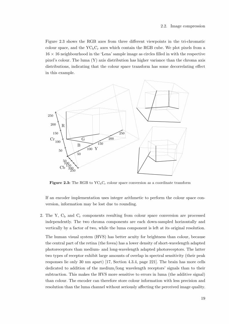
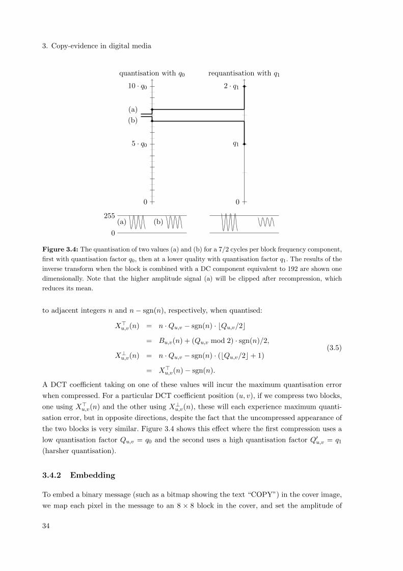
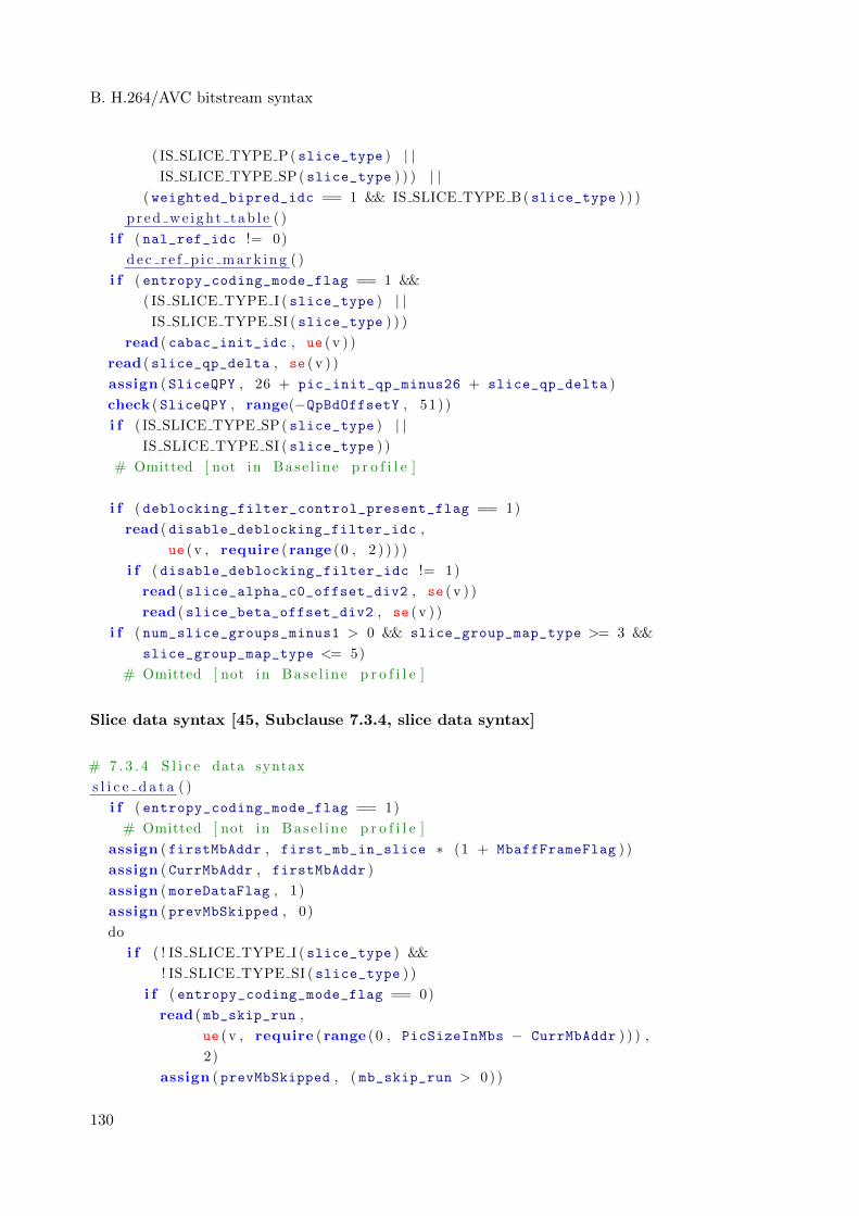
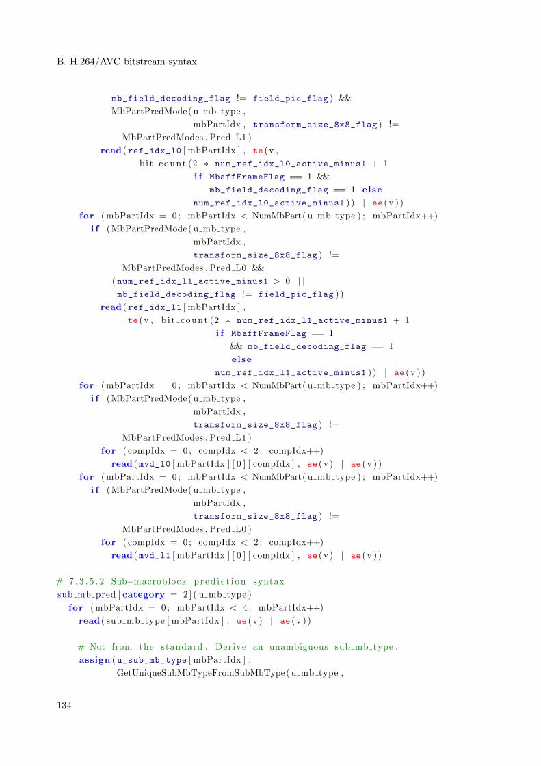
options --crf=21.0 --profile=baseline (average bitrate 609 kbit/s).

We refer to these six videos as iPod (H), iPod (L), Canon (H), Canon (L), YouTube (H) and

x264 (H) respectively.

We simulated fragmentation at block sizes of 4096, 2048, 1024 and 512 bytes. For each

clip/block size combination we created two images, one small image with 10 MiB of video

data and 2 MiB of other data (S), and one large image with 40 MiB of video data and 10 MiB

of other data (L).

5.7.2 Data bitstreams

For each input image, we ran the defragmentation tool with the appropriate block size and

recorded the number of data bitstreams recovered and their associated block sequences. We

limited the maximum number of decoding operations to 500 million. Table 5.6 show for each

source/block size/image size combination the number of data bitstreams reconstructed (in

the ‘Correct’ column). Some defragmenters skipped bitstreams due to the upper limit on the

number of decoding operations; the number of skipped bitstreams is given in the column

entitled ‘Skipped’. The number of bitstreams where the algorithm was unable to eliminate all

but one possible block ordering are listed in the ‘Multiple’ column.

CPU runtimes are quoted in order to give an approximate impression of the relative cost of

the algorithm with different inputs (‘Time taken’). Each defragmenter ran on a machine in a

cluster with CPU speeds of 1.8–2.2 GHz.

Error conditions

We also load the ground-truth block orderings generated when the image was shuffled, and

compare the block sequences to identify the following error conditions:

114

5.7. Results

• ‘Incorrect’ bitstreams have one single possible block ordering, but it is not the correct

one;

• ‘Failed’ bitstreams have no possible block orderings;

• ‘Missed’ bitstreams are present in the image but were not located by the defragmenter;

and

• ‘False +s’ (false positives) are bitstreams which are not present in the image but were

found by the defragmenter.

False positives occur when the image contains extents that are valid bitstreams, but are not

among the bitstreams originally indicated by the container format. False positives can cause

failed bitstreams, because they cause their blocks to be marked as occupied (or partially

occupied). They can also lead to incorrect bitstreams, when a bitstream has two possibilities,

and the correct one is eliminated due to the block occupancy of a false positive; the only

remaining possibility is incorrect. When the mapping stage has not found a complete chain

containing all the bitstreams, those bitstreams at the start of a chain whose first few bytes lie

across a block boundary will be missed.

Table 5.6 shows that the cost of the algorithm, measured in the number of parser invocations

required, is much greater at smaller block sizes, and in larger images. Missed bitstreams are

also more common in images with small fragmentation block sizes because there are more

block boundaries.

Several defragmenter instances did not terminate. In all these cases, the intermediate block

search did not parse even one data bitstream in the allotted time. In particular, the large

images proved too expensive to defragment at block sizes less than 4096 bytes. Some images

were too expensive to defragment even at this block size. Because these defragmenters did

not even construct one bitstream given many hours of processing time, due high cost of the

algorithm’s search stage, they seem to lie below the threshold of what is feasible to defragment

even with great computational effort.

Among the defragmenters which terminated without reaching the limit of 500 million decodes,

almost all data bitstreams were recovered successfully. The time taken varied quite widely,

but for block sizes greater than 512 bytes many small images were defragmented in less than

an hour.

The source of video data had a strong effect on the difficulty of defragmentation. For example,

the 4 KiB fragmentation block size, large Canon (L) image took several days to defragment,

while the same images with data from the iPod only took a couple of hours. This is because

errors are detected more quickly in video produced by certain encoders (see subsection 5.5.4).

115


5.7.3 Proportion of data recovered successfully

Table 5.7 shows the amount of video data recovered from each image, and the percentage of

all video data recovered. Among defragmenters that did not reach the limit of 500 million

decodes, all but one defragmenter instance recovered more than 90% of the video data.

5.8 Analysis

The algorithm recovered more than 90% of the fragmented video bitstreams in the majority

of our tests. Each sample storage image included a mixture of compressed non-video data and

uncompressed data, alongside video data produced by one of three video compressors. We

have therefore shown that the algorithm can recover a useful proportion of video in relatively

small but realistic storage images, with randomly-permuted disk blocks.

The remaining, unrecovered bitstreams were not found due to their blocks being marked as

occupied by false-positive bitstreams. We rely on eliminating blocks as we establish that they

are part of bitstreams, and recursively update the tree that encodes candidate paths for each

bitstream when we find that blocks are occupied. False positives disrupt this process, leading

to blocks being marked as occupied erroneously.

The bitstream mapping heuristics described in subsection 5.6.4 try to use information about

the layout of bitstreams to eliminate false positives. This process, called chaining, is impor-

tant to the performance of our algorithm. Ideally, our algorithm should find a single chain

containing all bitstreams present in the storage image.

Missed bitstreams (when the initial bytes straddle a block boundary, for example) make it

impossible to merge sequential chains. Additionally, we are unable to apply chaining if we do

not have length tags for each bitstream, and know how many bytes lie between them. As well

as causing false positives, the computational cost of the search step of the algorithm is greater

for bitstreams that are the last entry in their chain, as their final disk block is unknown.

The time cost of the algorithm is high, as it has to parse many disk blocks when searching for

sequences of blocks that yield valid bitstreams. While we demonstrated that the algorithm

performs well on fifty megabyte images, forensic investigators must sometimes handle multi-

gigabyte images.


The computational cost of our algorithm could be reduced by initially eliminating blocks

containing non-random data. In real-world forensics scenarios, our algorithm needs to handle

larger storage images. However, substantially more computing power will be available, a lot

of blocks are likely to contain non-video data, and the distribution of bitstream lengths will

116

5.9. Conclusion

be similar to that of our test images. Therefore, our algorithm is not necessarily limited to

small storage images.

The main search stage of our algorithm uses fast generated C code, while the initial bitstream

location step is written in Python. The latter will need to be optimised to handle multi-

gigabyte images.

Other improvements to our algorithm are likely to involve reducing the false-positive rate by

locating all bitstreams and improving chaining. In our testing, bitstreams were sometimes

missed when their initial bytes straddled a block boundary. These could be located by joining

all possible pairs of blocks (at quadratic cost) and searching for bitstreams over each boundary.

By associating an estimated probability that a given bitstream is a false positive (based on

the length of chain it participates in, for example), we could use backtracking to try removing

potential false positives systematically. This would increase the computational cost of the

algorithm.

The algorithm’s performance is dependent on the encoder used to produce the data being

defragmented. It would be interesting to measure how quickly errors can be detected on data

output by a wider selection of encoders than the ones considered in subsection 5.5.4. This

would help in establishing bounds on whether defragmentation is feasible for each encoder,

based on how quickly errors are detected.

The error detection rate for a given bitstream forms a useful discriminator for encoder classi-

fication. It is possible to adapt our flowgraph-based parser to provide other suitable metrics:

the subset of codec features used, or the amount of time spent parsing particular parts of the

syntax, for example.

Our automatic defragmentation tool will be very useful at forensics labs, where many devices

must be processed per day. The methodology is applicable to other file types where error

detection is possible. Eventually it might be possible to defragment bitstreams from several

codecs at the same time, thereby eliminating a larger proportion of blocks from consideration.

The technique of generating parsers based on a syntax specification has applications outside

forensics. It could be used as a syntax validator on the input of potentially vulnerable video

players, to filter out invalid bitstreams. The same methodology could also be used to generate

intentionally invalid input for fuzz testing.

5.9 Conclusion

We demonstrated a general-purpose defragmentation algorithm for storage images containing

compressed data bitstreams, relying on syntax errors to test whether a given sequence of

candidate blocks could be contiguous, as part of a search algorithm. Using a bitstream syn-

tax description for H.264/AVC Baseline profile bitstreams, we demonstrated the algorithm’s

117


efficacy in locating and rebuilding compressed video bitstreams generated by a variety of

devices.

Our algorithm is of practical use to forensic investigators. We have already applied it to a

fragmented hard disk image from a CCTV system provided by the London Metropolitan

Police Service, where it located several compressed bitstreams, outputting a valid elementary

stream for viewing. Because manual reconstruction of compressed video is difficult and time-

consuming, our automatic tool has the potential to improve the efficiency of practical evidence

processing procedures substantially.

118

5.9. Conclusion

Source video

Blo

cksi

ze

Image

size

Corr

ect

Mu

ltip

le

Inco

rrec

t

Fail

ed

Skip

ped

Mis

sed

Fal

se+

s

Time taken

(h:m:s)

Canon (L) 4,096 L 398 1 0 25 0 3 7 119:55:59

iPod (H) 4,096 L 920 0 0 0 0 3 0 2:13:47

iPod (L) 4,096 L 745 0 0 0 0 4 0 2:11:38

x264 (H) 4,096 L 15773 11 0 6 0 33 18 36:33:22

YouTube (H) 4,096 L 18354 6 0 1 0 655 3 28:46:48

Canon (H) 4,096 S 103 0 0 2 0 3 3 7:41:10

Canon (L) 4,096 S 104 0 0 2 0 3 3 0:27:21

iPod (H) 4,096 S 234 0 0 0 0 2 0 0:11:31

iPod (L) 4,096 S 185 0 0 0 0 3 0 0:10:29

x264 (H) 4,096 S 4421 1 0 1 0 12 1 1:13:32

YouTube (H) 4,096 S 5031 1 0 0 0 40 2 1:37:26

iPod (H) 2,048 L 917 1 0 0 0 5 0 7:47:51

iPod (L) 2,048 L 737 4 0 0 0 7 0 6:53:33

x264 (H) 2,048 L 15731 25 0 21 0 48 0 14:06:56

YouTube (H) 2,048 L 18808 39 0 10 5 154 0 15:33:48

Canon (L) 2,048 S 98 0 0 8 0 2 13 0:44:41

iPod (H) 2,048 S 234 0 0 0 0 2 0 0:27:57

iPod (L) 2,048 S 183 0 0 0 0 4 0 0:27:26

x264 (H) 2,048 S 4426 0 0 2 0 15 2 0:50:17

YouTube (H) 2,048 S 5024 2 0 0 0 46 2 1:08:49

iPod (L) 1,024 L 256 488 0 0 478 4 0 11:16:09

x264 (H) 1,024 L 6785 8924 0 0 8828 94 0 13:04:23

YouTube (H) 1,024 L 8925 9878 0 1 9658 207 0 16:42:45

Canon (L) 1,024 S 94 1 0 10 0 3 15 2:05:18

iPod (H) 1,024 S 233 1 0 0 0 2 0 1:54:49

iPod (L) 1,024 S 183 1 0 0 0 3 0 1:36:40

x264 (H) 1,024 S 3036 1357 0 0 1236 29 0 7:47:00

YouTube (H) 1,024 S 4056 954 0 0 807 56 0 8:19:28

iPod (L) 512 S 178 5 0 0 3 4 0 11:07:32

x264 (H) 512 S 1563 2806 0 0 2691 55 0 8:37:44

YouTube (H) 512 S 1292 3699 0 0 3574 76 0 8:23:27

Figure 5.6: This table summarises the results of running the defragmenter on 12/50 MiB images with

block sizes of 512, 1024, 2048 and 4096 bytes. The fourth to tenth columns show the number of data

bitstreams falling into each category described in subsection 5.7.2.

119


Source video

Blo

cksi

ze

Imag

esi

ze

Rec

over

ed(M

iB)

Rec

over

ed(%

)

Skip

ped Time taken

(h:m:s)

Canon (L) 4,096 L 36.31 93.24 0 119:55:59

iPod (H) 4,096 L 39.64 99.68 0 2:13:47

iPod (L) 4,096 L 39.65 99.65 0 2:11:38

x264 (H) 4,096 L 39.56 99.06 0 36:33:22

YouTube (H) 4,096 L 36.33 93.45 0 28:46:48

Canon (H) 4,096 S 9.47 96.02 0 7:41:10

Canon (L) 4,096 S 9.42 95.73 0 0:27:21

iPod (H) 4,096 S 9.90 99.67 0 0:11:31

iPod (L) 4,096 S 9.91 99.22 0 0:10:29

x264 (H) 4,096 S 9.89 99.17 0 1:13:32

YouTube (H) 4,096 S 9.55 95.67 0 1:37:26

iPod (H) 2,048 L 39.50 99.34 0 7:47:51

iPod (L) 2,048 L 39.27 98.77 0 6:53:33

x264 (H) 2,048 L 39.24 98.25 0 14:06:56

YouTube (H) 2,048 L 37.15 95.56 5 15:33:48

Canon (L) 2,048 S 8.86 90.83 0 0:44:41

iPod (H) 2,048 S 9.90 99.67 0 0:27:57

iPod (L) 2,048 S 9.81 98.53 0 0:27:26

x264 (H) 2,048 S 9.89 99.06 0 0:50:17

YouTube (H) 2,048 S 9.52 95.29 0 1:08:49

iPod (L) 1,024 L 9.51 23.92 478 11:16:09

x264 (H) 1,024 L 4.73 11.83 8828 13:04:23

YouTube (H) 1,024 L 7.04 18.12 9658 16:42:45

Canon (L) 1,024 S 8.54 87.52 0 2:05:18

iPod (H) 1,024 S 9.86 99.27 0 1:54:49

iPod (L) 1,024 S 9.81 98.55 0 1:36:40

x264 (H) 1,024 S 3.65 36.61 1236 7:47:00

YouTube (H) 1,024 S 5.57 55.82 807 8:19:28

iPod (L) 512 S 9.21 92.53 3 11:07:32

x264 (H) 512 S 0.75 7.53 2691 8:37:44

YouTube (H) 512 S 0.70 7.01 3574 8:23:27

Figure 5.7: The defragmentation algorithm normally recovers more than 90% of fragmented data.

120

Chapter 6

Conclusions

I have shown that it is possible to exploit the low-level details of compression schemes and their

implementations to develop automatic tampering detection and evidence recovery algorithms

that are applicable in scenarios involving compressed data.

Recompression is increasingly an issue for content producers and consumers, especially with

the popularity of images and videos recorded on consumer devices and transmitted over the

Internet. Understanding the detailed effects of recompression can be useful for developing algo-

rithms that warn users about hidden recompression steps, maintain quality in data processing

systems and reconstruct a document’s processing history.

The copy-evident marking algorithm presented in chapter 3 adds a high-frequency pattern

to a uniform region of an image, modulated with a message that is imperceptible in the

original marked image, but becomes visible after recompression using particular known quality

settings. Such an algorithm could be used to make a visible warning appear in lower quality

copies of a marked original document, or to expose a hidden recompression step performed

by an Internet service provider without relying on special software tools.

The presented copy-evident marking algorithm is still limited to uniform areas and a single,

known recompression quality factor. However, a message that appears after recompression to

one of several quality factors can be achieved by multiplexing several marks. The recompressed

image’s message is less visible when the image undergoes filtering operations (for example,

due to browser content resizing).

It may be possible to extend our technique to marking non-uniform images or video data. Cur-

rently, the distortion introduced by the high frequency checkerboard pattern is too noticeable

in marked photographs, but the effect may work better on very high resolution screens, or in

situations where we know that down-sampling by a particular factor will take place. Video

presents a particular challenge because the variation of quantisation factors due to rate control

can be quite unpredictable. However, motion compensation may provide an alternative op-

portunity to introduce objectionable distortion in recompressed versions. The combination of

121

6. Conclusions

JPEG’s chroma down-sampling operation with gamma correction might also allow for another

approach.

In chapter 4, I presented a new type of compressor, designed to process bitmaps output by

a JPEG decompressor. It recovers the set of all bitstreams that produce a given result on

decompression by inverting the computations performed during decompression. As a side-

effect, it also indicates any regions that have been modified since decompression, whenever

the changes have destroyed JPEG’s characteristic distortions.

The recompressor is necessarily matched with one particular decompressor implementation,

as it uses a precise model of the decompressor’s computations. Saturated pixel values are a

particular problem for exact recompressors, because they are produced by clipping operations

that discard information. In our results, we observed that images with many saturated pixels

were more expensive to recompress.

The same methodology may be applicable with other formats, such as compressed audio or

video data, but the functionality of complicated decompressors is likely to be difficult to model

and invert for the purposes of exact recompression.

By not relying on probabilistic techniques, we can be confident in the results of the algorithms,

but at the expense of greater computational cost.

In chapter 5, I demonstrated how to locate and rebuild fragmented compressed bitstreams,

by taking advantage of restrictions on bitstream syntax to eliminate incorrect candidate bit-

streams. Having proposed a general-purpose algorithm, I showed the practical applicability of

the algorithm on H.264/AVC Baseline profile compressed video streams, using source video

from a variety of devices.

The defragmentation algorithm has some limitations. Based on our results, it is clear that

missed bitstreams are a common problem, and can lead to false positives, or streams with

multiple possible block sequences. An initial search testing the boundary between each possible

pair of blocks (at quadratic cost) to find bitstreams whose first few bytes straddle two blocks

would help to ameliorate this problem. The mapping stage of the algorithm could be improved

by using any available information about interleaved audio streams.

The algorithm is suitable for applying in real-world evidence-processing pipelines. The search

stage is amenable to parallelisation. The current implementation is quite fast, using gener-

ated C code for the expensive search stage. Block classification algorithms (as described in

subsection 5.2.3) can be used to reduce the size of input to our tool, which can make the

search cheaper in filesystems with uncompressed data. Finally, our tool could be improved by

providing bitstream syntax descriptions for a variety of different compressed formats beyond

H.264/AVC. In particular, it would be interesting to investigate the feasibility of our approach

with standards employing arithmetic coding.

The approach of generating bitstream parsers automatically from a syntax description may

have applications outside forensic investigation. It could be used to generate and update soft-

122

ware video decoders without transmitting binaries. It may also be possible to prove assertions

about compressed bitstream formats by analysis of the syntax flowgraph, or justify properties

of decoding software generated based on the syntax description.

Our work on defragmentation raises several interesting questions regarding compressed bit-

stream resynchronisation, where a decoder has to resume decoding in the middle of a bitstream

due to data loss or corruption. The structure of the H.264/AVC Baseline profile syntax leads

to repeated codewords in heavily-compressed data, creating repetitions which might facilitate

resynchronisation.

123

Appendix A

JPEG encoder quality selection

The two quantisation tables used to quantise DCT coefficients in luma and chroma blocks

during JPEG compression are normally chosen based on a user-specified scalar quality factor.

Below are the mappings used by two popular implementations: the Independent JPEG Group

(IJG) codec [57] and Adobe Photoshop CS2 [37].

A.1 IJG encoder

A scalar quality factor in the range 1–100 is passed to the encoder. This is specified using a

slider in the graphical user interface of the GNU Image Manipulation Program (GIMP) [72],

or with the option -quality for the cjpeg tool.

The quantisation tables, QY and QC, are then chosen by scaling the tables suggested in the

standard [38, Tables K.1 and K.2], here denoted by KY and KC, based on the user’s choice

of quality factor q ∈ 1, . . . , 100 using the following formula:

(Qc)u,v =

divround((Kc)u,v · b5000/qc, 100) 1 ≤ q < 50,

max(1, divround((Kc)u,v · (200− 2 · q), 100)) 50 ≤ q ≤ 100.(A.1)

If the baseline option is chosen, the compressor clips output values to the range 0, . . . , 255.

These tables quantise higher spatial frequencies more aggressively than the low frequencies,

as they are less perceptually important.

A.2 Adobe Photoshop CS2

Adobe Photoshop CS2 contains another widely used JPEG encoder. The ‘save for web’ feature

lets the user choose an integer in 0, 1, . . . , 100, while the main ‘save as’ feature has thirteen

options for ‘quality’ ranging from 0 to 12.

124

A.2. Adobe Photoshop CS2

Considering the ‘save as’ feature in more detail, qualities 0–6 use 4 : 2 : 0 chroma down-

sampling, while qualities 7–12 do not use chroma down-sampling (4 : 4 : 4). There does not

appear to be a simple mapping from quality settings onto quantisation matrices. Figure A.1

shows what quantisation factors are used: each colour of line corresponds to a group of spa-

tial frequencies which are quantised in the same way as the quality option varies. There is

clearly no simple relationship as in the IJG encoder, so the mapping from quality options onto

quantisation matrices may be based on user studies or a more complex psychophysical model.

125

A. JPEG encoder quality selection

Adobe Photoshop CS 2 JPEG ‘save as’ quality setting

Quan

tisation

factor

Assignment of colours to spatial frequencies in(cycles per block horizontally, cycles per block vertically).

(02, 02

)

(02, 12

)

(02, 22

)

(02, 32

)

(02, 42

)

(02, 52

)

(02, 62

)

(02, 72

)

(12, 02

)

(12, 12

)

(12, 22

)

(12, 32

)

(12, 42

)

(12, 52

)

(12, 62

)

(12, 72

)

(22, 02

)

(22, 12

)

(22, 22

)

(22, 32

)

(22, 42

)

(22, 52

)

(22, 62

)

(22, 72

)

(32, 02

)

(32, 12

)

(32, 22

)

(32, 32

)

(32, 42

)

(32, 52

)

(32, 62

)

(32, 72

)

(42, 02

)

(42, 12

)

(42, 22

)

(42, 32

)

(42, 42

)

(42, 52

)

(42, 62

)

(42, 72

)

(52, 02

)

(52, 12

)

(52, 22

)

(52, 32

)

(52, 42

)

(52, 52

)

(52, 62

)

(52, 72

)

(62, 02

)

(62, 12

)

(62, 22

)

(62, 32

)

(62, 42

)

(62, 52

)

(62, 62

)

(62, 72

)

(72, 02

)

(72, 12

)

(72, 22

)

(72, 32

)

(72, 42

)

(72, 52

)

(72, 62

)

(72, 72

)

0

10

20

30

40

50

60

70

80

0 1 2 3 4 5 6 7 8 9 10 11 12

Figure A.1: Adobe Photoshop CS2 has thirteen options for JPEG image ‘quality’. This chart shows the

mapping from qualities onto quantisation factors, grouping spatial frequencies which are quantised in the same

way as quality is varied. Each 8 × 8 greyscale spatial domain block shows a sum of frequencies which are

quantised equally.

126

Appendix B

H.264/AVC bitstream syntax

This appendix includes the bitstream syntax description for some less commonly-used parts

of the H.264/AVC Baseline profile syntax than those given in subsection 5.5.3, which are also

used by our defragmentation tool’s parser.

Picture parameter set RBSP syntax [45, Subclause 7.3.2.2]

# 7 . 3 . 2 . 2 P ic ture parameter s e t RBSP syntax

p i c p a r a m e t e r s e t r b s p [ category = 1 ] ( )

read ( pic_parameter_set_id , ue (v , require ( range (0 , 2 5 5 ) ) ) )

read ( seq_parameter_set_id , ue (v , require ( range (0 , 3 1 ) ) ) )

read ( entropy_coding_mode_flag , u (1 , require ( 0 ) ) )

read ( bottom_field_pic_order_in_frame_present_flag , u (1 , require ( 0 ) ) )

read ( num_slice_groups_minus1 , ue (v , require ( 0 ) , possible ( range (0 , 7 ) ) ) )

i f ( num_slice_groups_minus1 > 0)

# Omitted [ mu l t ip l e s l i c e s ]

read ( num_ref_idx_l0_default_active_minus1 ,

ue (v , require ( range (0 , 3 1 ) ) ) )

read ( num_ref_idx_l1_default_active_minus1 ,

ue (v , require ( range (0 , 3 1 ) ) ) )

read ( weighted_pred_flag , u (1 , require ( 0 ) , possible (0 , 1 ) ) )

read ( weighted_bipred_idc , u (2 , require ( 0 ) , possible (0 , 1 , 2 ) ) )

read ( pic_init_qp_minus26 ,

se (v , require ( range(−(26 + QpBdOffsetY ) , 2 5 ) ) ) )

read ( pic_init_qs_minus26 ,

se (v , require ( range(−26 , 2 5 ) ) ) )

read ( chroma qp index o f f s e t , se (v , require ( range(−12 , 1 2 ) ) ) )

read ( deblocking_filter_control_present_flag , u ( 1 ) )

read ( constrained_intra_pred_flag , u ( 1 ) )

read ( redundant_pic_cnt_present_flag , u (1 , require ( 0 ) ) )

i f ( more rbsp data ( ) )

127

B. H.264/AVC bitstream syntax

# Omitted [ not pre sent in b a s e l i n e p r o f i l e ]

else

assign ( transform_8x8_mode_flag , Fa l se )

assign ( p i c s c a l i n g m a t r i x p r e s e n t f l a g , Fa l se )

assign ( s e cond chroma qp index o f f s e t , ch roma qp index o f f s e t )

r b s p t r a i l i n g b i t s ( )

Slice layer without partitioning RBSP syntax [45, 7.3.2.8 Slice layer without par-

titioning RBSP syntax]

# 7 . 3 . 2 . 8 S l i c e l a y e r without p a r t i t i o n i n g RBSP syntax

s l i c e l a y e r w i t h o u t p a r t i t i o n i n g r b s p ( )

s l i c e h e a d e r [ category = 2 ] ( )

s l i c e d a t a [ category = 2 | 3 | 4 ] ( )

r b s p s l i c e t r a i l i n g b i t s ( )

Slice header syntax [45, Subclause 7.3.3, slice header syntax] and associated syntax

# 7 . 3 . 3 S l i c e header syntax

s l i c e h e a d e r [ category = 2 ] ( )

read ( first_mb_in_slice , ue ( v ) )


read ( slice_type , ue (v , require (2 , 7 ) , possible (4 , 9 ) ) )

else

read ( slice_type , ue (v , require (0 , 1 , 5 , 6 ) , possible (3 , 8 ) ) )

read ( pic_parameter_set_id , ue (v , require ( range (0 , 2 5 5 ) ) ) )

i f ( separate_colour_plane_flag == 1)

read ( colour_plane_id , u (2 , require ( range (0 , 2 ) ) ) )

read ( frame_num , u (v , b i t c ount ( log2_max_frame_num_minus4 + 4 ) ) )


read ( field_pic_flag , u (1 , require ( 0 ) , possible ( 1 ) ) )

i f ( field_pic_flag )

read ( bottom_field_flag , u ( 1 ) )

else

assign ( field_pic_flag , 0)

assign ( MbaffFrameFlag , mb_adaptive_frame_field_flag &&

( ! field_pic_flag ) )

i f ( IdrPicFlag == 1)

read ( idr_pic_id , ue (v , require ( range (0 , 65535 ) ) ) )

assign ( PicHeightInMbs , FrameHeightInMbs / (1 + field_pic_flag ) )

assign ( PicSizeInMbs , PicWidthInMbs ∗ PicHeightInMbs )

check ( first_mb_in_slice , range (0 , PicSizeInMbs − 1

i f ! MbaffFrameFlag else

PicSizeInMbs / 2 − 1) )

i f ( pic_order_cnt_type == 0)

128

read ( pic_order_cnt_lsb ,

u (v , b i t c ount ( log2_max_pic_order_cnt_lsb_minus4 + 4 ) ) )

i f ( bottom_field_pic_order_in_frame_present_flag == 1 &&

field_pic_flag == 0)

read ( delta_pic_order_cnt_bottom , se ( v ) )

i f ( pic_order_cnt_type == 1 &&

delta_pic_order_always_zero_flag == 0)

read ( delta_pic_order_cnt [ 0 ] , se ( v ) )

i f ( bottom_field_pic_order_in_frame_present_flag &&

( ! field_pic_flag ) )

read ( delta_pic_order_cnt [ 1 ] , se ( v ) )

i f ( redundant_pic_cnt_present_flag )

read ( redundant_pic_cnt , ue ( v ) )

i f ( IS SLICE TYPE B( slice_type ) )

read ( direct_spatial_mv_pred_flag , u ( 1 ) )

i f ( IS SLICE TYPE P ( slice_type ) | |IS SLICE TYPE SP ( slice_type ) | |IS SLICE TYPE B( slice_type ) )

read ( num_ref_idx_active_override_flag , u ( 1 ) )

i f ( num_ref_idx_active_override_flag == 1)

read ( num_ref_idx_l0_active_minus1 ,

ue (v , require ( range (0 , 15

i f ! field_pic_flag else

3 1 ) ) ) )


read ( num_ref_idx_l1_active_minus1 ,

ue (v , require ( range (0 , 15

i f ! field_pic_flag else

3 1 ) ) ) )

else

assign ( num_ref_idx_l0_active_minus1 ,

num_ref_idx_l0_default_active_minus1 )


assign ( num_ref_idx_l1_active_minus1 ,

num_ref_idx_l1_default_active_minus1 )


r e f p i c l i s t m v c m o d i f i c a t i o n ( )

else

r e f p i c l i s t m o d i f i c a t i o n ( )

i f ( ( weighted_pred_flag == 1 &&

129


( IS SLICE TYPE P ( slice_type ) | |IS SLICE TYPE SP ( slice_type ) ) ) | |

( weighted_bipred_idc == 1 && IS SLICE TYPE B( slice_type ) ) )

p r ed we i gh t t ab l e ( )

i f ( nal_ref_idc != 0)

d e c r e f p i c m a r k i n g ( )

i f ( entropy_coding_mode_flag == 1 &&

( IS SLICE TYPE I ( slice_type ) | |IS SLICE TYPE SI ( slice_type ) ) )

read ( cabac_init_idc , ue ( v ) )

read ( slice_qp_delta , se ( v ) )

assign ( SliceQPY , 26 + pic_init_qp_minus26 + slice_qp_delta )

check ( SliceQPY , range(−QpBdOffsetY , 51) )

i f ( IS SLICE TYPE SP ( slice_type ) | |IS SLICE TYPE SI ( slice_type ) )

# Omitted [ not in Base l i n e p r o f i l e ]

i f ( deblocking_filter_control_present_flag == 1)

read ( disable_deblocking_filter_idc ,

ue (v , require ( range (0 , 2 ) ) ) )

i f ( disable_deblocking_filter_idc != 1)

read ( slice_alpha_c0_offset_div2 , se ( v ) )

read ( slice_beta_offset_div2 , se ( v ) )

i f ( num_slice_groups_minus1 > 0 && slice_group_map_type >= 3 &&

slice_group_map_type <= 5)


Slice data syntax [45, Subclause 7.3.4, slice data syntax]

# 7 . 3 . 4 S l i c e data syntax

s l i c e d a t a ( )



assign ( firstMbAddr , first_mb_in_slice ∗ (1 + MbaffFrameFlag ) )

assign ( CurrMbAddr , firstMbAddr )

assign ( moreDataFlag , 1)

assign ( prevMbSkipped , 0)

do

i f ( ! IS SLICE TYPE I ( slice_type ) &&

! IS SLICE TYPE SI ( slice_type ) )


read ( mb_skip_run ,

ue (v , require ( range (0 , PicSizeInMbs − CurrMbAddr ) ) ) ,

2)

assign ( prevMbSkipped , ( mb_skip_run > 0) )

130

for ( i = 0 ; i < mb_skip_run ; i++)

check ( CurrMbAddr , range (0 , PicSizeInMbs − 1) )

i f ( IS SLICE TYPE P ( slice_type ) | |IS SLICE TYPE SP ( slice_type ) )

context_mb_type [ CurrMbAddr ] = MbTypes . P Skip

else

context_mb_type [ CurrMbAddr ] = MbTypes . B Skip

assign ( CurrMbAddr , NextMbAddress ( CurrMbAddr ) )

i f ( CurrMbAddr != firstMbAddr | | mb_skip_run > 0)

assign ( moreDataFlag , more rbsp data ( ) )

else


i f ( moreDataFlag )

i f ( MbaffFrameFlag && ( CurrMbAddr % 2 == 0 | |( CurrMbAddr % 2 == 1 && prevMbSkipped ) ) )

read ( mb_field_decoding_flag , u (1 ) | ae ( v ) , 2)

else

assign ( mb_field_decoding_flag , field_pic_flag )

check ( CurrMbAddr , range (0 , PicSizeInMbs − 1) )

macrob lock layer [ category = 2 | 3 | 4 ] ( )


i f ( ! moreDataFlag )




else

i f ( ! IS SLICE TYPE I ( slice_type ) &&

! IS SLICE TYPE SI ( slice_type ) )

assign ( prevMbSkipped , mb_skip_flag )

i f ( MbaffFrameFlag && CurrMbAddr % 2 == 0)

assign ( moreDataFlag , 1)

else

read ( end_of_slice_flag , ae ( v ) , 2)

assign ( moreDataFlag , ! end_of_slice_flag )

i f ( moreDataFlag )


while ( moreDataFlag )

check ( CurrMbAddr , PicSizeInMbs )

Macroblock layer syntax [45, Subclause 7.3.5]

# 7 . 3 . 5 Macroblock l a y e r syntax

131


macrob lock layer ( )

read ( mb_type , ue ( v ) | ae ( v ) , 2)

# Not from the standard . This c r e a t e s unambiguous MB types .

assign ( u mb type , GetUniqueMbTypeFromMbType( mb_type , slice_type ) )

# Store t h i s in the decoding context .

assign ( context_mb_type [ CurrMbAddr ] , u mb type )

i f ( u mb type == MbTypes . I PCM)

# Omitted [ I PCM macroblock coding ]

else

assign ( noSubMbPartSizeLessThan8x8Flag , 1)

i f ( u mb type != MbTypes . I NXN &&

MbPartPredMode ( u mb type , 0 , Fa l se ) !=

MbPartPredModes . Int ra 16x16 &&

NumMbPart( u mb type ) == 4)

sub mb pred [ category = 2 ] ( u mb type )

for ( mbPartIdx = 0 ; mbPartIdx < 4 ; mbPartIdx++)

i f ( u_sub_mb_type [ mbPartIdx ] != SubMbTypes . B Direct 8X8 )

i f (NumSubMbPart( u_sub_mb_type [ mbPartIdx ] ) > 1)


else i f ( direct_8x8_inference_flag == 0)


else

i f ( transform_8x8_mode_flag && u mb type == MbTypes . I NXN)

read ( transform_size_8x8_flag , u (1 ) | ae ( v ) , 2)

else

assign ( transform_size_8x8_flag , 0)

mb pred [ category = 2 ] ( u mb type )

i f (MbPartPredMode ( u mb type , 0 , Fa l se ) !=

MbPartPredModes . Int ra 16x16 )

read ( coded_block_pattern , me( v ) | ae ( v ) , 2)

assign ( CodedBlockPatternLuma , coded_block_pattern % 16)

assign ( CodedBlockPatternChroma , coded_block_pattern / 16)

i f ( CodedBlockPatternLuma > 0 &&

transform_8x8_mode_flag == 1 &&

u mb type != MbTypes . I NXN &&

noSubMbPartSizeLessThan8x8Flag == 1 &&

( u mb type != MbTypes . B Direct 16X16 | |direct_8x8_inference_flag ) )

read ( transform_size_8x8_flag , u (1 ) | ae ( v ) , 2)

else

assign ( transform_size_8x8_flag , 0)

else

132

assign ( CodedBlockPatternLuma ,

GetIntra16x16CodedBlockPatternLuma ( u mb type ) )

assign ( CodedBlockPatternChroma ,

GetIntra16x16CodedBlockPatternChroma ( u mb type ) )

i f ( CodedBlockPatternLuma > 0 | |CodedBlockPatternChroma > 0 | |MbPartPredMode ( u mb type , 0 , transform_size_8x8_flag ) ==


read ( mb_qp_delta ,

se (v , require ( range(−(26 + QpBdOffsetY / 2) ,

25 + QpBdOffsetY / 2 ) ) ) | ae ( v ) , 2)

r e s i d u a l [ category = 3 | 4 ] ( 0 , 15)

Macroblock prediction syntax [45, Subclause 7.3.5.1, Macroblock prediction syn-

tax] and associated syntax

# 7 . 3 . 5 . 1 Macroblock p r e d i c t i o n syntax

mb pred [ category = 2 ] ( u mb type )

i f (MbPartPredMode ( u mb type , 0 , transform_size_8x8_flag ) ==

MbPartPredModes . In t ra 4x4 | |MbPartPredMode ( u mb type , 0 , transform_size_8x8_flag ) ==

MbPartPredModes . In t ra 8x8 | |MbPartPredMode ( u mb type , 0 , transform_size_8x8_flag ) ==



MbPartPredModes . In t ra 4x4 )

for ( luma4x4BlkIdx = 0 ; luma4x4BlkIdx < 16 ; luma4x4BlkIdx++)

read ( p r ev in t ra4x4 pred mode f l ag [ luma4x4BlkIdx ] ,

u (1 ) | ae ( v ) )

i f ( p r ev in t ra4x4 pred mode f l ag [ luma4x4BlkIdx ] == 0)

read ( rem_intra4x4_pred_mode [ luma4x4BlkIdx ] , u (3 ) | ae ( v ) )


MbPartPredModes . In t ra 8x8 )

for ( luma8x8BlkIdx = 0 ; luma8x8BlkIdx < 4 ; luma8x8BlkIdx++)

read ( p r ev in t ra8x8 pred mode f l ag [ luma8x8BlkIdx ] ,

u (1 ) | ae ( v ) )

i f ( p r ev in t ra8x8 pred mode f l ag [ luma8x8BlkIdx ] == 0)

read ( rem_intra8x8_pred_mode [ luma8x8BlkIdx ] , u (3 ) | ae ( v ) )

i f ( ChromaArrayType == 1 | | ChromaArrayType == 2)

read ( intra_chroma_pred_mode ,

ue (v , require ( range (0 , 3 ) ) ) | ae ( v ) )

else i f (MbPartPredMode ( u mb type , 0 , transform_size_8x8_flag ) !=

MbPartPredModes . D i rec t )

for ( mbPartIdx = 0 ; mbPartIdx < NumMbPart( u mb type ) ; mbPartIdx++)

i f ( ( num_ref_idx_l0_active_minus1 > 0 | |

133


mb_field_decoding_flag != field_pic_flag ) &&

MbPartPredMode ( u mb type ,

mbPartIdx , transform_size_8x8_flag ) !=

MbPartPredModes . Pred L1 )

read ( ref_idx_l0 [ mbPartIdx ] , te (v ,

b i t c ount (2 ∗ num_ref_idx_l0_active_minus1 + 1

i f MbaffFrameFlag == 1 &&

mb_field_decoding_flag == 1 else

num_ref_idx_l0_active_minus1 ) ) | ae ( v ) )


i f (MbPartPredMode ( u mb type ,

mbPartIdx ,

transform_size_8x8_flag ) !=

MbPartPredModes . Pred L0 &&

( num_ref_idx_l1_active_minus1 > 0 | |mb_field_decoding_flag != field_pic_flag ) )

read ( ref_idx_l1 [ mbPartIdx ] ,

te (v , b i t c ount (2 ∗ num_ref_idx_l1_active_minus1 + 1

i f MbaffFrameFlag == 1

&& mb_field_decoding_flag == 1

else




mbPartIdx ,



for ( compIdx = 0 ; compIdx < 2 ; compIdx++)

read ( mvd_l0 [ mbPartIdx ] [ 0 ] [ compIdx ] , se ( v ) | ae ( v ) )



mbPartIdx ,




read ( mvd_l1 [ mbPartIdx ] [ 0 ] [ compIdx ] , se ( v ) | ae ( v ) )

# 7 . 3 . 5 . 2 Sub−macroblock p r e d i c t i o n syntax

sub mb pred [ category = 2 ] ( u mb type )


read ( sub mb type [ mbPartIdx ] , ue ( v ) | ae ( v ) )

# Not from the standard . Derive an unambiguous sub mb type .

assign ( u_sub_mb_type [ mbPartIdx ] ,

GetUniqueSubMbTypeFromSubMbType( u mb type ,

134

sub mb type [ mbPartIdx ] ) )


i f ( ( num_ref_idx_l0_active_minus1 > 0 | |mb_field_decoding_flag != field_pic_flag ) &&

u mb type != MbTypes . P 8X8Ref0 &&

u_sub_mb_type [ mbPartIdx ] != SubMbTypes . B Direct 8X8 &&

SubMbPredMode( u_sub_mb_type [ mbPartIdx ] ) !=

SubMbPredModes . Pred L1 )







i f (SubMbPredMode( u_sub_mb_type [ mbPartIdx ] ) !=

SubMbPredModes . Pred L0 &&

u_sub_mb_type [ mbPartIdx ] != SubMbTypes . B Direct 8X8 &&

( num_ref_idx_l1_active_minus1 > 0 | |mb_field_decoding_flag != field_pic_flag ) )







i f ( u_sub_mb_type [ mbPartIdx ] != SubMbTypes . B Direct 8X8 &&



for ( subMbPartIdx = 0 ;

subMbPartIdx < NumSubMbPart( u_sub_mb_type [ mbPartIdx ] ) ;

subMbPartIdx++)


read ( mvd_l0 [ mbPartIdx ] [ subMbPartIdx ] [ compIdx ] ,

se ( v ) | ae ( v ) )


i f ( u_sub_mb_type [ mbPartIdx ] != SubMbTypes . B Direct 8X8 &&



for ( subMbPartIdx = 0 ;

subMbPartIdx < NumSubMbPart( u_sub_mb_type [ mbPartIdx ] ) ;

subMbPartIdx++)


read ( mvd_l1 [ mbPartIdx ] [ subMbPartIdx ] [ compIdx ] ,

se ( v ) | ae ( v ) )

135


Residual data syntax [45, Subclause 7.3.5.3, residual data syntax] and associated

syntax

# 7 . 3 . 5 . 3 Res idua l data syntax

r e s i d u a l [ category = 3 | 4 ] ( s ta r t Idx , endIdx )

# Set the component index e x p l i c i t l y f o r context c a l c u l a t i o n .

assign ( iCbCr , 2)

r e s idua l l uma ( i16x16DClevel , i16x16AClevel , level , level8x8 ,

s ta r t Idx , endIdx )

assign ( Intra16x16DCLevel , i16x16DClevel )

assign ( Intra16x16ACLevel , i16x16AClevel )

assign ( LumaLevel , level )

assign ( LumaLevel8x8 , level8x8 )

i f ( ChromaArrayType == 1 | | ChromaArrayType == 2)

assign ( NumC8x8 , 4 / ( SubWidthC ∗ SubHeightC ) )

for ( iCbCr = 0 ; iCbCr < 2 ; iCbCr++)

i f ( ( CodedBlockPatternChroma & 3) && s t a r t I d x == 0)


# Chroma DC l e v e l

assign (nC, GetCoeffTokenNc ( CtxBlockCats . ChromaDCLevel ) )

r e s i d u a l b l o c k c a v l c ( ChromaDCLevel [ iCbCr ] , 0 ,

4 ∗ NumC8x8 − 1 , 4 ∗ NumC8x8 )

else

r e s i d u a l b l o c k c a b a c ( ChromaDCLevel [ iCbCr ] , 0 ,

4 ∗ NumC8x8 − 1 , 4 ∗ NumC8x8 )

else

for ( i = 0 ; i < 4 ∗ NumC8x8 ; i++)

assign ( ChromaDCLevel [ iCbCr ] [ i ] , 0)

for ( iCbCr = 0 ; iCbCr < 2 ; iCbCr++)

for ( i8x8 = 0 ; i8x8 < NumC8x8 ; i 8x8++)

for ( i4x4 = 0 ; i4x4 < 4 ; i4x4++)

i f ( ( CodedBlockPatternChroma & 2) && endIdx > 0)


# Chroma AC l e v e l

assign (nC,

GetCoeffTokenNc ( CtxBlockCats . ChromaACLevel ) )

r e s i d u a l b l o c k c a v l c (

ChromaACLevel [ iCbCr ] [ i8x8 ∗ 4 + i4x4 ] ,

max(0 , s t a r t I d x − 1) , endIdx − 1 , 15)

else

r e s i d u a l b l o c k c a b a c (

ChromaACLevel [ iCbCr ] [ i8x8 ∗ 4 + i4x4 ] ,


else

for ( i = 0 ; i < 15 ; i++)

136

assign ( ChromaACLevel [ iCbCr ] [ i8x8 ∗ 4 + i4x4 ] [ i ] , 0)

else i f ( ChromaArrayType == 3)

# Set e x p l i c i t l y f o r context c a l c u l a t i o n .

assign ( iCbCr , 0)

r e s idua l l uma ( i16x16DClevel , i16x16AClevel ,

level , level8x8 , s t a r t Idx , endIdx )

assign ( CbIntra16x16DCLevel , i16x16DClevel )

assign ( CbIntra16x16ACLevel , i16x16AClevel )

assign ( CbLevel , level )

assign ( CbLevel8x8 , level8x8 )

# Set e x p l i c i t l y f o r context c a l c u l a t i o n .

assign ( iCbCr , 1)

r e s idua l l uma ( i16x16DClevel , i16x16AClevel ,

level , level8x8 , s t a r t Idx , endIdx )

assign ( CrIntra16x16DCLevel , i16x16DClevel )

assign ( CrIntra16x16ACLevel , i16x16AClevel )

assign ( CrLevel , level )

assign ( CrLevel8x8 , level8x8 )

# 7 . 3 . 5 . 3 . 1 Res idua l luma syntax

r e s idua l l uma ( i16x16DClevel , i16x16AClevel , level , level8x8 ,

s ta r t Idx , endIdx )

i f ( s t a r t I d x == 0 &&

MbPartPredMode ( u mb type , 0 , transform_size_8x8_flag ) ==



# Int ra 16x16 DC l e v e l

assign (nC,

GetCoeffTokenNc ( CtxBlockCats . iCbCrIntra16x16DClevel ) )

r e s i d u a l b l o c k c a v l c [ category = 3 ] ( i16x16DClevel , 0 , 15 , 16)

else

r e s i d u a l b l o c k c a b a c [ category = 3 ] ( i16x16DClevel , 0 , 15 , 16)

for ( i8x8 = 0 ; i8x8 < 4 ; i8x8++)

i f ( transform_size_8x8_flag == 0 | |entropy_coding_mode_flag == 0)

for ( i4x4 = 0 ; i4x4 < 4 ; i4x4++)

i f ( ( CodedBlockPatternLuma & (1 << i 8x8 ) ) != 0)

i f ( endIdx > 0 &&

MbPartPredMode ( u mb type , 0 ,

transform_size_8x8_flag ) ==



# Int ra 16x16 AC l e v e l

assign (nC, GetCoeffTokenNc (

137


CtxBlockCats . iCbCrIntra16x16AClevel ) )

r e s i d u a l b l o c k c a v l c [ category = 3 ] (

i16x16AClevel [ i 8x8 ∗ 4 + i4x4 ] ,


else

r e s i d u a l b l o c k c a b a c [ category = 3 ] (

i16x16AClevel [ i 8x8 ∗ 4 + i4x4 ] ,


else


# Luma/Cb/Cr l e v e l

assign (nC, GetCoeffTokenNc ( CtxBlockCats . iCbCrLevel ) )

r e s i d u a l b l o c k c a v l c [ category = 3 | 4 ] (

level [ i 8x8 ∗ 4 + i4x4 ] , s ta r t Idx , endIdx , 16)

else

r e s i d u a l b l o c k c a b a c [ category = 3 | 4 ] (

level [ i 8x8 ∗ 4 + i4x4 ] , s ta r t Idx , endIdx , 16)

else i f (MbPartPredMode ( u mb type ,

0 , transform_size_8x8_flag ) ==


for ( i = 0 ; i < 15 ; i++)

assign ( i16x16AClevel [ i 8x8 ∗ 4 + i4x4 ] [ i ] , 0)

else

for ( i = 0 ; i < 16 ; i++)

assign ( level [ i 8x8 ∗ 4 + i4x4 ] [ i ] , 0)

i f ( entropy_coding_mode_flag == 0 &&

transform_size_8x8_flag )

for ( i = 0 ; i < 16 ; i++)

assign ( level8x8 [ i 8x8 ] [ 4 ∗ i + i4x4 ] ,

level [ i 8x8 ∗ 4 + i4x4 ] [ i ] )

else i f ( CodedBlockPatternLuma & (1 << i 8x8 ) )


# Level 8x8

assign (nC, GetCoeffTokenNc ( CtxBlockCats . iCbCrLevel8x8 ) )

r e s i d u a l b l o c k c a v l c [ category = 3 | 4 ] ( level8x8 [ i 8x8 ] ,

4 ∗ s ta r t Idx , 4 ∗ endIdx + 3 , 64)

else

r e s i d u a l b l o c k c a b a c [ category = 3 | 4 ] ( level8x8 [ i 8x8 ] ,

4 ∗ s ta r t Idx , 4 ∗ endIdx + 3 , 64)

else

for ( i = 0 ; i < 64 ; i++)

assign ( level8x8 [ i 8x8 ] [ i ] , 0)

138

Residual block CAVLC syntax [45, Subclause 7.3.5.3.2, residual block CAVLC

syntax]

# 7 . 3 . 5 . 3 . 2 Res idua l b lock CAVLC syntax

r e s i d u a l b l o c k c a v l c [ category = 3 | 4 ] ( coeffLevel , startIdxBlock ,

endIdxBlock , maxNumCoeff )

assign ( coeffLevel , )

assign ( levelB , )

for ( i = 0 ; i < maxNumCoeff ; i++)

assign ( coeffLevel [ i ] , 0)

# This read r e q u i r e s nC to be s e t .

read ( coeff_token , ce ( v ) )

assign ( total_coeff , GetTotalCoef f ( coeff_token ) )

assign ( trailing_ones , GetTrai l ingOnes ( coeff_token ) )

# Cache t o t a l c o e f f f o r context−adapt ive reads l a t e r .

assign ( context_total_coeff [

CurrMbAddr ∗ 16 ∗ 3 + iCbCr ∗ 16 + CurrentBlockIndex ] ,

total_coeff )

i f ( total_coeff > 0)

i f ( total_coeff > 10 && trailing_ones < 3)

assign ( suffixLength , 1)

else


for ( i = 0 ; i < total_coeff ; i++)

i f ( i < trailing_ones )

read ( trailing_ones_sign_flag , u ( 1 ) )

assign ( levelB [ i ] , 1 − 2 ∗ trailing_ones_sign_flag )

else

read ( level_prefix , ce ( v ) )

assign ( levelCode , ( min (15 , level_prefix ) << suffixLength ) )

# Derive l e v e l S u f f i x S i z e ( 9 . 2 . 2 )

i f ( level_prefix == 14 && suffixLength == 0)

assign ( levelSuffixSize , 4)

else i f ( level_prefix >= 15)

assign ( levelSuffixSize , level_prefix − 3)

else

assign ( levelSuffixSize , suffixLength )

i f ( suffixLength > 0 | | level_prefix >= 14)

139


i f ( levelSuffixSize > 0)

read ( level_suffix , u (v , b i t c ount ( levelSuffixSize ) ) )

else

assign ( level_suffix , 0)

assign ( levelCode , levelCode + level_suffix )

i f ( level_prefix >= 15 && suffixLength == 0)

assign ( levelCode , levelCode + 15)

i f ( level_prefix >= 16)

assign ( levelCode , levelCode +

(1 << ( level_prefix − 3) ) − 4096)

i f ( i == trailing_ones && trailing_ones < 3)

assign ( levelCode , levelCode + 2)

i f ( levelCode % 2 == 0)

assign ( levelB [ i ] , ( levelCode + 2) >> 1)

else

assign ( levelB [ i ] , (−levelCode − 1) >> 1)

i f ( suffixLength == 0)


i f ( abs ( levelB [ i ] ) > (3 << ( suffixLength − 1) ) &&

suffixLength < 6)

suffixLength++

i f ( total_coeff < endIdxBlock − startIdxBlock + 1)

read ( total_zeros , ce ( v ) )

assign ( zerosLeft , total_zeros )

else

assign ( zerosLeft , 0)

for ( i = 0 ; i < total_coeff − 1 ; i++)

i f ( zerosLeft > 0)

read ( run_before , ce (v , require ( range (0 , zerosLeft ) ) ) )

assign ( run [ i ] , run_before )

assign ( zerosLeft , zerosLeft − run_before )

else

assign ( run [ i ] , 0)

assign ( run [ total_coeff − 1 ] , zerosLeft )

assign ( coeffNum , −1)

for ( i = total_coeff − 1 ; i >= 0 ; i−−)

assign ( coeffNum , coeffNum + run [ i ] + 1)

assign ( coeffLevel [ startIdxBlock + coeffNum ] , levelB [ i ] )

140

Bibliography

[1] Stefano Barbato. ‘Recover’ utility.

http://codesink.org/recover.html.

[2] Heinz H. Bauschke, Christopher H. Hamilton, Mason S. Macklem, Justin S. McMichael,

and Nicholas R. Swart. Recompression of JPEG images by requantization. IEEE Trans-

actions on Image Processing, 12(7):843–849, 2003.

[3] Bryce E. Bayer. An optimum method for two-level rendition of continuous-tone pictures.

IEEE International Conference on Communications, 1:11–15, 1973.

[4] Frank Benford. The law of anomalous numbers. Proceedings of the American Philo-

sophical Society, 78(4):551–572, 1938.

[5] Joeri Blokhuis and Axel Puppe. DFRWS challenge 2010 – mobile forensics entry. Tech-

nical report, University of Amsterdam, July 2010.

[6] Marcel Breeuwsma, Martien de Jongh, Coert Klaver, Ronald van der Knijff, and Mark

Roeloffs. Forensic data recovery from flash memory. Small Scale Digital Device Forensics

Journal, 1(1):1–17, 2007.

[7] Brian Carrier. File system forensic analysis. Addison-Wesley Professional, 2005.

[8] Eoghan Casey and Brian Carrier. Digital forensics research workshop.

http://www.dfrws.org/.

[9] Mo Chen, Jessica Fridrich, and Miroslav Goljan. Digital imaging sensor identification

(further study). Proceedings of the SPIE: Security, Steganography, and Watermarking

of Multimedia Contents, 6505, February 2007.

[10] John G. Cleary and Ian H. Witten. Data compression using adaptive coding and partial

string matching. IEEE Transactions on Communications, 32(4):396–402, April 1984.

[11] Video coding experts group. ITU-T recommendation H.264.2: Reference software for

H.264 advanced video coding (JM reference software).

http://www.itu.int/rec/T-REC-H.264.2/en.

141

http://codesink.org/recover.html

http://www.dfrws.org/

http://www.itu.int/rec/T-REC-H.264.2/en

Bibliography

[12] Michael I. Cohen. Advanced carving techniques. Journal of Digital Investigation, 4(3-

4):119–128, 2007.

[13] Michael I. Cohen. Advanced JPEG carving. Proceedings of the 1st international confer-

ence on forensic applications and techniques in telecommunications, information, and

multimedia, pages 1–6, 2008.

[14] Ingemar J. Cox, Matthew L. Miller, Jeffrey A. Bloom, Jessica Fridrich, and Ton Kalker.

Digital watermarking and steganography. Morgan Kaufmann, 2008.

[15] DataRescue. ‘PhotoRescue’ utility.

http://www.datarescue.com/photorescue/.

[16] EASEUS. ‘EASEUS JPG/JPEG/PNG recovery’ utility.

http://www.easeus.com/resource/jpg-jpeg-png-recovery-software.htm.

[17] Erik Reinhard, Erum Arif Khan, Ahmet Oguz Akyuz, and Garrett M. Johnson. Color

Imaging: Fundamentals and Applications. A K Peters/CRC Press, July 2008.

[18] ETSI. 3GPP TS 26.244; Transparent end-to-end packet switched streaming service

(PSS); 3GPP file format (3GP).

[19] Zhigang Fan and Ricardo L. de Queiroz. Identification of bitmap compression history:

JPEG detection and quantizer estimation. IEEE Transactions on Image Processing,

12(2):230–235, February 2003.

[20] Hany Farid. Digital image ballistics from JPEG quantization. Technical Report TR2006-

583, Department of Computer Science, Dartmouth College, 2006.

[21] Hany Farid. Digital image ballistics from JPEG quantization: a followup study. Tech-

nical Report TR2008-638, Department of Computer Science, Dartmouth College, 2008.

[22] Hany Farid. Exposing digital forgeries from JPEG ghosts. IEEE Transactions on

Information Forensics and Security, 4(1):154–160, 2009.

[23] Jessica Fridrich, Miroslav Goljan, and Rui Du. Steganalysis based on JPEG compat-

ibility. Proceedings of the SPIE: Multimedia Systems and Applications, 4518:275–280,

November 2001.

[24] Dongdong Fu, Yun Q. Shi, and Wei Su. A generalized Benford’s law for JPEG coefficients

and its applications in image forensics. Proceedings of the SPIE: Security, Steganography,

and Watermarking of Multimedia Contents, 2007.

[25] Eran Gal and Sivan Toledo. Algorithms and data structures for flash memories. ACM

Computing Surveys, 37:2005, 2005.

142

http://www.datarescue.com/photorescue/

http://www.easeus.com/resource/jpg-jpeg-png-recovery-software.htm

Bibliography

[26] Andrew C. Gallagher and Tsuhan Chen. Image authentication by detecting traces of

demosaicing. IEEE Computer Vision and Pattern Recognition Workshops (CVPRW),

pages 1–8, 2008.

[27] Simson L. Garfinkel. Forensic feature extraction and cross-drive analysis. Journal of

Digital Investigation, 3:71–81, 2006.

[28] Simson L. Garfinkel. Carving contiguous and fragmented files with fast object validation.

Journal of Digital Investigation, 4:2–12, 2007.

[29] Jason Garrett-Glaser. Flash, Google, VP8, and the future of internet video.

http://x264dev.multimedia.cx/archives/292.

[30] Zeno Geradts and Rikkert Zoun. ‘Defraser’ utility.

http://sourceforge.net/projects/defraser/.

[31] Miroslav Goljan, Jessica Fridrich, and Tomas Filler. Large scale test of sensor fingerprint

camera identification. Proceedings of the SPIE: Media Forensics and Security, 7254,

February 2009.

[32] Vivek K. Goyal. Theoretical foundations of transform coding. IEEE Signal Processing

Magazine, 18(5):9–21, 2001.

[33] Calvin Hass. ImpulseAdventure – JPEG compression quality from quantization tables.

http://www.impulseadventure.com/photo/jpeg-quantization.html.

[34] Jurgen Herre. Content based identification (fingerprinting). Lecture Notes in Computer

Science 2770: Digital Rights Management, pages 93–100, 2003.

[35] Nicholas Zhong-Yang Ho and Ee-Chien Chang. Residual information of redacted im-

ages hidden in the compression artifacts. Lecture Notes in Computer Science 5284:

Information Hiding, pages 87–101, 2008.

[36] Golden G. Richard III. ‘Scalpel’ utility.

http://www.digitalforensicssolutions.com/Scalpel/.

[37] Adobe Systems Incorporated. Adobe Photoshop CS2 program.

http://www.adobe.com/products/photoshop.

[38] ISO/IEC. Digital compression and coding of continuous-tone still images: Requirements

and guidelines, ITU-T recommendation T.81, ISO/IEC 10918-1, 1994.

[39] ISO/IEC. Digital compression and coding of continuous-tone still images: Compliance

testing, ITU-T recommendation T.83, ISO/IEC 10918-2, 1995.

[40] ISO/IEC. MP4 file format, ISO/IEC 14496-14, 2003.

143

http://x264dev.multimedia.cx/archives/292

http://sourceforge.net/projects/defraser/

http://www.impulseadventure.com/photo/jpeg-quantization.html

http://www.digitalforensicssolutions.com/Scalpel/

http://www.adobe.com/products/photoshop

Bibliography

[41] ISO/IEC. MPEG-4 Part 2: Visual, ISO/IEC 14496-2, 2004.

[42] ISO/IEC. ISO base media file format, ISO/IEC 14496-12, 2008.

[43] ISO/IEC. Advanced Video Coding (AVC) file format, ISO/IEC 14496-15, May 2010.

[44] ISO/IEC. JPEG file interchange format, ISO/IEC FCD 10918-5, 2011.

[45] ITU ISO/IEC. Advanced video coding for generic audiovisual services, ITU-T recom-

mendation H.264, ISO/IEC 14496-10 Advanced Video Coding, 2010.

[46] ITU. Studio encoding parameters of digital television for standard 4:3 and wide screen

16:9 aspect ratios, ITU-R recommendation BT.601, 1982.

[47] JEITA. Exchangeable image file format for digital still cameras: Exif version 2.2, JEITA

CP-3451, 2002.

[48] Martin Karresand and Nahid Shahmehri. Oscar – file type identification of binary data

in disk clusters and RAM pages. Security and Privacy in Dynamic Environments, pages

413–424, 2006.

[49] Martin Karresand and Nahid Shahmehri. Reassembly of fragmented JPEG images

containing restart markers. European Conference on Computer Network Defense, pages

25–32, 2008.

[50] Andrew D. Ker. Resampling and the detection of LSB matching in colour bitmaps.

Proceedings of the SPIE: Security, Steganography, and Watermarking of Multimedia

Contents, 5681, March 2005.

[51] Matthias Kirchner. Fast and reliable resampling detection by spectral analysis of fixed

linear predictor residue. ACM Multimedia and Security Workshop, 2008.

[52] Jesse Kornblum and Kris Kendall. ‘Foremost’ utility.

http://foremost.sourceforge.net/.

[53] Jesse D. Kornblum. Using JPEG quantization tables to identify imagery processed by

software. Journal of Digital Investigation, 5(Supplement 1):S21–S25, 2008.

[54] Neal Krawetz. The hacker factor blog.

http://www.hackerfactor.com/blog/.

[55] Neal Krawetz. A picture’s worth... Black Hat Briefings USA, 2007.

[56] Markus G. Kuhn. Compromising emanations: eavesdropping risks of computer displays.

Technical Report UCAM-CL-TR-577, University of Cambridge, Computer Laboratory,

December 2003.

144

http://foremost.sourceforge.net/

http://www.hackerfactor.com/blog/

Bibliography

[57] Thomas G. Lane. Independent JPEG Group library.

http://www.ijg.org.

[58] Andrew B. Lewis. JPEG canaries: exposing on-the-fly recompression.

http://www.lightbluetouchpaper.org/2011/02/04/jpeg-copy-evidence/.

[59] Andrew B. Lewis and Markus G. Kuhn. Towards copy-evident JPEG images. Lecture

Notes in Informatics, P154:171; 1582–91, 2009.

[60] Andrew B. Lewis and Markus G. Kuhn. Exact JPEG recompression. Proceedings of the

SPIE: Visual Information Processing and Communication, 7543:27, 2010.

[61] Bin Li, Yun Q. Shi, and Jiwu Huang. Detecting doubly compressed JPEG images by

using mode based first digit features. IEEE Workshop on Multimedia Signal Processing,

pages 730–735, 2008.

[62] Weihai Li, Nenghai Yu, and Yuan Yuan. Doctored JPEG image detection. Proceedings

of the IEEE International Conference on Multimedia and Expo (ICME), pages 253–256,

2008.

[63] Weihai Li, Yuan Yuan, and Nenghai Yu. Detecting copy-paste forgery of JPEG image

via block artifact grid extraction. Proceedings of the International Workshop on Local

and Non-Local Approximation in Image Processing, pages 121–126, 2008.

[64] Weihai Li, Yuan Yuan, and Nenghai Yu. Passive detection of doctored JPEG image via

block artifact grid extraction. Signal Processing (EURASIP), 89(9):1821–1829, 2009.

[65] Ching-Yung Lin and Shih-Fu Chang. A robust image authentication method surviving

JPEG lossy compression. Proceedings of the SPIE: Storage and Retrieval of Image/Video

Databases, 3312, 1998.

[66] Zhouchen Lin, Junfeng He, Xiaoou Tang, and Chi-Keung Tang. Fast, automatic and

fine-grained tampered JPEG image detection via DCT coefficient analysis. Pattern

Recognition (Pattern Recognition Society), 42(11):2492–2501, 2009.

[67] Christoph Loeffler, Adriaan Ligtenberg, and George S. Moschytz. Practical fast 1-D

DCT algorithms with 11 multiplications. IEEE International Conference on Acoustics,

Speech and Signal Processing, 2:988–991, May 1989.

[68] J. Luck and M. Stokes. An integrated approach to recovering deleted files from NAND

flash data. Small Scale Digital Device Forensics Journal, 2(1):1941–6164, 2008.

[69] Jan Lukas, Jessica Fridrich, and Miroslav Goljan. Digital camera identification from sen-

sor pattern noise. IEEE Transactions on Information Forensics and Security, 1(2):205–

214, 2006.

145

http://www.ijg.org

http://www.lightbluetouchpaper.org/2011/02/04/jpeg-copy-evidence/

Bibliography

[70] Weiqi Luo, Jiwu Huang, and Guoping Qiu. JPEG error analysis and its applications

to digital image forensics. IEEE Transactions on Information Forensics and Security,

5(3):480–491, September 2010.

[71] David J. C. MacKay. Information theory, inference, and learning algorithms. Cambridge

University Press, 2003.

[72] Peter Mattis, Spencer Kimball, Manish Singh, et al. GNU image manipulation program.

http://www.gimp.org.

[73] Mason McDaniel and M. Hossain Heydari. Content based file type detection algorithms.

Hawaii International Conference on System Sciences (HICSS’03), 2003.

[74] Mike Melanson. Google’s YouTube uses FFmpeg.

http://multimedia.cx/eggs/googles-youtube-uses-ffmpeg/.

[75] Ramesh Neelamani, Ricardo L. de Queiroz, Zhigang Fan, and Richard Baraniuk. JPEG

compression history estimation for color images. Proceedings of the IEEE International

conference on Image Processing (ICIP), 3:245–248, September 2003.

[76] Anandabrata Pal and Nasir D. Memon. The evolution of file carving. IEEE Signal

Processing Magazine, 26(2):59–71, 2009.

[77] Anandabrata Pal, Husrev T. Sencar, and Nasir D. Memon. Detecting file fragmentation

point using sequential hypothesis testing. Journal of Digital Investigation, 5:S2–S13,

2008.

[78] Fabien A. Petitcolas. Watermarking schemes evaluation. IEEE Signal Processing Mag-

azine, 17(5):58–64, 2002.

[79] Fabien A. Petitcolas, Ross J. Anderson, and Markus G. Kuhn. Attacks on copyright

marking systems. Lecture Notes in Computer Science 1525: Information Hiding, pages

218–238, 1998.

[80] Fabien A. Petitcolas, Ross J. Anderson, and Markus G. Kuhn. Information hiding –

a survey. Proceedings of the IEEE, special issue on protection of multimedia content,

87(7):1062–1078, July 1999.

[81] Tomas Pevny and Jessica Fridrich. Detection of double-compression in JPEG images

for applications in steganography. IEEE Transactions on Information Forensics and

Security, 3(2):247–258, 2008.

[82] Alessandro Piva and Mauro Barni. The first BOWS contest: break our watermark-

ing system. Proceedings of the SPIE: Security, Steganography, and Watermarking of

Multimedia Contents, 6505, February 2007.

146

http://www.gimp.org

http://multimedia.cx/eggs/googles-youtube-uses-ffmpeg/

Bibliography

[83] Better JPEG plug in. Lossless resave plug-in for Adobe Photoshop and Adobe Photo-

shop Elements.

http://www.betterjpeg.com/jpeg-plug-in.htm.

[84] Marie-Charlotte Poilpre, Patrick Perrot, and Hugues Talbot. Image tampering detection

using Bayer interpolation and JPEG compression. e-Forensics 2008, 2008.

[85] Alin C. Popescu and Hany Farid. Statistical tools for digital forensics. Lecture Notes

in Computer Science 3200: Information Hiding, pages 128–147, 2004.

[86] Alin C. Popescu and Hany Farid. Exposing digital forgeries in color filter array inter-

polated images. IEEE Transactions on Signal Processing, 53(10):3948–3959, 2005.

[87] Zhenhua Qu, Weiqi Luo, and Jiwu Huang. A convolutive mixing model for shifted

double JPEG compression with application to passive image authentication. IEEE

International Conference on Acoustics, Speech and Signal Processing, pages 1661–1664,

2008.

[88] Carlos Salazar and Trac D. Tran. A complexity scalable universal DCT domain image

resizing algorithm. IEEE Transactions on Circuits and Systems for Video Technology,

17(4):495–499, April 2007.

[89] David Salomon. Data compression: the complete reference (4th edition). Springer, 2007.

[90] Gerald Schaefer and Michal Stich. UCID – an uncompressed colour image database.

Storage and Retrieval Methods and Applications for Multimedia 2004, 5307:472–480,

2004.

[91] Mathias Schlauweg, Torsten Palfner, Dima Profrock, and Erika Muller. The Achilles’

heel of JPEG-based image authentication. Proceedings of the International Conference

on Communication, Network and Information Security, 499:1–6, 2005.

[92] Sijbrand Spannenburg. Optically and machine-detectable copying security elements.

Proceedings of SPIE: Conference on Optical Security and Counterfeit Deterrence Tech-

niques, 2659:76–96, 1996.

[93] Sijbrand Spannenburg. Developments in digital document security. Proceedings of the

SPIE: Conference on Optical Security and Counterfeit Deterrence Techniques, 3973:88–

98, January 2000.

[94] Matthew C. Stamm, Steven K. Tjoa, W. Sabrina Lin, and K. J. Ray Liu. Anti-forensics

of JPEG compression. IEEE International Conference on Acoustics, Speech and Signal

Processing (ICASSP), pages 1694–1697, 2010.

[95] Jian Sun, Lu Yuan, Jiaya Jia, and Heung-Yeung Shum. Image completion with structure

propagation. ACM Transactions on Graphics (TOG), 24(3):861–868, 2005.

147

http://www.betterjpeg.com/jpeg-plug-in.htm

Bibliography

[96] Luca Superiori, Olivia Nemethova, and Markus Rupp. Performance of a H.264/AVC

error detection algorithm based on syntax analysis. Journal of mobile multimedia,

3(1):314–330, March 2007.

[97] Andrey N. Tikhonov and Vasiliy Y. Arsenin. Solutions of ill-posed problems. V. H.

Winston & Sons, Washington D.C., 1977.

[98] Ronald van der Knijff (Netherlands Forensic Institute). 10 good reasons why you should

shift focus to small scale digital device forensics. DFRWS 2007.

[99] Rudolf L. van Renesse. Hidden and scrambled images – a review. Proceedings of the

SPIE: Conference on Optical Security and Counterfeit Deterrence Techniques, 4677:333–

348, January 2002.

[100] Rudolf L. van Renesse, editor. Optical Document Security. Artech House, 3rd edition,

2005.

[101] X-pire! GmbH. ‘X-pire’ website.

http://www.x-pire.de/.

[102] Shuiming Ye, Qibin Sun, and Ee-Chien Chang. Detecting digital image forgeries by

measuring inconsistencies of blocking artifact. Proceedings of the IEEE International

Conference on Multimedia and Expo, pages 12–15, 2007.

[103] Bin B. Zhu, Jeff Yan, Qiujie Li, Chao Yang, Jia Liu, Ning Xu, Meng Yi, and Kaiwei

Cai. Attacks and design of image recognition CAPTCHAs. Proceedings of the 17th

ACM conference on computer and communications security, pages 187–200, 2010.

148

http://www.x-pire.de/

Date post:	09-Feb-2022
Category:	Documents
Upload:	others
View:	2 times
Download:	0 times

Reconstructing compressed photo and video data - The Computer

Documents