1. INTRODUCTIONOptical imaging in turbid media such as biological tissueby means of near-infrared light is a very active area of re-search that has recently made rapid progress. Applica-tions in medical diagnostic methods such as monitoring ofbrain and muscle oxygenation as well as breast cancer de-tection are manifold. The theoretical description of lightpropagation in highly scattering media permits predictionof the light transmitted by a given light source. In con-trast, when a laser pulse is emitted through a tissuelikeobject, the spatial and the time-resolved measurement ofthe output photon flux contains information about the in-ner distribution of optical parameters. Consequently,there is a demand for reconstruction methods to deter-mine the spatially dependent absorption and scattering.On weak assumptions, the photon migration in scatter-dominated media can be modeled with the diffusion equa-tion for photon density that is known as the P1 approxi-mation of the Boltzmann transport equation. Theinverse imaging problem of optical tomography then ap-pears to be an identification problem of partial differen-tial equations with distributed parameters. Reconstruc-tion methods based on numerical algorithms (see, e.g.,Refs. 1–7) and on analytical perturbation analysis (see,e.g., Refs. 8 and 9) are known. A fundamental differencebetween them consists in the measurement types consid-ered: In the frequency domain one measures (i) thephase shift and the amplitude of the frequency-intensity-modulated signal, and in the time domain one measures(ii) the moments of the time of flight, or (iii) the time of
flight itself as a response of an ultrashort light pulse.Here we present a method that uses the full time-of-flightdata.In this paper a finite-element method (FEM) has been
used to solve the forward-imaging problem on the basis ofthe diffusion model introduced in Section 2. Here the ge-ometry and the spatially dependent optical properties ofthe object are known, and the time of flight at the bound-ary must be calculated for dependence on the light source,which is assumed to be an ultrashort pulse. Two-dimensional geometries are considered, and the domainchosen for simulations is rectangular. Comparisons be-tween the analytical and the numerical solutions in thecase of homogeneous objects offer the possibility of adapt-ing the numerical parameters of the FEM code, such astime-step size and FEM-grid configurations, to the prob-lem of light propagation. In Section 2 we also make someremarks on the identification of the boundary conditions,which are verified as boundary conditions of the thirdkind.In Section 3 a reconstruction algorithm for time-
domain data is presented. In most cases the parameteridentification problems are, however, ill posed, i.e., largedifferences between the optical parameters may lead tosmall differences in the measured or the simulated timeof flight. Basic numerical methods are known for han-dling parts of such problems, but detailed investigationsare needed to apply them to the inverse imaging problemof optical tomography. For the reconstruction of the in-terior structure, an iterative method based on the FEM
1997 Optical Society of America
314 J. Opt. Soc. Am. A/Vol. 14, No. 1 /January 1997 Model et al.
forward model is used in conjunction with a minimizationprocedure. As a cost function, the l2 norm of differencesbetween the measured and the simulated output photonflux for a selected combination of times, detectors, andsource positions as well as two regularization terms areused. Regularization methods10 are known to be welltried for ill-posed problems, especially inverse heat-conduction problems, which lead to difficulties similar tothose encountered in optical image reconstruction, andare suggested in Ref. 6, too. The detector arrangementwill have a considerable influence on the reconstructionresult even if the number of detectors is constant. It istherefore very advantageous to adapt the detector posi-tions as described in Section 3 as well.Reconstruction results for different test objects contain-
ing small inhomogeneities of several millimeters are pre-sented in Section 4. The input data are simulated by for-ward calculations with the diffusion model for values ofma and ms8 that are typical of biological tissue. The initialdistribution of absorption and scattering for the iterativereconstruction procedure is assumed to be constant.Conclusions are given in Section 5.
2. FORWARD PROBLEMA. Diffusion ModelPhoton migration in highly scattering media is given bythe one-speed Boltzmann transport equation.11 This in-tegrodifferential equation is too complex to treat the in-verse imaging problem. Different approaches have beenderived by expansion of the intensity, the source, and thephase function in spherical harmonics.12–14 However, atpresent only the simplest approximation, i.e., the P1 ap-proximation, which is known as the diffusion equation, isused to simulate the photon transport in generally inho-mogeneous, highly scattering media11:
]
]tF~x, t ! 5 div@D grad F~x, t !# 2 cma~x!F~x, t !
1 s~x, t ! x P V, 0 < t < T. (1)
Here F(x, t) is the photon density; c, the velocity of lightinside the turbid medium; ma(x), the absorption coeffi-cient; and s(x, t), the source term. The optical diffusioncoefficient D is given by
D 5c
3@ma~x! 1 ms8~x!#, (2)
where ms8 5 (1 2 g)ms is the transport scattering coeffi-cient, with g being the mean cosine of the scatteringangle. An initial condition F(x, 0) 5 F0(x), x P V mustbe given. The type of boundary condition is discussed be-low. The light source can be simplified and modeled asan isotropic point source at a depth equal to the transportmean free path ls8 5 1/ms8 below the tissue surface.15 Thesource may be described in two ways: first, by the photonsource s(x, t) in Eq. (1); and, second, by the initial func-tion F(x, 0) 5 F0(x) corresponding to a d impulse in time.For ultrashort pulses the results are approximately thesame.The output photon flux on the surface ] V:
J~x, t ! 5 2D~x!]F
]n~x, t !U
]V
(3)
is assumed to be proportional to the time-resolved mea-surements. ]/]n denotes the derivative in the normal di-rection of the boundary ] V.The FEM is an effective numerical tool for solving prob-
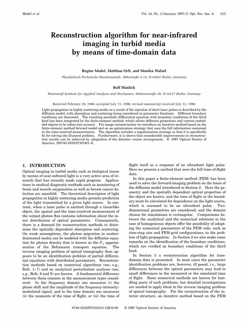
lem (1) even for inhomogeneous distributions of the opti-cal parameters and for complicated geometries andboundary conditions. On the basis of discretization inspace and time, the unknown photon density is approxi-mated by a piecewise linear function.2 Some useful prop-erties of this method led us to prefer it for our imagingalgorithm: (1) an adaptive grid refinement is standard,(2) arbitrary bounded domains can easily be discretizedwith sufficient accuracy, (3) boundary conditions of thethird kind are well approximated. In this paper a two-dimensional FEM code is used. Figure 1 is an example ofthe initial discretization of a rectangular object. Becauseof the large gradients of the photon density in a firstshort-time interval, a refinement around the source posi-tion (0.75, 20) is necessary (this can be seen more easilyin the detailed picture). In addition, the triangles nearthe boundary are smaller so that an appropriate accuracyof the numerical simulation of the boundary fluxes can beachieved. The grid used initially has 3427 nodes and6480 triangles. For one forward problem of this type thecalculation time was ;8 s on a DEC Alpha AXP worksta-tion (Digital Equipment) with a 275-MHz processor. Therectangular domain serves as an example; other geom-etries for clinical applications may be handled easily, too.
B. Boundary ConditionsA complete mathematical formulation of the forwardmodel requires that the boundary conditions be specified.In most previous papers, homogeneous Dirichlet condi-tions F(x, t) 5 0 were applied as suggested in Ref. 15,which describes a ‘‘perfectly absorbing’’ medium sur-rounding the object. A more realistic approach leads tothe boundary conditions of the third kind:
2D~x!]F
]n~x, t ! 5 chF~x, t ! ~x, t ! P ]V 3 ~0, T !.
(4)
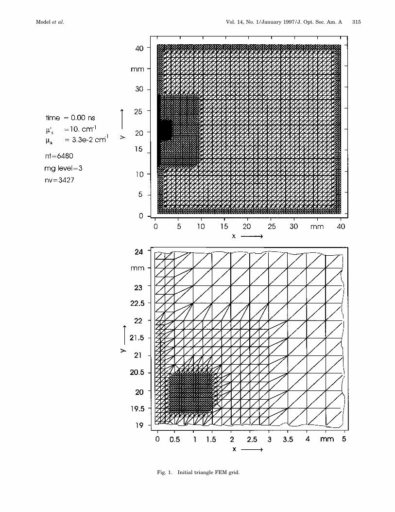
One derives these conditions by applying the diffusion ap-proximation to the general boundary condition of Boltz-mann’s transport equation, considering that no diffuse in-tensity enters the medium from outside and that partialreflection may occur. Different approaches resulting indifferent values for h are known.11,16,17 Generally, theconstant h depends on the refractive-index mismatch be-tween the tissue and the surrounding media and on theexperimental setup. It can be determined by a param-eter identification procedure as given in Ref. 18. In theliterature it is often suggested19–21 that one obtain an ap-proximation of condition (4) by theoretically shifting theboundary somewhat beyond the physical boundary andapplying Dirichlet conditions. However, the shift de-pends on the boundary parameter h. In Fig. 2 the iso-lines of the photon densities calculated under Dirichletconditions and, alternatively, with boundary conditions ofthe third kind are shown for a diffusion time of 0.5 ns.
Model et al. Vol. 14, No. 1 /January 1997 /J. Opt. Soc. Am. A 315
Fig. 1. Initial triangle FEM grid.
316 J. Opt. Soc. Am. A/Vol. 14, No. 1 /January 1997 Model et al.
Fig. 2. Isolines of the photon density (DENS) under different boundary conditions.
The differences can easily be seen; in particular, themaximum magnitude of one of them is approximately halfthat of the other. The numerical parameters, such as thegrid configuration and the size of the time steps, areadapted so that the numerical and the analytical solu-tions with Dirichlet conditions agree very well. Differ-ences between both would not be visible in the isolineplots. The analytical solution was constructed for a rect-angular object.3 Figure 3 shows the outward photonfluxes in two positions on the boundary calculated withfour different models: one detector opposite the sourcefor transmitted light, and one on the same side as thesource for reflected light (for positions, see Fig. 2). Theanalytical and the numerical solutions with Dirichlet con-ditions agree very well, and so do the solutions withboundary conditions of the third kind compared with thesolution with extrapolated boundary and Dirichlet condi-tions. But both pairs are quite different.
3. INVERSE PROBLEMA. Reconstruction Algorithm
In the inverse imaging algorithm the (given) measured in-formation about the time-resolved transmittance Jmes
5 @J1mes(x11 , t111), . . ., Ji
mes(xij , tijk), . . .# is used.The subscripts i, j, and k indicate current source, detec-tor, and time, respectively, so that one entry of the mea-surement vector Ji
mes(xij , tijk) is the photon flux that can
be detected in position xij and at the time tijk if the sourcedistribution F0i(x) has been applied to the object. Thisnotation allows the number of detectors and the detectorpositions to be chosen separately for each source and al-lows different times to be taken into account for each de-tector.The diffusion model (1) with the boundary condition (4)
and its numerical solution allow a vector Jsim(ma , ms8) tobe simulated under the assumption that ma(x) andms8(x) are the current spatially dependent optical param-eters of the object. The aim now is to find functionsma(x) and ms8(x), which provide a good fit between thesimulated data Jsim(ma , ms8) and the measured dataJmes. The basic strategy of the approximation consists inan iterative correction of the optical parameters and canbe demonstrated by a formal iteration procedure:
1. Choose an initial approximation ma and/or ms8 .2. Solve the forward problem, i.e., compute
Jsim(ma , ms8).3. Compare Jsim(ma , ms8) with Jmes; if iJsim(ma , ms8)
2 Jmesi , e, then go to step 5.4. Correct ma and/or ms8 ; go to step 2.5. End. (5)
The iteration process starts with a homogeneous initialguess for ma and ms8 . The norm to compare the vectors ofsimulated and measured data in the third step of the op-timization problem (5) is the l2 norm:
Model et al. Vol. 14, No. 1 /January 1997 /J. Opt. Soc. Am. A 317
iJsim~ma , ms8! 2 Jmesi2
5 (i51
l
(j51
mi
(k51
nij
uJisim~xij , tijk , ma ms8! 2 Ji
mes~xij , tijk!u2
5 (i51
p
Fi2 p 5 (
i51
l
(j51
mi
nij . (6)
Here p is the number of measurement data taken into ac-count in the reconstruction algorithm. In this paper,ma and ms8 have been set piecewise constant on a specialrectangular, not necessarily homogeneous, grid indepen-dent of the FEM grid. In each pixel the values of thesediscretized parameter functions of the grid are denotedmai , i 5 1, . . ., na and msi8 , i 5 1, . . ., ns for the ab-sorption and the reduced scattering, respectively. Withthese values the parameter functions ma(x) and ms8(x) are
mapped to a vector of finite length m 5 (ma , ms8)5 (ma 1 , . . ., ma na
, ms 18 , . . ., ms ns8 ), which has to be
determined by the reconstruction. The FEM grid mustbe considerably finer, and it is time dependent since a re-alistic description of the light propagation is a prerequi-site for solving the inverse problem of optical tomography.As expected, this inverse problem is seriously ill condi-
tioned. Large differences of the optical parameters maycause small differences in the simulated output flux.Regularization is a widely used stabilization strategy foralgorithms for the handling of ill-conditioned problems.Here the actual problem is replaced by a better-conditioned problem that approximates the original prob-lem if some additional regularization parameters tend tozero. The well-known Tikhonov regularization can beconsidered to be an addition of penalty terms to the errorfunction (6):
Fig. 3. (a) Photon flux in detector position opposite the source, (b) photon flux in detector position on the same side as the source.
318 J. Opt. Soc. Am. A/Vol. 14, No. 1 /January 1997 Model et al.
and Aj is the area of the jth rectangle of the absorptiongrid with absorption coefficient maj and Sj is the area ofthe jth rectangle of the scattering grid with scattering co-efficient msj8 . Each penalty term contains the norm ofthe optical parameter to be reconstructed.The dependence on the appropriate choice of the regu-
larization parameters ba and bs is very important. Bestresults can be achieved when the parameters ba and bsare chosen so that the penalty terms and the error func-tion (6) are of the same order of magnitude in the finalstep of iteration (5):
baimai2 ' iJsim~m! 2 Jmesi2,
bsims8i2 ' iJsim~m! 2 Jmesi2. (9)
In the tests the regularization parameters were deter-mined from condition (9) with imai2, ims8i2, and iJsim(m)2 Jmesi2 of the corresponding nonregularized reconstruc-tion result. It appears, however, that an automatic strat-egy determining the regularization parameter during theiteration process can be realized.For solving the optimization problem (7) the
Levenberg–Marquardt method from the program libraryof the International Mathematical Subroutine Library isapplied. It combines the Gauss–Newton method withthe gradient method:
mk11 5 mk 2 $@~F8!TF8#~mk! 1 lkI%21@~F8!TF#~mk!.
An iteration corresponds to a parameter correction thatagrees with step 4 of the formal procedure (5). Becauseof its trust region approach22 this method is appropriatefor handling ill-conditioned problems.
B. Detector Arrangement
In this section we discuss the influence of the detector ar-rangement on the image reconstruction. A method ispresented to improve the reconstruction results by anadapted detector arrangement. Here one should use asmuch of the available measurement information as pos-sible while taking into account as few measurement dataas possible. The idea consists in the following strategy5:
First an initial configuration of detectors for a givensource arrangement is chosen and is used to reconstruct atest object. A comparison between time-of-flight curvesfor the original object and those for the corresponding re-constructed object at test points between detector posi-tions not used for the reconstruction gives the informa-tion about the quality of the detector arrangement. Here
the l2 norm for the difference curves is used. In those ar-eas in which the norms at test points are clearly greaterthan the norm at the nearest detector position used, it canbe assumed that some unused measurement informationis available. Additional detectors in such regions aretaken into account. In contrast, in areas in which thenorms have the same order of magnitude, detectors areremoved. This basic strategy can be included in the fol-lowing formal procedure:
1. Choose a test object.2. Choose an initial detector configuration.3. Simulate time-of-flight curves at the detector posi-
tions and at additional test points between thesepositions.
4. Reconstruct the image only from detector curves.5. Simulate time-of-flight curves at test points and de-
tector positions, using the reconstructed image.6. Compare these curves at test points with the mea-
surement data.If the agreement is bad,modify the detector arrangement, and go to step 3.
7. End.
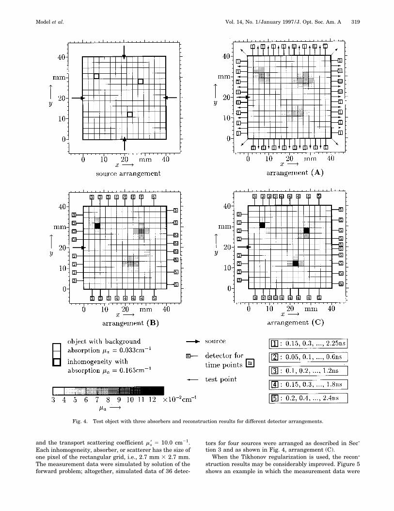
Figure 4 shows, on the top left, a two-dimensional rect-angular test example (40 mm 3 40 mm) with three ab-sorbers inside (2.7 mm 3 2.7 mm), with an absorption co-efficient ma 5 0.165 cm21 (five times the background),and, in the other parts of the figure, a series of reconstruc-tion results for different detector arrangements. The ar-rangement is illustrated for one of four sources in the po-sition x 5 1.0 mm, y 5 20.0 mm and the detectors andtest points in example (A). The arrangement in relation toeach source is, however, the same. The reconstructionresult on the top right is shown as obtained by equidis-tantly distributed detectors. For the results on the bot-tom left, the arrangement is adapted by analogy to thefirst step of the formal procedure; this is repeated for thepicture shown on the bottom right. It can clearly be seenthat the resolution is considerable better for adapted de-tector positions. The source–detector configuration wastested with respect to different object structures. In allthe cases, the resolution was improved.The strategy can include some constraints, such as the
maximal number of detectors as considered in the ex-ample; technical measurement conditions, such as mini-mal distances between detectors or between source anddetector; or areas impossible for use as detector positions.
4. TEST RESULTS
As in Section 3, which dealt with an adapted detector ar-rangement, a square object with a side length of 40 mm isused for several test series.First we give two examples with perturbations of only
the absorption coefficient and one with pure scatteringperturbations. The images here have been reconstructedon a 15 3 15 rectangular grid for the optical parameters.The optical properties are assumed to be constant in anyrectangle. For selected examples, the absorption coeffi-cient of the background is chosen to be ma 5 0.033cm21, except for the second one (here ma 5 0.03 cm21),
Model et al. Vol. 14, No. 1 /January 1997 /J. Opt. Soc. Am. A 319
Fig. 4. Test object with three absorbers and reconstruction results for different detector arrangements.
and the transport scattering coefficient ms8 5 10.0 cm21.Each inhomogeneity, absorber, or scatterer has the size ofone pixel of the rectangular grid, i.e., 2.7 mm 3 2.7 mm.The measurement data were simulated by solution of theforward problem; altogether, simulated data of 36 detec-
tors for four sources were arranged as described in Sec-tion 3 and as shown in Fig. 4, arrangement (C).When the Tikhonov regularization is used, the recon-
struction results may be considerably improved. Figure 5shows an example in which the measurement data were
320 J. Opt. Soc. Am. A/Vol. 14, No. 1 /January 1997 Model et al.
simulated with the test object of Section 3.B (compareFig. 4) with fixed reduced scattering and constant back-ground absorption. Unlike the last example in Fig. 4, thethree absorbers shown in Fig. 5 had only the fourfoldbackground absorption. A comparison between the gray-level pictures in Fig. 5 show the effect of regularization.With an inappropriate choice of the regularization param-eter the result gets worse. In the best tests, the regular-ization parameter was determined from condition (9) byuse of imai2 and iJsim(m) 2 Jmesi2 of the correspondingnonregularized reconstruction result. All three absorb-ers were precisely recognized, and the absorption coeffi-cient agree well with the original object.For testing our method, we often used the same struc-
ture, except with different optical properties.2,3,5 A posi-tive result of the development and the improvement of thealgorithm is that it was possible to improve the recogni-tion of minor inhomogeneities. In a previous paper,2 westarted with a 20-fold absorption coefficient for the ab-sorbers, and the reconstruction results that we obtainedwere not as good as for the next test example with a 1.25-
fold absorption coefficient. The first surface plot in Fig. 6shows the absorption distribution (z coordinate) over thetest object (xy plane) that has to be reconstructed. Allthree absorbers can be well recognized, as shown in Fig 7.In the middle of the object the absorption coefficientwaves somewhat, but this did not affect the recognition ofthe absorbers.The next example (Fig. 8) shows the reconstruction of a
structure with two scatterers whose 1.5-fold scattering co-efficient is much smaller than in Refs. 4 and 5, but thescatterers were well recognized, too. The quantitativeagreement of the scattering coefficient compared with theoriginal object is remarkable. The influence of the regu-larization strategy can be seen, but it is expected that itseffect on noisy experimental input data would be stron-ger.Finally, two test examples with both one absorber and
one scatterer inside the object are given (see Figs. 9 and10). Generally, the detection of mixed inhomogeneitiesseems to be more complicated than for perturbations ofonly one optical property. Until now, the resolution that
Fig. 5. Top left: object with three absorbers, top right: reconstruction results without regularization, bottom left: with regulariza-tion ba 5 1026, bottom right: ba 5 1027.
Model et al. Vol. 14, No. 1 /January 1997 /J. Opt. Soc. Am. A 321
we achieved was weaker than in the case of inhomogene-ities of the same type. In the first example the grid forthe scattering coefficient consists of 10 3 10 squares; thegrid for the absorption coefficient, 8 3 8 squares. Theperturbations have the size of one corresponding pixel,the scatterer with a threefold background value has thesize of 4 mm 3 4 mm, and the absorber with a fourfoldbackground value has the size of 5 mm 3 5 mm. The po-sitions of the inhomogeneities and their optical propertiesare well recognized, as shown in Fig. 9. The backgroundvalues are approximately constant at the correct level.In the second test example the discretization for both
optical coefficients are the same, containing 8 3 8squares. The optical properties of the scatterer and the
Fig. 6. Surface plot of the absorption coefficient for a test object.Absorbers have a 1.25-fold absorption.
Fig. 7. Surface plot of the absorption coefficient for the recon-structed object with three absorbers with a 1.25-fold absorption.
Fig. 8. Top: object with two scatterers, middle: reconstruc-tion result without regularization, bottom: result with regular-ization.
322 J. Opt. Soc. Am. A/Vol. 14, No. 1 /January 1997 Model et al.
Fig. 9. Left: object with one (fourfold) absorber and a smaller (threefold) scatterer, middle: reconstructed absorption, right: recon-structed reduced scattering.
Fig. 10. Left: object with one (fourfold) absorber and one (threefold) scatterer of the same size, middle: reconstructed absorption,right: reconstructed reduced scattering.
absorber are unchanged compared with the first test ex-ample, but now the size of the scatterer is 5 mm 3 5 mm,the same size as that of the absorber. Both perturba-tions are well recognized again, with optical propertiesclose to those of the original object (see Fig. 10). It is in-teresting that near the scatterer an artificial absorberwas detected. In test series this trend escalates. With a
growing scattering coefficient of the scatterer an artificialabsorber located near the scatterer, or in some tests in ex-actly the same place, will be more pronounced. In ex-treme cases, the scattering coefficient in this case is onlyweakly varying in the position of the theoretical scatterer,too. In contrast, in all the tests the reverse case of arti-ficial scatterers was not detected. The results suggest
Model et al. Vol. 14, No. 1 /January 1997 /J. Opt. Soc. Am. A 323
that a linear combination of the scattering and the ab-sorption coefficient may be a suitable property for tumordetection.
5. CONCLUSIONSIn this paper a two-dimensional iterative reconstructionalgorithm based on the time-dependent diffusion forwardmodel and on an optimization strategy that uses full timedata is presented. It allows one or more inhomogeneities(absorbers or scatterers or both) to be recognized in casesin which the detection of perturbations of different typesis more complicated. The inverse imaging problem is illconditioned. Reconstruction results therefore dependvery sensitively both on the measurement data and on thechoice of the reconstruction method and of the parameterscontrolling the algorithm. However, the results are en-couraging. Tests with simulated data for different struc-tures demonstrate the efficiency of the reconstructionmethod even for inhomogeneities that are small in sizeand have only slightly different optical properties. It isexpected that with experimental data the resolution ofthe images will be lower, especially for biological tissueobjects. Three main reasons are responsible for this ef-fect: first, only two-dimensional simulations are consid-ered; second, the assumption of isotropic light propaga-tion may be violated; and third, experimental noise ispresent in the measurements. Here the systematic mea-surement errors are a more serious problem than noisewith zero mean value, as we have checked in separatetests.The measurement configuration, especially the ar-
rangement of the detectors, has a great influence on thereconstruction result obtained. It is possible to improvethe results by use of appropriate configurations. Regu-larization methods can improve the reconstruction resultsor can reduce the computation time because of faster con-vergence. An automatic control of the regularization pa-rameter should be included.We believe that time-domain data generally contain ex-
tensive information about the interior structure of tissueobjects of several centimeters in size, which is sufficientfor optical image reconstruction. The iterative algorithmdescribed here seems to be an appropriate tool for han-dling this inverse problem. The computational effortcould be higher than for other reconstruction methodsbased on the fit of mean time of flight or on the treatmentin the frequency domain, but a higher resolution is ex-pected, too. In our ongoing research, priorities are set forsaving computational time, and some initial ideas are yetto be realized. In general, a comparison among the dif-ferent types of reconstruction method is an open question.The rapid development in this area complicates the taskof performing a definite evaluation.
ACKNOWLEDGMENTThis research was supported by the German Federal Min-istry of Education, Science, Research and Technology(Bundesministerium fur Bildung, Wissenschaft, For-schung und Technologie) under grant 13N6307.
REFERENCES1. B. W. Pogue, M. S. Patterson, and T. J. Farrell, ‘‘Forward
and inverse calculations for 3-D frequency-domain diffuseoptical tomography,’’ in Optical Tomography: Photon Mi-gration, and Spectroscopy of Tissue and Model Media:Theory, Human Studies, and Instrumentation, B. Chanceand R. Alfano, eds., Proc. SPIE 2389, 328–339 (1995).
2. R. Model, R. Hunlich, D. Richter, H. Rinneberg, H. Wab-nitz, and M. Walzel, ‘‘Imaging in random media: simulat-ing light transport by numerical integration of the diffusionequation,’’ in Photon Transport in Highly Scattering Tissue,S. Avrillier, B. Chance, G. Mueller, A. Priezzhev, and V.Tuchin, eds., Proc. SPIE 2326, 11–22 (1995).
3. R. Model, R. Hunlich, M. Orlt, and M. Walzel, ‘‘Image re-construction for random media by diffusion tomography,’’ inOptical Tomography: Photon Migration, and Spectroscopyof Tissue and Model Media: Theory, Human Studies, andInstrumentation, B. Chance and R. Alfano, eds., Proc. SPIE2389, 400–410 (1995).
4. R. Model and R. Hunlich, ‘‘Optical imaging of highly scat-tering media,’’ Z. Angew. Math. Mech. 76, 483–484 (1996).
5. M. Orlt, M. Walzel, and R. Model, ‘‘Transillumination im-aging performance using time domain data,’’ in PhotonPropagation in Tissues, B. Chance, D. Delpy, and G.Mueller, eds., Proc. SPIE 2626, 346–357 (1995).
6. S. R. Arridge, M. Schweiger, M. Hiraoka, and D. T. Delpy,‘‘Performance of an iterative reconstruction algorithm fornear-infrared absorption and scatter imaging,’’ in PhotonMigration and Imaging in Random Media and Tissues,R. Alfano and B. Chance, eds., Proc. SPIE 1888, 360–371(1993).
7. S. R. Arridge and M. Schweiger, ‘‘Sensitivity to prior knowl-edge in optical tomographic reconstruction,’’ in Optical To-mography: Photon Migration, and Spectroscopy of Tissueand Model Media: Theory, Human Studies, and Instru-mentation, B. Chance and R. Alfano, eds., Proc. SPIE 2389,378–388 (1995).
8. S. C. Feng and F.-A. Zeng, ‘‘Analytical perturbation theoryof photon migration in the presence of a single absorbing orscattering defect sphere,’’ in Optical Tomography: PhotonMigration, and Spectroscopy of Tissue and Model Media:Theory, Human Studies, and Instrumentation, B. Chanceand R. Alfano, eds., Proc. SPIE 2389, 54–63 (1995).
9. Y. Wang, J. Chang, R. Aronson, R. L. Barbour, H. L.Graber, and J. Lubowski, ‘‘Imaging of scattering media bydiffusion tomography: an iterative perturbation ap-proach,’’ in Physiological Monitoring and Early DetectionDiagnostic Methods, T. Mang, ed., Proc. SPIE 1641, 58–71(1992).
10. C. W. Groetsch, Inverse Problems in the Mathematical Sci-ence (Braunschweig, Wiesbaden, Germany, 1993).
11. A. Ishimaru, Wave Propagation in Random Scattering Me-dia (Academic, New York, 1978).
12. J.-M. Kaltenbach and M. Kaschke, ‘‘Frequency- and time-domain modelling of light transport in random media,’’ inMedical Optical Tomography: Functional Imaging andMonitoring, in Vol. IS11 of Institute Series of SPIE OpticalEngineering, G. Mueller, B. Chance, R. Alfano, S. Arridge,J. Beuthan, E. Gratton, M. Kaschke, B. Masters, S.Svanberg, and P. van der Zee, eds. (Society of Photo-OpticalInstrumentation Engineers, Bellingham, Wash., 1993),pp. 61–82.
13. D. A. Boas, H. Liu, M. A. O’Leary, B. Chance, and A. G.Yodh, ‘‘Photon migration within the P3 approximation,’’ inOptical Tomography: Photon Migration, and Spectroscopyof Tissue and Model Media: Theory, Human Studies, andInstrumentation, B. Chance and R. Alfano, eds., Proc. SPIE2389, 240–247 (1995).
14. W. M. Star, ‘‘Comparing the P3 approximation with the dif-fusion theory and with Monte Carlo calculations of lightpropagation in a slab geometry,’’ in Dosimetry of Laser Ra-diation in Medicine and Biology, G. Mueller and D. Sliney,eds., Proc. SPIE 1035, 146–154 (1989).
15. M. S. Patterson, B. Chance, and B. C. Wilson, ‘‘Time re-solved reflectance and transmittance for the noninvasive
324 J. Opt. Soc. Am. A/Vol. 14, No. 1 /January 1997 Model et al.
measurement of tissue optical properties,’’ Appl. Opt. 28,2331–2336 (1989).
16. F. Liu, K. M. Yoo, and R. R. Alfano, ‘‘How to describe thescattered ultrashort laser pulse profiles measured insideand at the surface of a random medium using the diffusiontheory,’’ in Photon Migration and Imaging in Random Me-dia and Tissues, R. Alfano and B. Chance, eds., Proc. SPIE1888, 103–106 (1993).
17. L. O. Svaasand, R. C. Haskell, B. J. Tromberg, and M.McAdams, ‘‘Properties of photon density waves at bound-aries,’’ in Photon Migration and Imaging in Random Mediaand Tissues, R. Alfano and B. Chance, eds., Proc. SPIE1888, 214–226 (1993).
18. R. Model and R. Hunlich, ‘‘Parameter sensitivity in near in-frared imaging,’’ in Photon Propagation in Tissues, B.Chance, D. Delpy, and G. Mueller, eds., Proc. SPIE 2626,56–65 (1995).
19. R. Aronson, ‘‘Extrapolation distance for diffusion of light,’’in Photon Migration and Imaging in Random Media andTissues, R. Alfano and B. Chance, eds., Proc. SPIE 1888,297–305 (1993).
20. A. H. Hielscher, S. L. Jacques, L. Wang, and F. K. Tittel,‘‘The influence of boundary conditions on the accuracy ofdiffusion theory in time-resolved reflectance spectroscopy ofbiological tissue,’’ Phys. Med. Biol. 40, 1957–1975 (1995).
21. M. Schweiger, S. R. Arridge, M. Hiraoka, and D. T. Delpy,‘‘The finite element method for the propagation of lightscattering media: boundary and source condition,’’ Med.Phys. 22, 1779–1792 (1995).
22. J. E. Dennis, Jr., and R. B. Schnabel, Numerical Methodsfor Unconstraint Optimization and Nonlinear Equations(Prentice-Hall, Englewood Cliffs, N.J., 1983).