Reconstruction of Surfaces from Point CloudsUsing a Lagrangian Surface Evolution Model

Patrik Daniel, Matej Medl’a, Karol Mikula, and Mariana Remesıkova(B)

Department of Mathematics, Faculty of Civil Engineering,Slovak University of Technology, Radlinskeho 11, 81005 Bratislava, Slovakia

patrik.daniel1@gmail.com, {medla,mikula,remesikova}@math.sk

Abstract. We present a method for reconstruction of surfaces in R3

from point clouds. Given a set of points, we construct a triangular meshapproximation of a surface that they represent. The triangulation isobtained by a Lagrangian surface evolution model consisting of an advec-tion and a curvature term. To construct them, we compute the distancefunction d to the given point cloud. Then the advection evolution isdriven by ∇d and the curvature term depends on d and the mean curva-ture of the evolving surface. In order to control the quality of the meshduring the evolution, we perform tangential redistribution of mesh pointsas the surface evolves.

Keywords: Point cloud · Surface evolution · Lagrangian methods ·Tangential redistribution

1 Introduction

One of the main tasks of modern computer graphics and computer vision is toobtain digital representation of real world objects. A common way of obtaining arepresentation of a 3D object is scanning a set of points lying on the object’s sur-face. However, such a basic representation is not sufficient for most applications.Therefore, a lot of effort has been put in designing algorithms for obtaining asurface representation of an object given a representative point cloud [1].

We present a method that constructs a triangular mesh representation ofan object’s surface. As an input, we need the corresponding point cloud and atriangulated surface – an approximation of the desired surface. After, we applyan appropriately designed Lagrangian surface evolution model to obtain the rep-resentation we are looking for. The driving force of the evolution is the distancefunction d to the point cloud – the model consists of an advection term withthe velocity proportional to ∇d and a curvature term with the evolution speedproportional do d. Moreover, the model is enriched with a specifically designedtangential movement term that moves the points around the evolving surface.This term is added to overcome one of the main difficulties arising in Lagrangianmanifold evolution – the possible deterioration of the mesh quality during theevolution process.c© Springer International Publishing Switzerland 2015J.-F. Aujol et al. (Eds.): SSVM 2015, LNCS 9087, pp. 589–600, 2015.DOI: 10.1007/978-3-319-18461-6 47

590 P. Daniel et al.

The method that we propose is that it provides a straightforward way toobtain a good quality triangular representation of an object’s surface. The initialcondition for the evolution process is usually a simple surface (e.g. a sphere or anellipsoid) that can be easily triangulated. Assuming that the initial condition istopologically equivalent to the desired surface, the topology of the triangulationremains intact during the evolution. The orientation of normals is also preserved;having oriented normals is important for determining the interior and exteriorof the surface, resolving visibility, shading etc. However, a practically applicablemethod should also be robust enough to manage difficulties caused by variousdata imperfections. The scanned point clouds often suffer from defects such asnon-uniform point distribution, noise, outlying points or missing parts (Figure1). As we demonstrate in the last section, our method is well able to deal withsuch problematic situations due to the properties of the model that we use.

Fig. 1. A surface and its various point cloud representations – an ideal uniform pointcloud, a non-uniform point cloud, a point cloud with 5% noise, a point cloud withseveral outlying points and a point cloud with a missing part.

The reason why we use a Lagrangian method is that obtaining a triangularrepresentation of an object is more simple than in the case of, e.g., level setmethods. Also, though not shown here, Lagrangian methods can be more easilyapplied to surfaces with boundaries. To our knowledge, Lagrangian evolutionmethods were so far only rarely applied to the point cloud problem and theexisting works do not consider any mesh adjustment [7]. The strategy that we usein this paper is based on some of our previous works concerning surface evolutionproblems [5,6]. This paper extends the ideas to the point cloud problem that hasnot appeared in the cited works. Also, we suggest a new tangential redistributiontechnique based on the curvature of the evolving surface.

2 Mathematical Model

Let Ω ⊆ R3 and let C ⊂ Ω be a set of np points with elements denoted by Pi,

i = 1 . . . np. Our goal is to find a closed surface approximating C.Let d0 : Ω → R represent the distance function to C. Starting at any point

of Ω, we can approach C following the direction of ∇d0. The basic idea of our

Reconstruction of Surfaces from Point Clouds Using a Lagrangian Surface 591

mathematical model is to take a smooth closed surface surrounding C and let itevolve based on ∇d0. Since d0 is not everywhere differentiable, instead we willconsider d = Gσ ∗ d0, where Gσ is a Gauss kernel.

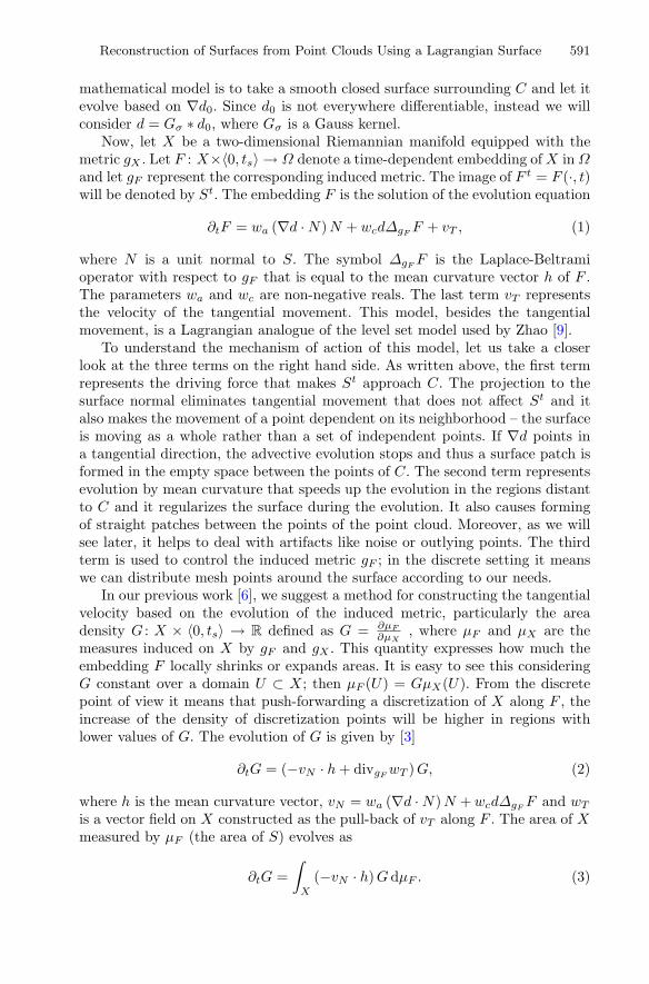
Now, let X be a two-dimensional Riemannian manifold equipped with themetric gX . Let F : X×〈0, ts〉 → Ω denote a time-dependent embedding of X in Ωand let gF represent the corresponding induced metric. The image of F t = F (·, t)will be denoted by St. The embedding F is the solution of the evolution equation

∂tF = wa (∇d · N) N + wcdΔgFF + vT , (1)

where N is a unit normal to S. The symbol ΔgFF is the Laplace-Beltrami

operator with respect to gF that is equal to the mean curvature vector h of F .The parameters wa and wc are non-negative reals. The last term vT representsthe velocity of the tangential movement. This model, besides the tangentialmovement, is a Lagrangian analogue of the level set model used by Zhao [9].

To understand the mechanism of action of this model, let us take a closerlook at the three terms on the right hand side. As written above, the first termrepresents the driving force that makes St approach C. The projection to thesurface normal eliminates tangential movement that does not affect St and italso makes the movement of a point dependent on its neighborhood – the surfaceis moving as a whole rather than a set of independent points. If ∇d points ina tangential direction, the advective evolution stops and thus a surface patch isformed in the empty space between the points of C. The second term representsevolution by mean curvature that speeds up the evolution in the regions distantto C and it regularizes the surface during the evolution. It also causes formingof straight patches between the points of the point cloud. Moreover, as we willsee later, it helps to deal with artifacts like noise or outlying points. The thirdterm is used to control the induced metric gF ; in the discrete setting it meanswe can distribute mesh points around the surface according to our needs.

In our previous work [6], we suggest a method for constructing the tangentialvelocity based on the evolution of the induced metric, particularly the areadensity G : X × 〈0, ts〉 → R defined as G = ∂μF

∂μX, where μF and μX are the

measures induced on X by gF and gX . This quantity expresses how much theembedding F locally shrinks or expands areas. It is easy to see this consideringG constant over a domain U ⊂ X; then μF (U) = GμX(U). From the discretepoint of view it means that push-forwarding a discretization of X along F , theincrease of the density of discretization points will be higher in regions withlower values of G. The evolution of G is given by [3]

∂tG = (−vN · h + divgFwT ) G, (2)

where h is the mean curvature vector, vN = wa (∇d · N) N + wcdΔgFF and wT

is a vector field on X constructed as the pull-back of vT along F . The area of Xmeasured by μF (the area of S) evolves as

∂tG =∫

X

(−vN · h) GdμF . (3)

592 P. Daniel et al.

An embedding F with constant G can be called area-uniform with respect togX . Let us use the notation AX = μX(X), A = μF (X). Since

∫X

GdμX = A, (4)

then for a constant G we must have G = AAX

.An embedding with this property provides a straightforward way to con-

struct a discretization mesh with uniformly sized 2D mesh elements. This typeof mesh has several practical advantages – it prevents mesh degeneration, it pro-vides a reasonable discrete representation of a surface and it is likely to captureimportant information coming from the external vector field that drives the evo-lution. Thus, it has sense to require G → A

AXas t → ∞. The corresponding

dimensionless condition isG

A−→t→∞

1AX

.

This can be guaranteed, if

∂t

(G

A

)= ω

(1

AX− G

A

), (5)

where ω : 〈0, ts〉×R+. This equality combined with (2) and (3) yields a conditionfor the divergence of wT ,

divgFwT = vN · h − 1

A

∫X

vN · h dμF + ω

(A

AXG− 1

). (6)

To obtain a unique wT , we can suppose, for example, that wT = ∇gFψ, ψ :

X × 〈0, ts〉 → R. Then we have

ΔgFψ = vN · h − 1

A

∫X

vN · h dμF + ω

(A

AXG− 1

). (7)

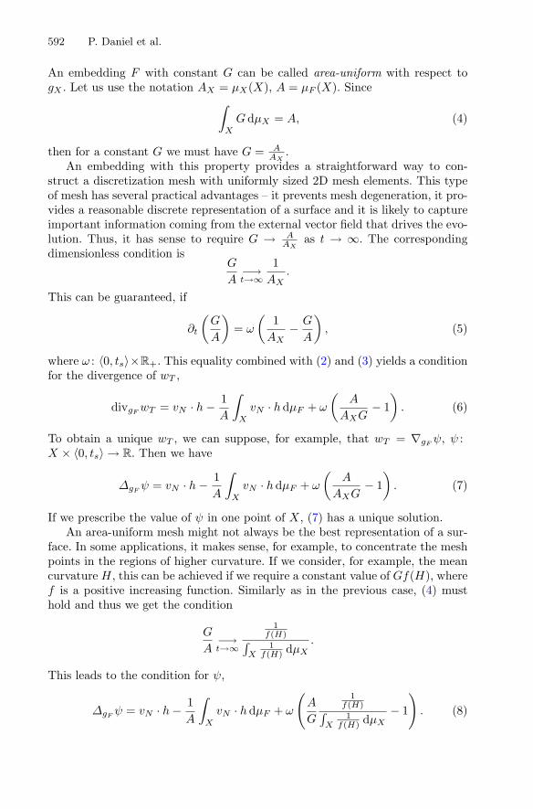
If we prescribe the value of ψ in one point of X, (7) has a unique solution.An area-uniform mesh might not always be the best representation of a sur-

face. In some applications, it makes sense, for example, to concentrate the meshpoints in the regions of higher curvature. If we consider, for example, the meancurvature H, this can be achieved if we require a constant value of Gf(H), wheref is a positive increasing function. Similarly as in the previous case, (4) musthold and thus we get the condition

G

A−→t→∞

1f(H)∫

X1

f(H) dμX

.

This leads to the condition for ψ,

ΔgFψ = vN · h − 1

A

∫X

vN · h dμF + ω

(A

G

1f(H)∫

X1

f(H) dμX

− 1

). (8)

Reconstruction of Surfaces from Point Clouds Using a Lagrangian Surface 593

3 Discretization of the Mathematical Model

Since the problem of point cloud reconstruction is in principle analogous to the3D image segmentation problem, we refer to our previous works concerning thistopic [5,6] and we only provide a brief explanation of the numerical method.

Before we can apply our model, we need to compute the distance function d.For this purpose, we consider Ω to be a box and we discretize it by constructinga voxel mesh where each voxel is a cube of side length h. Then we approximatethe value of d in each voxel. This approach is necessary since a brute-forcecomputation of the distance function is practically inapplicable in most cases.Having an approximation of d, we approximate ∇d simply by central differences.To identify the voxel corresponding to a point F (P, t), P ∈ X, we round itscoordinates divided by h.

We consider a uniform discretization of the time interval and we use thenotation Fn = F tn and Sn = Stn . The time discretization of (1) is semi-implicit,

Fn − Fn−1

τ= wa

(∇d · Nn−1

)Nn−1 + wcdΔgFn−1 Fn + vn−1

T . (9)

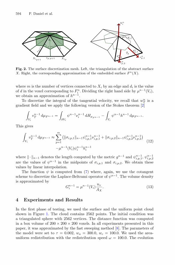
Now, we consider a triangular structure on X consisting of vertices Xi,i = 1 . . . nv, edges ej , j = 1 . . . ne, and triangles Tk, k = 1 . . . nt. We constructa piecewise linear approximation of Fn denoted by Fn – we set Fn(Xi) =Fn(Xi) and then, for any triangle Tp with vertices Xi, Xip , Xip+1 , we setFn(λ1Xi + λ2Xip + λ3Xip+1) = λ1F

n(Xi) + λ2Fn(Xip) + λ3F

n(Xip+1). Theembedding Fn induces a metric gn on X which induces a measure μn on X.The approximation of the unit normal to Sn = Fn(X) at Fn

i is denoted by Nni .

The numerical scheme that we apply uses the angles of Tp adjacent to Xip andXip+1 measured in the metric gn. We denote them by θn

p,1 and θnp,2.

The space discretization of (9) is done by the finite volume approach. Thecontrol volume mesh is constructed by barycentric subdivision of the triangles Tk

(Figure 2). We will denote by νnp,1, νn

p,2 the outward unit normals to the controlvolume edges Fn(σp,1) and Fn(σp,2) in the plane of T n

p . The principle of themethod is to integrate (9) over a control volume Vi,

∫Vi

Fn − Fn−1

τdμFn−1 =

∫Vi

wa

(∇d · Nn−1

)Nn−1 dμFn−1

+∫

Vi

wcdΔgFn−1 Fn dμFn−1 +∫

Vi

vn−1T dμFn−1 ,(10)

and then to approximate the integrals that we obtain.For the first term of the right hand side, we need to approximate the surface

normal at Fni . We take the arithmetic mean of the normals to all triangles

containing Fni . For the second term, we use the cotangent scheme [4],

∫Vi

wcdΔgFn−1 Fn dμFn−1 ≈ wcdi12

m∑p=1

(cot θn−1

i,p−1,1 + cot θn−1i,p,2

)(Fn

i − Fnip),

(11)

594 P. Daniel et al.

Xi

XipXip+1

ep

e p+1

ep,p+1

σp,1

σp,2

Nni

Fn(Xi)

νnp,1

νnp,2

Tp

θnp,1

θnp,2

Fig. 2. The surface discretization mesh. Left, the triangulation of the abstract surfaceX. Right, the corresponding approximation of the embedded surface Fn(X).

where m is the number of vertices connected to Xi by an edge and di is the valueof d in the voxel corresponding to Fn

i . Dividing the right hand side by μn−1(Vi),we obtain an approximation of hn−1.

To discretize the integral of the tangential velocity, we recall that wnT is a

gradient field and we apply the following version of the Stokes theorem [2]∫

Vi

vn−1T dμFn−1 =

∫∂Vi

ψn−1νn−1i dHμFn−1 −

∫Vi

ψn−1hn−1 dμFn−1 .

This gives∫

Vi

vn−1T dμFn−1 ≈

m∑p=1

(‖σi,p,1‖n−1ψ

n−1i,p,1ν

n−1i,p,1 + ‖σi,p,2‖n−1ψ

n−1i,p,2ν

n−1i,p,2

)

−μn−1(Vi)ψn−1i hn−1

i

(12)

where ‖ · ‖n−1 denotes the length computed by the metric gn−1 and ψn−1i,p,1, ψn−1

i,p,2

are the values of ψn−1 in the midpoints of σi,p,1 and σi,p,2. We obtain thesevalues by linear interpolation.

The function ψ is computed from (7) where, again, we use the cotangentscheme to discretize the Laplace-Beltrami operator of ψn−1. The volume densityis approximated by

Gn−1i = μn−1(Vi)

nv

AX. (13)

4 Experiments and Results

In the first phase of testing, we used the surface and the uniform point cloudshown in Figure 1. The cloud contains 2562 points. The initial condition wasa triangulated sphere with 2562 vertices. The distance function was computedin a box volume of 200 × 200 × 200 voxels. In all experiments presented in thispaper, it was approximated by the fast sweeping method [8]. The parameters ofthe model were set to τ = 0.002, wa = 300.0, wc = 100.0. We used the area-uniform redistribution with the redistribution speed ω = 100.0. The evolution

Reconstruction of Surfaces from Point Clouds Using a Lagrangian Surface 595

was stopped after 400 time steps. Since d is a distance function smoothed bya heat kernel, it is nowhere zero and thus there is no stopping time implied bythe model. However, we can stop the evolution if the difference between Sn−1

and Sn is lower than some threshold. Figure 3 shows the initial condition aswell as a few stages of the evolution. Since a point cloud is usually a roughapproximation of an object, the resulting representative surface might benefitfrom some additional smoothing after the evolution stops. In our case, this canbe done by using the same algorithm; we only need to set d = 1 in all voxels andwe obtain a mean curvature flow model. The last two pictures in Figure 3 showthe result of such smoothing. Here, we set wc = 300., ω = 2000, τ = 0.0005 andwe performed only 20 time steps to prevent excessive shrinking of our surface.

Fig. 3. Reconstruction of a surface from a uniform point cloud representation. Wecan see the initial surface together with the point cloud and the triangulation of thissurface. What follows is the evolved surface after 100, 150, 200 and 250 time steps, thesurface at the end of the evolution displayed with its triangulation and with the pointcloud. Finally, we show the smoothed surface after applying 20 steps of mean curvatureflow.

596 P. Daniel et al.

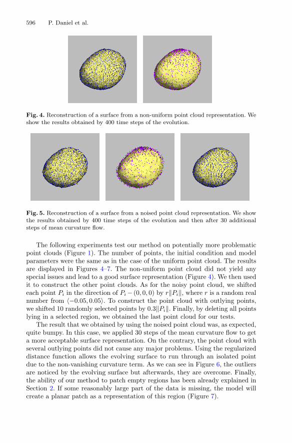
Fig. 4. Reconstruction of a surface from a non-uniform point cloud representation. Weshow the results obtained by 400 time steps of the evolution.

Fig. 5. Reconstruction of a surface from a noised point cloud representation. We showthe results obtained by 400 time steps of the evolution and then after 30 additionalsteps of mean curvature flow.

The following experiments test our method on potentially more problematicpoint clouds (Figure 1). The number of points, the initial condition and modelparameters were the same as in the case of the uniform point cloud. The resultsare displayed in Figures 4–7. The non-uniform point cloud did not yield anyspecial issues and lead to a good surface representation (Figure 4). We then usedit to construct the other point clouds. As for the noisy point cloud, we shiftedeach point Pi in the direction of Pi − (0, 0, 0) by r‖Pi‖, where r is a random realnumber from 〈−0.05, 0.05〉. To construct the point cloud with outlying points,we shifted 10 randomly selected points by 0.3‖Pi‖. Finally, by deleting all pointslying in a selected region, we obtained the last point cloud for our tests.

The result that we obtained by using the noised point cloud was, as expected,quite bumpy. In this case, we applied 30 steps of the mean curvature flow to geta more acceptable surface representation. On the contrary, the point cloud withseveral outlying points did not cause any major problems. Using the regularizeddistance function allows the evolving surface to run through an isolated pointdue to the non-vanishing curvature term. As we can see in Figure 6, the outliersare noticed by the evolving surface but afterwards, they are overcome. Finally,the ability of our method to patch empty regions has been already explained inSection 2. If some reasonably large part of the data is missing, the model willcreate a planar patch as a representation of this region (Figure 7).

Reconstruction of Surfaces from Point Clouds Using a Lagrangian Surface 597

Fig. 6. Reconstruction of a surface from a point cloud representation with outlyingpoints. We show the evolved surface after 180 time steps (first its triangulation andthen displayed together with the corresponding point cloud), after 220 and 400 timesteps of the evolution.

Fig. 7. Reconstruction of a surface from a point cloud representation with a missingpart. We show the results obtained by 400 time steps of the evolution.

In the next example, we took a point cloud representing a much more com-plicated object (Figure 8). In this case, we computed the distance function ona finer grid of 300 × 300 × 300 voxels. The initial surface was also more finelydiscretized, it was a sphere with 16386 vertices. The values of the model parame-ters were τ = 0.002, wa = 300., wc = 30., ω = 100.. We show the result obtainedafter 900 time steps and then after a slight smoothing by 5 steps of the meancurvature flow with parameter values mentioned above.

Finally, we present an experiment illustrating the effect of the curvature driv-en tangential redistribution. We use the uniform point cloud shown in Figure 3.The curvature driven redistribution was not used during the whole evolution

598 P. Daniel et al.

Fig. 8. Reconstruction of a more complicated surface (surface taken fromhttp://segeval.cs.princeton.edu/) . We show the original surface and the point cloudrepresenting it. In the second row, we can see our reconstruction obtained after 900 timesteps of evolution and the surface smoothed by 5 additional steps of mean curvatureflow.

process, but we rather used the area-uniform redistribution to optimally cap-ture the external vector field. After 400 time steps and additional 20 steps ofsmoothing, we obtained the surface representation shown in the last two picturesof Figure 3. This was the starting point for the curvature driven redistribution.We kept evolving the surface by mean curvature flow but it was now by ordersof magnitude slower; we set wc = 1.0. The redistribution speed changed toω = 200.0 and we performed 15 steps of the evolution. The function f used toredistribute the points was f(H) = e20H .

The result is shown in Figure 9. As we can see, the points are more denselydistributed in the regions with higher mean curvature (compare to the resultingmesh shown in Figure 3). To provide an evaluation of the redistribution otherthan a visual inspection of the resulting mesh, we add two graphs. Here, weconsider the ratio rA,i = μn(Vi)

AV, where AV is the average control volume area,

AV = A/nv. The graphs show the dependence of rA,i on H – each point of theplot represents one pair (Hi, rA,i). We can see that before the curvature driven

Reconstruction of Surfaces from Point Clouds Using a Lagrangian Surface 599

Fig. 9. A test example of a representation obtained with the help of curvature driventangential redistribution. We show the resulting surface representation obtained after15 time steps of the redistribution in two different views. Note that the density ofdiscretization points is higher in the regions with higher mean curvature. The graphsshow the dependence of rA,i on H before and after the curvature driven redistribution.

redistribution, rA,i is close to 1 in all vertices. After 15 steps of the redistribution,we can observe that rA,i is clearly decreasing with increasing Hi.

Acknowledgments. This work was supported by the grants APVV-0072-11 andAPVV-0161-12.

References

1. Berger, M., Tagliasacchi, A., Seversky, L. M.: State of the Art in Surface Recon-struction from Point Clouds. In: Eurographics 2014 - State of the Art Reports,pp. 161–185. The Eurographics Association (2014)

2. Dziuk, G., Elliott, C.M.: Finite elements on evolving surfaces. IMA J. Numer. Anal.27, 262–292 (2007)

3. Mantegazza, C.: Lecture Notes on Mean Curvature Flow. Springer (2011)4. Meyer, M., Desbrun, M., Schroeder, P., Barr, A.H.: Discrete differential geometry

operators for triangulated 2manifolds. Visualization and Mathematics III, 35–57(2003)

5. Mikula, K., Remesıkova, M.: 3D Lagrangian Segmentation with Simultaneous MeshAdjustment. In: Finite Volumes for Complex Applications VII. Springer Proceedingsin Mathematics and Statistics, vol. 77, pp. 685–694 (2014)

600 P. Daniel et al.

6. Mikula, K., Remesıkova, M., Sarkoci, P., Sevcovic, D.: Surface evolution with tan-gential redistribution of points. SIAM J. Sci. Comp. 36(4), 1384–1414 (2014)

7. Surynkova, P.: Curve and Surface Reconstruction Based on the Method of Evolu-tion. In: WDS 2010 Proceedings, Part I, MATFYZPRESS, pp. 139–144 (2010)

8. Zhao, H.: A Fast Sweeping Method for Eikonal Equations. Mathematics of Compu-tation 74(250), 603–627 (2004)

9. Zhao, H.K., Osher, S., Fedkiw, R.: Fast Surface Reconstruction Using the Level SetMethod. In: Proceedings of IEEE Workshop on Variational and Level Set Methodsin Computer Vision 2001, pp. 194–201. IEEE (2001)