RECOVERING CAPITAL EXPENDITURES: THE RAILROAD …

RECOVERING CAPITAL EXPENDITURES:THE RAILROAD INDUSTRY PARADOX

George Avery Grimes, Ph.D.Department of Civil and Environmental Engineering

University of Illinois at Urbana-ChampaignChristopher P. L. Barkan, Adviser

Following deregulation in 1980, the U.S. freight railroad industry invested large

amounts of capital, expanded output and increased earnings, but — paradoxically — it

did not earn a competitive return on investment. As a result, investors became

increasingly wary of expanding investment in this industry, even as demand for rail

transportation services continued to grow. In recent years, investment has been

constrained, capacity has become more restricted, prices have risen, and returns to

investment have improved but continue to fall below the industry's cost of capital.

This research examines the possibility that railroad capital expenditures represent

an incremental cost of traffic that was, and may continue to be, substantially

underestimated in industry calculations of marginal cost. As a result, railroad pricing

strategies may rely on overstated contribution ratios that do not consider the full

incremental capital cost associated with each shipment. Because railroads invest more

capital, as a percentage of revenue, than any other major industry sector, they are

particularly vulnerable to such miscalculations. All variable costs (expenses and

investments) must be included in marginal cost calculations if the economic value of the

firm is to be maximized in the way it prices its goods and services.

This research combines engineering, economic, and financial methods and makes

contributions in each area. Railroad maintenance strategies that rely more heavily on

capital investment are more cost effective. Infrastructure capital spending is caused by

current and future output, and is therefore a short run marginal cost. Railroad marginal

cost formulae appear to substantially underestimate the true incremental nature of

ongoing capital expenditures. Regulatory average variable cost formulae do not

incorporate variable capital expenditures suggesting that Surface Transportation Board

estimates of revenue to variable cost are overstated, subjecting a larger share of rail

traffic to potential economic regulation than would otherwise occur.

ii

© 2004 by George Avery Grimes. All rights reserved.

RECOVERING CAPITAL EXPENDITURES:THE RAILROAD INDUSTRY PARADOX

BY

GEORGE AVERY GRIMES

B.S., University of Illinois at Urbana-Champaign, 1978M.S., University of Nebraska at Lincoln, 1994

DISSERTATION

Submitted in partial fulfillment for the requirementsfor the degree of Doctor of Philosophy in Civil Engineering

in the Graduate College of theUniversity of Illinois at Urbana-Champaign, 2004

Urbana, Illinois

ii

This page is reserved for the (signed) Certificate of Committee Approval

A page number is not included on this certificate.

iii

Dedications

This dissertation is dedicated to my father, Dr. George Murray Grimes. Raised as a

depression era farm child in west Tennessee, he overcame many obstacles to study

veterinary medicine at Texas A&M University. He became a leader in veterinary

education in the U.S. Army, conducted advanced studies at Texas A&M and Tulane

Universities, served as a professor at the University of Illinois, and was a worldwide

missionary dedicated to improving the health of impoverished peoples. My father has

served as an inspiration on many levels, both personal and spiritual. When I was a child,

he showed me the world, from east to west. When I was a teenager, he was patient and

encouraging. He always demonstrated integrity in difficult decisions and perseverance in

difficult challenges. He demonstrated to me that love, family, spiritual matters and

knowledge were more important than personal possessions or wealth. He continues to be

my great inspiration and educator.

This dissertation is also dedicated to the memory of Professor W. W. Hay, who provided

guidance and inspiration during my undergraduate years, and kept railroad engineering

education alive and thriving almost single handedly. My last meeting with “Doc Hay”

was in late 1997 shortly before his death. Despite difficulties caused by his stroke, we

talked about the students that he had taught and his significant contributions to this

industry. He would be greatly pleased that his legacy has been carried forward at the

University of Illinois by a new group of dedicated educators, researchers, and students.

iv

Acknowledgements

The completion of this research could not have been possible without the efforts,

support, and inspiration of many individuals. First and foremost, Chris Barkan, principal

adviser and friend, for critical encouragement and significant support; and for his

dedication to this industry and the education of railroad engineering students. Carl

Nelson, economist and committee member, provided inspiration despite my relatively

new exposure to advanced economic theory. James Gentry, teacher and committee

member, provided encouragement and guidance in modern financial theory. Liang Liu,

committee member, provided guidance in engineering theory and decision analysis.

Gerard McCullough taught railroad economic theory and provided many contacts.

Others that contributed to my education were Scott Irwin (econometrics), Amy Ando

(economic theory), Jeff Douglas (statistics), Dick Hill (transportation), Hayri Onal

(dynamic modeling) and Lucio Soibelman (engineering). I also thank co-students Justin

Gardner and Maria Boerngen for assisting me with advanced economic theory. Bob

Gallamore provided encouragement and academic resources at critical points. Harry

MacLean and Eve Brady gave advice, encouragement and editing assistance.

I also want to acknowledge my friends and colleagues in the railroad industry.

Those persons that contributed and/or provided insights include Carl Martland, Craig

Rockey, Dale Lewis, Jeff Warren, Dave Burns, Jim Valentine, and Lou Anne Rinne. Of

special note are my “teachers” at Missouri Pacific and Union Pacific Railroads, including

(in chronological order) Art Mennell, Mike Godfrey, Sam Rice, Chuck Dettmann, Dick

Davidson, Art Shoener, Dennis Duffy, Jim Dunn, John Holm, Bill Wimmer, Ken Welch,

Lanny Schmid and Mike Hemmer. Many others should be in this list. To these

individuals I owe a mountain of gratitude for my real-world education.

Finally, and fundamentally, I could not have started much less completed this

effort without the support of my entire family, George, Lillian, Bill, Elizabeth, and Chris.

My father for his attentive ear, lifelong encouragement, and patience and faith. My

mother for her constant love and instilling a sense of confidence. And my son, Chris, for

encouragement and providing that last push, advising, “Ya gotta go for it, Dad.”

v

Table of Contents

1.0 Introduction.............................................................................................................. 1

1.1 Principal Hypothesis ............................................................................................ 11.2 Key Findings........................................................................................................ 21.3 Significance of and Reasons for Research........................................................... 31.4 Dissertation Organization .................................................................................... 41.5 Multi-Disciplinary Approach............................................................................... 7

2.0 Cost-Effectiveness of Railway Infrastructure Renewal Maintenance ..................... 9

2.1 Background......................................................................................................... 122.2 Methodology....................................................................................................... 142.3 Data Preparation.................................................................................................. 152.4 Renewal Strategy as a Single Independent Variable .......................................... 212.5 Alternative Hypothesis: Influence of Size .......................................................... 232.6 Alternative Hypothesis: Influence of Light Density Track Miles ...................... 242.7 Alternative Hypothesis: Influence of Average Density ...................................... 252.8 Combining Statistically Significant Variables.................................................... 252.9 Discussion........................................................................................................... 262.10 Conclusions......................................................................................................... 302.11 Appendix............................................................................................................. 30

3.0 Railway Output and Infrastructure Capital Expenditures....................................... 36

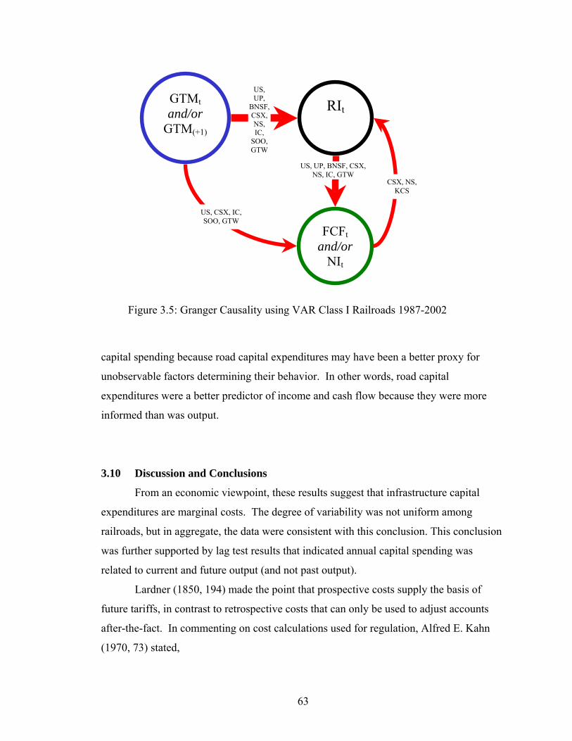
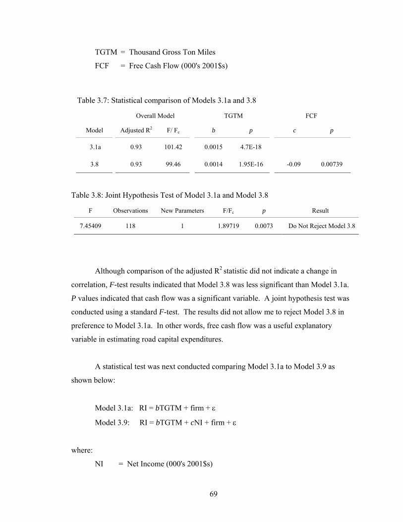
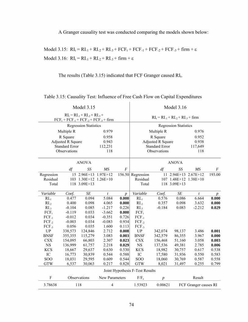
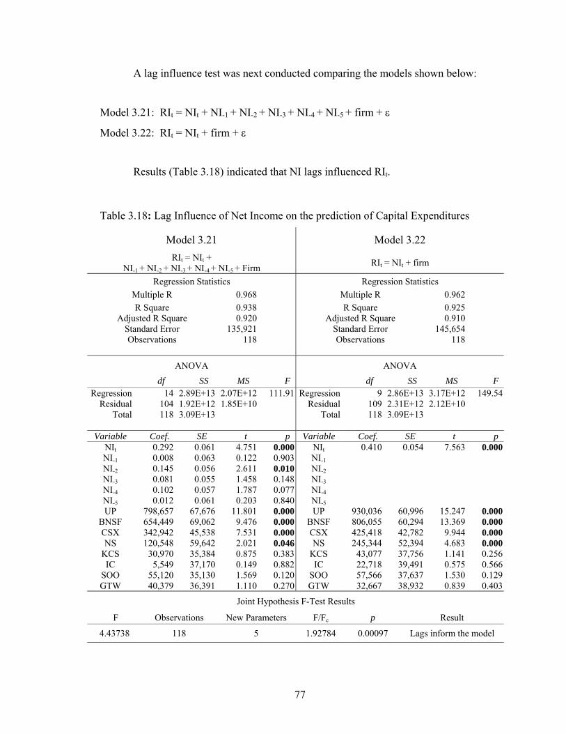
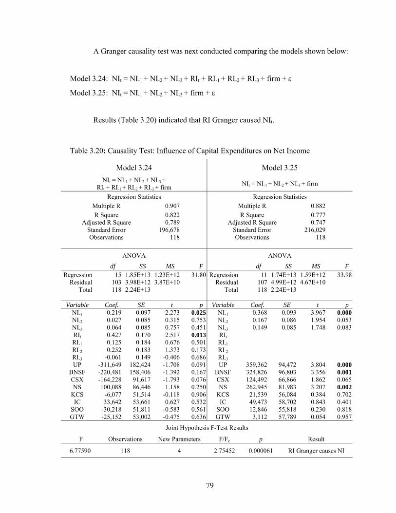
3.1 Historical Studies of Railroad Investment Variability........................................ 413.2 Engineering Foundations of Variable Capital Expenditures .............................. 433.3 Methodology and Decision Criteria.................................................................... 453.4 Data Preparation.................................................................................................. 473.5 Gross Ton Miles as Single Independent Variable............................................... 493.6 Influence of Free Cash Flow and Net Income .................................................... 513.7 Lag and Causality: Capital Expenditures and Output......................................... 523.8 Lag and Causality: Capital Expenditures, Net Income, and Free Cash Flow..... 583.9 Estimation of Causality using Vector Auto Regression ..................................... 603.10 Discussion and Conclusions ............................................................................... 633.11 Appendix............................................................................................................. 68

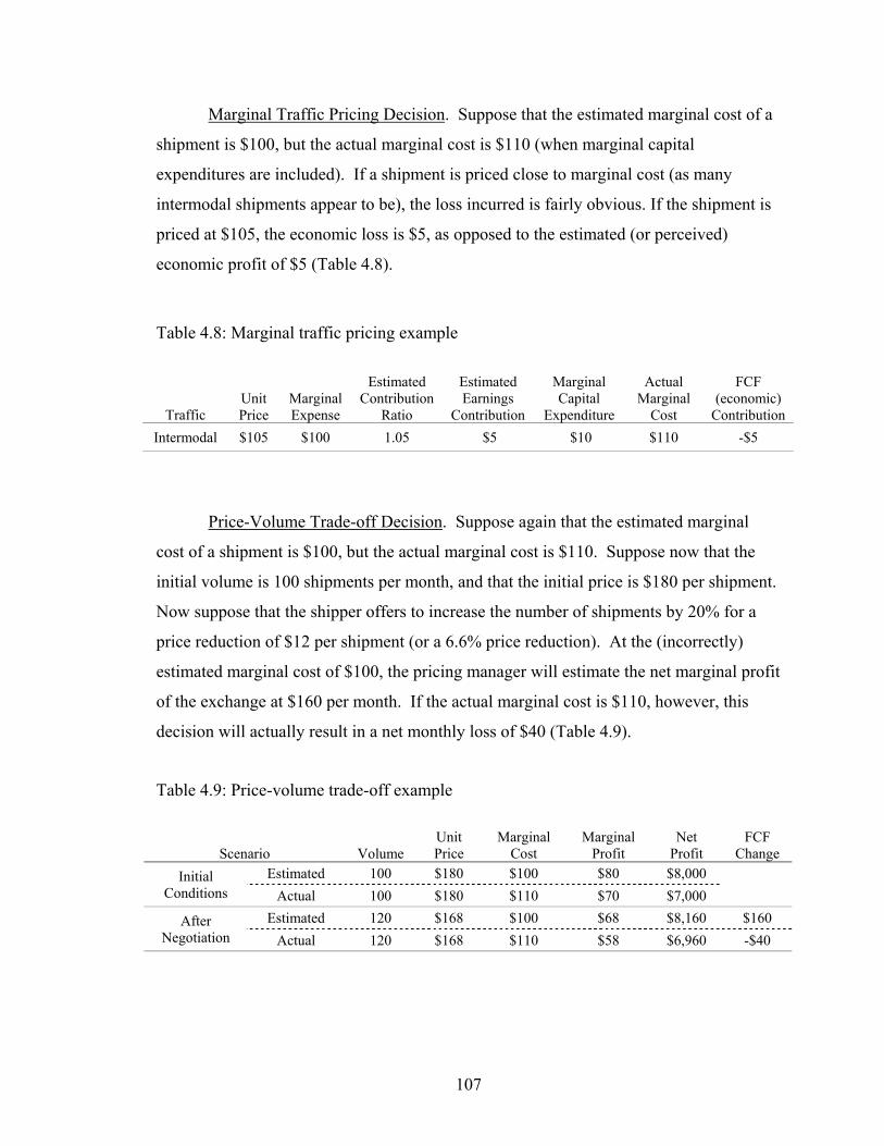
4.0 Recovering Capital Expenditures in Prices............................................................. 82

4.1 Integrating Economic and Financial Cost Concepts........................................... 844.2 Contractual Costs, Net Income and Free Cash Flow .......................................... 884.3 Price Components ............................................................................................... 894.4 Combining Price Components and Quasi-Economic Formulae ......................... 934.5 Methodology and Decision Criteria.................................................................... 944.6 Incorporating Financial Trends into Quasi-Economic Formulae ....................... 96

vi

4.7 Evaluating Results Using Sensitivity Analysis.................................................. 1034.8 How Economic Losses Result From Mis-estimated Marginal Costs ................ 1064.9 Discussion and Conclusions .............................................................................. 1124.10 Appendix............................................................................................................ 114

5.0 Summary and Discussion....................................................................................... 129

5.1 Review of Principal Hypothesis ........................................................................ 1295.2 Chapter 2............................................................................................................ 1305.3 Chapter 3............................................................................................................ 1305.4 Chapter 4............................................................................................................ 1315.5 Origins and Application of Marginal Analysis in the Railroad Industry........... 1325.6 Marginal Analysis and Engineering Practice..................................................... 1385.7 Efficient Resource Allocation............................................................................ 1415.8 The Public Policy Question ............................................................................... 1415.9 Maximizing Earnings v. Returns to Investment ................................................ 1455.10 The Executive’s Dilemma.................................................................................. 147

6.0 Future Research ..................................................................................................... 149

6.1 Allocation of Variable Capital Expenditures to Particular Traffic Segments.... 1506.2 Recovering Variable Capital Expenditures in Other Industries......................... 1516.3 Recovering Variable Working Capital and Other Investments ......................... 1516.4 Firm Value and Investment................................................................................ 153

7.0 Literature Survey ................................................................................................... 157

8.0 References Cited .................................................................................................... 248

Curriculum Vita ............................................................................................................. 263

1

1.0 Introduction

“Estimates of the cost of handling added traffic are as old as the railroads themselves.”

Interstate Commerce Commission, Rail freight service costs, 1943

“Some carriers are considering … the elimination of … whole lines of business.”

American Association of State Highway and Transportation Officials, 2002

“Being a ‘growth’ railroad is simply not a terribly sound business or investment

strategy.”

CitiGroup, 2003

1.1 Principal Hypothesis

The principal hypothesis of this dissertation is that railroad capital expenditures

represent an incremental cost of traffic but are largely excluded from marginal cost

estimates. This results in sub-optimal pricing decisions and sub-optimal returns to

invested capital. Because railroads invest more capital, as a percentage of revenue, than

any other major industry sector, they are particularly vulnerable to such mis-calculations.

I propose that infrastructure capital expenditures are, on the whole, correlated

with and caused by current and future output and should be included in marginal cost

estimates. I also propose that U.S. freight railroads and their economic regulators do not

properly interpret these incremental investments as marginal cost. If so, then (1) railroad

pricing and investment strategies do not optimize return on invested capital, and (2)

Surface Transportation Board estimates of revenue to variable cost (R/VC) are

overstated, subjecting a larger share of rail traffic to potential economic regulation than

would otherwise occur.

The concept that ongoing expenditures for investment should be considered in the

estimation of marginal cost, and therefore included in criteria for pricing decisions, was

not found in the financial literature but does have foundation in economic theory. It

2

appears to represent a gap in the application of economic theory to railroad cost

accounting methods.

Railroads have not mis-applied current financial theory but they may be

struggling to resolve the paradox of maximizing earnings (net income) or returns to

invested capital (free cash flow). The solution to this paradox, according to this thesis,

requires an extension of how cost accounting models incorporate economic theory. A

robust integration of these concepts highlights the need to treat incremental investment as

an incremental cost. Firms with large variable investment requirements can use pricing

strategies to either maximize earnings (net income) or returns to invested capital (free

cash flow), but not both at any given moment. Variable investment must be included in

marginal cost calculations if the economic value of a firm is to be maximized in the way

it prices its goods and services.

1.2 Key Findings

The key findings of this dissertation are:

1) The intrinsic cost of maintaining railroad infrastructure does not substantially vary

among Class I railroads, and apparent differences in unit maintenance cost can be

explained by the degree to which individual firms apply renewal strategies,

2) Railroad maintenance strategies that employ a greater portion of renewal-based

maintenance are more cost effective than those that use less renewal,

3) Railroad infrastructure investment (capital expenditures) is principally a function of

current and future demand,

4) Regulatory cost formulae underestimate actual cost variability by not including

variable capital expenditures, subjecting a larger share of rail traffic to potential

economic regulation than would otherwise occur,

3

5) Commercial pricing formulae used by railroads appear to underestimate the true

incremental nature of capital expenditures resulting in sub-optimal pricing decisions

and returns to invested capital,

6) Significant differences exist between accepted railroad cost accounting practice and

economic theory regarding marginal cost analysis, and

7) This analysis suggests that firms with substantial variable investment cannot

maximize both net income and free cash flow, at least in the short run.

1.3 Significance of and Reasons for Research

Following deregulation in 1980 through the late 1990’s, U.S. freight railroads

increased capital spending, expanded output, reduced costs, and improved service.

During the same period, they consistently failed to earn a rate of return commensurate

with their cost of capital (U.S. Congress House Committee 1998, 2001; Flower 2003a;

Flower 2003b; Gallagher 2004, Hatch 2004). Since 1998, railroads have become more

conservative with capital spending as investors have become increasingly skeptical about

the industry’s financial competitiveness (Flower 2003a; Flower 2003b; Gallagher 2004;

Hatch 2004). Shippers and public transportation officials are increasingly concerned

about the effects of further constraints on rail investment (U.S. Congress House

Committee 2001; AASHTO 2002; Hatch 2004; Hensel 2004). Transportation officials

predict there will be additional costs to transportation users of $400 to $900 billion if

future rail investment is constrained (AASHTO 2002). This research offers one

explanation as to why railroads earn poor returns on investment despite seemingly

healthy rates of earnings growth. If corrected, railroads may find it easier to earn their

cost of capital, resulting in fewer external constraints on capital investment.

Transportation industry professionals have often expressed concern over the

railroad industry’s inability to earn a competitive return on investment, or its cost of

capital (U.S. Congress Senate Committee 1987; U.S. Congress House Committee 1998,

4

2001; AASHTO 2002; Hatch 2004). The specific direction of this research was

established when I first discovered a correlation between capital expenditures and output

while studying economic and financial theory. An experiential knowledge of industry

and regulatory cost procedures lead me to suspect that there might be a systemic error in

the way capital expenditures were reflected in marginal cost estimates and pricing

strategy.

This research presents a new explanation for a chronic problem of significance to

the railroad industry, and it presents new financial techniques that may be useful to other

industries with substantial variable investment requirements.

1.4 Dissertation Organization

This dissertation is designed as a series of chapters, three of which are intended as

individually publishable papers. As a result, each chapter will cover some material

discussed in previous chapters. Chapters 2-4 form the core of the dissertation. Chapter 5

presents a summary of findings and additional conclusions. Chapter 6 identifies

additional research needs. Chapter 7 is a compendium of related literature dating from

the 1840’s to 2004. References cited and curriculum vita follow chapter 7.

Chapter 1: Introduction

This chapter presents the principal hypothesis, key findings, significance of the

research, a description of each chapter, and contributions claimed.

Chapter 2: Cost Effectiveness of Railway Infrastructure Renewal Maintenance

This chapter discusses how and why railroads make capital investments in

infrastructure from an engineering perspective. Railroads maintain their infrastructure

through a mix of ordinary maintenance activities and periodic renewal programs.

Different railways use different proportions of these two approaches and the cost

effectiveness of emphasizing one maintenance regime over the other has not been

previously analyzed empirically. The objective is to investigate the cost-effectiveness of

renewal-based maintenance strategies using data from industry sources. The primary

5

hypothesis is that an emphasis on infrastructure capital expenditures reduces total

infrastructure maintenance cost. Alternative hypotheses are tested with regard to the

effects of railroad size and density.

The results indicate that engineering management strategies that place more

weight on renewal maintenance relative to ordinary maintenance reduce total

maintenance cost. Railroad size and average density are significant but secondary

factors. The effects of size and density appear consistent with recent econometric studies

on the nature and behavior of railroad costs.

Chapter 3: Railway Output and Infrastructure Investment

This chapter investigates the relationship between infrastructure capital

expenditures and railroad output. The hypothesis tested is that infrastructure capital

expenditures are variable with, and caused by, changes in railroad output. Alternative

hypotheses tested are that free cash flow and/or net income are primary causal drivers of

infrastructure capital expenditures.

My analysis suggests that, over the past 15 years, changes in annual investment

were closely correlated with, and caused by, changes in annual output. Lag analysis

suggests that annual infrastructure investment is principally forward looking, determined

by current and future output, and not by past output. As a result, I conclude that capital

expenditures are marginal costs, and that regulatory variable cost formulae are incorrect

because they do not treat them as such. Annual investment appears to be a better

predictor of free cash flow and net income than output.

Chapter 4: Recovering Capital Expenditures in Prices

This chapter presents a new method to calculate the percentage of capital

expenditures that are reflected in railroad price floors. This methodology integrates

economic and accounting concepts of cost, and compares trends in net income and cash

flow to estimate the price component for recovery of variable investment and variable

capital expenditures. The primary hypothesis is that, contrary to rational economic

behavior, the proportion of variable capital expenditures included in railroad prices is

6

substantially less than one. A sensitivity analysis is conducted to determine the degree to

which other factors may influence the results of the analysis.

My analysis suggests that railroads systematically underestimate the true

incremental nature of capital expenditures in their estimates of marginal cost,

contribution ratios, and price floors.

Chapter 5: Summary and Discussion

This chapter provides a summary of Chapters 2-4. It presents an explanation,

from a historical viewpoint, for the mis-application of marginal analysis with respect to

railroad capital expenditures. Engineering practices are examined to highlight the

variable nature of capital expenditures. Public policy questions are analyzed, and

implications of this research for firms with substantial variable investment are discussed.

Chapter 6: Future Research

This chapter presents additional research needs based on the broader

interpretation of these findings. Research is needed to develop a method to properly

allocate capital expenditures to specific traffic movements using transportation network

theory and economic benefit analysis. The degree to which other industries may under-

allocate variable investment in marginal cost estimates should be investigated. Research

is recommended to test the relationship between firm value and investment strategy based

on new derivations of firm value and free cash flow with respect to variable investment.

Chapter 7: Literature Survey

The literature survey is a compendium of literature that was used, directly or

indirectly, in the development of the dissertation, and includes a combination of relevant

economic, regulatory, financial, and engineering topics. Part of this material is presented

in Chapters 2 through 5. The survey presents a broader and more complete picture than

provided in the previous chapters. The material is presented in chronological order so the

reader can more fully comprehend how railroad economic theory developed over 165

years to its present state.

7

1.5 Multi-Disciplinary Approach

The chapters that form the core of this research program tend to blend different

disciplines, but each has a different focus. Chapter 2 focuses on railroad engineering

issues related to optimal maintenance strategies. Chapter 3 combines engineering

practice and economic theory to define the relationship between infrastructure investment

and output. Chapter 4 combines economic and financial theory to analyze commercial

costing practices. Chapter 5 presents a history of economic theory and cost accounting

methods to explain current mis-interpretations, and demonstrates how to correct these

errors using current engineering practices. The chapters are designed to build upon each

other through a series of inquiries (primary discipline(s) in parentheses):

• Why do railroads make capital investments in infrastructure? (engineering)

• What are the most efficient strategies used to maintain infrastructure?

(engineering)

• What are the relevant economic attributes of capital investment? (economics)

• Can financial trends provide insight into the commercial interpretation of the

economic attributes of capital investment? (economics and finance)

• How do these economic attributes compare with current regulatory and

commercial interpretations? (economics and finance)

• Why would economic theory be mis-interpreted by industry and regulatory

institutions? (economics, engineering, and finance)

• What guidance can be used in future situations? (engineering and economics)

Specific contributions are claimed for each discipline, as follows:

Contributions to Civil (Railroad) Engineering

• A new technique that segregates railroad capital expenditures into renewal

maintenance and capacity expansion categories,

• A new model that estimates the effectiveness of renewal strategies in the

maintenance of rail infrastructure, and

• A finding that baseline maintenance costs do not vary from one railroad to the

next if renewal maintenance strategies are taken into account.

8

Contributions to Economics

• A new, post-facto, pricing analysis tool,

• A new method that estimates cost-related price components.

Contributions to Finance

• A new model of free cash flow using quasi-economic variables,

• A new method to estimate the degree to which investment cash flows are

reflected in price floors, and

• A new method to relate changes in firm value to changes in free cash flow

with respect to variable investment.

9

2.0 Cost-Effectiveness of Railway Infrastructure Renewal

Maintenance

“In his advice, the engineer rarely is able to confine himself to technological

considerations alone. The decision to install a new piece of equipment or to undertake a

new process must take into account demands and money costs. … But once all of the

elements are incorporated into his analysis the engineer … should not be surprised to

find that he has all along been talking economics.”

W. J. Baumol and S. M. Goldfield, Precursors

in Mathematical Economics, 1968

Since the railway infrastructure investment boom of the mid-1980’s, all Class I

railroads, have made significant efficiency gains in infrastructure maintenance that are

the result of improvements in a number of areas. Technological advancements in

infrastructure components such as cleaner and harder steel have reduced asset life cycle

costs. Improved component management has also reduced costs, for example new

developments in rail grinding and lubrication (IHHA 2001). Infrastructure maintenance

delivery systems and maintenance equipment technology has changed considerably.

Better performance measurement tools and cross-functional teamwork has transformed

additional engineering practices. (A Class I railroad is a U.S railroad that meets a

revenue threshold of $277.7 million.)

Railroads maintain their infrastructure using a combination of ordinary

maintenance and renewal maintenance techniques. Ordinary maintenance generally

includes the replacement of small quantities of infrastructure components using relatively

small gangs and small equipment, whereas renewal maintenance techniques involve the

replacement of larger quantities of components with larger gangs and bigger, more

sophisticated and more expensive equipment. Ordinary maintenance activities are

normally charged to operating expense and renewal maintenance programs to capital

expenditures according to Surface Transportation Board (STB) accounting requirements

(U.S. Senate Committee 1995).

10

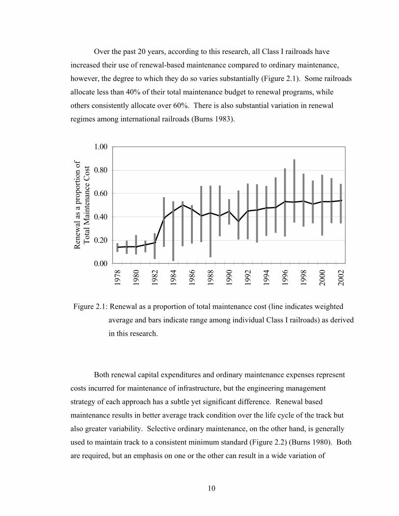
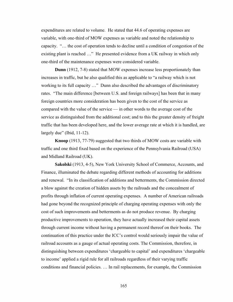
Over the past 20 years, according to this research, all Class I railroads have

increased their use of renewal-based maintenance compared to ordinary maintenance,

however, the degree to which they do so varies substantially (Figure 2.1). Some railroads

allocate less than 40% of their total maintenance budget to renewal programs, while

others consistently allocate over 60%. There is also substantial variation in renewal

regimes among international railroads (Burns 1983).

Both renewal capital expenditures and ordinary maintenance expenses represent

costs incurred for maintenance of infrastructure, but the engineering management

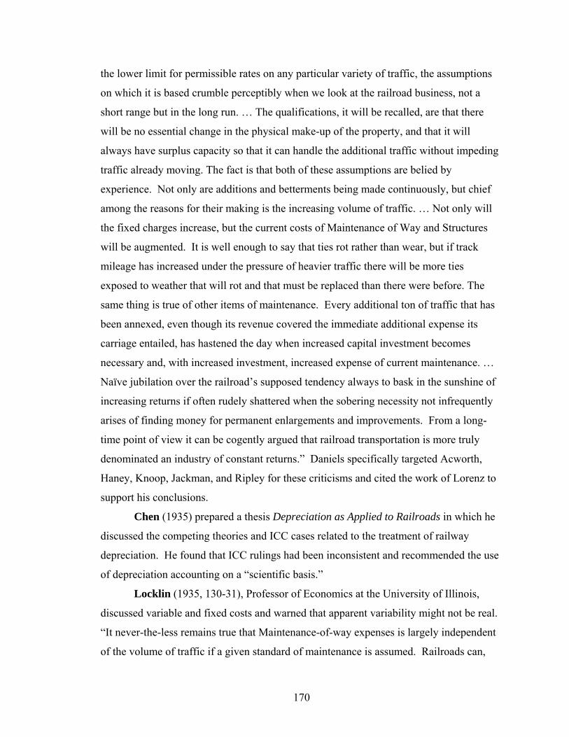
strategy of each approach has a subtle yet significant difference. Renewal based

maintenance results in better average track condition over the life cycle of the track but

also greater variability. Selective ordinary maintenance, on the other hand, is generally

used to maintain track to a consistent minimum standard (Figure 2.2) (Burns 1980). Both

are required, but an emphasis on one or the other can result in a wide variation of

0.00

0.20

0.40

0.60

0.80

1.00

1978

1980

1982

1984

1986

1988

1990

1992

1994

1996

1998

2000

2002

Ren

ewal

as a

pro

porti

on o

f To

tal M

aint

enan

ce C

ost

Figure 2.1: Renewal as a proportion of total maintenance cost (line indicates weighted

average and bars indicate range among individual Class I railroads) as derived

in this research.

11

maintenance costs. A low-quality track might support relatively high-axle loads with a

high maintenance regime; conversely higher investment can mean higher axle

loads and relatively low maintenance (Australian Government Bureau of Transport and

Regional Economics 2003). There are also substantial differences in the equipment

employed and the schedule of work.

In general, renewals involve capital expenditures made to replace and/or improve

infrastructure components in response to, or anticipation of, wear and tear caused by

output (defined here as gross ton miles). In contrast, capital expenditures for expansion

of facilities (terminals and yards, siding or mainline trackage, signal or dispatching

systems, etc.) are made to accommodate rail traffic growth and are called additions.

However, post facto railroad financial statements do not segregate capital expenditures

into these categories. For the purposes of this study, I classify Ordinary Maintenance as

maintenance that is expensed, Renewal Maintenance as maintenance activity that is

capitalized, and Additions as capacity expansion (Table 2.1).

The question addressed in this chapter is whether there is a relationship between

the engineering management strategy, in terms of its relative emphasis on renewal or

ordinary maintenance, and the overall cost effectiveness of the maintenance function.

Figure 2.2: Comparison of the temporal relationship between renewal and

ordinary maintenance, and track quality

Time

TrackQuality

Ordinary MaintenanceMinimumStandard

RenewalProject

RenewalProject

RenewalProject

Average (Renewal)

12

Table 2.1: Infrastructure Costs: Purpose, Study Classification and Accounting Category

Purpose Study Classification Accounting Category

Ordinary Maintenance Operating Expense(excluding depreciation)Infrastructure

MaintenanceRenewal Maintenance

Capacity Expansion AdditionsCapital Expenditures

2.1 Background

Track maintenance by renewal is not new. It was originally developed in the U.S.

in the early 1900's and even then it was believed to be less expensive (Burns 1981).

Renewal was originally performed by hand or with relatively simple machines. Recent

changes in technology and practice have led to improvements in overall efficiency for

both ordinary and renewal-based maintenance techniques. However, the efficiency

difference between small section gangs performing selective maintenance (characteristic

of ordinary maintenance) and large mechanized gangs (characteristic of renewal

maintenance) has increased. This difference results, in part, from improvements in

delivery technology including track renewal systems, tie-handling equipment, surface and

lining equipment, rail laying equipment, and ballast delivery systems. Newer

maintenance of way equipment is safer, cleaner, easier to maintain, and easier to operate

than earlier models (Judge 1999). Advances in computerization have improved the

reliability of this equipment (Brennan 1997). Although improvements have been made in

all types of machinery, the high-end, high-production equipment has provided much of

the recent productivity improvement (Kramer 1997). These advances and the larger scale

of equipment and gangs permit greater economies of scale compared to ordinary

maintenance.

Renewal programs also tend to have relatively long planning horizons so that

track possessions can be coordinated with transportation operations to minimize service

disruptions. These programs may target various track components for replacement and

the scope of individual programs may vary widely. For example, a tie program may

13

target replacement of crossties without renewing the ballast section of the track structure,

while a track surface and lining program may renew both crossties and ballast.

Maintenance “blitzes” are an ultimate kind of renewal program involving most or all

track components. The maintenance blitz is used to renew infrastructure in a manner

intended to minimize track downtime (Stagl 2001). Engineering departments co-ordinate

the large renewal projects with transportation and marketing departments (Foran 1997).

Maintenance planning has improved through advancements in information technology

(Brennan 1997) and railroads have transformed material handling systems as well as on-

site production (Kramer 1997).

Renewal activities normally require significant track possession windows that can

be difficult to obtain at high train densities. Spot or selective maintenance activities

normally require shorter track possession times and thus are less difficult to obtain even

at higher train densities. Consequently, high train densities can lead to a reduced reliance

on renewal work (Kovalev 1988). Additionally, renewal maintenance often involves

high-cost high-maintenance equipment that necessitates high utilization rates that are

difficult to justify for small maintenance regimes. For this and other reasons, routine

ordinary maintenance continues to be an important activity in conjunction with renewal

regimes to minimize total maintenance costs (Grassie 2000).

Studies on railway maintenance costs do not provide information on the relative

efficiency of emphasizing renewal-based maintenance in the U.S. Over the period 1994

to 2000, maintenance costs in Europe decreased while expenditures for renewals

increased, and enhanced renewal activity generally resulted in lower maintenance costs

(International Union of Railways 2002). Another study found that maintenance and

renewal practices on the Netherlands railway system had a direct influence on the

financial and operational performance and that the appropriate combination was critical

to overall operational performance (Swier 2004). However, neither of these European

studies provided data to support or quantify their conclusions.

These developments lead to the question, does reliance on renewal-based

maintenance strategy reduce total maintenance cost? Presumably the trend toward

renewal-based maintenance reflects a belief that it is more efficient or effective in some

manner. However, quantitative analyses of data evaluating this question have not

14

previously been published. In this chapter I develop an analytical method to evaluate this

issue using a cross sectional analysis of Class I railroad financial and operating data

reported to the Association of American Railroads (AAR 1978-2002a) under rules

promulgated by the STB (U.S. Senate Committee 1995).

2.2 Methodology

The overall process is illustrated in Figure 2.3.

Consolidate railroadfinancial data

Develop maintenance ofway cost index

Define renewal strategy,estimate renewal costs

Estimate totalmaintenance costs

(renewal + OE)

Check alternative hypotheses using joint hypothesis tests:1) effects of size (track miles)2) effects of light density track3) effects of average density

Estimate best model using joint hypothesis testsand explore implications

Decision Criteria: Does hypothesis yield best model for data?Identify limitations of findings

Conduct period by period analysis of relationshipbetween renewal strategy and total maintenance cost

Hypothesis:Does an emphasis on renewal reduce total maintenance costs?

Prepare data

Figure 2.3: Methodology and decision analysis

15

Financial and operating data for individual Class I railroads were modified to

permit study of the maintenance components of these data. A railroad infrastructure cost

index was developed from components of the AAR railroad cost index. Because railroad

financial statements do not segregate capital expenditures into renewals and additions, a

method was developed to estimate renewal capital expenditures so that total maintenance

costs, both renewal (capital expense) and ordinary maintenance (operating expense),

could be combined to evaluate total maintenance costs. Because of consolidations in the

industry during the study period, railroad financial and operating data were consolidated

to reflect the 2001 industry structure. A series of standard linear regression analyses and

F-tests were conducted to compare several alternate models regarding the effect on unit

maintenance cost, including the effect of renewal strategy, railroad size, the percentage of

light density track miles, and average track density. If renewal strategy is a significant

and influential variable in the best model, the hypothesis can be accepted.

2.3 Data Preparation

2.3.1 Infrastructure Cost Index

An infrastructure cost index (MOW RCR) was developed from components of the

AAR Railroad Cost Recovery Index (AAR RCR) (Table 2.2). The AAR RCR is based

on data provided by all Class I railroads (AAR 1980-2002b). It is comprised of 10

components, which are then combined into four groups, 1) labor, 2) fuel, 3) material &

supplies, and 4) all other. Calculation of the infrastructure cost index considered these

cost groups as follows:

1) The labor cost index (Labor) reflects changes in the average unit price of

wages and fringe benefits. The average wage for maintenance of way

employees compared to all railroad employees has remained fairly constant

over the period of the study, and the overall labor index was therefore

appropriate for an infrastructure cost index.

16

Table 2.2: AAR Railroad Cost Index Components Indexed to 1981, Railroad

Composite Cost Indexed to 1981 (AAR RCR), and Infrastructure

Composite Cost Indexed to 1981 and 2001 (MOW RCR)

Year LaborIndex

FuelIndex

M&SIndex

OtherIndex

AARRCR

MOWRCR

MOWRCR

1978 74 37 73 74 69 73 361979 81 56 80 81 77 81 401980 89 83 92 90 89 90 451981 100 100 100 100 100 100 491982 112 95 101 106 107 108 531983 123 83 96 110 111 116 571984 130 82 96 114 115 121 601985 132 77 100 116 117 123 601986 138 49 98 119 118 127 621987 144 53 92 121 121 130 641988 153 48 96 129 128 137 671989 158 56 101 135 133 142 701990 163 69 105 143 140 148 731991 172 67 115 148 146 155 761992 180 64 124 149 150 162 801993 180 64 128 151 151 163 811994 183 60 132 155 153 166 821995 192 60 133 164 167 174 861996 197 71 133 170 167 179 881997 201 69 136 173 169 184 911998 206 55 137 180 172 189 931999 204 56 137 180 171 188 932000 216 90 136 187 187 195 962001 228 88 140 191 192 203 1002002 238 76 140 193 194 208 103

2) The fuel cost index (Fuel) was not included in the MOW RCR because

maintenance of way fuel expense is not separately identified in financial

reports and, as a result, the proportion of fuel cost to overall cost could not be

calculated. Additionally, maintenance of way equipment is often fueled

directly from locomotive diesel storage tanks that are not charged to

maintenance. Fuel expenses represent a relatively small percentage of total

maintenance of way expenditures and should not affect the overall results.

3) The material & supplies cost index (M&S) measures cost changes in a group

of items that represent the preponderance of purchases by the largest railroads.

This index component was included in the MOW RCR because M&S costs

are a significant portion of total maintenance of way costs.

17

4) The other cost index (Other) includes equipment rents, depreciation,

purchased services, taxes other than income and payroll, and other expenses.

This index component was included in the MOW RCR because these costs are

a substantial portion of total maintenance costs.

The overall annual infrastructure cost index was then developed by multiplying

each index (Labor, M&S, and Other) times the relative proportion of each component of

total maintenance of way expense for each year. This calculation is shown below.

MOW RCR = [{RL (ML/MT)} + {RM (MM/MT)} + {RO (MO/MT}]

where:

RL = AAR Labor Index

ML = Class I RR MOW Labor Expense

MT = Class I RR Total Maintenance of Way Expense

RM = AAR Material and Supply Cost Index

MM = Class I RR MOW Material and Supply Expense

RO = AAR Other Cost Index

MO = Class I RR MOW Other Expense

This annual index was then calibrated with 2001 as the reference year (e.g.,

2001 index = 100%, 1978 index = 36.22%) so that all expenses could be referenced in

terms of relatively current prices. Maintenance of way nominal expenses and

investments were then divided by each year’s index to obtain constant 2001 dollars.

2.3.2 Defining Maintenance Cost and Renewal Strategy

Gross Ton Miles and Track Miles are standard units of measurement for U.S.

railroads. Gross Tonnage is the total weight of all locomotives, rail cars, and lading that

pass over a particular location, and a gross ton mile is one gross ton moving over one

mile of track. Unit maintenance cost was defined as the unit cost of maintaining track,

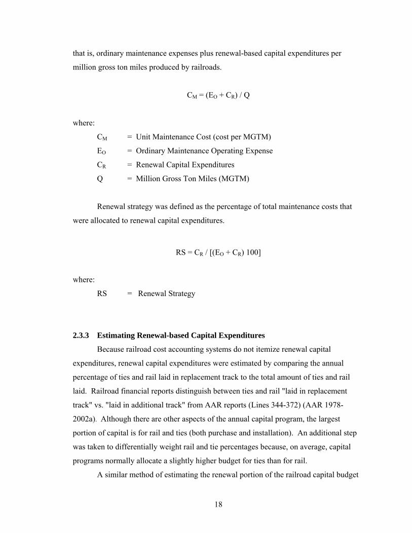
18

that is, ordinary maintenance expenses plus renewal-based capital expenditures per

million gross ton miles produced by railroads.

CM = (EO + CR) / Q

where:

CM = Unit Maintenance Cost (cost per MGTM)

EO = Ordinary Maintenance Operating Expense

CR = Renewal Capital Expenditures

Q = Million Gross Ton Miles (MGTM)

Renewal strategy was defined as the percentage of total maintenance costs that

were allocated to renewal capital expenditures.

RS = CR / [(EO + CR) 100]

where:

RS = Renewal Strategy

2.3.3 Estimating Renewal-based Capital Expenditures

Because railroad cost accounting systems do not itemize renewal capital

expenditures, renewal capital expenditures were estimated by comparing the annual

percentage of ties and rail laid in replacement track to the total amount of ties and rail

laid. Railroad financial reports distinguish between ties and rail "laid in replacement

track" vs. "laid in additional track" from AAR reports (Lines 344-372) (AAR 1978-

2002a). Although there are other aspects of the annual capital program, the largest

portion of capital is for rail and ties (both purchase and installation). An additional step

was taken to differentially weight rail and tie percentages because, on average, capital

programs normally allocate a slightly higher budget for ties than for rail.

A similar method of estimating the renewal portion of the railroad capital budget

19

using ratios of ties laid in replacement to total ties laid was first used by Ivaldi and

McCullough (2001), but their method did not consider rail laid in replacement or

addition.

Railroad financial data segregates capital investment for Road Communications,

Road Signals & Interlocker, and Road Other, with the majority of investment categorized

as Road Other. I assumed that capital expenditures for Signals and Communications

Systems were primarily for new technology and major system upgrades such as replacing

extant wire and relay based systems with fiber optic, wireless, and digital technologies,

and were appropriately classified as additions.

Renewal Capital Expenditures were calculated as follows:

PT = TE / (TE + TN)

where:

PT = Percentage Renewal Tie Program

TE = Number of Ties Laid In Existing Track

TN = Number of Ties Laid In New Track

PR = RE / (RE + RN )

where:

PR = Percentage Renewal Rail Program

RE = Tons of Rail Laid in Existing Track

RN = Tons of Rail Laid in New Track

P = [(0.6 PT) + (0.4 PR)]

CR = CO · P

where:

CO = Road Capital Other

P = Overall Percent Renewal

20

2.3.4 Railroad Groupings

The number of railroads reporting financial and operating data (in R1 standard

format to the AAR) declined from 36 in 1978 to eight in 2001. Most of this reduction

occurred through mergers and combinations, although there were also bankruptcies and

deletions by changes in Class I railroad definition. Individual railroad data were

combined into their 2001 industry structure (Table 2.3).

Table 2.3: Railroad Data Groupings

Railroad Group Individual Railroads and Years in which they wereindividually listed in AAR Reports

Union Pacific (UP)

Union Pacific Railroad (1978-2002)Missouri Pacific Railroad (1978-1985)Western Pacific Railroad (1978-1985)

Missouri-Kansas-Texas Railroad (1978-1988)Chicago North Western (1978-1994)

Southern Pacific Railroad (1978-1996)St Louis Southwestern Railroad (1978-1989)Denver & Rio Grande Railroad (1978-1993)

Burlington Northern Santa Fe (BNSF)

Burlington Northern Santa Fe (1996-2002)Burlington Northern Railroad (1978-1995)Colorado Southern Railroad (1978-1981)Ft Worth & Denver Railroad (1978-1981)

Atchison Topeka & Santa Fe Railroad (1978-1995)St Louis San Francisco Railroad (1978-1980)

CSX (CSX)

CSX (1986-2002)Baltimore & Ohio Railroad (1978-1985)

Chesapeake & Ohio Railroad (1978-1985)Western Maryland Railroad (1978-1983)

Seaboard Coast Line (1978-1985)Louisville & Nashville Railroad (1978-1982)

Clinchfield Railroad (1978-1982)

Norfolk Southern (NS)Norfolk Southern (1986-2002)

Norfolk & Western Railroad (1978-1985)Southern Railway (1978-1985)

Kansas City Southern Railroad (KCS) Kansas City Southern (1978-2002)

Illinois Central Railroad (IC) Illinois Central (1988-2001)Illinois Central Gulf (1978-1987)

SOO (SOO) SOO (1978-2002)

Grand Trunk Western (GTW) Grand Trunk Western (1978-2001)Detroit Toledo & Ironton (1978-1983)

21

The one major exception to this is the division of Conrail into CSX and NS in 1999. In

2002, the Grand Trunk Western and the Illinois Central were combined with other

Canadian National Railroad lines in the U.S.

Railroads excluded from these groupings but included in the overall Class I

statistics are:

• Conrail• Milwaukee• Bessemer & Lake Erie• Duluth, Missabe, & Iron Range• Elgin Joliet & Eastern• Florida East Coast• Long Island• Pittsburgh and Lake Erie• Delaware and Hudson

2.4 Renewal Strategy as a Single Independent Variable

The study period (1978-2002) was divided into five year increments beginning in

1978 with the last period (1999-2002) being a four-year increment. Each component

(renewal capital expenditures, ordinary maintenance operating expense, MGTM) was

averaged over each time period for each railroad. The model tested was:

Model 2.1: CM = a + bRS + ε

where:

CM = Unit Maintenance Cost ($ per MGTM)

a = Intercept

b = Coefficient for RS


ε = error term

Renewal strategy and unit (infrastructure) maintenance cost were calculated for

each railroad over each time period (Table 2.4). Data for IC and GTW did not include

22

2002 due to consolidation with CN. Data for all Class I railroads in the United States

were aggregated and labeled (US).

Table 2.4: Comparison of Renewal Strategy and Unit Maintenance Cost

Renewal Strategy Unit Maintenance CostRoad '78-‘82 '82-‘87 '88-‘92 '93-'98 ‘99-'02 '78-82 '82-87 '88-92 '93-'98 ‘99-'02

US 15.2% 44.4% 41.9% 50.0% 52.7% 5,803 4,737 3,499 2,589 2,207

UP 17.2% 48.1% 47.4% 55.7% 64.0% 4,885 4,537 3,140 2,149 1,933BNSF 16.6% 44.8% 34.7% 55.1% 62.9% 4,966 3,982 2,908 2,450 1,848CSX 13.2% 41.5% 40.8% 39.4% 41.3% 6,349 4,815 3,376 2,453 2,701NS 16.5% 40.0% 44.2% 45.4% 34.6% 5,167 5,529 5,011 3,539 3,207IC 16.4% 45.6% 58.0% 74.4% 67.2% 7,330 3,520 2,118 2,297 2,041

KCS 17.5% 44.8% 48.6% 52.8% 55.6% 6,659 4,329 4,543 3,629 2,869SOO 10.5% 21.6% 35.2% 38.1% 39.8% 7,228 4,730 3,985 4,224 3,029GTW 11.8% 20.8% 24.0% 29.1% 53.7% 7,747 5,115 5,159 4,035 2,520

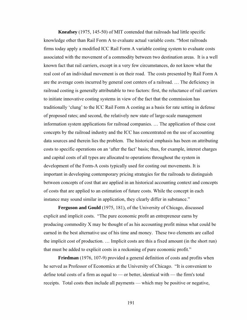
A series of linear regressions were conducted for each time period with renewal

strategy as the independent variable and unit maintenance cost as the dependent variable

(Model 2.1). The results indicate that there was a statistically significant relationship

only for the last time period, with an R2 of 0.80, a p value of 0.003, and F/Fc of 3.96 with

Fc calculated at a 95% confidence level (Table 2.5).

Table 2.5: Influence of Renewal Strategy on Unit Maintenance Cost

Period R2 F/ Fc p a b

1978 – 1982 0.38 0.62 0.103 10,188 -26,053

1983 – 1987 0.23 0.30 0.230 5,639 -2,784

1988 – 1992 0.28 0.39 0.175 6,075 -5,515

1993 – 1998 0.44 0.80 0.072 5,063 -4,032

1999 – 2002 0.80 3.96 0.003 4,496 -3,773

23

Comparison of the five periods indicates improving correlation over time with the

strongest correlation in 1999-2002. The only period with an F-test that indicated

significance was 1999-2002.

A plot of the data from the last period (1999-2002) along with the regression trend

line is shown in Figure 2.4.

Figure 2.4: Relationship of renewal strategy and maintenance cost, 1999-2002

2.5 Alternative Hypothesis: Influence of Size

An alternative hypothesis is that network size as measured in track miles is

responsible for the variation in unit maintenance cost. A statistical test was conducted

comparing the original model to one including a size variable as measured by track miles

(TM). The results indicate that while railroad size was a statistically significant variable,

it had far less influence than renewal strategy on maintenance cost. The results suggest

that (a) a 10% increase in track miles for the average railroad (equal to an additional

2,091 track miles in 2001) would result in a reduction of $18 per MGTM total

maintenance cost, and (b) an increase of 10% in renewal strategy would result in a

0

500

1,000

1,500

2,000

2,500

3,000

3,500

0.30 0.35 0.40 0.45 0.50 0.55 0.60 0.65 0.70

Renewal as a proportion of Total Maintenance

NS SOO

CSX

BNSF UP

ICGTW

KCS

Tota

l Mai

nten

ance

Cos

tpe

r MG

TM (2

001

$)

0.00

24

reduction of $369 per MGTM total maintenance cost, or a 12-18% cost reduction

depending on the individual railroad. Furthermore, the results suggest that the track mile

variable was significant only in combination with renewal strategy (at the 95%

confidence level). The analysis is described in additional detail in the appendix.

Two plausible explanations exist for the size effect. First, larger railroads may

have been slightly more cost effective in their maintenance programs because they could

employ renewal systems more effectively. This could have resulted from more

productive use of specialized equipment, by optimizing component renewal cycles for

any given piece of track, and/or by having more options to detour traffic thereby

permitting longer track possession windows. A second explanation for this effect is that

there may have been a quasi-fixed overhead (engineering) cost associated with

maintaining infrastructure regardless of railroad size.

2.6 Alternative Hypothesis: Influence of Light Density Track Miles

An alternative hypothesis is that light density lines are responsible for the

variation in unit maintenance cost between railroads. Class I railroads had reduced the

number of low density routes through sale, abandonment, or lease in order to reduce the

amount of low performing routes. According to current economic theory, each track mile

has a quasi-fixed cost associated with it that includes a maintenance-related component,

and those roads that were able to shed more of these low density lines may have had an

inherent cost advantage. A statistical test was conducted comparing the original model to

one including a variable for the percentage of light density track miles (DL). Light

density track was defined, for these purposes, as track with less than 10 million gross ton-

miles per mile per year and was based on Bureau of Transportation Statistics data from

2000 (U.S. DOT 2001). This analysis is described in detail in the appendix. Results

indicate that the percentage of light density track miles was not a statistically significant

variable in the determination of unit maintenance cost.

25

2.7 Alternative Hypothesis: Influence of Average Density

Another alternative hypothesis is that average density is responsible for the

variation in maintenance cost between railroads. This hypothesis is also related to the

theory that each track mile has a quasi-fixed maintenance cost. A statistical test was

conducted comparing the original model to one including a variable for average density

as measured in MGTM per Class I Railroad track mile (Line 343 AAR reports). This

analysis is described in the appendix. Results indicate that while average density (DA)

improved the model slightly and was statistically significant at a 94% level of confidence,

it had less influence than renewal strategy with respect to maintenance cost. The results

suggest that (a) a 10% increase in average track density (equal to an additional 1.8

MGTM per track mile in 2001) would result in a reduction of $74 per MGTM total

maintenance cost, and (b) an increase of 10% in renewal strategy would result in a

reduction of $312 per MGTM total maintenance cost. Furthermore, the analysis suggests

that average density was significant only in combination with renewal strategy.

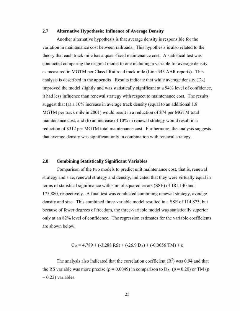
2.8 Combining Statistically Significant Variables

Comparison of the two models to predict unit maintenance cost, that is, renewal

strategy and size, renewal strategy and density, indicated that they were virtually equal in

terms of statistical significance with sum of squared errors (SSE) of 181,140 and

175,880, respectively. A final test was conducted combining renewal strategy, average

density and size. This combined three-variable model resulted in a SSE of 114,873, but

because of fewer degrees of freedom, the three-variable model was statistically superior

only at an 82% level of confidence. The regression estimates for the variable coefficients

are shown below.

CM = 4,789 + (-3,288 RS) + (-26.9 DA) + (-0.0056 TM) + ε

The analysis also indicated that the correlation coefficient (R2) was 0.94 and that

the RS variable was more precise (p = 0.0049) in comparison to DA (p = 0.20) or TM (p

= 0.22) variables.

26

2.9 Discussion

Three questions arise from the analysis:

• Why is a renewal strategy cost effective?

• How do these findings compare with other studies?

• Why was this relationship significant only in the most recent period?

As previously described, large mechanized track gangs are more productive not

only in terms of labor and materials, but with use of limited track possession time. Their

work is better planned and executed due to engineering management systems. The work

can be programmed in advance so that traffic patterns can be adjusted to provide long

track possession windows that maximize resource productivity.

It also appears that an emphasis on reducing ordinary maintenance expense was

important. I compared ordinary maintenance expense and renewal capital expenditures

per MGTM for the four time periods between 1982 and 2002 for each railroad (Table

2.6).

Table 2.6: Comparison of Ordinary Maintenance Expense and Renewal Capital

Expenditures per MGTM (constant 2001 $’s)

Ordinary Maintenance Expenseper MGTM

Renewal Capital Expendituresper MGTM

Road '82-‘87 '88-‘92 '93-'98 ‘99-'02 '82-87 '88-92 '93-'98 ‘99-'02

US 2,638 2,037 1,306 1,044 2,108 1,467 1,298 1,163

UP 2,365 1,660 958 698 2,181 1,491 1,201 1,239BNSF 2,202 1,899 1,131 686 1,787 1,010 1,353 1,163CSX 2,829 2,004 1,493 1,586 2,007 1,375 970 1,113NS 3,319 2,801 1,949 2,100 2,210 2,213 1,608 1,115IC 1,887 889 591 669 1,654 1,226 1,707 1,372

KCS 2,389 2,341 1,735 1,273 1,951 2,206 1,947 1,605SOO 3,869 2,590 2,604 1,835 1,207 1,389 1,629 1,213GTW 4,057 3,927 3,031 1,165 1,087 1,239 1,177 1,370

27

Some railroads made greater reductions in ordinary maintenance expense than

others. Other than average density and system size, there were no obvious characteristics

that appeared to offer a satisfactory alternative explanation for overall maintenance cost

other than renewal strategy. Although there was some appearance of an east-west

geographic effect for the large roads, results for smaller roads were not consistent with it

and I am not aware of any apriori reason for such an effect.

The renewal, density and size effects were fairly intuitive from an engineering

viewpoint and consistent with available studies. The renewal strategy effect was

consistent with International Union of Railways (2002) studies indicating a beneficial

effect of renewal in reducing total maintenance costs. The density effect was consistent

with a number of statistical studies that find economies of density (Braeutigam et al.

1984; Caves et al. 1985; Barbera et al. 1987; Lee and Baumol 1987; Dooley et al. 1991).

These studies differ as to the significance of the density effect, however. Braeutigam and

Caves found significant density effects, Lee found considerably smaller density effects

than in previous studies, and Dooley found only moderate returns to density. The size

effect was consistent with Caves’ findings of slightly increasing returns to scale, but was

not consistent with Barbera or Lee who found constant returns to scale. The results of

this study, which focused solely on infrastructure maintenance cost, are generally

consistent with many of these econometric studies that considered a broader range of

transportation costs than I did.

A complete response to the third question is less intuitive in part because track

renewal systems have been employed by railroads for many years, but involves a

combination of the following points:

1. The relationship would not have been apparent in the period prior to depreciation

accounting (1978 to 1982) because a large portion of renewal costs were

accounted for as ordinary maintenance operating expense due to betterment

accounting rules in effect during that period.

2. Delivery and information systems and planning technology have continued to

improve in recent years increasing the relative efficiency of renewal-based

maintenance in relation to ordinary maintenance.

28

3. The unit cost differences between ordinary and renewal-based maintenance may

not have been statistically apparent until reductions in ordinary maintenance

gangs were fully realized to their present level.

4. Increasing train densities may have increased the relative cost effectiveness of

renewal-based maintenance. From 1978 to 1987 average train density increased

by less than 1% per year; from 1988 to 2001 train density increased by almost 6%

per year. Reduction of light density track through sale or abandonment may also

have had an effect on the statistical relationships.

5. The railroads were consolidating to fewer and larger networks.

In summary, the results indicate that most of the variation in unit maintenance

costs among Class I railroads can largely be explained by variation in the degree to which

they emphasize renewal and de-emphasize ordinary maintenance in their engineering

strategies. Baseline ordinary maintenance cost was estimated for each railroad (Table

2.7).

Table 2.7: Estimation of Baseline Ordinary Maintenance Expense excluding effects of

Renewal Strategy (including Density and Size effects) (1999-2002)

Road

MaintenanceCost ($s)

per MGTMRenewalStrategy

AverageDensity

MGTM/TMTrackMiles

BaselineExpense

per MGTMUP $1,933 64.0% 21.7 48,005 $4,038

BNSF $1,848 62.9% 22.9 42,055 $3,917CSX $2,701 41.3% 14.0 34,006 $4,060NS $3,207 34.6% 11.9 31,645 $4,346IC $2,041 67.2% 12.6 3,901 $4,249

KCS $2,869 55.6% 10.2 3,882 $4,699SOO $3,029 39.8% 15.7 2,777 $4,339GTW $2,520 53.7% 19.1 1,392 $4,287

The baseline ordinary maintenance cost was calculated assuming that renewal

maintenance was eliminated altogether (100% ordinary maintenance), but allowed for

both density and size effects. The railroads fell into three groups in terms of baseline

expense per MGTM: UP, BNSF, and CSX (between $3,917 and $4,060 per MGTM); NS,

29

IC, SOO and GTW (between $4,249 and $4,346 per MGTM), and KCS ($4,699 per

MGTM).

This analysis necessarily made the supposition that rail infrastructure quality for

each road over each time horizon was not trending strongly in one direction or the other.

This is related to the supposition that gross ton miles produced in one period were

generally equivalent to gross ton miles produced in another period. These suppositions

are rarely true in absolute terms, but for a given class of track, track conditions can only

vary within a pre-determined range.

Although a distinction was made between costs for capacity expansion and

maintenance, capacity and maintenance cost are not entirely independent. As train

densities increase, track possessions for maintenance may become limited in duration and

frequency because track gangs must compete with trains for track time. Consequently,

capacity limitations increase unit cost because of the more frequent need for gangs to get

on and off track. Capacity expansion may thus have a secondary effect of decreasing unit

maintenance cost.

This analysis focused only on maintenance costs. An important consideration for

any railroad is the effect that different maintenance strategies have on transportation costs

and service quality. My initial tests were inconclusive in this regard, probably because of

more influential effects of factors not related to maintenance, for example reduction of

crew size, changes in transportation labor work rules, and improvements in motive power

efficiency.

This analysis is only valid for the range of data presented. Extending it beyond

the limits of demonstrated values may lead to inappropriate conclusions. As mentioned

previously, a 100% renewal strategy is neither attainable nor desirable based on current

technology or maintenance and accounting practices. This analysis is intended for use by

railroad engineering professionals as one tool (of many) in the determination of the

appropriate balance between ordinary and renewal maintenance options.

Two final questions are proposed for further research and discussion. First, what

are the real limits of cost efficiencies generated by renewal strategies? If UP, BNSF and

IC can achieve renewal levels in the 60 percent range, would a further shift from

operating expense to renewal investment result in even lower unit cost? Second, what

30

barriers exist for other roads, such as CSX, NS, and SOO, from gaining the apparent

benefits of shifting more ordinary maintenance to renewal regimes? Could these barriers

be technical (i.e. infrastructure characteristics), financial (i.e., tight capital or expense

budgets), philosophical (i.e., safety, management), operational (i.e., train densities), or a

combination?

2.10 Conclusions

The results are consistent with the hypothesis that an emphasis on renewal

programs for track maintenance was cost effective from an engineering viewpoint and

provided an explanation of why railroads have consistently increased capital expenditures

for renewal maintenance. Additionally, the intrinsic cost of maintaining railroad

infrastructure does not vary substantially among Class I railroads and apparent

differences in unit maintenance costs can be explained by the degree to which individual

firms apply renewal strategies.

2.11 Appendix

2.11.1 Maintenance Cost and Capital Expenditures: Alternative Hypothesis,

Influence of Size

A statistical test was conducted comparing the models shown below:


Model 2.2: CM = a + bRS + cTM + ε

where:

CM = Unit Maintenance Cost ($ per MGTM)

a = Intercept

b = Coefficient for RS


c = Coefficient for TM

31

TM = Track Miles

ε = error term

Test results (Tables 2.8 and 2.9) indicated that Model 2.2 was statistically

preferable to Model 2.1. The adjusted R2 statistic (adjusted R2) indicated improved

correlation and the F-test indicated improved significance of results. T-test results

indicated that renewal strategy was a more significant variable in combination with the

track miles. The t-statistic for the track miles variable was significant, and intercept and

slope coefficients all appeared reasonable. Furthermore, comparison of the sum of

squared errors for the two models indicated that they were statistically different (F/Fc =

1.00 at α = 0.1 or a 90% level of confidence).

The results of the joint hypothesis test did not allow me to reject Model 2.2 in

preference to Model 2.1. In other words, track miles was a useful explanatory variable in

estimating maintenance cost. A comparison of p values indicated that the influence of

the renewal strategy variable was much greater than the track mile variable in the

estimation of maintenance cost.

Table 2.8: Statistical comparison of Models 2.1 and 2.2

Overall Model Results Renewal Strategy Track Miles

Model AdjustedR2 F/ Fc a b p c p

2.1 0.76 3.96 4,496 -3,773 0.0028

2.2 0.87 4.12 4,636 -3,695 0.00144 -0.0086 0.06325

Table 2.9: Joint Hypothesis Test of Models 2.1 and 2.2

F Observations New Parameters F/Fc p Result

6.7911309 8 1 1.02773 0.03133 Do Not Reject Model 2.2

32

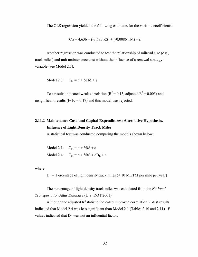
The OLS regression yielded the following estimates for the variable coefficients:

CM = 4,636 + (-3,695 RS) + (-0.0086 TM) + ε

Another regression was conducted to test the relationship of railroad size (e.g.,

track miles) and unit maintenance cost without the influence of a renewal strategy

variable (see Model 2.3).

Model 2.3: CM = a + bTM + ε

Test results indicated weak correlation (R2 = 0.15, adjusted R2 = 0.005) and

insignificant results (F/ Fc = 0.17) and this model was rejected.


Influence of Light Density Track Miles

A statistical test was conducted comparing the models shown below:


Model 2.4: CM = a + bRS + cDL + ε

where:

DL = Percentage of light density track miles (< 10 MGTM per mile per year)

The percentage of light density track miles was calculated from the National

Transportation Atlas Database (U.S. DOT 2001).

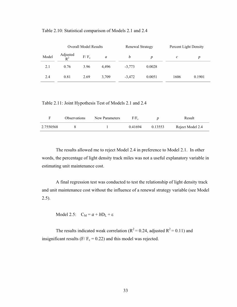
Although the adjusted R2 statistic indicated improved correlation, F-test results

indicated that Model 2.4 was less significant than Model 2.1 (Tables 2.10 and 2.11). P

values indicated that DL was not an influential factor.

33


Overall Model Results Renewal Strategy Percent Light Density


2.1 0.76 3.96 4,496 -3,773 0.0028

2.4 0.81 2.69 3,709 -3,472 0.0051 1606 0.1901



2.7550568 8 1 0.41694 0.13553 Reject Model 2.4

The results allowed me to reject Model 2.4 in preference to Model 2.1. In other

words, the percentage of light density track miles was not a useful explanatory variable in

estimating unit maintenance cost.

A final regression test was conducted to test the relationship of light density track

and unit maintenance cost without the influence of a renewal strategy variable (see Model

2.5).

Model 2.5: CM = a + bDL + ε

The results indicated weak correlation (R2 = 0.24, adjusted R2 = 0.11) and


34


Influence of Average Density

A statistical test was conducted comparing Model 2.1 to Model 2.6 shown below:


Model 2.6: CM = a + bRS + cDA + ε

where:

DA = Average Density (MGTM per track mile)

The results (Tables 2.12 and 2.13) indicated that Model 2.6 was statistically

preferable to Model 2.1. The adjusted R2 statistic indicated improved correlation, the F-

test results indicated that Model 2.6 was more significant than Model 2.1. P values

indicated that average density was an influential variable, but not as significant as the

renewal strategy variable.


Overall Model Results Renewal Strategy Average Density


2.1 0.76 3.96 4,496 -3,773 0.0028

2.6 0.87 4.26 4,802 -3,117 0.0044 -40.56 0.0582

The results of the joint hypothesis test did not allow me to reject Model 2.6 in

preference to Model 2.1. In other words, average density was a useful explanatory

variable in estimating unit maintenance cost in combination with renewal strategy.

35




A regression test was conducted to test the relationship of average density and

unit maintenance cost without the influence of renewal strategy (see Model 2.7).

Model 2.7: CM = a + bDA + ε

The results indicated weak correlation (R2 = 0.46, adjusted R2 = 0.37) and


36

3.0 Railway Output and Infrastructure Capital Expenditures

“The increase in total costs resulting from an expansion in a firm’s volume of business is

commonly referred to as incremental cost.”

William Baumol, 1962

“The application of these cost concepts by the railroad industry and the ICC has

concentrated on the use of accounting data sources and therein lies the problem.”

James Kneafsey, 1975

This chapter evaluates and estimates the degree to which changes in railway

output affect annual railway infrastructure capital expenditures. This relationship is

central to economic concepts of marginal and variable cost in an industry heavily

dependent on continuing annual capital expenditures. These economic concepts, in turn,

are important to both commercial pricing decisions and external economic regulation that

affect the financial viability of the industry. The focus on infrastructure in this chapter,

as opposed to rolling stock, is made because it is with respect to infrastructure capital

expenditures that questions arise regarding their consideration as a marginal cost.

Rolling stock investment has long been considered variable with traffic (ICC 1943) and

recent studies continue to treat equipment costs as variable with output (Ivaldi and

McCullough 2001).

Following deregulation in 1980, Class I railroads began a period of long-run

investment growth and, except for distortions caused by the Economic Tax Recovery Act

of 1981, infrastructure capital expenditures grew at about the same rate as output (Figure

3.1) (AAR 1978-2002a). This included capital expenditures for track (rail, ties, surface

and lining), structures (bridges, tunnels, buildings), signals and communication systems

(fiber optics, dispatching systems, microwave and digital communications systems),

facilities (yards, terminals), and new equipment and software. Because of the investment

distortions caused by the tax act, and technical changes in the industry, most of the

analyses presented in this paper focus on the period following 1987.

37

Rail output continued to expand although growth was not uniform and the greatest

increase in carload traffic was in intermodal traffic (Figure 3.2). The Association of

American Railroads (AAR) data combines intermodal and miscellaneous boxcar traffic.

Figure 3.1: Class I Railroad Gross Ton Miles and Road Investment (2001 $s)

Source: AAR Analysis of Class I Railroads

0

1

2

3

4

5

6

1978

1980

1982

1984

1986

1988

1990

1992

1994

1996

1998

2000

2002

0.0

0.5

1.0

1.5

2.0

2.5

3.0

3.5

Trill

ion

GTM

Roa

d In

vest

men

t (B

illio

ns)

Gross Ton Miles(GTM)

Road Investment

0

2

4

6

8

10

12

14

1978

1980

1982

1984

1986

1988

1990

1992

1994

1996

1998

2000

2002

Mill

ion

Car

load

s

Intermodal

Other CategoriesCoal

ChemicalVehicle

Figure 3.2: Class I Railroad Carloads by Commodity Group


38

On a tons originated basis, the largest growth was in coal (Figure 3.3).

Figure 3.3: Class I Railroad Tons Originated by Commodity Group


According to congressional testimony, railroads require more capital

expenditures, as a percentage of revenue, than any other major industry sector, and far

greater than any other transportation mode (U.S. Congress House Committee 1998, 125-

26). From 1988 to 2002, the industry’s annual capital expenditures averaged over 16% of

revenues. Railroads normally require about three times as much capital as the average

S&P (Standard and Poors) industrial company. As a result, it is particularly important to

railroads and their economic regulators that the relationship between capital expenditures

and output be properly defined so that capital expenditures are correctly reflected in

marginal and variable cost estimates. Marginal and variable cost estimates serve as a

foundation for internal price decisions and for economic regulation. Even small but

systematic miscalculations can result in significant financial losses. For example, if

actual marginal costs are under-estimated, contribution ratios will be overstated and a

decision to trade a slight reduction in price for a slight increase in volume may result in

unintended and unobservable losses to the firm. Or, if the Surface Transportation Board

0100200300400500600700800900

1978

1980

1982

1984

1986

1988

1990

1992

1994

1996

1998

2000

2002

Mill

ion

Tons

Orig

inat

edCoal

Other Categories

ChemicalIntermodal

Vehicle

39

(STB) under-estimates average variable cost used to establish the regulatory oversight

threshold, it might subject a larger share of traffic to economic regulation than would

otherwise occur.

A recent study by the American Association of State Highway and Transportation

Officials (AASHTO) estimates that without continued investment at a rate consistent

with transportation demand, shippers, taxpayers, and highway users will face additional

costs in the range of $400-$800 billion over the next 20 years for additional road

maintenance and congestion related delays (AASHTO 2002, 2-3). Concerns are

emerging about the industry’s capacity to continue to invest sufficiently to accommodate

rising transportation demand. Shippers have recently complained to Congress about

tightening capacity in the rail system (U.S. Congress House Committee 2001, 34-5).

Financial analysts have highlighted the low returns to rail investment and recommended

constraints on capital and capacity investments (Flower 2003a; Flower 2003b; Gallagher

2004). AASHTO (2002, 92) described the dilemma that railroads face: “To increase

profitability, and to adapt to capital and capacity constraints, railroads are examining

market segments not just for their contribution, but for their lost opportunity costs as

well, and are de-marketing the least attractive traffic. Some carriers are considering …

the elimination of … whole lines of business.”

An informed discussion of revenue and price adequacy requires an understanding

of the variability of capital expenditures in both short-run and long-run time horizons.

The most recent empirical estimate of investment variability dates back to 1939 and the

development of Rail Form A (RFA) by the Interstate Commerce Commission’s (ICC’s)

Section on Cost Analysis. ICC studies on variable costs conducted in 1948, 1954, and

1963 all referred to the original 1939 study on the subject of investment variability, and

did not recommend revisions (ICC 1948; ICC 1954; ICC 1963). Even the extensive

studies conducted for the Uniform Rail Costing System (URCS) in the 1980’s and 1990’s

addressed only the variability of expenses and did not consider investment as a variable

cost (ICC 1982; Westbrook 1988; AAR 1991). Academic studies of railroad costs have

not revisited the fundamental topic of investment variability as such, and focused on

other issues such as economies of scale and density, productivity and capacity effects

(Friedlaender 1969; Griliches 1972; Sidhu and Due 1974; Keeler 1974; Harris 1977;

40

Brown et al. 1979; Wilson 1980; Caves et al. 1980; Caves et al. 1981; Braeutigam et al.

1984; Caves et al. 1985; Barbera et al. 1987; Lee and Baumol 1987; Oum and Tretheway

1988; Dooley et al. 1991; Oum et al. 1998; Waters and Tretheway 1998; Bitzan 1999;

Bitzan 2000; Mancuso and Reverberi 2003).

Gomez-Ibanez (1999) warned that short-run and long-run costs may appear

different than they really are, implying that ongoing investment costs are more variable

than they appear.

[Railroad] congestion may be higher, capacity less lumpy, and sunk costs

smaller than they first appear, with the result that short-run marginal cost

may not be so different from long-run marginal cost … Beware of

arguments that marginal costs are very different from average costs.

Conditions under which railroads operate and invest have changed substantially

since deregulation in several ways that suggest revisiting this issue:

• Traffic levels have increased and track miles have decreased (from

abandonments and sale of low-density track),

• maintenance methods have become more investment intensive,

• railroads gained more decision-making authority over their commercial

environment, for example, price setting, contracting authority, abandonments,

operating conditions, etc., and

• the rail industry switched from betterment to depreciation accounting in 1983.

To test the hypothesis that infrastructure capital expenditures are variable with

and caused by output, meaning that they should be considered in marginal cost

calculations, a series of lag specification and causality tests were used. Granger causality

tests evaluate whether one variable influences or “causes” change in another variable by

determining whether lagged information on one variable has any statistically significant

role in explaining the other variable (Berndt 1991, 381). Lag specification tests determine

which and how many lags are important in the causality analysis. Vector Auto Regression

Granger Causality Wald tests are a more recent addition to causality analysis. The

41

decision criterion for accepting or rejecting the hypothesis was: Do causality tests indicate

that railroad output “causes” infrastructure capital expenditures? If yes, then capital

expenditures can be interpreted as a marginal cost of output. If not, then the hypothesis is

rejected.

3.1 Historical Studies of Railroad Investment Variability

Historical estimates of the variability of capital investment diverged widely, but

most experts found it variable to some degree. Lorentz (1915, 218) believed that both

operating costs and capital costs were variable with traffic. Miller (1925) found that,

from 1902 to 1923, property investment was 74% variable with traffic volume. Healy

(1940, 197) expressed the view that over a wide range of densities, the costs of handling

additional increments of business were not likely to be much below average costs.

Daggett (1941, 314-19) believed that capital investment was variable in both expansion

and contraction of railroad business. Edwards showed that from 1923 to 1929 investment

was 200 percent variable with ton mile growth (ICC 1943).

In 1939, the ICC developed RFA to estimate rail costs for use in regulating rail

rates (ICC 1943). In estimating “average variable cost”, it included the variable portion

of operating expenses, rents and taxes, plus a return on (aggregate) investment in rolling

stock and the variable portion of (aggregate) road investment. The provision for a return

on aggregate investment was only included in their calculation of average variable cost to

account for the perspective that economic regulators must consider in order to ensure

continued investment. The ICC’s calculations did not include any portion of annual

investment (or capital expenditures).

The ICC's original (1939) estimate of investment variability was derived from

earlier industry data (1915 to 1932) that showed that total (infrastructure and rolling

stock) annual investment was between 65% and 200% variable with traffic volume. The

ICC assumed that rolling stock investment was 100% variable and decided that aggregate

infrastructure investment “should be about 50% variable” (ICC 1941a). This (50%) was

applied to the return on investment for infrastructure, which was then included in the

calculation of RFA’s “average variable cost.”

42

The theory that the ICC should provide for a return on investment (to account for

the long-run perspective) when regulating railway rates had been established previously.

Merritt (1906, 16) stated that fair return on investment was required for future

investment, “for if investors were to be deprived of the privilege of earning such returns,

there would never be another mile of railway built in this country, which in the present

state of our economy would be disastrous.” Locklin (1935, 130-31) pointed out that the

cost of future capital depended on a return to capital: “(historic) capital must in the long

run receive its reward, or additional capital will not be forthcoming when needed.”

The 1939 study also established variability estimates for a wide range of other

costs that were applied to all railroads, regardless of size, density, territory, or other

characteristics. The AAR, and a number of economists, criticized this “one-size-fits-all”

method, citing the need to consider economies of density in cost functions (Meyer 1959;

Healy 1961; Poole 1962; AAR 1964; Friedlaender 1969; Griliches 1972; Sidhu and Due

1974; Keeler 1974; Harris 1977). The ICC revisited its original 1939 study several times

but continued to apply cost variabilities on a uniform basis (ICC 1948; ICC 1954; ICC

1963).

The ICC began development of URCS in 1977 following passage of the Railroad

Revitalization and Regulatory Reform Act (4R Act). The purpose of URCS was to

identify average or long-run variable costs more precisely than RFA and to estimate

variabilities on an individual railroad basis. Research and development of URCS was

completed by 1981, but it was not fully adopted until 1989 after further debate and

additional study. URCS employed new estimates of cost variability for expenses, but

treated investment in the same manner as RFA. The issue remained somewhat confused

because URCS, as did RFA, mixes concepts of investment variability and return on

investment, as well as concepts of variable and opportunity cost. The issue is further

complicated by the inclusion of 50% of depreciation expense in URCS variable cost

estimates.

In 1991, the AAR conducted research to address the most critical portions of the

URCS Phase I techniques and variable cost procedures. Although this critique included

detailed analysis of expense related accounts, it did not address the need to re-consider

annual investment as a variable cost, nor did it suggest revision of the original 1939

43

estimate for variability of aggregate investment that was now imbedded within URCS

(AAR 1991). The AAR used the ICC's convention of including 50% way and structures

depreciation (AAR 1991, 40) stating that these expenses were “primarily reflective of

accounting conventions rather than economic concepts most relevant to costing

purposes.”

Economic studies through the 1980's and 1990's differentiated economies of

density from economies of scale using translog cost functions (Caves et al. 1980; Caves

et al. 1981; Friedlaender and Spady 1981; Braeutigam et al. 1984; Caves et al. 1985;

Barbera et al. 1987; Lee and Baumel 1987; Dooley et al. 1991; Oum et al. 1998). Most

of the models used to estimate railroad cost functions yielded wrong signs for capital

stock, implying that the shadow value of capital input was negative. Oum explained this

by stating that there was a kink in the relationship between the annualized cost of capital

and the quantity of capital to produce a given current output (Oum and Waters 1996). To

solve this problem, Oum replaced capital stock (K) by a measure of service flow (from

capital) as the argument in the variable cost function. Service flow was computed by

multiplying capital stock by its utilization factor, reflecting an assumption that capital is

intrinsically variable with output. Some economists concluded that capital expenditures

were fixed in the short run (Lee and Baumol 1987). Ivaldi and McCullough (2001)

proposed that infrastructure capital played a significant role in explaining variable costs,

implying that renewal expenditures, which comprise the majority of infrastructure

investment, should be considered variable with output.

3.2 Engineering Foundations of Variable Capital Expenditures

Investments in transportation infrastructure have traditionally been considered to

come in large or “lumpy” increments (Starkie 1982a). Examples include a new lane for a

highway or a second main line or yard for a railway. Although relatively small projects

can easily be viewed as variable with output, it is the big lumpy projects that lead to a

common misinterpretation of the actual degree of variability of capital expenditures for

infrastructure.

44

Although individual capacity projects are often considerable in size and scale,

they typically represent a relatively small portion of the overall capital budget. Even

large projects normally represent only a small fraction of their ultimate size and are

designed to grow incrementally with demand. For example, a new intermodal yard may

cost as much as $200 million, but the initial capacity may be only a fraction of the

ultimate design capacity. As demand grows, tracks, parking space, and facilities are

added in smaller increments.

Engineering studies support the concept that capacity can be added in small or

variable increments as demand changes. Starkie (1982a) connected engineering practice

and economic theory and disputed the traditional assumption that transportation capacity

is subject to pronounced lumpiness or indivisibilities. He demonstrated that highway

capacity could be added in small increments, finding that although the number of lanes

was normally used to estimate capacity, there were many other factors that should be

considered. These included lane width, clearance from obstructions, shoulder level,

horizontal and vertical alignment, auxiliary lanes, surface quality, and traffic control

systems (stop signs, stop lights, automated signals, etc.). Such features could be added

incrementally to match capacity to demand. He also found, contrary to traditional

economic thought, that prices for transportation infrastructure were relatively inflexible

in comparison to capacity adjustments.

What Starkie pointed out was that economic theory traditionally treats prices as

flexible and easy to change. In reality, at least when the price charged is extracted by

taxes, tolls, contracts, or regulated tariffs, price changes require long periods for review

and approval. Traditional economic theory also considers capacity difficult to modify

presuming that it comes primarily in large, expensive increments requiring long periods

to construct. In reality, capacity is easy to adjust and changes are often made in small

increments over short periods of time. Gomez-Ibanez (1999) also supported the concept:

“[highway] capacity is less lumpy than it appears, making it easier to adjust investment

levels…”

Similarly, railway capacity can be judiciously adjusted to match demand. Siding

spacing, number of locomotives, train size distribution, train crew availability, signaling

systems, dispatching policies, management of slow orders, and distribution of train

45

speeds and priorities can all be employed to incrementally expand or contract capacity to

a predetermined level. Lengthening or shortening the time horizon between renewal

programs can also expand or contract capacity. As a result, there are many options to

adjust the capacity of even a single route to the point where it matches demand, and large

networks have even more options to fine-tune overall capacity to complement overall

demand.

Railroads calibrate their capital expenditures to accommodate incremental traffic

through incremental capacity improvements according to Haley (2003, II-54-55).

The railroad capacity planning process is focused on analyzing existing

and projected rail traffic and identifying “bottleneck” locations where the

railroad can expand throughput with incremental investment. For

example, one of the most basic steps a railroad can take to expand capacity

is to modernize its signaling system by replacing a less sophisticated

Track Warrant Control (TWC) or Automatic Block System (ABS) and

hand-thrown switches with more advanced Centralized Traffic Control

(CTC) and power switches. This is not an all-or-nothing process. Instead,

CTC can be installed on portions of line, and the CTC territory can be

extended as traffic growth warrants. Another step a railroad can take as

traffic grows is to construct new sidings at appropriate locations to relieve

bottlenecks. In time, as traffic grows, a railroad will add more and more

sidings. If traffic continues to grow even further, a railroad will begin to

connect those sidings to form stretches of double-track. This process

allows a railroad to increase its investment in road property as demand

increases.

3.3 Methodology and Decision Criteria

To determine if and to what degree infrastructure capital expenditures should be

considered in marginal cost calculations, a series of procedures and tests were

constructed (Figure 3.4).

46

Industry financial data was consolidated and normalized to the Producer Price

Index (PPI) as described in section 3.4. The elasticity of infrastructure capital

expenditures was estimated as described in section 3.5. Additional parameters, free cash

flow (FCF) and net income (NI), were tested to determine if they were significant in the

prediction of capital expenditures using ordinary least squares (OLS) regression and

standard F-tests (section 3.6). Lag specification tests determined (1) if lags were

influential, and, (2) which lags were significant and would be included in the models.

Granger causality tests were used to evaluate whether one variable influences or “causes”

change in another variable by determining whether lagged information on one variable

Identify important parameters to includein lag and causality tests

Capital Expenditures, Gross Ton Miles,Free Cash Flow, Net Income

Select significant lags to includein models for testing

Evaluate causalityusing

Granger Causalityand panel data

Evaluate causality usingVector Auto Regression

Granger Wald andindividual railroad data

Decision Criteria:Do causality tests indicate that

Gross Ton Miles causeInfrastructure Capital Expenditures?

Figure 3.4: Decision analysis process

Prepare Data: consolidate railroadfinancial data and normalize costs using

Producer Price Index

Estimate elasticity ofinfrastructure capital

expenditures with respect tooutput (Gross Ton Miles)

47

had any statistically significant role in explaining the other variable (Berndt 1991, 381).

Lag specification and Granger causality analysis was first conducted to establish the

relationship between road (infrastructure) capital expenditures (RI) and output (GTM) to

determine if GTM caused RI and/or if RI caused GTM. These same procedures were

then used to determine (1) if RI caused FCF and/or if FCF caused RI, and (2) if RI caused

NI and/or if NI caused RI.

Additional confirmation and refinement of these relationships was developed

using Vector Auto Regression Granger Causality Wald tests, a more recent addition to

causality analysis. Vector Auto Regression (VAR) techniques are useful where the

structure of a model is not clearly understood, including relationships between different

variables and their lags. The VAR approach, originally proposed by Sims (1980),

postulates that all variables in the system are endogenous and that each can be written as

a linear function of its own lagged variables and the lagged values of all the other

variables in the system. When all the variables are gathered into a single vector, the

vector is expressed as a linear function of its own lagged values plus an error vector.

VARs are usually estimated without restrictions and are considered a major

methodological approach to econometrics (Kennedy 1998, 227).

The decision criterion for accepting the hypothesis that railroad output causes

infrastructure capital expenditure was a causality test result that exceeded a 95% level of

confidence. Specifically, if the p value from a Granger Causality Test of the influence of

gross ton miles on capital expenditures was equal to or less than 0.05, then the hypothesis

would be accepted.

3.4 Data Preparation

Because of significant consolidations in the railroad industry (from 36 Class I

Railroads in 1978 to 8 in 2001), costs and output data are combined into railroad groups

representing the 2001 industry structure consisting of 8 railroads: UP, BNSF, CSX, NS,

KCS, IC, SOO, and GTW. These procedures are described in Chapter 2. Investment,

Net Income and Free Cash Flow cost data were derived from the AAR Analysis of Class

I Railroads (AAR 1978-2002a) and then normalized to 2001 using the Producer Price

48

Index. The PPI represents a group of investments that are roughly equivalent (in terms of

risk level) to investment in railroad infrastructure. In other words, if railroad managers

were looking for alternative investments (to railroad infrastructure) for available cash,

such investments would more likely be made for producer type goods (therefore PPI)

than for consumer type goods (CPI).

Net Income was broadly defined, in financial terms, as Total Revenues minus

Total Expenses where expenses were defined according to cost accounting rules,

including taxes and depreciation expense. For this analysis, Net Income was specifically

defined as Net Railroad Operating Income in Line 5 of the AAR (1978-2002a) reports.

Free Cash Flow was broadly defined as net income minus cash used for working capital

and cash used in investing activities. For this analysis, Free Cash Flow was specifically

defined as the sum of Net Cash provided from Operating Activities (Line 130) plus Net

Cash Used in Investing Activities (Line 137) (AAR 1978-2002a).

Three time periods were selected for initial comparison because of distinct

changes in economic conditions affecting rail investment in each of these periods. From

1978 to 1982, railroads were operating under betterment accounting rules in which track

renewals were largely expensed. Beginning in 1983, railroads started using depreciation

accounting rules under which most track renewal project costs were charged to

investment accounts and subject to depreciation. From 1983 to 1987, railroads benefited

from the Economic Recovery Tax Act of 1981 that allowed them to write off historical

assets during this period. This act allowed railroads to depreciate up to forty percent of

their asset base in one year (U.S. GAO 1981). This generated additional cash that was

used mostly for infrastructure improvements to eliminate deferred maintenance that had

accumulated in previous years. The greatest benefits were generated in the early years,

creating an additional $2.5 billion in cash flow through 1985 (U.S. Congress Senate

Committee 1987, 17). Following 1987, railroads continued to focus on cost reduction

and productivity improvement with significant mergers including UP and CNW in 1994,

BN and ATSF in 1995, UP and SP in 1996, and the division of Conrail between CSX and

NS in 1998-1999 and others.

49

3.5 Gross Ton Miles as Single Independent Variable

OLS regression estimates were made for each road for each time period and Fc (F

critical) was calculated at a 95% level of confidence. A value for the ratio of F/Fc equal

to or exceeding 1.0 indicates significance. In addition to R2 and F-tests, the sign and

absolute value of the variable coefficients were used to evaluate results. The null

hypothesis was that road investment was correlated with gross ton miles on a year to year

basis. The initial model tested is shown below:

Model 3.1: ln(RI) = a + [b ln(TGTM)] + ε

where:

RI = Road Capital Expenditures (000s)

a = Intercept

b = Coefficient for ln(TGTM), elasticity

TGTM = Thousand Gross Ton Miles

ε = error term

The use of the ln-ln form of this model allowed me to directly find the elasticity

of Road Capital Expenditures with respect to output from the coefficient (b), and the

precision with which this coefficient is estimated (from the p value).

As described in the preceding section, the three time periods for analysis (1978-

1982, 1983-1987, and 1988-2002) were selected because of their distinct and different

characteristics in relation to railroad accounting procedures (implementation of

depreciation accounting in 1983) and investment behavior (investment tax credits from

1983 through 1987). The statistical results for individual railroads for each of these

periods appeared to support the rationale for this temporal grouping (Table 3.1).

50

Table 3.1: Road Capital Expenditures (000s) vs. TGTM

1978-1982 1983-1987 1988-2002F/Fc b p F/Fc b p F/Fc b p

US 0.092 -61% 0.4050 0.005 -58% 0.8365 8.506 88% 0.0000

UP 0.297 -186% 0.1813 0.004 44% 0.8600 4.251 73% 0.0006BNSF 0.177 177% 0.2727 0.002 -44% 0.9079 5.794 156% 0.0002CSX 0.169 385% 0.2824 0.066 -349% 0.4748 4.348 136% 0.0006NS 0.021 -8% 0.6760 0.015 260% 0.7209 0.038 7% 0.6786

KCS 0.665 507% 0.0807 0.156 -959% 0.2974 0.162 86% 0.4001IC 0.299 87% 0.1800 0.001 -21% 0.9140 1.298 166% 0.0288

SOO 0.044 -46% 0.5533 0.013 -7% 0.7396 0.018 27% 0.7753GTW 0.373 645% 0.1472 0.465 -1430% 0.1183 4.085 113% 0.0009

For the period 1978 through 1982, the statistical results appeared fairly

conclusive. F-tests did not indicate significance, and p values were all greater than 0.08

with the p value for all Class I roads combined (US) being 0.4050. The estimated

elasticity (b) values varied substantially and some were negative.

For the period 1983 through 1987, the statistical results were similar and also

appeared fairly conclusive. F-tests did not indicate significance, and p values were all

greater than 0.11 with the p value for US being 0.8365. The coefficient (b) values varied

substantially and some were negative.

For the period 1988 through 2002, the F-test results for US, UP, BNSF, CSX, IC

and GTW indicated significance. The coefficients were positive and p values were all

less than 0.05. Except for KCS, NS, and SOO, the data were consistent with the

hypothesis that capital expenditures were variable with annual output for this period.

To summarize, I did not expect to find a correlation between capital expenditures

and output prior to 1988 because of financial (accounting and tax) distortions, but did

anticipate that such a relationship might exist, roughly beginning in 1988, because of the

fundamental engineering basis for such a relationship. The results (Table 3.1) were

consistent with this.

The elasticity calculations for individual railroads were made only to establish

firm-specific relationships between capital expenditures and output for the purpose of

defining individual investment variability. Comparability of these results assumes

51

relatively homogeneous prices for labor, material, and fuel. In the following sections,

such differences were accounted for by using a fixed effects model in which dummy

variables were used for each railroad and dummy coefficients absorb these individual

differences. (Sections 4.10.1, Model Form, and 4.10.2, Error Components, provide

additional discussion of these issues.)

3.6 Influence of Free Cash Flow and Net Income

Previous studies have established a significant role of cash flow as a determinant

of investment behavior depending on the degree of financial constraints faced by the

firm. Chapman (1996) found that where firms have greater financial constraints, free

cash flow plays a larger role in investment decisions. Free cash flow is cash generated by

operating activities minus cash used in investing activities, and is an important measure

of the financial health of the firm and one measure of a firm’s value. Additionally, for

railroads, infrastructure investment can be expected to be closely linked to free cash flow

as these types of investments are difficult to recover. Because a large portion (close to

50%) of infrastructure cost is for installation (labor and equipment use that cannot be

recovered) and therefore not fungible, internal cash generation is preferable (or less

costly) to debt for financing such projects.

In this analysis, a panel of railroad data was used and Model 3.1 was modified to

include dummy variables for each railroad (Model 3.1a). Statistical comparison of this

model (Model 3.1a) to one including an FCF variable indicated that FCF was statistically

significant in combination with output, and the estimated coefficient was negative.

Although FCF may appropriately be considered as a factor in the estimation of capital

expenditures, it could not be considered completely independent with respect to annual

investment. (Statistical details are shown in the appendix.)

Capital expenditures are related to net income for the same reasons as free cash

flow. Statistical comparison of Model 3.1a to one including a NI variable indicated that

NI was not useful in the estimation of annual capital expenditures in combination with

output (at a 95% confidence level).

52

A natural extension of the previous two tests was that FCF and NI variables

should be included in combination with an output variable to explain variation in capital

expenditures. Statistical comparison of Model 3.1a to one including both FCF and NI

variables indicated that these were useful in combination with output, although

correlation between output, free cash flow and net income was evident. The estimated

FCF coefficient was negative, the NI coefficient was positive, and both were significant

with p values of 0.0018 and 0.0159 respectively.

3.7 Lag and Causality Analysis: Capital Expenditures and Output

An important issue in this type of analysis is clarification of lag effects, including

both the length of the effect and magnitude and sign of lag variable coefficients. My lag

specification tests used six annual periods to determine which lags were significant.

Numerical subscripts on the variables indicate the lag period relative to the base

year (t). Specifically, a subscript (t) represents the base year, (-1) represents a lag of one

year, (-2) represents a lag of two years, up to (-5) which represents a lag of five years. If

RIt is capital expenditure in 2002, then RI-5 is capital expenditure in 1997; if RIt is capital

expenditure in 1997, then RI-5 is capital expenditure in 1992. Similarly, if TGTMt is

gross ton miles in 2002, then TGTM-5 is gross ton miles in 1997; if TGTMt is gross ton

miles in 1997, then TGTM-5 is gross ton miles in 1992.

OLS estimates were made in both directions with capital expenditure lags on

output and output lags on capital expenditure using the models shown below:

Model 3.1a: RIt = TGTMt + firm + ε

Model 3.2: RIt = TGTMt + TGTM-1 + TGTM-2 + TGTM-3 + TGTM-4 + TGTM-5 + firm + ε

Model 3.3: TGTMt = RIt + RI-1 + RI-2 + RI-3 + RI-4 + RI-5 + firm + ε

where:

RIt: RI-5 = Road Capital Expenditures (000s) years t through t-5

TGTMt : TGTM-5 = Gross Ton Miles (000s) in years t through t-5

53

The results (Table 3.2) indicated that gross ton mile lags did not influence current

capital expenditures, in other words, that past output did not affect current capital

expenditures.

Table 3.2: Lag Influence of Gross Ton Miles in predicting Road Capital Expenditures

Model 3.2 Model 3.1aRIt = TGTMt + TGTM-1 + TGTM-2 + TGTM-3

+ TGTM-4 + TGTM-5 + firm RIt = TGTMt + firm

Regression Statistics Regression StatisticsMultiple R 0.973 Multiple R 0.971R Square 0.946 R Square 0.943

Adjusted R Square 0.930 Adjusted R Square 0.929Standard Error 126,627 Standard Error 127,314Observations 118 Observations 118

ANOVA ANOVA df SS MS F df SS MS F

Regression 14 2.91E+13 2.08E+12 130.06 Regression 9 2.91E+13 3.23E+12 199.47Residual 104 1.66E+12 1.60E+10 Residual 109 1.76E+12 1.62E+10

Total 118 3.08E+13 Total 118 3.08E+13

Variable Coef. SE t p Variable Coef. SE t pTGTMt 0.0020 0.001 3.406 0.001 TGTMt 0.0015 0.000 10.418 0.000TGTM-1 0.0001 0.001 0.078 0.938 TGTM-1TGTM-2 -0.0016 0.001 -1.589 0.115 TGTM-2TGTM-3 0.0011 0.001 1.117 0.267 TGTM-3TGTM-4 0.0003 0.001 0.309 0.758 TGTM-4TGTM-5 -0.0004 0.001 -0.541 0.590 TGTM-5

UP -35,797 149,355 -0.240 0.811 UP -27,308 130,950 -0.209 0.835BNSF -27,673 133,587 -0.207 0.836 BNSF -19,194 118,095 -0.163 0.871CSX 17,573 71,903 0.244 0.807 CSX 17,722 63,168 0.281 0.780NS 102,361 55,862 1.832 0.070 NS 101,734 51,982 1.957 0.053

KCS 17,495 33,160 0.528 0.599 KCS 18,002 33,225 0.542 0.589IC 8,703 34,993 0.249 0.804 IC 9,574 34,566 0.277 0.782

SOO 2,422 33,679 0.072 0.943 SOO 2,832 33,475 0.085 0.933GTW -2,004 33,986 -0.059 0.953 GTW -1,496 34,144 -0.044 0.965

Joint Hypothesis F-Test Results


1.29649 118 5 0.56326 0.270087 Lags do not inform the model

54

The results of the second test (Table 3.3) indicated that significant lag effects of

capital expenditures on output were limited to three periods (i.e., RIt, RI-1, and RI-2) with

the most significant variable being RI-1. The sign and magnitude of significant lag

Table 3.3: Lag Influence of Road Capital Expenditures in predicting Gross Ton Miles

Model 3.3 Model 3.1aTGTMt = RIt +

RI-1 + RI-2 + RI-3 + RI-4 + RI-5 + firm TGTMt = RIt + firm


Adjusted R Square 0.967 Adjusted R Square 0.960Standard Error 5.08E+07 Standard Error 5.90E+07Observations 118 Observations 118



Total 118 1.31E+19 Total 118 1.31E+19

Variable Coef. SE t p Variable Coef. SE t pRIt 125.6 42.4 2.961 0.004 RIt 327.1 31.4 10.418 0.000RI-1 172.0 44.7 3.851 0.000 RI-1RI-2 128.5 45.9 2.797 0.006 RI-2RI-3 1.1 42.7 0.027 0.979 RI-3RI-4 -28.9 39.0 -0.740 0.461 RI-4RI-5 15.9 36.1 0.439 0.661 RI-5UP 3.4E+08 5.6E+07 6.019 0.000 UP 4.4E+08 4.3E+07 10.210 0.000

BNSF 3.1E+08 4.9E+07 6.381 0.000 BNSF 3.9E+08 4.0E+07 9.975 0.000CSX 1.3E+08 2.7E+07 4.870 0.000 CSX 1.8E+08 2.4E+07 7.536 0.000NS 6.0E+07 2.6E+07 2.348 0.021 NS 1.0E+08 2.2E+07 4.677 0.000

KCS 5.5E+06 1.3E+07 0.409 0.684 KCS 1.1E+07 1.5E+07 0.692 0.490IC 1.1E+07 1.4E+07 0.788 0.432 IC 1.8E+07 1.6E+07 1.111 0.269

SOO 1.5E+07 1.3E+07 1.134 0.259 SOO 2.1E+07 1.5E+07 1.348 0.181GTW 8.3E+06 1.4E+07 0.612 0.542 GTW 1.0E+07 1.6E+07 0.646 0.520



8.97242 118 5 3.89811 0.0000003 Lags inform the model

coefficients were all positive, with the largest coefficient on the current period variable

(RIt). The initial interpretation was that next year's capital spending plan drives current

output, an illogical relationship since transportation demand is derived principally from

55

general economic conditions. Because railroads are common carriers, they cannot

determine their own output in the short run, and output is logically an exogenous variable

in the short-run. This interpretation is somewhat ambiguous, however, as long-run

declines in capital expenditures will eventually constrict capacity and output of the rail

network.

A Granger causality test was conducted comparing the models shown below to

establish if GTM causes RI and/or if RI causes GTM. In this instance a variable with the

subscript (+1) indicates the opposite of a one-year lag. For example, if RIt is capital

expenditure in 2000, then RI+1 is capital expenditure in 2001; if RIt is capital expenditure

in 2001, then RI+1is capital expenditure in 2002. The same logic was applied to the other

variables.

Model 3.4: RIt = RI-1 + RI-2 + RI-3 + TGTM+1+ TGTMt + TGTM-1 + TGTM-2 + firm + ε

Model 3.5: RIt = RI-1 + RI-2 + RI-3 + firm + ε

where:

RIt : RI-3 = Road Capital Expenditures (000s) in years t through t-3

TGTM+1 = Gross Ton Miles (000s) in year t+1

TGTMt : TGTM-2 = Gross Ton Miles (000s) years t through t-2

Results (Table 3.4) indicated that TGTM Granger caused RIt and the hypothesis

that output causes road capital expenditures was accepted.

Table 3.4: Causality Test: Influence of Gross Ton Miles on Capital Expenditures

Model 3.4 Model 3.5RIt = RI-1 + RI-2 + RI-3 +

TGTM+1+ TGTMt + TGTM-1 + TGTM-2 + firm RIt = RI-1 + RI-2 + RI-3 + firm



56

Table 3.4 (continued)


TGTM+1+ TGTMt + TGTM-1 + TGTM-2 + firmRIt = RI-1 + RI-2 + RI-3 + firm



Total 110 2.79E+13 Total 110 2.79E+13

Variable Coef. SE t p Variable Coef. SE t pRI-1 0.286 0.096 2.982 0.004 RI-1 0.531 0.086 6.146 0.000RI-2 0.436 0.103 4.227 0.000 RI-2 0.467 0.104 4.477 0.000RI-3 -0.171 0.080 -2.139 0.035 RI-3 -0.251 0.085 -2.961 0.004

TGTM+1 0.002 0.000 4.569 0.000 TGTM+1TGTMt -0.001 0.001 -1.935 0.056 TGTMtTGTM-1 0.000 0.001 0.389 0.698 TGTM-1TGTM-2 -0.001 0.001 -0.937 0.351 TGTM-2

UP 11,193 127,952 0.087 0.930 UP 339,448 100,205 3.388 0.001BNSF 28,104 115,330 0.244 0.808 BNSF 327,280 88,200 3.711 0.000CSX 43,638 59,844 0.729 0.468 CSX 177,518 51,511 3.446 0.001NS 47,731 50,227 0.950 0.344 NS 137,399 50,916 2.699 0.008

KCS 11,206 28,107 0.399 0.691 KCS 20,567 31,269 0.658 0.512IC 6,768 29,390 0.230 0.818 IC 18,791 32,556 0.577 0.565

SOO 6,475 28,393 0.228 0.820 SOO 18,303 31,300 0.585 0.560GTW 1,031 28,813 0.036 0.972 GTW 9,868 32,089 0.308 0.759



7.44115 110 4 3.01567 0.000024 TGTM Granger causes RI

To further define the relationship between road investment and output, and to

look for other important variables that might cause road investment, additional tests were

conducted.

A causality test was conducted comparing the models shown below:

Model 3.6: TGTMt = TGTM-1 + TGTM-2 + TGTM-3 + RIt + RI-1 + RI-2 + RI-3 + firm + ε

Model 3.7: TGTMt = TGTM-1 + TGTM-2 + TGTM-3 + firm + ε

Results (Table 3.5) indicated that RI Granger caused TGTMt. A logical

explanation for these results is that demand in the near future (up to a two-year

57

Table 3.5: Causality Test: Influence of Capital Expenditures on Gross Ton Miles

Model 3.6 Model 3.7TGTMt = TGTM-1 + TGTM-2 + TGTM-3 +

RIt + RI-1 + RI-2 + RI-3 + firm TGTMt = TGTM-1 + TGTM-2 + TGTM-3 + firm





Total 118 1.31E+19 Total 118 1.31E+19

Variable Coef. SE t p Variable Coef. SE t pTGTM-1 1.014 0.096 10.599 0.000 TGTM-1 1.187 0.095 12.466 0.000TGTM-2 -0.387 0.134 -2.893 0.005 TGTM-2 -0.489 0.143 -3.422 0.001TGTM-3 0.276 0.099 2.798 0.006 TGTM-3 0.302 0.104 2.899 0.005

RIt 16.554 16.936 0.977 0.331 RItRI-1 62.357 17.578 3.547 0.001 RI-1RI-2 12.365 17.491 0.707 0.481 RI-2RI-3 -36.648 13.835 -2.649 0.009 RI-3UP 4.65E+07 2.08E+07 2.236 0.028 UP 3.41E+07 2.24E+07 1.525 0.130

BNSF 4.08E+07 1.88E+07 2.174 0.032 BNSF 2.82E+07 2.02E+07 1.395 0.166CSX 1.57E+07 9.97E+06 1.574 0.119 CSX 1.17E+07 1.08E+07 1.085 0.280NS 1.18E+07 8.56E+06 1.377 0.171 NS 1.31E+07 8.67E+06 1.511 0.134

KCS 4.03E+05 4.98E+06 0.081 0.936 KCS 1.03E+06 5.53E+06 0.186 0.852IC 7.52E+05 5.20E+06 0.145 0.885 IC 7.29E+05 5.77E+06 0.126 0.900

SOO 5.52E+05 5.02E+06 0.110 0.913 SOO 1.63E+05 5.59E+06 0.029 0.977GTW 1.31E+06 5.09E+06 0.257 0.798 GTW 1.11E+06 5.67E+06 0.196 0.845


F Observations New Parameters F/Fc p Result7.76373 118 4 3.15609 0.000014 RI Granger causes TGTM

horizon) was anticipated and included in railroad investment plans. This would suggest

that overall infrastructure capital spending budgets were determined by railroad finance

managers on the basis of anticipated near term demand for railroad services. Although

engineering departments may allocate capital funds partly on the basis of past wear and

tear, it appears that the overall capital budget was determined (or caused) by anticipated

output. Granger causality tests using balanced panel data, shown in the appendix,

58

confirmed the inter-relationship (or “feedback”) between current capital expenditures and

current and future output.

3.8 Lag and Causality Analysis: Capital Expenditures, Net Income, and Free

Cash Flow

Additional tests were conducted to further define potential causes of capital

expenditures to support or question earlier results that found that output causes road

capital expenditures.

Free Cash Flow and Capital Expenditure Lag Specification: Similar to the

previous analysis, lag specification tests used six annual periods to define significant lag

periods. Similar to previous tests, variable subscripts indicate either the base year (t) or

the lag year (-1, -2, -3, -4, or -5). Regression of free cash flow lags on capital

expenditures, similar in construction to output and capex regressions described above,

indicated that FCFt, FCF-1, FCF-2, and FCF-4 variables were significant (p values of 0.000,

0.002, 0.010, and 0.012, respectively). The coefficient of every FCF variable was

negative for the six periods included in the analysis. The correlation was strong (adjusted

R2 = 0.91) and F-tests indicated significant results. Adjusted correlation coefficients

(adjusted R2) were used because of different degrees of freedom inherent in the model

comparisons used in this analysis.

Regression of RI lags on FCF indicated that RIt and RI-4 were significant (p values

of 0.004 and 0.014, respectively). Coefficient signs were mixed and overall correlation

was weak (adjusted R2 = 0.32).

Free Cash Flow and Capital Expenditure Causality Analysis: Granger causality

test results were similar to lag specification test results. These indicated influence of FCF

on RI (p value = 0.0062) with only FCFt being significant. All FCF variables had

negative coefficients. Correlation was strong (adjusted R2 = 0.94) and F-tests indicated

significant results. Causality tests also indicated the influence of capital expenditures on

59

FCF (p = 0.0000) with RIt and RI-2 being significant (p values of 0.000 and 0.011,

respectively), but correlation was weak (adjusted R2 = 0.3).

In summary, there was evidence of feedback from FCF to RI, but RI was a more

reliable determinant of FCF than the other way around. Additionally, FCF coefficients

were consistently negative.

Net Income and Capital Expenditure Lag Specification: Regression of net income

lags on capital expenditures, similar in construction to the tests described above,

indicated that NIt and NI-2 were significant (p values of 0.000 and 0.010, respectively).

The coefficient of every NI variable was positive for each of the six periods. Correlation

was strong (adjusted R2 = 0.92) and F-tests indicated a significant regression estimate.

Regression of capital expenditure lags on net income indicated that only RIt was

significant (p = 0.009). Coefficient signs were generally positive and the correlation was

moderate (adjusted R2 = 0.78). RI lags had influence on NI but were not individually

significant (p values greater than 0.05).

Net Income and Capital Expenditure Causality Analysis: Causality test results

indicated influence of NI on RI (p = 0.0018) with NIt being the most significant variable.

All but one of the coefficients were positive. Correlation was strong (adjusted R2 = 0.94)

and F-tests indicated a significant regression estimate. Causality tests also indicated

influence of capital expenditures on net income (p = 0.0000) with only RIt having

significance (p = 0.025). Correlation was moderate (adjusted R2 = 0.79).

In summary, there was evidence of feedback from NI to RI, but RI was a more

reliable determinant of NI than the other way around. Lag effects were weak and NI

coefficients were generally positive.

Net Income and Free Cash Flow Lag Specification: A final test was used to

estimate lag effects of NI and FCF on RI, with output included as an independent

variable. Two lag periods were included for NI and FCF variables (NI-1, NI-2, FCF-1, and

FCF-2). The results indicated that, in this combination, lags for net income and cash flow

were not significant in the estimation of capital expenditures, while NIt, FCFt, and

60

TGTMt were all significant. In other words, in this combination, lags for NI and FCF did

not improve the model's ability to estimate RIt. Additionally, the estimated coefficient

for FCFt was negative and the estimated coefficient for NIt was positive.

In summary, the results of these tests did not cause me to question the previous

finding that road investment was caused by gross ton miles. RI was a more reliable

determinant of FCF and NI than the other way around, thus gross ton miles remained the

primary causal determinant of road capital expenditures.

3.9 Estimation of Causality using Vector Auto Regression

Variables tested included TGTM, NI, FCF and RI for the eight (8) U.S. railroads

for the period 1987 through 2002. Data for the year 1987 were added to the previous

analysis to permit a sufficient number of lags to estimate causality probability. Statistical

Analysis Software (SAS) Version 8 software was used for the analysis (SAS 2004). The

VAR method used was a Granger Causality Wald Test and significance was tested using

chi-square tests. All tests were conducted with a maximum lag of 3 years. The resulting

values are probabilities that the causal relationship is not present. For example, a result

of 0.05 is the probability that the causal relationship does not exist, in other words, a 0.95

probability that the causal relationship is present.

The first column of Table 3.6 lists the dependent variable(s) and the second

column lists the independent variable(s). Tests are presented in pairs of rows, with the

dependent and independent variable(s) being swapped in each pair. Probabilities of 0.05

or less are highlighted in bold.

The first two test pairs (1 & 2) included RI and TGTM and the results indicated

that TGTM causes RI for US and at UP, CSX, SOO and GTW, and RI causes TGTM at

BNSF and NS. A second pair of variables was tested using RI and TGTM+1, where

TGTM+1 is thousand gross ton miles in period t+1. The results indicated that TGTM +1

causes RI at UP, BNSF, and NS. Together, these results suggest that current capital

spending is dependent on current output for US and at UP, CSX, SOO and GTW, and

that current capital spending is dependent on next year’s output at UP, BNSF and NS.

61

Table 3.6: Results of Granger Wald Tests using VAR

Granger Causality Wald Test Class I Railroad Data 1987-2002

Large Class I Railroads Small Class I RailroadsTestPair

DependentVariable

IndependentVariable US UP BNSF CSX NS KCS IC SOO GTW

1 RI TGTM 0.020 0.001 0.469 0.026 0.266 0.778 0.372 0.048 0.000TGTM RI 0.996 0.950 0.000 0.444 0.000 0.537 0.507 0.572 0.977

2 RI TGTM+1 0.871 0.025 0.000 0.081 0.036 0.470 0.364 0.529 0.341

TGTM+1 RI 0.093 0.029 0.730 0.000 0.099 0.371 0.936 0.374 0.074

3 RI FCF 0.143 0.408 0.330 0.117 0.000 0.586 0.748 0.015 0.062

FCF RI 0.019 0.077 0.089 0.444 0.564 0.183 0.948 0.764 0.821

4 RI NI 0.827 0.315 0.376 0.266 0.490 0.181 0.491 0.219 0.424

NI RI 0.034 0.346 0.011 0.925 0.576 0.394 0.187 0.978 0.229

5 RI FCF NI 0.083 0.150 0.152 0.001 0.000 0.000 0.146 0.424 0.443

FCF NI RI 0.000 0.003 0.001 0.000 0.000 0.306 0.000 0.272 0.026

6 TGTM FCF NI 0.495 0.812 0.176 0.000 0.192 0.162 0.889 0.665 0.000FCF NI TGTM 0.035 0.748 0.876 0.000 0.237 0.230 0.000 0.000 0.000

7 TGTM NI 0.152 0.752 0.044 0.196 0.192 0.753 0.800 0.134 0.000NI TGTM 0.092 0.129 0.370 0.820 0.464 0.710 0.129 0.005 0.031

8 TGTM FCF 0.747 0.371 0.093 0.130 0.401 0.533 0.306 0.849 0.000FCF TGTM 0.050 0.844 0.947 0.018 0.187 0.054 0.816 0.112 0.765

9 FCF NI 0.254 0.906 0.729 0.575 0.216 0.000 0.322 0.009 0.053

NI FCF 0.491 0.739 0.460 0.429 0.373 0.805 0.545 0.192 0.364

10 RI NI+1FCF+1 0.958 0.463 0.828 0.000 0.890 0.069 0.934 0.055 NFR

NI+1FCF+1 RI 0.000 0.000 0.000 0.000 0.000 0.666 0.000 0.785 NFR

Note: Results indicate the probability that a causal relationship does not exist. In other words, a 0.05 result

indicates a 0.95 probability that the causal relationship exists

The two railroads that did not indicate significant causality in either direction are KCS

and IC.

The next two test pairs (3 & 4) included RI and FCF, and RI and NI. Significant

results in either direction for either pair were few. For aggregate industry data, RI causes

FCF and RI causes NI, but these relationships were not apparent for individual railroads

except in three instances. In the cases of NS and SOO, cash flow may play a particularly

significant role in the determination of capital spending because of financial constraints,

62

for example high debt to equity ratios.

Because capital expenditures, cash flow and net income are closely interwoven,

the next test pair (5) was selected to allow interaction of FCF and NI in combination.

Results were significant (or almost significant) for most railroads in one or both causal

directions. For example, for US, FCF and NI were clearly dependent on RI, but a reverse

relationship was also evident even if not significant at a 95% level of confidence (chi-

square value of 0.083). On balance, the primary direction of the causal relationship

(independent to dependent variables) was from RI to FCF and NI with a high degree of

feedback in the reverse direction.

It is understandable that net income and free cash flow would be more closely

related to output than to infrastructure capital spending because output should be a

primary determinant of revenue with direct effects on net income and cash flow,

regardless of capital spending. Oddly, the next three test pairs (6, 7, & 8) failed to

confirm this. In the few cases where a significant causal relationship was indicated,

TGTM was usually the exogenous or independent variable.

The next test pair (9), with FCF and NI, indicated only a slight preference for NI

as the independent variable, and was significant only for KCS and SOO. Finally, RI was

tested with variables for next year’s net income and cash flow (NI+1 and FCF+1) as a

corollary to TGTM in test pair 2 (TGTM+1). The results (test pair 10) indicated that

current period capital expenditures were a good predictor of next year’s income and cash

flow for aggregate US data and at UP, BNSF, CSX, NS, and IC.

Figure 3.5 is an illustration of the apparent statistical causal relationships for

individual railroads. TGTMt and TGTM+1 cause RIt, and RIt causes {FCFt, NIt} in most

instances, with some cases of feedback from {FCFt, NIt} to RIt. TGTMt also has a direct

effect on FCF and NI, but in fewer instances than does RI.

In summary, these tests appear to confirm that current and anticipated output was

the primary determinant of current capital spending. Unexpectedly, capital expenditures

were more useful than output in the prediction of free cash flow and net income. An

interpretation is that financial decision makers based capital spending plans on output,

but the amount of capital spending was tempered by other (non-output) related effects on

income and cash flow. In this instance, cash flow and net income appeared dependent on

63

GTMtand/or

GTM(+1)

RIt

FCFtand/or

NIt

US, CSX, IC,SOO, GTW

US,UP,

BNSF,CSX,NS,IC,

SOO,GTW

US, UP, BNSF, CSX,NS, IC, GTW

CSX, NS,KCS

Figure 3.5: Granger Causality using VAR Class I Railroads 1987-2002

capital spending because road capital expenditures may have been a better proxy for

unobservable factors determining their behavior. In other words, road capital

expenditures were a better predictor of income and cash flow because they were more

informed than was output.

3.10 Discussion and Conclusions

From an economic viewpoint, these results suggest that infrastructure capital

expenditures are marginal costs. The degree of variability was not uniform among

railroads, but in aggregate, the data were consistent with this conclusion. This conclusion

was further supported by lag test results that indicated annual capital spending was

related to current and future output (and not past output).

Lardner (1850, 194) made the point that prospective costs supply the basis of

future tariffs, in contrast to retrospective costs that can only be used to adjust accounts

after-the-fact. In commenting on cost calculations used for regulation, Alfred E. Kahn

(1970, 73) stated,

64

… even to the extent that depreciation does vary with use, what belongs in

the marginal cost calculation is not the book cost, the writing off of

investment cost historically incurred, but the amount by which this and

other capital costs will be higher than they would otherwise be in the

future by virtue of the incremental production in question. It is for the

higher future costs or the decline in future values — not for fixed,

historically sunk costs, — that the marginal production is causally

responsible; it is only the future, not the past, costs that will be saved if the

production is not undertaken. Notice how, at once, the traditional

practices of public utility price regulation diverge from economic

principles.

Wilson (1980) supported this viewpoint. “Kahn is therefore correct as long as we

remember that that economic costs are prospective, not historical, and that if a shipment

is to be repeated, all future costs associated with the prospective traffic need to be added.

These costs not only include the variable costs of labor, fuel, etc., but also the variable

capital inputs associated with the traffic.”

The findings of this research contrast with regulatory cost formulae that do not

include any portion of annual capital expenditures in average variable cost. The failure to

include variable capital costs, per se, in variable cost calculations leads to incorrect

estimates of marginal or variable cost. Although these (regulatory) formulae include a

portion of depreciation and return on investment (ROI), these are not suitable surrogates

for variable capital expenditures although they do serve a role in the regulatory process.

An approach used in regulatory situations is to permit regulated entities to charge

a price above marginal cost that is sufficient to earn a “fair” rate of return on investment

(Nicholson 2002, 518). To accomplish this, the ICC, in its development of RFA, added

to its estimate of marginal cost a return on investment that was based on its estimate of

the variability of investment. In doing so, the ICC (incorrectly) blended concepts of

variable cost with the (correct) notion that ROI should be included in rate regulation. It

(incorrectly) explained that this ROI add-on was necessary to compute “average variable

cost.” The ICC (1980, 35) went further in explaining the social desirability for ROI in

65

cost estimates. “Failure to consider new investment in facilities used to service captive

shippers would be inconsistent with our responsibility to encourage useful and socially

desirable investment by the railroads. Movement specific investments must be rewarded

if additional investments are to be encouraged” (emphasis added).

Depreciation may be a convenient method to even out annual fluctuation in

capital expenditures, but if used in this way, it must equal total variable capital

expenditures over a relatively short time horizon. Regardless of the method to smooth

out annual variation, it is the level of (variable) capital spending that ultimately

determines what goes into the cost formulae to account for variable investment.

To summarize, (1) the inclusion of ROI in cost formulae is appropriate for

maximum rate regulation, but not minimum rate regulation; (2) the exclusion of variable

capital expenditures in cost formulae results in understated variable cost estimates; and

(3) ROI and depreciation are not variable costs per se, and using them as such leads to

confusion.

With the development of URCS, Westbrook explained that average or

intermediate run “is defined in the RAPB [Railroad Accounting Principles Board] Final

Report as a ‘time period during which some but not all capacity limiting input factors

may be changed.” Although inconsistent with economic theory, this mis-interpretation of

variable cost may have derived from guidance given by Congress. “The House of

Representatives provided guidance to the ICC in defining variable cost as follows: … it is

the Committee’s intention that the Commission [ICC] apply modern cost accounting and

financial analysis and that such items as administrative expenses, depreciation, interest

payments, capital expenses, and other fixed costs or costs which do not vary immediately

and directly as a result of the service at issue shall not be included” (U.S. DOT 1978,

120). Although Congress’s intentions were somewhat vague, it appears that it did not

expressly forbid capital expenses from variable cost calculations if they could be shown

to be variable with traffic on a short-run basis.

To further clarify the appropriate role of ROI in the current regulatory cost

framework, I define ROI as an opportunity cost that is needed to assure a fair return when

maximum rate determinations are adjudicated. Combining this with the ICC’s original

cost framework, “average variable cost” would include a return on the variable portion of

66

investment. As a result, URCS’ average variable cost is then the sum of marginal cost

plus “variable opportunity cost” (even though variable opportunity cost is misleading as

opportunity cost is not variable, per se) as shown below.

The finding that capital expenditures are variable with and caused by output

suggests that aggregate investment is also variable with output. The fact that annual

capital expenditures substantially exceed annual depreciation expense supports this

conclusion. Although this thesis does not estimate the variability of aggregate investment

directly, it is logical that the variability of these two measures of investment (annual and

aggregate) are similar, a deduction used by the ICC in its original cost studies. A

reasonable extension suggests that return on (aggregate) investment was (and continues

to be) underestimated by URCS, given that industry output was expanding during this

period.

In total, average variable cost estimates made by URCS were, and continue to be,

erroneous in at least two respects: First, URCS does not use variable capital expenditures

in computations of marginal cost (Figure 3.6).

Variable OperatingExpenses

Depreciation50% Infrastructure+100% Equipment

URCS

Variable OperatingExpenses

Variable CapitalExpenditures

This Research

Figure 3.6: Comparison of marginal cost

URCS Marginal Cost+ URCS Variable Opportunity Cost (variable ROI) URCS Average Variable Cost

67

URCS uses 50% of infrastructure depreciation and the computation of marginal

cost is therefore erroneous in two additional respects: (a) incremental capital costs belong

in the calculation, not depreciation, and (b) the ICC used only 50% of depreciation based

on its 1939 assumption that 50% of aggregate investment was variable with output.

Second, in its ROI calculation, URCS uses only 50% of the (infrastructure) asset

base that ultimately derives from the ICC’s original assumption (of 50% investment

variability). In a period in which capital expenditures were made to expand capacity and

substantially exceeded depreciation costs, aggregate investment also expanded with

output. As a result, within this regulatory framework, “variable ROI” should be

calculated as a return on all investment that is variable with output (Figure 3.7).

The above descriptions of URCS and RFA are consistent with views of experts at

the STB based on personal discussions. It should also be noted that in certain types of

rate litigation hearings before the STB, railroads are allowed to include capital

expenditures that are made solely for the traffic at issue. These Stand-Alone-Railroad

(SAR) cases are modified from the normal URCS costing methodology and costs are

modified and closely tailored to fit the specific traffic under litigation.

Beyond the regulatory environment, in commercial settings, the degree to which

annual capital expenditures are included in marginal cost estimates was not directly

observable, but trends in free cash flow and net income provided clues that these

formulae might also need revision. In an industry heavily dependent on capital

expenditures, proper estimation of marginal cost is important to profitable pricing

ROI on 100%Equipment Assets

ROI on 50%Infrastructure Assets

URCS

ROI on 100%Equipment Assets

ROI on 100%of Variable(Aggregate)

Infrastructure Assets

This Research

Figure 3.7: Comparison of ‘variable ROI’

68

decisions.

The overall negative correlation of capital expenditures to free cash flow is

problematic from a long-run investment perspective. Although declining free cash flows

may occur in some rapidly growing companies, this comes from increasing requirements

for working capital and investments made for long-run growth. Net working capital for

railroads, however, has been falling and the largest portion of continuing investment

appears related to short run growth and ongoing renewal. Since current financial theory

holds that the firm value is related to the net present value of all current and future free

cash flows, investment that is inversely related to free cash flow will eventually be

constrained unless the long-run growth rate rises because of current investment.

The finding that capital spending is a better predictor of free cash flow and net

income than output is not intuitive at first glance. Output should be a primary

determinant of revenue and costs, from which free cash flow and net income are derived.

However, other non-output factors affect financial performance, and it is reasonable that

financial managers would consider these in their investment plans. This is consistent

with views of experts in the financial industry based on personal discussions. In this

manner, annual capital spending may serve as a better proxy (than output) for

unobservable factors that determine free cash flow and net income.

3.11 Appendix

3.11.1 Influence of Free Cash Flow and Net Income

A statistical test was conducted comparing Model 3.1a to Model 3.8 shown

below:

Model 3.1a: RI = bTGTM + firm + ε

Model 3.8: RI = bTGTM + cFCF + firm + ε

where:

RI = Road Capital Expenditures

69

TGTM = Thousand Gross Ton Miles

FCF = Free Cash Flow (000's 2001$s)

Table 3.7: Statistical comparison of Models 3.1a and 3.8

Overall Model TGTM FCF

Model Adjusted R2 F/ Fc b p c p

3.1a 0.93 101.42 0.0015 4.7E-18

3.8 0.93 99.46 0.0014 1.95E-16 -0.09 0.00739

Table 3.8: Joint Hypothesis Test of Model 3.1a and Model 3.8



Although comparison of the adjusted R2 statistic did not indicate a change in

correlation, F-test results indicated that Model 3.8 was less significant than Model 3.1a.

P values indicated that cash flow was a significant variable. A joint hypothesis test was

conducted using a standard F-test. The results did not allow me to reject Model 3.8 in

preference to Model 3.1a. In other words, free cash flow was a useful explanatory

variable in estimating road capital expenditures.

A statistical test was next conducted comparing Model 3.1a to Model 3.9 as

shown below:


Model 3.9: RI = bTGTM + cNI + firm + ε

where:

NI = Net Income (000's 2001$s)

70


Overall Model TGTM NI

Model Adjusted R2 F/ Fc b p c p

3.1a 0.93 101.42 0.0015 4.7E-18

3.9 0.93 95.66 0.0014 1.40E-08 0.12 0.00729

Table 3.10: Joint Hypothesis Test of Models 3.1a and 3.9


3.279 118 1 0.83456 0.07272 Reject Model 3.9

The adjusted R2 statistic indicated equivalent correlation, and F-test results

indicated that Model 3.9 was less significant than Model 3.1a. P values indicated that the

net income variable was influential, but not as significant as the output variable. Results

of a joint hypothesis test allowed me to reject Model 3.9 in preference to Model 3.1a, but

only with an alpha of 0.05 (p = 0.0727). In other words, net income was not a useful

explanatory variable in estimating road capital expenditures in combination with an

output variable.

A statistical comparison was made of Model 3.1a with Model 3.10 as shown

below:


Model 3.10: RI = bTGTM + cFCF + dNI + firm + ε

71


Overall Model TGTM FCF NI

Model Adjusted R2 F/ Fc b p c p d p

3.1a 0.93 99.5 0.0014 1.95E-16 -0.093 7.39E-03

3.10 0.94 96.9 0.0011 1.27E-06 -0.108 1.81E-03 0.159 1.59E-02

Table 3.12: Joint Hypothesis Test of Models 3.1a and 3.10



The adjusted R2 statistic indicated minor improvement in correlation, and F-test

results indicated that Model 3.10 was slightly less significant than Model 3.1a. P values

indicated that both free cash flow and net income were influential variables, but not as

significant as output. Results of a joint hypothesis test did not allow me to reject Model

3.10 in preference to Model 3.1a (p = 0.0157). In other words, net income in

combination with free cash flow and output was a useful explanatory variable in

estimating road capital expenditures.

3.11.2 Lag and Causality Analysis: Capital Expenditures, Net Income, and Free

Cash Flow

A lag influence test was conducted comparing the models shown below:

Model 3.11: FCFt = RIt + RI-1 + RI-2 + RI-3 + RI-4 + RI-5 + firm + ε

Model 3.12: FCFt = RIt + firm + ε

where:

FCFt = Free Cash Flow (000s) in current (t) year

RIt : RI-5 = Road Capital Expenditures (000s) years t through t-5

72

The results (Table 3.13) indicated that RI lags influenced FCFt.

Table 3.13: Lag Influence of Road Capital Expenditures on Free Cash Flow

Model 3.11 Model 3.12

FCFt = RIt + RI-1 + RI-2 + RI-3 + RI-4 + RI-5 + firm FCFt = RIt + firm





Total 118 1.70E+13 Total 118 1.70E+13

Variable Coef. SE t p Variable Coef. SE t pRIt -0.766 0.260 -2.952 0.004 RIt -0.694 0.179 -3.869 0.000RI-1 -0.275 0.273 -1.008 0.316 RI-1RI-2 0.487 0.281 1.731 0.086 RI-2RI-3 -0.211 0.261 -0.808 0.421 RI-3RI-4 0.599 0.239 2.508 0.014 RI-4RI-5 0.230 0.221 1.041 0.300 RI-5UP 267,065 343,068 0.778 0.438 UP 1,217,689 247,726 4.915 0.000

BNSF 450,619 300,616 1.499 0.137 BNSF 1,246,020 225,917 5.515 0.000CSX 197,179 166,945 1.181 0.240 CSX 607,508 135,546 4.482 0.000NS 170,664 157,105 1.086 0.280 NS 561,192 127,684 4.395 0.000

KCS 15,122 82,141 0.184 0.854 KCS 59,840 87,821 0.681 0.497IC 9,466 85,400 0.111 0.912 IC 68,471 90,961 0.753 0.453

SOO 11,687 82,029 0.142 0.887 SOO 58,520 87,831 0.666 0.507GTW -4,486 83,322 -0.054 0.957 GTW 9,491 90,155 0.105 0.916




73

A lag influence test was next conducted comparing the models shown below:

Model 3.13: RIt = FCFt + FCF-1 + FCF-2 + FCF-3 + FCF-4 + FCF-5 + firm + ε

Model 3.14: RIt = FCFt + firm + ε

The results (Table 3.14) indicated that FCF lags influenced RIt.

Table 3.14: Lag Influence of Free Cash Flow on Road Capital Expenditures

Model 3.13 Model 3.14RIt = FCFt +

FCF-1 + FCF-2 + FCF-3 + FCF-4 + FCF-5 + firm RIt = FCFt + firm





Total 118 3.09E+13 Total 118 3.09E+13

Variable Coef. SE t p Variable Coef. SE t pFCFt -0.175 0.042 -4.181 0.000 FCFt -0.174 0.045 -3.869 0.000FCF-1 -0.131 0.042 -3.154 0.002 FCF-1FCF-2 -0.111 0.042 -2.627 0.010 FCF-2FCF-3 -0.040 0.042 -0.940 0.349 FCF-3FCF-4 -0.112 0.044 -2.559 0.012 FCF-4FCF-5 -0.106 0.053 -1.978 0.051 FCF-5

UP 1,506,944 49,540 30.419 0.000 UP 1,348,973 45,867 29.411 0.000BNSF 1,429,472 52,681 27.135 0.000 BNSF 1,238,939 47,819 25.909 0.000CSX 764,335 47,562 16.070 0.000 CSX 615,391 44,513 13.825 0.000NS 672,036 43,864 15.321 0.000 NS 555,955 44,460 12.505 0.000

KCS 77,530 37,965 2.042 0.044 KCS 70,493 43,549 1.619 0.108IC 87,975 39,361 2.235 0.028 IC 76,080 45,081 1.688 0.094

SOO 74,745 37,954 1.969 0.052 SOO 70,610 43,548 1.621 0.108GTW 23,612 39,277 0.601 0.549 GTW 26,318 45,076 0.584 0.561




74

A Granger causality test was conducted comparing the models shown below:

Model 3.15: RIt = RI-1 + RI-2 + RI-3 + FCFt + FCF-1 + FCF-2 + FCF-3 + firm + ε


The results (Table 3.15) indicated that FCF Granger caused RIt.

Table 3.15: Causality Test: Influence of Free Cash Flow on Capital Expenditures


FCFt + FCF-1 + FCF-2 + FCF-3 + firm RIt = RI-1 + RI-2 + RI-3 + firm





Total 118 3.09E+13 Total 118 3.09E+13

Variable Coef. SE t p Variable Coef. SE t pRI-1 0.477 0.094 5.084 0.000 RI-1 0.576 0.086 6.664 0.000RI-2 0.400 0.098 4.065 0.000 RI-2 0.357 0.098 3.632 0.000RI-3 -0.104 0.085 -1.217 0.226 RI-3 -0.184 0.083 -2.212 0.029FCFt -0.119 0.033 -3.662 0.000 FCFtFCF-1 -0.012 0.034 -0.351 0.726 FCF-1FCF-2 -0.003 0.034 -0.083 0.934 FCF-2FCF-3 0.056 0.035 1.600 0.113 FCF-3

UP 338,573 124,846 2.712 0.008 UP 342,074 98,137 3.486 0.001BNSF 355,355 115,279 3.083 0.003 BNSF 342,579 86,355 3.967 0.000CSX 154,095 66,803 2.307 0.023 CSX 156,468 51,160 3.058 0.003NS 136,999 61,757 2.218 0.029 NS 137,536 49,381 2.785 0.006

KCS 18,667 29,637 0.630 0.530 KCS 18,982 30,757 0.617 0.538IC 16,773 30,839 0.544 0.588 IC 17,580 31,936 0.550 0.583

SOO 18,031 29,595 0.609 0.544 SOO 18,060 30,769 0.587 0.558GTW 6,537 30,063 0.217 0.828 GTW 8,021 31,497 0.255 0.799



3.78638 118 4 1.53923 0.00621 FCF Granger causes RI

75

A Granger causality test was next conducted comparing the models shown below:

Model 3.17: FCFt = FCF-1 + FCF-2 + FCF-3 + RIt + RI-1 + RI-2 + RI-3 + firm + ε

Model 3.18: FCFt = FCF-1 + FCF-2 + FCF-3 + firm + ε

Results (Table 3.16) indicated that RI Granger caused FCFt.

Table 3.16: Causality Test: Influence of Capital Expenditures on Free Cash Flow

Model 3.17 Model 3.18FCFt = FCF-1 + FCF-2 + FCF-3 +

RIt + RI-1 + RI-2 + RI-3 + firm FCFt = FCF-1 + FCF-2 + FCF-3 + firm





Total 118 1.70E+13 Total 118 1.70E+13

Variable Coef. SE t p Variable Coef. SE t pFCF-1 -0.038 0.097 -0.387 0.699 FCF-1 0.082 0.096 0.848 0.398FCF-2 0.084 0.097 0.859 0.392 FCF-2 0.092 0.097 0.946 0.346FCF-3 0.236 0.099 2.392 0.019 FCF-3 0.173 0.099 1.740 0.085

RIt -0.965 0.264 -3.662 0.000 RItRI-1 -0.268 0.297 -0.903 0.369 RI-1RI-2 0.759 0.292 2.601 0.011 RI-2RI-3 0.342 0.242 1.415 0.160 RI-3UP 438,492 364,969 1.201 0.232 UP 220,608 101,754 2.168 0.032

BNSF 562,108 338,135 1.662 0.099 BNSF 303,973 110,217 2.758 0.007CSX 212,431 193,705 1.097 0.275 CSX 109,390 100,539 1.088 0.279NS 196,516 178,736 1.099 0.274 NS 124,219 97,337 1.276 0.205

KCS 23,581 84,418 0.279 0.781 KCS 7,522 91,372 0.082 0.935IC 20,093 87,810 0.229 0.819 IC 12,128 94,586 0.128 0.898

SOO 22,017 84,292 0.261 0.794 SOO 9,136 91,354 0.100 0.921GTW -1,025 85,519 -0.012 0.990 GTW -8,275 94,562 -0.088 0.930



7.39054 118 4 3.00438 0.000024 RI Granger causes FCF

76

A lag influence test was conducted comparing the models shown below:

Model 3.19: NIt = RIt + RI-1 + RI-2 + RI-3 + RI-4 + RI-5 + firm + ε

Model 3.20: NIt = RIt + firm + ε

Results (Table 3.17) indicated that RI lags influenced NIt.

Table 3.17: Lag Influence of Capital Expenditures on the prediction of Net Income

Model 3.19 Model 3.20NIt = RIt +

RI-1 + RI-2 + RI-3 + RI-4 + RI-5 + firm NIt = RIt + firm





Total 118 2.24E+13 Total 118 2.24E+13

Variable Coef. SE t p Variable Coef. SE t pRIt 0.448 0.168 2.670 0.009 RIt 0.840 0.111 7.563 0.000RI-1 0.271 0.177 1.535 0.128 RI-1RI-2 0.282 0.182 1.552 0.124 RI-2RI-3 -0.024 0.169 -0.140 0.889 RI-3RI-4 0.166 0.154 1.072 0.286 RI-4RI-5 -0.138 0.143 -0.966 0.336 RI-5UP -402,648 221,850 -1.815 0.072 UP -199,919 153,438 -1.303 0.195

BNSF -264,859 194,398 -1.362 0.176 BNSF -106,579 139,930 -0.762 0.448CSX -196,812 107,957 -1.823 0.071 CSX -110,468 83,955 -1.316 0.191NS 147,624 101,594 1.453 0.149 NS 235,598 79,086 2.979 0.004

KCS -4,650 53,118 -0.088 0.930 KCS 4,239 54,395 0.078 0.938IC 47,623 55,225 0.862 0.390 IC 61,383 56,340 1.090 0.278

SOO -41,430 53,045 -0.781 0.437 SOO -30,502 54,402 -0.561 0.576GTW -38,029 53,882 -0.706 0.482 GTW -34,834 55,841 -0.624 0.534




77


Model 3.21: RIt = NIt + NI-1 + NI-2 + NI-3 + NI-4 + NI-5 + firm + ε

Model 3.22: RIt = NIt + firm + ε

Results (Table 3.18) indicated that NI lags influenced RIt.

Table 3.18: Lag Influence of Net Income on the prediction of Capital Expenditures

Model 3.21 Model 3.22RIt = NIt +

NI-1 + NI-2 + NI-3 + NI-4 + NI-5 + Firm RIt = NIt + firm





Total 118 3.09E+13 Total 118 3.09E+13

Variable Coef. SE t p Variable Coef. SE t pNIt 0.292 0.061 4.751 0.000 NIt 0.410 0.054 7.563 0.000NI-1 0.008 0.063 0.122 0.903 NI-1NI-2 0.145 0.056 2.611 0.010 NI-2NI-3 0.081 0.055 1.458 0.148 NI-3NI-4 0.102 0.057 1.787 0.077 NI-4NI-5 0.012 0.061 0.203 0.840 NI-5UP 798,657 67,676 11.801 0.000 UP 930,036 60,996 15.247 0.000


KCS 30,970 35,384 0.875 0.383 KCS 43,077 37,756 1.141 0.256IC 5,549 37,170 0.149 0.882 IC 22,718 39,491 0.575 0.566

SOO 55,120 35,130 1.569 0.120 SOO 57,566 37,637 1.530 0.129GTW 40,379 36,391 1.110 0.270 GTW 32,667 38,932 0.839 0.403




78

A Granger causality test was conducted comparing the models shown below:

Model 3.23: RIt = RI-1 + RI-2 + RI-3 + NIt + NI-1 + NI-2 + NI-3 + firm + ε


Results (Table 3.19) indicated that NI Granger caused RIt.

Table 3.19: Causality Test: Influence of Net Income on Capital Expenditures


NIt + NI-1 + NI-2 + NI-3 + firm RIt = RI-1 + RI-2 + RI-3 + firm





Total 118 3.09E+13 Total 118 3.09E+13

Variable Coef. SE t p Variable Coef. SE t pRI-1 0.509 0.091 5.572 0.000 RI-1 0.576 0.086 6.664 0.000RI-2 0.260 0.101 2.578 0.011 RI-2 0.357 0.098 3.632 0.000RI-3 -0.180 0.082 -2.192 0.031 RI-3 -0.184 0.083 -2.212 0.029NIt 0.136 0.054 2.517 0.013 NItNI-1 -0.101 0.055 -1.833 0.070 NI-1NI-2 0.107 0.047 2.293 0.024 NI-2NI-3 0.055 0.048 1.159 0.249 NI-3UP 394,140 96,720 4.075 0.000 UP 342,074 98,137 3.486 0.001


KCS 17,895 28,972 0.618 0.538 KCS 18,982 30,757 0.617 0.538IC 9,696 30,276 0.320 0.749 IC 17,580 31,936 0.550 0.583

SOO 24,713 29,137 0.848 0.398 SOO 18,060 30,769 0.587 0.558GTW 16,030 29,853 0.537 0.592 GTW 8,021 31,497 0.255 0.799



4.57440 118 4 1.85957 0.00181 NI Granger causes RI

79


Model 3.24: NIt = NI-1 + NI-2 + NI-3 + RIt + RI-1 + RI-2 + RI-3 + firm + ε

Model 3.25: NIt = NI-1 + NI-2 + NI-3 + firm + ε

Results (Table 3.20) indicated that RI Granger caused NIt.

Table 3.20: Causality Test: Influence of Capital Expenditures on Net Income

Model 3.24 Model 3.25NIt = NI-1 + NI-2 + NI-3 +

RIt + RI-1 + RI-2 + RI-3 + firm NIt = NI-1 + NI-2 + NI-3 + firm





Total 118 2.24E+13 Total 118 2.24E+13

Variable Coef. SE t p Variable Coef. SE t pNI-1 0.219 0.097 2.273 0.025 NI-1 0.368 0.093 3.967 0.000NI-2 0.027 0.085 0.315 0.753 NI-2 0.167 0.086 1.954 0.053NI-3 0.064 0.085 0.757 0.451 NI-3 0.149 0.085 1.748 0.083RIt 0.427 0.170 2.517 0.013 RItRI-1 0.125 0.184 0.676 0.501 RI-1RI-2 0.252 0.183 1.373 0.173 RI-2RI-3 -0.061 0.149 -0.406 0.686 RI-3UP -311,649 182,424 -1.708 0.091 UP 359,362 94,472 3.804 0.000

BNSF -220,481 158,406 -1.392 0.167 BNSF 324,826 96,803 3.356 0.001CSX -164,228 91,617 -1.793 0.076 CSX 124,492 66,866 1.862 0.065NS 100,088 86,446 1.158 0.250 NS 262,945 81,983 3.207 0.002

KCS -6,077 51,514 -0.118 0.906 KCS 21,539 56,084 0.384 0.702IC 33,642 53,661 0.627 0.532 IC 49,473 58,702 0.843 0.401

SOO -30,218 51,811 -0.583 0.561 SOO 12,846 55,818 0.230 0.818GTW -25,152 53,002 -0.475 0.636 GTW 3,112 57,789 0.054 0.957



6.77590 118 4 2.75452 0.000061 RI Granger causes NI

80


Model 3.26: RIt = NIt + NI-1 + NI-2 + FCFt + FCF-1 + FCF-2 + TGTMt + firm + ε

Model 3.6: RIt = NIt + FCFt + TGTMt + firm + ε

Results (Table 3.21) indicated that NI and FCF lags did not influence RIt.

Table 3.21: Influence of Free Cash Flow and Net Income Lags

Model 3.26 Model 3.6RIt = NIt + NI-1 + NI-2 +

FCFt + FCF-1 + FCF-2 + TGTMt + firm RIt = NIt + FCFt + TGTMt + firm





Total 118 3.09E+13 Total 118 3.09E+13

Variable Coef. SE t p Variable Coef. SE t pNIt 0.173 0.066 2.626 0.010 NIt 0.159 0.065 2.452 0.016NI-1 -0.079 0.064 -1.240 0.218 NI-1NI-2 0.070 0.059 1.190 0.237 NI-2FCFt -0.114 0.034 -3.316 0.001 FCFt -0.108 0.034 -3.201 0.002FCF-1 -0.013 0.039 -0.323 0.747 FCF-1FCF-2 -0.013 0.040 -0.319 0.751 FCF-2

TGTMt 0.001 0.000 2.968 0.004 TGTMt 0.001 0.000 5.133 0.000UP 345,822 233,115 1.483 0.141 UP 267,619 150,204 1.782 0.078


KCS 27,705 32,114 0.863 0.390 KCS 24,832 31,614 0.785 0.434IC 15,898 33,500 0.475 0.636 IC 11,249 32,939 0.342 0.733

SOO 23,557 33,787 0.697 0.487 SOO 19,696 32,203 0.612 0.542GTW 9,865 33,340 0.296 0.768 GTW 8,195 32,628 0.251 0.802



0.86339 118 4 0.35098 0.48819 NI and FCF lags are notinfluential

81


Model 3.27: RIt = TGTMt + TMt + firm + ε

Model 3.1a: RIt = TGTMt + firm + ε

where: TMt = Track Miles of each railroad in year t

Results (Table 3.22) indicated that track miles did not influence RIt.

Table 3.22: Influence of Track Miles in Model 3.1a

Model 3.27 Model 3.1a

RIt = TGTMt + TMt + firm RIt = TGTMt + firm





Total 118 3.09E+13 Total 118 3.09E+13

Variable Coef. SE t p Variable Coef. SE t pTGTMt 0.0014 0.000 8.692 0.000 TGTMt 0.0015 0.000 10.418 0.000

TMt -6.895 5.155 -1.338 0.184 TMtUP 423,229 361,223 1.172 0.244 UP -27,308 130,950 -0.209 0.835

BNSF 368,714 312,974 1.178 0.241 BNSF -19,194 118,095 -0.163 0.871CSX 270,850 199,438 1.358 0.177 CSX 17,722 63,168 0.281 0.780NS 307,395 162,248 1.895 0.061 NS 101,734 51,982 1.957 0.053

KCS 43,839 38,329 1.144 0.255 KCS 18,002 33,225 0.542 0.589IC 43,962 42,979 1.023 0.309 IC 9,574 34,566 0.277 0.782

SOO 37,499 42,241 0.888 0.377 SOO 2,832 33,475 0.085 0.933GTW 11,892 35,463 0.335 0.738 GTW -1,496 34,144 -0.044 0.965



1.806 118 1 0.460 0.18161 Track Miles are notinfluential

82

4.0 Recovering Capital Expenditures in Prices

“An analysis of the past expenses of a railway may have two objects – retrospective and

prospective. Considered retrospectively, its purposes can only be the adjustment of

accounts, an object which has no relation to our present purpose … the basis of a future

tariff.”

Dionysius Lardner, 1850

“If volume promises to build up substantially over time, the likelihood and cost of the

required expansion in capacity must be recognized in the computation of the price floor.”

William Baumol, 1962

In Chapter 3, I found that infrastructure capital expenditures changed

incrementally with railway output and therefore should be included in marginal and

variable cost calculations. I also observed that regulatory cost formulae, used to evaluate

the fairness of rail rates, fail to consider capital expenditures as an incremental cost. I

noted that free cash flow and net income trends might provide clues about the degree to

which capital expenditures were considered in commercial cost calculations and price

formulation.

Railroad price analysts rely, to a large extent, on the correct calculation of

marginal cost to make optimal pricing decisions for specific traffic. If the estimated

marginal cost of a prospective or existing movement is understated, the movement’s

contribution ratio will be overstated. If the contribution ratio is overstated, a decision to

reduce prices to increase traffic volume or a decision to engage in certain marginally

profitable traffic could lead to unintended and unobservable economic losses to the firm.

These types of losses will not depress net income — net income will increase — but the

true economic consequence is destructive. Free cash flow will decrease because the

additional revenue would fail to recover the additional capital investment. As a result, I

can estimate the extent of such losses, ceteris paribus, by comparing relative trends in net

income and free cash flow.

83

Financial theory holds that the value of a firm is the net present value of present

and future free cash flows (Brigham and Houston 1999, 36). Declining free cash flow

indicates that the value of the firm is also declining, except in those instances when

current investments are being made to increase the long-run growth factor (“g”) of future

free cash flows. In such instances, capital expenditures will not be correlated with

current or near term output, but with long term output. In the U.S. freight railroad

industry, however, current capital expenditures are primarily related to current and near

term (next year’s) output, as demonstrated in the previous chapter. Because these

investments are principally related to short-run growth, a downward trend in free cash

flow results in a decline of the value of railroad firms. Accordingly, investors would

eventually require correction through constraints on capital expenditures unless an

upward movement in rates could justify future investment. In the post-deregulation

environment, such constraints on capital expenditures began to appear in the railroad

industry in the late 1990s (U.S. Congress House Committee 2001, 34-35; Flower 2003a;

Flower 2003b; Hatch 2004).

My principal hypothesis is that railroad cost and pricing systems do not consider

variable capital expenditures, per se, as a component of marginal cost. Reasons for this

mis-calculation may include archaic regulatory cost formulae, the use of engineering

concepts in place of appropriate economic criteria, the difficulty of assigning specific

capital costs to specific traffic, a general misunderstanding of the concept of marginal

cost, or some combination of these. Because commercial marginal cost formulae are not

directly observable, I have developed a method to test this hypothesis using publicly

available industry data.

I first integrate economic concepts of variable and fixed cost with accounting

concepts of expense and investment, and define net income and free cash flow using

“quasi-economic” (defined in both economic and cost accounting terms) variables. I next

present a new definition of price, and estimate individual price components for recovery

of variable expense, fixed expense, and economic profit. I then compare trends in net

income and cash flow to estimate the price component for recovery of variable

investment and variable capital expenditures. I find that less than one fourth of annual

capital investment was reflected in price floor (or marginal cost) calculations.

84

I conducted a sensitivity analysis to determine if measurable levels of error in

factors used in the calculation would lead to a different conclusion. These factors include

estimates of fixed expenses, cost of capital, and standard error associated with the

regression estimates of variable capital expenditures. The results of the sensitivity

analysis support the conclusion that capital expenditures are largely excluded from

marginal cost calculations by Class I railroads.

4.1 Integrating Economic and Financial Cost Concepts

Generally accepted accounting principles categorize firm costs as either expenses

or investments. If the benefit of a cost lasts for more than one year, the cost is classified

as an investment; otherwise it is expensed. In railway accounting practice, the difference

is often related to a concept called “unit of property.” If a maintenance activity requires a

quantity of material (number of crossties, carloads of ballast, length of rail) that equals or

exceeds some threshold level for the particular unit of property for that material, the cost

of the material and installation is classified as a capital expenditure (or property

investment, PI). Otherwise, it is charged as an ordinary maintenance expense (OE).

As an example, suppose that the unit of property for ballast is one carload. In this

instance, using more than one carload of ballast will result in a charge to investment

accounts whereas using less than one carload will be categorized as operating expense.

Accordingly, the placement of three cars of ballast would be charged to PI, while the

placement of less than one car of ballast would be charged to OE. Similarly, if the unit of

property for crossties is one thousand, the replacement of a thousand crossties would be

considered property investment whereas the replacement of a dozen crossties would be

accounted for as ordinary maintenance expense.

Economists, on the other hand, normally classify cost with respect to its

relationship to output and alternative uses. Marginal cost is the change in total costs that

result from changes in output, and is normally related to a short-run time horizon.

Variable costs are costs that vary with output and the time horizon may be long, medium

or short. As a result, specifying “variable cost” requires defining the time horizon over

which the variation occurs and long-run variable costs. Long-run variable costs include

85

all shorter run variable costs. Short-run variable costs are marginal costs. Fixed costs do

not change as the level of output changes, and also require specification of a time horizon

to be meaningful.

Although it is convenient to use these terms (marginal, variable and fixed) to

describe costs, it is important to recognize the difference between factors required for

production (resources) and costs associated with those factors, and determine if such

differences are pertinent to this study. Friedman (1976, 107-9) illustrated the difference

between costs and factors: “… costs incurred on account of fixed factors do not

necessarily correspond to fixed costs, and costs incurred on account of variable factors do

not necessarily correspond with variable costs.” For example, the firm may be

committed to pay a fixed sum to the owner of a variable factor whether or not it uses any

of the factor, in which case it is a fixed cost. “The distinction between fixed and variable

costs will coincide with the distinction between fixed and variable factors if (1) total

payments to every variable factor equal the ordinate of its supply curve times the

associated quantity; (2) the horizontal sector of the supply curve of a fixed factor

coincides with the horizontal axis; the contractual payment to a fixed factor is not

changed by dispensing with its use entirely.”

For example, if Railroad A maintains its own track, and the cost of maintenance

varies directly with usage, the entire cost associated with maintaining that track is a

variable cost to Railroad A. If, on the other hand, Railroad A pays a fixed fee to Railroad

B for maintaining that same track, regardless of how many trains, cars, or tons Railroad A

runs over that track, then the cost of that track becomes a fixed cost to Railroad A. The

factors required to maintain that track are still variable with usage, but Railroad B must

absorb the variation in costs caused by Railroad A’s usage. However, U.S. freight

railroads rarely, if ever, opt for a fixed fee arrangement, choosing either to operate on

their own infrastructure, pay a variable usage fee for operating on other infrastructure

(trackage rights), or pay a percentage of the maintenance costs of a jointly operated

property based on usage (joint facility fees). As such, the distinction between fixed and

variable factors and fixed and variable cost is not pertinent to this study.

86

Friedman’s definition of cost also offered conceptual guidance on how

accounting concepts (payments and receipts) could be integrated with economic concepts

of cost (fixed and variable).

It is convenient to define total costs of a firm as equal to – or better,

identical with – the firm’s total receipts. Total costs then include all

payments – which may be positive or negative, actual or imputed – to all

factors of production, including the entrepreneurial capacity of the owner

of the firm. These total payments of factors of production can be divided,

at least conceptually, into three parts:

(1) Unavoidable contractual costs (“fixed cost”). There may be some

minimum sum that the firm is committed to pay to factors of production

no matter what it does and no matter how its actions turn out.

(2) Avoidable contractual costs (“variable costs”). Another part of the

firm’s costs depend on what it does but not how its actions turn out.

(3) Noncontractual costs (“profits”). Finally, there are payments whose

amount depends on the actual receipts of the firm; these we shall call

noncontractual costs. Their amount is equal to the difference between

total receipts and total contractual costs and, under our assumptions, are

received by the owner of the entrepreneurial capacity. These payments are

generally referred to as profits.

Friedman explained that some of these profits are expected and should be

regarded as rent. Unexpected profits constituted pure profits. In other words, the

difference between total receipts and {contractual costs + rent} is economic profit.

Other economists stated that the principal difference between accounting and

economic definitions of profit is called opportunity cost (Nicholson 2002, 298-99).

According to Ferguson, economic profit is accounting profit minus what could be earned

in the best alternative use of time and money, otherwise known as “implicit cost”

(Ferguson and Gould 1975, 181). Gwartney (1977, 97) stated that implicit costs include

opportunity costs associated with the use of the equity capital of the owners. Although

87

the terminology varies from one economist to another, the concepts of rent, opportunity

cost, and implicit cost are analogous. For convenience I choose to use the term

opportunity cost to explain the difference between accounting and economic profit.

Furthermore, because (1) this research concerns investment (and therefore returns to

investment factors) and (2) there are no other opportunity costs of consequence, the cost

of capital is defined as an opportunity cost. The Association of American Railroads

(AAR) (2004, 2) supported this viewpoint in statements made to the Surface

Transportation Board (STB) when defining cost of capital: “The cost of capital is the

minimum rate of return on investment which the providers of capital require as a

condition for undertaking an investment. In essence, it is the threshold rate of return on

investment that makes capital investment attractive. The cost of capital is an opportunity

cost in that it recognizes what investors sacrifice by not investing their funds elsewhere.

Investment funds generally flow to projects and companies where the expected returns

are thought to at least equal to the expected returns available from other investment

opportunities, giving consideration to the relative (or commensurate) risk of investment.”

A comparison of cost accounting definitions is illustrated in Figure 4.1.

Figure 4.1: Comparison of the cost definitions used in cost accounting, by

Friedman and in this research.

AvoidableContractual

Costs

UnavoidableContractual

Costs

Non-contractualCosts, Rent portion

Total Payments forlabor, services, and

materialequals

total expensesplus

total investmentexpenditures

Total Receiptsfor

Services and Products(or Revenues)

minusTotal Invoices

Variable Costs{Operating Expenses

and InvestmentExpenditures}

Fixed Costs{Operating Expenses

and InvestmentExpenditures}

Opportunity Cost (orCost of Capital times

Net Investment)

Economic Profit(positive or negative)

Non-contractualCosts, Economic

Profit portion

Milton Friedman This ResearchCost Accounting

88

4.2 Contractual Costs, Net Income and Free Cash Flow

I propose that a firm's expenses and investments, their total contractual costs

using Friedman’s definition, can be represented as either variable or fixed, and variable

and fixed costs can come in the form of either an expense or investment. This results in

four quasi-economic categories of cost: variable expense, fixed expense, variable

investment, and fixed investment.

Examples of variable expense are fuel, train crew labor, and infrastructure

maintenance expenses that vary directly with use. Examples of relatively fixed expenses

are overhead costs for administration and property taxes.

I propose a broad definition of investment that includes all cash flows that make

up free cash flow, but not net income. In the railroad industry, these include capital

expenditures, working capital, deferred income taxes, depreciation, property sales or

purchases, and other investments. Examples of fixed investment include capital

expenditures required regardless of output, for example safety technology that does not

improve capacity. Examples of variable investment include renewal capital expenditures

and investments in new capacity as well as other types of investment such as working

capital requirements that vary with output. Variable investment may also include

deferred income taxes to the degree to which they vary with output.

The formulation of total contractual cost can then be described as equation 4.1

shown below:

TC = EV + IV + EF + IF (4.1)

where:

TC = Total contractual cost

EV = Variable expense

IV = Variable investment

EF = Fixed expense

IF = Fixed investment

89

From a cost accounting viewpoint, net income is total revenue minus total

expense, including depreciation and taxes, and excludes direct or previous investment.

Net income can then be computed in quasi-economic terms as follows:

NI = TR - EV - EF (4.2)

where:

NI = Net income

TR = Total revenues

This definition of net income (equation 4.2) is found in Horngren and Foster

(1987, 48) in the treatment of costs for analysis of price and investment decisions.

Using my previous definition of investment, I propose that free cash flow can be

expressed using quasi-economic variables as follows:

FCF = TR - EV - IV - EF - IF (4.3)

where:

FCF = Free cash flow

Although this derivation of free cash flow (equation 4.3) is not found in the

literature, it is a logical extension of the cost accountant’s definition of net income

(equation 4.2) using this definition of investment. I will later narrow the definition of

investment to include only net capital expenditures (net cash flow from capital

expenditures and depreciation).

4.3 Price Components

I propose an uncommon definition of price derived from concepts of marginal

cost and producer surplus. I begin with the conventional assumption that a rational firm

will not knowingly provide a service that is below its estimate of marginal cost. Using

90

my previous definition of cost, I initially define two components of price: (1) that portion

of total price for recovery of variable expense (Pve) and (2) that portion of total price for

recovery of variable investment (Pvi). According to economic theory, the sum (Pve + Pvi)

form the price floor (marginal cost) that will justify minimum production. This is

analogous to a requirement that rates have a contribution ratio (or profitability index)

equal to or greater than one (1.0).

I next consider producer surplus, defined here as price for recovery of fixed cost

and for economic profit. The component of price for recovery of fixed costs is defined as

Pfc and the component of price for economic profit is defined as Pp. In combination, I

propose that total price can be defined as having four components:

P = Pve + Pvi + Pfc + Pp (4.4)

where:

P = Total price

Pve = Price component to recover variable expense

Pvi = Price component to recover variable investment

Pfc = Price component to recover fixed cost

Pp = Price component for economic profit

In other words, Pve is the component of total price for recovery of expenses that

vary with output, such as fuel and train crews. Pvi is the component for recovery of

investment that varies with output such as renewal programs and capacity investments

such as sidings and yard expansion. Pfc is the component for recovery of fixed costs such

as administrative overhead and property taxes. Pp is the component of total price for

economic profit.

Given these definitions, I propose a method to determine how these price

components are satisfied so that I can investigate and estimate Pvi in relation to IV.

Specifically, I want to estimate the value of b as shown below:

91

Pvi = bIV (4.5)

where:

b = the portion of variable investment recovered in price, 0 to 1

By definition, b cannot be less than 0 or greater than 1, because any excess

(greater than 1) is allocated to recovery of fixed costs and/or economic profit, and any

deficit (less than zero) is subtracted from recovery of fixed costs and/or negative

economic profit.

As a whole, the U.S. freight railroad industry has earned a positive net income in

every year since 1988 with the sole exception of 1991 in which there was a one-time

industry-wide accounting adjustment. Because railroads have sophisticated costing

systems that allocate variable expenses to specific traffic movements, I conclude that

virtually all traffic was priced such that revenues were, at a minimum, equal to the

variable expenses associated with the movement. By definition, Pve cannot exceed EV for

any given output. As a result, I conclude that, except in rare instances, this component of

price is equal to variable expense for any given traffic, as shown below:

Pve = EV (4.6)

Similarly, Pfc cannot exceed (EF+IF)/Q for any given output and cannot be

negative. I cannot assume homogeneous prices and recognize that some traffic is priced

below fully allocated costs, meaning that in aggregate, {Pfc ( Q} is less than total fixed

cost. Therefore Pfc is defined as follows:

Pfc = c(EF+IF)/Q (4.7)

where:

c = the portion of fixed costs recovered in price, 0 to 1

Q = units of output (Gross Ton Miles)

92

By definition, c cannot be less than 0 or greater than 1, because any excess (over

1) is allocated to economic profit, and any deficit (below zero) becomes negative

economic profit.

As noted previously, economic profit is the return on investment earned by

railroad investors minus the opportunity cost (rent, implicit cost) of that investment.

Opportunity cost is defined as the cost of capital (CoC) multiplied by total investment

(Net Assets) required for production. The cost of capital is an opportunity cost in that it

recognizes what investors sacrifice by not investing their funds elsewhere. Economic

profits are smaller than accounting profits and can be negative if opportunity costs exceed

the accounting profits earned by the business (Nicholson 2002, 298-99). The corollary

with respect to this price component (Pp) is that it may also be negative if opportunity

costs exceed the accounting profits of the business.

Estimates provided by the Association of American Railroads indicate that the

railroad industry has consistently failed to earn its cost of capital, meaning that economic

profits were negative. In other words, the industry’s internal rate of return (IRR) was less

than its weighted average cost of capital (WACC) or that IRR < WACC. Every year, the

AAR estimates the cost of capital for railroads using a method established by the STB,

and submits this calculation to the STB for their approval. A more extensive discussion

of how the CoC is calculated is presented in the appendix. Using these calculations along

with data on industry earnings and aggregate investment, I estimate Pp as the difference

between the actual return on investment and the cost of capital, multiplied by the

aggregate investment divided by output, as shown below:

Pp = [(ROIC – CoC) NA]/Q (4.8)

where:

ROIC = Return on invested capital

CoC = Cost of capital (WACC)

NA = Net assets

93

4.4 Combining Price Components and Quasi-Economic Formulae

Beginning with equation (4.2) and substituting {Price • Quantity} for TR, I obtain

equation (4.9):

NI = [(P - EV) Q] - EF (4.9)

Differentiating both sides with respect to (w.r.t.) output (Q):

dNI/dQ = P - EV (4.10)

Substituting equation (4.4):

dNI/dQ = Pve + Pvi + Pfc + Pp - EV (4.11)

where all units are listed in terms of dollars per Million Gross Ton Miles (MGTM).

Equations (4.5)–(4.8) are substituted into equation (4.11) resulting in equation

(4.12):

dNI/dQ = bIV + c(EF+IF)/Q + [(ROIC – CoC) NA]/Q (4.12)

The same process is performed beginning with equation (4.3) resulting in

equation (4.13):

dFCF/dQ = (b-1)IV + c(EF+IF)/Q + [(ROIC – CoC) NA]/Q (4.13)

Subtracting equation (4.13) from equation (4.12) I obtain:

dNI/dQ - dFCF/dQ = IV (4.14)

94

Equation (4.14) indicates that variable investment (IV) is the difference between

the rate of change in net income per unit of output (dNI/dQ) and free cash flow per unit

of output (dFCF/dQ). Therefore, IV can be estimated from regression estimates of

dNI/dQ and dFCF/dQ. This concept is illustrated graphically in Figure 4.2.

4.5 Methodology and Decision Criteria

Combining equations (4.14) and (4.12), an estimate of the percentage of variable

investment included in marginal cost estimates was made from regressions of FCF on

GTM and NI on GTM. Return on invested capital (ROIC), Net Assets (NA), output (Q)

was derived from industry financial data (AAR 1978-2002a) normalized to 2001 using

the Producer Price Index (PPI). Fixed cost per unit of output ((IF+EF)/Q) was estimated

from AAR variability studies using industry data. The percentage of fixed costs

recovered in prices (c) was estimated using AAR and General Accountability Office

(U.S. GAO) studies.

The methodology for estimating b and the decision process is illustrated in Figure

4.3.

Free Cash FlowSlope = dFCF/dQ

Net IncomeSlope = dNI/dQ

Variable InvestmentSlope = IV = dNI/dQ-dFCF/dQ

Output (Q)

$

Figure 4.2: Net Income, Free Cash Flow, and Variable Investment

95

If b was found to be substantially less than 1.0, the hypothesis that variable capital

expenditures were not sufficiently included in marginal cost estimates could not be

rejected. The sensitivity of the estimate of b was then tested with respect to estimates of

capital deficit (ROIC-CoC), the estimate of the percentage of fixed costs recovered in

price (c(EF+IF)/Q) and 95% confidence intervals for dNI/dQ and CEV. If the estimate of

Estimate variable investment (IV) fromregressions of

FCF on MGTM (dFCF/dQ) andNI on MGTM (dNI/dQ)

Decision Criteria for b w.r.t. Capital Expenditures:1) determine sensitivity of b to (ROIC-CoC) and c(EF+IF)/Q estimates

2) determine sensitivity of b to 95% confidence interval for dNI/dQ and CEV

Under these alternative scenarios, does b remain substantially less than 1.0?

Figure 4.3: Methodology and decision analysis process

Prepare Data: consolidate railroadfinancial data and normalize costs using

Producer Price Index

Estimate (EF+IF)/Q fromAAR studies

Estimate c from AAR& GAO studies

ROIC and NA from industry dataand CoC from

AAR/STB studies

Estimate b from:dNI/dQ = bIV + c(EF+IF)/Q + [(ROIC – CoC) NA]/Q

dNI/dQ = bCEV + c(EF+IF)/Q + [(ROIC – CoC) NA]/Q

Estimate variable capital expenditures(CEV) from regressions of

FCFCE on MGTM (dFCFCE/dQ) andNI on MGTM (dNI/dQ)

96

b remained substantially less than 1.0, the hypothesis could not be explained by these

variations and thus could not be rejected.

4.6 Incorporating Financial Trends into Quasi-Economic Formulae

Ordinary Least Squares (OLS) regression estimates of FCF and NI with respect to

Million Gross Ton Miles (MGTM) for 8 railroads were made using panel data from 8

railroad groups (representing 2001 industry configuration). Following 1998, railroads

appear to have reduced the degree to which output (MGTM) influenced capital

investment, in part because free cash flow had reached historical lows in 1998 and capital

investments had not generated a competitive return on investment. This division of time

periods with respect to investment trends was also noted in investment reports (Wolfe et

al. 2004, 14).

Regression estimates are provided separately for 1988-1998 and for 1999-2002

(Table 4.1).

Table 4.1: Regression Estimate of FCF and NI with respect to GTM for 8 railroads

Model:FCF = MGTM + firm

Model:NI = MGTM + firm Estimate of IV

PeriodMGTM

coefficient p MGTMcoefficient p dNI/dQ –

dFCF/dQLower95% CI

Upper95% CI

1988-1998 -3,973 0.0000 2,577 0.0000 6,550 5,162 7,938

1999-2002 2,231 0.1155 756 0.5709 -1,475 -4,151 1,201

The estimates of IV and dNI/dQ (the MGTM coefficient in the NI model)

calculated in Table 4.1 were substituted into equation (4.12) and yielded the following

results:

1988-1998: b ($6,550/MGTM) + c(EF+IF)/Q + [(ROIC – CoC) NA]/Q = $2,577/MGTM

1999-2002: b (-$1,475/MGTM) + c(EF+IF)/Q + [(ROIC – CoC) NA]/Q = $756/MGTM

97

For these periods, IV was $6,550 per MGTM (1988-1998) and -$1,475 per

MGTM (1999-2002). In other words, variable investment of all types was increasing in

the first period but decreasing in the second. What changed? On average, from period

one to period two, net income (w.r.t output) decreased and free cash flow (w.r.t. output)

increased. This means that investment of all types that varied with output changed from

being a net use of funds (in 1988-1998) to being a net source of funds (1999-2002). A

number of individual factors (working capital, capital expenditures, deferred income

taxes, property sales, sinking funds, long-term investments, etc.) were involved in this

change. These factors will be narrowed to net capital expenditures later in this section.

Estimating Fixed Cost Recovery (c(EF+IF)/Q)

Fixed cost, such as administrative overhead and property taxes, per unit of output

((EF+IF)/Q) was estimated for each period using AAR’s (1991) study of railroad cost

variability. The AAR estimated the overall variability at approximately 70%, equating to

a 30% fixed cost ratio. Given a number of changes in the industry over this period, this

percentage has probably changed, but such changes are likely modest. For example, the

1991 estimate of variable cost is remarkably close to a later estimate derived from

congressional testimony in 1998. In these hearings, the AAR stated that the average

Revenue to Variable Cost (R/VC) ratio must be 138 percent if all railroad costs (variable

and fixed) are to be recovered (U.S. Congress House Committee 1998, 305). This

implies that 28% of all costs are fixed using URCS formulae where 1.0 is defined as

variable cost (0.38/1.38 = 0.28).

Using this estimate, (EF+IF)/Q for each period was calculated as:

• 1988-1998: (EF+IF)/Q = $3,701 per MGTM

• 1999-2002: (EF+IF)/Q = $2,925 per MGTM

The decline in fixed cost per MGTM occurred for two reasons: (1) the total

amount of fixed costs declined from an average of $8.944 billion per year (1988-1998) to

$8.908 billion per year (1999-2002), and (2) total average annual output (billion gross ton

miles) increased from 2,417 (1988-1998) to 3,045 (2999-2002).

98

I next estimated (c), the proportion of revenues that recover average fixed costs,

using studies of railroad R/VC ratios conducted by the General Accountability Office

(GAO). The GAO (2002, 25-26) stated that the proportion of all railroad revenue that

came from shipments transported at rates that exceed 180 percent of variable cost stayed

relatively constant at just under 30 percent (1997-2000) and 28 percent (1990-1996). I

used an average of 29% meaning that traffic with rates that had an R/VC ratio under 180

contributed approximately 71% of total revenues, and this percentage did not vary

substantially over the time horizon. This point is shown as the intersection of a vertical

line (R/VC = 180) with a horizontal line (percentage of revenues = 71%) as shown in

Figure 4.4.

I next assumed that the percentage of aggregate railroad revenues (with respect to

the R/VC ratio) followed a generally linear pattern between an R/VC of 100 to 180. This

assumption is reasonable given the broad mix of transportation services provided by

freight railroads, the wide variation of transportation service value and the use of

differential pricing by railroads. It is also generally consistent with information I have

seen that was derived from STB’s costed waybill database. The slope of this line, which

I defined as the Aggregate Revenue to R/VC Ratio (ARVC) function, was 0.8875

[={71/(180-100)}].

100%

R/VC Ratio100 138 180

FC

240

50%

33.7

Figure 4.4: Percentage of fixed costs (FC) recovered by R/VC ratio

0

Percentageof Total

Revenues

71

Slope = 0.89

ARVC

99

Since railroads recover all variable and all fixed costs at a R/VC ratio of 138 (or

greater), a horizontal line was drawn that intersected the ARVC function at an R/VC of

138. This line (FC) can be thought of as representing the average fixed cost per revenue

dollar. Where the ARVC function lies above this line, all fixed costs are recovered in

revenues. Where it lies below (FC), less than all fixed costs are recovered. This line

(FC) intersects the y-axis at 33.7 [=(0.89)(138-100)].

Traffic priced up to an R/VC of 138 recovered different percentages of their fixed

expense, but the recovery rate followed the approximate geometric shape (the right

triangle) shown in the area to left of {R/VC = 138}. This geometry allowed me to

estimate that, in total for all traffic priced below or left of {R/VC = 138}, one-half of all

fixed costs was recovered in revenues. All traffic priced above or to the right of {R/VC =

138}, recovered 100% of fixed costs.

The proportion of revenue from traffic that recovered fixed costs for each R/VC

group was estimated as follows (Table 4.2):

1) Total proportion of revenues exceeding 180 = 29%,

2) Proportion of revenues between R/VC of 138 and 180 = 71% - 33.7% = 37.3%

3) Proportion of revenues below R/VC of 138 = 33.7%, of which only 50% of fixed

costs are recovered, on average, by revenue received.

Table 4.2: Estimate of c

Traffic group withR/VC ratio:

Source or supportingcalculation

Percentageof EF +IFrecovered

Percentage oftotal revenue thatrecovered EF +IF

Greater than 180 GAO Study 100% 29.0%Between 138 and 180 71% - 33.7% 100% 37.3%Less than 138 33.7% 50% 16.9%Estimate of c 82.1%

Multiplying (EF+IF)/Q by c, I estimated the portion of price for recovery of fixed

costs as follows:

• 1988-1998: c(EF+IF)/Q = $3,039 per MGTM

• 1999-2002: c(EF+IF)/Q = $2,402 per MGTM

100

Estimating Economic Profit [(ROIC – CoC) NA]/Q

The AAR provided an estimate of the implied capital deficit for the railroad

industry and individual Class I railroads by subtracting the actual rate of return from its

estimate of the cost of capital. The calculation of railroad cost of capital is described in

detail in the appendix. The average capital deficit was 5.03% (1988-1998) and 3.62%

(1999-2002). In combination with equation (4.8), the estimates were:

• 1988-1998: [(ROIC – CoC) NA]/Q = -$1,019 per MGTM

• 1999-2002: [(ROIC – CoC) NA]/Q = -$765 per MGTM

In other words, the price component for economic profit improved over the past

15 years, but remained negative because railroads continued to earn a rate of return that

was less than their cost of capital. The AAR uses a Discounted Cash Flow (DCF) model

to estimate the cost of capital, and other models, for example, the Capital Asset Pricing

Model (CAPM), may yield substantially different results. These are described in the

appendix and are considered in the formulation of alternative hypotheses.

Estimating b with respect to Variable Investment (IV)

Incorporating my estimates of IV, c(EF+IF)/Q and [(ROIC – CoC) NA]/Q into

equation (4.12), I obtained the following estimates of b:

• 1988-1998: b = [(2,577 − (3,039 + (-1019)))/6,550] = 0.085

• 1999-2002: b = [(756 − (2,402 + (1765)))/-1,475] = 0.597

In this calculation, b represents the proportion of total variable investment

reflected in this price component (Pvi). As noted earlier, this definition of investment

included cash flows from a number of sources including working capital, sale or disposal

of tangible assets, and depreciation and amortization offsets, deferred income taxes

(DIT), sale of property, capital expenditures, sale and purchase of long-term investments.

Substantial changes in these cash flows influence the estimate of IV.

101

A partial cash flow statement is presented for Class I railroads (using AAR

financial statistics adjusted to a 2001-year basis) in Table 4.3 to illustrate the magnitude

and influence of the various sources of cash flow included in this definition. On a gross

ton mile (GTM) adjusted basis, from 1988-1998 to 1999-2002:

• Net income (cash from continuing operations) fell by $125 per MGTM,

• Cash from depreciation fell by $114 per MGTM,

• Cash from deferred income taxes rose by $124 per MGTM,

• Cash from property sales fell by $235 per MGTM, and

• Cash used for capital expenditures fell by $301 per MGTM.

Table 4.3: Average Cash Flows in $’s per MGTM

AAR Report Line No. and Category 1988-1998 1999-2002 ChangeCash Flow – Operating Activities(sum of lines 119 through 127) 2,523 2,273 -250 Less Source

119. Income from Continuing Operations 1,088 963 -125 Less source120. Loss (Gain) on Sale/Disposal of Tang. -195 -59 136 Less use121. Depreciation and Amortization 1,200 1,085 -114 Less source122. Increase(Decrease) in Provision for DIT 282 406 124 More source123. Net Decrease (Increase) in Undist. Earn Aff -37 -21 16 Less use124. Decrease(Increase) in Accounts Receivable 2 -24 -26 Source to Use125. Decrease(Increase) in Materials & Supplies -18 25 43 Use to source126. (Decrease) Incr. In Current Liabilities OTD 85 -6 -92 Source to use127. Increase(Decrease) in Other—Net 129 -95 -224 Source to useCash Flow – Investing Activities(sum of lines 131 through 136) -1,923 -1,833 90 Less use

131. Proceeds from Sale of Property 383 148 -235 Less source132. Capital Expenditures -2,116 -1,815 301 Less use133. Proceeds from Sale/Repayment of Invest. 138 51 -87 Less source134. Purchase Price of Long-Term Investments -233 -45 188 Less use135. Net Decrease(Increase) in Sinking 4 -22 -26 Source to use136. Other Investments -99 -150 -51 More useNet Free Cash Flow 601 440 -161 Less source

Source: Data from AAR Analysis of Class I Railroads modified to 2001 basis using Producer Price Index

102

Estimating b with respect to Variable Capital Expenditures

To estimate b with respect to variable capital expenditures, that is, to isolate b

from the effects of cash flows other than net capital expenditures, the cash flows of Net

Income, Capital Expenditures, and Depreciation were added and labeled FCFCE (Free

Cash Flow of Capital Expenditures). In other words, FCFCE is the sum of lines 119, 121,

and 132 as shown in Table 4.3. Regression estimates using this modified definition of

free cash flow are shown in Table 4.4. Variable Capital Expenditures (CEV) is the

variable portion of Net Capital Expenditures (Capital Expenditures minus Depreciation).

Table 4.4: Regression Estimates of FCFCE and NI with respect to MGTM

Model:FCFCE = MGTM + firm

Model:NI = MGTM + firm Estimate of CEV

PeriodMGTM

coefficient pMGTM

coefficient pdNI/dQ –dFCF/dQ

Lower95% CI

Upper95% CI

1988-1998 -1,374 0.0030 2,577 0.0000 3,951 2,828 5,074

1999-2002 5,277 0.0002 756 0.5709 -4,521 -6,817 -2,225

A negative value for variable capital expenditures may indicate that available

capacity is being consumed by increases in output and/or that track conditions are

changing.

Incorporating my estimates of CEV, c(EF+IF)/Q and [(ROIC – CoC) NA]/Q into

equation (4.12), I obtained the following estimates of b (w.r.t. Capital Expenditures):

• 1988-1998: b = [ (2,577 − (3,039 + (-1,019)))/3,951] = 0.141

• 1999-2002: b = [ (756 − (2,402 + (-765)))/-4,521] = 0.195

Autocorrelation tests indicated that OLS was the best estimator in each of the

models above. Additionally, White’s Approximate Estimator, as applied to the data

above, indicated that the standard error for NI was less than 0.513 when

heteroskedasticity is considered. These calculations are shown in the appendix.

103

4.7 Evaluating Results Using Sensitivity Analysis

The estimate of b with respect to variable capital expenditures includes three

sources of error: (1) the estimate of fixed costs, (2) the estimate of cost of capital, and (3)

standard error in the regression estimates of dNI/dQ, dFCFCE/dQ, and CEV.

Sensitivity to c estimate: In the preceding section, c was estimated from studies

conducted by the AAR and GAO. To test the sensitivity of the results, I varied the

estimates of c by 25% to determine if b remained substantially less than 1.0. The results

indicated that b remained substantially less than 1.0 when c was increased or decreased

by 25% (Table 4.5).

Table 4.5: Sensitivity of b to changes in fixed cost estimates

1988-1998Estimate Reduce c by 25% Increase c by 25%

dNI/dQ 2,577 2,577 2,577dFCFCE/dQ -1,374 -1,374 -1,374

CEV 3,951 3,951 3,951c 82.1% 61.6% 102.6%

(EF+IF)/Q 3,701 3,701 3,701c(EF+IF)/Q 3,039 2,279 3,799ROIC-CoC -5.03% -5.03% -5.03%

NA/Q 20,259 20,259 20,259Pp -1,019 -1,019 -1,019

b estimate 0.141 0.333 -0.051

1999-2002

Estimate Reduce c(EF+IF) by 25% Increase c(EF+IF) by 25%dNI/dQ 756 756 756

dFCFCE/dQ 5,277 5,277 5,277CEV -4,521 -4,521 -4,521

c 82.1% 61.6% 102.6%(EF+IF)/Q 2,925 2,925 2,925c(EF+IF)/Q 2,402 1,801 3,002ROIC-CoC -3.62% -3.62% -3.62%

NA/Q 21,142 21,142 21,142Pp -765 -765 -765

b estimate 0.195 0.062 0.327

104

Sensitivity to Cost of Capital Estimate: Alternative methods exist to estimate cost

of capital and are described in the appendix. The estimate provided by the AAR uses the

DCF model. An alternative to the DCF model is the CAPM method, which yields

different results depending on the time period used for the estimate. To test the

sensitivity of the results, I varied the differential between Return on Invested Capital and

Cost of Capital (ROIC-CoC) by 50% to determine if the estimate of b remained

substantially less than 1.0. The results of this analysis indicated that b remained

substantially less than 1.0 when (ROIC-CoC) was increased or decreased by 50% (Table

4.6).

Table 4.6: Sensitivity of b to changes in ROIC-CoC estimates

1988-1998

EstimateReduce ROIC-CoCdifferential by 50%

Increase ROIC-CoCdifferential by 50%

dNI/dQ 2,577 2,577 2,577dFCFCE/dQ -1,374 -1,374 -1,374

CEV 3,951 3,951 3,951c 82.1% 82.1% 82.1%


NA/Q 20,259 20,259 20,259Pp -1,019 -510 -1,529

b estimate 0.141 0.012 0.270

1999-2002

EstimateReduce ROI-CoC

differential by 50%Increase ROI-CoC

differential by 50%dNI/dQ 756 756 756

dFCFCE/dQ 5,277 5,277 5,277CEV -4,521 -4,521 -4,521

c 82.1% 82.1% 82.1%(EF+IF)/Q 2,925 2,925 2,925c(EF+IF)/Q 2,402 2,402 2,402ROIC-CoC -3.62% -1.81% -5.43%

NA/Q 21,142 21,142 21,142Pp -765 -383 -1,148

b estimate 0.195 0.279 0.110

105

Sensitivity to Regression Estimates of dNI/dQ and CEV: The estimates of dNI/dQ

and dFCFCE/dQ were used to calculate CEV. The standard error associated with each of

these estimates is therefore a source of error in the estimate of b. To test the sensitivity of

the results, I calculated the upper and lower 95% confidence intervals for these estimates

to determine if the estimate of b remained substantially less than 1.0. Results (Table 4.7)

indicated that b remained substantially less than 1.0 even when regression error was

considered.

Table 4.7: Sensitivity of b to regression error

1988-1998

EstimateLower 95% CI for

CEV

Upper 95% CI forCEV

dNI/dQ 2,577 1,879 3,275dFCFCE/dQ -1,374 -2,254 -494

CEV 3,951 2,828 5,074c 82.1% 82.1% 82.1%


NA/Q 20,259 20,259 20,259Pp -1,019 -1,019 -1,019

b estimate 0.141 -0.050 0.247

1999-2002

EstimateLower 95% CI for

CEV

Upper 95% CI forCEV

dNI/dQ 756 499 1,013dFCFCE/dQ 5,277 2,996 7,558

CEV -4,521 -6,817 -2,225c 82.1% 82.1% 82.1%


NA/Q 21,142 21,142 21,142Pp -765 -765 -765

b estimate 0.195 0.167 0.280

106

For each potential source of error (fixed cost recovery, ROIC-CoC, and regression

estimate variance) the sensitivity analysis yielded results for b that were substantially less

than 1.0, with the highest estimate being 0.333 (Table 4.5).

The difference in the estimated value of b for the 1988-1998 period to the 1999-

2002 period, although relatively minor, raises the question of why it would change. It is

possible that railroads began including a smaller share of capital expense in marginal

costs although it is unlikely that they have modified their cost models in this manner in

recent years. A more plausible explanation is that the variability of capital expenditures

with respect to output has changed as a result of constraints on capital expenditures

related to growth. Statements by the industry, the investment community, and other

sources tend to confirm growing constraints on capital expenditures (U.S. Congress

House Committee 2001; Flower 2003a&b; Hatch 2004).

The most likely source of variation in b, however, are errors associated with the

OLS estimates. If this is the case, it could confirm that industry-costing techniques have

not materially changed from one period to the next. This would present reasonable

confirmation that the industry has not substantially changed its treatment of incremental

capital expenditures with respect to marginal cost estimates consistent with earlier AAR

guidance on the subject.

In summary, considering the potential sources of error, the conclusion remains

that b is substantially less than 1.0, meaning that railroads largely excluded variable

capital expenditures from marginal cost estimates, and the primary hypothesis could not

be rejected.

4.8 How Economic Losses Result From Mis-estimated Marginal Costs

The concept that accurate estimates of marginal cost are essential to profit

maximization may not be clear to the non-economist. Three examples of pricing

decisions faced by the railroad pricing manager are presented to illustrate this concept:

(1) a marginal cost traffic decision, (2) a price-volume trade-off decision, and (3) a

traffic-traffic trade-off decision.

107

Marginal Traffic Pricing Decision. Suppose that the estimated marginal cost of a

shipment is $100, but the actual marginal cost is $110 (when marginal capital

expenditures are included). If a shipment is priced close to marginal cost (as many

intermodal shipments appear to be), the loss incurred is fairly obvious. If the shipment is

priced at $105, the economic loss is $5, as opposed to the estimated (or perceived)

economic profit of $5 (Table 4.8).

Table 4.8: Marginal traffic pricing example

TrafficUnitPrice

MarginalExpense

EstimatedContribution

Ratio

EstimatedEarnings

Contribution

MarginalCapital

Expenditure

ActualMarginal

Cost

FCF(economic)

ContributionIntermodal $105 $100 1.05 $5 $10 $110 -$5

Price-Volume Trade-off Decision. Suppose again that the estimated marginal

cost of a shipment is $100, but the actual marginal cost is $110. Suppose now that the

initial volume is 100 shipments per month, and that the initial price is $180 per shipment.

Now suppose that the shipper offers to increase the number of shipments by 20% for a

price reduction of $12 per shipment (or a 6.6% price reduction). At the (incorrectly)

estimated marginal cost of $100, the pricing manager will estimate the net marginal profit

of the exchange at $160 per month. If the actual marginal cost is $110, however, this

decision will actually result in a net monthly loss of $40 (Table 4.9).

Table 4.9: Price-volume trade-off example

Scenario VolumeUnitPrice

MarginalCost

MarginalProfit

NetProfit

FCFChange

Estimated 100 $180 $100 $80 $8,000InitialConditions Actual 100 $180 $110 $70 $7,000

Estimated 120 $168 $100 $68 $8,160 $160AfterNegotiation Actual 120 $168 $110 $58 $6,960 -$40

108

To illustrate graphically, a comparison is made of marginal cost curves (MC) with

and without marginal capital expenditures included in Figures 4.5a and 4.5b.

Suppose the pricing manager considers whether to reduce price from P0 to P1 in

order to gain an increase in volume from Q0 to Q1. In Figure 4.5a, the price volume

trade-off decision would appear to increase in producer surplus if the loss incurred by a

reduction in price (area X) is more than offset from an increase in volume (area Y). As

long as (Y > X), the price-volume trade-off decision is profitable. However, if marginal

capital expenditures were included, the marginal cost curve shifts up (from MCopex to

Y'

X

MCopex

Demand

Output (Q)

$

Q0 Q1

P1

P0

Figure 4.5b: Price volume trade-off decision with marginal capital costs

MCopex+capex

Z'

Y

X

MCopex

Demand

Output (Q)

$

Q0 Q1

P1

P0

Figure 4.5a: Price volume trade-off decision without marginal capital costs

Z

109

MCopex+capex) and the trade-off could result in a loss of producer surplus if (Y' < X)

(Figure 4.5b).

The example data provided in Table 4.9 is applied to Figures 4.6a and 4.6b.

The initial price (P0) is $180 per unit and initial output (Q0) is 100 units. The net

producer surplus (areas X + Z) using a marginal cost estimate of $100 per unit is $8,000

($1,200 + $6,800). The trade-off price (P1) is $168 per unit and the new volume (Q1) is

120 units (Figure 4.6a). The new producer surplus (areas Y + Z) is estimated at $8,160

($1,360 + $6,800), a net gain of $160.

$1,360

$1,200

$100 per unit

Demand

Output (Q)

$

100 120

$168

$180

Figure 4.6a: Price volume trade-off example without marginal capital costs

$6,800

$1,160

$1,200

Demand

Output (Q)

$$168

$180

Figure 4.6b: Price volume trade-off example with marginal capital costs

100 120

$100 per unit

$110 per unit

$5,800

110

Marginal capital expenditures ($10 per unit) are now added to marginal operating

expenditures for a of total of $110 per unit (Figure 4.6b). The before-trade-off producer

surplus is $7,000 ($1,200 + $5,800) and the after-trade-off producer surplus is $6,960

($1,160 + $5,800), a net loss of $40.

Traffic trade-off decision. Suppose that the railroad is congested and the

marketing manager is required to make business decisions about which traffic to accept

and which traffic to “de-market.” In this example, excluding marginal capital

expenditures in contribution ratios results in a decision to keep the coal traffic and de-

market the chemical traffic. If marginal capital expenditures were included, however, the

best decision would be to keep the chemical traffic and de-market the coal traffic (Table

4.10, Figure 4.7).

Table 4.10: Traffic trade-off example

TrafficUnitPrice

MarginalExpense

EstimatedContribution

RatioNet

Income

MarginalCapital

Expenditure

ActualMarginal

Cost

FCF(economic)

ContributionChemical $180 $120 1.5 $60 $10 $130 $50

Coal $150 $80 1.9 $70 $30 $110 $40

Chemical opex+capex

$50

Chemical opex $40

Price

Profit

$70

$60

$150

Coal opex+capex

Figure 4.7: Traffic trade-off example with and without marginal capital costs

Coal opex

$180

111

The decision to choose coal over chemical traffic appears profitable from a net

income viewpoint ($70 > $60). However, when incremental capital expenditures are

considered, the profitable choice based on free cash flow contribution is the chemical

traffic ($50 > $40).

In each example described above (the marginal traffic decision, price-volume

trade-off decision, and traffic trade-off decision), the railroad will experience growing net

income concurrent with declining free cash flow as a result of not considering

incremental capital expenditures. Actual economic results of each pricing decision will

depend on a number of factors, and the examples provided are simply chosen to illustrate

the point. That said, an examination of railroad net income and free cash flow trends

(Figure 4.8) appear consistent with a hypothesis that these types of mis-calculations were

not infrequent.

Figure 4.8: Class I Infrastructure Capital Expenditures, Net Income and

Free Cash Flow (3-year moving average)

0.0

0.5

1.0

1.5

2.0

2.5

3.0

3.5

4.0

4.5

5.0

1988

1989

1990

1991

1992

1993

1994

1995

1996

1997

1998

1999

2000

2001

2002

Bill

ions

$s

Infrastructure CapitalExpenditures

Net Income

Free Cash Flow

112

4.9 Discussion and Conclusions

This chapter presented a method that estimates the degree to which prices, and in

turn, marginal cost estimates, reflect marginal investment and marginal capital

expenditures. In Chapter 3, I found that infrastructure capital expenditures, which

comprised the majority of annual capital expenditures, was incrementally variable with

output and, to that extent, should be treated as a marginal cost. These results indicate that

railroads underestimated the variable portion of capital expenditures in the prices they

charged for transportation services, implying these were also underestimated in estimates

of marginal cost. A failure to include all variable capital expenditures in marginal cost

formulae means that railroads may incur economic losses on normally profitable traffic

(when making price/volume trade-off decisions or traffic-traffic trade-off decisions) and

on traffic thought to be marginally profitable. These types of losses would not be directly

observable to the firm (or the pricing manager) except over the long term by comparing

trends in net income and free cash flow.

Railroads may not consider capital expenditures, per se, as an incremental cost for

several reasons. (1) Regulatory formulae do not recognize annual capital expenditures as

part of marginal or variable cost. Although it is likely that substantial improvements

have been made in railroad costing methods, these formulae were at one time the

foundation for these methods. (2) Railroads have historically attributed costs to specific

traffic on an “after-the-fact” basis rather than estimating future costs of traffic (Kneafsey

1975, 145-50). One of the key objectives of railroads in deregulation was the freedom to

reduce prices on truck-competitive traffic at a time when excess capacity supported

arguments against the inclusion of capital expenditures as an incremental cost (Fair 1972,

51-62). (3) Railroads may also take an engineering (as opposed to an economic)

viewpoint that focuses on historical wear and tear when allocating infrastructure costs

(AAR 1991, 71) and/or allocate depreciation costs as they recommended in their critique

of the Uniform Rail Costing System (URCS) (AAR 1991, 40). (The inclusion of

“variable depreciation” could account for the positive value of the b estimate.)

The appropriate economic perspective, however, considers all prospective costs as

marginal costs if they are related to prospective traffic. Railroads may consider capital

costs (as marginal costs) if they can be directly associated with a specific movement,

113

however, such instances are not typical. The majority of capital expenditures that support

overall traffic demand come in relatively small increments, and allocation of future

capital costs (other than direct wear and tear) to this type of traffic is difficult and may

appear arbitrary to the railroad cost analyst. For example, how would the analyst allocate

the cost of a new bridge deck to specific shipments? From one viewpoint, the

improvement is clearly a fixed capital cost required to keep the specific route open, and

not directly attributable to any particular traffic. However, when considering the

alternatives available given the need to replace a thousand bridges in the future, this type

of capital cost would appear far more variable.

A failure to sufficiently include all variable capital expenditures in marginal costs

could account for the situation that freight railroads face today: the inability to generate

sufficient return on investment necessary to justify increasing or even current levels of

capital expenditures. Including variable capital expenditures in marginal cost and pricing

formulae could eventually force overall price levels up and cause a shift of some traffic to

alternative transportation modes. Nevertheless, marginal cost formulae must correctly

incorporate all variable capital expenditures to establish efficient prices, investment and

production levels.

The estimates of b for each period (0.141 and 0.195, respectively) appear

(intuitively) low assuming that railroads include a substantial portion of depreciation

expense (at current price levels) in their estimates of marginal cost. The extent to which

they do so is not observable at this point, and detailed research into their methods could

confirm or modify the assumptions, theory and/or methods used for these estimates.

At present, rail prices are starting to rise as capacity in the rail network continues

to tighten. Rising prices will undoubtedly reduce the industry’s capital deficit, but unless

cost formulae are corrected to properly reflect all incremental capital expenditures,

railroads will continue to pursue sub-optimal pricing and investment strategies. In other

words, even if prices rise substantially, incorrect cost formulae lead to inefficient prices

that result in inefficient resource allocation (in this instance, inefficiently allocated

capital). Even if the industry is able to raise prices to the point where its current capital

deficit becomes a capital surplus, it still cannot optimize return on investment unless

marginal cost estimates include all marginal investment costs.

114

4.10 Appendix

4.10.1 Model Form

The Fixed Effects Model form was chosen to control for omitted variable bias in

the estimation of the coefficients for TGTM. This model form uses dummy variables for

each firm where the dummy variable coefficient captures the distinct firm effects

separately from time effects. These differential firm effects reflect cross-railroad

differences that did not change over time, such as network configuration, geographic

location, market type, and management characteristics. The differential time effects

capture variation that is constant across railroads, such as changes in macroeconomic

conditions, regulatory environment, productivity trends, labor contracts, and changes in

technology.

Daniel Westbrook, Professor of Economics at Georgetown University, who was

contracted by the ICC to evaluate and test URCS, also decided that the Fixed Effects

Model was the most appropriate form for this set of panel data in his study of URCS

(Westbrook 1998). Kennedy recommends using the Fixed Effects Model if “the data

exhaust the population” (sic) as they do in this instance (Kennedy 1998, 227).

4.10.2 Error Components

It is common with panel data to think of the error term as a composite of the

variation in each dimension, in this instance across both firms and time (years). The

concern with panel data is that a component of the composite error term may be

correlated with the explanatory variables. Specifically, if eit = ci + uit, is ci (the

individual specific time invariant effect) correlated with the explanatory variables?

Because I chose a Fixed Effects Model with dummy variables for each firm, I have

effectively decomposed these errors so that ci is represented in the dummy variable

coefficients and not in the composite error term. This error component (ci), represents

the unobserved attributes of the individual firms that do not vary across time.

Wooldridge (2002, 272-3) provided a thorough discussion of the dummy variable

115

regression and illustrated that ci (or more precisely, ĉ1, ĉ2, ĉ3, etc.) became the coefficient

for each dummy variable for each firm.

4.10.3 Auto correlation tests

Tests for autocorrelation were conducted for regression estimates of NI, FCF, and

FCFCE on Thousand Gross Ton Miles (TGTM) using balanced panel data for 8 railroads

over 15 years. Autocorrelation is a systematic pattern in regression errors and may be

negative or positive. With time series data, there is a possibility that successive errors

will be correlated to each other meaning that, in any one period, the current error term

may contain not only the effects of current shocks but also the carryover from previous

shocks. The carryover will be related to, or correlated with, the effects of earlier shocks.

This pattern violates one of the fundamental assumptions of the linear regression model.

The most common model is the first order autocorrelation process, or AR(1) for short

(Griffiths 1993, 517). That is:

et = ρet+1+ υt

where:

ρ = autocorrelation coefficient

υ = error term with constant variance

In this instance, ρ is the carryover of the random error term from the previous

period, where ρ determines the degree of carryover. According to Monte Carlo studies, if

ρ is less than 0.26, then OLS is the recommended estimation procedure, otherwise EGLS

should be used (Irwin 2003a).

To determine if the regression models should be transformed using Estimated

Generalized Least Squares (EGLS), ρ was estimated using the following procedure:

116

(1) Data for the two periods (1988-1998 and 1999-2002) was combined (i.e., 1988-2002).

OLS regression was used to estimate coefficients for NI FCF, and FCFCE on TGTM

(Tables 4.11 and 4.12).

Table 4.11: Regression of NI and FCF on TGTM

Model 4.1 Model 4.2

NIt = TGTMt + firm FCFt = TGTMt + firm



ANOVA ANOVA Df SS MS F df SS MS F


Total 118 2.24E+13 Total 118 1.70E+13

Variable Coef. SE t p Variable Coef. SE t pTGTMt 0.0022 0.0002 10.5017 3E-18 TGTMt -0.0011 0.0004 -2.6385 0.00955

UP -1,012,204 186,800 -5.419 0.000 UP 1,235,099 358,178 3.448 0.001BNSF -829,043 168,463 -4.921 0.000 BNSF 1,257,961 323,017 3.894 0.000CSX -431,477 90,109 -4.788 0.000 CSX 594,556 172,779 3.441 0.001NS 70,322 74,152 0.948 0.345 NS 490,111 142,182 3.447 0.001

KCS -10,719 47,396 -0.226 0.822 KCS 47,290 90,879 0.520 0.604IC 31,530 49,309 0.639 0.524 IC 61,753 94,546 0.653 0.515

SOO -67,510 47,753 -1.414 0.160 SOO 56,479 91,563 0.617 0.539GTW -53,754 48,707 -1.104 0.272 GTW 10,495 93,392 0.112 0.911

117

Table 4.12: Regression of FCFCE on TGTM

Model 4.3FCFCEt = TGTMt + firm

Regression StatisticsMultiple R 0.439

Square 0.193Adjusted R Square 0.125

Standard Error 2.52E+05Observations 118

ANOVA df SS MS F

Regression 9 1.66E+12 1.84E+11 2.90Residual 109 6.94E+12 6.37E+10

Total 118 8.60E+12

Variable Coef. SE t pTGTMt 0.0001 0.0003 0.2345 0.815

UP 79,531 259,555 0.306 0.760BNSF 65,980 234,075 0.282 0.779CSX -102,226 125,205 -0.816 0.416NS 280,225 103,032 2.720 0.008

KCS -21,636 65,856 -0.329 0.743IC 31,052 68,513 0.453 0.651

SOO -40,694 66,351 -0.613 0.541GTW -38,459 67,677 -0.568 0.571

(2) NI, FCF, and FCFCE were then estimated for each year and each railroad (i.e., NI^,

FCF^, and FCFCE^).

(3) The error for each year was computed by subtracting the estimated values for NI,

FCF, and FCFCE from the actual values (i.e., NIêt , FCFêt , FCFCEêt)

(4) The error associated with a one-year lag was regressed on the error for the current

year. Data for the year 1988 was dropped because there was no previous year,

reducing the number of observations from 118 to 110 (Tables 4.13 and 4.14).

118

Table 4.13: Regression of NI and FCF errors

Model 4.4 Model 4.5NIêt = ρNIêt-1 + υt FCFêt = ρFCFêt-1 + υt


Adjusted R Square 0.011 Adjusted R Square -0.009Standard Error 1.80E+05 Standard Error 3.48E+05Observations 110 Observations 110



Total 109 3.55E+12 Total 109 1.31E+13

Variable Coef. SE t p Variable Coef. SE t pIntercept 3,911 17,129 0.228 0.820 Intercept -4,342 33,233 -0.131 0.896

ρ 0.137 0.093 1.476 0.143 ρ 0.015 0.098 0.149 0.882

Table 4.14: Regression of FCFCE errors

Model 4.6

FCFCEêt = ρFCFCEêt-1 + υt

Regression StatisticsMultiple R 0.217R Square 0.047

Adjusted R Square 0.038Standard Error 3.71E+05Observations 110

ANOVA df SS MS F

Regression 1 7.34E+11 7.34E+11 5.34Residual 108 1.49E+13 1.38E+11

Total 109 1.56E+13

Variable Coef. SE t pIntercept 69,940 36,422 1.920 0.057

ρ 0.215 0.093 2.310 0.023

In all cases ρ was less than 0.26. Accordingly, OLS is the recommended

procedure for estimating NI, FCF, and FCFCE with respect to Gross Ton Miles.

119

4.10.4 Heteroskedasticity correction

One of the assumptions of the classical linear regression model is that the

variance of the error term is constant (homoskedastic). When this assumption is violated,

the variance of the error term is not constant (heteroskedastic) (Irwin 2003b).

Heteroskedasticity can arise in cross sectional data as a result of scale effects, for

example, larger railroads may behave somewhat differently than smaller railroads. It can

also arise in time series data as the result of learning curves or changes in technology.

For my purposes, the primary concern is with scale effects associated with railroads of

different sizes.

When the errors are heteroskedastic, the least squares estimator is still linear and

unbiased, but the least squares estimator is no longer minimum variance. The standard

errors produced by least squares procedures are inappropriate (Griffiths 1993, 485). The

standard error will be biased, but the direction of the bias cannot be predicted.

One method to seek the correct estimate of standard error in such instances is the

use of White’s Approximate Estimator. In this method, the variance (σt2 ) is replaced with

the estimated error term squared (êt2). White’s argument was that large variances were

likely to lead to large estimated squared residuals. Because of this approximation, White

standard error estimates are valid only with large sample sizes and are sometimes called

heteroskedastic-consistent variance-covariance estimates.

To calculate White’s Approximate Estimator, the following process was used:

(1) Gross Ton Miles for each railroad and each period (1988-1998 and 1999-2002) were

averaged and subtracted from GTM for each year and then squared and summed

(Σ{xt – xtbar}2).

(2) This amount ({xt – xtbar}2) was then multiplied by the estimated error squared (êt2).

(3) This amount [Σ{xt – xtbar}2 ( êt2] was then divided by the sum of {xt – xtbar}2 for each

time period within the railroad sample and then squared, that is:

(Σ{xt – xtbar}2)(êt2) / [Σ{xt – xtbar}2 ] 2. This is White’s variance estimator.

The results are shown in Table 4.15 below.

120

Table 4.15: Comparison of White’s and OLS Standard Errors

Model 4.1 Model 4.2 Model 4.3NIt = TGTMt + firm FCFt = TGTMt + firm FCFCEt = TGTMt + firm

Period LeastSquares SE

White’sSE

LeastSquares SE

White’sSE

LeastSquares SE

White’sSE

1988-2002 0.00021 0.00049 0.00040 0.00000 0.00029 0.000661988-1998 0.00036 0.00051 0.00061 0.00000 0.00045 0.000681999-2002 0.00131 0.00108 0.00136 0.00000 0.00116 0.00124

The estimate with the variance of concern was Model 4.1 for the period 1999-

2002 (shown in bold in Table 4.15). White’s estimator indicates that the actual variance

is smaller than the least squares variance, meaning that the 95% confidence interval is

actually less than that estimated by OLS.

The same process was conducted for the railroads within each time period. In

other words, a correction was made for heteroskedasticity in the time (as opposed to the

firm) dimension. In step 1, Gross Ton Miles for each year were averaged among the

railroads for each year and subtracted from GTM for each year. In all cases, the White's

estimator indicated a smaller variance than either the least squares standard error estimate

or the White's standard error estimate within the firm dimension.

4.10.5 Railroad Cost of Capital

A company’s cost of capital is the cost of the individual sources of capital,

weighted by their importance in the firm’s capital structure (Higgins 2004, 280). It is

also defined as the expected return on a portfolio of all the company's existing securities

(Brealey and Myers 2003, 222). From a shareholder perspective, management creates

value when it earns returns above a firm’s cost of capital and destroys value when it earns

returns below this target (Higgins 2004, 281). The two general sources of capital to a

firm are debt and equity. The cost of debt is fairly easy to calculate, but the cost of equity

is more difficult because it incorporates expectations of shareholders (Higgins 2004,

282).

121

The cost of common equity, Ks, is also called the cost of common stock. It is the

rate of return required by the firm’s stockholders, and can be estimated by three methods:

(1) the CAPM approach, (2) the dividend-yield-plus-growth-rate, or DCF approach, and

(3) the bond-yield-plus-risk-premium approach (Brigham and Ehrhardt 2002, 451). The

cost of equity derivation for each model is used in connection with the cost of debt to

estimate the weighted average cost of capital (WACC).

DCF is considered appropriate for mature, stable companies where dividend yield

growth can be forecasted with some accuracy (Brealey and Myers 2003, 65). DCF uses a

combination of dividend yield and a growth factor based on earnings forecasts to estimate

the cost of equity capital. The AAR estimates a cost of capital for the railroad industry

using a constant-growth DCF.

Earlier academic textbook writers referred to the dividend-yield-plus-growth-rate

model as the Gordon Model (Gordon 1962) or the Dividend Discount Model (DDM).

Gordon’s Model was an extension of the intrinsic valuation model developed by John

Burr Williams (Williams 1938). The modern approach is to refer to it as the DCF

approach or the dividend-yield-plus-growth-rate model.

CAPM and the bond-yield-plus-risk-premium approaches calculate the cost of

equity using the stock’s beta, a measure of a firm’s market risk. Difficulties with these

approaches often come from the degree of precision with which the beta can be estimated

if standard errors are large.

The Interstate Commerce Commission (1983b, 4-6) conducted several hearings in

1983 to determine the appropriate method to estimate the railroad industry’s cost of

capital. With one exception, the expert witnesses rejected the CAPM method.

Additionally, the shippers at these hearing objected to the use of the CAPM. The overall

method for determining the industry weighted average cost of capital (using the DCF

method) is discussed in the following paragraphs and includes a comparison to the

CAPM approach using recent financial data.

Substantial portions of the following discussion come from AAR testimony

(2004) on the calculation of the industry’s cost of capital.

122

Annual Determination of Railroad Industry Cost of Capital: The AAR computes a

cost of capital for the railroad industry each year and submits this calculation to the STB

for approval. Specifically the AAR calculates the cost of common equity capital and the

cost of capital of the railroad industry incorporating the cost of debt, cost of preferred

equity, and market value capital structure mix of the railroad industry as computed by the

AAR using procedures accepted in previous STB proceedings.

The Composite Railroad Approach: The AAR uses a composite railroad approach

to computing an industry-wide cost of capital. This approach relies upon data from a

sample of railroads meeting criteria established by the STB. The composite approach is

considered statistically and economically sound for several reasons. First, the current

cost of investment-grade debt does not vary significantly among major railroads. Second,

while there may be estimation errors associated with the direct measurement of the cost

of equity for individual railroads, industry-wide calculation tends to average out such

errors. Third, financial theory indicates that, when computing the cost of capital based on

current debt costs, increases (or decreases) in the debt/equity ratio cause corresponding

increases (or decreases) in the cost of equity that result in a relatively stable current cost

of capital. This relationship stems from the fact that as the percentage of debt in the

capital structure increases, the cost of equity also increases because of the increased risk.

“Use of an industry-wide debt/equity ratio and industry-wide costs of debt and equity are,

therefore, appropriate” (AAR 2004, 4).

Types of Railroad Capital: A firm’s overall cost of capital is the opportunity cost

of the funds available to the firm and to its investors. As an alternative to investing in a

new project of average risk, a firm could repurchase a fraction of its outstanding

securities at prevailing market prices. Because the expected rate of return on the total

market value of a firm’s outstanding securities reflects the opportunity cost of funds used

in repurchasing such securities, the expected rate of return on the total market value of

the firm’s outstanding securities is equal to its overall cost of capital. The total capital of

a firm includes common and preferred stock (equity), as well as debt. Each of these three

sources of capital have different expected rates of return, and thus the overall cost of

123

capital is a market value of the weighted average of the costs of common equity,

preferred equity, and debt (AAR 2004, 6-7).

The Cost of Common Equity Capital using DCF Method: The cost of equity is the

opportunity cost of investing in a share of a firm’s stock: i.e., the expected rate of return,

which investors require on the market value (purchase price) of the stock in light of

alternative investment opportunities of comparable risk. Because investor expectations

are not directly observable, analysts have developed methods of inferring the cost of

equity from available financial data. The DCF method used by the AAR relies on

observed stock prices and analysts’ growth forecasts. “The DCF method is recognized

as a valid approach to measuring the cost of equity by the overwhelming majority of

financial experts in the country, and among federal and state regulatory agencies it is the

most widely used method for determining the cost of equity” (AAR 2004, 7).

The AAR calculated the 2002 market value of common equity by multiplying the

number of shares outstanding by the daily closing price for each trading day during the

year for each of the sample railroad holding companies. The AAR determined the

average market value for the year 2001 was $40.836 billion, which was confirmed by the

STB.

The DCF method requires an estimate of expected growth in earnings (the “g”

component of the formula), and the AAR uses growth rate data developed by the

Institutional Brokers Estimate System (IBES) for this purpose. The cost of equity under

this method is the discount rate which makes the present value of all expected returns

from holding the stock, including both dividends and price appreciation equal to the

stock’s current market value. The DCF method of determining the cost of common equity

is used by the majority of state regulatory agencies and has been used by the ICC and

STB for many years.

In formulaic terms, the firm’s cost of equity capital may be expressed as:

K = (D1/P0) + g

where:

K = the firm’s cost of equity

124

D1 = the prospective annual dividend

P0 = the current price of the firm’s stock, and

g = the expected rate of earnings growth, used as a proxy for dividend growth

The two terms in the formula correspond to the two forms of return from holding

a stock – namely, dividends and price appreciation. The first term, D1/P0, is the expected

dividend yield. The price appreciation component (g) arises from the growth in the

firm’s earnings and dividends over time. If the earnings of the firm grow at a rate of g,

and if the earnings/price ratio of the firm’s stock remain constant, the value of a share in

the firm would also grow at a rate of g (AAR 2004, 7-9).

Composite Growth Rate: The STB uses a consensus of security analysts’ forecasts

to obtain an estimate of the composite growth rate over a five-year time horizon. The g

component of the DCF formula measures investor’s expectations, and a consensus of

analysts’ forecasts is considered by the STB as the most accurate method available for

estimating those expectations.

In its decision in Ex Parte No. 473, the STB expressed a preference for use of

consensus analysts’ five-year earnings-per-share forecasts that was employed in previous

proceedings. The AAR employs IBES data in determining the composite growth rate and

a truncated average of IBES survey forecasts wherein extreme values are excluded from

the average. The truncated average is calculated for each month and then averaged over

the annual period. From IBES data, the following are determined for each sample

railroad for each of the 12 sample months: a simple average, the highest forecast, the

lowest forecast, and a number of forecasts (AAR 2004, 9-12).

The percent composite growth estimate is calculated as follows:

1) A simple average is computed from the IBES estimates based on monthly

averages for each railroad.

2) The high and low rates are deleted in each month for each railroad and a

truncated simple average is derived,

3) Railroad weights are calculated using average daily closing prices and the

number of shares outstanding at the end of each quarter (as reported by the

125

sample railroads). Quarterly data is adjusted with specific monthly data when

there are changes in the number of shares of common stock; and

4) The weights for each railroad are multiplied by each railroad’s truncated

average to derive in a weighted average, truncated growth rate.

In 2002, the AAR concluded that the composite earnings per share growth rate

was 11.12% based on a truncated average of the forecasts for each company (STB 2003,

7).

Composite Dividend Yield: The AAR determines a composite dividend yield for

the railroad industry from an average of the dividends paid each month divided by an

average of the stock prices for that month. The daily closing stock prices are obtained

from Dow Jones News/Retrieval Services. In 2002, the AAR developed a composite

dividend yield of 1.40% for 2002, which was confirmed by the STB (AAR 2004, 12).

`

Cost of Debt: The cost of debt calculation includes market values of bonds, notes,

debentures, equipment trust certificates, and conditional sales agreements. Other debt

and capitalized leases are included at their book value, because market values are difficult

to determine (in some instances book values correspond to market values) and because

their other instruments are a minimal portion of all debt.

AAR/STB’s Estimate of the Composite Cost of Capital: In summary, the AAR

and STB concluded that for 2002 (STB 2004, 9-10):

1. The cost of railroad long-term debt equaled 6.0%.

2. The cost of common equity equaled 12.6%.

3. The cost of preferred equity equaled 6.3%.

4. The capital structure mix of the railroads equals 41.2% long-term debt, 56.7%

common equity, and 2.1% preferred equity.

5. The composite railroad industry cost of capital equaled 9.8%.

126

Discussion of AAR/STB Cost of Capital Estimates: Although the DCF method is

accepted for regulatory purposes, questions arise as to the growth rate (g) used to

calculate the cost of common equity. A growth rate of 11.12% appears intuitively high

for the railroad industry, especially given the long-run differences between the growth

rate of earnings and the growth rate in free cash flow. If the true value of the firm is

related to the net present value of free cash flows, then the growth rate used in these

calculations should be related to free cash flow growth, not earnings. It is generally

assumed that earnings and free cash flow growth rates are related, but because earning

are generally more stable than free cash flow, earnings are used to estimate growth

trends. Given the large disparity between net income and free cash flow trends in the

railroad industry, however, this assumption should be questioned.

Alternative Estimates using Capital Asset Pricing Model: The Capital Asset

Pricing Model calculates the cost of equity using the stock’s beta, a measure of market

risk. One way to measure the beta (β) of a stock is to estimate the variance of its total

rate of return (dividends and capital gain) in prior years with respect to the variance of

market index returns. The beta tells us how much on average the stock price changed for

each additional 1 percent change in the market index. To illustrate how this works,

Brealey estimated the returns expected by investors in July 2001 for a sample of stocks

(Table 4.16).

Table 4.16: Estimated betas and expected returnsβequity Expected Return

Amazon.com 3.25 29.5%General Motors 0.91 10.8%McDonald’s 0.68 8.9%Source: Brealey and Myers. 2003. Principles of Corporate Finance 7th ed., 196.

The estimated betas for large railroad companies is consistently less than 1.0 and,

as calculated by Brealey and Myers (2003, 226), averages 0.50 with a standard error of

0.17 (Table 4.17).

127

Table 4.17: Estimated betas for a sample of large railroad companiesβequity Standard Error

Burlington Northern Santa Fe 0.64 0.20CSX Transportation 0.46 0.24Norfolk Southern 0.52 0.26Union Pacific Corp. 0.40 0.21Industry Portfolio 0.50 0.17Source: Brealey and Myers. 2003. Principles of Corporate Finance 7th ed., 226.

The capital asset pricing model, developed in the mid-1960’s by three economists

(William Sharpe, John Lintner, and Jack Treynor) takes into account the risk premium on

the stock as shown below:

r – rf = β (rm - rf)

where:

r = expected return of firm

rf = no-risk interest rate (i.e., U.S. Treasury bond rate)

β = beta of a firm

rm = rate of return on market index

Over a period of 75 years the market risk premium (rm - rf) has ranged from 6 to

10%. Treasury securities have a beta of 0 and a risk premium of 0.

Brealey estimated the cost of capital for Union Pacific Corporation using the

industry average beta of 0.50 in mid-2001 when the risk-free rate of interest was 3.5

percent. The expected return on stock was calculated as follows:

Expected stock return = r = rf + β (rm - rf)

= 3.5 + 0.50 (8.0) = 7.5%

The company cost of capital is the weighted average of the expected returns on

the debt and equity:

128

Company cost of capital = rassets = [debt/(debt+equity)] rdebt + [equity/(debt+equity)] requity

Considering the railroads as a whole and using the 2002 estimated cost of debt for

the industry, these Brealey’s calculations yield the following result:

CAPM Railroad CoC (2002) = (43.3% • 6.0%) + (56.7% • 7.5%) = 6.85%

However, the standard error for the railroad industry beta (0.17) yields a two

standard deviation range with a low of 4.78% and a high of 10.22% in the estimation of

cost of capital, as shown below.

CoC (± 2 σ) = 3.5 + [0.50 ± {2(0.17)}] (8.0) = 4.78% ― 10.22%

This means that the AAR/STB estimate (9.8%) is within two standard deviations

of the CAPM estimate (6.85%).

129

5.0 Summary and Discussion

“[If Dupuit] had not hidden his light under a bridge, Jevons might have found himself

twenty years out of date.”

John R. Hicks, “Review of De l’utilite et sa

mesure par Jules Dupuit,” 1935

“it is definitely the current and future – not the historic – capital costs that are relevant.”

Alfred Kahn, 1970

“ … beware of arguments that marginal costs are very different from average costs.”

Tony Gomez-Ibanez, 1999

5.1 Review of Principal Hypothesis

I proposed that railroad capital expenditures represent an incremental cost of

traffic but are largely excluded from marginal cost estimates, and that this results in sub-

optimal returns to invested capital. This hypothesis was investigated by combining

elements of engineering, economic, and financial theory presented in Chapters 2, 3, and

4. Railroad financial data and operating statistics were employed to test the hypothesis

that an emphasis on capital expenditures for infrastructure, the largest component of

overall capital expenditures, led to more efficient maintenance regimes. Economic

theory and econometric techniques were used to evaluate if capital expenditures for

infrastructure were variable with output. Finally, economic and financial theory were

combined to determine if railroads had substantially underestimated variable capital

expenditures included in their estimates of marginal cost or price floors, and the degree to

which they had done so.

I found that infrastructure capital expenditures represented an incremental cost of

traffic that was substantially underestimated in railroads’ estimates of marginal cost.

130

5.2 Chapter 2

The question addressed by this chapter is whether there is a relationship between

engineering maintenance strategy, in terms of its relative emphasis on renewal or

ordinary maintenance (renewal strategy), and the overall cost effectiveness of the

maintenance function. The primary hypothesis is that an emphasis on capital

expenditures reduces total infrastructure maintenance cost. Alternative hypotheses

considered are that size, light density track miles and average network densities are

responsible for more efficient maintenance regimes.

The methodology used to test the hypotheses included a model adapted from

economic literature to segregate renewal capital expenditures from overall infrastructure

capital expenditures. A series of standard statistical tests were conducted using

alternative models to forecast unit maintenance cost including variables for renewal

capital expenditures, network size (track miles), percent light density track miles, and

average network density, or combinations thereof.

The results of these tests did not allow me to reject the primary hypothesis. Tests

on the alternative hypotheses indicated that variables for size and average density were

influential, but they were secondary to renewal strategy and influential only in

combination with renewal strategy. In other words, size and density were significant but

secondary factors with respect to renewal strategy, and they were significant only in

combination with a renewal strategy in the model.

5.3 Chapter 3

This chapter investigates the relationship between infrastructure capital

expenditures and output to determine the degree to which such expenditures should be

considered in marginal cost estimates. Specifically, the primary hypothesis is that

infrastructure capital expenditures are variable with, and caused by, changes in railroad

output. The alternative hypotheses are that Free Cash Flow and Net Income are the

primary causal drivers of these capital expenditures (as opposed to output).

The methodology used to test the hypotheses included lag specification and

Granger Causality tests, and Vector Auto Regression (VAR) analysis. These tests are

131

generally accepted econometric methods although VAR analysis is a fairly recent

innovation.

The results indicated that output was correlated with infrastructure capital

expenditures, and that such expenditures were caused by output. In a few instances there

was a causal effect of free cash flow and net income on capital expenditures, but these

appeared limited to the few instances where financial constraints existed. Additional

support for the primary hypothesis was demonstrated by the finding that capital

expenditures were a better predictor of net income and free cash flow than was output.

5.4 Chapter 4

This chapter presents a new method to calculate the percentage of capital

expenditures that is reflected in railroad prices. The primary hypothesis is that the

percentage of variable capital expenditures included in railroad prices is substantially less

than 1.0. Alternative hypotheses were tested using a sensitivity analysis by (1) changing

the estimates of the variability of operating expenses, (2) reducing the estimated capital

deficit, and (3) introducing price incrementalism.

The methodology used to evaluate these hypotheses integrated economic and

accounting concepts of cost and then compared trends in net income and free cash flow

with respect to output. Although this method was not found in the literature, support for

it was developed using economic principles established by Milton Friedman and methods

found in cost accounting literature.

The results indicated that railroad price floors and marginal cost estimates

substantially and systematically underestimate the true variable nature of ongoing capital

expenditures. Alternative scenarios (alternative hypotheses) were tested using sensitivity

analyses and the estimated percentage of variable capital expenditures reflected in prices

was still considerably less than 1.0. Accordingly, I could not reject the primary

hypothesis.

132

5.5 Origins and Application of Marginal Analysis in the Railroad Industry

The preceding analysis (Chapters 2-4) may be sufficient to support acceptance of

(or failure to reject) the principal hypothesis, but a comprehensive analysis warrants

further investigation into the potential causes of this mis-interpretation of economic

theory. A review of the literature provides some clues.

Jules Dupuit, a graduate of the French School of Engineering (Ecole des Ponts et

Chausses) in 1827, concerned himself with economic problems throughout his career as

an engineer. He was one of the most distinguished civil engineers of his time and had an

equally remarkable career as an economist. His contributions to the field of economics

were primarily related to his responsibility as an engineer of public works, primarily

transportation infrastructure. In 1844, Dupuit was the first economist to present a cogent

discussion of the concept of marginal utility by combining the concepts of intrinsic utility

and scarcity. In doing so, he defined the concept of value and related it to a demand

curve. Furthermore, he was able to relate concepts of marginal utility and marginal cost.

Dupuit’s rule for the provision of public goods, including railways, was that goods should

be provided if the marginal annual receipts of an enterprise could cover the marginal

costs (including capital costs) (Ekelund and Hebert 1999, 136). Among his insights are

two concepts of particular interest to this research. First is the concept that marginal cost

includes a component for capital costs (Ekelund and Hebert 1983, 270). Second is the

notion that marginal cost is forward looking, in other words, what belongs in the marginal

cost calculation is the amount by which costs will be higher as a result of incremental

production.

Preceding Dupuit’s development of marginal utility in 1844 were a series of

French econo-engineers, including Dutens, Navier, and Minard, that formulated benefit-

cost theory as a decision rule determining when to provide a public good (Ekelund and

Hebert 1999, 89). In such calculations, capital, upkeep and renovation were all costs that

must be considered. Capital costs were not considered different than upkeep or

renovation costs except in their periodicity.

Regulation of railroad rates, beginning in early 20th century, created the need to

assess the reasonableness of a specific rate in relation to the shipment's variable cost. In

the 1920’s and 1930’s the Interstate Commerce Commission (ICC) dealt with individual

133

cases requiring variable cost estimates. These individual estimates of variable cost led to

the need for a universal methodology to estimate variable costs. In 1939, the ICC’s

Section on Cost Finding, led by Ford Edwards, developed a universal and comprehensive

methodology to estimate carload costs (ICC 1941a, 3-5).

The ICC’s cost procedure, called Rail Form A (RFA), was designed to estimate

variable costs in the medium term. To account for the medium-run viewpoint (as

opposed to a short-run viewpoint), Edwards included a return for 100% of equipment

investment and 50% of infrastructure investment in RFA cost formulae. Annual capital

expenditures were not considered incremental (or variable) costs, per se, regardless of

whether business levels were expanding or contracting (ICC 1943).

Later authors took exception to the inclusion of a return on capital in RFA

variable cost estimates. They advised railroad management to use a narrow definition of

variable capital expenditures. Edward Poole published Costs – A Tool for Railroad

Management (1962, 20-27) in which he stated: “To consider 50% of the return on fixed

property as variable with the volume of business or out-of-pocket, is to draw conclusions

without analysis. ... capital expenditures are made both for increases in plant capacity

and for improvements to effect economies. Expenditures to accommodate growing

business are, of course, variable, … but capital expenditures to effect economies do not

fall into this category.” Poole argued that efficiencies obtained from any improvement

offset its inclusion in variable cost. “When the capacity of a track has increased to a

point where a second track is required for a particular section, an out-of-pocket cost

(from the capital cost) added to all traffic is not warranted. … The traffic over the 100-

mile section should provide sufficient margin of profit to cover the return on the added

investment required in that section. … In any event, when a single track has reached its

capacity and a second track is necessary, there are substantial out-of-pocket operating

savings realized from the second track, usually enough to cover the return plus a profit,

without the necessity for any extra costs to be assessed on existing traffic in advance of

the installation. … Expenditures to provide technological improvements in maintenance

and operation do not increase out-of-pocket costs, instead they decrease these costs.” His

definition thereby eliminated consideration of virtually all capital expenditures from

134

consideration as a marginal cost, even when such expenditures were incurred to expand

capacity.

In 1964, the Association of American Railroads (AAR) went further in narrowing

the definition of incremental capital costs (AAR 1964). One of the key authors of the

1964 study was Ford Edwards, who was also the key author of the original 1939 ICC

study leading to Rail Form A.

Only those incremental capital costs which can be associated with (i.e.,

traced to) particular movements are properly a part of cost floors for

pricing. … This contribution should be judged independently … rather

than being packed arbitrarily into floor-cost calculations by some average

apportionment of irrelevant factors such as unallocable ‘return’ on

investment. These customary procedures under Rail Form A usually give

the resulting cost calculations an upward bias. … To the extent that new

investment will have to be incurred or it is reasonably clear that

investment in existing facilities will have to be replaced in the foreseeable

future as a consequence of the movement of particular traffic increments,

the cost of such investment is properly included with other incremental

(variable) costs of that traffic in determining the minimum requirements of

a compensatory rule. … That a large amount of unused capacity exists in

the railroads’ facilities, especially in their basic plant is generally

recognized. The prevalence of this condition is indicated by the fact that

the average mile of road in the United States accommodates only five

trains a day in both directions combined. … What this means is that

increases in traffic could be handled with little or no additional capital

investment in plant capacity and, conversely, that reduced traffic volume

would not bring commensurate reduction in railroad capital investment

because of the general indivisibility of railroad plant facilities. … Most

railroad plant investments in recent years have, indeed, been made not in

response to or anticipation of changes in traffic volume but as part of cost

reduction programs. ‘Return’ on such investments cannot be properly

135

included as a volume-induced incremental cost of capital in establishing

cost floors for the pricing of particular traffic. … the superficial use of

statistical correlation techniques, assuming a causal relationship between

capital investments and traffic volume changes to the exclusion of other

responsible factors, will fail to identify and will usually exaggerate those

incremental costs of capital which are the consequence of volume change

alone. Moreover, if some standardized allowance for ‘return,’ which

includes the computed costs of capital on current investments made

primarily for cost reduction purposes, is added to historical operating costs

which do not reflect lower future operating costs, there will be a persistent

bias in the direction of overestimating the relevant measure of incremental

cost.

The problem with excluding capital expenditures that reduce operating expense

from marginal cost estimates is illustrated as follows. Suppose that a capital expenditure

is made that reduces operating expenses and, as a result, the contribution ratio of a

particular movement increases from 180 to 200 if the incremental capital costs are not

included in marginal cost estimate. The pricing manager will make price volume trade-

off decisions based on the new contribution ratio of 200. Suppose that the actual

contribution ratio, including the incremental capital expenditure, is 190. As illustrated in

section 4.8, if the pricing manager makes pricing decisions using a contribution ratio that

is overstated, because marginal cost is understated, economic losses may occur, in this

case because the pricing manager is using a contribution ratio of 200 instead of 190.

The AAR report cited a publication by W. J. Baumol, The Role of Cost in the

Minimum Pricing of Railroad Services, as its theoretical foundation (Baumol et al. 1962).

This is perplexing because Baumol’s definition of incremental cost was far from the

narrow version offered in the 1964 AAR report. Baumol stated, “The increase in total

costs resulting from an expansion in a firm’s volume of business is commonly referred to

as incremental cost.”

In practice, the AAR’s definition of incremental cost excluded virtually all

infrastructure capital expenditures because very few of these improvements resulted from

136

a particular traffic increment. Additionally, almost every infrastructure improvement has

some element of cost savings associated with it. In contrast, Baumol made no such

distinction in his definition of incremental cost. By establishing the twin requirements of

direct causation and not-for-cost-reduction before capital expenditures could be

considered variable, the AAR’s guidance may have been responsible for later

misinterpretation of the role of capital expenditures in marginal cost estimates when

business conditions changed.

Kneafsey (1975, 145-50) concisely described the problem although the situation

may have been reversed at the time.

The historical emphasis has been on attributing costs to specific operations

on an ‘after the fact’ basis … It is important in developing contemporary

pricing strategies for the railroads to distinguish between concepts of cost

that are applied in an historical accounting context and concepts of costs

that are applied to an estimation of future costs. While the concept in each

instance may sound similar in application, they clearly differ in substance.

Railroads had been experiencing a long period of excess capacity and wanted to

reverse the long-run decline in traffic volume. Passenger service was disappearing,

highway traffic was growing, and railroads needed flexibility to lower rates to compete

with highway/waterway traffic. The ICC mandated minimum rates on the basis of RFA

(when complaints were made), and RFA included ROI in variable cost estimates. But

ROI is not a variable cost in that it does not represent a prospective outlay of funds (it is

an opportunity cost of past expenditures). By including ROI, the ICC’s mandated

minimum rate levels were above railroad marginal costs. This kept railroads from

competing for marginal highway/waterway traffic from which they could have earned

some surplus revenue over and above marginal cost. The railroads’ (understandable)

frustration with the inclusion of a return on investment in rate floors may have led to

confusion about the nature of the problem.

The ICC erred in two related, but fundamentally different ways. First, by

including “variable ROI” in cost formulae and in mandated minimum rate levels, it was

137

using (or thought it was using) “average variable costs” (instead of marginal costs) to set

price floors. By using average cost criteria in place of short-run incremental costs,

regulated price floors deprived railroads of needed marginal revenue. Second, RFA

excluded variable capital expenditures (only variable expense) in variable cost

calculations. The cost accountants that designed RFA apparently did not consider capital

outlays a variable cost, and may have felt that including “variable ROI” took care of the

investment side on the variable cost calculation.

In summary, the ICC erred first by using the wrong mechanism to set price floors,

and secondly in the way it estimated variable costs. These errors may have been

generally offsetting (in terms of revenue) when railroads faced weak intermodal

competition. Furthermore, in combination, the economic distinction between them may

have been muddled. Although both involve “investment”, marginal analysis treats them

very differently because one is prospective (capital expenditures) and the other is

retrospective (ROI). It appears that there was confusion about the inherent differences

between these two viewpoints.

When highway and waterway competition began to drain away revenues, the

railroads knew they needed the flexibility to price services at or near marginal cost, and

that this should not include ROI. In their drive to get at marginal pricing, they may have

lumped ROI and incremental capital expenditures together as inappropriate for price floor

calculations not recognizing the different economic principles at work. This confusion

may not have been terribly important in the 1960’s when capacity was overbuilt and

capital expenditures were less substantial, but it sowed the seeds that may be at the root

of their economic problems today.

Following deregulation in 1980, railroad conditions changed: (1) unused capacity

was largely eliminated, (2) renewal maintenance became capitalized as a result of the

1981 tax act, (3) railroads became far more reliant on renewal investment as a more

efficient way to maintain infrastructure, and (4) capital expenditures grew rapidly with

output. As a result, the exclusion of incremental capital costs (in marginal costs and price

floors) may have resulted in deteriorating economic performance even though income

and output were growing.

138

5.6 Marginal Analysis and Engineering Practice

Part of the explanation for the mis-interpretation of investment variability may be

the apparent lumpiness of many infrastructure investments. The production of

transportation requires a broad range of resources, some of which are added in minute

increments (fuel, labor, materials and supplies) and others that are added in larger

increments (equipment, infrastructure). Transportation economists often think of

infrastructure as being provided in large increments necessary for minimum network

operation (replacement of bridges, rail) or for capacity improvements (second mainline,

terminal or yard, centralized traffic control systems). It is those infrastructure

components that come in large or “lumpy” increments that require further clarification to

illustrate their true marginal characteristics.

Bridges were often discussed by Dupuit, and provide a good example of a

production factor that appears to be fixed regardless of output. Bridges normally have

long life cycles; many in use today are over 100 years old. They are not easy to pick up

and move and are built for a particular site. Financial managers have argued that bridges

are a fixed factor (or cost) because they are essential to any movement of traffic.

Things look different from an engineering viewpoint. The railroad’s operating

department has a number of alternatives given the size and scope of the network. Even

the railroad engineer has a number of alternatives for a bridge needing replacement. A

hypothetical example of the capital budget process and the engineer’s decision

framework is used to illustrate this concept.

Each year the Bridge and Building (B&B) Manager submits a request for capital

funds for bridge replacements (along with other capital budget requests) to higher

engineering management. The capital budget request goes from the B&B Manager to the

Chief Engineer to the Vice President (VP) Engineering to the VP Operations. At each

level, it is added to other requests, and at each stage there is a reduction in the total “wish

list.” The VP Operations consults the VP of Marketing to obtain a forecast of future

demand, and adjusts capital spending priorities accordingly. The VP Finance establishes

a reasonable level of overall capital funding given a number of factors including

engineering priorities, financial indicators, the expected market demand, future revenues,

changes in expected operating expenses, dividend needs, and goals and incentives of

139

senior management. The VP Operations then apportions the available capital budget

among his departments (i.e., engineering, mechanical, risk management, etc.), and each

layer of hierarchy allocates the available budget based on its relative priorities.

In this process, the railroad’s managers balance the overall capital budget

(determined from anticipated demand) with overall capital needs (based on condition of

assets), the difference resulting in (more or less) slow orders, weight restrictions, and/or

maintenance expense. Asset conditions being equal, those route segments that have

higher traffic levels will receive more capital resources than those segments with less

traffic. Capital resources will be allocated based upon a number of factors (e.g., traffic

demand, asset condition, risk, anticipated effects on future operations, and maintenance

expenses).

The B&B Manager has a number of alternatives for capital budget items that were

not approved. He can add braces and supports, weld fatigue cracks, and use other means

to extend the life of the bridge. A “slow order” may be issued causing trains to operate at

lower speeds when crossing the bridge. These actions may add to operating expenses for

both the engineering and transportation department, but the capital expenditure is rarely

an absolutely immediate necessity. In almost all cases, it is justified on the basis of

controlling what would otherwise be considered variable maintenance and operating

expenses.

What principles should determine when a specific capital expenditure should be

treated as an incremental cost, particularly if it is long-lived or lumpy? One method is to

look at the set of alternatives available to the transportation engineer.

In the example of the bridge replacement, the B&B Manager has several choices,

for example:

• Implement slow orders to reduce dynamic loads,

• Increase the frequency of inspection and repair,

• Renew only critical components, or

• Renew the entire structure

Senior management also has several choices in their bridge replacement strategy,

for example:

140

• Reduce maximum carload weights,

• Prioritize routes for improvement and focus traffic on fewer lines,

• Lengthen average renewal cycles,

• Use less costly bridge materials such as wood in place of steel,

• Increase expense budgets for bridge gangs to do more repairs, and/or

• Increase capital expenditures for bridge renewals.

Only some of these choices involve capital expenditures. Because marginal cost

is forward looking, all viable alternatives that equally satisfy the market demand should

have the same intrinsic economic properties with respect to their incremental

characteristics. The only question is whether the alternative chosen is the most efficient

one.

As Friedman (1976, 122) explained, at any given output, there exist any number

of marginal cost curves that are steeper than the long-run marginal cost curve. “It follows

that at outputs greater than xo, long run marginal cost must be less than or equal to the

short-run marginal cost… It follows that at outputs less than xo, long run marginal cost

must be greater than or equal to the short-run marginal cost shown by any marginal cost

curve corresponding to output xo.” It also follows that all of the cost curves associated

with each alternative are marginal cost curves. An engineering decision that provides

resources more efficiently only affects along which marginal cost curve the firm chooses

to operate. If a factor is provided to support a firm’s output, the incremental nature of

that factor is indifferent to its categorization as an expense or as an investment. Only the

rate of change of the cost curve with respect to output is altered.

Fundamentally, the engineering decision (related to how best to provide a

resource), ceteris paribus, does not affect whether the related factor is fixed or

incremental with output. Stated in another way, the engineering decision only affects

along which marginal cost curve the firm will operate. Only a business decision can

change a variable factor into a fixed cost.

If the B&B Manager makes repairs more frequently due to additional traffic, the

maintenance cost is clearly incremental. If it is less expensive to rebuild the bridge, the

capital expenditure is therefore also an incremental cost related to incremental output.

141

5.7 Efficient Resource Allocation

In the view of economists, pricing is a tool for optimal resource allocation

(Gomez-Ibanez 1999). Charging transport users their marginal cost (at minimum)

ensures that they will make an extra trip or shipment only when the value to them of

doing so is at least as great as the cost of providing it.

One way to interpret the results of this research is that railroads, by not fully

charging for the incremental cost of capital expenditures, have not been efficiently or

optimally allocating these resources. Underestimating this portion of marginal cost will

lead to more demand for the under-priced resource than would otherwise occur.

5.8 The Public Policy Question

As the American Association of State Highway and Transportation Officials

(AASHTO) (2002) stated, if railroads decide to minimize capital costs, the additional

costs to the economy would be on the order of $400-$800 billion. AASHTO’s study

recommends various schemes for encouraging rail investment, including direct funding

from rail revenues, rail user fees or surcharges, federal appropriations, congestion

mitigation grants, loans to railroads, and relieving railroads from property taxes. None of

the recommendations included the use of a marginal cost framework for pricing highway

infrastructure.

By framing the capacity issue in this way, AASHTO missed the fundamental

point of why rail capacity may be constrained. Capacity flows from investment, and

investment flows from a competitive return on that investment. Constraints in rail

capacity and investment can only be resolved if prices rise to the level where ROIC can

attract additional capital.

If railroads fully include marginal investment costs in marginal price levels as

suggested by this thesis, the result will be twofold. First, railroads will improve their

ability to earn a competitive rate of return on investment, attracting more investment in

capacity. Second, there will also be a shift in the demand equilibrium from rail to

highway (Figure 5.1).

142

In other words, if the cost of rail transportation rises with respect to the cost of

highway (and/or waterway) transportation, demand will also shift (from QR0 to QR1 and

from QH0 to QH1) along the transportation utility curve (UQ) for goods where these modes

can be substituted for rail transportation.

If a competing mode charges a price that is no less than the marginal cost of

providing the service, such a demand shift could represent an efficient re-allocation of

total resources used to provide transportation. But this is not the case. According to

congressional testimony, rail competitive heavy trucks pay only 50 percent of their cost

responsibility, and the barge industry pays only 15 percent its cost responsibility (U.S.

Congress Senate Committee 1987). As a result, a demand shift resulting from an increase

in railroad prices will cause escalating public subsidies and rising economic inefficiencies

(Figure 5.2).

Highway

Rail

QH1

QR1

QH0

QR0

UQ

Figure 5.1: Substitution effect of an increase in rail price

143

Let SHIC represent the internal marginal cost (maintenance, operation, and

investment) curve for highway infrastructure. D0 represents the initial demand curve for

highway infrastructure. PHTC is the price (for infrastructure) that recovers all internal

marginal costs. PHS is the actual price charged under subsidy, which is less than PHTC.

Initially, the public subsidy required is PS0, the area bounded by PHS, SHIC, and QH0. The

net efficiency loss (“dead-weight loss” as defined by economists) is DW0, the area

bounded by QH0, SHIC, and D0.

Now suppose that, as a result of the substitution effect, the highway demand curve

shifts from D0 to D1. The public subsidy increases to PS1, the area bounded by PHS, SHIC,

and QH1. The net efficiency loss increases from DW0 to DW1, the area bounded by QH1,

SHIC, and D1.

The increase in public subsidy and economic (or efficiency) losses depends not

only on the actual shape of the demand and supply curves, but also on the price

differential created by the subsidy (PHTC/PHS). The greater the price subsidy, the larger

the effect on public funding requirements and economic losses that result from the

substitution highway effect.

PS1

$

QH0

PHS

Figure 5.2: Public subsidy needs and dead-weight losses resulting from increased

demand for highway infrastructure

Q

PS0

D0 D1

QH1

SHIC

QHTC

PHTC DW0

DW1

144

This effect is even more substantial when external costs are considered, for

example, traffic congestion, accidents and pollution from added truck traffic (Figure 5.3).

Let SHTSC represent the total external and internal marginal costs of added truck

traffic. DWS0 represents the initial dead-weight loss (bounded by SHTC, QH0, and D0) and

DWS1 represents the after-substitution dead-weight loss (bounded by SHTC, QH1, and D1).

The net welfare loss, including the external costs, increases from DWS0 to DWS1, and

represents an even greater loss of efficiency than just the direct or internal costs. In other

words, (DWS1 – DWS0) > (DW1 – DW0).

Figures 5.1, 5.2 and 5.3 are over-simplified versions of the real world situation

where highway infrastructure supply is constrained and additional external costs increase

at an exponential rate as demand approaches capacity. However, they are illustrative of

the effect that an increase in rail prices will have on demand, public subsidy, and direct

and total social costs attributable to highway transportation, ceteris paribus.

$

QH0

PHS

Figure 5.3: Dead-weight loss (with external social costs) resulting from increased

demand for highway infrastructure

Q

D0

QH1

SHIC

SHTC

DWS0

DWS1

D1

145

The result of that shift, while more efficient for rail investors, is substantially

greater cost for the public, perhaps on the scale that AASHTO describes. Contrary to the

implications in the AASHTO report, these escalating costs occur not because of an

inadequate supply of railroad infrastructure, but from subsidies provided to highway and

waterway users.

The public policy question is whether, as a result of an increase in railroad prices

to recover variable capital costs, there will be an inefficient equilibrium shift to highway

(and waterway) transportation, or whether public policy makers will choose to price

highway (and waterway) infrastructure more closely in line with marginal cost.

5.9 Maximizing Earnings v. Returns to Investment

The findings of Chapter 4 lead to the conclusion that a firm with large variable

investment can maximize earnings (net income) or returns to invested capital (free cash

flow), but not both. This can be demonstrated using economic theory and an example.

Recall equations (4.2) and (4.3) from Chapter 4 as shown below:

NI = TR - EV - EF (4.2)

FCF = TR - EV - IV - EF - IF (4.3)

Profit maximization requires that the first derivative of each equation with respect

to output is equal to zero (assuming the second derivative is negative to establish a

maximum or a concave down function) as follows:

dNI/dQ = (P-EV) = 0

dFCF/dQ = (P-EV-IV) = 0

By definition, if IV is not equal to zero, then:

146

(P-EV) ≠ (P-EV-IV)

thus,

dNI/dQ ≠ dFCF/dQ

As long as IV is substantially greater than zero, the profit maximization functions

are not equal. This means that firms with substantial variable investment cannot

maximize net income and free cash flow at the same time.

This proof is, however, only appropriate for instantaneous or short term pricing

calculations. Over the long run, investment is depreciable and capital expenditures flow

to the income sheet in the form of depreciation expense. But this requires consideration

of the time dimension in terms of investment life (asset life) and investor behavior.

Asset life affects the period over which investments are depreciated and expensed

in the income statement. The shorter the (average) asset life, the more closely net income

and free cash flow are related. With longer (average) asset lives (as in the railroad

industry where asset life may average 20 years or more), the less closely related these are.

In an inflationary environment, capital expenditures may continue to exceed depreciation

expense, as has been the case with railroads over the past 25 years. The firm will be able

to increase capital expenditures as long as it is still able to generate positive free cash

flow. (This assumes that debt loads are relatively constant. In the short run, a firm can

increase investment without positive cash flow if it uses debt to fund increasing levels of

investment, but eventually this results in greater interest expense that reduces net

income.)

Investor behavior must also be considered. If the firm continually earns less than

its cost of capital, investors will constrain capital expenditures to the point when,

eventually, depreciation expense exceeds capital expenditures. But this occurs only if

investors respond in this manner. If the firm is able to earn a return on investment that

exceeds the cost of capital, investors may not require reductions in capital expenditures.

Even if the firm does not maximize return on investment, it may be able to earn a capital

surplus (a positive ROIC minus CoC), and investors may be satisfied even though

economic profits are not maximized.

147

Suppose that railroads were able to increase prices as a result of relatively

inelastic demand for certain goods such as coal, grain or chemicals for which there are

relatively few substitutes. Revenues may rise to the point at which ROIC equals or

exceeds CoC, and the capital deficit declines or becomes positive. In fact, over the past

several years, the industry’s capital deficit has been declining. But this may result from

rising profits on some traffic (coal, grain, chemicals) even when prices for other goods

(intermodal) may not recover the full marginal cost of investment. The relative mix of

goods is an important factor, but as long as the net excess profit (profits over and above

the cost of capital) on some goods exceeds the net economic loss incurred on other goods,

then total return on investment will exceed the overall cost of capital. This is not cross-

subsidization of one commodity to another; it is sub-optimization of return on investment

(the subsidization of at least some shippers by investors). Investors may be satisfied with

improving economic profits, even if the true profit (ROIC) potential is not optimized.

5.10 The Executive’s Dilemma

This research suggests that firms with high variable investment can use pricing

strategies that either maximize earnings (net income) or returns to invested capital (free

cash flow), but not both. Excluding variable investment costs in marginal costs and

pricing decisions will tend to attract some marginal products and services that would

increase earnings, even though the additional investment costs would more than offset the

additional earnings. From an economic standpoint, the strategy of the firm should be to

maximize returns to investment. But this is a more complex issue in the real world of the

stock market.

The problem, to some degree, is a matter of how investors and investment

managers measure a firm’s performance and decide whether to make “buy, hold, or sell”

decisions regarding a particular stock. Investors generally use earnings as the nominal

measure of performance, but this is made with the expectation that net income is

reflective of the firm’s potential to produce cash flow (Brigham and Houston 1999, 23).

As a result, near-term stock performance normally follows earning performance. The

148

market’s signal to railroad executives is therefore a focus on improved earnings, not

returns to invested capital.

In the long run, if the return on invested capital (ROIC) does not follow earnings,

investors may eventually become skeptical about the stock’s real value. Indeed, a

growing number of investment analysts rely on cash flow to assess performance

(Brigham and Houston 1999, 23). Because railroads have high variable investment

requirements, railroad executives must decide whether to maximize stock values by

maximizing earnings or by maximizing returns to investment. From an economic

viewpoint, ROIC is what matters most, but the guidance of the marketplace may not

consistently reflect this viewpoint.

149

6.0 Future Research

In my review of the financial literature I did not find analyses or studies regarding

the concept that investment cash flows, whether for capital expenditures, working capital,

or other forms of ongoing investment, should be considered in the estimation of marginal

cost and therefore included in fundamental pricing criteria. As a result, the concepts and

methods developed in this research appear to have implications beyond the railroad

industry. In any situation where investment cash flows are related to incremental changes

in output, such flows should be considered in marginal cost calculations and therefore

pricing decisions. This concept does not appear in financial or cost accounting literature.

If true, the suggestion that railroads have mis-applied modern financial theory or

consciously failed to optimize ROIC is incorrect. My experience indicates that railroads

have worked strenuously to improve earnings and return on invested capital. But because

railroads require large ongoing capital expenditures, the absence of a theory that

incorporates such expenditures into marginal costs appears to have contributed to sub-

optimal returns to investment.

The correct allocation of investment cash flows to specific goods and services

may be more difficult than it appears at first glance. Capital expenditures may appear

lumpier at the product line level in comparison to the firm level. Some benefits are

indirect, for example when improvements made on one route reduce congestion costs on

a parallel route. In such instances, research is needed to develop a method that correctly

allocates such incremental investments to products and services that benefit from such

investments.

Other industries that have large variable capital expenditures may also sub-

optimize returns to invested capital as a result of not including variable capital

expenditures in marginal cost estimates. The methods employed in this analysis are not

necessarily specific to railroads even though estimates of certain factors, such as fixed

costs, are derived from railroad-specific studies.

In other commercial settings, for example rapidly growing enterprises, this

research may be beneficially applied to variable working capital. Pricing decisions for

products or services that require incremental growth in working capital, either because of

150

inventory requirements or net receivables (payables minus receivables), should

incorporate these costs in the marginal cost calculation for goods and services.

Finally, in the process of conducting this research, certain insights were

developed into the theoretical mathematical relationships between changes in firm value,

free cash flow, and investment. As described in chapter 3, the data suggest that, in the

railroad industry, changes in free cash flow are related to changes in capital expenditures.

This raises the question: what is the relationship between firm value and free cash flow

with respect to changes in investment? Specifically, what is the relationship between

changes in free cash flow with respect to investment (dFCFCE/dI) and firm value with

respect to investment (dFV/dI)?

Each of these research issues is addressed below.

6.1 Allocation of Variable Capital Expenditures to Particular Traffic Segments

If capital expenditures are incremental costs, how should the analyst allocate such

costs to particular shipments? Suppose a series of siding extensions is scheduled on one

of two parallel routes to relieve congestion on a simple network. Should the prospective

capital expenditures be allocated strictly to traffic operating over the route with the

improvements? While traffic on this route clearly benefits from the additional capacity,

traffic operating over the parallel route may also benefit from the capacity improvements

if congestion is reduced on both routes as a result of the improvement.

The allocation of variable capital expenditures to specific traffic movements

should be based upon more than simple usage criteria. When network improvements

from capital expenditures extend beyond the specific route in question, these costs should

be allocated to all traffic that benefits, directly or indirectly, from the prospective

investments. Methods to allocate such capital expenditures to particular traffic

movements need to be developed using economic and transportation engineering criteria

that consider benefits to other parts of the network.

151

6.2 Recovering Variable Capital Expenditures in Other Industries

Additional research is also needed to determine if, and to what degree, other

industries may not include incremental investment costs in marginal analysis, in

particular those with high levels of capital spending.

In chapter 4, I noted that a failure to include variable capital expenditures in

marginal costs (price floors) could be detected by comparing relative trends in net income

and free cash flow. Specifically, if (1) the relationship between net income and output is

positive, (2) the relationship between free cash flow and output is negative, and (3)

investment expenditures are principally related to current or near term output, then the

firm is incurring economic losses by not considering investment expenditures in marginal

cost estimates. My review of financial literature did not reveal any research on the role

of ongoing investment in marginal cost analysis, nor did it uncover any current research

on the implications of inverse relationships of net income and free cash flow with respect

to output. As a result, the role of capital expenditures in marginal analysis may not be

clearly understood on a broader scale than just this application to the railroad industry.

Although certain estimates (fixed expenses, recovery of fixed expense, cost of capital)

were based on railroad specific studies, the general methodology presented is not

restricted to this industry.

6.3 Recovering Variable Working Capital and Other Investments

The analysis presented in chapter 4 initially estimated the degree to which

variable investment was reflected in marginal prices, and then narrowed this definition of

variable investment (IV) to variable capital expenditures (CEV). In some industries,

working capital (inventories, accounts payable and receivables) may be the predominant

form of variable investment. In such instances, research may be directed to estimate the

degree to which working capital is reflected in marginal cost estimates. In other words,

this general approach may be used to determine if sub-optimal pricing and returns to

invested capital are occurring as a result of a failure to sufficiently include working

capital in marginal costs and marginal prices.

152

Using the broad definition of investment presented in Chapter 4, investment costs

can be defined as:

I = CE + WC + OI

where:

I = Ongoing annual investment

CE = Capital expenditures

WC = Changes in working capital

OI = Changes in other investments

Similarly, variable investment can be defined as:

IV = CEV + WCV + OIV

where:

IV = Variable ongoing annual investment

CEV = Variable capital expenditures

WCV = Variable working capital

OIV = Variable other ongoing investments

In chapter 4, I narrowed the definition of free cash flow (FCF) to free cash flow

with respect to capital expenditures (FCFCE) by considering only net income, capital

expenditures and depreciation. A similar approach may be used to calculate free cash

flow with respect to working capital (FCFWC) by considering only net income and

changes in working capital. Likewise, this approach may be used to calculate free cash

flow with respect to other investments (FCFOI) by considering only net income, deferred

income taxes, property sales and purchases, and other investments. The result is that

variable working capital and variable other investments may be estimated using the

method provided in chapter 4, modified as shown below.

153

dNI/dQ – dFCFWC = WCV

dNI/dQ – dFCFOI = OIV

where:

FCFWC = Free cash flow with respect to working capital

FCFOI = Free cash flow with respect to other investments

WCV = Variable working capital

OIV = Variable other investments

The price component for recovery of variable working capital and variable other

expenditures may be estimated using the procedures described in chapter 4. As stated

previously, this general approach may be used to determine if sub-optimal pricing and

returns to invested capital are occurring as a result of a failure to sufficiently include

working capital or other investments in marginal costs and marginal prices.

6.4 Firm Value and Investment

I found that the relationship between firm value and investment (capital

expenditures, working capital, and other ongoing investments) was a function of the

relationship between free cash flow and investment. If investment is related to current

and near term growth, then:

dFV/dI = ƒ(dFCF/dI)

This can be demonstrated as follows. Beginning with a basic computation of the

value of a firm being the net present value of all free cash flows generated by the firm

plus a terminal growth factor:

⎟⎟⎠

⎞⎜⎜⎝

⎛−

⎟⎠⎞

⎜⎝⎛+

+⎟⎠⎞

⎜⎝⎛+

=−

+

−

∑ gKiFCF

iFCFFV

w

t

t

tt

t1

11

11

10 (6.2)

(6.1)

154

where:

i = interest rate

Kw = Cost of Capital

g = long-run growth rate

Assume continuity and a growth rate equal to dFCF/dI. Differentiating each side

of equation (6.2) with respect to investment spending results in equation (6.3):

At the limit, as the time period goes to zero, i → 0 and FCF → 0; and equation

(6.3) simplifies to equation (6.4):

Assuming that future and current changes in FCF (w.r.t. investment spending) are

equal to historic changes in FCF, equation (6.4) simplifies to equation (6.5):

⎟⎟⎟⎟

⎠

⎞

⎜⎜⎜⎜

⎝

⎛

−+= +→

dIdFCFKdI

dFCFdI

dFCFdI

dFVt

w

tt 111 (6.4)

⎟⎟⎟⎟

⎠

⎞

⎜⎜⎜⎜

⎝

⎛

⎟⎟⎟⎟

⎠

⎞

⎜⎜⎜⎜

⎝

⎛

−+=

dIdFCFKdI

dFCFdI

dFV

w

11 (6.5)

⎟⎟⎟⎟

⎠

⎞

⎜⎜⎜⎜

⎝

⎛

−⎟⎠⎞

⎜⎝⎛+

+⎟⎟⎟⎟

⎠

⎞

⎜⎜⎜⎜

⎝

⎛

−⎟⎠⎞

⎜⎝⎛+

+⎟⎠⎞

⎜⎝⎛+

=−

+

−+

−→

2

2111 1

111

11

11

dIFCFdKi

FCF

dIdFCFKidI

dFCFidI

dFCFdI

dFV

tw

t

tt

w

tt

tt (6.3)

155

If dFCF/dI is negative, then dFV/dI will also be negative if investment

expenditures are made principally for short run growth as shown in Figure 6.1. Similarly,

if dFCF/dI is positive, then dFV/dI will also be positive.

Additional research into financial trends and changes in stock value could explore

this relationship, and could prove useful in predicting the long-run value of firms and/or

industries with significant investment in the form of either capital expenditures, working

capital, or other forms of investment.

Depending on the nature of the firm and the variable nature of the investments it

makes, one or more of the investment categories may be considered in equation (6.1). A

more general form of equation (6.1) may be written as shown in equation (6.6):

dFV/d(CE + WC + OI) = ƒ{dFCF/d(CE + WC + OI)}

Accordingly, equation (6.5) may be derived with respect to capital expenditures,

working capital, or other ongoing investments, or a combination of these. Because

working capital changes are clearly related to short run firm growth, equation (6.7) may

be of particular significance to firms with rapid growth in working capital requirements.

Figure 6.1: Relationship of dFV/dI, dFCF/dI, and Kw

Kw

-Kw

dIdFCF

dIdFV

(6.6)

156

dFV/dWC = ƒ(dFCF/dWC)

In other words, as illustrated in Figure (6.1), if the relationship between free cash

flow and working capital (i.e., dFCF/dWC) is negative, then firm value is declining if

working capital requirements are growing. This version (6.7) of equation (6.6) may have

potential for application in instances where incremental working capital is of more

concern than incremental capital expenditures.

(6.7)

157

7.0 Literature Survey

This survey is presented in chronological sequence and includes a wide variety of

sources. As such, the material tends to jump from subject to subject with little transition.

The information supplied herein provides a broad basis for the research presented in the

preceding chapters. To assist the reader in keeping track of new and previous sources,

when a new source is cited, it is emphasized with bold type. When the source is referred

to in a later section, it is underlined.

Ellet, an American railroad engineer, supported the need for long- and short-haul

discrimination (1839). “For that class of commodities for which there are other lines in

competition, and which can sustain the charge of carriage to either, the difficulty of

reaching the rival will increase, as we proceed along the improvement; and,

consequently, the tax which we may impose on the trade will likewise increase.” In a

broad sense, the demand for transportation is determined by the elasticity of demand for

the final output and by the number of substitutes for the good transported.

Dupuit established the importance of distinguishing variable and fixed costs in

the earliest days of railway construction (Ekelund & Hebert 1999, 135-136). “… it is

the nature of all production that it can be broken down into fixed costs and variable.

Now, for certain products the fixed costs constitute almost the entire expense, and it

becomes problematic whether these costs can be adequately covered by earnings.” Dupuit

was the first to fully develop the theory of utility as a separate concept from value.

“Utility and value are two different properties not independent, but having between them

a conjoined relationship in which enters another circumstance, which is rarity.” Dupuit

recognized that railroad rates had to cover short-run average variable costs in order for

the railroad to take traffic, and recognized that all costs had to be covered in the long-run.

“Interest charges would be marginal costs if the construction of the bridge were at issue.”

“Regarding what we now call first-degree discrimination, for example, Dupuit

argued that charging maximum demand price for each unit of the commodity should be

the foremost principle of rational price policy. In order to extend the use of certain

transport services … impose on each traveler, and on each merchandise, a price only

158

slightly less than the one that would prevent them from using the road” (Ibid, 199). “The

full social value of the entire system is maximized through this process (pricing based on

differences in demand elasticities), and the returns provide an investment criterion” (Ibid,

204).

Dupuit’s suggestion was formalized in a paper by David Freidman who

demonstrated that such “discriminations” are absolutely necessary in order to arrive at

investment criteria that maximize social gain (Freidman 1979). Dupuit’s support for

long- and short-haul discrimination was that competition was far more likely on a long

haul than on a short haul (Ekelund and Hebert 1999, 214). He helped provide the

scientific rationale that government pricing regulation suppressed profits, drove some

railroads out of business and reduced efficient investment in the overall transport system

(Ibid, 239).

Edgeworth (1910) considered Dupuit “the earliest, and still … the highest

authority on the theory of price discrimination.”

Ekelund and Hebert (1983, 270) discussed Dupuit’s general rule for marginal cost

that included a capital cost component. They described how Dupuit’s background as an

engineer gave him a particular understanding of the concept of marginal cost and

marginal utility because he was “… cut from the cloth of the engineer rather than the

cloth of the philosopher” (Ibid, 272). Dupuit defined marginal cost as the change in total

cost with respect to output. “The marginal cost is the change in total costs as output is

increased. … Marginal cost must equal average variable costs and average total costs

then the latter are at a minimum.”

Lardner (1850, 194) published a treatise on railway processes and costs and

identified the need to distinguish between retrospective and prospective costs. “An

analysis of the past expenses of a railway may have two objects – retrospective and

prospective. Considered retrospectively, its purposes can only be the adjustment of

accounts, an object which has no relation to our present purpose. Considered

prospectively, such an analysis has the most important purposes. 1st. It supplies the

grounds of an estimate of future expenses. 2nd. It supplies the basis of a future tariff. ….

The analysis required for the second purpose above mentioned, to supply the basis of a

tariff, must be one of a much more elaborate and a very different sort. For this purpose it

159

will not be sufficient to be informed of the gross sums expended under the usual heads of

expenditure, such as direction and management, of way and works, locomotive power

&c. It will be necessary to ascertain, with some degree of precision, the expense which

has attended in past years the transport of each class of traffic, such expenses being

obviously the first condition upon which a tariff can be based.” Lardner was a British

engineer and a champion of the new theory of demand developed by Dupuit and Cournot.

On classification of MOW costs, Lardner stated: “The expenses of the

maintenance of the way and works consist of two parts, distinct from each other, and

depending on different cases. 1st. Those which are appropriated to the repair of the wear

and damage produced by time…. 2nd. Those which are appropriated to the repairs of the

wear and damage produced by actions of the rolling stock and the traffic upon the road.

… The repairs .. produced by time and weather .. includes the slopes, of cuttings of

embankments, of the substructure of the road, consisting of ballasting and drains, of the

renewal of sleepers, the repairs of bridges, tunnels, and viaducts, gates and fences, and in

a word, of all of the appendages and accessories of the road. Altogether independent of

time and weather and depending exclusively on the traffic, includes the iron work of the

road, comprising the rails, chairs, and fastenings” (Ibid, 204-5). Lardner presented an

explanation of a method to maximize profits in recognition of the elasticity of demand to

price.

Hughitt stated that inferior construction was more expensive than better initial

construction, and described the practice of charging construction costs to operating

expenses (Kirkman 1880, 83, 134).

Wellington (1888, 109-11) believed that the majority of operating expenses was

independent of the amount of traffic. He estimated that only 33.4 percent of total

expenses were variable with traffic. However, this statement was later qualified. “Yet it

must be admitted that there are some strange anomalies in the records of maintenance of

way expenses which seem to indicate that such expenses will continue to bear a nearly

constant ratio to the train expenses” (Ibid, 127). Wellington described the changes in

railway plant that accompanied rapid growth of traffic at that time (1877-1887), including

the introduction of steel rail, the use of first class ballast, and the creosoting of cross-ties.

160

Wellington attributed the ability of carriers to reduce their costs per gross-ton-mile to

new locomotive power and expansion of plant.

Taussig (1891) provided early insight on the concept that rates were related to

elasticity of demand. “Traffic, which will continue to come, even at comparatively high

rates, will continue to be taxed high, and will contribute largely to fixed charges. …

traffic for which the demand is sensitive to price, and which can be got only at low rates,

will contribute little.” He argued that rail costs were preponderantly joint, which

supported a necessary or all or nothing case for price discrimination as a foundation for

railroad viability.

Kirkman (1892, 281-293) described early ways of accounting for construction

costs and the difficulty of separating operating expenses and capital investment. “Many

weak companies have made it a practice to systematically include the cost of additions

and improvements under the head of operating. … If the property should ever be able to

earn a return on its full cost, it will quite likely be prevented from do so, because of the

difficulty of making the cost appear. … In many cases, the accountant can not separate

that which comes under such head (property) from that which comes under the head of

operating. … In the early days of railroads, no attempt was made to properly classify

construction expenses…. Still another influence has operated to lessen the apparent cost

of railroads. … Another obstacle in the way of accurate accounting is the opening of new

roads before they are fairly completed. Construction and operating expenses, in such

cases, mingled in one indistinguishable mass. … Of all accounts, the construction

account is the most difficult to keep. Only those familiar with such matters know how

difficult it is to separate construction from ordinary working expenses. … Many items

entering into cost of construction are so mixed up with operating expenses that they can

only be approximated.”

Hadley (1886, 144-45) of Yale University argued that regulation of railroads or

other related industries was totally unnecessary and, in the long run, disastrous for the

welfare of society. “A commission with judicial powers is almost certain to magnify its

own office. This danger made itself strongly felt in England … The United States

Commission might decide a few cases; but its authority would be evaded in a hundred

times as many more. The worst evil which could possibly befall us, would be the attempt

161

to apply a great deal of regulation somewhere, by an agency which was not strong

enough to enforce such regulation everywhere.” Hadley (1895, 262) believed that the

expense of handling each additional carload varied considerably, including a moderate

share of track maintenance and general expenses. He also described why discriminatory

local rates were necessary if communities were to have access to railroads (Ibid, 115).

Standing alone among railway economics practitioners of his time and grounded in the

principles set forth by Ellet, Dupuit, and Lardner, Hadley opposed the Act to Regulate

Commerce and the Interstate Commerce Commission (Ekelund and Hebert 1999, 233).

“For Dupuit (and later Hadley), monopoly is never ‘absolute’. To tamper with the pricing

structure of firms said to have some degree of monopoly power is to disturb the ability of

a market system to respond competitively — that is, with respect to the opportunity costs

of transport — and to slow long-term adjustments toward lower and more competitive

prices for transport” (Ibid, 235).

Newcomb (1898), Chief of the Section of Freight Rates in the Division of

Statistics of the USDA and Instructor in Statistics and Transportation at Columbian

University, mentioned the variable nature of railway maintenance. He found an 18.5%

reduction in the number of MOW employees per mile of track from 1893 to 1884 as a

result of a 16.5% decrease in ton miles.

Talcott (1904, 56-58) believed that it was possible to double traffic and incur

only a 25 to 45% increase in freight cost. He did not include interest on capital as a

variable expense, seeing it as a cost which, only in the long run, was affected by traffic

volume. “Transportation is the product of a railway, and interest on the capital invested

in the business is not only a part of the cost of transportation, but is an obtrusive element

of cost, for the reason that railways are largely, if not exclusively, built with borrowed

capital, evidenced by securities, the holders of which want their interest with great

regularity, and failing to get it are prompt to inaugurate foreclosure proceedings.”

Pratt (1905, 27-28) discussed how rate legislation in Britain worked against the

interest of rail customers. “… railway companies now have to be exceedingly careful

before they reduce any particular rate — even when they could afford to do so — because

of the difficulties they would encounter if circumstances might require them to raise it

again to its original level. In other words, legislation intended to safeguard the interests

162

of traders has deprived railway rates to a considerable degree of that element of elasticity

from which, had the purely commercial relations of railways and traders been less

hampered, advantages much more practical than those secured under actual conditions

might have been gained.”

Acworth (1905, 55) believed that half of expenses were fixed and half variable

with traffic, and that MOW costs were almost entirely fixed. “Certain expenses — for

instance, maintenance of works — hardly increase at all.”

Meyer (1905), Professor of Political Economy at University of Chicago,

recommended against ICC control of rates, except in cases of unreasonable

discrimination. He found discriminatory rates beneficial. “When the Interstate

Commerce Commission was created, under the Act To Regulate Commerce, it found in

existence in this country a heterogeneous mass of railway rates made with the sole aim of

promoting trade, of making two blades of grass row in the place of one. Discrimination

— the result of the exercise of discretion — was the keystone of the situation. That

discrimination was not the result of caprice; it was the result of meeting with intelligence

and courage the needs of trade and industry. The effect of that discrimination was a

heterogeneous mass of railway rates that knit the different producing, distributing, and

consuming sections of this country into a more compact trading unit than was to be found

anywhere else in the world” (Ibid, 457). “It is impossible for the State to conserve and

promote public welfare by intervening in the regulation of railway rates, beyond the point

of seeking to abolish secret personal discriminations …” (Ibid, 472).

Colson (1907, 25) argued that variable expense associated with maintenance of

road were negligible. “Though the maintenance of a road and the expenses of

administration undoubtedly vary to a certain extent with traffic, they comprise a

sufficiently constant quantity for the variation to be ignored.”

Merritt (1906, 16) in his Ph.D. Dissertation of Economics, University of

Chicago, concluded that fair return on investment is essential for future investment: “for

if investors were to be deprived of the privilege of earning such returns, there would

never be another mile of railway built in this country, which in the present state of our

economy would be disastrous.”

163

Haney (1908, 210-15), Professor of Economics at University of Iowa, provided a

historical view on the subject of railroad rates and return on investment. In the early days

it was believed that railway rates would be similarly constructed to those on canals and

highways, consisting of two parts: one for the cost of service, another for “toll” being the

payment for use of track or “way”. Early charters restricted such tolls from exceeding 25

percent per annum of the aggregate amount of constructing and maintaining the railroad.

An 1835 charter restricted tolls to 20 percent of the capital invested. Rates for

transportation, however, were to be based solely on cost.

Cleveland (1909, 160-61), of the University of Pennsylvania, related the granting

of railroad charters and the original structure of rates. “The grant of a charter is an act of

sovereignty. … To obtain a charter during the early period of railway promotion, it was

only necessary to petition the legislature, setting forth the purpose of the proposed

improvement, the public advantage to accrue, and the powers to be exercised. … As the

first railways were regarded as improved highways, their charters in many cases

conferred the right to collect a toll for the use of the road, and an additional charge for

conducting transportation where the equipment of the company was used. Thus the

charter of the Boston and Providence gave the right to build a railroad which might be

used by any person who would comply with the necessary regulations, and authorized the

directors to erect toll houses, establish gates, appoint toll gatherers and demand toll upon

the road. A step in advance was taken in the charter of the Maine, New Hampshire, and

Massachusetts Railroad, which gave the corporation the privilege of buying cars and

locomotives for the transportation of passengers and freight. The Baltimore and Ohio

charter, however, although granted as early as 1827, conferred authority over the

directors to levy on all goods a mileage charge for toll and one for transportation, and the

fact that it preceded many charters which included the clause providing for state

operation shows that the form of legal phrasing persisted after the idea of the railroad as

an improved form of road had been generally abandoned.”

Johnson (1908, 272), Professor of Transportation at the University of

Pennsylvania, addressed the problem of confusing expenses and costs. “In discussing the

cost theory of railway rates, it is necessary to keep clearly in mind what is meant by cost,

because the word is used with several meanings. In the preceding paragraph the word is

164

used to include all the expenses chargeable against the service — interest on the capital

employed, deterioration of plant, insurance, wages, outlay for operating expenses,

ordinary business profits, etc. The word cost is, however, frequently used to mean only

operating expenses or the expenses incurred in using the plant to perform a service.”

Johnson described the need to cover incremental cost (Ibid, 278). “… a rate for any

particular service can hardly be just to the carrier unless it equals or somewhat exceeds

the additional costs incurred in performing that service — the expenses that would have

been avoided had that service not been rendered.” He also stated that investment was

needed to improve efficiency and earnings. “As gross earnings rose rapidly from 1890 to

1893, the net income available for dividends rose slowly and actually declined during

1892. The larger earnings were being absorbed by the fixed charges and the operating

expenses, especially the latter. It being the practice of American companies to pay for

additional equipment, for improvements and new construction largely from earnings, as

well by the sale of bonds and stocks, a portion of the earnings received in prosperous

times is used for betterments and extensions. What occurred during the three years prior

to 1893 has taken place on a much larger scale since 1897. The influence of the

bondholder is greater than that of the stockholder in shaping the finances and

management of American railways, and present profits of the stockholder are restricted in

order to strengthen the future earning capacity and value of the property. That is, on the

whole, fortunate, because this policy is bringing about constant improvements in our

railroad system, and giving a better and more economical service” (Ibid, 104-5).

Hammond (1911, 43), Professor of Economics, Ohio State University, stated that

the ICC had difficulty with assigning exact cost. “The members of the Commission have,

of course, never pretended that they could ascertain the exact proportion of the fixed and

operating expenses assignable to a given commodity. … Each commodity transported

should, as far as possible, be made to defray its own share not only of operating and

terminal costs but also of the fixed costs and dividends” (Ibid, 193).

Ripley (1912, 51-52), Professor of Economics, Harvard University, discussed

fixed and variable maintenance expenses and estimated that 5 to 10% should be

considered variable with “number or size of passing trains.” He described a 1907 rate

case in which it was ruled that 100% of rail costs, 33% of ties costs, and 10% of all other

165

expenditures are related to volume. He stated that 44.6 of operating expenses are

variable, with one-third of MOW expenses as variable and noted the relationship to

capacity. “… the cost of operation tends to decline until a condition of congestion of the

existing plant is reached …” He presented evidence from a UK railway in which only

one-third of the maintenance expenses were considered variable.

Dunn (1912, 7-8) stated that MOW expenses increase less proportionately than

increases in traffic, but he also qualified this as applicable to “a railway which is not

working to its full capacity …” Dunn also described the advantages of discriminatory

rates. “The main difference [between U.S. and foreign railways] has been that in many

foreign countries more consideration has been given to the cost of the service as

compared with the value of the service — in other words to the average cost of the

service as distinguished from the additional cost; and to this the greater density of freight

traffic that has been developed here, and the lower average rate at which it is handled, are

largely due” (Ibid, 11-12).

Knoop (1913, 77-79) suggested that two thirds of MOW costs are variable with

traffic and one third fixed based on the experience of the Pennsylvania Railroad (USA)

and Midland Railroad (UK).

Sakolski (1913, 4-5), New York University School of Commerce, Accounts, and

Finance, illuminated the debate regarding different methods of accounting for additions

and renewal. “In its classification of additions and betterments, the Commission directed

a blow against the creation of hidden assets by the railroads and the concealment of

profits through inflation of current operating expenses. A number of American railroads

had gone beyond the recognized principle of charging operating expenses with only the

cost of such improvements and betterments as do not produce revenue. By charging

productive improvements to operation, they have actually increased their capital assets

through current income without having a permanent record thereof on their books. The

continuation of this practice under the ICC’s control would seriously impair the value of

railroad accounts as a gauge of actual operating costs. The Commission, therefore, in

distinguishing between expenditures ‘chargeable to capital’ and expenditures ‘chargeable

to income’ applied a rigid rule for all railroads regardless of their varying traffic

conditions and financial policies. … In rail replacements, for example, the Commission

166

has ordered that when heavier rails than those replaced are put down, the difference in

cost arising from additional weight is capital expense and must not be charged against

operating expenses. … Many experienced railroad officers, however, claim that in all

such cases operating expenses should be charged with the full amount necessary to

preserve earning efficiency. They point out that by reason of the larger, heavier, more

frequent … traffic … it is vitally necessary to charge to operating expenses all extra

charges required to preserve the railroad in the same general earning status as it was

before. In other words, since railroad facilities are constantly improved and increased to

preserve earning capacity the necessary expenses for doing this must be met in part at

least from revenue.” Sakolski also described how traffic density affects unit cost. “The

more business is done, the lower the cost of performing each unit or item of business. …

Accordingly, to base rates entirely on the cost would be attempting to find one unknown

quantity by using another” (Ibid, 177-79).

Lorenz (1915), Director of the ICC Bureau of Statistics, studied sixty-six large

railroad companies and stated, “… if operating expenses per gross ton mile be plotted

along a vertical axis, and density (gross ton miles per mile of line) be plotted along the

horizontal axis, and the roads be located on a chart thus constructed. The curve which

indicates the relation descends rapidly at first and then gently.” He found that capital

investment increased with traffic density. Lorenz conducted statistical studies correlating

traffic density with the ICC valuations of various railroads. He related Maintenance of

Way and Structures expenditures with gross ton mile density for different railroads.

Ripley (1915, 75-79) stated that the net return on railroad capitalization average

6% in the U.S. and ranged from 3% on the Chicago Great Western to 10% on the Union

Pacific.

Brown (1916, 13-23), Professor of Economics, University of Missouri, discussed

the relationship of capital costs to operating costs. “However large are the yearly

expenses of a (rail) road, i.e., the expenses of doing, the expenses of becoming

overshadows these. The predominant fact in a railroad company’s history is building the

road, and the existence and relative magnitude of this primary cost has large significance

in the problem of rate making. It is commonly stated that the railroad business is subject

to a law of decreasing cost, or, as it is sometimes expressed, of increasing returns.

167

Taking expenses as a whole, they do not increase in proportion to business. But it should

be emphasized that the tendency to decreasing proportionate cost with increasing traffic

applies, in its full extent, only up to the point where the railroad plant is most

economically utilized. … After that point is reached, greater business may require the

construction and of maintenance of a larger plant than before. … But it should be

emphasized that if the total traffic of a railroad does not pay the necessary general

expenses, and if it is not expected to do so in the future, business will stop and the road

will be abandoned; or such general expenses as repairs may cease temporarily to be met,

and the road will finally be abandoned which it can no longer be used without its owners

meeting these expenses. … Social economy does not require that each train load of

freight should pay just as much as towards general expenses as every other train load. …

It is not enough to say that a railroad should not be constructed unless it will yield an

average profit on its labor cost. It should yield, also, a surplus above this amount, as

great as the land space required would yield in the best alternative use.”

Peabody (1916, 108-12), statistician at the ATSF railroad, provided a detailed

account of the organization of railroad management and maintenance, in particular the

use of floating and section gangs. “Section Gang: This force is in charge of a section

foreman and consists of from two to ten men, who maintain from five to seven miles of

main track with the appurtenant sidings and tracks. At certain periods these forces are

increased materially for extraordinary work, as during the times of tie-replacement and

rail-renewal, and in special work outside the ordinary routine. Stated generally, this force

lines and surfaces track, replaces and tamps ties, cleans ditches, cuts and burs weeds, and

repairs fences, road crossings, and other track structures. The policing of the track is one

of the important duties of the section force. Some member of the force is designated as a

‘trackwalker’ whose duty it is to inspect each rail and joint as he walks over the track, in

doing which he tightens all bolts in the joints and note all low joints and defects at

switches for the purpose of reporting to the foreman. … In addition, many roads work

what are called ‘floating gangs,’ who live in the boarding cars of the company and are

used over the entire division in tie-replacement work … They are often employed in

connection with large rail renewals.”

168

Vanderblue (1917, 115), Professor of Transportation at Northwestern University,

studied the valuation of railroads. He identified problems associated with differentiating

short run and long run costs, and the need for revenues to cover both. “Unless

instrumentalities which are to be used for years are paid for by the revenues of a single

day or year, the investment cannot be kept intact. The same principle is involved whether

replacement is in kind is effected or additional units of plant are added. Both represent

expenditures made for a future day.”

A number of ICC cases involved testimony on the variability of costs. MOW

costs were based on Federal wartime control allowance and not on actual studies (ICC

1920, 741-45).

Clark (1923, 274), of the University of Chicago, analyzed both short-run and

long-run effects of additional traffic and concluded that one-half was variable in the short

run. He was also cautious about what to consider as fixed costs for purposes in

ratemaking, which should consider long-run variable costs. “… it would be fair to

conclude that the least remunerative rate would be not much less than three quarters of

the average rate for the country as a whole” (Ibid, 282).

Ely (1924, 67-70), of the University of Michigan, discussed capacity and returns

to scale. In regard to a question on fixed costs, Ely replied “But doesn’t this imply that

the railroad possess a surplus of unused capacity? … This error in analyzing the character

of transportation apparently springs from several sources: 1) The idea of capacity is not

clearly defined as efficient capacity. A railroad can always, if required, perform service

beyond its normal capacity, but this results in poorer service, added wear and tear on

facilities, and an increase in the direct cost of transportation. 2) The early history of the

railroad presents instances of the condition which Professor Taussig assumes to be

normal and continuous. So far as main line mileage is concerned, the capacity for traffic

expansion is far less today than in 1870. The condition of excess capacity is therefore no

longer normal. 3) The meaning of the principle of increasing returns was not clearly

analyzed. The great increase in traffic during the past fifty years having been

accompanied by a considerable reduction in costs and rates, this decline is regarded as

largely, if not wholly, due to the ‘fixed-cost’ principle, whereas it is mainly due to the

operating of the principle of increasing returns, which applies to direct as well as joint

169

cost.” Ely pointed out that Taussig’s testimony in rate cases was flawed: Taussig cited

railroad officials in describing fixed costs, but also used the qualification that excess

capacity was required for this condition.

Ely challenged the concept of fixed costs preferring the concept of increasing

returns to scale. “The fact remains that, whatever the relation of cause and effect, rates

have declined year by year (1890-1920) in close agreement with the increase in traffic

density” (Ibid, 83).

Miller (1924), Professor of Railway Transportation at the University of Iowa,

showed that from 1902 to 1923, property investment rose from 90 to 195 and revenue ton

miles rose from 81 to 235 (1906 = 100). He found that one-third of maintenance of way

expense was variable with traffic.

Jones (1927, 74-77), Professor of Economics at Stanford University, stated that

less than one-half of railway expenses and one-third of MOW costs were variable up to

the point of full utilization of the plant. He further defined fixed charges (interest on

bonds, etc.) as constant provided that increases in traffic did not necessitate new capital

outlays.

The American Railway Engineering Association (1929, 1406-8) found that one-

third of MOW expense was variable with traffic.

The Oregon-Washington Railroad & Navigation Co. Lines in Oregon found

that 50.2 percent of MOW expenses were direct (short-run variable) (ICC 1928, exhibit

16).

The Southern Pacific Co. summarized the out-of-pocket portion on MOW

expenses (both yard and road) as 33.3 percent (ICC 1932, exhibit A-3).

Daniels (1932, 52-73) of Yale University believed that most railway

infrastructure investment was sunk. “But its right-of-way with the attendant grading, both

cuts and fills, with the sterilizing cover of ballast, its tunnels, culverts and ditches, if they

cannot be utilized for rail transportation, are made hopelessly unavailable for any other

purpose.” He cited “a battery of economists” that estimated that one-half to two-thirds of

maintenance of way expenses were independent of traffic. He identified the central

problem with most of these estimates: “Unfortunately for the finality of the forgoing

explanation that additional costs, approximately one-half of the average costs, always fix

170

the lower limit for permissible rates on any particular variety of traffic, the assumptions

on which it is based crumble perceptibly when we look at the railroad business, not a

short range but in the long run. … The qualifications, it will be recalled, are that there

will be no essential change in the physical make-up of the property, and that it will

always have surplus capacity so that it can handle the additional traffic without impeding

traffic already moving. The fact is that both of these assumptions are belied by

experience. Not only are additions and betterments being made continuously, but chief

among the reasons for their making is the increasing volume of traffic. … Not only will

the fixed charges increase, but the current costs of Maintenance of Way and Structures

will be augmented. It is well enough to say that ties rot rather than wear, but if track

mileage has increased under the pressure of heavier traffic there will be more ties

exposed to weather that will rot and that must be replaced than there were before. The

same thing is true of other items of maintenance. Every additional ton of traffic that has

been annexed, even though its revenue covered the immediate additional expense its

carriage entailed, has hastened the day when increased capital investment becomes

necessary and, with increased investment, increased expense of current maintenance. …

Naïve jubilation over the railroad’s supposed tendency always to bask in the sunshine of

increasing returns if often rudely shattered when the sobering necessity not infrequently

arises of finding money for permanent enlargements and improvements. From a long-

time point of view it can be cogently argued that railroad transportation is more truly

denominated an industry of constant returns.” Daniels specifically targeted Acworth,

Haney, Knoop, Jackman, and Ripley for these criticisms and cited the work of Lorenz to

support his conclusions.

Chen (1935) prepared a thesis Depreciation as Applied to Railroads in which he

discussed the competing theories and ICC cases related to the treatment of railway

depreciation. He found that ICC rulings had been inconsistent and recommended the use

of depreciation accounting on a “scientific basis.”

Locklin (1935, 130-31), Professor of Economics at the University of Illinois,

discussed variable and fixed costs and warned that apparent variability might not be real.

“It never-the-less remains true that Maintenance-of-way expenses is largely independent

of the volume of traffic if a given standard of maintenance is assumed. Railroads can,

171

and frequently do, defer maintenance when business is dull and speed it up when

business is good. This practice gives a semblance of variability to maintenance expenses;

but the variability is more apparent than real, since differed maintenance is an expense

properly chargeable to the period in which it is accrued.” Locklin considered that part of

the return on capital paid out as interest on bonds as a constant expense, but that part of

return paid out in dividends as a variable expense. His opinion as to the variability of

return on capital was ambiguous. “But in discussions of economic theory a return on

capital, or so much of it as is a normal return, may be properly considered as a cost of

production. This is so because capital must in the long run receive its reward, or

additional capital will not be forthcoming when needed. Interest on investment is

therefore considered to be a constant expense. It is sometimes said that in the long run

the return on capital is a variable expense. The more traffic there is, the larger the plant

becomes, and hence the greater the investment and the greater the sum necessary to pay a

return on the capital invested. This is true, but for the purpose of explaining certain

characteristics of railway rates, it is necessary to assume a given physical plant. When

this is done, interest on investment is clearly a cost which is independent of the traffic

handled.”

In 1936 the ICC made the case that investment was variable with traffic growth

(ICC 1936, 67). Lorenz, Director of Statistics at the ICC, stated in Docket No. 17,000

Rate Structure Investigation, “Although it may appear that a given railroad could

temporarily greatly increase its traffic without correspondingly increasing its investment,

as a matter of fact a large traffic growth will make itself felt in the investment account.”

The 1936 report laid the foundation for the establishment of uniform rail costing

methodology that eventually emerged in 1939 and 1940.

Healy (1940, 197), Professor of Economics at Yale, expressed the view that costs

varied with the level of traffic except for very light density lines. “… the additional cost

in the long run may be almost the same as the average over-all cost … most main-line

railroad facilities and the operation thereon have had a chance to become closely adjusted

to the level of traffic handled and the revenue derived therefrom, so that the average costs

tend to be nearly uniform over a wide range of densities and the costs of handling

172

additional increments of business are not likely to be much below the average costs.” He

found flaws in earlier studies.

Daggett (1941, 314-19) of the University of California recognized that variability

of costs depended on the time horizon and discussed the variable nature of capital

investment. “ … it is not completely true that the capital in a railroad enterprise is

irrevocably committed to that business. Terminal lands can be put to other use, machine

shops may engage in non-railroad work, equipment may be allowed to deteriorate, and

money normally used for maintenance of way may be invested elsewhere. Operations of

this sort may to a certain extent, reduce the amount of capital in a railroad business. … It

is to be remembered in this connection that a small withdrawal of capital may produce a

considerable effect upon service. It is not necessary therefore that the entire capital be

withdrawable in order that constant costs exercise an influence on price. What is more

important still, railroads normally require new capital each year so that they may expand

their facilities to take care for the needs of expanding business. … Unless the aggregate

returns from railroad service promise to cover interest on new investment such additional

capital cannot continue to be raised. … For this reason a community must be prepared to

pay the constant as well as the variable costs of railroad operation.”

Edwards became the Principal Economist in Charge of the Cost Section at the

ICC and the chief author of Railroad Freight Service Costs in the Various Rate

Territories 1939 (ICC 1941a, 3-5). This study was the forerunner of more extensive

study later published in 1943. The study provided a detailed analysis of costs using

procedures outlined in Rail Form A including variability estimates for 20 Maintenance of

Way expense sub-accounts. For example, Water Stations expense was found to be 10%

variable, ties (running tracks) 80% variable, ballast 80% variable, bridges 10% variable,

etc. Most of the calculations were based on findings of the American Railway

Engineering Association. The study estimated costs on the basis of several assumptions:

(1) “out-of-pocket” expenses (not including any return on investment), (2) fully

distributed costs including a return on total investment, and (3) and out-of-pocket and

fully allocated costs including deficits being experienced by passenger and less-than-

carload services cross subsidy. “Criticism may be leveled at the continued use of the

word ‘cost’ under the wider interpretation here given to this term. The term ‘levels of

173

revenue needs’ would probably be more proper when referring to levels IV ands V. For

simplicity of reference, however, the term ‘cost level’ is applied uniformly to all figures.”

The ICC (1941b, 54-55) Bureau of Accounts gave renewed consideration to

requiring depreciation accounting. The Bureau decided that all classes of railroad

property were to be subject to depreciation accounting except for ties, rails, OTM, ballast,

and track laying and surfacing (ICC 1942, 52-53). The explanation for this exception

was that replacements were more uniformly spread from year to year and cited the

“shortage of help available to perform the detail work that such accounting would

impose.” The report stated that the change to depreciation accounting had been deferred

for a number of years because of low railroad earnings and the fact that such a change in

accounting would entail a large initial expense. The sharp increase in earnings in 1942

made this change possible.

Cost data introduced in ICC Docket No. 28300, Class Rate Investigation, 1939,

were used for the initial development of Rail Form A formulae (ICC 1962, 85). The ICC

(1939, 13) Section on Cost Finding was then created within the Bureau of Statistics in

1940 to further develop Rail Form A and additional studies were conducted in 1940 and

1941. The Section on Cost Finding eventually published an extensive review of cost

procedures (ICC 1943). This provided a detailed description of costing procedures,

estimated the variability of costs with regard to a number of factors, reviewed various

studies on the cost variability, estimated the effect of added traffic on investment, and

provided detailed responses to questions and criticisms of the study. The report

concluded that total investment was approximately 60% variable based on a general study

that found a 33% increase in traffic was accompanied by a 20% increase in investment

from 1916 to 1930. The total investment was corrected for 1910-1914 price levels and

the traffic periods and investment periods were slightly different (ICC 1962, 69).

Of particular interest was the response to Senate question #79: “Criticism is

directed at the treatment of 100 percent of the value of equipment and 50 percent of the

value of the road as variable with traffic with the traffic volume over a long-term period.

It is pointed out that between 1929 and 1932 the traffic decreased by almost half, while

the carriers’ book investment in road and equipment actually increased by 3 percent.

Answer. The percentage used is based on the long-term trend. It is not expected that a

174

drop in traffic by almost half between 1929 and 1932 would be followed by a comparable

reduction in the carriers’ book investment. In view of the delay that occurs between the

period in which the traffic volume changes and the physical additions to the plant can be

financed and constructed, there cannot be an immediate response in the size of the plant

to changes in traffic volume. After some lag, following the reduction in plant traffic

starting in 1930, the railroad plant was contracting at an annual amount almost as great as

that at which it had increased during the period of 1915 to 1930. See Chapter XII. In the

criticism of the Bureau’s study, 1921 was used as a base year in making comparisons. By

referring to chapter XII, chart 16, it will be noted that the net ton miles for the year 1921

suffered the most severe decline in railroad history, more precipitate even than the annual

drop between 1929 and 1932. The index of net ton miles per mile of road dropped from

146.09 in 1920 to 109.70 in 1921 and rebounded to 147.09 in 1923. Had the year 1923

been used as a base, the figures would show that an increase in the revenue tons carries 1

mile from 412.7 to 447.3 billion, or 8.4 percent, was accompanied by an increase in the

investment from 21,439,000,000 to 25,062,000,000, or 16.9 percent. The investment,

unadjusted for price level, was increasing at a rate double that at which the volume of

traffic was increasing. On this basis the investment would be roughly 200 percent

variable. Such a study, however, is subject to error in that the figures are not corrected

for changes in the price levels with the result that figures reflect changing prices indexes

as well as changing traffic volumes. Furthermore, the use of net ton miles alone does not

correctly measure the increase in traffic handled in terminals over a period when the

average length of haul was increasing. No consideration was given to the change in the

cost of capital as reflected by interest and dividends paid. It is believed that the several

approaches made by the Cost Section to this subject are relatively free from the errors

that are inherent in the above approach. Attention is called at this point to one approach

that the Cost Section made to this subject which shows the effect of traffic on investment

based on the relationship of the investment per mile of road with the density per mile of

road. This study showed the variable portion of the value to constitute 73 percent in the

East, 65 percent in the South, 57 percent in the West and 65 percent for the United States

as a whole. This analysis was based on the freight gross ton miles and the freight portion

of the value. Had the analysis been based on the overall density measured by freight and

175

passenger gross ton miles and the total valuation, freight and passenger, these figures

would have been increased to 84, 80, 59, and 73 percent, respectively, for the territories

above-named.”

Metzman (1944), president of the New York Central System, speaking to the

Economic Club of Detroit stated, “If our government-owned transport plant – our super

highways, our waterways and our airports – were made really self-supporting, these

developments could be made free from appropriations and from politics. … If this were

done, private investment in railways could live along side of government investment. …

Unless some solution like this is acceptable to the American people, I do not know how

long the railways can get along without public aid and still provide the service the nation

needs.”

Lyne (1945) of the New York University submitted an extensive thesis on the

reasons for constrained infrastructure investment, and the relationship between

investment and output. “It is obvious that such part of the increased output of

transportation which the railroads have achieved during the recent war, which is

ascribable to improved and additional plant, must be credited primarily to the 1920’s

rather than to the 1930’s, because there were no net additions to the plant in the 1930’s”

(Ibid, 32). Lyne provided evidence that suggested that while railroad capital was readily

available for equipment that is mobile and can be recovered by creditors, it was not as

available for infrastructure because of the riskier nature of the investment. Infrastructure

investment risks were described as rate control actions by the government on one side

and cost pressures on the other. “ … it would not appear that the investing community is

quite prepared as yet to provide large sums for improvements to the railway plant …”

(Ibid, 41).

Lyne pointed out that during the 1920’s and 1930’s rail freight rates were also

significantly constrained by intermodal competition, especially in the 1930’s. “… there

have been many individual adjustment of rates, mostly reductions made voluntarily by

railroad carriers to meet actual or threatened competition from other agencies of

transport, which resulted in a appreciable lowering of the general freight level. (Quoting

248 ICC 606)” Although the railroads were profitable during the war, it was clear that

this resulted from a large diversion of traffic from other modes to rail, a situation that was

176

reversed following the conclusion of the war. ICC Price Administrator Eastman stated,

“… there has been a large diversion of traffic to the railroads from other forms of

transportation, because of war exigencies … but clearly it will not be possible for the

railroads to retain the large traffic … railroads will be faced with greatly intensified and

modernized competition by water, highway and air. … it is not strange that the railroads

should regard their present high earnings … as a reserve ... for the difficult times which

lie ahead” (255 ICC 397). It was apparent that the extensive infrastructure investments

made during the 1920’s, which created excess fixed costs and bankruptcies during the

1930’s, generated the transportation capacity needed during the Second World War. (255

ICC 404). The ICC warned that, unless railroads were allowed to earn generous returns

in good times (in balance against the lean times), investment and rail services would be

constrained. (255 ICC 408).

Lyne described the folly of shippers in taking a short run view of railroad

services. “The shipper or receiver of freight, in a time of an over-supply of transportation

services, is tempted to look upon ‘the problem’ as primarily one of maintaining

competition, so that he may, by playing one supplier against the other, secure the

maximum of service at a minimum of outlay. It is only after an experience of

transportation shortage that the purchaser of transportation is likely fully to realize that

assurance of a dependable supply of this service at a reasonable price is, really, his

primary concern” (Ibid, 117).

In targeting the underlying problem of railway infrastructure investment, Lyne

stated, “In any event, it is certainly desirable in the interest of maximization of national

income that funds to be invested in new plant for transport (of all modes) be divided

among several agencies on the basis of maximum utility per unit of outlay. Such division

can scarcely be achieved when the provision of capital funds is left to the whims of

politics, as is now the case with so large a proportion of capital investment in transport”

(Ibid, 144). He identified the problem of competing with a subsidized mode. “… the

cause of the peculiar troubles of the railways’ from a standpoint of capital outlay is

narrowed down to their comparative situation … with respect to … fixed plant which is

supplied by the government. ... it is the prospective future capital outlays on government-

owned transport plant rather than those made heretofore which are the deterrent to the

177

railways credit-for-expansion position, because in the years’ immediately preceding the

war, it appeared that the railways’ competitive position had become rather stable, at least

temporarily” (Ibid, 50). The railways knew that their competitors were about to be

heavily subsidized by the government, and were advised to limit their investments in

“risky” infrastructure.

Lyne summarized key steps to reestablishing railroad capital investment. “1) limit

capital outlays on future long-haul highways of the “super” category to those which can

be financed by tolls levied on the users. 2) Retain present fees for highway use at

approximately present levels on the average. 3) Set some dependable limitation beyond

which the size of vehicles using the public highways will not be permitted to go. 4) Limit

capital outlays on future improvements to navigation on inland waterways to those which

will be supported by tolls levied upon users” (Ibid, 156).

Leonard (1946, 16-21, 281-85), Transportation Officer of the War Production

Board, published a treatise on railroad consolidations, competition and the Transportation

Act of 1920. “The thing that set the railroad apart from other business enterprises at a

rather early date was the unusual burden placed upon it by unbridled competition. Two

important factors distinguished the railroad business: first, the high cost and degree of

specialization of railway equipment; and secondly, the large percentage of fixed costs

that had to be met. So great were construction costs that considerable economic waste

resulted if two roads were built where one could handle the traffic. … Intense

competition, especially characteristic of American railway history, has repeatedly

confronted the carriers with economic disaster, and repeatedly the carriers have reacted

by consolidating. … The ICC reported a total of 445 consolidations in the nine-year

period from 1880 through 1888. … The last decade of the 19th century witnessed an

unparalleled wave of consolidations. … By June 1894, one-fourth of the country’s rail

mileage was in the hands of receivers. … On the positive side, the lure of profits resulting

from promotion of these new and larger corporations and from the establishment of

traffic monopolies gave added impetus to consolidation. Greater availability of capital

increased the possibilities for financial penetration and manipulation, and several new

means of securing control became prominent. … In 1902 nineteen systems controlled

168,321 miles of line, or 81 percent of the total …” Leonard stated that six groups of

178

investors controlled nearly 95 percent of railroad lines in 1906. By 1917 railway

financial structures had become shaky as the result of disproportionate increases in long-

term debt and closed channels of credit. The consolidation provisions of the 1920

Transportation Act were intended to construct a rational national system of 21 carriers,

but this was opposed by rail interests and was defeated in the 1920’s (although not

officially declared dead until 1940). The consolidation program of the Transportation

Act of 1920 was deficient because it did not place enough emphasis on potential

operating economies and relied on the questionable assumption that problems of weak

roads would disappear when combined with strong roads. As Leonard noted,

“consolidation of weak roads may not cure but may actually spread the disease” (Ibid,

281-85).

In 1947, the Association of American Railroads published Railroad Finance, a

pamphlet that reviewed changes in railroad financial issues from 1932 to 1945. Railroad

debt had dropped to 72% of its 1932 level as the result of basic changes in the industry.

“From the beginning of American railroad history up to 1930, the rail traffic of the

country consistently doubled in volume every 15 years, on the average. That meant that

the capacity of the rail plant had been increased in the same geometric ratio, which in

turn made necessary new financing — new money — if the railroads were to keep up

with the needs of the country. This basic fact, so often overlooked, is the reason why

railroads are so largely financed by sale of bonds. … The railroad industry has thus

entered an era which it must rely, to a large degree, on a margin to be retained from

current earnings, in order to finance its capital needs. … The importance of adequate

earnings is thus doubly emphasized, because of its bearing on a) further reductions in

debt, and b) ability to finance by the issue of stock. … The burden of debt has not been

the primary cause of railroad difficulties … the primary source has been the failure to

accord the railroads, even in good times, earnings not greatly above a bare subsistence

level.” The AAR cited a recent Supreme Court decision. “From the investor or company

point of view it is important that there be enough revenue not only for operating

expenses, but also for the capital costs of the business. These include service on the debt

and dividends on the stock. By that standard the return to the equity owner should be

commensurate with returns on investments in other enterprises having corresponding

179

risks. That return, moreover, should be sufficient to assure confidence in the financial

integrity of the enterprise, so as to maintain its credit and to attract capital.” (320 US 603)1

The ICC Section on Cost Finding was transferred to the Bureau of Accounts and

Cost Finding on March 7, 1948 (ICC 1962, 247).

The ICC (1948, 87) stated, “The percent variable for the capital outlay in the rail

plant indicates a close correlation in the East and South to traffic density. The percent

variable in these territories for the various mileage group ranges, with one exception,

from 87 to 98. In the Western district the relationship is much less direct, … being 49.”

The overall percent variable for all roads was 89%. The regressions were based on a

cross section analysis and not a time series analysis. The correlations were drawn

between investment per mile of road (based on reproduction cost, land and rights, and

working capital) and GTM density per mile of road. Although the correlations indicated

an average variability of investment at 89%, the 50% variability estimate was retained

from the original RFA study. The 1948 report reflected on the original reasons for the

investment variability estimates. “A figure of 50 percent was used for the road property

investment and 100 percent for the investment in the rolling equipment. The treatment of

the investment in equipment as 100 percent variable was based on the assumption that the

carrier’s ownership of motive power and freight train cars would be adjusted (over an

extended period and with some lag) to the needs of traffic. The use of a figure of 50

percent for road property and 100 percent for equipment is approximately equivalent to

the use of an over-all figure for road and equipment of 60 percent. The latter is in accord

with the conclusion reached above that the percent variable for plant investment was 50

percent or more” (Ibid, 89). Evidential support for the choice of 50 percent variable was

vague. “Studies of prewar periods indicate that over the long run period the investment

per mile of road in the rail plant expanded at a rate which was between 50 and 70 percent

of the rate of increase in the traffic density” (referring to Ford Edward’s report Rail

Freight Service Costs in the Various Rate Territories of the U.S.). In summary, (1) the

investment variability estimate was designed for medium-run application and not short-

1 Federal Power Commission vs. Hope Natural Gas Company, 320 US 603 (1944)

180

run application, (2) little support was provided for the 50% estimate for infrastructure

variability, and (3) the overall investment variability estimate that was chosen (e.g., 60%)

was not consistent with the evidence that was provided (e.g., 89%).

The study also reported average variability of maintenance of way expense (with

respect to GTM) for various sections of the U.S.: 127% for the U.S. as a whole, 149% for

the Eastern District, 148% for the Southern District, and 98% for the Western District.

The report stated “The concept that the rail plant or the maintenance of such plant can be

held substantially constant in the face of upward trends in the traffic appears to have been

no more true 60 years ago than it is today” (Ibid, 63).

In 1951, the U.S. Department of Agriculture conducted an investigation into

factors affecting rail rates (USDA 1951, 29-30). “In its decisions in Increased Freight

Rates, 1948, the Commission (ICC) discussed at some length the question of railway

economy and efficiency. … the Commission criticized railroad efficiency, quoting from

its 62nd annual report (1948) to Congress ‘… we are of the view that much more must be

done to increase efficiency and reduce the costs of railroad operations. Opportunities of

this kind extend from practices to … substantial capital investments.”

In Price Theory, Joe Bain (1952, 83-84) of the University of California stated,

“The costs of production of any particular aggregate or unit of output, thus, may refer to

the monetary sacrifice of the firm in securing productive services used in producing that

output. This, in turn, will represent that proportion of all money payments or other

sacrifices in securing such services - past, present, or future - which the firm considers to

be allocable to the production of that output. In a general way this corresponds to the

amount of money the firm actually pays of contracts to pay to purchase the productive

services needed to produce a given output. But not exactly. This is primarily because the

firm may use some productive services which it does not purchase or ‘pay for’ directly

but in the using of which in production it implicitly makes a monetary sacrifice. … this

sacrifice is equal to the payments which these services could secure in their most

remunerative alternative employment - in general their market value as determined by

other uses. It is thus necessary in arriving at the full cost of production to add to

payments made or contracted for purchased services, an imputed value of non-purchased

services used in production, an amount sometimes called the ‘opportunity price’ of these

181

services. The cost of production of any output may then be defined as either the purchase

price or the imputed value of all productive services used in producing the output and is

equivalent to the total monetary sacrifice of the firm made to secure it” (Bain 1952, 83-

84).

Edwards, now Director Bureau of Coal Economics of the National Coal

Association, testified in support of rate discrimination and the appropriate use of out-of-

pocket costs and fully distributed costs (1953, 9-10). “While the application of fully

distributed costs as a basis for rates would no doubt eliminate rate discrimination, there is

little doubt but that it would also eliminate the railroads as we know them today.” On the

subject of investment and operating expenses: “It has been the more or less continuous

stream of capital outlay which alone has served to continuously hold a substantial

segment of the rail operating expenses constant in the face of the prodigiously rising

traffic volume and traffic density. The ‘ultimate capacity’ of the rail plant is no doubt as

far off today as it ever was.”

The ICC (1954, 64-81) updated the earlier study Rail Cost Finding Procedures

and Principles and found that from 1939 to 1952 that rail plant investment was 25%

variable with traffic density (in terms of GTM per mile of road). The study repeated

previous vague statements on infrastructure investment variability. “Studies of previous

periods indicate that over the long-run period that investment per mile of road in the rail

plant expanded at a rate which was from 50 to 70 percent of the rate of increase in the

traffic density.” The 1954 study reproduced tables and charts from the 1948 study

indicating that overall investment was 89 percent variable with changes in traffic and

made no attempt to develop new estimates based on more recent data or more current

techniques.

Meyer (1953, 50-56) of Harvard University estimated fixed and variable costs for

the periods 1947-1950 and 1952-1955 and discussed differences between long-run and

short-run marginal costs. He identified the problems in determining variable costs by

conventional accounting and statistical approaches. “Railway depreciation practices

appear to be based on assumptions of continued railway monopoly in the field of

transportation and the virtual absence of technological change in railroading. It is

apparent that developments in the past ten or fifteen years have made such assumptions

182

unrealistic” (Ibid, 58). Meyer believed that infrastructure investment costs can be

classified into variable and ‘threshold’ subcategories. He stated, “surprisingly, however,

investment in equipment … are not closely related to output…” in contrast with the

assumptions made by Ford Edwards and the ICC in the development of Rail Form A

methodology (i.e., 50% variable road investment and 100% variable equipment

investment) (Ibid, 55). Meyer also found that the variable portion of capital costs for

freight traffic had risen by 10% between the two periods (‘47-‘50 vs. ‘52-‘55).

Earley (1955) of the University of Wisconsin discussed changes in cost

accounting practice with respect to marginal costing requirements for pricing and other

management decisions. He cited a series of articles published by the American

Association on Cost Concepts and Standards in Accounting Review. He hinted at earlier

problems with cost accounting methodology. “Cost accounting principles appear to be

fast incorporating the wisdom of the economists. … Although the analysis uses many

short cuts, these follow fairly faithfully the logic of marginalism and profit maximization;

at least some of them, moreover, are backed by operations designed to test and validate

them.”

In 1957, the ICC Bureau of Accounts and Cost Finding re-visited the question of

whether track property should be subject to depreciation accounting rules (ICC 1962, 80).

The bureau found that the practice of charging replacement cost of track property to

operating expense should continue since it was an accepted procedure and found

satisfactory for more than 50 years.

Smith (1959) identified the change in the marginal cost function when output was

expanding in contrast to when output was contracting. “With a divisible capital good,

output expansion can occur promptly along the long-run marginal cost function.

However, for output contractions, the immediate adjustment will be along the short-run

marginal cost function. … Fundamentally, replacement is concerned with minimizing the

cost of producing a given output. … In its pure form, replacement, as such, is a problem

in least cost production, and should be so formulated. … Replacement and repair are

simply two alternative ways of maintaining the productive presence of capital goods.”

183

Locklin (1960, 153-54) discussed the relationship between density and cost

variability and attributed the relationship to a change in proportion of total variable costs

to fixed costs. He cited the work of Ford Edwards for his conclusions.

Borts (1960) found decreasing per unit costs with increasing density in Western

railroads and in Southern roads. In contrast he found increasing costs with increasing

density in Eastern roads.

Healy (1961) provided several performance measures that were negatively

correlated with scale above 10,000 employees and below 5,000 employees, indicating

that there was an optimal size for railroad systems at the time. He found that density was

positively related to return on investment for western systems, but not for southern or

eastern systems. He concluded that the maintenance share of revenue is “so greatly

affected by factors other than density and scale that no significant relationship with scale

is demonstrated.”

Poole (1962, 20-27) demonstrated that railroad maintenance expense had both

variable and fixed portions in relation to output and density, and that such ratios

depended on the individual characteristics of each railroad. He avoided making any

definitive statement about the degree to which expense was variable stating only that in

some situations it has been found to be 90% variable and in others, 5% variable. Poole

observed the relationship between investment (capital accounts) and expense

(maintenance accounts), stating, “there was evidence of ‘leakage’ (though unavoidable)

from capital accounts to the maintenance accounts.”

Baumol (1962, 89), Professor of Economics at Princeton, discussed incremental

railroad costs. “The increase in total costs resulting from an expansion in a firm’s

volume of business is commonly referred to as incremental cost. This cost is of vital

economic significance. For the businessman it provides an essential guide to his

production and pricing policy. … In determining incremental costs, it is necessary to

distinguish between sunk and prospective investments. Sometimes the pertinent

incremental costs involve making added investment (e.g., cars and locomotives). In that

event all the added costs to be incurred (including use-depreciation and cost of capital)

should be recognized as incremental. … Forward looking costs are essential because the

pricing decisions they must guide necessarily look to the future.” On the subject of

184

differential pricing, “Differential pricing is consistent with the public interest in the

economical utilization of resources. … If volume promises to build up substantially over

time, the likelihood and cost of the required expansion in capacity must be recognized in

the computation of the price floor” (Ibid, 92-94).

The ICC (1963, 64-65) Bureau of Accounts and Cost Findings revisited the

original 1948 study Explanation of Rail Cost Finding Procedures and Principles Relating

to the Use of Costs and repeated the findings in its 1954 study. On the basis of data from

1939 to 1952 it found that rail plant investment was 25% variable with traffic density

(GTM per mile of road). The study repeated earlier statements for its variable investment

formulae. “Studies of previous periods indicate that over the long-run period that

investment per mile of road in the rail plant expanded at a rate which was from 50 to 70

percent of the rate of increase in the traffic density.”

The Association of American Railroads (1964) published A Guide To Railroad

Cost Analysis. The report included a study of cost variability and provided statistical

tests for the analysis (i.e., significance tests, coefficients of determination, etc.). The

AAR identified a relationship between railroad size and Maintenance of Way cost per

GTM that rose asymptotically as the size of the railroad decreased. The report explained:

“A logical explanation can be found in the availability of improved technology and in the

utilization of this technology. On smaller roads, it is probably that a larger proportion of

the track work is done manually, while the larger carriers’ use of highly mechanized

equipment has, to an important degree, replaced manual labor with automated processes.”

The AAR report criticized Rail Form A as taking an “unduly long-run view of

railroad costs.” It concluded that, with under-utilized rail facilities, rail price floors

should not take a view of costs that “blindly assumes a continuous replacement of fixed

facilities … Such an approach to cost analysis is essentially static and ignores the

dynamics of changing operations, volume changes, technological and design innovations,

and the shifting cost functions relating thereto.” The report criticized the inclusion of a

return on one-half of road investment in variable cost estimates. “A similar defect of Rail

Form A as usually applied is the prescription of a 4-percent (after tax) return on

investment in equipment and a like return on one-half of other investment as an ‘out-of-

pocket’ or variable cost of capital. No such arbitrary dictum can apply uniformly to the

185

many different circumstances encountered in the railroad industry. … Furthermore, and

most important, because the application of Rail Form A tends generally to overstate the

extent of cost variation caused by changes in traffic volume, cost floors for rail rates that

are derived with its help are often artificially inflated.” It is important to note that AAR’s

objection to the use of return on investment applies to the determination of rate floors and

not rate ceilings in periods of under-utilization. On the subject of depreciation, the

report stated “Obsolescence and deterioration of facilities … are not traffic related to any

significant degree.”

A report prepared for the Under Secretary of Transportation, U.S. Department of

Commerce discussed the relationship between fixed and variable costs, pointing out that

long run variable costs could include changes in physical plant required for changes in

traffic (Systems Analysis and Research Corporation 1966, 47-48). “If existing plant is

already fully utilized before new loads are placed on it, these new loads may be

accompanied by unit costs much higher than those which would be incurred if the

transport enterprise had time to expand its load-handling capacity in the most efficient

possible way. … In addition, the opportunity cost of assets about to be acquired, i.e., the

price that must be paid for them to bid them away from other users, may be a great deal

higher than the opportunity cost of retaining assets already on hand.” The report goes on

to describe the formation of the ICC Cost Section in 1939 in response to the need for

development of costs for rate making purposes. “Cost finding for rate making purposes

is a progressive science which involves accounting principles, economic theory,

engineering studies, statistical procedures and most of all a practical knowledge of the

transportation industry. To be the most value to all concerned, cost finding procedures

must keep abreast with changing conditions and must therefore, remain flexible enough

to readily reflect current changes.” It stated that the first edition of Rail Form A was

developed in 1941, with additional revisions in 1948, 1957, and 1963 (Ibid, Appendix

IV-B, Note 72).

Friedlaender (1969, 32-34) of Boston College critiqued the ICC assumption that

all railroads were producing under identical increasing returns to scale. “However,

railroads differ dramatically in terms of their relation of output to capacity. At any given

point in time, it is highly unlikely that any given railroad will have costs that are 80

186

percent variable. Since the ICC insists on applying the same percentage variable to all

railroads, its estimates of out-of-pocket costs are often meaningless for specific point to

point movements.” She described the use of the return on 50% of road property as being

based on the conclusion (in regression estimates) that the percent variable for plant

investment was 50 percent or more (ICC 1963, 86-87).

Kahn (1970, 73) stated, “even to the extent that depreciation does vary with use,

what belongs in the marginal cost calculation is not the book cost, the writing off of

investment cost historically incurred, but the amount by which this and other capital costs

will be higher than they would otherwise be in the future by virtue of the incremental

production in question. It is for the higher future costs or the decline in future values —

not for fixed, historically sunk costs, — that the marginal production is causally

responsible; it is only the future, not the past, costs that will be saved if the production is

not undertaken. Notice how, at once, the traditional practices of public utility price

regulation diverge from economic principles. … Suppose, as is probably true of much

railway plant, production of the additional service is the only possible use of the

equipment in question, present or future, and that outlay cannot now or in the foreseeable

future be sold for a price that covers the additional depreciation, or the cost of the

eventual additional repairs, attributable to operating instead of not operating. As long as

users will pay a price covering the immediate price. … In this case, the buyers will have

been subsidized by the stockholders who made the mistake of financing the capacity in

the first place.”

“Depreciation, too, goes into cost of service and price; but it is not a money outlay

in the year it is charged. It is an imputed cost, introduced to take account of the fact that

the economic life of capital assets is limited; to distribute the decline in their value –

which is a genuine cost of production – over their economic life, in order to assure its

recoupment from customers. So the portion of total revenues it permits the company to

earn does not, as in the case with normal expenses, go out in payments to outside parties

– suppliers of raw materials, workers, and so on. It belongs to the owners; it is part of the

gross return they are permitted to earn on their net investment. The return to capital, in

other words, has two parts: the return of the money capital invested over the estimated

economic life of the investment and the return (interest and net profit) on the portion of

187

investment that remains outstanding. … Any economic discussion of depreciation should

really consider it along with the return on investment” (Ibid, 32).

Kahn clarified the relationship of demand, excess capacity, and marginal cost.

Using a roadway bridge in an example, Kahn stated, “Notice how the intensity and

elasticity of demand help determine the level of marginal costs. For those hours of the

day at which demand is insufficiently strong or responsive to a toll covering only

operating expenses, long-run marginal costs include only those operating expenses; for

those times of day at which demand is strong or not responsive to a lower toll as to cause

congestion, LMRC necessarily includes capital costs as well” (Ibid, 89).

“What gross cost of capital (depreciation plus return) should be entered into the

economically efficient price? … Setting aside the consideration that capital costs as such

do not enter at all into the computation of short run marginal costs, clearly it is an average

of future costs of capital over the planning period that properly belongs in LRMC” (Ibid,

111). He supported the use of reproduction cost as the correct cost of capital, and that it

should include a return on capital: “it is definitely the current and future – not the historic

– capital costs that are relevant” (Ibid, 115).

Kahn described how regulatory pricing constraints could lead to sub-optimal

results. “The way for a company to decide whether to replace a piece of machinery (or

plant or other equipment) is to compare the average variable cost of producing with it

(AVCo) with the average total cost of production with the new equipment (ATCn). Only

the variable costs of the old can be saved by turning to the new; the choice therefore is

between continuing to incur those AVC, on the one hand, or incurring the ATC –

including the capital costs as well – involved in purchasing a new machine. If the AVCo

are smaller than the ATCn it is economical to continue to use the old capital goods. But

if, regardless of the fixed costs of the old, the AVCo are the greater, it is foolish not to

scrap; every moment of continued production with the old means a greater drain on the

company’s resources, a greater avoidable cost of production, than would be involved in

replacement. … But it need not be true for a regulated company. That company cannot

ignore the fixed costs on existing assets, because the regulatory commission may or may

not choose to include them in its cost of service once the assets have been replaced ...

And the moral would seem to be that when this occurs, a regulated company will be

188

deterred from replacing assets with economically more efficient new ones unless it is

permitted to continue to charge the customers the capital costs of the unamortized portion

of previous investments. These customers will complain … but they are still better off

than if the company refused to install the new, lower cost equipment for service them”

(Ibid, 199).

Kahn argued that when investment is required to meet current needs, it should

charged to customers now and in the immediate future. “Clearly the charging of

depreciation raises interesting and difficult questions of who should pay what share of

capital costs over time. We have already posed the question of the proper rate when a

plant is built far in advance … the idle capacity is really for the benefit of future, not

present customers … concentrating capital charges in later years. Precisely the opposite

course is suggested with respect to an investment required to meet current needs, but

which may be expected to become rapidly outmoded … In this instance, the investment

should be written off rapidly … the effect would be to put the heaviest capital charges on

customers now and in the immediate future – and properly so since it is for their benefit

that the capacity is being built now instead of later” (Ibid, 122).

The ICC (1970) formally adopted Rules to Govern the Assembling and Presenting

of Cost Evidence. “ … differences in position regarding the proposed formulae … are

greatly exaggerated where railroads are involved because of the substantial excess

capacity in the industry’s facilities. More use of anticipated costs, including investment,

may eventually relieve somewhat the dilemma of the Commission.”

Joy (1971) of the British Railways Board described how British Rail constrained

freight investment because prices would not support long-run marginal costs. “British

Rail bases its freight prices on the prices of its competitors and not the relative qualities

of the services offered. … The role of long-run marginal cost is, therefore, as an

investment indicator and not as a pricing constraint. Thus B.R. will be relating its long-

run marginal costs to its prices, instead of the other way round. … Thus many of the

prices already fall far short of the Government’s ‘long-run marginal cost’ constraint. In

such circumstances B.R.’s prices must be based on the maximum the market is willing to

pay, which in turn depends on the competition of road hauliers, the private car, airlines,

and buses. This means there is no necessary relationship between each price and the

189

long-run marginal cost of handling the traffic concerned. … B.R. is under no constraint

as to the availability of its services. It can provide or not provide them at its discretion,

and in many markets there are available good substitutes for rail services, both passenger

and freight. It is the existence of these substitutes which limits the price which can be

obtained for rail services, and B.R. is therefore without any long-run opportunity to

exploit a monopoly situation. Its past financial record indicates that, overall, monopoly

profits are unlikely to be earned. And even if B.R. were able to earn monopoly profits,

(i.e., profits greater than necessary to retain resources in a particular business), legislative

restriction of its opportunities for expansion means that, under its legislative remit to

maximize service subject to a break even constraint, British Rail is likely to invest in any

potential monopoly situation with the effect of expanding output (either in volume or

quality) to a point where monopoly profits are eliminated. … If prices are not to be based

on costs, costs must be used to tell whether, and for how long, B.R. can profitably accept

traffic at prices determined in the market. … British Rail’s investment strategy is to

replace assets only to the capacity which is justified by traffics which are able to bear

their long-run marginal costs. In the future, investment will be made only in assets which

convey existing traffics at a long-run marginal cost which is covered by their respective

revenues, or in assets for new traffics which meet the same criterion. The use of market

based prices will provide a clear indication of the opportunities for profitable investment

in replacement or capacity-increasing assets.”

Joy pointed out, that when several private British Rail companies had existed,

“none was prepared to give up capacity for fear of not being followed by its competitors.”

But when the British Railway industry became one company, capacity reduction became

a way of improving long-run profitability. He summarized the revised B.R. dictum. “All

costs are potentially variable; as revenue totals fall below the long-run cost of the present

system, revenue must be maximized to find which costs can profitably be allowed to

remain fixed. … This method of control of long-run profitability, by accepting the market

and by varying capacity, requires a different approach to the measurement of railway

costs from that in the past.” Joy discussed methods needed to tackle the joint and

common cost problem, and developed a method to assess costs from a constrained

investment viewpoint.

190

Fair (1972, 51-62), Professor of Transportation American University, provided

insight into ICC theory and practice regarding the role of capacity and investment in rate

setting. “All carriers are subject to decreasing costs up to normal capacity. Because of

their cost characteristics … and due to the prevailing condition of unused plant facilities

… railroads strongly favor incremental or marginal costs as a true basis for minimum rate

relationship where different modes are in competition. It has been recognized by some

supporters that incremental cost may involve added investment. However, the critics of

incremental cost point out that railroad capacity is generally excessive and that therefore

no replacement cost will be involved in the determination of a relevant incremental cost.

On the other hand the fully allocated cost argument contends that the application of

principle of inherent advantage should not rest upon the accident of excess railroad

capacity which makes for an unrealistic determination of the economic carrier in the long

run.” Referring to the 1964 AAR Guide to Railroad Cost Analysis, Fair noted that

efficiencies may be gained in operations (and technological improvements stimulated) by

increasing traffic volume. He stated that bottlenecks could occur and inefficiencies could

develop to the point that costs could actually increase with increasing volume. He

discussed railroad cost analysis. “It is not at all surprising that the approach to railroad

costs, as set forth in this report, is at substantial variance with that of the regulatory body.

The purpose after all, is fundamentally different. … the objective of railroad cost analysis

… is to indicate floors below which particular rates should not fall.” Fair pointed out that

the ICC never officially adopted the cost formulae used by Rail Form A.

Griliches (1972) criticized the ICC’s development of average variable cost based

aggregate accounts of the approximately 100 railroads in the sample. He found very little

economies of scale in the railroad industry.

Sidhu and Due (1974) of the University of Illinois, in their studies of Class II

roads, found that average costs decrease as either weight or distance (or both) increase.

Keeler (1974) discussed the problem of estimating costs as a function of output

without including a measure of capacity. He argued that marginal maintenance costs

should rise with output and developed a short run cost function using a Cobb-Douglas

production function. He differentiated between economies of density and economies of

size.

191

Kneafsey (1975, 145-50) of MIT contended that railroads had little specific

knowledge other than Rail Form A to evaluate actual variable costs. “Most railroads

firms today apply a modified ICC Rail Form A variable costing system to evaluate costs

associated with the movement of a commodity between two destination areas. It is a well

known fact that rail carriers, except in a very few circumstances, do not know what the

real cost of an individual movement is on their road. The costs presented by Rail Form A

are the average costs incurred by general cost centers of a railroad. … The deficiency in

railroad costing is generally attributable to two factors: first, the reluctance of rail carriers

to initiate innovative costing systems in view of the fact that the commission has

traditionally ‘clung’ to the ICC Rail Form A costing as a basis for rate setting in defense

of proposed rates; and second, the relatively new state of large-scale management

information system applications for railroad companies. … The application of these cost

concepts by the railroad industry and the ICC has concentrated on the use of accounting

data sources and therein lies the problem. The historical emphasis has been on attributing

costs to specific operations on an ‘after the fact’ basis; thus, for example, interest charges

and capital costs of all types are allocated to operations throughout the system in

development of the Form-A costs typically used for costing out movements. It is

important in developing contemporary pricing strategies for the railroads to distinguish

between concepts of cost that are applied in an historical accounting context and concepts

of costs that are applied to an estimation of future costs. While the concept in each

instance may sound similar in application, they clearly differ in substance.”

Ferguson and Gould (1975, 181), of the University of Chicago, discussed

explicit and implicit costs. “The pure economic profit an entrepreneur earns by

producing commodity X may be thought of as his accounting profit minus what could be

earned in the best alternative use of his time and money. These two elements are called

the implicit cost of production. … Implicit costs are this a fixed amount (in the short run)

that must be added to explicit costs in a reckoning of pure economic profit.”

Friedman (1976, 107-9) provided a general definition of costs and profits when

he served as Professor of Economics at the University of Chicago. “It is convenient to

define total costs of a firm as equal to — or better, identical with — the firm's total

receipts. Total costs then include all payments — which may be positive or negative,

192

actual or imputed — to all factors of production, including the entrepreneurial capacity of

the owner of the firm. These total payments of factors of production can be divided, at

least conceptually, into three parts: (1) Unavoidable contractual costs (‘fixed cost’).

There may be some minimum sum that the firm is committed to pay to factors of

production no matter what it does and no matter how its actions turn out. … (2)

Avoidable contractual costs (‘variable costs’). Another part of the firm's costs depend on

what it does but not how its actions turn out. … The distinction between fixed and

variable costs will also depend on the range of choice considered open to the firm. For

example, there may be some costs that can be avoided by going out of business but that

cannot be avoided so long as the firm produces any output at all. Such costs will be

variable costs if the range of choices includes the alternative of going out of business;

otherwise they will be fixed costs. (3) Noncontractual costs (‘profits’). Finally, there are

payments whose amount depends on the actual receipts of the firm; these we shall call

noncontractual costs. … these payments are generally designated as profits. This term is,

however, somewhat misleading. The actual noncontractual costs can never be

determined in advance. They can be known only after the event and may be affected by

all sorts of random or accidental occurrences, mistakes on the part of the firm, and so on.

It is therefore important to distinguish between actual noncontractual costs and expected

noncontractual costs. The difference between actual and expected noncontractual costs

constitutes profits or pure profits — an unanticipated residual arising from uncertainty.

… The difficulty is … there are simply no simple institutional lines or accounting

categories that correspond to these distinctions” (Ibid, 149).

Gwartney (1977, 97) of Florida State University distinguished between

accounting and economic profits. “Accounting costs often exclude implicit cost. For

example, they always omit the opportunity cost associated with the use of the equity

capital of the owners. Thus, accounting costs will understate the opportunity cost of

production, while accounting profits will overstate the level of economic profits. …

Economic profits exist only when the business is earning an excess over and above the

opportunity cost of utilizing the assets owned by the firm. Losses result when the

earnings of the firm are insufficient to cover both explicit and implicit costs. …

193

Opportunity cost is the highest valued option sacrificed as the result of choosing an

alternative” (Ibid, 18).

Ryan and Pearce (1977, 230) discussed economic rent in Price Theory.

“Economic rent is the difference between the actual earnings of a unit of input and its

supply price. Opportunity cost and transfer earnings are synonyms for supply price. The

actual earning of a unit of input is the price it receives for the selling of its services for a

given period of time. Its supply price is the minimum sum of money that is required to

retain it in its existing use.”

Harris (1977) studied economies of density and found problems with the use of

gross ton miles as a measure of output and track miles as a measure of capacity. He used

revenue ton miles as a measure of output. He found significant economies of density

when return on investment costs were included, and that fixed operating costs accounted

for a significant portion of economies of density.

Lieb (1978, 40, 265) of Northeastern University discussed the problem of capital

related to poor rates of return. “Not once since 1944 has the aggregate rate of return for

the railroad industry reached 5 percent. The average rate of return on investment for

American industry in general during the same period ranged from 9 to 12 percent.

Consequently, railroads have experienced difficulty in competing in the capital markets.

… A prolonged lack of capital infusion leads to a deterioration of plant and equipment

and a resultant decline in traffic. In recognition of this capital access problem, on several

occasions the federal government has established short-term loan guarantee programs to

assist railroads in securing funds. These programs met with mixed response in the

industry; in retrospect they appear only to have postponed eventual financial crisis. For

example, all the major recipients of loan guarantees granted under the provisions of the

Transportation Act of 1958 subsequently declared bankruptcy.”

Lieb described some important aspects of the 4R act: (1) rates equal or exceeding

variable cost could not be found to be unreasonably low, (2) no rate could be considered

too high unless the ICC demonstrated the carrier had market dominance over the traffic,

and (3) the burden of proof was shifted to the complaining party. 2

2 Railroad Revitalization and Regulatory Reform Act of 1976, Section 101(a) (1976)

194

The Department of Transportation (1978) provided a comprehensive review of

the financial status of the industry, causal analysis of the problems, and alternatives for

the future. The report, A Prospectus for Change in the Freight Railroad Industry, was

commissioned as a result of 4R Act mandate. The report found that in 1977, (1) the Class

I railroads earned only a 1.26 percent rate of return on average investment, (2) cash flow

was insufficient to renew the existing plant and equipment, (3) efficiency and service

were declining as a result of deferred maintenance, and (4) that public control was

probable in the foreseeable future given the status quo. Causes of the problem included:

(1) changes in markets from heavy industry to high technology, (2) federal regulation, (3)

labor productivity limitations, (4) subsidy of competitors, and (5) sluggish adaptation of

technology. The report made several broad recommendations that led to the Staggers

Act: (1) consolidation and coordination efforts and mergers in order to foster needed

changes in its economic and physical structure, (2) implementation of user charges

sufficient to recover government costs for highway and water investments, (3) further

steps to deregulate the industry and provide more effect rate flexibility, and (4)

alternatives for federal financial assistance. In regard to structural regulation, “Even

though the United States has a private railroad industry, regulatory strictures … make it

clear that rail transportation is, in both law and practice, a public service” (Ibid, 80). In

regard to subsidy on intermodal competitors, “This market-oriented approach will not

work, however, if Federal actions distort prices and give competing modes unfair

competitive advantages” (Ibid, 103). “Federal subsidies causing distortions in the

marketplace have accelerated the decline of the railroad market share and railroad rate of

return. For rail to remain competitive … Government investment and regulatory policy

must provide for equitable competition” (Ibid, 111). “Many problems continue to impede

of a financially healthy railroad industry. Most importantly, regulatory and policy

imbalances in the treatment of different transportation modes must be reconsidered”

(Ibid, 133). In regard to economic regulation, “Congress intended that the market

dominance provision of the 4R Act be used in a manner that reflects the generally

competitive nature of the transportation markets served by the railroads. As interpreted

by the ICC, however, the market dominance provision is far narrower than Congress

intended. In view of the court’s affirmation of the ICC’s interpretation, additional

195

congressional action should be considered” (Ibid, 133). In regard to accounting

procedures, “The House of Representatives provided guidance to the ICC in defining

variable cost as follows: … it is the Committee’s intention that the Commission apply

modern cost accounting and financial analysis and that items such as administrative

expenses, depreciation, interest payments, capital expenses, and other fixed costs or costs

which do not vary immediately and directly as a result of this service at issue shall not be

included. In other words, it is the Committee’s intention that variable cost shall be the

direct operating expense or cost of providing the service to which the rate, fare, or charge

applies. … The relationship between ratemaking standards and costing and accounting

methods, while a highly technical issue, is not trivial” (Ibid, 120). “This report

consistently notes the fundamental imbalance in Federal policy on the question of

whether transportation companies should pay for their own rights-of-way” (Ibid, 129).

In hearings before the U.S. Senate in 1979, the ICC summarized changes made in

rail costing and accounting as a result of the 4R Act (U.S. Senate Committee 1979, 84).

“First, arbitrary allocation of costs to functions can be reduced: and second, we can better

determine how each type of cost varies with the volume of traffic services. During the

revision, we also updated financial accounting regulations to make them conform to

generally accepted accounting principles. In addition, a new Uniform Rail Cost System

is being developed in response to the 4R Act and it will revise the previous rail costing

system. Revisions to costing methodology will now recognize differences in rail carriers’

use of capacity in determination of costs. The variable costs of a particular segment of

track can also be more accurately determined. The new methodology will normalize, i.e.,

smooth out, the fluctuations of unit costs from year to year resulting from deferred

maintenance.”

Section 307 of the 4R Act specifically called for a new system to determine fixed

and variable costs. “(i) operating and non-operating revenue accounts; (ii) direct cost

accounts for determining fixed and variable costs … ; and (iii) indirect cost accounts …

and the method for the assignment of such costs to various functions …” The new

system was to be designed to “assure that the most accurate cost and revenue data can be

obtained with respect to light density lines, mainline operations, factors relevant in

establishing fair and reasonable rates, and other regulatory areas of responsibility.” The

196

statute required that the new uniform system of accounts (USOA) be: (1) in accordance

with generally accepted accounting principles; and (2) “cost effective, non-duplicative,

and compatible with the present and desired managerial and responsibility accounting

requirements of the carriers.” No specific requirements were given for the new costing

system (Ibid, 12).

Starrett (1978) addressed the problem of optimizing investment cycles and

developed pricing rules that were complete (an optimal decision rule for how much

capacity to build and when to build it) and operational (rules that are simple and use

observational data). He stated that because investment is lumpy, “between construction

dates, effective capacity falls either because of depreciation or because of demand

growth, … the problem is to decide how far to let it fall before building again.” He

developed a demand growth rule that equated total project cost on one side to excess

revenue over a time period, discounted at the growth rate of effective demand, and

weighted by the ratio of the discount rate to the rate of growth of effective demand. He

developed a physical depreciation rule that related the rate of interest to the exponential

depreciation rate and then combined the growth and depreciation rules: “As the date of

the next construction is pushed further and further back, the surplus from it ought to

increase monotonically.” He discussed the optimal scale of operations that was

determined by the trade-off between the efficiency of large size operations (assuming

scale economies) and the disutility associated with longer waits between construction. “It

appears that scale will be smaller the more essential is the product and the greater the

degree of time preference.”

Brown, Caves, and Christensen (1979) studied long-run railroad costs using a

unrestricted translog cost function. They found significant multi product scale economies

and significant errors in estimating marginal costs (and scale economies) when restricted

models were used.

The Committee of Railroad Shippers sponsored a detailed chronology of the

Staggers Act, a summary of key sections of the Act, and compares it to pre-Staggers

(after 4R) (Patton et al. 1980). Of particular interest is the conclusion that the impetus for

Staggers started with the 1978 DOT study Prospectus for Change in the Freight Rail

Industry of the financial prospects of the rail industry. “The Prospectus concluded that

197

between 1978 and 1985 the nation’s private freight railroads (excluding Conrail) would

be $13-$16 billion short of the funds needed to replace track and rolling stock and repay

debt. The Prospectus posed two alternatives: nationalization or giving the railroads

expanded regulatory freedom. … In 1979 the DOT published a report entitled

‘Innovation Versus Nationalization; Proposals for Change in the Nation’s Rail System’,

which was based on the October 1978 Prospectus.”

Teece (1980) of Stanford University discussed efficiency in the multi product

firm. He proposed that if economies of scope were based upon common and recurrent

use of proprietary know how or the common and recurrent use of a specialized and

indivisible physical asset, then the multi product enterprise (diversification) was an

efficient way of organizing economic activity. The article explains how a railroad could

efficiently expand into new ventures, and how efficiencies could result from the existing

multi product output of railroads.

Burns (1980) discussed benefits of renewal maintenance strategies. He stated

that the goal of renewal based maintenance was to provide a higher quality of track over

its life in contrast to ordinary selective maintenance where the goal was to maintain track

to a minimum standard.

Wilson (1980) of Indiana University discussed the importance of capacity in the

development of rail cost functions. “The notion and measurement of capacity in

transportation are extremely important, but they pose formidable conceptual and

empirical problems. … Decreasing unit costs related to increased density implies excess

capacity in one or all of a railroad’s dimensions — terminal yards, right-of-way, shops.

Indeed, the economic definition of full capacity utilization is the volume of traffic beyond

which unit costs begin to rise more or less rapidly. … since a railroad operation …

consists of many interrelated series of steps or processes … and since each of these

processes has a different capacity, increases in traffic can be expected to create rising unit

costs in some processes before others. … there are many different variables that

determine the capacity of a rail line.” Wilson went on to point out the many factors that

affect capacity (Ibid, 86-89). “Kahn is therefore correct as long as we remember that

economic costs are prospective, not historical, and that if a shipment is to be repeated, all

future costs associated with the prospective traffic need to be added. These costs include

198

not only variable labor, fuel, etc., but also the variable capital inputs associated with the

traffic” (Ibid, 63).

Caves et al. (1980) developed a generalized translog multi product cost function

(for railroads) that used Box-Cox metrics for output in place of the log of the outputs.

The use of the generalized translog form overcame many of the problems associated with

the quadratic, translog, and Leontif forms.

Burns (1981) discussed how mechanization has improved the productivity of

renewal process efficiency.

Caves et al. (1981) estimated railroad productivity growth using a flexible

production structure by imposing a few restrictions. The cost estimates included a short

run variable cost function that held infrastructure investment fixed. “The measurement

techniques that we utilize permit the production structure to have any degree of returns to

scales. In addition, we relax the assumption that the firm minimizes total cost, and

assume instead that the firm minimizes the cost of employing variable factors subject to

predetermined levels of quasi-fixed factors. … Our estimates of the variable cost model

show that returns to scale are sizeable for U.S. railroads if output changes are

accompanied by changes in haul and trip lengths.”

Friedlaender (1981, Chapter 4), now at MIT, conducted a study of infrastructure

capital, rail costs and profitability in Freight Transportation Regulation. She

demonstrated that optimizing investment could result in negative profits, that revenues

were generally below long run marginal costs, and that it was possible to earn normal

returns on capital. She also demonstrated that as maintenance of way capital increased,

overall variable costs declined, and found individual elasticities of factor demand with

respect to maintenance of way capital.

The U.S. General Accounting Office (1981) estimated the impact of changes in

accounting practices on railroad reported income. Their results are shown in Table 7.1.

The data indicated that a change in accounting practices to make railroad reported income

on the same basis as other corporations would significantly improve reported earnings.

The GAO recommended that the ICC adopt depreciation accounting for track structure.

199

Table 7.1: Impact on Railroad Earnings of a Change in Accounting

Practices

(Percentage Increase in Reported Net Income Due to Change from

Betterment to Depreciation Accounting)Railroad 1976 (%) 1977 (%) 1978 (%)BN 87.5 84.6 65.9SP 37.4 43.5 75.4ATSF 62.2 57.5 47.3UP 30.1 31.2 30.4SCL 19.8 28.6 13.4MP 29.7 28.7 29.0N&W 21.5 20.5 31.1B&O 59.7 23.9 46.2Southern 21.6 24.3 26.5C&O 12.2 16.0 27.0Average 33.4 33.9 35.4

“Coal shippers in general have supported the use of depreciation accounting. This stems

from the ICC’s reliance on cost based approaches to rail regulation. A switch from RRB

to depreciation accounting increases the investment base as track that was capitalized at

values that may be more than fifty years old is raised to the value of its last replacement

and then depreciated. At current capital costs, this increases the railroads’ allowable

return on investment. … However, offsetting this increase will be a decline in annual

expenditures as track replacements that were expensed are capitalized. This has the

impact of making carriers appear more profitable. It reduces the apparent revenue need

and lessens the pressure to increase rates on captive traffic such as coal. … Recognizing

that the Staggers Act ratios were developed with RRB accounting as the base, the ICC is

considering what adjustments would be necessary to make the threshold ratios in the Act

applicable once the accounting system changes are made.” In Docket No. 36988,

Alternative Methods of Accounting for Railroad Track Structures, the ICC proposed

changing from betterment to depreciation accounting. In this case, the ICC proposed a

methodology for accomplishing the conversion to depreciation accounting, and asked for

comments on a number of aspects of the proposal. Specifically, the ICC indicated that it

was considering revaluing track investment because track investment was understated in

the previous accounting system. The ICC was also concerned that depreciation write-offs

200

would not provide an adequate shield against inflation. “Because inflation is such a

significant factor today, depreciation charges based on existing track book value will be

so low as to not allow maintenance of the railroads’ track assets. The serious under

depreciation that would occur if no adjustment in existing track investment accounts were

made would affect the ratemaking process” (Ibid, 5). The ICC described the various uses

for railroad data in ratemaking proceedings and proposed a revaluation of track structure

based on the last programmed replacement of a particular track segment. Depreciation

accounts would be constructed based upon the remaining life of the asset. Depreciation

rates were to be established as a function of traffic density with each line segment

grouped into account by traffic density.

The Economic Tax Recovery Act of 1981 (ERTA) provided the railroads with

special tax benefits for writing off the “frozen” investment base created under betterment

accounting. Under this approach, the railroads could select the depreciation method used

for various track assets within guidelines set out by the Act. All expenditures made under

betterment accounting which had been capitalized but had not been retired as of

December 30, 1981 could be depreciated at between five and fifty years. A railroad

choosing a five-year write-off could depreciate forty percent of the base in year one. By

1985, the carriers were to convert to depreciation accounting for track related

investments. In the interim, special write-offs were allowed to adjust the investment

base. These changes had the effect of providing the carriers with tremendous tax benefits

(Ibid, 138-39).

Gove (1982), of the University of Illinois, challenged the use of the ICC Revenue

to Variable Cost (R/VC) threshold as an appropriate indicator of market dominance.

“This study emphasizes the inherent difficulties of a national regulatory criterion when

applied to a specific area. Since the revenue-to-variable cost ratio can be quite high for

this region, which is relatively competitive, the relevance of the measure for other regions

might also be questioned. The revenue-to-variable cost criterion of market dominance

presumes a stationary demand where changes in rail rates are a result of movement along

the demand curve rather than shifts of the total demand curve. Because of this the

criterion is more applicable to areas where other modes are not relevant, and where there

201

are few rail lines: that is where there are no relevant substitutes to cause shifts of the

demand curve.”

Starkie (1982a) of the University of Adelaide, disputed the common assumption

that “road capacity is subject to pronounced lumpiness or indivisibilities” because

capacity could be added in small increments or bundles. He defined a production

function for road services and demonstrated that efficient road user charges should not

diverge significantly from long-run marginal costs. He demonstrated that long-run

marginal costs should include use-related costs plus the capital costs of expanding output

at the margin when capacity was limited. “If capacity is infinitely divisible, the efficient

investment solution is always to expand the capacity of a road till the user charge, short-

run marginal cost, and long-run marginal cost are equal.”

Starkie (1982b) discussed implications for public policy in Pricing and Cost

Recovery in Long Distance Transport. “If, as suspected, lumpiness and increasing

returns-to-scale have been overplayed, where does that leave the cost recovery issue?

First of all it suggests that aiming not to cover costs, on the grounds that to do so is

incompatible with economic efficiency is justified less easily, at least in the non-urban

transport sector. It indicates also that is a user-pays approach was based on (long run)

marginal costs then we should expect to recover at least a sizeable proportion if not all of

total costs. … Secondly, there is a case for treating costs differently. … the focus would

be upon the use of additional resources to provide for additional consumption. … with a

pay-as-you-go treatment of capital investment. … annual expenditures on ‘track’ and

vehicles are treated as current costs to be recovered from revenues on an annual basis.

This was considered by the UK Ministry of Transport (1968) to be consistent with a long

run marginal cost approach because decreasing returns will tend to be reflected in higher

annual capital charges. The method is now used in both the UK and New Zealand to

assess the appropriate level of charge on freight vehicles” (Ibid, 66-67). “It provides one

justification for emphasizing an investment perspective, in what, traditionally has been

seen as a pricing issue. Economic theory has been inclined to assume that to clear

markets and reduce losses prices adjust easily, and without costs, to secular and spatial

variations in the level of demand. This is far from being the case. Frequently there are

severe pricing constraints. Railways have not been able to manipulate their rates,

202

because of government controls and because of strong competition from alternative

modes. Road prices have been constrained … Consequently, as the South Australian

road data shows, often it is the level of prices, and consequently revenues, that are

‘sticky’ and, in contrast, investment which is flexible. … In these circumstances,

therefore, it is arguable whether it would not be better to turn the problem inside out; to

view the cost recovery issue as an investment issue and not a pricing issue. The analyst

checks whether the level of investment in a particular sector can be sustained given the

amount of revenue to be expected from users faced with inflexible prices. At the end of

the day one wonders if this is not indeed the heart of the matter. If there is a future in a

cost recovery policy then it surely lies in gearing investment decisions in the first place to

a realistic assessment of the cash flow” (Ibid, 68-70).

The ICC (1982) Bureau of Accounts published technical documentation of the

new rail costing system (i.e., URCS) to replace Rail Form. “The Uniform Railroad

Costing System is a complex set of procedures, which transforms reported railroad

expense and activity data into estimates of the costs of providing specific services. It

includes the assemblage of the initial data base of expense and activity information, the

development of cause and effect relationships, the calculation of unit cost and the

application of those unit costs to the movement of specific shipments” (Ibid, 1-1). “In

those cases where no acceptable regression results are obtained, Phase II relies on default

procedures, which are based on either the treatment of similar accounts or Rail Form A

procedures” (Ibid, 1-2). “The present URCS application does not require the use of any

RFA default variables except for those related to the cost of capital allowance of 50

percent for road property and 100 percent for equipment property. These percentages are

also applied to depreciation, retirement, rents and leased expenses” (Ibid, 1-6).

“Rail Form A calculated unit costs are based on the reported expenses and

operating statistics for a single year. Because many maintenance cycles exceed one year,

this procedure could result in large fluctuations in certain unit costs from year to year.

This problem is intensified by the railroad system of betterment accounting and the

problem of deferred maintenance which has received a great deal of attention in recent

years. Betterment accounting provides for direct expensing of the cost of in-kind

replacement for rails, ties, and other elements of the right-of-way and structures. Under

203

depreciation accounting procedures, mush of this cost would be capitalized, placed in the

railroads’ investment accounts, and depreciated over the life of the property. Working

together, depreciation accounting and the annualization procedures contained in URCS

would tend to minimized variations in unit costs caused by economic fluctuations,

deferred maintenance, and ‘catch-up’ expenditures” (Ibid, 1-3 to 1-4).

The ICC revealed its underlying philosophy of the nature of the railroad industry.

“The railroad industry, from a technological viewpoint, is mature. While there are

progressive changes in railroad technology and productivity gains, they occur slowly over

time. Consequently, cost relationships are expected to yield stable results as additional

years of data are included in the analysis” (Ibid, 3-2). This turned out not to be true as

found by the AAR in its Preliminary Cost Study (1991) that found that cost variability

changed substantially as additional years of data were added.

Section 212 of the Staggers Act amended Section 10741 of the Interstate

Commerce Act to specify that different rates for different services were not

discriminatory (ICC 1983a, 25). The Commission’s concern was that “if too large a

share of constant costs is allocated to services facing strong intermodal competition, the

traffic may be lost to other modes.” Remaining rail shippers would suffer because fewer

of them are left to share the constant costs; “the economy suffers since traffic is shifted to

less efficient modes; the railroad’s plant deteriorate and service declines as traffic is lost

and profits suffer; and, finally, cross subsidization becomes necessary to keep the system

functioning.” The Commission concluded that it was necessary to “put an appropriately

large share of the burden of those costs on those shippers for whom reliable, high quality

rail service is of greatest importance” (Ibid, 32).

“The Commission found two areas of common grounds between coal shippers

and carriers concerning principles of maximum ratemaking and used these as a basis for

developing maximum reasonable rate guidelines. First, the Commission noted virtually

all parties to this proceeding are in agreement that the determination of the cost of

moving coal should be a principle-determining factor in maximum ratemaking. The

second area of agreement was that a rail rate should at least cover the full, long run cost

of transporting the coal at issue.”

204

“Recognizing then that costs were to be the major determinants of maximum

rates, the major bone of contention was how to compute the actual cost of service and in

particular how to determine the proportion of constant costs properly allocable to the

movement at issue” (ICC 1980, 31). “In some of the western coal cases, the Commission

had allowed the carriers a fixed plant investment additive to recover track rehabilitation

costs that were incurred to carry new coal traffic” (Ibid, 33). In the interim guidelines,

the Commission softened its stance on the use of investment additives recognizing that:

“Failure to consider new investment in facilities used to service captive shippers would

be inconsistent with our responsibility to encourage useful and socially desirable

investment by the railroads. Movement specific investments must be rewarded if

additional investments are to be encouraged” (Ibid, 35). “As defined by the ICC for

purposes of Rail Form A calculations, variable costs are costs which over a relatively

long-run period, and at the average density of traffic, have been found variable with

traffic changes” (ICC 1977, 3). Some costs would vary over the short run with the

volume of traffic, for example fuel costs, while others vary only over the longer run.

Long run variable costs could, for example, include track upgrading (Ibid, 36).

“The question of equipment and investment additives which have arisen in the

western coal rate cases have tried to handle the maximum rate issues by accounting

explicitly for such long run marginal investment costs. Shippers have generally not

objected to these investment additives on principle, but with the proviso that shippers not

be required also to pay for facilities of like kind which they do not use. The courts have

affirmed this approach and remanded these cases back to the ICC to handle the double

count problem. The NCA [National Coal Association] approach conceptually solves the

double count problem but doe not address the mechanics of implementation. Rail Form

A costing throws fifty percent of road investment into the constant cost category. NCA

presumably would argue that a larger portion of these investment costs should be treated

as variable.”

Heller (1983) provided a review of the numerous economic, practical, and

accounting issues leading up to and surrounding the Staggers Act.

Burns (1983) discussed the variation in renewal strategies among international

railroads.

205

Braeutigam et al. (1984) established that there were basic differences between

railroad firms and that estimation of a cost function should consider firm effects. They

included variables for service quality (using speed of service) and effective track (using

mileage and investment exceeding depreciation). They found significant economies of

density.

Caves et al. (1985) found substantial increasing returns density and slightly

increasing or constant returns to overall scale. They considered individual firm effects by

distinguishing route miles from infrastructure capital with variables for each (similar to

Friedlaender and Spady). They used railroad data from 1951 to 1975.

In Coal Rate Guidelines, Ex Parte No. 347 (Sub-No. 1), the ICC clearly

established a long run marginal cost standard (U.S. Senate Committee 1986). ICC

Chairman, Reese H Taylor testified: “In adopting the final coal rate guidelines, the

commission made significant changes to the interim guidelines in response to certain

concerns raised by shippers. These changes include … (2) adoption of a long-run

marginal cost standard to estimate any avoidable revenue need shortfall” (Ibid, 12-13).

In 1985 the ICC reported on the purpose and status of URCS. “This title (Title III

– Railroad Cost Determination) provides for the creation of a Railroad Accounting

Principles Board (RAPB) to establish principles for determining economically accurate

railroad costs directly and indirectly associated with particular movements of goods.”

The Board was to establish these principles within two years of enactment of the Staggers

Act. Once established, the Commission was to promulgate rules to implement and

enforce them. The RAPB was not funded at the time the Staggers Act was passed. In

1984, Congress passed legislation funding the RAPB for fiscal 1985. On November 13,

1984, the Commission issued a decision to hold Ex Parte No. 431, Adoption of the

Uniform Railroad Costing System for Determining Variable Costs for Purposes of

Surcharge and Jurisdiction Threshold Calculations, in abeyance until the RAPB had the

opportunity to review URCS. The proceeding was opened in 1982 to adopt URCS for

limited purposes (Ibid, 25).

Johnson and Kaplan (1987, 156) discussed the history of management

accounting and identified problems created by cost accountants in Relevance Lost: The

Rise and Fall of Management Accounting. “The LSE [London School of Economics]

206

economists recognized that the arbitrary systems accountants used for allocating costs to

products made product costs virtually useless for decision making. R.S. Edwards, a

practicing accountant before he turned to economic analysis, was particularly concerned

about the inability of cost systems to predict variable costs. To an economist, the most

important aspect of cost behavior was the extent to which costs changed with output.”

They also stated that engineers used the concept of the time value of money for project

evaluation long before the cost accountants started to (Ibid, 163-164).

The U.S. Senate (1987) conducted extensive hearings on Staggers in “Rail

Industry/Staggers Oversight”. These included testimony from many individuals

concerning the subject of investment in the rail industry. 3

William Dempsey (President AAR): “If congress imposes an even more hostile

government environment, railroad managers would have few choices; some indeed would

have none. Access to capital markets would essentially be denied and internally

generated cash would be the exclusive source for maintaining the physical integrity of the

system. Faced with a similar dilemma, railroad mangers in the 1960’s and 1970’s,

handicapped by a federal policy in cutting costs, resorted to across-the-board rate

increases. Because railroads had long lost their market strength against other modes, this

course led to massive diversions of traffic which further aggravated the cash shortfall.

For many companies this ultimately led to deferred maintenance, for some, bankruptcy,

liquidation. Shippers received poorer service at higher cost. To avoid repeating that

scenario in the 1990’s, those railroads that could, would shrink to the truncated core

systems, operating mileage well below anything presently contemplated. Many

communities and shippers would be deprived of rail transportation. If even that avenue

of relief were denied by law, the economic viability of the industry in the private sector

would be ended” (Ibid, 10). Concerning the underpayment of truck for their

infrastructure use: “Rail competitive trucks almost certainly pay less (than the average

truck), since the 65 percent refers to the average 75,000 pound truck and rail competitive

trucks travel at higher loaded weights and have much higher annual mileages. Using a

3 testimony given on June 9 & 17, 1987

207

methodology based on the 1982 HCAS (Federal Highway Cost Allocation Study, updated

for 1985), the AAR estimates that rail competitive heavy trucks pay only about 50

percent of their cost responsibility. … Waterway users receive an even larger percentage

of subsidy than heavy trucks. The Army Corps of Engineers spends annually about $575

million on shallow draft navigation — more than ten times the barge industry user charge

payment of about $50 million. … Even by 1995, when the barge industry user charge is

fully phased in, the barge industry will be covering no more than 15 percent of federal

spending on its behalf. Assuming that the total of these annual subsidies to motor and

water carriers are fully reflected in reduced rates, the competitive effect on rail rates is to

reduce rail revenues by more than $1 billion annually. Where a competitor’s costs are

lower due to efficiency the railroads cannot complain; however there is strong ground for

complaint where these costs are not lowered by efficiency but rather by burden of the

costs of competing carriers (and ultimately their shippers) to other highway users or the

general public, as the case may be” (Ibid, 13).

“During the 1981-1986 period, Federal tax laws had a very significant and

most positive impact on the improved cash flow of the railroads. … the Economic

Recovery Tax Act of 1981 materially enhanced cash flows. Among other things, that

legislation required a change in the railroads’ method of accounting for track

expenditures. While prescribing longer recovery periods for money for future track

outlays, it did permit a one-time recovery of past track expenditures which had not been

depreciated. We estimate that the one time recovery of the so called frozen base

produced as estimated $2.5 billion in added cash through 1985. Similarly, the

continuation of the investment tax credit produced almost as many savings during this

period. And ACRS depreciation also was beneficial. The principal benefits of the frozen

tax base ended in 1985. Investment tax credits and ACRS were terminated last year so

all of these sources of improved cash flow are now lost. Under the 1986 Tax Reform

Act, we have estimated that railroad's Federal income taxes for 1986-1991 will be $2.5

billion more than under the rules existing prior to its passage if earnings remain constant.

If rail earnings decline the losses will be even more severe. Those huge projected cash

drains stem from the elimination of the investment tax credit, less generous depreciation,

and a tougher alternative minimum tax — which overwhelm the gains made from lower

208

corporate rates. Moreover, those figures do not reflect the real possibility that production

by some of the railroads’ capital intensive shippers will decline due to the harsher, new

tax rules nor do they consider the stronger competitive position of trucks and barges

which, because of their less capital intensive nature, were less disadvantaged under the

new tax rules” (Ibid, 17). “In effect the (1986) Tax Act is a triple whammy for the

railroads — it reduces the demand for rail services by key rail shippers, it reduces the

relative costs of the railroads’ competitors, and it increases the taxes on what profits the

railroads manage to retain.”

“Railroads have been disinvesting in recent years by retiring and selling assets

which have not provided, and do not give promise of providing, an adequate return on

investment. Disinvestment is not a positive development because it is a clear sign of

inadequate earnings, and if earnings do not improve, the trend could continue to the point

where the critical mass of railroad service is threatened. … The railroads have not made

inadequate capital improvements since Staggers. The point is they have only made

improvements to those segments of the system where there is some hope of recovering

the investment, and … those segments are shrinking in number. The plant the railroads’

are retaining is not deteriorating due to inadequate capital investment. … This is due in

large part to the fact that (1) … marginal lines have been sold … (2) capital requirements

for equipment in the past six yeas have been less … and (3) the now lost tax advantages

of the old tax laws — particularly the write-off of the frozen base — covered a large part

of the railroads’ reduced capital needs in the past six years” (Ibid, 20).

“Profitability of intermodal service is not available at the AAR because the

needed investment, other cost, and reliable revenue data are not available. However, a

word of caution is offered in interpreting revenue-cost ratios to be a surrogate for return

on investment. Revenue-cost ratios are ratios of revenue to average, variable cost,

including a return on investment at the embedded cost rate. Those ratios do not include

coverage of fixed costs nor do they reflect the full true costs of capital. In this regard, for

any specific component of traffic, these ratios may be substantially above incremental or

marginal cost, and also provide significant returns on investment” (Ibid, 22). “ … to the

extent of new investment, the railroads are anticipating rates sufficient to cover the cost

209

of capital being invested. To the extent that anticipation is not realized, I am equally

certain that rail managers would scale back investment” (Ibid, 23).

Regarding the Consumers United for Rail Equity (CURE) bill requiring track

access at costs not exceeding the cost of the facilities: “Two implications of this change

are obvious. First, the Congress would be expressly rejecting the condemnation standard

which makes the owner whole. Second it would be adopting a cost-based standard which

takes no account of the revenue lost by the landlord carrier and which limits the costs

borne by the tenant carrier to those associated with the facilities ‘actually being used’.

The latter ignores the fact that a railroad is a system and, although each shipper does not

use every element of the system, each benefits from the existence of the entire system

because it creates economies of scale. Under the formula of section 9 it is quite likely

that trackage rights would be sought only for the purpose of service the most profitable

traffic. This cherry-picking would very likely take from the landlord carrier revenues

disproportionate to costs, otherwise neither tenant carrier nor shipper could gain from the

transaction. The wide-spread practice of cherry picking would ultimately weaken, if not

destroy, the entire rail system because its effect would be to severely restrain the

differential pricing necessary to recover total rail costs” (Ibid, 26).

Regarding the large amount of cash generated in the mid-1980s: “But far and

away the most important factor has been the 1981 Tax Act. We benefited in two ways.

One, as a capital intensive industry, we benefited by the accelerated depreciation that was

granted in the 1981 Act, the five year write-off period, as did most of our customers, our

shippers, who are also capital intensive. Beyond that, there was an enormously important

cash generator provision in that bill. … It had to do with the way in which we treat

expenditures on track, which is a big component of our capital expenditures. Before

1981, when we would replace track, we would write-off that amount as an expense in the

year which taken. We had been doing that before the Federal income tax on

corporations. We had been doing it forever. Treasury did not like that. It thought that

we, like everybody else, should be under ratable depreciation for track replacements. We

finally agreed to that primarily because of shortened ratable depreciation periods in the

1981 Act. We could see that we could phase into that period without undo damage to the

industry. However, and here is the crucially important factor, the original track

210

expenditures made by the industry, when the track was laid down for the first time, were

put in what we call a frozen account. They were never expensed. They were never

depreciated. And accordingly, Treasury obviously had to let us depreciate them” (Ibid,

41). “And so, we were permitted to do that over a five year period. That generated about

$2.5 billion in cash for the industry. … Now that is all over, of course. That five-year

write-off is over. We now have last year’s tax act, which will bear heavily upon the rail

industry because of the extension of the ratable depreciation periods, and upon our

customers.” Regarding the purchase of other industries by rail companies: “… when

U.S. Steel bought Marathon Oil for billions of dollars, no one suggested that meant U.S.

Steel was in good shape. What it meant was that it was retrenching and getting out of the

steel business. To some extent, that is true of some of these purchases. The railroad

managers look at these figures and they see a cloudy future for the industry. They want

to manage their money in the best way possible for stockholders and they will put their

money there instead of the rail business” (Ibid, 42).

“There is no question that the Staggers Act has improved the economic strength

of the our industry. … The track is in good shape. Enormous capital investments have

been made out of the cash flow that has been generated by the 1981 Tax Act. But the

industry is well positioned. Its service has improved dramatically.” Senator Exon: ‘Let

me point out here, just so we keep things straight here, that the question was with regard

to the Staggers Act and what it has done to the railroads. The fact that the tracks have

been fixed up, that is part of the Tax Act. It had nothing to do with Staggers, right?” Mr.

Dempsey: “Yes. … I look at the provisions of the CURE bill and what I see, and what a

lot of other people see, is an effort to move rail rates down to as close to 180 percent of

revenue to variable costs as possible. Now there is not a cap as such in the bill. But the

burden of proof shifts to the railroads when rates go above 180 percent. If I were the

Commission and I saw that the Staggers Act contained no presumption of illegality at all

— over 180 percent — and saw that the preexisting scheme with respect to burden of

proof was retained in Staggers (on the shipper) … even were the Commission ‘brain

dead’ … they would get the message. Rates would go down. … But if they [rates] did

[go down to 180 percent], the industry would have been, in 1985, $77 million in the red.

That is a going out of business sale. … If it were only partially successful and the rates

211

went down to 200 percent on average … it would have taken … two-thirds of out net

profit.” The number of rail customers with no rail alternative (according to Kearny

Associates) was estimated: “that 10 percent, maybe 15 percent, of railroad traffic was

captive in that sense. … If you eliminate all the traffic below 180 percent, we would lose

even more money” (Ibid, 49-51).

“There is a big difference, Senator, between being profitable and being revenue

adequate. Profitable means you are making a profit. You may make a substantial profit,

without being revenue adequate, because the test of revenue adequacy is a long range test

of making the cost of capital. Now you can go for some period of time without earning

the cost of capital and then you will begin to try to find ways to get to that level and you

will retrench. The industry has been disinvesting now for decades. You disinvest more

and more and more. You try to get to a core system. You cut your costs. You are

always trying to get to that goal” (Ibid, 54).

“The test of revenue adequacy was established in the Staggers Act as the target

for long-run viability of the rail industry. It is subscribed by some 56 economists in a

statement that I am sure is in the record as the appropriate standard. … There are a lot of

industries that do not make the current cost of capital, and in the end it will get them, and

it will get us in the end” (Ibid, 55).

Darius Gaskins (CEO Burlington Northern Railroad): “One of the comments I

would make goes along with what Mr. McKinnon [of NS] said on revenue adequacy.

The issue of revenue adequacy is really a question of how much of our railroad do we

replace. … Everything that is done to lower our rates to particular shippers, whether they

be coal shippers or grain shippers or whoever or to further restrict our activities just

means that in the long run we will operate less railroads. We are not revenue adequate,

and that means we cannot afford to replace the whole plant that we have in place today.

Quite frankly, the issue before us is how much of that plant will we be able to maintain

over the long run?” (Ibid, 306). “I do not believe these rates of return are nearly as high

as Congress envisioned when you passed the Staggers Act nor do I believe they are

sufficient to attract the capital necessary to maintain and improve Burlington Northern’s

railroad system in the future” (Ibid, 309).

212

Voytko (Paine Weber rail analyst): “The salient features of that larger picture are

these… First, that railroading is not a financially rewarding business at present. It offers

low returns, minimal pricing growth prospects, very competitive pricing, shrinking

market share, and serious regulatory and financial uncertainty for managers and

shareholders. … The second … is that rail managements are withdrawing assets from the

industry at what I think is an accelerating pace. In the seventies that took place through

bankruptcy. In the eighties this is taking place through the more controlled means of

abandonments, line sales, and the investment of funds outside of the railroad business. …

The third point is that nearly all the forces in my view spurring the rapid contraction of

the rail industry which can be influenced by changes in public policy — and that is a key

point — can be traced to a set of problems linked to rail labor and Federal law. … The

fourth point is that, viewed in this context, proposals to return to more restrictive

economic regulation or to burden the transfer of lines to newly created regional railroads

with labor protection…” (Ibid, 64). Responding to the charge that the rails are earning

monopoly profits from captive shippers: “My only comment as a rail securities analyst is

where exactly are these monopoly profits? The ICC ROI [Return on Investment] figures

show no evidence of any pervasive above average returns. … Instances of monopoly

profits must be rare since they seem difficult to find in significant micro-markets and in

any case are not large enough in the aggregate to significantly improve the rails overall

financial picture” (Ibid, 70). “Why must the rail industry be continually at regulatory risk

despite its modest financial performance and prospects? Some of those present today,

even those who believe the rails are sufficiently sound financially to bear greater

regulatory burdens, may have had cereal for breakfast this morning, made and sold to

them by companies which quite likely have ROIs considerably higher than the railroads.

… Imagine the attention the rail industry would get if it merely earned returns equal to

those industries whose profitability we contribute to with little question every day?”

(Ibid, 71).

“Across the industry, there appear to be strong indications that the companies

want to put less money back into the railroad business. They are selling off track assets.

They are proud of their programs to reduce capital spending, and when they come to Wall

Street they tell analysts how much they have reduced capital spending and how they hope

213

to keep it low. So I presume that they are going to try as much as possible to keep capital

spending down and reinvestment in the rail business at a minimum” (Ibid, 95).

Regarding the CURE legislation “If the CURE shippers see reregulation as a movement

toward a highly specialized railroad system, more economically regulated, designed to

serve their kinds of commodities, then what happens to the other shippers? Are they

supposed to go elsewhere or go to trucks? I would suspect that there are a lot of shippers

in this country that would be upset at that notion” (Ibid, 102).

McKinnon (CEO of Norfolk Southern Railroad): “I said at the same time that

that discussion was made that piggyback makes a contribution to our bottom line profit.

It does not meet the test of sustaining new investment in that business, but it is

contributing to our bottom line profit. And I went on to say that if … we can only haul it

at a rate below our long term variable cost, we will have to drop that business. … Coal is

contributing enough to make us keep investing in that business. Coal is more profitable

than piggyback. But if we give up the piggyback, you are going to have negative effect

on coal rates, because that profit that it gives, that bottom line profit without

reinvestment, helps us secure the funds to make the new capital investments in coal and

in the other parts, gut parts of our railroad” (Ibid, 343).

Barbera et al. (1987) used the replacement cost of capital instead of book value

when calculating return on investment costs, and depreciation accounting instead of

betterment accounting. The study treated replacement costs as expenses and found

increasing returns to density, and constant returns to scale. The study identified the

importance of using the current replacement cost of capital in cost estimates, but lacked

measures of service quality, traffic mix, unit train operations, or measures of high and

low density track.

Lee and Baumel (1987) estimated a short-run average variable cost function

using 1983-1984 data finding ‘mild’ economies of density and constant returns to scale.

They used elasticity of short run variable costs with respect to traffic to imply economies

of density and did not include fixed costs in their cost function. The study found

considerably smaller returns to density than other studies.

Kovalev (1988) found that high train densities could reduce reliance on renewal

maintenance.

214

Westbrook (1988), Professor of Economics at Georgetown University, was

contracted by the ICC to independently evaluate and test the regression study that

supported the estimation of cost variability in URCS. One of the concerns was how

URCS could affect the jurisdictional threshold. The study stated: “There has been a great

deal of concern by both shippers and carriers that the substitution of new variability

percentages for those in Rail Form A could materially change the amount of traffic

subject to ICC maximum rate regulation. The RAPB [Rail Accounting Principles Board]

recommended that the Commission implement a mechanism to prevent this from

happening. Although the RAPB did not suggest a specific approach, it did illustrate

several procedures that appear to be readily available. We are seeking comment on

whether the adoption of new cost variabilities should be predicated on the adjustment to

the jurisdictional threshold to ensure that the scope of regulation is not appreciably

altered. … Specifically the RAPB recommended that variability be measured using cost

elasticity rather than average percent variable; that nonlinear regression be considered as

a basis for computing elasticity and that additional; variables such as traffic density be

included in the model as explanatory variables. Dr. Westbrook rejects the RAPB’s

recommendations and proposes the use of average percent variable, linear formulations

and exclusion of density as an explanatory variable. … The Railroad Revitalization and

Regulatory Reform Act of 1976 (4R Act) required the Interstate Commerce Commission

(ICC) to develop a new and more accurate accounting and costing system. … The system

was to include operating and non-operating revenue accounts, direct cost accounts for

determining fixed and variable costs, indirect cost accounts, and a method for the

assignment of such costs to various functions. The costing system requirements of the

4R act were augmented and reinforced by the Stagers Rail Act of 1980. This new Act

requires the use of General Purpose Costing System (defined in the RAPB final report) to

calculate costs to be used in certain specific regulatory applications, including

establishment of cost-based standards that define the scope of the ICC’s regulatory

jurisdiction. … Research and development of the new costing system was completed in

1981. … It was subsequently found that as additional years of data were added to the data

base the estimated regression equations changed substantially. Several of the parties

215

commenting on the preliminary RCS expressed concern over the instability of the

regression results” (Ibid, 2-3).

The Westbrook report discussed whether to use elasticity of average variability as

a proper measure for jurisdictional threshold. It concluded that because the purpose of

URCS is to estimate variable costs, the variability ratio (and not elasticity) was the

appropriate measure. “Practical considerations compel us to adopt linear specification for

the regression equations; given this specification, the elasticity and variability ratio are

identical” (Ibid, 6-10).

The RAPB Final Report raised a number of policy and methodological issues that

were not directly related to the formation of the regression equations. These included the

cost of capital, treatment of productivity, and the substitution of depreciation accounting

for the replacement, retirement, betterment accounting currently used in general purpose

costing systems. The report used data based on the replacement, retirement, betterment

accounting method and stated that the methodology should apply equally well to data

constructed under depreciation accounting (Ibid, 11).

The report discussed the issue of time horizon: “The cost variability concept is

supposed to summarize the dichotomy between costs that vary with output and costs that

do not vary with output over an intermediate run time horizon. The intermediate run is

defined in the RAPB Final Report as ‘a time period during which some but not all

capacity limiting input factors may be changed.’ Availability of a panel data set allows

estimation of both the long-run (fixed) component and the intermediate-run (variable)

component of expenses. The fixed component is captured by the cross-railroad variation

in the capacity variable. The variable component is captured by the variation in the

output variable, controlling for railroad capacity. Having used the multiple regression to

control for railroad capacity, the variation in output must be accounted for by the

variation in variable inputs” (Ibid, 13). “URCS … is designed to provide benchmark

‘costs’ for particular regulatory applications … a compromise between the impossibly

complex revelation of full detail that would be most useful for movement costing and the

broad representation of general cost functions that would be least useful for movement

costing.”

216

“URCS methodology makes two crucial assumptions that related measures of

railroad capacity to fixed inputs and measures of annual railroad output to variable

inputs: 1) Annual railroad expenditures on fixed inputs devoted to the jth activity are

proportional to the capacity of the railroad, and 2) Annual railroad expenditures on

variable inputs devoted to the jth activity are proportional to the annual output of the

railroad. As it stands, the representation imposes restrictions upon the behavior of the

activity equations. First, there is no provision for expenditure E to change when relative

prices of the inputs change; there is no way to reflect factor substitution within an activity

equation. Second, this equation requires that the marginal expenditure with respect to

capacity and the marginal expenditure with respect to output are fixed constants for all

capacity/output combinations” (Ibid, 19).

Westbrook adopted, in his analysis, the “fixed effects model.” The model

restricted slope coefficient to be constant across railroads and over time, but allowed

distinct “firm effects” and “time effects” to be captured. The assumption was that

railroads behave similarly with regard to changes in expenses due to changes in

explanatory variables. This specification was attractive because the differential firm

effects captured cross-railroad differences that did not change over time, such as network,

terrain and geographical location effects. The differential time effects capture time-wise

variation that were constant across railroads, such as changes in macroeconomic

conditions, the regulatory environment, relative prices, and general productivity trends.

The major advantage of the fixed effects model was that it helped control for omitted

variable bias. The major advantage of the panel data set was that it could exploit firm

specific and time specific effects to control for omitted variable bias in the estimation of

the coefficient of interest. The model was deemed appropriate for inference based on the

effects actually present in the observed sample.

Westbrook attempted to use a logarithmic version of the model and found the

results unstable. “This points up one of the primary advantages of the linear model in

computing the ratio Rj: its flexibility” (Ibid, 33). He concluded that density could not be

used in a multiple regression model because it was the product of gross ton miles and

miles of track which were already (implicitly) accounted for in any model including these

two variables. He also concluded that productivity could not be used because there was

217

no appropriate measure (Ibid, 34-35). Westbrook found that individual carrier

variabilities were significant and logarithmic models were unstable (Ibid, 55).

Rhodes critiqued Westbrook’s report. “However, improved regression equations

cannot validate the overall URCS framework, nor the variability ratios that are key

components of it. This is a kind of reverse GIGO [garbage in garbage out] problem.

Cleaning up the garbage does not validate the uses made of it, washed or not. Until

URCS is put on solid footing by supplying appropriate conceptual foundation and

requisite statistical sampling, it cannot be rescued by improved regression analysis.”

Newbery (1988a) analyzed road damage externalities (costs to other vehicles

from damaged roads) in relation to road maintenance costs. He found that given certain

assumptions, the average marginal social cost of road use is equal to the average road

maintenance cost. He identified the distortion in the U.S. system of allocating road costs

to vehicle damage. “The optimal moment to resurface will involve balancing the extra

costs of advancing the date of resurfacing with the lowering of vehicle operating costs,

and will depend sensitively on the nature and magnitude of the road damage externality.”

Newbery (1988b) demonstrated that only a fraction of the maintenance costs

would be recovered if vehicles were charged only for the road damage they cause. “It is a

standard result in the efficient pricing of highways that, if vehicles can be charged for the

congestion they cause, and if there are constant returns to scale in expanding highway

capacity, then an optimally designed highway has capacity such that congestion charges

exactly recover the capital cost of the highway.” He found that the standard method for

allocating capital costs was “mistaken. Instead, all capital and a large fraction of

maintenance expenditures should be allocated as congestion costs on a PCU (passenger

car unit) basis if there are constant returns to scale in road construction.” He developed a

theory of congestion charges and congestion costs.

Oum and Tretheway (1988) derived the Ramsey pricing rule in the presence of

externality costs. The result was that the Ramsey pricing rule was computed on the basis

of the sum of marginal private cost and only a fraction of marginal externality costs. “In

other words, the quantity shares under the (first best) social marginal cost pricing rule

would not be preserved under Ramsey pricing.” Their work raised the question of how to

consider external service costs when the Ramsey pricing rule is used to determine prices

218

in regulatory situations, specifically if service costs be considered an external or internal

cost. The question arises as to whether marginal cost pricing implies a homogeneous

product requiring equivalent service quality. If so, then Stand Alone theory should also

require an equivalent product.

Joy (1989) provided a comprehensive review of railway cost studies and

highlighted the errors of the high fixed cost argument and marginal cost interpretation.

“Railway policy was profoundly affected by the belief that a very high proportion of

railway costs were fixed, and that, as changes in volume would only affect the small

proportion of costs which varied with output, rates for new traffic need only cover those

obviously variable costs… This argument depended on three conditions: 1) That the costs

of a railway did include a high proportion of fixed costs; 2) That only new traffic was

priced to cover only the ‘low’ variable costs; 3) The that revenues of all the other traffics

covered all the other costs. … The most important condition is the first: the whole

argument depended on the validity of the assertion that most railway costs would remain

unchanged in the face of changes in traffic volumes” (Ibid, 47). “The fallacy of this

approach to railway pricing by partial marginal costs is that eventually all traffic becomes

marginal traffic. … The theory was right: welfare is maximized, and there is no

misallocation of resources, as long as the outputs of an enterprise are priced closely as

possible to the marginal costs of the resources consumed in their production. What was

wrong was the railways’ estimation of the amount of their resources which were

consumed with production, and which would not need to be consumed if production were

reduced. This error, which first saw the light of day in 1956, persisted through the

following decade, despite some compelling evidence to the contrary — which

incidentally was based on British Railways’ own data … These misunderstandings about

variability and controllability of railway costs have not been limited to Britain. In the

United States, the convictions of many railroad managements, that a railway company, by

its very nature, had a core of fixed costs which would not rise if the scale of the

company’s operations were enlarged, but could not fall if the scale were reduced, were a

major basis of the merger movement in the 1960’s. This flew in the face of a number of

academic studies … Most recently, beginning with the work of Keeler (1974), and

extending to the modern translog cost models of Caves (1981), has come the distinction

219

between economies of density and economies of scale. Certainly, increase in traffic over

a given infrastructure will be met by less than proportionate increase in costs. However,

when the long-run adjustment of infrastructure to the level of traffic is fully allowed for,

the cost elasticity is much higher than it was conventionally thought to be. When the

scale of a railway as a whole — the length of its route network, number of terminals and

so forth — is changed in proportion to traffic, then costs change roughly in the same

proportion. It is thus when changes in the volume and scope of traffic handled are

sufficient for discrete changes in the scale of the undertaking that the assumption of high

fixed costs is most erroneous” (Ibid, 48-49). “In the face of these studies, railway

managers could have such a fundamental misunderstanding of the process under their

management only because they were confused about the effects of excess capacity,

thinking that it represented something fundamental to, and unavoidable in, the railway

process. Possibly this arose because, in the working lives of most railway managers,

excess capacity had been a normal situation: … The belief of railway managers that extra

traffic could always be accepted with only a small increase in total costs was based on

short-run cost evidence which could mean either (as they believed) sharply decreasing

long-run average costs or excess capacity. … The technical or managerial reason most

commonly offered for the continuance (of excess capacity) … is that railway capacity is

variable only in discrete lumps, and that variations may be made only at long intervals,

when major assets are due for replacement. But short run effective plant capacity is

determined by a combination of the physical assets and the chosen operating pattern. …

This stochastic variation of actual railway output means that the conventional

economists’ approach to the use of marginal cost is of limited usefulness, because it

assumes a constant product (quality) and a perfect knowledge of future demand.”

Jorgenson (1989, 10) of MIT conducted a series of studies on capital formation

and its economic impact and described various methods of capital measurement. “In the

correspondence between the perpetual inventory method and its price counterpart,

investment corresponds to the rental price of capital and replacement corresponds to

depreciation. … Depreciation may also be expressed in terms of present and future

changes in the price of acquisition of investment goods… The average depreciation rate

on the acquisition price of a capital good, is a weighted average of replacement rates with

220

weights given by the relative proportions of changes in future prices in the acquisition

price of investment goods in the current period. … The definition (of depreciation)

preferred by most economists, including ourselves, is the economic depreciation is the

decline in the value of an asset through time. … Replacement … is the level of

investment necessary to maintain the productive efficiency of the capital stock. … The

appropriate definition of capital stock depends on use … For questions of productivity

and factor inputs, the appropriate capital stock is cumulative investment less cumulative

replacement. … Replacement is equal to depreciation only when productive efficiency

declines geometrically as the asset ages” (Ibid, 456).

Winston et al. (1990) estimated the effects of railroad and trucking deregulation

on shippers, carriers, and labor. They used a ‘mode choice probability’ model to estimate

the amount of money shippers could sacrifice following rate and service quality changes

and be equally well off. They found that, under deregulation, shippers had a large

increase in welfare, railroad profits increased, and railroad wages fell. With single line

and interline competition, they found significant increases in consumer welfare for all

commodities except coal and grain.

The Association of American Railroads (1991) submitted recommended revisions

to URCS. The AAR made a number of suggestions including new account groupings and

new equations with improved statistical properties. AAR stated “it is possible that further

examination could lead to more extensive and fundamental changes than AAR proposes

here. AAR’s research not only identified weaknesses with statistical costing, but has

suggested there may be non-statistical costing procedures (such as engineering

approaches) that ultimately will produce better estimates of cost variability than do

statistical methods, at least for some account groupings.” The AAR study ran into

statistical problems when developing cost equations for maintenance of way expense “…

there are indications that the AAR regressions for some account groupings may not be

fully consistent with industry operational practices. For example, engineering research

demonstrates that maintenance-of-way expenses are more closely tied to gross ton miles

than to car miles. However, equations with gross ton miles did not meet the statistical

requirements the AAR established for acceptable equations, whereas equations with car

miles did. The unrealistically low variability for TRMAINT (34.45% when linear

221

functional form is used) coupled with the relatively poor fit of the regression for this

account grouping (RMSEF of 23.84) have led AAR to continue to examine non-statistical

means of calculating variability for this account grouping” (Ibid, 26).

Dooley et al. (1991) estimated a short-run variable cost function while

reexamining total factor productivity since deregulation using data from 1978 to 1989.

Their study included measurements of high and low density track speed (as a measure of

the quality of capital), percent unit train shipments, percent of traffic interlined with other

carriers, high and low density gross ton miles, and firm-specific dummy variables for

service quality and ‘effective track’ (mileage and investment in exiting track). Similar to

Lee and Baumel (1987), they used elasticity of short run variable costs to imply

economies of density and excluded fixed costs and found moderate returns to density.

Chapman et al. (1996) found that companies that face liquidity constraints

change their investment behavior in “Cash Flow constraints and firms' investment

behaviour.” Those firms that did not face liquidity constraints were more likely to make

capital investments are based upon the merit of the investment, whereas those that were

constrained were more likely to have Free Cash Flow affect investment considerations.

Foran (1997) stated that railroad engineering departments were improving their

planning coordination with transportation and marketing departments.

Kramer (1997) stated that railroads had improved material handling and

production systems that were used in large renewal systems. He found that most of the

recent maintenance of way productivity gains came from high production equipment.

Zarembski (1997) illustrated how improved component management had

reduced railroad maintenance costs.

Joy (1997) reviewed the history of British Railways from 1963 through 1997 and

discussed the freight pricing philosophy of BR and Railtrack. “Freight covers the

marginal infrastructure costs it imposes on a railway which capacity is determined by

passenger needs, and Railtrack, and BR before it, would have been worse off without

freight’s contribution. In recent years rates on the remaining traffic appear to have been

set to maximize net revenues, rather than a cost-covering exercise to maximize volume

and so limit freight on the roads, which would have been the socially optimal course for a

public owed utility. For BR, the question was how much could be extracted from each

222

traffic. From the statement of the new owners of the trainload business about prospects

for growth, and the growth already achieved, it now seems evident that BR may have

tried to extract too much.”

Kavussanos (1997, 147-58), City University Business School, London,

conducted a comparative analysis of industry risk for U.S. transport industries and found

railroads had the highest risk among them. In regressions conducted over the periods

1984-1995, 1984-1989, and 1990-1995, using both multifactor modal estimates and APM

estimates, railroads consistently higher betas than air transportation, trucks, water

transportation, electricity, gas, petroleum refining, and real estate. “Based on the

estimated numerical betas of the transportation sectors, their ranking in ascending order

is: Water (0.941), Trucks (0.968), Air (0.976), and Rail (1.011). Their ranking is

preserved in the second, more recent sub-period.”

Brennan and Kramer (1997) illustrated how railroad maintenance planning had

improved through improved information technology.

Feitler et al. (1997, 157-69) identified key factors that affected Less-Than-

Truckload (LTL) truckers’ ability to adapt and change strategic focus in response to

external and/or internal motivators. External factors such as recessions and fuel prices

reduced the pace of strategic change. Industry turbulence (in terms of entry and exit from

the market place) and national level legislative changes increased strategic change. Older

firms and those with positive past performance changed less, newer firms and those with

negative past performance exhibited greater strategic change.

Button and Nijkamp (1998, 13-24) examined competition in Network Industries

as a result of E.U. policy of increasing competition in networks such as railways. They

identified economic features of networks, stability issues and policy options. “The

economic evidence is that recent market liberalization has, in general, enhanced the

technical and dynamic efficiency of network industries in the transport and

telecommunications sectors. Markets, however, are not static entities, and there are

inevitable shifts over time on both the demand and supply sides. In normal

circumstances this may not pose any serious problem. Given the basic characteristics of

network industries, however, there is the possibility that instability may result and, in the

extreme condition, no supply being provided despite the net economic benefits that exist.

223

In other words, network industries may be characterized by an empty core if competition

is fostered. … Policy may take a number of courses, but it is unlikely that there is any

ideal approach to handling the problem of empty cores. … If the considerable

investments which now go towards developing infrastructure networks are to achieve

their primary goal of enhanced spatial economic integration, it is important that effective

policies for tackling empty core problems be derived.”

Jensen (1998) studied Swedish Railways to determine whether efficiencies

brought about by competition were enough to overcome the costs that might result from

loss of scale, vertical sub-optimization, and transactions. He found that, with a vertically

segregated railway, competition (for transport services) would result in net efficiencies.

He also found that competition would have resulted in net costs with a vertically

integrated railway.

Looney (1998) found no relationship between rail track expansion and economic

growth using World Bank statistics. “Per capita income, country size, and economic

growth are often seen as being major determinants of rail track expansion in developing

countries. However we could not empirically verify these explanations for rail

expansion using recent World Bank data for a set of 35 developing countries. … Rail

track expansion seemed to have little relationship to economic growth.”

Oum et al. (1978) provided an extensive review of productivity and efficiency

measurements in rail transport including Fishlow (1960), Kendrick (1961, 1973), Meyer

& Morton (1975), Gallop & Jorgenson (1980), Kendrick & Grossman (1980), Caves,

Christensen and Tretheway (1980), Caves, Christensen and Swanson (1981), Grabowski

& Mehdian (1990), Gordon (1991), Duke et al. (1992), Wilson (1997), and the STB/ICC

(1997). The authors described difficulties with capital input measures. “The most

contentious input measure is capital. Capital is a stock from which a flow of services is

derived. Ordinarily, capital is measured in currency units rather than physical quantities.

In order to weight capital relative to other inputs (Cost Share Weights) it is necessary to

have capital expressed in current dollars. The most common procedure is the

Christensen-Jorgenson (1969) perpetual inventory method. Historical investments are

accumulated for each year, converted to constant dollars by a price index for capital

assets, less an accumulated rate of economic depreciation. This method assumes that all

224

capital investments were ‘used and useful’; that is, there is no provision for inappropriate

investments, a dubious assumption for many railways. Obsolescence must be reflected in

the assumed depreciation rates; that is, economic depreciation is used, not regulatory

mandated or tax based depreciation rates. These are still stocks, rather than flows.

Rental or leased capital, typically, is incorporated by deflating lease payments by a price

index to put leased capital on an equal footing with owned capital. If we assume a

constant service flow from capital stock, then the growth of capital stock provides a

measure of the growth of capital inputs (flow) for calculating aggregate input quantity

growth. This assumes that a given stock produces a flow of capital services for that year,

independent of the level of actual output. This ‘lumpy’ flow of capital services assets

measured TFP (total factor productivity) to fluctuate with the business cycle; hence the

measured TFP may vary from ear to year. TFP growth is best thought of in terms of

productivity trends rather than specific year to year values. … Although the Christensen-

Jorgensen (1969) perpetual inventory method of measuring capital is preferred

methodologically, it is very data- and time- intensive. Simpler proxies for capital

measurement have been used; for example, miles of track as a proxy for the size of the

aggregate investment in way and structures (see Roy and Cofsky, 1985). … The

correspondence between these proxies and actual capital stocks is problematic; they may

be reliable for equipment capital, but are less convincing for way and structures capital.

It is still necessary to construct cost share weights, so it is necessary to convert whatever

measure of capital into a current dollar equivalent expenditure for comparison with other

input expenditures. To construct the cost share weights, the imputed expenditure on

capital is calculated by multiplying by a service price of capital. This is the imputed

required return to cover the costs of using a unit of capital. This is measured as the rate

of economic depreciation plus the cost of capital, and may include a capital gains

component if capital assets are appreciating in value because of inflation.”

Baumol and Willig (1998) discussed the application of stand-alone cost rules to

bottleneck routes. Of particular interest is the short discussion of the implications of

stand alone costs ceilings for excess capacity. “… the current rules preclude the recovery

of excess-capacity costs — that is, of any capacity for which there is no current demand,

and for which no sufficient future demand is in prospect. The rules do so by imposing

225

the stand-alone cost ceiling on the prices of O-D [Origin-Destination] services. Stand-

alone costs are defined to be the costs of an efficient firm, and any firm that is burdened

with excess capacity cannot be a most efficient supplier. Thus, current rules prevent any

recovery of the costs of such excess capacity.”

Waters and Tretheway (1998) raised the issue of capital in a comparison of total

factor productivity and price performance. “The capital stocks are measured using the

Christensen-Jorgenson perpetual inventory method; … The capital stocks include three

categories: way and structure capital, equipment capital, and land. Capital stocks were

accumulated since the earliest days of the railways, revalued each year by an appropriate

asset price index, plus that year’s investment and minus a measure of economic

depreciation (no depreciation for land). The capital service price includes real

depreciation (zero for land capital), the costs of capital (distinguished between debt and

equity) minus appreciation of the value of capital assets; all this is multiplied by a tax

multiplier than incorporates effective tax rates, including capital consumption allowing

for tax purposes.”

The U.S. House of Representatives conducted extensive hearings that were led

by the Committee on Transportation and Infrastructure House of Representatives (1998).

Testimony was provided by Anthony Hatch, Alfred Kahn (Economist), Stephan Month

(Credit Suisse First Boston), William J Rennicke (VP Mercer Management), David A

Wyss (Chief Economist, Standard and Poor’s DRI), Karen Phillips (Senior Vice

President of Policy - AAR) and Hass (Professor of Finance, Cornell, consultant to

NERA) regarding the revenue adequacy issues facing the railroads.

William J Rennicke stated that railroads had increased productivity taking $25

billion out of their cost structure since 1987, of which $20 billion was passed on to

shippers. He warned of slower productivity growth. “In recent years, however, the

productivity improvements for key items have slowed down. … What we are seeing is a

substantial shift in the source of productivity available to the railroads. They have

exhausted the operating productivity that was left in the system in 1980 when Staggers

came. They were able to find billions and billions of dollars in productivity without

having to rally invest heavily in capital during this period. Going forward, the

productivity will have to come, quite frankly, from a substantial increase in capital well

226

beyond the rates that they currently have. … If you use any metric, and one particularly

good one is EVA, or economic value added, the railroads have not had a positive EVA

for at least the last 10 years. And when you look at the key components that drive EVA,

volume, revenue yield, operating ratio, capital turnover and the cost of capital, you find

no signals that EVA will turn positive in the future. … The merger and other productivity

benefits have plateaued, and will be declining. Other types of productivity are flattening

out, and really the only major source of productivity change will come from capital

improvements. … So the cost cutting and productivity gains have allowed the railroads to

narrow the gap between return on capital and the cost of capital in the case of steadily

declining yields. However, it is unlikely that the industry can sustain this historic rate.

Productivity improvement was achieved by the rationalization of assets and resources in

the last 16 years. In order for railroads to remain competitive and grow, they will need to

find new sources of productivity, and we believe this can only come from massive

borrowings of external capital. … In order to attract capital, the railroads will have to

demonstrate that they can equal or exceed their cost of capital, and therefore, injecting

any type of uncertainty into the structure of the system at this point, we believe, will

severely diminish the railroad’s ability to borrow capital at attractive rates to fuel the

further productivity improvements” (Ibid, 124-25).

Month described productivity improvements since Staggers but warned of future

doubts. “Going forward, however, once again the sources of cost savings are not clear.

Savings due to deregulation have been achieved, under performing assets are off the

books, and not much, if any, significant consolidation opportunities are left. So while

growth in earnings in the railroad industry post the Stagers Act have been just over 9

percent per year, the EPS [Earnings per Share] of the S&P 500 has grown at 10.4 percent.

… Going forward, however, the railroad industry is likely going to find it difficult to

grow earnings even at this pace, and since the capital markets value companies more on

earnings growth potential than anything else, the prospects for access to capital are

somewhat hazy. … Since 1990, the railroads have invested more in capital expenditures

than any other major U.S. industry sector. Certainly no mode of transportation faces

these kinds of capital costs… In general, the railroads require about three times as much

capital as the average S&P industrial company. Looking forward, these capital

227

expenditures are not likely to end anytime soon. The high rate of investment is not

slowing. My colleagues at Mercer Management estimate that over the next decade the

railroad industry will have to significantly increase its capital expenditure budget in order

to sustain its economic viability. … We have established that the railroads have relied

heavily and will continue to rely heavily on external sources of debt and external

financing. The problem that the industry faces from Wall Street’s perspective is that

investors demand a particular rate of return on the investments they make. The lower the

likelihood of earning such a return, the less likely it is that the investment is going to be

made, and the less likely it is that the capital will be available to the railroads. … The

attack financial analysts make on the railroad industry is that it never earns its return on

capital, and indeed the railroads pay that gap, the difference between their cost of capital

and return on investment, from new money that they raise from investors year after year.

Now this money has been and will continue to be forthcoming, but only on the

expectation that the railroads will eventually return at least, if not more than, their cost of

capital. This expectation is not unfounded since the gap between return on investment

and cost of capital has been narrowing, in fact, since 1980, yet the prospects for earning

the cost of capital diminish as earnings growth prospects diminish… unless an

environment conducive to growing revenues and earnings is created, the railroads are

going to find it costlier to raise the money to maintain the infrastructure…” (Ibid, 125-

27).

Kahn argued that railroads were not revenue inadequate because market-to-book

ratios were approximately two to one. “That tells me … that the investors see every

prospect of earning more than the cost of capital. Therefore, they are willing to bid up

the price of securities to twice the amount of dollars that are actually invested in the

companies. … Now if in those 18 years (since Staggers) the industry had continuously

fallen short of earning a competitive ate of return, which is the market cost of capital,

where did they get thee crazy investment — investors willing to pay hundreds of millions

of dollars into the securities of these companies?” Kahn stated that cost of capital

measurements by the ICC and STB should be discredited (Ibid, 127-28).

Hatch: “… capital needs are huge, but the Street is skeptical. Unlike what you

have just heard (from Kahn), the rail stocks have under performed significantly. They

228

have missed this great bull market, and they are trading at a 40 percent discount to the

Street average, to the average S&P 500 stock. That reflects Wall Street’s skepticism

about the railroad’s ability to grow. … Without the likelihood of improving returns,

investment capital will dry up, and remember the market is based on expectations, not on

what is happening now” (Ibid, 131).

Wyss was critical of Kahn’s reliance on price to book ratios because “much of a

railroad’s valuable resources is carried on the books at near zero book cost” (Ibid, 132).

Month (on cross exam): “The concern is not that tomorrow the industry is going

to be denied access to capital, but the concern is that the cost of that capital is going to

increase because investors don’t believe that the railroads will have enough opportunities

to grow their revenues and grow their earnings. That is the equity markets. … With the

debt markets, the analogy is similar. … To the extent that the capital expenditures of the

railroads continue are exorbitant rates and at rates that well in excess of the ability of the

railroad to generate cash, to generate earnings, to generate EBITDA [Earnings Before

Taxes, Interest, Depreciation and Amortization], one of the measures we use a lot, the

cost of that debt capital is going to increase, and you are going to end up with a vicious

circle because the higher cost of the debt increases, the greater pressure is put on

earnings. The greater pressure that is put on earnings, the more the stock price is going to

be hurt and impacted” (Ibid, 132-33).

Hatch discussed railroad stock discounts. “They are trading at a 40-percent

discount to the average stock in the market. In 1993, when things seemed – the future

seemed bright and we were not in a congestion crisis – they were traded at a 10 percent

discount” (Ibid, 133).

Bachus (Stephan Bachus, representative from Alabama) pointed out that market

to book ratios for other transportation companies were far in excess of 2-to-1. “… for

example United Airlines has a book value of -$8 but is selling for $90, Delta with a nook

value of $12 is selling for $125.” Kahn countered that these were speculative stocks and

that railroads were able to sell massive securities. Hatch countered that this was only

possible because the securities were sold cheaply. Month cited concerns about the 2-to-1

ratio, stating, “And I think just two times book value is actually sort of close to perhaps a

liquidation or a bankruptcy-type of level. If you look at a company that is valued at one

229

time book value, that is basically what can be realized in a liquidation scenario. … And

the issue here is that if the environment going forward is not conducive to continued

revenue and earnings growth, stock prices will go down, P/E [Price to Earnings] ratios

will go down in the railroad industry, which make the cost more costly to issue stock,

rates on debt will go up, and what will happen is those earnings will be squeezed and the

railroads will ultimately find it very difficult to generate any positive earnings at all”

(Ibid, 136).

Rennicke: “So they (the railroads) have exhausted the non-capital items, they are

now facing the only way that they can find productivity, which is to buy more efficient

technology in machines and things that they have avoided more or less over time, and

that is where productivity is going to come from” (Ibid, 137).

Phillips testified on differential pricing. “Differential pricing by railroads

benefits all shippers. If the railroad shipper who had other options stopped using rail

service, the contribution he was paying (however small) toward the fixed plant would be

lost. Consequently, coverage of those fixed cost burdens would fall to the smaller group

of remaining more rail dependent shippers. … The economics become even more

obvious when visualizing the actual rail traffic base. The revenue to variable cost ratio at

which all traffic must move, on average, if all railroad costs (variable and fixed) are to be

recovered is 138 percent [based on 1996 URCS]. But the average R/VC ratio of all

traffic under 180 percent is only 108 percent. While this helps pay the carriers’ fixed cost

burden, a significantly greater proportion of the fixed cost must come from traffic carried

at rates in excess of 180 percent. … If differential pricing were curtailed, marketplace

efficiencies would be sacrificed. Low-demand rail shippers would gravitate to other

modes. As this cycle progressed, railroads would be increasingly unable to recover their

large fixed costs, and disinvestment in the rail system would inevitable follow” (Ibid,

305).

Hass criticized the STB’s Revenue Adequacy Determination. He critiqued ROI

calculations because they included one-time “special charges” and that the denominator

(investment) included acquisitions or mergers at market values not book value or

depreciated original cost. He stated that cost of capital calculations mixed before and

after tax costs of debt and equity, and that they should be based on the book value of debt

230

and equity. He stated that they also used a cost of equity that was based on constant

dividend growth, and that the cost of preferred stock was undervalued. He provided a

detailed analysis stating that there is no meaningful relationship between STB’s measure

of revenue adequacy and the financial well-being of railroads. In support of this he stated

that: 1) market values exceed book value, 2) railroads were retaining earnings instead of

paying those earnings out as dividends, 3) adequacy should not be based solely on

revenue but on operating ratio, 4) railroads issue debt that is rated as investment grade,

and 5) cost methodology was in error. On this last point he stated, “Under the

Depreciated Original Cost (DOC) methodology, the rate base is the depreciated original

cost of the net assets (assets at cost less accumulated depreciation) less accumulated

deferred income taxes and the return on the equity-financed portion of the rate base is set

in nominal terms (such as 13.4 percent as used by the STB). As accumulated

depreciation increases over time and the rate base declines, the cost-based price of the

service declines, other cost-of-service components held constant. Under the Trended

Original Cost (TOC) methodology, only the real portion of the return on equity is

reflected in current rates; the inflation component of the return on equity is deferred until

a later date. Hence the TOC rate base is greater than the DOC rate base by the

accumulated deferred return balance. The TOC methodology produces pricing that start

at a lower level than those under the DOC methodology, and these cost based prices drift

upward over time rather than downward, as they would under the DOC methodology.

However, if a regulated entity were pricing its services using a TOC based scheme, in the

early years of the life of the rate base (or, more generally, during the time when the firm

is adding to its asset base), its revenues will appear ‘inadequate’ when measured against

those necessary under a DOC methodology. … The STB’s methodology is effectively a

DOC based approach to cost of service. Yet, it is logical that railroads should be using a

TOC based approach to pricing their services over time (so that prices tend to rise with

inflation). Hence, it is entirely possible that the test applied by the Board is yielding

false-negative results: railroad revenues appear to be inadequate, but are factually

adequate when judged according to the inter-temporal scheme under which they are being

played out” (Ibid, 395-404).

231

Braeutigam (1999, 57-97) provided a comprehensive review of modern

developments in transportation cost theory. He began with a critique of the basic

fixed/variable cost equations and notes early misgivings by Taussig and Clark as to the

‘arbitrary’ allocation of common and fixed costs. He then described production functions

developed by Klein and Hasenkamp, cost functions developed by Nerlove (cost functions

depend on costs, output, and factor prices), Spady and Friedlaender (hedonic cost

functions used to simplify output measurements). Braeutigam discussed the limitations

of the Cobb-Douglas cost functions and its direct relationship to the translog cost

function. “Cobb-Douglas … is a special case of the translog cost function…” A concise

illustration and description of economies of size, density, scope, cost complementarities

was included along with a summary of important econometric (transportation) cost

studies conducted in recent years. He identified the necessity of accurately describing

variable costs in short run cost functions. He concluded with implications of current

research, stating, “… for railroads reasonably consistent evidence shows fairly strong

economies of density and suggests constant returns to size, especially for large railroads”

and described needed research into cost complementarities (later provided by

McCullough and Ivaldi).

Gomez-Ibanez (1999, 99-136), of the Kennedy School of Government (Harvard

University), provided a comprehensive review of modern pricing theory and its

complications. He recognized a key insight of John Meyer. “The characteristics that

complicate transport pricing and drive transport activities into the public sector are real,

but they are often exaggerated. … Interest groups seeking to justify low prices, cross-

subsidies, and other policies have incentives to overstate the difficulties in allocating

costs or the degree to which marginal costs fall short of average costs.” In regard to

marginal costs, “Note the marginal cost has two components — an average cost per user,

plus the change in average cost from serving an additional user.” In regard to congestion

externalities and tolls, “As a practical matter, pricing is more fungible than capacity

expansion; thus it would be the natural instrument for policymakers to use to optimize

infrastructure use. Unfortunately, policymakers often find raising prices politically more

controversial than spending more money on infrastructure capacity, so Americans

frequently enjoy more capacity and lower prices than would be optimal. … Many of

232

these complications disappear when the same company operates all the vehicles using the

facility… Railroads are a prime example… In such cases there is no congestion

externality because the delays of adding an extra train to the schedule are internal to the

company and its customers. The railroad does have to worry about the optimal mix of

inputs — train sets, train crews, track infrastructure, and so forth — but that becomes a

standard exercise in finding the cost-minimizing input mix and plant size for a firm. And

the basic marginal cost rule equation (4-2) applies for pricing the railroad’s services.”

He disputed the common assumption of that infrastructure leads to economies of scale.

“In general, economies of scale in the right-of-way are diminished by the rich

technological options available both within and among modes of transportation.” A

review of highway costs and pricing found serious undercharging of heavy trucks. “…

many of the potential efficiency gains from correctly pricing highway infrastructure are

lost.” Ibanez stated that transportation infrastructure costs may appear more sunk in the

short run than they really are: “however, congestion may be higher, capacity less lumpy,

and sunk costs smaller than they first appear, with the result that short-run marginal cost

may not be so different from long-run marginal cost and marginal cost pricing not so

inconsistent with long-run cost recovery.” In his summary Ibanez warned the reader to

“beware of arguments that marginal costs are very different from average costs.”

Gallamore (1999, 459-529) of Northwestern University illuminated the

relationship between deregulation and innovation in the rail industry. He used time series

analysis to demonstrate the effects of deregulation and presented theories on why

inefficiency results from regulation in the transportation industry. He connected the

financial resurgence with technological innovation. “The railroad industry’s financial

resurgence since the Staggers Act has had a powerful impact on the diffusion of

technology. It is long and well established in economics that the predominant way in

which new technology is diffused through an industry is by its embodiment in new

capital goods, something that occurs much more rapidly when an industry is profitable

and growing than when it is stagnant. The Staggers Act fed a financial recovery in

railroading that not only permitted reinvestment (from current cash flows), but made it

look smart (from a financial viewpoint).” Gallamore also connected the change in

technology with changes in maintenance practices. “Moreover, there is an incentive to

233

build stronger track structure for a densely used line so that maintenance-of-way crews

do not have to return to it for rehabilitation for a longer time. Lighter maintenance, such

as grinding and profiling, can be carried out intermittently, but taking track out of service

for rebuilding has a high opportunity cost when traffic is heavy.”

Bitzan (1999) of North Dakota State University found that railroads were natural

monopolies over a fixed network size and that STB efforts to maintain competition in the

face of mergers was not justified by railroad cost considerations. He found that that

railroads were not natural monopolies over multiple markets and that there may not be a

cost justification for further end-to-end mergers. His analysis employed a multi-product

model and tested for cost subadditivity over multiple markets.

Judge (1999) illustrated how newer maintenance of way equipment was safer and

more efficient than earlier technology.

Bitzan (2000) expanded on his previous work in a study funded by the Federal

Railroad Administration. He examined cost subadditivity when (1) network size was

held constant (e.g., parallel mergers), (2) while network size was expanded (e.g., end to

end mergers), and (3) when costs of maintenance of way and structures were eliminated

(e.g., open access operations). For all two-firm combinations, when network size was

held constant, he found strict cost subadditivity, and that the average increase in costs for

duplicate service would be over 40 percent. “Thus it is clear that Class I railroads are

natural monopolies over a fixed network size.” In the case of end-to-end mergers, he

found strict cost subadditivity in only 2.9 percent of the observations (simulations), with

monopoly costs lower than the two-firm costs only 13 percent of the time. “This suggests

that further end to end mergers may not be beneficial.” In the case of single firm and two

firm costs operating over a single network, he found that 95 percent of all simulations

indicate monopoly costs were lower than two-firm costs, and the condition of

subadditivity was met more than 60 percent of the time. “Costs would increase in cases

of total open access, or in cases of introducing competition to bottleneck segments.”

Bitzan cited Ivaldi and McCullough’s work on density and integration effects published

in 1999 at an IDEI seminar and later published in 2001. Bitzan also found economies

associated with vertically integrated roadway maintenance and transportation.

234

Hariton and Milne (2000), in a report commission by the Canada Transportation

Act Review, compared the competitive situations faced by rail and telecommunications.

“While rail and telecommunications are similar in that they are network industries, they

do differ as to demand characteristics and cost structure. These differences have

implications as to the role of open access in promoting competition in each industry. …

Rail transport is dominated by a small number of large shippers. In telecommunications,

there is also a number of large customers. However, the bulk of the long distance market

is a mass market, made up of millions of residential and small business users. … As a

result, access can be expected to be more of an obstacle to competition in

telecommunications than in rail. Large customers in either industry are attractive targets

for competitors, who may provide alternative access agreements. As well, a large

customer may supply his own access, to the network of his choice. However, rail does

not serve the very large number of small customers with their low levels of traffic that

telecommunications does. … Both enjoy economies of scale. However, it would seem

that these economies of scale are much larger in telecommunications than in rail

transport. … In conclusion, access is a more severe bottleneck in telecommunications

than in rail transport, both because of diffuse demand and more significant economies of

scale in the former” (Ibid, 32-33).

Dennis (2001), an economist at AAR, found that railroad productivity (cost

savings, heavier ladings, and increased shipment size) accounted for 90% of the reduction

in railroad rates since the Staggers Act. Only about 10% of the rate reduction were

accounted for by changes in railroad traffic characteristics, such as an increasing

percentage of bulk commodities, increased length of haul, and increased private

ownership of equipment. He examined the changes in individual commodity

characteristics (i.e., length of haul, weight, car ownership, railroad cost, truck transport

cost) and compared them with changes in revenue per ton-mile using regression

techniques. In summary, he concluded that shippers saved nearly $28 billion per year

(1996 dollars) in railroad revenue between 1982 and 1996.

Mercer Management Consulting found that shippers benefited from intense

intramodal and intermodal competition and that railroad managers should find new

sources of productivity. “Most of the low hanging fruit, however, has long since been

235

harvested” (Randall and Harsh 2000, 10). Regarding capacity: “While most of the

railroad network in North America presently has sufficient capacity to handle current and

reasonably anticipated projected traffic flow, choke points do exists today and will

inevitably emerge at other place in the system if the industry is successful in attracting

new traffic. Most of the are located in urban areas and terminals. Choke points can be

addressed by investing in additional capacity or by improving utilization of existing

assets. … Providing that the railroads operate in a regulatory and commercial

environment that permits them to continue to attract sufficient capital and skilled

management, we see no reason for them not to continue to address choke points as they

develop” (Ibid, 12).

McCullough and Ivaldi (2001) investigated cost complementarities between

infrastructure and different operational outputs in the U.S. rail industry. They found

strong complementarities between operational outputs (i.e., bulk, intermodal and general

freight operations), but not between operations and infrastructure. “We propose an

alternative approach based on the observation that on mature rail networks most

infrastructure related activity is aimed at maintaining the capacity of the existing network

rather then for expansion. In 1996, for example, U.S. railroads installed 14.3 million ties

and 840,000 tons of rail, according to the annual Analysis of Class I Railroads published

by the AAR. Some 13.4 million ties (94.25%) and 803,308 tons of rail (95.6%) were for

‘replacement’ rather than for ‘addition’, according to the AAR. In this respect,

maintenance behavior on the rail network is similar to that on mature highway systems

where each additional vehicle mile imposes a variable maintenance cost because it moves

forward in time the point at which the infrastructure must be rehabilitated. Rather than

defining way and structures costs as fixed costs, which by definition do not respond

directly to changes in output levels, we view maintenance activity on a mature network as

a variable output which imposes costs directly and which interacts directly with other

outputs. We use ‘ties laid-in-replacement’ from the AAR’s Analysis as a measure of

output for the infrastructure maintenance entities within each firm” (Ibid, 165). “The

overall return to network density for the U.S. freight railroad industry is derived…

estimated at the mean of out data is 1.65 (with a standard error of 0.15). … A 1%

increase in the level of activity controlled by a single firm would generate variable cost

236

increases of about 0.61%.” This finding was consistent with earlier studies on returns to

density by Keeler (1974) 1.79, Harris (1975) 1.72, Harmatuck (1979) 1.92, Caves et al.

(1985) 1.76, Berndt et al. (1993) 1.56, Wilson (2000) 1.31.

Hamberger (President AAR) reflected on the historical effects of constrained rail

capital (U.S. Congress House Committee 2001, 30). “History has taught us, Mr.

Chairman, what happens when railroad capital needs are not met. During the 1970s,

every major railroad in the northeast, as well as several in the midwest, were thrown into

bankruptcy. Rail infrastructure suffered enormously because of lack of capital, and by

1976, 47,000 route miles were bring operated under slow orders because of dangerous

conditions. … Fortunately the Staggers rail Act changed all that. By freeing railroads

from antiquated regulation, Staggers gave railroads the opportunity to earn revenues

sufficient to cover their cost of operation and to reinvest both in equipment and

infrastructure. … Unlike other transportation modes, railroads rely overwhelmingly on

private financing — not Government funds — to pay for infrastructure and equipment.

This means the major freight railroads must earn enough year after year to internally

generate investment funds and to attract capital market funds. Access to capital will

remain critically important in the future as demand for freight grows. … Anything that

threatens the railroad industry’s ability to generate capital internally or to attract capital in

the capital markets will in fact threaten future expansion of rail capacity” (Ibid, 30).

“There is a direct correlation between the amount of money that is invested and safe

operations” (Ibid, 36). Hamberger also discussed the problems with the proposed

legislation that would force freight railroads to accommodate passenger services, and the

problems of mixing passenger and freight operations (Ibid, 37-41). “However, the

industry’s internal cash flow is not sufficient to sustain the capital investment railroads

require, so railroads must access the outside capital markets every year. From 1981 to

2000, approximately 63 percent of Class I railroads’ capital expenditures was provided

from internally generated funds and 37 percent from external capital providers. The

‘funds shortfall’ over this period was nearly $32 billion, highlighting both the importance

that access to outside capital has to the railroad industry and the dangers that would be

involved if access was threatened by short-sighted legislation or other means. … The rail

industry’s limited ability to fund infrastructure investment from earnings is a reflection of

237

the historically low profitability of the industry. U.S. freight railroads have consistently

failed to earn their cost of capital, and rail profitability consistently ranks in the bottom

quartile of all U.S. industries” (Ibid, 89-90). “Railroads must be able to offer investors

returns comparable to what the investors could expect if they invested their funds

elsewhere at comparable risk. As one Wall Street analyst recently stated “Capital flows

to areas of highest return. If … new regulations change the rules of the game and ensure

poor returns, then the Street will disinvest (or further disinvest), causing management to

begin to reallocate cash and begin ‘harvesting’ the business. They will have no choice”

(Ibid, 97-98).

Warfel (Chairman of the Railroad Transportation Committee of the National

Industrial Transportation League) presented the shipper viewpoint of rail investment

problems (U.S. Congress House Committee 2001, 34-5). “One of the principal reasons

for the railroad’s overall reluctance to continue capital spending at the levels seen in the

late 1990s is the pressure from Wall Street analysts and their institutional investors.

These folks are far more interested in maximizing the return on past investments than

worrying about capacity constraints that may appear five to ten years from now. Despite

Wall Street’s next quarter’s earning approach to the railroad business, we firmly believe

that the Nation’s railroads need to begin spending now to upgrade their properties and

expand their capacity to handle future increases in traffic. Recent DOT estimates call for

a doubling of freight traffic in this country by the year 2020. … So how do we prepare

the railroads to accept this increased volume of traffic? The League feels there are five

possible solutions that warrant consideration. First, information technology, such as the

use of Positive Train Control, could enable the railroads to expand capacity without

having to add track. Second, rail system traffic flows could be redesigned to avoid

terminal areas perhaps by making up trains that bypass as many intermediate terminals as

possible. Third, shippers should be granted improved access to other rail carriers either

within terminal areas or to the nearest physical interchange with another carrier. Fourth,

paper barriers that prevent short line railroads from offering their online shippers access

to non-congested railroads should be eliminated. Finally, although the League has not

officially endorsed the concept yet, the possibility of using public funds for certain

nationally critical rail capacity improvement projects should be examined” (Ibid, 34-35).

238

Warfel described the emergence of capacity constraints. “… it appears that the

rail system is beginning to reach some capacity constraints, because the system appears to

unduly affected by internal and external ‘shocks’. Internal shocks include rail mergers,

which have fairly consistently thrown the rail system into major disarray. External

shocks include such things as weather-related events. Moreover, the recent past in the

economy’s growth may be concealing difficulties in the rail system’s capacity to handle

‘peak’ traffic periods, generally each from the late Summer to the end of November. In

our view, the rail system appears to have increasingly little ‘give’, or flexibility, to handle

these internal and external events, especially when a weather event such as a hurricane

occurs in a peak period. This situation, in turn, suggests to us that the rail system is

beginning to approach some limits on its ability to effectively handle new traffic growth.”

“The railroads have poured heavy investment dollars into their systems, including

improvements related to the mergers of the past decade. According to the testimony of

the BNSF’s CEO Matt Rose, in a recent hearing of the Senate Commerce Committee,

industry investment peaked in 1998 at $7.4 billion. However the level of investment

appears to be tapering off. Mr. Rose estimated Class I railroads’ invested amount $5

billion in 2001. Another witness at the Senate hearing, Dr. Alan Zarembski of Zeta-Tech,

estimated that the railroads needed to invest $8 billion per year, simply to maintain their

systems in their current condition.”

“One reason for the dropoff in investment seems to be pressure from Wall Street

analysts and their investors who are anxious to see quicker returns from the investments

of the past, and who would rather see the rail system be capacity restricted so that the

railroads can better dictate the price of their service, leading to higher rates, higher

revenues, and higher returns on invested capital” (Ibid, 145).

“On the other hand, there are constraints facing the railroads in their ability to

finance the capacity improvements necessary to handle the increased traffic we want

them to carry. Wall Street’s short term outlook is inconsistent with long term public

needs for an adequate transportation structure. This outlook hits the railroad industry the

hardest of all, because the entire industry, unlike all other transportation industries, is

privately financed” (Ibid, 146).

239

The Canadian Minister of Transport conducted a review of railway track

access pricing as required by the Canadian Transportation Act (Kieran Management

2001). The report described economic principles and costing methods for Europe, the

U.S., and Canada, along with economic cost factors to be considered. “Marginal Cost

Components can include: Operating costs, Infrastructure damage costs (maintenance

costs, wear and tear of the infrastructure, reflected by such as resurfacing of roads, rails

and runways) … Important parameters in the determination of rail capacity over a period

of time can include the following: Speed Limits, Distribution of train speeds and

priorities, Siding spacing (single track) and siding capacity relative to train length and

distribution of siding lengths, proportion of multiple tracks, crossover spacing, signal

block spacing, train characteristics, traffic peaking and directional imbalance, and

incidents of disruption.” Cost of capital is discussed. “a middle ground of 15% is used to

develop the base cases in this report.”

Stagl (2001) described how maintenance blitzes were used to avoid track

downtime. He also found that year to year variation in railroad expense and investment

budgets can be significant.

Allen et al. (2002) described changes in the ownership of regional and short lines

since the Staggers Act. “Including trackage rights, the Class Is operate 122,186 miles,

the regionals 20,978 miles, the locals 21,512 miles, and terminal and switching

companies 7,425. … Prior to 1980, there were a number of Ma and Pa owners in the

business. … Certain industries invested in railroads as part of the vertical integration in

their industries… Cities, counties, states and port authorities owned railroads as part of

their industrial development strategies. Terminal switching companies were jointly

owned by Class I carriers (or by a city/port authority) to provide unbiased railroad access

to all customers and interchange among railroads in a metropolitan area. … In general,

however, the image of the industry was one of Ma and Pa operations. … All of the above

exist today as owners today… but by far the leading fuel of the growth since 1980 has

been the entry of holding companies that own multiple railroads. … Of the approximately

48,000 non-class I miles today, about 31,000 are controlled by or are affiliated with

entities that control two or more U.S. railroads. Eighty-one entities control 341 of the

approximately 574 regional and short line carriers. … Prior to 1984, there were very few

240

regional carriers. From 1984 to 1993, the formation of regional railroads was one of the

big stories in short lines. … Of the new railroads started in this period, governments

owned 15.4%, the original carrier owned 8.9%, while the short line railroads owned 73%.

… In the 1993-1997 period, Due and Leever note the growth of sub-regional railroads,

i.e., those with track between 150 and 400 interconnected miles and continued growth of

short line holding companies. Only two regional were formed in this period.

Governments owned 14.9%, the abandoning railroads owned 15.2%, and the short lines

and regional railroads owned 69%. Of the short line and regional railroad owned miles,

85% were owned by the short line railroad holding companies. Shippers only accounted

for 2.8% of the total new mileage” (Ibid, 78-80).

Hausman and Myers (2002) of MIT evaluated the effects of sunk cost and

asymmetric risk in the application of contestable market policy to regulate dominant

freight movements. Specifically, they demonstrated that when evaluating “equilibrium”

rates for Stand Alone Costs, the STB undervalues the actual capital return required for a

potential new entrant in application of contestable market theory. This under-valuation

comes about as a result of the asymmetric risks that face railroads as a result of

significant sunk costs. Hausman applied a Real Options Approach to demonstrate the

degree to which equilibrium capital return is understated, which he calculates as 40%

understated in a recent SARR case (UPRR vs. FMC). Hausman stated that the result of

the miscalculation resulted in a finding for the shipper when it would have otherwise

decided in favor of the railroad (in the FMC case). He demonstrated that the railroad

industry was reasonably risky, and observed that the gap between actual and necessary

rate of return for U.S. Railroads had been steadily widening since 1989.

The International Union of Railways (2002) conducted a study that was sponsored

by the UiC Infrastructure Commission in June 2002. The report stated that enhanced

renewal activity reduced maintenance cost but did not quantify those findings.

Standard & Poor’s (2002) rated railroad stocks according to certain factors

including regulatory environment and business risk. One key measure was Earnings

Protection “EBIT [Earnings before interest and taxes] divided by interest”. Another was

cash flow adequacy: “Cash flow in relation to cash needed for capital expenditures, debt

maturities, and dividends often provides a better picture of near-term financial health and

241

credit strength than earnings measures. … Cash flow in relation to capital expenditures:

Funds flow divided by capital expenditures, funds flow in relation to committed and

probable capital expenditures, estimated maintenance level of capital expenditures,

timing of capital spending in relation to the economic cycle and cash flow benefits of

large capital projects.”

The American Association of State Highway and Transportation Officials

(2002) issued a study of the future capacity requirements and alternatives facing the U.S.

freight transportation system. The report expressed concerns about the freight rail

system’s ability to handle future needs: “the (railroad) productivity gains and competitive

rates have not been sufficient to rebuild market share and increase revenue. Railroad

revenues continue to drop. The industry’s return on investment has improved from about

4 percent in 1980 to about 8 percent in 2000; however, it is still below capital at 10

percent. Most of the benefits of railroad reorganization and productivity improvements

have accrued to shippers and the economy in the form of rate cuts, rather than to the

railroads and their investors. … This is a major problem for the railroad industry because

it is extraordinarily capital-intensive. Railroads spend about five times more to maintain

rail lines and equipment than the average U.S. manufacturing industry spends on plant

and equipment. Wary of the gap between the railroads’ capital needs and their income,

investors have backed away from railroad stocks. … The rail industry today is stable,

productive, and competitive, with enough business and profit to operate but not to

replenish its infrastructure quickly or row rapidly. Market forces will continue to

pressure the rail industry to streamline and downsize, to maximize revenues, and to

minimize capital costs.” The report provided four investment scenarios: (1) No Growth

– minimal Class I investments from revenue alone resulting in the same volume of freight

in 2020 as 2002 – would shift 900 million tons of freight, 31 billion truck VMT to

highways at a cost to shippers of $326 billion, cost highway users $492 billion, and add

$21 billion to highway costs over 20 years. (2) Constrained Investment – what the Class

Is can afford today from their revenue plus borrowing resulting in additional freight but

still loose half share – would shift 450 million tons of freight, 15 billion truck VMT to

highways at a cost to shippers of $162 billion, cost highway users $238 billion, and add

$10 billion to highway costs over 20 years. (3) Base Case – higher level of investment to

242

maintain current share – with funding coming from railroad investment and public-sector

participation. (4) Aggressive Investment – would increase its share of traffic and reduce

burden on highway system – funding from railroad investment and public sector

participation – shift 600 million tons of freight and 25 billion truck VMT off highways,

save shippers $239 billion, save highway users $397 billion, and reduce highway costs by

$17 billion” (Ibid, 2-3).

The report stated that railroads’ stock market value compared to the S&P 500 was

one fifth of its 1980 size (Ibid, 36). “A market driven evolution of the freight rail system

will accommodate some of the economic growth, but relieve little of the forecast

congestion on the highway system. A public policy driven expansion of the freight rail

system supported by public sector investment is needed if the system is to maintain its

share of forecast tonnage and help relieve pressure on the highway system. Without

coordinated public ands private action, congestion and capacity constraints will weaken

the freight industry, the economy, local communities, and the environment. … A first

approximation suggests that the freight-rail system needs an additional investment of $2.6

billion to $4 billion annually. This investment can be shared among the railroads, the

states, and the federal government, and portions of the public sector’s investment could

be paid pack from long-term growth in the railroads’ revenues” (Ibid, 80). “To increase

profitability, and to adapt to capital and capacity constraints, railroads are examining

market segments not just for their contribution, but for their lost opportunity costs as

well, and are de-marketing the least attractive traffic. Some carriers are considering not

only the elimination of unprofitable branch lines, but possible whole lines of business,

and in both cases the carload traffic is the prominent target. There may be serious

concerns for states that maintain short line systems…” (Ibid, 92). In suggesting

financing strategies for new investment the report made the following recommendations:

(1) Direct funding out of railroad revenues, (2) Rail user fees or surcharges, (3) Direct

Federal Appropriations and Earmarks, (4) Congestion Mitigation (CMAQ) grants, TIFIA

loans, Railroad rehabilitation -(RRIF) loans, Grade crossing funds, Federal Tax-Credit

Bond-Financing programs, Issuance of Tax Exempt Debt for Railroad Infrastructure, Use

of Rail-Share of Gas Tax for Trust Fund, State Based Loans, Sale of Freight Assets for

Rail Passenger Use, Relief from State Property Taxes on Rail (Ibid, 100-101). It is

243

significant to note that report never listed as a possible strategy the imposition of fully

allocated costs on truck freight transportation, or the reduction of regulatory limits on rail

pricing.

Mancuso and Reverberi (2003) used a translog short-run variable cost function

to analyze the Italian railway company (FS) using data from 1980 to 1995. They found

that the translog function provided a good approximation of FS technology, production

factor demands were inelastic and that the railroad had limited ability to substitute

between inputs, and that it operated at diseconomies of scale. The study suggested that

the railways either invest in more capacity or run fewer trains. It also stated that rail

service in Italy would not be a natural monopoly in the absence of regulation, with the

evolution of specialized small services. They stated that infrastructure investment is non-

optimal. “… adequate incentives should be provided to ensure that investment is at an

optimum level. In this framework, the application of marginal cost pricing will fall short

of covering total infrastructure costs by as much as 40% or more, so that a range of

options should be devised, from full public subsidy to various charging systems that do

cover total costs with a lesser degree of efficiency in terms of infrastructure fares. … Due

to the high level of travel demand, infrastructure investment to expand the current

capacity are recommended on primary routes as a main remedy to congestion problems.”

Flower (2003a), managing director at Salomon Smith Barney, reflected on the

financial dilemma facing U.S. railroads with respect to intermodal business. “The key

concern is that intermodal historically has garnered railroads a much lower profit margin.

… one of the lowest average margins — in the 10 percent to 20 percent range. … the rail

industry is notorious for not earning its cost of capital, and there are no guarantees that

significant amounts of public/private funding will be made available … several industry

participants have indicated that additional capital investment in railroads’ intermodal

networks is needed in order to make rail operations even more fluid…”

Flower (2003b) also described capital discipline as a new strategy for at least one

major railroad. “Avoiding one-size-fits-all approach, Davidson and President/Chief

Operating Officer Ike Evans continue to stay the yield strategy course, focusing on

improving asset use, capital discipline, productivity, pricing and service-product

introductions to supplement revenue growth. UP appears much more focused — the

244

railroad is not seeking to be all things to all customers — helping to firm pricing in the

western rail marketplace. However, we believe this shouldn’t be interpreted as an

opportunity for the western roads to try and over-exert any realistic pricing opportunities,

which could lead to unintended regulatory and/or competitive developments. … On a

final note, we again return to out mantra that, as the economy improves, UP must retain

very tight control of capital spending and not become lured into aggressively pursuing

growth that necessitates a notable capital expenditure increase. Getting caught up in

expanding an asset base to chase growth often can be a difficult strategy for a rail

industry concern. We believe that UP management will retain the discipline to facilitate

growth, but not over capitalize in an attempt to capture growth that might not make long-

term sustainable sense.”

Keane (2003) pointed out that the opinion of political officials towards railroads

was poor. Sen. Conrad Burns (R-Mont) stated, “The wheat producers in my state farm

one year out of three for the railroad, and that’s flatly wrong. … If we don’t take

responsibility for something that our shippers have no control over, then I think if there’s

a monopoly, we take control over it.” Sen. Jay Rockefeller (D-W.V.) stated, “What we

hope to convince our colleagues of is that the STB has been asleep at the switch. The

agency has done nothing, and Congress has done nothing to focus the agency’s energies,

while the railroads industry has enacted a business model that would do justice to the old

Soviet Union, unfettered and inefficient monopolies providing bad service with

customers left no other choice but to pay whatever the railroads demand.”

Tom Haley, (2003, II-54-55) Union Pacific's Assistant Vice President Network

and Capital Planning, provided expert testimony that illustrated how railroads calibrate

their investment to accommodate incremental traffic increases through incremental

capacity improvements in “Arizona Electric Power Cooperative, Inv., v. The Burlington

Northern and Santa Fe Railway Company and Union Pacific Railroad Company: Joint

Variable Cost Rebuttal Evidence.”

The Australian Government Bureau of Transport and Regional Economics

(2003) demonstrated how higher track investment could reduce maintenance costs and

conversely how low-quality (i.e., through low investment) track could support high axle

loads with a high maintenance expense.

245

CitiGroup/Smith Barney issued a report on railroad capital expenditures titled

“Zen and the Art of Railroad Management” (Flower et al. 2003). “Investment continues

to be more weighted toward the road infrastructure. We believe that rail capital spending

has become increasingly efficient in recent years.” The report divides investment and

cash flow trends into period before and after 1997. “Aggregate industry capex is

expected to be relatively flat in 2003. … We prefer to see capex growing at a rate that is

more in line with GTMs … The gap between the two measures (GTM and capex) is

likely to narrow as traffic growth is likely to rebound with the economy. … Being a

‘growth’ railroad is simply not a terribly sound business or investment strategy for a rail

company seeking to drive improving ROIC (Return On Invested Capital) and stock

performance.”

Swier (2004 34-36) stated that the appropriate combination of renewal and

maintenance practices had a direct influence on the financial performance of railway.

A Bear Sterns Equity Research report stated that “a modest rise in capital

expenditures that drove net income growth could be a positive for the rail stocks even if

this capital expenditure rise caused free cash generation to remain flat” (Wolfe et al.

2004, 10). “Following its acquisition, NSC had comparatively greater leverage than most

of the other rails, which may have been a factor in its relative capital discipline after the

joint acquisition of Conrail with CSX” (Ibid, 16). “Should traffic density continue to

improve, this could cause constraints on the rail infrastructure at some point in the future.

Such a scenario could precipitate an acceleration in overall infrastructure spending” (Ibid,

19). “During our analysis period (1990-2003), the major U.S. railroads experienced

significant volatility in their free cash generation. … For the group, capital spending

tends to have greater volatility then cash from operations. As a result, changes in capital

expenditure are the most important driver of free cash flow for the rail industry overall”

(Ibid, 31). “The eastern rails both spend a noticeably lower percentage of revenue on

capital over the analysis period we shoe from 1996 through 2003, with average spending

for these two rails in a range of 13% - 15% of revenue. … Our sense is that the relatively

greater capital intensity (as a function of revenues) is a meaningful factor that works

against the western U.S. rails in terms of free cash margin” (Ibid, 35). “The replacement

cost of these long-lived assets is well above the original purchase price of the asset being

246

replaced, which drives capital spending well above depreciation on a sustained basis”

(Ibid, 35). “… large negative working capital swings that were mostly recorded in both

2001 and 2002 (for UP). ..” (Ibid, 97).

Tony Hatch (2004) described current issues concerning railroad capital

expenditures. “ ‘Service issues cloud bright rail prospects.’ We’ve all head that one

before. One difference between this most recent rail network congestion problem and the

post-merger late ‘90’s crisis – aside, I hope, from the severity – is the question of capital.

Today, the whisper is: Did the rails spend enough? Is this congestion problem an issue of

capacity, beyond that of crews and forecasting? Rail ‘capex’ is never far from the

investors’ minds, nor that of rail managers, but only in times of trouble do shippers,

regulators, Congressfolk and lobbyists give it its due. Anticipating golden years of

growth rather than the consolidation blues, rails in the 1990’s spent, spent, spent –

peaking in 1999 at more than $7 billion, or more than one dollar of revenue in every five,

excluding leases. … To be fair, railroads’ history of almost never earning their cost of

capital — the criteria by which any and all business must be judged — is hard for the

financial community to ignore. … Capex to come. To that end, railroads are putting

money in intermodal, locomotives and technology. In the future, spending will trail

opportunity and shortages will occur because investors will demand a little “show me”

before they open up the purse. … capex will increase in measured steps as rail narrow

that all important capital gap…”

Hensel (2004) described the congestion problems of railroads in 2004. “Union

Pacific’s rail lines are again congested, meaning considerably higher costs for shippers

forced to seek out alternatives. … Houston based Lyondell Chemical said Thursday the

railroad’s congestion this year could cost it millions of dollars. … ‘We have shifted in

some instances to truck transportation to meet those (customer) needs and that is a

dramatic increase in costs. … So what would normally be 10 days is now more than 15.

… There will be a long-term impact on the regional economy.’ Union Pacific, in its

letters to customers, said it was making projections based on what it was being told. One

large customer said to plan on an increase of 6 percent for this year, but shipments are up

19 percent. There are many similar examples in all of our business groups where demand

was several times higher than predicted.”

247

David Goode, CEO of Norfolk Southern, described the prevailing attitude of the

investment community towards railroads at the North American Rail Shippers conference

(Gallagher 2004). “This is the strongest demand for rail service that I’ve seen in my 35

years in the rail industry. I’ve seen it strong in particular commodity areas, like coal, but

never across all businesses like I’ve seen it today. And all of the indicators — a

recovering economy, chronic highway congestion, and emphasis on public safety —

suggest that this demand will be with us for a long time. The way we handle it is to be

innovative and make investments.” Raising the money to make those investments is

difficult, Goode said, because railroads are under serious investor pressure. “(NS) has

had the best back-to-back (financial) quarters in seven years and the stock market has

absolutely yawned. That says nothing so much about NS but the attitude toward our

industry as one that can’t meet its cost of capital.”

248

8.0 References Cited

Acworth, W.M. 1905. The Elements of Railway Economics. Oxford, UK: TheClarendon Press.

Allen, W.B., M. Sussman and D. Miller. 2002. Regional and Short Line Railroads in theUnited States. Transportation Quarterly. vol. 56, no. 4. 78-80

American Association of State and Highway Transportation Officials. 2002.Transportation, Invest in America, Freight-Rail Bottom Line Report. Washington, D.C.:American Association of State Highway and Transport Officials. http://freight.transportation.org/doc/FreightRailReport.pdf. (accessed March 8, 2003)

American Railway Engineering Association. 1929. Manual for Railway Engineering.Washington, D.C.: American Railway Engineering Association

Association of American Railroads. 1947. Railroad Finance. Washington, D.C.:Association of American Railroads.

Association of American Railroads. 1964. A Guide to Railroad Cost Analysis.Washington, D.C.: Association of American Railroads.

Association of American Railroads. 1978-2002a (annual). Analysis of Class I Railroads.Washington, D.C.: Association of American Railroads.

Association of American Railroads. 1980-2002b (annual). Railroad Facts. Washington,D.C.: Association of American Railroads.

Association of American Railroads. 1991. Before the Interstate Commerce Commission,Ex Parte No. 431 (Sub-No. 2) Comments of the Association of American Railroads.(August 14). Washington, D.C.: Association of American Railroads.

Association of American Railroads. 2002. Ten Year Trends. Washington, D.C.:Association of American Railroads.

Association of American Railroads. 2004. Ex Parte No. 558 (Sub-No. 7) Railroad Costof Capital - 2003 Verified Statement of Craig Rockey Vice President Association ofAmerican Railroads.(March 29). Washington, D.C.: Association of American Railroads.

Australian Government Bureau of Transport and Regional Economics. 2003. RailInfrastructure Pricing: Principle and Practice. http://www.btre.gov.au/docs/r109/btre_r109.pdf. (accessed January 6, 2004)

Bain, Joe. 1952. Price Theory. New York, NY: Henry Holt and Company.

249

Barbera, A., C.M. Grimm, K.A. Philips and L.J. Selzer. 1987. Railroad Cost Structures –Revisited. Journal of the Transportation Research Forum. vol. 28, no. 1. 237-44

Baumol, W.J., B.N. Behling, J.C. Bonbright, Y. Brozen, J. Dean, F.K. Edwards, C.B.Hoover, D.F. Pegrum, M.J. Roberts and E.W. Williams Jr. 1962. The Role of Cost in theMinimum Pricing of Railroad Services. The Journal of Business of The University ofChicago. vol. 35, no. 4. 89-94

Baumol, W.J. and S.M. Goldfield. 1968. Precursors in Mathematical Economics: AnAnthology. London, UK: London School of Economics.

Baumol, W.J. and R.D. Willig. 1998. Competitive Rail Regulation Rules: Should PriceCeilings Constrain Final Products or Inputs? Journal of Transport Economics andPolicy. vol. 33, no. 1. 43-54

Berndt, Ernst R. 1991. The Practice of Econometrics. Reading, MA: Addison-WesleyPublishing Co.

Bitzan, J.D. 1999. The Structure of Railroad Costs and the Benefits/Costs of Mergers.Research in Transportation Economics. vol. 5. 1-52

Bitzan, J.D. 2000. Railroad Cost Conditions – Implications for Policy. http://www.fra.dot.gov/us/content/189 (accessed September 17, 2003)

Borts, George H. 1960. The Estimation of Rail Cost Functions. Econometrica. vol. 28,no. 1. 108-31

Braeutigam, R.R., A.F. Daughety and M.A. Turnquist. 1984. A Firm Specific Analysisof Economies of Density in the Railroad Industry. The Journal of Industrial Economics.vol. 33, no. 1. 3-20

Braeutigam, R.R. 1999. Learning About Transport Costs. Essays in TransportationEconomics and Policy: A Handbook in Honor of John R. Meyer. eds. Gomez-Ibanez, J.,William B. Tye and Clifford Winston. Washington, D.C.: Brookings Institution Press

Brealey, Richard A. and Stewart C. Myers. 2003. Principles of Corporate Finance. 7th

ed. Boston, MA: McGraw-Hill

Brennan, C. and J. Kramer. 1997. High Technology: M/W gains from softwareadvances. Railway Track & Structures. vol. 93, no. 12. (December) 24

Brigham, E.F. and M. C. Ehrhardt. 2002. Financial Management: Theory and Practice.10th ed. Fort Worth, TX: Harcourt College

Brigham, E.F. and J. F. Houston. 1999. Fundamentals of Financial Management. 2nd

ed. Fort Worth, TX: The Dryden Press

250

Brown, Harry G. 1916. Transportation Rates and their Regulation. New York, NY:Macmillan

Brown, R.S., D.W. Caves and L.R. Christensen. 1979. Modeling the Structure and Costand Production for Multiproduct Firms. Southern Economic Journal. vol. 46, no. 1. 256-73

Burns, D. 1980. The case for total renewal. Modern Railroads. vol. 35, no. 9.September. 38

Burns, D. 1981. Getting the best out of track renewal machines. Railway GazetteInternational. vol. 137, no. 3. March. 183

Burns, D. 1983. RT&S Foreign Scene: Track Maintenance. Railway Track &Structures. vol. 79, no. 3. March. 52

Button, K. and P. Nijkamp. 1998. Economic Stability in Network Industries.Transportation Research Part E. vol. 34, no. 1. 13-24

Caves, D.W., L.R. Christensen and M.W. Tretheway. 1980. Flexible Cost Functions forMultiproduct Firms. Review of Economics and Statistics. vol. 62, no. 3. 477-81

Caves, D.W., L.R. Christensen and J.A. Swanson. 1981. Productivity Growth, ScaleEconomies, and Capacity Utilization in U.S. Railroads, 1951-1974. The AmericanEconomic Review. vol. 71, no. 5. 48-49

Caves, D.W., L.R. Christensen, M.W. Tretheway and R.J. Windle. 1985. NetworkEffects and the Measurement Returns to Scale and Density: Analytical Studies inTransport Economics. Cambridge, MA: Cambridge University Press

Chapman, D.R., C.W. Junor and T.R. Stegman. 1996. Cash Flow constraints and firms'investment behaviour. Applied Economics. vol. 28. 1037-44

Chen, Robert C. 1935. Depreciation as Applied to Railroads. Master's thesis, Universityof Illinois

Clark, J. M. 1923. Studies in the Economics of Overhead Costs. Chicago, IL: TheUniversity of Chicago Press

Cleveland, Frederick A. 1909. Railroad Promotion and Capitalization in the UnitedStates. New York, NY: Longmans, Green, and Co.

Colson, C. 1907. Cours d'économiw politique professé à l'École nationale des ponts etchaussées. Paris, FR: Gauthier-Villars

251

Daggett, Stuart. 1941. Principles of Inland Transportation. New York, NY: Harper &Brothers

Daniels, W. M. 1932. The Price of Transportation Service, A Theory of AmericanRailroad Rates. New York, NY: Harper & Brothers

Dennis, S.M. 2001. Changes in railroad rates since the Staggers Act. TransportationResearch Part E. vol. 37, no. 1. 55-69

Dooley, F.J., W.W. Wilson, D.E. Benson and D.D. Tolliver. 1991. Post StaggersProductivity for Class I Railroads. MPC Report No. 91-6. Fargo, SD: Mountain PlainsConsortium. http://www.mountain-plains.org/pubs/ (accessed August 1, 2003)

Dunn, Samuel O. 1912. The American Transportation Question. New York, NY: D.Appleton and Company

Earley, James S. 1955. Recent Developments in Cost Accounting and the “MarginalAnalysis”. Journal of Political Economy. vol. 63, no. 3. 227-42

Edgeworth, F. Y. 1910. Applications of Probabilities to Economics. Economic Journal.vol. 12. 441

Edwards, Ford K. 1953. Cost Standards and Rate Discrimination. Washington, D.C.:National Coal Association, Bituminous Coal Institute

Ekelund, R. B. and R.F. Hebert. 1983. A History of Economic Theory and Method. NewYork, NY: McGraw-Hill Book Company

Ekelund, R. B. and R.F. Hebert. 1999. Secret Origins of Modern Microeconomics:Dupuit and the Engineers. Chicago, IL: The University of Chicago Press

Ellet Jr., Charles. 1939. An Essay on the Laws of Trade in Reference to the Works ofInternal Improvement in the United States. Richmond, VA: P. D. Bernard

Ely, Owen. 1924. Railway Rates and Cost of Service. Boston, MA: Houghton MifflinCompany

Fair, Marvin L. 1972. Economic Considerations in the Administration of the InterstateCommerce Act. Cambridge, MA: Cornell Maritime Press

Feitler, J.M., T.M. Corsi and C.M. Grimm. 1997. Measuring Firm Strategic Change inthe Regulated and Deregulated Motor Carrier Industry: An 18 Year Evaluation.Transportation Research Part E. vol. 33, no. 3.

Ferguson, C.E. and J.P. Gould. 1975. Microeconomic theory. 4th ed. Homewood, IL:Richard D. Irwin, Inc.

252

Flower, S., G. Petraglia and M. Troy. 2003. Zen and the Art of Railroad Management:Sixth Annual Capital Spending Survey. New York, NY: CitiGroup Global Markets

Flower, Scott. 2003a. Container volume is growing, but railroads’ intermodal profitmargins are marginal at best. Progressive Railroading. vol. 46, no. 6. May 6.

Flower, Scott. 2003b. UP focuses on maintaining operational discipline to lure long termbusiness, avoid unsustainable short term growth. Progressive Railroading. vol. 46, no. 7.June 17.

Foran, T. 1997. Re-Engineering The Engineering Department. Progressive Railroading.vol. 40, no. 3. March. 47

Freidman, David. 1979. In Defense of the Long Haul/Short Haul Discrimination. BellJournal of Economics. vol. 10. 706-8

Friedman, Milton. 1976. Price Theory. Chicago, IL: Aldine Publishing Company

Friedlaender, A. F. 1969. The Dilemma of Freight Transport Regulation. Washington,D.C.: Brookings Institution Press

Friedlaender, A. F. and R. H. Spady. 1981. Freight Transportation Regulation.Cambridge, MA: MIT Press

Gallagher, John. 2004. Railing over Rates: railroad price increases anger shippers asrecord freight levels test track, cars, terminal capacity. Traffic World. vol. 268, no. 22.May 31. 36

Gallamore, Robert E. 1999. Regulation and Innovation: Lessons from the AmericanRailroad Industry. Essays in Transportation Economics and Policy: A Handbook inHonor of John R. Meyer. eds. Gomez-Ibanez, J., William B. Tye and Clifford Winston.Washington, D.C.: Brookings Institution Press

Gomez-Ibanez, Jose A. 1999. Pricing. Essays in Transportation Economics and Policy.A Handbook in Honor of John R. Meyer. eds. Gomez-Ibanez, J., William B. Tye andClifford Winston. Washington, D.C.: Brookings Institution Press

Gordon, Myron J. 1962. The Investment, Financing, and Valuation of the Corporation.Homewood, IL: Richard D Irwin, Inc.

Gove, Lisa. 1982. An Evaluation of the Revenue to Variable Cost Ratio As A Criterionfor Market Dominance. Master’s thesis, University of Illinois at Urbana-Champaign

Grassie, S. and P. Baker. 2000. Routine maintenance extends rail life and offers long-term savings. Railway Gazette International. vol. 156, no. 2. February. 88

253

Griffiths, W.E., R.C. Hill and G.G. Judge. 1993. Learning and Practicing Economics.New York, NY: John Wiley and Sons

Griliches, Z. 1972. Cost Allocation in Railroad Regulation. Bell Journal of Economicsand Management Science. vol. 3, no. 1. 26-42

Gwartney, J.D. 1977. Microeconomics: Private and Public Choice. New York, NY:Academic Press

Hadley, A. T. 1895. Railroad Transportation: Its History and Its Laws. New York, NY:G.P. Putnam

Hadley, A. T. 1886. Railroad Transportation: Its History and Its Laws. 2nd ed. NewYork, NY: G.P. Putnam

Haley, T. 2003. Before the Surface Transportation Board. STB Docket No. 42058Arizona Electric Power Cooperative, Inv., v. The Burlington Northern and Santa FeRailway Company and Union Pacific Railroad Company: Joint Variable Cost RebuttalEvidence of the Burlington Northern and Santa Fe Railway Company and Union PacificRailroad Company. II-54-55 Washington, D.C.: Surface Transportation Board. (UnionPacific Assistant Vice President of Network Management and Capital Planning)

Hammond, M.B. 1911. Railway Rate Theories of the Interstate Commerce Commission.Cambridge, MA: Harvard University

Haney, Lewis H. 1908. A Congressional History of Railways in the United States to1850. Madison, WI: University of Wisconsin

Hariton, G. and P. Milne. 2000. Open Access in Network Industries: ResearchConducted for the Canada Transportation Act Review. http://www.reviewcta-examenltc.gc.ca/CTAReview/ CTAReview. (accessed May 20, 2002)

Harris, R.G. 1977. Economies of Density in the Railroad Freight Industry. Bell Journalof Economics. vol. 8, no. 2. 556-64

Hatch, Tony. 2004. The capital question – again. Progressive Railroading. vol. 100, no.6. May 11.

Hausman, J. and S. Myers. 2002. Regulating the United States Railroads: The Effects ofSunk Costs and Asymmetric Risk. Journal of Regulatory Economics. vol. 22, no. 3. 287-310

Healy, Kent T. 1940. The Economics of Transportation. New York, NY: The RonaldPress Company

254

Healy, Kent T. 1961. The Effects of Scale in The Railroad Industry. New Haven, CT:Yale University

Heller, James N. 1983. Coal Transportation and Deregulation: An Impact Analysis of theStaggers Act. Washington, D.C.: Serif Press

Hensel, Bill. 2004. Union Pacific’s ills costly to shippers. Houston Chronicle. May 14.

Hicks, J.R. 1935. Review of De l’utilite et sa mesure par Jules Dupuit. Economica vol.7. 341-42

Higgins, Robert C. 2004. Analysis for Financial Managers. 7th ed. Boston, MA:McGraw-Hill

Horngren, C.T. and G. Foster. 1987. Cost Accounting: A managerial emphasis.Englewood Cliffs, HJ: Prentice-Hall

International Heavy Haul Association. 2001. Guidelines to Best Practices for Heavy HaulRailway Operations: Wheel and Rail Interface Issues. eds. Harris, W.J., W. Ebersohn, J.Lundgren, H. Tournay and S. Zakharov. Virginia Beach, VA: International Heavy HaulAssociation

International Union of Railways. 2002. InfraCost: The Cost of Railway Infrastructure.Bern, CH: International Union of Railways

Interstate Commerce Commission. 1920. In the Matter of Final Settlement under section209 of the Transportation Act, 1920. ICC Finance Docket No. 160670. Washington,D.C.: GPO

Interstate Commerce Commission. 1928. ICC Docket No. 19680, (exhibit 16).Washington, D.C.: GPO

Interstate Commerce Commission. 1932. FSA Docket No. 13457, (exhibit A-3),statement V. Washington, D.C.: GPO

Interstate Commerce Commission. 1936. Report of Cost Finding in Railway FreightService for Regulatory Purposes. Washington, D.C.: GPO

Interstate Commerce Commission. 1939. 53rd Annual Report of the InterstateCommerce Commission. Washington, D.C.: GPO

Interstate Commerce Commission. 1941a. Rail freight service costs in the various rateterritories, 1939. Prepared under the direction of Ford K. Edwards. Washington, D.C.:GPO

255

Interstate Commerce Commission. 1941b. 55th Annual Report of the InterstateCommerce Commission. Washington, D.C.: GPO

Interstate Commerce Commission. 1942. 56th Annual Report of the Interstate CommerceCommission. Washington, D.C.: GPO

Interstate Commerce Commission. 1943. Rail freight service costs in the various rateterritories of the United States. Letter from the chairman, Interstate commercecommission, transmitting in response to Senate resolution no. 119, certain information onrail freight service costs in the various rate territories of the United States. Washington,D.C.: GPO

Interstate Commerce Commission. 1948. Explanation of Rail Cost Finding Proceduresand Principles Relating to the Use of Costs. Washington, D.C.: GPO

Interstate Commerce Commission. 1954. Explanation of Rail Cost Finding Proceduresand Principles Relating to the Use of Costs. Washington, D.C.: GPO

Interstate Commerce Commission. 1962. 25 Year History of the Commission: 1937-1962, Supplement to the 75th Annual Report. Washington, D.C.: GPO

Interstate Commerce Commission. 1963. Explanation of Rail Cost Finding Proceduresand Principles Relating to the Use of Costs, Statement 7-63. Washington, D.C.: GPO

Interstate Commerce Commission. 1970. Rules to Govern the Assembling andPresenting of Cost Evidence. Washington, D.C.: GPO

Interstate Commerce Commission. 1977. Rail Carload Cost Scales 1977, Statement No.IC1-77. Washington, D.C.: GPO

Interstate Commerce Commission. 1980. Ex Parte No. 347 Sub-No.1, Coal RateGuidelines – Nationwide, Notice of proposed Guidelines. Washington, D.C.: InterstateCommerce Commission

Interstate Commerce Commission. 1982. Uniform Railroad Costing System: 1980Railroad Cost Study. Washington, D.C.: GPO

Interstate Commerce Commission. 1983a. Ex parte no. 347 (sub-no.1) coal rateguidelines--nationwide: final environmental impact statement / prepared by InterstateCommerce Commission, Office of Transportation Analysis, Section of Energy andEnvironment with assistance from the Aerospace Corporation. Washington, D.C.:Interstate Commerce Commission

Interstate Commerce Commission. 1983b. Ex parte no. 436 Decision: Railroad Cost ofCapital – 1982. Washington, D.C.: Interstate Commerce Commission

256

Irwin, Scott. 2003a. ACE 364 Spring 2003 Lecture 10 Violation of Basic Assumptions:Autocorrelation. Urbana, IL: University of Illinois at Urbana-Champaign

Irwin, Scott. 2003b. ACE 364 Spring 2003 Lecture 9 Violation of Basic Assumptions II:Heteroskedasticity. Urbana, IL: University of Illinois at Urbana-Champaign

Ivaldi, M. and G. McCullough. 2001. Density and Integration Effects on Class I U.S.Freight Railroads. Journal of Regulatory Economics. vol. 19, no. 2. 161-82

Jensen, Arne. 1998. Competition in Railway Monopolies. Transportation Research PartE. vol. 34, no. 4. 267-68

Johnson, Emory R. 1908. American Railway Transportation. New York, NY: D.Appleton

Johnson H.T. and R.S. Kaplan. 1987. Relevance Lost, The Rise and Fall of ManagementAccounting. Boston, MA: Harvard University Press

Jones, Eliot. 1927. Principles of Railway Transportation. New York, NY: TheMacmillan Company

Jorgenson, D.W. 1989. Technology and Capital Formation. Cambridge, MA: MIT Press

Joy, Stewart. 1971. Pricing and Investment in Railway Freight Services. Journal ofTransport Economics and Policy. vol. 5, no. 3. 231-46

Joy, Stewart. 1989. Railway Costs and Planning. Journal of Transport Economics andPolicy. vol. 23, no. 1. 45-54

Joy, Stewart. 1997. Public and Private Railways. Journal of Transport Economics andPolicy. vol. 32, no. 1. 27-49

Judge, T. 1999. Standardizing coming to heavy equipment. Railway Track & Structures.vol. 95, no. 11. November. 17

Kahn, Alfred E. 1970. The Economics of Regulation: Principals and Institutions:Volume I. New York, NY: Wiley

Kavussanos, Manolis G. 1997. The Stock Market Perception of Industry Risk andMicroeconomic Factors: The Case of The U.S. Water Transportation Industry VersusOther Transport Industries. Transportation Research Part E. vol. 33, no. 2. 147-58

Keane, Angela Greiling. 2003. Rail Legislation Advances. Traffic World. vol. 267, no.30. July 28. 15

257

Keeler, T. 1974. Railroad Costs, Returns to Scale and Excess Capacity. Review ofEconomics and Statistics. vol. 56, no. 2. 201-8

Kennedy, Peter. 1998. A Guide to Econometrics. Cambridge, MA: The MIT Press

Kieran Management. 2001. Methods and Practices in Pricing Railway Track Access:Research Conducted for the Canada Transportation Act Review; Final Reporthttp://www.reviewcta-examenltc.gc.ca/CTAReview/CTAReview/english/reports/kieran.pdf (accessed August 1, 2003)

Kirkman, Marshall M. 1880. Railway Expenditures: Their Extent, Object and Economy.Chicago, IL: Railway Age Publishing Company

Kirkman, Marshall M. 1892. Railway Rates and Government Control: EconomicQuestions Surrounding These Subjects. Chicago, IL: Rand, McNally & Co.

Kneafsey, James T. 1975. Transportation Economic Analysis. Lexington, MA:Lexington Books

Knoop, Douglas. 1913. Outlines of Railway Economics. London, UK: Macmillan

Kovalev, V. I. 1988. Managing maintenance on the world's longest rail network.Railway Gazette International. vol. 144, no. 3. March. 159

Kramer, J. 1997. High-production maintenance: Looking for gains. Railway Track &Structures. vol. 93, no. 12. December. 21

Lardner, Dionysius DCL. 1850. Railway Economy: A Treatise on the New Art ofTransport. New York, NY: Harper & Bros.

Lee, T. and C.P. Baumol. 1987. The Cost Structure of the U.S. Railroad Industry underDeregulation. Journal of the Transportation Research Forum. vol. 28, no. 1. 245-53

Leonard, William N. 1946. Railroad Consolidation Under the Transportation Act of1920. New York, NY: Columbia University Press

Lieb, Robert C. 1978. Transportation: The Domestic System. Reston, VA: Reston Pub.Co.

Locklin, D. Phillip. 1935. Economics of Transportation. Chicago, IL: BusinessPublications, Inc.

Looney, Robert E. 1998. Rail Track Expansion in Developing Countries in the 1980s.Transportation Research Part E. vol. 43, no. 2. 131-36

Lorenz, M.O. 1915. Quarterly Journal of Economics. vol. 30. 218

258

Lyne, James G. 1947. The Need of the Railways for Additional Fixed-Plant Capital andPossible Means of Its Attainment. A Dissertation in the Department of Economics NewYork University. New York, NY: Simmons Boardman Pub. Corp.

Mancuso, P. and P. Reverberi. 2003. Operating costs and market organization in railwayservices. The case of Italy, 1980-1995. Transportation Research Part B. vol. 37. 43-61

Merritt, Albert N. 1906. Federal Regulation of Railway Rates. Dissertation, Universityof Chicago. Boston, MA: Houghton, Mifflin, and Co.

Meyer, Hugo R. 1905. Government Regulation of Railway Rates. New York, NY:Macmillan

Meyer, John R., Milton J. Peck, John Stenason and Charles Zwick. 1959. The Economicsof Competition in the Transportation Industries. Cambridge, MA: Harvard UniversityPress

Miller, Sidney L. 1925. Railway Transportation. Chicago, IL: A.W. Shaw Company

Newbery, David M. 1988a. Road Damage Externalities and Road User Charges.Econometrica. vol. 56, no. 2. 295-316

Newbery, David M. 1988b. Cost Recovery from Optimally Designed Roads. Economica.vol. 56, no. 3. 165-85

Newcomb, H.T. 1898. Railway Economics. Philadelphia, PA: Railway World Pub. Co.25-26

Nicholson, W. 2002. Microeconomic Theory. Toronto, ON: South-Western

Oum, T.H. and M.W. Tretheway. 1988. Ramsey Pricing In The Presence of ExternalityCosts. Journal of Transport Economics and Policy. vol. 22, no. 3. 307-17

Oum, T.H. and W.G. Waters. 1996. A Survey of Recent Developments inTransportation Cost Function Research. Transport and Logistics Review. vol. 32, no. 4.440

Oum, T.H., W.G. Waters and C. Yu. 1998. A Survey of Productivity and EfficiencyMeasurement in Rail Transport. Journal of Transport Economics and Policy. vol. 33, no.1. 9-42

Patton, Boggs, & Blow. 1980. The Staggers Rail Act of 1980: Legislative History andAnalysis of Key Provisions of Public Law No. 96-448, Prepared for The Committee ofRailroad Shippers. Washington, D.C.: Patton, Boggs, & Blow LLP

259

Peabody, James. 1916. Railway Organization and Management. Chicago, IL: La SalleExtension University

Poole, Ernest C. 1962. Costs – A Tool for Railroad Management. New York, NY:Simmons-Boardman Publishing Corp.

Pratt, Edwin A. 1905. Railways and Their Rates. London, UK: J. Murray

Randall, H. and W. Harsh. 2000. Before the Surface Transportation Board Ex Parte No.582 Public Views on Major Rail Consolidations. March 9. Reprinted by MercerManagement Consulting

Railroad Accounting Principles Board. 1987. Railroad Accounting Principles FinalReport. vol 1 and 2. Washington, D.C.: Railroad Accounting Principles Board

Ripley, W. Z. 1912. Railroads: Rates and Regulation. New York, NY: Longmans, Green

Ripley, W. Z. 1915. Railroads: Finance and Organization. New York, NY: Longmans,Green

Ryan, W.J.L. and D.W. Pearce. 1977. Price Theory. New York, NY: St. Martin's Press

Sakolski, A.M. 1913. American railroad economics; a text-book for investors andstudents. New York, NY: The Macmillan Company

Sidhu, N. and J. Due. 1974. Cost Functions of Class II Railroads and the Question ofRailway Abandonment. Urbana, IL: University of Illinois at Urbana-Champaign

Smith, Vernon L. 1959. The Theory of Investment and Production. The QuarterlyJournal of Economics. vol. 73. 61-87

Stagl, J. 2001. Details: Class Is. Progressive Railroading. vol. 44, no. 3. March. 40

Standard & Poor’s. 2002. Railroad Rating Methodology. http://www.standardandpoors.com. (accessed August 1, 2003)

Starkie, D.N.M. 1982a. Road Indivisibilities. Journal of Transport Economics andPolicy. vol. 16, no. 3. 259-65

Starkie, D.N.M. 1982b. Pricing and cost recovery in long distance transport. TheHague, NL: Kluwer Boston. vol. 3, no. 20. 3-20

Starrett, David A. 1978. Marginal Cost Pricing of Recursive Lumpy Investments. TheReview of Economic Studies. vol. 45, no. 2. 215-27

Statistical Analysis Software. 2003. SAS Version 8. http://www.sas.com

260

Surface Transportation Board. 2003. Ex parte no. 558 (Sub-No. 6) Railroad Cost ofCapital – 2002. Washington, D.C.: Surface Transportation Board

Swier, J. 2004. Exposing the real infrastructure cost drivers. Railway GazetteInternational. vol. 160, no. 1. January. 34

Systems Analysis and Research Corporation. 1966. Cost-Based Freight Rates –Desirability and Feasibility: Prepared for the Under Secretary for Transportation, U.S.Department of Commerce, Washington, D.C. Springfield, VA: Clearinghouse for FederalScientific and Technical Information

Talcott, T.M.R. 1904. Transportation by rail: an analysis of the maintenance andoperation of railroads, showing the character and cost of the service performed byrailway companies in the maintenance of highways for commerce and as carriers ofpassengers, freight and the United States mails over such highways. Richmond, VA:Whittet & Shepperson

Taussig, F. W. 1891. A Contribution to the Theory of Railway Rates. Quarterly Journalof Economics. vol. 5. 438-61

Teece, David J. 1980. Economies of Scope and the Scope of the Enterprise. Journal ofEconomic Behavior and Organization. vol. 1. 223-47

United States. Congress. House. Committee on Transportation and Infrastructure.Subcommittee on Railroads. 1998. Reauthorization of the Surface Transportation Board.105th Cong., 2nd sess. Washington, D.C.: GPO

United States. Congress. House. Committee on Transportation and Infrastructure. 2001.Congestion in the United States transportation system. 107th Cong., 1st sess. Washington,D.C.: GPO

United States. Congress. Senate. Committee on Commerce, Science, and Transportation.Subcommittee on Surface Transportation. 1979. Implementation of the 4R act. 96th

Cong., 1st sess. Washington, D.C.: GPO

United States. Congress. Senate. Committee on Commerce, Science, and Transportation.Subcommittee on Surface Transportation. 1986. Oversight of the Staggers Rail Act of1980. 99th Cong., 1st sess. Washington, D.C.: GPO.

United States. Congress. Senate. Committee on Commerce, Science, and Transportation.Subcommittee on Surface Transportation. 1987. Rail industry/Staggers Act oversight.100th Cong., 1st sess. Washington, D.C.: GPO.

United States. Congress. Senate. Committee on Commerce, Science, and Transportation.1995. ICC Termination Act of 1995. 104th Cong., 1st sess. Washington, D.C.: GPO

261

United States Department of Agriculture Bureau of Agricultural Economics. 1951. Chieffactors underlying general changes in rail freight rates, with special reference to farmproducts, 1910-51. Washington, D.C.: GPO

United States Department of Transportation, 1978. A prospectus for change in the freightrailroad industry: a preliminary report by the Secretary of Transportation / U. S. Dept. ofTransportation. October 10. Washington, D.C.: GPO

United States Department of Transportation Bureau of Transportation Statistics. 2001National Transportation Atlas Database. National Railway Network. Washington, D.C.:Bureau of Transportation Statistics

United States General Accounting Office. 1981. Accounting changes needed in therailroad industry : report to the Congress / by the Comptroller General of the UnitedStates. AFMD-81-26, February 4. Washington, D.C.: GAO

United States General Accountability Office. 2002. Railroad Regulation: Changes inFreight Railroad Rates from 1997 through 2000. Washington, D.C.: GPO

Vanderblue, Homer B. 1917. Railroad Valuation. Boston, MA: Houghton MifflinCompany

Waters, W.G. and M.W. Tretheway. 1998. Comparing Total Factor Productivity andPrice Performance; Concepts and Application to Canadian Railways. Journal ofTransport Economics and Policy. vol. 33, no. 2. 209-20

Wellington, A. M. 1888. Economic Theory of the Location of Railways. New York, NY:J. Wiley & Sons.

Westbrook, M. Daniel. 1988. Research Report on URCS Regression Equations.Washington, D.C.: Interstate Commerce Commission

Williams, John Burr. 1938. The Theory of Investment Value. Cambridge, MA: HarvardUniversity Press

Wilson, George W. 1980. Economic Analysis of Intercity Freight Transportation.Bloomington, IN: Indiana University Press

Winston, C., T. Corsi, C. Grimm and J. Evans. 1990. The Economic Effects of SurfaceFreight Deregulation. Washington, D.C.: The Brookings Institution

Wooldridge, Jeffrey M. 2002. Econometric Analysis of Cross Section and Panel Data.Cambridge, MA: MIT Press

262

Wolfe, E.M., T.R. Wadewitz and G.R. Ryan. 2004. Railroads Capital Spending andCash Flow. Bear Sterns Equity Research Report. New York, NY: Bear, Sterns & Co.

Zarembski, A. M. 1997. Intelligent use of rail grinding. Railway Gazette International.vol. 153, no. 2. February. 95

263

Curriculum Vita

George Avery Grimes

B.S., University of Illinois at Urbana-Champaign, 1978M.S., University of Nebraska at Lincoln, 1994

Expertise:

Railroad Operations, Engineering, Finance, Information Systems, EnvironmentalManagement, Emergency Response and Transportation Safety

Education:

University of Illinois, 2002-2004, Ph.D. Candidate (engineering/economics/finance)University of Nebraska, Lincoln, NE, (1991-1994) MSCE (environmental, business)University of Nebraska, Omaha, NE (1989-1991) MBA programSt. Louis University, St Louis, MO (1982-1984) MBA programUniversity of Illinois, Urbana, IL, BSCE (transportation/railroads) 1972-1977

Licenses:

Professional Engineer - Missouri (E20516) 1982; Washington (22682) 1985

Affiliations:

American Railway Engineering and Maintenance Association (AREMA)Committee 13 (Environmental Engineering)Committee 16 (Engineering Economics)

Transportation Research Forum

Personal:

Date of Birth: April 8, 1954 Birthplace: Frankfurt, West Germany Citizenship: USACurrent Address: 1572 Leyden St., Denver, CO 80220Current Email Address: [email protected] Telephone Number: 303-388-3017

Professional History:

Mr. Grimes has over 31 years of experience in the transportation industry, includingoperations, engineering, finance, information systems, environmental management,emergency response, safety and security issues.

264

(2002 to Present) Private ConsultantRailroad engineering research for the United Kingdom, railroad risk analysis for Mexicanrailroads, security guidelines for hazardous materials shippers.

(2002 to Present) University of Illinois at Urbana-Champaign, Department of Civil andEnvironmental Engineering, Railroad Engineering ProgramPrimary research concerns the nature of railway investment from the collectiveviewpoints of engineering, economic, and financial theory. Central thesis is that railwaycost methodologies miscalculate the actual marginal cost of investment thereby leading tosub-optimal pricing decisions. Responsibilities also included assisting and supervisingstudents on railway engineering research projects, and providing guest lectures in railwayengineering classes and seminars.

(1999 to 2002) University of Denver, Intermodal Transportation InstituteResponsible for graduate program lectures on Transportation Economics, Safety andHuman Factors, and Research Methods (adjunct faculty).

(1998 to 2002) Center for Toxicology, Director Division of Railroad OperationsResponsible for emergency response planning and response, environmental managementpolicy and planning, transportation risk analysis, railroad operations and economicsconsulting, and other services specializing in this industry.

(1996 to 1998) Dames & Moore Group, Director of Railroad ServicesResponsible for developing opportunities in the railroad industry including environmentalservices, engineering services, information systems development and implementation,emergency response services.

(1990 to 1995) Union Pacific Railroad, Director Environmental Operations(California, Oregon, Washington, Idaho, Nevada, Utah, Montana, Wyoming, Colorado,Iowa, Nebraska, Missouri, Kansas, Oklahoma, Texas, Arkansas, Wyoming).Responsible for management of operating and capital budgets; management ofprofessional and field staff distributed over region; policy development/implementation;all compliance and operating activities related to wastewater, storm water, hazardouswaste, air; emergency response activities.

(1987 to 1990) Union Pacific Railroad, Director Service/Transportation MeasurementsResponsible for development of system-wide measurements for the operatingdepartments, including customer commitments, service performance, train performance,operating unit budget performance, safety measurements, unit train operations,intermodal operations, identification of process failures and process analysis.Responsible for development and negotiation of service measurement standards withcustomers.

265

(1986 to 1987) Union Pacific Railroad, Director of EngineeringResponsible for planning and administration of engineering functions in the CentralRegion, including management of work order program management, equipment andsupply requirements, manpower planning, contract negotiation and auditing, labormanagement, claims handling.

(1984 to 1986) Union Pacific Railroad, Manager of BudgetsResponsible for financial and asset management of the operating department in theNorthwest District, including development of new cost and budgeting systems,development of operating budget projections, cost control, personal injury accidentanalysis, and capital program administration.

(1978 to 1984) Missouri Pacific Railroad, Senior Transportation PlannerResponsible for general support of senior transportation staff, including design of trainsystems, rate litigation testimony defense, capital improvement studies, operatingefficiency studies, accident investigation, personal injury studies, equipmentrequirements, train mile budgets, and various other senior management requests.

(1976 to 1978) City of Champaign Engineering Dept., Assistant EngineerResponsible for municipal capital and operating improvement studies, including streets,bikeways, sidewalks, storm and sanitary sewers, street lighting, fire station andemergency response facilities. Performed field engineering duties and served as liaisonto City Counsel.

(1975 to 1976) Champaign-Urbana Mass Transit District, Manager OperationsResponsible for direct management of municipal mass transit system, including laborrelations, day to day system operating performance, collection of revenues, operatingstudies, driver training, customer complaint handling, accident investigation.

(1973 to 1975) Chicago Transit Authority, Assistant EngineerResponsible for assistance with capital improvement programs, field engineering studies,railroad/highway grade crossing studies, park-and-ride capital improvement studies.

Publications:

• Grimes and Watson. 2001. Recognizing & Managing Carrier Security: A Handbookfor Hazardous Material Transporters. Denver, CO: Freberg EnvironmentalInsurance

• Grimes and Milner. 2000. Toxicology for Emergency Responders. Bureau ofExplosives Hazardous Material Proceedings

• Grimes and Milner. 1999. Toxicology for Emergency Responders. Bureau ofExplosives Hazardous Material Proceedings

• Grimes and Milner. 1997. Environmental Management of Derailments. Bureau ofExplosives Hazardous Material Proceedings

266

• Grimes. 1994. Alameda Creek Derailment - Emergency Response and Remediation.Contaminated Soils Conference Journal

• Grimes. 1994. Waste Minimization Issues for the Railroad Industry. Master’s Thesisat University of Nebraska Lincoln

• Grimes. 1990. Customer Service Planning and Measurement. Journal of theTransportation Research Forum

• Grimes. 1982. Terminal Facility Operations and Unitrain Planning. Journal of theTransportation Research Forum

• Grimes. 1981. Planning for Unitrain Operations. Journal of the TransportationResearch Forum

Date post:	04-Apr-2022
Category:	Documents
Upload:	others
View:	3 times
Download:	0 times

RECOVERING CAPITAL EXPENDITURES: THE RAILROAD …

Documents