Mathematics and Computers in Simulation 99 (2014) 95–107
Original article
Recovering functions: A method based on domain decomposition
Mira Bozzini a, Licia Lenarduzzi b,∗a Dip. Mat. Appl., Università di Milano Bicocca, via Cozzi 53, 20125 Milano, Italy
b IMATI CNR, via Bassini 15, 20133 Milano, Italy
Received 27 October 2011; received in revised form 18 October 2012; accepted 4 April 2013Available online 13 May 2013
bstract
When the data are unevenly distributed and the behaviour of a function changes abruptly, the approximant can present unduescillations. We present an algorithm to identify a domain decomposition, such that on each subdomain the behaviour of the functions sufficiently homogeneous in order to calculate separate approximants and to blend them together.
2013 IMACS. Published by Elsevier B.V. All rights reserved.
SC: 65D15; 65D18
eywords: Scattered data fitting; Contour tree; Computational topology
. Introduction
In this paper we present an algorithm that makes use of an adaptive geometric technique based on a contour treetrategy.
The contour tree is typically used in computational geometry to identify topological changes of the contours, see9]. In our context it is the tool to subdivide a domain in subdomains.
The algorithm that we propose is suitable to recover a surface when the modulus of the gradient of the function takesarge values in some regions of the domain and it is smooth in regions nearby, that is when there are abrupt changes ofehaviour.
In such a situation, an approximating function of global type on the whole domain can present false oscillations,ven when we make use of a radial basis with low regularity, such as the thin plate spline (TPS) of class C1.
The same drawback is also evident when using techniques of local type. In fact also the local approximant canresent false oscillations if the function has abrupt behaviour locally, see [2].
In order to avoid this drawback, we need to identify a split of the domain as union of subdomains such that, withinach one, there is no abrupt change of behaviour of f.
As it will be shown, the method provides effective results not only for the problem here presented but also in the
ore common case in which the sample is obtained on the basis of the behaviour of the function; it is effective in some
pplications of classification of subdomains.The paper is organized as follows.
96 M. Bozzini, L. Lenarduzzi / Mathematics and Computers in Simulation 99 (2014) 95–107
In Section 2 we describe the problem and we show the construction of a contour tree for gridded data.In Section 3 we construct the contour tree for the current problem, and in Section 4 we define how to identify the
subdomains by the tree. In Section 5 we present the construction of the approximant. At the end, in Section 6, wepresent some examples relevant to real data.
2. Definition of the problem and construction of a contour tree
We want to reconstruct a surface on a domain Ω ⊂ R2 where it presents very different behaviours. In particular insome subregions of Ω the surface can have a smooth behaviour while in other parts of Ω it can present abrupt changes.Such a problem arises, for instance, when reconstructing surfaces relevant to geophysical problems. In these cases, thesampling is obtained by devices that collect the data not always in relation with the behaviour of the surface. Amongall, a good example is the reconstruction of oceanographic surfaces where the data collection is entrusted to boats.The surface presents very heterogeneous behaviour and the data are not sampled according to the behaviour of it. Inaddition their locations are very irregular with varying density.
With this assumption, our purpose is to provide a faithful reconstruction of the surface with a moderate computationalcost. For this aim, we present a two-step method.
In the first step, we organize the information from the data by a contour tree strategy. Hence we identify thesubdomains of Ω where the behaviour of the function is reasonably homogeneous. In the second step, we recover thesurface by a partition of the unity method, by using the subdomains just identified.
2.1. Construction of the contour tree T for gridded data
Let a function z = f(x) be defined on a domain Ω ⊂ R2.Having fixed a value z� belonging to the range of f(x) on Ω, the plane z = z� intersects the surface along one or more
curves, which can in some cases be reduced to points.In order to obtain closed curves, it is necessary to extend f out of the domain Ω by considering a domain Ω� ⊃ Ω
and such that a constant value z ≤ minx∈Ω
f (x) is set at the border of Ω�.
In such a way the plane z = z intersects the extended function f̃ on Ω� along a closed curve and each curve, obtainedby the intersection between z = z� and the surface, is closed on Ω�.
In the following, we call: contour the set of curves associated to z� and we denote it by Γ , while we call componenteach one of these curves, which component we denote by γ . We call inner set the region contained within such acomponent and we denote it by R.
When a curve γ is reduced to a point, we call it singular component.Having assigned a sample of f̃ on a regular grid G, placed on Ω�, we subdivide the interval ωf̃ = [z, max
xi∈Gf (xi)] in
(n + 1) equal parts.Let
M := {mj = z + (j + 1) · ωf̃ /(n + 1), j = −1, . . . , n}be the set of the heights to be used to identify the contours. The contour tree T is a tree consisting of an orderedsequence of points (nodes of the tree). Each node is associated to one and only one component.
The association between node of the tree and component is given by the vector α = (α1, α2, α3) whose componentsare counters:
• α1 counts the number of bifurcations• α2 enumerates the branches originated at the α1-th bifurcation• α3 enumerates the nodes of the branch (α1, α2).
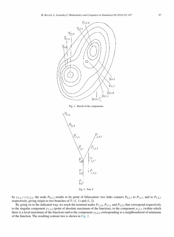
The construction of the contour tree is explained here by an example. Precisely, having assigned a set of contours(Fig. 1), we start with the contour Γ −1 that contains the only component γ0,a,a and we associate to it the point P0,1,1.
Following the order of inclusion, we consider the contour Γ 0 that contains the component γ0,1,b to which the nodeP0,1,2 corresponds. The first branch terminates with the node P0,1,3 corresponding to γ0,1,3. Since γ0,1,3 is followed
M. Bozzini, L. Lenarduzzi / Mathematics and Computers in Simulation 99 (2014) 95–107 97
Fig. 1. Sketch of the components.
br
tto
Fig. 2. Tree T.
y γ1,1,1 ∪ γ1,2,1, the node P0,1,3 results to be point of bifurcation: two links connect P0,1,3 to P1,1,1 and to P1,2,1espectively, giving origin to two branches of T: (1, 1) and (1, 2).
By going on in the indicated way, we reach the terminal nodes P , P and P that correspond respectively
1,1,4 2,1,1 2,2,2o the singular component γ1,1,4 (point of absolute maximum of the function), to the component γ2,1,1 (within whichhere is a local maximum of the function) and to the component γ2,2,2 corresponding to a neighbourhood of minimumf the function. The resulting contour tree is shown in Fig. 2.
98 M. Bozzini, L. Lenarduzzi / Mathematics and Computers in Simulation 99 (2014) 95–107
By this simple example we observe that there is a correspondence between complexity of behaviour of the surfaceand ramifications of the tree.
3. Construction of the contour tree T�
In this section we address the construction of the contour tree in the case of scattered data.Given a domain Ω ⊂ R2, let be assigned a sample S = {X, F} where the locations of the sample, X = {xi}N1 , are
unevenly scattered on Ω ⊂ R2 and the functional values F = {fi}N1 are relevant to the unknown function f(x) thatrepresents the surface.
Having fixed a value h, we construct the regular grid hZ2. Let G ⊂ hZ2 be the minimal rectangular subgrid thatcontains Ω ∩ hZ2.
We assign to the knots uk ∈ Xu : = G \ (Ω ∩ G) a value z < minfi∈F
fi. Let it be X̃ = {X ∪ Xu}, F̃ = {F ∪ z, . . . , z},S̃ = {X̃, F̃ } and Lf(·) be the linear interpolant of the set S̃. We construct the set of pseudodata
Y = {Lf (ui), ui ∈ G},whose elements are the values of the linear interpolant at the knots of the regular grid G.
By using the set Y we construct the tree T as described in Section 2.1, with interval ωLf= [z, max
ui∈GLf (ui)] for the
definition of M.In the following subsections we identify the features for a coarse representation of the surface in order to identify a
suitable split of Ω in subdomains.
3.1. Identification of the salient regions and of the tree T�
The aim of this section is to identify a tree T� relevant to a coarse representation of the surface and obtained bypruning those branches of T that the process described below defines not important.
For this purpose, at first we identify the flat zones, the humps and the dips.
3.1.1. Flat zonesWe prescribe a tolerance TOL = β · ωLf
/n with β real and of the order of 10−2. We call G� the set of the knotsui ∈ G for which the following fact is true. Consider the square Qi,h with centre at ui and side of length 4h; for everyknot uj ∈ G ∩ Qi,h the inequality
|Lf (ui) − Lf (uj)| < TOL (1)
holds.We classify as flat zone a connected region Zi of the domain Ω for which all the points of G contained in it are the
only points belonging to G� too.The detected flat zones are considered important.Let ui ∈ G� be contained within an inner set R� corresponding to a component γ�. The node P� associated to γ�
belongs to a branch (α1, α2) that we classify important.By covering all the points ui ∈ G� we identify all the branches of the contour tree corresponding to flat zones.
3.1.2. Humps and dipsWe want to identify those zones of the surface that correspond to humps or dips.In order not to point out possible wrinkles, having fixed a point ui ∈ G, we evaluate whether the inequality
Lf (ui) ≥ Lf (ui + 8hj) (2)
is satisfied for all j ∈ [−2, 2]2, the strong inequality holding for some values of j at least. Those knots for which (2) issatisfied, correspond to points of local maximum and the branches to which the points belong are considered importantbranches.
M. Bozzini, L. Lenarduzzi / Mathematics and Computers in Simulation 99 (2014) 95–107 99
t
pIF
4
B
4
o
Fig. 3. Tree T� .
In analogous way we identify those knots corresponding to the points of minimum by the inequality:
Lf (ui) ≤ Lf (ui + 8hj) for j ∈ [−2, 2]2 (3)
he strong inequality holding for some values of j at least, and the branches relevant to them are important.We prune the branches not classified as important and we obtain the pruned tree T�.Coming back to the sketched example of Figs. 1 and 2, while one maximum and the minimum are evident, the other
oint of maximum is less evident as its representation in T is the branch made of just one link between P1,2,1 and P2,1,1.f we do not identify any salient region relevant to such branch, we prune the branch and we obtain the pruned T� ofig. 3.
. Identification of the subdomains
In the previous section we have identified those zones that provide information about the behaviour of the function.y these informations we have obtained a new tree T� whose branches are now all important.
Now we are ready to identify the subdomains where to compute an approximation.
.1. Construction of the subdomains
We state in advance the following definitions.We consider the node P� and the node Pα directly preceding it.Definition: Pα is father of P� and we denote RFa(α) := Rα.Except for the terminal nodes, a node P� is followed directly by one node or by more nodes in the case of bifurcations.We call these nodes children of P�.Definition: RCh(�) is the union of the inner sets relevant to the children of P�.The identification of the subdomains relevant to those regions where there are evident changes of behaviour is
btained by the quantity Δ� here defined.Let us consider a grid G1 ⊃ G of step h/K, K > 1.Let P� a knot of T� and let us denote
μα := number of the knots of G1 ∩ Rα
Definition: ∀α with μ� /= 0
Δα = | (μFa(α) − μα) − (μα − μCh(α)) |μα
(4)
For α = (0, 1, 2) we define RFa(α) = R�, which implies μFa(α) = μ�.
100 M. Bozzini, L. Lenarduzzi / Mathematics and Computers in Simulation 99 (2014) 95–107
If α is a terminal node of T�, we set μCh(�) = 0.For each α with μ� = 0, we set μCh(�) = 0.Starting with the knot of the tree that corresponds to α = (0, 1, 2) we inspect the branch b = (α1, α2). For each node of
a branch b, we calculate the corresponding quantities Δ� that we shall denote Δ�(b) in the current context for clarity.Let us denote by Ib = {Δ�(b)} the set of the quantities relevant to the b branch and nb its size.We compute the median m(b) of Ib and the index of dispersion around its median
δ(b) =nb∑1
| Δα(b) − m(b)) |nb
.
For each branch b we save the components γ� corresponding to those nodes P� for which the value Δ�(b) has satisfiedthe inequality
|Δα(b) − m(b)|δ(b)
> 2.
Such components indicate evident changes of behaviour. Therefore Ω is split in subdomains {Ωr} bounded by thedetected components
Ω = ∪{Ωr}r=1,...,N(Ω)
5. Blending of the approximations
We associate to each subdomain Ωr a non negative function qr(x), of class C1 with compact support.Namely, let us consider a grid Gw of constant step hw = 2h on Ω and we denote with {tj} the points of Gw ∩ Ω.
Let
w(x, tj) = 1 − 3 · d2(x, tj) + 2 · d3(x, tj),
where
d(x, tj) =⎧⎨⎩
dist2(x, tj)
hw
ifdist2(x, tj)
hw
< 1
1 elsewhere,
and we consider the normalized function
w�(x, tj) = w(x, tj)∑tk∈Gw∩Ωw(x, tk)
.
We define:
qr(x) :=∑
tj∈Gw∩Ωr
w�(x, tj).
On each subdomain Ωr we calculate an approximant Sr(x) of class C1(Ω).The function that approximates the surface is then given by the blending
S(x) :=N(Ω)∑r=1
Sr(x)qr(x).
Remark: the choice hw = 2h allows us to obtain a surface of class C1(Ω) while maintaining the approximationsuitably local.
Hereafter we show an academic example to illustrate how the subdivision in subdomains is necessary for a
reconstruction that does not present undue oscillations.
We consider a function which is regular, radially symmetric with respect to the centre of Ω (see Fig. 5):
M. Bozzini, L. Lenarduzzi / Mathematics and Computers in Simulation 99 (2014) 95–107 101
0 0.1 0.2 0.3 0.4 0.5 0.6 0.7 0.8 0.9 10
0.1
0.2
0.3
0.4
0.5
0.6
0.7
0.8
0.9
1
Fig. 4. Data locations.
w
dF
l
Fig. 5. True function.
here
dist2(x) = ‖x − 0.5‖.For simplicity we consider a sampling depending on the behaviour of the function. That is to say with a larger
ensity in the zone of the peak and with a smaller density in the smooth region. The locations of the data are shown inig. 4 and the size of the sample is N = 271.
Our method identifies two subdomains Ω1 and Ω2. In Fig. 4 you see the contour of separation � = � and the dataocations.
For the approximation we choose the multiquadric radial basis φ(r) = (c2 + r2)1/2 with shape parameter c = 0.175.
102 M. Bozzini, L. Lenarduzzi / Mathematics and Computers in Simulation 99 (2014) 95–107
Fig. 6. One interpolant.
Fig. 7. Two interpolants.
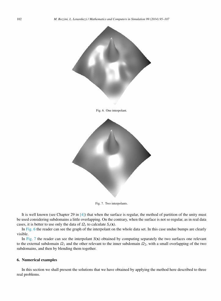
It is well known (see Chapter 29 in [4]) that when the surface is regular, the method of partition of the unity mustbe used considering subdomains a little overlapping. On the contrary, when the surface is not so regular, as in real datacases, it is better to use only the data of Ωr to calculate Sr(x).
In Fig. 6 the reader can see the graph of the interpolant on the whole data set. In this case undue bumps are clearlyvisible.
In Fig. 7 the reader can see the interpolant S(x) obtained by computing separately the two surfaces one relevantto the external subdomain Ω1 and the other relevant to the inner subdomain Ω2, with a small overlapping of the twosubdomains, and then by blending them together.
6. Numerical examples
In this section we shall present the solutions that we have obtained by applying the method here described to threereal problems.
M. Bozzini, L. Lenarduzzi / Mathematics and Computers in Simulation 99 (2014) 95–107 103
0 0.1 0.2 0.3 0.4 0.5 0.6 0.7 0.8 0.9 10
0.1
0.2
0.3
0.4
0.5
0.6
0.7
0.8
0.9
1
Fig. 8. Puertorico data locations.
0.5
0.55
0.6
0.65
0.7
0.75
0.8
0.85
0.9
0.95
1
cr
i
c
E
e
o
0 0.1 0.2 0.3 0.4 0.5 0.6 0.7 0.8 0.9 1
Fig. 9. Subdomains (upper half domain shown).
We shall show the identified subdomains according to the above said algorithm. We have run the MatLab codeontour.m for the contours; each component that crosses the boundary of Ω, rectangular domain, is made closed byunning along δΩ.
The first case is relevant to the reconstruction of a part of piece of the bottom of the sea out of Puertorico [10]. Thiss a suitable test for the problem addressed in the current paper.
A second example is relevant to the well known data set of the Monterey bay [5], considered also in [7,8,2].The last example is relevant to detecting the parts of ground of different nature, such as a glacier or a part of glacier
overed with debris in images from the Aster satellite. This last case shows how the method is a versatile tool.
xample 1. The size of the sample is N = 17, 089. We have set n = 50, TOL = 30.In Fig. 8 you see the data locations that are unevenly scattered, very dense in some zones and very sparse somewhere
lse, without any relation with the surface to be reconstructed.The method identifies nine subdomains presented in Fig. 9 (for the figures in colour please refer to the online version
f the paper).
104 M. Bozzini, L. Lenarduzzi / Mathematics and Computers in Simulation 99 (2014) 95–107
Fig. 10. Linear interpolation.
Fig. 11. C1 reconstruction.
Five subdomains are in blue and are relevant to zones of minimum. One subdomain, in black, is relevant to a zoneof stationarity and it is on the left. On the right you see an other subdomain in black and external to it a subdomain inred. The ninth subdomain is their complement to [0, 1]2.
Since for each subdomain the configuration of the data is too uneven, and it passes from very thick data to zonesempty of data, a suitable approximation, both accurate and not badly numerically conditioned, is provided by theusage of the pseudodata. We approximate the pseudodata on each subdomain Ωr, r = 1, . . ., 8 by the local interpolationdescribed in [6] based on shifts of the thin plate basis: φ(r) : = r2ln(r). On the Ω9-th subdomain we make use of theleast squares approximation by shifts of the thin plate basis with centers at one knot every two of the grid G and in alocal manner which is described in [3].
In Fig. 10 you see the linear interpolant of the data; in Fig. 11 you see our reconstructed surface.We provide the errors with respect to the data in the unity of measure of the data; the root mean squared error is
e2 = 27.6, the root mean squared error over the oscillation of the data is e2,rel = 0.0056, the error in the infinite norm ise∞ = 187.8 and it is e∞,rel = 0.038.
Example 2. The size of the sample is N = 1668. We have set n = 500, TOL = 5 ×10⁻⁴.
M. Bozzini, L. Lenarduzzi / Mathematics and Computers in Simulation 99 (2014) 95–107 105
0 0.5 1 1.5 20
0.05
0.1
0.15
0.2
0.25
0.3
0.35
0.4
0.45
Fig. 12. Data locations and division between Ω1 and Ω2.
Fig. 13. Two TPS interpolants.
Fig. 14. One TPS interpolant.
106 M. Bozzini, L. Lenarduzzi / Mathematics and Computers in Simulation 99 (2014) 95–107
Fig. 15. Aster image of Adamello.
Fig. 16. Detected zones very wet in grey.
The locations of the data from [5] are shown in Fig. 12 where there is also the contour that splits the two subdomainsΩ1 and Ω2 and identified by the method.
For the reconstruction of the phenomenon, that is not very regular, we use the thin plate splines and we interpolatethe data on each subdomain. The result is shown in Fig. 13: the shallow part is rendered quite flat, and this is whatthe data in the zone suggest it should be, because their associated functional values are zero. On the contrary thereconstruction by the classical global interpolation presents strong undue oscillations, see Fig. 14.
The result of Fig. 13 outperforms also the result shown in [2] which is nowadays the best approximation in theliterature.
Example 3. The current problem is the identification of the wet parts of the ground, lightened with sun, in the Asterimage of Adamello (dated 13/09/1999, RGB: 5 4 3, courtesy of the GLIMS project) shown in Fig. 15.
The B component is relevant to the visible spectrum while G and R are relevant to the infrared spectrum.The problem is solved by considering the subdivision in subdomains the first time for the albedo function to point
out the regions dark shadow, and the second time for the wetness function to identify the wet parts.
s
o
c
a
A
R
[
[
[
[[
[[
[
[1
M. Bozzini, L. Lenarduzzi / Mathematics and Computers in Simulation 99 (2014) 95–107 107
First we compute the albedo, or index of reflectance, relevant to each pixel of the image (it is defined as R + G + B);o we have the values of the albedo at the points of a regular grid on the domain Ω.
We split Ω in subdomains by our algorithm and we classify as dark shadow the subdomains with very low valuesf albedo.
Then we compute the index of wetness, defined as (G + B)/R. With respect to it, we split Ω in subdomains by theurrent method of subdivision. In Fig. 16 we depict the subdomains corresponding to the regions very wet.
They correspond to the glacier and to few small lakes. Only a small zone of the glacier is lacking to the classifications glacier, but this zone was previously classified as dark shadow.
cknowledgments
The authors are grateful to the referees for their suggestions that improved the presentation.
eferences
2] M. Bozzini, L. Lenarduzzi, An adaptive local procedure to approximate unevenly distributed data, in: Communications to SIMAI Congress, vol.3, 2009.
3] G. Casciola, D. Lazzaro, L.B. Montefusco, S. Morigi, Fast surface reconstruction and hole filling using positive definite radial basis functions,Numerical Algorithms 39 (2005) 289–305.
4] G. Fasshauer, Meshfree Approximation Methods with MATLAB, Interdisciplinary Mathematical Sciences, vol. 6, World Scientific Publishers,Singapore, 2007.
5] http://www.math.nps.navy.mil/rfranke6] D. Lazzaro, L. Montefusco, Radial basis functions for the multivariate interpolation of large scattered data sets, Journal of Computational and
Applied Mathematics 140 (2002) 521–536.7] J. McMahon, R. Franke, Knot selection for least squares thin plate splines, 1987, NPS-53-87-005.8] R. Schaback, H. Wendland, Adaptive greedy techniques for approximate solution of large RBF systems, Numerical Algorithms 24 (2000)
239–254.9] A. Solé, V. Caselles, G. Sapiro, F. Arándiga, Morse description and geometric encoding of digital elevation maps, IEEE Transactions on Image
Processing 13 (9) (2004) 1245–1260.0] vol05 at http://poseidon.uprm.edu/bathymetry/bathymetry.htm