Recovering the Optimal Solution by Dual Random...

JMLR: Workshop and Conference Proceedings vol 30 (2013) 1–23

Recovering the Optimal Solution by

Dual Random Projection

Lijun Zhang [email protected]

Mehrdad Mahdavi [email protected]

Rong Jin [email protected]

Department of Computer Science and Engineering

Michigan State University, East Lansing, MI 48824, USA

Tianbao Yang [email protected]

GE Global Research, San Ramon, CA 94583, USA

Shenghuo Zhu [email protected]

NEC Laboratories America, Cupertino, CA 95014, USA

Abstract

Random projection has been widely used in data classification. It maps high-dimensionaldata into a low-dimensional subspace in order to reduce the computational cost in solvingthe related optimization problem. While previous studies are focused on analyzing theclassification performance of using random projection, in this work, we consider the recoveryproblem, i.e., how to accurately recover the optimal solution to the original optimizationproblem in the high-dimensional space based on the solution learned from the subspacespanned by random projections. We present a simple algorithm, termed Dual RandomProjection, that uses the dual solution of the low-dimensional optimization problem torecover the optimal solution to the original problem. Our theoretical analysis shows thatwith a high probability, the proposed algorithm is able to accurately recover the optimalsolution to the original problem, provided that the data matrix is of low rank or can bewell approximated by a low rank matrix.

Keywords: Random projection, Primal solution, Dual solution, Low rank

1. Introduction

Random projection is a simple yet powerful dimensionality reduction technique that projectsthe original high-dimensional data onto a low-dimensional subspace using a random ma-trix (Kaski, 1998; Bingham and Mannila, 2001). It has been successfully applied to manymachine learning tasks, including classification (Fradkin and Madigan, 2003; Vempala, 2004;Rahimi and Recht, 2008), regression (Maillard and Munos, 2012), clustering (Fern and Brod-ley, 2003; Boutsidis et al., 2010), manifold learning (Dasgupta and Freund, 2008; Freundet al., 2008), and information retrieval (Goel et al., 2005).

In this work, we focus on random projection for classification. While previous studieswere devoted to analyzing the classification performance using random projection (Arriagaand Vempala, 1999; Balcan et al., 2006; Paul et al., 2012; Shi et al., 2012), we examine theeffect of random projection from a very different aspect. In particular, we are interestedin accurately recovering the optimal solution to the original high-dimensional optimization

c© 2013 L. Zhang, M. Mahdavi, R. Jin, T. Yang & S. Zhu.

Zhang Mahdavi Jin Yang Zhu

problem using random projection. This is particularly useful for feature selection (Guyonand Elisseeff, 2003), where important features are often selected based on their weights inthe linear prediction model learned from the training data. In order to ensure that similarfeatures are selected, the prediction model based on random projection needs to be close tothe model obtained by solving the original optimization problem directly.

The proposed algorithm for recovering the optimal solution consists of two simple steps.In the first step, similar to previous studies, we apply random projection to reducing thedimensionality of the data, and then solve a low-dimensional optimization problem. In thesecond step, we construct the dual solution of the low-dimensional problem from its primalsolution, and then use it to recover the optimal solution to the original high-dimensionalproblem. Our analysis reveals that with a high probability, we are able to recover the optimalsolution with a small error by using Ω(r log r) projections, where r is the rank of the datamatrix. A similar result also holds when the data matrix can be well approximated by alow rank matrix. We further show that the proposed algorithm can be applied iterativelyto recovering the optimal solution with a relative error ǫ by using O(log 1/ǫ) iterations.

The rest of the paper is arranged as follows. Section 2 describes the problem of recoveringoptimal solution by random projection, the theme of this work. Section 3 describes the dualrandom projection approach for recovering the optimal solution. Section 4 presents the maintheoretical results for the proposed algorithm. Section 5 presents the proof for the theoremsstated in Section 4. Section 6 concludes this work.

2. The Problem

Let (xi, yi), i = 1, . . . , n be a set of training examples, where xi ∈ Rd is a vector of d

dimension and yi ∈ −1,+1 is the binary class assignment for xi. Let X = (x1, . . . ,xn)and y = (y1, . . . , yn)

⊤ include input patterns and the class assignments of all trainingexamples. A classifier w ∈ R

d is learned by solving the following optimization problem:

minw∈Rd

λ

2‖w‖2 +

n∑

i=1

ℓ(yix⊤i w), (1)

where ℓ(z) is a convex loss function that is differentiable1. By writing ℓ(z) in its convexconjugate form, i.e.,

ℓ(z) = maxα∈Ω

αz − ℓ∗(α),

where ℓ∗(α) is the convex conjugate of ℓ(z) and Ω is the domain of the dual variable, weget the dual optimization problem:

maxα∈Ωn

−n∑

i=1

ℓ∗(αi)−1

2λα⊤Gα, (2)

where α = (α1, · · · , αn)⊤ and D(y) = diag(y) and G is the Gram matrix given by

G = D(y)X⊤XD(y). (3)

1. For non-differentiable loss functions such as hinge loss, we could apply the smoothing technique describedin (Nesterov, 2005) to make it differentiable.

2


In the following, we denote by w∗ ∈ Rd the optimal primal solution to (1), and by α∗ ∈ R

n

the optimal dual solution to (2). The following proposition connects w∗ and α∗.

Proposition 1 Let w∗ ∈ Rd be the optimal primal solution to (1), and α∗ ∈ R

n be theoptimal dual solution to (2). We have

w∗ = − 1

λXD(y)α∗, and [α∗]i = ∇ℓ

(yix

⊤i w∗

), i = 1, . . . , n. (4)

The proof of Proposition 1 and other omitted proofs are deferred to the Appendix. Whenthe dimensionality d is high and the number of training examples n is large, solving eitherthe primal problem in (1) or the dual problem in (2) can be computationally expensive.To reduce the computational cost, one common approach is to significantly reduce thedimensionality by random projection. Let R ∈ R

d×m be a Gaussian random matrix, whereeach entry Ri,j is independently drawn from a Gaussian distribution N (0, 1) and m issignificantly smaller than d. Using the random matrix R, we generate a low-dimensionalrepresentation for each input example by

xi =1√mR⊤xi, (5)

and solve the following low-dimensional optimization problem:

minz∈Rm

λ

2‖z‖2 +

n∑

i=1

ℓ(yiz⊤xi). (6)

The corresponding dual problem is written as

maxα∈Ωn

−n∑

i=1

ℓ∗(αi)−1

2λα⊤Gα, (7)

where

G = D(y)X⊤RR⊤

mXD(y). (8)

Intuitively, the choice of Gaussian random matrix R is justified by the expectation of thedot-product between any two examples in the projected space is equal to the dot-productin the original space, i.e.,

E[x⊤i xj ] = x⊤

i E

[1

mRR⊤

]xj = x⊤

i xj ,

where the last equality follows from E[RR⊤/m] = I. Thus, G = G holds in expectation.Let z∗ ∈ R

m denote the optimal primal solution to the low-dimensional problem (6),and α∗ ∈ R

n denote the optimal dual solution to (7). Similar to Proposition 1, the followingproposition connects z∗ and α∗.

Proposition 2 We have

z∗ = − 1

λ

1√mR⊤XD(y)α∗, and [α∗]i = ∇ℓ

(yi√mx⊤i Rz∗

), i = 1, . . . , n. (9)

3


Given the optimal solution z∗ ∈ Rm, the data point x ∈ R

d is classified by x⊤Rz∗/√m,

which is equivalent to defining a new solution w ∈ Rd given below, which we refer to as the

naive solution

w =1√mRz∗. (10)

The classification performance of w has been examined by many studies (Arriaga andVempala, 1999; Balcan et al., 2006; Paul et al., 2012; Shi et al., 2012). The general conclusionis that when the original data is linearly separable with a large margin, the classificationerror for w is usually small.

Although these studies show that w can achieve a small classification error under appro-priate assumptions, it is unclear whether w is a good approximation of the optimal solutionw∗. In fact, as we will see in Section 4, the naive solution is almost guaranteed to be aBAD approximation of the optimal solution, that is, ‖w −w∗‖2 = Ω(

√d/m‖w∗‖2). This

observation leads to an interesting question: is it possible to accurately recover the optimalsolution w∗ based on z∗, the optimal solution to the low-dimensional optimization problem?

Relationship to Compressive Sensing The proposed problem is closely related tocompressive sensing (Donoho, 2006; Candes and Wakin, 2008) where the goal is to recovera high-dimensional but sparse vector using a small number of random measurements. Thekey difference between our work and compressive sensing is that we do not have the directaccess to the random measurement of the target vector (which in our case is w∗ ∈ R

d).Instead, z∗ ∈ R

m is the optimal solution to (6), the primal problem using random projection.However, the following theorem shows that z∗ is a good approximation of R⊤w∗/

√m, which

includes m random measurements of w∗, if the data matrix X is of low rank and the numberof random measurements m is sufficiently large.

Theorem 1 For any 0 < ε ≤ 1/2, with a probability at least 1− δ− exp(−m/32), we have

‖√mz∗ −R⊤w∗‖2 ≤√2ε√

1− ε‖R⊤w∗‖2,

provided

m ≥ (r + 1) log(2r/δ)

cε2,

where constant c is at least 1/4, and r is the rank of X.

Given the approximation bound in Theorem 1, it is appealing to reconstruct w∗ using thecompressive sensing algorithm provided that w∗ is sparse to certain bases. We note thatthe low rank assumption for data matrix X implies that w∗ is sparse with respect to thesingular vectors of X. However, since z∗ only provides an approximation to the randommeasurements of w∗, running the compressive sensing algorithm will not be able to perfectlyrecover w∗ from z∗. In Section 3, we present an algorithm, that recovers w∗ with a smallerror, provided that the data matrix X is of low rank. Compared to the compressive sensingalgorithm, the main advantage of the proposed algorithm is its computational simplicity;it neither computes the singular vectors of X nor solves an optimization problem thatminimizes the ℓ1 norm.

4


Algorithm 1 A Dual Random Projection Approach for Recovering Optimal Solution

1: Input: input patterns X ∈ Rd×n, binary class assignment y ∈ −1,+1n, and sample

size m2: Sample a Gaussian random matrix R ∈ R

d×m and compute X = [x1, . . . , xn] =R⊤X/

√m

3: Obtain the primal solution z∗ ∈ Rm by solving the optimization problem in (6)

4: Construct the dual solution α∗ ∈ Rn by Proposition 2, i.e.,

[α∗]i = ∇ℓ

(yi√mx⊤i Rz∗

), i = 1, . . . , n

5: Compute w ∈ Rd according to (12), i.e., w = −XD(y)α∗/λ

6: Output: the recovered solution w

3. Algorithm

To motivate our algorithm, let us revisit the optimal primal solution w∗ to (1), which isgiven in Proposition 1, i.e.,

w∗ = − 1

λXD(y)α∗, (11)

where α∗ is the optimal solution to the dual problem (2). Given the projected data x =R⊤x/

√m, we have reached an approximate dual problem in (7). Comparing it with the

dual problem in (2), the only difference is that the Gram matrix G = D(y)X⊤XD(y) in (2)is replaced with G = D(y)X⊤RR⊤XD(y)/m in (7). Recall that E[RR⊤/m] = I. Thus,when the number of random projections m is sufficiently large, G will be close to the G andwe would also expect α∗ to be close to α∗. As a result, we can use α∗ to approximate α∗in (11), which yields a recovered prediction model given below:

w = − 1

λXD(y)α∗ = −

n∑

i=1

1

λyi[α∗]ixi. (12)

Note that the key difference between the recovered solution w and the naive solutionw is that w is computed by mapping the optimal primal solution z∗ in the projected spaceback to the original space via the random matrix R, while w is computed directly in theoriginal space using the approximate dual solution α∗. Therefore, the naive solution w liesin the subspace spanned by the column vectors in the random matrix R (denoted by AR),while the recovered solution w lies in the subspace that also contains the optimal solutionw∗, i,e., the subspace spanned by columns of X (denoted by A). The mismatch betweenspaces AR and A leads to the large approximation error for w.

According to Proposition 2, we can construct the dual solution α∗ from the primalsolution z∗. Thus, we do not need to solve the dual problem in (7) to obtain α∗. Instead,we solve the low-dimensional optimization problem in (6) to get z∗ and construct α∗ from it.Algorithm 1 shows the details of the proposed method. We note that although dual variableshave been widely used in the analysis of convex optimization (Boyd and Vandenberghe, 2004;Hazan et al., 2011) and online learning (Shalev-Shwartz and Singer, 2006), to the best of

5


Algorithm 2 An Iterative Dual Random Projection Approach for Recovering OptimalSolution

1: Input: input patterns X ∈ Rd×n, binary class assignment y ∈ −1,+1n, sample size

m, and number of iterations T2: Sample a Gaussian random matrix R ∈ R

d×m and compute X = R⊤X/√m

3: Initialize w0 = 04: for t = 1, . . . , T do5: Obtain zt∗ ∈ R

m by solving the following optimization problem

minz∈Rm

λ

2

∥∥∥∥z+1√mR⊤wt−1

∥∥∥∥2

2

+n∑

i=1

ℓ(yiz

⊤xi + yi[wt−1]⊤xi

)(13)

6: Construct the dual solution αt∗ ∈ R

n using

[αt∗]i = ∇ℓ

(yix

⊤i z

t∗ + yi[w

t−1]⊤xi

), i = 1, . . . , n

7: Update the solution by wt = −XD(y)αt∗/λ

8: end for9: Output the recovered solution wT

our knowledge, this is the first time that dual variables are used in conjunction with randomprojection for recovering the optimal solution.

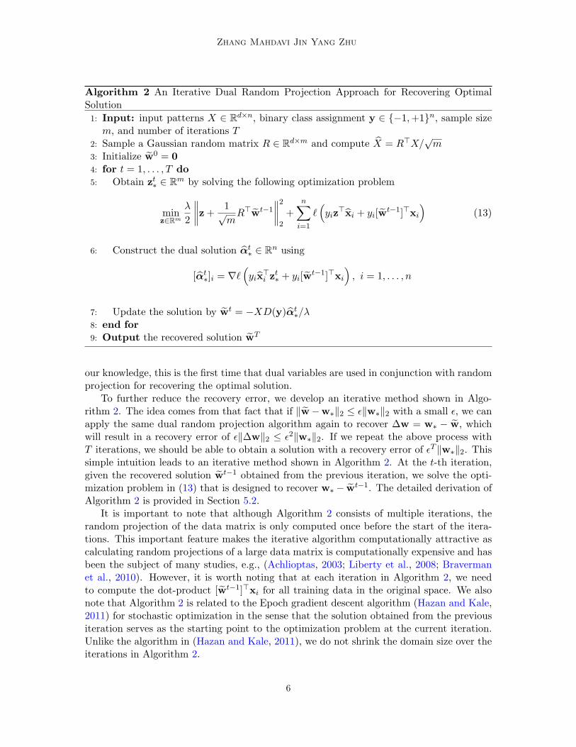
To further reduce the recovery error, we develop an iterative method shown in Algo-rithm 2. The idea comes from that fact that if ‖w−w∗‖2 ≤ ǫ‖w∗‖2 with a small ǫ, we canapply the same dual random projection algorithm again to recover ∆w = w∗ − w, whichwill result in a recovery error of ǫ‖∆w‖2 ≤ ǫ2‖w∗‖2. If we repeat the above process withT iterations, we should be able to obtain a solution with a recovery error of ǫT ‖w∗‖2. Thissimple intuition leads to an iterative method shown in Algorithm 2. At the t-th iteration,given the recovered solution wt−1 obtained from the previous iteration, we solve the opti-mization problem in (13) that is designed to recover w∗ − wt−1. The detailed derivation ofAlgorithm 2 is provided in Section 5.2.

It is important to note that although Algorithm 2 consists of multiple iterations, therandom projection of the data matrix is only computed once before the start of the itera-tions. This important feature makes the iterative algorithm computationally attractive ascalculating random projections of a large data matrix is computationally expensive and hasbeen the subject of many studies, e.g., (Achlioptas, 2003; Liberty et al., 2008; Bravermanet al., 2010). However, it is worth noting that at each iteration in Algorithm 2, we needto compute the dot-product [wt−1]⊤xi for all training data in the original space. We alsonote that Algorithm 2 is related to the Epoch gradient descent algorithm (Hazan and Kale,2011) for stochastic optimization in the sense that the solution obtained from the previousiteration serves as the starting point to the optimization problem at the current iteration.Unlike the algorithm in (Hazan and Kale, 2011), we do not shrink the domain size over theiterations in Algorithm 2.

6


Application to the Square Loss In the following, we take the square loss ℓ(z) =12(1 − z)2 as an example to illustrate the recovery procedure. The original optimizationproblem, which is refereed to as the ridge regression (Hastie et al., 2009), is

minw∈Rd

λ

2‖w‖2 + 1

2

n∑

i=1

(1− yix⊤i w)2

yi∈±1=

λ

2‖w‖2 + 1

2

n∑

i=1

(yi − x⊤i w)2.

Setting the derivative to 0, we obtain the optimal solution

w∗ =(λI +XX⊤

)−1Xy = X

(λI +X⊤X

)−1y. (14)

where the last equality follows from the Woodbury matrix identity (Golub and Van Loan,1996). Thus, the computational cost is either O(d2n+ d3) or O(n2d+ n3).

Following the dual random projection algorithm, we first solve the the low-dimensionalproblem in (6), whose solution is z∗ = (λI+ XX⊤)−1Xy, where X = R⊤X/

√m. Then, we

construct the dual solution α∗ = D(y)X⊤z∗ − 1. Finally, we recover the optimal solutionw = − 1

λXD(y)α∗. It is straightforward to check that computational cost of our algorithmis O(mnd+m2n+m3), which is significantly smaller than that of (14) when both d and nare large.

After some algebraic manipulation, we can show that

w = X

(λI +X⊤SS⊤

mX

)−1

y. (15)

Comparing (14) with (15), we can see the difference between w∗ and w comes from theGram matrix. When m is large enough, X⊤RR⊤X/m is close to the X⊤X, and as a resultw is also close to w∗.

4. Main Results

In this section, we will bound the recovery error ‖w∗− w‖2 of dual random projection. Wefirst assume X is of low rank, and then extend the results to the full rank case.

4.1. Low Rank

The low rank assumption is closely related to the sparsity assumption made in compressivesensing. This is because w∗ lies in the subspace spanned by the column vectors of X andthe low rank assumption directly implies that w∗ is sparse with respect to the singularvectors of X.

We denote by r the rank of matrix X. The following theorem shows that the recoveryerror of Algorithm 1 is small provided that (1) X is of low rank (i.e., r ≪ min(d, n)), and(2) the number of random projections is sufficiently large.

Theorem 2 Let w∗ be the optimal solution to (1) and let w be the solution recovered byAlgorithm 1. For any 0 < ε ≤ 1/2, with a probability at least 1− δ, we have

‖w −w∗‖2 ≤ε

1− ε‖w∗‖2,

7


provided

m ≥ (r + 1) log(2r/δ)

cε2,

where constant c is at least 1/4.

According to Theorem 2, the number of required random projections is Ω(r log r). Thisis similar to a compressive sensing result if we view rank r as the sparsity measure usedin compressive sensing. Following the same arguments as compressive sensing, it may bepossible to argue that Ω(r log r) is optimal due to the result of the coupon collector’s prob-lem (Mowani and Raghavan, 1995), although the rigorous analysis remains to be developed.

As a comparison, the following theorem shows that with a high probability, the naivesolution w given in (10) does not accurately recover the true optimal solution w∗.

Theorem 3 For any 0 < ε ≤ 1/3, with a probability at least 1 − exp(−(d − r)/32) −exp(−m/32)− δ, we have

‖w −w∗‖2 ≥1

2

√d− r

m

(1− ε

√2(1 + ε)

1− ε

)‖w∗‖2,

provided the condition on m in Theorem 2 holds.

As indicated by Theorem 3, when m is sufficiently larger than r but significantly smallerthan d, we have ‖w−w∗‖2 = Ω(

√d/m‖w∗‖2), indicating that w does not approximate w∗

well.It is important to note that Theorem 3 does not contradict the previous results showing

that the random projection based method could result in a small classification error if thedata is linearly separable with a large margin. This is because, to decide whether w carriesa similar classification performance to w∗, we need to measure the following term

maxx∈span(X),‖x‖2≤1

x⊤(w −w∗). (16)

Since ‖w −w∗‖2 can also be written as

‖w −w∗‖2 = max‖x‖2≤1

x⊤(w −w∗),

the quantity defined in (16) could be significantly smaller than ‖w−w∗‖2 if the data matrixX is of low rank. The following theorem quantifies this statement.

Theorem 4 For any 0 < ε ≤ 1/2, with a probability at least 1− δ, we have


x⊤(w −w∗) ≤ ε

(1 +

1

1− ε

)‖w∗‖2,


We note that Theorem 4 directly implies the result of margin classification error for randomprojection (Blum, 2006; Shi et al., 2012). This is because when a data point (xi, yi) can beseparated by w∗ with a margin γ, i.e., yiw

⊤∗ xi ≥ γ‖w∗‖, it will be classified by w with a

margin at least γ − ε(1 + 1

1−ε

)provided γ > ε

(1 + 1

1−ε

).

Based on Theorem 2, we now state the recovery result for the iterative method.

8


Theorem 5 Let w∗ be the optimal solution to (1) and let wT be the solution recovered byAlgorithm 2. For any 0 < ε < 1/2, with a probability at least 1− δ, we have

‖wT −w∗‖2 ≤(

ε

1− ε

)T

‖w∗‖2,


Notice that the number of random projectionm does not depend on the number of iterationsT . That is because we only apply random projection once to reducing the dimensionality ofthe data. Theorem 5 implies that we can recover the optimal solution with a relative errorǫ, i.e., ‖w∗ − wT ‖2 ≤ ǫ‖w∗‖2, by using log(1−ε)/ε 1/ǫ iterations.

4.2. Full Rank

If X has full rank, we established the following theorem to bound the recovery error.

Theorem 6 Assume w∗ lies in the subspace spanned by the first k left singular vectors ofX, and the loss ℓ(·) is γ-smooth. For any 0 < ε ≤ 1, with a probability at least 1 − δ, wehave

‖w −w∗‖2 ≤ε

1− ε

(1 +

√λ√

γσk

)‖w∗‖2,

provided

m ≥ rσ21

cε2(λ/γ + σ21)

log2d

δ,

where σi is the i-th singular value of X, r =∑d

i=1σ2i

λ/γ+σ2i, and the constant c is at least

1/32.

The above theorem implies the number of required random projections is Ω(r log d), which

can be significantly smaller than d. The number r is closely related to the numerical√

λγ -

rank of X (Hansen, 1998). We say that X has numerical ν-rank rν if

σrν > ν ≥ σrν+1.

Using the notation of numerical rank, we have

r ≤ r√λ/γ

+d∑

i=r√λ/γ

+1

σ2i

λ/γ + σ2i

.

Thus, when the singular value σi ≪√λ/γ for i > r√

λ/γ, which means that X can be well

approximated by a rank r√λ/γ

matrix, we have r = O(r√λ/γ

).

One remarking property of our approach is it enjoys a multiplicative bound even in the

full rank case. Thus, as long as ε1−ε

(1 +

√λ√

γσk

)< 1, we can use Algorithm 2 to reduce the

reconstruction error exponentially over the iterations. In contrast, the random projectionbased algorithm for SVD (Halko et al., 2011), although is able to accurately recover the

9


eigen-space when the matrix is of low rank, it will result in a significant error in uncoveringthe subspace spanned by the top singular vectors when applied to matrices of full rank, andtherefore is unable to recover the optimal solution w∗ accurately.

Finally, we note that the assumption that the optimal solution lies in the subspacespanned by the top singular vectors has been used in kernel learning (Guo and Zhou, 2012)and semi-supervised learning (Ji et al., 2012).

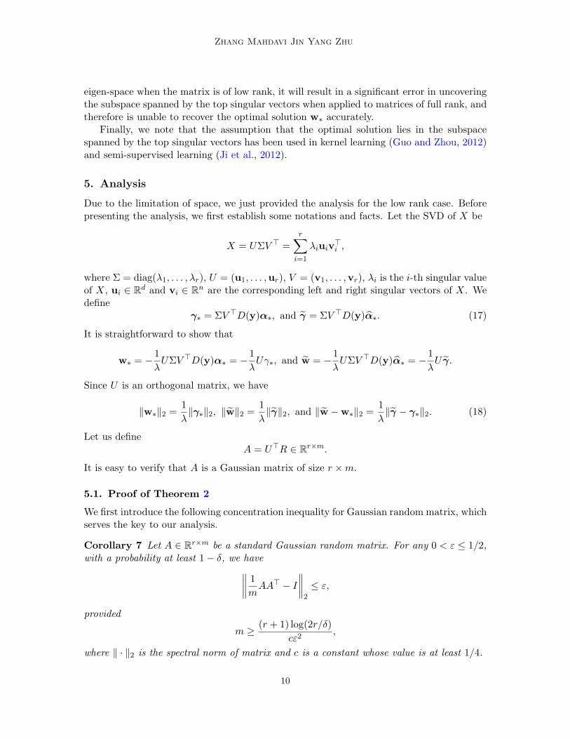
5. Analysis

Due to the limitation of space, we just provided the analysis for the low rank case. Beforepresenting the analysis, we first establish some notations and facts. Let the SVD of X be

X = UΣV ⊤ =r∑

i=1

λiuiv⊤i ,

where Σ = diag(λ1, . . . , λr), U = (u1, . . . ,ur), V = (v1, . . . ,vr), λi is the i-th singular valueof X, ui ∈ R

d and vi ∈ Rn are the corresponding left and right singular vectors of X. We

defineγ∗ = ΣV ⊤D(y)α∗, and γ = ΣV ⊤D(y)α∗. (17)

It is straightforward to show that

w∗ = − 1

λUΣV ⊤D(y)α∗ = − 1

λUγ∗, and w = − 1

λUΣV ⊤D(y)α∗ = − 1

λU γ.

Since U is an orthogonal matrix, we have

‖w∗‖2 =1

λ‖γ∗‖2, ‖w‖2 =

1

λ‖γ‖2, and ‖w −w∗‖2 =

1

λ‖γ − γ∗‖2. (18)

Let us defineA = U⊤R ∈ R

r×m.

It is easy to verify that A is a Gaussian matrix of size r ×m.

5.1. Proof of Theorem 2

We first introduce the following concentration inequality for Gaussian random matrix, whichserves the key to our analysis.

Corollary 7 Let A ∈ Rr×m be a standard Gaussian random matrix. For any 0 < ε ≤ 1/2,

with a probability at least 1− δ, we have

∥∥∥∥1

mAA⊤ − I

∥∥∥∥2

≤ ε,

provided

m ≥ (r + 1) log(2r/δ)

cε2,

where ‖ · ‖2 is the spectral norm of matrix and c is a constant whose value is at least 1/4.

10


Define L(α) and L(α) as

L(α) = −n∑

i=1

ℓ∗(αi)−1

2λα⊤Gα, and L(α) = −

n∑

i=1

ℓ∗(αi)−1

2λα⊤Gα.

Since α∗ maximizes L(α) over the domain Ωn, we have

L(α∗) ≥ L(α∗) +1

2λ(α∗ −α∗)

⊤G(α∗ −α∗). (19)

Using the concaveness of L(α), we have

L(α∗) +1

2λ(α∗ −α∗)

⊤G(α∗ −α∗)

≤ L(α∗) + (α∗ −α∗)⊤(∇L(α∗)−∇L(α∗) +∇L(α∗)

)

≤ L(α∗) +1

λ(α∗ −α∗)

⊤(G− G)α∗, (20)

where the last inequality follows from the fact that (α∗ − α∗)⊤∇L(α∗) ≤ 0 since α∗maximizes L(α) over the domain Ωn. Combining the inequalities in (19) and (20), we have

1

λ(α∗ −α∗)

⊤(G− G)α∗ ≥1

λ(α∗ −α∗)

⊤G(α∗ −α∗).

We rewrite G and G as

G = D(y)V ΣU⊤UΣV ⊤D(y) = D(y)V ΣΣV ⊤D(y),

G = D(y)V ΣU⊤RR⊤

mUΣV ⊤D(y) = D(y)V Σ

AA⊤

mΣV ⊤D(y).

Using the definitions of γ∗ and γ in (17), we obtain

(γ − γ∗)⊤(I − AA⊤

m

)γ∗ ≥ (γ − γ∗)

⊤AA⊤

m(γ − γ∗). (21)

From Corollary 7, with a probability at least 1− δ, we have∥∥I − 1

mAA⊤∥∥2≤ ε, under the

given condition on m. Therefore, we obtain

(1− ε)‖γ − γ∗‖2 ≤ ε‖γ∗‖2.

We complete the proof by using the equalities given in (18).

5.2. Proof of Theorem 5

At the t-th iteration, we consider the following optimization problem:

minw∈Rd

Lt(w;X,y) =λ

2‖w + wt−1‖22 +

n∑

i=1

ℓ(yi(w + wt−1)⊤xi

), (22)

11


where wt−1 is the solution obtained from the t−1-th iteration. It is straightforward to showthat ∆t

∗ = w∗ − wt−1 is the optimal solution to (22). Then we can use the dual randomprojection approach to recover ∆t

∗ by ∆t. If we can similarly show that

‖∆t −∆t∗‖2 ≤

ε

1− ε‖∆t

∗‖2,

then we update the recovered solution by wt = wt−1 + ∆t and have

‖wt −w∗‖2 = ‖∆t −∆t∗‖2 ≤

ε

1− ε‖∆t

∗‖2 =ε

1− ε‖wt−1 −w∗‖2.

As a result, if we repeat the above process for t = 1, . . . , T , the recovery error of the lastsolution wT is upper bounded by

‖wT −w∗‖2 ≤(

ε

1− ε

)T

‖w0 −w∗‖2 =(

ε

1− ε

)T

‖w∗‖2,

where we assume w0 = 0.The remaining question is how to compute the ∆t using the dual random projection

approach. In order to make the previous analysis remain valid for the recovered solution ∆t

to the problem (22), we need to write the primal optimization problem in the same formas in (1). To this end, we first note that wt−1 lies in the subspace spanned by x1, . . . ,xn,thus we write wt−1 as

wt−1 = − 1

λXD(y)αt−1

∗ = − 1

λ

n∑

i=1

[αt−1∗ ]iyixi.

Then, Lt(w;X,y) can be written as

Lt(w;X,y) =λ

2‖wt−1‖22 +

λ

2‖w‖22 + λw⊤wt−1 +

n∑

i=1

ℓ(yiw


)

=λ

2‖wt−1‖22 +

λ

2‖w‖22 +

n∑

i=1

ℓ(yiw


)− [αt−1

∗ ]iyiw⊤xi

=λ

2‖wt−1‖22 +

λ

2‖w‖22 +

n∑

i=1

ℓti

(yiw

⊤xi

),

where the new loss function ℓti(z), i = 1, . . . , n is defined as

ℓti(z) = ℓ(z + yi[w

t−1]⊤xi

)− [αt−1

∗ ]iz. (23)

Therefore, ∆t∗ is the solution to the following problem:

minw∈Rd

λ

2‖w‖22 +

n∑

i=1

ℓti

(yiw

⊤xi

).

12


To apply the dual random projection approach to recover ∆t∗, we solve the following

low-dimensional optimization problem:

minz∈Rm

λ

2‖z‖22 +

n∑

i=1

ℓti

(yiz

⊤xi

),

where xi ∈ Rm is the low-dimensional representation for example xi ∈ R

d. The followingderivation signifies that the above problem is equivalent to the problem in (13).

λ

2‖z‖22 +

n∑

i=1

ℓti

(yiz

⊤xi

)

=λ

2‖z‖22 +

n∑

i=1

ℓ(yiz


)− [αt−1

∗ ]iyiz⊤xi

=λ

2‖z‖22 +

λ√mz⊤(R⊤wt−1) +

n∑

i=1

ℓ(yiz


)

=λ

2

∥∥∥∥z+1√mR⊤wt−1

∥∥∥∥2

2

+n∑

i=1

ℓ(yiz


)− λ

2

∥∥∥∥1√mR⊤wt−1

∥∥∥∥2

2

,

where in the third line we use the fact that xi = R⊤xi/√m and wt−1 = −∑i[α

t−1∗ ]iyixi/λ.

Given the optimal solution zt∗ to the above problem, we can recover ∆t∗ by

∆t = − 1

λXD(y)at∗,

where at∗ is computed by

[at∗]i = ∇ℓti

(yix

⊤i z

t∗)= ∇ℓ

(yix

⊤i z

t∗ + yi[w

t−1]⊤xi

)− [αt−1

∗ ]i, i = 1, . . . , n.

The updated solution wt is computed by

wt = wt−1 + ∆t = − 1

λXD(y)

(αt−1

∗ + at∗)= − 1

λXD(y)αt

∗,

where [αt∗]i = [αt−1

∗ ]i + [at∗]i = ∇ℓ(yix⊤i z

t∗ + yi[w

t−1]⊤xi), i = 1, . . . , n.

6. Conclusion

In this paper, we consider the problem of recovering the optimal solution w∗ to the originalhigh-dimensional optimization problem using random projection. To this end, we proposeto use the dual solution α∗ to the low-dimensional optimization problem to recover w∗.Our analysis shows that with a high probability, the solution w returned by our proposedmethod approximates the optimal solution w∗ with small error.

Acknowledgments

This work is partially supported by Office of Navy Research (ONR Award N00014-09-1-0663and N000141210431).

13


References

Dimitris Achlioptas. Database-friendly random projections: Johnson-lindenstrauss withbinary coins. Journal of Computer and System Sciences, 66(4):671 – 687, 2003.

Rosa I. Arriaga and Santosh Vempala. An algorithmic theory of learning: robust conceptsand random projection. In Proceedings of the 40th Annual Symposium on Foundationsof Computer Science, pages 616–623, 1999.

Maria-Florina Balcan, Avrim Blum, and Santosh Vempala. Kernels as features: On kernels,margins, and low-dimensional mappings. Machine Learning, 65(1):79–94, 2006.

Ella Bingham and Heikki Mannila. Random projection in dimensionality reduction: appli-cations to image and text data. In Proceedings of the 7th ACM SIGKDD internationalconference on Knowledge discovery and data mining, pages 245–250, 2001.

Avrim Blum. Random projection, margins, kernels, and feature-selection. In Proceedingsof the 2005 international conference on Subspace, Latent Structure and Feature Selection,pages 52–68, 2006.

J.M. Borwein, A.S. Lewis, J. Borwein, and AS Lewis. Convex analysis and nonlinearoptimization: theory and examples. Springer New York, 2006.

Christos Boutsidis, Anastasios Zouzias, and Petros Drineas. Random projections for k-means clustering. In Advances in Neural Information Processing Systems 23, pages 298–306, 2010.

Stephen Boyd and Lieven Vandenberghe. Convex Optimization. Cambridge UniversityPress, 2004.

Vladimir Braverman, Rafail Ostrovsky, and Yuval Rabani. Rademacher chaos, ran-dom eulerian graphs and the sparse johnson-lindenstrauss transform. ArXiv e-prints,arXiv:1011.2590, 2010.

Emmanuel J. Candes and Michael B. Wakin. An introduction to compressive sampling.IEEE Signal Processing Magazine, 25(2):21 –30, 2008.

Nicolo Cesa-Bianchi and Gabor Lugosi. Prediction, Learning, and Games. CambridgeUniversity Press, 2006.

Sanjoy Dasgupta and Yoav Freund. Random projection trees and low dimensional manifolds.In Proceedings of the 40th annual ACM symposium on Theory of computing, pages 537–546, 2008.

David L. Donoho. Compressed sensing. IEEE Transaction on Information Theory, 52:1289–1306, 2006.

Xiaoli Zhang Fern and Carla E. Brodley. Random projection for high dimensional data clus-tering: a cluster ensemble approach. In Proceedings of the 20th International Conferenceon Machine Learning, pages 186–193, 2003.

14


Dmitriy Fradkin and David Madigan. Experiments with random projections for machinelearning. In Proceedings of the 9th ACM SIGKDD international conference on Knowledgediscovery and data mining, pages 517–522, 2003.

Yoav Freund, Sanjoy Dasgupta, Mayank Kabra, and Nakul Verma. Learning the structureof manifolds using random projections. In Advances in Neural Information ProcessingSystems 20, pages 473–480, 2008.

Alex Gittens and Joel A. Tropp. Tail bounds for all eigenvalues of a sum of random matrices.ArXiv e-prints, arXiv:1104.4513, 2011.

Navin Goel, George Bebis, and Ara Nefian. Face recognition experiments with randomprojection. In Proceedings of SPIE, pages 426–437, 2005.

Gene H. Golub and Charles F. Van Loan. Matrix computations, 3rd Edition. Johns HopkinsUniversity Press, 1996.

Xin Guo and Ding-Xuan Zhou. An empirical feature-based learning algorithm producingsparse approximations. Applied and Computational Harmonic Analysis, 32(3):389–400,2012.

Isabelle Guyon and Andre Elisseeff. An introduction to variable and feature selection.Journal of Machine Learning Research, 3:1157–1182, 2003.

N. Halko, P. G. Martinsson, and J. A. Tropp. Finding structure with randomness: Prob-abilistic algorithms for constructing approximate matrix decompositions. SIAM Review,53(2):217–288, 2011.

Per Christian Hansen. Rank-deficient and discrete ill-posed problems: numerical aspectsof linear inversion. Society for Industrial and Applied Mathematics, Philadelphia, PA,USA, 1998.

Trevor Hastie, Robert Tibshirani, and Jerome Friedman. The Elements of Statistical Learn-ing. Springer Series in Statistics. Springer New York, 2009.

Elad Hazan and Satyen Kale. Beyond the regret minimization barrier: an optimal algorithmfor stochastic strongly-convex optimization. In Proceedings of the 24th Annual Conferenceon Learning Theory (COLT), pages 421–436, 2011.

Elad Hazan, Tomer Koren, and Nati Srebro. Beating sgd: Learning svms in sublinear time.In Advances in Neural Information Processing Systems 24, pages 1233–1241, 2011.

Ming Ji, Tianbao Yang, Binbin Lin, Rong Jin, and Jiawei Han. A simple algorithm forsemi-supervised learning with improved generalization error bound. In Proceedings of the29th International Conference on Machine Learning (ICML-12), pages 1223–1230, 2012.

Samuel Kaski. Dimensionality reduction by random mapping: fast similarity computationfor clustering. In Proceedings of the 1998 IEEE International Joint Conference on NeuralNetworks, volume 1, pages 413–418, 1998.

15


Edo Liberty, Nir Ailon, and Amit Singer. Dense fast random projections and lean walshtransforms. In In Proceedings of the 12th International Workshop on Randomization andComputation (RANDOM), pages 512–522, 2008.

Oldalric-Ambrym Maillard and Remi Munos. Linear regression with random projections.Journal of Machine Learning Research, 13:2735–2772, 2012.

Rajeev Mowani and Prabhakar Raghavan. Randomized Algorithms. Cambridge UniversityPress, 1995.

Yu. Nesterov. Smooth minimization of non-smooth functions. Mathematical Programming,103(1):127–152, 2005.

Saurabh Paul, Christos Boutsidis, Malik Magdon-Ismail, and Petros Drineas. Randomprojections for support vector machines. ArXiv e-prints, arXiv:1211.6085, 2012.

Ali Rahimi and Benjamin Recht. Random features for large-scale kernel machines. InAdvances in Neural Information Processing Systems 20, pages 1177–1184, 2008.

Shai Shalev-Shwartz and Yoram Singer. Online learning meets optimization in the dual.In Proceedings of 19th Annual Conference on Learning Theory (COLT), pages 423–437,2006.

Qinfeng Shi, Chunhua Shen, Rhys Hill, and Anton van den Hengel. Is margin preservedafter random projection? In Proceedings of the 29th International Conference on MachineLearning, 2012.

Santosh S. Vempala. The Random Projection Method. American Mathematical Society,2004.

Shenghuo Zhu. A short note on the tail bound of wishart distribution. ArXiv e-prints,arXiv:1212.5860, 2012.

Appendix A. Proof of Proposition 1 and Proposition 2

Since the two propositions can be proved similarly, we only present the proof of Proposi-tion 1. First, if α∗ is the optimal dual solution, by replacing ℓ(·) in (1) with its conjugateform, the optimal primal solution can be solved by

w∗ = arg minw∈Rd

λ

2‖w‖22 +

n∑

i=1

[α∗]iyix⊤i w.

Setting the gradient with respect to w to zero, we obtain

w∗ = − 1

λ

n∑

i=1

[α∗]iyixi = − 1

λXD(y)α∗.

16


Second, let’s consider how to obtain the dual solution α∗ from the primal solution w∗.Note that

ℓ(yix⊤i w∗) = [α∗]i

(yix

⊤i w∗

)− ℓ∗ ([α∗]i) .

By the Fenchel conjugate theory (Borwein et al., 2006; Cesa-Bianchi and Lugosi, 2006), wehave α∗ satisfying

[α∗]i = ∇ℓ(yix

⊤i w∗

), i = 1, . . . , n.

Appendix B. Proof of Corollary 7

In the proof, we make use of the recent development in tail bounds for the eigenvalues of asum of random matrices (Gittens and Tropp, 2011; Zhu, 2012).

Theorem 8 (Theorem 1 (Zhu, 2012)) Let ξj : j = 1, . . . , n be i.i.d. samples drawnfrom a multivariate Gaussian distribution N (0, C), where C ∈ R

d×d. Define

Cn =1

n

n∑

j=1

ξjξ⊤j .

We denote the trace of X by tr(X), and the spectral norm of X by ‖X‖. Then, for anyθ ≥ 0

Pr

∥∥∥Cn − C∥∥∥ ≥

(√2θ(k + 1)

n+

2θk

n

)‖C‖

≤ 2d exp(−θ),

where k = tr(C)/‖C‖.

We write A = (ξ1, . . . , ξm), where ξi ∈ Rr is i.i.d. sampled from the Gaussian distribution

N (0, I), and write AA⊤/m as

1

mAA⊤ =

1

m

m∑

i=1

ηiη⊤i .

Following Theorem 8, we have, with a probability at least 1− 2r exp(−θ)

∥∥∥∥1

mAA⊤ − I

∥∥∥∥ ≤√

2θ(r + 1)

m+

2θr

m.

By setting 2r exp(−θ) = δ, we have, with a probability at least 1− δ

∥∥∥∥1

mAA⊤ − I

∥∥∥∥ ≤√

2(r + 1) log(2r/δ)

m+

2r log(2r/δ)

m≤ ε

√2c+ 2cε2 ≤ (

√2c+ c)ε ≤ ε,

provided

m ≥ (r + 1) log(2r/δ)

cε2, ε ≤ 1

2, and c = 2−

√3 ≥ 1

4.

17


Appendix C. Proof of Theorem 1

Before presenting our analysis, we first state a version of Johnson-Lindenstrauss theoremthat is useful to our analysis.

Theorem 9 (Theorem 2 (Blum, 2006)) Let x ∈ Rd, and x = R⊤x/

√m, where R ∈

Rd×m is a random matrix whose entries are chosen independently from N (0, 1). Then

Pr(1− ε)‖x‖22 ≤ ‖x‖22 ≤ (1 + ε)‖x‖22

≥ 1− 2 exp

(−m

4(ε2 − ε3)

).

According to (21) in the proof of Theorem 2, we have

(γ − γ∗)⊤(I − AA⊤

m

)γ∗ ≥ (γ − γ∗)

⊤AA⊤

m(γ − γ∗).

Notice that

√mz∗ = − 1

λR⊤XD(y)α∗ = − 1

λR⊤UΣV ⊤D(y)α∗ = − 1

λR⊤U γ = − 1

λA⊤γ,

R⊤w∗ = − 1

λR⊤Uγ∗ = − 1

λA⊤γ∗.

Then, we haveλ2

m‖√mz∗ −R⊤w∗‖22 ≤ (γ − γ∗)

⊤(I − AA⊤

m

)γ∗.

Using Corollary 7, with a probability at least 1− δ, we have

1

m‖√mz∗ −R⊤w∗‖22 ≤ ε‖w∗‖2‖w −w∗‖2.

Following Theorem 2, with a probability at least 1− δ, we have

1

m‖√mz∗ −R⊤w∗‖22 ≤

ε2

1− ε‖w∗‖22. (24)

To replace w∗ on R. H. S. of the above inequality with R⊤w∗, we make use of Theorem 9.With a probability at least 1− exp(−(τ2 − τ3)m/4), we have

(1− τ)‖w∗‖22 ≤1

m‖R⊤w∗‖22.

By choosing τ = 1/2, we have, with a probability at least 1− exp(−m/32)

1

2‖w∗‖22 ≤

1

m‖R⊤w∗‖22. (25)

We complete the proof by combining the two inequalities in (24) and (25).

18


Appendix D. Proof of Theorem 3

As discussed before, the key reason for the large difference between w and w∗ is becausethey do not lie in the same subspace: w∗ lies in the subspace spanned by the columns in Uwhile w lies in the subspace spanned by the column vectors in a random matrix.

In the subspace orthogonal to u1, . . . ,ur, we randomly choose a subset of d−r orthogonalbases, denoted by ur+1, . . . ,ud. Let U⊥ = (ur+1, . . . ,ud). Since

‖w −w∗‖2 = max‖x‖2≤1

x⊤(w −w∗),

to facilitate our analysis, we restrict the choice of x to the subspace spanned by ur+1, . . . ,ud

and have‖w −w∗‖2 ≥ max

x∈span(ur+1,...,ud),‖x‖2≤1x⊤w,

where we use the fact w∗ ⊥ span(ur+1, . . . ,ud). From Proposition 2, we can express w as

w =1√mRz∗ = − 1

mλRR⊤XD(y)α∗ = − 1

mλRR⊤UΣV ⊤D(y)α∗ = − 1

mλRR⊤U γ,

where γ is defined in (17). Write x as x = U⊥a, where a ∈ Rd−r. Define

Λ = U⊤⊥R ∈ R

(d−r)×m.

As a result, we bound ‖w∗ − w‖2 by

maxx∈span(ur+1,...,um),‖x‖2≤1

x⊤w = max‖a‖2≤1

1

mλa⊤U⊤

⊥RR⊤U γ =1

mλ‖ΛA⊤γ‖2. (26)

It is easy to verify that A and Λ are two independent Gaussian random matrices. There-fore, we can fix the vector A⊤γ and estimate how the random matrix Λ affect the normof vector A⊤γ. According to Theorem 9 (i.e., Johnson-Lindenstrauss theorem), for a fixedvector A⊤γ, with a probability at least 1− exp(−(d− r)/32)

1√d− r

‖ΛA⊤γ‖2 ≥1√2‖A⊤γ‖2. (27)

We now bound ‖A⊤γ‖2. Note that we cannot directly apply Theorem 9 to bound thenorm of A⊤γ because γ is a random variable depending on the random matrix A. Todecouple the dependence between A and γ, we expand ‖A⊤γ‖2 as

‖A⊤γ‖2 ≥ ‖A⊤γ∗‖2 − ‖A⊤(γ∗ − γ)‖2, (28)

where γ∗ is defined in (17). We bound the two terms on the right side of the inequality in(28) separately. Using Theorem 9, with a probability at least 1 − exp(−m/32), we bound‖A⊤γ∗‖ by

1√m‖A⊤γ∗‖2 ≥

1√2‖γ∗‖2 =

λ√2‖w∗‖2. (29)

19


To bound the second term ‖A⊤(γ∗ − γ)‖, with a probability at least 1− δ, we have

1√m‖A⊤(γ∗ − γ)‖2 ≤

√λmax(AA⊤/m)‖γ∗ − γ‖2 ≤

√1 + ελ‖w∗ − w‖2,

where we use the result in Corollary 7. According to Theorem 2, we have

‖w∗ − w‖2 ≤ε

1− ε‖w∗‖2.

As a result, with a probability at least 1− δ, we have

1√m‖A⊤(γ∗ − γ)‖2 ≤ λ

√1 + ε

ε

1− ε‖w∗‖2. (30)

We complete the proof by putting together (26), (27), (28), (29), and (30).

Appendix E. Proof of Theorem 4

It is straightforward to check that

w =RR⊤

mw.

Therefore,


x⊤(w −w∗)

≤ ‖w −w∗‖2 + max‖x‖2≤1,x∈span(X)

x⊤(w − w)

= ‖w −w∗‖2 + max‖a‖2≤1

a⊤(

1

mU⊤RR⊤U − I

)γ/λ

≤ ‖w −w∗‖2 + λmax

(1

mU⊤RR⊤U − I

)‖w‖2

≤ ‖w −w∗‖2 + λmax

(1

mAA⊤ − I

)‖w∗‖,

where in the fourth line we use the fact ‖w‖2 = ‖γ‖2/λ. Using Corollary 7, we have, witha probability at least 1− δ

λmax

(1

mAA⊤ − I

)≤ ε.

We complete the proof by using the bound for ‖w −w∗‖2 stated in Theorem 2.

Appendix F. Proof of Theorem 6

Define L(α) and L(α) as

L(α) = −n∑

i=1

ℓ∗(αi)−1

2λα⊤Gα, and L(α) = −

n∑

i=1

ℓ∗(αi)−1

2λα⊤Gα.

20


Since ℓ(·) is γ-smooth, and thus ℓ∗(·) is 1γ -strongly convex. Define

g∗(α) = ℓ∗(α)−1

2γα2, H = G+

λ

γI, and H = G+

λ

γI.

Evidently, g∗(α) is still a convex function. We write L(α) and L(α) as

L(α) = −n∑

i=1

g∗(αi)−1

2λα⊤Hα, and L(α) = −

n∑

i=1

g∗(αi)−1

2λα⊤Hα.

Since α∗ maximizes L(α) over the domain Ωn, we have

L(α∗) ≥ L(α∗) +1

2λ(α∗ −α∗)

⊤H(α∗ −α∗). (31)

Using the concaveness of L(α), we have

L(α∗) +1

2λ(α∗ −α∗)

⊤H(α∗ −α∗)

≤ L(α∗) + (α∗ −α∗)⊤(∇L(α∗)−∇L(α∗) +∇L(α∗)

)

≤ L(α∗) +1

λ(α∗ −α∗)

⊤(H − H)α∗, (32)

where the last inequality follows from the fact that (α∗ − α∗)⊤∇L(α∗) ≤ 0 since α∗maximizes L(α) over the domain Ωn. Combining the inequalities in (31) and (32), we have

1

λ(α∗ −α∗)

⊤(H − H)α∗ ≥1

λ(α∗ −α∗)

⊤H(α∗ −α∗). (33)

Define K = H−1/2HH−1/2. We rewrite the bound in (33) as

(α∗ −α∗)⊤H1/2 (I −K)H1/2α∗ ≥ (α∗ −α∗)

⊤H1/2KH1/2(α∗ −α∗).

To bound the spectral norm of K, we have the following lemma.

Lemma 3 With a probability at least 1− δ, we have

(1− ε)I K (1 + ε)I,


Proof [Lemma 3] Let the SVD of X be

X = UΣV ⊤ =d∑

i=1

σiuiv⊤i ,

where Σ = diag(σ1, . . . , σd), U = (u1, . . . ,ud), V = (v1, . . . ,vd), σi is the i-th singular valueof X, ui ∈ R

d and vi ∈ Rn are the corresponding left and right singular vectors of X. Since

yi ∈ −1,+1, it is straightforward to check that the SVD of XD(y) is given by

XD(y) = UΣ[D(y)V ]⊤ =d∑

i=1

σiui[D(y)vi]⊤,

21


and the eigen decomposition of G = D(y)X⊤XD(y) is

G =d∑

i=1

σ2i [D(y)vi][D(y)vi]

⊤.

Following the Corollary 11 in Appendix G, we obtain Lemma 3.

From Lemma 3, we have, with a probability at least 1− δ,

‖I −K‖2 ≤ ε,

and therefore

ε∥∥∥H1/2α∗

∥∥∥2≥ (1− ε)

∥∥∥H1/2(α∗ −α∗)∥∥∥2≥ (1− ε)

∥∥∥G1/2(α∗ −α∗)∥∥∥2. (34)

Since

w∗ = − 1

λXD(y)α∗ = − 1

λ

d∑

i=1

σi

([D(y)vi]

⊤α∗)ui,

the assumption that w∗ lies in the subspace spanned by u1, . . . ,uk implies α∗ lies in thesubspace spanned by D(y)v1, . . . , D(y)vk. Then, we have

α⊤∗ Gα∗ = α⊤

∗ Gkα∗ ≥ σ2kα

T∗ α∗,

where Gk is the rank-k best approximation of G and σk is the k-th singular value of X. Asa result, we conclude

‖H1/2α∗‖22 = α⊤∗

(G+

λ

γI

)α∗ ≤

(1 +

λ

γσ2k

)α⊤

∗ Gα∗ =

(1 +

λ

γσ2k

)‖G1/2α∗‖22. (35)

Combining (34) and (35), we have, with a probability at least 1− δ

ǫ

√1 +

λ

γσ2k

‖G1/2α∗‖2 ≥ (1− ǫ)‖G1/2(α∗ − α∗)‖2.

We complete the proof by using the relationship between w∗, w and α∗, α∗.

Appendix G. A matrix concentration inequality

Theorem 10 Let C = diag(c1, . . . , cp) and S = diag(s1, . . . , sp) be p× p diagonal matrices,where ci 6= 0 and c2i + s2i = 1 for all i. Let R be a Gaussian random matrix of size p × n.Let M = C2 + 1

nSRR⊤S and r =∑

i s2i .

Pr(λ1(M) ≥ 1 + t) ≤ q · exp(− cnt2

maxi(s2i )r

),

Pr(λp(M) ≤ 1− t) ≤ q · exp(− cnt2

maxi(s2i )r

),

where the constant c is at least 1/32, and q is the rank of S.

22


Proof [Theorem 10] The proof is similar to Theorems 5.3 and 7.1 of (Gittens and Tropp,

2011), expect for adding a bias matrix. Let g(θ) = θ2

2(1−θ) . We have

Pr

λ1(C

2 +1

nSRR⊤S) ≥ 1 + t

≤ infθ>0

tr exp

θ

(C2 +

1

nE[SRR⊤S

]− (1 + t)I

)+

1

ng(θ)E

[(SRR⊤S)2

]

≤ infθ>0

tr exp−θt+ 8g(θ)tr(S2)S2

≤ infθ>0

q exp −θt+ 8rg(θ) ≤ q exp

(−nt2

32r

),

Pr

λq(C

2 +1

nSRR⊤S) ≤ 1− t

≤ infθ>0

tr exp

−θ

(C2 +

1

nE[SRR⊤S

]− (1− t)I

)+

1

ng(θ)E

[(SRR⊤S)2

]

≤ infθ>0

q exp −θt+ 8rg(θ) ≤ q exp

(−nt2

32r

).

Corollary 11 Let A be a given matrix of size m× p, and R be a Gaussian random matrix

of size p × n. Let λ be a positive constant, σ2i = λi(A

⊤A) , and r =∑

iσ2i

λ+σ2i. Let

K = λIm +AA⊤, K = λIm + 1nARR⊤A⊤, and I = K−1/2KK−1/2. If n ≥ rσ2

1

ct2(λ+σ21)log 2p

δ ,

then with probability at least 1− δ,

(1− t)Im I (1 + t)Im. (36)

Proof [Corollary 11] Let s2i =σ2i

λ+σ2i, and c2i = 1 − s2i . By SVD and Theorem 10, we have

Pr(1− t ≤ λi(I) ≤ 1 + t) ≥ 1− δ.

23

Date post:	10-Mar-2019
Category:	Documents
Upload:	truongthu
View:	222 times
Download:	0 times

Recovering the Optimal Solution by Dual Random...

Documents