Figure 1. From left to right: Detail of two 150 × 274 pixels defocused images; depth map recovered without and with nonlocal-meansregularization; 3D rendering with texture mapping of the depth map recovered with the proposed algorithm.
Abstract
We propose a novel scheme to recover depth maps con-taining thin structures based on nonlocal-means filteringregularization. The scheme imposes a distributed smooth-ness constraint by relying on the assumption that pixels withsimilar colors are likely to belong to the same surface, andtherefore can be used jointly to obtain a robust estimateof their depth. This scheme can be used to solve shape-from-X problems and we demonstrate its use in the case ofdepth from defocus. We cast the problem in a variationalframework and solve it by linearizing the correspondingEuler-Lagrange equations. The linearized system is theninverted by using efficient numerical methods such as suc-cessive overrelaxations or more general methods such asconjugate gradient when the system is not diagonally dom-inant. One of the main benefits of this formulation is thatit can handle the regularization of highly fragmented sur-faces, which require large neighborhood structures typi-cally difficult to solve efficiently with graph-based meth-ods. We compare the performance of the proposed algo-rithm with methods recently proposed in the literature thatare analogous to neighborhood filters. Finally, experimen-tal results are shown on synthetic and real data.
1. IntroductionIn this paper we focus on the task of recovering 3D sur-
faces from images with particular attention to thin struc-
tures and accurate contour estimation. The main challengein dealing with thin structures is that corresponding pixelsacross the input images lie in an unknown elongated do-main. On the one hand pixel-based correspondence is ex-tremely unreliable and results in noisy estimates; on theother hand, region-based correspondence results in widerobject contours that may completely wipe out thin struc-tures (see Figure 1). We propose to use a novel classof nonparametric surface smoothness priors based on thenonlocal-means framework and show that very accuratecontours and thin structures can be recovered.
Our method is based on the principles of neighborhoodfiltering, and in particular nonlocal-means filtering, whichhas been successfully applied to image restoration and de-noising [6]. In neighborhood filtering pixels that share sim-ilar colors are averaged together to remove noise. One ofthe most important properties of these filters is that they ac-curately preserve edges and texture unlike Gaussian blurdenoising. This suggests that one could use a neighbor-hood filter strategy for recovering thin structures and definea regularization term to penalize depth discontinuities byaveraging corresponding pixels. Such strategy however, es-tablishes correspondences by using pixel by pixel compar-isons, which might not be always reliable especially in thepresence of noise. In our approach instead we propose todetermine correspondences by using region-based compar-isons, as done in nonlocal-means filtering. Using extendedregions however, might lead to finding few good correspon-dences in the case of thin structures. Therefore, to collect
as many valid correspondences as possible we do not usethe common square or circular regions, but rather regionswith elongated shapes (ellipsoids) and test them for a finiteset of directions. The resulting algorithm finds large sets ofreliable correspondences between pixels.
While large sets of correspondences provide a usefulsmoothness constraint, they also render the 3D surface es-timation task quite challenging. One approach is to sim-plify the correspondences and to keep only the most rele-vant ones in a discrete graph [20]. This however, results insmoothness terms that are too weak at thin structures (seesection 2.2). Hence, we propose a solution that keeps allthe correspondences at all times. We formulate the 3D sur-face estimation task as the minimization of a cost functionalin the continuous domain. Necessary conditions for a min-imum can be written in the form of Euler-Lagrange equa-tions which we solve with an iterative linearization [4]. Theresulting linear system is then inverted efficiently by em-ploying successive overrelaxations [28].
We illustrate this novel regularization scheme in the caseof depth from defocus, where one exploits changes in thelens settings of finite aperture cameras [18, 11, 9, 13, 25],although other shape-from-X problems could be used aswell. Notice that although we impose a smoothness con-straint where depths of pixels with similar colors are av-eraged, additional regularization is needed at pixels withoutcorrespondence to make the depth estimation problem well-posed. We employ total variation [7, 4, 28] which tends tofavor piecewise constant functions, and, therefore, yieldssmooth surfaces while allowing for sharp discontinuities.
Contributions
1. We introduce a novel depth smoothness constraintbased on nonlocal-means filtering, i.e., pixels whoseintensities match within windows should share simi-lar depth values; unlike previous approaches, the pro-posed nonlocal-means works on thin structures by us-ing directional elongated windows;
2. In contrast to [20], one of the top-performing algo-rithms in stereopsis that retains only a sparse set ofdominant matches established by pixel-to-pixel com-parisons, we propose a numerically efficient methodbased on iterated linearization that uses all correspon-dences;
3. We demonstrate the proposed strategy in depth fromdefocus and obtain performances that compare favor-ably with the state-of-the-art.
2. Regularized Shape EstimationThe family of problems that we consider take the form
of an energy minimization with three terms: a data fidelity
term, a depth smoothness regularization term, and a neigh-borhood regularization term:
s = arg minsE[s] .= arg min
sEdata[s] +αEtv[s] +βEn[s].
(1)where s denotes the unknown depth (or disparity) map andα and β are two positive constants. In this paper we con-sider the data fidelity term Edata[s] given in the case ofdepth from defocus (see section 3) and pay more attention tothe regularization terms. In particular, we consider isotropictotal variation (or its regularized version) so that solutionsare constrained to be piecewise constant [8]
Etv[s] =∫‖∇s(y)‖ dy. (2)
Implementation details of Etv will be explained in sec-tion 4. This term alone tends to yield sharp boundarieswhose support is broader than the true one. Furthermore,it tends to remove thin surfaces (see Figure 1). To contrastthis behavior we design a neighborhood regularization termEn. As mentioned in the previous sections, the main ideais to link the depth values of pixels sharing similar color (ortexture). In the next sections we show how to do so by usingneighborhood filtering.
2.1. Pixel Similarity and Neighborhood Filtering
The idea of correlating pixels with similar color or tex-ture has been shown to be particularly effective in preserv-ing accurate edges in stereopsis [3, 14, 23, 17, 20] as wellas image denoising [6, 27, 24]. In the case of thin structuresthis strategy is essential. The computation of the energyterms in eq. (1) requires combining values at multiple pix-els. If these pixels do not belong to the same surface thenvalues obtained from their combination might be highly in-correct. For this reason the piecewise smoothness energyterm Etv tends to misplace the edge location and to blendbackground with foreground at thin surfaces (see Figure 1).In this section we briefly review and analyze how neigh-borhood filtering methods establish pixel correspondence sothat we can devise a sensible strategy for thin structures. Adetailed account on neighborhood methods can be found in[6].
The neighborhood and nonlocal-means filters are ex-tremely effective in removing noise from images while pre-serving edges and texture structure. These filters satisfy thenoise to noise principle, i.e., when given white noise as in-put they return the white noise, are statistically optimal (fora given noise model), and can yield (with proper tuning) un-structured method noise. We begin with the simplest filter-ing method that one can consider: Gaussian blur. Its filter-ing strategy applies to most image filtering operations (e.g.,gradients), where pixel similarity is entirely based on how
1134
close two pixels are in the spatial domain. Given a noisyimage I , the Gaussian blur filter returns
I(y) =1πτ2
∫Ω⊂R2
e−|y−x|2τ I(x)dx (3)
where τ is a bandwidth parameter determining the size ofthe spatial filter. This filter averages together pixels thatmight not be related to each other, thus resulting in blurrededges. A better method is a technique called sigma-filter[27, 15], where averaging is done only between pixels withthe same color
I(y) =1
C(y)
∫B(x)
e−|I(y)−I(x)|2
τ I(x)dx (4)
andC(y) is the normalization factor. Similarly, the bilateralfilter [24] and SUSAN [21] combine the above two filters toobtain a localized sigma-filter
I(y) =1
C(y)
∫Ω
e−|y−x|2τ1 e−
|I(y)−I(x)|2τ2 I(x)dx (5)
where again C(y) is the normalization factor and τ1 andτ2 are the bandwidth parameters in the spatial and colordomains respectively. These filters however, create irreg-ularities at edges and leave some residual noise in uniformregions [6]. Such artifacts are due to the pixel-based match-ing that might be susceptible to noise. To be less sensi-tive to noise one could use region-based matching as in thenonlocal-means filter
I(y) =1
C(y)
∫Ω
e−Gρ∗|I(y)−I(x)|2(0)
τ I(x)dx (6)
where G is an isotropic Gaussian kernel with variance ρsuch that
Gρ∗|I(y)−I(x)|2(0) =∫
R2Gρ(t)|I(y+t)−I(x+t)|2dt.
(7)
2.2. Directional Nonlocal-Means Regularization
The nonlocal-means filter allows one to establish reli-able correspondences between pixels. However, in the caseof thin structures matching square or circular regions maylead to few useful correspondences. The first step towardsdealing with thin structures is to extend the nonlocal-meansfilter by changing square regions with elongated regions, forinstance by using a non isotropic Gaussian with variance ρin the direction v .= [cos(θ) sin(θ)]T defined by the angleθ, and variance approximately 0 along the orthogonal axis
Gρ,θ∗|I(y)−I(x)|2(0) .=∫
RGρ(t)|I(y+tv)−I(x+tv)|2dt.
(8)
Then, we can look for the best such region at each pixel anduse it for the pixel matching, i.e.,
I(y) =1
C∗(y)
∫Ω
e−minθGρ,θ∗|I(y)−I(x)|2(0)
τ I(x)dx (9)
where C∗(y) is the normalization factor corresponding tothe selected θ at each y. For notational simplicity, let usdefine the filtering weights
W(x,y) .= e−minθGρ,θ∗|I(y)−I(x)|2
τ . (10)
Now, we can use the pixel correspondence strategy not onlyto denoise images, but also to regularize depth maps. Wedefine the neighborhood regularization term so that pixelswith similar colors are encouraged to have similar depthvalues, i.e.,
En[s] =∫W(x,y) (s(y)− s(x))2
dxdy. (11)
If we evaluate the Euler-Lagrange equation with respect tothe depth s, we obtain∫
W(x,y)(s(y)− s(x))dx = 0 ∀y ∈ Ω. (12)
By rearranging eq. (12) one immediately obtains that theminimum of En[s] is the directional nonlocal-means filter-ing of s
s(y) =1
C∗(y)
∫W(x,y)s(x)dx. (13)
Remark 1 Notice the similarity between eq. (12) and theupper bound to the nonparametric smoothness term de-rived through a Bayesian formulation in [20]. Indeed, theupper bound in [20] could be approximately derived byusing the bilateral filter given in eq. (5) where also thespatial distance between pixels is taken into account andwhere correspondence is established via pixel-based match-ing. In contrast, in eq. (12) we use directional region match-ing, which yields more reliable correspondences, and avoidterms based on the spatial coordinates of pixels, which isequivalent to using a uniform probability density distribu-tion in the Bayesian formulation. Finally, notice that ourenergy term is quadratic in the unknown depth map s andtherefore it can be easily minimized.
3. Shape Estimation: Depth from DefocusThe last term left to be defined in the energy minimiza-
tion (1) is the data fidelity term. We consider the data termprovided by a formulation of the problem of depth from de-focus where there is no need for image restoration. Firstly,however, we need to introduce the notation and the imageformation model.
1135
Defocused images I : Z2 7→ [0,∞] have been success-fully described with linear models of the type
I(y) =∫
Ω⊂R2kσ(y,x)f(x)dx (14)
where kσ denotes the point spread function (PSF) of thecamera and f : Ω 7→ [0,∞] is the sharp image of the scene.The PSF kσ depends on the 3D surface s : Z2 7→ [0,∞]of the scene. The 2D coordinates y = [y1 y2]T lie onthe sensor array, while the 2D coordinates x = [x1 x2]T
parametrize points in 3D space. More specifically, the PSFis often approximated by a Gaussian kernel [9, 11]
kσ(y,x) .=1
2πσ2e−‖y−x‖2
2σ2
σ.= γ
Dv
2
∣∣∣∣ 1F− 1v− 1s(y)
∣∣∣∣ ,(15)
where σ is the spread of the PSF and γ is a calibration pa-rameter (the unit conversion of millimeters to pixels), D isthe lens aperture, F is the focal length of the lens, and v isthe spacing between the sensor and the camera lens. Othercommon choices are the Pillbox function
kσ(y,x) .=
1πσ2 ‖x− y‖ < σ
0 otherwise (16)
where σ is defined as above. Both of these models ig-nore diffraction and other aberration effects and thereforehold only approximately. Nonetheless, such effects are rel-atively negligible in our data as the dimensions at play inour camera (e.g., the pixel size) are sufficiently large. Ourproposed method does not exploit one or the other choice.However, we find that the Pillbox function leads to a morecomputationally and memory efficient algorithm as it usessmaller supports for a given depth value. Notice that in gen-eral a calibration procedure to register the defocused imagesneeds to be used, even if one employs telecentric optics [26]to eliminate scaling effects.
In shape from defocus, one is typically given two defo-cused images I1 and I2 obtained with different focus set-tings v1 and v2 respectively. This results in changes to thePSF k as shown in eqs. (15) and (16). The inference of scan be posed as the problem of matching the observationsI1 and I2 to the defocused image model eq. (14). However,this requires the estimation of an additional unknown, thesharp image f . One way to avoid estimating f is to formu-late the inference problem so that f is algebraically elimi-nated. This has been done in the literature with the so-calledequifocal planar approximation, where the model (14) is lo-cally approximated as a convolution and Fourier analysisallows to obtain a closed form solution. An alternative tosuch approximation is to match the observations to each
other as it is done in stereopsis. Matching defocused im-ages to each other has been done in the past in shape fromdefocus [10, 12, 11, 22]. The idea is to further blur with akernel one image until it matches the other. We thereforeconsider the following approximate models
I1(y) =∫kσ1(y,x)f(x)dx '
∫k∆σ(y, y)I2(y)dy
=∫k∆σ(y, y)
∫kσ2(y,x)f(x)dxdy
(17)
I2(y) =∫kσ2(y,x)f(x)dx '
∫k∆σ(y, y)I1(y)dy
=∫k∆σ(y, y)
∫kσ1(y,x)f(x)dxdy
(18)
where eq. (17) holds for Ξ .= y : σ21 > σ2
2 and eq. (18)holds in the complementary domain Ξc
.= y : σ22 > σ2
1.The relative spread ∆σ is defined as ∆σ .=
√σ2
1 − σ22 for
all y ∈ Ξ and as ∆σ .= −√σ2
2 − σ21 for all y ∈ Ξc. To
simplify the notation, we define
I2,∆σ(y) .=∫k∆σ(y, y)I2(y)dy
I1,∆σ(y) .=∫k∆σ(y, y)I1(y)dy.
(19)
This allows us to write the following data term for the en-ergy
Edata[s] =∫
Ξ
Ψ(I2,∆σ(y)− I1(y)
)dy
+∫
Ξc
Ψ(I1,∆σ(y)− I2(y)
)dy
=∫H(∆σ(y))Ψ
(I2,∆σ(y)− I1(y)
)dy
+∫
(1−H(∆σ(y)))Ψ(I1,∆σ(y)− I2(y)
)dy
(20)where H denotes the Heaviside function, and Ψ is a robustnorm. In our implementation we choose Ψ(z) .=
√z2 + ε2
with ε.= 10−3 and image intensities are in the range
[0, 255]. The estimation of the surface s can then be ob-tained from the spread ∆σ via
s(y) =(
1F −
1v2−v1
− 1|v2−v1|
√1 + 4∆σ|∆σ|
γ2D2v2−v1v2+v1
)−1
.
(21)
4. Iterated Linearization Scheme
The minimization (1) can be carried out in several ways.Because of numerical efficiency and the complexity of
1136
Table 1. Numerical approximations for the total variation regularization scheme [5].
∇ ·„∇sn,m‖∇sn,m‖
«≈ |∇s
n+ 12 ,m|(sn+1,m − sn,m)
− |∇sn− 1
2 ,m|(sn,m − sn−1,m)
+ |∇sn,m+ 1
2|(sn,m+1 − sn,m)
− |∇sn,m− 1
2|(sn,m − sn,m−1)
|∇sn+ 1
2 ,m| ≈
q(sn+1,m − sn,m)2 + 1
16 (sn+1,m+1 − sn+1,m−1 + sn,m+1 − sn,m−1)2
|∇sn− 1
2 ,m| ≈
q(sn,m − sn−1,m)2 + 1
16 (sn−1,m+1 − sn−1,m−1 + sn,m+1 − sn,m−1)2
|∇sn,m+ 1
2| ≈
q(sn,m+1 − sn,m)2 + 1
16 (sn+1,m+1 − sn−1,m+1 + sn+1,m − sn−1,m)2
|∇sn,m− 1
2| ≈
q(sn,m − sn,m−1)2 + 1
16 (sn+1,m−1 − sn−1,m−1 + sn+1,m − sn−1,m)2.
the neighborhood system, we choose to solve the Euler-Lagrange equations of the cost functional
∇E[s] .= ∇Edata[s] + α∇Etv[s] + β∇En[s] = 0 (22)
by iterative linearization [5]. The key idea is to describe theupdate to the depth map s as a small perturbation δ suchthat one can use the first-order approximation of the aboveequations
∇E[s+ δ] ≈ ∇E[s] + 〈∂∇E[s]∂s , δ〉 = 0. (23)
Then, once δ has been computed by inverting the linearisedsystem, the depth map s is updated with s + δ and the steprepeated until δ ≈ 0. To retain efficiency, the matrix ∂∇E[s]
∂sshould satisfy the necessary conditions for convergencewith the successive over-relaxation method [28]. Such con-ditions require that the relaxation parameter 0 < ω < 2and that ∂∇E[s]
∂s be symmetric and positive-definite, whichis typically not true. If we choose the relaxation parameterω = 1 successive over-relaxations reduces to Gauss-Seideland convergence is guaranteed also when ∂∇E[s]
∂s is strictlydiagonally dominant matrix, i.e., such that
∀i : |eii| >∑j 6=i
|eij | eij.=[∂∇E[s]∂s
]ij
. (24)
When neither of these conditions are satisfied, one needsto resort to slower methods to solve linear systems, suchas conjugate gradient on the least square formulation. Onesimple technique to help the convergence of the linearizedsystem is to introduce an artificial term µδ with µ > 0 ineq. (22) that penalizes large values of δ. In the first order ap-proximation (23) this results in an identity matrix scaled byµ. Then, one can choose µ so that the resulting linear sys-tem is diagonally dominant. Otherwise, one could use otherfast solvers such as Gaussian Belief Propagation providedthat ∂∇E[s]
∂s is walk-summable [19, 16]. More details on thecomputation of the gradients are reported in the Appendix.
4.1. A Note on Pyramid Schemes
We also have implemented a coarse-to-fine (pyramid)scheme where the above equations are solved first on adown-sampled version of the input images and then the so-lution is up-sampled and used to initialize the next iteration.However, we find that this procedure has several problems:
1) it introduces a bias in the depth estimate towards largeedges, and 2) the data term does not have useful matchesfor scales that are too low. The first issue might be dueto the coarse resolution of the initial depth map inheritedfrom the previous scale in the pyramid scheme. It seemsthat once a sharp edge is created, it is difficult for the algo-rithm to adjust its position at the higher scales. In the secondissue the low high-frequency content in the down-sampledimages seems to generate a plateau in the data fidelity term,i.e., there is a larger number of ambiguities in the solution.This is particularly evident in depth from defocus where thedifference in frequency content of texture is used to esti-mate the depth map. For these reasons we currently useonly 2 levels of the pyramid.
5. ExperimentsSynthetic Data: In this section we demonstrate how theproposed method performs with different levels of noise inthe input data and compare it to the bilateral filtering givenin eq. (5) (which is comparable to using the nonparametricsmoothness term in [20] at its best, i.e., where all correspon-dences are used). As one can see in Figure 2, the proposedmethod returns more reliable correspondences which thenallow an accurate estimation of the edges. We syntheticallygenerate defocused image pairs of a fronto-parallel planeoccluded by a regular grid in the foreground. Then, we add4 levels of Gaussian noise, namely, 0%, 1%, 2%, 5% ofthe maximum intensity. We also test the method for differ-ent number of neighbors used in the correspondences. Thisis shown in Figure 3 The test consists in keeping only thedominant components in the weight matrix for each neigh-borhood system. The weight matrix is then re-normalizedwith the remaining ones. We consider 5 cases: 2, 3, 4, 6,and 10 dominant components. It is evident that the numberof correspondences is key to achieving high accuracy in theshape and position of the depth map. Finally, we assess theaccuracy in the reconstruction of the depth map. For sim-plicity, we generate data with the Pillbox PSF and then usethe same model in the matching term and focus on the es-timation of the relative depth ∆σ as the depth map can beobtained via eq. (21). In general the PSF is not known un-less one performs a calibration procedure. Furthermore, thematching term used in the proposed method is an approx-imation unless the PSF is a Gaussian and the depth mapsare fronto-parallel planes. This results in distortions of the
1137
Figure 2. Comparison for different levels of noise in the input data.From left to right, each column shows experiments for additivenoise in the input data with levels 0%, 1%, 2%, 5% of the max-imum intensity. First row: one of the two input images. Secondrow: depth maps recovered with Bilateral filtering regularization.Third row: depth maps recovered with the proposed regulariza-tion. In all experiments only the 6 most significant weights werekept. The additive noise makes the depth estimation more difficultunless pixels move jointly.
Figure 3. Comparison for different numbers of correspondences.Each column shows the depth map recovered with the proposedmethod for different sets of correspondences. From left to right,we keep only 2, 3, 4, 6, 10 dominant components in the weightmatrix.
depth map especially around the locations where the relativeblur between the input data is approximately 0. We simulateplanes at 51 depth locations and plot the mean and 3 timesthe standard deviation of the relative estimated depth ∆σ byusing the proposed algorithm in Figure 4.
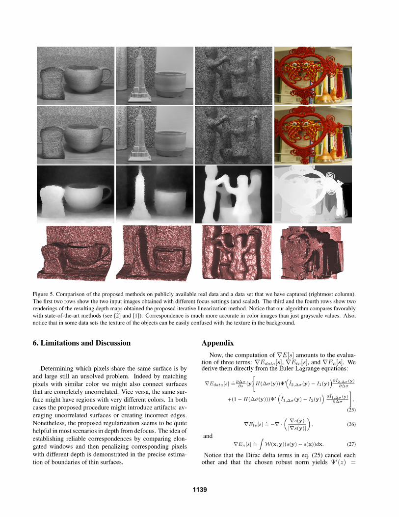
Real Data: We have tested our algorithms on real datathat is publicly available [1, 2], where also specificationsand settings of the hardware can be found, and on a dataset that we have captured with a CANON EOS 5D SLR.In Figure 5 the first two rows show 3 publicly availabledata sets and a data set that we have captured (last col-umn). Each set is made of two defocused images: In oneimage objects closer to the camera are in focus, and in theother image objects further away form the camera are infocus. The third and fourth rows show the resulting depthmap and metallic-rendered surfaces obtained with the pro-posed method. Depth maps are encoded with brightnessintensity values where dark intensities correspond to points
!1 !0.5 0 0.5 1
!1
!0.8
!0.6
!0.4
!0.2
0
0.2
0.4
0.6
0.8
1
true depth
estim
ate
d d
epth
no noise
2% noise
Figure 4. Estimated relative depth map (ordinate) versus groundtruth (abscissa). We plot the mean and 3 times the standard de-viation of the relative depth estimated at 51 planes with no noise(solid blue) and with 2% noise (dotted red).
far away from the camera and bright intensities correspondto points close to the camera. The metallic-rendered sur-faces are used to illustrate the fine-details of the estimatedsurfaces.
In the data set that we have captured, we consider ascene with more elaborate objects containing thin struc-tures. Also, to simulate a realistic scenario where a usercaptures two defocused images, the two images are cap-tured by changing the focus setting of the lens while hold-ing the camera in hand in two different time instants. Thisresulted in a small change in the viewpoint that needed ad-justment. We registered the two frames by using an affinetransformation and used a pyramid scheme to accelerate theconvergence. Notice that, due to the non-planar 3D surfaceof the scene, the alignment is reasonable but not perfect.However, the method is quite robust to such small misalign-ments and still retrieves accurate edges and thin structures(see magnification of a detail in Figure 1). In the simulationwe have used a MacBook 2.4GHz Core 2 Duo, with a (rea-sonably) optimized Matlab implementation of the iteratedlinearization methods. The running time for each simula-tion strongly depends on the amount of defocus in the inputdata. As a rule of thumb, more defocus requires more com-putational time. On average the simulations with the pro-posed method required about 10 minutes on 640× 480 pix-els images. Notice that the nonlocal-means neighborhoodterm increases the number of computations substantially notonly during the evaluation of the weights for each corre-spondence, but also by decreasing the convergence rate ofthe successive over-relaxations algorithm (due to the largerneighborhood structures).
1138
Figure 5. Comparison of the proposed methods on publicly available real data and a data set that we have captured (rightmost column).The first two rows show the two input images obtained with different focus settings (and scaled). The third and the fourth rows show tworenderings of the resulting depth maps obtained the proposed iterative linearization method. Notice that our algorithm compares favorablywith state-of-the-art methods (see [2] and [1]). Correspondence is much more accurate in color images than just grayscale values. Also,notice that in some data sets the texture of the objects can be easily confused with the texture in the background.
6. Limitations and Discussion
Determining which pixels share the same surface is byand large still an unsolved problem. Indeed by matchingpixels with similar color we might also connect surfacesthat are completely uncorrelated. Vice versa, the same sur-face might have regions with very different colors. In bothcases the proposed procedure might introduce artifacts: av-eraging uncorrelated surfaces or creating incorrect edges.Nonetheless, the proposed regularization seems to be quitehelpful in most scenarios in depth from defocus. The idea ofestablishing reliable correspondences by comparing elon-gated windows and then penalizing corresponding pixelswith different depth is demonstrated in the precise estima-tion of boundaries of thin surfaces.
AppendixNow, the computation of ∇E[s] amounts to the evalua-
tion of three terms: ∇Edata[s], ∇Etv[s], and ∇En[s]. Wederive them directly from the Euler-Lagrange equations:
∇Edata[s].=∂∆σ
∂s(y)
"H(∆σ(y))Ψ′
“I2,∆σ(y)− I1(y)
”∂I2,∆σ(y)
∂∆σ
+(1−H(∆σ(y)))Ψ′“I1,∆σ(y)− I2(y)
”∂I1,∆σ(y)
∂∆σ
#,
(25)
∇Etv [s].= −∇ ·
„∇s(y)
|∇s(y)|
«, (26)
and∇En[s]
.=
ZW(x,y)(s(y)− s(x))dx. (27)
Notice that the Dirac delta terms in eq. (25) cancel eachother and that the chosen robust norm yields Ψ′(z) =
1139
z√z2+ε2
. The second term ∂∇E[s]∂s is a matrix and can be
evaluated by defining
〈 ∂∇E[s]∂s
, δ〉 .= 〈 ∂∇Edata[s]∂s
, δ〉+ α〈 ∂∇Etv [s]∂s
, δ〉+ β〈 ∂∇En[s]∂s
, δ〉(28)
where
〈 ∂∇Edata[s]∂s
, δ〉≈“∂∆σ∂s
”2hH(∆σ)Ψ′
“I2,∆σ − I1
”„∂I2,∆σ∂∆σ
«2
+(1−H(∆σ))Ψ′“I1,∆σ − I2
”„∂I1,∆σ∂∆σ
«2 iδ,
(29)
〈 ∂∇Etv [s]∂s
, δ〉 ≈ −∇ ·“∇δ|∇s|
”, (30)
and〈 ∂∇En[s]
∂s, δ〉 = diag
ˆRW(x,y)dx
˜−W(y,x). (31)
Notice that in eq. (29) and eq. (30) we have ignored secondorder derivatives that appear as a result of the derivativeswith respect to s and the (highly nonlinear) terms in theDirac delta.
Rational Filters for Focus Analysis.[2] http://www.eps.hw.ac.uk/˜pf21/pages/page4/page4.html.
Shape from Defocus Code.[3] S. Birchfield and C. Tomasi. Multiway cut for stereo and
motion with slanted surfaces. In Proc. of the Intl. Conf. onComp. Vision, pages 489–495, 1999.
[4] T. Brox. From Pixels to Regions: Partial Differential Equa-tions in Image Analysis. PhD thesis, Saarland University,Apr 2005.
[5] T. Brox, A. Bruhn, N. Papenberg, and J. Weickert. Highaccuracy optical flow estimation based on a theory for warp-ing. European Conference on Computer Vision, 4:25–36,May 2004.
[6] A. Buades, B. Coll, and J.-M. Morel. Nonlocal image andmovie denoising. In International Journal of Computer Vi-sion, volume 76(2), pages 123–139, 2007.
[7] T. Chan, P. Blongren, P. Mulet, and C. Wong. Total variationblind deconvolution. IEEE Intl. Conf. on Image Processing,1997.
[8] T. F. Chan and J. Shen. Image processing and analysis :variational, PDE, wavelet, and stochastic methods. Societyfor Industrial and Applied Mathematics, Philadelphia, 2005.
[9] S. Chaudhuri and A. N. Rajagopalan. Depth from defocus: areal aperture imaging approach. Springer-Verlag, 1999.
[10] J. Ens and P. Lawrence. An investigation of methods fordetermining depth from focus. IEEE Trans. Pattern Anal.Mach. Intell., 15:97–108, 1993.
[11] P. Favaro and S. Soatto. 3-d shape reconstruction and imagerestoration: exploiting defocus and motion-blur. Springer-Verlag, 2006.
[12] P. Favaro, S. Soatto, L. A. Vese, and S. J. Osher. 3-d shapefrom anisotropic diffusion. Proc. IEEE Computer Vision andPattern Recognition, I:179–186, 2003.
[13] S. W. Hasinoff and K. N. Kutulakos. Confocal stereo. Euro-pean Conf. on Computer Vision, pages 620–634, 2006.
[14] A. Klaus, M. Sormann, and K. Karner. Segment-based stereomatching using belief propagation and a self-adapting dis-similarity measure. In Proceedings of Int. Conference onPattern Recognition, pages III: 15–18, 2006.
[15] J. Lee. Digital image smoothing and the sigma filter. Comp.Vision, Graphics and Image Proc., 24(2):255–269, Novem-ber 1983.
[16] D. M. Malioutov, J. K. Johnson, and A. S. Willsky. Walk-sums and belief propagation in gaussian graphical models.Journal of Machine Learning Research, 5, 2006.
[17] D. Nister, H. Stewenius, R. Yang, L. Wang, and Q. Yang.Stereo matching with color-weighted correlation, hierachicalbelief propagation and occlusion handling. In Proc. IEEEConf. on Comp. Vision and Pattern Recogn., pages II: 2347–2354, 2006.
[18] A. Pentland. A new sense for depth of field. IEEE Trans.Pattern Anal. Mach. Intell., 9:523–531, 1987.
[19] O. Shental, D. Bickson, P. H. Siegel, J. K. Wolf, andD. Dolev. Gaussian belief propagation solver for systemsof linear equations. in IEEE Int. Symp. on Inform. Theory(ISIT), 2008.
[20] B. Smith, L. Zhang, and H. Jin. Stereo matching with non-parametric smoothness priors in feature space. In Proc. IEEEConf. on Comp. Vision and Pattern Recogn., pages 485–492,2009.
[21] S. Smith and J. Brady. Susan: A new approach to low-levelimage-processing. Int. J. of Computer Vision, 23(1):45–78,May 1997.
[22] M. Subbarao and G. Surya. Appplication of spatial-domainconvolution/deconvolution transform for determining dis-tance from image defocus. In SPIE, 1992.
[23] H. Tao, H. Sawhney, and R. Kumar. Dynamic depth recoveryfrom multiple synchronized video streams. In Proc. IEEEConf. on Comp. Vision and Pattern Recogn., pages I:118–124, 2001.
[24] C. Tomasi and R. Manduchi. Bilateral filtering for gray andcolor images. In Proc. of the Intl. Conf. on Comp. Vision,pages 839–846, 1998.
[25] M. Watanabe and S. Nayar. Rational filters for passive depthfrom defocus. Intl. J. of Comp. Vision, 27(3):203–225, 1998.
[26] M. Watanabe and S. K. Nayar. Telecentric optics for focusanalysis. IEEE Transactions on Pattern Analysis and Ma-chine Intelligence, 19(12):1360–1365, December 1997.
[27] L. P. Yaroslavsky. Digital Picture Processing. Springer-Verlag New York, Inc., Secaucus, NJ, USA, 1985.
[28] D. M. Young. Iterative Solution of Large Linear Systems.Academic Press, New York, 1971.