ORIGINAL RESEARCH ARTICLEpublished: 22 June 2012

doi: 10.3389/fncom.2012.00039

Recurrent network of perceptrons with three statesynapses achieves competitive classification on real inputsYali Amit1* and Jacob Walker 2

1 Department of Statistics, University of Chicago, Chicago, IL, USA2 Department of Computer Science and Engineering, Michigan State University, East Lansing, MI, USA

Edited by:

Stefano Fusi, Columbia University,USA

Reviewed by:

Harel Z. Shouval, University of TexasMedical School at Houston, USAFlorentin Wörgötter, UniversityGoettingen, Germany

*Correspondence:

Yali Amit, Department of Statistics,University of Chicago, 5734S. University Ave., Chicago,IL 60615, USA.e-mail: amit@galton.uchicago.edu

We describe an attractor network of binary perceptrons receiving inputs from a retinotopicvisual feature layer. Each class is represented by a random subpopulation of the attractorlayer, which is turned on in a supervised manner during learning of the feed forwardconnections. These are discrete three state synapses and are updated based on asimple field dependent Hebbian rule. For testing, the attractor layer is initialized by thefeedforward inputs and then undergoes asynchronous random updating until convergenceto a stable state. Classification is indicated by the sub-population that is persistentlyactivated. The contribution of this paper is two-fold. This is the first example of competitiveclassification rates of real data being achieved through recurrent dynamics in the attractorlayer, which is only stable if recurrent inhibition is introduced. Second, we demonstratethat employing three state synapses with feedforward inhibition is essential for achievingthe competitive classification rates due to the ability to effectively employ both positiveand negative informative features.

Keywords: attractor networks, feedforward inhibition, randomized classifiers

1. INTRODUCTIONWork on attractor network models with Hebbian learning mech-anisms has spanned almost three decades (Hopfield, 1982; Amit,1989; Amit and Brunel, 1997; Wang, 1999; Brunel and Wang,2001; Curti et al., 2004). Most work has focused on the mathe-matical and biological properties of attractor networks with verynaive assumptions on the distribution of the input data; few haveattempted to test these on highly variable realistic data. Suchdata may violate the simple assumptions of the models; theymay have correlation between class prototypes or highly variableclass coding levels. Some attempts have been made to bridge thisgap between theory and practice. Amit and Mascaro (2001), inorder to deal with the complexity of real inputs, propose a twolayer architecture with a non-recurrent feature layer feeding intoa recurrent attractor layer. In the attractor layer, random sub-sets of approximately the same size were assigned to each class.The main role of learning was to update the feedforward connec-tions from the feature layer to the attractor layer. Classificationwas expressed through a majority vote in the attractor layer;actual attractor dynamics proved to be unstable. Assuming a fixedthreshold for all neurons in the attractor layer, it was neces-sary to introduce a field-dependent learning rule that controlledthe number of potentiated synapses that could feed into a sin-gle neuron. Furthermore, to achieve competitive classificationrates, it was necessary to perform a boosting operation withmultiple networks. Subsequent work (Senn and Fusi, 2005) pro-vided an analysis of field-dependent learning, and experimentswere performed on the Latex database. This analysis was fur-ther pursued in Brader et al. (2007) using complex spike-drivensynaptic dynamics. In both cases majority voting was used forclassification.

The contribution of this paper is two-fold. First, we achieveclassification through recurrent dynamics in the attractor layerwhich is stabilized with recurrent inhibition. Second, we employthree state synapses with feedforward inhibition, allowing us toachieve competitive classification rates with one network withoutthe boosting required in Amit and Mascaro (2001). The advantageof a three state feedforward synapse with feedforward inhibitionover a two state synapse stems from the ability to give a pos-itive effective weight to features with high probability on classand low probability off class and a negative effective weight tofeatures with low probability on class and high off class. Bothtypes of features are informative for class/non-class discrimina-tion. The intermediate “control” level of less informative featuresis assigned an effective zero weight. This modification in the num-ber of synaptic states coupled with the appropriate feedforwardinhibition leads to dramatic increases in classification rates. Theuse of inhibition to create effective negative synapses was pro-posed in Scofield and Cooper (1985) in a model of learning inprimary visual cortex. An inhibitory interneuron receives inputfrom the presynaptic neuron and feeds into the postsynaptic neu-ron. This type of feedforward system has since then been used inmany models. Recently in Parisien et al. (2008) a more generalapproach is proposed to achieve effective negative weights avoid-ing a dedicated interneuron for each synapse. This is the approachtaken here.

That synapses have a limited number of states has beenadvocated in a number of papers, see for example, Petersen etal. (1998), O’Connor et al. (2005a,b). Experimental reports onLTP and LTD typically show three synaptic levels for any givensynapse. These include a control level, a depressed state, and apotentiated state, see Mu and Poo (2006), Dong et al. (2008),

Frontiers in Computational Neuroscience www.frontiersin.org June 2012 | Volume 6 | Article 39 | 1

COMPUTATIONAL NEUROSCIENCE

Amit and Walker Recurrent networks of randomized perceptrons

and Collingridge et al. (2010), although the distribution of thestrengths of the potentiated states over the population of synapseshas a significant spread, see Brunel et al. (2004). In our model thethree states are uniformly set at 0, depressed; 1, control; and 2,potentiated.

There has been some work on analyzing the advantages ofmulti-state synapses versus binary synapses for feedforward sys-tems. This work has mainly been in the context of memorycapacity with the assumption of standard uncorrelated randomtype inputs with some coding level. See for example Ben DayanRubin and Fusi (2007), Leibold and Kempter (2008). In broadterms, it appears that multiple level synapses do not provide a sig-nificant increase in memory capacity for low coding levels. Herethe question is quite different. We are interested in the discrimina-tive power of the individual perceptrons on real-world data withsignificant overlap between the features of competing classes andsignificant noise in terms of the presence or absence of a featurein any given class.

2. MATERIALS AND METHODSThe network architecture consists of two layers, a retinotopicinput feature layer F and an attractor layer A that contains ran-dom populations Ac coding for the different classes. The attractorlayer has recurrent connections labeled Jij, between presynapticneuron ai ∈ A and post-synaptic neuron aj ∈ A. The input layerhas only feedforward connections labeled Jkj between feature fkand attractor neuron aj, see Figure 1. The two-layer separationwas initially motivated in Amit and Mascaro (2001) by the fail-ure to obtain stable attractor behavior in recurrent networks ofneurons coding input features such as edges or functions of edgeson real images. The variability in the number of high probabilityfeatures among the different classes was too large as well as theoverlap of features between classes. The coding of classes and the

memory retrieval phenomena—the important characteristics inattractor networks—are therefore pushed to an “abstract” attrac-tor layer with random subsets of neurons coding for each class.These subsets do not have any inherent relation to the sensory orvisual input. In Figure 1 the different color nodes in the attractorlayer A represent different class populations Ac, showing only asubset of the potentiated synapses connecting them. All neuronsin the network are binary, taking only values of 0 or 1. All synapsesin the network can take on three states, 1, baseline; 0, depressed;and 2, potentiated.

2.1. THE INPUT LAYERThe input layer consists of retinotopic arrays of local features com-puted from the input image. There are no connections betweenneurons in the input layer, only feedforward connections toattractor neurons. Each neuron in the input layer corresponds to aparticular visual feature at some location. If a feature is detected ata location, activation is spread to the surrounding neighborhood.Spreading introduces more robustness to local shape variabil-ity and is analogous to the abstraction of the complex neuron.This was first employed in the neo-cognitron (Fukushima andMiyake, 1982). It is a special case of the MAX operation fromRiesenhuber and Poggio (1999). Most experiments were per-formed with binary oriented edge features. These are selective todiscontinuity orientation at eight orientations—multiples of π/4,at each location in the image. The neuron activates at a location ifan edge is present with an angle that is within π/8 of the neuron’sdefined orientation. The neuron thus has a step function tuningcurve as opposed to the traditional bell-shaped tuning curve. Theinput may be compared to an abstraction of the retinotopic mapof complex cells in V1 (Hubel, 1988). In Figure 2 we show theeight edge orientations, an example of an edge detected on animage and illustrate the notion of spreading.

FIGURE 1 | Architecture of network. Input retinotopic feature layeroriented edge features with units denoted fk . Attractor layer A with unitsai , aj . Units of different colors correspond to different class populations Ac .

Feedforward connections (F → A) denoted Jkj and recurrentconnections A → A denoted Jij . Feedforward inhibition ηff and recurrentinhibition ηrc .

Frontiers in Computational Neuroscience www.frontiersin.org June 2012 | Volume 6 | Article 39 | 2

Amit and Walker Recurrent networks of randomized perceptrons

We also experimented with higher level features called edgepairs. These are spatial conjunctions of two different edges, acenter edge and another edge, in five possible relative orienta-tions, (±π/2, ±π/4, 0) anywhere in an adjacent constrainedregion. The size of the area searched for the second edge wasnine pixels. The set of edge pairs centered at a horizontal edgeis illustrated in Figure 3. Similar conjunctions are proposed inRiesenhuber and Poggio (2000). Neurons receptive to such fea-tures can be viewed as coarse curvature selectors and are areanalogous to curvature detectors found in Hegde and Van Essen(2000) and Ito and Komatsu (2004). Edge pairs are more sparselydistributed in generic images than single edges and are quitestable at particular locations on the object. A detailed study ofthe statistics of such features in generic images can be found inAmit (2002).The edge pairs are used without the input edge fea-tures since for each orientation the first pair shown in Figure 3

FIGURE 2 | (A) Eight oriented edges. (B) Neurons respond to a particularfeature at a particular location. (C) If an edge feature is detected at somepixel, neurons in the neighborhood are also activated. In this case, theneighborhood is 3 × 3.

detects orientation, but with higher specificity. The increase infeature specificity allows for an increase in the range of spread-ing, yielding more invariance. Increased spreading also allowsfor greater subsampling of the feature locations to a coarsergrid. The end result is an improvement in the classificationrate.

Feedforward connections to the attractor layer are random; aconnection is established between an input neuron fk and attrac-tor neuron aj with probability pff independently for each inputneuron. The set of input neurons feeding into unit aj is denotedF j. Each attractor neuron therefore functions as a perceptronwith highly constrained weights {0, 1, 2}, which classifies betweenits assigned class and “all the rest.” The random distributionof the feedforward connections is one way to ensure that theseperceptrons constitute different and hopefully weakly correlatedclassifiers [see Amit and Geman (1997)]. They respond to differ-ent subsets of features (Amit and Mascaro, 2001), whose size isdetermined by pff. This is one motivation for using multiple per-ceptrons as opposed to one unit per class. However, as we willsee below, the primary motivation is the ability to code classifi-cation as the sustained activity of this population in a recurrentnetwork.

A complementary approach to randomizing the perceptronsis through the learning process, as opposed to the physical net-work architecture. With full feedforward connectivity—pff = 1—this is achieved through randomization in the potentiation anddepression coupled with the field dependent learning, as detailedin Section 2.4.

2.2. THE ATTRACTOR LAYERClassification takes place in the attractor layer which is fullyconnected. Classes are represented by a population of attractorneurons selected at random with probability pcl. Because of therandom selection there will be some overlap between the popu-lations. Learning of synaptic connections in the attractor layer isdone prior to the presentation of any input images. A class labelis chosen at random, the units coding for that class are activated,and the synapses are updated based on the learning rule describedin Section 2.4. The synapses connecting units within the sameclass population end up potentiated with high probability, andsynapses from units of a class population to non-class units endup depressed with high probability.

Classification is represented as the stable sustained activity ofthe elements of one population and the elimination of activity inthe others. Upon presentation of an image to the network, theattractor layer is initialized with the response of each of the per-ceptrons to the stimulus coming from the input layer. Let Fj ⊂ Fbe the set of input neurons connected to aj. The feedforward

FIGURE 3 | Illustration of five edge pairs centered at a horizontal edge. There are five similar pairs for each of the other seven edge orientations.

Frontiers in Computational Neuroscience www.frontiersin.org June 2012 | Volume 6 | Article 39 | 3

Amit and Walker Recurrent networks of randomized perceptrons

field hff at aj is computed as:

hffj =

∑k∈Fj

Jkj fk − ηff

∑k∈Fj

fk,

ainitialj =

{1 if hff

j > θ

0 otherwise(1)

The inhibition term is local, namely depends on the activity in theset Fj connected to aj.

Typically the number of neurons in the correct class, initial-ized as in (1) by the feedforward connections, will be larger thanthat in other classes. The initialized activity ainitial is in itself suf-ficient for classifying the input, by assigning it to the populationwith the majority of active units, as in Amit and Mascaro (2001).However, classification through a win or take all process of con-vergence to an attractor is more biologically plausible and morepowerful as a tool for sustained short-term memory, for patterncompletion and noise elimination. After the initialization step thefeedforward input is removed, and the updates in the recurrentlayer proceed through stochastic asynchronous dynamics. At stept a random neuron j is selected for update, the field hrc

j is com-puted only from the recurrent layer inputs and compared to thethreshold.

hrcj =

∑i�=j

Jij a(t)i − ηrc

∑i

a(t)i

a(t+1)j =

{1 if hrc

j > θ

0 otherwise(2)

Stable convergence to an attractor state is only possible withthe recurrent inhibition, the second term of the field computationabove. The essential role of inhibition in stabilizing a recurrentnetwork of integrate and fire neurons has been well establishedsince Amit and Brunel (1997). More recently in Amit and Huang(2010) this has been demonstrated in the context of networksof binary neurons, and has been shown to increase the memorycapacity of these networks. Once the network converges, activityin all classes but the winner class is eliminated and the activity ofthe population of the winning class can be sustained for a verylong time, even in the presence of noise.

2.3. THREE STATE SYNAPSESAs indicated above, feedforward inhibition in the network islocal with each attractor neuron aj having its own pool of localinhibitory neurons, which are all connected to the set of inputsFj that feeds into aj. If the synaptic states are constrained toJ = 0, 1, 2, when ηff = 1 the effect of these local inhibitory cir-cuits is simply a constant subtraction of 1 from the synapticstate of every input neuron in Fj. Thus, (1) can be rewritten

as hffj = ∑

k∈Fj(Jkj − 1)fk, or the effective feedforward synaptic

weights become −1, 0, 1. We note that feedforward inhibitorycircuits, with presynaptic neurons having both direct excitatoryand interneuron inhibitory connections to post-synaptic neu-rons, have been found in the hippocampus (Buzsak, 1984), the

LGN (Blitz and Regehr, 2005), and the cerebellum (Mittmannet al., 2005). Models involving such circuits can be found inScofield and Cooper (1985) but would require an interneuronfor each synapse. Our approach is similar to that of Parisienet al. (2008) using a pool of inhibitory neurons receiving non-specific input from the afferent neurons of each attractor neuron.Moreover with full connectivity from the input layer to the attrac-tor layer, only one non-specific inhibitory pool of neurons isneeded that receives input from the feature layer and is con-nected to all neurons in the attractor layer. Regarding the discretestate synapses, there appears to be experimental evidence thatindividual synapses exhibit “three” states: depressed, control, andpotentiated. See for example O’Connor et al. (2005a,b), Mu andPoo (2006), Dong et al. (2008), and Collingridge et al. (2010).

The three synaptic states play a crucial role in distinguishingfeatures that are low probability on the class and higher probabil-ity on other classes. More specifically, imagine dividing the inputfeatures for the given class into three broad categories. “Positive”features are high probability on the class and lower probabilityon the rest, “negative” features are low probability on the classand higher probability on the rest, and all the remaining “null”features have more or less the same probability on the class andon the rest. The first two categories contain informative featuresthat can assist in classification. Features from the third categoryare not useful for classification. Any reasonable linear classifierwould assign the first category of features a positive weight, thesecond category a negative weight and ignore the third category.This is achieved with the three state synapses combined with localinhibition.

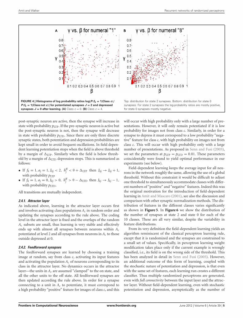
For each perceptron of a given class, the randomized learn-ing process described in Section 2.4, effectively potentiates thesynapses coming from some subset of “positive” features anddepresses the synapses from some subset of “negative” fea-tures. In Figure 4 we show the histograms of log[P(fk = 1|Class c)/P(fk= 1| Class not c)] (log probability ratio of feature onfor image from class c to feature on for image not from classc), for those synapses at state 2 at the end of the learning pro-cess. For state 2 synapses, we specifically focused on featuresfor which p(fk) > 0.3. We also show the histograms of the samequantity for all synapses at state 0 (bottom row). The former areskewed towards the positive side, namely state 2 synapses corre-spond to “positive” features that have higher probability on classthan off class. The state 0 synapses are skewed toward the neg-ative side of the axis corresponding to features that have higherprobability off class than on class. Both types of synapses areinformative for class/non-class discrimination. With only twosynaptic states it is impossible to separate these two types of fea-tures. Performance with two state feedforward synapses with thelocal inhibition is significantly worse, since the non-informative“null” features get confounded with either the “positive” ones orthe “negative” ones.

2.4. LEARNINGLearning in the network is Hebbian and field-dependent. As inprevious models with binary synapses, Amit and Fusi (1994),Senn and Fusi (2005), Romani et al. (2008), and Amit and Huang(2010), learning is stochastic. If both the pre-synaptic and the

Frontiers in Computational Neuroscience www.frontiersin.org June 2012 | Volume 6 | Article 39 | 4

Amit and Walker Recurrent networks of randomized perceptrons

FIGURE 4 | Histograms of log probability ratios log[P(fk = 1|Class c)/

P(fk = 1|Class not c)] for potentiated synapses J = 2 and depressed

synapses J = 0 after learning. (A) Class c = 0. (B) Class c = 4.

Top: distribution for state 2 synapses. Bottom: distribution for state 0synapses. For state 2 synapses the log-probability ratios are mostly positive,for state 0 synapses mostly negative.

post-synaptic neuron are active, then the synapse will increase instate with probability pLTP. If the pre-synaptic neuron is active butthe post-synaptic neuron is not, then the synapse will decreasein state with probability pLTD. Since there are only three discretesynaptic states, both potentiation and depression probabilities arekept small in order to avoid frequent oscillations. In field depen-dent learning potentiation stops when the field is above thresholdby a margin of �LTP. Similarly when the field is below thresh-old by a margin of �LTD depression stops. This is summarized asfollows:

• If fk = 1, aj = 1, Jkj < 2, hffj < θ + �LTP then Jkj → Jkj + 1,

with probability pLTP

• If fk = 1, aj = 0, Jkj > 0, hffj > θ − �LTD then Jkj → Jkj − 1,

with probability pLTD.

All transitions are mutually independent.

2.4.1. Attractor layerAs indicated above, learning in the attractor layer occurs firstand involves activating class populations Ac in random order andupdating the synapses according to the rule above. The codinglevel in the attractor layer is fixed and the overlaps of the randomAc subsets are small, thus learning is very stable and effectivelyends up with almost all synapses between neurons within Ac

potentiated at level 2 and all synapses from neurons in Ac to thoseoutside depressed at 0.

2.4.2. Feedforward synapsesThe feedforward synapses are learned by choosing a trainingimage at random, say from class c, activating its input featuresand activating the population Ac of neurons corresponding to itsclass in the attractor layer. No dynamics occurs in the attractorlayer—the units in Ac are assumed “clamped” to the on state, andall the other units to the off state. All feedforward synapses arethen updated according the rule above. In order for a synapseconnecting to a unit in Ac to potentiate, it must correspond toa high probability “positive” feature for images of class c, and this

will occur with high probability only with a large number of pre-sentations. However, it will only remain potentiated if it is lowprobability for images not from class c. Similarly, in order for asynapse to depress it must correspond to a low probability “nega-tive” feature for class c, with high probability on images not fromclass c. This will occur with high probability only with a largenumber of presentations. As proposed in Senn and Fusi (2005),we set the parameters at pLTP = pLTD = 0.01. These parameterscoincidentally were found to yield optimal performance in ourexperiments (see below).

Field-dependent learning keeps the average input for all neu-rons in the network roughly the same, allowing the use of a globalthreshold. Without this constraint it would be difficult to adjustone threshold to simultaneously accommodate classes with differ-ent numbers of “positive” and “negative” features. Indeed this wasthe original motivation for the introduction of field-dependentlearning in Amit and Mascaro (2001), see also the discussion andcomparison with other synaptic normalization methods. The dis-tribution of features in the different classes varies significantlyas shown in Figure 5. In Figure 6 we show the distribution ofthe number of synapses at state 2 and state 0 for each of the10 classes. These are all very similar, despite the variability infeature distributions.

From its very definition the field-dependent learning yields analgorithm reminiscent of the classical perceptron learning rule,except that it is randomized and the synapses are constrained toa small set of values. Specifically, in perceptron learning weightmodification takes place only if the current example is wronglyclassified, i.e., its field is on the wrong side of the threshold. Thishas been analyzed in detail in Senn and Fusi (2005). However,an additional outcome of this form of learning, coupled withthe stochastic nature of potentiation and depression, is that evenwith the same set of features, each learning run creates a differentclassifier. Thus multiple randomized perceptrons are generated,even with full connectivity between the input layer and the attrac-tor layer. Without field-dependent learning, even with stochasticpotentiation and depression, asymptotically as the number of

Frontiers in Computational Neuroscience www.frontiersin.org June 2012 | Volume 6 | Article 39 | 5

Amit and Walker Recurrent networks of randomized perceptrons

FIGURE 5 | Scatter plots of on-class γ and off-class β feature probabilities for all input features. (A) Class 1, (B) Class 8. There are significant differencesbetween the two classes in the fraction of positive and negative features.

FIGURE 6 | Means (blue) and standard deviations (red) of the number

of synapses in the two informative states (2/0) connected to attractor

neurons after learning with the base parameters. Mean overperceptrons in each class. The field dependent learning mechanismsgenerally create a stable number of potentiated and depressed synapsesacross classes.

pattern presentations for each class grows, all “positive” fea-tures for that class would be potentiated with high probability.As mentioned above the feedforward connectivity probability pff

determines the average size of the subset of features for each

randomized perceptron. Subsets that are too small will not con-tain enough information for the neurons to distinguish classes.Performance initially increases quickly and then slows down aspff reaches around 30%. Indeed, the percentage of synapses withstate 0 or 2 does not vary significantly as pff varies between 20and 100%. It remains around 17–20%. Performance thus almostsolely rests on choosing an appropriate threshold and learningprobabilities. For this reason in the experiments we used fullconnectivity between the input layer and each perceptron.

3. RESULTSThe network was tested on the MNIST handwritten digit dataset(Lecun, 2010). The 28 × 28 images were first treated with a basicform of slant correction. The network was then trained on 10,000randomly ordered examples, 1000 from each digit class, andtested on another 10,000 examples. Attractor neurons were ran-domly assigned to classes. For convenience, the learning phaseof the attractor classes was skipped. All the in-class attractorsynapses were thus assigned a state of 2 and the rest 0. This short-cut has no effect on the final behavior of the network. Duringfeedforward training, the attractor neurons of a given classes wereclamped on, while all other neurons in the layer were inactive.Learning of the feedforward synapses then took place after theinput pattern was presented and the field of each neuron in theattractor layer was calculated. Field-dependent learning impliedthat potentiation stopped if the feedforward field exceeded �LTP

units above threshold, and depression stopped if the field was lessthan �LTD units below threshold.

Testing began with an initial presentation of a pattern thatactivated the attractor neurons without any recurrent dynam-ics. Typically many attractor neurons of the correct class wereactivated together with a number of neurons in other classes.Then the input was removed, and classification was representedby the convergence to an attractor corresponding to a single class.

Frontiers in Computational Neuroscience www.frontiersin.org June 2012 | Volume 6 | Article 39 | 6

Amit and Walker Recurrent networks of randomized perceptrons

Table 1 | Base parameters for experiments.

No. of attractor neurons:

2000

Feedforward connection

probability: pff = 1

Class proportion: pcl = 0.1 Features: Edges Recurrent inhibition:

ηrc = 1.5

Potentiation probability:pLTP = 0.01

Depression probability:pLTD = 0.01

Threshold: θ = 0Margins: �LTP = �LTD = 5

Spreading: 5 × 5 Feedforward inhibitionηff = 1

Sustained activity is present only among neurons coding for oneclass. Neuron updates in the attractor layer were asynchronous,and continued until convergence to a steady state occurred–nochanges in neural states. Base parameters are in Table 1. Whenusing a training set of 10,000 images (1000 per class) eachimage was presented three times—all in random order. Withsmaller training sets the number of presentations was rescaledaccordingly. For example with 1000 images (100 per class) weused 30 presentations per image. The base classification ratewas 96.0%.

3.1. TWO STATE vs. THREE STATE SYNAPSESTo compare two state vs. three state synapses we kept all baseparameters listed in Table 1 the same and modified only the twoinhibition levels. Feedforward inhibition for two states was set at0.05 instead of 1 in the three state network, and attractor inhibi-tion was set at 0.75 instead of 1.5. Using one perceptron per classthe classification rates were 48.1% for two states and 81.2% forthree states. For the full size attractor layer, with two state synapsesthere is a drastic difference between performance of classificationwith straightforward voting and using attractor dynamics. Votingyields a 90.0% classification rate whereas the recurrent dynam-ics produced the much lower rate of 64.4%. In contrast the threestate network yields similar performance with voting or attractordynamics once the size of the class populations Ac is on the orderof several tens. For lower population sizes the attractor dynamicsis less stable and voting performs much better. The classificationrate at 96.0%., with the base parameter settings (Table 1), is com-parable to support vector machines. For the full size attractorlayer, convergence failed only with eight examples out of 10,000.

Of particular interest is the fact that with two state synapsesthere was significant sensitivity to the size of the margins. It isclear that the three state system not only performs better, but isalso much more stable to the margin settings and is nearly sym-metric. For the two state system there is a marked preference fora larger depression margin, meaning that it is “easier” to achievedepression. In this scenario, synapses corresponding to the lessinformative features will most likely be depressed. It is possiblethat the errors incurred by non-informative features “voting” fora class are larger than when they “vote” against. The results forclassification using a set of different margin values are shown inTable 2 for both two state and three state synapses.

3.2. SENSITIVITY TO PARAMETER SETTINGSKeeping all other parameters constant at the base level, eachparameter was modified over some range. The classification ratebased on recurrent dynamics was then compared. The networkseems to be fairly robust to changes in parameters in a neighbor-hood of the base parameters.

Table 2 | Classification results with different margin values.

(A)

�LTD�LTP 0 5 50 1000 69% 38% 5% 0%5 86% 69% 6% 0%50 88% 87% 8% 0%100 88% 86% 8% 0%(B)

�LTD�LTP 0 5 50 1000 96% 96% 94% 89%5 96% 96% 95% 91%50 94% 94% 95% 93%100 86% 86% 89% 90%

(A) two state synapses (B) three state synapses.

Table 3 | Dependence of classification rates on size of attractor layer

and mean size Ac of class populations.

Size of A, Ac 100, 10 250, 25 500, 50 1000, 100 2000, 200

Rate 81% 93.0% 94.6% 95.8% 96.0%pcl 0.05 0.1 0.15 0.2Ac 100 200 300 400Rate 95.7% 96.0% 95.6% 10.0%

3.2.1. Size of attractor layer and size of class populationEach class population is chosen randomly with proportion pcl,yielding some overlaps between class populations. When the sizeof the population coding for each class in the attractor layer is toosmall classification degrades due to a combination of the lack ofsufficient randomized perceptrons and instability in the attractordynamics. Thus with 100 neurons in A, namely 10 per class onaverage, the rate is 81%, with 250 neurons the classification raterises to 93%. In contrast when the proportion of each class getstoo large (e.g., pcl = 0.2) with the size of A held fixed, the overlapsare too large and recurrent dynamics collapses. These results aresummarized in Table 3.

3.2.2. Learning rateWe also see that slow learning is preferable. If the potentiationprobability is high many irrelevant features can get potentiated,and as mentioned above the randomizing effect on the perceptronsis lost. Sensitivity to the depression rate is not as pronounced,which may reflect the fact that most of the information forclassification lies in “negative features”, namely features that are lowprobability on class and high probability on the rest. See Table 4.

3.2.3. Other parametersFeedforward connectivity affects the number of features used ineach randomized perceptron. The baseline is full connectivity so

Frontiers in Computational Neuroscience www.frontiersin.org June 2012 | Volume 6 | Article 39 | 7

Amit and Walker Recurrent networks of randomized perceptrons

Table 4 | Dependence of classification rate on learning rates.

pLTP 0.001 0.01 0.05 0.1 0.5

Rate 95.2% 96.0% 95.7% 94.6% 73.2%

pLTD 0.001 0.01 0.05 0.1 0.5

Rate 94.2% 96.0% 95.7% 95.3% 93.6%

Table 5 | Classification rates as feedforward connectivity, the

threshold and the spreading vary individually around baseline

given in Table 1.

pff 0.05 0.125 0.25 0.5 1

Rate 90.6% 93.6% 94.8% 95.6% 96.0%

θ –30 –15 0 15 30

Rate 95.6% 95.8% 96.0% 95.9% 96.1%

Spread None 3 × 3 5 × 5

Rate 94.7% 96.3% 96.0%

that randomization is only a result of the combination of stochas-tic and field-dependent learning. Lowering the connectivity doesnot have a major effect until it drops by an order of magnitude atwhich point there are not enough input features to generate suffi-ciently good classifiers. The performance does not seem to dependsignificantly on the threshold in a reasonable range. We also seethat some advantage is gained from spreading. See Table 5.

3.3. COMPARISON TO OTHER CLASSIFIERSThe network performs at a level comparable to state of the artclassifiers such as support vector machines, which interestinglyperformed optimally with the simple linear kernel (see Table 6).The network performed slightly better with the smaller trainingsets of 1000 (100 per class) or 100 (10 per class). The softwarefor the SVMs was a specialized version of libsvm (Huang et al.,2011) that used one-versus-all classification. The input layer wastreated as an n-dimensional vector of 1s and 0s. All other libsvmparameters were set at the default level.

To assess the loss involved in using discrete three state synapsesand a classification decision based on convergence to a single sta-ble population (as opposed to simple voting) we experimentedwith a voting scheme among large numbers of classical per-ceptrons, 200 per class, each classifying one class against therest. Each perceptron was fully connected to the input layer andtrained using the classical perceptron learning rule, with continu-ous unbounded weights. Training data was presented in randomorder, with a step size of 0.001 for edges and 0.0001 for edge-pairs. The randomization of the presentation order of the trainingdata produced the randomization in the different perceptronsassigned to the same class. Classification was based on the groupof perceptrons with the highest aggregate output. The percep-trons were also trained on three iterations of the training datafor 10,000 examples, 30 iterations for 1000, and 300 iterations for100 examples. The results seem to indicate that nothing is lost inusing constrained perceptrons with discrete three state synapses.On the other hand the linear SVM, which is also a perceptron,albeit trained somewhat differently, achieves its high classificationrate with only one unit per class, showing that with a differ-ent learning scheme and unconstrained synapses a large pool of

Table 6 | Comparison of classifiers with edges.

Training Network SVM-linear SVM-gauss Multiple

examples (%) (%) (%) perceptrons

per class (%)

1000 96.0 97.1 96.9 96.0

100 95.3 95.9 94.0 92.3

10 86.8 86.6 78.7 73.7

Table 7 | Comparison of classifiers with edge-pairs.

Training Network SVM-linear SVM-gauss Multiple

examples (%) (%) (%) perceptrons

per class (%)

1000 97.4 97.9 97.1 96.5

100 96.2 96.5 93.7 92.8

10 87.1 86.9 80.8 70.1

perceptrons is not really needed—as long as classification is readout directly from the output of the units and not through thesustained activity of a class-population in the attractor layer.

Also in Table 7 observe that performance is improved with themore informative edge-pair features. It is to be expected that evenfurther improvements could be achieved with even more com-plex features; however, it is at this point unclear how these shouldbe defined. Using all triples, for example, is combinatorially pro-hibitive; there thus needs to be some mechanism for selection ofcomplex features.

4. DISCUSSIONWe find it encouraging that competitive classification rates canbe achieved with a highly constrained network of binary neu-rons, discrete three state synapses and simple field dependentHebbian learning. Moreover classification is successfully coded inthe dynamics of the attractor layer through the sustained activityof a class population. The use of a population of neurons to codefor a class together with the stochastic learning rule turn out tobe an asset in the sense that we gain a collection of weakly corre-lated randomized classifiers whose aggregate classification rate ismuch higher than that of any individual one. However, it shouldbe noted that for mere classification, using simple voting, only10–20 units per class are needed to achieve competitive rates. Thelarger number of units is needed to stabilize the attractor dynamics.

Of further interest is the comparison to the outcome of fullperceptron learning with multiple perceptrons. Here the only ran-domization is the order of the training example presentations,not the decision whether to modify a weight or not. It may bethat this does not introduce sufficient randomness in the classi-fiers. Another point is that no weight penalization occurs in theperceptron learning rule, whereas the network we propose has adrastic penalization in that weights are constrained to three states.Note that the best performance was recorded with linear SVM’swith only one unit per class. In other words, there exists a set ofweights for the synapses that can achieve very low error rates withonly 10 linear classifiers of class against non-class. This, however,

Frontiers in Computational Neuroscience www.frontiersin.org June 2012 | Volume 6 | Article 39 | 8

Amit and Walker Recurrent networks of randomized perceptrons

requires the weight penalization incorporated in the SVM lossfunction, which does not appear in ordinary perceptron learning.

The advantage of three state synapses with feedforward inhi-bition for feedforward processing is apparent already in thebehavior of a single perceptron. For simple recurrent networkswith random input patterns the advantage of signed synapses interms of capacity was noted in Nadal (1990). Recently, there hasbeen interest in the distribution of synaptic weights in Purkinjeecells in cerebellum (Brunel et al., 2004). The analysis of this dis-tribution made the assumption that all weights were positive.Based on the experiments reported here this would seem ratherwasteful. The experiments reported in Brunel et al. (2004) reporton the role of inhibition achieved by an individual interneu-ron, in forcing inputs to be highly coincident in time. However,

they do not show the behavior of the post-synaptic neuron inthe presence of stimulation of a large number of input neu-rons, which would trigger the collective inhibitory correction tothe synapses, yielding an effective negative effect for depressedsynapses. The assumption in Brunel et al. (2004) is that the silentsynapses correspond to those with lowest weights. A provocativebut not impossible alternative is that the silent synapses corre-spond to those that would have had no effect after factoring inthe inhibitory effect of the full array of stimuli, and that the spikein the distribution is actually located somewhere in middle of thedistribution.

ACKNOWLEDGMENTSPartially supported by NSF DMS-0706816.

REFERENCESAmit, D. J. (1989). Modelling Brain

Function: the World of AttractorNeural Networks. Cambridge, UK:Cambridge University Press.

Amit, Y. (2002). 2d Object Detection andRecognition: Models, Algorithms andNetworks. Cambridge, MA: MITPress.

Amit, D. J., and Brunel, N. (1997).Model of global spontaneousactivity and local structured activ-ity during delay periods in thecerebral cortex. Cereb. Cortex 7,237–252.

Amit, D. J., and Fusi, S. (1994).Learning in neural networks withmaterial synapses. Neural Comput.6, 957–982.

Amit, Y., and Geman, D. (1997). Shapequantization and recognition withrandomized trees. Neural Comput.9, 1545–1588.

Amit, Y., and Huang, Y. (2010). Precisecapacity analysis in binary networkswith multiple coding level inputs.Neural Comput. 22, 660–688.

Amit, Y., and Mascaro, M. (2001).Attractor networks for shaperecognition. Neural Comput. 13,1415–1442.

Ben Dayan Rubin, D. D., and Fusi,S. (2007). Long memory lifetimesrequire complex synapses andlimited sparseness. Front. Comput.Neurosci. 1:7. doi: 10.3389/neuro.10.007.2007

Blitz, D. M., and Regehr, W. G. (2005).Timing and specificity of feed-forward inhibition within the LGN.Neuron 45, 917–928.

Brader, J. M., Senn, W., and Fusi, S.(2007). Learning real-world stim-uli in a neural network with spike-driven synaptic dynamics. NeuralComput. 19, 2881–912.

Brunel, N., Hakim, V., Isope, P., Nadal,J.-P., and Barbour, B. (2004).Optimal information storage andthe distribution of synaptic weights:

perceptron versus purkinje cell.Neuron 43, 745–757.

Brunel, N., and Wang, X.-J. (2001).Effects of neuromodulation in acortical network model of objectworking memory dominated byrecurrent inhibition. J. Comput.Neurosci. 11, 63–85.

Buzsak, G. (1984). Feed-forwardinhibition in the hippocampalformation. Prog. Neurobiol. 22,131–153.

Collingridge, G. L., Peineau, S.,Howlang, J. G., and Wang, Y. T.(2010). Long-term depression inthe cns. Nat. Rev. Neurosci. 11,459–473.

Curti, E., Mongillo, G., La Camera,G., and Amit, D. J. (2004). Meanfield and capacity in realisticnetworks of spiking neuronsstoring sparsely coded randommemories. Neural Comput. 16,2597–2637.

Dong, Z., Han, H., Cao, H., Zhang, X.,and Xu, L. (2008). Coincident activ-ity of converging pathways enablessimultaneous long-term potentia-tion and long-term depression inhippocampal ca1 network in vivo.PLoS ONE 3:e2848. doi: 10.1371/journal.pone.0002848

Fukushima, K., and Miyake, S. (1982).Neocognitron: a new algorithmfor pattern recognition toler-ant of deformations and shiftsin position. Pattern Recogn. 15,455–469.

Hegde, J., and Van Essen, D. C. (2000).Selectivity for complex shapes inprimate visual area v2. J. Neurosci.20, RC61.

Hopfield, J. J. (1982). Neural networksand physical systems with emer-gent collective computational abili-ties. Proc. Natl. Acad. Sci. U.S.A. 79,2554–2558.

Huang, T.-K., Weng, R., and Lin, C.J. (2011). libsvm. www.csie.ntu.edu.tw/cjlin/libsvmtools/

Hubel, D. H. (1988). Eye, Brain, andVision. New York, NY: ScientificAmerican Library.

Ito, M., and Komatsu, H. (2004).Angle representation in area v2.J. Neurosci. 24, 3313–3324.

Lecun, Y. (2010). Mnist Database.yann.lecun.com/exdb/mnist/.

Leibold, C., and Kempter, R. (2008).Sparseness constrains the prolonga-tion of memory lifetime via synap-tic metaplasticity. Cereb. Cortex 18,67–77.

Mittmann, W., Koch, U., and Häusser,M. (2005). Feed-forward inhibitionshapes the spike output of cerebellarPurkinje cells. J. Physiol. 563(Pt 2),369–378.

Mu, Y., and Poo, M. (2006). Spiketiming-dependent ltp/ltd mediatesvisual experience-dependentplasticity in a developingretinotectal system. Neuron 50,115–125.

Nadal, J.-P. (1990). On the storagecapacity with sign-constrainedsynaptic couplings. Network 1,463–466.

O’Connor, D. H., Wittenberg, G. M.,and Wang, S. S. (2005a). Dissectionof biderctional synaptic plastic-ity into saturable unidirectionalprocesses. J. Neurophysiol. 94,1565–1573.

O’Connor, D. H., Wittenberg, G. M.,and Wang, S. S. (2005b). Gradedbidirectional synaptic plasticity iscomposed of switch-like unitaryevents. Proc. Natl. Acad. Sci. U.S.A.102, 9679–9684.

Parisien, C., Anderson, C. H., andEliasmith, C. (2008). Solvingthe problem of negative synapticweights in cortical models. NeuralComput. 20, 1473–1494.

Petersen, C. C. H., Malenka, R. C.,Nicoll, R. A., and Hopfield, J. J.(1998). All-or-none potentiation atca3-ca1 synapses. Proc. Natl. Acad.Sci. U.S.A. 95, 4732–4737.

Riesenhuber, M., and Poggio, T. (1999).Hierarchical models of object recog-nition in cortex. Nat. Neurosci. 2,1019–1025.

Riesenhuber, M., and Poggio, T. (2000).Models of object recognition. Nat.Neurosci. 3, 1199–1204.

Romani, S., Amit, D. J., and Amit, Y.(2008). Optimizing one-shot learn-ing with binary synapses. NeuralComput. 20, 1920–1958.

Scofield, C. L., and Cooper, L. N.(1985). Development and proper-ties of neural networks. Contemp.Phys. 26, 125–145.

Senn, W., and Fusi, S. (2005).Convergence of stochastic learningin perceptrons with binary synapses.Phys. Rev. E 71, 61907.1–61907.12.

Wang, X. J. (1999). Synaptic basisof cortical persistent activity: theimportance of NMDA receptors toworking memory. J. Neurosci. 19,9587–9603.

Conflict of Interest Statement: Theauthors declare that the researchwas conducted in the absence of anycommercial or financial relationshipsthat could be construed as a potentialconflict of interest.

Received: 08 March 2012; accepted: 05June 2012; published online: 22 June2012.Citation: Amit Y and Walker J (2012)Recurrent network of perceptrons withthree state synapses achieves competi-tive classification on real inputs. Front.Comput. Neurosci. 6:39. doi: 10.3389/fncom.2012.00039Copyright © 2012 Amit and Walker.This is an open-access article dis-tributed under the terms of theCreative Commons Attribution NonCommercial License, which permitsnon-commercial use, distribution, andreproduction in other forums, providedthe original authors and source arecredited.

Frontiers in Computational Neuroscience www.frontiersin.org June 2012 | Volume 6 | Article 39 | 9