Redalyc.Flow of multiparticle collision dynamics fluids confined by ...

Revista del Centro de Investigación.

Universidad La Salle

ISSN: 1405-6690

[email protected]


México

AYALA-HERNÁNDEZ, Arturo; HÍJAR, Humberto

Flow of multiparticle collision dynamics fluids confined by physical barriers

Revista del Centro de Investigación. Universidad La Salle, vol. 12, núm. 45, enero-junio,

2016, pp. 37-70


Distrito Federal, México

Disponible en: http://www.redalyc.org/articulo.oa?id=34247483003

Cómo citar el artículo

Número completo

Más información del artículo

Página de la revista en redalyc.org

Sistema de Información Científica

Red de Revistas Científicas de América Latina, el Caribe, España y Portugal

Proyecto académico sin fines de lucro, desarrollado bajo la iniciativa de acceso abierto

http://www.redalyc.org/revista.oa?id=342



http://www.redalyc.org/articulo.oa?id=34247483003

http://www.redalyc.org/comocitar.oa?id=34247483003

http://www.redalyc.org/fasciculo.oa?id=342&numero=47483

http://www.redalyc.org/articulo.oa?id=34247483003


http://www.redalyc.org

Revista del Centro de Investigación de la Universidad La Salle

Vol. 12, No. 45, enero-junio, 2016: 37-70

http://ojs.dpi.ulsa.mx/index.php/rci/

Flow of multiparticle collision dynamics fluids confined by physical

barriers

Flujo dinámico colisional de múltiples partículas de fluidos confinados por

barreras físicas

Arturo AYALA-HERNÁNDEZ, Humberto HÍJAR1

Universidad La Salle Ciudad de México (México)

Fecha de recepción: octubre de 2015

Fecha de aceptación: marzo de 2016

Resumen

En los últimos años, la Dinámica Colisional de Múltiples Partículas (MPC, por sus siglas

en inglés), se ha convertido en una herramienta computacional muy poderosa que permite

hacer simulaciones de fluidos con características muy parecidas a las de un sistema real.

Recientemente, hemos presentado un método que permite confinar fluidos de MPC en

geometrías complejas el cual está basado en el uso de fuerzas explícitas (Ayala-Hernández

and Híjar, 2016). En este trabajo extendemos este método para llevar a cabo simulaciones

de flujo en una geometría planar delgada. Lo anterior se logra al introducir dos superficies

sólidas planas y paralelas, constituidas por partículas que interactúan con las partículas de

fluido de MPC por medio de fuerzas repulsivas explícitas. Probamos la aplicabilidad del

método propuesto en simulaciones de un fluido confinado entre los dos planos paralelos y

sujeto a un campo de fuerza uniforme. Encontramos que nuestro modelo reproduce el flujo

de Poiseuille plano previsto por la hidrodinámica, con condiciones de frontera de

deslizamiento. Llevamos a cabo una gran cantidad de experimentos numéricos, variando

1 E-mail: [email protected]

Revista del Centro de Investigación de la Universidad La Salle por Dirección de Posgrado e

Investigación. Universidad La Salle Ciudad de México se distribuye bajo una Licencia Creative Commons Atribución-NoComercial-CompartirIgual 4.0 Internacional.

mailto:[email protected]

http://delasalle.ulsa.mx/rci/show/spanish/about/inicio.aspx

http://delasalle.ulsa.mx/rci/show/spanish/about/inicio.aspx

http://creativecommons.org/licenses/by-nc-sa/4.0/



Híjar, H., Ayala, A.

38 ISSN 1405-6690 impreso

ISSN 1665-8612 electrónico

los parámetros de simulación en un rango amplio y realizamos mediciones para caracterizar

al fluido y a la interacción fluido-sólido, e. g., el deslizamiento en la frontera sólida y la

viscosidad efectiva del fluido. Finalmente, determinamos las condiciones para las cuales

pueden ser simulados flujos de Poiseuille con condiciones de frontera de no deslizamiento.

Palabras clave: Técnicas computacionales en dinámica de fluidos, flujos laminares,

Colisión Dinámica de múltiples partículas (MPC), dinámicas moleculares.


Revista del Centro de Investigación. Universidad La Salle

Vol. 12, No. 45, enero-junio, 2016: 37-70 39

Abstract

In the last years, Multiparticle Collision Dynamics (MPC) has become a major

computational tool that allows for simulating fluids with properties closely resembling

those of a physical fluid. Recently, we have introduced a methodology for confining MPC

fluids in complex geometries based on the use of explicit forces (Ayala-Hernandez and

Híjar, 2016). In this work, we extend this method in order to simulate flow in a slitlike

geometry. This is achieved by introducing two solid parallel plane surfaces consisting of

particles that interact with the particles of the MPC fluid by means of explicit repulsive

forces. We test the applicability of the proposed technique in simulations of fluids confined

between these parallel planes and subjected to a uniform force field. We find that our model

yields the correct plane Poiseuille flow expected from hydrodynamics with slip boundary

conditions. We carry out a large amount of numerical experiments in which the simulations

parameters are varied in a wide range, in order to measure important quantities

characterizing the flow and the fluid-solid interaction, e.g., the slip at the solid boundary

and the effective viscosity of the fluid. Finally, we determine the conditions for which plane

Poiseuille flows with stick boundary condition can be simulated.

Keywords: Computational techniques in fluid dynamics, Laminar flows, Multiparticle

Collision Dynamics, Molecular Dynamics




Introducción

Multiparticle Collision Dynamics (MPC) is a simulation technique introduced by

Malevanets and Kapral (1999; 2000), that has been proved to be a very useful method for

studying diverse systems of soft condensed matter (Yeomans, 2006; Kapral, 2008;

Gompper et al, 2009). Some adventages of MPC that make it so appealing for the

simulation of complex fluids are summarized as follows. Fisrt, MPC is based on particles

and, consequently, can be combined with Molecular Dynamics (MD) (Frenkel and Smith,

2002; Griebel et al, 2007) in the study of systems where dissipative time and length-scales

coexist with microscopic scales, e.g., colloids and polymer solutions (Padding and Louis,

2004; Ali et al, 2004; Hecht et al, 2005; Padding and Louis, 2006). Second, the MPC

algorithm is stochastic and gives rise to the proper hydrodynamic fluctuations and

Brownian forces (Yeomans, 2006; Padding and Louis, 2004; Híjar and Sutmann, 2011).

Third, MPC is relatively simple and very stable over long-time simulations. Fourth, it has

been succesfully described analytically from the stand points of the kinetic theory and the

projection operator technique (Tüzel et al, 2003; Ihle and Kroll, 2001, 2003, Pooley and

Yeomans, 2005, Gompper et al., 2009).

Thus, in summary, MPC constitutes a powerful mesoscopic simulation method, for which

an excellent understanding has been achieved. Some applications of MPC include the

simulation of colloids and polymers (Malevanets and Kapral, 2000; Padding and Louis,

2004, Kikuchi et al, 2002), of polymers under flow (Yeomans, 2006; Malevanets and

Yeomans, 1999; Ripoll et al, 2004), of flow around objects (Lamura et al., 2001;

Allahyarov and Gompper, 2002), of vesicles under flow (Noguchi and Gompper, 2005), of

particle sedimentation (Jordá et al, 2010, 2012), and of tracking control of colloidal

particles immersed in steady shear flows (Híjar, 2013; Fernández and Híjar, 2015; Híjar,

2015).

Despite of the success that MPC has had, it should be mentioned that in most of the studied

cases, MPC fluids are assumed to extend ad infinitum, a situation that in practice is

approximated by imposing periodic boundary conditions. In this context, it is still an

uncompleted task to find a general procedure to impose spatial constraints on the motion of

fluids simulated by MPC. Diverse authors have achieved the confinement of MPC fluids by

supplementing the simulation with the so-called bounce-back boundary conditions, which

simply reflect the incoming particles back into the bulk system, and are in some sense

equivalent to impose the presence of hard walls (Malevanets and Kapral, 1999; Inoue et al,

2002; Jordá et al, 2010; Withmer and Luijten, 2010). A comparison of the performance of

some of these confining methods based on such hard walls can be found in (Withmer and




Luijten, 2010). Some fundamental issues that have been introduced in that reference

concern procedures that can be followed to simulate the presence of moving walls, and

quiescent and mobile surfaces with partial slip boundary conditions. More recently, the

modifications in the stress tensor produced by the interaction of the MPC particles with

reflecting walls have been rigorously calculated for confinement in a slit geometry with a

simple shear in (Winkler and Huang, 2009). The analysis carried out there, has yielded a

properly modified form of the MPC algorithm in the presence of walls that prevents any

surface slip of the confined fluid and allows for simulating the correct plane Couette

velocity profile.

More recently, we have proposed an alternative procedure for simulating restrictive

boundary conditions in MPC in which physical walls are explicitely considered by means

of interaction potentials yielding forces on the MPC particles (Ayala-Hernández and Híjar,

2016). We have been able to obtain a closed expression for these forces, which could be

integrated in a completely similar fashion as the equations of motion are integrated in

hybrid MD-MPC schemes. Using this procedure we have simulated cylindrical Poiseuille

flow of MPC fluids (Ayala-Hernández and Híjar, 2016) and observed the correct

hydrodynamic flow between two coaxial cylinders (Híjar and Ayala-Hernández, 2016;

Ayala 2016). These kind of force-based boundary conditions, could be preferable to those

imposed by hard walls from the physical point of view since they are closer to simulate the

situation encountered in real systems, where fluid-solid interactions always arise from laws

of force.

With the pursue of demostrating the analysis of the effects that force-based boundary

conditions have on MPC fluids, we will consider another application of the method

introduced in (Ayala-Hernández and Híjar, 2016), namely, the simulation of plane

Poiseuille flow between two parallel planes, a problem that has been considered by diverse

authors since the introduction of MPC. In their pioneering work, Malevanets and Kapral

implemented the simulation of two-dimensional plane Poiseuille flow with MPC, in order

to demonstrate the general viability of the algorithm (Malevanets and Kapral, 1999).

Simulations of two-dimensional Poiseuille flow of MPC fluids were subsequently carried

out in (Lamura et al., 2001). In these two cases, flow was forced through the two-

dimensional geometry by allowing particles within a specific region to have an average

velocity coinciding with the analytical expression at the collision step. Simulations of three-

dimensional Poiseuille flow using MPC were first reported in (Allahyarov and Gompper,

2002), where flow was promoted by the application of an explicit field of force. The

authors supplemented their method with a simple rescaling thermostat to avoid viscous

heating. Subsequent analysis of plane Poiseuille flow in MPC (Huang et al., 2010; Withmer

and Luijten, 2010; Imperio et al., 2011), have also considered the approach based on direct




forces and thermostats. An excellent comparison of these methods is presented in

(Bolintineanu et al., 2012) where it can be appreciated that details in the simulation

technique could produce rather large modifications in the simulated flow. For instance, the

use of different thermostats (Huang et al., 2015) could produce effective variations in the

viscosity of the fluid, and the implementation of different boundary conditions could yield

diverse degrees of slip at the confining walls. We will notice that our method based on

explicit fluid-solid interactions will exhibit some drawbacks similar to those present in the

aforementioned works. However, we will show that in the limit in which the MPC

dynamics is dominated by interparticle collisions, our methodology yields flows that match

very well the analytical expression.

We will also notice that our method will face some difficulties that are also present in

simulations of MPC fluids constrained by hard walls. These difficulties are, mainly, the

need for incorporating virtual particles in partially empty cells at the collision step, and the

problem of removing partial slip at the confining walls. We will carefully discuss the way

in which our method can be addapted to reproduce the correct velocity profile with no-slip

boundary conditions in the case of a slit geometry. It is important to stress that the problem

to be addressed, lies within a more general context in which the use of explicit forces could

yield the simulation of MPC fluids in complex geometries, as it has been discussed in detail

in (Ayala-Hernández, 2016). From a methodological point of view, it sounds plausible to

test the viability of the method in simple situations first and, subsequently, in more

complicated cases. The purpose of the present analysis is, precisely, to demonstrate that the

method based on forces is valid to simulate a simple flow, that is well understood and can

be analyzed from fluid mechanics for very well defined situations. In further publications,

we will progressively study the applicability of this technique in cases of increasing

geometric complexity (Ayala-Hernández, 2016; Híjar and Ayala-Hernández, 2016).

This paper is organized as follows. In section 2 we will present the expression for the

confinement force exerted by an even plane surface on the MPC particles, which will be

used subsequently in our simulations. In section 3 we will discuss the details about our

numerical implementation. In section 4 we will present the results obtained from a large

number of numerical experiments of simulation of plane Poiseuille flow. Finally, in Section

5 we will state our conclusions, and summarize the advantages and limitations of our

approach.




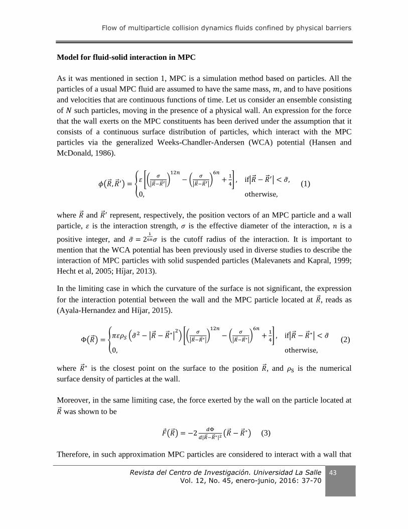
Model for fluid-solid interaction in MPC

As it was mentioned in section 1, MPC is a simulation method based on particles. All the

particles of a usual MPC fluid are assumed to have the same mass, 𝑚, and to have positions

and velocities that are continuous functions of time. Let us consider an ensemble consisting

of 𝑁 such particles, moving in the presence of a physical wall. An expression for the force

that the wall exerts on the MPC constituents has been derived under the assumption that it

consists of a continuous surface distribution of particles, which interact with the MPC

particles via the generalized Weeks-Chandler-Andersen (WCA) potential (Hansen and

McDonald, 1986).

𝜙(�⃗� , �⃗� ′) = {휀 [(

𝜎

|�⃗� −�⃗� ′|)12𝑛

− (𝜎

|�⃗� −�⃗� ′|)6𝑛

+1

4] , if|�⃗� − �⃗� ′| < �̃�,

0, otherwise,

(1)

where �⃗� and �⃗� ′ represent, respectively, the position vectors of an MPC particle and a wall

particle, 휀 is the interaction strength, 𝜎 is the effective diameter of the interaction, 𝑛 is a

positive integer, and �̃� = 21

6𝑛𝜎 is the cutoff radius of the interaction. It is important to

mention that the WCA potential has been previously used in diverse studies to describe the

interaction of MPC particles with solid suspended particles (Malevanets and Kapral, 1999;

Hecht et al, 2005; Híjar, 2013).

In the limiting case in which the curvature of the surface is not significant, the expression

for the interaction potential between the wall and the MPC particle located at �⃗� , reads as

(Ayala-Hernandez and Híjar, 2015).

Φ(�⃗� ) = {𝜋휀𝜌𝑆 (�̃�

2 − |�⃗� − �⃗� ∗|2) [(

𝜎

|�⃗� −�⃗� ∗|)12𝑛

− (𝜎

|�⃗� −�⃗� ∗|)6𝑛

+1

4] , if|�⃗� − �⃗� ∗| < �̃�

0, otherwise,

(2)

where �⃗� ∗ is the closest point on the surface to the position �⃗� , and 𝜌S is the numerical

surface density of particles at the wall.

Moreover, in the same limiting case, the force exerted by the wall on the particle located at

�⃗� was shown to be

𝐹 (�⃗� ) = −2𝑑Φ

𝑑|�⃗� −�⃗� ∗|2(�⃗� − �⃗� ∗) (3)

Therefore, in such approximation MPC particles are considered to interact with a wall that




at the local level is a plane with normal parallel to �⃗� − �⃗� ∗.

It can be seen that with the intention of getting a closed expression for this force, an

analytical function �⃗� ∗(�⃗� ) must be given, which dependes on the specific geometry of the

confining wall. Such a function can be obtained in some particular cases, when the

geometry of the confining wall is not too intricate. One important case is the one

corresponding to a plane wall, which will be, indeed, the case to be studied in section 3.

Before we proceed with this application, it will be important to emphasize that since [Eq. 2]

and [Eq. 3] give rise to purely repulsive forces, they can be used to simulate only surfaces

with slip boundary conditions. This can be readily seen for the particular case of a plane

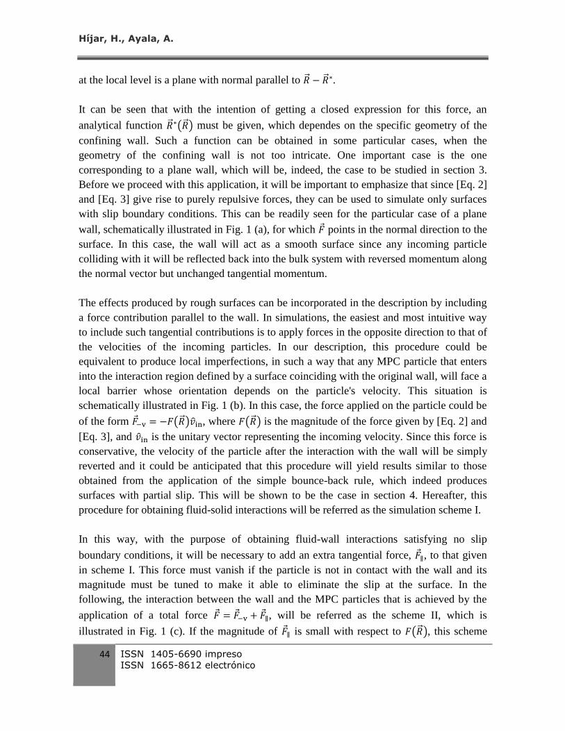
wall, schematically illustrated in Fig. 1 (a), for which 𝐹 points in the normal direction to the

surface. In this case, the wall will act as a smooth surface since any incoming particle

colliding with it will be reflected back into the bulk system with reversed momentum along

the normal vector but unchanged tangential momentum.

The effects produced by rough surfaces can be incorporated in the description by including

a force contribution parallel to the wall. In simulations, the easiest and most intuitive way

to include such tangential contributions is to apply forces in the opposite direction to that of

the velocities of the incoming particles. In our description, this procedure could be

equivalent to produce local imperfections, in such a way that any MPC particle that enters

into the interaction region defined by a surface coinciding with the original wall, will face a

local barrier whose orientation depends on the particle's velocity. This situation is

schematically illustrated in Fig. 1 (b). In this case, the force applied on the particle could be

of the form 𝐹 −v = −𝐹(�⃗� )𝑣in, where 𝐹(�⃗� ) is the magnitude of the force given by [Eq. 2] and

[Eq. 3], and 𝑣in is the unitary vector representing the incoming velocity. Since this force is

conservative, the velocity of the particle after the interaction with the wall will be simply

reverted and it could be anticipated that this procedure will yield results similar to those

obtained from the application of the simple bounce-back rule, which indeed produces

surfaces with partial slip. This will be shown to be the case in section 4. Hereafter, this

procedure for obtaining fluid-solid interactions will be referred as the simulation scheme I.

In this way, with the purpose of obtaining fluid-wall interactions satisfying no slip

boundary conditions, it will be necessary to add an extra tangential force, 𝐹 ∥, to that given

in scheme I. This force must vanish if the particle is not in contact with the wall and its

magnitude must be tuned to make it able to eliminate the slip at the surface. In the

following, the interaction between the wall and the MPC particles that is achieved by the

application of a total force 𝐹 = 𝐹 −v + 𝐹 ∥, will be referred as the scheme II, which is

illustrated in Fig. 1 (c). If the magnitude of 𝐹 ∥ is small with respect to 𝐹(�⃗� ), this scheme




will be equivalent to add a supplementary local inclination to the wall faced by the

incoming particles.

In principle, 𝐹 ∥ could be determined by calculating the stress tensor generated at the surface

by its application, e.g., by means of a kinetic theory model for the MPC dynamics

(Belushkin et al, 2011). Here, we will not perform such calculation, but, obtain 𝐹 ∥

empirically from the results of a large number of simulation experiments of MPC fluids

driven by a uniform force between two fixed parallel planes. It is worth mentioning that

similar procedures, in which fluid-solid interactions are supplemented with additional

tangential surface forces, have been employed also in MD simulations of particles in the

presence of physical barriers (Pivkin and Karniadakis, 2005; Spijker et al., 2008). For MPC

simulations, this work is the first one in which the effects of such forces are analyzed.

In summary, the three simulation schemes illustrated in Fig. 1, could be used to simulate

flow with boundary conditions that include total slip (a), partial slip (b), and no-slip (c). In

the present paper we will only consider cases (b) and (c).

Figure 1: Three procedures of implementing fluid-wall interactions in MPC. (a) Forces 𝐹

(blue arrows), are applied in the normal direction to the surface defining the wall. (b)

Scheme I: forces are applied against the incoming velocities of the particles (thin dashed

lines). (c) Scheme II: an additional force, 𝐹 ∥, is applied in the direction of the surface.

MPC algorithm for flow between parallel planes

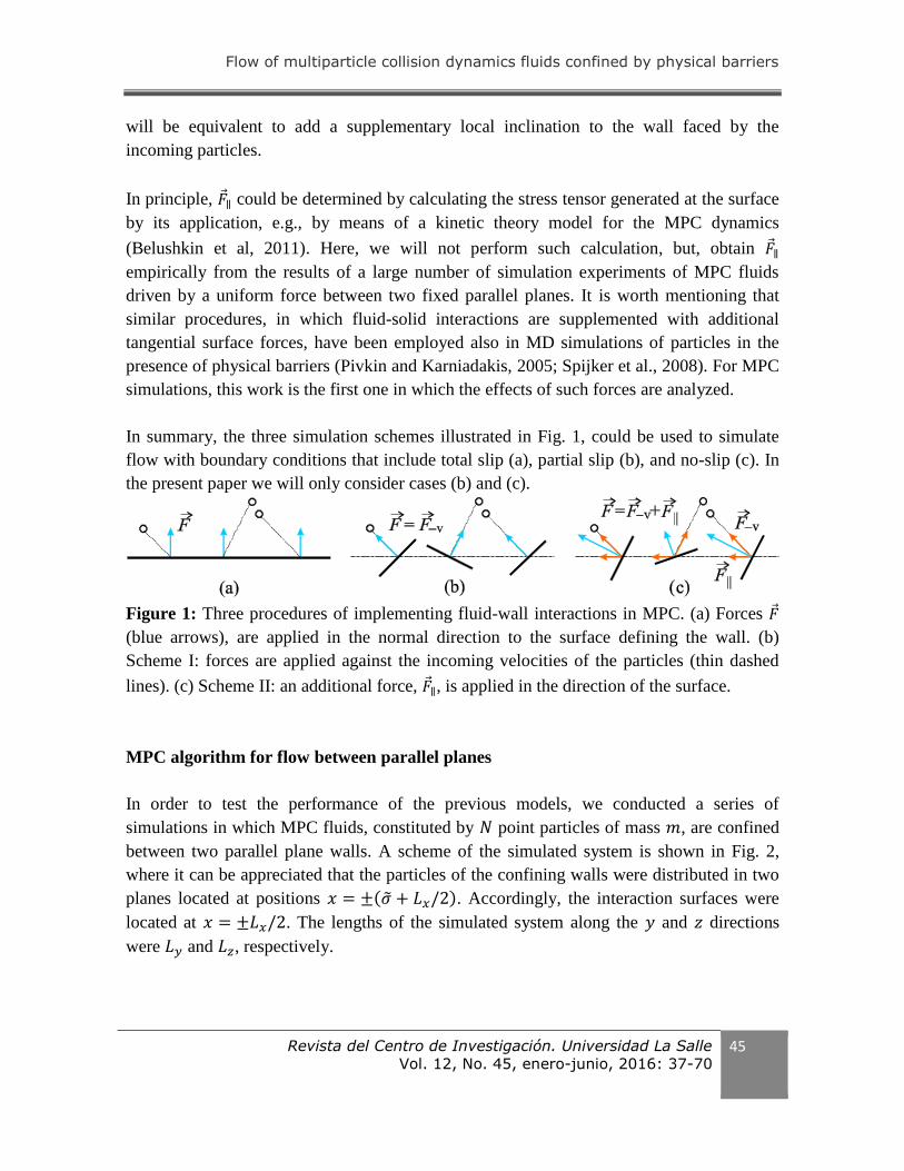
In order to test the performance of the previous models, we conducted a series of

simulations in which MPC fluids, constituted by 𝑁 point particles of mass 𝑚, are confined

between two parallel plane walls. A scheme of the simulated system is shown in Fig. 2,

where it can be appreciated that the particles of the confining walls were distributed in two

planes located at positions 𝑥 = ±(�̃� + 𝐿𝑥/2). Accordingly, the interaction surfaces were

located at 𝑥 = ±𝐿𝑥/2. The lengths of the simulated system along the 𝑦 and 𝑧 directions

were 𝐿𝑦 and 𝐿𝑧, respectively.




It can be seen from these definitions that the pure phase of the fluid, i.e., the set of MPC

particles that were not in contact with the wall particles, occupied a total volume 𝐿𝑥𝐿𝑦𝐿𝑧.

An external uniform field was considered to be present which exerted a force per unit mass

𝑔 = 𝑔�̂�𝑧 on the fluid particles in the pure phase.Observe that, in a general context, the field

𝑔 could result from a uniform pressure grandient acting on the fluid and, if the parallel

planes are properly oriented, from the gravitational field.

Figure 2: Schematic illustration of the simulated system. This figure also shows the

implementation used to introduce virtual particles.

The system evolved in time according to a hybrid scheme combining MD and MPC. On the

one hand, MD allowed us to simulate the behavior of the fluid particles at the microscopic

time-scale and took care of their interaction with the confining walls. On the other hand,

MPC considered the interaction between the fluid particles in a coarse-grained fashion

allowing us to incorporate collective effects occurring at the hydrodynamic time-scales.

Due to the presence of the confining walls, our hybrid MD-MPC simulation scheme had

particular features that do not appear in usual implementations. These features will be

discussed in detail below.

Typical MD-MPC simulations proceed in two main steps, commonly referred as the

streaming step and the collision step. During streaming, the positions and velocities of the

MPC particles are updated according to an MD integration method, e.g., the velocity

Störmer-Verlet method applied on a short time step of size Δ𝑡MD(Griebel et al, 2007).

Consequently, if vectors �⃗� 𝑖 and 𝑣 𝑖, for 𝑖 = 1,2, … , 𝑁, are used to represent the positions and

velocities of the MPC particles, in our algorithm they were updated according to




�⃗� 𝑖(𝑡 + Δ𝑡MD) = �⃗� 𝑖(𝑡) + Δ𝑡MD𝑣 𝑖(𝑡) +(Δ𝑡MD)

2

2𝑚𝐹 𝑖(𝑡), (4)

and

𝑣 𝑖(𝑡 + Δ𝑡MD) = 𝑣 𝑖(𝑡) +Δ𝑡MD

2𝑚[𝐹 𝑖(𝑡 + Δ𝑡MD) + 𝐹 𝑖(𝑡)], (5)

where 𝐹 𝑖 denotes the total force on the 𝑖-th particle. This force was calculated by adding the

confining force given by [Eq. 2] and [Eq. 3], and the external force field 𝑔 . For

completeness, we present here the explicit form of the forces 𝐹 𝑖 used in our simulations.

They were obtained for the particular case of confinement by the plane surfaces described

at the beginning of this section, and in the case in which 𝑔 is only applied on the particles

in the pure MPC phase. They read as

𝐹 𝑖 =

{

−2𝜋휀𝜌𝑆 {3𝑛

�̃�2−(�̃�−𝑙𝑖)2

𝜎2[2 (

𝜎

�̃�−𝑙𝑖)12𝑛+2

− (𝜎

�̃�−𝑙𝑖)6𝑛+2

]

+ [(𝜎

�̃�−𝑙𝑖)12𝑛

− (𝜎

�̃�−𝑙𝑖)6𝑛

+1

4]} (�̃� − 𝑙𝑖)𝑣in,𝑖 + 𝐹∥�̂�𝑧 , if − 𝐿𝑥/2 < 𝑥𝑖or𝑥𝑖 > 𝐿𝑥/2,

𝑚𝑔�̂�𝑧 , otherwise

(6)

where 𝑙𝑖 is the distance penetrated by the 𝑖th MPC particle in the region of interaction with

the wall, in the direction of its incoming velocity, 𝑣 in,𝑖. Notice that [Eq. 6] applies for the

simulation scheme II, while for the scheme I the same equation can be applied with 𝐹∥ = 0.

In the hybrid MD-MPC procedure, the characteristic collision step of MPC is applied at

regular time intervals of size Δ𝑡 = 𝑛MDΔ𝑡MD, i.e., after performing 𝑛MD steps of the

streaming integration method. In the usual implementation, also referred as Stochastic

Rotation Dynamics (SRD) (Yeomans, 2006; Kapral, 2008; Gompper et al, 2009), the

simulation box is subdivided into cells of volume 𝑎3, where interparticle collisions are

simulated. With this purpose, the center of mass velocity of each cell is calculated and

particles within the same cell are forced to change their velocities according to the rule

𝑣 𝑖 ′ = 𝑣 c.m. + 𝑅(𝛼; �̂�) ⋅ [𝑣 𝑖 − 𝑣 c.m.], (7)

where 𝑣 𝑖 ′ and 𝑣 𝑖 are the velocities of the 𝑖th particle after and before collision, respectively;

𝑣 c.m. is the center of mass velocity of the cell; and 𝑅(𝛼; �̂�) is a stochastic rotation matrix,

which rotates velocities by an angle 𝛼 around a random axis �̂�. It is worth stressing that 𝛼 is

a parameter whose value is fixed through the whole simulation, while �̂� is sampled in each




cell at every collision step by randomly selecting a point on the surface of a sphere with

unit radius.

Physically, 𝛼 is the angle at which the velocities of the MPC particles that happen to be at

the same MPC cell at the collision step are rotated. Accordingly, it represents the degree of

interaction between MPC particles and should not be confused with the angle at which

MPC particles collide with the solid walls. As it has been shown by diverse authors

(Malevanets and Kapral 1999; Malevanets and Kapral 2000; Pooley and Yeomans, 2005;

Gompper et al., 2009), 𝛼 determines the value of the transport coefficients of the simulated

fluid. Therefore, simulations carried out with different values of 𝛼, represent numerical

experiments with different fluids.

In order to preserve the property of Galilean invariance, a uniform random displacement of

the collision cells was implemented, before collisions take place (Ihle and Kroll, 2001,

2003). In the presence of confining surfaces, this random displacement procedure has

important implications for various aspects of MPC. In our case, without the random

displacement, the boundary cells coincide with the solid planes. However, when

displacement occurs, the cells at the bottom and top of the simulation box get partially

empty and the subsequent collisions inside them will take place in a fluid with modified

density, thus yielding different physical properties than in the interior cells (Winkler and

Huang, 2009). In favor of restoring the numerical density at the boundary, virtual particles

can be introduced that appear in the partially empty cells only at the collision step. With the

purpose of incorporating such phantom particles, we follow a procedure similar to that

introduced in (Winkler and Huang, 2009), by including an additional collision cell below

the lower plane. Then, the whole collision cells are displaced in the positive 𝑥-direction by

a uniform vector with components uniformly distributed within the range [−𝑎/2, 𝑎/2].

Afterwards, the partially empty cells are filled with virtual particles. The number of such

particles at a given cell, 𝑁v, is determined by the number of fluid particles, 𝑁f, in the

boundary cell cut off by the opposite plane, as it is schematically illustrated in Fig. 2. In

this manner, the average particle density is restored and the probability distribution for

observing a given number of particles at the collision cells is preserved (Winkler and

Huang, 2009).

It should be remarked that the collisional contribution to the stress tensor depends on the

velocity of the virtual particles. More precisely, it can be shown that the momentum

exchanged in a collision cell between fluid and virtual particles, after averaging over

fluctuations and stochastic rotations, reads as (Winkler and Huang, 2009)




⟨Δ𝑝 ⟩ =2(cos𝛼−1)𝑚

3𝑁𝑐⟨𝑁f𝑁v(𝑣 f − 𝑣 v)⟩, (8)

where 𝑣 f and 𝑣 v represent the average velocity of the fluid and virtual particles,

respectively. In this work, we decided to incorporate the virtual particles with a velocity

equals to the center of mass velocity of the partially empty layer in which they collide.

Consequently, in our implementation we have 𝑣 f = 𝑣 v, and this procedure will not modify

the stress at the boundary wall due to collisions.

It should be also punctuated that if particles interacting with the confining walls (−𝐿𝑥/2 <

𝑥𝑖 or 𝑥𝑖 > 𝐿𝑥/2), were allowed to participate in the stochastic collisions, their trajectories

would be deflected while still suffering the force given by [Eq. 6]. In that case, they would

have the chance to get out of the simulation box. Therefore, in order to prevent the escape

of fluid through the confining walls, only particles at the pure MPC phase were considered

in collisions.

We implemented periodic boundary conditions along the 𝑦 and 𝑧 directions. Furthermore,

in order to prevent heating of the simulated system due to the work performed by the

confinement and external forces, we applied a thermostatting procedure after each collision

step that fixed the temperature of the system at the value 𝑇0. Our thermostat consisted

simply of a local velocity rescale, completely analogous to that used recently in Refs.

(Híjar, 2013; Fernández and Híjar, 2015; Híjar, 2015).

Numerical experiments were performed by sorting the MPC particles into the simulation

box with random positions and velocities taken from uniform distributions. No initial

overlapping existed between the fluid particles and the confining surface, the total

momentum of the system was fixed to zero, and its total energy was adjusted to the value

dictated by the equipartition law at temperature 𝑇0. Then, the hybrid MD-MPC algorithm

was applied to the ensemble of fluid particles subjected to the external field 𝑔 and to the

constraining surface forces. This thermalization process was applied for a period of time

large enough to guarantee that the proper distribution of velocities and hydrodynamic fields

were established. Finally, a long enough simulation stage was conducted that allowed us to

calculate the hydrodynamic fields established in the system. In this work we will focus in

the velocity field which will be calculated locally as the time average of the center of mass

velocity measured in the MPC collision cells.

The independent parameters of the simulations were the length of the MPC cells, 𝑎; the

time-step between SRD collisions, Δ𝑡; the average number of particles per cell, 𝑁p; the

thermal energy, 𝑘𝐵𝑇0; the SRD rotation angle, 𝛼; and the mass of the individual MPC




particles, 𝑚. All our simulations were performed by fixing these parameters at 𝑎 = 1, 𝑚 =

1, 𝑘𝐵𝑇0 = 1, 𝑁𝑝 = 5, and Δ𝑡 = 0.05 𝑢𝑡, with 𝑢𝑡 = √𝑚 𝑎2 /(𝑘𝐵𝑇0) , the unit time. Notice

that here, as well in the rest of the paper we will use simulation units (s.u.) instead of

physical units. The size of the simulated system was defined by the quantities 𝐿𝑥 = 10𝑎,

and 𝐿𝑦 = 𝐿𝑧 = 20𝑎. The parameters characterizing the interaction between the particles

and the confining walls were chosen as 휀 = 𝑘𝐵𝑇0/2, 𝜎 = 𝑎/2, and 𝜌𝑆 = 1/2𝑎2. The MD

time-step was chosen as Δ𝑡MD = 0.1Δ𝑡, for which no instabilities of the simulations were

observed.

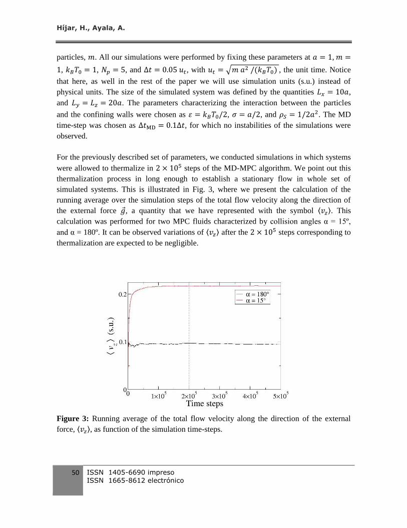
For the previously described set of parameters, we conducted simulations in which systems

were allowed to thermalize in 2 × 105 steps of the MD-MPC algorithm. We point out this

thermalization process in long enough to establish a stationary flow in whole set of

simulated systems. This is illustrated in Fig. 3, where we present the calculation of the

running average over the simulation steps of the total flow velocity along the direction of

the external force 𝑔 , a quantity that we have represented with the symbol ⟨𝑣𝑧⟩. This

calculation was performed for two MPC fluids characterized by collision angles α = 15º,

and α = 180º. It can be observed variations of ⟨𝑣𝑧⟩ after the 2 × 105 steps corresponding to

thermalization are expected to be negligible.

Figure 3: Running average of the total flow velocity along the direction of the external

force, ⟨𝑣𝑧⟩, as function of the simulation time-steps.




The velocity profiles developed by the simulated systems were calculated using 4 × 105

simulation steps after thermalization. With the purpose of calculating such velocity profiles,

we sort the simulated particles according to their positions along 𝑥-axis every time-step.

We calculated the average of the velocity along the 𝑧-axis of those particles located in

parallel layers of width 𝑎. Then, the a final averaging process was conducted over the afore

mentioned 4 × 105 time-steps.

Results

We shall present here the results obtained from the application of the algorithm described in

the previous section. With this purpose it will be convenient to show first in section 4.1,

those results obtained when the confining forces are applied according to the simulation

scheme I, [Eq. 6] with 𝐹∥ = 0. Subsequently in section 4.2 we will estimate the values of 𝐹∥

that must be used in the simulation scheme II, in order to achieve confining walls with no

slip boundary conditions.

Simulation scheme I

Velocity profile

First, we notice that the velocity profile expected for the geometry described in the previous

section is the classical plane Poiseuille flow (Landau and Lifshitz, 1959), which will be cast

in the form

𝑣𝑧(𝑥) =𝑔

2𝜈[(𝐷𝑥

2)2

− 𝑥2], (9)

where 𝜈 is the kinematic viscosity of the fluid and 𝐷𝑥 is the effective distance between the

parallel plates, i.e., the total distance between the planes of zero flow velocity.

In the first stage of our numerical analysis we pursued to verify that our implementation

gives to the correct velocity flow, as they are given by [Eq. 9With this purpose, we

conducted experiments in which 𝛼 took twelve different values uniformly distributed

within the range 𝛼 ∈ [15∘, 180∘]. It should be mentioned that for small values of the

collision angle, the simulated system is expected to behave close to the so-called gas

regime, in which contributions to the material properties of the fluid arising from streaming

(kinetic) dynamics dominate over contributions due to collisions (Kapral, 2008; Gompper

et al., 2009). On the opposite case, for values of 𝛼 close to 180∘, the dynamics of the

simulated fluid is expected to be in the so-called liquid regime, where collisional effects are

larger and dominate over kinetic effects. Consequently, in our numerical experiments we




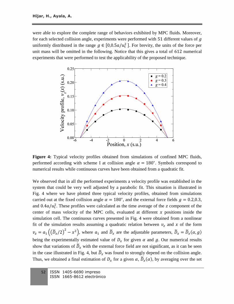
were able to explore the complete range of behaviors exhibited by MPC fluids. Moreover,

for each selected collision angle, experiments were performed with 51 different values of 𝑔

uniformly distributed in the range 𝑔 ∈ [0,0.5𝑎/𝑢t2 ]. For brevity, the units of the force per

unit mass will be omitted in the following. Notice that this gives a total of 612 numerical

experiments that were performed to test the applicability of the proposed technique.

Figure 4: Typical velocity profiles obtained from simulations of confined MPC fluids,

performed according with scheme I at collision angle 𝛼 = 180∘. Symbols correspond to

numerical results while continuous curves have been obtained from a quadratic fit.

We observed that in all the performed experiments a velocity profile was established in the

system that could be very well adjusted by a parabolic fit. This situation is illustrated in

Fig. 4 where we have plotted three typical velocity profiles, obtained from simulations

carried out at the fixed collision angle 𝛼 = 180∘, and the external force fields 𝑔 = 0.2,0.3,

and 0.4𝑎/𝑢t2. These profiles were calculated as the time average of the 𝑧 component of the

center of mass velocity of the MPC cells, evaluated at different 𝑥 positions inside the

simulation cell. The continuous curves presented in Fig. 4 were obtained from a nonlinear

fit of the simulation results assuming a quadratic relation between 𝑣𝑧 and 𝑥 of the form

𝑣𝑧 = 𝑎1 ((�̃�𝑥/2)2− 𝑥2), where 𝑎1 and �̃�𝑥 are the adjustable parameters, �̃�𝑥 = �̃�𝑥(𝛼, 𝑔)

being the experimentally estimated value of 𝐷𝑥 for given 𝛼 and 𝑔. Our numerical results

show that variations of �̃�𝑥 with the external force field are not significant, as it can be seen

in the case illustrated in Fig. 4, but �̃�𝑥 was found to strongly depend on the collision angle.

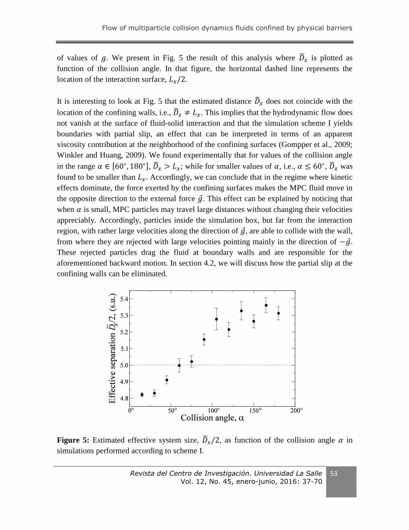
Thus, we obtained a final estimation of 𝐷𝑥 for a given 𝛼, �̃�𝑥(𝛼), by averaging over the set




of values of 𝑔. We present in Fig. 5 the result of this analysis where �̃�𝑥 is plotted as

function of the collision angle. In that figure, the horizontal dashed line represents the

location of the interaction surface, 𝐿𝑥/2.

It is interesting to look at Fig. 5 that the estimated distance �̃�𝑥 does not coincide with the

location of the confining walls, i.e., �̃�𝑥 ≠ 𝐿𝑥. This implies that the hydrodynamic flow does

not vanish at the surface of fluid-solid interaction and that the simulation scheme I yields

boundaries with partial slip, an effect that can be interpreted in terms of an apparent

viscosity contribution at the neighborhood of the confining surfaces (Gompper et al., 2009;

Winkler and Huang, 2009). We found experimentally that for values of the collision angle

in the range 𝛼 ∈ [60∘, 180∘], �̃�𝑥 > 𝐿𝑥; while for smaller values of 𝛼, i.e., 𝛼 ≤ 60∘, �̃�𝑥 was

found to be smaller than 𝐿𝑥. Accordingly, we can conclude that in the regime where kinetic

effects dominate, the force exerted by the confining surfaces makes the MPC fluid move in

the opposite direction to the external force 𝑔 . This effect can be explained by noticing that

when 𝛼 is small, MPC particles may travel large distances without changing their velocities

appreciably. Accordingly, particles inside the simulation box, but far from the interaction

region, with rather large velocities along the direction of 𝑔 , are able to collide with the wall,

from where they are rejected with large velocities pointing mainly in the direction of −𝑔 .

These rejected particles drag the fluid at boundary walls and are responsible for the

aforementioned backward motion. In section 4.2, we will discuss how the partial slip at the

confining walls can be eliminated.

Figure 5: Estimated effective system size, �̃�𝑥/2, as function of the collision angle 𝛼 in

simulations performed according to scheme I.




Viscosity estimation

We used the results of the numerical experiments described previously to estimate the

viscosity of the simulated MPC fluid, as function of the collision angle 𝛼. With this

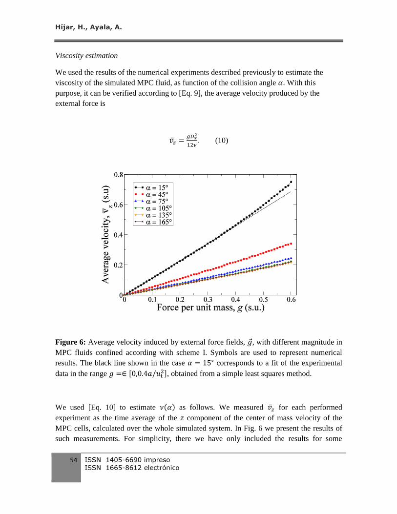
purpose, it can be verified according to [Eq. 9], the average velocity produced by the

external force is

�̅�𝑧 =𝑔𝐷𝑥

2

12𝜈. (10)

Figure 6: Average velocity induced by external force fields, 𝑔 , with different magnitude in

MPC fluids confined according with scheme I. Symbols are used to represent numerical

results. The black line shown in the case 𝛼 = 15∘ corresponds to a fit of the experimental

data in the range 𝑔 =∈ [0,0.4𝑎/𝑢t2], obtained from a simple least squares method.

We used [Eq. 10] to estimate 𝜈(𝛼) as follows. We measured �̅�𝑧 for each performed

experiment as the time average of the 𝑧 component of the center of mass velocity of the

MPC cells, calculated over the whole simulated system. In Fig. 6 we present the results of

such measurements. For simplicity, there we have only included the results for some




selected values of the collision angle, namely 𝛼 = 15∘, 45∘, 75∘, 105∘, 135∘, and 165∘. It

can be observed that for small values of the external force, all the experiments show that �̅�𝑧

increases linearly with 𝑔, as it is expected from [Eq. 10]. In Fig. 5 it is also shown that the

linear relation between the average velocity and the external force is broken for large values

of the latter, 𝑔 ≥ 0.4𝑎/𝑢t2. For simplicity, this situation is illustrated in Fig. 6 only for the

case 𝛼 = 15∘, however, it is indeed observed for the complete set of numerical

experiments. The departure of �̅�𝑧 from the linear behavior implies that the proposed

technique for confining MPC fluids might lead to a stress tensor that depends on the

external force.

This effect can be explained by taking into account that under confinement, the stress

tensor of the fluid has a kinetic contribution due to its interaction with the walls (Winkler

and Huang, 2009). The stress at the wall corresponding to our implementation could be

obtained from the average of the momentum exchange occurring during the streaming step.

Let 𝑡𝑞 and 𝑡𝑞 + Δ𝑡 denote the times at which two consecutive SRD collisions take place,

and consider a fluid particle that collides with the wall at time 𝑡𝑞 + 𝛿𝑡, with 0 ≤ 𝛿𝑡 ≤ Δ𝑡.

The total momentum change of this particle, relative to the center of mass velocity of the

fluid from where it comes, is

Δ𝑝𝑧 = 𝑚[𝑣𝑖,𝑧(𝑡𝑞 + Δ𝑡) − 𝑣𝑖,𝑧(𝑡𝑞 + 𝛿𝑡) − (Δ𝑡 − 𝛿𝑡)𝑔]. (11)

Notice that in our implementation particles interacting with the wall, are not affected by the

force field 𝑔 . Then, the last term in the previous equation represents the acceleration of the

fluid in the bulk phase with respect to the particles absorbed by the wall. This acceleration

generates a contribution to the stress that depends on the external force per unit mass 𝑔, as

it has been found in our simulations. Nevertheless, it is clear from Fig. 6 that this effect

could be neglected if simulations are kept in the limit of small values of the external force.

We restricted ourselves to consider this case and approximated the results presented in Fig.

6 by the simple numerical relation �̅�𝑧 = 𝑠(𝛼)𝑔, where the slope 𝑠(𝛼) was obtained by the

method of least squares, applied only over the limited range 0 < 𝑔 ≤ 0.4𝑎/𝑢t2. This result

can be used in combination with [Eq. 10] to give the estimation of the kinematic viscosity,

𝜈, according to 𝜈 = �̃�𝑥2(𝛼)/12𝑠(𝛼).




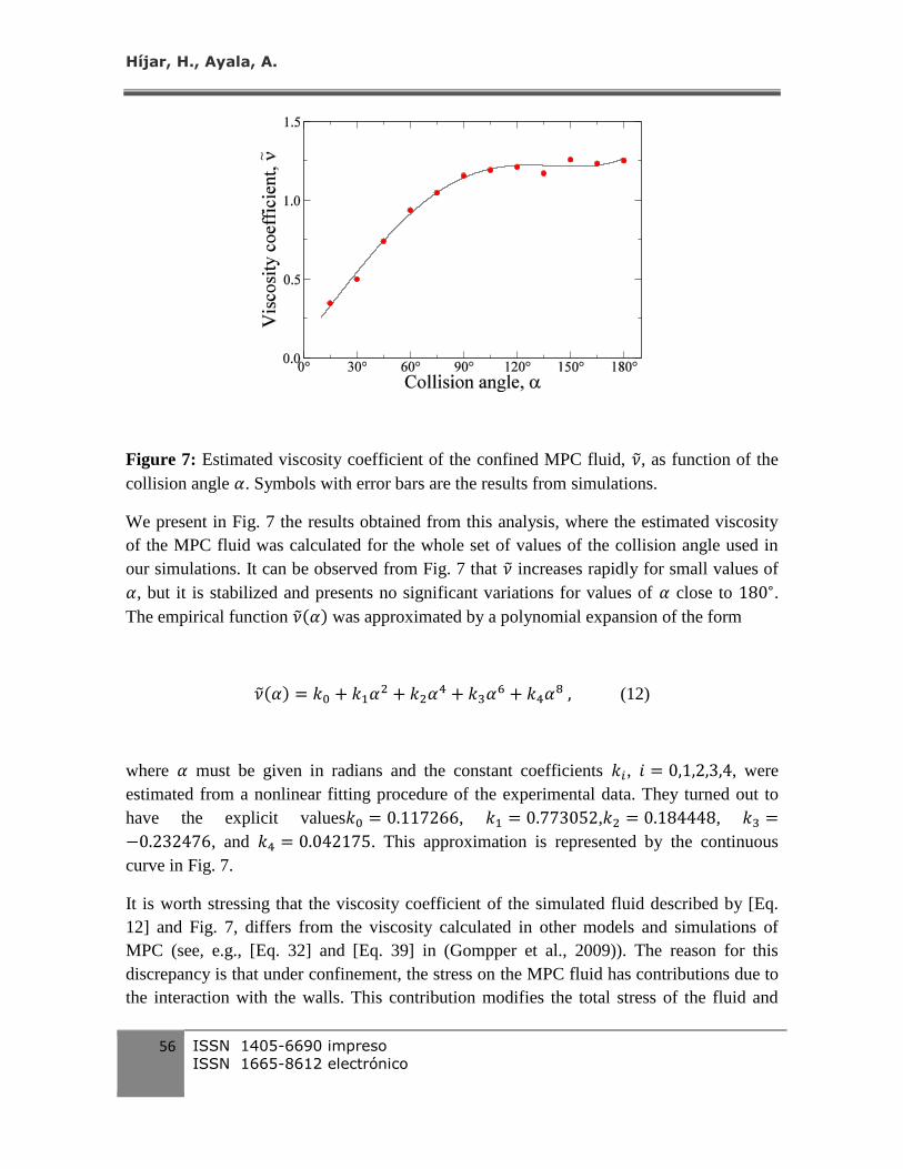
Figure 7: Estimated viscosity coefficient of the confined MPC fluid, 𝜈, as function of the

collision angle 𝛼. Symbols with error bars are the results from simulations.

We present in Fig. 7 the results obtained from this analysis, where the estimated viscosity

of the MPC fluid was calculated for the whole set of values of the collision angle used in

our simulations. It can be observed from Fig. 7 that 𝜈 increases rapidly for small values of

𝛼, but it is stabilized and presents no significant variations for values of 𝛼 close to 180∘.

The empirical function 𝜈(𝛼) was approximated by a polynomial expansion of the form

𝜈(𝛼) = 𝑘0 + 𝑘1𝛼2 + 𝑘2𝛼

4 + 𝑘3𝛼6 + 𝑘4𝛼

8 , (12)

where 𝛼 must be given in radians and the constant coefficients 𝑘𝑖, 𝑖 = 0,1,2,3,4, were

estimated from a nonlinear fitting procedure of the experimental data. They turned out to

have the explicit values𝑘0 = 0.117266, 𝑘1 = 0.773052,𝑘2 = 0.184448, 𝑘3 =

−0.232476, and 𝑘4 = 0.042175. This approximation is represented by the continuous

curve in Fig. 7.

It is worth stressing that the viscosity coefficient of the simulated fluid described by [Eq.

12] and Fig. 7, differs from the viscosity calculated in other models and simulations of

MPC (see, e.g., [Eq. 32] and [Eq. 39] in (Gompper et al., 2009)). The reason for this

discrepancy is that under confinement, the stress on the MPC fluid has contributions due to

the interaction with the walls. This contribution modifies the total stress of the fluid and




produces the particular behavior of 𝜈 observed in our experiments. In this sense, the

viscosity coefficient estimated empirically by [Eq. 12] can be considered as an effective

parameter valid to describe the flow produced in the simulated system. Subsequently, in

section 4.3, we will show that the values of the effective viscosity obtained empirically are

very well adjusted by the expected analytical expression of the viscosity in the liquid-like

regime of MPC and that, at least in such regime, the velocity profile obtained from our

implementation approaches the analytical reference Poiseuille flow.

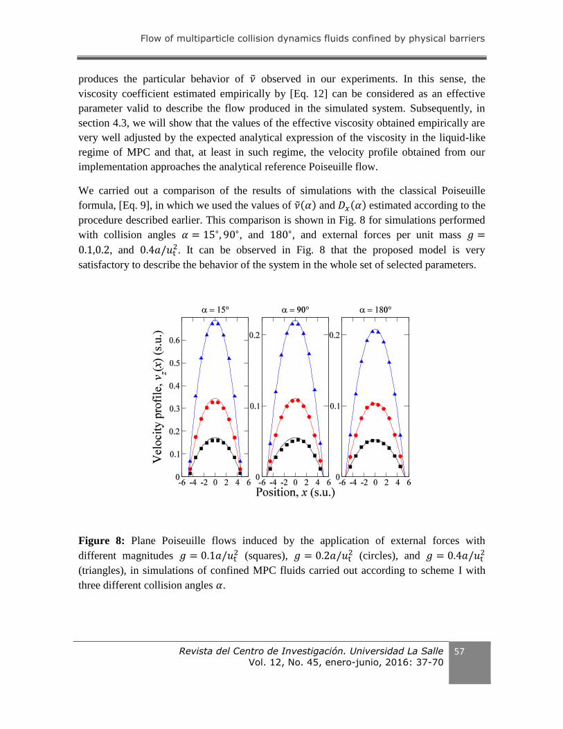
We carried out a comparison of the results of simulations with the classical Poiseuille

formula, [Eq. 9], in which we used the values of 𝜈(𝛼) and 𝐷𝑥(𝛼) estimated according to the

procedure described earlier. This comparison is shown in Fig. 8 for simulations performed

with collision angles 𝛼 = 15∘, 90∘, and 180∘, and external forces per unit mass 𝑔 =

0.1,0.2, and 0.4𝑎/𝑢t2. It can be observed in Fig. 8 that the proposed model is very

satisfactory to describe the behavior of the system in the whole set of selected parameters.

Figure 8: Plane Poiseuille flows induced by the application of external forces with

different magnitudes 𝑔 = 0.1𝑎/𝑢t2 (squares), 𝑔 = 0.2𝑎/𝑢t

2 (circles), and 𝑔 = 0.4𝑎/𝑢t2

(triangles), in simulations of confined MPC fluids carried out according to scheme I with

three different collision angles 𝛼.




Finally, it is worth stressing that in order to characterize the flow produced in our numerical

implementation and to relate it with the corresponding to a physical fluid, hydrodynamic

dimenssionless parameters can be used. In particular, we will consider the Reynolds

number, Re, which for a given flow quantifies the relevance of the inertial force with

respect to the viscous effects. For plane Poiseuille flow, Re can be written in the form

Re =�̅�𝑧𝐿𝑥𝜈.

Therefore, it can be appreciated from the results presented in Figs. 5 and 6, that our

simulations, corresponds to flows with a maximum Reynolds number Re 15. At the end

of the following section we will present the results of simulations with larger values of Re.

Simulation scheme II

It has been shown in section 4.1 that the simulation scheme I, in which confining forces act

in the opposite direction of the velocity of the incoming MPC particles, yields partial slip

boundary conditions. This indicates that an additional stress at the boundary needs to be

added in order to restore no slip conditions at the confining surfaces. The additional stress

might be generated from the force 𝐹 ∥ appearing in [Eq. 6]. In this work, we followed a

numerical approach to determine the strength of the force 𝐹 ∥ that must be applied in

simulations to obtain stick boundary conditions. More precisely, we implemented an

optimization procedure in which simulations at fixed 𝛼 and 𝑔 were carried out with

different values of 𝐹∥. We considered a steepest descendant method in which 𝐹∥ varied until

we observed that the magnitude of the average velocity of the MPC fluid at the location of

the confining surfaces, 𝑥 = ±𝐿𝑥/2, was smaller than a fixed error value 휀 = 0.001. We

performed this procedure for the whole set of values of the collision angle 𝛼, and for the

following eight values of the external force per unit mass 𝑔 = 0.05,0.10,0.15, … ,0.4𝑎/𝑢t2.




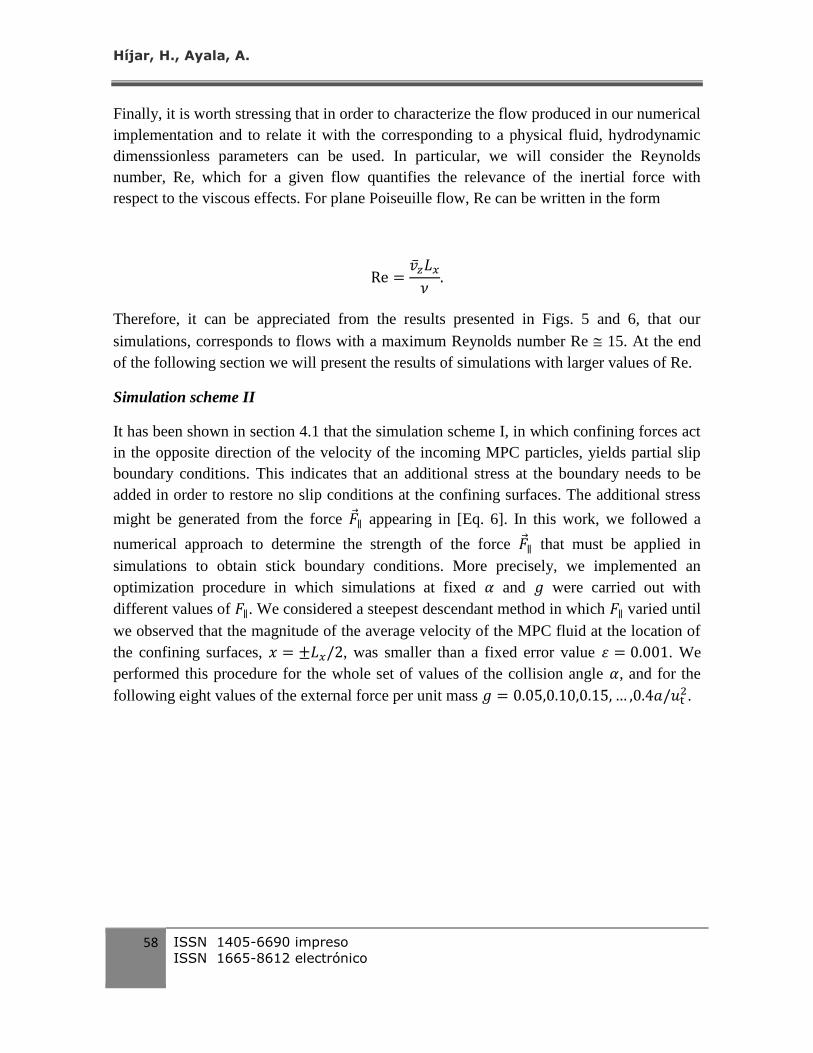
Figure 9: (a) Magnitude of the parallel force, 𝐹 ∥ = 𝐹∥�̂�𝑧 (see [Eq. 6]), that must be applied

in simulations of confined MPC fluids in order to restore stick boundary conditions. 𝐹∥ as

function of 𝑔 is well fitted by a linear relation 𝐹∥ = 𝑞(𝛼)𝑔. (b) Parameter 𝑞(𝛼) as function

of the collision angle.

Our results are presented in Fig. 9 (a). They show that 𝐹∥ can be very well approximated by

the linear relation

𝐹∥ = 𝑞(𝛼)𝑔, (13)

where 𝑞(𝛼) is the slope of the line obtained at a fixed value of 𝛼. We conclude that, with

the purpose of simultaing surfaces with no slip boundary conditions, the fluid-solid




interaction must occur with local walls whose inclination depart from that given by the

incoming velocity of the particles by an amount proportional to the force field acting on the

fluid phase.

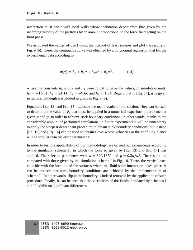
We estimated the values of 𝑞(𝛼) using the method of least squares and plot the results in

Fig. 9 (b). There, the continuous curve was obtained by a polynomial regression that fits the

experimental data according to

𝑞(𝛼) = ℎ0 + ℎ1𝛼 + ℎ2𝛼2 + ℎ3𝛼

3, (14)

where the constants ℎ0, ℎ1, ℎ2 and ℎ3 were found to have the values, in simulation units,

ℎ0 = −16.81, ℎ1 = 24.14, ℎ2 = −9.66 and ℎ3 = 1.34. Regard that in [Eq. 14], 𝛼 is given

in radians, although it is plotted in grads in Fig. 9 (b).

Equations [Eq. 13] and [Eq. 14] represent the main results of this section. They can be used

to determine the value of 𝐹∥ that must be applied in a numerical experiment, performed at

given 𝛼 and 𝑔, in order to achieve stick boundary conditions. In other words, thanks to the

considerable amount of performed simulations, in future experiments it will be unnecesary

to apply the steepest descendant procedure to obtain stick boundary conditions, but instead

[Eq. 13] and [Eq. 14] can be used to obtain flows whose velocities at the confining planes

will be smaller than the error parameter 휀.

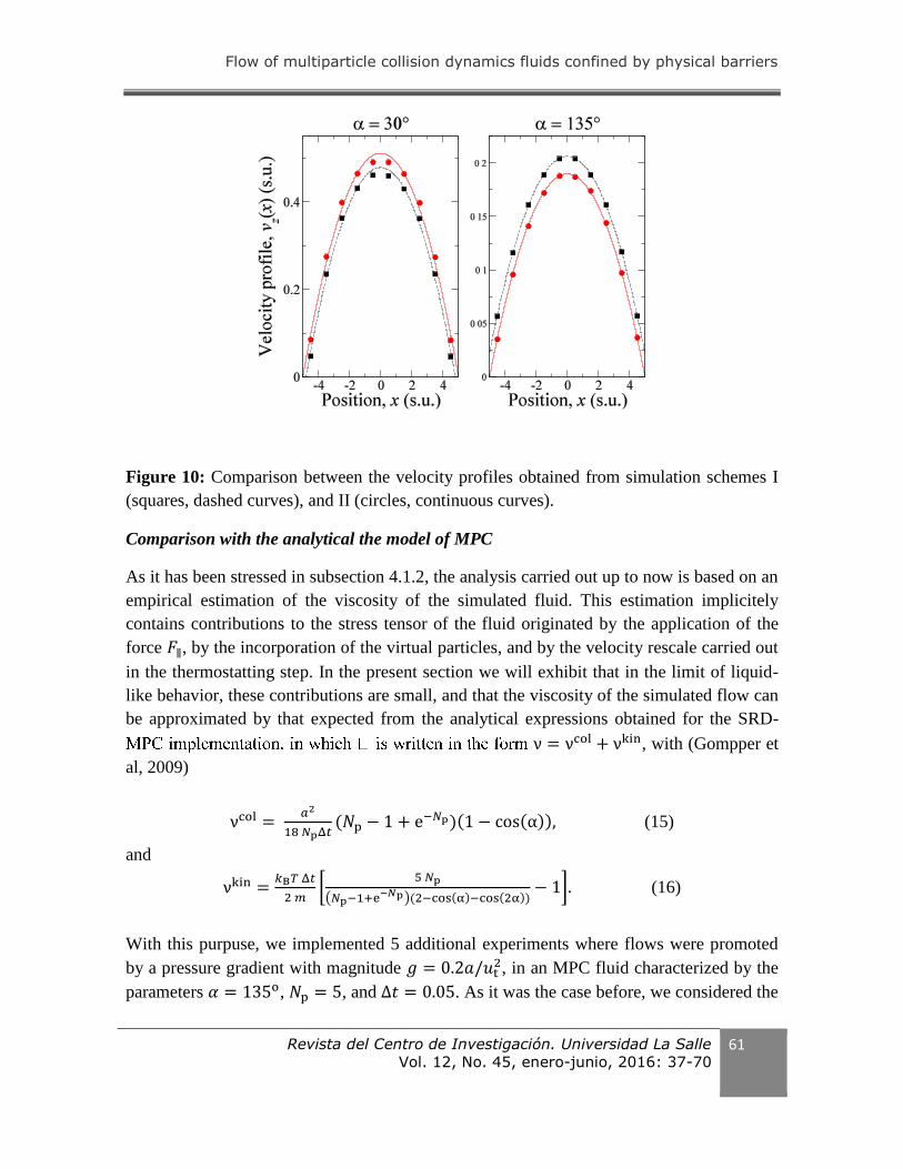
In order to test the applicability of our methodology, we carried out experiments according

to the simulation scheme II, in which the force 𝐹∥ given by [Eq. 13] and [Eq. 14] was

applied. The selected parameters were 𝛼 = 30∘, 135∘ and 𝑔 = 0.2𝑎/𝑢t2. The results are

compared with those given by the simulation scheme I in Fig. 10. There, the vertical axes

coincide with the location of the surfaces where the fluid-solid interaction takes place. It

can be noticed that stick boundary conditions are achieved by the implementation of

scheme II. In other words, slip at the boundary is indeed removed by the application of such

procedure. Finally, it can be seen that the viscosities of the fluids simulated by schemes I

and II exhibit no significant differences.




Figure 10: Comparison between the velocity profiles obtained from simulation schemes I

(squares, dashed curves), and II (circles, continuous curves).

Comparison with the analytical the model of MPC

As it has been stressed in subsection 4.1.2, the analysis carried out up to now is based on an

empirical estimation of the viscosity of the simulated fluid. This estimation implicitely

contains contributions to the stress tensor of the fluid originated by the application of the

force 𝐹∥, by the incorporation of the virtual particles, and by the velocity rescale carried out

in the thermostatting step. In the present section we will exhibit that in the limit of liquid-

like behavior, these contributions are small, and that the viscosity of the simulated flow can

be approximated by that expected from the analytical expressions obtained for the SRD-

ν = νcol + νkin, with (Gompper et

al, 2009)

νcol = 𝑎2

18 𝑁pΔ𝑡(𝑁p − 1 + e

−𝑁p)(1 − cos(α)), (15)

and

νkin =𝑘B𝑇 Δ𝑡

2 𝑚[

5 𝑁p

(𝑁p−1+e−𝑁p)(2−cos(α)−cos(2α))

− 1]. (16)

With this purpuse, we implemented 5 additional experiments where flows were promoted

by a pressure gradient with magnitude 𝑔 = 0.2𝑎/𝑢t2, in an MPC fluid characterized by the

parameters 𝛼 = 135o, 𝑁p = 5, and Δ𝑡 = 0.05. As it was the case before, we considered the




values 𝑘B𝑇 = 1, and 𝑚 = 1. For such parameters the theoretical expected value of the

viscosity of the fluid is, according to [Eq. (15)] and [Eq. (16)], ν = 1.55.

The difference between the new experiments and those considered in the previous sections

is that the size of the system was varyied. In the present case, simulations were performed

with 𝐿y = 𝐿z = 32𝑎, and 𝐿x = 8, 12,16,18 and 20𝑎. We carried out the procedure for

achieving non-slip boundary conditions described in section 4.2 in each one of the

considered cases, and estimated the empirical viscosity of the fluid by a non-linear fitting

procedure. We observed that this quantity depends on the distance between the confinning

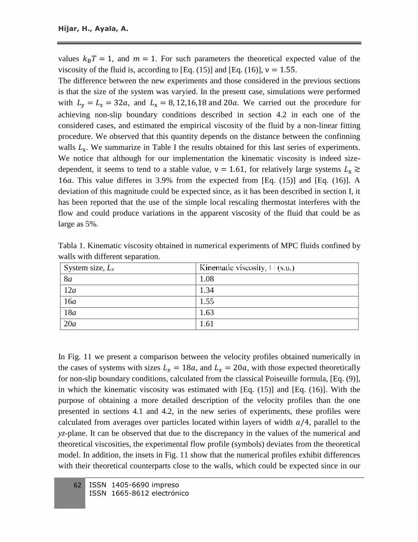
walls 𝐿x. We summarize in Table I the results obtained for this last series of experiments.

We notice that although for our implementation the kinematic viscosity is indeed size-

dependent, it seems to tend to a stable value, ν = 1.61, for relatively large systems 𝐿x ≳

16𝑎. This value differes in 3.9% from the expected from [Eq. (15)] and [Eq. (16)]. A

deviation of this magnitude could be expected since, as it has been described in section I, it

has been reported that the use of the simple local rescaling thermostat interferes with the

flow and could produce variations in the apparent viscosity of the fluid that could be as

large as 5%.

Tabla 1. Kinematic viscosity obtained in numerical experiments of MPC fluids confined by

walls with different separation.

System size, Lx

8a 1.08

12a 1.34

16a 1.55

18a 1.63

20a 1.61

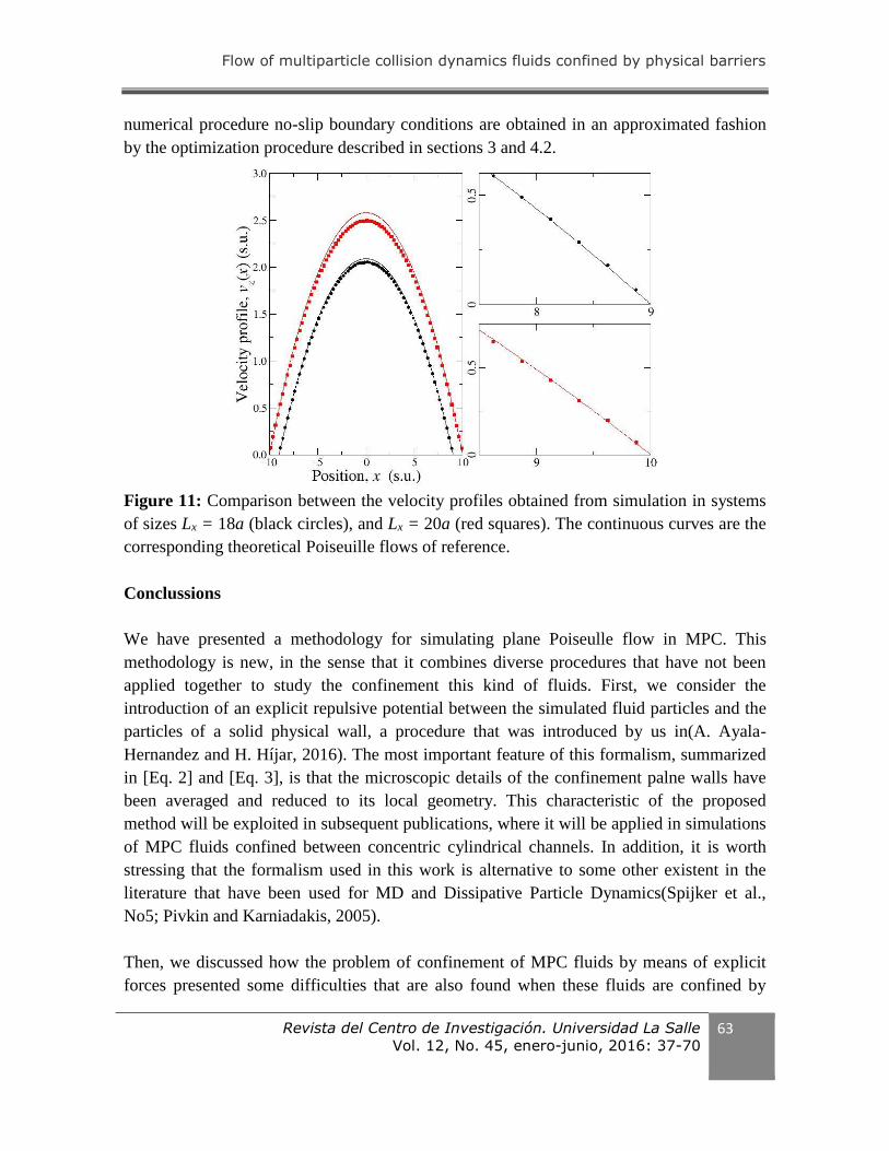
In Fig. 11 we present a comparison between the velocity profiles obtained numerically in

the cases of systems with sizes 𝐿𝑥 = 18𝑎, and 𝐿𝑥 = 20𝑎, with those expected theoretically

for non-slip boundary conditions, calculated from the classical Poiseuille formula, [Eq. (9)],

in which the kinematic viscosity was estimated with [Eq. (15)] and [Eq. (16)]. With the

purpose of obtaining a more detailed description of the velocity profiles than the one

presented in sections 4.1 and 4.2, in the new series of experiments, these profiles were

calculated from averages over particles located within layers of width 𝑎/4, parallel to the

yz-plane. It can be observed that due to the discrepancy in the values of the numerical and

theoretical viscosities, the experimental flow profile (symbols) deviates from the theoretical

model. In addition, the insets in Fig. 11 show that the numerical profiles exhibit differences

with their theoretical counterparts close to the walls, which could be expected since in our




numerical procedure no-slip boundary conditions are obtained in an approximated fashion

by the optimization procedure described in sections 3 and 4.2.

Figure 11: Comparison between the velocity profiles obtained from simulation in systems

of sizes Lx = 18a (black circles), and Lx = 20a (red squares). The continuous curves are the

corresponding theoretical Poiseuille flows of reference.

Conclussions

We have presented a methodology for simulating plane Poiseulle flow in MPC. This

methodology is new, in the sense that it combines diverse procedures that have not been

applied together to study the confinement this kind of fluids. First, we consider the

introduction of an explicit repulsive potential between the simulated fluid particles and the

particles of a solid physical wall, a procedure that was introduced by us in(A. Ayala-

Hernandez and H. Híjar, 2016). The most important feature of this formalism, summarized

in [Eq. 2] and [Eq. 3], is that the microscopic details of the confinement palne walls have

been averaged and reduced to its local geometry. This characteristic of the proposed

method will be exploited in subsequent publications, where it will be applied in simulations

of MPC fluids confined between concentric cylindrical channels. In addition, it is worth

stressing that the formalism used in this work is alternative to some other existent in the

literature that have been used for MD and Dissipative Particle Dynamics(Spijker et al.,

No5; Pivkin and Karniadakis, 2005).

Then, we discussed how the problem of confinement of MPC fluids by means of explicit

forces presented some difficulties that are also found when these fluids are confined by




hard walls methods. In particular, it was necessary to propose an algorithm for the

application of [Eq. 2] and [Eq. 3], that included a procedure for the introduction of virtual

particles at the collision step. Although diverse techniques for incorporating virtual

particles in MPC are available in the literature (Lamura et al., 2001; Lamura and Gompper,

2002; Winkler and Huang, 2009), they have not been used before in simulations of MPC

particles in the presence of physical walls.

Finally, an implementation for eliminating partial slip at the surface of fluid-solid

interaction was incorporated. In this procedure, an additional tangential force acting on the

particles interacting with the solid wall was applied. The strength of this force was

determined empirically from the results of a large number of numerical experiments.

Although this procedure resembles one used in other coarse-grained computer simulations

of fluids (Lamura and Gompper, 2008), we stress that our work is the first that considers

the effects of tangential forces in MPC simulations. We would like to emphasize also, that

this procedure for achieving no-slip boundary conditions differs from the one used in(A.

Ayala-Hernandez and H. Híjar, 2016), where velocity at the solid surface was controlled by

varying the momentum of the virtual particles.

We have shown that the combination of these techniques simulates the correct velocity

profile expected for no slip boundry conditions. Modifications of the present algorithm

could be introduced that would allow us for simulating solid surfaces with arbitrary slip

coefficient and moving confining walls. These problems are under current research.

A final comment concerns the comparison of the computational performance of the

proposed method with those existent in the literature that are also used to simulate

hydrodynamic flow in MPC. We have not carried out such comparison in the present work,

since our interest was focused in testing the validity of the proposed technique. However, it

can be anticipated that our implementation will have an inferior computational efficiency

when compared with, e.g., the hard-wall method for simulating plane Poiseuille flow in

MPC, due to the computational cost that must be paid during the streaming step by the

application of the MD integration scheme. Nevertheless, our method has the property of

yielding simulations that are in fact closer to real situations than those produced by hard-

wall schemes, because confinement of fluids by solids must always result from an explicit

potential existing between their microscopic components and not from an interaction of the

hard wall type.




Acknowledgments

H. Híjar thanks Dr. G. Sutmann from FZ-Jülich for useful discussions and Universidad La

Salle for financial support under grant NEC-04/15.

References

Ali, I.,Marenduzzo, D., and Yeomans, J. Dynamics of polymer packaging. (2004). J. Chem.

Phys., 121:8635.

Allahyarov, E. and Gompper, G. (2002). Mesoscopic solvent simulations: Multiparticle-

collision dynamics of three-dimensional flows.Phys. Rev. E, 66:036702.

Ayala-Hernández, A. (2016). Simulación Mesoscópica de fluidos confinados por fronteras

sólidas. (Master’s thesis, La Salle University Mexico) (in Spanish)

Ayala-Hernández, A. and Híjar H. (2016). Simulation of Cylindrical Poiseuille Flow in

Multiparticle Collision Dynamics using explicit Fluid-Wall confining forces. Rev.

Mex. Fis., 62:73.

Belushkin, M., Winkler, R. G. and Foffi, G. (2011). Backtracking of colloids: A

multiparticle collision dynamics simulation study. J. Phys. Chem. B, 115:14263.

Bolintineanu, D. S., Lechman, J. B., Plimpton, S. J., and Grest, G. S. (2012). Phys. Rev. E

86:066703.

Fernández , J. and Híjar, H. (2015). Mesoscopic simulation of Brownian particles confined

in harmonic traps and sheared fluids. Rev. Mex. Fis., 61:1.




Frenkel, D. and Smith, B. (2002) Understanding Molecular Simulations: from Algorithms

to Applications. Academic Press, San Diego.

Gompper, G., Ihle, T. , Kroll, D. M., and Winkler, R. G. (2009). Multi-Particle Collision

Dynamics: A particle-based mesoscale simulation approach to the hydrodynamics

of complex fluids. Adv. Polym. Sci., 221:1–87.

Griebel, M., Knapek, S., and Zumbusch, G. (2007). Numerical Simulation in Molecular

Dynamics. Numerics, Algorithms, Parallelization, Applications. Springer, Berlin

Heidelberg.

Hansen, J. P. and McDonald, I. R. (1986). Theory of simple liquids, 2nd ed.Academic

Press, London.

Hecht, M., Harting, J., Ihle, T., and Hermann, H. J. (2005). Simulation of claylike colloids.

Phys. Rev. E, 72:011408.

Híjar, H. and A. Ayala-Hernandez (2016). Flow between concentric cylinders simulated

with multiparticle collision dynamics. Rev. Mex. Fis. (In press)

Híjar, H. and Sutmann, G. (2011). Hydrodynamic fluctuations in thermostatted

multiparticle collision dynamics. Phys. Rev. E, 83:046708.

Híjar, H. (2013). Tracking control of colloidal particles through non-homogeneous

stationary flows. J. Chem. Phys., 139:234903.

Híjar, H. (2015). Harmonically bound Brownian motion in fluids under shear: Fokker-

Planck and generalized Langevin descriptions. Phys. Rev. E, 91:022139.




Huang, C. C., Chatterji, A., Sutmann, G., Gompper, G. and Winkler, R. G. (2010). Cell-

level canonical sampling by velocity scaling for multiparticle collision dynamics

simulations, J. Comput. Phys., 229:168.

Huang, C. C., Varghese, A., Gompper, G., and Winkler, R. G. (2015). Thermostat for non-

equilibrium multiparticle collision dynamics simulations. Phys. Rev. E, 91:013310.

Ihle, T. and Kroll, D. M. (2001). Stochastic rotation dynamics:a Galilean-invariant

mesoscopic model for fluid flow. Phys. Rev. E, 63:020201.

Ihle, T. and Kroll, D. M. (2003). Stochastic Rotation Dynamics II. transport coefficients,

numerics, and long-time tails. Phys. Rev. E, 67:066706.

Imperio, A., Padding, J. T. and Briels, W. (2011). Force calculation on walls and embedded

particles in multiparticle-collision-dynamics simulations, Phys. Rev. E 83:046704.

Inoue, Y., Chen, Y., and Ohashi, H. (2002). Development of a simulation model for solid

objects suspended in a fluctuating fluid. J. Stat. Phys., 107:85.

Moncho Jordá A., Louis, A. A., and Padding, J. T. (2010). Effects of interparticle

attractions on colloidal sedimentation. Phys. Rev. Lett., 104:068301.

Moncho Jordá, A., Louis, A. A., and Padding, J. T. (2012). How Peclet number affects

microstructure and transient cluster aggregation in sedimenting colloidal

suspensions. J. Chem. Phys., 136:064517.

http://arxiv.org/find/cond-mat/1/au:+Huang_C/0/1/0/all/0/1

http://arxiv.org/find/cond-mat/1/au:+Varghese_A/0/1/0/all/0/1

http://arxiv.org/find/cond-mat/1/au:+Gompper_G/0/1/0/all/0/1

http://arxiv.org/find/cond-mat/1/au:+Winkler_R/0/1/0/all/0/1




Kapral, R. (2008). Multiparticle Collision Dynamics: Simulation of complex systems on

mesoscales. Adv. Chem. Phys., 140:89.

Kikuchi, N., Gent, A., and Yeomans, J. M. (2002). Polymer collapse in the presence of

hydrodynamic interactions. Eur. Phys. J. E, 9:63.

Kikuchi, N., Ryder, J. F., Pooley, C. M., and Yeomans, J. M. (2005). Kinetics of the

polymer collapse transition: The role of hydrodynamics. Phys. Rev. E, 71:061804.

Lamura, A., Gompper, G., Ihle, T., and Kroll, D. M. (2001). Multi-particle collision

dynamics: Flow around a circular and a square cylinder. Europhys. Lett., 56:319.

Lamura, A. and Gompper, G. (2002). Numerical study of the flow around a cylinder using

multi-particle collision dynamics. Eur. Phys. J. E, 9:477.

Lamura, A. and Gompper, G. (2008). Tunable-slip boundaries for coarse-grained

simulations of fluid flow. Eur. Phys. J. E, 26:115.

Landau, L. D. and Lifshitz, E. M. (1959). Fluid Mechanics, 2nd revised English version.

Pergamon, London.

Lee, S. H. and Kapral, R. (2004). Friction and diffusion of a Brownian particle in a

mesoscopic solvent.J. Chem. Phys., 121:11163.

Malevanets, A. and Kapral, R. (1999). Mesoscopic model for solvent dynamics. J. Chem.

Phys., 110:8605.




Malevanets, A. and Kapral, R. (2000). Solute molecular dynamics in a mesoscale solvent.

J. Chem. Phys., 112:7260.

Malevanets, A. and Yeomans, J. M. (1999). Dynamics of short polymer chains in solution.

Europhys. Lett., 52:231.

Noguchi, H. and Gompper, G. (2005). Dynamics of fluid vesicles in shear flow: Effect of

membrane viscosity and thermal fluctuations. Phys. Rev. E, 72:011901.

Padding, J. T. and Louis, A. A. (2004). Hydrodynamic and Brownian fluctuations in

sedimenting suspensions. Phys. Rev. Lett., 93:220601.

Padding, J. T. and Louis, A. A. (2006). Hydrodynamic interactions and Brownian forces in

colloidal suspensions: Coarse-graining over time and length scales. Phys. Rev. E,

74:031402.

Pivkin, I. V. and Karniadakis, G. E. (2005). A new method to impose no-slip boundary

conditions in dissipative particle dynamics. J. Comp. Phys., 207:114.

Pooley, C. M. and Yeomans, J. M. (2005). Kinetic theory derivation of the transport

coefficients of stochastic rotation dynamics. J. Phys. Chem. B, 109:6505, 2005.

Ripoll, M., Mussawisade, K., and Winkler, R. G. (2004). Low-Reynolds-number

hydrodynamics of complex fluids by multi-particle-collision dynamics. Europhys.

Lett., 68:106.




Spijker, P., Eikelder, H. M. M., Markvoort, A. J., Nedea, S. V., and Hilbers, P. A. J. (2008).

Implicit Particle Wall Boundary Condition in Molecular Dynamics. Engineering

Science, 222:855–864, No.5.

Tüzel E., Strauss, M., Ihle, T., and Kroll, D. M. (2003). Transport coefficients for stochastic

rotationdynamics in three dimensions. Phys. Rev. E, 68:036701.

Winkler, R. G. and Huang, C. C. (2009). Stress tensors of multiparticle collision dynamics

fluids. J. Chem. Phys., 130:074907.

Withmer, J . K. and Luijten, E. (2010). Fluid-solid boundary conditions for multiparticle

collision dynamics. J. Phys.: Condens. Matter, 22:104106.

Yeomans, J. M. (2006). Mesoscale simulations: Lattice Boltzmann and particle algorithms.

Physica A, 369:159.

Date post:	04-Jan-2017
Category:	Documents
Upload:	doduong
View:	223 times
Download:	0 times

Redalyc.Flow of multiparticle collision dynamics fluids confined by ...

Documents