REDUCED-ORDER EXTENDED STATE OBSERVER AND FREQUENCY RESPONSE ANALYSIS GANG TIAN Bachelor of Science in Electrical Engineering Beijing University of Posts and Telecommunications July, 1997 submitted in partial fulfillment of the requirements for the degree Master of Science in Electrical Engineering at the CLEVELAND STATE UNIVERSITY May 2007
Transcript
REDUCED-ORDER EXTENDED STATE OBSERVER
AND FREQUENCY RESPONSE ANALYSIS
GANG TIAN
Bachelor of Science in Electrical Engineering
Beijing University of Posts and Telecommunications
July, 1997
submitted in partial fulfillment of the requirements for the degree
Master of Science in Electrical Engineering
at the
CLEVELAND STATE UNIVERSITY
May 2007
This thesis has been approved for the
Department of ELECTRICAL AND COMPUTER ENGINEERING
and the College of Graduate Studies by
Thesis Committee Chairperson, Dr. Zhiqiang Gao
Department/Date
Dr. Wenbing Zhao
Department/Date
Dr. Lili Dong
Department/Date
Dr. F. Eugenio Villaseca
Department/Date
To my loved wife Fei and new family...
ACKNOWLEDGMENTS
I would like to thank the following people:
Dr. Zhiqiang Gao for all his full-of-insight guidance as my supervisor, and
for the virtues I learned from him.
Dr. F. Eugenio Villaseca and Dr. Lili Dong for their patience to convey
the fundamental knowledge in the first semester.
Dr. Wenbing Zhao, Dr. Pong P. Chu, and Dr. Dan Simon for their
elaborately prepared lectures which imparted knowledge to me, and their perspectives
of different things that enriched my view.
Dr. George L. Kramerich for his jokes, for his encouraging me to practice
oral English language, and for his effort to make me strong.
Dr. Mary Murray for my improvement in English writing and better under-
standing of American culture.
Qing Zheng, Jeff Csank, Wankun Zhou, Aaron Radke, and Robert
Miklosovic for their kind help and friendship.
I would also thank my wife Fei. She supported me all the time.
REDUCED-ORDER EXTENDED STATE OBSERVER
AND FREQUENCY RESPONSE ANALYSIS
GANG TIAN
ABSTRACT
This work provides a survey of different disturbance estimation and rejection
methods, proposes a Reduced-order Extended State Observer (RESO), and carries
out the frequency response analysis of Active Disturbance Rejection Control (ADRC).
An extensive literature review of ADRC and other disturbance rejection methods
is first given to provide the background of the research. Compared to the other
disturbance rejection methods reviewed in this thesis, ADRC is the only method
that can deal with nonlinear time-varying plants and can estimate and reject both
external disturbances and unknown dynamics in the system. Relationship between
ADRC and the other disturbance rejection methods are also established through the
comprehensive study. Then a new controller, the ADRC with RESO, is proposed
to decrease phase lag, which is common in observer-based controller design. The
transfer functions under two-degree-of-freedom structure are also derived for this new
controller for analysis. Finally, based on the transfer functions, frequency response
of ADRC system is analyzed for a second-order linear time-invariant plant.
Also, fal is applied to substitute the linear observer gains in (2.5). Thus, an
nonlinear-gain ESO is generated, as shown in the following equation.
z = Azz + Bzu1 + Gf = V z
(2.11)
where
G =
l1fal (z1 − y, α1, δ)
l2fal (z1 − y, α2, δ)
l3fal (z1 − y, α3, δ)
Actually, the combination of (2.10) and (2.11), that is, ADRC with nonlinear
gains, is the original form of ADRC.
Multiple Extended States
In the original ADRC, there is only one extended state in ESO. R. Miklosovic
et al proposed an ESO with multiple extended states to improve the disturbance
20
rejection ability of ADRC when the disturbance type is not the step, for example, a
ramp or a sinusoid[14].
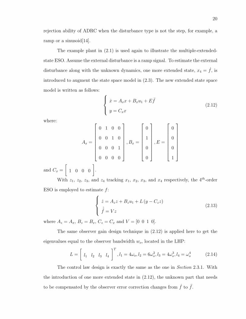
The example plant in (2.1) is used again to illustrate the multiple-extended-
state ESO. Assume the external disturbance is a ramp signal. To estimate the external
disturbance along with the unknown dynamics, one more extended state, x4 = f , is
introduced to augment the state space model in (2.3). The new extended state space
model is written as follows:
x = Axx + Bxu1 + Ef
y = Cxx(2.12)
where:
Ax =
0 1 0 0
0 0 1 0
0 0 0 1
0 0 0 0
, Bx =
0
1
0
0
, E =
0
0
0
1
and Cx =
[1 0 0 0
].
With z1, z2, z3, and z4 tracking x1, x2, x3, and x4 respectively, the 4th-order
ESO is employed to estimate f :
z = Azz + Bzu1 + L (y − Czz)
ˆf = V z
(2.13)
where Az = Ax, Bz = Bx, Cz = Cx and V = [0 0 1 0].
The same observer gain design technique in (2.12) is applied here to get the
eigenvalues equal to the observer bandwidth wo, located in the LHP:
L =
[l1 l2 l3 l4
]T
, l1 = 4ωo, l2 = 6ω2o , l3 = 4ω3
o , l4 = ω4o (2.14)
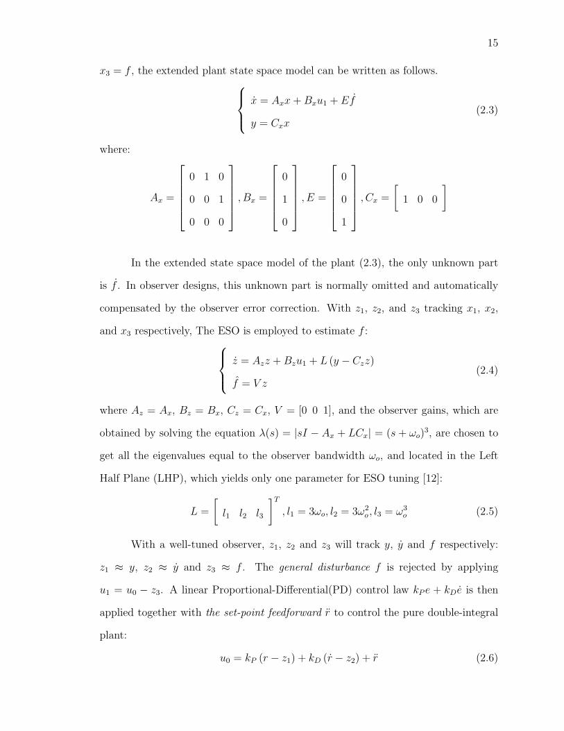
The control law design is exactly the same as the one in Section 2.3.1. With
the introduction of one more extended state in (2.12), the unknown part that needs
to be compensated by the observer error correction changes from f to f .
21
Simulations show that the ADRC with two extended states in the ESO can
estimate and reject a triangular disturbance (which represents bounded ramp signal)
better than the ADRC with one extended state in ESO [14].
Discrete version
Almost all the modern control algorithms are implemented in digital computers
or microprocessors. To be implemented in a digital environment, control algorithms
designed in the continuous-time domain need to be digitized first. A common way
of digitization is to approximate the differential equations to difference equations by
treating the sample value change rate of a signal over one sampling period as its
derivative. For example, assuming f ≈ 0, the plant state space model in (2.3) can be
approximated to the discrete version as shown in the following equation.
x(k + 1) = Φx(k) + Γu(k)
y(k) = Cx(k)(2.15)
where:
Φ =
1 T 0
0 1 T
0 0 1
, Γ =
0
bT
0
, C =
[1 0 0
]
The ESO form in (2.4) can also be approximated to the discrete version as
shown in the following equation.
z(k + 1) = Φz(k) + Γu(k) + Lp (y(k)− z1(k))
y(k) = Cz(k)(2.16)
where
Lp =
[3ωoT 3ω2
oT ω3oT
]T
, (2.17)
Here the design skill that put all the poles at ωo is still applied in continuous
time domain. Actually, pole location can be determined in z domain directly in
22
discrete design[19]. Besides the so-called Predictive Estimator (PE), the design of
which is the same as the ESO described in (2.16), G.F. Franklin also discusses the
Current Estimator (CE) in [19] . The ESO state space form of CE is the same as
PE except for its output. In CE, part of the current estimator error is included in
the estimator outputs to decrease the one-sampling-time delay, which improves the
estimation accuracy, especially when the sampling rate is low. The error compensation
gain matrix Lc is obtained from the equation Lp = ΦLc. R. Miklosovic et al applied
discrete pole location design and implemented the ESO in PE and CE forms in
2006, and named them as Predictive Discrete Extended State Observer (PDESO)
and Current Discrete Extended State Observer (CDESO) respectively [14].
The pole location determination in the z domain for ESO becomes the solution
of a discrete equation, λ(z) = |zI −Φ + LpC| = (z− β)3, where β = e−ωoT . Thus the
coefficient matrices of (2.16) in PDESO and CDESO under Euler and Zero-order-hold
discretization methods are obtained, as shown in the following table.
Table I: PDESO and CDESO coefficient matrices
Type Φ Γ Lp Lc
Euler
1 T 00 1 T0 0 1
0bT0
3(1− β)3(1− β)2 1
T
(1− β)3 1T 2
1− β3
(1− β)2(2 + β) 1T
(1− β)3 1T 2
ZOH
1 T T 2
2
0 1 T0 0 1
bT 2
2
bT0
3(1− β)3(1− β)2(β + 5) 1
2T
(1− β)3 1T 2
1− β3
(1− β)2(1 + β) 32T
(1− β)3 1T 2
The discrete implementations of ADRC show the advantage of controller design
in state space. The discrete pole location determination, the ZOH discretization, and
the current estimator design in the state space are not available for the controllers
designed in transfer function forms.
23
2.4 Other Disturbance Rejection Methods
2.4.1 Internal Model Control
IMC was the first method to estimate and compensate external disturbances
in LTI system. It was developed in the late 1970s and widely used in chemical
industries[4]. IMC is also the only one of the active disturbance rejection methods
discussed in this thesis that was collected in The Control Handbook in 1996[5].
Structure
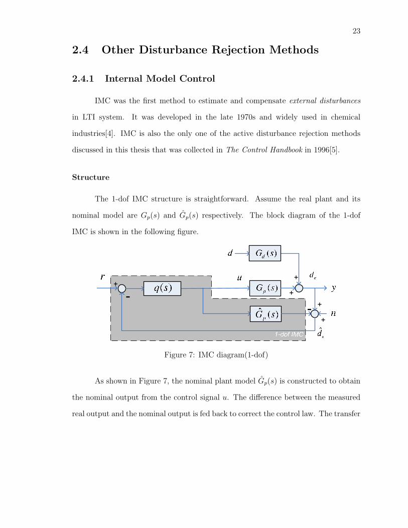
The 1-dof IMC structure is straightforward. Assume the real plant and its
nominal model are Gp(s) and Gp(s) respectively. The block diagram of the 1-dof
IMC is shown in the following figure.
Figure 7: IMC diagram(1-dof)
As shown in Figure 7, the nominal plant model Gp(s) is constructed to obtain
the nominal output from the control signal u. The difference between the measured
real output and the nominal output is fed back to correct the control law. The transfer
24
functions of the system shown in Figure 7 are as follows.
Gry(s) =Gp(s)q(s)
1 +(Gp(s)− Gp(s)
)q(s)
Gdy(s) =Gd(s)
(1− Gp(s)q(s)
)
1 +(Gp(s)− Gp(s)
)q(s)
(2.18)
If Gp(s) matches Gp(s), the denominators in (2.18) equals to 1. By choosing
q(s) = Gc(s)1+Gc(s)Gp(s)
, this open-loop controller q(s) acts as a closed-loop controller Gc
with closed-loop transfer function of the system as Gry(s) = Gp(s)q(s) = Gc(s)Gp(s)
1+Gc(s)Gp(s).
The one-degree-of-freedom (1-dof) IMC structure is not flexible since only one
controller is applied in the system. The disturbance rejection ability of this structure
is also limited: when Gp(s) = Gp(s), the transfer function Gdy equals to Gd(s)1+Gc(s)Gp(s)
,
which is same as a conventional closed-loop controller Gc(s). Fortunately, the 1-dof
IMC structure is easy to be extended to a 2-dof structure, which is shown as follows.
Figure 8: IMC diagram(2-dof)
From Figure 7 to Figure 8, only a simple block operation needs to be carried
out: the controller q(s) is moved ahead of the minus operator. Now there are two
filters: one filters r and is called set-point filter and denoted as qr(s), and the other
one is in the feedback loop and its notation remains as q(s). A filter qd(s) is then
25
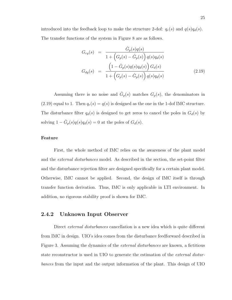
introduced into the feedback loop to make the structure 2-dof: qr(s) and q(s)qd(s).
The transfer functions of the system in Figure 8 are as follows.
Gry(s) =Gp(s)q(s)
1 +(Gp(s)− Gp(s)
)q(s)qd(s)
Gdy(s) =
(1− Gp(s)q(s)qd(s)
)Gd(s)
1 +(Gp(s)− Gp(s)
)q(s)qd(s)
(2.19)
Assuming there is no noise and Gp(s) matches Gp(s), the denominators in
(2.19) equal to 1. Then qr(s) = q(s) is designed as the one in the 1-dof IMC structure.
The disturbance filter qd(s) is designed to get zeros to cancel the poles in Gd(s) by
solving 1− Gp(s)q(s)qd(s) = 0 at the poles of Gd(s).
Feature
First, the whole method of IMC relies on the awareness of the plant model
and the external disturbances model. As described in the section, the set-point filter
and the disturbance rejection filter are designed specifically for a certain plant model.
Otherwise, IMC cannot be applied. Second, the design of IMC itself is through
transfer function derivation. Thus, IMC is only applicable in LTI environment. In
addition, no rigorous stability proof is shown for IMC.
2.4.2 Unknown Input Observer
Direct external disturbances cancellation is a new idea which is quite different
from IMC in design. UIO’s idea comes from the disturbance feedforward described in
Figure 3. Assuming the dynamics of the external disturbances are known, a fictitious
state reconstructor is used in UIO to generate the estimation of the external distur-
bances from the input and the output information of the plant. This design of UIO
26
does not require the direct measurement of the disturbance, which is needed in the
disturbance feedforward design.
The earliest direct external disturbances cancellation method is the Distur-
bance Accommodation Control (DAC) by C. D. Johnson in 1971 [20], which was
later referred to by E. Schrijver as UIO. Later on, J. Profeta et al proposed a discrete
version of UIO and showed some of its frequency responses[21]. Y. Guan et al applied
reduced-order observer design in UIO in 1991[22].
Structure
Figure 9: UIO diagram
Figure 9 shows the block diagram of UIO, where the plant is LTI, denoted
as Gp(s) and the UIO use the plant output and the control signal to estimate the
external disturbance. The UIO form described in [23] is used here to easily illustrate
the idea of UIO in order to make comparison between UIO and ESO easier in the
next chapter. Assume that the models of the plant and the external disturbances are
both known. The state space forms of the nominal plant model and the fictitious
external disturbances reconstructor are presented in (2.20) and (2.21) respectively:
x = Ax + B(u + d)
y = Cx(2.20)
27
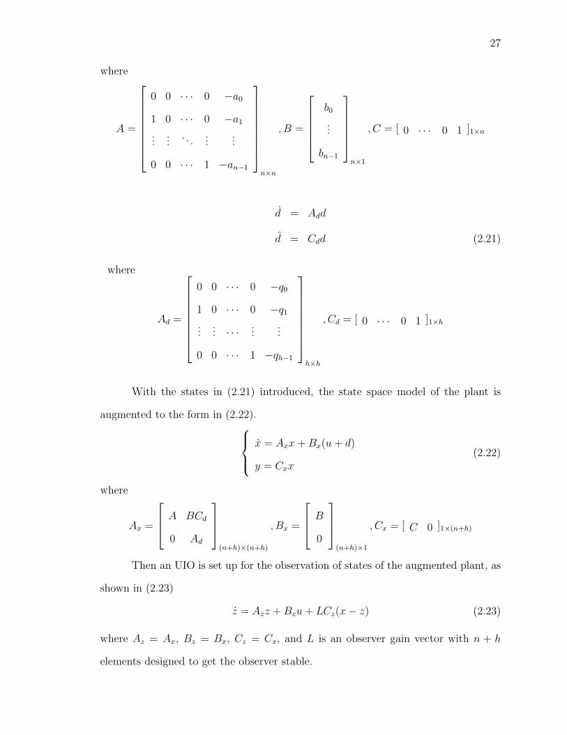
where
A =
0 0 · · · 0 −a0
1 0 · · · 0 −a1
......
. . ....
...
0 0 · · · 1 −an−1
n×n
, B =
b0
...
bn−1
n×1
, C = [ 0 · · · 0 1 ]1×n
d = Add
d = Cdd (2.21)
where
Ad =
0 0 · · · 0 −q0
1 0 · · · 0 −q1
...... · · · ...
...
0 0 · · · 1 −qh−1
h×h
, Cd = [ 0 · · · 0 1 ]1×h
With the states in (2.21) introduced, the state space model of the plant is
augmented to the form in (2.22).
x = Axx + Bx(u + d)
y = Cxx(2.22)
where
Ax =
A BCd
0 Ad
(n+h)×(n+h)
, Bx =
B
0
(n+h)×1
, Cx = [ C 0 ]1×(n+h)
Then an UIO is set up for the observation of states of the augmented plant, as
shown in (2.23)
z = Azz + Bzu + LCz(x− z) (2.23)
where Az = Ax, Bz = Bx, Cz = Cx, and L is an observer gain vector with n + h
elements designed to get the observer stable.
28
The estimated external disturbance, zn+h, is then subtracted from the control
signal to reject the real external disturbances. The estimated states(from z1 to zn)
are then fed back for the control signal generation.
Features
Although designed in different way, UIO is the closest one to ESO among all
the methods discussed in this research. Like ESO, the advantage of UIO is that, as
a state observer, UIO estimates not only disturbances but also states. This is the
benefit of ESO and UIO against DoB. With the estimation of the plant states, the
control system with UIO is a state feedback control system.
The disadvantage of UIO is that, like IMC, UIO is constructed on the basis
that the models of the plant and the disturbances are already known. Otherwise the
method cannot be applied. Also, no stability proof is given for UIO applied to NTV
systems.
2.4.3 Disturbance Observer
The idea of DoB is the input external disturbances estimation similar to UIO,
but implemented in frequency domain as a transfer function design.
The original DoB was proposed by T. Umeno et al in 1991 as part of a param-
eterized linear 2-dof controller designed to reject external disturbances [24]. Here the
equivalence between the 2-dof controller in the Type I system and some other distur-
bance observers, such as the disturbance torque observer developed by K. Ohishi et
al in 1987[25], and the torque observer proposed by Y. Hori in 1988[26], are verified.
The DoB design finally concentrates on the so-called Q-filter design.
Furthermore, in 1996, H. Lee et al applied DoB in the velocity loop together
with a feedforward nonlinear friction compensator in high-speed motion control to
29
get better performance against nonlinear friction[27]; Cheng et al [28] and Yang et al
[29] applied set-point feedforward along with DoB.
In 2002, E. Schrijver analyzed DoB (which is denoted as the Disturbance Es-
timating Filter (DEF) to be distinguished from UIO) in detail, disclosed the equiva-
lence between UIO and DoB in the aspect of external disturbances estimation under
certain conditions[23], and extended the application of DoB to non-minimum-phase
plant. Schrijver speculated that, besides the external disturbance rejection function,
DoB also presents the rejection ability against the discrepancy between the real plant
and its nominal model in the low frequency. However, there is no proof for the this
assertion.
Structure
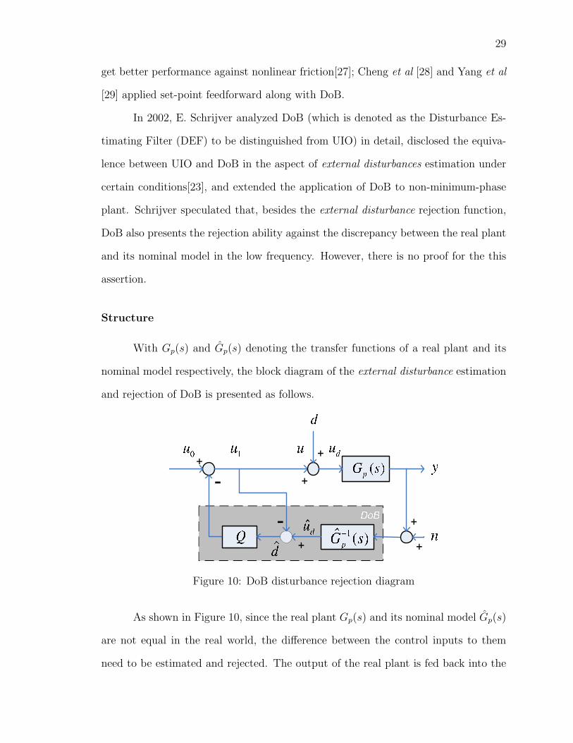
With Gp(s) and Gp(s) denoting the transfer functions of a real plant and its
nominal model respectively, the block diagram of the external disturbance estimation
and rejection of DoB is presented as follows.
Figure 10: DoB disturbance rejection diagram
As shown in Figure 10, since the real plant Gp(s) and its nominal model Gp(s)
are not equal in the real world, the difference between the control inputs to them
need to be estimated and rejected. The output of the real plant is fed back into the
30
inverse of the nominal plant to get the nominal control signal ud that will generate
the output in the nominal plant. Then d, the estimation of external disturbance d,
is obtained from the difference between u and ud and cancelled in the control signal
after a filter Q. Expressed in equation form, the external disturbance estimation of
DoB is expressed in the following equation:
d = Q(G−1
p (s)y(s)− u(s))
(2.24)
There are three reasons to introduce Q into DoB. One is that direct feedback of
d cannot be realized because normally the inverse plant is non-proper, which means
the degree of the numerator is greater than the degree of the denominator. The
filter Q in Figure 2.24 can be moved backwards before the subtraction operator.
With QG−1p (s) proper, DoB is then implementable. The second reason is that direct
feedback would result in an algebraic loop. The last reason is that Q filter can filter
the measurement noise in the feedback signal.
The transfer functions describing the relationship between input u0, d, n, and
output y in Figure 10 are as follows.
Gu0y(s) =Gp(s)Gp(s)
Q(Gp(s)− Gp(s)
)+ Gp(s)
Gdy(s) =Gp(s)Gp(s)(1−Q)
Q(Gp(s)− Gp(s)
)+ Gp(s)
Gny(s) = − Gp(s)Q
Q(Gp(s)− Gp(s)
)+ Gp(s)
(2.25)
The transfer functions in (2.25) show that the DoB structure effectively rejects
disturbance in low frequency. However, at the same time measurement noise is in-
troduced into the system through the disturbance rejection feedback. Therefore, the
design of the Q filter is an essential part of DoB. The bandwidth of Q cannot be too
high, which will introduce more noise. The bandwidth of Q can also not be too low,
31
which will degrade disturbance rejection performance. This trade-off also exists in all
the other disturbance rejection methods.
In the 2-dof control method implemented with DoB, one dof is used as output
feedback controller(which is the same as other controllers, such as PID), while the
other(which is DoB) is used to estimate and reject the external disturbance, as shown
in Figure 11.
Figure 11: DoB diagram
DoB can also be interpreted in feedback loop, as shown in the following dia-
gram.
Figure 12: Feedback Interpretation of the DoB
Assume the plant is given as Gp(s) = 1ms
and the Q filter is designed as 1sτ
.
The equivalent feedback controller (1 − Q)−1QG−1p (s) is now a constant m
τ. In this
case the design of DoB is simplified to a proportional controller.
32
Features
DoB simplifies the external disturbance rejection design to a low-pass filter
design, which makes it easy to understand. However, the explanation of how DoB
works in Schrijver’s work is kind of a contradiction. In the disturbance rejection
explanation, Q needs to be approximately equal to 1 at low frequency to get the
plant to act as the nominal plant. But in the feedback interpretation of DoB, as
shown in Figure 12, Q cannot equal to one. Otherwise the system would have infinite
gain which causes a singlarity in the system. Thus interpreting disturbance rejection
in the form of Q may not be a good choice.
As a frequency-domain design method, DoB also has some other disadvantages.
First, DoB requires that the nominal plant model and its inverse are available. If the
detailed plant information is unknown, the inverse of it is not available and then
the DoB method can not be applied. Second, DoB is designed for LTI systems
only; therefore it cannot deal with nonlinearities. That is why the nonlinear friction
compensation is introduced in [27]. Third, DoB can only estimate disturbance, which
is determined by its control structure. Fourth, in order to implement DoB, the product
QG−1p (s) must proper. Thus Q normally needs to be designed as high-order low-pass
filter and induce more phase lag into the system. Finally, except for the rigid body,
there is no explicit stability proof for DoB. Schrijver also claimed that, although the
nominal plant of DoB can be cascaded integrators, it is not recommended because
“for Gp(s) 6= Gp(s), stability and performance might be in danger”. This assertion
shows that the nominal model need to be accurate in DoB.
2.4.4 Perturbation Observer
Several years after the appearance of DoB, the initial form of PoB was proposed
together with a sliding mode controller as part of a tracking controller by S. Kwon
33
et al in 2001[30]. The concept of DoB is applied in the difference equation form to
obtain disturbance estimation. In his work, S. Kwon et al applied three different
PoBs(the Feedback Perturbation Observer (FBPO), the Feedforward Perturbation
Observer (FFPO), and the Sliding Mode Perturbation Observer (SMPO)) in a parallel
way, called the Multiloop Perturbation Compensation (MPEC) .
Getting an insight from the Time-Delayed Estimator (TDE), Kwon combined
TDE and the filter design in DoB in 2003 to get the discrete realization of PoB[31].
The newest work of PoB is the combination of PoB and Kalman Filter in 2006 by
Kwon[32].
Structure
PoB can be taken as a filtered version of TDE, or an implementation of DoB
in the discrete time domain.
In TDE, the inverse of the plant model is obtained by a pseudoinverse algo-
rithm. At the current time point, the states and control signal at the previous time
point are used to estimate the external disturbance at the previous time point through
the inverse plant model. Assume the disturbance remains the same during a sampling
time period and then the current external disturbance estimation is obtained. PoB
applies a Q filter(the low pass filter designed in DoB ) on the external disturbance es-
timation obtained from TDE to get rid of noise in high frequency. Finally the filtered
external disturbance estimation is rejected in the control signal.
Assume the discrete nominal plant model is the following equation.
x(k + 1) = Φx(k) + Γ(u(k) + d(k))
y(k) = Cx(k)(2.26)
Let Γ+ denote the pseudoinverse of Γ. At k time point, x(k), x(k − 1), and
u(k − 1) are known and can be used to calculate the previous external disturbance
34
d(k − 1) through the inverse operation as shown in the following equation.
d(k − 1) = Γ+ (x(k)− Φx(k − 1))− u(k − 1) (2.27)
Assuming that the external disturbance changes little during (k − 1, k) time
interval, d(k) ≈ d(k − 1), a digital Q filter is applied to smooth d(k − 1) and then
d(k) is obtained.
d(k) = Q(Γ+ (x(k)− Φx(k − 1))− u(k − 1)
)(2.28)
The perturbation observer described in (2.28) is called FBPO. If the reference
signals are used to replace the states in equation (2.28) under the assumption that
the states track the reference closely, equation (2.28) is changed to FFPO.
Features
Since PoB can be looked on as implementation of DoB in discrete-time domain,
this method has the same features as DoB except for that the external disturbance
estimation and rejection is carried out in discrete-time, and that the discrete states
of the system need to be available in PoB for the pseudoinverse operation.
2.4.5 Model Estimator
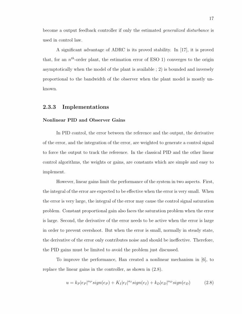
A PID Controller designed for the robust stabilization of SISO systems is
proposed in 1994 by A. Tornambe et al [33]. Although the expression of this controller
is quite different from DoB, UIO, or the other active disturbance rejection methods,
it can estimate internal dynamics pretty well. To be distinguished from the other
disturbance rejection methods, this controller is called ME in this thesis. Even though
there is no external disturbance rejection declaration in ME, it has the ability to reject
external disturbance.
35
Structure
ME deals with plants whose relative degree is equal to n(where the orders of
the numerator and denominator of plant transfer function are q and p respectively
and n = p − q). When expressed in state space, the plant model is the following
equation.
ε = Aε + Bu
y = Cε(2.29)
Choose new states as the follows.
xi := CAi−1ε, i = 1, · · · , n,
ηi := εi, i = 1, · · · , p− n(2.30)
where xi are observable states and ηi are unobservable states.
Then the plant model is simplified to
xi = xi+1, i = 1, · · · , n− 1,
xn = f + u
y = x1
(2.31)
where f = f(x1, · · · , xn−1, η1, · · · , ηq, u) is the discrepancy between the simplified
plant model and the desired model consisting of cascade integrators.
Assuming xn = y(n−1) is available, an ME is constructed to get f , the estima-
tion of f , as shown in the following equation.
ξ = −lξ − l2xn − lu
f = ξ + lxn
(2.32)
where l is a low pass filter bandwidth.
As derived in the next section, the relative degree of the equivalent Q filter in
ME equals one.
36
Features
ME is equivalent to one special case of RESO to be proposed in the next
chapter. The advantage of ME is that, the observer has the minimum phase lag since
the relative degree of the equivalent low pass filter is 1.
Although rigorous stability proof is provided for ME, it is under the assumption
that the plant model is completely known. Another disadvantage of ME is that,
its assumption that the up to (n − 1)th-order derivatives of the plant output are
measurable is not realistic.
2.5 Comparisons of active disturbance rejection
methods
2.5.1 Disturbance rejection diagram
From the diagram comparison among the different active disturbance estima-
tion algorithms, a general diagram can be sketched out, as shown in Figure 13.
Figure 13: Diagram of general disturbance estimator
In all the algorithms discussed in this chapter, the control signal u and the
system output y are used to estimate the disturbance, which is then rejected in the
control signal.
37
2.5.2 Equation equivalence
IMC versus DoB
After a simple block diagram manipulation of Figure 10, the DoB diagram
can be converted into following 2-dof IMC form. In the 2-dof IMC design in Section
2.4.1, one dof estimates and rejects disturbance, and the other one, as an open-
loop controller, forces the output to follow the reference. Putting the open-loop
controller aside, the disturbance rejection part of DoB is equivalent to that of IMC if
Q(s)G−1p (s) = q(s)qd(s).
Figure 14: DoB in IMC form
ESO versus UIO and DoB
For UIO with the nominal plant as a set of cascade integrators , its state space
form is identical to the form of ESO. This can be easily seen from the comparison
between the ESO equation in (2.13) and the UIO equation in (2.23) when n = 2,
h = 2 and the nominal plant of UIO is pure double integral plant (a0, a1, b1 in (2.20)
and q0, q1 in (2.21) all equal to zero).
The equivalence of DoB and UIO under certain conditions is already shown
by Schrijver in [23]. Although DoB is not designed to estimate unknown dynamics,
it is putted into the ESO framework for an nth-order LTI plant to make comparison
38
between DoB and ESO. The differential equation of the LTI plant is as follows.
y(n) +n−1∑i=0
aiy(i) = b(u + d) (2.33)
The transfer function between u and y is Gp(s) = b
sn+n−1∑i=0
aisi
. Defining F (s) =
−n−1∑i=0
aisi, which is assumed to be unknown and to be rejected, the transfer func-
tion of the plant can be written as Gp(s) = bsn−F (s)
. The essence of ESO is to treat
the plant as a series of cascade integraotrs no matter what it is. Therefore, assuming
the nominal plant transfer function of DoB is Gp(s) = bsn , substituting Gp(s), Gp(s)
and ρ = b/b in equation (2.25), the transfer functions to be compared to ESO transfer
functions in the next chapter are obtained, shown as follows.
Gu0y(s) =ρ
sn + (1−Q)ρsn − (1−Q)F (s)
Gdy(s) =b(1−Q)
sn + (1−Q)ρsn − (1−Q)F (s)= b(1−Q)Gu0y
Gny(s) = − ρsnQ
sn + (1−Q)ρsn − (1−Q)F (s)= −snQGu0y (2.34)
ME versus ESO and DoB
Substitute the second equation into the first equation in (2.32) and rearrange
it to get˙f = l(xn − u − f). Remember that the states xn−1 and xn are defined as
y(n−1) and y(n) respectively . Let z = f . Substitute xn−1, xn, and z into the previous
equation and get its Laplace form as follows.
Z(s) =l
s + l(snY (s)− U(s)) (2.35)
Compare (2.24) to (2.35), the two equations are the same when Q(s) = ls+l
and
G−1p (s) = sn. This derivation discloses that ME is equal to DoB when the nominal
plant of DoB is cascaded integrators and the Q filter in DoB is designed as first order.
Again, the nominal model of cascaded integrators is not suggested in DoB.
39
The equation (2.35) and the Laplace transform of the equation (3.5) are the
same. Thus, ME is a special case of ESO when y(n) is available in ESO design, as
shown in the next chapter.
2.5.3 General comparison
The overall comparison of different active disturbance rejection methods are
shown in the following table. Among all the disturbance estimators in Table II, only
ESO can deal with NTV plant. The NTV items are treated as a disturbance. IMC,
DoB, UIO, PoB, and ME are based on the known linearized plant model. That is to
say, these methods are applicable only near the equilibrium points where the plant
is linearized. In [23], Schrijver mentioned that a DoB was applied to nonlinear plant
in [34]. However, the nonlinearity of the plant is compensated by an Acceleration
Tracking Controller, in which the nonlinearity is constructed based on the nonlinear
plant model. Thus, in this nonlinear plant case, DoB only deals with the linear part
of the plant.
Table II: Comparison of ADRC, IMC, DoB, UIO, PoB, and ME
ESO IMC DoB UIO PoB MENonlinear Yes No No No No No
TV supportNeeded Model Min Max Max Max Max MinInformation
State Yes No No Yes No YesEstimationStability Yes Not Available Not Not YesProof on for special
NTV system case
Among the discussed disturbance estimators, ESO and ME require the mini-
mum plant information: the plant relative order n and the plant gain factor b. ADRC
and ME achieve this by treating the internal plant dynamics as part of the distur-
40
bance and treating the plant as a series of cascade integrators. IMC, DoB, UIO and
PoB need much more information: the nominal plant model. Real plants always con-
tain nonlinearities. To implement these model-based disturbance algorithms, the real
plants need to be linearized to get the approximated linear behavior of the plant near
the equilibrium points. As a result, in DoB and PoB implementation, the inverse and
the pseudo-inverse of the plant model need to be derived respectively, which adds
much difficulty in their implementation.
As state observers, ESO and UIO estimate states besides the disturbance. Thus
state feedback control methods can be applied with ESO or UIO. IMC, DoB, PoB,
and ME merely estimate the disturbance. Therefore IMC, DoB, PoB, and ME can
only be used with output feedback algorithms.
Finally, among these disturbance estimators, only ESO and ME have stability
proofs. For ME, stability is not guaranteed except for the fact that the plant dynamics
are given. The stability study of ESO goes further: not only the asymptotic stability
proof for systems with known dynamics is provided; but also for systems with un-
known dynamics, the estimation error and the closed-loop tracking error are shown
to be bounded and have the inverse relationship with bandwidths of the observer and
controller [17], [35].
CHAPTER III
REDUCED-ORDER EXTENDED
STATE OBSERVER
The comparisons among different disturbance rejection methods in the previ-
ous chapter disclose an idea: disturbance rejection is of a common structure. That is,
disturbance information obtained from the input and output data is manipulated and
fed back into the control signal in real-time in a certain manner to reject disturbance.
Under this common structure, the advantage of different methods can benefit each
other. For example, the stability proof of ADRC can be utilized in the other methods.
Another example is the filter design in DoB. This can also be used in the explanation
of ESO and UIO. Indeed, observers work as low pass filters which decrease the mea-
surement noise in the feedback loop. However, at the same time the low pass filters
also bring phase lag. The bigger the relative order, the more the phase lag. Under
this consideration, the equivalent first-order low pass filter in ME makes it attractive
because it operates with the least phase lag compared to other methods. But this
least phase lag is based on the assumption of ME that the (n− 1)th-order derivative
41
42
of the output is known. Therefore a question is raised: can we reduce the phase lag
in ESO or UIO if the higher order derivative of the output signal is known? or in
other words, can the order of the observer be reduced? This question natually leads
to the reduced order observer.
In the rest of this chapter, first, RESOs are proposed to estimate the states
and disturbance for a 2nd-order plant. Then the ADRC with RESO is generalized
for nth-order plant. Finally the 2-dof transfer functions of the ADRC with RESO are
derived to give some observations and to help the research on the frequency response
analysis of ADRC.
3.1 Reduced-order Extended State Observer
The reduced-order observer was first introduced in 1964 by D.G. Luenberger
[36]. The presumption of the reduced-order observer is that some of the plant outputs
are known and do not need to be observed. The reduced-order observer under the
condition that the derivatives of the system output are known was already discussed
in Luenberger’s work. In ADRC structure, application of reduced-order observer is
straightforward. In the example in (2.3), the system output y is known through
measurement and usually does not need to be estimated. The first derivative of y can
be approximated from the difference of two neighboring y sample values divided by
the sampling time, denoted as ˆy. Thus, the reduced-order observer can by applied in
ESO.
Before the proposal of RESO, the existing ESOs are reexamined to give some
insights. The augmented plant model in (2.3) and the ESO in (2.4) are compared in
43
the following equations.
(3.1)
The blue shadow in (3.1) shows that the ESO matrices Az and Bz are obtained
from Ax and Bx directly. Since the 3rd-order ESO in (3.1) contains the two original
states x1 and x2, it is of full order.
Assuming x2 = y is available, a RESO can be constructed with z1 and z2
estimating x2 = y and x3 = f , respectively. The relationship between the augmented
plant state space model and the RESO is shown as follows.
(3.2)
As shown in (3.2), the RESO matrices Az and Bz are obtained from the blue-
shadowed part of Ax and Bx respectively. Thus the order of this RESO is 2, smaller
than the order of the augmented plant model.
Here the observer equation is as follows:
z = Azz + Bzu1 + L(y − Czz)
f = V z(3.3)
where:
Az =
0 1
0 0
, Bz =
1
0
, L =
l1
l2
, Cz = [ 1 0 ], V = [ 0 1 ]
and l1 = 2ωo, l2 = ω2o .
44
The order reduction in the RESO may be continued under the assumption
that y is available (which is equivalent to the assumption that the state x3 = y − bu
is available). Another RESO can be constructed with z to track x3 = f . The
relationship between the augmented plant state space model and the new RESO is
shown in the following equations.
(3.4)
As shown in (3.4), the RESO matrices Az and Bz are also obtained from the
blue-shadowed part of Ax and Bx respectively. Thus the order of this RESO is 1.
The difference between this RESO and the previous RESO is that the requirement
changes from x2 = y available to x3 = y − bu available. The RESO equation is as
follows:
z = l(y − bu− z)
f = z(3.5)
where l = ωo.
Define f = ξ + ly. Let b = 1(The factor b is removed by its inverse in the
control law in ME). Substitute f into (3.5) and get the same equations as the ones
in (2.32). This demonstrates that ME is a special case of RESO.
The order reduction can also be applied when there are multiple extended
states in the ESO, as shown in the following equations.
(3.6)
45
(3.7)
(3.8)
As shown in (3.6), (3.7), and (3.8), the order of the ESO with two extended
states reduces from 4 to 3, to 2 respectively.
3.2 Generalization of ADRC controller with RESO
A common framework of ADRC with RESO dealing with nth-order plant is
generalized in this chapter to facilitate analysis. The block diagram of the ADRC
with RESO is shown as follows.
Figure 15: ADRC with Single-loop ESO Block Diagram
The plant in the Figure 15 is defined as an nth order plant with differential
46
equation as follows.
y(n) = f(y, y, · · · , d, t) + bu (3.9)
where f(y, y, · · · , d, t) denotes the generalized disturbance to be estimated and re-
jected.
Normally b, the estimation of b, can be obtained. The influence of the ratio
ρ = b/b on the system when it does not equal to 1 will be discussed later. Here
assuming b = b, a control law u1 = bu is applied to remove the b factor influence from
the system. Thus, with u1 as input and y as output, equation(3.9) becomes the unity
gain plant, shown as follows.
y(n) = f(y, y, · · · , d, t) + u1 (3.10)
Choose states as x1=y, x2=x1=y, · · · , xn=xn−1=y(n−1). Also choose h ex-
tended states as xn+1=f , xn+2=xn+1=f , · · · , xn+h=xn+h−1=f (h−1). The unity gain
plant (3.10) can now be expressed in the augmented matrix
(3.11)
or in state space form
x = Axx + Bxu1 + Ef (h)
y = Cxx(3.12)
47
where
Ax =
0 1 0 · · · 0
0 0 1 · · · 0
0 0 0. . .
...
......
. . . . . . 1
0 0 0 · · · 0
(n+h)×(n+h)
, Bx =
0
...
0
1
0
...
0
(n+h)×1
, E =
0
...
0
1
(n+h)×1
Cx = [ 1 0 · · · 0 ]1×(n+h)
where the nonzero element in Bx is in the nth row.
Assume y, y, · · · , y(n+h−m)are available. Then the states x1, x2, · · · , xn+h−m+1
are available (If m=h, the last state can be obtained from its definition: xn+1 = f =
y(n)−u1). Also assume f (h) does not change rapidly and can be ignored. According to
the reduced-order observer design in the previous chapter, ESO order can be reduced
to m, where h ≤ m ≤ n + h. Apply the order reduction operation in the same way
as the previous section and get the ESO as follows.
(3.13)
Now z1, · · · , zm are designed to estimate xn+h−m+1, · · · , xn+h, respectively. The
shadowed gain matrices in the ESO are obtained from the matrices of the augmented
plant directly. For tuning simplicity, the observer gains l1, · · · , lm are chosen as
48
li =
m
i
ωi
o where 0 < i ≤ m.
m
i
denotes the Binomial Coefficient m!
i!(m−i)!.
Also, to make the transfer function derivation easier, define l0 =
m
0
ω0
o = 1.
Equation (3.13) is also expressed as follows.
z = Azz + Bzu1 + L (xn+h−m+1 − Czz)
f = V z(3.14)
where
Az =
0 1 0 · · · 0
0 0 1 · · · 0
0 0 0. . .
...
......
. . . . . . 1
0 0 0 · · · 0
m×m
, L =
l1
l2...
lm
m×1
,
Cz =
[1 0 · · · · · · 0
]
1×m
if m = h,
Bz = [0]m×1, V =
1
0
...
0
m×1
;
if m > h,
Bz =
0
...
0
1
0
...
0
m×1
, V =
0
...
0
1
0
...
0
m×1
49
(when m > h, the nonzero elements of Bz and V are in the (m − h)th row and
(m− h + 1)th row respectively.)
When m = n + h, the ESO is of full order and estimates all the states x1, · · · ,xn, the disturbance f and its derivatives; when h < m < n + h, ESO estimates the
states xn+h−m+1, · · · , xn, f and its derivatives; when m = h, the ESO is of the least
order and estimates only f and its derivatives.
With the state zm−h+1 in the ESO to estimate f , a control law, u1 = u0 −zm−h+1, is applied to reduce the plant to a pure nth order plant y(n) = u0.
Then a parameterized general PD control law is applied to control the pure
nth order plant as follows.
u0 =n+1∑i=1
kir(i−1) −
n+h−m∑i=1
kiy(i−1) −
m−h∑i=1
kn+h−m+izi (3.15)
where ki =
n
i− 1
ωn+1−i
c , 1 ≤ i ≤ n + 1, and the itemn+h−m∑
i=1
ki does not exit
when m = n + h because all the feedback signals come from ESO output under this
condition.
3.3 Transfer Function Derivation
To analyze the ADRC in the frequency domain, the plant is narrowed to a
LTI system. Although this degradation hides some advantages of ADRC, such as the
ability to deal with nonlinear plant and the efficiency when the control law and the
ESO in ADRC are designed with nonlinear gains, the analysis will still give insights
of how ADRC works.
Suppose the plant is a nth-order LTI system with differential equation as the
follows.
y(n) +n−1∑i=0
aiy(i) = bu (3.16)
50
where ai, i = 0 : n− 1 and b are constant coefficients.
As shown in Figure 15, an external disturbance d is introduced into the plant.
Thus, the disturbed plant differential equation of (3.16) is as the follows.
y(n) +n−1∑i=0
aiy(i) = b(u + d) (3.17)
Define b as the estimation of b and apply u = u1/b in (3.17)to get
y(n) = u1 −n−1∑i=0
aiy(i) + (ρ− 1)u1 + bd (3.18)
where ρ is the ratio between real plant parameter b and it’s estimation, ρ = b/b.
The goal of disturbance rejection is to estimate the dynamics and disturbance
aisi−1. Thus the Laplace transform of the generalized
disturbance f can be expressed as L{f} = F (s)Y (s) + (ρ− 1)U1(s) + bD(s), and the
Laplace transform of (3.17) is expressed as follows.
snY (s) = F (s)Y (s) + U1(s) + (ρ− 1)U1(s) + bD(s) (3.19)
Furthermore, the Laplace Transform of the states are also expressed in vector
form
X(s) =
X1(s)
X2(s)
...
Xn(s)
Xn+1(s)
Xn+2(s)
...
Xn+h(s)
=
1
s
...
sn−1
F (s)
sF (s)
...
sh−1F (s)
Y (s) +
0
0
...
0
1
s
...
sh−1
((ρ− 1)U1(s) + D(s))
(3.20)
51
3.3.1 Procedure
To minimize the derivation work, the transfer functions needed in analysis are
derived in the following steps.
Compensated plant transfer function
The whole system is divided into two parts with respect to u0 and y. the part
of the system that between u0 and y, denoted as Gp0(s), is the approximated cascade
integrators(after disturbance estimation and rejection), as shown in Figure 16.
Figure 16: Compensated plant Block Diagram
The noise n introduced by disturbance rejection and the disturbance d are
derived to act on u0 with transfer functions Gn(s) and Gd(s) respectively, as shown
in Figure 17.
Figure 17: 2-dof (U0) Block Diagram
52
2-dof transfer function with respect to u0
The rest of the plant is then fit into a 2-dof control structure with r and y as
inputs and u0 as output, the two transfer functions in which are H0(s) and Gc0(s)
respectively, as shown in Figure 17.
2-dof transfer function with respect to u
Then from Figure 16, the disturbance rejection part and the scaling factor 1/b
are included into the control part and then H(s) and Gc(s), the transfer functions in
2-dof control structure with respect to u and y, are obtained, as shown in Figure 18.
Figure 18: 2-dof (U) Block Diagram
3.3.2 Results
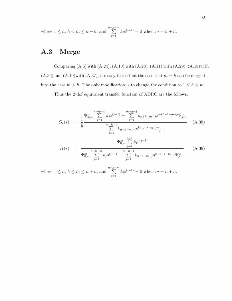
The detail derivation of the transfer functions are presented in Appendix A.
Here only the derivation results are shown.
Define Q =Ψm
m−h+1,m
Ψm0,m
(the defination of Ψ is in the begining part of Appendix
A), which is consistent with the Q filter in DoB and makes the comparison between
DoB and ADRC easier. Substitute Q into (A.24) and get the following equation.
Y (s) =ρU0(s) + (1−Q)bD(s)− ρQsnN(s)
sn + (ρ− 1)snQ− F (s)(1−Q)(3.21)
53
From (3.21), the transfer functions in Figure 17 are obtained, as the follows.
Gp0(s) =ρ
sn + (ρ− 1)snQ− F (s)(1−Q)
Gd(s) = b(1−Q)
Gn(s) = −Qsn (3.22)
The 2-dof transfer functions H0(s), Gc0(s), H(s), and Gc(s) are shown in
(A.33), (A.32), (A.37), and (A.36), respectively in Appendix A.
3.3.3 Analysis
Q filter design mapping
Transfer functions in (3.22) are in the same form as (2.34) . Thus, the mapping
between ADRC RESO design and DoB Q-filter design in disturbance rejection aspect
can be established when nominal plant of DoB is cascade integrators, as shown in the
following table.
Table III: Mapping between DoB and parameterized ESO
DoB ESO DoB ESOQ30 m=3, h=1 Q20 m=2, h=1Q31 m=3, h=2 Q21 m=2, h=2Q32 m=3, h=3 Q10 m=1, h=1
States and Disturbance Estimation
In the low frequency,Ψm
i,m
Ψm0,m
≈ 1, where 0 < i ≤ m;Ψm
i,j
Ψm0,m
≈ 0, where 0 ≤ i < m
and 0 ≤ j < m. Also, measurement noise can be ignored in low frequency. Substitute
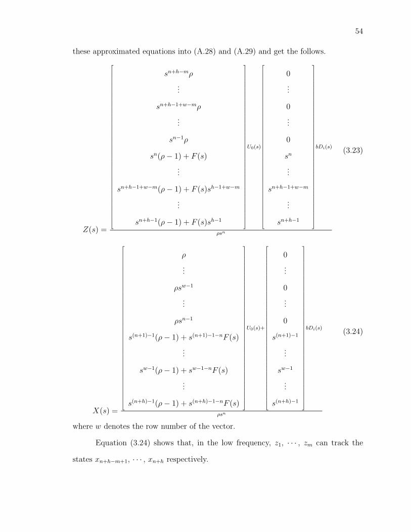
54
these approximated equations into (A.28) and (A.29) and get the follows.
Z(s) =
sn+h−mρ
...
sn+h−1+w−mρ
...
sn−1ρ
sn(ρ− 1) + F (s)
...
sn+h−1+w−m(ρ− 1) + F (s)sh−1+w−m
...
sn+h−1(ρ− 1) + F (s)sh−1
U0(s)
0
...
0
...
0
sn
...
sn+h−1+w−m
...
sn+h−1
bDi(s)
ρsn
(3.23)
X(s) =
ρ
...
ρsw−1
...
ρsn−1
s(n+1)−1(ρ− 1) + s(n+1)−1−nF (s)
...
sw−1(ρ− 1) + sw−1−nF (s)
...
s(n+h)−1(ρ− 1) + s(n+h)−1−nF (s)
U0(s)+
0
...
0
...
0
s(n+1)−1
...
sw−1
...
s(n+h)−1
bDi(s)
ρsn
(3.24)
where w denotes the row number of the vector.
Equation (3.24) shows that, in the low frequency, z1, · · · , zm can track the
states xn+h−m+1, · · · , xn+h respectively.
55
Controller Type and Phase Lag
The equivalent 2-dof controller transfer functions of ADRC with RESO (the
same as (A.38) ) are as follows.
Gc(s) =1
b
Ψm0,m
n+h−m∑j=1
kjs(j−1) +
m−h+1∑j=1
kn+h−m+jsn+h−1−m+jΨm
j,m
m−h+1∑j=1
kn+h−m+jsh−1+j−mΨm0,j−1
H(s) =
Ψm0,m
n+1∑j=1
kjs(j−1)
Ψm0,m
n+h−m∑j=1
kjs(j−1) +m−h+1∑
j=1
kn+h−m+jsn+h−1−m+jΨmj,m
where 1 ≤ h, h ≤ m ≤ n + h, andn+h−m∑
i=1
kis(i−1) = 0 when m = n + h.
The highest order of the numerator in Gc(s) is n+h−1. When m = n+h, the
lowest order of the numerator in Gc(s) is determined by its second item and equals
0; when m < n + h, the lowest order of the numerator in Gc(s) is determined by its
first item and equal to 0. The highest order and the lowest order of the denominator
in Gc(s) are m and h respectively. Therefore, Gc(s) can be expressed as follows.
Gc(s) =
n+h−1∑i=0
cnisi
m∑i=h
cdisi
(3.25)
where cni and cdi are constants.
Equation (3.25) shows that the relative degree of the Gc(s) is n + h − m −1. When m decreases, the phase lag decreases. It also can be concluded that this
controller contributes h integrators to the open-loop transfer function.
Similarly, H(s) can be expressed as follows.
H(s) =
n+m∑i=0
cnisi
n+h−1∑i=0
cdisi
(3.26)
where cni and cdi are constants, different from the ones in (3.25).
CHAPTER IV
FREQUENCY RESPONSE ANALYSIS
OF ADRC
In this thesis, for simplicity, only ADRC controllers with one-extended-state
ESO or RESO , which are applied on a linear time-invariant second-order plant, are
analyzed. The differential equation and the transfer function of the studied plant are
as follows:
y = −a1y − a0y + b(u + d) (4.1)
where a0 and a1 are unknown.
Gp(s) =b
s2 + a1s + a0
(4.2)
Since both the plant and the controller are linear, the robustness of the control
system can be evaluated using frequency response.
Consider a particular motion control example, where the plant in (4.1) comes
with the parameters of a0 = 0, a1 = 3.085 and b = 206.25, and a particular ADRC
designed with ωo = ωc = 100 rad/sec.
56
57
Three tasks will be carried out for each ADRC controller in the following
analysis. First, with b = b = 206.25, the stability boundaries of plant uncertainty
coefficients a0 and a1 for different ADRC control bandwidth are investigated. This
task is to show the plant uncertainty range within which the ADRC controller can
keep the system stable. Second, when the ADRC controller is fixed, the uncertainty
coefficients a0 and a1 are changed to investigate the stability margins. This task is
to verify the ability of ADRC to reject parametric uncertainties. The influence of the
ratio ρ between b and b are also studied. Finally, with the uncertainty coefficient a0
and a1 varying, the input disturbance sensitivity transfer function is investigated to
show the robustness of ADRC on external disturbance rejection.
Since the main difference between ESO and RESO is the observer order, the
analysis is focus on ADRC with ESO, while ADRC with RESO controllers are dis-
cussed in the later section.
4.1 ADRC with ESO
The original ADRC controller, as described in Section 2.3.1, is inspected in
this section. If ADRC indeed estimates f and cancels it out, then we should see
very little change in bandwidth and stability margins when a0 and a1 vary. To verify
this prediction in the frequency response, the 2-dof transfer functions, denoted by
Gc3(s) and H3(s), are obtained from (A.36) and (A.37) respectively, as shown in the
following equations.
Gc3(s) =1
b
(3ω2cωo + 6ωcω
2o + ω3
o)s2 + (3ω2
cω2o + 2ωcω
3o)s + ω2
cω3o
s(s2 + (2ωc + 3ωo)s + ω2c + 6ωcωo + 3ω2
o)
H3(s) =(s3 + 3ωos
2 + 3ω2os + ω3
o)(s2 + 2ωcs + ω2
c )
(3ω2cωo + 6ωcω2
o + ω3o)s
2 + (3ω2cω
2o + 2ωcω3
o)s + ω2cω
3o
(4.3)
(4.4)
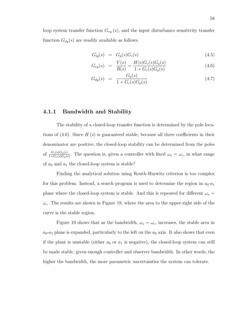
From these transfer functions, the loop gain transfer function Glg(s), the closed-
58
loop system transfer function Gry (s), and the input disturbance sensitivity transfer
function Gdy(s) are readily available as follows.
Glg(s) = Gp(s)Gc(s) (4.5)
Gry(s) =Y (s)
R(s)=
H(s)Gc(s)Gp(s)
1 + Gc(s)Gp(s)(4.6)
Gdy(s) =Gp(s)
1 + Gc(s)Gp(s)(4.7)
4.1.1 Bandwidth and Stability
The stability of a closed-loop transfer function is determined by the pole loca-
tions of (4.6). Since H (s) is guaranteed stable, because all three coefficients in their
denominator are positive, the closed-loop stability can be determined from the poles
of Gc(s)Gp(s)
1+Gc(s)Gp(s). The question is, given a controller with fixed ωo = ωc, in what range
of a0 and a1 the closed-loop system is stable?
Finding the analytical solution using Routh-Hurwitz criterion is too complex
for this problem. Instead, a search program is used to determine the region in a0-a1
plane where the closed-loop system is stable. And this is repeated for different ωo =
ωc. The results are shown in Figure 19, where the area to the upper-right side of the
curve is the stable region.
Figure 19 shows that as the bandwidth, ωo = ωc, increases, the stable area in
a0-a1 plane is expanded, particularly to the left on the a0 axis. It also shows that even
if the plant is unstable (either a0 or a1 is negative), the closed-loop system can still
be made stable, given enough controller and observer bandwidth. In other words, the
higher the bandwidth, the more parametric uncertainties the system can tolerate.