aDepartment of Mechanical Engineering, The Pennsylvania State University, University Park, PA,USA; bDepartment of Mathematics, The Pennsylvania State University, University Park, PA, USA;
cDepartment of Mechanical Engineering, Jadavpur University, Kolkata, India
(Received 12 September 2019; accepted 18 December 2019)
The topic of thermoacoustic instabilities in combustors is well-investigated, as it isimportant in the field of combustion, primarily in gas-turbine engines. In recent years,much attention has been focused on monitoring, diagnosis, prognosis, and control ofhigh-amplitude pressure oscillations in confined combustion chambers. The Rijke tubeis one of the most simple, yet very commonly used, laboratory apparatuses for emula-tion of thermoacoustic instabilities, which is also capable of capturing the physics ofthe thermally driven acoustics. A Rijke tube apparatus can be constructed with an elec-trical heater acting as the heat source, thus making it more flexible to operate and saferto handle than a fuel-burning Rijke tube or a fuel-fired combustor. Augmentation of theheat source of the Rijke tube with a secondary heater at a downstream location facili-tates better control of thermoacoustic instabilities. Along this line, much work has beenreported on the investigation of thermoacoustics by using computational fluid dynamics(CFD) modelling as well as reduced-order modelling for both single-heater and two-heater Rijke tube systems. However, since reduced-order models are often designed andbuilt upon certain empirical relations, they may not account for the dynamic behaviourof the heater itself, which is a critical factor in the analysis and synthesis of real-timerobust control systems. This issue is addressed in the current paper, where modifica-tions have been made to existing models by incorporating heater dynamics. The modelresults are systematically validated with experimental data, generated from an in-house(electrically heated) Rijke tube apparatus.
The prime source of thermoacoustic instabilities (TAI) [1] in a combustor is the strongcoupling between the unsteady heat release rate from fuel-air burning and natural acous-tics in the confined combustion chamber. The TAI phenomena lead to high-amplitudepressure oscillations (e.g. peak values reaching ∼ 1000 Pa) in the combustion chamber,which could be detrimental to the structural integrity of the combustor as these oscillationsmay produce thermomechanical fatigue stresses in the combustor wall and liners. The TAIphenomena also cause disruptions in the air flow through the combustor, often leading toflow reversal (which affects both upstream and downstream components in the combustion
system as well) and instigating flame blowout. It is well known that a very small amountof energy from the combustion process may lead to TAI due to low acoustic damping inthe combustors [2].
In recent years, much research has been conducted to investigate the nonlinear nature ofacoustic waves within the combustion chamber. The Rijke tube [3] is one of the simplestexperimental devices that can capture the essential physics of combustion chamber acous-tics and their coupling with the heat release rate. A thorough experimental and numericalstudy on Rijke tubes has been conducted by [4]. Other researchers such as [5–7] have alsoconducted studies using a Rijke tube apparatus and have attempted to implement variouscontrol methods in order to reduce the severity of TAI. Several researches (e.g. [8–12])have also conducted experimental research on TAI in fuel-burning laboratory-scale com-bustors. However, a major drawback of solely using an experimental apparatus for thepurpose of extensive research is the lack of versatility and operating range, which is pri-marily due to safety requirements or limitations of the facilities at hand. Thus, there is astrong need for the development of reduced-order numerical models for the study of com-bustion instabilities in the framework of computational models of affordable complexity.[13] proposed a simplified reduced-order model based on the principle of Galerkin-typemodal decomposition of the acoustic waves to solve the acoustic wave equation with aheat source. A similar method has been used by [14,15] for modelling the Rijke tube.Most current available Galerkin-based models try to account for the heater time lag usinga variable τ (e.g. [16]). However this is a flow time lag and does not include the timeresponse of the heater itself, i.e. the thermal inertia of the system or the dynamics of theheater; moreover, estimating of the parameter τ is not always easy. This may lead to mod-erately inaccurate response times, which is an important factor in designing a robust onlineactive control system. In the research work reported in the current paper, the authors haveattempted to modify the existing Galerkin-based numerical model to include heater andthermal dynamics as well as include some of the flow physics to provide more accuratetime responses, while still retaining much lower model complexity than a full-scale com-putational fluid dynamics (CFD) simulation. In the models available in the literature, theuser needs to specify parameters such as heater temperature, which cannot be directlycontrolled. The model, proposed in this paper, uses heater power as an input to the sys-tem, similar to the input that an experimental Rijke tube apparatus receives. Similarly,the reduced-order model is re-formulated such that, for the same model parameters, theentire range of operation of the Rijke tube can be simulated without re-tuning the criticalparameters.
Several methods exist for suppression of the generated high-amplitude pressure oscilla-tions in combustors. Passive control in the form of acoustic dampers [17] are widely usedfor mitigation of TAI. However, such acoustic dampers are only useful over certain fre-quency ranges, and they may not be effective at low frequencies. Several active controlmethods have also been proposed by researchers, such as the use of Helmholtz resonators[18], loudspeakers [7,14] and radial injection of air through micro-jets [19]. Usage of a sec-ondary heat source has been introduced by [20] as a method of controlling the TAI basedon the concept of destructive interference. This is a viable method of TAI control, espe-cially for large combustors in aircraft and land-based gas turbines. Numerical simulationshave been conducted in the current paper to investigate the efficacy of using a secondary(control) heater downstream for mitigating the instabilities of pressure oscillations in theRijke tube.
Combustion Theory and Modelling 3
Contributions: From the above perspectives, major contributions of the paper aresummarised below.
(1) Modification of established modal decomposition-based order reduction techniques:The objective here is to include the effects of heater dynamics, system thermal inertia,and flow dynamics on the reduced-order model.
(2) Modification of the simulation procedure for reduced-order modelling: The objectivehere is to develop a numerically efficient procedure that takes into account the effectsof time-varying thermal and flow conditions of the Rijke tube apparatus for numericalsolution.
(3) Demonstration of the efficacy of a secondary control heater as a method for suppress-ing the instabilities in the Rijke tube system: The objective here is to show how theresults of the numerical simulation compare to those reported in the standard literature.
(4) Experimental validation of the proposed reduced-order modelling technique: Theobjective here is to validate the aforesaid model against experimental results from anin-house Rijke tube and to show how the designed formulation works across the entireoperational regime.
Organisation: The rest of the paper is organised into the following sections:
• Section 2 describes the Rijke tube apparatus that is used to produce the experimentaldata for validating the proposed numerical model.• Section 3 presents the basic mathematical formulation of a reduced-order Galerkin-
based model of the two-heater Rijke tube, where the modifications pertaining to thethermal inertia effects are also described. Section 3.4 validates the proposed numericalmodel with the results that are obtained from the experiments.• Section 4 discusses the stability chart that is generated from the experimental data.
Section 4.4 briefly discusses the hysteresis effects as seen in the numerical model, andalso provides a comparison with the results of experimental studies that are reported inthe literature.• Section 5 demonstrates selected numerical simulations by using the secondary heater as
a control mechanism for suppression of instabilities, where the results are compared tothose available in the reported literature.• Section 6 summarises and concludes the paper along with recommendations for future
research.
2. The experimental Rijke tube apparatus
The experimental Rijke tube apparatus, which has been constructed in the laboratoriesof Penn State [21], consists of a 1.5 m long aluminium tube with a hollow square cross-section of inside lengths of 93 mm. There are two heating elements: a fixed primary heaterat 0.375 m from the flow inlet and a movable secondary heater downstream. Both heatersare made of compact wire-mesh Nichrome for generating thermal power, which emulatethe flame in a combustible fuel-air mixture in a real-life combustor. The secondary (control)heater has a maximum displacement of 500 mm from the centre of the tube towards the exitend. Figure 1 depicts the Rijke tube apparatus.
An array of eight wall-mounted pressure sensors are placed at equidistant axial loca-tions for capturing the pressure signals. The Rijke tube data are acquired at a sampling rate
4 C. Bhattacharya et al.
Figure 1. Rijke tube experimental apparatus.
of 8192 Hz. To measure the spatio-temporal temperature variation, 15 K- type transition-junction thermocouple probes are used. The mass-flow rate into the system is controlledaccurately using an Alicat Mass Flow Controller (0–1000 SLPM). The mass-flow rate con-trols not just the velocity over the heater but also affects the convective heat transfer fromthe wire mesh to the air and heat loss to the walls. The inlet and outlet of the tube arefitted with decouplers, which are large hollow enclosures serving the purpose of producingpressure waves under open-open end boundary conditions of the Rijke tube. Additionally,the upstream decoupler reduces flow fluctuations at the inlet while the downstream decou-pler serves as a heat sink, allowing the hot air exiting the outlet to be cooled, before it isreleased to the atmosphere.
The two Nichrome heaters are capable of handling high heating loads for a sufficientlylong time without being oxidised at the high operating temperatures. The square-weave40-mesh structure of each heater acts as an acoustically compact source of thermal energyand allows a uniform heating of air over a cross-section. Two copper rods are welded tothe copper strips and are electrically shielded from the walls of the chamber. The cop-per tubes are connected to a programmable DC power supply. The length of the tubedownstream of the heater is insulated to prevent heat loss from the walls allowing formaintaining the same initial and running conditions of different experimental runs. It alsoacts as a safety measure to prevent the operator from coming in contact with the hotmetal walls.
3. Reduced-order numerical modelling of the Rijke tube
This section addresses reduced-order modelling of both single-heater and two-heater Rijketubes, which include the thermal-hydraulic dynamics and their coupling with chamberacoustics.
3.1. Modelling of a single-heater Rijke tube
As mentioned previously, a simplified reduced-order model using Galerkin-type modaldecomposition was introduced by [13,22] to solve the acoustic wave equation with a heatsource in the system. The one-dimensional wave equation was derived for the pressure
Combustion Theory and Modelling 5
perturbations (p′) as
∂2p′
∂t2− a2 ∂
2p′
∂x2= (γ − 1)
∂Q
∂t(1)
where a denotes the speed of sound and Q is the volumetric rate of thermal power addition.Equation (1) does not include the effects of mean flow on the acoustic field. Culick’s expan-sion [13] is used for the pressure perturbations (p′) and velocity perturbations (u′) usingthe Galerkin eigen-acoustic modes. The decomposition into n modes having individualtime-varying modal amplitudes of ηj(t) yields:
p′(x, t) =n∑
j=1
p′j(x, t) = p0
n∑j=1
ηj(t)ψj(x) (2)
u′(x, t) =n∑
j=1
u′j(x, t) =n∑
j=1
ηj(t)
γ k2j
dψj(x)
dx(3)
where p0 is the mean undisturbed pressure; ψj(x) and kj are the mode shape (at the locationx) and the wavenumber of the jth mode, respectively, which has a natural frequency of ωj;and γ is the ratio of specific heats of air.
Substituting Equation (2) into Equation (1), expanding into eigen-modes, and adding adamping term ξj [23], the final expression is obtained as
d2ηj
dt2+ 2ξjωj
dηj
dt+ ω2
j ηj = γ − 1
p0
∫ψj∂Q
∂tdx (4)
where the left-hand expression in Equation (4) represents a set of n uncoupled linearoscillators that are excited by the forcing terms on the right-hand side. For a Rijke tube,[14] proposed a modified version of King’s law, which yields the volumetric rate of heataddition (Q) as
Q = 2Lw(Tw − T)
SL√
3
√πλCvρ0
dw
2
[√∣∣∣∣u0
3+ u′f (t − τ)
∣∣∣∣−√∣∣∣∣u0
3
∣∣∣∣]δ(x− xf ) (5)
where L is the length of the Rijke tube, Lw is the equivalent length of the wire, λ is thethermal conductivity of air, Cv is the constant volume specific heat capacity of air, τ isthe time lag between the heat transfer and the velocity as a result of thermal inertia, ρ0
is the mean density of the Rijke tube air, dw is the heater wire diameter, (Tw − T) is themean temperature difference between the heater and the air, S is the cross-sectional area ofthe Rijke tube, xf is the heater location, and u′f is the acoustic velocity perturbation at theheater location. Using Equation (5), the acoustic equation (Equation (4)) is modified to:
d2ηj
dt2+ 2ξjωj
dηj
dt+ ω2
j ηj =˙dQ′
dt(6)
where Q′ combines the remaining terms as
Q′ � 2(γ − 1)Lw(Tw − T)
p0SL√
3
√πλCvρ0
dw
2
[√∣∣∣∣u0
3+ u′f (t − τ)
∣∣∣∣−√∣∣∣∣u0
3
∣∣∣∣]ψj(xf ) (7)
6 C. Bhattacharya et al.
and the frequency-dependent damping ξj is given by [4] as
ξj �(
c1ωj
ω1+ c2
√ω1
ωj
)(8)
where the first term in Equation (8) is responsible for the end losses and the second termrepresents losses due to boundary layers; and the constants c1 and c2 are the dampingcoefficients that represent the amount of acoustic damping in the Rijke tube. The time lagτ is computed by using Lighthill’s correlation as: τ � 0.2 dw
u0.
The modal equations, derived above, can be cast in a linearised state-space form and thedimensionality of the ordinary differential equation (ODE) system depends on the numberof the selected ‘significant’ acoustic modes. For each mode, there are two states, ηj and ηj.This ODE system can be solved using a numerical method (e.g. Runge-Kutta).
3.2. Modelling of a two-heater Rijke tube
A secondary heat source is introduced in the Rijke tube in addition to the primary heatsource, with the secondary heater acting as a control heater. This arrangement changesEquation (6) to now having two heat source terms:
d2ηj
dt2+ 2ξjωj
dηj
dt+ ω2
j ηj =˙dQ′1dt+˙dQ′2dt
(9)
Q′i =2(γ − 1)Lw(Tw,i − T)
p0SL√
3
√πλCvρ0
dw
2
×[√∣∣∣∣u0
3+ u′f ,i(t − τi)
∣∣∣∣−√∣∣∣∣u0
3
∣∣∣∣]ψj(xf ,i), i = 1, 2 (10)
where the subscript i takes values 1 and 2 for the primary and secondary heaters,respectively.
3.3. Modelling of the heater and thermal dynamics
The state-space representation of the acoustics in Equation (4) for the jth mode is
[ηj
ηj
]=
[0 1−ω2
j −2ξjωj
] [ηj
ηj
]+
[0
˙dQ′1dt +
˙dQ′2dt
](11)
where the frequency ωj, computed from [13,24], is represented as
ωj = akj (12)
where the wavenumber kj is fixed for a given acoustic boundary condition with input–output specifications of a (pressure anti-node, or pressure open) fixed inlet velocity and(pressure node, or pressure closed) constant outlet pressure; and the speed of sound a is
Combustion Theory and Modelling 7
a function of the gas temperature in the tube. In this case, the tube has constant pres-sures at either end, and the speed of sound a is approximated to depend on the mean gastemperature, which yields the following expressions for ωj and ξj:
ωj =√γR Tavg
(jπ
L
)(13)
ξj
ξ1= ωj
ω1(14)
Since ωj directly depends on the time-dependent temperature T, the system matrix inEquation (11) is linear parameter varying (LPV) (which is effectively time varying) andhence needs to be recomputed at each time step.
For ease of computation, many researchers have used the above reduced-order equa-tions by making certain approximations, such as the mean values of temperature and flowvelocity, under the assumption that they are constants. However, this assumption may notalways be appropriate, not only because of the temporal changes but also due to the rate ofchange of these time-dependent parameters. In the experimental apparatus, it may not bepossible to control directly the temperature of the heaters, but instead the power input intothe heater is the directly controllable variable and the temperature changes occur as a resultof the power input and the heat transfer within the Rijke tube. Therefore, the temperatureitself has its own dynamics, which has been addressed in this paper and included into thecomputational procedure.
In view of the above discussion, the heater power is the variable that is set by theuser, and the temperatures evolve following the various relations of heat transfer andfluid mechanics. In the experimental apparatus, the power supply has its own transientbehaviour, which is assumed to be linear within the operational range such that the heateris able to go from 0 to 2000 W in a linear ramp in 1 s; and this limits the rate of powerrise or fall in the heaters. The rate of heat loss (Qheater) from the heater in a time step iscomputed from the following equation [15]:
Qheater(t) = Lw(Tw,i − T)
[λ+ 2
√πλCvρ0
dw
2
((1− 1
3√
3
)√u
+ 1√3
√∣∣∣∣u
3+ u′(t − τ)
∣∣∣∣)]
(15)
So the temperature of the heater wire (Tw) changes in the time interval [t, t + dt) as
Tw ← Tw + (P(t)− Qheater(t)) dt
MCpwire(Tw)(16)
where M is the mass of the wire mesh that can be obtained by measurement; P(t) is thetime-dependant power supplied to the heater; and Cpwire is the (temperature-dependent)specific heat capacity of the wire material, which is available from manufacturer’s speci-fications. For computing the temperature in the Rijke tube, the flow domain in the tube issplit into three segments; one containing the volume between the inlet and first heater, thenext being the volume between the two heaters, and the third being the volume betweenthe secondary heater and the outlet. It is assumed that the temperature in the first seg-ment is always the same as the inlet temperature (Tin). The temperatures in the remaining
8 C. Bhattacharya et al.
two sections are computed by doing energy flow analysis on the constant volume; Qadd isthe power added to a segment in a time step, where the subscript down denotes the valuedownstream:
Finally, the temperature of the volume segment Vsegment is computed in the time interval[t, t + dt) as
Tsegment ← Tsegment + Qadd dt
ρVsegmentCp(Tsegment)(19)
The average temperature is measured as the segment length-weighted average of thesegment temperatures.
Using all the above additional information that is computed by solving the heat transferand certain fluid equations, the reduced-order model can be improved by removing someof the typical assumptions. Values of parameters (e.g. the mean temperature, wire temper-ature, density and velocity at the wire) now become functions of time and are dependenton the changing operating conditions of the Rijke tube. This is in agreement with whatis observed experimentally as for the same heater input, the heater wire temperature issubstantially higher when the flow rate is low due to lower convective heat transfer asopposed to higher flow rate situations. These physical processes also dictate mean temper-ature, speed of sound and the natural frequency of the system. Thus, a single model canbe used for the entire operational range of the Rijke tube without having to make assump-tions and change the individual variable values for each operating region. Furthermore,accounting for heater lag produces a more accurate time response of the system to changesin the control power and thus is better for studying transient phenomena or for testing theeffectiveness of controllers on the system.
Equations (10) and (15) are modified to account for the local conditions of temperatureand density as follows. The assumption here is that only the upstream values are consideredwhen computing the heat transfer, where the subscripts in and down denote the values atthe inlet and the downstream sections, respectively. It is noted that the model parametersCv and λ are functions of temperature.
Qheater(t) = Lw(Tw,i − Tdown)×[λ+ 2
√πλ(T)Cv(T)ρin
Tin
Tdown
dw
2
×((
1− 1
3√
3
)uinTdown
Tin+ 1√
3
√∣∣∣∣uinTdown
3Tin+ u′(t − τ)
∣∣∣∣)]
(20)
Q′i =2(γ − 1)Lw(Tw,i − Tdown)√
3pinSL
√πλ(T)Cv(T)ρin
Tin
Tdown
dw
2
×[√∣∣∣∣uinTdown
3Tin+ u′f ,i(t − τi)
∣∣∣∣−√∣∣∣∣uinTdown
3Tin
∣∣∣∣]ψj(xf ,i) (21)
Combustion Theory and Modelling 9
The effects of uncertainties are realised in the simulation by modifying the acoustic veloc-ity perturbation u′ with a zero-mean additive Gaussian noise component that is chosen tohave an intensity equal to 0.5% of the mean flow velocity.
3.4. Parameterisation of the reduced-order model
This section parameterises the reduced-order model, developed in Section 3, to match theRijke tube apparatus described in Section 2. The geometry and other model parameters arechosen to be the same as those in the experimental apparatus. The length of the numericallymodelled Rijke tube is taken to be L = 1.5 m, area of cross-section S = 0.093× 0.093 m2.The primary heater is placed at x1 = 0.375 m, similar to the experimental apparatus, andthe pressure sensor is located at xp = 1 m; all lengths are measured downstream fromthe inlet. The heaters have properties similar to the actual wire mesh used in the exper-iment with Lw = 23.6 m, dw = 0.33 mm. The thermal heat capacity is taken to be thatof Nichrome and each wire mesh has a total mass of M = 170 gm. The thermal proper-ties of air used are fourth-order polynomials obtained from a NASA report (the NASApolynomials) [25].
In the numerical simulations reported in this paper, a total of 10 eigen-modes are con-sidered to adequately capture the dynamics of the acoustic system. This implies that thenumber of eigen-modes is n = 10, as seen in Equations (2) and (3). To model the damp-ing coefficients in Equation (8), the parameters c1 and c2 that are to be set by the userdepend on the actual observed damping. These parameters have been set to be c1 = 0.048and c2 = 0.040 to match the experimental results described in Section 4. Furthermore, theentire amount of the net heat transferred from the heater(s) enters the air, because a part of itis lost to the surroundings (primarily by radiation). Therefore, a factor α < 1 is multipliedto the value of Q(t). An empirical model of the parameter α is
α = 1−(
Tw − Tavg
Tw
)0.15
(22)
The above formulation assumes the system to be acoustically closed. However, that isnot actually true as though the presence of the decouplers maintain nearly constant pres-sures at the ends, the presence of a flow rate regulator ensures a constant flow. Thus, theaverage flow deviates from that computed directly in terms of the measured flow ratein LPM. Instead the flow velocity is obtained by multiplying the computed value of Uin
by a scaling factor β that is empirically defined as β = |Uin/U∗in|0.9, where U∗in � 1 m/s,making β a dimensionless quantity. A zero-mean Gaussian noise of standard deviation0.3Pa has been added to the output in order to emulate the process noise as well as thesensor noise. This choice is made to match the (non-dimensional) Prms value describedin Section 4.3. The numerical sensor measures the acoustic pressure of each Galerkin-mode and then computes the combined acoustic pressure at that location followingEquation (2).
For the remainder of the paper, the parameter values described in this section have beenused without any changes. In other words, with these parameters optimised a completemodel of the system is obtained, and the only changes that need to be made for eachnumerical experiment are the boundary conditions.
10 C. Bhattacharya et al.
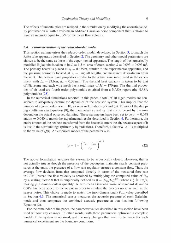
Figure 2. Stability map generated from experimental data of Rijke tube apparatus. Instabilityindicated by dark shading marked with ‘× ’, and stability by light shading with ‘°’.
4. Stability maps developed from experimental data and model data
This section develops and compares stability maps from data generated from the Rijketube apparatus (see Section 2) and reduced-order model (see Section 3.4) under the sameoperating conditions.
4.1. Stability map: experimental data
Experiments have been conducted with multiple combinations of heater power input (Ein)and air flow rate (Q) to record data of 30 s duration for each case. A typical stability map isshown in Figure 2 with the following notations: the spaces marked as ‘× ’ (with a darkershaded box) denote unstable operation with an audibly discernible resonating mode, andthose marked as ‘°’ (with lighter shading) denote stable operation.
Different values of initial temperatures affect the stability characteristics of the ther-moacoustic process as a consequence of changes in the mean temperature in the Rijketube. When a lower initial mean temperature of around ∼ 300◦K is maintained in theRijke tube apparatus, a lower frequency (∼ 114 Hz) mode of instability is observed; theinstability occurred at a higher frequency (∼ 131 Hz) mode at a higher initial mean tem-perature of ∼ 348◦K. These observations are attributed to the increase in the speed ofsound at an elevated mean temperature, which changes the fundamental frequency from ananalytically calculated value of 115– 127 Hz for an open-open tube, tallying closely withthe peak frequencies of experimental data. In this work, only the higher initial temper-ature mode has been reported for validation because it is more consistent and is easierto obtain experimentally because cooling the Rijke tube after each experiment is verytime-consuming.
4.2. Stability map: numerical simulation of the reduced-order model
The reduced-order model, described in Section 3, has been run with the same model param-eters for the same range of flow rates and primary heater power inputs as the experimentsdescribed above. The ambient temperature is taken to be 348◦K, which is the more appre-ciable ambient conditions as described above. Each simulation has been performed forsimulated time intervals of 30 s with a time step size�t = 10−4 s; and the root mean square(RMS) values of pressure oscillations are computed over the last 2 s as a measure of sta-bility. An operational condition is considered to be unstable if the Prms exceeds a threshold
Combustion Theory and Modelling 11
Figure 3. Stability map generated from simulation data of reduced-order model. Instabilityindicated by dark shading marked with ‘1’, and stability by light shading with ‘0’.
of 5 Pa. The generated stability map is shown in Figure 3. The boxes shaded darker bluewith the Boolean value of 1 indicates an unstable operating condition.
It is seen that the stability map matches very closely with that reported from experiments(shown in Figure 2). A comparison of the stability in Figures 2 and 3 reveals that, in thephysical experiments, the maximum range of unstable operation is bounded in the powerrange 1000– 2000 W and in flow range 132–246 LMP. For the numerical simulation, thepower range 1000–2000 W is identical to that in experiments, while the flow rate range is132–255 LPM, which is reasonably close. The frequency of the unstable mode was alsofound to be 117 Hz which is very close to the experimentally obtained value of 131 Hz.
A comparison of the experimental stability map and numerical stability map reveals thatthe discrepancies occur for 7 out of 57 unstable conditions, yielding an error rate of about12%. This discrepancy is possibly due to the fact that the numerical model is a determin-istic model of a stochastic process with a few outliers. In addition, there may be certainexperimental uncertainties such as the exact ambient temperature, the exact initial condi-tion of the tube, both of which are not perfectly repeatable. There are also some modellingsimplifications that may tend to lead to inaccuracies towards the edges of the unstableregion seen in the stability map. However, for the purpose at hand, a higher-fidelity modelmay not be necessary because this low-fidelity model yields a sufficiently close matchto the experimental ground truth. For another Rijke tube, the parameters (e.g. dampingcoefficients c1 and c2) of the numerical model should be tuned to match the experimentaldata.
It is also worthwhile to note that although theproposed reduced-order model is moredetailed than the traditional Galerkin-based models (which do not account for heater effectsor thermal inertia), the time required to run a simulation is reasonably low. In practice, itis observed that the simulation time required is approximately 1.5× (i.e. simulation of atime interval of 30 s takes ∼ 45 s of the machine run-time). The code has been developedand run on MATLAB 2019b utilising a single core of an Intel Xeon Workstation using theE5-2670 chipset.
4.3. Comparison of numerical simulation and experimental results
A major focus of this paper is to incorporate the thermal inertia of the heaters in themodel equations and to investigate the effects of the same on the system dynamics ofthe Rijke tube. In order to study these phenomena, each experiment has been conducted
12 C. Bhattacharya et al.
Figure 4. Time series of pressure oscillations: experimental and simulation data, where the upperparts (in black) are experimentally observed time series and the lower parts (in grey) are numericallysimulated from the reduced-order model under the same operating conditions.
for a duration of 30 s in the following fashion. The heater power is maintained at 200 W forthe first 10 s and then the heater power is abruptly increased to the final value. It is notedthat the resulting increase in the heater temperature is not linear over the entire period.Furthermore, there is a process-dependent time delay between the heater power and heatertemperature responses. As mentioned before, many reduced-order numerical models do notcapture this behaviour. The model proposed in this paper incorporates the heater dynamics,and thus captures these delays in the formulation of the reduced-order model.
The four plates in Figure 4 display four profiles of pressure oscillations to compare thedynamic behaviour of the Rijke tube both in the experiment as well as in the numericalsimulation under four different operating conditions. The primary power is maintainedat 1400, 1600 and 1800 W as shown in the figure. For all of these runs, the secondaryheater is kept inactive. For each of the operating condition reported here, the upper part(in black) of Figure 4 shows the pressure profile obtained from experiments following thesame power profile. The lower part (in grey) of Figure 4 shows the equivalent numericalsimulation. These responses have been scaled for ease of comparison, where the scalingfactor has been chosen to be the root mean square (RMS) value of the noise. With thisscale factor, the peak values of the numerically obtained instabilities match those that areobtained experimentally; from these observations, the noise in the reduced-order model isidentified to be a zero-mean Gaussian with intensity 0.3 Pa.
Form the results of comparisons in Figure 4, it is concluded that the model-predictedinstability growth is very close to that observed in the experimental results. This obser-vation suggests that the numerical model is capable of capturing the Rijke tube dynamicsvery well, which include heater dynamics and delays. The small deviations between themodel predictions and experimental observations, as seen in Figures 2 and 3 and in thefour plates of Figure 4, can be attributed to the uncertainties in modelling of experimentalconditions.
Combustion Theory and Modelling 13
Figure 5. Time series of hysteresis experiment simulation.
4.4. Hysteresis as a result of thermal dynamics
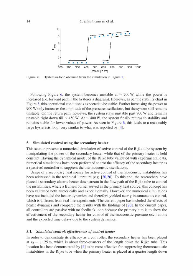
It has been observed by [4] that the onset of instability in the Rijke tube exhibits hysteresisdue to the thermal inertia of the system. The rationale is that the direction of approach-ing a particular operating condition may change depending on whether that it is stable orunstable; this effect is seen in the simulation as well. In order to observe the hysteresis phe-nomena, the simulation has been conducted for a total of 720 s duration when the air flowrate is held constant at 160 LPM and the primary heater power is varied in the followingway. For the first 90 s, the primary heater power is held at 600 W to ensure that a steadystate is reached. Subsequently, the primary heater power is increased in steps of 50 W onan interval of 30 s. Holding the power constant for each window of 30 s ensures that aquasi-steady state is reached for the respective power setting. These stepwise incrementsare continued till the power reaches a maximum of 900 W. The system is held steady ata power of 900 W for a minute and then the process is reversed by reducing the power indecrements of 50 W every 30 s. It is seen that the system remains unstable even at 600 Wduring the decreasing power steps although the system was initially stable at 600 W as seenin Figure 3. Therefore, the decrements in power are continued till a lower bound of 200 Wis reached as seen in Figure 5.
The top part in Figure 5 shows the profile of pressure signal for the above numericalexperiment, while the bottom part shows the temporal variations in power and the average(wire) temperature of the two heaters in the Rijke tube apparatus: P1 and TWire1 for theprimary heater, and P2 and TWire2 for the secondary (inactive) heater. It is seen that thetemperature profile has a lag as compared to the heater power profile, which is an effectof the thermal dynamics; these phenomena have not been captured by most reduced-ordernumerical models. Figure 6 presents the hysteresis loop for the numerical experiment,where the changes in the RMS values (Prms) of the pressure oscillations over the last 5 sof each 30 s window are shown along with the arrows that indicate the direction of theprimary heater power being varied.
14 C. Bhattacharya et al.
Figure 6. Hysteresis loop obtained from the simulation in Figure 5.
Following Figure 6, the system becomes unstable at ∼ 700 W while the power isincreased (i.e. forward path in the hysteresis diagram). However, as per the stability chart inFigure 3, this operational condition is expected to be stable. Further increasing the power to900 W only increases the amplitude of the pressure oscillations, but the system still remainsunstable. On the return path, however, the system stays unstable past 700 W and remainsunstable right down till ∼ 450 W. At ∼ 400 W, the system finally returns to stability andremains stable for lower values of power. As seen in Figure 6, this leads to a reasonablylarge hysteresis loop, very similar to what was reported by [4].
5. Simulated control using the secondary heater
This section presents a numerical simulation of active control of the Rijke tube system bymanipulating the power of the secondary heater while that of the primary heater is heldconstant. Having the dynamical model of the Rijke tube validated with experimental data,numerical simulations have been performed to test the efficacy of the secondary heater asa (passive) controller to suppress the thermoacoustic oscillations.
Usage of a secondary heat source for active control of thermoacoustic instabilities hasbeen addressed in the technical literature (e.g. [20,26]. To this end, the researchers haveplaced a secondary electric heater downstream in the flow path of the Rijke tube to controlthe instabilities, where a Bunsen burner served as the primary heat source; this concept hasbeen validated both numerically and experimentally. However, the numerical simulationshave not included the heater dynamics and therefore yielded nearly instantaneous control,which is different from real-life experiments. The current paper has included the effects ofheater dynamics and compared the results with the findings of [20]. In the current paper,all controllers are passive with no feedback loop because the primary aim is to show theeffectiveness of the secondary heater for control of thermoacoustic pressure oscillationsand the expected time delays due to the system dynamics.
5.1. Simulated control: effectiveness of control heater
In order to demonstrate its efficacy as a controller, the secondary heater has been placedat x2 = 1.125 m, which is about three-quarters of the length down the Rijke tube. Thislocation has been demonstrated by [4] to be most effective for suppressing thermoacousticinstabilities in the Rijke tube when the primary heater is placed at a quarter length down
Combustion Theory and Modelling 15
Figure 7. Time series of pressure, temperature, and power in two simulated control experiments.(a) Time series from the first control case: flow rate of 140 LPM and (b) time series from the secondcontrol case: Flow rate of 210 LPM.
from the inlet. Two trial cases are conducted to demonstrate the effects of the secondaryheater and the results are shown in Figure 7.
The first case consists of numerical simulations for a time interval of 90 s with a con-stant flow rate of 140 LPM. At the very start (i.e. time t = 0 s), as the primary heaterpower is increased to 1200 W, the system becomes unstable. The primary power is thenheld at a constant level of 1200 W for 90 s, while leaving the secondary heater turned
16 C. Bhattacharya et al.
off. At time t = 30 s, the secondary heater power is increased to 300 W and then furtherincreased to 450 W at t = 60 s. The profiles of the corresponding pressure time series andassociated power and temperature time series are shown in Figure 7(a). It is seen thatalthough the secondary heater power at 300 W is incapable of completely suppressingthe thermoacoustic instabilities, it modestly reduces the amplitude of the pressure oscil-lations. However, increasing the secondary power to 450W completely suppresses thehigh-amplitude pressure oscillations.
The second case consists of numerical simulations for a time interval of 90 s with aconstant flow rate of 210 LPM. At time t = 0 s, the primary heater power is increasedto 1600 W while the secondary heater is kept off till t = 30 s and then raised to 500 W;the secondary heater is switched off at t = 60 s. The corresponding pressure time seriesand the associated power and temperature time series are shown in Figure 7(b). It is seenthat the initially unstable system is adequately controlled by switching on the secondaryheater. However, when the secondary heater is switched off, the system reverts back toinstability.
5.2. Simulated control: effect of control heater location
The location of the control (secondary) heater largely determines whether the instabil-ity would be successfully suppressed. To demonstrate this phenomenon, numerically, twocases have been considered, each having a simulated time interval of 460 s. In both cases,the air flow rate is kept constant at 180 LPM and, at t = 0 s, the primary heater power israised to 1400 W; at t = 20 s, the secondary heater power is increased to 600 W. As seen inFigure 8(a), the instability is completely suppressed. Figure 8(b) shows that, although theamplitude is very modestly reduced, the pressure oscillations still prevail. This is due to thefact that the secondary heater is located at x2 = 1.125 m (i.e. 3L/4 from inlet) for first case(Figure 8(a)), which is the most effective location for control. In contrast, for Figure 8(b),the secondary heater is placed further upstream at x2 = 0.875 m (i.e. 7L/12 frominlet).
5.3. Simulated control: comparison with results reported in technical literature
In their research, [20] studied the effects of location of the secondary heater on suppres-sion of thermoacoustic instabilities in a Rijke tube. It was observed that, for a particularoperating condition, placing the secondary heater at 0.73 L causes the minimum powerneeded to mitigate instability to be 122.5 W in their apparatus. Placement of the secondaryheater at 0.80 and 0.87 L causes the needed minimum power levels to be 183 and 309 W,respectively.
In the current paper, similar numerical simulations have been conducted for the flowrate of 210 LPM and primary power of 1200 W. When the secondary heater is placed at0.73 L(1.095 m), the minimum power needed to completely suppress the oscillations isfound to be ∼ 268 W; and when the heater is placed at 0.80 L(1.2 m)and 0.87 L(1.305 m),the minimum power requirements are∼ 326 and∼ 513 W, respectively. Thus, a very sim-ilar trend is observed between the numerical simulations presented in this paper and thosegenerated experimentally by [20]. The values do not match exactly because of the fol-lowing reasons. The Rijke tube geometries are different and the primary heat source inthe experimental work by [20] is a flame while the heat source in the numerical model,presented in this paper, is an electric heater; hence the input conditions are dissimilar.
Combustion Theory and Modelling 17
Figure 8. Effects of the control heater location on system dynamics. (a) Time series of pressure,temperature, and power in the simulation with the control heater placed at x2 = 1.125 m (3L/4) and(b) time series of pressure, temperature, and power in the simulation with the control heater placedat x2 = 0.875 m (7L/12).
6. Summary, conclusions, and future work
This paper has proposed a modification of the traditional Galerkin-mode-based techniqueto construct a reduced-order model of an (electrically heated) Rijke tube, which includesthe inherent thermal physics of the heaters and the system dynamics in general. The modelequations are developed by including the heat transfer phenomena in the heaters and ther-moacoustics in the Rijke tube. This approach yields realistic time lags which are critical forevaluating dynamic performance and system stability for real-time monitoring and activecontrol. The model structure is flexible in the sense that it is capable of incorporating either
18 C. Bhattacharya et al.
a single heater or a combination of two heaters, where typically the secondary heater actsas an actuator for controlling the thermoacoustic instabilities.
The single-heater reduced-order model has been validated with experimental data col-lected from the Rijke tube apparatus, and the numerical results of the reduced-order modelhave yielded very good agreement with those obtained experimentally. The performanceof the two-heater model has been tested by numerical simulation and is seen to func-tion as expected. Numerical results of the two-heater model are compared with those ofother available models, reported in open literature, which are also in good agreement.The numerical simulations show the effectiveness of the secondary heater as a (passive)controller.
The following topics are suggested for future research:
(1) Experimental validation of the two-heater model results on the Rijke tube apparatus.(2) Detailed analysis of the fundamental frequencies in the system dynamics to serve as
indicators of anomalous operations.(3) Analysis and synthesis of a robust controller for real-time active control of thermoa-
coustic instabilities based on the two-heater numerical model.(4) Implementation and testing of the above active controller on the Rijke tube apparatus.
Disclosure statementNo potential conflict of interest was reported by the authors.
FundingThe work reported here has been supported in part by the U.S. Air Force Office of Scientific Research(AFOSR) [grant numbers FA9550-15-1-0400 and FA9550-18-1-0135] in the area of dynamic data-driven application systems (DDDAS). The authors also thank Indo-US Science and TechnologyForum (IUSSTF) for granting the Research Internship for Science and Engineering (RISE) schol-arship to the first author for collaboration between Pennsylvania State University and JadavpurUniversity.
References
[1] J.W.S. Rayleigh, The Theory of Sound, Dover, New York, 1845.[2] S. Candel, Combustion dynamics and control: Progress and challenges, Proc. Combust. Inst.
2(9) (2002), pp. 1–28.[3] P.L. Rijke, Notiz über eine neue art, die in einer an beiden enden offenen rhre enthaltene luft in
schwingungen zu versetzen, Ann. Phys. 18(3) (1859), pp. 339–343.[4] K.I. Matveev, Thermoacoustic instabilities in the rijke tube: Experiments and modeling, Ph.D.
diss., California Institute of Technology, 2003.[5] L. Kabiraj and R.I. Sujith, Nonlinear self-excited thermoacoustic oscillations: Intermittency
and flame blowout, J. Fluid. Mech. 71(3) (2012), pp. 376–397.[6] D. Zhao, Transient growth of flow disturbances in triggering a Rijke tube combustion
instability, Combust. Flame. 15(9) (2012), pp. 2126–2137.[7] D. Zhao and Z.H. Chow, Thermoacoustic instability of a laminar premixed flame in Rijke tube
with a hydrodynamic region, J. Sound. Vib. 33(2) (2013), pp. 3419–3437.[8] A. Sjunnesson, P. Henrikson, and C. Lofstrom, CARS measurements and visualization of react-
ing flows in a bluff body stabilized flame, in 28th Joint Propulsion Conference and Exhibit,Joint Propulsion Conferences, 1992.
[9] A. Fichera, C. Losenno, and A. Pagano, Experimental analysis of thermo-acoustic combustioninstability, Appl. Energy. 7 (2001), pp. 179–191.
Combustion Theory and Modelling 19
[10] J.G. Lee and D.A. Santavicca, Experimental diagnostics for the study of combustion instabilitiesin lean premixed combustors, J. Propul. Power 1(9) (2003), pp. 735–750.
[11] F. Richecoeur, S. Ducruix, P. Scouflaire and S. Candel, Experimental investigation of high-frequency combustion instabilities in liquid rocket engine, Acta. Astronaut. 6(2) (2008), pp.18–27.
[12] U. Sen, T. Gangopadhyay, C. Bhattacharya, A. Misra, P.S.S. Karmakar, A. Mukhopadhyay, andS. Sen, Investigation of ducted inverse nonpremixed flame using dynamic systems approach,in ASME Turbo Expo 2016: Turbomachinery Technical Conference and Exposition, Vol. 4B,2016.
[13] F.E.C. Culick, Nonlinear behavior of acoustic waves in combustion chambers-I, Acta. Astro-naut. 3 (1976), pp. 715–734.
[14] M.A. Heckl, Active control of the noise from a Rijke tube, J. Sound. Vib. 12(4) (1988), pp.117–133.
[15] M.A. Heckl, Non-linear acoustic effects in the Rijke tube, Acustica 7(2) (1990), pp. 63–71.[16] P. Subramanian, S. Mariappan, R.I. Sujith, and P. Wahi, Bifurcation analysis of thermoacoustic
instability in a horizontal rijke tube, Int. J. Spray Combust. Dyn. 2 (2010), pp. 325–355.[17] G.A. Richards, D.L. Straub, and E.H. Robey, Passive control of combustion dynamics in
stationary gas turbines, J. Propul. Power 1(9) (2003), pp. 795–810.[18] D. Zhao and A. Morgans, Tuned passive control of combustion instabilities using multiple
Helmholtz resonators, J. Sound. Vib. 32 (2009), pp. 744–757.[19] N.N. Deshmukh and S. Sharma, Experiments on heat content inside a Rijke tube with
suppression of thermo-acoustics instability, Int. J. Spray Combust. Dyn. 9 (2017), pp. 85–101.[20] D. Zhao, C. Ji, X. Li, and S. Li, Mitigation of premixed flame-sustained thermoacoustic
oscillations using an electrical heater, Int. J. Heat. Mass. Transf.8(6) (2015), pp. 309–318.[21] S. Mondal, N.F. Ghalyan, A. Ray, and A. Mukhopadhyay, Early detection of thermoacoustic
instabilities using hidden Markov models, Combust. Sci. Technol.19(1) (2019), pp. 1309–1336.[22] F.E.C. Culick, Combustion instabilities in liquid-fuelled propulsion systems, AGARD-CP-450,
1988.[23] K.I. Matveev and F.E.C. Culick, A model for combustion instability involving vortex shedding,
Combust. Sci. Technol. 17(5) (2003), pp. 1059–1083.[24] V. Nair, R.I. Sujith, A reduced-order model for the onset of combustion instability: Physical
mechanisms for intermittency and precursors, in Proceedings of the Combustion Institute, Vol.35, 2015, pp. 3193–3200
[25] J.R. Andrews, Temperature Dependence of Gas Properties in Polynomial Form, The NPSInstitutional Archive DSpace Repository, Calhoun, 1981.
[26] X. Jin, H. Zhao and S. Li, Experimental and numerical study of passive control of self-sustainedthermoacoustic oscillations using an electrical heater, Energy Procedia 105 (2017), pp. 4661–4667. 8th International Conference on Applied Energy, ICAE2016, 8–11 October 2016, Beijing,China.