Redundancies in X-ray images due to the epipolargeometry for transmission imaging

André Aichert, Nicole Maass, Yu Deuerling-Zheng, Martin Berger, Michael Manhart, Joachim Hornegger,Andreas K. Maier and Arnd Doerfler

Abstract—In Computer Vision, the term epipolar geometrydescribes the intrinsic geometry between two pinhole cameras.While the same model applies to X-ray source and detector,the imaging process itself is very different from visible light.This paper illustrates the epipolar geometry for transmissionimaging and makes the connection to Grangeat’s theorem,establishing constraints on redundant projection data alongcorresponding epipolar lines. Using these redundancies, ageometric consistency metric is derived. Our metric could beapplied to any pair of transmission images and could be usedfor pose refinement, calibration correction and rigid motionestimation in fluoroscopy and flat detector computed tomogra-phy (FD-CT) . In addition to the theoretical contribution, thispaper investigates the properties and behavior of the metricfor the purpose of re-calibration of an FD-CT short scan fornarrow angular range.

I. INTRODUCTION

In order to reconstruct a 3D image from a number of2D X-ray projections, one requires accurate knowledge ofthe underlying projection geometry. The trajectory for CTreconstruction is either assumed fixed by construction orare calibrated before acquisition. Artifacts in the recon-struction may arise from inaccuracies of the calibration andunpredictable or non-reproducible scanner motion. This isalso equivalent to rigid movement of the patient in medicalscenarios.

Each image is associated with a projection matrix, whichuses the same pinhole camera model as it is common inComputer Vision. The analogy opens up a field of estab-lished methods which are ready for application to trans-mission imaging problems [1], [2]. This paper studies theconnection between the epipolar geometry of two projectionsand Grangeat’s theorem [3] in order to exploit redundanciesin the projection data for image-based optimization of theassumed projection geometry after an acquisition. Both theepipolar geometry and Grangeat’s Theorem have previouslybeen used for this purpose [4], [5], but their connection hasnot been established. In contrast to [6], [5], the work ofDebbeler et al. [4] does not require reconstruction and usesa relatively simple and fast metric on 2D projections. We

Joachim Hornegger, Andreas K. Maier, André Aichert, Martin Bergerand Michael Manhart are associated with the Pattern RecognitionLab, Friedrich-Alexander-Universität Erlangen-Nürnberg, Germany; NicoleMaass and Yu Deuerling-Zheng with the Siemens AG, Healthcare Sector,Erlangen and Forchheim, Germany; Arnd Doerfler and André Aichert withDepartment of Neuroradiology, Universitätsklinikum Erlangen, Germany;Andreas K. Maier with the Erlangen Graduate School in Advanced OpticalTechnologies (SAOT)

CiC0

X

x0

xiliBx0

(λ)Epipole ei in

this direction

baseline

Figure 1. Epipolar geometry of two source positions C0 and Ci from acircular trajectory. An image point x0

∼= P0X on the detector is back-projected to a ray Bx0 (λ). The line li ∼= Fxi is the projection of thatray from Ci to the corresponding detector plane and hence contains theprojection xi

∼= PiX and the projection of the other source ei ∼= PiC0,called the epipole. It follows that the line can be written as the join of theimage point with the epipole li ∼= ei × xi.

derive a new formulation of that metric based on epipolargeometry, which allows us to model the reliability in acertain direction given a specific trajectory. Finally, we willinvestigate accuracy, precision and robustness of the X-raysource and detector, specifically for subsets of a short scantrajectory of an FD-CT C-arm system.

II. EPIPOLAR REDUNDANCIES IN X-RAY IMAGES

A. Epipolar Geometry

The term epipolar geometry describes the relative geome-try between two pinhole cameras defined by their projectionmatrices P0 and Pi. We rely on the real projective n-spacePn = Rn+1\ {0} and introduce an equality relation

a ∼= b ⇔ a,b ∈ Pn, ∃λ ∈ R, : λa− b = 0 (1)

for the equivalence classes of scalar multiples. We will de-note the location of the X-ray source as C ∼= (−tR, 1)T ∼=kernel(P) ∈ P3, for the projection matrix P ∼= K[R|t] ∈R4×3, according to the notation common in Computer Vi-sion. The projection matrix P maps a world point in real pro-jective three-space X ∈ P3 to an image point on the detectorin the real projective plane x ∼= (u, v, 1)T ∼= PX ∈ P2. Wewill work with a large number of views, but consider onlytwo pairs of projection matrices and images (P0, I0) and(Pi, Ii) at a time. For convenience, a lower index denotesthe view number, for example, xi ∼= PiX is a point inprojective two-space on image Ii. W.l.o.g., we will use theindex 0 as a reference view.

The third international conference on image formation in X-ray computed tomography Page 333

Suppose that the same world point is seen by two camerasas x0

∼= P0X and xi ∼= PiX. The intensity of a pixel x0

on the detector is the line integral along the back-projectionray Bx0(λ) ∼= P+

0 x0 + λC0, where ·+ denotes the pseudoinverse. There exists a 3 × 3 matrix of rank 2 called thefundamental matrix Fi0 defined up to scale which maps apoint x0 on the reference image I0 to a line li ∼= Fi0x0

on Ii. The epipolar line li is the forward projection of aback-projection ray from a point on I0 to Ii . Since theprojection of Bx0 is the line li and Bx0contains the sourceposition C0, the line li must also contain the projection ofC0 to the i-th image called the epipole ei ∼= PiC0. Henceepipolar lines form a bundle around the epipole li ∼= ei×xi.The fundamental matrix can be expressed directly in termsof the projection matrices

Fi0∼= [ei]×PiP

+0 (2)

where [ei]× denotes the skew symmetric matrix represent-ing the cross-product with the epipole. See also Figure 1 foran intuitive example and [1] for a thorough discussion.

B. 3D Radon Transform on Epipolar Planes

1) Notation: The key to finding redundancies imposedby this geometry is that the source positions C0, Ci andany back-projection ray Bx0 define a plane, which containsboth epipolar lines. There is a pencil of such planes aroundthe line joining the source positions. We will now estab-lish a relationship between the observed intensities alongepipolar lines and the plane integral of the object over thisepipolar plane. We call the plane E ∼= join (Bx0 ,Ci) ∼=(nT ,−n)T ∈ P3 with normal n and signed distance fromthe origin n. W.l.o.g. assume that the origin of our coordinatesystem is in the (finite) X-ray source C0 with the z-axis pointing in orthogonal direction to an epipolar planecontaining the back-projection ray Bx0 In this coordinatesystem the plane equation becomes E ∼= (0, 0, 1, 0)T , hencewe need only consider x and y coordinates in the following.For points xT0 l0 = b on the epipolar line we introduce thenotation Fx0

(r) := f(r · cos(ϕ), r · sin(ϕ), 0) , where r isthe distance to C0

∼= (0, 0, 0, 1)T and ϕ is the ray directionwithin the plane E and f : R3 → R denote the absorptioncoefficients of our object . Fx0

essentially samples f alongthe ray Bx0

.2) 2D Radon Transform ρI0 along epipolar lines: We

start from the X-ray intensity

I(u, v) = Itube · exp(−ˆFx0(r) dr

)(3)

detected in x0∼= (u, v, 1)T attenuated by an object f along

the ray Bx0with initial intensity Itube. The X-ray projectionfor a single detector point on the 2D plane reads

ln

(ItubeI(u, v)

)=

ˆFx0

(r) dr =

ˆf

r · cos(ϕ)r · sin(ϕ)

0

dr

(4)

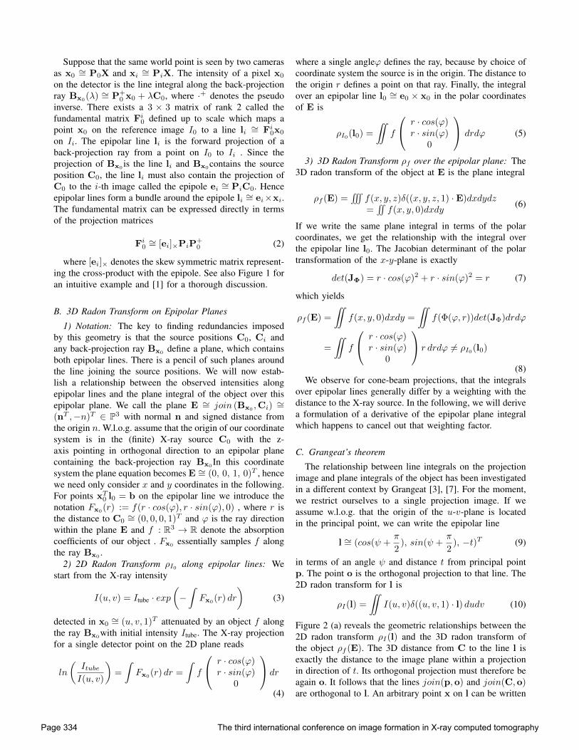
where a single angleϕ defines the ray, because by choice ofcoordinate system the source is in the origin. The distance tothe origin r defines a point on that ray. Finally, the integralover an epipolar line l0 ∼= e0 × x0 in the polar coordinatesof E is

ρI0(l0) =

¨f

r · cos(ϕ)r · sin(ϕ)

0

drdϕ (5)

3) 3D Radon Transform ρf over the epipolar plane: The3D radon transform of the object at E is the plane integral

ρf (E) =˝

f(x, y, z)δ((x, y, z, 1) ·E)dxdydz=˜f(x, y, 0)dxdy

(6)

If we write the same plane integral in terms of the polarcoordinates, we get the relationship with the integral overthe epipolar line l0. The Jacobian determinant of the polartransformation of the x-y-plane is exactly

det(JΦ) = r · cos(ϕ)2 + r · sin(ϕ)2 = r (7)

which yields

ρf (E) =

¨f(x, y, 0)dxdy =

¨f(Φ(ϕ, r))det(JΦ)drdϕ

=

¨f

r · cos(ϕ)r · sin(ϕ)

0

r drdϕ 6= ρI0(l0)

(8)We observe for cone-beam projections, that the integrals

over epipolar lines generally differ by a weighting with thedistance to the X-ray source. In the following, we will derivea formulation of a derivative of the epipolar plane integralwhich happens to cancel out that weighting factor.

C. Grangeat’s theorem

The relationship between line integrals on the projectionimage and plane integrals of the object has been investigatedin a different context by Grangeat [3], [7]. For the moment,we restrict ourselves to a single projection image. If weassume w.l.o.g. that the origin of the u-v-plane is locatedin the principal point, we can write the epipolar line

l ∼= (cos(ψ +π

2), sin(ψ +

π

2), −t)T (9)

in terms of an angle ψ and distance t from principal pointp. The point o is the orthogonal projection to that line. The2D radon transform for l is

ρI(l) =

¨I(u, v)δ((u, v, 1) · l) dudv (10)

Figure 2 (a) reveals the geometric relationships between the2D radon transform ρI(l) and the 3D radon transform ofthe object ρf (E). The 3D distance from C to the line l isexactly the distance to the image plane within a projectionin direction of t. Its orthogonal projection must therefore beagain o. It follows that the lines join(p,o) and join(C,o)are orthogonal to l. An arbitrary point x on l can be written

Page 334 The third international conference on image formation in X-ray computed tomography

in terms of the angles κ (between E and the principal ray)and ϕ (between o and x measured at C). The distance fromC to l is then cos(ϕ)r and the focal distance cos(κ)cos(ϕ)·r(via triangle p,C,o).

Now, we apply Grangeat’s trick and look at the derivativeof ρ(E) with respect to the distance to the origin n.d

dnρf (E) =

d

dn

¨Fx(r)r drdϕ =

¨d

dnFx(r)r drdϕ

(11)Observe in Figure 2 (b) that there is a relationship dn =

sin(dκ) · cos(ϕ)r. Because for small angles sin(dκ) = dκit holds

dκ

dn=

1

cos(ϕ)r(12)

and by chain rule we obtaind

dnFx(r)r =

d

dκ

1

cos(ϕ)Fx(r) (13)

Since the angle ϕ is small (bounded by half fan-ange), thecosine is almost one and we ignore it in our computations.We also ignore that n is tilted slightly out of the detectorplane, because κ is small. We can compute the derivativew.r.t t instead of n.

d

dnρf (E)

dκ≈0

=

¨d

dκ

1

cos(ϕ)Fx(r) drdϕ

ϕ small

≈ d

dκ

¨Fx(r) drdϕ

κ small

≈ d

dtρI(l)

(14)

p

l

φ

κ

C

r

t

ψ

∂n

∂κ

∂t

∂n

(a)

x

orthogonal view:

C

cos(φ)r

κ

∂κ∂t

∂n

x

tp

(b)

o

x

Figure 2. Grangeat’s theorem: relationship between angle κ and normal n.

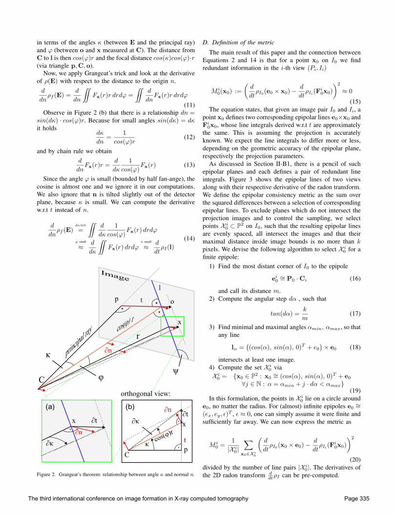
D. Definition of the metric

The main result of this paper and the connection betweenEquations 2 and 14 is that for a point x0 on I0 we findredundant information in the i-th view (Pi, Ii)

M i0(x0) :=

(d

dtρI0(e0 × x0)− d

dtρIi(F

i0x0)

)2

≈ 0

(15)The equation states, that given an image pair I0 and Ii, a

point x0 defines two corresponding epipolar lines e0×x0 andFi0x0, whose line integrals derived w.r.t t are approximatelythe same. This is assuming the projection is accuratelyknown. We expect the line integrals to differ more or less,depending on the geometric accuracy of the epipolar plane,respectively the projection parameters.

As discussed in Section II-B1, there is a pencil of suchepipolar planes and each defines a pair of redundant lineintegrals. Figure 3 shows the epipolar lines of two viewsalong with their respective derivative of the radon transform.We define the epipolar consistency metric as the sum overthe squared differences between a selection of correspondingepipolar lines. To exclude planes which do not intersect theprojection images and to control the sampling, we selectpoints X i0 ⊂ P2 on I0, such that the resulting epipolar linesare evenly spaced, all intersect the images and that theirmaximal distance inside image bounds is no more than kpixels. We devise the following algorithm to select X i0 for afinite epipole:

1) Find the most distant corner of I0 to the epipole

ei0∼= P0 ·Ci (16)

and call its distance m.2) Compute the angular step dα , such that

tan(dα) =k

m(17)

3) Find minimal and maximal angles αmin, αmax, so thatany line

lα =((cos(α), sin(α), 0)T + e0

)× e0 (18)

intersects at least one image.4) Compute the set X i0 viaX i0 = {x0 ∈ P2 : x0

∼= (cos(α), sin(α), 0)T + e0

∀j ∈ N : α = αmin + j · dα < αmax}(19)

In this formulation, the points in X i0 lie on a circle arounde0, no matter the radius. For (almost) infinite epipoles e0

∼=(ex, ey, ε)

T , ε ≈ 0, one can simply assume it were finite andsufficiently far away. We can now express the metric as

M i0 =

1

|X i0|∑

x0∈X i0

(d

dtρI0(x0 × e0)− d

dtρIi(F

i0x0)

)2

(20)divided by the number of line pairs |X i0|. The derivatives ofthe 2D radon transform d

dtρI can be pre-computed.

The third international conference on image formation in X-ray computed tomography Page 335

Figure 3. Two views with epipolar lines aligned to a plot of the derivativeof the line integrals for the left image (blue) and right image (green). Noticea shift in the signals due to imperfect geometry.

Finally, we sum up all those pairs of views, which changeduring optimization. If we want to optimize over parametersin P0, for example, we need not compute redundanciesbetween (Pi, Ii) and (Pj , Ij) for i 6= 0 6= j, because theyremain constant if only P0 changes: M0 =

∑iM

i0.

III. EXPERIMENTS AND RESULTS

A. Materials and methods

We validate against the digital phantom with randombeads in a full 360° rotation presented in [4] (512× 512 pxprojections, 1000 mm source-detector distance, phantom ofdiameter ∼ 100 mm). In addition, we conducted an ex-periment for this work using a 120° sweep of 190 pro-jections showing a real PDS2 calibration phantom usinga sequence of a Siemens C-arm system. Using [8] wecomputed the C-arm projection matrices from the projectionsof the metal beads in the calibration phantom and obtainedan average re-projection error of about 1.3 pixels (imagesize 960 × 1240 px, bead size about 8 − 12 px), which wealso verified by visual inspection. These projection matricesare the gold standard. In order to prove the robustness ofour method, we use the raw projection data directly fromthe scanner, without corrections of any kind (i.e. no I0correction, no correction for varying tube voltage etc.). Weuse a non-linear optimizer without gradient (Powell-Brent).In order to investigate accuracy, precision and stability ofour method, we conduct a series of random studies overa rigid transformation in world space. As an intuitive andmeaningful error metric, we compute the distance betweenthe bead centers projected with the ground truth versus thecurrent projection. This error is more informative, since themethod itself is entirely image based, while quantities inmillimeters and degrees of world space depend on overallscaling and most of the parameters a highly interdependent.

1) Sampling of radon space: In case of a circular trajec-tory, the epipole moves on a straight line from plus infinity,through the image to minus infinity. The epipolar lines arealmost parallel, when the epipole is far away. When wealign the detector v-axis with the axis of rotation, epipolarlines in most views will be almost parallel to the u-axis.This is visualized in Figure 4, where all the samples taken

120°

170°

0°

90°

Epipole moveson a line!

120°

170°

0°

90°t

ψ

t

ψ

Figure 4. Derivative of the radon transform of the digital phantom. Samplesfor a 170° rotation about Y-axis with a maximum distance between epipolarlines of one pixel (left) and 5 pixels (right). Sampled locations in black.

from radon space are marked with a black dot. Note that aline bundle corresponds to a sinoid curve in Radon Space.Also note a linear trajectory of the epipole leads to a singleintersection point of all sinoids. This is because the epipoleitself moves on a line, which is represented in a single pointin radon space, and that line is contained in any of the linebundles. Through the definition of X i0 , we can easily adjustthe number of lines, hence the sampling in radon space.

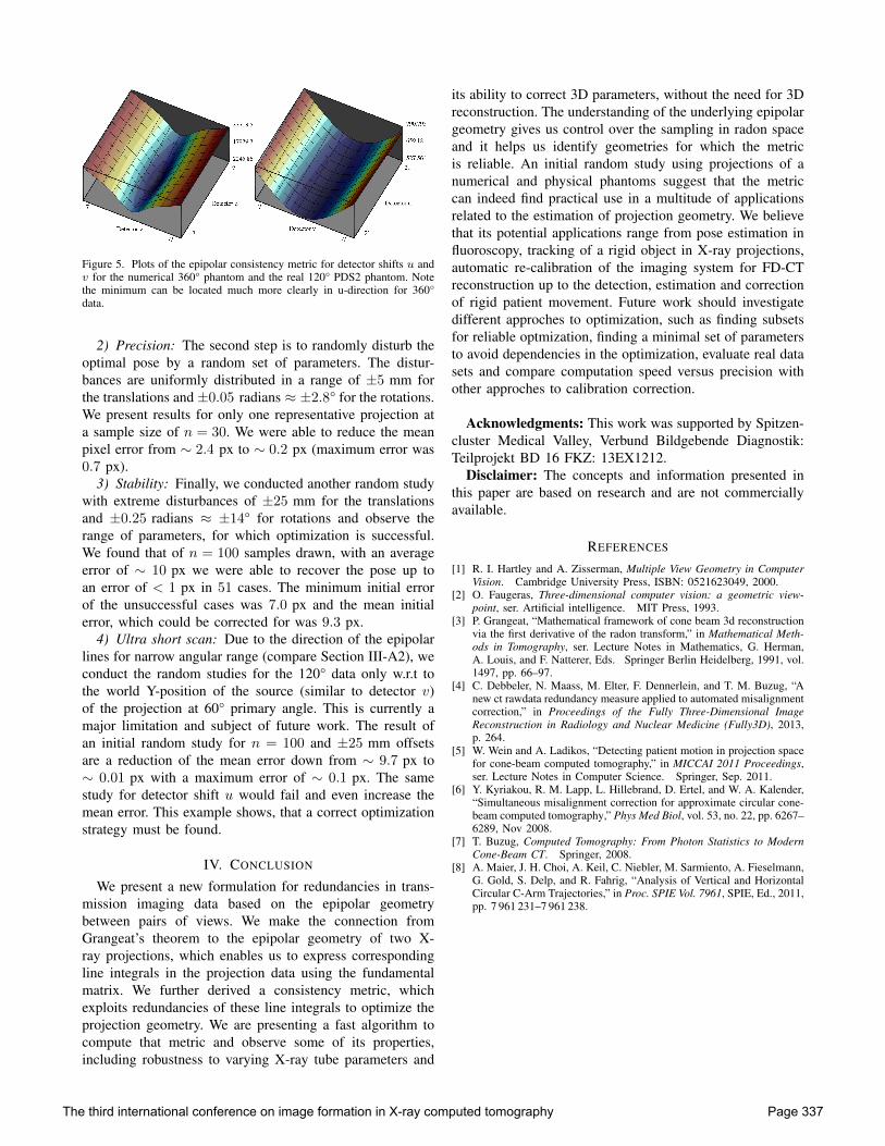
2) Dependency on direction of epipolar lines: We expectthe method to be reliable whenever the epipole is close tothe image or even inside the image. The epipole is insidethe image when the two views are related dominantly bya forward-backward translation, including opposing views.For cases, where the epipolar lines are almost parallel, weget little information in their direction (the direction of theintegrals) but only orthogonal to them. Note that a puretranslation parallel to the image plane results in parallelepipolar lines, a translation orthogonal to the image planeleaves the epipole in the center of the image. Rotationsaround the source merely apply a 2D homography to theimage. As a general motion is a combination of theseeffects, we can predict which geometries will give reliableinformation and in which spatial direction. Observe, forexample Figure 4, where sampling is dense close to theψ = 0 axis (horizontal). This is a property of any circulartrajectory. The epipole is within the image for views within± fan angle from the opposing view. For an opening angleof 40° this is just about 10 of all views. The method isthus much more robust for optimizing parameters orthogonalto the plane of rotation (usually denoted v-direction of thedetector). Only for opposing views is it similarly reliablein both u and v directions. This is a problem especially forshort scans, as visualized in the shape of the graphs in Figure5, which show a long and narrow valley in u-direction.

B. Random study

1) Accuracy: First, the gold standard geometry is as-sumed and optimized w.r.t the metric to find the distanceof the closest minimum. Any change away from the goldstandard is an inaccuracy. We obtained a mean accuracy overall projections of ∼ 0.25 px and a maximum of 1.00 px.

Page 336 The third international conference on image formation in X-ray computed tomography

Figure 5. Plots of the epipolar consistency metric for detector shifts u andv for the numerical 360° phantom and the real 120° PDS2 phantom. Notethe minimum can be located much more clearly in u-direction for 360°data.

2) Precision: The second step is to randomly disturb theoptimal pose by a random set of parameters. The distur-bances are uniformly distributed in a range of ±5 mm forthe translations and ±0.05 radians ≈ ±2.8° for the rotations.We present results for only one representative projection ata sample size of n = 30. We were able to reduce the meanpixel error from ∼ 2.4 px to ∼ 0.2 px (maximum error was0.7 px).

3) Stability: Finally, we conducted another random studywith extreme disturbances of ±25 mm for the translationsand ±0.25 radians ≈ ±14° for rotations and observe therange of parameters, for which optimization is successful.We found that of n = 100 samples drawn, with an averageerror of ∼ 10 px we were able to recover the pose up toan error of < 1 px in 51 cases. The minimum initial errorof the unsuccessful cases was 7.0 px and the mean initialerror, which could be corrected for was 9.3 px.

4) Ultra short scan: Due to the direction of the epipolarlines for narrow angular range (compare Section III-A2), weconduct the random studies for the 120° data only w.r.t tothe world Y-position of the source (similar to detector v)of the projection at 60° primary angle. This is currently amajor limitation and subject of future work. The result ofan initial random study for n = 100 and ±25 mm offsetsare a reduction of the mean error down from ∼ 9.7 px to∼ 0.01 px with a maximum error of ∼ 0.1 px. The samestudy for detector shift u would fail and even increase themean error. This example shows, that a correct optimizationstrategy must be found.

IV. CONCLUSION

We present a new formulation for redundancies in trans-mission imaging data based on the epipolar geometrybetween pairs of views. We make the connection fromGrangeat’s theorem to the epipolar geometry of two X-ray projections, which enables us to express correspondingline integrals in the projection data using the fundamentalmatrix. We further derived a consistency metric, whichexploits redundancies of these line integrals to optimize theprojection geometry. We are presenting a fast algorithm tocompute that metric and observe some of its properties,including robustness to varying X-ray tube parameters and

its ability to correct 3D parameters, without the need for 3Dreconstruction. The understanding of the underlying epipolargeometry gives us control over the sampling in radon spaceand it helps us identify geometries for which the metricis reliable. An initial random study using projections of anumerical and physical phantoms suggest that the metriccan indeed find practical use in a multitude of applicationsrelated to the estimation of projection geometry. We believethat its potential applications range from pose estimation influoroscopy, tracking of a rigid object in X-ray projections,automatic re-calibration of the imaging system for FD-CTreconstruction up to the detection, estimation and correctionof rigid patient movement. Future work should investigatedifferent approches to optimization, such as finding subsetsfor reliable optmization, finding a minimal set of parametersto avoid dependencies in the optimization, evaluate real datasets and compare computation speed versus precision withother approches to calibration correction.

Acknowledgments: This work was supported by Spitzen-cluster Medical Valley, Verbund Bildgebende Diagnostik:Teilprojekt BD 16 FKZ: 13EX1212.

Disclaimer: The concepts and information presented inthis paper are based on research and are not commerciallyavailable.

REFERENCES

[1] R. I. Hartley and A. Zisserman, Multiple View Geometry in ComputerVision. Cambridge University Press, ISBN: 0521623049, 2000.

[2] O. Faugeras, Three-dimensional computer vision: a geometric view-point, ser. Artificial intelligence. MIT Press, 1993.

[3] P. Grangeat, “Mathematical framework of cone beam 3d reconstructionvia the first derivative of the radon transform,” in Mathematical Meth-ods in Tomography, ser. Lecture Notes in Mathematics, G. Herman,A. Louis, and F. Natterer, Eds. Springer Berlin Heidelberg, 1991, vol.1497, pp. 66–97.

[4] C. Debbeler, N. Maass, M. Elter, F. Dennerlein, and T. M. Buzug, “Anew ct rawdata redundancy measure applied to automated misalignmentcorrection,” in Proceedings of the Fully Three-Dimensional ImageReconstruction in Radiology and Nuclear Medicine (Fully3D), 2013,p. 264.

[5] W. Wein and A. Ladikos, “Detecting patient motion in projection spacefor cone-beam computed tomography,” in MICCAI 2011 Proceedings,ser. Lecture Notes in Computer Science. Springer, Sep. 2011.

[6] Y. Kyriakou, R. M. Lapp, L. Hillebrand, D. Ertel, and W. A. Kalender,“Simultaneous misalignment correction for approximate circular cone-beam computed tomography,” Phys Med Biol, vol. 53, no. 22, pp. 6267–6289, Nov 2008.

[7] T. Buzug, Computed Tomography: From Photon Statistics to ModernCone-Beam CT. Springer, 2008.

[8] A. Maier, J. H. Choi, A. Keil, C. Niebler, M. Sarmiento, A. Fieselmann,G. Gold, S. Delp, and R. Fahrig, “Analysis of Vertical and HorizontalCircular C-Arm Trajectories,” in Proc. SPIE Vol. 7961, SPIE, Ed., 2011,pp. 7 961 231–7 961 238.

The third international conference on image formation in X-ray computed tomography Page 337