NUREG/CR-6672, Vols. 1,2 SAND2000-0234 Reexamination of Spent Fuel Shipment Risk Estimates Volume I: Main Report Manuscript Completed: February 2000 Date Published: March 2000 Prepared by J. L. Sprung, D. J. Ammerman, N. L. Breivik, R. J. Dukart, F. L. Kanipe, J. A. Koski, G. S. Mills, K. S. Neuhauser, H. D. Radloff, R. F. Weiner, H. R. Yoshimura Sandia National Laboratories Albuquerque, NM 87185-0718 Prepared for Spent Fuel Project Office Office of Nuclear Material Safety and Safeguards U.S. Nuclear Regulatory Commission Washington, DC 20555 NRC Job Code J5160
Transcript
NUREG/CR-6672, Vols. 1,2SAND2000-0234
Reexamination of SpentFuel Shipment RiskEstimates
Volume I: Main Report
Manuscript Completed: February 2000Date Published: March 2000
Prepared byJ. L. Sprung, D. J. Ammerman, N. L. Breivik, R. J. Dukart, F. L. Kanipe,J. A. Koski, G. S. Mills, K. S. Neuhauser, H. D. Radloff, R. F. Weiner, H. R. Yoshimura
Sandia National LaboratoriesAlbuquerque, NM 87185-0718
Prepared forSpent Fuel Project OfficeOffice of Nuclear Material Safety and SafeguardsU.S. Nuclear Regulatory CommissionWashington, DC 20555NRC Job Code J5160
ii
Page intentionally left blank.
iii
ABSTRACT
The risks associated with the transport of spent nuclear fuel by truck and rail are reexamined andcompared to results published in NUREG-0170 and the Modal Study. The reexaminationconsiders transport by truck and rail in four generic Type B spent fuel casks. Cask and spent fuelresponse to collision impacts and fires are evaluated by performing three-dimensional finiteelement and one-dimensional heat transport calculations. Accident release fractions aredeveloped by critical review of literature data. Accident severity fractions are developed fromModal Study truck and rail accident event trees, modified to reflect the frequency of occurrenceof hard and soft rock wayside route surfaces as determined by analysis of geographic data.Incident-free population doses and the population dose risks associated with the accidents thatmight occur during transport are calculated using the RADTRAN 5 transportation risk code. Thecalculated incident-free doses are compared to those published in NUREG-0170. The calculatedaccident dose risks are compared to dose risks calculated using NUREG-0170 and Modal Studyaccident source terms. The comparisons demonstrate that both of these studies made a numberof very conservative assumptions about spent fuel and cask response to accident conditions,which caused their estimates of accident source terms, accident frequencies, and accidentconsequences to also be very conservative. The results of this study and the previous studiesdemonstrate that the risks associated with the shipment of spent fuel by truck or rail are verysmall.
iv
Page intentionally left blank.
v
CONTENTS
ABSTRACT................................................................................................................................... iii
1.3 Need for Reevaluation of NUREG-0170 Spent Fuel Transportation Risks ............................................. 1-3
1.4 Study Objectives ...................................................................................................................................... 1-4
1.5 General Approach .................................................................................................................................... 1-5
3.2 RADTRAN 1 and RADTRAN 5 Input Variables .................................................................................... 3-3
vi
3.3 Variables Selected for Sampling ............................................................................................................ 3-123.3.1 Incident-Free Variables Selected for LHS Sampling ............................................................... 3-123.3.2 Incident-Free Variables Not Selected for LHS Sampling ........................................................ 3-133.3.3 Accident Variables................................................................................................................... 3-22
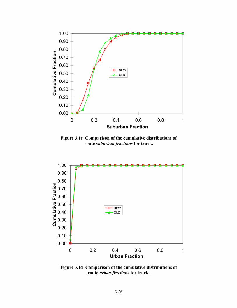
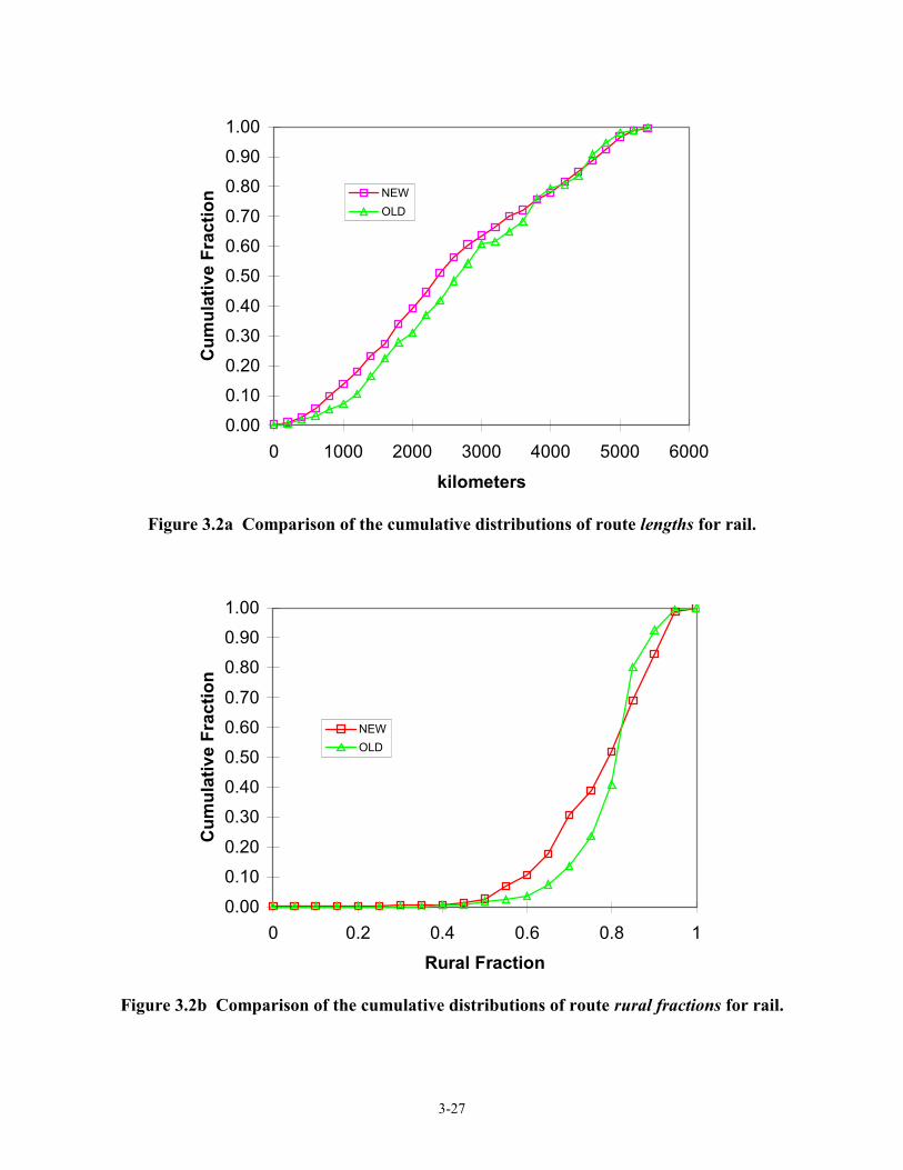
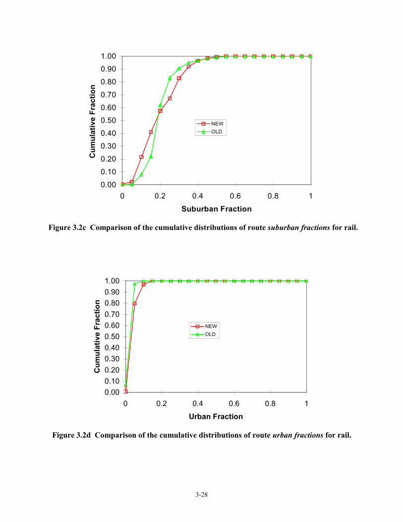
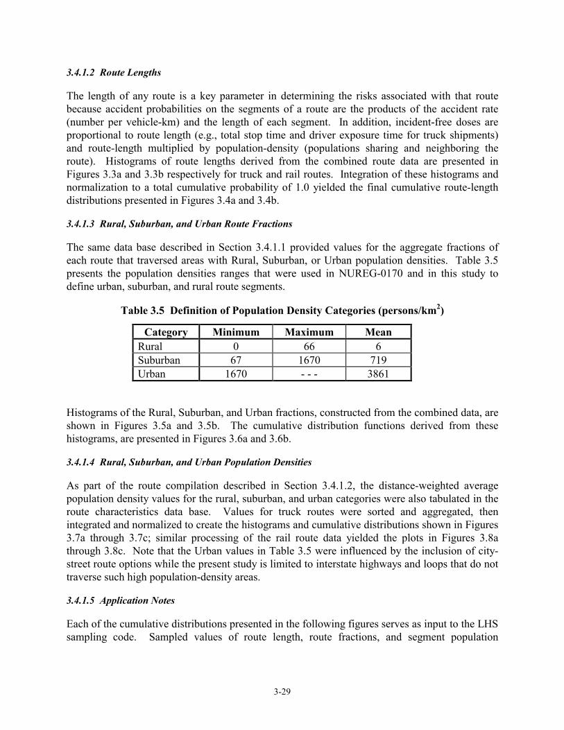
3.4 Development of Distribution Functions ................................................................................................. 3-243.4.1 Route Characteristics ............................................................................................................... 3-243.4.2 Truck and Train Accident Statistics......................................................................................... 3-373.4.3 Development of Miscellaneous Distributions .......................................................................... 3-44
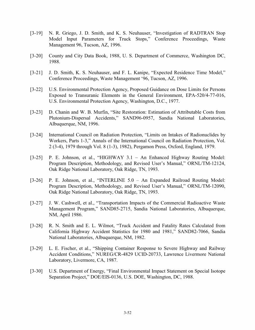
4. SELECTION OF GENERIC CASKS...................................................................................4-14.1 Description of Casks ................................................................................................................................ 4-1
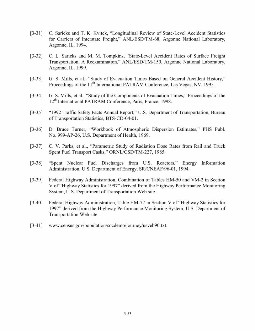
4.2 Conservatism in Cask Selection ............................................................................................................... 4-7
5. STRUCTURAL RESPONSE ...............................................................................................5-15.1 Finite Element Calculations for Impacts onto Rigid Targets.................................................................... 5-1
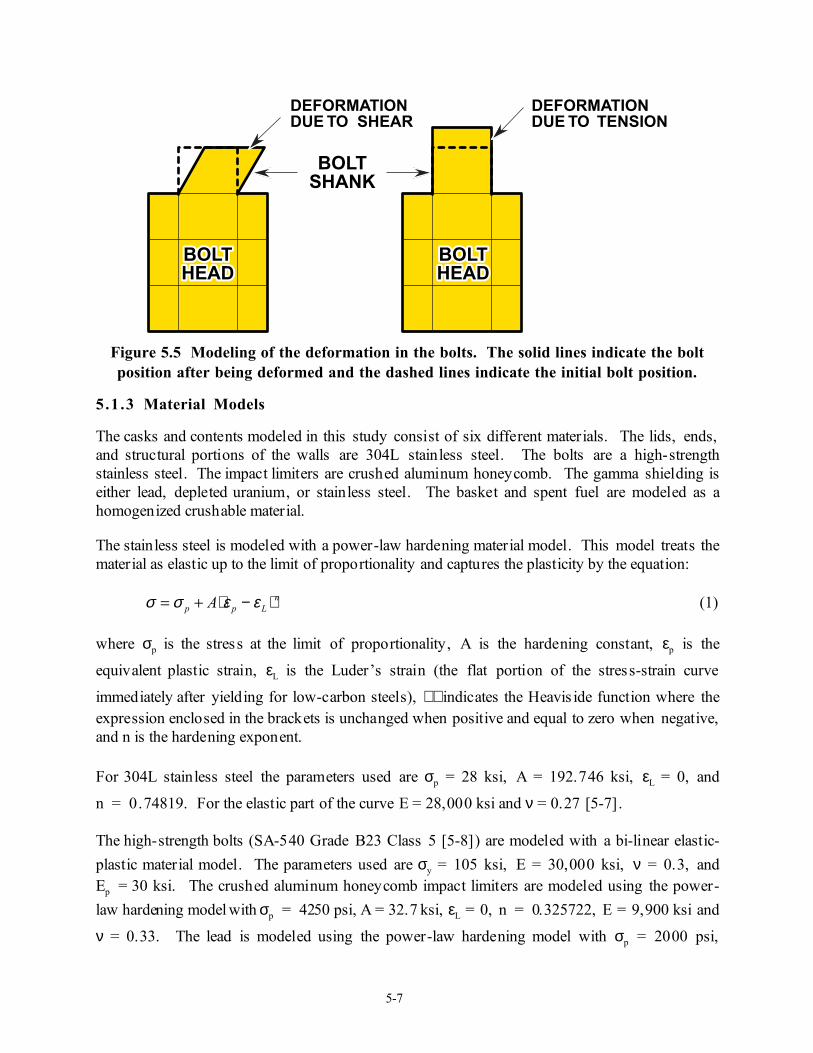
5.1.1 Introduction................................................................................................................................ 5-15.1.2 Assumptions for Finite Element Models.................................................................................... 5-25.1.3 Material Models......................................................................................................................... 5-75.1.4 Finite Element Results ............................................................................................................... 5-85.1.5 Benchmarking of Finite Element Calculations......................................................................... 5-15
5.2 Impacts onto Real Targets...................................................................................................................... 5-165.2.1 Introduction.............................................................................................................................. 5-165.2.2 Methodology............................................................................................................................ 5-165.2.3 Soil Targets.............................................................................................................................. 5-195.2.4 Concrete Targets ...................................................................................................................... 5-205.2.5 Hard Rock Targets ................................................................................................................... 5-245.2.6 Example Calculation ................................................................................................................ 5-245.2.7 Results for Real Target Calculations........................................................................................ 5-245.2.8 Impacts onto Water .................................................................................................................. 5-265.2.9 Correlation of Results with Modal Study Event Trees............................................................. 5-26
5.4 Failure of Rods....................................................................................................................................... 5-275.4.1 Rod Failure Strain Criterion..................................................................................................... 5-285.4.2 Estimation of the Fraction of Rods Failed During Impacts...................................................... 5-31
5.5 Conservatism in Calculating Structural Response .................................................................................. 5-31
6. THERMAL ANALYSIS OF THE GENERIC CASKSIN A LONG DURATION FIRE ...........................................................................................6-16.1 Introduction.............................................................................................................................................. 6-1
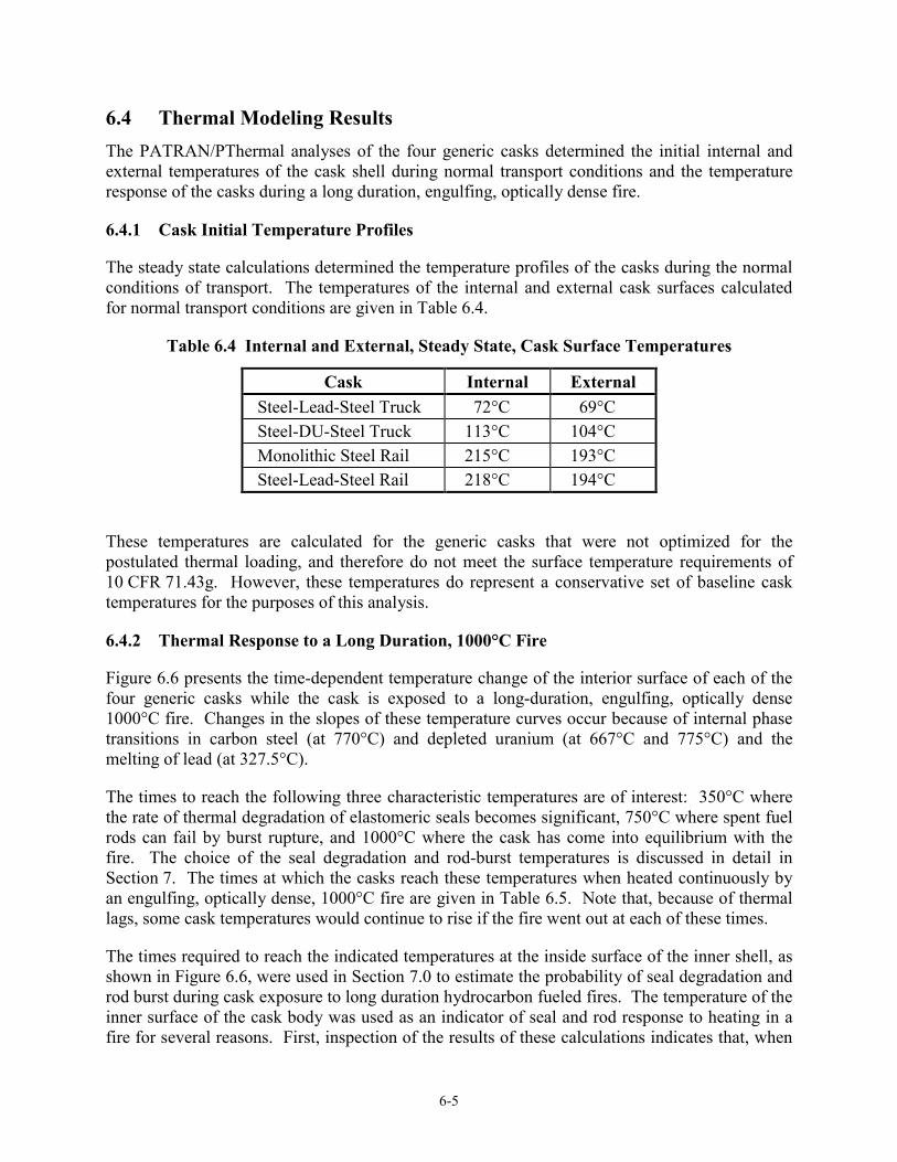
6.4 Thermal Modeling Results ....................................................................................................................... 6-56.4.1 Cask Initial Temperature Profiles ..............................................................................................6-56.4.2 Thermal Response to a Long Duration, 1000°C Fire .................................................................6-56.4.3 Thermal Response to a Long Duration 800°C Fire ....................................................................6-7
7. SOURCE TERMS AND SOURCE TERM PROBABILITIES............................................7-17.1 Truck and Train Accident Scenarios ........................................................................................................ 7-1
7.1.1 Event Trees ................................................................................................................................ 7-17.1.2 Route Wayside Surface Characteristics ..................................................................................... 7-47.1.3 Truck Accident Data .................................................................................................................. 7-77.1.4 Train Accident Data................................................................................................................... 7-9
7.2 Source Term and Source Term Probability Expressions........................................................................ 7-137.2.1 RADTRAN Risk Equations ..................................................................................................... 7-137.2.2 Accident Source Terms............................................................................................................ 7-137.2.3 Cask Inventories....................................................................................................................... 7-147.2.4 Chemical Element Classes ....................................................................................................... 7-167.2.5 Release Fractions ..................................................................................................................... 7-187.2.6 Accident Cases......................................................................................................................... 7-247.2.7 Source Term Probabilities........................................................................................................ 7-277.2.8 Accident Severities .................................................................................................................. 7-27
7.3 Values for Release Fraction Parameters................................................................................................. 7-307.3.1 Fission Product Release from Failed Rods to the Cask Interior............................................... 7-307.3.2 Noble Gases ............................................................................................................................. 7-307.3.3 Particles.................................................................................................................................... 7-307.3.4 Cesium ..................................................................................................................................... 7-357.3.5 Release Following Fuel Oxidation........................................................................................... 7-457.3.6 CRUD ...................................................................................................................................... 7-487.3.7 Impact Failure of Spent Fuel Rods........................................................................................... 7-497.3.8 Fission Product Transport from the Cask Interior to the Environment .................................... 7-517.3.9 Expansion Factor Values ......................................................................................................... 7-54
7.4 Values for Severity Fraction Parameters ................................................................................................ 7-557.4.1 Introduction.............................................................................................................................. 7-557.4.2 Cask Involvement .................................................................................................................... 7-557.4.3 Values for Collision Conditional Probabilities ........................................................................ 7-567.4.4 Values for Fire Probabilities .................................................................................................... 7-63
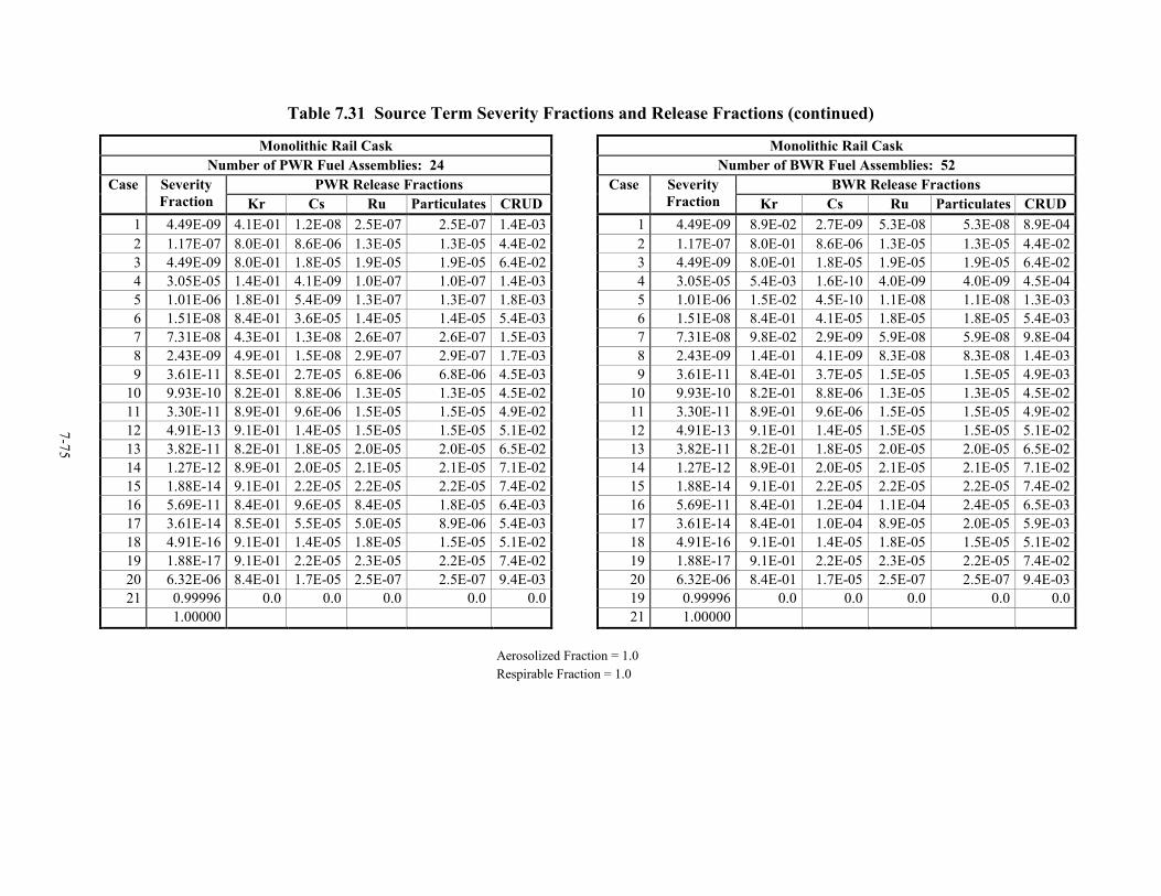
7.5 Values for Release Fractions and Severity Fractions ............................................................................. 7-717.5.1 Introduction.............................................................................................................................. 7-717.5.2 Calculational Method............................................................................................................... 7-717.5.3 Source Term Severity Fraction and Release Fraction Values .................................................. 7-72
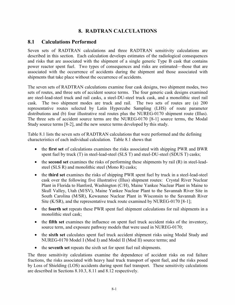
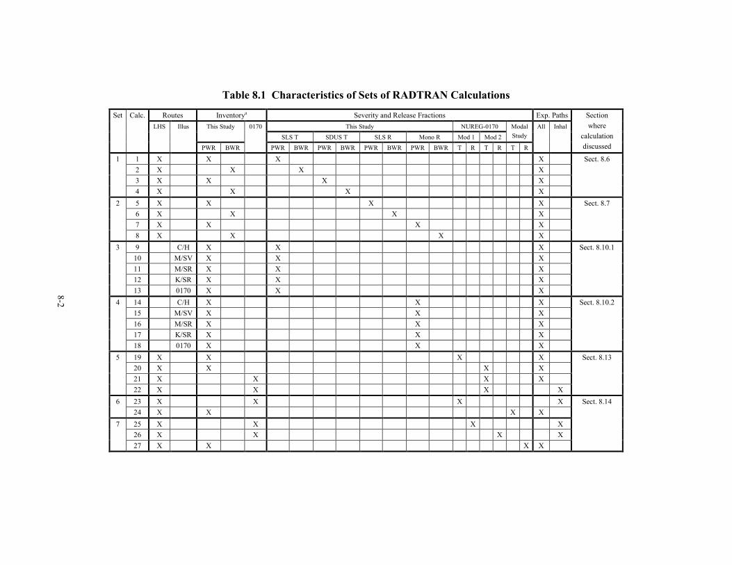
8. RADTRAN CALCULATIONS............................................................................................8-18.1 Calculations Performed ............................................................................................................................ 8-1
8.2 The RADTRAN 5 Computational Scheme .............................................................................................. 8-38.2.1 Latin Hypercube Sampling......................................................................................................... 8-38.2.2 Size of the LHS Sample ............................................................................................................. 8-3
8.3 Input Parameters and Results Calculated ................................................................................................. 8-4
8.4 Number of Cases Examined ..................................................................................................................... 8-5
8.5 Complementary Cumulative Distribution Functions ................................................................................ 8-6
8.6 Results for the Generic Steel-Lead-Steel and Steel-DU-Steel Truck Casks ............................................. 8-6
8.7 Results for the Generic Steel-Lead-Steel and Monolithic Steel Rail Casks............................................ 8-18
8.8 Comparison of Truck and Rail Transport Mean Risks ........................................................................... 8-24
8.9 Comparison of NUREG-0170 Incident-Free Doses to Those of This Study.......................................... 8-25
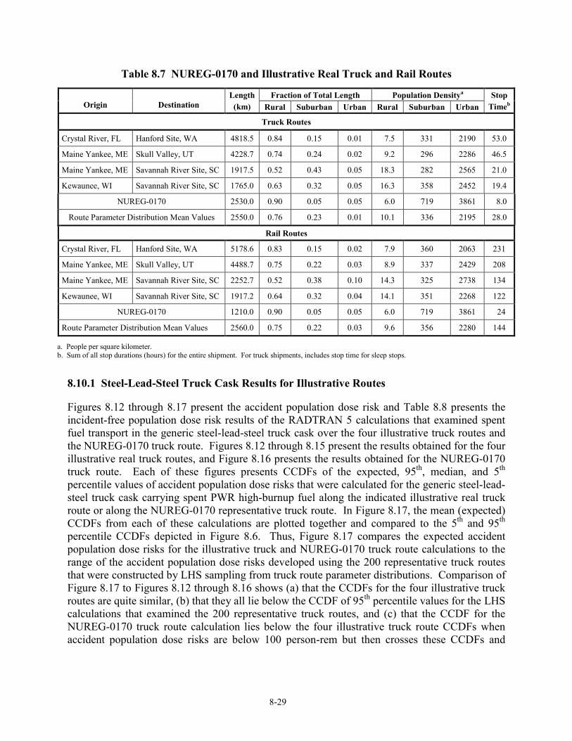
8.10 Illustrative Real Routes .......................................................................................................................... 8-288.10.1 Steel-Lead-Steel Truck Cask Results for Illustrative Routes ................................................... 8-298.10.2 Monolithic Steel Rail Cask Results for Illustrative Routes ...................................................... 8-378.10.3 Rod Strain Failure Criterion Sensitivity Calculation................................................................ 8-44
8.11 Rail Routes with Heavy-Haul Segments and Intermodal Transfers........................................................ 8-45
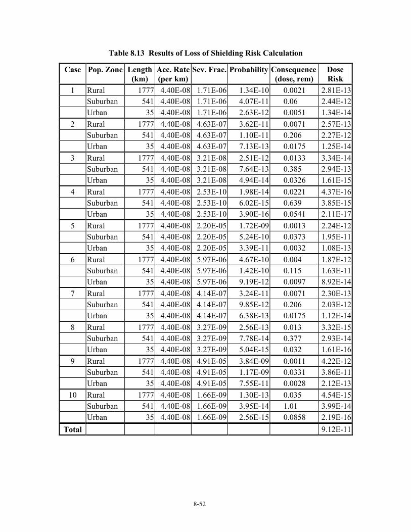
8.12 Loss of Shielding Accidents................................................................................................................... 8-478.12.1 Severity Fractions, Dose Rates, and Cask LOS Areas ............................................................. 8-488.12.2 Maximum Dimension of LOS Area ......................................................................................... 8-508.12.3 Final Calculation...................................................................................................................... 8-508.12.4 An Example of an LOS Calculation......................................................................................... 8-50
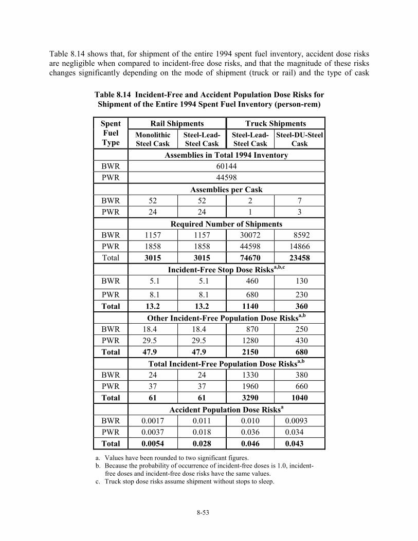
8.13 Population Dose Risks for Shipment of the Entire 1994 Spent Fuel Inventory...................................... 8-51
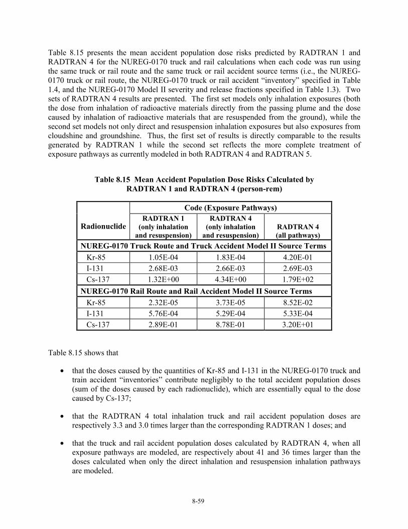
8.15 Effect of NUREG-0170 Source Term and Exposure Pathway Models on Dose Risk............................ 8-568.15.1 Source Term and Exposure Pathway Models in RADTRAN 1 and RADTRAN 5.................. 8-568.15.2 Comparison of Results Calculated with RADTRAN Versions 1, 4, and 5 .............................. 8-588.15.3 Effect of Treatments on RADTRAN 5 Accident Population Dose CCDFs ............................. 8-61
8.16 Population Dose Risk CCDFs from NUREG-0170, the Modal Study, and this Study........................... 8-648.16.1 CCDF Probability Axis Intercepts ........................................................................................... 8-648.16.2 CCDF Consequence Axis Intercepts........................................................................................ 8-69
9. SUMMARY AND CONCLUSIONS ...................................................................................9-1
ix
APPENDIX A STRUCTURAL RESPONSE INFORMATION...........................................A-1
APPENDIX B ANALYTICAL DETERMINATION OF PACKAGERESPONSE TO SEVERE IMPACTS .......................................................... B-1
APPENDIX C ORIGEN2 CALCULATIONS ...................................................................... C-1
APPENDIX D SOURCE TERM SPREADSHEETS............................................................D-1
APPENDIX E ILLUSTRATIVE LHS AND RADTRAN INPUTAND OUTPUT FILES.................................................................................. E-1
x
Figures
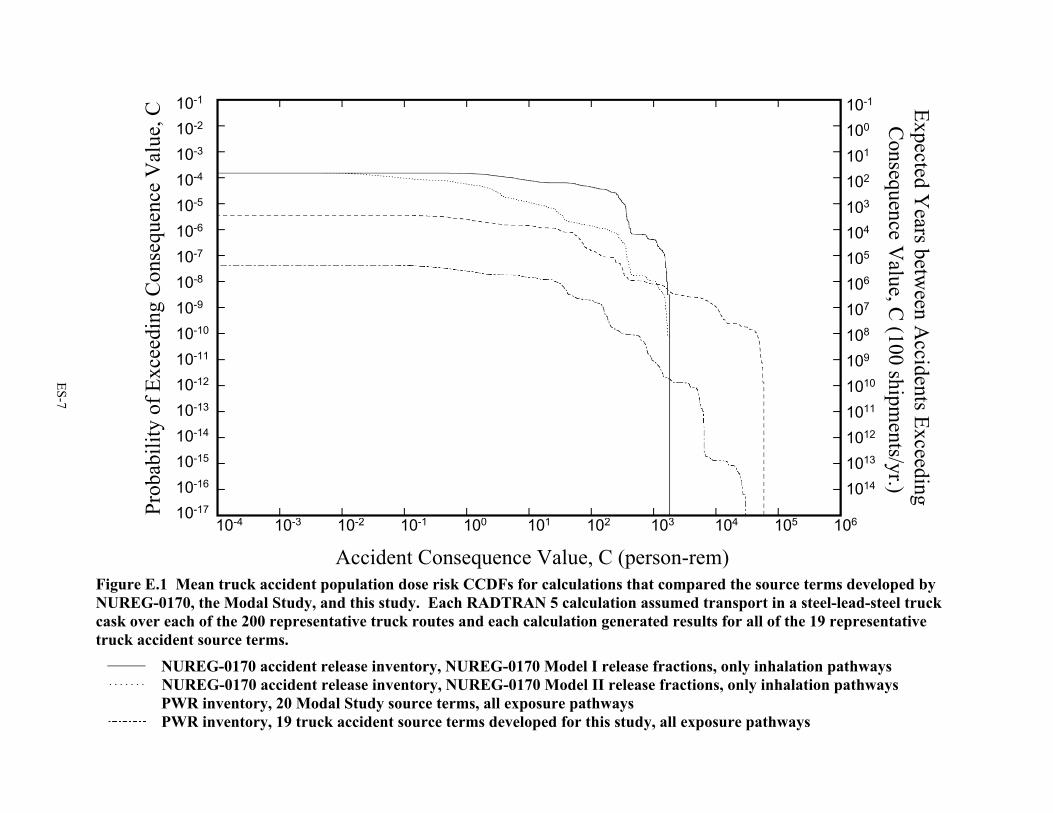
Figure E.1 Mean truck accident population dose risk CCDFs for calculations that compared the source termsdeveloped by NUREG-0170, the Modal Study, and this study. Each RADTRAN 5 calculation assumedtransport in a steel-lead-steel truck cask over each of the 200 representative truck routes and eachcalculation generated results for all of the 19 representative truck accident source terms............................. ES-7
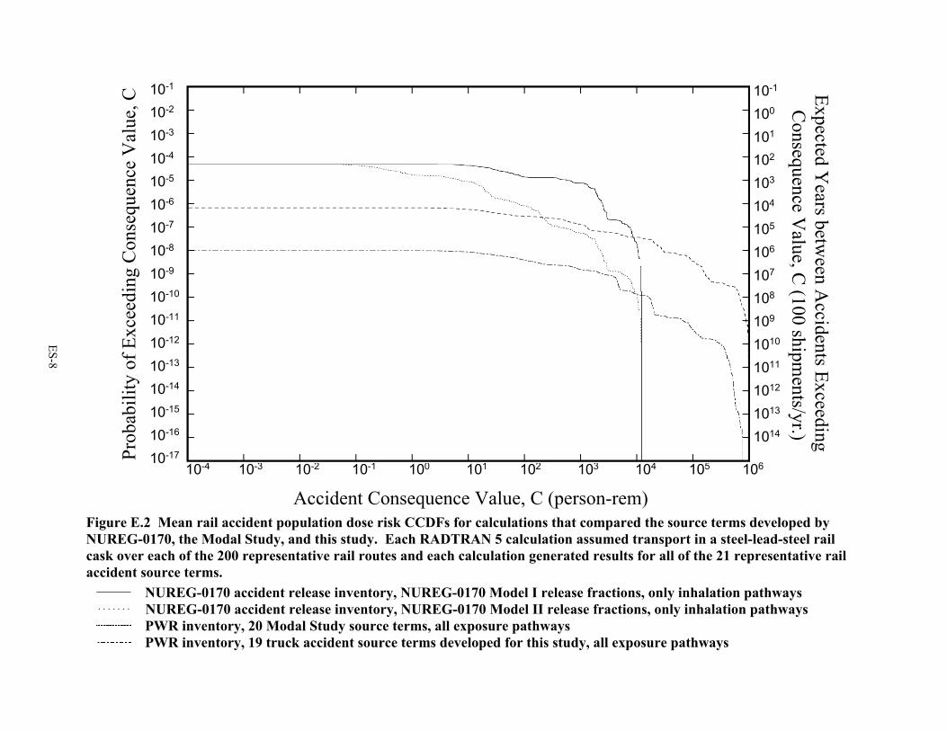
Figure E.2 Mean rail accident population dose risk CCDFs for calculations that compared the source termsdeveloped by NUREG-0170, the Modal Study, and this study. Each RADTRAN 5 calculation assumedtransport in a steel-lead-steel rail cask over each of the 200 representative rail routes and each calculationgenerated results for all of the 21 representative rail accident source terms.................................................. ES-8
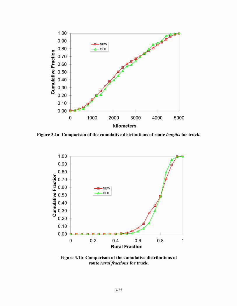
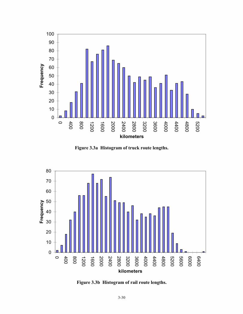
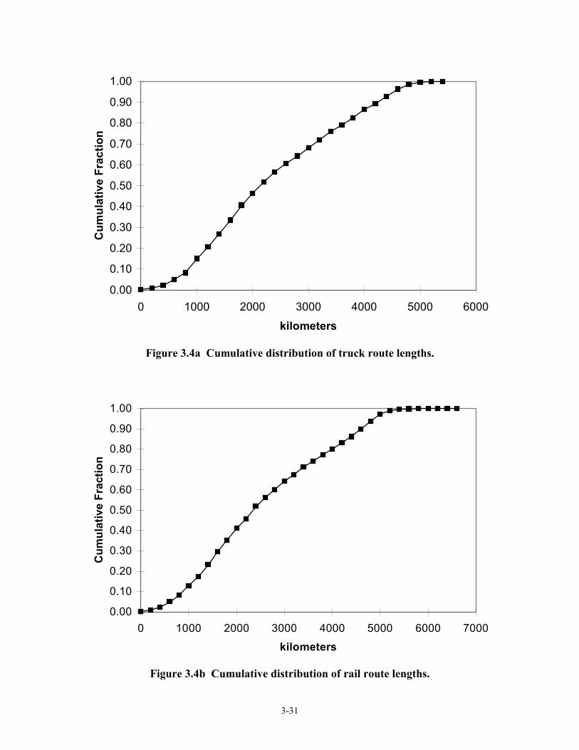
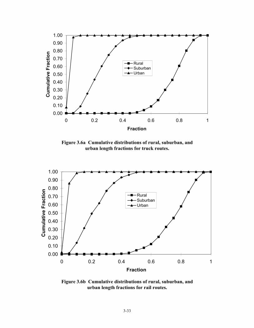
Figure 3.1a Comparison of the cumulative distributions of route lengths for truck ................................................3-25Figure 3.1b Comparison of the cumulative distributions of route rural fractions for truck ...................................3-25Figure 3.1c Comparison of the cumulative distributions of route suburban fractions for truck ............................3-26Figure 3.1d Comparison of the cumulative distributions of route urban fractions for truck...................................3-26Figure 3.2a Comparison of the cumulative distributions of route lengths for rail ...................................................3-27Figure 3.2b Comparison of the cumulative distributions of route rural fractions for rail .......................................3-27Figure 3.2c Comparison of the cumulative distributions of route suburban fractions for rail ................................3-28Figure 3.2d Comparison of the cumulative distributions of route urban fractions for rail......................................3-28Figure 3.3a Histogram of truck route lengths..........................................................................................................3-30Figure 3.3b Histogram of rail route lengths ............................................................................................................3-30Figure 3.4a Cumulative distribution of truck route lengths.....................................................................................3-31Figure 3.4b Cumulative distribution of rail route lengths .......................................................................................3-31Figure 3.5a Histograms of rural, suburban, and urban length fractions for truck routes .........................................3-32Figure 3.5b Histograms of rural, suburban, and urban length fractions for rail routes............................................3-32Figure 3.6a Cumulative distributions of rural, suburban, and urban length fractions for truck routes ....................3-33Figure 3.6b Cumulative distributions of rural, suburban, and urban length fractions for rail routes.......................3-33Figure 3.7a Histogram and cumulative distribution for rural population density for rural truck route
segments .........................................................................................................................................................3-34Figure 3.7b Histogram and cumulative distribution for suburban population density
for suburban truck route segments ..................................................................................................................3-34Figure 3.7c Histogram and cumulative distribution for urban population density for
urban truck route segments .............................................................................................................................3-35Figure 3.8a Histogram and cumulative distribution for rural population density for rural rail route
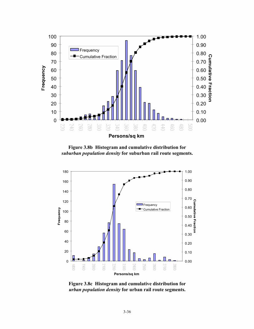
segments .........................................................................................................................................................3-35Figure 3.8b Histogram and cumulative distribution for suburban population density for suburb
an rail route segments .....................................................................................................................................3-36Figure 3.8c Histogram and cumulative distribution for urban population density for urban rail
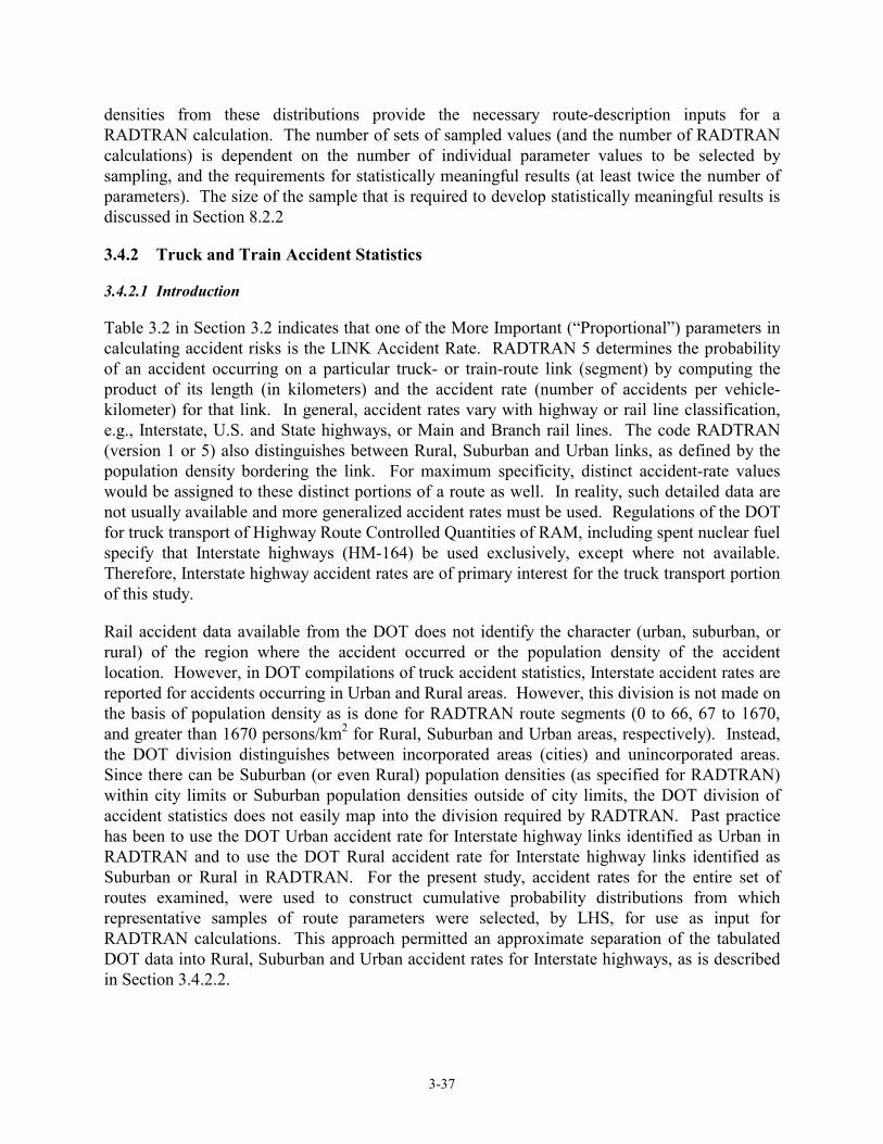
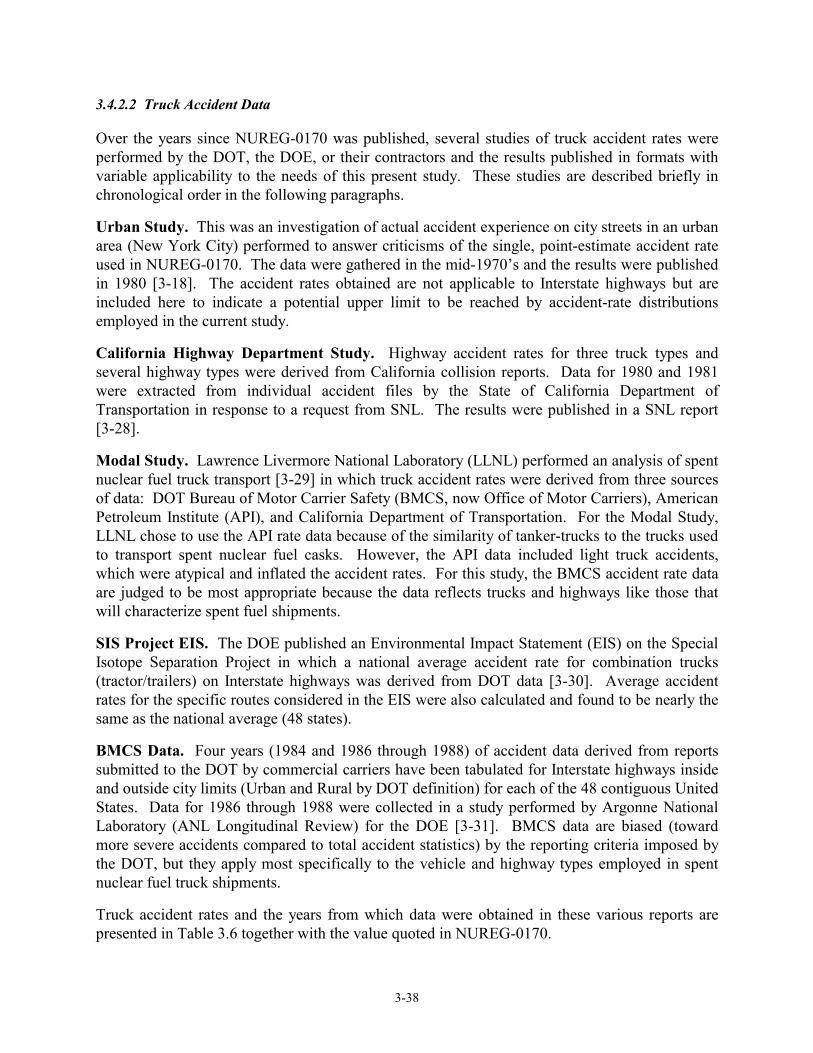
route segments ................................................................................................................................................3-36Figure 3.9a Accident rate versus rural population density ......................................................................................3-41Figure 3.9b Accident rate versus suburban population density ...............................................................................3-41Figure 3.10a Cumulative distribution of rural accident rates ..................................................................................3-42Figure 3.10b Cumulative distribution of suburban and urban accident rates ..........................................................3-42Figure 3.11 Cumulative distribution of rail accident rates (used for all segments: Rural,
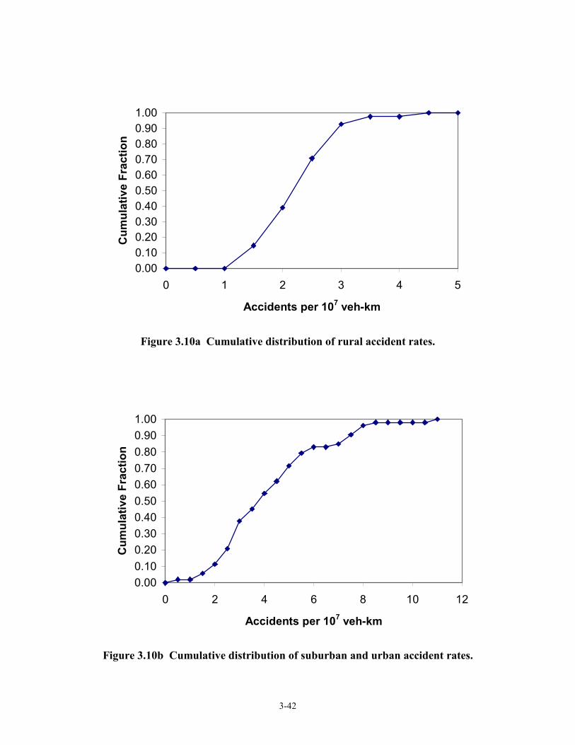
Suburban, and Urban).....................................................................................................................................3-43Figure 3.12 Distribution of normal commercial truck stop times............................................................................3-45Figure 3.13 Distribution of response team arrival plus evacuation times................................................................3-46Figure 3.14 Histogram and cumulative distribution of rural interstate traffic density.............................................3-49Figure 3.15 Histogram and cumulative distribution of interstate traffic density for urbanized areas ......................3-49Figure 3.16 Histogram and cumulative distribution of suburban interstate traffic density......................................3-50Figure 4.1 Conceptual design of a generic steel-lead-steel truck cask ......................................................................4-2Figure 4.2 Conceptual design of a generic steel-DU-steel truck cask .......................................................................4-3Figure 4.3 Conceptual design of a generic steel-lead-steel rail cask .........................................................................4-4Figure 4.4 Conceptual design of a generic monolithic steel rail cask........................................................................4-5
xi
Figure 4.5 Finite element representation of a typical closure lid for structural analysis,showing the locations of the bolts.....................................................................................................................4-7
Figure 5.1 Geometry of the initial and pre-crushed impact limiter ...........................................................................5-2Figure 5.2 Finite element model of the steel-lead-steel rail cask in the CG-over-corner drop orientation...............5-3Figure 5.3 Detail of the end of the steel-lead-steel rail cask finite element model ....................................................5-4Figure 5.4 Typical model of a bolt used in the finite element analyses.....................................................................5-6Figure 5.5 Modeling of the deformation in the bolts. The solid lines indicate the bolt position
after being deformed and the dashed lines indicate the initial bolt position .....................................................5-7Figure 5.6 Deformed shape and plastic strain fringes for the steel-lead-steel truck cask following
a 120-mph impact in the side-on orientation. The maximum plastic strain (indicated by the asterisk)occurs in the outer shell. The maximum strain in the inner shell is 0.27 ........................................................5-9
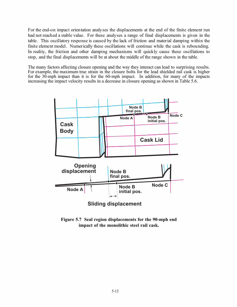
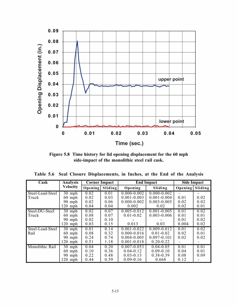
Figure 5.7 Seal region displacements for the 90-mph end impact of the monolithic steel rail cask .......................5-12Figure 5.8 Time history for lid opening displacement for the 60 mph side-impact of the monolithic
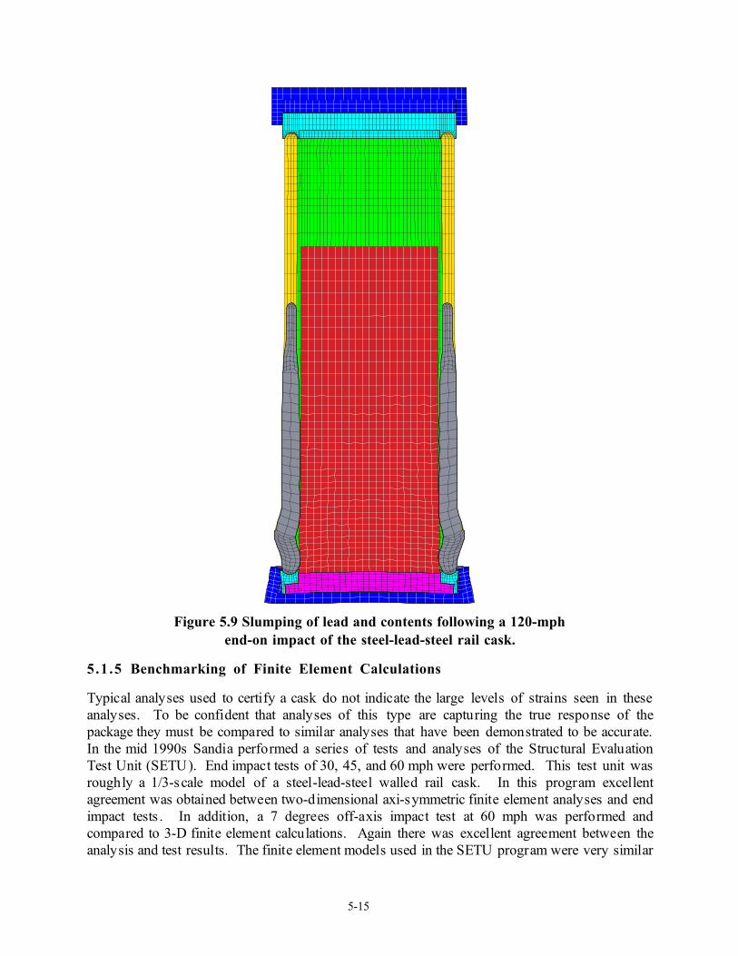
steel rail cask ..................................................................................................................................................5-13Figure 5.9 Slumping of lead and contents following a 120-mph end-on impact of the steel-lead-steel
rail cask...........................................................................................................................................................5-15Figure 5.10 Kinetic energy time histories for the steel-lead-steel truck cask from 120-mph impact
analyses in the end, side, and corner orientations ...........................................................................................5-17Figure 5.11 Force-deflection curves for the steel-lead-steel truck cask from the 120-mph impact
analyses in the end, side, and corner orientations ...........................................................................................5-18Figure 5.12 Force-deflection curves for impact onto hard desert soil .....................................................................5-20Figure 5.13 Comparison of test force-deflection curves with those derived from the empirical equations............5-22Figure 5.14 Force-deflection curves for concrete target impacts of the steel-lead-steel truck cask at 120 mph......5-23Figure 5.15 Fraction of railroad tank cars involved in puncture-type accidents that failed because
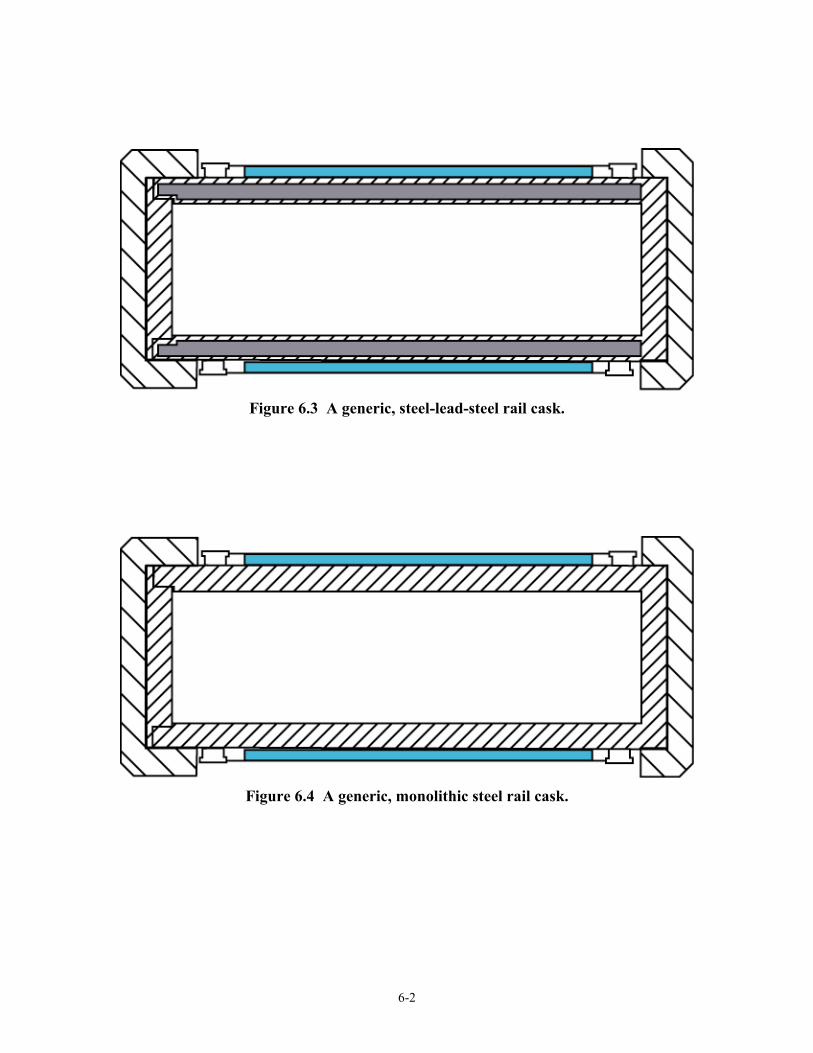
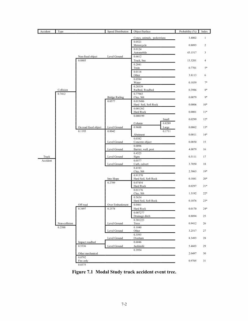
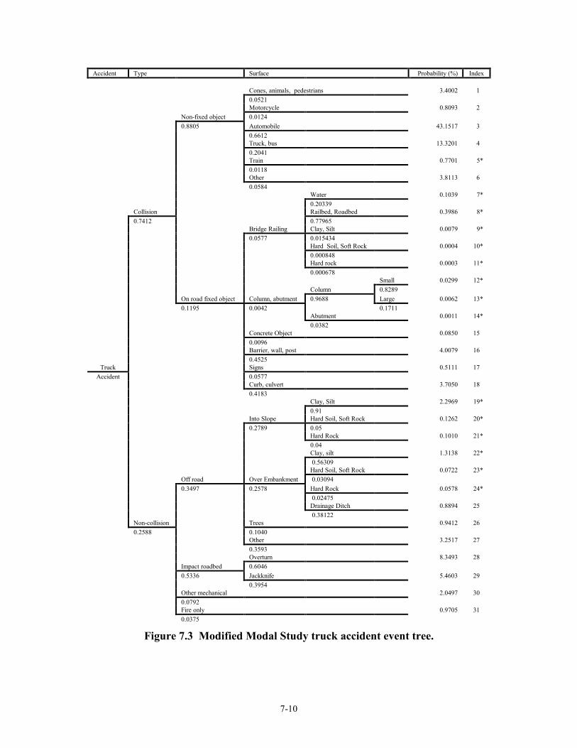
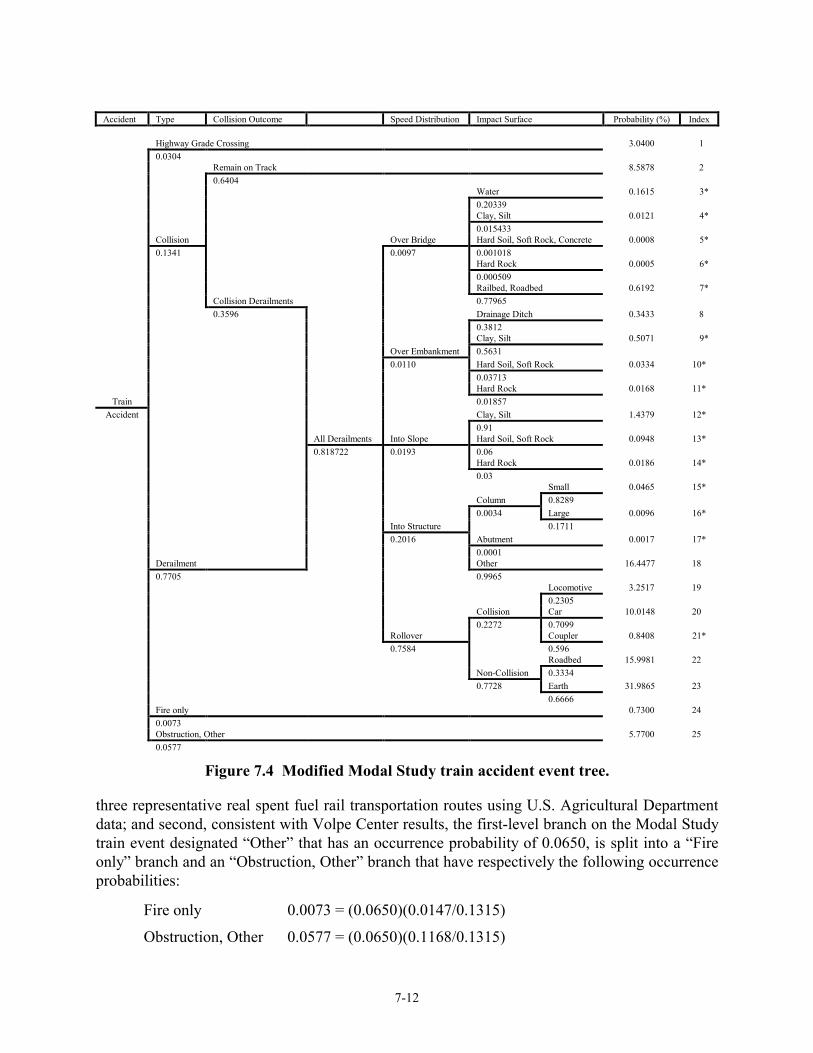
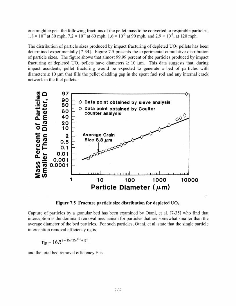
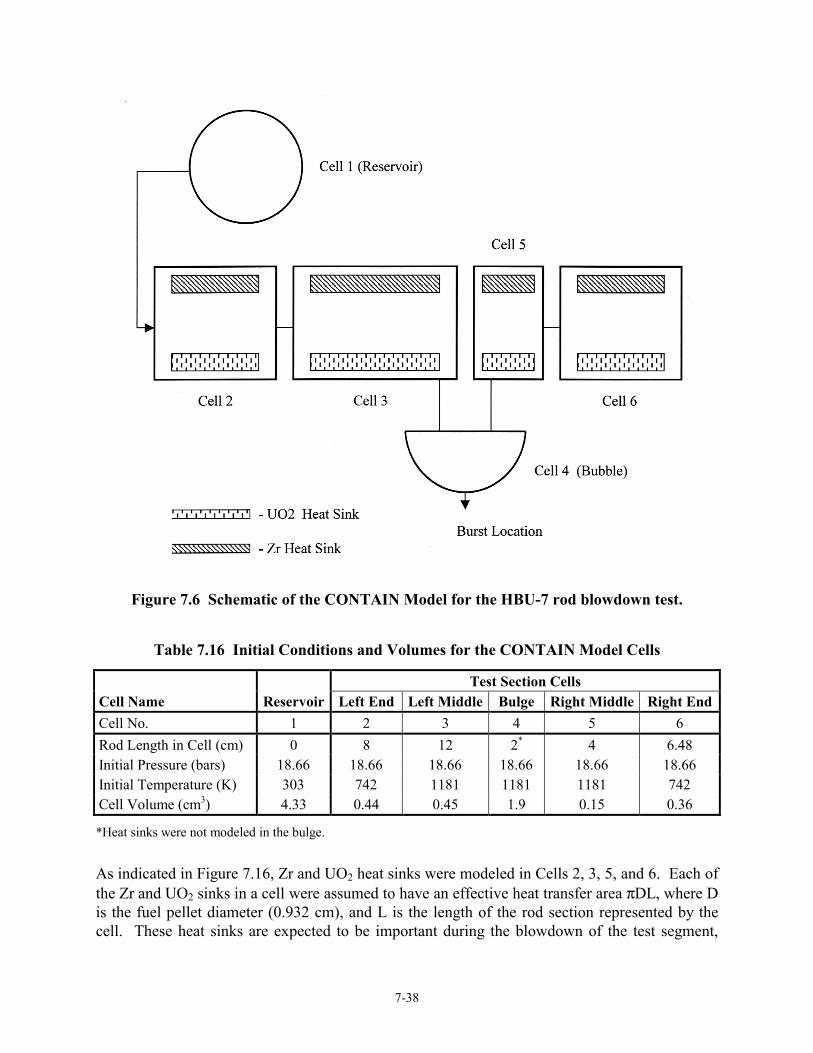
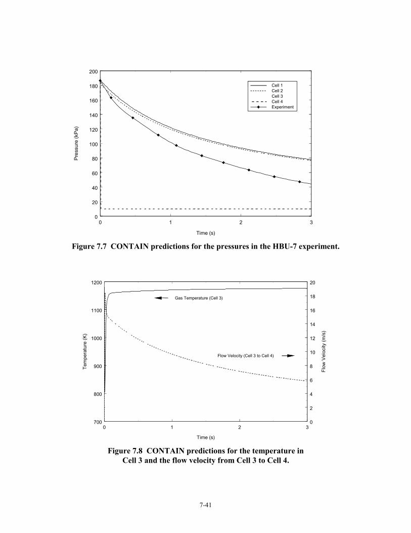
of puncture......................................................................................................................................................5-27Figure 6.1 A generic, steel-lead-steel truck cask.......................................................................................................6-1Figure 6.2 A generic, steel-DU-steel truck cask........................................................................................................6-1Figure 6.3 A generic, steel-lead-steel rail cask..........................................................................................................6-2Figure 6.4 A generic, monolithic steel rail cask ........................................................................................................6-2Figure 6.5 Generic wall cross section used in the 1-D axisymmetric, thermal modeling .......................................... 6-3Figure 6.6 Internal surface temperature histories of the generic casks in an 1000°C long duration fire ..................6-6Figure 7.1 Modal Study truck accident event tree.....................................................................................................7-2Figure 7.2 Modal Study train accident event tree......................................................................................................7-3Figure 7.3 Modified Modal Study truck accident event tree ...................................................................................7-10Figure 7.4 Modified Modal Study train accident event tree....................................................................................7-12Figure 7.5 Fracture particle size distribution for depleted UO2 ..............................................................................7-32Figure 7.6 Schematic of the CONTAIN Model for the HBU-7 rod blowdown test ................................................7-38Figure 7.7 CONTAIN predictions for the pressures in the HBU-7 experiment ...................................................... 7-41Figure 7.8 CONTAIN predictions for the temperature in Cell 3 and the flow velocity
from Cell 3 to Cell 4 .......................................................................................................................................7-41Figure 7.9 Variation with temperature of the concentrations of Cs vapor species predicted
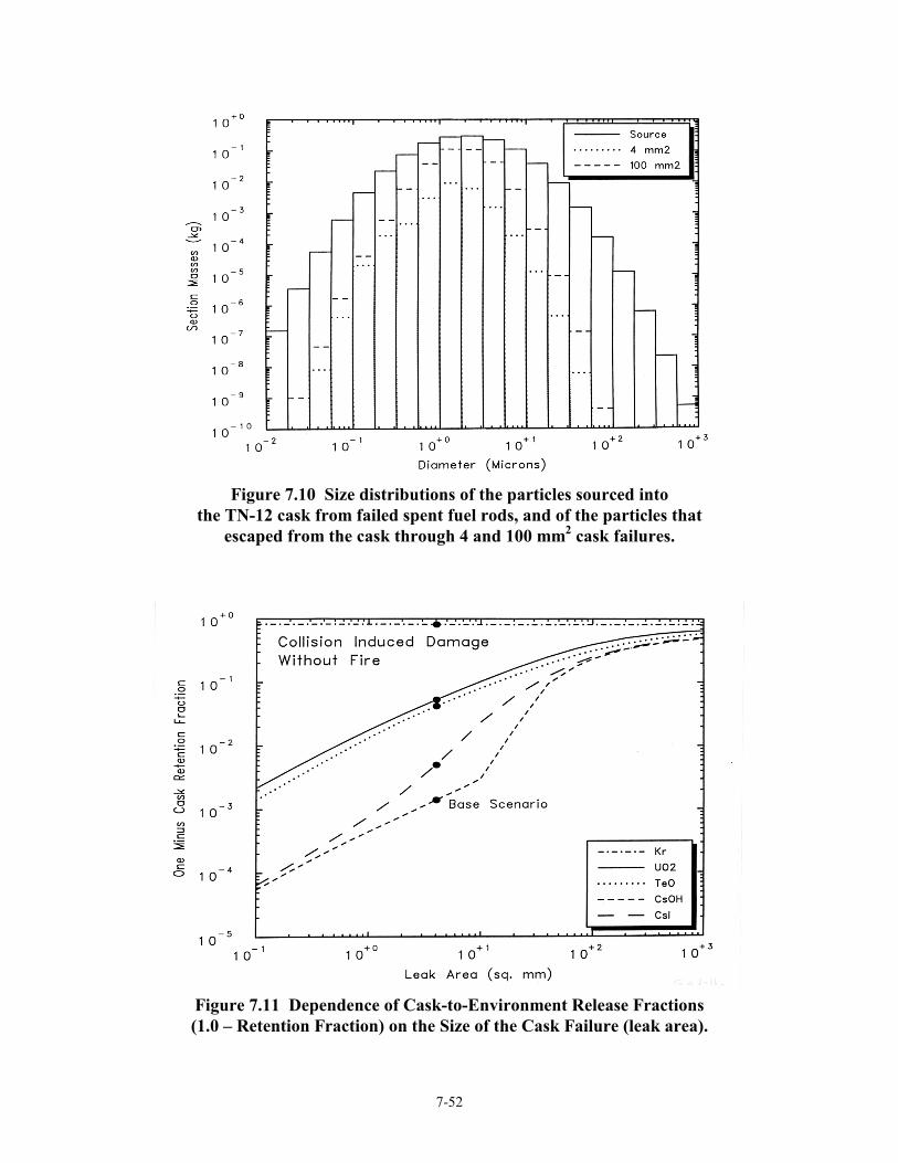
by the VICTORIA code..................................................................................................................................7-43Figure 7.10 Size distributions of the particles sourced into the TN-12 cask from failed spent fuel rods,
and of the particles that escaped from the cask through 4 and 100 mm2 cask failures....................................7-52Figure 7.11 Dependence of Cask-to-Environment Release Fractions (1.0 – Retention Fraction)
on the Size of the Cask Failure (leak area) .....................................................................................................7-52Figure 8.1 Two hundred truck accident population dose risk CCDFs, one CCDF for each representative
truck route. Each RADTRAN 5 calculation examined all 19 representative truck accident source termsand assumed transport of PWR spent fuel in the generic steel-lead-steel truck cask ........................................8-7
Figure 8.2 Truck accident population dose risk CCDFs for transport of PWR spent fuel in the genericsteel-lead-steel truck cask over the 200 representative truck routes. Each underlying RADTRAN 5calculation generated results for all of the 19 representative truck accident source terms................................8-8
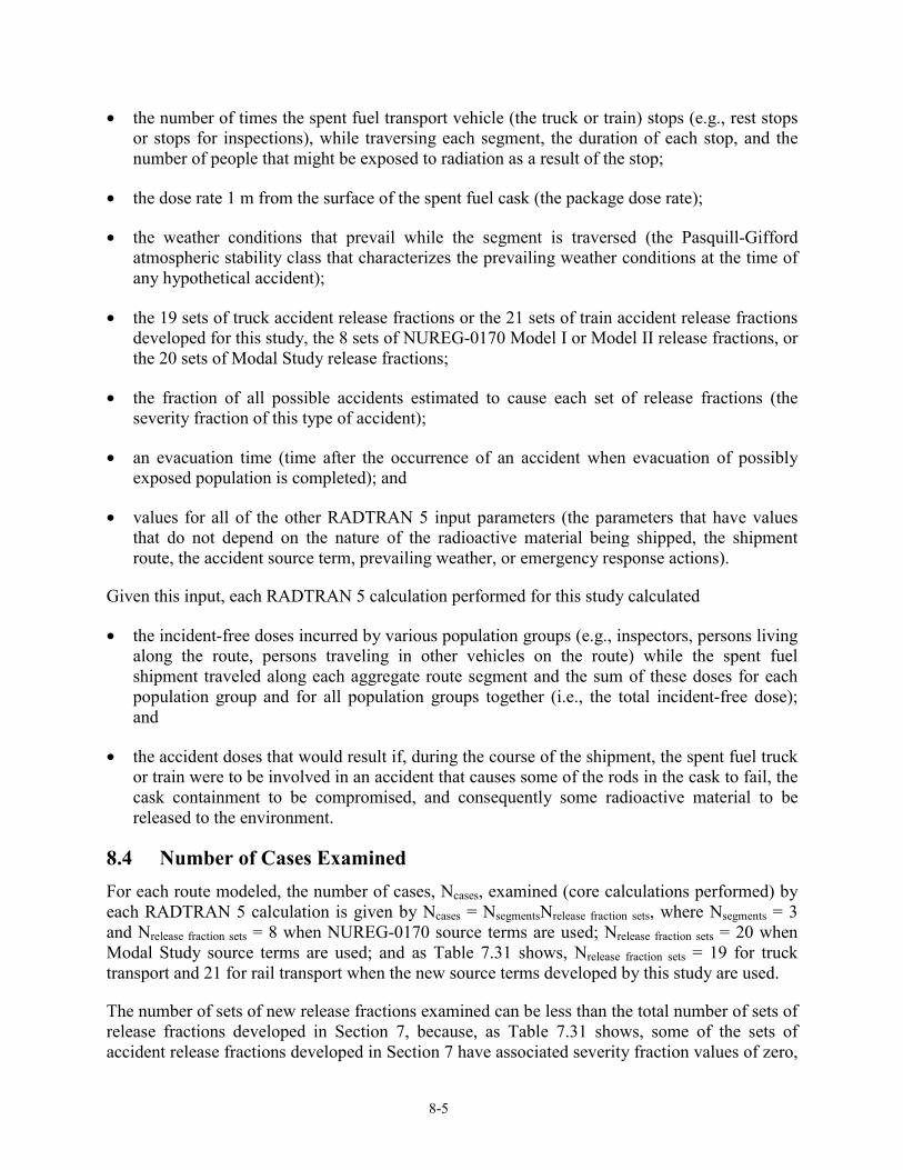
Figure 8.3 Truck accident population dose risk CCDFs for transport of BWR spent fuel in the genericsteel-lead-steel truck cask over the 200 representative truck routes. Each underlying RADTRAN 5calculation generated results for all of the 19 representative truck accident source terms..............................8-10
xii
Figure 8.4 Truck accident population dose risk CCDFs for transport of PWR spent fuel in the genericsteel-DU-steel truck cask over the 200 representative truck routes. Each underlying RADTRAN 5calculation generated results for all of the 19 representative truck accident source terms..............................8-11
Figure 8.5 Truck accident population dose risk CCDFs for transport of BWR spent fuel in the genericsteel-DU-steel truck cask over the 200 representative truck routes. Each underlying RADTRAN 5calculation generated results for all of the 19 representative truck accident source terms..............................8-12
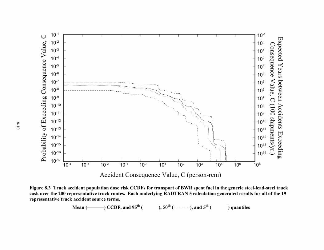
Figure 8.6 Comparison of truck accident population dose risk CCDFs for transport of PWR or BWRspent fuel in generic steel-lead-steel or steel-DU-steel truck casks over the 200 representativetruck routes. Each underlying RADTRAN 5 calculation generated results for all of the19 representative truck accident source terms ................................................................................................8-13
Figure 8.7 Rail accident population dose risk CCDFs for transport of PWR spent fuel in the genericsteel-lead-steel rail cask over the 200 representative rail routes. Each underlying RADTRAN 5alculation generated results for all of the 21 representative rail accident source terms ..................................8-19
Figure 8.8 Rail accident population dose risk CCDFs for transport of BWR spent fuel in the genericsteel-lead-steel rail cask over the 200 representative rail routes. Each underlying RADTRAN 5calculation generated results for all of the 21 representative rail accident source terms.................................8-20
Figure 8.9 Rail accident population dose risk CCDFs for transport of PWR spent fuel in the genericmonolithic steel rail cask over the 200 representative rail routes. Each underlying RADTRAN 5calculation generated results for all of the 21 representative rail accident source terms.................................8-21
Figure 8.10 Rail accident population dose risk CCDFs for transport of BWR spent fuel in the genericmonolithic steel rail cask over the 200 representative rail routes. Each underlying RADTRAN 5calculation generated results for all of the 21 representative rail accident source terms.................................8-22
Figure 8.11 Comparison of rail accident population dose risk CCDFs for transport of PWR or BWRspent fuel in generic steel-lead-steel or monolithic steel rail casks over the 200 representativerail routes. Each underlying RADTRAN 5 calculation generated results for all of the21 representative rail accident source terms ...................................................................................................8-23
Figure 8.12 Truck accident population dose risk CCDFs for transport of PWR spent fuel in the genericsteel-lead-steel truck cask over the Crystal River to Hanford illustrative truck route. Each underlyingRADTRAN 5 calculation generated results for all of the 19 representative truck accident source terms.......8-30
Figure 8.13 Truck accident population dose risk CCDFs for transport of PWR spent fuel in the genericsteel-lead-steel truck cask over the Maine Yankee to Skull Valley illustrative truck route. Eachunderlying RADTRAN 5 calculation generated results for all of the 19 representative truckaccident source terms......................................................................................................................................8-31
Figure 8.14 Truck accident population dose risk CCDFs for transport of PWR spent fuel in the genericsteel-lead-steel truck cask over the Maine Yankee to Savannah River Site illustrative truck route.Each underlying RADTRAN 5 calculation generated results for all of the 19 representative truckaccident source terms......................................................................................................................................8-32
Figure 8.15 Truck accident population dose risk CCDFs for transport of PWR spent fuel in the genericsteel-lead-steel truck cask over the Kewaunee to Savannah River Site illustrative truck route. Eachunderlying RADTRAN 5 calculation generated results for all of the 19 representative truckaccident source terms......................................................................................................................................8-33
Figure 8.16 Truck accident population dose risk CCDFs for transport of PWR spent fuel in the genericsteel-lead-steel truck cask over the NUREG-0170 representative truck route. Each underlyingRADTRAN 5 calculation generated results for all of the 19 representative truck accident source terms.......8-34
Figure 8.17 Comparison of truck accident population dose risk CCDFs for transport of PWR spentfuel in the generic steel-lead-steel cask over four illustrative truck routes and the NUREG-0170representative truck route. Each underlying RADTRAN 5 calculation generated results for allof the 19 representative truck accident source terms ......................................................................................8-35
Figure 8.18 Rail accident population dose risk CCDFs for transport of PWR spent fuel in the genericmonolithic steel rail cask over the Crystal River to Hanford illustrative rail route. Each underlying RADTRAN5 calculation generated results for all of the 21 representative rail accident source terms..............................8-38
Figure 8.19 Rail accident population dose risk CCDFs for transport of PWR spent fuel in the genericmonolithic steel rail cask over the Maine Yankee to Skull Valley illustrative rail route. Eachunderlying RADTRAN 5 calculation generated results for all of the 21 representative railaccident source terms......................................................................................................................................8-39
xiii
Figure 8.20 Rail accident population dose risk CCDFs for transport of PWR spent fuel in the genericmonolithic steel rail cask over the Maine Yankee to Savannah River Site illustrative rail route. Eachunderlying RADTRAN 5 calculation generated results for all of the 21 representative rail accidentsource terms....................................................................................................................................................8-40
Figure 8.21 Rail accident population dose risk CCDFs for transport of PWR spent fuel in the genericmonolithic steel rail cask over the Kewaunee to Savannah River Site illustrative rail route. Each underlyingRADTRAN 5 calculation generated results for all of the 21 representative rail accident source terms .........8-41
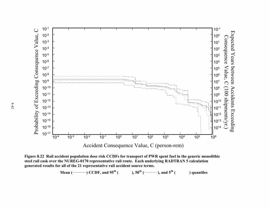
Figure 8.22 Rail accident population dose risk CCDFs for transport of PWR spent fuel in the genericmonolithic steel rail cask over the NUREG-0170 representative rail route. Each underlyingRADTRAN 5 calculation generated results for all of the 21 representative rail accident source terms .........8-42
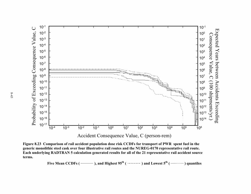
Figure 8.23 Comparison of rail accident population dose risk CCDFs for transport of PWR spent fuel in the genericmonolithic steel cask over four illustrative rail routes and the NUREG-0170 representativerail route. Each underlying RADTRAN 5 calculation generated results for all of the 21 representativerail accident source terms ...............................................................................................................................8-43
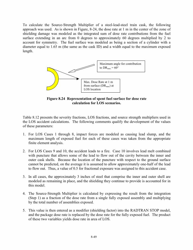
Figure 8.24 Representation of spent fuel surface for dose rate calculation for LOS scenarios ..............................8-49Figure 8.25 Mean truck accident population dose risk CCDFs for calculations that examined the impact
on dose risks of NUREG-0170 source terms and exposure pathway models. Each RADTRAN 5calculation assumed transport in a steel-lead- steel truck cask over each of the 200 representativetruck routes and each calculation generated results for all of the 19 representative truck accidentsource terms....................................................................................................................................................8-63
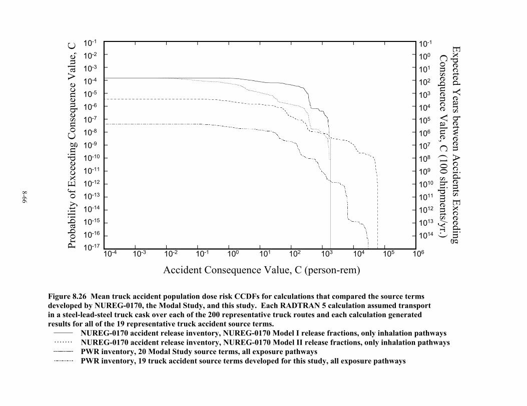
Figure 8.26 Mean truck accident population dose risk CCDFs for calculations that compared the source termsdeveloped by NUREG-0170, the Modal Study, and this study. Each RADTRAN 5 calculation assumedtransport in a steel-lead steel truck cask over each of the 200 representative truck routes and each calculationgenerated results for all of the 19 representative truck accident source terms ................................................8-66
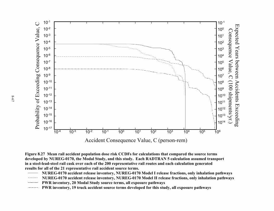
Figure 8.27 Mean rail accident population dose risk CCDFs for calculations that compared the source termsdeveloped by NUREG-0170, the Modal Study, and this study. Each RADTRAN 5 calculation assumedtransport in a steel-lead steel rail cask over each of the 200 representative rail routes and each calculationgenerated results for all of the 21 representative rail accident source terms...................................................8-67
Tables
Table E.1 Comparison of NUREG-0170 Incident-Free Doses (person-rem) to the Incident-FreeDoses Developed by this Studya .................................................................................................................... ES-5
Table E.2 Comparison of Mean Accident Population Dose Risks (person-rem) Calculated UsingNUREG-0170 Model I and Model II Source Terms and Modal Study Source Terms to ThoseCalculated Using the Source Terms Developed by this Study....................................................................... ES-6
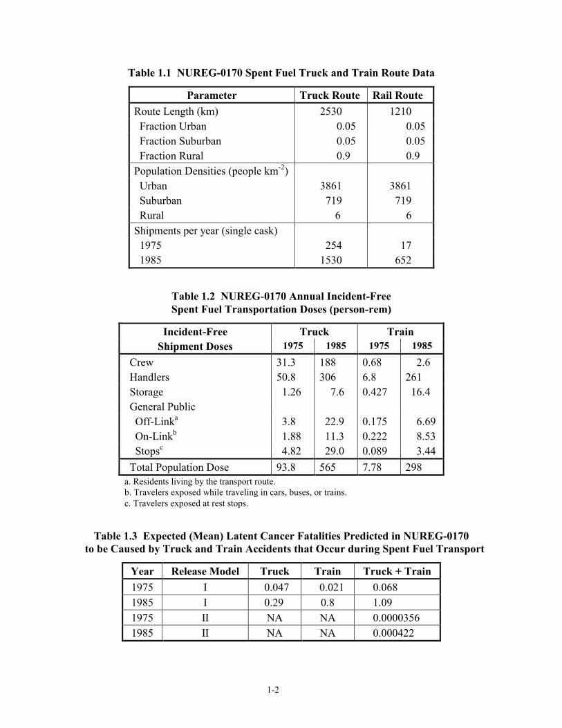
Table 1.1 NUREG-0170 Spent Fuel Truck and Train Route Data............................................................................1-2Table 1.2 NUREG-0170 Annual Incident-Free Spent Fuel Transportation Doses (person-rem)..............................1-2Table 1.3 Expected (Mean) Latent Cancer Fatalities Predicted in NUREG-0170 to be Caused
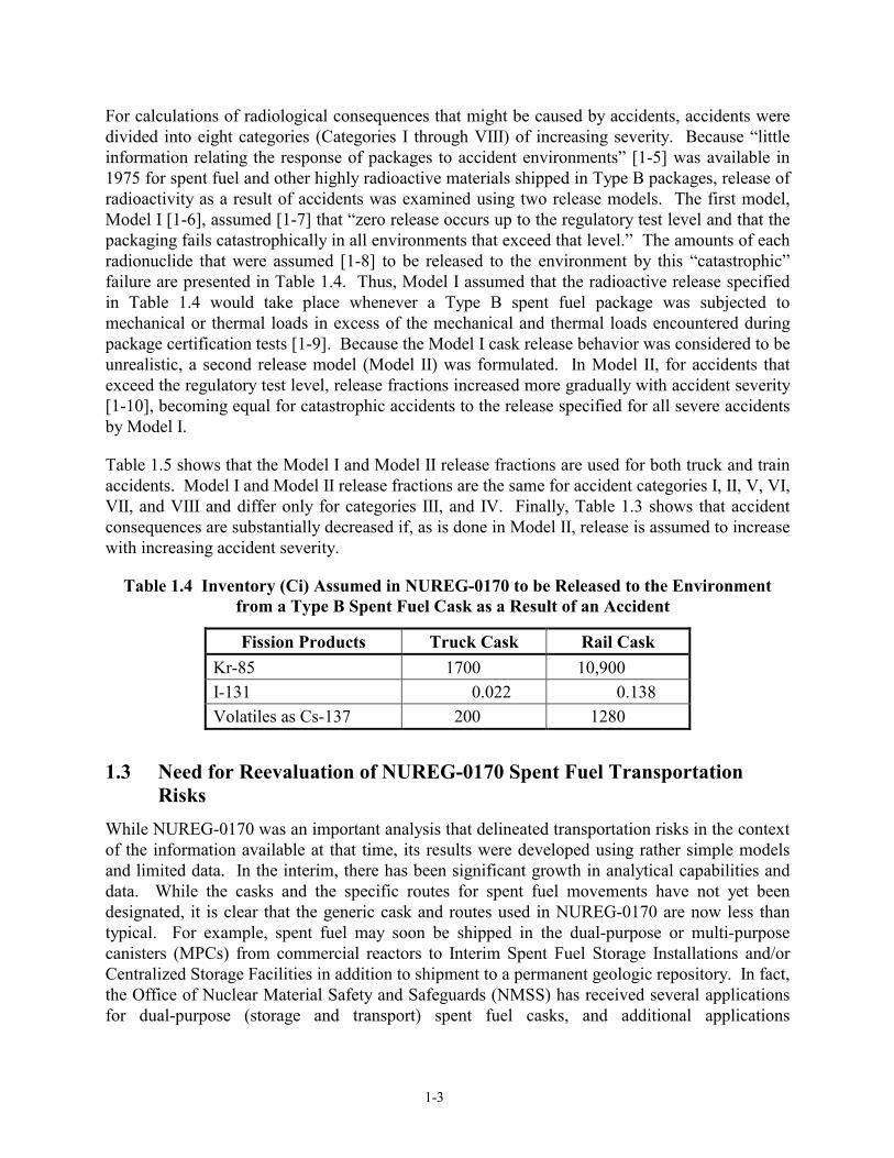
by Truck and Train Accidents that Occur during Spent Fuel Transport ...........................................................1-2Table 1.4 Inventory (Ci) Assumed in NUREG-0170 to be Released to the Environment
from a Type B Spent Fuel Cask as a Result of an Accident..............................................................................1-3Table 1.5 NUREG-0170 Model I and Model II Severity and Release Fractions for Spent
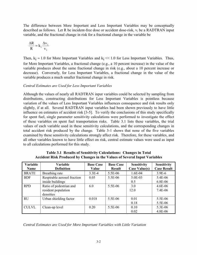
Fuel Transport by Truck and Rail.....................................................................................................................1-4Table 3.1 Results of Sensitivity Calculations: Changes in Total Accident Risk Produced
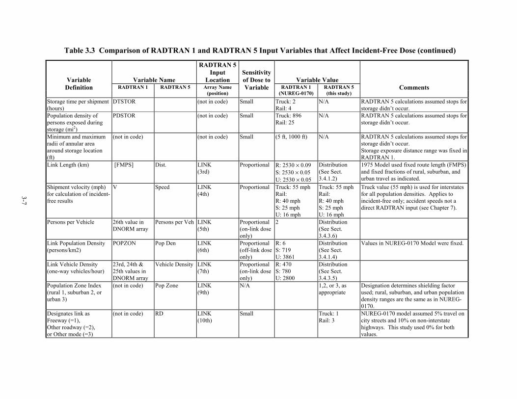
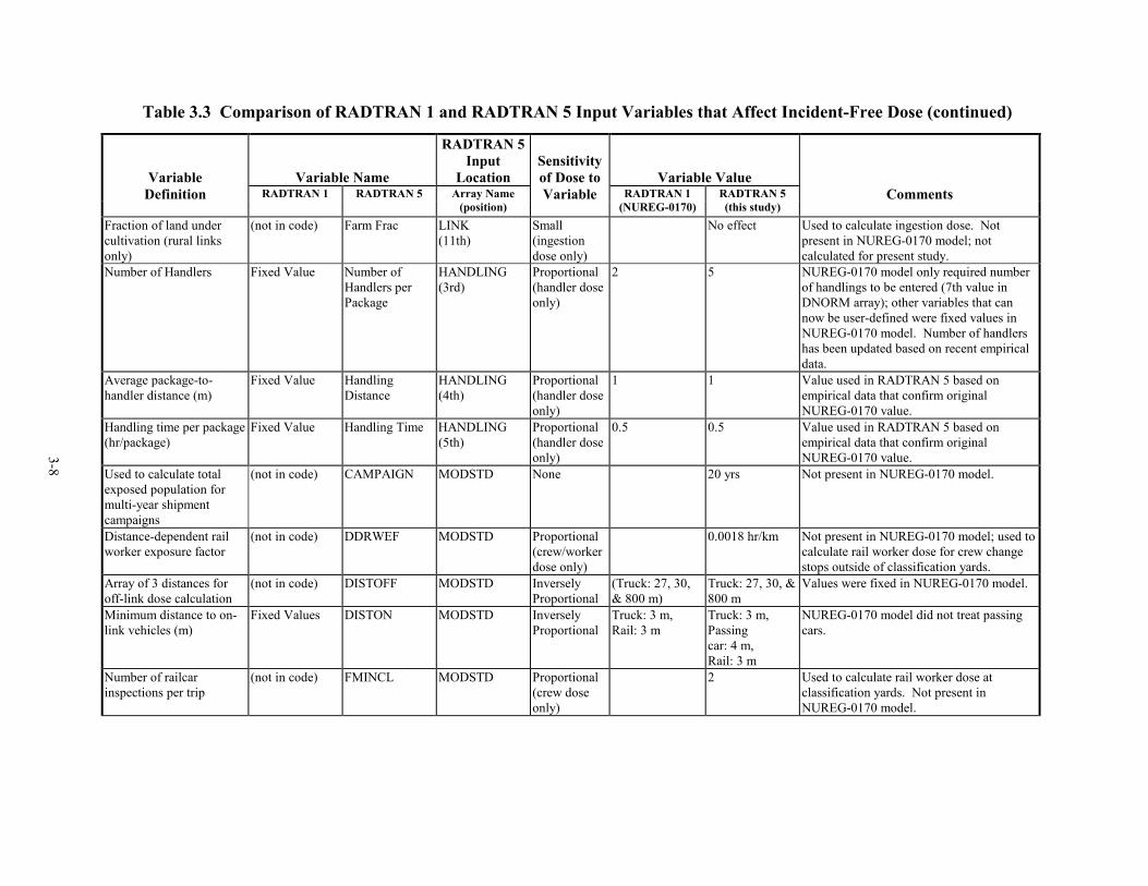
by Changes in the Values of Several Input Variables .......................................................................................3-2Table 3.2 Comparison of RADTRAN 1 and RADTRAN 5......................................................................................3-4Table 3.3 Comparison of RADTRAN 1 and RADTRAN 5 Input Variables that Affect Incident-Free Dose ...........3-5Table 3.4 Comparison of RADTRAN 1 and RADTRAN 5 Input Variables that Affect Accident Risk .................3-10Table 3.5 Definition of Population Density Categories (persons/km2) ...................................................................3-29Table 3.6 Truck Accident Rates (Accidents per Million Vehicle-Kilometers) .......................................................3-39Table 3.7 Rail Accident Rates per Million Rail Car km .........................................................................................3-43Table 3.8 Distribution of Normal Commercial Truck Stop Times..........................................................................3-44
xiv
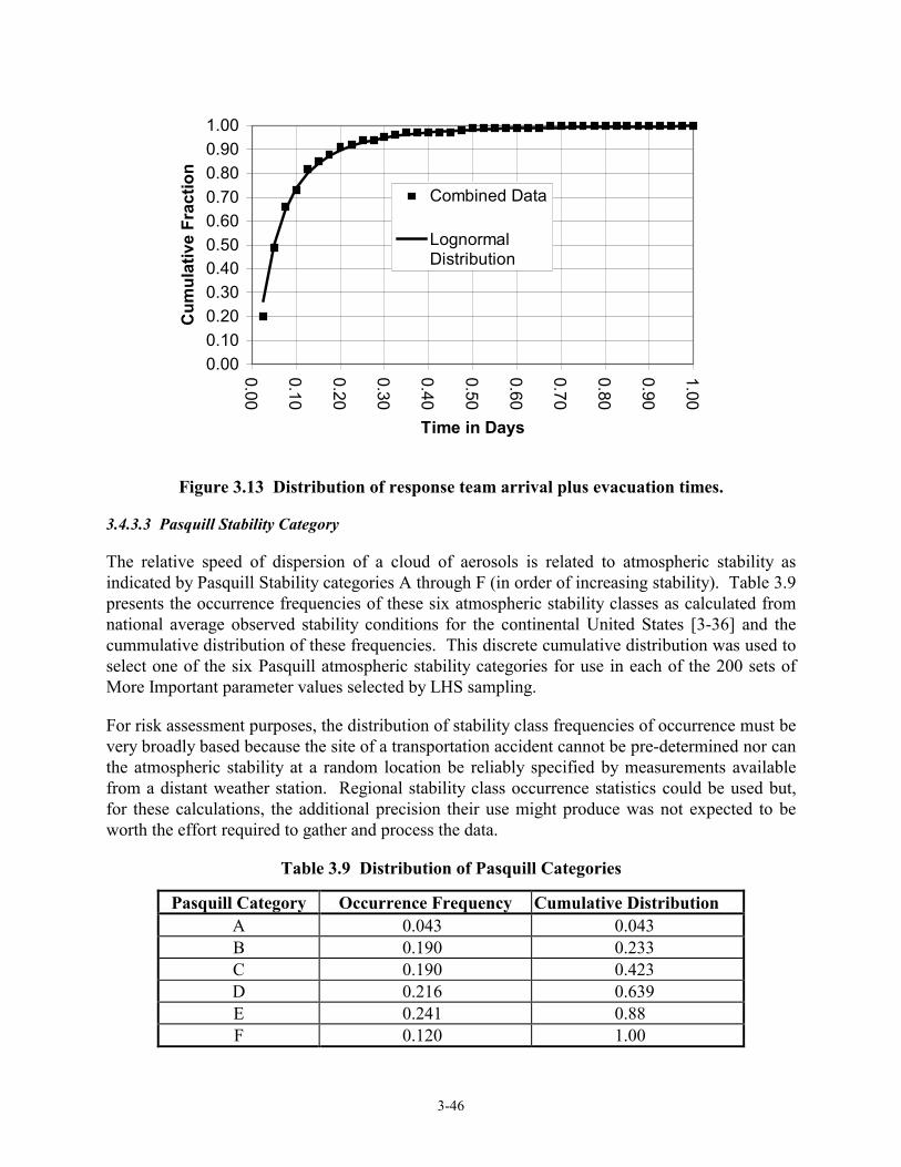
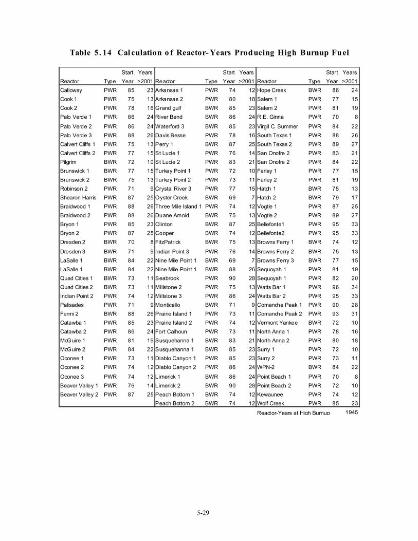
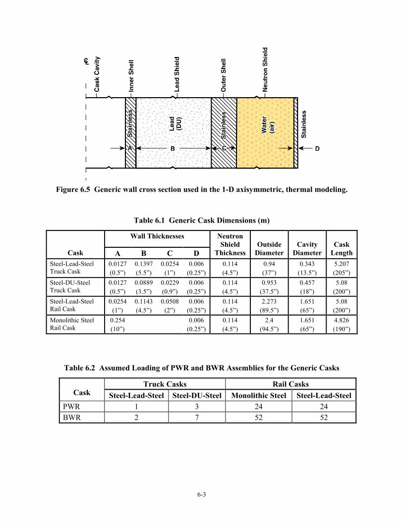
Table 3.9 Distribution of Pasquill Categories .........................................................................................................3-46Table 3.10 Distribution of Dose Rate at 1 m (RADTRAN parameter TI) for Truck Casks....................................3-47Table 3.11 Distribution of Dose Rate at 1 m (RADTRAN parameter TI) for Rail Casks.......................................3-47Table 3.12 Distribution of Persons per Vehicle on Highway Routes ......................................................................3-48Table 4.1 Steel-Lead-Steel Truck Casks ...................................................................................................................4-2Table 4.2 Steel-DU-Steel Truck Casks .....................................................................................................................4-3Table 4.3 Steel-Lead-Steel Rail Casks ......................................................................................................................4-4Table 4.4 Monolithic Rail Casks...............................................................................................................................4-5Table 5.1 Impact Limiter Geometry (in inches) ........................................................................................................5-2Table 5.2 Material Properties Used in the Finite Element Analyses .........................................................................5-8Table 5.3 Maximum Plastic Strain in the Inner Shell of the Sandwich Wall Casks ..................................................5-9Table 5.4 Maximum Plastic Strains on the Inside of the Monolithic Rail Cask......................................................5-10Table 5.5 Maximum True Strain in the Closure Bolts ............................................................................................5-11Table 5.6 Seal Closure Displacements, in Inches, at the End of the Analysis.........................................................5-13Table 5.7 Calculated Rail Cask Closure Leak Path Areas.......................................................................................5-14Table 5.8 Peak Contact Force from Impacts Onto Rigid Targets (Pounds) ............................................................5-19Table 5.9 Equivalent Diameters for Concrete Impacts............................................................................................5-23Table 5.10 Real Target Equivalent Velocities (mph) for the Steel-Lead-Steel Truck Cask....................................5-24Table 5.11 Real Target Equivalent Velocities (mph) for the Steel-DU-Steel Truck Cask ......................................5-25Table 5.12 Real Target Equivalent Velocities (mph) for the Steel-Lead-Steel Rail Cask.......................................5-25Table 5.13 Real Target Equivalent Velocities (mph) for the Monolithic Steel Rail Cask.......................................5-25Table 5.14 Calculation of Reactor-Years Producing High Burnup Fuel .................................................................5-29Table 5.15 Calculation of Mass Weighted Sum of Burnup Dependent Rod Strain Failure Levels.........................5-30Table 5.16 Peak Accelerations from Rigid Target Impacts without Impact Limiters, Gs .......................................5-31Table 5.17 Peak Strains in Fuel Rods Resulting from a 100 G Impact ...................................................................5-32Table 6.1 Generic Cask Dimensions (m) ..................................................................................................................6-3Table 6.2 Assumed Loading of PWR and BWR Assemblies for the Generic Casks ................................................6-3Table 6.3 Internal Heat Loads for Each of the Generic Casks for Three-Year-Old High Burnup Spent Fuel ..........6-4Table 6.4 Internal and External, Steady State, Cask Surface Temperatures..............................................................6-5Table 6.5 Time (hours) Required for the Generic Cask Internal Surface to get to the Three
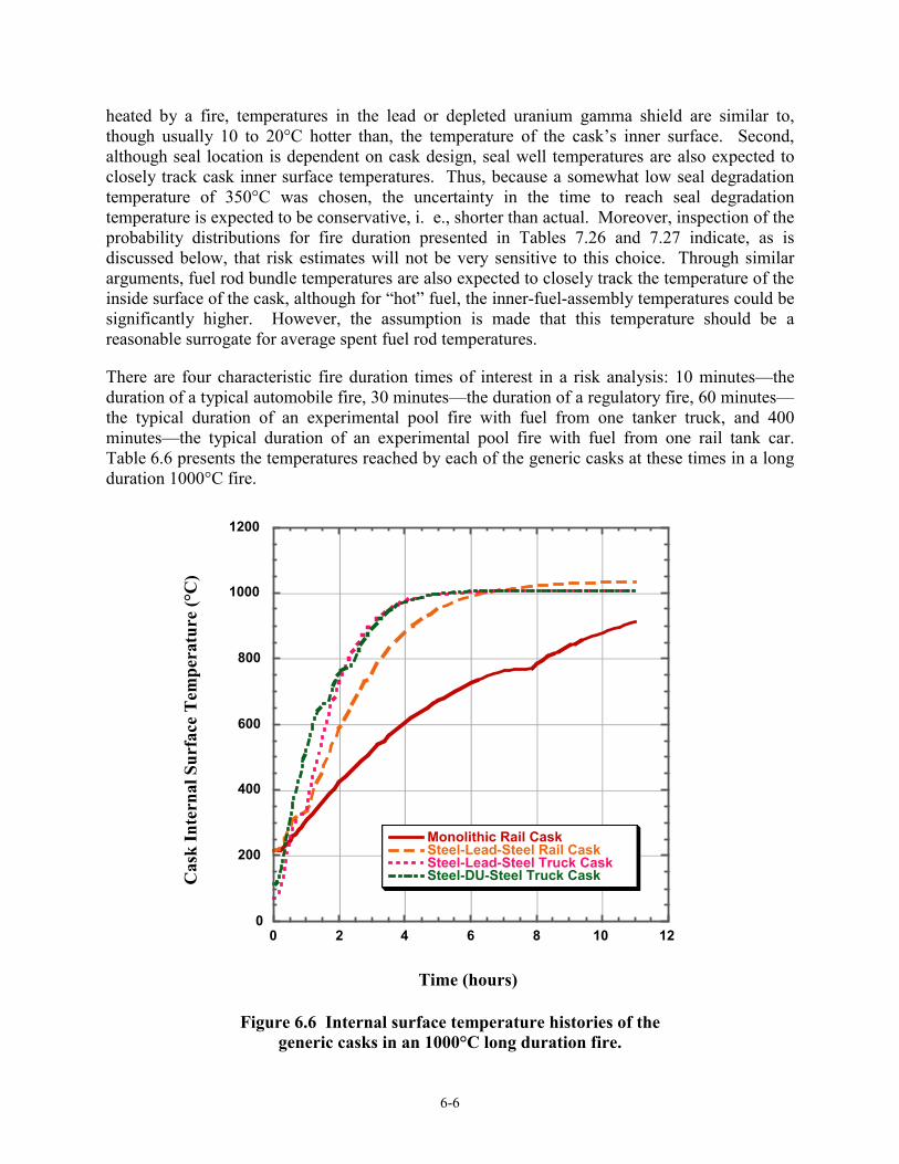
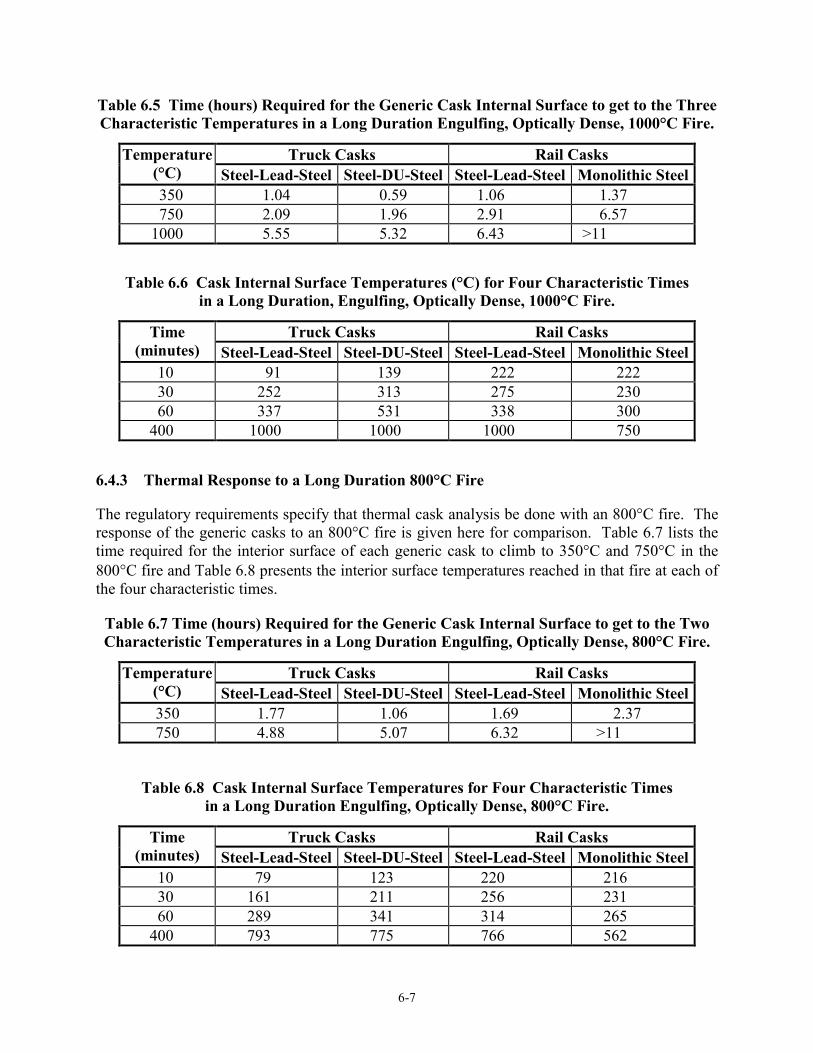
Characteristic Temperatures in a Long Duration Engulfing, Optically Dense, 1000°C Fire ............................6-7Table 6.6 Cask Internal Surface Temperatures (°C) for Four Characteristic Times in a Long
Duration, Engulfing, Optically Dense, 1000°C Fire .........................................................................................6-7Table 6.7 Time (hours) Required for the Generic Cask Internal Surface to get to the Two
Characteristic Temperatures in a Long Duration Engulfing, Optically Dense, 800°C Fire ..............................6-7Table 6.8 Cask Internal Surface Temperatures for Four Characteristic Times in a Long
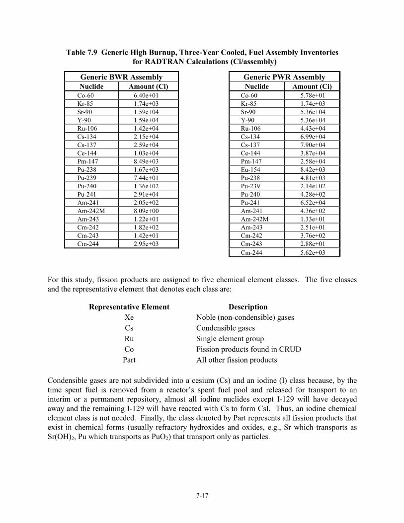
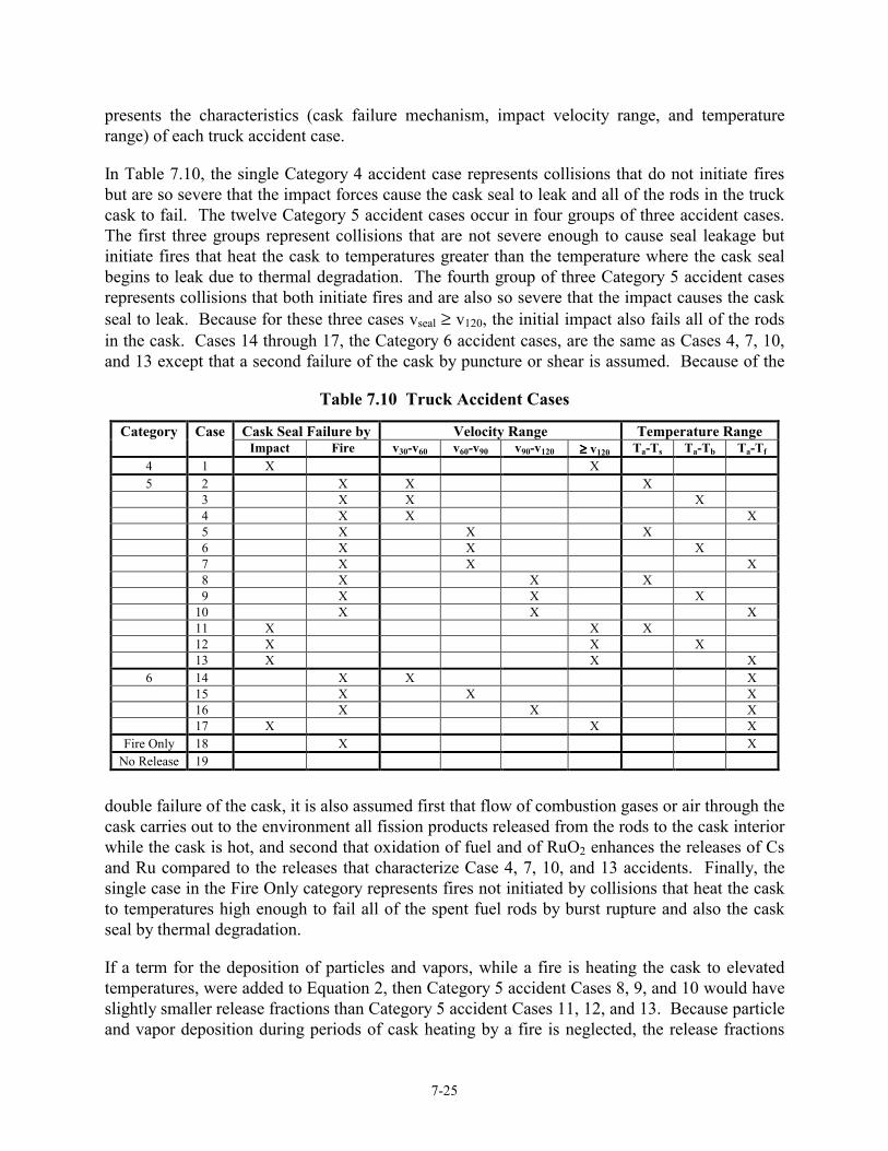
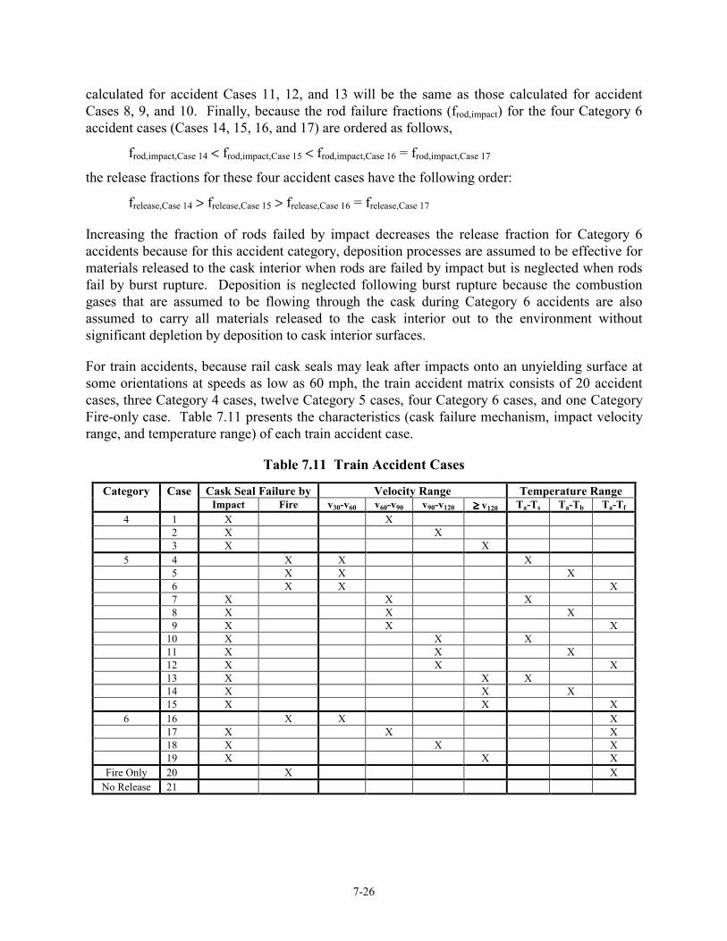
Duration Engulfing, Optically Dense, 800°C Fire ............................................................................................6-7Table 7.1 Wayside Hard Rock on Modal Study Segments of I-5 and I-80 ...............................................................7-5Table 7.2 Wayside Surfaces on Modal Study Segments of I-5 and I-80...................................................................7-6Table 7.3 Wayside Surface Characteristics for Three Illustrative Shipping Routes..................................................7-7Table 7.4 Fractional Occurrence Frequencies for Route Wayside Surfaces Selected for Use in This Study............7-7Table 7.5 Conditional Probabilities of Occurrence of Various Truck Accident Scenarios (%) ................................7-8Table 7.6 Truck Accidents that Initiate Fires (Percentages) .....................................................................................7-9Table 7.7 Conditional Probabilities of Occurrence of Various Train Accident Scenarios (%) ...............................7-11Table 7.8 Summary of ORIGEN Calculations, Total Curies per Assembly for All Radionuclides ........................7-15Table 7.9 Generic High Burnup, Three-Year Cooled, Fuel Assembly Inventories for RADTRAN
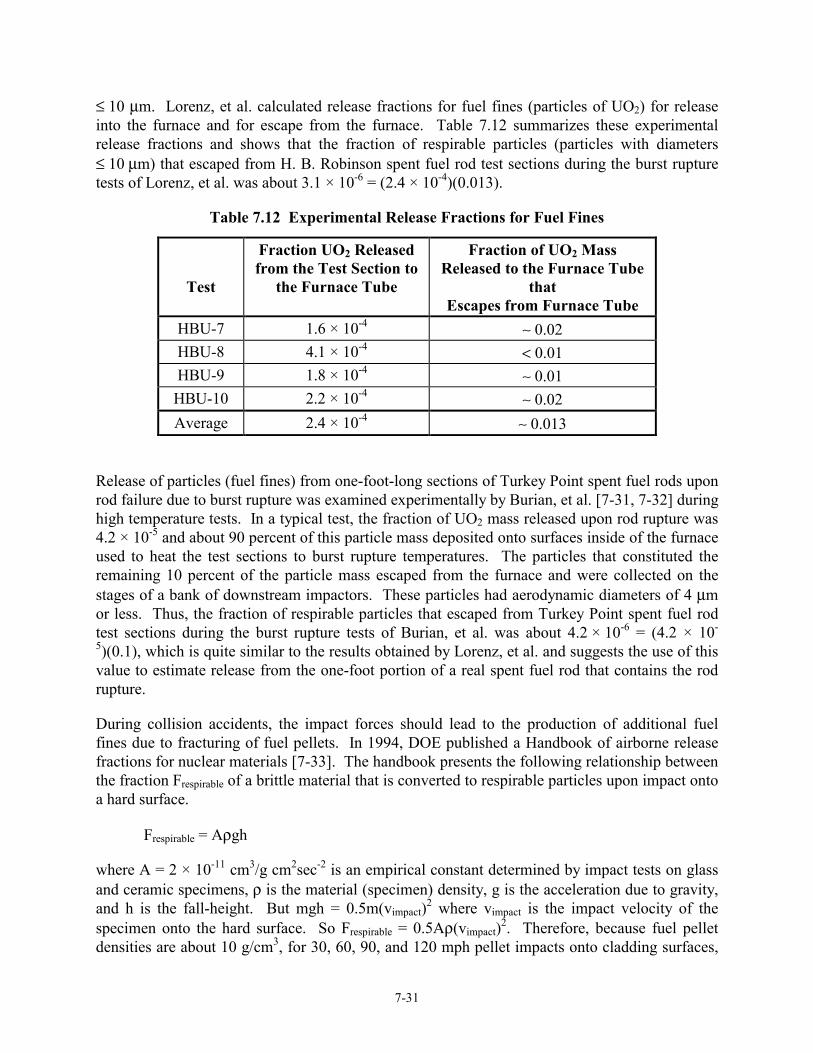
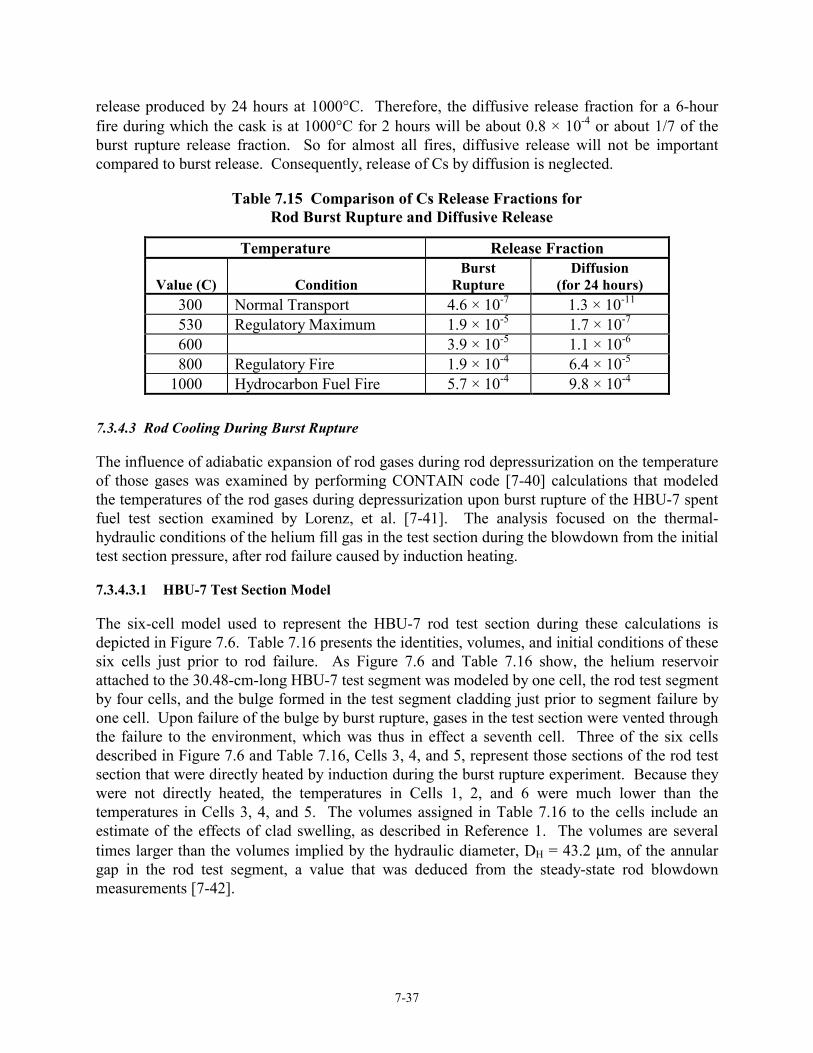
Calculations (Ci/assembly) .............................................................................................................................7-17Table 7.10 Truck Accident Cases ...........................................................................................................................7-25Table 7.11 Train Accident Cases ............................................................................................................................7-26Table 7.12 Experimental Release Fractions for Fuel Fines.....................................................................................7-31Table 7.13 Granular Bed Lengths that Provide 99 Percent Filtering Efficiencies...................................................7-33Table 7.14 Parameter Values for Lorenz Release Expressions for Cs ....................................................................7-36Table 7.15 Comparison of Cs Release Fractions for Rod Burst Rupture and Diffusive Release ...........................7-37Table 7.16 Initial Conditions and Volumes for the CONTAIN Model Cells..........................................................7-38Table 7.17 Flow Junction Characteristics in the CONTAIN Model .......................................................................7-40
xv
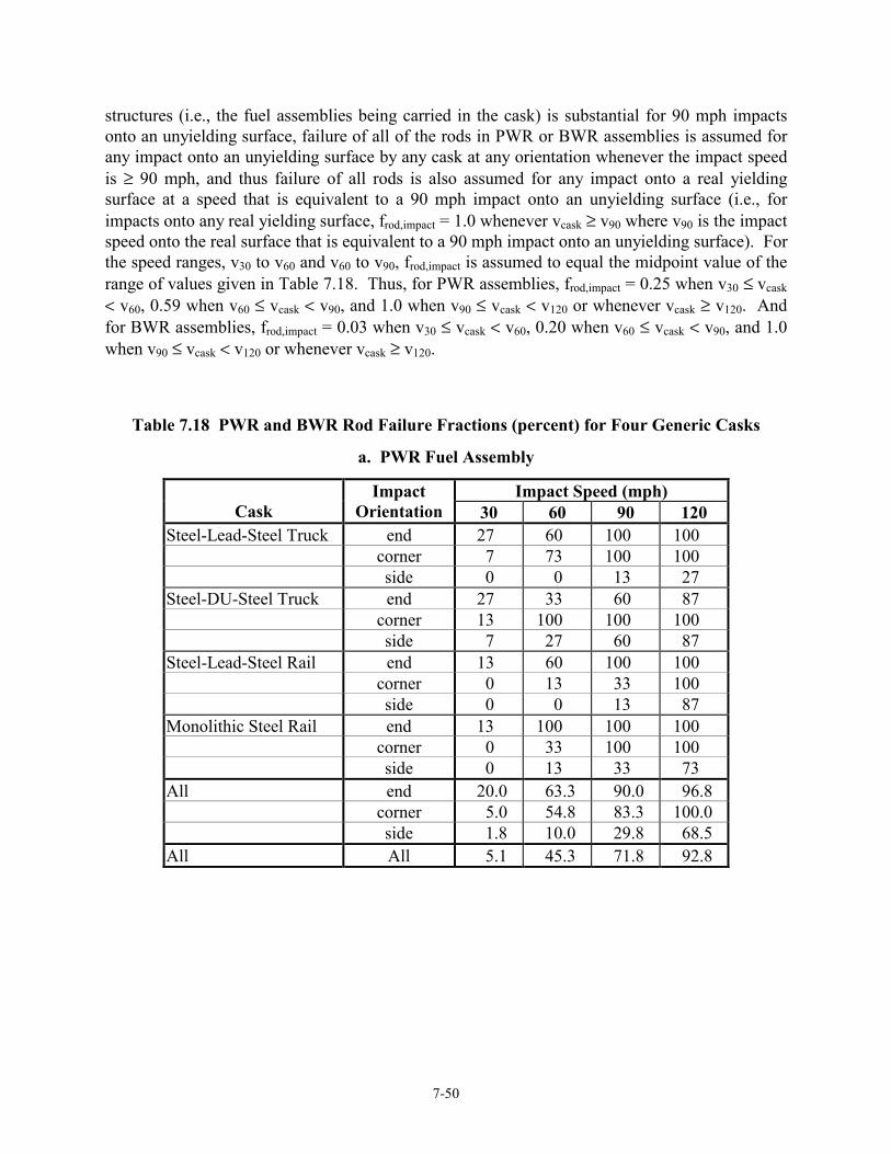
Table 7.18 PWR and BWR Rod Failure Fractions (percent) for Four Generic Casks ............................................7-50 a. PWR Fuel Assembly .......................................................................................................................................7-50 b. BWR Fuel Assembly.......................................................................................................................................7-51Table 7.19 Seal Leak Areas and Values of FCE for Rail Casks ...............................................................................7-53Table 7.20 Values of fdeposition for Rail Casks ..........................................................................................................7-54Table 7.21 Expansion Factor Values ......................................................................................................................7-55Table 7.22 Probability of Occurrence and Average Number of Cars Derailed
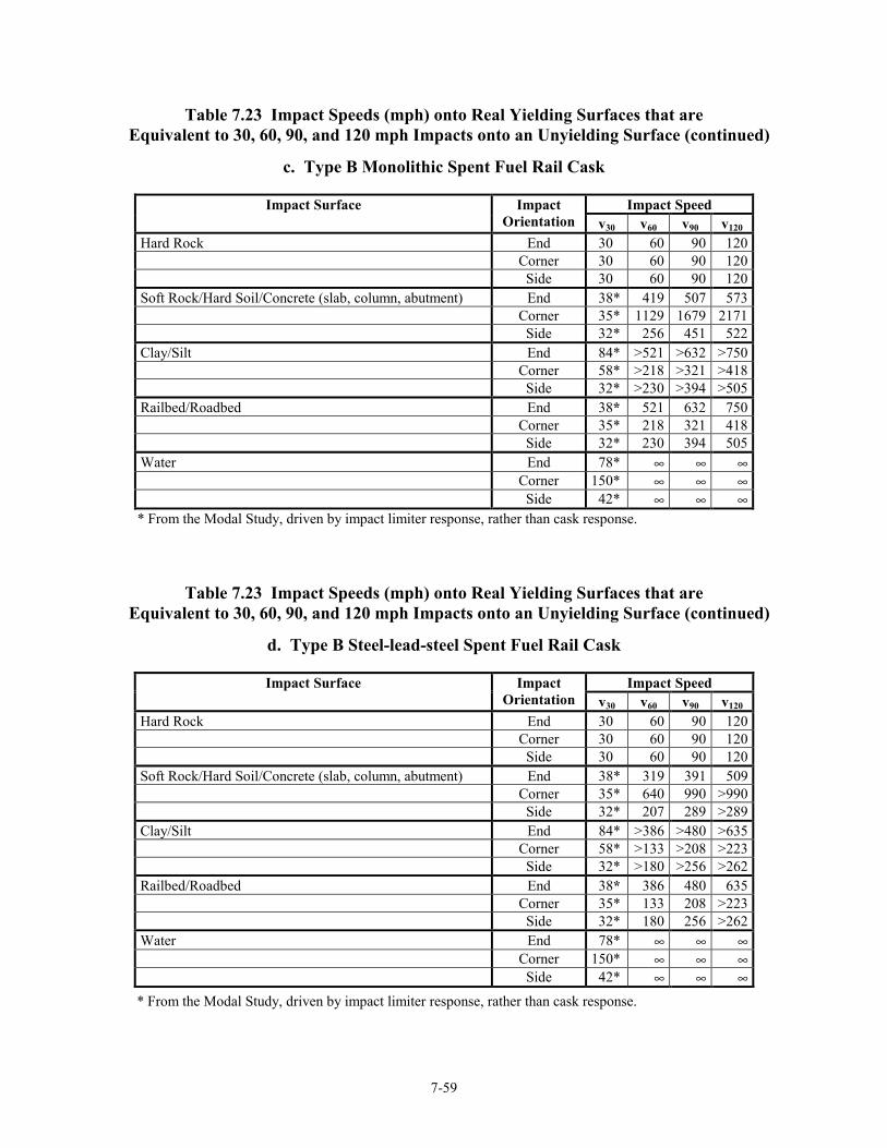
for Train Derailment Accidents by Accident Speed Range ............................................................................7-56Table 7.23 Impact Speeds (mph) onto Real Yielding Surfaces that are Equivalent
to 30, 60, 90, and 120 mph Impacts onto an Unyielding Surface ...................................................................7-58Table 7.24 Truck Accident Velocity Distributions .................................................................................................7-61Table 7.25 Train Accident Velocity Distributions ..................................................................................................7-62Table 7.26 Durations (hr) of Co-Located, Fully Engulfing, Optically Dense, Hydrocarbon
Fuel Fires that Raise the Temperature of Each Generic Cask to Ts, Tb, and Tf ..............................................7-65Table 7.27 Truck Accident Fire Durations..............................................................................................................7-66Table 7.28 Train Accident Fire Durations ..............................................................................................................7-67Table 7.29 Comparison of Modal Study Cumulative Fire Durations for Various Truck
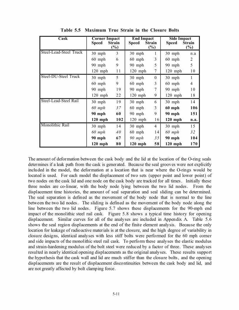
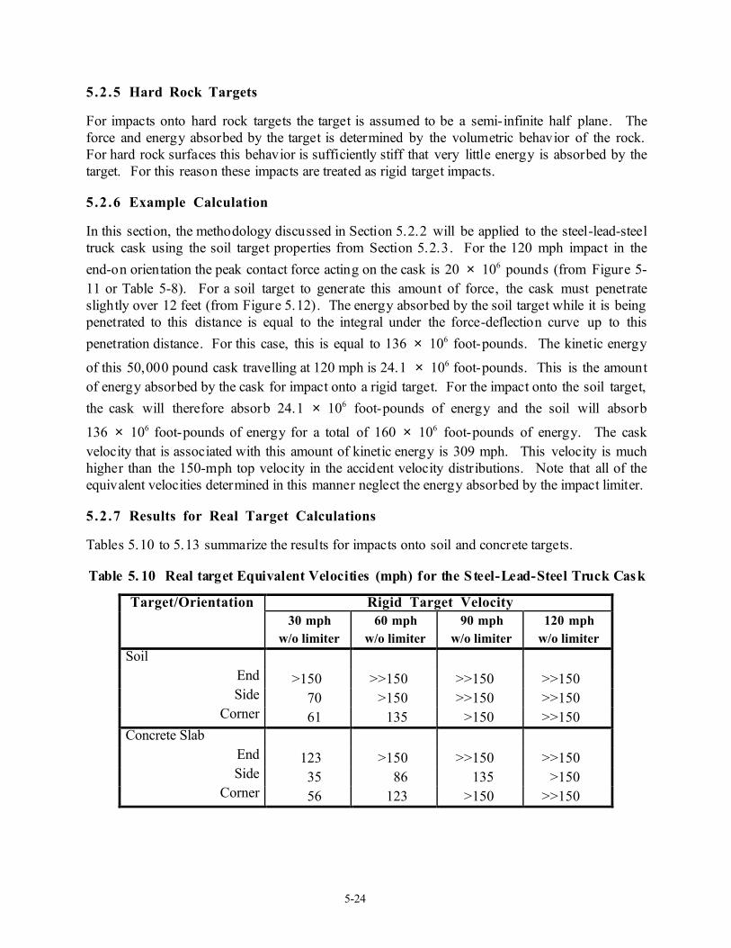
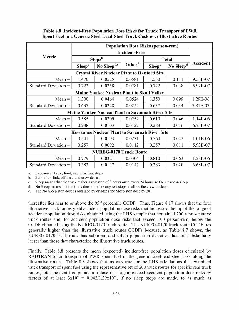
Accidents to Those Developed by Weighted Summation of Data from Clauss, et al. [7-5] ...........................7-68Table 7.30 Truck and Train Commodity Flow Statistics for 1993..........................................................................7-69Table 7.31 Source Term Severity Fractions and Release Fractions ........................................................................7-73Table 8.1 Characteristics of Sets of RADTRAN Calculations..................................................................................8-2Table 8.2 RADTRAN 5/LHS Accident-Risk Results versus Number of Observations ............................................8-4Table 8.3 RADTRAN 5/LHS Accident-Risk Results for 200 Observations versus “Seed”......................................8-4Table 8.4 Incident-Free and Accident Population Dose Risks for Truck Transport ...............................................8-15Table 8.5 Incident-Free Population Dose Risks for Rail Transport ........................................................................8-24Table 8.7 NUREG-0170 and Illustrative Real Truck and Rail Routes....................................................................8-29Table 8.8 Incident-Free Population Dose Risks for Truck Transport of PWR Spent Fuel in
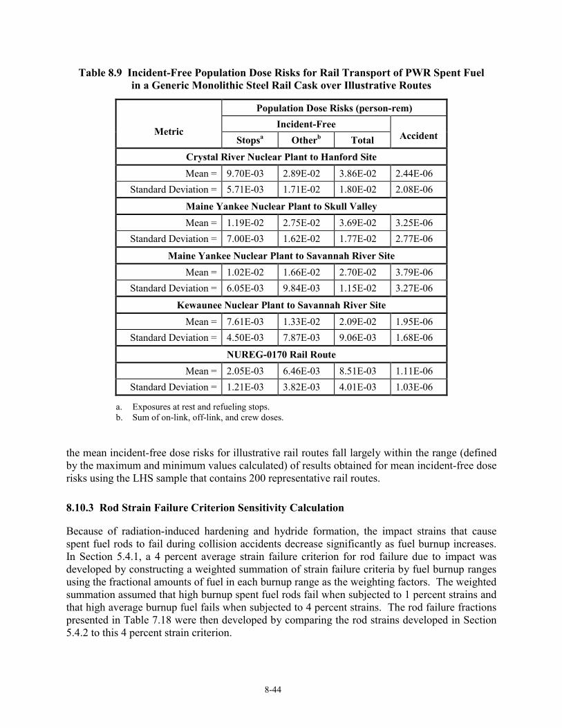
a Generic Steel-Lead-Steel Truck Cask over Illustrative Routes....................................................................8-36Table 8.9 Incident-Free Population Dose Risks for Rail Transport of PWR Spent Fuel in a
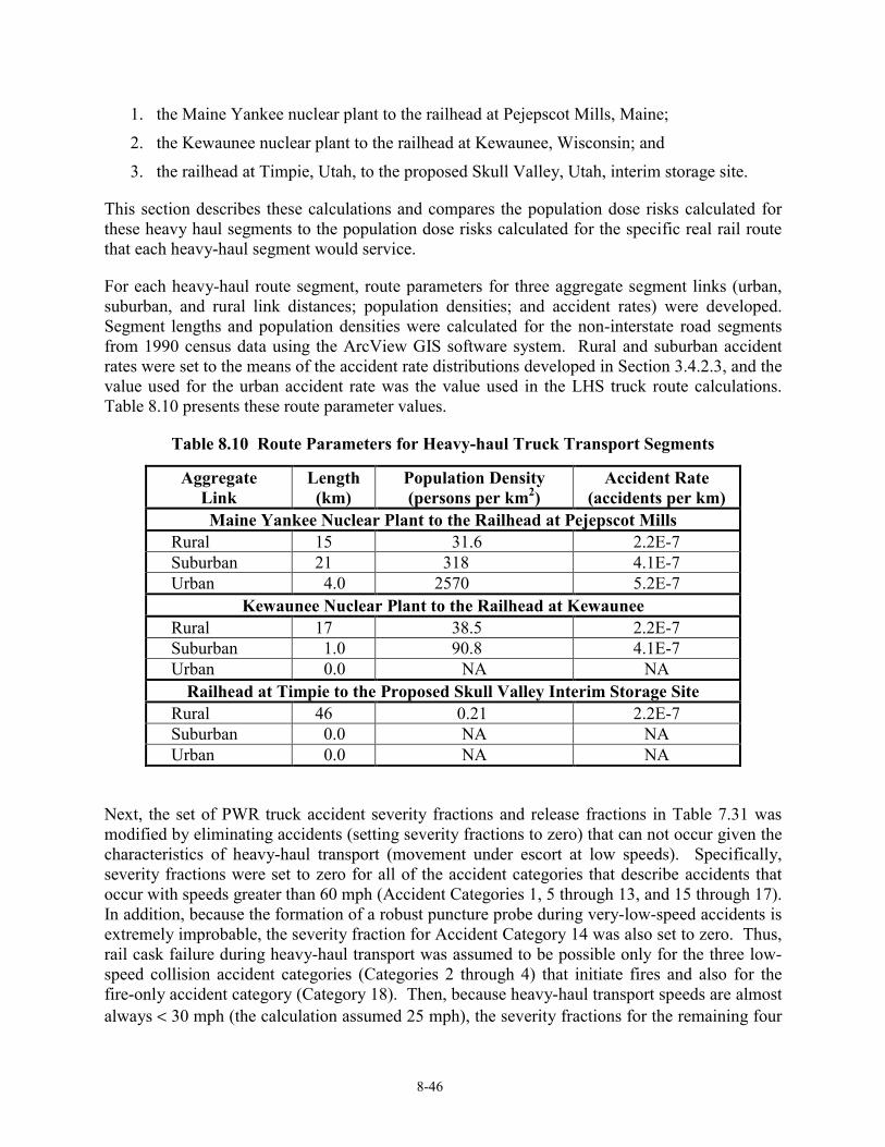
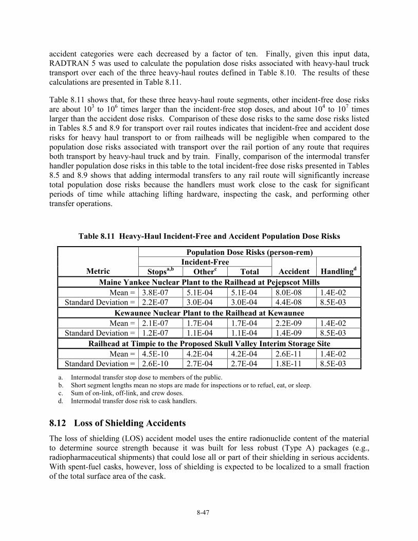
Generic Monolithic Steel Rail Cask over Illustrative Routes .........................................................................8-44Table 8.10 Route Parameters for Heavy-Haul Truck Transport Segments .............................................................8-46Table 8.11 Heavy-Haul Incident-Free and Accident Population Dose Risks..........................................................8-47Table 8.12 Values of Severity Fractions, LOS Fractions, .......................................................................................8-50
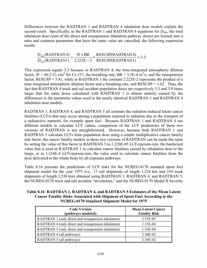
and Source-Strength Multipliers for Ten LOS Accident Cases ......................................................................8-50Table 8.13 Results of Loss of Shielding Risk Calculation ......................................................................................8-52Table 8.16 RADTRAN 1, RADTRAN 4, and RADTRAN 5 Estimates of the Mean Latent Cancer
Fatality Risks Associated with Shipment of Spent Fuel According to the NUREG-0170 StandardShipment Model for 1975...............................................................................................................................8-60
Table 8.17 Mean Accident Population Dose Risks (person-rem) for Five RADTRAN 5 Calculationsthat Used Different Source Terms and Exposure Pathways............................................................................8-62
Table 8.18 Modal Study Truck and Rail Accident Source Terms...........................................................................8-65Table 8.19 Comparison of NUREG-0170 Model I and Model II and Modal Study Probability
and Consequence Axis CCDF Intercepts to Those Developed by this Study .................................................8-68Table 8.20 Ratios of Probability Axis Intercepts ....................................................................................................8-68
xvi
Page intentionally left blank.
xvii
Acknowledgements
Thanks are owed to a number of people for the contributions they made to the performance ofthis study or the preparation of this report. The ORIGEN, CONTAIN, and VICTORIAcalculations described in Section 7 were performed on short notice by J.D Smith, Nathan Bixler,and Kenneth Murata, respectively. Philip Reardon ressurected the RADTRAN 1 code andsupported the analyses described in Section 7 of impact fracturing of spent fuel and also ofcesium release fractions. Mona Aragon prepared the conceptual design drawings of the genericcasks in Section 4 and almost all of the figures in Section 5.
Thanks are especially owed to the reviewers of this report. They identified many topics thatneeded to be better explained and even more sentences that required rewriting. Without theirefforts, many parts of this report would be close to inscrutable. At Sandia National Laboratories,David Harding reviewed Sections 4 and 5 of the report, Dana Powers reviewed Section 7, and theentire report was reviewed by Robert Luna and Charles Massey. External review of the reportwas performed by Brian Anderson, Moe Dehgahani, Larry Fisher, Edwin Jones, Mike Shaffer,and Monika Witte of Lawrence Livermore National Laboratories assisted by Theo Theofanous ofthe University of California at Santa Barbara. The report was also reviewed by a number oftechnical experts at NRC. The NRC reviews were directed and partly performed by M. WayneHodges and Earl Easton.
Lastly, we wish to acknowledge the support, guidance, encouragement, and patience of JohnCook, the NRC project manager for this study. Without his help, we would never have finished.
xviii
Page intentionally left blank.
xix
ACRONYMS
AAR American Association of Railroads
ANL Argonne National Laboratory
BDF building dose factor
BMCS Bureau of Motor Carrier Safety
BWR boiling water reactor
CCDF Complementary Cumulative Distribution Function
DOE Department of Energy
DOT U.S. Department of Transportation
DU depleted uranium
EIS Environmental Impact Statement
EQPS Equivalent Plastic Strain
G acceleration due to gravity
GES General Estimates System
GIS Geographic Information System
GWDt/MTU gigawatt-days thermal per metric ton of uranium
LCF latent cancer fatalities
LHS Latin Hypercube Sampling
LLNL Lawrence Livermore National Laboratory
LOS loss of shielding
MPC multi-purpose cask
NMSS Nuclear Material Safety and Safeguards
NRC Nuclear Regulatory Commission
PWR pressurized water reactor
RAM radioactive material
SETU Structural Evaluation Test Unit
SNL Sandia National Laboratories
TE total plastic elongation
TIFA Trucks Involved in Fatal Accidents
UE uniform plastic elongation
USGS U.S. Geologic Survey
xx
Page intentionally left blank.
1ES-
EXECUTIVE SUMMARY
IntroductionIn September of 1977, the Nuclear Regulatory Commission (NRC) issued a genericEnvironmental Impact Statement (EIS), titled “Final Environmental Statement on theTransportation of Radioactive Material by Air and Other Modes,” NUREG-0170, that coveredthe transport of all types of radioactive material by all transport modes (road, rail, air, and water)[E-1]. That EIS provides the regulatory basis for issuance of general licenses for transportationof radioactive material under 10 CFR 71. Based in part on the findings of NUREG-0170, theNRC’s Commission concluded that “present regulations are adequate to protect the publicagainst unreasonable risk from the transport of radioactive materials” (46 FR 21629, April 13,1981) and stated that “regulatory policy concerning transportation of radioactive materials besubject to close and continuing review.”
In 1996 the NRC decided to reexamine the risks associated with the shipment of spent powerreactor fuel by truck and rail. The reexamination was initiated (1) because many spent fuelshipments are expected to be made during the next few decades, (2) because these shipments willbe made to facilities along routes and in casks not specifically examined by NUREG-0170, and(3) because the risks associated with these shipments can be estimated using new data andimproved methods of analysis. This report documents the methodology and results of the studythat performed this reexamination of the risks of transporting spent fuel from commercial reactorsites to possible interim storage sites and/or permanent geologic repositories.
Overview of NUREG-0170
NUREG-0170 estimated the radiation doses and latent cancer fatalities that might be associatedwith the transportation of 25 different radioactive materials by plane, truck, train, and ship orbarge. The estimates were made using Version 1 of the RADTRAN code (RADTRAN 1) [E-2],that was developed specifically to perform the NUREG-0170 study. One of the 25 radioactivematerials examined by NUREG-0170 was spent power reactor fuel.
For spent fuel shipments that occur without accidents (incident-free transport), radiation doseswere estimated for two population groups: (1) shipment workers (e.g., the truck or train crew,cask handlers, and persons who inspect the cask, truck, or train) and (2) members of the generalpublic who would be exposed to low levels of radiation, because they lived near the shipmentroute or came near the cask while traveling on the route. For transportation accidents, release ofradioactive material from spent fuel to the environment, the probability of these releases, and thepopulation doses and radiation-induced latent cancer fatalities that such releases might causewere estimated.
The influence of accident severity on accident consequences was examined by dividing allaccidents into eight categories according to their severity. Because “little information relatingthe response of packages to accident environments” [E-3] was available in 1975, release ofradioactive materials to the environment as a result of accidents was examined using two releasemodels that were constructed largely by expert judgement. The first model, Model I [E-4],
2ES-
assumed [E-5] that “zero release occurs up to the regulatory test level and that the packaging failscatastrophically in all environments that exceed that level.” Because the Model I cask releasebehavior was considered to be unrealistic, a second release model (Model II) was formulated. InModel II, for accidents that exceed the regulatory test level, release fractions increased moregradually with accident severity [E-6], becoming equal for catastrophic accidents to the releasespecified for all severe accidents by Model I.
Because the NUREG-0170 spent fuel accident source terms were not developed by examiningthe response of spent fuel and spent fuel casks to severe accident conditions, NRC had theresponse of generic steel-lead-steel truck and rail spent fuel casks to collision and fire accidentconditions examined by the performance of finite element impact and thermal heat transportcalculations. The results of these calculations were published in 1987 in NUREG/CR-4829,“Shipping Container Response to Severe Highway and Railway Accident Conditions,” which isusually called the Modal Study [E-7]. Although that study did not perform any consequencecalculations, comparison of the probabilities and magnitudes of the accident source termsdeveloped for that study to those developed for NUREG-0170 allowed the authors of the ModalStudy to conclude that the risks per spent fuel shipment for shipments by both truck and rail were“at least 3 times lower that those documented in NUREG-0170” [E-1].
MethodologyThe risks associated with the transport of spent nuclear fuel were estimated using Version 5 ofthe RADTRAN code [E-8, E-9]. Risks were estimated (1) for incident-free transport, (2) fortransportation accidents so severe that they result in the release of radioactive materials from thecask to the environment, and (3) for less severe accidents that cause the cask shielding to bedegraded but result in no release of radioactive material (Loss of Shielding accidents).
Based on prior sensitivity studies [E-10, E-11, E-12], RADTRAN 5 input parameters weredivided into three groups: (1) source term parameters (severity and release fractions); (2) otherinput parameters that strongly influence RADTRAN estimates of radiation dose, which werecollectively called other “more important parameters”; and (3) RADTRAN input parameters thathave little impact on estimates of radiation dose, which were collectively called “less importantparameters.” Central (best) estimate values were selected for each of the “less important”parameters, e.g., breathing rate.
For the source term parameters, review of studies of transportation accidents, in particular theModal Study [E-7], allowed representative sets of truck and train accidents and their impact andfire environments to be defined. This analysis developed 19 representative truck accidents and21 representative train accidents. Severity fraction and release fraction values were estimated foreach representative accident.
Severity fractions specify the fraction of all possible accidents that are represented by each of therepresentative accidents. Severity fraction values were estimated by review of the accident eventtrees, accident speed distributions, and accident fire distributions that were developed for theModal Study [E-7]. Because only impact onto a very hard surface can result in the release ofradioactive materials during a collision accident, new event tree frequencies of occurrence of
3ES-
route wayside surfaces (e.g., hard rock; concrete, soft rock, and hard soil; soft soil; water) weredeveloped using Department of Agriculture data [E-13] and Geographic Information System(GIS) methods of analysis [E-14].
Release fractions were estimated as the product of (a) the fraction of the rods in the cask that arefailed by the severe accident, (b) the fraction of each class of radioactive materials (e.g., noblegases, volatile, particulates) that might escape from a failed spent fuel rod to the cask interior,and (c) the fraction of the amount of each radioactive material released to the cask interior that isexpected to escape from the cask to the environment. Rod failure during high speed collisionaccidents was estimated by scaling rod strains calculated for relatively low speed impacts [E-15]and then comparing the scaled rod strains to a strain failure criterion [E-15]. Heating of the caskby a hot long duration fire to rod burst rupture temperatures was assumed to fail all unfailed rods(those not failed by collision impact). Rod-to-cask release fractions were estimated by review ofliterature data, especially the experimental results of Lorenz [E-16, E-17, E-18]. Cask-to-environment release fractions were based on MELCOR [E-19] fission product transportcalculations [E-20] that estimated the dependence of these release fractions on the cross-sectionalarea of the cask leak path through which the release to the environment occurs.
Specifications for generic steel-lead-steel truck and rail casks and for a generic steel-DU-steeltruck cask and a generic monolithic steel rail cask were developed from literature data [E-21].The response of these generic casks to severe collisions (e.g., seal leak areas) was examined byperforming three-dimensional finite element calculations for impacts onto an unyielding surfaceat various impact speeds. Unyielding surface impact speeds were converted to equivalent impactspeeds onto yielding surfaces (e.g., soft rock) by considering the energy that would be absorbedby the yielding surface, increasing the energy of the unyielding surface calculation by thatamount, and converting the new total energy to an initial impact speed. Seal degradation and rodburst rupture temperatures due to heating during fires were estimated from literature data. Thedurations of engulfing, optically dense fires needed to produce seal leakage and rod burst rupturewere estimated by performing one-dimensional heat transport calculations.
For the other “more important” parameters (e.g., route lengths, population densities, accidentrates, durations of truck stops, and cask surface dose rates), distributions of parameter valueswere constructed that reflected the likely real-world range and frequency of occurrence of thevalue of each parameter. Next, 200 sets of parameter values were constructed by sampling thesedistributions using a structured Monte Carlo sampling technique called Latin HypercubeSampling (LHS) [E-12, E-22]. This procedure generated one set of 200 parameter values forspent fuel transportation by truck and a second set for transportation by rail. Each set includedparameter values for 200 representative highway or railway routes that spanned the length andbreadth of the continental United States but had no specific origins or destinations.
By taking all possible combinations of the single set of central estimate values for the “lessimportant” RADTRAN input parameters, the 200 sets of other “more important” truck parametervalues, and the 19 sets of representative truck accident severity and release fraction values, inputfor 3800 single-pass RADTRAN 5 truck spent fuel transportation calculations was developed foreach generic truck cask. Similarly, by taking all possible combinations of the set of “lessimportant” parameter values, the 200 sets of other “more important” rail parameter values, and
4ES-
the 21 sets of representative rail accident severity and release fraction values, input for 4200single-pass RADTRAN 5 rail spent fuel transportation calculations was developed. Finally,application of standard statistical methods to the results of these 3800 truck or 4200 railtransportation calculations then allowed the results to be displayed as ComplementaryCumulative Distribution Functions (CCDFs) and estimates of the expected (mean) result forradiological consequences (e.g., population dose) to be calculated.
ResultsSeven sets of RADTRAN calculations are described in the body of this report. Each set ofcalculations developed estimates of the radiological consequences and risks that are associatedwith the shipment of power reactor spent fuel. Two types of consequences and risks wereestimated, those that are associated with the occurrence of accidents during the shipment andthose associated with shipments that take place without the occurrence of accidents. Thecalculations examine four generic cask designs, two shipment modes, two sets of routes, andthree sets of accident source terms. The four generic cask designs examined are steel-lead-steeltruck and rail casks, a steel-DU-steel truck cask, and a monolithic steel rail cask. The twoshipment modes are truck and rail. The two sets of routes are (a) 200 representative truck or railroutes selected by LHS sampling of route parameter distributions and (b) for each mode, the fourillustrative real routes plus the NUREG-0170 shipment route. The three sets of accident sourceterms are the NUREG-0170 [E-1] source terms, the Modal Study source terms [E-7], and thenew source terms developed by this study.
Calculational sets one and two examine spent fuel transportation by truck and rail using the 200sets of other “more important” truck or rail input parameter values that were constructed by LHSsampling of the real-world distributions of the values of these parameters. Sets three and fourexamine transportation by truck and rail over four “illustrative” truck or rail routes and theNUREG-0170 truck or rail route. Comparison of the results of these illustrative routecalculations to the results obtained for the calculations that used the 200 representative routesshowed that the results obtained for the “illustrative” real routes fall within the range of theresults obtained for the representative routes. Set five examined the influence of NUREG-0170exposure pathway modeling on accident consequence predictions. And sets six and sevencompared the accident consequence predictions developed using the accident source termsdeveloped by this study to those developed using the accident source terms developed by theModal Study [E-7] and NUREG-0170 [E-1].
The full study provides results for transport of PWR and BWR spent fuel by truck or rail in fourgeneric casks. In this Executive Summary, results are presented only for the six RADTRAN 5calculations that examined transport of PWR spent fuel in steel-lead-steel truck or rail spent fuelcasks. These results are typical of those obtained for BWR spent fuel and/or transportation inother generic casks. Each of the six calculations discussed here used the set of “less important”values for all RADTRAN 5 input parameters assigned central estimate values. Each calculationused the other “more important” truck or rail parameter values, that were generated by LHSsampling. Thus, these calculations differed only in the source terms used (i.e., NUREG-0170source terms, Modal Study source terms, or the source terms developed by this study), and the setof exposure pathways modeled (the calculations that used Modal study source terms or the source
5ES-
terms developed by this study examined all exposure pathways; the calculations that usedNUREG-0170 source terms calculated exposures only for the inhalation pathway because onlythe inhalation pathway was examined by the NUREG-0170 study).
Table E.1 compares the NUREG-0170 incident-free truck and rail doses to the incident-freedoses developed by this study. Because the NUREG-0170 doses were developed for all of thespent fuel shipments expected to occur in 1975 or 1985, doses for single shipments are calculatedby dividing the 1975 or 1985 doses by the number of spent fuel shipments that NUREG-0170estimated would occur during these years. Table E.1 shows that for single shipments the sum ofthe other incident-free doses (i.e., crew, on-link, off-link, and stop doses) developed by this studyfor spent fuel transport by truck with two-person crews is about one-fourth of the sum of thecorresponding NUREG-0170 truck doses. It also shows that the sum of this study’s incident-freedoses for transport by rail is about two-thirds of the sum of the corresponding NUREG-0170 raildoses. The similarity of these incident-free results is not surprising, because both studies assumethat the surface dose rates of spent fuel transportation casks are somewhat below the regulatorylimit and both use along-route population densities and the population densities at rest stops thatare not very different. Table E-1 also shows that shipment of the 1994 spent fuel inventory at aconstant number of shipments per year over 30 years leads to average yearly population doses fortransport by truck and rail that are respectively about half and one-tenth of the NUREG-0170estimates for 1985.
Table E.1 Comparison of NUREG-0170 Incident-Free Doses (person-rem)to the Incident-Free Doses Developed by this Studya
Doses (person-rem)Multiple Shipments Single Shipment
Study Year Mode Number ofShipments
Hand/Storb Otherc Hand/Storb Otherc
NUREG-0170 1975 Truck 254 52.06 41.74 0.205 0.164NUREG-0170 1985 Truck 1530 313.6 251.4 0.205 0.164This Study Truck 2489d Not Calc.e 110 Not Calc.e 0.0441NUREG-0170 1975 Rail 17 7.227 0.553 0.425 0.0325NUREG-0170 1985 Rail 652 277.4 20.60 0.425 0.0316This Study Rail 100.5d Not Calc.e 2.040 Not Calc.e 0.0203
a. Modal Study incident-free doses are not presented because the Modal Study did not perform any consequence calculations.b. Handler + storage doses.c. Crew + on-link + off-link + stop doses.d. Average number of shipments per year required to ship the full 1994 spent fuel inventory over 30 years in steel-lead-steel
truck and rail casks.e. NUREG-0170 assumed that intermodal cask transfers and temporary storage of the cask would occur during cask shipments;
this study assumed that they would not occur and therefore did not calculate any handling/storage doses.
6ES-
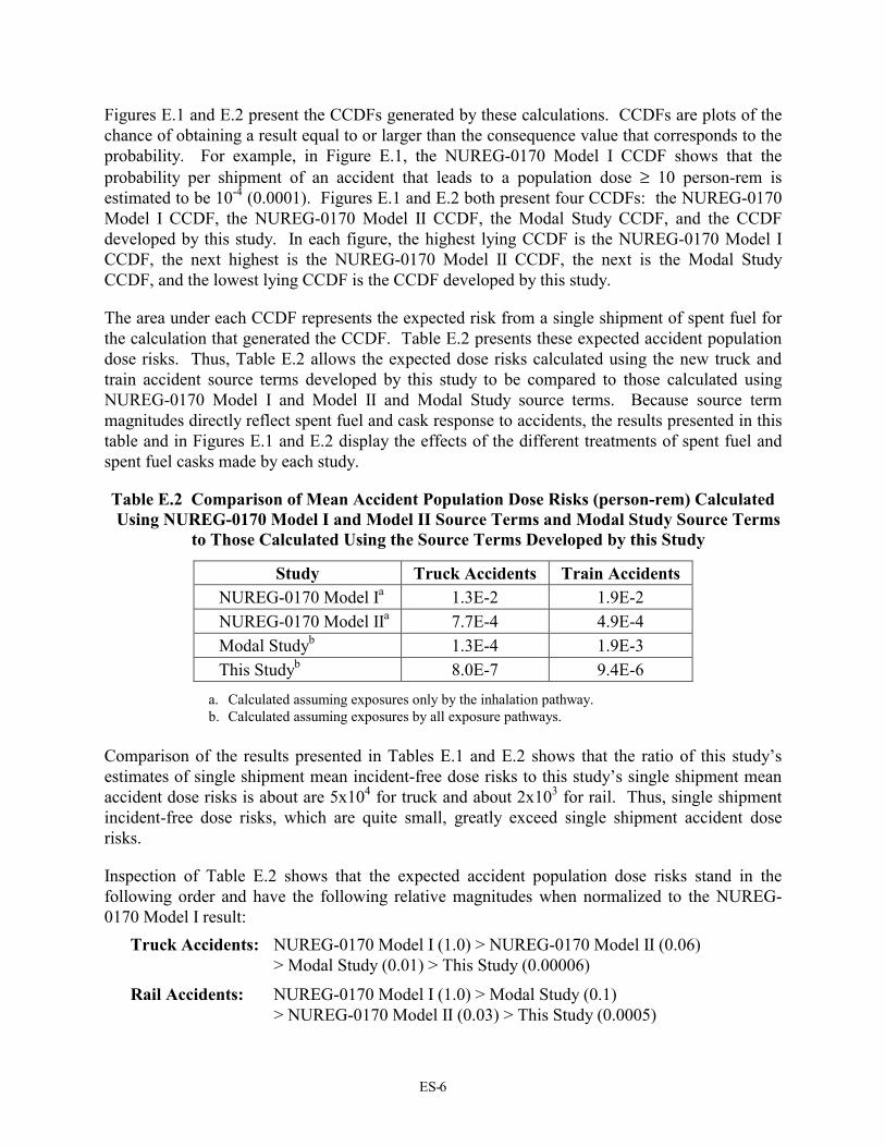
Figures E.1 and E.2 present the CCDFs generated by these calculations. CCDFs are plots of thechance of obtaining a result equal to or larger than the consequence value that corresponds to theprobability. For example, in Figure E.1, the NUREG-0170 Model I CCDF shows that theprobability per shipment of an accident that leads to a population dose ≥ 10 person-rem isestimated to be 10-4 (0.0001). Figures E.1 and E.2 both present four CCDFs: the NUREG-0170Model I CCDF, the NUREG-0170 Model II CCDF, the Modal Study CCDF, and the CCDFdeveloped by this study. In each figure, the highest lying CCDF is the NUREG-0170 Model ICCDF, the next highest is the NUREG-0170 Model II CCDF, the next is the Modal StudyCCDF, and the lowest lying CCDF is the CCDF developed by this study.
The area under each CCDF represents the expected risk from a single shipment of spent fuel forthe calculation that generated the CCDF. Table E.2 presents these expected accident populationdose risks. Thus, Table E.2 allows the expected dose risks calculated using the new truck andtrain accident source terms developed by this study to be compared to those calculated usingNUREG-0170 Model I and Model II and Modal Study source terms. Because source termmagnitudes directly reflect spent fuel and cask response to accidents, the results presented in thistable and in Figures E.1 and E.2 display the effects of the different treatments of spent fuel andspent fuel casks made by each study.
Table E.2 Comparison of Mean Accident Population Dose Risks (person-rem) CalculatedUsing NUREG-0170 Model I and Model II Source Terms and Modal Study Source Terms
to Those Calculated Using the Source Terms Developed by this Study
Study Truck Accidents Train Accidents NUREG-0170 Model Ia 1.3E-2 1.9E-2 NUREG-0170 Model IIa 7.7E-4 4.9E-4 Modal Studyb 1.3E-4 1.9E-3 This Studyb 8.0E-7 9.4E-6
a. Calculated assuming exposures only by the inhalation pathway.b. Calculated assuming exposures by all exposure pathways.
Comparison of the results presented in Tables E.1 and E.2 shows that the ratio of this study’sestimates of single shipment mean incident-free dose risks to this study’s single shipment meanaccident dose risks is about are 5x10⁴ for truck and about 2x10³ for rail. Thus, single shipmentincident-free dose risks, which are quite small, greatly exceed single shipment accident doserisks.
Inspection of Table E.2 shows that the expected accident population dose risks stand in thefollowing order and have the following relative magnitudes when normalized to the NUREG-0170 Model I result:
Truck Accidents: NUREG-0170 Model I (1.0) > NUREG-0170 Model II (0.06)> Modal Study (0.01) > This Study (0.00006)
Rail Accidents: NUREG-0170 Model I (1.0) > Modal Study (0.1)> NUREG-0170 Model II (0.03) > This Study (0.0005)
Figure E.1 Mean truck accident population dose risk CCDFs for calculations that compared the source terms developed byNUREG-0170, the Modal Study, and this study. Each RADTRAN 5 calculation assumed transport in a steel-lead-steel truckcask over each of the 200 representative truck routes and each calculation generated results for all of the 19 representativetruck accident source terms.
NUREG-0170 accident release inventory, NUREG-0170 Model I release fractions, only inhalation pathways. . . . . . . NUREG-0170 accident release inventory, NUREG-0170 Model II release fractions, only inhalation pathways
PWR inventory, 20 Modal Study source terms, all exposure pathways PWR inventory, 19 truck accident source terms developed for this study, all exposure pathways
Prob
abili
ty o
f Exc
eedi
ng C
onse
quen
ce V
alue
, C
10-4 10-3 10-2 10-1 100 101 102 103 104 105 106
Accident Consequence Value, C (person-rem)
10-1
100
101
102
103
104
105
106
107
108
109
1010
1011
1012
1013
1014
10-1
10-2
10-3
10-4
10-5
10-6
10-7
10-8
10-9
10-10
10-11
10-12
10-13
10-14
10-15
10-16
10-17
Expected Years betw
een Accidents Exceeding
Consequence V
alue, C (100 shipm
ents/yr.)
ES-7
8ES-
Figure E.2 Mean rail accident population dose risk CCDFs for calculations that compared the source terms developed byNUREG-0170, the Modal Study, and this study. Each RADTRAN 5 calculation assumed transport in a steel-lead-steel railcask over each of the 200 representative rail routes and each calculation generated results for all of the 21 representative railaccident source terms.
NUREG-0170 accident release inventory, NUREG-0170 Model I release fractions, only inhalation pathways. . . . . . . NUREG-0170 accident release inventory, NUREG-0170 Model II release fractions, only inhalation pathways
PWR inventory, 20 Modal Study source terms, all exposure pathways PWR inventory, 19 truck accident source terms developed for this study, all exposure pathways
Prob
abili
ty o
f Exc
eedi
ng C
onse
quen
ce V
alue
, C
10-4 10-3 10-2 10-1 100 101 102 103 104 105 106
Accident Consequence Value, C (person-rem)
10-1
100
101
102
103
104
105
106
107
108
109
1010
1011
1012
1013
1014
10-1
10-2
10-3
10-4
10-5
10-6
10-7
10-8
10-9
10-10
10-11
10-12
10-13
10-14
10-15
10-16
10-17
Expected Years betw
een Accidents Exceeding
Consequence V
alue, C (100 shipm
ents/yr.)
ES-8
ES-9
The relative ordering of these accident results is entirely consistent with the assumptions made byeach study regarding the probability of radionuclide leakage from the cask during transportationaccidents and the magnitude of the source terms generated by accidents of differing severities.Because both Model I and Model II in NUREG-0170 assumed that spent fuel casks might releasea portion of their contents when subjected to the loads that characterize minor accidents, thefraction of all truck and train accidents predicted by these models to cause releases is very largeand extremely conservative. Similarly, because the NUREG-0170 Model I assumed that all caskleaks led to the release of the entire NUREG-0170 accident inventory (the largest amount ofradioactive material expected to be released during a severe accident), the mean accidentpopulation doses calculated using the NUREG-0170 Model I for truck and rail accidents arequite large. When, as was done by the Modal Study, cask failure and thus source termprobabilities and magnitudes are estimated from the response of the cask shell to mechanical andthermal loads, both source term probabilities and most source term magnitudes decrease.Consequently, relative to the NUREG-0170 Model I result, mean accident population dose risksfor rail and truck are decreased respectively by one and two orders of magnitude. When, as wasdone by this study, cask release and thus source term probabilities and magnitudes are estimatedby examining the response of cask closures and spent fuel rods to impact loads and the burstrupture of spent fuel rods due to heating by fires, cask release is found to be even less likely andretention of particles and condensable vapors by deposition onto cask interior surfaces is found tobe substantial. Accordingly, source term probabilities and most source term magnitudes, exceptthose for the most severe accidents examined, decrease further. Consequently, relative to theModal Study result, expected (mean) accident population dose risks for both rail and truck areeach further decreased by about two orders of magnitude.
Source term magnitudes for the most severe accidents examined by the Modal Study and thisstudy are larger than the largest source term magnitude postulated in NUREG-0170. They arelarger because the product of the cask inventory and the largest accident release fractionsdeveloped by this study is larger than the largest source term examined by NUREG-0170.Nevertheless, although the largest source terms developed by the analyses performed by theModal Study and this study are larger than the largest NUREG-0170 source term, the accidentrisks posed by these source terms are substantially smaller because these source terms are so veryimprobable.
ConclusionsThe results described in detail in the body of this report lead to the following conclusions:
• The single cask truck shipment expected incident-free population doses developed by thisstudy are about one-quarter of those in NUREG-0170.
• The single cask rail shipment expected incident-free population doses developed by this studyare about two-thirds of those in NUREG-0170.
• The use of very conservative cask failure criteria in NUREG-0170 caused its estimates of thefraction of all accidents that release radioactive materials to be much too large and thus veryconservative.
ES-10
• The NUREG-0170 estimate of the largest source term that might be released from a failedspent fuel cask during an unusually severe transportation accident is significantly lower thanthe largest source terms calculated using Modal Study release fractions or the releasefractions developed by this study. However, the risks associated with these source terms arelower than the risk of the largest NUREG-0170 source term because these source terms are sovery improbable.
• The source terms developed by the Modal Study and by this study, which reflect thecomplexities of rod failure and cask response to transportation accident impact and thermalloads, yield estimates of expected (mean) spent fuel transportation accident population dosesthat are orders of magnitude smaller than those developed by the NUREG-0170 study.
Overall, the results of this study confirm the validity of the NUREG-0170 estimates of spent fuelincident-free population doses. The results also show that the NUREG-0170 estimates of spentfuel accident population dose risks were very conservative, as was believed to be true whenNUREG-0170 was published [E-23].
References[E-1] “Final Environmental Statement on the Transportation of Radioactive Material by Air
and Other Modes,” NUREG-0170, U.S. Nuclear Regulatory Commission, Washington,DC, December 1977.
[E-2] J. M. Taylor and S. L. Daniel, “RADTRAN: A Computer Code to AnalyzeTransportation of Radioactive Material,” SAND76-0243, Sandia National Laboratories,Albuquerque, NM, April 1977.
[E-3] Ref. [E-1], p. 5-20.
[E-4] Ref. [E-1], p. 5-22.
[E-5] Ref. [E-1], p. 5-21.
[E-6] Ref. [E-1], p. 5-23.
[E-7] L. E. Fischer, et al., “Shipping Container Response to Severe Highway and RailwayAccident Conditions,” NUREG/CR-4829, Lawrence Livermore National Laboratory,Livermore, CA, February 1987.
[E-8] K. S. Neuhauser and F. L. Kanipe, “RADTRAN 5, Technical Manual,” Sandia NationalLaboratories, Albuquerque, NM (in preparation, draft available on request).
[E-9] K. S. Neuhauser and F. L. Kanipe, “RADTRAN 5, User Guide,” Sandia NationalLaboratories, Albuquerque, NM (draft available on the RADTRAN web site).
[E-10] G. S. Mills, G. S., K. S. Neuhauser, and F. L. Kanipe, “RADTRAN 4 Truck AccidentRisk Sensitivity Analysis,” Proceedings of Waste Management 95, WM Symposia,Tucson, AZ, 1995.
ES-11
[E-11] G. S. Mills and K. S. Neuhauser, “Sensitivity Analysis for RADTRAN 4 InputParameters,” 88th Annual Meeting of the Air & Waste Management Association., SanAntonio, TX, 1995.
[E-12] G. S. Mills, et al., “Application of Latin Hypercube Sampling to RADTRAN 4 TruckAccident-Risk Sensitivity Analysis,” Proceedings of the 11th International Conferenceon the Packaging and Transportation of Radioactive Materials (PATRAM ’95), IAEA,Vol. 4, p. 705, 1995.
[E-13] State Soil Graphics (STATSGO) Data Base, available on the Internet atftp.ftw.nrcs.usda.gov/pub/statsgo.
[E-14] ARC/INFO Coverages and Arc View Project, K. C. Bayer Digital Map of the U.S.,purchased from Geologic Data Systems, Inc., 1600 Emerson St., Denver, CO 80218.
[E-15] T. L. Sanders, et al., “A Method for Determining the Spent-Fuel Contribution toTransport Cask Containment Requirements, Appendix III, Spent Fuel Response toTransport Environments,” SAND90-2406, Sandia National Laboratories, Albuquerque,NM, November 1992.
[E-16] R. A. Lorenz, et al., “Fission Product Release from Highly Irradiated LWR Fuel,”NUREG/CR-0722, Oak Ridge National Laboratory, Oak Ridge, TN, February 1980.
[E-17] R. A. Lorenz, et al., “Fission Product Release from Simulated LWR Fuel,” NUREG/CR-0274, Oak Ridge National Laboratory, Oak Ridge, TN, July 1978.
[E-18] R. A. Lorenz, et al., “Fission Product Source Terms for the LWR Loss-of-CoolantAccident,” NUREG/CR-1288, Oak Ridge National Laboratory, Oak Ridge, TN, July1980.
[E-19] R. M. Summers, et al., “MELCOR 1.8.0: A Computer Code for Nuclear Reactor SevereAccident Source Term and Risk Assessment Analyses,” NUREG/CR-5531, SAND90-0364, Sandia National Laboratories, Albuquerque, NM, January 1991.
[E-20] J. L. Sprung, et al., “Data and Methods for the Assessment of the Risks Associated withthe Maritime Transport of Radioactive Materials: Results of the SeaRAM Program,”SAND97-2222, Sandia National Laboratories, Albuquerque, NM, August 1997.
[E-21] “Shipping and Storage Cask Data for Commercial Spent Nuclear Fuel,” JAI Corp., July1996.
[E-22] G. D. Wyss and K. H. Jorgensen, “A User’s Guide to LHS: Sandia’s Latin HypercubeSampling Software,” SAND98-0210, Sandia National Laboratories, Albuquerque, NM,1998.
[E-23] Ref. [E-1], p. ix.
ES-12
Page intentionally left blank
1-1
1. INTRODUCTION
1.1 NUREG-0170In September of 1977, the Nuclear Regulatory Commission (NRC) issued a genericenvironmental impact statement (EIS), titled “Final Environmental Statement on theTransportation of Radioactive Material by Air and Other Modes,” NUREG-0170, that coveredthe transport of all types of radioactive material by all transport modes (road, rail, air, and water)[1-1]. That EIS provided the regulatory basis for continued issuance of general licenses fortransportation of radioactive material under 10 CFR 71. Based in part on the findings ofNUREG-0170, NRC staff concluded (1) that “the average radiation dose to the population at riskfrom normal transportation is a small fraction of the limits recommended for members of thegeneral public from all sources of radiation other than natural and medical sources and is a smallfraction of natural background dose” and (2) that “the radiological risk from accidents intransportation is small, amounting to about one-half percent of the normal transportation risk onan annual basis” [1-2]. In addition, the NRC Commission concluded that “present regulationsare adequate to protect the public against unreasonable risk from the transport of radioactivematerials” (46 FR 21629, April 13, 1981) and stated that “regulatory policy concerningtransportation of radioactive materials be subject to close and continuing review.”
1.2 NUREG-0170 Spent Fuel Transportation RisksNUREG-0170 estimated the radiation doses and latent cancer fatalities that might be associatedwith the transport of 25 different radioactive materials by plane, truck, train, and ship or barge.The 25 materials were chosen to encompass 90 percent of all shipments in the United States and90 percent of the activity contained in shipments. The estimates were made using Version 1 ofthe RADTRAN code (RADTRAN 1) [1-3], which was developed specifically to support theperformance of the NUREG-0170 study.
One of the 25 radioactive materials examined by NUREG-0170 was spent nuclear power reactorfuel. For spent fuel shipments that occur without accidents (incident-free transport), radiationdoses were estimated for members of the general public who would be exposed to radiation, forexample, because they lived near the shipment route, and also for workers (e.g., crew, handlers,inspectors). Release of radioactive materials from spent fuel to the environment as a result oftransportation accidents, the probability of these releases, and the latent cancer fatalities that suchreleases might cause were also estimated.
Spent fuel transport risks were estimated for shipment by truck and by train over a generichighway and a generic rail route [1-4]. Table 1.1 describes attributes of these two generic routes.Radiological consequences (population doses for incident-free transport and expected numbers oflatent cancer fatalities for transportation accidents) were estimated for spent fuel shipmentsexpected to occur during 1975 and 1985. Tables 1.2 and 1.3 respectively present the incident-free and accident consequences estimated for these spent fuel shipments.
1-2
Table 1.1 NUREG-0170 Spent Fuel Truck and Train Route Data
Crew 31.3 188 0.68 2.6 Handlers 50.8 306 6.8 261 Storage 1.26 7.6 0.427 16.4 General Public Off-Linka 3.8 22.9 0.175 6.69 On-Linkb 1.88 11.3 0.222 8.53 Stopsc 4.82 29.0 0.089 3.44 Total Population Dose 93.8 565 7.78 298a. Residents living by the transport route.b. Travelers exposed while traveling in cars, buses, or trains.c. Travelers exposed at rest stops.
Table 1.3 Expected (Mean) Latent Cancer Fatalities Predicted in NUREG-0170to be Caused by Truck and Train Accidents that Occur during Spent Fuel Transport
Year Release Model Truck Train Truck + Train1975 I 0.047 0.021 0.0681985 I 0.29 0.8 1.091975 II NA NA 0.00003561985 II NA NA 0.000422
1-3
For calculations of radiological consequences that might be caused by accidents, accidents weredivided into eight categories (Categories I through VIII) of increasing severity. Because “littleinformation relating the response of packages to accident environments” [1-5] was available in1975 for spent fuel and other highly radioactive materials shipped in Type B packages, release ofradioactivity as a result of accidents was examined using two release models. The first model,Model I [1-6], assumed [1-7] that “zero release occurs up to the regulatory test level and that thepackaging fails catastrophically in all environments that exceed that level.” The amounts of eachradionuclide that were assumed [1-8] to be released to the environment by this “catastrophic”failure are presented in Table 1.4. Thus, Model I assumed that the radioactive release specifiedin Table 1.4 would take place whenever a Type B spent fuel package was subjected tomechanical or thermal loads in excess of the mechanical and thermal loads encountered duringpackage certification tests [1-9]. Because the Model I cask release behavior was considered to beunrealistic, a second release model (Model II) was formulated. In Model II, for accidents thatexceed the regulatory test level, release fractions increased more gradually with accident severity[1-10], becoming equal for catastrophic accidents to the release specified for all severe accidentsby Model I.
Table 1.5 shows that the Model I and Model II release fractions are used for both truck and trainaccidents. Model I and Model II release fractions are the same for accident categories I, II, V, VI,VII, and VIII and differ only for categories III, and IV. Finally, Table 1.3 shows that accidentconsequences are substantially decreased if, as is done in Model II, release is assumed to increasewith increasing accident severity.
Table 1.4 Inventory (Ci) Assumed in NUREG-0170 to be Released to the Environmentfrom a Type B Spent Fuel Cask as a Result of an Accident
1.3 Need for Reevaluation of NUREG-0170 Spent Fuel TransportationRisks
While NUREG-0170 was an important analysis that delineated transportation risks in the contextof the information available at that time, its results were developed using rather simple modelsand limited data. In the interim, there has been significant growth in analytical capabilities anddata. While the casks and the specific routes for spent fuel movements have not yet beendesignated, it is clear that the generic cask and routes used in NUREG-0170 are now less thantypical. For example, spent fuel may soon be shipped in the dual-purpose or multi-purposecanisters (MPCs) from commercial reactors to Interim Spent Fuel Storage Installations and/orCentralized Storage Facilities in addition to shipment to a permanent geologic repository. In fact,the Office of Nuclear Material Safety and Safeguards (NMSS) has received several applicationsfor dual-purpose (storage and transport) spent fuel casks, and additional applications
1-1
Table 1.5 NUREG-0170 Model I and Model II Severity and ReleaseFractions for Spent Fuel Transport by Truck and Rail
Severity Fractionsa Release FractionsModels I and II Truck and RailAccident
Category Truck Rail Model I Model III 0.55 0.50 0.0 0.0II 0.36 0.30 0.0 0.0III 0.07 0.18 1.0 0.01IV 0.016 0.018 1.0 0.1V 0.0028 0.0018 1.0 1.0VI 0.0011 1.3×10⁻⁴ 1.0 1.0VII 8.5×10⁻⁵ 6.0×10⁻⁵ 1.0 1.0VIII 1.5×10⁻⁵ 1.0×10⁻⁵ 1.0 1.0
a. Fraction of accidents that fall into this severity range
are expected in the near future. In addition, many improvements have been made to the riskassessment models implemented in the RADTRAN code since the initial version of that codewas used to estimate spent fuel transportation risks for NUREG-0170, and a major study of theresponse of spent fuel casks to severe transportation accidents, “Shipping Container Response toSevere Highway and Railway Accident Conditions,” NUREG/CR-4829, often called the ModalStudy, has been published [1-11].
Because new data and analytical methods were now available to apply to the analysis of powerreactor spent fuel transportation risks, and because spent fuel is likely to be shipped to facilitiesalong routes and in casks not specifically examined by NUREG-0170, the NRC decided theconclusions reached in NUREG-0170 should be reexamined in order to determine if the risks ofthe spent fuel shipments that are expected to take place during the next few decades are boundedby the risk estimates published in NUREG-0170. Accordingly, this report documents themethodology and results of a reevaluation of the risks of transporting spent fuel from commercialreactor sites to possible interim storage sites and/or permanent geologic repositories.
1.4 Study ObjectivesThis study had three objectives:
• Estimation of the radiological and non-radiological, routine and accident, transportationrisks associated with the anticipated spent fuel shipments and determination of whetherthose risks are bounded by the estimates and projections of spent fuel shipment riskspublished in 1977 in NUREG-0170.
• Examination of any outstanding spent fuel transportation issues or environmentalconcerns not resolved by NUREG-0170 and the Modal Study.
1-2
• Documentation of the approach, data, and computational methods used to reestimatespent fuel transportation risks in detail sufficient to allow other transportation experts tofully understand the analyses performed, and preparation of a summary of the results in aform accessible to concerned citizens.
1.5 General ApproachThe risks associated with the transport of spent fuel were estimated using Version 5 of theRADTRAN code [1-12, 1-13]. As in NUREG-0170, risks were estimated for incident-freetransport and also for transportation accidents severe enough to cause radioactive material to bereleased from the cask to the environment.
Based on prior sensitivity studies [1-14, 1-15, 1-16], RADTRAN 5 input parameters weredivided into three groups:
• Source term parameters (accident severity fractions and their corresponding accidentrelease fractions),
• Other “more important” parameters that strongly influence RADTRAN estimates ofradiation dose (for values within their likely range), and
• “Less important” parameters which have little impact on estimates of radiation dose (forvalues within their likely range).
For each of the “less important parameters,” e.g., breathing rate, central (best) estimate valueswere selected. For each of the more important parameters (e.g., route lengths, populationdensities, accident rates, durations of truck stops, and cask surface dose rates), distributions ofparameter values were constructed that reflected the likely real-world range and frequency ofoccurrence of the value of each parameter. Next, for both truck and rail analyses, 200 sets of theother “more important” parameter values were constructed by sampling these distributions usinga structured Monte Carlo sampling technique called Latin Hypercube Sampling [1-16, 1-17].
For the source term parameters, review of studies of actual transportation accidents, in particularthe Modal Study [1-11], allowed representative sets of truck and train accidents and their impactand fire environments to be defined. This analysis developed 19 representative truck accidentsand 21 representative train accidents. Severity fraction and release fraction values wereestimated for each representative accident.
Severity fraction values were developed by a review of the accident event trees, accident speeddistributions, and accident fire distributions that were published in the Modal Study [1-11]. Newevent tree frequencies of occurrence of route wayside surfaces (e.g., hard rock; concrete, softrock, and hard soil; soft soil; water) were developed using Department of Agriculture data [1-18]and Geographic Information System (GIS) methods of analysis [1-19].
Release fractions were estimated as the product of (a) the fraction of the rods in the cask that arefailed by the severe accident, (b) the fraction of each class of radioactive materials (e.g.,particulates) that might escape from a failed spent fuel rod to the cask interior, and (c) the
1-3
fraction of the amount of radionuclides released to the cask interior that is expected to escapefrom the cask to the environment. Rod failure during high speed collision accidents wasestimated by scaling rod strains calculated for low speed impacts and then comparing the scaledrod strains to a strain failure criterion [1-20]. Heating of the cask by a fire to rod burst rupturetemperatures was assumed to fail all unfailed rods. Rod-to-cask release fractions were estimatedby review of literature data, especially the experimental results of Lorenz [1-21, 1-22, 1-23].Cask-to-environment release fractions were based on MELCOR fission product transportcalculations [1-24] that estimated the dependence of these release fractions on the size (cross-sectional area) of the cask failure that allows the release to the environment to occur.
Specifications for two generic truck and two generic rail spent fuel casks were developed fromliterature data [1-25]. Cask damage (e.g., seal leak areas) during severe collisions was estimatedfrom the results of finite element calculations that modeled impacts onto an unyielding surface atvarious impact speeds. Unyielding surface impact speeds were converted to equivalent impactspeeds onto yielding surfaces (e.g., soft rock) by considering the energy that would be absorbedby the yielding surface, increasing the energy of the unyielding surface calculation by thatamount, and converting the new total energy to an initial impact speed. Seal leakage and rodburst rupture temperatures due to heating during fires were estimated from literature data. Thedurations of engulfing optically dense fires needed to produce large seal leak areas and rodfailure by burst rupture were estimated by performing one-dimensional heat transportcalculations.
By taking all possible combinations of the single set of central estimate values for the “lessimportant” RADTRAN input parameters, the 200 sets of other “more important” truck parametervalues, and the 19 sets of representative truck accident severity and release fraction values, inputfor 3800 single-pass RADTRAN 5 truck spent fuel transportation calculations was developed foreach generic truck cask. Similarly, by taking all possible combinations of the set of “lessimportant” parameter values, the 200 sets of other “more important” rail parameter values, andthe 21 sets of representative rail accident severity and release fraction values, input for 4200single-pass RADTRAN 5 rail spent fuel transportation calculations was developed. Applicationof standard statistical methods to the results of these 3800 truck or 4200 rail transportationcalculations then allowed the results to be displayed as Complementary Cumulative DistributionFunctions (CCDFs) and estimates of the expected (mean) result for radiological consequences(e.g., population dose) to be calculated. Finally, the results of these RADTRAN 5 calculationswere compared to the results of RADTRAN 5 calculations that used the spent fuel source terms(severity fractions and release fractions) developed by the NUREG-0170 study [1-1] and thosedeveloped by the Modal Study [1-11] and differences in predicted risks are discussed.
1.6 References[1-1] “Final Environmental Statement on the Transportation of Radioactive Material by Air
and Other Modes,” NUREG-0170, U.S. Nuclear Regulatory Commission, Washington,DC, December 1977.
[1-2] Ref. [1-1], Summary and Conclusions, p. vii.
1-4
[1-3] J. M. Taylor and S. L. Daniel, “RADTRAN: A Computer Code to AnalyzeTransportation of Radioactive Material,” SAND76-0243, Sandia National Laboratories,Albuquerque, NM, April 1977.
[1-4] Ref. [1-1], Vol.1, pp. 1-17, 4-16, 4-23, A-13, and E-4.
[1-5] Ref. [1-1], p. 5-20.
[1-6] Ref. [1-1], p. 5-22.
[1-7] Ref. [1-1], p. 5-21.
[1-8] Ref. [1-1], p. A-14.
[1-9] Code of Federal Regulations, Volume 10, Part 71.73 (10 CFR 71.73).
[1-10] Ref. [1-1], p. 5-23.
[1-11] L. E. Fischer, et al., “Shipping Container Response to Severe Highway and RailwayAccident Conditions,” NUREG/CR-4829, Lawrence Livermore National Laboratory,Livermore, CA, February 1987.
[1-12] K. S. Neuhauser and F. L. Kanipe, “RADTRAN 5, Technical Manual,” Sandia NationalLaboratories, Albuquerque, NM (in preparation, draft available on request).
[1-13] K. S. Neuhauser and F. L. Kanipe, “RADTRAN 5, User Guide,” Sandia NationalLaboratories, Albuquerque, NM (draft available on the RADTRAN web site).
[1-14] G. S. Mills, K. S. Neuhauser, and F. L. Kanipe, “RADTRAN 4 Truck Accident RiskSensitivity Analysis,” Proceedings of Waste Management 95, WM Symposia, Tucson,AZ, 1995a.
[1-15] G. S. Mills and K. S. Neuhauser, “Sensitivity Analysis for RADTRAN 4 InputParameters,” 88th Annual Meeting of the Air & Waste Management Assoc., SanAntonio, TX, 1995.
[1-16] G. S. Mills, et al., “Application of Latin Hypercube Sampling to RADTRAN 4 TruckAccident-Risk Sensitivity Analysis,” Proceedings of the 11th International Conference onthe Packaging and Transportation of Radioactive Materials (PATRAM ’95), IAEA, Vol.4, p. 705, 1995.
[1-17] G. D. Wyss and K. H. Jorgensen, “A User’s Guide to LHS: Sandia’s Latin HypercubeSampling Software,” SAND98-0210, Sandia National Laboratories, Albuquerque, NM1998.
[1-18] State Soil Graphics (STATSGO) Data Base, available on the Internet atftp.ftw.nrcs.usda.gov/pub/statsgo.
1-5
[1-19] ARC/INFO Coverages and Arc View Project, K. C. Bayer Digital Map of the U.S.,purchased from Geologic Data Systems, Inc., 1600 Emerson St., Denver, CO 80218.
[1-20] T. L. Sanders, et al., “A Method for Determining the Spent-Fuel Contribution toTransport Cask Containment Requirements, Appendix III, Spent Fuel Response toTransport Environments,” SAND90-2406, Sandia National Laboratories, Albuquerque,NM, November 1992.
[1-21] R. A. Lorenz, et al., “Fission Product Release from Highly Irradiated LWR Fuel,”NUREG/CR-0722, Oak Ridge National Laboratory, Oak Ridge, TN, February 1980.
[1-22] R. A. Lorenz, et al., “Fission Product Release from Simulated LWR Fuel,” NUREG/CR-0274, Oak Ridge National Laboratory, Oak Ridge, TN, July 1978.
[1-23] R. A. Lorenz, et al., “Fission Product Source Terms for the LWR Loss-of-CoolantAccident,” NUREG/CR-1288, Oak Ridge National Laboratory, Oak Ridge, TN, July1980.
[1-24] J. L. Sprung, et al., “Data and Methods for the Assessment of the Risks Associated withthe Maritime Transport of Radioactive Materials: Results of the SeaRAM Program,”SAND97-2222, Sandia National Laboratories, Albuquerque, NM, August 1997.
[1-25] “Shipping and Storage Cask Data for Commercial Spent Nuclear Fuel,” JAI Corp., July1996.
2-1
2. METHODOLOGY OVERVIEW AND REPORT ROADMAP
2.1 IntroductionNUREG-0170 [2-1] documents estimates of the radiological consequences and risks associatedwith the shipment by truck, train, plane, or barge of about 25 different radioactive materials,including power reactor spent fuel. The estimates were calculated using Version 1 of theRADTRAN code [2-2], which was developed for the NRC by Sandia National Laboratories(SNL) specifically to support the conduct of the NUREG-0170 study. When the NRC askedSNL to reexamine the consequences and risks associated with the transport of spent fuel by truckand train, RADTRAN Version 5 [2-3, 2-4], the most recent version of the RADTRAN code, wasthe computational tool of choice.
The basic methodology employed in the RADTRAN code is widely accepted. Changes to thecode are tracked by a software quality assurance plan that is consistent with American NationalStandards Institute guidelines. Two reviews of RADTRAN Version 4, in which the RADTRANcalculations were benchmarked against hand calculations and other codes, have been published[2-5, 2-6]. Because the models implemented in RADTRAN 5 are almost identical to thoseimplemented in RADTRAN 4, the benchmarking results for RADTRAN 4 also apply toRADTRAN 5.
2.2 RADTRANThe RADTRAN code calculates the radiological consequences and risks associated with theshipment of a specific radioactive material (RAM) in a specific packaging along a specific route.The code estimates consequences and risks (a) for shipments that proceed without incident, thatis, for shipments during which no serious accidents occur, and (b) for accident scenarios thatmight occur during these shipments that could lead to a loss of package shielding or to the releaseof radioactive material to the environment. Radiation doses caused by shipments that take placewithout the occurrence of serious accidents are called “incident free.” The doses and risksassociated with accident scenarios are referred to as “accident consequences and accident risks,respectively.”
For incident-free shipments, RADTRAN calculates the radiological doses that would be receivedby workers (e.g., drivers, handlers, inspectors, escorts) and by members of the general public(e.g., persons who live near the RAM transport route and travelers who pass near the RAMtransport vehicle while it traverses the transport route). For each accident scenario severe enoughto cause a release of radioactive material, RADTRAN estimates (a) the doses that might bereceived by people who reside downwind of the assumed accident location during the passage ofthe windborne radioactive plume and as a result of deposition of radioactive materials from thatplume onto the ground, (b) the probability of the hypothesized accidental release, and (c) theradiological risks that would be caused by the release (i.e., the product of each radiologicalconsequence and the probability of the release that causes those consequences). RADTRAN canalso be used to estimate the radiation doses associated with loss of shielding accidents, that is,with accidents that do not result release of radioactive materials from the package but do causethe radiation shielding of the package to be degraded.
2-2
2.3 RADTRAN InputTo perform its calculations, RADTRAN requires values for a large number of input parameters.For many of these parameters (e.g., breathing rates, stop times), appropriate values are availablein the RADTRAN User’s Guide [2-4]. However, the following parameters, all of which stronglyinfluence consequences and risks, have values that vary greatly with route, radioactive material,or packaging characteristics: (a) route lengths; (b) the fractions of those lengths that are urban,suburban, or rural; (c) the population densities and accident rates that characterize those routefractions; (d) the number of people in other vehicles traveling on the route (e) the durations ofstops taken while traveling the route; (f) the weather conditions that might prevail at the time ofan accident; (g) the surface dose rate of the package; (h) the amount of each radionuclide in thepackage inventory that might be released to the atmosphere as the result of an accident; (i) theprobability of the release; and (j) the time required to conduct an evacuation should a releaseoccur. Because each of these parameters can take on a wide range of values, representative setsof parameter values were developed for each of these parameters. The following sections discussthe more complicated development methods.
2.3.1 Route Parameters
In the summer of 1996, when this study was initiated, power reactor spent fuel was stored at 79locations. Although DOE was required by law [2-7] to begin accepting this spent fuel in early1998 and overseeing its shipment to temporary and/or permanent storage sites, these shipmentshave yet to begin because no temporary or permanent storage sites have yet been built. Becausethe locations of the temporary and permanent storage sites that must eventually be built are notknown, this study could not examine a specific set of routes that were certain to be usedwhenever spent fuel shipments actually take place.
The study could have examined a few specific highway and rail routes that connect some of thesites where spent fuel is presently stored to a few sites that have been mentioned as possibleinterim or permanent storage site locations. However, because such a minimal set ofhypothetical routes could not be shown to be representative (i.e., could not be shown to includeroutes with characteristics that span the full range of possible routes), a different approach toroute construction was adopted.
First, six hypothetical interim storage site locations were selected. Each location selected hadbeen mentioned at some time as a possible site for interim storage of spent fuel and each site waslocated in a different geographic region of the continental United States, i.e., in the northeast,north-central, northwest, southeast, south-central, and southwest portions of the country. Inaddition, three possible permanent repository locations (three of the nine sites that entered theYucca Mountain down-select process [2-8]) were selected, one each in the southeast, southcentral, and southwest portions of the country. HIGHWAY [2-9] and INTERLINE [2-10] routecalculations were then performed that developed route lengths and urban, suburban, and ruralroute fractions and population densities for 492 routes for each transport mode. Four hundredseventy four of these routes connect the 79 current spent fuel storage locations to each of the 6hypothetical interim storage site locations. The remaining 18 routes connect these hypotheticalinterim site locations to the 3 hypothetical permanent storage site locations. These sets of 492
2-3
truck or rail routes were then substantially increased in size by adding the results of 249HIGHWAY and 249 INTERLINE route calculations that had been developed for a prior spentfuel transportation study [2-8]. Thus, route parameter values were available or were developedfor a total of 741 different truck and 741 different rail routes.
Next, for both highway and rail routes, distributions of route lengths as well as length fractionsand populations densities for the urban, suburban, and rural portions of these routes wereconstructed using the pooled route data. Then sets of 200 highway and 200 rail routes weregenerated by sampling these distributions using structured Monte Carlo sampling (LatinHypercube Sampling [2-11]) methods. Because this sample of routes was constructed bysampling distributions of route parameters based on the characteristics of 741 real truck or 741real rail routes located throughout the length and breadth of the continental United States, theyare believed to constitute a representative set of hypothetical spent fuel shipment routes, eventhough none of the routes constructed by sampling these route parameter distributionscorresponds exactly to any specific real truck or rail route and none has a specific origin or aspecific destination.
Because route segment accident rates are not calculated by HIGHWAY or INTERLINE, accidentrate distributions had to be developed separately. Heavy truck accident rates on interstatehighways and mainline rail accident rates were compiled by Saricks and Kvitek [2-12] for eachof the 48 states in the continental United States. For truck accidents (but not train accidents),separate accident rates were reported for accidents that occurred within and outside ofincorporated areas. Inspection of state population data for the unincorporated (i.e., rural) andincorporated (i.e., suburban and urban) regions of each state allowed the truck accident rates tobe divided into sets of urban, suburban, and rural accident rates. The sets of suburban and ruraltruck accident rates developed by this procedure were large enough to support the construction ofdistributions. Because the set of urban accident rates was small, these rates were averaged andthe resulting single average urban heavy truck accident rate was applied to all urban routesegments.
Because mainline rail accident rates were not developed separately for incorporated andunincorporated areas, a single mainline rail accident rate distribution was constructed using all ofthe state rail accident rates reported by Saricks and Kvitek [2-12]. Accident rates selected bysampling the resulting distribution were applied to each of the rail route segments in therepresentative set of 200 rail routes regardless of the population density of the segment. Becausemainline rail route traffic densities are determined principally by regional shipping schedules(local shipments are made by truck), they should be largely independent of local waysidepopulation densities. Thus, the use of rail accident rates that do not vary with route segmentpopulation density is believed to be reasonable.
2.3.2 Weather Parameters
Should a spent fuel shipment be involved in an accident (a collision and/or a fire) that releasesradioactive materials to the atmosphere, the radiological consequences of the accident would bedetermined principally by the amount released, the degree of dilution during downwind transportof the radioactive plume produced by the release, and the size of the exposed population. The
2-4
degree to which the plume is diluted during downwind transport is determined by the turbulenceof the air through which the plume passes, which in turn is determined by the prevailing weatherconditions. Because plume dilution is a strong function of atmospheric turbulence, RADTRANdevelops accident consequences for six sets of prevailing weather conditions that correspond tothe six Pasquill-Gifford atmospheric stability classes [2-13] using national average frequencies ofoccurrence for each of the classes.
The population exposed to significant levels of radiation is determined principally by thedirection in which the wind is blowing at the time of the accident. Because accident locationscannot be predicted and, for most locations, wind speed and direction data (wind roses) would beunavailable, the probability of a specific initial wind direction could not be determined.Therefore, for accident calculations, RADTRAN assumes that all wind directions are equallyprobable and uses a uniform population density for each route segment selected by sampling thepopulation density distributions developed from the HIGHWAY and INTERLINE results.Although accident consequences would be larger, when the wind is blowing from the accidentsite toward a small population center then when it is blowing away from that population center,the absence of wind direction data means that this effect could not be modeled. The use ofuniform population densities for route segments means that the population densities of smallpopulation centers are smeared out, which ensures that the plume always encounters populationno matter which way the wind is blowing, even for accidents that occur on lightly populated ruralroute segments. Thus, the neglect of wind direction, when combined with the use of the uniformsegment population densities, is expected to yield a reasonable estimate of mean (expected)accident consequences, even for rural route segments.
2.4 Package Inventories and Surface Dose RatesAlthough the surface dose rate of a package can be calculated from the package inventory andpackage design data, this calculation is not performed by the RADTRAN code. Instead surfacedose rate and package inventory are both RADTRAN input parameters. Because they are bothinput parameters, a package inventory may be specified that will not generate the specifiedpackage surface dose rate. This study uses package inventories calculated by the ORIGEN codeand a distribution of package surface dose rates. To be consistent with regulations, thedistribution of package surface dose rates had its maximum value set equal to the regulatory limitfor package surface dose rates. Then, in order to assure that accident source terms wereconservative, all accident calculations used PWR or BWR ORIGEN [2-14] inventories calculatedfor high burnup fuel that had cooled for only three years, even though these inventories, ifshipped in the generic casks examined by this study, would produce surface dose rates that wouldexceed the regulatory limit.
2.5 Accident Source TermsRepresentative accident source terms are developed for discrete sets of truck and train accidentconditions. The conditions that define the representative accidents are cask impact speed onto anunyielding surface, impact orientation, and fire duration. For each set of representative accidentconditions, the quantities of radionuclides available for release are calculated from the number ofrods that fail and the fraction of the rod inventory released upon failure. The amounts released to
2-5
the interior of the cask are reduced by deposition onto cask internal surfaces. The fraction of theremaining gasborne radionuclides that are transported out of the cask is determined from thefraction of the cask gases that escape from the cask after the cask is pressurized by rod failureand heating of cask gases by accident initiated fires. Deposition times are estimated from caskleak areas which are estimated from the results of finite element cask impact calculations. Theprobabilities of these representative accident source terms are estimated from the probabilities ofthe accident scenarios and the probabilities of the accident speeds, cask impact orientations,impact surface hardnesses, occurrence of fires, and fire durations that can be associated with eachscenario. These probabilities are called severity fractions because they specify the fraction of allaccidents that have characteristics like those that define each representative accident.
2.5.1 Source Term Probabilities
The probability of occurrence of a representative accident source term is the product of thechance that an accident of any severity occurs during shipment of the spent fuel and the fractionof all of the possible accidents that yield source terms similar to that source term. Severityfractions were calculated as follows. First, the accident scenarios depicted on the Modal Study[2-15] truck and train accident event trees were determined by inspection to encompass the fullspectrum of possible accidents. Next, each scenario probability on these trees was multiplied bythe chance that the accident speed falls within one of four speed ranges and/or the chance that thescenario involves a fire that heats the cask to temperatures in one of three temperature ranges.This was done because the conditional scenario probabilities do not reflect the chance that theaccident scenario occurs at some particular speed or leads to a fire of some particular severity.
Because Modal Study event trees specify impact surfaces for all collision scenarios, the productof a Modal Study event tree collision scenario conditional probability and the chance that theaccident speed falls within one of four speed ranges yields the severity fraction for that collisionscenario and speed range. If the collision can also initiate a fire, the product of the scenarioprobability and the speed range probability is multiplied by the chance that a fire ensues and thenby the chance that the fire falls within one of three severity ranges that specify the chance that thefire is an engulfing, optically dense fire that burns hot enough and long enough to cause orincrease the release of radioactive materials from the cask to the environment. For non-collisionaccidents that initiate fires, the chance that a fire of a particular severity ensues is simply thechance that the fire is a severe fire as defined in the preceding sentence. Finally, becauseaccidents of a given severity can be initiated by several different accident scenarios, theprobabilities of all scenario, speed, and fire combinations that lead to accidents having similarseverities are summed, which gives an estimate of the severity fraction for that set of accidents.
The chance that the accident speed falls within a given speed range is calculated as the differenceof the probabilities of the two speeds that define the speed range. These probabilities are readfrom the accident speed distributions presented in the Modal Study using the impact speeds ontothe yielding surface specified for each scenario that are equivalent to one of the four speeds (30,60, 90, and 120 mph after crushing of the impact limiter, which is equivalent to impact speeds of42, 67, 95, and 124 mph for an uncrushed impact limiter) examined by the finite elementcalculations of cask impacts onto unyielding surfaces. The chance that the fire duration is longenough to heat the cask to the temperature where its elastomer seal develops a substantial leak or
2-6
rods not failed by impact are failed by burst rupture is read from the fire duration distributionspresented in the Modal Study.
2.5.2 Source Term Magnitudes
The amount of radioactive material that might be released from a failed spent fuel Type B cask asa result of a collision and/or a fire is called the accident source term. The source term can beexpressed as the product of four parameters: (1) the inventory of each important radionuclidebeing transported in the spent fuel cask, (2) the fraction of the fuel rods in the cask failed by theaccident, (3) the fraction of the inventory of a single rod that is released from the failed rod to thecask interior, and (4) the fraction of the material that is released from the rods to the cask interiorthat also is released from the cask interior to the environment. Because cask radionuclideinventories can be precisely calculated by ORIGEN [2-14], development of reasonable estimatesof accident source term magnitudes depends on the development of reasonable estimates of rodfailure fractions and rod-to-cask and cask-to-environment release fractions for eachrepresentative accident examined.
Release of fission products from segments of real and surrogate spent fuel rods has beenexamined experimentally by Lorenz [2-16, 2-17, 2-18] and Burian [2-19]. A critical review ofthese experimental results allowed rod-to-cask release fractions to be developed for noble gases,cesium (Cs) compounds, ruthenium (Ru) compounds, and particulates and also for cobalt (Co) inthe CRUD [2-20] deposits on fuel rod external surfaces. The values developed reflect blowdownof the rods upon failure, release of Cs and Ru compounds both as vapors and as constituents ofparticulates, impact fracturing of fuel pellets, formation of particle beds in pellet crack networksand in the pellet-cladding gap, and filtering of particles by these beds during particle transporttoward the rod failure location.
Transport of fission products released to the interior of a TN-125 spent fuel cask has beenexamined by MELCOR [2-21] calculations [2-22]. These calculations show that the efficiencyof vapor and particle deposition processes inside of the cask is determined principally by the rateat which the cask depressurizes after pressurization by the failure of spent fuel rods. Thecalculations also show that depressurization times are determined by the cross-sectional area ofthe leak path. Because a large leak leads to short depressurization times while a small leak leadsto long depressurization times, cask-to-environment release fractions increase as cask leak areasincrease. Accordingly, cask-to-environment release fractions can be estimated using theMELCOR results provided the cross-sectional areas of the leaks can be estimated by othermethods.
2.6 Response of Representative Casks to Accident ConditionsCask leak areas will depend on cask design and on accident conditions. Specifications (materialsof construction and the dimensions of the cask body, lid, and closure) for four generic Type Bspent fuel casks (a steel-lead-steel truck cask, a steel-lead-steel rail cask, a steel-DU-steel truckcask, and a monolithic steel rail cask) were developed by review of the characteristics of existingType B spent fuel cask designs.
2-7
The response of these four generic casks to collision and fire accident conditions was thenexamined by performing finite element calculations and one-dimensional heat transportcalculations. The finite element calculations examined cask response to impacts. The heattransport calculations estimated the heating times in engulfing fires that would lead to seal failuredue to thermal degradation and rod failure by burst rupture. In addition, the probability of caskpuncture during collision accidents was estimated by review of rail tank car accident data.
2.6.1 Finite Element Impact Calculations
The response to end, center-of-gravity over corner, and side impacts onto an unyielding surface at30, 60, 90, and 120 mph of each generic cask, with its impact limiter already fully crushed, wasmodeled using a version of the PRONTO 3D finite element code [2-23] that runs on a parallelprocessing computer. PRONTO 3D is a three-dimensional, transient solid-dynamics code thatmodels the large deformations produced in highly nonlinear materials when these materials aresubjected to extremely high strain rates. Thus, PRONTO 3D can model the material andgeometric non-linearities associated with the large deformations of cask structures that would beproduced by high-speed cask impacts. In PRONTO 3D, the modeling of contact between distinctstructures allows the various components of the cask to properly transmit loads from onestructure to a neighboring structure. This is especially important for modeling the behavior of thecask closure (the cask lid, lid well, and lid bolts). Material failure was not included in any of themodels, but accurate depictions, for example, of the deformations and loads on bolts, allows thefailure of any single bolt to be predicted although sequential failure of bolts cannot be reliablypredicted. The PRONTO code has been validated by comparison of analysis and test results for awide range of problems, comparison to other finite element analysis results and to theoreticalsolutions for problems of simple geometry1. Many of the validation problems have beendeveloped to exercise the code in regimes typical of impact analyses of spent fuel casks. Forexample, the Structural Evaluation Test Unit Program [2-24] performed by SNL involvedcomparison of experimental and analytical results for cask impacts of up to 60 mph. Thus,impacts at speeds as great as 120 mph should be realistically modeled.
Regardless of impact speed and orientation, the strains in truck and rail cask bodies predicted bythe PRONTO 3D calculations were always too small to suggest failure of the cask body or of anypenetrations that enter the cask through its body. Cask seal leakage and leakage areas wereestimated by examining radial and circumferential displacements of the cask closure (i.e.,separation of the lid from the lid well). The calculations suggest that truck cask seals are notcompromised by impacts at any orientation onto an unyielding surface at 30, 60, and 90 mph andmay not leak even after impacts at any orientation at speeds as high as 120 mph. Nevertheless,all 120 mph truck cask impacts were arbitrarily assumed to cause seal leaks with 1 mm2 cross-
________1. A Validation and Verification Manual is being prepared, personal communication, M. Blanford, Sandia National
Laboratories, 1999.
2-8
sectional areas. The results obtained using the finite element models of the two generic rail caskssuggest seal leakage may occur for some impact orientations at speeds as low as 60 mph andcertainly occurs for some or all impact orientations for impact speeds of 90 and 120 mph.
2.6.2 Impacts onto Yielding Surfaces
For any impact speed and orientation, the damage done to the cask by impact onto an unyieldingsurface would be greater than the damage done by impact onto a yielding surface (hard and softrock, hard and soft soils, concrete, water, drainage ditches, and road and rail beds). Becauseunyielding surfaces rarely occur in the real world, the impact speeds onto real world yieldingsurfaces, that are equivalent (cause the same cask damage) to each impact speed used for theunyielding surface, finite element calculations (30, 60, 90, and 120 mph) had to be calculated.This was done as follows.
First, for each unyielding surface impact calculation, a cask velocity time-history was calculatedfrom the kinetic energy time-history. Next, the displacement of the center of gravity of the caskand the cask’s rigid body acceleration were calculated respectively by numerical integration anddifferentiation of the velocity time-history. A force time-history was now calculated assumingthat the contact force between the cask and the unyielding surface is equal to the rigid-bodyacceleration times the mass of the cask. Combination of the force time-history and thedisplacement time-history for any cask impact then produced a force-deflection curve for thatunyielding surface impact calculation.
Impact of a cask onto a real yielding surface will produce damage equivalent to that observed forimpact onto an unyielding surface only if the peak contact force for cask impact onto the yieldingsurface equals the peak contact force on the force-deflection curve developed for impact onto anunyielding surface. The energy absorbed by the yielding surface during each impact thatdeveloped a peak-contact force of this magnitude was now added to the initial kinetic energy ofthe unyielding surface impact. The velocity that corresponds to this total kinetic energy is thevelocity for impact onto the yielding surface that is equivalent to the unyielding surface impactvelocity (i.e., the velocity that would produce the same cask damage as that predicted for theunyielding surface impact at the specified impact velocity and orientation).
2.7 Rod Failure FractionsThe fraction of the fuel rods in each generic cask that are failed by end, corner, and side impactsof the cask at 30, 60, 90, or 120 mph onto an unyielding surface after crushing of the cask impactlimiter was estimated from the peak rigid-body accelerations predicted by finite element analysisat each speed and impact orientation. First, the rod cladding strains calculated by Sanders, et al.[2-25] for 100 G side impacts onto an unyielding surface by a spent fuel cask carrying a typicalpressurized water reactor or a typical boiling water reactor assembly were scaled to match thepeak rigid-body accelerations predicted by the finite element impact analyses for each genericcask at each impact speed and impact orientation. Then, the fraction of rods that fail wasestimated by comparing the scaled cladding strains to the 4 percent strain level predicted bySanders, et al. to lead to cladding failure in typical spent fuel rods. Because rod strains generatedby side impacts were used to evaluate all of the finite element results, the fraction of rods
2-9
estimated to be failed by end and corner impacts is conservative as rod damage for these impactsis expected to be less than that produced by side impacts with the same cask acceleration.
2.8 Thermal CalculationsRod failure by burst rupture and times to failure for fire accident scenarios were estimated usingthe PATRAN/PThermal [2-26] analysis code, which is available commercially [2-27].PATRAN/PThermal models all of the heat transfer processes (i.e., conduction, convection, andthermal radiation) that determine the heating rates of structures. Thus, the code can be used toperform one-, two-, and three-dimensional simulations of the effects of ambient conditions andfire conditions on the temperatures of spent fuel packages. PATRAN/Pthermal, formerly calledQ/TRAN, has been validated by comparison of its results to analytic solutions and to predictionsmade by other thermal transport codes widely used in the transportation industry [2-28, 2-29].
PATRAN/PThermal results were developed for each of the four generic spent fuel casksexamined by the finite element calculations. For these thermal calculations, the cask’s neutronshield material compartment was assumed to be empty. The compartment was modeled as emptybecause, after the shield material in the compartment drains or burns away, as would be expectedto happen during a severe fire accident, radiative and convective heat transport to the cask bodythrough the empty compartment will significantly influence the rate of temperature rise of thecask body.
For each generic cask, the PATRAN/PThermal calculations determined the duration of a fullyengulfing, optically dense, hydrocarbon fuel fire that would heat the cask to the temperature atwhich spent fuel rods would fail by burst rupture. The probability of fires of this duration wasthen used as an input to the calculation of accident severity fractions. During the calculation ofrelease fractions, it was assumed that any fire that raised cask internal temperatures to rod burstrupture temperatures would also cause the failure of all unfailed rods in the cask. To assure thatthe calculated fire durations were conservative (shorter than the times actually required to reachseal leakage or rod burst rupture temperature), all of these calculations used a heat flux to theinner surface of the shell of the cask that was appropriate for high burnup fuel that had cooled foronly three years.
The temperatures that cause seal leakage and the cross-sectional leak areas produced by thermaldegradation of cask seals are estimated from literature data as follows. About 70 percent of themass of elastomeric seal materials, including Viton, was lost during thermogravimetric analysis(TGA) experiments [2-30] during which these seal materials were heated to 500ºC at heatingrates like those predicted here for heating of the four generic casks in engulfing optically densehydrocarbon fires. Thus, heating a spent fuel cask to 500ºC is assumed to cause the cask’selastomeric seals to fail completely due to extensive thermal degradation. If a cask containmentis lost due to thermal degradation of its elastomeric seal, the cask depressurization time will bedetermined by the leak rate of cask gases through the metal-to-metal gap between the cask lidand the lid well. Because bolt softening during cask heating by a hot, long-duration fire isexpected to essentially eliminate the compression between the lid and the lid well around theentire circumference of the cask closure, the resulting leak area is assumed to equal the productof the surface roughness of the closure and the closure circumference.
2-10
2.9 RADTRAN CalculationsSeven sets of RADTRAN calculations were performed. Most of the calculations were performedwith RADTRAN Version 5. A few calculations in the fifth set of calculations were performedwith RADTRAN Version 1.
Sets one and two used the 200 representative truck and rail routes that were developed by LatinHypercube Sampling of the route parameter distributions. The results of these calculationsdepict the possible range of spent fuel transportation consequences and risks.
Sets three and four developed results for ten specific shipment routes, five truck and five railroutes. Two of the ten routes were the national average spent fuel shipment truck and trainroutes constructed for the NUREG-0170 study [2-1]. The other eight routes were the truck andtrain routes that connect reactor sites to hypothetical interim storage locations. This set ofcalculations was performed in order to show that the results obtained for real routes fall withinthe envelope of results developed using the 200 representative routes constructed by samplingroute parameter distributions.
Set five compared the consequences and risks predicted for spent fuel shipments by RADTRANVersion 1, the version of RADTRAN used during the NUREG-0170 study [2-1], to thosepredicted for this study using RADTRAN Version 5. These calculations depict the influence ofcask inventory, spent fuel release fractions, and exposure pathway models on spent fueltransportation consequences and risks.
Sets six and seven compared the consequences and risks obtained using the cask inventory andrelease assumptions developed for the NUREG-0170 study [2-1], the Modal Study [2-15], andthis study. These calculations illustrate the influence of the chemical and physical phenomenamodeled on source term magnitudes and thus on consequences and risks.
2.10 Report RoadmapThe methods briefly outlined in this section are fully described in the following sections of thisreport. RADTRAN input parameter values are discussed in Section 3. Section 3.1 describes theselection of the RADTRAN parameters for which distributions are developed, Section 3.2specifies values for the RADTRAN parameters for which central estimate values are used andprovides a brief description of the basis for each value, and Section 3.3 describes how theparameter distributions were constructed.
The review of spent fuel transportation cask properties and the development of specifications forthe four generic casks examined by this study is described in Section 4. Section 5 presents theresults of the finite element unyielding surface impact calculations performed using the finiteelement model of each generic cask and the extrapolation of these results to yielding surfaces.The thermal analyses of the four generic casks are presented in Section 6.
The development of accident source terms is described in Section 7. Section 7.1 reexamines thetruck and train accident scenarios depicted by the accident event trees constructed for the ModalStudy [2-30]. Severity fraction and release fraction expressions are developed in Section 7.2.
2-11
Sections 7.3 and 7.4 respectively develop values for the parameters in these severity and releasefraction expressions. Section 7.5 then presents the source terms (sets of release fractions and theseverity fraction to which they correspond) calculated using these parameter values.
The RADTRAN calculations performed for this study and the results (spent fuel transportationincident free and accident consequences and risks) of these calculations are described anddiscussed in Section 8. Section 8.1 presents the results of the calculations that used the routesamples of size 200 that were constructed by Latin Hypercube Sampling of route parameterdistributions; Section 8.2 presents the results obtained for the ten specific routes for whichcalculations were performed; Section 8.3 compares the estimates of consequences and risksobtained using the source terms developed for the NUREG-0170 study, the Modal Study, andthis study; and Section 8.4 examines the effects of changing the inventory, release fraction, andpathways modeled during the NUREG-0170 study to those used during this study.
Finally, Section 9 briefly discusses the results of the study and presents the study’s conclusions.
2.11 References[2-1] “Final Environmental Statement on the Transportation of Radioactive Material by Air
and Other Modes,” NUREG-0170, U.S. Nuclear Regulatory Commission, December1977.
[2-2] J. M. Taylor and S. L. Daniel, “RADTRAN: A Computer Code to AnalyzeTransportation of Radioactive Material,” SAND76-0243, Sandia National Laboratories,Albuquerque, NM, 1977.
[2-3] K. S. Neuhauser and F. L. Kanipe, “RADTRAN 5, Technical Manual,” Sandia NationalLaboratories, Albuquerque, NM (in preparation, draft available on request).
[2-4] K. S. Neuhauser and F. L. Kanipe, “RADTRAN 5, User Guide,” Sandia NationalLaboratories, Albuquerque, NM (draft available on the RADTRAN web site).
[2-5] J. J. Hancox and H. L. Wilkinson, “A Review of INTERTRAN/RADTRAN andAssociated Codes,” SRD/RMD 93/37/REP, SRD, UK Atomic Energy Authority,Culcheth, Cheshire, UK, 1993.
[2-6] S. Maheras, “Validation of the Transportation Computer Codes HIGHWAY,INTERLINE, RADTRAN 4, and RISKIND,” DOE/ID-10511, Idaho NationalEngineering Laboratory, Idaho Falls, ID, 1995.
[2-7] Nuclear Waste Policy Act of 1982, and its 1987 amendments.
[2-8] J. W. Cashwell, et al., “Transportation Impacts of the Commercial Radioactive WasteManagement Program,” SAND85-2715, Sandia National Laboratories, Albuquerque,NM, April 1986.
2-12
[2-9] P. E. Johnson, et al., “Highway 3.1 - An Enhanced Highway Routing Model: ProgramDescription, Methodology, and Revised User’s Manual,” ORNL/TM-12124, Oak RidgeNational Laboratory, Oak Ridge, TN, March 1993.
[2-10] P. E. Johnson, et al., “Interline 5.0 – An Expanded Railroad Routing Model: ProgramDescription, Methodology, and Revised User’s Manual,” ORNL/TM-12090, Oak RidgeNational Laboratory, Oak Ridge, TN, March 1993.
[2-11] G. D. Wyss and K. H. Jorgensen, “A User’s Guide to LHS: Sandia’s Latin HypercubeSampling Software,” SAND98-0210, Sandia National Laboratories, Albuquerque, NM1998.
[2-12] C. Saricks and T. K. Kvitek, “Longitudinal Review of State-Level Accident Statistics forCarriers of Interstate Freight,” ANL/ESD/TM-68, Argonne National Laboratory,Argonne, IL, 1994.
[2-13] F. A. Gifford, “Use of Routine Meteorological Observations for Estimating AtmosphericDispersion,” Nuclear Safety 2, 47 (1961).
[2-14] A. G. Croff, “ORIGEN2 - A Revised and Updated Version of the Oak Ridge IsotopeGeneration and Depletion Code,” ORNL-5621, Oak Ridge National Laboratory, OakRidge, TN, July 1980.
[2-15] L. E. Fischer, et al., “Shipping Container Response to Severe Highway and RailwayAccident Conditions,” NUREG/CR-4829, Lawrence Livermore National Laboratory,Livermore, CA, February 1987.
[2-16] R. A. Lorenz, et al., “Fission Product Release from Highly Irradiated LWR Fuel,”NUREG/CR-0722, Oak Ridge National Laboratory, Oak Ridge TN, February 1980.
[2-17] R. A. Lorenz, et al., “Fission Product Release from Simulated LWR Fuel,” NUREG/CR-0274, Oak Ridge National Laboratory, Oak Ridge TN, July 1978.
[2-18] R. A. Lorenz, et al., “Fission Product Source Terms for the LWR Loss-of-CoolantAccident,” NUREG/CR-1288, Oak Ridge National Laboratory, Oak Ridge TN, July1980.
[2-19] R. J. Burian, et al., “Response of Spent LWR Fuel to Extreme Environments,”Contractor Report, SAND85-7213, Battelle Columbus Laboratories, Columbus, OH,August 1985.
[2-20] R. P. Sandoval, et al., “Estimate of CRUD Contribution to Shipping Cask ContainmentRequirements,” SAND88-1358, Sandia National Laboratories, Albuquerque, NM,January 1991.
2-13
[2-21] R. M. Summers, et al., “MELCOR 1.8.0: A Computer Code for Nuclear Reactor SevereAccident Source Term and Risk Assessment Analyses,” NUREG/CR-5531, SAND90-0364, Sandia National Laboratories, Albuquerque, NM, January 1991.
[2-22] J. L. Sprung, et al., “Data and Methods for the Assessment of the Risks Associated withthe Maritime Transport of Radioactive Materials: Results of the SeaRAM Program,”SAND97-2222, Sandia National Laboratories, Albuquerque, NM, August 1997.
[2-23] L. M. Taylor and D. P. Flanagan, “PRONTO 3D: a Three-Dimensional Transient SolidDynamics Program,” SAND87-1912, Sandia National Laboratories, Albuquerque, NM,1987.
[2-24] J. S. Ludwigsen and D. J. Ammerman, Analytical Determination of Package Response toSevere Impacts, Proceedings of PATRAM ’95, Las Vegas, NV, December 1995.
[2-25] T. L. Sanders, et al., “A Method for Determining the Spent-Fuel Contribution toTransport Cask Containment Requirements,” SAND90-2406, Sandia NationalLaboratories, Albuquerque, NM, November 1992
[2-26] PATRAN Thermal User Guide and Model Description Manual(http://www.macsch.com/support/support.html).
[2-27] The MacNeal Schwindler Corp., 2975 Redhill Ave., Costa Mesa, CA,(http://www.macsch.com/cgibin/MSCStore.storefront/1771903604/Catalog/DOC&2AMSC&2FPATRAN).
[2-28] R. E. Glass, “Sample Problem Manual For Benchmarking of Cask Analysis Codes,SAND88-0190,” Sandia National Laboratories, Albuquerque, NM, February 1988.
[2-29] R. E. Glass, et al, “Standard Thermal Problem Set for the Evaluation of Heat TransferCodes Used in the Assessment of Transportation Packages,” SAND88-0380, SandiaNational Laboratories, Albuquerque, NM, August 1988.
[2-30] P. J. Nigrey, “Prediction of Packaging Seal Life Using Thermoanalytical Techniques,”Proceedings of the 12th International Conference on the Packaging and Transportation ofRadioactive Materials (PATRAM ’98), IAEA, Vol. 4, p. 1730, 1998.
The RADTRAN code [3-1, 3-2] calculates estimates of the risks associated with thetransportation of radioactive materials, for example spent nuclear fuel. For a specific material,package, and route, the code develops estimates of a variety of consequences and risks for bothincident-free transport and transport subject to accidents.
The RADTRAN code requires a very large quantity of data to describe the incident-freetransportation of a radioactive material and also the accident scenarios and the radiological dosesthat might be received by population groups located along the shipment route. Selectingappropriate values for all the parameters used by the RADTRAN code to estimate transportationconsequences and risks is a substantial undertaking. Selection of parameter values is furthercomplicated by the fact that the casks and routes that will be used in the real spent fuel shippingcampaigns are presently unknown. Fortunately, there is a large body of existing analyses thatprovide guidance on ranges of variables and their importance to the result. This knowledge baseis significant in performing multiple analyses addressing a variety of conditions contained in thisdocument. Experience allows the analyst to focus on identifying the variables that affect theresults directly and getting their reasonable ranges correct while spending much less time (andcomputing resources) on less important parameters.
3.1 Fixed and Sampled Input VariablesFor spent fuel shipments, many RADTRAN input variables can take on a wide range of real-world values (e.g., route lengths, wayside population densities, evacuation times). Fortunately,not all of these variables strongly influence predictions of the consequences and risks associatedwith the transportation of spent nuclear fuel. Spent fuel transportation risks are stronglyinfluenced by a number of RADTRAN input variables [3-3, 3-4], some of which may take on awide range of values in the real world. For these variables, construction of distributions andselection of values from these distributions by structured sampling methods offers an efficientway to assure coverage of the full range of each variable and also of the many possiblecombinations of the values of different variables that might be encountered in the real world.
RADTRAN input variables may be divided into two groups:
• those required for accident analysis, and
• those required for incident-free analysis.
Within each of these groups, RADTRAN input variables can be further divided into:
• variables that strongly affect incident-free or accident consequences or risks (MoreImportant Variables)
• variables that do not strongly affect incident-free or accident consequences or risks (LessImportant Variables)
Finally, the “More Important” RADTRAN variables can be divided into Source Term Variables(i.e., accident severity fractions and release fractions) and other “More Important” Variables.
3-2
The difference between More Important and Less Important Variables may be conceptuallydescribed as follows. Let R be incident-free dose or accident dose-risk, vi be a RADTRAN inputvariable, and the fractional change in risk for a fractional change in the variable be
i
ii v∆vk
R∆R =
Then, ki ≈=1.0 for More Important Variables and ki << 1.0 for Less Important Variables. Thus,for More Important Variables, a fractional change (e.g., a 10 percent increase) in the value of thevariable produces about the same fractional change in risk (e.g., about a 10 percent increase ordecrease). Conversely, for Less Important Variables, a fractional change in the value of thevariable produces a much smaller fractional change in risk.
Central Estimates are Used for Less Important Variables
Although the values of nearly all RADTRAN input variables could be selected by sampling fromdistributions, constructing distributions for Less Important Variables is pointless becausevariation of the values of Less Important Variables influences consequence and risk results onlyslightly, if at all. Several RADTRAN input variables had been shown previously to have littleinfluence on estimates of accident risk [3-5]. To verify the conclusions of this study specificallyfor spent fuel, single parameter sensitivity calculations were performed to investigate the effectof these variables on spent fuel transportation risks. Table 3.1 lists these variables, the trialvalues of each variable used in these sensitivity calculations, and the corresponding changes intotal accident risk produced by the change. Table 3-1 shows that none of the five variablesexamined by these sensitivity calculations strongly affect risk. Therefore, for these variables, andall other variables known to have little effect on risk, central estimate values were used as inputto all calculations performed for this study.
Table 3.1 Results of Sensitivity Calculations: Changes in TotalAccident Risk Produced by Changes in the Values of Several Input Variables
RPD Ratio of pedestrian andresident populationdensities
6.0 5.5E-06 3.012.0
4.6E-067.4E-06
RU Urban shielding factor 0.018 5.5E-06 0.010.18
5.5E-065.5E-06
CULVL Clean-up level 0.20 5.5E-06 0.100.02
5.3E-064.8E-06
Central Estimates are Used for More Important Variables with Little Variation
3-3
Distributions need not be constructed for More Important Variables that have values that arefixed or that only vary over a narrow range. For example, some Important Variables haveprecisely defined values (e.g., radionuclide half lives) or have values that are fixed byregulations. Thus, central estimate values were also used for all More Important Variables thatare invariant or that only vary over narrow ranges.
Central Estimates are Used for all Source Term Variables that can Vary Widely
RADTRAN source term magnitudes are specified by the product of the cask inventory, whichcan be precisely determined by ORIGEN calculations [3-6], and an accident release fraction. Theprobability of the release (the source term probability) is specified as the product of a severityfraction, which specifies the fraction of all possible accidents that lead to the given source term,and the probability that any accident occurs, which is calculated as the product of a route lengthand an accident rate. Because insufficient information exists from which to constructdistributions for these important RADTRAN variables, as is described in Section 7, theirvariation was treated by constructing representative sets of truck and train accident release andseverity fractions.
Distributions are Used for Other More Important Variables with Wide Value Ranges
Consequently, distributions were constructed only for other More Important Variables that havereal-world values spanning a wide range (e.g., route lengths, accident rates, route waysidepopulation densities, evacuation times). For these other More Important Variables, as isdiscussed below, distributions were constructed, usually by analysis of historic data for thevariable, and then representative sets of values for each variable were selected from thesedistributions by structured Monte Carlo Sampling using Sandia National Laboratories’ LatinHypercube Sampling (LHS) computer code [3-7].
3.2 RADTRAN 1 and RADTRAN 5 Input VariablesAlthough the exposure and dose models implemented in RADTRAN 5 are the same as thoseimplemented in RADTRAN 1, models for a variety of other phenomena have either beenmodified or added. In particular, RADTRAN 5 allows considerably greater flexibility in the waythat transportation routes are modeled. The principal differences between these two versions ofthe RADTRAN code are summarized in Table 3.2.
Tables 3.3 and 3.4 respectively describe the incident-free and accident analysis input variablesused in RADTRAN 1 and RADTRAN 5, and present the RADTRAN 1 and RADTRAN 5 namesof each variable, the location (array name and position in the array) of the variable in RADTRAN5, the sensitivity of RADTRAN output to each variable, the RADTRAN 1 and RADTRAN 5value used for each variable, and clarifying comments or explanations. In Tables 3.3 and 3.4, theterm “not in code” in the RADTRAN 1 or RADTRAN 5 variable name column indicates that nomodel implemented in the indicated version of the code uses this variable, and “Distribution” in
3-4
Table 3.2 Comparison of RADTRAN 1 and RADTRAN 5
RADTRAN 1 RADTRAN 5Route Entire route modeled in three segments
occurring in fixed proportions related topopulation density designations
Route may be divided into up to 60user-defined segments (links)
Right-of-way width Fixed for freeway, non-freeway, urban User-definedPopulation density Rural, suburban, urbana – fixed densities User-definedPopulation density distributionalong the route
Fraction of route that is rural = 0.9,suburban = 0.05, urban = 0.05
Population density can be definedfor each link
Distribution of populationalong the route
Population is distributed in bands ½ mile(800 m.) wide on either side of the route
Band depth is user defined
Lane width Fixed for rural, suburban, urban User-definedVehicle speed Fixed for rural, suburban, urban User-defined for each linkVehicle density (traffic count) Fixed for rural, suburban, urban User-defined for each linkTraffic distribution: rushhour, non-rush
Fixed fractions for rural, suburban, urban Not needed, because speeds areuser-defined
Traffic distribution by roadtype
Fixed fractions for rural, suburban, urban Road type is user-defined
Stop time, distance fromcargo, number of people
Fixed for rural, suburban, urban User defined: each stop can betreated separately, like a link
Package shape factor Not used directly UsedDose to close-in receptors approximately 1/r2 dependence approximately 1/r dependenceDose to handlers Treated like stop dose Activity-specific parameters
(distance, etc.) are user definedDose to crew Fixed for various modes User-definedLCF/person rem (incident-freetransportation)
2.57 × 10⁻⁴ LCF/person rem (acceptedregulatory value in late 1970s)(disaggregated by target organ)
User-defined; current guidance is:5 × 10⁻⁴ LCF/rem for public;4 × 10⁻⁴ LCF/rem for workers
For NUREG-0170, TIPKG was set to 1.0which forced the package dose rate factor Kto have a value of 1000 mrem-ft2/hr.
Maximum dose rate at1 m from vehicle surface(mrem/hr)
(not in code) Vehicle DoseRate
VEHICLE(3rd)
Proportional Distribution (seepackage doserate above)
The NUREG-0170 model did not treat thepackage and vehicle separately; for spentfuel, the package and vehicle dose rates wereassumed to be the same.
Fraction of package doserate that is gammaradiation
(not in code) Gamma Fraction PACKAGE(3rd)
Small (1.0) 1.0 NUREG-0170 model assumed 100% gammaradiation, which is conservative.
Fraction of package doserate that is neutronradiation
(not in code) NeutronFraction
PACKAGE(4th)
Small (0.0) 0.0 NUREG-0170 model assumed 100% gammaradiation. Neutrons readily attenuated byconcrete, humidity, etc.
Fraction of vehicle doserate that is gammaradiation
(not in code) Gamma Fraction VEHICLE(4th)
Small (1.0) 1.0 NUREG-0170 model assumed 100% gammaradiation, which is conservative.
Fraction of vehicle doserate that is neutronradiation
(not in code) NeutronFraction
VEHICLE(5th)
Small (0.0) 0.0 NUREG-0170 model assumed 100% gammaradiation. Neutrons readily attenuated byconcrete, humidity, etc.
Characteristic packagedimension (m)
PKGOE PackageSize
PACKAGE(5th)
Proportional (not used) 5.2 for truck4.8 for rail
Package dimension was not used by theNUREG-0170 spent fuel model. It was usedoffline to estimate the package dose ratefactor (see TIPKG above) Values are forcasks currently in service.
Characteristic vehicledimension (m)
(not in code) Vehicle Size VEHICLE(6th)
Proportional 5.2 for truck4.8 for rail
The NUREG-0170 model did not treat thepackage and vehicle separately.
Flag for exclusive use vsnon-exclusive use
(not in code) ExclusiveUse
VEHICLE(modifies 2ndvalue in array)
N/A Exclusive Use Exclusive Use
Number of shipments SPY Number ofShipments
VEHICLE(7th)
Proportional For 1975, 254for truck and 17for rail.
1 NUREG-0170 examined results per year(1975); this study looks at results pershipment.
3-5
N
Afrs“dCacNs
P(p
Mraa
S
S
3-6
Table 3.3 Comparison of RADTRAN 1 and RADTRAN 5 Input Variables that Affect Incident-Free Dose (continued)
Variable Name
RADTRAN 5Input
Location Variable ValueVariableDefinition RADTRAN 1 RADTRAN 5 Array Name
Truck: 2 Truck: 2 Because of distance from the cask rail car,both studies assume the train crew receivesnegligible in transit exposures.
verage distance of crewom nearest package
urface (m)
3rd valuein DNORMarray
CrewDistance
VEHICLE(9th)
Proportional(crew doseonly)
Truck: 3.0 m Truck: 7.4 m Dose calculated from package surfacenearest crew rather than from sourcelocation at geometric center of package.
Crew-view” packageimension (m)
(not in code) Crew View VEHICLE(11th)
Proportional Truck: 2 m See preceding comment on distance frompackage to crew.
rew Modification Factor;ccounts for shielding ofrew, if any
(not in code) CrewModfac
VEHICLE(10th)
(1.0) 1.0 RADTRAN 5 allows cab shielding to bemodeled; however, no shielding of crew wasassumed in current calculations.
umber of packages perhipment
PKGSHP Number ofPackages
VEHICLE Proportional 1 1
opulation Density at stopersons/km2)
POPZON PopulationDensity
STOP(3rd)
Proportional(stop doseonly)
Rural: 6Suburban: 719Urban: 3861
Truck: 3E+04Rail: Rural, 8;Suburban, 340
For RADTRAN 5, truck value based onempirical data; rail value reflects fact that,even in cities, rail yards are not surroundedby urban population density.
In NUREG-0170 model, aggregate stop timefor rural, suburban, and urban travel wasentered. In RADTRAN 5, stop time can beaggregated or entered separately for eachstop. Because trucks transporting spent fueldo not make stops to sleep. A correctionfactor to the results calculated using thetruck stop time distribution is developed inSection 8.6.
Table 3.3 Comparison of RADTRAN 1 and RADTRAN 5 Input Variables that Affect Incident-Free Dose (continued)
Variable Name
RADTRAN 5Input
Location Variable ValueVariableDefinition RADTRAN 1 RADTRAN 5 Array Name
Truck value (55 mph) is used for interstatesfor all population densities. Applies toincident-free only; accident speeds not adirect RADTRAN input (see Chapter 7).
Persons per Vehicle 26th value inDNORM array
Persons per Veh LINK(5th)
Proportional(on-link doseonly)
2 Distribution(See Sect.3.4.3.6)
Link Population Density(persons/km2)
POPZON Pop Den LINK(6th)
Proportional(off-link doseonly)
R: 6S: 719U: 3861
Distribution(See Sect.3.4.1.4)
Values in NUREG-0170 Model were fixed.
Link Vehicle Density(one-way vehicles/hour)
23rd, 24th &25th values inDNORM array
Vehicle Density LINK(7th)
Proportional(on-link doseonly)
R: 470S: 780U: 2800
Distribution(See Sect.3.4.3.5)
Population Zone Index(rural 1, suburban 2, orurban 3)
(not in code) Pop Zone LINK(9th)
N/A 1,2, or 3, asappropriate
Designation determines shielding factorused; rural, suburban, and urban populationdensity ranges are the same as in NUREG-0170.
Designates link asFreeway (=1),Other roadway (=2),or Other mode (=3)
(not in code) RD LINK(10th)
Small Truck: 1Rail: 3
NUREG-0170 model assumed 5% travel oncity streets and 10% on non-interstatehighways. This study used 0% for bothvalues.
3-7
Table 3.3 Comparison of RADTRAN 1 and RADTRAN 5 Input Variables that Affect Incident-Free Dose (continued)
Variable Name
RADTRAN 5Input
Location Variable ValueVariableDefinition RADTRAN 1 RADTRAN 5 Array Name
(position)
Sensitivityof Dose toVariable RADTRAN 1
(NUREG-0170)RADTRAN 5(this study)
Comments
Fraction of land undercultivation (rural linksonly)
(not in code) Farm Frac LINK(11th)
Small(ingestiondose only)
No effect Used to calculate ingestion dose. Notpresent in NUREG-0170 model; notcalculated for present study.
Number of Handlers Fixed Value Number ofHandlers perPackage
HANDLING(3rd)
Proportional(handler doseonly)
2 5 NUREG-0170 model only required numberof handlings to be entered (7th value inDNORM array); other variables that cannow be user-defined were fixed values inNUREG-0170 model. Number of handlershas been updated based on recent empiricaldata.
Average package-to-handler distance (m)
Fixed Value HandlingDistance
HANDLING(4th)
Proportional(handler doseonly)
1 1 Value used in RADTRAN 5 based onempirical data that confirm originalNUREG-0170 value.
Handling time per package(hr/package)
Fixed Value Handling Time HANDLING(5th)
Proportional(handler doseonly)
0.5 0.5 Value used in RADTRAN 5 based onempirical data that confirm originalNUREG-0170 value.
Used to calculate totalexposed population formulti-year shipmentcampaigns
(not in code) CAMPAIGN MODSTD None 20 yrs Not present in NUREG-0170 model.
Distance-dependent railworker exposure factor
(not in code) DDRWEF MODSTD Proportional(crew/workerdose only)
0.0018 hr/km Not present in NUREG-0170 model; used tocalculate rail worker dose for crew changestops outside of classification yards.
Array of 3 distances foroff-link dose calculation
(not in code) DISTOFF MODSTD InverselyProportional
(Truck: 27, 30,& 800 m)
Truck: 27, 30, &800 m
Values were fixed in NUREG-0170 model.
Minimum distance to on-link vehicles (m)
Fixed Values DISTON MODSTD InverselyProportional
Truck: 3 m,Rail: 3 m
Truck: 3 m,Passingcar: 4 m,Rail: 3 m
NUREG-0170 model did not treat passingcars.
Number of railcarinspections per trip
(not in code) FMINCL MODSTD Proportional(crew doseonly)
2 Used to calculate rail worker dose atclassification yards. Not present inNUREG-0170 model.
3-8
Table 3.3 Comparison of RADTRAN 1 and RADTRAN 5 Input Variables that Affect Incident-Free Dose (continued)
Variable Name
RADTRAN 5Input
Location Variable ValueVariableDefinition RADTRAN 1 RADTRAN 5 Array Name
(position)
Sensitivityof Dose toVariable RADTRAN 1
(NUREG-0170)RADTRAN 5(this study)
Comments
Ratio of pedestrian densityto residential density
(not in code) RPD MODSTD Proportional 6 Not present in NUREG-0170 model. Used tocalculate dose to unshielded persons in cities.
Rural shielding factor (not in code) RR MODSTD Small (1.0) 1.0 Recommended value reflects large fraction oftime spent outdoors on farms.
Suburban shielding factor (not in code) RS MODSTD Small (1.0) 0.87 Recommended value for wood frameconstruction. NUREG-0170 model assumedno shielding.
Urban shielding factor (not in code) RU MODSTD Small (1.0) 0.018 Recommended value for masonryconstruction. NUREG-0170 model assumedno shielding.
Threshold dimension forhandling by forklift or crane(m)
(not in code) SMALLPKG MODSTD Small (0.5 and 1.0) 0.5 RADTRAN 5 model has only one threshold –variables for large packages are defined byuser.
Latent cancer fatality (LCF)conversion factors(LCF/rem) for generalpublic and workers
NUREG-0170 model used organ-level factorsrather than CEDE or dose-equivalent-basedfactors and did not distinguish public andworker populations. RADTRAN 5 model isbased on BEIR V and ICRP 60.
Interdiction threshold forcontaminated land (µCi/m2)
(not in code) INTERDICT MODSTD Proportional 8 NUREG-0170 model didn’t include clean-up/interdiction thresholds.
Urban building fraction;fraction of land occupied bybuildings (aggregate routedata) or fraction ofpopulation indoors (route-specific data)
(not in code) UBF MODSTD Proportional(urban doseonly)
NUREG-0170 model did not account forfraction of urban area not occupied bybuildings (aggregate analyses) or fraction ofpopulation in buildings (route-specificanalyses).
Fraction urban landoccupied by sidewalks(aggregate route data) orfraction of populationoutdoors (route-specificdata)
(not in code) USWF MODSTD Proportional(urban doseonly)
0.1 NUREG-0170 model did not account forfraction of urban area occupied by pedestrianson sidewalks (aggregate analyses) or fractionof persons out of doors (route-specificanalyses)
3-9
Table 3.4 Comparison of RADTRAN 1 and RADTRAN 5 Input Variables that Affect Accident Risk
Variable Name RADTRAN 5Input
Location
Variable ValueVariable Definition
RADTRAN 1 RADTRAN 5 Array Name(position)
Sensitivityof Dose toVariable
RADTRAN 1(NUREG-0170)
RADTRAN 5(this study)
Comments
Accident Rate(accidents/vehicle-km)
APM Accidents pervehicle-km
LINK(8th)
Proportional Truck: 1.06E-6Rail: 9.3E-7
Distributions(See Sect.3.4.2)
In RADTRAN 1, for each AccidentCategory, APM and γ were entered asa product.
NUREG-0170 model used organ-levelfactors rather than CEDE or dose-equivalent-based factors and did notdistinguish public and workerpopulations. RADTRAN 5 model isbased on BEIR V and ICRP 60.
Genetic effects (GE)conversion factor (GE/rem)
(not in code) GECON MODSTD Proportional 1.00E-04 No genetic effects were computed inNUREG-0170 model.
Neutron emission factor forLOS accidents.
(not in code) NeutronEmission
MODSTD Small (0.0) 0.0 NUREG-0170 model did not treatneutron emission. This model was notused by this study. LOS exposureswere calculated from surface dose rateof an unshielded assembly.
Specifies radii for annularareas of exposure in LOSaccidents
(not in code) RPCTHYROID MODSTD Small isotope values Used to estimate early effects.
Time needed to surveycontaminated land (days)
(not in code) SURVEY MODSTD Small 10 Post-accident survey and clean-upactivities were not treated in NUREG-0170 model.
Time to evacuation followingLOS accident (days)
TIMENDE MODSTD Small 1.0 R: 0.67S: 0.67U: 0.42
In NUREG-0170 model, this variablewas defined as exposure time.
Urban building fraction;fraction of land occupied bybuildings (aggregate routedata) or fraction of populationindoors (route-specific data)
(not in code) UBF MODSTD Proportional(urban doseonly)
0.52 for aggregateanalyses;0.9 for route-specific analyses;
NUREG-0170 model did not accountfor fraction of urban area not occupiedby buildings (aggregate) or fraction ofpopulation in buildings (route-specific).
Urban sidewalk fraction;fraction land occupied bysidewalks (pedestrians)(aggregate route data) orfraction of population out ofdoors (route-specific data)
(not in code) USWF MODSTD Proportional(urban doseonly)
0.1 for all analyses NUREG-0170 model did not accountfor fraction of urban area occupied bypedestrians on sidewalks (aggregate)or fraction of persons out of doors(route-specific).
3-11
3-12
the RADTRAN 5 variable value column indicates that values for this variable were selected froma real-world distribution of the values of this variable. A “fixed value” is one that was heldconstant throughout this study, either because it was a Less Important Variable or for the otherreasons outlined previously in connection with Important Variables. If a variable that is notexplicitly modeled has an implicit value or a value that is not accessible through input (i.e., ahard-wired variable), then that value is enclosed in parentheses in the RADTRAN 1 orRADTRAN 5 variable value column. In the variable value columns, R, S, and U respectivelymean Rural, Suburban, and Urban. Finally, in the “Sensitivity” column, “Proportional” and“Small” have the meanings given above in the discussion of Important and Less ImportantVariables.
The rationale for the selection of RADTRAN incident-free and accident input variables for whichdistributions are constructed and the data used to construct each distribution are each presented indetail in Sections 3.3 and 3.4.
3.3 Variables Selected for SamplingLess Important Variables are identified in Tables 3.3 and 3.4 by the word “Small” in columnfive, the column that specifies the sensitivity of radiation dose estimates to changes in the valueof the indicated variable. Because these variables have little impact on calculated radiationdoses, a central estimate value (the value listed in column seven of these tables) was selected foreach of these variables and that value was used in all of the RADTRAN 5 calculations performedfor this study.
More Important Variables are identified in Tables 3.3 and 3.4 by the word “Proportional” incolumn five. Although radiation doses are strongly affected by changes in the value of any MoreImportant Variable, not all More Important Variables have values that take on a wide range ofvalues in the real world. Thus, More Important Variables can be subdivided into two groups,those that have values that are constant or that vary only slightly, and those that take on a widerange of values in the real world.
3.3.1 Incident-Free Variables Selected for LHS Sampling
All variables that have proportional effects on the value of the result (i.e., Important Variables)were initially candidates for probabilistic treatment. Variables were selected for probabilistictreatment (selection of variable value by LHS sampling of the variable’s distribution) principallyby examination of the importance analysis performed in RADTRAN output, which shows themagnitude of the effect that a specified value change (1 percent) has on the result. As describedin detail below, fixed values were assigned to those with a proportional effect but whichexperience little actual variation or are problem-specific. For example, incident-free dosecalculations are highly sensitive to the Package Dimension variable (PKGOE in RADTRAN 1),but the characteristic dimension used in the analyses in this study is invariant for a given cask.Thus, fixed values were assigned to that variable, 5.2 m for the truck cask and 4.8 m for the railcask (see Section 4). In contrast, an equally important variable (Package Dose Rate at 1 m) wasselected for probabilistic treatment (construction of a distribution of parameter values andselection of values by sampling from the distribution), because the variety of fuel ages and
3-13
burnups that characterize spent fuel causes the external dose rate of spent fuel casks to vary overa substantial range.
The incident-free variables for which distributions of parameter values were constructed are:
• Package Dose Rate at 1 m (mrem/hour)
• Link Length (km)
• Link Population Density (person/km2)
• Persons per Vehicle (truck only)
• Link Vehicle Density (one-way vehicles/hour)
• Stop Time (truck only)
The package dose rate variable has been discussed already. Link length is treated by constructingdistributions because dose to the general public residing near the road or railroad (off-link dose)is directly proportional to distance traveled and because the distances to possible destinationsinvestigated in this study vary considerably. Link population density also directly influences riskto the general public and varies from link to link. The persons per vehicle variable directlyinfluences dose to general public in vehicles that sharing the road with the spent fuel truck, andsufficient high-quality data regarding vehicle occupancy are now available from the Departmentof Transportation (DOT) to permit construction of a vehicle-occupancy distribution. Linkvehicle density has a similar influence on on-link dose, and distribution data are available. Thedistributions used to characterize these variables are described below in Sections 3.4.1 and 3.4.3.
3.3.2 Incident-Free Variables Not Selected for LHS Sampling
The remaining variables, some of which can affect consequences or risks proportionally, includethose
• that exhibit little or no actual variation,
• that cause only small changes in consequences or risks,
• for which there are not adequate data to determine the variable’s distribution,
• that are problem-specific and thus have different values for specific casks (e.g., thecharacteristic dimension of the cask), and shipping campaigns (e.g., the number ofshipments in the campaign), and
• that have no effect on truck or rail transport consequences or risks (e.g., variables usedonly for other modes, such as number of flight attendants).
Variables with small effects on risk and variables that vary over small ranges will be consideredtogether.
3-14
3.3.2.1 Variables with Little or No Variation or with Small Impacts
The following variables fall into this category:
• Number of Crew Persons
• Average Distance of Crew from Package Surface (m)
• Threshold Dimension for Handling by forklift or crane (SMALLPKG) (m)
• Genetic Effects Conversion Factor (GECON)
• Latent Cancer Fatality Conversion Factor (LCFCON)
Each of these variables is now discussed even though several of them (all of the handlingvariables, GECON, LCFCON) are not used in any of the risk calculations performed for thisstudy or are used only in sensitivity calculations.
The number of crew persons varies little because it is determined by trucking and rail industrypractices. The value of 2 for truck transportation is by far the most common [3-10]. There islittle variation in the value of this parameter, and the selected value is representative. No in-transit crew dose is calculated for rail mode because of the large separation distances and largeamount of shielding between the crew and the package(s).
The average distance of crew from package surface is a new variable in RADTRAN 5.Previously, the distance from the crew compartment to the geometric center of the package wasused and the same point-source model used to calculate off-link and on-link dose was used tocalculate crew dose. However, for cylindrical packages such as spent-fuel casks, where the crewview of the package is from the end rather than the side, a modification of the basic point-sourcemodel yields less conservative results. For a given cask design, there is still some variability inthis value because of variation in trailer length, but it is not large. The distance used is the oldvalue less half the cask length, which relocates the crew-view point source from the geometriccenter of the package to the center of the side closest to the crew.
The crew modification factor is part of a new model in RADTRAN 5 intended to account forcrew shielding (e.g., shielded truck cabs) and is not present in RADTRAN 1. It is a fraction that,when multiplied by the package dose rate, reflects the reduced dose rate to the crew from thepresence of shielding, if any. The crew dose is limited by the maximum permissible dose rate inthe crew area (2 mrem/hour). The contribution of crew dose to the total result consequentlycannot exceed a maximum value, which is determined for a given dose rate by the total time in
3-15
transit. Furthermore, the value of this variable has a relatively small effect on overall populationdose. It should be noted, however, that the effect of dose rate changes within the subgroup itselfis not necessarily small. The affected subgroup (in this case, truck or rail crew) is noted inparentheses under the column titled Sensitivity of Dose to Variable in Table 3.2.
The value of 2 assigned to FMINCL is determined by rail-carrier business practices, whichrequire one inspection at the beginning of a trip and one at the end. The possibility of otherinspections en route cannot be ruled out, but the experience base is insufficient to permitstatistical treatment of this variable. Thus, the value is set to 2, the total number of inspectionsthat are known to always occur (i.e., 1 at the beginning and 1 at end of each trip).
The DDRWEF applies to rail mode only. It is used to calculate the component of rail-workerdose that depends on distance traveled (e.g., engine changes and shift changes) rather than ontime spent in a classification yard. The value of 0.0018 hour/km was determined from industry-supplied data [3-11] and is relatively invariant because of the uniformity of industry practices,union agreements, etc. Furthermore, it is a small component of total rail worker dose because themajority of the worker dose is incurred in classification yards.
The number of handlers was originally fixed at 2 in RADTRAN 1. The number is user-definablein RADTRAN 5, and the recommended value for spent-fuel handling is now 5. Thisrecommendation is based on data from observations of 12 spent-fuel off loadings at the Port ofNewport News, Virginia [3-12]. The value includes workers who guide the crane to the properorientation for casks enclosed in ISO containers both to pick up the cask and to lower it intoposition on the vehicle. It also includes a spotter and workers who lock and check the tiedownsafter the cask is in place. There may be more than 5 individuals involved but no more than 5 inproximity to the cask at any given time. The standardization of handling equipment means thereis little variation in this value in normal operations.
Handling time per package was also a fixed value in RADTRAN 1 and was set to 1/2 hour(30 minutes). Empirical data on spent-fuel off-loadings has since confirmed that this is asomewhat conservative estimate [3-12]. As is the case for the other handling-related variables,standardization of handling equipment means there is little variation in this value in normaloperations. For spent fuel casks, which are lifted with cranes, the time during which workers arein proximity to a cask is 30 minutes or less. This includes the time required to guide a crane intoposition; attach the crane to cask trunnions or to an enclosing ISO container; lift the cask; moveit over to the transport vehicle (e.g., truck or rail car); lower it into place; fasten the tiedowns; anddetach the crane once the tiedowns have been fastened. The time required for the reverse processis the same. It includes additional safety steps (e.g., checking that the tiedowns are properlysecured) and also includes the time between cask movements for multiple cask handlings. Timeis required, for example, for a truck to drive out of the loading zone and be replaced by a secondtruck ready to receive a second cask. Time is also required to reposition the crane over the nextrailcar, ship hold, etc. from which the next cask is to be lifted. If only one cask is being handled,then the latter actions are not necessary, which reduces the total elapsed time and makes the 30-minute value somewhat conservative.
3-16
Package-to-handler distance was fixed at 1 m in RADTRAN 1. This value has since been shownto be somewhat conservative but generally correct on the basis of empirical data [3-12] and tohave little variation. It is the recommended value for RADTRAN 5.
SMALLPKG has no effect on the results for spent-fuel handling. It merely defines the minimumdimension above which mechanical handling methods must be used [3-13]. That dimension is afunction of the capabilities of the package-handling machinery available and is not subject towide variation.
Values of GECON and LDFCON are based on the most recent radiological data available. Thevalues used must conform with federal guidance [3-14]. The values change with time, however,as more and better data become available. That is clearly seen in the difference between the 1975and 1999 values.
3.3.2.2 Variables Where Distribution Data is Not Available
Variables for which distributions have not been developed include
• Gamma and Neutron Dose-Rate Fractions
• Rural, Suburban, and Urban Shielding Factors (RR, RS, and RU, respectively)
• Shipment velocity (km/hour)
• Urban building fraction or fraction of persons indoors (UBF)
• Urban sidewalk fraction or fraction of persons out of doors (USWF)
• Array of distances for off-link dose calculation (DISTOFF)
• Minimum distances to on-link vehicles (DISTON)
• Population density at stops (persons/km2)
• Minimum and maximum radii of annular area around stopped vehicle (m)
• Shielding factor
• Ratio of Pedestrian Density (RPD)
Gamma and neutron dose rates vary considerably with fuel age and burn-up and the mix of fuelages and burn-ups in any given shipment. For these reasons, especially the currentlyunpredictable mix of assemblies in any given shipment, no distribution of gamma/neutron ratioshas been developed, and the conservative point estimates of 100 percent gamma and 0 percentneutron are used instead. This approach is conservative because neutrons are more rapidlyattenuated by air and other hydrogen-rich media (e.g., concrete, shrubbery) through which theymight pass during the course of normal transport prior to reaching human receptors.
The rural, suburban, and urban shielding factors were not present in RADTRAN 1 (i.e., noshielding effects were accounted for in RADTRAN 1). The variables are present in RADTRAN5, but no distribution of weighted-average shielding factor values for urban or other areas hasbeen developed. In lieu of such distributions, point estimates based on typical or representative
3-17
construction types in the population zones have been used [3-15]. The value recommended forurban shielding (RU) in RADTRAN 5 is representative of masonry construction. The suburbanfactor represents frame construction. Although some suburban structures are constructed of brickor other materials, frame construction and its analogs (e.g., mobile homes) are commonthroughout the country. In the absence of a distribution, the frame-construction assumption alsois conservative. The rural factor is set somewhat conservatively to 1.0 (i.e., no shielding) toreflect the large amount of time spent outdoors by many rural residents. No actual data on timespent indoors versus out of doors has been combined with construction-type data to generate arural shielding factor distribution. These values were developed for RADTRAN II [3-16].
All spent-fuel shipments are highly regulated. Truck shipments have armed escorts for much ifnot all of their travel time. Although escorts are only required in urban areas, past experienceindicates that escorts will accompany spent-fuel shipments for greater distances (e.g., in Virgina,shipments are escorted over the entire route within the state). While speeds in excess of 88 kph(55 mph) are common for ordinary commercial trucking, it is anticipated that spent-fuelshipments would not significantly exceed 55 mph. Current experience with Waste Isolation PilotPlant (WIPP) shipments confirms this assumption [3-17]. Rail shipments travel at speedscontrolled by the rail companies, and speeds for trains carrying hazardous materials are generallylower than those for general freight, although trains generally traverse urban areas at reducedspeeds.
In the absence of adequate data from which to construct truck or train speed distributions, thetypical interstate truck speed and typical train speeds for hazardous material shipments were usedas point estimates. Thus, shipment velocity is set to 88 kph (55 mph) in all population zones forinterstate truck transportation. For rail transportation, different values were used for rural,suburban, and urban route segments: 64.37 kph (40 mph) on rural segments; 40.3 kph (25 mph)on suburban segments; and 24.1 kph (16 mph) on urban segments. Because these speeds arebelieved to be somewhat conservative (lower than may actually occur), they should lead to asmall overestimation of incident-free dose. Because these speeds are not used to estimate caskimpact speeds during collision accidents, they have no effect on accident risks.
UBF and USWF were not present in RADTRAN 1. They were added in RADTRAN II. At thattime, aggregated population-density data was the only type of population information available.The population density assigned to urban links, therefore, was treated as being uniform across theentire bandwidth (area within 800 m on either side of the road or railroad). This would have ledto an overestimate of the off-link urban population if used without modification. The UBF andUSWF correction factors restricted population to areas occupied by buildings and sidewalks; thevalues came from the Urban Study [3-18]. In current analyses, however, population densities arederived from GIS-based systems with census-block population data. That is, they representactual counts that should not be reduced by any correction factors. Thus, the UBF and USWFvalues are now used to simply designate what fraction of the population is indoors and whatfraction is out of doors. The sum of the two fractions must now be unity. The data indicatingwhat fraction of the urban population is out of doors at any given time are from the Urban Study,which examined only New York City. The 0.1 estimate (10 percent), which applies only to aweekday during working hours in Manhattan, has been used as a conservative point estimate; the0.9 indoors value (90 percent) was obtained by subtraction from 1.0. The Manhattan value is
3-18
conservative because of the number of workers who are out of doors for significant portions ofthe workday (e.g., garment-district carriers and messengers).
DISTOFF consists of an array of three distances, the first two of which define a pedestrian zoneadjacent to the road or railroad and the last of which establishes the maximum depth orbandwidth for off-link dose calculation. These variables were present in RADTRAN 1 and havenot changed since 1975. There undoubtedly is variation in the minimum distance to the road atwhich people may reside; it may frequently be greater than 30 m and occasionally may be less,but no distribution for this variable is available in the literature. The maximum distance was setat 800 m (0.5 mi) in the 1975 model to conform with the previously published Reactor SafetyStudy [3-8] although dose rates drop below measurable values at much shorter distances from theroad or railroad. All analyses since then have used the same value, and, even though RADTRAN5 allows the value to be altered, 800 m is used here to provide comparability with earlier studies.The pedestrian zone width was set at 3 m in RADTRAN 1 on the basis of civil-engineeringstandards for walkway widths, and in the absence of any data to support use of a distribution, the3 m width also is used here to provide comparability.
DISTON is used in the calculation of on-link dose and is the minimum distance from the packageto traffic in nearby lanes. The user enters up to four values for interstate highways, secondaryroads, city streets, railroads, and passing vehicles, respectively. The interstate value is based on a1986 model of a minimal four-lane configuration with an average lane width of 5 m. Thesecondary and city-street values, which are smaller (3 m), are not used in this study. The railroadvalue of 3 m is based on the minimum clearance between passing trains on double-rail routesegments. The value for passing vehicles (4 m) is the median value for all interstate andsecondary-road lane widths. These variables are not equally uncertain. The minimum interstatelane width, for example, is determined by engineering standards that apply to all interstatehighways. However, no published data are available that indicate the range of magnitudes ofthese variables, and the point estimates described above are used here.
Two population densities are used to calculate public dose at ordinary truck stops (rest andrefueling stops). The first population density is a derived value that yields approximately ninepersons fully unshielded within a 10-m radius in order to conform to the observations of Griegoet al. [3-19]. The second density is used to calculate exposures to more distantly located persons.It is set equal to the suburban aggregate value used in the 1975 model since it is not possible topredict exact stop locations in advance. The Griego et al. study [3-19] examined two separatetruck stops, one suburban and one rural in nature. Their data include many hours of observationof truck-stop operations. The standard deviation of their data for persons within 10 m is small.The reasons for this uniformity are that
• truck stops provide standardized services (refueling bays, restaurants, etc.),
• service area and refueling bay designs tend to be standardized, and
• truck parking parameters (average row spacing and average distance from the servicearea) have low variability.
3-19
Thus, the mean value of the Griego et al. data [3-19] was used in this analysis for the innerannulus of truck stops. For rail stops, public dose is also estimated using the suburban aggregatepopulation density. This is done because most rail yards are located in regions with suburbanpopulation densities, and because a distribution for this variable can not be constructed withoutknowing the actual locations of rail stops, which of course can only be specified for the realroutes used during a real shipping campaign.
The minimum and maximum radii in RADTRAN 1 established an annular area around a stoplocation in which exposed persons were located. They were arbitrarily fixed at 10 ft (≈ 3 m) and2600 ft (≈ 800 m). Recent observations of actual truck stops have shown that the minimum istoo large [3-19]. The minimum approach distance was in the 1 m range. These observations alsoled to the partitioning of the surrounding population into two nested annular areas. Theinnermost annulus has minimum and maximum radii of 1 and 10 m, and all persons within thearea are unshielded; the outer annulus has minimum and maximum radii of 10 and 800 m,respectively. Proximity of the shipment to structures and other trucks provides some shieldingfor this outer population. For calculation of public dose at rail stops in classification yards, theminimum radius coincides with the typical classification-yard boundary (400 m) and themaximum radius remains 800 m. For rail stops outside of classification yards, the minimumradius is 30 m and the maximum radius remains 800 m. The maximum radius is set to 800 msolely to provide calculational consistency between modes and between stop-related and in-transit contributions to dose. In the absence of advance knowledge of stop locations, exactminimum values cannot be used, and no distribution of population densities around possiblestops has been developed.
The shielding factor is set to 1.0 (no shielding) on the basis of the data in [3-19] for the innerannular area at truck stops (radii of 1 m and 10 m). References [3-19] and [3-10] are the basisfor the selection of 0.2 as a shielding factor for the outer annular area. The shielding factor of 0.1for rail classification stops was calculated in [3-11]. The shielding factor for rail stops outside ofclassification yards has been set to a conservative 1.0 because of the lack of empiricalinformation on presence or absence of surrounding structures at intermediate rail stops. Nodistribution that describes the frequency distribution of shielding factors for public exposure ateither truck or rail stops has been developed.
The ratio of pedestrian density allows the user to account for persons out of doors in urban areasand persons who are not residents (shoppers, drivers, etc.). It acts as a direct multiplier for theout-of-doors urban population. The value used in this study is 6 and it is taken from the UrbanStudy [3-18], which examined only New York City. The value is generally conservative becausecommercial districts remain robust, unlike many other American cities where much of thebusiness activity has relocated to suburban shopping centers and industrial parks. The ratio ofthe number of retail businesses to the residential population is 6.95 for New York City, asopposed to values near 1 for most other East Coast cities (e.g., 1.01 for Boston); it also is greaterthan the same ratio for large West Coast cities such as Los Angeles (ratio = 5.65) [3-20]. Nodistribution of values for this variable has been developed.
3-20
3.3.2.3 Problem-Specific Variables
Problem-Specific Variables include:
• Characteristic Package Dimension (m)• Number of Shipments• Number of Packages per Shipment• DTSTOR (Storage time per shipment; hours)• PDSTOR (Number of persons exposed during storage)• RSTOR (Radial distances defining annular area within which persons are located around
As noted in the introduction to this section, the characteristic package dimension is determinedby the choice of package for a given analysis. The values used in this study are 5.2 m for thetruck cask and 4.8 m for the rail cask (see Section 4).
The number of shipments is a variable found in all releases of RADTRAN. It clearly is problem-specific. All of the RADTRAN calculations performed for this study examined single shipmentsthat transport one spent fuel cask, i.e., the number of shipments was set to one, and the number ofshipments required to ship the entire on-site spent-fuel inventory (e.g., all of the spent fuelassemblies that will have to be shipped from the sites where they are presently stored) to arepository or intermediate storage facility is addressed in external calculations (spreadsheet). Thenumber of shipments needed to move the spent fuel inventory from on-site storage locations totemporary or permanent storage facilities is discussed in Section 8.6.
The number of packages per shipment also is found in all releases of RADTRAN. For theanalyses performed for this study, it was assumed that each shipment carried only one Type Bspent fuel cask. This assumption is clearly correct for transport by truck. For transport by rail, itis generally correct when transport is not by dedicated train (shipment by dedicated train was notexamined by this study).
The RADTRAN 1 variables DTSTOR, PDSTOR, and RSTOR are not present as distinctvariables in RADTRAN 5 because storage is modeled as a special type of stop in RADTRAN 5.No en route storage is anticipated in the spent-fuel shipments analyzed in this study, so storagevariables are set to zero for RADTRAN 1 and no special storage stop is modeled inRADTRAN 5.
The crew-view package dimension, like the basic package dimension variable, is determined bythe choice of cask and has no associated uncertainty. The values used in this study are 2 m forthe truck cask and 5 m for the rail cask.
3-21
3.3.2.4 Variables that Do Not Affect Truck or Rail Spent Fuel Transport
There are several variables that do not contribute to dose or risk calculation for spent-fueltransportation by truck and rail modes. They are
• Number of Flight Attendants (FNOATT)
• Fraction of Land under Cultivation
• Exclusive-Use Flag (computer code “switch”)
• Population Zone
• Link Type
• CAMPAIGN
Some variables have no effect on the result in this study, regardless of what values are assignedto them. One of these is the number of flight attendants; it applies only to modes oftransportation (air modes) not considered in this study. The term “No Effect” is entered for thisvariable in the Variable Value column in Table 3.1, and no value is entered for FNOATT in theinput file. The fraction of land under cultivation variable has no effect on the result in this studybecause ingestion dose is not computed.
Several flags and control variables found in RADTRAN 5 also should be mentioned. The first ofthese is the flag for exclusive-use versus non-exclusive use. It is set to exclusive use in all casesin this study. The population zone designation (rural, suburban, or urban) determines whichshielding factor is used and what column the link results are entered into in the output. Thedesignation is problem-specific. The designator was intended to allow use of non-standardshielding factors (e.g., use of an “urban” shielding factor in non-urban links with high proportionof masonry construction. However, such highly route-specific data are not employed in thisstudy and the designator thus depends on the definitions of rural, suburban, and urban populationdensities. The latter are 0 through 66 person/km2 for rural; 67 through 1,670 persons/km2 forsuburban; and greater than 1,670 persons/km2 for urban. These ranges were derived from thedemographic model in NUREG-0170, and they have been used to develop population zone datafor all releases of RADTRAN. The letters R, S, and U are used to designated rural, suburban,and urban zones in RADTRAN 5. A related variable is the Link Type designator. It is set to 1for interstate highways, 2 for other highway types, and 3 for rail or other modes. Thesedesignations are completely problem-specific, and there is no uncertainty as to what value isentered for each link once the route has been established.
The CAMPAIGN variable has no direct effect on the result. It is used to calculate the total off-link population for multi-year campaigns by taking account of in-migration and out-migration ofpopulation. It is based [3-21] on 1990 Census Bureau demographic data.
3-22
3.3.3 Accident Variables
This section gives information on RADTRAN variables required for accident-risk analysis(Table 3.4). The format is the same as that used for incident-free variables. Variables wereselected for probabilistic treatment on the basis of sensitivity analyses performed to determinethe magnitude of change in the result associated with a fixed amount of change in an input value.
3.3.3.1 Accident Variables not Selected for LHS Sampling
The following accident-risk variables have been assigned point-estimate values
• Sidewalk Width in early effects calculation (m)
• Building Dose Factor
• Clean-up Level (CULVL) (microCi/m2)
• Threshold for Interdiction of Contaminated Land (microCi/m2)
• Time to Survey Contaminated Land (days)
• Breathing Rate (m3/sec)
• Neutron Emission Factor for Loss of Shielding (LOS) Accidents
• One-year Dose to Thyroid (rem/rem inhaled)
• Radii of annular areas of exposure in an LOS Accident
• Time for Evacuation following an LOS Accident (hours)
Sidewalk width was a RADTRAN 1 variable and is no longer included as a variable inRADTRAN 5. It was used only in calculation of dose to persons following an LOS accident on acity street. Because travel on city streets during spent-fuel transportation historically hasoccurred only in the case of overseas shipment into U.S. ports, no travel on city streets isconsidered in this analysis, the model in which the variable is used in RADTRAN 1 is notinvoked and no correlation or adjustment is necessary.
The building dose factor is used to account for filtration of particulates from the air by buildingheating/cooling systems. It was not included in RADTRAN 1. The recommended value of 0.05for RADTRAN 5 is taken from [3-11]. This value is an average across a number of residential,office, and industrial building types and represents the best available estimate in the absence of adistribution.
Clean-up level (CULVL) was not a variable in RADTRAN 1. This variable is not treatedprobabilistically because it is defined by regulation. Although there is currently no finalguidance for the value of the regulatory clean-up level, draft guidance issued by the U.S.Environmental Protection Agency, recommends a value of 0.2 microCi/m2 [3-22]. This value isused in all of the RADTRAN calculations performed for this study. Like the clean-up level,there is currently no final regulatory guidance for the Interdiction Threshold contamination level.The value selected for use is 40 times higher than the value selected for CULVL, because the
3-23
decontamination factors achieved cleaning up two cases of weapons-related contamination [3-23]suggest that decontamination of areas of moderate size by factors as large as 40 is achievable.
The actual time required to perform a contamination survey would likely be prolonged, but it isnot possible to predict because of regulatory and legal complexities [3-23]. The longer depositedmaterial remains on the ground, however, the more is (a) removed by radioactive decay and(b) spread by forces such as wind and rain. In general, the shorter the elapsed time between anaccident occurrence and completion of a survey, the higher the survey results would be.Furthermore, because of the rarity of actual contamination events, there is a paucity of empiricaldata on which to base an estimate. For these reasons, the time to survey contaminated lands wasset at a radiologically conservative but practically unrealistic 10 days. The legal and practicalrealities associated with post-accident response are discussed in Chanin and Murfin [3-23].
The generally accepted standard for breathing rate is used for calculation of inhalation andresuspension doses. The breathing rate of the International Council on Radiation ProtectionReference Man (70-kg adult male at light work) is the recommended value; it is 3.3E-04 m3/sec[3-24]. While not a quantity prescribed by regulation, this variable was developed by arecognized international body (International Council on Radiation Protection) and is commonlyused in radiological consequence calculations. Thus, there is no need to treat this variableprobabilistically.
The dose-conversion factor for one-year dose to the thyroid is used to calculate thyroid dose viathe inhalation pathway. The factor is applied only to radioisotopes of iodine. Values specific toI-131, I-129, and I-125 have been developed for this variable and they are: 1.26E-06, 5.77E+06,and 9.25E+05 rem/Ci inhaled, respectively. These are radiological quantities and are not subjectto probabilistic treatment. Because none of the inventories used in this study contain significantquantities of radioiodines, the value of this parameter is not important.
3.3.3.2 Accident Variables Selected for LHS Sampling
The accident variables selected for probabilistic treatment and the sections that describe thetreatments are:
• Accident Rate on a Link (accidents/vehicle-km) − Sections 3.4.2.2 and 3.4.2.3
• Evacuation Time − Section 3.4.3.2
• Atmospheric Stability − Section 3.4.3.3
3-24
3.4 Development of Distribution Functions3.4.1 Route Characteristics
3.4.1.1 Introduction
The present study, which is intended to address the risk of transporting spent nuclear fuel fromall commercial power reactors to a repository, posed an unusual difficulty. While the locationsof the reactors where spent fuel is presently stored are known, final locations for interim storagesites and for a permanent repository have not yet been selected and formally approved.Therefore, specific spent fuel shipment routes could not be examined and small set ofhypothetical routes could be shown to be truly representative of all of the routes that mightsomeday be used. The method chosen to address this difficulty was to develop distributions ofshipment parameters and route characteristics using data for a very large number of real routesthat connect reactor sites to plausible interim storage site and permanent repository location, andthen to construct representative set of route parameter values by sampling these distributionsusing LHS sampling methods. Provided that the distributions constructed represent the fullspectrum of possible routes and that sufficient sets of RADTRAN input variables (generated bysampling the distributions) are analyzed, the mean risks and the risk ranges estimated using thesesets of route parameter values should accurately represent actual shipment risks.
The set of primary shipment origins is well known (commercial reactors with spent fuel inholding pools). One possible interim storage site location was identified in the northeast, north-central, northwest, southeast, south-central, and southwest portions of the continental UnitedStates. In addition, three possible permanent repository locations, one of which was YuccaMountain, were also selected. The set of interstate truck routes or mainline rail routes thatconnect each reactor site to each of the possible interim storage sites and each of these interimstorage sites to each of the three possible permanent repository locations were examined byperforming HIGHWAY [3-25] or INTERLINE [3-26] route calculations. In the case of truckshipments, the routes were specified in compliance with HM-164 rules for “highway routecontrolled quantity” shipments (49 CFR 177.825) such as the spent nuclear fuel shipmentsconsidered here. For rail shipments, the routes conformed to rail carrier practice. For both typesof shipments, any NRC regulations (10 CFR 73.37) that would affect route selection wereconsidered.
After the routing calculations were completed, a data base of the lengths, and rural, suburban,and urban length fractions was constructed using the data for the 492 truck or the 492 rail routes.Sets of parameter values from each data base were ordered and aggregated to create cumulativedistributions for each of these route parameters. In Figures 3.1a through 3.1d, these NEWdistributions for truck routes are compared to OLD distributions constructed from similar sets ofroute data tabulated in the Yucca Mountain down-select report [3-27]. Figures 3.2a through 3.2dpresent a similar comparison of NEW and OLD rail-route parameter distributions. After visualinspection of these distributions indicated that each NEW distribution was very similar to itscorresponding OLD distribution, the two data sets were combined thereby generating a larger,statistically more comprehensive data base. The final set of route parameter distributions wasthen constructed using the pooled data.
3-25
Figure 3.1a Comparison of the cumulative distributions of route lengths for truck.
0.00
0.10
0.20
0.30
0.40
0.50
0.60
0.70
0.80
0.90
1.00
0 0.2 0.4 0.6 0.8 1Rural Fraction
Cum
ulat
ive
Frac
tion
NEWOLD
Figure 3.1b Comparison of the cumulative distributions ofroute rural fractions for truck.
0.000.100.200.300.400.500.600.700.800.901.00
0 1000 2000 3000 4000 5000
kilometers
Cum
ulat
ive
Frac
tion
NEWOLD
3-26
0.00
0.10
0.200.30
0.400.50
0.600.70
0.800.90
1.00
0 0.2 0.4 0.6 0.8 1Suburban Fraction
Cum
ulat
ive
Frac
tion
NEWOLD
Figure 3.1c Comparison of the cumulative distributions ofroute suburban fractions for truck.
0.00
0.10
0.20
0.30
0.40
0.50
0.60
0.70
0.80
0.90
1.00
0 0.2 0.4 0.6 0.8 1Urban Fraction
Cum
ulat
ive
Frac
tion
NEWOLD
Figure 3.1d Comparison of the cumulative distributions ofroute urban fractions for truck.
3-27
0.000.100.200.300.400.500.600.700.800.901.00
0 1000 2000 3000 4000 5000 6000
kilometers
Cum
ulat
ive
Frac
tion NEW
OLD
Figure 3.2a Comparison of the cumulative distributions of route lengths for rail.
0.000.100.200.300.400.500.600.70
0.800.901.00
0 0.2 0.4 0.6 0.8 1Rural Fraction
Cum
ulat
ive
Frac
tion
NEWOLD
Figure 3.2b Comparison of the cumulative distributions of route rural fractions for rail.
3-28
0.000.100.200.300.400.500.600.700.800.901.00
0 0.2 0.4 0.6 0.8 1Suburban Fraction
Cum
ulat
ive
Frac
tion
NEWOLD
Figure 3.2c Comparison of the cumulative distributions of route suburban fractions for rail.
0.000.100.200.300.400.500.600.700.800.901.00
0 0.2 0.4 0.6 0.8 1
Urban Fraction
Cum
ulat
ive
Frac
tion
NEWOLD
Figure 3.2d Comparison of the cumulative distributions of route urban fractions for rail.
3-29
3.4.1.2 Route Lengths
The length of any route is a key parameter in determining the risks associated with that routebecause accident probabilities on the segments of a route are the products of the accident rate(number per vehicle-km) and the length of each segment. In addition, incident-free doses areproportional to route length (e.g., total stop time and driver exposure time for truck shipments)and route-length multiplied by population-density (populations sharing and neighboring theroute). Histograms of route lengths derived from the combined route data are presented inFigures 3.3a and 3.3b respectively for truck and rail routes. Integration of these histograms andnormalization to a total cumulative probability of 1.0 yielded the final cumulative route-lengthdistributions presented in Figures 3.4a and 3.4b.
3.4.1.3 Rural, Suburban, and Urban Route Fractions
The same data base described in Section 3.4.1.1 provided values for the aggregate fractions ofeach route that traversed areas with Rural, Suburban, or Urban population densities. Table 3.5presents the population densities ranges that were used in NUREG-0170 and in this study todefine urban, suburban, and rural route segments.
Table 3.5 Definition of Population Density Categories (persons/km2)
Histograms of the Rural, Suburban, and Urban fractions, constructed from the combined data, areshown in Figures 3.5a and 3.5b. The cumulative distribution functions derived from thesehistograms, are presented in Figures 3.6a and 3.6b.
3.4.1.4 Rural, Suburban, and Urban Population Densities
As part of the route compilation described in Section 3.4.1.2, the distance-weighted averagepopulation density values for the rural, suburban, and urban categories were also tabulated in theroute characteristics data base. Values for truck routes were sorted and aggregated, thenintegrated and normalized to create the histograms and cumulative distributions shown in Figures3.7a through 3.7c; similar processing of the rail route data yielded the plots in Figures 3.8athrough 3.8c. Note that the Urban values in Table 3.5 were influenced by the inclusion of city-street route options while the present study is limited to interstate highways and loops that do nottraverse such high population-density areas.
3.4.1.5 Application Notes
Each of the cumulative distributions presented in the following figures serves as input to the LHSsampling code. Sampled values of route length, route fractions, and segment population
3-30
0
10
20
30
40
50
60
70
80
90
100
0 400
800
1200
1600
2000
2400
2800
3200
3600
4000
4400
4800
5200
kilometers
Freq
uenc
y
Figure 3.3a Histogram of truck route lengths.
0
10
20
30
40
50
60
70
80
0 400
800
1200
1600
2000
2400
2800
3200
3600
4000
4400
4800
5200
5600
6000
6400
kilometers
Freq
uenc
y
Figure 3.3b Histogram of rail route lengths.
3-31
0.00
0.10
0.20
0.30
0.40
0.50
0.60
0.70
0.80
0.90
1.00
0 1000 2000 3000 4000 5000 6000kilometers
Cum
ulat
ive
Frac
tion
Figure 3.4a Cumulative distribution of truck route lengths.
0.00
0.10
0.20
0.30
0.40
0.50
0.60
0.70
0.80
0.90
1.00
0 1000 2000 3000 4000 5000 6000 7000kilometers
Cum
ulat
ive
Frac
tion
Figure 3.4b Cumulative distribution of rail route lengths.
3-32
0
50
100
150
200
250
300
Fraction
RuralSuburbanUrban
Figure 3.5a Histograms of rural, suburban, and urban length fractions for truck routes.
0
50
100
150
200
250
0 0.1
0.2
0.3
0.4
0.5
0.6
0.7
0.8
0.9
1
Fraction
Freq
uenc
y
RuralSuburbanUrban
Figure 3.5b Histograms of rural, suburban, and urban length fractions for rail routes.
3-33
0.000.100.200.300.400.500.600.700.800.901.00
0 0.2 0.4 0.6 0.8 1
Fraction
Cum
ulat
ive
Frac
tion
RuralSuburbanUrban
Figure 3.6a Cumulative distributions of rural, suburban, andurban length fractions for truck routes.
0.000.100.200.300.400.500.600.700.800.901.00
0 0.2 0.4 0.6 0.8 1Fraction
Cum
ulat
ive
Frac
tion
RuralSuburbanUrban
Figure 3.6b Cumulative distributions of rural, suburban, andurban length fractions for rail routes.
3-34
0
20
40
60
80
100
120
140
160
Persons/sq km
0.00
0.10
0.20
0.30
0.40
0.50
0.60
0.70
0.80
0.90
1.00
FrequencyCumulative Fraction
Figure 3.7a Histogram and cumulative distribution forrural population density for rural truck route segments.
0
20
40
60
80
100
120
140
Persons/sq km
0.000.100.200.300.400.500.600.700.800.901.00
FrequencyCumulative Fraction
Figure 3.7b Histogram and cumulative distribution forsuburban population density for suburban truck route segments.
3-35
0
20
40
60
80
100
120
140
160
Persons/sq km
0.00
0.10
0.20
0.30
0.40
0.50
0.60
0.70
0.80
0.90
1.00
FrequencyCumulative Fraction
Figure 3.7c Histogram and cumulative distribution forurban population density for urban truck route segments.
0
10
20
30
40
50
60
70
Persons/sq km
0.000.100.200.300.400.500.600.700.800.901.00
FrequencyCumulative Fraction
Figure 3.8a Histogram and cumulative distribution forrural population density for rural rail route segments.
3-36
0102030405060708090
100
Persons/sq km
0.000.100.200.300.400.500.600.700.800.901.00
FrequencyCumulative Fraction
Figure 3.8b Histogram and cumulative distribution forsuburban population density for suburban rail route segments.
0
20
40
60
80
100
120
140
160
180
Persons/sq km
0.00
0.10
0.20
0.30
0.40
0.50
0.60
0.70
0.80
0.90
1.00
FrequencyCumulative Fraction
Figure 3.8c Histogram and cumulative distribution forurban population density for urban rail route segments.
3-37
densities from these distributions provide the necessary route-description inputs for aRADTRAN calculation. The number of sets of sampled values (and the number of RADTRANcalculations) is dependent on the number of individual parameter values to be selected bysampling, and the requirements for statistically meaningful results (at least twice the number ofparameters). The size of the sample that is required to develop statistically meaningful results isdiscussed in Section 8.2.2
3.4.2 Truck and Train Accident Statistics
3.4.2.1 Introduction
Table 3.2 in Section 3.2 indicates that one of the More Important (“Proportional”) parameters incalculating accident risks is the LINK Accident Rate. RADTRAN 5 determines the probabilityof an accident occurring on a particular truck- or train-route link (segment) by computing theproduct of its length (in kilometers) and the accident rate (number of accidents per vehicle-kilometer) for that link. In general, accident rates vary with highway or rail line classification,e.g., Interstate, U.S. and State highways, or Main and Branch rail lines. The code RADTRAN(version 1 or 5) also distinguishes between Rural, Suburban and Urban links, as defined by thepopulation density bordering the link. For maximum specificity, distinct accident-rate valueswould be assigned to these distinct portions of a route as well. In reality, such detailed data arenot usually available and more generalized accident rates must be used. Regulations of the DOTfor truck transport of Highway Route Controlled Quantities of RAM, including spent nuclear fuelspecify that Interstate highways (HM-164) be used exclusively, except where not available.Therefore, Interstate highway accident rates are of primary interest for the truck transport portionof this study.
Rail accident data available from the DOT does not identify the character (urban, suburban, orrural) of the region where the accident occurred or the population density of the accidentlocation. However, in DOT compilations of truck accident statistics, Interstate accident rates arereported for accidents occurring in Urban and Rural areas. However, this division is not made onthe basis of population density as is done for RADTRAN route segments (0 to 66, 67 to 1670,and greater than 1670 persons/km2 for Rural, Suburban and Urban areas, respectively). Instead,the DOT division distinguishes between incorporated areas (cities) and unincorporated areas.Since there can be Suburban (or even Rural) population densities (as specified for RADTRAN)within city limits or Suburban population densities outside of city limits, the DOT division ofaccident statistics does not easily map into the division required by RADTRAN. Past practicehas been to use the DOT Urban accident rate for Interstate highway links identified as Urban inRADTRAN and to use the DOT Rural accident rate for Interstate highway links identified asSuburban or Rural in RADTRAN. For the present study, accident rates for the entire set ofroutes examined, were used to construct cumulative probability distributions from whichrepresentative samples of route parameters were selected, by LHS, for use as input forRADTRAN calculations. This approach permitted an approximate separation of the tabulatedDOT data into Rural, Suburban and Urban accident rates for Interstate highways, as is describedin Section 3.4.2.2.
3-38
3.4.2.2 Truck Accident Data
Over the years since NUREG-0170 was published, several studies of truck accident rates wereperformed by the DOT, the DOE, or their contractors and the results published in formats withvariable applicability to the needs of this present study. These studies are described briefly inchronological order in the following paragraphs.
Urban Study. This was an investigation of actual accident experience on city streets in an urbanarea (New York City) performed to answer criticisms of the single, point-estimate accident rateused in NUREG-0170. The data were gathered in the mid-1970’s and the results were publishedin 1980 [3-18]. The accident rates obtained are not applicable to Interstate highways but areincluded here to indicate a potential upper limit to be reached by accident-rate distributionsemployed in the current study.
California Highway Department Study. Highway accident rates for three truck types andseveral highway types were derived from California collision reports. Data for 1980 and 1981were extracted from individual accident files by the State of California Department ofTransportation in response to a request from SNL. The results were published in a SNL report[3-28].
Modal Study. Lawrence Livermore National Laboratory (LLNL) performed an analysis of spentnuclear fuel truck transport [3-29] in which truck accident rates were derived from three sourcesof data: DOT Bureau of Motor Carrier Safety (BMCS, now Office of Motor Carriers), AmericanPetroleum Institute (API), and California Department of Transportation. For the Modal Study,LLNL chose to use the API rate data because of the similarity of tanker-trucks to the trucks usedto transport spent nuclear fuel casks. However, the API data included light truck accidents,which were atypical and inflated the accident rates. For this study, the BMCS accident rate dataare judged to be most appropriate because the data reflects trucks and highways like those thatwill characterize spent fuel shipments.
SIS Project EIS. The DOE published an Environmental Impact Statement (EIS) on the SpecialIsotope Separation Project in which a national average accident rate for combination trucks(tractor/trailers) on Interstate highways was derived from DOT data [3-30]. Average accidentrates for the specific routes considered in the EIS were also calculated and found to be nearly thesame as the national average (48 states).
BMCS Data. Four years (1984 and 1986 through 1988) of accident data derived from reportssubmitted to the DOT by commercial carriers have been tabulated for Interstate highways insideand outside city limits (Urban and Rural by DOT definition) for each of the 48 contiguous UnitedStates. Data for 1986 through 1988 were collected in a study performed by Argonne NationalLaboratory (ANL Longitudinal Review) for the DOE [3-31]. BMCS data are biased (towardmore severe accidents compared to total accident statistics) by the reporting criteria imposed bythe DOT, but they apply most specifically to the vehicle and highway types employed in spentnuclear fuel truck shipments.
Truck accident rates and the years from which data were obtained in these various reports arepresented in Table 3.6 together with the value quoted in NUREG-0170.
3-39
Table 3.6 Truck Accident Rates (Accidents per Million Vehicle-Kilometers)
Source PeriodUrban or
Total Rate*Non-Urban
Rate CommentsNUREG-0170 pre-1975 0.46Urban Study (NY City) pre 1980 7.2 - 91 Depends on time of day
15 AverageCalif. Hwy. Dept. 1980 0.8 1.1 Truck/Trailers on Freeways
1981 0.7 1.0 Total AccidentsModal Study BMCS 1960-72 1.6 Reportable Accidents Am. Petrol. Inst. 1968-81 4.0 Used in the Study Calif. Hwy. Dept. 1981-83 0.6 Limited Access
* Urban rate if distinguished, otherwise Urban and Non-Urban rate** Average over 48 states
It should be noted that these values are not necessarily based on the same accident definition,truck type, highway type, or sample sizes. However, they give an indication of the range ofvalues that pertain to different types of highways, different demographic areas, and differentpoints in time. The data collection period was of particular concern because nearly all of thesedata were collected when the national speed limit, which was recently cancelled, was 55 mph.
In April of 1999, an update of the ANL Longitudinal Review was published which analyzesheavy combination truck accident data for 1994 to 1996 [3-32]. Because of changes in the waytruck accident data are currently reported, the data in this report are not directly comparable withthe data in the earlier ANL study [3-31]. Nevertheless, the average accident rate on Interstatehighways for the three-year period for the continental United States is 3.45 accidents per 10million truck-kilometers which is quite similar to the means of the Rural and Suburban accident-rate distributions (respectively 2.2 and 4.1 accidents per 10 million truck-kilometers) that arederived in the following paragraphs. In addition, the ANL report authors note that the accidentrate on Interstate highways increased by 37% in states which increased speed limits in 1995 or1996. The authors caution that available data do not yet establish whether this is a sustainedchange or a transient; in any case, it is not a large enough change to invalidate the accident-ratedistributions employed in the current analysis.
The most comprehensive and recent of the data sets available at the time accident-ratedistributions were developed were the BMCS accident-rate listings for all 48 states which relateddirectly to combination truck accidents on Interstate highways. However, they were notseparated into accidents within Rural, Suburban, and Urban portions of the Interstate highwaysystem, as required for RADTRAN input; they were distinguished only according to whetheraccidents occurred inside incorporated areas (“Urban,” referred to as City in the following
3-40
discussion) or outside incorporated areas (“Rural,” referred to as non-City in the followingdiscussion). A method for separating these sets of accident-rate data into the requiredpopulation-density groups, based on correlations between non-City or City accident rates withstate population densities outside or inside incorporated areas (as determined by the U.S. Bureauof the Census for 1990) for each state, was developed.
For each of the 48 states, the BMCS Interstate-highway city accident rates from 1984 and the cityaccident rates in the ANL Longitudinal Review (1986-88), were averaged; this was also done forthe non-city accident rates. In Figure 3.9a, the non-City average state accident rates thatcorrespond to rural population densities, as defined for RADTRAN calculations (i.e., ≤ 67persons/km2), are plotted versus the population densities of the state’s unincorporated areas (statepopulation minus incorporated population divided by state area minus incorporated area). InFigure 3.9b, the average City accident rates for each state that correspond to suburban or urbanpopulation densities, as defined for RADTRAN calculations (i.e., > 67 persons/km2), are plottedversus the average population densities of incorporated areas (cities with populations ≥ 25,000).This plot also contains six non-city accident rate points because they correspond to RADTRANsuburban population densities (densities greater than 67 persons/km2). This figure also containsthree points that correspond to RADTRAN urban population densities (densities greater than1670 persons/km2). After dropping the three urban points, histograms of the accident rates inFigures 3.9a and 3.9b were separately computed, summed, and normalized, thereby generatingcumulative distributions of accident rates for accidents on Rural Interstate Highways and also onSuburban plus Urban Interstate highways in areas that have population densities that fall withinthe RADTRAN population density range for rural or suburban regions. These cumulativedistributions are presented in Figures 3.10a and 3.10b.
These two cumulative distributions were sampled, using LHS, to provide accident-rate values forthe Rural and Suburban fractions of the 200 routes in the LHS sample of More Importantparameter values. Because of the lack of data for accidents in Urban areas, the three points inFigure 3.9b that have Urban densities (> 1670 persons/km2 ) were averaged to provide a point-estimate accident rate of 5.2 accidents per 107 vehicle-kilometer for the relatively small Urbanfractions of the 200 representative routes. Although less than the highest accident rate depictedin Figure 3.9b, this rate is considered reasonable for urban regions, since interstate highwayspeeds within the densely populated urban areas are generally lower than they are in suburban orrural regions, therefore there should be fewer reportable accidents and consequently a lowerfrequency of reportable accidents.
3.4.2.3 Train Accident Data
The additional sources of rail accident-rate data, that have become available since NUREG-0170was published, are not as numerous as those for truck accident-rate data. The sets of data thatwere used for this study are a subset of the sources described in Section 3.4.2.2; these sets of dataare listed in Table 3.7.
3-41
0.0
0.5
1.0
1.5
2.0
2.5
3.0
3.5
4.0
4.5
0 10 20 30 40 50 60 70
Population Density (persons/sq km)
Acc
iden
ts p
er 1
07 veh
-km
Figure 3.9a Accident rate versus rural population density.
0.0
2.0
4.0
6.0
8.0
10.0
12.0
0 1000 2000 3000 4000 5000
Population Density (persons/sq km)
Acc
iden
ts p
er 1
07 veh-
km
Figure 3.9b Accident rate versus suburban population density.
3-42
0.000.100.200.300.400.500.600.700.800.901.00
0 1 2 3 4 5
Accidents per 107 veh-km
Cum
ulat
ive
Frac
tion
Figure 3.10a Cumulative distribution of rural accident rates.
0.000.100.200.300.400.500.600.700.800.901.00
0 2 4 6 8 10 12
Accidents per 107 veh-km
Cum
ulat
ive
Frac
tion
Figure 3.10b Cumulative distribution of suburban and urban accident rates.
3-43
Table 3.7 Rail Accident Rates per Million Rail Car km
Source Date Urban or Total* CommentsNUREG-0170 pre-1975 0.9 Per Rail Car kmModal Study Fed. Rail Admin. 1975-82 7.5
[0.11]Per Train km, All trains & tracksPer Rail Car km @68 cars/train
ANL Long. Rev.** 1985-88 0.06 Per Rail Car km, All tracks 0.03 Per Rail Car km, Main Line Only
* Urban rate if distinguished, otherwise Urban and Non-Urban rate** Average over 48 states
Note that the rate from the Modal Study is per train-km which must be corrected to car-km forcomparison to the other values. Comparing car-miles to train-miles on Class I railroads for 1980and 1990, as obtained from the DOT Internet Web page, indicates that the approximate numberof cars per train is 68. This value leads to a Modal Study accident rate of 0.11E-6 per car-kmwhich lies between the NUREG-0170 and ANL values in Table 3.7.
A histogram and cumulative distribution of data for accidents on main lines by state, as compiledin the ANL study, were computed and the distribution is presented in Figure 3.11. The ANLstudy did not distinguish accidents on the basis of population densities; therefore, thisdistribution was sampled, using LHS, to provide accident rates for all portions of the rail routesanalyzed.
0.000.100.200.300.400.500.600.700.800.901.00
0 5 10 15 20 25Accidents per 108 railcar-km
Cum
ulat
ive
Frac
tion
Figure 3.11 Cumulative distribution of rail accident rates(used for all segments: Rural, Suburban, and Urban).
3-44
3.4.3 Development of Miscellaneous Distributions
In addition to route parameters (length, population zone fractions, population densities andaccident rates), several additional parameters were selected as suitable input for LHS. In thissection, the development of distributions for the remaining LHS parameters is described.
3.4.3.1 Truck Stop Time
Fueling, eating, and other stops were characterized in a study of commercial truck stops serving amajor truck transport route (Interstate 40) [3-19]. The study provided a tabulation of individualstop times (in minutes) versus number of observed stops suitable for constructing a histogramand a cumulative distribution. The results of the study were adapted to represent the totality ofstops made during a typical spent nuclear fuel shipment by scaling up the observed times tovalues appropriate for the length of the shipment. The parameter employed in previousRADTRAN versions for estimating total stop time (0.011 hours per km of shipment length) andthe average distance from the distribution of shipment distances (~1800 km) yielded an averagetotal stop time per truck shipment of: 1800 × 0.011 = 19.8 hours. The individual stop times (fromthe study, in hours) were scaled up to yield a stop time of 20 hours at the peak of the histogram(Number of Observed Stops = 10). Table 3.8 lists the original stop times in minutes (firstcolumn), the original stop times in hours (second column), the scaled stop times in hours (thirdcolumn) and the corresponding stop counts (fourth column). The cumulative distribution (fourthand fifth columns of Table 3.8) is shown in Figure 3.12; this distribution was added to the LHSinput file. Note that the value of 0.011 hours of stop time per km of shipment length isdescriptive of normal commercial trucking operations and includes time required by regulationsfor sleep.
Table 3.8 Distribution of Normal Commercial Truck Stop Times
Figure 3.12 Distribution of normal commercial truck stop times.
As is discussed in Section 8.6, industry practice for spent fuel shipments under exclusive useconditions is to use two-man crews and to minimize stop time by not making stops to sleep. Asis shown in Section 8.6, when spent fuel shipments are made under these special operatingconditions, the incident-free risks calculated using the stop times specified by the distribution inTable 3.8 and Figure 3.12 are found to be conservative by a factor of approximately 28. InSection 8.6, this factor is used to correct by scaling the incident-free doses that are calculatedusing the stop time distribution presented in Table 3.8 and Figure 3.12.
3.4.3.2 Evacuation Time
The elapsed time between an accident occurrence and completed evacuation of the area aroundan accident site was set at 24 hours in RADTRAN I. A study of evacuation times [3-33], inwhich news reports of accidents requiring evacuations (e.g., transportation, refinery, andchemical plant accidents) were followed up by telephone interviews of the authorities involved inhandling the accident/evacuation, provided a distribution of the times required to evacuate anaccident site and the surrounding area threatened by release of hazardous materials. The datafrom this study were subsequently supplemented [3-34] by Department of Transportation datadescribing elapsed time between accidents and arrival of first-responders (Emergency MedicalService personnel) [3-35]. A histogram and cumulative distribution were constructed from thecombined elapsed-time data sets. As Figure 3.13 shows, the points of the cumulative distributionare fit with high precision by a log-normal distribution. This log-normal distribution ofevacuation times in days was incorporated into the LHS input files for truck and rail shipments.
3-46
0.000.100.200.300.400.500.600.700.800.901.00
0.00
0.10
0.20
0.30
0.40
0.50
0.60
0.70
0.80
0.90
1.00
Time in Days
Cum
ulat
ive
Frac
tion
Combined Data
LognormalDistribution
Figure 3.13 Distribution of response team arrival plus evacuation times.
3.4.3.3 Pasquill Stability Category
The relative speed of dispersion of a cloud of aerosols is related to atmospheric stability asindicated by Pasquill Stability categories A through F (in order of increasing stability). Table 3.9presents the occurrence frequencies of these six atmospheric stability classes as calculated fromnational average observed stability conditions for the continental United States [3-36] and thecummulative distribution of these frequencies. This discrete cumulative distribution was used toselect one of the six Pasquill atmospheric stability categories for use in each of the 200 sets ofMore Important parameter values selected by LHS sampling.
For risk assessment purposes, the distribution of stability class frequencies of occurrence must bevery broadly based because the site of a transportation accident cannot be pre-determined nor canthe atmospheric stability at a random location be reliably specified by measurements availablefrom a distant weather station. Regional stability class occurrence statistics could be used but,for these calculations, the additional precision their use might produce was not expected to beworth the effort required to gather and process the data.
Values of cask dose rates at one meter from the cask surface (RADTRAN input parameter, TI)have been calculated for truck and rail spent fuel casks by Parks et al. [3-37] for spent fuel withvarious cooling times. Pairing of these values, with the number of PWR and BWR assemblies inthe 1994 spent fuel inventory [3-38] that have cooling times equal to the time that produced thecalculated surface dose rate at 1 m from the surface, allowed cumulative distributions of casksurface dose rates to be constructed for PWR and BWR spent fuel for both truck and rail casks.Tables 3.10 and 3.11 present these distributions. Because the upper limits of these distributionswere less than the regulatory limit for cask dose rates (10 mrem/hour at 2 m from the casksurface), in order to be conservative, the calculated dose rates at 1 m were scaled so that theupper limits of both distributions equaled 13 mrem/hour at 1 m, which for a cask with amaximum dimension of 5 meters is equivalent to the regulatory cask dose rate limit. Finally,because the difference between the PWR and BWR distributions was insignificant compared tothe expected accuracy of the model, a single distribution of TI values was constructed by poolingthe truck cask or rail cask PWR and the BWR data. These distributions are presented in the lastcolumn of Tables 3.10 and 3.11.
Table 3.10 Distribution of Dose Rate at 1 m (RADTRAN parameter TI) for Truck Casks
Traffic density information is used in calculating On-LINK incident-free doses in RADTRAN 5.Distributions of this parameter (in units of vehicles per hour per lane) for rural and suburbanareas were developed from Department of Transportation publications tabulating miles of ruralinterstate highway together with vehicle-miles per year for each state [3-39] and daily freewaytraffic per lane for 377 urbanized areas [3-40], respectively. For the rural distribution, the annualvehicle-miles value for each state was converted to vehicles per hour (dividing by the state’smiles of interstate and the number of hours per year). The value of vehicles per hour per lane (asrequired by RADTRAN) was approximated by assuming that rural interstate highways typicallyhave two lanes in each direction. These values were used to construct the histogram andcumulative distribution shown in Figure 3.14. The data for urbanized areas included populationdensity for each area. In an effort to separate the data into suburban and urban groups, the trafficdensities were plotted versus their respective population densities (Figure 3.15). Nearly all of thedata points lie in the suburban range (67 to 1670 persons/km2); the points within the range wereused to construct the suburban traffic density histogram and cumulative distribution shown inFigure 3.16. The 200 values of rural and suburban truck traffic density incorporated into the 200sets of More Important parameter values were selected from these distributions using LHSsampling methods.
Because there were so few points in the urban population density range (> 1670 persons/km2),the value of the largest traffic density, 930 vehicles per hour per lane, was assumed to be aconservative point-estimate for urban portions of the truck shipment routes.
3.4.3.6 Persons per Vehicle Sharing a Highway Route
Persons per vehicle data are used in RADTRAN 5 to calculate On-LINK incident-free doses. Atabulation of private vehicle occupancy in the United States for 1990 [3-41] derived from the1990 Census of Population by the Journey-to-Work and Migration Statistics Branch, PopulationDivision, U.S. Bureau of the Census was converted to a discrete cumulative distribution for LHSinput (Table 3.12). Because the original tabulation did not distinguish vehicle occupancyaccording to population density, the same distribution was used in the LHS input for rural,suburban, and urban portions of the truck shipment routes.
Table 3.12 Distribution of Persons per Vehicle on Highway Routes
Figure 3.14 Histogram and cumulative distribution of rural interstate traffic density.
0102030405060708090
Veh/hr/lane
0.000.100.200.300.400.500.600.700.800.901.00
Figure 3.15 Histogram and cumulative distribution of interstate traffic densityfor urbanized areas
Cum
ulative Fraction
3-50
0102030405060708090
0 100
200
300
400
500
600
700
800
More
Veh/hr/lane
Freq
uenc
y
0.000.100.200.300.400.500.600.700.800.901.00
Cum
ulative FractionFrequencyCumulative %
Figure 3.16 Histogram and cumulative distribution of suburban interstate traffic density.
3.5 References[3-1] K. S. Neuhauser and F. L. Kanipe, “RADTRAN 5, Technical Manual,” Sandia National
Laboratories, Albuquerque, NM (in preparation, draft available on request).
[3-2] K. S. Neuhauser and F. L. Kanipe, “RADTRAN 5, User Guide,” Sandia NationalLaboratories, Albuquerque, NM (draft available on the RADTRAN web site).
[3-3] G. S. Mills and K. S. Neuhauser, “Sensitivity Analysis for RADTRAN 4 InputParameters,” 88th Annual Meeting of the Air & Waste Management Association, SanAntonio, TX, 1995.
[3-4] G. S. Mills, K. S. Neuhauser, and F. L. Kanipe, “Application of Latin HypercubeSampling to RADTRAN 4 Truck Accident-Risk Sensitivity Analysis,” Proceedings ofPATRAM ’95, Las Vegas, NV, 1995.
[3-5] G. S. Mills, K. S. Neuhauser, and F. L. Kanipe, “RADTRAN 4 Truck Accident RiskSensitivity Analysis,” Proceedings of Waste Management 95, WM Symposia, Tucson,AZ, 1995a.
[3-6] A. G. Croff, “ORIGEN2 - A Revised and Updated Version of the Oak Ridge IsotopeGeneration and Depletion Code,” ORNL-5621, Oak Ridge National Laboratory, OakRidge, TN, July 1980.
3-51
[3-7] G. D. Wyss and K. H. Jorgensen, “A User’s Guide to LHS: Sandia’s Latin HypercubeSampling Software,” SAND98-0210, Sandia National Laboratories, Albuquerque, NM,1998.
[3-9] M. L. Abbott and A. S. Rood, “COMIDA: A Radionuclide Food-Chain Model forAcute Fallout Deposition,” EGG-GEO-10367, Idaho National Engineering Laboratory,Idaho Falls, ID, 1994.
[3-10] M. M. Madsen, and E. L. Wilmot, “Truck Transportation of Radioactive Materials,”Proceedings of the 7th International Conference on the Packaging and Transportation ofRadioactive Materials (PATRAM ‘83), Vol. I, p. 724, New Orleans, LA, 1983.
[3-11] R. M. Ostmeyer, “A Revised Rail-Stop Exposure Model for Incident-Free Transport ofNuclear Waste,” SAND85-1722, Sandia National Laboratories, Albuquerque, NM,1986.
[3-12] K. S. Neuhauser and R. F. Weiner, “Intermodal Transfer of Spent Fuel,” Proceedings ofthe 10th International Conference on the Packaging and Transportation of RadioactiveMaterials (PATRAM ’92), Vol. I, p. 427, Yokohama, Japan, 1992.
[3-13] H. S. Javitz, et al., “Transport of Radioactive Material in the United States: Results of aSurvey to Determine the Magnitude and Characteristics of Domestic, UnclassifiedShipments of Radioactive Materials,” SAND84-7174, Sandia National Laboratories,Albuquerque, NM, 1985.
[3-14] K. F. Eckerman and J. C. Ryman, Federal Guidance Report No. 12, “External Exposureto Radionuclides in Air, Water, and Soil,” Oak Ridge National Laboratory, Oak Ridge,TN, 1993.
[3-15] R. J. Engelman, “Effectiveness of Sheltering in Buildings and Vehicles for Plutonium,”DOE/EH-0159T, U.S. Department of Energy, Washington, DC, 1990.
[3-16] J. M. Taylor and S. L. Daniel, “RADTRAN II: Revised Computer Code to AnalyzeTransportation of Radioactive Materials,” SAND80-1943, Sandia NationalLaboratories, Albuquerque, NM, 1982.
[3-17] Waste Isolation Pilot Plant Disposal Phase Final Supplemental Environmental ImpactStatement, Volume II Appendices, DOE/EIS-0026-S-2, U.S. Department of Energy,Carlsbad, NM, 1997.
[3-18] N. Finley, et al., “Transportation of Radionuclides in Urban Environs: DraftEnvironmental Impact Assessment,” Volumes 1 and 2, NUREG/CR-4829, NuclearRegulatory Commission, Washington, DC, 1980.
3-52
[3-19] N. R. Griego, J. D. Smith, and K. S. Neuhauser, “Investigation of RADTRAN StopModel Input Parameters for Truck Stops,” Conference Proceedings, WasteManagement 96, Tucson, AZ, 1996.
[3-20] County and City Data Book, 1988, U. S. Department of Commerce, Washington DC,1988.
[3-21] J. D. Smith, K. S. Neuhauser, and F. L. Kanipe, “Expected Residence Time Model,”Conference Proceedings, Waste Management ‘96, Tucson, AZ, 1996.
[3-22] U.S. Environmental Protection Agency, Proposed Guidance on Dose Limits for PersonsExposed to Transuranic Elements in the General Environment, EPA-520/4-77-016,U.S. Environmental Protection Agency, Washington, D.C., 1977.
[3-23] D. Chanin and W. B. Murfin, “Site Restoration: Estimation of Attributable Costs fromPlutonium-Dispersal Accidents,” SAND96-0957, Sandia National Laboratories,Albuquerque, NM, 1996.
[3-24] International Council on Radiation Protection, “Limits on Intakes of Radionuclides byWorkers, Parts 1-3,” Annals of the International Council on Radiation Protection, Vol.2 (3-4), 1979 through Vol. 8 (1-3), 1982), Pergamon Press, Oxford, England, 1979.
[3-25] P. E. Johnson, et al., “HIGHWAY 3.1 – An Enhanced Highway Routing Model:Program Description, Methodology, and Revised User’s Manual,” ORNL/TM-12124,Oak Ridge National Laboratory, Oak Ridge, TN, 1993.
[3-26] P. E. Johnson, et al., “INTERLINE 5.0 – An Expanded Railroad Routing Model:Program Description, Methodology, and Revised User’s Manual,” ORNL/TM-12090,Oak Ridge National Laboratory, Oak Ridge, TN, 1993.
[3-27] J. W. Cashwell, et al., “Transportation Impacts of the Commercial Radioactive WasteManagement Program,” SAND85-2715, Sandia National Laboratories, Albuquerque,NM, April 1986.
[3-28] R. N. Smith and E. L. Wilmot, “Truck Accident and Fatality Rates Calculated fromCalifornia Highway Accident Statistics for 1980 and 1981,” SAND82-7066, SandiaNational Laboratories, Albuquerque, NM, 1982.
[3-29] L. E. Fischer, et al., “Shipping Container Response to Severe Highway and RailwayAccident Conditions,” NUREG/CR-4829 UCID-20733, Lawrence Livermore NationalLaboratory, Livermore, CA, 1987.
[3-30] U.S. Department of Energy, “Final Environmental Impact Statement on Special IsotopeSeparation Project,” DOE/EIS-0136, U.S. DOE, Washington, DC, 1988.
3-53
[3-31] C. Saricks and T. K. Kvitek, “Longitudinal Review of State-Level Accident Statisticsfor Carriers of Interstate Freight,” ANL/ESD/TM-68, Argonne National Laboratory,Argonne, IL, 1994.
[3-32] C. L. Saricks and M. M. Tompkins, “State-Level Accident Rates of Surface FreightTransportation, A Reexamination,” ANL/ESD/TM-150, Argonne National Laboratory,Argonne, IL, 1999.
[3-33] G. S. Mills, et al., “Study of Evacuation Times Based on General Accident History,”Proceedings of the 11th International PATRAM Conference, Las Vegas, NV, 1995.
[3-34] G. S. Mills, et al., “Study of the Components of Evacuation Times,” Proceedings of the12th International PATRAM Conference, Paris, France, 1998.
[3-35] “1992 Traffic Safety Facts Annual Report,” U.S. Department of Transportation, Bureauof Transportation Statistics, BTS-CD-04-01.
[3-36] D. Bruce Turner, “Workbook of Atmospheric Dispersion Estimates,” PHS Publ.No. 999-AP-26, U.S. Department of Health, 1969.
[3-37] C. V. Parks, et al., “Parametric Study of Radiation Dose Rates from Rail and TruckSpent Fuel Transport Casks,” ORNL/CSD/TM-227, 1985.
[3-38] “Spent Nuclear Fuel Discharges from U.S. Reactors,” Energy InformationAdministration, U.S. Department of Energy, SR/CNEAF/96-01, 1994.
[3-39] Federal Highway Administration, Combination of Tables HM-50 and VM-2 in SectionV of “Highway Statistics for 1997” derived from the Highway Performance MonitoringSystem, U.S. Department of Transportation Web site.
[3-40] Federal Highway Administration, Table HM-72 in Section V of “Highway Statistics for1997” derived from the Highway Performance Monitoring System, U.S. Department ofTransportation Web site.
4.1 Description of CasksGeneric casks were used in this study to relate the behavior of typical examples of a broadpackaging type to the risks that might be realized during a spent fuel shipping campaign.Detailed analyses of these casks can be used to demonstrate differences (or similarities) amongvarious construction features for this type of package. Casks for the transportation of powerreactor fuel are generally available in three weight classes (legal weight truck, overweight truck,and rail) and with three gamma-shielding materials (steel, lead, and depleted uranium). Casksthat are most likely to be used in future shipping campaigns only use four of the nine possiblecombinations of weight and shielding. These are lead and depleted uranium (DU) shielded truckcasks and steel and lead shielded rail casks. A survey of currently licensed and proposed caskswas used to develop the generic casks used for this study. Tables 4.1 to 4.4 list the casks thatwere examined to develop generic designs. Most of the information was obtained from“Shipping and Storage Cask Data for Commercial Spent Nuclear Fuel,” by JAI Corporation[4-1]. Other information was obtained from the certificates of compliance for the casks or fromsafety analysis reports.
Tables 4.1 to 4.4 list the casks used in derivation of the generic casks and provide details aboutthe generic casks. Because of the way the generic casks were developed, they may not meet allof the requirements of 10 CFR 71. Real packages must meet these requirements, and aretherefore, likely to be more robust than the generic casks used in this study. For the monolithicsteel rail casks, the currently licensed casks use some type of ferritic steel for the cask body andlid. The current regulatory position favors the use of stainless steel or a ferritic steel with veryhigh ductility (requirements are given in NRC Regulatory Guide 7.12 [4-2]). For this reason, andto be consistent with the sandwich wall casks, stainless steel was chosen as the material for themonolithic cask. Figures 4.1 to 4.4 show artist renditions of the generic casks. Other featuresthat are typical of transportation casks but are not included in the generic casks are fill and drainports, lifting and tiedown trunnions, and personnel barriers. The omission of these features is notbelieved to significantly effect the behavior of the casks. The personnel barrier absorbs energyduring an impact and acts as a thermal shield during a fire event. Therefore, omitting this featureis conservative. For the extra-regulatory impacts considered in this report, impact onto atrunnion is less damaging than impact onto the side of the cask, as the impact area is smaller andthe trunnion will act as an impact limiter. Therefore, omitting this feature is also conservative.The fill and drain ports are generally in the very substantial base and lid structure of the cask.These are regions with small deformations, and it is very unlikely that a failure will occur at thesepoints.
* This cask has a steel-lead-DU-steel wall configuration and was therefore not used in the determination of the generic cask.** These casks are overweight-truck casks and were therefore not used in the determination of the generic cask.
Figure 4.1 Conceptual design of a generic steel-lead-steel truck cask.
2.75DU,0.87547.125 13.375 195.25 balsa 10.6 metal 71-9010
Generic 50,000 stainless 12 1” 0.5,3.5,0.9 28 18 200 yes 2.5 elast. -* This cask has a steel-lead-DU-steel wall configuration and was therefore not used in the determination of the generic cask.
Figure 4.2 Conceptual design of a generic steel-DU-steel truck cask.
* Certificate pending** These casks are only licensed for storage in the U.S. but are used for transportation in other countries.
Figure 4.4 Conceptual design of a generic monolithic steel rail cask.
4-5
4-6
The capacity of the generic casks was assumed to be 24 pressurized water reactor (PWR) or52 boiling water reactor (BWR) assemblies for the steel-lead-steel and monolithic steel railcasks, 1 PWR or 2 BWR assemblies for the steel-lead-steel truck cask, and 3 PWR or 7 BWRassemblies for the steel-DU-steel truck cask. No attempt was made to specify a generic basket.It may not be physically possible to fit the assumed number of assemblies in the cavity volume ofthe generic casks. It may also be possible that the generic casks would not be suitable for theassumed number of assemblies for all conceivable fuel types that may be shipped. For example,the surface dose rate or internal temperatures may be too high for short-cooled high-burnup fuel.
The wall thickness listed in the tables does not include neutron shielding, which is generally inthe central region of the cask and outside of the containment system of the walls. The neutronshielding does not contribute significantly to the strength of the cask. Therefore, ignoring it willhave little effect on the results of the structural modeling discussed in the following chapter. Inthe structural finite element model, the weight of the neutron shielding and its liner are added tothe contents so that the total weight of the package is correct. For the thermal analyses a neutronshield consisting of 4.5 inches of water (considered empty in the analyses) contained by a0.25-inch steel shell is assumed for all of the casks. Even though most modern casks use a solidneutron-shielding material, the thermal analyses assumed that an empty neutron-shielding layerwould provide a more conservative assessment of the heating of the cask for cases where the firedoes not follow a severe impact that collapses the neutron shielding tank, thereby eliminating the4.5 inch air gap.
In other aspects of the cask construction where there is a major difference between older casksand newer casks, the generic casks specifications more closely simulated the newer designs.Many of the older casks are of designs where additional packages cannot be built, so a fleet ofthese casks will not be used for a major transportation campaign. For all casks to be used intransportation it is assumed there will be an impact limiter. The information available about theimpact limiters was not sufficient to develop a generic design, but it will be assumed that theregulatory impact (9-m free drop onto an unyielding target) uses the full amount of energyabsorbing capacity of the impact limiter prior to the lock-up region of the force-deflection curve.For all of the structural analyses, the finite element model includes an impact limiter that hasbeen fully crushed in all directions.
All of the generic casks are assumed to have elastomeric o-ring seals inboard of the bolt location.It is possible, using the results of the finite element analysis in the next section, to derive source-terms for casks with metallic seals in addition to the source-terms derived for the casks withelastomeric seals, but this has not been done. The closure on all of the casks is recessed into thecask body, with a face-seal configuration. Figure 4.5 shows the lid of one of the casks and thelocation of the bolts. This type of closure is the most common configuration used in spent fuelcasks, but other configurations are seen. For example, the 125-B cask uses bore seals instead offace seals.
4-7
Figure 4.5 Finite element representation of a typical closurelid for structural analysis, showing the locations of the bolts.
4.2 Conservatism in Cask SelectionThe specifications of the generic casks for this study were defined with the intent of producing aconservative analysis. That is, a design that is more likely to develop a leak path and losecontainment integrity than any of the certified/planned designs listed.
All of the sandwich wall generic casks have shell thicknesses that are less than those of moderndesigns. Thicker shells result in smaller deformations, lower probabilities of puncture, andreduced lead slump. For the rail casks the number of bolts chosen for the generic design is lowerthan the number being used for modern designs. Increasing the number of bolts decreases theclosure openings, resulting in reduced probabilities for radioactive material release.
Although generic specifications are likely to lead to conservative results, it should not beassumed that designs with similar dimensions could not be implemented in a real cask that couldgain certification by the NRC.
4-8
4.3 References
[4.1] JAI Corporation, “Shipping and Storage Cask Data for Commercial Spent Nuclear Fuel,”JAI-421, Fairfax, VA, July 1996.
[4.2] US Nuclear Regulatory Commission, “Fracture Toughness Criteria of Base Material forFerritic Steel Shipping Cask Containment Vessels with a Wall Thickness Greater Than4 inches (0.3m),” Regulatory Guide 7.12, June 1991.
5-1
5. STRUCTURAL RESPONSE
5.1 Finite Element Calculations for Impacts onto Rigid Targets5.1.1 Introduction
To deter mine the respo nse of the gener ic casks , finit e eleme nt calcu lations for impac ts onto rigid targe ts were condu cted. For all of the analy ses in this repor t, the Sandi a-develope d non-l ineartrans ient dynam ics finit e eleme nt progr am PRONT O-3D [5-1, 5-2, 5-3] was used to deter minethe damag e resul ting from each impac t. PRONT O is a shock -wave propa gation code, espec iallydevel oped for impac t probl em types . It uses a time march ing expli cit integ ration of the equat ionof motio n to deter mine the respo nse of the struc ture. Input s to the code are geome try (incl udingbound ary condi tions), mater ial prope rties, and initi al veloc ities. This type of code updat es theposit ion of each node at each time step, which allow s for both mater ial and geome tric non-linea rities. One resul t of this appro ach is that strai ns repor ted are true strai ns, rathe r thanengin eering strai ns that are based upon the undeforme d geome try. PRONT O has beenexten sively bench marked for analyses of cask respo nse [5-4, 5-5]. For each gener ic cask, calcu lations were perfo rmed for impac ts in end-o n, CG-ov er-corner, and side- on orien tations.The respo nse of the casks at other orien tations is sufficie ntly simil ar to (or bound ed by) these resul ts to be envel oped by them. For impac t angle s betwe en end-o n and 5 degre es from verti cal,the end-o n analy sis resul ts will be used. For impacts betwe en 5 degre es from verti cal to 70degre es from verti cal the CG-ov er-corn er analy sis resul ts will be used. For impac ts betwe en 70degre es from verti cal to horiz ontal, the side- on analy sis resul ts will be used. All impac ts areassum ed to be onto a flat, rigid surfa ce with the initi al veloc ity perpe ndicular to the surfa ce.While it is possi ble for a cask to impac t a surfa ce that is not flat (such as a bridg e colum n) in aside impac t orien tation (such that the conta ct occur s betwe en the impac t limit ers), this type ofaccid ent was not consi dered. An impac t of this type only provi des loadi ng and, there fore,defor mation to the cylin drical porti on of the cask away from the closu re area. This part of thecask is extre mely ducti le, and can withs tand defor mations great er than the cask diame ter witho utcausi ng the cask to relea se radio active mater ial.
To short en the analy sis times and avoid calcu lation of the very large shear strai ns that occur inthe impac t limit er, at the start of all of the analy ses it was assum ed that the impac t limit er hasalrea dy been drive n into the lock- up regio n (the point at which the mater ial stops behavin g in acrush able manne r). The initi al and crush ed size of the impac t limit ers for each cask are given inTable 5.1. Figur e 5.1 shows the initi al and pre-c rushed geome try of an impac t limiter. Theamoun t of energ y absor bed by the impac t limit er prior to lock- up is equiv alent to the kinet icenerg y from the regul atory drop test. Using the pre-c rushed impac t limit er, analy ses with impac tveloc ities of 30, 60, 90, and 120 mph are condu cted for each cask and orien tation. If the energ yrequi red to crush the impac t limit ers is added to the initi al kinet ic energ y of the cask, these analy sis veloc ities corre spond to actua l impac t veloc ities of 42, 67, 95, and 124 mph. Howev er,throughout this report the calculations will be identified as 30, 60, 90, and 120 mph impact cases.
Figure 5.1 Geometry of the initial and pre-crushed impact limiter.
5.1.2 Assumptions for Finite Element Models
While it is possi ble to creat e a finit e eleme nt mesh that accur ately model s all of the detai ls of thegener ic cask model s, using these model s requi res too much compu tation time for the many cases consi dered in this work. For this reaso n, simpl ifying assum ptions were made. All of theimpac ts consi dered have a plane of symme try throu gh the long axis of the cask, so it is onlyneces sary to model one-h alf of the struc ture. Figur e 5.2 shows the finit e eleme nt model used forthe lead shiel ded rail cask, typic al of the model s used for all of these analy ses.
5-3
Figure 5.2 Finite element model of the steel-lead-steel rail cask in theCG-over-corner drop orientation.
For all of the sandw ich-wall casks the inner and outer steel layer s were model ed with zero- thick ness shell eleme nts. This type of eleme nt accur ately captu res the bendi ng behav ior and axialforce s in the shell , but does not incor porate stres ses in the direc tion perpe ndicular to the shell surfa ce. Where this fact has the great est influ ence is in the conta ct betwe en the vario us layer s.If the geome try of the conte nts and shiel ding layer are model ed corre ctly, it is impos sible for azero- thickness shell eleme nt to be conta cting both the conte nts and the shiel ding. In these finit eeleme nt model s the shell eleme nts are locat ed at the mid-t hickness of the wall layer theyrepresent. This leave s a gap betwe en the conte nts and the shell and betwe en the gamma shiel ding and the shell . The gap betwe en the conte nts and the shell is typic al of spent fuel casks ,but the gap betwe en the gamma shiel ding and the shell s resul ts in havin g the gamma shiel ding(and the shell s) unsup ported for motio n in the direc tion trans verse to the shell s. This resul ts inlarge r defle ctions and strai ns in the sandw ich wall for the model than would occur in reali ty. Forcasks with lead gamma shiel ding the lack of later al suppo rt resul ts in a signi ficant over- predi ction of the amoun t of lead slump . Figur e 5.3 shows a detai led view of the end of the steel -lead- steel rail cask.
Figure 5.3 Detail of the end of the steel-lead-steel rail cask finite element model.
The behav ior of the neutr on shiel ding and its liner has littl e effec t on defor mations to theremai nder of the cask, but any effec t is benef icial. For this reaso n, these compo nents are notmodel ed, but rathe r their mass is lumpe d with the mass of the conte nts to achie ve the corre ctpacka ge weigh t. The conte nts and baske t are treat ed as a homogeno us crush able mater ial. Thecrush stren gth of this mater ial is chose n from the buckl ing stren gth of PWR fuel pins subje ctedto axial loads . The densi ty of this mater ial is adjus ted so that the total weigh t of the cask is equal to the speci fied weigh t from Chapt er 4. Model ing of the baske t and conte nts in this manne r doesnot allow direc t determinat ion of the behav ior of the fuel rods, but provi des an asses sment of theloads that these componen ts trans mit into the struc tural porti ons of the cask. Because the onlypurpo se of the conte nts withi n the model is to provi de loadi ng onto the cask, varia tions in their mater ial prope rties has littl e effec t on the analy sis resul ts. A descr iption of how fuel behav ior isdeter mined from the finit e eleme nt resul ts is given in Secti on 5.4.
As indic ated earli er, the crush ing behav ior of the impac t limit ers is not model ed. They are pre-crush ed at the beginning of the analy sis. To accou nt for the post- crush behav ior of the impac tlimit ers they are treat ed as a solid with a densi ty equiv alent to a typic al densi ty for fully crush edalumi num honeycom b. The yield stren gth of this crush ed mater ial is typic al for fully crush ed1000- psi aluminum honey comb. The finit e eleme nt model assum es that the entir e impac t limit erhas been fully crush ed, so the geome try in the model remai ns axi-s ymmetric. No attem pt ismade to model the attac hments of the impac t limit ers; they are held in place only by inert ia. If theinert ial force s are not suffi cient to keep the impac t limit er in place durin g the impac t event , thenthe cask body will impac t direc tly onto the rigid surfa ce. Real casks have impac t limit erattac hments that are usual ly desig ned so the impac t limit ers stay attac hed durin g the regul atoryimpac t tests .
For all of the analyses, the initi al veloc ity vecto r of the cask is assum ed to be perpe ndicular to therigid surfa ce. All of the inter ior conta ct surfa ces in the model (betw een the conte nts and theinner shell , the gamma shiel ding and both shell s, the lid and the cask body, and the cask bodyand the impac t limit er) are assum ed to be frict ionless. The conta ct betwe en the cask and the rigid
5-5
surfa ce is also frict ionless. For most aspec ts of the probl em this assum ption is conse rvative, asthere is no loss of impac t energ y because of frict ional heati ng. Inclu ding frict ion at conta ctsurfa ces tends to cause the vario us parts of the model ed struc ture to behav e more like a singl epiece (decr eases separ ation of the parts of the struc ture being model ed). Inclu ding frict ion would also decre ase the amoun t of impac t energ y avail able to cause struc tural defor mation, as some ofthe energ y would be absor bed by frict ional heati ng. Lack of frict ion and the direc tion of theinitial veloc ity guara ntee that the displ acement, veloc ity, and accelera tion vecto rs will alway s bein a direc tion that is perpe ndicular to the rigid surfa ce. This will be impor tant when deriv ing theforce -deflectio n curve s for the casks in Secti on 5.2.2 .
The closu re of the cask is expli citly model ed. The lid is reces sed into the body of the cask andheld in place with eithe r 12 (6 in the half- symmetric model ) 1-inc h diame ter bolts for the truck casks or 24 (12 in the half- symmetric model ) 1.75- inch diame ter bolts for the rail casks . Thebolt model cross -section is square with squar e heads . The area of the squar e bolt shank is thesame as the area of a round bolt. The edges of the heads are rigid ly attac hed to the cask lid, andthe botto m of the shank is rigid ly attac hed to the cask body. Figur e 5.4 shows the cross -section throu gh the cente r of a typic al bolt and an isome tric view of a singl e bolt. All of the conta cts aretied via coincid ent nodes . The initi al prelo ad in the bolts cause d by the torqu e appli ed to themwhen the cask is close d is negle cted. Negle cting this prelo ad is conse rvative becau se the prelo admust be overc ome by loadi ng from the conte nts befor e there is any defor mation to the bolts .This facto r makes a prelo aded closu re have small er openi ngs than a closu re witho ut prelo ad.
Model ing the bolt in this way force s all of the defor mation of the closu re to take place in theshort secti on that repre sents the shank of the bolt. Figur e 5.5 shows how this metho d ofmodel ing the bolt depic ts shear defor mations and tensi le defor mations. In a real closu re,movem ent betwe en the lid and the cask body will be accom modated by defor mation of the bolthead and seat, slidi ng in the clear ance hole, and stret ching over a longe r lengt h of the bolt. These diffe rences make the model ed bolts stiff er than the real bolts for tensi le defor mations,which leads to an over- prediction of bolt strai n and an under -predictio n of bolt stret ch. Becau sethe bolts (in the model and in reality ) are much less stiff than the closu re, the over- prediction ofstrai n is much more signi ficant than the under -predictio n of displ acement. The effec t on leakarea is discu ssed in secti on 5.1.4 .
The O-rin g groov es and O-rin gs for the seals are not inclu ded in the model , but the defor mationsin the seali ng surfa ces at the locat ions of the O-rin gs are track ed to deter mine when there issufficient openi ng to cause perma nent failu re of the seal. From tests perfo rmed at Sandi a onclosu re movem ents using 0.25- inch nomin al O-rin gs, it has been deter mined that elast omericO-rings can withs tand great er than 0.070 inche s of openi ng witho ut losin g their abili ty to conta inheliu m at one atmos phere of diffe rential press ure [5-6] . These O-rin gs had an initi al pre-compr ession of about 0.075 inche s. For the large r O-rin gs (comp ared to the Sandi a study )typic al of spent fuel casks , the large r amoun t of pre-c ompression impli es there shoul d be nomater ial relea se for openi ngs up to 0.100 inche s.
5-6
BOLT
CASK BODY
CASK LID
CASK BODY
BOLTCASK LID
NODES TIEDTO CASK LID
NODES TIED TOCASK BODY
Figure 5.4 Typical model of a bolt used in the finite element analyses.
5-7
DEFORMATIONDUE TO TENSION
DEFORMATIONDUE TO SHEAR
BOLTHEAD
BOLTHEAD
BOLTHEAD
BOLTHEAD
BOLTSHANK
Figure 5.5 Modeling of the deformation in the bolts. The solid lines indicate the boltposition after being deformed and the dashed lines indicate the initial bolt position.
5.1.3 Material Models
The casks and conte nts model ed in this study consi st of six diffe rent mater ials. The lids, ends, and struc tural porti ons of the walls are 304L stain less steel . The bolts are a high- strengthstainless steel . The impac t limit ers are crush ed alumi num honey comb. The gamma shiel ding iseither lead, deple ted uranium , or stain less steel . The baske t and spent fuel are model ed as ahomogen ized crush able mater ial.
The stain less steel is model ed with a power -law harde ning mater ial model . This model treat s themater ial as elast ic up to the limit of propo rtionality and captu res the plast icity by the equat ion:
σ σ ε ε= + ⟨ − ⟩p p LnA (1)
where σp is the stres s at the limit of propo rtionality , A is the harde ning const ant, εp is the
equiv alent plast ic strai n, εL is the Luder ’s strai n (the flat porti on of the stres s-strain curve
immed iately after yield ing for low-c arbon steel s), ⟨ ⟩ indic ates the Heavis ide funct ion where theexpre ssion enclo sed in the brack ets is uncha nged when posit ive and equal to zero when negat ive,and n is the harde ning expon ent.
For 304L stain less steel the param eters used are σp = 28 ksi, A = 192.7 46 ksi, εL = 0, and
n = 0 .74819. For the elast ic part of the curve E = 28,00 0 ksi and ν = 0.27 [5-7] .
The high- strength bolts (SA-5 40 Grade B23 Class 5 [5-8] ) are model ed with a bi-li near elast ic-plast ic mater ial model . The param eters used are σy = 105 ksi, E = 30,00 0 ksi, ν = 0.3, andEp = 30 ksi. The crush ed alumi num honey comb impac t limit ers are model ed using the power -law hardening model with σp = 4250 psi, A = 32.7 ksi, εL = 0, n = 0.325722, E = 9,900 ksi and
ν = 0.33. The lead is model ed using the power -law harde ning model with σp = 20 00 psi,
5-8
A = 8 00 psi, εL = 0, n = 0 .5, E = 2,000 ksi and ν = 0.27. These are the same mater ialprope rties that were used in the bench marking analy ses of Ludwi gsen and Ammer man [5-4] .The deple ted urani um is model ed with a bi-li near elast ic-plastic mater ial model with σy = 20 ksi,
E = 28,00 0 ksi, ν = 0.3, and Ep = 150 ksi [5-9] .
The homog enized baske t and spent fuel are model ed with a mater ial model origi nally devel opedfor low-d ensity polyu rethane foams . This model is defin ed by the initi al yield stren gth of themater ial (σy), initi al elast ic stiff ness (E) and Poiss on’s ratio (ν), the harde ning modul us (A), the
solid mater ial volum e fract ion (φ), the initi al gas press ure in the mater ial (po), and the stren gth of
the solid porti ons (poly ) [5-10 ]. For these analy ses the value s for the mater ial prope rties are σy
= 1700 psi, A = 1700 psi, poly = 30,00 0 psi, po = 14.7 psi, φ = 0.6, E = 1000 ksi, and ν =0.0.
A summa ry of the mater ial prope rties for all of the mater ials used in the analy ses is given inTable 5 .2. All of these mater ial model s accur ately captu re the three -dimension al state of stres sand strai n withi n finit e eleme nt analy ses.
Table 5.2 Material Properties Used in the Finite Element Analyses
ItemMaterialModel
E(ksi) ν
σy orσp
(ksi)A or Ep(ksi) n
poly(ksi) φ
po(ps i)
StainlessSteel
Power-lawhardening
28,000 0.27 28 193 0.7482
Bolts Elastic-plastic
30,000 0.30 105 30
ImpactLimiters
Power-lawhardening
9,900 0.33 4.25 32.7 0.3257
Lead Power-lawhardening
2,000 0.27 2 0.8 0.5
DepletedUranium
Elastic-plastic
28,000 0.3 20 150
Contents Crushable 1,000 0.0 1.7 1.7 30 0.6 14.7
5.1.4 Finite Element Results
Using finit e eleme nt analy ses to deter mine the abili ty of the casks to maint ain conta inmentrequire s inves tigation of all of the areas and facto rs that may resul t in a loss of conta inment. Forthese casks the main facto rs to consi der are maxim um tensi le plast ic strai ns in the conta inmentbound ary, maxim um tensi le plast ic strai ns in the closu re bolts , and defor mations in the regio n ofthe seals . For the sandw ich-wall casks the conta inment bound ary is the inner shell , but thedevelop ment of a tear in this shell does not neces sarily imply a loss of conta inment if the outer shell remai ns intac t. None of the finit e element impac t analy ses indic ated strai ns above 70percent in this shell , so no teari ng is predi cted to take place (the true strai n at failu re for 304L is
5-9
great er than 120 p ercent). Table 5.3 shows the maxim um level of plast ic strai n obser ved in theinner shell for the three sandw ich wall casks . The strai n level s in the other porti ons of the caskwere lower than those in the shell s. A strai n fring e plot for the 120-m ph impac t of the steel -lead-steel truck cask is shown in Figur e 5.6. EQPS is the equiv alent plast ic strai n, and is the non-direc tional three -dimension al measu re of stret ching in the mater ial. Simil ar figur es for all of theanaly ses are given in Appendix A.
Table 5.3 Maximum Plastic Strain in the Inner Shell of the Sandwich Wall Casks
Figure 5.6 Deformed shape and plastic strain fringes for the steel-lead-steeltruck cask following a 120-mph impact in the side-on orientation. The maximumplastic strain (indicated by the asterisk) occurs in the outer shell. The maximum
strain in the inner shell is 0.27.
5-10
For the monol ithic rail cask the maxim um strai n on the inter ior surfa ce of the cask is less than60 pe rcent for all analy ses. The maxim um occur s at the lid-c ask inter face for the 120-m ph sideimpact case. At this locat ion most of the plast icity is cause d by compr ession, so there is nopossi bility of mater ial failu re. Table 5.4 lists the maxim um strai ns on the insid e of the cask forthese analy ses.
Table 5.4 Maximum Plastic Strains on the Inside of the Monolithic Rail Cask
Corner ImpactSpeed Strain
(%)
End ImpactSpeed Strain
(%)
Side ImpactSpeed Strain
(%)30 mph < 1060 mph < 2090 mph < 30
120 mph < 50
30 mph < 260 mph < 590 mph < 10
120 mph < 17
30 mph < 1060 mph < 3090 mph < 50
120 mph < 60
The chanc e of a closu re failu re is direc tly relat ed to the defor mations betwe en the cask lid andcask body and tensi le or shear failu re of the bolts . For the conse rvative bolt model used in these analyses, the maximum strain in any of the bolts is shown in Table 5.5. Several of these analysesindic ate bolt strai ns that are high enoug h that failu re of the bolt is likel y (strains great er than 50perce nt). The bolt mater ial has a speci fied perce nt elong ation great er than 15 perce nt and aspeci fied perce nt reduc tion of area great er than 50 perce nt [5-8] . This corre lates to a true strai nat failu re of 69 perce nt. A value of 50 perce nt is conse rvatively chose n to indic ate bolt failu rebecau se the mater ial model used for the bolts has the true stres s in the bolts equal to the ultim atetensi le stres s (an engin eering stres s) at a strai n of 50 perce nt. Limit ing the bolt stres s to theultim ate tensi le stres s also assur es that the bolt threa ds will not fail. Bolt true strai ns that arehigher than 50 percent are shown in bold in the table. Several other analyses indicate bolt strainsthat are high enoug h that failu re of the bolts is possi ble (true strai ns highe r than 25 pe rcent).These bolt strai ns are shown in itali cs in the table . Analy sis for one of the cases where boltstrai ns indic ate that bolt failu re could occur inclu ding a failu re model for bolts with strai nsgreat er than 50 perce nt shows that even if some of the bolts fail, the remai ning bolts will hold thelid in place . Compa rison of the closu re defor mations for this case with those for the same casewitho ut the bolt failu re model indic ates only minor diffe rences (less than 20% for the side impac tand only a few perce nt for the corne r impac t). This is becau se the bolt loads are prima rily cause dby a displ acement disco ntinuity betwe en the cask body and the lid.
5-11
Table 5.5 Maximum True Strain in the Closure Bolts
The amoun t of defor mation betwe en the cask body and the lid at the locat ion of the O-rin g seals deter mines if a leak path from the cask is gener ated. Becau se the seal groov es were not expli citlyinclu ded in the model , the defor mation at a locat ion that is near where the O-rin gs would belocat ed is used. For each model the displ acement of two sets (uppe r point and lower point ) oftwo nodes on the cask lid and one node on the cask body are track ed for all times . Initi ally these three nodes are co-li near, with the body node lying betwe en the two lid nodes . From thedispl acement time histo ries, the amoun t of seal separ ation and seal slidi ng can be deter mined.The seal separ ation is defin ed as the movem ent of the body node that is norma l to the linebetwe en the two lid nodes . The slidi ng is defin ed as the movem ent of the body node along theline betwe en the two lid nodes . Figur e 5.7 shows these displ acements for the 90-mp h endimpac t of the monol ithic steel rail cask. Figure 5.8 shows a typic al time histo ry for openi ngdispl acement. Simil ar curves for all of the analy ses are inclu ded in Appen dix A. Table 5.6shows the seal regio n displ acements at the end of the finit e eleme nt analy sis. Becau se the onlylocat ion for leaka ge of radio active mater ials is at the closu re, and the high degre e of varia bilit y inclosu re desig ns, ident ical analy ses with less stiff bolts were perfo rmed for the 60 mph corne rand side impac ts of the monol ithic steel rail cask. To perfo rm these analy ses the elast ic modul usand strai n-hardenin g modul us of the bolt steel were reduc ed by a facto r of three . These analy sesresul ted in nearl y ident ical openi ng displ acements as the origi nal analy ses. These resul ts suppo rtthe hypot hesis that the cask wall and lid are much stiff er than the closu re bolts , and the openi ngdispl acements are the resul t of displ acement disco ntinuities betwe en the cask body and lid, andare not great ly affec ted by bolt clamp ing force .
5-12
For the end-o n impac t orien tation analy ses the displ acements at the end of the finit e eleme nt runhad not reach ed a stabl e value . For these analy ses a range of final displ acements is given in thetable . This oscil latory respo nse is cause d by the lack of friction and mater ial dampi ng withi n thefinit e eleme nt model . Numer ically these oscil lations will conti nue while the cask is rebou nding.In reali ty, the frict ion and other dampi ng mecha nisms will quick ly cause these oscil lations tostop, and the final displ acements will be at about the middle of the range shown in the table .
The many factors affecting closure opening and the way they interact can lead to surprising results.For example, the maximum true strain in the closure bolts for the lead shielded rail cask is higherfor the 30-mph impact than it is for the 60-mph impact. In addition, for many of the impactsincreasing the impact velocity results in a decrease in closure opening as shown in Table 5.6.
Node A Node Binitial pos.
Node Bfinal pos.
Node C
Sliding displacement
Openingdisplacement
Node A Node Binitial pos.
Node Bfinal pos.
Node C
Cask Lid
CaskBody
Figure 5.7 Seal region displacements for the 90-mph endimpact of the monolithic steel rail cask.
5-13
0
0.01
0.02
0.03
0.04
0.05
0.06
0.07
0.08
0.09
0 0.01 0.02 0.03 0.04 0.05
Time (sec.)
Ope
ning
Dis
plac
emen
t (in
.)
upper pointupper point
lower pointlower point
Figure 5.8 Time history for lid opening displacement for the 60 mphside-impact of the monolithic steel rail cask.
Table 5.6 Seal Closure Displacements, in Inches, at the End of the Analysis
Corner Impact End Impact Side ImpactCask AnalysisVelocity Opening Sliding Opening Sliding Opening Sliding
Steel-Lead-SteelTruck
30 mph60 mph90 mph
120 mph
0.020.020.020.04
0.010.030.060.04
0.000-0.0020.001-0.0030.000-0.002
0.002
0.000-0.0020.001-0.0040.003-0.005
0.02
-0.010.020.02
-0.020.020.01
Steel-DU-SteelTruck
30 mph60 mph90 mph
120 mph
0.020.080.020.03
0.070.070.100.15
0.005-0.0120.01-0.02
-0.013
0.001-0.0050.003-0.006
-0.03
0.010.010.010.004
0.020.010.020.02
Steel-Lead-SteelRail
30 mph60 mph90 mph
120 mph
0.010.080.240.51
0.140.320.741.18
0.001-0.0220.000-0.0160.004-0.0050.001-0.018
0.009-0.0120.01-0.02
0.097-0.1010.20-0.22
0.010.020.02-
0.020.010.02-
Monolithic Rail 30 mph60 mph90 mph
120 mph
0.040.100.220.44
0.200.360.480.59
0.007-0.0530.04-0.120.03-0.130.09-0.16
0.04-0.050.09-0.100.38-0.39
0.668
0.010.040.080.12
0.010.010.09-
5-14
To deter mine the leak area that resul ts from these openi ng displ acements, the influ ence of thepre-c ompression of the elast omeric O-rin g and the width of the openi ng must be consi dered. Forcases with maxim um openi ngs of less than 0.100 inche s, the pre-c ompression of the O-rin g (asmuch as 0.112 inche s for 3/8-i nch O-rin gs and 0.150 inche s for 1/2-i nch O-rin gs at 30 perce ntcompr ession for stati c face seal confi gurations [5-11 ]) will allow it to recov er suffi ciently tomaint ain an adequ ate seal to preve nt relea se of radio active mater ial. For openi ng displ acementsbetwe en 0.100 and 0.200 inche s, the diffe rence in bolt strai ns indic ates that the openi ng onlyoccur s at the locat ion of one bolt. The width of the leak path is then equal to the bolt spaci ng(6.38 inche s for the rail casks ). Howev er, for part of this width , the actua l openi ngdispl acement will be less than the O-rin g compr ession; there fore, the area of the resul ting hole iscalcu lated by trunc ating the base (the trunc ated part has a heigh t of 0.100 inche s) of an isosc elestrian gle with a heigh t of the openi ng displ acement and a width of the bolt spaci ng. For openi ngdispl acements betwe en 0.200 and 0.300 inche s, the openi ng occurs over two bolt spaci ngs, andfor openi ng displ acements great er than 0.300 inche s, it is assum ed the openi ng occur s over three bolt spaci ngs. For openi ng displ acements great er than 0.300 inche s, the resul ting leak area issuffi ciently large that incre asing the width of the openi ng has littl e or no effec t on the amoun t ofrelea se. Table 5.7 summa rizes the leak path calcu lations for the analy ses where the maxim umclosu re openi ng is great er than 0.100 inche s.
An addit ional resul t of impac t accid ents can be loss of shiel ding. For the two lead- shieldedcasks , loss of shiel ding is a resul t of the slump ing of the lead. For the monol ithic steel rail caskthere is no loss of shiel ding, but there may be some radia tion strea ming throu gh the closu re. Forthe steel -DU-steel truck cask, the model does not inclu de any gaps betwe en forge d DUsegme nts, so there is no loss of shiel ding. Lead slump occur s mostly in the end-o n impac torien tation, with a lesse r amoun t in the CG-ov er-corner orien tation. In the side- on orien tationthere is no signi ficant reduc tion in shiel ding. The zero- thickness shell eleme nts in the finit eeleme nt model allow the lead addit ional space to flow to befor e conta cting the wall. Thisincre ases the obser ved amoun t of lead slump . Figur e 5.9 shows the steel -lead-stee l rail caskfollo wing a 120-m ph end impac t.
5-15
Figure 5.9 Slumping of lead and contents following a 120-mphend-on impact of the steel-lead-steel rail cask.
5.1.5 Benchmarking of Finite Element Calculations
Typic al analy ses used to certi fy a cask do not indic ate the large level s of strai ns seen in these analy ses. To be confi dent that analy ses of this type are captu ring the true respo nse of thepackage they must be compa red to simil ar analy ses that have been demon strated to be accur ate.In the mid 1990s Sandi a perfo rmed a serie s of tests and analy ses of the Struc tural Evalu ationTest Unit (SETU ). End impac t tests of 30, 45, and 60 mph were perfo rmed. This test unit wasrough ly a 1/3-s cale model of a steel -lead-stee l walle d rail cask. In this progr am excel lentagreement was obtai ned betwe en two-d imensional axi-s ymmetric finit e eleme nt analy ses and endimpact tests . In addit ion, a 7 degre es off-a xis impac t test at 60 mph was perfo rmed andcompa red to 3-D finit e eleme nt calcu lations. Again there was excel lent agree ment betwe en theanaly sis and test resul ts. The finit e eleme nt model s used in the SETU progr am were very simil ar
5-16
to those used here [5-4] . For the 3-D finit e eleme nt analy sis the inner and outer shell s weremodel ed using the same shell eleme nts as this repor t. Howev er, in the SETU analy ses thelocat ion of the zero- thickness shell eleme nts was adjac ent to the lead because there was nopossi bility for 2-sid ed conta ct on the shell s. Appen dix B of this repor t gives a detai leddescr iption of the SETU analyses.
5.2 Impacts onto Real Targets5.2.1 Introduction
The finit e eleme nt resul ts discu ssed in the previ ous secti on are all for impact s onto a rigid targe t.For this type of impac t, the entir e kinet ic energ y of the impac t is absor bed by the cask. For finit eeleme nt analy ses a rigid targe t is easil y imple mented by enfor cing a no displ acement bound arycondi tion at the targe t surfa ce. In real life, the const ruction of a rigid targe t is impos sible, but itis possi ble to const ruct a targe t that is suffi ciently rigid that incre asing its rigid ity does notincre ase the amoun t of damag e to the cask. This is becau se in real impacts there is a shari ng ofenerg y absor ption betwe en the cask and the targe t. If the targe t is much weake r than the cask, the targe t will absor b most of the energ y. If the targe t is much stron ger than the cask, most ofthe energ y will be absor bed by the cask. In this secti on the parti tioning of the drop energ ybetwe en the four gener ic casks and sever al “real -world” targe ts will be devel oped in order toobtai n impac t speed s onto real surfa ces that give the same damag e as impac ts onto rigid targe ts.Impac ts onto hard deser t soil, concr ete highw ays, and hard rock are consi dered. Impac ts ontowater surfa ces are not expli citly treat ed, but are discu ssed. In addit ion, the proba bility ofpunct ure of the cask cause d by impac t again st a non-f lat surfa ce (or impac t by a puncture probe )is devel oped.
5.2.2 Methodology
The finit e eleme nt analy ses discu ssed in the prece ding secti ons were all condu cted assum ing theimpac t limit er had alrea dy been fully crush ed. As a resul t, it is not possi ble to use these analy sesto deter mine real target impac t veloc ities that equat e to the regul atory impac t. Impac t limit ers aretypic ally desig ned to prote ct the baske ts and spent fuel in a cask from high accel erations. Forthis reaso n, most spent -fuel casks have very simil ar impac t limit er desig ns. Cask behav ior forregul atory impac ts is prima rily a funct ion of impac t limit er desig n, and not cask desig n. Thisallow s the resul ts from the Modal Study [5-15 ] steel -lead-stee l casks (whic h inclu ded the impac tlimit ers for 30-mp h impac ts) to be used for the gener ic casks used in this study to deter mineequiv alent real targe t impac t veloc ities at rigid targe t impac t veloc ities of 30 mph. There fore, forimpac ts onto real targe ts that equat e to the regul atory impac t, the resul ts from the Modal Study are used for all surfa ces excep t hard rock. For the hard rock impac ts it is assum ed the targe tabsor bs no energ y and the equiv alent veloc ity is equal to the rigid targe t veloc ity. For impac ts athighe r veloc ities, the metho dology descr ibed below is used.
For each finit e eleme nt calcu lation for impac t onto a rigid targe t the total kinet ic energ y of thefinit e eleme nt model is outpu t at 100 time- steps throu gh the analy sis. The total kinet ic energ y isone half of the sum of the mass assoc iated with each node times the veloc ity of that nodesquar ed. Figur e 5.10 shows kinet ic energ y time- histories for the steel -lead-stee l truck cask for
5-17
each orien tation from the 120-m ph impac t analy ses with pre-c rushed impac t limit ers. From thetime- history of kinet ic energ y, a velocity time histo ry is deriv ed. The rigid -body veloc ity foreach time- step is calcu lated assum ing that all of the kinet ic energ y of the model is cause d byveloc ity in the direc tion of the impac t. Equat ion 2 shows this mathe matically.
vt2KE
mt
i= ∑ (2)
where vt is the veloc ity at time t, KEt is the kinet ic energ y at time t, mI is the mass assoc iatedwith node I, and the summa tion is over all of the nodes in the finit e eleme nt model .
0
5 106
1 107
1.5 107
2 107
2.5 107
0 0.01 0.02 0.03 0.04 0.05
Steel-lead-steel Truck Cask 120 mph ImpactKinetic Energy Time Histories
EndSideCorner
Kin
etic
Ene
rgy
(ft-lb
s)
Time (seconds)
Figure 5.10 Kinetic energy time histories for the steel-lead-steel truck cask from120-mph impact analyses in the end, side, and corner orientations.
5-18
Numer ical integ ration of the veloc ity time- history gives the displ acement of the cente r-of-gravi tyof the model . A large porti on of this displ acement is the resul t of the cente r-of-gravi ty movin gdown from the geome tric cente r of the cask due to lead and conte nts slump . Numer icaldiffe rentiation of the veloc ity time- history gives rigid -body accel eration. The conta ct force betwe en the rigid targe t and the cask at any time is assum ed to be equal to the rigid -bodyaccel eration times the mass of the cask. This resul ts in a force time- history. Combi nation of theforce time- history and the displ acement time- history resul ts in a force -deflectio n curve for eachcask and impact veloc ity. Figur e 5.11 shows the force defle ction curve s deriv ed from the kinet icenerg y time- histories shown in Figur e 5.10. Numer ical integ ration of the force -deflectio n curve resul ts in energ y absor bed by the cask. At the end of the analysis the energ y absorbe d by thecask is equal to the initi al kinet ic energ y.
Figure 5.11 Force-deflection curves for the steel-lead-steel truck cask from the 120-mphimpact analyses in the end, side, and corner orientations.
5-19
For each analy sis the peak conta ct force is deter mined. Table 5.8 lists these force s. For animpact onto a real targe t to be as damag ing to the cask as the impac t onto the rigid targe t, thetarge t must be able to impar t a force equal to this peak force to the cask.
The energ y absor bed by the targe t in devel oping this force is added to the initi al kinet ic energ y ofthe cask. This total absor bed energ y is used to calcu late an equiv alent veloc ity by repla cing KEtin Equat ion 2 with the total energ y.
Table 5.8 Peak Contact Force From Impacts Onto Rigid Targets (Pounds)
Cask Corner Impact End Impact Side ImpactSteel-Lead-SteelTruck
30 mph 2.3E660 mph 5.0E690 mph 7.0E6
120 mph 1.0E7
30 mph 9.0E660 mph 1.3E790 mph 1.7E7
120 mph 2.0E7
30 mph 5.7E660 mph 1.4E790 mph 2.2E7
120 mph 3.4E7Steel-DU-Steel Truck 30 mph 6.5E6
60 mph 1.1E790 mph 1.4E7
120 mph 1.7E7
30 mph 1.0E760 mph 1.3E790 mph 1.5E7
120 mph 1.7E7
30 mph 9.0E660 mph 2.3E790 mph 3.4E7
120 mph 4.9E7Steel-Lead-Steel Rail 30 mph 1.3E7
60 mph 2.3E790 mph 3.6E7
120 mph n.a.
30 mph 3.8E760 mph 6.8E790 mph 8.3E7
120 mph 1.1E8
30 mph 1.8E760 mph 4.4E790 mph 6.2E7
120 mph n.a.Monolithic Rail 30 mph 2.1E7
60 mph 3.9E790 mph 5.8E7
120 mph 7.5E7
30 mph 3.8E760 mph 9.5E790 mph 1.1E8
120 mph 1.3E8
30 mph 2.2E760 mph 5.4E790 mph 9.5E7
120 mph 1.1E8
5.2.3 Soil Targets
The force that hard deser t soil impar ts onto a cask follo wing an impac t was deriv ed from resul tsof impac t tests perfo rmed by Gonza les [5-13 ], Waddo ups [5-14 ], and Bonzo n and Scham aun[5-15]. The tests by Gonza les and Waddo ups used casks that were compa rable to the gener iccasks of this study . The tests by Bonzo n and Scham aun were with casks that were less stiff thanthe gener ic casks . This large amoun t of test data was used to devel op an empir ical soil targe tforce -deflectio n equat ion that is a funct ion of impac tor area. Figur e 5.12 shows the force -defle ction curve s for impac t of the steel -lead-stee l truck cask. Corne r impac ts were assum ed tohave the same conta ct area on the soil targe t as the end impac ts, so only two curve s are shown .Simil ar curve s were devel oped for each of the other casks . Compa rison of Figur e 5.12 with theforce s in Table 5.8 show that many of the impac ts will resul t in very large soil penet rations .This is consi stent with the resul ts seen in Waddo ups’ tests , where casks were dropp ed 2,000 feet from a helic opter. Penet ration depth s for these impac ts were up to 8 feet, and the equiv alentrigid target impac t veloc ity was less than 30 mph. Integrati on of the force -deflectio n curve up tothe peak conta ct force deter mines the amoun t of energ y absor bed by the targe t.
5-20
0
5 106
1 107
1.5 107
2 107
2.5 107
3 107
0 2 4 6 8 10 12
Steel-Lead-Steel Truck Cask
End ImpactSide Impact
Con
tact
For
ce (p
ound
s)
Penetration Distance (feet)
Figure 5.12 Force-deflection curves for impact onto hard desert soil.
5.2.4 Concrete Targets
The force impar ted to a cask by impac t onto a concr ete targe t is deriv ed from test resul ts byGonzales [5-13 ]. In his serie s of tests , a cask- like test unit was impac ted onto two types ofconcr ete targe ts, one 12 inche s thick and one 18 inche s thick , at veloc ities from 30 to 60 mph.All of the impacts were in an end-o n orien tation. Based upon the resul ts of these tests andengin eering mechani cs, an empir ical relat ionship betwe en the force and energ y absor bed wasderiv ed. For impacts onto concr ete slab targe ts there are two mecha nisms that produ ce large force s onto the cask. The first is the gener ation of a shear plug in the concr ete. The force requi red to produ ce this shear plug is linea rly relat ed to the impac t veloc ity, the diame ter of theimpac ting body, and the thick ness of the concr ete. Equati on 3 gives the empir ical equat ion forthe force requi red to produce the shear plug.
F C v d ts s e i c= (3)
5-21
where Fs is the force requi red to produ ce the shear plug, Cs is an empir ical const ant (16.8 4), veis the equiv alent impac t veloc ity, di is the diame ter of the impac tor, and tc is the thick ness of theconcr ete slab.
The energ y absor bed in produ cing this shear plug is linea rly relat ed to the cask diame ter, thesquar e of the impac t veloc ity, and the fourt h root of the slab thick ness. Equat ion 4 gives theempiric al equat ion for the energ y requi red to produ ce the shear plug.
E C d v ts e i e2
c0.25= (4)
where Es is the energ y requi red to produ ce the shear plug and Ce is an empir ical const ant(0.00 676).
After the shear plug is forme d, furth er resistan ce to penet ration is achie ved by the behav ior of thesubgr ade and soil benea th the concr ete. This mater ial is being penet rated by the cask and theshear plug. Gener ally, the shear plug forms with 45-de gree slope s on the side. There fore, thediame ter of the soil being penet rated is equal to the cask diame ter plus twice the slab thick ness.The behav ior of the subgr ade and soil is assum ed to be the same as the hard deser t soil used forthe soil targe t impac ts. Figur e 5.13 shows a compa rison of the empiric al relat ionship with oneof Gonza les’ tests . Figur e 5.14 shows the force -deflectio n curve for the steel -lead-stee l truck cask impac ting a 9-inc h thick concr ete roadw ay at 120 mph. For corne r and side impac ts anequiv alent diame ter is calcu lated to fit with the empir ical equat ions. For each case the diame ter iscalculat ed by assum ing the shear plug forms when the concr ete targe t has been penet rated twoinche s. The area of the equiv alent diame ter is equal to the area of the concr ete in conta ct with thecask when the penet ration depth is two inche s. To calcu late the equiv alent veloc ity for concrete targe ts the force requi red to gener ate the shear plug must be compa red to the peak conta ct force for the impac t onto the rigid targe t. The veloc ity requi red to produ ce this force can be calculat edfrom Equat ion 3. The kinet ic energ y assoc iated with this veloc ity is absor bed by a combinat ionof produ cing the shear plug, penet ration of the subgr ade and soil benea th the concr ete, anddefor mation of the cask. The energ y absor bed in produ cing the shear plug is calcu lated byEquat ion 4, the energ y absor bed by the cask is equal to the kinet ic energ y of the rigid targe timpact, and the energ y absor bed by the subgr ade and soil is calcu lated in a manne r simil ar to thatfor the soil impac t discu ssed above . If the amoun t of energ y to be absor bed by the soil issufficient ly high, the force in the soil will be highe r than the force requi red to produ ce the shear plug. In this case, an itera tive appro ach is neces sary to deriv e an equiv alent veloc ity so that themaximum force gener ated in penet rating the subgr ade and soil benea th the concr ete is equal to thepeak conta ct force for the rigid targe t impac t.
5-22
0
5 105
1 106
1.5 106
2 106
2.5 106
3 106
3.5 106
0 0.2 0.4 0.6 0.8 1 1.2
Gonzales Impacts onto Highway Targets
Test 44 fpsCalc. 44 fpsTest 88 fpsCalc. 88 fps
Con
tact
For
ce (p
ound
s)
Penetration Distance (feet)
Figure 5.13 Comparison of test force-deflection curveswith those derived from the empirical equations.
The only orien tation of impac ts onto concr ete targe ts where test data is avail able is for endimpacts . In this orien tation the conta ct area betwe en the cask and the concr ete does not incre asewith incre asing penet ration dista nce. In order to use the empir ical relat ionships devel oped forend impac ts with other impac t orien tations, an equiv alent diame ter must be deter mined. For boththe side and corne r impac ts, the equiv alent diame ter was calcu lated to have an area equal to thearea of the cask two inche s above the conta ct point . For side impac t orien tations, this area is arecta ngle. For corne r impac t orien tations this area is a trunc ated parab ola. Table 5.9 gives theequiv alent diame ters used for each of the casks. For all of the casks , the equiv alent diame ter forthe corne r impac t is much small er than the cask diame ter. This is espec ially prono unced for therail casks . In reali ty, the failu re mode for a concr ete targe t being impac ted by a large cask in acorne r orien tation is proba bly not gener ation of a shear plug, but rathe r a split ting tensi le failu reand subse quent rotat ion of the slab to allow perfo ration by the cask. After penet ration of theconcr ete occur s, the area of the cask plus concr ete penet rating the soil is equal to the cask cross -secti onal area (the same area used for the soil targe t impac ts).
Figure 5.14 Force-deflection curves for concrete target impactsof the steel-lead-steel truck cask at 120 mph.
Table 5.9 Equivalent Diameters for Concrete Impacts
Cask Orientation Equivalent Diameter(inches)
Corner 15.3End 27.5
Steel-Lead-Steel Truck
Side 61.1Corner 20.2
End 28.0Steel-DU-Steel Truck
Side 60.6Corner 13.6
End 80.0Steel-Lead-Steel Rail
Side 79.8Corner 13.0
End 85.0Monolithic Rail
Side 79.0
5-24
5.2.5 Hard Rock Targets
For impac ts onto hard rock targe ts the targe t is assum ed to be a semi- infinite half plane . Theforce and energ y absor bed by the targe t is deter mined by the volum etric behav ior of the rock. For hard rock surfa ces this behav ior is suffi ciently stiff that very littl e energ y is absor bed by thetarget. For this reaso n these impac ts are treat ed as rigid targe t impac ts.
5.2.6 Example Calculation
In this secti on, the metho dology discu ssed in Secti on 5.2.2 will be applied to the steel -lead-stee ltruck cask using the soil targe t prope rties from Secti on 5.2.3 . For the 120 mph impac t in theend-o n orien tation the peak conta ct force actin g on the cask is 20 × 106 pound s (from Figur e 5-11 or Table 5-8). For a soil targe t to gener ate this amoun t of force , the cask must penet ratesligh tly over 12 feet (from Figur e 5.12) . The energ y absor bed by the soil targe t while it is being penet rated to this dista nce is equal to the integ ral under the force -deflectio n curve up to thispenet ration distance . For this case, this is equal to 136 × 106 foot- pounds. The kinet ic energ y
of this 50,00 0 pound cask trave lling at 120 mph is 24.1 × 10⁶ foot- pounds. This is the amoun tof energ y absor bed by the cask for impac t onto a rigid targe t. For the impac t onto the soil targe t,the cask will there fore absor b 24.1 × 10⁶ foot- pounds of energ y and the soil will absor b
136 × 106 foot- pounds of energ y for a total of 160 × 106 foot- pounds of energ y. The caskveloc ity that is assoc iated with this amount of kinet ic energ y is 309 mph. This veloc ity is muchhighe r than the 150-m ph top veloc ity in the accid ent veloc ity distr ibutions. Note that all of theequiv alent veloc ities deter mined in this manne r negle ct the energ y absor bed by the impac t limit er.
5.2.7 Results for Real Target Calculations
Table s 5.10 to 5.13 summa rize the resul ts for impac ts onto soil and concr ete targe ts.
Table 5. 10 Real target Equivalent Velocities (mph) for the Steel-Lead-Steel Truck Cask
Rigid Target VelocityTarget/Orientation30 mph
w/o limiter60 mph
w/o limiter90 mph
w/o limiter120 mph
w/o limiterSoil
End >150 >>150 >>150 >>150Side 70 >150 >>150 >>150
Corner 61 135 >150 >>150Concrete Slab
End 123 >150 >>150 >>150Side 35 86 135 >150
Corner 56 123 >150 >>150
5-25
Table 5. 11 Real Target Equivalent Velocities (mph) for the Steel-DU-Steel Truck Cask
Rigid Target VelocityTarget/Orientation30 mph
w/o limiter60 mph
w/o limiter90 mph
w/o limiter120 mph
w/o limiterSoil
End >150 >>150 >>150 >>150Side 99 >>150 >>150 >>150
Corner 128 >150 >>150 >>150Concrete Slab
End 134 >150 >150 >150Side 56 142 >150 >>150
Corner 121 >150 >>150 >>150
Table 5. 12 Real Target Equivalent Velocities (mph) for the Steel-Lead-Steel Rail Cask
Rigid Target VelocityTarget/Orientation30 mph
w/o limiter60 mph
w/o limiter90 mph
w/o limiter120 mph
w/o limiterSoil
End >>150 >>150 >>150 >>150Side 72 >150 >>150 >>150
Corner 68 133 >150 >150Concrete Slab
End >150 >>150 >>150 >>150Side 85 >150 >>150 >>150
Corner >>150 >>150 >>150 >>150Table 5. 13 Real Target Equivalent Velocities (mph) for the Monolithic Steel Rail Cask
Rigid Target VelocityTarget/Orientation30 mph
w/o limiter60 mph
w/o limiter90 mph
w/o limiter120 mph
w/o limiterSoil
End >150 >>150 >>150 >>150Side 92 >150 >>150 >>150
Corner 111 >150 >>150 >>150Concrete Slab
End >150 >>150 >>150 >>150Side 104 >>150 >>150 >>150
Corner >>150 >>150 >>150 >>150
5-26
5.2.8 Impacts onto Water
Equiv alent veloc ities for impac ts onto water targets for veloc ities great er than the regul atoryimpact are assum ed to be above the range of possi ble impac t veloc ities (150 mph). Theincom pressible natur e of water makes perfe ctly flat impac ts quite sever e. As the impac t veloc ityincre ases small er deviati ons from the perfe ctly flat orien tation are suffi cient to cause the lack ofshear stren gth in water to domin ate the respo nse. Becau se perfe ctly flat impac ts are veryimpro bable, this appro ach is justi fied.
5.2.9 Correlation of Results with Modal Study Event Trees
The Modal Study [5-12 ] event trees speci fy impac t surfa ces for each accid ent type. Because these event trees are used in this study to deter mine accid ent proba bilities, this secti on willdiscu ss which of the veloc ities deter mined above corre late to the surfa ces speci fied in the event trees . For this study the event tree surfa ce of railb ed/roadbed will be treat ed as soil. The soilimpac ted in the tests used to calib rate the model was very hard deser t soil, typic al ofAlbuq uerque, New Mexic o. This soil is gener ally harde r than the soil found on railb eds androadb eds. For impac ts onto the event tree surfa ce of clay/ silt the equiv alent veloc ities willalway s be highe r than the soil impac t veloc ity deriv ed here, but this veloc ity will be conse rvativeand is there fore used. For the event tree surfa ce of soft rock/ hard rock/ concrete the data from theconcr ete slab analy ses will be used. In the Modal Study the equiv alent veloc ities for the event tree surfa ces of colum n and abutm ents were the same as those for the soft rock/ hard soil/ concretesurfa ce. This appro ach will be repea ted in this study . The event tree surfa ce of hard rock willbe treat ed as unyie lding at all veloc ities, becau se the amoun t of energ y absor bed by the rock isonly a small porti on of the impac t energ y. For all of the other impac t surfa ces the 30-mp hequiv alent veloc ity is taken direc tly from the Modal Study .
5.3 Puncture AnalysesRevie w of data from the Assoc iation of Ameri can Railr oads (AAR) on the punct ure of railr oadtank cars indic ates that cars with a shell thick ness great er than or equal to one inch rarel yexper ience punct ure failu res1. Becau se the steel -lead-stee l rail cask in this study has an outer shell thick ness of two inche s, it is highl y unlik ely that even the outer shell will be punctured inany rail accid ent. The conta inment bound ary on the sandw ich-wall casks is the inner shell , sopunct ure failu re of the outer wall will not resul t in any relea se. The resid ual energ y neces sary topunct ure the inner shell after the outer shell and shiel ding layer s have been perfo rated is similarin magni tude to that requi red to punct ure the outer shell , makin g loss of conta inment in punct ureaccid ents even more unlik ely. Figur e 5.15 shows the relat ionship betwe en tanke r shell thick nessand fract ion of cars invol ved in punct ure-type accid ents that were faile d becau se of punct ure.Even the truck casks , which have thinn er outer shell s than rail casks , have a compo site wallstren gth that is signi ficantly great er than the stren gth of the stron gest tank cars. The proba bilitythat these casks will be faile d becau se of punct ure is extre mely low. This_____________
1. Perso nal commun ication wi th D. J. Paste rnak and data from RPI-AAR Ra ilroad Tan k Car Safe ty Researc hand T est Projec t, June 19 98.
5-27
0
0.02
0.04
0.06
0.08
0.1
0.4 0.6 0.8 1 1.2
Shell Thickness (inches)
Frac
tion
of T
ank
Car
s Pu
nctu
red
Figure 5.15 Fraction of railroad tank cars involved inpuncture-type accidents that failed because of puncture.
is consi stent with recen t analy ses perfo rmed by the NRC in respo nse to quest ions from theAAR. These analy ses concl uded that it would be impos sible for a rail coupl er or a regul atorypuncture spike to punct ure the wall of a rail cask [5-16].
5.4 Failure of RodsThe perce ntage of fuel pins damag ed for each impac t is estim ated based on the peak rigid -bodyaccel eration. The STACE repor t [5-17] provi des strai ns in the fuel pin cladd ing for a 100-G sideimpac t for both PWR and BWR assem blies. In that repor t, it was shown that side impac tprovides the most sever e loadi ng to the fuel assem blies. Durin g end-o n impac ts, the fuelassem blies are loade d by axial compr essive loads . This type of loadi ng will cause the indiv idualrods to event ually buckl e. Becau se of the limit ed space for later al motio n that resul ts from thisbuckl ing and the very slend er natur e of the fuel rods, relat ively low strai ns are produ ced.There fore, in this repor t, the maxim um strai n gener ated in a fuel rod due to impac ts onto a rigid targe t at any of the four speed s and three impac t orien tations model ed by the finit e eleme ntcalcu lations will be estim ated using the peak accel eration of the impac t to scale the large st strai ngener ated in a fuel rod by a 100-G side impac t. The rod will then be said to fail whene ver thescale d strai n level equal s or excee ds the strai n failu re crite rion devel oped in the next secti on.
5-28
5.4.1 Rod Failure Strain Criterion
As of 1994, the U.S. comme rcial spent fuel inven tory conta ined about 49 perce nt low burnu p(0 to 30 GWDt/ MTU) fuel, about 49 perce nt inter mediate burnu p (30 to 45 GWDt/ MTU) fuel, about 2 perce nt inter mediate to high burnu p (45 to 50 GWDt/ MTU) fuel, and only 0.2 perce nthigh burnu p (50 to 60 GWDt/ MTU) fuel [5-18 ]. Recen t data sugge st that, as of 1998, about 25to 30 perce nt of PWRs and 15 to 20 perce nt of BWRs were produ cing high burnu p fuel1. Since hardl y any high burnu p fuel was being produ ced in 1994, linea r extra polation of this datasugge sts that by 2010 almos t all U.S. comme rcial react ors will be producin g high burnu p spent fuel and about half will be produ cing high burnu p fuel in 2002.
In 1994, the 109 power react ors that were opera ting in the United State s gener ated 1883 MT ofspent fuel [5-18] or 17.28 MT per react or-year. If all of the U.S. comme rcial power react orsopera ting in 1999 exten d their plant lives to 40 years , then data publi shed in Nucle ar News [5-19] allow s the amoun ts of spent fuel that will be gener ated over the remai ning life of these react ors to be calcu lated. The rate of conve rsion to high burnu p fuel can be captu red byassum ing that from 1995 throu gh 2001, all opera ting react ors will gener ate fuel with burnu ps of40-45 GWDt/ MTU and from 2002 throu gh the end of their opera ting lives they will all gener atehigh burnu p fuel (fuel with burnu ps of 55-60 GWDt/ MTU). Thus, durin g the seven year perio dfrom 1995 throu gh 2001, 13181 MTU = (7 yrs)(188 3 MTU per yr) of 40-45 GWDt/ MTU fuelwill be produ ced; and, after 2001, 33600 MTU = (17.2 8 MT per react or)(1945 react or-yrs) ofhigh burnu p fuel will be produ ced where , as Table 5.14 shows , 1945 is the numbe r of years ofreact or opera tion after 2001 that will occur if all of the react ors operati ng in 1999 exten d their plant lives to 40 years .
The strai ns that cause rod failu re are expec ted to lie somew here betwe en the unifo rm plast icelong ation (UE) and total plast ic elong ation (TE) strai ns that produ ce rod failu re, proba bly wellbelow the total elong ation strai ns and not much above the unifo rm elong ation strai ns2. Foravera ge burnu p fuel, the resul ts of Bauer and Lowry [5-20] sugge st that, when heate d to 200 to300° C, avera ge burnu p spent fuel will fail when UE strai n level s reach 4 perce nt or TE strai nlevel s reach 8 perce nt. For avera ge burnup fuel, Sande rs et al. [5-17 ] estim ate that theproba bility of rod failu re due to an impac t that gener ates a biaxi al stres s ratio (pres surized fuelunder tensi on) of 0.9 is 50 perce nt when the ruptu re strai n is 4 perce nt. For high burnu p fuel,the data of Smith et al . [5-21 ] and Garde et al. [5-22 ] indic ate that at 300° C high burnu p fuelwill fail when UE stain level s reach 1 perce nt or TE strai n level s reach 3.8 perce nt. Accor dingly,1 perce nt and 4 perce nt strai ns respe ctively are assum ed to cause the cladd ing of high (55-6 0GWDt/ MTU) and high inter mediate (40-4 5 GWDt/ MTU) burnu p spent fuel rods to fail, which sugge sts that the rod failu re strai n crite rion will incre ase 1 perce nt for each 5 GWDt/ MTUincre ase in burnu p.
____________1. Perso nal commu nications, J. Finuc ane, Coal, Nucle ar, and Renew able Fuels Divis ion, U.S. Depar tment of
Energ y, 1999. 2. Perso nal commu nication, M. Billo ne, Argon ne Natio nal Labor atory, 1999.
5-29
Table 5. 14 Cal culation o f Reactor- Years Prod ucing High Burnup Fu el
Start Years Start Years Start Years
Reactor Type Year >2001 Reactor Type Year >2001 Reactor Type Year >2001
Use of the combi nation of the extra polated amoun ts of inter mediate and high burnu p fuel withthe 1994 data for metri c tons of spent fuel by burnu p range produ ces the basis for const ructingan avera ge strai n failu re level as a weigh ted sum of strai n failu re level s weigh ted by the amount of spent fuel in each burnu p range . To do this, the cladd ing strai ns that produ ce rod failu re areassum ed to incre ase rough ly linea rly with decre asing fuel burnu p. High burnu p (55 to 60GWDt/ MTU) spent fuel is assum ed to fail at 1 perce nt strai n, interm ediate burnu p (40 to 45GWDt/ MTU) spent fuel fails at 4 perce nt strai n, and low burnu p (0 to 25 GWDt/ MTU) spent fuel fails at 8 per cent strai n. As Table 5.15 shows , weigh ted summa tion of these cladd ing strai nlevel s by burnu p range produ ces an avera ge failu re stain level of 3.6 perce nt. This avera ge isproba bly somew hat low for three reaso ns: (a) becau se it is deriv ed using unifo rm elong ationstrai ns which are expec ted to under estimate somew hat the strai ns requi red to produ ce rod failu re,(b) becau se not all opera ting reactor s will exten d their opera ting life to 40 years , and (c) becau senot all opera ting react ors will conve rt to a fuel manag ement cycle that produ ces high burnu p fuel. Accor dingly, in agree ment with the STACE repor t [5-17 ] and consi stent with failu re strai nsrepor ted by Westi nghouse for several burst tests [5-23 ], an avera ge strai n failu re crite rion of4 per cent seems reasonab le for the U.S. comme rcial power react or spent fuel inven tory evenafter corre cting for the amoun ts of high- burnup fuel likel y to be produ ced durin g the remai nderof the nucle ar fuel cycle in the Unite d State s. Final ly, a sensi tivity calcu lation descr ibed below in Secti on 8.10. 3, shows that, when rod failu re fract ions are set to 1.0 for all colli sion scena riosregar dless of their sever ity, mean accid ent dose risks are incre ased by only a facto r of 2.0.Thus, mean accid ent doses and dose risks are not parti cularly sensi tive to the avera ge value chose n for the strai n crite rion for rod failu re durin g colli sion accid ents.
Table 5. 15 Cal culation o f Mass Wei ghted Sumof Bu rnup Depen dent Rod S train Fail ure Levels
CriterionGWDTper MTU MTU Range Weighted0-25 8437 8 0.8825-30 6177 7 0.5630-35 6815 6 0.5335-40 5149 5 0.3440-45 2570 4 0.1345-50 636 3 0.0250-55 44 2 0.0055-60 5 1 0.00AvBU 13181 4 0.69HBU 33600 1 0.44Total 76614 Sum 3.60
5-31
5.4.2 Estimation of the Fraction of Rods Failed During Impacts
If the cladd ing strai ns are scale d by the ratio of peak rigid -body accel erations calcu lated inSecti on 5.2.2 to the 100-G accel eration used in the STACE repor t, the numbe r of pins withcladd ing strai ns large r than 4 perce nt can be deter mined. These resul ts are used to provi de anestim ate of fuel pin failu re percenta ges. Table 5.16 gives the peak rigid -body accel erations foreach of the analy ses. Table 5.17 gives the strai ns in the fuel rods resul ting from a 100-G impac t,taken from Figur es III-6 0 and III-6 4 of the STACE repor t. Scali ng the strai ns in Table 5.17 bythe accel erations in Table 5.16 and count ing the numbe r of rods with strai ns great er than 4perce nt resul ts in the fract ion of rods faile d given in Table 7.18 for each of the analy ses.
Table 5.16 Peak Accelerations from Rigid Target Impacts without ImpactLimiters, Gs
Side 127.0 312.1 490.4 757.8Corner 132.6 224.3 291.6 346.7
End 203.9 254.9 297.8 346.7Steel-DU-Steel Truck
Side 183.5 469.1 693.4 999.3Corner 50.6 94.4 145.9 n.a.
End 167.3 303.0 371.1 483.6Steel-Lead-Steel Rail
Side 73.3 178.8 349.7 n.a.Corner 93.8 174.2 259.1 335.1
End 169.8 424.4 513.8 580.8Monolithic Rail
Side 98.3 241.3 424.4 491.5
5.5 Conservatism in Calculating Structural ResponseIn this secti on the conse rvatism assoc iated with the vario us assum ptions in the deter mination ofthe struc tural respo nse of the gener ic casks will be discu ssed in appro ximately the same order asthe secti ons of this chapt er.
Treat ing all corne r impac ts as if they were CG-ov er-corner force s all of the impac t energ y to beabsor bed on the prima ry impac t end. For corne r impac ts away from CG-ov er-corner, some ofthe initi al kinet ic energ y of the cask will be conve rted into rotat ional kinet ic energ y at the end ofthe prima ry impac t. This rotat ional kinet ic energ y will be absor bed by a secon dary impac t on theoppos ite end of the cask. Anoth er conse rvatism in choos ing the impac t angle s to be analy zed isthe assum ption that all end and corne r impac ts occur on the closu re end of the cask. Thedefor mations on the end away from the impac t are much small er, so if the impac t occur s on theend away from the closu re there will only be small defor mations in the closu re regio n and norelea ses for even the 120 mph impac ts. In addit ion, the veloc ity vecto rs for all of the accid entsare assum ed to be perpe ndicular to the impac t surfa ce. In reali ty, there will be a distr ibution ofangle s betwe en the veloc ity vecto r and the impac t surfa ce, and only the compo nent of the
5-32
veloc ity vecto r that is perpe ndicular to the impac t surfa ce will cause damag e to the cask. If themedia n of the distr ibution is at 45 degre es, this resul ts in a 70% reduc tion, on avera ge, in thecompo nent of veloc ity that produ ces damag e.
Table 5.17 Peak Strains in Fuel Rods Resulting from a 100 G Impact
Treating the impact limiter material as completely locked-up from a 30-mph impact neglects thedesign margin that cask designers include in their impact limiter designs. For most cask designsthe regulatory impact only uses about 50% of the energy absorbing capability of the impact limiter.If the impact limiter can absorb twice as much energy (the energy from a 60-foot free drop) theaccident velocities associated with the 30, 60, 90 and 120 mph finite element calculations become52, 73, 99, and 127 mph respectively instead of the 42, 67, 95, and 124 mph respectively used inthis report.
The use of zero-thickness shell elements to represent the structural portions of the sandwich wallsfor the lead and DU shielded casks results in an overprediction of lead slump and strain in thewalls. Because none of the walls had strains that were sufficiently high to indicate tearing of thestainless steel, the overprediction of these strains did not have any consequences. Therefore, theonly consequence of the zero-thickness shells is for loss-of-shielding analyses.
Omitting the neutron shielding and any liner that is outside of it ignores the energy that will beabsorbed by these components. During regulatory drops (30 mph) this is insignificant, but forhigher velocity side impacts it is possible for the neutron shielding and its liner to absorb enoughenergy to reduce the damage to the remainder of the cask.
5-33
The seal leak path areas are only calculated at the location of one of the two o-rings typical in casks(the one that is closest to the interior of the cask). In reality, the o-rings at both locations canprovide containment. For most of the analyses, the opening deflection at the location of the secondo-ring is about half of the deflection at the inner o-ring.
The use of minimum material properties for the closure bolts results in a reduction of bolt clampingforce and an over-estimation of bolt elongation. The specified bolt material (SA-540 Grade B23Class 5) can have yield strengths more than 50% higher than the values used. Using more realisticvalues for bolt material parameters would result in smaller openings.
For soil impacts all of the results are based upon soil properties around Albuquerque, NM. Thisdesert location has very hard soils (generally not tillable) compared to most of the rest of thenation. For impacts onto more typical soils even higher velocities would be required to obtain thedamage levels from the rigid target finite element analyses. For impacts onto highway surfaces, allof the surfaces are assumed to be concrete. Impacts onto asphalt highway surfaces would be lesssevere. For impacts onto rock these analyses assumed the rock would absorb none of the impactenergy. In reality, if a spent fuel cask were to impact into solid rock there would be some crackingand spalling of the rock surface as a result of the impact. This damage to the rock surface impliesthat it is absorbing some amount of energy.
Although the puncture data given in this chapter indicate the probability for puncturing a cask witha wall thickness greater than 1 inch is extremely remote, the risk analyses in this report assume thetruck casks are punctured in 0.1% of the accidents. Even more conservative is the assumption thatthe rail casks are punctured in 1% of the rail-coupling impacts and 0.1% of all other impacts.
Scaling the strains in the spent fuel rods calculated for a 100 G impact by the accelerations for moresevere impacts significantly overestimates the rod strains. As the geometry of a spent fuelassembly changes in the more severe impacts, the deformations become constrained due to limitedspace. Once this happens, the strains will no longer increase with increasing load.
5.6 References[5-1] L. M. Taylo r and D. P. Flana gan, “PRON TO 3D, A Three -Dimension al Trans ient Solid
[5-2] S. W. Attaw ay, “Upda te of PRONT O 2D and PRONTO 3D Trans ient Solid Dynam icsProgr am,” SAND9 0-0102, Sandi a Natio nal Labor atories, Albuq uerque, NM,Novem ber 1990.
[5-3] V. L. Bergm ann, “Tran sient Dynam ics Analy sis of Plate s and Shell s with PRONT O3D,” SAND9 1-1182, Sandi a Natio nal Labor atories, Albuq uerque, NM, Septembe r1991.
[5-4] J. S. Ludwi gsen and D. J. Ammer man, “Anal ytical Deter mination of Packa ge Respo nseto Sever e Impac ts,” Proce edings of PATRA M 95, Las Vegas , NV, Decem ber 1995.
[5-5] D. J. Ammer man, “Benc hmarking of Finit e Eleme nt Codes for Radioact ive Mater ialTrans portation Packa ges,” in Devel opment, Valid ation, and Appli cation of Inela sticMetho ds for Struc tural Analy sis and Desig n, PVP-V ol. 343, ASME, New York, NY,1996.
5-34
[5-6] D. J. Ammer man, “Effe ct of Closu re Movem ent and O-rin g Prope rties on Leak Rate, ”Contr act repor t #2390 04, Sandi a Natio nal Labor atories, Albuq uerque, NM, Septe mber1993.
[5-7] G. W. Wellm an and R. Salzb renner, “Quas istatic Model ing and Testi ng of Exclu sionRegio n Barri er Mock- Ups”, SAND9 2-0024, Sandi a Natio nal Labor atories,Albuq uerque, New Mexic o, March 1992.
[5-8] Ameri can Socie ty of Mecha nical Engin eers, “Spec ification for Alloy -Steel Bolti ngMateria ls for Speci al Appli cations,” SA-54 0, ASME, New York, NY, 1998.
[5-9] H. J. Rack and G. A. Knoro vsky, "An Asses sment of Stress -Strain Data Suita ble forFinit e-Element Elast ic-Plastic Analy sis of Shipp ing Conta iners," NUREG /CR-0481,SAND7 7-1872, Sandi a Natio nal Laborator ies, Albuq uerque, NM, Sept. 1978.
[5-10 ] M. K. Niels en, H. S. Morga n, and R. D. Krieg , “A Pheno menologica l Const itutiveModel for Low Densi ty Polyu rethane Foams ,” SAND8 6-2927, Sandi a Natio nalLaborator ies, Albuq uerque, NM, April 1987.
[5-11 ] Parke r Seal Group , “Park er O-Rin g Handb ook,” Parke r Hanni fin Corpo ration,Cleve land, OH, 1992, pp. A4-7.
[5-12 ] L. E. Fisher, et al. , “Ship ping Conta iner Respo nse to Sever e Highw ay and Railw ayAcciden t Condi tions,” NUREG /CR-4829, Lawre nce Liver more Natio nal Labor atory,Liver more, CA, February 1987.
[5-13 ] A. Gonza les, “Targ et Effec ts on Packa ge Respo nse: An Exper imental and Analy ticalEvalu ation,” SAND8 6-2275, Sandi a Natio nal Labor atories, Albuq uerque, NM, May1987.
[5-14 ] I. G. Waddo ups, “Air Drop Test of Shiel ded Radio active Mater ial Conta iners,”SAND7 5-0276, Sandi a Natio nal Labor atories, Albuq uerque, NM, Septe mber 1975.
[5-15 ] L. L. Bonzo n and J. T. Schau mann, “Cont ainer Damag e Corre lation with Impac tVelocity and Targe t Hardn ess,” IAEA- SR-10/21, Trans port Packa ging for Radio activeMater ials, IAEA, Vienn a, Austr ia, 1976.
[5-16 ] S. F. Shank man, Lette r to R. E. Fronc zak, Assoc iation of Ameri can Railr oads –Respons es to AAR’s Febru ary 7, 1997 Quest ions, Nucle ar Regul atory Commi ssion,May 23, 1997.
[5-17 ] T. L. Sande rs, et al. , “A Metho d for Determi ning the Spent -Fuel Contr ibution toTrans port Cask Conta inment Requi rements,” SAND9 0-2406, Sandi a Natio nalLabor atories, Albuq uerque, NM, Novem ber 1992.
[5-18 ] Spent Nucle ar Fuel Disch arges from U.S. React ors, Energ y Infor mationAdmin istration, U.S. Depar tment of Energ y, SR/CN EAF/96-01, 1994.
5-35
[5-19 ] “Worl d List of Nucle ar Power Plants ,” Nucle ar News, p. 52, March 1999.
[5-20 ] A. A. Bauer and L. M. Lowry , Nucle ar Techn ology 41 , 359 (1978 ).
[5-21 ] G. P. Smith , et al. , The Evalu ation and Demon stration of Methods for Impro vedNucle ar Fuel Utili zation, DOE.E T/34013-15 , Combu stion Engin eering, Inc., Winds or,CT, 1994.
[5-22 ] A. M. Garde , et al. , “Effe cts of Hydri de Preci pitate Local ization and Neutr on Fluen ceon the Ducti lity of Irrad iated Zirco loy-4,” Zirco nium in the Nucle ar Indus try: 11th
Inter national Symp., ASTM STP 1295, Ameri can Socie ty for Testi ng and Mater ials,1996, p. 407.
[5-23 ] M. G. Balfo ur, et al. , “Fina l Repor t, EP80- 16, Hot Cell Exami nation of Zion FuelCycle s 1 Throu gh 4,” WCAP- 10473, Westi nghouse Energ y Syste ms, Pitts burgh PA15230 , April 1985.
6-1
6. THERMAL ANALYSIS OF THE GENERICCASKS IN A LONG DURATION FIRE
6.1 IntroductionThermal analyses were performed on the four generic casks defined in Section 4. The analysesexamined two fire environments, a 1000°C extra-regulatory fire environment and an 800°Cregulatory fire environment. Both fires were assumed to be fully engulfing and optically dense.The analyses were performed with PATRAN/PThermal, a commercial heat transfer code [6-1],that includes the conduction, convection and radiation heat transfer modes. The casks weremodeled as one-dimensional (1-D) axisymmetric cylinders, including a neutron shield. The heatthat would be released to the cask interior by the decay of radionuclides in the spent fuel thateach cask would be carrying was treated as an internal heat source.
6.2 Generic Casks ModeledFigures 6.1 through 6.4 present schematic drawings of the four generic casks modeled in theseanalyses. The two generic truck casks modeled were a steel-lead-steel cask (Figure 6.1) and asteel-DU-steel cask (Figure 6.2), where DU refers to depleted uranium. The rail casks modeledwere a steel-lead-steel cask (Figure 6.3) and a monolithic steel cask (Figure 6.4). These caskshave dimensions similar to currently available casks, but have not been optimized for theirthermal properties for any particular fuel load. Figure 6.5 presents a radial cross section at thecenter of these generic casks. The dimensions of these four generic casks, including thethicknesses of the four shells labeled A, B, C, and D in Figure 6.5, are given in Table 6.1. Themaximum number of fuel assemblies assumed to be shipped in each cask is given in Table 6.2.
Figure 6.1 A generic, steel-lead-steel truck cask.
Figure 6.2 A generic, steel-DU-steel truck cask.
6-2
Figure 6.3 A generic, steel-lead-steel rail cask.
Figure 6.4 A generic, monolithic steel rail cask.
6-3
Figure 6.5 Generic wall cross section used in the 1-D axisymmetric, thermal modeling.
Table 6.1 Generic Cask Dimensions (m)
Wall Thicknesses
Cask A B C D
NeutronShield
ThicknessOutside
DiameterCavity
DiameterCask
LengthSteel-Lead-SteelTruck Cask
0.0127(0.5”)
0.1397(5.5”)
0.0254(1”)
0.006(0.25”)
0.114(4.5”)
0.94(37”)
0.343(13.5”)
5.207(205”)
Steel-DU-SteelTruck Cask
0.0127(0.5”)
0.0889(3.5”)
0.0229(0.9”)
0.006(0.25”)
0.114(4.5”)
0.953(37.5”)
0.457(18”)
5.08(200”)
Steel-Lead-SteelRail Cask
0.0254(1”)
0.1143(4.5”)
0.0508(2”)
0.006(0.25”)
0.114(4.5”)
2.273(89.5”)
1.651(65”)
5.08(200”)
Monolithic SteelRail Cask
0.254(10”)
0.006(0.25”)
0.114(4.5”)
2.4(94.5”)
1.651(65”)
4.826(190”)
Table 6.2 Assumed Loading of PWR and BWR Assemblies for the Generic Casks
6.3 PATRAN/PThermal ModelThe thermal effects of a long duration, external fire conditions on the casks were modeled in 1-Dwith an axisymmetric model (see Figure 6.5). The simulations were done in two steps. First, asteady-state simulation of the cask with its internal heat load from the fuel assemblies was doneto obtain initial conditions for the analysis. A transient analysis in the presence of a longduration fire was then completed.
In the first stage, the neutron shield was assumed to be filled with water. Ambient temperaturewas set at 38°C. The internal heat load in each cask, generated by the decay of radionuclides inthe spent fuel as calculated by ORIGEN [6-2], was set to the value presented in Table 6.3. Notethat the generic casks are similar to modern casks designed for ten-year-old, moderate-burn-upfuel. This heat load was modeled as a flux onto the internal surface of each cask. Heat depositedin the inner shell of the cask by this heat flux was transferred by conduction in the solid shells ofthe cask, by conduction and convection in the water in the cask’s neutron shield compartment,and by convection [6-3] and radiation in the air surrounding the cask. Thermal radiation wascalculated with the gray-body approximation. In all cases, a cask outer surface emittance of 0.8and a fire emittance of 0.9, consistent with 10 CFR 71 and at the high end of the normal range ofsurface emittances, were assumed. Thermal radiation across the neutron shield interior, whenempty, was calculated using a typical stainless steel surface emittance of 0.5. Conduction andconvection in the neutron shield water was modeled with a convection correlation that providedan effective value for conductivity in the water [6-4]. This model provided a steady statetemperature profile in the cask characteristic of normal conditions of transport.
Table 6.3 Internal Heat Loads for Each of the Generic Casks forThree-Year-Old High Burnup Spent Fuel
The temperature profile from the steady state calculation was used as a starting point for atransient calculation for the cask in the presence of an engulfing, optically dense, long durationfire. In the transient calculation, the water was replaced with air, the ambient temperature wasincreased from 38°C to 1000°C over one minute and held at 1000°C for 11 hours. Heat transferto the outer surface of the cask from the fire was calculated with convection and radiation,through the air in the empty neutron shield compartment with conduction and radiation, andthrough the cask shells to the interior surface of the cask by conduction. All of the calculationsused PWR decay heat loads, because these loads represent a conservative upper limit for the heatflux from spent fuel to the cask’s internal surface.
6-5
6.4 Thermal Modeling ResultsThe PATRAN/PThermal analyses of the four generic casks determined the initial internal andexternal temperatures of the cask shell during normal transport conditions and the temperatureresponse of the casks during a long duration, engulfing, optically dense fire.
6.4.1 Cask Initial Temperature Profiles
The steady state calculations determined the temperature profiles of the casks during the normalconditions of transport. The temperatures of the internal and external cask surfaces calculatedfor normal transport conditions are given in Table 6.4.
Table 6.4 Internal and External, Steady State, Cask Surface Temperatures
These temperatures are calculated for the generic casks that were not optimized for thepostulated thermal loading, and therefore do not meet the surface temperature requirements of10 CFR 71.43g. However, these temperatures do represent a conservative set of baseline casktemperatures for the purposes of this analysis.
6.4.2 Thermal Response to a Long Duration, 1000°C Fire
Figure 6.6 presents the time-dependent temperature change of the interior surface of each of thefour generic casks while the cask is exposed to a long-duration, engulfing, optically dense1000°C fire. Changes in the slopes of these temperature curves occur because of internal phasetransitions in carbon steel (at 770°C) and depleted uranium (at 667°C and 775°C) and themelting of lead (at 327.5°C).
The times to reach the following three characteristic temperatures are of interest: 350°C wherethe rate of thermal degradation of elastomeric seals becomes significant, 750°C where spent fuelrods can fail by burst rupture, and 1000°C where the cask has come into equilibrium with thefire. The choice of the seal degradation and rod-burst temperatures is discussed in detail inSection 7. The times at which the casks reach these temperatures when heated continuously byan engulfing, optically dense, 1000°C fire are given in Table 6.5. Note that, because of thermallags, some cask temperatures would continue to rise if the fire went out at each of these times.
The times required to reach the indicated temperatures at the inside surface of the inner shell, asshown in Figure 6.6, were used in Section 7.0 to estimate the probability of seal degradation androd burst during cask exposure to long duration hydrocarbon fueled fires. The temperature of theinner surface of the cask body was used as an indicator of seal and rod response to heating in afire for several reasons. First, inspection of the results of these calculations indicates that, when
6-6
heated by a fire, temperatures in the lead or depleted uranium gamma shield are similar to,though usually 10 to 20°C hotter than, the temperature of the cask’s inner surface. Second,although seal location is dependent on cask design, seal well temperatures are also expected toclosely track cask inner surface temperatures. Thus, because a somewhat low seal degradationtemperature of 350°C was chosen, the uncertainty in the time to reach seal degradationtemperature is expected to be conservative, i. e., shorter than actual. Moreover, inspection of theprobability distributions for fire duration presented in Tables 7.26 and 7.27 indicate, as isdiscussed below, that risk estimates will not be very sensitive to this choice. Through similararguments, fuel rod bundle temperatures are also expected to closely track the temperature of theinside surface of the cask, although for “hot” fuel, the inner-fuel-assembly temperatures could besignificantly higher. However, the assumption is made that this temperature should be areasonable surrogate for average spent fuel rod temperatures.
There are four characteristic fire duration times of interest in a risk analysis: 10 minutes—theduration of a typical automobile fire, 30 minutes—the duration of a regulatory fire, 60 minutes—the typical duration of an experimental pool fire with fuel from one tanker truck, and 400minutes—the typical duration of an experimental pool fire with fuel from one rail tank car.Table 6.6 presents the temperatures reached by each of the generic casks at these times in a longduration 1000°C fire.
Figure 6.6 Internal surface temperature histories of thegeneric casks in an 1000°C long duration fire.
6-7
Table 6.5 Time (hours) Required for the Generic Cask Internal Surface to get to the ThreeCharacteristic Temperatures in a Long Duration Engulfing, Optically Dense, 1000°C Fire.
6.4.3 Thermal Response to a Long Duration 800°C Fire
The regulatory requirements specify that thermal cask analysis be done with an 800°C fire. Theresponse of the generic casks to an 800°C fire is given here for comparison. Table 6.7 lists thetime required for the interior surface of each generic cask to climb to 350°C and 750°C in the800°C fire and Table 6.8 presents the interior surface temperatures reached in that fire at each ofthe four characteristic times.
Table 6.7 Time (hours) Required for the Generic Cask Internal Surface to get to the TwoCharacteristic Temperatures in a Long Duration Engulfing, Optically Dense, 800°C Fire.
6.5 Sensitivity DiscussionThree-year high burn-up spent fuel was used for the thermal calculations in contrast with the ten-year average burn-up fuel that will typically be transported in the casks of the design typesconsidered. The conservatism introduced by this assumption is large. For example, thermalloads for a three-year high-burn-up PWR fuel assemblies are on the order of 2.8 kilowatts, whilethe ten-year average-burn-up fuel assembly produces less than 600 watts of decay heat. Withthermal calculations, the three-year high burn-up spent-fuel assumption leads to conservative riskestimates, because more rapid heating means that seal degradation and rod burst temperaturescan be reached with fires of shorter duration.
While conservative, the calculations in the report do not include some secondary effects thatwould need to be considered if the cask designs were to be used for transport of three-year high-burn-up fuel. For example, the use of the cask inner-surface temperature to estimate rod burst-rupture temperature would not be acceptable with three-year spent fuel. This is because theoverall temperature increase from the cask inner surface to highest fuel rod temperature couldreach several hundred degrees Celsius for multiple three-year assemblies. For the ten-yearaverage burn-up fuel, the temperature increase from the cask inner surface to the center of thefuel assemblies is typically less than 100°C [6-5]. Inspection of the calculations used in thissection demonstrated that the use of the three-year high burn-up fuel in the risk calculationsadequately compensates for the neglect of the temperature increase between the cask innersurface and the fuel rods for ten-year average burn-up fuel.
In an additional conservatism, the phase change of the neutron shield material at the outside ofthe cask is also neglected. The neutron shield can be water or a solid hydrogenous material. Forthis analysis water is assumed. The neutron shield material thermal properties are changed in thecalculation instantaneously at the start of the fire from water to air. In the calculations, when theneutron shield is voided instantaneously, the inner surface of the neutron shield rapidly reachesfire temperature within one to two minutes. When the liquid remains, the increase to boilingtemperature and the boiling of the water limits the temperature increase of the cask interior to100°C for several minutes, depending on the amount of water left in the collision-damagedshield. For example, for a full shield on the SDUST cask, the boiling of water would limit theshield-inner-surface temperature to near 100°C for about 20 minutes at the start of a fire. Similarconservative results would be obtained if a solid neutron shield material were to be used.
To estimate the conservatism introduced with the three-year spent fuel assumption, an additional1000°C long-duration fire calculation was performed for the most rapidly responding cask, thesteel-DU-steel truck cask. The time to reach the seal degradation temperature of 350°C, given inTable 6.5 for three-year high burnup fuel, increased from 0.59 hours to 0.86 hours. Similarly,the time to reach the rod burst temperature of 750°C increased from 1.96 to 2.68 hours. Thisindicates that time-to-temperature increases on the order of 30 to 50 percent are anticipated iften-year average burn-up fuel is used in calculations rather than three-year high burnup fuel. Theeffect of this change on overall risk probabilities is much smaller, however, because for theassumed fuel, times-to-failure already fall into the low-probability tail of the fire durationprobability distribution curves (see Tables 7.26 and 7.27). Increasing these times simply placesthe probabilities further out on the tail of these distribution curves.
6-9
6.6 SummaryThermal analysis of the generic casks provided input for risk analysis of characteristic times atwhich the casks may undergo elastomeric seal failure or rod burst/rupture. This analysis wasconservative for the following reasons:
• The casks, although similar in dimension to casks available from manufacturers, were notoptimized for their thermal response.
• The analysis assumed that the casks were uniformly engulfed in the fire.
• The fire temperature was assumed to be 1000°C.
• The water in the neutron shield was immediately replaced by air at the onset of the longduration fire to simulate fluid loss as a result of puncture of the neutron shield.
6.7 References[6-1] PATRAN Thermal User Guide and Model Description Manual
(http://www.macsch.com/support/support.html).
[6-2] A. G. Croff, “ORIGEN2: A Versatile Computer Code for Calculating the NuclideCompositions and Characteristics of Nuclear Materials,” Nuclear Technology 62, p. 335(1983).
[6-3] B. V. Karlekar, and R. M. Desmond, Engineering Heat Transfer, West PublishingCo., 1977.
[6-4] G. D. Raithby, and K. G. T. Hollands, “A General Method of Obtaining ApproximateSolutions to Laminar and Turbulent Free Convection Problems,” Advances in HeatTransfer, Academic Press, NY, 1974.
[6-5] G. W. Thomas and R. W. Carlson, “Evaluation of the Use of Homogeneous FuelAssemblies in the Thermal Analysis of Spent Fuel Storage Casks,” UCRL-ID-134567,Lawrence Livermore National Laboratory, Livermore, CA, July, 1999.
7-1
7. SOURCE TERMS AND SOURCE TERM PROBABILITIES
7.1 Truck and Train Accident Scenarios7.1.1 Event Trees
To estimate accident source terms, the mechanical and thermal environments that a cask mightexperience during truck and train accidents must be estimated. Because all of the variations ofall of the accidents in the historic record plus all plausible accidents not yet observed constitutesfar too many accidents to examine individually, a smaller representative set of accidents isformulated and the frequencies of occurrence of each representative accident are estimated.
Representative sets of accidents can be developed by constructing accident event trees. Eventtrees for truck and train accidents were developed during the course of the Modal Study [7-1].Figures 7.1 and 7.2 present these event trees. Inspection of these figures shows that an event treedepicts an accident scenario as a sequence of events and also gives the probability of each eventin the sequence. Thus, a path on the event tree constitutes a unique sequence of events and theproduct of all of the probabilities of the events on a path (branch point probabilities) gives theprobability of that accident scenario. For example, in the truck accident event tree shown inFigure 7.1, a truck accident that leads to a collision with a pedestrian is depicted by theuppermost branches of the tree, specifically the branches labeled “Collision,” “Non-fixed object,”and “Cones, animals, pedestrians.” Because the probabilities of these branches are 0.7412,0.8805, and 0.0521, the chance that this accident scenario occurs (expressed as a percent), giventhat any truck accident has been initiated, is 3.4002 = 100 [(0.7412)(0.8805)(0.0521)], where3.4002 is called the path (scenario) probability and gives the fraction of all truck accidents thatfollow this path. Because the probability of any accident occurring is not included in thisproduct, the resulting fraction is a conditional probability, that is conditional on the occurrence ofan accident of any severity and type. Further, because of the way the tree is constructed, eachprobability on the tree is conditional on the branch point probabilities that precede it and manybranch point probabilities are represented by far more significant figures than is warranted by theunderlying data because the sum of the branch point probabilities for any single branch of thetree must sum exactly to one.
Because each event tree path (accident scenario) defines a set of accident conditions (mechanicaland/or thermal environments), the impact of each scenario on a radioactive materialtransportation cask can be estimated by hypothetically subjecting the cask to the conditions thatcharacterize the end point of the path. The Modal Study performed such an analysis for eachpath on their truck and train accident trees. On these trees, paths that seemed capable of failing aType B spent fuel cask are indicated by placing an asterisk (*) after the path number (pathAccident Index). Thus, the Modal Study analyses found, for example, that collisions of a truckwith a train might generate mechanical loads large enough to fail a Type B spent fuel caskthereby allowing radioactivity to be released from the cask to the environment. Accordingly, thetruck accident scenario, denoted by the Accident Index 5, which has a conditional chance ofoccurring of 0.7701 percent (conditional on the occurrence of some truck accident), is taggedwith an asterisk.
7-2
Accident Type Speed Distribution Object/Surface Probability (%) Index
The suitability of an event tree depends on whether it depicts a suitable representative set ofaccidents and on the whether the data used to estimate the event tree branch point probabilities,and thus the probability of occurrence of each accident scenario, are still current. Inspection ofFigures 7.1 and 7.2 shows that early branches on these event trees define accident conditions(e.g., on the truck event tree, a collision with a non-fixed object) while later branches provideinformation that specifies the accident speed distribution (e.g., the branch labeled “OverEmbankment” on the train event tree) and the object (e.g., column or abutment on both trees) orsurface (e.g., hard rock, clay/silt on both trees) that is struck. Inspection of these trees suggeststhat each tree depicts a comprehensive set of credible accidents (i.e., all probable accidentscenarios appear to have been included and no unusually severe but credible accident scenarios
7-4
appear to have been omitted). Accordingly, the structures of both trees seem appropriate.Therefore, the suitability of these trees for use in this study depends principally on the currencyof the branch point probabilities. For each tree, this was investigated by comparing tree branchpoint probabilities to similar but more recent data.
7.1.2 Route Wayside Surface Characteristics
The occurrence frequencies of route wayside surfaces (clay/silt, hard soil/soft rock, hard rock),presented in the Modal Study were developed by performing visual surveys of two segments ofCalifornia interstate highways (Interstate 80 from Davis, California, to the Nevada border andInterstate 5 from the San Diego County/Orange County line to the Los Angeles County/KernCounty line). Each survey classified visible wayside surfaces as hard rock, untilled soil (whichwas equated to hard soil/soft rock), and tilled soil (which was equated to clay/silt). Aftercomparing the results of these visual surveys to data available from agricultural soil surveys andgeological highway maps, Modal Study analysts chose the following values for wayside routesurface frequencies of occurrence: clay/silt, 0.9137; hard soil/soft rock, 0.07454, and hard rock,0.01176. Moreover, although developed by survey of interstate highway wayside surfaces,because rail wayside surface data was not available, as the “Into Slope” branches on Figures 7.1and 7.2 show, these surface occurrence frequencies were used for both the truck and the trainevent trees.
Because the finite element cask impact calculations described in Section 5 showed that onlyimpact at a high speed onto an essentially unyielding surface (e.g., a large monolithic chunk ofrock that doesn’t fragment easily) was likely to cause the seal of a Type B spent fuel cask to leak,the frequency of occurrence of wayside hard rock becomes an unusually important branch pointprobability. But for high-speed impacts, shallow layers of soft soil will easily be penetratedwithout significant expenditure of kinetic energy. Therefore, if only high-speed impacts ontohard rock are likely to cause a spent fuel cask seal to leak, then not only is visible hard rock ofconcern, but so is hard rock that lies beneath but close to the soil surface.
7.1.2.1 U.S. Geologic Survey Data
The amount of hard rock (expressed as a percent of the route length) traversed by the twosegments of I-80 and I-5 surveyed for the Modal Study was reestimated using data developed bythe U.S. Geologic Survey (USGS) [7-2]. To do this, a digital (electronic) USGS map of thesurface geology of the continental United States was analyzed using a Geographic InformationSystem (GIS). The analysis identified the number of kilometers of each interstate segment thattraverse plutonic and intrusive rock formations, the two hardest rock-types depicted on the USGSmap. Table 7.1 compares the Modal Study visual estimates of the percentage of each routesegment length that is hard rock to the results developed by GIS analysis of the USGS data.
The USGS data in the table suggest that substantially larger portions of the two interstatesegments traverse hard rock than was found by the Modal Study visual surveys of these two routesegments. However, because the USGS map does not indicate the depth of the soil layers that lieover these hard rock layers, it is not possible to decide whether a cask impacting the overlyingsoil would penetrate to and be damaged by impacting the underlying hard rock layer.
7-5
Table 7.1 Wayside Hard Rock on Modal Study Segments of I-5 and I-80
Route Segment Hard Rock (%)Interstate 5 Modal Study Visual Survey 0.0 GIS Analysis of USGS Data 5.7Interstate 80 Modal Study Visual Survey 2.4 GIS Analysis of USGS Data 22.9
7.1.2.2 U.S. Agricultural Department Data
Because the USGS data could not identify overlying soil layers thick enough to absorb most ofthe cask impact energy before the layer was penetrated, the GIS analysis performed using theUSGS data was repeated using a digitized U.S. Agricultural Department map [7-3] that showedthe locations of coherent, monolithic rock formations in the continental United States that mustbe removed by blasting (i.e., hard rock) and rock that can be removed by a backhoe because itfragments relatively easily (i.e., soft rock), and also specified the amount of dirt that lies aboveeach type of rock. In addition, the map showed the locations of surface soil layers of variousdepths (thicknesses) that contained rocks with average diameters (drock) larger than somereference diameters (e.g., drock ≥ 3 inches, drock ≥ 10 inches). Given the information about thecharacter of near-surface soil and rock layers provided by the Agricultural Department map, thefollowing definitions were adopted for hard rock, soft rock, hard soil, and soft soil.
Hard Rock: Rock that must be removed by blasting that lies on average within 24 inches ofthe route wayside surface (minimum distance to the rock layer ≤ 12 inches; maximumdistance to the rock layer ≤ 36 inches).
Soft Rock: Rock that can be removed by a backhoe that lies on average within 24 inches ofthe route wayside surface (minimum distance to the rock layer ≤ 12 inches; maximumdistance to the rock layer ≤ 36 inches).
Hard Soil: Soil that contains ≥ 10 percent rocks with average diameters ≥ 3 inches.
Soft Soil: Everything else.
Four observations about these definitions are in order. First, rock layers that lie more than threefeet below the surface are not of concern because penetration by the cask of three feet of surfacesoil will consume so much of the cask’s impact energy that impact onto a rock layer that liesbelow this soil will be unlikely to cause the cask seal to leak. Second, a layer of soil thatcontains rocks of a significant size (e.g., diameters ≥ 3 inches) that occupy a significant fraction(e.g., ≥ 10 percent) of the volume of the layer will significantly increase the effective hardness ofthe layer. Third, the preceding definitions mean that any wayside surface that isn’t hard or softrock will be hard soil if the surface soil layer contains ≥ 10 percent rocks with average diameters
7-6
≥ 3 inches; if it does not, it will be soft soil. And fourth, implicit in the definition of hard soil isthe assumption that a thin layer of surface soil that contains rocks is unlikely to lie over a thicklayer of rock-free soil. Thus, if the surface soil layer is thin, then the wayside surface characterwill be determined by the near-surface underlying rock layer, and if the surface layer is not thin,then its characteristics will be determined by the characteristics of the rocks that it contains.
The wayside surface characteristics of the two interstate highway segments surveyed for theModal Study were reanalyzed using GIS techniques to interrogate the digitized U.S. AgriculturalDepartment map. Table 7.2 presents the results (expressed as percentages) obtained for the twoCalifornia interstate segments and compares them to the results obtained by the visual surveysconducted for the Modal Study. Inspection of Table 7.2 again suggests that the Modal Studyvisual survey of wayside interstate highway surfaces significantly underestimated the presence ofhard rock, soft rock, and hard soil layers that lie close enough to the surface of the ground so thatcask penetration to and/or impact onto these layers will determine the extent of cask damageduring collision accident scenarios.
Table 7.2 Wayside Surfaces on Modal Study Segments of I-5 and I-80
I-80 I-5Route Segment Modal Study US Ag. Data Modal Study US Ag. Data
Hard Rock 2.4 17.4 0.0 0.0Hard Soil/Soft Rock 7.4 7.2Soft Rock 13.4 20.3Hard (rocky) Soil 21.0 0.0Soft Soil 90.2 48.2 92.9 79.7
7.1.2.3 New Route Wayside Surface Occurrence Frequencies
Because of the importance of impacts onto hard rock and because the visual surveys of interstatewayside surfaces conducted for the Modal Study appeared to significantly underestimate surfaceor near-surface hard rock layers, new wayside surface occurrence frequencies were developed forthe four illustrative real truck and rail routes described in Section 8.3 (Crystal River to Hanford,Maine Yankee to Skull Valley, Maine Yankee to the Savannah River Site, and Kewaunee to theSavannah River Site) by GIS interrogation of the digitized U.S. Agricultural Department map.Table 7.3 presents the results of these GIS analyses.
Finally, in order to be somewhat conservative with respect to the wayside occurrence of hardrock and soft rock/hard soil, the average fractional frequencies of occurrence of hard rock andsoft rock/hard soil presented in Table 7.3, rounded up to the next integer, were chosen for use inthis study, and the frequency of occurrence of soft soil was calculated by subtraction of the sumof these two occurrence frequencies from 1.0. Table 7.4 presents the frequencies of occurrenceobtained by this procedure.
7-7
Table 7.3 Wayside Surface Characteristics for Three Illustrative Shipping Routes
RouteHardRock
SoftRock
Hard(Rocky) Soil
TruckCrystal River to Hanford 2.1% 4.0% 2.9%Maine Yankee to Savannah River Site 5.4% 0.0% 6.9%Kewaunee to Savannah River Site 2.7% 0.0% 0.9%
RailCrystal River to Hanford 2.5% 1.9% 3.9%Maine Yankee to Savannah River Site 2.8% 0.0% 2.5%Kewaunee to Savannah River Site 0.3% 0.0% 1.4%
Table 7.4 Fractional Occurrence Frequencies for Route Wayside SurfacesSelected for Use in This Study
Mode Clay/Silt Hard Soil/Soft Rock Hard Rock
Truck 0.91 0.05 0.04
Rail 0.91 0.06 0.03
7.1.3 Truck Accident Data
The Modal Study truck accident event tree was constructed using Bureau of Motor Carrier Safety(BMCS) accident data for the years 1973 through 1983 for all trucks (no accidents werediscarded based on truck size) and all types of roads (i.e., city streets, county roads, statehighways, interstate highways) [7-4]. The frequency with which various roadside structures(e.g., bridge railings, columns, abutments, barriers, and signs) are struck during collisions wasdeveloped from California Department of Transportation reports for the years 1975 through1983. The sizes of columns and abutments next to highways, a distribution of highway bridgeheights and of the surfaces below highway bridges were all developed during the Modal Study bycounting these features while conducting the two surveys of segments of Interstate Highways 5and 80.
Because the Modal Study truck event tree is based on data that is now more than 15 years old,that data was compared to more recent accident data developed by Clauss, et al. [7-5]. The datadeveloped by Clauss, et al. was drawn from two databases, the TIFA (Trucks Involved in FatalAccidents) file maintained by the University of Michigan Transportation Research Institute, andthe GES (General Estimates System) file maintained by the National Highway Traffic SafetyAdministration. TIFA file entries report data for medium and heavy duty truck accidents thatoccurred on U.S. highways and caused fatalities. GES file entries report data extracted from
7-8
police reports for fatal and non-fatal accidents. Clauss, et al. used TIFA file data for the years1980 through 1990, and GES file data for the years 1988 through 1990.
Table 7.5 compares the conditional probabilities of occurrence of Modal Study truck accidentscenarios to estimates of the probabilities of occurrence of the same type of accident drawn fromthe study of Clauss, et al. Inspection of Table 7.5 shows that Modal Study conditional accidentprobabilities are similar to TIFA and GES accident probabilities, usually differing from the TIFAor GES result by about a factor of two. As the Modal Study examined all truck accidents (bothfatal and non-fatal) without any restriction on truck size, while the TIFA and GES data excludessmall truck accidents, the fact that the probabilities agree to about a factor of two suggests thattruck accidents that occurred during the 1980s are not substantially different in character fromthose that occurred during the late 1970s and early 1980s. Thus, the Modal Study conditionalprobabilities would seem to still be representative of current truck accidents. Accordingly, it wasconcluded that the structure of the tree (set of scenarios embedded in the tree) reasonablydepicted the variety of possible truck accidents and did not omit important accident branches.
Table 7.5 Conditional Probabilities of Occurrenceof Various Truck Accident Scenarios (%)
Scenario/AccidentModalStudy
TIFA(fatal) GES (all) GES (fatal)
Collision ScenariosTruck + BusTruck + Tanker
13.326.13 6.65 7.90
Car 43.15 68.83 66.05 74.88Train 0.77 0.57 0.18 0.42WaterImmersion
Fire 0.97 1.80 0.46 0.39a. For Modal Study, sum of Hard Soil, Soft Rock, Hard Rock, and Columns and Abutments.b. For Modal Study, sum of Clay, Silt, Railbed, Roadbed, and Drainage Ditch.
Both the Modal Study and the study of Clauss, et al. developed estimates of the probability that atruck collision would initiate a fire. The Modal Study developed estimates of the fractions(expressed as percentages) of various types of truck collisions (e.g., collision with a car) thatinitiated fires. The study of Clauss, et al. developed estimates of the fractions (expressed aspercentages) of all truck accidents that were collisions with trucks, cars, tankers, or other objectsthat also caused both fires and a fatality. Clauss, et al. also found that 1.7 percent of all fataltruck collisions led to fires. Therefore, multiplication of the results of Clauss, et al. for fatal
7-9
collisions with cars, or trucks and tankers, or other objects that initiate fires and cause a fatalityby 1.7 percent (e.g., for truck collisions with cars, 37.5 × 0.017 = 0.6) yields a result directlycomparable with the results given in the Modal Study. Table 7.6 presents and compares theseestimates. Inspection of Table 7.6 shows that the Modal Study results and those of Clauss, et al.differ by factors of two, which suggests that the Modal Study results are most likely stillrepresentative.
Table 7.6 Truck Accidents that Initiate Fires (Percentages)
Clauss, et al. Modal StudyFraction All Fatal Collisions
that Initiate Fires thatImpact Listed Object (%)
Fraction Accidents of thisType that Initiate Fires (%)
Fraction Accidents of thisType that Initiate Fires (%)
Collision with Car 37.5 0.6 0.3 Truck, Tankers Truck Tanker
24.022.1 1.9
0.4 0.37 0.03
0.8
Other Objects 38.6 0.7 1.3Non-Collisions Ran off road 1.1 Overturns 1.2 Other 13.0
Finally, weighted summation of the Modal Study results in Table 7.6 using the probabilities ofoccurrence of each accident type as given in Figure 7.1 shows that, in agreement with Clauss, etal., 1.8 percent of all of the truck accidents examined by the Modal Study initiate fires, where
Accordingly, as Figure 7.3 shows, the Modal Study truck accident event tree was used in thisstudy with only one modification, replacement of the Modal Study wayside route surfacefrequencies of occurrence, that were developed by visual surveys of interstate highway segments,by the frequencies developed by GIS analysis of three representative real spent fuel highwaytransportation routes using U.S. Agricultural Department data.
7.1.4 Train Accident Data
The Modal Study train accidents event tree was constructed using data published in FederalRailroad Administration Accident/Incident Bulletins for the years 1975 through 1982 [7-6].Because no rail line wayside surface data were available and because rail and highway routeswere believed to traverse similar terrain [7-7], the Modal Study used the results of the survey ofCalifornia Interstates 5 and 80 to specify the branch point probabilities for the train derailmentaccident branches labeled “Over Bridge,” “Over Embankment,” and “Into Slope,” and also forthe occurrence frequencies of the impact surfaces “Water,” “Clay, Silt,” “Hard Soil, Soft Rock,Concrete,” “Hard Rock,” “Railbed, Roadbed,” and “Drainage Ditch.” In addition, although trainaccident experts stated [7-8] that most train derailments leave the derailed cars upright or tipped
Hard Soil, Soft Rock 0.0004 10*0.000848Hard rock 0.0003 11*0.000678
Small 0.0299 12*Column 0.8289
On road fixed object Column, abutment 0.9688 Large 0.0062 13*0.1195 0.0042 0.1711
Abutment 0.0011 14*0.0382
Concrete Object 0.0850 150.0096Barrier, wall, post 4.0079 160.4525
Truck Signs 0.5111 17Accident 0.0577
Curb, culvert 3.7050 180.4183
Clay, Silt 2.2969 19*0.91
Into Slope Hard Soil, Soft Rock 0.1262 20*0.2789 0.05
Hard Rock 0.1010 21*0.04Clay, silt 1.3138 22* 0.56309Hard Soil, Soft Rock 0.0722 23*
Off road Over Embankment 0.030940.3497 0.2578 Hard Rock 0.0578 24*
0.02475Drainage Ditch 0.8894 25 0.38122
Non-collision Trees 0.9412 260.2588 0.1040
Other 3.2517 270.3593Overturn 8.3493 28
Impact roadbed 0.60460.5336 Jackknife 5.4603 29
0.3954Other mechanical 2.0497 300.0792Fire only 0.9705 310.0375
Figure 7.3 Modified Modal Study truck accident event tree.
7-11
over but only slightly damaged, the Modal Study train accident event tree does not dividederailment accidents into minor derailments (those where the derailed cars remain upright orsimply tip over) and major derailments (those where at least some of the derailed cars areseverely damaged). Lastly, the Modal Study train accident event tree does not contain a branchfor fire-only accidents (i.e., fires not initiated by collisions or derailments).
Rail accident data for the years 1988 through 1995 were reviewed for this study by Departmentof Transportation (DOT) Volpe Center staff. Table 7.7 compares the conditional occurrenceprobabilities developed by the Modal Study for train accidents to those developed by the DOTVolpe Center. Inspection of Table 7.7 shows that train accident scenario probabilitiesconstructed from recent data generally differ from the probabilities constructed during the ModalStudy by factors of two or less. Inspection of the Modal Study train accident event tree suggeststhat the following three derailment paths probably lead only to minor damage: (1) derailmentsthat lead to impacts into structures other than columns or abutments, (2) rollover derailments thatdo not lead to additional collisions, and (3) rollover derailments where the cars that roll overbump into other cars or locomotives and that the fraction of all derailments that these pathsaccount for is 0.9490, where
Now, because (1) this fraction agrees well with the Volpe Center estimate of 0.9782 for thefrequency of occurrence of minor derailments, (2) the paths that contribute to this fraction wereall judged in the Modal Study to generate minor accidents, and (3) Table 7.7 shows that recenttrain accident data are consistent with the data developed by the Modal Study, as Figure 7.4shows, the Modal Study train accident tree is used with only two modifications. First, the ModalStudy wayside route surface frequencies of occurrence, that were developed by visual surveys ofInterstate Highway segments, were replaced by the frequencies developed by GIS analysis of
0.6666Fire only 0.7300 240.0073Obstruction, Other 5.7700 250.0577
Figure 7.4 Modified Modal Study train accident event tree.
three representative real spent fuel rail transportation routes using U.S. Agricultural Departmentdata; and second, consistent with Volpe Center results, the first-level branch on the Modal Studytrain event designated “Other” that has an occurrence probability of 0.0650, is split into a “Fireonly” branch and an “Obstruction, Other” branch that have respectively the following occurrenceprobabilities:
Fire only 0.0073 = (0.0650)(0.0147/0.1315)
Obstruction, Other 0.0577 = (0.0650)(0.1168/0.1315)
7-13
7.2 Source Term and Source Term Probability ExpressionsType B spent fuel trans portation casks are massi ve, extre mely stron g struc tures delib eratelydesigne d to withs tand large mecha nical and/o r therm al loads witho ut losin g conta inmentintegri ty. Never theless, altho ugh unlik ely, it is possi ble that a truck or a train that is carry ing aType B spent fuel cask could be invol ved in an accid ent so sever e that both the cask and at least some of the spent fuel rods in the cask may fail. Were this to happe n, radio active speci es would be relea sed from the spent fuel into the cask inter ior and some of these speci es could betransporte d from the cask inter ior throu gh the cask leak to the envir onment.
To estim ate the risks assoc iated with accid ents that might occur durin g the trans port of spent fuelby truck or train , estim ates of the magni tude of the radio active relea ses that might be cause d bysever e trans portation accid ents and of the proba bility of occur rence of these relea ses must bedevelop ed for three broad class es of trans portation accid ents: fires withou t colli sions, colli sionswitho ut fires , and colli sions that lead to fires .
7.2.1 RADTRAN Risk Equations
By defin ition, risk is the produ ct of the magni tude (M) of an undes irable accid ent conse quenceand its proba bility of occur rence (P). Thus, risk = P×M where M is calcu lated using atrans portation conse quence code, for examp le RADTR AN [7-9, 7-10] , and is a stron g funct ionof the acciden t sourc e term, the preva iling meteo rology at the time of the hypot hesized accid ent,the popul ation that might be expos ed to radia tion as a resul t of the accid ent, and the effec tivenessof any actio ns taken to avoid radia tion expos ures, for examp le, evacu ation and/o r reloc ation ofpopul ation, and decon tamination , tempo rary inter diction, and/o r conde mnation of conta minatedprope rty. The meteo rological, popul ation, and emerg ency respo nse input requi red by theRADTRAN code are discu ssed in Secti ons 3.4.3 .3, 3.4.1 .4, and 3.4.3 .2. This secti on deriv esexpre ssions for accid ent sourc e terms and for their proba bilities of occur rence. Value s for theparam eters in these expre ssions are develop ed in subse quent secti ons.
7.2.2 Accident Source Terms
Accid ent sourc e terms (STjk) depen d on the accid ent scena rio (j) and on the cask (k) invol ved inthe accid ent. Here they are calcu lated as the product of the inven tory of each radio nuclide (i) inthe spent fuel being carri ed in the trans portation cask and two relea se fract ions, the fract ion ofthat inven tory that is relea sed from each faile d rod to the cask inter ior, and the fract ion of theinvento ry that is relea sed to the cask inter ior that is trans ported throu gh the cask leak to theenvironme nt. Thus,
ST ST I f f I f fjk ijk ik release,ijk rod, jk ik RCijk CEijkiii
= = = ∑∑∑
where STijk is the amoun t of radio nuclide i relea sed from cask k durin g accid ent scena rio j, Iik isthe numbe r of curie s of nucli de i in the inven tory of cask k, frelea se,ijk is the fract ion of theinven tory of radio nuclide i in cask k that is relea sed to the envir onment durin g accid ent scena rioj, frod,j k is the fract ion of the rods in cask k that fail durin g accid ent scena rio j, fRCijk is the fract ion
7-14
of nuclide i that is released during scenario j to the interior of cask k from each failed rod, andfCEijk is the fraction of the amount of each radionuclide released to the cask interior that istransported to the environment through the cask leak.
7.2.3 Cask Inventories
Spent fuel assemblies contain radionuclides that were produced by fissioning of uranium and byactivation of assembly hardware and of materials in deposits on assembly surfaces. For thisstudy, the ORIGEN code [7-11, 7-12] was used to calculate inventories for a generic pressurizedwater reactor (PWR) assembly that contained 289 fuel rods and for a generic boiling waterreactor (BWR) assembly that contained 64 rods. As is described below, after droppingradionuclides that do not contribute significantly to radiation doses and adding importantradionuclides formed by activation of deposits on assembly surfaces (e.g., Co-60), caskinventories were calculated by multiplying the modified single assembly inventories by thenumber of assemblies transported in each of the four generic casks defined in Tables 4.1 through4.4.
7.2.3.1 Fuel Burnup
Because inventory size depends on fuel burnup, which is an ORIGEN input, and the length of thefuel cooling time after fuel discharge from the reactor, which is an ORIGEN output, initially aDOE report [7-13] was consulted to identify average and maximum BWR and PWR fuelburnups, and then, for each burnup, an ORIGEN calculation was performed that depicted thevariation of inventory size with fuel cooling time. The DOE report contains data on spent fuelthat has been discharged from commercial power reactors located in the United States. Table 7in that report presents a tabulation by fuel burnup ranges of the number of metric tons of uraniumin BWR and PWR spent fuel discharged during the years 1968 through 1994. This table showedthat the maximum burnups reported were about 45 to 50 GWDt/MTU (gigawatt-days thermal permetric ton of uranium) for BWR spent fuel and about 55 to 60 GWDt/MTU for PWR spent fuel;and that the most probable burnups were approximately 30 GWDt/MTU for BWR spent fuel and35 GWDt/MTU for PWR spent fuel. In addition, extrapolation to 1998 of data in Table 5 in thatreport showed that ten years was the quantity-weighted (weight in MTU) average age of all of thetabulated spent fuel.
7.2.3.2 ORIGEN Calculations
ORIGEN calculations were performed for the most probable and the maximum PWR and BWRfuel burnup levels, where these levels are 30 and 50 GWDt/MTU for BWR spent fuel and 35 and60 GWDt/MTU for PWR spent fuel. Full descriptions of these calculations are presented inAppendix C. Table 7.8 summarizes the results of these calculations. Table 7.8 shows that—forboth BWR and PWR spent fuel and for any fuel cooling time—the total number of curies in high(maximum) burnup spent fuel is less than a factor of two greater than the number in spent fuelhaving the most probable burnup. The table also shows that, due to decay, the number of curiesdecreases rapidly during the first three years after discharge and rather slowly after five years ofcooling, and also that the number of curies at three years after discharge is approximately a factorof two greater than the number of curies at ten years, which is the quantity-weighted average age
7-15
of the fuel. Nevertheless, even though most of the spent fuel that will eventually be shipped islikely to be average burnup fuel that has cooled for about ten years, in order to be conservative,the ORIGEN results for maximum burnup fuel after three years of cooling were chosen for use inthis study. This choice means that the total curie content of the inventories used in theRADTRAN risk calculations described in Section 8 are most likely conservative by about afactor of four.
Table 7.8 Summary of ORIGEN Calculations,Total Curies per Assembly for All Radionuclides
An ORIGEN inventory contains approximately 800 radionuclides. This large set ofradionuclides was reduced to a much smaller set that contained only radionuclides that togetheraccounted for 99.9 percent of the health hazard posed by the total inventory using radionuclideA2 values [7-14, 7-15] as a measure of radiation health hazard. The RADSEL code [7-16] wasused to perform this reduction. For each radionuclide in the total inventory, RADSEL computesthe ratio of the nuclide’s number of curies and its A2 value, sums and normalizes these ratios,sorts the ratios according to magnitude, and then retains the smallest set of radionuclides whoseratios sum to 0.999.
7.2.3.4 Radioactive Gases
Although tritium gas and tritiated water are very active biologically, the quantities per assemblycalculated by ORIGEN for three-year cooled PWR (482 Ci) and BWR (168 Ci) fuel are so smallcompared to the A2 value for tritium (1080 Ci) that they contribute less than 0.1% to the healthhazard of the total inventory. Therefore, tritium was not included in the reduced, maximumburnup, three-year cooled, BWR or the PWR inventories. However, although the relativecontribution to total health hazard of Kr-85 is also less than 0.1% for the three-year cooled fuel,because Kr is the most important member of the non-condensible gas chemical element group, itwas retained in the reduced BWR and PWR assembly inventories despite its minor contributionto health hazard. Accordingly, the following quantities per assembly of Kr-85 were added backinto the reduced BWR and PWR inventories generated by RADSEL: 5.87E3 Ci to the PWRassembly inventory, and 1.74E3 Ci to the BWR assembly inventory.
7-16
7.2.3.5 CRUD
During reactor operation, corrosion products formed in the reactor’s primary cooling systemdeposit on fuel assembly surfaces where elements in these deposits are activated by neutronbombardment. The resulting radioactive deposits are called CRUD [7-17]. Due to vibratoryloads during incident free transportation, impact loads during collision accidents, and thermalloads during accidents that lead to fires, portions of these radioactive deposits may spall from therods. Then, if some of these spalled materials become airborne during an accident, their releaseto the atmosphere could contribute to the radiation exposures caused by the accident. AlthoughCRUD contains a number of radionuclides, only Co-60 would contribute significantly to theseradiation exposures. Since the CRUD deposits on typical PWR and BWR spent fuel rods containrespectively 0.2 and 1.0 Ci of Co-60 per rod [7-17] and the generic PWR and BWR assembliesfor which ORIGEN inventories were calculated contain respectively 289 and 64 spent fuel rods,the amounts of Co-60 produced by activation of deposits on assembly surfaces is 57.8 Ci for thegeneric PWR assembly and 64 Ci for the generic BWR assembly.
7.2.3.6 Inventories for Generic PWR and BWR Assemblies
The final generic PWR and BWR assembly inventories were now constructed by adding theamounts per assembly of Kr-85 and of the Co-60 in CRUD to the reduced generic assemblyinventories that were generated by eliminating all radionuclides shown by the RADSELcalculation to contribute negligibly to radiation exposures from the full assembly inventoriescalculated by ORIGEN. Table 7.9 presents these reduced modified generic assembly inventories.
7.2.4 Chemical Element Classes
To simplify the development of accident source terms, fission products are assigned to chemicalelement classes that have similar physical and chemical properties and therefore are expected tohave similar transport characteristics. Each group is called a chemical element class and forconvenience each is denoted by one of the elements assigned to the class. After assignment toclasses, rod-to-cask and cask-to-environment release fractions are developed for each chemicalelement class.
Fission products are usually assigned to one of three general chemical element classes: non-condensible gases, condensible gases, and particulates. Each class may be further subdivided ifthe transport properties of its member elements differ widely. For example, because the volatileforms of cesium and iodine, Cs, CsOH, CsI, I2, have very different volatilities and chemicalproperties, Cs and I are usually assigned to different classes of condensible gasses. In addition,elements with unique chemistries are placed in special chemical element classes. Fortransportation accident analysis, Co and Ru are usually placed in special classes. Co is placed ina special element class because it is the major constituent of the radioactive deposits calledCRUD that form on the outside of spent fuel rods during reactor operation. Ru is placed in aspecial element class because, if exposed to oxygen while at elevated temperatures, involatileRuO2 can be converted to RuO3 and RuO4, which are much more easily vaporized, therebygreatly increasing the rate of release of Ru from fuel pellets.
For this study, fission products are assigned to five chemical element classes. The five classesand the representative element that denotes each class are:
Representative Element DescriptionXe Noble (non-condensible) gasesCs Condensible gasesRu Single element groupCo Fission products found in CRUDPart All other fission products
Condensible gases are not subdivided into a cesium (Cs) and an iodine (I) class because, by thetime spent fuel is removed from a reactor’s spent fuel pool and released for transport to aninterim or a permanent repository, almost all iodine nuclides except I-129 will have decayedaway and the remaining I-129 will have reacted with Cs to form CsI. Thus, an iodine chemicalelement class is not needed. Finally, the class denoted by Part represents all fission products thatexist in chemical forms (usually refractory hydroxides and oxides, e.g., Sr which transports asSr(OH)2, Pu which transports as PuO2) that transport only as particles.
7-18
7.2.5 Release Fractions
This section develops expressions for accident release fractions. Expressions are developed forfour broad classes of accidents: collision accidents that do not initiate fires (Collision only),collision accidents that initiate fires and generate mechanical or thermal loads that cause the caskseal to leak (Collision + Fire, 1 leakage path), collision accidents that initiate fires and generatemechanical or thermal loads that cause the cask seal to leak and also lead to failure of the caskshell by puncture or shear (Collision + Fire, 2 leakage paths), and fire accidents that do notinvolve collisions (Fire only). The first three of these four accident categories correspond toaccident categories 4, 5, and 6 in the six-category accident severity scheme that is frequently usedwhen performing RADTRAN calculations [7-18]. The last accident category, fires not initiatedby collisions, leads to accidents that have severities that are similar to those of Category 5accidents, but release fraction expressions that are different than those used to calculate releasefor accidents initiated by collisions that lead to fires. Because their release fraction expressionsare unique, they are here not lumped into Category 5, but are placed in a separate fire-onlycategory. Collisions that lead both to double cask failures and to fires are separated fromcollisions that lead to fires, but only a single cask failure, because differential thermal heating ofa cask with a double failure may cause combustion gases, including some air, to flow through thecask. Flow of gas through the cask could sweep most fission products released to the caskinterior out of the cask to the environment, thereby minimizing fission product retention in thecask. Flow of air into the cask could also lead to the oxidation of UO2 to UO3 and of RuO2 toRuO3 and RuO4 [7-19]. Because Cs diffuses though UO3 more easily than through UO2,oxidation of fuel enhances Cs release rates. Because RuO3 and RuO4 are much more volatilethan RuO2, conversion of RuO2 to RuO3 and RuO4 substantially increases release of Ru.
7.2.5.1 Mechanical Failure of Cask Seals and Spent Fuel Rods.
The response of four generic Type B spent fuel casks—two truck casks and two rail casks—andof the spent fuel rods carried in the casks, to high-speed impacts onto yielding real-worldsurfaces (clay/silt, hard soil/soft rock, hard rock, water, railbed/roadbed) and objects (smallcolumns, large columns, abutments) is discussed in Section 5. Puncture and shear failures of railtank cars during collision accidents were also analyzed in that section.
The analysis of puncture and failures presented in Section 5.3 suggests that formation of apuncture or shear probe during a collision accident depends only weakly on accident speed.Therefore, probe formation is possible during any collision accident. But a probe, if formed (oralready present at the accident site), can puncture a cask only if the probe (a) is sharp enough andso oriented upon impact with the cask that it initiates a puncture or tear in the cask shell (does notglance off of the cask surface) and (b) has a stem that is sufficiently robust so that it does notbreak before the cask shell is completely penetrated by the probe. Since these two conditions areboth improbable, the analysis concluded that failure of a cask by puncture or shear was possibleduring any collision accident but also was most unlikely.
The finite element calculations described in Section 5 and their extrapolation to real-worldyielding surfaces strongly suggest that only extremely high-speed impacts onto slightly yieldingsurfaces (e.g., hard rock) are likely to cause the seals of Type B steel-lead-steel and steel-DU-
7-19
steel spent fuel truck casks to leak. Specifically, the calculations show so little distortion of thecask closures of the generic steel-lead-steel and steel-DU-steel spent fuel truck casks following120 mph impacts onto an unyielding surface that seal leakage cannot be predicted with certaintyeven for impacts this severe. Nevertheless, even though not large enough to predict that sealleakage is certain to occur, because distortion of the cask closure is clearly discernable, 120 mphimpacts onto an unyielding surface are assumed to cause the seal of truck casks to leak and thatleak path is arbitrarily assumed to have a cross-sectional area of 1 mm2. Thus, if vseal is the speedthat produces a seal leak, then by definition vseal = 120 mph for impacts of truck casks onto anunyielding surface at any orientation and vseal = v120 for impacts of truck casks at any orientationonto real world yielding surfaces, where v120 is the impact speed for the specified impactorientation onto the real yielding surface that causes the same damage to the truck cask and itscontents as is caused by a 120 mph impact at the same impact orientation onto an unyieldingsurface.
For rail casks, the finite element calculations indicate that seal leakage occurs for impacts onto anunyielding surface at some impact orientations at speeds as low as 60 mph. Specifically, for boththe steel-lead-steel and the monolithic steel generic rail casks, closure region distortions aresufficiently large for 60 mph impacts onto an unyielding surface in the center of gravity overcorner impact orientation to allow seal leakage to be predicted (i.e., the predicted separation ofthe lid well from the cask lid is larger than the compliance of the O-ring seal, which means thatsealing function should be lost). Closure region distortion also appears to be large enough topredict seal leakage for side impacts of the monolithic steel generic rail cask onto an unyieldingsurface at 60 mph.
The finite element calculations also show that, for some yielding surfaces, many impactaccidents, that do not cause the cask seal to leak, will cause slumping of cask contents or inwardcollapse of the cask shell that is sufficiently severe so that fuel rods would be expected to faileither by buckling or tearing and also that the impact speed that produces failure of some fractionof the rods in the cask will be different for end, corner, and side impacts. Thus, the impactspeeds that cause rod to fail or seals to leak depend on both the nature of the impact surface andthe cask orientation at the time of impact.
Although failure of some fuel rods is expected for most severe collision accidents, the finiteelement analyses described in Section 5.1 do not predict the fraction of rods failed. They did,however, provide estimates of the peak rigid body accelerations that the fuel rods wouldexperience as a result of cask impacts onto unyielding surfaces. This allowed results from ananalysis of the strains generated in PWR and BWR fuel rods carried in a typical PWR or BWRassembly [7-20] for regulatory impacts to be scaled to match the accelerations produced byimpacts onto unyielding surfaces at 60, 90, and 120 mph. Comparison of the scaled rod strains tothe rod failure criterion developed for the analysis of regulatory impacts [7-21] then allowed thefraction of the rods in a typical PWR or BWR assembly failed by 30, 60, 90, and 120 mphimpacts onto an unyielding surface to be estimated.
Accordingly, for each impact orientation examined in Section 5.1 and each class of real-worldyielding surfaces, four speeds were determined, v30, v60, v90, and v120, where v30, v60, v90, and v120are the impact speeds for the stated impact orientation (end, corner, or side) onto the real yielding
7-20
surface that inflict damage onto the cask and its contents equivalent to the damage caused by 30,60, 90, and 120 mph impacts onto an unyielding surface. These four speeds define four speedranges, v30 ≤ v < v60, v60 ≤ v < v90, v90 ≤ v < v120 and v120 ≤ v, where v is the cask impact speedonto the real yielding surface or object at the stated impact orientation.
7.2.5.2 Thermal Failure of Cask Seals and Spent Fuel Rods
During normal transport under ambient conditions, the peak temperature of spent fuel in a TypeB spent fuel cask is about 300°C [7-22]. Because the average temperature of free burninghydrocarbon fuel fires is about 1000°C [7-23], elastomeric cask seals and spent fuel rods canboth fail if the cask that contains them is heated long enough by a hot fire.
Type B spent fuel casks are usually equipped with elastomer seals (e.g., Viton O-rings). Whenheated to temperatures above 350°C at rates comparable to the heating rates of engulfinghydrocarbon fuel fires, these seal materials degrade thermally losing about 5 percent of theirmass if heated to 380°C, 10 percent if heated to 400°C, and 70 percent if heated to 450°C [7-24].Elastomeric O-rings lose sealing function, as measured by helium leak detection, if heated toabout 400°C, but can be repeatedly cycled from ambient temperatures to temperaturesapproaching 380°C without loss of sealing function [7-25]. Loss of mass without loss of sealingfunction upon heating to 380°C occurs because elastomeric O-rings usually contain or are coatedwith volatile organics (e.g., oils). Thus, the mass loss that occurs first upon heating is due to thevaporization of these volatile organics and not to thermal decomposition of rubber matrixmaterials, which causes the O-ring to shrink and, when shrinkage is appreciable, sealing functionto be lost. Accordingly, heating of elastomeric cask seals to temperatures above 400°C isprobably required, if loss of sealing function is to be large enough to allow significant quantitiesof gasborne aerosols to escape from the cask through the failed seal. Nevertheless, it is hereassumed that elastomeric cask seals begin to leak when heated to 350°C and, in order to beconsistent with the treatment of seal failures caused by impacts, it is also assumed that the sealleak produced by heating to 350°C has a cross-sectional leak area of about 1 mm2 (because nocredit is taken for vapor and particle deposition during most of the 60 to 80 minutes that isrequired for an engulfing fire to heat a cask to seal failure temperatures, source term magnitudesand thus accident consequences are relatively insensitive to seal failure temperatures). Finally,the substantial mass loss that is caused by heating to 450°C is assumed to cause O-ring sealingfunction to be lost around the entire circumference of the cask closure producing a leak area thatis determined by the roughness of the surfaces of the cask lid and lid well where they contacteach other and the length of the closure circumference.
When heated to elevated temperatures, spent fuel rods fail by burst rupture. During theexperiments of Lorenz, et al. [7-26], sections of spent fuel rods that had been heated to 900°Cfailed by burst rupture when rod pressures reached 275 psig. Wilmot’s analysis of release offission products from spent fuel rods during transportation accidents assumes rod failure by burstrupture occurs at 850°C [7-27]. The critical review of spent fuel transportation accidentconditions by Sanders, et al. [7-28] indicates that rod burst rupture is expected to occur attemperatures near 725 to 750°C. And, after correcting for differences in burnup and internalpressure, data in the Cask Designers Guide suggest that spent fuel rods may fail due to creep
7-21
ruptu re occurs at 850°C [7-27 ]. The criti cal revie w of spent fuel trans portation accid entcondi tions by Sande rs, et al. [7-28 ] indic ates that rod burst ruptu re is expec ted to occur attempe ratures near 725 to 750°C. And, after corre cting for diffe rences in burnu p and inter nalpress ure, data in the Cask Desig ners Guide sugge st that spent fuel rods may fail due to creep ruptu re at tempe ratures as low as 700°C [7-29 ]. Becau se the relea se of Cs vapor s will be great erwhen rods fail at highe r rathe r than lower tempe ratures, the tempe rature at which rods fail bytherm al burst ruptu re is assum ed to be 750°C, the middl e of this range , rathe r than 700°C, thebotto m of the range .
Let the inter nal tempe rature of a Type B spent fuel cask durin g norma l trans port under ambie ntcondi tions be Ta = 300°C, the tempe rature where elast omeric spent fuel cask seals begin to leakthrou gh a leak path with a cross -sectional area of 1 mm2 be Ts = 350°C, the tempe rature where spent fuel rods fail by burst ruptu re be Tb = 750°C, and the avera ge tempe rature of hydro carbonfuel fires be Tf = 1000°C. These four tempe ratures defin e three tempe rature range s, Ta ≤ Tcask
≤ Ts, Ts < Tcask < Tb, and Tb ≤ Tcask ≤ Tf, where Tcask is the inter nal tempe rature of the cask.
7.2.5.3 Collision-Only Scenarios
Colli sions that do not initi ate fires must be unusu ally sever e if seal leakage is to cause d byimpact. For impac ts onto an unyie lding surfa ce at 60 mph by a Type B rail cask and at 120 mphby a Type B truck cask, the finit e eleme nt cask impac t calcu lations descr ibed in Secti on 5 indic atethat, even thoug h slump ing of cask inter nal struc tures is so great that many of the rods in thecask are likel y to fail, disto rtion of the cask seal regio n is not great enoug h to concl ude that sealleaka ge defin itely occur s. Despi te this, here it is assum ed that (a) leaka ge of the cask’ selast omeric seals is produ ced by all colli sions that lead to impac t of a Type B spent fuel caskonto a yield ing surfa ce at a veloc ity that subje cts the cask to mecha nical loads equal to those gener ated by impac ts onto an unyie lding surfa ce at 60 mph for rail casks and at 120 mph fortruck casks , (b) the leaka ge area produ ced by these impac ts is about 1 mm2, and (c) such impac tscause at least some of the rods in the cask to fail.
MELCO R calcu lations [7-30 ] indic ate that, when cask leak path cross -sectional areas are small (∼ 1 mm2), the mass depos ition rate of vapor s and parti cles onto cask inter ior surfa ces is rapid compa red to the mass rate of their relea se from the cask to the envir onment. Thus, unles s caskdepre ssurizatio n is rapid , depos ition of vapor s and large parti cles onto cask inter ior surfa ces willbe effic ient which means that depos ition of radio active mater ials will also be effic ient.There fore, for colli sion accid ents that do not initi ate fires , depos ition of parti cles and vapor s ontocask inter ior surfa ces durin g rod depre ssurizatio n is assum ed to be appre ciable whene ver caskseal leaka ge areas are small . Thus, for Collision- Only scena rios (Cate gory 4 accid ents), frelea se,the total relea se fract ion for relea se of fissi on produ cts from faile d rods to the envir onment, isgiven by
f f f 1 f 1 pprelease rod,impact RC deposition
atm
Imp
= −( ) −
÷(1)
7-22
where frod,impact = 1.0 is the fraction of the rods in the cask that are failed by the collision impact,fRC is the fraction of the materials in a spent fuel rod that is released to the cask interior upon rodfailure, fdeposition is the fraction of those materials that rapidly deposit onto cask interior surfacesupon release from the failed spent fuel rods, patm is atmospheric pressure, and pImp is the caskinternal pressure after depressurization of the fuel rods that failed as a result of the collisionimpact. Note that although the values of fRC and fdeposition will depend on the physical andchemical properties of the materials (radionuclide species) being released from the failed fuelrods, for simplicity in this and subsequent equations, they are written without attachment of theradionuclide species subscript i (e.g., as fRC rather than fRCi).
7.2.5.4 Collision Plus Fire Scenarios
Consider a collision accident that is severe enough to fail some of the rods in the spent fuel cask,but not the cask seal, and that also initiates a fire that heats the cask to the temperature Ts wherethe cask seal fails due to thermal degradation causing the cask to depressurize. Now let patm beatmospheric pressure, pImp be the cask internal pressure after depressurization of the fuel rods thatfailed as a result of the collision impact, Ta be the cask internal temperature during normaltransport under ambient conditions, Vcask be the internal free volume of the cask, Vexpansion be thevolume that the gases initially in the cask plus the gases released to the cask by rod failure wouldoccupy at Ts and atmospheric pressure, and fCE be the fraction of the gasborne radioactivematerials that escape from the cask to the environment when the cask seal fails due to thermaldegradation. But
expansion
caskCE V
V1f −= and s
expansionatm
a
caskImp
TVp
TVp
= and therefore sImp
aatm
expansion
cask
TpTp
VV =
So, if deposition of particles and vapors is neglected during the time required for the fire to heatthe cask from Ta to Ts,
sImp
aatm
expansion
caskCE Tp
Tp1
VV
1f −=−=
By extending this approach, a conservative expression can now be developed for release due tofailure of some rods by an impact that does not fail the cask seal followed by heating of the caskin a fire first to the temperature Ts where the cask seal begins to leak, then to the temperature Tbwhere the remaining rods fail by burst rupture, and finally to the temperature of the fire Tf. Asbefore, let pImp be the cask pressure after rod failure due to impact and patm be atmosphericpressure. In addition, let fimp be the fraction of the rods failed by impact, fbur be the fraction ofrods failed by thermal burst rupture, pb be the cask pressure after rod failure due to burst rupture,fRCimp be the release fraction for fission products to the cask interior from a rod failed by impact,fRCf be the release fraction for fission products to the cask interior from a rod failed by thermalburst rupture due to a fire, and fdep be the fraction of the materials released from failed rods to thecask interior that deposits rapidly onto cask internal surfaces. Then, the total release fraction frel
7-23
for relea se of fissi on produ cts from faile d rods to the environme nt durin g Categ ory 5 accid ents isgiven by
f f f 1 f 1 pp
TT
pp
TT
1 TT
pp
TT
1 pp
TT
f f 1 f
rel imp RCimp depatm
imp
a
s
atm
imp
a
s
s
b
atm
imp
a
b
atm
b
b
f
bur RCf dep
= −( ) −
+
−
+
−
+ −( ) 1 −−
pp
TT
atm
b
b
f
(2)
where fbur = 1−fimp, becau se all rods not faile d by impac t are assum ed to fail when the rod burst ruptu re tempe rature is reach ed, and the expre ssion is conse rvative becau se depos ition of partic lesand vapor s is assum ed to occur only immed iately follo wing rod failu re and not durin g the timeperio ds durin g which the cask is heate d by the fire to eleva ted tempe ratures .
Inspe ction of Equat ion 2 shows that the first term in the equat ion gives the relea se fract ion formater ials relea sed due to rod failu re cause d by colli sion impac ts and the secon d term gives therelea se fract ion for mater ials relea sed due to rod failu re cause d by therm al burst . In addit ion, thethree parts of the first term respe ctive ly refle ct the effec t on relea se of (1) cask press urization dueto rod depre ssurizatio n upon impac t failu re follo wed by heati ng of cask gases to the tempe raturewhere seal leaka ge begin s, (2) heati ng of cask gases from the tempe rature of seal leaka ge almos tto the temperat ure of rod burst ruptu re, and (3) cask press urization due to burst ruptu re of theremai ning unfai led rods follo wed by heati ng of cask gases from the burst ruptu re tempe rature tothe temperat ure of the engulfi ng fire.
Equat ion 2 also is used to calcu late the relea se fract ion for Categ ory 6 accid ents, colli sions thatiniti ate fires and fail not only the cask seal by impac t but also the cask body by punct ure orshear . For these accid ents, fdep in the last term of the equat ion is set to zero, becau se the flow ofgases throu gh the cask durin g these accid ents is assum ed to trans port all mater ials relea sed to thecask inter ior from the faile d rods throu gh the cask failu res to the envir onment.
Final ly, for Categ ory 5 and Categ ory 6 accid ents that heat the cask to tempe ratures ≥ Tb, all Cs inparti cles depos ited on cask inter nal surfa ces is assum ed to volat ilize. Volat ilization of all Ru inparti cles depos ited on cask inter nal surfa ces is also assum ed to occur durin g all Categ ory 6accidents since, durin g these accid ents, air is assum ed to be flowi ng throu gh the faile d caskwhich would cause involat ile RuO2 to be oxidi zed to volat ile RuO4.
7.2.5.5 Fire-only Scenarios
For fires not initi ated by colli sions (Cate gory Fire- only accid ents), when the inner wall of thecask shell reach es a tempe rature of 350°C = Ts, therm al degra dation of the cask’ s elast omericseal is assum ed to cause the cask seal to begin to leak throu gh a leak path that has a cross -secti onal area of 1 mm2. In addit ion, whene ver the cask shell tempe rature excee ds 450°C,decom position of the elast omeric seal is assum ed to be so exten sive that the effec tive leak pathhas a cross -sectional area equal to the produ ct of the closu re circu mference and the rough nessheigh t of the lid and the lid well where they conta ct insid e of the closu re. In addit ion, all of the
7-24
rods in the cask are assum ed to fail by burst ruptu re when the cask inner shell tempe raturereaches 750°C = Tb, and, whenever rod failure occurs, the fire is assumed to burn long enough toheat the cask to Tf = 1000°C, the avera ge tempe rature Tf of a hydro carbon fuel fire which is hereassum ed to be 1000°C. There fore, for Categ ory Fire- only accidents ,
f f f 1 f pp
TTrel bur RCf dep
atm
b
b
f
= −( ) −
1 (3)
where fbur = 1.0 is the fract ion of rods in the cask that fail when the cask inter nal tempe raturereach es the rod burst tempe rature Tb.
7.2.5.6 Expansion Factor Ratios
Now let fe1 = (patm/pimp)(Ta/Ts), fe2 = Ts/Tb, fe3 = (patm/pimp)(Ta/Tb), fe4 = (patm/pb)(Tb/Tf), and fe5 =(patm/pImp). After subst itution of these expan sion facto r symbo ls, the equat ions for relea se cause dby colli sions that do not initi ate fires , by colli sions that do initi ate fires , and fires not initi ated bycolli sions reduce to:
Accid ent Categ ory Term Part Failu reMode
Temperat ureRange
Colli sions that do not initi ate Fires frel = fimpfRCimp (1−fdep)(1−fe5) 1 Impac t Ta
Colli sions that initi ate Fires
frel = f,impfRCimp (1−fdep)(1−fe1) 1 1 Impac t Ta ≤ Tcask ≤ Ts
The four accid ent categ ories, the four veloc ity range s, and the three tempe rature range s defin edabove allow 18 truck accid ent cases and 20 train accid ent cases that lead to relea se ofradio nuclides to be defin ed (beca use RADTR AN requi res that the proba bilities of the cases suppl ied as input sum to one, befor e being input to RADTR AN, these accid ent cases areaugme nted by one case that inclu des shipm ents not subje ct to accid ents and shipm ents thatinvol ve accid ents that do not lead to a relea se of radio nuclides, i.e. , 19 total truck cask and 21total train cases ). For truck accidents , the 18 accid ent cases consi st of one Categ ory 4 case, twelv e Categ ory 5 cases , four Category 6 cases , and one Categ ory Fire- only case. Table 7.10
7-25
presents the characteristics (cask failure mechanism, impact velocity range, and temperaturerange) of each truck accident case.
In Table 7.10, the single Category 4 accident case represents collisions that do not initiate firesbut are so severe that the impact forces cause the cask seal to leak and all of the rods in the truckcask to fail. The twelve Category 5 accident cases occur in four groups of three accident cases.The first three groups represent collisions that are not severe enough to cause seal leakage butinitiate fires that heat the cask to temperatures greater than the temperature where the cask sealbegins to leak due to thermal degradation. The fourth group of three Category 5 accident casesrepresents collisions that both initiate fires and are also so severe that the impact causes the caskseal to leak. Because for these three cases vseal � v120, the initial impact also fails all of the rodsin the cask. Cases 14 through 17, the Category 6 accident cases, are the same as Cases 4, 7, 10,and 13 except that a second failure of the cask by puncture or shear is assumed. Because of the
Table 7.10 Truck Accident Cases
Category Case Cask Seal Failure by Velocity Range Temperature RangeImpact Fire v30-v60 v60-v90 v90-v120 ≥≥≥≥ v120 Ta-Ts Ta-Tb Ta-Tf
4 1 X X5 2 X X X
3 X X X 4 X X X 5 X X X 6 X X X 7 X X X 8 X X X 9 X X X10 X X X11 X X X12 X X X13 X X X
6 14 X X X15 X X X16 X X X17 X X X
Fire Only 18 X XNo Release 19
double failure of the cask, it is also assumed first that flow of combustion gases or air through thecask carries out to the environment all fission products released from the rods to the cask interiorwhile the cask is hot, and second that oxidation of fuel and of RuO2 enhances the releases of Csand Ru compared to the releases that characterize Case 4, 7, 10, and 13 accidents. Finally, thesingle case in the Fire Only category represents fires not initiated by collisions that heat the caskto temperatures high enough to fail all of the spent fuel rods by burst rupture and also the caskseal by thermal degradation.
If a term for the deposition of particles and vapors, while a fire is heating the cask to elevatedtemperatures, were added to Equation 2, then Category 5 accident Cases 8, 9, and 10 would haveslightly smaller release fractions than Category 5 accident Cases 11, 12, and 13. Because particleand vapor deposition during periods of cask heating by a fire is neglected, the release fractions
7-26
calculated for accident Cases 11, 12, and 13 will be the same as those calculated for accidentCases 8, 9, and 10. Finally, because the rod failure fractions (frod,impact) for the four Category 6accident cases (Cases 14, 15, 16, and 17) are ordered as follows,
Increasing the fraction of rods failed by impact decreases the release fraction for Category 6accidents because for this accident category, deposition processes are assumed to be effective formaterials released to the cask interior when rods are failed by impact but is neglected when rodsfail by burst rupture. Deposition is neglected following burst rupture because the combustiongases that are assumed to be flowing through the cask during Category 6 accidents are alsoassumed to carry all materials released to the cask interior out to the environment withoutsignificant depletion by deposition to cask interior surfaces.
For train accidents, because rail cask seals may leak after impacts onto an unyielding surface atsome orientations at speeds as low as 60 mph, the train accident matrix consists of 20 accidentcases, three Category 4 cases, twelve Category 5 cases, four Category 6 cases, and one CategoryFire-only case. Table 7.11 presents the characteristics (cask failure mechanism, impact velocityrange, and temperature range) of each train accident case.
Table 7.11 Train Accident Cases
Category Case Cask Seal Failure by Velocity Range Temperature RangeImpact Fire v30-v60 v60-v90 v90-v120 ≥≥≥≥ v120 Ta-Ts Ta-Tb Ta-Tf
4 1 X X 2 X X 3 X X
5 4 X X X 5 X X X 6 X X X 7 X X X 8 X X X 9 X X X10 X X X11 X X X12 X X X13 X X X14 X X X15 X X X
6 16 X X X17 X X X18 X X X19 X X X
Fire Only 20 X XNo Release 21
7-27
7.2.7 Source Term Probabilities
For trans portation accid ents, the proba bility P that an accid ent is so sever e that it gener ates asourc e term that leads to conse quences with magni tude M is expre ssed as the produ ct of theproba bility that any accid ent occur s (Paccid ent), the proba bility that the truck or rail car carry ing thecask is invol ved in the accid ent (Pvehic le), and the fract ion of all possi ble accid ents (Fsever ity) thatlead to relea ses of radio activity that cause conse quences of magni tude M. Therefore,
P = Paccid ent Pvehic le Fsever ity (4)
7.2.7.1 Accident Probabilities
The proba bility that a truck or train is invol ved in an accid ent of any sever ity while trave ling aroute of lengt h L is usual ly expre ssed as the sum of the chanc es that an accid ent occur s on theurban , subur ban, and rural porti ons of the route . Thus,
P Lf Rateaccident m accident,mm 1
3
==
∑
where m is a link index , which is here used to denot e the urban , subur ban, and rural porti ons ofthe route , Rateaccid ent,m is the accid ent frequ ency, witho ut regar d to sever ity, per unit dista ncetraveled on the urban , subur ban, and rural porti ons of the route , and fm is the fract ion of theroute lengt h that is urban , subur ban, or rural . Value s for L, fm, and Rateaccid ent,m were devel opedin Sections 3.3.1 and 3.3.2 .
7.2.7.2 Vehicle Involvement
Value s for Pvehic le, the proba bility that the vehic le carry ing the spent fuel cask is invol ved in theaccid ent, are devel oped in Secti on 7.4.2 direc tly from accid ent data. Thus, Pvehic le is notformulated as an algeb raic combinatio n of other varia bles.
7.2.8 Accident Severities
The massi ve natur e and robus t const ruction of Type B spent fuel casks mean that only anextreme ly sever e colli sion and/o r a hot, long- durati on fire can cause both the cask and asigni ficant fract ion of the spent fuel rods being trans ported in the cask to fail. The sever ity of acolli sion acciden t depen ds on accid ent type, accid ent speed , cask impac t angle , the hardn ess ofthe impac t surface, the fract ion of the accid ent energ y that is consu med damag ing struc tures other than the cask, the size of the cask leak, and the fract ion of the rods in the cask that are faile d bythe impact loads . Becau se only a hot, long durat ion fire can heat a spent fuel cask totempe ratures that are high enoug h to cause both the cask seal and spent fuel rods to fail, thesever ity of fire accidents depen ds on fuel type (comb ustion chara cteristics ), the amoun t of fuelavail able to be burne d, the effec ts of fuel runoff and of adsor ption of fuel by the groun d, fuelavail ability and rate of combu stion, the stand -off dista nce of the fire from the cask, and the sizeof the cask leak.
7-28
7.2.8.1 Severity Fraction Expressions
Let Pscenario,j be the probability that an accident follows accident scenario j (the probability of pathj on the truck or rail accident event trees depicted in Figures 7.3 and 7.4). For collisionaccidents, let Ppuncture/shear be the conditional probability that during the collision the cask shell isfailed by puncture or shear and Pspeed,j be the probability that the cask impact speed v for collisionaccident scenario j is large enough to cause consequences of magnitude M by itself for collision-only accidents or in conjunction with the effects of any ensuing fires for collision accidents thatinitiate fires. For accidents that involve fires (collisions that initiate fires and fire-onlyaccidents), let Pfire/scenario,j be the probability that accident scenario j initiates a fire and Psevere fire,kbe the probability that the fire raises the temperature of cask k high enough to cause theadditional damage (seal leakage due to thermal degradation and rod failure by burst rupture)required to produce consequences of magnitude M.
Given these definitions and assuming that these probabilities are largely independent, forcollisions that don’t initiate fires (Category 4 accidents),
Fseverity,j = Pscenario,j Pspeed,j (5)
where Pscenario,j is the probability of accident scenario j and Pspeed,j is the probability that the caskimpact speed for accident scenario j is large enough to cause consequences of magnitude M, andall of the probabilities are conditional probabilities that are conditional on the occurrence of anaccident and each probability in this and subsequent expressions is also conditional on theprobabilities in the expression that precede it.
For Category 5 accidents that involve collisions that initiate fires,
For Category 6 accidents that involve collisions sufficiently severe to fail the cask shell bypuncture or shear and its seal by warping of the seal seat,
And for Category Fire-only accidents that don’t involve collisions,
Fseverity,j = Pscenario,j Psevere fire,k (8)
because by definition Pfire/scenario,j = 1.0 for fire-only accidents.
7.2.8.2 Accident Velocity Probabilities
In Section 7.2.5.1, four ranges for the cask impact speed v were defined, v30 ≤ v < v60, v60 ≤ v <v90, v90 ≤ v < v120, and v120 ≤ v, where v30, v60, v90, and v120 are the impact speeds for end, corner,or side impact orientations onto real yielding surfaces that cause the same damage to the cask andits contents (spent fuel) as is caused respectively by end, corner, and side impacts at speeds of 30,60, 90, and 120 mph onto an unyielding surface. Thus, Pspeed,j, the probability that the cask
7-29
impac t speed v for colli sion accid ent scena rio j is large enoug h to cause conse quences ofmagni tude M has four value s, one for each speed range . Specific ally,
P v ,v P P v P vspeed, j 30 60 orientation,m speed, jm 60 speed, jm 30m 1
3
( ) = ( ) − ( )[ ]=
∑
P v ,v P P v P vspeed, j 60 90 orientation,mm 1
3
speed, jm 90 speed, jm 60( ) = ( ) − ( )[ ]=
∑
P v ,v P P v P vspeed, j 90 120 orientation,mm 1
3
speed, jm 120 speed, jm 90( ) = ( ) − ( )[ ]=
∑
P v P 1.0 P vspeed, j 120 orientation,mm 1
3
speed, jm 120≥( ) = − ( )[ ]=
∑
where v30, v60, v90, and v120 have diffe rent value s for each cask/ surface combi nation, Porien tation,mis the proba bility that the cask impac t is an end, corne r, or side impac t and Pspeed ,jm(v30),Pspeed ,jm(v60), Pspeed ,jm(v90), and Pspeed ,jm(v120) are respe ctively the cumul ative proba bilities forimpac t orien tation m and accid ent scena rio j that the cask impac t speed v is ≤ v30, ≤ v60, ≤ v90,
and ≤ v120.
7.2.8.3 Accident Fire Probabilities
In Secti on 7.2.5 .2, the inter nal tempe rature of the cask under ambie nt condi tions Ta, the caskseal leaka ge tempe rature Ts, the rod burst ruptu re tempe rature Tb, and the avera ge tempe rature ofhydroca rbon fuele d fires Tf were used to defin e three tempe rature range s: Ta ≤ Tcask ≤ Ts, Ts <
Tcask < Tb, and Tb ≤ Tcask ≤ Tf . Now, for fire- only accid ents or colli sions that initi ate fires , letPco-lo cated be the proba bility that the cask and the fire are co-lo cated (i.e. , that the cask is notsigni ficantly offse t from the fire) , Poptic ally dense be the proba bility that the fire diame ter is large enoug h to make the fire optic ally dense to loss of energ y from the cask (i.e. , the fire diame ter isabout 3 m large r than the fire diame ter that just engul fs the cask) , Pflame temp be the proba bility thatthe flame temperat ure of the fire is high enoug h to raise the tempe rature of the cask inter nals to atempe rature that falls withi n one of the three tempe rature range s, and Pdurat ion be the proba bilitythat the fire burns long enoug h so that the cask inter nals actua lly reach a tempe rature in thattempe rature range . Final ly, for colli sions that initi ate fires , let Pfire/ scenario,j be the condi tionalproba bility that scena rio j initi ates a fire.
Given these defin itions
Psever e fire, k = Pco-lo cated Poptic ally dense Pflame temp Pdurat ion,k (9)
where Pco-located, Poptically dense, Pengulfing, Pflame temp, and Pduration,k will have different cask-specific valuesfor each of the three temperature ranges, Ta ≤ Tcask ≤ Ts, Ts < Tcask < Tb, and Tb ≤ Tcask ≤ Tf .
7-30
7.3 Values for Release Fraction Parameters7.3.1 Fission Product Release from Failed Rods to the Cask Interior
When a spent fuel rod is failed during a transportation accident, depressurization of the rodcauses particles (fuel fines) and fission product gases, for example, noble gases and condensiblevapors such as Cs atoms, gasborne at the time of rod failure, to be carried into the cask by theflow of He out of the failed rod. Release of fuel fines may be increased if fines on pellet surfacesare entrained into the depressurization flow of rod gases and might be decreased if these finesmust flow through and thus be filtered by a bed of larger fines before they reach the location ofthe rod failure. Release of vapors may be increased if exposure of fuel pellets to the caskatmosphere upon rod failure leads to changes that increase the rate of release of fission productspecies from the pellets (e.g., oxidation of UO2 or RuO2).
7.3.2 Noble Gases
Because spent fuel rods are usually pressurized with He to about 30 atm, when a rod fails,depressurization to 1 atm causes 29/30 of the He in the rod to flow into the cask. Thus, the rod-to-cask release fraction FRC for noble gases is 29/30 = 0.97 ≈ 1.0.
7.3.3 Particles
When first removed from a reactor, spent fuel rods contain particles of UO2 called fuel fines. Ifduring a transportation accident a spent fuel rod is subjected to large impact forces, fracturing offuel pellets will generate additional particles of UO2. If these impact forces or heating of the rodby a fire cause the rod to fail, the rush of rod gases over pellet surfaces during roddepressurization will cause some of the UO2 particles to be entrained into the depressurizationflow of gases which may then transport them to and through the rod failure into the cask interior.Transport of particles through the gap to the rod failure will be inefficient for particles withdiameters similar to the gap width. In addition, if the large fuel fines in the gap act as a granularbed, then transport of particles with diameters smaller than the gap width may also be inefficientif these particles are efficiently captured by the bed of larger fuel fines.
Significant transport of particles from failed rods to the cask interior will occur only during roddepressurization. Once rod depressurization has occurred, deposition of particles still gasbornewithin the failed rod onto cladding and pellet surfaces will be much more rapid than transport bydiffusion out of the rod to the cask interior, and entrainment of particles off of fuel pellet andcladding surfaces into diffusive gas flows will not occur as the velocities of diffusive flows aremuch to small to cause particle entrainment.
Release of particles (fuel fines) from H. B. Robinson one-foot-long spent fuel rod sections uponrod failure due to burst rupture was examined experimentally by Lorenz, et al. [7-26] during hightemperature tests. Most of the particles released from the rod were found to be of sizes thatdeposited very rapidly onto surfaces inside of the furnace tube used to heat the test sections toburst rupture temperatures. Examination of five radioactive particles by scanning electronmicroscopy indicated that the particles deposited in the furnace tube were large (range ofdiameters, 140 to 210 µm) while the particles that escaped from the furnace tube had diameters
7-31
≤ 10 µm. Lorenz, et al. calculated release fractions for fuel fines (particles of UO2) for releaseinto the furnace and for escape from the furnace. Table 7.12 summarizes these experimentalrelease fractions and shows that the fraction of respirable particles (particles with diameters≤ 10 µm) that escaped from H. B. Robinson spent fuel rod test sections during the burst rupturetests of Lorenz, et al. was about 3.1 × 10-6 = (2.4 × 10⁻⁴)(0.013).
Table 7.12 Experimental Release Fractions for Fuel Fines
Release of particles (fuel fines) from one-foot-long sections of Turkey Point spent fuel rods uponrod failure due to burst rupture was examined experimentally by Burian, et al. [7-31, 7-32] duringhigh temperature tests. In a typical test, the fraction of UO2 mass released upon rod rupture was4.2 × 10-5 and about 90 percent of this particle mass deposited onto surfaces inside of the furnaceused to heat the test sections to burst rupture temperatures. The particles that constituted theremaining 10 percent of the particle mass escaped from the furnace and were collected on thestages of a bank of downstream impactors. These particles had aerodynamic diameters of 4 µmor less. Thus, the fraction of respirable particles that escaped from Turkey Point spent fuel rodtest sections during the burst rupture tests of Burian, et al. was about 4.2 × 10-6 = (4.2 × 10-
5)(0.1), which is quite similar to the results obtained by Lorenz, et al. and suggests the use of thisvalue to estimate release from the one-foot portion of a real spent fuel rod that contains the rodrupture.
During collision accidents, the impact forces should lead to the production of additional fuelfines due to fracturing of fuel pellets. In 1994, DOE published a Handbook of airborne releasefractions for nuclear materials [7-33]. The handbook presents the following relationship betweenthe fraction Frespirable of a brittle material that is converted to respirable particles upon impact ontoa hard surface.
Frespirable = Aρgh
where A = 2 × 10-11 cm3/g cm2sec-2 is an empirical constant determined by impact tests on glassand ceramic specimens, ρ is the material (specimen) density, g is the acceleration due to gravity,and h is the fall-height. But mgh = 0.5m(vimpact)2 where vimpact is the impact velocity of thespecimen onto the hard surface. So Frespirable = 0.5Aρ(vimpact)2. Therefore, because fuel pelletdensities are about 10 g/cm3, for 30, 60, 90, and 120 mph pellet impacts onto cladding surfaces,
7-32
one might expect the following fractions of the pellet mass to be converted to respirable particles,1.8 × 10-4 at 30 mph, 7.2 × 10⁻⁴ at 60 mph, 1.6 × 10⁻³ at 90 mph, and 2.9 × 10⁻³, at 120 mph.
The distribution of particle sizes produced by impact fracturing of depleted UO2 pellets has beendetermined experimentally [7-34]. Figure 7.5 presents the experimental cumulative distributionof particle sizes. The figure shows that almost 99.99 percent of the particles produced by impactfracturing of depleted UO2 pellets have diameters ≥ 10 µm. This data suggests that, duringimpact accidents, pellet fracturing would be expected to generate a bed of particles withdiameters ≥ 10 µm that fills the pellet cladding gap in the spent fuel rod and any internal cracknetwork in the fuel pellets.
Figure 7.5 Fracture particle size distribution for depleted UO2.
Capture of particles by a granular bed has been examined by Otani, et al. [7-35] who find thatinterception is the dominant removal mechanism for particles that are somewhat smaller than theaverage diameter of the bed particles. For such particles, Otani, et al. state that the single particleinterception removal efficiency ηR is
ηR = ])1[Re/(Re2 33/116 +−R
and the total bed removal efficiency E is
7-33
η = − −
−23
1 1αα
dL
Eg ln( )
where R = dp/dg, dp is the diame ter of the particle s entra ined in the gases flowi ng throu gh thegranu lar bed, dg is the diame ter of the parti cles that compr ise the granu lar bed; Re = ρfdgui/µ is
the Reyno lds numbe r of the gas flowi ng throu gh the bed (He for spent fuel rods) ; ui = us/α ; ρf,
ui, us, and µ are the densi ty, inter stitial veloc ity, super ficial veloc ity, and dynam ic visco sity of
the gas flowi ng throu gh the bed; α is the parti cle volum etric packi ng densi ty, and L is the bedlengt h.
Now, if η is equat ed to ηR (i.e. , all remov al mecha nisms other than inter ception are negle cted),then for a fixed value of E, for examp le 0.99, L incre ases as ηR decre ases. Thus, use of large rvalue s for dg and Re will gener ate large r value s for L. Accor dingly, since the exper iments ofLorenz, et al. show that the large st parti cles that escap ed from the spent fuel rod secti ons uponburst ruptu re had diame ters of about 200 µm, let dg = 200 µm. A CONTA IN calcu lationdescr ibed below indic ates that us = 6 x 102 cm s-1 for He flow throu gh a one-f oot secti on of aspent fuel rod that has a 20 µm gap and is press urized to 18.6 atm. Becau se us shoul d beincre ased by highe r press ures and decre ased by longe r flow lengt hs, this value is reaso nable fora full lengt h rod pressuriz ed to 30 atm. Thus, ui = 1.2 x 103 cm s-1. Because a bed of 200 µmparti cles forme d in the 20 µm pelle t cladd ing gap must look somet hing like a singl e layer ofspher es, α = (4/3) πr3/(2r) 3 = 0.5. For He at 750 C, the likel y burst ruptu re tempe rature forspent fuel rods press urized to 30 atm, Re = 77 and thus ηR = 16R1.47. For He at 350°C, theappro ximate tempe rature of spent fuel rods durin g norma l trans port and thus the roddepre ssurizatio n tempe rature when failu re is cause d by colli sion impac t rathe r than burst ruptu re,Re = 311 and ηR = 16R1.34.
Now, let the bed effic iency E = 0.99, where upon L = 6.14 x 10⁻²/ηR. Table 7.13 prese nts, forsever al parti cle diame ters dp of inter est, value s of ηR and L for a singl e layer bed of 200 µmparticles with He Reyno lds numbe rs of Re = 77 or 311. The table shows that this bed willremov e parti cles with diame ters ≥ 1 µm with an effic iency of 0.99. Thus, respi rable fines withdiame ters of 1 to 10 µm shoul d also be remov ed with simil ar effic iencies from thedepre ssurizatio n flow of He throu gh the gap of a full lengt h spent fuel rod that occur s when therod fails due to impac t loads or therm al burst rupture.
Table 7.13 Granular Bed Lengths that Provide 99 Percent Filtering Efficiencies
Re = 77 Re = 310dp(µm) ηR L(cm) ηR L(cm)
30 1.00 0.06 1.00 0.0610 0.20 0.31 0.29 0.21 1 6.6 x 10⁻³ 9.3 1.3 x 10⁻² 4.7
0.1 8.4 x 10⁻⁵ 728 6.0 x 10⁻⁴ 102
7-34
Table 7.13 indicates that beds with lengths of 0.06, 0.31, and 9.26 cm would be expected toprovide 99 perce nt filte ring effic iency respe ctively for parti cles with diame ters ≥ 30, ≥ 10, and≥ 1 µm. Thus, it seems reasonable to conclude that only about one percent of the respirable fuelfines in a spent fuel rod will be able to be transported by depressurization gas flows through a rodgap filled with fuel fines with diameters of order 50 to 200 µm.
Based on the prece ding discu ssion, a rod not subje ct to impac t (no parti cle produ ction byfracturin g of UO2) might be expec ted to gener ate durin g depre ssurizatio n a plug (bed) of fuelfines in the rod gap that would cause fines not in the one-f oot secti on of the rod that conta ins therod ruptu re to be filte red while the fines in the one-f oot secti on would escap e with negli gibledimin ution due to filte ring. There fore, a reaso nable estim ate for FRC, the rod to cask relea sefract ion for respi rable fuel fines (part iculates), for a rod not subje cted to impac t (no parti cleprodu ction by fract uring of UO2) is
F 4.2 10 112
1112
(0.01) 3.9 10RC6 7= ×( ) +
= ×− −
and becau se an 0.3 cm long bed of 200 µ parti cles will captu re 99 perce nt of the respir able fuelfines that enter the bed, reaso nable estim ates for rods subje ct to impac t fract uring are
F 4.2 10 2.9 10 0.25144
143.75144
3.4 10RC-6 -3 -5= × + ×( ) + ( )
= ×0 01. for 120 mph impac ts,
F 4.2 10 1.6 10 0.25144
143.75144
1.9 10RC-6 -3 -5= × + ×( ) + ( )
= ×0 01. for 90 mph impac ts,
F 4.2 10 7.2 10 0.25144
143.75144
8.5 10RC-6 -4 -6= × + ×( ) + ( )
= ×0 01. for 60 mph impac ts,
F 4.2 10 1.8 10 0.25144
143.75144
2.2 10RC-6 -4 -6= × + ×( ) + ( )
= ×0 01. for 30 mph impac ts,
where the first term in the brack ets in these expre ssions repre sents parti cle relea se from the0.25 inch (0.25 inch = 2 x 0.3 cm) porti on of the rod that conta ins the ruptu re and the secon dterm repre sents parti cle release from the other 143.7 5 inche s of the rod, 0.01 repre sents thefract ion of respi rable fines that will pass throu gh a plug or a bed of large r fuel fines , the relea sefract ion value of 4.2 x 10⁻⁶ refle cts the exper imental relea se fract ions for respi rable fuel fines measu red for the one-f oot-long exper imental test secti ons of Loren z, et al. [7-26 ] and Buria n, etal. [7-31 ], and 2.9 x 10⁻³, 1.6 x 10⁻³, 7.2 x 10⁻⁴, and 1.8 x 10⁻⁴ are estim ates of the fract ions ofUO2 mass in fuel pellets conve rted to respi rable fuel fines by impac t fract uring as a resul t of 120,90, 60, and 30 mph impac ts. Final ly, given the preci sion of this analy sis, use of value s of4 x 1 0-7 and 3 x 10⁻⁵ respe ctivel y for FRC for relea se of parti cles durin g non-i mpact and impac taccid ents seems appropriat e.
7-35
7.3.4 Cesium
The amoun t of a conde nsible vapor (e.g. , Cs atoms ) carri ed from a faile d rod to the cask inter iorshoul d be deter mined by the free volum e of the rod (the sum of the rod plenu m volum es, thecladd ing gap volum e, and the volum e of the inter nal netwo rk of crack s in the fuel pelle tscontaine d in the rod) and by the parti al press ure of the conde nsible vapor at the rod tempe ratureat the time of rod failu re. If rod depre ssurizatio n leads to the adiab atic expan sion of rod gases ,signific ant cooli ng of those gases and of the cladd ing and pelle t surfa ces that they conta ct could take place . If this happe ns and if the conde nsible vapor s in the rod heliu m encou nter a coole dsurfa ce befor e they are carri ed out of the rod into the cask, signi ficant conde nsation onto fuelpelle t and rod inter nal cladd ing surfa ces may take place which would signi ficantly decre ase theamoun ts of conde nsible vapor s relea sed to the cask. Thus, one might expec t relea se fract ions forconde nsible vapor s to refle ct the partial press ure of the vapor at eithe r the burst ruptu retempe rature of the rod or the tempe rature of pelle t and/o r cladd ing surfa ces that have beensubst antially coole d by adiab atic expan sion of gases durin g rod depre ssurization.
After a faile d rod has depressu rized, if the cask and rods are heate d by a fire to eleva tedtemperat ures, fissi on produ cts volat ile at fire tempe ratures may vapor ize from pelle t surfa ces andthen diffu se out of the rod into the cask inter ior. Thus, conde nsible vapor s could be releasedboth by trans port in rod depre ssurizatio n gas flows and, after rod depre ssurizatio n, by diffu sionfrom the rod free volum e throu gh the rod failu re into the cask.
7.3.4.1 Cs Release Fractions for Burst Rupture and Diffusion
Loren z, et al. exami ned relea se of Cs from heate d secti ons of simul ated [7-36 ] and real [7-26 ]spent fuel rods by diffu sion and durin g depre ssurizatio n follo wing rod failu re due to burst ruptu re. By fitti ng their exper imental resul ts, Loren z, et al. devel oped empir ical model s for therelea se of volat ile fissi on produ cts due to burst ruptu re of press urized spent fuel rods anddiffu sion subsequent to burst ruptu re [7-37 , 7-38] . For burst ruptu re, the follo wing model appli es,
F MM
V MFA
exp CTburst
burst
inventoryburst inventory
0.2 gap
clad
0.8
= =
÷
−( )[ ]−α (10)
where Mburst is the mass (g) of the volatile fissi on produ ct relea sed due to ruptu re of the fuel rodwhile press urized, Minven tory is the mass (g) of the total inven tory of the fissi on produ ct in the rod,Vburst is the volum e (cm3) of rod gases relea sed from the rod due to rod ruptu re calcu lated at 0°Cand system pressure (0.3 MPa in the experiments of Lorenz, et al.), Fgap is the fraction of the totalinven tory of the fissi on produ ct that was in the fuel- clad gap at the time the rod ruptu red, Aclad isthe area (cm2) of the clad with which the fissio n produ cts in the fuel- clad gap are assoc iated (thesurfa ce area of the activ e lengt h of the fuel rod), T is the tempe rature (K) of the gap gases at thetime of rod ruptu re, and α and C are adjus table const ants deter mined exper imentally for eachfission produ ct.
7-36
For release by diffusion after rod failure, the following model applies,
where R0 is the initial rate of diffusive release (g/hr), T is the diffusion temperature (K), t is thetime at the diffusion temperature (hr), W is the width of the fuel-cladding gap (µm), P is thesystem pressure (MPa), and δ and γ are adjustable constants determined experimentally for eachfission product.
Table 7.14 presents the values determined experimentally for Cs by Lorenz, et al. for theadjustable constants in Equations 10 and 11.
Table 7.14 Parameter Values for Lorenz Release Expressions for Cs
7.3.4.2 Relative Importance of Cs Release by Burst Rupture and Diffusion
Table 7.15 presents release fractions for Cs from spent fuel for several temperatures of interestfor release due to burst rupture and for 24 hours of release by diffusion. These release fractionswere calculated by Sanders et al. [7-39] using Equations 10 and 11 and the values of theadjustable constants presented in Table 7.14.
Table shows (1) that, relative to burst release, release by diffusion is not significant at or below600°C and (2) that, during a long duration (24 hours) engulfing hydrocarbon fuel fire, diffusionincreases total release by a factor of about three over release by burst rupture:
The thermal analyses presented in Section 6 showed that it takes about six hours for an engulfinghydrocarbon fire to heat a spent fuel cask to the average temperature of the fire (1000°C) and thefire statistics presented in Section 7.4.4.1 show that hydrocarbon fires with durations of 6 hoursor more are quite rare. Therefore, only a highly improbable fire will be able to heat a cask toaverage hydrocarbon fire temperatures for more than a few hours. Now, because the exponent inEquation 11 is small, diffusive release for 2 hours at 1000°C will be about 1/12 of the diffusive
7-37
release produced by 24 hours at 1000°C. Therefore, the diffusive release fraction for a 6-hourfire during which the cask is at 1000°C for 2 hours will be about 0.8 × 10⁻⁴ or about 1/7 of theburst rupture release fraction. So for almost all fires, diffusive release will not be importantcompared to burst release. Consequently, release of Cs by diffusion is neglected.
Table 7.15 Comparison of Cs Release Fractions forRod Burst Rupture and Diffusive Release
Temperature Release Fraction
Value (C) ConditionBurst
RuptureDiffusion
(for 24 hours) 300 Normal Transport 4.6 × 10⁻⁷ 1.3 × 10⁻¹¹
530 Regulatory Maximum 1.9 × 10⁻⁵ 1.7 × 10⁻⁷
600 3.9 × 10⁻⁵ 1.1 × 10⁻⁶
800 Regulatory Fire 1.9 × 10⁻⁴ 6.4 × 10⁻⁵
1000 Hydrocarbon Fuel Fire 5.7 × 10⁻⁴ 9.8 × 10⁻⁴
7.3.4.3 Rod Cooling During Burst Rupture
The influence of adiabatic expansion of rod gases during rod depressurization on the temperatureof those gases was examined by performing CONTAIN code [7-40] calculations that modeledthe temperatures of the rod gases during depressurization upon burst rupture of the HBU-7 spentfuel test section examined by Lorenz, et al. [7-41]. The analysis focused on the thermal-hydraulic conditions of the helium fill gas in the test section during the blowdown from the initialtest section pressure, after rod failure caused by induction heating.
7.3.4.3.1 HBU-7 Test Section Model
The six-cell model used to represent the HBU-7 rod test section during these calculations isdepicted in Figure 7.6. Table 7.16 presents the identities, volumes, and initial conditions of thesesix cells just prior to rod failure. As Figure 7.6 and Table 7.16 show, the helium reservoirattached to the 30.48-cm-long HBU-7 test segment was modeled by one cell, the rod test segmentby four cells, and the bulge formed in the test segment cladding just prior to segment failure byone cell. Upon failure of the bulge by burst rupture, gases in the test section were vented throughthe failure to the environment, which was thus in effect a seventh cell. Three of the six cellsdescribed in Figure 7.6 and Table 7.16, Cells 3, 4, and 5, represent those sections of the rod testsection that were directly heated by induction during the burst rupture experiment. Because theywere not directly heated, the temperatures in Cells 1, 2, and 6 were much lower than thetemperatures in Cells 3, 4, and 5. The volumes assigned in Table 7.16 to the cells include anestimate of the effects of clad swelling, as described in Reference 1. The volumes are severaltimes larger than the volumes implied by the hydraulic diameter, DH = 43.2 µm, of the annulargap in the rod test segment, a value that was deduced from the steady-state rod blowdownmeasurements [7-42].
7-38
Figure 7.6 Schematic of the CONTAIN Model for the HBU-7 rod blowdown test.
Table 7.16 Initial Conditions and Volumes for the CONTAIN Model Cells
Test Section CellsCell Name Reservoir Left End Left Middle Bulge Right Middle Right EndCell No. 1 2 3 4 5 6Rod Length in Cell (cm) 0 8 12 2* 4 6.48Initial Pressure (bars) 18.66 18.66 18.66 18.66 18.66 18.66Initial Temperature (K) 303 742 1181 1181 1181 742Cell Volume (cm3) 4.33 0.44 0.45 1.9 0.15 0.36
*Heat sinks were not modeled in the bulge.
As indicated in Figure 7.16, Zr and UO2 heat sinks were modeled in Cells 2, 3, 5, and 6. Each ofthe Zr and UO2 sinks in a cell were assumed to have an effective heat transfer area πDL, where Dis the fuel pellet diameter (0.932 cm), and L is the length of the rod section represented by thecell. These heat sinks are expected to be important during the blowdown of the test segment,
7-39
because they tend to offset the cooling effects caused by gas expansion. Note that the heattransfer areas of the UO2 heat sinks were calculated assuming that the gas in the rod test sectionis confined to the rod’s annular gap. Because this assumption neglects the surface area of anyinternal crack network in the fuel pellets, the UO2 heat sink areas are minimums.
The time constant th for heating of gas within the annular gap can be estimated by
k4NuρDC
t2
Hph =
where Cp is the specific heat of the gas, ρ is the gas density, k is the gas conductivity, and Nu isthe heat transfer Nusselt number. Here, Nu is taken to be Nu = 8.32, the Nusselt numberappropriate for fully developed laminar flow in an annular gap [7-43]. This value corresponds tothe case with equal heat flux from the inner and outer walls into the gap. As discussed below, anorder of magnitude result, not a precise value, is of interest here. For this Nusselt number, theabove equation gives very small values for the time constant, e.g., th = 5.5 × 10⁻⁷ s at 1180°K.This value for th implies nearly instantaneous equilibration between the heat sinks and the gaspassing through the annular gap. However, it also indicates that the timesteps required forstability in the CONTAIN calculation would be much less than the code was designed for.Therefore in the CONTAIN results discussed below, Nu was taken to be 1,000 times smaller (Nu= 0.00832), a value that allows reasonable calculation times but still demonstrates the isothermalnature of the blowdown at late time.
Along with the heating time constant, the time constant tm for equilibration of volatile fissionproduct concentrations in the gap is also needed. From the heat and mass transfer analogy[7-44], this time constant is given by
f
2H
m D4NuDt =
where Df is the diffusivity of the fission product in helium. One can estimate this time constantfrom kinetic theory. For I2, for example, at 1180°K and a total pressure of 20 atm, one obtains tm
= 2.9 × 10⁻⁶ s, which is also a very short time.
In the CONTAIN calculation, flow between cells was assumed to be governed by a combinationof laminar and turbulent losses of the form
2
2
FC ρAWCKυ∆P += W
where ν is the gas kinematic viscosity, K is the laminar loss coefficient (m-3), W is the mass flowrate, CFC is the CONTAIN turbulent loss coefficient, and A is the flow area. To determine K, theeffective hydraulic diameter DH for the annular gap was used. From the standard expression for
7-40
laminar flow, this corresponds to a coefficient K equal to 4.07 × 10¹⁶ L, where L is in meters. Inthe CONTAIN model, the laminar loss along the rod was allocated to the flow junctions so thatone-half of the laminar loss within a cell was assigned to each junction involving that cell. Theflow junction characteristics are summarized in Table 7.17.
Table 7.17 Flow Junction Characteristics in the CONTAIN Model
Figures 7.7 and 7.8 present the CONTAIN predictions for the HBU-7 rod burst rupture test.Figure 7.7 gives the pressures in the cells along the principal blowdown path, starting with Cell 1(the reservoir) and ending with the bulge region (Cell 4) where the rod failure occurred. Thisfigure indicates that the bulge region depressurizes on a very short time scale. The reservoir, onthe other hand, blows down on a much longer time scale. There is reasonable agreement betweenthe measured depressurization rate and the CONTAIN prediction. Note that somewhat higherexperimental depressurization rate may be the result of clad swelling effects, which would lead toa larger DH than was deduced from the steady-state experiments. Figure 7.8 indicates that gasinitially in the bulge cools rapidly due to adiabatic expansions. However, as gas from the rest ofthe system refills the bulge, there is a rapid temperature rise, and after the initial transient, theblowdown is essentially isothermal. The gas velocity in the flow junction between Cells 3 and 4,based on the gap flow area from the steady-state experiments, is also shown in Figure 7.8. Theindicated velocities are consistent with an isothermal process, given the time constant for gasequilibration in the annular gap as discussed above.
Since the temperature behavior shown in Figure 7.8 corresponds to a Nusselt number that is threeorders of magnitude smaller than it should be, there is ample margin to accommodate factorssuch as clad swelling that were ignored in this analysis. The discrepancy between the measuredand calculated depressurization rates indicates that clad swelling could have been important.Because the laminar loss coefficient (which depends on DH to the third power) is somewhat moresensitive to DH than the time constant for equilibration (which depends on DH squared), one canconclude that the effect on gap heat transfer would be at most comparable to that in thedepressurization rate. The clad swelling would therefore not be large enough to change theessentially isothermal nature of the blowdown at late time.
These results suggest that the work done expanding the gases in the plenum region of the rodcauses the gases in the plenum region to cool significantly. However, during transport of plenumgases through the gap region of the rod to the burst rupture location, heat transfer from claddingand fuel pellets to the gases flowing through the gap region heats these gases back to thetemperatures near to the rod burst rupture temperature. Therefore, since the characteristic time
7-41
0 1 2 3
Time (s)
Pres
sure
(kPa
)
Cell 1Cell 2Cell 3Cell 4Experiment
0
20
40
60
80
100
120
140
160
180
200
Figure 7.7 CONTAIN predictions for the pressures in the HBU-7 experiment.
0 1 2 3
Time (s)
700
800
900
1000
1100
1200
Tem
pera
ture
(K)
0
2
4
6
8
10
12
14
16
18
20
Flow
Vel
ocity
(m/s
)
Flow Velocity (Cell 3 to Cell 4)
Gas Temperature (Cell 3)
Figure 7.8 CONTAIN predictions for the temperature inCell 3 and the flow velocity from Cell 3 to Cell 4.
7-42
for heat transfer to these gases during flow through the gap region is significantly shorter than thetime required to flow through the gap region, when these gases reach the burst rupture location,they will again be saturated with Cs vapor species at the burst rupture temperature of the rod.
7.3.4.4 Burst Rupture Release Expressions for Vapors that Contain Cs
Release of a vapors that contain Cs from a failed spent fuel rod, when depressurization does notlead to significant cooling of the gases escaping from the rupture, should be determined by thevapor pressure of the Cs containing vapor at the temperature (Tb) of the rod at the time burstrupture occurs. For this case, the mass of elemental Cs released (MR) is given by combining anexperimental or theoretical expression for the vapor pressure of the Cs species (Log P = −a/T+b)with the ideal gas equation (PV = nRT) to obtain the following expression:
ba/T
b
rod
bRR
b10RTVMW
RTPVMWMWnM +−=== (12)
where nR is the moles of Cs vapors released, MW is the molecular weight of Cs (133 g mole-1), Pis the saturation vapor pressure of the Cs vapor at the rod burst rupture temperature Tb, Vrod is thefree volume of the spent fuel rod, and R is the gas constant.
7.3.4.4.1 Cs Vapor Species
Condensible Cs vapors likely to exist in the free volume of a spent fuel rod (or rod section) atburst rupture temperatures were identified using the VICTORIA equilibrium thermodynamicscode [7-45], which models chemical equilibrium between 288 chemical species. Of these 288species, 27 were active during these VICTORIA calculations.
The initial molar abundances for active species were taken from the output of the ORIGENcalculation described in Section 7.2.3.2. In addition, all of the calculations assumed that:
• The spent fuel rod (or rod section) is moisture free.
This assumption is consistent with manufacturing specifications which limit moisturein fuel pellets to 1 ppm by mass and moisture in rod gases to 115 ppm by volume1.
• All cesium and iodine had migrated to the surfaces of the fuel pellets.
This is a conservative assumption, because only a few percent of the cesium andiodine in a fuel pellet would be present on or would migrate to the surface of thepellet under transportation accident conditions. Moreover, the calculation ofequilibrium is insensitive to the abundances of species on fuel surfaces as long asthere are sufficient amounts of the equilibrating species to establish an equilibriumbetween species that exist in both the condensed and vapor phases.
______________ 1. Personal Communication, J. Clauss, 1998.
7-43
• All iodine is initially present as cesium iodide (CsI).
• Excess cesium not initially present as CsI is initially present as Cs2UO4.
• CsI and Cs2UO4 form an ideal solution.
• The gas phase (free volume of the rod) is initially pure helium.
Figure 7.9 shows the variation with temperature of the concentrations of Cs vapor speciespredicted by the VICTORIA code to exist in the rod free volume. The figure shows that theimportant cesium species are predicted to be Cs2I2, CsI, Cs, and Cs2O. The figure also showsthat at 750°C (1023°K), the likely burst rupture temperature of intact spent fuel rods, CsI(g) isthe dominant Cs vapor.
Finally, to test the importance of the assumptions that the rod was dry and that Cs not initiallypresent CsI is present as Cs2UO4, calculations were performed with Cs2U2O7 as the initialdominant cesium species and with about 0.01 mole-percent steam in the gas phase. The neteffect of these changes was to reduce the vapor pressures of Cs species.
Figure 7.9 Variation with temperature of the concentrations ofCs vapor species predicted by the VICTORIA code.
7-44
7.3.4.4.2 Exponential Terms in Release Expressions
Becau se
gapinventorygap MMF =
where Mgap is the mass of a radio nuclide, for examp le Cs, on surfa ces in the gap of the spent fuelrod or rod test secti on, Equat ion 10 can be rearr anged to yield
M VMA
exp CTburst burst
gap
clad
0.8
=
÷
−( )[ ]α (13)
The experiments of Lorenz, et al. yielded a value of 7240 K-1 for C. Now, if the exponential termin this equat ion expre sses the depen dence of Cs vapor s on tempe rature, then one might expec tthat C/2.3 03 = 7240/ 2.303 = 3144 K-1 to be simil ar in magni tude to the value of a for CsI(g ) inEquat ion 12. But for CsI(g ), a = 7960 K-1. Thus, the value of C deter mined by Loren z, et al.does not seem to be consi stent with relea se of Cs princ ipally as CsI(g ). Howev er, as thefollo wing deriv ation shows , the Loren z value of C is quite consi stent with the relea se of vapor forms of Cs that are comprise d princ ipally of CsI(g ), provi ded relea se of Cs in parti cles is alsoconsi dered.
As was state d above , Cs shoul d be relea sed both as a const ituent of Cs conta ining vapor s andalso as a constituent of fuel fines blown out of the failed rod or rod section upon burst rupture. IfEquat ion 13 is equat ed to the sum of a vapor relea se term and a parti cle relea se term, then thefollo wing equat ion resul ts
α VMA
exp CT MW V
RT10 M Fburst
gap
clad
0.8
b
rod
b
a/T binventory particles
b
÷
−
= +− + (14)
where Fparticles is the fraction of the mass of the fuel pellets in the rod or rod section that is releasedas fuel fines. But for the 900°C burst rupture tests conducted by Lorenz, et al. using sections of
1173°K, Minventory = 0.456 g Cs, and Fparticles = 2.4 x 10⁻⁴; and for Cs, MW = 133 g, and, when P isexpressed in MPa, R = 8.2 cm3 MPa K-1 mole-1, a = 7960 K-1, and b = 4.18. Substitution of thesevalues into Equation 14 followed by solving for C now yields a value of 6250 K-1 for C, whichagrees quite well with the value determined experimentally by Lorenz, et al., which suggests thatCs release at temperatures like those examined by Lorenz, et al. (700 to 900°C) can be treat ed asthe sum of a term for relea se of vapor s that conta in Cs, princ ipally CsI(g ), and a term for relea seof fuel fines that conta in Cs atoms . Accor dingly, divis ion of the right hand side of Equat ion 14by Minven tory yield s a pheno menologica lly reaso nable expre ssion for the rod-t o-cask relea sefract ion for Cs that is consi stent with the exper imental resul ts of Loren z, et al. There fore, for Cs
7-45
particlesba/T
b
rod
inventoryRC F10
RTV
MMWF b += +− (15)
A maximum value for FRC for Cs can be calculated by substituting values of a and b for CsI(g)into this expression and using the values for Fparticles calculated above for impact and non-impactevents. Accordingly, because MWCs = 133 g mole-1, Vrod = 30 cm3, MCs,rod = 8.0 g, Tb = 1023°K,Fparticles = 4 × 10⁻⁷ and 3 × 10⁻⁵ respectively, for non-impact and impact events, and for CsI(g) a= 7960 K-1 and b = 4.18 when P is in MPa, FRC = 1.5 × 10⁻⁵ + 4 × 10-7 = 1.5 × 10⁻⁵ for fire-onlyevents and 1.5 × 10⁻⁵ + 3 × 10-5 = 4.5 × 10⁻⁵ for impact events that initiate fires. As a check, ifthe CONTAIN result for the molar concentration of Cs in Cs vapors (e.g., CsI, Cs, Cs2O, andCs2I2) in the free volume of a PWR fuel rod at T = 1025°K is used to calculate FRC, then for non-impact and impact events, respectively, FRC = 1.3 × 10⁻⁵ and 4.3 × 10⁻⁵. Therefore, to be slightlyconservative, use of FRC = 2 × 10⁻⁵ for fire-only events and 5 × 10⁻⁵ for impact events that initiatehot, engulfing, optically dense, long-duration fires seems appropriate. Finally, to ensure thatthese release fractions for cesium vapors are somewhat conservative, for fire scenarios that heatthe cask to rod burst rupture temperatures, no credit is taken for deposition of cesium vapors ontocool cask surfaces (say at the ends of the cask), and for collision scenarios that initiate fires,revaporization of cesium from particles that deposited onto cask interior surfaces followingrelease to the cask due to impact failure of rods is modeled whenever cask internal temperaturesequal or exceed rod burst rupture temperatures.
7.3.5 Release Following Fuel Oxidation
Lorenz, et al. found [7-46] that the diffusive release of Cs, I, and Ru at 700°C was increasedrespectively by factors of 54.6, 22.4, and 2.02 × 10⁴ during tests that lasted 5 hours, when theexperimental atmosphere was dry air (test HBU-6) rather than steam (test HBU-1). Increasedrelease of Cs and I was attributed to the substantial increase in UO2 surface area thataccompanies the oxidation of UO2 to UO2+x when UO2 is exposed to air while at elevatedtemperatures. Increased release of Ru was attributed to the oxidation of non-volatile asymmetricRuO2 to volatile symmetric RuO4.
Assume that release of Cs and Ru from the test segment is complete (release fraction = 1.0) forthat region of the test segment that is subject to extensive fuel oxidation. Let Fdiffusion be therelease fraction per hour for Cs or Ru caused by diffusive release in a steam atmosphere, Foxidizedbe the release fraction per hour for Cs or Ru caused by extensive oxidation of a portion of the testsegment, and Rair/steam be the ratio of the total release fraction from the test segment per hour inair to that in steam. Then,
air/steamdiffusion
oxidized
diffusion
diffusionoxidized R1FF
FFF
=+=+
(16)
The diffusive release fractions for Cs and Ru in steam were found by Lorenz, et al. [7-47] to havethe following experimental values for test HBU-1: 2.62 × 10⁻⁷ for Cs and 3.6 × 10⁻¹⁰ for Ru.Substitution of values for Fdiffusion and Rair/steam into Equation 16 allows the following values to becalculated for Foxidized: 1.40 × 10⁻⁵ for Cs and 7.27 × 10⁻⁶ for Ru. Now, given the precision of the
7-46
experimental data, these two values are essentially the same, which suggests that the enhancedrelease of Cs and Ru does occur from the same volume, the volume of the fuel which isextensively oxidized as a result of the exposure to air while at elevated temperatures, and thatrelease of volatile species from this small volume of fuel that becomes extensively oxidized isessentially complete. Now, because Foxidized is referenced to the total volume of the test segment(VT) rather than to the portion of the test segment that is extensively oxidized due to exposure toair while at elevated temperatures (Voxidized),
Foxidized VT = 1.0 Voxidized (17)
Because the test segment has a length of 12 inches and the fuel pellets that occupy that lengthhave a diameter of 9.32 mm, the total volume of the test segment (VT) is 2.08 × 104 mm3.Therefore, use of the larger value for Foxidized, the value for Cs, yields Voxidized = 0.29 mm3. Now,assume that the enhanced release of Cs and Ru occurs from a disc of oxidized fuel that lies justunder the hole predrilled in the cladding of the test segment used in test HBU-6, the test thatmeasured diffusive release in air at 700°C through a predrilled hole with a diameter of 1.6 mm.Thus, if the diameter of the disc is 2doxidized + dhole, then
( )[ ] oxidized2
holeoxidizedoxidized d2d2dπV += (18)
whereupon substitution of 1.6 mm for dhole and 0.29 mm3 for Voxidized gives doxidized = 0.11 mmand doxidized + dhole = ddisc = 1.71 mm. Since the rate of weight gain by UO2 powder, whenoxidized by exposure to low partial pressures of oxygen ( mm 1p
2O = ) at 500 or 1000°C, is 0.3mg min-1 [7-48], oxidation of the amount of UO2 in a disc of sintered UO2 powder having adiameter of 1.61 mm and thickness of 0.11 mm should occur in less than a minute, provided thatdiffusion of oxygen into the surface layer of a sintered UO2 pellet isn’t extremely slow.Accordingly, oxidation of a disc of sintered UO2 with dimensions similar to those consideredhere, and also of all of the Ru in that disc, seems quite reasonable if the disc is exposed to oxygenfor several hours while at elevated temperatures (500 to 1000°C).
Fuel pellet surfaces can be exposed to an oxidizing agent (oxygen or carbon dioxide) while atelevated temperatures only during accidents that involve fires. For Category 5 and Fire-onlyaccidents, air can enter the cask through the single cask leakage path only after the fire dies outand cask cooling causes air to flow into the cask. Because cooling will cause any fission productvapors (e.g., CsI or RuO4) to condense onto cask interior surfaces before they can diffuse out ofthe cask to the atmosphere, oxidation of fuel during accidents that fall into either of these fireaccident categories is not of concern. However, fuel oxidation during Category 6 accidents is ofconcern because these accidents by definition lead to double failures of the cask. Because of thedouble failure, differential heating of the cask could induce a buoyant flow of gases through thecask. While the fire is burning, the gases flowing through the cask would be combustion gases,which should contain little molecular oxygen. After the fire dies out, the gas flow would be air.Because fuel cladding is a getter and UO2 is more easily oxidized the RuO2, oxidation of Ru andRuO2 to RuO4 will not be significant until all of the cladding and all of the UO2 near the burstrupture hole in the cladding has been oxidized. Nevertheless, because hydrocarbon fuel fireswith durations of several hours may occur, if the collision that initiates these fires also causes a
7-47
double failure of the cask, then any sizeable buoyancy driven flow of combustion gases or airthrough the cask would be expected to significantly oxidize exposed spent fuel surfaces, whichwould substantially increase the release of fission products from these oxidized fuel regions.Finally, if combustion gases or air is flowing through the cask, any fission products released tothe cask interior would be transported to the environment by the gases that are flowing throughthe cask with little deposition onto cask interior surfaces.
By definition, Category 6 accidents fail all of the rods in the cask. The finite element caskimpact calculations described in Section 5.1.4 show (see Figure 5.6) that severe impacts ontohard surfaces cause substantial slumping of the materials carried in the cask, that is, slumping ofthe fuel baskets and the rods they contain. Severe slumping means that most of the rods in thecask will be subjected to significant bending. Rod failure mechanisms due to rod bending havebeen discussed by Sanders, et al., who identified three failure modes, transverse tearing,longitudinal tearing, and rod breakage [7-49]. Assume that tearing of clad produces a crack witha width (wcrack) of 1 mm and a length equal to half the circumference of the rod. Then, sincetypical PWR and BWR rods have inside diameters respectively of about 0.9 and 1.2 cm [7-50],typical cladding tears will expose about 15 mm2 of pellet surface area to the cask atmosphere,where 15 mm2 = πdpelletwcrack/2 = π(10 mm)(1 mm)/2. By comparison, a full rod break willexpose at least the ends of two fuel pellets to the cask atmosphere (more if pellets spill from thebroken rod) and thus at least 160 mm2 = 2π(dpellet/2)2 of pellet surface area. So, rod breakage willexpose much more pellet surface area to the cask atmosphere than will be exposed by a singlecladding tear.
In typical spent fuel baskets, the PWR and BWR rods carried in the baskets are supported by sixor seven spacers. Thus, the rods will have seven or eight regions between spacers that mightundergo bending during a severe accident. Since all of the unsupported portions of a single rodwill not undergo the same amount of bending and different rods will be bent in different ways,most rods will fail by cracking or tearing, usually at a single location, some rods may fail bycracking or tearing at more than one location, and a few rods may experience full circumferentialbreaks. Here, it is assumed that the average set of failures per rod exposes an amount of pelletsurface equal to three times the cross-sectional area of a fuel pellet, which is equivalent toassuming that each rod suffers three full rod breaks. But Equation 17 shows that Foxidized =Voxidized/VT. So if rod failure exposes on average an amount of pellet surface equal to six pelletends, then Voxidized = 6π(dpellet/2)2doxidized and VT = π(dpellet/2)2Lactive, where Lactive is the totallength of the all of the pellets in the fuel rod (the active length of the rod), typical values of Lactivefor PWRs and BWRs are 3.6 and 3.0 m, respectively [7-50], and doxidized = 0.11(2/5) = 0.044 mmwhen fuel oxidation occurs over a two-hour rather than a five-hour time period. Therefore, amaximum value for Foxidized for a full spent fuel rod subject to multiple breaks and exposed to airfor about two hours is
53
active
oxidized
active2
pellet
oxidized2
pellet
T
oxidizedoxidized 108.8
mm103mm)6(0.044
L6d
L/2)(dd/2)(d6
VVF −×=
×====
ππ
and, given the approximate nature of this analysis, rounding up to the next order of magnitude isappropriate. Therefore, Foxidized = 10-4 and thus for Category 6 accidents FRC,6 = FRC,5 + Foxidized
7-48
which means that for Cs FRC,6 = 5 × 10⁻⁵ + 10-4 = 1.5 × 10⁻⁴, and for particles FRC,6 = 3 × 10⁻⁵ +10-4 = 1.3 × 10⁻⁴.
7.3.6 CRUD
The formation of radioactive deposits called CRUD on the surfaces of spent fuel rods and therelease to the cask interior by spallation of these materials during transportation in a spent fuelcask has been critically reviewed by Sandoval, et al. [7-17]. Sandoval, et al. state that “CRUD isa mixture of reactor primary cooling system corrosion products that have deposited on fuel rodsurfaces,” that the “deposits contain neutron-activated nuclides,” and that during transport in aspent fuel cask portions of the deposits “may spall from the rods, become airborne in the caskcavity, and be released to the environment should a leak develop in the cask….” During routine(accident free) transportation of spent fuel, CRUD spallation from rod surfaces is principallycaused by vibration of the rods. However, should an accident occur during the course of the trip,the mechanical loads experienced by the rods during the accident might cause large fractions ofthe CRUD on the rods to spall from the rod surfaces forming flakes and particles, some of whichwould become gasborne in the cask interior. To develop an expression for STCRUD,i, thecontribution of radionuclide i in CRUD to a transportation accident source term, let ICRUD,i be theinventory of radionuclide i in all of the CRUD on all of the spent fuel rods in the spent fueltransportation cask, FCRUD,RCi be the fraction of the CRUD on an average rod that spalls from therod surface during an accident to form particles that become gasborne in the cask interior, andFCEi be the fraction of the gasborne CRUD particles that is transported from the cask interior tothe environment through the cask leak. Then, STCRUD,i = ICRUD,iFCRUD,RCiFCEi.
Sandoval, et al. measured surface concentrations of radionuclides in CRUD on rod surfaces upondischarge from the reactor [7-51]. They found that the following radionuclides accounted formost of the radioactivity at the time of fuel discharge: 58Co, 60Co, 54Mn, 51Cr, 59Fe, 95Zr, 125Sband 65Zn. However, because all of these radionuclides except 60Co decay rapidly, after storagefor 5 years, 60Co accounts for 92 percent of the radioactivity in CRUD on PWR rods and 98percent on BWR rods. The measurements also showed that maximum 60Co activity densities atdischarge ranged from 2 to 140 µCi/cm2 on rods from U.S. PWRs and from 11 to 595 µCi/cm2
on rods from U.S. BWRs. Now given that PWR and BWR spent fuel rods have total surfacesareas of approximately 1200 and 1600 cm2, respectively [7-50], maximum 60Co CRUDinventories per rod are respectively about 2 × 10⁵ µCi = (1200 cm2)(140 µCi/cm2) for PWRs and1 × 106 µCi = (1600 cm2)(595 µCi/cm2) for BWRs. Finally, multiplication of these maximum60Co inventories per rod by the number of rods per cask will yield maximum values for 60Co forICRUD,i.
Scanning Electron Microscopic examination of CRUD shows [7-52] that CRUD deposits are notsolid films but instead consist of agglomerates comprised of irregularly shaped particles withdiameters that range from approximately 0.1 to 10 µm. The agglomerates have a log-normal sizedistribution that has a number geometric mean diameter of 3.0 µm and a geometric standarddeviation of 1.87. The CRUD layer has a density of 1.1 g cm-3 and a void fraction of 0.8. Thus,the density of the CRUD particles is about 5.5 g cm-3, which means that the aerodynamicequivalent Geometric Mass Median Diameter of the particles is about 22.8 µm and the fraction ofthe mass of the CRUD layer that is in particles with sizes ≤ 10 µm is about 0.094.
7-49
Spallation of CRUD from spent fuel rods was reviewed by Sandoval, et al. [7-53]. That reviewfound data for CRUD spallation (a) from rods exposed to flowing gases (air, nitrogen, argon) forlong periods of time at ambient or moderately elevated temperatures (230°C), (b) from rodsheated to elevated temperatures (300 to 450°C) for short time periods (0.5 to 2.0 hours), but nodata for spallation of CRUD from rods subjected to impact loads. Heating of PWR and BWRrods to 230°C for 0.5 hours caused at least 5 to 6 percent of the CRUD on the rods to be removedby spallation and possibly 8 percent when experimental uncertainties are considered. Heating to300°C for 0.5 hours, then to 400°C for 1.0 hour, and finally to 450°C for 2.0 hours was estimatedto cause 12 to 15 percent of the CRUD on the rods to be removed by spallation.
The following equation gives the fraction Frespirable of a brittle material that is converted torespirable particles upon impact onto a hard surface,
Frespirable = Aρgh
where A = 2 × 10-11 cm3/g cm2sec-2 is an empirical constant determined by impact tests on glassand ceramic specimens, ρ is the material (specimen) density, g is the acceleration due to gravity,and h is the fall-height [7-33]. But mgh = 0.5m(vimpact)2 where vimpact is the impact velocity of thespecimen onto the hard surface. So Frespirable = 0.5Aρ(vimpact)2. Therefore, because the density ofCRUD is 5.5 g/cm3, if CRUD behaved like a brittle solid, it would have a spallation fraction forrespirable particles of about 1.6 × 10⁻³ for a 120 mph impact onto a hard surface. BecauseCRUD spallation fractions when subjected to thermal loads are so much larger than this value, itseems likely that CRUD spallation fractions during collisions will also be much larger than 10-3,probably similar to the values found for spallation due to thermal loads, and thus of order 10-1.Therefore, since citation and key-word searches identified no additional CRUD spallation dataother than that presented by Sandoval, et al., the following values were used for FCRUD,RC, theCRUD spallation fraction: for fires not initiated by collisions, FCRUD,RC = 0.15; for collisions thatdon’t initiate fires, FCRUD,RC = 0.1; and for collisions that lead to fires, FCRUD,RC,impact = 0.1 andFCRUD,RC,fire = 0.05.
7.3.7 Impact Failure of Spent Fuel Rods
In Section 5.4, estimates of the fraction of rods failed by end, corner, and side impacts onto anunyielding surface at four speeds, 30, 60, 90, and 120 mph, were developed for each of the fourgeneric casks being examined by this study when each cask is carrying PWR or BWR fuelassemblies. Table 7.18 presents these fractions (expressed as percents), the average result foreach impact orientation, and a weighted summation of these average results using as weights theexpected frequencies of end (0.056), corner (0.722), and side (0.222) impacts that are definedbelow in Section 7.4.3.2.
Inspection of Table 7.18 shows that failure of all of the rods in a PWR assembly is predicted for60 mph corner impacts onto an unyielding surface by steel-DU-steel truck casks and 60 mph endimpacts onto an unyielding surface by monolithic steel rail casks. For BWR assemblies, failureof all of the rods is not predicted at 60 mph for any cask or impact orientation but is predicted forcorner impacts at 90 mph onto an unyielding surface by steel-DU-steel truck casks.Nevertheless, because the finite element calculations show that slumping of cask internal
7-50
structures (i.e., the fuel assemblies being carried in the cask) is substantial for 90 mph impactsonto an unyielding surface, failure of all of the rods in PWR or BWR assemblies is assumed forany impact onto an unyielding surface by any cask at any orientation whenever the impact speedis ≥ 90 mph, and thus failure of all rods is also assumed for any impact onto a real yieldingsurface at a speed that is equivalent to a 90 mph impact onto an unyielding surface (i.e., forimpacts onto any real yielding surface, frod,impact = 1.0 whenever vcask ≥ v90 where v90 is the impactspeed onto the real surface that is equivalent to a 90 mph impact onto an unyielding surface). Forthe speed ranges, v30 to v60 and v60 to v90, frod,impact is assumed to equal the midpoint value of therange of values given in Table 7.18. Thus, for PWR assemblies, frod,impact = 0.25 when v30 ≤ vcask
< v60, 0.59 when v60 ≤ vcask < v90, and 1.0 when v90 ≤ vcask < v120 or whenever vcask ≥ v120. Andfor BWR assemblies, frod,impact = 0.03 when v30 ≤ vcask < v60, 0.20 when v60 ≤ vcask < v90, and 1.0when v90 ≤ vcask < v120 or whenever vcask ≥ v120.
Table 7.18 PWR and BWR Rod Failure Fractions (percent) for Four Generic Casks
All end 0 7.3 21.3 35.8corner 0 7.3 46.5 75.0side 0 0.0 0.0 0.0
All All 0 5.6 34.8 56.2
7.3.8 Fission Product Transport from the Cask Interior to the Environment
Transport of aerosols and fission product vapors, released to the interior of a Type B TN-125cask, from the cask interior to the environment was modeled by Shaffer using the MELCOR code[7-30]. Figures 7.10 and 7.11 present results from this study for a collision scenario that does notinitiate a fire.
Figure 7.10 compares the size distribution of the particles sourced into the cask from the spentfuel rods upon failure due to impact to the distribution of the particles that escape from the cask.The figure shows that for leak paths with cross-sectional areas of 4 and 100 mm2, depositionprocesses largely deplete the source distribution of particles with diameters larger than 10 µm.
Figure 7.11 displays the dependence of cask-to-environment release fractions (FCE) on the cross-sectional area of the seal leakage path that was calculated for a TN-125 cask, when the cask ispressurized to 5 atm by the failure of all of the rods in the cask during a high-speed collision andthen depressurizes to atmospheric pressure (patm) at a rate determined by the seal leak area.Figure 7.11 shows that cask-to-environment release fractions (FCE) increase as cask leak areasincrease. This is to be expected since, after pressurization due to the failure of the fuel rods, caskdepressurization times decrease as cask leak areas increase. Thus, a large leak area means a shortdepressurization time, little time for fission product deposition to cask interior surfaces, and
7-52
Figure 7.10 Size distributions of the particles sourced intothe TN-12 cask from failed spent fuel rods, and of the particles that
escaped from the cask through 4 and 100 mm2 cask failures.
Figure 7.11 Dependence of Cask-to-Environment Release Fractions(1.0 – Retention Fraction) on the Size of the Cask Failure (leak area).
7-53
consequently large cask-to-environment release fractions. In Figure 7.11, the curve for TeOclosely tracks the curve for fuel fines (i.e., UO2), while the curves for CsI and CsOH, which existpartly as vapors at cask internal temperatures, diverge from the UO2 curve as hole sizes decrease.The TeO curve tracks the UO2 curve because TeO is released and transports as a constituent ofparticles. The CsI and CsOH curves diverge from the UO2 curve as hole sizes decrease because,when hole sizes are small and there is significant time for deposition to occur, deposition ontocool interior cask surfaces of the small fraction of CsI and CsOH that is initially released asvapors is significantly more efficient than is deposition of CsI and CsOH that is released as aconstituent of particles.
As was stated in Sections 7.2.5.1 and 7.2.5.2, leakage of elastomeric truck and train cask sealsdue to heating by fires to 350ºC and of elastomeric rail and truck cask seals due to cask impactsonto yielding surfaces at speeds equivalent respectively to 60 and 120 mph impacts onto anunyielding surface are assumed to produce 1 mm2 leak areas. In Section 7.2.5.2, it wasconcluded that, when heated above 450ºC, elastomeric seals will fail catastrophically causingseal leak areas to be set by the space between the contacting surfaces of the cask lid and the casklid well. In Section 5.1.4, the closure region distortions in rail casks produced by impacts onto anunyielding surface at speeds of 60, 90, and 120 mph were used to estimate the seal leak areas thatthese impacts would cause. Table 7.19 presents the estimates of rail cask seal leak areasdeveloped by this analysis, the values selected for use in developing release fractions, and thevalues of the cask-to-environment release fractions for particles and CsI(g) that Figure 7.11shows correspond to these leak areas.
Table 7.19 Seal Leak Areas and Values of FCE for Rail Casks
Cask Impact Leak Area (mm2) FCECalculated Values Analysis Values
a. Rounded to 1 mm2 so as to be consistent with treatment of truck cask leak areas.b. The oblong nature of seal leak cross sections and the log-normal character of particle size distributions means
that leaks with areas significantly smaller than 1 mm2 need not be considered. For example, an 0.1 mm2 leakthat is one bolt spacing (35 to 60 mm) long is only 1.5 to 3 µm wide and thus will not transmit significantquantities (by mass) of respirable particles (particles with diameters ≤ 10 µm).
c. Average of steel-lead-steel and monolithic steel rail cask results.d. Scaled by a factor of six, the average of the ratios of calculated 120 and 90 mph results.
Let fdeposition be the fraction of the particles or vapors, released to the interior of a RAM transportcask upon rod failure, that deposit onto cask interior surfaces before they can escape from thecask to the environment. This fraction is related to FCE by the following equation:
FCE = (1 − fdeposition)(1 − patm/pImp)
7-54
Since patm =1.0 and pImp = 5.0 for the TN-125 cask calculation, values for fdeposition can becalculated for the rail cask leak areas presented in Table 7.19 by substitution of the values for FCEthat correspond to these leak areas. Then weighted summation of the resulting orientation-dependent leak areas using as weights the expected frequencies of end (0.056), corner (0.722),and side (0.222) impacts that are defined below in Section 7.4.3.2 yields the values for fdepositionfor the indicated speed ranges listed in Table 7.20.
Table 7.20 Values of fdeposition for Rail Casks
Speed Range fdeposition(mph) Particles CsI(g)
60 to 90 0.98 0.999 90 to 120 0.45 0.64 � 120 0.2 0.26
Finally, because elastomeric cask seal leakage caused by heating by a fire to 350ºC andelastomeric truck cask seal leakage caused by cask impacts at 120 mph and any orientation ontoan unyielding surface are assumed to produce 1 mm2 seal leak areas, for these seal leak, fdepositionequals 0.98 for particles and 0.999 for CsI(g). However, no credit is taken for deposition of Csvapor species during scenarios that involve fires that heat the cask to temperatures ≥ 750ºC.Thus, whenever release of Cs as a vapor (e.g., CsI) is significant, deposition of that vapor speciesonto cool cask interior surfaces is neglected (e.g., fdeposition,CsI = 0.0). Thus, Cs vapor deposition istreated when rod failure is caused by impact but not when it is caused by burst rupture.
7.3.9 Expansion Factor Values
Transport of radioactive species from the cask to the environment during depressurization of thecask or due to heating of cask gases by a fire was discussed in Sections 7.2.5.4 and 7.2.5.5. InSection 7.2.5.6, expansion factor expressions were derived that allowed the fraction of the caskgases that escape from the cask to the environment during cask depressurization or heating by afire to be calculated. Table 7.21 presents the values of the parameters that enter each expansionfactor and the value of the expansion factor produced by these parameter values. Values of pImpand pb, which are respectively the pressure of the cask after some fraction of the rods in the caskare failed by impact and by burst rupture, are calculated using the following equations:
where 1.0 atm is the internal pressure of the cask during normal transport and 4.0 atm is thepressure rise produced by the failure of all of the rods in the cask. Thus, for example, pimp = 3.36atm = 1.0 + 4.0(0.59), when 59 percent of the rods in the cask fail upon impact and pb = 4.20 atm= 1.0 + 4.0(1.0 � 0.20), when the 80 percent of the rods not failed by collision impact are laterfailed by burst rupture due to heating by an ensuing fire.
7.4 Values for Severity Fraction Parameters7.4.1 Introduction
Severity fraction expressions were formulated in Section 7.2.8. In this section, values aredeveloped first for the parameters that enter those expressions and then for the severity fractionsthemselves by substitution of the parameter values into the individual severity fractionexpressions.
7.4.2 Cask Involvement
When a spent fuel cask is transported by truck, the truck is always a tractor semi-trailer. Trucksthat haul more than one trailer are never used. Therefore, for truck accidents, Pcask = 1.0, becausethe vehicle that is carrying the cask, the tractor semi-trailer, is always involved in the accident.
Train accident data for 1972 were reviewed by Clarke, et al. [7-54] who found that freight trainstypically contain about 66 cars, that on average 10 cars are involved in side or raking collisions,and that the number of cars involved in derailment accidents is speed dependent. For derailmentaccidents, Clarke, et al. determined the average number of cars derailed during derailmentaccidents that had derailment speeds that fell into the following four speed ranges: 0 to 10, 10 to30, 30 to 60, and 60 to 80 mph. Now because the Modal Study [7-55] developed a cumulativedistribution of derailment accident speeds, the chance that a derailment accident occurs at a speed
7-56
that falls withi n each of these four speed range s can be calcu lated. Table 7.22 prese nts, for eachderailm ent accid ent speed range , the proba bility of occur rence of derai lment accid ents withderai lment speed s that fall in each speed range and the avera ge numbe r of cars derai led durin gthose accidents .
Table 7.22 Probability of Occurrence and Average Number of CarsDerailed for Train Derailment Accidents by Accident Speed Range
Speed Range (mph) 0 to 10 10 to 30 30 to 60 30 to 60Probability of Occurrence 0.402 0.4079 0.1829 0.0050Average Number of Cars Derailed 5 6 11 17
If the derai lment data of Clark e, et al. is weigh ted using the cumul ative speed distr ibution datafor derai lment accid ents prese nted in the Modal Study [7-55 ], the follo wing weigh ted summa tionresults :
N W N 5(0.402) 6(0.4079) 11(0.1829) 17(0.0050) 6.6cars/derailment i ii
= = + + + =∑
where the four speed ranges are respectively 0 to 10, 10 to 30, 30 to 60, and 60 to 80 mph. Thus,about six or seven cars will derai l durin g a typic al derai lment accid ent. But derailme nt accid entsthat occur at speed s < 30 mph will fail neith er the cask seal nor any of the spent fuel rods being carri ed in the cask. So if these accid ents are ignor ed, const ruction of a weigh ted sum for thespeed range s 30 to 60 and 60 to 80 mph shows that the avera ge numbe r of cars invol ved inderailm ent accid ents of conce rn is
N W N 11(0.9734) 17(0.0266) 11.2cars/derailment i ii
= = + =∑
There fore, becau se the avera ge numbe r of cars invol ved in side and rakin g colli sions is usual lyabout ten and the avera ge numbe r of cars invol ved in derailm ent accid ents that occur with speed s≥ 30 mph is about 11, 0.17 = 11/66 is a reaso nable estim ate for Pcask for train accid ents.
7.4.3 Values for Collision Conditional Probabilities
Truck and train accid ent scena rios were discu ssed in Secti on 7.1. That section prese nted event trees that depic ted possi ble accid ent scena rios, where a speci fic scena rio is a uniqu e path on thetree. Inspe ction of the truck and rail event trees depic ted in Figur es 7.3 and 7.4 shows that eachtree lists the condi tional proba bilities of occur rence of each scena rio (path ) on the tree, ident ifiesthe scena rios that may lead to cask failu re (the paths marke d with an aster isk), and for colli sionscena rios speci fies an assoc iated accid ent speed distr ibution and an impac t surfa ce. Accor dingl y,the value of the condi tional proba bility of truck or train accid ent scena rio j, Pscena rio,j is read fromthe appro priate event tree.
7-57
7.4.3.1 Accident Velocity Probabilities
For colli sion accid ents, Pspeed ,j(v30,v60), Pspeed ,j(v60,v90), Pspeed ,j(v90,v120), and Pspeed ,j(≥v120) arecalculated using the followin g equat ions:
P v ,v P P v P vspeed, j 30 60 orientation,m speed, jm 60 speed, jm 30m 1
3
( ) = ( ) − ( )[ ]=
∑
P v ,v P P v P vspeed, j 60 90 orientation,mm 1
3
speed, jm 90 speed, jm 60( ) = ( ) − ( )[ ]=
∑
P v ,v P P v P vspeed, j 90 120 orientation,mm 1
3
speed, jm 120 speed, jm 90( ) = ( ) − ( )[ ]=
∑
P v P 1.0 P vspeed, j 120 orientation,mm 1
3
speed, jm 120≥( ) = − ( )[ ]=
∑
where v30, v60, v90, and v120 are the impact speeds for end, corner, or side impact orientations ontoreal yield ing surfa ces that would cause the same damag e to the cask and its conte nts (spen t fuel) as is predi cted respe ctively for end, corne r, and side impac ts at speed s of 30, 60, 90, and 120mph onto an unyieldi ng surfa ce; v30, v60, v90, and v120 have diffe rent value s for each cask/ surfacecombinat ion; Porien tation,m is the proba bility that the cask impac t is an end, corne r, or side impac t;and Pspeed ,jm(v30), Pspeed ,jm(v60), Pspeed ,jm(v90), and Pspeed ,jm(v120) are respe ctively the cumul ativeproba bilities for impac t orien tation m and accid ent scena rio j that the cask impac t speed v is ≤
v30, ≤ v60, ≤ v90, and ≤ v120.
In Secti on 5.1, cask- specific value s for the impac t veloc ities, v30, v60, v90, and v120, weredetermined by finit e eleme nt analy ses for impac ts onto an unyie lding surfa ce for each of the fourgeneric casks being exami ned by this study . In Secti on 5.2, these unyie lding surfa ce impac tveloc ities were extra polated to yield ing surfa ces by parti tioning the impac t energ y betwe en thecask and the yield ing surfa ce. Table 7.23 prese nts the cask speci fic real surfa ce impac t veloc itiesdetermined by those analy ses.
7.4.3.2 Cask Impact Orientation Probabilities
The finit e eleme nt cask impac t calcu lations descr ibed in Secti on 5 exami ned three cask impac torien tations, side, corne r, and end, where the cask impac t orien tation is speci fied by the angle betwe en the cask axis and the plane of the impac t surfa ce. By defin ition, side impac ts haveimpac t angle s betwe en 0 and 20 degre es, corne r impac ts have impac t angle s betwe en 20 and 85degre es, and end impac ts have angle s betwe en 85 and 90 degre es. Thus, for examp le, a caskmust strik e an impac t surfa ce nearl y end-o n for the impac t orien tation to be class ed as an endimpac t. Now, altho ugh the proba bility of occur rence of each of these impac t orien tations is
7-58
Table 7.23 Impact Speeds (mph) onto Real Yielding Surfaces that areEquivalent to 30, 60, 90, and 120 mph Impacts onto an Unyielding Surface
Side 30 60 90 120Soft Rock/Hard Soil/Concrete (slab, column, abutment) End 38* 167 196 228
Corner 35* 204 266 316Side 32* 142 210 303
Clay/Silt End 84* >253 >303 >360Corner 58* >223 >298 >360
Side 32* >263 >394 >575Railbed/Roadbed End 38* 253 303 360
Corner 35* 223 298 360Side 32* 263 394 575
Water End 78* ∞ ∞ ∞Corner 150* ∞ ∞ ∞
Side 42* ∞ ∞ ∞* From the Modal Study, driven by impact limiter response, rather than cask response.
7-59
Table 7.23 Impact Speeds (mph) onto Real Yielding Surfaces that areEquivalent to 30, 60, 90, and 120 mph Impacts onto an Unyielding Surface (continued)
Side 30 60 90 120Soft Rock/Hard Soil/Concrete (slab, column, abutment) End 38* 419 507 573
Corner 35* 1129 1679 2171Side 32* 256 451 522
Clay/Silt End 84* >521 >632 >750Corner 58* >218 >321 >418
Side 32* >230 >394 >505Railbed/Roadbed End 38* 521 632 750
Corner 35* 218 321 418Side 32* 230 394 505
Water End 78* ∞ ∞ ∞Corner 150* ∞ ∞ ∞
Side 42* ∞ ∞ ∞* From the Modal Study, driven by impact limiter response, rather than cask response.
Table 7.23 Impact Speeds (mph) onto Real Yielding Surfaces that areEquivalent to 30, 60, 90, and 120 mph Impacts onto an Unyielding Surface (continued)
Side 30 60 90 120Soft Rock/Hard Soil/Concrete (slab, column, abutment) End 38* 319 391 509
Corner 35* 640 990 >990Side 32* 207 289 >289
Clay/Silt End 84* >386 >480 >635Corner 58* >133 >208 >223
Side 32* >180 >256 >262Railbed/Roadbed End 38* 386 480 635
Corner 35* 133 208 >223Side 32* 180 256 >262
Water End 78* ∞ ∞ ∞Corner 150* ∞ ∞ ∞
Side 42* ∞ ∞ ∞* From the Modal Study, driven by impact limiter response, rather than cask response.
7-60
likely to depend on accident scenario, because such scenario dependencies cannot be easilyestimated, it is assumed that impacts at any angle are equally probable. Therefore, theprobabilities of side, corner, and end impacts (values of Porientation,m) are Pside = 20/90 = 0.222,Pcorner = 65/90 = 0.722 and Pend = 5/90 = 0.056.
7.4.3.3 Modal Study Accident Velocity Distributions
The Modal Study developed eight cumulative velocity distributions for truck and train accidents,four truck accident and four train accident distributions. These distributions are presented inTables 7.24 and 7.25. Values of Pspeed,jm were calculated by linear interpolation using the datapresented in these tables.
The cumulative velocity distributions presented in Tables 7.24 and 7.25 are of three types: (1) avelocity distribution for accidents that occur on level ground, which means that the velocity ataccident initiation of the cask and the truck or train is assumed to be the cask impact velocity,(2) a velocity distribution for accidents where the cask and the truck or train plunge off of abridge and fall to the ground below and thus have an impact velocity that depends on the heightof the bridge, and (3) a velocity distribution for accidents where the cask and the truck or trainplunge down an embankment and then strike an object or a surface. As stated in the ModalStudy, the velocity distributions for truck accidents on level ground (velocity distribution v1)reflect a reduction in velocity due to braking, the velocity distribution for train accidents thatoccur on level ground (velocity distribution Tv1) take no credit for braking, and the velocitydistributions for accidents where the cask and the truck or train plunge down an embankmentwere developed by constructing the vector sum of the level ground and bridge height velocitydistributions [7-56].
7.4.3.4 Puncture/Shear Probability
Collision accidents may generate sharp objects that could fail a cask by puncture or shearing ofthe cask shell. Puncture and shear failure data for rail tank cars was reviewed in Section 5.3.The review developed an estimate for the probability that a probe capable of causing puncture orshear failures of a Type B spent fuel cask will be both formed during a collision accident, willstrike the cask in an orientation that might allow it to cause a cask failure, and will not breakbefore it causes the failure. The review concluded that a sharp probe capable of failing a cask bypuncture or shear might be formed during any collision accident, that probe formation would bepossible at any accident speed, and that formation was most unlikely at any speed. Accordingly,although there are no data on the frequency of formation of very sharp very robust puncture/shearprobes during truck or train accidents, because spent fuel casks have two 1 inch steel shells andonly about 4 tank car puncture accidents in 100 lead to puncture of tank cars with 1 inch shells, itis assumed that Ppuncture/shear = 0.001 = (0.04)2 for all truck accidents and also for all trainaccidents except train pileup accidents during which the cask is struck by a train car coupler. Fortrain pileup accidents, where the cask is struck by a coupler and therefore puncture or shear ismore likely to occur, it is assumed that Ppuncture/shear = 0.01.
a. Probability that the accident or impact velocity is less than or equal to the listed velocity.
7-63
7.4.4 Values for Fire Probabilities
For fires that are initiated by collisions, the probability that a fire of concern occurs is the productof the conditional probability that the collision scenario j initiates a fire, Pfire/scenario,j, and thefraction of these fires, Psevere fire,k, that are severe enough to cause the cask seal to leak and/or thespent fuel rods being transported in the cask k to fail. Of course, if the accident in question is afire not initiated by a collision (a fire-only accident), then Pfire/scenario,j = 1.0.
Because of the large mass of Type B spent fuel transportation casks, only a hot, co-located, fullyengulfing, optically dense, long-duration fire can heat one of these casks to temperatures wherespent fuel rods being transported in the cask will fail by burst rupture. Therefore, the fraction ofall fires that can cause thermal burst rupture of spent fuel rods (heat a cask to temperatures in thetemperature range Tb ≤ Tcask ≤ Tf ) is given by
where Pco-located is the probability that the cask and the fire are co-located (i.e., that the cask is notsignificantly offset from the fire), Poptically dense is the probability that the fire diameter is largeenough to make the fire optically dense to loss of energy from the cask to the atmosphere (i.e.,the fire diameter is about 3 m larger than the fire diameter that just engulfs the cask), Pflame temp isthe probability that the average temperature of the fire is high enough to heat the cask to atemperature ≥ Tb, the temperature at which intact spent fuel rods fail by thermal burst rupture,Pduration,k is the probability that the fire will burn long enough to heat generic cask k to thattemperature, Tcask is the temperature of the cask internals, and Tf is the average flame temperatureof a hydrocarbon fuel fire.
It is important to note that the four probabilities that enter the preceding expression for Psevere fire,kshould usually be largely independent. For example, large truck fires can occur only if more thanone vehicle is involved in the accident and train fires always involve more that one rail car as thecar carrying the spent fuel cask carries no fuel. So fire size and fire location should not becorrelated for large fires. Similarly, fuel character and thus fire temperature should not dependon fire location or fire size or fire duration (smoldering smoky fires are probably optically densebut are not likely to be large enough or hot enough to be of concern). And although fire durationmight be expected to be inversely proportional to fire size, runoff or soaking of fuel into theground will cause the seeming correlation to be greatly weakened. So, although some of thesefour probabilities may be weakly correlated, for this analysis they are treated as though they areuncorrelated.
Although only an unusually severe long-duration fire can heat the internals of a spent fuel cask torod burst rupture temperatures, less severe fires should be easily able to heat a spent fuel cask tolower temperatures. To capture the lessened fire severity needed to heat a cask to lowertemperatures, some of the probabilities in the preceding formula can be relaxed by assuming thatall fires meet the requirement represented by that probability. For example, because elastomericcask seals begin to leak at about 350ºC, a temperature only 50 to 100ºC above normal caskinternal temperatures, it would seem that most fires that burn hot enough and long enough to heata spent fuel cask to 350ºC would be able to do so even if they were somewhat offset (not co-
7-64
located) and weren’t optically dense (smoldering fires, very small collocated fires, and largeoffset fires located far from the cask are exceptions to this statement). Accordingly, the fractionof all fires that can heat a spent fuel cask to a temperature in the temperature range Ta ≤ Tcask ≤Ts, where Ta is the cask internal temperature under ambient (normal transport) conditions and Tsis the cask seal leakage temperature, is here taken to be
since for this temperature range it is assumed that Pco-located = Poptically dense = 1.0.
Similarly, any moderately large fire not well-separated from the cask that burns hot enough andlong enough should be able to heat the cask to a temperature greater than the temperature thatcause the cask seal to leak but not to the temperature where rods fail by burst rupture, that is, tosome temperature in the temperature range Ts<Tcask<Tb. Thus, the fraction of all fires that canheat a spent fuel cask to a temperature in the temperature range Ts<Tcask<Tb is taken to be
since, for a fire to heat a cask to temperature in this temperature range, the fire must either befairly large (i.e., Poptically dense = 1.0) but not colocated (i.e., Pco-located < 1.0) or it must be co-located(i.e., Pco-located = 1.0) but not optically dense (Poptically dense < 1.0).
Finally, the conditional probability, Pduration,k, that the fire burns long enough so that generic caskk is heated to a temperature that falls within one of the three temperature ranges, Ta ≤ Tcask ≤ Ts,Ts < Tcask < Tb, and Tb ≤ Tcask ≤ Tf, is calculated using the following expressions:
where for example sTk,t is the time that it takes an optically dense, co-located, hydrocarbon
fueled fire to heat generic cask k to its seal leakage temperature Ts given that the normal internaltemperature of the cask is Ta, and )(tP
sTk,kduration, and )(tPbTk,kduration, are respectively the
cumulative probabilities that the fire duration is sTk,t≤ and
bTk,t≤ .
Cask-specific values for the heating times, sTk,t ,
bTk,t , and fTk,t , were determined by 1-D
thermal calculations for each of the four generic casks being examined by this study. Thosecalculations were described in Section 6. Table 7.26 presents the cask specific heating timesdetermined by those calculations.
7-65
Table 7.26 Durations (hr) of Co-Located, Fully Engulfing, Optically Dense, HydrocarbonFuel Fires that Raise the Temperature of Each Generic Cask to Ts, Tb, and Tf
The Modal Study developed eight cumulative fire duration distributions for truck and train fires,five truck fire distributions and three train fire distributions. Tables 7.27 and 7.28 present thesecumulative fire duration distributions. Values of )(tP
sTk,kduration, , )(tPbTk,kduration, , and
)(tPfTk,kduration, were determined by linear interpolation using the data in these tables.
7.4.4.2 Optically Dense Fire Size
The four generic casks being examined by this study all have lengths of about 5 m (200 inches).Therefore, if engulfed by a fire, the fire must have a diameter of about 8 m (26.7 ft) if it is to beoptically dense with respect to the engulfed cask (large enough so that the cask doesn’t lose heatby radiation through the fire plume to the atmosphere) [7-57,7-58].
7.4.4.3 Truck Collision Fire Statistics
Cumulative distributions of fire temperatures, diameters, stand-off distances, and durations forfires initiated by collisions of trucks with other vehicles, with trains, or with fixed and non-fixedobjects have been developed by Clauss, et al. [7-5]. Clauss, et al. find that
• essentially all fires have average fire temperatures greater than 650ºC, which agreeswell with the results of Lopez, et al. who found [7-59] that essentially all fires haveaverage flame temperatures greater than 725ºC,
• only one fire in two reaches average fire temperatures of 1000ºC,
• no more than one fire in two is an engulfing fire,
• 80 percent of all fires not caused by train collisions have diameters < 25 ft,
• all fires caused by train collisions have diameters > 25 ft,
• fires with diameters ≥ 25 ft initiated by truck collisions with other trucks, with cars,and with fixed or non-fixed objects all have fire durations < 60 minutes (i.e., there isnot enough fuel available to support fires of longer durations),
7-66
• 85 percent of all fires initiated by truck collisions with tankers have durations longerthan 60 minutes, and
• only 25 percent of all fires initiated by the collision of a train with a truck havedurations longer than 60 minutes (this is because most train fires are so large, i.e.,have such large diameters, that they do not burn very long).
Now because only hydrocarbon fuel (or liquid chemical) fires will have average fire temperatures≥ 1000ºC, while essentially all fires will have average fire temperatures > 650ºC, for trucks, Pflame
temp(Ta ≤ Tcask ≤ Tb) = 1.0 and Pflame temp(Tb ≤ Tcask ≤ Tf) = 0.5. Since only fully engulfing fireswith diameters > 25 ft will be optically dense and all truck/train accident fires have diameters >25 ft, Poptically dense/train = 1.0. Because 80 percent of all other truck accidents lead to fires withdiameters < 25 ft, Poptically dense/not train = 0.2. Because one truck fire in two is an engulfing fire, Pco-
located = 0.5. Substitution of these values into Equation 9 yields the following expressions for theprobability of fires sufficiently severe to heat a truck spent fuel cask to a temperature in theindicated temperature range.
7-68
Psever e fire,k(Tb ≤ Tcask ≤ Tf = Poptic ally dens e Pco-lo cated Pflame temp(Tb ≤ Tcask ≤ Tf) Pdurat ion,k(Tb ≤ Tcask ≤ Tf)
= (0.2) (0.5)(0.5) Pdurat ion,k = 0. 05 Pdurat ion,k(Tb ≤ Tcask ≤ Tf)for t ruck accidents that don’ t involve trains
= (1.0) (0.5)(0.5) Pdurat ion,k = 0. 25 Pdurat ion,k(Tb ≤ Tcask ≤ Tf)for t rain collisions with truc ks
Psever e fire,k(Ts ≤ Tcask ≤ Tb) = Poptic ally dens e Pco-loca ted Pflame temp(Ts ≤ Tcask ≤ Tb) Pdurat ion,k(Ts ≤ Tcask ≤ Tb)
= (0.2) (1.0)(1.0) Pdurat ion,k = 0. 2 Pduration, k(Ts ≤ Tcask ≤ Tb)for t ruck accidents that don’ t involve trains
= (1.0) (1.0)(1.0) Pdurat ion,k = Pdurat ion,k(Ts ≤ Tcask ≤ Tb)for t rain collisions with truc ks at grad e crossing s
since , for fires in this tempe rature range , it is assum ed that Pco-lo cated = 1.0.
= (1.0) (1.0)(1.0) Pdurat ion,k = Pdurat ion,k(Ta ≤ Tcask ≤ Ts)for a ll truck a ccidents
since , for fires in this tempe rature range , it is assumed that Poptic ally dense = Pco-lo cated = 1.0.
Final ly, Claus s et al. devel oped cumul ative distr ibutions of fire diame ters for truck colli sionswith cars, trucks, trains, and off-road objects. In addition, for each of these classes of collisions,they also devel oped cumul ative distr ibutions of fire durat ion for fires of diffe rent sizes (rang es offire diame ters). Now, if Pdi is the proba bility that a truck colli sion with anoth er truck leads to afire with a diame ter d that lies in the diame ter range di to di+1, and Pi is the proba bility that fires inthis size range have durat ions ≤ 1 hour, then the chanc e PT that a truck colli sion will produ ce a
fire of any size that has a durat ion ≤ 1 hour is
P P PT di ii
= ∑
Table 7.29 compa res the value s of cumul ative fire durat ion proba bilities for fires of any size withdurat ions ≤ 1.0 hour for vario us truck colli sions devel oped using this summa tion and the data ofClaus s, et al. to the value s developed by the Modal Study .
Table 7.29 Comparison of Modal Study Cumulative Fire Durations for Various TruckAccidents to Those Developed by Weighted Summation of Data from Clauss, et al. [7-5]
Collision With Car With Truck With Train Off-RoadClauss, et al. 0.99 0.80 0.94 0.995Modal Study 0.9898 0.8257 0.8859 0.9989
7-69
Inspection of the table suggests that the results of Clauss, et al. are quite consistent with thosepresented in the Modal Study. Accordingly, use of values of Poptically dense, Pco-located, and Pflame tempdeveloped from the data of Clauss, et al. with Modal Study fire duration data and truck accidentevent tree probabilities seems appropriate.
7.4.4.4 Train Collision Fire Statistics
Because a modern study of train collision fire statistics was not identified, estimates of Poptically
dense, Pco-located, and Pflame temp for fires initiated by train collisions had to be developed byconsidering other data. The results of Clauss, et al. show that fires initiated by the collision of atrain with a truck almost always have diameters ≥ 25 ft and that half of these fires have diameters≥ 30 ft. Because these collisions are unlikely to lead to train derailments, the fires they initiatemay involve the fuel that powers the diesel engine that was hauling the train but are not likely toinvolve liquid chemicals in tank cars further back in the train’s consist (the set of cars that makeup the train). Accordingly, because train accidents that lead to derailments that also initiate firesfrequently involve more than one car in the consist, the cumulative probability distribution of thesizes of fires initiated by train derailments should lie higher than the distribution found for firesinitiated by train collisions with trucks. Therefore, because (a) fires with diameters ≥ 25 ft willbe optically dense to a cask that is engulfed by the fire, (b) fires initiated by train derailments arelikely to be larger than fires initiated by the collision of a train with a truck, and (c) essentially allfires initiated by train collisions with a truck have diameters ≥ 25 ft, for all train fires it isassumed that Poptically dense = 1.0.
Data on truck and train cargoes, specifically commodity flow statistics, has been compiled by theDepartment of Transportation for the year 1993. Table 7.30 presents the ton-miles and ton-milefractions of highly combustible cargoes (commodities) that were transported over long distancesby trucks and by trains during 1993.
Table 7.30 Truck and Train Commodity Flow Statistics for 1993
w Coal w/o Coal w Coal w/o CoalCoal 3.93×10⁵ 0.417 7.24×10³ 0.012Petroleum na na na na na naChemicals 1.13×10⁵ 0.120 0.205 5.73×10⁴ 0.091 0.092Petroleum Products 4.76×10⁴ 0.050 0.087 3.00×10⁴ 0.048 0.048Rubber, Plastics 1.11×10³ 0.001 0.002 1.94×10⁴ 0.031 0.031Lumber, Wood Products 3.04×10⁴ 0.032 0.055 2.29×10⁴ 0.036 0.037Pulp, Paper 3.77×10⁴ 0.040 0.069 4.74×10⁴ 0.075 0.076All Highly Combustible – w Coal 6.23×10⁵ 0.661 4.28×10⁵ 0.680All Highly Combustible – w/o Coal 2.30×10⁵ 0.418 4.21×10⁵ 0.677All – w Coal 9.43×10⁵ 6.29×10⁵
All – w/o Coal 5.50×10⁵ 6.22×10⁵
7-70
Table 7.30 shows that, when coal is excluded from consideration, the number of ton-miles ofhighly combustible cargoes transported by truck is about twice that transported by train, and thatthe relative amounts of the types of combustibles carried by the two transport modes are quitesimilar, differing principally in that trains carry more chemicals and petroleum products thantrucks while trucks carry more rubber and plastics than trains. Because, when shipped by train,most coal is hauled in unit trains, and because little petroleum is transported by train (longdistance transport of gaseous and liquid hydrocarbons is almost always done by pipeline), whilepetroleum fuels (diesel, gasoline) are almost always transported from tank farms to gasolinestations by truck, it is clear that large quantities of petroleum are transported by truck but little bytrain. Therefore, derailments of regular trains which haul little coal or petroleum should be lesslikely to initiate fires fueled by highly combustible fuels than are fires initiated by truckcollisions. Accordingly, the chance that a train derailment will initiate a fire that has an averagetemperature ≥ 1000°C should be smaller than the chance that a fire initiated by truck collisioninitiates such a fire. But Pflame temp(Tb ≤ Tcask ≤ Tf) = 0.5 for fires initiated by truck collisions.Therefore, for fires initiated by train derailments, use of Pflame temp(Tb ≤ Tcask ≤ Tf) = 0.5 should beconservative.
The discussion presented in Section 7.4.2 above suggests that side and raking collisions and trainderailments typically involve about ten rail cars. Inspection of Table 7.30 shows that about 42percent of all cargo in regular trains (not unit trains such as coal trains) is highly combustible. Soa typical train accident will involve four cars that are carrying highly combustible cargo. Now,given that the train accident has led to a fire and that the car carrying the spent fuel cask is one ofthe cars involved in the accident, an upper bound on the chance that the ensuing fire engulfs thecask can be calculated as the ratio of the 50 percentile fire area to the minimum area occupied bythe ten cars. Thus,
( )( )
( )( ) 3.0
21ftx10ft10ft 15π
lw10rπP
2
carcar
2fire
engulfing ===
where 10 ft and 21 ft are the width and length of a typical flat bed rail car.
Substitution of the values developed for Poptically dense, Pflame temp, and Pco-located for train fires intoEquation 9 yields the following expressions for the probability of train fires sufficiently severe toheat a rail spent fuel cask to a temperature in the indicated temperature range.
since, for fires in this temperature range, it is assumed that Pflame temp = Pco-located = 1.0.
7-71
7.5 Values for Release Fractions and Severity Fractions7.5.1 Introduction
Severity fraction values can now be calculated by substituting the severity fraction parametervalues developed in Section 7.4 into the severity fraction expressions developed in Section 7.2.When this is done, four sets of severity fractions are obtained, one for each of the four genericcasks, the steel-lead-steel and steel-DU-steel truck casks, and the steel-lead-steel and monolithicsteel rail casks, for which specifications were developed in Section 4.
Similarly, release fraction values can now be calculated by substituting the release fractionparameter values developed in Section 7.3 into the release fraction expressions developed inSection 7.2. When this is done, because low to moderate impact loads are estimated to fail morePWR rods than BWR rods, two sets of release fractions are obtained for each generic cask, onefor PWR spent fuel and another for BWR spent fuel. Thus, eight sets of release fractions areconstructed, four sets of PWR release fractions (one set for each generic cask) and four sets ofBWR release fractions (again one set for each generic cask).
7.5.2 Calculational Method
Release fractions and severity fractions were calculated using spreadsheets. Copies of thesespreadsheets are presented in the Appendix D. Calculation of release fraction values was doneusing a single spreadsheet. Four linked spreadsheets were used to calculate the severity fractionvalues for each generic cask.
The first of the four severity fraction spreadsheets is the truck or train accident event tree thatgives constructs values for individual accident scenarios, Pscenario,j values. The second severityfraction spreadsheet calculates values for Pspeed,j (v30,v60), Pspeed,j (v60,v90), Pspeed,j (v90,v120), andPspeed,j (≥ v120), where v30, v60, v90, and v120 are the cask impact speeds for accident scenario andaccident surface j that are equivalent to 30, 60, 90, and 120 mph impacts onto an unyieldingsurface, and for example Pspeed,j (v30,v60) is the chance that the cask impact velocity onto thatsurface falls within the speed range (v30,v60). These speed range probabilities are calculated bylinear interpolation using the appropriate Modal Study cumulative accident velocity distributionand the real-surface values of v30, v60, v90, and v120 developed from the finite element cask impactresults for unyielding surfaces described in Section 5.1 by partitioning of the impact energybetween the cask and the real yielding surface as described in Section 5.2.
The third severity fraction spreadsheet calculate values for Pduration,k (Ta,Ts), Pduration,k (Ts,Tb), andPduration,k (Tb,Tf), where Ta, Ts, and Tf are respectively the normal internal temperature of the spentfuel cask, the temperature at which cask elastomeric seals begin to leak due to thermal loads, andthe average temperature of a hydrocarbon fuel fire, and for example Pduration,k (Ta,Ts) is the chancethat the fire initiated by the accident burns long enough to raise the temperature of cask k into thetemperature range (Ta,Ts). As was done for cask impact velocities, these fire durationprobabilities are calculated by linear interpolation using the appropriate Modal Study cumulativeaccident fire duration distribution and the values of Ta, Ts, and Tf that were developed in Section6 for each of the four generic casks. Finally, the fourth severity fraction spreadsheet calculates
7-72
individual severity fraction values for each combination of one of the 31 truck accident scenarioswith one of the 18 truck accident cases, or one of the 25 train accident scenarios with one of the20 rail accident cases, and then sums the results for each accident case over all of the accidentscenarios that contribute to that accident case thereby producing a set of 18 truck accidentseverity fractions for each generic truck cask or 20 train accident severity fractions for eachgeneric rail cask.
7.5.3 Source Term Severity Fraction and Release Fraction Values
Finally, Table 7.31 presents the severity fraction and release fraction values developed by theprocess outlined in the preceding section.
7.6 ConservatismsSome of the source term models developed in this section use treatments of phenomena orparameter values that are significantly conservative. The more significant of these conservatismsare:
• the use of high burnup, three year cooled cask inventories rather than average burnup, tenyear cooled cask inventories that would better represent the average characteristics of thespent fuel generated to date;
• the assumption that during collision accidents all of the pellets in a fuel rod fracture and thecalculation of the degree of fracturing assuming that the pellets are subjected to forcesequal to those generated by a 120 mph impact onto an unyielding surface;
• the assumption that the particle size distribution produced by spallation of CRUD from rodsurfaces due to mechanical or thermal loads is identical to the size distribution of theagglomerated crystalites that comprise the CRUD deposits on the rod surfaces;
• the treatment of particle and vapor deposition onto cask interior surfaces only during theshort time period that immediately follows rod failure (e.g., during collisions accidents thatlead to fires, particle and vapor deposition is neglected during the long time periodsbetween the failure of some of the rods due to impact and the failure of the rest of the rodsdue to burst rupture, and the neglect of vapor deposition onto cooler cask interior surfacesfollowing rod failure by burst rupture); and
• the neglect of plugging of small seal leak paths (leaks with cross sectional areas of order1 mm2) which are likely to be cracks that are much longer (at least one bolt spacing) thanthey are wide (< 30 µm) and thus easily subject to plugging by larger particles entrained inthe cask’s blowdown gas flow.
Table 7.31 Source Term Severity Fractions and Release Fractions
Steel-DU-Steel Truck Cask Steel-DU-Steel Truck CaskNumber of PWR Fuel Assemblies: 3 Number of BWR Fuel Assemblies: 7
7.7 References[7-1] L. E. Fischer, et al., “Shipping Container Response to Severe Highway and Railway
Accident Conditions,” NUREG/CR-4829, Lawrence Livermore National Laboratory,Livermore, CA, February 1987.
[7-2] ARC/INFO Coverages and Arc View Project, K. C. Bayer Digital Map of the U.S.,purchased from Geologic Data Systems, Inc., 1600 Emerson St., Denver, CO 80218.
[7-3] State Soil Graphics (STATSGO) Data Base, available on the Internet atftp.ftw.nrcs.usda.gov/pub/statsgo.
[7-4] Accidents of Motor Carriers of Property (for the years 1973 through 1983), Bureau ofMotor Carrier Safety, Federal Highway Administration, U.S. Department ofTransportation, Washington, DC, 1975-1984.
[7-5] D. B. Clauss, et al., “A Statistical Description of the Types and Severities of AccidentsInvolving Tractor Semi-Trailers,” SAND93-2580, Sandia National Laboratories,Albuquerque, NM, June 1994.
[7-6] Accident/Incident Bulletins Nos. 145 through 151, Office of Safety, Federal RailroadAdministration, U.S. Department of Transportation, Washington, DC, 1977-1983.
[7-7] Ref. [7-1], p. 2-30.
[7-8] Comments by meeting attendees at the Rail Accident Event Tree Meeting held at theAmerican Association of Railroads Offices in Washington, DC, November 3, 1997.
[7-9] K. S. Neuhauser and F. L. Kanipe, “RADTRAN 4, Volume II, Technical Manual,”SAND89-2370, Sandia National Laboratories, Albuquerque, NM, May 1994.
[7-10] K. S. Neuhauser and F. L. Kanipe, “RADTRAN 4, Volume III, User Guide,” SAND89-2370, Sandia National Laboratories, Albuquerque, NM, January 1992.
[7-11] A. G. Croff, “ORIGEN2 - A Revised and Updated Version of the Oak Ridge IsotopeGeneration and Depletion Code,” ORNL-5621, Oak Ridge National Laboratory, OakRidge, TN, July 1980.
[7-12] ORIGEN2 Isotope Generation and Depletion Code, CCC-371, Oak Ridge NationalLaboratory, Oak Ridge, TN, 1991.
[7-13] Spent Nuclear Fuel Discharges from U.S. Reactors, Energy Information Administration,U.S. Department of Energy, SR/CNEAF/96-01, 1994.
[7-14] International Atomic Energy Agency, Safety Series No. 7, IAEA Safety Guides,Explanatory Material for the IAEA Regulations for the Safe Transport of RadioactiveMaterial (1985 Edition), 2nd Edition, Vienna, 1987.
7-78
[7-15] Code of Federal Regulations, Volume 49, Part 173.435 (49 CFR 173.435).
[7-16] RADSEL, unpublished Sandia code, available upon request.
[7-17] R. P. Sandoval, et al., “Estimate of CRUD Contribution to Shipping Cask ContainmentRequirements,” SAND88-1358, Sandia National Laboratories, Albuquerque, NM,January 1991.
[7-18] “Environmental Assessment of Urgent-Relief Acceptance of Foreign Research ReactorSpent Nuclear Fuel,” DOE/EA-0912, U.S. Department of Energy, Washington, DC,April 1994, Table E-7, p. E-12.
[7-19] D. A. Powers, et al., “A Review of the Technical Issues of Air Ingression During SevereReactor Accidents,” NUREG/CR-6218, Sandia National Laboratories, Albuquerque,NM, September 1994.
[7-20] T. L. Sanders, et al., “A Method for Determining the Spent-Fuel Contribution toTransport Cask Containment Requirements, Appendix III, Spent Fuel Response toTransport Environments,” SAND90-2406, Sandia National Laboratories, Albuquerque,NM, November 1992.
[7-21] Ref. [7-20], p. III-48.
[7-22] Ref. [7-20], p. II-138.
[7-23] J. J. Gregory, et al., Thermal Measurements in Large Pool Fires, J. Heat Transfer 111,446 (1989).
[7-24] P. J. Nigrey, “Prediction of Packaging Seal Life Using Thermoanalytical Techniques,”Proceedings of the 12th International Conference on the Packaging and Transportation ofRadioactive Materials (PATRAM ’98), IAEA, Vol. 4, p. 1730, 1998.
[7-25] H.-P. Weise, et al., “Untersuchung der Sicherheitreserven von Dichtsytemen fürUmschliessungen zum Transport und zur Lagerung Radioaktiver Stoffe,” ResearchProject BMU/St. Sch. 1081, Final Report, 1992.
[7-26] R. A. Lorenz, et al., “Fission Product Release from Highly Irradiated LWR Fuel,”NUREG/CR-0722, Oak Ridge National Laboratory, Oak Ridge, TN, February 1980, pp.48-80.
[7-27] E. L. Wilmot, “Transportation Accident Scenarios for Commercial Spent Fuel,”SAND80-2124, Sandia National Laboratories, Albuquerque, NM, February 1981.
[7-28] Ref. [7-20], p. II-149.
[7-29] L. B. Shappert, et al., “Cask Designers Guide,” ORNL-NSIC-68, Oak Ridge NationalLaboratory, Oak Ridge TN, February 1970, p. 156.
7-79
[7-30] J. L. Sprung, et al., “Data and Methods for the Assessment of the Risks Associated withthe Maritime Transport of Radioactive Materials: Results of the SeaRAM Program, Vol.2, Appendix IV, Cask-to-Environment Release Fractions,” SAND97-2222, SandiaNational Laboratories, Albuquerque, NM, August 1997.
[7-31] R. J. Burian, et al., “Response of Spent LWR Fuel to Extreme Environments,” SAND85-7213, Sandia National Laboratories, Albuquerque, NM, August 1985 (unpublishedcontractor report prepared by Battelle Columbus Laboratories; available on request).
[7-32] R. P. Sandoval, R. J. Burian, et al., “Response of Spent LWR Fuel to ExtremeEnvironments,” Proceedings of International Symposium on the Packaging andTransportation of Radioactive Materials (PATRAM ’86), IAEA, Vol. 2, p. 695, 1987.
[7-33] Airborne Release Fractions/Rates and Respirable Fractions for Nonreactor NuclearFacilities, DOE-HDBK-3010-94, U.S. Department of Energy, Washington, DC, Vol. 1,p. 5-23.
[7-34] Ref. [7-20], p. IV-13.
[7-35] Y. Otani, Aerosol Science Technol. 10, 463 (1989).
[7-36] R. A. Lorenz, “Fission Product Release from Simulated LWR Fuel,” NUREG/CR-0274,Oak Ridge National Laboratory, Oak Ridge, TN, October 1978.
[7-37] R. A. Lorenz, et al., “Fission Product Source Terms for the Light Water Reactor Loss-of-Coolant Accident, Nuclear. Technology. 46, 404 (1979).
[7-38] R. A. Lorenz, et al., “Fission Product Source Terms for the Light Water Reactor Loss-of-Coolant Accident,” NUREG/CR-1288, Oak Ridge National Laboratory, Oak Ridge, TN,July 1980.
[7-39] Ref. [7-20], p. IV-5.
[7-40] K. K. Murata, et al., “Code Manual for CONTAIN 2.0: A Computer Code for NuclearReactor Containment Analysis,” NUREG/CR-6533, SAND97-1735, Sandia NationalLaboratories, Albuquerque, NM, December 1977.
[7-41] Ref. [7-26], p. 48.
[7-42] Ref. [7-26], p. 128.
[7-43] F. P. Incropera and D. P. DeWitt, Fundamentals of Heat and Mass Transfer, John Wiley& Sons, New York, 1985.
[7-44] R. B. Bird, W. E. Stewart, and E. N. Lightfoot, Transport Phenomena, John Wiley &Sons, New York, 1960.
7-80
[7-45] N. E. Bixler, “VICTORIA 2.0: A Mechanistic Model for Radionuclide Behavior in aNuclear Reactor Coolant System Under Severe Accident Conditions,” NUREG/CR-6131, Sandia National Laboratories, Albuquerque, NM, 1998.
[7-46] Ref. [7-26], p. 104.
[7-47] Ref. [7-26], pp. 18-22.
[7-48] S. R. Dharwadkar and M. D. Karkhanavala, Indian J. Chem, 13, 685 (1975).
[7-49] Ref. [7-20], p. III-51.
[7-50] Ref. [7-20], Table I-3, p. I-10.
[7-51] Ref. [7-20], Table I-17, p. I-51.
[7-52] Ref. [7-20], Figures I-10 through I-12, p. I-36.
[7-53] Ref. [7-20], p. I-30.
[7-54] R. K. Clarke, et al., “Severities of Transportation Accidents, Vol. IV, Train,” SLA-74-0001, Sandia National Laboratories, Albuquerque, NM, July 1976, pp. 15-17.
[7-55] Ref. [7-1], Table 5.2, p. 5-10.
[7-56] Ref. [7-1], Table 5.1, p. 5-8 and Table 5.2, p. 5-10.
[7-57] 10CFR71.73
[7-58] L. A. Gritzo, et al., “Transient Measurements of Radiative Properties, Soot VolumeFraction and Soot Temperature in a Large Pool Fire,” Combust. Sci. and Tech. 139, 113(1998).
[7-59] A. R. Lopez, et al., “Risk Assessment Compatible Fire Models (RACFMs),” SAND97-1562, Sandia National Laboratories, Albuquerque, NM, July 1998.
8-1
8. RADTRAN CALCULATIONS
8.1 Calculations PerformedSeven sets of RADTRAN calculations and three RADTRAN sensitivity calculations aredescribed in this section. Each calculation develops estimates of the radiological consequencesand risks that are associated with the shipment of a single generic Type B cask that containspower reactor spent fuel. Two types of consequences and risks are estimated—those that areassociated with the occurrence of accidents during the shipment and those associated withshipments that take place without the occurrence of accidents.
The seven sets of RADTRAN calculations examine four cask designs, two shipment modes, twosets of routes, and three sets of accident source terms. The four generic cask designs examinedare steel-lead-steel truck and rail casks, a steel-DU-steel truck cask, and a monolithic steel railcask. The two shipment modes are truck and rail. The two sets of routes are (a) 200representative routes selected by Latin Hypercube Sampling (LHS) of route parameterdistributions and (b) four illustrative real routes plus the NUREG-0170 shipment route (Illus).The three sets of accident source terms are the NUREG-0170 [8-1] source terms, the ModalStudy source terms [8-2], and the new source terms developed by this study.
Table 8.1 lists the seven sets of RADTRAN calculations that were performed and the definingcharacteristics of each individual calculation. Table 8.1 shows that
• the first set of calculations examines the risks associated with shipping PWR and BWRspent fuel by truck (T) in steel-lead-steel (SLS T) and steel-DU-steel (SDUS T) casks;
• the second set examines the risks of performing these shipments by rail (R) in steel-lead-steel (SLS R) and monolithic steel (Mono R) casks;
• the third set examines the risks of shipping PWR spent fuel by truck in a steel-lead-steelcask over the following five illustrative (Illus) shipment routes: Crystal River NuclearPlant in Florida to Hanford, Washington (C/H), Maine Yankee Nuclear Plant in Maine toSkull Valley, Utah (M/SV), Maine Yankee Nuclear Plant to the Savannah River Site inSouth Carolina (M/SR), Kewaunee Nuclear Plant in Wisconsin to the Savannah RiverSite (K/SR), and the representative truck route examined by NUREG-0170 [8-1];
• the fourth set repeats these PWR spent fuel shipment calculations for rail shipments in amonolithic steel cask;
• the fifth set examines the influence on spent fuel truck accident risks of the inventory,source term, and exposure pathway models that were used in NUREG-0170;
• the sixth set calculates spent fuel truck accident shipment risks using Modal Study andNUREG-0170 Model I (Mod I) and Model II (Mod II) source terms; and
• the seventh set repeats the sixth set for spent fuel rail shipments.The three sensitivity calculations examine the dependence of accident risks on rod failurefractions, the risks associated with heavy haul truck transport of spent fuel, and the risks posedby Loss of Shielding (LOS) accidents during spent fuel transport. These sensitivity calculationsare described in Sections 8.10.3, 8.11 and 8.12 respectively.
Table 8.1 Characteristics of Sets of RADTRAN Calculations
Routes Inventorya Severity and Release Fractions Exp. PathsThis Study NUREG-0170This Study
SLS T SDUS T SLS R Mono R Mod 1 Mod 2
ModalStudy
Set Calc.LHS Illus
PWR BWR
0170
PWR BWR PWR BWR PWR BWR PWR BWR T R T R T R
All Inhal
Sectionwhere
calculationdiscussed
1 X X X X2 X X X X3 X X X X
1
4 X X X X
Sect. 8.6
5 X X X X6 X X X X7 X X X X
2
8 X X X X
Sect. 8.7
9 C/H X X X10 M/SV X X X11 M/SR X X X12 K/SR X X X
3
13 0170 X X X
Sect. 8.10.1
14 C/H X X X15 M/SV X X X16 M/SR X X X17 K/SR X X X
4
18 0170 X X X
Sect. 8.10.2
19 X X X X20 X X X X21 X X X X
5
22 X X X X
Sect. 8.13
23 X X X X624 X X X X25 X X X X26 X X X X
7
27 X X X X
Sect. 8.14
8-2
8-3
Table 8.1 also shows that (a) calculations, that do not examine a single specific real route,examine the representative set of 200 truck or rail routes constructed by LHS sampling of routeparameter distributions and (b) four of the five calculations, that use the NUREG-0170inventory, model only radiation exposures occur via inhalation pathways (Inhal).
8.2 The RADTRAN 5 Computational SchemeThe core computation embedded in the RADTRAN 5 code estimates the risks associated withthe shipment of a single radioactive material along a single route. Given a radioactive material,package specifications, route data, prevailing weather conditions, an accident source term, andemergency response actions (i.e., population evacuation and decontamination and/orcondemnation of contaminated property), RADTRAN 5 calculates the population dose thatwould result if the specified accident occurs (the accident dose) and if the accident does notoccur (the incident-free dose). RADTRAN’s computational scheme allows this core calculationto be repeated by looping over additional route segments, weather conditions, and accidentsource terms. The number of cases that can be examined using this internal loop structure islimited. Therefore, when a very large number of cases needs to be examined, the examination isaccomplished using code’s Latin Hypercube Sampling computational shell [8-3], which allowslarge sets of parameter values, selected by sampling from distributions, to be sequentiallyprovided to RADTRAN 5 as separate input files.
8.2.1 Latin Hypercube Sampling
LHS is a structured Monte Carlo sampling method that produces results comparable to thoseobtained with random Monte Carlo sampling methods using samples that are much smaller thanthose required by the random sampling methods. Although originally developed to supportuncertainty and sensitivity studies, Latin Hypercube Sampling was used in this study to generaterepresentative sets of values for a number of RADTRAN 5 input parameters, for example, routeparameters, that can take on a wide range of values in the real world.
8.2.2 Size of the LHS Sample
The size of the LHS sample that provides adequate coverage of the sampled distributions wasdetermined by comparing results calculated (a) with samples of different sizes and (b) withsamples of the same size selected using different random seed values. Table 8.2 compares theaccident population dose risks (maximum value, minimum value, and the mean value and itsstandard deviation) obtained for a particular spent fuel shipment calculation using 100, 200, 300,400, and 500 sets of RADTRAN 5 input selected by LHS sampling. Table 8.2 shows that meanresult and its standard deviation are quite stable for samples of size 200 or larger (for example,the mean and standard deviation for the samples of size 200 and 500 are nearly identical), andthat increasing sample size beyond 200 principally affects the values of the largest (maximum)and smallest (minimum) observations in the sample. The adequacy of a sample of size 200 wasfurther examined by varying the value of the random seed used to generate the LHS sample.Table 8.3 shows that for samples of size 200, changing the value of the random seed principallyaffects the values of the maximum and minimum observations in the sample and has little effecton the value of the mean or its standard deviation. Thus, the results presented in these two tablesindicate that an LHS sample of size 200 (a sample that contains 200 sets of RADTRAN 5 input
8-4
values for the parameters sampled) will develop a representative set of values for each sampledparameter (e.g., for the parameters that define the truck and rail routes used in the calculationsthat examine representative rather than illustrative routes), and consequently reasonableestimates of the mean values for calculated results.
Table 8.2 RADTRAN 5/LHS Accident-Risk Results versus Number of Observations
8.3 Input Parameters and Results CalculatedAll of the RADTRAN 5 calculations performed for this study examined spent fuel transported ina Type B cask. All of the routes examined had three aggregate segments, one urban, onesuburban, and one rural. Thus, all of the RADTRAN 5 calculations used the following input:
• the cask’s spent fuel inventory (three-year cooled, high-burnup PWR and BWR inventorieswith respective burnups of 60 and 50 gigawatt-days per metric ton of uranium) or theNUREG-0170 inventory that specifies the curie amounts released to the atmosphere duringspent fuel transportation accidents of the three radionuclides (Kr-85, I-131, and Cs-137) usedto represent all radionuclides contained in the cask inventory;
• 200 representative routes, 1 illustrative route, or the NUREG-0170 route, each having threesegments;
• traffic densities and speeds, average vehicle occupancy, accident rates, population densities,and lengths for each of the three aggregate route segments;
8-5
• the number of times the spent fuel transport vehicle (the truck or train) stops (e.g., rest stopsor stops for inspections), while traversing each segment, the duration of each stop, and thenumber of people that might be exposed to radiation as a result of the stop;
• the dose rate 1 m from the surface of the spent fuel cask (the package dose rate);
• the weather conditions that prevail while the segment is traversed (the Pasquill-Giffordatmospheric stability class that characterizes the prevailing weather conditions at the time ofany hypothetical accident);
• the 19 sets of truck accident release fractions or the 21 sets of train accident release fractionsdeveloped for this study, the 8 sets of NUREG-0170 Model I or Model II release fractions, orthe 20 sets of Modal Study release fractions;
• the fraction of all possible accidents estimated to cause each set of release fractions (theseverity fraction of this type of accident);
• an evacuation time (time after the occurrence of an accident when evacuation of possiblyexposed population is completed); and
• values for all of the other RADTRAN 5 input parameters (the parameters that have valuesthat do not depend on the nature of the radioactive material being shipped, the shipmentroute, the accident source term, prevailing weather, or emergency response actions).
Given this input, each RADTRAN 5 calculation performed for this study calculated
• the incident-free doses incurred by various population groups (e.g., inspectors, persons livingalong the route, persons traveling in other vehicles on the route) while the spent fuelshipment traveled along each aggregate route segment and the sum of these doses for eachpopulation group and for all population groups together (i.e., the total incident-free dose);and
• the accident doses that would result if, during the course of the shipment, the spent fuel truckor train were to be involved in an accident that causes some of the rods in the cask to fail, thecask containment to be compromised, and consequently some radioactive material to bereleased to the environment.
8.4 Number of Cases ExaminedFor each route modeled, the number of cases, Ncases, examined (core calculations performed) byeach RADTRAN 5 calculation is given by Ncases = NsegmentsNrelease fraction sets, where Nsegments = 3and Nrelease fraction sets = 8 when NUREG-0170 source terms are used; Nrelease fraction sets = 20 whenModal Study source terms are used; and as Table 7.31 shows, Nrelease fraction sets = 19 for trucktransport and 21 for rail transport when the new source terms developed by this study are used.
The number of sets of new release fractions examined can be less than the total number of sets ofrelease fractions developed in Section 7, because, as Table 7.31 shows, some of the sets ofaccident release fractions developed in Section 7 have associated severity fraction values of zero,
8-6
which means that the accident conditions that lead to the specified set of release fractions areestimated to have zero probability of occurrence (i.e., are estimated to be unattainable duringcredible accidents). For example, when the steel-DU-steel truck cask is carrying PWR spentfuel, 6 of its 19 sets of release fractions have severity fraction values of zero. Thus, for eachroute modeled, all of the RADTRAN 5 calculations that used this set of severity fractions andrelease fractions examined 39 cases where 39 = Ncases = NsegmentsNrelease fraction sets = 3 × 13.
In summary, for each route modeled, the number of cases examined (core calculationsperformed) by each RADTRAN 5 calculation were as follows: 24 = 3 × 8 for calculations thatused NUREG-0170 source terms; 60 = 3 × 20 for calculations that used Modal Study sourceterms; and 39 = 3 × 13, 45 = 3 × 15, and 63 = 3 × 21 for calculations that used respectively thesteel-DU-steel truck cask source terms, the steel-lead-steel truck cask source terms, and the steel-lead-steel and monolithic steel rail cask source terms developed for this study.
8.5 Complementary Cumulative Distribution FunctionsThe results calculated for the sets of 24, 60, 39, 45, or 63 cases are displayed as ComplementaryCumulative Distribution Functions (CCDFs), which are plots of the probability of occurrence ofan accident population dose of a given size or larger (i.e., the probability associated with eachconsequence value is the sum of the probabilities of that and all larger consequence values). Inaddition, the area under any of these CCDFs is the expected (mean) population dose risk inperson-rem for the set of accidents represented by that curve.
Because 200 different sets of input were examined during each RADTRAN 5 calculation, eachof these calculations generated 200-accident dose CCDFs. Figure 8.1 displays the 200 CCDFsthat were calculated for the steel-lead-steel cask when that cask was transporting one PWR spentfuel assembly. Because of the density of the CCDF curves plotted in this figure, this plot depictspoorly the information that is embedded in the set of 200 CCDFs that are plotted on the figure.
To better depict the spread of possible consequences and their probabilities of occurrence, fourcompound CCDFs are constructed. These four compound CCDFs are the expected (mean)result, and the 5th, 50th (median), and 95th percentile results, where for any specific singleconsequence value the corresponding 5th and 95th percentile probabilities are the probabilities ofthe CCDFs that lie 10 up from the bottom and 10 down from the top of the set of 200 CCDFs,the corresponding median percentile probability is the average of the probability values forCCDF 100 and CCDF 101, and the expected (mean) result is the average of all of the CCDFprobability values that correspond to the specified consequence value.
8.6 Results for the Generic Steel-Lead-Steel and Steel-DU-Steel TruckCasks
The four compound CCDFs that correspond to Figure 8.1 are plotted in Figure 8.2. Specifically,Figure 8.2 presents the expected (mean) CCDF and the CCDFs that represent the 5th, 50th
(median), and 95th percentile values of the set of 200 CCDFs that were calculated using the PWRsource terms developed for the generic steel-lead-steel truck cask and the representative LHSinput sample of size 200. Each element in this LHS sample specified values for all route related
Prob
abili
ty o
f Exc
eedi
ng C
onse
quen
ce V
alue
, C
10-4 10-3 10-2 10-1 100 101 102 103 104 105 106
Accident Consequence Value, C (person-rem)
10-1
10-2
10-3
10-4
10-5
10-6
10-7
10-8
10-9
10-10
10-11
10-12
10-13
10-14
10-15
10-16
10-17
Figure 8.1 Two hundred truck accident population dose risk CCDFs, one CCDF for each representative truck route. EachRADTRAN 5 calculation examined all 19 representative truck accident source terms and assumed transport of PWR spentfuel in the generic steel-lead-steel truck cask.
8-7
Prob
abili
ty o
f Exc
eedi
ng C
onse
quen
ce V
alue
, C
10-4 10-3 10-2 10-1 100 101 102 103 104 105 106
Accident Consequence Value, C (person-rem)
10-1
100
101
102
103
104
105
106
107
108
109
1010
1011
1012
1013
1014
10-1
10-2
10-3
10-4
10-5
10-6
10-7
10-8
10-9
10-10
10-11
10-12
10-13
10-14
10-15
10-16
10-17
Expected Years betw
een Accidents Exceeding
Consequence V
alue, C (100 shipm
ents/yr.)
Figure 8.2 Truck accident population dose risk CCDFs for transport of PWR spent fuel in the generic steel-lead-steel truckcask over the 200 representative truck routes. Each underlying RADTRAN 5 calculation generated results for all of the19 representative truck accident source terms.
Mean ( ) CCDF, and 95th ( ), 50th ( . . . . . . . . . .), and 5th ( ) quantiles
8-8
8-9
parameters (e.g., segment length, segment population and segment vehicle densities, and averagesegment vehicle occupancy and speed), a type of prevailing weather (Pasquill-Gifford stabilitycategory), a package dose rate, a set of STOP parameter values, and the time after accidentinitiation when any evacuation of downwind population is completed. Because the LHS samplecontained 200 sets of input data, the compound CCDF for the expected (mean) population doseis based on (derived from) 200 × 45 = 9000 cases (core calculations) that each examine one routesegment, one prevailing weather, and one value for all of the other sampled parameters. Becausethe 15 source terms examined by this calculation are not specified in the LHS sample, the effectof the range of source term sizes on accident population dose is depicted by the curvature of eachof the four compound CCDFs while the effects of the parameters that are varied within the LHSsample are depicted by the range (spread) of the four compound CCDFs at any single value ofaccident population dose.
The CCDF in Figure 8.2 and all subsequent CCDFs contain a second y-axis scale that was notpresent in the CCDF in Figure 8.1. That scale gives an estimate of the expected time betweenaccidents that have consequences that exceed the corresponding x-axis value (consequences >C). Thus, an accident that has an expected time between accidents of 100 years would beexpected on average to occur about once every 100 years, although there is a slight chance thattwo of these accidents could occur within a few years of each other. For example, inspection ofthe figure shows that an accident that produces a population dose that exceeds 1 rem is expectedto occur about once every million years .
The values on the left-hand y-axis, the probability axis, are converted to those on the right-handy-axis, the expected time between accidents axis, by taking the reciprocal of the product of theprobability axis value and an estimate of the number spent fuel shipments likely to occur eachyear, i.e., years per accident = [(accidents per shipment)(shipments per year)]-1. The followingqualitative arguments allow an order-of-magnitude estimate of the number of spent fuelshipments per year to be developed.
An interim or permanent storage facility can probably receive at most a few casks per day orperhaps several hundred per year. The U.S. DOE has estimated [8-4] that during the first decadeof spent fuel shipments, about 900 MTU will be shipped per year, which is equivalent to about80 rail shipments per year. If 900 MTU are shipped per year by truck, about 1000 shipments peryear would be needed; however, because rail is the preferred shipment mode, many fewer truckshipments are likely to be made per year. The entire spent fuel inventory can be shipped by railover thirty years at a rate of about 200 shipments per year. Forty rail casks making a round-tripby regular freight once every two weeks can handle about 200 shipments per year. Therefore,because it is easy to scale (e.g., at 200 rather than 100 shipments per year, all of the right-handy-axis values would be halved), an order-of-magnitude value of 100 shipments per year was usedto convert the probability axis values to the values on the expected time between accidents axis.
Figures 8.3 through 8.5 respectively present sets of compound CCDFs for the generic steel-lead-steel truck cask carrying BWR spent fuel, for the generic steel-DU-steel truck cask carryingPWR spent fuel, and for the generic steel-DU-steel truck cask carrying BWR spent fuel, that are
Prob
abili
ty o
f Exc
eedi
ng C
onse
quen
ce V
alue
, C
10-4 10-3 10-2 10-1 100 101 102 103 104 105 106
Accident Consequence Value, C (person-rem)
10-1
100
101
102
103
104
105
106
107
108
109
1010
1011
1012
1013
1014
10-1
10-2
10-3
10-4
10-5
10-6
10-7
10-8
10-9
10-10
10-11
10-12
10-13
10-14
10-15
10-16
10-17
Expected Years betw
een Accidents Exceeding
Consequence V
alue, C (100 shipm
ents/yr.)
Figure 8.3 Truck accident population dose risk CCDFs for transport of BWR spent fuel in the generic steel-lead-steel truckcask over the 200 representative truck routes. Each underlying RADTRAN 5 calculation generated results for all of the 19representative truck accident source terms.
Mean ( ) CCDF, and 95th ( ), 50th ( . . . . . . . . . .), and 5th ( ) quantiles
8-10
Prob
abili
ty o
f Exc
eedi
ng C
onse
quen
ce V
alue
, C
10-4 10-3 10-2 10-1 100 101 102 103 104 105 106
Accident Consequence Value, C (person-rem)
10-1
100
101
102
103
104
105
106
107
108
109
1010
1011
1012
1013
1014
10-1
10-2
10-3
10-4
10-5
10-6
10-7
10-8
10-9
10-10
10-11
10-12
10-13
10-14
10-15
10-16
10-17
Expected Years betw
een Accidents Exceeding
Consequence V
alue, C (100 shipm
ents/yr.)
Figure 8.4 Truck accident population dose risk CCDFs for transport of PWR spent fuel in the generic steel-DU-steel truckcask over the 200 representative truck routes. Each underlying RADTRAN 5 calculation generated results for all of the 19representative truck accident source terms.
Mean ( ) CCDF, and 95th ( ), 50th ( . . . . . . . . . .), and 5th ( ) quantiles
8-11
Prob
abili
ty o
f Exc
eedi
ng C
onse
quen
ce V
alue
, C
10-4 10-3 10-2 10-1 100 101 102 103 104 105 106
Accident Consequence Value, C (person-rem)
10-1
100
101
102
103
104
105
106
107
108
109
1010
1011
1012
1013
1014
10-1
10-2
10-3
10-4
10-5
10-6
10-7
10-8
10-9
10-10
10-11
10-12
10-13
10-14
10-15
10-16
10-17
Expected Years betw
een Accidents Exceeding
Consequence V
alue, C (100 shipm
ents/yr.)
Figure 8.5 Truck accident population dose risk CCDFs for transport of BWR spent fuel in the generic steel-DU-steel truckcask over the 200 representative truck routes. Each underlying RADTRAN 5 calculation generated results for all of the 19representative truck accident source terms.
Mean ( ) CCDF, and 95th ( ), 50th ( . . . . . . . . . .), and 5th ( ) quantiles
8-12
Prob
abili
ty o
f Exc
eedi
ng C
onse
quen
ce V
alue
, C
10-4 10-3 10-2 10-1 100 101 102 103 104 105 106
Accident Consequence Value, C (person-rem)
10-1
100
101
102
103
104
105
106
107
108
109
1010
1011
1012
1013
1014
10-1
10-2
10-3
10-4
10-5
10-6
10-7
10-8
10-9
10-10
10-11
10-12
10-13
10-14
10-15
10-16
10-17
Expected Years betw
een Accidents Exceeding
Consequence V
alue, C (100 shipm
ents/yr.)
Figure 8.6 Comparison of truck accident population dose risk CCDFs for transport of PWR or BWR spent fuel in genericsteel-lead-steel or steel-DU-steel truck casks over the 200 representative truck routes. Each underlying RADTRAN 5calculation generated results for all of the 19 representative truck accident source terms.Four Mean CCDFs ( ), and Highest 95th ( ) and Lowest 5th ( ) quantiles
8-13
8-14
exactly analogous to those presented in Figure 8.2. The expected (mean) CCDFs fromFigures 8.2 through 8.5 and the highest 95th percentile and lowest 5th percentile CCDF in thesefour figures are plotted together in Figure 8.6. Thus, this figure depicts the likely range of truckaccident population doses for accidents that are severe enough to cause a Type B spent fuel caskto lose containment and to fail some of the rods in the cask.
The area under the expected (mean) CCDF in Figures 8.2 through 8.5 is the expected value oftruck accident population dose for the entire set of RADTRAN 5 spent fuel truck transportcalculations performed for each generic truck cask and type of spent fuel. Table 8.4 presentsthese expected truck accident population doses and compares them to the expected (average)values of three incident-free population doses (stop, other, and total incident-free dose) that weredeveloped by the same set of calculations. Because all incident-free doses have a probability ofoccurrence of one (i.e., if the spent fuel shipment is completed without an accident occurring, theestimated incident-free doses presented in Table 8.4 will be incurred), the value of any incident-free population dose is also the value of the corresponding incident-free population dose-risk,and the average of all of the values of any specific incident-free population dose is the expected(mean) value of that incident-free dose.
In Table 8.4, two values for Stop Dose are presented for each metric. The first value, the “Sleep”value, was calculated assuming that the one-person truck crew makes stops for inspections, toeat, to refuel, and to sleep. Because of these stops, on average the truck stops for 0.011 hour foreach kilometer traveled [8-5], where this value was developed by surveying the types of stopsand stop times made by typical commercial tractor semi-trailer trucks [8-5]. The second stopdose value, the “No Sleep” value, was calculated by dividing the first value, the “Sleep” value,by 28. This was done after phone calls to shippers of Hazardous materials [8-6] indicated thattrucks transporting spent fuel casks have two-person crews, do not make sleep stops, and thushave a stop time per kilometer of travel much smaller than 0.011 hours per kilometer.
The phone calls [8-6] to shippers of Hazardous Material developed the following picture of thetypes of stops and stop times made by trucks transporting spent fuel casks. First, the 2-personcrews of these trucks alternate driving on 4-hour shifts. During each 12-hour period, one driverdrives for eight hours and sleeps for four hours and the other driver drives for four hours, sleepsfor four hours, and rides as an escort for four hours. During the second 12-hour period in eachday, this pattern is reversed. Two types of stops are made, food/refueling stops and inspectionstops. Inspection stops are made every 100 miles or every two hours, whichever comes first.Since average truck speeds on interstate highways are greater than 50 mph, an inspection stop ismade once every 100 miles, preferably at a truck stop, sometimes on a freeway exit ramp, or, ifnecessary, on the freeway shoulder. Regulations stipulate that the first inspection stop should bemade after 25 miles of travel so that the cask tiedowns can be checked. Additional inspectionstops are then made after each additional 100 miles of travel. After each 800 miles of travel, astop is made for refueling and to eat or buy food. These stops may last as long as an hour, buttypically take only 30 minutes. Because the inspections are “walk-around” inspections, they takeat most 15 minutes and usually about 10 minutes. Thus, industry practice for spent fuelshipments under exclusive use conditions is to use two-man crews and to minimize stop time bynot making stops to sleep.
8-15
Table 8.4 Incident-Free and Accident Population Dose Risks for Truck Transport
Population Dose Risks (person-rem)Incident-Free
Stopsa TotalMetric
Sleepc No Sleepd,e OtherbSleepc No Sleepd Accident
a. Exposures at rest, food, and refueling stops.b. Sum of on-link, off-link, and crew doses.c. Sleep means that the truck makes a rest stop of 8 hours once every 24 hours so the crew can sleep.d. No Sleep means that the truck doesn’t make any rest stops to allow the crew to sleep.e. The No Sleep stop dose is obtained by dividing the Sleep stop dose by 28.
The pattern of spent fuel shipment stops described above suggests that seven 10 minuteinspection stops and one 30 minute food/refueling stop will be made during each 1280 kilometer= 800 mile portion of a truck spent fuel shipment. Thus, the total stop time for each 1280kilometers of travel when no stops to sleep are made will be 1.67 hrs = [7(10 minutes) +1(30minutes)]/60 minutes hr-1.
The effect on stop doses of eliminating sleep stops is now developed for two spent fuel shipmentroutes. The first route, Crystal River to Hanford, is one of the four illustrative real routesexamined below in Section 8.10, while the second route has route parameter values that are set to
8-16
the means of the distributions of route parameter values that were used to construct the LHSsample of size 200. The lengths and urban, suburban, and rural length fractions and populationdensities of these two routes are given below in Table 8.7.
The stop model implemented in RADTRAN 5, the version of RADTRAN used in this study,calculates stop doses to people in two radial intervals centered on the stopped truck that istransporting the spent fuel cask, 1 to 10 m and 10 to 800 m. The population density of the firstinterval is assumed to be 30,000 people per square kilometer (0.03 people per square meter).The population density of the second interval is set equal to the average population density of thesuburban portions of the route. No shielding is assumed for persons in the first interval.Because of intervening trucks and buildings, a shielding factor of 0.2 is assumed for persons inthe second interval.
When stops to sleep are assumed to occur, the total stop time for the Crystal River-to-Hanfordroute, which has a length of 4818.5 km, is 53 hours = (4818.5 km)(0.011 hr km-1). Using thistotal stop time, RADTRAN predicts that the aggregate stop dose received by persons in thesetwo intervals aggregated over all stops will be 0.128 person-rem to persons exposed in the firstinterval, the area immediately adjacent to the spent fuel truck, and 5.4x10⁻⁴ person-rem to otherpersons at the truck stop and residents of the area that immediately neighbors the truck stop.
An estimate of the stop doses that would result for the Crystal River-to-Hanford route if the routeis traveled without making stops to sleep can be developed by scaling these two stop doses usingscale factors that reflect (a) the smaller stop times incurred when stops to sleep are not made, (b)changes in the densities of the exposed populations, and (c) changes in the shielding factors thatapply to each exposed population group. To do this let
D1 = the dose to persons exposed in the first radial interval = 0.128 person-remD2 = be the dose to persons exposed in the second radial interval = 5.4x10⁻⁴ person-rem
fshielding = the shielding factor assumed for persons in the second radial interval = 0.2trest,sleep = the stop time at rest stops when sleep stops are made = 53 hrs
trest,no sleep = the stop time at rest stops when sleep stops are made = 1.9 hrs = 0.5 hrs (4818.5 km/1280 km)tinspections = the time spent at inspection stops = 4.4 hrs = (70 min/60 min per hr)(4818.5 km/1280 km)
ρrest = the population density of the first radial interval = 3x10⁴ persons/km2
ρurban = the population density of urban portions of the Crystal River-top-Hanford route = 2190 persons/km2
ρsuburban = the population density of suburban portions of the Crystal River-top-Hanford route = 331 persons/km2
ρrural = the population density of rural portions of the Crystal River-top-Hanford route = 7.5 persons/km2
furban = the urban length fraction of the Crystal River-top-Hanford route = 0.01fsuburban = the suburban length fraction of the Crystal River-top-Hanford route = 0.15
frural = the rural length fraction of the Crystal River-top-Hanford route = 0.84
Given these definitions, the population dose for transit of the Crystal River-to-Hanford route ifno sleep stops are made is
Dose D Dtt
D D 1f
tt
Fno sleep 1 2rest,no sleep
rest,sleep1
suburban
rest2
shielding
inspections
rest,sleeppopulation= +( )
÷+
+
÷
÷ρ
ρ
8-17
where
F f f fpopulation urbanurban
suburbansuburban
suburban
suburbanrural
rural
suburban
=
÷
+
÷
+
÷
ρρ
ρρ
ρρ
In the first equation, the factor (trest,no sleep/trest,sleep) corrects D1 + D2, the rest stop dose for travelwith sleep stops, for the decrease in time spent at rest stops when travel takes place without sleepstops; the factor (ρsuburban/ρrest) adjusts D1, the dose in the first radial interval, to the dose thatwould be received if the first radial interval had a suburban population density; the factor( 1 / f sh ie ld in g ) co r r ect s D2 , th e dos e rec ei ve d i n the sec ond radi al i nt e r v al , whi ch is as su m e d t o hav ea suburban population density, to the dose that would be received by the population of thisinterval if their shielding factor had a value of 1.0, the value used in RADTRAN for persons whoa r e ou t d oo r s ; an d t h e f a c t or ( t i n sp e c t i o n s / t r e st , s l e e p ) F p o p u l a t i o n = ( t i n sp e c t i o n s / t r e st , s l e e p ) Σ f i ρ i / ρ s u b u r b a n , wh e r e i = urban, suburban, or rural, scales this adjusted rest stop dose for travel with sleep stops for thefraction of time spent at inspection stops in urban, suburban, and rural areas and also for the ratioof the population density of each of these regions to that of the suburban region, which is thereference population density for the adjusted rest stop dose.
Finally, substitution of the values for the parameters that enter these two equations into theequations yields Doseno sleep = 4.69x10⁻³ person-rem (note that this value is essentially unchangedif the first radial interval at inspection stops is assumed to be devoid of population, which wouldlikely be true for inspection stops conducted on freeway offramps or shoulders). Accordingly,
A nearly identical scale factor can be derived using the mean values of the distributions of routelengths and urban, suburban, and rural length fractions and population densities, that weresampled to produce the LHS sample of size 200. Thus, for an 800 mile = 1280 km portion ofthis route,
Dose
Doseperson hours
person hours1280 km 0.011 hr km
t N tsleep
no sleep
sleep
no sleep
rest1
inspection stop i i rest stop resti
=−( )
−( ) =( )( )
+
−
∑ρ
ρ ρ
where tinspection stop = 0.17 hr = 10 min/60 min, trest stop = 0.5 hr = 30 mi/60 min, as before i = urban,suburban, or rural, Ni = the number of inspection stops in each portion of the route, and, giventhe fractions of the route length that are urban, suburban, and rural, Nurban = 0, Nsuburban = 2, andNrural = 5. Substitution of parameter values into this equation now yields
Since the average of this value and the value for the Crystal River-to-Hanford route is 28.2, stopdoses for travel without sleep stops was estimated by dividing the stop dose calculated byRADTRAN for travel with sleep stops by 28.
8-18
Table 8.4 shows that all four truck spent fuel transport calculations yield the same set ofincident-free population doses. Each calculation yields the same set of incident-free dosesbecause the incident-free portion of these calculations each used the same set of 200 routes and200 cask dose rate values. Table 8.4 also shows (a) that incident-free population dose incurred atstops exceeds all other incident-free population doses by a factor of 15 if sleep stops are assumedto be taken, (b) that other incident-free doses exceed stop dose by about a factor of 2 if transportis assumed to occur without sleep stops, and (c) that for any combination of a cask and a type ofspent fuel (e.g., the steel-lead-steel cask carrying PWR spent fuel) the expected value of the totalincident-free population dose risk exceeds the expected value of the accident population doserisk by at least a factor of 2x104 = 0.0441/2.29x10-6, if no stops for sleep are taken, or as much as1.4x106 = 0.456/3.3x10-7, were sleep stops to be taken. Thus, for any truck shipment, incident-free dose risks greatly exceed accident dose risks.
Division of the dose risk values presented in Table 8.4 by the number of assemblies thatproduced those dose risks shows that, on a per assembly basis, the expected accident populationdoses for PWR and BWR spent fuel are respectively about 7.8E-7 and 1.6E-7 person-rem. Thus,the expected accident population dose per assembly for truck transport of PWR spent fuel isabout 5 times greater than that for BWR spent fuel, which was to be expected because the rodfailure fractions for PWR spent fuel during accidents are about twice those of BWR spent fueland the curie amounts of those radionuclides that drive population dose in three-year cooled,high-burnup PWR assemblies are about three times greater than those for three-year cooled,high-burnup BWR assemblies.
8.7 Results for the Generic Steel-Lead-Steel and Monolithic Steel RailCasks
Figures 8.7 through 8.11 and Table 8.5 present for the generic steel-lead-steel and monolithicsteel rail casks the same set of results that were developed for the generic truck casks.Figures 8.7 through 8.10 present the CCDFs of expected, 95th, median, and 5th percentile valuesof accident population dose that were calculated for each generic rail cask using first a PWR andthen a BWR cask inventory. Figure 8.11 plots the four expected value CCDFs and comparesthem to the highest lying 95th and the lowest lying 5th percentile CCDF found in Figures 8.7, 8.8,8.9, or 8.10. Thus, this figure depicts the likely range of rail accident population doses foraccidents that are sufficiently severe to fail a Type B spent fuel rail cask and at least some of therods in the cask.
Table 8.5 compares the expected values of incident-free population doses to the expected valueof the corresponding accident population dose. Table 8.5 shows that, as was true for trucktransport, each of the four spent fuel rail transport calculations yields the same set of incident-free doses (again because each calculation uses the same set of routes and cask dose rate values)and that the value of total incident-free rail transport population dose risk again greatly exceeds(by factors of approximately 103 to 104) the four values of rail transport accident population doserisk. However, in contrast to the result obtained for truck transport, other rail incident-free dosesare larger than rail incident-free stop doses (by a factor of 3.6) because in general rail stopsexpose fewer people to radiation than truck stops, e.g., there are more people at truck rest stopsand they are closer to the spent fuel cask and less shielded than at rail classification yards.
Prob
abili
ty o
f Exc
eedi
ng C
onse
quen
ce V
alue
, C
10-4 10-3 10-2 10-1 100 101 102 103 104 105 106
Accident Consequence Value, C (person-rem)
10-1
100
101
102
103
104
105
106
107
108
109
1010
1011
1012
1013
1014
10-1
10-2
10-3
10-4
10-5
10-6
10-7
10-8
10-9
10-10
10-11
10-12
10-13
10-14
10-15
10-16
10-17
Expected Years betw
een Accidents Exceeding
Consequence V
alue, C (100 shipm
ents/yr.)
Figure 8.7 Rail accident population dose risk CCDFs for transport of PWR spent fuel in the generic steel-lead-steel rail caskover the 200 representative rail routes. Each underlying RADTRAN 5 calculation generated results for all of the 21representative rail accident source terms.
Mean ( ) CCDF, and 95th ( ), 50th ( . . . . . . . . . .), and 5th ( ) quantiles
8-19
Prob
abili
ty o
f Exc
eedi
ng C
onse
quen
ce V
alue
, C
10-4 10-3 10-2 10-1 100 101 102 103 104 105 106
Accident Consequence Value, C (person-rem)
10-1
100
101
102
103
104
105
106
107
108
109
1010
1011
1012
1013
1014
10-1
10-2
10-3
10-4
10-5
10-6
10-7
10-8
10-9
10-10
10-11
10-12
10-13
10-14
10-15
10-16
10-17
Expected Years betw
een Accidents Exceeding
Consequence V
alue, C (100 shipm
ents/yr.)
Figure 8.8 Rail accident population dose risk CCDFs for transport of BWR spent fuel in the generic steel-lead-steel rail caskover the 200 representative rail routes. Each underlying RADTRAN 5 calculation generated results for all of the 21representative rail accident source terms.
Mean ( ) CCDF, and 95th ( ), 50th ( . . . . . . . . . .), and 5th ( ) quantiles
8-20
Prob
abili
ty o
f Exc
eedi
ng C
onse
quen
ce V
alue
, C
10-4 10-3 10-2 10-1 100 101 102 103 104 105 106
Accident Consequence Value, C (person-rem)
10-1
100
101
102
103
104
105
106
107
108
109
1010
1011
1012
1013
1014
10-1
10-2
10-3
10-4
10-5
10-6
10-7
10-8
10-9
10-10
10-11
10-12
10-13
10-14
10-15
10-16
10-17
Expected Years betw
een Accidents Exceeding
Consequence V
alue, C (100 shipm
ents/yr.)
Figure 8.9 Rail accident population dose risk CCDFs for transport of PWR spent fuel in the generic monolithic steel rail caskover the 200 representative rail routes. Each underlying RADTRAN 5 calculation generated results for all of the 21representative rail accident source terms.
Mean ( ) CCDF, and 95th ( ), 50th ( . . . . . . . . . .), and 5th ( ) quantiles
8-21
Prob
abili
ty o
f Exc
eedi
ng C
onse
quen
ce V
alue
, C
10-4 10-3 10-2 10-1 100 101 102 103 104 105 106
Accident Consequence Value, C (person-rem)
10-1
100
101
102
103
104
105
106
107
108
109
1010
1011
1012
1013
1014
10-1
10-2
10-3
10-4
10-5
10-6
10-7
10-8
10-9
10-10
10-11
10-12
10-13
10-14
10-15
10-16
10-17
Expected Years betw
een Accidents Exceeding
Consequence V
alue, C (100 shipm
ents/yr.)
Figure 8.10 Rail accident population dose risk CCDFs for transport of BWR spent fuel in the generic monolithic steel railcask over the 200 representative rail routes. Each underlying RADTRAN 5 calculation generated results for all of the 21representative rail accident source terms.
Mean ( ) CCDF, and 95th ( ), 50th ( . . . . . . . . . .), and 5th ( ) quantiles
8-22
Prob
abili
ty o
f Exc
eedi
ng C
onse
quen
ce V
alue
, C
10-4 10-3 10-2 10-1 100 101 102 103 104 105 106
Accident Consequence Value, C (person-rem)
10-1
100
101
102
103
104
105
106
107
108
109
1010
1011
1012
1013
1014
10-1
10-2
10-3
10-4
10-5
10-6
10-7
10-8
10-9
10-10
10-11
10-12
10-13
10-14
10-15
10-16
10-17
Expected Years betw
een Accidents Exceeding
Consequence V
alue, C (100 shipm
ents/yr.)
Figure 8.11 Comparison of rail accident population dose risk CCDFs for transport of PWR or BWR spent fuel in genericsteel-lead-steel or monolithic steel rail casks over the 200 representative rail routes. Each underlying RADTRAN 5 calculationgenerated results for all of the 21 representative rail accident source terms.
Four Mean CCDFs ( ), and Highest 95th ( ) and Lowest 5th ( ) quantiles
8-23
8-24
Table 8.5 Incident-Free Population Dose Risks for Rail Transport
a. Exposures at rest and refueling stops.b. Sum of on-link, off-link, and crew doses.
Table 8.5 also shows that when shipped in the same cask, the expected accident population doserisk per assembly for shipping PWR spent fuel exceeds that for BWR spent fuel by factors ofabout 2 to 3. This ratio is smaller than what might have been expected given that rod failurefractions for PWR spent fuel during accidents are about twice those of BWR spent fuel and thecurie amounts of those radionuclides that drive population dose in three-year cooled, high-burnup PWR assemblies are about three times greater than those for three-year cooled, high-burnup BWR assemblies.
8.8 Comparison of Truck and Rail Transport Mean RisksComparison of the incident-free doses (incident-free risks and incident-free doses are the samebecause the probability of occurrence of the incident-free dose is unity) presented in Tables 8.4and 8.5 shows that, for shipment of a single truck or train spent fuel cask, truck stop dosesexceed train stop doses by a factor of 100, if trucks make sleep stops, and by a factor of 35, if
8-25
truck sleep stops are not taken; other truck doses exceed other train doses by only a factor of two;and total truck incident-free doses exceed total train incident-free doses by a factor of 22.5, iftruck sleep stops are made, and by a factor of 2, if trucks do not make sleep stops. Other truckand other train doses are similar because truck and train spent fuel casks, when undamaged, havesimilar surface dose rates, so people who reside by the route or are traveling on the route, whenthe cask passes by, receive similar radiation exposures. Even though rail casks carry many morefuel assemblies than are carried by truck casks, truck and train cask surface dose rates are similarbecause in rail casks, inner assemblies are shielded by outer assemblies and because cask surfacedose rates are limited by regulation. However, because typical truck casks carry either 1 or 3PWR assemblies or 2 or 7 BWR assemblies, while typical rail casks carry 24 PWR or 52 BWRassemblies, it will take at least 8 = 24/3 and possibly 24 = 24/1 times as many truck shipments astrain shipments to transport any given quantity of PWR spent fuel, and at least 7.4 = 52/7 andpossibly 26 = 52/2 times as many truck shipments as train shipment to transport a given quantityof BWR spent fuel. Therefore, on a campaign basis, truck incident-free doses might be expectedto exceed rail incident-free doses by factors of about 180 = 8 × 22.5 to 585 = 26 × 22.5.Although this factor seems large, it is really of no concern, since all individual incident-freedoses will be within regulatory limits and also small when compared to normal yearlybackground radiation doses.
Because truck casks carry fewer assemblies than rail casks, should a truck cask and a rail caskboth be involved in accidents that inflict the same damage on both casks (i.e., both accidents failthe same fraction of the rods in each cask and both fail each cask in the same way, e.g., sealfailures of the same size), the overall impact from a train accident would be expected to be largerbecause the radioactive release from the rail cask would be larger than that from the truck cask.Comparison of Tables 8.4 and 8.5 shows that, depending on the casks used, mean train accidentdose risks are either about the same as or about ten times greater than mean truck accident doserisks. Because, for any shipment campaign, transport by truck will require 8 to 26 moreshipments than transport by rail on a campaign basis, truck accident dose risks will exceed trainaccident dose risks by factors of at least 8 = 8 × 1 and possibly as much as 260 = 26 × 10.
8.9 Comparison of NUREG-0170 Incident-Free Doses to Those of ThisStudy
NUREG-0170 [8-1] developed estimates of incident-free doses for eight population groups:passengers, crew, attendants (e.g., flight attendants), handlers, population that resides along theroute (off-link population), persons traveling on the route (on-link population), persons exposedat stops, and persons exposed at en route storage locations. For transport by truck or freighttrain, there are no passenger or attendant doses. Storage doses and handler doses were notexamined during this study. Storage doses were not examined because direct shipment from thereactor to the temporary or permanent storage site without storage at any intermediate locationwas assumed. Handler doses were not examined because the doses incurred by workers loadingthe spent fuel cask at the reactor site and unloading the spent fuel cask at the temporary orpermanent storage site are treated by most recent National Environmental Policy Act analyses asfacility doses, not transportation doses. Therefore, incident-free doses were limited to thosedoses incurred while en route.
8-26
Table 8.6 compares the NUREG-0170 expected incident-free truck and rail doses presented inTable 1.2 to the expected incident-free doses presented in Tables 8.4 and 8.5 that were developedby this study. Because the NUREG-0170 doses were developed for all of the spent fuelshipments expected to occur in 1975 or 1985, doses for single shipments are calculated bydividing the 1975 or 1985 doses by the number of spent fuel shipments that NUREG-0170 [8-1]estimated would occur during these years.
Table 8.6 Comparison of NUREG-0170 Incident-Free Doses to theIncident-Free Doses Developed by this Study
Mode Truck RailStudy NUREG-0170 This Study NUREG-0170 This StudyYear 1975 1985 1975 1985Number of Shipments 254 1530 2489a 17 652 100.5a
a. Average number of shipments per year required to ship the full 1994 spent fuel inventory over 30 years in steel-lead-steel truck and rail casks.
b. Sum of crew, on-link, and off-link doses.c. Result for truck shipments that proceed without taking sleep stops.
Table 8.6 shows that for truck transport the single shipment incident-free other doses (i.e., crew,on-link, and off-link doses) calculated for NUREG-0170 are about 5 times larger than thosecalculated for this study, that the single shipment incident-free stop doses calculated forNUREG-0170 are about 25 percent larger than those calculated for this study, and thus the singleshipment total incident-free doses calculated for NUREG-0170 are about 3.7 times thosecalculated for this study. NUREG-0170 other doses exceed those calculated by this study by afactor of five because the average population density over the entire NUREG-0170 truck routeexceeds the average population density of the set of 200 truck routes examined by this study byabout a factor of 2.5 and the NUREG-0170 spent fuel cask surface dose rate is about twice themean of the surface dose rate distribution used in this study.
The fact that NUREG-0170 truck stop doses exceed those developed by this study by 25 percentcan be qualitatively explained as follows. Truck stop doses, Dstop, are proportional to the productof the cask surface dose rate, the population density at the truck stop, ρpop, the exposure time ofthat population, ∆t, and the following slowly varying function of radial distance, f(r), thatexpresses the variation of radiation intensity with distance over the annular area of interest:
f(r) 2 r e B(r)r
drr
2a
b
=−
∫ πµ
8-27
where µ is the absorption coefficient for radiation by air and B(r) is the Berger buildup factor inair. When stops are made at locations that have different population densities, for example,urban, suburban, and rural rest stops, Dstop is proportional to the product of the cask dose rate,f(r), and Σ(∆tρpop)i, where ∆t and ρpop are the exposure time and the population density thatcharacterize each stop made on the route.
The NUREG-0170 value for f(r) differs from the value used in this study because differentintegration limits are used for the function. For NUREG-0170, f(r) is evaluated from 3 to800 meters and that annulus is assumed to have a population density that is the same as thepopulation density of the urban, suburban, or rural region in which the stop is made. For thisstudy, stop doses are evaluated over two concentric annuli with inner and outer radii of 1 and10 meters and 10 and 800 meters. Because the population density of the inner annulus is takento be 0.03 persons per square meter (3x10⁴ persons per square kilometer) while the populationdensity of the outer annulus is assumed to be that of a suburban route segment, the doseaccumulated in the inner annulus dominates the stop dose. Therefore, the integration limits forf(r) for the calculations performed for this study are effectively 1 and 10 meters.
Since the values of TI, f(r), and Σ(∆tρpop)i are respectively 9.5, 27.3, and 1.1x10⁴ where
when NUREG-0170 data is used, and 4.5, 14.2, and 3x10⁴ where
3x104 = ∆t ρ1-10 m = (1 hr)(3x10⁴ km-2)
when data from this study is used, the ratio of NUREG-0170 truck stop doses to those estimatedby this study should be approximately 1.49 = [(9.5)(1.1x10⁴)(27.3)/[(4.5)(3x104)(14.2)], which isin reasonable agreement with the actual ratio of 1.25.
Table 8.6 also shows that the NUREG-0170 single shipment incident-free stop and other dosesfor transport by rail are larger than the corresponding doses calculated by this study by factors of1.2 = 0.0052/0.0044 and 1.7 = 0.0263/0.0159, and therefore, NUREG-0170 total rail incident-free doses exceed those calculated for this study by about a factor of 1.6 = 0.0316/0.0203. Thefact that the NUREG-0170 other incident-free rail doses exceed by a factor of 1.7 thosecalculated for this study is explained as follows. Other incident-free population dose isproportional the product of the cask dose rate and Σ(∆t ρpop)i where ∆t = Lfi/vi, L is the routelength, fi is the fraction of the length that is urban, suburban, or rural, and vi is the train speed inthese regions. Substitution of the values of these parameters used for the NUREG-0170calculations and the means of the distributions of values used for the calculations performed forthis study yields, in good agreement with the actual result, an estimate of 1.8 for this dose ratio,where
8-28
1 8
9 5 1210 0 964
6 0 0540
719 0 0524
3861
4 5 2560 0 7564
9 6 0 2240
356
.
. ( ) . . .
. ( ) . . .
=
=
=( ) + ( ) + ( )
( ) + (
∑
∑−
DD
(TI)(L) f
v
(TI)(L) fv
other incident-free, NUREG-0170
other incident-free, this study
i
ii NUREG 0170
i
ii this study
ρ
ρ
i
i)) + ( )
0 0324
2280.
8.10 Illustrative Real RoutesAll of the results presented in Sections 8.6 and 8.7 were calculated using 200 sets of RADTRAN5 input (an LHS sample of size 200) that contains data for 200 different representative truck orrail routes, none of which exactly matches any real truck or rail route located in the continentalUnited States. In this section, results for four illustrative real truck or rail routes and also for theNUREG-0170 representative truck or rail route are compared to the results developed using the200 representative truck or rail routes embedded in the LHS samples that provided the input forthe calculations described in Sections 8.6 and 8.7. All of the truck calculations examinedtransport of spent high-burnup PWR fuel in the generic steel-lead-steel truck cask, and all of therail calculations examined transport of spent high-burnup PWR fuel in the generic monolithicsteel rail cask.
Table 8.7 presents route parameter values for the four illustrative real truck and rail routes andalso for the NUREG-0170 representative truck and rail routes that were examined by this set ofRADTRAN 5 calculations. Also presented in the table are the mean values of the distributionsof route parameters that were sampled in order to construct the 200 representative routes thatwere examined by the calculations described in Sections 8.6 and 8.7.
The four illustrative routes were chosen for the following reasons. The truck and rail routes fromthe Crystal River nuclear plant to Hanford are about the longest routes possible in the continentalUnited States. Because they traverse the Boston-Washington urban corridor, the routes from theMaine Yankee nuclear plant to the Savannah River Site have urban length fractions andpopulation densities that are about as high as is possible in the continental United States. Theroutes from the Maine Yankee nuclear plant to Skull Valley represent long routes to the YuccaMountain area that traverse the urban Midwest. Finally, as Table 8.7 shows, the routes from theKewaunee nuclear plant to the Savannah River Site have route parameter values (especially theurban parameter values) similar to the means of the route parameter distributions used toconstruct the 200 representative truck and rail routes contained in the LHS sample of size 200.
8-29
Table 8.7 NUREG-0170 and Illustrative Real Truck and Rail Routes
Crystal River, FL Hanford Site, WA 4818.5 0.84 0.15 0.01 7.5 331 2190 53.0
Maine Yankee, ME Skull Valley, UT 4228.7 0.74 0.24 0.02 9.2 296 2286 46.5
Maine Yankee, ME Savannah River Site, SC 1917.5 0.52 0.43 0.05 18.3 282 2565 21.0
Kewaunee, WI Savannah River Site, SC 1765.0 0.63 0.32 0.05 16.3 358 2452 19.4
NUREG-0170 2530.0 0.90 0.05 0.05 6.0 719 3861 8.0
Route Parameter Distribution Mean Values 2550.0 0.76 0.23 0.01 10.1 336 2195 28.0
Rail Routes
Crystal River, FL Hanford Site, WA 5178.6 0.83 0.15 0.02 7.9 360 2063 231
Maine Yankee, ME Skull Valley, UT 4488.7 0.75 0.22 0.03 8.9 337 2429 208
Maine Yankee, ME Savannah River Site, SC 2252.7 0.52 0.38 0.10 14.3 325 2738 134
Kewaunee, WI Savannah River Site, SC 1917.2 0.64 0.32 0.04 14.1 351 2268 122
NUREG-0170 1210.0 0.90 0.05 0.05 6.0 719 3861 24
Route Parameter Distribution Mean Values 2560.0 0.75 0.22 0.03 9.6 356 2280 144
a. People per square kilometer.b. Sum of all stop durations (hours) for the entire shipment. For truck shipments, includes stop time for sleep stops.
8.10.1 Steel-Lead-Steel Truck Cask Results for Illustrative Routes
Figures 8.12 through 8.17 present the accident population dose risk and Table 8.8 presents theincident-free population dose risk results of the RADTRAN 5 calculations that examined spentfuel transport in the generic steel-lead-steel truck cask over the four illustrative truck routes andthe NUREG-0170 truck route. Figures 8.12 through 8.15 present the results obtained for the fourillustrative real truck routes, and Figure 8.16 presents the results obtained for the NUREG-0170truck route. Each of these figures presents CCDFs of the expected, 95th, median, and 5th
percentile values of accident population dose risks that were calculated for the generic steel-lead-steel truck cask carrying spent PWR high-burnup fuel along the indicated illustrative real truckroute or along the NUREG-0170 representative truck route. In Figure 8.17, the mean (expected)CCDFs from each of these calculations are plotted together and compared to the 5th and 95th
percentile CCDFs depicted in Figure 8.6. Thus, Figure 8.17 compares the expected accidentpopulation dose risks for the illustrative truck and NUREG-0170 truck route calculations to therange of the accident population dose risks developed using the 200 representative truck routesthat were constructed by LHS sampling from truck route parameter distributions. Comparison ofFigure 8.17 to Figures 8.12 through 8.16 shows (a) that the CCDFs for the four illustrative truckroutes are quite similar, (b) that they all lie below the CCDF of 95th percentile values for the LHScalculations that examined the 200 representative truck routes, and (c) that the CCDF for theNUREG-0170 truck route calculation lies below the four illustrative truck route CCDFs whenaccident population dose risks are below 100 person-rem but then crosses these CCDFs and
Prob
abili
ty o
f Exc
eedi
ng C
onse
quen
ce V
alue
, C
10-4 10-3 10-2 10-1 100 101 102 103 104 105 106
Accident Consequence Value, C (person-rem)
10-1
100
101
102
103
104
105
106
107
108
109
1010
1011
1012
1013
1014
10-1
10-2
10-3
10-4
10-5
10-6
10-7
10-8
10-9
10-10
10-11
10-12
10-13
10-14
10-15
10-16
10-17
Expected Years betw
een Accidents Exceeding
Consequence V
alue, C (100 shipm
ents/yr.)
Figure 8.12 Truck accident population dose risk CCDFs for transport of PWR spent fuel in the generic steel-lead-steel truckcask over the Crystal River to Hanford illustrative truck route. Each underlying RADTRAN 5 calculation generated resultsfor all of the 19 representative truck accident source terms.
Mean ( ) CCDF, and 95th ( ), 50th ( . . . . . . . . . .), and 5th ( ) quantiles
8-30
Prob
abili
ty o
f Exc
eedi
ng C
onse
quen
ce V
alue
, C
10-4 10-3 10-2 10-1 100 101 102 103 104 105 106
Accident Consequence Value, C (person-rem)
10-1
100
101
102
103
104
105
106
107
108
109
1010
1011
1012
1013
1014
10-1
10-2
10-3
10-4
10-5
10-6
10-7
10-8
10-9
10-10
10-11
10-12
10-13
10-14
10-15
10-16
10-17
Expected Years betw
een Accidents Exceeding
Consequence V
alue, C (100 shipm
ents/yr.)
Figure 8.13 Truck accident population dose risk CCDFs for transport of PWR spent fuel in the generic steel-lead-steel truckcask over the Maine Yankee to Skull Valley illustrative truck route. Each underlying RADTRAN 5 calculation generatedresults for all of the 19 representative truck accident source terms.
Mean ( ) CCDF, and 95th ( ), 50th ( . . . . . . . . . .), and 5th ( ) quantiles
8-31
Prob
abili
ty o
f Exc
eedi
ng C
onse
quen
ce V
alue
, C
10-4 10-3 10-2 10-1 100 101 102 103 104 105 106
Accident Consequence Value, C (person-rem)
10-1
100
101
102
103
104
105
106
107
108
109
1010
1011
1012
1013
1014
10-1
10-2
10-3
10-4
10-5
10-6
10-7
10-8
10-9
10-10
10-11
10-12
10-13
10-14
10-15
10-16
10-17
Expected Years betw
een Accidents Exceeding
Consequence V
alue, C (100 shipm
ents/yr.)
Figure 8.14 Truck accident population dose risk CCDFs for transport of PWR spent fuel in the generic steel-lead-steel truckcask over the Maine Yankee to Savannah River Site illustrative truck route. Each underlying RADTRAN 5 calculationgenerated results for all of the 19 representative truck accident source terms.
Mean ( ) CCDF, and 95th ( ), 50th ( . . . . . . . . . .), and 5th ( ) quantiles
8-32
Prob
abili
ty o
f Exc
eedi
ng C
onse
quen
ce V
alue
, C
10-4 10-3 10-2 10-1 100 101 102 103 104 105 106
Accident Consequence Value, C (person-rem)
10-1
100
101
102
103
104
105
106
107
108
109
1010
1011
1012
1013
1014
10-1
10-2
10-3
10-4
10-5
10-6
10-7
10-8
10-9
10-10
10-11
10-12
10-13
10-14
10-15
10-16
10-17
Expected Years betw
een Accidents Exceeding
Consequence V
alue, C (100 shipm
ents/yr.)
Figure 8.15 Truck accident population dose risk CCDFs for transport of PWR spent fuel in the generic steel-lead-steel truckcask over the Kewaunee to Savannah River Site illustrative truck route. Each underlying RADTRAN 5 calculation generatedresults for all of the 19 representative truck accident source terms.
Mean ( ) CCDF, and 95th ( ), 50th ( . . . . . . . . . .), and 5th ( ) quantiles
8-33
Prob
abili
ty o
f Exc
eedi
ng C
onse
quen
ce V
alue
, C
10-4 10-3 10-2 10-1 100 101 102 103 104 105 106
Accident Consequence Value, C (person-rem)
10-1
100
101
102
103
104
105
106
107
108
109
1010
1011
1012
1013
1014
10-1
10-2
10-3
10-4
10-5
10-6
10-7
10-8
10-9
10-10
10-11
10-12
10-13
10-14
10-15
10-16
10-17
Expected Years betw
een Accidents Exceeding
Consequence V
alue, C (100 shipm
ents/yr.)
Figure 8.16 Truck accident population dose risk CCDFs for transport of PWR spent fuel in the generic steel-lead-steel truckcask over the NUREG-0170 representative truck route. Each underlying RADTRAN 5 calculation generated results for all ofthe 19 representative truck accident source terms.
Mean ( ) CCDF, and 95th ( ), 50th ( . . . . . . . . . .), and 5th ( ) quantiles
8-34
Prob
abili
ty o
f Exc
eedi
ng C
onse
quen
ce V
alue
, C
10-4 10-3 10-2 10-1 100 101 102 103 104 105 106
Accident Consequence Value, C (person-rem)
10-1
100
101
102
103
104
105
106
107
108
109
1010
1011
1012
1013
1014
10-1
10-2
10-3
10-4
10-5
10-6
10-7
10-8
10-9
10-10
10-11
10-12
10-13
10-14
10-15
10-16
10-17
Expected Years betw
een Accidents Exceeding
Consequence V
alue, C (100 shipm
ents/yr.)
Figure 8.17 Comparison of truck accident population dose risk CCDFs for transport of PWR spent fuel in the generic steel-lead-steel cask over four illustrative truck routes and the NUREG-0170 representative truck route. Each underlyingRADTRAN 5 calculation generated results for all of the 19 representative truck accident source terms.
Five Mean CCDFs ( ), and Highest 95th ( ) and Lowest 5th ( ) quantiles
8-35
8-36
Table 8.8 Incident-Free Population Dose Risks for Truck Transport of PWRSpent Fuel in a Generic Steel-Lead-Steel Truck Cask over Illustrative Routes
Population Dose Risks (person-rem)Incident-Free
Stopsa TotalMetric
Sleepc No Sleepd,e OtherbSleepc No Sleepd Accident
Crystal River Nuclear Plant to Hanford SiteMean = 1.470 0.0525 0.0581 1.530 0.111 9.53E-07
Standard Deviation = 0.722 0.0258 0.0281 0.722 0.038 5.92E-07Maine Yankee Nuclear Plant to Skull Valley
Standard Deviation = 0.383 0.0137 0.0147 0.383 0.020 6.68E-07
a. Exposures at rest, food, and refueling stops.b. Sum of on-link, off-link, and crew doses.c. Sleep means that the truck makes a rest stop of 8 hours once every 24 hours so the crew can sleep.d. No Sleep means that the truck doesn’t make any rest stops to allow the crew to sleep.e. The No Sleep stop dose is obtained by dividing the Sleep stop dose by 28.
thereafter lies near to or above the 95th percentile CCDF. Thus, Figure 8.17 shows that the fourillustrative truck routes yield accident population dose risks that lie toward the top of the range ofaccident population dose risks obtained using the LHS sample that contained 200 representativetruck routes and, for accident population dose risks that exceed 100 person-rem, below theCCDF obtained using the NUREG-0170 truck route. The NUREG-0170 truck route CCDF liesgenerally higher than the illustrative truck routes CCDFs because, as Table 8.7 shows, theNUREG-0170 truck route has suburban and urban population densities that are substantiallylarger than those that characterize the illustrative truck routes.
Finally, Table 8.8 presents the mean (expected) incident-free population doses calculated byRADTRAN 5 for transport of PWR spent fuel in the generic steel-lead-steel cask along theillustrative routes. Table 8.8 shows that, as was true for the LHS calculations that examinedtruck transport of spent fuel using the representative set of 200 truck routes for specific real truckroutes, total incident-free population dose risks again exceed accident population dose risks byfactors of at least 3x104 = 0.042/1.29x10-6, if no sleep stops are made, to as much as
8-37
2x106 = 1.530/9.53x10-7, if sleep stops are made; and that population doses incurred when thetruck stops, for example to refuel, are quite similar, when no sleep stops are taken, and exceed allother incident-free population doses (e.g., on-link and off-link doses) by factors of about 25, ifsleep stops are taken. Comparison of the results in Table 8.8 to those in Table 8.4 shows that allof the incident-free doses for illustrative truck routes, both those calculated with sleep stops andthose calculated without sleep stops, fall within the range (defined by the maximum andminimum values calculated) of results obtained for incident-free doses using the LHS samplethat contains 200 representative truck routes.
8.10.2 Monolithic Steel Rail Cask Results for Illustrative Routes
Figures 8.18 through 8.23 present the accident population dose risks and Table 8.9 presents theincident-free population dose risks for the RADTRAN 5 calculations that examined spent fueltransport in the generic monolithic steel rail cask over the four illustrative rail routes and theNUREG-0170 rail route. Figures 8.18 through 8.21 present the results obtained for the fourillustrative real rail routes, and Figure 8.22 presents the results obtained for the NUREG-0170rail route. Each of these figures presents CCDFs of the expected, 95th, median, and 5th percentilevalues of accident population doses that were calculated for the generic monolithic Steel rail caskcarrying spent PWR high-burnup fuel along the indicated illustrative real rail route or for theNUREG-0170 representative rail route. In Figure 8.23, the mean (expected) CCDFs from eachof these calculations are plotted and compared to the 5th and 95th percentile CCDFs depicted inFigure 8.11. Thus, Figure 8.23 compares the expected accident population dose results of theillustrative rail and NUREG-0170 rail route calculations to the range of the accident populationdoses results developed using the 200 representative rail routes that were constructed by LHSsampling from rail route parameter distributions. Figure 8.23 shows that (a) the CCDFs for thefour illustrative rail routes are quite similar, (b) they all lie below the CCDF of 95th percentilevalues for the LHS calculation that examined the 200 representative rail routes, and (c) theCCDF for the NUREG-0170 rail route calculation lies below the illustrative route CCDFs untilaccident population doses exceed 1000 person-rem and then lies among them until the highestaccident population doses are reached, whereupon it crosses all of the illustrative route CCDFsand even crosses the 95th percentile CCDF. Thus, Figure 8.23 shows that the four illustrative railroutes yield accident population doses that lie toward the top of the range of accident populationdoses obtained using the LHS sample that contained 200 representative rail routes and at all butthe very highest population doses above the CCDF of mean population doses obtained using theNUREG-0170 rail route. The NUREG-0170 rail route lies generally lower than the illustrativerail route CCDFs because it is only half as long and because its suburban route fraction is 4 to 6times smaller than those of the illustrative rail routes.
Finally, Table 8.9 presents the mean (expected) incident-free population doses calculated byRADTRAN 5 for transport of PWR high-burnup spent fuel in the monolithic steel rail cask alongthe illustrative rail routes. Table 8.9 shows that, as was true for the LHS calculations thatexamined truck transport of spent fuel using the representative set of 200 rail routes for specificreal rail routes, incident-free population dose risks exceed accident population dose risks byfactors of about 104, and other incident-free population doses (e.g., on- link and off-link doses)are larger than the population doses incurred when the train stops, for example in a classificationyard, by factors of 2 to 3. Comparison of the results in Table 8.9 to those in Table 8.5 shows that
Prob
abili
ty o
f Exc
eedi
ng C
onse
quen
ce V
alue
, C
10-4 10-3 10-2 10-1 100 101 102 103 104 105 106
Accident Consequence Value, C (person-rem)
10-1
100
101
102
103
104
105
106
107
108
109
1010
1011
1012
1013
1014
10-1
10-2
10-3
10-4
10-5
10-6
10-7
10-8
10-9
10-10
10-11
10-12
10-13
10-14
10-15
10-16
10-17
Expected Years betw
een Accidents Exceeding
Consequence V
alue, C (100 shipm
ents/yr.)
Figure 8.18 Rail accident population dose risk CCDFs for transport of PWR spent fuel in the generic monolithicsteel rail cask over the Crystal River to Hanford illustrative rail route. Each underlying RADTRAN 5calculation generated results for all of the 21 representative rail accident source terms.
Mean ( ) CCDF, and 95th ( ), 50th ( . . . . . . . . . .), and 5th ( ) quantiles
8-38
Prob
abili
ty o
f Exc
eedi
ng C
onse
quen
ce V
alue
, C
10-4 10-3 10-2 10-1 100 101 102 103 104 105 106
Accident Consequence Value, C (person-rem)
10-1
100
101
102
103
104
105
106
107
108
109
1010
1011
1012
1013
1014
10-1
10-2
10-3
10-4
10-5
10-6
10-7
10-8
10-9
10-10
10-11
10-12
10-13
10-14
10-15
10-16
10-17
Expected Years betw
een Accidents Exceeding
Consequence V
alue, C (100 shipm
ents/yr.)
Figure 8.19 Rail accident population dose risk CCDFs for transport of PWR spent fuel in the generic monolithicsteel rail cask over the Maine Yankee to Skull Valley illustrative rail route. Each underlying RADTRAN 5calculation generated results for all of the 21 representative rail accident source terms.
Mean ( ) CCDF, and 95th ( ), 50th ( . . . . . . . . . .), and 5th ( ) quantiles
8-39
Prob
abili
ty o
f Exc
eedi
ng C
onse
quen
ce V
alue
, C
10-4 10-3 10-2 10-1 100 101 102 103 104 105 106
Accident Consequence Value, C (person-rem)
10-1
100
101
102
103
104
105
106
107
108
109
1010
1011
1012
1013
1014
10-1
10-2
10-3
10-4
10-5
10-6
10-7
10-8
10-9
10-10
10-11
10-12
10-13
10-14
10-15
10-16
10-17
Expected Years betw
een Accidents Exceeding
Consequence V
alue, C (100 shipm
ents/yr.)
Figure 8.20 Rail accident population dose risk CCDFs for transport of PWR spent fuel in the generic monolithicsteel rail cask over the Maine Yankee to Savannah River Site illustrative rail route. Each underlying RADTRAN5 calculation generated results for all of the 21 representative rail accident source terms.
Mean ( ) CCDF, and 95th ( ), 50th ( . . . . . . . . . .), and 5th ( ) quantiles
8-40
Prob
abili
ty o
f Exc
eedi
ng C
onse
quen
ce V
alue
, C
10-4 10-3 10-2 10-1 100 101 102 103 104 105 106
Accident Consequence Value, C (person-rem)
10-1
100
101
102
103
104
105
106
107
108
109
1010
1011
1012
1013
1014
10-1
10-2
10-3
10-4
10-5
10-6
10-7
10-8
10-9
10-10
10-11
10-12
10-13
10-14
10-15
10-16
10-17
Expected Years betw
een Accidents Exceeding
Consequence V
alue, C (100 shipm
ents/yr.)
Figure 8.21 Rail accident population dose risk CCDFs for transport of PWR spent fuel in the generic monolithicsteel rail cask over the Kewaunee to Savannah River Site illustrative rail route. Each underlying RADTRAN 5calculation generated results for all of the 21 representative rail accident source terms.
Mean ( ) CCDF, and 95th ( ), 50th ( . . . . . . . . . .), and 5th ( ) quantiles
8-41
Prob
abili
ty o
f Exc
eedi
ng C
onse
quen
ce V
alue
, C
10-4 10-3 10-2 10-1 100 101 102 103 104 105 106
Accident Consequence Value, C (person-rem)
10-1
100
101
102
103
104
105
106
107
108
109
1010
1011
1012
1013
1014
10-1
10-2
10-3
10-4
10-5
10-6
10-7
10-8
10-9
10-10
10-11
10-12
10-13
10-14
10-15
10-16
10-17
Expected Years betw
een Accidents Exceeding
Consequence V
alue, C (100 shipm
ents/yr.)
Figure 8.22 Rail accident population dose risk CCDFs for transport of PWR spent fuel in the generic monolithicsteel rail cask over the NUREG-0170 representative rail route. Each underlying RADTRAN 5 calculationgenerated results for all of the 21 representative rail accident source terms.
Mean ( ) CCDF, and 95th ( ), 50th ( . . . . . . . . . .), and 5th ( ) quantiles
8-42
Prob
abili
ty o
f Exc
eedi
ng C
onse
quen
ce V
alue
, C
10-4 10-3 10-2 10-1 100 101 102 103 104 105 106
Accident Consequence Value, C (person-rem)
10-1
100
101
102
103
104
105
106
107
108
109
1010
1011
1012
1013
1014
10-1
10-2
10-3
10-4
10-5
10-6
10-7
10-8
10-9
10-10
10-11
10-12
10-13
10-14
10-15
10-16
10-17
Expected Years betw
een Accidents Exceeding
Consequence V
alue, C (100 shipm
ents/yr.)
Figure 8.23 Comparison of rail accident population dose risk CCDFs for transport of PWR spent fuel in thegeneric monolithic steel cask over four illustrative rail routes and the NUREG-0170 representative rail route.Each underlying RADTRAN 5 calculation generated results for all of the 21 representative rail accident sourceterms.
Five Mean CCDFs ( ), and Highest 95th ( ) and Lowest 5th ( ) quantiles
8-43
8-44
Table 8.9 Incident-Free Population Dose Risks for Rail Transport of PWR Spent Fuelin a Generic Monolithic Steel Rail Cask over Illustrative Routes
Population Dose Risks (person-rem)Incident-Free
MetricStopsa Otherb Total Accident
Crystal River Nuclear Plant to Hanford SiteMean = 9.70E-03 2.89E-02 3.86E-02 2.44E-06
Standard Deviation = 5.71E-03 1.71E-02 1.80E-02 2.08E-06
Maine Yankee Nuclear Plant to Skull ValleyMean = 1.19E-02 2.75E-02 3.69E-02 3.25E-06
Standard Deviation = 7.00E-03 1.62E-02 1.77E-02 2.77E-06
Maine Yankee Nuclear Plant to Savannah River SiteMean = 1.02E-02 1.66E-02 2.70E-02 3.79E-06
Standard Deviation = 6.05E-03 9.84E-03 1.15E-02 3.27E-06
Kewaunee Nuclear Plant to Savannah River SiteMean = 7.61E-03 1.33E-02 2.09E-02 1.95E-06
Standard Deviation = 4.50E-03 7.87E-03 9.06E-03 1.68E-06
Standard Deviation = 1.21E-03 3.82E-03 4.01E-03 1.03E-06
a. Exposures at rest and refueling stops.b. Sum of on-link, off-link, and crew doses.
the mean incident-free dose risks for illustrative rail routes fall largely within the range (definedby the maximum and minimum values calculated) of results obtained for mean incident-free doserisks using the LHS sample that contains 200 representative rail routes.
8.10.3 Rod Strain Failure Criterion Sensitivity Calculation
Because of radiation-induced hardening and hydride formation, the impact strains that causespent fuel rods to fail during collision accidents decrease significantly as fuel burnup increases.In Section 5.4.1, a 4 percent average strain failure criterion for rod failure due to impact wasdeveloped by constructing a weighted summation of strain failure criteria by fuel burnup rangesusing the fractional amounts of fuel in each burnup range as the weighting factors. The weightedsummation assumed that high burnup spent fuel rods fail when subjected to 1 percent strains andthat high average burnup fuel fails when subjected to 4 percent strains. The rod failure fractionspresented in Table 7.18 were then developed by comparing the rod strains developed in Section5.4.2 to this 4 percent strain criterion.
8-45
In order to examine the effect of the rod strain failure criterion on accident risks, one of theillustrative route calculations, the Crystal River to Hanford rail calculation that assumed spentfuel transport in a monolithic steel rail cask, was repeated assuming that all of the rods in thecask would fail during any collision accident, rather than some failing during collision accidentswith speeds between 30 and 60 mph, more failing at speeds between 60 and 90 mph, and allfailing when accident speeds exceed 90 mph. Because high burnup fuel rods will fail wheversubjected to strains greater than 1 percent, besides examining the sensitivity of the accident riskanalyses to rod failure strain criterion, this calculation also develops a result for high burnup fuelrods which are expected to fail during all collisions that exceed regulatory conditions (a 30 mphimpact onto an unyielding surface).
Table 8.9 shows that, when a 4 percent average rod strain failure criterion was assumed, themean accident risk for the Crystal River to Hanford rail route for a monolithic steel rail cask wascalculated to be 2.44E-6 person-rem. When this calculation was repeated assuming rod failurefractions of 1.0 for all accident speed ranges, the calculated mean accident risk was found to be4.69E-6 person-rem. Thus, even if all of the rods in a spent fuel cask were assumed to failduring any collision accident with a speed greater than 30 mph, accident risk estimates wouldincrease by only a factor of two.
Accident risks increase by only a factor of two for two reasons. First, as the tables in AppendixD show, 10 of the 20 rail accident cases that lead to radioactive releases already have rod failurefractions for collision accidents that have values of 1.0, and 2 of the 10 that have failure fractionsfor collisions that are less than 1.0 lead to fires that fail all remaining unfailed rods. Second,although failing more rods increases the release of particulates (fuel fines), it decreases therelease of Cs vapors because, once generated by heating by a fire, these vapors can now escapefrom failed rods only by diffusion, which is a very inefficient transport process. Thus, failing allof the rods on impact decreases the total release of Cs (Cs release in particulates increases butnot enough to compensate for the virtual elimination of Cs release in vapors). Therefore,accident source terms increase much less than might be expected given the strong dependence ofrod failure on rod strain levels. Finally, the fact that accident risks are increased by only a factorof two, when rod failure fractions are set to 1.0, shows that the approximate nature of theanalysis used in Section 5.4.1 to develop the 4 percent average rod failure strain criterion wasentirely justified.
8.11 Rail Routes with Heavy-Haul Segments and Intermodal TransfersTransport of spent fuel by rail in a rail cask will require special heavy-haul truck transport overshort route segments when either the nuclear power plant (e.g., the Maine Yankee and Kewauneenuclear plants) or the storage site (e.g., the proposed Skull Valley interim storage site) are notserviced directly by a rail spur. Because the need for heavy-haul truck transport to or from railroute termini was neglected in all of the rail route calculations described in Sections 8.7 and8.10.2, the magnitude of the incident-free dose risks (including handler dose risks incurredduring intermodal transfers) and accident population dose risks that might result during heavy-haul truck transport to or from railheads was investigated for three real heavy-haul routesegments:
8-46
1. the Maine Yankee nuclear plant to the railhead at Pejepscot Mills, Maine;
2. the Kewaunee nuclear plant to the railhead at Kewaunee, Wisconsin; and
3. the railhead at Timpie, Utah, to the proposed Skull Valley, Utah, interim storage site.
This section describes these calculations and compares the population dose risks calculated forthese heavy haul segments to the population dose risks calculated for the specific real rail routethat each heavy-haul segment would service.
For each heavy-haul route segment, route parameters for three aggregate segment links (urban,suburban, and rural link distances; population densities; and accident rates) were developed.Segment lengths and population densities were calculated for the non-interstate road segmentsfrom 1990 census data using the ArcView GIS software system. Rural and suburban accidentrates were set to the means of the accident rate distributions developed in Section 3.4.2.3, and thevalue used for the urban accident rate was the value used in the LHS truck route calculations.Table 8.10 presents these route parameter values.
Table 8.10 Route Parameters for Heavy-haul Truck Transport Segments
AggregateLink
Length(km)
Population Density(persons per km2)
Accident Rate(accidents per km)
Maine Yankee Nuclear Plant to the Railhead at Pejepscot Mills Rural 15 31.6 2.2E-7 Suburban 21 318 4.1E-7 Urban 4.0 2570 5.2E-7
Kewaunee Nuclear Plant to the Railhead at Kewaunee Rural 17 38.5 2.2E-7 Suburban 1.0 90.8 4.1E-7 Urban 0.0 NA NA
Railhead at Timpie to the Proposed Skull Valley Interim Storage Site Rural 46 0.21 2.2E-7 Suburban 0.0 NA NA Urban 0.0 NA NA
Next, the set of PWR truck accident severity fractions and release fractions in Table 7.31 wasmodified by eliminating accidents (setting severity fractions to zero) that can not occur given thecharacteristics of heavy-haul transport (movement under escort at low speeds). Specifically,severity fractions were set to zero for all of the accident categories that describe accidents thatoccur with speeds greater than 60 mph (Accident Categories 1, 5 through 13, and 15 through 17).In addition, because the formation of a robust puncture probe during very-low-speed accidents isextremely improbable, the severity fraction for Accident Category 14 was also set to zero. Thus,rail cask failure during heavy-haul transport was assumed to be possible only for the three low-speed collision accident categories (Categories 2 through 4) that initiate fires and also for thefire-only accident category (Category 18). Then, because heavy-haul transport speeds are almostalways � 30 mph (the calculation assumed 25 mph), the severity fractions for the remaining four
8-47
accident categories were each decreased by a factor of ten. Finally, given this input data,RADTRAN 5 was used to calculate the population dose risks associated with heavy-haul trucktransport over each of the three heavy-haul routes defined in Table 8.10. The results of thesecalculations are presented in Table 8.11.
Table 8.11 shows that, for these three heavy-haul route segments, other incident-free dose risksare about 103 to 106 times larger than the incident-free stop doses, and about 104 to 107 timeslarger than the accident dose risks. Comparison of these dose risks to the same dose risks listedin Tables 8.5 and 8.9 for transport over rail routes indicates that incident-free and accident doserisks for heavy haul transport to or from railheads will be negligible when compared to thepopulation dose risks associated with transport over the rail portion of any route that requiresboth transport by heavy-haul truck and by train. Finally, comparison of the intermodal transferhandler population dose risks in this table to the total incident-free dose risks presented in Tables8.5 and 8.9 shows that adding intermodal transfers to any rail route will significantly increasetotal population dose risks because the handlers must work close to the cask for significantperiods of time while attaching lifting hardware, inspecting the cask, and performing othertransfer operations.
Table 8.11 Heavy-Haul Incident-Free and Accident Population Dose Risks
Population Dose Risks (person-rem)Incident-Free
Metric Stopsa,b Otherc Total Accident Handlingd
Maine Yankee Nuclear Plant to the Railhead at Pejepscot MillsMean = 3.8E-07 5.1E-04 5.1E-04 8.0E-08 1.4E-02
Standard Deviation = 2.2E-07 3.0E-04 3.0E-04 4.4E-08 8.5E-03Kewaunee Nuclear Plant to the Railhead at Kewaunee
Railhead at Timpie to the Proposed Skull Valley Interim Storage SiteMean = 4.5E-10 4.2E-04 4.2E-04 2.6E-11 1.4E-02
Standard Deviation = 2.6E-10 2.7E-04 2.7E-04 1.8E-11 8.5E-03a. Intermodal transfer stop dose to members of the public.b. Short segment lengths mean no stops are made for inspections or to refuel, eat, or sleep.c. Sum of on-link, off-link, and crew doses.d. Intermodal transfer dose risk to cask handlers.
8.12 Loss of Shielding AccidentsThe loss of shielding (LOS) accident model uses the entire radionuclide content of the materialto determine source strength because it was built for less robust (Type A) packages (e.g.,radiopharmaceutical shipments) that could lose all or part of their shielding in serious accidents.With spent-fuel casks, however, loss of shielding is expected to be localized to a small fractionof the total surface area of the cask.
8-48
Although the STOP subroutine is generally used to evaluate incident-free doses at stops, it is alsosuited to spent fuel cask LOS scenarios because the subroutine requires only dose rate, sourcedimension, and exposure duration as input values. These are used to construct a point source ofthe appropriate source strength to estimate radiation exposure fields, as is used for theRADTRAN incident-free exposure model. Population may be modeled as being uniformlydistributed around the source in one or more annular areas with user-defined radii and populationdensities. Exposure duration is taken to be the time that passes before emergency respondersestablish an exclusion area around the accident site. In the absence of specific information forthis variable, 25 minutes in urban areas and 40 minutes in rural and suburban areas were thevalues used.
To use the RADTRAN STOP model to assess LOS consequences for accidents involving casks,three factors must be calculated for each accident severity category:
• Severity fraction for each LOS accident case.
• Dose rate (dose rate at 1 m from surface of cask after the LOS accident has occurred).
• Maximum dimension and geometry of the unshielded area.
8.12.1 Severity Fractions, Dose Rates, and Cask LOS Areas
Severity fractions for ten LOS accident cases are developed by combining the train accidentcases presented in Table 7.11 into 6 groups as follows: Cases 4, 5, and 6 which have accidentspeeds from 30 to 60 mph, Cases 1, 7, 8, and 9 which have accident speeds from 60 to 90 mph,Cases 2, 10, 11, 12, and 13 which have accident speeds from 90 to 120 mph, Cases 3, 13, 14, 15,and 16 which have speeds > 120 mph, Case 20 which is all fire only accidents that produce leadslump by melting, and Cases 16, 17, 18, and 19 which are collision accidents during which thecask shell is punctured, which also lead to large fires and thus to the loss of melted lead out theshell puncture. Severity fractions for these ten LOS accident cases are developed by summingthe severity fractions for the accident cases which contribute to each LOS case and multiplyingby the chance that the accident is an end or a corner impact (the finite element calculations donot show LOS for side impact accidents).
The maximum exposed length of a spent-fuel assembly (at least for end drops where lead slumpsand separates from one end of the cask) is determined from the finite element analyses of caskshielding damage for each scenario. This exposed length is then expressed as a fraction of thelength of a full PWR assembly (200 inches).
The LOS fraction is then used to calculate a Source-Strength Multiplier, which is the number bywhich the maximum dose rate at 1 m from an unshielded fuel assembly must be multiplied toyield the maximum dose rate 1 m from the cask on the centerline of the field of view of theshielding damage. Because lead slump often occurs at the ends of the cask where the fittings areand where the lowest burnup fuel is located, neglect of this consideration increases theconservatism of the source strength estimates.
8-49
To calculate the Source-Strength Multiplier of a steel-lead-steel train cask, the followingapproach was used. As is shown in Figure, 8-24, the dose rate at 1 m in the center of the zone ofshielding damage was modeled as the integrated sum of dose rate contributions from the fuelsurface extending in an arc from 0 degrees to approximately 60 degrees multiplied by 2 toaccount for symmetry. The fuel surface was modeled as being a section of a cylinder with adiameter equal to 1.65 m (the same as the cask ID) and a width equal to the maximum exposedlength.
Figure 8.24 Representation of spent fuel surface for dose ratecalculation for LOS scenarios.
Table 8.12 presents the severity fractions, LOS fractions, and source strength multipliers used inthe LOS accident calculations. The following comments qualify the development of the valuesof these parameters:
1. For LOS Cases 1 through 8, impact forces are modeled as causing lead slump, and themaximum length of exposed fuel for each of these cases was taken from the appropriatefinite element analysis.
2. For LOS Cases 9 and 10, the accident leads to a fire. Case 10 involves lead melt combinedwith puncture that allows some of the lead to flow out of the cavity between the inner andouter cask shells. Because the location of the puncture with respect to the ground surfacecannot be predicted, on the average it is assumed to allow approximately one-half of the leadto flow out. Thus, a value of 0.5 for fractional exposure was assigned to this accident case.
3. In all cases, the approximately 3 inches of steel that comprise the inner and outer shell aremodeled as remaining in place, and the shielding they continue to provide is accounted for inthis model.
4. The Source-Strength Multiplier is calculated by expressing the result from the integration(Step 1) as a fraction of the dose rate from a single fully exposed assembly and multiplyingby the total number of assemblies exposed.
5. This value is then entered as a modifier (shielding factor) into the RADTRAN STOP model,and the package dose rate is replaced by the dose rate for the fully exposed fuel. The productof these two variables yields dose rate in area of LOS.
Max. Dose Rate at 1 mfrom surface (DRmax) atLOS location
Maximum angle for contributionto DRmax = 60°
8-50
Table 8.12 Values of Severity Fractions, LOS Fractions, and Source-Strength Multipliers for Ten LOS Accident Cases
LOSCase
AccidentType
AccidentConditions
TrainAccident
CasesSum Case
ProbabilitiesSeverityFraction
LOSFraction
Source-Strength
Multiplier1 Collision end 4,5,6 3.049E-05 1.707E-06 0.052 0.2152 Collision end 1,7,8,9 8.273E-06 4.633E-07 0.158 0.6373 Collision end 2,10,11,12 5.730E-07 3.209E-08 0.264 1.0174 Collision end 3,13,14,15 4.524E-09 2.534E-10 0.368 1.3365 Collision corner 4,5,6 3.049E-05 2.201E-05 0.033 0.1376 Collision corner 1,7,8,9 8.273E-06 5.973E-06 0.096 0.3947 Collision corner 2,10,11,12 5.730E-07 4.137E-07 0.158 0.6378 Collision corner 3,13,14,15 4.524E-09 3.266E-09 0.255 0.9869 Fire Only T > 350° 20 4.905E-05 4.905E-05 0.029 0.120
10 Fire T > 350°C &puncture
16,17,18,19 4.150E-10 1.660E-09 0.500 1.668
11 No LOS 9.999E-01 0.000
8.12.2 Maximum Dimension of LOS Area
The maximum LOS area is obtained in a relatively conservative manner by using the product ofLOS fraction and fuel assembly length as one dimension of a rectangle. The second dimensionis set equal to the ID of the cask. The diagonal of this rectangle is entered into RADTRAN asthe maximum characteristic dimension, which is used internally to calculate a shape factor (k0)for a point source.
8.12.3 Final Calculation
The dose rate and dimension values entered as described above allow the user to calculatepopulation dose for persons, who remain at specified distances from the LOS accident locationfor specified lengths of time, by treating the results of the LOS event as a point source. For realLOS accidents, cask orientation combined with shielding by the undamaged portions of the caskshell and also by nearby buildings would mean that radiation exposures would be limited inextent by the view factor to the spent fuel through the damaged portions of the cask shell thatnow provide no shielding. However, because the exact geometry of an accident cannot bepredicted in advance, a point-source model and a uniformly distributed surrounding exposedpopulation was used. Accordingly the estimates of the LOS accident dose risks should besomewhat conservative.
8.12.4 An Example of an LOS Calculation
As an example of an LOS risk estimate, a steel-lead-steel rail cask containing PWR fuelassemblies was considered. For an approximate surface dose rate of 50,000 rem/hr for five-yearcooled spent fuel, the dose rate at 1 m from the surface of one face at mid-length of the assemblywas calculated by modeling the assembly as a line source 5 m long. The resulting value,3500 rem/hour, was then attenuated by 3 inches of steel using an approximate photon spectrum
8-51
derived from the isotopic inventory for PWR spent fuel before subtracting insignificant isotopesrelative to their A2 values [8-7]. Since the source of the surface dose rate quoted above did notspecify neutron and gamma fractions, the attenuation due to 3 inches of steel treats the radiationas 100% gamma; this yields a conservative result for radiation outside the cask. Theradionuclides that account for 97 percent of the resulting dose rate are Co-60, Cs-134, Cs-137,and Eu-154, as may be expected from the their photon energies. The result, 20 rem/hr,representing the dose rate from a single PWR fuel assembly in a steel-lead-steel rail cask withoutthe lead shielding, was then multiplied by the appropriate Source-Strength Multiplier in Table8.12 to provide the required RADTRAN 5 input. The source dimension used in modeling thecask as a point source in RADTRAN 5 was taken to be the diagonal of the rectangular exposedarea (viewed at right angles to the cask axis) for each case in Table 8.12. These two sets ofparameters were used to define ten “VEHICLEs” in RADTRAN 5, one for each of the ten casesin Table 8.12.
The RADTRAN 5 stop model was used to define three LOS accident locations, i.e. rural,suburban, and urban. Population densities for these three stop definitions were assumed to equalthe means of the respective population density distributions for each region (i.e., 10.1, 336, and2195 persons per square kilometer, respectively). The area occupied by these populations was anannulus with a 10 m inner radius and an 800 m (1/2 mile) outer radius; the latter yields a doserate well below 10 mrem/hour in each case. The standard shielding factors (1.0, 0.87 and 0.018)and emergency response times (0.67, 0.67, and 0.42) for rural, suburban, and urban areas,respectively, were applied to the three stop definitions. Table 8.13 presents route-portionlengths, mean rail accident rates, the severity fractions given in Table 8.13, the consequencescalculated by RADTRAN 5, and the risks (probability times consequence) for each of the tencases defined. The total LOS risk of 9.1E-11 person-rem may be compared with the PWR steel-lead-steel rail cask results given in Table 8.5 to see that this risk is much smaller than thedispersion accident value. In addition, the sum of the two risks (representing an accident inwhich there is loss of shielding and dispersion of cask contents) is well within the variability ofthe dispersion value alone.
8.13 Population Dose Risks for Shipment of the Entire 1994 Spent FuelInventory
The incident-free and accident population dose risks reported in the previous sections werecalculated for single shipments of one Type B spent fuel cask by truck or by train. In thissection, the results of those calculations are used to estimate the population dose risks that wouldbe associated with the shipment of the entire 1994 inventory of commercial BWR and PWRspent fuel [8-2]. Table 8.14 presents the total numbers of BWR and PWR assemblies in the 1994spent fuel inventory, the number of truck or rail shipments required to ship all of the BWR or allof the PWR assemblies in each of the four generic casks examined by this study, and theincident-free and accident population dose risks associated with the shipment of all of the BWRassemblies, all of the PWR assemblies, and their sums (i.e., the population dose risks forshipping the entire 1994 inventory). The population dose risks for transport by rail presented inthis table do not include any doses to handlers that might be incurred during intermodal transfers(e.g., from heavy haul truck to rail car).
8-52
Table 8.13 Results of Loss of Shielding Risk Calculation
Table 8.14 shows that, for shipment of the entire 1994 spent fuel inventory, accident dose risksare negligible when compared to incident-free dose risks, and that the magnitude of these riskschanges significantly depending on the mode of shipment (truck or rail) and the type of cask
Table 8.14 Incident-Free and Accident Population Dose Risks forShipment of the Entire 1994 Spent Fuel Inventory (person-rem)
Rail Shipments Truck ShipmentsSpentFuelType
MonolithicSteel Cask
Steel-Lead-Steel Cask
Steel-Lead-Steel Cask
Steel-DU-SteelCask
Assemblies in Total 1994 InventoryBWR 60144PWR 44598
Assemblies per CaskBWR 52 52 2 7PWR 24 24 1 3
Required Number of ShipmentsBWR 1157 1157 30072 8592PWR 1858 1858 44598 14866Total 3015 3015 74670 23458
a. Values have been rounded to two significant figures.b. Because the probability of occurrence of incident-free doses is 1.0, incident-
free doses and incident-free dose risks have the same values.c. Truck stop dose risks assume shipment without stops to sleep.
8-54
used for the shipments. The dependence of incident-free doses on shipment mode and cask typemeans that the incident-free doses for each year in the full spent fuel shipment campaign couldvary significantly depending on the mix of assemblies shipped and the mode and cask used foreach shipment made during a given year. For example, if the shipments take place over 20 years,the ratio of PWR to BWR assemblies shipped each year is the same as the ratio in the totalinventory, all shipments are by rail in monolithic steel and/or steel-lead-steel rail casks, andhandler doses during any intermodal transfers are neglected, then the total incident-freepopulation dose per year would be about 1.3 person-rem. Conversely, if the shipments takeplace over 20 years, the ratio of PWR to BWR assemblies shipped each year is the same as theratio in the total inventory, and all shipments are by truck in steel-lead-steel truck casks (thesmaller capacity truck cask), then the total incident-free population dose per year would be about130 person-rem, which is 100 times larger than the incident-free population dose for railshipments.
8.14 Individual Dose EstimatesBesides the population dose estimates that are the basis of the CCDF’s described above,RADTRAN estimates dose within areas downwind of the accident site. Individuals who mightbe within these areas at various distances from the accident site are counted as having receivedthe dose predicted for that area. These doses are directly dependent on the magnitude of thesource term for the specific representative accident being considered and assume that theindividual remains outdoors directly in the path of the passing radioactive plume for the entireperiod of the accident/release event. Under these unlikely conditions and the very unlikelysequence of events that yield a source term at all, there is a potential for persons close to theaccident location to receive a relatively large radiation dose. These accident conditions areassociated with the population doses at the extreme right edge of the CCDF’s in the precedingfigures.
As an example of the doses that might be received from accidents involving spent fuelshipments, results from the RADTRAN calculations for rail shipment from Maine Yankee toSkull Valley, one of the illustrative routes discussed earlier, will examined in greater detail. Forthis discussion, a rail shipment was used because it presented the largest possible source term(because of the large number of spent fuel assemblies a rail cask contains). Generally speaking,the dose that could be received by a person decreases rapidly with distance from the point ofrelease and the highest doses are received at the points closest to the accident. Similarly dosedecreases with lateral distance from the maximum dose point (centerline) at any distance, i.e., asthe distance from the center of a radioactive plume increases the inhalation/immersion dosedecreases. As a result, the areas in which the highest doses could be received have a relativelysmall area. In addition, locations very close to the site of the accident are unlikely to be occupiedby people for any length of time after an accident because of evacuation and crowd controlmeasures by first responders. Thus, the shortest distance at which individuals might be expectedto receive doses should be beyond 100 to 200 meters (330 to 660 feet) from the accident site.
In the distance range given, doses that could be received by individuals standing outdoors anddirectly under the passing radioactive plume for the entire time of passage range from 3 to500 rem (50 yr CEDE) for the extremely unlikely collision/fire events (on the order of 1 x 10⁻¹⁰
per shipment) estimated to result in a significant release of material from a cask. The doses
8-55
associated with these extremely unlikely events are relatively high but not so large that any earlyfatality is predicted (as is true for all RADTRAN calculations completed for this report) norwould an early fatality from radiation actually be expected to result. The largest of these doses,if received, could pose a significant, though not life threatening, health hazard to anyone soexposed, but there are many conservative factors in the RADTRAN calculations that come intoplay to make the likelihood of experiencing such doses very small, given that the representativeaccident producing the dose could even occur (which in itself is a very implausible event).
The principal RADTRAN conservatisms that make it unlikely that these large doses would everbe realized are as follow:
• RADTRAN uses a ground level plume formulation, i.e., the highest concentration pointof the plume containing the release material moves along the ground from the releasepoint to the farthest point of the calculation. However, in 17 of the 20 representativeaccidents that produce high population doses, the source term is the result (in part) of asignificant fire event. These fires are hot, fully engulfing, and of duration exceeding1 hour. In reality, a fire of sufficient duration and temperature to cause a release wouldcause the released plume to be lofted to an altitude in which the centroid is hundreds ofmeters off the ground surface. In such situations, zero or extremely low doses will berealized inside of distance that are 10 or more times the lofted height. Beyond thatdistance the calculated maximum doses will approach those predicted by RADTRAN ,but certainly are below 5 rem. The remaining three doses also result from release plumesthat are likely to be lofted, though not by the presence of a major fire, though it is likelythat there will be fires present near accidents with these collision/impact magnitudes.Lofting for these plumes is a result of the fact that the major component of the gaspressurizing the cask is helium which has a density one seventh that of air. Thus, theplumes from these accidents (even in the absence of a fire) will also be lofted and theresultant dose will be lower than predicted.
• RADTRAN assumes that no measures will be taken by emergency response personnel tolimit the progression of the accident. In urban and suburban and most rural areas wherepeople could be exposed, emergency response actions will limit the chain of events thatproduce many of the source terms and thus act to preclude such releases. In remote areaswhere there are few people, it is unlikely that there will be any one within the relativelysmall area of high dose to receive it. Even more unlikely is that individuals wouldremain close to the scene of an accident and stay outside directly in the passage of aradioactive plume (that looks like a fire cloud/smoke) for the entire passage of the plume.
Thus, in spite of the predicted high doses realized for the high severity accident cases, it isdeemed unlikely that the predicted doses would ever be realized in an accident situation. Moreimportantly, it is assumed in this analysis that such accidents can occur, but, in fact, thecombination of circumstances needed to release material from a modern spent fuel cask are soimprobable as to be impossible.
8-56
8.15 Effect of NUREG-0170 Source Term and Exposure Pathway Models onDose Risk
The treatments of spent fuel accident source terms and exposure pathways used in RADTRAN 5differ markedly from those used in RADTRAN 1. This section describes these treatments andthe effects they have on predictions of population dose risks in three steps. First, the inventories,accident source term equations, and exposure pathways models used in NUREG-0170 arecontrasted with those used in this study. Second, results of RADTRAN 4 and RADTRAN 5calculations are compared to RADTRAN 1 results in order to show that these codes can be madeto mimic RADTRAN 1 results. Finally, a series of RADTRAN 5 calculations are performed thatdepict the effect of the NUREG-0170 source term and exposure pathway treatments onpredictions of population dose risks.
8.15.1 Source Term and Exposure Pathway Models in RADTRAN 1 and RADTRAN 5
Both RADTRAN 1 and RADTRAN 5 calculate spent fuel accident source terms (STi) as theproduct of an inventory (Iinventory,i) of radionuclide I and the fraction (frelease,i) of that inventorythat could be released to the atmnosphere should the spent fuel cask fail during a severe accident.Thus, STi = Iinventory,i frelease,i.
In Section 1.2, it was stated that, as it was used in NUREG-0170, Iinventory,i is not a caskinventory. Instead, it is the number of curies of radionuclide i estimated to be released from thespent fuel cask to the atmosphere should the cask fail during a severe accident. Thus, for theRADTRAN 1 calculations performed for NUREG-0170, Iinventory = STsevere accident,i, where valuesfor STsevere accident,i were developed largely on the basis of conservative engineering judgment andSTsevere accident,i is the source term for a severe spent fuel accident. Accordingly, as used forNUREG-0170, frelease,i is the fraction of the severe accident source term that is released duringaccidents of lessor severity.
For this study, the number of curies of radionuclide i that is released from a Type B spent fuelcask should the cask and some of the rods in the cask both fail during an accident is calculated asthe product of five numbers: the number of assemblies in the cask (Nassemblies), the inventory ofradionuclide i in a single fuel assembly (Ii), the fraction of the number of rods in an assemblythat fail (frods), the fraction of the inventory of radionuclide i in a single rod that escapes to thecask interior upon rod failure (frod-to-cask,i), and the fraction of the amount of radionuclide i thatreaches the cask interior that escapes from the cask interior through the cask leak to theenvironment (fcask-to-environment,i). Thus, for this study, the source term for radionuclide i (STi) iscalculated as
STi = NassembliesIifrodsfrod-to-cask,ifcask-to-environment,i
where Iinventory,i = NassembliesIi and frelease,i = frodsfrod-to-cask,ifcask-to-environment,i.
Table 7.9 shows that the single assembly BWR and PWR inventories used in this study contain19 and 20 radionuclides, respectively. In marked contrast to Table 7.9, Table 1.4 shows that thetruck and rail cask accident “inventories” used with RADTRAN 1 for the NUREG-0170 spentfuel calculations contain only three radionuclides, Kr-85, I-131, and Cs-137. Here “inventories”
8-57
is in quotes to emphasize the fact that the NUREG-0170 meaning for this term is different fromthe common meaning. That is, in NUREG-0170 [8-1], “inventory” means the amount of eachradionuclide released to the environment upon package failure and not the amount of eachradionuclide that is contained (carried) in the package, here the Type B spent fuel cask.Table 7.9 shows that the BWR and PWR inventories developed for this study do not containI-131. They do not contain I-131 because the RADSEL code calculation described in Section7.2.3.3 showed that iodine radionuclides in three-year cooled, high-burnup spent fuel do notcontribute significantly to radiation health hazards at the level of one-tenth of one percent.
Table 7.31 shows that the source term analysis performed for this study developed 19 sourceterms for a steel-lead-steel Type B spent fuel truck cask, one of which, Case 19, represents thefraction of all truck accidents that do not lead to a release of radioactivity from the cask becauseeither the cask containment is not compromised or because none of the rods in the cask fail. Thetable also shows that for a steel-lead-steel Type B spent fuel rail cask, 21 source terms weredeveloped, one of which represents accidents that do not lead to any release of radioactivity. Asdescribed in Section 1.2, the source term scheme used in NUREG-0170 [8-1] had eightcategories and two release models, Models I and II. Categories I and II represented accidentsthat respectively do not result in releases from Type A and Type B packages. Categories IIIthrough VIII represented accidents that are severe enough to cause radionuclides to be releasedfrom a Type B package. Both release models assumed that all materials released from the caskwere respirable, that is they were either gases, vapors, or respirable aerosols. Thus, all solidmaterials released from the cask were assumed to be aerosols with sizes (aerodynamic massmedian diameters) � 10 �. Model I assumed that 100 percent of the NUREG-0170 truck and railaccident “inventories” of Kr-85, I-131, and Cs-137 was released by any accident that fell intoCategories III through VIII. Model II tempered this conservative assumption by decreasing thefraction of the NUREG-0170 accident “inventories” released for Categories III and IV accidentsfrom 100 percent to 1 and 10 percent respectively.
RADTRAN 5 models radiation exposures caused by transportation accidents that are deliveredvia four pathways: direct exposure to the passing radioactive airborne plume (cloudshine),exposures caused by inhalation of radioactive materials in the passing airborne plume (directinhalation), exposures to radioactivity deposited onto the ground from the passing airborneplume (groundshine), and exposures caused by inhalation of radioactive materials that areresuspended from contaminated ground into the air (resuspension inhalation). In markedcontrast to this, RADTRAN 1 only modeled inhalation exposures (both direct inhalation andresuspension inhalation).
Two sets of calculations were performed to examine the impact on estimates of accidentconsequences calculated with RADTRAN 1 and RADTRAN 5 of these differing treatments ofaccident source terms and exposure pathways. The first set of calculations compared the meanaccident population doses and the mean number of latent cancer fatalities that are obtained whenthe NUREG-0170 spent fuel transport accident calculation is run using RADTRAN 1,RADTRAN 4, and RADTRAN 5. The second set of calculations examined the impact ofvarious combinations of these treatments on RADTRAN 5 steel-lead-steel truck cask accidentCCDFs.
8-58
8.15.2 Comparison of Results Calculated with RADTRAN Versions 1, 4, and 5
When this study was initiated, RADTRAN 1, the first version of the RADTRAN code that wasdeveloped to support the performance of NUREG-0170 [8-1], existed only as a listing onmicrofiche appended to the Sandia National Laboratories report that describes RADTRAN 1[8-8]. Thus, for this study, in order to compare RADTRAN 1 results to results obtained withlater versions of the RADTRAN code, RADTRAN 1 had again to be made operational.Reference [8-9] describes the resurrection and verification of RADTRAN 1.
Ideally, RADTRAN 1 results would be compared directly to results obtained using RADTRAN5, the version of the RADTRAN code used to support this study. This was not done for thefollowing reasons. RADTRAN 1 is able to examine only one radionuclide at a time.Accordingly, three RADTRAN 1 calculations must be performed to develop results for the threeradionuclides (Kr-85, I-131, and Cs-137) in the NUREG-0170 spent fuel accident “inventory.”RADTRAN 4 and RADTRAN 5 can examine many radionuclides during a single calculation.However, while RADTRAN 4 can output the accident population dose attributable to eachradionuclide examined, RADTRAN 5 outputs only the total population dose and not the dosesattributable to the individual radionuclides in its package inventory. Further, differences in codeinput mean that essentially identical input can be developed for RADTRAN 1 and RADTRAN 4or for RADTRAN 4 and RADTRAN 5, but not for RADTRAN 1 and RADTRAN 5. BecauseRADTRAN 4 and RADTRAN 5 yield essentially identical results for the NUREG-0170 spentfuel calculation (i.e., total truck and train accident population doses respectively of 2.12E+02versus 2.13E+02 person-rem), RADTRAN 4 results are an excellent surrogate for RADTRAN 5results. Therefore, because identical input could be developed for RADTRAN 1 andRADTRAN 4 and because RADTRAN 4 generates population dose results for each radionuclideexamined, the calculations that compared accident doses compared RADTRAN 1 results to thoseobtained with RADTRAN 4.
Replication of RADTRAN 1 input data in the formats required by RADTRAN 4 and RADTRAN5 was not simple for all input parameters. For example, in RADTRAN 4, the fraction of landoccupied by buildings is 0.52, fixed values are used for the fractions of the population that areoutdoors and in buildings, and doses for people in buildings are calculated by multiplying thedose for people outdoors by a building dose factor (BDF) which accounts for the lower dosesthat are received by people in buildings because of particle filtering during air infiltration intobuildings. Because RADTRAN 1 does not model the particle filtration during air infiltration intobuildings, in order to force RADTRAN 4 to mimic RADTRAN 1, the value of BDF used in theRADTRAN 4 calculations was chosen so 0.52 × BDF = 1.0, which made RADTRAN 4 doses forpeople in buildings the same as the doses received by people outside of the buildings. ForRADTRAN 5, because the fraction of land occupied by buildings and the BDF are both inputparameters, RADTRAN 5 could be made to mimic RADTRAN 1 by setting both of theseparameters equal to 1.0. RADTRAN 4 and RADTRAN 5 but not RADTRAN 1 calculatepedestrian doses in urban areas. Therefore, for the RADTRAN 4 and RADTRAN 5 calculations,this dose was forced to zero by setting the value of RPD, the ratio of pedestrian density to regionpopulation density, to zero. Finally, the value of the inhalation dose conversion factor currentlyused for RADTRAN 4 and RADTRAN 5 calculations, which is somewhat larger than the valueused in RADTRAN 1, was reset to the RADTRAN 1 value.
8-59
Table 8.15 presents the mean accident population dose risks predicted by RADTRAN 1 andRADTRAN 4 for the NUREG-0170 truck and rail calculations when each code was run usingthe same truck or rail route and the same truck or rail accident source terms (i.e., the NUREG-0170 truck or rail route, the NUREG-0170 truck or rail accident “inventory” specified in Table1.4, and the NUREG-0170 Model II severity and release fractions specified in Table 1.3). Twosets of RADTRAN 4 results are presented. The first set models only inhalation exposures (boththe dose from inhalation of radioactive materials directly from the passing plume and the dosecaused by inhalation of radioactive materials that are resuspended from the ground), while thesecond set models not only direct and resuspension inhalation exposures but also exposures fromcloudshine and groundshine. Thus, the first set of results is directly comparable to the resultsgenerated by RADTRAN 1 while the second set reflects the more complete treatment ofexposure pathways as currently modeled in both RADTRAN 4 and RADTRAN 5.
Table 8.15 Mean Accident Population Dose Risks Calculated byRADTRAN 1 and RADTRAN 4 (person-rem)
Code (Exposure Pathways)
RadionuclideRADTRAN 1
(only inhalationand resuspension)
RADTRAN 4(only inhalation
and resuspension)RADTRAN 4(all pathways)
NUREG-0170 Truck Route and Truck Accident Model II Source Terms Kr-85 1.05E-04 1.83E-04 4.20E-01 I-131 2.68E-03 2.66E-03 2.69E-03 Cs-137 1.32E+00 4.34E+00 1.79E+02NUREG-0170 Rail Route and Rail Accident Model II Source Terms Kr-85 2.32E-05 3.73E-05 8.52E-02 I-131 5.76E-04 5.29E-04 5.33E-04 Cs-137 2.89E-01 8.78E-01 3.20E+01
Table 8.15 shows that
• that the doses caused by the quantities of Kr-85 and I-131 in the NUREG-0170 truck andtrain accident “inventories” contribute negligibly to the total accident population doses(sum of the doses caused by each radionuclide), which are essentially equal to the dosecaused by Cs-137;
• that the RADTRAN 4 total inhalation truck and rail accident population doses arerespectively 3.3 and 3.0 times larger than the corresponding RADTRAN 1 doses; and
• that the truck and rail accident population doses calculated by RADTRAN 4, when allexposure pathways are modeled, are respectively about 41 and 36 times larger than thedoses calculated when only the direct inhalation and resuspension inhalation pathwaysare modeled.
8-60
Differences between the RADTRAN 1 and RADTRAN 4 inhalation dose models explain thesecond result. Specifically, in the RADTRAN 1 and RADTRAN 4 equations for Dinh, the totalinhalation dose (sum of the direct and resuspension inhalation pathway doses) are formed into aratio and common parameters that have the same value are cancelled, the following expressionresults
3.31)TRANRESUSP(RAD4)TRANRESUSP(RAD
22.223EBRxIF
1)(RADTRAND4)(RADTRAND
inh
inh =×−
=
This expression equals 3.3 because in RADTRAN 4, the time-integrated atmospheric dilutionfactor, IF = 66.2 Ci s/m2 for Cs-137, the breathing rate, BR = 3.3E-4 m3/s, and the resuspensionfactor, RESUSP = 5.41, while in RADTRAN 1 the constant 2.223E-2 represents the product of atime integrated atmospheric dilution factor and a breathing rate, and RESUSP = 1.62. Thus, thefact that RADTRAN 4 truck and rail accident population doses are respectively 3.3 and 3.0 timeslarger that the same doses calculated with RADTRAN 1 is almost entirely caused by thedifferences in the parameter values used in the nearly identical RADTRAN 1 and RADTRAN 4inhalation dose models.
RADTRAN 1, RADTRAN 4, and RADTRAN 5 all estimate the radiation induced latent cancerfatalities (LCFs) that may occur among a population exposed to radiation due to the transport ofa radioactive material, for example spent fuel. Because RADTRAN 1 and RADTRAN 4 usedifferent models to calculate LCF values, comparison of the LCF predictions of these twoversions of RADTRAN is not straightforward. However, because both RADTRAN 1 andRADTRAN 5 calculate LCFs from population dose using a simple multiplicative cancer fatalityrisk factor, the cancer fatality models in these two versions of RADTRAN can be made the sameby setting the value of this factor in RADTRAN 5 to 2.220E-05 LCFs/person-rem, the hardwiredvalue that is used in RADTRAN 1 to calculate cancer fatalities caused by inhalation dose to thelungs, or to 1.216E-4 LCFs/person-rem, the value used to calculate cancer fatalities from thedose delivered to the whole body by all exposure pathways.
Table 8.16 presents the predictions of LCF risks for the NUREG-0170 standard spent fuelshipment model for the year 1975 (i.e., 17 rail shipments of length 1,210 km and 254 truckshipments of length 2,530 km) obtained using RADTRAN 1, RADTRAN 4, and RADTRAN 5,the NUREG-0170 truck and rail accident “inventories,” and the NUREG-0170 Model II Severity
Table 8.16 RADTRAN 1, RADTRAN 4, and RADTRAN 5 Estimates of the Mean LatentCancer Fatality Risks Associated with Shipment of Spent Fuel According to the
NUREG-0170 Standard Shipment Model for 1975
Code Version(pathways modeled)
Mean Latent CancerFatality Risk
RADTRAN 1 (only direct and resuspension inhalation) 3.57E-05RADTRAN 4 (only direct and resuspension inhalation) 1.15E-04RADTRAN 5 (only direct and resuspension inhalation) 1.16E-04RADTRAN 4 (all pathways) 2.50E-02RADTRAN 5 (all pathways) 2.54E-02
8-61
and Release Fractions. Table 8.16 shows that the RADTRAN 5 and RADTRAN 1 LCFpredictions differ by a factor of 3.3 when RADTRAN 5 is made to model only the direct andresuspension inhalation pathways, while the RADTRAN 5 result when all exposure pathways aremodeled is 700 times larger than the result obtained using RADTRAN 1, which models onlyinhalation pathways.
Because RADTRAN 4 inhalation doses exceed those predicted by RADTRAN 1 by factors ofapproximately 3.3, the mean latent cancer fatality prediction of RADTRAN 4 also exceeds thatof RADTRAN 1 by about 3.3. Because the dosimetric models in RADTRAN 4 and 5 areessentially identical, and their cancer risk models are equivalent, RADTRAN 4 and RADTRAN5 yield essentially identical predictions of latent cancer fatalities when these fatalities are basedonly on inhalation dose and also when they are based on dose delivered by all exposurepathways.
The preceding results demonstrate that RADTRAN 4 and RADTRAN 5 yield nearly identicallatent cancer fatality predictions when both run the same problem. Therefore, becauseRADTRAN 4 inhalation doses exceed those predicted by RADTRAN 1 by a factor that is almostentirely explicable in terms of differences in a few inhalation dose parameter values, the fact thatRADTRAN 4 and RADTRAN 5 yield identical results for the same problem means thatRADTRAN 5 is a reasonable surrogate for RADTRAN 1. Accordingly, RADTRAN 5 was usedto examine the impact that the various components of the NUREG-0170 treatments of sourceterms and exposure pathways have on population dose CCDFs.
8.15.3 Effect of Treatments on RADTRAN 5 Accident Population Dose CCDFs
Because the accident source terms developed for NUREG-0170 [8-1] are very different fromthose developed for this study and because RADTRAN 1 models only inhalation exposureswhile RADTRAN 5 models cloudshine and groundshine exposures in addition to inhalationexposures, five RADTRAN 5 truck transport calculations were performed to illustrate the effectof these different treatments on accident population dose risk. Except for source terms, the inputdata used in these five calculations (the LHS sample and the values for all other parametersexcept source term parameters) was identical. Thus, each calculation used the same set of 200representative routes and route characteristics, and each used the same set of values for all otherinput parameters except severity fractions and release fractions. Table 8.17 lists for eachcalculation the source term used, the exposure pathways modeled, and the resulting MeanAccident Population Dose Risk.
Figure 8.25 presents the five Accident Population Dose Risk CCDFs developed by thesecalculations. Figure 8.25 shows that the five Accident Population Dose Risk CCDFs are orderedas follows:
where � means “lies above.” Calculation 1 in Tables 8.1 and 8.17 is the RADTRAN 5calculation that examined the risks associated with the transport of a single PWR assembly in thegeneric steel-lead-steel truck cask and used as input (a) the LHS sample of size 200 that
8-62
Table 8.17 Mean Accident Population Dose Risks (person-rem) for Five RADTRAN 5Calculations that Used Different Source Terms and Exposure Pathways
InventorySeverity and Release
FractionsExposurePathways
0170c
CalculationNumber
fromTable 8.1
PWRa 0170b
Model I Model IISLS-Td All Inhalation
Only
MeanAccident
PopulationDose Risk
19 X X X 1.2E+420 X X X 7.0E+221 X X X 2.2E-222 X X X 7.7E-41 X X X 8.0E-7
a. See Table 7.9.b. See Table 1.4.c. See Table 1.3 in this report and Table 5-8 in Reference [8-1].d. See Table 7.31.
contained the set of 200 representative truck routes and (b) the set of 19 new steel-lead-steeltruck cask source terms developed by this study. Calculation 22 in these tables is theRADTRAN 5 calculation that best replicates, when 200 representative routes are examined, theNUREG-0170 accident population dose risk results for the shipment of a single spent fuel truckcask. Although the CCDFs for these two calculations cross at a population dose of about 2E+3person-rem, Table 8.17 shows that the mean accident population dose risk for Calculation 22, thecalculation that used the NUREG-0170 truck accident source term and modeled only inhalationexposures, is 1000 times larger than the mean accident population dose risk predicted byCalculation 1, the steel-lead-steel truck transport calculation that used the 19 truck accidentsource terms developed for this study and modeled all exposure pathways. Comparison of themean accident population dose risk results for Calculations 22 and 21, 21 and 20, and 20 and 19then shows, respectively, that modeling cloudshine and groundshine increases mean accidentpopulation dose risks by about a factor of 30; using the PWR cask inventory instead of theNUREG-0170 truck accident “inventory,” which represents the radioactivity released to theenvironment by the most severe accidents examined by NUREG-0170 [8-1], greatly increasesmean accident population dose risks by a factor of about 30,000; and finally, replacing theNUREG-0170 Model II severity and release fractions by the Model I severity and releasefractions pushes the knee of the CCDF up a bit and further increases mean accident populationdoses by a factor of about 20. Mean accident population dose risks increase by a factor of30,000 when the NUREG-0170 accident “inventory” is replaced by the PWR truck caskinventory, because the NUREG-0170 Models I and II treat all solid materials released as 100percent aerosolized and 100 percent respirable. Thus, use of a real cask inventory with theseassumptions means that all of the actinides in spent fuel contribute to inhalation doses, whichgreatly increases direct inhalation doses and very greatly increases long-term resuspensioninhalation doses.
Figure 8.25 Mean truck accident population dose risk CCDFs for calculations that examined the impact on dose risks ofNUREG-0170 source terms and exposure pathway models. Each RADTRAN 5 calculation assumed transport in a steel-lead-steel truck cask over each of the 200 representative truck routes and each calculation generated results for all of the 19representative truck accident source terms.
PWR inventory, NUREG-0170 Model I release fractions, all exposure pathways PWR inventory, NUREG-0170 Model II release fractions, all exposure pathways NUREG-0170 accident release inventory, NUREG-0170 Model II release fractions, all exposure pathways
. . . . . . . NUREG-0170 accident release inventory, NUREG-0170 Model II release fractions, only inhalation pathways
8.16 Population Dose Risk CCDFs from NUREG-0170, the Modal Study,and this Study
Because the spent fuel risk assessment methodology developed by the Modal Study [8-2] was thebasis for all of the analyses conducted by this study, it is of interest to compare accidentpopulation dose risk CCDFs and mean accident population doses calculated by RADTRAN 5using NUREG-0170 Model I and Model II source terms, Modal Study source terms, and thesource terms developed by this study. Each of these calculations examined transport of PWRspent fuel in a steel-lead-steel spent fuel cask and used the LHS sample of size 200 thatcontained the representative set of 200 truck or rail routes. Except for inhalation dose and sourceterm parameters, each calculation used the same set of parameter values for all parameters thathad fixed values. Thus, the calculations differed only in the sets of source terms used and intheir treatments of exposure pathways (the NUREG-0170 calculations modeled only inhalationdose while the Modal Study calculation and the calculation that used the source terms developedfor this study modeled all exposure pathways). Accordingly, these calculations compare theNUREG-0170 result to the Modal Study result and to the result developed by this study.
The NUREG-0170 Model I and Model II source terms were presented in Table 1.5. Table 8.18presents the Modal Study truck and rail accident source terms developed for generic steel-lead-steel casks. The source terms developed by this study for generic steel-lead-steel casks werepresented in Table 7.31.
Figures 8.26 and 8.27 present respectively the truck and rail accident population dose riskCCDFs generated by these calculations. Each figure presents four CCDFs: the NUREG-0170Model I CCDF, the NUREG-0170 Model II CCDF, the Modal Study CCDF, and the CCDFdeveloped by this study. In each figure, the highest lying CCDF is the NUREG-0170 Model ICCDF, the next highest is the NUREG-0170 Model II CCDF, the next is the Modal StudyCCDF, and the lowest lying CCDF is the CCDF developed by this study. The impact of thedifferences in the source term models used to generate these CCDFs can best be understood bycomparing the probability and consequence axis intercepts of these CCDFs and the meanpopulation dose risk associated with each CCDF (the area under each CCDF). The values of theCCDF intercepts and the areas under each CCDF (the mean accident population dose risk) arepresented in Table 8.19.
8.16.1 CCDF Probability Axis Intercepts
The probability axis intercepts of the CCDFs in Table 8.19 can each be viewed as the product ofan average accident probability per shipment (averaged over the 200 representative truck or railroutes examined) and one minus the chance that the shipment occurs without an accident severeenough to cause the spent fuel cask to fail and release radioactivity to the atmosphere. Tables1.5, 8.18, and 7.31 show that the chance that an accident will not be severe enough to fail a spentfuel cask was estimated by NUREG-0170 [8-1], the Modal Study [8-2], and this study to be 0.91,0.994316, and 0.99993, respectively, for truck accidents, and 0.80, 0.993962, and 0.99996,respectively, for rail accidents. But all of the truck calculations used the same set of truck routedata and all of the train calculations used the same set of rail route data. So the average accidentprobability per truck shipment was the same for all truck calculations and the average accidentprobability per rail shipment was the same for all train shipments. Therefore, ratios of
8-65
Table 8.18 Modal Study Truck and Rail Accident Source Terms
a. Cited figures and tables are in the Modal Study, Reference [8-2].
8-65
8-66
Figure 8.26 Mean truck accident population dose risk CCDFs for calculations that compared the source termsdeveloped by NUREG-0170, the Modal Study, and this study. Each RADTRAN 5 calculation assumed transportin a steel-lead-steel truck cask over each of the 200 representative truck routes and each calculation generatedresults for all of the 19 representative truck accident source terms.
NUREG-0170 accident release inventory, NUREG-0170 Model I release fractions, only inhalation pathways. . . . . . . NUREG-0170 accident release inventory, NUREG-0170 Model II release fractions, only inhalation pathways
PWR inventory, 20 Modal Study source terms, all exposure pathways PWR inventory, 19 truck accident source terms developed for this study, all exposure pathways
8-66
Prob
abili
ty o
f Exc
eedi
ng C
onse
quen
ce V
alue
, C
10-4 10-3 10-2 10-1 100 101 102 103 104 105 106
Accident Consequence Value, C (person-rem)
10-1
100
101
102
103
104
105
106
107
108
109
1010
1011
1012
1013
1014
10-1
10-2
10-3
10-4
10-5
10-6
10-7
10-8
10-9
10-10
10-11
10-12
10-13
10-14
10-15
10-16
10-17
Expected Years betw
een Accidents Exceeding
Consequence V
alue, C (100 shipm
ents/yr.)
8-67
Figure 8.27 Mean rail accident population dose risk CCDFs for calculations that compared the source termsdeveloped by NUREG-0170, the Modal Study, and this study. Each RADTRAN 5 calculation assumed transportin a steel-lead-steel rail cask over each of the 200 representative rail routes and each calculation generatedresults for all of the 21 representative rail accident source terms.
NUREG-0170 accident release inventory, NUREG-0170 Model I release fractions, only inhalation pathways. . . . . . . NUREG-0170 accident release inventory, NUREG-0170 Model II release fractions, only inhalation pathways
PWR inventory, 20 Modal Study source terms, all exposure pathways PWR inventory, 19 truck accident source terms developed for this study, all exposure pathways
8-67
Prob
abili
ty o
f Exc
eedi
ng C
onse
quen
ce V
alue
, C
10-4 10-3 10-2 10-1 100 101 102 103 104 105 106
Accident Consequence Value, C (person-rem)
10-1
100
101
102
103
104
105
106
107
108
109
1010
1011
1012
1013
1014
10-1
10-2
10-3
10-4
10-5
10-6
10-7
10-8
10-9
10-10
10-11
10-12
10-13
10-14
10-15
10-16
10-17
Expected Years betw
een Accidents Exceeding
Consequence V
alue, C (100 shipm
ents/yr.)
8-68
Table 8.19 Comparison of NUREG-0170 Model I and Model II and Modal StudyProbability and Consequence Axis CCDF Intercepts to Those Developed by this Study
Truck AccidentCCDFs
Train AccidentCCDFs
Probability Axis Intercepts NUREG-0170 Model I 1.5E-4 4.8E-4 NUREG-0170 Model II 1.5E-4 4.8E-4 Modal Study 3.6E-6 6.8E-7 This Study 4.4E-8 9.4E-9
Consequence Axis Intercepts NUREG-0170 Model I 1.8E+3 1.2E+4 NUREG-0170 Model II 1.8E+3 1.2E+4 Modal Study 6.0E+4 1.0E+6 This Study 3.0E+4 7.7E+5
Mean Accident Population Dose Risk NUREG-0170 Model I 1.3E-2 1.9E-2 NUREG-0170 Model II 7.7E-4 4.9E-4 Modal Study 1.3E-4 1.9E-3 This Study 8.0E-7 9.4E-6
probability intercepts ought to qualitatively equal ratios of the differences from one of the chancethat the shipment takes place without a severe accident occurring. As the ratios in Table 8.20show, within a factor of about two, this prediction holds true.
Table 8.20 Ratios of Probability Axis Intercepts
Truck RailRatio
ProbabilityIntercepts
Ratio Values of1- fnot severe accident
RatioProbabilityIntercepts
Ratio Values of1- fnot severe accident
NUREG-0170/Modal Study 42 16 71 33Modal Study/This Study 82 81 70 151
This simple analysis shows that the values of the probability axis intercepts on the truck or trainaccident population dose risk CCDFs are primarily determined by the substantially differentestimates developed by each study of the chance that an accident will not be severe enough tocause radionuclides to be released from a spent fuel cask.
The estimates of the fraction of all accidents that lead to radionuclide release from a spent fuelcask differ greatly because whenever cask failure was examined in greater detail, first by theModal Study [8-2] and then by this study, the chance of encountering impact or thermal loadsable to fail a spent fuel cask was found to decrease substantially. For example, the eight-category accident scheme used in the NUREG-0170 analyses derives its severity fraction values
8-69
from analyses performed by Clarke, et al. [8-10], who estimated the fraction of all truck and trainaccidents that were “minor, moderate, severe, extra severe, or extreme.” For NUREG-0170, theprobabilities of the accidents assigned to each of these five severity categories werereapportioned into two categories that did not lead to cask failure and six that did (the NUREG-0170 Categories I through VIII). When this was done, some of the accidents that fell into the“minor” accident category of Clarke, et al. were judged to be able to cause cask failure, and the“extra severe” and “extreme” categories were split into three categories that became NUREG-0170 Categories VI, VII, and VIII. Inspection of the boundaries between the “minor” and“moderate” truck and rail accident categories of Clarke, et al. shows that some “minor” accidentsmight involve fires with durations less than 10 minutes, punctures with impact speeds of only afew miles per hour, and crush loadings less than 20,000 pounds. Because some “minor”accidents were apportioned into NUREG-0170 accident Category III, these conditions for theboundary between “minor” and “moderate” accidents show that NUREG-0170 [8-1] made veryconservative assumptions about the accident conditions that might produce cask failure. Becauseof these conservative assumptions, NUREG-0170 found that 9 percent of all truck accidents and20 percent of all rail accidents were severe enough to fail a spent fuel cask.
The finite element and thermal analyses of cask response to impact and thermal loads performedby the Modal Study [8-2] allowed the NUREG-0170 estimates of the chance of failure of spentfuel truck and rail casks to be lowered respectively by factors of 16 and 33 to 0.57 and 0.60percent. Moreover, when the Modal Study methodology was extended by this study to allowexamination of the response of the cask closure to mechanical and thermal loads, the chance thata severe accident would fail a truck or a rail cask was estimated to be even smaller, specifically,0.007 percent for truck casks and 0.004 percent for rail casks.
8.16.2 CCDF Consequence Axis Intercepts
Consequence axis intercept values give the largest accident population dose calculated duringany of the many trials (cases) examined by a single RADTRAN run. In the absence ofdecontamination or interdiction of contaminated property, the largest population dose calculatedwould be expected to be approximately proportional to the size of the radioactive release.However, because the RADTRAN code interdicts ground that (a) is contaminated above an inputcontamination criterion and (b) cannot be decontaminated to levels less than or equal to thecriterion, the maximum population dose calculated (i.e., the consequence axis intercept) may notbe caused by the largest set of release fractions examined during the calculation. Despite thecomplications introduced by decontamination and interdiction, the relative values of theconsequence axis intercepts presented in Table 8.17 are instructive.
As Table 8.17 shows, the maximum values of the accident population doses listed in Table 8.17and depicted in Figures 8.25 and 8.26 are ordered as follows: Modal Study value > value fromthis study > NUREG-0170 value. As the table shows, the maximum accident population dosescalculated by the Modal Study [8-2] and by this study for truck accidents and also for railaccidents differ only slightly (by a factor of two or less). This was to be expected because bothaccident population dose calculations used the same cask inventory, both assumed failure of allof the rods in the cask for the most severe accidents, both used rod-to-cask release fractionsbased on the experimental results of Lorenz, and both assumed no deposition onto cask surfacesof materials released to the cask interior from failed spent fuel rods (the Modal Study assumed
8-70
fcask-to-environment = 1.0 for all accidents; this study assumed fcask-to-environment = 1.0 for the mostsevere accidents, i.e., for all Category 6 accidents, which by definition involve a double caskfailure).
Although NUREG-0170 source terms contain only Kr-85, I-131, and Cs-137, NUREG-0170accident population doses are essentially caused exclusively by the Cs-137 in the source term.Therefore, one would expect the ratio of the maximum NUREG-0170 rail accident populationdose and the maximum NUREG-0170 truck accident population dose (the NUREG-0170consequence axis intercepts listed in Table 8.17) to about equal the ratio of Cs-137 in theNUREG-0170 source terms. The NUREG-0170 Cs-ratio (rail/truck) is 6.4 = 1280 Ci/200 Ci andthe NUREG-0170 population dose ratio is 15. So again, the predicted and observed results agreeto about a factor of two. However, because interdiction would be expected to perturb the dosecaused by the larger release more than that caused by the smaller release, the ratio of the trainaccident maximum population dose to the truck accident population dose might have beenexpected to be less than rather than, as is observed, greater than 6.4.
Because the NUREG-0170 accident population doses are entirely caused by Cs-137 and becausethe maximum amount of Cs-137 that can be released by these source terms is fixed at 200 Ci fortruck accidents and 1280 Ci for rail accidents, maximum NUREG-0170 accident populationdoses are in effect capped. In contrast to this, because the Modal Study source terms and thesource terms developed for this study are both calculated as the product of a PWR cask inventorythat contains 19 radionuclides, a rod failure fraction, and a set of rod-to-cask and cask-to-environment release fractions, the source term constructs developed by the Modal Study [8-2]and by this study allow larger releases (larger source terms) to occur than are allowed to occur bythe NUREG-0170 source term construct. Accordingly, the fact that both the Modal Studycalculation and the calculation of this study both predict maximum accident population dosesthat are larger than those predicted by the NUREG-0170 calculation was to be expected.
Comparison of the expected (mean) accident population dose risks and dose risk CCDFsobtained using NUREG-0170 Model I and Model II source terms shows that, although bothcalculations yield CCDFs that have identical probability and consequence axis intercepts, theModel I expected accident population dose risk is about 17 times greater for truck accidents andabout 39 times greater for rail accidents than the Model II dose risk. This clearly shows thatdose risk is determined by the area under the CCDF in the region where the CCDF bends overand then plunges toward the consequence axis.
Each of these calculations examined transport of PWR spent fuel assemblies in steel-lead-steelspent fuel casks and each used the same PWR assembly inventory. For truck and rail transport,the cask was assumed to carry, respectively, 1 and 24 assemblies. Therefore, because the releasefractions for the largest truck and train accident source terms of this study and the Modal Studyare very similar, the ratio of the maximum accident population doses predicted using thesesource terms (the consequence axis intercepts of the CCDFs generated by these calculations)should be approximately equal 24, the ratio of the number of assemblies carried by a rail cask tothe number carried by a truck cask. In fact, as Table 8.17 shows, the ratio of these maximumdoses for the Modal Study is 17 = 1E6/6E4, and the ratio for this study is 26 = 7.7E5/3.0E4.
8-71
Lastly, Table 8.17 shows that the expected accident population dose risks stand in the followingorder and have the following relative magnitudes when normalized to the NUREG-0170 Model Iresult:
Truck Accidents: NUREG-0170 Model I (1.0) > NUREG-0170 Model II (0.06)> Modal Study (0.01) > This Study (0.00006)
Rail Accidents: NUREG-0170 Model I (1.0) > Modal Study (0.1)> NUREG-0170 Model II (0.03) > This Study (0.0005)
Thus, the detailed analysis of the mechanical and thermal response of the cask shell performedby the Modal Study [8-2] shows that spent fuel cask failure is significantly less probable andspent fuel source terms substantially smaller than was estimated by NUREG-0170. In addition,the analysis of closure behavior performed by this study by extending the Modal Studymethodology suggests that the probability of spent fuel cask failure and the magnitudes of spentfuel accident source terms are both much smaller than the estimates developed by the ModalStudy.
8.17 References[8-1] “Final Environmental Statement on the Transportation of Radioactive Material by Air
and Other Modes,” NUREG-0170, U.S. Nuclear Regulatory Commission, December1977.
[8-2] L. E. Fischer, et al., “Shipping Container Response to Severe Highway and RailwayAccident Conditions,” NUREG/CR-4829, Lawrence Livermore National Laboratory,Livermore, CA, February 1987.
[8-3] G. S. Mills et al., “Application of Latin Hypercube Sampling to RADTRAN 4 TruckAccident-Risk Sensitivity Analysis,” Proceedings of the 11th International Conferenceon the Packaging and Transportation of Radioactive Materials (PATRAM ’95), IAEA,Vol. 4, p. 705, 1995.
[8-4] “Acceptance Priority Ranking and Annual Capacity Report,” DOE/RW-0457, U.S.Department of Energy, Washington DC 20585, March 1995.
[8-5] N. R. Griego, J. D. Smith, and K. S. Neuhauser, “Investigation of RADTRAN StopModel Input Parameters for Truck Stops,” Conference Proceedings, Waste Management96, Tucson, AZ, 1996.
[8-6] Personal Communications, B. Jody (Davis Transport, November 23, 1999); R. Ledford(TriState, November 24, 1999); and Blake Williams (NAC, November 30, 1999).
[8-7] Regulations for the Safe Transport of Radioactive Material, Safety Standard Series No.ST-1/Requirements, 1996, International Atomic Energy Agency (IAEA), Vienna,Austria (reproduced in Code of Federal Regulations, Volume 10, Part 71, Appendix A).
8-72
[8-8] J. M. Taylor and S. L. Daniel, “RADTRAN: A Computer Code to AnalyzeTransportation of Radioactive Material,” SAND76-0243, Sandia National Laboratories,Albuquerque, NM, 1977.
[8-9] P. C. Reardon, “RADTRAN 1 Release 1: Retrieval and Verification from Archive,”SAND99-1149, Sandia National Laboratories, Albuquerque, NM, to be published, copyavailable on request.
[8-10] R. K. Clarke, et al., “Severities of Transportation Accidents, Volume III – MotorCarriers and Volume IV – Train,” SLA-74-0001, Sandia National Laboratories,Albuquerque, NM, 1976.
9-1
9. SUMMARY AND CONCLUSIONS
Risk assessment is inherently an attempt to anticipate the impact of future events. Because theevents that might take place sometime in the future are infinite, no risk analysis can examine allof the possible sequences of events that might characterize the activity of interest, here thetransport of spent fuel. Risk analysts address this problem by constructing representative sets ofdata for each important characteristic of the activity of interest. Then, by estimating theoutcomes for all possible combinations of the representative sets of data, a set of outcomes (herethe radiological consequences associated with the transport of spent fuel) is developed that isexpected to adequately explore the range and variability of the space that contains the infinity ofpossible outcomes.
Cask design, route characteristics (e.g., accident rates and on-route and wayside populationdensities), package external dose rates, prevailing weather, accident source terms, and evacuationtimes are the principal characteristics of spent fuel shipments that affect the radiologicalconsequences associated with spent fuel shipments. For this study, three representative sets ofdata were developed. The first set developed generic design data for four representative casks,steel-lead-steel truck and rail casks, a steel-DU-steel truck cask, and a monolithic steel rail cask.The second set contained 200 sets of representative truck or rail route data. Associated with eachrepresentative set of route data was one possible set of prevailing weather conditions, an externalpackage dose rate, and an evacuation time. The values of these parameters were selected bystructured Monte Carlo (Latin Hypercube) sampling from distributions of these parameter valuesthat were derived from actual routes that might be used in spent fuel shipping campaigns. Thethird set contained 19 representative truck or 21 representative train accident source termsdeveloped by analysis of the
• response of spent fuel casks, including the cask closure, and of the spent fuel rods beingtransported in the cask to the mechanical and thermal environments that the cask mightexperience during collision and fire accidents;
• size of the cask leak and the numbers of spent fuel rods that might fail due to thesemechanical and thermal environments; and
• amounts of radioactive materials that would escape from the failed rods to the caskinterior and then be released through the cask leak path to the environment before beingdeposited onto cask interior surfaces.
Cask response to mechanical (collision) loads was estimated from the results of finite elementcalculations. These calculations examined the impact of each of the four generic casks onto anunyielding surface at three impact orientations. The impact speed onto a yielding surface thatwould cause the same cask damage as was predicted for the impact onto the unyielding surfacewas then estimated by partitioning the available impact energy between the cask and the yieldingsurface. Cask response to thermal loads, specifically the times required to heat the cask seal toseal decomposition temperatures and spent fuel rods to burst rupture temperatures, wereestimated by performing one-dimensional thermal analyses of the cask shell that took account of
9-2
the cask neutron shield compartment and the decay heat load produced by the spent fuel beingcarried in the cask.
These impact and thermal results were used to estimate the dependence of cask leak areas oncollision speed and on the heating times required for an engulfing hydrocarbon fuel fire to heatthe cask to temperatures where elastomeric seals are seriously degraded or rods burst rupture.Leak areas were used to estimate cask depressurization times following pressurization due tofailure of spent fuel rods. The depressurization time estimates then allowed cask-to-environmentrelease fractions to be estimated from the results of another study that examined transport ofnoble gases, condensible vapors, and aerosols from a TN-12 cask through leak paths with variouscross-sectional areas to the environment. The results of that study show that, when cask leakareas are small, cask depressurization is slow. Thus, considerable time is available during whichparticles and condensible vapors can deposit onto cask interior surfaces. Conversely, when caskleak areas are large, the rapid flow of gases out of the cask carries most materials released fromfailed rods out to the environment before they can deposit onto cask interior surfaces. Totalrelease fraction values were calculated by combining the values estimated for cask-to-environment release fractions with rod-to-cask release fraction values based on the experimentalresults of Lorenz.
The fraction of all accidents that might produce a given source term was estimated using theModal Study truck and rail accident event trees, accident speed distributions, and accident fireduration distributions. Because only impact onto hard rock at high speed appears to be able tocause a spent fuel cask to leak, the Modal Study event trees were updated to reflect thefrequencies of occurrence of hard rock along three long interregional transportation routes asdetermined by GIS analyses.
Given this input data, the radiological consequences associated with the shipment of spent fuelwere then estimated by performing RADTRAN calculations. Two types of radiologicalconsequences were examined: (1) consequences attributable to the population exposures thatresult from the external dose rate of the undamaged package (incident-free consequences), and(2) consequences caused by accidents that lead to the release of radioactive materials from thedamaged cask (accident consequences). Consequences were calculated for PWR and BWR spentfuel shipped in each generic cask via each of the 200 routes in the representative sets of inputdata, for four illustrative real truck and real rail routes, and for the NUREG-0170 truck and railroutes. All of these calculations used the representative sets of 19 truck and 21 rail accidentsource terms developed by this study.
The results obtained for the four generic casks using the 200 representative routes and therepresentative truck and rail accident source terms showed that accident dose risks are negligiblewhen compared to incident-free dose risks, that truck transport stop doses exceed all other truckincident-free doses, and that all other rail incident free doses are comparable in magnitude to railstop doses. These calculations also showed that for each transport mode the results obtained forthe illustrative routes and the NUREG-0170 route fall within the range of results generated by therepresentative sets of 200 truck or rail routes.
9-3
The dependence of accident consequences on accident source terms was examined further bycomparing the results of calculations that differed only in the source terms used. Four sets oftruck and four sets of rail accident source terms were examined: the NUREG-0170 Model I andModel II source terms, the Modal Study sets of 20 truck and 20 rail accident source terms, andthe sets of 19 truck and 21 rail accident source terms developed by this study. Comparison of themean (expected) accident population dose risks produced by these calculations indicates that, fortruck accidents, the NUREG-0170 Model I risks are about 17 times larger than NUREG-0170Model II risks, which are about 6 times larger than the risks estimated using Modal Study truckaccident source terms, which in turn are about 160 times larger than the risks estimated using thetruck accident source terms developed by this study. For rail transport, NUREG-0170 Model Iaccident population dose risks are about 10 times larger than the rail accident risks estimatedusing Modal study rail accident source terms, which are about 4 times larger than the risksestimated using NUREG-0170 Model II source terms, which are about 50 times larger than therisks estimated using the rail accident source terms developed by this study.
The relative ordering of these accident results is entirely consistent with the assumptions made byeach study regarding the probability of radionuclide release during transportation accidents andthe magnitude of the source terms generated by accidents of differing severities. BecauseNUREG-0170 assumed that spent fuel casks might fail when subjected to the loads thatcharacterize minor accidents, the fraction of all truck and train accidents estimated to lead to caskfailure is very large and extremely conservative. Similarly, because the NUREG-0170 Model Iassumed that all cask failures allowed the entire NUREG-0170 accident inventory (the maximumamount of radioactivity that could be released during an accident) to be released, NUREG-0170Model I mean accident population doses for truck and rail accidents are quite large. The ModalStudy estimated cask leakage from the response of the cask shell to mechanical and thermalloads. As a result, both source term probabilities and source term magnitudes decrease and theaccident population dose risks calculated using these source terms are one or two orders ofmagnitude below those calculated using NUREG-0170 source terms. In this study, source termprobabilities and magnitudes were estimated by examining the response of cask closures andspent fuel rods to impact loads, and the burst rupture of spent fuel rods due to heating by fires.Based on this more detailed analysis, cask leakage is found to be even less likely than theestimates of the Modal Study, and retention of particles and condensible vapors by depositiononto cask interior surfaces is found to be substantial. Accordingly, both source term probabilitiesand magnitudes decrease further, and consequently accident population dose risks are reducedfurther by factors of 10 to 100.
This summary and the detailed analyses described in Sections 2.0 through 9.0 lead to thefollowing conclusions:
• The single cask truck shipment expected incident-free population doses developed by thisstudy are about one-quarter of those in NUREG-0170.
• The single cask rail shipment expected incident-free population doses developed by this studyare about two-thirds of those in NUREG-0170.
9-4
• The use of very conservative cask failure criteria in NUREG-0170 caused its estimates of thefraction of all accidents that release radioactive materials to be much too large and thus veryconservative.
• The NUREG-0170 estimate of the largest source term that might be released from a failedspent fuel cask during an unusually severe transportation accident is significantly lower thanthe largest source terms calculated using Modal Study release fractions or the releasefractions developed by this study. However, the risks associated with these source terms arelower than the risk of the largest NUREG-0170 source term because these source terms are sovery improbable.
• The source terms developed by the Modal Study and by this study, which reflect thecomplexities of rod failure and cask response to transportation accident impact and thermalloads, yield estimates of expected (mean) spent fuel transportation accident population dosesthat are orders of magnitude smaller than those developed by the NUREG-0170 study.
Consequently, the results of this study show that the NUREG-0170 estimates of spent fueltransportation incident-free doses are somewhat conservative and the NUREG-0170 estimates ofaccident population dose risks are very conservative. Since the NUREG-0170 dose and riskestimates were not large enough to require regulatory action, the fact that the incident-free dosesestimated by this study are significantly smaller than the NUREG-0170 estimates and theaccident dose risks estimated by this study are orders of magnitude smaller than those estimatedby NUREG-0170 confirms that spent fuel transportation regulations adequately protect publichealth and safety.