Page 1
Lettershttps://doi.org/10.1038/s41588-018-0282-x
Reference genome sequences of two cultivated allotetraploid cottons, Gossypium hirsutum and Gossypium barbadenseMaojun Wang 1,8, Lili Tu 1,8, Daojun Yuan 2,3,8, De Zhu1, Chao Shen1, Jianying Li1, Fuyan Liu4, Liuling Pei1, Pengcheng Wang1, Guannan Zhao1, Zhengxiu Ye1, Hui Huang1, Feilin Yan1, Yizan Ma1, Lin Zhang1, Min Liu4, Jiaqi You1, Yicheng Yang1, Zhenping Liu1, Fan Huang1, Baoqi Li1, Ping Qiu1, Qinghua Zhang1, Longfu Zhu 1, Shuangxia Jin1, Xiyan Yang1, Ling Min2, Guoliang Li 5, Ling-Ling Chen5, Hongkun Zheng 4, Keith Lindsey 6*, Zhongxu Lin 2*, Joshua A. Udall 7* and Xianlong Zhang 1*
1National Key Laboratory of Crop Genetic Improvement, Huazhong Agricultural University, Wuhan, China. 2College of Plant Science and Technology, Huazhong Agricultural University, Wuhan, China. 3Plant and Wildlife Science Department, Brigham Young University, Provo, UT, USA. 4Biomarker Technologies Corporation, Beijing, China. 5Hubei Key Laboratory of Agricultural Bioinformatics, College of Informatics, Huazhong Agricultural University, Wuhan, China. 6Department of Biosciences, Durham University, Durham, UK. 7Department of Ecology, Evolution, and Organismal Biology, Iowa State University, Ames, IA, USA. 8These authors contributed equally: Maojun Wang, Lili Tu, Daojun Yuan. *e-mail: [email protected] ; [email protected] ; [email protected] ; [email protected]
SUPPLEMENTARY INFORMATION
In the format provided by the authors and unedited.
NATURe GeNeTiCS | www.nature.com/naturegenetics
Page 2
1
Supplementary Note
Materials and Methods
TE annotation
Due to the low conservation of repeat sequences in different species, we first managed
to construct a library for annotating repeats in cotton. A total of four programs including
LTR_FINDER (version 1.05)1, MITE-Hunter (20100819)2, RepeatScout (version
1.0.5)3 and PILER-DF (version 2.4)4 were used for library construction, which
combined a structure-based method and de novo prediction. The PASTEClassifier
(version 1.0)5 software was used to classify those repeats and then merged with the all
the repeats in the Repbase (version 19.06) database6. The RepeatMasker (version
4.0.6)7 program was used to scan repeats in genomes of G. hirsutum and G. barbadense.
Gene prediction and annotation
A total of three different approaches including de novo prediction, homolog-based
prediction and transcript-based prediction, were integrated to predict protein-coding
genes in G. hirsutum and G. barbadense. For the de novo prediction, five software
programs were used, including Genscan8, Augustus (version 2.4)9, GlimmerHMM
(version 3.0.4)10, GeneID (version 1.4)11 and SNAP (version 2006-07-28) to scan the
repeat-masked genome. For the homolog-based approach, GeMoMa (version 1.3.1)12
software was applied by using protein sequences from Populus trichocarpa,
Arabidopsis thaliana, Vitis vinifera, Theobroma cacao and Gossypium raimondii. For
the transcript-based prediction, the Hisat (version 2.0.4)13 and Stringtie (version 1.2.3)14
programs were used to carry out reference-based transcriptome assembly (data from
NCBI BioProject of PRJNA248163 and PRJNA266265)15,16. TransDecoder (version
2.0; https://github.com/TransDecoder/TransDecoder/) and GeneMarkS-T (version
5.1)17 were used to predict genes based on transcripts. The PASA (version 2.0.2)
software was used to predict genes based on unigenes and full-length transcripts from
the PacBio sequencing18. Gene models from these different approaches were combined
using the EVM software (version 1.1.1)19. The gene annotation result was evaluated by
identifying 1,415 (98.2%) and 1,420 (98.6%) complete BUSCO hits for G. hirsutum
and G. barbadense, respectively (Supplementary Fig. 10). All these predicted genes
Page 3
2
were annotated by searching the GenBank Non-Redundant (NR, 20150226), TrEMBL
(20151014), Pfam (30.0), SwissProt (20151014), eukaryotic orthologous groups (KOG,
20110125), gene ontology (GO, 20160907) and Kyoto Encyclopedia of Genes and
Genomes (KEGG, 20170310) databases.
Pseudogene prediction
Pseudogenes usually have similar sequences to functional genes, but may have lost their
biological function because of some genetic mutations, such as insertion and deletion.
The GenBlastA (version 1.0.4) program was used to scan the whole genomes after
masking predicted functional genes20. Putative candidates were then analyzed by
searching for non-mature mutations and frame-shift mutations using GeneWise
(version 2.4.1)21.
Noncoding RNAs annotation
Non-coding RNAs are usually divided into several groups, including miRNA, rRNA,
tRNA and cirRNA. These different kinds of non-coding RNAs have different structural
features which can be taken as references for genome-wide prediction. The Rfam
(release 13.0) and miRBase (release 21) databases were searched to predict rRNA,
snRNA, snoRNA and miRNA using the Infernal software (version 1.1)22. The
tRNAscan-SE (version 1.3.1) was run to predict tRNA23. The CIRI software (version
1.2) was run to identify cirRNAs by integrating transcriptome data from multiple tissues
of G. hirsutum and G. barbadense15,16.
Epigenetic features along the chromosomes
The 5mC base modification sites were detected by using bisulfite-treated DNA-
sequencing data for each species. The method for identification of 5mC modification
sites was described previously24. The 6mA base modifications were identified using
PacBio SMRT Analysis 2.3.0 with default settings
(https://www.pacb.com/documentation/smrt-analysis-software-installation-v2-3-0/).
Briefly, raw data were first filtered by running the filter_plsh5.py script with the
parameter setting (MinReadScore, 0.75). Then, the filtered reads were mapped to
genome sequences using the pbalign program, which was followed by the load of
polymerase kinetics information using loadChemistry.py and loadPulses scripts. These
Page 4
3
mapping files were merged and ordered by running cmph5tools. The putative 6mA
modification sites were detected using the ipdSummary.py program and finally filtered
with the quality of 20. To explore genome-wide chromatin modifications, the
previously published ChIP-Seq data (SRR4996233–SRR4996235, SRR5885463–
SRR5885464 and SRR5885473) for H3K4me3 (an active histone modification marker)
and H3H9me2 (a heterochromatin marker) were aligned to each genome using Bowtie2
software (version 2.2.4)24-26. The unique mapping data for each modification were
retained to explore their chromosome-level distribution using BEDTools (version
2.13.3)27. The chromosomal landscape of epigenetic modifications was visualized in 1
Mb windows sliding 200 Kb.
Phylogenetic analysis and genome evolution
All the SNPs in each species were used for a phylogenetic analysis by using snphylo
(version 20160204) software28. The SNPs for wild tetraploid species which were
published previously were obtained from CottonGen (see URLs)29,30. The principal
component method was used to categorize these species. The Ka and Ks values for each
gene were calculated by using KaKs_Calculator (version 2.0) software with the yn00
model31.
Page 5
4
Supplementary Figures
Supplementary Figure 1
The pipeline for Hi-C directed chromosome assembly in this study.
After quality assessment of Hi-C library, those valid interactions were used for genome
assembly, including grouping, ordering and orienting scaffolds.
Page 6
5
Supplementary Figure 2
Chromatin interactions in each chromosome of G. hirsutum.
The Hi-C data in G. hirsutum were mapped to the G. hirsutum genome. Each heatmap
is shown at a resolution of 100 Kb. The dark red dots show high probability of
interaction and light yellow show low probability of interaction. Heatmaps for
chromosomes A06 and D12 are shown in Fig. 2a and Supplementary Figure 24.
Page 7
6
Supplementary Figure 3
Chromatin interactions in each chromosome of G. barbadense.
The Hi-C data in G. barbadense were mapped to the G. barbadense genome. Each
heatmap is shown at a resolution of 100 Kb. The dark red dots show high probability
of interaction and light yellow show low probability of interaction. Heatmaps for
chromosomes A06 and D12 are shown in Fig. 2a and Supplementary Figure 24.
Page 8
7
Supplementary Figure 4
Characterization of chromatin interactions by mapping Hi-C in G. barbadense
against G. hirsutum genome.
The Hi-C data in G. barbadense were mapped to the G. hirsutum genome. Each
heatmap is shown at a resolution of 100 Kb. The dark red dots show high probability
of interaction and light yellow show low probability of interaction. Heatmaps for
chromosomes A06 and D12 are shown in Fig. 2a and Supplementary Figure 24.
Page 9
8
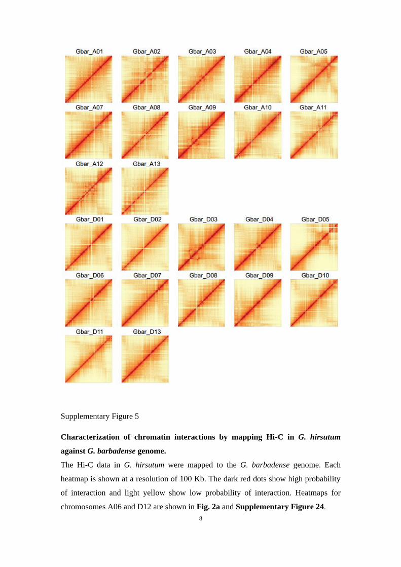
Supplementary Figure 5
Characterization of chromatin interactions by mapping Hi-C in G. hirsutum
against G. barbadense genome.
The Hi-C data in G. hirsutum were mapped to the G. barbadense genome. Each
heatmap is shown at a resolution of 100 Kb. The dark red dots show high probability
of interaction and light yellow show low probability of interaction. Heatmaps for
chromosomes A06 and D12 are shown in Fig. 2a and Supplementary Figure 24.
Page 10
9
Supplementary Figure 6
Comparison of Hi-C directed chromosome assembly with genetic map for the A-
subgenome in G. hirsutum.
The assembled chromosomes based on Hi-C data were compared with the previously
published genetic map between G. hirsutum and G. barbadense32. The x-axes show
position of sequences in assembled chromosomes (Mb) and the y-axes show the
position of sequences on the genetic map (cM).
Page 11
10
Supplementary Figure 7
Comparison of Hi-C directed chromosome assembly with genetic map for the D-
subgenome in G. hirsutum.
The assembled chromosomes based on Hi-C data were compared with the previously
published genetic map between G. hirsutum and G. barbadense. The x-axes show
position of sequences in assembled chromosomes (Mb) and the y-axes show the
position of sequences on the genetic map (cM).
Page 12
11
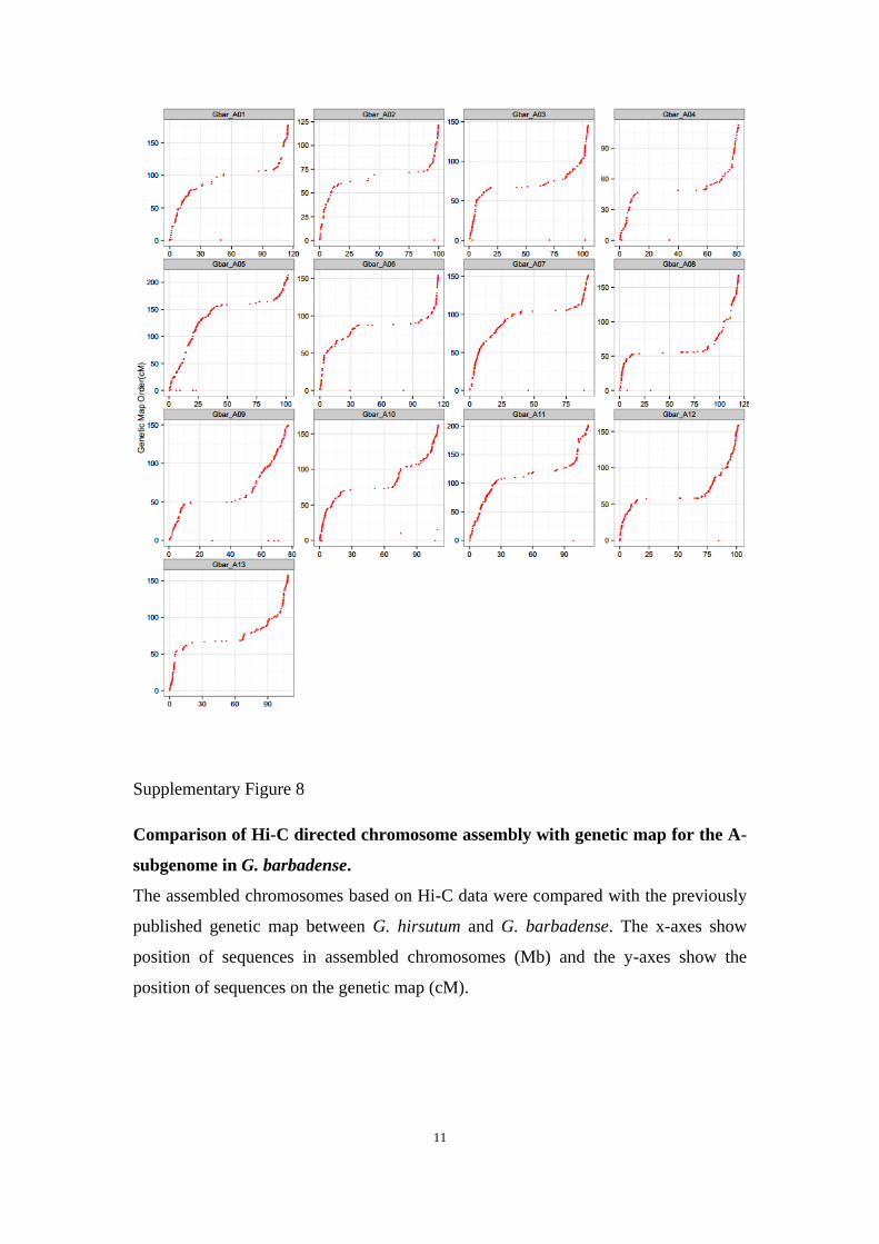
Supplementary Figure 8
Comparison of Hi-C directed chromosome assembly with genetic map for the A-
subgenome in G. barbadense.
The assembled chromosomes based on Hi-C data were compared with the previously
published genetic map between G. hirsutum and G. barbadense. The x-axes show
position of sequences in assembled chromosomes (Mb) and the y-axes show the
position of sequences on the genetic map (cM).
Page 13
12
Supplementary Figure 9
Comparison of Hi-C directed chromosome assembly with genetic map for the D-
subgenome in G. barbadense.
The assembled chromosomes based on Hi-C data were compared with the previously
published genetic map between G. hirsutum and G. barbadense. The x-axes show
position of sequences in assembled chromosomes (Mb) and the y-axes show the
position of sequences on the genetic map (cM).
Page 14
13
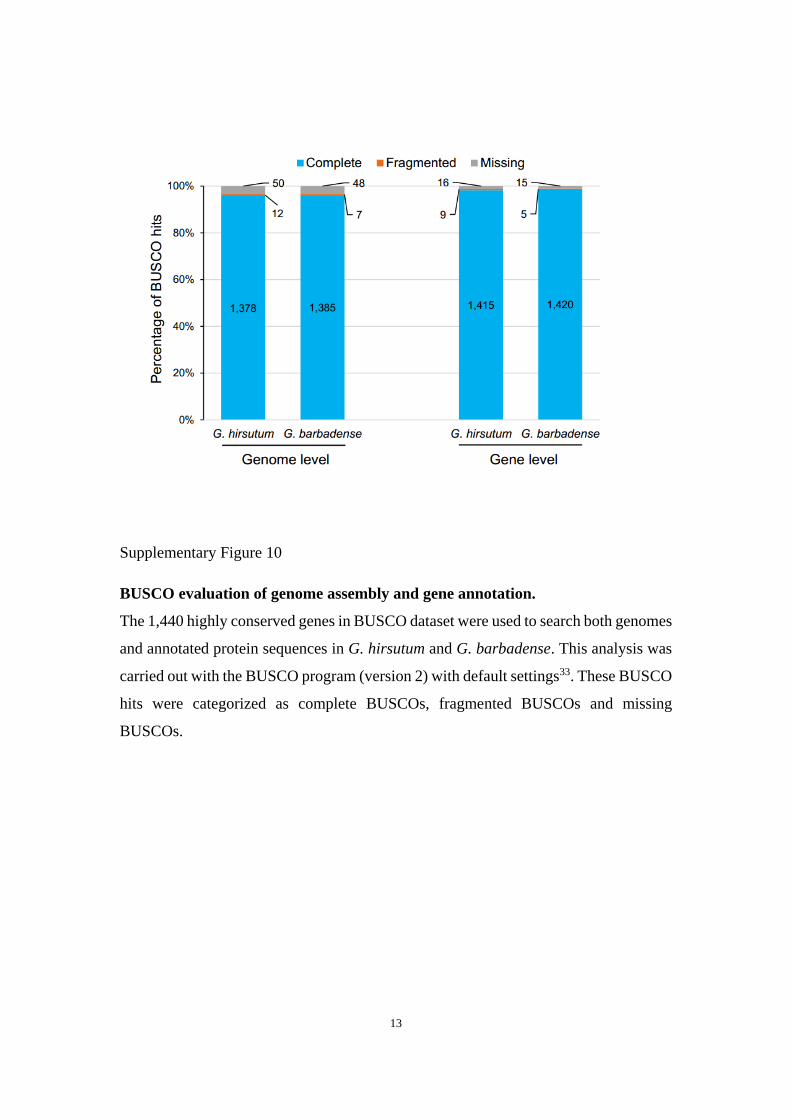
Supplementary Figure 10
BUSCO evaluation of genome assembly and gene annotation.
The 1,440 highly conserved genes in BUSCO dataset were used to search both genomes
and annotated protein sequences in G. hirsutum and G. barbadense. This analysis was
carried out with the BUSCO program (version 2) with default settings33. These BUSCO
hits were categorized as complete BUSCOs, fragmented BUSCOs and missing
BUSCOs.
Page 15
14
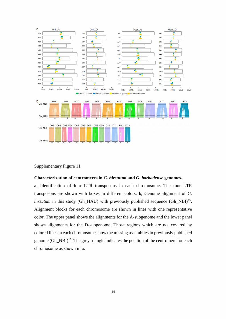
Supplementary Figure 11
Characterization of centromeres in G. hirsutum and G. barbadense genomes.
a, Identification of four LTR transposons in each chromosome. The four LTR
transposons are shown with boxes in different colors. b, Genome alignment of G.
hirsutum in this study (Gh_HAU) with previously published sequence (Gh_NBI)15.
Alignment blocks for each chromosome are shown in lines with one representative
color. The upper panel shows the alignments for the A-subgenome and the lower panel
shows alignments for the D-subgenome. Those regions which are not covered by
colored lines in each chromosome show the missing assemblies in previously published
genome (Gh_NBI)15. The grey triangle indicates the position of the centromere for each
chromosome as shown in a.
Page 16
15
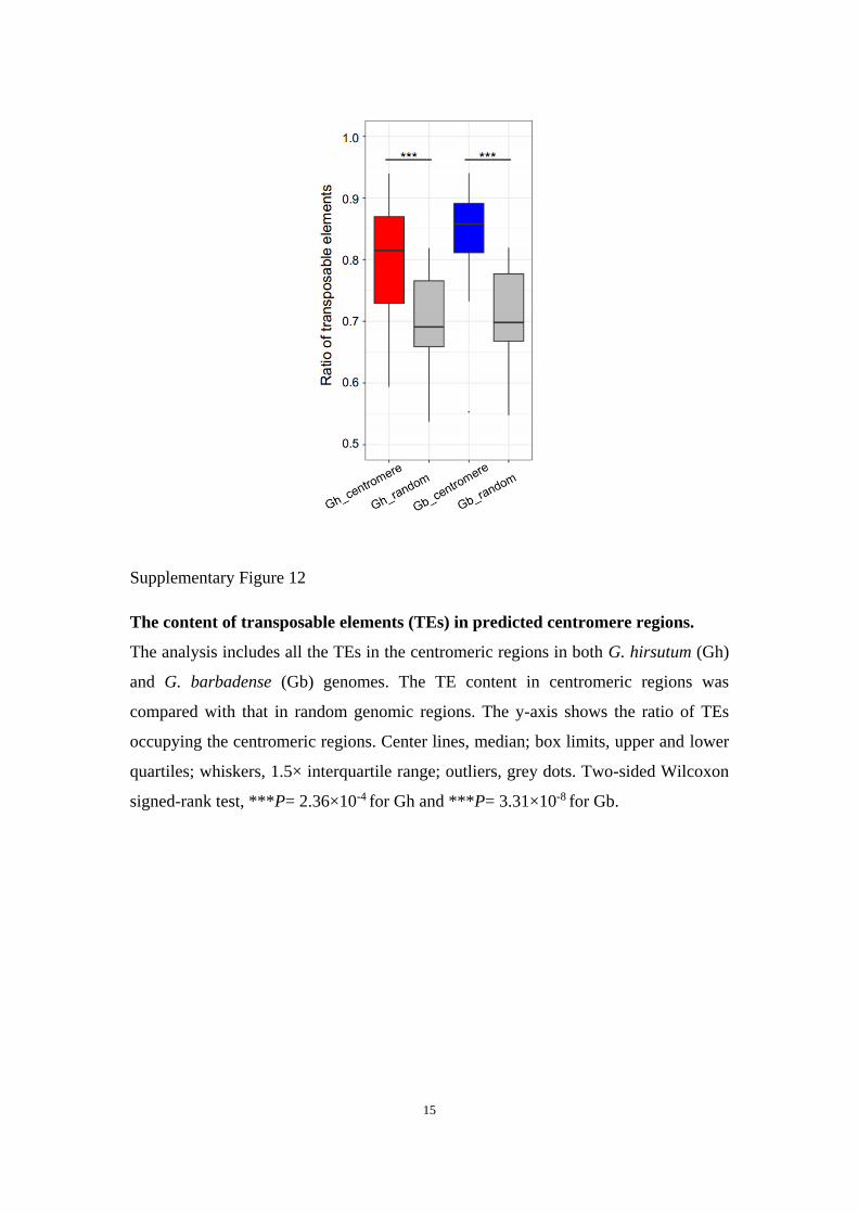
Supplementary Figure 12
The content of transposable elements (TEs) in predicted centromere regions.
The analysis includes all the TEs in the centromeric regions in both G. hirsutum (Gh)
and G. barbadense (Gb) genomes. The TE content in centromeric regions was
compared with that in random genomic regions. The y-axis shows the ratio of TEs
occupying the centromeric regions. Center lines, median; box limits, upper and lower
quartiles; whiskers, 1.5× interquartile range; outliers, grey dots. Two-sided Wilcoxon
signed-rank test, ***P= 2.36×10⁻⁴ for Gh and ***P= 3.31×10⁻⁸ for Gb.
Page 17
16
Supplementary Figure 13
Density distribution of SNPs in the A and D subgenomes.
In this analysis, each chromosome was split into 1-Mb windows sliding 200-Kb. SNPs
in each window were counted and compared with the total bases after discarding gaps.
The x-axis shows the number of SNPs in each 1-Kb sequence. The red line indicates
SNP distribution in the A-subgenome and green line indicates SNP distribution in the
D-subgenome.
Page 18
17
Supplementary Figure 14
The length distribution of small insertions/deletions (InDels) in cotton genomes.
a, The length of insertions and deletions in the G. barbadense genome by comparing
with G. hirsutum. b, The length of insertions and deletions in the G. hirsutum genome
by comparing with G. barbadense. For a and b, all InDels were categorized into those
from gene coding sequences (CDS), introns, un-translated regions (UTR) and
intergenic regions. All these variants were annotated by ANNOVAR program34.
Page 19
18
Supplementary Figure 15
The number of genes affected by SNPs and InDels.
This analysis involves SNPs and InDels which may have functional effects on genes
including variations on transcription splicing, frameshift, gain of stop codon and loss
of stop codon. The yellow histogram shows data for G. barbadense and the blue
histogram shows data for G. hirsutum. All these variants were annotated using the
ANNOVAR program34. This figure includes a total of 14,076 genes in G. hirsutum and
14,880 genes in G. barbadense.
Page 20
19
Supplementary Figure 16
Gene ontology (GO) enrichment analysis of positively selected genes.
In this analysis, GO terms for biological processes for 4,039 positively selected genes
were compared with those of genes at the whole genome level. The red dashed line
shows the cutoff of significance. The two-sided Fisher’s exact test was used for
significance analysis (False discovery rate, FDR <0.05).
Page 21
20
Supplementary Figure 17
Genome alignment of the G. hirsutum and G. barbadense.
Both genome sequences are assembled in this study. Alignment blocks for each
chromosome are shown in lines with one representative color. The upper panel shows
the alignments for the A-subgenome and the lower panel shows alignments for the D-
subgenome. These genome alignments were parsed using the MUMmer (version 3.23)
program35.
Page 22
21
Supplementary Figure 18
Gene synteny between G. hirsutum and G. barbadense for A- and D-subgenomes.
a, Dot plot showing gene synteny in the A-subgenome (chromosome A01-A13)
between G. hirsutum (x-axis) and G. barbadense (y-axis). b, Dot plot showing gene
synteny in the D-subgenome (chromosome D01-D13) between G. hirsutum (x-axis)
and G. barbadense (y-axis). Genome alignment was carried out using the MCScanX
package36. Each syntenic block has at least five genes.
Page 23
22
Supplementary Figure 19
Gene synteny between A- and D-subgenomes in G. hirsutum and G. barbadense.
a, Dot plot showing gene synteny between the A- and D-subgenomes in G. hirsutum.
b, Dot plot showing gene synteny between the A- and D-subgenomes in G. barbadense.
For a and b, the x-axes show chromosomes in the A-subgenome and y-axes show
chromosomes in the D-subgenome. The genome alignment was carried out using the
MCScanX package36. Each syntenic block has at least five genes.
Page 24
23
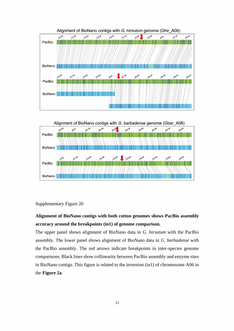
Supplementary Figure 20
Alignment of BioNano contigs with both cotton genomes shows PacBio assembly
accuracy around the breakpoints (in1) of genome comparison.
The upper panel shows alignment of BioNano data in G. hirsutum with the PacBio
assembly. The lower panel shows alignment of BioNano data in G. barbadense with
the PacBio assembly. The red arrows indicate breakpoints in inter-species genome
comparisons. Black lines show collinearity between PacBio assembly and enzyme sites
in BioNano contigs. This figure is related to the inversion (in1) of chromosome A06 in
the Figure 2a.
Page 25
24
Supplementary Figure 21
Alignment of BioNano contigs with both cotton genomes shows PacBio assembly
accuracy around the breakpoints (in2) of genome comparison.
The upper panel shows alignment of BioNano data in G. hirsutum with the PacBio
assembly. The lower panel shows alignment of BioNano data in G. barbadense with
the PacBio assembly. The red arrows indicate breakpoints in inter-species genome
comparisons. Black lines show collinearity between PacBio assembly and enzyme sites
in BioNano contigs. This figure is related to the inversion (in2) of chromosome A06 in
the Figure 2a.
Page 26
25
Supplementary Figure 22
Alignment of BioNano contigs with both cotton genomes shows PacBio assembly
accuracy around the breakpoints (in3) of genome comparison.
The upper panel shows alignment of BioNano data in G. hirsutum with the PacBio
assembly. The lower panel shows alignment of BioNano data in G. barbadense with
the PacBio assembly. The red arrows indicate breakpoints in inter-species genome
comparisons. Black lines show collinearity between PacBio assembly and enzyme sites
in BioNano contigs. This figure is related to the inversion (in3) of chromosome A06 in
the Figure 2a.
Page 27
26
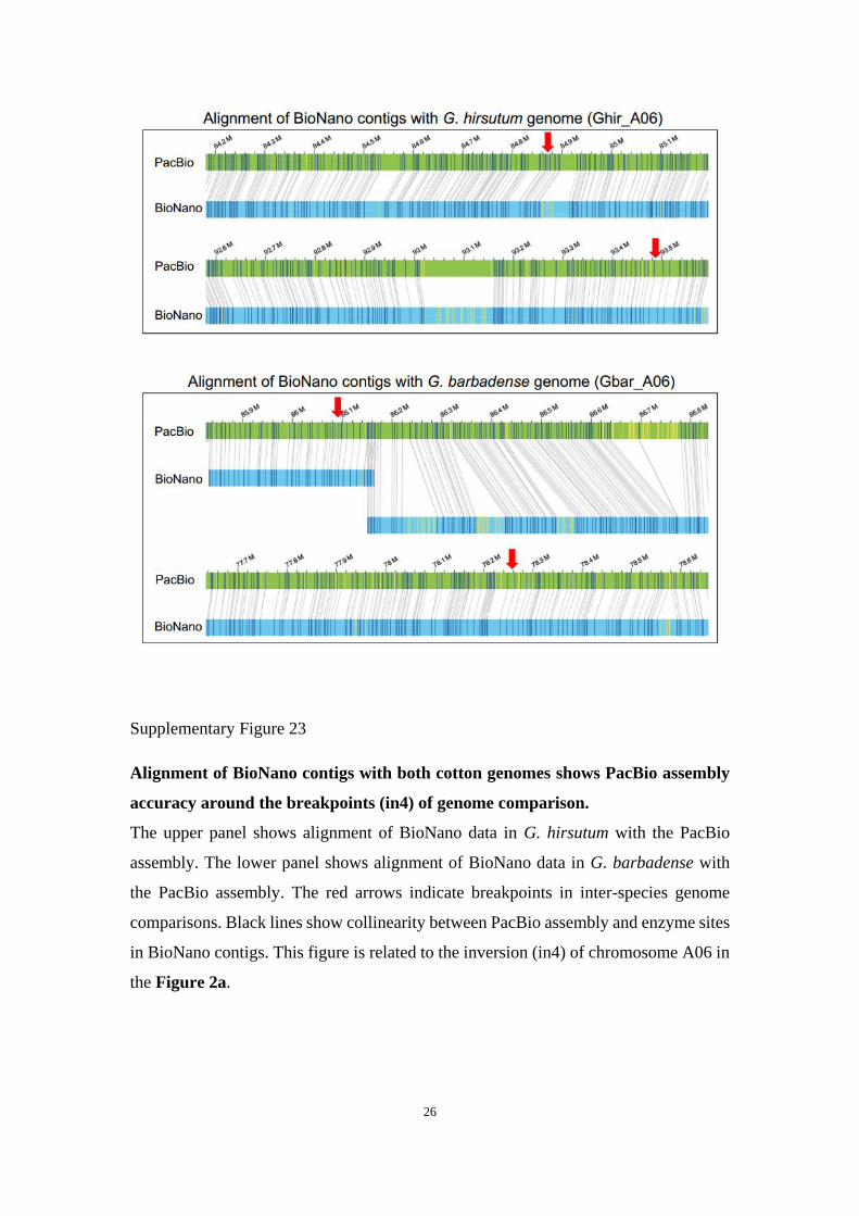
Supplementary Figure 23
Alignment of BioNano contigs with both cotton genomes shows PacBio assembly
accuracy around the breakpoints (in4) of genome comparison.
The upper panel shows alignment of BioNano data in G. hirsutum with the PacBio
assembly. The lower panel shows alignment of BioNano data in G. barbadense with
the PacBio assembly. The red arrows indicate breakpoints in inter-species genome
comparisons. Black lines show collinearity between PacBio assembly and enzyme sites
in BioNano contigs. This figure is related to the inversion (in4) of chromosome A06 in
the Figure 2a.
Page 28
27
Supplementary Figure 24
Hi-C data supports a pericentromeric inversion in chromosome D12.
The upper track shows the chromatin interaction matrix with Hi-C data mapping against
the G. barbadense genome. These include Hi-C data in G. barbadense mapping G.
barbadense genome (Gb_map_Gb), Hi-C data in G. hirsutum mapping G. barbadense
genome (Gh_map_Gb), and Hi-C data in G. barbadense mapping G. barbadense
genome with the reordering of this inversion region (Gb_map_Gb_reorder). The middle
track shows the alignment of G. barbadense against G. hirsutum. The centromere
region is shown by a grey triangle. The lower track shows the chromatin interaction
matrix with Hi-C data mapping against the G. hirsutum genome. These include Hi-C
data in G. hirsutum mapping G. hirsutum genome (Gh_map_Gh), Hi-C data in G.
barbadense mapping G. hirsutum genome (Gb_map_Gh), and Hi-C data in G. hirsutum
mapping G. hirsutum genome with the reordering of this inversion region
(Gh_map_Gh_reorder). Red dots show higher probability of chromatin contacts while
yellow dots show lower probability of contacts.
Page 29
28
Supplementary Figure 25
Alignment of BioNano contigs with both cotton genomes shows PacBio assembly
accuracy around the breakpoints of genome comparison in the chromosome D12.
The upper panel shows alignment of BioNano data in G. hirsutum with the PacBio
assembly. The lower panel shows alignment of BioNano data in G. barbadense with
the PacBio assembly. The red arrows indicate breakpoints in inter-species genome
comparison. Black lines show collinearity between PacBio assembly and enzyme sites
in BioNano contigs. This figure is related to the inversion of chromosome D12 in the
Supplementary Figure 24.
Page 30
29
Supplementary Figure 26
Expression patterns of genes in presence/absence variation regions.
a, Heatmap showing expression patterns of genes in the unique presence regions in G.
hirsutum. b, Heatmap showing expression patterns of genes in the unique presence
regions in G. barbadense. Those genes which have no expression levels in all samples
were not included in this analysis. This figure (a and b) shows the comparison of
expression levels of each gene in different tissues/samples. The RNA-Seq data used in
this analysis were published previously15,16. DPA, days post anthesis.
Page 31
30
Supplementary Figure 27
Genome alignment for the Expansin gene region between G. hirsutum and G.
barbadense.
Compared with the EXPANSIN gene (Ghir_A10G015240) in G. hirsutum, the
homologous gene (Gbar_A10G016120) in G. barbadense has a 450 bp deletion in the
third exon. The middle grey box shows alignment between the two genomes. The upper
and lower tracks show the coordinates (at the bp level) of chromosome A10 in G.
barbadense and G. hirsutum respectively. For each gene model, the coding regions are
shown in red, and the 5' and 3' untranslated regions are shown in white.
Page 32
31
Supplementary Figure 28
Short-reads mapping supports a 450-bp deletion in an Expansin gene in different
G. barbadense accessions.
In this analysis, Illumina short reads of 13 G. hirsutum accessions including TM-1 and
16 G. barbadense accessions including 3-79 were mapped to the G. hirsutum genome.
These Illumina sequencing data were downloaded from the NCBI SRA database. Each
SRA accession number (SRR1534918-SRR1975564) represents one cotton accession
which was described in a previous publication29.
Page 33
32
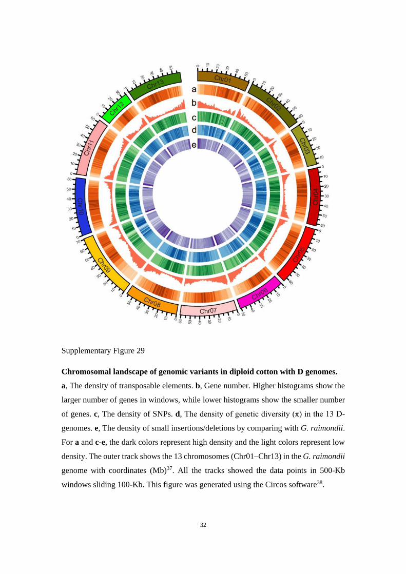
Supplementary Figure 29
Chromosomal landscape of genomic variants in diploid cotton with D genomes.
a, The density of transposable elements. b, Gene number. Higher histograms show the
larger number of genes in windows, while lower histograms show the smaller number
of genes. c, The density of SNPs. d, The density of genetic diversity (π) in the 13 D-
genomes. e, The density of small insertions/deletions by comparing with G. raimondii.
For a and c-e, the dark colors represent high density and the light colors represent low
density. The outer track shows the 13 chromosomes (Chr01–Chr13) in the G. raimondii
genome with coordinates (Mb)37. All the tracks showed the data points in 500-Kb
windows sliding 100-Kb. This figure was generated using the Circos software38.
Page 34
33
Supplementary Figure 30
Phylogenetic analysis of D-subgenomes in tetraploid cotton with diploids.
a, Phylogenetic analysis of D genomes in diploids with the D-subgenomes of wild and
domesticated tetraploids. This analysis was conducted using the snphylo software by
using all the SNPs in each species. b, Principal component analysis (PCA) of D
genomes in diploids with D-subgenomes in tetraploids. The 13 diploids are shown in
pink cycles, while the other tetraploids are shown in brown for G. hirsutum (Gh) and
blue for G. barbadense (Gb). All these accessions are the same as those in a. The x-
axis shows the first component and the y-axis shows the second component with
contribution values shown in parentheses. The red arrows in a and b show G. raimondii
(D5 genome). The variants for tetraploids in this analysis were published previously29.
Page 35
34
Supplementary Figure 31
Ks (synonymous substitution rate) distribution of diploid cotton with tetraploid
subgenomes.
In this analysis, all the SNPs in coding sequences of genes are included. Data in
different species are represented in different colors. The data from the comparison of
D5 against the D-subgenome in G. hirsutum (GhDt) is highlighted with a black arrow
(D5_vs_GhDt). The x-axis shows Ks value and the y-axis shows the distribution density
in each comparison.
Page 36
35
Supplementary Figure 32
Characterization of chromatin interactions by mapping Hi-C data in G. arboreum
against the A-subgenomes of G. hirsutum (Ghir) and G. barbadense (Gbar).
The discrete interaction shows where a chromosome rearrangement may occur. Each
heatmap is shown at a resolution of 100 Kb. The dark red dots show high probability
of interaction and light yellow show low probability of intetraction. Heatmaps for
chromosomes A06 are shown in Supplementary Figure 33.
Page 37
36
Supplementary Figure 33
Mapping of Hi-C data in G. arboreum against the A-subgenomes of both
tetraploids supports an inversion in chromosome A06.
a, Chromatin interactions in the A06 chromosome by mapping Hi-C data in G.
arboreum (Ga) against G. hirsutum (Gh). b, Chromatin interactions in the A06
chromosome by mapping Hi-C data in G. arboreum (Ga) against G. barbadense (Gb).
The pericentric inversion is shown in the left heatmap, which is the same as that in the
Fig. 2a. Each heatmap is shown at a resolution of 100 Kb. The dark red dots show high
probability of interaction and light yellow show low probability of intetraction.
Page 38
37
Supplementary Figure 34
The flowchart for construction of cotton introgression lines.
The elite G. hirsutum Emian22 was used as a recurrent parent and G. barbadense 3-79
was used as a donor parent. This introgression population was constructed with a ten-
year effort (from 2004 to 2014). For identification of introgression segments, the first
genetic map (MAP1) was used for a whole genome survey and the second genetic map
(MAP2) was only used in target regions. The final population has 148 multiple
chromosome segment substitution lines (CSSLs) and 177 single chromosome segment
substitution lines (SSSLs).
Page 39
38
Supplementary Figure 35
Correlation of the expression level of gene (Ghir_A02G003440) with fiber length.
a, RNA-Seq data show the expression level of gene (Ghir_A02G003440) in fibers at
10 days post anthesis (DPA). The gene expression level (FPKM) in each fiber sample
was calculated by Cufflinks software39. b, Quantitative real‐time (qRT) PCR result of
gene (Ghir_A02G003440) expression in fibers at 10 DPA. The expression level was
normalized using UB7 as described previously40. Barplots, average values; error bars,
± SD of three independent experiments (n=3); blue circle points, true expression values
(n=3). For a and b, Emian22 (G. hirsutum) and 3-79 (G. barbadense) represent parents
of the introgression line population; and N54, N55, N181 and N182 represent four
introgression lines with an introgression segment (2.97–3.94 Mb) containing this gene
from G. barbadense. c, Scatter-plot showing the negative correlation between gene
Page 40
39
expression (Ghir_A02G003440) from RNA-Seq and fiber length in the introgression
line population. This plot includes 170 samples including all the introgressions lines
(168) and their two parents. The Pearson's correlation coefficient (r= -0.3443) was
estimated with a R function (two-sided method, P-value = 4.27×10⁻⁶). d, Box-plot
showing the distribution of normalized expression (log2(FPKM)) by categorizing all
the 170 samples into 5 groups based on fiber length. Group1 has 29 lines with fiber
length <27.5 mm, Group2 has 48 lines with fiber length between 27.5 mm and 28.0
mm, Group3 has 38 lines with fiber length between 28 mm and 28.5 mm, Group4 has
29 lines with fiber length between 28.5 mm and 29.0 mm, and Group5 has 26 lines with
fiber length >29.0 mm. Center lines, median; box limits, upper and lower quartiles;
whiskers, 1.5× interquartile range; outliers, black dots.
Page 41
40
Supplementary Tables
Supplementary Table 1 Summary of PacBio reads for two tetraploid cotton
accessions. These represent a summary of raw sequence data generated from PacBio
RSII and reads after filtering.
Species Filter
Total read bases
(bp)
Read
number
Read
N50
Mean
read
length
Average
read
quality
G. hirsutum
(TM-1)
before filtering 204,761,480,176 28,405,188 18,676 7,209 0.48
after filtering 194,404,226,471 16,125,309 18,849 12,056 0.84
G. barbadense
(3-79)
before filtering 219,544,837,024 30,058,400 16,215 7,303 0.53
after filtering 211,529,794,660 17,834,884 16,410 11,860 0.83
Page 42
41
Supplementary Table 2 Summary of subreads for tetraploid cotton accessions.
These are from further filtering of reads with too small size and sequencing adapters.
Species Length (bp) Number Total length (bp) Average length (bp)
G. hirsutum
0-2000 2,447,018 3,230,659,903 1,320
2000-4000 3,026,992 8,891,791,456 2,938
4000-6000 2,648,467 13,218,284,548 4,991
6000-8000 2,540,876 17,762,995,632 6,991
8000-10000 2,395,505 21,545,507,249 8,994
10000-12000 2,157,357 23,669,089,839 10,971
12000-14000 1,750,913 22,693,966,931 12,961
14000-16000 1,431,608 21,430,103,620 14,969
16000-18000 1,129,035 19,133,125,558 16,946
>18000 1,937,952 42,431,520,455 21,895
Total 21,465,723 194,007,045,191 9,038
G. barbadense
0-2000 3,864,875 5,460,210,344 1,413
2000-4000 4,101,616 11,636,400,973 2,837
4000-6000 2,878,489 14,334,616,635 4,980
6000-8000 2,586,218 18,053,890,821 6,981
8000-10000 2,298,260 20,638,352,654 8,980
10000-12000 2,146,968 23,617,288,198 11,000
12000-14000 2,073,358 26,909,972,288 12,979
14000-16000 1,628,586 24,328,464,469 14,938
16000-18000 1,095,399 18,544,974,075 16,930
>18000 2,098,587 47,454,374,098 22,613
Total 24,772,356 210,978,544,555 8,517
Page 43
42
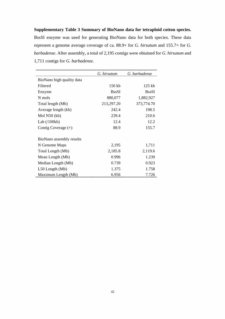
Supplementary Table 3 Summary of BioNano data for tetraploid cotton species.
BssSI enzyme was used for generating BioNano data for both species. These data
represent a genome average coverage of ca. 88.9× for G. hirsutum and 155.7× for G.
barbadense. After assembly, a total of 2,195 contigs were obtained for G. hirsutum and
1,711 contigs for G. barbadense.
G. hirsutum G. barbadense
BioNano high quality data
Filtered 150 kb 125 kb
Enzyme BssSI BssSI
N mols 880,077 1,882,927
Total length (Mb) 213,297.20 373,774.70
Average length (kb) 242.4 198.5
Mol N50 (kb) 239.4 210.6
Lab (/100kb) 12.4 12.2
Contig Coverage (×) 88.9 155.7
BioNano assembly results
N Genome Maps 2,195 1,711
Total Length (Mb) 2,185.8 2,119.6
Mean Length (Mb) 0.996 1.239
Median Length (Mb) 0.739 0.923
L50 Length (Mb) 1.375 1.758
Maximum Length (Mb) 6.956 7.726
Page 44
43
Supplementary Table 4 Summary of genome assemblies for cotton species. This table shows metrics of contigs and scaffolds in four genome
assembly stages. The PacBio Assembly column shows the original metrics of contigs by using PacBio data. The Hi-C Grouping column shows
the final metrics for both genomes.
Statistics
PacBio
Assembly
BioNano
Corrected
BioNano
Scaffolding*
BioNano
Scaffolding# Hi-C Grouping
G. hirsutum
Contig/Scaffold number 3,900 4,378 4,746 3,434 2,190
Contig/Scaffold length 2,279,141,197 2,279,141,197 2,281,853,441 2,347,017,486 2,347,160,336
Contig/Scaffold N50 (bp) 2,105,682 1,941,992 1,891,906 5,224,257 97,738,592
Contig/Scaffold N90 (bp) 309,067 268,419 227,891 559,537 56,408,347
Contig/Scaffold Max (bp) 25,517,463 25,517,463 25,005,934 28,168,993 124,007,235
Gap length (bp) 0 0 0 65,164,045 65,164,045
G. barbadense
Contig/Scaffold number 4,532 4,793 4,930 3,919 3,032
Contig/Scaffold length 2,222,455,976 2,222,455,976 2,222,525,789 2,266,656,771 2,266,746,731
Contig/Scaffold N50 (bp) 2,309,033 2,274,153 2,151,565 6,891,847 92,880,876
Contig/Scaffold N90 (bp) 345,101 310,032 295,036 673,086 51,526,817
Contig/Scaffold Max (bp) 19,604,892 19,604,892 19,605,216 24,400,926 119,882,356
Gap length (bp) 0 0 0 44,130,982 44,130,982
*Characterization of contigs after BioNano scaffolding.
#Characterization of scaffolds after BioNano scaffolding.
Page 45
44
Supplementary Table 5 Summary of Hi-C reads mapping. This information was
obtained using the HiC-Pro software.
Number of Reads Percentage%
G. hirsutum
Total read pairs 513,574,899 100
Uniquely mapped read pairs 302,541,679 58.91
Valid interaction pairs 175,245,872 34.12
Dangling end pairs 103,469,125 20.15
Re-ligation pairs 10,555,014 2.06
Self-cycle pairs 7,413,146 1.44
Dumped pairs 5,858,522 1.14
G. barbadense
Total read pairs 489,551,129 100
Uniquely mapped read pairs 301,975,255 61.68
Valid interaction pairs 184,445,111 37.68
Dangling end pairs 96,244,323 19.66
Re-ligation pairs 3,683,712 0.75
Self-cycle pairs 11,847,417 2.42
Dumped pairs 5,754,692 1.18
Page 46
45
Supplementary Table 6 Summary of the Hi-C grouping result in each
chromosome. This table shows the number of scaffolds which were anchored and their
total length by LACHESIS software in both genomes.
G. hirsutum G. barbadense
Chr* Scaffold number Total length Chr Scaffold number Total length
A01 151 122,457,788 A01 146 119,613,973
A02 116 110,592,961 A02 73 104,069,895
A03 128 117,239,150 A03 91 107,755,541
A04 114 90,261,271 A04 95 84,713,681
A05 92 114,230,473 A05 111 109,023,791
A06 158 129,848,352 A06 146 119,344,906
A07 105 100,928,286 A07 97 96,394,192
A08 217 130,050,879 A08 120 123,260,820
A09 81 85,126,726 A09 81 80,434,361
A10 132 119,219,355 A10 75 112,880,626
A11 112 127,032,608 A11 129 119,187,993
A12 128 111,421,337 A12 92 104,863,077
A13 125 114,905,076 A13 122 113,429,765
D01 34 66,001,629 D01 38 64,226,660
D02 54 72,997,442 D02 49 69,171,070
D03 30 55,429,277 D03 43 53,705,698
D04 30 58,525,357 D04 31 56,516,165
D05 39 67,747,306 D05 69 66,801,527
D06 32 67,837,932 D06 28 63,656,615
D07 37 60,118,816 D07 39 58,990,986
D08 61 71,105,725 D08 41 67,293,257
D09 39 54,499,262 D09 44 53,716,294
D10 41 70,082,484 D10 51 67,696,783
D11 25 74,061,581 D11 68 72,801,813
D12 47 64,684,132 D12 36 61,543,513
D13 40 65,753,992 D13 51 63,030,776
*The pseudo-chromosomes.
Page 47
46
Supplementary Table 7 Alignment of the previously published genetic map against
the Hi-C directed pseudochromosomes32. A total of 4,049 bins were used to aligned
to both genomes. This genetic map covered 310 and 336 scaffolds in G. hirsutum and
G. barbadense, respectively. The consensus ratios between Hi-C assemblies and
genetic map were estimated to be 98.86% in G. hirsutum and 96.92% in G. barbadense.
Species
Total bin
number
(Markers)
Aligned bin
number
Aligned scaff
-old number
Aligned
length (%)
Consensus
ratio
G. hirsutum 4,049 3,915 310 1,580,481,685
(67.34%) 98.86%
G. barbadense 4,049 3,598 336 1,699,132,210
(74.96%) 96.92%
Page 48
47
Supplementary Table 8 The alignment results of BAC sequences against G.
hirsutum genome. These BAC sequences were downloaded from NCBI Nucleotide
database (https://www.ncbi.nlm.nih.gov/nuccore/).
Origin BAC ID
BAC
length Chr Start (bp) End (bp)
Identity
%
Coverage
%
TM-1 HQ650105.1 35,934 Ghir_A12 107,501,325 107,537,209 99.85 100
TM-1 HQ650106.1 121,433 Ghir_D12 62,404,074 62,525,401 99.89 100
TM-1 HQ650107.1 110,706 Ghir_A12 37,060,357 37,191,853 99.90 100
TM-1 HQ650108.1 60,529 Ghir_D12 22,355,640 22,416,146 99.95 100
Maxxa AY632359.1 103,930 Ghir_A10 2,809,673 2,913,428 99.64 100
Maxxa AY632360.1 135,862 Ghir_D10 3,326,965 3,466,272 99.50 100
Maxxa AC243131.1 121,823 Ghir_D12 1,114,303 1,235,970 99.79 100
Maxxa AC243133.1 163,851 Ghir_A01 65,506,551 65,664,238 99.80 96.3
Maxxa AC243137.1 137,066 Ghir_A10 104,632,700 104,769,570 99.81 100
Maxxa AC243138.1 132,457 Ghir_D02 55,811,730 55,944,217 99.24 100
Maxxa AC243139.1 58,716 Ghir_D11 53,686,893 53,745,592 99.94 100
Maxxa AC243140.1 110,533 Ghir_D08 40,406,854 40,517,270 99.85 100
Maxxa AC243141.1 89,174 Ghir_D12 15,425,487 15,514,614 99.92 100
Maxxa AC243142.1 102,430 Ghir_D12 59,141,356 59,243,684 99.70 100
Maxxa AC243143.1 137,405 Ghir_A12 99,876,139 100,013,448 99.88 100
Maxxa AC243144.1 94,928 Ghir_D02 23,485,105 23,579,928 99.85 100
Maxxa AC243145.1 134,387 Ghir_D11 30,393,122 30,527,353 99.76 100
Maxxa AC243146.1 141,129 Ghir_D12 55,249,741 55,390,746 99.84 100
Maxxa AC243148.1 108,382 Ghir_A11 16,570,617 16,679,004 99.92 100
Maxxa AC243149.1 113,692 Ghir_D12 46,488,826 46,602,375 99.80 100
Maxxa AC243150.1 86,390 Ghir_D07 54,320,125 54,406,404 99.76 100
Maxxa AC243151.1 108,361 Ghir_D01 8,225,818 8,334,043 99.82 100
Maxxa AC243152.1 104,306 Ghir_D01 29,045,423 29,149,628 99.64 100
Maxxa AC243153.1 152,015 Ghir_D12 29,921,755 30,073,703 99.92 100
Maxxa AC243154.1 104,636 Ghir_D01 17,060,395 17,164,944 99.85 100
Maxxa AC243155.1 120,301 Ghir_A12 1,114,872 1,235,019 99.70 100
Maxxa AC243156.1 119,216 Ghir_A12 34,021,921 34,162,178 99.89 100
Maxxa AC243157.1 144,980 Ghir_A01 20,968,327 21,113,532 99.79 100
Maxxa AC243158.1 118,603 Ghir_D01 37,436,367 37,554,910 99.91 100
Maxxa AC243159.1 58,828 Ghir_D10 26,935,828 26,994,641 99.90 100
Maxxa AC243160.1 113,785 Ghir_A01 19,250,133 19,363,789 99.79 100
Maxxa AC243161.1 59,488 Ghir_A12 86,989,295 87,047,968 99.50 100
Maxxa AC243162.1 98,696 Ghir_A06 113,059,465 113,158,096 99.81 100
Maxxa AC243163.1 138,301 Ghir_A12 25,759,535 25,990,628 99.69 100
Maxxa AC243164.1 113,782 Ghir_D01 15,199,570 15,313,224 99.70 100
Maxxa AC243165.1 142,351 Ghir_A12 100,667,287 100,809,454 99.72 100
Page 49
48
Supplementary Table 9 Summary of short reads mapping in both genomes. These
data were generated previously15,41, from the same accessions (TM-1 and 3-79) as those
for PacBio sequencing in this study. The paired-end (PE) data were mapped against
their respective genome by BWA software with default settings (the mem option).
Species Library* Accession
number
Number of
read pairs
Read
length
Data
(Gb)
Mapping
percentag
e (%)
~0.5 Kb SRX849524,
SRX849525 220,716,818 PE100 44.1 98.72
G. hirsutum
(TM-1) ~5 Kb SRX849531 242,651,604 PE100 48.5 98.07
~10 Kb SRX849536 209,442,706 PE100 41.8 96.80
~0.5 Kb SRX669474 413,387,034 PE100 82.6 99.35
G. barbadense
(3-79) ~5 Kb SRX2676956 475,547,319 PE75 71.3 99.97
~10 Kb SRX2676957 421,377,268 PE75 63.2 99.92
*The library insertion size.
Page 50
49
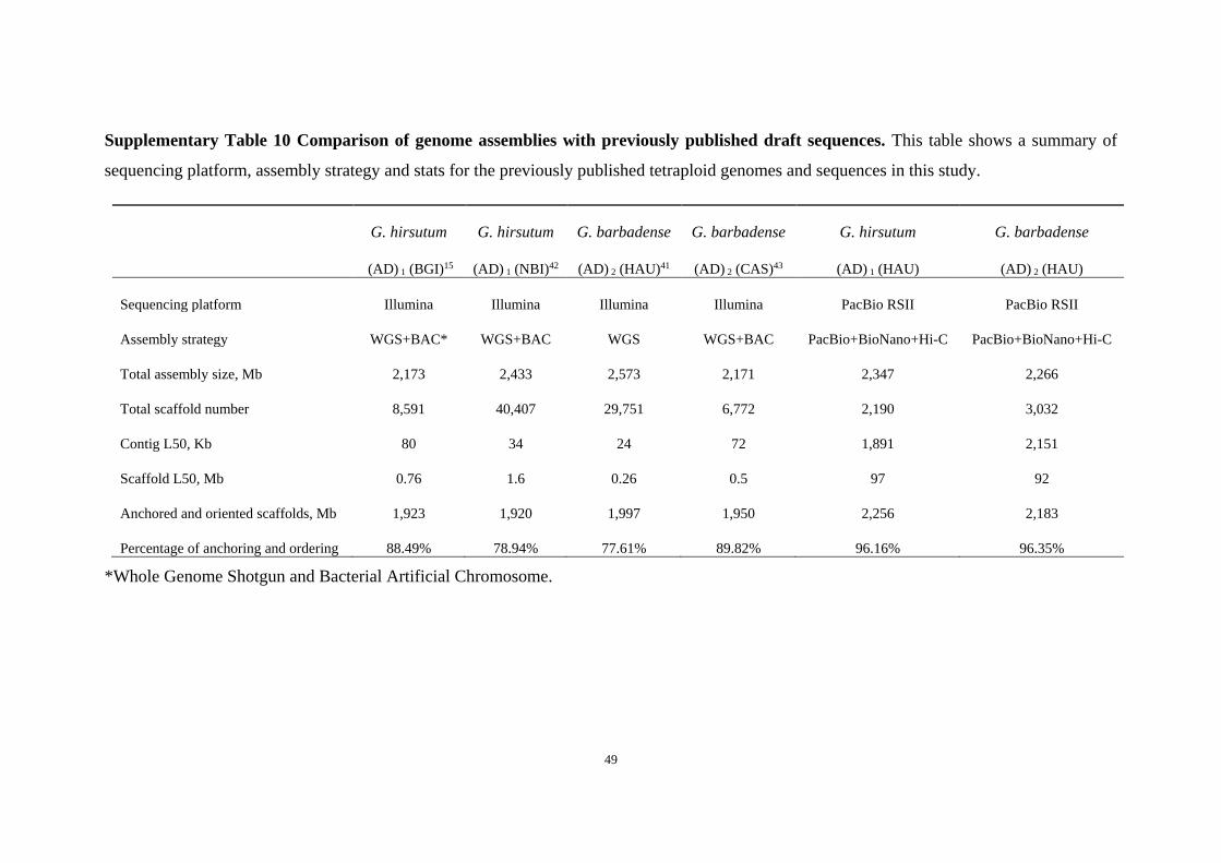
Supplementary Table 10 Comparison of genome assemblies with previously published draft sequences. This table shows a summary of
sequencing platform, assembly strategy and stats for the previously published tetraploid genomes and sequences in this study.
G. hirsutum G. hirsutum G. barbadense G. barbadense G. hirsutum G. barbadense
(AD) 1 (BGI)15 (AD) 1 (NBI)42 (AD) 2 (HAU)41 (AD) 2 (CAS)43 (AD) 1 (HAU) (AD) 2 (HAU)
Sequencing platform Illumina Illumina Illumina Illumina PacBio RSII PacBio RSII
Assembly strategy WGS+BAC* WGS+BAC WGS WGS+BAC PacBio+BioNano+Hi-C PacBio+BioNano+Hi-C
Total assembly size, Mb 2,173 2,433 2,573 2,171 2,347 2,266
Total scaffold number 8,591 40,407 29,751 6,772 2,190 3,032
Contig L50, Kb 80 34 24 72 1,891 2,151
Scaffold L50, Mb 0.76 1.6 0.26 0.5 97 92
Anchored and oriented scaffolds, Mb 1,923 1,920 1,997 1,950 2,256 2,183
Percentage of anchoring and ordering 88.49% 78.94% 77.61% 89.82% 96.16% 96.35%
*Whole Genome Shotgun and Bacterial Artificial Chromosome.
Page 51
50
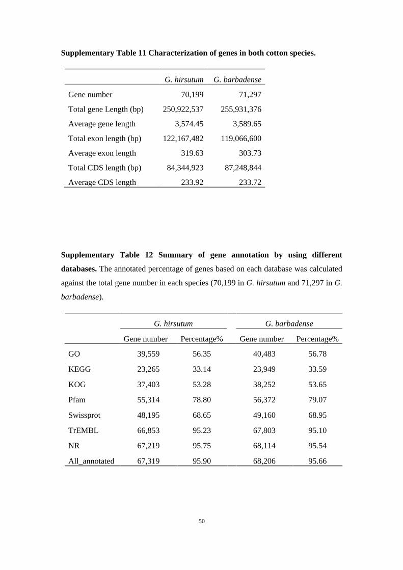
Supplementary Table 11 Characterization of genes in both cotton species.
G. hirsutum G. barbadense
Gene number 70,199 71,297
Total gene Length (bp) 250,922,537 255,931,376
Average gene length 3,574.45 3,589.65
Total exon length (bp) 122,167,482 119,066,600
Average exon length 319.63 303.73
Total CDS length (bp) 84,344,923 87,248,844
Average CDS length 233.92 233.72
Supplementary Table 12 Summary of gene annotation by using different
databases. The annotated percentage of genes based on each database was calculated
against the total gene number in each species (70,199 in G. hirsutum and 71,297 in G.
barbadense).
G. hirsutum
G. barbadense
Gene number Percentage% Gene number Percentage%
GO 39,559 56.35
40,483 56.78
KEGG 23,265 33.14 23,949 33.59
KOG 37,403 53.28 38,252 53.65
Pfam 55,314 78.80 56,372 79.07
Swissprot 48,195 68.65 49,160 68.95
TrEMBL 66,853 95.23 67,803 95.10
NR 67,219 95.75 68,114 95.54
All_annotated 67,319 95.90 68,206 95.66
Page 52
51
Supplementary Table 13 Identification of centromeres in G. hirsutum. The query LTRs (GhCR1-GhCR4) were from the previous publication44.
This table includes the examined median of each centromere region and the 95% confidence interval for the median (CIM). The aligned number
(n) shows the number of targeted sequences of each query LTR in each chromosome.
LTRs Chromosome Median
(Mb)
Aligned
number
(n)
95% CIM
(Mb)
Size of
95%
CIM
(Mb)
Chromosome Median
(Mb)
Aligned
number
(n)
95% CIM
(Mb)
Size of
95%
CIM
(Mb)
GhCR1-5'LTR
A01 67.58 172 62.95-70.64 7.69 D01 34.76 229 34.62-36.05 1.43
A02 71.75 219 66.35-71.88 5.53 D02 33.07 273 33.04-35.60 2.53
A03 40.77 372 38.60-40.92 2.32 D03 21.33 324 19.84-21.45 1.61
A04 33.55 97 32.87-34.67 1.8 D04 26.35 250 25.06-27.14 2.08
A05 56.42 247 52.90-56.57 3.67 D05 40.65 287 40.17-42.17 2
A06 56.20 182 50.56-57.17 6.61 D06 35.22 435 34.26-36.12 1.86
A07 61.12 154 57.96-61.34 3.38 D07 40.90 438 39.97-41.23 1.26
A08 51.17 126 50.85-58.66 7.81 D08 27.49 542 26.87-28.43 1.56
A09 19.22 85 19.06-26.96 7.9 D09 20.55 313 20.11-21.59 1.48
A10 46.05 271 45.53-51.31 5.78 D10 39.05 377 38.99-40.95 1.96
A11 74.27 257 70.07-75.06 4.99 D11 44.59 514 43.79-44.93 1.14
A12 35.10 219 35.00-37.89 2.89 D12 19.06 449 19.05-20.24 1.19
A13 33.17 153 33.07-35.38 2.31 D13 29.62 304 28.98-31.15 2.17
GhCR2-5'LTR
A01 67.65 61 67.45-70.65 3.20 D01 34.76 25 33.95-35.89 1.94
A02 71.59 59 65.33-72.26 6.93 D02 34.36 26 34.34-37.83 3.49
A03 40.82 54 40.81-42.38 1.57 D03 19.20 35 17.67-23.31 5.64
A04 33.53 15 33.45-33.67 0.22 D04 26.38 29 26.19-27.00 0.81
Page 53
52
A05 56.71 43 56.53-56.82 0.29 D05 41.77 30 40.90-43.90 3
A06 56.33 15 56.27-56.42 0.15 D06 35.99 119 35.30-36.25 0.95
A07 61.34 57 61.00-63.64 2.64 D07 42.31 122 41.95-42.33 0.38
A08 50.71 23 50.46-51.62 1.16 D08 27.45 108 27.01-28.03 1.02
A09 19.26 16 17.00-21.14 4.14 D09 20.43 111 20.18-20.85 0.67
A10 46.30 82 46.19-46.48 0.29 D10 39.13 112 38.39-39.70 1.31
A11 74.12 55 72.83-76.30 3.47 D11 44.86 43 40.29-44.93 4.64
A12 35.11 54 32.90-35.20 2.30 D12 18.94 113 18.79-19.17 0.37
A13 33.00 16 29.27-37.97 8.70 D13 29.67 60 29.19-31.16 1.97
GhCR3-5'LTR
A01 67.70 52 64.37-70.68 6.31 D01 34.67 137 32.76-34.92 2.16
A02 71.53 63 63.83-72.05 8.22 D02 33.02 199 31.94-33.58 1.64
A03 40.81 149 39.54-41.30 1.76 D03 19.84 330 19.45-21.27 1.82
A04 33.55 38 32.70-34.73 2.03 D04 26.60 204 25.83-27.21 1.38
A05 56.77 81 55.89-57.50 1.61 D05 40.77 193 40.14-41.49 1.35
A06 56.11 40 50.87-56.40 5.53 D06 36.40 259 35.12-36.70 1.58
A07 61.11 41 57.81-62.82 5.01 D07 40.89 321 40.85-41.79 0.94
A08 51.23 41 48.28-54.94 6.66 D08 27.45 338 27.15-28.38 1.23
A09 19.23 18 17.52-26.63 9.11 D09 20.13 177 19.39-20.93 1.54
A10 46.04 62 45.15-54.91 9.76 D10 38.65 226 37.87-39.45 1.58
A11 73.79 84 73.62-75.78 2.16 D11 44.34 350 43.57-44.37 0.8
A12 34.73 61 33.96-39.34 5.38 D12 19.18 236 19.15-20.15 1
A13 33.14 40 32.96-35.54 2.58 D13 29.54 144 27.98-30.56 2.58
GhCR4-5'LTR
A01 67.42 42 62.13-67.82 5.69 D01 34.63 19 33.62-36.19 2.57
A02 71.74 63 67.79-72.08 4.29 D02 33.27 35 33.14-35.85 2.61
A03 40.85 55 40.22-41.11 0.89 D03 18.30 38 18.28-23.07 4.79
A04 33.48 30 31.71-34.66 2.59 D04 25.98 38 25.13-29.13 4
Page 54
53
A05 56.64 95 55.79-56.80 1.01 D05 41.05 30 40.42-43.18 2.76
A06 56.25 26 56.17-56.32 0.15 D06 35.99 150 35.41-36.13 0.72
A07 61.27 62 58.64-63.22 4.58 D07 42.11 96 40.50-42.21 1.71
A08 50.79 38 49.01-52.30 3.29 D08 27.48 165 26.41-27.50 1.09
A09 19.23 19 17.75-20.15 2.40 D09 20.31 135 19.93-20.58 0.65
A10 46.24 95 45.33-47.95 2.62 D10 39.25 167 38.68-40.02 1.34
A11 74.19 79 73.62-74.22 0.60 D11 44.78 87 43.53-44.83 1.3
A12 35.06 45 35.00-35.19 0.19 D12 18.88 115 18.86-19.53 0.67
A13 33.09 29 31.71-34.04 2.33 D13 29.74 80 29.04-29.98 0.94
Page 55
54
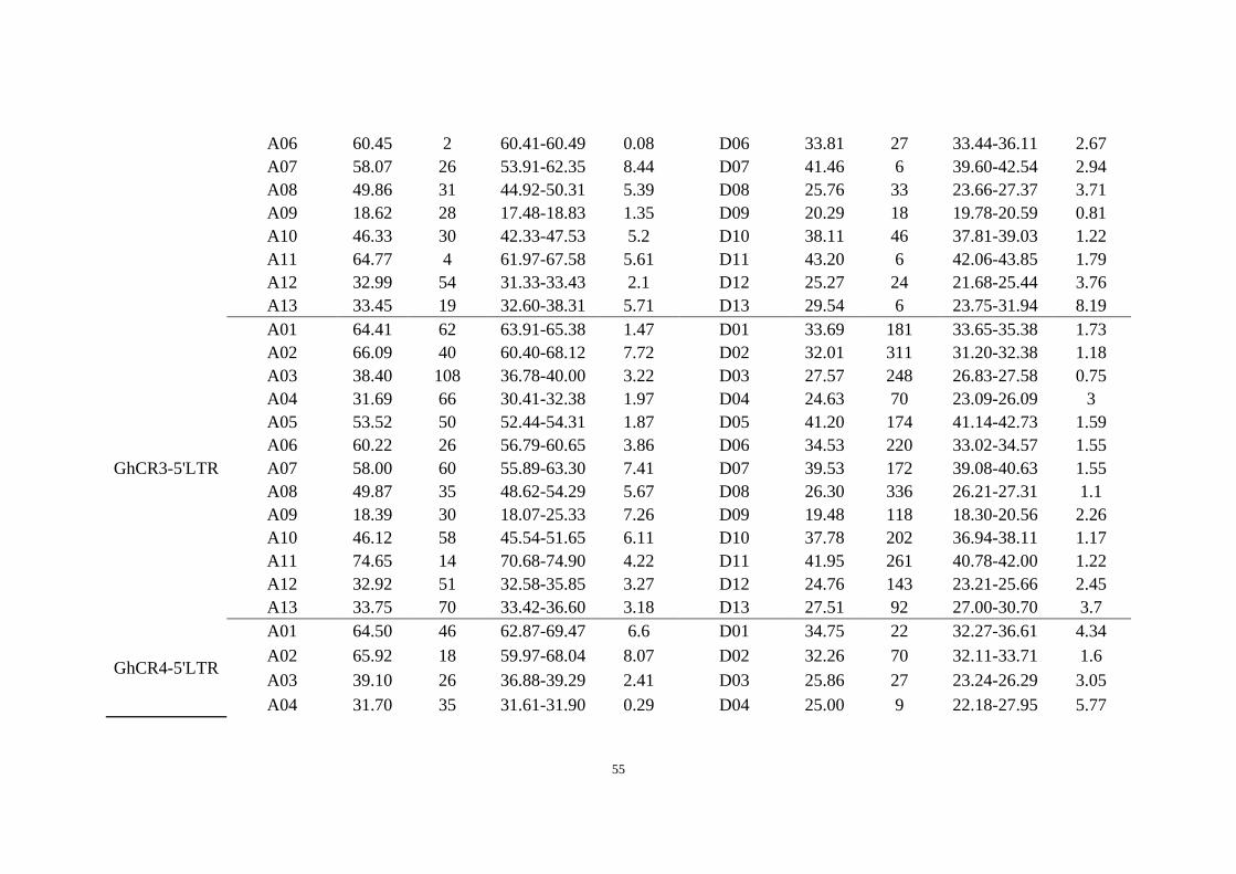
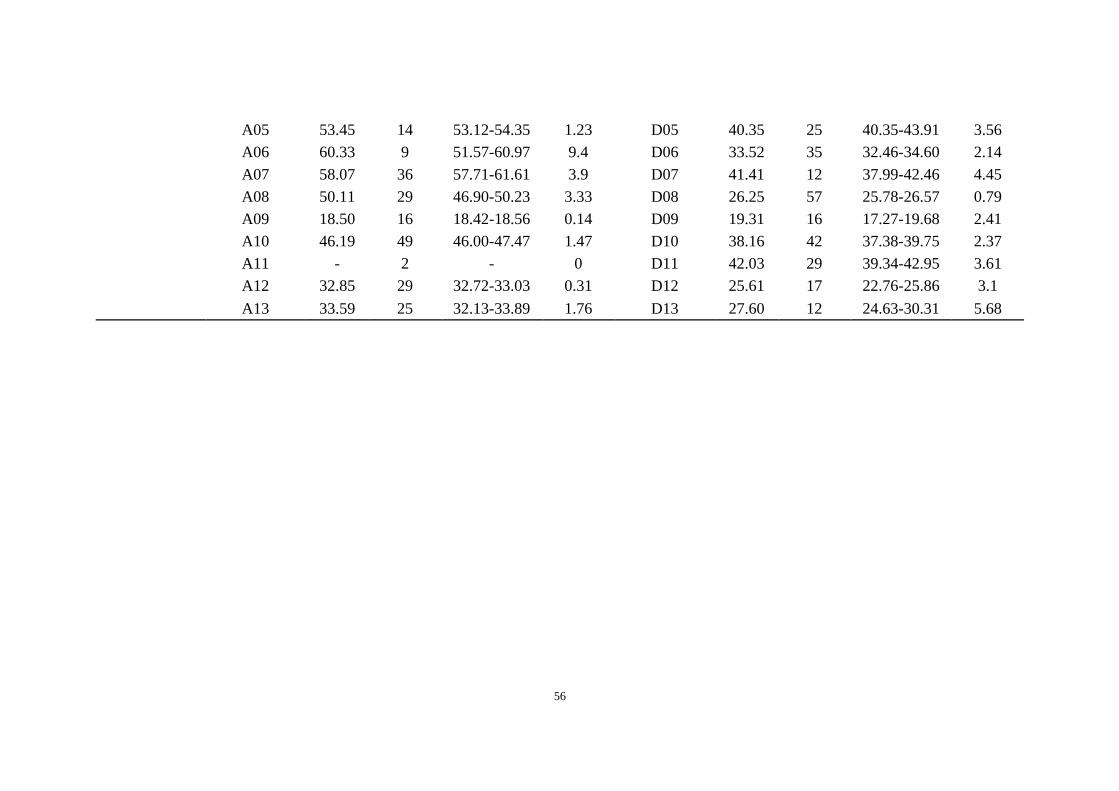
Supplementary Table 14 Identification of centromeres in G. barbadense. The query LTRs (GhCR1-GhCR4) were from the previous
publication44. This table includes the examined median of each centromere region and the 95% confidence interval for the median (CIM). The
aligned number (n) shows the number of targeted sequences of each query LTR in each chromosome.
LTRs Chromosome Median
(Mb)
Aligned
number
(n)
95% CIM
(Mb)
Size of
95%
CIM
(Mb)
Chromosome Median
(Mb)
Aligned
number
(n)
95% CIM
(Mb)
Size of
95%
CIM
(Mb)
GhCR1-5'LTR
A01 64.38 205 61.06-66.13 5.5 D01 34.70 312 34.26-36.19 1.93
A02 66.09 124 63.29-67.74 4.45 D02 31.19 423 31.64-33.00 1.36
A03 38.43 267 37.90-40.80 2.9 D03 26.22 260 24.36-26.34 1.98
A04 31.63 206 31.04-32.24 1.2 D04 24.37 103 23.71-29.00 5.29
A05 53.40 198 51.52-55.76 4.24 D05 41.70 258 41.61-43.75 2.14
A06 60.17 104 54.58-60.85 6.27 D06 33.83 368 33.03-34.71 1.68
A07 58.14 235 56.25-60.63 4.38 D07 39.55 215 39.20-41.12 1.92
A08 50.03 180 49.22-53.43 4.21 D08 26.24 445 26.06-27.27 1.21
A09 18.45 119 18.25-21.86 3.61 D09 19.61 188 19.58-22.08 2.5
A10 46.08 198 45.21-49.91 4.7 D10 37.99 350 36.43-38.32 1.89
A11 74.30 47 70.27-74.67 4.4 D11 42.05 289 40.30-42.12 1.82
A12 32.92 168 32.01-36.60 4.59 D12 25.50 218 24.89-27.54 2.65
A13 33.73 229 33.39-35.29 1.9 D13 27.50 147 27.92-31.66 3.64
GhCR2-5'LTR
A01 64.47 55 63.87-68.59 4.72 D01 34.85 31 33.96-38.28 4.32
A02 65.65 22 65.17-66.88 1.71 D02 31.82 38 31.60-33.96 2.36
A03 39.08 21 37.92-39.13 1.21 D03 22.27 21 22.42-25.68 3.26
A04 31.18 34 31.69-32.20 0.51 D04 23.48 9 23.61-26.32 2.71
A05 53.50 14 53.16-53.56 0.4 D05 41.04 22 40.87-44.73 3.86
Page 56
55
A06 60.45 2 60.41-60.49 0.08 D06 33.81 27 33.44-36.11 2.67
A07 58.07 26 53.91-62.35 8.44 D07 41.46 6 39.60-42.54 2.94
A08 49.86 31 44.92-50.31 5.39 D08 25.76 33 23.66-27.37 3.71
A09 18.62 28 17.48-18.83 1.35 D09 20.29 18 19.78-20.59 0.81
A10 46.33 30 42.33-47.53 5.2 D10 38.11 46 37.81-39.03 1.22
A11 64.77 4 61.97-67.58 5.61 D11 43.20 6 42.06-43.85 1.79
A12 32.99 54 31.33-33.43 2.1 D12 25.27 24 21.68-25.44 3.76
A13 33.45 19 32.60-38.31 5.71 D13 29.54 6 23.75-31.94 8.19
GhCR3-5'LTR
A01 64.41 62 63.91-65.38 1.47 D01 33.69 181 33.65-35.38 1.73
A02 66.09 40 60.40-68.12 7.72 D02 32.01 311 31.20-32.38 1.18
A03 38.40 108 36.78-40.00 3.22 D03 27.57 248 26.83-27.58 0.75
A04 31.69 66 30.41-32.38 1.97 D04 24.63 70 23.09-26.09 3
A05 53.52 50 52.44-54.31 1.87 D05 41.20 174 41.14-42.73 1.59
A06 60.22 26 56.79-60.65 3.86 D06 34.53 220 33.02-34.57 1.55
A07 58.00 60 55.89-63.30 7.41 D07 39.53 172 39.08-40.63 1.55
A08 49.87 35 48.62-54.29 5.67 D08 26.30 336 26.21-27.31 1.1
A09 18.39 30 18.07-25.33 7.26 D09 19.48 118 18.30-20.56 2.26
A10 46.12 58 45.54-51.65 6.11 D10 37.78 202 36.94-38.11 1.17
A11 74.65 14 70.68-74.90 4.22 D11 41.95 261 40.78-42.00 1.22
A12 32.92 51 32.58-35.85 3.27 D12 24.76 143 23.21-25.66 2.45
A13 33.75 70 33.42-36.60 3.18 D13 27.51 92 27.00-30.70 3.7
GhCR4-5'LTR
A01 64.50 46 62.87-69.47 6.6 D01 34.75 22 32.27-36.61 4.34
A02 65.92 18 59.97-68.04 8.07 D02 32.26 70 32.11-33.71 1.6
A03 39.10 26 36.88-39.29 2.41 D03 25.86 27 23.24-26.29 3.05
A04 31.70 35 31.61-31.90 0.29 D04 25.00 9 22.18-27.95 5.77
Page 57
56
A05 53.45 14 53.12-54.35 1.23 D05 40.35 25 40.35-43.91 3.56
A06 60.33 9 51.57-60.97 9.4 D06 33.52 35 32.46-34.60 2.14
A07 58.07 36 57.71-61.61 3.9 D07 41.41 12 37.99-42.46 4.45
A08 50.11 29 46.90-50.23 3.33 D08 26.25 57 25.78-26.57 0.79
A09 18.50 16 18.42-18.56 0.14 D09 19.31 16 17.27-19.68 2.41
A10 46.19 49 46.00-47.47 1.47 D10 38.16 42 37.38-39.75 2.37
A11 - 2 - 0 D11 42.03 29 39.34-42.95 3.61
A12 32.85 29 32.72-33.03 0.31 D12 25.61 17 22.76-25.86 3.1
A13 33.59 25 32.13-33.89 1.76 D13 27.60 12 24.63-30.31 5.68
Page 58
57
Supplementary Table 15 Summary of TE annotation in the G. hirsutum genome.
Type Number Length(bp) Percentage%
ClassI 329 174,985 0.01
ClassI/DIRS 109,814 211,885,852 9.02
ClassI/LARD 171,961 215,163,934 9.16
ClassI/LINE 3,980 3,526,907 0.15
ClassI/LINE/L1 18,988 20,598,140 0.88
ClassI/LINE/RTE 10 7,358 0
ClassI/LTR 1,190 1,394,971 0.06
ClassI/LTR/Copia 158,715 206,562,373 8.8
ClassI/LTR/Gypsy 595,979 1,159,573,495 49.39
ClassI/LTR/Retrovirus 1,205 1,617,051 0.07
ClassI/PLE 1,032 2,222,583 0.09
ClassI/PLE/Penelope 2,820 5,783,818 0.25
ClassI/SINE 1,386 632,632 0.03
ClassI/TRIM 1,498 2,004,452 0.09
ClassII 28 58,995 0
ClassII/MuDR 588 420,172 0.02
ClassII/Crypton/Crypton 58 123,895 0.01
ClassII/Helitron 165 224,935 0.01
ClassII/Helitron/Helitron 7,484 8,090,055 0.34
ClassII/MITE 1,076 480,589 0.02
ClassII/Maverick 474 361,096 0.02
ClassII/TIR 16,604 25,007,113 1.07
ClassII/TIR/CACTA 11,548 17,712,009 0.75
ClassII/TIR/PIF-Harbinger 7,415 8,722,732 0.37
ClassII/TIR/Tc1-Mariner 2,317 1,894,298 0.08
ClassII/TIR/hAT 5,605 6,936,724 0.3
PotentialHostGene 6,196 5,558,071 0.24
SSR 1,054 609,707 0.03
Unknown 164,145 138,124,355 5.88
Total 1,293,664 1,640,099,595 69.86
Page 59
58
Supplementary Table 16 Summary of TE annotation in the G. barbadense genome.
Type Number Length (bp) Percentage%
ClassI 117 110,097 0
ClassI/DIRS 108,422 207,160,435 9.14
ClassI/LARD 175,428 211,635,000 9.34
ClassI/LINE 1,300 1,114,019 0.05
ClassI/LINE/L1 19,201 22,906,423 1.01
ClassI/LTR 2,433 3,014,017 0.13
ClassI/LTR/Copia 156,332 201,203,918 8.88
ClassI/LTR/Gypsy 590,346 1,127,390,765 49.74
ClassI/LTR/Retrovirus 1,002 1,492,617 0.07
ClassI/PLE 390 691,066 0.03
ClassI/PLE/Penelope 1,600 4,062,216 0.18
ClassI/PLE|LARD 24 21,575 0
ClassI/SINE 493 181,521 0.01
ClassI/TRIM 1,116 1,423,619 0.06
ClassII/?/MuDR 164 112,635 0
ClassII/Crypton/Crypton 161 152,654 0.01
ClassII/Helitron/Helitron 10,203 9,590,452 0.42
ClassII/MITE 1,077 517,763 0.02
ClassII/Maverick 36 94,507 0
ClassII/TIR 19,323 27,623,213 1.22
ClassII/TIR/CACTA 10,390 16,894,819 0.75
ClassII/TIR/PIF-Harbinger 7,597 8,557,010 0.38
ClassII/TIR/Tc1-Mariner 91 102,287 0
ClassII/TIR/hAT 5,694 5,788,681 0.26
PotentialHostGene 7,918 7,157,442 0.32
SSR 701 519,804 0.02
Unknown 118,191 104,004,607 4.59
Total 1,239,750 1,582,832,728 69.83
Page 60
59
Supplementary Table 17 Summary of SNP annotation in the G. hirsutum genome.
Chr Total SNPs Intergenic Upstream Downstream Exonic Intronic Nonsynonymous Synonymous
Ghir_A01 389,987 342,837 14,073 12,797 8,500 11,780 3,216 1,729
Ghir_A02 643,170 593,273 15,734 14,525 8,866 10,772 3,354 1,802
Ghir_A03 667,512 607,842 19,923 17,708 10,790 11,249 3,956 2,220
Ghir_A04 510,907 467,614 13,284 12,862 7,494 9,653 3,076 1,544
Ghir_A05 592,897 497,763 29,380 27,257 18,610 19,887 6,636 3,572
Ghir_A06 730,538 672,840 18,970 16,772 10,274 11,682 3,659 2,101
Ghir_A07 596,066 531,453 21,431 18,911 11,061 13,210 3,944 2,111
Ghir_A08 740,462 674,796 21,475 19,129 12,214 12,848 4,448 2,426
Ghir_A09 490,954 425,314 20,729 18,536 12,051 14,324 4,301 2,360
Ghir_A10 688,973 624,716 20,605 18,307 11,087 14,258 4,104 2,257
Ghir_A11 729,494 642,272 27,550 25,331 16,610 17,731 6,353 3,434
Ghir_A12 678,010 607,653 22,624 20,817 13,054 13,862 4,843 2,576
Ghir_A13 672,306 607,557 20,858 18,934 11,433 13,524 4,187 2,264
Ghir_D01 361,219 292,121 21,509 19,765 11,643 16,181 4,298 2,545
Ghir_D02 450,781 365,708 26,379 24,219 14,893 19,582 5,128 3,080
Ghir_D03 317,628 267,790 17,382 15,243 8,431 8,782 2,930 1,611
Ghir_D04 308,491 247,409 19,858 19,018 10,325 11,881 3,533 1,985
Ghir_D05 317,978 222,514 30,235 27,387 18,526 19,316 6,762 3,826
Ghir_D06 396,973 325,985 23,097 21,091 12,360 14,440 4,101 2,397
Ghir_D07 331,943 261,163 24,372 21,201 11,944 13,263 4,126 2,272
Ghir_D08 384,994 310,839 24,110 22,262 12,750 15,033 4,396 2,669
Ghir_D09 329,007 255,659 23,671 21,010 13,344 15,323 4,443 2,681
Ghir_D10 411,657 325,881 27,944 24,946 14,504 18,382 5,224 3,023
Ghir_D11 348,911 260,157 28,734 24,914 17,216 17,890 6,146 3,492
Ghir_D12 345,473 272,961 24,196 21,572 13,156 13,588 4,505 2,523
Ghir_D13 380,367 306,828 24,659 22,064 12,884 13,932 4,107 2,504
Page 61
60
Supplementary Table 18 Summary of InDel annotation in the G. hirsutum genome.
Chr Total InDels Intergenic Upstream Downstream Exonic Intronic Frameshift Nonframeshift
Ghir_A01 105,352 86,469 5,767 4,577 2,944 5,595 535 132
Ghir_A02 106,409 89,978 5,111 4,199 2,664 4,457 373 135
Ghir_A03 116,763 96,827 6,346 5,067 3,290 5,233 548 164
Ghir_A04 86,072 72,266 4,165 3,594 2,157 3,890 407 119
Ghir_A05 137,442 101,895 11,187 9,177 6,099 9,084 1,104 283
Ghir_A06 122,197 102,620 5,837 5,103 3,085 5,552 518 128
Ghir_A07 113,475 91,644 6,911 5,663 3,457 5,800 601 175
Ghir_A08 128,344 105,800 6,909 5,818 3,892 5,925 637 162
Ghir_A09 102,316 78,727 7,527 5,976 3,714 6,372 614 161
Ghir_A10 126,140 104,422 6,957 5,475 3,309 5,977 595 155
Ghir_A11 140,073 110,237 9,374 7,809 4,916 7,737 780 242
Ghir_A12 122,183 98,321 7,658 6,441 4,039 5,724 701 228
Ghir_A13 117,733 95,840 7,027 5,403 3,663 5,800 570 178
Ghir_D01 86,414 65,790 6,096 5,095 3,145 6,288 500 199
Ghir_D02 97,005 74,290 6,715 5,538 3,620 6,842 554 199
Ghir_D03 72,901 57,825 4,832 4,057 2,508 3,679 388 111
Ghir_D04 74,354 56,501 5,493 4,858 2,863 4,639 450 121
Ghir_D05 97,713 65,323 9,811 8,186 5,526 8,867 959 252
Ghir_D06 90,048 69,535 6,227 5,186 3,382 5,718 536 186
Ghir_D07 87,987 66,189 6,890 5,820 3,542 5,546 549 175
Ghir_D08 94,000 70,721 7,080 6,246 3,802 6,151 624 231
Ghir_D09 80,618 57,674 7,248 6,063 3,549 6,084 503 201
Ghir_D10 99,839 74,723 7,708 6,528 3,759 7,121 583 210
Ghir_D11 100,160 70,987 9,115 7,415 4,691 7,952 804 268
Ghir_D12 88,255 64,791 7,497 6,163 3,856 5,948 643 217
Ghir_D13 88,896 67,113 6,773 5,323 3,801 5,886 594 207
Page 62
61
Supplementary Table 19 Summary of Ka and Ks values in G. hirsutum by comparing with
G. barbadense (included as a separate excel file).
Supplementary Table 20 Characterization of inversions between G. hirsutum and G.
barbadense genomes (included as a separate excel file).
Supplementary Table 21 Summary of large chromosome inversions between G. hirsutum and
G. barbadense genomes. The columns 1–3 show chromosome coordinates in G. hirsutum and
columns 4–6 show chromosome coordinates in G. barbadense.
Chr1 Start1 End1 Chr2 Start2 End2 Type
Ghir_A02 54,642,102 71,988,045 Gbar_A02 51,821,746 66,543,001 pericentric
Ghir_A03 56,556,126 63,553,704 Gbar_A03 52,371,473 60,207,452 paracentric
Ghir_A03 78,064,256 80,376,788 Gbar_A03 72,835,211 74,581,567 paracentric
Ghir_A06 24,850,414 28,077,498 Gbar_A06 23,472,033 26,339,683 paracentric
Ghir_A06 45,515,934 74,455,488 Gbar_A06 42,859,341 68,747,575 pericentric
Ghir_A06 78,685,929 83,020,537 Gbar_A06 72,503,583 76,700,600 paracentric
Ghir_A06 84,870,622 93,487,208 Gbar_A06 78,259,488 86,094,318 paracentric
Ghir_A08 59,764,788 72,744,429 Gbar_A08 57,420,323 72,029,495 paracentric
Ghir_A09 24,150,085 34,764,618 Gbar_A09 23,410,632 33,165,553 pericentric
Ghir_A11 75,019,078 85,950,616 Gbar_A11 67,814,347 78,269,222 pericentric
Ghir_A12 30,309,118 38,279,104 Gbar_A12 29,769,466 37,044,028 pericentric
Ghir_A12 45,804,322 50,054,424 Gbar_A12 46,276,585 50,034,820 pericentric
Ghir_A12 50,448,397 54,909,350 Gbar_A12 57,159,079 61,208,257 pericentric
Ghir_D03 13,012,229 22,793,340 Gbar_D03 12,635,016 22,002,954 pericentric
Ghir_D03 27,202,411 29,108,911 Gbar_D03 26,280,851 27,675,085 pericentric
Ghir_D04 27,905,003 32,573,112 Gbar_D04 24,831,653 29,331,531 pericentric
Ghir_D05 41,388,005 51,258,368 Gbar_D05 41,480,541 51,183,285 pericentric
Ghir_D06 36,238,727 41,276,220 Gbar_D06 33,920,053 38,175,402 pericentric
Ghir_D07 46,763,671 48,712,726 Gbar_D07 44,233,281 46,129,102 paracentric
Ghir_D08 25,647,253 32,477,573 Gbar_D08 25,334,207 29,499,273 pericentric
Ghir_D08 34,540,780 37,367,644 Gbar_D08 30,696,325 33,351,411 pericentric
Ghir_D12 14,146,577 31,542,946 Gbar_D12 13,854,598 28,736,159 pericentric
Page 63
62
Supplementary Table 22 Characterization of chromosome translocations between G.
hirsutum and G. barbadense genomes (included as a separate excel file).
Supplementary Table 23 Characterization of unique genome regions in G. hirsutum (included
as a separate excel file).
Supplementary Table 24 Characterization of unique genome regions in G. barbadense
(included as a separate excel file).
Supplementary Table 25 Summary of PAV-related genes in G. hirsutum and G. barbadense
(included as a separate excel file).
Page 64
63
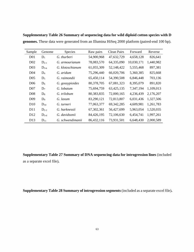
Supplementary Table 26 Summary of sequencing data for wild diploid cotton species with D
genomes. These data were generated from an Illumina HiSeq 2000 platform (paired-end 100 bp).
Sample Genome Species Raw pairs Clean Pairs Forward Reverse
D01 D1 G. thurberi 54,900,968 47,632,729 4,658,128 826,641
D02 D2-1 G. armourianum 78,083,570 64,335,090 10,030,171 1,440,982
D03 D3-k G. klotzschianum 61,055,309 52,148,422 5,555,468 897,381
D04 D4 G. aridum 75,296,440 66,020,706 5,360,385 825,668
D05 D5 G. raimondii 65,450,114 54,390,508 6,846,448 703,136
D06 D6 G. gossypioides 80,378,705 67,081,323 8,395,079 891,820
D07 D7 G. lobatum 75,694,759 63,425,135 7,347,194 1,109,013
D08 D8 G. trilobum 80,383,835 72,000,165 4,236,439 2,176,207
D09 D9 G. laxum 83,290,121 72,813,807 6,031,436 1,327,506
D10 D10 G. turneri 77,063,377 69,342,285 4,609,981 1,261,783
D11 D2-2 G. harknessii 67,302,361 56,427,699 5,963,054 1,520,035
D12 D3-d G. davidsonii 84,426,195 72,106,630 6,454,741 1,997,261
D13 D11 G. schwendimanii 86,432,116 73,931,501 6,648,430 2,000,589
Supplementary Table 27 Summary of DNA sequencing data for introgression lines (included
as a separate excel file).
Supplementary Table 28 Summary of introgression segments (included as a separate excel file).
Page 65
64
Supplementary Table 29 The phenotypic data for introgression lines (included as a separate
excel file).
Supplementary Table 30 Summary of QTLs identified by using the introgression line
population.
Trait* Marker Chr Start End LOD PVE(%) Additive Publication
MV M158 Ghir_A06 111,158,459 113,691,815 2.90 4.41 -0.54
MV M374 Ghir_D07 35,544 1,376,493 5.10 8.01 0.60 Said et al., 201545
FL M55 Ghir_A02 2,978,719 3,945,306 4.81 13.85 0.96
FL M132 Ghir_A06 965,145 1,817,691 3.38 9.53 1.25
FU M402 Ghir_D08 93,636 339,033 2.61 6.82 0.81
FU M417 Ghir_D08 18,209,640 18,264,724 2.52 7.59 -0.88
FU M55 Ghir_A02 2,978,719 3,945,306 3.44 8.91 0.54
FS M158 Ghir_A06 111,158,459 113,691,815 3.47 10.66 2.18 Fang et al., 201746
FS M271 Ghir_A13 88,662 1,373,398 4.26 13.22 1.99
FS M443 Ghir_D09 40,961,072 43,211,847 2.78 8.46 1.14 Said et al., 201545
FS M112 Ghir_A05 26,177,037 26,341,805 3.91 10.31 1.60
FE M52 Ghir_A02 1,337,980 1,651,830 3.69 8.03 -0.86
FE M402 Ghir_D08 93,636 339,033 5.45 12.15 0.55 Said et al., 201545
*These traits include micronaire value (MV), fiber length (FL), fiber uniformity (FU), fiber
strength (FS) and fiber elongation rate (FE).
Supplementary Table 31 Summary of functional genes in QTL regions (included as a separate
excel file).
Page 66
65
Supplementary Table 32 Prediction of possible candidate genes by integration of genomic
variants data.
Supplementary Table 33 Summary of RNAseq data for introgression lines (included as a
separate excel file).
Supplementary Table 34 Summary of eQTLs identified by the introgression line population
(included as a separate excel file).
Page 67
66
References
1. Xu, Z. & Wang, H. LTR_FINDER: an efficient tool for the prediction of full-length LTR
retrotransposons. Nucleic Acids Res. 35, W265–W268 (2007).
2. Han, Y. & Wessler, S.R. MITE-Hunter: a program for discovering miniature inverted-
repeat transposable elements from genomic sequences. Nucleic Acids Res. 38, e199 (2010).
3. Price, A.L., Jones, N.C. & Pevzner, P.A. De novo identification of repeat families in large
genomes. Bioinformatics 21 Suppl 1, i351–i358 (2005).
4. Edgar, R.C. & Myers, E.W. PILER: identification and classification of genomic repeats.
Bioinformatics 21 Suppl 1, i152–i158 (2005).
5. Hoede, C. et al. PASTEC: an automatic transposable element classification tool. PLoS One
9, e91929 (2014).
6. Jurka, J. Repbase update: a database and an electronic journal of repetitive elements.
Trends Genet. 16, 418–420 (2000).
7. Tarailo-Graovac, M. & Chen, N. Using RepeatMasker to Identify Repetitive Elements in
Genomic Sequences. in Curr. Protoc. Bioinformatics (John Wiley & Sons, Inc., 2009).
8. Burge, C. & Karlin, S. Prediction of complete gene structures in human genomic DNA. J.
Mol. Biol. 268, 78–94 (1997).
9. Stanke, M. et al. AUGUSTUS: ab initio prediction of alternative transcripts. Nucleic Acids
Res. 34, W435–W439 (2006).
10. Majoros, W.H., Pertea, M. & Salzberg, S.L. TigrScan and GlimmerHMM: two open source
ab initio eukaryotic gene-finders. Bioinformatics 20, 2878–2879 (2004).
11. Korf, I. Gene finding in novel genomes. BMC Bioinformatics 5, 59 (2004).
12. Keilwagen, J. et al. Using intron position conservation for homology-based gene prediction.
Nucleic Acids Res. 44, e89 (2016).
13. Kim, D., Langmead, B. & Salzberg, S.L. HISAT: a fast spliced aligner with low memory
requirements. Nat. Methods 12, 357–360 (2015).
14. Pertea, M. et al. StringTie enables improved reconstruction of a transcriptome from RNA-
seq reads. Nat. Biotechnol. 33, 290–295 (2015).
15. Zhang, T. et al. Sequencing of allotetraploid cotton (Gossypium hirsutum L. acc. TM-1)
provides a resource for fiber improvement. Nat. Biotechnol. 33, 531–537 (2015).
Page 68
67
16. Wang, M. et al. Long noncoding RNAs and their proposed functions in fibre development
of cotton (Gossypium spp.). New Phytol. 207, 1181–1197 (2015).
17. Tang, S., Lomsadze, A. & Borodovsky, M. Identification of protein coding regions in RNA
transcripts. Nucleic Acids Res. 43, e78 (2015).
18. Haas, B.J. et al. Improving the Arabidopsis genome annotation using maximal transcript
alignment assemblies. Nucleic Acids Res. 31, 5654–5666 (2003).
19. Haas, B.J. et al. Automated eukaryotic gene structure annotation using EVidenceModeler
and the program to assemble spliced alignments. Genome Biol. 9, R7 (2008).
20. She, R., Chu, J.S.C., Wang, K., Pei, J. & Chen, N.S. GenBlastA: Enabling BLAST to
identify homologous gene sequences. Genome Res. 19, 143–149 (2009).
21. Birney, E., Clamp, M. & Durbin, R. GeneWise and Genomewise. Genome Res. 14, 988–
995 (2004).
22. Nawrocki, E.P. & Eddy, S.R. Infernal 1.1: 100-fold faster RNA homology searches.
Bioinformatics 29, 2933–2935 (2013).
23. Lowe, T.M. & Eddy, S.R. tRNAscan-SE: a program for improved detection of transfer
RNA genes in genomic sequence. Nucleic Acids Res. 25, 955–964 (1997).
24. Wang, M. et al. Asymmetric subgenome selection and cis-regulatory divergence during
cotton domestication. Nat. Genet. 49, 579–587 (2017).
25. Wang, M. et al. Evolutionary dynamics of 3D genome architecture following
polyploidization in cotton. Nat. Plants 4, 90–97 (2018).
26. Langmead, B. & Salzberg, S.L. Fast gapped-read alignment with Bowtie 2. Nat Methods
9, 357–359 (2012).
27. Quinlan, A.R. & Hall, I.M. BEDTools: a flexible suite of utilities for comparing genomic
features. Bioinformatics 26, 841–842 (2010).
28. Lee, T.H., Guo, H., Wang, X.Y., Kim, C. & Paterson, A.H. SNPhylo: a pipeline to
construct a phylogenetic tree from huge SNP data. BMC Genomics 15, 162 (2014).
29. Page, J.T. et al. DNA sequence evolution and rare homoeologous conversion in tetraploid
cotton. PLoS Genet. 12, e1006012 (2016).
30. Yu, J. et al. CottonGen: a genomics, genetics and breeding database for cotton research.
Nucleic Acids Res. 42, D1229–D1236 (2014).
Page 69
68
31. Zhang, Z. et al. KaKs_Calculator: Calculating Ka and Ks through model selection and
model averaging. Genomics Proteomics Bioinformatics 4, 259–263 (2006).
32. Wang, S. et al. Sequence-based ultra-dense genetic and physical maps reveal structural
variations of allopolyploid cotton genomes. Genome Biol. 16, 108 (2015).
33. Simao, F.A. et al. BUSCO: assessing genome assembly and annotation completeness with
single-copy orthologs. Bioinformatics 31, 3210–3212 (2015).
34. Wang, K., Li, M. & Hakonarson, H. ANNOVAR: functional annotation of genetic variants
from high-throughput sequencing data. Nucleic Acids Res. 38, e164 (2010).
35. Delcher, A.L., Phillippy, A., Carlton, J. & Salzberg, S.L. Fast algorithms for large-scale
genome alignment and comparison. Nucleic Acids Res. 30, 2478–2483 (2002).
36. Wang, Y. et al. MCScanX: a toolkit for detection and evolutionary analysis of gene synteny
and collinearity. Nucleic Acids Res. 40, e49 (2012).
37. Paterson, A.H. et al. Repeated polyploidization of Gossypium genomes and the evolution
of spinnable cotton fibres. Nature 492, 423–427 (2012).
38. Krzywinski, M. et al. Circos: an information aesthetic for comparative genomics. Genome
Res. 19, 1639–1645 (2009).
39. Trapnell, C. et al. Transcript assembly and quantification by RNA-Seq reveals unannotated
transcripts and isoform switching during cell differentiation. Nat. Biotechnol. 28, 511–515
(2010).
40. Tan, J. et al. A genetic and metabolic analysis revealed that cotton fiber cell development
was retarded by flavonoid naringenin. Plant Physiol. 162, 86–95 (2013).
41. Yuan, D. et al. The genome sequence of Sea-Island cotton (Gossypium barbadense)
provides insights into the allopolyploidization and development of superior spinnable
fibres. Sci. Rep. 5, 17662 (2015).
42. Li, F. et al. Genome sequence of cultivated Upland cotton (Gossypium hirsutum TM-1)
provides insights into genome evolution. Nat. Biotechnol. 33, 524–530 (2015).
43. Liu, X. et al. Gossypium barbadense genome sequence provides insight into the evolution
of extra-long staple fiber and specialized metabolites. Sci. Rep. 5, 14139 (2015).
44. Zhang, W. et al. Identification of centromeric regions on the linkage map of cotton using
centromere-related repeats. Genomics 104, 587–593 (2014).
Page 70
69
45. Said, J.I. et al. A comparative meta-analysis of QTL between intraspecific Gossypium
hirsutum and interspecific G. hirsutum × G. barbadense populations. Mol. Genet.
Genomics 290, 1003–1025 (2015).
46. Fang, L. et al. Genomic analyses in cotton identify signatures of selection and loci
associated with fiber quality and yield traits. Nat. Genet. 49, 1089–1098 (2017).