GNU Linear Programming Kit

Reference Manual

Version 4.1

(Draft Edition, August 2003)

2

The GLPK package is a part of the GNU project released under the aegis of GNU.

Copyright c© 2000, 2001, 2002, 2003 Andrew Makhorin, Department for Applied Infor-matics, Moscow Aviation Institute, Moscow, Russia. All rights reserved.

Free Software Foundation, Inc., 59 Temple Place — Suite 330, Boston, MA 02111, USA.

Permission is granted to make and distribute verbatim copies of this manual provided thecopyright notice and this permission notice are preserved on all copies.

Permission is granted to copy and distribute modified versions of this manual under theconditions for verbatim copying, provided also that the entire resulting derived work isdistributed under the terms of a permission notice identical to this one.

Permission is granted to copy and distribute translations of this manual into anotherlanguage, under the above conditions for modified versions.

Contents

1 Introduction 71.1 LP Problem . . . . . . . . . . . . . . . . . . . . . . . . . . . . . . . . . . . . 71.2 MIP Problem . . . . . . . . . . . . . . . . . . . . . . . . . . . . . . . . . . . 91.3 Brief Example . . . . . . . . . . . . . . . . . . . . . . . . . . . . . . . . . . . 9

2 API Routines 132.1 Problem object . . . . . . . . . . . . . . . . . . . . . . . . . . . . . . . . . . 142.2 Problem creating and modifying routines . . . . . . . . . . . . . . . . . . . 17

2.2.1 lpx create prob — create problem object . . . . . . . . . . . . . . 172.2.2 lpx add rows — add new rows to problem object . . . . . . . . . . 172.2.3 lpx add cols — add new columns to problem object . . . . . . . . 172.2.4 lpx check name — check correctness of symbolic name . . . . . . . 172.2.5 lpx set prob name — assign (change) problem name . . . . . . . . 182.2.6 lpx set row name — assign (change) row name . . . . . . . . . . . . 182.2.7 lpx set col name — assign (change) column name . . . . . . . . . . 182.2.8 lpx set row bnds — set (change) row bounds . . . . . . . . . . . . 182.2.9 lpx set col bnds — set (change) column bounds . . . . . . . . . . 192.2.10 lpx set obj name — assign (change) objective function name . . . . 192.2.11 lpx set obj dir — set (change) optimization direction . . . . . . . 202.2.12 lpx set obj c0 — set (change) constant term of the objective function 202.2.13 lpx set row coef — set (change) row objective coefficient . . . . . 202.2.14 lpx set col coef — set (change) column objective coefficient . . . 202.2.15 lpx load mat — load the constraint matrix . . . . . . . . . . . . . . 212.2.16 lpx load mat3 — load the constraint matrix . . . . . . . . . . . . . 212.2.17 lpx set mat row — change row of the constraint matrix . . . . . . . 222.2.18 lpx set mat col — change column of the constraint matrix . . . . . 222.2.19 lpx unmark all — unmark all rows and columns . . . . . . . . . . . 222.2.20 lpx mark row — assign mark to row . . . . . . . . . . . . . . . . . . 232.2.21 lpx mark col — assign mark to column . . . . . . . . . . . . . . . . 232.2.22 lpx clear mat — clear rows and columns of the constraint matrix . 232.2.23 lpx del items — remove rows and columns from problem object . . 232.2.24 lpx delete prob — delete problem object . . . . . . . . . . . . . . 24

2.3 Problem querying routines . . . . . . . . . . . . . . . . . . . . . . . . . . . . 252.3.1 lpx get num rows — determine number of rows . . . . . . . . . . . 252.3.2 lpx get num cols — determine number of columns . . . . . . . . . 252.3.3 lpx get num nz — determine number of non-zero constraint coeffi-

cients . . . . . . . . . . . . . . . . . . . . . . . . . . . . . . . . . . . 25

3

4

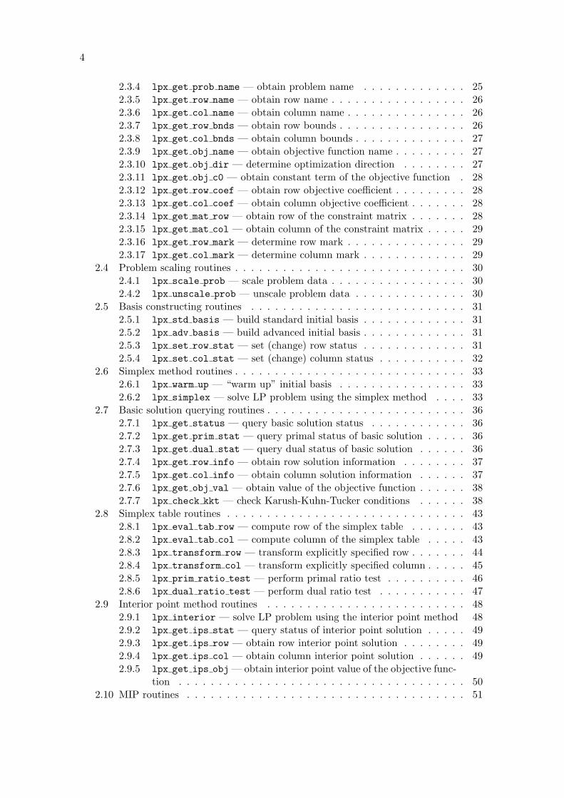
2.3.4 lpx get prob name — obtain problem name . . . . . . . . . . . . . 252.3.5 lpx get row name — obtain row name . . . . . . . . . . . . . . . . . 262.3.6 lpx get col name — obtain column name . . . . . . . . . . . . . . . 262.3.7 lpx get row bnds — obtain row bounds . . . . . . . . . . . . . . . . 262.3.8 lpx get col bnds — obtain column bounds . . . . . . . . . . . . . . 272.3.9 lpx get obj name — obtain objective function name . . . . . . . . . 272.3.10 lpx get obj dir — determine optimization direction . . . . . . . . 272.3.11 lpx get obj c0 — obtain constant term of the objective function . 282.3.12 lpx get row coef — obtain row objective coefficient . . . . . . . . . 282.3.13 lpx get col coef — obtain column objective coefficient . . . . . . . 282.3.14 lpx get mat row — obtain row of the constraint matrix . . . . . . . 282.3.15 lpx get mat col — obtain column of the constraint matrix . . . . . 292.3.16 lpx get row mark — determine row mark . . . . . . . . . . . . . . . 292.3.17 lpx get col mark — determine column mark . . . . . . . . . . . . . 29

2.4 Problem scaling routines . . . . . . . . . . . . . . . . . . . . . . . . . . . . . 302.4.1 lpx scale prob — scale problem data . . . . . . . . . . . . . . . . . 302.4.2 lpx unscale prob — unscale problem data . . . . . . . . . . . . . . 30

2.5 Basis constructing routines . . . . . . . . . . . . . . . . . . . . . . . . . . . 312.5.1 lpx std basis — build standard initial basis . . . . . . . . . . . . . 312.5.2 lpx adv basis — build advanced initial basis . . . . . . . . . . . . . 312.5.3 lpx set row stat — set (change) row status . . . . . . . . . . . . . 312.5.4 lpx set col stat — set (change) column status . . . . . . . . . . . 32

2.6 Simplex method routines . . . . . . . . . . . . . . . . . . . . . . . . . . . . . 332.6.1 lpx warm up — “warm up” initial basis . . . . . . . . . . . . . . . . 332.6.2 lpx simplex — solve LP problem using the simplex method . . . . 33

2.7 Basic solution querying routines . . . . . . . . . . . . . . . . . . . . . . . . . 362.7.1 lpx get status — query basic solution status . . . . . . . . . . . . 362.7.2 lpx get prim stat — query primal status of basic solution . . . . . 362.7.3 lpx get dual stat — query dual status of basic solution . . . . . . 362.7.4 lpx get row info — obtain row solution information . . . . . . . . 372.7.5 lpx get col info — obtain column solution information . . . . . . 372.7.6 lpx get obj val — obtain value of the objective function . . . . . . 382.7.7 lpx check kkt — check Karush-Kuhn-Tucker conditions . . . . . . 38

2.8 Simplex table routines . . . . . . . . . . . . . . . . . . . . . . . . . . . . . . 432.8.1 lpx eval tab row — compute row of the simplex table . . . . . . . 432.8.2 lpx eval tab col — compute column of the simplex table . . . . . 432.8.3 lpx transform row — transform explicitly specified row . . . . . . . 442.8.4 lpx transform col — transform explicitly specified column . . . . . 452.8.5 lpx prim ratio test — perform primal ratio test . . . . . . . . . . 462.8.6 lpx dual ratio test — perform dual ratio test . . . . . . . . . . . 47

2.9 Interior point method routines . . . . . . . . . . . . . . . . . . . . . . . . . 482.9.1 lpx interior — solve LP problem using the interior point method 482.9.2 lpx get ips stat — query status of interior point solution . . . . . 492.9.3 lpx get ips row — obtain row interior point solution . . . . . . . . 492.9.4 lpx get ips col — obtain column interior point solution . . . . . . 492.9.5 lpx get ips obj — obtain interior point value of the objective func-

tion . . . . . . . . . . . . . . . . . . . . . . . . . . . . . . . . . . . . 502.10 MIP routines . . . . . . . . . . . . . . . . . . . . . . . . . . . . . . . . . . . 51

5

2.10.1 lpx set class — set (change) problem class . . . . . . . . . . . . . 512.10.2 lpx get class — query problem class . . . . . . . . . . . . . . . . . 512.10.3 lpx set col kind — set (change) column kind . . . . . . . . . . . . 512.10.4 lpx get col kind — query column kind . . . . . . . . . . . . . . . . 512.10.5 lpx get num int — determine number of integer columns . . . . . . 522.10.6 lpx get num bin — determine number of binary columns . . . . . . 522.10.7 lpx integer — solve MIP problem using the branch-and-bound

method . . . . . . . . . . . . . . . . . . . . . . . . . . . . . . . . . . 522.10.8 lpx get mip stat — query status of MIP solution . . . . . . . . . . 532.10.9 lpx get mip row — obtain row activity for MIP solution . . . . . . 542.10.10lpx get mip col — obtain column activity for MIP solution . . . . 542.10.11lpx get mip obj — obtain value of the objective function for MIP

solution . . . . . . . . . . . . . . . . . . . . . . . . . . . . . . . . . . 542.11 Control parameters and statistics routines . . . . . . . . . . . . . . . . . . . 55

2.11.1 lpx reset parms — reset control parameters to default values . . . 552.11.2 lpx set int parm — set (change) integer control parameter . . . . . 552.11.3 lpx get int parm — query integer control parameter . . . . . . . . 552.11.4 lpx set real parm — set (change) real control parameter . . . . . . 552.11.5 lpx get real parm — query real control parameter . . . . . . . . . 562.11.6 Parameter list . . . . . . . . . . . . . . . . . . . . . . . . . . . . . . . 56

2.12 Utility routines . . . . . . . . . . . . . . . . . . . . . . . . . . . . . . . . . . 592.12.1 lpx read mps — read problem data in MPS format . . . . . . . . . 592.12.2 lpx read lpt — read problem data in CPLEX LP format . . . . . . 592.12.3 lpx read model — read model written in GNU MathProg modeling

language . . . . . . . . . . . . . . . . . . . . . . . . . . . . . . . . . . 592.12.4 lpx write mps — write problem data in MPS format . . . . . . . . 602.12.5 lpx write lpt — write problem data in CPLEX LP format . . . . . 602.12.6 lpx print prob — write problem data in plain text format . . . . . 612.12.7 lpx read bas — read predefined basis in MPS format . . . . . . . . 612.12.8 lpx write bas — write current basis in MPS format . . . . . . . . . 612.12.9 lpx print sol — write basic solution in printable format . . . . . . 622.12.10lpx print ips — write interior point solution in printable format . 622.12.11lpx print mip — write MIP solution in printable format . . . . . . 62

A Installing GLPK on Your Computer 64A.1 Obtaining GLPK distribution file . . . . . . . . . . . . . . . . . . . . . . . . 64A.2 Unpacking the distribution file . . . . . . . . . . . . . . . . . . . . . . . . . 64A.3 Configuring the package . . . . . . . . . . . . . . . . . . . . . . . . . . . . . 64A.4 Compiling and checking the package . . . . . . . . . . . . . . . . . . . . . . 65A.5 Installing the package . . . . . . . . . . . . . . . . . . . . . . . . . . . . . . 65A.6 Uninstalling the package . . . . . . . . . . . . . . . . . . . . . . . . . . . . . 66

B MPS Format 67B.1 Prelude . . . . . . . . . . . . . . . . . . . . . . . . . . . . . . . . . . . . . . 67B.2 NAME indicator card . . . . . . . . . . . . . . . . . . . . . . . . . . . . . . 68B.3 ROWS section . . . . . . . . . . . . . . . . . . . . . . . . . . . . . . . . . . 68B.4 COLUMNS section . . . . . . . . . . . . . . . . . . . . . . . . . . . . . . . . 69B.5 RHS section . . . . . . . . . . . . . . . . . . . . . . . . . . . . . . . . . . . . 69

6

B.6 RANGES section . . . . . . . . . . . . . . . . . . . . . . . . . . . . . . . . . 70B.7 BOUNDS section . . . . . . . . . . . . . . . . . . . . . . . . . . . . . . . . . 70B.8 ENDATA indicator card . . . . . . . . . . . . . . . . . . . . . . . . . . . . . 71B.9 Specifying objective function . . . . . . . . . . . . . . . . . . . . . . . . . . 71B.10 Example of MPS file . . . . . . . . . . . . . . . . . . . . . . . . . . . . . . . 72B.11 MIP features . . . . . . . . . . . . . . . . . . . . . . . . . . . . . . . . . . . 73B.12 Specifying predefined basis . . . . . . . . . . . . . . . . . . . . . . . . . . . 75

C CPLEX LP Format 77C.1 Prelude . . . . . . . . . . . . . . . . . . . . . . . . . . . . . . . . . . . . . . 77C.2 Objective function definition . . . . . . . . . . . . . . . . . . . . . . . . . . 78C.3 Constraints section . . . . . . . . . . . . . . . . . . . . . . . . . . . . . . . . 79C.4 Bounds section . . . . . . . . . . . . . . . . . . . . . . . . . . . . . . . . . . 80C.5 General, integer, and binary sections . . . . . . . . . . . . . . . . . . . . . . 81C.6 End keyword . . . . . . . . . . . . . . . . . . . . . . . . . . . . . . . . . . . 81C.7 Example of CPLEX LP file . . . . . . . . . . . . . . . . . . . . . . . . . . . 82

D Stand-alone LP/MIP Solver 83

Chapter 1

Introduction

GLPK (GNU Linear Programming Kit) is a set of routines written in the ANSI C pro-gramming language and organized in the form of a callable library. It is intended forsolving linear programming (LP), mixed integer programming (MIP), and other relatedproblems.

1.1 LP Problem

GLPK assumes the following formulation of linear programming (LP) problem:

minimize (or maximize)

Z = c1x1 + c2x2 + . . . + cm+nxm+n + c0 (1.1)

subject to linear constraints

x1 = a11xm+1 + a12xm+2 + . . . + a1nxm+n

x2 = a21xm+1 + a22xm+2 + . . . + a2nxm+n

. . . . . . . . . . . . . . . . . .xm = am1xm+1 + am2xm+2 + . . . + amnxm+n

(1.2)

and bounds of variables

l1 ≤ x1 ≤ u1

l2 ≤ x2 ≤ u2

. . . . . . . . .lm+n ≤ xm+n ≤ um+n

(1.3)

where: x1, x2, . . . , xm — auxiliary variables; xm+1, xm+2, . . . , xm+n — structural vari-ables; Z — objective function; c1, c2, . . . , cm+n — coefficients of the objective function;c0 — constant term of the objective function; a11, a12, . . . , amn — constraint coefficients;l1, l2, . . . , lm+n — lower bounds of variables; u1, u2, . . . , um+n — upper bounds of variables.

Auxiliary variables are also called rows, because they correspond to rows of the con-straint matrix (i.e. a matrix built of the constraint coefficients). Analogously, structuralvariables are also called columns, because they correspond to columns of the constraintmatrix.

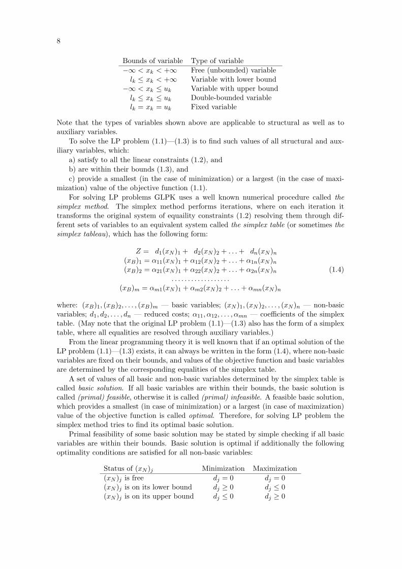
Bounds of variables can be finite as well as infinite. Besides, lower and upper boundscan be equal to each other. Thus, the following types of variables are possible:

7

8

Bounds of variable Type of variable−∞ < xk < +∞ Free (unbounded) variable

lk ≤ xk < +∞ Variable with lower bound−∞ < xk ≤ uk Variable with upper bound

lk ≤ xk ≤ uk Double-bounded variablelk = xk = uk Fixed variable

Note that the types of variables shown above are applicable to structural as well as toauxiliary variables.

To solve the LP problem (1.1)—(1.3) is to find such values of all structural and aux-iliary variables, which:

a) satisfy to all the linear constraints (1.2), andb) are within their bounds (1.3), andc) provide a smallest (in the case of minimization) or a largest (in the case of maxi-

mization) value of the objective function (1.1).For solving LP problems GLPK uses a well known numerical procedure called the

simplex method. The simplex method performs iterations, where on each iteration ittransforms the original system of equaility constraints (1.2) resolving them through dif-ferent sets of variables to an equivalent system called the simplex table (or sometimes thesimplex tableau), which has the following form:

Z = d1(xN )1 + d2(xN )2 + . . . + dn(xN )n

(xB)1 = α11(xN )1 + α12(xN )2 + . . . + α1n(xN )n

(xB)2 = α21(xN )1 + α22(xN )2 + . . . + α2n(xN )n

. . . . . . . . . . . . . . . . . .(xB)m = αm1(xN )1 + αm2(xN )2 + . . . + αmn(xN )n

(1.4)

where: (xB)1, (xB)2, . . . , (xB)m — basic variables; (xN )1, (xN )2, . . . , (xN )n — non-basicvariables; d1, d2, . . . , dn — reduced costs; α11, α12, . . . , αmn — coefficients of the simplextable. (May note that the original LP problem (1.1)—(1.3) also has the form of a simplextable, where all equalities are resolved through auxiliary variables.)

From the linear programming theory it is well known that if an optimal solution of theLP problem (1.1)—(1.3) exists, it can always be written in the form (1.4), where non-basicvariables are fixed on their bounds, and values of the objective function and basic variablesare determined by the corresponding equalities of the simplex table.

A set of values of all basic and non-basic variables determined by the simplex table iscalled basic solution. If all basic variables are within their bounds, the basic solution iscalled (primal) feasible, otherwise it is called (primal) infeasible. A feasible basic solution,which provides a smallest (in case of minimization) or a largest (in case of maximization)value of the objective function is called optimal. Therefore, for solving LP problem thesimplex method tries to find its optimal basic solution.

Primal feasibility of some basic solution may be stated by simple checking if all basicvariables are within their bounds. Basic solution is optimal if additionally the followingoptimality conditions are satisfied for all non-basic variables:

Status of (xN )j Minimization Maximization(xN )j is free dj = 0 dj = 0(xN )j is on its lower bound dj ≥ 0 dj ≤ 0(xN )j is on its upper bound dj ≤ 0 dj ≥ 0

9

In other words, basic solution is optimal if there is no non-basic variable, which changingin the feasible direction (i.e. increasing if it is free or on its lower bound, or decreasingif it is free or on its upper bound) can improve (i.e. decrease in case of minimization orincrease in case of maximization) the objective function.

If all non-basic variables satisfy to the optimality conditions shown above (indepen-dently on whether basic variables are within their bounds or not), the basic solution iscalled dual feasible, otherwise it is called dual infeasible.

It may happen that some LP problem has no primal feasible solution due to incorrectformulation — this means that its constraints conflict with each other. It also may happenthat some LP problem has unbounded solution again due to incorrect formulation — thismeans that some non-basic variable can improve the objective function, i.e. the optimalityconditions are violated, and at the same time this variable can infinitely change in thefeasible direction meeting no resistance from basic variables. (May note that in the lattercase the LP problem has no dual feasible solution.)

1.2 MIP Problem

Mixed integer linear programming (MIP) problem is LP problem in which some variablesare additionally required to be integer.

GLPK assumes that MIP problem has the same formulation as ordinary (pure) LPproblem (1.1)—(1.3), i.e. includes auxiliary and structural variables, which may have lowerand/or upper bounds. However, in case of MIP problem some variables may be requiredto be integer. This additional constraint means that a value of each integer variable mustbe only integer number. (Should note that GLPK allows only structural variables to beof integer kind.)

1.3 Brief Example

In order to understand what GLPK is from the user’s standpoint, consider the followingsimple LP problem:

maximize

Z = 10x1 + 6x2 + 4x3

subject to

x1 + x2 + x3 ≤ 10010x1 +4x2 +5x3 ≤ 6002x1 +2x2 +6x3 ≤ 300

where all variables are non-negative

x1 ≥ 0, x2 ≥ 0, x3 ≥ 0

At first this LP problem should be transformed to the standard form (1.1)—(1.3).It can be easily done introducing auxiliary variables, by one for each original inequalityconstraint. Thus, the considered problem can be reformulated as follows:

10

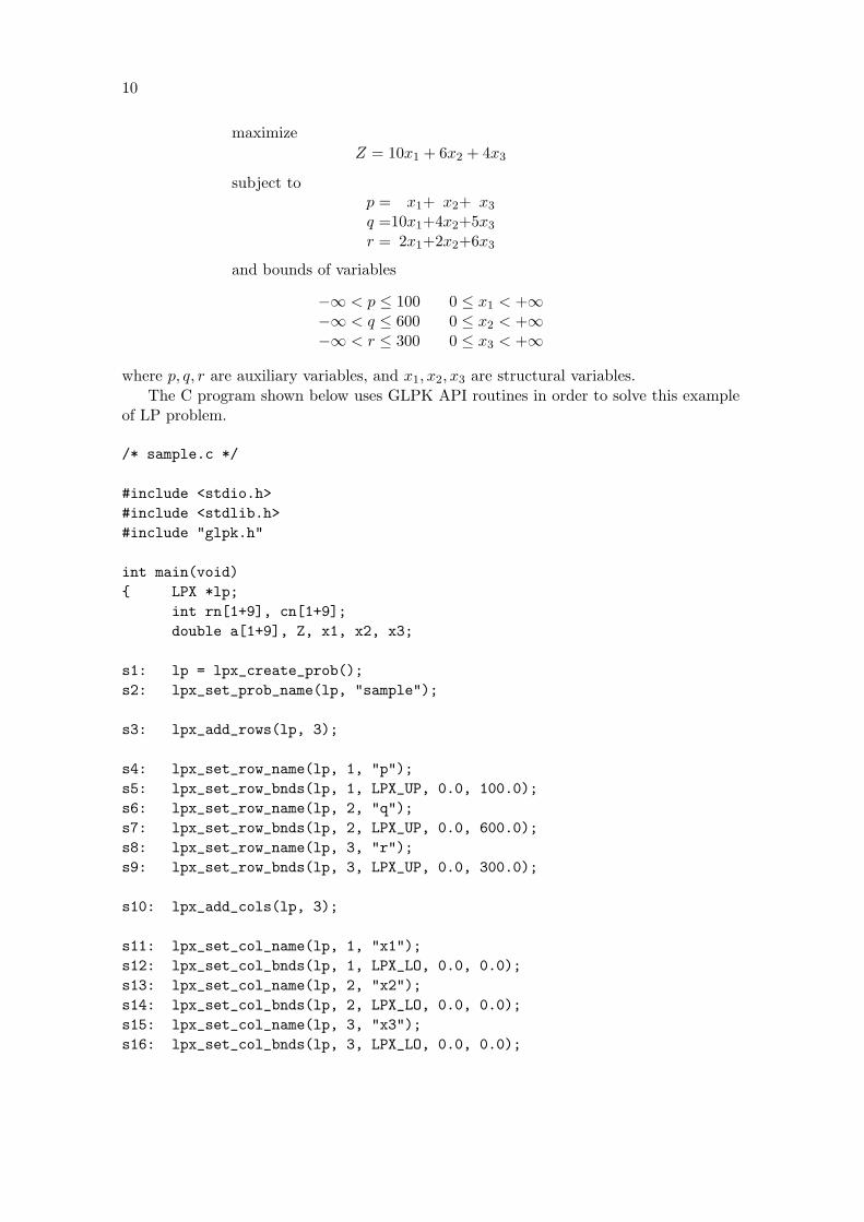
maximizeZ = 10x1 + 6x2 + 4x3

subject top = x1+ x2+ x3

q =10x1+4x2+5x3

r = 2x1+2x2+6x3

and bounds of variables

−∞ < p ≤ 100 0 ≤ x1 < +∞−∞ < q ≤ 600 0 ≤ x2 < +∞−∞ < r ≤ 300 0 ≤ x3 < +∞

where p, q, r are auxiliary variables, and x1, x2, x3 are structural variables.The C program shown below uses GLPK API routines in order to solve this example

of LP problem.

/* sample.c */

#include <stdio.h>#include <stdlib.h>#include "glpk.h"

int main(void){ LPX *lp;

int rn[1+9], cn[1+9];double a[1+9], Z, x1, x2, x3;

s1: lp = lpx_create_prob();s2: lpx_set_prob_name(lp, "sample");

s3: lpx_add_rows(lp, 3);

s4: lpx_set_row_name(lp, 1, "p");s5: lpx_set_row_bnds(lp, 1, LPX_UP, 0.0, 100.0);s6: lpx_set_row_name(lp, 2, "q");s7: lpx_set_row_bnds(lp, 2, LPX_UP, 0.0, 600.0);s8: lpx_set_row_name(lp, 3, "r");s9: lpx_set_row_bnds(lp, 3, LPX_UP, 0.0, 300.0);

s10: lpx_add_cols(lp, 3);

s11: lpx_set_col_name(lp, 1, "x1");s12: lpx_set_col_bnds(lp, 1, LPX_LO, 0.0, 0.0);s13: lpx_set_col_name(lp, 2, "x2");s14: lpx_set_col_bnds(lp, 2, LPX_LO, 0.0, 0.0);s15: lpx_set_col_name(lp, 3, "x3");s16: lpx_set_col_bnds(lp, 3, LPX_LO, 0.0, 0.0);

11

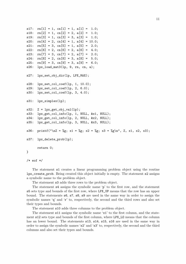
s17: rn[1] = 1, cn[1] = 1, a[1] = 1.0;s18: rn[2] = 1, cn[2] = 2, a[2] = 1.0;s19: rn[3] = 1, cn[3] = 3, a[3] = 1.0;s20: rn[4] = 2, cn[4] = 1, a[4] = 10.0;s21: rn[5] = 3, cn[5] = 1, a[5] = 2.0;s22: rn[6] = 2, cn[6] = 2, a[6] = 4.0;s23: rn[7] = 3, cn[7] = 2, a[7] = 2.0;s24: rn[8] = 2, cn[8] = 3, a[8] = 5.0;s25: rn[9] = 3, cn[9] = 3, a[9] = 6.0;s26: lpx_load_mat3(lp, 9, rn, cn, a);

s27: lpx_set_obj_dir(lp, LPX_MAX);

s28: lpx_set_col_coef(lp, 1, 10.0);s29: lpx_set_col_coef(lp, 2, 6.0);s30: lpx_set_col_coef(lp, 3, 4.0);

s31: lpx_simplex(lp);

s32: Z = lpx_get_obj_val(lp);s33: lpx_get_col_info(lp, 1, NULL, &x1, NULL);s34: lpx_get_col_info(lp, 2, NULL, &x2, NULL);s35: lpx_get_col_info(lp, 3, NULL, &x3, NULL);

s36: printf("\nZ = %g; x1 = %g; x2 = %g; x3 = %g\n", Z, x1, x2, x3);

s37: lpx_delete_prob(lp);

return 0;}

/* eof */

The statement s1 creates a linear programming problem object using the routinelpx_create_prob. Being created this object initially is empty. The statement s2 assignsa symbolic name to the problem object.

The statement s3 adds three rows to the problem object.The statement s4 assigns the symbolic name ‘p’ to the first row, and the statement

s5 sets type and bounds of the first row, where LPX_UP means that the row has an upperbound. The statements s6, s7, s8, s9 are used in the aame way in order to assign thesymbolic names ‘q’ and ‘r’ to, respectively, the second and the third rows and also settheir types and bounds.

The statement s10 adds three columns to the problem object.The statement s11 assigns the symbolic name ‘x1’ to the first column, and the state-

ment s12 sets type and bounds of the first column, where LPX_LO means that the columnhas an lower bound. The statements s13, s14, s15, s16 are used in the same way inorder to assign the symbolic names ‘x2’ and ‘x3’ to, respectively, the second and the thirdcolumns and also set their types and bounds.

12

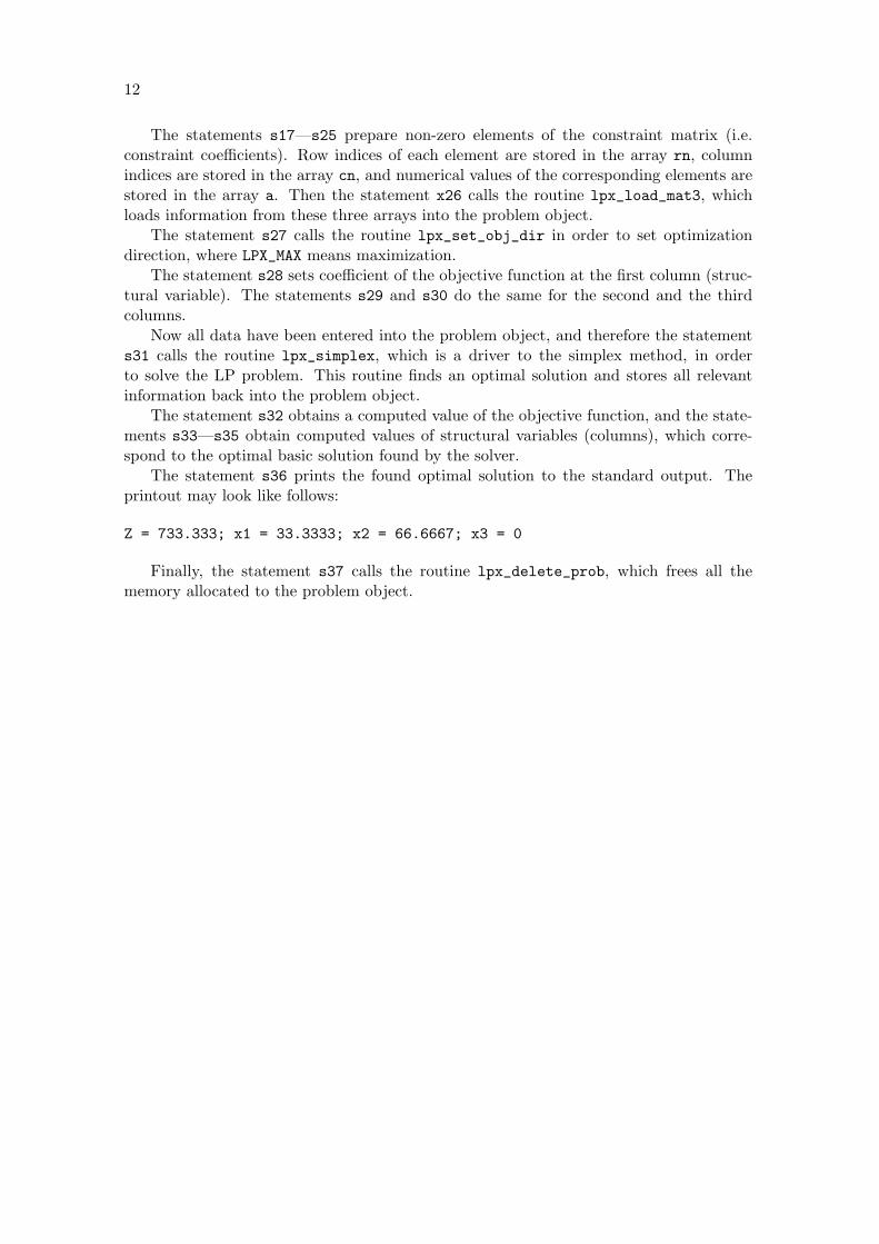
The statements s17—s25 prepare non-zero elements of the constraint matrix (i.e.constraint coefficients). Row indices of each element are stored in the array rn, columnindices are stored in the array cn, and numerical values of the corresponding elements arestored in the array a. Then the statement x26 calls the routine lpx_load_mat3, whichloads information from these three arrays into the problem object.

The statement s27 calls the routine lpx_set_obj_dir in order to set optimizationdirection, where LPX_MAX means maximization.

The statement s28 sets coefficient of the objective function at the first column (struc-tural variable). The statements s29 and s30 do the same for the second and the thirdcolumns.

Now all data have been entered into the problem object, and therefore the statements31 calls the routine lpx_simplex, which is a driver to the simplex method, in orderto solve the LP problem. This routine finds an optimal solution and stores all relevantinformation back into the problem object.

The statement s32 obtains a computed value of the objective function, and the state-ments s33—s35 obtain computed values of structural variables (columns), which corre-spond to the optimal basic solution found by the solver.

The statement s36 prints the found optimal solution to the standard output. Theprintout may look like follows:

Z = 733.333; x1 = 33.3333; x2 = 66.6667; x3 = 0

Finally, the statement s37 calls the routine lpx_delete_prob, which frees all thememory allocated to the problem object.

Chapter 2

API Routines

This chapter describes GLPK API routines intended for using in application programs.

Error handling If some GLPK API routine detects erroneous or incorrect data passedby the application program, it sends appropriate diagnostic messages to the standardoutput and then abnormally terminates the application program. In most practical casesthis allows to simplify programming avoiding numerous checks of return codes. Thus,in order to prevent crashing the application program should check all data, which aresuspected to be incorrect, before calling GLPK API routines.

Should note that this kind of error handling is used only in the cases of incorrect datapassed by the application program. If, for example, the application program calls someGLPK API routine to read data from an input file and these data are incorrect, the GLPKAPI routine reports about error in the usual way by means of return code.

Thread safety Currently GLPK API routines are non-reentrant and therefore cannotbe used in multi-threaded programs.

Array indexing Normally all GLPK routines start array indexing from 1, not from 0(except the specially stipulated cases). This means, for example, if some vector x of thelength n is passed as an array to some GLPK routine, the latter expects vector componentsto be placed in locations x[1], x[2], . . . , x[n], and the location x[0] normally is notused.

In order to avoid indexing errors it is most convenient and most reliable to declare thearray x as follows:

double x[1+n];

or to allocate it as follows:

double *x;. . .x = calloc(1+n, sizeof(double));

In both cases one extra location x[0] is reserved that allows passing this array to GLPKroutines in a usual way.

13

14

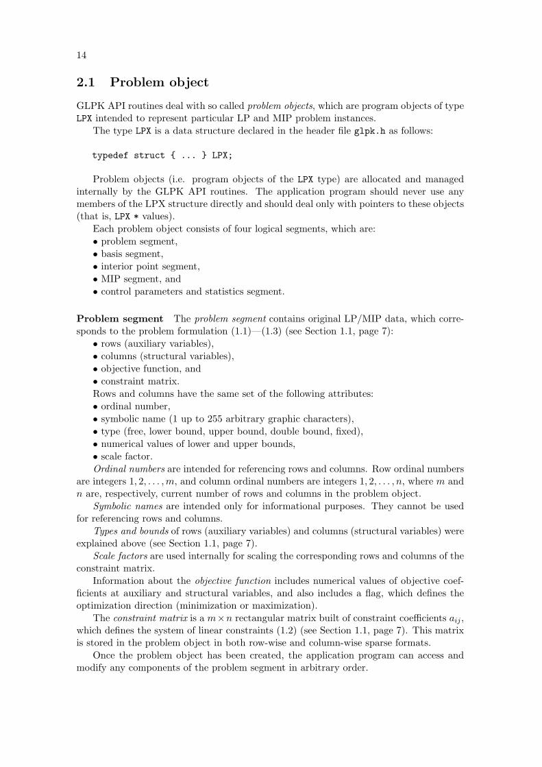
2.1 Problem object

GLPK API routines deal with so called problem objects, which are program objects of typeLPX intended to represent particular LP and MIP problem instances.

The type LPX is a data structure declared in the header file glpk.h as follows:

typedef struct { ... } LPX;

Problem objects (i.e. program objects of the LPX type) are allocated and managedinternally by the GLPK API routines. The application program should never use anymembers of the LPX structure directly and should deal only with pointers to these objects(that is, LPX * values).

Each problem object consists of four logical segments, which are:• problem segment,• basis segment,• interior point segment,• MIP segment, and• control parameters and statistics segment.

Problem segment The problem segment contains original LP/MIP data, which corre-sponds to the problem formulation (1.1)—(1.3) (see Section 1.1, page 7):

• rows (auxiliary variables),• columns (structural variables),• objective function, and• constraint matrix.Rows and columns have the same set of the following attributes:• ordinal number,• symbolic name (1 up to 255 arbitrary graphic characters),• type (free, lower bound, upper bound, double bound, fixed),• numerical values of lower and upper bounds,• scale factor.Ordinal numbers are intended for referencing rows and columns. Row ordinal numbers

are integers 1, 2, . . . ,m, and column ordinal numbers are integers 1, 2, . . . , n, where m andn are, respectively, current number of rows and columns in the problem object.

Symbolic names are intended only for informational purposes. They cannot be usedfor referencing rows and columns.

Types and bounds of rows (auxiliary variables) and columns (structural variables) wereexplained above (see Section 1.1, page 7).

Scale factors are used internally for scaling the corresponding rows and columns of theconstraint matrix.

Information about the objective function includes numerical values of objective coef-ficients at auxiliary and structural variables, and also includes a flag, which defines theoptimization direction (minimization or maximization).

The constraint matrix is a m×n rectangular matrix built of constraint coefficients aij ,which defines the system of linear constraints (1.2) (see Section 1.1, page 7). This matrixis stored in the problem object in both row-wise and column-wise sparse formats.

Once the problem object has been created, the application program can access andmodify any components of the problem segment in arbitrary order.

15

Basis segment The basis segment of the problem object keeps information related to acurrent basic solution. This information includes:

• row and column statuses,• basic solution statuses,• factorization of the current basis matrix, and• basic solution components.The row and column statuses define which rows and columns are basic and which are

non-basic. These statuses may be assigned either by the application program of by someAPI routines. Note that these statuses are always defined independently on whether thecorresponding basis valid or not.

The basic solution statuses include the primal status and the dual status, which are setby the simplex-based solver once the problem has been solved. The primal status showswhether a primal basic solution is feasible, infeasible, or undefined. The dual status showsthe same for a dual basic solution.

The factorization of the basis matrix is some factorized form (like LU-factorization) ofthe current basis matrix (defined by the current row and column statuses). The factoriza-tion is used by the simplex-based solver and kept when the solver terminates the search.This feature allows efficiently reoptimizing the problem after some modifications (for ex-ample, after changing some bounds or objective coefficients). It also allows performing apost-optimal analysis (for example, computing components of the simplex table, etc.).

The basic solution components include primal and dual values of all auxiliary andstructural variables for the most recently obtained basic solution.

Interior point segment The interior point segment is automatically allocated after theproblem has been solved using the interior point solver. It contains interior point solutioncomponents, which include the solution status, and primal and dual values of all auxiliaryand structural variables.

MIP segment The MIP segment is used only for MIP problems. This segment includes:• column kinds,• MIP solution status, and• MIP solution components.The column kinds define which columns (i.e. structural variables) are integer and

which are continuous.The MIP solution status is set by the MIP solver and shows whether a MIP solution

is integer optimal, integer feasible (non-optimal), or undefined.The MIP solution components are computed by the MIP solver and includes primal

values of all auxiliary and structural variables for the most recently obtained MIP solution.Note that in the case of MIP problem the basis segment corresponds to an optimal

solution of LP relaxation, which is also available to the application program.Currently the search tree is not kept in the MIP segment. Therefore if the search has

been finished or terminated, it cannot be continued.

Control parameters and statistics segment This segment contains a fixed set ofparameters, where each parameter has the following three attributes:

• code,• type, and• current value.

16

The parameter code is intended for referencing a particular parameter. All the param-eter codes have symbolic names, which are macros defined in the header file glpk.h. Notethat the parameter codes are distinct positive integers.

The parameter type can be integer, real (floating-point), and text (character string).The parameter value is its current value kept in the problem object. Initially (once the

problem object has been created) all parameters are assigned to some standard defaultvalues.

Parameters are intended for several purposes. Some of them, which are called con-trol parameters, affect on the behavior of API routines (for example, the parameterLPX_K_ITLIM limits maximal number of simplex iterations available to the solver). Others,which are called statistics, just represent some additional information about the problemobject (for example, the parameter LPX_K_ITCNT shows how many simplex iterations wereperformed for a particular problem object).

17

2.2 Problem creating and modifying routines

2.2.1 lpx create prob — create problem object

Synopsis

#include "glpk.h"LPX *lpx_create_prob(void);

Description The routine lpx_create_prob creates a new problem object, which is“empty”, i.e. has no rows and no columns.

Returns The routine returns a pointer to the created object, which should be used inany subsequent operations on this object.

2.2.2 lpx add rows — add new rows to problem object

Synopsis

#include "glpk.h"void lpx_add_rows(LPX *lp, int nrs);

Description The routine lpx_add_rows adds nrs rows (constraints) to the specifiedproblem object. New rows are always added to the end of the row list, so ordinal numbersof existing rows are not changed.

Being added each new row is free (unbounded) and has no constraint coefficients.

2.2.3 lpx add cols — add new columns to problem object

Synopsis

#include "glpk.h"void lpx_add_cols(LPX *lp, int ncs);

Description The routine lpx_add_cols adds ncs columns (structural variables) to thespecified problem object. New columns are always added to the end of the column list, soorinal numbers of existing columns are not changed.

Being added each new structural variable is fixed at zero and has no constraint coef-ficients.

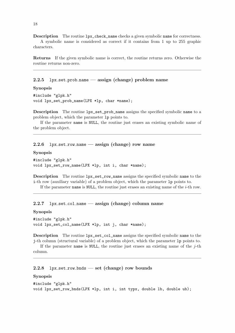
2.2.4 lpx check name — check correctness of symbolic name

Synopsis

#include "glpk.h"int lpx_check_name(char *name);

18

Description The routine lpx_check_name checks a given symbolic name for correctness.A symbolic name is considered as correct if it contains from 1 up to 255 graphic

characters.

Returns If the given symbolic name is correct, the routine returns zero. Otherwise theroutine returns non-zero.

2.2.5 lpx set prob name — assign (change) problem name

Synopsis

#include "glpk.h"void lpx_set_prob_name(LPX *lp, char *name);

Description The routine lpx_set_prob_name assigns the specified symbolic name to aproblem object, which the parameter lp points to.

If the parameter name is NULL, the routine just erases an existing symbolic name ofthe problem object.

2.2.6 lpx set row name — assign (change) row name

Synopsis

#include "glpk.h"void lpx_set_row_name(LPX *lp, int i, char *name);

Description The routine lpx_set_row_name assigns the specified symbolic name to thei-th row (auxiliary variable) of a problem object, which the parameter lp points to.

If the parameter name is NULL, the routine just erases an existing name of the i-th row.

2.2.7 lpx set col name — assign (change) column name

Synopsis

#include "glpk.h"void lpx_set_col_name(LPX *lp, int j, char *name);

Description The routine lpx_set_col_name assigns the specified symbolic name to thej-th column (structural variable) of a problem object, which the parameter lp points to.

If the parameter name is NULL, the routine just erases an existing name of the j-thcolumn.

2.2.8 lpx set row bnds — set (change) row bounds

Synopsis

#include "glpk.h"void lpx_set_row_bnds(LPX *lp, int i, int typx, double lb, double ub);

19

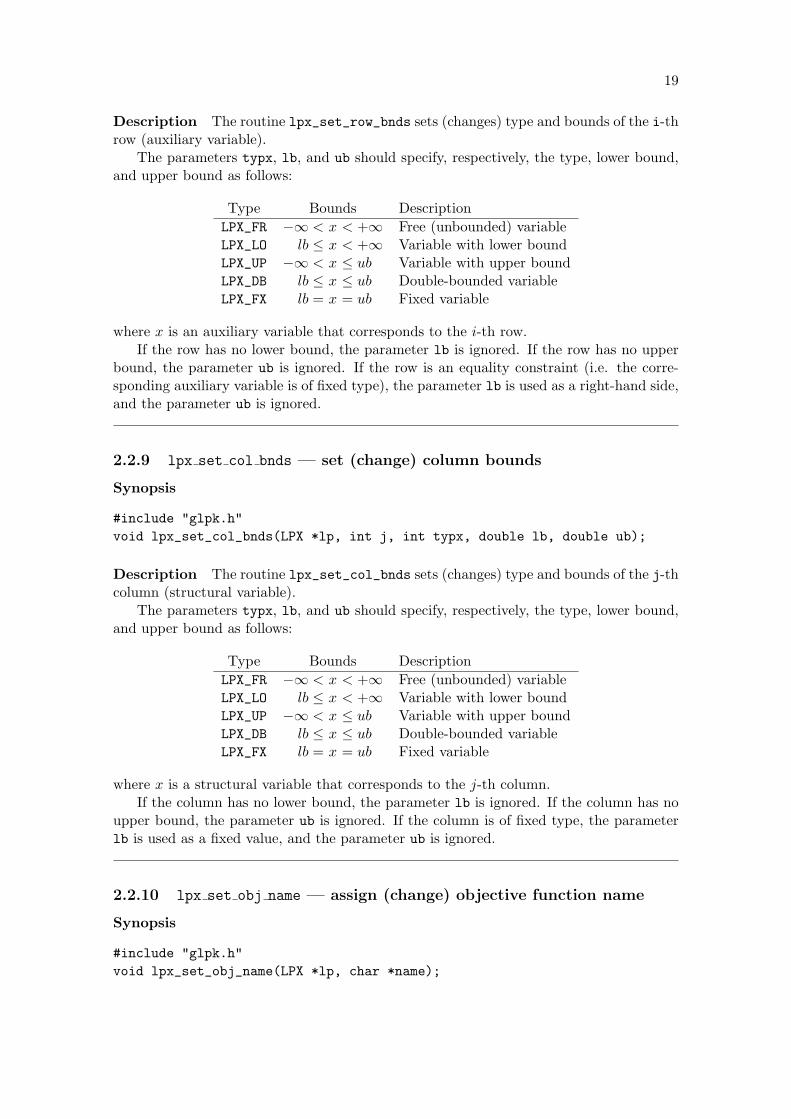
Description The routine lpx_set_row_bnds sets (changes) type and bounds of the i-throw (auxiliary variable).

The parameters typx, lb, and ub should specify, respectively, the type, lower bound,and upper bound as follows:

Type Bounds DescriptionLPX_FR −∞ < x < +∞ Free (unbounded) variableLPX_LO lb ≤ x < +∞ Variable with lower boundLPX_UP −∞ < x ≤ ub Variable with upper boundLPX_DB lb ≤ x ≤ ub Double-bounded variableLPX_FX lb = x = ub Fixed variable

where x is an auxiliary variable that corresponds to the i-th row.If the row has no lower bound, the parameter lb is ignored. If the row has no upper

bound, the parameter ub is ignored. If the row is an equality constraint (i.e. the corre-sponding auxiliary variable is of fixed type), the parameter lb is used as a right-hand side,and the parameter ub is ignored.

2.2.9 lpx set col bnds — set (change) column bounds

Synopsis

#include "glpk.h"void lpx_set_col_bnds(LPX *lp, int j, int typx, double lb, double ub);

Description The routine lpx_set_col_bnds sets (changes) type and bounds of the j-thcolumn (structural variable).

The parameters typx, lb, and ub should specify, respectively, the type, lower bound,and upper bound as follows:

Type Bounds DescriptionLPX_FR −∞ < x < +∞ Free (unbounded) variableLPX_LO lb ≤ x < +∞ Variable with lower boundLPX_UP −∞ < x ≤ ub Variable with upper boundLPX_DB lb ≤ x ≤ ub Double-bounded variableLPX_FX lb = x = ub Fixed variable

where x is a structural variable that corresponds to the j-th column.If the column has no lower bound, the parameter lb is ignored. If the column has no

upper bound, the parameter ub is ignored. If the column is of fixed type, the parameterlb is used as a fixed value, and the parameter ub is ignored.

2.2.10 lpx set obj name — assign (change) objective function name

Synopsis

#include "glpk.h"void lpx_set_obj_name(LPX *lp, char *name);

20

Description The routine lpx_set_obj_name assigns the specified symbolic name to theobjective function.

If the parameter name is NULL, the routine just erases an existing symbolic name ofthe objective function.

2.2.11 lpx set obj dir — set (change) optimization direction

Synopsis

#include "glpk.h"void lpx_set_obj_dir(LPX *lp, int dir);

Description The routine lpx_set_obj_dir sets (changes) the optimization direction(i.e. the sense of the objective function) as specified by the parameter dir:

LPX_MIN the objective function should be minimized;LPX_MAX the objective function should be maximized.

2.2.12 lpx set obj c0 — set (change) constant term of the objectivefunction

Synopsis

#include "glpk.h"void lpx_set_obj_c0(LPX *lp, double c0);

Description The routine lpx_set_obj_c0 sets (changes) a constant term of the objec-tive function for an LP problem object, which the parameter lp points to. A new valueof the constant term is specified by the parameter c0.

2.2.13 lpx set row coef — set (change) row objective coefficient

Synopsis

#include "glpk.h"void lpx_set_row_coef(LPX *lp, int i, double coef);

Description The routine lpx_set_row_coef sets (changes) an objective coefficient atthe i-th auxiliary variable (row). A new value of the objective coefficient is specified bythe parameter coef. (Note that zero objective coefficients are allowed.)

2.2.14 lpx set col coef — set (change) column objective coefficient

Synopsis

#include "glpk.h"void lpx_set_col_coef(LPX *lp, int j, double coef);

21

Description The routine lpx_set_col_coef sets (changes) an objective coefficient atthe j-th structural variable (column). A new value of the objective coefficient is specifiedby the parameter coef. (Note that zero objective coefficients are allowed.)

2.2.15 lpx load mat — load the constraint matrix

Synopsis

#include "glpk.h"void lpx_load_mat(LPX *lp,

void *info, double (*mat)(void *info, int *i, int *j));

Description The routine lpx_load_mat loads non-zero elements of the constraint ma-trix (i.e. constraint coefficients) from a file specified by the formal routine mat. All existingcontents of the constraint matrix is destroyed.

The parameter info is a transit pointer passed to the formal routine mat (see below).The formal routine mat specifies a set of non-zero elements, which should be loaded

into the matrix. The routine lpx_load_mat calls the routine mat in order to obtain a nextnon-zero element aij . In response the routine mat should store row and column indices ofthis next element to the locations *i and *j, respectively, and return a numerical valueof this next element. Elements may be enumerated in arbirary order. Note that zeroelements and multiplets (i.e. elements with identical row and column indices) are notallowed. If there is no next element, the routine mat should store zero to both locations*i and *j and then “rewind” the file in order to begin enumerating again from the firstelement.

Using the routine lpx_load_mat is the most efficient way for initial loading the con-straint matrix.

2.2.16 lpx load mat3 — load the constraint matrix

Synopsis

#include "glpk.h"void lpx_load_mat3(LPX *lp, int nz, int rn[], int cn[], double a[]);

Description The routine lpx_load_mat3 loads non-zero elements of the constraint ma-trix (i.e. constraint coefficients) from the arrays rn, cn, and a. All existing contents ofthe constraint matrix is destroyed.

The parameter nz specifies number of non-zero coefficients to be loaded.A particular constraint coefficient aij is specified as a triplet (rn[k], cn[k], a[k]),

k = 1, . . . , nz, where rn[k] is its row index i, cn[k] is its column index j, and a[k] is itsnumerical value aij . Coefficients may be enumerated in arbitrary order. Note that zerocoefficients as well as multiplets (i.e. coefficients with identical row and column indices)are not allowed.

22

2.2.17 lpx set mat row — change row of the constraint matrix

Synopsis

#include "glpk.h"void lpx_set_mat_row(LPX *lp, int i, int len, int ndx[], double val[]);

Description The routine lpx_set_mat_row sets (replaces) the i-th row of the constraintmatrix for the problem object, which the parameter lp points to.

Column indices and numerical values of new non-zero coefficients of the i-th row shouldbe placed in the locations ndx[1], . . . , ndx[len] and val[1], . . . , val[len], respectively,where 0 ≤ len ≤ n is the new length of the i-th row, n is number of columns.

Note that zero coefficients and multiplets (i.e. coefficients with identical column in-dices) are not allowed.

The routine lpx_set_mat_row is intended mainly for modifying the constraint matrix.Using this routine for initial loading the constraint matrix is possible, but not very efficient.

2.2.18 lpx set mat col — change column of the constraint matrix

Synopsis

#include "glpk.h"void lpx_set_mat_col(LPX *lp, int j, int len, int ndx[], double val[]);

Description The routine lpx_set_mat_col sets (replaces) the j-th column of the con-straint matrix for the problem object, which the parameter lp points to.

Row indices and numerical values of new non-zero coefficients of the j-th column shouldbe placed in the locations ndx[1], . . . , ndx[len] and val[1], . . . , val[len], respectively,where 0 ≤ len ≤ m is the new length of the j-th column, m is number of rows.

Note that zero coefficients and multiplets (i.e. coefficients with identical row indices)are not allowed.

The routine lpx_set_mat_col is intended mainly for modifying the constraint matrix.Using this routine for initial loading the constraint matrix is possible, but not very efficient.

2.2.19 lpx unmark all — unmark all rows and columns

Synopsis

#include "glpk.h"void lpx_unmark_all(LPX *lp);

Description The routine lpx_unmark_all resets marks of all rows and columns of thespecified problem object to zero.

It is recommended to use this routine before subsequent calls to the routineslpx_mark_row and lpx_mark_col.

23

2.2.20 lpx mark row — assign mark to row

Synopsis

#include "glpk.h"void lpx_mark_row(LPX *lp, int i, int mark);

Description The routine lpx_mark_row assigns an integer mark to the i-th row.The sense of marking depends on what operation will then be performed on the prob-

lem object.

2.2.21 lpx mark col — assign mark to column

Synopsis

#include "glpk.h"void lpx_mark_col(LPX *lp, int j, int mark);

Description The routine lpx_mark_col assigns an integer mark to the j-th column.The sense of marking depends on what operation will then be performed on the prob-

lem object.

2.2.22 lpx clear mat — clear rows and columns of the constraint matrix

Synopsis

#include "glpk.h"void lpx_clear_mat(LPX *lp);

Description The routine lpx_clear_mat clears (nullifies) marked rows and columns ofthe constraint matrix.

Note that a row (column) is considered as marked, if its mark assigned by using theroutine lpx_mark_row (lpx_mark_col) is non-zero.

On exit the routine remains the row and column marks unchanged.

2.2.23 lpx del items — remove rows and columns from problem object

Synopsis

#include "glpk.h"void lpx_del_items(LPX *lp);

24

Description The routine lpx_del_items deletes all marked rows and columns from aproblem object, which the parameter lp points to.

Note that a row (column) is considered as marked, if its mark assigned by using theroutine lpx_mark_row (lpx_mark_col) is non-zero.

Deleting rows and columns involves changing oridinal numbers of other rows andcolumns, which are remaining in the problem object. Let, for example, before deletionthere were 5 rows a, b, c, d, e with ordinal numbers 1, 2, 3, 4, 5, and 6 columns p, q, r,s, t, u with ordinal numbers 1, 2, 3, 4, 5, 6. Let rows b, d and columns p, r, t, u weredeleted. Then after deletion the remaining rows a, c, e will have new oridinal numbers 1,2, 3, and the remaining columns q, s will have new ordinal numbers 1, 2. In other words,new ordinal numbers can be determined in the assumption that the order of the remainingrows and columns is not changed.

2.2.24 lpx delete prob — delete problem object

Synopsis

#include "glpk.h"void lpx_delete_prob(LPX *lp);

Description The routine lpx_delete_prob deletes a problem object, which the param-eter lp points to, freeing all the memory allocated to this object.

25

2.3 Problem querying routines

2.3.1 lpx get num rows — determine number of rows

Synopsis

#include "glpk.h"int lpx_get_num_rows(LPX *lp);

Returns The routine lpx_get_num_rows returns current number of rows in a problemobject, which the parameter lp points to.

2.3.2 lpx get num cols — determine number of columns

Synopsis

#include "glpk.h"int lpx_get_num_cols(LPX *lp);

Returns The routine lpx_get_num_cols returns current number of columns in a prob-lem object, which the parameter lp points to.

2.3.3 lpx get num nz — determine number of non-zero constraint coeffi-cients

Synopsis

#include "glpk.h"int lpx_get_num_nz(LPX *lp);

Returns The routine lpx_get_num_nz returns current number non-zero elements in theconstraint matrix, which is a part of the specified problem object.

2.3.4 lpx get prob name — obtain problem name

Synopsis

#include "glpk.h"char *lpx_get_prob_name(LPX *lp);

Returns The routine lpx_get_prob_name returns a pointer to an internal buffer, whichcontains a symbolic name assigned to the specified problem object. However, if the problemobject has no assigned name, the routine returns NULL.

26

2.3.5 lpx get row name — obtain row name

Synopsis

#include "glpk.h"char *lpx_get_row_name(LPX *lp, int i);

Returns The routine lpx_get_row_name returns a pointer to an internal buffer, whichcontains a symbolic name assigned to the i-th row. However, if the row has no assignedname, the routine returns NULL.

2.3.6 lpx get col name — obtain column name

Synopsis

#include "glpk.h"char *lpx_get_col_name(LPX *lp, int j);

Returns The routine lpx_get_col_name returns a pointer to an internal buffer, whichcontains a symbolic name assigned to the j-th column. However, if the column has noassigned name, the routine returns NULL.

2.3.7 lpx get row bnds — obtain row bounds

Synopsis

#include "glpk.h"void lpx_get_row_bnds(LPX *lp, int i, int *typx, double *lb,

double *ub);

Description The routine lpx_get_row_bnds stores the type, lower bound and upperbound of the i-th row (auxiliary variable) to locations, which the parameters typx, lb,and ub point to, respectively.

If some of the parameters typx, lb, ub is NULL, the corresponding value is not stored.Types and bounds have the following meaning:

Type Bounds DescriptionLPX_FR −∞ < x < +∞ Free (unbounded) variableLPX_LO lb ≤ x < +∞ Variable with lower boundLPX_UP −∞ < x ≤ ub Variable with upper boundLPX_DB lb ≤ x ≤ ub Double-bounded variableLPX_FX lb = x = ub Fixed variable

where x is an auxiliary variable that corresponds to the i-th row.If the row has no lower bound, *lb is set to zero. If the row has no upper bound, *ub

is set to zero. If the row is an equality constraint (i.e. the corresponding auxiliary variableis of fixed type), *lb and *ub are set to the same value.

27

2.3.8 lpx get col bnds — obtain column bounds

Synopsis

#include "glpk.h"void lpx_get_col_bnds(LPX *lp, int j, int *typx, double *lb,

double *ub);

Description The routine lpx_get_col_bnds stores the type, lower bound and upperbound of the j-th column (structural variable) to locations, which the parameters typx,lb, and ub point to, respectively.

If some of the parameters typx, lb, ub is NULL, the corresponding value is not stored.Types and bounds have the following meaning:

Type Bounds DescriptionLPX_FR −∞ < x < +∞ Free (unbounded) variableLPX_LO lb ≤ x < +∞ Variable with lower boundLPX_UP −∞ < x ≤ ub Variable with upper boundLPX_DB lb ≤ x ≤ ub Double-bounded variableLPX_FX lb = x = ub Fixed variable

where x is a structural variable that corresponds to the j-th column.If the column has no lower bound, *lb is set to zero. If the column has no upper

bound, *ub is set to zero. If the column is of fixed type, *lb and *ub are set to the samevalue.

2.3.9 lpx get obj name — obtain objective function name

Synopsis

#include "glpk.h"char *lpx_get_obj_name(LPX *lp);

Returns The routine lpx_get_obj_name returns a pointer to an internal buffer, whichcontains a symbolic name assigned to the objective function. However, if the objectivefunction has no assigned name, the routine returns NULL.

2.3.10 lpx get obj dir — determine optimization direction

Synopsis

#include "glpk.h"int lpx_get_obj_dir(LPX *lp);

Returns The routine lpx_get_obj_dir returns a flag, which defines the optimizationdirection (i.e. the sense of the objective function):

LPX_MIN the objective function should be minimized;LPX_MAX the objective function should be maximized.

28

2.3.11 lpx get obj c0 — obtain constant term of the objective function

Synopsis

#include "glpk.h"double lpx_get_obj_c0(LPX *lp);

Returns The routine lpx_get_obj_c0 returns a constant term of the objective functionfor the specified problem object.

2.3.12 lpx get row coef — obtain row objective coefficient

Synopsis

#include "glpk.h"double lpx_get_row_coef(LPX *lp, int i);

Returns The routine lpx_get_row_coef returns an objective coefficient at the i-thauxiliary variable (row) for the specified problem object.

2.3.13 lpx get col coef — obtain column objective coefficient

Synopsis

#include "glpk.h"double lpx_get_col_coef(LPX *lp, int j);

Returns The routine lpx_get_col_coef returns an objective coefficient at the j-thstructural variable (column) for the specified problem object.

2.3.14 lpx get mat row — obtain row of the constraint matrix

Synopsis

#include "glpk.h"int lpx_get_mat_row(LPX *lp, int i, int ndx[], double val[]);

Description The routine lpx_get_mat_row looks through (non-zero) elements of thei-th row of the constraint matrix and stores their column indices and values to locationsndx[1], . . . , ndx[len] and val[1], . . . , val[len], respectively, where 0 ≤ len ≤ n isnumber of elements in the i-th row, n is number of columns. It is allowed to specify valas NULL, in which case only column indices are stored.

Returns The routine returns len, which is number of stored elements (length of thei-th row).

29

2.3.15 lpx get mat col — obtain column of the constraint matrix

Synopsis

#include "glpk.h"int lpx_get_mat_col(LPX *lp, int j, int ndx[], double val[]);

Description The routine lpx_get_mat_col looks through (non-zero) elements of thej-th column of the constraint matrix and stores their row indices and values to locationsndx[1], . . . , ndx[len] and val[1], . . . , val[len], respectively, where 0 ≤ len ≤ m isnumber of elements in the j-th column, m is number of rows. It is allowed to specify valas NULL, in which case only row indices are stored.

Returns The routine returns len, which is number of stored elements (length of thej-th column).

2.3.16 lpx get row mark — determine row mark

Synopsis

#include "glpk.h"int lpx_get_row_mark(LPX *lp, int i);

Returns The routine lpx_get_row_mark returns an integer mark assigned to the i-throw. Zero means the row is not marked.

2.3.17 lpx get col mark — determine column mark

Synopsis

#include "glpk.h"int lpx_get_col_mark(LPX *lp, int j);

Returns The routine lpx_get_col_mark returns an integer mark assigned to the j-thcolumn. Zero means the column is not marked.

30

2.4 Problem scaling routines

2.4.1 lpx scale prob — scale problem data

Synopsis

#include "glpk.h"void lpx_scale_prob(LPX *lp);

Description The routine lpx_scale_prob performs scaling problem data for the spec-ified problem object.

The purpose of scaling is to replace the original constraint matrix A by the scaledmatrix A′ = RAS, where R and S are diagonal scaling matrices, in the hope that A′ hasbetter numerical properties than A.

On API level the scaling effect is almost invisible, since all data entered into theproblem object (say, constraint coefficients or bounds of variables) are automatically scaledby API routines using the scaling matrices R and S, and vice versa, all data obtained fromthe problem object (say, values of variables or reduced costs) are automatically unscaled.However, round-off errors may involve small distortions (of order DBL_EPSILON) of theoriginal problem data.

2.4.2 lpx unscale prob — unscale problem data

Synopsis

#include "glpk.h"void lpx_unscale_prob(LPX *lp);

The routine lpx_unscale_prob performs unscaling problem data for the specifiedproblem object.

“Unscaling” means replacing the current scaling matrices R and S by unity matricesthat cancels the scaling effect.

31

2.5 Basis constructing routines

2.5.1 lpx std basis — build standard initial basis

Synopsis

#include "glpk.h"void lpx_std_basis(LPX *lp);

Description The routine lpx_std_basis builds the “standard” (trivial) initial basis fora problem object, which the parameter lp points to.

In the “standard” basis all auxiliary variables (rows) are basic, and all structuralvariables (columns) are non-basic, so the corresponding basis matrix is unity.

2.5.2 lpx adv basis — build advanced initial basis

Synopsis

#include "glpk.h"void lpx_adv_basis(LPX *lp);

Description The routine lpx_adv_basis build an advanced initial basis for a problemobject, which the parameter lp points to.

In order to build the advanced initial basis the routine does the following:1) includes in the basis all non-fixed auxiliary variables;2) includes in the basis as many as possible non-fixed structural variables preserving

triangular form of the basis matrix;3) includes in the basis appropriate (fixed) auxiliary variables in order to complete the

basis.As a result the initial basis has as few as possible fixed variables and the corresponding

basis matrix is (implicitly) triangular.

2.5.3 lpx set row stat — set (change) row status

Synopsis

#include "glpk.h"void lpx_set_row_stat(LPX *lp, int i, int stat);

Description The routine lpx_set_row_stat sets (changes) the current status of thei-th row (auxiliary variable) as specified by the parameter stat:

32

LPX_BS make the row basic (make the constraint inactive);LPX_NL make the row non-basic (make the constraint active);LPX_NU make the row non-basic and set it to the upper bound; if the row is not

double-bounded, this status is equivalent to LPX_NL (only in the case of thisroutine);

LPX_NF the same as LPX_NL (only in the case of this routine);LPX_NS the same as LPX_NL (only in the case of this routine).

2.5.4 lpx set col stat — set (change) column status

Synopsis

#include "glpk.h"void lpx_set_col_stat(LPX *lp, int j, int stat);

Description The routine lpx_set_col_stat sets (changes) the current status of thej-th column (structural variable) as specified by the parameter stat:

LPX_BS make the column basic;LPX_NL make the column non-basic;LPX_NU make the column non-basic and set it to the upper bound; if the column is

not of double-bounded type, this status is the same as LPX_NL (only in thecase of this routine);

LPX_NF the same as LPX_NL (only in the case of this routine);LPX_NS the same as LPX_NL (only in the case of this routine).

33

2.6 Simplex method routines

2.6.1 lpx warm up — “warm up” initial basis

Synopsis

#include "glpk.h"int lpx_warm_up(LPX *lp);

Description The routine lpx_warm_up is intended to “warm up” the initial basis speci-fied by the current statuses of rows (auxiliary variables) and columns (structural variables).

This operation includes (if necessary) reinverting (factorizing) the initial basis matrix,computing the initial basic solution components (values of basic variables, simplex multi-pliers, reduced costs of non-basic variables), and determining primal and dual statuses ofthe initial basic solution.

“Warming up” is an optional operation. It can be used before starting optimizationin order to obtain basic solution information in the initial point.

Returns The routine lpx_warm_up returns one of the following exit codes:LPX_E_OK the initial basis has been successfully “warmed up”.LPX_E_EMPTY the problem has no rows and/or no columns.LPX_E_BADB the initial basis is invalid, because number of basic variables and

number of rows are different.LPX_E_SING the initial basis matrix is numerically singular or ill-conditioned.Note that additional exit codes may appear in the future versions of this routine.

2.6.2 lpx simplex — solve LP problem using the simplex method

Synopsis

#include "glpk.h"int lpx_simplex(LPX *lp);

Description The routine lpx_simplex is an interface to the LP problem solver basedon the two-phase revised simplex method.

This routine obtains problem data from the problem object, which the parameter lppoints to, calls the solver to solve the LP problem, and stores the found solution and otherrelevant information back in the problem object.

Generally, the simplex solver does the following:• “warming up” the initial basis;• searching for (primal) feasible basic solution (phase I);• searching for optimal basic solution (phase II)• storing the final basis and found basic solution back in the problem object.Since large scale problems may take a long time, the solver reports some information

about the current basic solution, which is sent to the standard output. This informationhas the following format:

34

*nnn: objval = xxx infeas = yyy (ddd)

where: ‘nnn’ is the iteration number, ‘xxx’ is the current value of the objective function(which is unscaled and has correct sign), ‘yyy’ is the current sum of primal infeasibilities(which is scaled and therefore may be used for visual estimating only), ‘ddd’ is the currentnumber of fixed basic variables. If the asterisk ‘*’ precedes to ‘nnn’, the solver is searchingfor an optimal solution (phase II), otherwise the solver is searching for a primal feasiblesolution (phase I).

Note that the simplex solver implemented in GLPK is not perfect. Although it hasbeen successfully tested on a wide set of LP problems, there are hard problems, whichcan’t be solved by this solver.

Using built-in LP presolver The simplex solver has the built-in LP presolver, whichis a subprogram that transforms the original LP problem specified in the problem objectto an equivalent LP problem, which may be easier for solving with the simplex methodthan the original one. This is attained mainly due to reducing the problem size andimproving its numeric properties (for example, by removing some inactive constraints orby fixing some non-basic variables). Once the transformed LP problem has been solved,the presolver transforms its basic solution back to a corresponding basic solution of theoriginal problem.

Presolving is an optional feature of the routine lpx_simplex, and by default it isnot used. In order to use the LP presolver the user should set on the control parameterLPX_K_PRESOL (see Subsection 2.11.6, page 56) before calling the routine lpx_simplex.As a rule presolving is useful when the problem is solved for the first time. However, it isnot recommended to use presolving when the problem should be re-optimized.

Presolving procedure is transparent to the API user in the sense that all necessaryprocessing is performed internally, and a basic solution of the original problem recoveredby the presolver is the same as if it were computed directly, i.e. without presolving.

Note that the presolver is able to recover only optimal solutions. If a computed solutionis infeasible or non-optimal, the corresponding solution of the original problem cannot berecovered and therefore remains undefined. If the user needs to know a basic solution evenif it is infeasible or non-optimal, the presolver should not be used.

Returns If the LP presolver is not used (the flag LPX_K_PRESOL is off), the routinelpx_simplex returns one of the following exit codes:

LPX_E_OK the LP problem has been successfully solved. (Note that, for exam-ple, if the problem has no feasible solution, this exit code is reported.)

LPX_E_FAULT unable to start the search because either the problem has norows/columns, or the initial basis is invalid, or the initial basis matrixis singular or ill-conditioned.

LPX_E_OBJLL the search was prematurely terminated because the objective func-tion being maximized has reached its lower limit and continues de-creasing (the dual simplex only).

LPX_E_OBJUL the search was prematurely terminated because the objective func-tion being minimized has reached its upper limit and continues in-creasing (the dual simplex only).

LPX_E_ITLIM the search was prematurely terminated because the simplex itera-tions limit has been exceeded.

35

LPX_E_TMLIM the search was prematurely terminated because the time limit hasbeen exceeded.

LPX_E_SING the search was prematurely terminated due to the solver failure (thecurrent basis matrix got singular or ill-conditioned).

If the LP presolver is used (the flag LPX_K_PRESOL is on), the routine lpx_simplexreturns one of the following exit codes:

LPX_E_OK optimal solution of the LP problem has been found.LPX_E_FAULT the LP problem has no rows and/or columns.LPX_E_NOPFS the LP problem has no primal feasible solution.LPX_E_NODFS the LP problem has no dual feasible solution.LPX_E_ITLIM same as above.LPX_E_TMLIB same as above.LPX_E_SING same as above.Note that additional exit codes may appear in the future versions of this routine.

36

2.7 Basic solution querying routines

2.7.1 lpx get status — query basic solution status

Synopsis

#include "glpk.h"int lpx_get_status(LPX *lp);

Returns The routine lpx_get_status reports the status of the current basic solutionobtained for an LP problem object, which the parameter lp points to:

LPX_OPT solution is optimal;LPX_FEAS solution is feasible;LPX_INFEAS solution is infeasible;LPX_NOFEAS problem has no feasible solution;LPX_UNBND problem has unbounded solution;LPX_UNDEF solution status is undefined.More detailed information about the solution status can be obtained using the routines

lpx_get_prim_stat and lpx_get_dual_stat.

2.7.2 lpx get prim stat — query primal status of basic solution

Synopsis

#include "glpk.h"int lpx_get_prim_stat(LPX *lp);

Returns The routine lpx_get_prim_stat reports the primal status of the current basicsolution obtained by the solver for an LP problem object, which the parameter lp pointsto:

LPX_P_UNDEF the primal status is undefined;LPX_P_FEAS the solution is primal feasible;LPX_P_INFEAS the solution is primal infeasible;LPX_P_NOFEAS no primal feasible solution exists.

2.7.3 lpx get dual stat — query dual status of basic solution

Synopsis

#include "glpk.h"int lpx_get_dual_stat(LPX *lp);

37

Returns The routine lpx_get_dual_stat reports the dual status of the current basicsolution obtained by the solver for an LP problem object, which the parameter lp pointsto:

LPX_D_UNDEF the dual status is undefined;LPX_D_FEAS the solution is dual feasible;LPX_D_INFEAS the solution is dual infeasible;LPX_D_NOFEAS no dual feasible solution exists.

2.7.4 lpx get row info — obtain row solution information

Synopsis

#include "glpk.h"void lpx_get_row_info(LPX *lp, int i, int *tagx, double *vx,

double *dx);

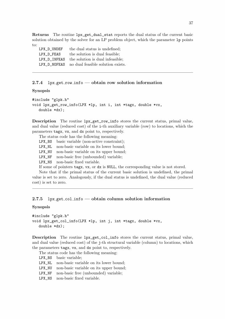
Description The routine lpx_get_row_info stores the current status, primal value,and dual value (reduced cost) of the i-th auxiliary variable (row) to locations, which theparameters tagx, vx, and dx point to, respectively.

The status code has the following meaning:LPX_BS basic variable (non-active constraint);LPX_NL non-basic variable on its lower bound;LPX_NU non-basic variable on its upper bound;LPX_NF non-basic free (unbounded) variable;LPX_NS non-basic fixed variable.If some of pointers tagx, vx, or dx is NULL, the corresponding value is not stored.Note that if the primal status of the current basic solution is undefined, the primal

value is set to zero. Analogously, if the dual status is undefined, the dual value (reducedcost) is set to zero.

2.7.5 lpx get col info — obtain column solution information

Synopsis

#include "glpk.h"void lpx_get_col_info(LPX *lp, int j, int *tagx, double *vx,

double *dx);

Description The routine lpx_get_col_info stores the current status, primal value,and dual value (reduced cost) of the j-th structural variable (column) to locations, whichthe parameters tagx, vx, and dx point to, respectively.

The status code has the following meaning:LPX_BS basic variable;LPX_NL non-basic variable on its lower bound;LPX_NU non-basic variable on its upper bound;LPX_NF non-basic free (unbounded) variable;LPX_NS non-basic fixed variable.

38

If some of pointers tagx, vx, or dx is NULL, the corresponding value is not stored.Note that if the primal status of the current basic solution is undefined, the primal

value is set to zero. Analogously, if the dual status is undefined, the dual value (reducedcost) is set to zero.

2.7.6 lpx get obj val — obtain value of the objective function

Synopsis

#include "glpk.h"double lpx_get_obj_val(LPX *lp);

Returns The routine lpx_get_obj_val returns the current value of the objective func-tion for an LP problem object, which the parameter lp points to.

Note that if the primal status of the current basic solution is undefined, the routinereturns zero.

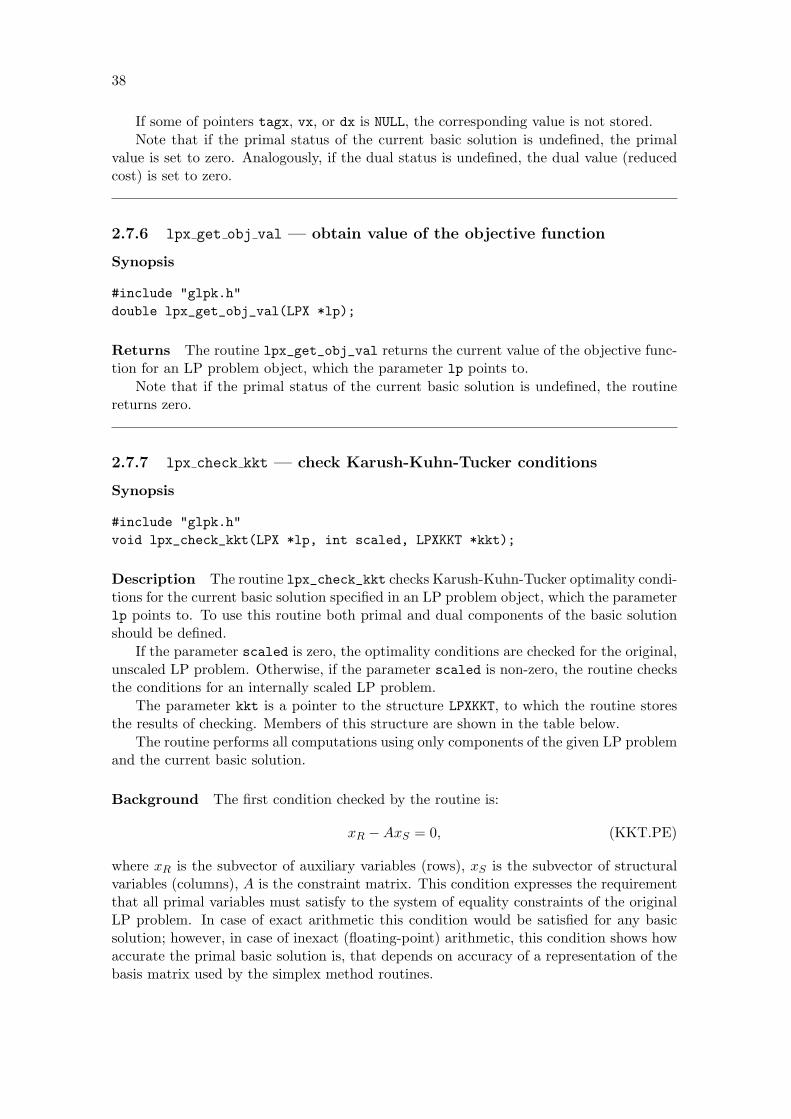
2.7.7 lpx check kkt — check Karush-Kuhn-Tucker conditions

Synopsis

#include "glpk.h"void lpx_check_kkt(LPX *lp, int scaled, LPXKKT *kkt);

Description The routine lpx_check_kkt checks Karush-Kuhn-Tucker optimality condi-tions for the current basic solution specified in an LP problem object, which the parameterlp points to. To use this routine both primal and dual components of the basic solutionshould be defined.

If the parameter scaled is zero, the optimality conditions are checked for the original,unscaled LP problem. Otherwise, if the parameter scaled is non-zero, the routine checksthe conditions for an internally scaled LP problem.

The parameter kkt is a pointer to the structure LPXKKT, to which the routine storesthe results of checking. Members of this structure are shown in the table below.

The routine performs all computations using only components of the given LP problemand the current basic solution.

Background The first condition checked by the routine is:

xR −AxS = 0, (KKT.PE)

where xR is the subvector of auxiliary variables (rows), xS is the subvector of structuralvariables (columns), A is the constraint matrix. This condition expresses the requirementthat all primal variables must satisfy to the system of equality constraints of the originalLP problem. In case of exact arithmetic this condition would be satisfied for any basicsolution; however, in case of inexact (floating-point) arithmetic, this condition shows howaccurate the primal basic solution is, that depends on accuracy of a representation of thebasis matrix used by the simplex method routines.

39

Condition Member Comment(KKT.PE) pe_ae_max Largest absolute error

pe_ae_row Number of row with largest absolute errorpe_re_max Largest relative errorpe_re_row Number of row with largest relative errorpe_quality Quality of primal solution

(KKT.PB) pb_ae_max Largest absolute errorpb_ae_ind Number of variable with largest absolute errorpb_re_max Largest relative errorpb_re_ind Number of variable with largest relative errorpb_quality Quality of primal feasibility

(KKT.DE) de_ae_max Largest absolute errorde_ae_col Number of column with largest absolute errorde_re_max Largest relative errorde_re_col Number of column with largest relative errorde_quality Quality of dual solution

(KKT.DB) db_ae_max Largest absolute errordb_ae_ind Number of variable with largest absolute errordb_re_max Largest relative errordb_re_ind Number of variable with largest relative errordb_quality Quality of dual feasibility

The second condition checked by the routine is:

lk ≤ xk ≤ uk for all k = 1, . . . ,m + n, (KKT.PB)

where xk is auxiliary (1 ≤ k ≤ m) or structural (m + 1 ≤ k ≤ m + n) variable, lk anduk are, respectively, lower and upper bounds of the variable xk (including cases of infinitebounds). This condition expresses the requirement that all primal variables must satisfyto bound constraints of the original LP problem. Since in case of basic solution all non-basic variables are placed on their bounds, actually the condition (KKT.PB) needs to bechecked for basic variables only. If the primal basic solution has sufficient accuracy, thiscondition shows primal feasibility of the solution.

The third condition checked by the routine is:

grad Z = c = (A)T π + d,

where Z is the objective function, c is the vector of objective coefficients, (A)T is a matrixtransposed to the expanded constraint matrix A = (I| − A), π is a vector of Lagrangemultipliers that correspond to equality constraints of the original LP problem, d is avector of Lagrange multipliers that correspond to bound constraints for all (auxiliaryand structural) variables of the original LP problem. Geometrically the third conditionexpresses the requirement that the gradient of the objective function must belong tothe orthogonal complement of a linear subspace defined by the equality and active boundconstraints, i.e. that the gradient must be a linear combination of normals to the constraintplanes, where Lagrange multipliers π and d are coefficients of that linear combination.

To eliminate the vector π the third condition can be rewritten as:(I

−AT

)π =

(dR

dS

)+

(cR

cS

),

40

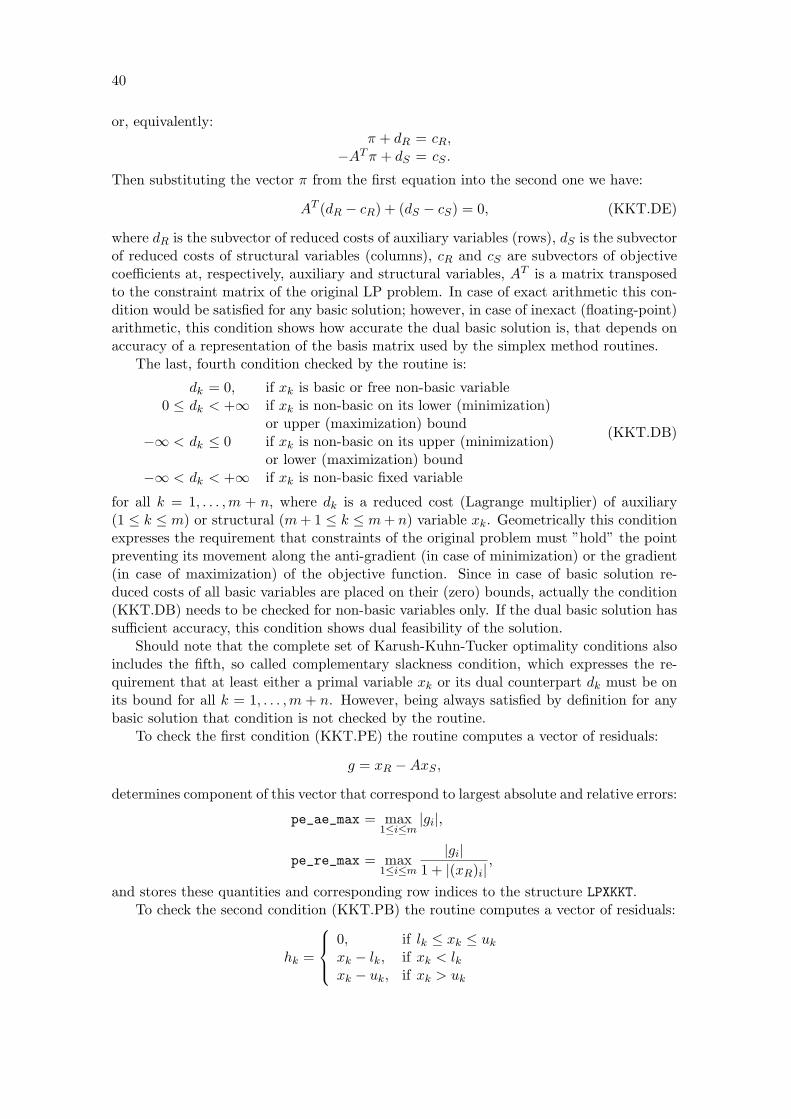
or, equivalently:π + dR = cR,

−AT π + dS = cS .

Then substituting the vector π from the first equation into the second one we have:

AT (dR − cR) + (dS − cS) = 0, (KKT.DE)

where dR is the subvector of reduced costs of auxiliary variables (rows), dS is the subvectorof reduced costs of structural variables (columns), cR and cS are subvectors of objectivecoefficients at, respectively, auxiliary and structural variables, AT is a matrix transposedto the constraint matrix of the original LP problem. In case of exact arithmetic this con-dition would be satisfied for any basic solution; however, in case of inexact (floating-point)arithmetic, this condition shows how accurate the dual basic solution is, that depends onaccuracy of a representation of the basis matrix used by the simplex method routines.

The last, fourth condition checked by the routine is:

dk = 0, if xk is basic or free non-basic variable0 ≤ dk < +∞ if xk is non-basic on its lower (minimization)

or upper (maximization) bound−∞ < dk ≤ 0 if xk is non-basic on its upper (minimization)

or lower (maximization) bound−∞ < dk < +∞ if xk is non-basic fixed variable

(KKT.DB)

for all k = 1, . . . ,m + n, where dk is a reduced cost (Lagrange multiplier) of auxiliary(1 ≤ k ≤ m) or structural (m + 1 ≤ k ≤ m + n) variable xk. Geometrically this conditionexpresses the requirement that constraints of the original problem must ”hold” the pointpreventing its movement along the anti-gradient (in case of minimization) or the gradient(in case of maximization) of the objective function. Since in case of basic solution re-duced costs of all basic variables are placed on their (zero) bounds, actually the condition(KKT.DB) needs to be checked for non-basic variables only. If the dual basic solution hassufficient accuracy, this condition shows dual feasibility of the solution.

Should note that the complete set of Karush-Kuhn-Tucker optimality conditions alsoincludes the fifth, so called complementary slackness condition, which expresses the re-quirement that at least either a primal variable xk or its dual counterpart dk must be onits bound for all k = 1, . . . ,m + n. However, being always satisfied by definition for anybasic solution that condition is not checked by the routine.

To check the first condition (KKT.PE) the routine computes a vector of residuals:

g = xR −AxS ,

determines component of this vector that correspond to largest absolute and relative errors:

pe_ae_max = max1≤i≤m

|gi|,

pe_re_max = max1≤i≤m

|gi|1 + |(xR)i|

,

and stores these quantities and corresponding row indices to the structure LPXKKT.To check the second condition (KKT.PB) the routine computes a vector of residuals:

hk =

0, if lk ≤ xk ≤ uk

xk − lk, if xk < lkxk − uk, if xk > uk

41

for all k = 1, . . . ,m + n, determines components of this vector that correspond to largestabsolute and relative errors:

pb_ae_max = max1≤k≤m+n

|hk|,

pb_re_max = max1≤k≤m+n

|hk|1 + |xk|

,

and stores these quantities and corresponding variable indices to the structure LPXKKT.To check the third condition (KKT.DE) the routine computes a vector of residuals:

u = AT (dR − cR) + (dS − cS),

determines components of this vector that correspond to largest absolute and relativeerrors:

de_ae_max = max1≤j≤n

|uj |,

de_re_max = max1≤j≤n

|uj |1 + |(dS)j − (cS)j |

,

and stores these quantities and corresponding column indices to the structure LPXKKT.To check the fourth condition (KKT.DB) the routine computes a vector of residuals:

vk =

{0, if dk has correct signdk, if dk has wrong sign

for all k = 1, . . . ,m + n, determines components of this vector that correspond to largestabsolute and relative errors:

db_ae_max = max1≤k≤m+n

|vk|,

db_re_max = max1≤k≤m+n

|vk|1 + |dk − ck|

,

and stores these quantities and corresponding variable indices to the structure LPXKKT.Using the relative errors for all the four conditions the routine lpx_check_kkt also

estimates a ”quality” of the basic solution from the standpoint of these conditions andstores corresponding quality indicators to the structure LPXKKT:

pe_quality — quality of primal solution;pb_quality — quality of primal feasibility;de_quality — quality of dual solution;db_quality — quality of dual feasibility.Each of these indicators is assigned to one of the following four values:’H’ means high quality,’M’ means medium quality,’L’ means low quality, or’?’ means wrong or infeasible solution.If all the indicators show high or medium quality (for an internally scaled LP problem,

i.e. when the parameter scaled in a call to the routine lpx_check_kkt is non-zero), theuser can be sure that the obtained basic solution is quite accurate.

If some of the indicators show low quality, the solution can still be considered asrelevant, though an additional analysis is needed depending on which indicator shows lowquality.

42

If the indicator pe_quality is assigned to ’?’, the primal solution is wrong. If theindicator de_quality is assigned to ’?’, the dual solution is wrong.

If the indicator db_quality is assigned to ’?’ while other indicators show a goodquality, this means that the current basic solution being primal feasible is not dual feasible.Similarly, if the indicator pb_quality is assigned to ’?’ while other indicators are not,this means that the current basic solution being dual feasible is not primal feasible.

43

2.8 Simplex table routines

2.8.1 lpx eval tab row — compute row of the simplex table

Synopsis

#include "glpk.h"int lpx_eval_tab_row(LPX *lp, int k, int ndx[], double val[]);

Description The routine lpx_eval_tab_row computes a row of the current simplextable for the basic variable, which is specified by the number k: if 1 ≤ k ≤ m, xk is k-thauxiliary variable; if m + 1 ≤ k ≤ m + n, xk is (k −m)-th structural variable, where m isnumber of rows, and n is number of columns. The current basis must be valid.

The routine stores column indices and numerical values of non-zero elements of thecomputed row using sparse vector format to the locations ndx[1], . . . , ndx[len] andval[1], . . . , val[len], respectively, where 0 ≤ len ≤ n is number of non-zeros returnedon exit.

Element indices stored in the array ndx have the same sense as the index k, i.e. indices1 to m denote auxiliary variables and indices m + 1 to m + n denote structural ones (allthese variables are obviously non-basic by the definition).

The computed row shows how the specified basic variable xk = (xB)i depends on thenon-basic variables:

(xB)i = αi1(xN )1 + αi2(xN )2 + . . . + αin(xN )n,

where αij are elements of the simplex table row, (xN )j are non-basic (auxiliary and struc-tural) variables.

Even if the problem is (internally) scaled, the routine returns the specified simplextable row as if the problem were unscaled.

Returns The routine returns number of non-zero elements in the simplex table rowstored in the arrays ndx and val.

2.8.2 lpx eval tab col — compute column of the simplex table

Synopsis

#include "glpk.h"int lpx_eval_tab_col(LPX *lp, int k, int ndx[], double val[]);

Description The routine lpx_eval_tab_col computes a column of the current simplextable for the non-basic variable, which is specified by the number k: if 1 ≤ k ≤ m, xk isk-th auxiliary variable; if m + 1 ≤ k ≤ m + n, xk is (k −m)-th structural variable, wherem is number of rows, and n is number of columns. The current basis must be valid.

The routine stores row indices and numerical values of non-zero elements of the com-puted column using sparse vector format to the locations ndx[1], . . . , ndx[len] and

44

val[1], . . . , val[len], respectively, where 0 ≤ len ≤ m is number of non-zeros returnedon exit.

Element indices stored in the array ndx have the same sense as the index k, i.e. indices1 to m denote auxiliary variables and indices m + 1 to m + n denote structural ones (allthese variables are obviously non-basic by the definition).

The computed column shows how the basic variables depend on the specified non-basicvariable xk = (xN )j :

(xB)1 = . . . + α1j(xN )j + . . .(xB)2 = . . . + α2j(xN )j + . . .

. . . . . . . . .(xB)m = . . . + αmj(xN )j + . . .

where αij are elements of the simplex table column, (xB)i are basic (auxiliary and struc-tural) variables.

Even if the problem is (internally) scaled, the routine returns the specified simplextable column as if the problem were unscaled.

Returns The routine returns number of non-zero elements in the simplex table columnstored in the arrays ndx and val.

2.8.3 lpx transform row — transform explicitly specified row

Synopsis

#include "glpk.h"int lpx_transform_row(LPX *lp, int len, int ndx[], double val[]);

Description The routine lpx_transform_row performs the same operation as the rou-tine lpx_eval_tab_row, except that the transformed row is specified explicitly.

The explicitly specified row may be thought as a linear form

x = a1xm+1 + a2xm+2 + . . . + anxm+n, (1)

where x is an auxiliary variable for this row, aj are coefficients of the linear form, xm+j

are structural variables.On entry column indices and numerical values of non-zero coefficients aj of the

transformed row should be placed in locations ndx[1], . . . , ndx[len] and val[1], . . . ,val[len], where len is number of non-zero coefficients.

This routine uses the system of equality constraints and the current basis in orderto express the auxiliary variable x in (1) through the current non-basic variables (as ifthe transformed row were added to the problem object and the auxiliary variable x werebasic), i.e. the resultant row has the form:

x = α1(xN )1 + α2(xN )2 + . . . + αn(xN )n, (2)

where αj are influence coefficients, (xN )j are non-basic (auxiliary and structural) variables,n is number of columns in the specified problem object.

On exit the routine stores indices and numerical values of non-zero coefficients αj ofthe resultant row (2) in locations ndx[1], . . . , ndx[len’] and val[1], . . . , val[len’],

45

where 0 ≤len’≤ n is count of non-zero coefficients in the resultant row returned by theroutine. Note that indices of non-basic variables stored in the array ndx correspond tooriginal ordinal numbers of variables: indices 1 to m mean auxiliary variables and indicesm + 1 to m + n mean structural ones.

Even if the problem is (internally) scaled, the routine returns the resultant row as ifthe problem were unscaled.

Returns The routine returns len’ that is number of non-zero coefficients in the resultantrow stored in the arrays ndx and val.

2.8.4 lpx transform col — transform explicitly specified column

Synopsis

#include "glpk.h"int lpx_transform_col(LPX *lp, int len, int ndx[], double val[]);

Description The routine lpx_transform_col performs the same operation as the rou-tine lpx_eval_tab_col, except that the transformed column is specified explicitly.

The explicitly specified column may be thought as it were added to the original systemof equality constraints:

x1 = a11xm+1 + . . . + a1nxm+n + a1xx2 = a21xm+1 + . . . + a2nxm+n + a2x

. . . . . . . . .xm = am1xm+1 + . . . + amnxm+n + amx

(1)

where xi are auxiliary variables, xm+j are structural variables (presented in the problemobject), x is a structural variable for the explicitly specified column, ai are constraintcoefficients for x.

On entry row indices and numerical values of non-zero coefficients ai of the transformedcolumn should be placed in locations ndx[1], . . . , ndx[len] and val[1], . . . , val[len],where len is number of non-zero coefficients.

This routine uses the system of equality constraints and the current basis in orderto express the current basic variables through the structural variable x in (1) (as if thetransformed column were added to the problem object and the variable x were non-basic):

(xB)1 = . . . + α1x(xB)2 = . . . + α2x

. . . . . . . . .(xB)m = . . . + αmx

(2)

where αi are influence coefficients, xB are basic (auxiliary and structural) variables, m isnumber of rows in the specified problem object.

On exit the routine stores indices and numerical values of non-zero coefficients αi ofthe resultant column (2) in locations ndx[1], . . . , ndx[len’] and val[1], . . . , val[len’],where 0 ≤len’≤ m is count of non-zero coefficients in the resultant column returned bythe routine. Note that indices of basic variables stored in the array ndx correspond to

46

original ordinal numbers of variables, i.e. indices 1 to m mean auxiliary variables, indicesm + 1 to m + n mean structural ones.

Even if the problem is (internally) scaled, the routine returns the resultant column asif the problem were unscaled.

Returns The routine returns len’ that is number of non-zero coefficients in the resultantcolumn stored in the arrays ndx and val.

2.8.5 lpx prim ratio test — perform primal ratio test

Synopsis

#include "glpk.h"int lpx_prim_ratio_test(LPX *lp, int len, int ndx[], double val[],

int how, double tol);

Description The routine lpx_prim_ratio_test performs the primal ratio test for anexplicitly specified column of the simplex table.

The primal basic solution associated with an LP problem object, which the parameterlp points to, should be feasible. No components of the LP problem object are changed bythe routine.

The explicitly specified column of the simplex table shows how the basic variables xB

depend on some non-basic variable y (which is not necessarily presented in the problemobject):

(xB)1 = . . . + α1y(xB)2 = . . . + α2y

. . . . . . . . .(xB)m = . . . + αmy

(1)

The column (1) is specifed on entry to the routine using the sparse format. Ordinalnumbers of basic variables (xB)i should be placed in locations ndx[1], . . . , ndx[len],where ordinal number 1 to m denote auxiliary variables, and ordinal numbers m + 1 tom + n denote structural variables. The corresponding non-zero coefficients αi should beplaced in locations val[1], . . . , val[len]. The arrays ndx and val are not changed bythe routine.

The parameter how specifies in which direction the variable y changes on entering thebasis: +1 means increasing, −1 means decreasing.

The parameter tol is a relative tolerance (small positive number) used by the routineto skip small αi in the column (1).

The routine determines the ordinal number of some basic variable (among specified inndx[1], . . . , ndx[len]), which reaches its (lower or upper) bound first before any otherbasic variables do and which therefore should leave the basis instead the variable y inorder to keep primal feasibility, and returns it on exit. If the choice cannot be made (i.e.if the adjacent basic solution is primal unbounded due to y), the routine returns zero.

Note If the non-basic variable y is presented in the LP problem object, the column (1)can be computed using the routine lpx_eval_tab_col. Otherwise it can be computedusing the routine lpx_transform_col.

47

Returns The routine lpx_prim_ratio_test returns the ordinal number of some basicvariable (xB)i, which should leave the basis instead the variable y in order to keep primalfeasibility. If the adjacent basic solution is primal unbounded and therefore the choicecannot be made, the routine returns zero.

2.8.6 lpx dual ratio test — perform dual ratio test

Synopsis

#include "glpk.h"int lpx_dual_ratio_test(LPX *lp, int len, int ndx[], double val[],

int how, double tol);

Description The routine lpx_dual_ratio_test performs the dual ratio test for anexplicitly specified row of the simplex table.

The dual basic solution associated with an LP problem object, which the parameterlp points to, should be feasible. No components of the LP problem object are changed bythe routine.

The explicitly specified row of the simplex table is a linear form, which shows how somebasic variable y (not necessarily presented in the problem object) depends on non-basicvariables xN :

y = α1(xN )1 + α2(xN )2 + . . . + αn(xN )n. (1)

The linear form (1) is specified on entry to the routine using the sparse format. Ordinalnumbers of non-basic variables (xN )j should be placed in locations ndx[1], . . . , ndx[len],where ordinal numbers 1 to m denote auxiliary variables, and ordinal numbers m + 1 tom + n denote structural variables. The corresponding non-zero coefficients αj should beplaced in locations val[1], . . . , val[len]. The arrays ndx and val are not changed bythe routine.

The parameter how specifies in which direction the variable y changes on leaving thebasis: +1 means increasing, −1 means decreasing.

The parameter tol is a relative tolerance (small positive number) used by the routineto skip small αj in the form (1).

The routine determines the ordinal number of some non-basic variable (among specifiedin ndx[1], . . . , ndx[len]), whose reduced cost reaches its (zero) bound first before thishappens for any other non-basic variables and which therefore should enter the basisinstead the variable y in order to keep dual feasibility, and returns it on exit. If the choicecannot be made (i.e. if the adjacent basic solution is dual unbounded due to y), the routinereturns zero.

Note If the basic variable y is presented in the LP problem object, the row (1) can becomputed using the routine lpx_eval_tab_row. Otherwise it can be computed using theroutine lpx_transform_row.

Returns The routine lpx_dual_ratio_test returns the ordinal number of some non-basic variable (xN )j , which should enter the basis instead the variable y in order to keepdual feasibility. If the adjacent basic solution is dual unbounded and therefore the choicecannot be made, the routine returns zero.

48

2.9 Interior point method routines

2.9.1 lpx interior — solve LP problem using the interior point method

Synopsis

#include "glpk.h"int lpx_interior(LPX *lp);

Description The routine lpx_interior is an interface to the LP problem solver basedon the primal-dual interior point method.

This routine obtains problem data from the problem object, which the parameter lppoints to, calls the solver to solve the LP problem, and stores the found solution back inthe problem object.

Interior point methods (also known as barrier methods) are more modern and morepowerful numerical methods for large scale linear programming. They especially fit forvery sparse LP problems and allow solving such problems much faster than the simplexmethod.

Solving large LP problems may take a long time, so the routine lpx_interior displaysinformation about every interior point iteration1. This information is sent to the standardoutput and has the following format:

nnn: F = fff; rpi = ppp; rdi = ddd; gap = ggg

where nnn is iteration number, fff is the current value of the objective function (in thecase of maximization it has wrong sign), ppp is the current relative primal infeasibility,ddd is the current relative dual infeasibility, and ggg is the current primal-dual gap.

Should note that currently the GLPK interior point solver doesn’t include many im-portant features, in particular:

it is not able to process dense columns. So if the constraint matrix of the LP problemhas dense columns, the solving process will be highly inefficient;

it has no features against numerical instability. For some LP problems prematuretermination may happen if the matrix ADAT becomes singular or ill-conditioned;

it computes only primal values of (auxiliary and structural variables) and doesn’tcompute dual values (i.e. reduced costs), which are just set to zero;

it is not able to identify optimal basis that corresponds to the found interior pointsolution.

Returns The routine lpx_interior returns one of the following exit codes:LPX_E_OK the LP problem has been successfully solved (to optimality).LPX_E_FAULT the solver can’t start the search because either the problem has no

rows and/or no columns, or some row has non-zero objective coeffi-cient.

LPX_E_NOFEAS the problem has no feasible (primal or dual) solution.

1Unlike the simplex method the interior point method usually needs 30—50 iterations (independentlyon the problem size) in order to find an optimal solution.

49

LPX_E_NOCONV the search was prematurely terminated due to very slow convergenceor divergence.

LPX_E_ITLIM the search was prematurely terminated because the simplex itera-tions limit has been exceeded.

LPX_E_INSTAB the search was prematurely terminated due to numerical instabilityon solving Newtonian system.

Note that additional exit codes may appear in the future versions of this routine.

2.9.2 lpx get ips stat — query status of interior point solution

Synopsis

#include "glpk.h"int lpx_get_ips_stat(LPX *lp);

Returns The routine lpx_get_ips_stat reports the status of an interior point solutionfound by the solver for an LP problem object, which the parameter lp points to:

LPX_T_UNDEF the interior point solution is undefined.LPX_T_OPT the interior point solution is optimal.Note that additional status codes may appear in the future versions of this routine.

2.9.3 lpx get ips row — obtain row interior point solution

Synopsis

#include "glpk.h"void lpx_get_ips_row(LPX *lp, int i, double *vx, double *dx);

Description The routine lpx_get_ips_row stores primal and dual interior point valuesfor the i-th auxiliary variable (row) to locations, which the parameters vx and dx pointto, respectively. If some of the pointers vx or dx is NULL, the corresponding value is notstored.

2.9.4 lpx get ips col — obtain column interior point solution

Synopsis

#include "glpk.h"void lpx_get_ips_col(LPX *lp, int j, double *vx, double *dx);

Description The routine lpx_get_ips_col stores primal and dual interior point valuesfor the j-th structural variable (column) to locations, which the parameters vx and dxpoint to, respectively. If some of the pointers vx or dx is NULL, the corresponding value isnot stored.

50

2.9.5 lpx get ips obj — obtain interior point value of the objective func-tion

Synopsis

#include "glpk.h"double lpx_get_ips_obj(LPX *lp);

Returns The routine lpx_get_ips_obj returns an interior point value of the objectivefunction.

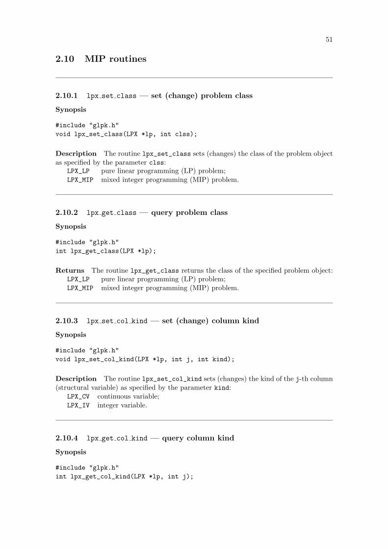
51

2.10 MIP routines

2.10.1 lpx set class — set (change) problem class

Synopsis

#include "glpk.h"void lpx_set_class(LPX *lp, int clss);

Description The routine lpx_set_class sets (changes) the class of the problem objectas specified by the parameter clss:

LPX_LP pure linear programming (LP) problem;LPX_MIP mixed integer programming (MIP) problem.

2.10.2 lpx get class — query problem class

Synopsis

#include "glpk.h"int lpx_get_class(LPX *lp);

Returns The routine lpx_get_class returns the class of the specified problem object:LPX_LP pure linear programming (LP) problem;LPX_MIP mixed integer programming (MIP) problem.

2.10.3 lpx set col kind — set (change) column kind

Synopsis

#include "glpk.h"void lpx_set_col_kind(LPX *lp, int j, int kind);

Description The routine lpx_set_col_kind sets (changes) the kind of the j-th column(structural variable) as specified by the parameter kind:

LPX_CV continuous variable;LPX_IV integer variable.

2.10.4 lpx get col kind — query column kind

Synopsis

#include "glpk.h"int lpx_get_col_kind(LPX *lp, int j);

52

Returns The routine lpx_get_col_kind returns the kind of the j-th column (structuralvariable):

LPX_CV continuous variable;LPX_IV integer variable.

2.10.5 lpx get num int — determine number of integer columns

Synopsis

#include "glpk.h"int lpx_get_num_int(LPX *lp);

Returns The routine lpx_get_num_int returns number of columns (structural vari-ables) in the problem object, which are marked as integer.

2.10.6 lpx get num bin — determine number of binary columns

Synopsis

#include "glpk.h"int lpx_get_num_bin(LPX *lp);

Returns The routine lpx_get_num_bin returns number of columns (structural vari-ables) in the problem object, which are marked as integer and have zero lower bound andunity upper bound.

2.10.7 lpx integer — solve MIP problem using the branch-and-boundmethod

Synopsis

#include "glpk.h"

Description The routine lpx_integer is an interface to the MIP problem solver basedon the branch-and-bound method.

This routine obtains problem data from the problem object, which the parameter lppoints to, calls the solver to solve the MIP problem, and stores the found solution andother relevant information back in the problem object.

On entry to this routine the problem object should contain an optimal basic solutionfor LP relaxation, which can be obtained by means of the simplex-based solver.

Since many MIP problems may take a long time, the solver reports some informationabout the best known solution, which is sent to the standard output. This informationhas the following format:

+nnn: mip = xxx; lp = yyy (mmm; nnn)

53

where ‘nnn’ is the simplex iteration number, ‘xxx’ is a value of the objective function forthe best known integer feasible solution (if no integer feasible solution has been foundyet, ‘xxx’ is the text ‘not found yet’), ‘yyy’ is an optimal value of the objective functionfor LP relaxation (this value is not changed during all the search), ‘mmm’ is number ofsubproblems in the active list, ‘nnn’ is number of subproblems which have been solved(considered).

Note that the branch-and-bound solver implemented in GLPK uses easiest heuristicsfor branching and backtracking, and therefore it is not perfect. Most probably this solvercan be used for solving MIP problems with one or two hundreds of integer variables. Hardor very large scale MIP problems can’t be solved by this routine.

Returns The routine lpx_integer returns one of the following exit codes:LPX_E_OK the MIP problem has been successfully solved. (Note that, for ex-

ample, if the problem has no integer feasible solution, this exit codeis reported.)

LPX_E_FAULT unable to start the search because either:the problem is not of MIP class, orthe problem object doesn’t contain optimal solution for LP relax-ation, orsome integer variable has non-integer lower or upper bound, orsome row has non-zero objective coefficient.

LPX_E_ITLIM the search was prematurely terminated because the simplex itera-tions limit has been exceeded.

LPX_E_TMLIM the search was prematurely terminated because the time limit hasbeen exceeded.

LPX_E_SING the search was prematurely terminated due to the solver failure (thecurrent basis matrix got singular or ill-conditioned).

Note that additional exit codes may appear in the future versions of this routine.

2.10.8 lpx get mip stat — query status of MIP solution

Synopsis

#include "glpk.h"int lpx_get_mip_stat(LPX *lp);

Returns The routine lpx_get_mip_stat reports the status of a MIP solution found bythe solver for a MIP problem object, which the parameter lp points to:

LPX_I_UNDEF the status is undefined (either the problem has not been solved orno integer feasible solution has been found yet).

LPX_I_OPT the solution is integer optimal.LPX_I_FEAS the solution is integer feasible but its optimality (or non-optimality)

has not been proven, perhaps due to premature termination of thesearch.

LPX_I_NOFEAS the problem has no integer feasible solution (proven by the solver).

54

2.10.9 lpx get mip row — obtain row activity for MIP solution

Synopsis

#include "glpk.h"double lpx_get_mip_row(LPX *lp, int i);

Returns The routine lpx_get_mip_row returns a value of the i-th auxiliary variable(row) for a MIP solution contained in the specified problem object.

Note that if the MIP solution is neither integer optimal nor integer feasible, zero isreturned.

2.10.10 lpx get mip col — obtain column activity for MIP solution

Synopsis

#include "glpk.h"double lpx_get_mip_col(LPX *lp, int j);

Returns The routine lpx_get_mip_col returns a value of the j-th structural variable(column) for a MIP solution contained in the specified problem object.

Note that if the MIP solution is neither integer optimal nor integer feasible, zero isreturned.

2.10.11 lpx get mip obj — obtain value of the objective function for MIPsolution

Synopsis

#include "glpk.h"double lpx_get_mip_obj(LPX *lp);

Returns The routine lpx_get_mip_obj returns a value of the objective function for aMIP solution contained in the specified problem object.

Note that if the MIP solution is neither integer optimal nor integer feasible, zero isreturned.

55

2.11 Control parameters and statistics routines

2.11.1 lpx reset parms — reset control parameters to default values

Synopsis

#include "glpk.h"void lpx_reset_parms(LPX *lp);

Description The routine lpx_reset_parms resets all control parameters associatedwith a problem object, which the parameter lp points to, to their default values.

2.11.2 lpx set int parm — set (change) integer control parameter

Synopsis

#include "glpk.h"void lpx_set_int_parm(LPX *lp, int parm, int val);

Description The routine lpx_set_int_parm sets (changes) the current value of an in-teger control parameter parm. The parameter val specifies a new value of the controlparameter.

2.11.3 lpx get int parm — query integer control parameter

Synopsis

#include "glpk.h"int lpx_get_int_parm(LPX *lp, int parm);

Returns The routine lpx_get_int_parm returns the current value of an integer controlparameter parm.

2.11.4 lpx set real parm — set (change) real control parameter

Synopsis

#include "glpk.h"void lpx_set_real_parm(LPX *lp, int parm, double val);

Description The routine lpx_set_real_parm sets (changes) the current value of a real(floating point) control parameter parm. The parameter val specifies a new value of thecontrol parameter.

56

2.11.5 lpx get real parm — query real control parameter

Synopsis

#include "glpk.h"double lpx_get_real_parm(LPX *lp, int parm);

Returns The routine lpx_get_real_parm returns the current value of a real (floatingpoint) control parameter parm.

2.11.6 Parameter list

This subsection describes all control parameters currently implemented in the package.Symbolic names of control parameters (which are macros defined in the header file glpk.h)are given on the left. Types, default values, and descriptions are given on the right.

LPX_K_MSGLEV type: integer, default: 3Level of messages output by solver routines:0 — no output1 — error messages only2 — normal output3 — full output (includes informational messages)

LPX_K_SCALE type: integer, default: 3Scaling option:0 — no scaling1 — equilibration scaling2 — geometric mean scaling, then equilibration scaling

LPX_K_DUAL type: integer, default: 0Dual simplex option:0 — do not use the dual simplex1 — if initial basic solution is dual feasible, use the dual simplex

LPX_K_PRICE type: integer, default: 1Pricing option (for both primal and dual simplex):0 — textbook pricing1 — steepest edge pricing

LPX_K_RELAX type: real, default: 0.07Relaxation parameter used in the ratio test. If it is zero, the textbookratio test is used. If it is non-zero (should be positive), Harris’ two-pass ratio test is used. In the latter case on the first pass of the ratiotest basic variables (in the case of primal simplex) or reduced costs ofnon-basic variables (in the case of dual simplex) are allowed to slightlyviolate their bounds, but not more than (RELAX · TOLBND) or (RELAX ·TOLDJ) (thus, RELAX is a percentage of TOLBND or TOLDJ).

LPX_K_TOLBND type: real, default: 10−7

Relative tolerance used to check if the current basic solution is primalfeasible. (Do not change this parameter without detailed understand-ing its purpose.)

57

LPX_K_TOLDJ type: real, default: 10−7

Absolute tolerance used to check if the current basic solution is dualfeasible. (Do not change this parameter without detailed understand-ing its purpose.)

LPX_K_TOLPIV type: real, default: 10−9

Relative tolerance used to choose eligible pivotal elements of the sim-plex table. (Do not change this parameter without detailed under-standing its purpose.)

LPX_K_ROUND type: integer, default: 0Solution rounding option:0 — report all primal and dual values “as is”1 — replace tiny primal and dual values by exact zero

LPX_K_OBJLL type: real, default: -DBL_MAXLower limit of the objective function. If on the phase II the objectivefunction reaches this limit and continues decreasing, the solver stopsthe search. (Used in the dual simplex only.)

LPX_K_OBJUL type: real, default: +DBL_MAXUpper limit of the objective function. If on the phase II the objectivefunction reaches this limit and continues increasing, the solver stopsthe search. (Used in the dual simplex only.)

LPX_K_ITLIM type: integer, default: −1Simplex iterations limit. If this value is positive, it is decreased byone each time when one simplex iteration has been performed, andreaching zero value signals the solver to stop the search. Negativevalue means no iterations limit.

LPX_K_ITCNT type: integer, initial: 0Simplex iterations count. This count is increased by one each timewhen one simplex iteration has been performed.

LPX_K_TMLIM type: real, default: −1.0Searching time limit, in seconds. If this value is positive, it is de-creased each time when one simplex iteration has been performed bythe amount of time spent for the iteration, and reaching zero valuesignals the solver to stop the search. Negative value means no timelimit.

LPX_K_OUTFRQ type: integer, default: 200Output frequency, in iterations. This parameter specifies how fre-quently the solver sends information about the solution to the standardoutput.

LPX_K_OUTDLY type: real, default: 0.0Output delay, in seconds. This parameter specifies how long the solvershould delay sending information about the solution to the standardoutput. Non-positive value means no delay.

LPX_K_BRANCH type: integer, default: 2Branching heuristic option (for MIP only):0 — branch on the first variable1 — branch on the last variable2 — branch using a heuristic by Driebeck and Tomlin

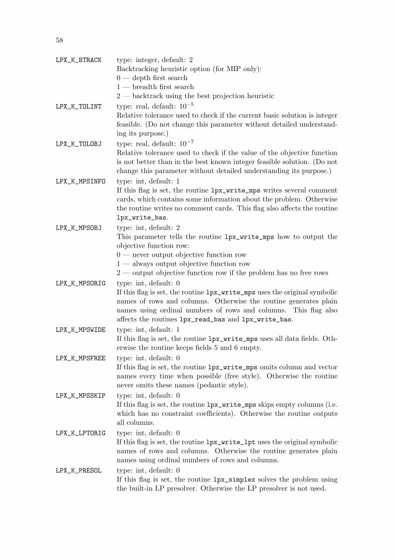
58

LPX_K_BTRACK type: integer, default: 2Backtracking heuristic option (for MIP only):0 — depth first search1 — breadth first search2 — backtrack using the best projection heuristic

LPX_K_TOLINT type: real, default: 10−5

Relative tolerance used to check if the current basic solution is integerfeasible. (Do not change this parameter without detailed understand-ing its purpose.)

LPX_K_TOLOBJ type: real, default: 10−7

Relative tolerance used to check if the value of the objective functionis not better than in the best known integer feasible solution. (Do notchange this parameter without detailed understanding its purpose.)

LPX_K_MPSINFO type: int, default: 1If this flag is set, the routine lpx_write_mps writes several commentcards, which contains some information about the problem. Otherwisethe routine writes no comment cards. This flag also affects the routinelpx_write_bas.

LPX_K_MPSOBJ type: int, default: 2This parameter tells the routine lpx_write_mps how to output theobjective function row:0 — never output objective function row1 — always output objective function row2 — output objective function row if the problem has no free rows

LPX_K_MPSORIG type: int, default: 0If this flag is set, the routine lpx_write_mps uses the original symbolicnames of rows and columns. Otherwise the routine generates plainnames using ordinal numbers of rows and columns. This flag alsoaffects the routines lpx_read_bas and lpx_write_bas.

LPX_K_MPSWIDE type: int, default: 1If this flag is set, the routine lpx_write_mps uses all data fields. Oth-erwise the routine keeps fields 5 and 6 empty.

LPX_K_MPSFREE type: int, default: 0If this flag is set, the routine lpx_write_mps omits column and vectornames every time when possible (free style). Otherwise the routinenever omits these names (pedantic style).

LPX_K_MPSSKIP type: int, default: 0If this flag is set, the routine lpx_write_mps skips empty columns (i.e.which has no constraint coefficients). Otherwise the routine outputsall columns.

LPX_K_LPTORIG type: int, default: 0If this flag is set, the routine lpx_write_lpt uses the original symbolicnames of rows and columns. Otherwise the routine generates plainnames using ordinal numbers of rows and columns.

LPX_K_PRESOL type: int, default: 0If this flag is set, the routine lpx_simplex solves the problem usingthe built-in LP presolver. Otherwise the LP presolver is not used.

59

2.12 Utility routines

2.12.1 lpx read mps — read problem data in MPS format

Synopsis

#include "glpk.h"LPX *lpx_read_mps(char *fname);

Description The routine lpx_read_mps reads LP/MIP problem data in MPS formatfrom a text file whose name is the character string fname. (The MPS format is describedin Appendix B, page 67.)

Returns If no errors occurred, the routine returns a pointer to the created problemobject. Otherwise the routine sends diagnostics to the standard output and returns NULL.

2.12.2 lpx read lpt — read problem data in CPLEX LP format

Synopsis

#include "glpk.h"LPX *lpx_read_lpt(char *fname);

Description The routine lpx_read_lpt reads LP/MIP problem data in CPLEX LPformat from a text file whose name is the character string fname. (The CPLEX LPformat is described in Appendix C, page 77.)

Returns If no errors occurred, the routine returns a pointer to the created problemobject. Otherwise the routine sends diagnostics to the standard output and returns NULL.

2.12.3 lpx read model — read model written in GNU MathProg model-ing language

Synopsis

#include "glpk.h"LPX *lpx_read_model(char *model, char *data, char *output);

Description The routine lpx_read_model reads and translates LP/MIP model (prob-lem) written in the GNU MathProg modeling language.2

The character string model specifies name of input text file, which contains modelsection and, optionally, data section. This parameter cannot be NULL.

The character string data specifies name of input text file, which contains data section.This parameter can be NULL. (If the data file is specified and the model file also containsdata section, that section is ignored and data section from the data file is used.)

2The GNU MathProg modeling language is a subset of the AMPL language.

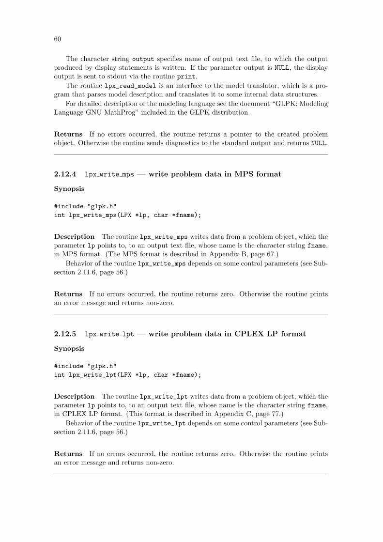
60

The character string output specifies name of output text file, to which the outputproduced by display statements is written. If the parameter output is NULL, the displayoutput is sent to stdout via the routine print.

The routine lpx_read_model is an interface to the model translator, which is a pro-gram that parses model description and translates it to some internal data structures.

For detailed description of the modeling language see the document “GLPK: ModelingLanguage GNU MathProg” included in the GLPK distribution.

Returns If no errors occurred, the routine returns a pointer to the created problemobject. Otherwise the routine sends diagnostics to the standard output and returns NULL.

2.12.4 lpx write mps — write problem data in MPS format

Synopsis

#include "glpk.h"int lpx_write_mps(LPX *lp, char *fname);

Description The routine lpx_write_mps writes data from a problem object, which theparameter lp points to, to an output text file, whose name is the character string fname,in MPS format. (The MPS format is described in Appendix B, page 67.)

Behavior of the routine lpx_write_mps depends on some control parameters (see Sub-section 2.11.6, page 56.)

Returns If no errors occurred, the routine returns zero. Otherwise the routine printsan error message and returns non-zero.

2.12.5 lpx write lpt — write problem data in CPLEX LP format

Synopsis

#include "glpk.h"int lpx_write_lpt(LPX *lp, char *fname);

Description The routine lpx_write_lpt writes data from a problem object, which theparameter lp points to, to an output text file, whose name is the character string fname,in CPLEX LP format. (This format is described in Appendix C, page 77.)

Behavior of the routine lpx_write_lpt depends on some control parameters (see Sub-section 2.11.6, page 56.)

Returns If no errors occurred, the routine returns zero. Otherwise the routine printsan error message and returns non-zero.

61

2.12.6 lpx print prob — write problem data in plain text format

Synopsis

#include "glpk.h"int lpx_print_prob(LPX *lp, char *fname);

Description The routine lpx_print_prob writes data from a problem object, whichthe parameter lp points to, to an output text file, whose name is the character stringfname, in plain text format.

Information reported by the routine lpx_print_prob is intended mainly for visualanalysis.

Returns If no errors occurred, the routine returns zero. Otherwise the routine printsan error message and returns non-zero.

2.12.7 lpx read bas — read predefined basis in MPS format

Synopsis

#include "glpk.h"int lpx_read_bas(LPX *lp, char *fname);

Description The routine lpx_read_bas reads a predefined basis prepared in MPS for-mat for an LP problem object, which the parameter lp points to, from a text file, whosename is the character string fname. (About this feature of the MPS format see SectionB.12, page 75.)

Behavior of the routine lpx_read_bas depends on some control parameters (see Sub-section 2.11.6, page 56.)

Returns If no errors occurred, the routine returns zero. Otherwise the routine printsan error message and returns non-zero.

2.12.8 lpx write bas — write current basis in MPS format

Synopsis

#include "glpk.h"int lpx_write_bas(LPX *lp, char *fname);

Description The routine lpx_write_bas writes the current basis information from aproblem object, which the parameter lp points to, to an output text file, whose name isthe character string fname, in MPS format. (About this feature of the MPS format seeSection B.12, page 75.)

Behavior of the routine lpx_write_bas depends on some control parameters (see Sub-section 2.11.6, page 56.)

62

Returns If no errors occurred, the routine returns zero. Otherwise the routine printsan error message and returns non-zero.

2.12.9 lpx print sol — write basic solution in printable format

Synopsis

#include "glpk.h"int lpx_print_sol(LPX *lp, char *fname);

Description The routine lpx_print_sol writes the current basic solution of an LPproblem, which is specified by the pointer lp, to a text file, whose name is the characterstring fname, in printable format.

Information reported by the routine lpx_print_sol is intended mainly for visualanalysis.

Returns If no errors occurred, the routine returns zero. Otherwise the routine printsan error message and returns non-zero.

2.12.10 lpx print ips — write interior point solution in printable format

Synopsis

#include "glpk.h"int lpx_print_ips(LPX *lp, char *fname);

Description The routine lpx_print_ips writes the current interior point solution of anLP problem, which the parameter lp points to, to a text file, whose name is the characterstring fname, in printable format.

Information reported by the routine lpx_print_ips is intended mainly for visualanalysis.

Returns If no errors occurred, the routine returns zero. Otherwise the routine printsan error message and returns non-zero.

2.12.11 lpx print mip — write MIP solution in printable format

Synopsis

#include "glpk.h"int lpx_print_mip(LPX *lp, char *fname);

Description The routine lpx_print_mip writes a best known integer solution of a MIPproblem, which is specified by the pointer lp, to a text file, whose name is the characterstring fname, in printable format.

Information reported by the routine lpx_print_mip is intended mainly for visualanalysis.

63

Returns If no errors occurred, the routine returns zero. Otherwise the routine printsan error message and returns non-zero.

Appendix A

Installing GLPK on YourComputer

A.1 Obtaining GLPK distribution file

The distrubution file for the most recent version of the GLPK package can be downloadedfrom <ftp://ftp.gnu.org/gnu/glpk/> or from some mirror GNU ftp sites; for detailssee <http://www.gnu.org/order/ftp.html>.

A.2 Unpacking the distribution file

The GLPK package (like all other GNU software) is distributed in the form of packedarchive. This is one file named glpk-x.y.tar.gz, where x is the major version numberand y is the minor version number.

In order to prepare the distribution for installation you should:1. Copy the GLPK distribution file to some subdirectory.2. Enter the command gzip -d glpk-x.y.tar.gz in order to unpack the distribution

file. After unpacking the name of the distribution file will be automatically changed toglpk-x.y.tar.

3. Enter the command tar -x < glpk-x.y.tar in order to unarchive the distribution.After this operation the subdirectory glpk-x.y, which is the GLPK distribution, will beautomatically created.

A.3 Configuring the package

After you have unpacked and unarchived GLPK distribution you should configure thepackage, i.e. automatically tune it for your computer (platform).

Normally, you should just cd to the subdirectory glpk-x.y and enter the command./configure. If you are using csh on an old version of System V, you might need to typesh configure instead to prevent csh from trying execute configure itself.

The configure shell script attempts to guess correct values for various system-dependent variables used during compilation, and creates Makefile. It also creates afile config.status that you can run in the future to recreate the current configuration.

Running configure takes about a few minutes. While it is running, it displays someinformational messages that tell you what it is doing. If you don’t want to see these

64

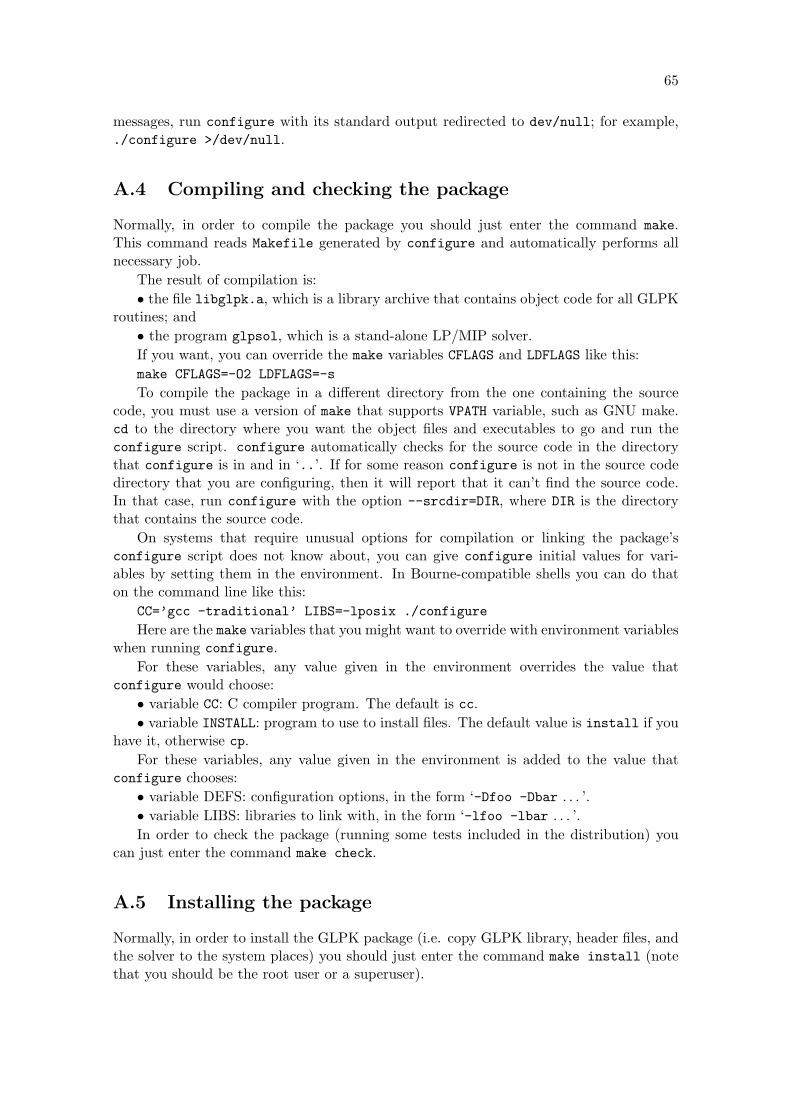
65

messages, run configure with its standard output redirected to dev/null; for example,./configure >/dev/null.

A.4 Compiling and checking the package

Normally, in order to compile the package you should just enter the command make.This command reads Makefile generated by configure and automatically performs allnecessary job.

The result of compilation is:• the file libglpk.a, which is a library archive that contains object code for all GLPK

routines; and• the program glpsol, which is a stand-alone LP/MIP solver.If you want, you can override the make variables CFLAGS and LDFLAGS like this:make CFLAGS=-O2 LDFLAGS=-s

To compile the package in a different directory from the one containing the sourcecode, you must use a version of make that supports VPATH variable, such as GNU make.cd to the directory where you want the object files and executables to go and run theconfigure script. configure automatically checks for the source code in the directorythat configure is in and in ‘..’. If for some reason configure is not in the source codedirectory that you are configuring, then it will report that it can’t find the source code.In that case, run configure with the option --srcdir=DIR, where DIR is the directorythat contains the source code.

On systems that require unusual options for compilation or linking the package’sconfigure script does not know about, you can give configure initial values for vari-ables by setting them in the environment. In Bourne-compatible shells you can do thaton the command line like this:

CC=’gcc -traditional’ LIBS=-lposix ./configure

Here are the make variables that you might want to override with environment variableswhen running configure.

For these variables, any value given in the environment overrides the value thatconfigure would choose:

• variable CC: C compiler program. The default is cc.• variable INSTALL: program to use to install files. The default value is install if you

have it, otherwise cp.For these variables, any value given in the environment is added to the value that

configure chooses:• variable DEFS: configuration options, in the form ‘-Dfoo -Dbar . . . ’.• variable LIBS: libraries to link with, in the form ‘-lfoo -lbar . . . ’.In order to check the package (running some tests included in the distribution) you

can just enter the command make check.

A.5 Installing the package

Normally, in order to install the GLPK package (i.e. copy GLPK library, header files, andthe solver to the system places) you should just enter the command make install (notethat you should be the root user or a superuser).

66

By default, make install will install the package’s files in the subdirectoriesusr/local/bin, usr/local/lib, etc. You can specify an installation prefix other than/usr/local by giving configure the option --prefix=PATH. Alternately, you can do soby consistently giving a value for the prefix variable when you run make, e.g.

make prefix=/usr/gnumake prefix=/usr/gnu installAfter installing you can remove the program binaries and object files from the source

directory by typing make clean. To remove all files that configure created (Makefile,config.status, etc.), just type make distclean.

The file configure.in is used to create configure by a program called autoconf.You only need it if you want to remake configure using a newer version of autoconf.

A.6 Uninstalling the package

In order to uninstall the GLPK package (i.e. delete all GLPK files from the system places)you can enter the command make uninstall.

Appendix B

MPS Format

B.1 Prelude

The MPS format1 is intended for coding LP/MIP problem data. This format assumes theformulation of LP/MIP problem (1.1)—(1.3) (see Section 1.1, page 7).

MPS file is a text file, which contains two types of cards2: indicator cards and datacards.

Indicator cards determine a kind of succeeding data. Each indicator card has one wordin uppercase letters beginning at the column 1.

Data cards contain problem data. Each data card is divided into six fixed fields:

Field 1 Field 2 Field 3 Field 4 Field 5 Feld 6Columns 2—3 5—12 15—22 25—36 40—47 50—61Contents Code Name Name Number Name Number

On a particular data card some fields may be optional.Names are used to identify rows, columns, and some vectors (see below).Aligning the indicator code in the field 1 to the left margin is optional.All names specified in the fields 2, 3, and 5 should contain from 1 up to 8 arbitrary

characters (except control characters). If a name is placed in the field 3 or 5, its firstcharacter should not be the dollar sign ‘$’. If a name contains spaces, the spaces areignored.

All numerical values in the fields 4 and 6 should be coded in the form sxxEsyy, wheres is the plus ‘+’ or the minus ‘-’ sign, xx is a real number with optional decimal point, yyis an integer decimal exponent. Any number should contain up to 12 characters. If thesign s is omitted, the plus sign is assumed. The exponent part is optional. If a numbercontains spaces, the spaces are ignored.

If a card has the asterisk ‘*’ in the column 1, this card is considered as a comment andignored. Besides, if the first character in the field 3 or 5 is the dollar sign ‘$’, all charactersfrom the dollar sign to the end of card are considered as a comment and ignored.

1The MPS format was developed in 1960’s by IBM as input format for their mathematical programmingsystem MPS/360. Today the MPS format is a most widely used format understood by most mathemat-ical programming packages. This appendix describes only the features of the MPS format, which areimplemented in the GLPK package.

2In 1960’s MPS file was a deck of 80-column punching cards, so the author decided to keep the word“card”, which may be understood as “line of text file”.

67

68

MPS file should contain cards in the following order:• NAME indicator card;• ROWS indicator card;• data cards specifying rows (constraints);• COLUMNS indicator card;• data cards specifying columns (structural variables) and constraint coefficients;• RHS indicator card;• data cards specifying right-hand sides of constraints;• RANGES indicator card;• data cards specifying ranges for double-bounded constraints;• BOUNDS indicator card;• data cards specifying types and bounds of structural variables;• ENDATA indicator card.Section is a group of cards consisting of an indicator card and data cards succeeding

this indicator card. For example, the ROWS section consists of the ROWS indicator cardand data cards specifying rows.

The sections RHS, RANGES, and BOUNDS are optional and may be omitted.

B.2 NAME indicator card

The NAME indicator card should be the first card in the MPS file (except optional com-ment cards, which may precede the NAME card). This card should contain the word NAMEin the columns 1—4 and the problem name in the field 3. The problem name is optionaland may be omitted.

B.3 ROWS section

The ROWS section should start with the indicator card, which contains the word ROWS inthe columns 1—4.

Each data card in the ROWS section specifies one row (constraint) of the problem.All these data cards have the following format.

‘N’ in the field 1 means that the row is free (unbounded):

−∞ < xi = ai1xm+1 + ai2xm+2 + . . . + ainxm+n < +∞;

‘L’ in the field 1 means that the row is of “less than or equal to” type:

−∞ < xi = ai1xm+1 + ai2xm+2 + . . . + ainxm+n ≤ bi;

‘G’ in the field 1 means that the row is of “greater than or equal to” type:

bi ≤ xi = ai1xm+1 + ai2xm+2 + . . . + ainxm+n < +∞;

‘E’ in the field 1 means that the row is of “equal to” type:

xi = ai1xm+1 + ai2xm+2 + . . . + ainxm+n ≤ bi,

where bi is a right-hand side. Note that each constraint has a corresponding implictlydefined auxiliary variable (xi above), whose value is a value of the corresponding linearform, therefore row bounds can be considered as bounds of such auxiliary variable.

69

The filed 2 specifies a row name (which is considered as the name of the correspondingauxiliary variable).

The fields 3, 4, 5, and 6 are not used and should be empty.Numerical values of all non-zero right-hand sides bi should be specified in the RHS

section (see below). All double-bounded (ranged) constraints should be specified in theRANGES section (see below).

B.4 COLUMNS section

The COLUMNS section should start with the indicator card, which contains the wordCOLUMNS in the columns 1—7.

Each data card in the COLUMNS section specifies one or two constraint coefficientsaij and also introduces names of columns, i.e. names of structural variables. All thesedata cards have the following format.

The field 1 is not used and should be empty.The field 2 specifies a column name. If this field is empty, the column name from the

immediately preceeding data card is assumed.The field 3 specifies a row name defined in the ROWS section.The field 4 specifies a numerical value of the constraint coefficient aij , which is placed

in the corresponding row and column.The fields 5 and 6 are optional. If they are used, they should contain a second pair

“row name—constraint coefficient” for the same column.Elements of the constraint matrix (i.e. constraint coefficients) should be enumerated

in the column wise manner: all elements for the current column should be specified beforeelements for the next column. However, the order of rows in the COLUMNS section maydiffer from the order of rows in the ROWS section.

Constraint coefficients not specified in the COLUMNS section are considered as zeros.Therefore zero coefficients may be omitted, although it is allowed to explicitly specifythem.

B.5 RHS section

The RHS section should start with the indicator card, which contains the word RHS in thecolumns 1—3.

Each data card in the RHS section specifies one or two right-hand sides bi (see SectionB.3, page 68). All these data cards have the following format.

The field 1 is not used and should be empty.The field 2 specifies a name of the right-hand side (RHS) vector3. If this field is empty,

the RHS vector name from the immediately preceeding data card is assumed.The field 3 specifies a row name defined in the ROWS section.The field 4 specifies a right-hand side bi for the row, whose name is specified in the

field 3. Depending on the row type bi is a lower bound (for the row of G type), an upperbound (for the row of L type), or a fixed value (for the row of E type).4

3This feature allows the user to specify several RHS vectors in the same MPS file. However, beforesolving the problem a particular RHS vector should be chosen.

4If the row is of N type, bi is considered as a constant term of the corresponding linear form. Shouldnote, however, this convention is non-standard.

70

The fields 5 and 6 are optional. If they are used, they should contain a second pair“row name—right-hand side” for the same RHS vector.

All right-hand sides for the current RHS vector should be specified before right-handsides for the next RHS vector. However, the order of rows in the RHS section may differfrom the order of rows in the ROWS section.

Right-hand sides not specified in the RHS section are considered as zeros. Thereforezero right-hand sides may be omitted, although it is allowed to explicitly specify them.

B.6 RANGES section

The RANGES section should start with the indicator card, which contains the wordRANGES in the columns 1—6.

Each data card in the RANGES section specifies one or two ranges for double-sideconstraints, i.e. for constraints that are of the types L and G at the same time:

li ≤ xi = ai1xm+1 + ai2xm+2 + . . . + ainxm+n ≤ ui,

where li is a lower bound, ui is an upper bound. All these data cards have the followingformat.

The field 1 is not used and should be empty.The field 2 specifies a name of the range vector5. If this field is empty, the range vector

name from the immediately preceeding data card is assumed.The field 3 specifies a row name defined in the ROWS section.The field 4 specifies a range value ri (see the table below) for the row, whose name is

specified in the field 3.The fields 5 and 6 are optional. If they are used, they should contain a second pair

“row name—range value” for the same range vector.All range values for the current range vector should be specified before range values

for the next range vector. However, the order of rows in the RANGES section may differfrom the order of rows in the ROWS section.

For each double-side constraint specified in the RANGES section its lower and upperbounds are determined as follows:

Row type Sign of ri Lower bound Upper boundG + or − bi bi + |ri|L + or − bi − |ri| bi

E + bi bi + |ri|E − bi − |ri| bi

where bi is a right-hand side specified in the RHS section (if bi is not specified, it isconsidered as zero), ri is a range value specified in the RANGES section.

B.7 BOUNDS section

The BOUNDS section should start with the indicator card, which contains the wordBOUNDS in the columns 1—6.

5This feature allows the user to specify several range vectors in the same MPS file. However, beforesolving the problem a particular range vector should be chosen.

71

Each data card in the BOUNDS section specifies one (lower or upper) bound for onestructural variable (column). All these data cards have the following format.

The indicator in the field 1 specifies the bound type:LO lower bound;UP upper bound;FX fixed variable (lower and upper bounds are equal);FR free variable (no bounds);MI no lower bound (lower bound is “minus infinity”);PL no upper bound (upper bound is “plus infinity”);The field 2 specifies a name of the bound vector6. If this field is empty, the bound

vector name from the immediately preceeding data card is assumed.The field 3 specifies a column name defined in the COLUMNS section.The field 4 specifies a bound value. If the bound type in the field 1 differs from LO,

UP, and FX, the value in the field 4 is ignored and may be omitted.The fields 5 and 6 are not used and should be empty.All bound values for the current bound vector should be specified before bound values

for the next bound vector. However, the order of columns in the BOUNDS section maydiffer from the order of columns in the COLUMNS section. Specification of a lower boundshould precede specification of an upper bound for the same column (if both the lowerand upper bounds are explicitly specified).

By default, all columns (structural variables) are non-negative, i.e. have zero lowerbound and no upper bound. Lower (lj) and upper (uj) bounds of some column (structuralvariable xj) are set in the following way, where sj is a corresponding bound value explicitlyspecified in the BOUNDS section:

LO sets lj to sj ;UP sets uj to sj ;FX sets both lj and uj to sj ;FR sets lj to −∞ and uj to +∞;MI sets lj to −∞;PL sets uj to +∞.

B.8 ENDATA indicator card

The ENDATA indicator card should be the last card of MPS file (except optional commentcards, which may follow the ENDATA card). This card should contain the word ENDATAin the columns 1—6.

B.9 Specifying objective function

It is impossible to explicitly specify the objective function and optimization direction inthe MPS file. However, the following implicit rule is used by default: the first row of Ntype is considered as a row of the objective function (i.e. the objective function is thecorresponding auxiliary variable), which should be minimized.

GLPK also allows specifying a constant term of the objective function as a right-handside of the corresponding row in the RHS section.

6This feature allows the user to specify several bound vectors in the same MPS file. However, beforesolving the problem a particular bound vector should be chosen.

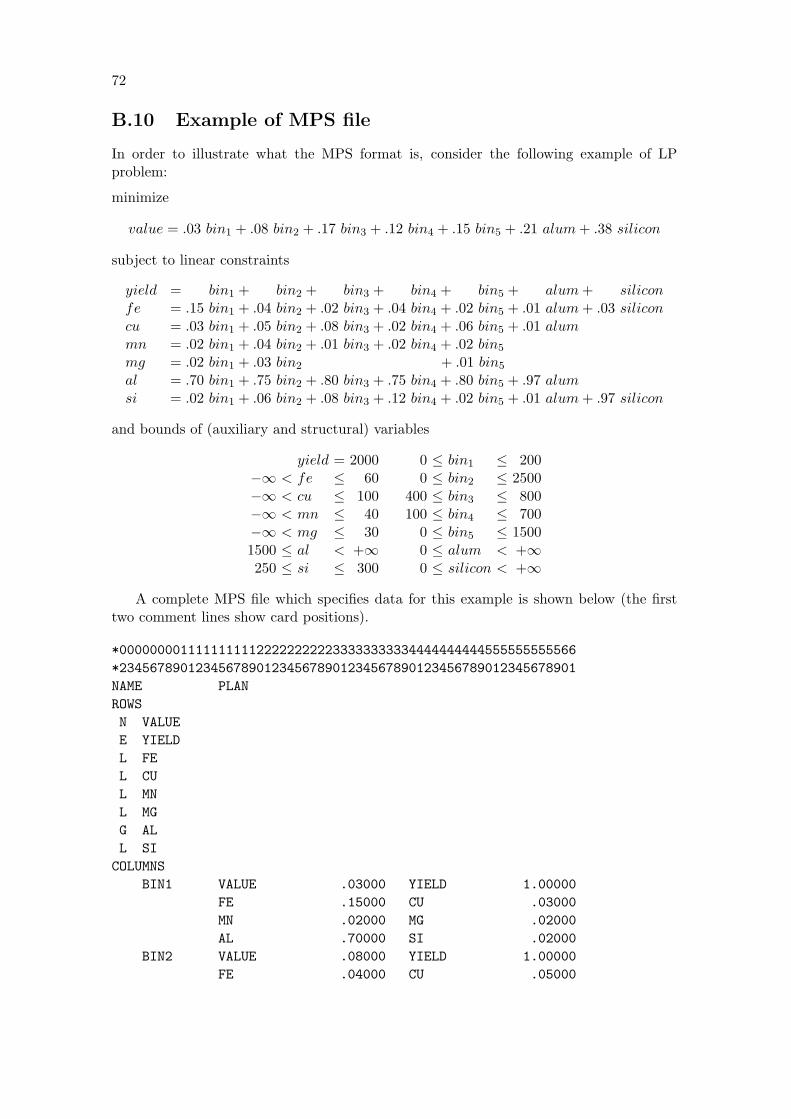
72

B.10 Example of MPS file

In order to illustrate what the MPS format is, consider the following example of LPproblem:

minimize

value = .03 bin1 + .08 bin2 + .17 bin3 + .12 bin4 + .15 bin5 + .21 alum + .38 silicon

subject to linear constraints

yield = bin1 + bin2 + bin3 + bin4 + bin5 + alum + siliconfe = .15 bin1 + .04 bin2 + .02 bin3 + .04 bin4 + .02 bin5 + .01 alum + .03 siliconcu = .03 bin1 + .05 bin2 + .08 bin3 + .02 bin4 + .06 bin5 + .01 alummn = .02 bin1 + .04 bin2 + .01 bin3 + .02 bin4 + .02 bin5

mg = .02 bin1 + .03 bin2 + .01 bin5

al = .70 bin1 + .75 bin2 + .80 bin3 + .75 bin4 + .80 bin5 + .97 alumsi = .02 bin1 + .06 bin2 + .08 bin3 + .12 bin4 + .02 bin5 + .01 alum + .97 silicon

and bounds of (auxiliary and structural) variables

yield = 2000 0 ≤ bin1 ≤ 200−∞ < fe ≤ 60 0 ≤ bin2 ≤ 2500−∞ < cu ≤ 100 400 ≤ bin3 ≤ 800−∞ < mn ≤ 40 100 ≤ bin4 ≤ 700−∞ < mg ≤ 30 0 ≤ bin5 ≤ 15001500 ≤ al < +∞ 0 ≤ alum < +∞250 ≤ si ≤ 300 0 ≤ silicon < +∞

A complete MPS file which specifies data for this example is shown below (the firsttwo comment lines show card positions).

*000000001111111111222222222233333333334444444444555555555566*234567890123456789012345678901234567890123456789012345678901NAME PLANROWSN VALUEE YIELDL FEL CUL MNL MGG ALL SICOLUMNS

BIN1 VALUE .03000 YIELD 1.00000FE .15000 CU .03000MN .02000 MG .02000AL .70000 SI .02000

BIN2 VALUE .08000 YIELD 1.00000FE .04000 CU .05000

73

MN .04000 MG .03000AL .75000 SI .06000

BIN3 VALUE .17000 YIELD 1.00000FE .02000 CU .08000MN .01000 AL .80000SI .08000

BIN4 VALUE .12000 YIELD 1.00000FE .04000 CU .02000MN .02000 AL .75000SI .12000

BIN5 VALUE .15000 YIELD 1.00000FE .02000 CU .06000MN .02000 MG .01000AL .80000 SI .02000

ALUM VALUE .21000 YIELD 1.00000FE .01000 CU .01000AL .97000 SI .01000

SILICON VALUE .38000 YIELD 1.00000FE .03000 SI .97000

RHSRHS1 YIELD 2000.00000 FE 60.00000

CU 100.00000 MN 40.00000SI 300.00000MG 30.00000 AL 1500.00000

RANGESRNG1 SI 50.00000

BOUNDSUP BND1 BIN1 200.00000UP BIN2 2500.00000LO BIN3 400.00000UP BIN3 800.00000LO BIN4 100.00000UP BIN4 700.00000UP BIN5 1500.00000ENDATA

B.11 MIP features

The MPS format provides two ways for introducing integer variables into the problem.The first way is most general and based on using special marker cards INTORG and

INTEND. These marker cards are placed in the COLUMNS section. The INTORG cardindicates the start of a group of integer variables (columns), and the card INTEND indi-cates the end of the group. The MPS file may contain arbitrary number of the markercards.

The marker cards have the same format as the data cards (see Section B.1, page 67).The fields 1, 2, and 6 are not used and should be empty.The field 2 should contain a marker name. This name may be arbitrary.The field 3 should contain the word ’MARKER’ (including apostrophes).

74

The field 5 should contain either the word ’INTORG’ (including apostrophes) for themarker card, which begins a group of integer columns, or the word ’INTEND’ (includingapostrophes) for the marker card, which ends the group.

The second way is less general but more convenient in some cases. It allows the userto declare integer columns using two additional types of bounds, which are specified inthe field 1 of data cards in the BOUNDS section (see Section B.7, page 70):

UI upper integer. This bound type specifies that the corresponding column (struc-tural variable), whose name is specified in the field 3, is of integer kind. In thiscase an upper bound of the column should be specified in the field 4 (like in thecase of UP bound type).

BV binary variable. This bound type specifies that the corresponding column (struc-tural variable), whose name is specified in the field 3, is of integer kind, its lowerbound is zero, and its upper bound is one (thus, such variable being of integerkind can have only two values zero and one). In this case a numeric value specifiedin the field 4 is ignored and may be omitted.

Consider the following example of MIP problem:

minimizeZ = 3x1 + 7x2 − x3 + x4

subject to linear constraints

r1 = 2x1 − x2 + x3 − x4

r2 = x1 − x2 − 6x3 + 4x4

r3 = 5x1 + 3x2 + x4

and bound of variables

1 ≤ r1 < +∞ 0 ≤ x1 ≤ 4 (continuous)8 ≤ r2 < +∞ 2 ≤ x2 ≤ 5 (integer)5 ≤ r3 < +∞ 0 ≤ x3 ≤ 1 (integer)

3 ≤ x4 ≤ 8 (continuous)

The corresponding MPS file may look like the following:

NAME SAMP1ROWSN ZG R1G R2G R3COLUMNS

X1 R1 2.0 R2 1.0X1 R3 5.0 Z 3.0MARK0001 ’MARKER’ ’INTORG’X2 R1 -1.0 R2 -1.0X2 R3 3.0 Z 7.0X3 R1 1.0 R2 -6.0X3 Z -1.0MARK0002 ’MARKER’ ’INTEND’X4 R1 -1.0 R2 4.0

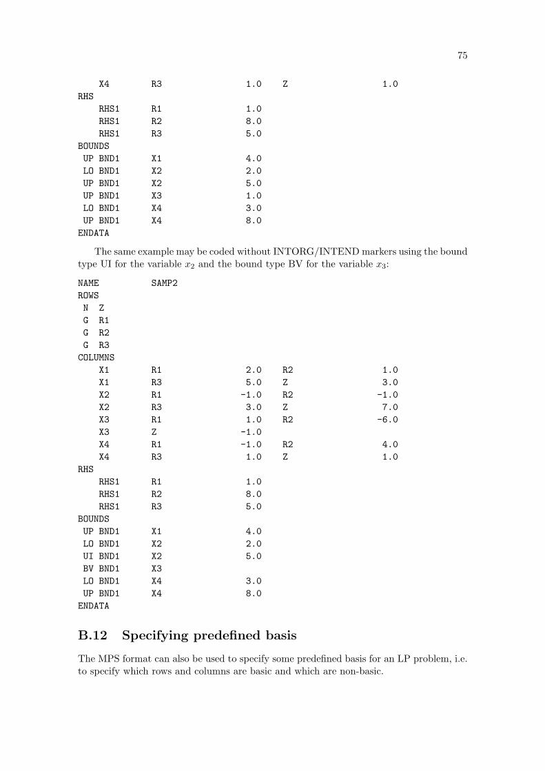
75

X4 R3 1.0 Z 1.0RHS

RHS1 R1 1.0RHS1 R2 8.0RHS1 R3 5.0

BOUNDSUP BND1 X1 4.0LO BND1 X2 2.0UP BND1 X2 5.0UP BND1 X3 1.0LO BND1 X4 3.0UP BND1 X4 8.0

ENDATA

The same example may be coded without INTORG/INTEND markers using the boundtype UI for the variable x2 and the bound type BV for the variable x3:

NAME SAMP2ROWSN ZG R1G R2G R3

COLUMNSX1 R1 2.0 R2 1.0X1 R3 5.0 Z 3.0X2 R1 -1.0 R2 -1.0X2 R3 3.0 Z 7.0X3 R1 1.0 R2 -6.0X3 Z -1.0X4 R1 -1.0 R2 4.0X4 R3 1.0 Z 1.0

RHSRHS1 R1 1.0RHS1 R2 8.0RHS1 R3 5.0

BOUNDSUP BND1 X1 4.0LO BND1 X2 2.0UI BND1 X2 5.0BV BND1 X3LO BND1 X4 3.0UP BND1 X4 8.0ENDATA

B.12 Specifying predefined basis

The MPS format can also be used to specify some predefined basis for an LP problem, i.e.to specify which rows and columns are basic and which are non-basic.

76

The order of a basis file in the MPS format is:• NAME indicator card;• data cards (can appear in arbitrary order);• ENDATA indicator card.Each data card specifies either a pair ”basic column—non-basic row” or a non-basic

column. All the data cards have the following format.‘XL’ in the field 1 means that a column, whose name is given in the field 2, is basic,

and a row, whose name is given in the field 3, is non-basic and placed on its lower bound.‘XU’ in the field 1 means that a column, whose name is given in the field 2, is basic,

and a row, whose name is given in the field 3, is non-basic and placed on its upper bound.‘LL’ in the field 1 means that a column, whose name is given in the field 3, is non-basic

and placed on its lower bound.‘UL’ in the field 1 means that a column, whose name is given in the field 3, is non-basic

and placed on its upper bound.The field 2 contains a column name.If the indicator given in the field 1 is ‘XL’ or ‘XU’, the field 3 contains a row name.

Otherwise, if the indicator is ‘LL’ or ‘UL’, the field 3 is not used and should be empty.The field 4, 5, and 6 are not used and should be empty.A basis file in the MPS format acts like a patch: it doesn’t specify a basis completely,

instead that it is just shows in what a given basis differs from the ”standard” basis, whereall rows (auxiliary variables) are assumed to be basic and all columns (structural variables)are assumed to be non-basic.

As an example here is a basis file that specifies an optimal basis for the example LPproblem given in Section B.10, Page 72:

*000000001111111111222222222233333333334444444444555555555566*234567890123456789012345678901234567890123456789012345678901NAME PLANXL BIN2 YIELDXL BIN3 FEXL BIN4 MNXL ALUM ALXL SILICON SILL BIN1LL BIN5ENDATA

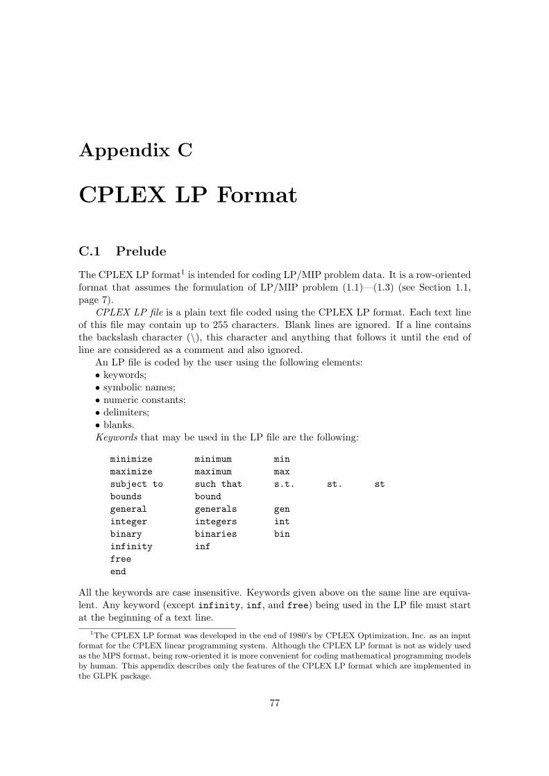
Appendix C

CPLEX LP Format

C.1 Prelude

The CPLEX LP format1 is intended for coding LP/MIP problem data. It is a row-orientedformat that assumes the formulation of LP/MIP problem (1.1)—(1.3) (see Section 1.1,page 7).

CPLEX LP file is a plain text file coded using the CPLEX LP format. Each text lineof this file may contain up to 255 characters. Blank lines are ignored. If a line containsthe backslash character (\), this character and anything that follows it until the end ofline are considered as a comment and also ignored.

An LP file is coded by the user using the following elements:• keywords;• symbolic names;• numeric constants;• delimiters;• blanks.Keywords that may be used in the LP file are the following:

minimize minimum minmaximize maximum maxsubject to such that s.t. st. stbounds boundgeneral generals geninteger integers intbinary binaries bininfinity inffreeend

All the keywords are case insensitive. Keywords given above on the same line are equiva-lent. Any keyword (except infinity, inf, and free) being used in the LP file must startat the beginning of a text line.

1The CPLEX LP format was developed in the end of 1980’s by CPLEX Optimization, Inc. as an inputformat for the CPLEX linear programming system. Although the CPLEX LP format is not as widely usedas the MPS format, being row-oriented it is more convenient for coding mathematical programming modelsby human. This appendix describes only the features of the CPLEX LP format which are implemented inthe GLPK package.

77

78

Symbolic names are used to identify the objective function, constraints (rows), andvariables (columns). All symbolic names are case sensitive and may contain up to 16alphanumeric characters (a, . . . , z, A, . . . , Z, 0, . . . , 9) as well as the following characters:

! " # $ % & ( ) / , . ; ? @ _ ‘ ’ { } | ~

(except that no symbolic name can begin with a digit or a period). If a symbolic name islonger than 16 characters, it is truncated from the right.

Numeric constants are used to denote constraint and objective coefficients, right-handsides of constraints, and bounds of variables. They are coded in the standard form xxEsyy,where xx is a real number with optional decimal point, s is a sign (+ or -), yy is an integerdecimal exponent. Numeric constants may contain arbitrary number of characters. Theexponent part is optional. The letter ‘E’ can be coded as ‘e’. If the sign s is omitted, plusis assumed.

Delimiters that may be used in the LP file are the following:

:+-< <= =<> >= =>=

Delimiters given above on the same line are equivalent. The meaning of the delimiters willbe explained below.

Blanks are non-significant characters. They may be used freely to improve readabilityof the LP file. Besides, blanks should be used to separate elements from each other if thereis no other way to do that (for example, to separate a keyword from a following symbolicname).

The order of an LP file is:• objective function definition;• constraints section;• bounds section;• general, integer, and binary sections (can appear in arbitrary order);• end keyword.These components are discussed in following sections.

C.2 Objective function definition

The objective function definition must appear first in the LP file. It defines the objectivefunction and specifies the optimization direction.

The objective function definition has the following form:{minimizemaximize

}f : s c x s c x . . . s c x

where f is a symbolic name of the objective function, s is a sign + or -, c is a numericconstant that denotes an objective coefficient, x is a symbolic name of a variable.

79

If necessary, the objective function definition can be continued on as many text linesas desired.

The name of the objective function is optional and may be omitted (together with thesemicolon that follows it). In this case the default name ‘obj’ is assigned to the objectivefunction.

If the very first sign s is omitted, the sign plus is assumed. Other signs cannot beomitted.

If some objective coefficient c is omitted, 1 is assumed.Symbolic names x used to denote variables are recognized by context and therefore

needn’t to be declared somewhere else.Here is an example of the objective function definition:

Minimize Z : - x1 + 2 x2 - 3.5 x3 + 4.997e3x(4) + x5 + x6 +x7 - .01x8

C.3 Constraints section

The constraints section must follow the objective function definition. It defines a systemof equality and/or inequality constraints.

The constraint section has the following form:

subject toconstraint1constraint2

. . .constraintm

where constrainti, i = 1, . . . ,m, is a particular constraint definition.Each constraint definition can be continued on as many text lines as desired. How-

ever, each constraint definition must begin on a new line except the very first constraintdefinition which can begin on the same line as the keyword ‘subject to’.

Constraint definitions have the following form:

r : s c x s c x . . . s c x

<=>==

b

where r is a symbolic name of a constraint, s is a sign + or -, c is a numeric constant thatdenotes a constraint coefficient, x is a symbolic name of a variable, b is a right-hand side.

The name r of a constraint (which is the name of the corresponding auxiliary variable)is optional and may be omitted (together with the semicolon that follows it). In this casethe default names like ‘r.nnn’ are assigned to unnamed constraints.

The linear form s c x s c x . . . s c x in the left-hand side of a constraint definition hasexactly the same meaning as in the case of the objective function definition (see above).

After the linear form one of the following delimiters that indicate the constraint sensemust be specified:

<= means ‘less than or equal to’>= means ‘greater than or equal to’= means ‘equal to’

80

The right hand side b is a numeric constant with an optional sign.Here is an example of the constraints section:

Subject Toone: y1 + 3 a1 - a2 - b >= 1.5y2 + 2 a3 + 2

a4 - b >= -1.5two : y4 + 3 a1 + 4 a5 - b <= +1.20y5 + 5 a2 - b = 01.7 y6 - a6 + 5 a777 - b >= 1

(Should note that it is impossible to express ranged constraints in the CPLEX LPformat. Each a ranged constraint can be coded as two constraints with identical linearforms in the left-hand side, one of which specifies a lower bound and other does an upperone of the original ranged constraint.)

C.4 Bounds section

The bounds section is intended to define bounds of variables. This section is optional; ifit is specified, it must follow the constraints section. If the bound section is omitted, allvariables are assumed to be non-negative (i.e. that they have zero lower bound and noupper bound).

The bounds section has the following form:

boundsdefinition1

definition2

. . .definitionp

where definitionk, k = 1, . . . , p, is a particular bound definition.Each bound definition must begin on a new line2 except the very first bound definition

which can begin on the same line as the keyword ‘bounds’.Syntactically constraint definitions can have one of the following six forms:

x >= l specifies a lower boundl <= x specifies a lower boundx <= u specifies an upper boundl <= x <= u specifies both lower and upper boundsx = t specifies a fixed valuex free specifies free variable

where x is a symbolic name of a variable, l is a numeric constant with an optional signthat defines a lower bound of the variable or -inf that means that the variable has nolower bound, u is a numeric constant with an optional sign that defines an upper boundof the variable or +inf that means that the variable has no upper bound, t is a numericconstant with an optional sign that defines a fixed value of the variable.

2The GLPK implementation allows several bound definitions to be placed on the same line.

81

By default all variables are non-negative, i.e. have zero lower bound and no upperbound. Therefore definitions of these default bounds can be omitted in the bounds section.

Here is an example of the bounds section:

Bounds-inf <= a1 <= 100-100 <= a2b <= 100x2 = +123.456x3 free

C.5 General, integer, and binary sections

The general, integer, and binary sections are intended to define some variables as integeror binary. All these sections are optional and needed only in case of MIP problems. Ifthey are specified, they must follow the bounds section or, if the latter is omitted, theconstraints section.

All the general, integer, and binary sections have the same form as follows:generalintegerbinary

x1

x2

. . .xq

where xk is a symbolic name of variable, k = 1, . . . , q.Each symbolic name must begin on a new line3 except the very first symbolic name

which can begin on the same line as the keyword ‘general’, ‘integer’, or ‘binary’.If a variable appears in the general or the integer section, it is assumed to be general

integer variable. If a variable appears in the binary section, it is assumed to be binaryvariable, i.e. an integer variable whose lower bound is zero and upper bound is one. (Notethat if bounds of a variable are specified in the bounds section and then the variableappears in the binary section, its previously specified bounds are ignored.)

Here is an example of the integer section:

Integerz12z22z35

C.6 End keyword

The keyword ‘end’ is intended to end the LP file. It must begin on a separate line and noother elements (except comments and blank lines) must follow it. Although this keywordis optional, it is strongly recommended to include it in the LP file.

3The GLPK implementation allows several symbolic names to be placed on the same line.

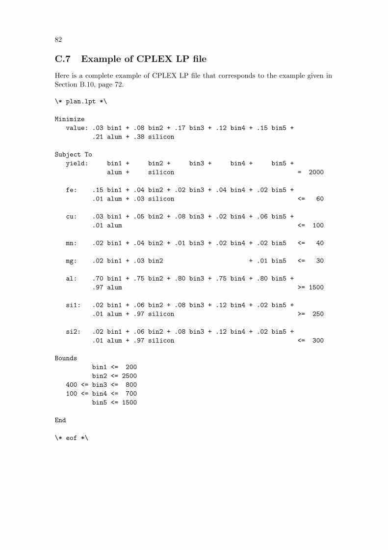
82

C.7 Example of CPLEX LP file

Here is a complete example of CPLEX LP file that corresponds to the example given inSection B.10, page 72.

\* plan.lpt *\

Minimizevalue: .03 bin1 + .08 bin2 + .17 bin3 + .12 bin4 + .15 bin5 +

.21 alum + .38 silicon

Subject Toyield: bin1 + bin2 + bin3 + bin4 + bin5 +

alum + silicon = 2000

fe: .15 bin1 + .04 bin2 + .02 bin3 + .04 bin4 + .02 bin5 +.01 alum + .03 silicon <= 60

cu: .03 bin1 + .05 bin2 + .08 bin3 + .02 bin4 + .06 bin5 +.01 alum <= 100

mn: .02 bin1 + .04 bin2 + .01 bin3 + .02 bin4 + .02 bin5 <= 40

mg: .02 bin1 + .03 bin2 + .01 bin5 <= 30

al: .70 bin1 + .75 bin2 + .80 bin3 + .75 bin4 + .80 bin5 +.97 alum >= 1500

si1: .02 bin1 + .06 bin2 + .08 bin3 + .12 bin4 + .02 bin5 +.01 alum + .97 silicon >= 250

si2: .02 bin1 + .06 bin2 + .08 bin3 + .12 bin4 + .02 bin5 +.01 alum + .97 silicon <= 300

Boundsbin1 <= 200bin2 <= 2500

400 <= bin3 <= 800100 <= bin4 <= 700

bin5 <= 1500

End

\* eof *\

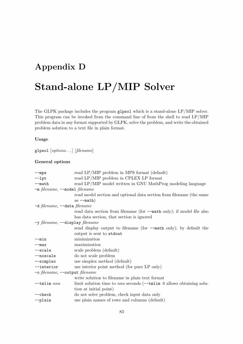
Appendix D

Stand-alone LP/MIP Solver

The GLPK package includes the program glpsol which is a stand-alone LP/MIP solver.This program can be invoked from the command line of from the shell to read LP/MIPproblem data in any format supported by GLPK, solve the problem, and write the obtainedproblem solution to a text file in plain format.

Usage

glpsol [options. . . ] [filename]

General options

--mps read LP/MIP problem in MPS format (default)--lpt read LP/MIP problem in CPLEX LP format--math read LP/MIP model written in GNU MathProg modeling language-m filename, --model filename

read model section and optional data section from filename (the sameas --math)

-d filename, --data filenameread data section from filename (for --math only); if model file alsohas data section, that section is ignored

-y filename, --display filenamesend display output to filename (for --math only); by default theoutput is sent to stdout

--min minimization--max maximization--scale scale problem (default)--noscale do not scale problem--simplex use simplex method (default)--interior use interior point method (for pure LP only)-o filename, --output filename

write solution to filename in plain text format--tmlim nnn limit solution time to nnn seconds (--tmlim 0 allows obtaining solu-

tion at initial point)--check do not solve problem, check input data only--plain use plain names of rows and columns (default)

83

84

--orig try using original names of rows and columns--wmps filename write problem to filename in MPS format--wlpt filename write problem to filename in CPLEX LP format--wtxt filename write problem to filename in plain text format-h, --help display this help information and exit-v, --version display program version and exit

Options specific to simplex method

--std use standard initial basis of all slacks--adv use advanced initial basis (default)--steep use steepest edge technique (default)--nosteep use standard “textbook” pricing--relax use Harris’ two-pass ratio test (default)--norelax use standard “textbook” ratio test--presol use LP presolver (default; assumes --scale and --adv)--nopresol do not use LP presolver

Options specific to MIP

--nomip consider all integer variables as continuous (allows solving MIP aspure LP)

--first branch on first integer variable--last branch on last integer variable--drtom branch using heuristic by Driebeck and Tomlin (default)--dfs backtrack using depth first search--bfs backtrack using breadth first search--bestp backtrack using the best projection heuristic (default)

For description of the MPS format see Appendix B, page 67.

For description of the CPLEX LP format see Appendix C, page 77.

For description of the modeling language see the document “GLPK: Modeling LanguageGNU MathProg” included in the GLPK distribution.