REFINED KATO INEQUALITIES AND CONFORMAL WEIGHTS IN RIEMANNIAN GEOMETRY DAVID M. J. CALDERBANK, PAUL GAUDUCHON, AND MARC HERZLICH Abstract. We establish refinements of the classical Kato inequality for sections of a vector bundle which lie in the kernel of a natural injectively elliptic first-order linear differential operator. Our main result is a general expression which gives the value of the constants appearing in the refined inequalities. These constants are shown to be optimal and are computed explicitly in most practical cases. Introduction The Kato inequality is an elementary and well-known estimate in Riemannian geometry, which has proved to be a powerful technique for linking vector-valued and scalar-valued problems in analysis on manifolds [3, 5, 6, 16, 20, 28]. Its content may be stated as follows: for any section ξ of any Riemannian (or Hermitian) vector bundle E endowed with a metric connection ∇ over a Riemannian manifold (M,g ), and at any point where ξ does not vanish, (0.1) d|ξ | 6 |∇ξ |. This estimate is easily obtained by applying the Schwarz inequality to the right hand side of the trivial identity: d ( |ξ | 2 ) =2h∇ξ,ξ i. Hence equality is achieved at a given point x if and only if ∇ξ is a multiple of ξ at x, i.e., if and only if there is a 1-form α such that (0.2) ∇ξ = α ⊗ ξ. The present work is motivated by circumstances in which more subtle versions of the Kato inequality appear. Examples include: the treatment of the Bernstein problem for minimal hypersurfaces in R n by R. Schoen, L. Simon and S. T. Yau [26], where it is shown that the second fundamental form h of any minimal immersion satisfies (0.3) d|h| 6 r n n +2 |∇h|, (see also [4]); the study by S. Bando, A. Kasue and H. Nakajima of Ricci flat and asymptotically flat manifolds [1], where a key role is played by the inequality (0.4) d|W | 6 r n - 1 n +1 |∇W | Date : October 1999. 1
Transcript
REFINED KATO INEQUALITIES AND CONFORMAL WEIGHTS
IN RIEMANNIAN GEOMETRY
DAVID M. J. CALDERBANK, PAUL GAUDUCHON, AND MARC HERZLICH
Abstract. We establish refinements of the classical Kato inequality for sections
of a vector bundle which lie in the kernel of a natural injectively elliptic first-orderlinear differential operator. Our main result is a general expression which gives
the value of the constants appearing in the refined inequalities. These constantsare shown to be optimal and are computed explicitly in most practical cases.
Introduction
The Kato inequality is an elementary and well-known estimate in Riemanniangeometry, which has proved to be a powerful technique for linking vector-valuedand scalar-valued problems in analysis on manifolds [3, 5, 6, 16, 20, 28]. Its contentmay be stated as follows: for any section ξ of any Riemannian (or Hermitian) vectorbundle E endowed with a metric connection ∇ over a Riemannian manifold (M, g),and at any point where ξ does not vanish,
(0.1)∣∣d|ξ|
∣∣ 6 |∇ξ|.
This estimate is easily obtained by applying the Schwarz inequality to the righthand side of the trivial identity: d
(|ξ|2)
= 2〈∇ξ, ξ〉. Hence equality is achieved at agiven point x if and only if ∇ξ is a multiple of ξ at x, i.e., if and only if there is a1-form α such that
(0.2) ∇ξ = α⊗ ξ.
The present work is motivated by circumstances in which more subtle versionsof the Kato inequality appear. Examples include: the treatment of the Bernsteinproblem for minimal hypersurfaces in R
n by R. Schoen, L. Simon and S. T. Yau [26],where it is shown that the second fundamental form h of any minimal immersionsatisfies
(0.3)∣∣d|h|
∣∣ 6√
n
n+ 2|∇h|,
(see also [4]); the study by S. Bando, A. Kasue and H. Nakajima of Ricci flat andasymptotically flat manifolds [1], where a key role is played by the inequality
(0.4)∣∣d|W |
∣∣ 6√n− 1
n+ 1|∇W |
Date: October 1999.1
2 DAVID M. J. CALDERBANK, PAUL GAUDUCHON, AND MARC HERZLICH
for the Weyl curvature W of any Einstein metric; and the proof given by J. Rade ofthe classical decay at infinity of any Yang-Mills field F on R
4 [23], which relies onthe estimate
(0.5)∣∣d|F |
∣∣ 6√
2
3|∇F |.
Other examples may be found in the work of S. T. Yau on the Calabi conjecture[29], or more recently in work of P. Feehan [11] and of M. Gursky and C. LeBrun[15]. For a survey of these techniques, see also [21].
In all of these examples, the classical Kato inequality (0.1) is insufficient to obtainthe desired results. Moreover, the knowledge of the best constant involved betweenthe two terms of the inequality seems to be a key element of all the proofs. Forinstance, in the case of Yang-Mills fields on R
4, the classical Kato inequality (0.1)gives only the decay estimate |F | = O(r−2) at infinity, whereas the (optimal) refinedinequality (0.5) yields the expected |F | = O(r−4) and thus paves the way for provingthat any finite energy Yang-Mills field on flat space is induced from one on the sphere.
These examples suggest that it is an interesting question to determine when sucha refined Kato inequality may occur and to compute its optimal constant. A con-vincing explanation of the principle underlying this phenomenon was first providedby J.P. Bourguignon in [7]. He remarked that in all the cases quoted above, thesections under consideration are solutions of a natural linear first-order injectivelyelliptic system, and that in such a situation, equality cannot occur in (0.1) except atpoints where ∇ξ = 0. To see this, suppose that equality is achieved (at a point) bya solution ξ of such an elliptic system. At that point, ∇ξ = α ⊗ ξ for some 1-formα. Now a natural first-order linear differential operator may be written as Π ◦ ∇,where Π is a projection onto a (natural) subbundle of T ∗M ⊗ E. Hence Π(α ⊗ ξ)vanishes and so, by ellipticity, α⊗ ξ vanishes.
Hence it is reasonable to expect that a refined Kato constant might appear in thissituation, i.e., that there should exist a constant kP < 1, depending only on thechoice of elliptic operator P , such that
(0.6)∣∣d|ξ|
∣∣ 6 kP |∇ξ|
if ξ lies in the kernel of P .In this paper we attack the task of establishing explicitly the existence of re-
fined Kato constants for the injectively elliptic linear first-order operators naturallydefined on bundles associated to a Riemannian (spin) manifold by an irreduciblerepresentation of the special orthogonal group SO(n) or its nontrivial double-coverSpin(n). We devise a systematic method to obtain the values of the refined constantskP and we compute the constants explicitly in a large number of cases. We expressthe constants in terms of the conformal weights of generalized gradients (those oper-ators given by projection on an irreducible component of the tensor product above)which are numbers canonically attached to any such operator, and which can be
KATO INEQUALITIES AND CONFORMAL WEIGHTS 3
easily computed from representation theoretic data (see section 2 for details). As aby-product of our approach, we obtain a number of representation-theoretic formu-lae, relating conformal weights to higher Casimirs of so(n), some of which appearto be new.
The structure of the paper is as follows. In the first section, we present the basicdefinitions and strategy that will be followed to obtain the Kato constants. Then, insection 2, we review the representation-theoretic background that will be needed forour study. We do this in part for the benefit of the reader with a limited knowledgeof representation theory, but also to set up some notation, and to demonstrate thatthe conformal weights used in the sequel are easy to compute. Most importantly,we discuss the question of which first order natural operators are injectively elliptic.This question has been settled by Branson [8], whose result we restate in the notationof this paper.
Before developing the main machinery, we use some elementary computations togive the Kato constants when the number N of irreducible components of T ∗M ⊗Eis 2. Although this is entirely straightforward, the results are sufficient to obtaina new proof of the Hijazi inequality in spin geometry, which we sketch. For morecomplicated representations, we need more tools, which we develop in section 4.Building on work of Perelomov and Popov [22], and also more recent ideas of Diemerand Weingart (personal communication), we study higher Casimir elements in theuniversal enveloping algebra of so(n) and obtain formulae relating them to conformalweights. The main result in this direction is Theorem 4.8. We use this in section 5to prove our main theorem, which reduces the search for Kato constants to linearprogramming. Section 6 gives some explicit constants for N odd, whereas section 7deals with the case that N is even. In each we give the Kato constants for a largenumber of operators and we detail the precise values for N = 3 and N = 4. Wealso deal with the sharpness of our inequalities by giving the (algebraic) equalitycase. Finally, as an appendix, we present tables listing all of the Kato constants indimensions 3 and 4.
Acknowledgements. During the course of this work it became clear thatthere is a close relationship between Kato constants and the spectral results ofBranson [8]. Following the presentation of an early version of our results at ameeting in Luminy, Tom Branson has clarified this relationship very nicely [9] andindependently obtained a general minimization formula for the Kato constants. Weare very grateful to him for sharing with us his results. The formula that followsfrom our methods is slightly different from his and does not cover one special case.We present it in a similar way to permit easy comparison.
We are also deeply indebted to Tammo Diemer and Gregor Weingart for informingus of their recent work, which plays a crucial role in our approach. Finally we thankChristian Bar and Andrei Moroianu for the application of refined Kato inequalitiesto Hijazi’s inequality.
4 DAVID M. J. CALDERBANK, PAUL GAUDUCHON, AND MARC HERZLICH
1. Strategy
We consider an irreducible natural vector bundle E over a Riemannian (spin)manifold (M, g) of dimension n with scalar product 〈. , .〉 and a metric connection∇. By assumption, E is attached to an irreducible representation λ of SO(n) orSpin(n) on a vector space V . If τ is the standard representation on R
n, then the(real) tensor product τ ⊗ λ splits in N irreducible components as
τ ⊗ λ =N⊕
j=1
µ(j)
Rn ⊗ V =
N⊕
j=1
Wj.
This induces a decomposition of T ∗M ⊗E into irreducible subbundles Fj associatedto the representations µ(j). Projection on the jth summand (of R
n⊗V or T ∗M⊗E)will be denoted Πj.
Following [12, 14, 18], we can describe this decomposition in terms of the equi-variant endomorphism B : R
n ⊗ V → Rn ⊗ V defined by
(1.1) B(α⊗ v) =
n∑
i=1
ei ⊗ dλ(ei ∧ α)v,
where e1, . . . en is an orthonormal basis of Rn and dλ is the representation of so(n)
induced by λ.
1.1. Notation. For a linear map T : Rn ⊗ V → R
n ⊗ V we write α⊗ β 7→ Tα⊗β forthe unique linear map R
n ⊗ Rn → End(V ) satisfying
(1.2) T (α⊗ v) =
n∑
i=1
ei ⊗ Tei⊗α(v).
Note that (S ◦ T )α⊗β =∑n
i=1 Sα⊗ei◦ Tei⊗β.
Observe that Bα⊗β = dλ(α ∧ β) is a skew endomorphism of V which is skew inα⊗ β, and that B itself is symmetric. Therefore, the eigenvalues of B are real andso, by Schur’s lemma, on the irreducible summands Wj, it acts by scalar multipleswj of the identity, called conformal weights. The conformal weights are all distinct,except in the case that V is an representation of SO(n) such that R
n ⊗ V containstwo irreducible components whose sum is an irreducible representation of O(n).Therefore, apart from this exceptional situation, the decomposition of R
n ⊗ V intoirreducibles corresponds precisely to its eigenspace decomposition under B. We shalladopt the convention that irreducible representations of O(n) in R
n ⊗ V will not
be split under SO(n), so that the conformal weights wj of Wj are always distinct.Henceforth, therefore, Wj will denote the eigenspaces of B arranged so that the
KATO INEQUALITIES AND CONFORMAL WEIGHTS 5
conformal weights wj are (strictly) decreasing, and N will denote the number ofeigenspaces, i.e., the number of (distinct) conformal weights.
The origin of this terminology is the following fact [12, 14]: when the connection∇ on E is induced by the Levi-Civita connection of (M, g), the natural first orderoperators Pj = Πj ◦ ∇, sometimes called generalized gradients, are conformallyinvariant with conformal weight wj.
The operators of interest in this paper are the first order linear differential oper-ators PI :=
∑i∈I Πi ◦ ∇ acting on sections of E, where I is a subset of {1, . . .N}.
Such operators are called Stein-Weiss operators [27]. The operator PI is said tobe (injectively, i.e., possibly overdetermined) elliptic iff its symbol ΠI :=
∑i∈I Πi
does not vanish on any nonzero decomposable elements α⊗ v of the tensor productR
n ⊗ V . Note that PI is (injectively) elliptic if and only if P ∗I ◦ PI is elliptic in the
usual sense.We could consider, more generally, the operators
∑i∈I aiPi for any nonzero coef-
ficients ai: such an operator will be elliptic iff PI is, and the methods of this papercan be adapted to apply to this situation. Also note that throughout the paper,∇ can be an arbitrary metric connection on E, i.e., it need not be induced by theLevi-Civita connection of M .
We shall obtain refined Kato inequalities from refined Schwarz inequalities of theform
(1.3)|〈Φ, v〉|
|v|6 k|Φ|,
where Φ ∈ Rn ⊗ V and v ∈ V . For k = 1, this holds for any Φ and nonzero
v, with equality if Φ = α ⊗ v for some α ∈ Rn. Recall that the classical Kato
inequality (0.1) is obtained from this by lifting it to the associated bundles andputting v = ξ, Φ = ∇ξ for a section ξ of E. If ξ lies in the kernel of the operator PI
then ∇ξ is a section of ker ΠI = WbI, where I is the complement of I in {1, . . .N} and
WbI denotes the image of ΠbI . Hence to obtain a Kato inequality for the operator PI,we only need an estimate of the form (1.3) for Φ ∈ WbI and v ∈ V . The supremum,over all nonzero v, of the left hand side of (1.3) is the operator norm |Φ|op of 〈Φ, .〉,viewed as a linear map from V to R
n. Now observe that for any Φ ∈ WbI , we have:
|Φ|op = sup|v|=1
|〈Φ, v〉| = sup|α|=|v|=1
|〈Φ, α⊗ v〉| = sup|α|=|v|=1
|〈Φ,ΠbI(α⊗ v)〉
6
(sup
|α|=|v|=1
|ΠbI(α⊗ v)|
)|Φ|.
6 DAVID M. J. CALDERBANK, PAUL GAUDUCHON, AND MARC HERZLICH
This gives a refined Schwarz inequality with k = sup|α|=|v|=1
|ΠbI(α⊗ v)|:
|〈Φ, v〉|
|v|=
|〈Φ, α0 ⊗ v〉|
|v|=
|〈Φ,ΠbI(α0 ⊗ v)〉|
|v|
6|ΠbI(α0 ⊗ v)|
|v||Φ| 6
(sup
|α|=|v|=1
|ΠbI(α⊗ v)|
)|Φ|,
where α0 is any unit 1-form such that 〈Φ, v〉 = cα0 for some c ∈ R.We therefore have the following Ansatz which reduces the search for refined Kato
inequalities to a purely algebraic problem.
1.2. Ansatz. Consider the operator PI on the natural vector bundle E over (M, g).Then, for any section ξ in the kernel of PI, and at any point where ξ does not vanish,we have: ∣∣d|ξ|
∣∣ 6 kI |∇ξ|,
where the constant kI is defined by
kI = sup|α|=|v|=1
|ΠbI(α⊗ v)|.
Furthermore equality holds at a point if and only if ∇ξ = ΠbI(α⊗ ξ) for a 1-form αat that point such that |ΠbI(α⊗ ξ)| = kI |α⊗ ξ|.
1.3. Remark. Equality holds in this Kato inequality if and only if it holds in therefined Schwarz inequality with v = ξ, Φ = ∇ξ. Hence the above Ansatz is alge-braically sharp: the supremum sup|α|=|v|=1 |ΠbI
(α ⊗ v)| is attained by compactness.We also deduce that the Kato inequality is sharp in the flat case: equality is attainedby a suitable chosen affine solution of PIξ = 0.
In order to turn this Ansatz into a useful result, we must:
(i) Find when PI is elliptic.(ii) Show that when PI is elliptic, kI is less than one.(iii) Give a formula for kI in terms of easily computable data.(iv) Obtain a more explicit description of the equality case.
The first question has been answered by T. Branson [8]. We shall discuss hisresult at the end of the next section. Also in that section we shall give a moreexplicit description of the operators and representations involved, together with theassociated conformal weights. The conformal weights are easy to compute and soour guiding philosophy will be: find kI in terms of the conformal weights.
Since kI = sup|α|=|v|=1 |ΠbI(α⊗ v)| and
|ΠbI(α⊗ v)|2 =∑
j∈bI
|Πj(α⊗ v)|2,
KATO INEQUALITIES AND CONFORMAL WEIGHTS 7
a key step in our task is to find a convenient formula for |Πj(α ⊗ v)| for eachj = 1, . . . N .
To do this, note that Πj is the projection onto an eigenspace of B, and so Lagrangeinterpolation gives the standard formulae:
(1.4) Πj =∏
k 6=j
B − wkid
wj − wk
=
N−1∑
k=0
wN−1−kj
k∑
`=0
(−1)`σ`(w)Bk−`
∏
k 6=j
(wj − wk),
where σi(w) denotes the ith elementary symmetric function in the eigenvalues wj.We define Ak to be the operators
(1.5) Ak =
k∑
`=0
(−1)`σ`(w)Bk−`
appearing in this formula, which are manifestly symmetric in the conformal weights.Using these operators, we have:
(1.6) |Πj(α⊗ v)|2 = 〈Πj(α⊗ v), α⊗ v〉 =
N−1∑
k=0
wN−1−kj 〈Ak(α⊗ v), α⊗ v〉
∏
k 6=j
(wj − wk).
This formula for the N quantities |Πj(α ⊗ v)| in terms of the N quantities qk =〈Ak(α ⊗ v), α ⊗ v〉 lies at the heart of our method. Note first that A0 = 1, and soq0 = |α ⊗ v|2, which we set equal to 1. Secondly, the formula (1.1) for B impliesthat
(1.7) 〈B(α⊗ v), α⊗ v〉 = 0, ∀α ∈ Rn, v ∈ V.
Hence q1 is also computable. These two observations alone will allow us to find theKato constants for N 6 4. For larger N we shall need to obtain more informationabout the operators Ak.
We shall find that approximately half of the qk’s can be eliminated. The remaindercan then be estimated from above and below using the non-negativity of |Πj(α⊗v)|.These bounds can in turn be used to estimate |ΠbI
(α⊗ v)|.
2. Representation theoretic background
The description of representations of the special orthogonal group SO(n), or itsLie algebra so(n), differs slightly according to the parity of n. We write n = 2m ifn is even and n = 2m + 1 if n is odd; m is then the rank of so(n).
We fix an oriented orthonormal basis (e1, . . . en) of Rn, so that ei ∧ ej (for i < j)
is a basis of the Lie algebra so(n), identified with Λ2R
n. We also fix a Cartan
8 DAVID M. J. CALDERBANK, PAUL GAUDUCHON, AND MARC HERZLICH
subalgebra h of so(n) by the basis E1 = e1 ∧ e2, . . . Em = e2m−1 ∧ e2m, and denotethe dual basis of h∗ by (ε1, . . . εm). We normalize the Killing form so that this basisis orthonormal. For further information on this, and the following, see [13, 24, 25].
An irreducible representation of so(n) will be identified with its dominant weightλ ∈ h∗. Roots and weights can be given by their coordinates with respect to theorthonormal basis εi. Then the weight λ = (λ1, λ2, . . . λm), whose coordinates areall integers or all half-integers, is dominant iff
λ1 > · · · > λm−1 > |λm|, n = 2m,
λ1 > · · · > λm−1 > λm > 0, n = 2m + 1.
In this notation, the standard representation τ is given by the weight (1, 0, ...0), theweight λ = (1, 1, ...1, 0, ...0) (with k ones) corresponds to the k-form representationΛk
Rn, the weights λ = (1, 1, ...1,±1) (for n = 2m) correspond to the selfdual and
antiselfdual m-forms, and the weights λ =(
12, ...1
2, (±)1
2
)correspond to the spin or
half-spin representations ∆(±). The Cartan product of two representations is thesubrepresentation λ � µ of highest weight λ + µ in λ ⊗ µ. If λ and µ are integralthen λ�µ is the subrepresentation of “alternating-free, trace-free” tensors in λ⊗µ;for instance, the k-fold Cartan product �k
Rn is the representation Sk
0 Rn of totally
symmetric traceless tensors, with weight (k, 0, ...0).Notice that we take the real form of the representations wherever possible: in
particular, when discussing elements of the tensor product τ ⊗λ, only real elementsof the standard representation will be used, even if λ is complex.
The decomposition of the tensor product τ ⊗ λ into irreducibles is described bythe following rule: an irreducible representation of weight µ appears in the decom-position if and only if
(i) µ = λ± εj for some j, or n = 2m+ 1, λm > 0 and µ = λ(ii) µ is a dominant weight.
Weights µ satisfying (i) will be called virtual weights associated to λ. We shall sayµ is effective if it also satisfies (ii). It will be convenient to have a notation forthe virtual weights which is compatible with the outer automorphism equivalenceof representations of so(2m). We define µ0 = λ and µi,± = λ ± εi, unless n = 2m,j = m and λm 6= 0, in which case we define µm,± to be the virtual weights suchthat |µm,+
m | = |λm| + 1 and |µm,−m | = |λm| − 1. This notation allows us to assume,
without loss of generality, that λm = |λm|, and we shall omit the modulus signs inthe following.
The Casimir number of a representation λ is given by
where δ is the half-sum of positive roots, i.e., δi = (n− 2i)/2.
KATO INEQUALITIES AND CONFORMAL WEIGHTS 9
The conformal weight associated to a component µ of τ ⊗ λ may be computedexplicitly by the formula
(2.2) w(µ, λ) = 12(c(µ) − c(λ) − c(τ)),
which continues to make sense for virtual weights. We let w0 and wi,± denote the(virtual) conformal weights of µ0 and µi,±. Expanding the definition of the Casimir,and applying some Euclidean geometry in h∗, we obtain the explicit formulae (as-suming λm = |λm|):
w0 = (1 − n)/2(2.3)
wi,+ = 1 + λi − i(2.4)
wi,− = 1 − n− (λi − i).(2.5)
These formulae show that conformal weights are simple to compute in practice,which is one of our motivations for using them. We note that the virtual conformalweights wi,± satisfy
with equality in the middle if and only if n = 2m and λm = 0. If n = 2m + 1 andλm > 0, then the conformal weight w0 lies strictly between wm,+ and wm,−. Thisverifies our earlier claim that the conformal weights are almost always distinct.
For effective weights, we remind the reader of our convention not to split subrep-resentations with the same conformal weight. This means that we write τ ⊗ λ =⊕N
j=1µ(j), where the representations µ(j) are all irreducible, unless n = 2m and
λm = 0, in which one of the components is taken to be µm,+ ⊕ µm,−.In order to say which of the weights are effective (and hence, which representations
occur in τ ⊗ λ), it is useful to make explicit any repetitions among the coordinatesλj by writing λ in the form:
for the two possible signs of the last entry. Here ν is the number of groups of equalentries and we let p1 denote the number of k1’s, p2 − p1 the number of k2’s, etc., sothat pj is the number of entries greater than or equal to kj.
10 DAVID M. J. CALDERBANK, PAUL GAUDUCHON, AND MARC HERZLICH
We first note that the following 2ν − 1 weights, at least, are effective for anyrepresentation λ, and are associated with the conformal weights listed.
µ1,+ w1,+ = k1
µp1+1,+ wp1+1,+ = k2 − p1
......
µpν−1+1,+ wpν−1+1,+ = kν − pν−1
µpν−1,− wpν−1,− = pν−1 − kν−1 + 1 − n
......
µp1,− wp1,− = p1 − k1 + 1 − n.
If kν = 0 there are no further effective weights unless n = 2m and pν−1 = m − 1,in which case µm,± are both effective with the same conformal weight. Hence, byconvention, if kν = 0 then N = 2ν − 1.
If kν > 0 and n = 2m then µm,− is effective and N = 2ν. If kν > 0 and n = 2m+1then µ0 is a possible target; furthermore µm,− is effective for kν > 1/2.
We therefore see that the number of components N in the decomposition Rn⊗V =
⊕Nj=1Wj is either 2ν − 1, 2ν or 2ν + 1.The case N = 2ν − 1 arises when λm = 0. The representations occuring, in order
The case N = 2ν arises when n = 2m + 1 and λm = 1/2 or when n = 2m andλm 6= 0. The representations occuring, in order of decreasing conformal weight, areas follows.
Note that for “most” representations (e.g., if λm 6= 0) N and n have the sameparity. Indeed, if λ1 > λ2 > · · · > |λm| > 0 we see that N = n. However, therepresentations arising in practice are not at all generic: N is usually very small.
We are now in a position to describe T. Branson’s classification of the ellipticoperators [8]. Firstly, note that if J is a subset of I such that PJ is elliptic, then PI
is elliptic. Hence it suffices to find the minimal elliptic operators PI , i.e., the ellipticPI such that PJ is not elliptic for any proper subset J of I.
2.1. Theorem (Branson [8]). Let λ be an irreducible representation of SO(n) or
Spin(n). Then the minimal elliptic operators associated to λ are either elementary
or the sum of two elementary operators. The elementary elliptic operators are:
(i) P1 with target µ1,+.
(ii) For N = 2ν : Pν+1 with target µm,− or µ0.
(iii) For N = 2ν + 1 : Pν+1 with target µ0, provided λ is properly half-integral.
The other minimal elliptic operators are:
(iv) P{j,N+2−j} with target µpj−1+1,+ ⊕ µpj−1,− or µm,+ ⊕ µm,− ⊕ µm−1,− for all
j ∈ {2, ...ν}. (For N = 2ν − 1, j = ν and pν−1 = m − 1, P{ν,ν+1} is
obtained by combining the operators with targets µm,± ⊕ µm−1,−, which are
both elliptic.)(v) For N = 2ν + 1 : P{ν+1,ν+2} with target µ0 ⊕ µm,−, provided λ is integral.
Notice that the subsets of N corresponding to the minimal elliptic operatorspartition N (where we combine the operators with targets µm,± ⊕ µm−1,−), unlessN = 2ν + 1 and λ is properly half-integral, in which case there is one “useless”operator Pν+2. This means that there are non-elliptic operators with relatively largetargets. Indeed, the above theorem may equivalently be viewed as a description ofthe maximal non-elliptic operators. These play an important role in our later work,so we shall describe them explicitly here.
2.2. Definition. Let NE denote the set of subsets of {1, . . . N} whose elements areobtained by choosing exactly one index in each of the sets {j, N + 2− j} for each jwith 2 6 j 6 ν if N = 2ν − 1, 2ν (giving 2ν−1 elements in NE) and for each j with2 6 j 6 ν + 1 if N = 2ν + 1 (giving 2ν elements in NE).
Branson’s theorem implies that the set NE is precisely the set of subsets of{1, . . . N} corresponding to the maximal non-elliptic operators, unless N = 2ν + 1and λ is properly half-integral, in which case the maximal non-elliptic operatorscorrespond to the elements of NE which do not contain ν + 1. This last case willcause us problems because there are not enough non-elliptic subsets.
Branson proves Theorem 2.1 by reducing the problem to the study of the spectrumof the operator on the sphere M = Sn, which he computes by applying powerfultechniques from harmonic analysis. For the benefit of the reader not familiar with
12 DAVID M. J. CALDERBANK, PAUL GAUDUCHON, AND MARC HERZLICH
these global techniques, we remark that there are some cases in which ellipticity ornon-ellipticity can be established by elementary local arguments.
Since ellipticity depends only on the symbol ΠI on Rn ⊗ V and since SO(n) is
transitive on the unit sphere in Rn, it follows that PI is elliptic if and only if the
linear map v → ΠI(en ⊗ v) is injective (for a fixed unit vector en).First note that this map is SO(n − 1)-equivariant and so we have the following
necessary (but not sufficient) condition for ellipticity.
2.3. Lemma. PI cannot be elliptic unless every subrepresentation of V under the
group SO(n− 1) occurs as a subrepresentation of Wj for some j ∈ I.
To use this lemma, one must apply the standard branching rule branching rulefor restricting a representation of SO(n) to SO(n − 1)—see, for example [13, page426]. For N = 2ν − 1 and N = 2ν it is straightforward to verify the non-ellipticityof the maximal non-elliptic operators and hence obtain most of the non-ellipticityresults in Branson’s theorem. For N = 2ν + 1 this naive method does not cover allthe cases: Pν+1 is not elliptic if λ is an integral weight, even though λ itself is thetarget representation.
Secondly, note the following sufficient (but not necessary) condition for ellipticity.
2.4. Lemma. If the space of local solutions of PI on Rn is finite dimensional, then
PI is elliptic.
Proof. If PI is not elliptic then for some v ∈ V , en ⊗ v belongs to ker ΠI 6 Rn ⊗ V .
Now consider the operator PI on Rn (with respect to the trivial connection on
E ∼= Rn × V ). If Lv denotes the line subbundle of E corresponding to the span of
v ∈ V then any section of Lv which is independent of x1, ...xn−1 belongs the kernelof PI . Hence the kernel of PI is infinite dimensional on R
n. �
As observed (for instance) in [19], this second lemma shows that the highest
gradient is always elliptic. This is the operator P1 with the highest conformalweight w1 whose target µ(1) is the highest weight subrepresentation of τ ⊗ λ. Weshall also refer to P1 as the Penrose or twistor operator, since it reduces to the usualPenrose twistor operator if one views the representation λ as a subrepresentationof a tensor product of spinor representations. The kernel of a twistor operator onSn (or any simply connected open subset) is well-known to be a finite dimensionalrepresentation space for SO(n+1, 1): the twistor operator is the first operator in theBernstein-Gelfand-Gelfand resolution of this representation (see for instance [2]).
Finally in this section, we recall the following ellipticity result:
2.5. Proposition. [14] PI is elliptic in either of the following cases:
(i) I contains all j with wj > 0(ii) I contains all j with wj 6 0.
KATO INEQUALITIES AND CONFORMAL WEIGHTS 13
These operators are of special interest because of a simple Weitzenbock formularelating them [14].
3. Refined Kato inequalities with N = 2
The case N = 2 often arises in spin geometry and in two and four dimensionaldifferential geometry. It occurs in the following two cases:
(i) When the dimension n is even, λ = (k, . . . k,±k) with k an arbitrary integeror half-integer, i.e., V = �2k∆+ or V = �2k∆−. Therefore the bundle E is
either �kΛm±M or, if M is spin, �k− 1
2 Λm±M � Σ± (Σ± denote positive and
negative spinor bundles of M); one thus gets w1 = k > w2 = 1 − n2− k.
(ii) When the dimension n is odd, λ = ( 12, . . . 1
2), i.e., V = ∆, E is the spinor
bundle Σ and w1 = 12> w2 = 1−n
2.
Note that the operators P1 and P2 are both elliptic.
3.1. Theorem. Let E be associated to a representation λ with N = 2.
(i) For any nonvanishing section ξ of E in the kernel of the twistor operator
P1,
(3.1)∣∣d|ξ|
∣∣ 6√
w1
w1 − w2
|∇ξ| =
√k
2k + n2− 1
|∇ξ|
with equality if and only if, for some 1-form α,
∇ξ = Π2(α⊗ ξ).
(ii) For any section ξ of E in the kernel of P2,
(3.2)∣∣d|ξ|
∣∣ 6√
−w2
w1 − w2|∇ξ| =
√k + n
2− 1
2k + n2− 1
|∇ξ|
with equality if and only if, for some 1-form α,
∇ξ = Π1(α⊗ ξ).
Proof. From the Ansatz 1.2, we have to estimate the norms of Πj(α⊗v) for j = 1, 2.The crucial ingredient here is equation (1.7), which gives the following system ofequations for the components of a unit length vector α⊗ v in R
n ⊗ V :
|Π1(α⊗ v)|2 + |Π2(α⊗ v)|2 = 1,
w1|Π1(α⊗ v)|2 + w2|Π2(α⊗ v)|2 = 0.(3.3)
The solution is a special case of equation (1.6):
(3.4) |Π1(α⊗ v)|2 =w2
w2 − w1
, |Π2(α⊗ v)|2 =w1
w1 − w2
and moreover this is valid for any choice of unit α and v. These formulae easilyyield the refined Kato inequalities and their equality cases. �
14 DAVID M. J. CALDERBANK, PAUL GAUDUCHON, AND MARC HERZLICH
3.2. Remark. The calculations above also yield some (possibly not optimal) refinedKato inequalities for any N and the operators
P+ =∑
wj>0
Pj or P− =∑
wj<0
Pj
(for simplicity, we consider here only the case when conformal weights do not vanish).The reasoning for P+ relies on the system of equations
|Π+(α⊗ v)|2 + |Π−(α⊗ v)|2 = 1
w1|Π+(α⊗ v)|2 + wmax<0 |Π−(α⊗ v)|2 >0,
(3.5)
where wmax<0 = max
wj<0wj and Π± are the projections associated to both operators. One
easily gets the refined Kato inequality
(3.6)∣∣d|ξ|
∣∣ 6√
w1
w1 − wmax<0
|∇ξ|
for any section ξ in the kernel of P+ and similarly
(3.7)∣∣d|ξ|
∣∣ 6√
wN
wN − wmin>0
|∇ξ|, with wmin>0 = min
wj>0wj
for any section ξ in the kernel of P−.
3.3. Remark. As an application of these results, we give a new proof of the Hijazi
inequality in spin geometry relating the first eigenvalue of the Dirac operator on aRiemannian spin manifold to the first eigenvalue of its conformal Laplacian. Thisapplication is due to Christian Bar and Andrei Moroianu (private communication),and we thank them for their permission to reproduce it in this work.
3.4. Proposition (Hijazi [17]). Let M be a compact Riemannian spin manifold of
dimension n > 3. Then the first eigenvalue λ1 of the Dirac operator and the first
eigenvalue µ1 of the conformal Laplacian 4n−1n−2
∆ + scal satisfy:
(3.8) λ21 >
n
4(n− 1)µ1.
Proof. If ψ is an eigenspinor with eigenvalue λ, then ψ lies in the kernel of the Diracoperator given by the Friedrich connection ∇Xψ = ∇Xψ + (λ/n)X · ψ, which is ametric connection on spinors. Hence we have the following refined Kato inequalityfor ψ, wherever it is nonzero:
(3.9)∣∣d|ψ|
∣∣2 6n− 1
n|∇ψ|2.
We next consider the conformal Laplacian of |ψ|2α where α = n−22(n−1)
: the conformal
Laplacian is invariant on scalars of weight 2−n2
and so this power is natural in view
of the conformal weight 1−n2
for the Dirac operator. Using the Lichnerowicz formula
KATO INEQUALITIES AND CONFORMAL WEIGHTS 15
and the elementary identity d∗d(fα) = αfα−1d∗df−α(α−1)fα−2|df |2 with f = |ψ|2,we obtain the following equalities on the open set where ψ is nonzero:
12αd∗d(|ψ|2α
)+ 1
4scal |ψ|2α − n−1
nλ2|ψ|2α
= 12(1 − α)|ψ|2α−4
∣∣d(|ψ|2
)∣∣2 + 12|ψ|2α−2d∗d
(|ψ|2
)+(
14scal − n−1
nλ2)|ψ|2α
= |ψ|2α−2(2(1 − α)
∣∣d|ψ|∣∣2 + 〈∇∗∇ψ, ψ〉 − |∇ψ|2 + 1
4scal |ψ|2 − n−1
nλ2|ψ|2
)
= |ψ|2α−2(2(1 − α)
∣∣d|ψ|∣∣2 +
(1 − n−1
n
)λ2|ψ|2 − |∇ψ|2
)
= |ψ|2α−2(
nn−1
∣∣d|ψ|∣∣2 − |∇ψ|2
)
since |∇ψ|2 = |∇ψ|2 + 1nλ2|ψ|2. This is nonpositive by (3.9). Notice that this gives a
local version of the Hijazi inequality, with equality iff ∇ψ is the projection of α⊗ψonto the kernel of Clifford multiplication, for some 1-form α. If the eigenvalue λ isnonzero, then differentiating and commuting derivatives shows in fact that ∇ψ =0. The case λ = 0 is distinguished by conformal invariance and the fundamentalsolutions ψ(x) = c(x)φ/|x|n give examples with ∇ψ 6= 0.
In order to globalize, we consider the Rayleigh quotient for the first eigenvalue µ1
of the conformal Laplacian:
µ1 6
∫M
4n−1n−2
|dϕ|2 + scal ϕ2
∫Mϕ2
.
We can estimate the integral in the numerator by setting ϕ = |ψ|2α on the open setwhere ψ is nonzero and writing
4n− 1
n− 2
∣∣(d|ψ|2α)∣∣2 + scal |ψ|4α
= 4|ψ|2α(n− 1
n− 2d∗d(|ψ|2α
)+
1
4scal |ψ|2α
)−
2(n− 1)
n− 2d∗d(|ψ|4α
)
64(n− 1)
nλ2|ψ|4α −
2(n− 1)
n− 2d∗d(|ψ|4α
).
Taking λ = λ1, integrating over {x ∈M : |ψ|(x) > ε} and letting ε→ 0 gives (3.8).The equality case is also easy to establish. �
A similar argument can be used to provide an alternative proof the N = 2 van-ishing theorems of Branson-Hijazi [10].
4. Casimir numbers and conformal weights
One way to understand the powers B` : Rn ⊗ V → R
n ⊗ V of the operator Bis to relate them to invariants of V . Let ptr B` =
∑i(B
`)ei⊗ei: V → V be the
partial trace of B obtained by contracting over Rn. Since V is irreducible and B
16 DAVID M. J. CALDERBANK, PAUL GAUDUCHON, AND MARC HERZLICH
is symmetric and equivariant, this partial trace must be a scalar multiple of theidentity. The explicit expression (1.1) for B yields the following formula:
This is the action on V of an element of the centre of the universal envelopingalgebra U(so(n)) called a higher Casimir, since it reduces to the Casimir elementwhen ` = 2 (and vanishes when ` = 1). The (scalar) action of the Casimir elementon V is the Casimir number c(λ) of V , and it is of some interest to compute thehigher Casimir numbers. This computation was carried out by A. Perelomov andV. Popov in [22], where a generating series for the higher Casimir numbers in termsof polynomials in λ is given.
Our aim in this section is to obtain instead relations between higher Casimirs andconformal weights. These relations will enable us to find a more convenient basisfor the higher Casimirs in terms of certain linear combinations of the B`.
In fact it is more natural to work with the translated operator B = B+ n−12
id and
its eigenvalues, the translated conformal weights wj = wj + n−12
= 12
(c(µ(j))− c(λ)
).
The translated virtual conformal weights are then wi,± = 12± (λi + n
2− i) = 1
2± xi
where x = λ + δ. These translated conformal weights are more convenient becauseif λi = λi+1 then
(4.2) wi+1,+ + wi,− = 0.
which is a useful cancellation property for non-effective weights. In particular, thereis the following immediate consequence, which already suggests that (translated)conformal weights are a convenient tool for handling Casimir numbers.
4.1. Proposition. Let P` be the polynomial on (the dual of ) the Cartan subalgebra
defined by
P`(λ) =m∑
i=1
(1
2+ xi
)`
+m∑
i=1
(1
2− xi
)`
for ` ∈ N,
where x = λ+ δ. Then:
(i) if N is odd,
(4.3)
N∑
j=1
w2k+1j −
(n− 1
2
)2k+1
= P2k+1(x) − P2k+1(δ) ∀ k ∈ N;
(ii) if N is even
(4.4)
N∑
j=1
w2k+1j −
(n− 1
2
)2k+1
−(1
2
)2k+1
= P2k+1(x) − P2k+1(δ) ∀ k ∈ N.
KATO INEQUALITIES AND CONFORMAL WEIGHTS 17
Proof. The starting point is the trivial formula
P2k+1(x) =∑
(wi,±)2k+1 ∀ k ∈ N,
where the summation is over all virtual weights (it does not matter whether weinclude µ0 as w0 = 0). However, by the cancellation formula (4.2), almost all of thenon-effective weights cancel. Examining the cases, we find that
P2k+1(x) =∑
j
w2k+1j N ≡ n mod 2
P2k+1(x) =∑
j
w2k+1j + (−1)n
(12
)2k+1N 6≡ n mod 2.
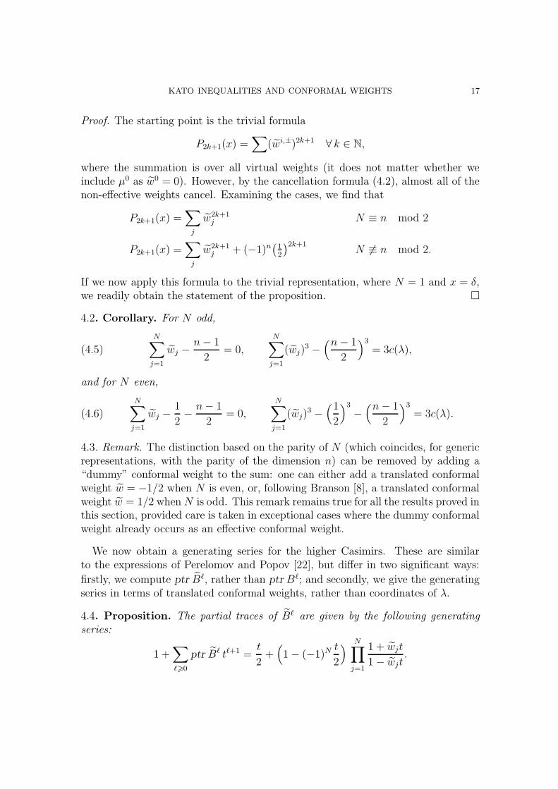
If we now apply this formula to the trivial representation, where N = 1 and x = δ,we readily obtain the statement of the proposition. �
4.2. Corollary. For N odd,
(4.5)
N∑
j=1
wj −n− 1
2= 0,
N∑
j=1
(wj)3 −
(n− 1
2
)3
= 3c(λ),
and for N even,
(4.6)
N∑
j=1
wj −1
2−n− 1
2= 0,
N∑
j=1
(wj)3 −
(1
2
)3
−(n− 1
2
)3
= 3c(λ).
4.3. Remark. The distinction based on the parity of N (which coincides, for genericrepresentations, with the parity of the dimension n) can be removed by adding a“dummy” conformal weight to the sum: one can either add a translated conformalweight w = −1/2 when N is even, or, following Branson [8], a translated conformalweight w = 1/2 when N is odd. This remark remains true for all the results proved inthis section, provided care is taken in exceptional cases where the dummy conformalweight already occurs as an effective conformal weight.
We now obtain a generating series for the higher Casimirs. These are similarto the expressions of Perelomov and Popov [22], but differ in two significant ways:
firstly, we compute ptr B`, rather than ptr B`; and secondly, we give the generatingseries in terms of translated conformal weights, rather than coordinates of λ.
4.4. Proposition. The partial traces of B` are given by the following generating
series:
1 +∑
`>0
ptr B` t`+1 =t
2+(1 − (−1)N t
2
) N∏
j=1
1 + wjt
1 − wjt.
18 DAVID M. J. CALDERBANK, PAUL GAUDUCHON, AND MARC HERZLICH
Proof. For each `,
ptr B` =tr B`
dimV=∑
(wj)` dimWj
dimV,
since the partial traces act by scalars on V . The relative dimensions dimWj/ dimVmay be computed as follows.
4.5. Lemma. Let Resz= ewj
(·) denote the residue at wj of the rational function within
parentheses. Then:
(i) if N is odd,
dimWj
dimV= (2wj + 1)
∏
k 6=j
wj + wk
wj − wk
= Resz= ewj
(z + 1
2
z
N∏
k=1
z + wk
z − wk
),
(ii) if N is even,
dimWj
dimV= (2wj − 1)
∏
k 6=j
wj + wk
wj − wk
= Resz= ewj
(z − 1
2
z
N∏
k=1
z + wk
z − wk
).
Proof of the lemma. Weyl’s dimension formula (see for instance [13, 25]) gives
(4.7) dimWj =∏
α∈R+
〈µ(j) + δ, α〉
〈δ, α〉, dimV =
∏
α∈R+
〈λ+ δ, α〉
〈δ, α〉,
where R+ is the set of positive roots of so(n), hence
(4.8)dimWj
dimV=∏
α∈R+
〈µ(j) + δ, α〉
〈λ+ δ, α〉.
Unless the dominant weight µ(j) of Wj is equal to λ, µ(j) is one of the 2m virtualweights µi,± = λ± εi. Hence
(4.9)dimWj
dimV=∏
α∈R+
(1 ±
αi
〈λ+ δ, α〉
)
so that
(4.10)dimWj
dimV=
∏
{ ewk,±:k 6=i(j)}
wi,± + wk,±
wi,± − wk,±,
if n = 2m is even, and
(4.11)dimWj
dimV=wi,± + 1
2
wi,± − 12
∏
{ ewk,±:k 6=i(j)}
wi,± + wk,±
wi,± − wk,±,
if n = 2m + 1 is odd. Applying the cancellation rule (4.2) and analyzing each casein turn completes the proof. �
KATO INEQUALITIES AND CONFORMAL WEIGHTS 19
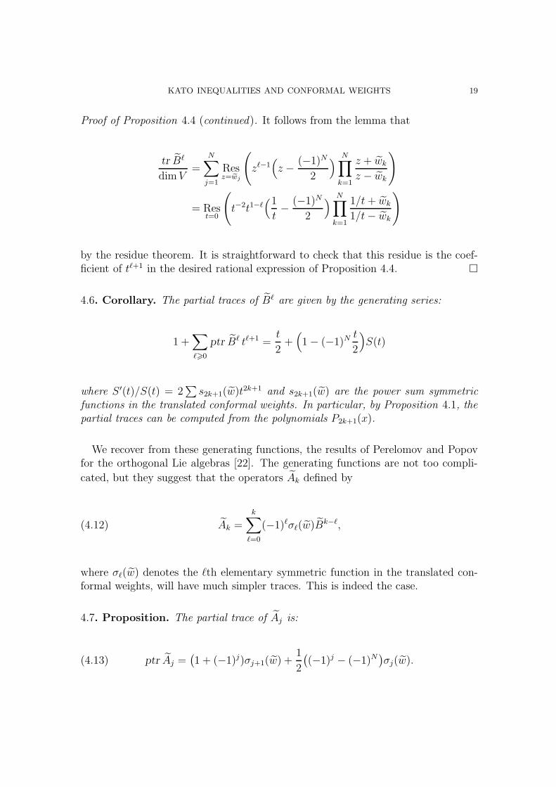
Proof of Proposition 4.4 (continued). It follows from the lemma that
tr B`
dimV=
N∑
j=1
Resz= ewj
(z`−1
(z −
(−1)N
2
) N∏
k=1
z + wk
z − wk
)
= Rest=0
(t−2t1−`
(1
t−
(−1)N
2
) N∏
k=1
1/t+ wk
1/t− wk
)
by the residue theorem. It is straightforward to check that this residue is the coef-ficient of t`+1 in the desired rational expression of Proposition 4.4. �
4.6. Corollary. The partial traces of B` are given by the generating series:
1 +∑
`>0
ptr B` t`+1 =t
2+(1 − (−1)N t
2
)S(t)
where S ′(t)/S(t) = 2∑s2k+1(w)t2k+1 and s2k+1(w) are the power sum symmetric
functions in the translated conformal weights. In particular, by Proposition 4.1, the
partial traces can be computed from the polynomials P2k+1(x).
We recover from these generating functions, the results of Perelomov and Popovfor the orthogonal Lie algebras [22]. The generating functions are not too compli-
cated, but they suggest that the operators Ak defined by
(4.12) Ak =
k∑
`=0
(−1)`σ`(w)Bk−`,
where σ`(w) denotes the `th elementary symmetric function in the translated con-formal weights, will have much simpler traces. This is indeed the case.
4.7. Proposition. The partial trace of Aj is:
(4.13) ptr Aj =(1 + (−1)j)σj+1(w) +
1
2
((−1)j − (−1)N
)σj(w).
20 DAVID M. J. CALDERBANK, PAUL GAUDUCHON, AND MARC HERZLICH
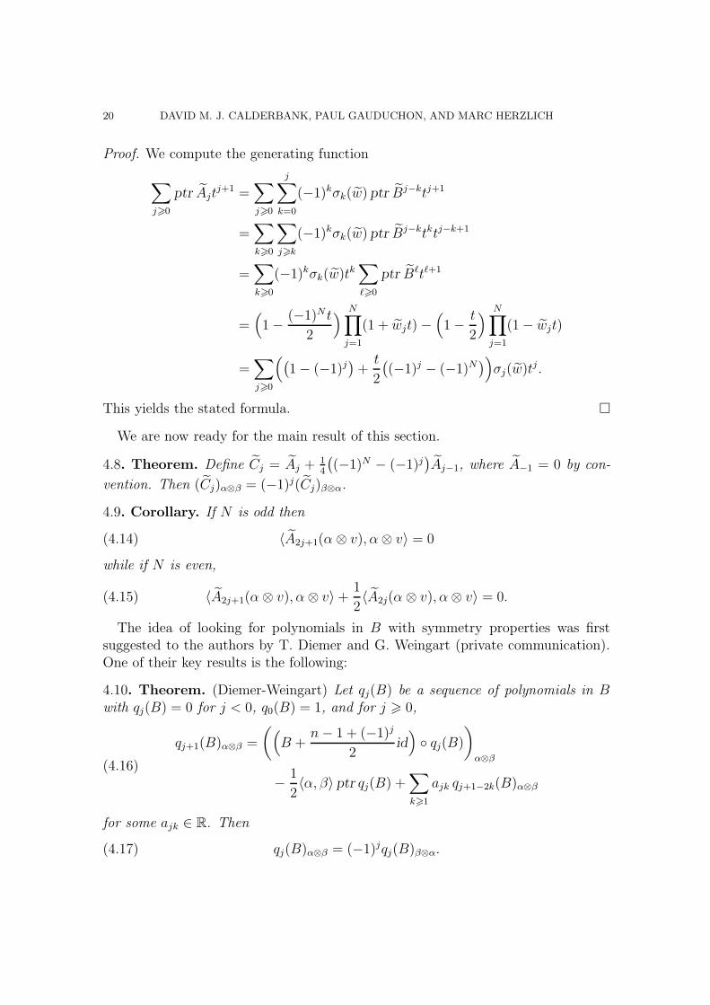
Proof. We compute the generating function
∑
j>0
ptr Ajtj+1 =
∑
j>0
j∑
k=0
(−1)kσk(w) ptr Bj−ktj+1
=∑
k>0
∑
j>k
(−1)kσk(w) ptr Bj−ktktj−k+1
=∑
k>0
(−1)kσk(w)tk∑
`>0
ptr B`t`+1
=(1 −
(−1)N t
2
) N∏
j=1
(1 + wjt) −(1 −
t
2
) N∏
j=1
(1 − wjt)
=∑
j>0
((1 − (−1)j
)+t
2
((−1)j − (−1)N
))σj(w)tj.
This yields the stated formula. �
We are now ready for the main result of this section.
4.8. Theorem. Define Cj = Aj + 14
((−1)N − (−1)j
)Aj−1, where A−1 = 0 by con-
vention. Then (Cj)α⊗β = (−1)j(Cj)β⊗α.
4.9. Corollary. If N is odd then
(4.14) 〈A2j+1(α⊗ v), α⊗ v〉 = 0
while if N is even,
(4.15) 〈A2j+1(α⊗ v), α⊗ v〉 +1
2〈A2j(α⊗ v), α⊗ v〉 = 0.
The idea of looking for polynomials in B with symmetry properties was firstsuggested to the authors by T. Diemer and G. Weingart (private communication).One of their key results is the following:
4.10. Theorem. (Diemer-Weingart) Let qj(B) be a sequence of polynomials in Bwith qj(B) = 0 for j < 0, q0(B) = 1, and for j > 0,
qj+1(B)α⊗β =
((B +
n− 1 + (−1)j
2id
)◦ qj(B)
)
α⊗β
−1
2〈α, β〉 ptr qj(B) +
∑
k>1
ajk qj+1−2k(B)α⊗β
(4.16)
for some ajk ∈ R. Then
(4.17) qj(B)α⊗β = (−1)jqj(B)β⊗α.
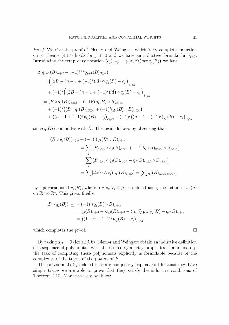
KATO INEQUALITIES AND CONFORMAL WEIGHTS 21
Proof. We give the proof of Diemer and Weingart, which is by complete inductionon j: clearly (4.17) holds for j 6 0 and we have an inductive formula for qj+1.Introducing the temporary notation (cj)α⊗β = 1
2〈α, β〉
(ptr qj(B)
)we have
2(qj+1(B)α⊗β − (−1)j+1qj+1(B)β⊗α
)
=((
2B + (n− 1 + (−1)j)id)◦ qj(B) − cj
)α⊗β
+ (−1)j((
2B + (n− 1 + (−1)j)id)◦ qj(B) − cj
)β⊗α
= (B ◦ qj(B))α⊗β + (−1)j(qj(B) ◦B)β⊗α
+ (−1)j((B ◦ qj(B))β⊗α + (−1)j(qj(B) ◦B)α⊗β
)
+((n− 1 + (−1)j)qj(B) − cj
)α⊗β
+ (−1)j((n− 1 + (−1)j)qj(B) − cj
)β⊗α
since qj(B) commutes with B. The result follows by observing that
(B ◦ qj(B))α⊗β + (−1)j(qj(B) ◦B)β⊗α
=∑
i
(Bα⊗ei
◦ qj(B)ei⊗β + (−1)jqj(B)β⊗ei◦Bei⊗α
)
=∑
i
(Bα⊗ei
◦ qj(B)ei⊗β − qj(B)ei⊗β ◦Bα⊗ei
)
=∑
i
[dλ(α ∧ ei), qj(B)ei⊗β] =∑
i
qj(B)α∧ei.(ei⊗β)
by equivariance of qj(B), where α ∧ ei.(ei ⊗ β) is defined using the action of so(n)on R
By taking ajk = 0 (for all j, k), Diemer and Weingart obtain an inductive definitionof a sequence of polynomials with the desired symmetry properties. Unfortunately,the task of computing these polynomials explicitly is formidable because of thecomplexity of the traces of the powers of B.
The polynomials Cj defined here are completely explicit and because they havesimple traces we are able to prove that they satisfy the inductive conditions ofTheorem 4.10. More precisely, we have:
22 DAVID M. J. CALDERBANK, PAUL GAUDUCHON, AND MARC HERZLICH
4.11. Lemma. For j > 0,
Cj+1 =(B +
(−1)j
2id
)◦ Cj −
1
2ptr Cj
+ 18
(1 − (−1)N+j
)Cj−1 + 1
2
(1 − (−1)j
)(σj+1(w) − 1
2
(1 − (−1)N
)σj(w)
)id
Proof. Note that Cj = Aj + 14
((−1)N − (−1)j
)Cj−1 and so
Cj+1 − BCj −12(−1)jCj = Aj+1 − BAj −
12(−1)jCj + 1
4
((−1)N + (−1)j
)Cj
− 14
((−1)N − (−1)j
)BCj−1
= Aj+1 − BAj + 14
((−1)N − (−1)j
)(Cj − BCj−1
)
= Aj+1 − BAj + 14
((−1)N − (−1)j
)(Cj − BCj−1 −
12(−1)jCj−1
)
+ 18
(1 − (−1)N+j
)Cj−1
= Aj+1 − BAj + 14
((−1)N − (−1)j
)(Aj − BAj−1
)+ 1
8
(1 − (−1)N+j
)Cj−1.
Now, by definition, we have Aj+1 − BAj = (−1)j+1σj+1(w)id and so
Cj+1 − BCj −12(−1)jCj = 1
8
(1 − (−1)N+j
)Cj−1
− (−1)jσj+1(w)id − 14
(1 − (−1)N+j
)σj(w)id.
(4.18)
Finally, observe that
ptr Cj =(1 + (−1)j
)(σj+1(w) + 1
4(1 − (−1)N+j)σj(w)
)id.
Adding one half of this onto (4.18) completes the proof. �
Theorem 4.8 follows immediately from this Lemma and Theorem 4.10.
5. Refined Kato inequalities
In the last section we learnt that by working with B and Aj instead of B and Aj,
we could obtain some explicit formulae. Of course B = B+ 12(n−1)id has the same
eigenspaces as B and so we can rewrite (1.6) as:
(5.1) |Πj(α⊗ v)|2 =
N−1∑
k=0
wN−1−kj 〈Ak(α⊗ v), α⊗ v〉
∏
k 6=j
(wj − wk).
If N is odd, Corollary 4.9 implies that the terms with k odd vanish, while for Neven, we have
〈A2j+1(α⊗ v), α⊗ v〉 +1
2〈A2j(α⊗ v), α⊗ v〉 = 0.
Our main result will readily follow from this.
KATO INEQUALITIES AND CONFORMAL WEIGHTS 23
5.1. Main Theorem. Let I a subset of {1, . . . , N} corresponding to an operator PI
acting on E. Then a Kato constant kI for sections in the kernel of PI is given by
the following expressions.
If N is odd, then
(5.2) k2I = max
J∈NE
(∑
i∈bI∩ bJ
∏j∈J(wi + wj)∏
j∈ bJ\{i}(wi − wj)
)= 1− min
J∈NE
(∑
i∈I∩ bJ
∏j∈J(wi + wj)∏
j∈ bJ\{i}(wi − wj)
).
If N is even, then
(5.3) k2I = max
J∈NE
(∑
i∈bI∩ bJ
(wi −
12
)∏j∈J(wi + wj)∏
j∈ bJ\{i}(wi − wj)
)
= 1 − minJ∈NE
(∑
i∈I∩ bJ
(wi −
12
)∏j∈J(wi + wj)∏
j∈ bJ\{i}(wi − wj)
).
These constants are sharp, unless N = 2ν + 1, λ is properly half-integral, and the
set J achieving the extremum contains ν + 1.
Recall that NE denotes the set of subsets of {1, . . .N} whose elements are obtainedby choosing exactly one index in each of the sets {j, N + 2 − j} for each j with2 6 j 6 ν if N = 2ν − 1, 2ν and for each j with 2 6 j 6 ν + 1 if N = 2ν + 1.These correspond to the maximal non-elliptic operators unless N = 2ν + 1 and λ isproperly half-integral, when there are also some elliptic subsets in NE.
Explicit values of the constants for a number of cases, including all minimal ellipticoperators, will be given in sections 6 and 7, and in the appendix. Note that kI = 1for non-elliptic operators, as one would expect.
Proof of the Main Theorem. We let first N = 2ν − 1 and denote Qk =
(−1)k−1〈A2k−2(α⊗ v), α⊗ v〉. We have
(5.4) |Πj(α⊗ v)|2 =
ν∑
k=1
w2(ν−k)j (−1)k−1Qk
∏
k 6=j
(wj − wk)=
w2(ν−1)j −
ν∑
k=2
w2(ν−k)j (−1)kQk
∏
k 6=j
(wj − wk)
since Q1 = 1. We can now obtain bounds on Q2, . . . Qν using the non-negativity ofthe norms. Since the denominator in (5.4) has sign (−1)j−1 these inequalities are:
(5.5)ν∑
k=2
(−1)j+kw2(ν−k)j Qk > (−1)jw
2(ν−1)j
with equality iff |Πj(α⊗ v)|2 = 0.This system of linear inequalities confines the values of the Qk’s to a convex region
in Rν−1. Our first goal is to show that this region is compact, hence polyhedral,
24 DAVID M. J. CALDERBANK, PAUL GAUDUCHON, AND MARC HERZLICH
and to identify its vertices. For this we let πj denote the affine functions of Q =(Q2, . . . Qν) given by |Πj(α⊗ v)|2 and note the following.
5.2. Lemma. Let J be a subset of {1, ..., N} with ν − 1 elements. Then the inter-
section of the ν − 1 affine hyperplanes πj = 0 for all j ∈ J consists of the single
point QJ = (Q2, . . . Qν) with Qk = σk−1
((w2
j )j∈J
). At this point the affine functions
πj take the values
(5.6) πj(QJ) =
∏
k∈J
(w2j − w2
k)
∏
k 6=j
(wj − wk)=
∏
k∈J,k 6=j
(wj + wk)
∏
k∈ bJ,k 6=j
(wj − wk)εj(J)
where εj(J) = 0 if j ∈ J and 1 if not.
This lemma follows simply by observing that the affine function πj is obtained byevaluating a polynomial independent of j on w2
j , and then using the fact that thecoefficients of a polynomial are the elementary symmetric functions of the roots.
Compactness of the convex region is obtained by taking J = {2, . . . ν} and J ={ν + 1, . . . 2ν − 1}. The inverse of the Vandermonde system of inequalities forJ = {2, . . . ν} has non-negative entries, while for J = {ν + 1, . . . 2ν − 1}, it hasnon-positive entries.
5.3. Proposition. Let N = 2ν − 1. Then for k = 2, . . . ν,
(5.7) σk−1(w22, . . . w
2ν) 6 Qk 6 σk−1(w
2ν+1, . . . w
22ν−1).
The lower bounds are all attained if and only if Π{2,...ν}(α⊗ v) = 0, while the upper
bounds are all attained if and only if Π{ν+1,...2ν−1}(α ⊗ v) = 0. These bounds are
sharp by non-ellipticity of P{2,...ν} and P{ν+1,...2ν−1}.
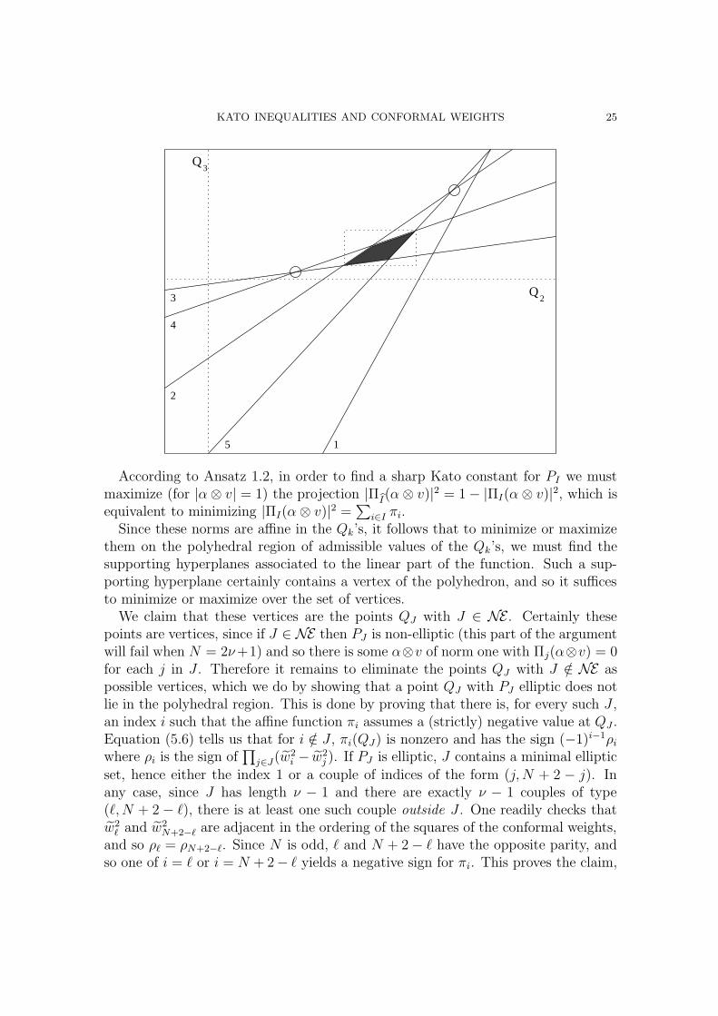
When N = 2ν − 1 = 3, the case most commonly occuring in practice, it is nowstraightforward to obtain sharp Kato constants. However, for N > 5, the upperbound for some Qk and the lower bound for another (as given in this proposition)will not be simultaneously attained: the convex region is smaller. We illustrate thisin the case N = 5 (ν = 3).
In this diagram, the numbered lines represent the conditions on Q2 and Q3 for thenorms of Π1, . . .Π5 to vanish. The shaded region represents the range of possiblevalues for (Q2, Q3), while the dotted rectangle represents the bounds on (Q2, Q3)we have found. We have circled the points corresponding to the non-elementaryminimal elliptic operators.
KATO INEQUALITIES AND CONFORMAL WEIGHTS 25
3
4
2
5 1
Q
Q
3
2
According to Ansatz 1.2, in order to find a sharp Kato constant for PI we mustmaximize (for |α⊗ v| = 1) the projection |ΠbI
(α⊗ v)|2 = 1 − |ΠI(α⊗ v)|2, which isequivalent to minimizing |ΠI(α⊗ v)|2 =
∑i∈I πi.
Since these norms are affine in the Qk’s, it follows that to minimize or maximizethem on the polyhedral region of admissible values of the Qk’s, we must find thesupporting hyperplanes associated to the linear part of the function. Such a sup-porting hyperplane certainly contains a vertex of the polyhedron, and so it sufficesto minimize or maximize over the set of vertices.
We claim that these vertices are the points QJ with J ∈ NE. Certainly thesepoints are vertices, since if J ∈ NE then PJ is non-elliptic (this part of the argumentwill fail when N = 2ν+1) and so there is some α⊗v of norm one with Πj(α⊗v) = 0for each j in J . Therefore it remains to eliminate the points QJ with J /∈ NE aspossible vertices, which we do by showing that a point QJ with PJ elliptic does notlie in the polyhedral region. This is done by proving that there is, for every such J ,an index i such that the affine function πi assumes a (strictly) negative value at QJ .Equation (5.6) tells us that for i /∈ J , πi(QJ) is nonzero and has the sign (−1)i−1ρi
where ρi is the sign of∏
j∈J(w2i − w2
j ). If PJ is elliptic, J contains a minimal elliptic
set, hence either the index 1 or a couple of indices of the form (j, N + 2 − j). Inany case, since J has length ν − 1 and there are exactly ν − 1 couples of type(`, N + 2 − `), there is at least one such couple outside J . One readily checks thatw2
` and w2N+2−` are adjacent in the ordering of the squares of the conformal weights,
and so ρ` = ρN+2−`. Since N is odd, ` and N + 2 − ` have the opposite parity, andso one of i = ` or i = N + 2− ` yields a negative sign for πi. This proves the claim,
26 DAVID M. J. CALDERBANK, PAUL GAUDUCHON, AND MARC HERZLICH
and now maximizing or minimizing over the vertices using (5.6) proves the maintheorem for N = 2ν − 1.
The argument for the case N = 2ν + 1 is completely analogous, by replacingν with ν − 1. When λ properly half-integral, the lower bounds in the analogueof (5.7) will not be sharp since P{2,...ν+1} is elliptic. However, we only used thesebounds to establish compactness of the convex region defined by the nonnegativityof the norms, so this does not matter. The ellipticity of Pν+1 means that some of thevertices of this polyhedral region are not possible values for the Qk’s. More precisely,the index sets corresponding to the vertices are still contained in the set NE, and sowe can maximize or minimize over NE , but we will not obtain sharp results if theextremum is obtained at a vertex corresponding to an index set containing ν + 1.
Now suppose N = 2ν and let Qk = (−1)k−1〈A2k−2(α⊗ v), α⊗ v〉. We have
|Πj(α⊗ v)|2 =wj −
12∏
k 6=j
(wj − wk)
ν∑
k=1
w2(ν−k)j (−1)k−1Qk
=wj −
12∏
k 6=j
(wj − wk)
(w
2(ν−1)j −
ν∑
k=2
w2(ν−k)j (−1)kQk
)(5.8)
since Q1 = 1. Our strategy is now the same as before: we obtain the polyhe-dron using the non-negativity of the norms and its vertices by looking at maximallength non-elliptic operators. Since the denominator in (5.8) has sign (−1)j−1 theseinequalities are:
ν∑
k=2
(−1)j+kw2(ν−k)j Qk > (−1)jw
2(ν−1)j for j 6 ν
ν∑
k=2
(−1)j+kw2(ν−k)j Qk 6 (−1)jw
2(ν−1)j for j > ν + 1.
(5.9)
Lemma 5.2 is unchanged except that the formula for πj(QJ) has an additional wj−12.
To obtain compactness, we consider J = {2, . . . ν} and J = {ν+2, . . . 2ν} and againobserve that the inverses of these Vandermonde systems have entries all of one sign.
5.4. Proposition. Let N = 2ν. Then for k = 2, . . . ν,
(5.10) σk−1(w22, . . . w
2ν) 6 Qk 6 σk−1(w
2ν+2, . . . w
22ν).
The lower bounds are all attained if and only if Π{2,...ν}(α⊗ v) = 0, while the upper
bounds are all attained if and only if Π{ν+2,...2ν}(α⊗ v) = 0. These bounds are sharp
by non-ellipticity of P{2,...ν} and P{ν+2,...2ν}.
The vertices are identified with NE in a similar way to the case N = 2ν − 1. Theonly difference comes from the way the sign changes when passing from i = ` to
KATO INEQUALITIES AND CONFORMAL WEIGHTS 27
i = N + 2 − `: the parity of i does not change but the sign of the factor wi − 1/2does. This proves the main theorem for N = 2ν. �
In the next two sections we shall calculate some of the constants more explicitly,by finding the vertex at which the maximum or minimum is achieved. This is onlyfeasible when the number of terms in the sum is small and in general, the vertexdepends on the coordinates of λ. Nevertheless, this is a worthwhile task, as explicitconstants are of more practical use than extrema over exponentially large sets.
Our main tool is the order of the conformal weights, together with the fact that,for j ∈ {2, . . . ν}, we have wj + wN+2−j = kj − kj−1 < 0. Similarly, for N = 2ν + 1,wν+1 + wν+2 = wν+2 = −λm < 0. Hence for any i ∈ {1, . . .N} and j ∈ {2 . . . ν}:
(wi + wj)(wi − wj) − (wi + wN+2−j)(wi − wN+2−j)
= −(wj + wN+2−j)(wj − wN+2−j) > 0
and this also holds for N = 2ν + 1 and j = ν + 1.By considering the possible signs of the terms, we obtain:
5.5. Proposition. For any i ∈ {1, . . .N} and j ∈ {2 . . . ν} (or j = ν + 1 when
N = 2ν + 1) with i 6= j and i 6= N + 2 − j, we have:
wi + wj
wi − wN+2−j
>wi + wN+2−j
wi − wj
> 0 iff i < j or N + 2 − j < i
wi + wN+2−j
wi − wj
>wi + wj
wi − wN+2−j
> 0 iff j < i < N + 2 − j.
6. Refined Kato inequalities with N odd
When N is odd, we have to minimize or maximize over J ∈ NE, a sum of a subsetof the following terms:
∏j∈J(wi + wj)∏
j∈ bJ\{i}(wi − wj)=wi + wN+2−i
wi − w1
∏
j∈Jj 6=N+2−i
wi + wj
wi − wN+2−j
for i ∈ J \ {1}
∏j∈J(w1 + wj)∏
j∈ bJ\{i}(w1 − wj)=∏
j∈J
w1 + wj
w1 − wN+2−j
.
Using Proposition 5.5, the first expression is minimized (subject to J 63 i) by Jmini =
{2, . . . i − 1, N + 2 − ν, . . . N + 2 − i} (together with ν + 2 if N = 2ν + 1) and ismaximized by Jmax
i = {i+1, . . . ν, N+2−i, . . . N} (together with ν+1 if N = 2ν+1).The second expression is minimized by Jmin
1 = {N + 2 − ν, . . . N} (together withν + 2 if N = 2ν + 1) and maximized by Jmax
28 DAVID M. J. CALDERBANK, PAUL GAUDUCHON, AND MARC HERZLICH
This information suffices to find Kato constants for the elementary elliptic oper-ators and the complements of generalized gradients. Note that Jmin
i = JminN−1−i and
Jmaxi = Jmax
N−1−i, which will give a few more explicit results.We shall now show how the values of the constants can be computed for the
non-elementary (i.e., length 2) minimal elliptic operators.Let I = {i, N +2− i} for i ∈ {2, · · · , ν} (or i = ν+1 when N = 2ν+1). Then for
any J ∈ NE, J ∩ I has precisely one element, and hence so does J ∩ I. Therefore,for each J , the sum has only one term, indexed by either i or N − 2− i, and so theminimum, over all J , is given by the minimum over Jmin
i and JminN+2−i. Unfortunately,
each of these two quantities may be the smallest, depending on the precise valuesof the conformal weights, so that we are forced to keep a minimum in our formulae.However, if N = 2ν − 1 and i = ν, then the following argument, together with thefact that w1 − wν+1 > w1 − wν, shows that the minimum is obtained by using Jmin
Replacing ν by ν + 1 gives analogous results for N = 2ν + 1, but note that equality
cases with Πν+1(α⊗ v) = 0 will not be attained if λ is properly half-integral.
We now give more detailed formulas when N = 3, which is the most common casearising in practice: the representation τ ⊗ λ splits into N = 3 components when:
30 DAVID M. J. CALDERBANK, PAUL GAUDUCHON, AND MARC HERZLICH
(i) V = �kΛp (k a positive integer) and 0 < p 6 m − 1 (p = m − 1 ineven dimension belongs to this case only by virtue of our convention ondistinctness of conformal weights). Then λ = (k, . . . k, 0, . . . 0) where k isrepeated p times and w1 = k > w2 = −p > w3 = p− k + 1 − n.
(ii) in odd dimensions, either V = �kΛm (k a positive integer) or V = �k− 1
2 Λm�∆ (k > 1/2 and half-integral), where ∆ is the spin representation. Thiscorresponds in both cases to λ = (k, . . . k) and w1 = k > w2 = −n−1
2>
w3 = −k − n−12
.
Note that P1 and P2 + P3 are elliptic, whereas P2 and P3 are non-elliptic, unlessν = 1 and λ is properly half-integral, when P2 is elliptic, but the results above donot cover this case.
6.3. Theorem. If ξ is a nonvanishing section in the kernel of one of the elliptic
operators P1, P2 +P3, P1 +P3 or P1 +P2, we have a refined Kato inequality∣∣d|ξ|
∣∣ 6kI |∇ξ| with kI given as follows.
(i) For P1 or P1 + P3,
k2{1} = k2
{1,3} =w1
w1 − w2
=k
k + p.
Equality holds iff ∇ξ = Π2(α⊗ ξ) for a 1-form α such that Π3(α⊗ ξ) = 0.(ii) For P2 + P3,
k2{2,3} =
−w3
w1 − w3=
k + n− p− 1
2k + n− p− 1.
Equality holds iff ∇ξ = Π1(α⊗ ξ) for a 1-form α such that Π2(α⊗ ξ) = 0.(iii) For P1 + P2,
k2{1,2} =
w1
w1 − w3=
k
2k + n− p− 1.
Equality holds iff ∇ξ = Π3(α⊗ ξ) for a 1-form α such that Π2(α⊗ ξ) = 0.
When λ is properly half-integral, only the first constant is sharp and we do not geta nontrivial constant for P2. Since this case sometimes arises in practice (e.g., theRarita-Schwinger operator), we note briefly how the Kato constant can be found.
Since wν+1 = 0, the projection Πν+1 = Π2 is a equal to AN−1 = A2 divided by
w1w3 < 0. Hence we need to obtain a better upper bound on 〈A2(α⊗ v), α⊗ v〉 =〈(B2 − w1w3)(α⊗ v), α⊗ v〉. Now for fixed α 6= 0, say α = en, we can break this upunder so(n−1) and use the fact, easily verified, that B2 is the difference between theCasimir number of λ and the Casimir operator of so(n−1). Applying the branching
rule, we see that the eigenvalues of (A2)en⊗enare −(k− `)2 for ` ∈ N with k− ` > 0.
KATO INEQUALITIES AND CONFORMAL WEIGHTS 31
Hence if k is half-integral, 〈A2(α⊗ v), α⊗ v〉 6 −1/4. This gives:
k2{2} = 1 −
1
2k(2k + n− 1)
k{2,3} =(2k + n− 1)2 − 1
(2k + n− 1)(4k + n− 1)k{1,2} =
k2 − 1
k(4k + n− 1)
The analogues of these sharper results for larger N = 2ν + 1, can be derived fromBranson’s minimization formula [9]. In particular he gives the formula for k{ν+1}
explicitly there.Most “uncomplicated” tensor bundles, such as vectors, forms, symmetric traceless
tensors and algebraic Weyl tensors, have N = 3 (except in low dimensions, whereN might be 2).
(i) For Λ1, the constants are 12
(conformal or Killing vector fields), n−1n
(har-
monic 1-forms) and 1n
(closed 1-forms dual to a conformal vector field). Thelast of these is trivial, since the only non-vanishing component of ∇ξ in thiscase is 1
ndiv ξ id.
(ii) For Λ2, the constants are 13, n−2
n−1and 1
n−1. The second of these is the constant
for harmonic 2-forms.(iii) For S2
0 , the constants are 23, n
n+2and 2
n+2. The second of these is the constant
appearing in the work of R. Schoen, L. Simon and S. T. Yau [26].(iv) For Λ2 � Λ2, the constants are 1
2, n−1
n+1and 2
n+1. The second of these is the
constant for the second Bianchi identity appearing in the work of S. Bando,A. Kasue and H. Nakajima [1].
7. Refined Kato inequalities with N even
When N = 2ν is even, we have to minimize or maximize over J ∈ NE, a sum ofa subset of the following terms:
(wi −12)(wi + wN+2−i)
(wi − w1)(wi − wν+1)
∏
j∈Jj 6=N+2−i
wi + wj
wi − wN+2−j
for i ∈ J \ {1, ν + 1}
w1 −12
w1 − wν+1
∏
j∈J
w1 + wj
w1 − wN+2−j
wν+1 −12
wν+1 − w1
∏
j∈J
wν+1 + wj
wν+1 − wN+2−j
Using Proposition 5.5, the first expression is minimized (subject to J 63 i) by Jmini =
{2, . . . i− 1, N + 2− ν, . . . N + 2− i} and is maximized by Jmaxi = {i+ 1, . . . ν, N +
2 − i, . . . N}. The second expression is minimized by Jmin1 = {N + 2 − ν, . . . N}
32 DAVID M. J. CALDERBANK, PAUL GAUDUCHON, AND MARC HERZLICH
and maximized by Jmax1 = {2, . . . ν), while the third expression is minimized by
Jminν+1 = {2, . . . ν) and maximized by Jmax
ν+1 = {N + 2 − ν, . . . N}.We now proceed as in the odd dimensional case, except that the analogue of
Lemma 6.1 is no longer useful, due to the additional w − 12
factors. The results aresummarized below.
7.1. Theorem. Let E be associated to a representation λ with N = 2ν and let PI
be an elliptic operator on sections of E associated to a subset I of {1, . . .N}. Then
in the following cases, a refined Kato inequality of the type∣∣d|ξ|
∣∣ 6 kI |∇ξ| holds
outside the zero set of ξ for ξ in the kernel of PI .
(i) For {1} ⊆ I ⊆ {1, ν + 2, . . . 2ν}, we have
k2I = 1 −
(w1 −12)∏2ν
k=ν+2(w1 + wk)∏ν+1k=2(w1 − wk)
.
Equality case: ∇ξ = Π{2,...ν+1}(α⊗ ξ) for α with Π{ν+2,...2ν}(α⊗ ξ) = 0.(ii) For {ν + 1} ⊆ I ⊆ {2, . . . ν, ν + 1}, we have
k2I = 1 −
(wν+1 −12)∏ν
k=2(wν+1 + wk)
(wν+1 − w1)∏2ν
k=ν+2(wν+1 − wk).
Equality case: ∇ξ = Π{1,ν+2...2ν}(α⊗ ξ) for α with Π{2,...ν}(α⊗ ξ) = 0.(iii) For {i, 2ν + 2 − i} ⊆ I ⊆ {i, 2ν + 2 − i} ∪ J0, with i ∈ {2, . . . , ν} and
J0 = {j : 2 6 j < i} ∪ {2ν + 2 − j : i < j 6 ν}, we have
k2I = 1 − min(C1, C2)
where
C1 =(wi + w2ν+2−i)(wi −
12)
(wi − wν+1)(wi − w1)
∏
k∈J0
wi + wk
wi − w2ν+2−k
,
C2 =(wi + w2ν+2−i)(w2ν+2−i −
12)
(w2ν+2−i − wν+1)(w2ν+2−i − w1)
∏
k∈J0
w2ν+2−i + wk
w2ν+2−i − w2ν+2−k
.
Equality case: ∇ξ = Π bJ0\{i,2ν+2−i}(α⊗ ξ) for α with
Π{i}∪J0(α⊗ ξ) = 0 if C2 < C1 or Π{2ν+2−i}∪J0
(α⊗ ξ) = 0 if C1 < C2.
(iv) For I = {2, . . . 2ν}, we have
k2I =
(w1 −12)∏ν
k=2(w1 + wk)∏2ν
k=ν+1(w1 − wk).
Equality case: ∇ξ = Π1(α⊗ ξ) for α with Π{2,...ν}(α⊗ ξ) = 0.(v) For I = {1, . . . ν, ν + 2, . . . 2ν}, we have
k2I =
(wν+1 −12)∏2ν
k=ν+2(wν+1 + wk)∏ν
k=1(wν+1 − wk).
KATO INEQUALITIES AND CONFORMAL WEIGHTS 33
Equality case: ∇ξ = Πν+1(α⊗ ξ) for α with Π{ν+2,...2ν}(α⊗ ξ) = 0.
(vi) For I = {i} with i ∈ {2, . . . ν, ν + 2, . . . 2ν}, we have
k2I =
(wi −12)(wi + w2ν+2−i)
(wi − w1)(wi − wν+1)
∏
j∈Jmaxi
j 6=2ν+2−i
wi + wj
wi − w2ν+2−j
.
Equality case: ∇ξ = Πi(α ⊗ ξ) for α with ΠJmaxi
(α ⊗ ξ) = 0. Here Jmaxi =
{i+ 1, . . . ν, 2ν + 2 − i, . . . 2ν}.(vii) For I = {2, . . . 2ν − 1}, we have
k2I =
(w1 −12)∏ν
k=2(w1 + wk)∏2ν
k=ν+1(w1 − wk)+
(w2ν −12)∏ν
k=2(w2ν + wk)
(w2ν − w1)∏2ν−1
k=ν+1(w2ν − wk).
Equality case: ∇ξ = Π{1,2ν}(α⊗ ξ) for α with Π{2,...ν}(α⊗ ξ) = 0.(viii) For I = {1, . . . ν − 1, ν + 2, . . . 2ν} we have
k2I =
(wν −12)∏2ν
k=ν+2(wν + wk)
(wν − wν+1)∏ν−1
k=1(wν − wk)+
(wν+1 −12)∏2ν
k=ν+2(wν+1 + wk)∏ν
k=1(wν+1 − wk).
Equality case: ∇ξ = Π{ν,ν+1}(α⊗ ξ) for α with Π{ν+2,...2ν}(α⊗ ξ) = 0.
(ix) For I = {i, 2ν + 1 − i} with i ∈ {2, . . . ν − 1}, we have
k2I =
(wi + w2ν+2−i)(wi −12)
(wi − w1)(wi − wν+1)
∏
j∈Jmaxi
j 6=2ν+2−i
wi + wj
wi − w2ν+2−j
+(wi+1 + w2ν+1−i)(wi −
12)
(w2ν+1−i − w1)(w2ν+1−i − wν+1)
∏
j∈Jmaxi
j 6=i+1
w2ν+1−i + wj
w2ν+1−i − w2ν+2−j
.
Equality case: ∇ξ = Π{i,2ν+1−i}(α ⊗ ξ) for α with ΠJmaxi
(α ⊗ ξ) = 0. Here
Jmaxi = {i+ 1, . . . ν, 2ν + 2 − i, . . . 2ν}.
We now give more detailed formulas when N = 4, which is the generic case infour dimensional differential geometry: the representation τ ⊗ λ splits into N = 4components whenever
(i) if n = 2m is even and V = �`Λ±�k−`Λp or V = �`− 1
2 Λ±�k−`Λp�∆± wherek > ` > 0 are (simultaneously) integers or half-integers, p < m are integers,Λm
± stand for selfdual or antiselfdual m-forms and ∆± for positive or negativespin representations. The associated weights are λ = (k, . . . k, `, . . . `,±`),with k repeated p times. One gets w1 = k > w2 = `− p > w3 = 1− n
2− ` >
w4 = −k + p+ 1 − n.(ii) if n = 2m + 1 is odd, V = �k− 1
2 Λp � ∆ with p < m integer and k > 12
and half-integer, so that λ = (k, . . . k, 12, . . . 1
2). Conformal weights are a
34 DAVID M. J. CALDERBANK, PAUL GAUDUCHON, AND MARC HERZLICH
specialization of the previous formula with ` = 12: w1 = k > w2 = 1
2− p >
w3 = (1−n)2
> w4 = −k + p + 1 − n.
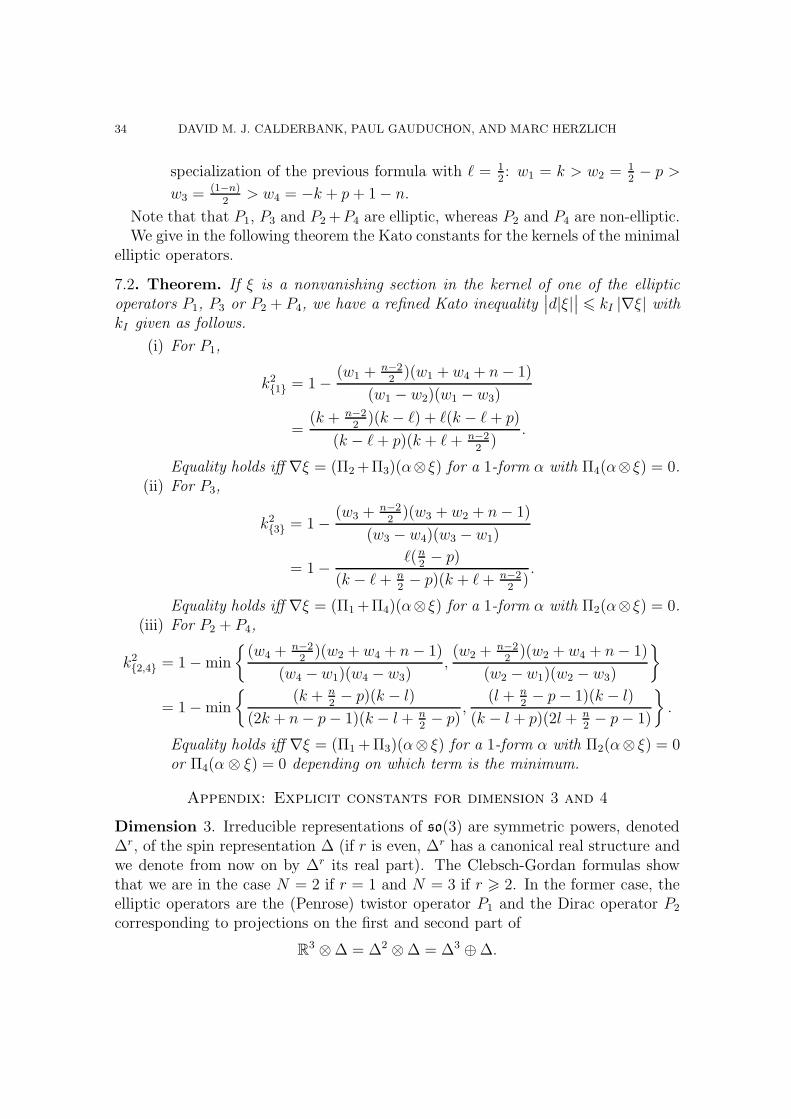
Note that that P1, P3 and P2 +P4 are elliptic, whereas P2 and P4 are non-elliptic.We give in the following theorem the Kato constants for the kernels of the minimal
elliptic operators.
7.2. Theorem. If ξ is a nonvanishing section in the kernel of one of the elliptic
operators P1, P3 or P2 + P4, we have a refined Kato inequality∣∣d|ξ|
∣∣ 6 kI |∇ξ| with
kI given as follows.
(i) For P1,
k2{1} = 1 −
(w1 + n−22
)(w1 + w4 + n− 1)
(w1 − w2)(w1 − w3)
=(k + n−2
2)(k − `) + `(k − `+ p)
(k − `+ p)(k + `+ n−22
).
Equality holds iff ∇ξ = (Π2 +Π3)(α⊗ ξ) for a 1-form α with Π4(α⊗ ξ) = 0.(ii) For P3,
k2{3} = 1 −
(w3 + n−22
)(w3 + w2 + n− 1)
(w3 − w4)(w3 − w1)
= 1 −`(n
2− p)
(k − `+ n2− p)(k + `+ n−2
2).
Equality holds iff ∇ξ = (Π1 +Π4)(α⊗ ξ) for a 1-form α with Π2(α⊗ ξ) = 0.(iii) For P2 + P4,
k2{2,4} = 1 − min
{(w4 + n−2
2)(w2 + w4 + n− 1)
(w4 − w1)(w4 − w3),(w2 + n−2
2)(w2 + w4 + n− 1)
(w2 − w1)(w2 − w3)
}
= 1 − min
{(k + n
2− p)(k − l)
(2k + n− p− 1)(k − l + n2− p)
,(l + n
2− p− 1)(k − l)
(k − l + p)(2l + n2− p− 1)
}.
Equality holds iff ∇ξ = (Π1 +Π3)(α⊗ ξ) for a 1-form α with Π2(α⊗ ξ) = 0or Π4(α⊗ ξ) = 0 depending on which term is the minimum.
Appendix: Explicit constants for dimension 3 and 4
Dimension 3. Irreducible representations of so(3) are symmetric powers, denoted∆r, of the spin representation ∆ (if r is even, ∆r has a canonical real structure andwe denote from now on by ∆r its real part). The Clebsch-Gordan formulas showthat we are in the case N = 2 if r = 1 and N = 3 if r > 2. In the former case, theelliptic operators are the (Penrose) twistor operator P1 and the Dirac operator P2
corresponding to projections on the first and second part of
R3 ⊗ ∆ = ∆2 ⊗ ∆ = ∆3 ⊕ ∆.
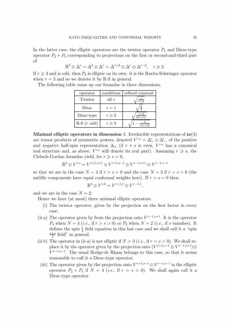
KATO INEQUALITIES AND CONFORMAL WEIGHTS 35
In the latter case, the elliptic operators are the twistor operator P1 and Dirac-typeoperator P2 + P3 corresponding to projections on the first or second-and-third partof
R3 ⊗ ∆r = ∆2 ⊗ ∆r = ∆r+2 ⊕ ∆r ⊕ ∆r−2, r > 2.
If r > 3 and is odd, then P2 is elliptic on its own: it is the Rarita-Schwinger operatorwhen r = 3 and so we denote it by R-S in general.
The following table sums up our formulae in three dimensions.
operator conditions refined constant
Twistor all r
√r
r+2
Dirac r = 1√
23
Dirac-type r > 2√
r+22(r+1)
R-S (r odd) r > 3√
1 − 1r(r+2)
Minimal elliptic operators in dimension 4. Irreducible representations of so(4)are tensor products of symmetric powers, denoted V r,s = ∆r
+ ⊗ ∆r−, of the positive
and negative half-spin representation ∆± (if r + s is even, V r,s has a canonicalreal structure and, as above, V r,s will denote its real part). Assuming r > s, theClebsch-Gordan formulas yield, for r > s > 0,
R4 ⊗ V r,s = V r+1,s+1 ⊕ V r+1,s−1 ⊕ V r−1,s+1 ⊕ V r−1,s−1
so that we are in the case N = 4 if r > s > 0 and the case N = 3 if r = s > 0 (themiddle components have equal conformal weights here). If r > s = 0 then
R4 ⊗ V r,0 = V r+1,1 ⊕ V r−1,1,
and we are in the case N = 2.Hence we have (at most) three minimal elliptic operators.
(i) The twistor operator, given by the projection on the first factor in everycase.
(ii-a) The operator given by from the projection onto V r−1,s+1. It is the operatorP3 when N = 4 (i.e., if r > s > 0) or P2 when N = 2 (i.e., if s vanishes). Itdefines the spin r
2field equation in this last case and we shall call it a “spin
r+s2
field” in general.
(ii-b) The operator in (ii-a) is not elliptic if N = 3 (i.e., if r = s > 0). We shall re-place it by the operator given by the projection onto (V s+1,s−1 ⊕ V s−1,s+1)⊕V s−1,s−1. The usual Hodge-de Rham belongs to this case, so that it seemsreasonable to call it a Dirac-type operator.
(iii) The operator given by the projection onto V r+1,s−1 ⊕V r−1,s−1 is the ellipticoperator P2 + P4 if N = 4 (i.e., if r > s > 0). We shall again call it aDirac-type operator.
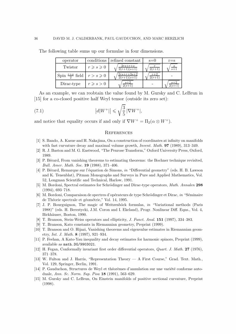
36 DAVID M. J. CALDERBANK, PAUL GAUDUCHON, AND MARC HERZLICH
The following table sums up our formulae in four dimensions.
operator conditions refined constant s=0 r=s
Twistor r > s > 0√
2rs+r+s2(r+1)(s+1)
√r
2(r+1)
√s
s+1
Spin r+s2 field r > s > 0
√2rs+r+3s+22(r+1)(s+1)
√r+2
2(r+1) -
Dirac-type r > s > 0√
s+22(s+1) -
√s+2
2(s+1)
As an example, we can reobtain the value found by M. Gursky and C. LeBrun in[15] for a co-closed positive half Weyl tensor (outside its zero set):
(7.1)∣∣d|W+|
∣∣ 6√
3
5|∇W+|,
and notice that equality occurs if and only if ∇W+ = Π2(α⊗W+).
References
[1] S. Bando, A. Kasue and H. Nakajima, On a construction of coordinates at infinity on manifolds
with fast curvature decay and maximal volume growth, Invent. Math. 97 (1989), 313–349.[2] R. J. Baston and M. G. Eastwood, “The Penrose Transform,” Oxford University Press, Oxford,
1989.
[3] P. Berard, From vanishing theorems to estimating theorems: the Bochner technique revisited,Bull. Amer. Math. Soc. 19 (1988), 371–406.
[4] P. Berard, Remarque sur l’equation de Simons, in “Differential geometry” (eds. H. B. Lawsonand K. Tenenblat), Pitman Monographs and Surveys in Pure and Applied Mathematics, Vol.
52, Longman Scientific and Technical, Harlow, 1991.
[5] M. Bordoni, Spectral estimates for Schrodinger and Dirac-type operators, Math. Annalen 298
(1994), 693–718.
[6] M. Bordoni, Comparaison de spectres d’operateurs de type Schrodinger et Dirac, in “Seminairede Theorie spectrale et geometrie,” Vol. 14, 1995.
[7] J. P. Bourguignon, The magic of Weitzenbock formulas, in “Variational methods (Paris
1988)” (eds. H. Berestycki, J.M. Coron and I. Ekeland), Progr. Nonlinear Diff. Eqns., Vol. 4,Birkhauser, Boston, 1990.
[8] T. Branson, Stein-Weiss operators and ellipticity, J. Funct. Anal. 151 (1997), 334–383.[9] T. Branson, Kato constants in Riemannian geometry, Preprint (1999).
[10] T. Branson and O. Hijazi, Vanishing theorems and eigenvalue estimates in Riemannian geom-
etry, Int. J. Math. 8 (1997), 921–934.[11] P. Feehan, A Kato-Yau inequality and decay estimates for harmonic spinors, Preprint (1999),
available as math.DG/9903021.
[12] H. Fegan, Conformally invariant first order differential operators, Quart. J. Math. 27 (1976),371–378.
[13] W. Fulton and J. Harris, “Representation Theory — A First Course,” Grad. Text. Math.,Vol. 129, Springer, Berlin, 1991.
[14] P. Gauduchon, Structures de Weyl et theoremes d’annulation sur une variete conforme auto-
duale, Ann. Sc. Norm. Sup. Pisa 18 (1991), 563–629.[15] M. Gursky and C. LeBrun, On Einstein manifolds of positive sectional curvature, Preprint
(1998).
KATO INEQUALITIES AND CONFORMAL WEIGHTS 37
[16] H. Hess, R. Schrader and D. Uhlenbrock, Kato’s inequality and the spectral distribution of
Laplacians on compact Riemannian manifolds, J. Diff. Geom. 15 (1980), 27–38.[17] O. Hijazi, A conformal lower bound for the smallest eigenvalue of the Dirac operator and
[18] N. Hitchin, Linear fields on self-dual spaces, Proc. Roy. Soc. London A 370 (1980), 173–191.[19] J. Kalina, B. Ørsted, A. Pierzchalski, P. Walczak and G. Zhang, Elliptic gradients and highest
weights, Bull. Acad. Polon. Sci. Ser. Math. 44 (1996), 511–519.[20] D. Meyer, Une inegalite de geometrie hilbertienne et ses applications a la geometrie rieman-
nienne, C. R. Acad. Sci. Paris 295 (1982), 467–469.
[21] H. Nakajima, Yau’s trick, Sugaku 41 (1989), 253–258.[22] A. M. Perelomov and V. S. Popov, Casimir operators for semi-simple Lie groups, Izv. Akad.
Nauk SSSR, Ser. Mat. Tom 32 (1968), English translation: Math. USSR Izvestija 2 (1968),
1313–1335.[23] J. Rade, Decay estimates for Yang-Mills fields: two new proofs, in “Global analysis in modern
mathematics (Orono 1991, Waltham 1992)” (ed. K. Uhlenbeck), Publish or Perish, Houston,1993.
[24] S. Salamon, “Riemannian Geometry and Holonomy Groups,” Pitman Research Notes in
Math., Vol. 201, Longman Scientific and Technical, Harlow, 1989.[25] H. Samelson, “Notes on Lie Algebras,” 2nd ed., Universitext, Springer-Verlag, New York,
1990.[26] R. Schoen, L. Simon and S. T. Yau, Curvature estimates for minimal hypersurfaces, Acta
Math. 134 (1975), 275–288.
[27] E. Stein and G. Weiss, Generalization of the Cauchy-Riemann equations and representationsof the rotation group, Amer. J. Math. 90 (1968), 163–196.
[28] K. Uhlenbeck, Removable singularities for Yang-Mills fields, Commun. Math. Phys. 83 (1982),11–30.
[29] S. T. Yau, On the Ricci curvature of a compact Kahler manifold and the complex Monge-
Ampere equation, I, Commun. Pure Appl. Math. 31 (1978), 339–411.
D.M.J.C.: Department of Mathematics and Statistics, University of Edinburgh,