Reflecting upon the impact of the gate-price system under perfect and imperfect competition -Introducing a spatial equilibrium model under consideration of a realistic, differential tariff system to the Japanese pork import market- Abstract: Key words: international pork market, spatial equilibrium model, imperfect market competition, Japanese gate-price system Introduction Albeit an increasing health awareness and the possibility to obtain a variety of meat products, due to improved trade conditions, pork remains the main meat consumed in most developed countries. In addition, pork consumption grows in transition countries where supplementary available income is primarily spent on food products. All the same, the international pork market is a rather narrow market according to participating trading regions and traded volume. Only about nine percent of the world pork production is internationally traded. Key exporters include the United States, Canada, and the European Union. Key importers constitute Japan and Russia. The latter also produce pork themselves at high production costs. This is only possible because of a remaining heavy protection rate in these countries. Although the international pork market when compared to other markets seems to be de- regulated this is not true for each single market in particular. In other words, protection remains high in countries such as Japan and Russia. In this context, the Japanese gate-price system is especially being targeted by key exporters. The gate-price system is, thus, subject to revision in the current WTO negotiation round on agricultural trade. However, the gate-price system as it has been negotiated during the Uruguay round is a specific variable tariff which has not been endogenously computed in most of the existing trade models. This study aims at introducing a partial equilibrium model of international trade as it has been first developed by SHONO and KAWAGUCHI (1999A). It has been extended by BERGEN, KAWAGUCHI and KANO (2004) to include the gate-price system, in order to apply it to the international pork market. Following a brief explanation of the Japanese gate-price system, the model will be presented and applied under perfect and imperfect market conditions.
Transcript
Reflecting upon the impact of the gate-price system under perfect and imperfect competition
-Introducing a spatial equilibrium model under consideration of a realistic, differential tariff system to the Japanese pork import market-
Abstract:
Key words: international pork market, spatial equilibrium model, imperfect market competition, Japanese gate-price system Introduction
Albeit an increasing health awareness and the possibility to obtain a variety of meat products,
due to improved trade conditions, pork remains the main meat consumed in most developed
countries. In addition, pork consumption grows in transition countries where supplementary
available income is primarily spent on food products. All the same, the international pork
market is a rather narrow market according to participating trading regions and traded
volume. Only about nine percent of the world pork production is internationally traded. Key
exporters include the United States, Canada, and the European Union. Key importers
constitute Japan and Russia. The latter also produce pork themselves at high production costs.
This is only possible because of a remaining heavy protection rate in these countries.
Although the international pork market when compared to other markets seems to be de-
regulated this is not true for each single market in particular. In other words, protection
remains high in countries such as Japan and Russia.
In this context, the Japanese gate-price system is especially being targeted by key exporters.
The gate-price system is, thus, subject to revision in the current WTO negotiation round on
agricultural trade. However, the gate-price system as it has been negotiated during the
Uruguay round is a specific variable tariff which has not been endogenously computed in
most of the existing trade models.
This study aims at introducing a partial equilibrium model of international trade as it has been
first developed by SHONO and KAWAGUCHI (1999A). It has been extended by BERGEN,
KAWAGUCHI and KANO (2004) to include the gate-price system, in order to apply it to the
international pork market. Following a brief explanation of the Japanese gate-price system,
the model will be presented and applied under perfect and imperfect market conditions.
The Japanese gate-price system for pork imports
Japan’s pork market illustrates the role of both, import and domestic measures for protecting
commodity markets, and also the rapid restructuring of agriculture following a market price
decline. Japan’s agricultural policies in the pork sector pursue to support producers’ income
while keeping market prices stable. The specific domestic protection instrument to implement
government policies in the pork sector applies a price stabilisation band.
The midpoint price of the band is set to meet the objective of maintaining a standard of living
in rural areas, while the floor and ceiling prices are set to constrain excess upward price
movements. The Livestock Industry Promotion Corporation (LIPC)1 intervenes in the market
through its purchase or storage subsidies granted to producers and selling activities to ensure
that market price always moves within the limits of the band.2
Moreover, the price band is supported at the border by requiring that all imports enter at a
minimum import price, the so-called gate-price, which used to be linked directly to the
midpoint of the stabilisation band (stabilisation price = administrative price). Before the
GATT Uruguay round agreement (URRA) a variable levy was used to implement the gate
price policy. Imports with CIF values above the gate-price were charged an ad valorem tariff
of five percent. Since then, these rules have altered due to an agreement between Japan and
the United States. Although the gate-price was maintained, it is now (officially) decoupled
from the stabilisation price band (see Figure 1).
Concluding, the Japanese pork market is now protected in two ways, which are still
interlined. While subsidies are being paid through prefectural governments according to a
complicated system, which has to be individually traced, a differential tariff system based on
the concept of the gate-price system provides the basis for these payments. Accordingly, the
gate-price is annually set, although it was subject to gradual reduction commitment until
2000. Since then it remains at 393 ¥/kg of carcass meat until the end of the next WTO round
agreement. The variable levy has been converted into a specific tax, and together with the ad
valorem tariff of currently 4.3 percent, it was also subject to reduction commitments.
1 Agriculture & Livestock Industry Corporation (ALIC) was established in October, 1996 as a quasi-government institution by the integration of the LIPC and the Japan Raw Silk & Sugar Price Stabilisation Agency. Its object is to contribute to the sound development of the agricultural and livestock industries, along with their related industries, by stabilising ad adjusting the prices of major livestock products, raw silk and sugar, and by promoting the agricultural and livestock industries. 2 Applicable Law: Law concerning the Stabilisation of Livestock Prices.
Figure 1: Differential tariff system for pork in Japan In other words, the
Japanese differential
tariff system for
pork- or more
precisely meat of
swine- constitutes of
a relatively low ad
valorem tariff of 4.3
percent and the gate-
price system which
confronts imports at the border. It imposes a minimum import price on pork shipments. For
shipments valued below the minimum price, importers have to pay the difference between the
shipment’s value and the minimum price. Hence, the system taxes the importation of lower-
valued pork cuts.
In addition, related to the gate-price system the so-called emergency import safeguard
measures are automatically invoked whenever the import volume for a particular fiscal
quarter exceeds the average for the same quarter of the past three years by more than 19
percent (see Figure 2). The safeguard then raises the gate-price from 393 ¥/kg to 489 ¥/kg for
carcass meat of swine. This has been the case for the last five years.
Figure 2: Emergency safeguard for pork in Japan
Standardimport priceis beingraised
Exceeds 119% of the imported volume of last three years
Standardimport priceis beingraised
Exceeds 119% of the imported volume of lastthree years
Standard import price is being raisedExceeds 119% of theimported volume of lastthree years
Standard import price is being raisedExceeds 119%of the importedvolume of lastthree years
Apr.-JuneJan.-MarchOct.- Dec.July-Sep.Apr.-June
1.quarter 2.quarter 3.quarter 4.quarter 1.quarter
The effect of the gate-price system, particularly in case the safeguard is triggered, is a thorn
especially in the side of the major pork exporters to Japan. Major pork exporters to Japan
include the United States, Canada, the European Union mainly represented by Denmark, and
recently also Mexico.
Table 1: Export of pork to Japan (in 10 Mio. US$, in 10’000 tons cut base)
1998 1999 2000 2001 2002
volume value volume value volume value volume value volume value
United States 16.02 7.33 16.77 8.15 18.91 10.25 24.49 14.47 24.89 15.08
Although opinions on the gate-price system may differ among exporters it has been stated
clearly by the US and Canada that an amendment shall be necessary in order to do justice to
an agricultural market liberalisation. An elimination of the gate-price system- or alternatively
of the safeguard is called for.
Hence, the objective of this research is to analyse future pork trade flows among nine major
pork importers and exporters, along the following hypotheses:
This research aims at forecasting a future prognosis for the year 2011 under the assumption of
a mid-term analysis following a possible outcome of the present WTO negotiations on
agriculture by 2006. Therefore, effects of the EU enlargement as well as the increasing
production and consumption capacity in pork producing and consuming regions such as
Brazil, China and Russia also need to be taken into account. Hence, this research includes
1. The gate-price system including the safeguard will be abolished by 2011, while import
tariff remains at 4.3 percent.
2. The gate-price system will remain, while import tariff will be reduced or abolished.
3. The gate-price system and the import tariff will be abolished by 2011.
4. The safeguard will be abolished, however gate-price and import tariff remain.
nine regions constituting Japan, the US, Canada, the EU, Mexico, Brazil, Russia, China and
the rest-of-the-world (ROW), in order to close the model. The following figure shows basic
trade flows between these regions in volume terms (metric tons unit).
Figure 3: Participating regions in international pork trade
Source: Own composition taken from various statistical yearbooks.
Theoretical Model and its application
Following the above introduction to the problem at hand, this research applies a spatial
equilibrium model under differing imperfect market competition, which is of partial,
comparative-static nature. Moreover, it emphasises the significant characteristics of the
Japanese pork market underlying the exceptional position of the gate-price, which proves to
be influential to the world pork market. Yet, despite the model’s originality, its explanatory
power remains limited due to its constraints as a partial, one-product model. Thus, results of
this model have to be linked to the circumstances as a whole, including national policies,
international circumstances, environmental issues, farm level etc.
In order to apply the model, its conceptual framework shall be briefly explained. The SHONO
and KAWAGUCHI (1998) spatial equilibrium model for international trade, introduces realistic
tariffs in that it emphasises the existence of a tariff-quota system, which was not considered in
previous models. In reality, although of homogenous quality, merchandised goods are divided
into a primary and a secondary market. At the primary market goods can be imported at a
low-level tax rate up to a fixed quantity (current access quantity). Exceeding this quantity
level, goods have to be imported at a high-level tax rate to the secondary market. In addition,
apart from the existing quantity-based specific tariff, one also finds a price-based ad valorem
tariff, which are often combined to a third compound tariff.
Figure 4: Compound tariff in two separately regarded markets
Remark: the tax rate level shown in the solid as well as the perforate line exist in various pairs of countries, and in general the relation αij < aij ,βii < bii is solely to be found. In this figure there is no special meaning to the larger or smaller size relation of α and β (or a and b).
The above figure presents a subdivision of imports to country j into a primary and secondary
market separated from each other by a fixed current access quantity. Accordingly, αij and βii
CAj
a ij
ßij
aij
bij
Import from country i to country j
Tax rate
represent the ad valorem and specific tariff of the primary market, whereas aij and bii present
the secondary market.3
At first, in order to understand and finally apply the spatial equilibrium model of international
trade among n (n ≥ 2) countries the following notations are used. If there is no specific
definition, i, j refers to any integer from 1 to n.
In correspondence to the tariff-quota system mentioned above, we consider the markets of all
countries as two different tariff markets, the primary and secondary market with a
corresponding primary and secondary tariff rate.
Table 2: Compound tariff system of country j for imports from country i Primary market Secondary market
Price-based tariff rate αij aij
Quantity-based tariff rate βij bij
Source: SHONO, KAWAGUCHI (1998)
a) CAj represents the current access quantity in the primary market of country j. With regard
to exports from country i to country j the compound tariff composition of the importing
country j is shown in Table 2. In addition, the compound tariff rates as shown in the above
Figure 4 generally result in the following relation αij ≤ aij (Price), βij ≤ bij (Quantity), with
α, β representing the primary market, and a, b the secondary market. As a formality,
domestic supply within country i is also considered to be an export to the primary market
of country i. Hence, αii = βii = 0. However, domestic supply is not considered to be part of
the general import quantity. As a formal prerequisite aii and bii for imports are adjusted to
prohibitive values at a high level by which an import to the secondary market becomes
impossible.
b) Quantity is marked for all trading countries as shown below in Table 3. For formality reasons the quantity traded from country i to country i in the secondary market is market by Xsii, but its value equals 0. Further Dj = D1j+D2j introduces total demand in country j, whereas in country i, Si defines the supply quantity, and in country j, Dj marks the demand quantity.
3 SHONO and KAWAGUCHI have further extended the model by introducing export quota and minimum export prices, and later export subsidies under perfect competition as well as under imperfectly competitive conditions. The gate-price system, however, had not yet been explicitly integrated into this model. Arguably, the gate-price was taken into consideration by various other models such as the ERS model of the USDA. The ERS model, however, used a range of tariffs instead of endogenously computing the gate-price. Tariffs substituted for the gate-price (and the current 4.3 percent ad valorem tariff) were 15 percent and 25 percent.
Table 3: Traded quantity and supply and demand quantity for all countries (n) 1 2 … n 1 2 … n Sum Importing country
Exporting country Primary market Secondary market
1 X11 X12 … X1n Xs11 Xs12 … Xs1n S1
2 X21 X22 … X2n Xs21 Xs22 … Xs2n S2
⋮ ⋮ ⋮ ⋮ ⋮ ⋮ ⋮ ⋮ ⋮ ⋮
n Xn1 Xn2 … Xnn Xsn1 Xsn2 … Xsnn Sn
Sum D11 D12 … D1n D21 D22 … D2n
c) We use PSi to refer to the production price in country i, and PDj to represent the market
price in country j, respectively. Tij reflect the transportation costs (more generally
transaction costs) per unit traded good from country i to country j. Insurance premium per
unit for export from country i to j is defined as Iij,.
The following function shows the resulting log-linear supply function in country i.
logSi = logµi + ηi log(PSi) (generally ηi > 0)
Its adverse function is given as:
logPSi = (logµi / ηi ) + (1 / ηi) logSi
In addition, in country j the log-linear demand function is as follows:
The total import quantity to the primary market of country j does not exceed the current
access quantity CAj of the relevant market. In case the total import quantity is lower than the
current access quantity, the shadow price SPj of the relevant market equals 0.
The shadow price SPj can be positive if and only if these two are equal.
X1j + X2j + X3j – Xjj ≤ CAj (j = 1,2,3)
(CAj – X1j-X2j – X3j + Xjj) SPj = 0
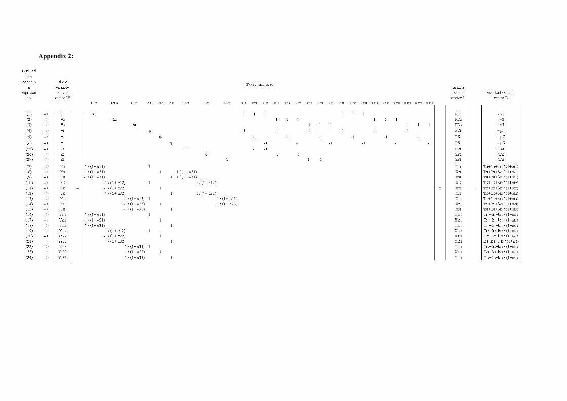
The above explanation of equilibrium conditions for perfect market competition can be
expressed in 27 steps of equations and inequalities. First, slack variables are introduced in
each of these 27 inequalities, and then the equilibrium conditions are transformed in the way
as are given in Appendix 1. Note, all variables including slack variables are assumed to be
non-negative. The equations are subject to n=3, as an example. 4 Condition of perfect competition
Complementarity problems belong to the general problem formulation of the variational inequality theory which also encompasses various mathematical problems such as non-linear equations, optimisation problems. Variational inequality theory, however, is utilised as a fundamental methodology in synthesising economic equilibrium models including spatial equilibrium models under a spectrum of behavioural mechanism (NAGURNEY 1993, pp. 1-12). In this context, it is relevant to differentiate between the ‘equilibrium’ modelling approach following a complementarity problem and an ‘optimisation’ approach where one derives necessary conditions from an optimisation model (MATHIESEN. 1985, p. 114). In a LCP there is no objective function to be optimised. The problem is: find w = (w1,…,wn), z = (z1, …zn)T satisfying: (1.1) w – Mz = q w ≥ 0, z ≥ 0 and wi zi = 0 for all i The only data in this problem is the column vector q and the square matrix M. The LCP is denoted by
finding w nℜ∈ , z nℜ∈ satisfying (1.1) by the symbol (q,M). It is said to be a LCP of order n. Summarizing, the LCP can be applied as a modelling format. An equilibrium is then computed by either solving the particular LCP via various existent pivoting algorithms or by iterative methods.
Further, because taxation regulations usually do not count for domestic supply X11, X22, X33
tariff rates α11 = α22 = α33, β11 = β22 = β33 generally become 0. Also, if at the primary market
of country j a tariff, as it is the case for the markets of Japan, only exists as ad valorem tariff,
βij becomes 0.
Further, if the requirements of the 27 mathematical expressions5 are presented in a matrix and
vector symbols, it is clear that the problem can be specified as the problem to find the value
of vectors P and W that meet the requirements of W = AP + B and WT P = 0, as suggested by
the particular LCP problem. In other words, the problem can be specified as a linear
complementarity problem.6 Therefore, if the linear complementarity problem can be solved,
the equilibrium solution can be found. The table in Appendix 2 according to KAWAGUCHI and
SHONO (1999a) stresses the formulation of these specific equilibrium conditions as a
complementarity problem for the case of perfect market competition.
Box 4: Introducing the basic idea of the linear complementarity problem (LCP) in few words
For the given problem, the so-called symmetric parametric principal pivoting method
processes this specific LCP as the solving algorithm.7 Each of the algorithmic rules are then
translated into the Visual Basic computer language and executed by machine.
For the case of imperfect market competition as it is finally applied in this research, the above
equilibrium conditions are amended according to the following Cournot-Nash theorem for
oligopolistic market behaviour:
5 In the case of n = 9 there are 189. 6 For further information on the mathematical background of the linear complementarity problem (LCP) please refer to COTTLE ET AL. (1992). 7 See COTTLE ET AL. (1992; pp. 293-296).
1) Consumers in each country act as price takers, while producing areas in each country do not form alliances
but act independently as one country-one producing area in terms of the Cournot-Nash theorem.
2) In other words, consumers’ demand in each country are set to be linear (or non-linear), while production
costs of producers in each country constitute fixed costs and a linear (or non-linear) marginal cost function.
3) The connecting transportation network between producing area and market of each country is assumed a
simplified direct route from the centre of the producing area to the market of each country, where each route’s
unit transportation cost is fixed based on ad-valorem tax.
4) In each producing country, producers know about demand functions prevailing in each market. Following
this, in case the difference between marginal costs and marginal income is greater than unit transaction costs of
the connecting exporting route, exporting countries’ producers will increase exporting quantity along these
routes. Contrary, if this difference is smaller than unit transaction costs, there will be no transport along this
route.
In each country forwarding between markets does not take place.
Box 2: The Cournot-Nash theorem for oligopolistic market behaviour, in brief
Based on the same principle as introduced above, the main difference in the case of imperfect
market competition refers to the difference between the prevailing market price PDj and the
marginal revenue. In other words, the revenue from selling export goods from country i to the
market of country j can be denoted by Rij and further expressed by using Dj = xij + xsij + Eij
Based on the model as it has been developed by our research team (Professor KAWAGUCHI
and Mr. H. KANO, Kyushu University, Japan, M. BERGEN, University of Hohenheim,
Germany) the gate-price is finally integrated as a further restriction by converting it into an
ad-valorem equivalent rate following the mathematical interrelation.
To begin with, as became clear, the gate-price system takes different taxation forms
depending on whether the CIF import price levied by the “usual” ad valorem tariff exceeds or
is less than the standard import price (gate-price).
In detail, the import CIF price from country i is denoted by PCi. The gate-price as it is applied
in country j is expressed as PDj , while the equivalent ad valorem tariff rate is set as δj. Here,
in case the price levied by the ad valorem tax rate on the CIF import price is less than the
gate-price, country j directly pays PDj - PCi and then divides this tax by PCi. In other words,
in case it is less than the gate-price it can be evaluated as ad valorem equivalent rate (EQR).
In case the EQR δj exceeds the gate-price only the usual ad valorem tariff rate is applied.
Replacing the “usual” ad valorem tariff for the country applying the gate-price system (in case
of Japan 4.3%) by an ad valorem equivalent rate levied on the gate-price all tariffs are treated
uniformly as an ad valorem tariff depending on the import CIF price. For country j applying
the gate-price system it seems realistic not to implement a tariff-quota-system with a
secondary market. Hence, seeking equilibrium the current access quantity is extremely high,
prohibitively disregarding the secondary market. In addition, for country j the general
meaning of a specific tariff does not exist. Besides, as explained above, imports at low prices
are levied by a tax exceptional specific tariff. But, in reality it is difficult to imagine imports at
such low a price so that this research does not consider that specific case.
Moreover, the above formula integrates the CIF price, which can also be written as PCi = PSi
+ Tij + Iij . Hitherto, the occurring ad valorem tariff rate αij is replaced by the term of fj (PCi).
This means, by introducing the gate-price to the basic model, the matrix M (alternatively
denoted A) and the fixed variable column vector z (alternatively denoted B) of the LCP are
now constituting a further element depending on the CIF price. The problem cannot be solved
as a LCP anymore but as a non-linear complementarity problem (NLCP). Finding a solution
to this NLCP leads to solution of the equilibrium conditions. Accordingly, one way to solve
this particular NLCP is by applying the same Symmetric Parametric Principal Pivoting
Method (Symmetric PPPM) combined with Newton's Method.8 This methodology has already
been presented in detail by two members of our research team.9
Once, the model is amended to meet the above requirements a solution can be found when
computing these equations and solving the equilibrium conditions, provided accurate data are
imputed.
8 The Newton method solves nonlinear equations by step by step approximating nonlinear curve with a tangent linear line. See COTTLE ET AL. (1992, pp.87-95). 9 See KAWAGUCHI and KANO (2004, completely). Not yet published.
Data applied and preliminary base year results
Applying the above model to the international pork market secondary statistical data sources
were referred to. However, differing categories, denomination and definitions can be found
for the product of pork. Hence, a consistent definition is set and deviating data values are
adjusted accordingly.
Referring to the World Customs Organisation Harmonised System meat of swine can be
subdivided into fresh or chilled and frozen pork (often referred to simply as pork) on the one
hand (HS 0203), and into pork variety meats on the other hand (HS 0206). In addition,
prepared meat products also include pork-based products. However, this research neglects the
class of prepared meat products.
Further, while quantities are given in cut base for traded pork national statistics often present
production volume as carcass weight equivalent (CWE) using a country specific conversion
factor. The average CWE to cut base in the case of Japan is 0.73.10
Although national statistics such as from the MAFF (農林水産者) and ALIC (農畜産業振興機構) in
case of Japan, and Dansk Slagterier in case of Denmark were reviewed also, for conformation
reason most data were taken from the FAOstat database, the EUROstat database, the USDA,
FAPRI and the OECD.
Despite the availability of most of the data required some crucial parameters are not
obtainable. This is especially the case with elasticities. Alternatively, these exogenous
parameters were estimated by parameterization. Doing so, initial estimates of elasticities are
referred to from outside sources and adjusted to arrive at an initial estimating point.
Table 5: Parameterized own price elasticities of demand and supply for pork
Country Elasticity of Demand Elasticity of Supply
Japan -0.290 +0.432 Canada -0.100 +1.290 EU15 -0.100 +0.200 United States -0.495 +0.910 Mexico -0.250 +0.550 Brazil -0.470 +0.200 China -0.410 +0.400 Russia -0.540 +0.250 ROW -0.210 +0.200
10 United States = 0.7484; EU15 = 0.74; Canada = 0.74; Mexico = 0.7614; Brazil = 0.74, Russia = 0.78437, China = 0.74, ROW = 0.74.
Assuming that the demand for pork is weakly separable from demands for other goods
including other meat products such as beef, chicken and turkey and also including marine
products this assumption allows to model meat demand conditional only on meat prices.
According to HAHN11 the assumption of separability is common in the analysis of meat
demand. In addition, the purpose and hypotheses of this research allow for an isolated
observation of the pork sector rather than the need for integrating cross-price elasticities with
other meat products.
Wholesale prices on a CWE basis are used as market prices for calculating the demand
functions. Producer prices, deflating by implicit deflators, are used as marginal costs in each
country. However, in the case of Mexico the supply function needed to be adjusted. Currency
exchange rate fluctuations and the impact of the NAFTA had to be taken into further
consideration.
In the case of Japan ministerial order (省令) prices are used as representative prices. The
ministerial ordinance is not necessarily related to the price stabilisation band but it moves
within it. It describes the mean value between the high quality and the good quality price for
pork meat. In general, an average is taken for the separately defined markets (Tokyo and
Oosaka). The ministerial ordinance is regarded as the mean domestic pork price for carcass,
and is close to the actual annual average price of pork.
For a future scenario, this research assumes that transportation costs for staple goods being
transported by vessel are slightly increasing within the near future. Backed up by rising crude
oil prices transportation costs in general are forecasted to increase by 5 percent within the next
five to ten years.12
This may also include an introduced taxation for international goods traffic justified by
environmental issues, which has not been applied so far. Since technical progress cannot be
presumed in the near future transportation costs are not likely to decrease, respectively.
In a first step, the so-called FEFC Tariff System gives some detailed information on freight
costs, which are referred to in the first place. Reverting to the Maersk Sealand-13, Evergreen
Marine Cooperation-, Orient Overseas Container Line Limited- and Hapag Lloyd shipment
rates then completes the required data. According to these sources the following transportation
costs per container of 20000 tons of pork can be expected.
11 See HAHN (1994, pp. 22). 12 Based on information from various articles on increasing transportation costs and after conferring with experts from various freight companies etc. 13 http://www.maersksealand.com/ provides rates via the internet (20.05.04).
Table 6: Transportation cost US $ per ton of pork (0203); cut base by sea freight, includes base freight only; 2002
Further, insurance costs may play a role, especially in the case of perishable goods. However,
since pork comes in frozen or chilled, insurance costs in the first place are neglected, also due
to lack of data available. Insurance premium is mainly negotiated on between importers and
insurance companies in the exporting country, which makes it rather difficult to get access to
these data. According to experts however, in general insurance premium are approximately
0.8 percent of the CIF price when landing.
Finally, the benchmark and scenarios are defined by the tariffs and other border
measurements. The following table outlines the actual situation for the year 2002, while the
second table lists up expected changes for tariffs and quotas according to countries for the
future scenario.
Table 7: Trade Policies in each country and area for the base year 2002 Unit: NC per mt carcass weight equivalent, %, ‘000mt Trade Policies Instruments
In-quota import Market Over-quota Import Market Country and Area
Specific Duty
Ad valorem Tariff
Differential Tariff
Tariff-Rate Quota Specific Duty Ad valorem Tariff
Specific Export Subsidy
Upper limit of subsidized Exports
Percentage PSE
Japan (Yen) NO 4.3 (393000-CIF)/CIF NO NO NO NO NO 57
U.S. ($) NO NO NO NO NO NO NO NO 4
EU 15 (Euro)
467-867 (536.3) NO NO 133.1 NO NO In special cases 444 21
EU 25 - - - -. - -. - -
Canada NO NO NO NO NO NO NO NO 6
Mexico NO 20 NO NO NO NO NO NO 22
Brazil NO 11.5 (12.7) NO NO NO NO NO NO n.a.
Russia NO 15 NO YES NO NO NO NO n.a.
China NO 12 (17.3) NO NO NO NO NO NO n.a.
ROW NO NO NO NO NO NO NO NO n.a.
Note: Mexico: Bound tariff lowered from 50% to 45%, 1995-2004. Applied Tariff was 20% in 2002. Tariff for imports from U.S. and Canada is zero as from January 1st, 2003.Until then, pig meat NAFTA tariff is set at 6%. Special safeguard provisions were put in place to limit import surges. Quota for fresh and frozen pork from Canada to Mexico was 8865 tonnes, In-Quota tariff 2%, Out-of-Quota tariff was 20 %. Japan: Tariff lowered from 5% to 4.3%, 1995-2000. Gate-price lowered from 612 to 524 Yen/kg for cut meat, 460 to 393 Yen/kg for carcasses, and 1038 to 898Yen/kg for processed products, 1995-2000. Special safeguard provisions were put in place to limit import surges. EU15: Duty is sum of ad valorem and specific tariffs. Ad valorem tariff ceiling on meat lowered from 3% to zero, 1995-2000. Additional specific tariffs lowered from range of 728-1358 ECU/ton in 1995 to range of 467-869 ECU/ton, 2000. Tariff rate quota of 7,000 tons for loins and bellies. Preferential tariff with EU accession countries. Brazil: China: ROW: United States: Tariffs on cuts specially prepared for retail lowered from 2.2 cents/kg to 1.4 cents/kg, 1995-2000. Aside from these cuts, tariffs are zero. Canada: zero Russia: Introduction of a quota-system in
Table 8: Trade policies in each country and area for initial scenario year 2011 Unit: NC per mt carcass weight equivalent %, ‘000mt Trade Policies Instruments
In-quota import Market Over-quota Import Market Country and Area
Specific Duty
Ad valorem Tariff
Differential Tariff
Tariff-Rate Quota Specific Duty Ad valorem Tariff
Specific Export Subsidy
Upper limit of subsidized Exports
Comment
Japan (Yen) NO 4.3 (393000-CIF)/CIF NO NO NO NO
U.S. ($) NO NO NO NO NO NO NO
EU 25 (Euro)
467-867 (536.3) NO NO 168 (76+) NO NO In special cases 560
KAWAGUCHI, T. AND SHONO, C. (1999A), Studies on spatial Equilibrium Model of International Trade under
Tariff Quota System with Specific and Ad Valorem Duties- The case of Perfectly Competitive
International Trade-, Kyushu University, Japan. (In Japanese)
KAWAGUCHI, T. AND SHONO, C. (1999B), Studies on spatial Equilibrium Model of International Trade under
Tariff Quota System with Specific and Ad Valorem Duties- The case of Perfectly Competitive and
Oligopolistic International Trade-, Kyushu University, Japan. (In Japanese)
KAWAGUCHI, T. AND SHONO, C. (2000A), Introduction of Export Quota and minimum Export Prices to Spatial
Equilibrium Model of International Trade under Tariff Quota System with Specific and Ad Valorem
Duties –The case of Perfectly and oligopolistic International Trade, Kyushu University, Japan. (In
Japanese)
KAWAGUCHI, T. AND SHONO, C. (2000B), On the Existence of a Solution to Linear Complementarity Problem in
Spatial Equilibrium Model of International Trade and its Algorithm, Kyushu University, Japan. (In
Japanese)
KAWAGUCHI, T. AND SHONO, C. AND SUZUKI, N. (2001), Introduction of Export Subsidies to Spatial Equilibrium
Model of International Trade under Tariff Quota System with Specific and Ad valorem Duties and
its Application to international Dairy Products market - The case of Perfectly Competitive
International Trade-, Kyushu University, Japan. (In Japanese)
KAWAGUCHI, TSUNEMASA (2003), On the Direction of Development of Spatial Equilibrium Model in Recent Years. In Japanese: 川口雅正2003空間均衡モデルの近年の展開方向について、九大農学芸誌(Sci. Bull. Fac. Agr., Kyushu Univ.) 第57 第2号 261-272 (2003).
MATHIESEN, LARS (1985), Computation of Economic Equilibria by a sequence of linear complementarity Problems, In: Mathematical Programming Study 23 (1985) 144-162, North-Holland.
NAGURNEY, ANNA (1993), Network Economics: A Variational Inequality Approach. Kluwer Academic Publishers, Dordrecht, Boston, London.
OBARA, K., DYCK, J., STOUT, J. (2003), Pork policies in Japan, Electronic Outlook Report from the Economic Research Service, www.ers.usda.gov .
OECD (2004), OECD Agricultural Outlook 2004-2013, OECD Publications, France.
YANG, C.W., HWANG, M.J., SOHNG, S.N. (2002), The Cournot competition in the spatial equilibrium model, In: Energy economics 24 (2002) 139-154.