Reflective Cracking Study: First-Level Report on ... · First-Level Report on Laboratory Fatigue...

October 2006

Research Report: UCPRC-RR-2006-08

RRReeefffllleeeccctttiiivvveee CCCrrraaaccckkkiiinnnggg SSStttuuudddyyy:::

FFFiiirrrsssttt---LLLeeevvveeelll RRReeepppooorrrttt ooonnn LLLaaabbbooorrraaatttooorrryyy

FFFaaatttiiiggguuueee TTTeeessstttiiinnnggg

Authors: B. Tsai, D. Jones, J. Harvey, and C. Monismith

Partnered Pavement Research Program (PPRC) Contract Strategic Plan Element 4.10:

Development of Improved Rehabilitation Designs for Reflective Cracking

PREPARED FOR:

California Department of Transportation

Division of Research and Innovation

Office of Roadway Research

PREPARED BY:

University of California

Pavement Research Center

UC Davis, UC Berkeley

ii

i

DOCUMENT RETRIEVAL PAGE Research Report: UCPRC-RR-2006-08

Title: Reflective Cracking Study: First-Level Report on Laboratory Fatigue Testing

Authors: B. Tsai, D. Jones, J. Harvey and C Monismith

Prepared for: Caltrans

FHWA No: CA091073E

Date:

October 2006

Contract No: 65A0172

Client Reference No: SPE 4.10

Status: Stage 6, Approved Version

Abstract: This report contains a summary of the laboratory fatigue tests on mixes used as overlays on the Reflective Cracking

Study Test Track at the Richmond Field Station. Evaluation of the results of the laboratory study on fatigue

response of the overlay mixes reported herein included the effects of mix temperatures, air-void content, aging,

mixing and compaction conditions, aggregate gradation, and time of loading. Five binders were assessed, namely

AR4000, asphalt rubber (Type G), and three modified binders, termed MB4, MB15, and MAC15. A full factorial

considering all the variables required a total of 1,440 tests. This was reduced to 172 tests to accommodate time and

fund constraints. Based on the fatigue test results for the mixes used in the overlay experiment, mix rankings for

initial stiffness and fatigue life are, from highest to lowest, as follows:

Initial stiffness Fatigue life

AR4000-D MB4-G

RAC-G MB15-G and MAC15-G

MAC15-G RAC-G

MB4-G and MB15-G AR4000-D

Until a range of pavement types and environments are evaluated in the 2nd

Level Analysis, only a general indication

of the relative performance of the modified binders can be deduced. It would appear that the MB4, MB15, and

MAC15 binders used in gap-graded mixes as overlays on existing cracked asphalt concrete pavements should

provide comparable lives (at least) to RAC-G mixes when used in comparable thicknesses in thin layers (less than

about 60 mm). Recommendations for the use of MB4, MB15 and MAC15 binders in thicker layers and as dense-

graded mixes await the results of the shear test results and pavement performance analyses.

Keywords:

Reflective cracking, overlay, modified binder, fatigue testing, HVS test, MB Road

Proposals for implementation:

Related documents: UCPRC-RR-2005-03, UCPRC-RR-2006-09

Signatures:

B. Tsai

1st Author

C Monismith

Technical Review

D. Spinner

Editor

J. Harvey

Principal Investigator

M Samadian

Caltrans Contract Manager

ii

DISCLAIMER

The contents of this report reflect the views of the authors who are responsible for the facts and accuracy

of the data presented herein. The contents do not necessarily reflect the official views or policies of the

State of California or the Federal Highway Administration. This report does not constitute a standard,

specification, or regulation.

PROJECT OBJECTIVES

The objective of this project is to develop improved rehabilitation designs for reflective cracking for

California.

This objective will be met after completion of four tasks identified by the Caltrans/Industry Rubber

Asphalt Concrete Task Group (RACTG):

1. Develop improved mechanistic models of reflective cracking in California,

2. Calibrate and verify these models using laboratory and HVS testing,

3. Evaluate the most effective strategies for reflective cracking, and

4. Provide recommendations for reflective cracking strategies

This document is one of a series addressing Tasks 2 and 3.

ACKNOWLEDGEMENTS

The University of California Pavement Research Center acknowledges the assistance of the Rubber

Pavements Association, Valero Energy Corporation, and Paramount Petroleum which contributed funds

and asphalt binders for the construction of the Heavy Vehicle Simulator test track discussed in this study.

iii

REFLECTIVE CRACKING STUDY REPORTS

The reports prepared during the reflective cracking study document data from construction, Heavy

Vehicle Simulator (HVS) tests, laboratory tests, and subsequent analyses. These include a series of first-

and second-level analysis reports and two summary reports. On completion of the study this suite of

documents will include:

1. Reflective Cracking Study: Summary of Construction Activities, Phase 1 HVS testing and Overlay

Construction (UCPRC-RR-2005-03).

2. Reflective Cracking Study: First-level Report on the HVS Rutting Experiment (UCPRC-RR-

2007-06).

3. Reflective Cracking Study: First-level Report on HVS Testing on Section 590RF — 90 mm

MB4-G Overlay (UCPRC-RR-2006-04).




RAC-G Overlay (UCPRC-RR-2006-06).


AR4000-D Overlay (UCPRC-RR-2006-07).




MAC15-G Overlay (UCPRC-RR-2007-04).

9. Reflective Cracking Study: HVS Test Section Forensic Report (UCPRC-RR-2007-05).

10. Reflective Cracking Study: First-level Report on Laboratory Fatigue Testing (UCPRC-RR-

2006-08).

11. Reflective Cracking Study: First-level Report on Laboratory Shear Testing (UCPRC-RR-2006-11).

12. Reflective Cracking Study: Backcalculation of FWD Data from HVS Test Sections (UCPRC-RR-

2007-08).

13. Reflective Cracking Study: Second-level Analysis Report (UCPRC-RR-2007-09).

14. Reflective Cracking Study: Summary Report (UCPRC-SR-2007-01). Detailed summary report.

15. Reflective Cracking Study: Summary Report (UCPRC-SR-2007-03). Four-page summary report.

iv

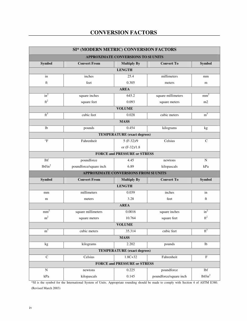
CONVERSION FACTORS

SI* (MODERN METRIC) CONVERSION FACTORS

APPROXIMATE CONVERSIONS TO SI UNITS

Symbol Convert From Multiply By Convert To Symbol

LENGTH

in inches 25.4 millimeters mm

ft feet 0.305 meters m

AREA

in2 square inches 645.2 square millimeters mm2

ft2 square feet 0.093 square meters m2

VOLUME

ft3 cubic feet 0.028 cubic meters m3

MASS

lb pounds 0.454 kilograms kg

TEMPERATURE (exact degrees)

°F Fahrenheit 5 (F-32)/9 Celsius C

or (F-32)/1.8

FORCE and PRESSURE or STRESS

lbf poundforce 4.45 newtons N

lbf/in2 poundforce/square inch 6.89 kilopascals kPa

APPROXIMATE CONVERSIONS FROM SI UNITS

Symbol Convert From Multiply By Convert To Symbol

LENGTH

mm millimeters 0.039 inches in

m meters 3.28 feet ft

AREA

mm2 square millimeters 0.0016 square inches in2

m2 square meters 10.764 square feet ft2

VOLUME

m3 cubic meters 35.314 cubic feet ft3

MASS

kg kilograms 2.202 pounds lb

TEMPERATURE (exact degrees)

C Celsius 1.8C+32 Fahrenheit F

FORCE and PRESSURE or STRESS

N newtons 0.225 poundforce lbf

kPa kilopascals 0.145 poundforce/square inch lbf/in2

*SI is the symbol for the International System of Units. Appropriate rounding should be made to comply with Section 4 of ASTM E380.

(Revised March 2003)

v

GLOSSARY OF TERMS

av Percent air-void content

BBR Bending Beam Rheometer

binder Binder types including AR4000, ARB, MB4, MB15, and MAC15

comp Compaction including FMFC, FMLC, and LMLC

cond Conditioning, either aging or non-aging

DSR Dynamic Shear Rheometer

E* Dynamic mix elastic complex modulus in MPa

G* Dynamic binder shear complex modulus in kPa

grad Gradation

FMFC Field-mixed field-compacted

FMLC Field-mixed laboratory-compacted

LMLC Laboratory-mixed laboratory-compacted

lnaT Natural logarithm of temperature shift factor

lnα1 and β1 Intercept and slope of Stage I of a three-stage fatigue/shear Weibull curve

lnα2 and β2 Intercept and slope of Stage II of a three-stage fatigue/shear Weibull curve

lnα3 and β3 Intercept and slope of Stage III of a three-stage fatigue/shear Weibull curve

lnG Initial resilient shear modulus (MPa) in natural logarithm

lnkcy5 Permanent shear strain after 5,000 loading cycles

lnn1 Separation point between Stage I and Stage II of a three-stage fatigue/shear Weibull

curve

lnn2 Separation point between Stage II and Stage III of a three-stage fatigue/shear Weibull

curve

lnNf Traditional fatigue life (repetitions at 50 percent loss of initial stiffness) in natural

logarithm

lnpct5 Cycles to 5 percent permanent shear strain (in natural logarithm)

lnstif Initial stiffness (MPa) in natural logarithm

lnstn Strain level in natural logarithm

lnsts Stress level (kPa) in natural logarithm

nf Fatigue life

pa Phase angle

PAV Pressure Aging Vessel

PSS Permanent shear strain

RSS Residual sum of squares

RTFO Rolling Thin Film Oven

SR Stiffness ratio

srn1 Stage I stiffness ratio in a three-stage fatigue Weibull curve

srn2 Stage II stiffness ratio in a three-stage fatigue Weibull curve

temp Temperature in °C

γ1 Parameter that determines the degree of slope change from Stage I to Stage II of a three-

stage fatigue/shear Weibull curve

γ2 Parameter that determines the degree of slope change from Stage II to Stage III of a

three-stage fatigue/shear Weibull curve

vi

vii

EXECUTIVE SUMMARY

This report contains a summary of the laboratory fatigue tests on mixes used as overlays on the Reflective

Cracking Study Test Road at the Richmond Field Station. The laboratory mix fatigue study is one phase

of the overall program to evaluate reflective cracking performance of conventional asphalt and modified

binder mixes used as overlays for the rehabilitation of cracked asphalt concrete pavements in California.

The study is a part of the Partnered Pavement Research Center (PPRC) Strategic Plan Element (SPE) 4.10

entitled, “Development of Improved Rehabilitation Designs for Reflective Cracking.” The SPE includes:

• Development of an improved analytical methodology for analysis and design of structural

overlays;

• Laboratory studies to define the fatigue and permanent deformation characteristics of the overlay

mixes; and

• Heavy Vehicle Simulator (HVS) accelerated pavement tests on a full-scale pavement structure

containing overlays including both a conventional asphalt mix and mixes containing binders

modified with crumb rubber and polymers.

The overlays and the underlying pavement structure for the full scale tests were designed and constructed

according to standard Caltrans specifications and procedures. HVS testing was divided into two phases:

• Phase 1: the specially constructed test pavement was trafficked on six different sections to induce

fatigue cracking in the asphalt concrete layer; and

• Phase 2: the overlay mixes containing the conventional and modified binders were placed to

evaluate both their reflective cracking response on the cracked existing pavement sections and

their rutting response on the uncracked adjacent portions of the underlying asphalt concrete.

Evaluation of the results of the laboratory study on fatigue response of the overlay mixes reported herein

included the effects of the following variables:

• Mix temperatures

• Air-void content,

• Aging,

• Mixing and compaction conditions,

• Aggregate gradation, and

• Time of loading (load frequency)

viii

Five binders were included in this study: AR4000, asphalt rubber (Type G), and three modified binders,

termed MB4, MB15, and MAC15. The modified binders were used in all gap-graded mixes, the AR4000

was used in a dense-graded asphalt concrete (DGAC) mix, and the asphalt rubber Type G binder (ARB)

was used in a gap-graded rubber asphalt concrete (RAC-G) mix. The modified binders were terminal-

blended, rubber modified binders whereas the Type G asphalt rubber binder was blended on site prior to

mixing with aggregate to produce the RAC-G mix. The mixes containing the five binders comprised the

overlay sections for the accelerated loading tests using the HVS.

A comprehensive experimental design was prepared for the study. To test the full factorial considering

all the variables, a total of 1,440 tests would have been required. Because of time and fund constraints, a

partial factorial experiment was completed with 172 tests.

Laboratory fatigue testing was carried out on beams cut from slabs prepared using rolling wheel

compaction. Materials were sampled from:

• Loose mix collected from the paver during construction and stored in sealed containers until

ready for compaction and testing, referred to as field-mixed, laboratory-compacted (FMLC)

samples in the report, and

• Binder and aggregate stockpiles at the asphalt plant, referred to as laboratory-mixed, laboratory-

compacted (LMLC) samples in the report. These samples were included in the study to assess the

potential for using the modified binders in dense-graded as well as in gap-graded mixes.

The binder contents for the AR4000-D and RAC-G mixes were based on Caltrans mix design

requirements (Section 39 of the Standard Specifications for the DGAC and Section 39-10 of the Standard

Special Provisions for the RAC-G). Binder contents for the gap-graded mixes with the MB4, MB15 and

MAC15 binders were recommended by the binder suppliers.

Flexural fatigue testing and stiffness (frequency sweep) determinations followed the AASHTO T321

procedure (four point bending). Fatigue tests were all conducted at 10 Hz. Stiffness measurements were

conducted over the range of 15 Hz to 0.01 Hz and at temperatures of 10°C (50°F), 20°C (68°F), and 30°C

(86°F) to define the effect of time-of-loading and temperature on this mix characteristic. These mix

stiffnesses are essential for the performance evaluation to be presented in the 2nd

Level Analysis report.

For the LMLC dense-graded mixes containing the modified binders, the standard California procedure for

mix design (Section 39 of the Standard Specifications) was followed to define the binder contents used

for the beam specimens.

ix

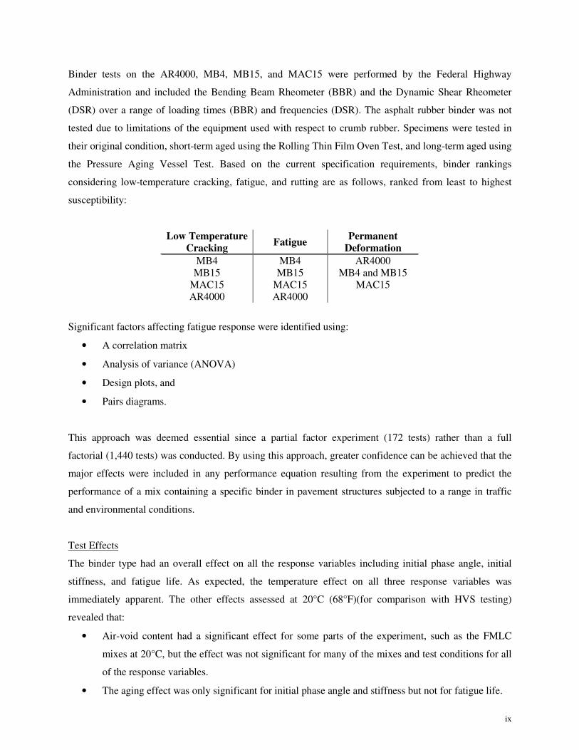
Binder tests on the AR4000, MB4, MB15, and MAC15 were performed by the Federal Highway

Administration and included the Bending Beam Rheometer (BBR) and the Dynamic Shear Rheometer

(DSR) over a range of loading times (BBR) and frequencies (DSR). The asphalt rubber binder was not

tested due to limitations of the equipment used with respect to crumb rubber. Specimens were tested in

their original condition, short-term aged using the Rolling Thin Film Oven Test, and long-term aged using

the Pressure Aging Vessel Test. Based on the current specification requirements, binder rankings

considering low-temperature cracking, fatigue, and rutting are as follows, ranked from least to highest

susceptibility:

Low Temperature

Cracking Fatigue

Permanent

Deformation

MB4 MB4 AR4000

MB15 MB15 MB4 and MB15

MAC15 MAC15 MAC15

AR4000 AR4000

Significant factors affecting fatigue response were identified using:

• A correlation matrix

• Analysis of variance (ANOVA)

• Design plots, and

• Pairs diagrams.

This approach was deemed essential since a partial factor experiment (172 tests) rather than a full

factorial (1,440 tests) was conducted. By using this approach, greater confidence can be achieved that the

major effects were included in any performance equation resulting from the experiment to predict the

performance of a mix containing a specific binder in pavement structures subjected to a range in traffic

and environmental conditions.

Test Effects

The binder type had an overall effect on all the response variables including initial phase angle, initial

stiffness, and fatigue life. As expected, the temperature effect on all three response variables was

immediately apparent. The other effects assessed at 20°C (68°F)(for comparison with HVS testing)

revealed that:

• Air-void content had a significant effect for some parts of the experiment, such as the FMLC

mixes at 20°C, but the effect was not significant for many of the mixes and test conditions for all

of the response variables.

• The aging effect was only significant for initial phase angle and stiffness but not for fatigue life.

x

• All the response variables were significantly affected by the change from a gap-gradation to a

dense-gradation for the MAC15-G, MB15-G, and MB4-G mixes.

Ranking of Initial Stiffness and Fatigue Performance

The ranking of predicted initial stiffness and fatigue life under various specimen preparation and testing

conditions, and specifically for the controlled strain mode of loading used in this experiment, was

normally in the order listed below. For initial stiffness, no apparent differences existed between the

MB15-G and MB4-G mixes, while for fatigue life, no apparent differences existed between the

MAC15-G and MB15-G mixes. As expected, the two orders are reversed.

Initial Stiffness Fatigue Life

1. AR4000-D

2. RAC-G

3. MAC15-G

4. MB4-G and MB15-G

1. MB4-G

2. MB15-G and MAC15-G

3. RAC-G

4. AR4000-D

While the fatigue tests on the dense-graded mixes containing the three modified binders were limited, the

initial stiffnesses of these three dense-graded mixes were generally greater than those of the

corresponding gap-graded mixes but less than those of the AR4000-D and RAC-G mixes. Beam fatigue

lives at a given tensile strain of the dense-graded mixes were generally less than those of the

corresponding gap-graded mixes, but greater than those of the AR4000-D and RAC-G mixes. Any

improvement in rutting resistance from increased stiffnesses of the dense-graded mixes with MB4, MB15,

and MAC15 binders over those of the corresponding gap-graded mixes will be discussed in the report on

laboratory shear testing.

Fatigue test results indicated that initial stiffness and fatigue life were moderately negative-correlated (ρ =

-0.604), confirming a general observation that lower stiffnesses equate to higher fatigue life at a given

tensile strain under controlled-strain testing when ranking fatigue life performance against initial stiffness

or vice versa. However, when using this observation, consideration must also be given to rutting, as mixes

with low stiffness are generally susceptible to this distress.

Preliminary analysis of stiffness versus strain repetition curves using three-stage Weibull analysis

indicated differences in crack initiation and propagation. The AR4000-D mix had different behavior from

that of the RAC-G mix, while the RAC-G mix performed differently than the MB4-G, MB15-G, and

MAC15-G mixes. The results indicate that damage may slow during the propagation phase of the latter

four mixes, while it accelerates for the AR4000-D mix.

xi

Dense-Graded versus Gap-Graded Mixes (laboratory-mix, laboratory compact)

The optimum binder contents used in the mix designs for the MAC15, MB15, and MB4 dense-graded

mixes (6.0, 6.0, and 6.3 percent respectively) were lower than the optimum binder contents used in the

mix designs of the gap-graded mixes (7.4, 7.1, and 7.2 percent respectively).

Limited fatigue testing of modified binders in dense-graded mixes led to the following observations:

• The initial stiffness of the dense-graded mixes was generally greater than those of the

corresponding gap-graded mixes but less than those of the AR4000-D and RAC-G mixes. The

beam fatigue life at a given tensile strain of the dense-graded mixes was generally less than those

of the corresponding gap-graded mixes, but greater than those of the AR4000-D and RAC-G

mixes.

• The mix ranking of initial stiffness, from most to least stiff, for laboratory mixed, laboratory

compacted specimens at 6 percent air-voids was:

1. AR4000-D

2. MAC15-D

3. RAC-G

4. MB15-D

5. MB4-D

6. MAC15-G

7. MB15-G

8. MB4-G

• The mix ranking for the same conditions for beam fatigue life at 400 microstrain showed exactly

the reverse trend from the above except that MAC15-D and RAC-G changed places:

1. MAC15-G

2. MB4-G

3. MB15-G

4. MB4-D

5. MB15-D

6. MAC15-D

7. RAC-G

Complex Modulus Master Curves of Mixes (laboratory-mix, laboratory compact)

Complex modulus master curves from flexural frequency sweep tests showed mix stiffnesses for a wide

range of temperature and time of loading conditions. These curves allow a stiffness modulus for a

particular mix to be selected for times of loading other than the 10 Hz value associated with the fatigue

test data, allowing the effect of vehicle speed to be incorporated in pavement performance analyses. The

mix ranking of the complex modulus master curves under various combinations of material properties and

testing conditions was generally in the order listed below, and is comparable to the overall general

ranking of beam fatigue performance in the controlled-strain testing. The MB4-G and MB15-G mixes

showed no significant difference in master curves.

xii

Master curve stiffness Beam fatigue life

1. AR4000-D

2. RAC-G

3. MAC15-G

4. MB15-G

5. MB4-G

1. MB4-G

2. MB15-G

3. MAC15-G

4. RAC-G

5. AR4000-D

• The ranking of complex modulus master curves for dense-graded mixes considering the effect of

gradation was in the order below, with no significant difference between the MB4-D and MB15-

D mixes:

1. MAC15-D

2. MB4-D

3. MB15-D

In conclusion, it must be emphasized that until a range of pavement types and environments are evaluated

in the 2nd

Level Analysis, only a general indication of the relative performance of the modified binders

can be deduced. It would appear that the MB4, MB15, and MAC15 binders used in gap-graded mixes as

overlays on existing cracked asphalt concrete pavements should provide comparable lives (at least) to

RAC-G mixes when used in comparable thicknesses in thin layers (less than about 60 mm).

Recommendations for the use of MB4, MB15 and MAC15 binders in thicker layers and as dense-graded

mixes await the results of the shear test results and pavement performance analyses.

xiii

TABLE OF CONTENTS

GLOSSARY OF TERMS........................................................................................................................... v

EXECUTIVE SUMMARY ......................................................................................................................vii

LIST OF TABLES ...................................................................................................................................xvi

LIST OF FIGURES ................................................................................................................................xvii

1. INTRODUCTION ......................................................................................................................... 1

1.1. Objectives............................................................................................................................ 1

1.2. Overall Project Organization............................................................................................... 1

1.3. Structure and Content of this Report................................................................................... 4

1.4. Measurement Units ............................................................................................................. 4

2. EXPERIMENT DESIGN.............................................................................................................. 5

2.1. Introduction ......................................................................................................................... 5

2.2. Test Protocols...................................................................................................................... 5

2.2.1 Flexural Controlled-Deformation Fatigue Test (AASHTO T321) ......................... 5

2.2.2 Flexural Controlled-Deformation Frequency Sweep (Modified AASHTO T321). 6

2.3. Experiment Design.............................................................................................................. 6

2.3.1 Temperature Effect (FMLC)................................................................................. 10

2.3.2 Air-Void Content Effect (FMLC)......................................................................... 10

2.3.3 Aging Effect (FMLC) ........................................................................................... 10

2.3.4 Mixing and Compaction Effect (FMLC and LMLC) ........................................... 10

2.3.5 Gradation Effect (LMLC) ..................................................................................... 10

2.4. Specimen Preparation........................................................................................................ 11

2.4.1 Laboratory-Mixed, Laboratory-Compacted Specimens........................................ 11

2.4.2 Field-Mixed, Laboratory Compacted Specimens ................................................. 14

2.5. Ignition Oven Tests ........................................................................................................... 14

2.5.1 Test Method .......................................................................................................... 14

2.5.2 Results................................................................................................................... 14

3. BINDER TESTING..................................................................................................................... 17

3.1. Introduction ....................................................................................................................... 17

3.2. Bending Beam Rheometer ................................................................................................ 17

3.2.1 Test Method .......................................................................................................... 17

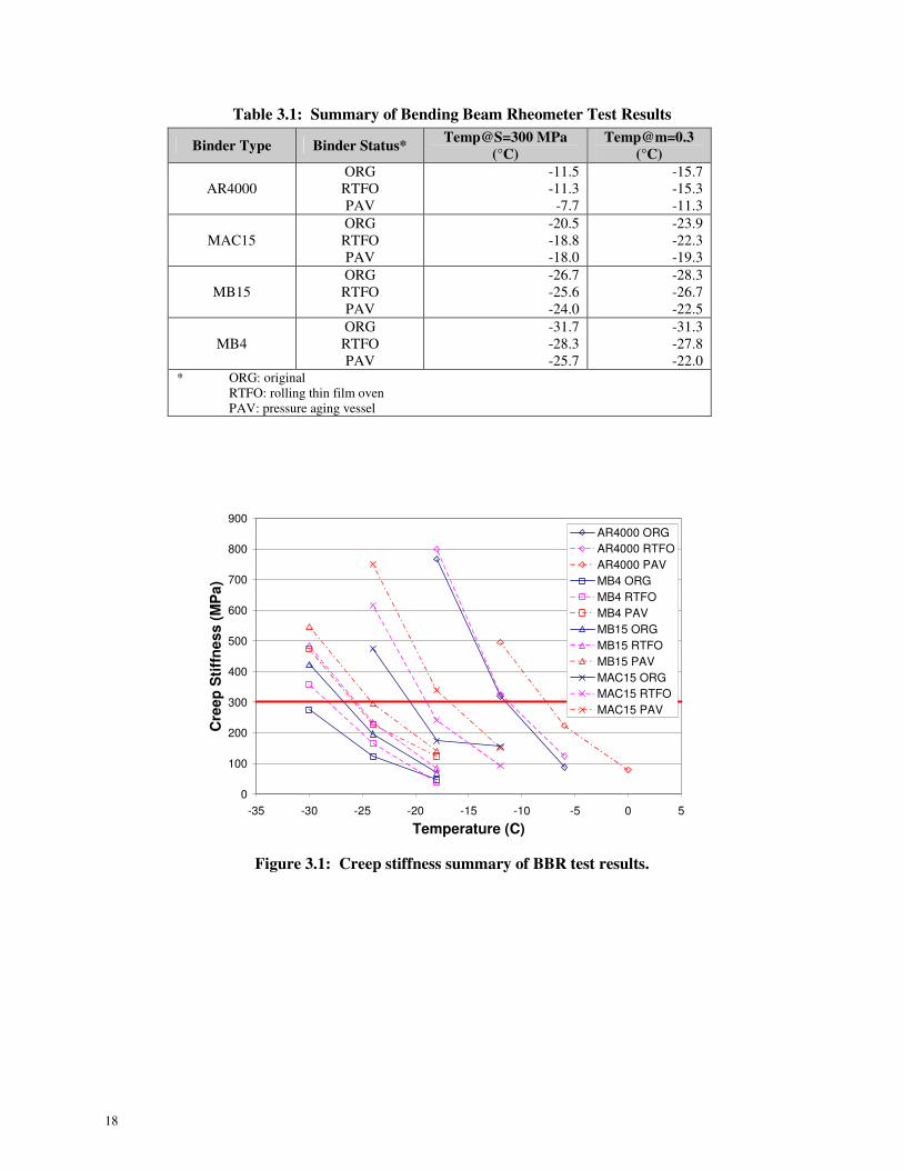
3.2.2 Results................................................................................................................... 17

3.3. Dynamic Shear Rheometer................................................................................................ 19

3.3.1 Test Method .......................................................................................................... 19

xiv

3.3.2 Results................................................................................................................... 19

3.3.3 Master Curve of Shear Complex Modulus ........................................................... 22

4. FATIGUE TESTING .................................................................................................................. 27

4.1. Introduction ....................................................................................................................... 27

4.1.1 Definitions Used in Statistical Analyses............................................................... 27

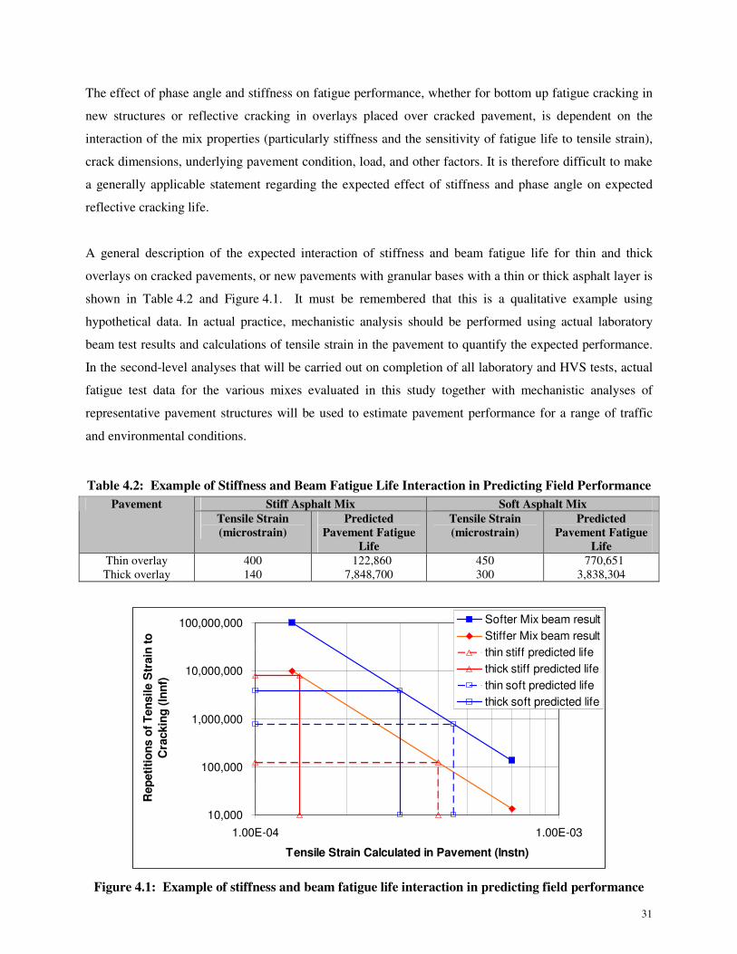
4.1.2 Expected Effects of Response Variables on Performance .................................... 29

4.1.3 Presentation of Results.......................................................................................... 32

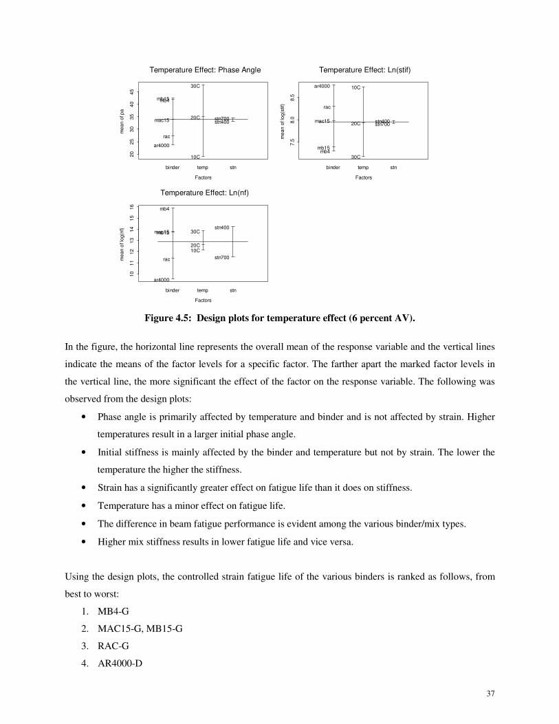
4.2. Temperature Effect............................................................................................................ 33

4.2.1 Results................................................................................................................... 33

4.2.2 Identification of Significant Factors ..................................................................... 35

4.2.3 Regression Analysis.............................................................................................. 39

4.3. Air-Void Content Effect.................................................................................................... 41

4.4. Aging Effect ...................................................................................................................... 44

4.5. Mixing and Compaction Effect ......................................................................................... 47

4.6. Gradation Effect ................................................................................................................ 51

4.7. Grouped Fatigue Tests ...................................................................................................... 54

4.8. Summary of Factor Identification ..................................................................................... 56

4.9. Summary of Regression Analysis ..................................................................................... 57

4.9.1 Initial Stiffness ...................................................................................................... 57

4.9.2 Fatigue Life........................................................................................................... 60

4.10. Transition from Crack Initiation to Crack Propagation..................................................... 60

4.11. Correlation of Phase Angle versus Stiffness versus Fatigue Life ..................................... 64

4.12. Second-Level Analysis...................................................................................................... 65

5. FLEXURAL FREQUENCY SWEEP TESTING ..................................................................... 67

5.1. Introduction ....................................................................................................................... 67

5.2. Results and Analysis ......................................................................................................... 68

5.2.1 E* Master Curves and Temperature Shift Relationships ...................................... 68

5.2.2 Mix Ranking ......................................................................................................... 68

5.2.3 Comparison between LMLC-DG and LMLC-GG................................................ 73

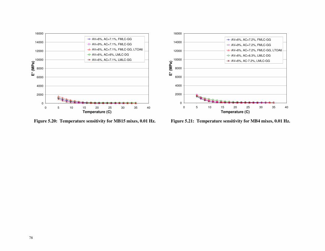
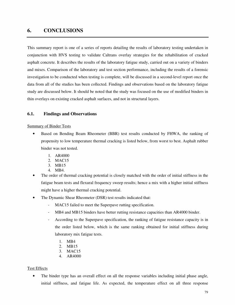
5.2.4 Temperature Sensitivity ........................................................................................ 74

6. CONCLUSIONS.......................................................................................................................... 79

6.1. Findings and Observations ................................................................................................ 79

6.2. Recommendations ............................................................................................................. 82

7. REFERENCES ............................................................................................................................ 83

APPENDIX A: SUMMARY OF RESULTS.......................................................................................... 85

xv

APPENDIX B: PROCEDURE FOR REGRESSION ANALYSIS...................................................... 95

B.1 Model Selection................................................................................................................. 95

B.1.1 Phase I: Model Identification ............................................................................... 95

B.1.2 Phase II: Model Building ..................................................................................... 96

B.2 Example of Regression Analysis: Temperature Effect ..................................................... 96

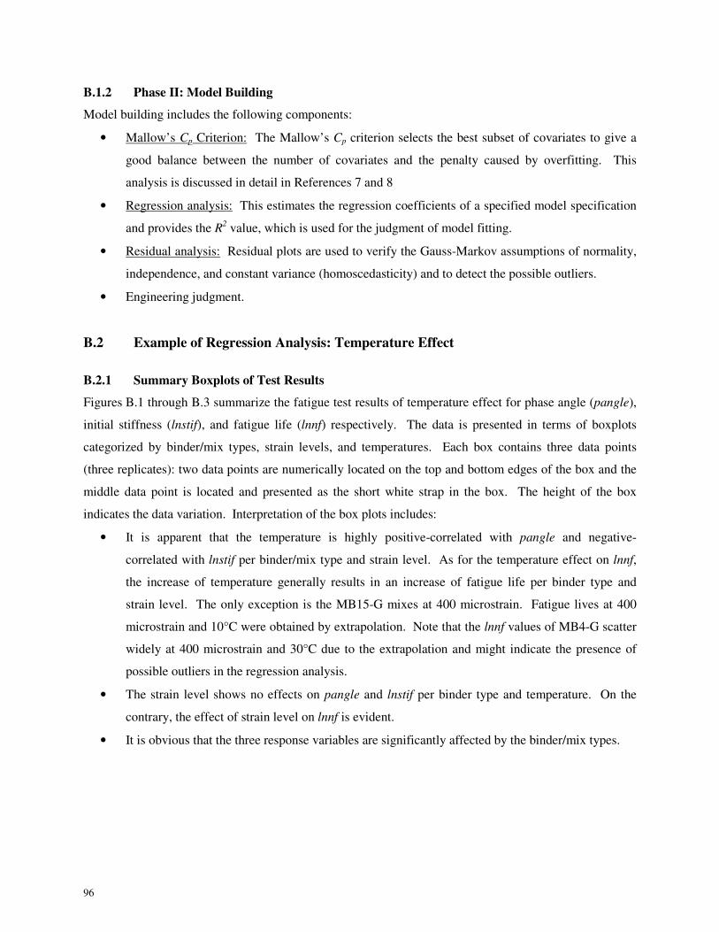
B.2.1 Summary Boxplots of Test Results ...................................................................... 96

B.2.2 Identification of Significant Factors..................................................................... 97

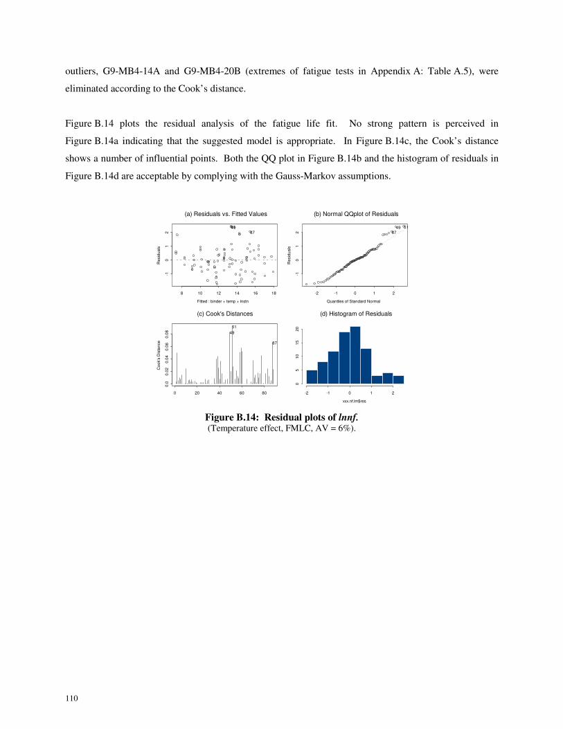
B.2.3 Regression Analysis ........................................................................................... 105

xvi

LIST OF TABLES

Table 2.1: Overall Laboratory Testing Test Plan including Fatigue and Frequency Sweep........................ 7

Table 2.2: Experimental Design for Laboratory Fatigue Testing ................................................................ 8

Table 2.3: Summary of Gradation Curves ................................................................................................. 11

Table 2.4: Design Binder Contents of Laboratory Mixes .......................................................................... 11

Table 2.5: LMLC Binder Mixing Temperatures........................................................................................ 13

Table 2.6: Compaction Temperatures for LMLC and FMLC.................................................................... 13

Table 2.7: Summary of Binder Ignition Tests............................................................................................ 15

Table 2.8: Summary of Binder Ignition Tests (pooled standard deviation)............................................... 15

Table 3.1: Summary of Bending Beam Rheometer Test Results............................................................... 18

Table 3.2: Summary of SSV and SSD Values from DSR Test Results ..................................................... 22

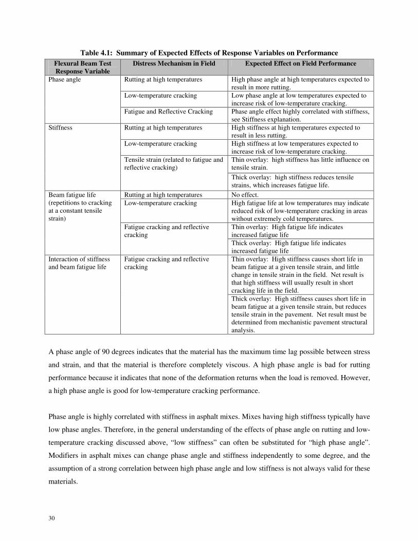
Table 4.1: Summary of Expected Effects of Response Variables on Performance ................................... 30

Table 4.2: Example of Stiffness and Beam Fatigue Life Interaction in Predicting Field Performance..... 31

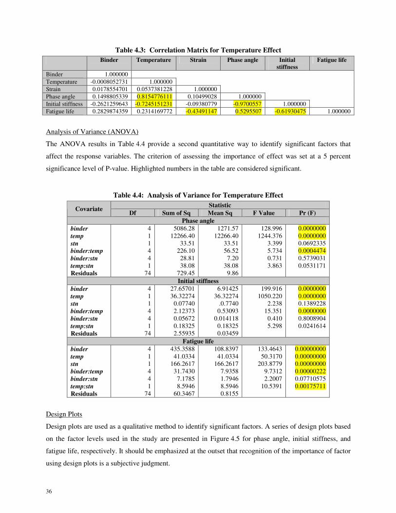
Table 4.3: Correlation Matrix for Temperature Effect............................................................................... 36

Table 4.4: Analysis of Variance for Temperature Effect ........................................................................... 36

Table 4.5: Contrast Tables of Category Covariates Used in Regression Analyses.................................... 40

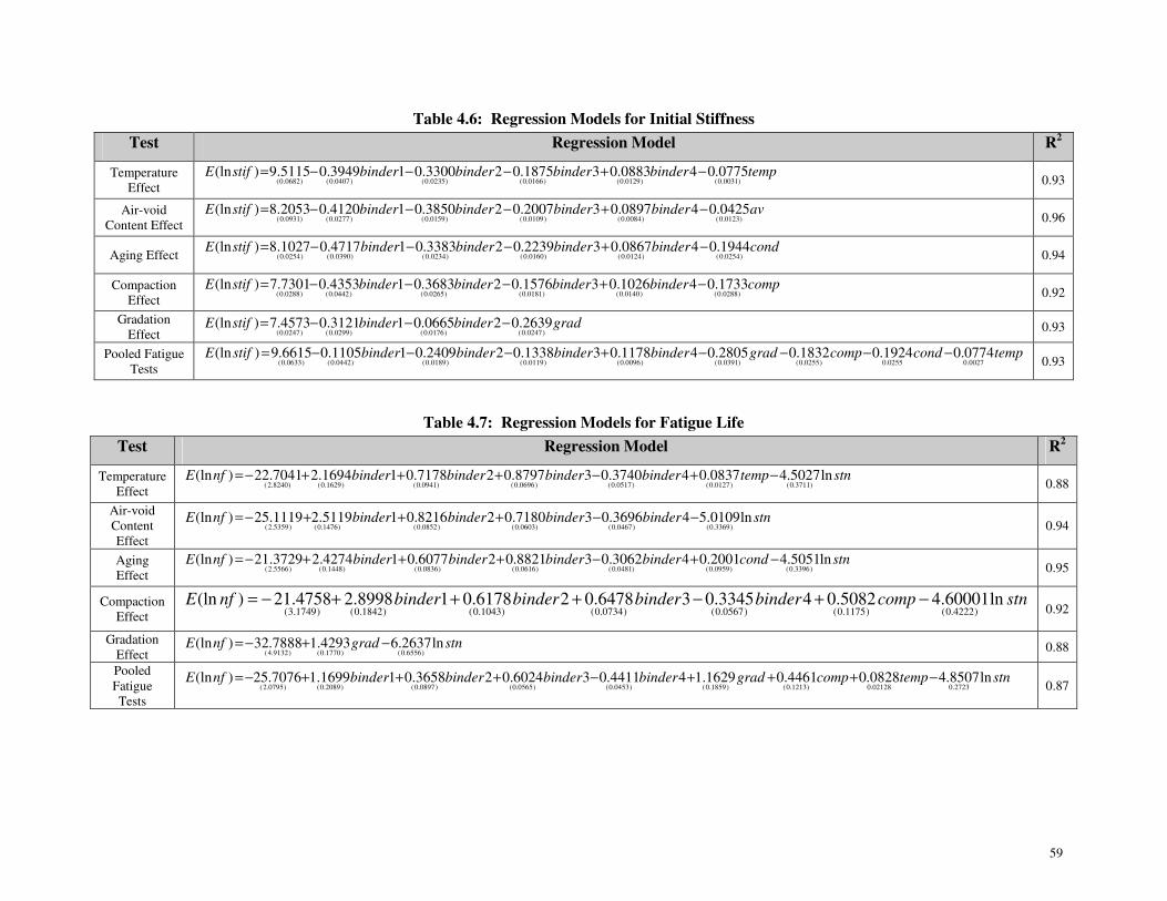
Table 4.6: Regression Models for Initial Stiffness..................................................................................... 59

Table 4.7: Regression Models for Fatigue Life ......................................................................................... 59

Table 5.1: Summary of Categories for Comparing the E* Master Curves ................................................ 67

Table 5.2: Summary of Temperature Sensitivity of E* at 10 Hz............................................................... 75

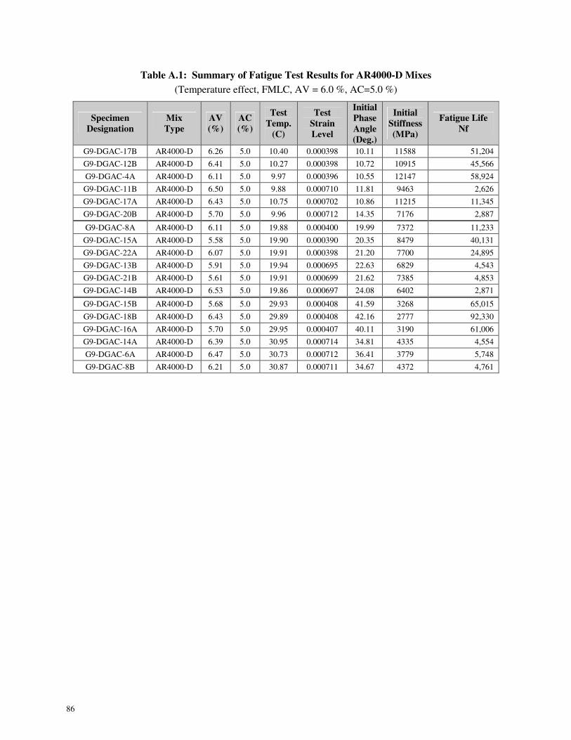
Table A.1: Summary of Fatigue Test Results for AR4000-D Mixes......................................................... 86

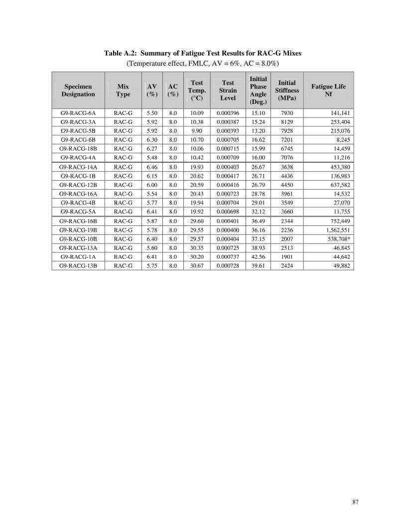
Table A.2: Summary of Fatigue Test Results for RAC-G Mixes .............................................................. 87

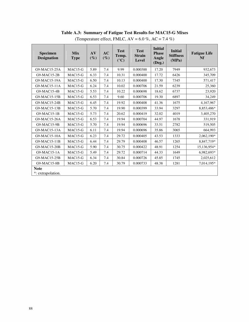
Table A.3: Summary of Fatigue Test Results for MAC15-G Mixes ......................................................... 88

Table A.4: Summary of Fatigue Test Results for MB15-G Mixes ............................................................ 89

Table A.5: Summary of Fatigue Test Results for MB4-G Mixes .............................................................. 90

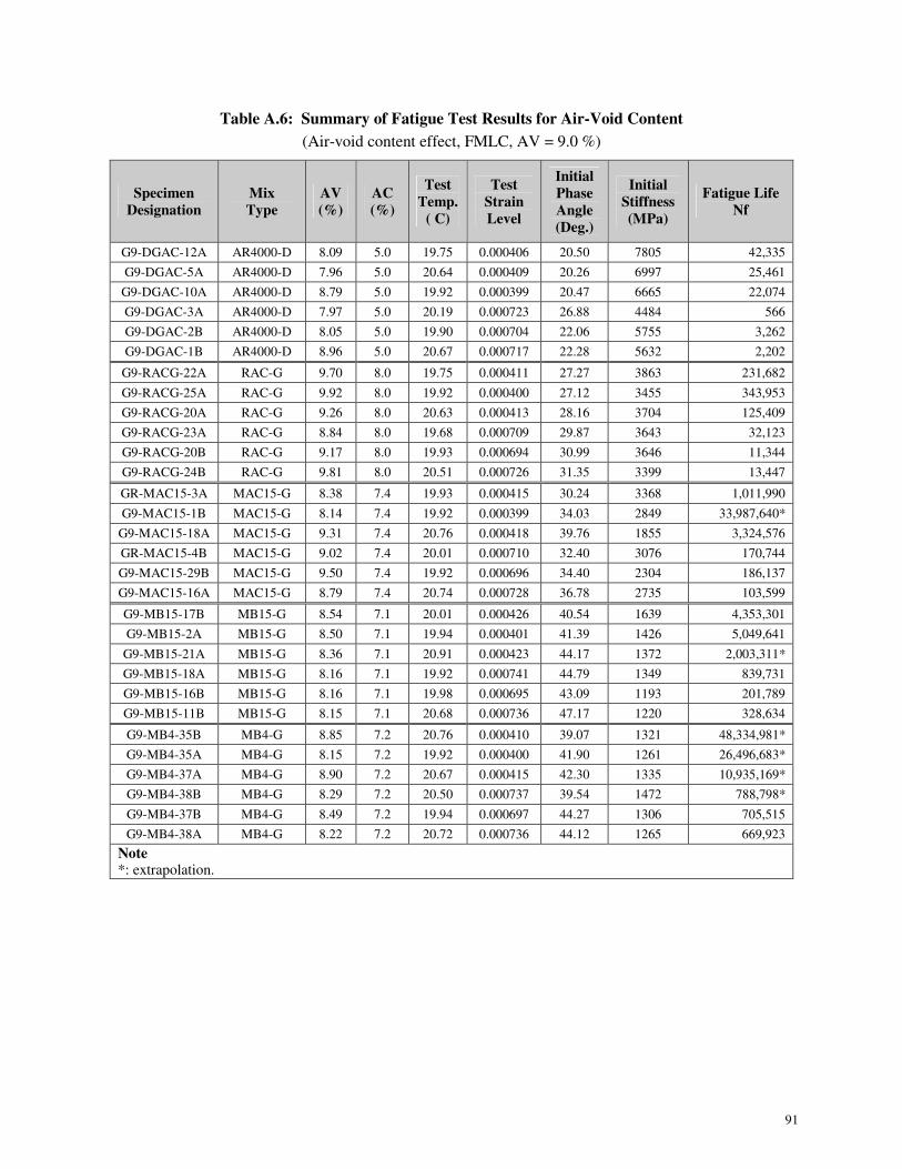
Table A.6: Summary of Fatigue Test Results for Air-Void Content ......................................................... 91

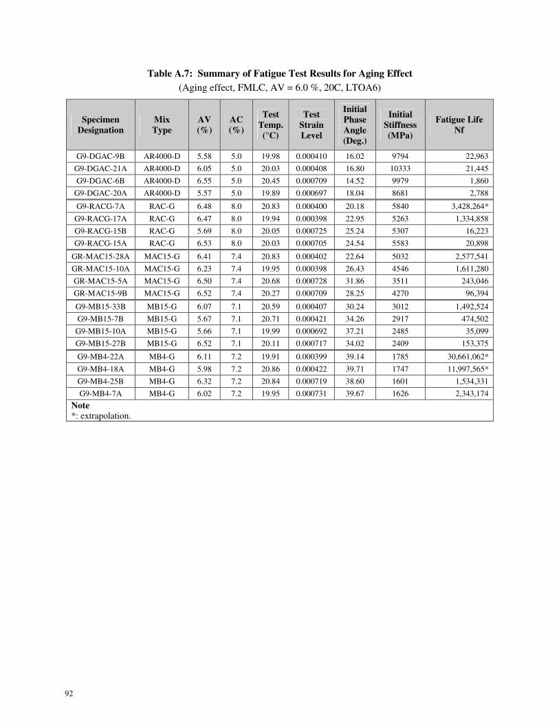
Table A.7: Summary of Fatigue Test Results for Aging Effect................................................................. 92

Table A.8: Summary of Fatigue Test Results for Compaction Effect ....................................................... 93

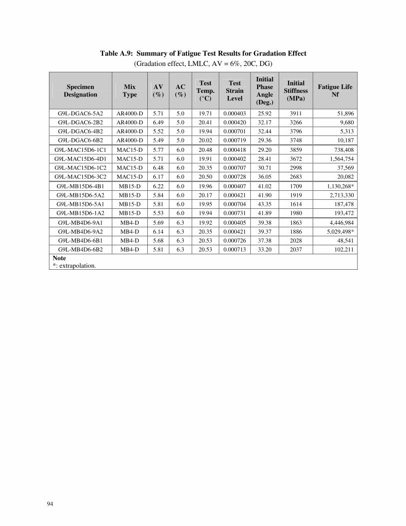
Table A.9: Summary of Fatigue Test Results for Gradation Effect........................................................... 94

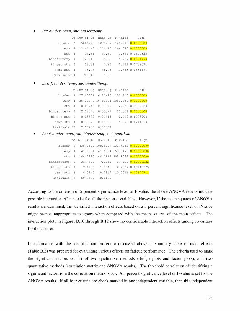
Table B.1: Correlation Matrix and ANOVA Results................................................................................. 99

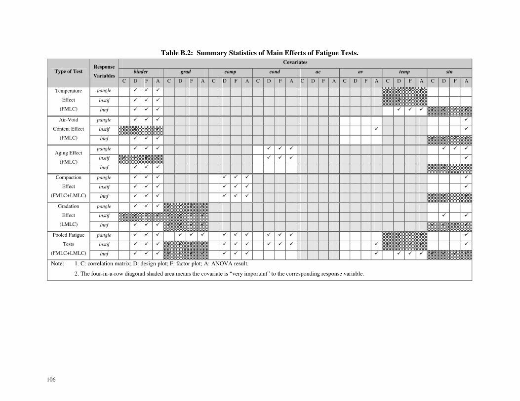
Table B.2: Summary Statistics of Main Effects of Fatigue Tests. ........................................................... 106

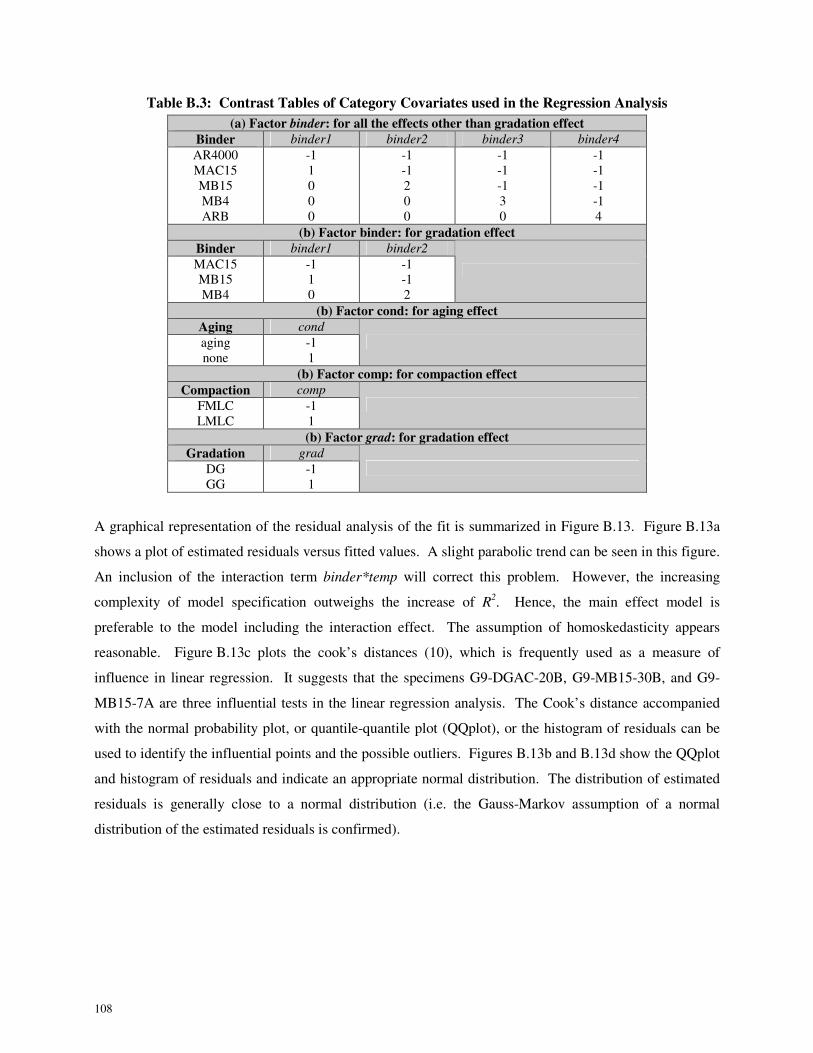
Table B.3: Contrast Tables of Category Covariates used in the Regression Analysis............................. 108

xvii

LIST OF FIGURES

Figure 1.1: Timeline for the Reflective Cracking Study.............................................................................. 3

Figure 2.1: Gradation curves for gap-graded mixes................................................................................... 12

Figure 2.2: Gradation curves for dense-graded mixes. .............................................................................. 12

Figure 3.1: Creep stiffness summary of BBR test results. ......................................................................... 18

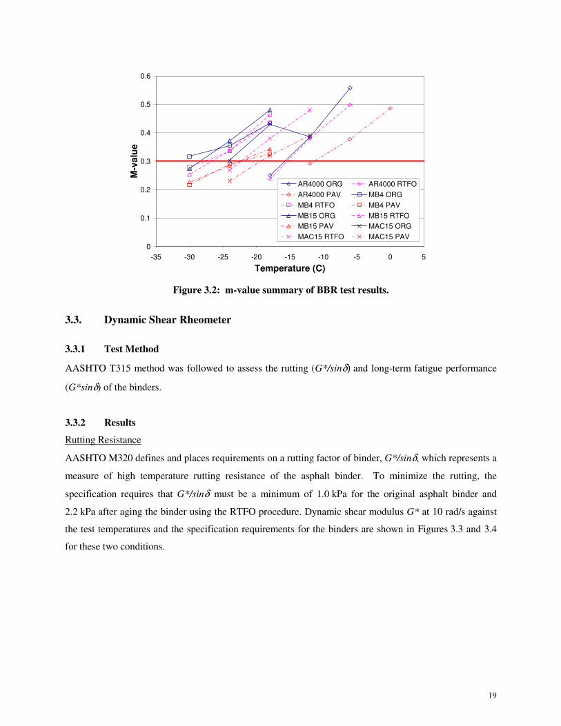
Figure 3.2: m-value summary of BBR test results..................................................................................... 19

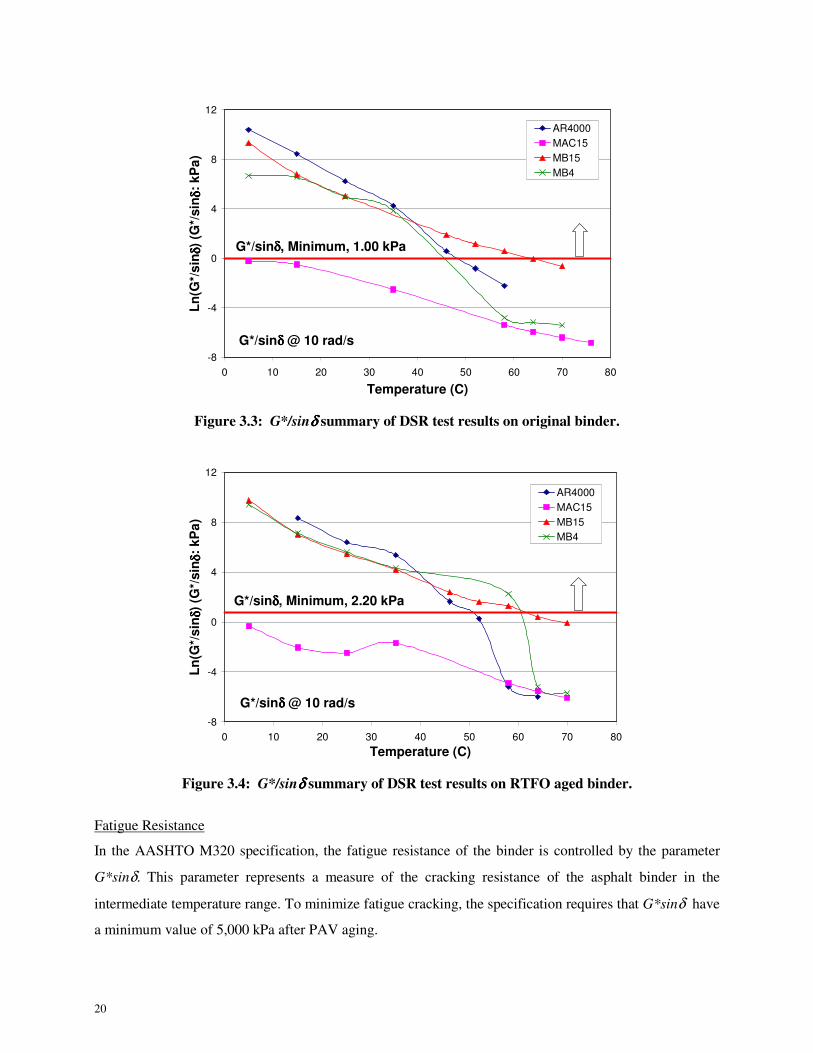
Figure 3.3: G*/sinδ summary of DSR test results on original binder. ....................................................... 20

Figure 3.4: G*/sinδ summary of DSR test results on RTFO aged binder.................................................. 20

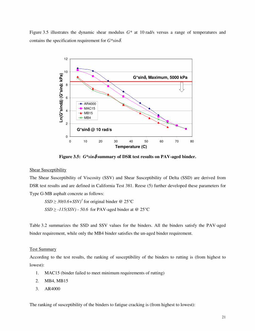
Figure 3.5: G*sinδ summary of DSR test results on PAV-aged binder..................................................... 21

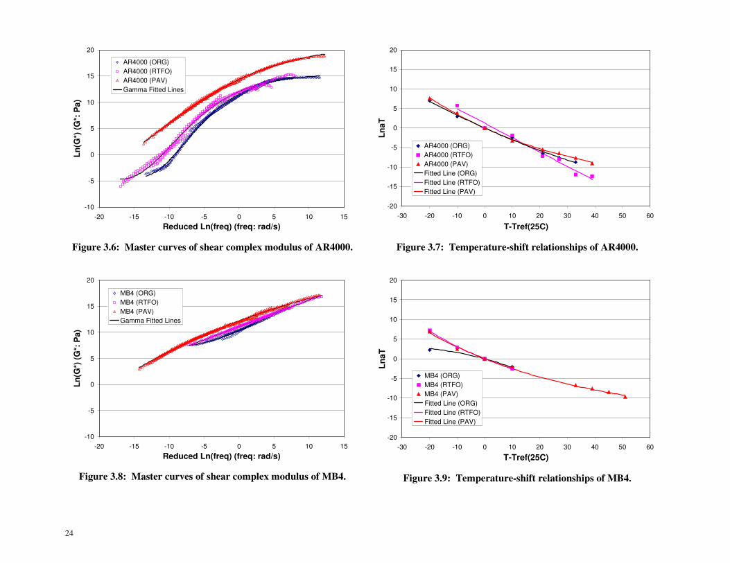
Figure 3.6: Master curves of shear complex modulus of AR4000. ........................................................... 24

Figure 3.7: Temperature-shift relationships of AR4000. ........................................................................... 24

Figure 3.8: Master curves of shear complex modulus of MB4.................................................................. 24

Figure 3.9: Temperature-shift relationships of MB4. ................................................................................ 24

Figure 3.10: Master curves of shear complex modulus of MB15.............................................................. 25

Figure 3.11: Temperature-shift relationships of MB15. ............................................................................ 25

Figure 3.12: Master curves of shear complex modulus of MAC15........................................................... 25

Figure 3.13: Temperature-shift relationships of MAC15. ......................................................................... 25

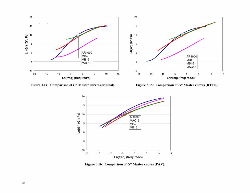
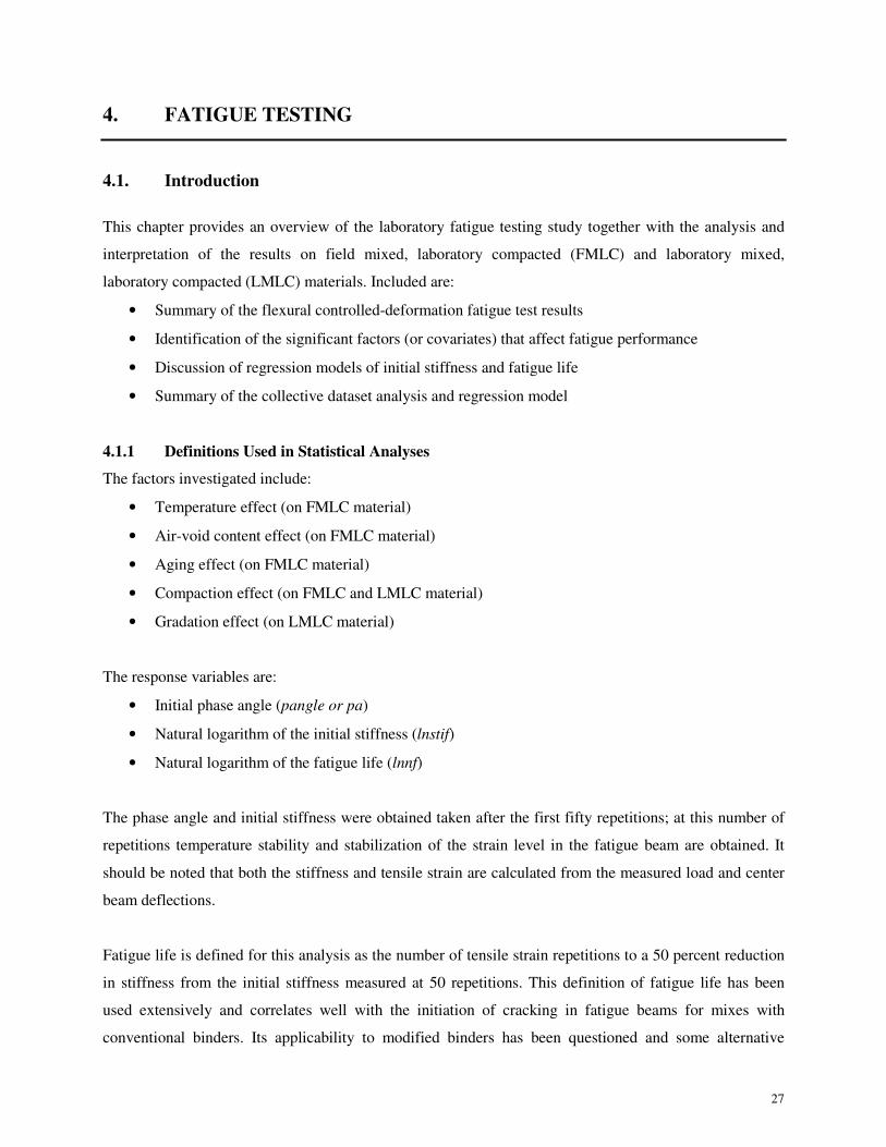
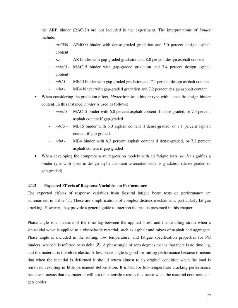
Figure 3.14: Comparison of G* Master curves (original).......................................................................... 26

Figure 3.15: Comparison of G* Master curves (RTFO). ........................................................................... 26

Figure 3.16: Comparison of G* Master curves (PAV). ............................................................................. 26

Figure 4.1: Example of stiffness and beam fatigue life interaction in predicting field performance......... 31

Figure 4.2: Summary plots of temperature effect and phase angle (6 percent AV)................................... 33

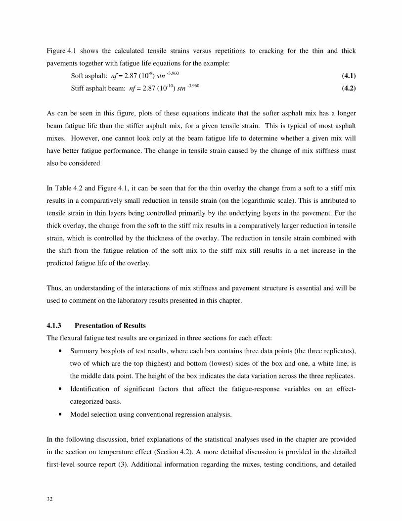
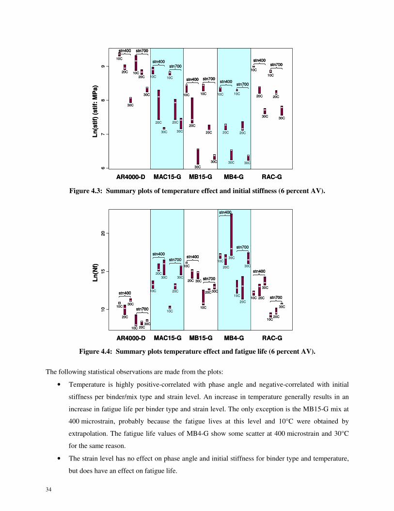
Figure 4.3: Summary plots of temperature effect and initial stiffness (6 percent AV).............................. 34

Figure 4.4: Summary plots temperature effect and fatigue life (6 percent AV). ....................................... 34

Figure 4.5: Design plots for temperature effect (6 percent AV). ............................................................... 37

Figure 4.6: Summary boxplots of air-void content effect and phase angle (AV=9 percent). .................... 42

Figure 4.7: Summary boxplots of air-void content effect and initial stiffness (AV=9 percent). ............... 42

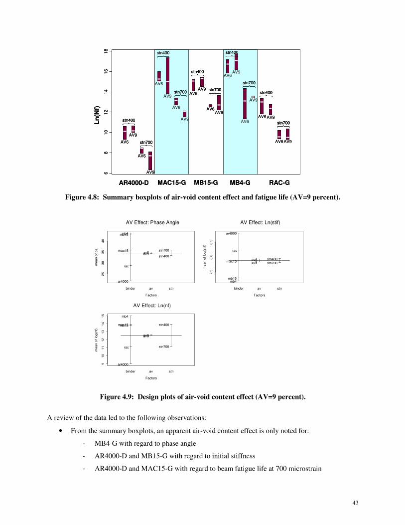
Figure 4.8: Summary boxplots of air-void content effect and fatigue life (AV=9 percent)....................... 43

Figure 4.9: Design plots of air-void content effect (AV=9 percent).......................................................... 43

Figure 4.10: Summary boxplots of aging effect and phase angle (6 days aging, 6 percent AV, 20°C)..... 45

Figure 4.11: Summary boxplots aging effect and initial stiffness (6 days aging, 6 percent AV, 20°C). ... 45

Figure 4.12: Summary boxplots of aging effect and fatigue life (6 days aging, 6 percent AV, 20°C)...... 46

Figure 4.13: Design plots for aging effect (6 day aging, 6 percent AV, 20°C). ........................................ 46

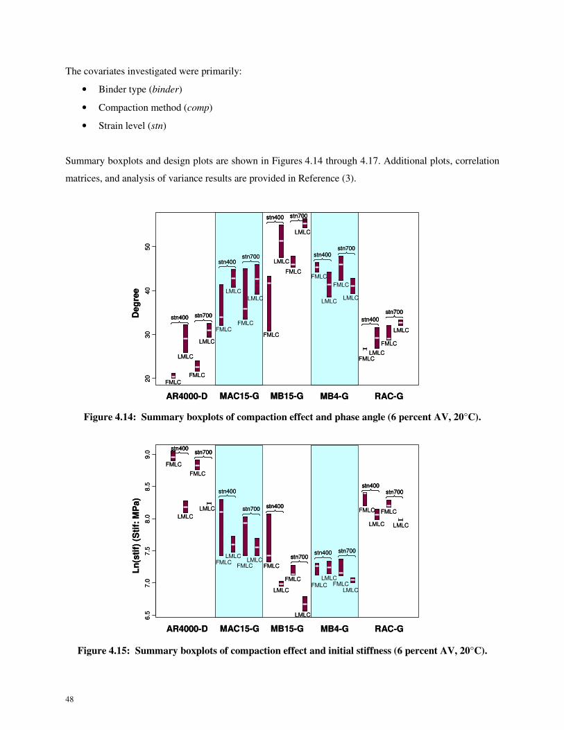
Figure 4.14: Summary boxplots of compaction effect and phase angle (6 percent AV, 20°C). ................ 48

xviii

Figure 4.15: Summary boxplots of compaction effect and initial stiffness (6 percent AV, 20°C). ........... 48

Figure 4.16: Summary boxplots of compaction effect and fatigue life (6 percent AV, 20°C). ................. 49

Figure 4.17: Design plots for compaction effect (6 percent AV, 20°C). ................................................... 49

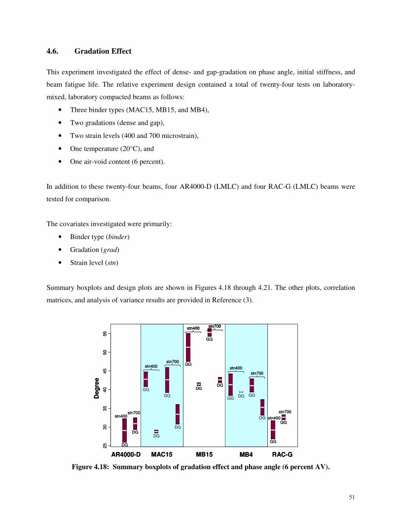
Figure 4.18: Summary boxplots of gradation effect and phase angle (6 percent AV)............................... 51

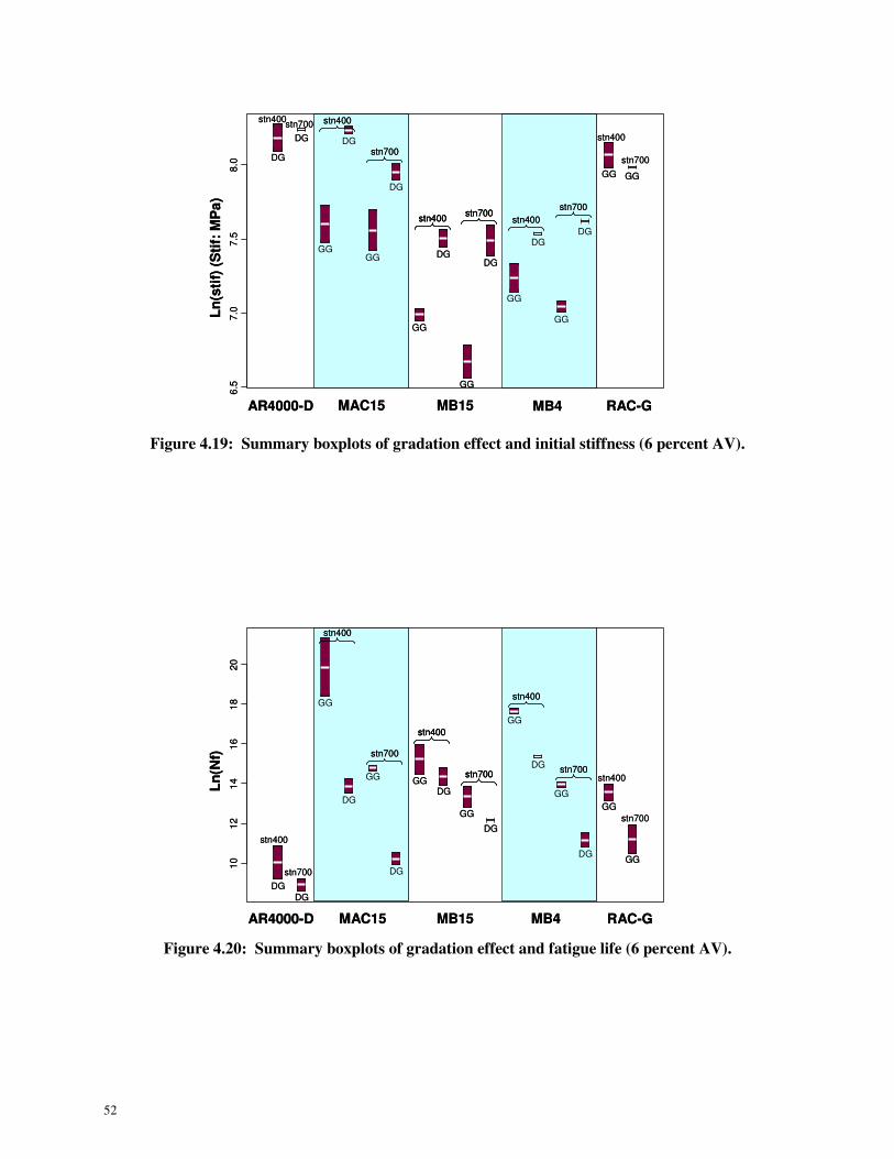
Figure 4.19: Summary boxplots of gradation effect and initial stiffness (6 percent AV).......................... 52

Figure 4.20: Summary boxplots of gradation effect and fatigue life (6 percent AV). ............................... 52

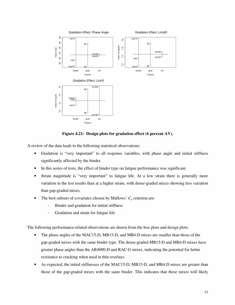
Figure 4.21: Design plots for gradation effect (6 percent AV). ................................................................. 53

Figure 4.22: Example design plots for pooled fatigue tests. ...................................................................... 55

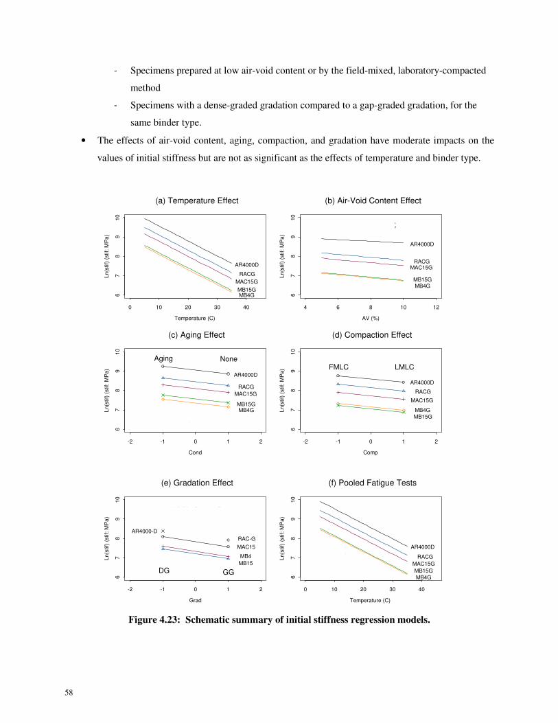
Figure 4.23: Schematic summary of initial stiffness regression models.................................................... 58

Figure 4.24: Schematic summary of fatigue life regression models .......................................................... 61

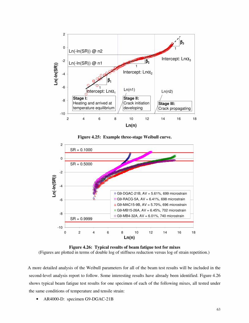
Figure 4.25: Example three-stage Weibull curve....................................................................................... 63

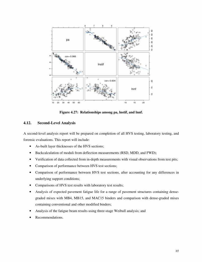
Figure 4.26: Typical results of beam fatigue test for mixes....................................................................... 63

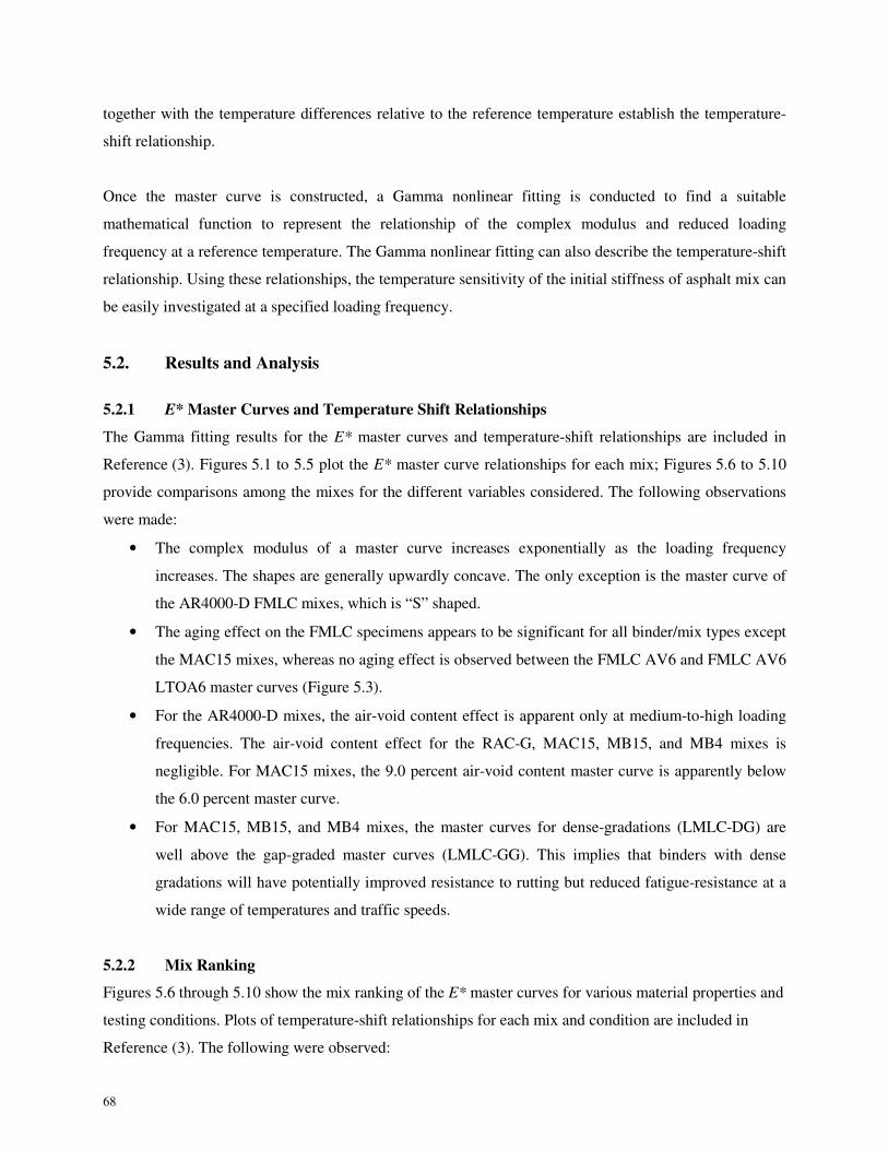
Figure 4.27: Relationships among pa, lnstif, and lnnf. .............................................................................. 65

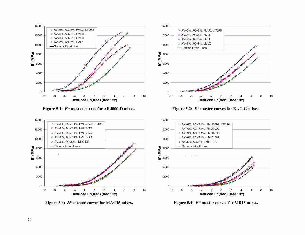
Figure 5.1: E* master curves for AR4000-D mixes................................................................................... 70

Figure 5.2: E* master curves for RAC-G mixes. ....................................................................................... 70

Figure 5.3: E* master curves for MAC15 mixes. ...................................................................................... 70

Figure 5.4: E* master curves for MB15 mixes. ......................................................................................... 70

Figure 5.5: E* master curves for MB4 mixes. ........................................................................................... 71

Figure 5.6: E* master curves - FMLC, 6% AV. ........................................................................................ 71

Figure 5.7: E* master curves - FMLC, 9% AV. ........................................................................................ 71

Figure 5.8: E* master curves - FMLC, 6% AV, LTOA6........................................................................... 71

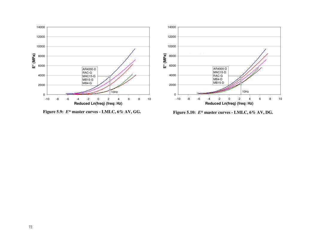
Figure 5.9: E* master curves - LMLC, 6% AV, GG. ................................................................................ 72

Figure 5.10: E* master curves - LMLC, 6% AV, DG. .............................................................................. 72

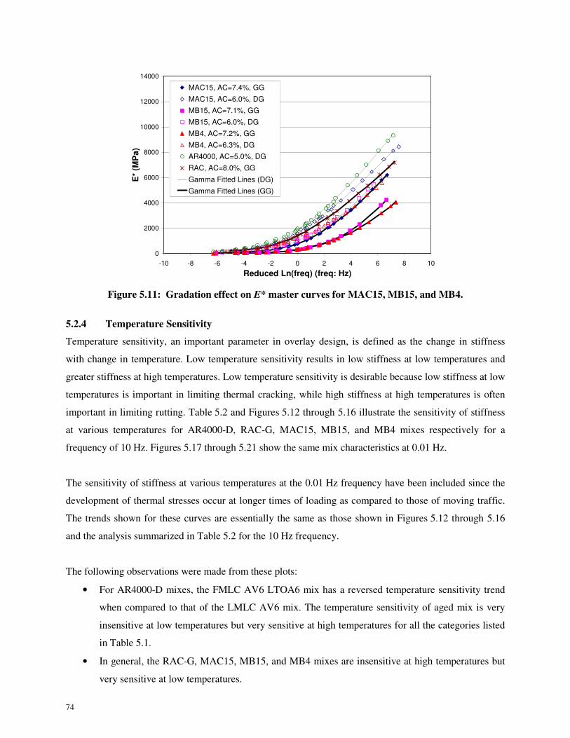
Figure 5.11: Gradation effect on E* master curves for MAC15, MB15, and MB4................................... 74

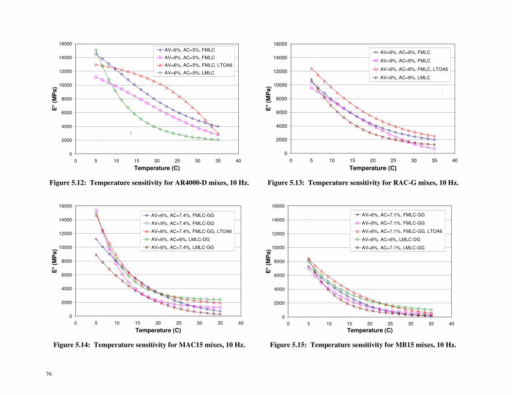
Figure 5.12: Temperature sensitivity for AR4000-D mixes, 10 Hz........................................................... 76

Figure 5.13: Temperature sensitivity for RAC-G mixes, 10 Hz. ............................................................... 76

Figure 5.14: Temperature sensitivity for MAC15 mixes, 10 Hz. .............................................................. 76

Figure 5.15: Temperature sensitivity for MB15 mixes, 10 Hz. ................................................................. 76

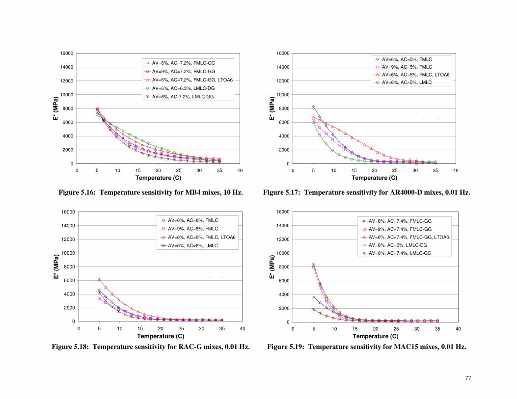
Figure 5.16: Temperature sensitivity for MB4 mixes, 10 Hz. ................................................................... 77

Figure 5.17: Temperature sensitivity for AR4000-D mixes, 0.01 Hz........................................................ 77

Figure 5.18: Temperature sensitivity for RAC-G mixes, 0.01 Hz. ............................................................ 77

Figure 5.19: Temperature sensitivity for MAC15 mixes, 0.01 Hz. ........................................................... 77

Figure 5.20: Temperature sensitivity for MB15 mixes, 0.01 Hz. .............................................................. 78

Figure 5.21: Temperature sensitivity for MB4 mixes, 0.01 Hz. ................................................................ 78

Figure B.1: Summary boxplots of phase angle. ......................................................................................... 97

xix

Figure B.2: Summary boxplots of ln(stif). ................................................................................................. 97

Figure B.3: Summary boxplots of ln(Nf). .................................................................................................. 97

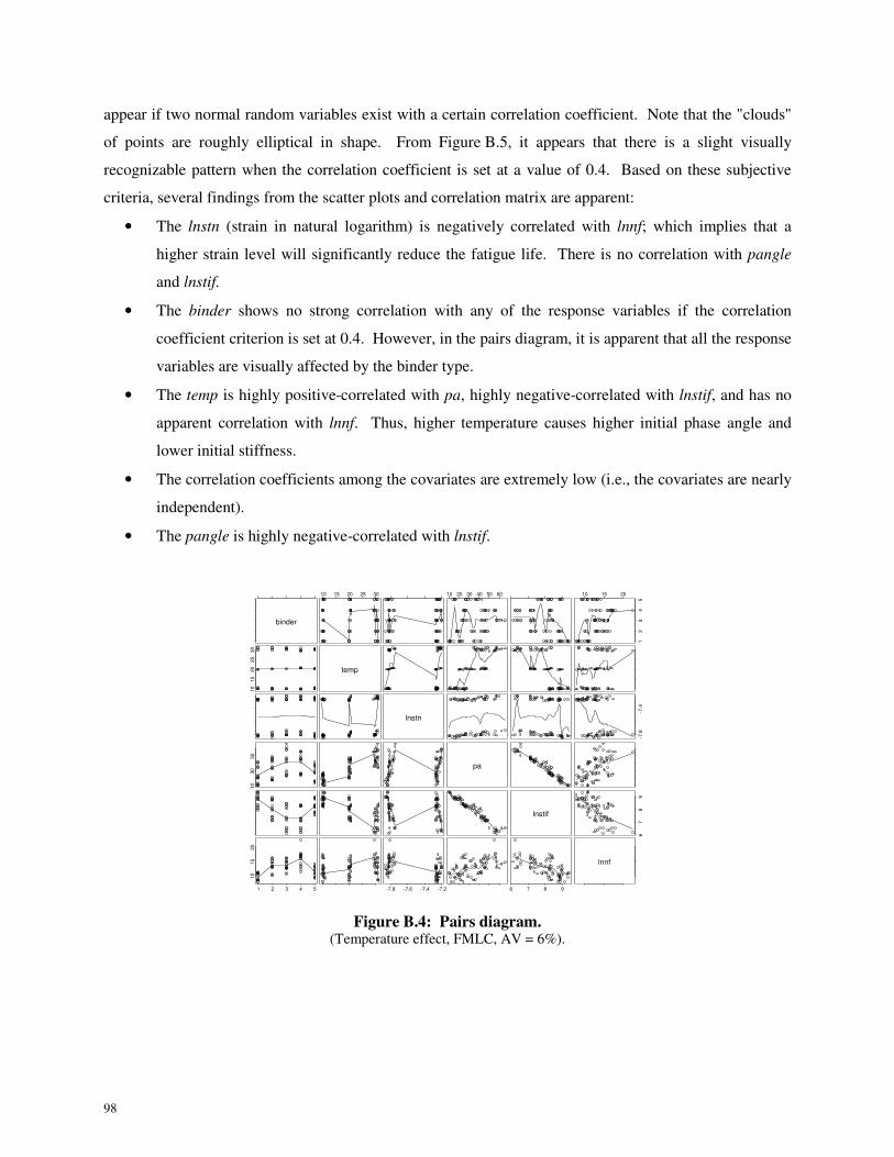
Figure B.4: Pairs diagram. ......................................................................................................................... 98

Figure B.5: Scatterplots of 500 independent pairs of bivariate normal random variables. ........................ 99

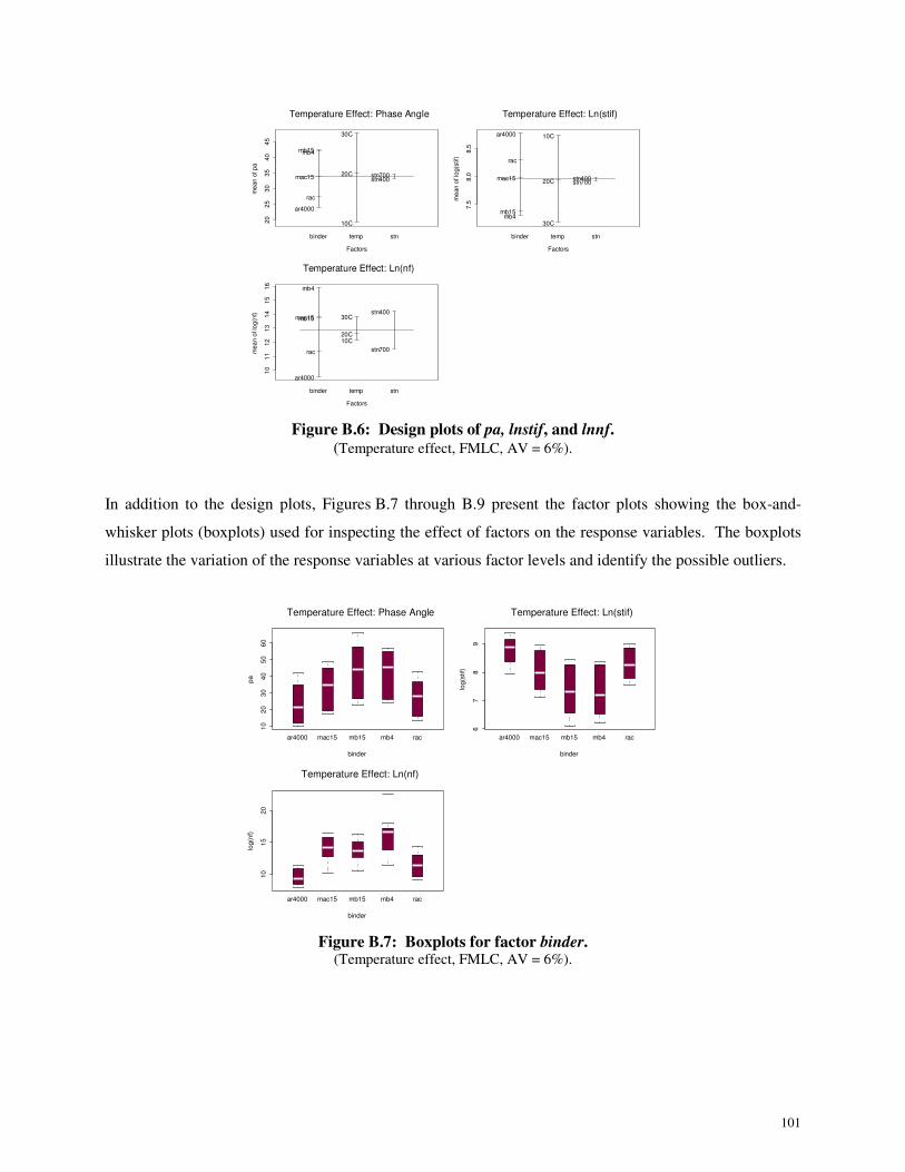
Figure B.6: Design plots of pa, lnstif, and lnnf. ....................................................................................... 101

Figure B.7: Boxplots for factor binder..................................................................................................... 101

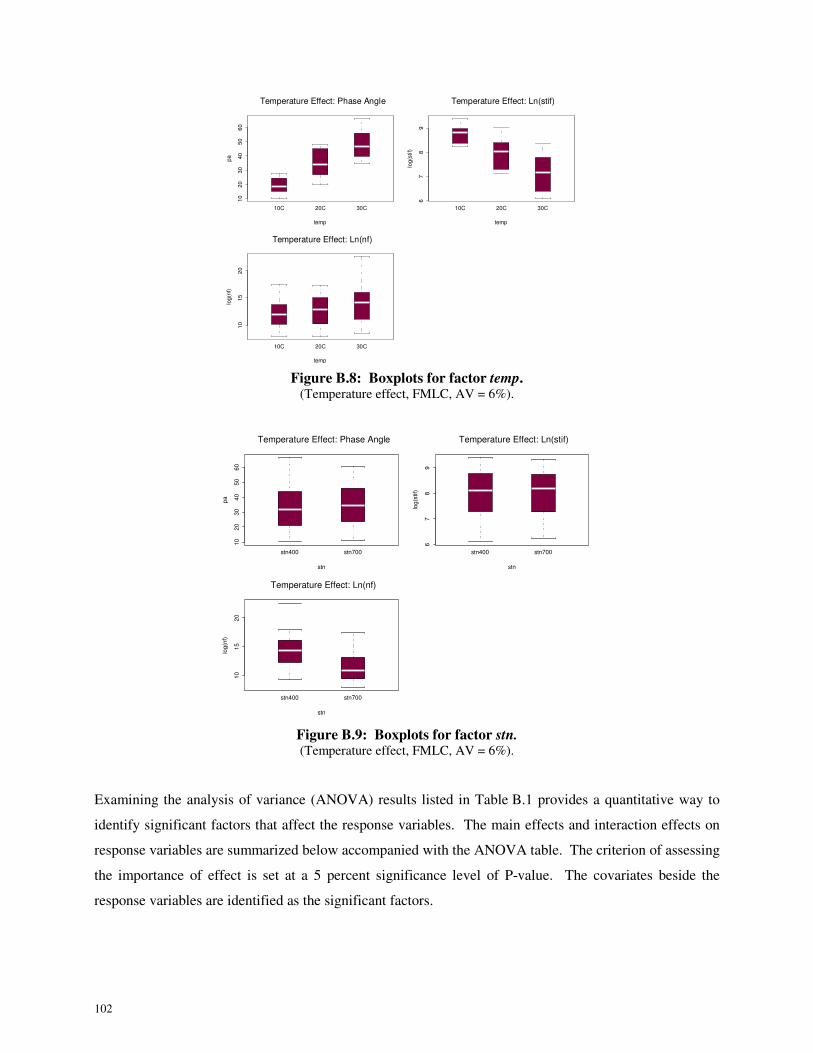
Figure B.8: Boxplots for factor temp. ...................................................................................................... 102

Figure B.9: Boxplots for factor stn. ......................................................................................................... 102

Figure B.10: Interaction plots of binder*temp......................................................................................... 104

Figure B.11: Interaction plots of binder*stn. ........................................................................................... 104

Figure B.12: Interaction plots of temp*stn............................................................................................... 105

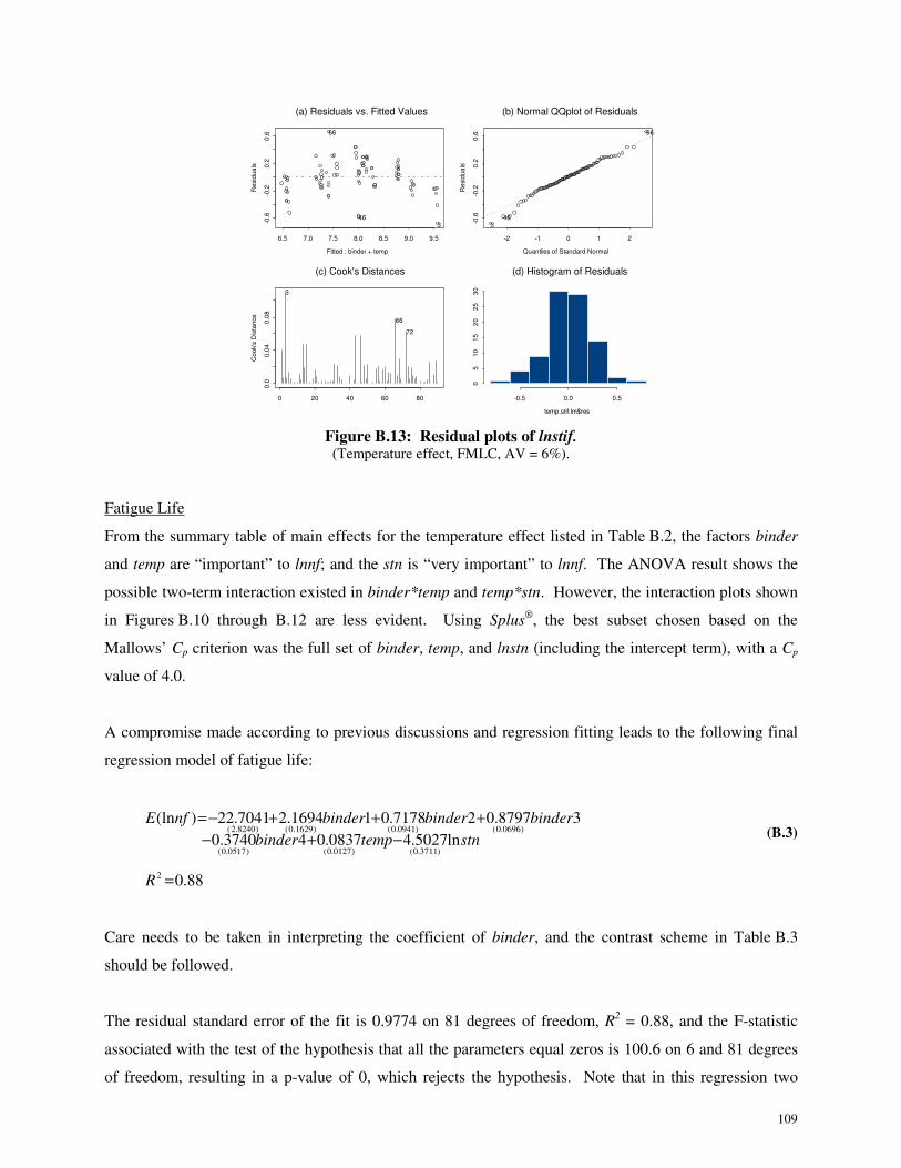
Figure B.13: Residual plots of lnstif. ....................................................................................................... 109

Figure B.14: Residual plots of lnnf. ......................................................................................................... 110

xx

1

1. INTRODUCTION

1.1. Objectives

The first-level analysis presented in this report is part of Partnered Pavement Research Center Strategic

Plan Element 4.10 (PPRC SPE 4.10) being undertaken for the California Department of Transportation

(Caltrans) by the University of California Pavement Research Center (UCPRC). The objective of the study

is to evaluate the reflective cracking performance of asphalt binder mixes used in overlays for

rehabilitating cracked asphalt concrete pavements in California. The study includes mixes modified with

rubber and polymers, and it will develop tests, analysis methods, and design procedures for mitigating

reflective cracking in overlays. This work is part of a larger study on modified binder (MB) mixes being

carried out under the guidance of the Caltrans Pavement Standards Team (PST) (1) that includes

laboratory and accelerated pavement testing using the Heavy Vehicle Simulator (carried out by the

UCPRC), and the construction and monitoring of field test sections (carried out by Caltrans).

1.2. Overall Project Organization

This UCPRC project is a comprehensive study, carried out in three phases, involving the following

primary elements (2):

• Phase 1

- The construction of a test pavement and subsequent overlays;

- Six separate Heavy Vehicle Simulator (HVS) tests to crack the pavement structure;

- Placing of six different overlays on the cracked pavement;

• Phase 2

- Six HVS tests to assess the susceptibility of the overlays to high-temperature rutting

(Phase 2a);

- Six HVS tests to determine the low-temperature reflective cracking performance of the

overlays (Phase 2b);

- Laboratory shear and fatigue testing of the various hot-mix asphalts (Phase 2c);

- Falling Weight Deflectometer (FWD) testing of the test pavement before and after

construction and before and after each HVS test;

- Forensic evaluation of each HVS test section;

• Phase 3

- Performance modeling and simulation of the various mixes using models calibrated with data

from the primary elements listed above.

2

Phase 1

In this phase, a conventional dense-graded asphalt concrete (DGAC) test pavement was constructed at the

Richmond Field Station (RFS) in the summer of 2001. The pavement was divided into six cells, and

within each cell a section of the pavement was trafficked with the HVS until the pavement failed by either

fatigue (2.5 m/m2 [0.76 ft/ft

2]) or rutting (12.5 mm [0.5 in]). This period of testing began in the summer

of 2001 and was concluded in the spring of 2003. In June 2003 each test cell was overlaid with either

conventional DGAC or asphalt concrete with modified binders as follows:

• Full-thickness (90 mm) AR4000-D dense-graded asphalt concrete overlay, included as a control

for performance comparison purposes (AR-4000 is approximately equivalent to a PG64-16

performance grade binder);

• Full-thickness (90 mm) MB4-G gap-graded overlay;

• Half-thickness (45 mm) rubberized asphalt concrete gap-graded overlay (RAC-G), included as a

control for performance comparison purposes;

• Half-thickness (45 mm) MB4-G gap-graded overlay;

• Half-thickness (45 mm) MB4-G gap-graded overlay with minimum 15 percent recycled tire

rubber (MB15-G), and

• Half-thickness (45 mm) MAC15-G gap-graded overlay with minimum 15 percent recycled tire

rubber.

The conventional overlay was designed using the current (2003) Caltrans overlay design process. The

various modified overlays were either full (90 mm) or half thickness (45 mm). Mixes were designed by

Caltrans. The overlays were constructed in one day.

Phase 2

Phase 2 included high-temperature rutting and low-temperature fatigue testing with the HVS as well as

laboratory shear and fatigue testing. The rutting tests were started and completed in the fall of 2003. For

these tests, the HVS was placed above a section of the underlying pavement that had not been trafficked

during Phase 1. A fatigue test was next conducted on each overlay from the winter of 2003-2004 to the

summer of 2007. For these tests, the HVS was positioned precisely on top of the sections of failed

pavement from the Phase 1 HVS tests to investigate the extent and rate of crack propagation through the

overlay.

In conjunction with Phase 2 HVS testing, a full suite of laboratory testing, including shear and fatigue

testing, was carried out on field-mixed, field-compacted (FMFC); field-mixed, laboratory-compacted

(FMLC); and laboratory-mixed, laboratory-compacted (LMLC) specimens.

3

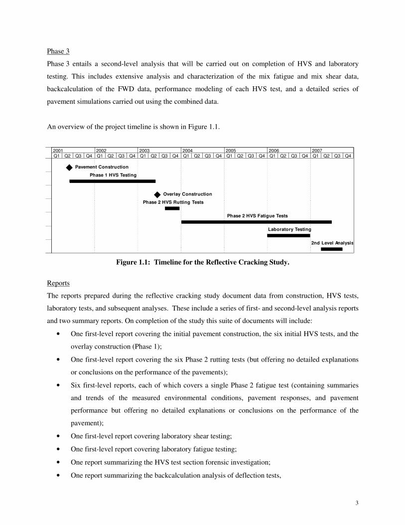
Phase 3

Phase 3 entails a second-level analysis that will be carried out on completion of HVS and laboratory

testing. This includes extensive analysis and characterization of the mix fatigue and mix shear data,

backcalculation of the FWD data, performance modeling of each HVS test, and a detailed series of

pavement simulations carried out using the combined data.

An overview of the project timeline is shown in Figure 1.1.

Pavement Construction

Phase 1 HVS Testing

Overlay Construction

Phase 2 HVS Rutting Tests

Phase 2 HVS Fatigue Tests

Laboratory Testing

2nd Level Analysis

Q1 Q2 Q3 Q4 Q1 Q2 Q3 Q4 Q1 Q2 Q3 Q4 Q1 Q2 Q3 Q4 Q1 Q2 Q3 Q4 Q1 Q2 Q3 Q4 Q1 Q2 Q3 Q42001 2002 2003 2004 2005 2006 2007

Figure 1.1: Timeline for the Reflective Cracking Study.

Reports

The reports prepared during the reflective cracking study document data from construction, HVS tests,

laboratory tests, and subsequent analyses. These include a series of first- and second-level analysis reports

and two summary reports. On completion of the study this suite of documents will include:

• One first-level report covering the initial pavement construction, the six initial HVS tests, and the

overlay construction (Phase 1);

• One first-level report covering the six Phase 2 rutting tests (but offering no detailed explanations

or conclusions on the performance of the pavements);

• Six first-level reports, each of which covers a single Phase 2 fatigue test (containing summaries

and trends of the measured environmental conditions, pavement responses, and pavement

performance but offering no detailed explanations or conclusions on the performance of the

pavement);

• One first-level report covering laboratory shear testing;

• One first-level report covering laboratory fatigue testing;

• One report summarizing the HVS test section forensic investigation;

• One report summarizing the backcalculation analysis of deflection tests,

4

• One second-level analysis report detailing the characterization of shear and fatigue data, pavement

modeling analysis, comparisons of the various overlays, and simulations using various scenarios

(Phase 3), and

• One four-page summary report capturing the entire study’s conclusions and one longer, more

detailed summary report that covers the findings and conclusions from the research conducted by

the UCPRC.

1.3. Structure and Content of this Report

This report presents the results of a first-level analysis of laboratory fatigue testing results. The laboratory

flexural beam test results are available in the University of California Pavement Research Center

(UCPRC) relational database, and are documented in detail in a related document (3). This report is

organized as follows:

• Chapter 2 details the test plan and describes specimen preparation and conditioning.

• Chapter 3 provides information on the binders used in the study.

• Chapter 4 presents and discusses the results of fatigue testing in terms of the effects of the

variables listed above.

• Chapter 5 presents and discusses the results of flexural frequency sweep testing.

• Chapter 6 provides conclusions.

1.4. Measurement Units

Metric units have always been used in the design and layout of HVS test tracks, all the measurements and

data storage, and all associated laboratory testing at the eight HVS facilities worldwide (as well as all

other international accelerated pavement testing facilities). Use of the metric system facilitates

consistency in analysis, reporting, and data sharing.

In this report, metric and English units (provided in parentheses after the metric units) are used in the

Executive Summary, Chapter 1 and 2, and the Conclusion. In keeping with convention, only metric units

are used in Chapters 3, 4, and 5. A conversion table is provided on Page iv at the beginning of this report.

5

2. EXPERIMENT DESIGN

2.1. Introduction

The laboratory fatigue study was undertaken in conjunction with HVS testing, which was carried out on

the following sections:

1. Full-thickness (90 mm) AR4000 dense-graded asphalt concrete (DGAC), included as a control for

performance comparison purposes

2. Half-thickness rubberized asphalt concrete gap-graded (RAC-G) overlay, included as a control for

performance comparison purposes

3. Full-thickness (90 mm) MB4 gap-graded (MB4-G) overlay

4. Half-thickness (45 mm) MB4 gap-graded (MB4-G) overlay

5. Half-thickness MB4 gap-graded overlay with minimum 15 percent recycled tire rubber (MB15-G)

6 Half-thickness MAC15TR gap-graded overlay with minimum 15 percent recycled tire rubber

(MAC15-G)

Samples of loose asphalt mix were collected from the HVS test site during construction of the test

sections. In addition, samples of the asphalt binders and aggregates were obtained at the hot-mix site. Both

sets of materials were used to prepare laboratory mixed, laboratory compacted (LMLC) specimens for the

laboratory fatigue study reported herein. The resulting specimens were used to evaluate the influence on

fatigue performance of the binders considering the effects of temperature, relative compaction (air-void

content), aging, aggregate gradation, and loading frequency and amplitude.

This chapter discusses the test protocols, experimental design, and specimen preparation.

2.2. Test Protocols

The laboratory fatigue study followed the AASHTO T321 test procedures, developed by the Strategic

Highway Research Program (SHRP) A-003A project. It should be noted that this test procedure is

included as a part of the characterization process for asphalt mixes for use in the New Design Guide. The

test consists of flexural controlled-deformation fatigue tests and frequency sweep tests.

2.2.1 Flexural Controlled-Deformation Fatigue Test (AASHTO T321)

Beam test specimens, 50 mm thick by 63 mm wide by 380 mm long, are subjected to four-point bending

using a sinusoidal waveform at a loading frequency of 10 Hz. While the majority of testing is performed at

6

20°C, temperatures in the range 5°C to 30°C can be used. A major advantage of this form of loading test is

that the middle one-third of the beam is theoretically subjected to “pure” flexural bending and the size of

the specimen has been set to minimize shear deformations.

2.2.2 Flexural Controlled-Deformation Frequency Sweep (Modified AASHTO T321)

The flexural frequency sweep test establishes the relationship between complex modulus and load

frequency. The same sinusoidal waveform as in fatigue testing is used in the frequency sweep testing in

the controlled deformation mode and at frequencies of 15, 10, 5, 2, 1, 0.5, 0.2, 0.1, 0.05, 0.02, and

0.01 Hz. The upper limit of 15 Hz is a constraint imposed by the capabilities of the test machine. To

ensure that the specimen is tested in a nondestructive manner, the frequency sweep test is conducted at a

small strain amplitude level (200 microstrain), proceeding from the highest frequency to the lowest in the

sequence noted above.

2.3. Experiment Design

The experiment design was formulated to quantify the effects of:

• Temperature,

• Relative compaction (air voids),

• Aging, and

• Gradation.

Table 2.1 shows the overall experiment design including fatigue and frequency sweep testing. Table 2.2

provides the detailed experiment designs for the study. The following sections briefly discuss the effects

mentioned, and the motivation and application for the study. With each effect, the type of specimen tested

[laboratory-mixed laboratory-compacted (LMLC) or field-mixed laboratory-compacted (FMLC)] is noted

in parentheses. LMLC specimens were prepared from the aggregate and asphalt samples taken at the plant

and refinery during construction, and later mixed and compacted in the laboratory. FMLC specimens were

compacted in the laboratory using mix collected from the plant during construction of the HVS test

section overlays.

In order to test a full factorial, a total of 1,440 tests (three replicates of five binder types, two compaction

types, two condition types, two gradations, two air-void contents, three temperatures, and two strain

levels) would need to have been undertaken. This quantity was unrealistic in terms of time and resources.

A partial factorial was therefore tested (Table 2.1), and where possible, the same tests under different

effects were not repeated. In addition, results were extrapolated where required.

7

Table 2.1: Overall Laboratory Testing Test Plan including Fatigue and Frequency Sweep

Mix/Compaction1,2

Air-Voids (%) Binder

Content (%)4

Grad. Test Type Variables Total

Fatigue

3 temperatures (10,20,30°C)

2 strain levels (400,700 µε)

3 replicates

18

Design AV

(6±0.5%)

Field binder

content

Gap-graded and dense-

graded

Frequency sweep


1 strain level (200 µε)

2 replicates

6

Fatigue

1 temperature (20°C)

2 strain levels (400, 700 µε)

3 replicates

6

FMLC

(Temperature

susceptibility and 20°C

fatigue)

Field AV

(9±1%)

Field binder

content


graded

Frequency sweep



1 replicates

3

Fatigue


LTOA (6 days)

2 strain levels (400, 700 µε)

2 replicates

4

FMLC

(Aging)

Design AV

(6±0.5%)

Field binder

content


graded

Frequency sweep


LTOA (6 days)


1 replicates

3

Fatigue



2 replicates

4

LMLC3

(20°C fatigue)

Design AV

(6±0.5%)

Design binder

content Gap-graded

Frequency sweep


1 strain levels (200 µε)

1 replicates

3

Fatigue

1 temperatures (20°C)


2 replicates

4

LMLC3

(20°C fatigue)

Design AV

(6±0.5%)

Design binder

content Dense-graded

Frequency sweep



1 replicates

3

Total tests per mix type 54

5 mixes 256* 1. FMLC: field-mixed laboratory-compacted; LMLC: laboratory-mixed laboratory-compacted.

2. Binders: AR4000, ARB (asphalt rubber binder), MAC15, MB15, and MB4.

3. LMLC gap-graded tests consider MB4, MB15, MAC15, and Asphalt Rubber binders. LMLC dense-graded tests consider MB4, MB15, MAC15, and AR4000 binders.

4. Design binder content for dense gradations and MB binders performed by UCPRC; other design binder contents performed by producer or Caltrans.

8

Table 2.2: Experimental Design for Laboratory Fatigue Testing

Type of

Fatigue Study

(Total number

of specimens

tested)

Mix1

Condition2 Binder Gradation

Design

Binder

Content

(%)4

Air-voids

(%)

Temperature

(°C)

Strain

(µµµµεεεε) Replicates

Number of

Tests

AR4000 Dense 5.0 3 x 2 x 3 = 18

ARB 8.0 3 x 2 x 3 = 18

MAC15 7.4 3 x 2 x 3 = 18

MB15 7.1 3 x 2 x 3 = 18

Temperature

effect

(90)

FMLC none

MB4

Gap

7.2

6 ± 0.5 10, 20, 30 400 and

700 3

3 x 2 x 3 = 18

6 ± 0.5 1 x 2 x 3 = 6 AR4000 Dense 5.0

9 ± 1 1 x 2 x 3 = 6

6 ± 0.5 1 x 2 x 3 = 6 ARB 8.0

9 ± 1 1 x 2 x 3 = 6

6 ± 0.5 1 x 2 x 3 = 6 MAC15 7.4

9 ± 1 1 x 2 x 3 = 6

6 ± 0.5 1 x 2 x 3 = 6 MB15 7.1

9 ± 1 1 x 2 x 3 = 6

6 ± 0.5 1 x 2 x 3 = 6

Air-void

content effect

(60)

FMLC none

MB4

Gap

7.2 9 ± 1

20 400 and

700 3

1 x 2 x 3 = 6

AR4000 Dense 5.0 1 x 2 x 3 = 6

ARB 8.0 1 x 2 x 3 = 6

MAC15 7.4 1 x 2 x 3 = 6

MB15 7.1 1 x 2 x 3 = 6

none

MB4

Gap

7.2

3

1 x 2 x 3 = 6

AR4000 Dense 5.0 1 x 2 x 2 = 4

ARB 8.0 1 x 2 x 2 = 4

MAC15 7.4 1 x 2 x 2 = 4

MB15 7.1 1 x 2 x 2 = 4

Aging effect

(50) FMLC

aging

MB4

Gap

7.2

6 ± 0.5 20 400 and

700

2

1 x 2 x 2 = 4 1. FMLC: field-mixed laboratory-compacted; LMLC: laboratory-mixed laboratory-compacted.

2. Aging is 6 days at 85°C for compacted beam.

3. The shaded area in “Total Runs” column represents the tests borrowed from the other effects.

4. Percent by mass of aggregate.

9

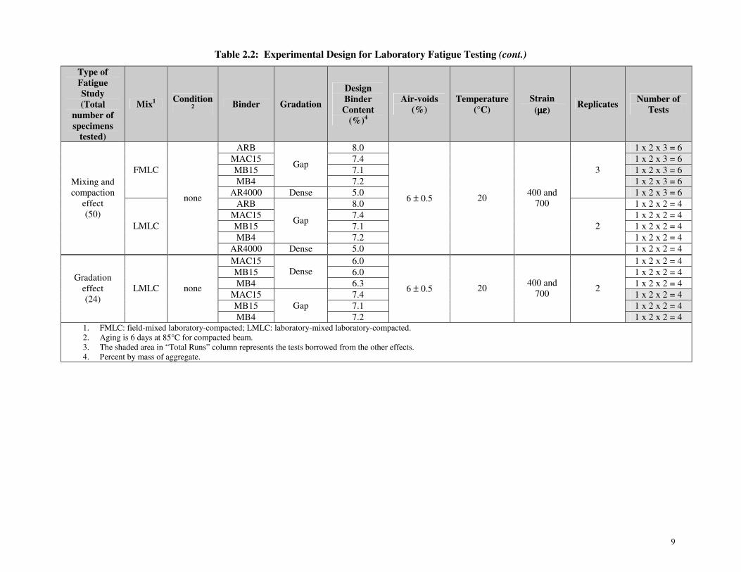
Table 2.2: Experimental Design for Laboratory Fatigue Testing (cont.)

Type of

Fatigue

Study

(Total

number of

specimens

tested)

Mix1 Condition

2

Binder Gradation

Design

Binder

Content

(%)4

Air-voids

(%)

Temperature

(°C)

Strain

(µµµµεεεε) Replicates

Number of

Tests

ARB 8.0 1 x 2 x 3 = 6

MAC15 7.4 1 x 2 x 3 = 6

MB15 7.1 1 x 2 x 3 = 6

MB4

Gap

7.2 1 x 2 x 3 = 6

FMLC

AR4000 Dense 5.0

3

1 x 2 x 3 = 6

ARB 8.0 1 x 2 x 2 = 4

MAC15 7.4 1 x 2 x 2 = 4

MB15 7.1 1 x 2 x 2 = 4

MB4

Gap

7.2 1 x 2 x 2 = 4

Mixing and

compaction

effect

(50)

LMLC

none

AR4000 Dense 5.0

6 ± 0.5 20 400 and

700

2

1 x 2 x 2 = 4

MAC15 6.0 1 x 2 x 2 = 4

MB15 6.0 1 x 2 x 2 = 4

MB4

Dense

6.3 1 x 2 x 2 = 4

MAC15 7.4 1 x 2 x 2 = 4

MB15 7.1 1 x 2 x 2 = 4

Gradation

effect

(24)

LMLC none

MB4

Gap

7.2

6 ± 0.5 20 400 and

700 2

1 x 2 x 2 = 4 1. FMLC: field-mixed laboratory-compacted; LMLC: laboratory-mixed laboratory-compacted.

2. Aging is 6 days at 85°C for compacted beam.

3. The shaded area in “Total Runs” column represents the tests borrowed from the other effects.

4. Percent by mass of aggregate.

10

2.3.1 Temperature Effect (FMLC)

This part of the experiment evaluated the temperature susceptibility of the mixes in the field-mixed,

laboratory-compacted (FMLC) specimens. Testing was carried out at three temperatures (10°C, 20°C, and

30°C) and two strain levels (400 and 700 microstrain). Three replicates were tested.

2.3.2 Air-Void Content Effect (FMLC)

The effect of construction quality in terms of compaction on pavement performance was considered by

conducting tests on specimens at two different air-void contents, 6.0 ± 0.5 percent and 9.0 ± 1.0 percent.

Three replicates of fatigue tests were run at one temperature (20°C) and two strain levels (400 and

700 microstrain).

2.3.3 Aging Effect (FMLC)

The aging effect simulates extended environmental exposure, primarily oxidizing of the binder. For

conventional asphalt binders (steam refined, no modifiers), fatigue resistance is generally reduced as a

more brittle binder is more susceptible to cracking. The AASHTO PP2-94 protocol, which conditions a

compacted specimen for five days at 85°C, is typically followed for long-term oven aging. In the

SHRP-A-390 protocol, long-term oven aging at 85°C for eight days represents (conservatively)

approximate aging at sites nine years or older in the dry-freeze zone, and eighteen years or older in the wet

no-freeze zone (4). For this experiment, an aging period of six days at 85°C was used, based on previous

experience (5). Specimens are aged in a forced-draft oven for the six days, cooled to room temperature,

then conditioned at 20°C for two hours prior to testing.

To evaluate the aging effect of the asphalt binder on the fatigue performance each binder, the test plan

compared four aged beams (two strain levels, two replicates) with six non-aged beams (two strain levels,

three replicates) for temperature effect with the same air-void content (6.0 ± 0.5%) and the same test

temperature (20°C).

2.3.4 Mixing and Compaction Effect (FMLC and LMLC)

In this test, twenty LMLC beams (two replicates of five binder types at two strain levels) and thirty FMLC

beams (three replicates of five binder types at two strain levels) were compared. Air-void content

(6.0 ± 0.5%) and test temperature (20°C) were constant.

2.3.5 Gradation Effect (LMLC)

HVS testing is being conducted only on gap-graded mixes containing the MAC15, MB15, and MB4

binders. However, the laboratory study was extended to assess the use of these three modified binders in

11

both gap- and dense-graded mixes. The dense-graded mix designs were performed by the UCPRC

according to the CTM 304, 366, and 367 procedures. These mixes were compared with the dense-graded

mix containing the AR4000 binder (DGAC) and the gap-graded mix with the rubber asphalt (RA) binder

(ARB).

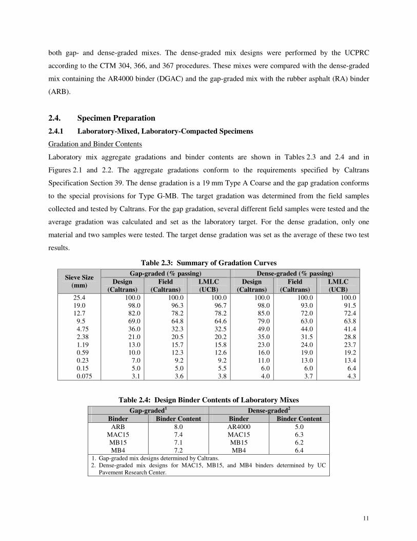
2.4. Specimen Preparation

2.4.1 Laboratory-Mixed, Laboratory-Compacted Specimens

Gradation and Binder Contents

Laboratory mix aggregate gradations and binder contents are shown in Tables 2.3 and 2.4 and in

Figures 2.1 and 2.2. The aggregate gradations conform to the requirements specified by Caltrans

Specification Section 39. The dense gradation is a 19 mm Type A Coarse and the gap gradation conforms

to the special provisions for Type G-MB. The target gradation was determined from the field samples

collected and tested by Caltrans. For the gap gradation, several different field samples were tested and the

average gradation was calculated and set as the laboratory target. For the dense gradation, only one

material and two samples were tested. The target dense gradation was set as the average of these two test

results.

Table 2.3: Summary of Gradation Curves

Gap-graded (% passing) Dense-graded (% passing) Sieve Size

(mm) Design

(Caltrans)

Field

(Caltrans)

LMLC

(UCB)

Design

(Caltrans)

Field

(Caltrans)

LMLC

(UCB)

25.4

19.0

12.7

9.5

4.75

2.38

1.19

0.59

0.23

0.15

0.075

100.0

98.0

82.0

69.0

36.0

21.0

13.0

10.0

7.0

5.0

3.1

100.0

96.3

78.2

64.8

32.3

20.5

15.7

12.3

9.2

5.0

3.6

100.0

96.7

78.2

64.6

32.5

20.2

15.8

12.6

9.2

5.5

3.8

100.0

98.0

85.0

79.0

49.0

35.0

23.0

16.0

11.0

6.0

4.0

100.0

93.0

72.0

63.0

44.0

31.5

24.0

19.0

13.0

6.0

3.7

100.0

91.5

72.4

63.8

41.4

28.8

23.7

19.2

13.4

6.4

4.3

Table 2.4: Design Binder Contents of Laboratory Mixes

Gap-graded1

Dense-graded2

Binder Binder Content Binder Binder Content

ARB

MAC15

MB15

MB4

8.0

7.4

7.1

7.2

AR4000

MAC15

MB15

MB4

5.0

6.3

6.2

6.4 1. Gap-graded mix designs determined by Caltrans.

2. Dense-graded mix designs for MAC15, MB15, and MB4 binders determined by UC

Pavement Research Center.

12

0

10

20

30

40

50

60

70

80

90

100

0.01 0.1 1 10 100

Sieve Size (mm)

Perc

en

t P

assin

g

Design (Caltrans)

Field (Caltrans)

LMLC (UCB)

3/8" 1"3/4"1/2"

#4#8#16#30#50#100#200

19 mm Maximum Operating Range(Gap-Graded)

Figure 2.1: Gradation curves for gap-graded mixes.

0

10

20

30

40

50

60

70

80

90

100

0.01 0.1 1 10 100

Sieve Size (mm)

Perc

en

t P

assin

g

Design (Caltrans)

Field (Caltrans)

LMLC (UCB)

3/8" 1"3/4"1/2"

#4#8#16#30#50#100#200

19 mm Maximum Coarse Operating Range(Dense-Graded)

Figure 2.2: Gradation curves for dense-graded mixes.

Preparation

Specimens were prepared from raw materials supplied by the contractor constructing the HVS Test Track,

Syar Industries, Inc. The aggregate, a basalt, was obtained from Syar’s Lake Herman quarry, located near

Vallejo, CA. The aggregate blend was obtained from four bins with size ranges as follows:

19 mm x 12.5mm, 12.5 mm x 9.5 mm, 9.5 mm x dust, and 4.75 mm x dust. Binders produced for the HVS

Test Track were obtained from a number of California refineries.

13

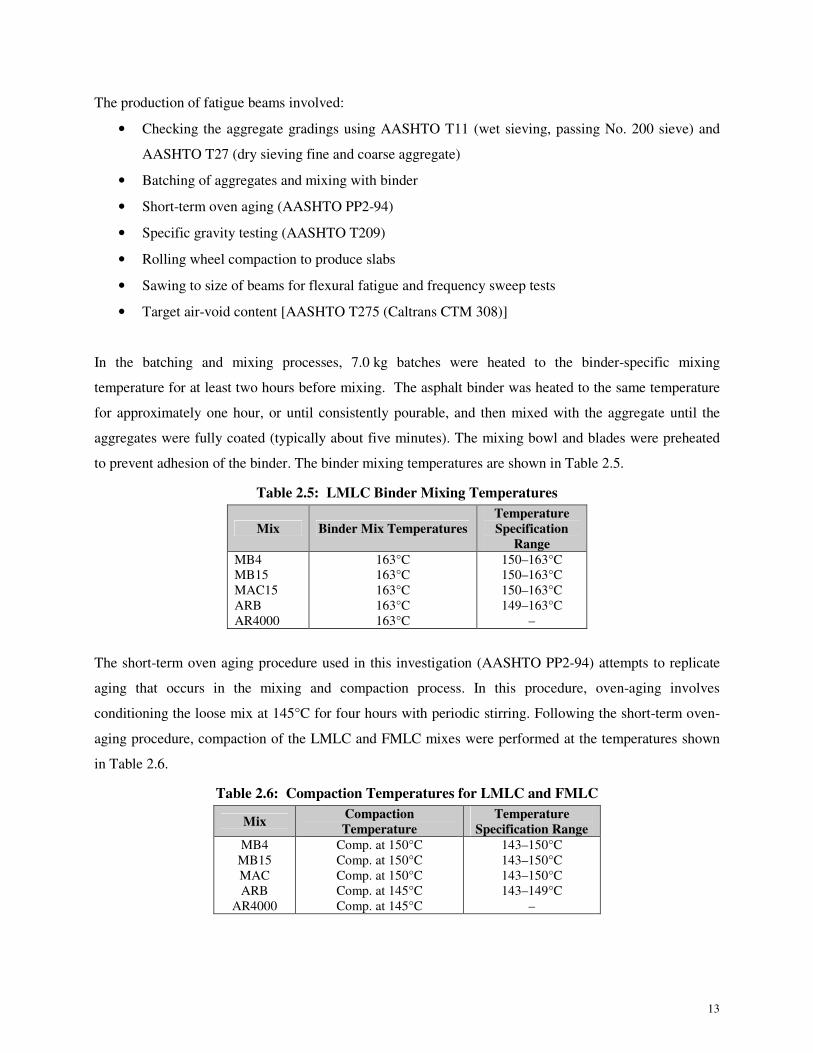
The production of fatigue beams involved:

• Checking the aggregate gradings using AASHTO T11 (wet sieving, passing No. 200 sieve) and

AASHTO T27 (dry sieving fine and coarse aggregate)

• Batching of aggregates and mixing with binder

• Short-term oven aging (AASHTO PP2-94)

• Specific gravity testing (AASHTO T209)

• Rolling wheel compaction to produce slabs

• Sawing to size of beams for flexural fatigue and frequency sweep tests

• Target air-void content [AASHTO T275 (Caltrans CTM 308)]

In the batching and mixing processes, 7.0 kg batches were heated to the binder-specific mixing

temperature for at least two hours before mixing. The asphalt binder was heated to the same temperature

for approximately one hour, or until consistently pourable, and then mixed with the aggregate until the

aggregates were fully coated (typically about five minutes). The mixing bowl and blades were preheated

to prevent adhesion of the binder. The binder mixing temperatures are shown in Table 2.5.

Table 2.5: LMLC Binder Mixing Temperatures

Mix Binder Mix Temperatures

Temperature

Specification

Range

MB4

MB15

MAC15

ARB

AR4000

163°C

163°C

163°C

163°C

163°C

150–163°C

150–163°C

150–163°C

149–163°C

–

The short-term oven aging procedure used in this investigation (AASHTO PP2-94) attempts to replicate

aging that occurs in the mixing and compaction process. In this procedure, oven-aging involves

conditioning the loose mix at 145°C for four hours with periodic stirring. Following the short-term oven-

aging procedure, compaction of the LMLC and FMLC mixes were performed at the temperatures shown

in Table 2.6.

Table 2.6: Compaction Temperatures for LMLC and FMLC

Mix Compaction

Temperature

Temperature

Specification Range

MB4

MB15

MAC

ARB

AR4000

Comp. at 150°C

Comp. at 150°C

Comp. at 150°C

Comp. at 145°C

Comp. at 145°C

143–150°C

143–150°C

143–150°C

143–149°C

–

14

2.4.2 Field-Mixed, Laboratory Compacted Specimens

The field-mixed laboratory-compacted specimens were prepared using the loose mix collected during

construction of the HVS test road. After construction, this material was stored in five-gallon sealed metal

cans at room temperature in a warehouse without temperature control for up to several years before

compaction. Some further aging may have occurred during the time between site sampling and specimen

production. For specimen production, the mix was tested for its maximum specific gravity and compacted

following the procedures described above.

The compaction temperatures for field-mixed, lab-compacted specimens were the same as for the LMLC

mixes.

2.5. Ignition Oven Tests

2.5.1 Test Method

California Test CTM382 (Determination of Asphalt Binder Content of Bituminous Mixtures by the

Ignition Method) was used to determine binder contents for the field mix collected during construction of

the HVS test sections. The ignition oven values were corrected for ignition of the aggregate using

aggregate samples also collected during construction. Mixes tested for binder content were RAC-G,

MAC15-G, MB15-G, and MB4-G.

2.5.2 Results

Table 2.7 summarizes the results of the ignition oven test on the selected mixes. Table 2.8 lists revised

95 percent confidence intervals based on a pooled standard deviation. The results show that the mean

field binder contents were approximately 0.5, 0.15, 0.4, and 0.3 percent above the design binder contents

for the ARB, MAC15, MB15, and MB4 gap-graded mixes, respectively.

15

Table 2.7: Summary of Binder Ignition Tests

Test Results of Field Mixes Mix Type

Design Binder

Content

(%)

Ignition Oven

Correction

Factor 1 2 3 4 5

Mean Standard

Error

95%

Confidence

Interval

RAC-G 8.0 1.86 8.79 8.35 8.54 8.26 - 8.485 0.117 (8.112, 8.857)

MAC15-G 7.4 1.86 7.64 7.42 7.65 7.48 - 7.548 0.058 (7.363, 7.733)

MB15-G 7.1 1.76 7.89 7.66 7.41 7.08 7.58 7.524 0.135 (7.149, 7.899)

MB4-G 7.2 2.15 7.84 7.84 7.62 6.71 - 7.503 0.269 (6.647, 8.359)

Table 2.8: Summary of Binder Ignition Tests (pooled standard deviation)

Test Results of Field Mixes Mix Type

Design Binder

Content

(%)

Ignition Oven

Correction

Factor 1 2 3 4 5

Mean Standard

Error

95%

Confidence

Interval

RAC-G 8.0 1.86 8.79 8.35 8.54 8.26 - 8.485 0.166 (7.957, 9.013)

MAC15-G 7.4 1.86 7.64 7.42 7.65 7.48 - 7.548 0.166 (7.020, 8.076)

MB15-G 7.1 1.76 7.89 7.66 7.41 7.08 7.58 7.524 0.148 (7.053, 7.995)

MB4-G 7.2 2.15 7.84 7.84 7.62 6.71 - 7.503 0.166 (6.974, 8.031)

16

17

3. BINDER TESTING

3.1. Introduction

A total of five binders have been used in this investigation including: a conventional AR4000 asphalt

cement, asphalt rubber (ARB), and three modified binders designated MB4, MB15, and MAC15. This

chapter provides a summary of the Bending Beam Rheometer (BBR) and Dynamic Shear Rheometer

(DSR) tests conducted at the Turner-Fairbank Highway Research Center of the Federal Highway

Administration (FHWA) as part of this study. Tests were conducted on binders in their original condition

and after the Rolling Thin Film Oven (RTFO) and Pressure Aging Vessel (PAV) conditioning. These five

binders were used in the HVS test program and the laboratory fatigue study; all but the AR binder were

tested by the FHWA using tests associated with the AASTHO PG Binder Specification M320.

3.2. Bending Beam Rheometer

3.2.1 Test Method

AASHTO T313 was used to assess the propensity of the binders to develop thermal stresses at low

pavement temperature. The two values obtained from the Bending Beam Rheometer are the creep

stiffness and the m-value (the rate of change of the creep stiffness versus time of loading). The PG binder

specification M320 includes limiting values for these two parameters associated with the low temperature

of the PG binder grade. The allowable maximum creep stiffness value is 300 MPa and the minimum

m-value is 0.3, both determined at a loading time of 60 seconds.

3.2.2 Results

Table 3.1 lists the temperatures at which creep stiffnesses reached 300 MPa, and m-values reached 0.3.

Figures 3.1 and 3.2 plot the creep stiffnesses and m-values versus temperature for the un-aged condition

and after RTFO and PAV aging. According to the test results and the Superpave specification for thermal

cracking, the ranking of susceptibility of the binders to low-temperature thermal cracking is (from highest

to lowest susceptibility):

1. AR4000

2. MAC15

3. MB15

4. MB4

18

Table 3.1: Summary of Bending Beam Rheometer Test Results

Binder Type Binder Status* Temp@S=300 MPa

(°C)

Temp@m=0.3

(°C)

AR4000

ORG

RTFO

PAV

-11.5

-11.3

-7.7

-15.7

-15.3

-11.3

MAC15

ORG

RTFO

PAV

-20.5

-18.8

-18.0

-23.9

-22.3

-19.3

MB15

ORG

RTFO

PAV

-26.7

-25.6

-24.0

-28.3

-26.7

-22.5

MB4

ORG

RTFO

PAV

-31.7

-28.3

-25.7

-31.3

-27.8

-22.0 * ORG: original

RTFO: rolling thin film oven

PAV: pressure aging vessel

0

100

200

300

400

500

600

700

800

900

-35 -30 -25 -20 -15 -10 -5 0 5

Temperature (C)

Cre

ep

Sti

ffn

es

s (

MP

a)

AR4000 ORG

AR4000 RTFO

AR4000 PAV

MB4 ORG

MB4 RTFO

MB4 PAV

MB15 ORG

MB15 RTFO

MB15 PAV

MAC15 ORG

MAC15 RTFO

MAC15 PAV

Figure 3.1: Creep stiffness summary of BBR test results.

19

0

0.1

0.2

0.3

0.4

0.5

0.6

-35 -30 -25 -20 -15 -10 -5 0 5

Temperature (C)

M-v

alu

e

AR4000 ORG AR4000 RTFO

AR4000 PAV MB4 ORG

MB4 RTFO MB4 PAV

MB15 ORG MB15 RTFO

MB15 PAV MAC15 ORG

MAC15 RTFO MAC15 PAV

Figure 3.2: m-value summary of BBR test results.

3.3. Dynamic Shear Rheometer

3.3.1 Test Method

AASHTO T315 method was followed to assess the rutting (G*/sinδ) and long-term fatigue performance

(G*sinδ) of the binders.

3.3.2 Results

Rutting Resistance

AASHTO M320 defines and places requirements on a rutting factor of binder, G*/sinδ, which represents a

measure of high temperature rutting resistance of the asphalt binder. To minimize the rutting, the

specification requires that G*/sinδ must be a minimum of 1.0 kPa for the original asphalt binder and

2.2 kPa after aging the binder using the RTFO procedure. Dynamic shear modulus G* at 10 rad/s against

the test temperatures and the specification requirements for the binders are shown in Figures 3.3 and 3.4

for these two conditions.

20

-8

-4

0

4

8

12

0 10 20 30 40 50 60 70 80

Temperature (C)

Ln

(G*/

sin

δδ δδ)

(G*/

sin

δδ δδ:

kP

a)

AR4000

MAC15

MB15

MB4

G*/sinδδδδ, Minimum, 1.00 kPa

Original

G*/sinδδδδ @ 10 rad/s

Figure 3.3: G*/sinδδδδ summary of DSR test results on original binder.

-8

-4

0

4

8

12

0 10 20 30 40 50 60 70 80

Temperature (C)

Ln

(G*/

sin

δδ δδ)

(G*/

sin

δδ δδ:

kP

a)

AR4000

MAC15

MB15

MB4

G*/sinδδδδ, Minimum, 2.20 kPa

RTFO

G*/sinδδδδ @ 10 rad/s

Figure 3.4: G*/sinδδδδ summary of DSR test results on RTFO aged binder.

Fatigue Resistance

In the AASHTO M320 specification, the fatigue resistance of the binder is controlled by the parameter

G*sinδ. This parameter represents a measure of the cracking resistance of the asphalt binder in the

intermediate temperature range. To minimize fatigue cracking, the specification requires that G*sinδ have

a minimum value of 5,000 kPa after PAV aging.

21

Figure 3.5 illustrates the dynamic shear modulus G* at 10 rad/s versus a range of temperatures and

contains the specification requirement for G*sinδ.

0

2

4

6

8

10

12

0 10 20 30 40 50 60 70 80

Temperature (C)

Ln

(G*s

ind

δδ δδ)

(G*s

inδδ δδ:

kP

a)

AR4000

MAC15

MB15

MB4

G*sinδδδδ, Maximum, 5000 kPa

PAV

G*sinδδδδ @ 10 rad/s

Figure 3.5: G*sinδδδδ summary of DSR test results on PAV-aged binder.

Shear Susceptibility

The Shear Susceptibility of Viscosity (SSV) and Shear Susceptibility of Delta (SSD) are derived from

DSR test results and are defined in California Test 381. Reese (5) further developed these parameters for

Type G-MB asphalt concrete as follows:

SSD ≥ 30(0.6+SSV)3 for original binder @ 25°C

SSD ≥ -115(SSV) - 50.6 for PAV-aged binder at @ 25°C

Table 3.2 summarizes the SSD and SSV values for the binders. All the binders satisfy the PAV-aged

binder requirement, while only the MB4 binder satisfies the un-aged binder requirement.

Test Summary

According to the test results, the ranking of susceptibility of the binders to rutting is (from highest to

lowest):

1. MAC15 (binder failed to meet minimum requirements of rutting)

2. MB4, MB15

3. AR4000

The ranking of susceptibility of the binders to fatigue cracking is (from highest to lowest):

22

1. AR4000

2. MAC15

3. MB15

4. MB4

The MB4 and MB15 binders had similar rutting and fatigue resistance capacities. The AR4000 binder

appeared to have better rutting resistance below 40°C than the MB4 and MB15 binders.

Table 3.2: Summary of SSV and SSD Values from DSR Test Results

Binder Binder

Status* SSV@25°C SSD@25°C SSD for ORG SSD for PAV

ORG -0.2085 -12.848 No

RTFO -0.4264 -4.454

AR4000

PAV -0.2983 -11.428

Yes

ORG -0.4523 6.388 Yes

RTFO -0.4369 2.944

MB4

PAV -0.3059 -2.376

Yes

ORG -0.2201 -2.742 No

RTFO -0.2742 -2.013

MB15

PAV -0.2490 -5.911

Yes

ORG -0.2289 -0.210 No

RTFO -0.2585 2.358

MAC15

PAV -0.2623 -6.898

Yes * ORG: original

RTFO: rolling thin film oven

PAV: pressure aging vessel.

3.3.3 Master Curve of Shear Complex Modulus

The master curves of the binder shear complex moduli were constructed using time-temperature

superposition and a genetic algorithm (3). Figures 3.6 through 3.13 present the G* master curves and

temperature-shift relationships at various aging conditions for AR4000, MB4, MB15, and MAC15 binders

respectively. Observations based on the results of this analysis are:

• For binders aged with the PAV procedure, the complex shear moduli increase across all

frequencies for the four binders.

• The MB4 and MB15 binders show small-to-moderate changes between the various aging

conditions.

• For original and RTFO aging conditions, the master curves of MAC15 binder are similar;

however, the master curve at PAV stage exhibits some deviation from the other two curves. The

reason is not clear at this time.

• In general, the temperature-shift relationship does not change significantly for different aging

conditions. The only exception is the MAC15 binder. Its temperature sensitivity for the PAV-aged

23

condition increases rapidly at low temperatures and is greater than the temperature sensitivity in

the original and RTFO conditions.

Figures 3.14 through 3.16 compare the master curves at various aging conditions, respectively. In the

original and RTFO conditioning, the master curves of MAC15 binder are significantly lower than the

master curves for the AR4000, MB4, and MB15 binders. The ranking of the master curves for PAV

conditioning is changed with the order from highest to lowest as follows:

1. AR4000

2. MAC15

3. MB4

4. MB15

24

-10

-5

0

5

10

15

20

-20 -15 -10 -5 0 5 10 15

Reduced Ln(freq) (freq: rad/s)

Ln

(G*)

(G

*: P

a)

AR4000 (ORG)

AR4000 (RTFO)

AR4000 (PAV)

Gamma Fitted Lines

AR4000

Tref = 25C

Figure 3.6: Master curves of shear complex modulus of AR4000.

-20

-15

-10

-5

0

5

10

15

20

-30 -20 -10 0 10 20 30 40 50 60

T-Tref(25C)

Ln

aT

AR4000 (ORG)

AR4000 (RTFO)

AR4000 (PAV)

Fitted Line (ORG)

Fitted Line (RTFO)

Fitted Line (PAV)

Tref = 25C

AR4000 Shear Complex Modulus

Figure 3.7: Temperature-shift relationships of AR4000.

-10

-5

0

5

10

15

20

-20 -15 -10 -5 0 5 10 15


Ln

(G*)

(G

*: P

a)

MB4 (ORG)

MB4 (RTFO)

MB4 (PAV)

Gamma Fitted Lines

MB4

Tref = 25C

Figure 3.8: Master curves of shear complex modulus of MB4.

-20

-15

-10

-5

0

5

10

15

20

-30 -20 -10 0 10 20 30 40 50 60

T-Tref(25C)

Ln

aT

MB4 (ORG)

MB4 (RTFO)

MB4 (PAV)

Fitted Line (ORG)

Fitted Line (RTFO)

Fitted Line (PAV)

Tref = 25C

MB4 Shear Complex Modulus

Figure 3.9: Temperature-shift relationships of MB4.

25

-10

-5

0

5

10

15

20

-20 -15 -10 -5 0 5 10 15


Ln

(G*)

(G

*: P

a)

MB15 (ORG)

MB15 (RTFO)

MB15 (PAV)

Gamma Fitted Lines

MB15

Tref = 25C

Figure 3.10: Master curves of shear complex modulus of MB15.

-20

-15

-10

-5

0

5

10

15

20

-30 -20 -10 0 10 20 30 40 50 60

T-Tref(25C)

Ln

aT

MB15 (ORG)

MB15 (RTFO)

MB15 (PAV)

Fitted Line (ORG)

Fitted Line (RTFO)

Fitted Line (PAV)

Tref = 25C

MB15 Shear Complex Modulus

Figure 3.11: Temperature-shift relationships of MB15.

-10

-5

0

5

10

15

20

-20 -15 -10 -5 0 5 10 15


Ln

(G*)

(G

*: P

a)

MAC15 (ORG)

MAC15 (RTFO)

MAC15 (PAV)

Gamma Fitted Lines

MAC15

Tref = 25C

Figure 3.12: Master curves of shear complex modulus of MAC15.

-20

-15

-10

-5

0

5

10

15

20

-30 -20 -10 0 10 20 30 40 50 60

T-Tref(25C)

Ln

aT

MAC15 (ORG)

MAC15 (RTFO)

MAC15 (PAV)

Fitted Line (ORG)

Fitted Line (RTFO)

Fitted Line (PAV)

Tref = 25C

MAC15 Shear Complex Modulus

Figure 3.13: Temperature-shift relationships of MAC15.

26

-10

-5

0

5

10

15

20

-20 -15 -10 -5 0 5 10 15

Ln(freq) (freq: rad/s)

Ln

(G*)

(G

*: P

a)

ORG

AR4000MB4MB15MAC15

Tref = 25C

Figure 3.14: Comparison of G* Master curves (original).

-10

-5

0

5

10

15

20

-20 -15 -10 -5 0 5 10 15


Ln

(G*)

(G

*:P

a)

RTFO

AR4000MB4MB15MAC15

Tref = 25C

Figure 3.15: Comparison of G* Master curves (RTFO).

-10

-5

0

5

10

15

20

-20 -15 -10 -5 0 5 10 15


Ln

(G*)

(G

*: P

a)

PAV

AR4000MAC15MB4MB15

Tref = 25C

Figure 3.16: Comparison of G* Master curves (PAV).

27

4. FATIGUE TESTING

4.1. Introduction

This chapter provides an overview of the laboratory fatigue testing study together with the analysis and

interpretation of the results on field mixed, laboratory compacted (FMLC) and laboratory mixed,

laboratory compacted (LMLC) materials. Included are:

• Summary of the flexural controlled-deformation fatigue test results

• Identification of the significant factors (or covariates) that affect fatigue performance

• Discussion of regression models of initial stiffness and fatigue life

• Summary of the collective dataset analysis and regression model

4.1.1 Definitions Used in Statistical Analyses

The factors investigated include:

• Temperature effect (on FMLC material)

• Air-void content effect (on FMLC material)

• Aging effect (on FMLC material)

• Compaction effect (on FMLC and LMLC material)

• Gradation effect (on LMLC material)

The response variables are:

• Initial phase angle (pangle or pa)

• Natural logarithm of the initial stiffness (lnstif)

• Natural logarithm of the fatigue life (lnnf)

The phase angle and initial stiffness were obtained taken after the first fifty repetitions; at this number of

repetitions temperature stability and stabilization of the strain level in the fatigue beam are obtained. It

should be noted that both the stiffness and tensile strain are calculated from the measured load and center

beam deflections.

Fatigue life is defined for this analysis as the number of tensile strain repetitions to a 50 percent reduction

in stiffness from the initial stiffness measured at 50 repetitions. This definition of fatigue life has been

used extensively and correlates well with the initiation of cracking in fatigue beams for mixes with

conventional binders. Its applicability to modified binders has been questioned and some alternative

28

definitions of flexural fatigue beam life recently have been proposed. Analyses that consider alternative

definitions of fatigue life will be included in the second-level analysis report.

The category covariates and factor levels evaluated include:

• Binder type (binder)

- AR4000 (ar4000)

- ARB (rac)

- MAC15 (mac15)

- MB15 (mb15)

- MB4 (mb4)

• Gradation (grad)

- Dense-graded (dg)

- Gap-graded (gg)

• Compaction (comp)

- Field-mixed, laboratory-compacted (fmlc)

- Laboratory-mixed, laboratory-compacted (lmlc)

• Conditioning (cond)

- No conditioning (none)

- Long-term oven aging for 6 days (aging)

• Air-void content (av)

- 6 percent air-void content (av6)

- 9 percent air-void content (av9)

• Test temperature (temp)

- 10°C (10C)

- 20°C (20C)

- 30°C (30C)

• Test strain levels (stn)

- 400 microstrain (stn400)

- 700 microstrain (stn700).

The covariate binder has different meanings depending on the test, as follows:

• On all effects other than gradation, binder implies a binder type with a specific gradation type and

corresponding design binder content as used in this experiment, regardless of compaction type

(FMLC or LMLC). It should be noted that AR4000-D and RAC-G are defined by specification

and hence a gap-graded mix with the AR4000 binder (AR4000-G) and a dense-graded mix with

29

the ARB binder (RAC-D) are not included in the experiment. The interpretations of binder

include:

- ar4000 - AR4000 binder with dense-graded gradation and 5.0 percent design asphalt

content

- rac - AR binder with gap-graded gradation and 8.0 percent design asphalt content

- mac15 - MAC15 binder with gap-graded gradation and 7.4 percent design asphalt

content

- mb15 - MB15 binder with gap-graded gradation and 7.1 percent design asphalt content

- mb4 - MB4 binder with gap-graded gradation and 7.2 percent design asphalt content

• When considering the gradation effect, binder implies a binder type with a specific design binder

content. In this instance, binder is used as follows:

- mac15 - MAC15 binder with 6.0 percent asphalt content if dense-graded, or 7.4 percent

asphalt content if gap-graded

- mb15 - MB15 binder with 6.0 asphalt content if dense-graded, or 7.1 percent asphalt

content if gap-graded.

- mb4 - MB4 binder with 6.3 percent asphalt content if dense-graded, or 7.2 percent

asphalt content if gap-graded

• When developing the comprehensive regression models with all fatigue tests, binder signifies a

binder type with specific design asphalt content associated with its gradation (dense-graded or

gap-graded).

4.1.2 Expected Effects of Response Variables on Performance

The expected effects of response variables from flexural fatigue beam tests on performance are

summarized in Table 4.1. These are simplifications of complex distress mechanisms, particularly fatigue

cracking. However, they provide a general guide to interpret the results presented in this chapter.

Phase angle is a measure of the time lag between the applied stress and the resulting strain when a

sinusoidal wave is applied to a viscoelastic material, such as asphalt and mixes of asphalt and aggregate.

Phase angle is included in the rutting, low temperature, and fatigue specification properties for PG

binders, where it is referred to as delta (δ). A phase angle of zero degrees means that there is no time lag,

and the material is therefore elastic. A low phase angle is good for rutting performance because it means

that when the material is deformed it should return almost to its original condition when the load is

removed, resulting in little permanent deformation. It is bad for low-temperature cracking performance

because it means that the material will not relax tensile stresses that occur when the material contracts as it

gets colder.

30

Table 4.1: Summary of Expected Effects of Response Variables on Performance

Flexural Beam Test

Response Variable

Distress Mechanism in Field Expected Effect on Field Performance

Rutting at high temperatures High phase angle at high temperatures expected to

result in more rutting.

Low-temperature cracking Low phase angle at low temperatures expected to

increase risk of low-temperature cracking.

Phase angle

Fatigue and Reflective Cracking Phase angle effect highly correlated with stiffness,

see Stiffness explanation.

Rutting at high temperatures High stiffness at high temperatures expected to

result in less rutting.

Low-temperature cracking High stiffness at low temperatures expected to

increase risk of low-temperature cracking.

Thin overlay: high stiffness has little influence on

tensile strain.

Stiffness

Tensile strain (related to fatigue and

reflective cracking)

Thick overlay: high stiffness reduces tensile

strains, which increases fatigue life.

Rutting at high temperatures No effect.

Low-temperature cracking High fatigue life at low temperatures may indicate

reduced risk of low-temperature cracking in areas

without extremely cold temperatures.

Thin overlay: High fatigue life indicates

increased fatigue life

Beam fatigue life

(repetitions to cracking

at a constant tensile

strain)

Fatigue cracking and reflective

cracking

Thick overlay: High fatigue life indicates

increased fatigue life

Thin overlay: High stiffness causes short life in

beam fatigue at a given tensile strain, and little

change in tensile strain in the field. Net result is

that high stiffness will usually result in short

cracking life in the field.

Interaction of stiffness

and beam fatigue life

Fatigue cracking and reflective

cracking

Thick overlay: High stiffness causes short life in

beam fatigue at a given tensile strain, but reduces

tensile strain in the pavement. Net result must be

determined from mechanistic pavement structural

analysis.

A phase angle of 90 degrees indicates that the material has the maximum time lag possible between stress

and strain, and that the material is therefore completely viscous. A high phase angle is bad for rutting

performance because it indicates that none of the deformation returns when the load is removed. However,

a high phase angle is good for low-temperature cracking performance.

Phase angle is highly correlated with stiffness in asphalt mixes. Mixes having high stiffness typically have

low phase angles. Therefore, in the general understanding of the effects of phase angle on rutting and low-

temperature cracking discussed above, “low stiffness” can often be substituted for “high phase angle”.

Modifiers in asphalt mixes can change phase angle and stiffness independently to some degree, and the

assumption of a strong correlation between high phase angle and low stiffness is not always valid for these

materials.

31

The effect of phase angle and stiffness on fatigue performance, whether for bottom up fatigue cracking in

new structures or reflective cracking in overlays placed over cracked pavement, is dependent on the

interaction of the mix properties (particularly stiffness and the sensitivity of fatigue life to tensile strain),

crack dimensions, underlying pavement condition, load, and other factors. It is therefore difficult to make

a generally applicable statement regarding the expected effect of stiffness and phase angle on expected

reflective cracking life.

A general description of the expected interaction of stiffness and beam fatigue life for thin and thick

overlays on cracked pavements, or new pavements with granular bases with a thin or thick asphalt layer is

shown in Table 4.2 and Figure 4.1. It must be remembered that this is a qualitative example using

hypothetical data. In actual practice, mechanistic analysis should be performed using actual laboratory

beam test results and calculations of tensile strain in the pavement to quantify the expected performance.

In the second-level analyses that will be carried out on completion of all laboratory and HVS tests, actual

fatigue test data for the various mixes evaluated in this study together with mechanistic analyses of

representative pavement structures will be used to estimate pavement performance for a range of traffic

and environmental conditions.

Table 4.2: Example of Stiffness and Beam Fatigue Life Interaction in Predicting Field Performance

Stiff Asphalt Mix Soft Asphalt Mix Pavement

Tensile Strain

(microstrain)

Predicted

Pavement Fatigue

Life

Tensile Strain

(microstrain)

Predicted

Pavement Fatigue

Life

Thin overlay

Thick overlay

400

140

122,860

7,848,700

450

300

770,651

3,838,304

10,000

100,000

1,000,000

10,000,000

100,000,000

1.00E-04 1.00E-03

Tensile Strain Calculated in Pavement (lnstn)

Rep

eti

tio

ns o

f T

en

sile S

train

to

Cra

ckin

g (

lnn

f)

Softer Mix beam result

Stiffer Mix beam result

thin stiff predicted life

thick stiff predicted life

thin soft predicted life

thick soft predicted life

Figure 4.1: Example of stiffness and beam fatigue life interaction in predicting field performance

32

Figure 4.1 shows the calculated tensile strains versus repetitions to cracking for the thin and thick

pavements together with fatigue life equations for the example:

Soft asphalt: nf = 2.87 (10-9

) stn -3.960

(4.1)

Stiff asphalt beam: nf = 2.87 (10-10

) stn -3.960

(4.2)

As can be seen in this figure, plots of these equations indicate that the softer asphalt mix has a longer

beam fatigue life than the stiffer asphalt mix, for a given tensile strain. This is typical of most asphalt

mixes. However, one cannot look only at the beam fatigue life to determine whether a given mix will

have better fatigue performance. The change in tensile strain caused by the change of mix stiffness must

also be considered.

In Table 4.2 and Figure 4.1, it can be seen that for the thin overlay the change from a soft to a stiff mix

results in a comparatively small reduction in tensile strain (on the logarithmic scale). This is attributed to

tensile strain in thin layers being controlled primarily by the underlying layers in the pavement. For the

thick overlay, the change from the soft to the stiff mix results in a comparatively larger reduction in tensile

strain, which is controlled by the thickness of the overlay. The reduction in tensile strain combined with

the shift from the fatigue relation of the soft mix to the stiff mix still results in a net increase in the

predicted fatigue life of the overlay.

Thus, an understanding of the interactions of mix stiffness and pavement structure is essential and will be

used to comment on the laboratory results presented in this chapter.

4.1.3 Presentation of Results

The flexural fatigue test results are organized in three sections for each effect:

• Summary boxplots of test results, where each box contains three data points (the three replicates),

two of which are the top (highest) and bottom (lowest) sides of the box and one, a white line, is

the middle data point. The height of the box indicates the data variation across the three replicates.

• Identification of significant factors that affect the fatigue-response variables on an effect-

categorized basis.

• Model selection using conventional regression analysis.

In the following discussion, brief explanations of the statistical analyses used in the chapter are provided

in the section on temperature effect (Section 4.2). A more detailed discussion is provided in the detailed

first-level source report (3). Additional information regarding the mixes, testing conditions, and detailed

33

test results are also provided in the first-level analysis report (3). Summary tables of the results of the

fatigue tests for each mix are attached to this report as Appendix A.

4.2. Temperature Effect

This dataset includes the test results of ninety field-mixed, laboratory-compacted (FMLC) beams, tested

with the following experiment design:

• Five binder types (AR4000, ARB, MAC15, MB15, and MB4)

• One air-void content (6.0 ± 0.5 percent)

• Three test temperatures (10°C, 20°C, and 30°C)

• Two strain levels (400 and 700 microstrain)

• Three replicates

The covariates investigated were:


• Temperature (temp)

• Strain level (stn)

4.2.1 Results

Figures 4.2 through 4.4 are boxplots summarizing the fatigue test results of temperature effect for phase

angle, initial stiffness, and fatigue life. The boxplots are categorized by binder/mix type, strain level, and

temperature.

10

20

30

40

50

60

AR4000-D MAC15-G MB4-GMB15-G RAC-G

stn400

stn700

stn400 stn700

stn400

stn700

stn400 stn700

stn400

stn700

Deg

ree

10C

20C

30C

10C

20C

30C

10C

20C

30C

10C

20C

30C

10C

20C

30C

10C

20C

30C

10C

20C

30C

10C

20C

30C

10C

20C

30C

10C

20C

30C

10

20

30

40

50

60


stn400stn400

stn700stn700

stn400stn400 stn700stn700

stn400stn400

stn700stn700


stn400stn400

stn700stn700

Deg

ree

10C

20C

30C

10C

20C

30C

10C

20C

30C

10C

20C

30C

10C

20C

30C

10C

20C

30C

10C

20C

30C

10C

20C

30C

10C

20C

30C

10C

20C

30C

Figure 4.2: Summary plots of temperature effect and phase angle (6 percent AV).

34

67

89


stn400 stn700

stn400stn700

stn400 stn700stn400

stn700

stn400stn700

Ln

(sti

f) (

sti

f: M

Pa)

10C

20C

30C

10C20C

30C

10C

20C

30C

10C

20C

30C

10C

20C

30C

10C

20C

30C

10C

20C

30C

10C

20C

30C

10C

20C

30C

10C

20C

30C

67

89



stn400stn400stn700stn700

stn400stn400 stn700stn700stn400stn400

stn700stn700


Ln

(sti

f) (

sti

f: M

Pa)

10C

20C

30C

10C20C

30C

10C

20C

30C

10C

20C

30C

10C

20C

30C

10C

20C

30C

10C

20C

30C

10C

20C

30C

10C

20C

30C

10C

20C

30C

Figure 4.3: Summary plots of temperature effect and initial stiffness (6 percent AV).

10

15

20


stn400

stn700

stn400

stn700stn400

stn700

stn400

stn700

stn400

stn700

Ln

(Nf)

10C

20C

30C

10C 20C30C

10C

20C30C

10C

20C

30C

10C

20C 30C

10C

20C30C

10C

20C

30C

10C

20C

30C

10C 20C

30C

10C20C

30C

10

15

20


stn400stn400

stn700stn700

stn400stn400


stn700stn700

stn400stn400

stn700stn700

stn400stn400

stn700stn700

Ln

(Nf)

10C

20C

30C

10C 20C30C

10C

20C30C

10C

20C

30C

10C

20C 30C

10C

20C30C

10C

20C

30C

10C

20C

30C

10C 20C

30C

10C20C

30C

Figure 4.4: Summary plots temperature effect and fatigue life (6 percent AV).

The following statistical observations are made from the plots:

• Temperature is highly positive-correlated with phase angle and negative-correlated with initial

stiffness per binder/mix type and strain level. An increase in temperature generally results in an

increase in fatigue life per binder type and strain level. The only exception is the MB15-G mix at

400 microstrain, probably because the fatigue lives at this level and 10°C were obtained by

extrapolation. The fatigue life values of MB4-G show some scatter at 400 microstrain and 30°C

for the same reason.

• The strain level has no effect on phase angle and initial stiffness for binder type and temperature,

but does have an effect on fatigue life.

35

• All three response variables are significantly affected by the binder/mix types.

The following observations are made regarding performance implications from the plots:

• The strain level has no effect on phase angle and initial stiffness for binder type and temperature,

but does have an effect on fatigue life, as expected.

• Phase angles are lower and stiffnesses are larger at lower temperatures, as expected, and without

exception.

• The beam fatigue lives at 700 microstrain are generally greater at higher temperatures, with few

exceptions. However, at 400 microstrain the effect of temperature on beam fatigue life is less

consistent. This is probably partly due to the larger number of specimens where the repetitions to

failure had to be extrapolated because they never reached 50 percent loss of stiffness. It may also

be partly due to the fact that asphalts from some crude sources do not show much temperature

susceptibility of beam fatigue life, such as asphalt made from California Valley sources.

• In general, the MB4-G, MB15-G, and MAC15-G mixes have larger phase angles, lower

stiffnesses, and longer beam fatigue lives at a given tensile strain than the RAC-G mix. The

AR4000-D mix has even smaller phase angles, greater stiffness, and shorter beam fatigue lives at

a given tensile strain compared with the RAC-G mix.

4.2.2 Identification of Significant Factors

Correlation Matrix

The correlation matrix (Table 4.3) shows the strength of linear relationship between the pairs of variables

and was used as a quantitative method of identifying significant factors. Correlations that are significant

based on an initial threshold correlation of 0.4 are highlighted in the table. The following is observed from

the correlation matrix:

• Temperature is highly positive-correlated with phase angle, highly negative-correlated with initial

stiffness, and has no apparent correlation with fatigue. This implies that higher temperatures result

in higher initial phase angles and lower initial stiffness.

• Strain (lnstn) is negatively correlated with fatigue life, but does not correlate with phase angle and

initial stiffness. This implies that fatigue life will decrease with increasing strain levels.

• Phase angle is highly negative-correlated with initial stiffness.

• All response variables appear to be somewhat affected by binder type.

36

Table 4.3: Correlation Matrix for Temperature Effect

Binder Temperature Strain Phase angle Initial

stiffness

Fatigue life

Binder 1.000000

Temperature -0.0008052731 1.000000

Strain 0.0178554701 0.0537381228 1.000000

Phase angle 0.1498805339 0.8154776111 0.10499028 1.000000

Initial stiffness -0.2621259643 -0.7245151231 -0.09380779 -0.9700557 1.000000

Fatigue life 0.2829874359 0.2314169772 -0.43491147 0.5295507 -0.61930475 1.000000

Analysis of Variance (ANOVA)

The ANOVA results in Table 4.4 provide a second quantitative way to identify significant factors that

affect the response variables. The criterion of assessing the importance of effect was set at a 5 percent

significance level of P-value. Highlighted numbers in the table are considered significant.

Table 4.4: Analysis of Variance for Temperature Effect

Statistic Covariate

Df Sum of Sq Mean Sq F Value Pr (F)

Phase angle

binder

temp

stn

binder:temp

binder:stn

temp:stn

Residuals

4

1

1

4

4

1

74

5086.28

12266.40

33.51

226.10

28.81

38.08

729.45

1271.57

12266.40

33.51

56.52

7.20

38.08

9.86

128.996

1244.376

3.399

5.734

0.731

3.863

0.0000000

0.0000000

0.0692335

0.0004474

0.5739031

0.0531171

Initial stiffness

binder

temp

stn

binder:temp

binder:stn

temp:stn

Residuals

4

1

1

4

4

1

74

27.65701

36.32274

0.07740

2.12373

0.05672

0.18325

2.55935

6.91425

36.32274

.0.7740

0.53093

0.014118

0.18325

0.03459

199.916

1050.220

2.238

15.351

0.410

5.298

0.0000000

0.0000000

0.1389228

0.0000000

0.8008904

0.0241614

Fatigue life

binder

temp

stn

binder:temp

binder:stn

temp:stn

Residuals

4

1

1

4

4

1

74

435.3588

41.0334

166.2617

31.7430

7.1785

8.5946

60.3467

108.8397

41.0334

166.2617

7.9358

1.7946

8.5946

0.8155

133.4643

50.3170

203.8779

9.7312

2.2007

10.5391

0.00000000

0.00000000

0.00000000

0.00000222

0.07710575

0.00175711

Design Plots

Design plots are used as a qualitative method to identify significant factors. A series of design plots based

on the factor levels used in the study are presented in Figure 4.5 for phase angle, initial stiffness, and

fatigue life, respectively. It should be emphasized at the outset that recognition of the importance of factor

using design plots is a subjective judgment.

37

Temperature Effect: Phase Angle

Factors

me

an

of p

a

20

25

30

35

40

45

ar4000

mac15

mb15mb4

rac

10C

20C

30C

stn400stn700

binder temp stn

Temperature Effect: Ln(stif)

Factors

me

an

of lo

g(s

tif)

7.5

8.0

8.5

ar4000

mac15

mb15mb4

rac

10C

20C

30C

stn400stn700

binder temp stn

Temperature Effect: Ln(nf)

Factors

me

an

of lo

g(n

f)

10

11

12

13

14

15

16

ar4000

mac15mb15

mb4

rac

10C20C

30Cstn400

stn700

binder temp stn

Figure 4.5: Design plots for temperature effect (6 percent AV).

In the figure, the horizontal line represents the overall mean of the response variable and the vertical lines

indicate the means of the factor levels for a specific factor. The farther apart the marked factor levels in

the vertical line, the more significant the effect of the factor on the response variable. The following was

observed from the design plots:

• Phase angle is primarily affected by temperature and binder and is not affected by strain. Higher

temperatures result in a larger initial phase angle.

• Initial stiffness is mainly affected by the binder and temperature but not by strain. The lower the

temperature the higher the stiffness.

• Strain has a significantly greater effect on fatigue life than it does on stiffness.

• Temperature has a minor effect on fatigue life.

• The difference in beam fatigue performance is evident among the various binder/mix types.

• Higher mix stiffness results in lower fatigue life and vice versa.

Using the design plots, the controlled strain fatigue life of the various binders is ranked as follows, from

best to worst:

1. MB4-G

2. MAC15-G, MB15-G

3. RAC-G

4. AR4000-D

38

The ranking of initial stiffness is generally reversed, going from stiffest to least stiff:

1. AR4000-D

2. RAC-G

3. MAC15-G

4. MB15-G

5. MB4-G

Pairs Diagram

A pairs diagram [contained in Reference (3)] was used as a second qualitative method of identifying the

significance of correlation. This analysis confirmed the initial observations from the boxplots. (N.B. An

example of a pairs diagram is included subsequently in Figure 4.27.)

Summary

The significant factors were identified from the correlation matrix, analysis of variance, design plot, and

other plots (e.g., pairs diagram and interception plots). If all four criteria show significance in one

independent variable, then this is considered as a “very important” factor. If three criteria are check-

marked, the factor is considered as being “important”. If only one or two criteria are checked, the variable

is considered “less important.”

Using this approach for the dataset of temperature effect, the following are noted:

• Binder is “important” to all three response variables (phase angle, initial stiffness, and fatigue

life).

• Temperature is “very important” to both phase angle and initial stiffness and “important” to

fatigue life.

• Strain is “very important” to fatigue life and has no impact on phase angle and initial stiffness.

The results indicate that the MB4-G, MB15-G, and MAC15-G mixes may have better reflective cracking

performance than the RAC-G and AR4000-D mixes when used as thin overlays. They would also likely

have better low-temperature cracking resistance, but would have a greater risk of rutting of the asphalt

mix. They would also provide less structural protection to underlying layers because of their lower

stiffnesses.

It should be emphasized, based on the discussion presented earlier, that the observations presented are

directly related only to the use of thin overlays over cracked pavements. If these mixes are used as

39

structural overlays, analyses like that illustrated including individual layer thickness and stiffness, loads,

temperature, and fatigue-versus-strain results, should be used.

4.2.3 Regression Analysis

Mallows’ Cp criterion was used to identify the best subset of covariates for each regression equation, in

addition to the analysis of the significance of variables described in much greater detail in Reference 3.

The analysis of the significance of explanatory variables included the correlation matrix, Analysis of

Variance, design plots, and pairs diagrams.

Initial Stiffness

Temperature and binder were identified as the two factors most influencing initial stiffness. The final

model chosen for initial stiffness is therefore:

tempbinderbinderbinderbinderstifE)0031.0()0129.0()0166.0()0235.0()0407.0()0682.0(

0775.040883.031875.023300.013949.05115.9)(ln −+−−−= (4.3)

R2 = 0.93

where initial stiffness (stif) has the unit MPa and temperature (temp) is in °C.

The term E(lnstif) is the expected value of lnstif and the number in parentheses shown under each

regression coefficient is the standard error of the estimate of the regression coefficient. The residual

standard error is 0.244 on 84 degrees of freedom and the regression line explains as high as 93 percent of

the variation in the data.

The term binder in the formulation is a category covariate (or factor), which needs to be coded (or

parameterized) by “contrasts” for use in the linear regression equation for stiffness. To find the stiffness

for a given mix, the appropriate set of integers shown in Table 4.5 must be used in the equation.

Example

To determine the regression equation of initial stiffness (lnstif) for MB4, the factor values should be set as

follows (from Table 4.5):

binder1 = 0, binder2 = 0, binder3 = 3, and binder4 = -1.

This results in the following initial stiffness regression equation for the MB4 mixes:

E(lnstif) = 8.8607-0.0775temp (4.4)

40

Table 4.5: Contrast Tables of Category Covariates Used in Regression Analyses

Factor binder: for all the effects other than gradation effect

Binder binder1 binder2 binder3 binder4

AR4000

MAC15

MB15

MB4

ARB

-1

1

0

0

0

-1

-1

2

0

0

-1

-1

-1

3

0

-1

-1

-1

-1

4

Factor binder: for gradation effect

Binder binder1 binder2

MAC15

MB15

MB4

-1

1

0

-1

-1

2

Factor cond: for aging effect

Condition cond

aging

none

-1

1

Factor comp: for compaction effect

Compaction comp

FMLC

LMLC

-1

1

Factor grad: for gradation effect

Grading grad

DG

GG

-1

1

An analysis of the residuals of the fit was performed, and is described in detail in Reference 3. The results

of the analysis showed that there was a slight parabolic trend in the residuals. Inclusion of the interaction

term binder*temp would correct this; however, the increasing complexity of the model specification

outweighs the increase of R2. The assumption of homoscedasticity appeared reasonable. The Cook’s

distance accompanied with the normal probability plot, the quantile-quantile plot (QQ plot), and the

histogram of residuals was used to identify the influential points and possible outliers. The distribution of

estimated residuals was found to be close to a normal distribution, which is an assumption of the

regression equation.

Fatigue Life

In evaluating the significance of variables affecting the beam fatigue life, strain was identified as “very

important,” while temperature and binder were identified as “important” in terms of influencing fatigue

life. Using Mallows’ Cp criterion, the same factors were identified as the best subset of covariates.

The final model chosen for fatigue life is:

stntempbinderbinderbinderbindernfE ln5027.40837.043740.038797.027178.011694.27041.22)(ln)3711.0()0127.0()0517.0()0696.0()0941.0()1629.0()8240.2(

−+−+++−=

R2 = 0.88 (4.5)

41

The residual standard error of the fit is 0.9774 on 81 degrees of freedom. It should be noted that two

outliers (G9-MB4-14A and G9-MB4-20B) were eliminated according to the Cook’s distance (3). The

residuals analysis of the fatigue life fit showed no significant patterns, indicating that the suggested model

is appropriate. Both the QQ plot and the histogram showed results that are considered acceptable.

As with the final regression equation for initial stiffness, care should be used when interpreting the

coefficient of binder, and the contrast scheme in Table 4.5 should be followed.

Similar analysis procedures to that described above are followed in Sections 4.3 through 4.6 and only the

results are presented. Additional information and data tables are provided in the first-level report (3).

4.3. Air-Void Content Effect

This test investigated the effect of degree of compaction (the air-void content effect) on fatigue

performance at 20°C for various mixes. The experiment design contained a total of sixty tests comprising:

• Five binder types (AR4000, ARB, MAC15, MB15, and MB4),

• Two air-void contents (6.0 ± 0.5 percent and 9.0 ± 1.0 percent),

• Two strain levels (400 and 700 microstrain), and

• Three replicates.

The results of thirty tests from the temperature effect study (6.0 percent air void at 20 C) were included in

this experiment.

The covariates investigated were primarily:




Example summary boxplots and design plots are shown in Figures 4.6 through 4.9. The other plots,

correlation matrices, and analysis of variance results are provided in Reference (3).

42

20

25

30

35

40

45


AV6 AV9

AV6

AV9

AV9

AV6

AV9

AV9

AV6

AV9AV6

AV6

AV9AV6

AV9

AV6

AV9AV6

AV9AV6

stn400

stn700

stn400

stn700stn400

stn700stn400

stn700

stn400

stn700

Deg

ree

20

25

30

35

40

45


AV6 AV9

AV6

AV9

AV9

AV6

AV9

AV9

AV6

AV9AV6

AV6

AV9AV6

AV9

AV6

AV9AV6

AV9AV6

stn400stn400

stn700stn700

stn400stn400



stn700stn700

stn400stn400

stn700stn700

Deg

ree

Figure 4.6: Summary boxplots of air-void content effect and phase angle (AV=9 percent).

7.5

8.0

8.5

9.0


AV6

AV9AV6

AV9

AV9

AV6

AV9AV9

AV6

AV9 AV6AV6

AV9

AV6

AV9AV6

AV9AV6AV9

AV6

stn400stn700

stn400

stn700stn400

stn700 stn400stn700

stn400

stn700

Ln

(sti

f) (

Sti

f: M

Pa)

7.5

8.0

8.5

9.0


AV6

AV9AV6

AV9

AV9

AV6

AV9AV9

AV6

AV9 AV6AV6

AV9

AV6

AV9AV6

AV9AV6AV9

AV6


stn400stn400



stn400stn400

stn700stn700

Ln

(sti

f) (

Sti

f: M

Pa)

Figure 4.7: Summary boxplots of air-void content effect and initial stiffness (AV=9 percent).

43

68

10

12

14

16

18


AV6

AV9

AV6

AV9

AV9

AV6

AV9

AV9AV6

AV9

AV6

AV6

AV9

AV6

AV9

AV6

AV9AV6

AV9AV6stn400

stn700

stn400

stn700

stn400

stn700

stn400

stn700

stn400

stn700Ln

(Nf)

68

10

12

14

16

18


AV6

AV9

AV6

AV9

AV9

AV6

AV9

AV9AV6

AV9

AV6

AV6

AV9

AV6

AV9

AV6

AV9AV6

AV9AV6stn400stn400

stn700stn700

stn400stn400

stn700stn700

stn400stn400

stn700stn700

stn400stn400

stn700stn700

stn400stn400

stn700stn700Ln

(Nf)

Figure 4.8: Summary boxplots of air-void content effect and fatigue life (AV=9 percent).

AV Effect: Phase Angle

Factors

me

an

of

pa

25

30

35

40

ar4000

mac15

mb15mb4

rac

av6av9stn400

stn700

binder av stn

AV Effect: Ln(stif)

Factors

me

an

of

log

(stif)

7.5

8.0

8.5

ar4000

mac15

mb15mb4

rac

av6av9

stn400stn700

binder av stn

AV Effect: Ln(nf)

Factors

me

an

of

log

(nf)

91

01

11

21

31

41

5

ar4000

mac15mb15

mb4

rac

av6av9

stn400

stn700

binder av stn

Figure 4.9: Design plots of air-void content effect (AV=9 percent).

A review of the data led to the following observations:

• From the summary boxplots, an apparent air-void content effect is only noted for:

- MB4-G with regard to phase angle

- AR4000-D and MB15-G with regard to initial stiffness

- AR4000-D and MAC15-G with regard to beam fatigue life at 700 microstrain

44

• There is no air-void content effect on the response variables. Instead, the beam fatigue

performance is mainly dominated by the binder type. The strain factor is “very important” to the

beam fatigue life, but not phase angle and initial stiffness.

• In the analysis of variance, phase angle and initial stiffness are sensitive to the strain level, with

the higher strain causing higher phase angle and lower stiffness. Overall, there are no obvious

interaction effects on fatigue performance.

• The best subsets of covariates chosen by Mallows’ Cp criterion are:

- Binder and air-void content for initial stiffness

- Binder and strain for fatigue life

The final regression models after the identification of significant factors and the iterative procedure of

model building are:

avbinderbinderbinderbinderstifE)0123.0()0084.0()0109.0()0159.0()0277.0()0931.0(

0425.040897.032007.023850.014120.02053.8)(ln −+−−−= (4.6)

R2 = 0.96

and

stnbinderbinderbinderbindernfE ln0109.543696.037180.028216.015119.21119.25)(ln)3369.0()0467.0()0603.0()0852.0()1476.0()5359.2(

−−+++−= (4.7)

R2 = 0.94

4.4. Aging Effect

This experiment investigated the effect of long-term oven aging (six days) on beam fatigue performance

for the various mixes. The relative experiment design contained a total of fifty tests, thirty of which were

taken as part of the temperature effect study (6.0 percent air void at 20 C). The experimental design for the

other twenty tests included:

• Five binder types (AR4000, ARB, MAC15, MB15, and MB4)

• Two strain levels (400 and 700 microstrain)

• Two replicates

The compacted beam specimens were conditioned in a forced draft oven for six days at 85°C. The

covariates investigated were:


• Conditioning (cond)


45

Example summary boxplots and design plots are shown in Figures 4.10 through 4.13. Additional statistical

plots, correlation matrices, and analysis of variance results are provided in Reference (3).

20

30

40


None

Aging

NoneAging

Aging

None

Aging

AgingNone

Aging

NoneNone

Aging

None

Aging

None

Aging

None

Aging

None

stn400

stn700

stn400

stn700

stn400

stn700 stn400 stn700

stn400

stn700

Deg

ree

20

30

40


None

Aging

NoneAging

Aging

None

Aging

AgingNone

Aging

NoneNone

Aging

None

Aging

None

Aging

None

Aging

None

stn400stn400

stn700stn700

stn400stn400

stn700stn700

stn400stn400

stn700stn700 stn400stn400 stn700stn700

stn400stn400

stn700stn700

Deg

ree

Figure 4.10: Summary boxplots of aging effect and phase angle (6 days aging, 6 percent AV, 20°C).

7.5

8.0

8.5

9.0


None

Aging

None

Aging

Aging

NoneAging

Aging

None

Aging

NoneNone

Aging

NoneAging

None

Aging

None

Aging

None

stn400 stn700

stn400

stn700

stn400

stn700

stn400stn700

stn400stn700

Ln

(sti

f) (

Sti

f: M

Pa)

7.5

8.0

8.5

9.0


None

Aging

None

Aging

Aging

NoneAging

Aging

None

Aging

NoneNone

Aging

NoneAging

None

Aging

None

Aging

None


stn400stn400

stn700stn700

stn400stn400

stn700stn700



Ln

(sti

f) (

Sti

f: M

Pa)

Figure 4.11: Summary boxplots aging effect and initial stiffness (6 days aging, 6 percent AV, 20°C).

46

81

012

14

16


None

Aging

None

Aging

Aging

None

Aging

Aging

None

Aging

None

None

Aging

None

Aging

None

AgingNone

Aging

None

stn400

stn700

stn400

stn700

stn400

stn700

stn400

stn700stn400

stn700

Ln

(Nf)

81

012

14

16


None

Aging

None

Aging

Aging

None

Aging

Aging

None

Aging

None

None

Aging

None

Aging

None

AgingNone

Aging

None

stn400stn400

stn700stn700

stn400stn400

stn700stn700

stn400stn400

stn700stn700

stn400stn400


stn700stn700

Ln

(Nf)

Figure 4.12: Summary boxplots of aging effect and fatigue life (6 days aging, 6 percent AV, 20°C).

Aging Effect: Phase Angle

Factors

me

an

of

pa

20

25

30

35

40

ar4000

mac15

mb15

mb4

racaging

none

stn400

stn700

binder cond stn

Aging Effect: Ln(stif)

Factors

me

an

of

log

(stif)

7.5

8.0

8.5

9.0 ar4000

mac15

mb15

mb4

racaging

none

stn400stn700

binder cond stn

Aging Effect: Ln(nf)

Factors

me

an

of

log

(nf)

91

01

11

21

31

41

5

ar4000

mac15

mb15

mb4

rac

agingnone

stn400

stn700

binder cond stn

Figure 4.13: Design plots for aging effect (6 day aging, 6 percent AV, 20°C).

A review of the data led to the following observations regarding performance and the statistical

significance of explanatory variables:

• From the summary boxplots, it is apparent that aging results in a decrease in initial phase angle

and an increase in initial stiffness for all binder types and strain levels. In general, aging causes

reduced beam fatigue life for each binder type and strain level, but opposite trends are noted for

47

MB4-G at 700 microstrain and RAC-G at 400 microstrain, implying that aging increases the

fatigue life for these binders. This has been observed for some mixes in other experiments (5).

• From the design plots, it appears that aging [shown as “conditioning” (cond) in Figure 4.13] is

“important” to phase angle and initial stiffness but appears to have no effect on beam fatigue life

when evaluated across all of the mixes together. This reflects the fact that the aging had the

opposite effect for the MB4-G and RAC-G compared to AR4000-D, MAC15-G, and MB15-G.

• The ranking of the mixes for beam fatigue life, stiffness, and phase angle is the same for the aged

and un-aged tests.

• Strain is “very important” to fatigue life but has no effect on phase angle and initial stiffness.

• Beam fatigue performance is significantly affected by binder type.

• The interaction effect of binder and conditioning on fatigue life is apparent


- Binder and conditioning for initial stiffness

- Binder, conditioning, and strain for fatigue life


model building are:

condbinderbinderbinderbinderstifE)0254.0()0124.0()0160.0()0234.0()0390.0()0254.0(

1944.040867.032239.023383.014717.01027.8)(ln −+−−−= (4.8)

R2 = 0.94

and

stncondbinderbinderbinderbindernfE ln5051.42001.043062.038821.026077.014274.23729.21)(ln)3396.0()0959.0()0481.0()0616.0()0836.0()1448.0()5566.2(

−+−+++−=

(4.9)

R2 = 0.95

4.5. Mixing and Compaction Effect

This test investigated the effect of mixing and compaction methods on fatigue performance. The relative

experiment design contained a total of fifty tests, thirty of which were undertaken as part of the

temperature effect study (6.0 percent air void at 20 C) on field-mixed, laboratory-compacted specimens.

The experimental design for the other twenty tests on laboratory-mixed, laboratory compacted beams

included:

• Five binder types (AR4000-D, RAC-G, MAC15-G, MB15-G, and MB4-G),

• Two strain levels (400 and 700 microstrain), and

• Two replicates.

48



• Compaction method (comp)


Summary boxplots and design plots are shown in Figures 4.14 through 4.17. Additional plots, correlation

matrices, and analysis of variance results are provided in Reference (3).

20

30

40

50


FMLC

LMLC

FMLC

LMLC

LMLC

FMLC

LMLC

LMLC

FMLC

LMLC

FMLCFMLC

LMLC

FMLC

LMLC

FMLC

LMLC

FMLC

LMLCFMLC

stn400 stn700

stn400stn700

stn400 stn700

stn400stn700

stn400

stn700Deg

ree

20

30

40

50


FMLC

LMLC

FMLC

LMLC

LMLC

FMLC

LMLC

LMLC

FMLC

LMLC

FMLCFMLC

LMLC

FMLC

LMLC

FMLC

LMLC

FMLC

LMLCFMLC





stn400stn400

stn700stn700Deg

ree

Figure 4.14: Summary boxplots of compaction effect and phase angle (6 percent AV, 20°C).

6.5

7.0

7.5

8.0

8.5

9.0


FMLC

LMLC

FMLC

LMLC

LMLC

FMLC

LMLC

LMLC

FMLC

LMLC

FMLCFMLC

LMLCFMLC

LMLCFMLC

LMLC

FMLC

LMLC

FMLC

stn400stn700

stn400

stn700 stn400

stn700stn400 stn700

stn400stn700

Ln

(sti

f) (

Sti

f: M

Pa)

6.5

7.0

7.5

8.0

8.5

9.0


FMLC

LMLC

FMLC

LMLC

LMLC

FMLC

LMLC

LMLC

FMLC

LMLC

FMLCFMLC

LMLCFMLC

LMLCFMLC

LMLC

FMLC

LMLC

FMLC


stn400stn400


stn700stn700stn400stn400 stn700stn700


Ln

(sti

f) (

Sti

f: M

Pa)

Figure 4.15: Summary boxplots of compaction effect and initial stiffness (6 percent AV, 20°C).

49

81

01

21

416

18

20


FMLCLMLC

FMLC

LMLC

LMLC

FMLC

LMLC

LMLCFMLC

LMLC

FMLC

FMLC

LMLC

FMLC

LMLC

FMLC

LMLC

FMLC

LMLC

FMLCstn400

stn700

stn400

stn700

stn400

stn700

stn400

stn700stn400

stn700

Ln

(Nf)

81

01

21

416

18

20


FMLCLMLC

FMLC

LMLC

LMLC

FMLC

LMLC

LMLCFMLC

LMLC

FMLC

FMLC

LMLC

FMLC

LMLC

FMLC

LMLC

FMLC

LMLC

FMLCstn400stn400

stn700stn700

stn400stn400

stn700stn700

stn400stn400

stn700stn700

stn400stn400


stn700stn700

Ln

(Nf)

Figure 4.16: Summary boxplots of compaction effect and fatigue life (6 percent AV, 20°C).

Compaction Effect: Phase Angle

Factors

me

an

of

pa

25

30

35

40

45

ar4000

mac15

mb15

mb4

rac

fmlc

lmlc

stn400

stn700

binder comp stn

Compaction Effect: Ln(stif)

Factors

me

an

of

log

(stif)

7.2

7.6

8.0

8.4

ar4000

mac15

mb15mb4

rac

fmlc

lmlc

stn400

stn700

binder comp stn

Compaction Effect: Ln(nf)

Factors

me

an

of

log

(nf)

10

11

12

13

14

15

ar4000

mac15

mb15

mb4

rac

fmlc

lmlc

stn400

stn700

binder comp stn

Figure 4.17: Design plots for compaction effect (6 percent AV, 20°C).

A review of the data led to the following observations regarding performance and statistical significance:

• The LMLC specimens had generally had greater phase angles, were less stiff, and had longer

beam fatigue lives compared to the FMLC. These results are consistent with less aging of the

LMLC specimens. This is to be expected considering that the FMLC mixes were mixed in the

plant, stored in cans, and then reheated for laboratory compaction, while the LMLC specimens

were mixed from binder that had been stored in sealed containers, short-term oven aged, then

50

immediately compacted. The LMLC specimens also generally spent less time on the shelf waiting

for testing than did the FMLC specimens.

• The ranking of the mixes for phase angle for LMLC is the same as for FMLC, except that the

MB4-G mix had a greater phase angle for the FMLC mix than for the LMLC mix, which changed

its place in the rankings. The ranking for phase angle from highest to lowest is:

AR4000-D > RAC-G > MB4-G, MB15-G, MAC15-G, with the latter three changing rank

depending upon strain level.

• The ranking of the mixes for initial stiffness for LMLC is the same as for FMLC, except for some

overlap between MAC15-G, MB4-G, and MB15-G at the low strain level. In general, the ranking

from stiffest to least stiff is: AR4000-D > RAC-G > MAC15-G > MB4-G > MB15-G.

• The ranking of the mixes for beam fatigue life for LMLC and FMLC is the same as for FMLC,

except for some overlap and interchange between MB15-G, MAC15-G, and MB4-G, depending

on strain level and specimen preparation. In general, the ranking from best to worst beam fatigue

life is: MAC15-G, MB4-G > MB15-G > RAC-G > AR4000-D. It must be remembered that this is

the beam fatigue life under constant deformation testing, and that mechanistic analysis must be

performed to determine which mix will have the best expected best fatigue life in the pavement

structure.

• Compaction and binder are “important” to all three response variables.

• Strain is “very important” to beam fatigue life.

• The interaction of binder and compaction is significant at the 5 percent significance level.

However, if the mean square in the analysis of variance is used for comparison, the interaction

effects can be ignored (3).


- Binder and compaction for initial stiffness

- Binder, compaction, and strain for fatigue life


model building are:

compbinderbinderbinderbinderstifE)0288.0()0140.0()0181.0()0265.0()0442.0()0288.0(

1733.041026.031576.023683.014353.07301.7)(ln −+−−−= (4.10)

R2 = 0.92

and

(3.1749) (0.1842) (0.1043) (0.0734) (0.0567) (0.1175) (0.4222)(ln ) 21.4758 2.8998 1 0.6178 2 0.6478 3 0.3345 4 0.5082 4.60001lnE nf binder binder binder binder comp stn=− + + + − + − (4.11)

R2 = 0.92

51

4.6. Gradation Effect

This experiment investigated the effect of dense- and gap-gradation on phase angle, initial stiffness, and

beam fatigue life. The relative experiment design contained a total of twenty-four tests on laboratory-

mixed, laboratory compacted beams as follows:

• Three binder types (MAC15, MB15, and MB4),

• Two gradations (dense and gap),

• Two strain levels (400 and 700 microstrain),

• One temperature (20°C), and

• One air-void content (6 percent).

In addition to these twenty-four beams, four AR4000-D (LMLC) and four RAC-G (LMLC) beams were

tested for comparison.





Summary boxplots and design plots are shown in Figures 4.18 through 4.21. The other plots, correlation

matrices, and analysis of variance results are provided in Reference (3).

25

30

35

40

45

50

55

Deg

ree

GG

DG

stn400

GG

DG

GG

DG

GG

DG

GGDG

GG

DG

stn700

stn400 stn700

stn400

stn700

stn400

stn700stn400

stn700

DG

DG

GG

GG

MAC15 MB4MB15 RAC-GAR4000-D

25

30

35

40

45

50

55

Deg

ree

GG

DG

stn400stn400

GG

DG

GG

DG

GG

DG

GGDG

GG

DG

stn700stn700


stn400stn400

stn700stn700

stn400

stn700stn400

stn700

DG

DG

GG

GG

MAC15 MB4MB15 RAC-GAR4000-D

Figure 4.18: Summary boxplots of gradation effect and phase angle (6 percent AV).

52

6.5

7.0

7.5

8.0

Ln

(sti

f) (

Sti

f: M

Pa)

GG

DG

stn400

GG

DG

GG

DG

GG

DG

GG

DG

GG

DG

MAC15 MB4MB15

stn700

stn400stn700

stn400

stn700

stn400

stn700stn400

stn700DG

DG

GG

GG

RAC-GAR4000-D

6.5

7.0

7.5

8.0

Ln

(sti

f) (

Sti

f: M

Pa)

GG

DG

stn400stn400

GG

DG

GG

DG

GG

DG

GG

DG

GG

DG

MAC15 MB4MB15

stn700stn700


stn400stn400

stn700stn700

stn400

stn700stn400

stn700DG

DG

GG

GG

RAC-GAR4000-D

Figure 4.19: Summary boxplots of gradation effect and initial stiffness (6 percent AV).

10

12

14

16

18

20

Ln

(Nf)

GG

DG

stn400

GG

DG

GGDG

GG

DG

GG

DG

GG

DG

MAC15 MB4MB15

stn700

stn400

stn700

stn400

stn700stn400

stn700

stn400

stn700

DGDG

GG

GG

RAC-GAR4000-D

10

12

14

16

18

20

Ln

(Nf)

GG

DG

stn400stn400

GG

DG

GGDG

GG

DG

GG

DG

GG

DG

MAC15 MB4MB15

stn700stn700

stn400stn400

stn700stn700

stn400stn400

stn700stn700stn400

stn700

stn400

stn700

DGDG

GG

GG

RAC-GAR4000-D

Figure 4.20: Summary boxplots of gradation effect and fatigue life (6 percent AV).

53

Gradation Effect: Phase Angle

Factors

me

an

of

pa

38

40

42

44

46

48

mac15

mb15

mb4

dg

gg

stn400stn700

binder grad stn

Gradation Effect: Ln(stif)

Factors

me

an

of

log

(stif)

7.2

7.4

7.6

7.8 mac15

mb15

mb4

dg

gg

stn400

stn700

binder grad stn

Gradation Effect: Ln(nf)

Factors

me

an

of

log

(nf)

13

14

15

16

mac15

mb15

mb4

dg

ggstn400

stn700

binder grad stn

Figure 4.21: Design plots for gradation effect (6 percent AV).

A review of the data leads to the following statistical observations:

• Gradation is “very important” to all response variables, with phase angle and initial stiffness

significantly affected by the binder.

• In this series of tests, the effect of binder type on fatigue performance was significant.

• Strain magnitude is “very important” to fatigue life. At a low strain there is generally more

variation in the test results than at a higher strain, with dense-graded mixes showing less variation

than gap-graded mixes.


- Binder and gradation for initial stiffness

- Gradation and strain for fatigue life

The following performance-related observations are drawn from the box plots and design plots:

• The phase angles of the MAC15-D, MB15-D, and MB4-D mixes are smaller than those of the

gap-graded mixes with the same binder type. The dense-graded MB15-D and MB4-D mixes have

greater phase angles than the AR4000-D and RAC-G mixes, indicating the potential for better

resistance to cracking when used in thin overlays.

• As expected, the initial stiffnesses of the MAC15-D, MB15-D, and MB4-D mixes are greater than

those of the gap-graded mixes with the same binder. This indicates that these mixes will likely

54

have smaller tensile strains compared to the gap-graded mixes when placed in overlays that are

thicker than thin blankets, which will tend to increase pavement fatigue life.

• The beam fatigue lives of the MAC15-D, MB15-D, and MB4-D mixes are shorter than those of

the gap-graded mixes with the same binder type. This indicates that when used in thin blanket

overlays for reflective cracking they will likely have shorter fatigue lives than the gap-graded

mixes with the same binder type.

• The stiffnesses of the MAC15-D, MB15-D, and MB4-D mixes are less than the stiffnesses of the

AR4000-D and RAC-G mixes, except for the MAC15-D mix at 400 microstrain. The beam

fatigue lives of the MAC15-D, MB15-D, and MB4-D mixes are greater than the beam fatigue

lives of the AR4000D and RAC-G mixes, except for the MAC15-D mix at 700 microstrain. The

net result for the predicted pavement fatigue life and the reflective cracking life of thicker

overlays will depend on the interaction of the mix stiffness, greater values of which reduce tensile

strains, and the beam fatigue life at a given tensile strain as explained in Section 1.1.2. The results

do indicate that structural analysis calculations should be performed for various structures and

loading conditions to evaluate the expected cracking performance of MAC15-D, MB15-D, and

MB4-D mixes compared to typical structural mixes in structural overlay and new pavement

applications.

• In general, these dense-graded mixes are likely to have greater mix rutting resistance, reduce the

risk of rutting of the unbound layers, and have somewhat less low-temperature cracking resistance

than the corresponding gap-graded mixes. However, performance with regard to these distresses

should be evaluated using appropriate tests before drawing definitive conclusions.


model building are:

gradbinderbinderstifE)0247.0()0176.0()0299.0()0247.0(

2639.020665.013121.04573.7)(ln −−−= (4.12)

R2 = 0.93

and

stngradnfE ln2637.64293.17888.32)(ln)6556.0()1770.0()9132.4(

−+−= (4.13)

R2 = 0.88

4.7. Grouped Fatigue Tests

Analyses of grouped results were undertaken to develop comprehensive models that better describe the

beam fatigue performance of the materials tested. The dataset used consisted of all 172 fatigue tests. The

covariates inspected were:

55



• Compaction (comp)

• Aging (cond)


• Temperature (temp)

• Strain (stn)

A sample design plot is shown in Figure 4.22. The other plots, correlation matrices, and analysis of

variance results are provided in Reference (3).

Pooled Fatigue: Phase Angle

Factors

me

an

of

pa

20

25

30

35

40

45

ar4000

mac15

mb15mb4

rac dg

gg

fmlc

lmlc

aging

none av6av9

10C

20C

30C

stn400stn700

binder grad comp cond av temp stn

Pooled Fatigue: Ln(stif)

Factors

me

an

of

log

(stif)

7.5

8.0

8.5

ar4000

mac15

mb15mb4

rac

dg

gg

fmlc

lmlc

aging

noneav6av9

10C

20C

30C

stn400stn700


Pooled Fatigue: Ln(nf)

Factors

me

an

of

log

(nf)

10

11

12

13

14

15

ar4000

mac15mb15

mb4

rac

dg

gg

fmlc

lmlc

agingnone av6

av910C

20C

30Cstn400

stn700


Figure 4.22: Example design plots for pooled fatigue tests.

A review of the data (summarized in Table 4.4) led to the following statistical observations:

• Temperature is “very important” to phase angle, while the covariates binder, gradation,

compaction, and conditioning are “important.” The air-void content and strain covariates are “less

important” to phase angle.

• Initial stiffness is mainly affected by gradation and temperature, which were identified as “very

important.” The binder, compaction, and conditioning covariates are “important,” while air-void

content and strain were again “less important.”

56

• Strain and gradation are “very important” in fatigue performance, with binder, compaction, and

temperature considered “important.” Air-void content was considered “less important,” while

conditioning had no effect on fatigue performance.

• The analysis of variance and interaction plots showed a 5 percent significance level of P-value for

interactions between:

- Binder and compaction, and binder and temperature on phase angle,

- Binder and temperature, and temperature and strain on initial stiffness, and

- Temperature and strain, and binder and temperature on fatigue life.

• When analyzed using mean squares and interaction plots, the interaction effects of all the response

variables could be ignored when compared to the main effects.


- For initial stiffness: binder, gradation, compaction, conditioning, and temperature, based

on Mallows’ Cp criterion.

- For fatigue life: binder, gradation, compaction, air-void content, temperature, and strain,

based on Mallows’ Cp criterion. Although air-void content was selected based on the Cp

criterion, it was excluded from the regression models, based on an analysis of all data and

preliminary regression analyses.

The final regression models for grouped fatigue testing after the identification of significant factors and

the iterative procedure of model building are:

tempcondcomp

gradbinderbinderbinderbinderstifE

0027.00255.0)0255.0(

)0391.0()0096.0()0119.0()0189.0()0442.0()0633.0(

0774.01924.01832.0

2805.041178.031338.022409.011105.06615.9)(ln

−−−

−+−−−= (4.14)

R2 = 0.93

and

stntempcomp

gradbinderbinderbinderbindernfE

ln8507.40828.04461.0

1629.144411.036024.023658.011699.17076.25)(ln

2723.002128.0)1213.0(

)1859.0()0453.0()0565.0()0897.0()2089.0()0795.2(

−++

+−+++−= (4.15)

R2 = 0.87

4.8. Summary of Factor Identification

A main-effect summary table was developed based on quantitative and qualitative analyses to identify the

significant factors of the study. Although this identification process is somewhat subjective, the significant

factors identified closely match the covariates selected for regression analysis using Mallow’s Cp criterion.

A summary of the factor identification process includes:

57

• The temperature effect on fatigue performance is apparent on all three response variables, namely

phase angle, initial stiffness, and fatigue life.

• The air-void content effect on fatigue performance is not significant for all the response variables.

• The aging effect on fatigue performance is only significant for phase angle and initial stiffness.

• The compaction effect on fatigue performance is important for all the response variables.

• The gradation effect (dense- versus gap-grading) on fatigue performance is significant for the

MAC15, MB15, and MB4 mixes for all the response variables. AR4000 and ARB were excluded

from this test.

• Strain has a dominant effect on fatigue life but not on phase angle and initial stiffness, as

expected. It should be noted that the selection of strain levels and observations from the test are

directly related to the use of thin overlays over cracked pavement, and are not related to structural

overlays, which should be designed and analyzed using a mechanistic analysis.

• Binder type has a universal effect on all the response variables. The only exception was a limited

effect on fatigue performance when comparing the effect of gradation with the MAC15, MB15,

and MB4 mixes.

4.9. Summary of Regression Analysis

The regression models are summarized in Tables 4.6 and 4.7. Given that a partial factorial experimental

design (172 tests selected from a full factorial of 1,440 tests) was followed, extrapolations or inferences of

model predictions beyond the data range should be undertaken with caution.

4.9.1 Initial Stiffness

Figure 4.23 schematically summarizes the initial stiffness regression models listed in Table 4.6.

Evaluations of these data suggest the following:

• The ranking of initial stiffness of the binders, from stiffest to least stiff, under various effects is in

the order listed below for the FMLC specimens. It will be noted that the LMLC specimens with

the MB4 and MB15 binders exhibit essentially the same behavior.

1. AR4000-D

2. RAC-G

3. MAC15-G

4. MB15-G

5. MB4-G

• The values of initial stiffness increase under the following situations:

- Specimens tested at low temperature or aging-conditioned

58

- Specimens prepared at low air-void content or by the field-mixed, laboratory-compacted

method

- Specimens with a dense-graded gradation compared to a gap-graded gradation, for the

same binder type.

• The effects of air-void content, aging, compaction, and gradation have moderate impacts on the

values of initial stiffness but are not as significant as the effects of temperature and binder type.

Temperature (C)

Ln

(stif)

(stif:

MP

a)

0 10 20 30 40

67

89

10

AR4000D

RACG

MAC15G

MB15GMB4G

FMLC

(a) Temperature Effect

AV (%)

Ln

(stif)

(stif:

MP

a)

4 6 8 10 12

67

89

10

AR4000D

RACGMAC15G

MB15GMB4G

(b) Air-Void Content Effect

FMLC 20C

Cond

Ln

(stif)

(stif:

MP

a)

-2 -1 0 1 2

67

89

10

AR4000D

RACG

MAC15G

MB15GMB4G

(c) Aging Effect

FMLC 20C

Aging None

Comp

Ln

(stif)

(stif:

MP

a)

-2 -1 0 1 2

67

89

10

AR4000D

RACG

MAC15G

MB15GMB4G

(d) Compaction Effect

20C

FMLC LMLC

Grad

Ln

(stif)

(stif:

MP

a)

-2 -1 0 1 2

67

89

10

MAC15

MB15

MB4

(e) Gradation Effect

LMLC 20C

DG GG

AR4000-D

RAC-G

Temperature (C)

Ln

(stif)

(stif:

MP

a)

0 10 20 30 40

67

89

10

AR4000D

RACG

MAC15G

MB15GMB4G

FMLCNon-Aging

(f) Pooled Fatigue Tests

Figure 4.23: Schematic summary of initial stiffness regression models.

59

Table 4.6: Regression Models for Initial Stiffness

Test Regression Model R2

Temperature

Effect

tempbinderbinderbinderbinderstifE)0031.0()0129.0()0166.0()0235.0()0407.0()0682.0(

0775.040883.031875.023300.013949.05115.9)(ln −+−−−= 0.93

Air-void

Content Effect

avbinderbinderbinderbinderstifE)0123.0()0084.0()0109.0()0159.0()0277.0()0931.0(

0425.040897.032007.023850.014120.02053.8)(ln −+−−−= 0.96

Aging Effect condbinderbinderbinderbinderstifE

)0254.0()0124.0()0160.0()0234.0()0390.0()0254.0(1944.040867.032239.023383.014717.01027.8)(ln −+−−−=

0.94

Compaction

Effect

compbinderbinderbinderbinderstifE)0288.0()0140.0()0181.0()0265.0()0442.0()0288.0(

1733.041026.031576.023683.014353.07301.7)(ln −+−−−= 0.92

Gradation

Effect gradbinderbinderstifE

)0247.0()0176.0()0299.0()0247.0(2639.020665.013121.04573.7)(ln −−−= 0.93

Pooled Fatigue

Tests

tempcondcompgradbinderbinderbinderbinderstifE0027.00255.0)0255.0()0391.0()0096.0()0119.0()0189.0()0442.0()0633.0(

0774.01924.01832.02805.041178.031338.022409.011105.06615.9)(ln −−−−+−−−= 0.93

Table 4.7: Regression Models for Fatigue Life

Test Regression Model R2

Temperature

Effect

stntempbinderbinderbinderbindernfE ln5027.40837.043740.038797.027178.011694.27041.22)(ln)3711.0()0127.0()0517.0()0696.0()0941.0()1629.0()8240.2(

−+−+++−= 0.88

Air-void

Content

Effect

stnbinderbinderbinderbindernfE ln0109.543696.037180.028216.015119.21119.25)(ln)3369.0()0467.0()0603.0()0852.0()1476.0()5359.2(

−−+++−= 0.94

Aging

Effect

stncondbinderbinderbinderbindernfE ln5051.42001.043062.038821.026077.014274.23729.21)(ln)3396.0()0959.0()0481.0()0616.0()0836.0()1448.0()5566.2(

−+−+++−= 0.95

Compaction

Effect (3.1749) (0.1842) (0.1043) (0.0734) (0.0567) (0.1175) (0.4222)

(ln ) 21.4758 2.8998 1 0.6178 2 0.6478 3 0.3345 4 0.5082 4.60001lnE nf binder binder binder binder comp stn= − + + + − + − 0.92

Gradation

Effect stngradnfE ln2637.64293.17888.32)(ln

)6556.0()1770.0()9132.4(−+−= 0.88

Pooled

Fatigue

Tests

stntempcompgradbinderbinderbinderbindernfE ln8507.40828.04461.01629.144411.036024.023658.011699.17076.25)(ln2723.002128.0)1213.0()1859.0()0453.0()0565.0()0897.0()2089.0()0795.2(

−+++−+++−= 0.87

60

4.9.2 Fatigue Life

Figure 4.24 summarizes the regression models for beam fatigue life at a given tensile strain listed in

Table 4.7. The following are observed:

• The ranking of beam fatigue life of the binders under various effects, including different strains, is

always in the order listed below, from longest life to shortest life. There appears to be little

difference between the MAC15-G and MB15-G mixes.

1. MB4-G

2. MB15-G

3. MAC15-G

4. RAC-G

5. AR4000-D

• Beam fatigue life at a given tensile strain generally increases under the following situations:

- Higher temperature (regardless of strain level)

- Lower strain levels (regardless of mix properties and testing conditions)

- The specimen was not aged

• In this project, no significant effect of air-void content on beam fatigue life was noted.

• Laboratory-mixed, laboratory compacted specimens performed better than field-mixed, laboratory

compacted specimens in fatigue life.

• Figure 4.23f shows the dense- and gap-graded beam fatigue life for the three modified binder

types (MAC15, MB15, and MB4) pooled together. The dense-graded MAC15, MB15, and MB4

mixes had better beam fatigue life performance than the AR4000-D and RAC-G mixes. However,

they had less stiffness than the AR4000-D and RAC-G mixes. This implies that modified binders

could be considered in dense-graded applications in structural overlays. However, additional

testing and a thorough mechanistic analysis of the entire pavement structure, traffic loading, and

environment would need to be carried out before any recommendation could be made.

• The stiffness of the modified binder mixes, which are typically lower than conventional binder

mixes, would also need to be considered in terms of rutting potential, if the dense-graded MAC15,

MB15, and MB4 mixes are to be considered for thicker overlays or structural layers.

4.10. Transition from Crack Initiation to Crack Propagation

Beam fatigue tests in the constant deformation mode-of-loading can be plotted in terms of the double

natural logarithm ln (ln taken twice) of the stiffness ratio (SR) versus the number of repetitions of the

tensile strain in the test. Stiffness ratio is defined as the stiffness at a specific number of repetitions divided

by the initial stiffness:

Stiffness Ratio (SR) = stiffness / initial stiffness

61

Temperature (C)

Ln(n

f)

0 10 20 30 40

510

15

20

AR4000D

RACG

MAC15GMB15G

MB4G

(a) Temperature Effect

400 microstrainFMLC

Temperature (C)

Ln(n

f)

0 10 20 30 40

510

15

20

AR4000D

RACG

MAC15GMB15G

MB4G

(b) Temperature Effect

700 microstrain

FMLC

Ln(stn)

Ln(n

f)

-8.0 -7.5 -7.0

510

15

20

AR4000D

RACG

MAC15GMB15GMB4G

(c) Air-Void Content Effect

(No Significant AV Effect)

FMLC 20C

Ln(stn)

Ln(n

f)

-8.0 -7.5 -7.0

510

15

20

AR4000D

RACG

MAC15G

MB15G

MB4G

agingnone

(d) Aging Effect

FMLC 20C

Ln(stn)

Ln(n

f)

-8.0 -7.5 -7.0

510

15

20

AR4000D

RACG

MAC15GMB15G

MB4G

FMLCLMLC

(e) Compaction Effect

20C

Ln(stn)

Ln(n

f)

-8.0 -7.5 -7.0

510

15

20

AR4000D

RACG

DG

GG

(f) Gradation Effect

LMLC 20C

Temperature (C)

Ln(n

f)

0 10 20 30 40

510

15

20

AR4000D

RACG

MAC15GMB15GMB4G

(g) Pooled Fatigue Tests

400 microstrainFMLC

Temperature (C)

Ln(n

f)

0 10 20 30 40

510

15

20

AR4000D

RACG

MAC15GMB15G

MB4G

(h) Pooled Fatigue Tests

700 microstrain

FMLC

Figure 4.24: Schematic summary of fatigue life regression models. (Figures a, b, c, d only include regression of results from each experiment, Figures g, h include regression

of all results pooled together).

62

As a beam or pavement is subjected to more repetitions of a tensile strain it loses stiffness, i.e., it incurs

fatigue damage, and the stiffness ratio is reduced from the initial value of 100 percent. A beam with an SR

of zero would have a crack extending completely through it. The ln(-ln(SR)) value for approximately

100 percent (actually 99.99 percent) is about -6, and the ln(-ln(SR)) value for 10 percent stiffness ratio

is 0.83.

This concept has been long recognized and is incorporated, for example, in the current Caltrans empirical

design method for asphalt overlays, in which deflections are measured and compared with expected (or

“tolerable”) deflections for a given thickness of asphalt concrete. If the stiffness ratio of the existing

asphalt concrete has been significantly reduced due to fatigue damage, the deflection will be greater and a

thicker overlay will be required to restore the pavement’s structural capacity.

When plotted as a double log of SR versus log of repetitions, the fatigue damage curve for a beam fatigue

test typically consists of three stages (Figure 4.25), namely:

1. Stage I, an initial or warm-up stage during which the temperature of the beam increases with

energy dissipation until it reaches a fairly stable temperature;

2. Stage II, crack initiation, during which there is a steady rate of stiffness reduction versus

repetitions; and

3. Stage III, crack propagation, during which the rate of stiffness reduction versus repetitions is

greater than in Stage II.

Based on extensive testing and use of this approach, a 50 percent stiffness ratio has been found to correlate

with the end of crack initiation (Stage II) and the beginning of crack propagation (Stage III) for dense-

graded mixes with conventional binders; this transition is fairly distinct in a plot of this type. A 50 percent

stiffness ratio corresponds to a value of ln(-ln(SR)) of -0.36 in Figure 4.25.

These three stages can be analyzed using a three-stage Weibull equation (3, 5); in this study it was used to

evaluate each fatigue test. The associated fatigue parameters that define the three-stage Weibull fatigue

curve are:

• Six parameters taken directly from the curve: lnα1, β1, lnα2, β2, lnα3, β3; and

• Two parameters derived from the curve. i.e., the repetitions at which the transitions between

Stages I and II, and Stage II and Stage III occur: n1, n2, respectively.

63

-10

-8

-6

-4

-2

0

2

2 4 6 8 10 12 14 16 18

Ln(n)

Ln

(-ln

(SR

))

Ln(n1) Ln(n2)

Stage I:

Heating and arrived at temperature equilibrium

Stage II:

Crack initiation developing

Stage III:

Crack propagating

1

1

1

ββββ1111

ββββ2222

ββββ3333

Ln(-ln(SR)) @ n1

Ln(-ln(SR)) @ n2

Intercept: Lnα3

Intercept: Lnα2

Intercept: Lnα1

Figure 4.25: Example three-stage Weibull curve.

-10

-8

-6

-4

-2

0

2

0 2 4 6 8 10 12 14 16 18

Ln(n)

Ln

(-ln

(SR

))

G9-DGAC-21B, AV = 5.61%, 699 microstrain

G9-RACG-5A, AV = 6.41%, 698 microstrain

G9-MAC15-9B, AV = 5.70%, 696 microstrain

G9-MB15-26A, AV = 6.45%, 702 microstrain

G9-MB4-32A, AV = 6.01%, 740 microstrain

Goal 9 FMLC

20C

SR = 0.1000

SR = 0.5000

SR = 0.9999

Figure 4.26: Typical results of beam fatigue test for mixes

(Figures are plotted in terms of double log of stiffness reduction versus log of strain repetition.)

A more detailed analysis of the Weibull parameters for all of the beam test results will be included in the

second-level analysis report to follow. Some interesting results have already been identified. Figure 4.26

shows typical beam fatigue test results for one specimen of each of the following mixes, all tested under

the same conditions of temperature and tensile strain:

• AR4000-D: specimen G9-DGAC-21B

64

• RAC-G: specimen G9-RACG-5A

• MAC15-G: specimen G9MAC15-9B

• MB15-G: specimen G9MB15-26A

• MB4-G: specimen G9MB4-32A

Each of these specimens is field-mixed, lab compacted, and all have air-void contents (AV) of

approximately 6 percent.

Initial observations from these typical results can be summarized as follows:

• The plots for the AR4000-D show behavior that is different from that of the RAC-G mixes, and

the behavior of the MAC15-G, MB15-G, and MB4-G mixes is different from that of the AR4000-

D and RAC-G mixes.

• The results from the beam fatigue tests on the RAC-G, MAC15-G, MB15-G, and MB4-G mixes

in this study indicate that Stage III did not always occur. Instead, the fatigue damage rate (the rate

at which SR changes with each repetition) actually reduced to below that of Stage II, rather than

increased as occurred with the AR4000-D mixes and as is typical of most dense-graded mixes

with conventional asphalt binders. This finding should be considered in the context that the

duration of a fatigue test is usually less than one week (~6 million repetitions at 10 Hz) and will

need to be substantiated with HVS and long-term field performance tests. A longer testing period

may also result in a characteristic Stage III condition being reached after many more repetitions.

4.11. Correlation of Phase Angle versus Stiffness versus Fatigue Life

Figure 4.27 illustrates the paired scatter plots of phase angle, initial stiffness, and fatigue life for all fatigue

tests. The phase angle (pa) and the natural logarithm of initial stiffness (lnstif) are highly negative-

correlated (ρ = -0.966) regardless of the mix type, and thus the higher the stiffness, the smaller the phase

angle. With a correlation as high as -0.966, the phase angle (pa) and initial stiffness (lnstif) can be

regarded as the same variables. Any covariates that affect one will certainly affect the other.

The relationship between the natural logarithms of initial stiffness and fatigue life, as shown in the figure,

indicates that these two response variables are moderately negative-correlated (ρ = -0.604). Given that

lower stiffnesses result in higher beam fatigue life at a given tensile strains, it is appropriate to infer the

ranking of fatigue life based on the ranking of initial stiffness, for instances of controlled strain, applicable

to thin overlays over cracked pavement.

65

pa

6 7 8 9

10

20

30

40

50

60

67

89

lnstif

10 20 30 40 50 60 10 15 20

10

15

20

lnnf

cor=-0.966

cor=-0.604

Figure 4.27: Relationships among pa, lnstif, and lnnf.

4.12. Second-Level Analysis

A second-level analysis report will be prepared on completion of all HVS testing, laboratory testing, and

forensic evaluations. This report will include:

• As-built layer thicknesses of the HVS sections;

• Backcalculation of moduli from deflection measurements (RSD, MDD, and FWD);

• Verification of data collected from in-depth measurements with visual observations from test pits;

• Comparison of performance between HVS test sections;

• Comparison of performance between HVS test sections, after accounting for any differences in

underlying support conditions;

• Comparisons of HVS test results with laboratory test results;

• Analysis of expected pavement fatigue life for a range of pavement structures containing dense-

graded mixes with MB4, MB15, and MAC15 binders and comparison with dense-graded mixes

containing conventional and other modified binders;

• Analysis of the fatigue beam results using three-stage Weibull analysis; and

• Recommendations.

66

67

5. FLEXURAL FREQUENCY SWEEP TESTING

5.1. Introduction

The complex modulus master curve (E* master curve) obtained from flexural frequency sweep tests is

useful for characterizing the effects of loading frequency and temperature on the initial stiffness of an

asphalt mix. The main objective of conducting flexural frequency sweep tests in this study is to compare

the loading frequency and temperature responses for various mix types under different material properties

and testing conditions. The comparison is based on the following categories (Table 5.1):

• FMLC, AV= 6 percent

• FMLC, AV = 9 percent,

• FMLC, AV = 6 percent, LTOA6,

• LMLC-GG, AV = 6 percent, and

• LMLC-DG, AV = 6 percent.

Table 5.1: Summary of Categories for Comparing the E* Master Curves

Grading3,4,5

Mix1,2

AR4000 ARB MAC15 MB15 MB4

FMLC AV6

FMLC AV9

FMLC AV6 LTOA6

LMLC AV6

LMLC AV6 DG

DG

DG

DG

DG

Not tested

GG

GG

GG

GG

Not tested

GG

GG

GG

GG

DG

GG

GG

GG

GG

DG

GG

GG

GG

GG

DG 1. AV6: 6 percent air-void content; AV9: 9 percent air-void content

2. LTOA6: long-term oven aging for 6 days

3. DG: dense-graded; GG: gap-graded

4. LMLC GG - asphalt content is the same as the asphalt content of field mix.

5. LMLC DG - asphalt content is optimum binder content.

A function that describes flexural stiffness as a function of temperature and time of loading can be used

for pavement design, and is referred to as a “master curve” for stiffness. The initial stiffness analyses

presented in Chapter 4 of this report are for a loading frequency of 10 Hz only. With a master curve, the

inferences based on stiffness of the mix and its effects on fatigue cracking, rutting, and low-temperature

cracking can be extended to additional traffic loading speeds and a wider range of temperatures.

Flexural frequency sweep tests are mostly conducted from 15 to 0.01 Hz at three or four temperature

levels. Under the assumption that asphalt mix is a time-temperature-rheologically simple material, the

curves can be shifted horizontally relative to one of the test temperatures to obtain the full spectrum of

complex moduli. With the aid of a genetic algorithm (3), the shifted horizontal distances can be

determined and the master curve of the complex modulus constructed. The shifted horizontal distances

68

together with the temperature differences relative to the reference temperature establish the temperature-

shift relationship.

Once the master curve is constructed, a Gamma nonlinear fitting is conducted to find a suitable

mathematical function to represent the relationship of the complex modulus and reduced loading

frequency at a reference temperature. The Gamma nonlinear fitting can also describe the temperature-shift

relationship. Using these relationships, the temperature sensitivity of the initial stiffness of asphalt mix can

be easily investigated at a specified loading frequency.

5.2. Results and Analysis

5.2.1 E* Master Curves and Temperature Shift Relationships

The Gamma fitting results for the E* master curves and temperature-shift relationships are included in

Reference (3). Figures 5.1 to 5.5 plot the E* master curve relationships for each mix; Figures 5.6 to 5.10

provide comparisons among the mixes for the different variables considered. The following observations

were made:

• The complex modulus of a master curve increases exponentially as the loading frequency

increases. The shapes are generally upwardly concave. The only exception is the master curve of

the AR4000-D FMLC mixes, which is “S” shaped.

• The aging effect on the FMLC specimens appears to be significant for all binder/mix types except

the MAC15 mixes, whereas no aging effect is observed between the FMLC AV6 and FMLC AV6

LTOA6 master curves (Figure 5.3).

• For the AR4000-D mixes, the air-void content effect is apparent only at medium-to-high loading

frequencies. The air-void content effect for the RAC-G, MAC15, MB15, and MB4 mixes is

negligible. For MAC15 mixes, the 9.0 percent air-void content master curve is apparently below

the 6.0 percent master curve.

• For MAC15, MB15, and MB4 mixes, the master curves for dense-gradations (LMLC-DG) are

well above the gap-graded master curves (LMLC-GG). This implies that binders with dense

gradations will have potentially improved resistance to rutting but reduced fatigue-resistance at a

wide range of temperatures and traffic speeds.

5.2.2 Mix Ranking

Figures 5.6 through 5.10 show the mix ranking of the E* master curves for various material properties and

testing conditions. Plots of temperature-shift relationships for each mix and condition are included in

Reference (3). The following were observed:

69

• If the gradation effect (LMLC AV6 DG) is excluded, the mix ranking of master curve stiffness

from the stiffest to the least stiff is generally as is listed below. As expected. this ranking is the

opposite of the fatigue performance ranking observed in Chapter 4.

1. AR4000-D

2. RAC-G

3. MAC15-G

4. MB15-G

5. MB4-G.

• The MB15 and MB4 mixes show no significant differences in their master curves for all the

categories listed in Table 5.1.

• The ranking of the dense-graded mixes with MB15, MB4, and MAC15 binders (LMLC AV6

DG), from the stiffest to the least stiff, is as listed below. There is no significant difference in the

master curves for the MB15-D and MB4-D mixes.

1. MAC15-D

2. MB4-D

3. MB15-D

70

0

2000

4000

6000

8000

10000

12000

14000

-10 -8 -6 -4 -2 0 2 4 6 8 10

Reduced Ln(freq) (freq: Hz)

E*

(MP

a)

AV=6%, AC=5%, FMLC, LTOA6

AV=6%, AC=5%, FMLC

AV=9%, AC=5%, FMLC

AV=6%, AC=5%, LMLC

Gamma Fitted Lines

Goal 9

AR4000 (DG)

Tref = 20C

Figure 5.1: E* master curves for AR4000-D mixes.

0

2000

4000

6000

8000

10000

12000

14000

-10 -8 -6 -4 -2 0 2 4 6 8 10


E*

(MP

a)


AV=6%, AC=8%, FMLC

AV=9%, AC=8%, FMLC

AV=6%, AC=8%, LMLC

Gamma Fitted Lines

Goal 9

RAC (GG)

Tref = 20C

Figure 5.2: E* master curves for RAC-G mixes.

0

2000

4000

6000

8000

10000

12000

14000

-10 -8 -6 -4 -2 0 2 4 6 8 10


E*

(MP

a)

AV=6%, AC=7.4%, FMLC-GG, LTOA6

AV=6%, AC=7.4%, FMLC-GG


AV=6%, AC=7.4%, LMLC-GG

AV=6%, AC=6%, LMLC-DG

Gamma Fitted Lines

Goal 9

MAC15

Tref = 20C

Figure 5.3: E* master curves for MAC15 mixes.

0

2000

4000

6000

8000

10000

12000

14000

-10 -8 -6 -4 -2 0 2 4 6 8 10


E*

(MP

a)






Gamma Fitted Lines

Goal 9

MB15

Tref = 20C

Figure 5.4: E* master curves for MB15 mixes.

71

0

2000

4000

6000

8000

10000

12000

14000

-10 -8 -6 -4 -2 0 2 4 6 8 10


E*

(MP

a)





AV=6%, AC=6.3%, LMLC-DG

Gamma Fitted Lines

Goal 9

MB4

Tref = 20C

Figure 5.5: E* master curves for MB4 mixes.

0

2000

4000

6000

8000

10000

12000

14000

-10 -8 -6 -4 -2 0 2 4 6 8 10


E*

(MP

a)

AR4000-DRAC-GMAC15-GMB15-GMB4-G

10Hz

Goal 9 FMLC

AV = 6%

Tref = 20C

Figure 5.6: E* master curves - FMLC, 6% AV.

0

2000

4000

6000

8000

10000

12000

14000

-10 -8 -6 -4 -2 0 2 4 6 8 10


E*

(MP

a)


10Hz

Goal 9 FMLC

AV = 9%

Tref = 20C

Figure 5.7: E* master curves - FMLC, 9% AV.

0

2000

4000

6000

8000

10000

12000

14000

-10 -8 -6 -4 -2 0 2 4 6 8 10


E*

(MP

a)


10Hz

Goal 9 FMLC

AV = 6%

Tref = 20C

LTOA6

Figure 5.8: E* master curves - FMLC, 6% AV, LTOA6.

72

0

2000

4000

6000

8000

10000

12000

14000

-10 -8 -6 -4 -2 0 2 4 6 8 10


E*

(MP

a)


10Hz

Goal 9 LMLC

AV = 6%

Tref = 20C

Figure 5.9: E* master curves - LMLC, 6% AV, GG.

0

2000

4000

6000

8000

10000

12000

14000

-10 -8 -6 -4 -2 0 2 4 6 8 10


E*

(MP

a)

AR4000-DMAC15-DRAC-GMB4-DMB15-D

10Hz

Goal 9 LMLC

AV = 6%

Tref = 20C

Figure 5.10: E* master curves - LMLC, 6% AV, DG.

73

5.2.3 Comparison between LMLC-DG and LMLC-GG

Figure 5.11 summarizes the E* master curves of the LMLC dense-graded (DG) and LMLC gap-graded

(GG) mixes at 20°C and 6.0 percent air-void content. Asphalt contents for each mix (AC) are also shown

in the figure.

The mix ranking of the E* master curves, from the most to the least stiff is:

1. AR4000-D

2. MAC15-D

3. RAC-G

4. MB15-D

5. MB4-D

6. MAC15-G

7. MB15-G

8. MB4-G

The mix ranking for beam fatigue life at 400 microstrain shows exactly the reverse trend, except that

MAC15-D and RAC-G change places:

1. MAC15-G

2. MB4-G

3. MB15-G

4. MB4-D

5. MB15-D

6. MAC15-D

7. RAC-G

8. AR4000-D

The mixes with dense-gradations have increased stiffness but poorer fatigue performance when compared

to gap-graded mixes. Any improvement in rutting resistance from increased stiffness for the dense-graded

mixes with MB4, MB15, and MAC15 binders will be discussed in the report on laboratory shear testing.

74

0

2000

4000

6000

8000

10000

12000

14000

-10 -8 -6 -4 -2 0 2 4 6 8 10


E*

(MP

a)

MAC15, AC=7.4%, GG

MAC15, AC=6.0%, DG

MB15, AC=7.1%, GG

MB15, AC=6.0%, DG

MB4, AC=7.2%, GG

MB4, AC=6.3%, DG

AR4000, AC=5.0%, DG

RAC, AC=8.0%, GG

Gamma Fitted Lines (DG)

Gamma Fitted Lines (GG)

Goal 9 LMLC

AV = 6%

Tref = 20C

Figure 5.11: Gradation effect on E* master curves for MAC15, MB15, and MB4.

5.2.4 Temperature Sensitivity

Temperature sensitivity, an important parameter in overlay design, is defined as the change in stiffness

with change in temperature. Low temperature sensitivity results in low stiffness at low temperatures and

greater stiffness at high temperatures. Low temperature sensitivity is desirable because low stiffness at low

temperatures is important in limiting thermal cracking, while high stiffness at high temperatures is often

important in limiting rutting. Table 5.2 and Figures 5.12 through 5.16 illustrate the sensitivity of stiffness

at various temperatures for AR4000-D, RAC-G, MAC15, MB15, and MB4 mixes respectively for a

frequency of 10 Hz. Figures 5.17 through 5.21 show the same mix characteristics at 0.01 Hz.

The sensitivity of stiffness at various temperatures at the 0.01 Hz frequency have been included since the

development of thermal stresses occur at longer times of loading as compared to those of moving traffic.

The trends shown for these curves are essentially the same as those shown in Figures 5.12 through 5.16

and the analysis summarized in Table 5.2 for the 10 Hz frequency.

The following observations were made from these plots:

• For AR4000-D mixes, the FMLC AV6 LTOA6 mix has a reversed temperature sensitivity trend

when compared to that of the LMLC AV6 mix. The temperature sensitivity of aged mix is very

insensitive at low temperatures but very sensitive at high temperatures for all the categories listed

in Table 5.1.

• In general, the RAC-G, MAC15, MB15, and MB4 mixes are insensitive at high temperatures but

very sensitive at low temperatures.

75

• The MAC15 mixes appear particularly temperature-sensitive at low temperatures, becoming as

stiff as the AR4000 mix.

• The MB15 and MB4 mixes have similar behavior with respect to temperature sensitivity.

• The master curves indicate that the AR4000 mix will likely have the best rutting resistance,

although this inference is drawn from stiffness results at 35°C, and must be checked with repeated

load testing. Results from other experiments indicate that modified mixes may have lower

stiffnesses but superior rutting resistance compared to conventional binder mixes.

• The results indicate that the MB4 and MB15 mixes, both gap- and dense-graded, will likely have

superior low-temperature cracking resistance compared with the other mixes. They also indicate

that the MAC15 mixes may become very stiff at lower temperatures, resulting in low-temperature

cracking resistance similar to that of AR4000. These inferences are based on stiffness results at

5°C and would need to be verified with appropriate low-temperature cracking laboratory testing

before definitive conclusions are drawn.

Table 5.2: Summary of Temperature Sensitivity of E* at 10 Hz

Temperature Sensitivity (MPa/°C) Binder

Type Comp. AV AC Aging Grad.

10C 20C 30C

6.0 5.0 None DG -485 -375 -213

9.0 5.0 None DG -301 -321 -237 FMLC

6.0 5.0 LTOA6 DG -142 -295 -565

6.0 5.0 None DG -855 -252 -80

AR4000

LMLC 6.0 5.0 None GG

6.0 8.0 None GG -466 -255 -120

9.0 8.0 None GG -380 -327 -199 FMLC

6.0 8.0 LTOA6 GG -523 -309 -155

6.0 8.0 None DG

ARB

LMLC 6.0 8.0 None GG -607 -219 -76

6.0 7.4 None GG -576 -318 -137

9.0 7.4 None GG -1006 -182 -38 FMLC

6.0 7.4 LTOA6 GG -896 -236 -61

6.0 6.0 None DG -910 -173 -35

MAC15

LMLC 6.0 7.4 None GG -513 -239 -82

6.0 7.1 None GG -429 -207 -63

9.0 7.1 None GG -413 -140 -48 FMLC

6.0 7.1 LTOA6 GG -426 -221 -103

6.0 6.0 None DG -419 -159 -65

MB15

LMLC 6.0 7.1 None GG -537 -116 -29

6.0 7.2 None GG -455 -147 -48

9.0 7.2 None GG -478 -114 -33 FMLC

6.0 7.2 LTOA6 GG -440 -168 -65

6.0 6.3 None DG -338 -222 -110

MB4

LMLC 6.0 7.2 None GG -515 -117 -29

76

0

2000

4000

6000

8000

10000

12000

14000

16000

0 5 10 15 20 25 30 35 40

Temperature (C)

E*

(MP

a)

AV=6%, AC=5%, FMLC

AV=9%, AC=5%, FMLC


AV=6%, AC=5%, LMLC

10 Hz

Goal 9

AR4000 (DG)

Figure 5.12: Temperature sensitivity for AR4000-D mixes, 10 Hz.

0

2000

4000

6000

8000

10000

12000

14000

16000

0 5 10 15 20 25 30 35 40

Temperature (C)

E*

(MP

a)

AV=6%, AC=8%, FMLC

AV=9%, AC=8%, FMLC


AV=6%, AC=8%, LMLC

10 Hz

Goal 9 RAC (GG)

Figure 5.13: Temperature sensitivity for RAC-G mixes, 10 Hz.

0

2000

4000

6000

8000

10000

12000

14000

16000

0 5 10 15 20 25 30 35 40

Temperature (C)

E*

(MP

a)






10 Hz

Goal 9 MAC15

Figure 5.14: Temperature sensitivity for MAC15 mixes, 10 Hz.

0

2000

4000

6000

8000

10000

12000

14000

16000

0 5 10 15 20 25 30 35 40

Temperature (C)

E*

(MP

a)






10 Hz

Goal 9

MB15

Figure 5.15: Temperature sensitivity for MB15 mixes, 10 Hz.

77

0

2000

4000

6000

8000

10000

12000

14000

16000

0 5 10 15 20 25 30 35 40

Temperature (C)

E*

(MP

a)





AV=6%, AC-7.2%, LMLC-GG

10 Hz

Goal 9

MB4

Figure 5.16: Temperature sensitivity for MB4 mixes, 10 Hz.

0

2000

4000

6000

8000

10000

12000

14000

16000

0 5 10 15 20 25 30 35 40

Temperature (C)

E*

(MP

a)

AV=6%, AC=5%, FMLC

AV=9%, AC=5%, FMLC


AV=6%, AC=5%, LMLC

0.01 Hz

Goal 9

AR4000 (DG)

Figure 5.17: Temperature sensitivity for AR4000-D mixes, 0.01 Hz.

0

2000

4000

6000

8000

10000

12000

14000

16000

0 5 10 15 20 25 30 35 40

Temperature (C)

E*

(MP

a)

AV=6%, AC=8%, FMLC

AV=9%, AC=8%, FMLC


AV=6%, AC=8%, LMLC

0.01 Hz

Goal 9 RAC (GG)

Figure 5.18: Temperature sensitivity for RAC-G mixes, 0.01 Hz.

0

2000

4000

6000

8000

10000

12000

14000

16000

0 5 10 15 20 25 30 35 40

Temperature (C)

E*

(MP

a)






0.01 Hz

Goal 9 MAC15

Figure 5.19: Temperature sensitivity for MAC15 mixes, 0.01 Hz.

78

0

2000

4000

6000

8000

10000

12000

14000

16000

0 5 10 15 20 25 30 35 40

Temperature (C)

E*

(MP

a)






0.01 Hz

Goal 9

MB15

Figure 5.20: Temperature sensitivity for MB15 mixes, 0.01 Hz.

0

2000

4000

6000

8000

10000

12000

14000

16000

0 5 10 15 20 25 30 35 40

Temperature (C)

E*

(MP

a)





AV=6%, AC-7.2%, LMLC-GG

0.01 Hz

Goal 9

MB4

Figure 5.21: Temperature sensitivity for MB4 mixes, 0.01 Hz.

79

6. CONCLUSIONS

This summary report is one of a series of reports detailing the results of laboratory testing undertaken in

conjunction with HVS testing to validate Caltrans overlay strategies for the rehabilitation of cracked

asphalt concrete. It describes the results of the laboratory fatigue study, carried out on a variety of binders

and mixes. Comparison of the laboratory and test section performance, including the results of a forensic

investigation to be conducted when testing is complete, will be discussed in a second-level report once the

data from all of the studies has been collected. Findings and observations based on the laboratory fatigue

study are discussed below. It should be noted that the study was focused on the use of modified binders in

thin overlays on existing cracked asphalt surfaces, and not in structural layers.

6.1. Findings and Observations

Summary of Binder Tests

• Based on Bending Beam Rheometer (BBR) test results conducted by FHWA, the ranking of

propensity to low temperature thermal cracking is listed below, from worst to best. Asphalt rubber

binder was not tested.

1. AR4000

2. MAC15

3. MB15

4. MB4.

• The order of thermal cracking potential is closely matched with the order of initial stiffness in the

fatigue beam tests and flexural frequency sweep results; hence a mix with a higher initial stiffness

might have a higher thermal cracking potential.

• The Dynamic Shear Rheometer (DSR) test results indicated that:

- MAC15 failed to meet the Superpave rutting specification.

- MB4 and MB15 binders have better rutting resistance capacities than AR4000 binder.

- According to the Superpave specification, the ranking of fatigue resistance capacity is in

the order listed below, which is the same ranking obtained for initial stiffness during

laboratory mix fatigue tests.

1. MB4

2. MB15

3. MAC15

4. AR4000

Test Effects

• The binder type has an overall effect on all the response variables including initial phase angle,

initial stiffness, and fatigue life. As expected, the temperature effect on all three response

80

variables is immediately apparent. The other effects assessed at 20°C (68°F)(for comparison with

HVS testing) reveal that:

- Air-void content had a significant effect for some parts of the experiment, such as the

FMLC mixes at 20°C, but the effect was not significant for many of the mixes and test

conditions for all of the response variables.

- The aging effect is only significant for initial phase angle and stiffness but not for fatigue

life.

- For MAC15, MB15, and MB4 mixes, all the response variables are significantly affected

by the change from a gap-gradation to a dense-gradation.

Ranking of Initial Stiffness and Fatigue Performance

• The ranking of predicted initial stiffness and fatigue life under various specimen preparation and

testing conditions, and specifically for the controlled strain mode of loading used in this

experiment, is normally in the order listed below. For initial stiffness, no apparent differences

exist between MB15-G and MB4-G mixes, while for fatigue life, no apparent differences exist

between MAC15-G and MB15-G mixes. As expected, the two orders are reversed.


1. AR4000-D

2. RAC-G

3. MAC15-G

4. MB15-G

5. MB4-G

1. MB4-G

2. MAC15-G

3. MB15-G

4. RAC-G

5. AR4000-D

• Fatigue test results indicate that initial stiffness (lnstif) and fatigue life (lnnf) are moderately

negative-correlated (ρ = -0.604), confirming a general observation that lower stiffnesses equate to

higher fatigue life at a given tensile strain under controlled-strain testing when ranking fatigue life

performance against initial stiffness or vice versa. However, when using this observation,

consideration must also be given to rutting, as mixes with low stiffness are generally susceptible

to this distress.

• Preliminary analysis of stiffness versus strain repetition curves using three-stage Weibull analysis

indicates differences in crack initiation and propagation. The AR4000-D mix has different

behavior from that of the RAC-G mix, while the RAC-G mix performed differently than the

MB4-G, MB15-G, and MAC15-G mixes. The results indicate that damage may slow during the

propagation phase of the latter four mixes, while it accelerates for the AR4000-D mix.

81

Dense-Graded versus Gap-Graded Mixes

• The optimum binder contents used in the mix designs for the MAC15, MB15, and MB4 dense-

graded mixes (6.0, 6.0, and 6.3 percent respectively) were lower than the optimum binder contents

used in the mix designs of the gap-graded mixes (7.4, 7.1, and 7.2 percent respectively).

• Limited fatigue testing of modified binders in dense-graded mixes led to the following

observations:

- The initial stiffness of the dense-graded mixes was generally greater than those of the

corresponding gap-graded mixes but less than those of the AR4000-D and RAC-G mixes.

The beam fatigue life at a given tensile strain of the dense-graded mixes was generally

less than those of the corresponding gap-graded mixes, but greater than those of the

AR4000-D and RAC-G mixes. Any improvement in rutting resistance from increased

stiffness of the dense-graded mixes with MB4, MB15, and MAC15 binders over that of

the corresponding gap-graded mixes will be discussed in the report on laboratory shear

testing.

- The mix ranking of the E* master curves, from most to least stiff, for laboratory mixed,

laboratory compacted specimens at 6 percent air-voids is:

1. AR4000-D

2. MAC15-D

3. RAC-G

4. MB15-D

5. MB4-D

6. MAC15-G

7. MB15-G

8. MB4-G

- The mix ranking for the same conditions for beam fatigue life at 400 microstrain shows

exactly the reverse trend from the above except that MAC15-D and RAC-G change

places:

1. MAC15-G

2. MB4-G

3. MB15-G

4. MB4-D

5. MB15-D

6. MAC15-D

7. RAC-G

8. AR4000-D

Complex Modulus (E*) Master Curves of Mixes

• E* master curves from flexural frequency sweep tests show mix stiffnesses for a wide range of

temperature and time of loading conditions. Initial stiffnesses determined from beam fatigue tests

are only for 10 Hz and the temperature at which the fatigue test was performed. Nevertheless, the

82

mix ranking of E* master curves under various combinations of material properties and testing

conditions is generally in the order listed below, and is comparable to the overall general ranking

of beam fatigue performance in the controlled-strain testing. The MB4 and MB15 mixes show no

significant difference in E* master curves.


1. AR4000-D

2. RAC-G

3. MAC15-G

4. MB15-G

5. MB4-G

1. MB4-G

2. MB15-G

3. MAC15-G

4. RAC-G

5. AR4000-D

• The ranking of E* master curves for dense-graded mixes considering the effect of gradation is in

the order below, with no significant difference between the MB4-D and MB15-D mixes:

1. MAC15-D

2. MB4-D

3. MB15-D

6.2. Recommendations

No recommendations as to the use of modified binder mixes are made at this time. These

recommendations will be included in the second-level analysis report that will be prepared and submitted

on completion of all HVS and laboratory testing.

83

7. REFERENCES

1. Generic experimental design for product/strategy evaluation - crumb rubber modified

materials. 2005. Sacramento, CA: Caltrans, Materials and Engineering Testing Services, Office

of Flexible Pavement Materials. Sacramento, CA. 55 pp.

2. Reflective Cracking Study: Workplan for the Comparison of MB, RAC-G, and DGAC

Mixes Under HVS and Laboratory Testing. 2003. Davis and Berkeley, CA: University of

California Pavement Research Center. (UCPRC-WP-2003-01).

3. TSAI, B.W., Guada, I. and Lu, Q. 2006. Reflective Cracking Study: Detailed Results of

Laboratory Fatigue Testing. Davis and Berkeley, CA: University of California Pavement

Research Center. (UCPRC-2006-09).

4. BELL, C.A. and Sosnovske, D. 1994. Aging: Binder Validation. SHRP-A-384, Strategic

Highway Research Program, National Research Council, Washington, D.C.

5. TSAI, B.W., Harvey, J. and Monismith, C. 2005. Characterization of Mix Fatigue Damage

Process Using a Three-Stage Weibull Equation and a Tree-Based Model. Transportation

Research Record 1929. Washington, D.C.: Transportation Research Board. pp. 227-237.

6. REESE, R.E. 1997. Properties of Aged Binder Related to Asphalt Concrete Fatigue Life. Journal

Association of Asphalt Paving Technologists, Vol. 66, 1997, pp. 604-632.

7. MALLOWS, C.L. 1973. Some comments on Cp. Technometrics. Vol.15, pp. 661 – 675.

8. SEBER, G.A.F. 1977. Linear Regression Analysis. New York, NY: John Wiley & Sons.

9. CHAMBERS, J.M. and Hastie, T.J. 1993. Statistical Models in S. London: Chapman & Hall.

10. SEN, A. and Srivastava, M. 1990. Regression Analysis: Theory, Methods, and Applications.

Springer-Verlag.

84

85

APPENDIX A: SUMMARY OF RESULTS

Summary results are presented as follows:

Table A.1: Summary of fatigue test results for AR4000-D mixes

(Temperature effect, FMLC, AV = 6.0 %, AC=5.0 %)

Table A.2: Summary of fatigue test results for RAC-G mixes

(Temperature effect, FMLC, AV = 6%, AC = 8.0%)

Table A.3: Summary of fatigue test results for MAC15-G mixes

(Temperature effect, FMLC, AV = 6.0 %, AC = 7.4 %)

Table A.4: Summary of fatigue test results for MB15-G mixes


Table A.5: Summary of fatigue test results for MB4-G mixes


Table A.6: Summary of fatigue test results

(Air-void content effect, FMLC, AV = 9.0 %)


(Aging effect, FMLC, AV = 6.0 %, 20C, LTOA6)


(Compaction effect, LMLC, AV = 6%, 20C, GG)


(Gradation effect, LMLC, AV = 6%, 20C, DG)

86

Table A.1: Summary of Fatigue Test Results for AR4000-D Mixes

(Temperature effect, FMLC, AV = 6.0 %, AC=5.0 %)

Specimen

Designation

Mix

Type

AV

(%)

AC

(%)

Test

Temp.

(C)

Test

Strain

Level

Initial

Phase

Angle

(Deg.)

Initial

Stiffness

(MPa)

Fatigue Life

Nf

G9-DGAC-17B AR4000-D 6.26 5.0 10.40 0.000398 10.11 11588 51,204

G9-DGAC-12B AR4000-D 6.41 5.0 10.27 0.000398 10.72 10915 45,566

G9-DGAC-4A AR4000-D 6.11 5.0 9.97 0.000396 10.55 12147 58,924

G9-DGAC-11B AR4000-D 6.50 5.0 9.88 0.000710 11.81 9463 2,626

G9-DGAC-17A AR4000-D 6.43 5.0 10.75 0.000702 10.86 11215 11,345

G9-DGAC-20B AR4000-D 5.70 5.0 9.96 0.000712 14.35 7176 2,887

G9-DGAC-8A AR4000-D 6.11 5.0 19.88 0.000400 19.99 7372 11,233

G9-DGAC-15A AR4000-D 5.58 5.0 19.90 0.000390 20.35 8479 40,131

G9-DGAC-22A AR4000-D 6.07 5.0 19.91 0.000398 21.20 7700 24,895

G9-DGAC-13B AR4000-D 5.91 5.0 19.94 0.000695 22.63 6829 4,543

G9-DGAC-21B AR4000-D 5.61 5.0 19.91 0.000699 21.62 7385 4,853

G9-DGAC-14B AR4000-D 6.53 5.0 19.86 0.000697 24.08 6402 2,871

G9-DGAC-15B AR4000-D 5.68 5.0 29.93 0.000408 41.59 3268 65,015

G9-DGAC-18B AR4000-D 6.43 5.0 29.89 0.000408 42.16 2777 92,330

G9-DGAC-16A AR4000-D 5.70 5.0 29.95 0.000407 40.11 3190 61,006

G9-DGAC-14A AR4000-D 6.39 5.0 30.95 0.000714 34.81 4335 4,554

G9-DGAC-6A AR4000-D 6.47 5.0 30.73 0.000712 36.41 3779 5,748

G9-DGAC-8B AR4000-D 6.21 5.0 30.87 0.000711 34.67 4372 4,761

87

Table A.2: Summary of Fatigue Test Results for RAC-G Mixes


Specimen

Designation

Mix

Type

AV

(%)

AC

(%)

Test

Temp.

(°C)

Test

Strain

Level

Initial

Phase

Angle

(Deg.)

Initial

Stiffness

(MPa)

Fatigue Life

Nf

G9-RACG-6A RAC-G 5.50 8.0 10.09 0.000396 15.10 7930 141,141

G9-RACG-3A RAC-G 5.92 8.0 10.38 0.000387 15.24 8129 253,404

G9-RACG-5B RAC-G 5.92 8.0 9.90 0.000393 13.20 7928 215,076

G9-RACG-6B RAC-G 6.30 8.0 10.70 0.000705 16.62 7201 8,245

G9-RACG-18B RAC-G 6.27 8.0 10.06 0.000715 15.99 6745 14,459

G9-RACG-4A RAC-G 5.48 8.0 10.42 0.000709 16.00 7076 11,216

G9-RACG-14A RAC-G 6.46 8.0 19.93 0.000403 26.67 3638 453,380

G9-RACG-1B RAC-G 6.15 8.0 20.62 0.000417 26.71 4436 136,983

G9-RACG-12B RAC-G 6.00 8.0 20.59 0.000416 26.79 4450 637,582

G9-RACG-16A RAC-G 5.54 8.0 20.43 0.000723 28.78 3961 14,532

G9-RACG-4B RAC-G 5.77 8.0 19.94 0.000704 29.01 3549 27,070

G9-RACG-5A RAC-G 6.41 8.0 19.92 0.000698 32.12 3660 11,755

G9-RACG-16B RAC-G 5.87 8.0 29.60 0.000401 36.49 2344 752,449

G9-RACG-19B RAC-G 5.78 8.0 29.55 0.000400 36.16 2236 1,562,551

G9-RACG-10B RAC-G 6.40 8.0 29.57 0.000404 37.15 2007 538,708*

G9-RACG-13A RAC-G 5.60 8.0 30.35 0.000725 38.93 2513 46,845

G9-RACG-1A RAC-G 6.41 8.0 30.20 0.000737 42.56 1901 44,642

G9-RACG-13B RAC-G 5.75 8.0 30.67 0.000728 39.61 2424 49,882

88

Table A.3: Summary of Fatigue Test Results for MAC15-G Mixes


Specimen

Designation

Mix

Type

AV

(%)

AC

(%)

Test

Temp.

(°C)

Test

Strain

Level

Initial

Phase

Angle

(Deg.)

Initial

Stiffness

(MPa)

Fatigue Life

Nf

G9-MAC15-25A MAC15-G 5.89 7.4 9.99 0.000388 17.20 7949 932,673

G9-MAC15-2B MAC15-G 6.33 7.4 10.31 0.000400 17.72 6426 345,709

G9-MAC15-19A MAC15-G 6.50 7.4 10.13 0.000400 17.30 7345 571,417

G9-MAC15-11A MAC15-G 6.24 7.4 10.02 0.000706 21.59 6239 25,360

G9-MAC15-4B MAC15-G 5.53 7.4 10.22 0.000698 18.62 6737 23,920

G9-MAC15-15B MAC15-G 6.53 7.4 9.60 0.000706 19.30 6897 34,249

G9-MAC15-24B MAC15-G 6.45 7.4 19.92 0.000408 41.36 1675 4,167,967

G9-MAC15-13B MAC15-G 5.70 7.4 19.90 0.000399 33.94 3297 8,853,486*

G9-MAC15-1B MAC15-G 5.73 7.4 20.62 0.000419 32.02 4019 3,405,270

G9-MAC15-26A MAC15-G 6.53 7.4 19.94 0.000704 44.97 1678 331,919

G9-MAC15-9B MAC15-G 5.70 7.4 19.94 0.000696 33.51 2782 519,505

G9-MAC15-13A MAC15-G 6.11 7.4 19.94 0.000696 35.86 3065 664,993

G9-MAC15-10A MAC15-G 6.23 7.4 29.72 0.000405 43.53 1333 2,062,190*

G9-MAC15-11B MAC15-G 6.44 7.4 29.79 0.000408 46.57 1265 8,847,719*

G9-MAC15-20B MAC15-G 5.90 7.4 30.75 0.000422 48.91 1254 15,136,954*

G9-MAC15-1A MAC15-G 5.49 7.4 29.72 0.000714 44.33 1649 6,982,693*

G9-MAC15-25B MAC15-G 6.34 7.4 30.84 0.000726 45.85 1745 2,025,612

G9-MAC15-8B MAC15-G 6.20 7.4 30.79 0.000733 48.38 1281 7,014,195*

Note

*: extrapolation.

89

Table A.4: Summary of Fatigue Test Results for MB15-G Mixes


Specimen

Designation

Mix

Type

AV

(%)

AC

(%)

Test

Temp.

(°C)

Test

Strain

Level

Initial

Phase

Angle

(Deg.)

Initial

Stiffness

(MPa)

Fatigue Life

Nf

G9-MB15-20B MB15-G 6.43 7.1 10.20 0.000407 26.55 3770 9,803,239*

G9-MB15-27A MB15-G 6.44 7.1 9.93 0.000406 22.72 4640 10,728,429*

G9-MB15-23B MB15-G 5.50 7.1 10.26 0.000403 24.35 4708 10,352,525*

G9-MB15-32B MB15-G 6.40 7.1 10.20 0.000705 24.10 4637 38,892

G9-MB15-29B MB15-G 6.48 7.1 9.96 0.000706 23.65 4764 51,073

G9-MB15-9A MB15-G 5.53 7.1 10.19 0.000699 27.40 3912 292,775

G9-MB15-20A MB15-G 6.04 7.1 20.52 0.000424 43.24 1673 1,303,284

G9-MB15-1A MB15-G 6.46 7.1 19.92 0.000405 41.69 1522 3,406,799

G9-MB15-30B MB15-G 6.24 7.1 19.91 0.000408 30.79 3209 4,191,041

G9-MB15-25B MB15-G 6.31 7.1 19.92 0.000702 45.28 1446 355,412

G9-MB15-34A MB15-G 5.86 7.1 19.91 0.000701 47.88 1244 286,651

G9-MB15-26A MB15-G 6.45 7.1 19.93 0.000702 45.92 1248 337,904

G9-MB15-19B MB15-G 6.41 7.1 30.33 0.000431 62.30 717 1,273,806

G9-MB15-5A MB15-G 6.23 7.1 30.68 0.000433 66.30 712 2,760,082

G9-MB15-7A MB15-G 6.02 7.1 29.95 0.000402 57.72 448 3,122,129

G9-MB15-12A MB15-G 6.54 7.1 30.80 0.000746 57.85 579 628,905

G9-MB15-26B MB15-G 6.11 7.1 30.06 0.000748 60.07 523 318,278

G9-MB15-33A MB15-G 6.49 7.1 30.74 0.000747 57.64 602 408,079

Note

*: extrapolation.

90

Table A.5: Summary of Fatigue Test Results for MB4-G Mixes


Specimen

Designation

Mix

Type

AV

(%)

AC

(%)

Test

Temp.

(°C)

Test

Strain

Level

Initial

Phase

Angle

(Deg.)

Initial

Stiffness

(MPa)

Fatigue Life

Nf

G9-MB4-13A MB4-G 5.50 7.2 9.91 0.000402 23.88 4372 17,664,495*

G9-MB4-17A MB4-G 5.83 7.2 9.94 0.000404 26.33 3850 35,231,219*

G9-MB4-17B MB4-G 5.50 7.2 9.97 0.000402 24.69 4350 27,633,563*

G9-MB4-5B MB4-G 6.07 7.2 9.81 0.000699 24.99 4070 372,928

G9-MB4-12B MB4-G 5.58 7.2 9.80 0.000701 25.66 3893 186,987

G9-MB4-11A MB4-G 6.40 7.2 10.13 0.000700 26.72 3921 1,019,530

G9-MB4-30B MB4-G 6.27 7.2 20.49 0.000424 45.37 1429 18,774,076*

G9-MB4-8B MB4-G 6.37 7.2 20.56 0.000427 46.40 1243 29,211,530*

G9-MB4-26B MB4-G 5.84 7.2 20.65 0.000424 44.15 1483 7,725,081*

G9-MB4-14A MB4-G 5.86 7.2 20.44 0.000737 42.28 1590 85,028

G9-MB4-32A MB4-G 6.01 7.2 20.60 0.000740 47.82 1279 1,682,779

G9-MB4-7B MB4-G 5.80 7.2 20.55 0.000742 46.02 1226 492,375

G9-MB4-20B MB4-G 5.47 7.2 29.47 0.000406 54.82 512 6,241,325,854*

G9-MB4-11B MB4-G 5.50 7.2 29.36 0.000405 50.19 689 26,790,763*

G9-MB4-30A MB4-G 5.70 7.2 30.12 0.000430 55.96 686 66,007,390*

G9-MB4-21B MB4-G 5.96 7.2 29.29 0.000706 55.61 584 9,169,275*

G9-MB4-26A MB4-G 5.50 7.2 29.51 0.000712 55.95 505 38,534,397*

G9-MB4-25A MB4-G 5.68 7.2 30.76 0.000739 56.73 593 14,971,040*

Note

*: extrapolation.

91

Table A.6: Summary of Fatigue Test Results for Air-Void Content

(Air-void content effect, FMLC, AV = 9.0 %)

Specimen

Designation

Mix

Type

AV

(%)

AC

(%)

Test

Temp.

( C)

Test

Strain

Level

Initial

Phase

Angle

(Deg.)

Initial

Stiffness

(MPa)

Fatigue Life

Nf

G9-DGAC-12A AR4000-D 8.09 5.0 19.75 0.000406 20.50 7805 42,335

G9-DGAC-5A AR4000-D 7.96 5.0 20.64 0.000409 20.26 6997 25,461

G9-DGAC-10A AR4000-D 8.79 5.0 19.92 0.000399 20.47 6665 22,074

G9-DGAC-3A AR4000-D 7.97 5.0 20.19 0.000723 26.88 4484 566

G9-DGAC-2B AR4000-D 8.05 5.0 19.90 0.000704 22.06 5755 3,262

G9-DGAC-1B AR4000-D 8.96 5.0 20.67 0.000717 22.28 5632 2,202

G9-RACG-22A RAC-G 9.70 8.0 19.75 0.000411 27.27 3863 231,682

G9-RACG-25A RAC-G 9.92 8.0 19.92 0.000400 27.12 3455 343,953

G9-RACG-20A RAC-G 9.26 8.0 20.63 0.000413 28.16 3704 125,409

G9-RACG-23A RAC-G 8.84 8.0 19.68 0.000709 29.87 3643 32,123

G9-RACG-20B RAC-G 9.17 8.0 19.93 0.000694 30.99 3646 11,344

G9-RACG-24B RAC-G 9.81 8.0 20.51 0.000726 31.35 3399 13,447

GR-MAC15-3A MAC15-G 8.38 7.4 19.93 0.000415 30.24 3368 1,011,990

G9-MAC15-1B MAC15-G 8.14 7.4 19.92 0.000399 34.03 2849 33,987,640*

G9-MAC15-18A MAC15-G 9.31 7.4 20.76 0.000418 39.76 1855 3,324,576

GR-MAC15-4B MAC15-G 9.02 7.4 20.01 0.000710 32.40 3076 170,744

G9-MAC15-29B MAC15-G 9.50 7.4 19.92 0.000696 34.40 2304 186,137

G9-MAC15-16A MAC15-G 8.79 7.4 20.74 0.000728 36.78 2735 103,599

G9-MB15-17B MB15-G 8.54 7.1 20.01 0.000426 40.54 1639 4,353,301

G9-MB15-2A MB15-G 8.50 7.1 19.94 0.000401 41.39 1426 5,049,641

G9-MB15-21A MB15-G 8.36 7.1 20.91 0.000423 44.17 1372 2,003,311*

G9-MB15-18A MB15-G 8.16 7.1 19.92 0.000741 44.79 1349 839,731

G9-MB15-16B MB15-G 8.16 7.1 19.98 0.000695 43.09 1193 201,789

G9-MB15-11B MB15-G 8.15 7.1 20.68 0.000736 47.17 1220 328,634

G9-MB4-35B MB4-G 8.85 7.2 20.76 0.000410 39.07 1321 48,334,981*

G9-MB4-35A MB4-G 8.15 7.2 19.92 0.000400 41.90 1261 26,496,683*

G9-MB4-37A MB4-G 8.90 7.2 20.67 0.000415 42.30 1335 10,935,169*

G9-MB4-38B MB4-G 8.29 7.2 20.50 0.000737 39.54 1472 788,798*

G9-MB4-37B MB4-G 8.49 7.2 19.94 0.000697 44.27 1306 705,515

G9-MB4-38A MB4-G 8.22 7.2 20.72 0.000736 44.12 1265 669,923

Note *: extrapolation.

92

Table A.7: Summary of Fatigue Test Results for Aging Effect

(Aging effect, FMLC, AV = 6.0 %, 20C, LTOA6)

Specimen

Designation

Mix

Type

AV

(%)

AC

(%)

Test

Temp.

(°C)

Test

Strain

Level

Initial

Phase

Angle

(Deg.)

Initial

Stiffness

(MPa)

Fatigue Life

Nf

G9-DGAC-9B AR4000-D 5.58 5.0 19.98 0.000410 16.02 9794 22,963

G9-DGAC-21A AR4000-D 6.05 5.0 20.03 0.000408 16.80 10333 21,445

G9-DGAC-6B AR4000-D 6.55 5.0 20.45 0.000709 14.52 9979 1,860

G9-DGAC-20A AR4000-D 5.57 5.0 19.89 0.000697 18.04 8681 2,788

G9-RACG-7A RAC-G 6.48 8.0 20.83 0.000400 20.18 5840 3,428,264*

G9-RACG-17A RAC-G 6.47 8.0 19.94 0.000398 22.95 5263 1,334,858

G9-RACG-15B RAC-G 5.69 8.0 20.05 0.000725 25.24 5307 16,223

G9-RACG-15A RAC-G 6.53 8.0 20.03 0.000705 24.54 5583 20,898

GR-MAC15-28A MAC15-G 6.41 7.4 20.83 0.000402 22.64 5032 2,577,541

GR-MAC15-10A MAC15-G 6.23 7.4 19.95 0.000398 26.43 4546 1,611,280

GR-MAC15-5A MAC15-G 6.50 7.4 20.68 0.000728 31.86 3511 243,046

GR-MAC15-9B MAC15-G 6.52 7.4 20.27 0.000709 28.25 4270 96,394

G9-MB15-33B MB15-G 6.07 7.1 20.59 0.000407 30.24 3012 1,492,524

G9-MB15-7B MB15-G 5.67 7.1 20.71 0.000421 34.26 2917 474,502

G9-MB15-10A MB15-G 5.66 7.1 19.99 0.000692 37.21 2485 35,099

G9-MB15-27B MB15-G 6.52 7.1 20.11 0.000717 34.02 2409 153,375

G9-MB4-22A MB4-G 6.11 7.2 19.91 0.000399 39.14 1785 30,661,062*

G9-MB4-18A MB4-G 5.98 7.2 20.86 0.000422 39.71 1747 11,997,565*

G9-MB4-25B MB4-G 6.32 7.2 20.84 0.000719 38.60 1601 1,534,331

G9-MB4-7A MB4-G 6.02 7.2 19.95 0.000731 39.67 1626 2,343,174

Note

*: extrapolation.

93

Table A.8: Summary of Fatigue Test Results for Compaction Effect

(Compaction effect, LMLC, AV = 6%, 20C, GG)

Specimen

Designation

Mix

Type

AV

(%)

AC

(%)

Test

Temp.

(°C)

Test

Strain

Level

Initial

Phase

Angle

(Deg.)

Initial

Stiffness

(MPa)

Fatigue Life

Nf

G9L-RACG-4A1 RAC-G 5.61 8.0 20.65 0.000410 26.82 2927 1,171,604*

G9L-RACG-6A2 RAC-G 5.73 8.0 19.81 0.000414 31.66 3452 520,228

G9L-RACG-6A1 RAC-G 6.46 8.0 19.95 0.000693 31.96 2938 36,322

G9L-RACG-3A1 RAC-G 5.81 8.0 19.97 0.000722 33.27 2910 151,182

G9L-MAC15G-3A2 MAC15-G 6.08 7.4 19.96 0.000420 44.78 1765 1,860,333,570*

G9L-MAC15G-2A1 MAC15-G 6.30 7.4 20.19 0.000411 40.76 2269 96,539,623*

G9L-MAC15G-3A1 MAC15-G 6.39 7.4 20.61 0.000708 39.18 2203 2,979,048*

G9L-MAC15G-5A2 MAC15-G 6.55 7.4 19.96 0.000700 45.95 1668 2,322,056

G9L-MB15G-1A1 MB15-G 6.39 7.1 20.78 0.000407 47.57 1127 1,896,344*

G9L-MB15G-6A1 MB15-G 5.54 7.1 20.08 0.000428 55.00 1044 8,815,565*

G9L-MB15G-2A1 MB15-G 6.34 7.1 19.96 0.000699 56.35 708 370,451

G9L-MB15G-6A2 MB15-G 5.93 7.1 20.35 0.000711 54.26 886 1,046,590

G9L-MB4G-2A1 MB4-G 5.47 7.2 20.55 0.000423 44.27 1264 53,953,532*

G9L-MB4G-1A1 MB4-G 5.59 7.2 19.98 0.000420 38.47 1536 40,412,562*

G9L-MB4G-3A1 MB4-G 5.97 7.2 20.25 0.000723 39.29 1102 1,348,690

G9L-MB4G-4B1 MB4-G 5.52 7.2 19.93 0.000696 42.87 1189 996,318

Note

*: extrapolation.

94

Table A.9: Summary of Fatigue Test Results for Gradation Effect

(Gradation effect, LMLC, AV = 6%, 20C, DG)

Specimen

Designation

Mix

Type

AV

(%)

AC

(%)

Test

Temp.

(°C)

Test

Strain

Level

Initial

Phase

Angle

(Deg.)

Initial

Stiffness

(MPa)

Fatigue Life

Nf

G9L-DGAC6-5A2 AR4000-D 5.71 5.0 19.71 0.000403 25.92 3911 51,896

G9L-DGAC6-2B2 AR4000-D 6.49 5.0 20.41 0.000420 32.17 3266 9,680

G9L-DGAC6-4B2 AR4000-D 5.52 5.0 19.94 0.000701 32.44 3796 5,313

G9L-DGAC6-6B2 AR4000-D 5.49 5.0 20.02 0.000719 29.36 3748 10,187

G9L-MAC15D6-1C1 MAC15-D 5.77 6.0 20.48 0.000418 29.20 3859 738,408

G9L-MAC15D6-4D1 MAC15-D 5.71 6.0 19.91 0.000402 28.41 3672 1,564,754

G9L-MAC15D6-1C2 MAC15-D 6.48 6.0 20.35 0.000707 30.71 2998 37,569

G9L-MAC15D6-3C2 MAC15-D 6.17 6.0 20.50 0.000728 36.05 2683 20,082

G9L-MB15D6-4B1 MB15-D 6.22 6.0 19.96 0.000407 41.02 1709 1,130,268*

G9L-MB15D6-5A2 MB15-D 5.84 6.0 20.17 0.000421 41.90 1919 2,713,330

G9L-MB15D6-5A1 MB15-D 5.81 6.0 19.95 0.000704 43.35 1614 187,478

G9L-MB15D6-1A2 MB15-D 5.53 6.0 19.94 0.000731 41.89 1980 193,472

G9L-MB4D6-9A1 MB4-D 5.69 6.3 19.92 0.000405 39.38 1863 4,446,984

G9L-MB4D6-9A2 MB4-D 6.14 6.3 20.35 0.000421 39.37 1886 5,029,498*

G9L-MB4D6-6B1 MB4-D 5.68 6.3 20.53 0.000726 37.38 2028 48,541

G9L-MB4D6-6B2 MB4-D 5.81 6.3 20.53 0.000713 33.20 2037 102,211

Note

*: extrapolation.

95

APPENDIX B: PROCEDURE FOR REGRESSION ANALYSIS

This Appendix includes the process followed to develop the equations discussed in Chapter 4, as well as a

worked example.

B.1 Model Selection

Model selection includes two phases, namely model identification and model building. In the first phase,

the objective is to identify the significant covariates (or factors) that affect the response variables, a

process that uncovers the significant factors that are embedded in a data structure. In the second phase, a

best fitting regression model is selected that appropriately represents the response variables as a function

of correctly-selected covariates, and includes fitting and overfitting, and residual analysis.

The conventional fatigue analysis discussed below is primarily the model selection of initial stiffness and

fatigue life. It should be noted that the model selection of fatigue life and stiffness is a trade-off procedure

between engineering judgment and theoretical considerations.

B.1.1 Phase I: Model Identification

Model identification includes the following components:

• Summary boxplots: Boxplots provide an immediately visual investigation of test results in the

underlying trends of dataset and in the data variation.

• Pairs diagram: Paired scatter plots with smoothed lines among the variables (covariates and

response variables) provide an instantly visual examination of possible relationships amongst

paired variables.

• Design plots and factor plots: The design plot shows the relative locations of means of factor

levels. The factor plot utilizes the boxplot to present the data variation of each factor level.

• Correlation matrix: The correlation matrix measures the strength of linear relationship between

the pairs of variables. The threshold of correlation to judge the strength is set at 0.4 in this report.

• Interaction plots: These plots are used to investigate the two-term interaction effects on response

variables.

• ANOVA table: The analysis of variance (ANOVA) table is used to identify the significant

covariates that affect the response variables. Normally, the 5 percent significance level of

P-values is used to judge the importance of covariates.

96

B.1.2 Phase II: Model Building

Model building includes the following components:

• Mallow’s Cp Criterion: The Mallow’s Cp criterion selects the best subset of covariates to give a

good balance between the number of covariates and the penalty caused by overfitting. This

analysis is discussed in detail in References 7 and 8

• Regression analysis: This estimates the regression coefficients of a specified model specification

and provides the R2 value, which is used for the judgment of model fitting.

• Residual analysis: Residual plots are used to verify the Gauss-Markov assumptions of normality,

independence, and constant variance (homoscedasticity) and to detect the possible outliers.

• Engineering judgment.

B.2 Example of Regression Analysis: Temperature Effect

B.2.1 Summary Boxplots of Test Results

Figures B.1 through B.3 summarize the fatigue test results of temperature effect for phase angle (pangle),

initial stiffness (lnstif), and fatigue life (lnnf) respectively. The data is presented in terms of boxplots

categorized by binder/mix types, strain levels, and temperatures. Each box contains three data points

(three replicates): two data points are numerically located on the top and bottom edges of the box and the

middle data point is located and presented as the short white strap in the box. The height of the box

indicates the data variation. Interpretation of the box plots includes:

• It is apparent that the temperature is highly positive-correlated with pangle and negative-

correlated with lnstif per binder/mix type and strain level. As for the temperature effect on lnnf,

the increase of temperature generally results in an increase of fatigue life per binder type and

strain level. The only exception is the MB15-G mixes at 400 microstrain. Fatigue lives at 400

microstrain and 10°C were obtained by extrapolation. Note that the lnnf values of MB4-G scatter

widely at 400 microstrain and 30°C due to the extrapolation and might indicate the presence of

possible outliers in the regression analysis.

• The strain level shows no effects on pangle and lnstif per binder type and temperature. On the

contrary, the effect of strain level on lnnf is evident.

• It is obvious that the three response variables are significantly affected by the binder/mix types.

97

10

20

30

40

50

60


stn400

stn700

stn400 stn700

stn400

stn700

stn400 stn700

stn400

stn700

De

gre

e

10C

20C

30C

10C

20C

30C

10C

20C

30C

10C

20C

30C

10C

20C

30C

10C

20C

30C

10C

20C

30C

10C

20C

30C

10C

20C

30C

10C

20C

30C

10

20

30

40

50

60


stn400stn400

stn700stn700


stn400stn400

stn700stn700


stn400stn400

stn700stn700

De

gre

e

10C

20C

30C

10C

20C

30C

10C

20C

30C

10C

20C

30C

10C

20C

30C

10C

20C

30C

10C

20C

30C

10C

20C

30C

10C

20C

30C

10C

20C

30C

67

89


stn400 stn700

stn400stn700

stn400 stn700stn400

stn700

stn400stn700

Ln

(sti

f) (

sti

f: M

Pa)

10C

20C

30C

10C20C

30C

10C

20C

30C

10C

20C

30C

10C

20C

30C

10C

20C

30C

10C

20C

30C

10C

20C

30C

10C

20C

30C

10C

20C

30C

67

89





stn700stn700


Ln

(sti

f) (

sti

f: M

Pa)

10C

20C

30C

10C20C

30C

10C

20C

30C

10C

20C

30C

10C

20C

30C

10C

20C

30C

10C

20C

30C

10C

20C

30C

10C

20C

30C

10C

20C

30C

Figure B.1: Summary boxplots of phase angle. (Temperature effect, FMLC, AV = 6%).

Figure B.2: Summary boxplots of ln(stif). (Temperature effect, FMLC, AV = 6%).

10

15

20


stn400

stn700

stn400

stn700stn400

stn700

stn400

stn700

stn400

stn700

Ln

(Nf)

10C

20C

30C

10C 20C30C

10C

20C30C

10C

20C

30C

10C

20C 30C

10C

20C 30C

10C

20C

30C

10C

20C

30C

10C 20C

30C

10C20C

30C

10

15

20


stn400stn400

stn700stn700

stn400stn400


stn700stn700

stn400stn400

stn700stn700

stn400stn400

stn700stn700

Ln

(Nf)

10C

20C

30C

10C 20C30C

10C

20C30C

10C

20C

30C

10C

20C 30C

10C

20C 30C

10C

20C

30C

10C

20C

30C

10C 20C

30C

10C20C

30C

Figure B.3: Summary boxplots of ln(Nf). (Temperature effect, FMLC, AV = 6%).

B.2.2 Identification of Significant Factors

Pairs Diagram and Correlation Matrix

Figure B.4 is the pairs diagram with smoothed lines that is used to explore the relationships among

variables. The information presented in Figure B.4 for pa, lnstif, and lnnf clearly demonstrates the

following:

• The temp has obvious effects on pangle and lnstif and less effect on lnnf.

• The stn has significant effect on lnnf but not on pangle and lnstif.

• The binder/mix effect is apparent on pa, lnstif, and lnnf.

• There is a strong linear relationship between pangle and lnstif.

The correlation matrix shown in Table B.1 measures the strength of linear relationship between the pairs

of variables. Figure B.5 presents a series of scatter plots of 500 independent pairs of bivariate normal

random variables with various correlation coefficients, which gives an indication of how the scatter plots

98

appear if two normal random variables exist with a certain correlation coefficient. Note that the "clouds"

of points are roughly elliptical in shape. From Figure B.5, it appears that there is a slight visually

recognizable pattern when the correlation coefficient is set at a value of 0.4. Based on these subjective

criteria, several findings from the scatter plots and correlation matrix are apparent:

• The lnstn (strain in natural logarithm) is negatively correlated with lnnf; which implies that a

higher strain level will significantly reduce the fatigue life. There is no correlation with pangle

and lnstif.

• The binder shows no strong correlation with any of the response variables if the correlation

coefficient criterion is set at 0.4. However, in the pairs diagram, it is apparent that all the response

variables are visually affected by the binder type.

• The temp is highly positive-correlated with pa, highly negative-correlated with lnstif, and has no

apparent correlation with lnnf. Thus, higher temperature causes higher initial phase angle and

lower initial stiffness.

• The correlation coefficients among the covariates are extremely low (i.e., the covariates are nearly

independent).

• The pangle is highly negative-correlated with lnstif.

binder

10 15 20 25 30 10 20 30 40 50 60 10 15 20

12

34

5

10

15

20

25

30

temp

lnstn

-7.8

-7.4

10

30

50

pa

lnstif

67

89

1 2 3 4 5

10

15

20

-7.8 -7.6 -7.4 -7.2 6 7 8 9

lnnf

Figure B.4: Pairs diagram. (Temperature effect, FMLC, AV = 6%).

99

•

•

•

•

•

••

•

•

•

• •

•

•

••

••

••

•

•

••••

•••

•

•

•

•

••

•

•

•

•

•

•

•

••

•

•

•• •

•

• ••

•

• •

••

•

••

••

•

•

•

••

••

•

•

•

••

••

•

•

••

• • •

••

•

••

•

•

••

••

•

•

•

•

•

•

•

•

•

••

•

•• •••

•

•

•

•

•

•

•

•

•

•

• •

••

•

•••

•

•••

•

•

•

•

•

•

•• ••

••

•

••

•

•

•

•• •

••

•

•

•

•

•

•

• •

•

•

••

•

•

•

•• •••

•••

•

••

•

• ••

•• •

•

•

•

•

•

• •

•••

••

•

••

•

•

••

•

•

•

••

•

••

••

•

•

•

•

•

••

•

•

••

•

• •

•

•••

•

•

•

•• •

•

•

•

••

• • •• •

•

•

•

••••

••

•

•

•• •

•

•

•

•

•

••

•

•

•

•• ••

•

•

••

•

•

•

•

•

•••

•

•

• ••

•

• •

•

•

••

•

•

•

••

••

•

•

•

•

••

•

•• •

•

•

•

•

•

•

••

•

•

•

•

••

•

•• •

••

••

•

•

•

•

•

••

•

•

• •

•

• ••

••

•

•

•

•••

•

•

•

••

•

•

•

••

•

•

•

•

•

••

••

••

••

••

•

••

•

•••

••

•

•

••

•

•

••

••

•

•••

•

•

•

•

•

••

•

•

•

•

•

•

•

••

••

•• •

•

•

••

••

•

•

•• •• ••

••

•

•••

•

•

•

•

•

••

•

•

••

•

•

• •

••

•

•• ••

••

•

••

•

•

•

•

•

•

•• •

•

•

•

••

•

•

•

Correlation Coef.=0.2

xy

-2 -1 0 1 2

-3-1

12

3

• •

••

•

•

•

••

•

•

•

•

•

••

•

•

•

•

•••

•

•

•

•

•

••

•

•

••

•

••

•

•••

•

•

•

•

••

•

• ••

•

•

•

••

• •

•

•

• •

••

•

• •••

•

•

•

•

•

••

•• •

• •

•

•

••

• •

•

•

•

•

• •

•

•

•••

•

•

•

•

• •

•

••• •

•

••

••

•

•

•

•

••

•

••

•

••

•

•

•

•

•

••

•

•

•

•

••

••

•

•••

•

• •

•

•

••••

•

•

•

•

•

•

•

•

•

•

•

••

•••

••••

•

••

••

•

•

•

•

•

•

••• ••

•

••

•

•

••

•

•

•

••

•

••••

••

••

• •

•

•

••

••

•

•

•

•

•

•

•••

•

••

•

••

•

•

•

••

•

•

•

•

•

•••

••

•

•

••

•

•

••

•

•••

•••

•

•

•

•

•

•

•

•

•••

•

••

•

•

•

• •

•

•

•

•

•

•

•

••

••

•

••

•

•

••

•

•

•••

••

•

•

•

•• •

• • •••

•

•

•

•• •

••

••

•

•

•

•

••

•••

•

••

•

••

•

••

•

•

•

••

•

•

•

••

•

•

•••

•

•

•

•

••

••

•

• •

• ••

•

• • •

•

••

•

••

••

•

•

•

•

•

•

•

•

•

•

••• • •

•

•

•

•

•

••

• •

•

•

•

••

••

••

•

•

•

••

••

•••

•

•

•

•

•

• ••

•

•

•

•

••

• •

••

•

•

•

••

•

••

•• •

•

••

•

•

•

•

•

•

••

•

•

•

•

••

•

•

•

•

•

•

•

•

••

••

•

••

•

•••

•

•

• •


x

y

-3 -2 -1 0 1 2 3

-3-1

01

23

•

••

••

•

••

•

•••

•

•

•

••

•

•

•

••

•

•

•

•

•

•

•

•

••

•

•

•

••

•

•

•

•

•

•• •

•

•

•

••

• •

••

•

•

•

•

•

•

•

•

•

•

•••

•••

•

•

•

•

•

••

•

• •

••

•

•

• •

•

•

•

•••

••

•

••

• ••

•

•

•

•

•

•

•

•

••

•

•

•

•

•

•

• •

•

•

••

•

••

•

•

•

•

•

•

•

•

•

•

• ••

• •

•

• ••

•

•

••

••

••

•

••

•

•

••

•

••

••

•

•

•

••

•• •

•

•

•

• •

••

•

••

•

•

•

• •• • •

•

•

•

••

•••

•••

••

•

•

•

••

•

•

••

•

•

•

•

•

•

••

••

•

••

•

••

•

•

•

•

•

••••

•

•

• •

•

•

•

•

•

•

•

••

•

•

•

•

•

••

•

•

•• •

•

•

•

•

•

••

•

••

•

•

••

••

••

•

•••

•

•• •

••

•

•

•

••

•

•

•

•

•

•

•

•

•• •

• •

•

•

•

•

•

•

•

•

•

•

••

•

•

•

•

•

•

•

••

•

•

•

•

••

•

•

• •• •••

•

••

••

•

•

••

•

•

•

••

•

•

•

•

•• •••

•

•

•

••

•

•

•

••

•

•

•

•

•

•

•

•

•

••• •

• •

•• •

••

••

••

•

•

•

•

•

• •

•

•

•

•

•

••••

•

•

•

•

••

•

• •

• •

•

••

••

••

•• ••• •

••

•

• •

••

•

•

•

•

•

•

•

••

•••

•

•

•

••

••

• •

• •

•

•

•

••

•

•

••

••

•

••

•

••

• •

•

•

• •

•

•

•

•

•

••


x

y

-3 -2 -1 0 1 2 3

-3-1

01

2

••

• •

•

••

••

•

•

•

••

•

•

•

•

•

•

•

••

•

•

•

•

•

•

••

•

••

•

•

•

•

•

•

•

•

••

••

••

•

•

•

•

••

•

•• •

• •

•

••

•

•••

••

••

••

•

•

•

•

••

•

•

•

•

•

•

•

•

•

•

•

•

•

••

•

• •

•

••

•

•

•

•

•

•

•

•

• ••

•• •

••

••• ••

•

•••

•

•

•

•

•

•

••

•

•

•

•

••

•

•

••

•

•

••

•

•

• •• •

•

•

•

••

•

•

•

••

••

•

•

••

•• •••

•

•

•

•

••

••

•

•

•••

•

••

•

•

•

•

••

•

•

•

•

••

•

•

•••

••

•

•

•

•

•

••

•

••

•

•

•

••

•

•••

•

••

•

•

•

•

•

•••

•

••

•

•

•

•

•

•••

•

•

•

•••••

•

•

•

•

•

•

•

•

•

•

•

• •

••

•

•

•

•

•

•

•

•

•

•

•

•

••

••

•

• •

•• •

•

••

•

••

•

••

•

•

•

•

•

••

••

••

•

•

••

•

•• •

•

•

•

•

•

•

•

•

••

•

•

•

•

•••

•

•

•

•

•

•

•

•

•

•

•

•

•

•

••

•

•

•

•

• •

•

•

•

•

•

•

•

••••

•

•

•

•

•

•

••

••

•

•

•

•

•••

• • •

•

•

•

•• ••

• •

•

•

•

••

•

••

• ••

•••

•••

•

•

•

•

••

•

•

•

••

•

•

• •

•••

•

•

••

•

••••

• •

•

• •

••

•

••

•

•

••

•

•

•

•

••

•

•

•

•

•

•

••

••

•

•

•

•

•• •

•

•

•

•

••

•

•

•

•

••

••

•

••


x

y

-3 -2 -1 0 1 2 3

-20

12

3

••

•

•

•

•

•

•

•

••

••

•

•

•

••

•

••

•

••

•

• •

•

•

•

•

•

••

•

•

•••

•

•

•

•• •

•

•

•

••

•

••

•

•

•

•

•

••

•

•

••

•

••

••

•

•

••

•

••

•

••

•

••

••

••

•

•

••

•

••

•

•

••

•

•

• ••

••

•

•

•

•

•

•

••

•

•

••

•

••

• • •

•

•

• •

•••

•

••

•

•

•

•

•

••

••

•

•

••

•

••

• •

•

•

••• •

•

•

••

•

••

••

•

••

••

•

••

• ••

•

•

••

•

•

• •

•

•

•

• •

•

••

•

•

•

••

••

•

•••

•

•

•

••

••

•

••

•

•

•

•

•

••

•

• •

••

•

••

•

••

• •

•

•

•

•

•

•

••

•••

•

•

•

•

• • •

••

•

•

•

•

••

•

•

•

•

•

•

•

••

•

•

•

•

•

••

•

•

•• •

•

•

•

•

•

•

• •

•

•

••

•

•

•

••

•

•

•

•••

••

••

•

•

•

••

•

••

••

•

••

•

•

•

•

•

•

•

• ••

•

•

•

•

•

•

••

••

•

•

•

•

•

••

•

•

•

••

•

•

• ••

•

••

••

•

•

•

••

•• •

•

•

••

•

••

•

•

•

•

•

••

•

•

•

•

•

•

•

•

•

••

•

••

•

•

•

•

•

•

••

•• •

•

••

•

•

•

•

••

••

•

•

••

•

•••

••

•

•

•

••

••

•

•

•

•

•

••

••

•• •

•

•• •

••

••

• •

•

••

•

••

••

•

•

•

•

•

•

•

•

•

•

••

• •

•

•

•

•

•

•

•

•

•

•

•

•••

•••

••


x

y

-2 -1 0 1 2

-3-1

01

23

•

•

•

••

•

• •

• •

••

•

•••

•

•

••

•

•

••

•

•

• •

•

•

••

•

•

•

• •

•

••

•

•

••

•

••

•

••

•

•

•

•••

• •

•

•

•

•

•

•••

•

•• ••

•

••

•

•

•

•••

•

••

•

•

•

•

••

•

•

••

•

•

•

••

•

•

•

•

•

• ••

•

•

•

•

•

•

•

•

•

•

• ••

•

•

•

•

••

•

•

•

••

•

••

•

•

•

•••

•

•

•

•

•

•

••

••

•

•••

••

•

•

•

•

•

•

••

•

••

•

••

•

•

•

•

•

• •••

••

•

•

•

••

••

•

••

••

•

••

•

••

•

•••

•

••

•

• •

•

•

•

• ••

•

•

•• •

•

••

•

•

•

•

•

•

•

••

•• •

•

•

•

•

•

•••

•

••

•

••

••

••••

•

•

•

•

•

••

•

•

•

•

•

• •

•

•

•••• •

•

•

•

••

•

••

•

••

•

•

•

•

•

•

••

•

•

••

•

•

•

••

•

••

•

•

••

•

•

•

•

••

•

•

••

•

•••

••

•

•

•

•

•

•

••

•

•

••

•

•

•

•

•

•

••

•

••

•

•

• ••

•••

•

•

•

•

•

•

•

•

•

•

•

•

•

•

• • •

•

•

•

•

•

•

•

•

•

•••

••

••

•

•

•

•

•

••

••

•

•

•

••

•

•

•

•

•

••

•

••

••

•

•

•

•• •

•

•

•

••

•

•

•••

•

•

•

•

••

•

•

•

•

•

•

•

•

•

••

•• •

••

•

•

•

•

•

•

•

••

•

•

•

••

•

•

•

•

••

•

••

••

••

•••

•

• •

••

•

•

•

•

•

•

••

• •

•


x

y

-3 -2 -1 0 1 2 3

-20

12

3

Figure B.5: Scatterplots of 500 independent pairs of bivariate normal random variables. (With correlation coefficients ρ = 0.2, ρ = 0.4, ρ = 0.6, ρ = 0.8, ρ = 0.0, and ρ = 0.99)

Table B.1: Correlation Matrix and ANOVA Results

(Temperature effect, FMLC, AV = 6%).

(a) correlation matrix

binder temp lnstn pa lnstif lnnf

binder 1.0000000000 -0.0008052731 0.01785547 0.1498805 -0.26212596 0.2829874

temp -0.0008052731 1.0000000000 0.05373812 0.8154776 -0.72451512 0.2314170

lnstn 0.0178554701 0.0537381228 1.00000000 0.1049903 -0.09380779 -0.4349115

pa 0.1498805339 0.8154776111 0.10499028 1.0000000 -0.97005572 0.5295507

lnstif -0.2621259643 -0.7245151231 -0.09380779 -0.9700557 1.00000000 -0.6193047

lnnf 0.2829874359 0.2314169772 -0.43491147 0.5295507 -0.61930475 1.0000000

(b) ANOVA result of pa

Df Sum of Sq Mean Sq F Value Pr(F)

binder 4 5086.28 1271.57 128.996 0.0000000

temp 1 12266.40 12266.40 1244.376 0.0000000

stn 1 33.51 33.51 3.399 0.0692335

binder:temp 4 226.10 56.52 5.734 0.0004474

binder:stn 4 28.81 7.20 0.731 0.5739031

temp:stn 1 38.08 38.08 3.863 0.0531171

Residuals 74 729.45 9.86

100

(c) ANOVA result of lnstif


binder 4 27.65701 6.91425 199.916 0.0000000

temp 1 36.32274 36.32274 1050.220 0.0000000

stn 1 0.07740 0.07740 2.238 0.1389228

binder:temp 4 2.12373 0.53093 15.351 0.0000000

binder:stn 4 0.05672 0.01418 0.410 0.8008904

temp:stn 1 0.18325 0.18325 5.298 0.0241614

Residuals 74 2.55935 0.03459

(d) ANOVA result of lnnf


binder 4 435.3588 108.8397 133.4643 0.00000000

temp 1 41.0334 41.0334 50.3170 0.00000000

stn 1 166.2617 166.2617 203.8779 0.00000000

binder:temp 4 31.7430 7.9358 9.7312 0.00000222

binder:stn 4 7.1785 1.7946 2.2007 0.07710575

temp:stn 1 8.5946 8.5946 10.5391 0.00175711

Residuals 74 60.3467 0.8155

Design Plots, Factor Plots, Interaction Plots, and ANOVA Results

According to the experimental design, the covariate binder was categorized into five factor levels of

AR4000, ARB, MAC15, MB15, and MB4; the factor stn was separated into two factor levels of stn400

and stn700, and the factor temp was classified by three factor levels, namely 10C, 20C, and 30C. A series

of design plots based on the factor levels described above are presented in Figure B.6 for pa, lnstif, and

lnnf respectively. In the figure, the horizontal line represents the grand mean of the response variable, and

the vertical line marked with short ticks indicates the means of factor levels for a specific factor.

Therefore, the further apart the marked factor levels in the vertical line, the more significant the effect of

the factor on the response variable. It should be noted that the recognition of importance of factors using

design plots is also subjective. Several findings are relevant:

• The pangle is primarily affected by the temp and binder and insensitive to stn. Note that the

higher the temperature the bigger the initial phase angle.

• The lnstif is mainly affected by the binder and temp but not by the stn. Thus the lower the

temperature the higher the stiffness.

• The stn has a significantly greater effect on the fatigue life than it does on stiffness, while temp

has a minor effect on fatigue life. The difference of fatigue performance is evident among various

binder/mix types.

• The ranking of fatigue life is MB4 > MAC15 > MB15 > ARB > AR4000 whereas the ranking of

initial stiffness is roughly reversed as AR4000 > ARB > MAC15 > MB15 > MB4. Therefore,

higher mix stiffnesses will result in lower fatigue life and vice versa.

101


Factorsm

ea

n o

f p

a

20

25

30

35

40

45

ar4000

mac15

mb15mb4

rac

10C

20C

30C

stn400stn700

binder temp stn


Factors

me

an

of lo

g(s

tif)

7.5

8.0

8.5

ar4000

mac15

mb15mb4

rac

10C

20C

30C

stn400stn700

binder temp stn


Factors

me

an

of lo

g(n

f)

10

11

12

13

14

15

16

ar4000

mac15mb15

mb4

rac

10C20C

30Cstn400

stn700

binder temp stn

Figure B.6: Design plots of pa, lnstif, and lnnf.

(Temperature effect, FMLC, AV = 6%).

In addition to the design plots, Figures B.7 through B.9 present the factor plots showing the box-and-

whisker plots (boxplots) used for inspecting the effect of factors on the response variables. The boxplots

illustrate the variation of the response variables at various factor levels and identify the possible outliers.

10

20

30

40

50

60


pa

ar4000 mac15 mb15 mb4 rac

binder

67

89


log

(stif

)


binder

10

15

20


log

(nf)


binder

Figure B.7: Boxplots for factor binder. (Temperature effect, FMLC, AV = 6%).

102

10

20

30

40

50

60


pa

10C 20C 30C

temp

67

89


log

(stif)

10C 20C 30C

temp

10

15

20


log

(nf)

10C 20C 30C

temp

Figure B.8: Boxplots for factor temp. (Temperature effect, FMLC, AV = 6%).

10

20

30

40

50

60


pa

stn400 stn700

stn

67

89


log

(stif

)

stn400 stn700

stn

10

15

20


log

(nf)

stn400 stn700

stn

Figure B.9: Boxplots for factor stn. (Temperature effect, FMLC, AV = 6%).

Examining the analysis of variance (ANOVA) results listed in Table B.1 provides a quantitative way to

identify significant factors that affect the response variables. The main effects and interaction effects on

response variables are summarized below accompanied with the ANOVA table. The criterion of assessing

the importance of effect is set at a 5 percent significance level of P-value. The covariates beside the

response variables are identified as the significant factors.

103

• Pa: binder, temp, and binder*temp.


binder 4 5086.28 1271.57 128.996 0.0000000

temp 1 12266.40 12266.40 1244.376 0.0000000

stn 1 33.51 33.51 3.399 0.0692335

binder:temp 4 226.10 56.52 5.734 0.0004474

binder:stn 4 28.81 7.20 0.731 0.5739031

temp:stn 1 38.08 38.08 3.863 0.0531171

Residuals 74 729.45 9.86

• Lnstif: binder, temp, and binder*temp.


binder 4 27.65701 6.91425 199.916 0.0000000

temp 1 36.32274 36.32274 1050.220 0.0000000

stn 1 0.07740 0.07740 2.238 0.1389228

binder:temp 4 2.12373 0.53093 15.351 0.0000000

binder:stn 4 0.05672 0.01418 0.410 0.8008904

temp:stn 1 0.18325 0.18325 5.298 0.0241614

Residuals 74 2.55935 0.03459

• Lnnf: binder, temp, stn, binder*temp, and temp*stn.


binder 4 435.3588 108.8397 133.4643 0.00000000

temp 1 41.0334 41.0334 50.3170 0.00000000

stn 1 166.2617 166.2617 203.8779 0.00000000

binder:temp 4 31.7430 7.9358 9.7312 0.00000222

binder:stn 4 7.1785 1.7946 2.2007 0.07710575

temp:stn 1 8.5946 8.5946 10.5391 0.00175711

Residuals 74 60.3467 0.8155

According to the criterion of 5 percent significance level of P-value, the above ANOVA results indicate

possible interaction effects exist for all the response variables. However, if the mean squares of ANOVA

results are examined, the identified interaction effects based on a 5 percent significance level of P-value

might be not inappropriate to ignore when compared with the mean squares of the main effects. The

interaction plots in Figures B.10 through B.12 show no considerable interaction effects among covariates

for this dataset.

In accordance with the identification procedure discussed above, a summary table of main effects

(Table B.2) was prepared for evaluating various effects on fatigue performance. The criteria used to mark

the significant factors consist of two qualitative methods (design plots and factor plots), and two

quantitative methods (correlation matrix and ANOVA results). The threshold correlation of identifying a

significant factor from the correlation matrix is 0.4. A 5 percent significance level of P-value is set for the

ANOVA results. If all four criteria are check-marked in one independent variable, then this independent

104

variable is considered as a “very important” factor. If three criteria are check-marked, the factor is

considered as being “important”. If only one or two criteria are matched, it is deemed “less important”.

Temperature Effect: Phase Angle-binder*temp

aovtemp$binder

mean o

f aovte

mp$pa

10

20

30

40

50

60


aovtemp$temp

30C20C10C

Temperature Effect: Ln(stif)-binder*temp

aovtemp$binder

mean o

f lo

g(a

ovte

mp$stif)

6.5

7.0

7.5

8.0

8.5

9.0


aovtemp$temp

10C20C30C

Temperature Effect: Ln(nf)-binder*temp

aovtemp$binder

mean o

f lo

g(a

ovte

mp$nf)

10

12

14

16

18


aovtemp$temp

30C20C10C

Figure B.10: Interaction plots of binder*temp. (Temperature effect, FMLC, AV = 6%).

Temperature Effect: Phase Angle-binder*stn

aovtemp$binder

mean o

f aovte

mp$pa

25

30

35

40


aovtemp$stn

stn700stn400

Temperature Effect: Ln(stif)-binder*stn

aovtemp$binder

mean o

f lo

g(a

ovte

mp$stif)

7.5

8.0

8.5


aovtemp$stn

stn400stn700

Temperature Effect: Ln(nf)-binder*stn

aovtemp$binder

mean o

f lo

g(a

ovte

mp$nf)

10

12

14

16


aovtemp$stn

stn400stn700

Figure B.11: Interaction plots of binder*stn. (Temperature effect, FMLC, AV = 6%).

105

Temperature Effect: Phase Angle-temp*stn

aovtemp$tempm

ean o

f aovte

mp$p

a

20

25

30

35

40

45

10C 20C 30C

aovtemp$stn

stn400stn700

Temperature Effect: Ln(stif)-temp*stn

aovtemp$temp

me

an o

f lo

g(a

ovte

mp$stif)

7.5

8.0

8.5

10C 20C 30C

aovtemp$stn

stn700stn400

Temperature Effect: Ln(nf)-temp*stn

aovtemp$temp

mean

of lo

g(a

ovte

mp$

nf)

11

12

13

14

15

10C 20C 30C

aovtemp$stn

stn400stn700

Figure B.12: Interaction plots of temp*stn. (Temperature effect, FMLC, AV = 6%).

Using the above mentioned criteria for this dataset of temperature susceptibility fatigue tests, several

findings are apparent:

• The binder is “important” to all three response variables, pangle, lnstif and lnnf.

• The temp is “very important” to both pangle and lnstif and “important” to lnnf.

• The stn is “very important” to lnnf and has no impacts on the pangle and lnstif.

B.2.3 Regression Analysis

Fitting, overfitting and residual analysis are important issues that have to be considered in regression

analysis. Overfitting occurs when the regression model attempts to match a particular dataset too closely.

It is recognized that most datasets contain a certain amount of "noise" or inherent randomness. As a

consequence of overfitting, both the underlying trend and the noise are modelled. The Mallow’s Cp

criterion provides an effective tool for balancing the number of covariates and the penalty caused by

overfitting. Residual analysis is used to verify the Gauss-Markov assumptions of normality,

independence, and constant variance (homoscedasticity). Violations of any assumptions are normally

corrected by variable transformation, such as taking the logarithm of the variable, or by modifying the

model specification.

Inclusion of more covariates (main effects and interaction effects) in a regression model results in a higher

value of R2 but the risk of overfitting increases simultaneously. Hence, the regression analyses used in

this study were iterative, but only the final models are presented.

106

Table B.2: Summary Statistics of Main Effects of Fatigue Tests.

Covariates

binder grad comp cond ac av temp stn Type of Test Response

Variables C D F A C D F A C D F A C D F A C D F A C D F A C D F A C D F A

pangle � � � � � � �

lnstif � � � � � � �

Temperature

Effect

(FMLC) lnnf � � � � � � � � � �

pangle � � � �

lnstif � � � � � �

Air-Void

Content Effect

(FMLC) lnnf � � � � � � �

pangle � � � � � � � � �

lnstif � � � � � � � � Aging Effect

(FMLC) lnnf � � � � � � �

pangle � � � � � � �

lnstif � � � � � � �

Compaction

Effect

(FMLC+LMLC) lnnf � � � � � � � � � �

pangle � � � � � � �

lnstif � � � � � � � � � �

Gradation

Effect

(LMLC) lnnf � � � � � � � � � � �

pangle � � � � � � � � � � � � � � � � �

lnstif � � � � � � � � � � � � � � � � � � �

Pooled Fatigue

Tests

(FMLC+LMLC) lnnf � � � � � � � � � � � � � � � � � �

Note: 1. C: correlation matrix; D: design plot; F: factor plot; A: ANOVA result.

2. The four-in-a-row diagonal shaded area means the covariate is “very important” to the corresponding response variable.

107

Initial Stiffness

From the summary table of main effects (Table B.2), the temp and binder are the two major factors that

have the main effects on the lnstif. Figure B.10 shows no obvious interaction effect of binder and temp on

lnstif; however, the ANOVA result (Table B.1) indicates a possible interaction effect between binder and

temp. To keep the model as simple and acceptable as possible, the binder and temp interaction were

excluded.

The leaps() function of Splus®, based on the Mallows’ Cp criterion, selected binder and temp as being the

best subset of covariates. The selected subset with size 3 (including the intercept term) has Cp=2.538,

which closely complies with the Mallows’ Cp criterion that pCp

≅ .

The final model chosen for initial stiffness is:

tempbinder

binderbinderbinderstifE

)0031.0()0129.0(

)0166.0()0235.0()0407.0()0682.0(

0775.040883.0

31875.023300.013949.05115.9)(ln

−+

−−−= (B.1)

93.02 =R

where stif has the unit MPa and the temp is in °C. Note that the E(lnstif) term is the expected value

of lnstif and the number in parentheses is the standard error of the estimate of regression coefficient.

The residual standard error is 0.244 on 84 degrees of freedom, R2 = 0.93 (i.e. the regression line explains

as high as 93 percent of the variation in the data) and the F-statistic pertaining to the test of the hypothesis

that all parameters equal zero is 215 on 5 and 84 degrees of freedom, resulting in a p-value of 0.

Accordingly, the hypothesis that all regression coefficients are zeros can be rejected.

It should be recognized that the binder term in the formulation is a category covariate. The category

covariate (or factor) needs to be coded (or parameterized) by contrasts so as to be manipulative with

numeric covariates in the linear regression. The default contrasts utilized in Splus® is the Helmert

parameterization (9). Table B.3 lists the Helmert contrasts for all the category covariates utilized in this

project. For example, to determine the regression equation of lnstif for MB4, according to the contrast, the

values need to be set as follows:

binder1 as 0, binder2 as 0, binder3 as 3, and binder4 as -1.

This results in the following lnstif regression equation for the MB4 mixes:

E(lnstif) = 8.8607- 0.0775temp (B.2)

108

Table B.3: Contrast Tables of Category Covariates used in the Regression Analysis

(a) Factor binder: for all the effects other than gradation effect

Binder binder1 binder2 binder3 binder4

AR4000

MAC15

MB15

MB4

ARB

-1

1

0

0

0

-1

-1

2

0

0

-1

-1

-1

3

0

-1

-1

-1

-1

4

(b) Factor binder: for gradation effect

Binder binder1 binder2

MAC15

MB15

MB4

-1

1

0

-1

-1

2

(b) Factor cond: for aging effect

Aging cond

aging

none

-1

1

(b) Factor comp: for compaction effect

Compaction comp

FMLC

LMLC

-1

1

(b) Factor grad: for gradation effect

Gradation grad

DG

GG

-1

1

A graphical representation of the residual analysis of the fit is summarized in Figure B.13. Figure B.13a

shows a plot of estimated residuals versus fitted values. A slight parabolic trend can be seen in this figure.

An inclusion of the interaction term binder*temp will correct this problem. However, the increasing

complexity of model specification outweighs the increase of R2. Hence, the main effect model is

preferable to the model including the interaction effect. The assumption of homoskedasticity appears

reasonable. Figure B.13c plots the cook’s distances (10), which is frequently used as a measure of

influence in linear regression. It suggests that the specimens G9-DGAC-20B, G9-MB15-30B, and G9-

MB15-7A are three influential tests in the linear regression analysis. The Cook’s distance accompanied

with the normal probability plot, or quantile-quantile plot (QQplot), or the histogram of residuals can be

used to identify the influential points and the possible outliers. Figures B.13b and B.13d show the QQplot

and histogram of residuals and indicate an appropriate normal distribution. The distribution of estimated

residuals is generally close to a normal distribution (i.e. the Gauss-Markov assumption of a normal

distribution of the estimated residuals is confirmed).

109

Fitted : binder + tempR

esi

du

als

6.5 7.0 7.5 8.0 8.5 9.0 9.5

-0.6

-0.2

0.2

0.6

46

66

3

(a) Residuals vs. Fitted Values

Quantiles of Standard Normal

Re

sid

ua

ls

-2 -1 0 1 2

-0.6

-0.2

0.2

0.6

46

66

3

(b) Normal QQplot of Residuals

Co

ok'

s D

ista

nce

0 20 40 60 80

0.0

0.0

40

.08

72

66

3

(c) Cook's Distances

-0.5 0.0 0.5

05

10

15

20

25

30

temp.stif.lm$res

(d) Histogram of Residuals

Figure B.13: Residual plots of lnstif. (Temperature effect, FMLC, AV = 6%).

Fatigue Life

From the summary table of main effects for the temperature effect listed in Table B.2, the factors binder

and temp are “important” to lnnf; and the stn is “very important” to lnnf. The ANOVA result shows the

possible two-term interaction existed in binder*temp and temp*stn. However, the interaction plots shown

in Figures B.10 through B.12 are less evident. Using Splus®, the best subset chosen based on the

Mallows’ Cp criterion was the full set of binder, temp, and lnstn (including the intercept term), with a Cp

value of 4.0.

A compromise made according to previous discussions and regression fitting leads to the following final

regression model of fatigue life:

stntempbinder

binderbinderbindernfE

ln5027.40837.043740.0

38797.027178.011694.27041.22)(ln

)3711.0()0127.0()0517.0(

)0696.0()0941.0()1629.0()8240.2(

−+−

+++−= (B.3)

88.02 =R

Care needs to be taken in interpreting the coefficient of binder, and the contrast scheme in Table B.3

should be followed.

The residual standard error of the fit is 0.9774 on 81 degrees of freedom, R2 = 0.88, and the F-statistic

associated with the test of the hypothesis that all the parameters equal zeros is 100.6 on 6 and 81 degrees

of freedom, resulting in a p-value of 0, which rejects the hypothesis. Note that in this regression two

110

outliers, G9-MB4-14A and G9-MB4-20B (extremes of fatigue tests in Appendix A: Table A.5), were

eliminated according to the Cook’s distance.

Figure B.14 plots the residual analysis of the fatigue life fit. No strong pattern is perceived in

Figure B.14a indicating that the suggested model is appropriate. In Figure B.14c, the Cook’s distance

shows a number of influential points. Both the QQ plot in Figure B.14b and the histogram of residuals in

Figure B.14d are acceptable by complying with the Gauss-Markov assumptions.

Fitted : binder + temp + lnstn

Re

sid

ua

ls

8 10 12 14 16 18

-10

12 87

4951

(a) Residuals vs. Fitted Values

Quantiles of Standard Normal

Re

sid

ua

ls-2 -1 0 1 2

-10

12 87

49 51

(b) Normal QQplot of Residuals

Co

ok'

s D

ista

nce

0 20 40 60 80

0.0

0.0

20

.04

0.0

60

.08

87

49

51

(c) Cook's Distances

-2 -1 0 1 2

05

10

15

20

xxx.nf.lm$res

(d) Histogram of Residuals

Figure B.14: Residual plots of lnnf. (Temperature effect, FMLC, AV = 6%).

111

Date post:	27-Jun-2018
Category:	Documents
Upload:	vulien
View:	221 times
Download:	0 times

Reflective Cracking Study: First-Level Report on ... · First-Level Report on Laboratory Fatigue...

Documents