SANDIA REPORT SAND2008-0396 Unlimited Release Printed January 2008 Reflectors for SAR Performance Testing Armin W. Doerry Prepared by Sandia National Laboratories Albuquerque, New Mexico 87185 and Livermore, California 94550 Sandia is a multiprogram laboratory operated by Sandia Corporation, a Lockheed Martin Company, for the United States Department of Energy’s National Nuclear Security Administration under Contract DE-AC04-94AL85000. Approved for public release; further dissemination unlimited.
Transcript
SANDIA REPORT SAND2008-0396 Unlimited Release Printed January 2008
Reflectors for SAR Performance Testing Armin W. Doerry Prepared by Sandia National Laboratories Albuquerque, New Mexico 87185 and Livermore, California 94550 Sandia is a multiprogram laboratory operated by Sandia Corporation, a Lockheed Martin Company, for the United States Department of Energy’s National Nuclear Security Administration under Contract DE-AC04-94AL85000. Approved for public release; further dissemination unlimited.
- 2 -
Issued by Sandia National Laboratories, operated for the United States Department of Energy by Sandia Corporation. NOTICE: This report was prepared as an account of work sponsored by an agency of the United States Government. Neither the United States Government, nor any agency thereof, nor any of their employees, nor any of their contractors, subcontractors, or their employees, make any warranty, express or implied, or assume any legal liability or responsibility for the accuracy, completeness, or usefulness of any information, apparatus, product, or process disclosed, or represent that its use would not infringe privately owned rights. Reference herein to any specific commercial product, process, or service by trade name, trademark, manufacturer, or otherwise, does not necessarily constitute or imply its endorsement, recommendation, or favoring by the United States Government, any agency thereof, or any of their contractors or subcontractors. The views and opinions expressed herein do not necessarily state or reflect those of the United States Government, any agency thereof, or any of their contractors. Printed in the United States of America. This report has been reproduced directly from the best available copy. Available to DOE and DOE contractors from U.S. Department of Energy Office of Scientific and Technical Information P.O. Box 62 Oak Ridge, TN 37831 Telephone: (865) 576-8401 Facsimile: (865) 576-5728 E-Mail: [email protected] Online ordering: http://www.osti.gov/bridge Available to the public from U.S. Department of Commerce National Technical Information Service 5285 Port Royal Rd. Springfield, VA 22161 Telephone: (800) 553-6847 Facsimile: (703) 605-6900 E-Mail: [email protected] Online order: http://www.ntis.gov/help/ordermethods.asp?loc=7-4-0#online
- 3 -
SAND2008-0396 Unlimited Release
Printed January 2008
Reflectors for SAR Performance Testing
Armin Doerry SAR Applications Department
Sandia National Laboratories PO Box 5800
Albuquerque, NM 87185-1330
Abstract Synthetic Aperture Radar (SAR) performance testing and estimation is facilitated by observing the system response to known target scene elements. Trihedral corner reflectors and other canonical targets play an important role because their Radar Cross Section (RCS) can be calculated analytically. However, reflector orientation and the proximity of the ground and mounting structures can significantly impact the accuracy and precision with which measurements can be made. These issues are examined in this report.
- 4 -
Acknowledgements The author thanks Billy Brock of Sandia National Laboratories for his help in researching some of the RCS equations presented herein.
4 Conclusions............................................................................................................... 33 Appendix A – Geometrical Optics Derivation of RCS for Triangular Trihedral ............. 35 Appendix B – Ground Reflection at Oblique Angles ....................................................... 39 Appendix C – Three-Barrel Tank Image .......................................................................... 49 Reference .......................................................................................................................... 53 Distribution ....................................................................................................................... 56
- 6 -
Foreword During recent testing of a Synthetic Aperture Radar (SAR) it became apparent to the author that widespread misconceptions existed with regard to the finer points of making measurements of Radar Cross Section (RCS) of trihedral corner reflectors with the radar and validating its calibration. Beneath the veneer of a seemingly simple instrument, trihedral corner reflectors nevertheless interact with their environment in substantially more complex manners. Often, fairly simple modifications to their employment can substantially improve the accuracy, repeatability, and robustness of measurements made of them. At the very least, an understanding of the issues will improve judgment of the utility of resultant measurements. This report attempts to provide a better understanding of the issues.
- 7 -
1 Introduction The ability for a radar to reflect incident energy is embodied in its Radar Cross Section (RCS). The target effectively intercepts an incident power density with an effective area, and reradiates it with some aperture gain, hence the units of area, typically square-meters, or dBsm.
A fundamental test for a radar is to gauge its response to a target with known RCS. For relatively simple targets, the RCS can be calculated analytically with a good degree of accuracy and precision. Such canonical reflectors are used extensively in radar testing and evaluation. For monostatic radars, there are a handful of such canonical reflector types used most often. For bistatic radars, the set is considerably less. We will concern ourselves in this report only with testing monostatic radars.
While RCS can be calculated for many canonical reflectors, there is often a presumption for those formulas that the reflector is placed in free space, absent any influence from surrounding objects, most notably the ground itself. This is frequently an erroneous assumption in that the ground can substantially modify the apparent RCS of a target. This is also true of any mounting structure for the reflector.
This report presents formulas for common canonical reflectors, and then investigates the influence of the proximate ground. Also briefly investigated is the potential interference of a mounting structure. Mitigation techniques are also briefly discussed.
Figure 1. An array of trihedral corner reflectors for SAR performance testing.
- 8 -
There are three kinds of men. The one that learns by reading. The few who learn by observation. The rest of them have to pee on the electric fence for themselves.
- Will Rogers
- 9 -
2 Canonical Reflectors We shall here examine several canonical reflectors with respect to free space RCS.
2.1 The Trihedral “Corner” Reflector
The typical trihedral corner reflector is comprised of three orthogonal planar plates joined such they intersect at a corner point or apex. Common plate shapes are right triangles, squares, and quarter-discs as shown in Figure 2. These are discussed in some detail by Ruck, et al.1, Bonkowski, et al.2, Crispen and Siegel3, and Sarabandi and Chiu4. Summaries are provided below.
a a a
(a) (b) (c)
a a aa a a
(a) (b) (c) Figure 2. Common trihedral corner reflector shapes. We define ‘a’ as the dimension of the interior edge, likewise the height of the reflector if sitting with one plate flat, i.e. horizontal.
2.1.1 Triangular Trihedral
Consider a trihedral with sides comprised of isosceles right triangles. The peak RCS of such a trihedral is calculating using geometrical optics as
2
4
, 34
λπσ a
peaktriangle = (1)
where λ is the nominal wavelength. This assumes that edge dimension a is large with respect to a wavelength. Note that this is the peak RCS, and the actual observable RCS will be aspect dependent, that is, it will vary with both azimuth and elevation angle changes. The direction of peak RCS, or the bore-sight of the trihedral, is in a direction that makes a grazing angle of ( )21tan 1− or approximately 35.26 degrees with any of the side plates. A simple geometrical optics derivation of this peak response is given in Appendix A.
- 10 -
RCS will diminish in directions away from the bore-sight (directions normal or parallel to the plates notwithstanding). With the geometry defined as in Figure 3, we identify the relative RCS as a function of orientation as
( )⎪⎪
⎩
⎪⎪
⎨
⎧
≥+⎟⎟⎠
⎞⎜⎜⎝
⎛++
−++
≤+⎟⎟⎠
⎞⎜⎜⎝
⎛++
=
321
2
321321
42
321
2
321
2142
for24
for44
,
cccccc
ccca
cccccc
cca
triangle
λπ
λπ
θψσ (2)
where 321 ,, ccc are each assigned one of
⎪⎩
⎪⎨
⎧=
⎪⎭
⎪⎬
⎫
θψθψ
ψ
coscossincos
sin
3
2
1
ccc
(3)
such that 321 ccc ≤≤ .
Figure 4 plots contours of constant RCS as a function of azimuth and elevation angles.
θψ
x
y
z
θψ
x
y
z
Figure 3. Geometry definition for RCS characteristics.
- 11 -
-10
-10
-10
-10 -10
-10
-6
-6
-6
-6 -6
-6
-6
-6
-3
-3
-3
-3
-3
-3
-1
-1-1
-1 -0.1
azimuth (deg.)
elev
atio
n (d
eg.)
10 20 30 40 50 60 70 8010
20
30
40
50
60
70
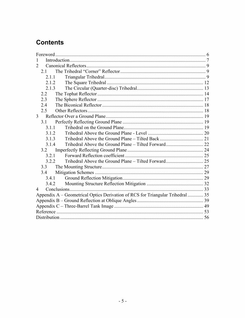
Figure 4. Contours of constant relative RCS for triangular trihedral corner reflector. Contour labels are in dBc.
Note that the −3 dB width of the trihedral response spans nearly 50 degrees in azimuth, and 40 degrees in elevation. Ruck, et al.1, indicate a 40 degree useful cone about the symmetry axis, i.e. the peak bore-sight direction, where useful is defined by the −3 dB response contour. They also describe alterations to the shape of the panels to “flatten” the response as a function of angles.
Table 1 shows some peak RCS values for trihedrals with different dimensions at Ku-band.
Table 1. Peak RCS for Triangle Trihedral Corner Reflector at Ku-band.
Interior edge dimension (a)
RCS
12 inches 20.5 dBsm
16 inches 25.5 dBsm
20 inches 29.3 dBsm
In addition, should the side panels be other than triangles, the formula for RCS changes somewhat.
- 12 -
2.1.2 The Square Trihedral
For a trihedral corner reflector made up of square plates, as in Figure 2(b), the peak RCS is calculated as
2
4
,12
λπσ a
peaksquare = . (4)
This is also maximum at a 35.26 degree grazing angle. More generally,
( )⎪⎪
⎩
⎪⎪
⎨
⎧
≥⎟⎟⎠
⎞⎜⎜⎝
⎛⎟⎟⎠
⎞⎜⎜⎝
⎛−
≤⎟⎟⎠
⎞⎜⎜⎝
⎛
=
2for44
2for44
,3
2
2
2
31
42
32
2
3
2142
ccccca
ccc
cca
square
λπ
λπ
θψσ (5)
where 321 ,, ccc are each assigned one of
⎪⎩
⎪⎨
⎧=
⎪⎭
⎪⎬
⎫
θψθψ
ψ
coscossincos
sin
3
2
1
ccc
(6)
such that 321 ccc ≤≤ .
Ruck, et al.1, indicate a 23 degree useful cone about the symmetry axis, i.e. the peak bore-sight direction. This width is considerably less than the triangular trihedral, although the peak response is greater for an equal dimension a. In fact, for equal dimension a, the square trihedral offers greater RCS than the triangular trihedral at all relevant angles, just more so in the bore-sight direction.
- 13 -
-10
-10 -10
-10
-10
-10
-10
-10
-6
-6
-6
-6
-6
-6
-3-3
-3
-3 -1
-1azimuth (deg.)
elev
atio
n (d
eg.)
10 20 30 40 50 60 70 8010
20
30
40
50
60
70
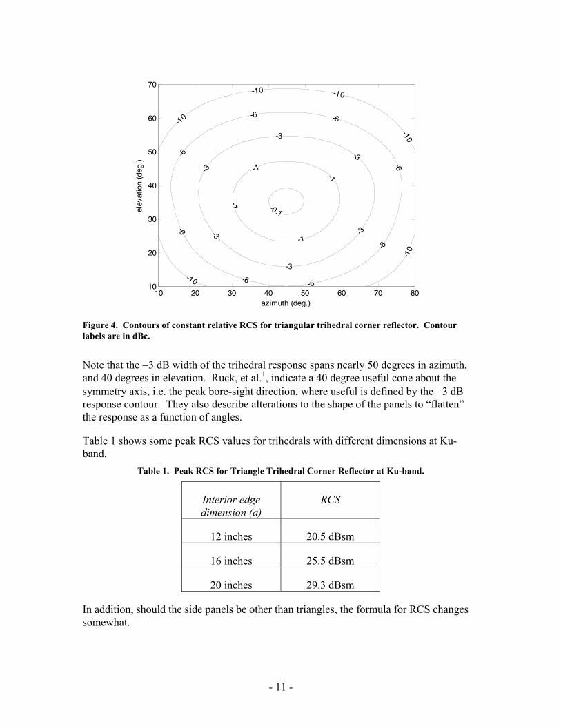
Figure 5. Contours of constant relative RCS for square trihedral corner reflector. Contour labels are in dBc.
2.1.3 The Circular (Quarter-disc) Trihedral
For a trihedral corner reflector made up of circular, or quarter-disc plates, as in Figure 2(c), the peak RCS is calculated as
2
4
,6.15λ
σ apeakcircular = . (7)
Ruck, et al.1, indicate a 32 degree useful cone about the symmetry axis, i.e. the peak bore-sight direction. This falls between the triangular trihedral and the square trihedral, as does the peak response for an equal dimension a.
- 14 -
2.2 The Tophat Reflector
The tophat reflector is shown in Figure 6 with dimensions defined.
a
b
L
a
b
L
Figure 6. Tophat reflector.
The tophat functions as an effective dihedral reflector that is isotropic with azimuth angle. Its peak RCS is given by
22
2
,8
bL
Labpeaktophat
+=
λπσ . (8)
This again assumes a geometrical optics model analysis which assumes that dimensions are large with respect to a wavelength. Note that this is the peak RCS, and the observable RCS will be somewhat elevation angle dependent. Figure 7 simplifies the geometry definitions of the relevant reflecting surfaces of the tophat.
b
L
ψ
Figure 7. Dihedral geometry definitions.
The elevation angle dependence of the tophat is reported by Silverstein and Bender5 as
- 15 -
( )⎪⎪⎩
⎪⎪⎨
⎧
≤
≥=
LbforaLLbforab
tophatψ
λψψπ
ψλ
ψπ
ψσtancostan8
tancos8
22
2
(9)
where peak response is at an elevation angle such that
Lb=0tanψ . (10)
The RCS may also be expressed as
( ) ( )ψψψλ
πψσ 2222 sin,cosmincos8 Lba
tophat ⎟⎟⎠
⎞⎜⎜⎝
⎛= . (11)
The two cases basically depend on whether the effective ‘aperture’ of the tophat is limited by the tophat height (b), or the tophat plate (L). Figure 8 illustrates how RCS depends on elevation angle for various ratios of L to b.
10 20 30 40 50 60 70 80-20
-15
-10
-5
0
5
0.5
1
2
3
elevation (deg.)
dBc
Figure 8. Tophat RCS relative to peak value as a function of elevation angle for various ratios (L/b).
Note that as the elevation angles approach normal to any surface, direct reflection dominates and this formula becomes inaccurate.
A derivative of the tophat reflector is one that implements just an angular segment of the tophat, and is sometimes referred to as a Bruderhedral. An example is illustrated in Figure 9.
- 16 -
Figure 9. The Bruderhedral is a section of a tophat reflector.
A more complete discussion of tophats and related Bruderhedrals can be found in the literature.5
Table 2 shows some peak RCS values for tophats with different dimensions at Ku-band.
Table 2. Peak RCS for tophats at Ku-band.
Cylinder radius (a)
Cylinder height (b)
Plate extension (L)
RCS
12 inches 12 inches 12 inches 14.5 dBsm
16 inches 16 inches 16 inches 18.2 dBsm
20 inches 20 inches 20 inches 21.1 dBsm
- 17 -
2.3 The Sphere Reflector
The RCS of a sphere is isotropic, and if the sphere is large compared to a wavelength, can be calculated as
2asphere πσ = (12)
where a is the radius of the sphere. The characteristics of a sphere at dimensions approaching a wavelength, and at dimensions less than a wavelength are also well studied and reported in the literature, including by Barton6 among others.
Table 3 shows some RCS values for spheres of various dimensions.
Table 3. Peak RCS for Conducting Spheres at Ku-band.
Sphere radius RCS
8 inches −14.9 dBsm
10 inches −13.0 dBsm
20 inches −6.9 dBsm
- 18 -
2.4 The Biconical Reflector
An interesting reflector that exhibits useful azimuth isotropic RCS at low grazing angles is the biconical reflector, illustrated in Figure 10.
2a1
90o
a2
2a1
90o
a2
Figure 10. Biconical reflector.
Its peak RCS is given by Whitrow7, as
( )2
23
11221, 2298
⎥⎦⎤
⎢⎣⎡ −−+= aaaaapeakbiconical λ
πσ . (13)
Whitrow states that the formulas given by Bonkowski, et al. 2, and Crispin and Siegel3, contain errors due to “mathematical errors in the evaluation of an integral”, and that in Ruck, et al.1, contains a further “typographical error”.
2.5 Other Reflectors
Numerous other canonical reflector types exist. A short listing of some of them includes dihedrals, flat plates, cylinders, Luneberg lenses, cylindrical Eaton-Lippman lens, and Van Atta arrays.
An interesting standard target for a number of SAR target recognition studies is known as “Slicey”, which is made up of a special arrangement of cutouts and other canonical components.8
- 19 -
3 Reflector Over a Ground Plane The previous discussion of canonical reflectors assumed their employment in free space. However, for SAR and GMTI measurements, these reflectors are placed in the target scene where the target scene is the ground itself or objects in proximity to the ground. Consequently, the interaction of the ground with the reflector needs to be considered for accurate RCS prediction. This is the classical problem for outdoor RCS ranges.9
Additional surfaces in proximity to the reflector provide the possibility of undesired reflections. These are collectively termed ‘multipath’ effects.
Hereafter we will limit our discussion to triangular trihedral corner reflectors. We will use the term ‘level’ reflector to refer to a trihedral with one plate parallel to the ground surface. Anything else is ‘tilted’.
3.1 Perfectly Reflecting Ground Plane
3.1.1 Trihedral on the Ground Plane
Consider a level reflector placed directly onto a perfectly reflecting ground plane, as illustrated in Figure 11. We will assume that the lower plate is negligibly thin. With this configuration, the ground plane acts as an extension of the lower plate. Consequently, the dimensions of the trihedral have effectively been altered in a manner to yield a larger reflecting surface, thereby increasing the trihedral’s RCS somewhat. From the analysis in Appendix A, the additional reflecting area of one ‘tip’ will provide an increase of 1.34 dB in the bore-sight direction of the trihedral at a 35.26 grazing angle. This is expected to be greater at lower grazing angles.
Figure 11. Placing a trihedral on a ground plane adds reflection opportunities thereby increasing effective RCS. The shaded region of the corner now contributes to the RCS.
- 20 -
3.1.2 Trihedral Above the Ground Plane - Level
Now consider the case where we elevate the level trihedral to some height above the ground, as illustrated in Figure 12. The desired echo from the trihedral corresponds to the phase center at point A. However, the shaded region of the trihedral combines with the reflective ground plane to yield a secondary normally undesired response with phase center at point B.
h
A
B ψ
Primary phase center response
Secondary phase center response
h
A
B ψ
Primary phase center response
Secondary phase center response
Figure 12. Trihedral corner reflector placed above a ground plane. Note that this yields responses from two phase centers due to reflection from the upper ‘tip’ of the trihedral.
The responses are at different ranges, with the range differential given by
ψsinhr =Δ . (14)
If the range differential is less than the range resolution of the radar, then the two responses will interfere with each other, perhaps adding in-phase constructively, perhaps adding out-of-phase destructively, depending on exactly what rΔ is.
Note that at Ku-band with a wavelength of 18 mm, a difference in rΔ of 4.5 mm marks the difference between maximum constructive and maximum destructive addition. For a trihedral placed 1 m above the ground plane and a nominal 30 degree grazing angle, this amounts to a change of 0.3 degrees in grazing angle. This is achieved with a 22 m altitude difference at a 5 km range.
Adding constructively will yield an RCS enhancement similar to placement of the trihedral on the ground, e.g. a gain of 1.34 dB at a 35.26 grazing angle.
- 21 -
Adding destructively will diminish the apparent RCS of the trihedral by effectively cancelling the contribution from a portion of the open face of the trihedral. At a 35.26 degree grazing angle this amounts to about 1.58 dB loss from the nominal value.
These gains and losses are both expected to be greater at lower grazing angles
If the range differential is greater than the range resolution of the radar, then the echoes of the two phase centers (A and B) will appear in different range bins. However, their sidelobes may still interfere with each other.
One way to avoid interference from the ground plane is to choose a height sufficient to separate the two phase centers by several resolution units. For example, if we wish to operate at a 10 degree grazing angle with =rρ 0.3 m resolution, with three resolution units of separation, then we require
rhr ρψ 3sin >=Δ (15)
or for our example >h 5.2 m. This is a pretty tall pole.
3.1.3 Trihedral Above the Ground Plane – Tilted Back
Another mitigation scheme is to tip the trihedral back (away from the radar) by an amount sufficient to spoil the right angle between the ground plane and the formerly upright plates. This is illustrated in Figure 13. The question is “How much should we tilt?” Since geometrical optics is not adequate for this task we revert to Fourier analysis.
β
2β
desired reflection
undesired reflection
β
2β
desired reflection
undesired reflection
Figure 13. Geometry of trihedral tilted back to mitigate undesired reflections.
For a uniformly aperture of length D we identify the nominal beamwidth of the aperture as
- 22 -
Dλθ = . (16)
Along the bore-sight of the trihedral, using the analysis of Appendix A, the elevation aperture is given by
32aD = . (17)
The elevation aperture of the indirectly illuminated tip is half this.
The tilt angle β needs to be great enough to cause the beams from these regions to not overlap. The difference in beam directions is β2 . Consequently, we identify the necessary condition
⎟⎟⎟⎟⎟
⎠
⎞
⎜⎜⎜⎜⎜
⎝
⎛
⎟⎟⎠
⎞⎜⎜⎝
⎛+
⎟⎟⎟⎟⎟
⎠
⎞
⎜⎜⎜⎜⎜
⎝
⎛
⎟⎟⎠
⎞⎜⎜⎝
⎛>
32
212
1
322
12aa
λλβ . (18)
This can be solved to yield
⎟⎠⎞
⎜⎝⎛≈⎟
⎠⎞
⎜⎝⎛>
aaλλβ 92.0
2433 (19)
where β is in radians, or
⎟⎠⎞
⎜⎝⎛>
aλβ 53 degrees. (20)
For example, a trihedral with 30 cm height at Ku-band has a nominal 4.2 degree beamwidth. Consequently it would need to be tilted back at least 3.2 degrees. At grazing angles other than trihedral bore-sight, the tilt would need to increase somewhat.
This concept also works for a forward tilt up to an angle equal to the grazing angle with respect to the ground plane.
3.1.4 Trihedral Above the Ground Plane – Tilted Forward
Often the desired grazing angle is substantially less than the bore-sight grazing angle from a level trihedral. The temptation is to tilt the trihedral forward to better align the trihedral’s bore-sight with the actual grazing angle. This is illustrated in Figure 14.
- 23 -
βh
desired reflection
undesired reflection
ψ
ψβh
desired reflection
undesired reflection
ψ
ψ
Figure 14. Trihedral tilted forward to reduce the grazing angle of its bore-sight.
A problem with this arrangement is that the ground-bounce now is within the response envelope of the trihedral itself. That is, there exists a ground-trihedral-ground bounce back in the direction of the radar. This will, of course, potentially interfere with the desired direct reflection.
As with the level trihedral, the responses are at different ranges, however now the range differential is given by
ψsin2hr =Δ . (21)
As before, if the range differential is less than the range resolution of the radar, then the two responses will interfere with each other, perhaps adding in-phase constructively, perhaps adding out-of-phase destructively, depending on exactly what rΔ is.
The relative magnitude of the desired and undesired reflections depends on the relative RCS difference corresponding to the ψ2 angular aspect difference of the trihedral to the two signals, the direct and the ground bounce signals.
We define the relationship of the undesired RCS ( undesiredσ ) to the desired RCS ( desiredσ ) as
desiredtrihedralundesired σασ = (22)
where trihedralα is the attenuation factor due to the trihedral, which is orientation dependent.
As example, for a trihedral oriented with bore-sight towards a radar at a 10 degree elevation angle with respect to ground, the undesired ground bounce is only 20 degrees below the trihedral bore-sight, which from Figure 4 may exhibit an RCS only 3.5 dB below the bore-sight response. In this case trihedralα = 0.45.
- 24 -
In general, the phase associated with rΔ is fairly sensitive to even small variations in h and/or ψ . Consequently, we can typically treat the phase due to rΔ as pretty much random from one radar pass to the next. Therefore, we can calculate the combined RCS as
where ϕ is the phase difference between the desired and undesired echo signals. From this expression we may readily observe that
( ) ( )trihedraldesiredcombined ασσ += 1mean , and
( ) trihedraldesiredcombined ασσ 2std = . (24)
For our earlier example with trihedralα = 0.45, the net RCS will be anywhere from 9.65 dB below the bore-sight RCS to 4.46 dB above the bore-sight RCS. The mean net RCS will exhibit a bias of 1.6 dB above the trihedral bore-sight RCS, with a standard deviation of −0.23 dB with respect to the trihedral bore-sight RCS. That is, the standard deviation of the net RCS will be nearly the trihedral’s bore-sight RCS itself.
As before, if the range differential is greater than the range resolution of the radar, then the two echo signals will appear in different range bins. However, their sidelobes may still interfere with each other.
Once again, we may avoid interference from the ground plane by choosing a height sufficient to separate the two phase centers by several resolution units. For example, at a 10 degree grazing angle with =rρ 0.3 m resolution, with three resolution units of separation, then we require
rhr ρψ 3sin2 >=Δ (25)
or for our example >h 2.6 m. While perhaps useful for RCS measurements, this would be inadequate for Impulse Response (IPR) evaluation.
3.2 Imperfectly Reflecting Ground Plane
We now extend the results of the previous section to a ground plane that does not reflect perfectly.
- 25 -
3.2.1 Forward Reflection coefficient
Data on forward scattering of the ground is rather meager in the literature. This is a subset of bistatic reflectivity. Appendix B details some analytical results. These are summarized as follows.
For Ku-band at shallow grazing angles over reasonably flat terrain as one might find at a radar reflector test site, it is not unreasonable to encounter high-single-digit (in dB) attenuation from a ground bounce for V polarization, and low-single-digit (in dB) attenuation from a ground bounce for H polarization. The V polarization will be more sensitive to soil moisture content, exhibiting the least attenuation (most reflection) for arid soils.
We will henceforth denote the magnitude of forward reflection power attenuation factor as groundα . We relate this to the factors in Appendix B as
2sground ρα Γ= . (26)
3.2.2 Trihedral Above the Ground Plane – Tilted Forward
We repeat the case where the desired grazing angle is substantially less than the bore-sight grazing angle from a level trihedral. Furthermore, we tilt the trihedral forward to better align the trihedral’s bore-sight with the actual grazing angle. This is illustrated in Figure 15, except that now the ground bounce will also attenuate the signal.
βh
desired reflection
undesired reflection
ψ
ψβh
desired reflection
undesired reflection
ψ
ψ
Figure 15. We repeat Figure 14 here but now recognize that the ground bounce will also attenuate the signal.
As before, the problem with this arrangement is that the ground-bounce is within the response envelope of the trihedral itself. That is, there exists a ground-trihedral-ground bounce back in the direction of the radar. This will, of course, potentially interfere with the desired direct reflection.
- 26 -
As with the perfectly reflecting ground plane, if the range differential is less than the range resolution of the radar, then the two responses will interfere with each other, perhaps adding in-phase constructively, perhaps adding out-of-phase destructively, depending on exactly what rΔ is, and what phase change the ground bounces induce.
The relative magnitude of the desired and undesired reflections still depends on the relative RCS difference corresponding to the ψ2 angular aspect difference between the direct and the ground bounce signals, but now also depends on the attenuation encountered with the two ground bounces.
We alter the relationship of the undesired RCS ( undesiredσ ) to the desired RCS ( desiredσ ) as
We can typically continue to treat the phase due to rΔ as pretty much random from one radar pass to the next, and any phase changes due to the ground bounces will not alter the distribution. Therefore, we can calculate the combined RCS as
We repeat our earlier example with a trihedral oriented with bore-sight towards a radar at a 10 degree elevation angle with respect to ground, but now assuming, say,
25.0=groundα or a −6 dB single-bounce reflection, consistent with a VV polarization radar operating over an arid test range. Note that we still have trihedralα = 0.45. With
these parameters, 028.02 =groundtrihedralαα , or −15.5 dB. This will cause the apparent RCS to be anywhere from −1.59 dB to +1.35 dB with respect to the bore-sight RCS.
The mean net RCS will exhibit a bias of 0.12 dB above the trihedral bore-sight RCS, with a standard deviation of −6.25 dB with respect to the trihedral bore-sight RCS. That is, the standard deviation of the net RCS will be approximately 6 dB below the trihedral’s bore-sight RCS.
As before, if the range differential is greater than the range resolution of the radar, then the two echo signals will appear in different range bins. However, their sidelobes may
- 27 -
still interfere with each other. An example of an attenuated ground bounce appearing in a different range bin is given in Appendix C.
3.3 The Mounting Structure
If a reflector is mounted above the ground, then the possibility exists of undesired reflections from the mounting structure interfering with the echo from the desired reflector itself. While mounting structures can take many forms, e.g. poles, tripods, tables, etc., we will consider herein as example a vertical metal cylindrical pole, with geometry shown in Figure 16.
desired reflection
undesired reflection
ψ
d
b
desired reflection
undesired reflection
ψ
d
b
Figure 16. Trihedral mounted on vertical metal cylindrical pole.
Note that the mounting pole makes a tophat reflector with the ground. If the pole dimensions are large with respect to wavelength, then we can estimate its effective RCS as
( ) ψλπαψσ cos4 2dbgroundpole = . (30)
For example, consider a 10 cm wide pole that is 1 m tall over ground with −6 dB forward scattering, with a 1.8 cm wavelength at 10 degree grazing angle. Using this formula will yield an RCS of about +12 dBsm that will likely fall in the same range gate as the desired reflection from the trihedral.
Let us define the relative RCS of the pole as
trihedral
polepole σ
σα = . (31)
Then we can estimate the combined RCS as
- 28 -
( )ϕαασσ cos21 polepoledesiredcombined ++= (32)
where ϕ is a relative phase, and can be presumed to be random from one radar pass to another.
Continuing the earlier example, if the pole mounts a 16 inch trihedral, then the mounting pole echo is only 6 dB below the trihedral’s reflection. This will cause the apparent RCS to be anywhere from −6 dB to +3.5 dB with respect to the bore-sight RCS. The mean net RCS will exhibit a bias of 0.97 dB above the trihedral bore-sight RCS, with a standard deviation of −1.5 dB with respect to the trihedral bore-sight RCS.
Reflections from a mounting pole are clearly undesirable.
A secondary concern is the increased susceptibility of a pole-mounted corner reflector to wind-induced motions.
Figure 17. Trihedral reflector mounted on a pole. Note downward tilt of corner.
- 29 -
3.4 Mitigation Schemes
Two interference phenomena have been identified. The first was multipath ground bounce into the reflector directly. The second was undesired reflections from the mounting structure of the reflector. Mitigating the effects of these is precisely the problem that faces RCS calibration and test ranges, and a number of techniques have been developed for these ranges. Knott, et al.9, discuss some of these issues. We mention some possible mitigation techniques here.
3.4.1 Ground Reflection Mitigation
The most obvious scheme for mitigating problematic ground reflections is to minimize the opportunity for them altogether. Placing the reflector with phase center or apex at ground level eliminates any double ground bounces, although single ground bounces may still be a problem. This configuration, of course, often limits the RCS available at very shallow grazing angles. Consequently, other techniques may sometimes need to be considered as well.
Range Gating
Range gating takes advantage of the range difference between the direct reflection and any ground bounce reflections. This has already been discussed in earlier sections. Note that intentionally increasing range differences at shallow grazing angles requires fairly tall mounting structures. Consequently this may often not be a viable technique.
Attenuating Reflections
If ground reflections are problematic, then perhaps viable techniques for minimizing ground reflections is to minimize the reflectivity of the ground in the region of the reflection. This is illustrated in Figure 18.
h
desired reflection
undesired reflectionregionh
desired reflection
undesired reflectionregion
Figure 18. Reducing the reflectivity in the region of ground bounce will reduce ground reflections.
- 30 -
From Appendix B, we note that wetter soils are less reflective than dryer soils at shallow grazing angles. Consequently, wetting the soil in the region of the expected ground bounce would reduce ground reflections.
A more robust method might be to use radar absorber material in the region of the ground bounce.
Redirecting Reflections
Energy that would otherwise interfere with the desired reflection via one or more ground bounces might be intentionally reflected in non-interfering directions.
A radar ‘fence’ may be erected in front of the desired reflector as illustrated in Figure 19. A properly dug pit in front of the reflector might serve the same purpose as illustrated in Figure 20. Often such fences have serrated edges to mitigate diffraction effects.
desired reflections
redirected reflection
desired reflections
redirected reflection
Figure 19. A radar 'fence' may be used to redirect otherwise problematic reflections.
desired reflections
redirected reflection
desired reflections
redirected reflection
Figure 20. A pit dug in front of the reflector might also redirect otherwise problematic reflections.
- 31 -
A technique used in RCS test and measurement ranges is to employ an inverted “Vee” apron in front of the reflector, as is illustrated in Figure 21.
Figure 21. Sandia National Laboratories inverted "Vee" outdoor RCS test range. The stationary radar instrument is at the far end of the Vee. The device under test was mounted on a pedestal to the right of the camera. Currently the test range is used principally as a base for reflector placement for airborne tests. Note trihedral reflector array placed along peak of the Vee.
- 32 -
3.4.2 Mounting Structure Reflection Mitigation
The most obvious mitigation scheme to mitigating reflections from mounting structures is to not use mounting structures at all. That is, set the desired reflector on the ground itself. Only if this is not practical for other reasons, then other mitigation schemes might find utility.
Attenuating Reflections
If a mounting structure is non-reflecting, then reflections are not an issue. Consequently choosing a material that has reduced reflective properties might be considered. Otherwise, a fence or coating of radar energy absorber material might also be considered.
Redirecting Reflections
The problem is energy that is reflected back towards a monostatic radar from the mounting structure. Energy reflected in other directions is not problematic. Avoiding back-reflections is achieved by avoiding normal planar surfaces, and avoiding right angles where surfaces join.
The tophat effect can be avoided by using a mounting pole that is not vertical on horizontal ground, and/or using a ‘blade’ or ‘wedge’ instead of a round pole.
Otherwise a reflecting ‘skirt’ might be employed to hide any right angles in a radar shadow.
Examples are shown in Figure 22. Of course, combinations of these may also be used. Furthermore, a creative mind may conjure a seemingly infinite variety of similar strategies and techniques.
(a) (b) (c)(a) (b) (c) Figure 22. Example techniques for redirecting reflections from mounting structures. These include (a) mounting pole in non-vertical position, (b) using a blade or wedge ‘pole’, and (c) using a skirt.
- 33 -
4 Conclusions The following points are worth repeating.
• Most canonical reflectors have an RCS that is aspect dependent.
• Most equations for RCS for canonical targets presume the target is in free space. A number of these were provided in this report.
• Reflections from the ground will modify the apparent RCS of a reflector. RCS may increase or decrease depending on whether ground-bounce energy adds in-phase or out-of-phase. This effect can be quite severe.
• Reflections from the ground are particularly problematic when reflectors are tilted to present large RCS aspects in low grazing-angle directions.
• Ground-bounce at shallow grazing angles is substantially more severe for horizontal polarization than for vertical polarization.
• Reflections from any reflector mounting structure will also modify the apparent RCS of a reflector. RCS may also increase or decrease depending on whether ground-bounce energy adds in-phase or out-of-phase. This effect can also be quite severe.
• Mitigation techniques are possible to minimize deleterious effects of reflections from the ground and/or mounting structure.
- 34 -
If you want a guarantee, buy a toaster.
- Clint Eastwood
- 35 -
Appendix A – Geometrical Optics Derivation of RCS for Triangular Trihedral The intent of this appendix is to provide justification for several points made in the main text. The following development will presume a trihedral corner reflector in free space, using geometrical optics as a basis for analysis. A more rigorous development can be found in the literature.
The purpose of a trihedral corner reflector is to reflect energy back in the direction of its distant source. This is the attractive feature to radar testing.
Consider a trihedral corner reflector made up of three isosceles right triangle plates with dimensions as shown in Figure 23. A perspective towards the open face of the trihedral is given in Figure 23(b). A perspective parallel to the open face is given in Figure 23(c).
2a
a
2a
a
(a) (b)
a
(c)
2a
a
2a
a
2a
a
(a) (b)
a
(c) Figure 23. Trihedral corner reflector made up of three isosceles right triangle plates, with (a) an oblique view, (b) normal to the open face view, and (c) a profile parallel to the open face view. Dimensions are of the actual edges, and not of edge projections.
We can calculate the area of the planar segment that makes up the open face as
223 aAface = . (A1)
If the trihedral were substituted with a flat plate with area equal to the open face, the RCS of the flat plate would be calculated as
42
22
34 aAfaceface λπ
λπσ == . (A2)
- 36 -
However, from a geometrical optics model, not all areas of the face will reflect energy back towards the source. Consequently, the actual RCS will be somewhat less than this.
Consider Figure 23(c), which we redraw and augment as Figure 24 below, where dimensions are now the projected lengths or distances as viewed. Figure 24 allows us to perform relevant analysis in two dimensions, thereby simplifying the analysis for the moment.
a
(a)
2a
ψ0
2a
ψ0
d
(b)
a
(a)
2a
ψ0
2a
ψ0
d
(b) Figure 24. Trihedral projection parallel to the open face, with (a) showing the direction of maximum reflection, and (b) showing the ray path of a ‘bounce’ from the bottom edge of the reflector.
First we identify the direction of maximum RCS as normal to the open face of the reflector. From Figure 24 we can readily calculate
26.352
1tan 10 ≈⎟
⎠⎞
⎜⎝⎛= −ψ degrees. (A3)
Figure 24(b) shows how a ray entering the open face at the bottom edge of the open face is bounced back to the direction of its distant source. In fact, any ray entering the bold portion of the face will be so reflected. However, rays entering the face outside of the bold region will not be reflected back to the source. This represents a length d in the figure. Consequently, this portion of the face will not contribute to the RCS. The length d can readily be calculated as
6ad = . (A4)
Returning to a plan view of the open face, we identify the regions of no useful reflection in Figure 25. These areas do not contribute to the RCS of the trihedral when viewed from its perspective of maximum RCS.
- 37 -
2a
6a
26a
2a
6a
2a
6a
26a
Figure 25. Regions of the trihedral open face not contributing to the RCS are shaded.
The area of a single of the three ‘tips’ or regions of no reflection is calculated as
36
2aAtip = . (A5)
Consequently, the hexagonal area of the face that contributes to the RCS is given by
3363
233
22 aaAAA tipfaceRCS =⎟⎟
⎠
⎞⎜⎜⎝
⎛−=−= . (A6)
The RCS of a flat plate with this remaining area is given by
2
42
2 344
λπ
λπσ aARCStrihedral == . (A7)
This is the classical formula found in the literature.
With malice of forethought, we can calculate the effect of adding back reflections from a single ‘tip’, which yields
⎟⎠⎞
⎜⎝⎛=⎟
⎟⎠
⎞⎜⎜⎝
⎛+=+ 36
493
4363
42
4222
2 λπ
λπσ aaa
tiptrihedral . (A8)
This is a net 1.34 dB increase in RCS.
- 38 -
We reiterate that the previous development for RCS assumed a bore-sight direction. Consequently, the noncontributing regions of the trihedral to the RCS also assumed a bore-sight direction. The noncontributing regions will depend on aspect angle, that is, they will change in directions other than the bore-sight.
Nevertheless, it is interesting to note that sometimes trihedrals are constructed with these noncontributing regions trimmed away. Figure 26 and Figure 27 illustrate examples of this. This is also discussed in some detail by Sarabandi and Chiu.4
Figure 26. A ‘trimmed’ trihedral corner reflector for orbital SAR calibration. (courtesy of Wade Albright, Calibration Engineer, Alaska Satellite Facility)
Figure 27. Another example of a trimmed trihedral corner reflector. (courtesy of Institut für Geotechnik und Markscheidewesen).
- 39 -
Appendix B – Ground Reflection at Oblique Angles An excellent summary of ground surface scattering is given in a report by Brock & Patitz.10 Another good discussion is by Ruck, et al.1 Nevertheless, for completeness in this report, we develop a similar model and provide relevant comments in this appendix.
Dielectric Effects at a Planar Interface
Consider an oblique incidence on a planar dielectric boundary. Then from Balanis11 we identify the reflection coefficients as ratios of electric field strengths given by
ti
tibθηθηθηθη
coscoscoscos
12
12+−=Γ⊥ for perpendicular polarization, and
ti
tibθηθηθηθη
coscoscoscos
21
21|| +
−−=Γ for parallel polarization, (B1)
where
iθ = the incidence angle,
it θγγθ sinsin
2
1= from Snell’s law of refraction, (B2)
and where for medium k
kk
kk j
jωεσ
ωμη+
= = wave impedance,
kμ = magnetic permeability (H/m),
kε = electric permittivity (F/m),
kσ = electric conductivity (S/m),
kkk jβαγ += = propagation constant,
21
2
1121
⎪⎭
⎪⎬⎫
⎪⎩
⎪⎨⎧
⎥⎥⎥
⎦
⎤
⎢⎢⎢
⎣
⎡−⎟⎟
⎠
⎞⎜⎜⎝
⎛+=
k
kkkk ωε
σεμωα = attenuation constant (Np/m),
21
2
1121
⎪⎭
⎪⎬⎫
⎪⎩
⎪⎨⎧
⎥⎥⎥
⎦
⎤
⎢⎢⎢
⎣
⎡+⎟⎟
⎠
⎞⎜⎜⎝
⎛+=
k
kkkk ωε
σεμωβ = phase constant (rad/m), and
ω = frequency (rad/sec). (B3)
- 40 -
We shall presume medium 1 is free space. Then
701 104 −×== πμμ H/m,
1201 10854.8 −×≈= εε F/m,
1σ = 0, and
00
1εμ
=c = velocity of propagation in free space. (B4)
For our purposes, this is also a reasonable approximation for the earth’s atmosphere.
In general, 2μ and 2ε may be complex. Furthermore we define relative quantities as
where conductivity has been accounted for within the effective relative permittivity.
- 41 -
We also identify the electric and magnetic loss tangents as
2
2tanr
re ε
εδ′′′
= , and
2
2tanr
rm μ
μδ′′′
= . (B9)
Combining some relationships yields
( )
( )⎥⎥⎥⎥⎥⎥
⎦
⎤
⎢⎢⎢⎢⎢⎢
⎣
⎡
⎟⎟⎠
⎞⎜⎜⎝
⎛−⎟⎟
⎠
⎞⎜⎜⎝
⎛+
⎟⎟⎠
⎞⎜⎜⎝
⎛−⎟⎟
⎠
⎞⎜⎜⎝
⎛−
=Γ⊥
22
2
1
2
1
22
2
1
2
1
sin1cos
sin1cos
ii
iib
θγγ
ηηθ
θγγ
ηηθ
, and
( )
( )⎥⎥⎥⎥⎥⎥
⎦
⎤
⎢⎢⎢⎢⎢⎢
⎣
⎡
⎟⎟⎠
⎞⎜⎜⎝
⎛−+⎟⎟
⎠
⎞⎜⎜⎝
⎛
⎟⎟⎠
⎞⎜⎜⎝
⎛−−⎟⎟
⎠
⎞⎜⎜⎝
⎛
−=Γ2
2
2
1
2
1
22
2
1
2
1
||
sin1cos
sin1cos
ii
iib
θγγθ
ηη
θγγθ
ηη
. (B10)
We identify
2
2
2
1
r
rμε
ηη = . (B11)
Soil dielectric property data by several authors suggest that loss tangents for soils at microwave frequencies are rather small. Some of this data is discussed later. Consequently we may presume
12
2 <<ωεσ . (B12)
This allows the approximation
222
1 1
rr εμγγ ≈ . (B13)
Combining these with the previous results yields
- 42 -
( )( ) ⎥
⎥
⎦
⎤
⎢⎢
⎣
⎡
−+
−−=Γ⊥ 2
222
2222
sincos
sincos
irrir
irrirb
θεμθμ
θεμθμ , and
( )( ) ⎥
⎥
⎦
⎤
⎢⎢
⎣
⎡
−+
−−−=Γ
2222
2222
||sincos
sincos
irrir
irrirb
θεμθε
θεμθε . (B14)
At this point we make some observations.
• This development is treated from strictly an electromagnetic reflection problem, and used the notation of Balanis. We will now begin to translate these results into some terms more familiar to radar engineers.
• Perpendicular polarization corresponds to horizontal (H) polarization. Parallel polarization corresponds to vertical polarization (V). The behavior of reflections is different for the two.
• The incidence angle iθ is with respect to the normal vector to the planar surface. It is the complement to the grazing angle ψ.
• Soils are frequently presumed to be nonmagnetic, that is, with 12 =rμ . Nevertheless, we shall carry along the option for a magnetic soil for the time being.
We refine our reflection equations to
( )( ) ⎥
⎥
⎦
⎤
⎢⎢
⎣
⎡
−+
−−=Γ
2222
2222
cossin
cossin
ψεμψμ
ψεμψμ
rrr
rrrbH , and
( )( ) ⎥
⎥
⎦
⎤
⎢⎢
⎣
⎡
−+
−−−=Γ
2222
2222
cossin
cossin
ψεμψε
ψεμψε
rrr
rrrbV . (B15)
A number of sources define the reflection coefficient of the parallel, or vertical, polarization case in terms of the magnetic field. This causes a sign difference in b
||Γ and
consequently in bVΓ . Such is the case with Knot, et al.,9 although they also assume
12 =rμ . In any case, since we will ultimately be interested in magnitudes, this is inconsequential for our purposes.
- 43 -
Soil Characteristics
Dielectric properties for soils at microwave frequencies of X-band and above are not extensively reported in the literature. This is compounded by the fact that virtually infinite types of soil exist, and their dielectric properties are heavily dependent on moisture content and even temperature.
A classic paper on soil electromagnetic properties for two types of clay-loam mixtures is by Hipp12, but limits analysis to 3.84 GHz.
Another classic source by von Hippel13 presents measurements sometimes up to 10 GHz for several soils with varying water contents.
A NASA report by Wang, et al.14, presents complex dielectric parameters for a number of soil types with varying degrees of moisture content at 5 and 19.35 GHz
Sano, et al.15, report Ku-band dielectric constants for fields at the Maricopa Agricultural Center in Arizona with varying amounts of soil moisture.
A short paper by Abdulla, et al.16, presents complex dielectric constant measurements of several Iraqi soils at 10 GHz.
We note that several of these also point to other literature sources.
For our purposes, we do not wish to form a complete catalog of soil properties, nor a complete listing of literature on the subject. We do wish to bound reasonable forward scattering attenuation properties of common soil types. A perusal of the aforementioned literature suggests that typically at Ku-band, the real part of the relative dielectric constant may be anywhere from 2 to 20, with the imaginary part anywhere from 0 to 2/3 the value of the real part, with percentage increasing with moisture content. At 10% moisture content, the imaginary part of the relative dielectric constant is typically 20% of the real part.
While so-called ‘magnetic’ soils exist with non-unitary and complex relative permeability, these are treated in the literature as more of an aberration. Hence the default presumption is that relative permeability is unity.
Figure 28 through Figure 31 plot the magnitude of the reflection coefficient for both horizontal and vertical polarization over the real part of the dielectric constant, for various grazing angles. The imaginary part of the relative dielectric constant is limited to between 0 and 2/3 of the real part.
Clearly, at shallow grazing angles, and for low dielectric constant values, single-digit (in dB) attenuation of reflections is to be expected. The fact that V polarization exhibits greater attenuation for larger dielectric constants for the shallower grazing angles is due to those angles being below the Brewster angle. The minimums observed in the curves in Figure 30 and Figure 31 identify the Brewster angle.
- 44 -
0 5 10 15 20 25-25
-20
-15
-10
-5
0
5
H pol
V pol
dB
single bounce reflection at 5 deg.
Re(er) Figure 28. Magnitude of reflection coefficients at H and V polarization over the real part of the relative dielectric constant at 5 degree grazing angle. Imaginary parts of the relative dielectric constant are limited to between 0 and 2/3 of the real value.
0 5 10 15 20 25-25
-20
-15
-10
-5
0
5
H pol
V pol
dB
single bounce reflection at 10 deg.
Re(er) Figure 29. Magnitude of reflection coefficients at H and V polarization over the real part of the relative dielectric constant at 10 degree grazing angle. Imaginary parts of the relative dielectric constant are limited to between 0 and 2/3 of the real value.
- 45 -
0 5 10 15 20 25-25
-20
-15
-10
-5
0
5
H pol
V pol
dB
single bounce reflection at 15 deg.
Re(er) Figure 30. Magnitude of reflection coefficients at H and V polarization over the real part of the relative dielectric constant at 15 degree grazing angle. Imaginary parts of the relative dielectric constant are limited to between 0 and 2/3 of the real value.
0 5 10 15 20 25-25
-20
-15
-10
-5
0
5
H pol
V pol
dB
single bounce reflection at 20 deg.
Re(er) Figure 31. Magnitude of reflection coefficients at H and V polarization over the real part of the relative dielectric constant at 20 degree grazing angle. Imaginary parts of the relative dielectric constant are limited to between 0 and 2/3 of the real value.
- 46 -
Ground Roughness Effects
The effect of surface roughness on reflection coefficient is adapted from Ruck, et al.1, as
⎪⎭
⎪⎬⎫
⎪⎩
⎪⎨⎧
⎟⎠⎞
⎜⎝⎛−=
2sin22exp ψ
λσπρ h
s (B16)
where
hσ = RMS surface variations, and
λ = nominal wavelength = ωπc2 . (B17)
This equation presumes “(a) surface slopes everywhere must be somewhat less than unity and (b) radii of curvature everywhere must be larger than the wavelength.” The equation is plotted in Figure 32. Note that attenuation is minimal for very shallow grazing angles. Furthermore, even in the region 10-20 degrees, RMS roughness of even a substantial fraction of a wavelength allows significant reflection.
While more complex models of roughness exist, the point is adequately made that even some roughness in the reflecting surface can be tolerated with little effect in signal attenuation.
-20
-20
-20
-10
-10
-10
-10
-6
-6
-6
-6
-3
-3
-3
-3
-1-1
-1
-1-1
-0.1
-0.1
-0.1-0.1 -0.1
grazing angle (deg.)
norm
aliz
ed R
MS
rou
ghne
ss
0 2 4 6 8 10 12 14 16 18 200
0.2
0.4
0.6
0.8
1
1.2
1.4
1.6
1.8
2
Figure 32. Contours of constant attenuation in dB due to ground roughness as a function of grazing angle. Roughness is RMS normalized with respect to wavelength.
- 47 -
Combined Effects
Knott, et al., combine dielectric properties and surface roughness to calculate an effective reflection coefficient as
sρρ Γ= (B18)
where Γ is either bHΓ or b
VΓ , as the polarization of the signal demands. Note that the
power loss from a single-bounce ground reflection is proportional to 2ρ .
From the previous analysis, for Ku-band at shallow grazing angles over reasonably flat terrain as one might find at a radar reflector test site, it is not unreasonable to encounter high-single-digit (in dB) attenuation from a ground bounce for V polarization, and low-single-digit (in dB) attenuation from a ground bounce for H polarization. The V polarization will be more sensitive to soil moisture content, exhibiting the least attenuation (most reflection) for arid soils.
For example, we might expect in the fairly arid and flat terrain of Sandia’s test site to encounter about −10 dB of attenuation for a ground bounce at 15 degrees of grazing angle.
As a final note, we observe that vegetation has been ignored in this development. We can certainly expect some influence of vegetation on the forward scattering of terrain, even in rather arid areas such as the desert southwest of the US. However, bistatic scattering from vegetation is even less reported in the literature than soil electromagnetic properties. Cosgriff17 of Ohio State University presents results at L-band where two-inch grass at 16 degrees grazing angle exhibits −4 dB (H) and −10 dB (V) signal strength with respect to the direct signal, and a soybean field at 11.5 degree grazing angle exhibits up to −5 dB (H) and −14 dB (V). Studies summarized in Skolnik18 also support strong specular reflection even for vegetation clutter.
- 48 -
It isn't what we don't know that gives us trouble, it's what we know that ain't so.
- Will Rogers
- 49 -
Appendix C – Three-Barrel Tank Image An interesting SAR image for a number of reasons is given in Figure 33. This is a 0.1 m resolution Ku-band VV-polarization image produced by the Lynx SAR on 8 February 1999 of a column of M-47 tanks on Kirtland AFB near Albuquerque, New Mexico. In this image, near range is towards the bottom of the image.
The arrow points to a particular vehicle that is enlarged in Figure 34. Of particular interest is the flash off of the tank cannon barrel. In fact there are three apparent barrels, although only a single barrel actually exists. The brightest and nearest is the direct reflection, and the others are due to multipath. This is explored below.
freq = 16.7 GHz, res = 0.1016 x 0.1016 m, range = 6.5339 km, dep = 17.3717 deg, squint = 85.3646 deg
----
-->
357
.703
4 de
g
file: f1_171463_893.limg - magnitude only
200 400 600 800 1000 1200
100
200
300
400
500
600
700
800
900
Figure 33. SAR image of a 0.1 m resolution Ku-band image produced by the Lynx SAR, of a column of M-47 tanks on Kirtland AFB near Albuquerque, New Mexico.
From the image, we identify the nearest barrel return as the direct return. The next nearest barrel return is 7 pixels downrange from the direct return and the farthest of the three barrels is 13 pixels downrange from the direct return. Consequently, at 0.0847 m slant-range per pixel, the second and third barrels are apparently 0.6 m and 1.1 m further away than the direct return.
- 50 -
freq = 16.7 GHz, res = 0.1016 x 0.1016 m, range = 6.5339 km, dep = 17.3717 deg, squint = 85.3646 deg
----
-->
357
.703
4 de
g
file: f1_171463_893.limg - magnitude only
700 750 800 850 900
560
580
600
620
640
660
680
700
720
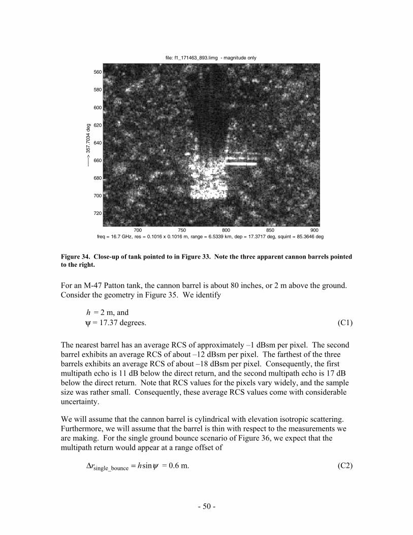
Figure 34. Close-up of tank pointed to in Figure 33. Note the three apparent cannon barrels pointed to the right.
For an M-47 Patton tank, the cannon barrel is about 80 inches, or 2 m above the ground. Consider the geometry in Figure 35. We identify
h = 2 m, and ψ = 17.37 degrees. (C1)
The nearest barrel has an average RCS of approximately –1 dBsm per pixel. The second barrel exhibits an average RCS of about –12 dBsm per pixel. The farthest of the three barrels exhibits an average RCS of about –18 dBsm per pixel. Consequently, the first multipath echo is 11 dB below the direct return, and the second multipath echo is 17 dB below the direct return. Note that RCS values for the pixels vary widely, and the sample size was rather small. Consequently, these average RCS values come with considerable uncertainty.
We will assume that the cannon barrel is cylindrical with elevation isotropic scattering. Furthermore, we will assume that the barrel is thin with respect to the measurements we are making. For the single ground bounce scenario of Figure 36, we expect that the multipath return would appear at a range offset of
ψsinncesingle_bou hr =Δ = 0.6 m. (C2)
- 51 -
h
ψ
hh
ψ
Figure 35. Direct return from the cannon barrel.
ψψ
Figure 36. Multipath return with ground-barrel bounce, and barrel-ground bounce.
ψψ
Figure 37. Multipath return with ground-barrel-ground bounce.
- 52 -
For the double ground bounce scenario of Figure 37, we expect that the multipath return would appear at a range offset from the direct return of
ψsin2ncedouble_bou hr =Δ = 1.2 m. (C3)
Accounting for cannon barrel thickness would reduce this slightly.
Considering the uncertainties in our measurements and assumptions, these are in excellent agreement with the measured offsets of 0.6 m and 1.1 m from the SAR image.
There does not appear to be any sign of a barrel-ground-barrel bounce.
We may also use this data to estimate the forward scattering properties of the ground around the tank. Since the ground-barrel and barrel-ground bounces involve oblique reflections from the barrel, we will confine our subsequent analysis to only the direct return and the ground-barrel-ground bounce. The ratio of these was measured to be approximately 17 dB. Since both ground bounces occurred at the same angles, this implies that 8.5 dB attenuation is due to each bounce.
Consequently, we infer that the forward scattering loss of the ground around the tank is about 8.5 dB at a 17.4 degree grazing angle at Ku-band for a single bounce. This value is consistent with analysis in Appendix B.
Figure 38. Photograph of the column of M-47 tanks in Figure 33.
Figure 39. Close-up of tank in Figure 38.
- 53 -
References
1 George T. Ruck, Donald E. Barrick, William D. Stuart, Clarence K. Krichbaum, Radar Cross Section Handbook, Vol. 2, SBN 306-30343-4, Plenum Press, 1970.
2 R. R. Bonkowski, C. R. Lubitz, C. E. Schensted, “Studies in Radar Cross-Sections VI, Cross-Sections of Corner Reflectors and Other Multiple Scatterers at Microwave Frequencies”, Project MIRO, UMM-106, University of Michigan Radiation Laboratory, October, 1953.
3 J. W. Crispin, Jr., K. M. Siegel, Methods of Radar Cross Section Analysis, Academic Press, New York, 1968.
4 K. Sarabandi, Tsen-Chieh Chiu, “Optimum corner reflectors for calibration of imaging radars”, IEEE Transactions on Antennas and Propagation, Volume: 44, Issue: 10, pp. 1348-1361, Oct 1996.
5 J. D. Silverstein, R. Bender, “Measurements and Predictions of the RCS of Bruderhedrals at Millimeter Wavelengths”, IEEE Transactions on Antennas and Propagation, Volume: 45, Issue: 7, pp. 1071-1079, Jul 1997.
6 David K. Barton, Radar System Analysis, Prentice-Hall, Inc., 1964.
7 J. L. Whitrow, “A Theoretical Analysis of the Radar Cross Section of the Biconical Corner Reflector”, Report Number ERL-0134-TR, Electronic Research laboratory, Defence Research Centre Salisbury, May 1980.
8 Warren E. Smith, Paul Barnes, Dan Filiberti, Andrew Horne, Darren Muff, Richard White, “Sub-aperture imaging in SAR: results and directions”, Proceedings of SPIE, Algorithms for Synthetic Aperture Radar Imagery VII, Vol. 4053, pp. 152-163, 2000.
9 Eugene F. Knott, John F. Shaeffer, Michael T. Tuley, Radar Cross Section - Its Prediction, Measurement and Reduction, ISBN 0-89006-174-2, Artech House, Inc., 1985.
10 B. C. Brock, W. E. Patitz, “Optimum Frequency for Subsurface-Imaging Synthetic-Aperture Radar”, Sandia Report SAND93-0815, Unlimited Release, May 1993.
11 Constantine A. Balanis, Advanced Engineering Electromagnetics, ISBN 0-471-62194-3, John Wiley & Sons, Inc., 1989.
12 Jackie E. Hipp, “Soil Electromagnetic Parameters as Functions of Frequency, Soil Density, and Soil Moisture”, Proceedings of the IEEE, Vol. 62, No. 1, pp. 98-103, January 1974.
- 54 -
13 Arthur R. von Hippel, ed., Dielectric Materials and Applications, M.I.T. Press, Cambridge, MA, 1954.
14 J. Wang, T. Schmugge, D. Williams, “Dielectric Constants of Soils at Microwave Frequencies – II”, NASA Technical Paper 1238, May 1978.
15 E. E. Sano, M. S. Moran, A. R. Huete, T. Miura, “C- and Multiangle Ku-band Synthetic Aperture Radar Data for Bare Soil Moisture Estimation in Agricultural Areas”, Remote Sensing of Environment, Elsevier Science Inc., Vol. 64, pp. 77-90, 1998.
16 Shaker A. Abdulla, Abdul-Kareem A. Mohammed, Hussain M. Al-Rizzo, “The Complex Dielectric Constant of Iraqi Soils as a Function of Water Content and Texture”, IEEE Transactions on Geoscience and Remote Sensing, Vol. 26, No. 6, pp. 882-885, November 1988.
17 R. L. Cosgriff, W. H. Peake, R. C. Taylor, “Scattering Properties for Sensor System Design”, Terrain Handbook II, Antenna Lab., Eng. Expt. Sta., Ohio State University, 1959.
18 Merrill Skolnik, Radar Handbook, second edition, ISBN 0-07-057913-X, McGraw-Hill, Inc., 1990.
- 55 -
I tried being reasonable, I didn't like it.
- Clint Eastwood
- 56 -
Distribution Unlimited Release
1 MS 1330 S. C. Holswade 5340 1 MS 1330 B. L. Burns 5340
1 MS 0519 T. J. Mirabal 5341
1 MS 1330 M. S. Murray 5342 1 MS 1330 W. H. Hensley 5342 1 MS 1330 T. P. Bielek 5342 1 MS 1330 A. W. Doerry 5342 1 MS 1330 D. W. Harmony 5342 1 MS 1330 J. A. Hollowell 5342 1 MS 1330 S. Nance 5342 1 MS 1330 B. G. Rush 5342 1 MS 1330 D. G. Thompson 5342
1 MS 0501 P. R. Klarer 5343 1 MS 1330 K. W. Sorensen 5345 1 MS 1330 S. E. Allen 5345 1 MS 0529 B. C. Brock 5345 1 MS 1330 D. F. Dubbert 5345 1 MS 0529 W. E. Patitz 5345 1 MS 1330 G. R. Sloan 5345 1 MS 1330 S. M. Becker 5348
1 MS 1330 S. A. Hutchinson 5349 1 MS 0519 D. L. Bickel 5354
1 MS 0980 T. D. Atwood 5711 1 MS 0899 Technical Library 9536 (electronic copy)