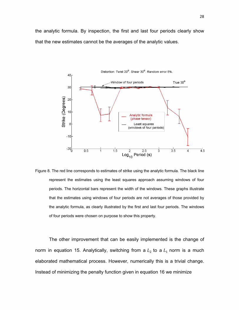
Reframing the magnetotelluric phase tensor for monitoring applications: improved accuracy and precision in strike determinations Ana Gabriela Bravo-Osuna ( [email protected]) Centro de Investigacion Cientiヲca y de Educacion Superior de Ensenada https://orcid.org/0000-0002- 6848-2806 Enrique Gómez-Treviño Centro de Investigacion Cientiヲca y de Educacion Superior de Ensenada Olaf Josafat Cortés-Arroyo Bundesanstalt für Geowissenschaften und Rohstoffe (BGR) Néstor Fernando Delgadillo-Jáuregui Centro de Investigacion Cientiヲca y de Educacion Superior de Ensenada Rocío Fabiola Arellano-Castro Centro de Investigacion Cientiヲca y de Educacion Superior de Ensenada Full paper Keywords: Magnetotelluric monitoring, Phase tensor, Swift strike, Galvanic distortion Posted Date: August 28th, 2020 DOI: https://doi.org/10.21203/rs.3.rs-23277/v2 License: This work is licensed under a Creative Commons Attribution 4.0 International License. Read Full License Version of Record: A version of this preprint was published on February 2nd, 2021. See the published version at https://doi.org/10.1186/s40623-021-01354-y.
Transcript
Reframing the magnetotelluric phase tensor formonitoring applications: improved accuracy andprecision in strike determinationsAna Gabriela Bravo-Osuna ( [email protected] )
Centro de Investigacion Cienti�ca y de Educacion Superior de Ensenada https://orcid.org/0000-0002-6848-2806Enrique Gómez-Treviño
Centro de Investigacion Cienti�ca y de Educacion Superior de EnsenadaOlaf Josafat Cortés-Arroyo
Bundesanstalt für Geowissenschaften und Rohstoffe (BGR)Néstor Fernando Delgadillo-Jáuregui
Centro de Investigacion Cienti�ca y de Educacion Superior de EnsenadaRocío Fabiola Arellano-Castro
Centro de Investigacion Cienti�ca y de Educacion Superior de Ensenada
Full paper
Keywords: Magnetotelluric monitoring, Phase tensor, Swift strike, Galvanic distortion
Posted Date: August 28th, 2020
DOI: https://doi.org/10.21203/rs.3.rs-23277/v2
License: This work is licensed under a Creative Commons Attribution 4.0 International License. Read Full License
Version of Record: A version of this preprint was published on February 2nd, 2021. See the publishedversion at https://doi.org/10.1186/s40623-021-01354-y.
Ana G. Bravo-Osuna1, Enrique Gómez-Treviño1, Olaf J. Cortés-Arroyo1,2, Nestor
F. Delgadillo-Jauregui1and Rocío F. Arellano-Castro1
1 Departamento de Geofísica Aplicada, División de Ciencias de la Tierra,
CICESE, Ensenada, Baja California, México. 22860.
2 Presently at Federal Institute for Geosciences and Natural Resources (BGR),
Berlin, Germany.
ABSTRACT
The magnetotelluric method is increasingly being used to monitor electrical
resistivity changes in the subsurface. One of the preferred parameters derived
from the surface impedance is the strike direction, which is very sensitive to
changes in the direction of the subsurface electrical current flow. The preferred
method for estimating the strike changes is that provided by the phase tensor
because it is immune to galvanic distortions. However, it is also a fact that the
associated analytic formula is unstable for noisy data, something that limits its
applicability for monitoring purposes, because in general this involves
comparison of two or more very similar data sets. On the other hand, the
classical Swift’s approach for strike is very stable for noisy data but it is severely
Correspondence to: Ana G. Bravo-Osuna
División Ciencias de la Tierra, Centro de Investigación Científica y de Educación Superior de Ensenada. Baja California, México, 22860. e-mail: [email protected]
2
affected by galvanic distortions. In this paper we impose the criterion of Swift’s
approach to the phase tensor. Rather than developing an analytical formula we
optimize numerically the same criterion. This stabilizes the estimation of strike by
relaxing an exact condition to an optimal condition in the presence of noise. This
has the added benefit that it can be applied to windows of several periods, thus
providing tradeoffs between variance and resolution. The performance of the
proposed approach is illustrated by its application to synthetic data and to real
data from a monitoring array in the Cerro Prieto geothermal field, México.
Keywords: Magnetotelluric monitoring Phase tensor Swift strike
Galvanic distortion
3
INTRODUCTION
The evolution of the magnetotelluric (MT) method, from its scalar to its
tensorial version, brought about issues regarding the best ways to process the
impedance tensor to obtain information about the subsurface. In many instances
what is required is to identify the directionality of the electric currents because
this is related to lateral changes in electrical resistivity. In the case of two-
dimensional (2D) models this translates into finding the strike angle for which the
measured tensor reduces in some manner to a special case. When one of the
axes of the coordinate system is parallel to the strike, the diagonal elements of
the impedance tensor are zeroes. Swift’s (1967) approach to find the appropriate
angle is to assume a rotated version of the measured tensor, which in general is
not aligned along strike, and then look for the angle that best fits the 2D criterion.
The approach leads to an analytical formula. Another analytic formula that
converts the elements of the impedance tensor into a strike angle was developed
by Bahr (1988) by imposing the condition that the elements of the columns of the
impedance tensor must have the same phases in the case of 2D structures.
Groom and Bailey (1989) proposed an approach that numerically fits, in a least
square sense, the measured impedances with an appropriate model that
includes the strike angle. In this case the solution is not an analytic formula.
Finally, there is the phase tensor of Caldwell et al. (2004) from which an analytic
formula is derived for the strike angle.
4
The approaches described above for strike determinations differ from each
other in several ways, and are also similar in other ways. Let us consider first the
similarities between Bahr’s and the phase tensor approaches. Both are devised
with the explicit purpose in mind of avoiding the effect of galvanic distortions.
Also, they impose rigorous criteria in the sense that, strictly speaking, they can
be met only by error-free data. A third similarity is that in both cases the
approaches lead to analytic formulae. Let us now consider the similarities
between the Swift’s and Groom-Bailey’s approaches. Both impose somewhat
relaxed criteria as opposed to the exact requirements in the other two options.
Instead of an exact fit a best fit is sought in the least squares sense. In Swift’s
case, the anti-diagonal elements are not forced to be exactly zeroes but only to
have their minimum possible amplitude. The Groom-Bailey approach also
complies with a least squares criterion.
In the case of error-free data all approaches cannot but produce the same
result. However, in the case of data with errors the least squares criterion
provides a balanced solution by design, by acknowledging from the begining the
possibility of inconsistencies. Our hypothesis is that imposing the least squares
criterion on the phase tensor determination of strike will improve the performance
of the analytic formula.
Presently it is almost a requirement to include phase tensor ellipses as
part of the interpretation of any data set. Usually they are drawn over maps of the
study area to reveal directionality of shallow or deep structures depending on the
period of interest (e.g. Martí et al., 2020; Comeau et al., 2020). It is not
5
uncommon for the axes of the ellipses to point in inconsistent directions because
of random noise. Any improvement in this respect would be certainly welcome.
However, where better determinations of strikes are most needed is in the recent
application of the magnetotelluric method in monitoring applications. The
preferred formula for monitoring purposes is that derived from the phase tensor
(e.g. Peacock et al. 2012; 2013). One of the reasons is that there is no
assumption about dimensionality. All other approaches assume 2D structures.
Another reason is that it is immune to galvanic distortions, something that Swift’s
formula is not. However, its drawback is that it is unstable for noisy data (Jones,
2012). This limits its applicability for monitoring purposes to very precise data, to
ensure a precise estimation of strike. The question then arises of whether we can
improve the estimation of strikes beyond the application of the analytic formula.
All the analytic formulae provide strike estimates period by period. That is, each
estimate and its variance are independent from the others. However, it is
possible to link contiguous periods by assuming smooth variations of strike over
period and produce a stable profile in the manner of the Occam philosophy (e.g.
Constable et al., 1987). Muñiz et al. (2017) explored this path for the phase
tensor using as seeds the estimations that are better constrained. Another
possibility for stabilization is exemplified by the Groom-Bailey approach as
generalized by McNeice and Jones (2001); the estimates can be made period by
period, for a given number of periods or for all periods together. The variance of
the estimates generally diminishes as the number of periods increases. In a way,
this follows the philosophy of Backus and Gilbert (1968) in the sense that the
6
variance can be improved at the cost of resolution. In this paper we adhere to
this viewpoint and look for estimates that can be made period by period, for a
given number of periods, or for all periods at the same time.
THEORY
Phase tensor
The history of the magnetotelluric method is plentiful of examples where
the problem to be solved consists of avoiding something undesirable. For
instance, consider the chaotic variations of the source strength when making
telluric measurements. The variations were neutralized by the inclusion of the
magnetic field into the telluric method (Cagniard, 1953). In turn, the also chaotic
polarizations of the source were taken care of by the impedance tensor
(Cantwell, T., 1960). The not less chaotic distribution of small, near surface
heterogeneities that produce galvanic distortions was neutralized by the phase
tensor (Caldwell et al., 2004). The present work also centers on an avoidance. In
this case, mitigate the effect of random noise in the estimations of strike using
the phase tensor.
Let us start by a brief account of the development of the phase tensor
itself. In relation to distortions, small, near surface heterogeneities means that
depth, size and distance to the electric line must be smaller than the skin depth.
All things considered, local electromagnetic induction is small so that only
galvanic effects due to electric charges are important. Physically, the source of
7
the charges is the undistorted electric field, so their strength must be proportional
to the strength of the source. In short, that the measured or distorted electric
field𝑬! can be modeled as 𝑬! = 𝑪𝑬,where 𝑪 is a distortion matrix and 𝑬 is the
undistorted electric field. In terms of 𝑥 and 𝑦 components
(𝐸"!𝐸#!* = (𝐶$$ 𝐶$%𝐶%$ 𝐶%%* (𝐸"𝐸#*.(1)
The elements of the distortion matrix 𝑪 are real on behalf of the large skin-
depth assumption. The charges are in phase and follow the undistorted electric
field. The diagonal elements account for the distortion produced by a component
to the same the component, while the off diagonal for the orthogonal
contributions. To see how the distorted electric fields affect the impedance
tensor, consider the undistorted fields expressed in terms of the impedances
(𝐸"𝐸#* = (𝑍"" 𝑍"#𝑍#" 𝑍##* (
𝐻𝑥𝐻𝑦*,(2)
where 𝐻" and 𝐻# are the corresponding components of the magnetic field and 𝑍&' represents the elements of the impedance tensor. The distorted impedance
tensor can be written as
(𝑍""! 𝑍"#!𝑍#"! 𝑍##!* = (𝐶$$ 𝐶$%𝐶%% 𝐶%%* (
𝑍"" 𝑍"#𝑍#" 𝑍##*(3)
8
The real elements of the distortion matrix affect only the amplitude of the
impedances, but this is solely for the individual products. The actual linear
combination can produce distorted impedances that resemble none of the
originals. This explains the importance of the subject and the attempts to
neutralize the effects of the distortion matrix. The formula developed by Bahr
(1988) for the strike of 2D structures might be considered a precursor to the more
general formula derived from the phase tensor. It happens that for the strike
angle the product of the distortion matrix and the impedance tensor has a special
property: the elements of each column must have the same phase. Imposing
this condition on the measured impedance Bahr (1988) developed his formula for
the strike which holds regardless of the distortion matrix. The phase tensor of
Caldwell et al. (2004) generalizes this formula and provides other parameters
equally immune to distortions. Separating the impedance tensor 𝒁 in terms of its
real 𝑿and imaginary 𝒀 parts such that 𝒁 = 𝑿 + 𝑖𝒀, the phase tensor is defined,
Cantwell T (1960) Detection and analysis of low frequency magnetotelluric
signals. PhD Thesis, Massachusetts Institute of Technology.
Chave, A. D., & Jones, A. G. (Eds.). (2012). The magnetotelluric method: Theory
and practice. Cambridge University Press.
Chave, A.D. ,Thomson, D.J., and Ander, M.E. (1987) On the robust estimation of
power spectra, coherences, and transfer functions, J. Geophys. Res., 92: 633-
648.
Chave, A.D., and Thomson, D.J.(1989) Some comments on magnetotelluric
response function estimation, J. Geophys. Res., 94: 14215−14225.
Clarke, J., Gamble, T. D., Goubau, W. M., Koch, R. H., &Miracky, R. (1983).
Remote-reference magnetotellurics: equipment and procedures. Geophysical
Prospecting, 31(1), 149-170.
Constable, S. C., Parker, R. L., & Constable, C. G. (1987). Occam’s inversion: A
practical algorithm for generating smooth models from electromagnetic sounding
data. Geophysics, 52(3), 289-300.
Cortés-Arroyo, O.J. (2018) Monitoreo electromagnético temporal como
herramienta de evaluación en un yacimiento geotérmico. Doctoral thesis.
CICESE, Ensenada, Baja California.
Cortés-Arroyo, O. J., Romo-Jones, J. M., & Gómez-Treviño, E. (2018). Robust
estimation of temporal resistivity variations: Changes from the 2010 Mexicali, Mw
7.2 earthquake and first results of continuous monitoring. Geothermics, 72, 288-
300.
44
Electromagnetic Instruments Inc (1996) MT-1 magnetotelluric system operation
manual.
Gamble, T.D., Goubau, W.M., and Clarke, J. (1979) Magnetotellurics with a
remote magnetic reference. Geophysics,44 (1): 53–68.
Groom, R. W., & Bailey, R. C. (1989). Decomposition of magnetotelluric
impedance tensors in the presence of local three-dimensional galvanic
distortion. Journal of Geophysical Research: Solid Earth, 94(B2), 1913-1925.
Jones, A. (2012) Distortion of magnetotelluric data: its identification and removal.
The Magnetotelluric Method. Theory and Practice: 219-302.
McNeice, G. W., & Jones, A. G. (2001). Multisite, multifrequency tensor
decomposition of magnetotelluric data. Geophysics, 66(1), 158-173.
Muñíz, Y., Gómez-Treviño, E., Esparza, F. J., & Cuellar, M. (2017). Stable 2D
magnetotelluric strikes and impedances via the phase tensor and the quadratic
equation. Geophysics, 82(4), E169-E186.
Peacock, J. R., Thiel, S., Heinson, G. S., & Reid, P. (2013). Time-lapse
magnetotelluric monitoring of an enhanced geothermal
system. Geophysics, 78(3), B121-B130.
Peacock, J.R., Thiel, S., Reid, P., and Heinson, G. (2012) Magnetotelluric
monitoring of a fluid injection: Example from an enhanced geothermal system.
Geophysical Research Letters,39, L18403.
Petiau, G. (2000) Second Generation of Lead-lead Chloride Electrodes for Geophysical Applications. Pure and Applied Geophysics 157, 357 -382. Simpson, F., & Bahr, K. (2005). Practical magnetotellurics. Cambridge University
Press.
Swift, C. M. (1967). A magnetotelluric investigation of an electrical conductivity
anomaly in the southwestern United States (Doctoral dissertation, Massachusetts
Institute of Technology).
Varentsov, I.M., 1998. 2D synthetic data sets COPROD-2S to study MT inversion
techniques, Presented at the 14th Workshop on Electromagnetic Induction in the
Earth, Sinaia, Romania, Available at: http://mtnet.dias.ie.
Vozoff, K. (1972). The magnetotelluric method in the exploration of sedimentary
basins. Geophysics, 37(1), 98-141.
45
Figures
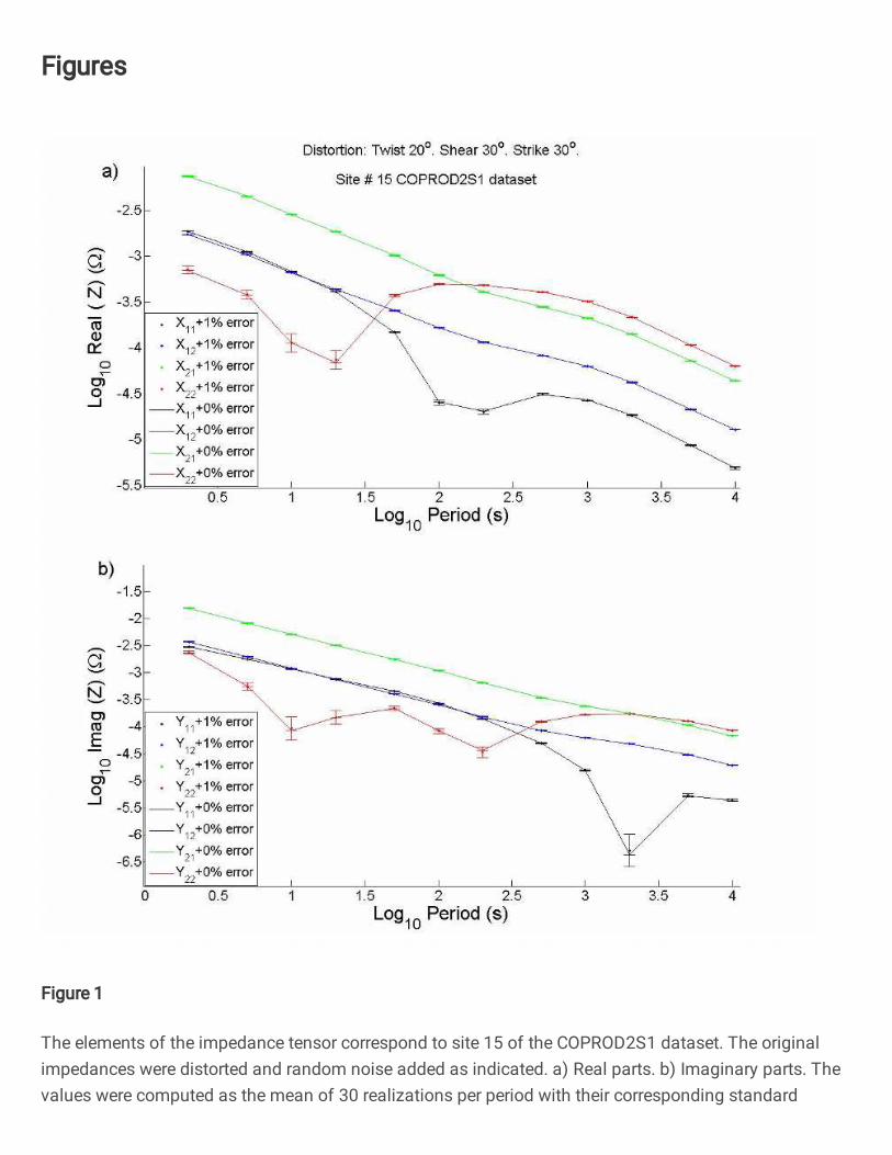
Figure 1
The elements of the impedance tensor correspond to site 15 of the COPROD2S1 dataset. The originalimpedances were distorted and random noise added as indicated. a) Real parts. b) Imaginary parts. Thevalues were computed as the mean of 30 realizations per period with their corresponding standard
deviations. The continuous lines join the error-free values which in most cases are practically identical tothe mean values.
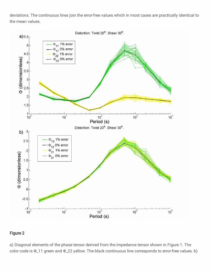
Figure 2
a) Diagonal elements of the phase tensor derived from the impedance tensor shown in Figure 1. Thecolor code is Φ_11 green and Φ_22 yellow. The black continuous line corresponds to error-free values. b)
The corresponding off-diagonal elements. The color code is. Φ_12 green and Φ_21 yellow. The blackdashed line corresponds to error-free values.
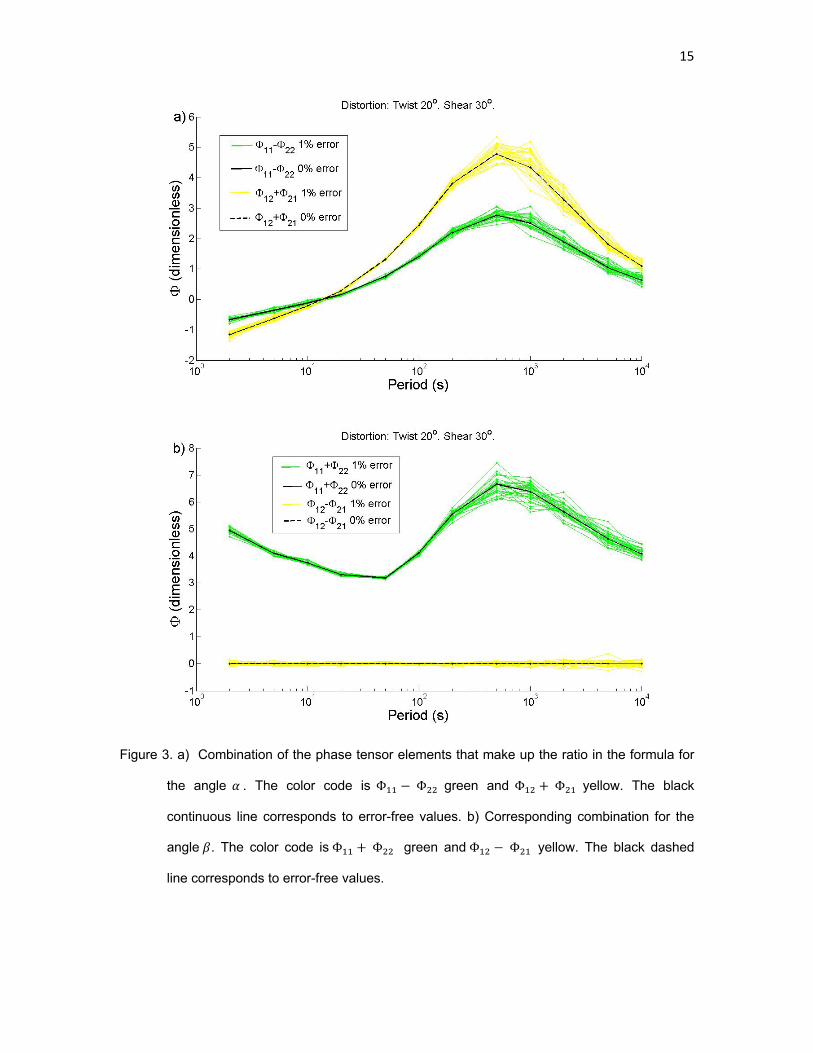
Figure 3
a) Combination of the phase tensor elements that make up the ratio in the formula for the angle α. Thecolor code is Φ_11 - Φ_22 green and Φ_12 + Φ_21 yellow. The black continuous line corresponds to error-
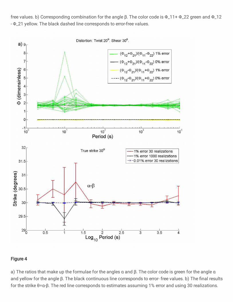
free values. b) Corresponding combination for the angle β. The color code is Φ_11+ Φ_22 green and Φ_12- Φ_21 yellow. The black dashed line corresponds to error-free values.
Figure 4
a) The ratios that make up the formulae for the angles α and β. The color code is green for the angle αand yellow for the angle β. The black continuous line corresponds to error- free values. b) The �nal resultsfor the strike θ=α-β. The red line corresponds to estimates assuming 1% error and using 30 realizations.
The black line corresponds to 1% error and 1000 realizations. The dashed blue line corresponds to 0.01%error and 30 realizations.
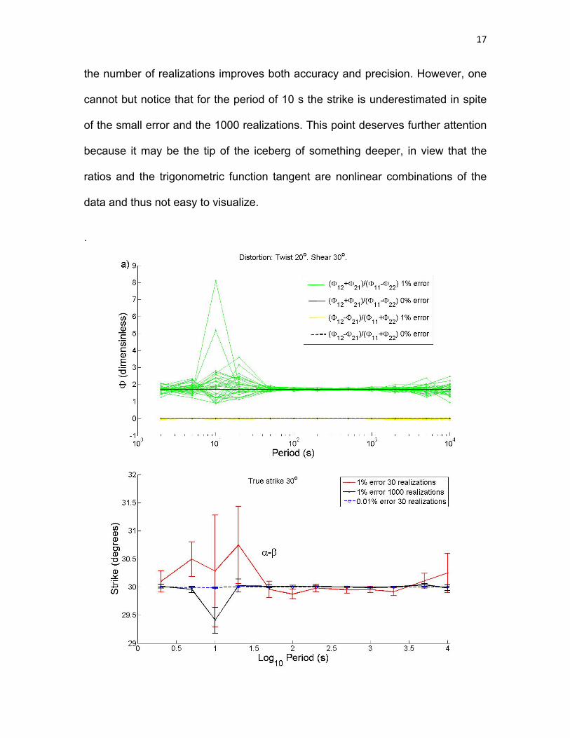
Figure 5
The analysis of the formula for strike indicates that it is biased with respect to random noise: a) theindividual strikes for each realization are plotted for two levels of error. The green lines correspond to 1%error and 1000 realizations. The yellow lines correspond to 5% error and 1000 realizations. The data were
distorted assuming twist= 20° and shear =30°. The dashed line represents the true strike as computedwith 0.01 % error. b) The black line represents the estimates of strikes using 5 % error and 30 realizations.The red line represents the estimates using 5 % error and 1,000 realizations The analysis of the formulafor strike indicates that it is biased with respect to random noise: a) the individual strikes for eachrealization are plotted for two levels of error. The green lines correspond to 1% error and 1000realizations. The yellow lines correspond to 5% error and 1000 realizations. The data were distortedassuming twist= 20° and shear =30°. The dashed line represents the true strike as computed with 0.01 %error. b) The black line represents the estimates of strikes using 5 % error and 30 realizations. The red linerepresents the estimates using 5 % error and 1,000 realizations
Figure 6
Determination of strike angles using the phase tensor and Swift’s approach: a) with no galvanicdistortions. The black dashed line represents the true strike. The black continuous line represents theestimates using Swift’s least squares approach applied to the elements of the impedance tensor. The redline corresponds to the estimates using the analytic formula derived from the phase tensor. b) Withgalvanic distortions. The black dashed line represents the true strike. The black continuous line
represents the estimates using Swift’s least squares approach applied to the elements of the impedancetensor. The red line corresponds to the estimates using the analytic formula derived from the phasetensor.
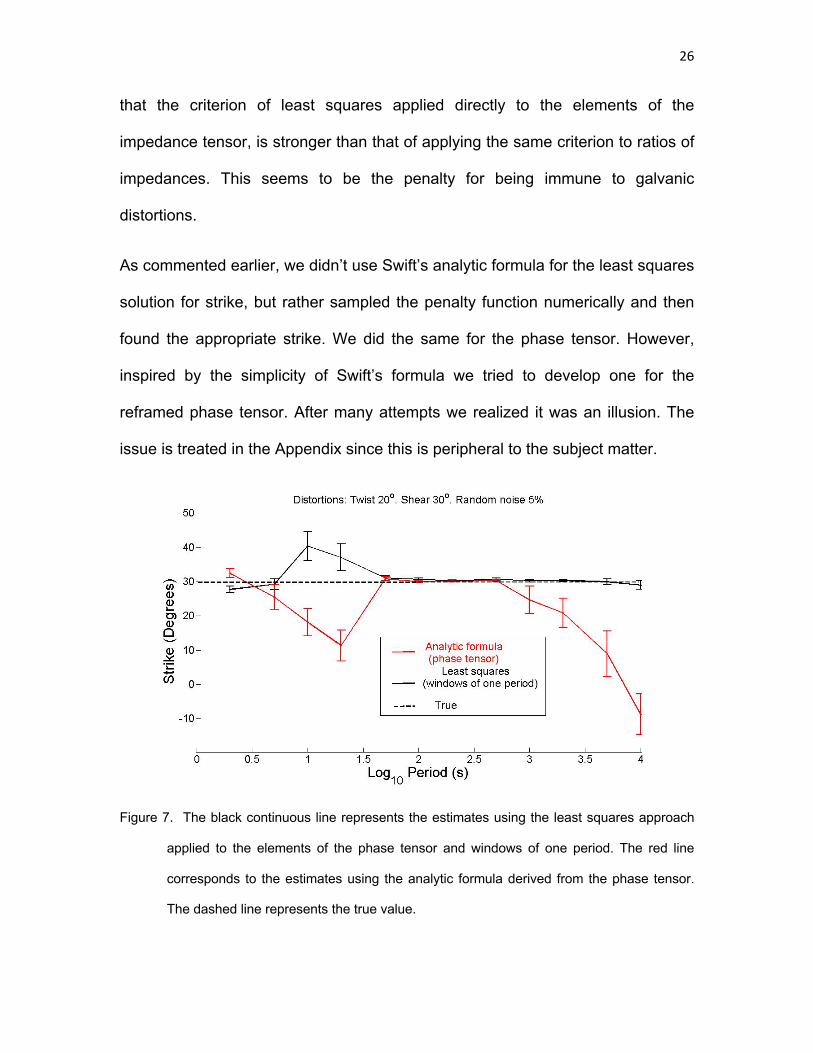
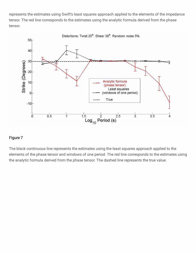
Figure 7
The black continuous line represents the estimates using the least squares approach applied to theelements of the phase tensor and windows of one period. The red line corresponds to the estimates usingthe analytic formula derived from the phase tensor. The dashed line represents the true value.
Figure 8
The red line corresponds to estimates of strike using the analytic formula. The black line represent theestimates using the least squares approach assuming windows of four periods. The horizontal barsrepresent the width of the windows. These graphs illustrate that the estimates using windows of fourperiods are not averages of those provided by the analytic formula, as clearly illustrated by the �rst andlast four periods. The windows of four periods were chosen on purpose to show this property.
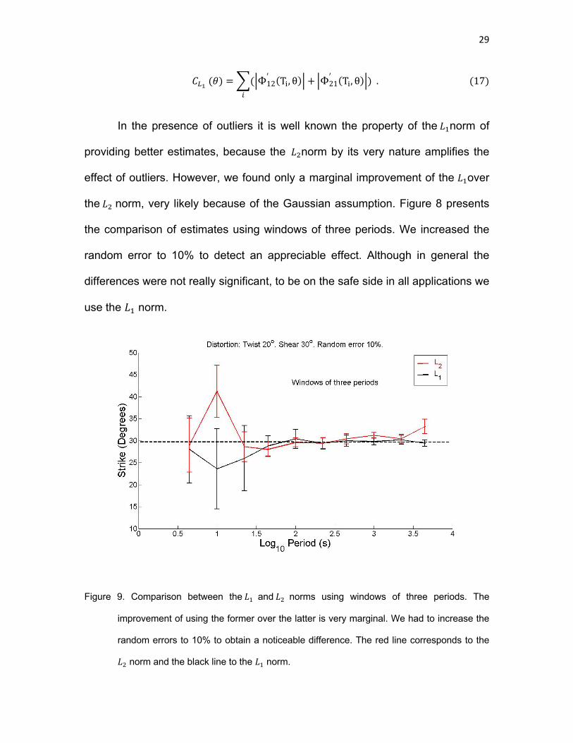
Figure 9
Comparison between theL_1 andL_2 norms using windows of three periods. The improvement of usingthe former over the latter is very marginal. We had to increase the random errors to 10% to obtain anoticeable difference. The red line corresponds to the L_2 norm and the black line to the L_1 norm.
Figure 10
Variation of the penalty functions for a pro�le of strikes of 20, 30 and 40 degrees. a) No random erroradded to the impedances. The minima of the penalty function fall, as they should, exactly at the assumedstrikes. b) With random errors of 1%. The minima in this case spread around the assumed values. Thedegree of dispersion in each case re�ects the accuracy and precision of the estimates of strike.
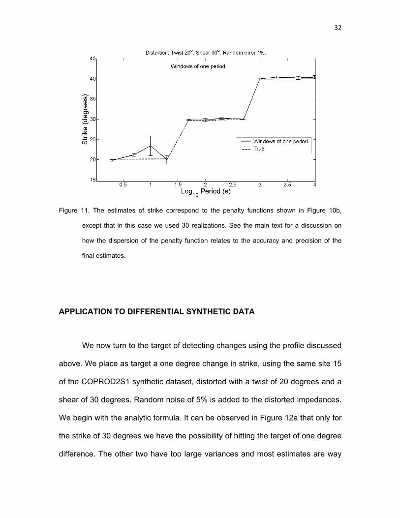
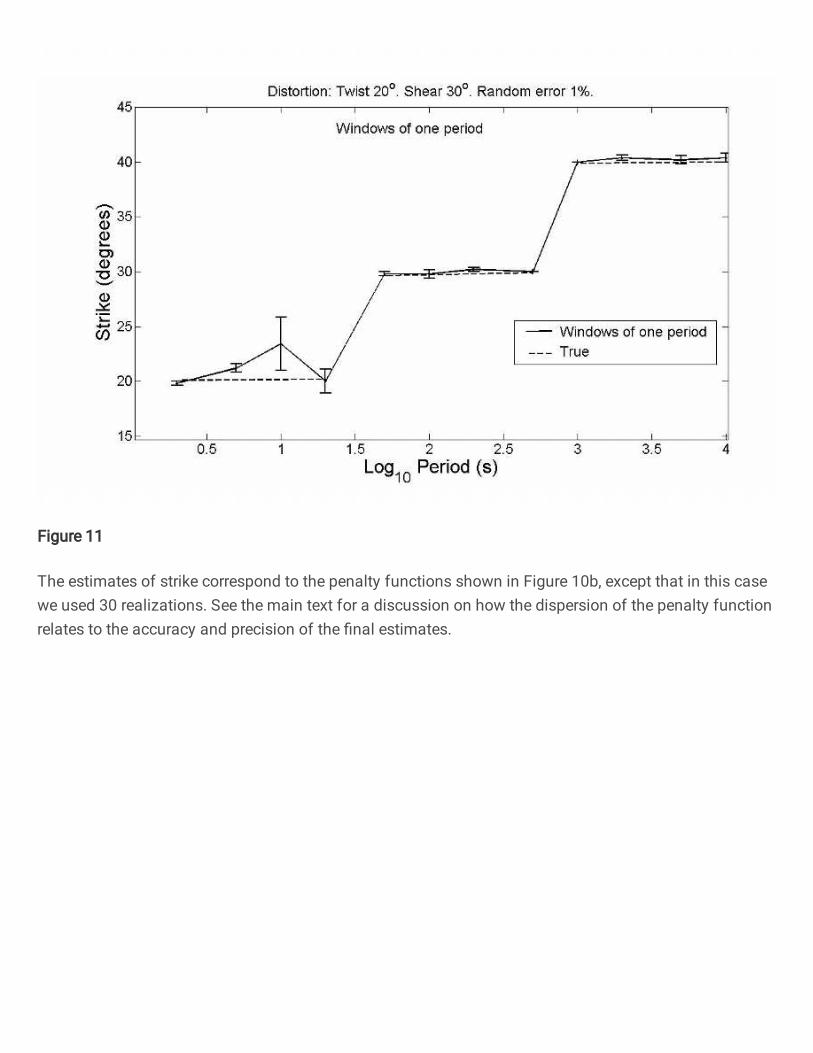
Figure 11
The estimates of strike correspond to the penalty functions shown in Figure 10b, except that in this casewe used 30 realizations. See the main text for a discussion on how the dispersion of the penalty functionrelates to the accuracy and precision of the �nal estimates.
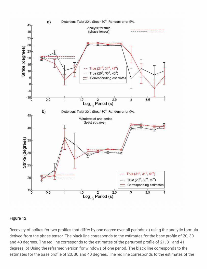
Figure 12
Recovery of strikes for two pro�les that differ by one degree over all periods: a) using the analytic formuladerived from the phase tensor. The black line corresponds to the estimates for the base pro�le of 20, 30and 40 degrees. The red line corresponds to the estimates of the perturbed pro�le of 21, 31 and 41degrees. b) Using the reframed version for windows of one period. The black line corresponds to theestimates for the base pro�le of 20, 30 and 40 degrees. The red line corresponds to the estimates of the
perturbed pro�le of 21, 31 and 41 degrees. In both cases the dashed lines represents the correspondingtrue values.
Figure 13
Recovery of strikes using windows of different widths. The dashed lines correspond to the base pro�le of20, 30 and 40 degrees and the continuous ones to the altered or perturbed pro�le of 21, 31 and 41degrees. a) Windows of four and six periods. b) Windows of eight and ten periods.
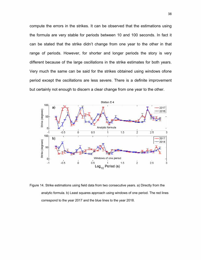
Figure 14
Strike estimations using �eld data from two consecutive years. a) Directly from the analytic formula. b)Least squares approach using windows of one period. The red lines correspond to the year 2017 and theblue lines to the year 2018.
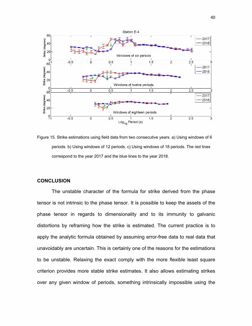
Figure 15
Strike estimations using �eld data from two consecutive years. a) Using windows of 6 periods. b) Usingwindows of 12 periods. c) Using windows of 18 periods. The red lines correspond to the year 2017 andthe blue lines to the year 2018.
Supplementary Files
This is a list of supplementary �les associated with this preprint. Click to download.