Achieving Cryogenic Temperatures Ronald G. Ross, Jr. 6.1 Introduction — Achieving Cryogenic Temperatures A sort of workingman's definition of cryogenic temperatures is temperatures below around 123 K, which equals -150°C or -238°F. In this temperature range and below, a number of physical phenomena begin to change rapidly from room temperature behaviors, and new phenomena achieve greatly increased importance. Thus, study at cryogenics temperatures typically involves a whole set of new temperature-specific discipline skills, operational constraints, and testing methodolo- gies. One of these special attributes of cryogenics is the science and engineering of achieving cryogenic temperatures, both in the laboratory as well as in a sustained "production" environment. The latter can extend from a hospital Magnetic Resonance Imaging (MRI) machine, to a long-wave instrument on a space telescope, to a night-vision scope on a military battlefield. A number of technologies can provide the cooling required for these and other applications; the choice generally depends on the desired temperature level, the amount of heat to be removed, the required operating life, and a number of operational interface issues such as ease of resupply, sensitivity to noise and vibration, available power, etc. This chapter provides an overview of the common means of achieving cryogenic temperatures for useful exploitation, including both passive systems involving the use of liquid and frozen cryo- gens, as well as active cryorefrigeration systems—commonly referred to as cryocoolers. Separate subsections articulate the basic operating principles and engineering aspects of the leading cryo- cooler types: Stirling, pulse-tube, Gifford-McMahon, Joule-Thomson and Brayton. Because this field is very extensive, the goal of the chapter is to provide an introductory description of the available technologies and to summarize the key decision factors and engineering considerations in the acquisition and use of cryogenic cooling systems. After summarizing the details of the refrigeration systems themselves, the remaining 40% of the chapter is devoted to reviewing the critical aspects of cryogenic cooling system design and sizing—including load estimation and margin management—and cryocooler application and inte- gration considerations. Key integration topics include thermal interfaces and heatsinking, struc- tural support and mounting, vibration and Electromagnetic Interference (EMI) suppression, and interface issues with electrical power supplies. The final subsection touches on techniques for measuring the performance of cryogenic refrigeration systems. 6.2 Passive Cooling Systems — Liquid and Frozen Cryo- gens, and Radiators in Space For many years, the use of stored cryogen systems has provided a reliable and relatively simple method of cooling over a wide range of temperatures—from below 4 K for liquid helium, to 77 K for liquid nitrogen, up to 150 K for solid ammonia. These systems rely on the boiling or sublimation of the low-temperature fluid or solid cryogens to provide cooling of the desired load. For solid- cryogens, the temperature achieved may be modulated to a modest extent by varying the backpressure on the vented gas from atmospheric pressure down to a hard vacuum. California Institute of Technology Pasadena, CA 91109 Jet Propulsion Laboratory Chapter 6 of Low Temperature Materials and Mechanisms, Ed. by Yoseph Bar-Cohen, CRC Press, Boca Raton, FL, 2016, pp. 109-181. Refrigeration Systems for
A sort of workingman's definition of cryogenic temperatures is temperatures below around123 K, which equals -150°C or -238°F. In this temperature range and below, a number of physical
phenomena begin to change rapidly from room temperature behaviors, and new phenomena achievegreatly increased importance. Thus, study at cryogenics temperatures typically involves a wholeset of new temperature-specific discipline skills, operational constraints, and testing methodolo-
gies. One of these special attributes of cryogenics is the science and engineering of achievingcryogenic temperatures, both in the laboratory as well as in a sustained "production" environment.
The latter can extend from a hospital Magnetic Resonance Imaging (MRI) machine, to a long-waveinstrument on a space telescope, to a night-vision scope on a military battlefield. A number of
technologies can provide the cooling required for these and other applications; the choice generallydepends on the desired temperature level, the amount of heat to be removed, the required operatinglife, and a number of operational interface issues such as ease of resupply, sensitivity to noise and
vibration, available power, etc.This chapter provides an overview of the common means of achieving cryogenic temperatures
for useful exploitation, including both passive systems involving the use of liquid and frozen cryo-gens, as well as active cryorefrigeration systems—commonly referred to as cryocoolers. Separatesubsections articulate the basic operating principles and engineering aspects of the leading cryo-
cooler types: Stirling, pulse-tube, Gifford-McMahon, Joule-Thomson and Brayton. Because thisfield is very extensive, the goal of the chapter is to provide an introductory description of the
available technologies and to summarize the key decision factors and engineering considerations inthe acquisition and use of cryogenic cooling systems.
After summarizing the details of the refrigeration systems themselves, the remaining 40% of
the chapter is devoted to reviewing the critical aspects of cryogenic cooling system design andsizing—including load estimation and margin management—and cryocooler application and inte-
gration considerations. Key integration topics include thermal interfaces and heatsinking, struc-tural support and mounting, vibration and Electromagnetic Interference (EMI) suppression, and
interface issues with electrical power supplies. The final subsection touches on techniques formeasuring the performance of cryogenic refrigeration systems.
6.2 Passive Cooling Systems — Liquid and Frozen Cryo-
gens, and Radiators in Space
For many years, the use of stored cryogen systems has provided a reliable and relatively simple
method of cooling over a wide range of temperatures—from below 4 K for liquid helium, to 77 Kfor liquid nitrogen, up to 150 K for solid ammonia. These systems rely on the boiling or sublimation
of the low-temperature fluid or solid cryogens to provide cooling of the desired load. For solid-cryogens, the temperature achieved may be modulated to a modest extent by varying the backpressureon the vented gas from atmospheric pressure down to a hard vacuum.
California Institute of Technology
Pasadena, CA 91109
Jet Propulsion Laboratory
Chapter 6 of Low Temperature Materials and Mechanisms, Ed. by Yoseph Bar-Cohen,CRC Press, Boca Raton, FL, 2016, pp. 109-181.
Refrigeration Systems for
2
Figure 1. Operating temperature ranges for common expendable coolants.
In most cases, stored-cryogen cooling technology is fairly well developed with proven designprincipals and many years of experience in the trade. The advantages of these systems are tempera-
ture stability, freedom from vibration and electromagnet interference, and negligible power re-quirements. The disadvantages are the systems’ limited life or requirement for constant replenish-
ment, the inability to smoothly control the cryogenic load over a broad range of temperatures, andthe high weight and volume penalty normally associated with long-life, stand-alone systems.
In systems where the temperature stability and heat transfer associated with cooling with aliquid cryogen is advantageous, one can often extend the useful life of the cryogen or greatly mini-mize needs for replenishment by adding in a mechanical refrigerator with the cryogen dewar to
either recondense the boiled off vapor and return it to the dewar, or to simply intercept a significantfraction of the parasitic thermal load entering the dewar.
The use of stored cryogens such as liquid nitrogen or liquid helium has often been the preferredmethod for cryogenic cooling of a wide variety of devices—from a laboratory apparatus to an MRImachine in a hospital setting. Cryogenic liquids can be used for cooling in a number of different
states, including normal two-phase liquid-vapor (subcritical), low-pressure liquid-vapor (densi-fied), and high-pressure, low-temperature single-phase (supercritical) states. Subcritical fluids such
as low-pressure helium have long been the cooling means of choice for very-low-temperature (1.8 K)sensors for space astronomy missions.
Solid cryogens are mostly used below their triple point where sublimation occurs directly tothe vapor state. They provide several advantages over liquid cryogens including elimination ofphase-separation issues, providing higher density and heat capacity, and yielding more stable tem-
perature control, which is desirable for many applications.
6.2.1 Available Temperatures from Various Cryogens
The detailed thermodynamic properties of common cryogens are available in the literature for
those designing cryogenic systems. However, it is useful to provide a brief overview of the practi-cal operating temperature ranges and properties of common cryogens, along with an introduction tothe thermodynamic operating regimes for their solid, liquid, vapor, and gas states.
Figure 1 describes the operating temperatures attainable with ten common cryogens that can beused to directly cool cryogenic loads or other components. Each cryogen is represented by a bar that
extends from its minimum operating temperature as a solid—based on sublimation at a vapor pres-
3
Figure 2. Idealized temperature-entropy diagram for a cryogenic fluid.
sure of 0.10 torr—to its maximum operating temperature—its critical point, which is the maximumtemperature at which a cryogen can exist as a two-phase liquid vapor. Within each bar, the region
of solid phase is denoted by the shaded area defined at its maximum temperature by the cryogen'striple point, which is the maximum temperature at which a cryogen can exist as a solid. Above this,
the cryogen's boiling point at a pressure of one atmosphere is noted by the dashed line. The use of0.10 torr to define the lowest achievable temperature is for convenience, as the temperature can be
lowered if the ability to pull a stronger vacuum is available.
6.2.2 Thermodynamic Principles of Cryogen Coolers
A modest familiarity with thermodynamics fundamentals is useful for understanding the limi-tations and constraints of stored-cryogen system operating states. Figure 2 expands on the key fluid
parameters noted in Fig. 1 via an idealized temperature-entropy (T-S) diagram for a pure cryogenicfluid. Since entropy is defined as the heat transferred divided by the temperature at which the
change occurs, the T-S chart is not only useful to visualize the boundaries between fluid states, butto also quantify the amount of heat transferred when a fluid undergoes a change of state.
Starting with the point C, the apex of the dome is called the critical point, and the conditions at
that point are called the critical pressure, critical temperature, etc. When the fluid is at or above thecritical temperature, it can never exist in the liquid state, but will remain as a single-phase, homoge-
neous gas. Fluids stored under these conditions are sometimes called cryo-gases.The line described by curve ABD in Fig. 2 represents the path of a gas being cooled at constant
atmospheric pressure. The horizontal line drawn at C represents the dividing line between a vaporand a gas. While they are technically in the same state, the points along the line DE represent aliquid and vapor mixture at constant temperature and pressure — point D being 100% saturated
vapor while point E being 100% saturated liquid. As an example, for water, this DE line would beat 100°C, the boiling point of water at a pressure of one atmosphere. The change in energy from
point E to D is the heat of vaporization. When a liquid is heated along this line, point E is alsocalled the bubble point, because it is where the first vapor bubbles appear.
Further cooling of the liquid from E to F reduces the vapor pressure, and eventually the liquid
freezes into a solid. Point F is defined as the triple point (or melting point), where the fluid existsas solid, vapor, and liquid. For water, this would be the temperature of an ice/water mixture, i.e.
0°C.For a cryogen that is below the triple point temperature, such as point G, any addition of heat
will cause the solid to sublimate, as opposed to melting to a liquid. For the conditions of point G, theheat of sublimation is given by the change in energy from G to H.
4
Figure 3. Boiling-point temperature of common gases as a function of external pressure.
Figure 3 expands on Fig. 2 by describing the dependence of boiling-point or sublimation tempera-
ture on external pressure for common cryogens. Also noted is the triple point where the cryogentransitions to a solid. This plot also indicates the temperature and pressure where external contami-
nant gases, such as water vapor, will begin to condense on cryogenic surfaces such as low-emit-tance shields and MLI. Preventing such condensation is a critical issue for managing radiant para-sitic loads on low-emittance shields and cryogenic surfaces. This topic of emittance degradation
from contaminant films is covered later in this chapter in Section 6.4.3.5.
6.2.3 Cooling with Liquid Cryogens
Over the years, many liquid cryogenic systems have been developed, fabricated, and operatedin both ground environments and in space. They cover a wide range of cryogen fluids and construc-tion features in terms of stored volume, pressure and temperature limitations, and relative effi-
ciency in terms of the parasitic heat leaks. Many of these systems utilize liquid helium for achiev-ing temperatures between 1.4 K and 4 K or liquid nitrogen for achieving temperatures around 77 K.
To achieve temperatures below 4.2 K requires that liquid helium be stored under partial vacuumconditions. At pressures from 10 to 40 torr, temperatures in the range of 1.4 K to 1.8 K are achiev-
able with liquid helium.
6.2.3.1 Engineering Aspects of Liquid Cryogen Systems
Typical Dewar Construction Features. As illustrated in Fig. 4, liquid cryogen systems typi-cally involve a nested storage tank concept whereby the inner tank, which holds the liquid cryogen,
is suspended inside an outer vacuum shell with low-conductivity structural supports. These struc-tural supports are typically made of low-conductivity tubes, struts or tension bands in order to
achieve high structural efficiency and minimum conductivity between the two tanks. The gapbetween the two tanks is then evacuated and filled with Multilayer Insulation (MLI). In addition, ahigh efficiency dewar may also contain one or more strategically placed vapor-cooled shields (VCS)
that are cooled by the evaporating cryogen as it vents from the inner tank.The goal of the gap construction is to prevent gaseous conduction and radiation between the
outer an inner tank and to achieve maximum thermal benefit from the evaporating cryogen. Al-though the heat of vaporization of the cryogen is the primary cooling force in the system, there is
also considerable benefit associated with extracting the available heat from the vapor as it rises upin temperature from the cryogen temperature to the external vent temperature. This is accom-plished by piping the venting gas through the vapor cooled shields, which serve to intercept much
of the radiant energy coming through the MLI layers from the outer tank. The VCS can also beattached to the support struts or plumbing to further reduce conductive heat leaks.
5
Applicationmounting
space
Figure 4. Example liquid cryogen dewar construction features.
An extensive summary of the construction features for representative stored cryogen tanksfabricated for space applications—and in some cases airborne use—has been assembled byDonabedian and is available in the Spacecraft Thermal Control Handbook, Vol II: Cryogenics
[Donabedian, 2003b] and in Chapter 15 of the earlier Infrared Handbook [Donabedian, 1993].Those reviews include tanks built for a variety of uses, fluids, and pressures, and contains designs
for both subcritical and supercritical cryogen storage. As part of that work, a general performance,figure-of-merit database was also developed to serve as a convenient means of comparing andevaluating the performance of the various stored cryogen systems. The figure of merit is defined as
the net heat leakage of the fluid (Q) divided by the surface area of the pressure vessel (A) in units ofW/m2. This Q/A parameter varies from as high as 0.1 to as low as 0.003 W/m2 depending on the
temperature and properties of the fluid stored, the tank design, and the external temperature.
Multilayer Insulation (MLI). High quality multilayer insulation (MLI) has been found toplay a particularly critical role in achieving high-efficiency stored cryogen systems, and as a result,
has been a focus for much research over the years within the cryogenic community. Lockheed-Martin Palo Alto, in particular, spent years testing and optimizing MLI for space cryogen dewars
and has assembled a substantial data base on performance attributes, lessons learned and preferredpractices (see for example [Johnson 1974], [Nast ,1993]).
Because MLI is also a key element of solid cryogen systems and cryocooler-cooled systems, aseparate subsection of this chapter (section 6.4.3) has been devoted to a detailed summary of cryo-genic MLI performance attributes and measured data. Its particular focus is on the use of MLI at
cryogenic temperatures, which places greatly increased emphasis on the conduction properties ofMLI.
Porous Plugs. For liquid helium systems, when the temperature is dropped below about 2 K,a point referred to as the lambda point, liquid helium undergoes a phase transition and becomes a"super fluid" with very special properties. These properties include: infinite thermal conductivity,
zero viscosity and zero entropy. The substance, which looks like a normal liquid, will flow withoutfriction along any surface and circulate over obstructions and through pores in containers which
attempt to hold it. The porous plug was invented to contain super fluid helium in a cryogen dewarwhile allowing for evaporative cooling. Its micron-level pore sizes are required to separate the
liquid and vapor phases to ensure that liquid does not escape before its heat of vaporization can beutilized. Selzer, et al. provide a summary of the physics behind the porous plug's operation as partof their paper on its original development at Stanford University in 1970 [Selzer, et al., 1970].
Zero Boil-off (ZBO) Systems. In the last 10 years or so, the concept of zero boil-off (ZBO)systems utilizing mechanical refrigerators combined with high-efficiency cryogenic tanks has been
pursued to provide long-term storage of cryogenic fluids while minimizing storage volume andrefrigerator power. These ZBO systems are being used for many ground-based systems and arebeing examined to provide liquid oxygen, methane, or hydrogen for future space planetary-mission
Liquid Cryogen
MLI invacuumspace
Vapor cooled shields (VCS)
Low conductancestructural supports
Applicationaccess ports
6propulsion and life-support systems. Helium, hydrogen, and deuterium ZBO systems are alsobeing considered for future space-based lasers.
6.2.3.2 Liquid Cryogen Cooler Development History and Availability
As noted earlier, liquid cryogenic systems have been developed, fabricated, and operated formany years, in both ground environments and in space [Ross, 2007]. They cover a wide range of
cryogen fluids and construction features in terms of temperatures, stored volume, and thermal iso-lation systems. Many present-day systems are used for cooling superconductor electronics and
magnetics in applications such as Magnetic Resonance Imaging (MRI) systems and for coolingspacecraft instruments utilizing liquid helium to achieve temperatures below 2 K. Although notreally a "cooling" application, much of the same technology is also used in liquid cryogen "storage"
systems for liquid helium, hydrogen, oxygen, and nitrogen.A number of manufacturers provide generic liquid cryogen dewars for laboratory and commer-
cial applications. In space most dewars have been custom built for particular missions by contrac-tors such as Lockheed Martin in Palo Alto, CA and Ball Aerospace and Technology Corp. (BATC)in Boulder, CO.
The tanks developed for NASA’s Gemini and Apollo programs for storage of supercriticaloxygen and hydrogen for their 7- to 14-day missions were the earliest space-qualified tanks for
operation in near-zero-gravity environments. More advanced and larger tanks were developed bythe Beech Aircraft Corp. Boulder Division (now BATC) for longer life. They were designed for
general-purpose storage of LO2, LH2, LN2, and LHe for extended periods.Nearly all actual liquid cryogen cooling applications in space have involved the use of super
fluid helium to achieve temperatures below 2 K for cooling long-wavelength infrared sensors in
space telescopes. The first of these was the IRAS dewar in 1983, followed by COBE in 1989,Spitzer in 2003, GPB in 2004, and XRS in 2005. For most other temperatures, space cryogen-
cooled missions used solid cryogens, which are discussed next. A summary of the history of cryo-gen systems used in space is provided by Ross [Ross, 2007].
6.2.4 Cooling with Solid Cryogens
A second efficient way to use stored cryogens is in the frozen state. As indicated in Fig. 5, thenormal operating regime of a solid cryogen cooler is below its triple-point temperature. In this
region, the addition of heat causes conversion of the solid directly into vapor through the process ofsublimation, bypassing the liquid state. Operating below the triple point also eliminates the prob-
lems of fluid management and phase separation associated with fluid systems. From an efficiency
Figure 5. Solid cryogen operating regime; heat of sublimation = T´(SH- S
G).
7Table 1. Thermal Properties of Selected Solid Cryogens
Heat of Density of Solid Temperature Range (K)
Cryogen Sublimation at Melting Point
(J/g) (kg/m3) 0.1 Torr Triple Point
Ammonia (NH3) 1719 822 150 195
Carbon dioxide (CO2) 574 1562 125 216
Methane (CH4) 569 498 60 90
Oxygen (O2) 227 1302 48 55
Argon (A) 186 1714 48 84
Carbon monoxide (CO) 293 929 46 68
Nitrogen (N2) 225 1022 43 63
Neon(Ne) 106 1439 14 25
Hydrogen (H2) 508 80.4 8 14
point-of-view, working with the solid phase provides greater density (and thus lower storage vol-
ume) and higher heat content per unit mass of cryogen. Other advantages of a solid cooler arerelative simplicity, absence of moving parts, absence of noise and vibration, excellent temperaturestability, and no power requirements.
The primary limitations or disadvantages include a limited number of suitable cryogens, verylarge mass and volume required for large heat loads or long design lives, the need for very signifi-
cant ground servicing facilities and manpower support, and safety implications associated withventing toxic or flammable vapors or having a vent become clogged—causing an explosion.
For space applications, the overboard vent of a solid cooler must also be designed to maintainthe necessary pressure level on the cryogen and to not create unacceptable torques on the space-craft. If the vent rate is significant, the gas may have to be vented along an axis passing directly
through the center of gravity of the satellite and/or thrust compensation devices must be used toprevent attitude disturbances. Sustaining the desired operating temperature also requires that the
back pressure on the sublimating cryogen be maintained at the fixed value associated with thedesign temperature.
This important interrelationship between the temperature and pressure of a frozen cryogen is
presented in the vapor pressure-temperature plot presented earlier as Fig. 3. As noted, the sublima-tion temperature is strongly dependent on the vapor pressure maintained above the solid. Thus,
given a fixed back pressure, a solid cryogen can be designed to maintain a very stable temperature.
6.2.4.1 Thermodynamics of Solid Cryogens
Table 1 tabulates the key thermophysical properties of a number of cryogens traditionally used
in solid coolers, including their operating temperature range. The cryogens are listed in descendingorder of minimum practical operating temperature (the table’s fourth column) based on a reason-ably achievable back pressure of 0.1 torr.
As was shown in Fig. 3 the minimum operating temperature depends on the minimum backpressure that can be sustained during cooler operation. If the heat load is small enough and the
applied vacuum is high enough, then lower pressures, and thus lower temperatures, can be attained.The maximum temperature (the fifth column) is the highest temperature at which the solid phasecan exist, which is its triple-point temperature. By proper design of the back pressure imposed by
the vent gas system, any temperature between these two extremes can be achieved. The operatingtemperature range of a solid cooler is thus much wider than the range for a stored liquid cryogen
cooler.
8
Applicationmounting
space
6.2.4.2 Engineering Aspects of Solid Cryogen Coolers
Solid Cryogen Dewar Construction Features. As illustrated in Fig. 6, solid cryogen dewarsystems are fundamentally similar to liquid cryogen dewars in their structural support and thermal
insulation systems. Both include a nested storage tank concept whereby the inner tank, which holdsthe solid cryogen, is suspended inside an outer vacuum shell with low-conductivity structural sup-ports. As with liquid cryogen dewars, these structural supports are typically made using low-con-
ductivity tubes, struts or tension bands in order to achieve high structural efficiency and minimumconductivity between the two tanks. The gap between the two tanks is evacuated and filled with
Multilayer Insulation (MLI), and for high efficiency dewars, one or more vapor-cooled shields(VCS) may be strategically placed inside the gap.
As with liquid cryogen dewars, the goal of the gap construction is to prevent gaseous conduc-
tion and radiation between the outer and inner tank and to achieve maximum thermal benefit fromthe evaporating cryogen. Although the heat of sublimation of the solid cryogen is the primary
cooling force in the system, there is also considerable benefit associated with extracting the avail-able heat from the vapor as it rises up in temperature from the cryogen temperature to the external
vent temperature. This is accomplished by piping the venting gas through the vapor cooled shields,which can serve to intercept much of the radiant and conducted heat coming through the MLI layersfrom the outer tank. The VCS can also be attached to the support struts or plumbing to further
reduce conductive heat leaks.Two key differences between liquid and solid-cryogen dewars are the need for a thermally
conductive matrix and freezing coils in a solid cryogen dewar. Because the solid cryogen evapo-rates selectively near the interface with the cryogenic load, it tends to withdraw away from thiscritical thermal interface as it is depleted and requires a means to keep it thermally connected to the
load. This is accomplished by filling the cryogen tank with a high-conductivity open-cell metallicmatrix or foam to provide a known thermal bridge to the load interface during all stages of evapo-
ration of the solid cryogen.The second addition to a solid cryogen dewar is a means to freeze the cryogen in place within
the foam-filled dewar. This is accomplished by providing a cooling coil within the dewar that canbe connected to an external coolant source sufficiently cold to freeze the cryogen. A second use ofthe cooling coil can be to keep the cryogen frozen during system integration and test periods.
This process of freezing the cryogen, or precooling it to temperatures well below its freezingpoint, requires great care and experience to avoid damaging the dewar. Like water ice—the frozen
state of the cryogen often has a different density, and thus occupies a different volume than theliquid state. In the solid state, it is also likely to have a different coefficient of thermal expansion(CTE) than the metallic dewar. If not fully accommodated in the dewar design and filling proce-
dure, these expansions or contractions of the cryogen can lead to rupturing portions of the dewar.
Figure 6. Example solid cryogen dewar construction features.
Vapor cooled shields (VCS)
External coolant loopfreezing coils
Solid Cryogen infoam matrix
Low conductancestructural supports
Applicationaccess ports
MLI invacuumspace
9A compounding issue with solid cryogens is their ability to relocate themselves within a dewarby evaporative transport from warmer regions to cooler regions; this involves the physics of
cyropumping and can lead to a solid cryogen filling in the space critically needed for expansionduring a subsequent warm-up operation. A very traumatic failure of the NICMOS solid nitrogen
dewar occurred due to this cause during preparation for use on the Hubble Space Telescope [Miller,1998a; Miller, 1998b].
6.2.4.3 Solid Cryogen Cooler Development History and Availability
The first operational long-life solid cooler used in space was a single-stage carbon dioxidesystem developed by Lockheed Martin and launched aboard an Air Force satellite (STP-72-1) onOctober 20, 1972 [Nast and Murray, 1976]. Since that time nearly a dozen cooler designs, both
single- and two-stage, have been used to cool sensors to temperatures over a range of 10 to 65 K,with operational lifetimes from 10 months to 2.5 years.
Two-stage designs have been used several times to optimize the overall cooler performanceand minimize cooler mass by using a high-temperature cryogen such as carbon dioxide or ammonia(both of which have higher operating temperatures and high heat content) to provide a shield for
cryogens that have lower operating temperatures, such as hydrogen, neon, and methane. In somecases, methane has been used as the shield cryogen for low-heat-content cryogens like neon.
With the rapid development of long-life mechanical refrigerators and the relatively high cost ofdesigning and servicing solid coolers, mechanical cryocoolers have increasingly become the cooler
of choice for space missions that historically would have used solid cryogen coolers. An overviewof the history of cryogenic coolers in space is provided by Ross [Ross, 2007].
6.2.5 Radiation to Deep Space
For spaceborne applications, cryogenic temperatures as low as 40 to 60 K can also be achievedusing very carefully designed radiant cooler systems radiating into deep space. Although the effec-
tive radiation temperature in space is approximately 3 K, achieving these 40 to 60 K temperatures isgenerally limited to sophisticated cryoradiators on spacecraft well separated from the much warmer
environment of Earth orbit. In Earth orbit, practical cryoradiator temperatures are closer to 80 Kand above.
When striving for cryogenic temperatures above these levels, radiant cooling to deep space can
provide an effective and cost effective means of cooling, although even then, elaborate shields fromthe sun and Earth, and from the warm environment of the supporting spacecraft are required.
The advantage of cryoradiators is relatively stable long-term performance without the need forpower, or concerns about mechanical wearout, electronics failures, or depletion of a stored cryogensupply. Countering this attractiveness is the relatively challenging design associated with achiev-
ing sufficiently low parasitic thermal loads and maintaining sufficient structural robustness to sur-vive the launch loading environment. To achieve useful performance, constraints are also typically
required on the spacecraft's geometric configuration and orbital attitudes.As with nearly all cryogenic applications there is a strong competition between structural ro-
bustness and thermal isolation (minimum thermal conductivity). This invariably leads to highly
optimized structural/thermal designs often involving mechanical mechanisms for latching or un-latching supplementary structural supports used only to survive launch. Added to this is the diffi-
culty of isolating from direct solar and Earth reflected solar (albedo) radiation, which typicallyrequires Earth and sun shades; these too can often end up with mechanically deployed mechanisms.
Lastly, isolating the radiator and cold plumbing from the warm spacecraft requires careful applica-tion of low-emittance surfaces and cryo multilayer-insolation (cryo MLI). At cryogenic tempera-tures, such surfaces and MLI can perform much more poorly than they do in room-temperature
applications, so these contribute to additional engineering challenges in the design process.The bottom line is that a significant number of cryo radiators have been successfully used in
space since the early 1970s [Nast and Murray, 1976], but a modest fraction of these have hadsignificant schedule and cost growths associated with meeting the design challenges; and, each
10design tends to be a new custom design for each new spacecraft and mission. For higher tempera-tures, like the 150 K to 170 K temperatures needed for space optics, design criticality is much less
severe, and cold radiators in this temperature range—just above cryogenic temperatures—haveprovided very effective long-term cooling of space instruments. See, for example, the 12-year
space radiator performance on the Atmospheric Infrared Sounder (AIRS) instrument [Ross, 2014].Crawford [Crawford, 2003] and Donabedian [Donabedian, 2003c] provide excellent reviews
of the more detailed design principals developed for space cryo radiators over the past 40 years.Donabedian also presents comparative performance data for nearly two dozen flight designs. Theirchapters in the Spacecraft Thermal Control Handbook, Vol II: Cryogenics are an excellent starting
point for those wishing to more carefully examine the design options for space cryo radiators.
6.3 Active Refrigeration Systems—Stirling, Pulse Tube, GM,
JT and Brayton
For cryogenic applications where stored cryogens like liquid nitrogen and liquid helium are not
readily available or are inconvenient to use, mechanical refrigerators, or cryocoolers, are often thepreferred design solution. The primary considerations that differentiate mechanical refrigeratorsfrom stored cryogen cooling systems are the issues of cryogen storage, resupply and safety for
cryogen systems and the requirement for electrical power and a means of heat rejection for cryo-coolers. Because cryocoolers, or cryorefrigerators, are typically driven by electrical powered com-
pressors, means must be available to provide both the electrical power and the means to reject theresulting heat dissipation. The power dissipation issue is particularly important because the result-
ing heat reject temperature strongly effects the thermodynamic efficiency of the cryocooler. Asecond aspect of the electrically driven compressor is the strong likelihood of measurable levels ofequipment vibration, EMI, and audible noise that may interact negatively with the intended cryo-
genic application. Achieving low levels of vibration and noise has been an important focus in thecryocooler development industry, and is an important distinguishing attribute of certain cryocooler
types and constructions. Another key advantage of a cryocooler is the ability of a single unit toprovide cooling over a broad range of temperatures, many with closed-loop temperature control.
Some of the most important applications for cryocoolers include achieving high vacuum levels
with cryopumps in semiconductor processing facilities, cooling infrared detectors and supercon-ducting devices in a broad range of military, space, and laboratory instruments, and reliquefying
cryogens to provide a zero-boil-off recapture of the cryogen in systems using liquid helium ornitrogen. Key decision factors include the cooling system operational cost, complexity and reliabil-ity/maintainability.
To meet these broad needs, a wide range of cryocoolers has been developed, and these coolersuse a number of different thermodynamic cycles. In general, the size (cooling capacity) and avail-
able cooling temperature range of mechanical cryocoolers span many orders of magnitude—fromroom temperature down to 1 K and below, and from microwatts to kilowatts of cooling power. The
most common mechanical refrigeration cycles include Stirling, Pulse Tube, Gifford McMahon (GM),Joule-Thomson (JT), and reverse-Brayton cycles. The attributes of each of these types of coolersare discussed in the subsections that follow, including a brief description of their thermodynamic
cycle, their operational features, representative performance, and general commercial availability.In addition to these five cooler types, there are a number of lesser known cycles such as adia-
batic demagnetization and the dilution cycle that are used primarily for achieving ultra-low tem-peratures below 1 K. The reader is referred to the literature on subKelvin coolers for further infor-mation on these specialty cooler types.
To achieve the lowest temperatures, typically 30 K and below, cryocoolers generally employtwo or more linked stages, where an upper stage (higher temperature) cooler is used to provide a
low-temperature heat rejection path for a lower-temperature stage. Although many multiple stagecoolers employ the same thermodynamic cycle for each of the linked stages, there is sometimes an
advantage to linking different types of coolers using different thermodynamic cycles. These aregenerally referred to as hybrid coolers and include combinations such as Stirling, Pulse Tube, or
11GM upper stage with a Joule-Thomson bottom stage. Such a cooler can take advantage of the highefficiency of the Stirling cycle for higher-temperature precooling and also capture the remote-coldhead
low-vibration attributes of a JT system for the final interface with the application load.
6.3.1 Cryocooler Cycle Types and Efficiency Measures
6.3.1.1 Cryocooler Classifications and Practical Systems
All mechanical refrigerators generate cooling by basically expanding a gas from a high pres-sure to a low pressure. The primary distinguishing feature between cycles is how the compression
is accomplished, what pressure-ratio is used, what method of expansion is used to achieve the coldtemperature, how well and where heat is rejected, and how well thermodynamic efficiency is main-tained using heat exchangers, regenerators, and recuperators.
Probably the most fundamental distinction between cryocooler types is the nature of the refrig-erant flow within the cryocooler: either alternating flow (AC systems) or continuous flow (DC
systems). This distinction is also denoted as regenerative systems versus recuperative systems
based on the type of heat recovery heat exchanger that is applicable: regenerators for an alternating
flow (AC system), or recuperators for a continuous flow (DC system).In an AC-type cooler system, a regenerative heat exchanger stores and releases energy to the
alternating refrigerant stream using a regenerator made of, for example, fine mesh screens or densely
packed particles with good specific heat properties. In a DC-type system, a recuperative heat ex-changer exchanges energy between two opposing streams of flowing gas or liquid using a counter-
flow heat exchanger referred to as a recuperator. Of the common cooler types, Stirling, pulse tube,and Gifford McMahon use regenerative (AC flow) cycles, while Joule-Thomson and turbo-Braytonsystems use recuperative (DC) flows. A key distinguishing feature of such systems is that the
compressor generally must be quite close to the coldend expander in a regenerative AC-flow cooler,and can be very remote (many meters away) for a recuperative DC-flow cooler. This has important
implications on managing the compressor's heat dissipation and possible vibration and noise inclose proximity to the cryogenic load. One exception is the Gifford-McMahon cooler; it uses aregenerative refrigeration cycle, but uses a constant flow DC compressor that can be remotely lo-
cated. To do this a GM cooler chops the DC flow into an AC flow within the coldhead itself,remote from the GM compressor.
6.3.1.2 The Carnot Cycle and Efficiency References for Cryocoolers
As background before delving into the details of the various cryo refrigerator types, it is usefulto touch briefly on the standard measure of cryocooler efficiency: the percent of Carnot Coefficient
of Performance. The coefficient of refrigeration performance (COP) for any refrigerator is definedas the ratio of the extracted heat to the applied work, i.e.
cooling power
COPCooler = ______________ (1)
input power
Next, let's examine the Carnot-cycle refrigerator, which has the highest efficiency of any re-frigeration cycle, and thus serves as a reference for all other refrigeration cycles. As shown in Fig. 7(a temperature-entropy (T-S) diagram of the cycle), the cycle consists of gas compression on the
right, constant-temperature heat-rejection at the top, an expansion phase on the left, and constanttemperature heat absorption on the bottom. Heat absorbed during the process corresponds to the
line with endpoints 1 and 4 (the refrigeration), while the heat rejected to the environment during theprocess (work done plus heat absorbed) is the line 2 to 3. Note that the compression and the
expansion are both done isothermally (at constant temperature), while the expansion and the com-pression processes are done isentropically (i.e., with no heat transfer).
Applying Eq. (1) to the Carnot cycle in Fig. 7, we find that the ratio of cooling power (heat
absorbed) to input power (heat rejected minus cooling power) is purely a function of the cold andhot temperature. Thus the COP of the Carnot-cycle refrigerator is uniquely defined in terms of the
12
Figure 8. Efficiency for 80 K cooling for various measured cryocoolers
of different types and input powers [Radebaugh, 2004].
Figure 7. The Carnot refrigeration cycle.
coldtip temperature (Tcold) and heatsink temperature (Thot) as:
COPCarnot = Tcold ¤(Thot - Tcold) (2)
Cryocooler Efficiency as Percent of Carnot. An important figure-of-merit for cryocoolers is the
thermodynamic COP of the refrigerator expressed as a percentage of the ideal Carnot COP. Thisefficiency measure is applicable to all the various cryocooler cycles discussed in the remainingsubsections of this chapter and is thus defined as
Notice that the percent Carnot COP is strongly dependent on both the hot and cold operatingtemperatures. Thus, when comparing the efficiency of various cooler candidates it is important to
use common reference temperatures (both hot and cold) for the comparison. Figure 8 providessuch a comparison assembled by Radebaugh, based on the reported performance of a broad number
of cryocoolers with data available in the 2004 timeframe. This particular comparison is made forcryocooler operation at 80 K with a 300 K reject temperature [Radebaugh, 2004].
From the plot, the relative efficiency trends of the various cryocooler types are evident, as well
as their typical range of available cooling powers at 80 K and their required input powers. Thesetrends will be one of the key factors that influences the applications most appropriate for each
cryocooler type as they are discussed later in this chapter.
13Dissecting Cryocooler Efficiency. To provide visibility into the principal parameters con-
trolling cryocooler efficiency, it is sometimes useful to separate the overall efficiency or COP of a
cryocooler, Eq. (1), into its two main components: the thermodynamic efficiency of the compres-sor/expander combination, and the efficiency of the compressor drive motor. Cryocooler compres-
sor motor efficiency is often found to be around 80%, or even less, and can represent a sizablefraction of the inefficiency of a cryocooler. Thus, it can be useful to break it out separately in
understanding overall cryocooler efficiency.Compressor/expander thermodynamic COP, which is a measure of the ability of the cooler to
convert work done on the gas into net cooling power to the load, is thus defined as
In this expression, the work done on the gas is referred to as the Pressure-Volume work or PV-work and is often approximated as the compressor input electrical power minus the drive-motor i2Rlosses. This is a relatively good approximation because the other compressor loss mechanisms
such as windage, mechanical friction, and eddy current forces, are minor loss terms in a goodcompressor compared to its i2R losses.
Similarly, because i2R losses are generally the dominant loss term in a good motor, coolermotor efficiency can be usefully estimated as
Motor efficiency = (input power - i2R)¤(input power) (5)
There are four principal contributors to high i2R losses: 1) low magnetic flux density in the
motor's magnet circuit, which requires greater current to generate a given drive force, 2) higher coilresistance for a given number of coil turns, 3) higher operating temperature of the coil and magnet,
and 4) excessive capacitive or inductive circulating currents that contribute to i2R losses, but do nouseful work. Eliminating circulating currents is the same as requiring that the motor have a nearunity power factor, where power factor is defined as the cosine of the phase angle between the input
drive voltage and the input drive current. The power factor is also the input power consumeddivided by the product of the true rms voltage times the true rms current. In calculating the i2R
losses, a common practice is to estimate the coil resistance based on the temperature of the com-pressor motor casing using the measured temperature dependence of the resistivity of copper.
6.3.2 Stirling and Pulse Tube Cryocoolers
Stirling coolers (both mechanical displacer and pulse¶tube-based) are one of the most widelyused cryorefrigerator types for small remote and aerospace applications. Here small size & mass
and high thermodynamic efficiency are paramount. These applications are often remote from avail-able utility-supplied power, and are often mass and space constrained. Classic examples of Stirling
applications include remote cell phone towers, military infrared vision sensors, and spacecraft-instrument infrared and gamma-ray sensors. However, the development of large commercial-scaleStirling-type pulse tube coolers has recently increased, aimed at efficiency and reliability improve-
ments for large cost-sensitive continuous cooling applications such as cooling high-temperaturesuperconductors, liquid oxygen/nitrogen production, as well as LNG production and LNG storage
tank boil-off prevention. For these large coolers with multi-kilowatt input powers, efficiencies ashigh as 22% of Carnot have been achieved based on net useful cooling capacity on the order of
650 watts at 77 K and 8.5 kW total electrical power to the cryocooler.
6.3.2.1 Stirling Thermodynamic Cycle & Operational Features
Stirling-cycle coolers tend to come in two flavors: those using a mechanical-displacer to effect
the thermodynamic cycle, and those based on a pneumatic Pulse Tube (PT) circuit to achieve thethermodynamic cycle. Both use an oscillating-flow compressor to generate the AC flow needed by
the cold head. However, the pulse tube version replaces the mechanical displacer of the classicStirling cycle with a pneumatic (no moving part) expander to achieve the desired mass flow/gas
14
pressure phase relationship needed for high thermodynamic efficiency. The benefit of the PT ver-sion is lower expander vibration and elimination of complexity and possible mechanical wear asso-
ciated with the moving displacer. These days, most of the industry is moving to the use of pulsetube expanders.
Because of the direct coupling between the compressor drive frequency and the expander drive
frequency, most Stirling-based coolers operate at between 30 Hz and 70 Hz using helium in the 10to 35 bar pressure range as the refrigerant gas. This relatively high AC frequency is an advantage
for cooling in the temperature range above 80 K, but serves as a disadvantage for obtaining highefficiency at very low operating temperatures (below 20 K), where the reduced specific heat ofregenerator materials drastically limits heat storage between cycle phases.
Figure 9 schematically illustrates the thermodynamic cycles of the mechanical Stirling-cyclecryocooler. Generally, for the mechanical-displacer Stirling cycle the regenerator and the displacer
are combined in one single unit as noted.The cycle can be roughly divided into four steps, as follows:
• The cycle starts with the compressor compressing the gas in the expander cold finger. Be-cause the gas is heated by compression, the displacer is used to position the expander's gaspocket at the warm end of the cold finger which is coupled to a heatsink to dissipate thegenerated heat.
• At the completion of the compression phase, the displacer moves to the left to reposition theexpander's gas pocket to the cold end of the cold finger to ready it for the upcoming expan-sion phase. During this part of the cycle, the gas passes through the regenerator entering theregenerator at ambient temperature THigh and leaving it with temperature TLow. Thus, the heatstorage feature of the regenerator smooths out the cyclic temperature of the gas in the twoends of the expander cold finger.
• Next, the compressor enters its expansion phase, thus expanding and cooling the gas in theexpander's coldfinger—adjacent to the cryocooler's cold load. This is where the useful cool-ing power is produced.
• In the final portion of the cycle, the displacer moves to the right to reposition the expander'sgas pocket to the hot end of the coldfinger to ready it for the upcoming compression phase.During this part of the cycle, the gas again passes through the regenerator entering the regen-erator at the cold temperature TCold and leaving it with temperature THot. Thus, the heatstorage feature of the regenerator again smooths out the cyclic temperature of the gas as itflows between the two ends of the expander cold finger.
Figure 9. Schematic of Stirling cooler refrigeration cycle.
15
Figure 10. Schematic of pulse tube cooler refrigeration cycle.
6.3.2.2 Pulse Tube Stirling Cycle
In contrast to the mechanical driven displacer of the classic Stirling cycle, the pulse tube ver-sion of the cooler uses a tuned pneumatic circuit with no moving parts to accomplish the gas posi-
tion management functions accomplished by the conventional Stirling mechanical displacer.The key elements of the pulse tube tuned circuit are analogous to the principal elements of an
electrical Resistance-Inductance-Capacitance (RLC) phase shifting network. In the pulse tube themechanical analogs are the reservoir volume, which provides the capacitance function, and an iner-
tance tube, whose flow resistance provides the resistance function. The inductance or inertia func-tion comes from the inertia of the gas flowing in the inertance tube, thus its name. The designobjective of the circuit is to achieve an optimum phase shift (~70 degrees) between the mass flow
through the regenerator and the instantaneous pressure from the compressor. This is accomplishedby carefully tuning the pulse tube cold head's RLC parameters: the length and diameter of the
inertance tube and volume of the reservoir.The gas displacing function of the expander is carried out by the pulse tube itself. In addition
to being the name of this type of expander, it is the name given to a short hollow tube between the
inertance tube circuit and the regenerator. The objective of the hollow pulse tube is to isolate thecold end of the regenerator from the hot gases returning from the inertance tube circuit. It does this
by achieving a careful stratification of temperatures along its length and having sufficient volumesuch that the gas at the hot (inertance) end of the pulse tube never reaches the cold-load interface
end during each pressure/expansion cycle. In order to maintain this strict stratification of tempera-tures, the pulse tube design must carefully prevent any kind of gas mixing in the pulse tube due toturbulent flow or gravity caused convection.
The four cyclic phases of the pulse tube cooler are illustrated in Fig. 10. In this figure thedisplacer function of the pulse tube is noted by a virtual-displacer which represents the cold and hot
boundaries of the stratified gas plug that oscillates back and forth in the pulse tube during thecooler's operation.
• As with the conventional Stirling cycle, the cycle starts with the compressor compressingthe gas in the expander cold finger. Because the gas is heated by compression, the pulsetube's pneumatic circuit is used to position the expander's gas at the warm end of the regen-erator which is coupled to a heatsink to dissipate the generated heat.
• At the compression phase ends, the pulse tube's pneumatic circuit repositions the expander'sgas to the cold end of the regenerator to ready it for the upcoming expansion phase. Duringthis part of the cycle, the gas passes through the regenerator to dampen out the cyclic tem-perature variations and preserve the temperatures at the two ends of the regenerator.
16
Crankshafthousing
Cold Finger(displacer/regenerator inside)
Rotaryelectricmotor
Coldtip
Figure 11. Miniature Ricor K508 rotary
Stirling cooler (500 mW at 80 K).
• Next, the compressor enters its expansion phase, thus expanding and cooling the gas in theexpander's coldfinger—adjacent to the cryocooler's cold load interface. This is where theuseful cooling power is produced.
• In the final portion of the cycle, the pulse tube's pneumatic circuit repositions the expander'sgas to the hot end of the regenerator to ready it for the upcoming compression phase. Duringthis part of the cycle, the gas again passes through the regenerator to dampen out the cyclictemperature variations and preserve the temperatures at the two ends of the regenerator.
6.3.2.2 Engineering Aspects of Stirling and Pulse Tube Cryocoolers
Supporting the requirement for an alternating fluid flow with a frequency of from 30 to 70 Hz,
Stirling cooler compressors are invariably piston-type compressors driven either by a rotating crankshaft like a car engine, or by a linear voice-coil motor, like a HiFi loud speaker.
Rotary Crank Compressor. The advantage of the rotary-crankshaft design is that the dis-placer can also be driven off the same crank shaft as the piston, thus achieving both gas compres-sion and displacer control with the needed phase relationship between them from the same drive
motor. The key disadvantage of the rotary crank design is the life issues associated with piston,displacer and bearing wear, and contamination of the helium working fluid by outgassing products
of the required bearing lubricants. Note that a rotary compressor is essentially a constant-strokevariable-frequency compressor, the frequency being determined by the motor drive speed (rpm). A
miniature Ricor K508 rotary-drive Stirling cooler in pictured in Fig. 11.Linear Compressors. Over the past 25 years, the vast majority of Stirling coolers have mi-
grated over to the linear compressor configuration to achieve higher-reliability, longer-life designs.
An example is the DRS (formerly Texas Instruments) 1.75W at 80 K dual piston linear drive Stirlingcooler shown in Fig. 12. This design uses a variable stroke and constant drive frequency, where the
linear piston's mechanical resonant frequency is closely aligned with the drive frequency to achievehigh drive motor efficiency. Maintaining a close match minimizes the required drive current andresults in the drive current being closely in phase with the drive voltage. This minimizes circulating
reactive currents that add to the i2R losses, but do not contribute to work done by the motor.The primary determiners of the compressor resonant frequency are the moving mass of the
compressor piston assembly and the elastic spring constant of the combination of the gas undercompression by the piston and the piston suspension springs. The resonant frequency is tuned tothe desired value by adjusting these parameters.
To minimize exported vibration caused by the internal moving piston mass, most Stirling com-pressors are manufactured as a balanced head-to-head pair with two pistons moving in opposition
into a common compression chamber. In this way, the momentum of the two pistons is cancelledout to a high degree, leaving a very quiet and relatively vibration-free compressor.
Although early linear compressor designs avoided the bearing wear and lubricant-caused is-sues of rotary Stirling coolers, they still contained rubbing pistons and displacers, which limitedtheir useful lives to around 10,000 hours.
Figure 12. 1.75 W at 80¶K DRS linear-motor
dual-piston Stirling cooler.
17
FLEXURE
FLEXURE SPRING
Fig. 13 Construction features of the 1980s Oxford Stirling cooler which incorporates a flexure
bearing supported linear-drive compressor and a flexure bearing supported linear-driven active displacer.
The Oxford Compressor Design. In the mid-1980s, Steve Werrett, Gordon Davey and theirassociates at Oxford University in England attempted to greatly extend the life of a linear Stirlingcooler by supporting both the compressor piston and the displacer-regenerator/piston on linear flex-
ure bearings [Werrett, et al., 1986; and Bradshaw, et al., 1986]. These were designed to preventpiston and displacer contact with the cylinder wall while maintaining a tight (~0.0003") clearance
between the piston and cylinder to achieve good compression efficiency. Figure 13 illustrates themechanical features of the original 1980s Oxford cooler, including its spiral flexure spring design.
This design was highly successful and was launched into space to support 80 K cooling of theImproved Stratospheric and Mesospheric Sounder (ISAMS) instrument on board NASA’s UpperAtmospheric Research Satellite (UARS) in September 1991 [Ross, 2007].
Based on the demonstrated long life and mechanical simplicity of its flexure bearing design,the Oxford cooler concept was quickly adopted world wide by nearly all the leading manufacturers
of long-life Stirling coolers. Since then, Oxford-style flexure supports have been adopted into allsizes of Stirling coolers from the lowest cost "tactical coolers" used in short life military applica-tions, to large-scale multi-kilowatt machines targeted at liquefaction of natural gas.
Mechanical Displacer. The classic mechanical Stirling-cycle expander combines a regenera-tor with a mechanical piston displacer, often integrated into a single regenerator/displacer unit as
shown in Fig. 13. For rotary-crank driven coolers, such as that in Fig. 11, the regenerator/displaceris driven off the crank shaft, offset from the piston position by around 70 degrees. For linearcompressors with mechanical displacers, such as that shown in Fig. 12, the displacer is generally a
passive resonant system like the compressor, but tuned to have its phase shifted from that of thecompressor by that needed for good Stirling-cycle efficiency.
With the introduction of the long-life Oxford cooler design in the late 1980s, a greater degreeof control over piston/displacer phasing was introduced by embedding a second linear motor in the
displacer as shown in Fig. 13. This displacer motor was then used to provide precise stroke andphase control to the displacer via closed-loop drive electronics. However, the downside of thishigh-efficiency, long-life design was that the displacer and electronics complexity, mass, and cost
increased substantially.Pulse Tube Expander. The first pulse tube research dates from the 1960s with the work of
Gifford and Longsworth [Gifford and Longsworth, 1965] and progressed rather slowly over thenext 20 years [Radebaugh, et al., 1986]. However, in the early 1990's, research with pulse-tubeexpanders for Stirling cryocoolers made a giant leap forward in terms of efficiency. This was
brought about by the introduction of the inertance tube, first introduced by TRW (now NorthropGrumman Aerospace Systems—NGAS) into cryocoolers being developed for space applications.
This technology allowed substantially improved Stirling-cycle tuning over that achievable with theuse of the existing orifice pulse tube. As noted earlier, the inertance tube introduced the ability to
provide 3-parameter Resistance/Inductance/Capacitance (RLC-type) tuning, and thus achieved themore extensive phase-angle control required for high cryocooler efficiency. Since the late 1990s,pulse tube expanders have been adopted worldwide as a leading expander type for Stirling cycle
coolers. Figures 14 and 15 illustrate the features and appearance of a typical single-stage pulse tubecooler utilizing an integral head-to-head Oxford-style linear compressor. Pulse tube coldheads are
also being adapted for use on Gifford-McMahon coolers, as described in Section 6.3.3.Drive Electronics. A second area of advanced development first introduced by the Oxford
cooler and its space-cooler derivatives is advanced solid-state drive electronics for precise controlof cooler operation. For Stirling coolers with mechanical displacers this typically involves precisecontrol of compressor and displacer stroke amplitude and the phase between them; with pulse tube
coolers, only compressor stroke needs to be controlled. Taking advantage of the precise control ofcompressor stroke, many electronics expand this capability to also provide closed-loop control of
the coldtip temperature and active nulling of vibration harmonics in the drive axis [Harvey, et al.,2004]. A representative set of modern pulse tube drive electronics is pictured in Fig. 16.
In addition to controlling and managing the power interface, many advanced electronics also
provide a digital interface for remote programming of the cooler and feedback of cryocooler-relateddigital data such as coldtip temperature, stroke level, and vibration level.
A common electrical interface issue with linear-drive coolers is the feedback of large ripplecurrents at twice the cooler drive frequency into the power supply bus. This and other electrical andmechanical interface considerations are discussed later in this chapter in Sections 6.5.2 and 6.5.3.
196.3.2.3 Stirling and Pulse Tube Cooler Development History and Availability
Small Stirling cycle cryocoolers (such as those shown in Figs. 11 and 12) were first used inmilitary/space applications in the early 1970s and first launched into space in 1975 [Ross, 2007].
Since that time, they have become the workhorse of the military and space industry. Starting in themid 1990s high efficiency pulse tube coolers (such as that shown in Fig. 15) emerged and have all
but replaced the mechanical displacers of earlier generations of Stirling-cycle refrigerators [Raaband Tward, 2010].
Presently there are a number of active manufacturers of Stirling and pulse tube cryocoolerslocated all over the world: in the US, Europe, Israel and Asia. Starting originally with modest sizeunits with a cooling capacity of around 1W at 80 K, the recent stable of available Stirling-cycle
coolers ranges from palm-size units weighing just a few ounces and providing a cooling capacity of500 mW at 80 K, to units that weigh 350 lbs and provide 650 W of cooling at 80 K. As shown in
Table 2 Stirling and pulse tube cryocoolers have developed an enviable record in space applicationsover the last 20 years, with some units having demonstrated lives of greater than 139,000 hours(over 15 years) of continuous 24/7 operation [Ross, 2007].
Cooler / Mission Hours/Unit Comments
Ball Aerospace (BATC) StirlingHIRDLS (60K 1-stage Stirling) 80,000 Turn on 8/04, Ongoing, No degradationTIRS cooler (35K two-stage Stirling) 7,000 Turn on 3/6/13, Ongoing, No degradation
Fujitsu Stirling (ASTER 80K TIR system) 119,400 Turn on 3/00, Ongoing, No degradationMitsubishi Stirling (ASTER 77K SWIR system) 115,200 Turn on 3/00, Ongoing, Load off at 71,000 h
NGAS (TRW) CoolersCX ¶þ150K Mini PT (2 units)ÿ 139,000 Turn on 2/98, Ongoing, No degradationHTSSE-2 ¶þ80K mini Stirlingÿ 24,000 3/99 thru 3/02, Mission End, No degrad.MTI ¶þ60K 6020 10cc PTÿ 119,000 Turn on 3/00, Ongoing, No degradationHyperion ¶þ110K Mini PTÿ 111,000 Turn on 12/00, Ongoing, No degradationSABER ¶þ75K Mini PTÿ 107,000 Turn on 1/02, Ongoing, No degradationAIRS ¶þ55K 10cc PT (2 units)ÿ 99,000 Turn on 6/02, Ongoing, No degradationTES ¶þ60K 10cc PT (2 units)ÿ 80,000 Turn on 8/04, Ongoing, No degradationJAMI ¶þ65K HEC PT (2 units)ÿ 72,000 Turn on 4/05, Ongoing, No degradationGOSAT/IBUKI ¶þ60K HEC PT ) 40,700 Turn on 2/09, Ongoing, No degradationSTSS ¶þMini PT (4 units)ÿ 30,200 Turn on 4/10, Ongoing, No degradation
Oxford/BAe/MMS/Astrium StirlingISAMS ¶þ80 K Oxford/RALÿ 15,800 10/91 thru 7/92, Instrument failedHTSSE-2 ¶þ80K BAeÿ 24,000 3/99 thru 3/02, Mission End, No degrad.MOPITT ¶þ50-80K BAe (2 units)ÿ 114,000 Turn on 3/00, lost one disp. at 10,300 hODIN ¶þ50-80K Astrium (1 unit)ÿ 110,000 Turn on 3/01, Ongoing, No degradationAATSR on ERS-1 þ50-80K Astrium (2 units)ÿ 88,200 3/02 to 4/12, No Degrad, Satellite failedMIPAS ¶on ERS-1 þ50-80K Astrium (2 units)ÿ 88,200 3/02 to 4/12, No Degrad, Satellite failedINTEGRAL ¶þ50-80K Astrium (4 units)ÿ 96,100 Turn on 10/02, Ongoing, No degradationHelios 2A ¶þ50-80K Astrium (2 units)ÿ 74,000 Turn on 4/05, Ongoing, No degradationHelios 2B þ50-80K Astrium (2 units)ÿ 30,200 Turn on 4/10, Ongoing, No degradation
Raytheon ISSC Stirling þSTSS (2 units)ÿ 30,200 Turn on 4/10, Ongoing, No degradationRutherford Appleton Lab (RAL)
ATSR 1 on ERS-1 (80K Integral Stirling) 75,300 7/91 thru 3/00, Satellite failedATSR 2 on ERS-2 (80K Integral Stirling) 112,000 4/95 thru 2/08, Instrument failedPlanck (4K JT) 38,500 5/09 thru 10/13, Mission End, No Degrad.
Sumitomo Stirling CoolersSuzaku ¶(100K 1-stg) 59,300 7/05 thru 4/12, Mission End, No degradationAkari ¶þ20K 2-stg (2 units)ÿ 39,000 2/06 to 11/11 EOM, 1 Degr., 2nd failed at 13 khKaguya GRS (70K 1-stg) 14,600 10/07- 6/09, Mission End, No degradationJEM/SMILES on ISS (4.5K JT) 4,500 Turn on 10/09, Could not restart at 4,500 h
Table 2. Space Stirling and Pulse Tube Cryocooler Flight Operating Experience as of Oct 2013
206.3.3 Gifford-McMahon (GM) and GM/Pulse Cryocoolers
Gifford-McMahon (GM) cryocoolers (with both mechanical displacer and pulse tube coldheads)
are one of the most widely used coolers for commercial and laboratory use where low cost and
operational convenience is important, and lots of electrical power is widely available. The GM
cycle is very similar to the Stirling cycle in that its expander is based on an AC oscillating flow,
typically using helium in the 10 to 30 bar range as the refrigerant gas with a working frequency of 1
to 2.4 Hz.
The one significant difference between Stirling-type coolers and GM coolers is that the GM
cooler uses a low-cost high-availability DC flow compressor (typically acquired from a commercial
air conditioning application) to provide the primary gas-compression function. The alternating
flow needed by the GM expander is then provided by a rotary valve mounted on the GM cooler's
cold head assembly. This valve chops the DC flow into an AC flow by alternately connecting the
expander to the high- and low-pressure sides of the compressor at the required oscillatory fre-
quency of 1 to 2 Hz. This low frequency is particularly useful for obtaining improved efficiency at
very low operating temperatures where the reduced specific heat of regenerator materials limits
heat storage between cycle phases. The required phase relationship between refrigerant pressure
and mass flow is achieved by synchronizing the rotary valve with the motor- or pneumatic-driven
motion of the displacer. Because the compressor is a DC-flow device, it can be located remote
from the actual cryogenic application, connected only by high-pressure hoses. However, the GM
compressor must also use a highly efficient oil separator and a high-quality gas purification trap to
prevent compressor oil vapor from reaching the expander.
6.3.3.1 GM Thermodynamic Cycle & Operational Features
Gifford-McMahon cryocoolers tend to come in two flavors, those based on the historic GM
motor-driven mechanical-displacer expander, and those based on the more recently developed Pulse
Tube (PT) expander. Both use the same DC-flow compressor and rotary valve to generate the AC
flow needed by the cold head. However, the pulse tube version replaces the motor-driven mechani-
cal displacer of the GM cycle with a pneumatic (no moving part) expander to achieve the desired
mass flow/pressure phase relationship needed for high thermodynamic efficiency. The benefit of
the PT version is lower vibration and elimination of mechanical wear in the moving displacer.
Figure 17 schematically illustrates the thermodynamic cycle of the mechanically driven GM
refrigerator. Generally, for the mechanical GM cycle the regenerator and the displacer are com-
bined into one displacer/regenerator unit as noted. The cooling cycle for a GM-pulse tube type
cooler is essentially identical, except that the phasing of the gas flow in the cold finger is controlled
by the pulse tube's tuned pneumatic circuit instead of by the motion of the mechanical displacer.
The GM cooling cycle can be divided into four steps as follows:
• The cycle starts with the rotary valve connecting the expander to the high-pressure room-
temperature gas from the compressor. This fills the expander's gas pocket, which has beenpreviously positioned at the warm end of the cold finger, with high pressure gas
• At the completion of the high-pressure filling phase, the displacer moves to the left to repo-sition the expander's gas pocket to the cold end of the cold finger to ready it for the upcom-
ing expansion phase. During this part of the cycle, the gas passes through the regeneratorentering the regenerator at ambient temperature T
Ambient and leaving it with temperature T
Low.
Thus, the heat storage feature of the regenerator retains the temperature gradient betweenthe warm and cold ends of the cold finger and smooths out the cyclic temperature variation
of the gas.
• Next, the rotary valve connects the low pressure suction from the compressor return to the
expander, thus expanding and cooling the gas in the expander's coldfinger tip—adjacent tothe cryocooler's cold load. This is where the useful cooling power is produced.
• In the final portion of the cycle, the displacer moves to the right to reposition the expander'sgas pocket to the room temperature end of the coldfinger to ready it for the upcoming high
high-pressure gas filling phase. Again, during this part of the cycle, the gas passes through
21
Figure 17. Schematic of Gifford McMahon refrigeration cycle.
the regenerator, and the heat storage feature of the regenerator smooths out the cyclic tem-perature of the gas as it flows between the two ends of the regenerator.
6.3.3.2 Engineering Aspects of Gifford-McMahon Cryocoolers
Compressor. A key engineering attribute of the GM process is the use of readily available,
mature, DC-flow air conditioning compressors for the compression part of the cycle. This allows
GM coolers to directly benefit from the years of reliability development and cost reduction of these
OEM compressors. In addition, the DC-flow nature of these compressors allows them to be re-
motely located (up to 10s of feet) from the application cold load — a big advantage in many appli-
cations. The one downside is probably that these compressors are almost all sized for large loads
and draw input powers from 1 to 14 kW. Thus, they have serious electrical power and heat dissipa-
tion requirements — typically requiring 220 to 440 volt electrical supplies and facility-based chilled
water for cooling. In summary, GM machines are generally associated with modest to large loads
in institutional settings, and are not particularly well suited to small, compact or portable applica-
tions.
Cold Head. Having the GM coldhead operational frequency decoupled from the compressor's
drive frequency provides another big advantage for the GM cooler. This allows the cold head
operational frequency to be optimized for maximum cold head performance without regard to the
compressor's operation. The ability to select a low expander frequency of around 1 Hz greatly
simplifies the design of the regenerator beds for low-temperature applications where the low spe-
cific heat of materials is a severe constraint. The low drive frequency allows the use of much larger
regenerator particles (on the order of 0.25 mm diameter) which are much easier to package and
contain in comparison to ~0.05 mm particles that would be required for say a 20 Hz Stirling-cycle
coldhead.
The one disadvantage of the GM coldhead, particularly those with the classic mechanically
driven displacer, is a modest (some would say high) level of mechanical vibration and audible noise
22
Figure 18 Example GM cooler components: a) 200 W at 80 K Cryomech GM expander; b) 0.5 W at
4.2 K Cryomech two-stage GM pulse tube expander; c) Example Sumitomo GM compressor.
Figure 19. Representative cooling curves for the family of Cryomech GM refrigerators. Sumitomo
has a similar family.
generated directly by the coldhead. However, the recent GM pulse tube coldheads are a big im-
provement in this regard, leaving the rotary valve as the only noise source in these units; and the
rotary vave can be separated away from the cold head in some units to further reduce vibration
[Wang, 2005; Xu, 2003].
6.3.3.3 GM Development Status and Typical Performance
Gifford-McMahon refrigerators have been the workhorse of the domestic cryogenic cooler
industry for many years. Primary applications include cryopumping vacuum chambers used for
semiconductor processing, cooling superconductor magnets such as in MRI machines in hospitals,
and providing general purpose cooling in cryogenic laboratories. Another common use these days
is in zero-boil-off systems where the GM cooler is used to reliquefy the evaporated gases from
liquid nitrogen and liquid helium systems. Where the use of liquid nitrogen and liquid helium were
once the preferred cooling means in the past, GM cryocoolers have replaced the stored cryogen
systems in many places because of their ability to cool to a wide range of temperatures from 4 K to
150 K and at loads as large as 1.5 watt at 4.2 K and 600 watts at 80 K. Both single and two-stage
machines are widely available (see Fig. 18), with two-stage machines offering simultaneous cool-
ing of loads at two different temperatures. Leading suppliers of GM machines include Sumitomo
Heavy Industries (SHI) in Japan and Cryomech and CTI-Cryodyne in the US. Figure 19 provides
23
Figure 20. Basic mechanical setup of the closed JT cycle.
representative cooling curves for a variety of GM coolers manufactured by Cryomech. SHI and
CTI have their own offerings. In addition, both Cryomech and SHI have units for substantial cool-
ing down to 4.2 K [Wang, 2005; Wang & Gifford, 2003; Xu, 2003].
In general, GM cryocoolers have a good mean time to maintenance of around 10,000 hours or
more, comparable to a commercial air conditioning system. This has been improved to 30,000 to
45,000 hours with some of the latest of pulse tube cold heads.
As shown earlier in Fig. 8, GM machines tend to be less efficient than Stirling coolers and tend
to have large power draws (typically from 1 to 8 kW and often utilize 3-phase electricity at 200 to
440 volts). To manage the rejected heat from their large compressors, most provide facilities for
water cooling via user-provided coolant water supplies. Smaller compressor units can also be
acquired with interfaces for air cooling and utilizing 120 volt single-phase power.
6.3.4 Joule-Thomson Refrigeration Systems
Joule-Thomson (JT) based refrigeration systems are probably the most familiar type of refrig-
eration system to the general public. A variant of this cycle, referred to as the vapor compression or
throttle cycle, is used in nearly all domestic refrigerators and freezers, and residential, commercial
and automotive air conditioning systems. A second major use of the vapor compression cycle is the
liquefaction of oxygen and nitrogen for industrial uses. However, today, the use of the JT or throttle
cycle is not particularly common for general cryogenic cooling applications. Two specialized uses
include the cooling of the small tip of cryogenic surgical probes and as a bottoming cycle for cool-
ing focal planes to 4-6 K in vibration sensitive space-viewing instruments and telescopes. In years
past, JT open-cycle blow-down systems were commonly used to cool infrared detectors in many
tactical military applications [Longsworth and Steyert, 1988; Bonney and Longsworth, 1990]. How-
ever, such applications have greatly diminished in recent years, replaced mostly by small fast-
cooldown tactical Stirling cryocoolers.
6.3.4.1 JT Thermodynamic Cycle & Operational Features
Fundamentally, the Joule-Thomson (JT) cycle is a recuperative cycle that is built on a constant
DC flow of high-pressure fluid that is expanded isenthalpically (no heat transfer) to a low pressure
through a JT expansion valve [Maytal and Pfotenhauer, 2012]. Except for the open-cycle, fast-
cooldown military applications mentioned above, most JT cooling systems are closed-cycle sys-
tems, meaning that the fluid is circulated in a closed-cycle system as shown in Fig. 20.
Such systems incorporate a high pressure compressor to first pressurize the refrigerant stream
to a relatively high pressure—much higher than that of a Stirling-cycle cooler, for example. Here,
the heat of compression is extracted via heat exchange to an ambient-temperature heatsink. For the
vapor compression or throttle-cycle version of the JT cycle, the refrigerant is chosen so that it is
actually liquefied at this temperature and pressure; for the conventional JT cycle it is generally still
a gas, but must be cooled below its inversion temperature before reaching the expansion valve.
To achieve maximum efficiency, the circulating refrigerant may be passed through a counter-
24flow heat exchanger (recuperator) to utilize the remaining cooling capacity of the spent refrigerant
to precool the refrigerant stream entering the JT valve. Typically, the vapor compression or throttle-
cycle version of the JT cycle does not incorporate the recuperative heat exchanger.
The refrigerant is next expanded through the JT valve, or throttle valve in the case of a liquid,
to where it is used to cool the refrigeration load. Depending on the refrigerant gas and pressures
used, the resulting cold refrigerant can be a pure gas or a mixture of gas and liquid. After cooling
the load, the refrigerant is circulated back to the compressor for repressurization. For the case
where the refrigerant is a liquid following the expansion process, the liquid may be contained in a
reservoir or "evaporator" where it is boiled off as it is used to cool the load.
6.3.4.2 Basic Thermodynamics of the JT Cycle
A key feature of the Joule-Thomson effect is that it critically depends on gas properties that
deviate from those of an ideal gas; in fact, an ideal gas exhibits no JT cooling effect when expanded.
As a result, the JT cycle is highly dependent on the choice of refrigerants and the temperatures and
pressures used. Table 3 tabulates some of the key properties of common gases used in cryogenic JT
cooling systems. When using these gases, conditions close to gas liquefaction temperature typi-
cally lead to properties that deviate the most from ideal gas properties, and thus tend to be ideal for
the maximum JT cooling effect. For refrigerators using a vapor-compression or throttle cycle, the
fluid is kept very close to liquefaction and thus very non-ideal. Thus, those applications tend to
have the highest efficiency.
From a physics point of view, as a non-ideal gas expands, the average distance between mol-
ecules grows. Because of the attractive part of the intermolecular force, expansion causes an in-
crease in the potential energy of the gas. If no external work is extracted in the process and no heat
is transferred (the isenthalpic JT process), the total energy of the gas remains the same because of
the conservation of energy. The increase in potential energy thus implies a decrease in kinetic
energy and therefore a decrease in temperature of the gas.
Unfortunately, a second mechanism has the opposite effect. During gas molecule collisions,
kinetic energy is temporarily converted into potential energy (corresponding to the repulsive part of
the intermolecular force). As the average intermolecular distance increases, there is a drop in the
number of collisions per time unit, which causes a decrease in average potential energy. Again,
total energy is conserved, so this leads to an increase in kinetic energy and an increase in gas
temperature upon expansion.
Below what is referred to as a gas' inversion temperature (column 5 in Table 3) the former
effect dominates, and JT expansion results in gas cooling; above the inversion temperature, the
second process dominates, and JT expansion causes the gas to increase in temperature.
The rate of change of temperature for a change in pressure in a Joule-Thomson expansion
process is referred to as the JT coefficient of a gas. It is commonly expressed in °C/bar or K/Pa and
Normal Boiling Freezing Point Critical Point Max. InversionFluid Point (K) (K) (K) Temp. (K)
Helium 4.2 1.8 5.2 39
Hydrogen 20.4 13.8 33.2 195
Neon 27.1 24.6 44.5 220
Nitrogen 77.4 63.3 126.2 608
Argon 87.3 83.8 150.7 763
Oxygen 90.2 54.4 154.6 758
Methane 111.7 90.7 190.6 980
Krypton 119.8 115.8 209.4 1054
Table 3. Fluid properties important to JT coolers.
25
Figure 21. Joule-Thomson coefficients for various gases at atmospheric pressure.
depends critically on the type of gas and on the temperature of the gas before expansion. Its pres-
sure dependence is usually only a few percent for pressures up to 100 bar. Figure 21 plots the JT
coefficient for a number of common gases at atmospheric pressure. For positive JT cooling to take
place, the JT coefficient must be positive; thus the zero crossings in the plot define the inversion
temperatures of the displayed gases.
Use of Mixed Gas Refrigerants. When trying to achieve cryogenic temperatures between
80 K and 120 K with conventional gases such as Nitrogen one finds that the efficiency is quite low
and the required pressure ratio for good efficiency is impractical to achieve with an inexpensive
single-stage compressor. To combat these limitations, experimentation initiated in the 1970s ex-
amining the possibility of combining nitrogen with various hydrocarbon gases to yield a mixed gas
with substantially improved JT properties that would allow efficient operation with a lower-pres-
sure-ratio single-stage compressor. The primary challenges involved achieving throttle-cycle per-
formance at the higher temperatures while achieving gas-liquid solubilities that prevented expan-
sion valve plugging as the higher temperature constituents drop in temperature. Other constraints
on the constituents include oil solubility and flammability. Progress on the development of mixed
gases over the years has been quite successful and has led to a variety of proven mixed-gas refrig-
erants for various cryogenic temperature ranges [Boiarski, 1998; Arkhipov, et al., 1999][Bradley, et
al., 2009].
One of the first commercial cryogenic JT coolers, called the Cryotiger, was developed by Ralph
Longsworth in 1994 [Longsworth, et al., 1995; Longsworth, 1997]. It married the use of a mixed-
gas refrigerant with an inexpensive oil-lubricated compressor and Gifford-McMahon oil stripping
technology to yield a low-cost, relatively long-life JT cryocooler for use in the range of 80 K.
6.3.4.3 Engineering Aspects of JT Cycle Cryocoolers
High-Pressure Piston Compressors. Key engineering attributes of the JT process are the
need for high pressure ratios, relatively low refrigerant mass flow rates, and needs to prevent block-
age of the JT valve by refrigerant contaminants such as water ice or compressor lubricants. For
ground-based systems, this typically leads to a high-pressure piston or scroll-type compressor with
oil lubrication and the complimentary need to have the refrigerant compatible with the oil lubricant.
For applications near room temperature (like domestic refrigeration and air conditioning) the com-
pressor lubricant is allowed to flow freely around the JT circuit as it remains dissolved in the
refrigerant. However, for cryogenic applications, the oil from a lubricated compressor must be
stripped from the refrigerant stream before entering the expansion valve where it could freeze out
and plug the valve. A similar need exists in the implementation of Gifford-McMahon compressors,
and thus this technology has been well developed for a mean time between maintenance of 10,000
hours and more.
26
Figure 22. Oxford-compressor driven 4¶K JT cryocooler at Rutherford Appleton Labs in 1988.
Oxford-based Linear-Motor Compressors. For long-life applications, the desire for a lubri-
cant-free JT compressor has led to the use of oil-free, linear-motor compressors based on the Ox-
ford-cooler technology used in Stirling and PT coolers. Such compressors are fitted with reed
valves to effect a DC flow, but the low piston forces available from such compressors severely limit
the allowable JT pressure ratios available to around 3:1; at a cost of increased complexity, this can
be overcome by using multiple compressor stages as required.
Initial research on Oxford-based JT compressors was conducted by Bradshaw and Orlowska at
England's Rutherford Appleton Laboratory in the late 1980s [Bradshaw & Orlowska, 1991]. This
technology, shown in Fig. 22, utilized a two-stage JT compressor with helium gas to achieve cool-
ing at 4.2 K. When matured, this technology successfully flew on the European Plank mission
launched in May 2009 [Bradshaw, et al.,1999]. More recently, the Oxford-JT-compressor technol-
ogy is being used to provide 6 K cooling for the MIRI instrument on the James Webb Space Tele-
scope. This application, scheduled to launch in 2018, uses a single-stage Oxford-style JT compres-
sor with helium that is precooled to ~18 K via a three-stage Oxford-style pulse tube refrigerator
[Raab and Tward, 2010; Petach and Michaelian, 2014].
Sorption Compressors. Another compressor technology that is sometimes used in a JT cooler
is a sorption compressor. Such a compressor uses a chemical or physical sorbent material to absorb
a refrigerant at low pressure and temperature and then to desorb it at high pressure and high
temperature...thus achieving the required compression. Microporous activated carbons, zeolites
and silica gels are some typical physical sorbers, whereas metal-hydrides and oxides are well-known
chemical sorbers for hydrogen and oxygen, respectively. Here, the driving force is thermal input,
either from electrical heaters or other heat source. A sorption compressor cell basically consists of
a container that is filled with the sorbent material that is fitted with a means of being heated and
cooled (thermally cycled) while the gas flow to and from the system is controlled with check valves.
As a result, a sorption compressor has no moving parts and generates no vibration that would
disturb a sensitive application.
Sorption based cryogenic JT systems tend to be a speciality technology focused mainly at
space observatory applications requiring extremely low levels of vibration. The Planck sorption
cooler developed by NASA's Jet propulsion Laboratory for the European Planck mission is a promi-
nent recent sorption cryocooler development [Wade, et al., 2000]. This system uses a metal-hy-
dride compressor to compress hydrogen gas for cooling to 18 K. Another prominent research
center for sorption cryocooler technology is the University of Twente in the Netherlands [ter Brake,
et al., 2011].
JT Blockage. Experience has shown that water vapor is the most common cause of blockage
of a JT valve, even with oil lubricated compressors. Generally, moisture concentration must be less
27than around 2 ppm to achieve long blockage-free operational periods [Bonney and Longsworth,
1990]. The probability of blockage tends to increase for smaller systems with low flow rates, as the
orifices tend to be smaller and the gas spends a greater time cold prior to reaching the JT valve, thus
producing larger ice crystals. The shape of the JT restrictor is also important. A large-ID capillary
tube is least prone to plugging, followed by an equivalent round orifice. The annular gap of a needle
valve is worst. Systems with high flow rates and relatively large JT restrictions tolerate much
higher levels of contamination. For long-lifetime systems, often an in-line getter is incorporated in
the system to maintain the necessary low level of contaminant gases to prevent JT blockage over
long operating periods [Bradshaw, et al.,1999].
Integration Features. From an integration point-of-view, the DC-flow nature of a JT system
makes it easy to provide cooling at relatively large distances (many meters) from the compressor,
thus minimizing exposure of the cryogenic load to compressor-generated vibration and electro-
magnetic interference (EMI). The long flow path also allows flexibility in packaging and integra-
tion. Cooling can be distributed over large areas or multiple cold heads. For applications where
saturated liquid is generated, the pooled liquid can provide temperature stability and load-leveling
for varying heat loads.
Hybrid Coolers. One means of achieving higher efficiency or lower temperatures is to pre-
cool the JT gas stream using a second cooler, either a second JT cooler (as with the Planck cryo-
cooler system), or another active cooler such as a Stirling, pulse tube, or GM, as with the JWST/
MIRI cooler [Petach and Michaelian, 2014]. This can significantly reduce the temperature range
required for the JT working fluid and significantly (by a factor of 10) reduce the operating pressures
required of the JT compressor. The disadvantage of using multiple coolers is a somewhat lower
level of reliability that may result from increased system complexity.
6.3.4.4 JT Cryocooler Development History and Availability
An important downside of JT cryo refrigerators is their relative scarcity. The 4 - 6 K hybrid JT
bottoming-stage units developed for the Planck and JWST MIRI space applications are one-of-a-
kind custom units costing millions of dollars each and are not easily transferrable to other applica-
tions. However, in the area of commercial hybrid 4 K JT coolers, Sumitomo acquired the cryo-
cooler and cryopump business of the Daikin company in 2005. One of the cryocooler products
acquired was the line of Gifford-McMahon (GM) refrigerators with a Joule-Thomson (JT) third
stage. Designed primarily for radio telescope astronomers, these three-stage cryocoolers, an ex-
ample of which is shown in Fig. 23, have high cooling powers of up to 5 watts at 4.3 K as well as
very stable temperatures at the third stage.
Figure 24. Cryotiger 70 K JT cryocooler
Figure 23. Sumitomo hybrid Gifford-
McMahon/JT coldhead for 4K cooling.
28
Figure 25. Turbo-Brayton cryocooler schematic.
In terms of commercial units providing 80 K temperatures, the Cryotiger developed by Ralph
Longsworth of APD Cryogenics in the 1995 timeframe is one of the few commercial units available
[Longsworth, et al., 1995; Longsworth, 1997]. The latest reincarnation of this cooler is now being
sold by Brooks as their Polycold PCC cooler. This unit (shown in Fig. 24) uses a separate GM-type
compressor with a remote cold head to achieve cooling powers of around 5 watts at 70 K using a
mixed-gas refrigerant.
Another application of custom JT coolers has been for cooling cryogenic medical catheters and
cryosurgical probes. Here, the small size of a JT cold end can be successfully integrated into the
medical probe's tip while the compressor unit is external, some distance away [Dobak, et al., 1998;
Marquardt, et al., 1998; Longsworth, 2002;].
6.3.5 Brayton Refrigeration Systems
A reverse-Brayton cycle cryocooler is a second type of recuperative or DC-flow cryocooler.
However, it differs considerably from the JT cycle by using a high-flowrate, low-pressure-ratio
refrigerant stream to produce cooling. As a result, it generally uses an entirely different type of
compressor, a high speed gas turbine which operates at speeds of 100,000 to 600,000 rpm. Positive
displacement compressors and expanders could also meet the functional needs of the cycle; how-
ever their mass and vibration characteristics tend to make them less desirable.
As shown in Fig. 25 the reverse-Brayton cycle schematic looks very similar to that of the JT
cycle, but with the JT expansion valve replaced with a gas turbine expander. This turbine expander
both expands the gas and withdraws some work from the gas; this provides near isentropic expan-
sion as opposed to the isenthalpic expansion (constant energy expansion) used in the JT cycle.
Because of the use of the turbine compressor and expander, the cycle is also commonly referred to
as the turbo-Brayton cycle.
Unfortunately, like the JT cycle, the turbo-Brayton cycle is not particularly common in general
cryogenic cooling applications. Its key advantages, like the JT cycle, are very low generated vibra-
tion and the ability of the compressor to be remotely located from the cold load. The low-mass
turbine rotors are the only moving parts in the system, and because they are precision balanced and
operate at very high rotational speeds (1000 to 10,000 revolutions per second), the systems generate
extremely low levels of vibration. With the use of non-wearing gas bearings, they also tend to have
high reliability for long-life applications. This is achieved by avoiding the oil lubricated compres-
sors and oil stripping issues associated with common JT and GM systems.
The primary disadvantage of the turbo-Brayton cycle is its manufacturing challenges which are
driven by the need for a very high construction quality to achieve competitive efficiencies. Both the
tiny turbines and the recuperator must be designed and fabricated to very exacting standards if high
efficiency is to be realized. Because of the issues with achieving the build precision required with
very small turbine parts and high-effectiveness recuperators, the technology tends to be better suited
to larger applications requiring several watts of cooling and requiring the unique features of an
ultra-low-vibration, long life refrigerator.
29
Recent specialized uses of the turbo-Brayton technology include building a long-life, ultra-
low-vibration cryocooler (the NICMOS cooler) for use on the Hubble Space Telescope, building a
low vibration freezer for the International Space Station, and building helium liquefiers for large
industrial-scale liquid helium applications.
6.3.5.1 Engineering Aspects of Brayton Cycle Cryocoolers
Three factors influence the efficiency of a turbo-Brayton cryocooler: the speed of the compres-
sor, the thermal effectiveness of the recuperator, and the precision of the small-scale turbine blades.
A fourth key element of the cooler is the specialized electronics used to drive the compressor and
control the cooler's operation.
Compressor. A typical turbo-Brayton compressor comprises a small-diameter, low-mass ro-
tor with a centrifugal impeller at one end. This rotor is driven by a three-phase variable-frequency
motor built into the assembly. Radial and longitudinal support for the rotor is commonly provided
by self-acting gas bearings. The compressor assembly may also incorporate an integral heat ex-
changer to reject the heat of compression and motor losses to a suitable thermal interface
From a practical point-of-view, the pressure ratio that can be achieved depends primarily on
the speed of the compressor. Mechanical features (centrifugal stresses, shaft dynamics, etc.) and
gas properties (molecular weight, Mach number, etc.) constrain the maximum pressure ratio that
can be achieved in a single compression stage to about 1.8 in neon and 1.26 in helium. Compres-
sion efficiency, on the other hand, is driven by the precision of the turbines and their internal losses,
both of which result in an increasing proportion of losses as size is decreased.
Expansion Turbine. The expansion turbine provides the refrigeration to the cycle by expand-
ing the gas from high pressure to low pressure; this reduces the temperature of the gas and also
produces shaft work. This work may be used to drive a brake or an alternator; if the work is re-
moved by a brake, the component is referred to as a turboexpander. If the work is converted to
electric power, the component is a turboalternator.
To be reasonably efficient, the expansion turbines in small capacity machines must be ex-
tremely small as shown in Fig. 26. Rotational speeds are comparable to the turbo compressors,
with speeds of 100,000 to 500,000 rpm. Self-acting gas bearings similarly provide radial and lon-
gitudinal support for the rotors, and the rotors must be balanced to a high degree of precision,
resulting in vibration levels that are nearly undetectable.
Recuperator. The thermal effectiveness of the recuperator is also very critical to the refrigera-
tion efficiency of the reverse-Brayton cycle. The recuperator's primary purpose is to efficiently
precool the high-pressure gas flow between the compressor and the expansion turbine. Achieving
the high thermal effectiveness values (greater than 0.99) that are typically needed to achieve com-
petitive Brayton-cycle efficiencies requires very thoughtfully developed, highly optimized designs,
Figure 26. Fully assembled turboalternater (left) and rotor assemblies (right) for 2 kW class
turboalternater and 2 watt class turboalternater [Zagarola, et al., 2012].
2 kW at 50 K rotor
1-2 watt at 30 K rotor
30particularly given the low pressure-ratio and high flowrate of the reverse-Brayton cycle. The major
contributor to ineffectiveness of the recuperator is generally the longitudinal heat conduction be-
tween its warm end and its cold end. Thus, a major consideration in the design of the devices is the
reduction of axial conduction to the lowest practical value. Meeting these needs frequently results
in the recuperator being the highest-mass device in the cooler system.
Electronics. The electronics of a turbo-Brayton cryocooler perform two functions. First, they
convert power from the available power source to regulated, three-phase AC power at the multi-
kilohertz drive frequency of the centrifugal compressor. To achieve high overall cryocooler electri-
cal efficiency, a key driver on the power supply design is achieving high electronic conversion
efficiency. A second key function of the cooler's electronics is to provide the control functions
needed to operate the cooler system. A key one of these is to adjust the frequency of the compressor
drive (i.e. the turbine speed) to increase or decrease the pressure ratio. This increases or decreases
the available refrigeration to allow control of the cold-load temperature to correct for possible
changes in the heat-rejection temperature or variations in the cold load.
Both of these processes (power conversion and control) tend to be highly specialized functions
that lead to carefully optimized, highly customized electronics [Konkel and Bradley, 1999].
6.3.5.2 Turbo-Brayton Cryocooler Development History and Availability
Turbo-Brayton cryogenic expanders have been under development for many years, starting in
the late 1950s and early 1960s [Sixsmith, 1984]. In the early 1970s, under DoD sponsorship, large
DoD contracts to General Electric and Garrett AiResearch were made to develop high capacity
12 K cryocoolers for military space reconnaissance applications [Ross, 2007]. The original system
goal for the GE unit was for cooling loads of 1.5 W at 12 K plus 30 W at 60 K, with a 30,000 hour
lifetime and a maximum power consumption of 4 kW [Sherman, 1982]. The Defense Advanced
Research Project Agency (DARPA) initiated a follow-on turbo-Brayton program in 1978 with Garrett
AiResearch [Harris, 1981]. This system was designed, fabricated and performance tested in the
early 1980s. Although, it exhibited satisfactory operation, contamination and other issues prevented
performance goals from ever being fully reached.
Creare Coolers. In the early 1980s Creare, Inc. in Hanover, NH began work on critical ele-
ments of smaller turbo-Brayton systems for both the DoD and NASA applications. These activities
eventually led to the development of a successful engineering model cooler [Swift and Sixsmith,
1993; Dolan, et al., 1997] and to eventual selection of Creare to build a very low vibration turbo-
Brayton cooler to cool the NICMOS instrument on the Hubble Space Telescope. This cooler was
designed to replace the instrument's 65 K solid-nitrogen dewar, which was severely degraded dur-
ing launch in 1997 [Miller, 1998b]. This NICMOS turbo-Brayton cooler, which was installed by
astronauts on orbit in March 2002, worked exceptionally well providing around 7 watts of cooling
at 77 K to the NICMOS instrument over the next 7 years [Swift, et al., 2008]. The cryocooler
refrigerant gas in the NICMOS cooler is neon at a nominal pressure ratio of 1.6:1. The inlet pres-
sure to the compressor is 1.5 atm and the compressor operates at variable speeds up to 440,000 rpm.
Under these conditions, the input power to the compressor is 315 W at a rejection temperature of
280 K. [Swift, et al., 2008].
Since the NICMOS instrument development and launch, Creare has been developing a number
of additional advanced turbo-Brayton technologies focused on future NASA and DoD cooler op-
portunities, both smaller than and larger than the NICMOS cooler [Zagarola, et al., 2012].
Air Liquide. In Europe, Air Liquide has developed, qualified, and delivered a reversed turbo-
Brayton cooler for the –80°C MELFI freezer on the International Space Station (ISS) in 2006 [Ravex,
et al., 2005]. The MELFI cooler, like the Creare NICMOS cooler, is based on high-speed turbo
machinery supported on gas bearings, and carrying the compressor and expander turbine wheels.
For 840 W of electrical power the unit is designed to provide 60 W of cooling at 178 K, and for
1000 W input power to produce 90 W at 178 K. The mass is 8.5 kg.
31Air Liquid, like Creare, is also actively expanding its base of turbo-Brayton technologies to
support additional future missions on board scientific satellites. One key focus is on turbo ma-
chines for applications of around 110 mW in the 2 to 5 K temperature range.
6.4 Cryogenic Cooling System Design and Sizing
The intent in this section is to cover some important aspects of cryogenic cooling system de-
sign that are generic in nature, and thus applicable to any cooling means, passive or active. Sec-
tion 6.5 will then expand on a number of cryocooler-specific considerations associated with inte-
grating with active cryocoolers. In general, the cryogenic system design process includes a number
of iterative steps:
1) Derive a strawman cryogenic system design including rough estimates of all key param-
eters such as geometric sizes, power dissipations and active cooling loads, and candidatecooling approaches.
2) Estimate the total cooling load over the system's total operating range and life including bothactive loads and passive parasitic loads
3) Acquire performance data for the candidate cooling approaches for the full range of pro-jected cooling loads, cooling temperatures, and external environmental temperatures
4) Iterate the cryogenic load projections with the cooler performance projections to achieve asuccessful cooling system design
5) Validate the design with detailed calculations and engineering tests.
Unfortunately, for many cryogenic applications, parasitic loads, which typically carry large
uncertainties, often represent 80% of the total load. Thus, it is best to apply large conservative
margins for these poorly predictable loads during the design process and to implement a process to
"burn down" the uncertainties as the design progresses toward the final implemented system. This
process of resolving the uncertainties over time to lower the risk of poor system performance or the
cost of excessive conservatism is a critical part of the cryogenic system design process.
6.4.1 Cryogenic Load Estimation and Management
Generally, one of the most important and difficult tasks in cryogenic system design is estab-
lishing what the expected cryogenic loads are going to be and what the primary drivers are in
determining the loads. Knowing the load drivers allows emphasis to be focused on these specific
areas of the design and to perhaps integrate in additional cooling stages to carry some of the loads at
higher temperatures, or to refine specific load estimates or reduce them through experiments or
technology developments. It is also important to recognize that the total range of loads that can be
efficiently provided at a given temperature by a given cryogenic cooling system is generally not
much greater than a factor of two. Therefore, in practical terms, the cooling system design must be
matched to the load early in the design process with relatively good accuracy, that is, better than a
factor of two. Achieving a proper match between system design and load, and maintaining the
match over a multiyear project development cycle is an important integration challenge faced by
cryogenic system engineers.
To estimate the cryogenic load it is essential to address a number of key issues. These include:
1) Accurately estimate the active part of the cryogenic load and the rough details of the overallcooling system configuration. By active loads we mean the loads other than parasitic con-
duction and radiation loads. An example would be direct electric power dissipation by focalplanes, motors, electronics, etc at the cryogenic temperature. Other active loads would bethe cryogenic load associated with liquefying gases or cooling a fluid as part of the cryo-
genic application.
2) Estimate any conduction loads associated with connecting the application to the outsideworld. Connection parasitics include conduction down electronic wires from outside thecryogenic application or conduction down tubing and pipes from the cryogenic stage to
32outside the application. Wiring and harness loads can often be large contributors to thecryogenic load if very special low-conductance wiring is not employed.
3) With the proposed system configuration in mind, attempt to accurately estimate the totalparasitic conduction loads associated with structurally supporting the application. These are
often difficult to estimate without at least a conceptual structural design and estimates of anyapplied structural loads such as vibration and handling during transportation to the applica-
tion site. Helpful tips on estimating structural conduction loads are presented below inSection 6.4.2.
4) As with the conduction parasitics, attempt to estimate the total parasitic radiation loadsabsorbed by the application from the external thermal environment. These are often the
most challenging to accurately quantify, as radiation loads are a strong function of the sur-face emittance of application materials, and these emittances can have very large uncertain-ties and change over the life of an application. Background on the prediction of radiation
loads and MLI performance is presented in Section 6.4.3.
6.4.2 Estimating Structural Support Thermal Conduction Loads
For structural support conduction there are four key issues: (1) achieving a high strength and
low thermal conductivity structural support design using low conductivity, high strength materials
such as stainless steel, titanium, fiberglass, and Kevlar, (2) supporting the assembly from an inter-
mediate-temperature support to reduce the ÓT across the support structure, (3) using vacuum insu-
lation systems to avoid gaseous conduction loads, and (4) minimizing the mass and size of the
assembly to reduce the structural loads that the supports must carry.
In a relatively mature design, the conduction loads can be computed with good accuracy based
on the design details and the relatively well known conductivity properties of common cryogenic
Figure 27. Thermal conductivity of common cryogenic structural materials as a function of temperature.
33structural materials; representative properties of common low-conductance materials are shown in
Figure 27. The most structurally and thermally efficient structural designs are generally ones that
use structural members in pure axial tension and compression and minimize loads carried in bend-
ing.
6.4.2.1 Load Estimating "Rule of Thumb"
Unfortunately, early in an application's conceptual design, details of the design don't yet exist,
and what is needed are some generic "rules of thumb" for estimating overall support conductance in
terms of the ÓTs involved, the candidate structural materials, and the supported masses. Such a
load estimating algorithm has been developed for space applications, based on examining a wide
variety of flight-proven space-instrument designs with cryogenic structural supports [Ross, 2004].
The developed rules account for the known relationships between material conductivity and tem-
perature, between launch acceleration level and assembly mass, between launch acceleration loads
and required support-member cross-sections, and between support-member cross-section and con-
ductive thermal load.
Although, these estimates were generated for space applications with typical launch loading
environments, they should also be useful for estimating conductive loads for systems subject to
common transportation loads, and may serve as useful bounds for stationary laboratory facilities, as
often considerations of structural robustness may lead to similar design-load levels.
The general relationship derived for predicting cryogenic structural conduction loads is given
1) Providing for removal of the cryocooler's rejected heat with acceptable thermal gradients.This includes such things as understanding the amount and distribution of heat rejectionbetween the compressor and expander heat rejection interfaces and understanding the depen-dence of cryocooler cooling performance on its heat sink temperature.
2) Providing structural support to hold and align the cryocooler in its intended application. Themounting structure must address both gravity mounting loads, differential expansion cool-down loads, and transportation loads if the application is to be transported to its final destina-tion. The structural design must also limit the maximum static and dynamic displacementsthat will be transmitted into the cryocooler's coldend flexbraid assembly and prevent warpingloads that would distort or destroy the tight clearances and alignments of the cryocooler'ssensitive piston and/or displacer mechanisms
4) Managing cryocooler-generated vibration and minimizing any negative interactions betweenthe cooler-generated vibration and the cryogenic application. This includes providing for themeasurement of the cryocooler vibratory response either through the use of accelerometers orload cells; these measurements are often an integral part of a Stirling or pulse tube cooler'sclosed-loop vibration suppression system
5) Managing the electrical interfaces with the facility power source and managing the effects ofany cryocooler-generated ripple-currents on the input power bus or radiated electromagneticinterference (EMI).
6.5.1 Cryocooler Thermal Interfaces and Heatsinking Considerations
Integrating cryocoolers into a cryogenic system involves four key heatsinking/thermal issues,
plus some consideration of cryocooler internal parasitic loads and their sensitivity to gravity orien-
tation:
6.5.1.1 Managing Compressor and Expander Heat Rejection
By their nature, cryocooler compressors draw and thus must dissipate a significant amount of
power — typically >100 watts for modest size units and kilowatts for larger machines. Since the
efficiency of a cryocooler strongly depends on its heatsink temperature, a fundamental design
trade-off involves increasing the thermal-system size, mass and complexity to avoid large tem-
perature gradients that increase heatsink temperature and degrade refrigeration performance. Overall,
the performance sensitivity closely follows the generic Carnot equation and results in the coldend
rising approximately 1 K in temperature for each 5 K rise in the cryocooler heatsink temperature
[Ross and Johnson, 1998].
Most cryocoolers prefer to operate in the -20°C to +40°C temperature range, with non-operat-
ing temperatures in the range -40°C to 60°C. This temperature range is limited by constraints
imposed by the cooler’s precision mechanisms, electronics components, and internal construction
materials. Often a heatsink temperature around 0°C is considered ideal, but such a low tempera-
42ture is often not feasible from a system mass/temperature trade-off point-of-view. In the end, most
cryocooler systems end up requiring a very robust heat-rejection system to achieve the necessary
temperature control and heatsink temperatures of around 20°C. As a result, a key lesson learned is
to address the heat rejection system early and thoroughly during the cryogenic system thermal
design.
6.5.1.2 Spatial Distribution of Rejected Heat
Given the strong sensitivity to heatsink temperature, understanding where the heat is dissi-
pated is critical to the heatsink design process. Generally, the primary source of the power that
must be rejected by a cryocooler comes from the electrical power input to its compressor. In addi-
tion, there is a small amount of heat that is absorbed from the cryogenic load. However, for regen-
erative cryocoolers (e.g., pulse tube and Stirling coolers) a significant fraction (25% to 50%) of the
power input to the compressor is rejected at the hot end of the expander rather than at the compres-
sor. The division of heat between the compressor and expander is also influenced by the relative
temperatures of the two. If the compressor and expander are run at different temperatures, heat
dissipation will shift toward the colder of the two [Kotsubo, et al., 1992; Johnson and Ross, 1994].
GM, JT and Brayton cryocoolers, on the other hand, tend to dissipate all their heat at the
compressor. In summary, for sizing heat-rejection systems and calculating thermal gradients be-
tween the sensitive cooler stages and external heatsink temperatures it is critical to know how much
heat is rejected and at what location.
6.5.1.3 Implications of Heatsink Temperature on Coldend Temperature Fluctuations
Because of the fundamental Carnot equation that governs the efficiency of cryocoolers, chang-
ing the heat sink temperature directly impacts the cooler thermal efficiency. The net result is that
changes in cryocooler heatsink temperature due to any cause are likely to directly reflect into changes
of the cooler's coldend temperature...and thus to fluctuations in the cryogenic load temperature.
Common causes of heatsink temperature variability include compressor cooling-loop control cy-
cling, room temperature variations, orbital heating variations in space, and changes in the power
dissipated by the cryocooler. For a typical Stirling-cycle cryocooler, each 5 K change in the cryo-
cooler heatsink temperature will result in the cold load changing approximately 1 K in temperature
[Ross and Johnson, 1998].
The bottom line is that tightly controlling heatsink temperature has a large benefit in helping to
minimize cryocooler coldtip temperature fluctuations and easing the problem of achieving precise
control of the cold load temperature via closed-loop cryocooler stroke control or an independent
heater on the cold load.
6.5.1.4 Implications of Cryocooler Temperature Control on Thermal Runaway
The strong dependency of cooler performance on heatsink temperature also raises the possibil-
ity of thermal runaway under unfavorable heatsinking conditions. Common heat rejection tempera-
ture control modes include constant reject temperature (generally maintained via closed-loop tem-
perature control), heat rejection temperature rising linearly with power dissipation (typical of con-
duction/convection to a constant temperature heatsink), and heat rejection temperature dependent
on the fourth root of power dissipation (typical for radiation to deep space). Any mode other than
constant heatsink temperature can significantly alter the performance attributes of the cooler and
can raise the possibility of thermal runaway, whereby increased input power required at elevated
heatsink temperatures further increases the heatsink temperature in an unstable spiral until maxi-
mum cryocooler stroke is exceeded. A good overview and analysis of the thermal stability of
various heat rejection modes is described by Ross and Johnson [Ross and Johnson, 1998]. As
described, operational stability limits are most in danger of being exceeded at high operating pow-
ers and the lowest operating temperatures for a given cooler.
In summary, to understand the system-level thermal implications of the cryocooler’s operation
it is necessary to analyze not just the cryocooler by itself, but the complete cryocooler system
43including its heat rejection system. In general, the safest cooling system is one that guarantees a
roughly constant heat rejection temperature independent of compressor power dissipation.
6.5.1.5 Cold Finger Off-State Conduction
Parasitic conduction down the coldfinger of Stirling, pulse tube and GM refrigerators can be-
come an important design consideration in systems that incorporate non-operating standby coolers
of these types for added redundancy. This is because the parasitic heat load placed on operating
coolers by a non-operating cooler can be a substantial fraction (30 to 50%) of the available cooling
power of such coolers. Data on representative off-state conduction and means of measuring it are
provided using both the transient warm-up rate method [Orlowska and Davey, 1987; Kotsubo et al,
1991] and by measuring the actual conductance in a cryogenic conductance measurement facility
[Kotsubo et al, 1991]. In general, the second technique is the more accurate, as it assures true
equilibrium thermal gradients within the off-cooler coldfinger and regenerator.
6.5.1.6 Pulse Tube Sensitivity to Gravity Orientation
For pulse tube cryocoolers, the off-state conduction can additionally have a strong dependence
on gravity orientation. This is caused by convection heat transfer occurring in the pulse tube when
the cold end of the pulse tube becomes level with or higher than its hot end. Figure 32 provides
example data for the AIRS pulse tube measured at JPL [Ross, 2003b]. Note that the off-state
conduction is a near-constant 0.5 watts when the hot end of the pulse to is pointed up, but abruptly
increases to very high levels as a horizontal attitude is reached. When the hot end is pointed down,
convection-caused loads increase to over 3 watts.
Pulse tube convection also affects the cooling performance of operational pulse tube refrigera-
tors by adding a gravity-dependent convection load onto the operating cooler. This convection
loading tends to be quite dependent on the diameter/length aspect ratio of the pulse tube itself and
varies with angle similar to that shown in Figure 32. For very long and slim pulse tubes the gravity
affect in minimal, where as short, squat pulse tubes can have an appreciable gravity sensitivity.
Even for sensitive pulse tubes, their performance is minimally affected as long as the warm end of
the pulse tube is 10 degrees or more above horizontal. Typical gravity-sensitivity data for opera-
tional pulse tubes is provided by [Ross, Johnson and Rodriguez, 2004].
compressor drive frequency or speed (rpm), expander stroke and phase, and working-fluid fill pres-
sure. As a result, understanding and predicting cryocooler performance in a given application can
require an extensive set of performance data, together with a knowledge of how to interpolate and
extrapolate the data trends for the type of cooler being examined.
Over the years, Oxford-type Stirling and pulse tube coolers have received great attention, and
means of generating and displaying thermal performance data for this class of coolers have been
highly refined. For example, an entire chapter is devoted to this topic in the Spacecraft Thermal
Control Handbook, Vol. II: Cryogenics [Ross, 2003d].
50However, many times, the performance of a specific cooler model is only specified in the prod-
uct literature for a single operating point (e.g., 1W at 80 K with a 20°C heatsink temperature) even
though the same cooler will perform usefully over a broad range of refrigeration temperatures,
cooling loads, and operating conditions. The goal of refrigeration performance characterization is
to map out this complete operating space of a cryocooler.
6.5.4.1 Measurement Procedures and Equipment
Accurately measuring the performance of a cryocooler requires careful control of the key per-
formance-determining parameters, particularly the heatsink temperature. For space applications,
where cooling by convective heat transfer is generally not feasible, duplicating the expected con-
ductive heat transfer paths and their associated thermal gradients is critically important. During
measurements, it is necessary to insure that equilibrium conditions have been reached for a given
cooling load prior to acquiring the cooler electrical input power data and the achieved coldend
temperature. Also, it is necessary to protect the coldend from parasitic radiation or conduction
loads. This is achieved by shielding the cold end with multilayer insulation (MLI) and by using low
conductivity wiring for the coldend thermometry and heater leads.
To prevent significant gaseous conduction loads, tests need to be conducted in a vacuum that is
kept well below 10-4 torr. Fig. 28, presented earlier in Section 6.4.3, presents a handy means of
roughly estimating gaseous conduction loads as a function of vacuum level and hardware surface
area. However, much lower vacuum levels are required to prevent long-term buildup of contami-
nants that degrade the emittance of low-e surfaces and MLI. Minimizing parasitic load buildup
during multi-month life tests can easily demand vacuum levels of 10-8 torr. Detailed calculational
procedures for estimating contaminant buildup versus residual gas pressure levels and the corre-
sponding emittance changes that will occur are presented by [Ross, 2003a].
An effective means of achieving the low-contaminant environments needed for long-term tests
is to envelope the cryogenic hardware under test with a separate cryogenically-cooled shield that is
maintained well below the dew point of gases that could condense on the test hardware's surfaces.
A common means of doing this is to use a separate GM cryocooler that is running at temperatures
near 10 K to cool the shields. This prevents degrading contaminants from building up on the
cryogenic surfaces of the test hardware.
6.5.4.2 Data Presentation Formats and Examples
A common means of displaying the refrigeration performance of regenerative cryocoolers such
as Stirling, pulse tube and GM coolers, is a load-line plot. Such plots display the cryogenic load-
carrying capability of a cryocooler as a function of its refrigeration temperature. The plot may
include a second parameter such as stroke, input power, or heatsink temperature. Since the heat-
sink temperature has a strong effect, it is important to indicate on the plot the value of the heatsink
temperature used for the measurements. Figure 36 shows an example load-line plot for a Stirling
cooler with a heatsink temperature of 20°C and with the compressor piston stroke amplitude as a
parameter.
As noted in Fig. 36, cooling load versus temperature lines are generally quite linear, and this
allows easy interpolation and extrapolation to additional conditions of interest from only a few
measurements. A key attribute of each of the load lines is their slope and the temperature corre-
sponding to zero refrigeration load (the ‘no-load’ temperature). However, a weakness of this type
of plot is that it doesn’t provide information to conveniently understand the dependence of the
measured cooling performance on input power or information on thermodynamic efficiency.
6.5.4.3 Multiparameter Plots
To expand the ability to view a cryocooler’s efficiency performance dependencies simulta-
neously with its cooling capacity, refrigeration performance can be presented as input power versus
cooling power as shown in Fig. 37. Radial lines from the origin are then lines of constant specific
power, i.e. watts of cooling power generated per watt of input power — a measure of efficiency.
Refrigeration temperature is then displayed as a family of isotherms to allow easy determination of
51
Figure 36. Example Stirling cooler load-line plot with piston stroke as a parameter.
Figure 37. Multiparameter plot for the AIRS pulse tube cryocooler with piston stroke as a parameter.
information over a broad range of temperatures. Since the input voltage and compressor stroke
generally have a smooth dependency on the input power, these curves are often added as was done
in Fig. 37.
As shown, the multiparameter-plot format can easily display five parameters simultaneously
on a single two-dimensional plot; this greatly aids in understanding the strong interrelationships
among many cryocooler performance variables. Such plots also allow documenting cryocooler
performance dependence on other key operational variables, such as drive frequency, heatsink tem-
perature, and fill pressure [Johnson, et al., 1997]. Even though it requires a bit more effort to
generate such plots, building on the well-behaved load-line characteristics, only three to four mea-
surement points are needed per stroke load-line. Means of efficiently generating such plots are
presented in Appendix A of the Spacecraft Thermal Control Handbook, Vol. II: Cryogenics [Ross,
2003g].
52
Figure 38. Multiparameter plot generated with data taken at two heatsink temperatures.
Displaying the Effect of Heat Sink Temperature. Drawing from the Carnot relationship
presented earlier as Eq. (2) in Section 6.3.1.2, heatsink temperature has a large influence on cryo-
cooler performance. Using the multiparameter plot, one can plot this dependence for a measured
cryocooler and develop a useful algorithm for computing the refrigeration performance dependence
on heatsink temperature.
Figure 38 displays the heat sink temperature dependency for a representative pulse tube cryo-
cooler by displaying the shift in the cooler performance caused by lowering the heatsink tempera-
ture from 20°C to 0°C. Note that the new isotherms (lines of constant refrigeration temperature) for
a 0°C heatsink temperature are positioned on top of similar 20°C-isotherms corresponding to re-
frigeration temperatures approximately 3 K warmer; i.e. the performance at 55 K with a 0°C heat-
sink temperature is the same as the performance at 58 K with a 20°C heatsink temperature. Note
that this shift is also quite constant over the complete range of refrigeration temperatures plotted.
For this particular cooler the proportionality constant (¦) between heatsink temperature and
coldend temperature is 20°C ¤ 3 K » 7. This fixed relationship between coldtip temperature and
change in heatsink temperature has been found to be approximately true for a wide variety of cryo-
coolers, not just the pulse tube cooler shown here. However, the actual value of the proportionality
(¦) is found to vary somewhat between cooler models from a low value of around 2°C/K to a high
value of around 10°C/K [Ross and Johnson, 1998]. If measured values don't exist for a refrigerator
of interest, a good mean value for estimating purposes is around 5°C/K.
Based on this empirically derived finding between coldtip temperature (Ð) and heatsink tem-
perature (T), one can derive the cooling power P¶(ÐA,TA) at coldend temperature ÐA and heatsink
temperature TA as equal to the cooling power P¶(ÐB,T0) at coldend temperature ÐB at the baseline
heatsink temperature T0, i.e.
P¶(ÐA,TA) =P¶(ÐB,T0); where ÐB= ÐA– (TA¶-¶T0)¤ℜ (8 )
where ℜ is the measured change in heatsink temperature required to shift the coldend performance
by 1 K. Equation (8) allows a performance plot such as Fig. 37 to be used to determine refrigeration
performance for a broad range of heatsink temperatures.
6.6 Summary
This chapter has provided an overview of the common means of achieving cryogenic tempera-
tures, including both passive systems involving the use of liquid and frozen cryogens, as well as
53active cryocoolers. In addition, the critical aspects of cryogenic cooling system design and sizing—
including load estimation and margin management—and cryocooler application and integration
considerations have been reviewed. Because this field is very extensive, a single chapter precludes
delving into specific details and must by necessity be limited to providing an introductory descrip-
tion of the available technologies and to summarizing the key decision factors and engineering
considerations in the acquisition and use of cryogenic cooling systems.
For the process of pursuing this topic in more detail, the reader is directed to the many refer-
ences in the References section of this chapter, but even more important, to the prominent journals
and proceedings that they are a published in. Within the cryogenics community there is a relatively
finite number of prominent conferences and journals covering the field. Within the U.S. there are
two primary conferences held every two years on staggered years: The Cryogenic Engineering
Conference/International Cryogenic Materials Conference (CEC/ICMC), which publishes the Ad-
vances in Cryogenic Engineering proceedings, and the International Cryocooler Conference, which
publishes the Cryocoolers X proceedings. Both of these conferences have been active for more than
30 years and contain a wealth of knowledge in their past proceedings. Complementing these con-
ference proceedings is the monthly journal Cryogenics, which publishes a wealth of cryogenics
related articles, including the proceedings of the Space Cryogenics Workshop, which is held every
two years with a specific focus on cryogenics applications in space.
Also available, but somewhat less accessible, are the proceedings of the International Cryo-
genic Engineering Conference/International Cryogenic Materials Conference (ICEC/ICMC) that is
held every two years, typically in Europe or Asia
In terms of texts, the Spacecraft Thermal Control Handbook, Vol II: Cryogenics provide an
extensive review of cryogenics technologies associated with space missions [Donabedian, 2003a].
The key drawback here is the absence of data on ground-based technologies such as Gifford-
McMahon cryocoolers.
6.7 Acknowledgment
Some of the research reported in this Chapter was conducted at the Jet Propulsion Laboratory
(JPL), California Institute of Technology, under a contract with the National Aeronautics and Space
Administration. The author would like to express his appreciation of the many scientists and engi-
neers who contributed to the reported technologies and would like to express a special thanks to Dr.
Dean Johnson, Jet Propulsion Laboratory, Saul Miller, The Aerospace Corp., Jeff Raab, Northrup
Grumman AS, and Dr. Chao Wang, Cryomech, for reviewing this chapter and providing valuable
technical comments and suggestions.
6.8 References
Arentz, R.F., et al.,“Design and Verification of Stirling Cooler Interfaces Suitable for Long-lifetime, Space-borne Sensor Systems,” Cryocoolers 8, Plenum Publishing Corp., New York (1995), pp. 855-867.
Arkhipov, V.T., et al., “Multicomponent Gas Mixtures for J-T Cryocoolers,” Cryocoolers 10, R. Ross Jr.,
ed., Kluwer Academic/Plenum Publishers, New York (1999), pp. 487-495.
Boiarski, M.J., Brodianski, V.M. and Longsworth, R.C., “Retrospective of Mixed Refrigerant Technologyand Modern Status of Cryocoolers Based on One-Stage, Oil-lubricated Compressors,” Advances in
Cryogenic Engineering, Vol. 43, Plenum Press, NY (1998), pp. 1701-1708.
Bonney, G.E. and Longsworth, R.C., “Considerations in Using Joule-Thomson Coolers,” Proceedings ofthe Sixth International Cryocoolers Conference, Vol. 1, David Taylor Research Center, Bethesda, MD
(1990), pp. 231-244.
Bradley, P., Radebaugh, R., Huber, M., Lin, M. and Lee, Y., “Development of a Mixed-Refrigerant Joule-Thomson Microcryocooler,” Cryocoolers 15, ICC Press, Boulder, CO (2009), pp. 425-432.
Bradshaw, T.W., Delderfield, J., Werrett, S.T. and Davey, G.,“Performance of the Oxford Miniature Stirling
Cycle Refrigerator,” Advances in Cryogenic Engineering, Vol. 31, Plenum Press, NY (1986), pp. 801-809.
Bradshaw, T.W. and Orlowska, A.H., “A Closed-Cycle 4K Mechanical Cooler for Space Applications,”
Proc. of 9th European Symposium on Space Environmental Control Systems, Florence, Italy (1991).
54Bradshaw, T.W., Orlowska, A.H. and Jewell, C., Life Test and Performance Testing of a 4K Cooler for
Space Applications, Cryocoolers 10, Kluwer Academic, New York (1999), pp. 521-528.
Clappier, R.R. and Kline-Schoder, R.J., “Precision Temperature Control of Stirling-cycle Cryocoolers,”Advances in Cryogenic Engineering, Vol. 39, Plenum Press, NY (1994), pp. 1177-1184.
Collins, S.A., Johnson, D.L., Smedley, G.T. and Ross, R.G., Jr., “Performance Characterization of the TRW
Crawford, L., “Radiant Coolers,” Spacecraft Thermal Control Handbook, Vol. II: Cryogenics, M. DonabedianEditor, The Aerospace Press, El Segundo, CA (2003), pp. 55-90.
Dobak, J.,Yu, X. and Ghaerzadeh, K., “A Novel Closed-Loop Cryosurgical Device,” Advances in Cryogenic
Engineering, Vol. 43, Plenum Press, NY (1998), pp. 897-902.
Dolan, E.X., Swift, W.L, Tomliison, B.J., Gilbert, A. and Bruning, J., “A Single Stage Reverse BraytonCryocooler: Performance and Endurance Tests on the Engineering Model,’’ Cryocoolers 9, R. Ross Jr.,
ed., Plenum Press, New York (1997), pp. 465-474.
Donabedian, M., “Chapter 15: Cooling Systems,” The Infrared Handbook, revised edition, IRIA Series inInfrared & Electro-Optics, George J. Zissis (Editor), William L Wolfe (Editor) (1993), pp. 15-1 to 15-
85.
Donabedian, M., Spacecraft Thermal Control Handbook, Vol. II: Cryogenics, The Aerospace Press, ElSegundo, CA (2003a).
Donabedian, M., “Chapter 2: Cryogenic Fluid Storage,” Spacecraft Thermal Control Handbook, Vol. II:
Cryogenics, The Aerospace Press, El Segundo, CA (2003b), pp. 13-29.
Donabedian, M., “Chapter 6: Cryogenic Radiator Design and Comparative Performance,” Spacecraft Ther-mal Control Handbook, Vol. II: Cryogenics, M. Donabedian Editor, The Aerospace Press, El Segundo,
CA (2003c), pp. 91-117.
Fowler, B.L., Flinta, E.M., Olson, S.E., “Design Methodology for Particle Damping,” Proc. SPIE 4331,Smart Structures and Materials 2001: Damping and Isolation, 186, July (2001).
Gifford, W.E. and Longsworth, R.C., “Pulse Tube Refrigeration Progress,” Advances in Cryogenic Engi-
neering, Vol. 10B, Plenum Press, NY (1965), pp. 69-79.
Harris, R., Chenoweth, J., and White, R., “Cryocooler Development for Space Flight Applications,” SPIETechnical Symposium Paper 280-10, Washington, DC, April (1981).
Harvey, D., et al., “Advanced Cryocooler Electronics for Space,” Cryogenics, Vol. 44, Issues 6–8, June–
August (2004), pp. 589-593.
Johnson, D.L. and Ross, R.G., Jr., “Spacecraft Cryocooler Thermal Integration,” Proceedings of the Space-craft Thermal Control Symposium, Albuquerque, NM, November (1994).
Johnson, D.L., Smedley, G.T., Mon, G.R., Ross, R.G., Jr. and Narvaez, P., “Cryocooler ElectromagneticCompatibility,” Cryocoolers 8, Plenum Publishing Corp., New York (1995), pp. 209-220.
Johnson, D.L., Collins, S.A., Heun, M.K. and Ross, R.G., Jr., “Performance Characterization of the TRW
3503 and 6020 Pulse Tube Coolers,” Cryocoolers 9, Plenum Publishing Corp., New York (1997), pp.183-193.
Johnson, D.L., Collins, S.A. and Ross, R.G., Jr., "EMI Performance of the AIRS Cooler and Electronics,"
Cryocoolers 10, Plenum Publishing Corp., New York (1999), pp. 771-780.
Johnson, W.R., Final Report, Thermal Performance of Multilayer Insulations, NASA CR-134477, LMSC-D349866, prepared for NASA LeRC by Lockheed Missiles and Space Co., 5 April (1974).
Kawecki, T., “High Temperature Superconducting Space Experiment II (HTSSE II) Overview and Prelimi-
nary Cryocooler Integration Experience,” Cryocoolers 8, Plenum Publishing Corp., New York (1995),pp. 893-900.
Konkel, C. and Bradley, W., “Design and Qualification of Flight Electronics for the HST NICMOS Reverse
Brayton Cryocooler,” Cryocoolers 10, R.G. Ross Jr., ed., Kluwer Academic Plenum Publishers, NewYork (1999), pp. 439-448.
Kotsubo, V., Johnson, D.L. and Ross, R.G., Jr., “Cold-tip Off-state Conduction Loss of Miniature Stirling
Cycle Cryocoolers,” Advances in Cryogenic Engineering, Vol. 37B, Plenum Press, NY (1991), pp.1037-1043.
ization of the BAe 80 K Space Cryocooler,” SAE Paper No. 929037, Proceedings of the 27th IntersocietyEnergy Conversion Engineering Conference, P-259, Vol. 5, San Diego, California, August 3-7, (1992),
pp. 5.101-5.107.
55Kutzner, K., Schmidt, F. and Wietzke, “Radiative and Conductive Heat Transmission through
Superinsulations—Experimental Results for Aluminum Coated Plastic Films,” Cryogenics, July (1973),pp. 396-404.
Lin, E.I., Stultz, J.W., and Reeve, R.T., “Test-derived Effective Emittance for Cassini MLI Blankets and
Heat Loss Characteristics in the Vicinity of Seams,” AIAA paper 95-2015, 30th AIAA ThermophysicsConference, San Diego, CA, June 19-22, (1995).
Longsworth, R.C. and Steyert, W.A., “JT Refrigerators for Fast Cooldown to < 100 K and < 80 K,” Pro-ceedings of the Third Interagency Meeting on Cryocoolers, David Taylor Research Center, Bethesda,
MD (1988), pp. 133-148.
Longsworth, R.C., Boiarski, M.J., and Klusmier, L.A., “Closed Cycle Throttle Refrigerator,” Cryocoolers8, Plenum, New York (1995), pp. 537-541.
Longsworth, R.C., “80K Throttle-Cycle Refrigerator Cost Reduction,” Cryocoolers 9, Plenum, New York
(1997), pp. 521-528.
Longsworth, R.C., “Considerations in Applying Open Cycle JT Cryostats to Cryosurgery,” Cryocoolers 11,Kluwer Academic Plenum Press, NY (2001), pp. 783-792.
Marquardt, E.D., Radebaugh, R. and Dobak, J.,“A Cryogenic Catheter for Treating Heart Arrhythmia,”
Advances in Cryogenic Engineering, Vol. 43, Plenum Press, NY (1998), pp. 903-910.
Maytal, B-Z. and Pfotenhauer, J.M., Miniature Joule-Thomson Cryocooling: Principles and Practice, Springer(2012).
Miller, C.D., “Development of the Long-Lifetime Solid Nitrogen Dewar for NICMOS,” Adv. in Cryogenic
Engin., Vol. 43, Plenum Press, NY, (1998a), pp. 927-933.
Miller, C.D., “Pre- and Post-Launch Performance of the NICMOS Dewar,” Advances in Cryogenic Engi-neering, Vol. 43, Plenum Press, NY, (1998b), pp. 935-940.
Mon, G.R., Smedley, G.T., Johnson, D.L. and Ross, R.G., Jr., “Vibration Characteristics of Stirling-Cycle
Cryocoolers for Space Application,” Cryocoolers 8, Plenum Publishing Corp., New York (1995), pp.197-208.
Nast, T.C. and Murray, D.O., “Orbital Cryogenic Cooling of Sensor Systems,” AIAA Paper 76-979, Pro-
ceedings of the Systems Designs Driven by Sensors, AIAA Technical Specialists Conference, Pasadena,CA, October 19-20 (1976).
Nast, T.C., “A Review of Multilayer Insulation Theory, Calorimeter Measurements, and Applications,”
Recent Advances in Cryogenic Engineering - 1993, ASME HTD-Vol. 267, J.P. Kelley and J. Goodman,eds., American Society of Mechanical Engineers, New York (1993), p. 29-43.
Orlowska, A.H. and Davey, G., “Measurement of Losses in a Stirling-cycle Cooler,” Cryogenics, vol. 27(1987), p. 645-651.
Petach, M. and Michaelian, M., “Mid InfraRed Instrument (MIRI) Cooler Cold Head Assembly Acceptance
Testing and Characterization,” Cryocoolers 18, ICC Press, Boulder, CO (2014), pp. 11-17.
Raab, J. and Tward, M., “Northrop Grumman Aerospace Systems Cryocooler Overview,” Cryogenics, Vol.50, Issue 9, September (2010), pp. 572–581.
Radebaugh, R., Zimmerman, J. and Smith, D.R., “A Comparison of Three Types of Pulse Tube Refrigera-
tors: New Methods for Reaching 60 K,” Advances in Cryogenic Engineering, Vol. 31, Plenum Press,NY (1986), pp. 779-789.
Radebaugh, R. “Refrigeration for Superconductors,” Proc. IEEE, Special Issue on Applications of Super-
conductivity, vol. 92, October (2004), pp. 1719-1734.
Ravex, A., Trollier, T., Sentis, L., Durand, F., Crespi, P., “Cryocoolers Development and Integration forSpace Applications at Air Liquide,” Proceedings of the Twentieth International Cryogenic Engineering
Conference (ICEC 20), Elsevier (2005), pp. 427-436.
Ross, R.G., Jr. and Green, K.E., “AIRS Cryocooler System Design and Development,” Cryocoolers 9,Plenum Publishing Corp., New York (1997), pp. 885-894.
Ross, R.G., Jr. and Johnson, D.L., “Effect of Heat Rejection Conditions on Cryocooler Operational Stabil-
ity,” Advances in Cryogenic Engineering, Vol. 43B (1998), pp. 1745-1752.
Ross, R.G., Jr., “Cryocooler Load Increase due to External Contamination of Low-¶Ý Cryogenic Surfaces,”
Cryocoolers 12, Kluwer Academic/Plenum Publishers, New York (2003a), pp. 727-736.
Ross, R.G., Jr., “AIRS Pulse Tube Cooler System Level Performance and In-Space Performance Compari-
son,” Cryocoolers 12, Kluwer Academic/Plenum Publishers, New York (2003b), pp. 747-754.
56Ross, R.G., Jr., “Vibration Suppression of Advanced Space Cryocoolers — An Overview,” Proceedings of
the International Society of Optical Engineering (SPIE) Conference, San Diego, CA, March 2-6, (2003c).
Ross, R.G., Jr., “Chapter 11: Cryocooler Performance Characterization,” Spacecraft Thermal Control Hand-book, Vol. II: Cryogenics, The Aerospace Press, El Segundo, CA (2003d), pp. 217-261.
Control Handbook, Vol. II: Cryogenics, The Aerospace Press, El Segundo, CA (2003e), pp. 263-284.
Ross, R.G., Jr., “Chapter 13: Cryocooler Integration Considerations,” Spacecraft Thermal Control Hand-book, Vol. II: Cryogenics, The Aerospace Press, El Segundo, CA (2003f), pp. 285-324.
Ross, R.G., Jr., “Appendex A: Constructing a Cryocooler Multiparameter Plot,” Spacecraft Thermal Con-trol Handbook, Vol. II: Cryogenics, The Aerospace Press, El Segundo, CA, (2003g), pp. 605-608.
Ross, R.G., Jr., Johnson, D.L. and Rodriguez, J.I., “Effect of Gravity Orientation on the Thermal Perfor-
mance of Stirling-type Pulse Tube Cryocoolers,” Cryogenics, Vol. 44, Issue: 6-8, June - August (2004),pp. 403-408.
Ross, R.G., Jr., “Estimation of Thermal Conduction Loads for Structural Supports of Cryogenic Spacecraft
Assemblies,” Cryogenics, Vol. 44, Issue: 6-8, June - August, (2004), pp. 421-424.
Ross, R.G., Jr., “Chapter 11: Aerospace Coolers: a 50-Year Quest for Long-life Cryogenic Cooling in Space,”Cryogenic Engineering: Fifty Years of Progress, Ed. by K. Timmerhaus and R. Reed, Springer Publish-
ers, New York (2007), pp. 225-284.
Ross, R.G., Jr., Johnson, D.L., Elliott, D. “AIRS Pulse Tube Coolers Performance Update –Twelve Years in
Space,” Cryocoolers 18, ICC Press, Boulder, CO (2014), pp. 87-95.
Saes, St 171 and St 172 - Sintered Porous Getters, SAES Getters Group (2007).
Scott, Russell B., Cryogenic Engineering, Met-Chem Research, Inc., Boulder, CO (1988), pp. 146-147.
Selzer, P.M., Fairbank, W.M. and Everitt, C.W.F., "A Superfluid Plug for Space," Advances in Cryogenic
Engineering, Vol. 16, Plenum Press, NY (1971), pp. 277-281.
Sixsmith, H., “Miniature Cryogenic Expansion Turbines—a Review,” Advances in Cryogenic Engineering,Vol. 29, Plenum Press, NY (1984), pp. 511-523.
Sherman, A., “History, Status and Future Applications of Spaceborne Cryogenic Systems,” Advances in
Cryogenic Engineering, Vol. 27, Plenum Press, NY (1982), pp. 1007-1029.
Sugimura, R.S., Russo, S.C. and Gilman, D.C., “Lessons Learned During the Integration Phase of the NASAIN-STEP Cryo System Experiment,” Cryocoolers 8, Plenum Publishing Corp., New York (1995), pp.
869-882.
Swift, W. and Sixsmith, H. “Performance of a Long Life Reverse Brayton Cryocooler,” 7th InternationalCryocooler Conference Proceedings, Air Force Phillips Laboratory Report PL-CP--93-1001, Kirtland
Air Force Base, NM, April (1993), pp. 84-97.
Swift, W.L., Dolan, F.X. and Zagarola, M.V., “The NICMOS Cooling System—5 Years of Successful On-Orbit Operation,” Advances in Cryogenic Engineering, Vol. 53, Amer. Institute of Physics, Melville,
NY (2008), pp. 799-806.
ter Brake, H.J.M., et al., “14.5 K Hydrogen Sorption Cooler: Design and Breadboard Tests,” Cryocoolers16, ICC Press, Boulder, CO (2011), pp. 445-454.
Viehmann, W. and Eubanks, A.G., Effects of Surface Contamination on the Infrared Emissivity and Visible-
Light Scattering of Highly Reflective Surfaces at Cryogenic Temperatures, NASA Technical Note TND6585, NASA Goddard Space Flight Center, February (1972).
Wade, L.A., et al., “Hydrogen Sorption Cryocoolers for the Planck Mission,” Advances in Cryogenic Engi-
neering, Vol. 45, Plenum Press, New York (2000), pp. 499-506.
Wang, C. and Gifford, P.E., “Two-Stage Pulse TubeCryocoolers for 4 K and 10 K Operation,” Cryocool-ers 12, Kluwer Academic/Plenum Press, NY (2003), pp. 293-300.
Wang, C., “Characteristics of 4 K Pulse Tube Cryocoolers in Applications,” Proceedings of the TwentiethInternational Cryogenic Engineering Conference (ICEC 20), Beijing, China, Elsevier, Ltd. (2005),
pp. 265-268.
Werrett, S.T., Peskett, G.D., Davey, G., Bradshaw, T.W. and Delderfield, J., “Development of a SmallStirling Cycle Cooler for Space Applications,” Advances in Cryogenic Engineering, Vol. 31 (1986), pp.
791-799.
Williams, B., Jensen, S., and Batty, J.C., “An Advanced Solderless Flexible Thermal Link,” Cryocoolers 9,Plenum Publishing Corp., New York (1997), pp. 807-812.
57Xu, M.Y.,Yan, P.D., Koyama, T., Ogura, T., and Li, R., “Development of a 4K Two-Stage Pulse Tube
Cryocooler,” Cryocoolers 12, Kluwer Academic/Plenum Press, NY (2003), pp. 301-307.
Zagarola, M., McCormick, J., Cragin, K., “Demonstration of an Ultra-Miniature Turboalternator for Space-Borne Turbo-Brayton Cryocooler,” Cryocoolers 17, ICC Press, Boulder, CO (2012), pp. 453-460.


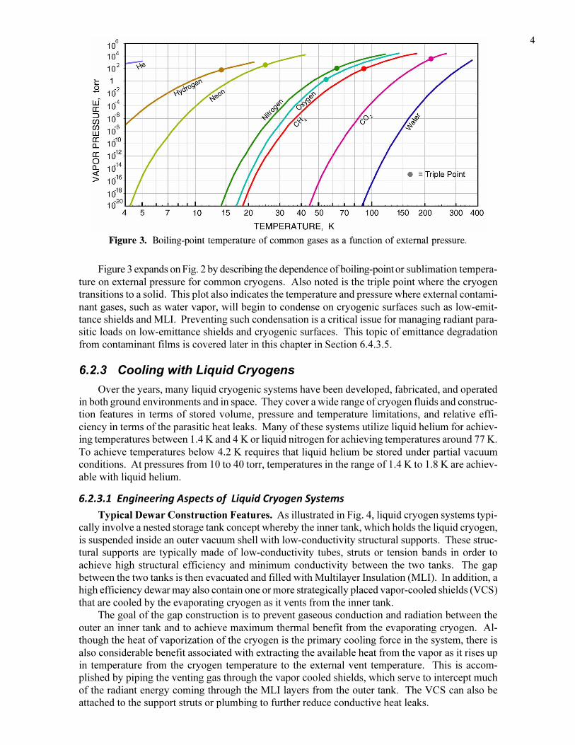


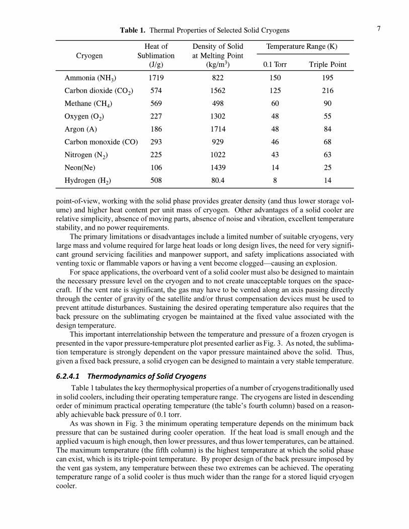


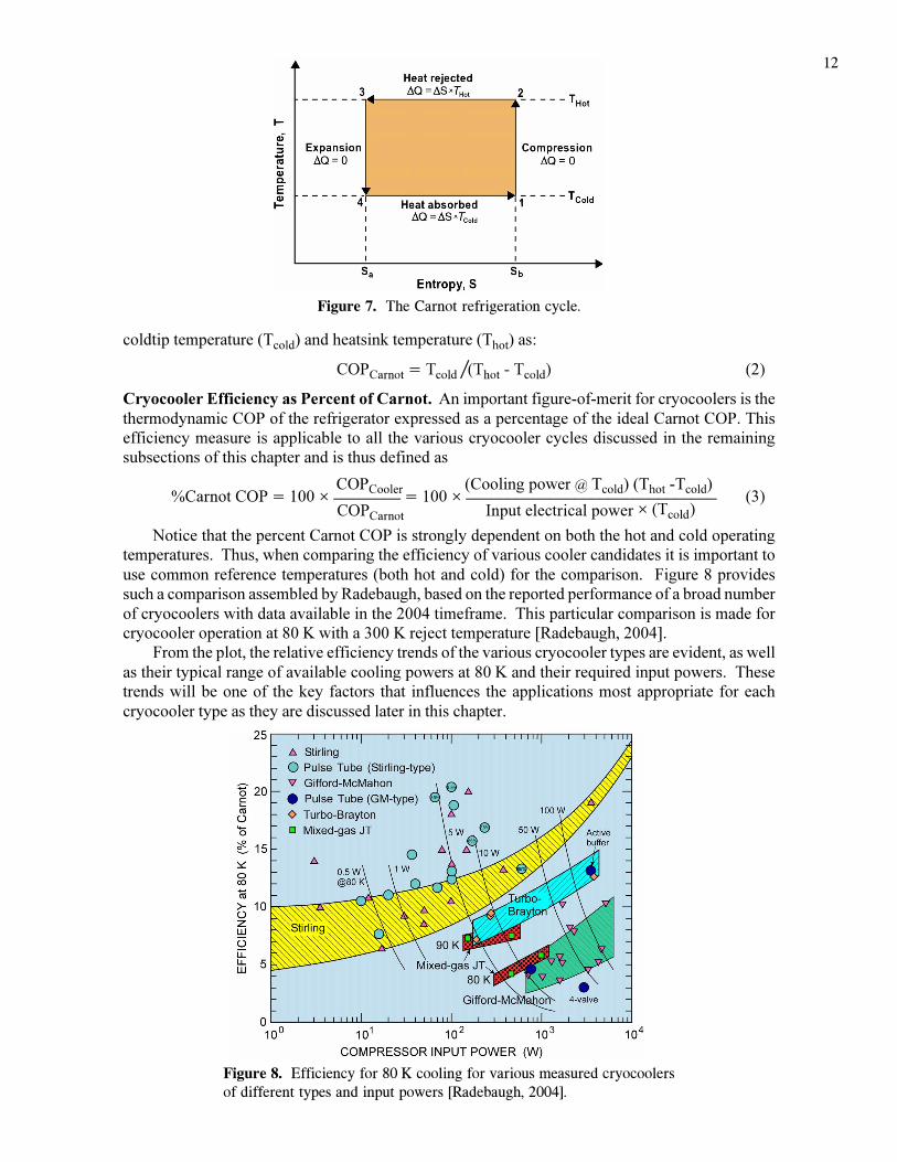
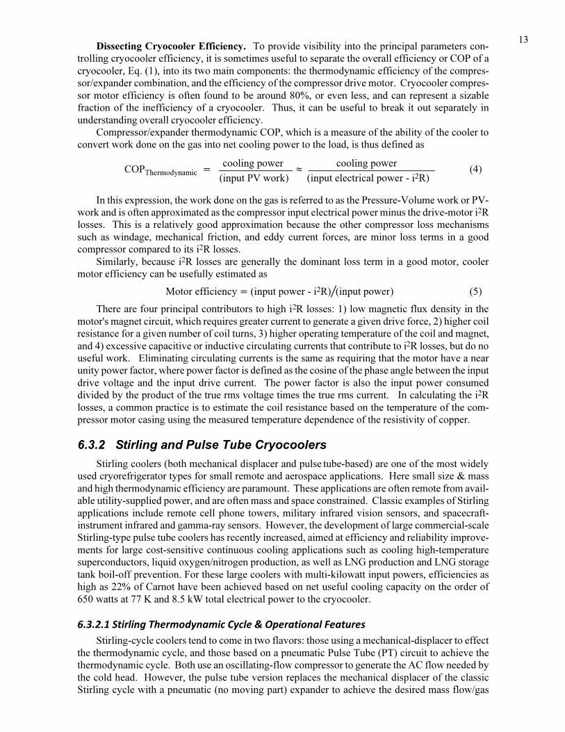
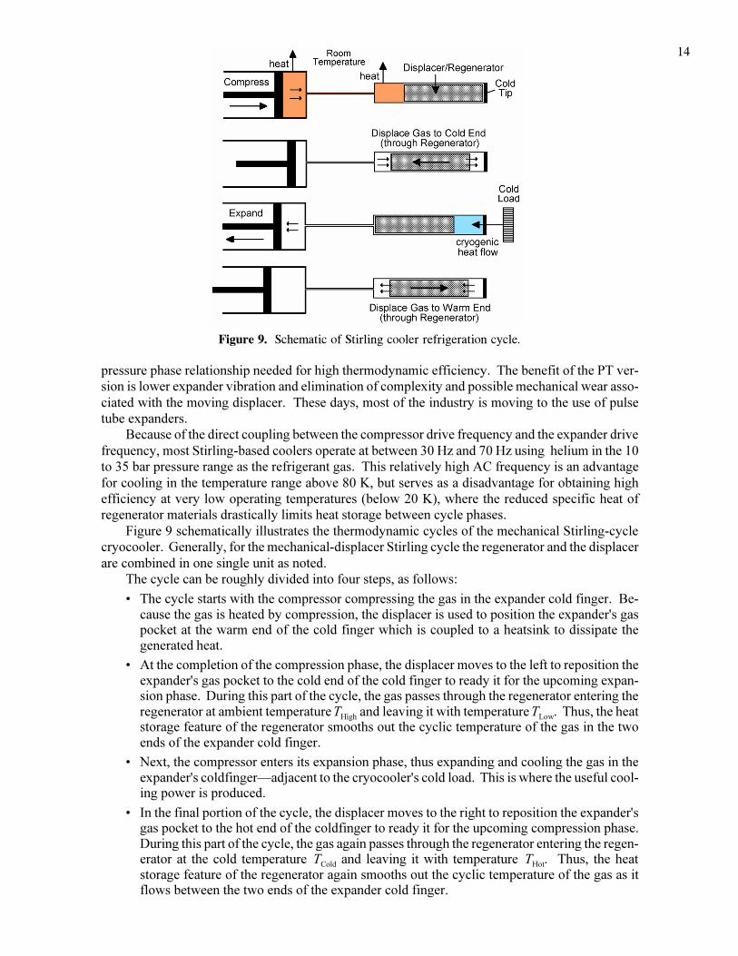


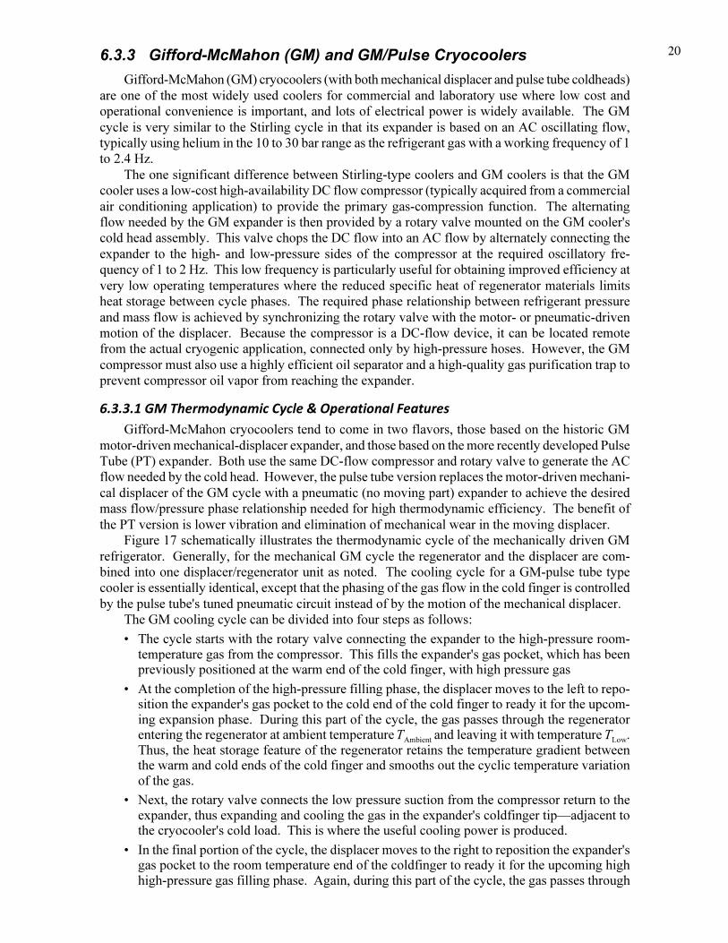
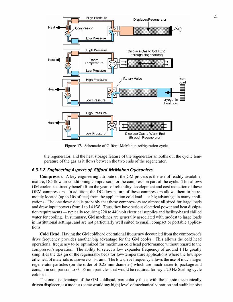


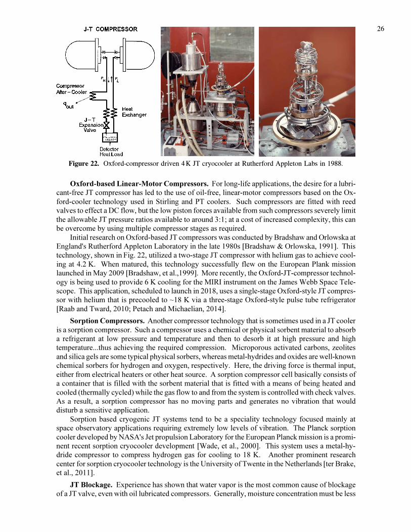


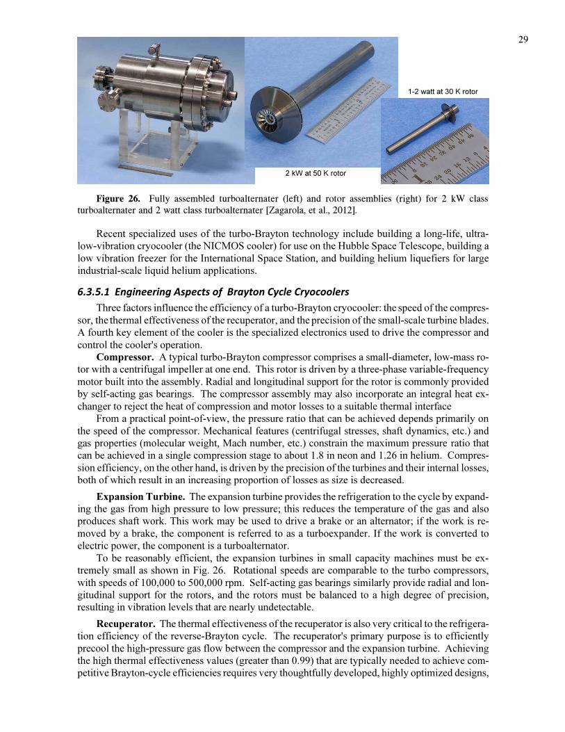


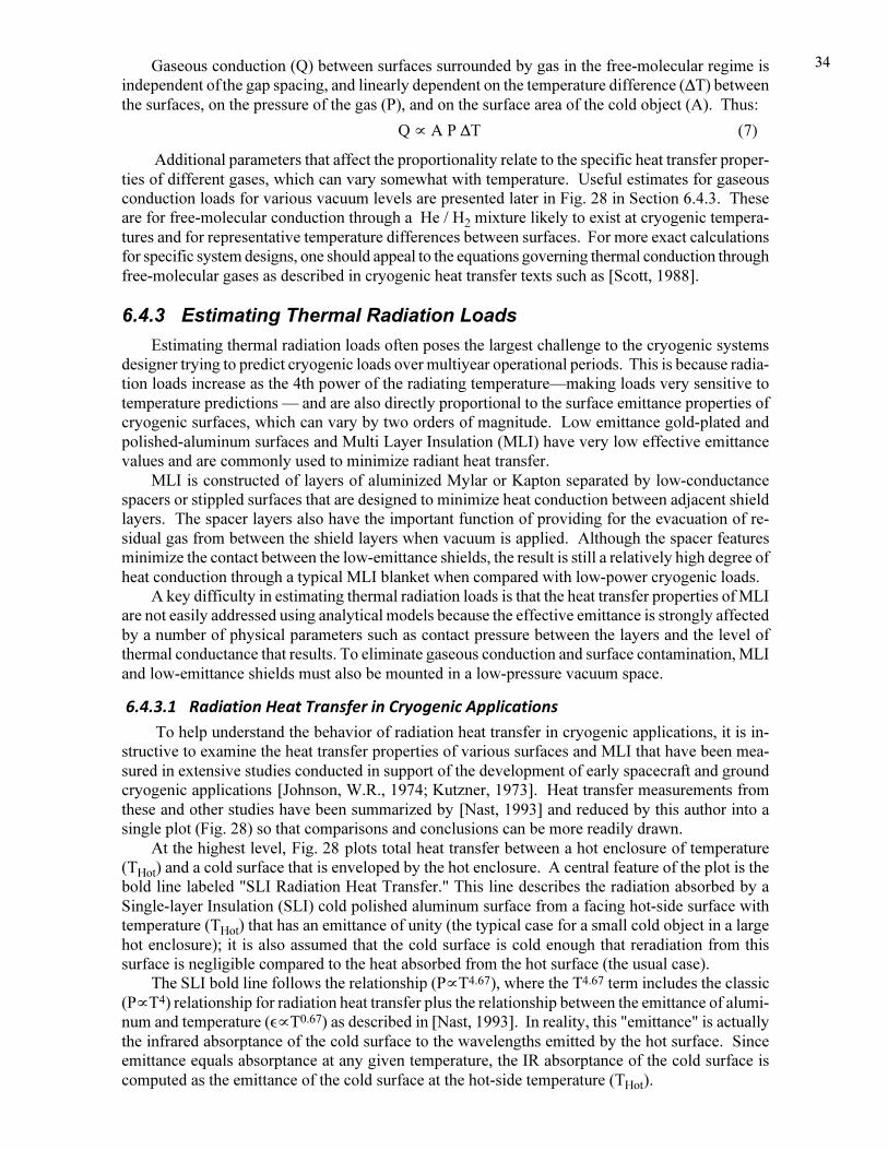


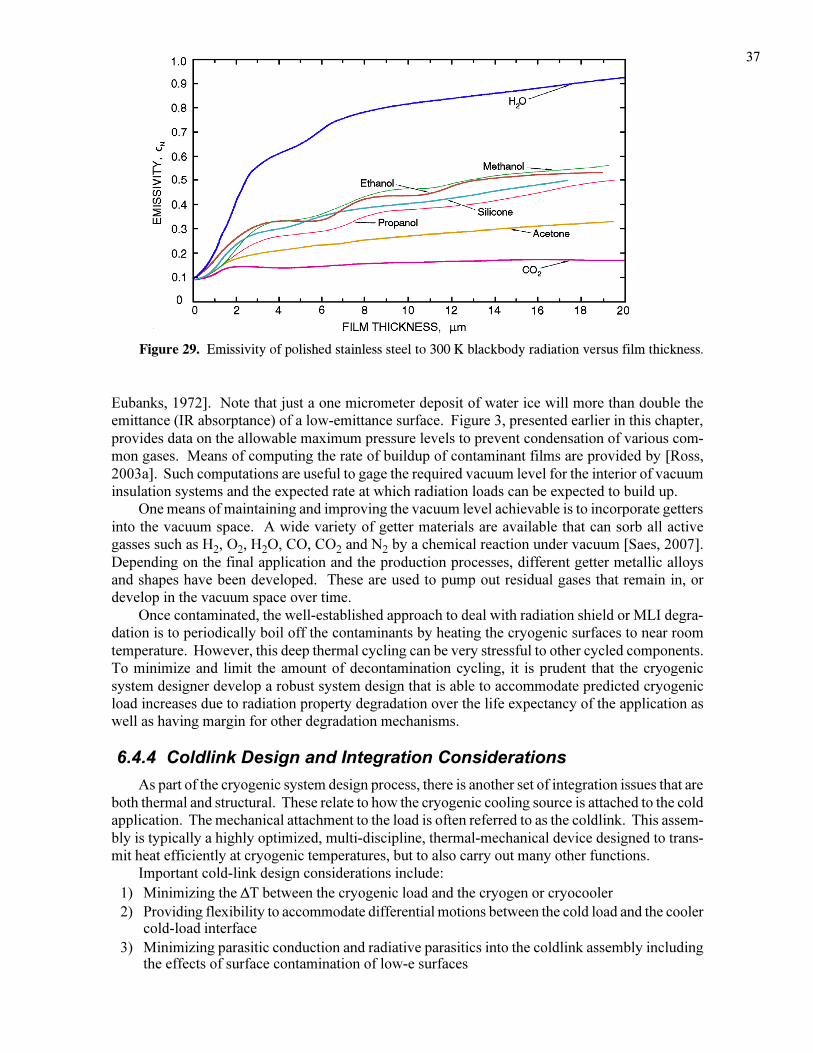

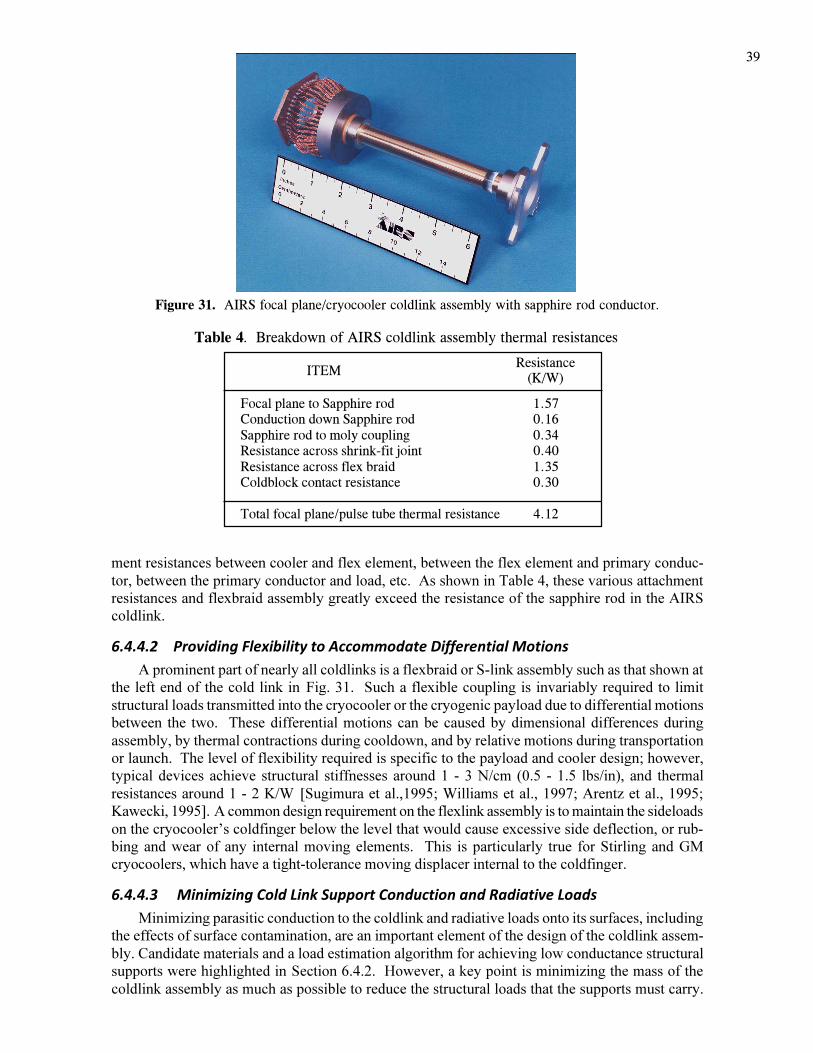


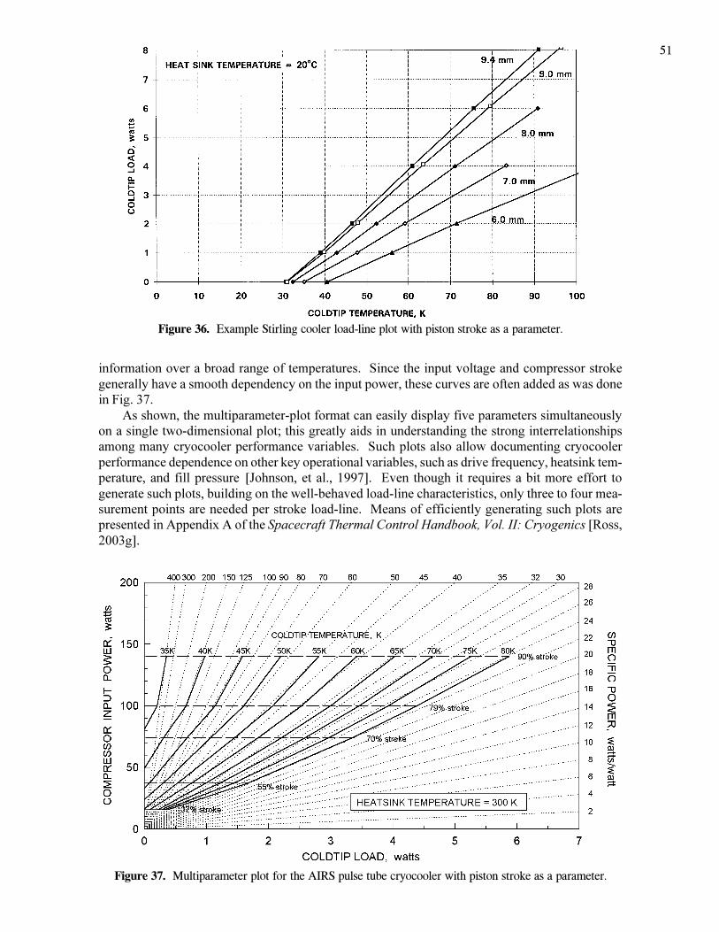
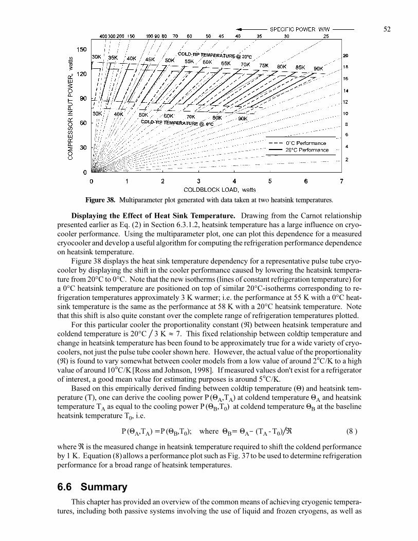


![Study Guide Commercial Refrig REV 1 1[1]](https://static.documents.pub/doc/80x56/54eab3c94a7959b1798b4578/study-guide-commercial-refrig-rev-1-11.jpg)


