Regarding Soil–Vegetation–Atmosphere Interactions

water

Article

Monitoring of a Full-Scale Embankment ExperimentRegarding Soil–Vegetation–Atmosphere Interactions

Raül Oorthuis * ID , Marcel Hürlimann ID , Alessandro Fraccica, Antonio Lloret ID , José Moya,Càrol Puig-Polo ID and Jean Vaunat ID

Division of Geotechnical Engineering and Geosciences, Department of Civil and Environmental Engineering,UPC BarcelonaTECH, 08034 Barcelona, Spain; [email protected] (M.H.);[email protected] (A.F.); [email protected] (A.L.); [email protected] (J.M.);[email protected] (C.P.-P.); [email protected] (J.V.)* Correspondence: [email protected]

Received: 21 March 2018; Accepted: 19 May 2018; Published: 25 May 2018��

Abstract: Slope mass-wasting like shallow slides are mostly triggered by climate effects, such asrainfall, and soil–vegetation–atmosphere (SVA) interactions play a key role. SVA interactions arestudied by a full-scale embankment with different orientations (North and South) and vegetationcovers (bare and vegetated) in the framework of the prediction of climate change effects on slopestability in the Pyrenees. A clayey sand from the Llobregat river delta was used for the construction ofthe embankment and laboratory tests showed the importance of suction on the strength and hydraulicconductivity. Sixty sensors, which are mostly installed at the upper soil layer of the embankment,registered 122 variables at four vertical profiles and the meteorological station with a 5 min scanrate. Regarding temperature, daily temperature fluctuation at the shallow soil layer disappearedat a depth of about 0.5 m. There was great influence of orientation with much higher values at theSouth-facing slope (up to 55 ◦C at −1 cm depth) due to solar radiation. Regarding rainfall infiltration,only long duration rainfalls produced an important increase of soil moisture and pore water pressure,while short duration rainfalls did not trigger significant variations. However, these changes mostlyaffected the surface soil layer and decreased with depth.

Keywords: monitoring; embankment; rainfall infiltration; heat flux

1. Introduction

The understanding of soil–vegetation–atmosphere interactions is fundamental for the correctassessment of rainfall-induced slides and other slope mass-wasting processes [1]. These interactionsare of great importance due to future global changes associated with climate changes [2–5]. The fifthassessment report of the Intergovernmental Panel on Climate Change [6] states that number of warmdays has likely increased at the global level and that extreme precipitation events have increased inEurope since 1950. All these effects will largely affect the soil–vegetation–atmosphere interactions andalso influence the mechanisms of slope mass-wasting in the future [7,8].

Mass-wasting due to shallow slope failures represents one of the most important erosional processin many mountainous regions and may also be the most dangerous [9]. In addition, superficial failuresin artificial slopes are a particularly important issue at transportation embankments [10–12].

Soil–vegetation–atmosphere (SVA) models have generally received little attention in geotechnicalengineering, maybe due to the absence of thermo-hydro-mechanical formulations able to couple allthe processes with the soil mechanical response. With the exception of some pioneering work suchas Blight [13], it is only in recent years that research has developed on the overall effect of the SVAinteractions on responses of natural and artificial slopes [14–16]. However, most studies focus on

Water 2018, 10, 688; doi:10.3390/w10060688 www.mdpi.com/journal/water

http://www.mdpi.com/journal/water

http://www.mdpi.com

https://orcid.org/0000-0003-4722-7838

https://orcid.org/0000-0003-0119-1438

https://orcid.org/0000-0001-7991-8487

https://orcid.org/0000-0002-8820-6446

https://orcid.org/0000-0003-3579-9652

http://www.mdpi.com/2073-4441/10/6/688?type=check_update&version=1

http://dx.doi.org/10.3390/w10060688

http://www.mdpi.com/journal/water

Water 2018, 10, 688 2 of 23

the infiltration processes in unsaturated soils by performing laboratory tests on slopes with limitedextension [17–19]. There are also some large-scale experiments [20] and a few studies that constructeda full-scale embankment in order to monitor the soil–atmosphere interactions [21–23]. Finally, multipleresearch studies have been performed on the monitoring of natural slopes affected by different typesof slope mass-wasting mechanisms [24–27].

The preceding state-of-the-art techniques show that most research focuses on the soil–atmosphereinteraction and studies on SVA mechanisms are rather scare. There are studies regardingsoil–vegetation interactions [28], but principally neglecting geotechnical aspects. These aspects, suchas the effect of suction and root reinforcement on the shear strength, are important to evaluatethe engineering behavior of earth materials and the stability of natural and man-made slopes [29].Therefore, the principal goal of our study is to achieve detailed data on the SVA interactions byperforming an extensive monitoring of a full-scale physical embankment located close to our university.The registered data will improve our understanding about the thermo-hydraulic processes occurringat the soil–plants–atmosphere interface and their coupling with mechanical effects. In the presentpublication, we describe the monitoring set-up and present the first monitoring results on the heat andwater flow across the upper soil layer of the test embankment.

2. Methods

2.1. Construction of Embankment

At the end of 2016, the test embankment was built with help of a backhoe loader at the ParcUPCAgròpolis, which includes outdoor experimental facilities for research purposes. It is situated onthe deltaic floodplain of the Llobregat River about 20 km southwest from Barcelona downtown.The embankment was made using a clayey sand of the zone.

The embankment measures 18 m long, 12 m wide, and 2.5 m high, which incorporates a totalvolume of about 326 m3. The slopes are built at 33.7 degrees, corresponding to 3H:2V. The constructionphases included three steps: first, the core was built; then an irregular, studded structured, andimpermeable polyethylene geomembrane was laid out; and finally, a 50–70 cm thick soil layerwas accumulated on the geomembrane. A shallow soil layer on an impermeable bedrock is a verycommon condition in many mountainous areas including the Pyrenees or the Catalan Coastal Ranges,where multiple slope rainfall-induced failures have occurred in the past [30–32]. Figure 1a shows aphotograph of the embankment during the accumulation of the surficial soil layer on the geomembrane.

The surficial soil layer includes four monitored slope partitions, which are laterally separated bythe geomembrane: a vegetated and a bare slope at the South side of the embankment and another twopartitions with and without vegetation at the North-facing slope. This set-up provided information onthe effect of orientation (solar radiation) and of vegetation, two fundamental aspects in the evaluation ofthe influence of future changes on slope mass-wasting. The growth of vegetation was impeded in twopartitions by the periodic application of herbicide, while Cynodon Dactylon and Festuca Arundinaceaseeds were sowed in the other two partitions. These species are common in the application of sloperevegetation, are resistant against drought, and increase soil strength due to their roots [33–36].

In addition, displacement measurements by different geomatic techniques are performedperiodically to observe ground movements. At the moment, terrestrial laser scanning (Figure 1b)and dual constellation real-time kinematic positioning with GPS were used. In the future, digitalphotogrammetry using data of time-lapse cameras is planned to achieve movements with a smallertime interval.

Water 2018, 10, 688 3 of 23

Water 2018, 10, x FOR PEER REVIEW 3 of 23

(a)

(b)

Figure 1. (a) Photograph of the embankment during the construction ; (b) 3D view of the point cloud obtained by terrestrial laser scanning.

2.2. Soil Sampling and Laboratory Tests

Different soil samples of the material used for the construction of the embankment from the Llobregat river delta were taken prior to and during the development of the experiment. A detailed test program was performed at a geotechnical laboratory focusing on the basic, hydraulic, and mechanical characterization of the soil. The different laboratory tests included: (i) particle-size distribution by sieve and sedimentation methods [37,38], (ii) Atterberg limits [39], (iii) permeability, (iv) specific gravity (by pycnometer method) [40], (v) direct shear tests (in shear box device) [41], and (vi) soil–water retention curve.

Estimation of the soil permeability is important for the correct understanding of the hydro-mechanical behavior of the embankment. However, it must be stated that laboratory measurements of a small sample may be different from field permeability, where heterogeneities in the soil mostly exist [42]. For example, small movements in the slope can produce cracks that greatly increase vertical permeability.

The saturated hydraulic conductivity was determined in the laboratory by different tests: (i) triaxial tests with constant back pressure, (ii) constant and variable head permeameter tests, and (iii) consolidation tests in saturated consolidation by using the oedometer apparatus

Multiple direct shear tests were performed to determine the strength parameters of the soil including four consolidated drained (CD) tests in saturated conditions, and 15 CD tests at constant water content under partially saturated conditions. Normal stress applied to the samples was up to about 30 kN/m2, which roughly corresponds to a 1.7 m thick soil layer, using the density of the materials under consideration. Samples were statically compacted until they reached the specified dry density (ρd = 15.5 ± 0.7 Mg/m3) using three different water contents (15, 19, and 25%).

The soil–water retention curve (SWRC) was achieved by different methods. The relation between soil suction and soil volumetric water content is important information to understand the hydro-mechanical behavior of unsaturated soils [43]. The SWRC was measured in the laboratory using drying/wetting cycles on samples with a dry density of 1.62 Mg/m3. On one side, a standard ceramic tip laboratory tensiometer (T5x, UMS , München, Germany) was used for low suction values up to 200 kPa. On the other side, a dielectric water potential sensor (MPS-6, Decagon Devices, Pullman, WA, USA) and a chilled mirror dew point hygrometer (WP4, Decagon Devices, Pullman, WA, USA) were applied to measure high suction values up to 100 and 300 MPa respectively.

After constructing the embankment, in situ undisturbed soil block samples were taken at several depths between 5 and 20 cm, in order to determine moisture and natural/dry bulk density. These

Figure 1. (a) Photograph of the embankment during the construction; (b) 3D view of the point cloudobtained by terrestrial laser scanning.

2.2. Soil Sampling and Laboratory Tests

Different soil samples of the material used for the construction of the embankment from theLlobregat river delta were taken prior to and during the development of the experiment. A detailed testprogram was performed at a geotechnical laboratory focusing on the basic, hydraulic, and mechanicalcharacterization of the soil. The different laboratory tests included: (i) particle-size distribution by sieveand sedimentation methods [37,38], (ii) Atterberg limits [39], (iii) permeability, (iv) specific gravity(by pycnometer method) [40], (v) direct shear tests (in shear box device) [41], and (vi) soil–waterretention curve.

Estimation of the soil permeability is important for the correct understanding of thehydro-mechanical behavior of the embankment. However, it must be stated that laboratorymeasurements of a small sample may be different from field permeability, where heterogeneitiesin the soil mostly exist [42]. For example, small movements in the slope can produce cracks that greatlyincrease vertical permeability.

The saturated hydraulic conductivity was determined in the laboratory by different tests:(i) triaxial tests with constant back pressure, (ii) constant and variable head permeameter tests, and(iii) consolidation tests in saturated consolidation by using the oedometer apparatus.

Multiple direct shear tests were performed to determine the strength parameters of the soilincluding four consolidated drained (CD) tests in saturated conditions, and 15 CD tests at constantwater content under partially saturated conditions. Normal stress applied to the samples was upto about 30 kN/m2, which roughly corresponds to a 1.7 m thick soil layer, using the density of thematerials under consideration. Samples were statically compacted until they reached the specified drydensity (ρd = 15.5 ± 0.7 Mg/m3) using three different water contents (15%, 19%, and 25%).

The soil–water retention curve (SWRC) was achieved by different methods. The relationbetween soil suction and soil volumetric water content is important information to understand thehydro-mechanical behavior of unsaturated soils [43]. The SWRC was measured in the laboratory usingdrying/wetting cycles on samples with a dry density of 1.62 Mg/m3. On one side, a standard ceramictip laboratory tensiometer (T5x, UMS, München, Germany) was used for low suction values up to200 kPa. On the other side, a dielectric water potential sensor (MPS-6, Decagon Devices, Pullman, WA,USA) and a chilled mirror dew point hygrometer (WP4, Decagon Devices, Pullman, WA, USA) wereapplied to measure high suction values up to 100 and 300 MPa respectively.

Water 2018, 10, 688 4 of 23

After constructing the embankment, in situ undisturbed soil block samples were taken at severaldepths between 5 and 20 cm, in order to determine moisture and natural/dry bulk density. Theseundisturbed soil samples were obtained from thin-walled sampling tubes and clods. Since themonitoring is installed at the two principal orientations (North and South) of the embankment,material was sampled at these two slope faces. The paraffin method [44] was applied to measure thedensity of these undisturbed samples.

2.3. Monitoring Set-Up

The sensors were installed at vertical infiltration profiles inside the upper soil layer of each of thefour partitions. In addition, a meteorological station was fixed at the top of the embankment. All thesensors are connected by wires to a datalogger (CR1000, Campbell Scientific, Logan, UT, USA) thatwas used in combination with two multiplexers due to the large amount of sensors. The data of allsensors are recorded at a constant sampling rate of 5 min. Every 24 h, the data files are sent via FTP tothe university sever. The power supply of the entire monitoring system is provided by solar panelsand batteries.

The experiment includes four different zones: (i) South slope with vegetation (SV), (ii) Southslope without vegetation (SnV), (iii) North slope with vegetation (NV), (iv) North slope withoutvegetation (NnV). Each of the four zones is equipped by a vertical profile of different sensors (Figure 2)and the devices that measure the surface runoff and seepage. Thus, a complete analysis of thesoil–vegetation–atmosphere interaction is possible by incorporating observations gathered by themeteorological station. The installation of the sensors was performed in two main phases. First,the setup of the non-vegetated profiles (SnV and NnV) was performed in spring 2017. Second,the vegetated profiles (SV and NV) were installed in autumn 2017. Finally, some complementarysensors were mounted at the beginning of 2018. Figure 3 shows a photograph of the embankment afterthe installation of the sensors looking towards the North-faced slope.


undisturbed soil samples were obtained from thin-walled sampling tubes and clods. Since the monitoring is installed at the two principal orientations (North and South) of the embankment, material was sampled at these two slope faces. The paraffin method [44] was applied to measure the density of these undisturbed samples.

2.3. Monitoring Set-Up

The sensors were installed at vertical infiltration profiles inside the upper soil layer of each of the four partitions. In addition, a meteorological station was fixed at the top of the embankment. All the sensors are connected by wires to a datalogger (CR1000, Campbell Scientific, Logan, UT, USA) that was used in combination with two multiplexers due to the large amount of sensors. The data of all sensors are recorded at a constant sampling rate of 5 min. Every 24 h, the data files are sent via FTP to the university sever. The power supply of the entire monitoring system is provided by solar panels and batteries.

The experiment includes four different zones: (i) South slope with vegetation (SV), (ii) South slope without vegetation (SnV), (iii) North slope with vegetation (NV), (iv) North slope without vegetation (NnV). Each of the four zones is equipped by a vertical profile of different sensors (Figure 2) and the devices that measure the surface runoff and seepage. Thus, a complete analysis of the soil–vegetation–atmosphere interaction is possible by incorporating observations gathered by the meteorological station. The installation of the sensors was performed in two main phases. First, the setup of the non-vegetated profiles (SnV and NnV) was performed in spring 2017. Second, the vegetated profiles (SV and NV) were installed in autumn 2017. Finally, some complementary sensors were mounted at the beginning of 2018. Figure 3 shows a photograph of the embankment after the installation of the sensors looking towards the North-faced slope.

Figure 2. Schematic overview of the full-scale experiment divided into four partitions: SV, SnV, NV, and NnV (see text for explanations). The position of the four vertical sensor profiles (red squares) and the meteorological station (red dot) is illustrated.

Figure 2. Schematic overview of the full-scale experiment divided into four partitions: SV, SnV, NV,and NnV (see text for explanations). The position of the four vertical sensor profiles (red squares) andthe meteorological station (red dot) is illustrated.

Water 2018, 10, 688 5 of 23


Figure 3. Photograph of the embankment after installation of the sensors looking towards the North slope.

2.3.1. Vertical Sensor Profiles

Each vertical profile measures air and soil temperature, relative humidity, barometric pressure, heat flux, pore water pressure (PWP), and volumetric water content (VWC) at different positions. A complete list of all the sensors and the recorded parameters is given in Table 1. Net solar radiation devices were installed at each of the orientations (North and South). The general distribution of the different devices is shown by the example of vertical profile NnV (Figure 4a). In addition, photographs of the soil texture format profiles NnV and NV during the sensors installation are shown in Figure 4b,c respectively. They show the sandy loamy soil with isolated gravel particles at both trenches, while the presence of organic material in the form of plant roots is visible in the vegetated North (NV) profile.

Not each vertical profile has the distribution of sensors as shown in Figure 4a and the final number of devices installed in each profile ranges from 13 to 14 (Table 2). The parameter that is measured at most positions is temperature, which is monitored at least at 7 positions along each vertical profile, while PWP and VWC are registered at a minimum of 3 and 4 positions, respectively. The total number of records measured at all sensors for each of the non-vegetated slopes (SnV and NnV) and for each of the vegetated slopes (SV and NV) is 27 and 29, respectively. Some sensors had technical problems during the first year or were installed in the second phase. That’s why the time series of specific sensors are not complete when presented in the results section.

Figure 3. Photograph of the embankment after installation of the sensors looking towards theNorth slope.

2.3.1. Vertical Sensor Profiles

Each vertical profile measures air and soil temperature, relative humidity, barometric pressure,heat flux, pore water pressure (PWP), and volumetric water content (VWC) at different positions.A complete list of all the sensors and the recorded parameters is given in Table 1. Net solar radiationdevices were installed at each of the orientations (North and South). The general distribution of thedifferent devices is shown by the example of vertical profile NnV (Figure 4a). In addition, photographsof the soil texture format profiles NnV and NV during the sensors installation are shown in Figure 4b,crespectively. They show the sandy loamy soil with isolated gravel particles at both trenches, while thepresence of organic material in the form of plant roots is visible in the vegetated North (NV) profile.

Table 1. Characteristics of the sensors installed in the vertical slope profiles.

Parameter Measured Model Measuring Range

Soil temperature Campbell 107 35 to +50 ◦C

Volumetric water contentDecagon 5TE

0 to 1 m3/m3

Soil temperature −40 to +50 ◦CElectric conductivity 0 to 23 dS/m

Pore water pressure Decagon MPS-6 −9 to −100,000 kPaSoil temperature −40 to +60 ◦C

Pore water pressure UMS T4 −85 to +100 kPa

Air temperatureDecagon VP-4

−40 to +80 ◦CRelative air humidity 0 to 100%Atmospheric pressure 49 to 109 kPa

Wind speed Davis Cup Anemometer 0.9 to 78 m/sWind direction 0 to 360◦

Heat flux Hukseflux HFP01 ±2000 W/m2

Net solar radiation Kipp & Zonnen NR Lite2 ±2000 W/m2

Water 2018, 10, 688 6 of 23

Not each vertical profile has the distribution of sensors as shown in Figure 4a and the final numberof devices installed in each profile ranges from 13 to 14 (Table 2). The parameter that is measured atmost positions is temperature, which is monitored at least at 7 positions along each vertical profile,while PWP and VWC are registered at a minimum of 3 and 4 positions, respectively. The total numberof records measured at all sensors for each of the non-vegetated slopes (SnV and NnV) and for eachof the vegetated slopes (SV and NV) is 27 and 29, respectively. Some sensors had technical problemsduring the first year or were installed in the second phase. That’s why the time series of specificsensors are not complete when presented in the results section.Water 2018, 10, x FOR PEER REVIEW 6 of 23

NnV NnV NV

(a) (b) (c)

Figure 4. (a) Schematic design of the vertical profile of NnV indicating the location of the sensors; (b) photograph taken during installation of sensors at the NnV profile; (c) photograph taken during installation of sensors at the NV profile.

Table 1. Characteristics of the sensors installed in the vertical slope profiles.

Parameter Measured Model Measuring Range Soil temperature Campbell 107 35 to +50 °C

Volumetric water content Decagon 5TE

0 to 1 m3/m3 Soil temperature −40 to +50 °C

Electric conductivity 0 to 23 dS/m Pore water pressure

Decagon MPS-6 −9 to −100000 kPa

Soil temperature −40 to +60 °C Pore water pressure UMS T4 −85 to +100 kPa

Air temperature Decagon VP-4

−40 to +80 °C Relative air humidity 0 to 100% Atmospheric pressure 49 to 109 kPa

Wind speed Davis Cup Anemometer

0.9 to 78 m/s Wind direction 0 to 360°

Heat flux Hukseflux HFP01 ±2000 W/m2 Net solar radiation Kipp & Zonnen NR Lite2 ±2000 W/m2

Table 2. Location of selected sensor in the four vertical profiles. Only devices focusing on temperature, volumetric water content, and pore water pressure are listed.

Sensor Depth of Installation (cm)

SV SnV NV NnV

Air/soil temperature +9.5, −1, −6, −11, −16, −36, −43

+9.5, −1, −6, −11, −16, −32, −36, −57

+9.5, −1, −6, −11, −16, −36, −56

+9.5, −1, −6, −11, −16, −36, −56

Volumetric water content −6, −16, −36, −43 −6,−16, −36, −57 −6, −16, −36, −56 −6, −16, −36, −56 Pore water pressure −16, −36, −40, −43 −11, −32, −72 −16, −36, −56, −59 −16, −36, −56

In the following, the different types of devices will be described and some characteristics discussed. In this study, two types of sensors are considered: (1) devices measuring temperature

Figure 4. (a) Schematic design of the vertical profile of NnV indicating the location of the sensors;(b) photograph taken during installation of sensors at the NnV profile; (c) photograph taken duringinstallation of sensors at the NV profile.

Table 2. Location of selected sensor in the four vertical profiles. Only devices focusing on temperature,volumetric water content, and pore water pressure are listed.

SensorDepth of Installation (cm)

SV SnV NV NnV

Air/soil temperature +9.5, −1, −6, −11,−16, −36, −43

+9.5, −1, −6, −11,−16, −32, −36, −57

+9.5, −1, −6, −11,−16, −36, −56

+9.5, −1, −6, −11,−16, −36, −56

Volumetric water content −6, −16, −36, −43 −6,−16, −36, −57 −6, −16, −36, −56 −6, −16, −36, −56Pore water pressure −16, −36, −40, −43 −11, −32, −72 −16, −36, −56, −59 −16, −36, −56

In the following, the different types of devices will be described and some characteristics discussed.In this study, two types of sensors are considered: (1) devices measuring temperature changes andheat flux along the atmosphere–soil interface, and (2) devices focusing on the infiltration of rainfallinto the soil layer.

Air and soil temperature is measured at different positions close to the surface. In the mostsuperficial part of the soil layer, three thermistors encapsulated in an aluminum housing (107, CampbellScientific, Logan, UT, USA) were buried. The rest of the soil temperature is monitored by thethermistors incorporated in other sensors (MPS-6, Decagon Devices, Pullman, WA, USA, and 5TE,

Water 2018, 10, 688 7 of 23

Decagon Devices, Pullman, WA, USA). Another sensor (VP-4, Decagon Devices, Pullman, WA, USA)measures the air temperature at 9.5 cm above the terrain surface.

The heat flux across a soil section is measured close and parallel to the surface, where most of theheat transfer is expected. For this reason, a thermopile (HFP01, Hukseflux, Delft, The Netherlands)is installed at 8 cm depth and transforms the measured voltage into heat flux. Finally, wind speedand direction is also registered at each vertical profile by a cup and vane anemometer installed 15 cmabove the terrain surface.

Water content and pore water pressure are fundamental parameters to understand theatmosphere–vegetation–soil interactions related to rainfall infiltration into the soil. In the experiment,multiple devices register these processes in the vertical profiles, principally tensiometers and soilmoisture sensors.

Two different types of tensiometers were installed for measuring pore water pressure: (i) porousceramic disc tensiometers (MPS-6, Decagon Devices, Pullman, WA, USA), and (ii) porous ceramiccup tensiometer (T4, UMS, München, Germany). The MPS-6 dielectric water potential sensors aredesigned to measure suction values up to 100 MPa and are located close to the surface (Table 2), wherehigh suction values are expected. In contrast, the UMS T4 is a tensiometer that measures PWP ina negative and positive range. Thus, its installation is at the lower part of the monitored soil layer,where low suction or positive PWP values are expected. The UMS T4 device is a rather delicate sensorin comparison with the robust MPS-6. The UMS T4 tensiometers were refilled and calibrated in thelaboratory before their installation. The refilling was made with de-aired water, ensuring no air bubblesremained inside the ceramic cup, which would lead to an incorrect pressure reading. In addition,the pressure measured by the transducer has to be corrected twice: (i) due to the elevation differencebetween the pressure transducer and the ceramic cup, and (ii) because of the different power excitation(our system supplies 12 V, while the manufacturer calibration is performed at 10.6 V). The installationof the UMS T4 tensiometers has to be carried out very carefully. To prevent surface runoff runningdown into the borehole along the tensiometer, a rubber water-retaining disk was slipped aroundthe sensor at the soil surface and a perfect fit between the previously drilled hole and the devicewas performed.

The volumetric water content (VWC) is measured by Decagon 5TE sensors (Decagon Devices,Pullman, WA, USA), which are installed at different depths in the soil layer (Table 2). The 5TE usesan electromagnetic field to measure the dielectric permittivity of the surrounding medium. Priorto field installation, a calibration of the sensor was performed in the laboratory using soil sampleswith a similar bulk density as the embankment slope. The VWC that was recorded by the sensorwas compared with the one determined by the standard procedure incorporating the void ratio, thegravimetric water content, and the specific gravity of the soil samples. The calibration results showedthat there was no significance difference with the equation given by the manufacturer, therefore thisequation was finally used for the transformation of the sensor reading into VWC.

2.3.2. Meteorological Station

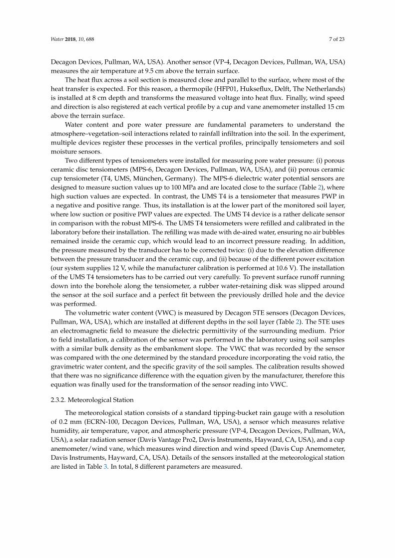
The meteorological station consists of a standard tipping-bucket rain gauge with a resolutionof 0.2 mm (ECRN-100, Decagon Devices, Pullman, WA, USA), a sensor which measures relativehumidity, air temperature, vapor, and atmospheric pressure (VP-4, Decagon Devices, Pullman, WA,USA), a solar radiation sensor (Davis Vantage Pro2, Davis Instruments, Hayward, CA, USA), and a cupanemometer/wind vane, which measures wind direction and wind speed (Davis Cup Anemometer,Davis Instruments, Hayward, CA, USA). Details of the sensors installed at the meteorological stationare listed in Table 3. In total, 8 different parameters are measured.

Water 2018, 10, 688 8 of 23

Table 3. Sensors installed at the meteorological station.

Parameter Measured Model Measurement Range

Rainfall Decagon ECRN-100 0.2 mm *

Air temperatureDecagon VP-4

−40 to +80 ◦CRelative air humidity 0 to 100%Atmospheric pressure 49 to 109 kPa

Solar radiation Davis Vantage Pro2 0 to 1800 W/m2

Wind speed Davis Cup Anemometer 0.9 to 78 m/sWind direction 0 to 360◦

* Minimum resolution of sensor.

3. Results

3.1. Laboratory Results

The laboratory results from different soil samples of the material used for the construction of theembankment from the Llobregat river delta are summarized in Table 4.

Table 4. Soil properties of the material used for the construction of the embankment.

Soil Property Value

Gravel content (%) 34–42Sand content (%) 30–43Silt content (%) 20–25

Clay content (%) 4–6Fines (%) 25–31

Liquid limit (%) 29.5–34.4Plastic limit (%) 19.9–21.2

Plasticity index (%) 9.7–13.5Specific gravity (Mg/m3) 2.65–2.70

Cohesion (kPa) 0Friction angle (◦) 58

Hydraulic conductivity (m/s) 7.7 × 10−8–1.8 × 10−7

Table 5 lists a summary of the most important parameters determined from undisturbed soilsamples. Differences in density between the North and South slopes may be due to the compactionprocess during the construction.

Table 5. Soil properties of materials sampled after construction of the embankment at the two monitoredslopes (South and North).

Soil Property South Slope North Slope

Bulk density (Mg/m3) 1.72–1.78 1.85–1.93Dry density (Mg/m3) 1.52–1.57 1.55–1.61

Water content (%) 13.23–15.11 19.08–19.84Void ratio (-) 0.70–0.76 0.66–0.72Porosity (-) 0.41–0.43 0.40–0.42

3.1.1. Basic Soil Characterization

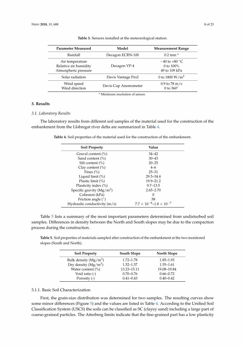
First, the grain-size distribution was determined for two samples. The resulting curves showsome minor differences (Figure 5) and the values are listed in Table 4. According to the Unified SoilClassification System (USCS) the soils can be classified as SC (clayey sand) including a large part ofcoarse-grained particles. The Atterberg limits indicate that the fine-grained part has a low plasticity

Water 2018, 10, 688 9 of 23

behavior (Table 4). This low plasticity index indicates that small changes in soil humidity involveimportant changes of its consistency.


behavior (Table 4). This low plasticity index indicates that small changes in soil humidity involve important changes of its consistency.

Figure 5. Particle-size distribution of the material used for the construction of the monitored embankment.

3.1.2. Strength Parameters

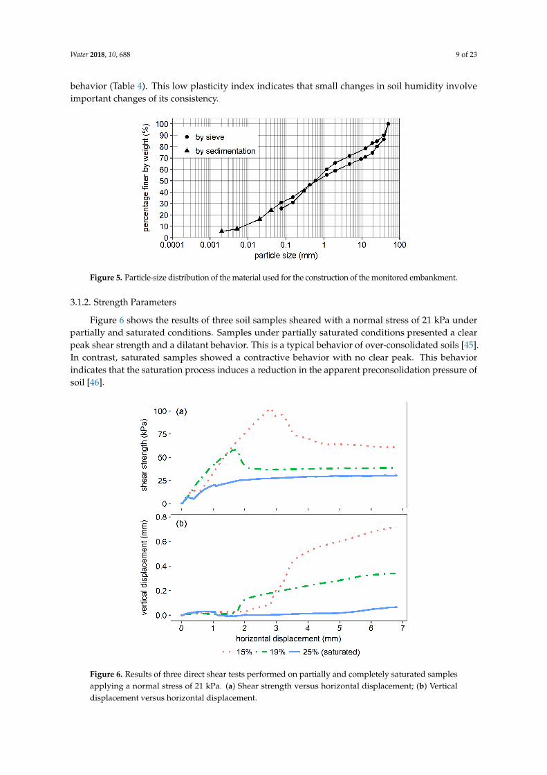
Figure 6 shows the results of three soil samples sheared with a normal stress of 21 kPa under partially and saturated conditions. Samples under partially saturated conditions presented a clear peak shear strength and a dilatant behavior. This is a typical behavior of over-consolidated soils [45]. In contrast, saturated samples showed a contractive behavior with no clear peak. This behavior indicates that the saturation process induces a reduction in the apparent preconsolidation pressure of soil [46].

Figure 6. Results of three direct shear tests performed on partially and completely saturated samples applying a normal stress of 21 kPa. (a) Shear strength versus horizontal displacement; (b) Vertical displacement versus horizontal displacement.



Figure 6 shows the results of three soil samples sheared with a normal stress of 21 kPa underpartially and saturated conditions. Samples under partially saturated conditions presented a clearpeak shear strength and a dilatant behavior. This is a typical behavior of over-consolidated soils [45].In contrast, saturated samples showed a contractive behavior with no clear peak. This behaviorindicates that the saturation process induces a reduction in the apparent preconsolidation pressure ofsoil [46].


behavior (Table 4). This low plasticity index indicates that small changes in soil humidity involve important changes of its consistency.



Figure 6 shows the results of three soil samples sheared with a normal stress of 21 kPa under partially and saturated conditions. Samples under partially saturated conditions presented a clear peak shear strength and a dilatant behavior. This is a typical behavior of over-consolidated soils [45]. In contrast, saturated samples showed a contractive behavior with no clear peak. This behavior indicates that the saturation process induces a reduction in the apparent preconsolidation pressure of soil [46].

Figure 6. Results of three direct shear tests performed on partially and completely saturated samples applying a normal stress of 21 kPa. (a) Shear strength versus horizontal displacement; (b) Vertical displacement versus horizontal displacement.

Figure 6. Results of three direct shear tests performed on partially and completely saturated samplesapplying a normal stress of 21 kPa. (a) Shear strength versus horizontal displacement; (b) Verticaldisplacement versus horizontal displacement.

Water 2018, 10, 688 10 of 23

The normal versus shear stress relation of all tests are plotted in Figure 7. Results confirm theimportance of water content in the soil, when strength parameters are analyzed. In particular, the greatcontribution of suction to the shear strength must be taken into account. The data of the direct sheartest also shows that peak shear stress decreases and gets closer to constant volume shear stress whenthe sample is closer to saturated conditions. For unsaturated soils, the intergranular stress may bedefined as [47]:

σ′n = σn + χ·s = σn + Sr·s, (1)

where σ′n is the Bishop’s generalized normal effective stress for unsaturated soils, σn is the normalstress, χ is the Bishop’s parameter and s is suction. Bishop’s parameter χ is a function of the saturationdegree Sr and is imposed to vary between 0 for dry soils to 1 for saturated soils which can be roughlyassumed to have the value of the saturation degree [48].

In addition, the shear strength of unsaturated soils can be defined in terms of two independentstress variables, the normal stress and suction [49]:

τ = c′ + σn tan φ′ + s tan φb, (2)

where τ is the shear strength, c′ the effective cohesion, σn the normal stress, s is suction, φ′ the effectivefriction angle and φb represents the frictional contribution by suction to shear strength. ReplacingBishop’s generalized effective stress for unsaturated soils in Equation (1) with Fredlund’s unsaturatedshear strength of Equation (2) and considering χ = Sr, the following expression is obtained:

τ = c′ + σn tan φ′ + s Sr tan φ′ = c′ + σn tan φ′ + s tan φb (3)

from which can be deduced that:tan φb = Sr tan φ′ (4)


The normal versus shear stress relation of all tests are plotted in Figure 7. Results confirm the importance of water content in the soil, when strength parameters are analyzed. In particular, the great contribution of suction to the shear strength must be taken into account. The data of the direct shear test also shows that peak shear stress decreases and gets closer to constant volume shear stress when the sample is closer to saturated conditions. For unsaturated soils, the intergranular stress may be defined as [47]: 𝜎 = 𝜎 + 𝜒 · 𝑠 = 𝜎 + 𝑆 · 𝑠, (1)

where 𝜎 is the Bishop’s generalized normal effective stress for unsaturated soils, 𝜎 is the normal stress, 𝜒 is the Bishop’s parameter and s is suction. Bishop’s parameter 𝜒 is a function of the saturation degree 𝑆 and is imposed to vary between 0 for dry soils to 1 for saturated soils which can be roughly assumed to have the value of the saturation degree [48].

In addition, the shear strength of unsaturated soils can be defined in terms of two independent stress variables, the normal stress and suction [49]: 𝜏 = 𝑐 + 𝜎 tan𝜙 + 𝑠 tan𝜙 , (2)

where 𝜏 is the shear strength, c′ the effective cohesion, 𝜎 the normal stress, s is suction, 𝜙 the effective friction angle and 𝜙 represents the frictional contribution by suction to shear strength. Replacing Bishop’s generalized effective stress for unsaturated soils in Equation (1) with Fredlund’s unsaturated shear strength of Equation (2) and considering 𝜒 = 𝑆 , the following expression is obtained: 𝜏 = 𝑐 + 𝜎 tan𝜙 + 𝑠 𝑆 tan𝜙 = 𝑐 + 𝜎 tan𝜙′ + 𝑠 tan𝜙 (3)

from which can be deduced that: tan𝜙 = 𝑆 tan𝜙 (4)

Figure 7. Results of direct shear tests performed on partially and completely saturated samples. (a) Normal stress versus peak shear stress; (b) normal stress versus constant volume shear stress; (c) Bishop’s generalized effective normal stress versus constant volume shear stress. Shaded grey area represents the range of normal stresses expected on the monitored soil layer.

Figure 7. Results of direct shear tests performed on partially and completely saturated samples.(a) Normal stress versus peak shear stress; (b) normal stress versus constant volume shear stress;(c) Bishop’s generalized effective normal stress versus constant volume shear stress. Shaded grey arearepresents the range of normal stresses expected on the monitored soil layer.

Water 2018, 10, 688 11 of 23

The resulting failure envelope using Bishop’s generalized effective stress for partially saturatedsoils at constant volume shear strength is defined by a friction angle of 58◦ and zero cohesion (Figure 7c).This high friction angle is the result of the low normal stress up to 30 kPa applied to the samples. Forhigher normal stress values, a lower friction angle and a non-linear failure envelope are expected [50].

3.1.3. Hydraulic Behavior

The permeability ranges over almost four orders of magnitude (Figure 8), while values arebetween 7.7 × 10−8 and 1.8 × 10−7 m/s regarding void ratios observed in the embankment (0.66–0.76).However, in situ infiltration tests must be performed to finally determine the permeability, since fieldhydraulic conductivity may be much higher than the one achieved in the laboratory [42].


The resulting failure envelope using Bishop’s generalized effective stress for partially saturated soils at constant volume shear strength is defined by a friction angle of 58° and zero cohesion (Figure 7c). This high friction angle is the result of the low normal stress up to 30 kPa applied to the samples. For higher normal stress values, a lower friction angle and a non-linear failure envelope are expected [50].

3.1.3. Hydraulic Behavior

The permeability ranges over almost four orders of magnitude (Figure 8), while values are between 7.7 × 10−8 and 1.8 × 10−7 m/s regarding void ratios observed in the embankment (0.66–0.76). However, in situ infiltration tests must be performed to finally determine the permeability, since field hydraulic conductivity may be much higher than the one achieved in the laboratory [42].

Figure 8. Saturated hydraulic conductivity for different void ratios obtained by different laboratory tests. Dashed line shows the best-fit relation. Grey shaded area represents the expected void ratio in the embankment.

In addition, an experiment was performed using a column with a diameter of 14.3 cm and a height of 35 cm, filled with a soil dry density of 1.52 Mg/m3. A laboratory and field ceramic cup tensiometer (UMS T5x and UMS T4) and a dielectric water potential sensor (Decagon MPS-6) were installed in the column in order to measure suction and a capacitance moisture probe (Decagon 5TE) was used to measure volumetric water content. This soil column experiment provided supplementary data using a slightly smaller dry density sample. Initially, the sample was fully saturated, and it dried out progressively with time.

An extra experiment was performed on samples with a dry density of 1.39 Mg/m3, using a dielectric water potential sensor (Decagon MPS-6) to measure suction and a capacitance moisture probe (Decagon 5TE) to measure volumetric water content. This experiment was performed without following a specific drying-wetting path, measuring the suction on statically compacted samples with different water contents. An important aspect is that all these experiments helped to check the handling and accuracy of the sensors that later were placed at the embankment.

The data measured by the different methods allowed defining the wetting and drying SWRCs (Figure 9). The suction readings obtained by T5x sensor during the soil column experiment were not

Figure 8. Saturated hydraulic conductivity for different void ratios obtained by different laboratorytests. Dashed line shows the best-fit relation. Grey shaded area represents the expected void ratio inthe embankment.

In addition, an experiment was performed using a column with a diameter of 14.3 cm and aheight of 35 cm, filled with a soil dry density of 1.52 Mg/m3. A laboratory and field ceramic cuptensiometer (UMS T5x and UMS T4) and a dielectric water potential sensor (Decagon MPS-6) wereinstalled in the column in order to measure suction and a capacitance moisture probe (Decagon 5TE)was used to measure volumetric water content. This soil column experiment provided supplementarydata using a slightly smaller dry density sample. Initially, the sample was fully saturated, and it driedout progressively with time.

An extra experiment was performed on samples with a dry density of 1.39 Mg/m3, using adielectric water potential sensor (Decagon MPS-6) to measure suction and a capacitance moistureprobe (Decagon 5TE) to measure volumetric water content. This experiment was performed withoutfollowing a specific drying-wetting path, measuring the suction on statically compacted sampleswith different water contents. An important aspect is that all these experiments helped to check thehandling and accuracy of the sensors that later were placed at the embankment.

The data measured by the different methods allowed defining the wetting and drying SWRCs(Figure 9). The suction readings obtained by T5x sensor during the soil column experiment were not

Water 2018, 10, 688 12 of 23

represented, since they were identical to those measured by sensor T4. A modified van Genuchtenmodel that is more suitable for high suction values was applied. It can be expressed as [51]:

Se =Sr − SrlSls − Srl

=

(1 +

( sP

) 11−λ

)−λ(1− s

Ps

)λs

, (5)

where Se is the effective degree of saturation, Sr is the current saturation degree, Sls and Srl arethe maximum and residual degree of saturation respectively, s is suction, and P and λ are the vanGenuchten material parameters. λs and Ps are the modified van Genuchten material parameters,which reduce high suction values, Ps is the maximum suction at the minimum degree of saturation.The resulting modified van Genuchten fitted parameters for both drying and wetting paths aresummarized in Table 6.

Table 6. Modified van Genuchten soil–water retention curve (SWRC) fitting parameters fordrying-wetting paths.

Fitted Parameters Drying Wetting

P (kPa) 66.7 9.5λ (-) 0.28 0.20

Ps (kPa) 2.5 × 105 2.5 × 105

λs (-) 1.30 2.80Sls 1 1Srl 0 0


represented, since they were identical to those measured by sensor T4. A modified van Genuchten model that is more suitable for high suction values was applied. It can be expressed as [51]:

𝑆 = = 1 + 1 − , (5)

where 𝑆 is the effective degree of saturation, 𝑆 is the current saturation degree, 𝑆 and 𝑆 are the maximum and residual degree of saturation respectively, 𝑠 is suction, and 𝑃 and 𝜆 are the van Genuchten material parameters. 𝜆 and 𝑃 are the modified van Genuchten material parameters, which reduce high suction values, 𝑃 is the maximum suction at the minimum degree of saturation. The resulting modified van Genuchten fitted parameters for both drying and wetting paths are summarized in Table 6.

Table 6. Modified van Genuchten soil–water retention curve (SWRC) fitting parameters for drying-wetting paths.

Fitted Parameters Drying Wetting 𝑃 (kPa) 66.7 9.5 𝜆 (-) 0.28 0.20 𝑃 (kPa) 2.5 × 105 2.5 × 105 𝜆 (-) 1.30 2.80 𝑆 1 1 𝑆 0 0

Figure 9. SWRC obtained by laboratory tests using different sensors. The resulting curves were calculated for drying-wetting conditions applying the modified van Genuchten (VG) model.

3.2. Monitoring Results

In this section, the data measured during the first year are presented and discussed. Emphasis has been given on the complete time series registered by the sensors installed at the bare slopes (NnV and SnV). The time series cover the period of almost one year between April 2017 and the end of March 2018. Data measured at the two vegetated slopes are not presented, because on one side, there is no complete time series and on the other side, the vegetation is not fully developed. Data loss between the 7th and the 22th of September occurred due to technical problems.

Figure 9. SWRC obtained by laboratory tests using different sensors. The resulting curves werecalculated for drying-wetting conditions applying the modified van Genuchten (VG) model.

3.2. Monitoring Results

In this section, the data measured during the first year are presented and discussed. Emphasis hasbeen given on the complete time series registered by the sensors installed at the bare slopes (NnV andSnV). The time series cover the period of almost one year between April 2017 and the end of March2018. Data measured at the two vegetated slopes are not presented, because on one side, there is nocomplete time series and on the other side, the vegetation is not fully developed. Data loss betweenthe 7th and the 22th of September occurred due to technical problems.

Water 2018, 10, 688 13 of 23

3.2.1. Temperature Data

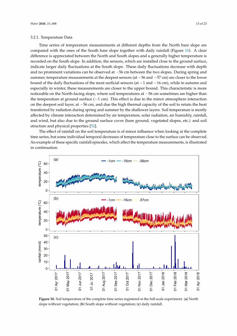
Time series of temperature measurements at different depths from the North bare slope arecompared with the ones of the South bare slope together with daily rainfall (Figure 10). A cleardifference is appreciated between the North and South slopes and a generally higher temperature isrecorded on the South slope. In addition, the sensors, which are installed close to the ground surface,indicate larger daily fluctuations at the South slope. These daily fluctuations decrease with depthand no prominent variations can be observed at −56 cm between the two slopes. During spring andsummer, temperature measurements at the deepest sensors (at−56 and−57 cm) are closer to the lowerbound of the daily fluctuations of the most surficial sensors (at −1 and −16 cm), while in autumn andespecially in winter, these measurements are closer to the upper bound. This characteristic is morenoticeable on the North-facing slope, where soil temperatures at −56 cm sometimes are higher thanthe temperature at ground surface (−1 cm). This effect is due to the minor atmosphere interactionon the deepest soil layer, at −56 cm, and due the high thermal capacity of the soil to retain the heattransferred by radiation during spring and summer by the shallower layers. Soil temperature is mostlyaffected by climate interaction determined by air temperature, solar radiation, air humidity, rainfall,and wind, but also due to the ground surface cover (bare ground, vegetated slopes, etc.) and soilstructure and physical properties [52].

The effect of rainfall on the soil temperature is of minor influence when looking at the completetime series, but some individual temporal decreases of temperature close to the surface can be observed.An example of these specific rainfall episodes, which affect the temperature measurements, is illustratedin continuation.


3.2.1. Temperature Data

Time series of temperature measurements at different depths from the North bare slope are compared with the ones of the South bare slope together with daily rainfall (Figure 10). A clear difference is appreciated between the North and South slopes and a generally higher temperature is recorded on the South slope. In addition, the sensors, which are installed close to the ground surface, indicate larger daily fluctuations at the South slope. These daily fluctuations decrease with depth and no prominent variations can be observed at −56 cm between the two slopes. During spring and summer, temperature measurements at the deepest sensors (at −56 and −57 cm) are closer to the lower bound of the daily fluctuations of the most surficial sensors (at −1 and −16 cm), while in autumn and especially in winter, these measurements are closer to the upper bound. This characteristic is more noticeable on the North-facing slope, where soil temperatures at −56 cm sometimes are higher than the temperature at ground surface (−1 cm). This effect is due to the minor atmosphere interaction on the deepest soil layer, at −56 cm, and due the high thermal capacity of the soil to retain the heat transferred by radiation during spring and summer by the shallower layers. Soil temperature is mostly affected by climate interaction determined by air temperature, solar radiation, air humidity, rainfall, and wind, but also due to the ground surface cover (bare ground, vegetated slopes, etc.) and soil structure and physical properties [52].

The effect of rainfall on the soil temperature is of minor influence when looking at the complete time series, but some individual temporal decreases of temperature close to the surface can be observed. An example of these specific rainfall episodes, which affect the temperature measurements, is illustrated in continuation.

Figure 10. Soil temperature of the complete time series registered at the full-scale experiment. (a) North slope without vegetation; (b) South slope without vegetation; (c) daily rainfall.

Figure 10. Soil temperature of the complete time series registered at the full-scale experiment. (a) Northslope without vegetation; (b) South slope without vegetation; (c) daily rainfall.

Water 2018, 10, 688 14 of 23

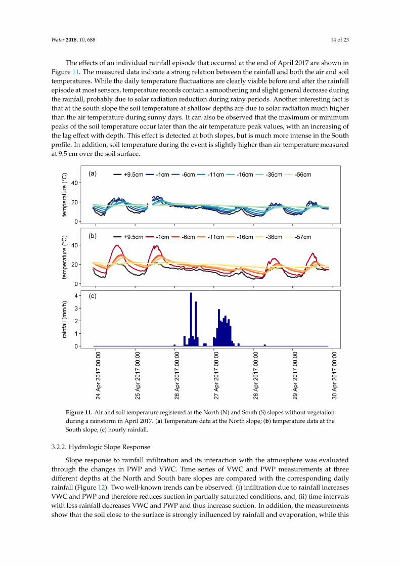
The effects of an individual rainfall episode that occurred at the end of April 2017 are shown inFigure 11. The measured data indicate a strong relation between the rainfall and both the air and soiltemperatures. While the daily temperature fluctuations are clearly visible before and after the rainfallepisode at most sensors, temperature records contain a smoothening and slight general decrease duringthe rainfall, probably due to solar radiation reduction during rainy periods. Another interesting fact isthat at the south slope the soil temperature at shallow depths are due to solar radiation much higherthan the air temperature during sunny days. It can also be observed that the maximum or minimumpeaks of the soil temperature occur later than the air temperature peak values, with an increasing ofthe lag effect with depth. This effect is detected at both slopes, but is much more intense in the Southprofile. In addition, soil temperature during the event is slightly higher than air temperature measuredat 9.5 cm over the soil surface.


The effects of an individual rainfall episode that occurred at the end of April 2017 are shown in Figure 11. The measured data indicate a strong relation between the rainfall and both the air and soil temperatures. While the daily temperature fluctuations are clearly visible before and after the rainfall episode at most sensors, temperature records contain a smoothening and slight general decrease during the rainfall, probably due to solar radiation reduction during rainy periods. Another interesting fact is that at the south slope the soil temperature at shallow depths are due to solar radiation much higher than the air temperature during sunny days. It can also be observed that the maximum or minimum peaks of the soil temperature occur later than the air temperature peak values, with an increasing of the lag effect with depth. This effect is detected at both slopes, but is much more intense in the South profile. In addition, soil temperature during the event is slightly higher than air temperature measured at 9.5 cm over the soil surface.

Figure 11. Air and soil temperature registered at the North (N) and South (S) slopes without vegetation during a rainstorm in April 2017. (a) Temperature data at the North slope; (b) temperature data at the South slope; (c) hourly rainfall.

3.2.2. Hydrologic Slope Response

Slope response to rainfall infiltration and its interaction with the atmosphere was evaluated through the changes in PWP and VWC. Time series of VWC and PWP measurements at three different depths at the North and South bare slopes are compared with the corresponding daily rainfall (Figure 12). Two well-known trends can be observed: (i) infiltration due to rainfall increases VWC and PWP and therefore reduces suction in partially saturated conditions, and, (ii) time intervals with less rainfall decreases VWC and PWP and thus increase suction. In addition, the measurements show that the soil close to the surface is strongly influenced by rainfall and evaporation, while this

Figure 11. Air and soil temperature registered at the North (N) and South (S) slopes without vegetationduring a rainstorm in April 2017. (a) Temperature data at the North slope; (b) temperature data at theSouth slope; (c) hourly rainfall.

3.2.2. Hydrologic Slope Response

Slope response to rainfall infiltration and its interaction with the atmosphere was evaluatedthrough the changes in PWP and VWC. Time series of VWC and PWP measurements at threedifferent depths at the North and South bare slopes are compared with the corresponding dailyrainfall (Figure 12). Two well-known trends can be observed: (i) infiltration due to rainfall increasesVWC and PWP and therefore reduces suction in partially saturated conditions, and, (ii) time intervalswith less rainfall decreases VWC and PWP and thus increase suction. In addition, the measurementsshow that the soil close to the surface is strongly influenced by rainfall and evaporation, while this

Water 2018, 10, 688 15 of 23

effect decreases with depth. The relation between rainfall and both VWC and PWP is confirmed bysharp increases at the shallow sensors (at −16 cm and with minor magnitude at −36 cm) and at bothslopes. The rainfall episodes with clearest VWC and PWP response occurred on 26–27 April 2017,18–19 October 2017, 26 January 2018, and 4–5 February 2018. A comparison of the two slopes showsthat the North slope is generally characterized by slightly higher soil moisture than the South slope.

Regarding the entire time series, the highest VWC values and reduced suction were recorded justafter the installation of the sensors for approximately two months (April and May 2017). Followingthis period, the most important drying phase occurred, which took place during the month of Junewith a suction increase of ~36–60 kPa/day for the shallower sensors (−11 and −16 cm respectively),~31–48 kPa/day for the middle sensors (−32 and −36 cm respectively), and ~3–4 kPa/day for thedeepest sensors (−72 and −62 cm respectively). In the following months (July–mid October), a smoothdecrease in both VWC and PWP was recorded. This trend breaks with an extreme rainfall episoderecorded on the 18th and 19th of October 2017, when 64 mm rainfall over 24 h were measured. Thisrainfall provoked a sharp and important increase at the shallow sensors of both slopes. The increasein VWC and PWP is less important with soil depth and has no prominent variation at the deepestsoil moisture sensors (located at −56 and −57 cm respectively). After this heavy and long durationrainfall, the shallow soil layer down to 16 cm depth was near to saturation for both slopes, since thesuction measurements were close to 0 kPa. The VWC registered very high values at the south slope,while the same sensor at −16 cm at the North slope exhibited technical problems with some data lost.Nevertheless, it can be deduced from the readings recorded during the month of November that theVWC increase was also important. Two rainfall events at the beginning of 2018 triggered an importantincrease in water content and pore water pressure. One on the 26th of January with 34 mm rain in24 h, and the highest rainfall recorded during the entire study, which occurred on the 4th and 5th ofFebruary 2018 and included 90 mm rain in 30 h. After these two rainfall episodes, VWC and PWPvalues strongly increased and continued at high values with only a slight decreasing trend.

In the following, special attention is given to the pore water pressure measurements gatheredby the T4 ceramic cup tensiometers (Figure 12c). These tensiometers are the most delicate devicesin the monitoring set-up, because the water-filled cup starts to de-saturate when the soil gets dryerthan ~90 kPa suction. In this case, it needs to be uninstalled in the field and saturated again in thelaboratory with de-aired water. The initial T4-readings show a similar behavior as the ones recorded bythe MPS-6 dielectric water potential sensors (Figure 12b): very low suction values close to saturationduring the first 2 months. After the high drying rate of June, the North tensiometer, at 62 cm depth,reached its maximum suction value of about 85 kPa and remained constant for several days. Then, themeasures changed abruptly to 0 kPa. The interpretation of this sharp change is that the soil at thatdepth got even dryer at that moment, reaching the ceramic bubble point of 1500 kPa. Consequently,the cup, which is filled with de-aired water, quickly ran out and was fully filled with air. Therefore, thetensiometer was extracted on the 20th of September and saturated with de-aired water in the laboratory,reinstalling it on the 5th of October. The measurements after reinstalling the North tensiometer reachedits maximum suction value of 85 kPa in 36 h, indicating suction at that depth was higher than 85 kPa,partially de-saturating the ceramic cup. This reading remained almost constant for two weeks until aheavy and long duration rainfall on the 18th and 19th of October saturated the ceramic cup and itsreadings reached the value of 4 kPa suction over 24 h. In contrast, the South T4 tensiometer did notreach its maximum suction value of 85 kPa during the month of June and suction values were slightlydecreasing from August 2017 (~30 kPa) until February 2018 (~17 kPa). Then, the very importantrainfall event on the 4th and 5th of February 2018 produced a sharp change. After this heavy rainfall,readings at the North and South tensiometers indicate a complete saturation at that depth (0.85 kPaand 1.13 kPa). These PWP values represent a water column of 8.7 cm and 11.6 cm above the sensors atthe North and South slope, respectively.

Water 2018, 10, 688 16 of 23Water 2018, 10, x FOR PEER REVIEW 16 of 23

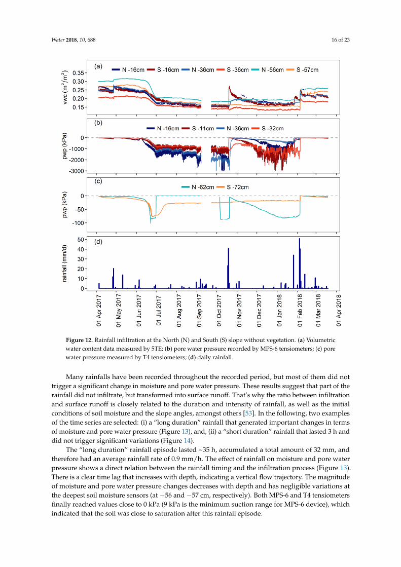
Figure 12. Rainfall infiltration at the North (N) and South (S) slope without vegetation. (a) Volumetric water content data measured by 5TE; (b) pore water pressure recorded by MPS-6 tensiometers; (c) pore water pressure measured by T4 tensiometers; (d) daily rainfall.

Many rainfalls have been recorded throughout the recorded period, but most of them did not trigger a significant change in moisture and pore water pressure. These results suggest that part of the rainfall did not infiltrate, but transformed into surface runoff. That’s why the ratio between infiltration and surface runoff is closely related to the duration and intensity of rainfall, as well as the initial conditions of soil moisture and the slope angles, amongst others [53]. In the following, two examples of the time series are selected: (i) a “long duration” rainfall that generated important changes in terms of moisture and pore water pressure (Figure 13), and, (ii) a “short duration” rainfall that lasted 3 h and did not trigger significant variations (Figure 14).

The “long duration” rainfall episode lasted ~35 h, accumulated a total amount of 32 mm, and therefore had an average rainfall rate of 0.9 mm/h. The effect of rainfall on moisture and pore water pressure shows a direct relation between the rainfall timing and the infiltration process (Figure 13). There is a clear time lag that increases with depth, indicating a vertical flow trajectory. The magnitude of moisture and pore water pressure changes decreases with depth and has negligible variations at the deepest soil moisture sensors (at −56 and −57 cm, respectively). Both MPS-6 and T4 tensiometers finally reached values close to 0 kPa (9 kPa is the minimum suction range for MPS-6 device), which indicated that the soil was close to saturation after this rainfall episode.

Figure 12. Rainfall infiltration at the North (N) and South (S) slope without vegetation. (a) Volumetricwater content data measured by 5TE; (b) pore water pressure recorded by MPS-6 tensiometers; (c) porewater pressure measured by T4 tensiometers; (d) daily rainfall.

Many rainfalls have been recorded throughout the recorded period, but most of them did nottrigger a significant change in moisture and pore water pressure. These results suggest that part of therainfall did not infiltrate, but transformed into surface runoff. That’s why the ratio between infiltrationand surface runoff is closely related to the duration and intensity of rainfall, as well as the initialconditions of soil moisture and the slope angles, amongst others [53]. In the following, two examplesof the time series are selected: (i) a “long duration” rainfall that generated important changes in termsof moisture and pore water pressure (Figure 13), and, (ii) a “short duration” rainfall that lasted 3 h anddid not trigger significant variations (Figure 14).

The “long duration” rainfall episode lasted ~35 h, accumulated a total amount of 32 mm, andtherefore had an average rainfall rate of 0.9 mm/h. The effect of rainfall on moisture and pore waterpressure shows a direct relation between the rainfall timing and the infiltration process (Figure 13).There is a clear time lag that increases with depth, indicating a vertical flow trajectory. The magnitudeof moisture and pore water pressure changes decreases with depth and has negligible variations atthe deepest soil moisture sensors (at −56 and −57 cm, respectively). Both MPS-6 and T4 tensiometersfinally reached values close to 0 kPa (9 kPa is the minimum suction range for MPS-6 device), whichindicated that the soil was close to saturation after this rainfall episode.


Figure 13. Soil moisture and pore water pressure registered during a rainstorm in April 2017 at the North (N) and South (S) slopes without vegetation. (a) Volumetric water content data measured by 5TE; (b) pore water pressure recorded by MPS-6 tensiometers; (c) pore water pressure measured by T4 tensiometers; (d) hourly rainfall.

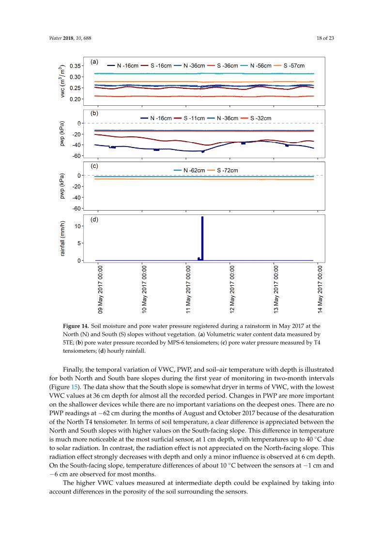
The “short duration” rainfall lasted only three hours, accumulated a total amount of 13.8 mm, and had a clear hourly peak with an intensity of 12.7 mm/h. There is no response on the volumetric water content sensors at all depths, while pore water pressure slightly increase on the most superficial sensors located at 16 cm depth (Figure 14). This suggests a clear relationship between rainfall duration and intensity and the subsequent infiltration process. Therefore, a runoff measurement system will be installed in 2018 at each of the four monitored slopes in order to understand better the rainfall infiltration and runoff process and to corroborate the infiltration rate.

Figure 13. Soil moisture and pore water pressure registered during a rainstorm in April 2017 at theNorth (N) and South (S) slopes without vegetation. (a) Volumetric water content data measured by5TE; (b) pore water pressure recorded by MPS-6 tensiometers; (c) pore water pressure measured by T4tensiometers; (d) hourly rainfall.

The “short duration” rainfall lasted only three hours, accumulated a total amount of 13.8 mm,and had a clear hourly peak with an intensity of 12.7 mm/h. There is no response on the volumetricwater content sensors at all depths, while pore water pressure slightly increase on the most superficialsensors located at 16 cm depth (Figure 14). This suggests a clear relationship between rainfall durationand intensity and the subsequent infiltration process. Therefore, a runoff measurement system willbe installed in 2018 at each of the four monitored slopes in order to understand better the rainfallinfiltration and runoff process and to corroborate the infiltration rate.


Figure 14. Soil moisture and pore water pressure registered during a rainstorm in May 2017 at the North (N) and South (S) slopes without vegetation. (a) Volumetric water content data measured by 5TE; (b) pore water pressure recorded by MPS-6 tensiometers; (c) pore water pressure measured by T4 tensiometers; (d) hourly rainfall.

Finally, the temporal variation of VWC, PWP, and soil–air temperature with depth is illustrated for both North and South bare slopes during the first year of monitoring in two-month intervals (Figure 15). The data show that the South slope is somewhat dryer in terms of VWC, with the lowest VWC values at 36 cm depth for almost all the recorded period. Changes in PWP are more important on the shallower devices while there are no important variations on the deepest ones. There are no PWP readings at −62 cm during the months of August and October 2017 because of the desaturation of the North T4 tensiometer. In terms of soil temperature, a clear difference is appreciated between the North and South slopes with higher values on the South-facing slope. This difference in temperature is much more noticeable at the most surficial sensor, at 1 cm depth, with temperatures up to 40 °C due to solar radiation. In contrast, the radiation effect is not appreciated on the North-facing slope. This radiation effect strongly decreases with depth and only a minor influence is observed at 6 cm depth. On the South-facing slope, temperature differences of about 10 °C between the sensors at −1 cm and −6 cm are observed for most months.

The higher VWC values measured at intermediate depth could be explained by taking into account differences in the porosity of the soil surrounding the sensors.

Figure 14. Soil moisture and pore water pressure registered during a rainstorm in May 2017 at theNorth (N) and South (S) slopes without vegetation. (a) Volumetric water content data measured by5TE; (b) pore water pressure recorded by MPS-6 tensiometers; (c) pore water pressure measured by T4tensiometers; (d) hourly rainfall.

Finally, the temporal variation of VWC, PWP, and soil–air temperature with depth is illustratedfor both North and South bare slopes during the first year of monitoring in two-month intervals(Figure 15). The data show that the South slope is somewhat dryer in terms of VWC, with the lowestVWC values at 36 cm depth for almost all the recorded period. Changes in PWP are more importanton the shallower devices while there are no important variations on the deepest ones. There are noPWP readings at −62 cm during the months of August and October 2017 because of the desaturationof the North T4 tensiometer. In terms of soil temperature, a clear difference is appreciated between theNorth and South slopes with higher values on the South-facing slope. This difference in temperatureis much more noticeable at the most surficial sensor, at 1 cm depth, with temperatures up to 40 ◦C dueto solar radiation. In contrast, the radiation effect is not appreciated on the North-facing slope. Thisradiation effect strongly decreases with depth and only a minor influence is observed at 6 cm depth.On the South-facing slope, temperature differences of about 10 ◦C between the sensors at −1 cm and−6 cm are observed for most months.

The higher VWC values measured at intermediate depth could be explained by taking intoaccount differences in the porosity of the soil surrounding the sensors.

Water 2018, 10, 688 19 of 23


Figure 15. Temporal variation of the variations in volumetric water content (VWC), pore water pressure (PWP), and temperature (temp.) with depth at the North and South bare profiles. The data are represented in two-month intervals from April 2017–February 2018. (a) Volumetric water content at North slope; (b) pore water pressure at North slope; (c) air and soil temperature at North slope; (d) volumetric water content at South slope; (e) pore water pressure at South slope; (f) air and soil temperature at South slope.

4. Conclusions

The monitoring of soil–vegetation–atmosphere interactions is a necessary but difficult task. The experience of installing and verifying the correct sensing of all devices confirms that the monitoring of so many different processes is complex in an outdoor experiment and strongly differs from laboratory tests, which are performed under controlled conditions. The correct calibration, adequate installation and permanent maintenance of the sensors is time-consuming, but fundamental. In our set-up, the most critical devices are the water-filled ceramic cup tensiometers, which de-saturated sometimes.

A good laboratory characterization of strength and hydrologic parameters is essential to understand correctly the infiltration process and to model the slope failure mechanisms. In this case, the laboratory tests indicate that there is a great contribution of suction to the shear strength. However, laboratory results may diverge from field observations, since heterogeneities are much

Figure 15. Temporal variation of the variations in volumetric water content (VWC), pore waterpressure (PWP), and temperature (temp.) with depth at the North and South bare profiles. The dataare represented in two-month intervals from April 2017–February 2018. (a) Volumetric water contentat North slope; (b) pore water pressure at North slope; (c) air and soil temperature at North slope;(d) volumetric water content at South slope; (e) pore water pressure at South slope; (f) air and soiltemperature at South slope.

4. Conclusions

The monitoring of soil–vegetation–atmosphere interactions is a necessary but difficult task.The experience of installing and verifying the correct sensing of all devices confirms that the monitoringof so many different processes is complex in an outdoor experiment and strongly differs from laboratorytests, which are performed under controlled conditions. The correct calibration, adequate installationand permanent maintenance of the sensors is time-consuming, but fundamental. In our set-up,the most critical devices are the water-filled ceramic cup tensiometers, which de-saturated sometimes.

A good laboratory characterization of strength and hydrologic parameters is essential tounderstand correctly the infiltration process and to model the slope failure mechanisms. In thiscase, the laboratory tests indicate that there is a great contribution of suction to the shear strength.

Water 2018, 10, 688 20 of 23

However, laboratory results may diverge from field observations, since heterogeneities are muchmore common in large experiments like this embankment. For example, in the trenches which wereexcavated at the four slope partitions, we observed cracks, fissures, and macropores that may havedeveloped due to small displacements in the soil or due to root growing. All these features createpreferential flow paths of the water and increase soil permeability and reduce suction and consequentlyalso its strength. Therefore, permeability in the embankment is certainly much higher than the onemeasured in the laboratory (in the order of 10−8 and 10−7 m/s), which was obtained from a smallhomogeneous soil sample.

Preliminary analysis of the recorded data during the first year revealed the following outcomesregarding temperature and heat flux: (i) soil temperature strongly differs from North to South. (ii) Atthe terrain surface (sensors installed at −1 cm) of the South-facing slope, the temperatures are muchhigher (up to 55 ◦C) than the air temperature due to the solar radiation. This effect was not observed atthe North-facing slope. (iii) A clear daily temperature fluctuation is visible at the most surficial sensors,while this effect is negligible at about −50 cm.

Regarding the rainfall infiltration, the results show: (i) high soil moisture during winter/springand a dry period during summer and autumn. Only the most important rainfall, recorded on the4th and 5th of February 2018 (90 mm rain in 30 h), saturated the deepest soil layer at both North andSouth bare slopes. The highest drying rate took place during the month of June. (ii) There is a clearrelationship between rainfall duration and intensity and the subsequent infiltration process. Mostof the short duration rainfalls did not trigger significant variations in terms of VWC and PWP at alldepths. In contrast, long duration rainfalls triggered a sharp increase on both VWC and PWP, whilethis effect decreases with depth.

All the monitored data will improve the understanding of the soil–vegetation–atmosphereinteractions. Furthermore, the records provide essential input data for numerical modelling of thecoupled thermo-hydro-mechanical processes in geological media and will serve to validate the SVAmodels with the aim of applying them to natural slopes of the Pyrenees.

Author Contributions: The laboratory tests were principally carried out by R.O. and A.F., and supervised by A.L.All the authors contributed to the design, installation and maintenance of the full-scale experiment, while the dataanalysis was mainly performed by R.O., M.H. and R.O. wrote the paper and the other authors reviewed it.

Funding: The study is funded by the national research project called “Slope mass-wasting under climate change(SMuCPhy)” granted by the Ministry of Economy and Competitiveness of Spain (project reference number BIA2015-67500-R) and co-funded by AEI/FEDER, UE.

Acknowledgments: Alessandro Fraccica acknowledges the Marie Skłodowska-Curie ITN-ETN projectTERRE ‘Training Engineers and Researchers to Rethink geotechnical Engineering for a low carbon future’(H2020-MSCA-ITN-2015-675762). Enrique Romero, Miquel Masip (UPC Parc), Andrés Cevallos and VinicioGuachizaca helped during field and laboratory tasks.

Conflicts of Interest: The authors declare no conflict of interest. The founding sponsors had no role in the designof the study; in the collection, analyses, or interpretation of data; in the writing of the manuscript, and in thedecision to publish the results.

References

1. Gabarrón-Galeote, M.A.; Ruiz-Sinoga, J.D.; Quesada, M.A. Influence of aspect in soil and vegetation waterdynamics in dry Mediterranean conditions: Functional adjustment of evergreen and semi-deciduous growthforms. Ecohydrology 2013, 6, 241–255. [CrossRef]

2. Coyle, D.R.; Nagendra, U.J.; Taylor, M.K.; Campbell, J.H.; Cunard, C.E.; Joslin, A.H.; Mundepi, A.;Phillips, C.A.; Callaham, M.A. Soil fauna responses to natural disturbances, invasive species, and globalclimate change: Current state of the science and a call to action. Soil Biol. Biochem. 2017, 110, 116–133.[CrossRef]

3. Drabo, A. Climate change mitigation and agricultural development models: Primary commodity exports orlocal consumption production? Ecol. Econ. 2017, 137, 110–125. [CrossRef]

http://dx.doi.org/10.1002/eco.1262

http://dx.doi.org/10.1016/j.soilbio.2017.03.008

http://dx.doi.org/10.1016/j.ecolecon.2017.03.014

Water 2018, 10, 688 21 of 23

4. Imeson, A.C.; Lavee, H. Soil erosion and climate change: The transect approach and the influence of scale.Geomorphology 1998, 23, 219–227. [CrossRef]

5. Corominas, J. Landslides and climate. In Proceedings of the VIII International Symposium on Landslides,Cardiff, UK, 26–30 June 2000; Bromhead, E.N., Dixon, N., Ibsen, M.L., Eds.; Volume 4, pp. 1–33.

6. Intergovernmental Panel on Climate Change Climate Change 2013—The Physical Science Basis: Working GroupI Contribution to the Fifth Assessment Report of the Intergovernmental Panel on Climate Change; CambridgeUniversity Press: Cambridge, UK, 2014; ISBN 9781107057999.

7. Nearing, M.A.; Polyakov, V.O.; Nichols, M.H.; Hernandez, M.; Li, L.; Zhao, Y.; Armendariz, G. Slope–velocityequilibrium and evolution of surface roughness on a stony hillslope. Hydrol. Earth Syst. Sci. 2017, 21,3221–3229. [CrossRef]

8. Panagos, P.; Meusburger, K.; Ballabio, C.; Borrelli, P.; Alewell, C. Soil erodibility in Europe: A high-resolutiondataset based on LUCAS. Sci. Total Environ. 2014, 479–480, 189–200. [CrossRef] [PubMed]

9. Hovius, N.; Stark, C.P.; Allen, P.A. Sediment flux from a mountain belt derived by landslide mapping.Geology 1997, 25, 231–234. [CrossRef]

10. Alonso, E.; Lloret, A.; Romero, E. Rainfall induced deformations of road embackments. Riv. Ital. di Geotec.1999, 33, 8–15.

11. Sajjan, A.K.; Gyasi-Agyei, Y.; Sharma, R.H. Rainfall–runoff modelling of railway embankment steep slopes.Hydrol. Sci. J. 2013, 58, 1162–1176. [CrossRef]

12. Briggs, K.M.; Loveridge, F.A.; Glendinning, S. Failures in transport infrastructure embankments. Eng. Geol.2017, 219, 107–117. [CrossRef]

13. Blight, G.E. Interactions between the atmosphere and the earth. Geotechnique 1997, 47, 715–767.14. Elia, G.; Cotecchia, F.; Pedone, G.; Vaunat, J.; Vardon, P.J.; Pereira, C.; Springman, S.M.; Rouainia, M.;

Van Esch, J.; Koda, E.; et al. Numerical modelling of slope–vegetation–atmosphere interaction: An overview.Q. J. Eng. Geol. Hydrogeol. 2017, 50, 249–270. [CrossRef]

15. Tsiampousi, A.; Zdravkovic, L.; Potts, D.M. Soil-atmosphere interaction in unsaturated cut slopes. E3S Web Conf.2016, 9, 8004. [CrossRef]

16. Tang, A.M.; Hughes, P.N.; Dijkstra, T.A.; Askarinejad, A.; Brencic, M.; Cui, Y.J.; Diez, J.J.; Firgi, T.; Gajewska, B.;Gentile, F.; et al. Atmosphere–vegetation–soil interactions in a climate change context; impact of changingconditions on engineered transport infrastructure slopes in Europe. Q. J. Eng. Geol. Hydrogeol. 2018, 51,156–168. [CrossRef]

17. Huang, C.-C.; Yuin, S.-C. Experimental investigation of rainfall criteria for shallow slope failures.Geomorphology 2010, 120, 326–338. [CrossRef]

18. Orense, R.P.; Shimoma, S.; Maeda, K.; Towhata, I. Instrumented Model Slope Failure due to Water Seepage.J. Nat. Disaster Sci. 2004, 26, 15–26. [CrossRef]

19. Tohari, A.; Nishigaki, M.; Komatsu, M. Laboratory Rainfall-Induced Slope Failure with Moisture ContentMeasurement. J. Geotech. Geoenviron. Eng. 2007, 133, 575–587. [CrossRef]

20. Moriwaki, H.; Inokuchi, T.; Hattanji, T.; Sassa, K.; Ochiai, H.; Wang, G. Failure processes in a full-scalelandslide experiment using a rainfall simulator. Landslides 2004, 1, 277–288. [CrossRef]

21. Cooper, M.R.; Bromhead, E.N.; Petley, D.J.; Grants, D.I. The Selborne cutting stability experiment.Géotechnique 1998, 48, 83–101. [CrossRef]

22. Cui, Y.J.; Gao, Y.B.; Ferber, V. Simulating the water content and temperature changes in an experimentalembankment using meteorological data. Eng. Geol. 2010, 114, 456–471. [CrossRef]

23. Glendinning, S.; Hughes, P.; Helm, P.; Chambers, J.; Mendes, J.; Gunn, D.; Wilkinson, P.; Uhlemann, S.Construction, management and maintenance of embankments used for road and rail infrastructure:Implications of weather induced pore water pressures. Acta Geotech. 2014, 9, 799–816. [CrossRef]

24. Ng, C.W.W.; Springman, S.M.; Alonso, E.E. Monitoring the Performance of Unsaturated Soil Slopes.Geotech. Geol. Eng. 2008, 26, 799–816. [CrossRef]

25. Bogaard, T.A.; van Asch, T.W.J. The role of the soil moisture balance in the unsaturated zone on movementand stability of the Beline landslide, France. Earth Surf. Process. Landforms 2002, 27, 1177–1188. [CrossRef]

26. Springman, S.M.; Jommi, C.; Teysseire, P. Instabilities on moraine slopes induced by loss of suction: A casehistory. Géotechnique 2003, 53, 3–10. [CrossRef]

http://dx.doi.org/10.1016/S0169-555X(98)00005-1

http://dx.doi.org/10.5194/hess-21-3221-2017

http://dx.doi.org/10.1016/j.scitotenv.2014.02.010

http://www.ncbi.nlm.nih.gov/pubmed/24561925

http://dx.doi.org/10.1130/0091-7613(1997)025<0231:SFFAMB>2.3.CO;2

http://dx.doi.org/10.1080/02626667.2013.802323

http://dx.doi.org/10.1016/j.enggeo.2016.07.016

http://dx.doi.org/10.1144/qjegh2016-079

http://dx.doi.org/10.1051/e3sconf/20160908004

http://dx.doi.org/10.1144/qjegh2017-103

http://dx.doi.org/10.1016/j.geomorph.2010.04.006

http://dx.doi.org/10.2328/jnds.26.15

http://dx.doi.org/10.1061/(ASCE)1090-0241(2007)133:5(575)

http://dx.doi.org/10.1007/s10346-004-0034-0

http://dx.doi.org/10.1680/geot.1998.48.1.83

http://dx.doi.org/10.1016/j.enggeo.2010.06.006

http://dx.doi.org/10.1007/s11440-014-0324-1

http://dx.doi.org/10.1007/s10706-008-9203-6

http://dx.doi.org/10.1002/esp.419


Water 2018, 10, 688 22 of 23

27. Rahardjo, H.; Rezaur, R.B.; Leong, E.C.; Alonso, E.E.; Lloret, A.; Gens, A. Monitoring and modeling of sloperesponse to climate changes. In Proceedings of the 10th International Symposium on Landslides, Xi’an,China, 30 June–4 July 2008; pp. 67–84.

28. Cassiani, G.; Boaga, J.; Rossi, M.; Putti, M.; Fadda, G.; Majone, B.; Bellin, A. Soil–plant interaction monitoring:Small scale example of an apple orchard in Trentino, North-Eastern Italy. Sci. Total Environ. 2016, 543,851–861. [CrossRef] [PubMed]

29. Schmidt, K.M.; Roering, J.J.; Stock, J.D.; Dietrich, W.E.; Montgomery, D.R.; Schaub, T. The variability of rootcohesion as an influence on shallow landslide susceptibility in the Oregon Coast Range. Can. Geotech. J. 2001,38, 995–1024. [CrossRef]

30. Portilla, M.; Chevalier, G.; Hürlimann, M. Description and analysis of the debris flows occurred during 2008in the Eastern Pyrenees. Nat. Hazards Earth Syst. Sci. 2010, 10, 1635–1645. [CrossRef]

31. Corominas, J.; Moya, J. Reconstructing recent landslide activity in relation to rainfall in the Llobregat Riverbasin, Eastern Pyrenees, Spain. Geomorphology 1999, 30, 79–93. [CrossRef]

32. Gallart, F.; Clotet-Perarnau, N. Some aspects of the geomorphic processes triggered by an extreme rainfallevent: The November 1982 flood in the Eastern Pyrenees. Catena Suppl. 1988, 13, 79–95.

33. Zhang, M.; Chen, F.Q.; Zhang, J.X. The Temporal Dynamics of Cynodon Dactylon Soil—Root System in SoilConservation and Slope Reinforcement. Adv. Mater. Res. 2013, 838–841, 675–679. [CrossRef]

34. Chen, F.; Zhang, J.; Zhang, M.; Wang, J. Effect of Cynodon dactylon community on the conservation andreinforcement of riparian shallow soil in the Three Gorges Reservoir area. Ecol. Process. 2015, 4, 1–8.[CrossRef]

35. Garg, A.; Coo, J.L.; Ng, C.W.W. Field study on influence of root characteristics on soil suction distribution inslopes vegetated with Cynodon dactylon and Schefflera heptaphylla. Earth Surf. Process. Landforms 2015, 40,1631–1643. [CrossRef]

36. Katritzidakis, M.; Liapis, A.; Stathakopoulos, I.; Pipinis, E.; Kekis, G.; Ververidou, E.; Sevastou, E. Erosioncontrol by application of hydroseeding methods along the Egnatia Motorway (Greece). Eco-and Gr.Bio-Engineering Use Veg. Improv. Slope Stab. 2007, 103, 393–400. [CrossRef]

37. ASTM D6913/D6913M-17: Standard Test Methods for Particle-Size Distribution (Gradation) of Soils Using SieveAnalysis; ASTM International: West Conshohocken, PA, USA, 2017.

38. ASTM D7928-17: Standard Test Method for Particle-Size Distribution (Gradation) of Fine-Grained Soils Using theSedimentation (Hydrometer) Analysis; ASTM International: West Conshohocken, PA, USA, 2017.

39. ASTM D4318-17e1: Standard Test Methods for Liquid Limit, Plastic Limit, and Plasticity Index of Soils; ASTMInternational: West Conshohocken, PA, USA, 2017.

40. ASTM D854-14: Standard Test Methods for Specific Gravity of Soil Solids by Water Pycnometer; ASTM International:West Conshohocken, PA, USA, 2014.

41. ASTM D3080/D3080M-11: Standard Test Method for Direct Shear Test of Soils Under Consolidated DrainedConditions; ASTM International: West Conshohocken, PA, USA, 2011.

42. Day, S.R.; Daniel, D.E. Hydraulic Conductivity of Two Prototype Clay Liners. J. Geotech. Eng. 1985, 111,957–970. [CrossRef]

43. Fredlund, D.G.; Xing, A.; Fredlund, M.D.; Barbour, S.L. The relationship of the unsaturated soil shear to thesoil-water characteristic curve. Can. Geotech. J. 1996, 33, 440–448. [CrossRef]

44. ASTM D7263-09(2018)e1: Standard Test Methods for Laboratory Determination of Density (Unit Weight) of SoilSpecimens ASTM International: West Conshohocken, PA, USA, 2018.

45. Skempton, A.W. Long-Term Stability of Clay Slopes. Géotechnique 1964, 14, 77–102. [CrossRef]46. Alonso, E.E.; Gens, A.; Josa, A. A constitutive model for partially saturated soils. Géotechnique 1990, 40,

405–430. [CrossRef]47. Bishop, A.W. The principle of effective stress. Tek. Ukebl. 1959, 106, 859–863.48. Schrefler, B.A. The Finite Element Method in Soil Consolidation (with Applications to Surface Subsidence).

Ph.D. Thesis, University College of Swansea, Swansea, UK, 1984.49. Fredlund, D.G.; Morgenstern, N.R.; Widger, R.A. The shear strength of unsaturated soils. Can. Geotech. J.

1978, 15, 313–321. [CrossRef]50. Maksimovic, M. Nonlinear Failure Envelope for Soils. J. Geotech. Eng. 1989, 115, 581–586. [CrossRef]

http://dx.doi.org/10.1016/j.scitotenv.2015.03.113

http://www.ncbi.nlm.nih.gov/pubmed/25841636

http://dx.doi.org/10.1139/t01-031

http://dx.doi.org/10.5194/nhess-10-1635-2010

http://dx.doi.org/10.1016/S0169-555X(99)00046-X

http://dx.doi.org/10.4028/www.scientific.net/AMR.838-841.675

http://dx.doi.org/10.1186/s13717-014-0029-2

http://dx.doi.org/10.1002/esp.3743

http://dx.doi.org/10.1007/978-1-4020-5593-5_40


http://dx.doi.org/10.1139/t96-065



http://dx.doi.org/10.1139/t78-029


Water 2018, 10, 688 23 of 23

51. Sánchez Castilla, M. Thermo-Hydro-Mechanical Coupled Analysis in Low Permeability Media. Ph.D. Thesis,Universitat Politècnica de Catalunya, Barcelona, Spain, 2004.

52. Florides, G.; Kalogirou, S. Measurements of Ground Temperature at Various Depths. In Proceedings of theSET 2004, 3rd International Conference on Sustainable Energy Technologies, Nottingham, UK, 28–30 June2004; pp. 1–6.

53. Horton, R.E. An Approach Toward a Physical Interpretation of Infiltration-Capacity. Soil Sci. Soc. Am. J.1940, 5, 399–417. [CrossRef]

© 2018 by the authors. Licensee MDPI, Basel, Switzerland. This article is an open accessarticle distributed under the terms and conditions of the Creative Commons Attribution(CC BY) license (http://creativecommons.org/licenses/by/4.0/).

http://dx.doi.org/10.2136/sssaj1941.036159950005000C0075x

http://creativecommons.org/

http://creativecommons.org/licenses/by/4.0/.

Date post:	26-Jan-2022
Category:	Documents
Upload:	others
View:	2 times
Download:	0 times

Regarding Soil–Vegetation–Atmosphere Interactions

Documents