REGIME SWITCHING VECTOR AUTOREGRESSIONS: A BAYESIAN MARKOV CHAIN MONTE CARL0 APPROACH Glen R. Harris Australian Mutual Provident Society 33 Alfred Street SYDNEY AUSTRALIA 2000 Telephone: 61 2 9257 6752 Facsimile : 61 2 9257 5278 Email: [email protected]Many financial time series processes appear subject to periodic structural changes in their dynamics. Regression relationships are often not robust to outliers nor stable over time, whilst the existence of changes in variance over time is well documented. This paper considers a vector autoregression subject to pseudocyclical structural changes. The parameters of a vector autoregression are modelled as the outcome of an unobserved discrete Markov process with unknown transition probabilities. The unobserved regimes, one for each time point, together with the regime transition probabilities, are to be determined in addition to the vector autoregression parameters within each regime. A Bayesian Markov Chain Monte Carlo estimation procedure is developed which generates the joint posterior density of the parameters and the regimes, rather than the more common point estimates. The complete likelihood surface is generated at the same time. The procedure can readily be extended to produce joint prediction densities for the variables, incorporating parameter uncertainty. Results using simulated and real data are provided. A clear separation of the variance between regimes is observed. Ignoring regime shifts is very likely to produce misleading volatility estimates, and is unlikely to be robust to outliers. A comparison with commonly used models suggests that the regime switching vector autoregression provides a particularly good description of the data. Keywords: regime switching; joint parameter density, joint prediction densities; outliers; robust estimation; Gibbs sampler, Markov chains; Bayesian estimation.
Transcript
REGIME SWITCHING VECTOR AUTOREGRESSIONS: A BAYESIAN MARKOV CHAIN MONTE CARL0 APPROACH
Stock & Watson (1996) examined the stability and predictive ability of 8 univariate
models for each of 76 monthly U S times series, and 8 bivariate models for each of 5,700
bivariate relationships They found evidence of substantial instability in a significant proportion
of the univariate and bivariate autoregressive models considered.
Conditional heteroscedasticity, or changes in the level of volatility, has been found in
financial series by numerous researchers, both actuarial and from the wider financial and
econometric fields. Examples of the former include Praetz (1969), Becker (1991), Harris
(1995b), Frees et al (1996) and Harris (1996) Examples of the latter include McNees (1979),
Engle (1982), Akgiray (1989), Hamilton & Susmel (1994), Hamilton & Lin (1996) and Gray
(1996).
The proposition underlying regime switching models is that, over time, changes in the
financial environment may be closely associated with relatively discrete specific events. The
process may have quite different characteristics in different regimes. A tractable mathematical
model of structural changes and discrete market phases is the univariate Markov regime
switching autoregressive process introduced by Hamilton (1989), and considered by Albert &
Chib (1993) and Harris (1996).
Given that financial series appear interdependent, both in terms of their levels and their
volatilities, e.g. Harris (1994, 1995b, 1995c) and Hamilton & Lin (1996), a vector regime
switching process would seem to be an attractive description of the data. Hamilton (1990)
proposed an EM maximum likelihood algorithm for estimating a Markov regime switching
vector autoregression. The present paper develops an alternative Bayesian Markov Chain
Monte Carlo (MCMC) estimation procedure which is more informative, flexible, and efficient
than a maximum likelihood based approach.
In the process being considered, the various series are able to interact through regression
relationships in the conditional means and through contemporaneous correlations in the
residuals, as well as through joint regime switching in the conditional means, regressive
correlations, variances and contemporaneous error correlations. Within each regime the
process is assumed linear stationary. Joint regime switching produces nonlinear dependence
between the series, and can account for discrete market phases and cycles, episodes of
instability, and ieptokurtic (i.e. fat-tailed) frequency distributions. In the univariate case, the
model fitting results of Gray (1996) and Harris (1996) suggest that regime switching models
compare more than favourably with common autoregressive and conditional heteroscedasticity
models. The results in section 6.3 of the present paper suggest that the same is true of regime
switching vector autoregressions.
- ~ i ~ ( ~ , ) = 0 and E C , ( ~ , )i:p,, = qp,, V t > q . X , and are n q x l column vectors, while the
A are mqxniq matrices.
The total parameter set to be estimated is h r , p j x , , A(,) , .., A j r l , n( l l , . ., qx,, P] ,
which can be partitioned as h = (O,P). To ensure that the process is identifiable, it will
sometimes be necessary to define the regimes by insisting upon prior restrictions on the
parameters, such as ordering of the variances of at least one of the variables (components of
the x,). If this is not done, it is possible that the regime associated with essentially the same set
of data points could be labelled differently in different iterations of the estimation procedure.
The next 3 sections, sections 3 to 5, develop the procedure used to generate the joint
parameter density and estimate the model. Those who do not wish to consider the mathematics
of the estimation procedure at this stage may wish to skip the next 14 or so pages and go
directly to section 6.2, which reports the results of fitting the model to real data.
Draws from the joint posterior distribution of the regimes and the parameters, given the
sample data, can be simulated using Markov Chain Monte Carlo methods, such as the Gibbs
sampler and Metropolis-Hastings algorithm. Chib & Greenberg (1995) provide a usehl and
readable description of MCMC methods
Markov Chain theory would usually start with a transition matrix in the case of discrete
states, pT = @,I, or a transition kernel density in the case of continuous states, p(xy) Since
the process must end up somewhere at each transition, x , p U = 1 or ly(x ,y)dy = 1 The
probability of the process being in state j after n transitions, given that it was initially in state i , is given by p!'') = xkp!; - ' )pb (discrete case). A limiting or invariant distribution is said to
exist whenever pj;") -+ rr, as 11 + m It follows therefore that i?, = ~ , r r r p V or
X(Y) = j +)P(x> Y)&
A major concern of the theory is to determine conditions under which there exists an
invariant distribution, and conditions under which iterations of the transition matrix or kernel
converge to the invariant distribution.
MCMC methods look at the theory from a different perspective. The invariant distribution
is the target distribution from which we wish to sample, generally a Bsyesian posterior
distribution. The transition matrix or kernel is unknown.
3.1 THE GIBBS SAMPLER
The Gibbs Sampler generates samples from a joint density fo = ~(XI,..,XN) via a
sequence of random draws or samples from full conditional densities, as follows
xy'' c f (x, xir'. . ., x;))
That completes a transition from p' to pi". The sequence {p') forms a realisation of a
Markov chain which converges in distribution to a random sample from the joint distribution
fo =f(x,,..,x~).
3.2 THE METROPOLIS-HASTINGS ALGORITHM
Suppose p(xy) is unknown, but that a density q(xy) exists, Jq(x ,~)dy = 1 , from which
candidate values of y can be generated for given x, to be accepted or rejected. The candidate
generating density, q(xy), is a first approximation to the unknown transition kernel density,
p(xy). q(x8) needs to be modified to ensure convergence to the desired target density. This is
done by introducing a move probability, a ( x j ) < 1 If a move is not made, with probability
1 - a(xy), then the process remains at x and again returns a value of x as a value from the
target distribution. The move probability is given by
I 1 otherwise
An important feature of the algorithm is that the calculation of a(x8) only requires
knowledge of the target density 4 . ) up to proportionality (which in the case of a Bayesian
posterior is given by the product of the likelihood and the prior), since 4 . ) only appears as a
ratio.
A particularly useful application of the Metropolis-Hastings algorithm is where an
intractable density arises within a Gibbs Sampler as the product of a standard density and
another density, e.g n(x) oc Hx).&), where Kx) is a standard density that can be sampled.
Then q(xy) = &) can be used to generate candidate y, which are accepted with probability
a ( q ) = min{yliy)/tp(x), 1 ) The Metropolis-Hastings algorithm will be superior to direct
acceptancelrejection methods since the move probability will be higher than H.), the
acceptance probability under the acceptancelrejection method, particularly where tp(.) is small.
4. THE LIKELIHOOD FUNCTION
The contribution of the 1-th data vector to the likelihood conditional on the regime is
~ ( ~ , I P , . Y ~ - ~ > ~ ) = ( ~ ~ ) - ~ ~lq;,)li ~ e x ~ ( - i 5 ; ~ , , q ; , ) 5 , , ~ , ) ]
6=1
in the case o f t > q, where Y, - (XI ,.., x,)
The first q data vectors can be taken together. I(X,lp,,h) can be obtained by exploiting
stationarity, i.e.
Ex, = p, and assuming the process is stable' within each regime,
The unconditional or stationary r n q x n q variance-covariance matrix, V, can also be determined
from
vecv = (I,, - A 8 A)-' vecB,
as described by Liitkepohl (1991, p21-22). vec is the column stacking operator2, and 8 is the
(right) kronecker product3 The contribution to the likelihood from the first q data vectors is
therefore
"'9
' ( X ~ I P ~ > L ) = (2z)-y 'exp{-i(xq - & ( k ) ) T v ( ~ k ) > ~ ( k i ) - l ( x q -F (~ ) ) } ,
where p, = k.
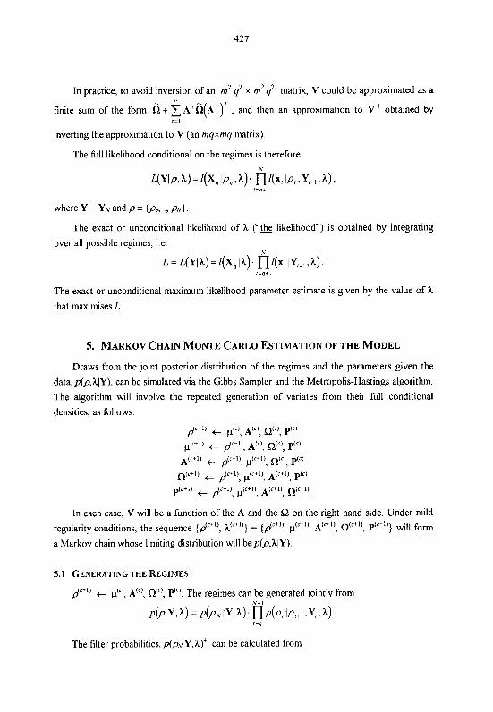
In practice, to avoid inversion of an nz2 q2 x nl2 q2 matrix, V could be approximated as a
finite sum of the form 61 ~ A r 6 ( A z ) ' , and then an approximation to V-I obtained by r = l
inverting the approximation to V (an rnqxlnq matrix)
The full likelihood conditional on the regimes is therefore
where Y = Y ~ a n d p = (p,,.., PN}
The exact or unconditional likelihood of h ("h likelihood) is obtained by integrating
over all possible regimes, i.e.
The exact or unconditional maximum likelihood parameter estimate is given by the value of h
that maximises L.
5. MARKOV CHAIN MONTE CARLO ESTIMATION OF THE MODEL
Draws from the joint posterior distribution of the regimes and the parameters given the
data,p@,hlY), can be simulated via the Gibbs Sampler and the Metropolis-Hastings algorithm.
The algorithm will involve the repeated generation of variates from their full conditional
densities, as follows:
p(CCl ) + p(C), A(C), ~ ( c ) , p'c)
p ( ~ + l l + P(C+Il AIC) , ~ ( 0 , pW
A(ctl) + P('+I) p(c+l)r Q(c), P '~'
n(Ctl) + p(C"), p ( ~ i l ) , A(ctl) p(C)
p(c+l) p(C+l), p (C+l ) , A(c+~), Q ( C + l ) ,
In each case, V will be a function of the A and the R on the right hand side. Under mild
regularity conditions, the sequence {p'"", h("") = {p""', p'c'l', A'"", o'"", P'""} will form
a Markov chain whose limiting distribution will bep(p,hlY).
5.1 GENERATING THE REGIMES
p'"" t p@', A"', R'"), P"'. The regimes can be generated jointly from . A - 1
P(Pl Y , h) = P(P, IY, A). n P(P, I,,+, ,Y,. A) t=q
The filter probabilities, p @ ~ ~ ~ , h ) J , can be calculated from
Once the filter probabilities, p@NIY,h), have been calculated, a sample can easily be generated
fromp@~IY,h), since it is a discrete density.
The above iterations require the evaluation of the contributions to the conditional
likelihood, l(~,(p,,Y,~,h). These will require evaluation of the mxni determinants of the K a - I 5 .
To initialise the previous iterations, the K p@,/h) will be required. They can be derived as
the limiting distribution of the Markov chain6 Define the Kxl column vector
x - @@,=ilk), i = l, . . ,K}, then x = Pn:. n: can be estimated by iterating on x'""' = ~x'"' until
convergence to the desired level of accuracy. T h e p h l h ) are given as the elements of n:.
Thus to generate a sample from the joint distribution of p we first generate p~ from
p@~lY,h). Then for t = N-1 to q, calculate p@rlpt+l,Yr,h) using the most recently generated
value of p,+, and the previously calculated filter probabilities, as follows
P ( P ~ + I > P ~ I ~ , > ~ ) = P ( P , + ~ I P , J ) ~ P (P , IY ,>~) for Pl= l , . . J
Once the probabilities, p@,lpl+l,Y,,h), have been calculated, pl can easily be generated
from p@llpl+l,Yl,h), since it is a discrete density. For the regime switching process to be
defined, each of the K regimes needs to be visited.
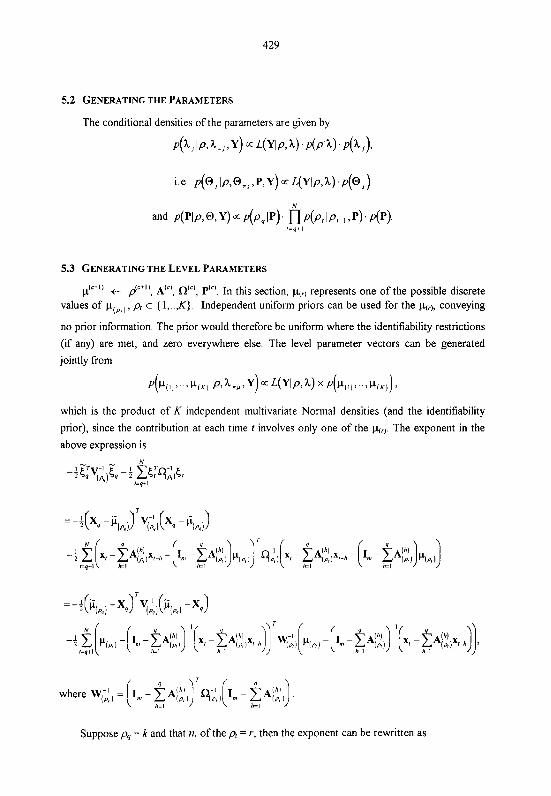
5.2 GENERATING THE PARAMETERS
The conditional densities of the parameters are given by
~ ( h , lp, hs, > Y) oc L(YlP. h) . ~ ( P l h ) . P(h ,).
pic+') +- pic+'", A'"', a"', Pic'. In this section, pi,.) represents one of the possible discrete values of p(p, ) , pI E ( I , ,K) . Independent uniform priors can be used for the pi,), conveying
no prior information. The prior would therefore be uniform where the identifiability restrictions
(if any) are met, and zero everywhere else. The level parameter vectors can be generated
jointly from
which is the product of K independent multivariate Normal densities (and the identifiability
prior), since the contribution at each time t involves only one of the pi,,. The exponent in the
above expression is
Suppose p, = k and that n, of the pl = r, then the exponent can be rewritten as
Ignoring the first term in V-', which is a function of p(klr the above expression is in the
form of K independent vector Normal densities in the p(,,.
where N(.,.) is the multivariate or vector Normal density7 The K-1 p,,,, r * k, can therefore
be independently generated from the above multivariate Normal densities Asymptotically, the
means of the above densities, for each regime, are the average of the data vectors in each
regime, as expected.
The terms in ~ k , are not quite vector Normal, since V" is also a function of ~ k , A Metropolis-Hastings step can be used to generate p(~,. First, a candidate p(k, is generated,
- ( n, - 1 - A ) , = , =(., - t A ; : p + l , ) , l W , i , and accepted i e . p,=P /,=I ?Ik - 1 ,>q
p&') = pji\, with probability
otherwise the value from the previous Gibbs iteration is retained, i e. = pi;;. Here,
VG;(') is a hnction of Alf), and Qil;", while v(;~;" is a function of A&') and q;yc-"
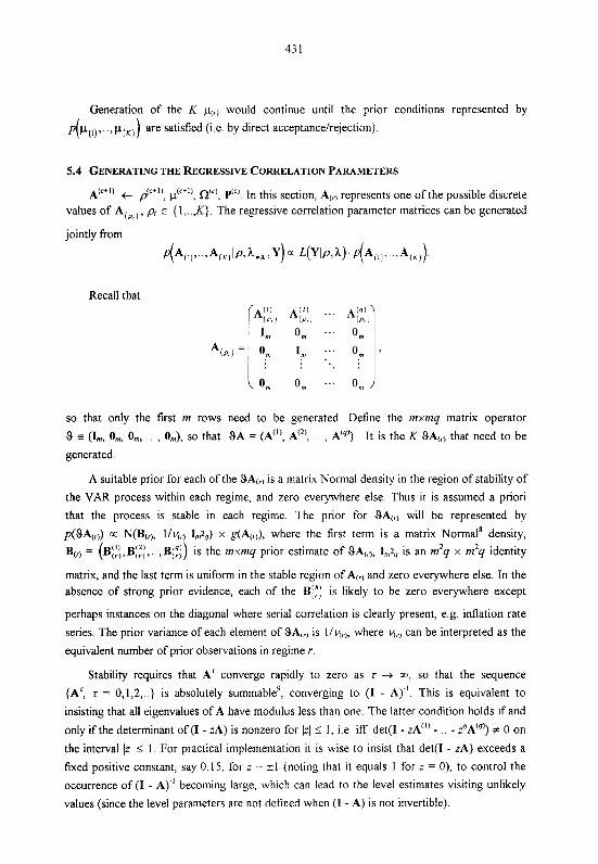
Generation of the K k,., would continue until the prior conditions represented by
~ ( p ( , ) , . . , pix,) are satisfied ( i e by direct acceptancelrejection).
5.4 GENERATING THE REGRESSIVE CORRELATION PARAMETERS
A ( ~ + ~ ) + d c i l ) , p'c'l', R'", P'"'. In this section, A',, represents one of the possible discrete values of Aip,,, p, E (l , . . ,K). The regressive correlation parameter matrices can be generated
Recall that
so that only the first 111 rows need to be generated Define the liixniq matrix operator
9 = (I,, Om, On,, .. , Om), so that 9 A = (A'", . , A'~)). It is the K 9A(,., that need to be
generated.
A suitable prior for each of the 9A(,-, is a matrix Normal density in the region of stability of
the VAR process within each regime, and zero everywhere else Thus it is assumed a priori
that the process is stable in each regime. The prior for 9Af,, will be represented by
p(9A(,]) a N(B(,), lly,., I&) x &A(,)), where the first term is a matrix ~ o r m a l ' density,
B(,) = ( B ~ ~ ~ , B ~ : ~ , . . ,B;:;) is the nlxniq prior estimate of SA,,.,, I,&, is an ni2q x m2q identity
matrix, and the last term is uniform in the stable region of A(,, and zero everywhere else In the absence of strong prior evidence, each of the B::: is likely to be zero everywhere except
perhaps instances on the diagonal where serial correlation is clearly present, e.g. inflation rate
series. The prior variance of each element of 9A(,, is I/!+,, where I+, can be interpreted as the
equivalent number of prior observations in regime r.
Stability requires that A' converge rapidly to zero as r + so, so that the sequence
{A7, s = 0,1,2,..) is absolutely summable9, converging to (I - A).'. This is equivalent to
insisting that all eigenvalues of A have modulus less than one The latter condition holds if and
only if the determinant of (I - :A) is nonzero for lzl i 1, i.e iff det(1 - :A"' - . - Z ~ A ' ~ ) ) # 0 on
the interval lzl 5 1. For practical implementation it is wise to insist that det(1 - :A) exceeds a
fixed positive constant, say 0.15, for z = i l (noting that it equals 1 for : = 0), to control the
occurrence of (I - A).' becoming large, which can lead to the level estimates visiting unlikely
values (since the level parameters are not defined when (I - A) is not invertible)
Supposing p, = k, consider regimes p, = r (z k), and define the nrxn,. matrix of regime r residual vectors, , , , ( , : p , = r ) , and matrices of
deviation vectors, i,,, r ( ( x , - Fir)) p f = r) and x,,, = ((x, - ) : = 7 ) . Noting that -
-tt = A,,,(X.-, - c,,) - (x, - F ( ~ ) from the VAR(1) form, consider the following
(dropping the references to regime r, for brevity).
where C = s ( ~ x ~ ) ( ~ ~ ~ ) ~ ' is an mxnq sample correlation matrix at lag 1. Note that
summary of the properties of the kronecker product and the vec and trace operators.
The contribution at each time t involves only one of the A(,,. The exponent of the
likelihood term can be expressed as
where G ( ~ , = (t, p , = k. f > q) is the m x ( n ~ - 1) matrix of regime k residual vectors, excluding
the first ( I = q) The exponent, including the prior, can therefore be expressed as
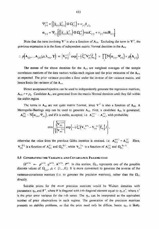
where %(,) and C(,, are defined to exclude the first vector (f = q), and
Note that the term involving V-' is also a function of A(h-,. Excluding the term in V-', the
previous expression is in the form of independent matrix Normal densities in the A(,).
The means of the above densities for the A(,., are weighted averages of the sample
correlation matrices of the data vectors within each regime and the prior estimates of the A(,),
as expected. The prior variance provides a floor under the inverse of the variance matrix, and
hence limits the variance of the A,,,.
Direct acceptance/rejection can be used to independently generate the regression matrices,
A(,), r # p,. Candidate A(,, are generated from the matrix Normal densities until they fall within
the stable region.
The terms in A(k) are not quite matrix Normal, since v-' is also a function of A(r A
Metropolis-Hastings step can be used to generate A(h, First, a candidate A(kl is generated,
A!;), - ~(cx~,,,~;,,), and if it is stable, accepted, i e A~C" = A;;\. with probability
otherwise the value from the previous Gibbs iteration is retamed, i e A::') = A;?, Here,
v;/') is a hnction of A;:\ and q;:('), while v ~ ~ " ' is a function of and q;Yc-"
5.5 GENERATING THE VARIANCE AND COVARIANCE PARAMETERS
D'~+') +- p'"", p'c+", A'"", P'". In this section, a(,, represents one of the possible discrete values of q,p,,, p, E {l,..,K). It is more convenient to generate the inverse of the
variance-covariance matrices (i.e. to generate the precision matrices), rather than the Q , ,
directly.
Suitable priors for the nmnl precision matrices would be Wishart densities with
parameters g,) and F', where F is diagonal with i-th diagonal element equal to where s:
is the prior error variance for the I-th series. The %,., can be interpreted as the equivalent
number of prior observations in each regime. The generation of the precision matrices
presents no stability problems, so that the prior need only be diffuse, hence q,) is likely
to be smaller than 4,). The complete prior would therefore be of the form
~ (q ; ; , . . .q:,) = fi wm,(l~(rI. *,;:) x h ( 4 , ) . . . . qK)). where h(q,, , . . . qK,) captures the ,=I
identifiability prior restrictions (if any). An example of an identifiability restriction might be that
the variance of the second series increases with the regime, i.e. &2(1) < .. < & 2 ( ~ ) , where a,,,,) is the 1-th diagonal element of Ol,.). As before, detine c,,, - ( ~ , : p , = r ) , r # pq and
G ( ~ ) = = k, 1 > q ) , k = p, (noting that the 5, are functions of the most recently
generated A(,)).
The precision matrices can be generated jointly from
Therefore the precision matrices, other than Or,',, can be generated independently
from Wishart densities. O;:, can be generated via a Metropolis-Hastings step
with a Wishart candidate generating density, i.e, generate a candidate a:;,,
"I;:" - wn,(nk + n,,, - I , (c,,c,:l + F,,,)-l) , and accept it, i e set Q::'" = O;i\*', with
probability
otherwise retain the value from the previous Gibbs iteration, i e set QriY1' = RT~;" Here,
VG;(') is a function of C$.'jm) and A!;T1', while V,;'jC' is a functlon of q,;") and A!?)
A variate from the Wlshart density, W - Wm(?l,C), can be generated as
W = QQ', where Q = LU, L is lower triangular given by the Choleski decomposition
C = LL', and U is upper triangular given by the Bartlett decomposition, I,,, = 0 for I > J, I,,: - X : (I = J) and I,,, - N(0,l) for I < I (so that U'U - W,,(11,1~,) )
5.6 GENERATING THE TRANSITION PROBABILITIES
Pee") + p'"", p'"", A'"", Q'c'". The transition probability matrix can be generated
from
P(PIP>@Y) a ~ ( f q l ~ ) fJP(P, lP ,-,, P).P(P). ,=,,+I
Suppose that p represents ti,, transltlons from reglme 1 to reglme I Define the prior for the
p, to be Beta(n~,, + 1, m,, + I), where m,, has the mterpretation as the equivalent number of
prior transitions, then
In the above expression, p(p,lP) IS a function of each of the p,, Draws from the above
jomt denslty can be generated using a Metropolls-Hast~ngs step, uslng Independent Beta
dens~t~es as the cand~date generating densltles Generate cand~date P, P"', from p;) - Beta(n, + m, + 1, n,, + m,, + 1) for 1 $1, p!" = 1 - xPr) , untd p(," > 0, wh~ch IS then
! = I
accepted, i e P'"" set equal to P"', with probability min
otherwise the value from the previous Gibbs iteration is retained, i e set P'"" = P'"'. Recall
thatp@,IP) is given by iterating on P.
The acceptance rate is high for stable regimes where thep,, are small The acceptance rate
can become very low when a p,, becomes small, since then p,, = 1 - Cp, < II(1 - p,), and
hence their ratio can become very small when raised to the power n,, +m,, However if ap, , is
small, perhaps the appropriateness of modelling the regime at all should be questioned
The estimation procedure was tested against a number of simulated data sets. The mean
parameter estimates were found to converge extremely rapidly, even when the initial parameter
estimates were very poor and the order of the fitted model was incorrect. The effects of the
initial parameter estimates appeared to dissipate after only several iterations/samples. The
MCMC procedure can therefore be expected to supply a good estimate of the mean parameter
values within seconds, regardless of the initial parameter estimates, in contrast to an EM
maximum likelihood approach. The results of one of the simulation tests are briefly reported
below.
2000 observations were generated from a bivariate RSVAR(2,2) process. The data
generating process was a random noise process within each regime, apart from variable 2 in
regime 1, which was generated from an AR(2) process with autoregressive parameters of 0.75
and -0.25, i.e. xn = 0.01 + 0.75(x,.,,, - 0 01) - 0.25(~,.2,2 - 0.01) + 0.005z,, where z, - iid
N O , 1).
The MCMC estimation procedure described in section 5 was used to generate 2000
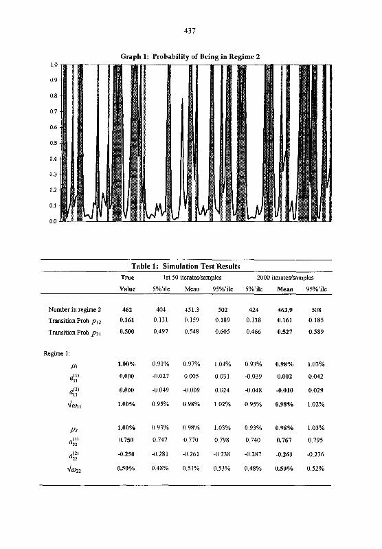
samples from the joint parameter density of the model. The mean parameter estimates are
summarked in table 1. The procedure successfully identified the data generating process with
very tight densities centred over the true parameter values. The significance or otherwise of the
various parameter estimates is beyond doubt. Maximum likelihood estimated (MLE)
parameters were taken as the set of parameters corresponding to the sampleliteration with the
highest log-likelihood of the 2000 samplesliterations. The mean and MLE parameters were
very close, which is to be expected, given the large data set (2000 observations). In the test
shown the initial parameter estimates were reasonably close to the true parameters. Other tests
demonstrated the robustness of the estimation procedure to various starting values.
Graph 1 compares the mean regime (line) with the true regime (shaded bands) for the first 150
time points. The procedure successfully differentiated between the low and high volatility
independent GARCHI', Vector Autoregression and RSVAR. The results are summarised in
table 3
Non-Gaussian error distributions are sometimes used in an attempt to directly capture the
leptokurtosis observed in the frequency distribution of many series. Two densities were tried as
alternatives to the standard Normal density, the Student t density and the Generalised Error or
Exponential Power Density (GED)'~ (both standardised). As the GED provided the better fit
to the data, only the GED results are reported.
The models were compared in terms of their likelihood and prediction errors, their ability
to predict volatility, and their ability to explain the observed excess kurtosis (a measure of non-
Normality).
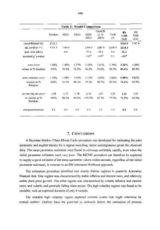
The log-likelihoods, both unconditional and conditional on the first data point, are
reported in table 3. Where one model is completely nested within another, the increase in the
log-likelihood is asymptotically distributed as '/zX,? where p is the number of additional
parameters fitted in the more general of the two models. Thus the AR(1) model is significantly
more likely than the Random model and both the GED-AR(1) and the GARCH-AR(1) models
are significantly more likely than the AR(1) model. The introduction of the non-Normal error
density (GED) produced a substantial increase in the likelihood with the addition of only 4
parameters. It is important to note however that neither the GED nor GARCH models were
able to produce lower prediction errors than the AR(1) model. The VAR model is not
significantly more likely than the AR(1) model.
Since the transition probabilities are not defined under the null hypothesis that the regime
switching model is inappropriate, the usual asymptotic statistical distribution theory fails to
apply in this case. If it did, the RSVAR(1,2) model would be extremely more likely than either
the AR(1) or VAR(1) models. Though not a statistical test, it is at least reassuring that there is
a large increase in the log-likelihood, even after allowing for the larger number of parameters.
The addition of the second lag in the RSVAR(2,2) model produced only a very modest
increase in the log-likelihood ('-value of 0.38). The addition of a hrther regime (K = 3)
proved problematic, due to the degree of instability of the third regime in iterations wherep,, = 0. A third regime would appear to be superfluous given its virtual unidentifiability.
The average prediction or forecast errors for each model were assessed using the root-
mean-square, or standard, error, which for series I was defined as rnise, = dm, where
E, is the residual or one-period-ahead prediction error at time t The rnis errors for each series
were combined into a single weighted rnis error for each model for ease of comparison The
weights used were proportional to the reciprocals of the corresponding AR(1) residual
variances, i e wrrns error = 4- As noted earlier, both the GED-AR(1) and
GARCH(1,l)-AR(1) models produced forecasts no better than the simpler AR(1) model on
average. The RSVAR models however produced the smallest errors on average by a
consideraMe margin.
Two measures were used to assess the ability to predict volatility. The first measure used
was the root-mean-square absolute error, defined for series i as rnisae, = &z(le,l- . where q is the one-period-ahead predicted error standard deviation according to the model.
The rms absolute errors were also combined into a single iveighted rnis absolute error using
the same weights as used for the ivrnis error The second measure used was the
root-mean-square log-absolute error, defined for series r as n n s h , = ,/- =
The GED model produced particularly poor forecasts of volatility. The RSVAR models
produced considerably better predictions of volatility on the whole, and notably better than the
GARCH model, which also explicitly models conditional heteroscedasticity. Regime switching
would appear to be a better explanation of conditional heteroscedasticity than the commonly
used GARCH and ARCH processes, which generally impute too much persistency in the
volatility (see, for example, Hamilton & Susmel (1994)).
The frequency distribution of financial series typically display excess kurtosis, i.e. are fat-
tailed and peaked at the mean (e.g. Mandelbrot (1963), Praetz (1969), Akgiray (1989), Peters
(1991), Becker (1991) and Harris (1994, 1995a)). The excess kurtosis of the residuals of each
series was calculated, and the average reported in table 3. Autoregressive, VAR and GARCH
models failed to explain the observed excess kurtosis. The RSVAR models were able to
successfUlly account for the excess kurtosis in terms of regime switching in the variance, i.e.
conditional heteroscedasticity. The only other model to account for the excess kurtosis was the
GED model, which explicitly models excess kurtosis by assuming the residuals are drawn from
a non-Normal distribution, without explaining the mechanism leading to the non-Normality.
Table 3: Model Comparison GARCH
Randon1 AR(1) AR(1) GED- (I,!)- RS RS
VAR VAR VAR AN1) ( 1 ) (1.2) (2,2)
unconditional lnL
lnL cond on r=l
AlnL over AR(1)
standard 2 p-value
~vr111s error
wriiise as % Random
wrms absolute error
>vrnrsae as % Random
av rim log obs error
av rilislae as % Random
ave escess kurtosis
A Bayesian Markov Chain Monte Carlo procedure was developed for estimating the joint
parameter and regime density for a regime switching vector autoregression given the observed
data. The mean parameter estimates were found to converge extremely rapidly, even when the
initial parameter estimates were very poor. The MCMC procedure can therefore be expected
to supply a good estimate of the mean parameter values within seconds, regardless of the initial
parameter estimates, in contrast to an EM maximum likelihood approach.
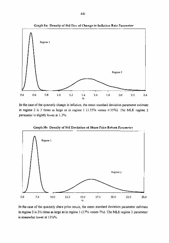
The estimation procedure identified two clearly distinct regimes in quarterly Australian
financial data One regime was characterised by stable inflation and interest rates, and relatively
stable share price growth. The other regime was characterised by volatile inflation and interest
rates, and volatile and generally falling share prices. The high volatility regime was found to be
unstable, with an expected duration of only 6 months.
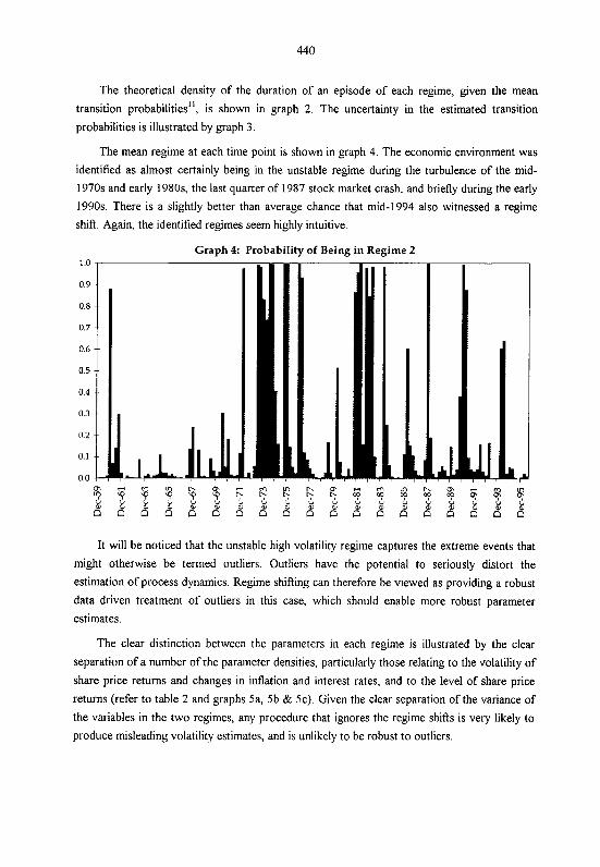
The unstable high volatility regime captured extreme events that might otherwise be
termed outliers. Outliers have the potential to seriously distort the estimation of process
dynamics. Regime shifting can therefore be viewed as providing a robust data driven treatment
of outliers in this case, which should enable more robust parameter estimates.
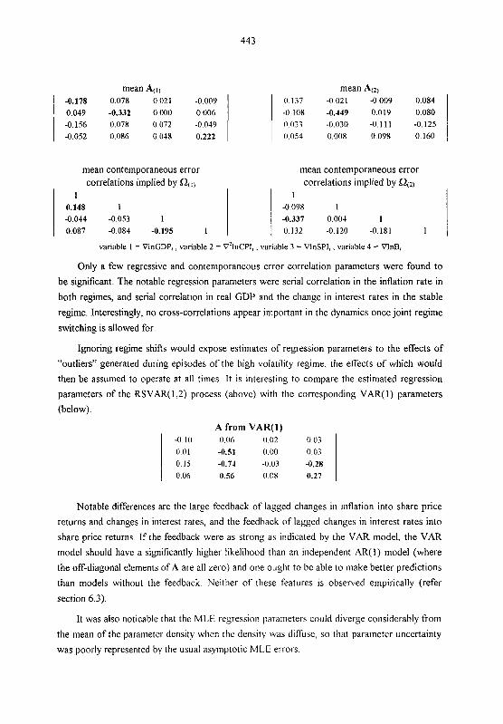
No cross-correlations appeared important in the dynamics once joint regime switching
was allowed for, in contrast to the large cross-correlation terms observed when a standard
vector autoregression was fitted to the data If the feedback were as strong as indicated by the
VAR model, the VAR model should have a significantly higher likelihood than an independent
autoregressive model (where there are no cross-correlation terms) and one ought to be able to
make better predictions than models without the feedback. Neither of these features was
observed empirically.
Whilst the GARCH and non-Normal Generalised Error Distribution models were able to
produce significant increases in the likelihood over the simpler autoregressive model, it was
noted that neither model was able to produce lower average prediction errors than the simple
AR model. The RSVAR models produced the lowest average prediction errors by a
considerable margin, however.
The RSVAR models produced considerably better predictions of volatility on the whole,
and notably better than the GED and GARCH models. Regime switching would appear to be a
better explanation of conditional heteroscedasticity than the commonly used GARCH and
ARCH processes.
Autoregressive, VAR and GARCH models failed to explain the fat tails observed in the
frequency distribution of the data. The RSVAR models were able to successfilly account for
the excess kurtosis in terms of regime switching in the variance, i.e. conditional
heteroscedasticity The only other model to account for the excess kurtosis was the GED
model, which explicitly nlodels excess kurtosis by assuming the residuals are drawn from a
non-Normal distribution, without explaining the mechanism leading to the non-Normality.
In conclusion, many financial time series processes appear subject to periodic structural
changes in their dynamics. Regression relationships are often not robust to outliers nor stable
over time, whilst the existence of changes in variance over time is well known. This paper
presented an attempt to deal with such difficulties in financial time series, a Regime Switching
Vector Autoregression, the parameters of which are subject to pseudocyclical discrete
changes. The regime switching vector autoregression model was found to provide a
particularly good description of an Australian quarterly financial data set.
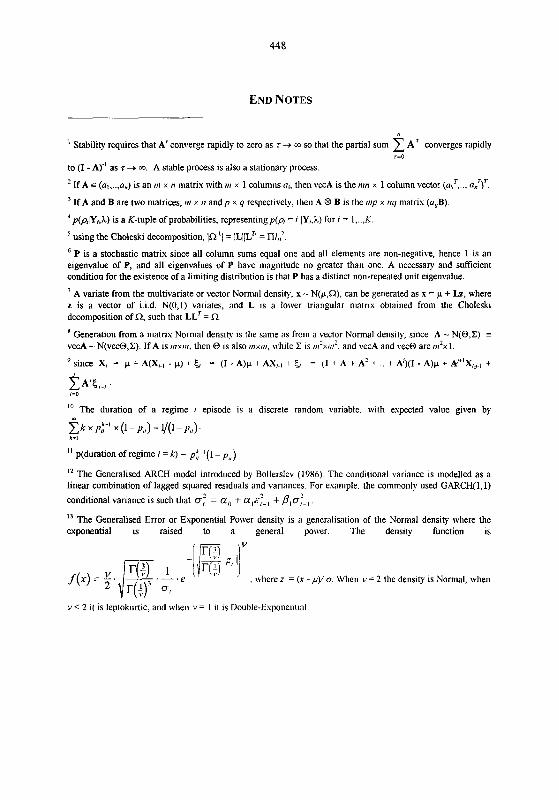
' Stability requires that A' converge rapidly to zero as 7 -+ ao so that the partial sum A' converges rapidly r=O
to (I -A)" as 7 -+ m. A stable process is also a stationary process.
If A E (ol,..,a,) is an rrr x rt matrix with rrr x 1 columns o,, then vecA is the rim x 1 column vector (qT,.., a,'jT.
If A and B are two matrices, rrr x n andp x q respectively, then A 63 B is the rrrp x riq matrix (o,B).
p@,IY,,X) is a K-tuple of probabilities, representingp(p, = i /Y,.k) for r = 1, ... K.
using the Choleski decomposition, P I / = ]L\/LT1= Ill,,'.
P is a stochastic matrix since all column sums equal one and all elenlents are non-negative, hence 1 is an eigenvalue of P, and all eigenvalues of P have magnitude no greater than one A necessary and sufficient condition for the existence of a limiting distribution is that P has a distinct non-repeated unit eigenvalue.
A variate from the multivariate or vector Nornlal density, x - N(p,n), can be generated as x = p + Lz, where z is a vector of i.i.d. N(0,l) variates. and L is a lower triangular matrix obtained from the Choleski decomposition of Q, such that LL'= 0.
Generation from a matrix Normal dens~ty IS the same as from a vector Normal density, since A - N(O,X) = vecA - N(ve&,Z). If A is mxrv, then O is also rrrxrrr. while 1 is rrr'xrrr:. and vecA and vecO are nr2xl. 9 . slnce X, = p + A(X,., - p) + 5, = (I - A)p + AX,.] + 5, = (I + A + A' + .. + AJ)(l - A)p + A'+'x,,., +
l o The duration of a regime i episode is a discrete random variable. w~ th expected value given by
2 k X pi-' x (1 - P,,) = 1/(1- A). k-I
' I duration of regime i = k ) = p,t-'(l - p,,)
l2 The Generalised ARCH model introduced by Bollerslev (1986). The conditional variance is modelled as a linear combination of lagged squared res~duals and variances. For esample, the commonly used GARCH(1,l)
conditional variance is such that a; = a, + a , & L 1 + Pla;., l3 The Generalised Error or Exponential Power density is a generalisation of the Normal density where the exponential is raised to a general power. The density function is
. where z = (x - ,u)l cz When v = 2 the density is Normal, when
v < 2 it is leptokurtic, and when r. = I it is Double-Esponenttal
AKGIRAY, V. (1989). Conditional Heteroscedasticity in Time Series of Stock Returns:
Evidence and Forecasts. Jor~rnal of Brrsiness 62, 55-80.
ALBERT, J H AND CHIB, S (1993) Bayes Inference via Gibbs Sampling of Autoregressive
Tune Series Subject to Markov Mean and Variance Shifts Joiirnal of Bzlsrness and
Econonzlc Stat~st~cs 1 1, 1, 1 - 15
BARNETT G., KOHN R. AND SHEATHER, S. (1996). Bayesian Estimation of an Autoregressive
Model Using Markov Chain Monte Carlo. Jorlrnal of Econonietrics 74 (October 1996),
237-254.
BECKER, D. (1991). Statistical Tests of the Lognormal Distribution as a Basis for Interest Rate
Changes. Transactions of the Society of Actiinries XLIII.
BOLLERSLEV, T (1986). Generalized Autoregressive Conditional Heteroskedasticity. Journal
of Econonietrics 3 1 (June 1986), 307-327.
CASELLA, G. AND GEORGE, E. I. (1992). Explaining the Gibbs Sampler. The American
Statistician 46, No 3, 167-174.
CHIB, S. AND GREENBERG, E. (1995). Understanding the Metropolis-Hastings Algorithm. The
American Stafisfician 49, No.4, 327-335.
ENGLE, R. F. (1982) Autoregressive Conditional Heteroscedasticity with Estimates of the
Variance of U.K Inflation. Econonietrica 50, 987-1008.
FREES, E. W., KUNG, Y-C., ROSENBERG, M. A,, YOUNG, V. R. AND LAI, S-W. (1996).
Forecasting Social Security Actuarial Assumptions. Submitted to the North American
Act~larial Journal
GELFAND, A. AND SMITH, A. (1990). Sampling-Based Approaches to Calculating Marginal