Regional and Income Distribution Effects ofAlternative Retail Electricity Tariffs
Severin Borenstein1
October 2011
Abstract: Since 2001, California’s investor-owned utilities have operated with very steepincreasing-block residential electricity tariffs, under which the marginal price increases asthe customer’s monthly usage rises. At the same time, these utilities have imposed little orno monthly fixed charge, despite the fact that a significant share of their costs do not varywith the customer’s consumption quantity. There are now moves to reduce the steepnessof the increasing-block pricing (IBP) and to impose fixed monthly charges (FCs). Buildingon Borenstein (forthcoming), I examine how such changes would impact different regionsof the state and households in different income brackets. I find that, contrary to frequentassertions, IBP does not penalize customers in high-use (i.e., hot) areas on average becausethe baseline quantities for IBP reflect regional differences in average consumption. In fact,a switch to a flat electricity price would not change average customer bills in these areas.Imposing a FC that is equal for customers in all regions and reducing the price on thehigher tiers to offset that revenue would have a slight benefit for customers in hot areas.In my earlier work, I showed that moving from IBP to a flat tariff would harm low-incomecustomers, though the impact is muted by the CARE program, a means-tested programthat offers lower rates to low-income households. I examine here the impact on householdsin different income brackets of imposing a FC and reducing the price on higher tiers tooffset the revenue change. I find that low-income households who are not on the CAREprogram would receive little of the benefit from lowering marginal prices, so the bills ofsuch households in the lowest income quintile (approximately) would increase on average by69%-92% of the fixed charge. Unlike moving to a flatter marginal rate schedule, imposingfixed charges is likely to have little or no incentive effect for low-income households.
1 E.T. Grether Professor of Business Economics and Public Policy, Haas School of Business, Univer-sity of California, Berkeley (faculty.haas.berkeley.edu/borenste); Co-Director of the Energy Instituteat Haas (ei.haas.berkeley.edu); Director of the U.C. Energy Institute (www.ucei.berkeley.edu) andResearch Associate of the National Bureau of Economic Research (www.nber.org). Email: [email protected]. I am grateful to Koichiro Ito and Karen Notsund for helpful discussions.
I. Introduction
The residential electricity tariffs of California’s investor-owned utilities differ from typi-
cal rates elsewhere in the U.S. in three significant ways. First, California has the steepest
increasing-block price (IBP) schedules in the country, with marginal consumption on higher
tiers costing three times or more the level of baseline consumption. Second, residential cus-
tomers pay little or no fixed monthly fee. And, third, the effective tariff schedule exhibits
substantial differences regionally within a utility’s service territory. This is because, while
the same IBP prices apply throughout the service territory, the baseline quantities that de-
termine the amount of consumption available on each step of the IBP tariff differ regionally.
Areas of higher average consumption have higher baseline quantities.
Increasing-block pricing, also called inclining-block pricing, is fairly common in the
United States, with over 40% of the largest utilities employing it at least part of the year.2
Many energy consultants advocate use of IBP on the argument that raising marginal rates
reduces consumption.3 While this may be true, it will depend on where the marginal rate
increases occur and how customers respond to more complex non-linear rates, as shown
by Ito (2010). More importantly, the goal is not to simply reduce consumption, but to
do so to the optimal extent. If consumers face marginal rates that are above the true
social marginal cost of supplying power, they will inefficiently over-conserve on electricity.
That is almost certainly the case in California for customers on the higher tiers of the IBP
tariffs.
Many market participants and regulators in California have suggested changing residen-
tial tariffs to make them more like tariffs elsewhere in the U.S.: eliminating or greatly re-
ducing the steepness of the increasing-block pricing and instituting significant fixed charges.
While some of the policy discussion has focused on aligning prices with costs, there has
also been concern about distributional impacts of these changes. Much of the concern is
for low-income customers as a ratepayer class. Another focus has been the regional impact
of these potential rate changes.
2 See BC Hydro, 2008.
3 See, for instance, Faruqui, 2008, Orans et al, 2009, and Pollock and Shumilkina, 2010.
1
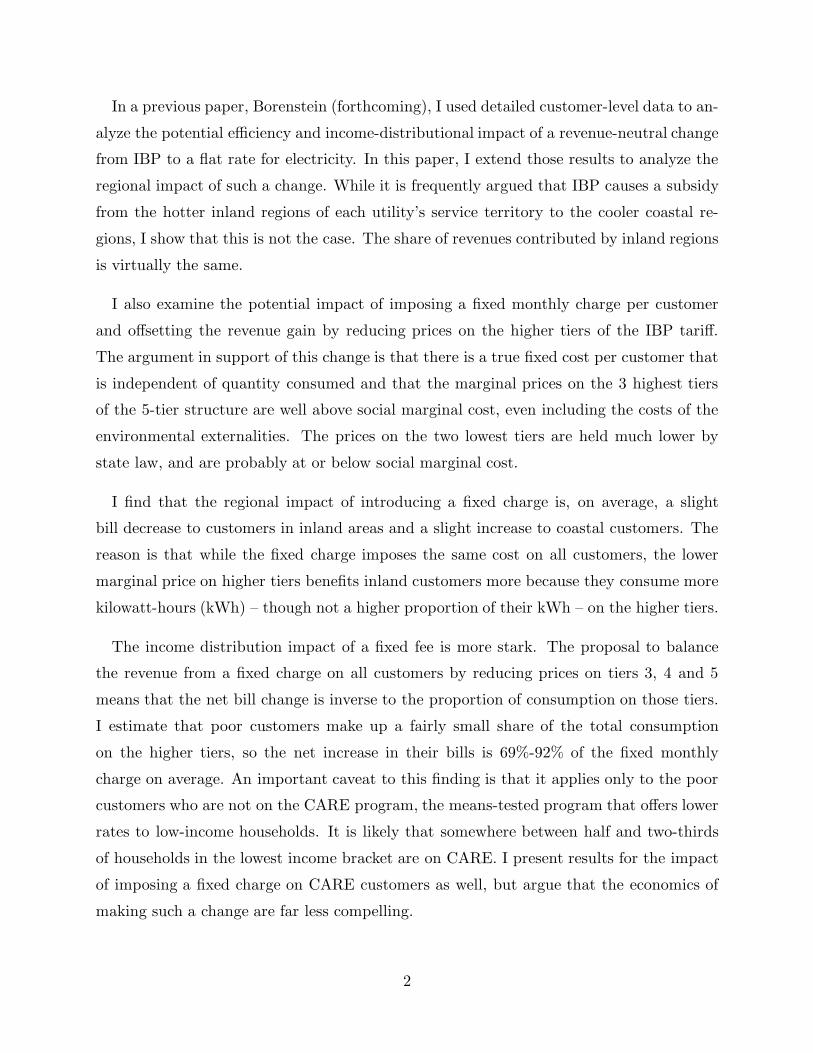
In a previous paper, Borenstein (forthcoming), I used detailed customer-level data to an-
alyze the potential efficiency and income-distributional impact of a revenue-neutral change
from IBP to a flat rate for electricity. In this paper, I extend those results to analyze the
regional impact of such a change. While it is frequently argued that IBP causes a subsidy
from the hotter inland regions of each utility’s service territory to the cooler coastal re-
gions, I show that this is not the case. The share of revenues contributed by inland regions
is virtually the same.
I also examine the potential impact of imposing a fixed monthly charge per customer
and offsetting the revenue gain by reducing prices on the higher tiers of the IBP tariff.
The argument in support of this change is that there is a true fixed cost per customer that
is independent of quantity consumed and that the marginal prices on the 3 highest tiers
of the 5-tier structure are well above social marginal cost, even including the costs of the
environmental externalities. The prices on the two lowest tiers are held much lower by
state law, and are probably at or below social marginal cost.
I find that the regional impact of introducing a fixed charge is, on average, a slight
bill decrease to customers in inland areas and a slight increase to coastal customers. The
reason is that while the fixed charge imposes the same cost on all customers, the lower
marginal price on higher tiers benefits inland customers more because they consume more
kilowatt-hours (kWh) – though not a higher proportion of their kWh – on the higher tiers.
The income distribution impact of a fixed fee is more stark. The proposal to balance
the revenue from a fixed charge on all customers by reducing prices on tiers 3, 4 and 5
means that the net bill change is inverse to the proportion of consumption on those tiers.
I estimate that poor customers make up a fairly small share of the total consumption
on the higher tiers, so the net increase in their bills is 69%-92% of the fixed monthly
charge on average. An important caveat to this finding is that it applies only to the poor
customers who are not on the CARE program, the means-tested program that offers lower
rates to low-income households. It is likely that somewhere between half and two-thirds
of households in the lowest income bracket are on CARE. I present results for the impact
of imposing a fixed charge on CARE customers as well, but argue that the economics of
making such a change are far less compelling.
2
Section II describes the data I analyze and the alternative tariffs that I study in the
paper. Section III evaluates the regional impact of IBP and FCs using the climate regions
defined by each utility. Section IV reviews my earlier work on the income distributional
impact of IBP and then applies the same techniques to study the income distributional
impact of FCs. In section V, I consider the how the results change when customers can
respond to changes in the marginal and average price they face. I show that for the most
plausible parameters, demand response will have almost no impact on the distributional
impact. Section VI concludes.
II. Data and Alternative Tariffs
The analysis is based on customer-level residential electricity billing data from the three
largest investor-owned utilities in California: Pacific Gas & Electric (PG&E), Southern
California Edison (SCE), and San Diego Gas & Electric (SDG&E). The data are described
in detail in Borenstein (forthcoming). With the exception of master-metered premises,
the data include nearly every residential customer in these utilities’ service territories.
They include the customer premise id, dates of the billing period, consumption during the
billing period, the quantities of consumption assigned to each of the 5 tiers, and whether
the customer was on the CARE program. I combine these data with the average tariff of
each utility during 2006 to create bills for each billing period and then aggregate up to
annual bills for each customer.4
I compare bills from the average IBP tariff to two alternative scenarios. One is a flat
rate for all customers of the utility. The flat rate is set to raise the same total revenue
under an assumption of zero price elasticity. Borenstein (forthcoming) discusses in detail
the impact of elasticity on income redistribution and economic efficiency. I discuss the
topic briefly here as well, showing that the results of this analysis would change very little
with the incorporation of demand elasticity.
The second alternative is an IBP tariff with a fixed monthly charge (FC). In this analysis,
I consider a monthly charge of $5. This is approximately the middle of the distribution of
fixed monthly charges imposed by utilities in the U.S. with most fixed charges between $2
4 I use an average tariff for the year, but there was very little change in any of the utilties’ tariffs during2006.
3
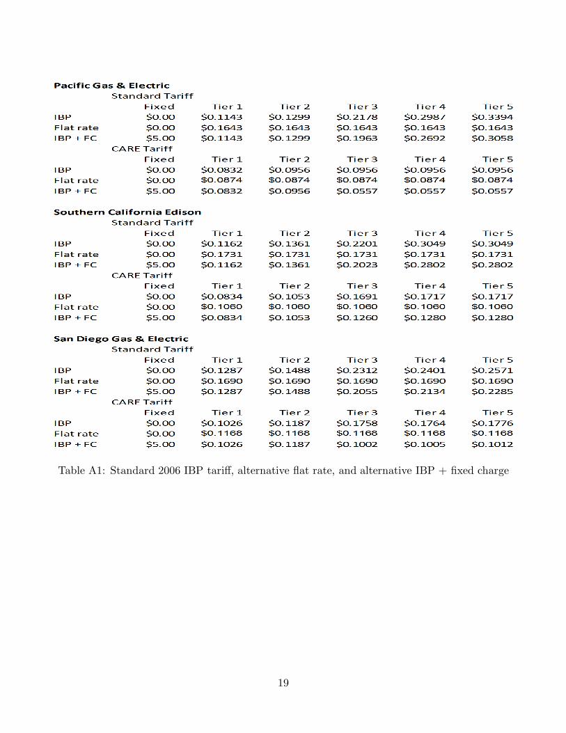
Table 1: Standard 2006 IBP tariff, alternative flat rate, and alternative IBP + fixed charge
and $10 per month. I then calculate equal-proportion decreases in the prices on tiers 3, 4
and 5 that would make the change revenue-neutral under the assumption that there would
be no change in consumption in response to the tariff change. This allocation of the fixed
charge revenue is the focus in California, because rates on the two lowest tiers have been
essentially frozen since 2001, while rates on the top 3 tiers have increased substantially. I
then also discuss the impact that price elasticity would have.
In all cases, I maintain the revenue separation of CARE and standard tariff customers.
The argument for making these tariff changes for CARE customers – holding constant the
revenue from such customers – is much less compelling than for standard tariff customers.
Though CARE customers face IBP in California, the price changes across the blocks are
substantially smaller for CARE customers than for standard tariff customers. In the case
of PG&E at least, even the highest rate may be below long-run marginal cost. Unless the
suggestion of flattening IBP tariffs or introducing a FC is coupled with the suggestion that
the discounts in the CARE program be altered overall, the policy is hard to justify. So,
I maintain separation of the revenue streams. Results for CARE customers are presented
in the appendix.
Table 1 presents the rates under the standard IBP tariff, the alternative flat tariff and
4
Figure 1: Monthly price schedule for households in two PG&E climate regions
the alternative IBP with $5/month FC.
I do not focus in this paper on the efficiency gains from tariff changes. Borenstein
(forthcoming) explores that issue in detail for a switch from IBP to a flat tariff. For the
switch from IBP to IBP with a fixed charge, the effect is relatively straightforward. The
elasticity of electricity hookups with respect to a fixed charge is likely to be extremely close
to zero, so the FC would have not a direct efficiency effect. Lowering the marginal prices
on higher tiers is likely to improve efficiency if marginal prices are above the marginal cost
of the power delivered. For the standard IBP tariffs shown in table 1, the marginal price
is well above most estimates of marginal cost, even including environmental and other
externalities, and likely to remain well above marginal cost after the offsetting reductions
from adding a FC. The reductions would move marginal prices closer to marginal cost, so
5
would be likely to improve efficiency.5
III. Regional Impacts of Alternative Tariffs
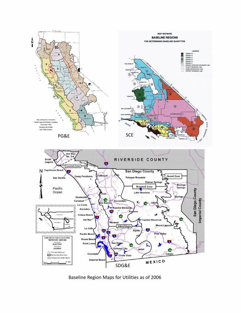
All three of the utilities that I study here have multiple climate regions that are assigned
different baseline quantities for use in the IBP tariffs. In 2006, PG&E had 10 climate
regions, SCE had 6, and SDG&E had 4, as shown in the baseline region maps in the
appendix. For a given utility, the baselines in each climate region are set in order to reflect
approximately the same proportion of average household consumption within the climate
region. So, for instance, SCE’s hottest inland climate regions have much higher baselines
in the summer months than the coastal regions, but in each region the baseline quantity
is intended to be approximately 55% of the average residential consumption. As a result,
while consumers in different climate regions face the same prices on each tier, they face
different price schedules. Figure 1 presents the price schedules for the two most populous
baseline regions in PG&E’s service territory. Region T is on the coast and quite temperate,
while region X is further inland and experiences wider temperature swings.
The effect of this targeting of baseline quantities is that the distribution of consumption
across the tiers does not vary a great deal across climate regions. Table 2 shows the share
of consumption on each tier within each climate region, broken out by CARE and standard
tariff customers. The table also shows the summer baseline quantity for customers who are
not on the all-electric tariff (which has higher baselines). This is a good indication of the
harshness of summer weather. Table 2 shows that the hot summer areas do not system-
atically have more consumption on high tiers. While there is some variation, particularly
among the climate regions that include a very small share of total load, the larger climate
regions have very similar distributions due to the baseline setting process.
As a result, table 3 shows that the average bill by region would not change very much
if customers were charged a simple flat rate per kWh rather than the standard IBP tariff.
There would, of course, be quite a bit of variation within each climate region – lower-use
consumers would pay more and higher-use consumers would pay less – but there would
5 Ito (2010) shows that customers facing IBP are more likely to respond to average price than marginalprice. Even average price is likely at or above marginal cost for customers on tiers 4 and 5. But on tier3, a conclusion about the effect of lowering marginal price is more uncertain if customers respond toaverage price.
6
Table 2: Consumption on tiers of IBP tariff by climate region
not be a systematic redistribution of payments to or from the hotter climate regions.
One way to see an aggregate picture of whether and in which direction revenue obliga-
tions shift is to look at the share of revenue coming from the climate regions with more
extreme temperatures, as measured by the summer baseline of the regions. For each of
the utilities, I have grouped the regions into the above-average and below-average summer
baseline groups, though the split isn’t exactly at 50% of total demand due to the lumpiness
of regions. I’ve then calculated the share of total revenue coming from the regions with
more extreme climate under alternative tariffs.
The results are shown in the bottom row of each panel. In the case of SCE for instance,
the more extreme climate regions are 13, 14, 15 and 17. These regions in aggregate
constituted 63.73% of standard tariff residential usage in 2006, so they would have paid
7
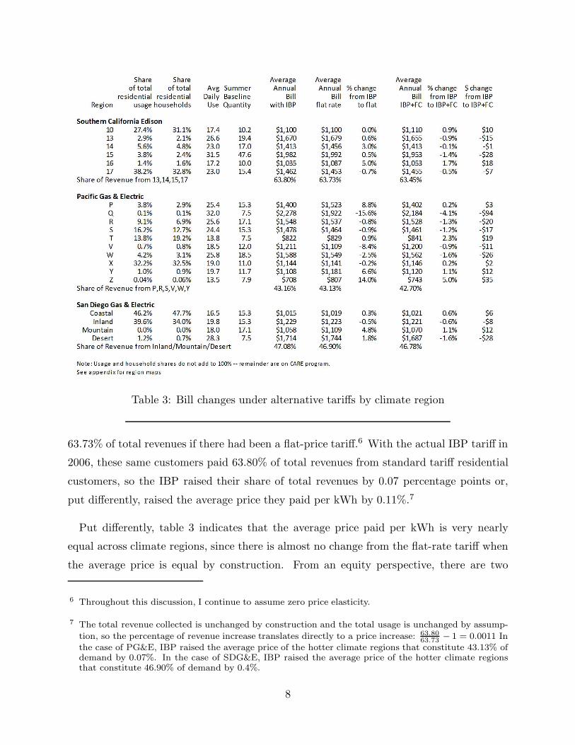
Table 3: Bill changes under alternative tariffs by climate region
63.73% of total revenues if there had been a flat-price tariff.6 With the actual IBP tariff in
2006, these same customers paid 63.80% of total revenues from standard tariff residential
customers, so the IBP raised their share of total revenues by 0.07 percentage points or,
put differently, raised the average price they paid per kWh by 0.11%.7
Put differently, table 3 indicates that the average price paid per kWh is very nearly
equal across climate regions, since there is almost no change from the flat-rate tariff when
the average price is equal by construction. From an equity perspective, there are two
6 Throughout this discussion, I continue to assume zero price elasticity.
7 The total revenue collected is unchanged by construction and the total usage is unchanged by assump-
tion, so the percentage of revenue increase translates directly to a price increase: 63.80
63.73− 1 = 0.0011 In
the case of PG&E, IBP raised the average price of the hotter climate regions that constitute 43.13% ofdemand by 0.07%. In the case of SDG&E, IBP raised the average price of the hotter climate regionsthat constitute 46.90% of demand by 0.4%.
8
sources of significant cost differences across regions that could justify different average
prices by climate region. First, hotter climates consume a higher share of their power
during peak demand periods, which is when power is more expensive to provide, suggesting
that cost-based tariffs would be higher in hotter regions. In ongoing work, I am exploring
the impact of the time variation in consumption, including how consumption patterns vary
across climate areas (Borenstein 2011). Second, there are fixed costs per customer that are
recovered through these volumetric charges and that probably don’t vary systematically
across climate regions – billing and metering, local distribution, and overhead. Since,
customers in hotter climate consume more overall, tariffs designed to cover each customer’s
total cost (including equal share of fixed cost for each customer) would tend to have a
lower price per kWh in the hotter regions as these fixed costs per customer are spread over
more consumption. Given that prices don’t vary by hour, however, and that recovering
fixed costs through volumetric charges generally results in inefficient marginal prices, these
arguments have more traction in terms of fairness than in terms of economic efficiency.
The right-hand set of columns of table 3 show the impact of switching from the standard
IBP tariff to a IBP with a $5/month fixed charge, where the additional revenue is offset by
equal-proportion reductions in marginal rates on tiers 3, 4, and 5. For all three utilities,
this causes the revenue share of the hotter regions to decline by 0.2 to 0.5 percentage
points, implying price drops of 0.6% to 1.1%. The change is small, but it isn’t a random
occurrence. It results from the fact that the fixed charge harms all customers equally, but
the decline in prices on the upper tiers disproportionately benefits customers in higher-use
regions. These customers consume more kWh on those high tiers, even though they don’t
consume a higher share of their total usage on those tiers.
Overall, the regional impact of these possible changes in retail tariffs is very limited.
Switching to a flat retail price for all power would have essentially no redistributive impact
across regions. Adding a fixed charge to the 5-tier tariff structure – then using the revenue
to lower the rates on higher tiers – would slightly benefit the areas with more extreme
climates, but the effect would still be 1.1% of bills or less on average.
IV. Impacts of Tariff Changes on Low-Income Customers
In contrast to the regional impacts, the impact of these potential tariff changes on
9
low-income customers is potentially substantial. This section presents an approach to
analyzing these impacts that I developed in earlier work and applies the approach to
the same potential tariff changes that were analyzed in the previous section. Instead of
comparing the relative impact on hotter versus milder climates, the comparison here is
between households in different income brackets. In particular, I divide customers into five
household income brackets and evaluate differential impacts across these brackets.
The exercise would be as straightforward as in the previous section if one knew the
income of every household, but those data are not available. Instead, census data are used
to estimate the incomes of households. The customers are identified at the 9-digit zip code
level and those data are matched to census block groups (CBGs). The census releases data
on the income distribution of households in every CBG, based on the long-form census,
which is collected from one out of every 6 households. Among the CBG-level information
is the proportion of households in each of 16 income brackets. In many CBGs, many of
the brackets are empty, and the variation in actual household income probably can’t be
identified with that much precision, so I aggregate these brackets to 5 income brackets that
are approximately quintiles in California: $0-$20,000, $20,000-$40,000, $40,000-$60,000,
$60,000-$100,000 and over $100,000.8
With household-level electricity billing data and only CBG level income distribution
data, the question is how to assign households within a CBG to different income brackets.
I first do this in two ways that are intended to give bounds on the variation. Then I create
an estimate of the actual distribution by taking a weighted average of the bounds, where
the weights are set by calibration to other indicators. The approach is described in much
more detail in Borenstein (forthcoming).
A. A bit more explanation of assigning household to income brackets
To give somewhat more detail here, households within each CBG are first assigned ran-
domly to income brackets in proportion to the actual census distribution of household
incomes in that CBG. This ignores any within-CBG correlation between income and elec-
8 As discussed in Borenstein (forthcoming), many studies use median household income by CBG torepresent the income of all households in the CBG. I show that there is a great deal of heterogeneitywithin CBGs, so such analyses fail to capture much of the cross-sectional income variation.
10
tricity usage – a correlation that is almost certainly positive – so it tends to assign too
many low-usage households to high income brackets and too many high-usage households
to low brackets. Then, as an alternative, households within a CBG are ordered by usage
and are then assigned to income brackets in the order of usage, so the lowest-usage house-
holds are assigned to the lowest income brackets and the highest-usage households to the
highest brackets. The bracket breaks are still determined by the census data so that the
proportion of households in each bracket still matches the census data for each CBG.
The matching is complicated (or actually assisted) by the fact that the billing data also
indicate whether the customer is on the CARE tariff or not. Thus, for each CBG, the share
of customers on CARE is known. Furthermore, there are estimates of the penetration of
CARE participation among eligible customers. I use this information to separately allocate
CARE and standard tariff customers across income brackets in a way that causes CARE
customers to be disproportionately allocated to the lower income brackets within each
CBG. See Borenstein (forthcoming) for further details.
The two bounding approaches deliver estimates of average bill by income bracket and
tariff, but the estimates differ substantially across the approaches. That is, the bounds are
not very tight. Luckily, the approaches also yield estimates of average annual consumption
by household within each income bracket. This ancillary attribute is then used to calibrate
the estimation by comparing the implied averages to estimates of these averages that I
derive from a completely different dataset. Essentially, I take a weighted average of the
results from the bounding approaches where the weight is the value that yields average
consumption levels by income bracket that most closely match the estimates from the other
dataset. Because the estimates from the other dataset are imprecise, so is the estimate of
the weighting that most closely matches these estimates. I use the distribution of possible
weightings to derive the mean, distribution, and confidence intervals of the estimated
changes in bills from the alternative tariff structures.
The result is an estimated change in average annual customer bill and a confidence
interval for that change. In the remainder of this section, I present those estimates.
B. Results
As in the previous section, I present results separately for customers on the standard
11
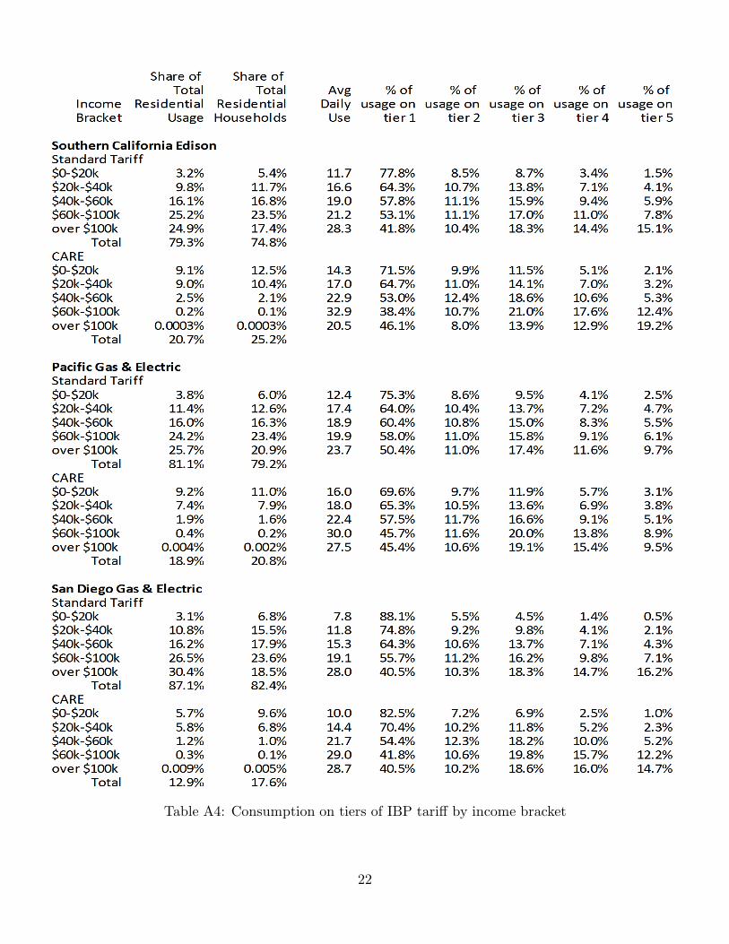
Table 4: Consumption on tiers of IBP tariff by income bracket
tariff and on CARE, focusing on the customers on the standard tariff. The results for
customers on CARE are shown in the appendix. Implicit in this approach is the assumption
that tariff changes will not alter CARE participation.
The format of the presentation follows that in the previous section, except customers
are now differentiated by income bracket instead of climate region and average bill changes
are estimated for each group, rather than just calculated, because the match of households
to income brackets is estimated by the method just discussed.
Table 4 shows the estimated distribution of consumption across the tiers by income
bracket for customers who are on the standard tariff. Though all customers with household
income below $20,000 per year are eligible for CARE, I estimate that about 26% of SCE
low-income customers are not on it.9 Table 4 shows that among standard tariff customers,
9 The number is somewhat higher for PG&E and SDG&E. The data indicate this because, for instance,there are some CBGs in which there are a higher proportion of households with income below $20,000
12
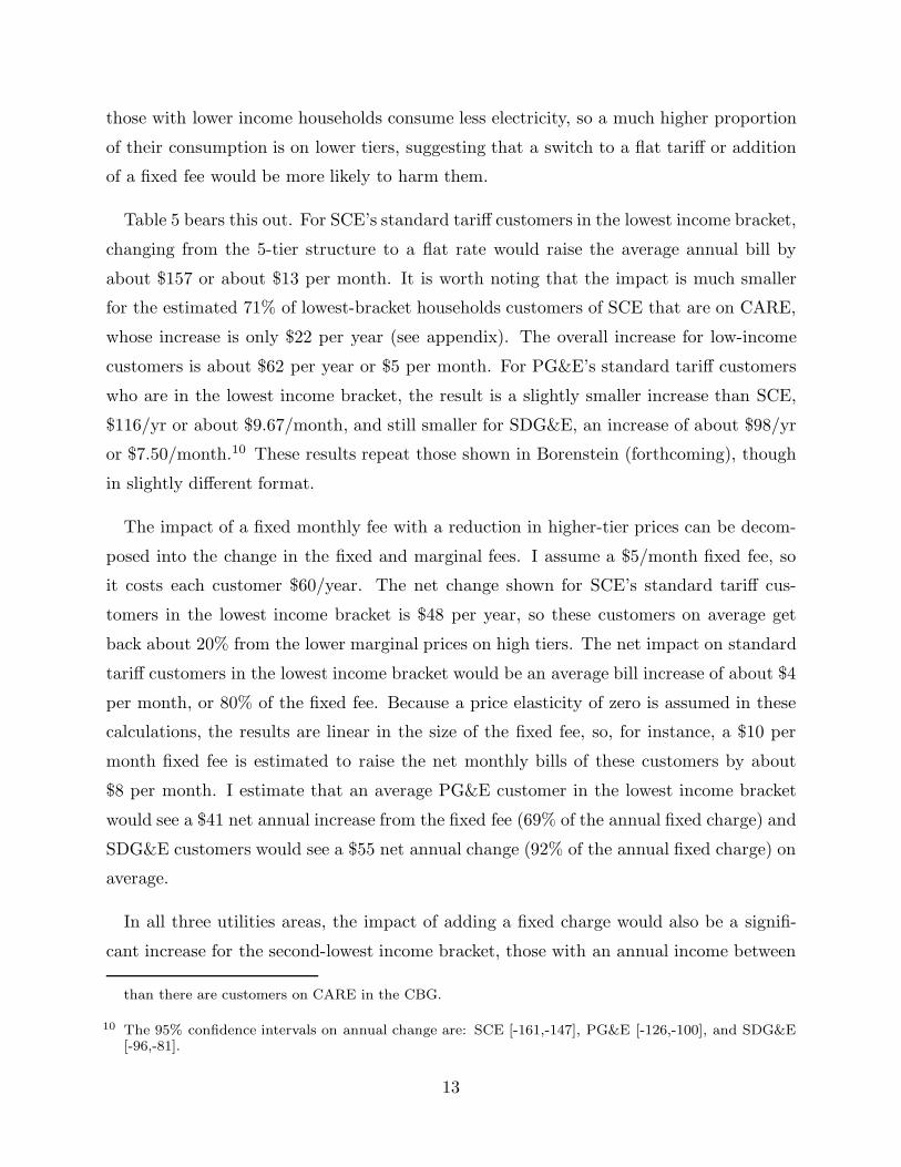
those with lower income households consume less electricity, so a much higher proportion
of their consumption is on lower tiers, suggesting that a switch to a flat tariff or addition
of a fixed fee would be more likely to harm them.
Table 5 bears this out. For SCE’s standard tariff customers in the lowest income bracket,
changing from the 5-tier structure to a flat rate would raise the average annual bill by
about $157 or about $13 per month. It is worth noting that the impact is much smaller
for the estimated 71% of lowest-bracket households customers of SCE that are on CARE,
whose increase is only $22 per year (see appendix). The overall increase for low-income
customers is about $62 per year or $5 per month. For PG&E’s standard tariff customers
who are in the lowest income bracket, the result is a slightly smaller increase than SCE,
$116/yr or about $9.67/month, and still smaller for SDG&E, an increase of about $98/yr
or $7.50/month.10 These results repeat those shown in Borenstein (forthcoming), though
in slightly different format.
The impact of a fixed monthly fee with a reduction in higher-tier prices can be decom-
posed into the change in the fixed and marginal fees. I assume a $5/month fixed fee, so
it costs each customer $60/year. The net change shown for SCE’s standard tariff cus-
tomers in the lowest income bracket is $48 per year, so these customers on average get
back about 20% from the lower marginal prices on high tiers. The net impact on standard
tariff customers in the lowest income bracket would be an average bill increase of about $4
per month, or 80% of the fixed fee. Because a price elasticity of zero is assumed in these
calculations, the results are linear in the size of the fixed fee, so, for instance, a $10 per
month fixed fee is estimated to raise the net monthly bills of these customers by about
$8 per month. I estimate that an average PG&E customer in the lowest income bracket
would see a $41 net annual increase from the fixed fee (69% of the annual fixed charge) and
SDG&E customers would see a $55 net annual change (92% of the annual fixed charge) on
average.
In all three utilities areas, the impact of adding a fixed charge would also be a signifi-
cant increase for the second-lowest income bracket, those with an annual income between
than there are customers on CARE in the CBG.
10 The 95% confidence intervals on annual change are: SCE [-161,-147], PG&E [-126,-100], and SDG&E[-96,-81].
13
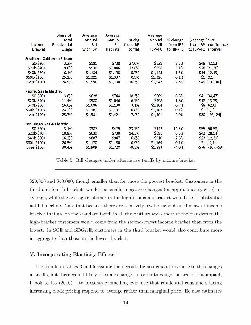
Table 5: Bill changes under alternative tariffs by income bracket
$20,000 and $40,000, though smaller than for those the poorest bracket. Customers in the
third and fourth brackets would see smaller negative changes (or approximately zero) on
average, while the average customer in the highest income bracket would see a substantial
net bill decline. Note that because there are relatively few households in the lowest income
bracket that are on the standard tariff, in all three utility areas more of the transfers to the
high-bracket customers would come from the second-lowest income bracket than from the
lowest. In SCE and SDG&E, customers in the third bracket would also contribute more
in aggregate than those in the lowest bracket.
V. Incorporating Elasticity Effects
The results in tables 3 and 5 assume there would be no demand response to the changes
in tariffs, but there would likely be some change. In order to gauge the size of this impact,
I look to Ito (2010). Ito presents compelling evidence that residential consumers facing
increasing block pricing respond to average rather than marginal price. He also estimates
14
Figure 2: Consumer Surplus change from IBP to flat rate for SCE customer
with and without demand elasticity
that the average elasticity for customers in his sample – a set of SCE and SDG&E customers
located near the boundary between the two utilities – is between -0.1 and -0.2.
In order to explore how much customer price response is likely to change the results,
figure 2 presents the change in consumer surplus with and without such response using
the standard SCE IBP and the alternative flat rate. The solid line shows the change in
annual consumer surplus for a customer with a baseline quantity allocation of 15 kWh
per day, which was about the customer-weighted average for SCE residential customers
in 2006. The dashed line shows the change in consumer surplus under the assumption
that the customer responds to a change in average price with an elasticity of -0.2.11 In
11 To be precise, the starting quantity (on the horizontal axis) is assumed to be the customer’s possiblynon-optimizing response to the average price implied by the standard IBP in table 1. That is, the
15
all cases, ignoring consumer adaptation to the price change biases the consumer surplus
change in the negative direction, but the bias is quite small. Incorporating consumer
response changes the change in consumer surplus by less than 5% at all consumption levels
up to 400% of baseline.
Figure 2 is calculated for a change from the standard IBP to a flat rate. The effect of
consumer response is even smaller for the change from standard IBP to IBP plus a fixed
charge. The $5/month fixed charge changes no marginal price so it creates virtually zero
consumer response.12 The associated change in the upper three tiers still leaves those
marginal prices well above the counterfactual flat-rate tariff, and there is no change in the
marginal prices on the lower two tiers. Thus, the bias is much smaller than the already
small bias in analyzing the change to a flat rate.
VI. Conclusion
There are strong policy arguments for regulators to avoid the sort of steeply increasing
block electricity rates that California now has. The rates are not cost based and add
complexity to billing that makes it more difficult to incorporate price variation that is
cost-based, such as time-varying pricing. While household consumption level is correlated
with income, the distributions make clear that there are many poor households with high
electricity consumption and many wealthy customers with low consumption. Borenstein
and Davis (forthcoming) found the same result in natural gas, and present evidence that
it is caused by the poorer energy efficiency of low-income households. Of course, one of
the concerns with marginal prices that don’t reflect cost is that they distort behavior. In
previous work, Borenstein (forthcoming), I showed that the distortion from IBP tariffs is
likely to be large relative to the amount of income they redistribute to poorer households,
making this an unattractive approach to accomplishing such redistribution.
Nonetheless, I find no support for one of the most common arguments against IBP in
customer has chosen the quantity at which her marginal value is equal to average price, consistent withthe idea that she knows her value, but has not taken the time or attention to figure out the true marginalprice. Then the alternative quantity is calculated assuming a price change from the average price atthe starting quantity to the flat rate and an elasticity of -0.2. The net change in consumer surplus ismeasured as the change in gross consumer surplus along the customer’s actual marginal value curveminus the change in payments.
12 Income effects change the analysis very little, as discussed in Borenstein (forthcoming).
16
California, that it hurts customers in regions with more extreme climate. Moving to a flat
rate would have virtually no impact on the average bill paid by customers in the areas
of the state that have hotter summers and colder winters. Introducing a significant fixed
monthly charge and lowering the rates on the higher tiers of the IBP tariff would benefit
these customers on average, but the effect would be very small, likely no more than a 1%
savings.
In Borenstein (forthcoming), I estimated the change in consumer surplus for low-income
households that would result from moving from IBP to a flat-rate tariff. I present those
results in a slightly different format here, focusing on the subset of low-income customers
who are not on the means-tested CARE program and showing that those customers would
see bills increase by 18% to 27% across the three large utilities. I then extend the analysis to
examine the impact of introducing a fixed charge while maintaining the IBP and lowering
the prices on the highest tiers. I find that among the lowest-income households (less than
$20,000 per year household income) that are not on the CARE program, introducing a
fixed monthly charge would on average cause a net increase in their bills of between 69%
Borenstein, Severin. “The Redistributional Impact of Nonlinear Electricity Pricing,” forth-coming in American Economic Journal: Economic Policy,available at http://ei.haas.berkeley.edu/pdf/working papers/WP204.pdf .
Borenstein, Severin. “Effective and Equitable Adoption of Opt-In Residential DynamicElectricity Pricing, working paper, March 2011.
Borenstein, Severin and Lucas W. Davis. “The Equity and Efficiency of Two-Part Tariffsin U.S. Natural Gas Markets,” Energy Institute at Haas Working Paper #213, U.C.Berkeley, December 2010, forthcoming in Journal of Law and Economics, available athttp://ei.haas.berkeley.edu/pdf/working papers/WP213.pdf .
Faruqui, Ahmad, “Inclining Toward Efficiency,” Public Utilities Fortnightly, August 2008.
Ito, Koichiro. “Do Consumers Respond to Marginal or Average Price? Evidence from Non-linear Electricity Pricing,” Energy Institute at Haas Working Paper #210, November2010.
Orans, Ren, C.K. Woo, Michael King and William Morrow. “Inclining for the Climate:GHG reduction via residential electricity making,” Public Utilities Fortnightly, May2009.
Pollock, Adam and Evgenia Shumilkina. “How to Induce Customers to Consume En-ergy Efficiently: Rate Design Options and Methods,” National Regulatory ResearchInstitute Working Paper, 10-03, January 2010.
18
Table A1: Standard 2006 IBP tariff, alternative flat rate, and alternative IBP + fixed charge
19
Table A2: Consumption on tiers of IBP tariff by climate region
20
Table A3: Bill changes under alternative tariffs by climate region
21
Table A4: Consumption on tiers of IBP tariff by income bracket
22
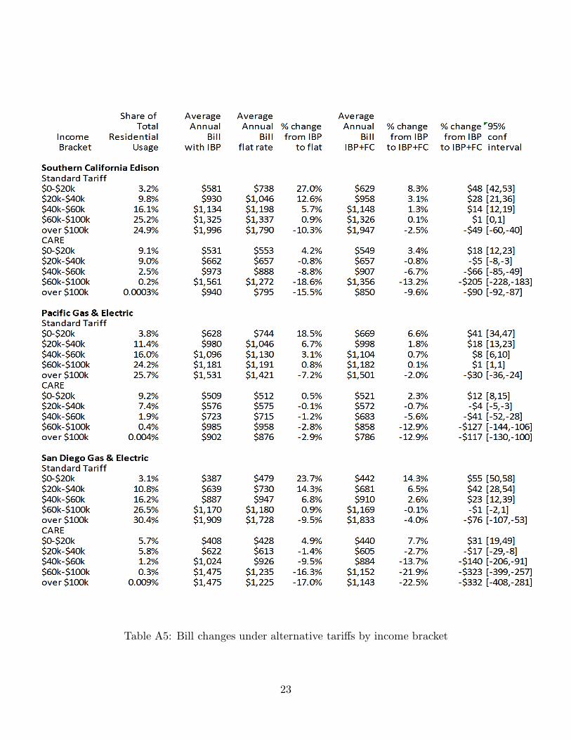
Table A5: Bill changes under alternative tariffs by income bracket