73 May 2011

Research Spotlight Regional Price Parities by Expenditure Class, 2005–2009 By Bettina H. Aten, Eric B. Figueroa, and Troy M. Martin

PRICE indexes are commonly used to measure price level differences between time periods; the con­

sumer price index (CPI), published by the Bureau of Labor Statistics (BLS), is among the better known ex­amples of these temporal measures of inflation. Less common are price indexes that measure price level dif­ferences between one place and another. These spatial price indexes are less common, in part because the methodology and sampling requirements for the two measures differ in important ways. Fortunately, ad­vances in regional analysis and in the techniques used in estimating period-to-period indexes, such as he­donic regressions, are applicable to the estimation of place-to-place indexes.

This article describes an update to the method de­veloped by the Bureau of Economic Analysis (BEA) to create measures of regional price level differences. Per­cent differences in regional price levels are called re­gional price parities (RPPs).

The main difference between a temporal index and the price parities described here is that the former measures changes in price levels across different time periods for one specific place, while the latter captures differences in price levels across various places for one specific time period.

RPPs have several applications. They can be used to compare price levels across different geographic areas, such as states or metropolitan areas. For more infor­mation on such comparisons, see the box “How to In­terpret Regional Price Parities.” Another important application of RPPs is to adjust measures of income

and output for price level differences. This provides users with a better sense of differences in quantities, also known as volume differences, because the price level differences have been removed to the extent pos­sible (Schreyer and Koechlin 2002). The “Selected Re­sults” section below includes discussion of using the RPPs to adjust regional measures of per capita per­sonal income published by BEA.1

BEA, in a joint project with BLS, first estimated re­gional price parities for 38 metropolitan and urban ar­eas of the United States for 2003 and 2004 (Aten 2005, 2006). These areas, for which BLS produces the CPI, represent about 87 percent of the total population. The method was expanded to cover the remaining nonmet­ropolitan portions of each state, and estimates for 2005 and 2006 were reported in the SURVEY OF CURRENT BUSI­NESS in November 2008 (Aten 2008; Aten and D’Souza 2008).

The estimates in this article differ from previously published prototype estimates in a number of impor­tant ways. They incorporate the recently released 5­year American Community Survey (ACS) from the Census Bureau, which includes rural areas; they use updated expenditure data that reflect a regional distri­bution of rural weights; and they parallel the rolling

1. Annual income data for 2005 to 2009 are adjusted using a single RPP covering the 5-year period. Although the RPPs do not vary across the 5-year period, the ratio of unadjusted to adjusted incomes does vary slightly. This is a result of rebalancing so that for each year, total unadjusted incomes across geographic areas equal the sum of RPP-adjusted incomes across the areas. The adjustments are relatively minor as the balancing factors are close to one.

How to Interpret Regional Price Parities (RPPs) RPPs compare the price level of a geographical region We can also compare price levels across regions within (such as a state or metropolitan area) with the total expenditure categories. Education services (including col-national average price level over all reference areas. The lege tuition) are higher in states such as New York (125.8) national price level is 100. The price level of the compari- and Maryland (134.6) but lower in Florida (82.6) and son area is expressed as a percentage of the national aver- Kansas (83.3). Furthermore, we can compare the relative age price level. For example, the price level of all goods cost of education services to goods (such as college text-and services in California is about 15 percent higher books) within an area. The price level of education ser­(114.8 /100) than the national average (table 2). We can vices relative to goods in Maryland (1.3=134.6/104) is also use the RPPs to compare two areas by examining also higher than in Kansas (0.8=83.3/99.3), where educa­their RPP ratio. While the price level in California is tion services are relatively less expensive than goods. The high when compared with the national average, it is overall RPP for the education services category (100.2) is about 1.4 percent lower than in the state of New York the average price of education services in all areas relative (114.8 / 116.4). to the price of all other expenditures at national prices.

74 Regional Price Parities May 2011

multiyear average of the ACS that begins in 2005–2009 and continues next year with 2006–2010 and so forth. In addition, RPPs will be available on an experimental basis for expenditure classes such as food, apparel, rec­reation, transportation, housing, education, medical, and other goods and services as well as for rents.

The remainder of this article is organized as follows. First, the article discusses the 2005–2009 RPP esti­mates and the results of their application to adjusting measures of income. Second, the article explains the updated, two-stage methodology used to estimate the RPPs. Finally, the article discusses areas of future re­search.

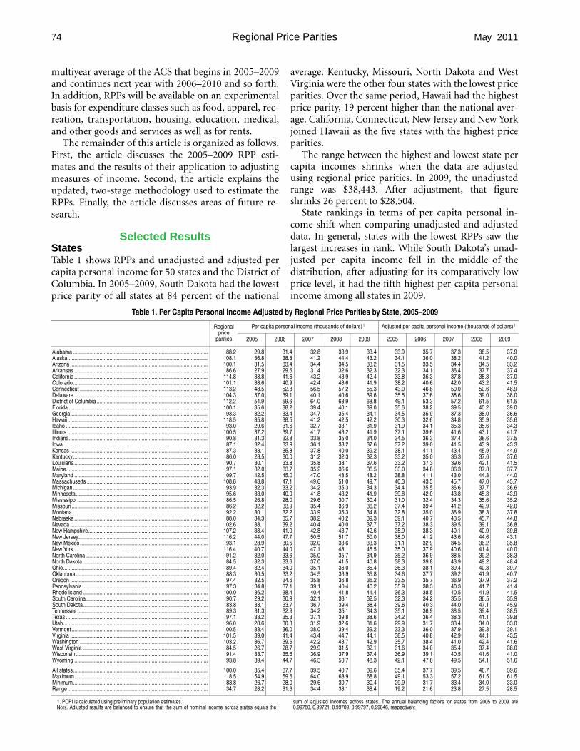
Selected Results States Table 1 shows RPPs and unadjusted and adjusted per capita personal income for 50 states and the District of Columbia. In 2005–2009, South Dakota had the lowest price parity of all states at 84 percent of the national

average. Kentucky, Missouri, North Dakota and West Virginia were the other four states with the lowest price parities. Over the same period, Hawaii had the highest price parity, 19 percent higher than the national aver­age. California, Connecticut, New Jersey and New York joined Hawaii as the five states with the highest price parities.

The range between the highest and lowest state per capita incomes shrinks when the data are adjusted using regional price parities. In 2009, the unadjusted range was $38,443. After adjustment, that figure shrinks 26 percent to $28,504.

State rankings in terms of per capita personal in­come shift when comparing unadjusted and adjusted data. In general, states with the lowest RPPs saw the largest increases in rank. While South Dakota’s unad­justed per capita income fell in the middle of the distribution, after adjusting for its comparatively low price level, it had the fifth highest per capita personal income among all states in 2009.

Table 1. Per Capita Personal Income Adjusted by Regional Price Parities by State, 2005–2009

Regional price

parities

Per capita personal income (thousands of dollars) 1 Adjusted per capita personal income (thousands of dollars) 1

2005 2006 2007 2008 2009 2005 2006 2007 2008 2009

Alabama ................................................................................................ 88.2 29.8 31.4 32.8 33.9 33.4 33.9 35.7 37.3 38.5 37.9 Alaska.................................................................................................... 108.1 36.8 38.8 41.2 44.4 43.2 34.1 36.0 38.2 41.2 40.0 Arizona .................................................................................................. 100.1 31.5 33.4 34.4 34.5 33.2 31.5 33.5 34.4 34.5 33.2 Arkansas ............................................................................................... 86.6 27.9 29.5 31.4 32.6 32.3 32.3 34.1 36.4 37.7 37.4 California ............................................................................................... 114.8 38.8 41.6 43.2 43.9 42.4 33.8 36.3 37.8 38.3 37.0 Colorado................................................................................................ 101.1 38.6 40.9 42.4 43.6 41.9 38.2 40.6 42.0 43.2 41.5 Connecticut ........................................................................................... 113.2 48.5 52.8 56.5 57.2 55.3 43.0 46.8 50.0 50.6 48.9 Delaware ............................................................................................... 104.3 37.0 39.1 40.1 40.6 39.6 35.5 37.6 38.6 39.0 38.0 District of Columbia ............................................................................... 112.2 54.9 59.6 64.0 68.9 68.8 49.1 53.3 57.2 61.5 61.5 Florida ................................................................................................... 100.1 35.6 38.2 39.4 40.1 39.0 35.6 38.2 39.5 40.2 39.0 Georgia.................................................................................................. 93.3 32.2 33.4 34.7 35.4 34.1 34.5 35.9 37.3 38.0 36.6 Hawaii.................................................................................................... 118.5 35.8 38.5 41.2 42.5 42.2 30.3 32.6 34.8 35.9 35.6 Idaho ..................................................................................................... 93.0 29.6 31.6 32.7 33.1 31.9 31.9 34.1 35.3 35.6 34.3 Illinois .................................................................................................... 100.5 37.2 39.7 41.7 43.2 41.9 37.1 39.6 41.6 43.1 41.7 Indiana................................................................................................... 90.8 31.3 32.8 33.8 35.0 34.0 34.5 36.3 37.4 38.6 37.5 Iowa....................................................................................................... 87.1 32.4 33.9 36.1 38.2 37.6 37.2 39.0 41.5 43.9 43.3 Kansas .................................................................................................. 87.3 33.1 35.8 37.8 40.0 39.2 38.1 41.1 43.4 45.9 44.9 Kentucky................................................................................................ 86.0 28.5 30.0 31.2 32.3 32.3 33.2 35.0 36.3 37.6 37.6 Louisiana............................................................................................... 90.7 30.1 33.8 35.8 38.1 37.6 33.2 37.3 39.6 42.1 41.5 Maine..................................................................................................... 97.1 32.0 33.7 35.2 36.6 36.5 33.0 34.8 36.3 37.8 37.7 Maryland ............................................................................................... 109.7 42.5 45.0 47.0 48.5 48.2 38.8 41.1 43.0 44.3 44.0 Massachusetts ...................................................................................... 108.8 43.8 47.1 49.6 51.0 49.7 40.3 43.5 45.7 47.0 45.7 Michigan................................................................................................ 93.9 32.3 33.2 34.2 35.3 34.3 34.4 35.5 36.6 37.7 36.6 Minnesota.............................................................................................. 95.6 38.0 40.0 41.8 43.2 41.9 39.8 42.0 43.8 45.3 43.9 Mississippi ............................................................................................. 86.5 26.8 28.0 29.6 30.7 30.4 31.0 32.4 34.3 35.6 35.2 Missouri ................................................................................................. 86.2 32.2 33.9 35.4 36.9 36.2 37.4 39.4 41.2 42.9 42.0 Montana ................................................................................................ 92.2 30.1 32.2 33.9 35.3 34.8 32.8 35.0 36.9 38.3 37.8 Nebraska ............................................................................................... 88.0 34.3 35.7 38.2 40.2 39.3 39.1 40.7 43.5 45.7 44.8 Nevada .................................................................................................. 102.6 38.1 39.2 40.4 40.0 37.7 37.2 38.3 39.5 39.1 36.8 New Hampshire..................................................................................... 107.2 38.4 41.0 42.8 43.7 42.6 35.9 38.3 40.1 40.9 39.8 New Jersey............................................................................................ 116.2 44.0 47.7 50.5 51.7 50.0 38.0 41.2 43.6 44.6 43.1 New Mexico ........................................................................................... 93.1 28.9 30.5 32.0 33.6 33.3 31.1 32.9 34.5 36.2 35.8 New York ............................................................................................... 116.4 40.7 44.0 47.1 48.1 46.5 35.0 37.9 40.6 41.4 40.0 North Carolina ....................................................................................... 91.2 32.0 33.6 35.0 35.7 34.9 35.2 36.9 38.5 39.2 38.3 North Dakota ......................................................................................... 84.5 32.3 33.6 37.0 41.5 40.8 38.3 39.8 43.9 49.2 48.4 Ohio....................................................................................................... 89.4 32.4 34.0 35.1 36.0 35.4 36.3 38.1 39.4 40.3 39.7 Oklahoma.............................................................................................. 88.3 30.5 33.2 34.5 36.9 35.8 34.6 37.7 39.2 41.9 40.7 Oregon .................................................................................................. 97.4 32.5 34.6 35.8 36.8 36.2 33.5 35.7 36.9 37.9 37.2 Pennsylvania ......................................................................................... 97.3 34.8 37.1 39.1 40.4 40.2 35.9 38.3 40.3 41.7 41.4 Rhode Island ......................................................................................... 100.0 36.2 38.4 40.4 41.8 41.4 36.3 38.5 40.5 41.9 41.5 South Carolina....................................................................................... 90.7 29.2 30.9 32.1 33.1 32.5 32.3 34.2 35.5 36.5 35.9 South Dakota......................................................................................... 83.8 33.1 33.7 36.7 39.4 38.4 39.6 40.3 44.0 47.1 45.9 Tennessee ............................................................................................. 89.3 31.3 32.9 34.2 35.1 34.3 35.1 36.9 38.5 39.4 38.5 Texas ..................................................................................................... 97.1 33.2 35.3 37.1 39.8 38.6 34.2 36.4 38.3 41.1 39.8 Utah....................................................................................................... 96.0 28.6 30.3 31.9 32.6 31.6 29.9 31.7 33.4 34.0 33.0 Vermont ................................................................................................. 100.5 33.4 36.0 38.0 39.4 39.2 33.3 36.0 37.9 39.3 39.1 Virginia .................................................................................................. 101.5 39.0 41.4 43.4 44.7 44.1 38.5 40.8 42.9 44.1 43.5 Washington ........................................................................................... 103.2 36.7 39.6 42.2 43.7 42.9 35.7 38.4 41.0 42.4 41.6 West Virginia ......................................................................................... 84.5 26.7 28.7 29.9 31.5 32.1 31.6 34.0 35.4 37.4 38.0 Wisconsin .............................................................................................. 91.4 33.7 35.6 36.9 37.9 37.4 36.9 39.1 40.5 41.6 41.0 Wyoming ............................................................................................... 93.8 39.4 44.7 46.3 50.7 48.3 42.1 47.8 49.5 54.1 51.6

All states................................................................................................ 100.0 35.4 37.7 39.5 40.7 39.6 35.4 37.7 39.5 40.7 39.6 Maximum............................................................................................... 118.5 54.9 59.6 64.0 68.9 68.8 49.1 53.3 57.2 61.5 61.5 Minimum................................................................................................ 83.8 26.7 28.0 29.6 30.7 30.4 29.9 31.7 33.4 34.0 33.0 Range.................................................................................................... 34.7 28.2 31.6 34.4 38.1 38.4 19.2 21.6 23.8 27.5 28.5

1. PCPI is calculated using preliminary population estimates. sum of adjusted incomes across states. The annual balancing factors for states from 2005 to 2009 are NOTE. Adjusted results are balanced to ensure that the sum of nominal income across states equals the 0.99780, 0.99721, 0.99709, 0.99797, 0.99846, respectively.

75 May 2011 SURVEY OF CURRENT BUSINESS

States with the highest RPPs saw the largest declines in rank. Hawaii’s unadjusted per capita income fell in the top third of the distribution; however, after adjust­ing for its relatively high price level, it dropped to the fifth-lowest among all states in terms of per capita per­sonal income in 2009. Despite its inclusion among the five states with the highest RPPs, Connecticut saw only a slight drop in its 2009 rank, from second to third highest on an unadjusted and adjusted basis, respec­tively. The slight drop was due to the state’s relatively high level of per capita personal income, which was 40 percent higher than the national average in 2009.

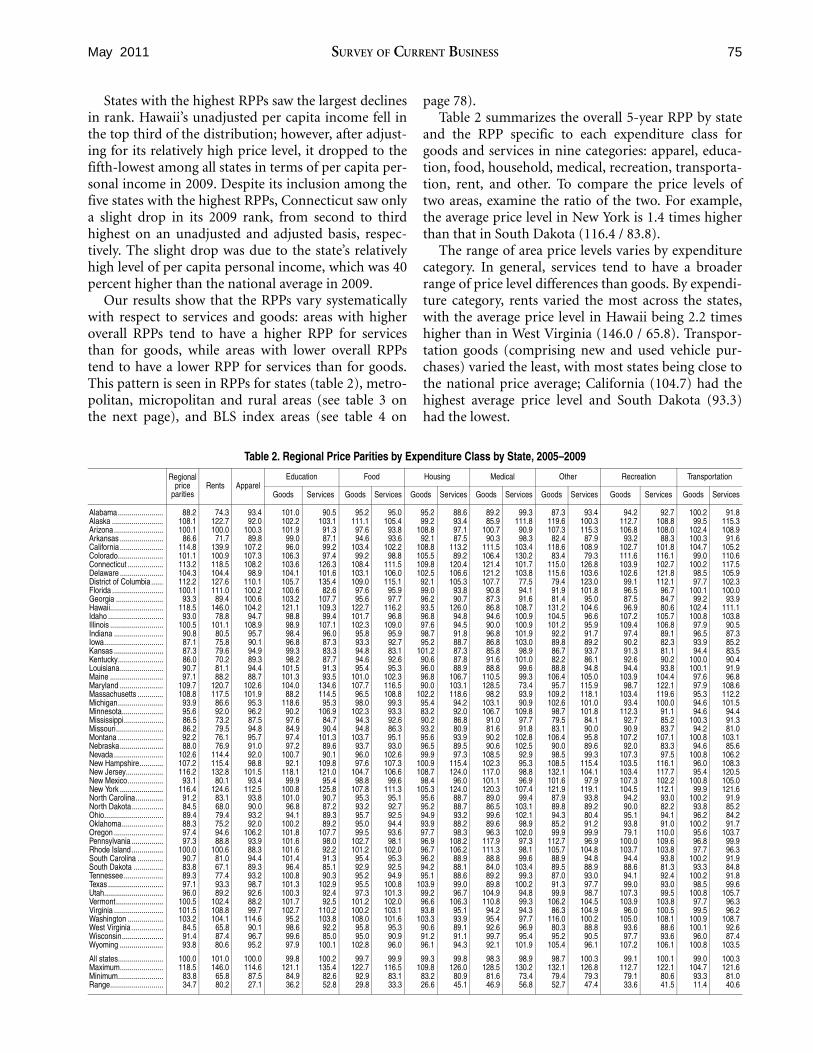
Our results show that the RPPs vary systematically with respect to services and goods: areas with higher overall RPPs tend to have a higher RPP for services than for goods, while areas with lower overall RPPs tend to have a lower RPP for services than for goods. This pattern is seen in RPPs for states (table 2), metro­politan, micropolitan and rural areas (see table 3 on the next page), and BLS index areas (see table 4 on

page 78). Table 2 summarizes the overall 5-year RPP by state

and the RPP specific to each expenditure class for goods and services in nine categories: apparel, educa­tion, food, household, medical, recreation, transporta­tion, rent, and other. To compare the price levels of two areas, examine the ratio of the two. For example, the average price level in New York is 1.4 times higher than that in South Dakota (116.4 / 83.8).

The range of area price levels varies by expenditure category. In general, services tend to have a broader range of price level differences than goods. By expendi­ture category, rents varied the most across the states, with the average price level in Hawaii being 2.2 times higher than in West Virginia (146.0 / 65.8). Transpor­tation goods (comprising new and used vehicle pur­chases) varied the least, with most states being close to the national price average; California (104.7) had the highest average price level and South Dakota (93.3) had the lowest.

Table 2. Regional Price Parities by Expenditure Class by State, 2005–2009

Regional price

parities Rents Apparel

Education Food Housing Medical Other Recreation Transportation

Goods Services Goods Services Goods Services Goods Services Goods Services Goods Services Goods Services

Alabama ....................... 88.2 74.3 93.4 101.0 90.5 95.2 95.0 95.2 88.6 89.2 99.3 87.3 93.4 94.2 92.7 100.2 91.8 Alaska .......................... 108.1 122.7 92.0 102.2 103.1 111.1 105.4 99.2 93.4 85.9 111.8 119.6 100.3 112.7 108.8 99.5 115.3 Arizona ......................... 100.1 100.0 100.3 101.9 91.3 97.6 93.8 108.8 97.1 100.7 90.9 107.3 115.3 106.8 108.0 102.4 108.9 Arkansas ...................... 86.6 71.7 89.8 99.0 87.1 94.6 93.6 92.1 87.5 90.3 98.3 82.4 87.9 93.2 88.3 100.3 91.6 California ...................... 114.8 139.9 107.2 96.0 99.2 103.4 102.2 108.8 113.2 111.5 103.4 118.6 108.9 102.7 101.8 104.7 105.2 Colorado....................... 101.1 100.9 107.3 106.3 97.4 99.2 98.8 105.5 89.2 106.4 130.2 83.4 79.3 111.6 116.1 99.0 110.6 Connecticut .................. 113.2 118.5 108.2 103.6 126.3 108.4 111.5 109.8 120.4 121.4 101.7 115.0 126.8 103.9 102.7 100.2 117.5 Delaware ...................... 104.3 104.4 98.9 104.1 101.6 103.1 106.0 102.5 106.6 121.2 103.8 115.6 103.6 102.6 121.8 98.5 105.9 District of Columbia...... 112.2 127.6 110.1 105.7 135.4 109.0 115.1 92.1 105.3 107.7 77.5 79.4 123.0 99.1 112.1 97.7 102.3 Florida .......................... 100.1 111.0 100.2 100.6 82.6 97.6 95.9 99.0 93.8 90.8 94.1 91.9 101.8 96.5 96.7 100.1 100.0 Georgia ........................ 93.3 89.4 100.6 103.2 107.7 95.6 97.7 96.2 90.7 87.3 91.6 81.4 95.0 87.5 84.7 99.2 93.9 Hawaii........................... 118.5 146.0 104.2 121.1 109.3 122.7 116.2 93.5 126.0 86.8 108.7 131.2 104.6 96.9 80.6 102.4 111.1 Idaho ............................ 93.0 78.8 94.7 98.8 99.4 101.7 96.8 96.8 94.8 94.6 100.9 104.5 96.6 107.2 105.7 100.8 103.8 Illinois ........................... 100.5 101.1 108.9 98.9 107.1 102.3 109.0 97.6 94.5 90.0 100.9 101.2 95.9 109.4 106.8 97.9 90.5 Indiana ......................... 90.8 80.5 95.7 98.4 96.0 95.8 95.9 98.7 91.8 96.8 101.9 92.2 91.7 97.4 89.1 96.5 87.3 Iowa.............................. 87.1 75.8 90.1 96.8 87.3 93.3 92.7 95.2 88.7 86.8 103.0 89.8 89.2 90.2 82.3 93.9 85.2 Kansas ......................... 87.3 79.6 94.9 99.3 83.3 94.8 83.1 101.2 87.3 85.8 98.9 86.7 93.7 91.3 81.1 94.4 83.5 Kentucky....................... 86.0 70.2 89.3 98.2 87.7 94.6 92.6 90.6 87.8 91.6 101.0 82.2 86.1 92.6 90.2 100.0 90.4 Louisiana...................... 90.7 81.1 94.4 101.5 91.3 95.4 95.3 96.0 88.9 88.8 99.6 88.8 94.8 94.4 93.8 100.1 91.9 Maine ........................... 97.1 88.2 88.7 101.3 93.5 101.0 102.3 96.8 106.7 110.5 99.3 106.4 105.0 103.9 104.4 97.6 96.8 Maryland ...................... 109.7 120.7 102.6 104.0 134.6 107.7 116.5 90.0 103.1 128.5 73.4 95.7 115.9 98.7 122.1 97.9 108.6 Massachusetts ............. 108.8 117.5 101.9 88.2 114.5 96.5 108.8 102.2 118.6 98.2 93.9 109.2 118.1 103.4 119.6 95.3 112.2 Michigan....................... 93.9 86.6 95.3 118.6 95.3 98.0 99.3 95.4 94.2 103.1 90.9 102.6 101.0 93.4 100.0 94.6 101.5 Minnesota..................... 95.6 92.0 96.2 90.2 106.9 102.3 93.3 83.2 92.0 106.7 109.8 98.7 101.8 112.3 91.1 94.6 94.4 Mississippi.................... 86.5 73.2 87.5 97.6 84.7 94.3 92.6 90.2 86.8 91.0 97.7 79.5 84.1 92.7 85.2 100.3 91.3 Missouri........................ 86.2 79.5 94.8 84.9 90.4 94.8 86.3 93.2 80.9 81.6 91.8 83.1 90.0 90.9 83.7 94.2 81.0 Montana ....................... 92.2 76.1 95.7 97.4 101.3 103.7 95.1 95.6 93.9 90.2 102.8 106.4 95.8 107.2 107.1 100.8 103.1 Nebraska...................... 88.0 76.9 91.0 97.2 89.6 93.7 93.0 96.5 89.5 90.6 102.5 90.0 89.6 92.0 83.3 94.6 85.6 Nevada ......................... 102.6 114.4 92.0 100.7 90.1 96.0 102.6 99.9 97.3 108.5 92.9 98.5 99.3 107.3 97.5 100.8 106.2 New Hampshire............ 107.2 115.4 98.8 92.1 109.8 97.6 107.3 100.9 115.4 102.3 95.3 108.5 115.4 103.5 116.1 96.0 108.3 New Jersey................... 116.2 132.8 101.5 118.1 121.0 104.7 106.6 108.7 124.0 117.0 98.8 132.1 104.1 103.4 117.7 95.4 120.5 New Mexico.................. 93.1 80.1 93.4 99.9 95.4 98.8 99.6 98.4 96.0 101.1 96.9 101.6 97.9 107.3 102.2 100.8 105.0 New York ...................... 116.4 124.6 112.5 100.8 125.8 107.8 111.3 105.3 124.0 120.3 107.4 121.9 119.1 104.5 112.1 99.9 121.6 North Carolina.............. 91.2 83.1 93.8 101.0 90.7 95.3 95.1 95.6 88.7 89.0 99.4 87.9 93.8 94.2 93.0 100.2 91.9 North Dakota................ 84.5 68.0 90.0 96.8 87.2 93.2 92.7 95.2 88.7 86.5 103.1 89.8 89.2 90.0 82.2 93.8 85.2 Ohio.............................. 89.4 79.4 93.2 94.1 89.3 95.7 92.5 94.9 93.2 99.6 102.1 94.3 80.4 95.1 94.1 96.2 84.2 Oklahoma..................... 88.3 75.2 92.0 100.2 89.2 95.0 94.4 93.9 88.2 89.6 98.9 85.2 91.2 93.8 91.0 100.2 91.7 Oregon ......................... 97.4 94.6 106.2 101.8 107.7 99.5 93.6 97.7 98.3 96.3 102.0 99.9 99.9 79.1 110.0 95.6 103.7 Pennsylvania ................ 97.3 88.8 93.9 101.6 98.0 102.7 98.1 96.9 108.2 117.9 97.3 112.7 96.9 100.0 109.6 96.8 99.9 Rhode Island ................ 100.0 100.6 88.3 101.6 92.2 101.2 102.0 96.7 106.2 111.3 98.1 105.7 104.8 103.7 103.8 97.7 96.3 South Carolina ............. 90.7 81.0 94.4 101.4 91.3 95.4 95.3 96.2 88.9 88.8 99.6 88.9 94.8 94.4 93.8 100.2 91.9 South Dakota ............... 83.8 67.1 89.3 96.4 85.1 92.9 92.5 94.2 88.1 84.0 103.4 89.5 88.9 88.6 81.3 93.3 84.8 Tennessee.................... 89.3 77.4 93.2 100.8 90.3 95.2 94.9 95.1 88.6 89.2 99.3 87.0 93.0 94.1 92.4 100.2 91.8 Texas ............................ 97.1 93.3 98.7 101.3 102.9 95.5 100.8 103.9 99.0 89.8 100.2 91.3 97.7 99.0 93.0 98.5 99.6 Utah.............................. 96.0 89.2 92.6 100.3 92.4 97.3 101.3 99.2 96.7 104.9 94.8 99.9 98.7 107.3 99.5 100.8 105.7 Vermont........................ 100.5 102.4 88.2 101.7 92.5 101.2 102.0 96.6 106.3 110.8 99.3 106.2 104.5 103.9 103.8 97.7 96.3 Virginia ......................... 101.5 108.8 99.7 102.7 110.2 100.2 103.1 93.8 95.1 94.2 94.3 86.3 104.9 96.0 100.5 99.5 96.2 Washington .................. 103.2 104.1 114.6 95.2 103.8 108.0 101.6 103.3 93.9 95.4 97.7 116.0 100.2 105.0 108.1 100.9 108.7 West Virginia ................ 84.5 65.8 90.1 98.6 92.2 95.8 95.3 90.6 89.1 92.6 96.9 80.3 88.8 93.6 88.6 100.1 92.6 Wisconsin..................... 91.4 87.4 96.7 99.6 85.0 95.0 90.9 91.2 91.1 99.7 95.4 95.2 90.5 97.7 93.6 96.0 87.4 Wyoming ...................... 93.8 80.6 95.2 97.9 100.1 102.8 96.0 96.1 94.3 92.1 101.9 105.4 96.1 107.2 106.1 100.8 103.5

All states....................... 100.0 101.0 100.0 99.8 100.2 99.7 99.9 99.3 99.8 98.3 98.9 98.7 100.3 99.1 100.1 99.0 100.3 Maximum...................... 118.5 146.0 114.6 121.1 135.4 122.7 116.5 109.8 126.0 128.5 130.2 132.1 126.8 112.7 122.1 104.7 121.6 Minimum....................... 83.8 65.8 87.5 84.9 82.6 92.9 83.1 83.2 80.9 81.6 73.4 79.4 79.3 79.1 80.6 93.3 81.0 Range........................... 34.7 80.2 27.1 36.2 52.8 29.8 33.3 26.6 45.1 46.9 56.8 52.7 47.4 33.6 41.5 11.4 40.6

76 Regional Price Parities May 2011

Metropolitan, micropolitan, and rural areas Table 3 summarizes RPPs by three geographical cate­gories (metropolitan, micropolitan, and rural) as well as for nine expenditure classes of goods and services within those areas.2

Table 3. Regional Price Parities for Metropolitan, Micropolitan, and Rural Areas, by Expenditure Class, 2005–2009

Regional price parities for all classes by area

Metropolitan Micropolitan Rural

102.8 88.0 84.6

Expenditure class Goods Services Goods Services Goods Services

Apparel ....................................... 102.8 ............. 88.6 ............. 84.3 ............. Education ................................... 100.7 103.4 97.2 87.1 94.9 80.5 Food ........................................... 100.5 101.3 97.2 93.9 94.8 91.9 Household .................................. 101.9 102.0 92.0 91.3 88.0 88.0 Medical ....................................... 102.2 98.9 89.5 101.3 86.7 100.2 Other .......................................... 103.0 102.9 90.4 89.2 82.1 83.0 Recreation .................................. 101.0 102.8 94.4 90.5 91.1 82.3 Rent............................................ ............. 106.4 ............ 74.7 ............ 67.4 Transportation............................. 99.6 101.8 97.7 91.7 97.5 89.7 All classes ................................. 100.8 103.8 94.9 84.3 92.6 79.5

Metropolitan area price levels are 1.2 times higher on average than rural areas (102.8 / 84.6). Additionally, as these economic areas become less rural and more urban, services by expenditure class tend to become more expensive relative to goods. For example, the price level ratios of transportation services to goods in rural, micropolitan, and metropolitan areas were 0.92, 0.94, and 1.02, respectively. One category that defies this tendency is medical services, including visits to physicians, dentists and other professionals. While the RPPs of medical goods such as over-the-counter drugs are lower in rural and micropolitan areas, they are rela­tively constant across the three geographic definitions for medical services, with metropolitan areas having a slightly lower price level (98.9) than in micropolitan (101.3) and rural (100.2) areas.

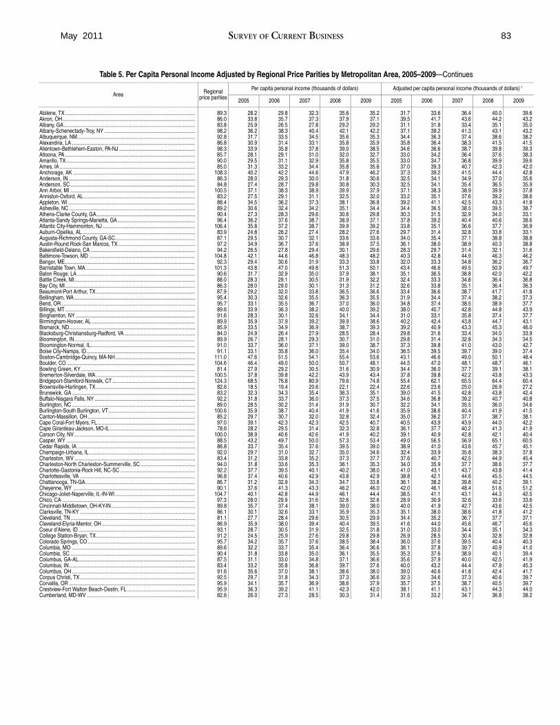
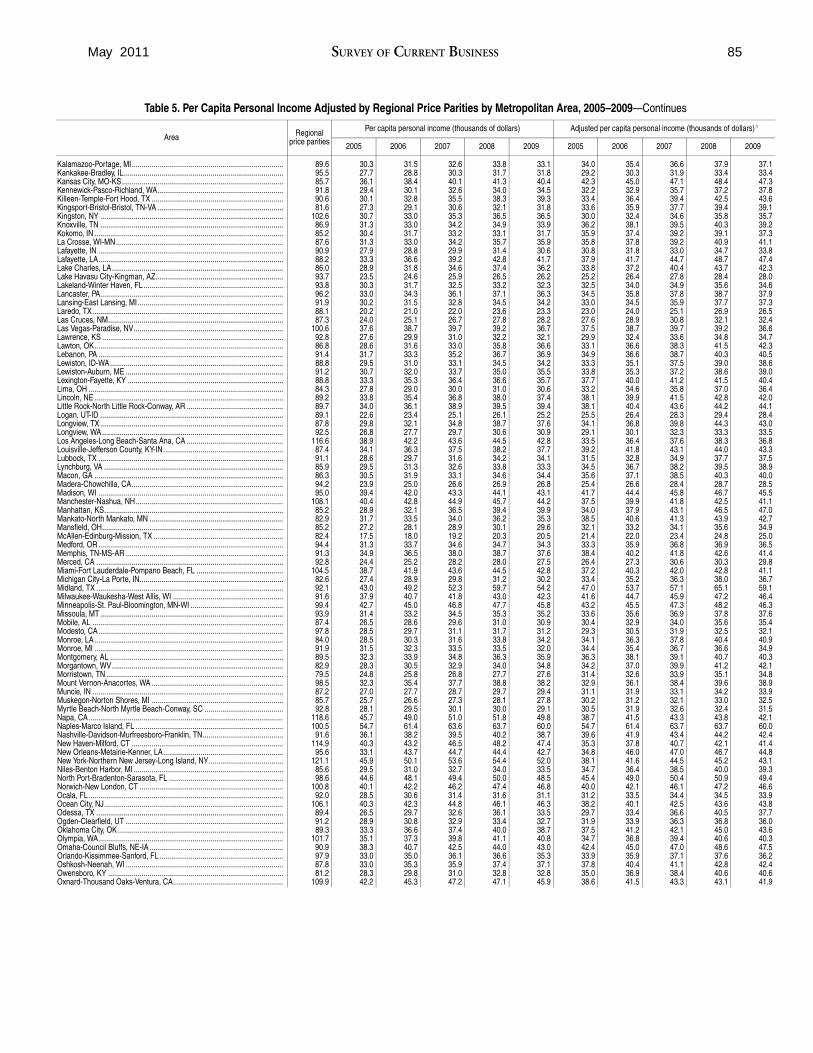
Detailed metropolitan areas Table 5 (page 83) shows metropolitan area per capita personal income adjusted by RPPs for 2005–2009. Over this period, Jefferson City, MO, had the lowest price parity at 79 percent of the national average. Met­ropolitan areas with the lowest RPPs also include Jonesboro, AR, Cape Girardeau-Jackson, MO-IL, Mor­ristown, TN, and Danville, IL. Over the same period, Bridgeport-Stamford-Norwalk, CT, had the highest RPP, which was 24 percent higher than the national av­erage. Metropolitan areas with the highest RPPs also

2. A metropolitan area is defined by the Office of Management and Bud­get as one or more counties with a high degree of social and economic inte­gration, with a core urban population of 50,000 or more. Micropolitan areas have an urban core population of less than 50,000 but more than 10,000, and the remaining areas are rural.

include San Jose-Sunnyvale-Santa Clara, CA, San Francisco-Oakland-Fremont, CA, New York-North­ern New Jersey-Long Island, NY, and Santa Cruz-Wat­sonville, CA.

For metropolitan areas, the range between the high­est and lowest per capita incomes shrank when these data were adjusted using RPPs In 2009, the unadjusted range was $54,258. After adjustment, the figure shrank 29 percent to $38,510.

Metropolitan area rankings of per capita personal income change when comparing unadjusted and ad­justed data. Among all metropolitan areas in 2009, Jef­ferson City, MO, increased the most. In 2009, the area increased from the second quartile in terms of unad­justed per capita personal income to the top quartile on an adjusted basis.

The five metropolitan areas with the highest RPPs were not among the areas with the largest declines in rank when comparing adjusted and unadjusted per capita personal income. For example, the area with the largest RPP, Bridgeport-Stamford-Norwalk, CT, only experienced a slight drop in its 2009 rank, from first on an unadjusted basis to third on an adjusted basis. The slight decrease is due to the area’s relatively high level of per capita personal income, which was 81 percent higher than the national average in 2009.

Among all metropolitan areas in 2009, Pough­keepsie-Newburgh-Middletown, NY, experienced the largest decline in rank when comparing unadjusted and adjusted per capita personal income. The area dropped from the top quartile of metropolitan areas in terms of unadjusted per capita personal income to the bottom quartile on an adjusted basis.

Overview of the Methodology First stage Hedonic adjustment. The BEA estimation begins with the individual price observations used in the CPI. The CPI collects price quotes for hundreds of consumer goods and services, ranging from new automobiles to haircuts, as well as price information on rents and owners’ equivalent rents. There are more than 1 mil­lion price quotes observed each year, which are orga­nized into eight groups of goods and services: housing excluding rents, transportation, food, education, recre­ation, medical, apparel, and other goods and services. Rents and owners’ equivalent rents are treated sepa­rately and discussed in the following section.

Each of the eight groups is subdivided into catego­ries termed “item strata,” such as major appliances, and then into more detailed categories termed “elementary level items (ELIs),” such as refrigerators

77 May 2011 SURVEY OF CURRENT BUSINESS

and freezers. Some ELIs are further subdivided into clusters. A full listing of item strata, ELIs and clusters can be found in “CPI Requirements of CE” by William Casey (2010).

In cooperation with BLS, we estimate hedonic re­gression models that take into account differences in characteristics of the goods and services, such as differences in packaging, unit size, and type of outlet where they are sold.

We derive approximately 150 individual hedonic re­gressions for each year at the most detailed level possi­ble, subject to the data.3 The regressions cover the 75 most important item strata in terms of their overall contribution to total expenditures. These item strata account for approximately 85 percent of total expendi­tures.4

Rents and owners’ equivalent rents. Rents and owners’ equivalent rents account for 30 percent of overall consumer expenditures.5 As a result, the regres­sion models for these two categories will have the larg­est impact on the overall price levels. An analysis of this sensitivity is given in Aten (2005). Because of their importance, regressions that account for differences in characteristics of rents and owners’ equivalent rents re­quire a more sophisticated treatment than the regres­sions described above for other goods and services. 6

Characteristics used in the regressions of rents in­clude the timing of the collection cycle and the classifi­cation of each observation as a rental or as an owners’ equivalent rental. In addition, numerous housing characteristics are available, including structure type, number of rooms and bathrooms, utilities, parking, air conditioning, rent control status, length of occupancy, and approximate age of the unit.

As described above, relative price levels are obtained from hedonic regressions for the top 75 item strata and from the detailed regressions for rents and owners’ equivalent rents. For the remaining item strata, we es­timate relative price levels using a short cut approach called a weighted country product dummy method.7

This is equivalent to a weighted geometric mean across

3. Details of a hedonic regression for an ELI are available in Aten (2005). 4. We use the term “expenditures” to refer to the cost weights associated

with each item and each area. Cost weights are derived from the Consumer Expenditure Survey (CE) but are adjusted internally by BLS for use with CPI price data and do not match exactly the CE distributions which are published every two years.

5. Owners’ equivalent rents (also referred to as rental equivalence) are estimates of the amount a homeowner would pay to rent, or would earn from renting, his or her home in a competitive market. For more informa­tion, see www.bls.gov/cpi/cpifact6.htm.

6. See Moulton (1995). 7. For information about the weighted country product dummy method,

see Summers (1973), Sergeev (2004), Silver (2004), Diewert (2002), Rao (2004), and Selvanathan and Rao (1994).

all ELIs within an item stratum when there are no missing observations.

Multilateral aggregation. The price observations and the relative price levels undergo an outlier check­ing procedure called Quaranta analysis, modeled after the methods used in the OECD, Eurostat, and in the International Comparison Program of the United Na­tions and World Bank. For each year of data, three rounds of Quaranta analysis were completed, remov­ing approximately 1.3 percent of the observations.

Once the Quaranta analysis has been completed, we take the individual item strata price levels for each of the 38 areas and aggregate them into 16 expenditure classes: food (at home and away-from-home), apparel, education (goods and services), medical (goods and services), housing (goods and services), recreation (goods and services), transport (goods and services), other (goods and services), and imputed and actual rents.

Chart 1 shows the percentage of all expenditures in each class, categorized by goods and services. Goods account for about one-third of expenditures, while ser­vices are two-thirds, but the number of item strata in each grouping is reversed: only one-third for services (68 out of 207) and two-thirds for goods (139 out of 207).

CCharhart 1.t 1. Share of Household ExpendituresShare of Household Expenditures bby Expenditure Classy Expenditure Class

U.S. Bureau of Economic Analysis

Services Goods

Rents

Transportation

Food

Household items

Medical

Education

Recreation

Apparel

Other

0 5 10 15 20 25 30

29.5

5.7 11.9

6.6 8.6

9.3 3.8

4.3 1.5

5.5 0.5

3.2 2.4

3.7

1.8 1.7

Percent

---------------------------

-------------------------------------

78 Regional Price Parities May 2011

The detailed item strata price levels for the 38 geo- Second stage graphic areas are aggregated to the 16 expenditure BLS index area and states and metropolitan areas. To classes using the Geary multilateral formula below.8 extend the study beyond these 38 areas to states and

metropolitan areas, it is necessary to obtain an esti-Geary Aggregation mate of price levels for the broad BLS index areas and

price levels for the rural areas not covered by the CPI. N c cp q Once again, we separate the process into two stages: es­n n 1 timates of rents and estimates of all other goods and 6

Pc n = = Geary N services. c qS6 With respect to rents, the only comprehensive nn

n = 1 price level measure available for both the broad BLS index areas and for the rural areas not covered by the CPI is in the housing data from the 5-year American M c cp q Community Survey (ACS) released by the Census Bu­n¦ nS = reau in December 2010. The ACS consists of nearly 8 Mn

Pc Geary dq6 nc 1 d 1= =

Geary multilateral price index Table 4. Regional Price Parities for BLS Index Areas, 2005–2009 Ranked by Total Regional Price Parity

PGeary =

p = item price

q = notional quantity = (pq)/p

Subscript n = 1 ... N indicates items

Superscript c, d = 1 ... M indicates areas

One advantage of the Geary system is that it is addi­tive, meaning that we can obtain price indexes at any level of aggregation and that they are consistent with the overall index. This is done by dividing the unadjusted expenditures (pq) by the adjusted expendi­tures (πq), where π is the reference price defined as the average price level across all areas for each item n.

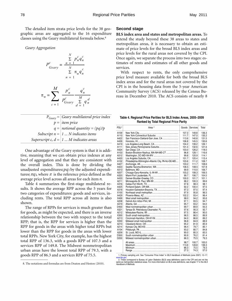
Table 4 summarizes the first-stage multilateral re­sults. It shows the average RPP across the 5 years for two categories of expenditures: goods and services, in­cluding rents. The total RPP across all items is also shown.

The range of RPPs for services is much greater than for goods, as might be expected, and there is an inverse relationship between the two with respect to the total RPP; that is, the RPP for services is higher than the RPP for goods in the areas with higher total RPPs but lower than the RPP for goods in the areas with lower total RPPs. New York City, for example, has the highest total RPP of 136.3, with a goods RPP of 107.3 and a services RPP of 149.8. The Midwest nonmetropolitan urban areas have the lowest total RPP of 79.3, with a

PSU 1 Area 2 Goods Services Total

A109 New York City................................................................. 107.3 149.8 136.3 A110 New York-Connecticut Suburbs ..................................... 111.7 147.0 135.2 A422 San Francisco-Oakland-San Jose, CA .......................... 113.6 140.8 131.5 A426 Honolulu, HI ................................................................... 106.8 145.5 130.6 A419 Los Angeles-Long Beach, CA........................................ 104.2 139.2 126.1 A111 New Jersey-Pennsylvania Suburbs................................ 101.4 132.6 121.6 A424 San Diego, CA ............................................................... 103.0 126.2 118.0 A103 Boston-Brockton-Nashua, MA-NH-ME-CT .................... 96.8 128.1 116.6 A312 Washington, DC-MD-VA-WV ......................................... 99.8 120.9 114.1 A420 Los Angeles Suburbs, CA.............................................. 101.7 120.4 113.4 A102 Philadelphia-Wilmington-Atlantic City, PA-NJ-DE-MD.... 103.6 111.2 108.7 A427 Anchorage, AK............................................................... 103.2 111.7 108.6 A423 Seattle-Tacoma-Bremerton, WA .................................... 106.5 108.5 107.8 A313 Baltimore, MD ................................................................ 99.9 110.0 106.7 A207 Chicago-Gary-Kenosha, IL-IN-WI.................................. 103.2 108.3 106.5 A320 Miami-Fort Lauderdale, FL ............................................ 99.7 106.7 104.5 A433 Denver-Boulder-Greeley, CO ......................................... 100.0 101.7 101.1 A211 Minneapolis-St. Paul, MN-WI......................................... 98.2 100.3 99.6 A316 Dallas-Fort Worth, TX.................................................... 97.8 98.3 98.1 A425 Portland-Salem, OR-WA................................................ 92.2 100.4 97.5 A318 Houston-Galveston-Brazoria, TX ................................... 97.3 97.5 97.4 X100 Northeast small metroplitan........................................... 97.9 95.8 96.5 A429 Phoenix-Mesa, AZ ......................................................... 102.2 93.4 96.4 X499 West small metropolitan................................................. 98.0 94.2 95.6 A208 Detroit-Ann Arbor-Flint, MI............................................. 97.1 93.5 94.7 A319 Atlanta, GA .................................................................... 95.7 93.2 94.0 D400 West nonmetropolitan urban.......................................... 99.7 89.9 93.3 A321 Tampa-St. Petersburg-Clearwater, FL............................ 97.6 90.3 92.7 A212 Milwaukee-Racine, WI ................................................... 97.5 86.4 90.0 X300 South small metropolitan ............................................... 96.5 86.5 89.9 A213 Cincinnati-Hamilton, OH-KY-IN ...................................... 94.0 86.8 89.2 X200 Midwest small metropolitan ........................................... 96.8 84.9 88.9 A210 Cleveland-Akron, OH ..................................................... 95.2 81.9 85.9 A214 Kansas City, MO-KS ...................................................... 96.4 79.7 85.1 A104 Pittsburgh, PA ................................................................ 93.2 80.7 84.8 A209 St. Louis, MO-IL............................................................. 90.0 80.3 83.5 D300 South nonmetropolitan urban ........................................ 90.9 76.2 81.4 D200 Midwest nonmetropolitan urban..................................... 86.3 75.5 79.3

All areas......................................................................... 98.7 100.7 100.0 Maximum ....................................................................... 113.6 149.8 136.3 Minimum ........................................................................ 86.3 75.5 79.3 Range ............................................................................ 27.3 74.3 57.0

goods RPP of 86.3 and a services RPP of 75.5. 1. Primary sampling unit. See “Consumer Price Index” in BLS Handbook of Methods (June 2007): 12–17; www.bls.gov.

2. These correspond to Bureau of Labor Statistics (BLS) area definitions used in the CPI and are not the same as metropolitan statistical areas. For more information on BLS area definitions, see chapter 17 in the BLS

8. The notations and formulas are from Deaton and Heston (2010). Handbook of Methods.

79 May 2011 SURVEY OF CURRENT BUSINESS

million observations on housing units for 2005–2009. Approximately 3 million of these are for rents, en­abling us to make estimates at a very detailed level of geography, including for rural versus urban portions of counties.

We estimate a hedonic regression for rents from the ACS with the following characteristics: the number of rooms and bedrooms and the age and type of housing unit. In our previous work, we included the housing cost data for owners, and ran separate regressions for those with mortgages and those without (Aten and D’Souza 2008). However, since the ACS does not col­lect information on the length of mortgage loans or the applicable interest rates, we focus only on the rental price levels. The rents in the ACS and the rents in the BLS are conceptually the same, but owner-cost levels in the ACS are different conceptually from the owner-equivalent rents of the BLS.9

For the remaining goods and services other than rents, we assume that the within-area price levels are the same as the average for the area; that is, if a BLS in-dex-area is made up of n counties, the price level for each of the n counties will be the same. This applies to all counties within an area, including rural counties.

Of the 38 index areas, 31 are metropolitan areas made up of predominantly urban counties, 4 areas are denoted as “small metropolitan areas,” and 3 areas are

9. See Crone, Nakamura, and Voith (2004), Short and O’Hara (2008), Garner and Short (2009), Garner and Verbrugge (2007), Heston and Naka­mura (2009).

Acknowledgments Part of the work reported here is based on a 5-year agreement with the Bureau of Labor Statistics (BLS) to access consumer price index data in the Office of Prices and Living Conditions. We would like to thank Walter Lane, Frank Ptacek, Josh Klick, Robert Cage and Lyubov Rozental in the Consumer Price Indexes program, at BLS as well as Roger D’Souza at BEA for their technical and programmatic assistance in this and in previous versions of our estimates. Another important part of the work was based on the five-year American Community Survey housing data, and we thank the support of Trudi Renwick in the Poverty Statistics Branch and David Johnson in the Housing and Household Economic Statistics Division of the Census Bureau.

denoted as “urban, nonmetropolitan areas.” The latter two groups may have rural counties or parts of coun­ties that are sparsely populated and would thus fall un­der Census Bureau-designated rural tracts.

Although we did not have any price level informa­tion for these rural counties or for the parts of counties that are rural, BLS provides a distribution of expendi­ture weights for four broad rural regions, correspond­ing to the Northeast, Midwest, South and West.

We distribute the expenditure weights to counties within an index area based on a uniform per capita ex­penditure distribution; that is, the per capita expendi­ture distribution in the index area is assumed to be equal to the per capita expenditure distribution in the counties within that area, with the exception of the ru­ral counties. For rural counties, we use the rural re­gional distribution and assume that the per capita expenditure distribution in each region is equal to that of the rural counties within the region. In other words, we allocate expenditure weights to the counties based on the ratio of their populations to the total popula­tion of the index area or rural region.

Multilateral aggregation. Once the price levels and weights by all expenditure classes have been allocated to all the counties in each year, we reaggregate them up to (1) the states and to (2) the metropolitan areas as defined by the Office of Management and Budget. This reaggregation is simply the weighted geometric mean of the counties within states and metropolitan areas.

At this stage, we substitute the BLS rents price levels with the ACS rents price levels. The latter are more ro­bust because they are derived directly at the state and metropolitan area levels and are not weighted geomet­ric means built up from the 38 allocated index areas.

Thus, we have a stacked panel of five years of annual data, one each for states and for metro areas, with price levels and weights for the 16 major expenditure classes. The panels are the final inputs to a multilateral Geary aggregation that yields the overall regional price parity (RPP). These multiyear RPPs cover the 5-year period; RPPs are not developed for individual years.

The state-level RPP estimates are summarized in chart 2. The lowest RPP is for South Dakota at 84, and the highest is for Hawaii at 119. New York and New Jersey are close behind at 116, and California is ranked fourth at 115. West Virginia and North Dakota join South Dakota on the lower end of the scale with RPPs of 85. (The RPP for the entire United States is 100).

80 Regional Price Parities May 2011

CharChartt 2.2. Regional Price PRegional Price Paarities brities byy StateState

South Dakota North Dakota West Virginia

Kentucky Missouri

Mississippi Arkansas

Iowa Kansas

Nebraska Alabama

Oklahoma Tennessee

Ohio South Carolina

Louisiana Indiana

North Carolina Wisconsin

Montana Idaho

New Mexico Georgia

Wyoming Michigan

Minnesota Utah

Maine Texas

Pennsylvania Oregon

Rhode Island Arizona Florida

Vermont Illinois

Colorado Virginia Nevada

Washington Delaware

New Hampshire Alaska

Massachusetts Maryland

District of Columbia Connecticut

California New Jersey

New York Hawaii

Regional price parities

NOTE. The U.S. overall price parity is 100.

U.S. Bureau of Economic Analysis

Future Research An important extension of this work would be to ex­plore the development of RPPs that reflect more than consumption goods and services, such as investment and government price level differences. In interna­tional comparisons, the price level of consumption is often a good approximation for gross domestic prod­

80 85 90 95 100 105 110 115 120

uct price levels from the expenditure side because the relative prices of investment and government change systematically in opposite directions when measured across per capita incomes. It is not clear whether this pattern would be found across states or metropolitan areas within a country, but it seems worth examining. One approach to this would be to see if there is a geo­graphic pattern in the prices of inputs and outputs re­lated to construction, producers’ durable equipment, and government compensation.

Another extension would be to use additional indi­cators of housing costs, perhaps creating a hybrid ap­proach using BLS owner-equivalent data, ACS owner cost data, and other sources of asset-based estimates of housing. Since rents and owners’ equivalent rents are jointly the most important expenditure heading, it is critical to make explicit the commonalities and differ­ences between the two sources of data.

A separate but important issue with respect to rents is how to reconcile the personal consumption expendi­ture (PCE) weights in the national accounts with the expenditure weights in the Consumer Expenditure Survey (CE). The national share of rents out of total expenditures is significantly lower in the PCE than in the CE. Although the PCE does not have a regional dis­tribution of weights, we would like to analyze whether redistributing that share to all other expenditure cate­gories would affect the RPPs systematically.

Lastly, we made a strong, albeit transparent, as­sumption about the price levels of all other goods and services excluding rents: that they are uniformly dis­tributed across counties within a BLS index area. For example, the food price level in Jefferson County (WV), in Prince George’s County (MD), and in Alex­andria City (VA), are assumed to be the same as the av­erage in the entire Washington-DC-MD-VA-WV area. Arguably, the more remote areas may purchase goods and services in the larger population centers, but there may be food “deserts” and higher transportation costs that are not captured by using the average for the met­ropolitan area. However, neither BLS nor the Census Bureau collects relative prices of other consumption goods and services at this finer detail of geography, and obtaining supplementary local price and expenditure information was beyond the scope of this study.

Similarly, we do not have the relative distribution of expenditures across item strata below the 38 BLS index areas. Thus we assume the same relative distribution for the smaller counties and for the larger area. Since total expenditures are highly correlated with total pop­ulations, this is a reasonable assumption. Research is

81 May 2011 SURVEY OF CURRENT BUSINESS

underway to possibly use a measure of income or of earnings. But whether we use income, earnings, or population, the main constraint is that we would still not capture variations across expenditure headings within the areas; that is, the proportion spent on food versus apparel or rents for different counties within larger areas is unknown. The ACS does have a measure of the proportion of unadjusted income that house­holds spend on rents, and we would try to incorporate that information in future estimates.

References Aten, Bettina H. 2008. “Estimates of State and Metro­politan Price Parities for Consumption Goods and ser­vices in the United States, 2005.” BEA Paper; www.bea.gov/papers.

Aten, Bettina H. 2006. “Interarea Price Levels: An Experimental Methodology.” Monthly Labor Review 129 (September): 47–61.

Aten, Bettina H. 2005. “Report on Interarea Price Levels, 2003.” Bureau of Economic Analysis (BEA) Working Paper 2005–11; www.bea.gov/papers.

Aten, Bettina H., and Roger J. D’Souza. 2008. “Re­gional Price Parities: Comparing Price Level Differ­ences Across Geographic Areas.” SURVEY OF CURRENT

BUSINESS 88 (November): 64–74. Aten, Bettina H., and Marshall B. Reinsdorf. 2010.

“Comparing the Consistency of Price Parities for Re­gions of the United States in an Economic Approach Framework.” Paper presented at the 31st General Con­ference of the International Association for Research in Income and Wealth in St. Gallen, Switzerland, August 27; www.bea.gov.

Balk, Bert M. 2009. “Aggregation Methods in Inter­national Comparisons: An Evaluation.” In Purchasing Power Parities of Currencies: Recent Advances in Meth­ods and Applications, edited by D.S. Prasada Rao, 59–95. Northampton, MA: Edward Elger Publishing, Inc.

BLS Handbook of Methods. 2011. Bureau of Labor Statistics. Washington, DC: April; www.bls.gov.

Casey, William. 2010. “CPI Requirements of CE.” Bureau of Labor Statistics, June; www.bls.gov/cex.

Crone, Theodore M., Leonard I. Nakamura, and Ri­chard P. Voith. 2004. “Hedonic Estimates of the Cost of Housing Services: Rental and Owner-Occupied Units.” Federal Reserve Board of Philadelphia Working Paper No. 04–22, October.

Deaton, Angus, and Alan W. Heston. 2010. “Under­standing PPPs and PPP-Based National Accounts.” American Economic Journal: Macroeconomics 2, no. 4

(October): 1–35. Diewert, W. Erwin. 1999. “Axiomatic and Economic

Approaches to International Comparisons.” In Inter­national and Interarea Comparisons of Income, Output, and Prices, edited by Alan W. Heston and Robert E. Lipsey. Chicago: University of Chicago Press.

Diewert, W. Erwin. 2002. “Weighted Country Prod­uct Dummy Variable Regressions and Index Number Formulae.” Department of Economics Discussion Pa­per 02–15. Vancouver, BC: University of British Co­lumbia, Canada.

Feenstra, Robert C., Hong Ma, and D.S. Prasada Rao. 2009. “Consistent Comparisons of Real Incomes Across Time and Space.” Macroeconomic Dynamics 13, no. 2 (April): 169–193.

Garner, Thesia I., and Kathleen Short. 2009. “Ac­counting for Owner-Occupied Dwelling Services: Aggregates and Distributions.” Journal of Housing Eco­nomics 18, no. 3 (September): 233–248.

Garner, Thesia I., and Randal Verbrugge. 2007. “The Puzzling Divergence of Rents and User Costs, 1980–2004. In Price and Productivity Measurement, Volume 1: Housing, edited by W. Erwin Diewert, Bert M. Balk, Dennis J. Fixler, Kevin J. Fox, and Alice O. Na­kamura, 125–146. Bloomington, IN: Trafford Press.

Heston, Alan W., and Alice O. Nakamura. 2009. “Questions About the Equivalence of Market Rents and User Costs for Owner-Occupied Housing.” Journal of Housing Economics 18, no. 3 (September): 273–79.

Joliffe, Dean. 2004. “How Sensitive is the Geo­graphic Distribution of Poverty to Cost of Living Dif­ferences: An Analysis of Fair Market Rents Index.” Economic Research Service, U.S. Department of Agri­culture, June.

Lane, Walter, and Mary Lynn Schmidt. 2006. “Com­paring U.S. and European Inflation: The CPI and the HICP.” Monthly Labor Review 129 (May): 20–27; www.bls.gov.

Lenze, David G. 2007. “State Personal Income: First Quarter of 2007.” SURVEY OF CURRENT BUSINESS 87 (July): 140.

Malpezzi, Stephen, Gregory Chun, and Richard Green. 1998. “New Place-to-Place Housing Price In­dexes for U.S. Metropolitan Areas and their Determi­nants.” Real Estate Economics 26 (Summer): 235–274.

Moulton, Brent R. 1995. “Interarea Indexes of the Cost of Shelter Using Hedonic Quality Adjust­ment Techniques.” Journal of Econometrics 68 (July) 181–204.

Neary, J. Peter. 2004. “Rationalizing the Penn World Table: True Multilateral Indices for International

82 Regional Price Parities May 2011

Comparisons of Real Income.” American Economic Re­view 94, no. 56 (December): 1,411–1,428.

Nichols, Joseph B., Stephen D. Oliner, and Michael R. Mulhal. 2010. “Commercial and Residential Land Prices Across the United States,” Finance and Eco­nomic Discussion Series 2010–165. Washington, DC: Federal Reserve Board, July; www.federalreserve.gov.

Oulton, Nicholas. 2008. “Chain Indices of the Cost­of-Living and the Path-Dependence Problem: An Em­pirical Solution.” Journal of Econometrics 144, no.1 (May): 306–324.

Poole, Robert, Frank Ptacek, and Randal Verbrugge. 2005. “Treatment of Owner-Occupied Housing in the CPI.” Washington, DC: Bureau of Labor Statistics; www.bls.gov.

Ptacek, Frank, and R. Basking. 1996. “Revision of the CPI Housing Sample and Estimators.” Monthly La­bor Review 119 (December): 31–39.

Rao, D.S. Prasada. 2004. “The Country-Product-Dummy Method: A Stochastic Approach to the Com­putation of Purchasing Power Parities in the ICP.” CEPA Sroking Papers Series WP032004. University of Queensland, Australia: School of Economics.

Rao, D.S. Prasada. 2005. “On the Equivalence of Weighted Country-Product-Dummy (CPD) Method and the Rao System for Multilateral Price Compari­son.” The Review of Income and Wealth 51, no. 4 (De­cember): 571–580.

Schreyer, Paul, and Francette Koechlin. 2002. “Pur­

chasing Power Parities: Measurement and Uses.” OECD Statistics Brief, no. 3 (March); www.oecd.org.

Selvanathan, E. Antony, and D.S. Prasada Rao. 1994. Index Numbers: A Stochastic Approach. Ann Arbor, MI: the University of Michigan Press.

Sergeev, Sergey. 2004. “The Use of Weights within the CPD and EKS Methods at the Basic Heading Level.” Mimeograph. Vienna: Statistics Austria.

Silver, Mick. 2004. “Missing Data and the Hedonic Country-Product-Dummy (CPD) Variable Method.” Mimeograph. Cardiff University, United Kingdom.

Short, Kathleen, and Amy O’Hara. 2008. “Valuing Housing in Measures of Household and Family Eco­nomic Well-Being.” Paper presented at the Annual Meeting of the Allied Social Sciences Associations in New Orleans, LA, January 4–6; www.census.gov.

Simans, Stacy, Lynn MacDonal, and Emily Zietz. 2005. “The Value of Housing Characteristics: A Meta-Analysis.” Paper presented at the mid-year meeting of the American Real Estate and Urban Economics Asso­ciation in Washington, DC, May 31–June 1.

Summers, Robert. 1973. “International Price Com­parisons Based Upon Incomplete Data.” The Review of Income and Wealth 19, no. 1 (March): 1–16.

Summers, Robert, and Alan W. Heston. 1991. “The Penn World Table (Mark 5): An Expanded Set of Inter­national Comparisons, 1950–1988.” Quarterly Journal of Economics 106, no. 2 (May): 327–368.

May 2011 SURVEY OF CURRENT BUSINESS 83

Table 5. Per Capita Personal Income Adjusted by Regional Price Parities by Metropolitan Area, 2005–2009—Continues

Area Regional price parities

Per capita personal income (thousands of dollars) Adjusted per capita personal income (thousands of dollars) 1

2005 2006 2007 2008 2009 2005 2006 2007 2008 2009

Abilene, TX................................................................................................ 89.3 28.2 29.8 32.3 35.6 35.2 31.7 33.6 36.4 40.0 39.6 Akron, OH.................................................................................................. 86.0 33.8 35.7 37.3 37.9 37.1 39.5 41.7 43.6 44.2 43.2 Albany, GA................................................................................................. 83.8 25.9 26.5 27.8 29.2 29.2 31.1 31.8 33.4 35.1 35.0 Albany-Schenectady-Troy, NY ................................................................... 98.2 36.2 38.3 40.4 42.1 42.2 37.1 39.2 41.3 43.1 43.2 Albuquerque, NM....................................................................................... 92.8 31.7 33.5 34.5 35.6 35.3 34.4 36.3 37.4 38.6 38.2 Alexandria, LA ........................................................................................... 86.8 30.9 31.4 33.1 35.8 35.9 35.8 36.4 38.3 41.5 41.5 Allentown-Bethlehem-Easton, PA-NJ ........................................................ 98.3 33.9 35.8 37.8 39.0 38.5 34.6 36.6 38.7 39.8 39.3 Altoona, PA ................................................................................................ 85.7 28.1 29.1 31.0 32.0 32.7 33.0 34.2 36.4 37.6 38.3 Amarillo, TX ............................................................................................... 90.0 29.5 31.1 32.9 35.8 35.5 33.0 34.7 36.8 39.9 39.6 Ames, IA.................................................................................................... 85.0 31.3 33.2 34.4 35.8 35.6 37.0 39.3 40.7 42.3 42.0 Anchorage, AK .......................................................................................... 108.3 40.2 42.2 44.6 47.9 46.2 37.3 39.2 41.5 44.4 42.8 Anderson, IN ............................................................................................. 86.3 28.0 29.3 30.0 31.8 30.6 32.5 34.1 34.9 37.0 35.6 Anderson, SC ............................................................................................ 84.8 27.4 28.7 29.8 30.8 30.3 32.5 34.1 35.4 36.5 35.9 Ann Arbor, MI ............................................................................................ 100.5 37.1 38.3 38.9 39.9 37.9 37.1 38.3 38.9 39.9 37.8 Anniston-Oxford, AL .................................................................................. 83.2 27.5 29.1 31.1 32.5 32.0 33.2 35.1 37.6 39.2 38.6 Appleton, WI.............................................................................................. 88.4 34.5 36.2 37.3 38.1 36.8 39.2 41.1 42.5 43.3 41.8 Asheville, NC ............................................................................................. 89.2 30.6 32.4 34.2 35.1 34.4 34.4 36.5 38.5 39.5 38.7 Athens-Clarke County, GA......................................................................... 90.4 27.3 28.3 29.6 30.6 29.8 30.3 31.5 32.9 34.0 33.1 Atlanta-Sandy Springs-Marietta, GA ......................................................... 96.4 36.2 37.6 38.7 38.9 37.1 37.8 39.2 40.4 40.6 38.6 Atlantic City-Hammonton, NJ .................................................................... 106.4 35.8 37.2 38.7 39.9 39.2 33.8 35.1 36.6 37.7 36.9 Auburn-Opelika, AL ................................................................................... 83.9 24.8 26.2 27.4 28.2 27.6 29.7 31.4 32.8 33.8 33.1 Augusta-Richmond County, GA-SC........................................................... 87.1 29.5 30.7 32.1 33.6 33.6 34.0 35.4 37.1 38.8 38.8 Austin-Round Rock-San Marcos, TX......................................................... 97.2 34.9 36.7 37.6 38.9 37.5 36.1 38.0 38.9 40.3 38.8 Bakersfield-Delano, CA ............................................................................. 94.2 26.5 27.8 29.4 30.1 29.6 28.3 29.7 31.4 32.1 31.6 Baltimore-Towson, MD .............................................................................. 104.8 42.1 44.6 46.8 48.3 48.2 40.3 42.8 44.9 46.3 46.2 Bangor, ME................................................................................................ 92.3 29.4 30.6 31.9 33.3 33.8 32.0 33.3 34.8 36.2 36.7 Barnstable Town, MA................................................................................. 101.3 43.8 47.0 49.8 51.3 50.1 43.4 46.6 49.5 50.9 49.7 Baton Rouge, LA ....................................................................................... 90.6 31.7 32.9 35.0 37.9 38.1 35.1 36.5 38.8 42.0 42.2 Battle Creek, MI......................................................................................... 88.0 28.3 29.1 30.5 31.9 32.2 32.4 33.3 34.8 36.4 36.8 Bay City, MI................................................................................................ 86.3 28.0 29.0 30.1 31.3 31.2 32.6 33.8 35.1 36.4 36.3 Beaumont-Port Arthur, TX ......................................................................... 87.9 29.2 32.0 33.8 36.5 36.6 33.4 36.6 38.7 41.7 41.8 Bellingham, WA ......................................................................................... 95.4 30.3 32.6 35.5 36.3 35.5 31.9 34.4 37.4 38.2 37.3 Bend, OR................................................................................................... 95.7 33.1 35.5 36.7 37.0 36.0 34.8 37.4 38.5 38.9 37.7 Billings, MT................................................................................................ 89.6 33.9 36.3 38.2 40.0 39.2 38.0 40.7 42.8 44.8 43.9 Binghamton, NY ........................................................................................ 91.6 28.3 30.1 32.6 34.1 34.4 31.0 33.1 35.8 37.4 37.7 Birmingham-Hoover, AL ............................................................................ 89.9 35.9 37.9 39.2 39.9 38.6 40.2 42.4 43.8 44.7 43.1 Bismarck, ND............................................................................................. 85.9 33.5 34.9 36.9 38.7 39.3 39.2 40.9 43.3 45.3 46.0 Blacksburg-Christiansburg-Radford, VA .................................................... 84.0 24.9 26.4 27.9 28.5 28.4 29.8 31.6 33.4 34.0 33.9 Bloomington, IN......................................................................................... 89.9 26.7 28.1 29.3 30.7 31.0 29.8 31.4 32.8 34.3 34.5 Bloomington-Normal, IL............................................................................. 91.0 33.7 36.0 37.1 39.0 38.7 37.3 39.8 41.0 43.0 42.7 Boise City-Nampa, ID................................................................................ 91.1 33.1 35.8 36.0 35.4 34.0 36.5 39.5 39.7 39.0 37.4 Boston-Cambridge-Quincy, MA-NH........................................................... 111.0 47.6 51.5 54.1 55.4 53.6 43.1 46.6 49.0 50.1 48.4 Boulder, CO............................................................................................... 104.6 46.4 49.0 50.0 50.7 48.1 44.5 47.0 48.1 48.7 46.1 Bowling Green, KY .................................................................................... 81.4 27.9 29.2 30.5 31.6 30.9 34.4 36.0 37.7 39.1 38.1 Bremerton-Silverdale, WA ......................................................................... 100.5 37.8 39.8 42.2 43.9 43.4 37.8 39.8 42.2 43.8 43.3 Bridgeport-Stamford-Norwalk, CT ............................................................. 124.3 68.5 76.8 80.9 79.6 74.8 55.4 62.1 65.5 64.4 60.4 Brownsville-Harlingen, TX ......................................................................... 82.6 18.5 19.4 20.6 22.1 22.4 22.6 23.6 25.0 26.9 27.2 Brunswick, GA ........................................................................................... 83.2 32.3 34.3 35.4 36.3 35.1 39.0 41.5 42.8 43.8 42.4 Buffalo-Niagara Falls, NY .......................................................................... 92.2 31.8 33.7 36.0 37.3 37.5 34.6 36.8 39.2 40.7 40.8 Burlington, NC ........................................................................................... 89.0 28.5 30.2 31.4 31.9 30.7 32.2 34.1 35.5 36.0 34.6 Burlington-South Burlington, VT................................................................ 100.6 35.9 38.7 40.4 41.9 41.6 35.9 38.6 40.4 41.9 41.5 Canton-Massillon, OH ............................................................................... 85.2 29.7 30.7 32.0 32.8 32.4 35.0 36.2 37.7 38.7 38.1 Cape Coral-Fort Myers, FL........................................................................ 97.0 39.1 42.3 42.3 42.5 40.7 40.5 43.9 43.9 44.0 42.2 Cape Girardeau-Jackson, MO-IL............................................................... 78.6 28.2 29.5 31.4 32.3 32.8 36.1 37.7 40.2 41.3 41.9 Carson City, NV ......................................................................................... 100.0 38.9 40.6 42.6 41.9 40.2 39.1 40.9 42.8 42.1 40.4 Casper, WY ............................................................................................... 88.5 43.2 49.7 50.0 57.3 53.4 49.0 56.5 56.9 65.1 60.5 Cedar Rapids, IA ....................................................................................... 86.8 33.7 35.4 37.6 39.5 39.0 38.9 41.0 43.6 45.7 45.1 Champaign-Urbana, IL .............................................................................. 92.0 29.7 31.0 32.7 35.0 34.6 32.4 33.9 35.8 38.3 37.8 Charleston, WV ......................................................................................... 83.4 31.2 33.8 35.2 37.3 37.7 37.6 40.7 42.5 44.9 45.4 Charleston-North Charleston-Summerville, SC ........................................ 94.0 31.8 33.6 35.3 36.1 35.3 34.0 35.9 37.7 38.6 37.7 Charlotte-Gastonia-Rock Hill, NC-SC ....................................................... 92.2 37.7 39.5 40.1 40.2 38.0 41.0 43.1 43.7 43.8 41.4 Charlottesville, VA ..................................................................................... 96.8 37.4 40.6 42.9 43.8 42.9 38.8 42.1 44.6 45.5 44.5 Chattanooga, TN-GA................................................................................. 86.7 31.2 32.9 34.3 34.7 33.8 36.1 38.2 39.8 40.2 39.1 Cheyenne, WY .......................................................................................... 90.1 37.6 41.3 43.3 46.2 46.0 42.0 46.1 48.4 51.6 51.2 Chicago-Joliet-Naperville, IL-IN-WI ........................................................... 104.7 40.1 42.8 44.9 46.1 44.4 38.5 41.1 43.1 44.3 42.5 Chico, CA .................................................................................................. 97.3 28.0 29.9 31.6 32.6 32.6 28.9 30.9 32.6 33.6 33.6 Cincinnati-Middletown, OH-KY-IN.............................................................. 89.8 35.7 37.4 38.1 39.0 38.0 40.0 41.9 42.7 43.6 42.5 Clarksville, TN-KY ..................................................................................... 86.1 30.1 32.6 33.1 35.9 35.3 35.1 38.0 38.6 41.8 41.2 Cleveland, TN............................................................................................ 81.1 27.7 28.4 29.6 30.5 29.9 34.4 35.2 36.7 37.7 37.1 Cleveland-Elyria-Mentor, OH..................................................................... 86.9 35.9 38.0 39.4 40.4 39.5 41.6 44.0 45.6 46.7 45.6 Coeur d’Alene, ID ...................................................................................... 93.1 28.7 30.5 31.9 32.5 31.8 31.0 33.0 34.4 35.1 34.3 College Station-Bryan, TX......................................................................... 91.2 24.5 25.9 27.6 29.8 29.8 26.9 28.5 30.4 32.8 32.8 Colorado Springs, CO ............................................................................... 95.7 34.2 35.7 37.6 38.5 38.4 36.0 37.6 39.5 40.4 40.3 Columbia, MO ........................................................................................... 89.6 32.2 33.7 35.4 36.4 36.6 36.1 37.8 39.7 40.9 41.0 Columbia, SC ............................................................................................ 90.4 31.8 33.8 35.0 36.1 35.5 35.3 37.6 38.9 40.1 39.4 Columbus, GA-AL...................................................................................... 87.5 31.1 33.0 34.8 37.1 36.6 35.6 37.9 40.0 42.5 41.9 Columbus, IN............................................................................................. 83.4 33.2 35.8 36.8 39.7 37.6 40.0 43.2 44.4 47.8 45.3 Columbus, OH ........................................................................................... 91.6 35.6 37.0 38.1 38.6 38.0 39.0 40.6 41.8 42.4 41.7 Corpus Christi, TX..................................................................................... 92.5 29.7 31.8 34.3 37.3 36.6 32.3 34.6 37.3 40.6 39.7 Corvallis, OR ............................................................................................. 95.9 34.1 35.7 36.9 38.6 37.9 35.7 37.5 38.7 40.5 39.7 Crestview-Fort Walton Beach-Destin, FL .................................................. 95.9 36.3 39.2 41.1 42.3 42.0 38.1 41.1 43.1 44.3 44.0 Cumberland, MD-WV ................................................................................ 82.6 26.0 27.3 28.5 30.3 31.4 31.6 33.2 34.7 36.8 38.2

84 Regional Price Parities May 2011

Table 5. Per Capita Personal Income Adjusted by Regional Price Parities by Metropolitan Area, 2005–2009—Continues

Area Regional price parities

Per capita personal income (thousands of dollars) Adjusted per capita personal income (thousands of dollars) 1

2005 2006 2007 2008 2009 2005 2006 2007 2008 2009

Dallas-Fort Worth-Arlington, TX ................................................................ 99.8 37.9 39.9 41.5 43.7 41.8 38.2 40.2 41.8 44.0 42.0 Dalton, GA ................................................................................................. 83.1 27.4 28.0 29.1 28.9 28.0 33.2 33.9 35.3 35.0 33.9 Danville, IL ................................................................................................. 79.3 26.1 27.0 28.2 30.6 30.7 33.0 34.2 35.7 38.8 38.9 Danville, VA ............................................................................................... 84.1 27.1 27.5 29.1 29.9 30.1 32.4 32.9 34.8 35.8 35.9 Davenport-Moline-Rock Island, IA-IL......................................................... 87.5 33.0 35.0 37.1 39.2 38.7 37.9 40.2 42.6 45.0 44.3 Dayton, OH................................................................................................ 89.0 32.1 33.8 34.9 35.4 35.3 36.2 38.2 39.4 40.0 39.7 Decatur, AL................................................................................................ 82.8 28.4 29.9 31.2 32.2 32.0 34.5 36.3 37.9 39.0 38.8 Decatur, IL ................................................................................................. 86.0 33.6 35.3 37.7 39.6 39.2 39.2 41.3 44.0 46.2 45.7 Deltona-Daytona Beach-Ormond Beach, FL............................................. 95.0 29.3 30.9 32.3 32.8 32.3 31.0 32.7 34.2 34.7 34.1 Denver-Aurora-Broomfield, CO.................................................................. 100.5 43.2 46.2 47.3 48.6 46.6 43.2 46.2 47.4 48.6 46.6 Des Moines-West Des Moines, IA ............................................................. 91.4 38.3 40.4 42.0 43.0 42.0 42.1 44.4 46.2 47.2 46.1 Detroit-Warren-Livonia, MI......................................................................... 95.6 36.5 37.3 38.5 39.6 37.9 38.4 39.2 40.5 41.6 39.8 Dothan, AL................................................................................................. 82.2 29.6 30.8 32.5 33.4 33.0 36.2 37.7 39.8 40.9 40.4 Dover, DE .................................................................................................. 93.6 28.7 29.5 30.7 31.3 31.1 30.9 31.7 33.0 33.6 33.4 Dubuque, IA............................................................................................... 87.1 30.8 32.8 34.7 36.1 35.6 35.6 37.9 40.0 41.6 41.1 Duluth, MN-WI ........................................................................................... 87.7 30.2 31.9 33.7 35.2 34.9 34.6 36.6 38.7 40.4 39.9 Durham-Chapel Hill, NC............................................................................ 93.0 36.3 38.5 40.8 41.5 41.0 39.3 41.6 44.1 44.9 44.3 Eau Claire, WI ........................................................................................... 88.7 29.7 31.5 32.7 33.8 33.7 33.6 35.7 37.1 38.2 38.1 El Centro, CA............................................................................................. 91.4 24.3 25.5 26.7 28.6 28.7 26.7 28.0 29.4 31.5 31.5 Elizabethtown, KY ..................................................................................... 81.0 29.9 32.1 33.0 34.6 35.1 37.1 39.8 41.0 43.0 43.5 Elkhart-Goshen, IN.................................................................................... 89.1 31.5 32.6 33.4 32.7 30.1 35.5 36.8 37.7 36.8 33.9 Elmira, NY ................................................................................................. 91.8 27.9 29.4 31.3 33.3 32.9 30.6 32.2 34.3 36.4 36.0 El Paso, TX................................................................................................ 84.6 24.1 25.5 27.0 28.9 29.4 28.7 30.4 32.1 34.3 34.9 Erie, PA...................................................................................................... 90.1 27.8 29.3 31.2 32.6 32.6 31.0 32.6 34.8 36.3 36.3 Eugene-Springfield, OR ............................................................................ 93.9 30.1 32.4 33.1 34.1 33.6 32.2 34.7 35.4 36.5 35.9 Evansville, IN-KY....................................................................................... 87.2 32.6 34.5 34.9 37.0 36.5 37.6 39.7 40.2 42.6 42.0 Fairbanks, AK ............................................................................................ 103.5 32.3 34.9 36.4 39.5 38.9 31.3 33.9 35.3 38.4 37.7 Fargo, ND-MN............................................................................................ 87.9 34.0 35.9 37.8 41.0 39.9 38.9 41.0 43.3 46.8 45.5 Farmington, NM......................................................................................... 90.5 25.0 27.4 29.2 31.9 30.7 27.7 30.4 32.4 35.4 34.0 Fayetteville, NC.......................................................................................... 89.0 32.3 33.9 36.7 39.4 40.0 36.4 38.4 41.5 44.5 45.2 Fayetteville-Springdale-Rogers, AR-MO.................................................... 87.5 29.1 30.6 32.0 32.5 31.8 33.4 35.1 36.7 37.4 36.4 Flagstaff, AZ .............................................................................................. 97.5 29.5 31.8 33.2 34.8 34.5 30.4 32.8 34.3 35.8 35.5 Flint, MI...................................................................................................... 89.6 27.3 28.2 28.9 29.4 29.5 30.6 31.7 32.4 33.0 33.1 Florence, SC.............................................................................................. 83.4 28.5 30.5 31.7 32.8 32.7 34.3 36.8 38.2 39.5 39.4 Florence-Muscle Shoals, AL...................................................................... 81.2 26.4 27.7 29.6 30.8 30.8 32.6 34.3 36.7 38.2 38.1 Fond du Lac, WI ........................................................................................ 81.8 32.5 33.8 35.4 36.3 35.4 39.9 41.6 43.5 44.6 43.4 Fort Collins-Loveland, CO ......................................................................... 95.2 35.0 36.9 38.8 39.3 37.8 36.9 39.0 41.0 41.5 39.9 Fort Smith, AR-OK..................................................................................... 83.4 27.1 28.7 30.1 31.6 30.9 32.6 34.6 36.3 38.1 37.2 Fort Wayne, IN........................................................................................... 87.7 31.3 33.0 34.0 34.6 33.7 35.8 37.8 39.1 39.7 38.5 Fresno, CA................................................................................................. 95.2 27.8 29.3 30.5 31.1 30.6 29.3 31.0 32.3 32.8 32.3 Gadsden, AL.............................................................................................. 82.2 26.4 27.4 29.1 30.2 30.0 32.2 33.5 35.7 36.9 36.6 Gainesville, FL........................................................................................... 95.5 31.1 32.8 34.2 35.4 35.1 32.7 34.5 36.0 37.2 37.0 Gainesville, GA.......................................................................................... 86.4 29.0 29.9 30.3 30.5 29.0 33.7 34.8 35.3 35.5 33.7 Glens Falls, NY.......................................................................................... 96.3 28.7 29.9 31.4 32.9 33.1 30.0 31.2 32.8 34.3 34.5 Goldsboro, NC........................................................................................... 82.8 27.2 28.5 30.5 31.7 31.7 33.0 34.6 37.1 38.5 38.4 Grand Forks, ND-MN................................................................................. 87.4 29.7 31.4 34.1 36.6 36.1 34.1 36.1 39.2 42.0 41.5 Grand Junction, CO................................................................................... 94.0 30.1 32.1 34.9 37.3 34.8 32.2 34.3 37.4 39.9 37.2 Grand Rapids-Wyoming, MI ...................................................................... 89.4 31.4 32.7 33.0 33.5 32.4 35.3 36.7 37.1 37.6 36.4 Great Falls, MT .......................................................................................... 83.8 30.6 33.7 35.2 37.1 37.4 36.7 40.4 42.3 44.6 44.9 Greeley, CO ............................................................................................... 93.6 26.6 27.2 28.2 28.7 27.2 28.5 29.2 30.3 30.8 29.1 Green Bay, WI............................................................................................ 88.6 33.4 35.0 36.2 37.2 36.7 37.9 39.8 41.1 42.1 41.6 Greensboro-High Point, NC....................................................................... 88.4 32.6 34.2 35.3 35.7 34.9 37.1 38.9 40.1 40.5 39.7 Greenville, NC ........................................................................................... 87.4 28.9 30.1 31.4 32.7 32.3 33.3 34.7 36.2 37.6 37.1 Greenville-Mauldin-Easley, SC .................................................................. 87.6 30.4 32.3 33.7 34.5 33.4 34.9 37.0 38.7 39.5 38.3 Gulfport-Biloxi, MS..................................................................................... 91.6 29.2 32.4 37.6 36.1 35.9 32.0 35.5 41.3 39.6 39.3 Hagerstown-Martinsburg, MD-WV............................................................. 94.5 29.4 30.9 32.0 32.8 33.1 31.2 32.9 34.1 34.8 35.2 Hanford-Corcoran, CA............................................................................... 94.5 23.7 24.1 26.8 27.3 26.4 25.2 25.7 28.5 29.0 28.1 Harrisburg-Carlisle, PA .............................................................................. 94.5 35.3 36.7 38.5 39.7 39.7 37.5 39.0 40.9 42.2 42.2 Harrisonburg, VA ....................................................................................... 86.6 27.6 29.0 30.7 31.4 30.7 32.1 33.7 35.6 36.4 35.6 Hartford-West Hartford-East Hartford, CT ................................................. 100.7 43.6 46.9 50.5 51.7 50.7 43.6 46.8 50.4 51.6 50.5 Hattiesburg, MS......................................................................................... 83.2 26.1 27.7 28.5 29.5 29.3 31.5 33.5 34.5 35.6 35.3 Hickory-Lenoir-Morganton, NC.................................................................. 85.7 28.2 29.3 30.2 30.6 29.8 33.1 34.3 35.4 35.8 35.0 Hinesville-Fort Stewart, GA ....................................................................... 83.8 22.7 24.4 25.5 28.3 26.4 27.2 29.2 30.6 33.9 31.6 Holland-Grand Haven, MI .......................................................................... 91.0 30.6 32.0 32.4 32.8 32.3 33.8 35.4 35.8 36.3 35.7 Honolulu, HI............................................................................................... 120.2 38.1 41.0 43.9 45.6 45.5 31.8 34.3 36.7 38.1 38.0 Hot Springs, AR......................................................................................... 83.0 28.9 30.7 32.8 33.9 33.7 34.9 37.2 39.8 41.0 40.8 Houma-Bayou Cane-Thibodaux, LA.......................................................... 86.2 29.1 33.3 37.0 41.1 40.5 34.0 38.8 43.2 47.9 47.2 Houston-Sugar Land-Baytown, TX ............................................................ 100.2 39.6 42.7 44.6 48.9 46.6 39.7 42.8 44.8 49.1 46.7 Huntington-Ashland, WV-KY-OH................................................................ 81.7 25.9 27.6 29.1 30.9 31.6 31.9 34.0 35.9 38.0 38.8 Huntsville, AL............................................................................................. 87.3 33.5 35.3 37.0 38.7 38.4 38.6 40.6 42.7 44.6 44.1 Idaho Falls, ID............................................................................................ 90.2 30.4 31.9 33.1 33.8 32.6 33.8 35.5 37.0 37.6 36.3 Indianapolis-Carmel, IN............................................................................. 91.6 36.5 38.3 38.8 39.8 38.5 40.0 42.0 42.6 43.7 42.2 Iowa City, IA............................................................................................... 92.6 33.1 35.0 37.2 38.9 38.3 35.9 38.0 40.4 42.2 41.5 Ithaca, NY.................................................................................................. 101.3 28.3 29.7 31.9 33.9 33.7 28.0 29.4 31.6 33.6 33.4 Jackson, MI................................................................................................ 88.0 26.9 27.5 28.5 29.8 29.5 30.8 31.4 32.6 34.0 33.6 Jackson, MS .............................................................................................. 90.2 31.9 34.0 34.9 36.5 36.0 35.6 37.9 38.9 40.7 40.1 Jackson, TN............................................................................................... 81.4 29.2 30.1 31.6 32.8 32.1 36.0 37.1 39.0 40.4 39.5 Jacksonville, FL ......................................................................................... 94.8 36.5 39.3 40.3 40.5 39.4 38.7 41.7 42.7 43.0 41.7 Jacksonville, NC ........................................................................................ 90.1 31.7 33.1 36.9 40.3 42.5 35.4 36.9 41.2 44.9 47.3 Janesville, WI............................................................................................. 89.4 29.2 31.1 31.6 32.1 31.3 32.8 34.9 35.6 36.1 35.1 Jefferson City, MO ..................................................................................... 78.6 30.4 31.5 33.2 34.8 34.7 38.8 40.3 42.4 44.5 44.3 Johnson City, TN ....................................................................................... 82.1 26.7 28.2 29.9 31.2 30.8 32.7 34.5 36.7 38.2 37.6 Johnstown, PA ........................................................................................... 80.9 26.7 28.0 30.1 31.6 32.0 33.1 34.8 37.4 39.2 39.6 Jonesboro, AR........................................................................................... 78.7 26.6 27.7 29.0 30.6 30.2 33.9 35.4 37.1 39.1 38.5 Joplin, MO ................................................................................................. 84.6 26.6 27.7 28.8 30.0 29.8 31.5 32.9 34.3 35.6 35.4

May 2011 SURVEY OF CURRENT BUSINESS 85

Table 5. Per Capita Personal Income Adjusted by Regional Price Parities by Metropolitan Area, 2005–2009—Continues

Area Regional price parities

Per capita personal income (thousands of dollars) Adjusted per capita personal income (thousands of dollars) 1

2005 2006 2007 2008 2009 2005 2006 2007 2008 2009

Kalamazoo-Portage, MI............................................................................. 89.6 30.3 31.5 32.6 33.8 33.1 34.0 35.4 36.6 37.9 37.1 Kankakee-Bradley, IL................................................................................. 95.5 27.7 28.8 30.3 31.7 31.8 29.2 30.3 31.9 33.4 33.4 Kansas City, MO-KS.................................................................................. 85.7 36.1 38.4 40.1 41.3 40.4 42.3 45.0 47.1 48.4 47.3 Kennewick-Pasco-Richland, WA................................................................ 91.8 29.4 30.1 32.6 34.0 34.5 32.2 32.9 35.7 37.2 37.8 Killeen-Temple-Fort Hood, TX ................................................................... 90.6 30.1 32.8 35.5 38.3 39.3 33.4 36.4 39.4 42.5 43.6 Kingsport-Bristol-Bristol, TN-VA ................................................................ 81.6 27.3 29.1 30.6 32.1 31.8 33.6 35.9 37.7 39.4 39.1 Kingston, NY ............................................................................................. 102.6 30.7 33.0 35.3 36.5 36.5 30.0 32.4 34.6 35.8 35.7 Knoxville, TN ............................................................................................. 86.9 31.3 33.0 34.2 34.9 33.9 36.2 38.1 39.5 40.3 39.2 Kokomo, IN ................................................................................................ 85.2 30.4 31.7 33.2 33.1 31.7 35.9 37.4 39.2 39.1 37.3 La Crosse, WI-MN..................................................................................... 87.6 31.3 33.0 34.2 35.7 35.9 35.8 37.8 39.2 40.9 41.1 Lafayette, IN .............................................................................................. 90.9 27.9 28.8 29.9 31.4 30.6 30.8 31.8 33.0 34.7 33.8 Lafayette, LA.............................................................................................. 88.2 33.3 36.6 39.2 42.8 41.7 37.9 41.7 44.7 48.7 47.4 Lake Charles, LA....................................................................................... 86.0 28.9 31.8 34.6 37.4 36.2 33.8 37.2 40.4 43.7 42.3 Lake Havasu City-Kingman, AZ................................................................. 93.7 23.5 24.6 25.9 26.5 26.2 25.2 26.4 27.8 28.4 28.0 Lakeland-Winter Haven, FL ....................................................................... 93.8 30.3 31.7 32.5 33.2 32.3 32.5 34.0 34.9 35.6 34.6 Lancaster, PA............................................................................................. 96.2 33.0 34.3 36.1 37.1 36.3 34.5 35.8 37.8 38.7 37.9 Lansing-East Lansing, MI.......................................................................... 91.9 30.2 31.5 32.8 34.5 34.2 33.0 34.5 35.9 37.7 37.3 Laredo, TX................................................................................................. 88.1 20.2 21.0 22.0 23.6 23.3 23.0 24.0 25.1 26.9 26.5 Las Cruces, NM......................................................................................... 87.3 24.0 25.1 26.7 27.8 28.2 27.6 28.9 30.8 32.1 32.4 Las Vegas-Paradise, NV............................................................................ 100.6 37.6 38.7 39.7 39.2 36.7 37.5 38.7 39.7 39.2 36.6 Lawrence, KS ............................................................................................ 92.8 27.6 29.9 31.0 32.2 32.1 29.9 32.4 33.6 34.8 34.7 Lawton, OK................................................................................................ 86.8 28.6 31.6 33.0 35.8 36.6 33.1 36.6 38.3 41.5 42.3 Lebanon, PA .............................................................................................. 91.4 31.7 33.3 35.2 36.7 36.9 34.9 36.6 38.7 40.3 40.5 Lewiston, ID-WA........................................................................................ 88.8 29.5 31.0 33.1 34.5 34.2 33.3 35.1 37.5 39.0 38.6 Lewiston-Auburn, ME ................................................................................ 91.2 30.7 32.0 33.7 35.0 35.5 33.8 35.3 37.2 38.6 39.0 Lexington-Fayette, KY ............................................................................... 88.8 33.3 35.3 36.4 36.6 35.7 37.7 40.0 41.2 41.5 40.4 Lima, OH ................................................................................................... 84.3 27.8 29.0 30.0 31.0 30.6 33.2 34.6 35.8 37.0 36.4 Lincoln, NE ................................................................................................ 89.2 33.8 35.4 36.8 38.0 37.4 38.1 39.9 41.5 42.8 42.0 Little Rock-North Little Rock-Conway, AR ................................................. 89.7 34.0 36.1 38.9 39.5 39.4 38.1 40.4 43.6 44.2 44.1 Logan, UT-ID ............................................................................................. 89.1 22.6 23.4 25.1 26.1 25.2 25.5 26.4 28.3 29.4 28.4 Longview, TX ............................................................................................. 87.8 29.8 32.1 34.8 38.7 37.6 34.1 36.8 39.8 44.3 43.0 Longview, WA............................................................................................ 92.5 26.8 27.7 29.7 30.6 30.9 29.1 30.1 32.3 33.3 33.5 Los Angeles-Long Beach-Santa Ana, CA ................................................. 116.6 38.9 42.2 43.6 44.5 42.8 33.5 36.4 37.6 38.3 36.8 Louisville-Jefferson County, KY-IN............................................................. 87.4 34.1 36.3 37.5 38.2 37.7 39.2 41.8 43.1 44.0 43.3 Lubbock, TX .............................................................................................. 91.1 28.6 29.7 31.6 34.2 34.1 31.5 32.8 34.9 37.7 37.5 Lynchburg, VA ........................................................................................... 85.9 29.5 31.3 32.6 33.8 33.3 34.5 36.7 38.2 39.5 38.9 Macon, GA ................................................................................................ 86.3 30.5 31.9 33.1 34.6 34.4 35.6 37.1 38.5 40.3 40.0 Madera-Chowchilla, CA............................................................................. 94.2 23.9 25.0 26.6 26.9 26.8 25.4 26.6 28.4 28.7 28.5 Madison, WI .............................................................................................. 95.0 39.4 42.0 43.3 44.1 43.1 41.7 44.4 45.8 46.7 45.5 Manchester-Nashua, NH........................................................................... 108.1 40.4 42.8 44.9 45.7 44.2 37.5 39.9 41.8 42.5 41.1 Manhattan, KS........................................................................................... 85.2 28.9 32.1 36.5 39.4 39.9 34.0 37.9 43.1 46.5 47.0 Mankato-North Mankato, MN .................................................................... 82.9 31.7 33.5 34.0 36.2 35.3 38.5 40.6 41.3 43.9 42.7 Mansfield, OH............................................................................................ 85.2 27.2 28.1 28.9 30.1 29.6 32.1 33.2 34.1 35.6 34.9 McAllen-Edinburg-Mission, TX .................................................................. 82.4 17.5 18.0 19.2 20.3 20.5 21.4 22.0 23.4 24.8 25.0 Medford, OR.............................................................................................. 94.4 31.3 33.7 34.6 34.7 34.3 33.3 35.9 36.8 36.9 36.5 Memphis, TN-MS-AR ................................................................................ 91.3 34.9 36.5 38.0 38.7 37.6 38.4 40.2 41.8 42.6 41.4 Merced, CA ............................................................................................... 92.8 24.4 25.2 28.2 28.0 27.5 26.4 27.3 30.6 30.3 29.8 Miami-Fort Lauderdale-Pompano Beach, FL ............................................ 104.5 38.7 41.9 43.6 44.5 42.8 37.2 40.3 42.0 42.8 41.1 Michigan City-La Porte, IN......................................................................... 82.6 27.4 28.9 29.8 31.2 30.2 33.4 35.2 36.3 38.0 36.7 Midland, TX ............................................................................................... 92.1 43.0 49.2 52.3 59.7 54.2 47.0 53.7 57.1 65.1 59.1 Milwaukee-Waukesha-West Allis, WI ........................................................ 91.6 37.9 40.7 41.8 43.0 42.3 41.6 44.7 45.9 47.2 46.4 Minneapolis-St. Paul-Bloomington, MN-WI ............................................... 99.4 42.7 45.0 46.8 47.7 45.8 43.2 45.5 47.3 48.2 46.3 Missoula, MT ............................................................................................. 93.9 31.4 33.2 34.5 35.3 35.2 33.6 35.6 36.9 37.8 37.6 Mobile, AL ................................................................................................. 87.4 26.5 28.6 29.6 31.0 30.9 30.4 32.9 34.0 35.6 35.4 Modesto, CA.............................................................................................. 97.8 28.5 29.7 31.1 31.7 31.2 29.3 30.5 31.9 32.5 32.1 Monroe, LA................................................................................................ 84.0 28.5 30.3 31.6 33.8 34.2 34.1 36.3 37.8 40.4 40.9 Monroe, MI ................................................................................................ 91.9 31.5 32.3 33.5 33.5 32.0 34.4 35.4 36.7 36.6 34.9 Montgomery, AL ........................................................................................ 89.5 32.3 33.9 34.8 36.3 35.9 36.3 38.1 39.1 40.7 40.3 Morgantown, WV....................................................................................... 82.9 28.3 30.5 32.9 34.0 34.8 34.2 37.0 39.9 41.2 42.1 Morristown, TN .......................................................................................... 79.5 24.8 25.8 26.8 27.7 27.6 31.4 32.6 33.9 35.1 34.8 Mount Vernon-Anacortes, WA ................................................................... 98.5 32.3 35.4 37.7 38.8 38.2 32.9 36.1 38.4 39.6 38.9 Muncie, IN ................................................................................................. 87.2 27.0 27.7 28.7 29.7 29.4 31.1 31.9 33.1 34.2 33.9 Muskegon-Norton Shores, MI ................................................................... 85.7 25.7 26.6 27.3 28.1 27.8 30.2 31.2 32.1 33.0 32.5 Myrtle Beach-North Myrtle Beach-Conway, SC ........................................ 92.8 28.1 29.5 30.1 30.0 29.1 30.5 31.9 32.6 32.4 31.5 Napa, CA................................................................................................... 118.6 45.7 49.0 51.0 51.8 49.8 38.7 41.5 43.3 43.8 42.1 Naples-Marco Island, FL ........................................................................... 100.5 54.7 61.4 63.6 63.7 60.0 54.7 61.4 63.7 63.7 60.0 Nashville-Davidson-Murfreesboro-Franklin, TN......................................... 91.6 36.1 38.2 39.5 40.2 38.7 39.6 41.9 43.4 44.2 42.4 New Haven-Milford, CT ............................................................................. 114.9 40.3 43.2 46.5 48.2 47.4 35.3 37.8 40.7 42.1 41.4 New Orleans-Metairie-Kenner, LA............................................................. 95.6 33.1 43.7 44.7 44.4 42.7 34.8 46.0 47.0 46.7 44.8 New York-Northern New Jersey-Long Island, NY...................................... 121.1 45.9 50.1 53.6 54.4 52.0 38.1 41.6 44.5 45.2 43.1 Niles-Benton Harbor, MI ............................................................................ 85.6 29.5 31.0 32.7 34.0 33.5 34.7 36.4 38.5 40.0 39.3 North Port-Bradenton-Sarasota, FL .......................................................... 98.6 44.6 48.1 49.4 50.0 48.5 45.4 49.0 50.4 50.9 49.4 Norwich-New London, CT ......................................................................... 100.8 40.1 42.2 46.2 47.4 46.8 40.0 42.1 46.1 47.2 46.6 Ocala, FL................................................................................................... 92.0 28.5 30.6 31.4 31.6 31.1 31.2 33.5 34.4 34.5 33.9 Ocean City, NJ........................................................................................... 106.1 40.3 42.3 44.8 46.1 46.3 38.2 40.1 42.5 43.6 43.8 Odessa, TX ............................................................................................... 89.4 26.5 29.7 32.6 36.1 33.5 29.7 33.4 36.6 40.5 37.7 Ogden-Clearfield, UT ................................................................................ 91.2 28.9 30.8 32.9 33.4 32.7 31.9 33.9 36.3 36.8 36.0 Oklahoma City, OK .................................................................................... 89.3 33.3 36.6 37.4 40.0 38.7 37.5 41.2 42.1 45.0 43.6 Olympia, WA.............................................................................................. 101.7 35.1 37.3 39.8 41.1 40.8 34.7 36.8 39.4 40.6 40.3 Omaha-Council Bluffs, NE-IA .................................................................... 90.9 38.3 40.7 42.5 44.0 43.0 42.4 45.0 47.0 48.6 47.5 Orlando-Kissimmee-Sanford, FL ............................................................... 97.9 33.0 35.0 36.1 36.6 35.3 33.9 35.9 37.1 37.6 36.2 Oshkosh-Neenah, WI ................................................................................ 87.8 33.0 35.3 35.9 37.4 37.1 37.8 40.4 41.1 42.8 42.4 Owensboro, KY ......................................................................................... 81.2 28.3 29.8 31.0 32.8 32.8 35.0 36.9 38.4 40.6 40.6 Oxnard-Thousand Oaks-Ventura, CA........................................................ 109.9 42.2 45.3 47.2 47.1 45.9 38.6 41.5 43.3 43.1 41.9

86 Regional Price Parities May 2011

Table 5. Per Capita Personal Income Adjusted by Regional Price Parities by Metropolitan Area, 2005–2009—Continues

Area Regional price parities

Per capita personal income (thousands of dollars) Adjusted per capita personal income (thousands of dollars) 1

2005 2006 2007 2008 2009 2005 2006 2007 2008 2009

Palm Bay-Melbourne-Titusville, FL............................................................ 95.8 33.4 35.6 37.0 37.6 37.5 35.0 37.4 38.8 39.4 39.2 Palm Coast, FL.......................................................................................... 91.9 29.0 30.9 31.8 32.8 32.7 31.7 33.8 34.8 35.9 35.7 Panama City-Lynn Haven-Panama City Beach, FL ................................... 94.9 31.8 33.6 35.5 36.4 36.3 33.7 35.6 37.6 38.6 38.4 Parkersburg-Marietta-Vienna, WV-OH....................................................... 83.8 26.7 28.6 30.0 31.5 31.9 32.1 34.4 36.0 37.8 38.2 Pascagoula, MS......................................................................................... 89.7 27.8 28.9 33.6 33.9 33.9 31.2 32.4 37.6 37.9 38.0 Pensacola-Ferry Pass-Brent, FL................................................................ 92.5 29.3 31.4 33.0 33.8 33.9 31.8 34.2 35.8 36.7 36.8 Peoria, IL ................................................................................................... 88.5 34.3 37.2 39.0 41.0 39.8 39.0 42.2 44.3 46.5 45.2 Philadelphia-Camden-Wilmington, PA-NJ-DE-MD .................................... 107.3 40.4 43.4 45.3 46.7 46.1 37.9 40.6 42.4 43.7 43.1 Phoenix-Mesa-Glendale, AZ ..................................................................... 99.5 33.9 36.0 36.7 36.2 34.5 34.2 36.3 37.1 36.5 34.8 Pine Bluff, AR ............................................................................................ 84.0 24.8 25.9 27.6 29.0 29.5 29.7 31.0 33.0 34.7 35.3 Pittsburgh, PA ............................................................................................ 86.1 35.8 38.9 40.9 42.6 42.3 41.8 45.4 47.8 49.7 49.3 Pittsfield, MA.............................................................................................. 93.9 37.3 39.6 41.8 43.3 42.8 39.9 42.4 44.8 46.3 45.8 Pocatello, ID............................................................................................... 87.8 25.6 26.8 28.2 28.9 28.5 29.3 30.7 32.3 33.1 32.6 Portland-South Portland-Biddeford, ME .................................................... 98.2 36.4 38.9 40.5 42.0 41.4 37.3 39.8 41.5 42.9 42.3 Portland-Vancouver-Hillsboro, OR-WA ...................................................... 96.8 35.9 38.0 39.4 40.4 39.2 37.2 39.5 41.0 41.9 40.7 Port St. Lucie, FL....................................................................................... 96.9 36.9 39.5 40.3 41.0 39.6 38.2 40.9 41.9 42.5 41.0 Poughkeepsie-Newburgh-Middletown, NY ................................................ 120.2 34.4 36.4 38.9 39.9 39.1 28.8 30.4 32.5 33.4 32.6 Prescott, AZ............................................................................................... 96.7 26.7 28.1 29.9 30.1 29.1 27.8 29.3 31.1 31.3 30.3 Providence-New Bedford-Fall River, RI-MA............................................... 98.2 35.7 37.9 39.9 41.2 40.8 36.5 38.8 40.8 42.2 41.7 Provo-Orem, UT ........................................................................................ 93.0 22.1 22.9 23.9 24.4 23.4 23.9 24.8 25.9 26.3 25.3 Pueblo, CO ................................................................................................ 87.6 26.8 27.6 29.5 31.0 31.6 30.7 31.7 33.9 35.6 36.2 Punta Gorda, FL ........................................................................................ 95.0 31.9 34.4 35.8 36.4 35.9 33.7 36.5 37.9 38.5 37.9 Racine, WI ................................................................................................. 88.8 33.2 34.9 36.0 37.1 36.7 37.5 39.5 40.7 42.0 41.5 Raleigh-Cary, NC....................................................................................... 93.5 36.9 38.8 40.0 39.7 38.0 39.7 41.8 43.1 42.7 40.8 Rapid City, SD ........................................................................................... 86.3 33.4 35.0 36.8 38.1 37.3 38.9 40.8 42.9 44.3 43.4 Reading, PA............................................................................................... 94.4 32.0 34.2 35.7 36.7 36.3 34.1 36.5 38.1 39.0 38.6 Redding, CA .............................................................................................. 96.2 30.9 32.9 34.4 34.4 34.1 32.2 34.4 36.0 35.9 35.6 Reno-Sparks, NV....................................................................................... 99.4 43.0 44.0 45.4 44.9 42.4 43.4 44.5 46.0 45.4 42.8 Richmond, VA............................................................................................ 94.2 38.0 40.0 41.7 42.4 41.2 40.5 42.7 44.5 45.2 43.8 Riverside-San Bernardino-Ontario, CA ..................................................... 103.1 28.1 29.5 30.4 30.5 29.7 27.4 28.7 29.6 29.8 28.9 Roanoke, VA.............................................................................................. 88.2 33.7 35.4 37.6 38.8 38.3 38.4 40.4 42.9 44.2 43.6 Rochester, MN........................................................................................... 90.7 37.7 39.7 41.8 42.7 42.2 41.8 44.0 46.3 47.2 46.7 Rochester, NY ........................................................................................... 96.3 34.1 35.9 38.0 39.4 39.0 35.6 37.4 39.7 41.1 40.7 Rockford, IL ............................................................................................... 89.2 29.3 31.2 32.2 32.8 32.0 33.1 35.1 36.3 37.0 36.0 Rocky Mount, NC ...................................................................................... 85.5 28.1 29.2 30.6 31.7 31.9 33.0 34.3 36.0 37.3 37.5 Rome, GA.................................................................................................. 82.0 28.5 29.6 31.1 32.3 31.8 35.0 36.3 38.2 39.5 39.0 Sacramento-Arden-Arcade-Roseville, CA ................................................. 101.4 37.0 39.0 40.5 41.3 40.3 36.6 38.6 40.2 41.0 39.9 Saginaw-Saginaw Township North, MI ...................................................... 87.5 27.3 28.2 29.3 30.1 30.1 31.4 32.4 33.7 34.6 34.6 St. Cloud, MN ............................................................................................ 89.7 29.9 31.5 32.7 34.4 33.6 33.5 35.3 36.7 38.5 37.6 St. George, UT .......................................................................................... 95.4 24.2 25.4 26.9 27.0 26.1 25.5 26.8 28.3 28.4 27.5 St. Joseph, MO-KS.................................................................................... 84.5 27.0 28.5 30.2 31.8 32.2 32.1 33.9 35.9 37.8 38.2 St. Louis, MO-IL......................................................................................... 85.5 36.5 38.8 40.3 42.3 40.7 42.8 45.6 47.4 49.7 47.8 Salem, OR ................................................................................................. 91.4 28.3 30.4 31.4 32.6 32.3 31.1 33.4 34.6 35.8 35.5 Salinas, CA................................................................................................ 104.5 37.3 40.9 42.3 42.5 41.7 35.8 39.4 40.7 40.9 40.1 Salisbury, MD............................................................................................. 87.5 29.3 30.1 31.7 32.9 33.2 33.6 34.6 36.5 37.8 38.0 Salt Lake City, UT ...................................................................................... 96.1 33.8 36.2 38.0 38.6 37.5 35.4 37.9 39.8 40.3 39.2 San Angelo, TX.......................................................................................... 88.8 29.7 30.8 32.4 36.0 35.9 33.6 34.8 36.7 40.7 40.6 San Antonio-New Braunfels, TX ................................................................ 91.5 31.2 33.0 34.7 36.5 36.3 34.3 36.2 38.2 40.1 39.8 San Diego-Carlsbad-San Marcos, CA....................................................... 111.7 41.5 44.0 45.8 47.0 45.7 37.3 39.6 41.2 42.3 41.1 Sandusky, OH............................................................................................ 82.2 33.5 34.7 35.7 36.8 36.2 40.9 42.5 43.7 45.0 44.3 San Francisco-Oakland-Fremont, CA........................................................ 123.5 54.9 59.4 61.7 62.4 60.0 44.7 48.4 50.3 50.8 48.8 San Jose-Sunnyvale-Santa Clara, CA....................................................... 124.1 51.6 55.8 59.3 58.4 55.2 41.8 45.2 48.1 47.2 44.6 San Luis Obispo-Paso Robles, CA............................................................ 104.1 35.6 38.6 40.7 41.1 40.1 34.4 37.2 39.3 39.7 38.7 Santa Barbara-Santa Maria-Goleta, CA .................................................... 107.7 41.7 46.0 47.1 48.0 46.6 38.9 42.9 44.0 44.8 43.4 Santa Cruz-Watsonville, CA ...................................................................... 120.4 44.0 48.2 51.3 51.2 49.1 36.8 40.3 42.9 42.8 41.0 Santa Fe, NM............................................................................................. 97.0 39.1 41.5 43.3 44.4 42.6 40.5 43.0 44.9 46.0 44.1 Santa Rosa-Petaluma, CA......................................................................... 117.3 42.3 46.0 47.8 47.3 44.8 36.3 39.4 41.0 40.5 38.3 Savannah, GA ........................................................................................... 93.8 33.7 36.0 38.0 39.5 38.3 36.1 38.6 40.7 42.3 41.0 Scranton-Wilkes-Barre, PA ........................................................................ 88.9 30.9 32.5 34.5 35.9 36.2 35.0 36.7 39.1 40.6 40.8 Seattle-Tacoma-Bellevue, WA ................................................................... 106.0 43.2 47.0 49.9 51.6 50.4 40.9 44.6 47.4 49.0 47.7 Sebastian-Vero Beach, FL......................................................................... 89.0 50.3 56.3 56.9 59.6 56.3 56.7 63.6 64.2 67.3 63.5 Sheboygan, WI .......................................................................................... 88.0 34.7 36.6 37.9 38.5 37.8 39.6 41.9 43.3 44.0 43.1 Sherman-Denison, TX............................................................................... 89.5 26.6 27.9 30.0 32.0 32.1 29.8 31.3 33.7 35.9 36.0 Shreveport-Bossier City, LA....................................................................... 87.5 31.4 33.6 34.5 38.7 38.4 36.1 38.7 39.7 44.5 44.0 Sioux City, IA-NE-SD ................................................................................. 85.9 30.0 30.7 33.0 35.6 34.7 35.1 35.9 38.7 41.6 40.6 Sioux Falls, SD .......................................................................................... 88.6 36.4 37.7 39.1 40.4 39.8 41.3 42.8 44.4 45.8 45.1 South Bend-Mishawaka, IN-MI .................................................................. 88.0 31.5 33.3 34.4 35.7 34.2 36.0 38.1 39.3 40.8 39.0 Spartanburg, SC........................................................................................ 85.5 27.9 29.1 30.1 31.1 30.2 32.7 34.2 35.4 36.5 35.5 Spokane, WA............................................................................................. 91.5 29.6 31.6 33.6 34.8 34.6 32.5 34.8 36.9 38.2 37.9 Springfield, IL ............................................................................................ 88.8 34.4 35.9 37.9 40.3 40.5 38.9 40.6 43.0 45.6 45.8 Springfield, MA .......................................................................................... 95.5 32.9 34.6 36.5 38.0 37.9 34.6 36.4 38.5 39.9 39.8 Springfield, MO.......................................................................................... 86.0 28.7 29.8 31.3 32.2 31.8 33.6 34.9 36.6 37.6 37.1 Springfield, OH .......................................................................................... 86.1 29.0 30.4 31.5 32.5 32.6 33.9 35.5 36.8 37.9 38.0 State College, PA....................................................................................... 97.9 29.0 30.6 32.6 33.9 34.0 29.7 31.4 33.5 34.7 34.9 Steubenville-Weirton, OH-WV ................................................................... 82.1 26.2 27.8 29.4 31.4 31.7 32.1 34.0 36.0 38.4 38.7 Stockton, CA.............................................................................................. 99.7 28.0 29.5 31.1 31.6 31.1 28.2 29.8 31.4 31.8 31.3 Sumter, SC ................................................................................................ 85.2 25.5 27.1 28.4 29.5 29.5 30.1 32.0 33.5 34.8 34.7 Syracuse, NY............................................................................................. 93.8 31.5 33.1 35.5 36.7 36.8 33.7 35.5 38.0 39.3 39.4

May 2011 SURVEY OF CURRENT BUSINESS 87

Table 5. Per Capita Personal Income Adjusted by Regional Price Parities by Metropolitan Area, 2005–2009—Table Ends

Area Regional price parities

Per capita personal income (thousands of dollars) Adjusted per capita personal income (thousands of dollars) 1

2005 2006 2007 2008 2009 2005 2006 2007 2008 2009

Tallahassee, FL ......................................................................................... 94.7 30.9 32.3 33.5 34.2 33.8 32.8 34.3 35.6 36.3 35.9 Tampa-St. Petersburg-Clearwater, FL ....................................................... 93.1 34.6 36.7 37.8 38.4 37.6 37.4 39.6 40.8 41.5 40.6 Terre Haute, IN .......................................................................................... 84.7 26.2 27.2 28.6 30.0 30.1 31.1 32.3 33.9 35.6 35.6 Texarkana, TX-Texarkana, AR................................................................... 84.8 27.9 29.2 31.4 33.3 33.1 33.0 34.6 37.3 39.4 39.2 Toledo, OH................................................................................................. 87.1 30.5 32.0 32.9 33.5 33.2 35.2 36.9 38.1 38.7 38.3 Topeka, KS ................................................................................................ 87.4 30.9 32.8 34.9 36.6 36.8 35.5 37.8 40.2 42.1 42.3 Trenton-Ewing, NJ ..................................................................................... 112.3 45.9 50.4 52.5 54.0 51.9 41.1 45.1 47.0 48.3 46.4 Tucson, AZ................................................................................................. 94.6 30.1 32.1 33.2 34.6 33.8 32.0 34.1 35.3 36.7 35.9 Tulsa, OK ................................................................................................... 88.5 34.9 38.5 39.5 42.1 40.4 39.6 43.8 44.9 47.8 45.8 Tuscaloosa, AL .......................................................................................... 88.2 29.4 31.1 32.8 34.0 33.5 33.5 35.5 37.4 38.8 38.1 Tyler, TX..................................................................................................... 92.2 32.6 33.8 35.7 39.2 38.3 35.5 36.9 39.0 42.7 41.7 Utica-Rome, NY......................................................................................... 91.1 28.0 29.3 31.4 32.9 33.3 30.9 32.4 34.7 36.3 36.7 Valdosta, GA.............................................................................................. 82.4 25.9 26.7 28.2 29.6 29.2 31.5 32.6 34.4 36.1 35.5 Vallejo-Fairfield, CA ................................................................................... 115.8 34.7 36.6 38.5 39.2 39.0 30.1 31.8 33.4 34.0 33.8 Victoria, TX................................................................................................ 89.2 30.3 32.4 34.7 37.7 36.4 34.1 36.5 39.1 42.5 41.0 Vineland-Millville-Bridgeton, NJ................................................................. 99.3 27.8 29.2 30.3 31.7 31.9 28.1 29.6 30.7 32.1 32.2 Virginia Beach-Norfolk-Newport News, VA-NC ......................................... 96.2 34.1 36.3 38.4 39.8 39.5 35.6 38.0 40.1 41.6 41.2 Visalia-Porterville, CA................................................................................ 91.3 25.3 26.0 28.3 28.5 27.7 27.9 28.6 31.2 31.3 30.5 Waco, TX ................................................................................................... 89.6 27.3 28.6 30.1 31.9 32.3 30.6 32.1 33.8 35.8 36.1 Warner Robins, GA ................................................................................... 90.1 29.5 30.9 32.2 33.2 33.1 32.9 34.5 35.9 37.0 36.9 Washington-Arlington-Alexandria, DC-VA-MD-WV ................................... 115.2 50.1 53.4 56.0 57.8 57.0 43.7 46.6 48.9 50.4 49.6 Waterloo-Cedar Falls, IA ........................................................................... 87.1 30.9 32.5 34.5 36.6 36.4 35.7 37.5 39.8 42.2 41.9 Wausau, WI ............................................................................................... 87.7 33.4 34.8 36.2 36.7 36.1 38.2 39.9 41.5 42.1 41.3 Wenatchee-East Wenatchee, WA ............................................................. 91.7 28.2 29.8 31.8 33.5 33.3 30.9 32.6 34.9 36.7 36.4 Wheeling, WV-OH ..................................................................................... 79.5 27.7 29.3 30.4 32.3 32.3 35.0 37.1 38.4 40.8 40.8 Wichita, KS................................................................................................ 88.3 34.0 37.6 38.3 40.3 38.9 38.7 42.8 43.7 45.8 44.3 Wichita Falls, TX........................................................................................ 89.3 30.0 33.0 34.5 38.9 38.2 33.8 37.1 38.8 43.7 42.9 Williamsport, PA ........................................................................................ 89.0 27.4 28.7 30.1 31.5 31.9 30.9 32.5 34.1 35.5 36.0 Wilmington, NC ......................................................................................... 90.9 30.9 32.4 33.8 34.7 34.0 34.2 35.8 37.4 38.3 37.5 Winchester, VA-WV ................................................................................... 88.1 30.8 32.7 33.9 34.6 34.1 35.1 37.3 38.7 39.4 38.8 Winston-Salem, NC................................................................................... 87.8 33.5 34.8 35.8 36.4 35.0 38.4 39.8 41.0 41.7 40.0 Worcester, MA ........................................................................................... 102.1 36.9 39.3 41.6 42.8 42.0 36.3 38.7 41.0 42.1 41.3 Yakima, WA ............................................................................................... 88.5 26.0 27.3 29.6 31.6 31.3 29.5 31.0 33.6 35.9 35.5 York-Hanover, PA....................................................................................... 93.8 32.5 33.4 35.2 36.3 36.0 34.8 35.8 37.7 38.9 38.5 Youngstown-Warren-Boardman, OH-PA.................................................... 85.0 28.5 30.1 31.5 32.0 31.7 33.7 35.6 37.2 37.8 37.4 Yuba City, CA............................................................................................. 95.6 27.3 28.6 29.7 30.9 31.3 28.7 30.1 31.2 32.4 32.8 Yuma, AZ................................................................................................... 91.8 22.8 23.3 24.7 25.2 25.4 25.0 25.6 27.1 27.6 27.7

All metropolitan areas................................................................................ 100.0 37.1 39.5 41.3 42.4 41.2 37.1 39.5 41.3 42.4 41.2 Maximum................................................................................................... 124.3 68.5 76.8 80.9 79.6 74.8 56.7 63.6 65.5 67.3 63.5 Minimum.................................................................................................... 78.6 17.5 18.0 19.2 20.3 20.5 21.4 22.0 23.4 24.8 25.0 Range........................................................................................................ 45.7 51.0 58.7 61.7 59.3 54.3 35.4 41.6 42.1 42.5 38.5

1. Adjusted results are balanced to ensure that the sum of nominal income across metropolitan areas equals the sum are 0.99522, 0.99455, 0.99436, 0.99528, 0.99617, respectively. of adjusted incomes across metropolitan areas. The annual balancing factors for metropolitan areas from 2005 to 2009