Regression analysis of doubly truncated data Zhiliang Ying * Department of Statistics Columbia University * Corresponding author: [email protected]Wen Yu Department of Statistics School of Management Fudan Uninversity Ziqiang Zhao Novartis Pharmaceuticals Ming Zheng Department of Statistics School of Management Fudan Uninversity 1 arXiv:1701.00902v1 [stat.ME] 4 Jan 2017
Doubly truncated data are found in astronomy, econometrics and survival analysisliterature. They arise when each observation is confined to an interval, i.e., only thosewhich fall within their respective intervals are observed along with the intervals. Unlikethe more widely studied one-sided truncation that can be handled effectively by thecounting process-based approach, doubly truncated data are much more difficult tohandle. In their analysis of an astronomical data set, Efron and Petrosian (1999)proposed some nonparametric methods, including a generalization of Kendall’s tautest, for doubly truncated data. Motivated by their approach, as well as by the workof Bhattacharya et al. (1983) for right truncated data, we proposed a general methodfor estimating the regression parameter when the dependent variable is subject to thedouble truncation. It extends the Mann-Whitney-type rank estimator and can becomputed easily by existing software packages. We show that the resulting estimatoris consistent and asymptotically normal. A resampling scheme is proposed with largesample justification for approximating the limiting distribution. The quasar data inEfron and Petrosian (1999) are re-analyzed by the new method. Simulation resultsshow that the proposed method works well. Extension to weighted rank estimation arealso given.
In their analysis of quasar data, Efron and Petrosian (1999) proposed nonparametric methodsfor doubly truncated data. Their methods deal with two common statistical issues: 1. testingindependence between the explanatory variable and the dependent variable when the latter issubject to the double truncation; 2. estimating nonparametrically the marginal distributionof the response variable when the independence is true. For the first issue, they constructedan extension of Kendall’s tau that corrects for possible bias due to the truncation. Forthe second issue, they applied the nonparametric EM algorithm to obtain a self-consistentestimator.
The existing literature contains many nonparametric methods for dealing with truncateddata. Turnbull (1976) developed a general algorithm for finding the nonparametric maximumlikelihood estimator of distribution for arbitrarily grouped, censored and truncated data.This estimator was obtained earlier by Lynden-Bell (1971) for singly truncated data. Thelarge sample properties of Lynden-Bell’s estimator were established by Woodroofe (1985).Wang, Jewell, and Tsai (1986), Keiding and Gill (1990) and Lai and Ying (1991a) appliedthe counting process-martingale techniques.
There is a substantial literature on regression analysis with the response variable sub-ject to right or left truncation. Motivated from an application in astronomy, Bhattacharya,Chernoff, and Yang (1983) formulated the relationship between luminosity and red shift asa linear regression model in which the response variable is subject to right truncation. Theyextended the Mann-Whitney estimating function with a modification to correct for possiblebias due to the truncation, and showed that their estimator is consistent and asymptoticallynormal. Tsui, Jewell, and Wu (1988) developed an iterative bias adjustment technique toestimate the regression parameter in the linear regression model. Tsai (1990) made use ofKendall’s tau to construct tests for independence between the response and the explana-tory variables. Lai and Ying (1991b) constructed a semiparametrically efficient estimatorusing rank based estimating functions. For modeling and analysis of truncated data in theeconometrics literature, see Amemiya (1985) and Greene (2012), and references therein. Forgeneral biased sampling that contains truncation as special cases, we refer to recent worksof Kim, Lu, Sit and Ying (2013) and Liu, Ning, Qin and Shen (2016).
Compared with singly truncated data, dealing with doubly truncated data is technicallymore challenging. Very few results have been obtained for doubly truncated data due tolack of explicit tools. Similar difficulties also arise for doubly censored data. Chang andYang (1987) and Gu and Zhang (1993) discussed nonparametric estimators based on dou-bly censored data and established their asymptotic properties. Semiparametric regressionM-estimators with doubly censored responses were studied by Ren and Gu (1997). Fordoubly truncated data, besides Efron and Petrosian (1999)’s work, Bilker and Wang (1996)extended the two-sample Mann-Whitney test, with parametric modeling of the truncationvariables. Also for doubly truncated data, Shen (2013) considered semiparametric transfor-
3
mation models and used nonparametric EM algorithm as in Efron and Petrosian (1999) toobtain regression parameter estimation.
This paper proposes a general approach to estimating the regression parameter in thelinear regression model when the response variable is subject to double truncation. An ex-tended Mann-Whitney type loss function is introduced that takes into consideration of thedouble truncation. A Mann-Whitney-type rank estimator is then defined as its minimizer.The minimization can be carried out easily and efficiently using existing software packages.Additionally, a random perturbation approach is proposed for variance estimation and dis-tributional approximation. By applying large sample theory for U-processes, a quadraticapproximation is developed for the loss function and, as a consequence, the usual asymp-totic properties are established for the proposed estimator. Large sample justification for therandom perturbation approach is also given. Extensive simulation results are reported toassess the finite sample performance of the proposed method. The method is applied to thequasar data. Extensions to weighted Mann-Whitney-type pairwise comparisons that mayimprove efficiency are also proposed.
The rest of the paper is organized as follows. The next section introduces some basicnotation and defines the doubly truncated linear regression which is the focus of this paper.In Section 3, we introduce an extension of the Mann-Whitney-type objective function forregression parameter estimation that adjusts for double truncation. The usual large sampleproperties of the proposed method are established in Section 4. In Section 5, we proposea weighting scheme for efficiency improvement. Sections 6 and 7 are devoted to simulationresults and analysis of the quasar data, respectively. Some concluding remarks are given inSection 8. Some technical developments are given in the Appendix.
2 Notation and model specification
We will be concerned with the standard linear regression model
Y = β⊺X + ε, (1)
where Y is the response variable, X the p-dimensional covariate vector with β the corre-sponding regression parameter vector and ε the error term that is independent of covariates.This model becomes much more complicated when the response variable Y is subject to dou-ble truncation. Specifically, let L and R denote the left and right truncation variables. Theresponse Y , the truncation pair (L, R) and covariates X are observed if and only if L < Y < R.Throughout this paper, we will make the usual independent truncation assumption: Y and(L, R) are conditionally independent given X or, equivalently, ε is independent of (X, L, R).We will use f and F to denote respectively the density and distribution functions of ε.
Let Z = (Y , X⊺, L, R)⊺ and denote by Z1, . . . , Zn n independent and identically distributed(i.i.d.) copies of Z. Because of truncation, for each i, Zi is observed if and only if Li <
4
Yi < Ri. Let n = #{i ∶ Li < Yi < Ri}, the number of observations. Furthermore, let Zi =(Yi,X
⊺i , Li,Ri)
⊺, i = 1, . . . , n be the observed Zi’s with εi the corresponding error terms.
There are two approaches to formulate the truncation data. The first one, as being usedhere, is from the missing data viewpoint with Zi, i = 1, . . . , n as the complete data. Thesecond one is to directly model the observed data, i.e. to assume that Zi, i = 1, . . . , n arei.i.d. observations with joint density
f(Yi − β⊺Xi)
F (Ri − β⊺Xi) − F (Li − β⊺Xi)h(Li,Ri,Xi), Li < Yi < Ri, (2)
where h is the joint density of (Li,Ri,X⊺i )
⊺. It can be shown that these two approachesare essentially equivalent. We used the first approach in the next section to motivate ourestimator. However, rigorous asymptotic properties will be developed based on the secondformulation.
The following notation will be used. For each i = 1, . . . , n, let Li(β) = Li − β⊺Xi, Ri(β) =Ri − β⊺Xi and ei(β) = Yi − β⊺Xi. Correspondingly, let Li(β) = Li − β⊺Xi, Ri(β) = Ri − β⊺Xi
and ei(β) = Yi − β⊺Xi, i = 1, . . . , n.
3 Methods
We are concerned with inference about the regression parameter β. If Z1, . . . , Zn were ob-served, one could use the following Mann-Whitney-type estimating equation (Jin, Ying, andWei, 2001)
Un(β) =n
∑i=1
n
∑j=1
(Xi − Xj)sgn{ei(β) − ej(β)} = 0, (3)
where sgn{⋅} is the sign function. This estimating function is unbiased since, by symmetry,E(sgn{ei(β)− ej(β)}∣Xi, Xj) = 0 when β takes the true value. Under the double truncation,only those ei(β) satisfying Li(β) < ei(β) < Ri(β) are observed. Un(β) would be biased ifthe summation on the right-hand-side of (3) only include those observed pairs. However,this bias can be corrected if we impose an artificial symmetrical truncation with furtherrestriction Lj(β) < ei(β) < Rj(β). To this end, we define
where I{⋅} is the indicator function and ∧ (∨) is the minimum (maximum) operator. Again,by symmetry, Un(β) is an unbiased estimating function as its conditional expectation given
5
the Li, Ri, Xi is zero. Furthermore, the non-zero terms in Un(β) are observed because of theconstraints imposed. In fact, we can write
Estimating function Un(β) is a step function, thus discontinuous. Finding root of adiscontinuous function is typically not easy, especially for multidimensional cases. However,in the case of no truncation, finding root of Un(β) is equivalent to minimizing an L1-type lossfunction Gn(β) = ∑
ni=1∑
nj=1 ∣ei(β) − ej(β)∣ = ∑
ni=1∑
nj=1 ∣Yi − Yj − β⊺(Xi − Xj)∣, which is convex
(Jin et al., 2001). In fact, this is a linear programming problem (Koenker and Bassett, 1978).
For doubly truncated data, we propose the following loss function
Clearly, Gn(β) becomes Gn(β) when there is no truncation, i.e. Li ≡ −∞ and Ri ≡∞. UnlikeGn(β), Gn(β) is generally not a convex function. To see this, let Dij = (Lj − Yj)∨ (Yi −Ri),
Dij = (Rj − Yj) ∧ (Yi −Li), Yij = Yi − Yj and Xij =Xi −Xj. We have
Gn(β) =n
∑i=1
n
∑j=1
∣(Yij − β⊺Xij) ∧Dij ∨Dij ∣ .
Since for any constants a < b, function g(x) = ∣x∧a∨ b∣ is neither convex nor concave, Gn(β)is generally not a convex function.
To see that minimizing the loss function Gn(β) induces a consistent estimator, let
It can be proved that under mild conditions, G(β) is the limit of [n(n−1)]−1Gn(β) uniformlyfor β over a compact set. Differentiation of the right-hand-side of (5) can be carried out byinterchanging the differentiation and the expectation. Except on a set with zero probability,the derivative of the term inside the expectation sign is equal to
occurs if and only if Lj(β) < ei(β) < Rj(β) and Li(β) < ej(β) < Ri(β). Thus, by symmetry,the expectation of (6) equals to zero when β takes its true value, implying that G(β) has aminimizer at the true value of β.
6
Although Gn(β) is generally not convex, in many cases it has a global minimizer, es-pecially when the truncation is mild, making Gn(β) close to Gn(β). In our experience, wefind that optimization functions in standard software packages can be used effectively to findthe minimizer of Gn(β) directly. For instance, ‘fminsearch’ in the ‘Optimization Toolbox’ ofMATLAB may be used for finding the global minimizer.
Alternatively, the computation can be formulated as an iterative L1-minimization prob-lem. To be specific, consider the following modification of (4)
If β(k) converges to a limit as the number of k →∞, then the limit must satisfy Un(β) = 0.
Let βn denote the minimizer of Gn(β) over a suitable parameter space. We show in Sec-tion 4 that βn is consistent and asymptotically normal under suitable regularity conditions.Like most estimators derived from non-smooth objective functions or discontinuous estimat-ing functions, there is no simple plug-in variance estimator. Following Jin et al. (2001), wepropose using resampling approach based on random weighting. Specifically, generate i.i.d.nonnegative random variables Wi, i = 1, . . . , n, with mean µ and variance 4µ2. Define thefollowing perturbed version of Gn(β)
and let β∗ = argminβG∗n(β). We show in Section 4 that the conditional distribution of
√n(β∗ − βn) given data converges to the same limiting distribution as that of
√n(βn − β0),
where β0 is the true value of β. By repeatedly generating {Wi, i = 1, . . . , n}, we can obtain alarge number of replications of β∗. Then the conditional distribution of
√n(β∗ − βn) given
data can be approximated arbitrarily closely.
7
4 Large sample theory
This section is devoted to the development of a large sample theory for the methods proposedin the preceding section. Assume that Zi, i = 1, . . . , n are i.i.d. observations from (2). Let β0denote the true parameter value. As we mention in Section 3, βn is the minimizer of Gn(β)over a parameter space B. We shall assume that B is compact and β0 is an interior point ofB. Let
and V = E[ξ(Zi, Zj, β0)ξ⊺(Zi, Zk, β0)]. Also, let A = ∂2G/∂β∂β⊺∣β=β0 . The following regular-ity conditions will be used.
A1 The error density f is bounded and has a bounded and continuous derivative.
A2 The covariate vector has a bounded second moment, i.e., E(∥X∥2) <∞.
A3 The true parameter value β0 is the unique global minimizer of the limiting loss functionG(β) over B.
A4 The second derivative of G(β) at β0 is nonsingular, i.e., A strictly positive definite.
Conditions A1, A2 and A4 are mild conditions. Condition A3 is generally not verifiable.It is assumed to guarantee that the proposed estimator is consistent. The following theoremgives out the asymptotic properties of the proposed estimator.
Theorem 1. Under conditions A.1-A.4, βn is consistent and√n(βn − β0) converges in
distribution to N(0,A−1V A−1).
The objective function Gn(⋅) is a typical U -process of order 2. Thus, we can apply resultson quadratic approximations U -processes to prove the above result. The details are providedin the Appendix.
The limiting covariance matrix is, among other things, a functional of the error density.Thus, direct variance estimation involves density estimation. In principle, one may applythe nonparametric method proposed by Efron and Petrosian (1999) to the residuals to firstestimate the error distribution and then, via smoothing, density. As being proposed inSection 3, we approach the variance estimation through random weighting. The theoreticaljustification of this approach is given by the following theorem. The proof of the theorem isgiven in the Appendix .
Theorem 2. Let β∗ be the minimizer of the perturbed loss function G∗n(β) as defined by (7).
Then under conditions A.1-A.4, the conditional distribution of√n(β∗− βn) given Z1, . . . , Zn
converges in probability to N(0,A−1V A−1). In particular, the conditional covariance matrixof β∗ given Z1, . . . , Zn converges to A−1V A−1.
8
5 Weighted estimation
It is well known that choosing proper weights can improve the estimating efficiency of therank estimator; see, for example, Hajek and Sidak (1967), Prentice (1978), Harrington andFleming (1982) and Jin et al. (2003). For the full data, we may extend the estimatingfunction Un(β) in (3) by assigning weights to its summands. Specifically, we consider thefollowing weighted estimating function
Un,w(β) =n
∑i=1
n
∑j=1
wij(Xi − Xj)sgn{ei(β) − ej(β)} , (8)
where the weights wij, which may depend on β, are symmetric, i.e., wij = wji. By symmetry,we can easily see that the estimating function is unbiased, i.e., E[Un,w(β0)] = 0. The choiceof wij ≡ 1 corresponds to the Wilcoxon-Mann-Whitney statistic. It is asymptotically efficientwhen ε in model (1) follows the standard logistic distribution. Under this weighting scheme,Un,w(β) reduces to the unweighted estimating function Un(β). Another commonly usedweighting scheme in rank estimation is that of the log-rank, which is asymptotically efficientwhen ε follows the extreme minimum value distribution. Let wij = wij(β) = ψn(β, ei(β) ∧ej(β)), where ψn(b, t) = (∑
ni=1 I{ei(b) ⩾ t})−1. We show in Lemma 2 in the Appendix that
such choice of wij leads Un,w(β) to become the log-rank estimation function for β.
For the doubly truncated data, similar to (8), we can also introduce weights to theproposed estimating function Un(β), that is, to consider
where the wij are again symmetric, i.e. wij = wji. Mimicking the full-data situation, we treatwij = 1 as the Wilcoxon weight, corresponding to the originally proposed estimating functionUn(β). For the log-rank version, we let wij(β) = ψn(β, ei(β) ∧ ej(β)), where ψn(b, t) =
(∑ni=1 I{ei(b) ⩾ t})−1. Other weighting schemes can also be considered. Though the data is
subject to double truncation, we still expect, as simulation results in the subsequent sectionalso indicate, that proper choices of weights will generally improve the estimation efficiency.
Similar to Un(β), Un,w(β) is discontinuous and solving Un,w(β) = 0 directly may not beeasy. As in the case of the log-rank estimation function, wij typically depends on β. Writewij = wij(β). We consider loss function
which becomes the weighted estimating function Un,w(β). Therefore, we propose the follow-
ing iterative algorithm. First set the initial b to be βw(0), and then find the estimator iteratively
through βw(k) = argminβGn,w(β, βw
(k−1)), k ⩾ 1. From (9) we see that if βw(k) converges to a
limit, say βwn , as k goes to infinity, then the limit satisfies Un,w(βw
n ) = 0.
For the weights wij with form ψn(β, ei(β) ∧ ej(β)), where ψn(b, t) may depend on thedata, we assume the following condition.
A5 There exists a deterministic function ψ(t) such that supt ∣ψn(β0, t)−ψ(t)∣ = op(n−η) for
some η > 0.
The asymptotic properties of the weighted estimator is given by the following theorem.
Theorem 3. Under conditions A.1-A.5, βwn is consistent and
√n(βw
n − β0) converges indistribution to N(0,A−1
w VwA−1w ).
Matrices Aw and Vw are the asymptotic slope and the covariance matrices for the weightedestimating function Un,w that reduce to A and V when wij = 1. As noted in Jin et al. (2003),
when using the above algorithm, for a fixed k, βw(k) is itself a legitimate estimator, i.e. it is
consistent and asymptotically normal. Specifically, we have the following result.
Theorem 4. Under conditions A.1-A.5, for each k ⩾ 0,√n(βw
(k) − β0) converges in distri-bution to a normal distribution with zero mean and some variance-covariance matrix.
In view of the above result, one may in practice consider the proposed iterative algorithmonly for a relatively small number of the iterations to obtain a reasonable estimator. In oursimulation study, we set the number of iterations to be 3 to get the log-rank estimate. Wealso iterated the algorithm until the difference between successive estimates attains a pre-specified accuracy as “convergence”. We found that βw
(k) converged in all the cases and the
converged estimate was quite close to the βw(k) after 3 iterations.
For the variance estimation, we may follow Jin et al. (2003) by applying the randomweighting approach. We introduce the following perturbed version of Gn,w(β, b):
where Wi, i = 1, . . . , n, are i.i.d. nonnegative random variables with mean µ and variance4µ2. The perturbed estimate is solved by exactly following the above iterative algorithm.We first obtain β∗ from minimizing G∗
n,w by setting wij(b) = 1. Note that this β∗ is just
the minimizer of (7). Then let β∗(0) = β∗, and iterate the value of the estimate by β∗(k) =
argminβG∗n,w(β, β
∗(k−1)). It is important to point out that here the number of iteration should
10
stay the same as that for solving the point estimate. The asymptotic distribution of√n(βw
(k)−
β0) can be approximated by the conditional distribution of√n(β∗(k)−β
w(k)) given the observed
data. By repeatedly generating the Wi sequences, we can obtain many realizations of β∗(k)and make inference based on the empirical distribution of the realized β∗(k)’s.
6 Simulation study
In this section, simulation studies were conducted to assess the finite sample performanceof the proposed method. For model (1), we considered a two-dimensional covariate vector,i.e., X = (X1, X2)
⊺, where X1 and X2 were independently drawn from a binomial distribu-tion with success probability 0.5 and uniform distribution on [0,2], respectively. We setthe two regression coefficients, denoted by β1 and β2, to be 0 and 1. For the error distri-bution F , three distributions, standard normal distribution, standard logistic distributionand extreme minimum value (EV) distribution, were used. We considered two truncationschemes. The first one was covariate-independent, with the truncation variables L and Rbeing independently generated from uniform distribution on [c1,1] and uniform distributionon [1, c2], respectively. The second one was covariate-dependent, with L and R being inde-pendently generated from uniform distribution on [c3, X1 + X2/2] and uniform distributionon [X1 + X2/2, c4]. The constants c1 to c4 were chosen to yield about 30% percentage oftruncation under various error distributions (with both left and right truncation proportionsbeing of 15%). The observable sample size n was chosen to be 200, 300 and 400. Under eachscenario, 1,000 replications were carried out. We first used the originally proposed loss func-tion (4), which corresponds to the Wilcoxon weight in the view of the weighted approach,to get the estimate. Then we considered the log-rank weight, using the proposed iterativealgorithm with the iteration number being 3, as we mention in Section 5. The minimizationwas implemented using the MATLAB function ‘fminsearch’ in the ‘Optimization Toolbox’of MATLAB, which uses a simplex search method to find the minimizer. For estimatingstandard errors using the proposed resampling approach, 500 sets of i.i.d. random variablesWi, i = 1, . . . , n, of Gamma(0.25,0.5) were generated.
Besides the proposed estimates, we also calculated “naive” estimates for the regressioncoefficients by ignoring the truncation. That is, we treated the observed data as data with-out double truncation, and solved the Mann-Whitney type estimating equation (3) for theestimates. The random weighting approach proposed by Jin et al. (2001) was applied to getthe estimated standard errors. For all the estimates, we recorded the average bias, empiricalstandard error, the average of the standard errors estimated from the random weightingapproach, and the empirical coverage probability of the 95% Wald-type confidence inter-vals. The results under covariate-independent truncation scenario are summarized in Table1, while the results under covariate-dependent truncation are in Table 2.
[Insert Table 1 here]
11
[Insert Table 2 here]
We found that under covariate-independent truncation, the naive estimate for β1 still hadreasonable performance, but the naive estimate for β2 was obviously biased, resulting in poorempirical coverage for the corresponding confidence interval. Under the covariate-dependentcensoring, both naive estimates for β1 and β2 were biased and the empirical coverage prob-abilities of the confidence intervals were far less than the nominal level. However, under allscenarios, the proposed estimates obtained from the original loss function (i.e., Wilcoxonweight) and log-rank weight with k = 3 were both essentially unbiased. The average of thestandard error estimates were quite close to the corresponding empirical standard errors.The empirical coverage probabilities of the Wald-type confidence intervals were close to thenominal level. For the normally distributed random error, the estimates with the two weight-ing schemes had comparable efficiency. For the logistic random error, the Wilcoxon weightgave slightly more efficient estimates than those with the log-rank weight, while for theextreme minimum value random error, the estimate with log-rank weight was significantlymore efficient. The results implied that for the doubly truncated data, one could still expectsubstantial efficiency improvement if a proper weighting scheme was chosen, as one wouldexpect for the case with no truncation. In general, the simulation results showed that theproposed method worked well for practical sample sizes.
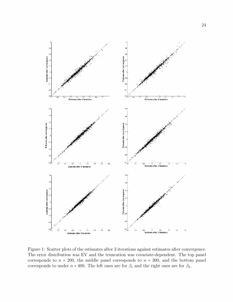
We also examined the difference between the log-rank estimates with 3 iterations versusthose obtained after convergence. The algorithm was treated as convergence in the sense thatthe sum of absolute component differences between two consecutive estimates was less than0.01. We took EV error distribution and covariate-dependent truncation for illustration. Theestimates with 3 iterations and at convergence were plotted for the two regression parametersunder different sample sizes. In Figure 1, the top panel corresponds to the plots for β1 andβ2 under n = 200, the middle panel corresponds to the plots for β1 and β2 under n = 300,and the bottom panel corresponds to the plots for β1 and β2 under n = 400. The two setsof estimates were quite similar, implying that a small number of iterations (such as 3) wassufficient. The situation was quite similar for the other error distributions and truncationmechanisms.
[Insert Figure 1 here]
7 Application to quasar data
We applied the proposed methods to the quasar data analyzed by Efron and Petrosian (1999).The dataset consists of quadruplets (zi,mi, ai, bi), i = 1, . . . , n, where zi is the redshift of theith quasar, mi is its apparent magnitude, and the two numbers ai and bi are lower and uppertruncation bounds on apparent magnitude, respectively. Quasars with mi above bi were toodim to yield dependable redshifts, while the lower limit ai was used to avoid confusion with
12
nonquasar steller objects. Thus, the apparent magnitude was doubly truncated. In thisstudy ai = 16.08 remains the same for all i, and bi varies between 18.494 and 18.93. The fulldataset has n = 1,052 quasars.
Father quasars tend to have bigger values of mi. According to Hubble’s law, one cantransform apparent magnitudes into a luminosity measurement which should be independentof distance. The transformation depends on the cosmological model supposed. Following theEinstein-deSitter cosmological model (Weinberg, 1972), one can obtain the log luminosityvalues yi from a formula
yi = t(zi,mi) = 19.894 − 2.303mi
2.5+ log(Zi −Z
12i ) −
1
2log(Zi), (10)
where Zi = 1 + zi. Larger values of yi correspond to intrinsically brighter quasars. Thetruncation limits Li and Ri for yi are obtained by applying (10) to ai and bi, i.e., Li = t(zi, ai)and Ri = t(zi, bi).
The main purpose of the quasar investigation is to study luminosity evolution. Quasarsmay have been intrinsically brighter in the early universe and evolved toward a dimmer stateas time went out. However, if there is no luminosity evolution, yi should be independent of ziexcept for truncation effects. Thus, testing the absence of luminosity evolution amounts totesting for independence. A convenient one-parameter model for luminosity evolution saysthat the expected log luminosity increases linearly as θ log(1 + z), with θ = 0 correspondingto no evolution. If θ is a hypothesized value of the evolution parameter, instead of directlytesting for the independence of yi and zi, Efron and Petrosian (1999) tested the null hypoth-esis that Hθ: yi(θ) = yi − θ log(1 + zi) is independent of zi, using their proposed approach.Correspondingly, in their analysis, the truncation regions for yi(θ) also changed with θ, thatis, Li(θ) = Li − θ log(1 + zi) and Ri(θ) = Ri − θ log(1 + zi).
Since the one-parameter model for luminosity evolution assumes linear relationship be-tween the expected log luminosity and log(1+z), it is quite natural to consider the followinglinear model
yi = θ log(1 + zi) + εi, (11)
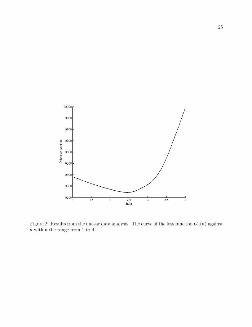
where the response yi is subject to double truncation with the truncation region [Li,Ri],εi is independent of zi, and the evolution parameter θ becomes the unknown regressionparameter. We can estimate θ by our proposed method. To make comparison, we used thesame subset selected by Efron and Petrosian (1999) with n = 210 to do the analysis. Herewe considered the original loss function Gn(θ) defined in (4). The point estimate, denotedby θn, was obtained by minimizing Gn(θ). Figure 2 plots the curve Gn(θ) against θ withinthe range from 1 to 4.
[Insert Figure 2 here]
13
The estimate θn, which is the minimizer of the displayed loss function, was 2.458. Theproposed random weighting approach is used to estimate the standard error of θn. Fivehundred draws of i.i.d. random variables following Gamma(0.25,0.5) were generated. Theestimated standard error was 0.641. Consequently, an approximate 90% Wald-type confi-dence interval was [1.40,3.51]. Under the linear model (11), the hypothesis of no evolution,i.e., H0: yi is independent of zi, is equivalent to H0 ∶ θ = 0. To test for H0 ∶ θ = 0 against a pos-itive evolution parameter Ha ∶ θ > 0, a Wald-type test statistic can be used. The test statisticequaled to the ratio of θn and its estimated standard error, giving the value of 3.835. Thecorresponding one-sided p-value was about 6×10⁻⁵, implying rejection of the null hypothesisof no evolution in favor of a positive value of θ at any commonly used significance level.
The tau test proposed by Efron and Petrosian (1999) for the no evolution hypothesis hasan one-sided p-value 0.015. At 0.05 significance level, their test also rejected H0 in favor ofa positive value of θ, but failed to do so at 0.01 significance level. By inverting their teststatistic, Efron and Petrosian (1999) obtained a point estimate for θ with the value of 2.38and an approximate 90% central confidence interval [1.00,3.20] which is slightly longer thanthe proposed Wald-type confidence interval.
The proposed approach is easy to handle multiple covariates. Here we further consideredthe following model with linear and quadratic term
yi = θ1 log(1 + zi) + θ2 [log(1 + zi)]2+ εi,
where εi is independent of zi and θ1 and θ2 are unknown regression parameters. The regres-sion parameters were estimated by minimizing (4), and the standard errors were estimatedby the random weighting method with 500 i.i.d. Gamma(0.25,0.5) random variables beinggenerated. The corresponding p-values of significance test for H0 ∶ θj = 0 against Ha ∶ θj ≠ 0,j = 1,2, were calculated. The results are summarized in Table 3.
[Insert Table 3 here]
The significance tests showed that the effect of linear term, θ1, was statistically signif-icantly different from 0, while that of the quadratic term, θ2, was apparently not. Thisprovided some evidence to say the one-parameter model for luminosity evolution given by(11) is adequate for the current subset we analyzed.
8 Discussion
This paper is concerned with linear regression analysis when the response variable is subjectto double truncation. Truncated data can be found in many applications, including thosefrom biomedical researches, economics and astronomy. Most statistical methods for dealingwith truncated data are for observations with left or right truncation. The left (right)
14
truncation is relatively easy to handle due to the simple form of re-distribution-to-left (right)algorithm and applicability of counting process-martingale formulation. However, for thedoubly truncated data, less technical tools are available, resulting much fewer results.
We propose a novel method to estimate the regression parameter in the linear regres-sion model with doubly truncated responses. To eliminate the bias introduced by doubletruncation, we extend the Mann-Whitney type loss function for estimating regression param-eters by symmetrization. The proposed estimator is obtained by minimizing the extendedMann-Whitney type loss function. The minimization can be done by some standard soft-ware packages directly, or by an iterative algorithm with an L1-type minimization in eachiteration. The proposed estimator is proved to be consistent and asymptotically normalunder some regularity conditions. A simple random perturbation approach is used to getthe variance estimator. We also provide a weighted estimation procedure for improving theestimation efficiency. Simulation studies show that the proposed approach works well formoderate sample sizes. The application to the quasar data gives new insights.
In addition to handling multiple covariates, another major advantage of the proposedloss function-based approach to estimation over the test score-based approach of Efron andPetrosian (1999) is that it can easily incorporate a penalty function, such as LASSO, to dovariable selection. Note that when LASSO penalty is used, our iterative algorithm is prefer-able since in each iteration the optimization can still be formulated into an L1-minimizationproblem, facilitating the computation. It is also of interest to consider if the idea of the pro-posed approach can be extended to do regression analysis with doubly censored responses,such that discussed by Ren and Gu (1997). These topics certainly warrant future research.
Appendix
A.1 Two lemmas
The first lemma is crucial for the intuition towards the proposed loss function Gn(β) definedby (4).
Lemma 1. Let Li(β), Ri(β) and ei(β), i = 1, . . . , n be defined in Section 3. Then the event
occurs if and only if Lj(β) < ei(β) < Rj(β) and Li(β) < ej(β) < Ri(β).
Proof: We first show “if”. From ei(β) < Rj(β), we have
ei(β) − ej(β) < Rj(β) − ej(β) = Rj − Yj. (13)
From Li(β) < ej(β), we have
ei(β) − ej(β) < ei(β) −Li(β) = Yi −Li. (14)
15
Thus, the second inequality of (12) holds. The second inequality can be shown similarly.
Next we show “only if”. This can be done by reversing the above argument. From (13),we obviously have ei(β) < Rj(β), while from (14), we get Li(β) < ej(β). Additionally, from(Lj − Yj) ∨ (Yi −Ri) < ei(β) − ej(β), we get ei(β) > Lj and ej(β) < Ri(β).
The second lemma shows that the choice of wij = ψn(β, ei(β)∧ ej(β)) makes the weightedestimation function becomes the log-rank estimation function.
Lemma 2. When wij = ψn(β, ei(β) ∧ ej(β)), where ψn(b, t) = (∑ni=1 I{ei(b) ⩾ t})−1, Un,w(β)
becomes the log-rank estimating function for β.
Proof: When wij = ψ(ei(β) ∧ ej(β)), it can be seen that
Un,w(β) =n
∑i=1
n
∑j=1
(n
∑k=1
I{ek(β) ⩾ ei(β) ∧ ej(β)})
−1(Xi − Xj)sgn{ei(β) − ej(β)}
= −2n
∑i=1
n
∑j=1
(n
∑k=1
I{ek(β) ⩾ ei(β)})
−1(Xi − Xj)I {ej(β) ⩾ ei(β)}
= −2n
∑i=1
⎛
⎝
∑nj=1 XiI {ej(β) ⩾ ei(β)}
∑nk=1 I{ek(β) ⩾ ei(β)}
−∑nj=1 XjI {ej(β) ⩾ ei(β)}
∑nk=1 I{ek(β) ⩾ ei(β)}
⎞
⎠
= −2n
∑i=1
⎛
⎝Xi −
∑nj=1 XjI {ej(β) ⩾ ei(β)}
∑nk=1 I{ek(β) ⩾ ei(β)}
⎞
⎠.
This completes the proof.
A.2 Proof of Theorem 1
We first prove consistency. Let Gn = [n(n − 1)]−1Gn. By the uniform law of large numbersfor U-process (Arcones and Gine, 1993), we have that Gn(β) converges uniformly to G(β)for β over B. Since by assumption A3 G(β) has a unique minimizer β0, βn must convergeto β0 as G(β) is obviously continuous.
The proof of asymptotic normality follows closely the technical developments given inSherman (1993) for the maximum rank correlation estimator which is also defined as theoptimizer of a U-type objective function. In fact, the situation there is more complicatedas it deals with a discontinuous objective function. An essential ingredient of Sherman’sapproach is the quadratic approximation to the objective function.
Following Sherman (1993), define τ(z, β) = Eξ(Zi, z;β). Let τ(z, β) and τ(z, β) be itsfirst and second derivatives with respect to β. Then it can be seen from conditions A1 andA2 that we have
E[∥τ(Zi, β)∥2 + ∥τ(Zi, β)∥] <∞
16
and there exists K(z) ≥ 0 such that EK(Zi) <∞ and
∥τ(z, β) − τ(z, β0)∥ ≤K(z)∥β − β0∥.
From these and conditions A1-A4, we can verify the four assumptions in Sherman (1993,Theorem 4) from which the asymptotic normality of βn follows.
A.3 Proof of Theorem 2
Because of scale invariance for β∗ to change in Wi, we may assume, without loss of generality,that E(Wi) = 1/2. Similarly to the proof of consistency of βn, we can argue in the same waythat β∗ is consistent. Let
Each summand on the right-hand side of (15) clearly has mean 0 conditional on data. Stan-dard asymptotic normality for U-statistics can then be used to show that, conditional on thedata, n3/2U∗
n(βn) to a limiting normal distribution. Simple calculation shows that the con-ditional covariance matrix of n−3/2U∗
n(βn) given data converges in probability to V . HenceTheorem 2 holds.
A.4 Proof of Theorem 3
We know that βwn is the solution to the estimating equation Un,w(β) = 0. By the asymptotic
linearity of Un,w, we have, ignoring an asymptotically negligible term,
0 = Un,w(βwn ) ≈ Un,w(β0) + n
2Aw(βwn − β0)
17
or√n(βw
n −β0) ≈ −n3/2A−1
w Un,w(β0). Since n−3/2Un,w(β0) converges to N(0, Vw) by the asymp-totic normality of the U-statistics, we get the desired result.
A.5 Proof of Theorem 4
Similarly to (A.5) of Jin et al. (2001), we can show that for each k, there exists a p×p matrixDk such that
√n(βw
(k) − β0) = −n− 3
2DkA−1Un(β0) − n−
32 (I −Dk)A
−1w Un,w(β0) + op(1).
From this and the joint asymptotic normality of n−3/2Un(β0) and n−3/2Un,w(β0)), we conclude
that√n(βw
(k) − β0) is asymptotically normal.
References
[1] Amemiya, T. (1985), Advanced Econometrics, Harvard University Press, Cambridge,MA.
[2] Arcones, M. A., and Gine, E. (1993), “Limit Theorems for U -Processes,” The Annals ofProbability, 21, 1494-1542.
[3] Bhattacharya, P. K., Chernoff, H., and Yang, S. S. (1983),“Nonparametric Estimationof the Slope of a Truncated Regression,” The Annals of Statistics, 11, 505-514.
[4] Bilker, W., and Wang, M.-C. (1996), “Generalized Wilcoxon Statistics in SemiparametricTruncation Models,” Biometrics, 52, 10-20.
[5] Chang, M. N., and Yang, G. L. (1987), “Strong Consistency of a Nonparametric Estima-tor of the Survival Function with Doubly Censored Data,” The Annals of Statistics, 15,1536-1547.
[6] Efron, B., and Petrosian, V. (1999), “Nonparametric Methods for Doubly TruncatedData,” Journal of the American Statistical Association, 94, 824–834.
[7] Greene, W. H. (2012), Econometric Analysis (7th Ed.), Prentice Hall, Upper SaddleRiver, NJ.
[8] Gu, M. G., and Zhang, C.-H. (1993), “Asymptotic Properties of Self-Consistent Estima-tors Based on Doubly Censored Data,” The Annals of Statistics, 21, 611-624.
[9] Hajek, J. and Sidak, Z. (1967). Theory of Rank Tests, Academic Press, New York.
[10] Harrington, D.P. and Fleming, T.R. (1982), “A Class of Rank Test Procedures for Cen-sored Survival Data,” Biometrika, 69, 133-143.
18
[11] Jin, Z., Lin, D. Y., Wei, L. J., and Ying, Z. (2003), “Rank-based inference for theaccelerated failure time model,” Biometrika, 90, 341–353.
[12] Jin, Z., Ying, Z., and Wei, L. J. (2001), “A Simple Resampling Method by Perturbingthe Minimand,” Biometrika, 88, 381–390.
[13] Keiding, N., and Gill, R. D. (1990), “Random Truncation Models and Markov Processes,”The Annals of Statistics, 18, 582-602.
[14] Kim, J.P., Lu, W., Sit, T. and Ying, Z. (2013), “A unified approach to semiparamet-ric transformation models under generalized biased sampling schemes,” Journal of theAmerican Statistical Association, 108, 217-227.
[15] Koenker, R., and Bassett, G. (1978), “Regression Quantiles,” Econometrica, 46, 33-50.
[16] Lai, T. L., and Ying, Z. (1991a), “Estimating a Distribution Function with Truncatedand Censored Data,” The Annals of Statistics, 19, 417-442.
[17] Lai, T. L., and Ying, Z. (1991b), “Rank Regression Methods for Left-truncated andRight-censored Data,” The Annals of Statistics, 19, 531-556.
[18] Liu, H., Ning, J., Qin, J. and Shen, Y. (2016), “Semiparametric Maximum LikelihoodInference for Truncated or Biased-Sampling Data”, Statistica Sinica, 26, 1087-1115.
[19] Lynden-Bell, D. (1971), “A Method of Allowing for Known Observational Selection inSmall Samples Applied to 3CR Quasars,” Monthly Notices of the Royal AstronomicalSociety, 155, 95-118.
[20] Pollard, D. (1990), Empirical Processes: Theory and Applications Reginal ConferenceSeries Probability and Statistics 2. Institute of Mathematical Statistics, Hayward, CA.
[21] Prentice, R.L. (1978), “Linear Rank Tests with Right Censored Data,” Biometrika, 65,167-179.
[22] Ren, J.-J., and Gu, M. (1997), “Regression M-Estimators with Doubly Censored Data,”The Annals of Statistics, 25, 2638-2664.
[23] Shen, P.-S., (2013), “Regression Analysis of Interval Censored and Doubly TruncatedData with Linear Transformation Models,” Computational Statistics, 28, 581-596.
[24] Sherman, R. P. (1993), “The Limiting Distribution of the Maximum Rank CorrelationEstimator,” Econometrica, 61, 123-138.
[25] Tsai, W.-Y. (1990), “Testing the Independence of Truncation Time and Failure Time,”Biometrika, 77, 167-177.
19
[26] Tsui, K.-L., Jewell, N. P., and Wu, C. F. J. (1988), “A Nonparametric Approach tothe Truncated Regression Problem,” Journal of the American Statistical Association, 83,785-792.
[27] Turnbull, B. W. (1976), “The Empirical Distribution Function with Arbitrarily Grouped,Censored and Truncated Data,” Journal of the Royal Statistical Society, Ser. B, 38, 290–295.
[28] Wang, M.-C., Jewell, N. P., and Tsai, W.-Y. (1986), “Asymptotic Properties Of TheProduct Limit Estimate Under Random Truncation,” The Annals of Statistics, 14, 1597-1605.
[29] Weinberg, S. (1972), Gravitation and Cosmology, New York: Wiley.
[30] Woodroofe, M. (1985), “Estimating a Distribution Function with Truncated Data,” TheAnnals of Statistics, 13, 163-177.
20
Tab
le1.
Sum
mar
ized
sim
ula
tion
resu
lts
for
the
wei
ghte
des
tim
ates
under
cova
riat
e-in
dep
enden
ttr
unca
tion
.
Err
or
Wei
ght
Nai
veW
ilco
xon
log-
ran
k3
nD
istr
ibu
tion
Para
met
erB
IAS
SE
SE
EC
P95
%B
IAS
SE
SE
EC
P95
%B
IAS
SE
SE
EC
P95
%
200
Norm
al
β1
0.0
117
0.11
480.
1141
94.6
%0.
0181
0.20
650.
2152
95.4
%0.
0233
0.21
130.
2182
95.5
%β2
−0.3
619
0.10
420.
1013
6.8
%−
0.0
068
0.19
670.
2085
94.6
%−
0.0
054
0.20
450.
2102
94.3
%L
ogis
tic
β1
−0.0
003
0.18
380.
1858
94.2
%−
0.0
016
0.32
250.
3374
94.8
%0.
0086
0.33
240.
3528
95.4
%β2
−0.3
464
0.16
950.
1627
43.7
%0.
0162
0.30
420.
3047
94.7
%0.
0205
0.31
270.
3140
95.0
%E
Vβ1
0.00
110.
1363
0.13
0393.5
%0.
0040
0.26
870.
2919
95.0
%0.
0029
0.22
680.
2477
94.9
%β2
−0.3
799
0.12
240.
1149
11.2
%0.
0226
0.27
970.
3708
95.0
%0.
0202
0.24
200.
3213
95.9
%
300
Nor
mal
β1
0.00
470.
0938
0.09
3995.1
%0.
0059
0.16
570.
1750
95.3
%0.
0043
0.17
240.
1761
94.1
%β2
−0.3
603
0.08
230.
0837
0.9
%0.
0059
0.16
310.
1680
95.6
%0.
0046
0.16
700.
1687
95.8
%L
ogis
tic
β1
0.00
080.
1503
0.15
1195.5
%0.
0024
0.26
100.
2666
94.8
%0.
0050
0.26
740.
2787
96.0
%β2
−0.3
535
0.13
550.
1326
25.4
%0.
0011
0.23
380.
2382
95.3
%−
0.0
016
0.24
400.
2494
95.4
%E
Vβ1
0.00
370.
1065
0.10
6294.8
%0.
0065
0.20
640.
2170
95.5
%0.
0089
0.17
970.
1833
95.4
%β2
−0.3
822
0.09
570.
0938
1.8
%0.
0081
0.21
020.
2285
95.2
%0.
0055
0.18
670.
1963
95.0
%
400
Nor
mal
β1
0.00
580.
0818
0.08
1694.5
%0.
0110
0.15
010.
1504
95.1
%0.
0133
0.14
970.
1508
95.4
%β2
−0.3
627
0.07
500.
0725
0.1
%0.
0002
0.14
160.
1427
95.0
%−
0.0
002
0.13
980.
1439
95.2
%L
ogis
tic
β1
0.0
031
0.13
580.
1312
93.5
%0.
0034
0.22
580.
2294
94.8
%−
0.0
004
0.23
290.
2400
95.8
%β2
−0.3
553
0.11
320.
1151
11.8
%−
0.0
033
0.20
100.
2048
94.6
%0.
0000
0.21
050.
2140
94.5
%E
Vβ1
0.00
180.
0936
0.09
2193.7
%0.
0031
0.17
990.
1821
95.2
%0.
0029
0.15
380.
1542
94.3
%β2
−0.3
805
0.08
380.
0816
0.4
%0.
0082
0.17
610.
1869
95.8
%0.
0054
0.15
590.
1624
96.2
%
Nai
ve:
nai
vees
tim
ate
by
ign
orin
gd
oub
letr
unca
tion
;W
ilco
xon
:W
ilco
xon
wei
ght
esti
mate
;lo
g-r
an
k3:
log-r
an
kw
eight
esti
mate
wit
hk=
3;B
IAS:
aver
age
bia
sof
the
esti
mat
es;
SE
:st
an
dard
erro
rof
the
esti
mate
s;S
EE
:av
erage
of
the
esti
mate
dst
an
dard
erro
rs;
CP
95%
:em
pir
ical
cove
rage
pro
bab
ilit
ies
ofW
ald
-typ
eco
nfi
den
cein
terv
als
wit
h95%
con
fid
ence
level
.
21
Tab
le2.
Sum
mar
ized
sim
ula
tion
resu
lts
for
the
wei
ghte
des
tim
ates
under
cova
riat
e-dep
enden
ttr
unca
tion
.
Err
or
Wei
ght
Nai
veW
ilco
xon
log-
ran
k3
nD
istr
ibu
tion
Para
met
erB
IAS
SE
SE
EC
P95
%B
IAS
SE
SE
EC
P95
%B
IAS
SE
SE
EC
P95
%
200
Norm
al
β1
0.2
316
0.11
390.
1151
48.3
%0.
0183
0.20
240.
2176
95.0
%0.
0217
0.20
350.
2205
95.9
%β2
−0.2
490
0.10
220.
0991
28.6
%−
0.0
042
0.19
440.
2053
95.1
%−
0.0
035
0.19
930.
2075
94.9
%L
ogis
tic
β1
0.21
960.
1834
0.18
6178.2
%−
0.0
070
0.31
600.
3381
95.5
%0.
0016
0.32
540.
3508
96.6
%β2
−0.2
358
0.16
490.
1611
69.1
%0.
0129
0.29
760.
3287
93.9
%0.
0168
0.30
610.
3360
93.9
%E
Vβ1
0.22
920.
1375
0.13
0856.7
%−
0.0
003
0.26
940.
3059
95.8
%0.
0013
0.23
050.
2596
95.8
%β2
−0.2
605
0.12
030.
1126
36.2
%0.
0206
0.27
110.
3403
95.5
%0.
0187
0.23
570.
2893
95.4
%
300
Nor
mal
β1
0.22
680.
0957
0.09
4833.4
%0.
0068
0.16
890.
1755
95.7
%0.
0051
0.17
330.
1767
95.6
%β2
−0.2
461
0.08
170.
0817
14.2
%0.
0049
0.16
330.
1630
94.9
%0.
0052
0.16
710.
1635
94.8
%L
ogis
tic
β1
0.21
900.
1503
0.15
1868.8
%−
0.0
039
0.25
560.
2661
95.3
%−
0.0
005
0.26
500.
2778
95.8
%β2
−0.2
444
0.13
460.
1310
53.0
%−
0.0
064
0.22
990.
2353
94.6
%−
0.0
100
0.24
120.
2455
95.4
%E
Vβ1
0.23
510.
1051
0.10
6840.6
%0.
0060
0.20
830.
2194
95.9
%0.
0093
0.18
270.
1869
94.9
%β2
−0.2
444
0.09
360.
0919
16.8
%0.
0045
0.20
190.
2169
95.4
%0.
0014
0.18
110.
1875
95.2
%
400
Nor
mal
β1
0.22
960.
0810
0.08
2120.4
%0.
0150
0.14
530.
1505
96.2
%0.
0169
0.14
700.
1510
96.2
%β2
−0.2
454
0.07
120.
0709
6.3
%0.
0032
0.13
420.
1394
95.3
%0.
0019
0.13
250.
1402
94.4
%L
ogis
tic
β1
0.22
270.
1362
0.13
1660.1
%−
0.0
023
0.22
870.
2294
95.0
%−
0.0
047
0.23
580.
2392
95.3
%β2
−0.2
437
0.11
230.
1140
43.6
%−
0.0
059
0.19
930.
2033
95.6
%−
0.0
018
0.20
940.
2120
95.0
%E
Vβ1
0.23
210.
0942
0.09
2828.8
%0.
0021
0.18
240.
1844
95.2
%0.
0014
0.15
660.
1575
95.1
%β2
−0.2
614
0.08
110.
0799
9.2
%0.
0044
0.16
780.
1787
95.8
%0.
0022
0.15
090.
1561
95.5
%
Nai
ve:
nai
vees
tim
ate
by
ign
orin
gd
oub
letr
unca
tion
;W
ilco
xon
:W
ilco
xon
wei
ght
esti
mate
;lo
g-r
an
k3:
log-r
an
kw
eight
esti
mate
wit
hk=
3;B
IAS:
aver
age
bia
sof
the
esti
mat
es;
SE
:st
an
dard
erro
rof
the
esti
mate
s;S
EE
:av
erage
of
the
esti
mate
dst
an
dard
erro
rs;
CP
95%
:em
pir
ical
cove
rage
pro
bab
ilit
ies
ofW
ald
-typ
eco
nfi
den
cein
terv
als
wit
h95%
con
fid
ence
level
.
22
Table 3. Results from the quasar data: estimation for the model with linear and quadraticterm.
Parameter EST SE p-valueθ1 7.6776 2.6396 0.0036θ2 −3.3173 2.2408 0.1388
EST: estimate of the parameter; SE: estimated standard error; p-value: asymptotic p-value of thesignificance test for H0 ∶ θj = 0 against Ha ∶ θj ≠ 0, j = 1,2.
23
24
Figure 1: Scatter plots of the estimates after 3 iterations against estimates after convergence.The error distribution was EV and the truncation was covariate-dependent. The top panelcorresponds to n = 200, the middle panel corresponds to n = 300, and the bottom panelcorresponds to under n = 400. The left ones are for β1 and the right ones are for β2.
25
Figure 2: Results from the quasar data analysis. The curve of the loss function Gn(θ) againstθ within the range from 1 to 4.