Regression Modeling Regression models are often constructed based on certain conditions that must be verified for the model to fit the data well, and to be able to predict accurately. This site provides the necessary diagnostic tools for the verification process and taking the right remedies such as data transformation. Prior to using this JavaScript it is necessary to construct the scatter-diagram of your data. If by visual inspection of the scatter-diagram, you cannot reject "linearity condition", then you may use this JavaScript. Enter your up-to-84 sample paired-data sets (X, Y), and then click the Calculate button. Blank boxes are not included in the calculations but zeros are. In order to perform serial-residual analysis you must enter the independent variable X in increasing order. Notice:In entering your data to move from cell to cell in the data-matrix use the Tab key not arrow or enter keys. Predictions by Regression: Confidence interval provides a useful way of assessing the quality of prediction. In prediction by regression often one or more of the following constructions are of interest: 1. A confidence interval for a single future value of Y corresponding to a chosen value of X. 2. A confidence interval for a single pint on the line. 3. A confidence region for the line as a whole.
Transcript
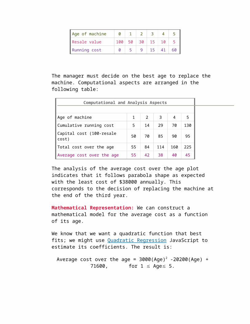
Regression Modeling
Regression models are often constructed based on certain conditions that must be verified for the model to fit the data well, and to be able to predict accurately. This site provides the necessary diagnostic tools for the verification process and taking the right remedies such as data transformation.
Prior to using this JavaScript it is necessary to construct the scatter-diagram of your data. If by visual inspection of the scatter-diagram, you cannot reject "linearity condition", then you may use this JavaScript.
Enter your up-to-84 sample paired-data sets (X, Y), and then click the Calculate button. Blank boxes are not included in the calculations but zeros are. In order to perform serial-residual analysis you must enter the independent variable X in increasing order.
Notice:In entering your data to move from cell to cell in the data-matrix use the Tab key not arrow or enter keys.
Predictions by Regression: Confidence interval provides a useful way of assessing the quality of prediction. In prediction by regression often one or more of the following constructions are of interest:
1. A confidence interval for a single future value of Y corresponding to a chosen value of X.
2. A confidence interval for a single pint on the line. 3. A confidence region for the line as a whole.
Confidence Interval Estimate for a Future Value: A confidence interval of interest can be used to evaluate the accuracy of a single (future) value of y corresponding to a chosen value of X (say, X0). This JavaScript provides confidence interval for an estimated value Y corresponding to X0 with a desirable confidence level 1 - .
Confidence Interval Estimate for a Single Point on the Line: If a particular value of the predictor variable (say, X0) is of special importance, a confidence interval on the value of the criterion variable (i.e. average Y at X0) corresponding to X0 may be of interest. This JavaScript provides
confidence interval on the estimated value of Y corresponding to X0 with a desirable confidence level 1 - .
It is of interest to compare the above two different kinds of confidence interval. The first kind has larger confidence interval that reflects the less accuracy resulting from the estimation of a single future value of y rather than the mean value computed for the second kind confidence interval. The second kind of confidence interval can also be used to identify any outliers in the data.
Confidence Region the Regression Line as the Whole: When the entire line is of interest, a confidence region permits one to simultaneously make confidence statements about estimates of Y for a number of values of the predictor variable X. In order that region adequately covers the range of interest of the predictor variable X; usually, data size must be more than 10 pairs of observations.
In all cases the JavaScript provides the results for the nominal data. For other values of X one may use computational methods directly, graphical method, or using linear interpolations to obtain approximated results. These approximation are in the safe directions i.e., they are slightly wider that the exact values.
Linear Interpolation: To estimate the lower (and upper) limits at given value X, one may use the following by taking a linear interpolations at two known neighboring points to X, say XL and XU, as follow:
The approximate lower limit at X is:
LL(XL) + [ LL(XU) – LL (XL) ] [X – XL] / [ XU – XL ] Similarly the upper limit at X is:
UL(XL) + [ UL(XU) – UL (XL) ] [X – XL] / [ XU – XL ] The resulting approximation is conservative; therefore it is in the safe side.
In practice, a confidence interval is used to express the uncertainty in a quantity being estimated. The following JavaScript that that computes confidence interval for standard deviation, confidence interval for variance, and confidence interval for expected value of the population based on a set of
random observations. Since the Confidence Intervals (CI) are the duals of tests of hypothesis, one may use CI for testing too.
While the confidence interval for the mean is applicable to any population even with discrete random variables, such as proportion, the other two confidence intervals required testing for normality in order to be valid.
Let's say you compute a 95% confidence interval for a mean (or variance) of the population. The way to interpret this is to imagine an infinite number of samples from the same population, at least 95% of the computed intervals will contain the population mean (or variance), and at most 5% will not. However, it is wrong to state, "I am 95% confident that the population parameter falls within the interval."
Notice that care must be taken when rounding the confidence limits to a desirable number of digit the lower limit must be rounded up, while the upper limit must be rounded down. Know that a confidence interval computed from one sample will be different from a confidence interval computed from another sample.
One-sided Confidence Limits: To obtain the one sided (upper or lower) confidence interval with level of significance, enter 1- 2 as the confidence level.
Test of Hypotheses by Confidence Interval: As an alternative to direct test of hypothesis for the Mean and the Variance one may use a two-sided or one-sided confidence interval to test a hypothesis with a two-sided or one sided alternative hypothesis , respectively. In this approach if the confidence interval with a desirable confidence level contains the null hypothesis value, then one might not reject the null hypothesis.
Enter your up-to-80 sample data, and the Desirable Confidence Level, and then click the Calculate button. Blank boxes are not included in the calculations but zeros are.
In entering your data to move from cell to cell in the data-matrix use the Tab key not arrow or enter keys.
To edit your data, including add/change/delete, you do not have to click on the "clear" button, and re-enter your data all over again. You may simply add a number to any blank cell, change a
number to another in the same cell, or delete a number from a cell. After editing, then click the "calculate" button.
For extensive edit or to use the JavaScript for a new set of data, then use the "clear" button.
Introduction & Summary
Rules of thumb, intuition, tradition, and simple financial analysis are often no longer sufficient for addressing such common decisions as make-versus-buy, facility site selection, and process redesign. In general, the forces of competition are imposing a need for more effective decision making at all levels in organizations.
Decision analysts provide quantitative support for the decision-makers in all areas including engineers, analysts in planning offices and public agencies, project management consultants, manufacturing process planners, financial and economic analysts, experts supporting medical/technological diagnosis, and so on and on.
Progressive Approach to Modeling: Modeling for decision making involves two distinct parties, one is the decision-maker and the other is the model-builder known as the analyst. The analyst is to assist the decision-maker in his/her decision-making process. Therefore, the analyst must be equipped with more than a set of analytical methods.
Specialists in model building are often tempted to study a problem, and then go off in isolation to develop an elaborate mathematical model for use by the manager (i.e., the decision-maker). Unfortunately the manager may not understand this model and may either use it blindly or reject it entirely. The specialist may feel that the manager is too ignorant and unsophisticated to appreciate the model, while the manager may feel that the specialist lives in a dream world of unrealistic assumptions and irrelevant mathematical language.
Such miscommunication can be avoided if the manager works with the specialist to develop first a simple model that provides a crude but understandable analysis. After the manager has built up confidence in this model, additional detail and sophistication can be added, perhaps progressively only a bit at a time. This process requires an investment of time on the part of the manager and sincere interest on the part of the specialist in solving the manager's real problem, rather than in creating and trying to explain sophisticated models. This progressive model building is often referred to as the bootstrapping approach and is the most important factor in determining successful implementation of a
decision model. Moreover the bootstrapping approach simplifies otherwise the difficult task of model validating and verification processes.
What is a System: Systems are formed with parts put together in a particular manner in order to pursuit an objective. The relationship between the parts determines what the system does and how it functions as a whole. Therefore, the relationship in a system are often more important than the individual parts. In general, systems that are building blocks for other systems are called subsystems
The Dynamics of a System: A system that does not change is a static (i.e., deterministic) system. Many of the systems we are part of are dynamic systems, which are they change over time. We refer to the way a system changes over time as the system's behavior. And when the system's development follows a typical pattern we say the system has a behavior pattern. Whether a system is static or dynamic depends on which time horizon you choose and which variables you concentrate on. The time horizon is the time period within which you study the system. The variables are changeable values on the system.
In deterministic models, a good decision is judged by the outcome alone. However, in probabilistic models, the decision-maker is concerned not only with the outcome value but also with the amount of risk each decision carries
As an example of deterministic versus probabilistic models, consider the past and the future: Nothing we can do can change the past, but everything we do influences and changes the future, although the future has an element of uncertainty. Managers are captivated much more by shaping the future than the history of the past.
Uncertainty is the fact of life and business; probability is the guide for a "good" life and successful business. The concept of probability occupies an important place in the decision-making process, whether the problem is one faced in business, in government, in the social sciences, or just in one's own everyday personal life. In very few decision making situations is perfect information - all the needed facts - available. Most decisions are made in the face of uncertainty. Probability enters into the process by playing the role of a substitute for certainty - a substitute for complete knowledge.
Probabilistic Modeling is largely based on application of statistics for probability assessment of uncontrollable events (or factors), as well as risk assessment of your decision. The original idea of statistics was the collection of information about and for the State. The word statistics is not derived from any classical Greek or Latin roots, but from the Italian word
for state. Probability has a much longer history. Probability is derived from the verb to probe meaning to "find out" what is not too easily accessible or understandable. The word "proof" has the same origin that provides necessary details to understand what is claimed to be true.
Probabilistic models are viewed as similar to that of a game; actions are based on expected outcomes. The center of interest moves from the deterministic to probabilistic models using subjective statistical techniques for estimation, testing, and predictions. In probabilistic modeling, risk means uncertainty for which the probability distribution is known. Therefore risk assessment means a study to determine the outcomes of decisions along with their probabilities.
Decision-makers often face a severe lack of information. Probability assessment quantifies the information gap between what is known, and what needs to be known for an optimal decision. The probabilistic models are used for protection against adverse uncertainty, and exploitation of propitious uncertainty.
Difficulty in probability assessment arises from information that is scarce, vague, inconsistent, or incomplete. A statement such as "the probability of a power outage is between 0.3 and 0.4" is more natural and realistic than their "exact" counterpart such as "the probability of a power outage is 0.36342."
It is a challenging task to compare several courses of action and then select one action to be implemented. At times, the task may prove too challenging. Difficulties in decision making arise through complexities in decision alternatives. The limited information-processing capacity of a decision-maker can be strained when considering the consequences of only one course of action. Yet, choice requires that the implications of various courses of action be visualized and compared. In addition, unknown factors always intrude upon the problem situation and seldom are outcomes known with certainty. Almost always, an outcome depends upon the reactions of other people who may be undecided themselves. It is no wonder that decision-makers sometimes postpone choices for as long as possible. Then, when they finally decide, they neglect to consider all the implications of their decision.
Emotions and Risky Decision: Most decision makers rely on emotions in making judgments concerning risky decisions. Many people are afraid of the possible unwanted consequences. However, do we need emotions in order to be able to judge whether a decision and its concomitant risks are morally acceptable. This question has direct practical implications: should engineers, scientists and policy makers involved in developing risk regulation take the emotions of the public seriously or not? Even though
emotions are subjective and irrational (or a-rational), they should be a part of the decision making process since they show us our preferences. Since emotions and rationality are not mutually exclusive, because in order to be practically rational, we need to have emotions. This can lead to an alternative view about the role of emotions in risk assessment: emotions can be a normative guide in making judgments about morally acceptable risks.
Most people often make choices out of habit or tradition, without going through the decision-making process steps systematically. Decisions may be made under social pressure or time constraints that interfere with a careful consideration of the options and consequences. Decisions may be influenced by one's emotional state at the time a decision is made. When people lack adequate information or skills, they may make less than optimal decisions. Even when or if people have time and information, they often do a poor job of understanding the probabilities of consequences. Even when they know the statistics; they are more likely to rely on personal experience than information about probabilities. The fundamental concerns of decision making are combining information about probability with information about desires and interests. For example: how much do you want to meet her, how important is the picnic, how much is the prize worth?
Business decision making is almost always accompanied by conditions of uncertainty. Clearly, the more information the decision maker has, the better the decision will be. Treating decisions as if they were gambles is the basis of decision theory. This means that we have to trade off the value of a certain outcome against its probability.
To operate according to the canons of decision theory, we must compute the value of a certain outcome and its probabilities; hence, determining the consequences of our choices.
The origin of decision theory is derived from economics by using the utility function of payoffs. It suggests that decisions be made by computing the utility and probability, the ranges of options, and also lays down strategies for good decisions:
This Web site presents the decision analysis process both for public and private decision making under different decision criteria, type, and quality of available information. This Web site describes the basic elements in the analysis of decision alternatives and choice, as well as the goals and objectives that guide decision making. In the subsequent sections, we will examine key issues related to a decision-maker’s preferences regarding alternatives, criteria for choice, and choice modes.
Objectives are important both in identifying problems and in evaluating alternative solutions. Evaluating alternatives requires that a decision-maker’s objectives be expressed as criterion that reflects the attributes of the alternatives relevant to the choice.
The systematic study of decision making provides a framework for choosing courses of action in a complex, uncertain, or conflict-ridden situation. The choices of possible actions, and the prediction of expected outcomes, derive from a logical analysis of the decision situation.
A Possible Drawback in the Decision Analysis Approach: You might have already noticed that the above criteria always result in selection of only one course of action. However, in many decision problems, the decision-
maker might wish to consider a combination of some actions. For example, in the Investment problem, the investor might wish to distribute the assets among a mixture of the choices in such a way to optimize the portfolio's return. Visit the Game Theory with Applications Web site for designing such an optimal mixed strategy.
Further Readings:Arsham H., A Markovian model of consumer buying behavior and optimal advertising pulsing policy, Computers and Operations Research, 20(2), 35-48, 1993. Arsham H., A stochastic model of optimal advertising pulsing policy, Computers and Operations Research, 14(3), 231-239, 1987. Ben-Haim Y., Information-gap Decision Theory: Decisions Under Severe Uncertainty, Academic Press, 2001.Golub A., Decision Analysis: An Integrated Approach, Wiley, 1997.Goodwin P., and G. Wright, Decision Analysis for Management Judgment, Wiley, 1998. van Gigch J., Metadecisions: Rehabilitating Epistemology, Kluwer Academic Publishers, 2002.Wickham Ph., Strategic Entrepreneurship: A Decision-making Approach to New Venture Creation and Management, Pitman, 1998.
Probabilistic Modeling: From Data to a Decisive Knowledge
Knowledge is what we know well. Information is the communication of knowledge. In every knowledge exchange, there is a sender and a receiver. The sender make common what is private, does the informing, the communicating. Information can be classified as explicit and tacit forms. The explicit information can be explained in structured form, while tacit information is inconsistent and fuzzy to explain. Know that data are only crude information and not knowledge by themselves.
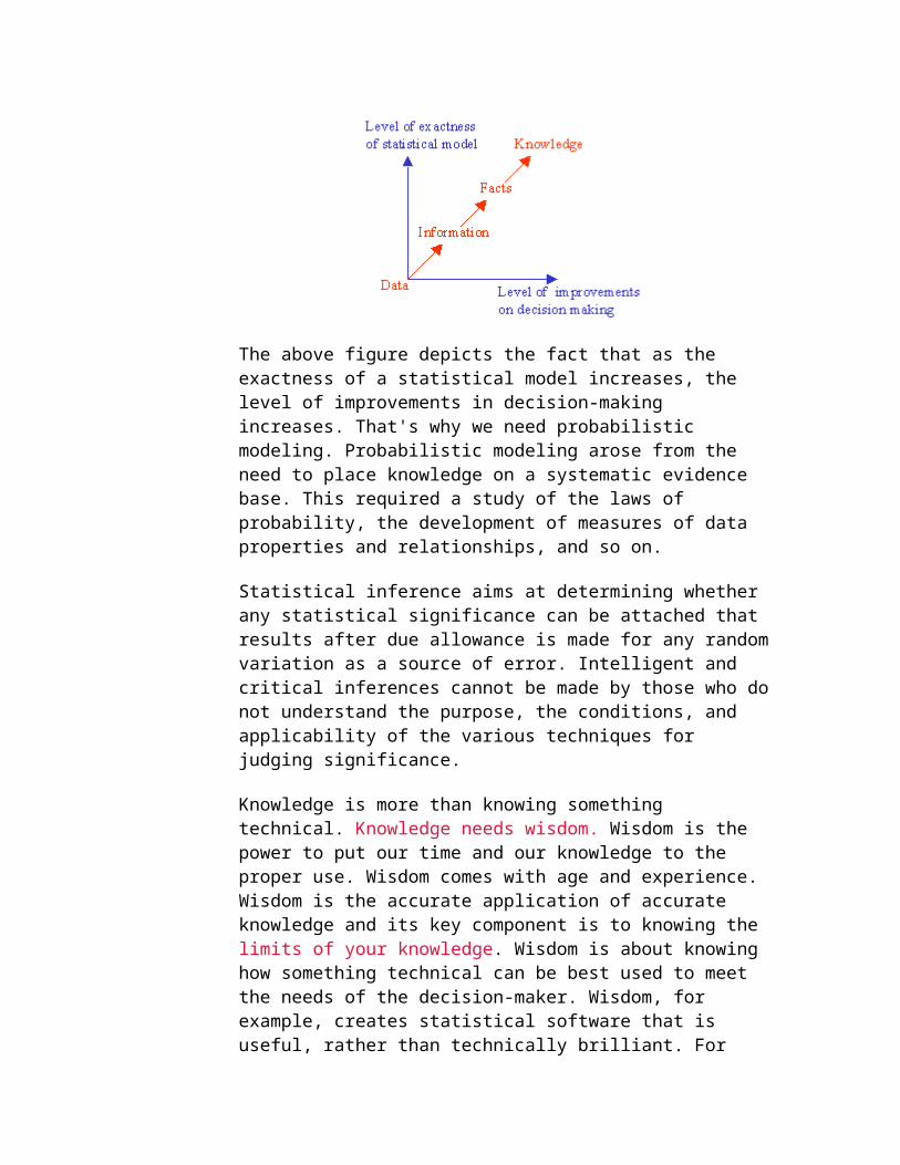
Data is known to be crude information and not knowledge by itself. The sequence from data to knowledge is: from Data to Information, from Information to Facts, and finally, from Facts to Knowledge. Data becomes information, when it becomes relevant to your decision problem. Information becomes fact, when the data can support it. Facts are what the data reveals. However the decisive instrumental (i.e., applied) knowledge is expressed together with some statistical degree of confidence.
Fact becomes knowledge, when it is used in the successful completion of a decision process. Once you have a massive amount of facts integrated as knowledge, then your mind will be superhuman in the same sense that mankind with writing is superhuman compared to mankind before writing. The following figure illustrates the statistical thinking process based on data in constructing statistical models for decision making under uncertainties.
The above figure depicts the fact that as the exactness of a statistical model increases, the level of improvements in decision-making increases. That's why we need probabilistic modeling. Probabilistic modeling arose from the need to place knowledge on a systematic evidence base. This required a study of the laws of probability, the development of measures of data properties and relationships, and so on.
Statistical inference aims at determining whether any statistical significance can be attached that results after due allowance is made for any random variation as a source of error. Intelligent and critical inferences cannot be made by those who do not understand the purpose, the conditions, and applicability of the various techniques for judging significance.
Knowledge is more than knowing something technical. Knowledge needs wisdom. Wisdom is the power to put our time and our knowledge to the proper use. Wisdom comes with age and experience. Wisdom is the accurate application of accurate knowledge and its key component is to knowing the limits of your knowledge. Wisdom is about knowing how something technical can be best used to meet the needs of the decision-maker. Wisdom, for example, creates statistical software that is useful, rather than technically brilliant. For example, ever since the Web entered the popular consciousness, observers have noted that it puts information at your fingertips but tends to keep wisdom out of reach.
Considering the uncertain environment, the chance that "good decisions" are made increases with the availability of "good information." The chance that "good information" is available increases with the level of structuring the process of Knowledge Management. One may ask, "What is the use of decision analysis techniques without the best available information delivered by Knowledge Management?" The answer is: one can not make responsible decisions until one possess enough knowledge. However, for private decisions one may rely on, e.g., the psychological motivations, as discusses under "Decision Making Under Pure Uncertainty" in this site. Moreover, Knowledge Management and Decision Analysis are indeed
interrelated since one influences the other, both in time, and space. The notion of "wisdom" in the sense of practical wisdom has entered Western civilization through biblical texts. In the Hellenic experience this kind of wisdom received a more structural character in the form of philosophy. In this sense philosophy also reflects one of the expressions of traditional wisdom.
Making decisions is certainly the most important task of a manager and it is often a very difficult one. This site offers a decision making procedure for solving complex problems step by step.
The Decision-Making Process: Unlike the deterministic decision-making process, in the decision making process under uncertainty the variables are often more numerous and more difficult to measure and control. However, the steps are the same. They are:
1. Simplification 2. Building a decision model 3. Testing the model 4. Using the model to find the solution
o It is a simplified representation of the actual situation o It need not be complete or exact in all respects o It concentrates on the most essential relationships and
ignores the less essential ones. o It is more easily understood than the empirical situation
and, hence, permits the problem to be more readily solved with minimum time and effort.
5. It can be used again and again for like problems or can be modified.
Fortunately the probabilistic and statistical methods for analysis and decision making under uncertainty are more numerous and powerful today than even before. The computer makes possible many practical applications. A few examples of business applications are the following:
An auditor can use random sampling techniques to audit the account receivable for client.
A plant manager can use statistic quality control techniques to assure the quality of his production with a minimum of testing or inspection.
A financial analyst may use regression and correlation to help understand the relationship of a financial ratio to a set of other variables in business.
A market researcher may use test of significant to accept or reject the hypotheses about a group of buyers to which the firm wishes to sell a particular product.
A sale manager may use statistical techniques to forecast sales for the coming year.
Further Readings:Berger J., Statistical Decision Theory and Bayesian Analysis, Springer, 1978.Corfield D., and J. Williamson, Foundations of Bayesianism, Kluwer Academic Publishers, 2001. Contains Logic, Mathematics, Decision Theory, and Criticisms of Bayesianism.Grünig R., Kühn, R.,and M. Matt, (Eds.), Successful Decision-Making: A Systematic Approach to Complex Problems, Springer, 2005. It is intended for decision makers in companies, in non-profit organizations and in public administration.Lapin L., Statistics for Modern Business Decisions, Harcourt Brace Jovanovich, 1987.Lindley D., Making Decisions, Wiley, 1991.Pratt J., H. Raiffa, and R. Schlaifer, Introduction to Statistical Decision Theory, The MIT Press, 1994.Press S., and J. Tanur, The Subjectivity of Scientists and the Bayesian Approach, Wiley, 2001. Comparing and contrasting the reality of subjectivity in the work of history's great scientists and the modern Bayesian approach to statistical analysis.Tanaka H., and P. Guo, Possibilistic Data Analysis for Operations Research, Physica-Verlag, 1999.
Decision Analysis: Making Justifiable, Defensible Decisions
Decision analysis is the discipline of evaluating complex alternatives in terms of values and uncertainty. Values are generally expressed monetarily because this is a major concern for management. Furthermore, decision analysis provides insight into how the defined alternatives differ from one another and then generates suggestions for new and improved alternatives. Numbers quantify subjective values and uncertainties, which enable us to understand the decision situation. These numerical results then must be translated back into words in order to generate qualitative insight.
Humans can understand, compare, and manipulate numbers. Therefore, in order to create a decision analysis model, it is necessary to create the model structure and assign probabilities and values to fill the model for computation. This includes the values for probabilities, the value functions for evaluating alternatives, the value weights for measuring the trade-off objectives, and the risk preference.
Once the structure and numbers are in place, the analysis can begin. Decision analysis involves much more than computing the expected utility of each alternative. If we stopped there, decision makers would not gain much insight. We have to examine the sensitivity of the outcomes, weighted utility for key probabilities, and the weight and risk preference parameters. As part of the sensitivity analysis, we can calculate the value of perfect information for uncertainties that have been carefully modeled.
There are two additional quantitative comparisons. The first is the direct comparison of the weighted utility for two alternatives on all of the objectives. The second is the comparison of all of the alternatives on any
two selected objectives which shows the Pareto optimality for those two objectives.
Complexity in the modern world, along with information quantity, uncertainty, and risk, make it necessary to provide a rational decision making framework. The goal of decision analysis is to give guidance, information, insight, and structure to the decision-making process in order to make better, more 'rational' decisions.
A decision needs a decision maker who is responsible for making decisions. This decision maker has a number of alternatives and must choose one of them. The objective of the decision-maker is to choose the best alternative. When this decision has been made, events that the decision-maker has no control over may have occurred. Each combination of alternatives, followed by an event happening, leads to an outcome with some measurable value. Managers make decisions in complex situations. Decision tree and payoff matrices illustrate these situations and add structure to the decision problems.
Further Readings:Arsham H., Decision analysis: Making justifiable, defensible decisions, e-Quality, September, 2004. Forman E., and M. Selly, Decision by Objectives: How to Convince Others That You Are Right, World Scientific, 2001.Gigerenzer G., Adaptive Thinking: Rationality in the Real World, Oxford University Press, 2000.Girón F., (Ed.), Applied Decision Analysis, Kluwer Academic, 1998.Manning N., et al., Strategic Decision Making In Cabinet Government: Institutional Underpinnings and Obstacles, World Bank, 1999. Patz A., Strategic Decision Analysis: A General Management Framework, Little and Brown Pub., 1981.Vickers G., The Art of Judgment: A Study of Policy Making, Sage Publications, 1995. Von Furstenberg G., Acting Under Uncertainty: Multidisciplinary Conceptions, Kluwer Academic Publishers, 1990.
The mathematical models and techniques considered in decision analysis are concerned with prescriptive theories of choice (action). This answers the question of exactly how a decision maker should behave when faced with a choice between those actions which have outcomes governed by chance, or the actions of competitors.
Decision analysis is a process that allows the decision maker to select at least and at most one option from a set of possible decision alternatives. There must be uncertainty regarding the future along with the objective of optimizing the resulting payoff (return) in terms of some numerical decision criterion.
The elements of decision analysis problems are as follow:
1. A sole individual is designated as the decision-maker. For example, the CEO of a company, who is accountable to the shareholders.
2. A finite number of possible (future) events called the 'States of Nature' (a set of possible scenarios). They are the circumstances under which a decision is made. The states of nature are identified and grouped in set "S"; its members are denoted by "s(j)". Set S is a collection of mutually exclusive events meaning that only one state of nature will occur.
3. A finite number of possible decision alternatives (i.e., actions) is available to the decision-maker. Only one action may be taken. What can I do? A good decision requires seeking a better set of alternatives than those that are initially presented or traditionally accepted. Be brief on the logic and reason portion of your decision. While there are probably a thousand facts about an automobile, you do not need them all to make a decision. About a half dozen will do.
4. Payoff is the return of a decision. Different combinations of decisions and states of nature (uncertainty) generate different payoffs. Payoffs are usually shown in tables. In decision analysis payoff is represented by positive (+) value for net revenue, income, or profit and negative (-) value for expense, cost or net loss. Payoff table analysis determines the decision alternatives using different criteria. Rows and columns are assigned possible decision alternatives and possible states of nature, respectively.Constructing such a matrix is usually not an easy task; therefore, it may take some practice.
Source of Errors in Decision Making: The main sources of errors in risky decision-making problems are: false assumptions, not having an accurate estimation of the probabilities, relying on expectations, difficulties in measuring the utility function, and forecast errors.
Consider the following Investment Decision-Making Example:
The Investment Decision-Making Example:
States of Nature
Growth Medium G No Change Low
G MG NC L
Bonds 12% 8 7 3
Actions Stocks 15 9 5 -2
Deposit 7 7 7 7
The States of Nature are the states of economy during one year. The problem is to decide what action to take among three possible courses of action with the given rates of return as shown in the body of the table.
Further Readings:Borden T., and W. Banta, (Ed.), Using Performance Indicators to Guide Strategic Decision Making, Jossey-Bass Pub., 1994. Eilon S., The Art of Reckoning: Analysis of Performance Criteria, Academic Press, 1984. Von Furstenberg G., Acting Under Uncertainty: Multidisciplinary Conceptions, Kluwer Academic Publishers, 1990.
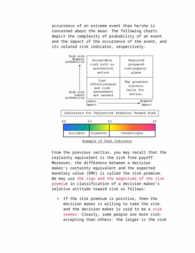
Coping With Uncertainties
There are a few satisfactory description of uncertainty, one of which is the concept and the algebra of probability.
To make serious business decisions one is to face a future in which ignorance and uncertainty increasingly overpower knowledge, as ones
planning horizon recedes into the distance. The deficiencies about our knowledge of the future may be divided into three domains, each with rather murky boundaries:
Risk: One might be able to enumerate the outcomes and figure the probabilities. However, one must lookout for non-normal distributions, especially those with “fat tails”, as illustrated in the stock market by the rare events.
Uncertainty: One might be able to enumerate the outcomes but the probabilities are murky. Most of the time, the best one can do is to give a rank order to possible outcomes and then be careful that one has not omitted one of significance.
Black Swans: The name comes from an Australian genetic anomaly. This is the domain of events which are either “extremely unlikely” or “inconceivable” but when they happen, and they do happen, they have serious consequences, usually bad. An example of the first kind is the Exxon Valdez oil spill, of the second, the radiation accident at Three Mile Island.
In fact, all highly man-made systems, such as, large communications networks, nuclear-powered electric-generating stations and spacecraft are full of hidden “paths to failure”, so numerous that we cannot think of all of them, or not able to afford the time and money required to test for and eliminate them. Individually each of these paths is a black swan, but there are so many of them that the probability of one of them being activated is quite significant.
While making business decisions, we are largely concerned with the domain of risk and usually assume that the probabilities follow normal distributions. However, we must be concerned with all three domains and have an open mind about the shape of the distributions.
Continuum of pure uncertainty and certainty: The domain of decision analysis models falls between two extreme cases. This depends upon the degree of knowledge we have about the outcome of our actions, as shown below:
One "pole" on this scale is deterministic, such as the carpenter's problem. The opposite "pole" is pure uncertainty. Between these two extremes are problems under risk. The main idea here is that for any given problem, the degree of certainty varies among managers depending upon how much knowledge each one has about the same problem. This reflects the recommendation of a different solution by each person.
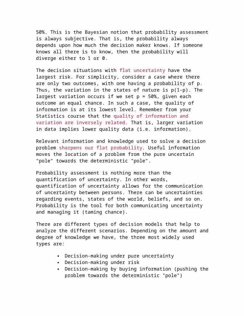
Probability is an instrument used to measure the likelihood of occurrence for an event. When you use probability to express your uncertainty, the deterministic side has a probability of 1 (or zero), while the other end has a flat (all equally probable) probability. For example, if you are certain of the occurrence (or non-occurrence) of an event, you use the probability of one (or zero). If you are uncertain, and would use the expression "I really don't know," the event may or may not occur with a probability of 50%. This is the Bayesian notion that probability assessment is always subjective. That is, the probability always depends upon how much the decision maker knows. If someone knows all there is to know, then the probability will diverge either to 1 or 0.
The decision situations with flat uncertainty have the largest risk. For simplicity, consider a case where there are only two outcomes, with one having a probability of p. Thus, the variation in the states of nature is p(1-p). The largest variation occurs if we set p = 50%, given each outcome an equal chance. In such a case, the quality of information is at its lowest level. Remember from your Statistics course that the quality of information and variation are inversely related. That is, larger variation in data implies lower quality data (i.e. information).
Relevant information and knowledge used to solve a decision problem sharpens our flat probability. Useful information moves the location of a problem from the pure uncertain "pole" towards the deterministic "pole".
Probability assessment is nothing more than the quantification of uncertainty. In other words, quantification of uncertainty allows for the communication of uncertainty between persons. There can be uncertainties regarding events, states of the world, beliefs, and so on. Probability is the tool for both communicating uncertainty and managing it (taming chance).
There are different types of decision models that help to analyze the different scenarios. Depending on the amount and degree of knowledge we have, the three most widely used types are:
Decision-making under pure uncertainty Decision-making under risk Decision-making by buying information (pushing the problem towards the
deterministic "pole")
In decision-making under pure uncertainty, the decision maker has absolutely no knowledge, not even about the likelihood of occurrence for any state of nature. In such situations, the decision-maker's behavior is purely based on his/her attitude toward the
unknown. Some of these behaviors are optimistic, pessimistic, and least regret, among others. The most optimistic person I ever met was undoubtedly a young artist in Paris who, without a franc in his pocket, went into a swanky restaurant and ate dozens of oysters in hopes of finding a pearl to pay the bill.
Optimist: The glass is half-full.Pessimist: The glass is half-empty.Manager: The glass is twice as large as it needs to be.
Or, as in the follwoing metaphor of a captain in a rough sea:
The pessimist complains about the wind;the optimist expects it to change;the realist adjusts the sails.
Optimists are right; so are the pessimists. It is up to you to choose which you will be. The optimist sees opportunity in every problem; the pessimist sees problem in every opportunity.
Both optimists and pessimists contribute to our society. The optimist invents the airplane and the pessimist the parachute.
Whenever the decision maker has some knowledge regarding the states of nature, he/she may be able to assign subjective probability for the occurrence of each state of nature. By doing so, the problem is then classified as decision making under risk.
In many cases, the decision-maker may need an expert's judgment to sharpen his/her uncertainties with respect to the likelihood of each state of nature. In such a case, the decision-maker may buy the expert's relevant knowledge in order to make a better decision. The procedure used to incorporate the expert's advice with the decision maker's probabilities assessment is known as the Bayesian approach.
For example, in an investment decision-making situation, one is faced with the following question: What will the state of the economy be next year? Suppose we limit the possibilities to Growth (G), Same (S), or Decline (D). Then, a typical representation of our uncertainty could be depicted as follows:
Further Readings:Howson C., and P. Urbach, Scientific Reasoning: The Bayesian Approach, Open Court Publ., Chicago, 1993. Gheorghe A., Decision Processes in Dynamic Probabilistic Systems, Kluwer Academic, 1990. Kouvelis P., and G. Yu, Robust Discrete Optimization and its Applications, Kluwer Academic Publishers, 1997. Provides a comprehensive discussion of motivation for sources of uncertainty in decision process, and a good discussion on minmax regret and its advantages over other criteria.
Decision Making Under Pure Uncertainty
In decision making under pure uncertainty, the decision-maker has no knowledge regarding any of the states of nature outcomes, and/or it is costly to obtain the needed information. In such cases, the decision making depends merely on the decision-maker's personality type.
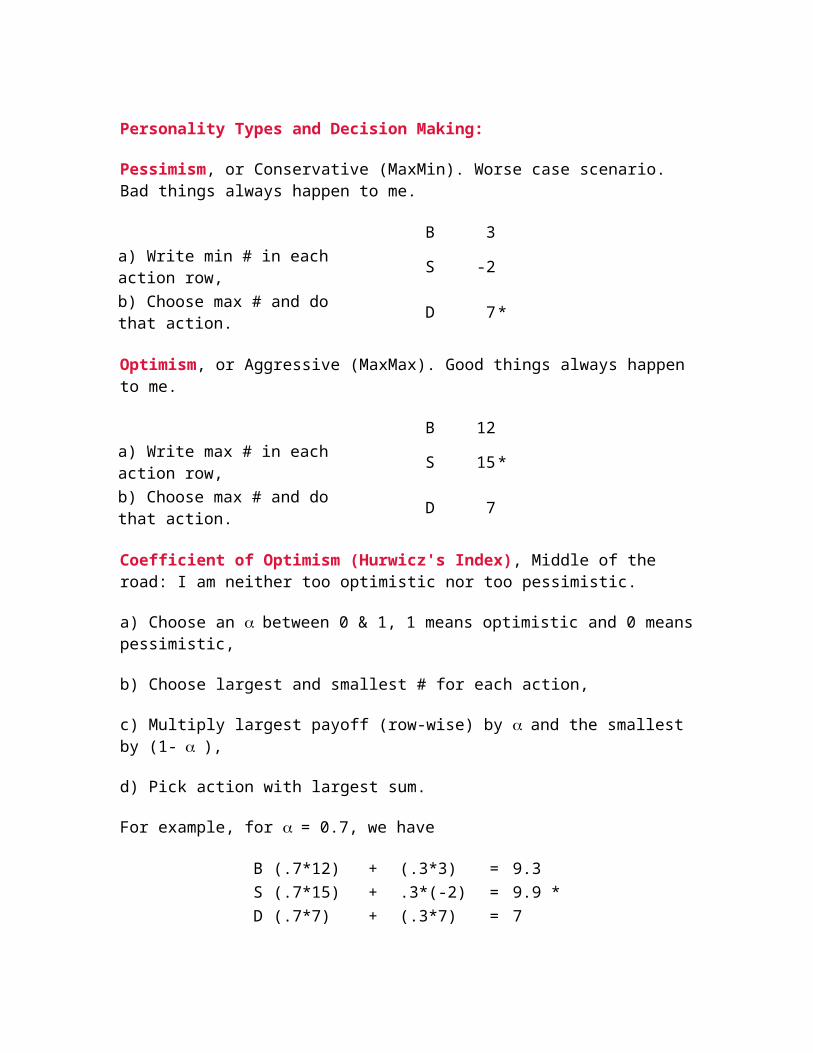
Personality Types and Decision Making:
Pessimism, or Conservative (MaxMin). Worse case scenario. Bad things always happen to me.
B 3a) Write min # in each action row, S -2b) Choose max # and do that action. D 7*
Optimism, or Aggressive (MaxMax). Good things always happen to me.
B 12a) Write max # in each action row, S 15* b) Choose max # and do that action. D 7
Coefficient of Optimism (Hurwicz's Index), Middle of the road: I am neither too optimistic nor too pessimistic.
a) Choose an between 0 & 1, 1 means optimistic and 0 means pessimistic,
b) Choose largest and smallest # for each action,
c) Multiply largest payoff (row-wise) by and the smallest by (1-),
Minimize Regret: (Savag's Opportunity Loss) I hate regrets and therefore I have to minimize my regrets. My decision should be made so that it is worth repeating. I should only do those things that I feel I could happily repeat. This reduces the chance that the outcome will make me feel regretful, or disappointed, or that it will be an unpleasant surprise.
Regret is the payoff on what would have been the best decision in the circumstances minus the payoff for the actual decision in the circumstances. Therefore, the first step is to setup the regret table:
a) Take the largest number in each states of nature column (say, L).b) Subtract all the numbers in that state of nature column from it (i.e. L - Xi,j).c) Choose maximum number of each action.d) Choose minimum number from step (d) and take that action.
You may try checking your computations using Decision Making Under Pure Uncertainty JavaScript, and then performing some numerical experimentation for a deeper understanding of the concepts.
Limitations of Decision Making under Pure Uncertainty
1. Decision analysis in general assumes that the decision-maker faces a decision problem where he or she must choose at least and at most one option from a set of options. In some cases this limitation can be overcome by formulating the decision making under uncertainty as a zero-sum two-person game.
2. In decision making under pure uncertainty, the decision-maker has no knowledge regarding which state of nature is "most likely" to happen. He or she is probabilistically ignorant concerning the state of nature therefore he or she cannot be optimistic or pessimistic. In such a case, the decision-maker invokes consideration of security.
3. Notice that any technique used in decision making under pure uncertainties, is appropriate only for the private life decisions. Moreover, the public person (i.e., you, the manager) has to have some knowledge of the state of nature in order to predict the probabilities of the various states of nature. Otherwise, the decision-maker is not capable of making a reasonable and defensible decision.
You might try to use Decision Making Under Uncertainty JavaScript E-lab for checking your computation, performing numerical experimentation for a deeper understanding, and stability analysis of your decision by altering the problem's parameters.
Further Readings:Biswas T., Decision Making Under Uncertainty, St. Martin's Press, 1997. Driver M., K. Brousseau, and Ph. Hunsaker, The Dynamic Decisionmaker: Five Decision Styles for Executive and Business Success, Harper & Row, 1990. Eiser J., Attitudes and Decisions, Routledge, 1988.Flin R., et al., (Ed.), Decision Making Under Stress: Emerging Themes and Applications, Ashgate Pub., 1997. Ghemawat P., Commitment: The Dynamic of Strategy, Maxwell Macmillan Int., 1991. Goodwin P., and G. Wright, Decision Analysis for Management Judgment, Wiley, 1998.
Decision Making Under Risk
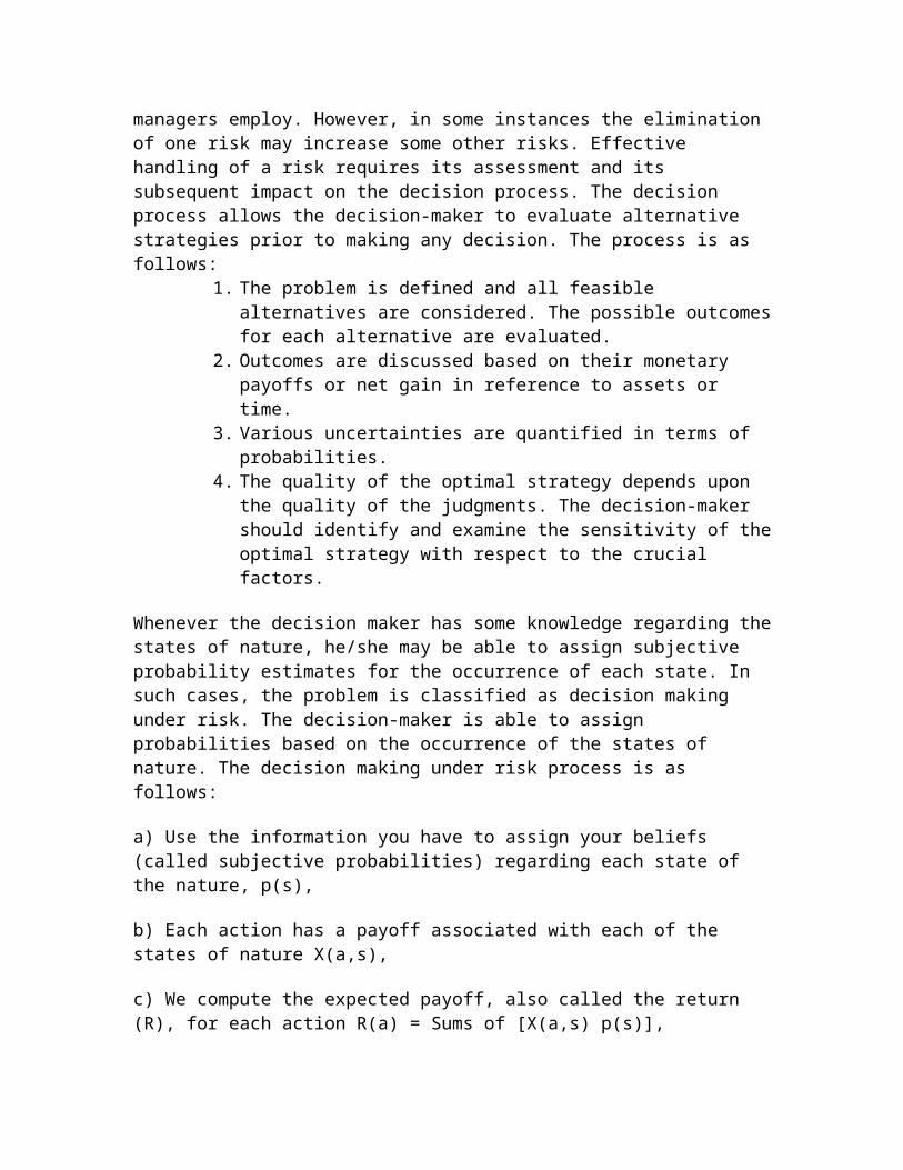
Risk implies a degree of uncertainty and an inability to fully control the outcomes or consequences of such an action. Risk or the elimination of risk is an effort that managers employ. However, in some instances the elimination of one risk may increase some other risks. Effective handling of a risk requires its assessment and its subsequent impact on the decision process. The decision process allows the decision-maker to evaluate alternative strategies prior to making any decision. The process is as follows:
1. The problem is defined and all feasible alternatives are considered. The possible outcomes for each alternative are evaluated.
2. Outcomes are discussed based on their monetary payoffs or net gain in reference to assets or time.
3. Various uncertainties are quantified in terms of probabilities.
4. The quality of the optimal strategy depends upon the quality of the judgments. The decision-maker should identify and examine the sensitivity of the optimal strategy with respect to the crucial factors.
Whenever the decision maker has some knowledge regarding the states of nature, he/she may be able to assign subjective probability estimates for the occurrence of each state. In such cases, the problem is classified as decision making under risk. The decision-maker is able to assign probabilities based on the occurrence of the states of nature. The decision making under risk process is as follows:
a) Use the information you have to assign your beliefs (called subjective probabilities) regarding each state of the nature, p(s),
b) Each action has a payoff associated with each of the states of nature X(a,s),
c) We compute the expected payoff, also called the return (R), for each action R(a) = Sums of [X(a,s) p(s)],
d) We accept the principle that we should minimize (or maximize) the expected payoff,
e) Execute the action which minimizes (or maximize) R(a).
Expected Payoff: The actual outcome will not equal the expected value. What you get is not what you expect, i.e. the "Great Expectations!"
a) For each action, multiply the probability and payoff and then,b) Add up the results by row,c) Choose largest number and take that action.
The Most Probable States of Nature (good for non-repetitive decisions)
a) Take the state of nature with the highest probability (subjectively break any ties), b) In that column, choose action with greatest payoff.
In our numerical example, there is a 40% chance of growth so we must buy stocks.
Expected Opportunity Loss (EOL):
a) Setup a loss payoff matrix by taking largest number in each state of nature column(say L), and subtract all numbers in that column from it, L - Xij,b) For each action, multiply the probability and loss then add up for each action,c) Choose the action with smallest EOL.
Loss Payoff MatrixG (0.4) MG (0.3) NC (0.2) L (0.1) EOL
Computation of the Expected Value of Perfect Information (EVPI)
EVPI helps to determine the worth of an insider who possesses perfect information. Recall that EVPI = EOL.
a) Take the maximum payoff for each state of nature,b) Multiply each case by the probability for that state of nature and then add them up,c) Subtract the expected payoff from the number obtained in step (b)
The efficiency of the perfect information is defined as 100 [EVPI/(Expected Payoff)]%
Therefore, if the information costs more than 1.3% of investment, don't buy it. For example, if you are going to invest $100,000, the maximum you should pay for the information is [100,000 * (1.3%)] = $1,300
I Know Nothing: (the Laplace equal likelihood principle) Every state of nature has an equal likelihood. Since I don't know anything about the nature, every state of nature is equally likely to occur:
a) For each state of nature, use an equal probability (i.e., a Flat Probability),b) Multiply each number by the probability,c) Add action rows and put the sum in the Expected Payoff column,d) Choose largest number in step (c) and perform that action.
A Discussion on Expected Opportunity Loss (Expected Regret): Comparing a decision outcome to its alternatives appears to be an important component of decision-making. One important factor is the emotion of regret. This occurs when a decision outcome is compared to the outcome that would have taken place had a different decision been made. This is in contrast to disappointment, which results from comparing one outcome to another as a result of the same decision. Accordingly, large contrasts with counterfactual results have a disproportionate influence on decision making.
Regret results compare a decision outcome with what might have been. Therefore, it depends upon the feedback available to decision makers as to which outcome the alternative option would have yielded. Altering the potential for regret by manipulating uncertainty resolution reveals that the decision-making behavior that appears to be risk averse can actually be attributed to regret aversion.
There is some indication that regret may be related to the distinction between acts and omissions. Some studies have found that regret is more intense following an action, than an omission. For example, in one study, participants concluded that a decision maker who switched stock funds from one company to another and lost money, would feel more regret than another decision maker who decided against switching the stock funds but also lost money. People usually assigned a higher value to an inferior outcome when it resulted from an act rather than from an omission. Presumably, this is as a way of counteracting the regret that could have resulted from the act.
You might like to use Making Risky Decisions JavaScript E-lab for checking your computation, performing numerical experimentation for a deeper understanding, and stability analysis of your decision by altering the problem's parameters.
Further Readings:Beroggi G., Decision Modeling in Policy Management: An Introduction to the Analytic Concepts, Boston, Kluwer Academic Publishers, 1999. George Ch., Decision Making Under Uncertainty: An Applied Statistics Approach, Praeger Pub., 1991.Rowe W., An Anatomy of Risk, R.E. Krieger Pub. Co., 1988.Suijs J., Cooperative Decision-Making Under Risk, Kluwer Academic, 1999.
Making a Better Decision by Buying Reliable Information (Bayesian Approach)
In many cases, the decision-maker may need an expert's judgment to sharpen his/her uncertainties with respect to the probable likelihood of each state of nature. For example, consider the following decision problem a company is facing concerning the development of a new product:
States of NatureHigh Sales Med. Sales Low SalesA(0.2) B(0.5) C(0.3)
The probabilities of the states of nature represent the decision-maker's (e.g. manager) degree of uncertainties and personal judgment on the occurrence of each state. We will refer to these subjective probability assessments as 'prior' probabilities.
so the company chooses A2 because of the expected loss associated with A1, and decides not to develop.
However, the manager is hesitant about this decision. Based on "nothing ventured, nothing gained" the company is thinking about seeking help from a marketing research firm. The marketing research firm will assess the size of the product's market by means of a survey.
Now the manager is faced with a new decision to make; which marketing research company should he/she consult? The manager has to make a decision as to how 'reliable' the consulting firm is. By sampling and then reviewing the past performance of the consultant, we can develop the following reliability matrix:
1. Given What Actually Happened in the PastA B C
2. What the Ap 0.8 0.1 0.1Consultant Bp 0.1 0.9 0.2Predicted Cp 0.1 0.0 0.7
All marketing research firms keep records (i.e., historical data) of the performance of their past predictions. These records are available to their clients free of charge. To construct a reliability matrix, you must consider the marketing research firm's performance records for similar products with high sales. Then, find the percentage of which products the marketing research firm correctly predicted would have high sales (A), medium sales (B), and little (C) or almost no sales. Their percentages are presented byP(Ap|A) = 0.8, P(Bp|A) = 0.1, P(Cp|A) = 0.1,in the first column of the above table, respectively. Similar analysis should be conducted to construct the remaining columns of the reliability matrix.
Note that for consistency, the entries in each column of the above reliability matrix should add up to one. While this matrix provides the conditional probabilities such as P(Ap|A) = 0.8, the important information the company needs is the reverse form of these conditional probabilities. In this example, what is the numerical value of P(A|Ap)? That is, what is the chance that the marketing firm predicts A is going to happen, and A actually will happen? This important information can be obtained by applying the Bayes Law (from your probability and statistics course) as follows:
a) Take probabilities and multiply them "down" in the above matrix, b) Add the rows across to get the sum,c) Normalize the values (i.e. making probabilities adding up to 1) by dividing each column number by the sum of the row found in Step b,
You might like to use Computational Aspect of Bayse' Revised Probability JavaScript E-lab for checking your computation, performing numerical experimentation for a deeper understanding, and stability analysis of your decision by altering the problem's parameters.
d) Draw the decision tree. Many managerial problems, such as this example, involve a sequence of decisions. When a decision situation requires a series of decisions, the payoff table cannot accommodate the multiple layers of decision-making. Thus, a decision tree is needed.
Do not gather useless information that cannot change a decision: A question for you: In a game a player is presented two envelopes containing money. He is told that one envelope contains twice as much money as the other envelope, but he does not know which one contains the larger amount. The player then may pick one envelope at will, and after he has made a decision, he is offered to exchange his envelope with the other envelope.If the player is allowed to see what's inside the envelope he has selected at first, should the player swap, that is, exchange the envelopes? The outcome of a good decision may not be good, therefor one must not confuse the quality of the outcome with the quality of the decision. As Seneca put it "When the words are clear, then the thought will be also".
Decision Tree and Influence Diagram
Decision Tree Approach: A decision tree is a chronological representation of the decision process. It utilizes a network of two types of nodes: decision (choice) nodes (represented by square shapes), and states of nature (chance) nodes (represented by circles). Construct a decision tree utilizing the logic of the problem. For the chance nodes, ensure that the probabilities along any outgoing branch sum to one. Calculate the expected payoffs by rolling the tree backward (i.e., starting at the right and working toward the left).
You may imagine driving your car; starting at the foot of the decision tree and moving to the right along the branches. At each square you have control, to make a decision and then turn the wheel of your car. At each circle, Lady Fortuna takes over the wheel and you are powerless.
Here is a step-by-step description of how to build a decision tree:
1. Draw the decision tree using squares to represent decisions and circles to represent uncertainty,
2. Evaluate the decision tree to make sure all possible outcomes are included, 3. Calculate the tree values working from the right side back to the left, 4. Calculate the values of uncertain outcome nodes by multiplying the value
of the outcomes by their probability (i.e., expected values).
On the tree, the value of a node can be calculated when we have the values for all the nodes following it. The value for a choice node is the largest value of all nodes immediately following it. The value of a chance node is the expected value of the nodes following that node, using the probability of the arcs. By rolling the tree backward, from its branches toward its root, you can compute the value of all nodes including the root of the tree. Putting these numerical results on the decision tree results in the following graph:
A Typical Decision TreeClick on the image to enlarge it
Determine the best decision for the tree by starting at its root and going forward.
Based on proceeding decision tree, our decision is as follows:
Hire the consultant, and then wait for the consultant's report. If the report predicts either high or medium sales, then go ahead and manufacture the product. Otherwise, do not manufacture the product.
Check the consultant's efficiency rate by computing the following ratio:
(Expected payoff using consultant dollars amount) / EVPI.
Using the decision tree, the expected payoff if we hire the consultant is:
EP = 1000 - 500 = 500,
EVPI = .2(3000) + .5(2000) + .3(0) = 1600.
Therefore, the efficiency of this consultant is: 500/1600 = 31%
If the manager wishes to rely solely on the marketing research firm's recommendations, then we assign flat prior probability [as opposed to (0.2, 0.5, 0.3) used in our numerical example].
Clearly the manufacturer is concerned with measuring the risk of the above decision, based on decision tree.
Coefficient of Variation as Risk Measuring Tool and Decision Procedure: Based on the above decision, and its decision-tree, one might develop a coefficient of variation (C.V) risk-tree, as depicted below:
Coefficient of Variation as a Risk Measuring Tool and Decision ProcedureClick on the image to enlarge it
Notice that the above risk-tree is extracted from the decision tree, with C.V. numerical value at the nodes relevant to the recommended decision. For example the consultant fee is already subtracted from the payoffs.
From the above risk-tree, we notice that this consulting firm is likely (with probability 0.53) to recommend Bp (a medium sales), and if you decide to manufacture the product then the resulting coefficient of variation is very high (403%), compared with the other branch of the tree (i.e., 251%).
Clearly one must not consider only one consulting firm, rather one must consider several potential consulting during decision-making planning stage. The risk decision tree then is a necessary tool to construct for each consulting firm in order to measure and compare to arrive at the final decision for implementation.
The Impact of Prior Probability and Reliability Matrix on Your Decision: To study how important your prior knowledge and/or the accuracy of the expected information from the consultant in your decision our numerical example, I suggest redoing the above numerical example in performing some numerical sensitivity analysis. You may start with the following extreme and interesting cases by using this JavaScript for the needed computation:
Consider a flat prior, without changing the reliability matrix. Consider a perfect reliability matrix (i.e., with an identity matrix), without
Consider a perfect prior, without changing the reliability matrix. Consider a flat reliability matrix (i.e., with all equal elements), without
changing the prior. Consider the consultant prediction probabilities as your own prior, without
changing the reliability matrix.
Influence diagrams: As can be seen in the decision tree examples, the branch and node description of sequential decision problems often become very complicated. At times it is downright difficult to draw the tree in such a manner that preserves the relationships that actually drive the decision. The need to maintain validation, and the rapid increase in complexity that often arises from the liberal use of recursive structures, have rendered the decision process difficult to describe to others. The reason for this complexity is that the actual computational mechanism used to analyze the tree, is embodied directly within the trees and branches. The probabilities and values required to calculate the expected value of the following branch are explicitly defined at each node.
Influence diagrams are also used for the development of decision models and as an alternate graphical representations of decision trees. The following figure depicts an influence diagram for our numerical example.
In the influence diagram above, the decision nodes and chance nodes are similarly illustrated with squares and circles. Arcs (arrows) imply relationships, including probabilistic ones.
Finally, decision tree and influence diagram provide effective methods of decision-making because they:
Clearly lay out the problem so that all options can be challenged Allow us to analyze fully the possible consequences of a decision Provide a framework to quantify the values of outcomes and the
probabilities of achieving them
Help us to make the best decisions on the basis of existing information and best guesses
Visit also:Decision Theory and Decision Trees
Further ReadingsBazerman M., Judgment in Managerial Decision Making, Wiley, 1993. Connolly T., H. Arkes, and K. Hammond (eds), Judgment and Decision Making: An Interdisciplinary Reader, Cambridge University Press, 2000. Cooke R., Experts in Uncertainty, Oxford Univ Press, 1991. Describes much of the history of the expert judgment problem. It also includes many of the methods that have been suggested to do numerical combination of expert uncertainties. Furthermore, it promotes a method that has been used extensively by us and many others, in which experts are given a weighting that judge their performance on calibration questions. This is a good way of getting around the problem of assessing the "quality" of an expert, and lends a degree of objectivity to the results that is not obtained by other methods. Bouyssou D., et al., Evaluation and Decision Models: A Critical Perspective, Kluwer Academic Pub, 2000. Daellenbach H., Systems and Decision Making: A Management Science Approach, Wiley, 1994.Goodwin P., and G. Wright, Decision Analysis for Management Judgment, Wiley, 1998.Klein D., Decision-Analytic Intelligent Systems: Automated Explanation and Knowledge Acquisition, Lawrence Erlbaum Pub., 1994. Thierauf R., Creative Computer Software for Strategic Thinking and Decision Making: A Guide for Senior Management and MIS Professionals, Quorum Books, 1993.
Why Managers Seek the Advice From Consulting Firms
Managers pay consultants to provide advisory service work that falls into one of the following categories:
Work they are not -- or feel they are not — competent to do themselves.
Work they do not want to do themselves. Work they do not have time to do themselves.
All such work falls under the broad umbrella of consulting service. Regardless of why managers pay others to advise them, they typically have high expectations concerning the quality of the recommendations, measured in terms of reliability and cost. However, the manager is solely responsible for the final decision he/she is making and not the consultants.
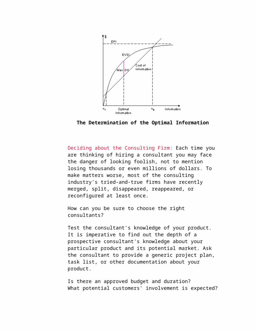
The following figure depicts the process of the optimal information determination. For more details, read the Cost/Benefit Analysis.
Deciding about the Consulting Firm: Each time you are thinking of hiring a consultant you may face the danger of looking foolish, not to mention losing thousands or even millions of dollars. To make matters worse, most of the consulting industry's tried-and-true firms have recently merged, split, disappeared, reappeared, or reconfigured at least once.
How can you be sure to choose the right consultants?
Test the consultant's knowledge of your product. It is imperative to find out the depth of a prospective consultant's knowledge about your particular product and its potential market. Ask the consultant to provide a generic project plan, task list, or other documentation about your product.
Is there an approved budget and duration?What potential customers' involvement is expected?Who is expected to provide the final advice and provide sign-off?
Even the best consultants are likely to have some less-than-successful moments in their work history. Conducting the reliability analysis process is essential. Ask specific questions about the consultants' past projects, proud moments, and failed efforts. Of course it's important to check a potential consultant's references. Ask for specific referrals from as many previous clients or firms with similar businesses to yours. Get a clearly written contract, accurate cost estimates, the survey statistical sample size, and the commitment on the completion and written advice on time.
Further ReadingHoltz H., The Complete Guide to Consulting Contracts: How to Understand, Draft, and Negotiate Contracts and Agreements that Work, Dearborn Trade, 1997.Weinberg G., Secrets of Consulting: A Guide to Giving and Getting Advice Successfully, Dorset House, 1986.
Revising Your Expectation and its Risk
In our example, we saw how to make decision based on objective payoff matrix by computing the expected value and the risk expressed as coefficient of variation as our decision criteria. While, an informed decision-maker might be able to construct his/her subjective payoff matrix, and then following the same decision process, however, in many situations it becomes necessary to combine the two.
Application: Suppose the following information is available from two independent sources:
Revising the Expected Value and the Variance
Estimate Source Expected value Variance
Sales manager 1 = 110 12 = 100
Market survey 2 = 70 22 = 49
The combined expected value is:
[1/12 + 2/2
2 ] / [1/12 + 1/2
2] The combined variance is:
2 / [1/12 + 1/2
2] For our application, using the above tabular information, the combined estimate of expected sales is 83.15 units with combined variance of 65.77, having 9.6% risk value.
You may like using Revising the Mean and Variance JavaScript to performing some numerical experimentation. You may apply it for validating the above example and for a deeper understanding of the concept where more than 2-sources of information are to be combined.
Determination of the Decision-Maker's Utility Function
We have worked with payoff tables expressed in terms of expected monetary value. Expected monetary value, however, is not always the best criterion to use in decision making. The value of money varies from
situation to situation and from one decision maker to another. Generally, too, the value of money is not a linear function of the amount of money. In such situations, the analyst should determine the decision-maker's utility for money and select the alternative course of action that yields the highest expected utility, rather than the highest expected monetary value.
Individuals pay insurance premiums to avoid the possibility of financial loss associated with an undesirable event occurring. However, utilities of different outcomes are not directly proportional to their monetary consequences. If the loss is considered to be relatively large, an individual is more likely to opt to pay an associated premium. If an individual considers the loss inconsequential, it is less likely the individual will choose to pay the associated premium.
Individuals differ in their attitudes towards risk and these differences will influence their choices. Therefore, individuals should make the same decision each time relative to the perceived risk in similar situations. This does not mean that all individuals would assess the same amount of risk to similar situations. Further, due to the financial stability of an individual, two individuals facing the same situation may react differently but still behave rationally. An individual's differences of opinion and interpretation of policies can also produce differences.
The expected monetary reward associated with various decisions may be unreasonable for the following two important reasons:
1. Dollar value may not truly express the personal value of the outcome. This is what motivates some people to play the lottery for $1.
2. Expected monetary values may not accurately reflect risk aversion. For example, suppose you have a choice of between getting $10 dollars for doing nothing, or participating in a gamble. The gamble's outcome depends on the toss of a fair coin. If the coin comes up heads, you get $1000. However, if it is tails, you take a $950 loss.
The first alternative has an expected reward of $10, the second has an expected reward of0.5(1000) + 0.5(- 950) = $25. Clearly, the second choice is preferred to the first if expected monetary reward were a reasonable criterion. But, you may prefer a sure $10 to running the risk of losing $950.
Why do some people buy insurance and others do not? The decision-making process involves psychological and economical factors, among others. The utility concept is an attempt to measure the usefulness of money for the individual decision maker. It is measured in 'Utile'. The utility concept enables us to explain why, for example, some people buy
one dollar lotto tickets to win a million dollars. For these people 1,000,000 ($1) is less than ($1,000,000). These people value the chance to win $1,000,000 more than the value of the $1 to play. Therefore, in order to make a sound decision considering the decision-maker's attitude towards risk, one must translate the monetary payoff matrix into the utility matrix. The main question is: how do we measure the utility function for a specific decision maker?
Consider our Investment Decision Problem. What would the utility of $12 be?
a) Assign 100 utils and zero utils to the largest and smallest ($) payoff, respectively in the payoff matrix. For our numerical example, we assign 100 utils to 15, and 0 utils to -2,
b) Ask the decision maker to choose between the following two scenarios:
1) Get $12 for doing nothing (called, the certainty equivalent, the difference between a decision maker's certainty equivalent and the expected monetary value is called the risk premium.)
OR
2) Play the following game: win $15 with probability (p) OR -$2 with probability (1-p), where p is a selected number between 0 and 1.
By changing the value of p and repeating a similar question, there exists a value for p at which the decision maker is indifferent between the two scenarios. Say, p = 0.58.
c) Now, the utility for $12 is equal to0.58(100) + (1-0.58)(0) = 58.
d) Repeat the same process to find the utilities for each element of the payoff matrix. Suppose we find the following utility matrix:
Monetary Payoff Matrix Utility Payoff MatrixA B C D A B C D12 8 7 3 58 28 20 1315 9 5 -2 100 30 18 07 7 7 7 20 20 20 20
At this point, you may apply any of the previously discussed techniques to this utility matrix (instead of monetary) in order to make a satisfactory decision. Clearly, the decision could be different.
Notice that any technique used in decision making with utility matrix is indeed very subjective; therefore it is more appropriate only for the private life decisions.
You may like to check your computations using Determination of Utility Function JavaScript, and then perform some numerical experimentation for a deeper understanding of the concepts.
Utility Function Representations with Applications
Introduction: A utility function transforms the usefulness of an outcome into a numerical value that measures the personal worth of the outcome. The utility of an outcome may be scaled between 0, and 100, as we did in our numerical example, converting the monetary matrix into the utility matrix . This utility function may be a simple table, a smooth continuously increasing graph, or a mathematical expression of the graph.
The aim is to represent the functional relationship between the entries of monetary matrix and the utility matrix outcome obtained earlier. You may ask what is a function?
What is a function? A function is a thing that does something. For example, a coffee grinding machine is a function that transforms the coffee beans into powder. A utility function translates (converts) the input domain (monetary values) into output range, with the two end-values of 0 and 100 utiles. In other words, a utility function determines the degrees of the decision-maker sensible preferences.
This chapter presents a general process for determining utility function. The presentation is in the context of the previous chapter's numerical results, although there are repeated data therein.
Utility Function Representations with Applications: There are three different methods of representing a function: The Tabular, Graphical, and Mathematical representation. The selection of one method over another depends on the mathematical skill of the decision-maker to understand and use it easily. The three methods are evolutionary in their construction process, respectively; therefore, one may proceed to the next method if needed.
The utility function is often used to predict the utility of the decision-maker for a given monetary value. The prediction scope and precision increases form the tabular method to the mathematical method.
Tabular Representation of the Utility Function: We can tabulate the pair of data (D, U) using the entries of the matrix representing the monetary values (D) and their corresponding utiles (U) from the utility matrix obtained already. The Tabular Form of the utility function for our numerical example is given by the following paired (D, U) table:
Utility Function (U) of the Monetary Variable (D) in Tabular Form
Tabular Representation of the Utility Function for the Numerical Example
As you see, the tabular representation is limited to the numerical values within the table. Suppose one wishes to obtain the utility of a dollar value, say $10. One may apply an interpolation method: however since the utility function is almost always non-linear; the interpolated result does not represent the utility of the decision maker accurately. To overcome this difficulty, one may use the graphical method.
Graphical Representation of the Utility Function: We can draw a curve using a scatter diagram obtained by plotting the Tabular Form on a graph paper. Having the scatter diagram, first we need to decide on the shape of the utility function. The utility graph is characterized by its properties of being smooth, continuous, and an increasing curve. Often a parabola shape function fits well for relatively narrow domain values of D variable. For wider domains, one may fit few piece-wise parabola functions, one for each appropriate sub-domain.
For our numerical example, the following is a graph of the function over the interval used in modeling the utility function, plotted with its associated utility (U-axis) and the associated Dollar values (D-axis). Note that in the scatter diagram the multiple points are depicted by small circles.
Graphical Representation of the Utility Function for the Numerical Example
The graphical representation has a big advantage over the tabular representation in that one may read the utility of dollar values say $10, directly from the graph, as shown on the above graph, for our numerical example. The result is U = 40, approximately. Reading a value from a graph is not convenient; therefore, for prediction proposes, a mathematical model serves best.
Mathematical Representation of the Utility Function: We can construct a mathematical model for the utility function using the shape of utility function obtained by its representation by Graphical Method. Often a parabola shape function fits well for relatively narrow domain values of D variable. For wider domains, one may fit a few piece-wise parabola functions, one for each appropriate sub-domain.
We know that we want a quadratic function that best fits the scatter diagram that has already been constructed. Therefore, we use a regression analysis to estimate the coefficients in the function that is the best fit to the pairs of data (D, U).
Parabola models: Parabola regressions have three coefficients with a general form:
b = [(Di- Dbar) Ui]/[(Di - Dbar)2] - 2cDbar a = {Ui - [c(D i - Dbar) 2)}/n - (cDbarDbar + bDbar),
where Dbar is the mean of Di's.
For our numerical example i = 1, 2,..., 12. By evaluating these coefficients using the information given in tabular form section, the "best" fit is characterized by its coefficients estimated values: c = 0.291, b = 1.323, and a = 0.227. The result is; therefore, a utility function approximated by the following quadratic function:
U = 0.291D2 + 1.323D + 0.227, for all D such that -2 D 15. The above mathematical representation provides more useful information than the other two methods. For example, by taking the derivative of the function provides the marginal value of the utility; i.e.,
Marginal Utility = 1.323 + 0.582D, for all D such that -2 D 15. Notice that for this numerical example, the marginal utility is an increasing function, because variable D has a positive coefficient; therefore, one is able to classify this decision- maker as a mild risk-taker.
You might like to use Quadratic Regression JavaScript to check your hand computation. For higher degrees than quadratic, you may like to use the Polynomial Regressions JavaScript.
A Classification of Decision Maker's Relative Attitudes Toward Risk and Its Impact
Probability of an Event and the Impact of its Occurrence: The process-oriented approach of managing the risk and uncertainty is part of any probabilistic modeling. It allows the decision maker to examine the risk within its expected return, and identify the critical issues in assessing, limiting, and mitigating risk. This process involves both the qualitative and quantitative aspects of assessing the impact of risk.
Decision theory does not describe what people actually do since there are difficulties with both computations of probability and the utility of an outcome. Decisions can also be affected by people's subjective rationality and by the way in which a decision problem is perceived.
Traditionally, the expected value of random variables has been used as a major aid to quantify the amount of risk. However, the expected value is not necessarily a good measure alone by which to make decisions since it blurs the distinction between probability and severity. To demonstrate this, consider the following example:
Suppose that a person must make a choice between scenarios 1 and 2 below:
Scenario 1: There is a 50% chance of a loss of $50, and a 50% chance of no loss.
Scenario 2: There is a 1% chance of a loss of $2,500, and a 99% chance of no loss.
Both scenarios result in an expected loss of $25, but this does not reflect the fact that the second scenario might be considered to be much more risky than the first. (Of course, this is a subjective assessment). The decision maker may be more concerned about minimizing the effect of the occurrence of an extreme event than he/she is concerned about the mean. The following charts depict the complexity of probability of an event and
the impact of the occurrence of the event, and its related risk indicator, respectively:
From the previous section, you may recall that the certainty equivalent is the risk free payoff. Moreover, the difference between a decision maker's certainty equivalent and the expected monetary value (EMV) is called the risk premium. We may use the sign and the magnitude of the risk premium in classification of a decision maker's relative attitude toward risk as follows:
If the risk premium is positive, then the decision maker is willing to take the risk and the decision maker is said to be a risk seeker. Clearly, some people are more risk-accepting than others: the larger is the risk premium, the more risk-accepting the decision-maker.
If the risk premium is negative, then the decision-maker would avoid taking the risk and the decision maker is said to be risk averse.
If the risk premium is zero, then the decision maker is said to be risk neutral.
Buying Insurance: As we have noticed, often it is not probability, but expectation that acts a measuring tool and decision-guide. Many decision cases are similar to the following: The probability of a fire in your neighborhood may be very small. But, if it occurred, the cost to you could
be very great. Not only property but also your "dear ones", so the negative expectation of not ensuring against fire is so much greater than the cost of premium than ensuring is the best.
Further ReadingsChristensen C., The Innovator's Dilemma: When New Technologies Cause Great Firms to Fail, Harvard Business School Publishing, 1997. Eilon S., The Art of Reckoning: Analysis of Performance Criteria, Academic Press, 1984. Hammond J., R. Keeney, and H. Raiffa, Smart Choices: A Practical Guide to Making Better Decisions, Harvard Business School Press., 1999.Richter M., and K. Wong, Computable preference and utility, Journal of Mathematical Economics, 32(3), 339-354, 1999.Tummala V., Decision Analysis with Business Applications, Educational Publishers, 1973.
The Discovery and Management of Losses
In discovery and management of losses (expressed in the monetary terms) perception and measuring the chance of events is crucial. Losses might have various sources. These sources include Employees, Procedures, and External factors.
Employees: Some employees may have concentration problem, insufficient knowledge, and engage in fraud.
Procedures: Some procedures are wrongly designed, or they are wrongly implemented.
External factors: These include dependency on external unreliable services and suppliers, lack of security form external criminal activities, and finally disasters, such as strong earthquakes.
A rare or unexpected event with potentially significant consequences for decision-making could be conceived as a risk or an opportunity. The main concerns are: How to predict, identify or explain chance events and their consequences? How to assess, prepare for or manage them?
A decision-maker who is engaged in planning, needs to adopt a view for the future, in order to decide goals, and to decide the best sequence of actions to achieve these goals by forecasting their consequences. Unfortunately, the unlikeness of such events makes them difficult to predict or explain by methods that use historical data. However, focusing on the decision-maker's psychological-attitude factors and its environment is mostly relevant.
The following figure provides a classification of the loss frequency function together with the ranges for the Expected, Unexpected, and the Stress, which must be determined by the decision-makers ability and resources.
The manager's ability to discover both unexpected and stress loss events and forecast their consequences is the major task. This is because, these event are very unlikely, therefore making them difficult to predict or explain. However, once a rare event has been identified, the main concern is its consequences for the organization. A good manager cannot ignore these events, as their consequences are significant. For example, although strong earthquakes occur in major urban centers only rarely such earthquakes tend to have human and economic consequences well beyond that of the typical tremor. A rational public safety body for a city in an earthquake-prone area would plan for such contingencies even though the chance of a strong quake is still very small.
Further ReadingsBelluck D., and S. Benjamin, A Practical Guide to Understanding, Managing and Reviewing Risk Assessment Reports, CRC Press, 1999.Koller G., Risk Assessment and Decision Making in Business and Industry: A Practical Guide, CRC Press, 1999.Hoffman D., Managing Operational Risk: 20 Firmwide Best Practice Strategies, Wiley, 2002Van Asselt M., Perspectives on Uncertainty and Risk: The Prima Approach to Decision Support, Kluwer Academic Publishers, 2000.
Risk Assessment & Coping Strategies:How Good Is Your Decision?
Risk is the downside of a gamble, which is described in terms of probability. Risk assessment is a procedure of quantifying the loss or gain values and supplying them with proper values of probabilities. In other words, risk assessment means constructing the random variable that describes the risk. Risk indicator is a quantity describing the quality of the decision.
The states of nature are the states of economy during, an arbitrary time frame, as in one year.
The expected value (i.e., the averages) is defined by:
Expected Value = = Xi . Pi, the sum is over all i's.
The expected value alone is not a good indication of a quality decision. The variance must be known so that an educated decision may be made. Have you ever heard the dilemma of the six-foot tall statistician who drowned in a stream that had an average depth of three feet?
In the investment example, it is also interesting to compare the 'risk' between alternative courses of action. A measure of risk is generally reported by variation, or its square root called standard deviation. Variation or standard deviation are numerical values that indicate the variability inherent to your decision. For risk, smaller values indicate that what you expect is likely to be what you get. Therefore, risk must also be used when you want to compare alternate courses of action. What we desire is a large expected return, with small risk. Thus, high risk makes a manager very worried.
Variance: An important measure of risk is variance which is defined by:
Variance = 2 = [Xi2 . Pi] - 2, the sum is over all i's.
Since the variance is a measure of risk, therefore, the greater the variance, the higher the risk. The variance is not expressed in the same units as the expected value. So, the variance is hard to understand and explain as a result of the squared term in its computation. This can be alleviated by working with the square root of the variance which is called the Standard Deviation:
Standard Deviation = = (Variance) ½
Both variance and standard deviation provide the same information and, therefore, one can always be obtained from the other. In other words, the process of computing standard deviation always involves computing the
variance. Since standard deviation is the square root of the variance, it is always expressed in the same units as the expected value.
For the dynamic decision process, the Volatility as a measure for risk includes the time period over which the standard deviation is computed. The Volatility measure is defined as standard deviation divided by the square root of the time duration.
What should you do if the course of action with the larger expected outcome also has a much higher risk? In such cases, using another measure of risk known as the Coefficient of Variation is appropriate.
Coefficient of Variation (CV) is the relative risk, with respect to the expected value, which is defined as:
Coefficient of Variation (CV) is the absolute relative deviation with respect to size provided is not zero, expressed in percentage:
CV =100 |S/ | %
Notice that the CV is independent from the expected value measurement. The coefficient of variation demonstrates the relationship between standard deviation and expected value, by expressing the risk as a percentage of the (non-zero) expected value. The inverse of CV (namely 1/CV) is called the Signal-to-Noise Ratio.
The quality of your decision may be computed by using Measuring Risk.
The following table shows the risk measurements computed for the Investment Decision Example:
Risk AssessmentG(0.4) MG(0.3) NC(0.2) L(0.1) Exp. Value St. Dev. C. V.
The Risk Assessment columns in the above table indicate that bonds are much less risky than the stocks, while its return is lower. Clearly, deposits are risk free.
Now, the final question is: Given all this relevant information, what action do you take? It is all up to you.
The following table shows the risk measurements computed for the Investment Decision under pure uncertainty (i.e., the Laplace equal likelihood principle):
The Risk Assessment columns in the above table indicate that bonds are much less risky than the stocks. Clearly, deposits are risk free.
Again, the final question is: Given all this relevant information, what action do you take? It is all up to you.
Ranking Process for Preference among Alternatives: Referring to the Bonds and Stocks alternatives in our numerical example, we notice that based in mean-variance, the Bonds alternative Dominates the Stocks alternative. However this is not always the case.
For example, consider two independent investment alternatives: Investment I and Investment II with the characteristics outlined in the following table:
Two Investments PortfoliosInvestment I Investment II
To rank these two investments under the Standard Dominance Approach in Finance, first we must compute the mean and standard deviation and then analyze the results. Using the above Applet for calculation, we notice that the Investment I has mean = 6.75% and standard deviation = 3.9%, while the second investment has mean = 5.36% and standard deviation = 2.06%. First observe that under the usual mean-variance analysis, these two investments cannot be ranked. This is because the first investment has the greater mean; it also has the greater standard deviation. Therefore, the Standard Dominance Approach is not a useful tool here. We have to resort to the coefficient of variation as a systematic basis of comparison. The
C.V. for Investment I is 57.74% and for investment II is 38.43%. Therefore, Investment II has preference over the other one. Clearly, this approach can be used to rank any number of alternative investments.
Application of Signal-to-Noise Ratio In Investment Decisions: Suppose you have several portfolios, which are almost uncorrelated (i.e., all paired-wise covariance's are almost equal to zero), then one may distributed the total capital among all portfolios proportional to their signal-to-noise ratios.
For Negatively Correlated portfolios you may use the Beta Ratio, or Bivariate Discrete Distributions Javascript.
Consider the above two independent investments with the given probabilistic rate of returns. Given you wish to invest $12,000 over a period of one year, how do you invest for the optimal strategy?
The C.V. for Investment-I is 57.74% and for investment-II is 38.43%, therefore signal-to-noise ratio are 1/55.74 = 0.0179 and 1/38.43 = 0.0260, respectively.
Now, one may distribute the total capital ($12000) proportional to the Beta values:
Sum of signal-to-noise ratios = 0.0179 + 0.0260 = 0.0439
Y1 = 12000 (0.0179 / 0.0439) = 12000(0.4077) = $4892, Allocating to the investment-I
Y2 = 12000 (0.0260 / 0.0439) = 12000(0.5923) = $7108, Allocating to the investment-II
That is, the optimal strategic decision based upon the signal-to-noise ratio criterion is: Allocate $4892 and $7108 to the investment-I and investment-II, respectively.These kinds of mixed-strategies are known as diversifications that aim at reducing your risky.
The quality of your decision may be computed by using Performance Measures for Portfolios.
Copping with Risk
Risk avoidance is refusing to undertake an activity where the risk seems too costly.
Risk prevention (loss control) is using various methods to reduce the possibility of a loss occurring.
Risk transfer is shifting a risk to someone outside your company. Risk assumption or self-insurance is setting aside funds to meet
losses that are uncertain in size and frequency. Risk reduction by, for example, diversifications.
Further Readings:Crouhy M., R. Mark, and D. Galai, Risk Management, McGraw-Hill, 2002.Koller G., Risk Modeling for Determining Value and Decision Making, Chapman & Hall/CRC, 2000.Moore P., The Business of Risk, Cambridge University Press, 1984.Morgan M., and M. Henrion, Uncertainty: A Guide to Dealing with Uncertainty in Quantitative Risk and Policy Analysis, Cambridge University Press, 1998. Shapira Z., Risk Taking: A Managerial Perspective, Russell Sage Foundation, 1997.Vose D., Risk Analysis: A Quantitative Guide, John Wiley & Sons, 2000.Wahlstrom B., Models, Modeling And Modellers: An Application to Risk Analysis, European Journal of Operations Research, Vol. 75, No. 3, 477-487, 1994.
Time series Analysis
Time-Critical Decision Modeling and AnalysisThe ability to model and perform decision modeling and analysis is an essential feature of many real-world applications ranging from emergency medical treatment in intensive care units to military command and control systems. Existing formalisms and methods of inference have not been effective in real-time applications where tradeoffs between decision quality and computational tractability are essential. In practice, an effective approach to time-critical dynamic decision modeling should provide explicit support for the modeling of temporal processes and for dealing with time-critical situations.
One of the most essential elements of being a high-performing manager is the ability to lead effectively one's own life, then to model those leadership skills for employees in the
organization. This site comprehensively covers theory and practice of most topics in forecasting and economics. I believe such a comprehensive approach is necessary to fully understand the subject. A central objective of the site is to unify the various forms of business topics to link them closely to each other and to the supporting fields of statistics and economics. Nevertheless, the topics and coverage do reflect choices about what is important to understand for business decision making.
Almost all managerial decisions are based on forecasts. Every decision becomes operational at some point in the future, so it should be based on forecasts of future conditions.
Forecasts are needed throughout an organization -- and they should certainly not be produced by an isolated group of forecasters. Neither is forecasting ever "finished". Forecasts are needed continually, and as time moves on, the impact of the forecasts on actual performance is measured; original forecasts are updated; and decisions are modified, and so on.
For example, many inventory systems cater for uncertain demand. The inventory parameters in these systems require estimates of the demand and forecast error distributions. The two stages of these systems, forecasting and inventory control, are often examined independently. Most studies tend to look at demand forecasting as if this were an end in itself, or at stock control models as if there were no preceding stages of computation. Nevertheless, it is important to understand the interaction between demand forecasting and inventory control since this influences the performance of the inventory system. This integrated process is shown in the following figure:
The decision-maker uses forecasting models to assist him or her in decision-making process. The decision-making often uses the modeling process to investigate the impact of different courses of action retrospectively; that is, "as if" the decision has already been made under a course of action. That is why the sequence of steps in the modeling process, in the above figure must be considered in reverse order. For example, the output (which is the result of the action) must be considered first.
It is helpful to break the components of decision making into three groups: Uncontrollable, Controllable, and Resources (that defines the problem situation). As indicated in the above activity chart, the decision-making process has the following components:
1. Performance measure (or indicator, or objective): Measuring business performance is the top priority for managers. Management by objective works if you know the objectives. Unfortunately, most business managers do not know explicitly what it is. The development of effective performance measures is seen as increasingly important in almost all organizations. However, the challenges of achieving this in the public and for non-profit sectors are arguably considerable. Performance measure provides the desirable level of outcome, i.e., objective of your decision. Objective is important in identifying the forecasting activity. The following table provides a few examples of performance measures for different levels of management:
Level Performance Measure
Strategic Return of Investment, Growth, and Innovations
Tactical Cost, Quantity, and Customer satisfaction
Operational Target setting, and Conformance with standard
2. Clearly, if you are seeking to improve a system's performance, an operational view is really what you are after. Such a view gets at how a forecasting system really works; for example, by what correlation its past output behaviors have generated. It is essential to understand how a forecast system currently is working if you want to change how it will work in the future. Forecasting activity is an iterative process. It starts with effective and efficient planning and ends in compensation of other forecasts for their performance
3. What is a System? Systems are formed with parts put together in a particular manner in order to pursue an objective. The relationship between the parts determines what the system does and how it functions as a whole. Therefore, the relationships in a system are often more important than the individual parts. In general, systems that are building blocks for other systems are called subsystems
4. The Dynamics of a System: A system that does not change is a static system. Many of the business systems are dynamic systems, which mean their states change over time. We refer to the way a system changes over time as the system's behavior. And when the system's development follows a typical pattern, we say the system has a behavior pattern. Whether a system is static or dynamic depends on which time horizon you choose and on which variables you concentrate. The time horizon is the time period within which you study the system. The variables are changeable values on the system.
5. Resources: Resources are the constant elements that do not change during the time horizon of the forecast. Resources are the factors that define the decision
problem. Strategic decisions usually have longer time horizons than both the Tactical and the Operational decisions.
6. Forecasts: Forecasts input come from the decision maker's environment. Uncontrollable inputs must be forecasted or predicted.
7. Decisions: Decisions inputs ate the known collection of all possible courses of action you might take.
8. Interaction: Interactions among the above decision components are the logical, mathematical functions representing the cause-and-effect relationships among inputs, resources, forecasts, and the outcome.
Interactions are the most important type of relationship involved in the decision-making process. When the outcome of a decision depends on the course of action, we change one or more aspects of the problematic situation with the intention of bringing about a desirable change in some other aspect of it. We succeed if we have knowledge about the interaction among the components of the problem.
There may have also sets of constraints which apply to each of these components. Therefore, they do not need to be treated separately.
9. Actions: Action is the ultimate decision and is the best course of strategy to achieve the desirable goal.
Decision-making involves the selection of a course of action (means) in pursue of the decision maker's objective (ends). The way that our course of action affects the outcome of a decision depends on how the forecasts and other inputs are interrelated and how they relate to the outcome.
Controlling the Decision Problem/Opportunity: Few problems in life, once solved, stay that way. Changing conditions tend to un-solve problems that were previously solved, and their solutions create new problems. One must identify and anticipate these new problems.
Remember: If you cannot control it, then measure it in order to forecast or predict it.
Forecasting is a prediction of what will occur in the future, and it is an uncertain process. Because of the uncertainty, the accuracy of a forecast is as important as the outcome predicted by the forecast. This site presents a general overview of business forecasting techniques as classified in the following figure:
Progressive Approach to Modeling: Modeling for decision making involves two distinct parties, one is the decision-maker and the other is the model-builder known as the analyst. The analyst is to assist the decision-maker in his/her decision-making process. Therefore, the analyst must be equipped with more than a set of analytical methods.
Integrating External Risks and Uncertainties: The mechanisms of thought are often distributed over brain, body and world. At the heart of this view is the fact that where the causal contribution of certain internal elements and the causal contribution of certain external elements are equal in governing behavior, there is no good reason to count the internal elements as proper parts of a cognitive system while denying that status to the external elements.
In improving the decision process, it is critical issue to translating environmental information into the process and action. Climate can no longer be taken for granted:
Societies are becoming increasingly interdependent. The climate system is changing. Losses associated with climatic hazards are rising.
These facts must be purposeful taken into account in adaptation to climate conditions and management of climate-related risks.
The decision process is a platform for both the modeler and the decision maker to engage with human-made climate change. This includes ontological, ethical, and historical aspects of climate change, as well as relevant questions such as:
Does climate change shed light on the foundational dynamics of reality structures?
Does it indicate a looming bankruptcy of traditional conceptions of human-nature interplays?
Does it indicate the need for utilizing nonwestern approaches, and if so, how? Does the imperative of sustainable development entail a new groundwork for
decision maker? How will human-made climate change affect academic modelers -- and how can
they contribute positively to the global science and policy of climate change?
Quantitative Decision Making: Schools of Business and Management are flourishing with more and more students taking up degree program at all level. In particular there is a growing market for conversion courses such as MSc in Business or Management and post experience courses such as MBAs. In general, a strong mathematical background is not a pre-requisite for admission to these programs. Perceptions of the content frequently focus on well-understood functional areas such as Marketing, Human Resources, Accounting, Strategy, and Production and Operations. A Quantitative Decision Making, such as this course is an unfamiliar concept and often considered as too hard and too mathematical. There is clearly an important role this course can play in contributing to a well-rounded Business Management degree program specialized, for example in finance.
Specialists in model building are often tempted to study a problem, and then go off in isolation to develop an elaborate mathematical model for use by the manager (i.e., the decision-maker). Unfortunately the manager may not understand this model and may either use it blindly or reject it entirely. The specialist may believe that the manager is too ignorant and unsophisticated to appreciate the model, while the manager may believe that the specialist lives in a dream world of unrealistic assumptions and irrelevant mathematical language.
Such miscommunication can be avoided if the manager works with the specialist to develop first a simple model that provides a crude but understandable analysis. After the manager has built up confidence in this model, additional detail and sophistication can be added, perhaps progressively only a bit at a time. This process requires an investment of time on the part of the manager and sincere interest on the part of the specialist in solving the manager's real problem, rather than in creating and trying to explain sophisticated models. This progressive model building is often referred to as the bootstrapping approach and is the most important factor in determining successful implementation of a decision model. Moreover the bootstrapping approach simplifies the otherwise difficult task of model validation and verification processes.
The time series analysis has three goals: forecasting (also called predicting), modeling, and characterization. What would be the logical order in which to tackle these three goals such that one task leads to and /or and justifies the other tasks? Clearly, it depends on what the prime objective is. Sometimes you wish to model in order to get better forecasts. Then the order is obvious. Sometimes, you just want to understand and explain what is going on. Then modeling is again the key, though out-of-sample forecasting may be used to test any model. Often modeling and forecasting proceed in an iterative way and there is no 'logical order' in the broadest sense. You may model to get forecasts, which enable better control, but iteration is again likely to be present and there are sometimes special approaches to control problems.
Outliers: One cannot nor should not study time series data without being sensitive to outliers. Outliers can be one-time outliers or seasonal pulses or a sequential set of outliers with nearly the same magnitude and direction (level shift) or local time trends. A pulse is a difference of a step while a step is a difference of a time trend. In order to assess or declare "an unusual value" one must develop "the expected or usual value". Time series
techniques extended for outlier detection, i.e. intervention variables like pulses, seasonal pulses, level shifts and local time trends can be useful in "data cleansing" or pre-filtering of observations.
Further Readings:Borovkov K., Elements of Stochastic Modeling, World Scientific Publishing, 2003.Christoffersen P., Elements of Financial Risk Management, Academic Press, 2003.Holton G., Value-at-Risk: Theory and Practice, Academic Press, 2003.
Effective Modeling for Good Decision-MakingWhat is a model? A Model is an external and explicit representation of a part of reality, as it is seen by individuals who wish to use this model to understand, change, manage and control that part of reality.
"Why are so many models designed and so few used?" is a question often discussed within the Quantitative Modeling (QM) community. The formulation of the question seems simple, but the concepts and theories that must be mobilized to give it an answer are far more sophisticated. Would there be a selection process from "many models designed" to "few models used" and, if so, which particular properties do the "happy few" have? This site first analyzes the various definitions of "models" presented in the QM literature and proposes a synthesis of the functions a model can handle. Then, the concept of "implementation" is defined, and we progressively shift from a traditional "design then implementation" standpoint to a more general theory of a model design/implementation, seen as a cross-construction process between the model and the organization in which it is implemented. Consequently, the organization is considered not as a simple context, but as an active component in the design of models. This leads logically to six models of model implementation: the technocratic model, the political model, the managerial model, the self-learning model, the conquest model and the experimental model.
Succeeding in Implementing a Model: In order that an analyst succeeds in implementing a model that could be both valid and legitimate, here are some guidelines:
1. Be ready to work in close co-operation with the strategic stakeholders in order to acquire a sound understanding of the organizational context. In addition, the QM should constantly try to discern the kernel of organizational values from its more contingent part.
2. The QM should attempt to strike a balance between the level of model sophistication/complexity and the competence level of stakeholders. The model must be adapted both to the task at hand and to the cognitive capacity of the stakeholders.
3. The QM should attempt to become familiar with the various preferences prevailing in the organization. This is important since the interpretation and the use of the model will vary according to the dominant preferences of the various organizational actors.
4. The QM should make sure that the possible instrumental uses of the model are well documented and that the strategic stakeholders of the decision making process are quite knowledgeable about and comfortable with the contents and the working of the model.
5. The QM should be prepared to modify or develop a new version of the model, or even a completely new model, if needed, that allows an adequate exploration of heretofore unforeseen problem formulation and solution alternatives.
6. The QM should make sure that the model developed provides a buffer or leaves room for the stakeholders to adjust and readjust themselves to the situation created by the use of the model and
7. The QM should be aware of the pre-conceived ideas and concepts of the stakeholders regarding problem definition and likely solutions; many decisions in this respect might have been taken implicitly long before they become explicit.
In model-based decision-making, we are particularly interested in the idea that a model is designed with a view to action.
Descriptive and prescriptive models: A descriptive model is often a function of figuration, abstraction based on reality. However, a prescriptive model is moving from reality to a model a function of development plan, means of action, moving from model to the reality.
One must distinguishes between descriptive and prescriptive models in the perspective of a traditional analytical distinction between knowledge and action. The prescriptive models are in fact the furthest points in a chain cognitive, predictive, and decision making.
Why modeling? The purpose of models is to aid in designing solutions. They are to assist understanding the problem and to aid deliberation and choice by allowing us to evaluate the consequence of our action before implementing them.
The principle of bounded rationality assumes that the decision maker is able to optimize but only within the limits of his/her representation of the decision problem. Such a requirement is fully compatible with many results in the psychology of memory: an expert uses strategies compiled in the long-term memory and solves a decision problem with the help of his/her short-term working memory.
Problem solving is decision making that may involves heuristics such as satisfaction principle, and availability. It often, involves global evaluations of alternatives that could be supported by the short-term working memory and that should be compatible with various kinds of attractiveness scales. Decision-making might be viewed as the achievement of a more or less complex information process and anchored in the search for a dominance structure: the Decision Maker updates his/her representation of the problem with the goal of finding a case where one alternative dominant all the others for example; in a mathematical approach based on dynamic systems under three principles:
1. Parsimony: the decision maker uses a small amount of information. 2. Reliability: the processed information is relevant enough to justify -- personally
or socially -- decision outcomes. 3. Decidability: the processed information may change from one decision to
another.
Cognitive science provides us with the insight that a cognitive system, in general, is an association of a physical working device that is environment sensitive through perception and action, with a mind generating mental activities designed as operations, representations, categorizations and/or programs leading to efficient problem-solving strategies.
Mental activities act on the environment, which itself acts again on the system by way of perceptions produced by representations.
Designing and implementing human-centered systems for planning, control, decision and reasoning require studying the operational domains of a cognitive system in three dimensions:
An environmental dimension, where first, actions performed by a cognitive system may be observed by way of changes in the environment; and second, communication is an observable mode of exchange between different cognitive systems.
An internal dimension, where mental activities; i.e., memorization and information processing generate changes in the internal states of the system. These activities are, however, influenced by partial factorizations through the environment, such as planning, deciding, and reasoning.
An autonomous dimension where learning and knowledge acquisition enhance mental activities by leading to the notions of self- reflexivity and consciousness.
Validation and Verification: As part of the calibration process of a model, the modeler must validate and verified the model. The term validation is applied to those processes, which seek to determine whether or not a model is correct with respect to the "real" system. More prosaically, validation is concerned with the question "Are we building the right system?" Verification, on the other hand, seeks to answer the question "Are we building the system right?"
Balancing Success in BusinessWithout metrics, management can be a nebulous, if not impossible, exercise. How can we tell if we have met our goals if we do not know what our goals are? How do we know if our business strategies are effective if they have not been well defined? For example, one needs a methodology for measuring success and setting goals from financial and operational viewpoints. With those measures, any business can manage its strategic vision and adjust it for any change. Setting a performance measure is a multi-perspective
at least from financial, customer, innovation, learning, and internal business viewpoints processes.
The financial perspective provides a view of how the shareholders see the company; i.e. the company's bottom-line.
The customer perspective provides a view of how the customers see the company.
While the financial perspective deals with the projected value of the company, the innovation and learning perspective sets measures that help the company compete in a changing business environment. The focus for this innovation is in the formation of new or the improvement of existing products and processes.
The internal business process perspective provides a view of what the company must excel at to be competitive. The focus of this perspective then is the translation of customer-based measures into measures reflecting the company's internal operations.
Each of the above four perspectives must be considered with respect to four parameters:
1. Goals: What do we need to achieve to become successful? 2. Measures: What parameters will we use to know if we are successful? 3. Targets: What quantitative value will we use to determine success of the measure? 4. Initiatives: What will we do to meet our goals?
Clearly, it is not enough to produce an instrument to document and monitor success. Without proper implementation and leadership, creating a performance measure will remain only an exercise as opposed to a system to manage change.
Further Readings:Calabro L. On balance, Chief Financial Officer Magazine, February 01, 2001. Almost 10 years after developing the balanced scorecard, authors Robert Kaplan and David Norton share what they've learned.Craven B., and S. Islam, Optimization in Economics and Finance, Springer , 2005. Kaplan R., and D. Norton, The balanced scorecard: Measures that drive performance, Harvard Business Review, 71, 1992.
Modeling for Forecasting:Accuracy and Validation Assessments
Forecasting is a necessary input to planning, whether in business, or government. Often, forecasts are generated subjectively and at great cost by group discussion, even when relatively simple quantitative methods can perform just as well or, at very least; provide an informed input to such discussions.
Data Gathering for Verification of Model: Data gathering is often considered "expensive". Indeed, technology "softens" the mind, in that we become reliant on devices; however, reliable data are needed to verify a quantitative model. Mathematical models, no matter how elegant, sometimes escape the appreciation of the decision-maker. In other words, some people think algebraically; others see geometrically. When the data are complex or multidimensional, there is the more
reason for working with equations, though appealing to the intellect has a more down-to-earth undertone: beauty is in the eye of the other beholder - not you; yourself.
The following flowchart highlights the systematic development of the modeling and forecasting phases:
Modeling for ForecastingClick on the image to enlarge it and THEN print it
The above modeling process is useful to:
understand the underlying mechanism generating the time series. This includes describing and explaining any variations, seasonallity, trend, etc.
predict the future under "business as usual" condition. control the system, which is to perform the "what-if" scenarios.
Statistical Forecasting: The selection and implementation of the proper forecast methodology has always been an important planning and control issue for most firms and agencies. Often, the financial well-being of the entire operation rely on the accuracy of the forecast since such information will likely be used to make interrelated budgetary and operative decisions in areas of personnel management, purchasing, marketing and advertising, capital financing, etc. For example, any significant over-or-under sales forecast error may cause the firm to be overly burdened with excess inventory carrying costs or else create lost sales revenue through unanticipated item shortages. When demand is fairly stable, e.g., unchanging or else growing or declining at a known constant rate, making an accurate forecast is less difficult. If, on the other hand, the firm has historically experienced an up-and-down sales pattern, then the complexity of the forecasting task is compounded.
There are two main approaches to forecasting. Either the estimate of future value is based on an analysis of factors which are believed to influence future values, i.e., the explanatory method, or else the prediction is based on an inferred study of past general data behavior over time, i.e., the extrapolation method. For example,
the belief that the sale of doll clothing will increase from current levels because of a recent advertising blitz rather than proximity to Christmas illustrates the difference between the two philosophies. It is possible that both approaches will lead to the creation of accurate and useful forecasts, but it must be remembered that, even for a modest degree of desired accuracy, the former method is often more difficult to implement and validate than the latter approach.
Autocorrelation: Autocorrelation is the serial correlation of equally spaced time series between its members one or more lags apart. Alternative terms are the lagged correlation, and persistence. Unlike the statistical data which are random samples allowing us to perform statistical analysis, the time series are strongly autocorrelated, making it possible to predict and forecast. Three tools for assessing the autocorrelation of a time series are the time series plot, the lagged scatterplot, and at least the first and second order autocorrelation values.
Standard Error for a Stationary Time-Series: The sample mean for a time-series, has standard error not equal to S / n ½, but S[(1-r) / (n-nr)] ½, where S is the sample standard deviation, n is the length of the time-series, and r is its first order correlation.
Performance Measures and Control Chart for Examine Forecasting Errors: Beside the Standard Error there are other performance measures. The following are some of the widely used performance measures:
Performance Measures for ForecastingClick on the image to enlarge it and THEN print it
If the forecast error is stable, then the distribution of it is approximately normal. With this in mind, we can plot and then analyze the on the control charts to see if they might be a need to revise the forecasting method being used. To do this, if we divide a normal distribution into zones, with each zone one standard deviation wide, then one obtains the approximate percentage we expect to find in each zone from a stable process.
Modeling for Forecasting with Accuracy and Validation Assessments: Control limits could be one-standard-error, or two-standard-error, and any point
beyond these limits (i.e., outside of the error control limit) is an indication the need to revise the forecasting process, as shown below:
A Zone on a Control Chart for Controlling Forecasting ErrorsClick on the image to enlarge it and THEN print it
The plotted forecast errors on this chart, not only should remain with the control limits, they should not show any obvious pattern, collectively.
Since validation is used for the purpose of establishing a model’s credibility it is important that the method used for the validation is, itself, credible. Features of time series, which might be revealed by examining its graph, with the forecasted values, and the residuals behavior, condition forecasting modeling.
An effective approach to modeling forecasting validation is to hold out a specific number of data points for estimation validation (i.e., estimation period), and a specific number of data points for forecasting accuracy (i.e., validation period). The data, which are not held out, are used to estimate the parameters of the model, the model is then tested on data in the validation period, if the results are satisfactory, and forecasts are then generated beyond the end of the estimation and validation periods. As an illustrative example, the following graph depicts the above process on a set of data with trend component only:
Estimation Period, Validation Period, and the ForecastsClick on the image to enlarge it and THEN print it
In general, the data in the estimation period are used to help select the model and to estimate its parameters. Forecasts into the future are "real" forecasts that are made for time periods beyond the end of the available data.
The data in the validation period are held out during parameter estimation. One might also withhold these values during the forecasting analysis after model selection, and then one-step-ahead forecasts are made.
A good model should have small error measures in both the estimation and validation periods, compared to other models, and its validation period statistics should be similar to its own estimation period statistics.
Holding data out for validation purposes is probably the single most important diagnostic test of a model: it gives the best indication of the accuracy that can be expected when forecasting the future. It is a rule-of-thumb that one should hold out at least 20% of data for validation purposes.
You may like using the Time Series' Statistics JavaScript for computing some of the essential statistics needed for a preliminary investigation of your time series.
Stationary Time SeriesStationarity has always played a major role in time series analysis. To perform forecasting, most techniques required stationarity conditions. Therefore, we need to establish some conditions, e.g. time series must be a first and second order stationary process.
First Order Stationary: A time series is a first order stationary if expected value of X(t) remains the same for all t.
For example in economic time series, a process is first order stationary when we remove any kinds of trend by some mechanisms such as differencing.
Second Order Stationary: A time series is a second order stationary if it is first order stationary and covariance between X(t) and X(s) is function of length (t-s) only.
Again, in economic time series, a process is second order stationary when we stabilize also its variance by some kind of transformations, such as taking square root.
You may like using Test for Stationary Time Series JavaScript.
Statistics for Correlated DataWe concern ourselves with n realizations that are related to time, that is having n correlated observations; the estimate of the mean is given by
mean = Xi / n, where the sum is over i = 1 to n.
Let
A = [1 - j/(m + 1)] j,x
where the sum is over j = 1 to m, then the estimated variance is:
[1 + 2A ] S2 / n
Where
S2 = the usual variance estimate j,x = the jth coefficient of autocorrelation m = the maximum time lag for which autocorrelations are computed, such that j = 1, 2, 3, ..., m
As a good rule of thumb, the maximum lag for which autocorrelations are computed should be approximately 2% of the number of n realizations, although each j,x could be tested to determine if it is significantly different from zero.
Sample Size Determination: We can calculate the minimum sample size required by
n = [1 + 2A ] S2 t2 / (2 mean2)
Application: A pilot run was made of a model, observations numbered 150, the mean was 205.74 minutes and the variance S2 = 101, 921.54, estimate of the lag coefficients were computed as: 1,x = 0.3301 2,x = 0.2993, and 3,x = 0.1987. Calculate the minimum sample size to assure the estimate lies within + = 10% of the true mean with = 0.05.
Ideally, organizations which can afford to do so will usually assign crucial forecast responsibilities to those departments and/or individuals that are best qualified and have the necessary resources at hand to make such forecast estimations under complicated demand patterns. Clearly, a firm with a large ongoing operation and a technical staff comprised of statisticians, management scientists, computer analysts, etc. is in a much better position to select and make proper use of sophisticated forecast techniques than is a company with more limited resources. Notably, the bigger firm, through its larger resources, has a competitive edge over an unwary smaller firm and can be expected to be very diligent and detailed in estimating forecast (although between the two, it is usually the smaller firm which can least afford miscalculations in new forecast levels).
A time series is a set of ordered observations on a quantitative characteristic of a phenomenon at equally spaced time points. One of the main goals of time series analysis is to forecast future values of the series.
A trend is a regular, slowly evolving change in the series level. Changes that can be modeled by low-order polynomials
We examine three general classes of models that can be constructed for purposes of forecasting or policy analysis. Each involves a different degree of model complexity and presumes a different level of comprehension about the processes one is trying to model.
Many of us often either use or produce forecasts of one sort or another. Few of us recognize, however, that some kind of logical structure, or model, is implicit in every forecast.
In making a forecast, it is also important to provide a measure of how accurate one can expect the forecast to be. The use of intuitive methods usually precludes any quantitative measure of confidence in the resulting forecast. The statistical analysis of the individual relationships that make up a model, and of the model as a whole, makes it possible to attach a measure of confidence to the model’s forecasts.
Once a model has been constructed and fitted to data, a sensitivity analysis can be used to study many of its properties. In particular, the effects of small changes in individual variables in the model can be evaluated. For example, in the case of a model that describes and predicts interest rates, one could measure the effect on a particular interest rate of a change in the rate of inflation. This type of sensitivity study can be performed only if the model is an explicit one.
In Time-Series Models we presume to know nothing about the causality that affects the variable we are trying to forecast. Instead, we examine the past behavior of a time series in order to infer something about its future behavior. The method used to produce a forecast may involve the use of a simple deterministic model such as a linear extrapolation or the use of a complex stochastic model for adaptive forecasting.
One example of the use of time-series analysis would be the simple extrapolation of a past trend in predicting population growth. Another example would be the development of a complex linear stochastic model for passenger loads on an airline. Time-series models have been used to forecast the demand for airline capacity, seasonal telephone demand, the movement of short-term interest rates, and other economic variables. Time-series models are particularly useful when little is known about the underlying process one is trying to forecast. The limited structure in time-series models makes them reliable only in the short run, but they are nonetheless rather useful.
In the Single-Equation Regression Models the variable under study is explained by a single function (linear or nonlinear) of a number of explanatory variables. The equation will often be time-dependent (i.e., the time index will appear explicitly in the model), so that one can predict the response over time of the variable under study to changes in one or more of the explanatory variables. A principal purpose for constructing single-equation regression models is forecasting. A forecast is a quantitative estimate (or set of estimates) about the likelihood of future events which is developed on the basis of past and current information. This information is embodied in the form of a model—a single-equation structural model and a multi-equation model or a time-series model. By extrapolating our models beyond the period over which they were estimated, we can make forecasts about near future events. This section shows how the single-equation regression model can be used as a forecasting tool.
The term forecasting is often thought to apply solely to problems in which we predict the future. We shall remain consistent with this notion by orienting our notation and discussion toward time-series forecasting. We stress, however, that most of the analysis applies equally well to cross-section models.
An example of a single-equation regression model would be an equation that relates a particular interest rate, such as the money supply, the rate of inflation, and the rate of change in the gross national product.
The choice of the type of model to develop involves trade-offs between time, energy, costs, and desired forecast precision. The construction of a multi-equation simulation model may require large expenditures of time and money. The gains from this effort may include a better understanding of the relationships and structure involved as well as the ability to make a better forecast. However, in some cases these gains may be small enough to be outweighed by the heavy costs
involved. Because the multi-equation model necessitates a good deal of knowledge about the process being studied, the construction of such models may be extremely difficult.
The decision to build a time-series model usually occurs when little or nothing is known about the determinants of the variable being studied, when a large number of data points are available, and when the model is to be used largely for short-term forecasting. Given some information about the processes involved, however, it may be reasonable for a forecaster to construct both types of models and compare their relative performance.
Two types of forecasts can be useful. Point forecasts predict a single number in each forecast period, while interval forecasts indicate an interval in which we hope the realized value will lie. We begin by discussing point forecasts, after which we consider how confidence intervals (interval forecasts) can be used to provide a margin of error around point forecasts.
The information provided by the forecasting process can be used in many ways. An important concern in forecasting is the problem of evaluating the nature of the forecast error by using the appropriate statistical tests. We define the best forecast as the one which yields the forecast error with the minimum variance. In the single-equation regression model, ordinary lest-squares estimation yields the best forecast among all linear unbiased estimators having minimum mean-square error.
The error associated with a forecasting procedure can come from a combination of four distinct sources. First, the random nature of the additive error process in a linear regression model guarantees that forecasts will deviate from true values even if the model is specified correctly and its parameter values are known. Second, the process of estimating the regression parameters introduces error because estimated parameter values are random variables that may deviate from the true parameter values. Third, in the case of a conditional forecast, errors are introduced when forecasts are made for the values of the explanatory variables for the period in which the forecast is made. Fourth, errors may be introduced because the model specification may not be an accurate representation of the "true" model.
Multi-predictor regression methods include logistic models for binary outcomes, the Cox model for right-censored survival times, repeated-measures models for longitudinal and hierarchical outcomes, and generalized linear models for counts and other outcomes. Below we outline some effective forecasting approaches, especially for short to intermediate term analysis and forecasting:
Modeling the Causal Time Series: With multiple regressions, we can use more than one predictor. It is always best, however, to be parsimonious, that is to use as few variables as predictors as necessary to get a reasonably accurate forecast.
Multiple regressions are best modeled with commercial package such as SAS or SPSS. The forecast takes the form:
Y = 0 + 1X1 + 2X2 + . . .+ nXn,
where 0 is the intercept, 1, 2, . . . n are coefficients representing the contribution of the independent variables X1, X2,..., Xn.
Forecasting is a prediction of what will occur in the future, and it is an uncertain process. Because of the uncertainty, the accuracy of a forecast is as important as the outcome predicted by forecasting the independent variables X1, X2,..., Xn. A forecast control must be used to determine if the accuracy of the forecast is within acceptable limits. Two widely used methods of forecast control are a tracking signal, and statistical control limits.
Tracking signal is computed by dividing the total residuals by their mean absolute deviation (MAD). To stay within 3 standard deviations, the tracking signal that is within 3.75 MAD is often considered to be good enough.
Statistical control limits are calculated in a manner similar to other quality control limit charts, however, the residual standard deviation are used.
Multiple regressions are used when two or more independent factors are involved, and it is widely used for short to intermediate term forecasting. They are used to assess which factors to include and which to exclude. They can be used to develop alternate models with different factors.
Trend Analysis: Uses linear and nonlinear regression with time as the explanatory variable, it is used where pattern over time have a long-term trend. Unlike most time-series forecasting techniques, the Trend Analysis does not assume the condition of equally spaced time series.
Nonlinear regression does not assume a linear relationship between variables. It is frequently used when time is the independent variable.
You may like using Detective Testing for Trend JavaScript.
In the absence of any "visible" trend, you may like performing the Test for Randomness of Fluctuations, too.
Modeling Seasonality and Trend: Seasonality is a pattern that repeats for each period. For example annual seasonal pattern has a cycle that is 12 periods long, if the periods are months, or 4 periods long if the periods are quarters. We need to get an estimate of the seasonal index for each month, or other periods, such as quarter, week, etc, depending on the data availability.
1. Seasonal Index: Seasonal index represents the extent of seasonal influence for a particular segment of the year. The calculation involves a comparison of the expected values of that period to the grand mean.
A seasonal index is how much the average for that particular period tends to be above (or below) the grand average. Therefore, to get an accurate estimate for the seasonal index, we compute the average of the first period of the cycle, and the second period, etc, and divide each by the overall average. The formula for computing seasonal factors is:
Si = Di/D, where:Si = the seasonal index for ith period,Di = the average values of ith period,D = grand average,i = the ith seasonal period of the cycle.
A seasonal index of 1.00 for a particular month indicates that the expected value of that month is 1/12 of the overall average. A seasonal index of 1.25 indicates that the expected value for that month is 25% greater than 1/12 of the overall average. A seasonal index of 80 indicates that the expected value for that month is 20% less than 1/12 of the overall average.
2. Deseasonalizing Process: Deseasonalizing the data, also called Seasonal Adjustment is the process of removing recurrent and periodic variations over a short time frame, e.g., weeks, quarters, months. Therefore, seasonal variations are regularly repeating movements in series values that can be tied to recurring events. The Deseasonalized data is obtained by simply dividing each time series observation by the corresponding seasonal index.
Almost all time series published by the US government are already deseasonalized using the seasonal index to unmasking the underlying trends in the data, which could have been caused by the seasonality factor.
3. Forecasting: Incorporating seasonality in a forecast is useful when the time series has both trend and seasonal components. The final step in the forecast is to use the seasonal index to adjust the trend projection. One simple way to forecast using a seasonal adjustment is to use a seasonal factor in combination with an appropriate underlying trend of total value of cycles.
4. A Numerical Application: The following table provides monthly sales ($1000) at a college bookstore. The sales show a seasonal pattern, with the greatest number when the college is in session and decrease during the summer months.
M Jan Feb Mar Apr May Jun Jul Aug Sep Oct Nov Dec Total
Suppose we wish to calculate seasonal factors and a trend, then calculate the forecasted sales for July in year 5.
The first step in the seasonal forecast will be to compute monthly indices using the past four-year sales. For example, for January the index is:
S(Jan) = D(Jan)/D = 208.6/181.84 = 1.14, where D(Jan) is the mean of all four January months, and D is the grand mean of all past four-year sales.
Similar calculations are made for all other months. Indices are summarized in the last row of the above table. Notice that the mean (average value) for the monthly indices adds up to 12, which is the number of periods in a year for the monthly data.
Next, a linear trend often is calculated using the annual sales:
Y = 1684 + 200.4T, The main question is whether this equation represents the trend.
Determination of the Annual Trend for the Numerical Example
Year No: Actual Sales Linear Regression Quadratic Regression
Often fitting a straight line to the seasonal data is misleading. By constructing the scatter-diagram, we notice that a Parabola might be a better fit. Using the Polynomial Regression JavaScript, the estimated quadratic trend is:
Y = 2169 - 284.6T + 97T2
Predicted values using both the linear and the quadratic trends are presented in the above tables. Comparing the predicted values of the two models with the actual data indicates that the quadratic trend is a much superior fit than the linear one, as often expected.
We can now forecast the next annual sales; which, corresponds to year 5, or T = 5 in the above quadratic equation:
Y = 2169 - 284.6(5) + 97(5)2 = 3171 sales for the following year. The average monthly sales during next year is, therefore: 3171/12 = 264.25.
Finally, the forecast for month of July is calculated by multiplying the average monthly sales forecast by the July seasonal index, which is 0.79; i.e., (264.25).(0.79) or 209.
You might like to use the Seasonal Index JavaScript to check your hand computation. As always you must first use Plot of the Time Series as a tool for the initial characterization process.
For testing seasonality based on seasonal index, you may like to use the Test for Seasonality JavaScript.
Trend Removal and Cyclical Analysis: The cycles can be easily studied if the trend itself is removed. This is done by expressing each actual value in the time series as a percentage of the calculated trend for the same date. The resulting time series has no trend, but oscillates around a central value of 100.
Decomposition Analysis: It is the pattern generated by the time series and not necessarily the individual data values that offers to the manager who is an observer, a planner, or a controller of the system. Therefore, the Decomposition Analysis is used to identify several patterns that appear simultaneously in a time series.
A variety of factors are likely influencing data. It is very important in the study that these different influences or components be separated or decomposed out of the 'raw' data levels. In general, there are four types of components in time series analysis: Seasonality, Trend, Cycling and Irregularity.
The first three components are deterministic which are called "Signals", while the last component is a random variable, which is called "Noise". To be able to make a proper forecast, we must know to what extent each component is present in the data. Hence, to understand and measure these components, the forecast procedure involves initially removing the component effects from the data (decomposition). After the effects are measured, making a forecast involves putting back the components on forecast estimates (recomposition). The time series decomposition process is depicted by the following flowchart:
Definitions of the major components in the above flowchart:
Seasonal variation: When a repetitive pattern is observed over some time horizon, the series is said to have seasonal behavior. Seasonal effects are usually associated with calendar or climatic changes. Seasonal variation is frequently tied to yearly cycles.
Trend: A time series may be stationary or exhibit trend over time. Long-term trend is typically modeled as a linear, quadratic or exponential function.
Cyclical variation: An upturn or downturn not tied to seasonal variation. Usually results from changes in economic conditions.
1. Seasonalities are regular fluctuations which are repeated from year to year with about the same timing and level of intensity. The first step of a times series decomposition is to remove seasonal effects in the data. Without deseasonalizing the data, we may, for example, incorrectly infer that recent increase patterns will continue indefinitely; i.e., a growth trend is present, when actually the increase is 'just because it is that time of the year'; i.e., due to regular seasonal peaks. To measure seasonal effects, we calculate a series of seasonal indexes. A practical and widely used method to compute these indexes is the ratio-to-moving-average approach. From such indexes, we may quantitatively measure how far above or below a given period stands in comparison to the expected or 'business as usual' data period (the expected data are represented by a seasonal index of 100%, or 1.0).
2. Trend is growth or decay that is the tendencies for data to increase or decrease fairly steadily over time. Using the deseasonalized data, we now wish to consider the growth trend as noted in our initial inspection of the time series. Measurement of the trend component is done by fitting a line or any other function. This fitted function is calculated by the method of least squares and represents the overall trend of the data over time.
3. Cyclic oscillations are general up-and-down data changes; due to changes e.g., in the overall economic environment (not caused by seasonal effects) such as recession-and-expansion. To measure how the general cycle affects data levels, we calculate a series of cyclic indexes. Theoretically, the deseasonalized data still contains trend, cyclic, and irregular components. Also, we believe predicted data levels using the trend equation do represent pure trend effects. Thus, it stands to reason that the ratio of these respective data values should provide an index which reflects cyclic and irregular components only. As the business cycle is usually longer than the seasonal cycle, it should be understood that cyclic analysis is not expected to be as accurate as a seasonal analysis.
Due to the tremendous complexity of general economic factors on long term behavior, a general approximation of the cyclic factor is the more realistic aim. Thus, the specific sharp upturns and downturns are not so much the primary interest as the general tendency of the cyclic effect to gradually move in either direction. To study the general cyclic movement rather than precise cyclic changes (which may falsely indicate more accurately than is present under this situation), we 'smooth' out the cyclic plot by replacing each index calculation often with a centered 3-period moving average. The reader should note that as the number of periods in the moving average increases, the smoother or flatter the data become. The choice of 3 periods perhaps viewed as slightly subjective may be justified as an attempt to smooth out the many up-and-down minor actions of the cycle index plot so that only the major changes remain.
4. Irregularities (I) are any fluctuations not classified as one of the above. This component of the time series is unexplainable; therefore it is unpredictable. Estimation of I can be expected only when its variance is not too large. Otherwise, it is not possible to decompose the series. If the magnitude of variation is large, the projection for the future values will be inaccurate. The best one can do is to give a probabilistic interval for the future value given the probability of I is known.
5. Making a Forecast: At this point of the analysis, after we have completed the study of the time series components, we now project the future values in making forecasts for the next few periods. The procedure is summarized below.
o Step 1: Compute the future trend level using the trend equation. o Step 2: Multiply the trend level from Step 1 by the period seasonal
index to include seasonal effects. o Step 3: Multiply the result of Step 2 by the projected cyclic index
to include cyclic effects and get the final forecast result.
Exercise your knowledge about how to forecast by decomposition method? by using a sales time series available at
An Illustrative Application (a pdf file).
Therein you will find a detailed workout numerical example in the context of the sales time series which consists of all components including a cycle.
Smoothing Techniques: A time series is a sequence of observations, which are ordered in time. Inherent in the collection of data taken over time is some form of random variation. There exist methods for reducing of canceling the effect due to random variation. A widely used technique is "smoothing". This technique, when properly applied, reveals more clearly the underlying trend, seasonal and cyclic components.
Smoothing techniques are used to reduce irregularities (random fluctuations) in time series data. They provide a clearer view of the true underlying behavior of the series. Moving averages rank among the most popular techniques for the preprocessing of time series. They are used to filter random "white noise" from the data, to make the time series smoother or even to emphasize certain informational components contained in the time series.
Exponential smoothing is a very popular scheme to produce a smoothed time series. Whereas in moving averages the past observations are weighted equally, Exponential Smoothing assigns exponentially decreasing weights as the observation get older. In other words, recent observations are given relatively more weight in forecasting than the older observations. Double exponential smoothing is better at handling trends. Triple Exponential Smoothing is better at handling parabola trends.
Exponential smoothing is a widely method used of forecasting based on the time series itself. Unlike regression models, exponential smoothing does not imposed any deterministic model to fit the series other than what is inherent in the time series itself.
Simple Moving Averages: The best-known forecasting methods is the moving averages or simply takes a certain number of past periods and add them together; then divide by the number of periods. Simple Moving Averages (MA) is effective and efficient approach provided the time series is stationary in both mean and variance. The following formula is used in finding the moving average of order n, MA(n) for a period t+1,
MAt+1 = [Dt + Dt-1 + ... +Dt-n+1] / n
where n is the number of observations used in the calculation.
The forecast for time period t + 1 is the forecast for all future time periods. However, this forecast is revised only when new data becomes available.
You may like using Forecasting by Smoothing Javasript, and then performing some numerical experimentation for a deeper understanding of these concepts.
Weighted Moving Average: Very powerful and economical. They are widely used where repeated forecasts required-uses methods like sum-of-the-digits and trend adjustment methods. As an example, a Weighted Moving Averages is:
Weighted MA(3) = w1.Dt + w2.Dt-1 + w3.Dt-2
where the weights are any positive numbers such that: w1 + w2 + w3 = 1. A typical weights for this example is, w1 = 3/(1 + 2 + 3) = 3/6, w2 = 2/6, and w3 = 1/6.
You may like using Forecasting by Smoothing JavaScript, and then performing some numerical experimentation for a deeper understanding of the concepts.
An illustrative numerical example: The moving average and weighted moving average of order five are calculated in the following table.
Week Sales ($1000) MA(5) WMA(5)
1 105 - -
2 100 - -
3 105 - -
4 95 - -
5 100 101 100
6 95 99 98
7 105 100 100
8 120 103 107
9 115 107 111
10 125 117 116
11 120 120 119
12 120 120 119
Moving Averages with Trends: Any method of time series analysis involves a different degree of model complexity and presumes a different level of comprehension about the underlying trend of the time series. In many business time series, the trend in the smoothed series using the usual moving average method indicates evolving changes in the series level to be highly nonlinear.
In order to capture the trend, we may use the Moving-Average with Trend (MAT) method. The MAT method uses an adaptive linearization of the trend by means of incorporating a combination of the local slopes of both the original and the smoothed time series.
The following formulas are used in MAT method:
X(t): The actual (historical) data at time t.
M(t) = X(i) / n i.e., finding the moving average smoothing M(t) of order n, which is a positive odd integer number 3, for i from t-n+1 to t.
F(t) = the smoothed series adjusted for any local trendF(t) = F(t-1) + a [(n-1)X(t) + (n+1)X(t-n) -2nM(t-1)], where constant coefficient a = 6/(n3 – n).
In making a forecast, it is also important to provide a measure of how accurate one can expect the forecast to be. The statistical analysis of the error terms known as residual time-series provides measure tool and decision process for modeling selection process. In applying MAT method sensitivity analysis is needed to determine the optimal value of the moving average parameter n, i.e., the optimal number of period m. The error time series allows us to study many of its statistical properties for goodness-of-fit decision. Therefore it is important to evaluate the nature of the forecast error by using the appropriate statistical tests. The forecast error must be a random variable distributed normally with mean close to zero and a constant variance across time.
For computer implementation of the Moving Average with Trend (MAT) method one may use the forecasting (FC) module of WinQSB which is commercial grade stand-alone software. WinQSB’s approach is to first select the model and then enter the parameters and the data. With the Help features in WinQSB there is no learning-curve one just needs a few minutes to master its useful features.
Exponential Smoothing Techniques: One of the most successful forecasting methods is the exponential smoothing (ES) techniques. Moreover, it can be modified efficiently to use effectively for time series with seasonal patterns. It is also easy to adjust for past errors-easy to prepare follow-on forecasts, ideal for situations where many forecasts must be prepared, several different forms are used depending on presence of trend or cyclical variations. In short, an ES is an averaging technique that uses unequal weights; however, the weights applied to past observations decline in an exponential manner.
Single Exponential Smoothing: It calculates the smoothed series as a damping coefficient times the actual series plus 1 minus the damping coefficient times the lagged value of the smoothed series. The extrapolated smoothed series is a constant, equal to the last value of the smoothed series during the period when actual data on the underlying series are available. While the simple Moving Average method is a special case of the ES, the ES is more parsimonious in its data usage.
Ft+1 = Dt + (1 - ) Ft
where:
Dt is the actual value Ft is the forecasted value is the weighting factor, which ranges from 0 to 1 t is the current time period.
Notice that the smoothed value becomes the forecast for period t + 1.
A small provides a detectable and visible smoothing. While a large provides a fast response to the recent changes in the time series but provides a smaller amount of smoothing. Notice that the exponential smoothing and simple moving average techniques will generate forecasts having the same average age of information if moving average of order n is the integer part of (2-)/.
An exponential smoothing over an already smoothed time series is called double-exponential smoothing. In some cases, it might be necessary to extend it even to a triple-exponential smoothing. While simple exponential smoothing requires stationary condition, the double-exponential smoothing can capture linear trends, and triple-exponential smoothing can handle almost all other business time series.
Double Exponential Smoothing: It applies the process described above three to account for linear trend. The extrapolated series has a constant growth rate, equal to the growth of the smoothed series at the end of the data period.
Triple Double Exponential Smoothing: It applies the process described above three to account for nonlinear trend.
Exponenentially Weighted Moving Average: Suppose each day's forecast value is based on the previous day's value so that the weight of each observation drops exponentially the further back (k) in time it is. The weight of any individual is
(1 - )k, where a is the smoothing constant. An exponenentially weighted moving average with a smoothing constant , corresponds roughly to a simple moving average of length n, where and n are related by
= 2/(n+1) OR n = (2 - )/. Thus, for example, an exponenentially weighted moving average with a smoothing constant equal to 0.1 would correspond roughly to a 19 day moving average. And a 40-day simple moving average would correspond roughly to an exponentially weighted moving average with a smoothing constant equal to 0.04878.
This approximation is helpful, however, it is harder to update, and may not correspond to an optimal forecast.
Smoothing techniques, such as the Moving Average, Weighted Moving Average, and Exponential Smoothing, are well suited for one-period-ahead forecasting as implemented in the following JavaScript: Forecasting by Smoothing.
Holt's Linear Exponential Smoothing Technique: Suppose that the series { yt } is non-seasonal but does display trend. Now we need to estimate both the current level and the current trend. Here we define the trend Tt at time t as the difference between the current and previous level.
The updating equations express ideas similar to those for exponential smoothing. The equations are:
Lt = yt + (1 - ) Ft for the level and
Tt = ( Lt - Lt-1 ) + (1 - ) Tt-1 for the trend. We have two smoothing parameters and ; both must be positive and less than one. Then the forecasting for k periods into the future is:
Fn+k = Ln + k. Tn
Given that the level and trend remain unchanged, the initial (starting) values are
T2 = y2 – y1, L2 = y2, and F3 = L2 + T2 An Application: A company’s credit outstanding has been increasing at a relatively constant rate over time:
Applying the Holt’s techniques with smoothing with parameters = 0.7 and = 0.6, a graphical representation of the time series, its forecasts, together wit a few-step ahead forecasts, are depicted below:
Year-end Past credit
Year credit (in millions)
1 133
2 155
3 165
4 171
5 194
6 231
7 274
8 312
9 313
10 333
11 343
K-Period Ahead Forecast
K Forecast (in millions)
1 359.7
2 372.6
3 385.4
4 398.3
Demonstration of the calculation procedure, with = 0.7 and = 0.6
The Holt-Winters' Forecasting Technique: Now in addition to Holt parameters, suppose that the series exhibits multiplicative seasonality and let St be the multiplicative seasonal factor at time t. Suppose also that there are s periods in a
year, so s=4 for quarterly data and s=12 for monthly data. St-s is the seasonal factor in the same period last year.
In some time series, seasonal variation is so strong it obscures any trends or cycles, which are very important for the understanding of the process being observed. Winters’ smoothing method can remove seasonality and makes long term fluctuations in the series stand out more clearly. A simple way of detecting trend in seasonal data is to take averages over a certain period. If these averages change with time we can say that there is evidence of a trend in the series. The updating equations are:
Lt = (Lt-1 + Tt-1) + (1 - ) yt / St-s for the level,
Tt = ( Lt - Lt-1 ) + (1 - ) Tt-1
for the trend, and
St = St-s + (1- ) yt / Lt
for the seasonal factor.
We now have three smoothing parameters , , and all must be positive and less than one.
To obtain starting values, one may use the first a few year data. For example for quarterly data, to estimate the level, one may use a centered 4-point moving average:
L10 = (y8 + 2y9 + 2y10 + 2y11 + y12) / 8 as the level estimate in period 10. This will extract the seasonal component from a series with 4 measurements over each year.
For Monthly Data, the correspondingly we use a centered 12-point moving average:
L30 = (y24 + 2y25 + 2y26 +.....+ 2y35 + y36) / 24
as the level estimate in period 30.
T30 = L30 - L29
as the trend estimate for period 30.
S19 = (y19 / L19 + y7 / L7 ) / 2 as the estimate of the seasonal factor in period 19, and so on, up to 30:
S30 = (y30 / L30 + y18 / L18 ) / 2 Then the forecasting k periods into the future is:
Fn+k = (Ln + k. Tn ) St+k-s, for k = 1, 2, ....,s
Forecasting by the Z-ChartAnother method of short-term forecasting is the use of a Z-Chart. The name Z-Chart arises from the fact that the pattern on such a graph forms a rough letter Z. For example, in a situation where the sales volume figures for one product or product group for the first nine months of a particular year are available, it is possible, using the Z-Chart, to predict the total sales for the year, i.e. to make a forecast for the next three months. It is assumed that basic trading conditions do not alter, or alter on anticipated course and that any underlying trends at present being experienced will continue. In addition to the monthly sales totals for the nine months of the current year, the monthly sales figures for the previous year are also required and are shown in following table:
Year
Month2003
$ 2004
$
January 940 520
February 580 380
March 690 480
April 680 490
May 710 370
June 660 390
July 630 350
August 470 440
September 480 360
October 590
November 450
December 430
Total Sales 2003 7310
The monthly sales for the first nine months of a particular year together with the monthly sales for the previous year.
From the data in the above table, another table can be derived and is shown as follows:
The first column in Table 18 relates to actual sales; the seconds to the cumulative total which is found by adding each month’s sales to the total of preceding sales. Thus, January 520 plus February 380 produces the February cumulative total of 900; the March cumulative total is found by adding the March sales of 480 to the previous cumulative total of 900 and is, therefore, 1,380.
The 12 months moving total is found by adding the sales in the current to the total of the previous 12 months and then subtracting the corresponding month for last year.
Month2004
ActualSales
$
CumulativeTotal
$
12 monthsmoving total
$
January 520 520 6890
February 380 900 6690
March 480 1380 6480
April 490 1870 6290
May 370 2240 5950
June 390 2630 5680
July 350 2980 5400
August 440 3420 5370
September 360 3780 5250
Showing processed monthly sales data, producing a cumulative total and a 12 months moving total.
For example, the 12 months moving total for 2003 is 7,310 (see the above first table). Add to this the January 2004 item 520 which totals 7,830 subtract the corresponding month last year, i.e. the January 2003 item of 940 and the result is the January 2004, 12 months moving total, 6,890.
The 12 months moving total is particularly useful device in forecasting because it includes all the seasonal fluctuations in the last 12 months period irrespective of the month from which it is calculated. The year could start in June and end the next July and contain all the seasonal patterns.
The two groups of data, cumulative totals and the 12 month moving totals shown in the above table are then plotted (A and B), along a line that continues their present trend to the end of the year where they meet:
Forecasting by the Z-ChartClick on the image to enlarge it
In the above figure, A and B represent the 12 months moving total,and the cumulative data, respectively, while their projections into future are shown by the doted lines.
Notice that, the 12 months accumulation of sales figures is bound to meet the 12 months moving total as they represent different ways of obtaining the same total. In the above figure these lines meet at $4,800, indicating the total sales for the year and forming a simple and approximate method of short-term forecasting.
The above illustrative monthly numerical example approach might be adapted carefully to your set of time series data with any equally spaced intervals.
As an alternative to graphical method, one may fit a linear regression based on the data of lines A and/or B available from the above table, and then extrapolate to obtain short-term forecasting with a desirable confidence level.
Concluding Remarks: A time series is a sequence of observations which are ordered in time. Inherent in the collection of data taken over time is some form of random variation. There exist methods for reducing of canceling the effect due to random variation. Widely used techniques are "smoothing". These techniques, when properly applied, reveals more clearly the underlying trends. In other words, smoothing techniques are used to reduce irregularities (random fluctuations) in time series data. They provide a clearer view of the true underlying behavior of the series.
Exponential smoothing has proven through the years to be very useful in many forecasting situations. Holt first suggested it for non-seasonal time series with or
without trends. Winters generalized the method to include seasonality, hence the name: Holt-Winters Method. Holt-Winters method has 3 updating equations, each with a constant that ranges from (0 to 1). The equations are intended to give more weight to recent observations and less weight to observations further in the past. This form of exponential smoothing can be used for less-than-annual periods (e.g., for monthly series). It uses smoothing parameters to estimate the level, trend, and seasonality. Moreover, there are two different procedures, depending on whether seasonality is modeled in an additive or multiplicative way. We will present its multiplicative version; the additive can be applied on an ant-logarithmic function of the data.
The single exponential smoothing emphasizes the short-range perspective; it sets the level to the last observation and is based on the condition that there is no trend. The linear regression, which fits a least squares line to the historical data (or transformed historical data), represents the long range, which is conditioned on the basic trend. Holt’s linear exponential smoothing captures information about recent trend. The parameters in Holt’s model are the levels-parameter which should be decreased when the amount of data variation is large, and trends-parameter should be increased if the recent trend direction is supported by the causal some factors.
Since finding three optimal, or even near optimal, parameters for updating equations is not an easy task, an alternative approach to Holt-Winters methods is to deseasonalize the data and then use exponential smoothing. Moreover, in some time series, seasonal variation is so strong it obscures any trends or cycles, which are very important for the understanding of the process being observed. Smoothing can remove seasonality and makes long term fluctuations in the series stand out more clearly. A simple way of detecting trend in seasonal data is to take averages over a certain period. If these averages change with time we can say that there is evidence of a trend in the series.
How to compare several smoothing methods: Although there are numerical indicators for assessing the accuracy of the forecasting technique, the most widely approach is in using visual comparison of several forecasts to assess their accuracy and choose among the various forecasting methods. In this approach, one must plot (using, e.g., Excel) on the same graph the original values of a time series variable and the predicted values from several different forecasting methods, thus facilitating a visual comparison.
You may like using Forecasting by Smoothing Techniques JavaScript.
Further Reading:Yar, M and C. Chatfield (1990), Prediction intervals for the Holt-Winters forecasting procedure, International Journal of Forecasting 6, 127-137.
Filtering Techniques: Often on must filters an entire, e.g., financial time series with certain filter specifications to extract useful information by a transfer function expression. The aim of a filter function is to filter a time series in order to extract useful information hidden in the data, such as cyclic component. The filter is a direct implementation of and input-output function.
Data filtering is widely used as an effective and efficient time series modeling tool by applying an appropriate transformation technique. Most time series analysis techniques involve some form of filtering out noise in order to make the pattern more salient.
Differencing: A special type of filtering which is particularly useful for removing a trend, is simply to difference a given time series until it becomes stationary. This method is useful in Box-Jenkins modeling. For non-seasonal data, first order differencing is usually sufficient to attain apparent stationarity, so that the new series is formed from the original series.
Adaptive Filtering Any smoothing techniques such as moving average which includes a method of learning from past errors can respond to changes in the relative importance of trend, seasonal, and random factors. In the adaptive exponential smoothing method, one may adjust to allow for shifting patterns.
Hodrick-Prescott Filter: The Hodrick-Prescott filter or H-P filter is an algorithm for choosing smoothed values for a time series. The H-P filter chooses smooth values {st} for the series {xt} of T elements (t = 1 to T) that solve the following minimization problem:
min { {(xt-st)2 ... etc. } the positive parameter is the penalty on variation, where variation is measured by the average squared second difference. A larger value of makes the resulting {st} series smoother; less high-frequency noise. The commonly applied value of l is 1600.
For the study of business cycles one uses not the smoothed series, but the jagged series of residuals from it. H-P filtered data shows less fluctuation than first-differenced data, since the H-P filter pays less attention to high frequency movements. H-P filtered data also shows more serial correlation than first-differenced data.
This is a smoothing mechanism used to obtain a long term trend component in a time series. It is a way to decompose a given series into stationary and non-stationary components in such a way that their sum of squares of the series from the non-stationary component is minimum with a penalty on changes to the derivatives of the non-stationary component.
Kalman Filter: The Kalman filter is an algorithm for sequentially updating a linear projection for a dynamic system that is in state-space representation. Application of the Kalman filter transforms a system of the following two-equation kind into a more solvable form:
x t+1=Axt+Cw t+1, and yt=Gxt+vt in which: A, C, and G are matrices known as functions of a parameter q about which inference is desired where: t is a whole number, usually indexing time; xt is a true state variable, hidden from the econometrician; yt is a measurement of x with scaling factor G, and measurement errors vt, wt are innovations to the hidden xt process, E(wt+1wt')=1 by normalization (where, ' means the transpose), E(vtvt)=R, an unknown matrix, estimation of which is necessary but ancillary to the problem of interest, which is to get an estimate of q. The Kalman filter defines two matrices St and Kt such that the system described above can be transformed into the one below, in which estimation and inference about q and R is more straightforward; e.g., by regression analysis:
zt+1=Azt+Kat, and yt=Gzt+at where zt is defined to be Et-1xt, at is defined to be yt-E(yt-1yt, K is defined to be limit Kt as t approaches infinity.
The definition of those two matrices St and Kt is itself most of the definition of the Kalman filters: Kt=AStG'(GStG'+R)-1, and St-1=(A-KtG)St (A-KtG)'+CC'+Kt RKt' , Kt is often called the Kalman gain.
Further Readings:Hamilton J, Time Series Analysis, Princeton University Press, 1994.Harvey A., Forecasting, Structural Time Series Models and the Kalman Filter, Cambridge University Press, 1991.Mills T., The Econometric Modelling of Financial Time Series, Cambridge University Press, 1995.
Neural Network: For time series forecasting, the prediction model of order p, has the general form:
Dt = f (Dt-1, Dt-1,..., Dt-p) + et
Neural network architectures can be trained to predict the future values of the dependent variables. What is required are design of the network paradigm and its parameters. The multi-layer feed-forward neural network approach consists of an input layer, one or several hidden layers and an output layer. Another approach is known as the partially recurrent neural network that can learn sequences as time evolves and responds to the same input pattern differently at different times, depending on the previous input patterns as well. None of these approaches is superior to the other in all cases; however, an additional dampened feedback, that possesses the characteristics of a dynamic memory, will improve the performance of both approaches.
Outlier Considerations: Outliers are a few observations that are not well fitted by the "best" available model. In practice, any observation with standardized residual greater than 2.5 in absolute value is a candidate for being an outlier. In such case, one must first investigate the source of data. If there is no doubt about the accuracy or veracity of the observation, then it should be removed, and the model should be refitted.
Whenever data levels are thought to be too high or too low for "business as usual", we call such points the outliers. A mathematical reason to adjust for such occurrences is that the majority of forecast techniques are based on averaging. It is well known that arithmetic averages are very sensitive to outlier values; therefore, some alteration should be made in the data before continuing. One approach is to replace the outlier by the average of the two sales levels for the periods, which immediately come before and after the period in question and put this number in place of the outlier. This idea is useful if outliers occur in the middle or recent part of the data. However, if outliers appear in the oldest part of the data, we may follow a second alternative, which is to simply throw away the data up to and including the outlier.
In light of the relative complexity of some inclusive but sophisticated forecasting techniques, we recommend that management go through an evolutionary progression in adopting new forecast techniques. That is to say, a simple forecast method well understood is better implemented than one with all inclusive features but unclear in certain facets.
Modeling and Simulation: Dynamic modeling and simulation is the collective ability to understand the system and implications of its changes over time including forecasting. System Simulation is the mimicking of the operation of a real system, such as the day-to-day operation of a bank, or the value of a stock portfolio over a time period. By advancing the simulation run into the future, managers can quickly find out how the system might behave in the future, therefore making decisions as they deem appropriate.
In the field of simulation, the concept of "principle of computational equivalence" has beneficial implications for the decision-maker. Simulated experimentation accelerates and replaces effectively the "wait and see" anxieties in discovering new insight and explanations of future behavior of the real system.
Probabilistic Models: Uses probabilistic techniques, such as Marketing Research Methods, to deal with uncertainty, gives a range of possible outcomes for each set of events. For example, one may wish to identify the prospective buyers of a new product within a community of size N. From a survey result, one may estimate the probability of selling p, and then estimate the size of sales as Np with some confidence level.
An Application: Suppose we wish to forecast the sales of new toothpaste in a community of 50,000 housewives. A free sample is given to 3,000 selected randomly, and then 1,800 indicated that they would buy the product.
Using the binomial distribution with parameters (3000, 1800/3000), the standard error is 27, and the expected sale is 50000(1800/3000) = 30000. The 99.7% confidence interval is within 3 times standard error 3(27) = 81 times the total population ratio 50000/3000; i.e., 1350. In other words, the range (28650, 31350) contains the expected sales.
Event History Analysis: Sometimes data on the exact time of a particular event (or events) are available, for example on a group of patients. Examples of events could include asthma attack; epilepsy attack; myocardial infections; hospital admissions. Often, occurrence (and non-occurrence) of an event is available on a regular basis, e.g., daily and the data can then be thought of as having a repeated measurements structure. An objective may be to determine whether any concurrent events or measurements have influenced the occurrence of the event of interest. For example, daily pollen counts may influence the risk of asthma attacks; high blood pressure might precede a myocardial infarction. One may use PROC GENMOD available in SAS for the event history analysis.
Predicting Market Response: As applied researchers in business and economics, faced with the task of predicting market response, we seldom know the functional form of the response. Perhaps market response is a nonlinear monotonic, or even a non-monotonic function of explanatory variables. Perhaps it is determined by interactions of explanatory variable. Interaction is logically independent of its components.
When we try to represent complex market relationships within the context of a linear model, using appropriate transformations of explanatory and response variables, we learn how hard the work of statistics can be. Finding reasonable models is a challenge, and justifying our choice of models to our peers can be even more of a challenge. Alternative specifications abound.
Modern regression methods, such as generalized additive models, multivariate adaptive regression splines, and regression trees, have one clear advantage: They can be used without specifying a functional form in advance. These data-adaptive, computer- intensive methods offer a more flexible approach to modeling than traditional statistical methods. How well do modern regression methods perform in predicting market response? Some perform quite well based on the results of simulation studies.
Delphi Analysis: Delphi Analysis is used in the decision making process, in particular in forecasting. Several "experts" sit together and try to compromise on something upon which they cannot agree.
System Dynamics Modeling: System dynamics (SD) is a tool for scenario analysis. Its main modeling tools are mainly the dynamic systems of differential equations and simulation. The SD approach to modeling is an important one for the following, not the least of which is that e.g., econometrics is the established methodology of system dynamics. However, from a philosophy of social science perspective, SD is deductive and econometrics is inductive. SD is less tightly bound to actuarial data and thus is free to expand out and examine more complex, theoretically informed, and postulated relationships. Econometrics is more tightly bound to the data and the models it explores, by comparison, are simpler. This is not to say the one is better than the other: properly understood and combined, they are complementary. Econometrics examines historical relationships through correlation and least squares regression model to compute the fit. In contrast, consider a simple growth scenario analysis; the initial growth portion of say, population is driven by the amount of food available. So there is a correlation between population level and food. However, the usual econometrics techniques are limited in their scope. For example, changes in the direction of the growth curve for a time population is hard for an econometrics model to capture.
Further Readings:Delbecq, A., Group Techniques for Program Planning, Scott Foresman, 1975.Gardner H.S., Comparative Economic Systems, Thomson Publishing, 1997.Hirsch M., S. Smale, and R. Devaney, Differential Equations, Dynamical Systems, and an Introduction to Chaos, Academic Press, 2004.Lofdahl C., Environmental Impacts of Globalization and Trade: A Systems Study, MIT Press, 2002.
Combination of Forecasts: Combining forecasts merges several separate sets of forecasts to form a better composite forecast. The main question is "how to find the optimal combining weights?" The widely used approach is to change the weights from time to time for a better forecast rather than using a fixed set of weights on a regular basis or otherwise.
All forecasting models have either an implicit or explicit error structure, where error is defined as the difference between the model prediction and the "true" value. Additionally, many data snooping methodologies within the field of statistics need to be applied to data supplied to a forecasting model. Also, diagnostic checking, as defined within the field of statistics, is required for any model which uses data.
Using any method for forecasting one must use a performance measure to assess the quality of the method. Mean Absolute Deviation (MAD), and Variance are the most useful measures. However, MAD does not lend itself to making further inferences, but the standard error does. For error analysis purposes, variance is preferred since variances of independent (uncorrelated) errors are additive; however, MAD is not additive.
Regression and Moving Average: When a time series is not a straight line one may use the moving average (MA) and break-up the time series into several intervals with common straight line with positive trends to achieve linearity for the whole time series. The process involves transformation based on slope and then a moving average within that interval. For most business time series, one the following transformations might be effective:
Further Readings:Armstrong J., (Ed.), Principles of Forecasting: A Handbook for Researchers and Practitioners, Kluwer Academic Publishers, 2001.Arsham H., Seasonal and cyclic forecasting in small firm, American Journal of Small Business, 9, 46-57, 1985.Brown H., and R. Prescott, Applied Mixed Models in Medicine, Wiley, 1999.Cromwell J., W. Labys, and M. Terraza, Univariate Tests for Time Series Models, Sage Pub., 1994.Ho S., M. Xie, and T. Goh, A comparative study of neural network and Box-Jenkins ARIMA modeling in time series prediction, Computers & Industrial Engineering, 42, 371-375, 2002.Kaiser R., and A. Maravall, Measuring Business Cycles in Economic Time Series, Springer, 2001. Has a good coverage on Hodrick-Prescott Filter among other related topics.Kedem B., K. Fokianos, Regression Models for Time Series Analysis, Wiley, 2002. Kohzadi N., M. Boyd, B. Kermanshahi, and I. Kaastra , A comparison of artificial neural network and time series models for forecasting commodity prices, Neurocomputing, 10, 169-181, 1996.Krishnamoorthy K., and B. Moore, Combining information for prediction in linear regression, Metrika, 56, 73-81, 2002.Schittkowski K., Numerical Data Fitting in Dynamical Systems: A Practical Introduction with Applications and Software, Kluwer Academic Publishers, 2002. Gives an overview of numerical methods that are needed to compute parameters of a dynamical model by a least squares fit.
How to Do Forecasting by Regression Analysis
Introduction
Regression is the study of relationships among variables, a principal purpose of which is to predict, or estimate the value of one variable from known or assumed values of other variables related to it.
Variables of Interest: To make predictions or estimates, we must identify the effective predictors of the variable of interest: which variables are important indicators? and can be measured at the least cost? which carry only a little information? and which are redundant?
Predicting the Future Predicting a change over time or extrapolating from present conditions to future conditions is not the function of regression analysis. To make estimates of the future, use time series analysis.
Experiment: Begin with a hypothesis about how several variables might be related to another variable and the form of the relationship.
Simple Linear Regression: A regression using only one predictor is called a simple regression.
Multiple Regressions: Where there are two or more predictors, multiple regressions analysis is employed.
Data: Since it is usually unrealistic to obtain information on an entire population, a sample which is a subset of the population is usually selected. For example, a sample may be either randomly selected or a researcher may choose the x-values based on the capability of the equipment utilized in the experiment or the experiment design. Where the x-values are pre-selected, usually only limited inferences can be drawn depending upon the particular values chosen. When both x and y are randomly drawn, inferences can generally be drawn over the range of values in the sample.
Scatter Diagram: A graphical representation of the pairs of data called a scatter diagram can be drawn to gain an overall view of the problem. Is there an apparent relationship? Direct? Inverse? If the points lie within a band described by parallel lines, we can say there is a linear relationship between the pair of x and y values. If the rate of change is generally not constant, then the relationship is curvilinear.
The Model: If we have determined there is a linear relationship between t and y we want a linear equation stating y as a function of x in the form Y = a + bx + e where a is the intercept, b is the slope and e is the error term accounting for variables that affect y but are not included as predictors, and/or otherwise unpredictable and uncontrollable factors.
Least-Squares Method: To predict the mean y-value for a given x-value, we need a line which passes through the mean value of both x and y and which minimizes the sum of the distance between each of the points and the predictive line. Such an approach should result in a line which we can call a "best fit" to the sample data. The least-squares method achieves this result by calculating the minimum average squared deviations between the sample y points and the estimated line. A procedure is used for finding the values of a and b which reduces to the solution of simultaneous linear equations. Shortcut formulas have been developed as an alternative to the solution of simultaneous equations.
Solution Methods: Techniques of Matrix Algebra can be manually employed to solve simultaneous linear equations. When performing manual computations, this technique is especially useful when there are more than two equations and two unknowns.
Several well-known computer packages are widely available and can be utilized to relieve the user of the computational problem, all of which can be used to solve both linear and polynomial equations: the BMD packages (Biomedical Computer Programs) from UCLA; SPSS (Statistical Package for the Social Sciences)
developed by the University of Chicago; and SAS (Statistical Analysis System). Another package that is also available is IMSL, the International Mathematical and Statistical Libraries, which contains a great variety of standard mathematical and statistical calculations. All of these software packages use matrix algebra to solve simultaneous equations.
Use and Interpretation of the Regression Equation: The equation developed can be used to predict an average value over the range of the sample data. The forecast is good for short to medium ranges.
Measuring Error in Estimation: The scatter or variability about the mean value can be measured by calculating the variance, the average squared deviation of the values around the mean. The standard error of estimate is derived from this value by taking the square root. This value is interpreted as the average amount that actual values differ from the estimated mean.
Confidence Interval: Interval estimates can be calculated to obtain a measure of the confidence we have in our estimates that a relationship exists. These calculations are made using t-distribution tables. From these calculations we can derive confidence bands, a pair of non-parallel lines narrowest at the mean values which express our confidence in varying degrees of the band of values surrounding the regression equation.
Assessment: How confident can we be that a relationship actually exists? The strength of that relationship can be assessed by statistical tests of that hypothesis, such as the null hypothesis, which are established using t-distribution, R-squared, and F-distribution tables. These calculations give rise to the standard error of the regression coefficient, an estimate of the amount that the regression coefficient b will vary from sample to sample of the same size from the same population. An Analysis of Variance (ANOVA) table can be generated which summarizes the different components of variation.
When you want to compare models of different size (different numbers of independent variables and/or different sample sizes) you must use the Adjusted R-Squared, because the usual R-Squared tends to grow with the number of independent variables.
The Standard Error of Estimate, i.e. square root of error mean square, is a good indicator of the "quality" of a prediction model since it "adjusts" the Mean Error Sum of Squares (MESS) for the number of predictors in the model as follow:
MESS = Error Sum of Squares/(N - Number of Linearly Independent Predictors)
If one keeps adding useless predictors to a model, the MESS will become less and less stable. R-squared is also influenced by the range of your dependent value; so, if two models have the same residual mean square but one model has a much
narrower range of values for the dependent variable that model will have a higher R-squared. This explains the fact that both models will do as well for prediction purposes.
You may like using the Regression Analysis with Diagnostic Tools JavaScript to check your computations, and to perform some numerical experimentation for a deeper understanding of these concepts.
Predictions by RegressionThe regression analysis has three goals: predicting, modeling, and characterization. What would be the logical order in which to tackle these three goals such that one task leads to and /or and justifies the other tasks? Clearly, it depends on what the prime objective is. Sometimes you wish to model in order to get better prediction. Then the order is obvious. Sometimes, you just want to understand and explain what is going on. Then modeling is again the key, though out-of-sample predicting may be used to test any model. Often modeling and predicting proceed in an iterative way and there is no 'logical order' in the broadest sense. You may model to get predictions, which enable better control, but iteration is again likely to be present and there are sometimes special approaches to control problems.
The following contains the main essential steps during modeling and analysis of regression model building, presented in the context of an applied numerical example.
Formulas and Notations:
= x /nThis is just the mean of the x values.
= y /n This is just the mean of the y values.
Sxx = SSxx = (x(i) - )2 = x2 - (x)2 / n Syy = SSyy = (y(i) - )2 = y2 - (y) 2 / n Sxy = SSxy = (x(i) - )(y(i) - ) = x y – (x) (y) / n Slope m = SSxy / SSxx Intercept, b = - m . y-predicted = yhat(i) = mx(i) + b. Residual(i) = Error(i) = y – yhat(i). SSE = Sres = SSres = SSerrors = [y(i) – yhat(i)]2. Standard deviation of residuals = s = Sres = Serrors = [SSres / (n-2)]1/2. Standard error of the slope (m) = Sres / SSxx
1/2. Standard error of the intercept (b) = Sres[(SSxx + n. 2) /(n SSxx] 1/2.
An Application: A taxicab company manager believes that the monthly repair costs (Y) of cabs are related to age (X) of the cabs. Five cabs are selected randomly and from their records we obtained the following data: (x, y) = {(2, 2), (3, 5), (4, 7), (5, 10), (6, 11)}. Based on our practical knowledge and the scattered diagram of the data, we hypothesize a linear relationship between predictor X, and the cost Y.
Now the question is how we can best (i.e., least square) use the sample information to estimate the unknown slope (m) and the intercept (b)? The first step in finding the least square line is to construct a sum of squares table to find the sums of x values (x), y values (y), the squares of the x values (x2), the squares of the x values (y2), and the cross-product of the corresponding x and y values (xy), as shown in the following table:
Use the first two values to compute the estimated slope:
Slope = m = SSxy / SSxx = 23 / 10 = 2.3
To estimate the intercept of the least square line, use the fact that the graph of the least square line always pass through ( , ) point, therefore,
The intercept = b = – (m)( ) = (y)/ 5 – (2.3) (x/5) = 35/5 – (2.3)(20/5) = -2.2
Therefore the least square line is:
y-predicted = yhat = mx + b = -2.2 + 2.3x.
After estimating the slope and the intercept the question is how we determine statistically if the model is good enough, say for prediction. The standard error of slope is:
Standard error of the slope (m)= Sm = Sres / Sxx1/2,
and its relative precision is measured by statistic
tslope = m / Sm.
For our numerical example, it is:
tslope = 2.3 / [(0.6055)/ (101/2)] = 12.01
which is large enough, indication that the fitted model is a "good" one.
You may ask, in what sense is the least squares line the "best-fitting" straight line to 5 data points. The least squares criterion chooses the line that minimizes the sum of square vertical deviations, i.e., residual = error = y - yhat:
SSE = (y – yhat)2 = (error)2 = 1.1 The numerical value of SSE is obtained from the following computational table for our numerical example.
SSE = SSyy – m SSxy = 54 – (2.3)(23) = 54 - 52.9 = 1.1, as expected
Notice that this value of SSE agrees with the value directly computed from the above table. The numerical value of SSE gives the estimate of variation of the errors s2:
s2 = SSE / (n -2) = 1.1 / (5 - 2) = 0.36667
The estimate the value of the error variance is a measure of variability of the y values about the estimated line. Clearly, we could also compute the estimated standard deviation s of the residuals by taking the square roots of the variance s2.
As the last step in the model building, the following Analysis of Variance (ANOVA) table is then constructed to assess the overall goodness-of-fit using the F-statistics:
For practical proposes, the fit is considered acceptable if the F-statistic is more than five-times the F-value from the F distribution tables at the back of your textbook. Note that, the criterion that the F-statistic must be more than five-times the F-value from the F distribution tables is independent of the sample size.
Notice also that there is a relationship between the two statistics that assess the quality of the fitted line, namely the T-statistics of the slope and the F-statistics in the ANOVA table. The relationship is:
t2slope = F
This relationship can be verified for our computational example.
Predictions by Regression: After we have statistically checked the goodness of-fit of the model and the residuals conditions are satisfied, we are ready to use the model for prediction with confidence. Confidence interval provides a useful way of assessing the quality of prediction. In prediction by regression often one or more of the following constructions are of interest:
1. A confidence interval for a single future value of Y corresponding to a chosen value of X.
2. A confidence interval for a single pint on the line. 3. A confidence region for the line as a whole.
Confidence Interval Estimate for a Future Value: A confidence interval of interest can be used to evaluate the accuracy of a single (future) value of y corresponding to a chosen value of X (say, X0). This JavaScript provides
confidence interval for an estimated value Y corresponding to X0 with a desirable confidence level 1 - .
Yp Se . tn-2, /2 {1/n + (X0 – )2/ Sx}1/2
Confidence Interval Estimate for a Single Point on the Line: If a particular value of the predictor variable (say, X0) is of special importance, a confidence interval on the value of the criterion variable (i.e. average Y at X0) corresponding to X0 may be of interest. This JavaScript provides confidence interval on the estimated value of Y corresponding to X0 with a desirable confidence level 1 - .
Yp Se . tn-2, /2 { 1 + 1/n + (X0 – )2/ Sx}1/2
It is of interest to compare the above two different kinds of confidence interval. The first kind has larger confidence interval that reflects the less accuracy resulting from the estimation of a single future value of y rather than the mean value computed for the second kind confidence interval. The second kind of confidence interval can also be used to identify any outliers in the data.
Confidence Region the Regression Line as the Whole: When the entire line is of interest, a confidence region permits one to simultaneously make confidence statements about estimates of Y for a number of values of the predictor variable X. In order that region adequately covers the range of interest of the predictor variable X; usually, data size must be more than 10 pairs of observations.
Yp Se { (2 F2, n-2, ) . [1/n + (X0 – )2/ Sx]}1/2
In all cases the JavaScript provides the results for the nominal (x) values. For other values of X one may use computational methods directly, graphical method, or using linear interpolations to obtain approximated results. These approximation are in the safe directions i.e., they are slightly wider that the exact values.
Planning, Development, and Maintenance of a Linear ModelA. Planning:
1. Define the problem; select response; suggest variables. 2. Are the proposed variables fundamental to the problem, and are they variables?
Are they measurable/countable? Can one get a complete set of observations at the same time? Ordinary regression analysis does not assume that the independent variables are measured without error. However, they are conditioned on whatever errors happened to be present in the independent data set.
3. Is the problem potentially solvable? 4. Find correlation matrix and first regression runs (for a subset of data).
Find the basic statistics, correlation matrix. How difficult is the problem? Compute the Variance Inflation Factor:
For moderate VIF's, say between 2 and 8, you might be able to come-up with a ‘good' model.
Inspect rij's; one or two must be large. If all are small, perhaps the ranges of the X variables are too small.
5. Establish goal; prepare budget and time table.
a. The final equation should have Adjusted R2 = 0.8 (say). b. Coefficient of Variation of say; less than 0.10 c. Number of predictors should not exceed p (say, 3), (for example for p = 3, we need at least 30 points). Even if all the usual assumptions for a regression model are satisfied, over-fitting can ruin a model's usefulness. The widely used approach is the data reduction method to deal with the cases where the number of potential predictors is large in comparison with the number of observations. d. All estimated coefficients must be significant at = 0.05 (say). e. No pattern in the residuals
6. Are goals and budget acceptable?
B. Development of the Model:
1. Collect date; check the quality of date; plot; try models; check the regression conditions.
2. Consult experts for criticism. Plot new variable and examine same fitted model. Also transformed Predictor Variable may be used.
3. Are goals met? Have you found "the best" model?
C. Validation and Maintenance of the Model:
1. Are parameters stable over the sample space? 2. Is there a lack of fit?
Are the coefficients reasonable? Are any obvious variables missing? Is the equation usable for control or for prediction?
3. Maintenance of the Model. Need to have control chart to check the model periodically by statistical techniques.
Regression Analysis ProcessClick on the image to enlarge it and THEN print it
You might like to use Regression Analysis with Diagnostic Tools in performing regression analysis.
Transfer Functions MethodologyIt is possible to extend regression models to represent dynamic relationships between variables via appropriate transfer functions used in the construction of feedforward and feedback control schemes. The Transfer Function Analyzer module in SCA forecasting & modeling package is a frequency spectrum analysis package designed with the engineer in mind. It applies the concept of the Fourier integral transform to an input data set to provide a frequency domain representation of the function approximated by that input data. It also presents the results in conventional engineering terms.
Testing for and Estimation of Multiple Structural ChangesThe tests for structural breaks that I have seen are designed to detect only one break in a time series. This is true whether the break point is known or estimated using iterative methods. For example, for testing any change in level of the dependent series or model specification, one may use an iterative test for detecting points in time by incorporating level shift (0,0,0,0,...,1,1,1,1,1) variables to account for a change in intercept. Other causes are the change in variance and changes in parameters.
Further Reading:Bai J., and P. Perron, Testing for and estimation of multiple structural changes, Econometrica, 66, 47-79, 1998.Clements M., and D. Hendry, Forecasting Non-Stationary Economic Time Series, MIT Press, 1999.Maddala G., and I-M. Kim, Unit Roots, Cointegration, and Structural Change, Cambridge Univ. Press, 1999. Chapter 13.Tong H., Non-Linear Time Series: A Dynamical System Approach, Oxford University Press, 1995.
Forecasting Basics: The basic idea behind self-projecting time series forecasting models is to find a mathematical formula that will approximately generate the historical patterns in a time series.
Time Series: A time series is a set of numbers that measures the status of some activity over time. It is the historical record of some activity, with measurements taken at equally spaced intervals (exception: monthly) with a consistency in the activity and the method of measurement.
Approaches to time Series Forecasting: There are two basic approaches to forecasting time series: the self-projecting time series and the cause-and-effect approach. Cause-and-effect methods attempt to forecast based on underlying series that are believed to cause the behavior of the original series. The self-projecting time series uses only the time series data of the activity to be forecast to generate forecasts. This latter approach is typically less expensive to apply and requires far less data and is useful for short, to medium-term forecasting.
Box-Jenkins Forecasting Method: The univariate version of this methodology is a self- projecting time series forecasting method. The underlying goal is to find an appropriate formula so that the residuals are as small as possible and exhibit no pattern. The model- building process involves a few steps, repeated as necessary, to end up with a specific formula that replicates the patterns in the series as closely as possible and also produces accurate forecasts.
Box-Jenkins Methodology
Box-Jenkins forecasting models are based on statistical concepts and principles and are able to model a wide spectrum of time series behavior. It has a large class of models to choose from and a systematic approach for identifying the correct model form. There are both statistical tests for verifying model validity and statistical measures of forecast uncertainty. In contrast, traditional forecasting models offer a limited number of models relative to the complex behavior of many time series, with little in the way of guidelines and statistical tests for verifying the validity of the selected model.
Data: The misuse, misunderstanding, and inaccuracy of forecasts are often the result of not appreciating the nature of the data in hand. The consistency of the data must be insured, and it must be clear what the data represents and how it was gathered or calculated. As a rule of thumb, Box-Jenkins requires at least 40 or 50 equally-spaced periods of data. The data must also be edited to deal with extreme or missing values or other distortions through the use of functions such as log or inverse to achieve stabilization.
Preliminary Model Identification Procedure: A preliminary Box-Jenkins analysis with a plot of the initial data should be run as the starting point in determining an appropriate model. The input data must be adjusted to form a stationary series, one whose values vary more or less uniformly about a fixed level over time. Apparent trends can be adjusted by having the model apply a technique of "regular differencing," a process of computing the difference between every two successive values, computing a differenced series which has overall trend behavior removed. If a single differencing does not achieve stationarity, it may be repeated, although rarely, if ever, are more than two regular differencing required. Where irregularities in the differenced series continue to be displayed, log or inverse functions can be specified to stabilize the series, such that the remaining residual plot displays values approaching zero and without any pattern. This is the error term, equivalent to pure, white noise.
Pure Random Series: On the other hand, if the initial data series displays neither trend nor seasonality, and the residual plot shows essentially zero values within a 95% confidence level and these residual values display no pattern, then there is no real-world statistical problem to solve and we go on to other things.
Model Identification Background
Basic Model: With a stationary series in place, a basic model can now be identified. Three basic models exist, AR (autoregressive), MA (moving average) and a combined ARMA in addition to the previously specified RD (regular differencing): These comprise the available tools. When regular differencing is applied, together with AR and MA, they are referred to as ARIMA, with the I indicating "integrated" and referencing the differencing procedure.
Seasonality: In addition to trend, which has now been provided for, stationary series quite commonly display seasonal behavior where a certain basic pattern tends to be repeated at regular seasonal intervals. The seasonal pattern may additionally frequently display constant change over time as well. Just as regular differencing was applied to the overall trending series, seasonal differencing (SD) is applied to seasonal non-stationarity as well. And as autoregressive and moving average tools are available with the overall series, so too, are they available for seasonal phenomena using seasonal autoregressive parameters (SAR) and seasonal moving average parameters (SMA).
Establishing Seasonality: The need for seasonal autoregression (SAR) and seasonal moving average (SMA) parameters is established by examining the autocorrelation and partial autocorrelation patterns of a stationary series at lags that are multiples of the number of periods per season. These parameters are required if the values at lags s, 2s, etc. are nonzero and display patterns associated with the theoretical patterns for such models. Seasonal differencing is indicated if the autocorrelations at the seasonal lags do not decrease rapidly.
B-J Modeling Approach to Forecasting Click on the image to enlarge it
Referring to the above chart know that, the variance of the errors of the underlying model must be invariant, i.e., constant. This means that the variance for each subgroup of data is the same and does not depend on the level or the point in time. If this is violated then one can remedy this by stabilizing the variance. Make sure that there are no deterministic patterns in the data. Also, one must not have any pulses or one-time unusual values. Additionally, there should be no level or step shifts. Also, no seasonal pulses should be present.
The reason for all of this is that if they do exist, then the sample autocorrelation and partial autocorrelation will seem to imply ARIMA structure. Also, the presence of these kinds of model components can obfuscate or hide structure. For example, a single outlier or pulse can create an effect where the structure is masked by the outlier.
Improved Quantitative Identification Method
Relieved Analysis Requirements: A substantially improved procedure is now available for conducting Box-Jenkins ARIMA analysis which relieves the requirement for a seasoned perspective in evaluating the sometimes ambiguous autocorrelation and partial autocorrelation residual patterns to determine an appropriate Box-Jenkins model for use in developing a forecast model.
ARMA (1, 0): The first model to be tested on the stationary series consists solely of an autoregressive term with lag 1. The autocorrelation and partial autocorrelation patterns are examined for significant autocorrelation often early terms and to see whether the residual coefficients are uncorrelated; that is the value of coefficients are zero within 95% confidence limits and without apparent pattern. When fitted values are as close as possible to the original series values, then the sum of the squared residuals will be minimized, a technique called least
squares estimation. The residual mean and the mean percent error should not be significantly nonzero. Alternative models are examined comparing the progress of these factors, favoring models which use as few parameters as possible. Correlation between parameters should not be significantly large and confidence limits should not include zero. When a satisfactory model has been established, a forecast procedure is applied.
ARMA (2, 1): Absent a satisfactory ARMA (1, 0) condition with residual coefficients approximating zero, the improved model identification procedure now proceeds to examine the residual pattern when autoregressive terms with order 1 and 2 are applied together with a moving average term with an order of 1.
Subsequent Procedure: To the extent that the residual conditions described above remain unsatisfied, the Box-Jenkins analysis is continued with ARMA (n, n-1) until a satisfactory model reached. In the course of this iteration, when an autoregressive coefficient (phi) approaches zero, the model is reexamined with parameters ARMA (n-1, n-1). In like manner, whenever a moving average coefficient (theta) approaches zero, the model is similarly reduced to ARMA (n, n-2). At some point, either the autoregressive term or moving average term may fall away completely, and the examination of the stationary series is continued with only the remaining term, until the residual coefficients approach zero within the specified confidence levels.
Model Selection in B-J Approach to ForecastingClick on the image to enlarge it
Seasonal Analysis: In parallel with this model development cycle and in an entirely similar manner, seasonal autoregressive and moving average parameters are added or dropped in response to the presence of a seasonal or cyclical pattern in the residual terms or a parameter coefficient approaching zero.
Model Adequacy: In reviewing the Box-Jenkins output, care should be taken to insure that the parameters are uncorrelated and significant, and alternate models
should be weighted for these conditions, as well as for overall correlation (R2), standard error, and zero residual.
Forecasting with the Model: The model must be used for short term and intermediate term forecasting. This can be achieved by updating it as new data becomes available in order to minimize the number of periods ahead required of the forecast.
Monitor the Accuracy of the Forecasts in Real Time: As time progresses, the accuracy of the forecasts should be closely monitored for increases in the error terms, standard error and a decrease in correlation. When the series appears to be changing over time, recalculation of the model parameters should be undertaken.
Autoregressive ModelsThe autoregressive model is one of a group of linear prediction formulas that attempt to predict an output of a system based on the previous outputs and inputs, such as:
Y(t) = 1 + 2Y(t-1) + 3X(t-1) + t,
where X(t-1) and Y(t-1) are the actual value (inputs) and the forecast (outputs), respectively. These types of regressions are often referred to as Distributed Lag Autoregressive Models, Geometric Distributed Lags, and Adaptive Models in Expectation , among others.
A model which depends only on the previous outputs of the system is called an autoregressive model (AR), while a model which depends only on the inputs to the system is called a moving average model (MA), and of course a model based on both inputs and outputs is an autoregressive-moving-average model (ARMA). Note that by definition, the AR model has only poles while the MA model has only zeros. Deriving the autoregressive model (AR) involves estimating the coefficients of the model using the method of least squared error.
Autoregressive processes as their name implies, regress on themselves. If an observation made at time (t), then, p-order, [AR(p)], autoregressive model satisfies the equation:
The current value of the series is a linear combination of the p most recent past values of itself plus an error term, which incorporates everything new in the series at time t that is not explained by the past values. This is like a multiple regressions
model but is regressed not on independent variables, but on past values; hence the term "Autoregressive" is used.
Autocorrelation: An important guide to the properties of a time series is provided by a series of quantities called sample autocorrelation coefficients or serial correlation coefficient, which measures the correlation between observations at different distances apart. These coefficients often provide insight into the probability model which generated the data. The sample autocorrelation coefficient is similar to the ordinary correlation coefficient between two variables (x) and (y), except that it is applied to a single time series to see if successive observations are correlated.
Given (N) observations on discrete time series we can form (N - 1) pairs of observations. Regarding the first observation in each pair as one variable, and the second observation as a second variable, the correlation coefficient is called autocorrelation coefficient of order one.
Correlogram: A useful aid in interpreting a set of autocorrelation coefficients is a graph called a correlogram, and it is plotted against the lag(k); where is the autocorrelation coefficient at lag(k). A correlogram can be used to get a general understanding on the following aspects of our time series:
1. A random series: if a time series is completely random then for Large (N), will be approximately zero for all non-zero values of (k).
2. Short-term correlation: stationary series often exhibit short-term correlation characterized by a fairly large value of 2 or 3 more correlation coefficients which, while significantly greater than zero, tend to get successively smaller.
3. Non-stationary series: If a time series contains a trend, then the values of will not come to zero except for very large values of the lag.
4. Seasonal fluctuations: Common autoregressive models with seasonal fluctuations, of period s are:
X(t) = a + b X(t-s) + t
and
X(t) = a + b X(t-s) + c X(t-2s) +t
where t is a White-Noise series.
Partial Autocorrelation: A partial autocorrelation coefficient for order k measures the strength of correlation among pairs of entries in the time series while accounting for (i.e., removing the effects of) all autocorrelations below order k. For example, the partial autocorrelation coefficient for order k=5 is computed in such a manner that the effects of the k=1, 2, 3, and 4 partial
autocorrelations have been excluded. The partial autocorrelation coefficient of any particular order is the same as the autoregression coefficient of the same order.
Fitting an Autoregressive Model: If an autoregressive model is thought to be appropriate for modeling a given time series then there are two related questions to be answered: (1) What is the order of the model? and (2) How can we estimate the parameters of the model?
The parameters of an autoregressive model can be estimated by minimizing the sum of squares residual with respect to each parameter, but to determine the order of the autoregressive model is not easy particularly when the system being modeled has a biological interpretation.
One approach is, to fit AR models of progressively higher order, to calculate the residual sum of squares for each value of p; and to plot this against p. It may then be possible to see the value of p where the curve "flattens out" and the addition of extra parameters gives little improvement in fit.
Selection Criteria: Several criteria may be specified for choosing a model format, given the simple and partial autocorrelation correlogram for a series:
1. If none of the simple autocorrelations is significantly different from zero, the series is essentially a random number or white-noise series, which is not amenable to autoregressive modeling.
2. If the simple autocorrelations decrease linearly, passing through zero to become negative, or if the simple autocorrelations exhibit a wave-like cyclical pattern, passing through zero several times, the series is not stationary; it must be differenced one or more times before it may be modeled with an autoregressive process.
3. If the simple autocorrelations exhibit seasonality; i.e., there are autocorrelation peaks every dozen or so (in monthly data) lags, the series is not stationary; it must be differenced with a gap approximately equal to the seasonal interval before further modeling.
4. If the simple autocorrelations decrease exponentially but approach zero gradually, while the partial autocorrelations are significantly non-zero through some small number of lags beyond which they are not significantly different from zero, the series should be modeled with an autoregressive process.
5. If the partial autocorrelations decrease exponentially but approach zero gradually, while the simple autocorrelations are significantly non-zero through some small number of lags beyond which they are not significantly different from zero, the series should be modeled with a moving average process.
6. If the partial and simple autocorrelations both converge upon zero for successively longer lags, but neither actually reaches zero after any
particular lag, the series may be modeled by a combination of autoregressive and moving average process.
The following figures illustrate the behavior of the autocorrelations and the partial autocorrelations for AR(1) models, respectively,
AR1 Autocorrelations and Partial AutocorrelationsClick on the image to enlarge it and THEN print it
Similarly, for AR(2), the behavior of the autocorrelations and the partial autocorrelations are depicted below, respectively:
AR2 Autocorrelations and Partial AutocorrelationsClick on the image to enlarge it and THEN print it
Adjusting the Slope's Estimate for Length of the Time Series: The regression coefficient is biased estimate and in the case of AR(1), the bias is -(1 + 3 1) / n, where n is number of observations used to estimate the parameters. Clearly, for large data sets this bias is negligible.
Stationarity Condition: Note that an autoregressive process will only be stable if the parameters are within a certain range; for example, in AR(1), the slope must be within the open interval (-1, 1). Otherwise, past effects would accumulate and the successive values get ever larger (or smaller); that is, the series would not be
stationary. For higher order, similar (general) restrictions on the parameter values can be satisfied.
Inevitability Condition: Without going into too much detail, there is a "duality" between a given time series and the autoregressive model representing it; that is, the equivalent time series can be generated by the model. The AR models are always invertible. However, analogous to the stationarity condition described above, there are certain conditions for the Box-Jenkins MA parameters to be invertible.
Forecasting: The estimates of the parameters are used in Forecasting to calculate new values of the series, beyond those included in the input data set and confidence intervals for those predicted values.
An Illustrative Numerical Example: The analyst at Aron Company has a time series of readings for the monthly sales to be forecasted. The data are shown in the following table:
Aron Company Monthly Sales ($1000)
t X(t) t X(t) t X(t) t X(t) t X(t)
1 50.8 6 48.1 11 50.8 16 53.1 21 49.7
2 50.3 7 50.1 12 52.8 17 51.6 22 50.3
3 50.2 8 48.7 13 53.0 18 50.8 23 49.9
4 48.7 9 49.2 14 51.8 19 50.6 24 51.8
5 48.5 10 51.1 15 53.6 20 49.7 25 51.0
By constructing and studying the plot of the data one notices that the series drifts above and below the mean of about 50.6. By using the Time Series Identification Process JavaScript, a glance of the autocorrelation and the partial autocorrelation confirm that the series is indeed stationary, and a first-order (p=1) autoregressive model is a good candidate.
X(t) = 0 + 1X(t-1) + t,
where t is a White-Noise series.
Stationary Condition: The AR(1) is stable if the slope is within the open interval (-1, 1), that is:
| 1| 1
is expressed as a null hypothesis H0 that must be tested before forecasting stage. To test this hypothesis, we must replace the t-test used in the regression analysis
for testing the slope with the -test introduced by the two economists, Dickey and Fuller. This test is coded in the Autoregressive Time Series Modeling JavaScript.
Notice: As always, it is necessary to construct the graph and compute statistics and check for stationary both in mean and variance, as well as the seasonality test. For many time-series, one must perform, differencing, data transformation, and/or deasonalitization prior to using this JavaScript.
Further Reading:Ashenfelter , et al., Statistics and Econometrics : Methods and Applications , Wiley, 2002.
IntroductionThe five major economic sectors, as defined by economists, are agriculture, construction, mining, manufacturing and services. The first four identified sectors concern goods, which production dominated the world's economic activities. However, the fastest growing aspect of the world's advanced economies includes wholesale, retail, business, professional, education, government, health care, finance, insurance, real estate, transportation, telecommunications, etc. comprise the majority of their gross national product and employ the majority of their workers. In contrast to the production of goods, services are co-produced with the customers. Additionally, services should be developed and delivered to achieve maximum customer satisfaction at minimum cost. Indeed, services provide an ideal setting for the appropriate application of systems theory, which, as an interdisciplinary approach, can provide an integrating framework for designing, refining and operating services, as well as significantly improving their productivity.
We are attempting to 'model' what the reality is so that we can predict it. Statistical Modeling, in addition to being of central importance in statistical decision making, is critical in any endeavor, since essentially everything is a model of reality. As such, modeling has applications in such disparate fields as marketing, finance, and organizational behavior. Particularly compelling is econometric modeling, since, unlike most disciplines (such as Normative Economics), econometrics deals only with provable facts, not with beliefs and opinions.
Modeling Financial Time SeriesTime series analysis is an integral part of financial analysis. The topic is interesting and useful, with applications to the prediction of interest rates, foreign currency risk, stock market volatility, and the like. There are many varieties of econometric and multi-variate techniques. Specific examples are regression and multi-variate regression; vector auto-regressions; and co- integration regarding tests of present value models. The next section presents the underlying theory on which statistical models are predicated.
Financial Modeling: Econometric modeling is vital in finance and in financial time series analysis. Modeling is, simply put, the creation of representations of reality. It is important to be mindful that, despite the importance of the model, it is in fact only a representation of reality and not the reality itself. Accordingly, the model must adapt to reality; it is futile to attempt to adapt reality to the model. As representations, models cannot be exact. Models imply that action is taken only after careful thought and reflection. This can have major consequences in the financial realm. A key element of financial planning and financial forecasting is the ability to construct models showing the interrelatedness of financial data. Models showing correlation or causation between variables can be used to improve financial decision-making. For example, one would be more concerned about the consequences on the domestic stock market of a downturn in another economy, if it can be shown that there is a mathematically provable causative impact of that nation's economy and the domestic stock market. However, modeling is fraught with dangers. A model which heretofore was valid may lose validity due to changing conditions, thus becoming an inaccurate representation of reality and adversely affecting the ability of the decision-maker to make good decisions.
The examples of univariate and multivariate regression, vector autoregression, and present value co-integration illustrate the application of modeling, a vital dimension in managerial decision making, to econometrics, and specifically the study of financial time series. The provable nature of econometric models is impressive; rather than proffering solutions to financial problems based on intuition or convention, one can mathematically demonstrate that a model is or is not valid, or requires modification. It can also be seen that modeling is an iterative process, as the models must change continuously to reflect changing realities. The ability to do so has striking ramifications in the financial realm, where the ability of models to accurately predict financial time series is directly related to the ability of the individual or firm to profit from changes in financial scenarios.
Univariate and Multivariate Models: The use of regression analysis is widespread in examining financial time series. Some examples are the use of foreign exchange rates as optimal predictors of future spot rates; conditional variance and the risk premium in foreign exchange markets; and stock returns and
volatility. A model that has been useful for this type of application is called the GARCH-M model, which incorporates computation of the mean into the GARCH (generalized autoregressive conditional heteroskedastic) model. This sounds complex and esoteric, but it only means that the serially correlated errors and the conditional variance enter the mean computation, and that the conditional variance itself depends on a vector of explanatory variables. The GARCH-M model has been further modified, a testament of finance practitioners to the necessity of adapting the model to a changing reality. For example, this model can now accommodate exponential (non-linear) functions, and it is no longer constrained by non-negativity parameters.
One application of this model is the analysis of stock returns and volatility. Traditionally, the belief has been that the variance of portfolio returns is the primary risk measure for investors. However, using extensive time series data, it has been proven that the relationship between mean returns and return variance or standard deviation are weak; hence the traditional two-parameter asset pricing models appear to be inappropriate, and mathematical proof replaces convention. Since decisions premised on the original models are necessarily sub-optimal because the original premise is flawed, it is advantageous for the finance practitioner to abandon the model in favor of one with a more accurate representation of reality.
Correct specification of a model is of paramount importance, and a battery of mis-specification testing criteria has been established. These include tests of normality, linearity, and homoskedasticity, and these can be applied to a variety of models. A simple example, which yields surprising results in the Capital Asset Pricing Model (CAPM), one of the cornerstones of elementary economics is the application of the testing criteria to data concerning companies' risk premium shows significant evidence of non-linearity, non-normality and parameter non-constancy. The CAPM was found to be applicable for only three of seventeen companies that were analyzed. This does not mean, however, that the CAPM should be summarily rejected; it still has value as a pedagogic tool, and can be used as a theoretical framework. For the econometrician or financial professional, for whom the misspecification of the model can translate into sub-optimal financial decisions, the CAPM should be supplanted by a better model, specifically one that reflects the time-varying nature of betas. The GARCH-M framework is one such model.
Multivariate linear regression models apply the same theoretical framework. The principal difference is the replacement of the dependent variable by a vector. The estimation theory is essentially a multivariate extension of that developed for the univariate, and as such can be used to test models such as the stock and volatility model and the CAPM. In the case of the CAPM, the vector introduced is excess asset returns at a designated time. One application is the computation of the CAPM with time-varying covariances. Although, in this example the null hypothesis that all intercepts are zero cannot be rejected, the misspecification
problems of the univariate model still remain. Slope and intercept estimates also remain the same, since the same regression appears in each equation.
Vector Autoregression: General regression models assume that the dependent variable is a function of past values of itself and past and present values of the independent variable. The independent variable, then, is said to be weakly exogenous, since its stochastic structure contains no relevant information for estimating the parameters of interest. While the weak exogenicity of the independent variable allows efficient estimation of the parameters of interest without any reference to its own stochastic structure, problems in predicting the dependent variable may arise if "feedback" from the dependent to the independent variable develops over time. (When no such feedback exists, it is said that the dependent variable does not Granger-cause the independent variable.) Weak exogenicity coupled with Granger non-causality yields strong exogenicity which, unlike weak exogenicity, is directly testable. To perform the tests requires utilization of the Dynamic Structural Equation Model (DSEM) and the Vector Autoregressive Process (VAR). The multivariate regression model is thus extended in two directions, by allowing simultaneity between the endogenous variables in the dependent variable, and explicitly considering the process generating the exogenous variables in the dependent variable, and explicitly considering the process generating the exogenous independent variables.
Results of this testing are useful in determination of whether an independent variable is strictly exogenous or is predetermined. Strict exogenicity can be tested in DSEMs by expressing each endogenous variable as an infinite distributed lag of the exogenous variables. If the independent variable is strictly exogenous, attention can be limited to distributions conditional on the independent variable without loss of information, resulting in simplification of statistical inference. If the independent variable is strictly exogenous, it is also predetermined, meaning that all of its past and current values are independent of the current error term. While strict exogenicity is closely related to the concept of Granger non-causality, the two concepts are not equivalent and are not interchangeable.
It can be seen that this type of analysis is helpful in verifying the appropriateness of a model as well as proving that, in some cases, the process of statistical inference can be simplified without losing accuracy, thereby both strengthening the credibility of the model and increasing the efficiency of the modeling process. Vector autoregressions can be used to calculate other variations on causality, including instantaneous causality, linear dependence, and measures of feedback from the dependent to he independent and from the independent to the dependent variables. It is possible to proceed further with developing causality tests, but simulation studies which have been performed reach a consensus that the greatest combination of reliability and ease can be obtained by applying the procedures described.
Co-Integration and Present Value Modeling: Present value models are used extensively in finance to formulate models of efficient markets. In general terms, a present value model for two variables y1 and x1, states that y1 is a linear function of the present discounted value of the expected future values of x1, where the constant term, the constant discount factor, and the coefficient of proportionality are parameters that are either known or need to be estimated. Not all financial time series are non-integrated; the presence of integrated variables affects standard regression results and procedures of inference. Variables may also be co-integrated, requiring the superimposition of co-integrating vectors on the model, and resulting in circumstances under which the concept of equilibrium loses all practical implications, and spurious regressions may occur. In present value analysis, cointegration can be used to define the "theoretical spread" and to identify co-movements of variables. This is useful in constructing volatility-based tests.
One such test is stock market volatility. Assuming co-integration, second-order vector autoregressions are constructed, which suggest that dividend changes are not only highly predictable but are Granger-caused by the spread. When the assumed value of the discount rate is increased, certain restrictions can be rejected at low significance levels. This yields results showing an even more pronounced "excess volatility" than that anticipated by the present value model. It also illustrates that the model is more appropriate in situations where the discount rate is higher. The implications of applying a co-integration approach to stock market volatility testing for financial managers are significant. Of related significance is the ability to test the expectation hypotheses of interest rate term structure.
Mean absolute error is a robust measure of error. However, one may also use the sum of errors to compare the success of each forecasting model relative to a baseline, such as a random walk model, which is usually used in financial time series modeling.
Further Reading:Franses Ph., and D. Van Dijk, Nonlinear Time Series Models in Empirical Finance, Cambridge University Press, 2000.Taylor S., Modelling Financial Time Series, Wiley, 1986.Tsay R., Analysis of Financial Time Series, Wiley, 2001.
Econometrics and Time Series ModelsEconometrics models are sets of simultaneous regressions models with applications to areas such as Industrial Economics, Agricultural Economics, and Corporate Strategy and Regulation. Time Series Models require a large number of observations (say over 50). Both models are used successfully for business applications ranging from micro to macro studies, including finance and endogenous growth. Other modeling approaches include structural and classical modeling such as Box-Jenkins approaches, co-integration analysis and general micro econometrics in probabilistic models; e.g., Logit, and Probit, panel data and
cross sections. Econometrics is mostly studying the issue of causality; i.e. the issue of identifying a causal relation between an outcome and a set of factors that may have determined this outcome. In particular, it makes this concept operational in time series, and exogenetic modeling.
Further Readings:Ericsson N., and J. Irons, Testing Exogeneity, Oxford University Press, 1994.Granger C., and P. Newbold, Forecasting in Business and Economics, Academic Press, 1989.Hamouda O., and J. Rowley, (Eds.), Time Series Models, Causality and Exogeneity, Edward Elgar Pub., 1999.
Simultaneous EquationsThe typical empirical specification in economics or finance is a single equation model that assumes that the explanatory variables are non-stochastic and independent of the error term.
This allows the model to be estimated by Least Squares Regression (LSR) analysis, such an empirical model leaves no doubt as to the assumed direction of causation; it runs directly from the explanatory variables to the dependent variable in the equation.
The LSR analysis is confined to the fitting of a single regression equation. In practice, most economic relationships interact with others in a system of simultaneous equations, and when this is the case, the application of LSR to a single relationship in isolation yields biased estimates. Therefore, it is important to show how it is possible to use LSR to obtain consistent estimates of the coefficients of a relationship.
The general structure of a simultaneous equation model consists of a series of interdependent equations with endogenous and exogenous variables. Endogenous variables are determined within the system of equations. Exogenous variables or more generally, predetermined variables, help describe the movement of endogenous variables within the system or are determined outside the model.
Applications: Simultaneous equation systems constitute a class of models where some of the economic variables are jointly determined. The typical example offered in econometrics textbooks is the supply and demand model of a good or service. The interaction of supply and demand forces jointly determine the equilibrium price and quantity of the product in the market. Due to the potential correlation of the right-hand side variables with the error term in the equations, it no longer makes sense to talk about dependent and independent variables. Instead we distinguish between endogenous variables and exogenous variables.
Simultaneous equation estimation is not limited to models of supply and demand. Numerous other applications exist such as the model of personal consumption expenditures, the impact of protectionist pressures on trade and short-term interest
rate model. Simultaneous equation models have natural applications in the banking literature Due to the joint determination of risk and return and the transformation relationship between bank deposits and bank assets.
Structural and Reduced-Form Equations: Consider the following Keynesian model for the determination of aggregate income based on a consumption function and an income identity:
C = 1 + 2Y + Y = C + I,
Where:
C is aggregate consumption expenditure in time period t,I is aggregate investment in period t, Y is aggregate income in period t, and is a disturbance (error) term with mean zero and constant variance.
These equations are called Structural Equations that provide a structure for how the economy functions. The first equation is the consumption equation that relates consumption spending to income. The coefficient 2 is the marginal propensity to consume which is useful if we can estimate it. For this model, the variables C and Y are the endogenous variables. The other variables are called the exogenous variables, such as investment I. Note that there must be as many equations as endogenous variables.
Reduced-Form Equations: On the condition that I is exogenous, derive the reduced-form equations for C and Y.
Substituting for Y in the first equation,
C = 1 + 2 (C + I) + . Hence
C = 1 / (1 - 2) + 2 I / (1 - 2) + / (1 - 2),
and
Y = 1 / (1 - 2) + I / (1 - 2) + / (1 - 2),
Now we are able to utilize the LSR analysis in estimating this equation. This is permissible because investment and the error term are uncorrelated by the fact that the investment is exogenous. However, using the first equation one obtains an estimate slope 2 /(1 - 2), while the second equation provides another estimate of 1 /(1 - 2). Therefore taking the ration of these reduced-form slopes will provide an estimate for .
An Application: The following table provides consumption capital and domestic product income in US Dollars for 33 countries in 1999.
Country C I Y Country C I Y
Australia 15024 4749 19461 South Korea 4596 1448 6829
Austria 19813 6787 26104 Luxembourg 26400 9767 42650
Belgium 18367 5174 24522 Malaysia 1683 873 3268
Canada 15786 4017 20085 Mexico 3359 1056 4328
China-PR 446 293 768 Netherlands 17558 4865 24086
China-HK 17067 7262 24452 New Zealand
11236 2658 13992
Denmark 25199 6947 32769 Norway 23415 9221 32933
Finland 17991 4741 24952 Pakistan 389 79 463
France 19178 4622 24587 Philippines 760 176 868
Germany 20058 5716 26219 Portugal 8579 2644 9976
Greece 9991 2460 11551 Spain 11255 3415 14052
Iceland 25294 6706 30622 Sweden 20687 4487 26866
India 291 84 385 Switzerland 27648 7815 36864
Indonesia 351 216 613 Thailand 1226 479 1997
Ireland 13045 4791 20132 UK 19743 4316 23844
Italy 16134 4075 20580 USA 26387 6540 32377
Japan 21478 7923 30124
By implementing the Regression Analysis JavaScript, two times, once for (C and I), and then for (Y and I), the estimated coefficient 2, the marginal propensity to consume, is 0.724.
Further Readings:Dominick, et al, Schaum's Outline of Statistics and Econometrics, McGraw-Hill, 2001.Fair R., 1984, Specification, Estimation, and Analysis of Macroeconometric Models , Harvard University Press), 1984.
Prediction Interval for a Random VariableIn many applied business statistics, such as forecasting, we are interested in construction of statistical interval for random variable rather than a parameter of a population distribution. For example, let X be a random variable distributed normally with estimated mean and standard deviation S, then a prediction interval for the sample mean with 100(1- )% confidence level is:
- t . S (1 + 1/n) , + t . S (1 + 1/n)
This is the range of a random variable with 100(1- )% confidence, using t-table. Relaxing the normality condition for sample mean prediction interval requires a large sample size, say n over 30.
Census II Method of Seasonal AnalysisCensus-II is a variant of X-11. The X11 procedure provides seasonal adjustment of time series using the Census X-11 or X-11 ARIMA method. The X11 procedure is based on the US Bureau of the Census X-11 seasonal adjustment program, and it also supports the X-11 ARIMA method developed by Statistics Canada.
Further Readings:Ladiray D., and B. Quenneville, Seasonal Adjustment with the X-11 Method, Springer-Verlag, 2001.
Measuring for AccuracyThe most straightforward way of evaluating the accuracy of forecasts is to plot the observed values and the one-step-ahead forecasts in identifying the residual behavior over time.
The widely used statistical measures of error that can help you to identify a method or the optimum value of the parameter within a method are:
Mean absolute error: The mean absolute error (MAE) value is the average absolute error value. Closer this value is to zero the better the forecast is.
Mean squared error (MSE): Mean squared error is computed as the sum (or average) of the squared error values. This is the most commonly used lack-of-fit indicator in statistical fitting procedures. As compared to the mean absolute error value, this measure is very sensitive to any outlier; that is, unique or rare large error values will impact greatly MSE value.
Mean Relative Percentage Error (MRPE): The above measures rely on the error value without considering the magnitude of the observed values. The MRPE is computed as the average of the APE values:
Relative Absolute Percentage Errort = 100|(Xt - Ft )/Xt|%
Durbin-Watson statistic quantifies the serial correlation of serial correlation of the errors in time series analysis and forecasting. D-W statistic is defined by:
D-W statistic = 2n (ej - ej-1)2 / 1
n ej2,
where ej is the jth error. D-W takes values within [0, 4]. For no serial correlation, a value close to 2 is expected. With positive serial correlation, adjacent deviates tend to have the same sign; therefore D-W becomes less than 2; whereas with negative serial correlation, alternating signs of error, D-W takes values larger than 2. For a forecasting where the value of D-W is significantly different from 2, the
estimates of the variances and covariances of the model's parameters can be in error, being either too large or too small.
In measuring the forecast accuracy one should first determine a loss function and hence a suitable measure of accuracy. For example, quadratic loss function implies the use of MSE. Often we have a few models to compare and we try to pick the "best". Therefore one must be careful to standardize the data and the results so that one model with large variance does not 'swamp' the other model.
An Application: The following is a set of data with some of the accuracy measures:
Periods Observations Predictions
1 567 597
2 620 630
3 700 700
4 720 715
5 735 725
6 819 820
7 819 820
8 830 831
9 840 840
10 999 850
Some Widely Used Accuracy Measures
Mean Absolute Errors 20.7
Mean Relative Errors (%) 2.02
Standard Deviation of Errors 50.91278
Theils Statatistic 0.80
Mc Laughlins Statatistic 320.14
Durbin-Watson Statatistic 0.9976
You may like checking your computations using Measuring for Accuracy JavaScript, and then performing some numerical experimentation for a deeper understanding of these concepts.
The Best Age to Replace EquipmentThe performance of almost everything declines with age such as machines. Although routine maintenance can keep equipment working efficiently, there comes a point when the repairs are too expensive, and it is less expensive to buy a replacement.
Numerical Example: The following table shows the cost of replacing a ($100000) machine, and the expected resale value, together with the running cost (in $1000) for each year.
Data for Decision on the Age of Replacing Equipment
Age of machine 0 1 2 3 4 5
Resale value 100 50 30 15 10 5
Running cost 0 5 9 15 41 60
The manager must decide on the best age to replace the machine. Computational aspects are arranged in the following table:
Computational and Analysis Aspects
Age of machine 1 2 3 4 5
Cumulative running cost 5 14 29 70 130
Capital cost (100-resale cost) 50 70 85 90 95
Total cost over the age 55 84 114 160 225
Average cost over the age 55 42 38 40 45
The analysis of the average cost over the age plot indicates that it follows parabola shape as expected with the least cost of $38000 annually. This corresponds to the decision of replacing the machine at the end of the third year.
Mathematical Representation: We can construct a mathematical model for the average cost as a function of its age.
We know that we want a quadratic function that best fits; we might use Quadratic Regression JavaScript to estimate its coefficients. The result is:
Average cost over the age = 3000(Age)2 -20200(Age) + 71600, for 1 Age5.
Its derivative is: 6000(Age) - 20200 which, vanishes at Age = 101/30. That is, the best time for replacement is at the end of 3 years and 4.4 months.
You may like to use Optimal Age for Equipment Replacement JavaScript for checking your computation and perform some experiments for a deeper understanding.
Further ReadingWaters D., A Practical Introduction to Management Science, Addison-Wesley, 1998.
Pareto Analysis: The ABC Inventory ClassificationVilfredo Pareto was an Italian economist who noted that approximately 80% of wealth was owned by only 20% of the population. Pareto analysis helps you to choose the most effective changes to make. It uses the Pareto principle that, e.g., by doing 20% of work you can generate 80% of the advantage of doing the entire job. Pareto analysis is a formal technique for finding the changes that will give the biggest benefits. It is useful where many possible courses of action are competing for your attention. To start the analysis, write out a list of the changes you could make. If you have a long list, group it into related changes. Then score the items or groups. The first change to tackle is the one that has the highest score. This one will give you the biggest benefit if you solve it. The options with the lowest scores will probably not even be worth bothering with because solving these problems may cost you more than the solutions are worth.
Application to the ABC Inventory Classification: The aim is in classifying inventory according to some measure of importance and allocating control efforts accordingly. An important aspect of this inventory control system is the degree of monitoring necessary. Demand volume and the value of items vary; therefore, inventory can be classified according to its value to determine how much control is applied.
The process of classification is as follow: Determine annual dollar usage for each item; that is, the annual demand times the cost for each item, and orders them in decreasing order. Compute the total dollar usage. Compute % dollar usage for each item. Rank the items according to their dollar % usage in three classes:A = very important B = moderately important and C = least important.
Numerical Example: Consider a small store having nine types of products with the following cost and annual demands:
Compute the annual use of each product in terms of dollar value, and then sort the numerical results into decreasing order, as is shown in the following table. The total annual use by value is 1064.
Annual use by value 300 300 120 88 72 60 50 42 32
Product name P6 P7 P8 P9 P1 P3 P2 P5 P4
% Annual use 28 28 11 8 7 6 5 4 3
Category A B C
Working down the list in the table, determine the dollar % usage for each item. This row exhibits the behavior of the cumulative distribution function, where the change from one category to the next is determined. Rank the items according to their dollar % usage in three classes: A = very important, B = moderately important, and C = least important.
The ABC Inventory Classification JavaScript constructs an empirical cumulative distribution function (ECDF) as a measuring tool and decision procedure for the ABC inventory classification. The following figure depicts the classification based upon the ECDF of the numerical example:
ABC inventory classificationClick on the image to enlarge it and THEN print it
Even with this information, determination of the boundary between categories of items is often subjective. For our numerical example, Class A-items require very tight inventory control, which is more accurate forecasting, better record-keeping, lower inventory levels; whereas Class C-items tend to have less control.
The Impacts of the ABC Classification on Managerial Policies and Decisions
Policies and decisions that might be based on ABC classification include the following :
Purchasing resources expended should be much higher for A-items than for C-items.
Physical inventory control should be tighter for A-items; perhaps they belong in more secure area, with the accuracy of their records being verified more frequently.
Forecasting A-items may warrant more care than forecasting other items.
Better forecasting, physical control, supplier reliability, and an ultimate reduction in safety stock and inventory investment can all result from ABC analysis.
Inventory systems require accurate records. Without them, managers cannot make precise decisions about ordering, scheduling and shipping.
To ensure accuracy, incoming and outgoing record keeping must be good, as must be stockroom security.
Well-organized inventory storage will have limited access, good housekeeping, and storage areas that hold fixed amounts of inventory. Bins, shelf space, and parts will be labeled accurately.
Cycle counting: Even though an organization may have gone to substantial efforts to maintain accurate inventory records, these records must be verified through continuing audits - are known as cycle counting. Most cycle counting procedures are established so that some of each classification is counted each day. A-items will be counted frequently, perhaps once a month. B-items will be counted less frequently, perhaps once a quarter. C- items will be counted even less frequently, perhaps once every 6 months. Cycle counting also has the following advantages: Eliminating the shutdown and interruption of production necessary of annual physical inventories. Eliminating annual inventory adjustments. Providing professional personnel to audit the accuracy of inventory. Allowing the cause of the errors to be identified and remedial action to be taken. Maintaining accurate inventory records.
You might like to use the ABC Inventory Classification JavaScript also for checking your hand computation.
Further ReadingKoch R., The 80/20 Principle: The Secret to Success by Achieving More with Less, Doubleday, 1999.
Cost/Benefit Analysis: Economic QuantityCost-benefit analysis is a process of finding a good answer to the following question: Given the decision-maker's assessment of costs and benefits, which choice should be recommended? The cost-benefit analysis involves the following general steps: Specify a list of all possible courses of actions. Assign a value
(positive or negative) to the outcome for each action, and determine the probability of each outcome. Compute the expected outcome for each action. Take the action that has the best-expected outcome.
Economic Quantity Determination Application: The cost-benefit analysis is often used in economics for the optimal production strategy. Costs are the main concern, since every additional unit adds to total costs. After start-up production cost, the marginal cost of producing another unit is usually constant or rising as the total number of unit increases. Each additional product tends to cost as much or more than the last one. At some point, the additional costs of an extra product will outweigh the additional benefits.
The best strategy can be found diagrammatically by plotting both benefits and costs on the horizontal axis and choosing the point where the distance between them is the greatest, as shown in the following figure:
Alternatively, one may plot net profit and find the optimal quantity where it is at its maximum as depicted by the following figure:
Finally, one may plot the marginal benefit and marginal cost curves and choosing the point where they cross, as shown in the following figure:
Notice that, since "net gains" are defined as (benefits-costs), at the maximum point its derivative vanishes; therefore, the slope of the net gains function is zero at the optimal quantity. Therefore, to determine the maximum distance between two curves, the focus is on the incremental or marginal change of one curve relative to another. If the marginal benefit from producing one more unit is larger than the marginal cost, producing more is a good strategy. If the marginal benefit from producing one more product is smaller than the additional cost, producing more is a bad strategy. At the optimum point, the additional benefit will just offset the marginal cost; therefore, there is no change in net gains; i.e., the optimal quantity is where its
Marginal benefit = Marginal cost
You might like to use Quadratic Regression JavaScript to estimate the cost and the benefit functions based on a given data set.
Further Reading:Brealey R., and S. Myers, Principles of Corporate Finance, McGraw, 2002.
IntroductionInventory control is concerned with minimizing the total cost of inventory. In the U.K. the term often used is stock control. The three main factors in inventory control decision-making process are:
The cost of holding the stock; e.g., based on the interest rate. The cost of placing an order; e.g., for raw material stocks, or the set-up
cost of production. The cost of shortage; i.e., what is lost if the stock is insufficient to meet all
demand.
The third element is the most difficult to measure and is often handled by establishing a "service level" policy; e. g, a certain percentage of demand will be met from stock without delay.
Production systems and Inventory Control: In a production process, it is expected to obtain the minimum levels of work-in-process (WIP), possible, satisfying its demands and due dates. Working under these conditions, lead times, inventory levels and processing costs can be reduced. However, the stochastic nature of production, i.e. the arrival of demands and the uncertainty of a machine failure produce inevitable increases of WIP levels. For these and other reasons, many new heuristic production control policies have been developed, introduced and applied in order to control production in existing plants.
Production control systems are commonly divided into push and pull systems. In push systems, raw materials are introduced in the line and are pushed from the first to the last work station. Production is determined by forecasts in a production-planning center. One of the best-known push systems is material requirement planning (MRP) and manufacturing resources planning (MRPII), both developed in western countries. Meanwhile, in pull systems production is generated by actual demands. Demands work as a signal, which authorizes a station to produce. The most well-known pull systems are Just in time (JIT) and Kanban developed in Japan.
Comparing what both systems accomplish, push systems are inherently due-date driven and control release rate, observing WIP levels. Meanwhile, pull systems are inherently rate driven and control WIP level, observing throughput.
Both push and pull systems offer different advantages. Therefore, new systems have been introduced that adopts advantages of each, as a result obtaining hybrid (push-pull) control policies. The constant work in process and the two-boundary control are the best know hybrid systems with a push-pull interface. In both systems, the last station provides an authorization signal to the first one in order to start production, and internally production in pushed from one station to another until the end of the line as finished good inventory.
Simulation models are tools developed to observe systems behavior. They are used to examine different scenarios allowing evaluating the performance measure for deciding on the best policy.
Supply Chain Networks and Inventory Control: A supply chain is a network of facilities that procure raw materials, transform them into intermediate goods and then final products, and deliver the products to customers through a distribution system. To achieve an integrated supply chain management, one must have a standard description of management processes, a framework of relationships among the standard processes, standard metrics to measure process performance, management practices that produce best-in-class performance, and a standard alignment to software features and functionality, together with a users’ friendly computer-assisted tools.
Highly effective coordination, dynamic collaborative and strategic alliance relationships, and efficient supply chain networks are the key factors by which corporations survive and succeed in today's competitive marketplace. Thus all existing supply chain management models rightly focus on inventory control policies and their coordinating with delivery scheduling decisions.
Inventory control decisions are both problem and opportunity for at least three parties Production, Marking, and Accounting departments. Inventory control decision-making has an enormous impact on the productivity and performance of many organizations, because it handles the total flow of materials. Proper inventory control can minimize stock out, thereby reducing capital of an organization. It also enables an organization to purchase or produce a product in economic quantity, thus minimizing the overall cost of the product.
Further Readings:Hopp W., and M. Spearman, Factory Physics Examines operating policies and strategic objectives within a factory.Louis R., Integrating Kanban With Mrpii: Automating a Pull System for Enhanced Jit Inventory Management, Productivity Press Inc, 1997. It describes an automated kanban principle that integrates MRP into a powerful lean manufacturing system that substantially lowers inventory levels and significantly eliminates non-value-adding actions.
Economic Order Quantity (EOR) and Economic Production Quantity (EPQ)Inventories are, e.g., idle goods in storage, raw materials waiting to be used, in-process materials, finished goods, individuals. A good inventory model allows us to:
smooth out time gap between supply and demand; e.g., supply of corn. contribute to lower production costs; e.g., produce in bulk provide a way of "storing" labor; e.g., make more now, free up labor later provide quick customer service; e.g., convenience.
For every type of inventory models, the decision maker is concerned with the main question: When should a replenishment order be placed? One may review stock levels at a fixed interval or re-order when the stock falls to a predetermined level; e. g., a fixed safety stock level.
Keywords, Notations Often Used for the Modeling and Analysis Tools for Inventory Control
Demand rate: x A constant rate at which the product is withdrawn from inventory
Ordering cost: C1 It is a fixed cost of placing an order independent of the amount ordered.Set-up cost
Holding cost: C2 This cost usually includes the lost investment income caused by having the asset
tied up in inventory. This is not a real cash flow, but it is an important component of the cost of inventory. If P is the unit price of the product, this component of the cost is often computed by iP, where i a percentage that includes opportunity cost, allocation cost, insurance, etc. It is a discount rate or interest rate used to compute the inventory holding cost.
Shortage cost: C3 There might be an expense for which a shortage occurs.
Backorder cost: C4 This cost includes the expense for each backordered item. It might be also an expense for each item proportional to the time the customer must wait.
Lead time: LIt is the time interval between when an order is placed and when the inventory is replenished.
The widely used deterministic and probabilistic models are presented in the following sections.
The Classical EOQ Model: This is the simplest model constructed based on the conditions that goods arrive the same day they are ordered and no shortages allowed. Clearly, one must reorder when inventory reaches 0, or considering lead time L
The following figure shows the change of the inventory level with time:
The figure shows time on the horizontal axis and inventory level on the vertical axis. We begin at time 0 with an order arriving. The amount of the order is the lot size, Q. The lot is delivered all at one time causing the inventory to shoot from 0 to Q instantaneously. Material is withdrawn from inventory at a constant demand rate, x, measured in units per time. After the inventory is depleted, the time for another order of size Q arrives, and the cycle repeats.
The inventory pattern shown in the figure is obviously an abstraction of reality in that we expect no real system to operate exactly as shown. The abstraction does provide an estimate of the optimum lot size, called the economic order quantity (EOQ), and related quantities. We consider alternatives to those assumptions later on these pages.
Ordering Holding
Total Cost = C1x/Q + C2/(2Q)
The Optimal Ordering Quantity = Q* = (2xC1/C2) 1/2, therefore, The Optimal Reordering Cycle = T* = [2C1/(xC2)]1/2
Numerical Example 1: Suppose your office uses 1200 boxes of typing paper each year. You are to determine the quantity to be ordered, and how often to order it. The data to consider are the demand rate x = 1200 boxes per year; the ordering cost C1 = $5 per order; holding cost C2 = $1.20 per box, per year.
The optimal ordering quantity is Q* = 100 boxes, this gives number of orders = 1200/100 = 12, i.e., 12 orders per year, or once a month.
Notice that one may incorporate the Lead Time (L), that is the time interval between when an order is placed and when the inventory is replenished.
Models with Shortages: When a customer seeks the product and finds the inventory empty, the demand can be satisfied later when the product becomes available. Often the customer receives some discount which is included in the backorder cost.
A model with backorders is illustrated in the following figure:
In this model, shortages are allowed some time before replenishment. Regarding the response of a customer to the unavailable item, the customer will accept later delivery which is called a backorder. There are two additional costs in this model; namely, the shortage cost (C3), and the backorder cost (C4).
Since replenishments are instantaneous, backordered items are delivered at the time of replenishment and these items do not remain in inventory. Backorders are as a negative inventory; so the minimum inventory is a negative number; therefore the difference between the minimum and maximum inventory is the lot size.
Ordering Holding Shortage + Backorder
Total Cost = xC1/Q + (Q-S)2C2/(2Q) + xSC3/Q + S2C4/(2Q)
Numerical Example 2: Given C3 = 0, and C4 = 2 C2, would you choose this model? Since S* = Q*/3 under this condition, the answer is, a surprising "Yes". One third of orders must be back-ordered.
Numerical Example 3: Consider the numerical example no. 1 with shortage cost of C4 = $2.40 per unit per year.
The optimal decision is to order Q* = 122 units, allowing shortage of level S = 81.5 units.
Production and Consumption Model: The model with finite replenishments is illustrated in the following figure:
Rather than the lot arrives instantaneously, the lot is assumed to arrive continuously at a production rate K. This situation arises when a production process feeds the inventory and the process operates at the rate K greater than the demand rate x.
The maximum inventory level never reaches Q because material is withdrawn at the same time it is being produced. Production takes place at the beginning of the cycle. At the end of production period, the inventory is drawn down at the demand rate x until it reaches 0 at the end of the cycle.
Numerical Example 3: Suppose the demand for a certain energy saving device is x = 1800 units per year (or 6 units each day, assuming 300 working days in a year). The company can produce at an annual rate of K = 7200 units (or 24 per day). Set up cost C1 = $300. There is an inventory holding cost C2 = $36 per unit, per year. The problem is to find the optimal run size, Q.
Q* = 200 units per production run. The optimal production cycle is 200/7200 = 0.0278 years, that is 8 and 1/3 of a day. Number of cycle per year is 1800/200 = 9 cycles.
Production and Consumption with Shortages: Suppose shortages are permitted at a backorder cost C4 per unit, per time period. A cycle will now look like the following figure:
If we permit shortages, the peak shortage occurs when production commences at the beginning of a cycle. It can be shown that:
Optimal Production = q* = {[(2C1x)/C2][K/(K- x)][(C2+C4)/C4]}1/2
Period per Cycle Is: T = q/x
Optimal Inventory Is: Q* = t2(K-x)
Optimal Shortage Is: P* = t1(K-x);
Total Cost Is: TC = {[(C2t22 + C4t1
2)(K-x)] + [(2C1x)/K] }/ {2(t1+t2)},
where,
t1 = {[2xC1C2]/[C4K(K-x)(C2+C4)]}1/2,
and
t2 = {[2xC1C4]/[C2K(K-x)(C2+C4)]}1/2
You may like using Inventory Control Models JavaScript for checking your computation. You may also perform sensitivity analysis by means of some numerical experimentation for a deeper understanding of the managerial implications in dealing with uncertainties of the parameters of each model
Further Reading:Zipkin P., Foundations of Inventory Management, McGraw-Hill, 2000.
Optimal Order Quantity DiscountsThe solution procedure for determination of the optimal order quantity under discounts is as follows:
Step 1: Compute Q for the unit cost associated with each discount category.
Step 2: For those Q that are too small to receive the discount price, adjust the order quantity upward to the nearest quantity that will receive the discount price.
Step 3: For each order quantity determined from Steps 1 and 2, compute the total annual inventory price using the unit price associated with that quantity. The quantity that yields the lowest total annual inventory cost is the optimal order quantity.
Quantity Discount Application: Suppose the total demand for an expensive electronic machine is 200 units, with ordering cost of $2500, and holding cost of $190, together with the following discount price offering:
computation. You may also perform sensitivity analysis by means of some numerical experimentation for a deeper understanding of the managerial implications in dealing with uncertainties of the parameters in the model
Further Reading:Zipkin P., Foundations of Inventory Management, McGraw-Hill, 2000.
Finite Planning Horizon Inventory We already know from our analysis of the "Simple EOQ" approach that any fixed lot size will create "leftovers" which increase total cost unnecessarily. A better approach is to order "whole periods worth" of stock. But the question is should you order one (period worth), or two, or more? As usual, it depends. At first, increasing the buy quantity saves money because order costs are reduced since fewer buys are made. Eventually, though, large order quantities will begin to increase total costs as holding costs rise.
The Silver-Meal Method: The Silver-Meal Algorithm trades-off ordering and holding costs by analyzing the problem "one buy at a time". The idea is should the first buy cover period 1, periods 1 and 2, periods 1, 2, and 3, and so forth. To answer this question, the procedure considers each potential buy quantity sequentially and calculates the "average cost per period covered" as the sum of the ordering and holding costs implied by the potential buy divided by the number of periods which would be covered by such an order. Simply put, the decision rule is: "Add the next period's demand to the current order quantity unless the average cost per period covered would not be reduced, that is, as long as the average cost per period covered by the order would be reduced by adding an additional period worth to the order, we will do so. If adding an additional period worth to the order would not reduce the average cost per period covered, then we will consider that the order size is determined, and we will begin to calculate the next order using the same procedure. We will continue one order at a time until every period has been covered with an order.
Silver-Meal Logic: Increase T, the number of periods covered by next replenishment order, until the total relevant costs per period (over the periods covered by the order) start to decrease. The Silver-Meal method is a "near optimal" heuristic which builds order quantities by taking a marginal analysis approach. Start with the first period in which an order is required. Calculate the average per-period cost of ordering for the next t periods: ACi, i = 1, 2, ... Select the smallest i* that satisfies ACi* < ACi*+1
Notice that this method assumes that ACi/i initially decreases then increases, and never decreases again as t increases, but this is not always true. Moreover, solution is myopic so it may leave only one, two, or a few periods for the final batch, even if the setup cost is high. However, Extensive numerical studies show
that the results are usually within 1 or 2 percent of optimal (using mixed-integer linear programming) if horizon is not extremely short.
Finite Planning Horizon Inventory Application: Suppose the forecasted demand for a row material in a manufacturing process for the beginning of the next twelve periods is:
The ordering cost is $500, the unit price is $50 and the holding cost is $1 per unit per period. The main questions are the usual questions in general inventory management, namely: What should be the order quantity? and When should the orders placed? The following table provides the detailed computations of the Silver-Meal approach with the resulting near optimal ordering strategy:
Period Demand Lot
QTY Holding Cost Lot Cost
Mean Cost
First Buy
1 200 200 0 500 500
2 150 350 150 650 325
3 100 450 150+2(100)=350 850 283
4 50 500 150+200+3(50)=500 1000 250
5 50 550 150+200+150+4(50)=700 1200 240
6 100 650 15+200+150+200+5(100)=1200 1700 283
Second Buy
6 100 100 0 500 500
7 150 250 150 650 325
8 200 450 150+2(200)=550 1050 350
Third Buy
8 200 200 0 500 500
9 200 400 200 700 350
10 250 650 200 + 2(250)=700 1200 400
Fourth Buy
10 250 250 0 500 500
11 300 550 300 800 400
12 250 800 300+2(250)=800 1300 433
Fifth Buy
12 250 250 0 500 500
Solution Summary
Period Demand Order QTY
Holding $ ordering
$ Period Cost
1 200 550 350 500 850
2 150 0 200 0 200
3 100 0 100 0 100
4 50 0 50 0 50
5 50 0 0 0 0
6 100 250 150 500 650
7 150 0 0 0 0
8 200 400 200 500 700
9 200 0 0 0 0
10 250 550 300 500 800
11 300 0 0 0 0
12 250 250 0 500 500
Total 2000 2000 1350 2500 3850
Wagner and Whitin Approach: It is a considerably more laborious procedure than Silver-Meal which is based on the principles of dynamic programming.
Mixed Integer Linear Programming: The Finite Planning Horizon Inventory decision can be formulated and solved exactly as an integer program. Zero-one integer variables are introduced to accommodate the ordering costs. Decision Variables are: quantity purchased in period i , buy variable = 1 if Qi is positive, = 0 o.w., Beginning inventory for period i, Ending inventory for period i. The objective is to minimize the total overall costs, subject to mixed-integer linear constraints.
Formulating the above application as an mixed-integer linear program, the optimal solution is:
Order 550 at the beginning of period 1 Order 450 at the beginning of period 6 Order 450 at the beginning of period 9 Order 550 at the beginning of period 11 The optimal total cost is $3750.
Conclusions: Optimal solutions trade-off ordering and holding costs across time periods based on the certainty of the demand schedule. In practice, the procedure would be re-run each month, with a new month added on the end, and the old month eliminated. Only the most immediate orders would be placed; the later orders would be held. In this sort of "rolling horizon" application, short-term look-ahead procedures like Silver-Meal typically can out-perform the "optimal" approaches, particularly if updates are made to demand forecasts within the planning horizon.
Further Reading:Zipkin P., Foundations of Inventory Management, McGraw-Hill, 2000.
Inventory Control with Uncertain DemandSuppose you are selling a perishable item (e.g., flower bunches in a florist shop) having random demands X. Your decision under uncertainty is mainly the following question: How many should I order to maximize my profit?
Your profit is:
P X - (D-X) L, for any X less than D, and P D, for any X at least equal to D
where D is the daily order, P is your unit profit, and L is the loss for any left over item.
It can be shown that the optimal ordering quantity D* with the largest expected daily profit is a function of the Empirical Cumulative Distribution Function (ECDF) = F(x). More specifically, the optimal quantity is X* where F(x) either equals or exceeds the ratio P/(P + L) for the first time.
The following numerical example illustrates the process. Given P = $20, L = $10, suppose you have taken records of the past frequency of the demand D over a period of time. Based on this information one can construct the following table.
Optimal Ordering Quantity DemandDaily (x)
RelativeFrequency
ECDF Expected
Profit
0 0.0067 0.0067 0.000
1 0.0337 0.0404 19.800
2 0.0842 0.1246 38.59
3 0.1404 0.2650 54.85
4 0.1755 0.4405 66.90
5 0.1755 0.6160 73.37
6 0.1462 0.7622 75.20
7 0.1044 0.8666 72.34
8 0.0653 0.9319 66.34
9 0.0363 0.9682 58.38
10 0.0181 0.9863 49.34
11 0.0082 0.9945 39.75
12 0.0034 0.9979 19.91
13 0.0013 0.9992 19.98
14 0.0005 0.9997 10.00
15 0.0002 1 -29.99
The critical ratio P/(P + L) = 20/30 = 0.6667, indicating D* = X* = 6 units.
To verify this decision, one may use the following recursive formula in computing:
The daily expected profit using this formula computed and recorded in the last column of the above table with the optimal daily profit is $75.20.
You may like using Single-period Inventory Analysis JavaScript to check your computation.
Further Reading:Silver E., D. Pyke, and R. Peterson, Inventory Management and Production Planning and Scheduling, Wiley, 1998.
Managing and Controlling Inventory
Inventory models give answers to two questions. When should an order be placed or a new lot be manufactured? And how much should be ordered or purchased?
Inventories are held for the following reasons:
To meet anticipated customer demand with large fluctuations. To protect against shortages. To take advantage quantity discounts. To maintain independence of operations. To smooth production requirements.
To guard against price increases. To take advantage of order cycles. To overcome the variations in delivery times. To guard against uncertain production schedules. To count for the possibility of large number of defects. To guard against poor forecasts of customer demand.
A Factors-Guideline for Developing a "good" Inventory System
A system to keep track of inventory by reviewing continuously or periodically.
A reliable forecast of demand. Reasonable estimates of:
o Holding costs o Ordering costs o Shortage costs o Lead Time
Interest on loans to purchase inventory or opportunity costs because of funds tied up in inventory.
Taxes, and insurance costs. Ordering and setup costs. Costs of holding an item in inventory. Cost of funds tied up in inventory. Transportation & shipping cost. Receiving and inspection costs. Handling & storage cost. Accounting and auditing cost. Storage costs such as rent, heating, lighting, and security. Depreciation cost. Obsolescence cost.
How to Reduce the Inventory Costs?
Cycle inventory. Streamline ordering/production process. Increase repeatability. Safety Stock inventory. Better timing of orders. Improve forecasts. Reduce supply uncertainties. Use capacity cushions instead. Anticipation inventory. Match production rate with demand rate. Use complementary products. Off-season promotions. Creative pricing.
Pipeline inventory. Reduce lead time. More responsive suppliers. Decrease lot size when it affects lead times.
The ABC Classification The ABC classification system is to grouping items according to annual sales volume, in an attempt to identify the small number of items that will account for most of the sales volume and that are the most important ones to control for effective inventory management.
Types of Inventory Control Reviews: The inventory level for different products can be monitored either continuously or on a periodic basis.
Continuous review systems: Each time a withdrawal is made from inventory, the remaining quantity of the item is reviewed to determine whether an order should be placed
Periodic review systems: The inventory of an item is reviewed at fixed time intervals, and an order Is placed for the appropriate amount
Advantage and Disadvantage of Fixed-Period Model:
Do not have to continuously monitor inventory levels. Does not require computerized inventory system. Low cost of maintenance. Higher inventory carrying cost. Orders placed at fixed intervals. Inventory brought up to target amount. Amounts ordered may vary. No continuous inventory count is needed; however there is a possibility of
being out of stock between intervals. Useful when lead time is very short.
Cash Flow and Forecasting: Balance sheets and profit and loss statements indicate the health of your business at the end of the financial year. What they fail to show you is the timing of payments and receipts and the importance of cash flow.
Your business can survive without cash for a short while but it will need to be "liquid" to pay the bills as and when they arrive. A cash flow statement, usually constructed over the course of a year, compares your cash position at the end of the year to the position at the start, and the constant flow of money into and out of the business over the course of that year.
The amount your business owes and is owed is covered in the profit and loss statement; a cash flow statement deals only with the money circulating in the
business. It is a useful tool in establishing whether your business is eating up the cash or generating the cash.
Working Capital Cycle: Cash flows in a cycle into, around and out of a business. It is the business's life blood and every manager's primary task is to help keep it flowing and to use the cash flow to generate profits. If a business is operating profitably, then it should, in theory, generate cash surpluses. If it doesn't generate surpluses, the business will eventually run out of cash and expire.
Each component of working capital, namely inventory, receivable and payable has two dimensions, time, and money. When it comes to managing working capital -- Time is money. If you can get money to move faster around the cycle, e.g. collect moneys due from debtors more quickly or reduce the amount of money tied up, e.g. reduce inventory levels relative to sales, the business will generate more cash or it will need to borrow less money to fund working capital. As a consequence, you could reduce the cost of interest or you will have additional money available to support additional sales growth. Similarly, if you can negotiate improved terms with suppliers e.g. get longer credit or an increased credit limit, you effectively create free finance to help fund future sales.
The following are some of the main factors in managing a “good” cash flow system:
If you collect receivable (debtors) faster then you release cash from the cycle
If you collect receivable slower, then your receivable soak up cash If you get better credit, in terms of duration or amount from suppliers then
you increase your cash resources.
If you sift inventory faster then you free up cash. If you move inventory slower then you consume more cash.
Further Reading:Schaeffer H., Essentials of Cash Flow, Wiley, 2002. Silver E., D. Pyke, and R. Peterson, Inventory Management and Production Planning and Scheduling, Wiley, 1998.Simini J., Cash Flow Basics for Nonfinancial Managers, Wiley, 1990.
Marketing and Modeling Advertising CampaignIntroduction: A broad classification of mathematical advertising models results in models based on concept of selling with some assumed advertising/sales response functions and those based on marketing using the theory of consumer buying behavior.
The Evolution of Marketing
Production Orientation: Utilities having a production orientation would view their only responsibility to the customer as ensuring that product (electric or gas) is available to the customer when needed. Regulators set prices after public hearings and a regulatory process established within the state systems, and bills are rendered to customers based upon consumption.
Sales Orientation: Utilities having excess capacity of either electric or gas would focus efforts on enticing customers to buy more of their products without specific regard for how customers may need or use the products, making sales orientation dominant.
Marketing Orientation: What is meant by a "marketing orientation?" essentially, it calls for every employee in a firm to focus on satisfying the wants and needs of the customer; it claims that customers do not so much buy a product or service as seek to have their wants and need satisfied and that firms exist to produce satisfied customers. Consistent with this is the construct that the customer, not the firm, determines value.
Selling ModelsSelling focuses on the needs of seller. Selling models are concerned with the sellers need to convert the product into cash. One of the most well known selling models is the advertising/sales response model (ASR) that assumes the shape of the relationship between sales and advertising is known.
The Vidale and Wolfe Model: Vidale and Wolfe developed a single-equation model of sales response to advertising based on experimental studies of
advertising effectiveness. This sales behavior through time relative to different levels of advertising expenditure for a firm, consistent with their empirical observation, has been developed.
The three parameters in this model are:
The sales decay constant (): the sales decay constant is defined as the rate at which sales of the product decrease in the absence of advertising.
The saturation level (m): the saturation level of a product is defined as the practical limit of sales that can be captured by the product.
The sales response constant (r): the sales response constant is defined as the addition to sales per round of advertising when sales are zero.
The fundamental assumptions in this model are as follows:
1. Sales would decrease in the absence of advertising; 2. The existence of a saturation level beyond which sales would not increase; 3. The rate of response to advertising is constant per dollar spent; 4. The advertising is assumed to be operative only on those potential
customers who are not customers at the present time; i.e., advertising merely obtains new customers and does not make existing customers increase their volume of purchase;
5. The effectiveness of different media is negligible over one another; 6. On the basis of empirical evidence, it is assumed that the sales
phenomenon can be represented mathematically by the relation:
dS/dt = r A(t)[(m-S)/m - S(t)
where dS/dt is the instantaneous change in the rate of sales at time t, S is the rate of sales at time t, A(t) is the rate of advertising at time t, r is the sales response constant, is the sales decay constant and m is the saturation level of sales.
This equation suggests that the change or increase in the rate of sales will be greater the higher the sales response constant; the lower the sales decay constant , the higher the saturation level, and the higher the advertising expenditure.
The three parameters r, , and m are constant for a given product and campaign.
The sales response, r, is assessed by measuring the increase in the rate of sales resulting from a given amount of advertising in a test area with controlled conditions. The sales decay constant , is assessed by measuring the decline in sales in a test area when advertising is reduced to zero. The saturation level of sales, m, is assessed from market research information on the size of the total market. Note that the term (m-S)/S is the sales potential remaining in the market which can be captured by advertising campaigns.
The model can be rearranged and written as:
dS/dt + [r A(t)/m + )] S(t) = r A(t)
The following depict a typical sales response to an advertising campaign.
A Typical Sales ResponseClick on the image to enlarge it and THEN print it
A Typical Advertising CampaignClick on the image to enlarge it and THEN print it
The advertising campaign has a constant rate A(t) =A of advertising expenditure maintained for duration T, after which A is almost zero:
A for 0 t T,A(t) = 0 for t T
While many marketing researchers have aligned the ASR approach as an established school in advertising modeling, nevertheless they readily admit the most aggravating problem is the assumption on the shape of the ASR function. Moreover, ASR models do not consider the need and motives leading to consumer behavior. It is well established that marketing managers are concerned
about delivering product benefit, changing brand attitudes, and influencing consumer perceptions. Marketing management realizes that advertising plans must be based on the psychological and social forces that condition consumer behavior; that is, what goes on inside the consumer's head.
Buying ModelsModern business firms have oriented their advertising campaigns into a fully consumer buying behavior approach rather than selling. This approach is based on the marketing wisdom: in order to sell something the marketer must know what the potential buyer wants and/or wants to hear. There has been considerable discussion in marketing literature about "consumer behavior". This discussion centers around the need for marketing to be consumer-oriented, to be concerned with the idea of satisfying the needs of the consumer by means of the product and the whole cluster of factors associated with creating, delivering, and finally consuming it. This is now possible by considering the needed technological advances such as "brain-storming".
Modeling Consumer Choice: When the modular and the decision maker come up with a good model of customer choice among discrete options, they often implement their model of customer choice. However, one might take the advantage of using multi-method object -oriented software (e.g., AnyLogic ) that the practical problem can be modeled at multiple levels of aggregation, where, e.g., the multi-nominal logit of discrete choice methods are represented by object state-chart transitions (e.g. from "aware" state to "buy" state) -- the transition is the custom probability function estimated by the discrete choice method. Multi-level objects representing subgroups easily represent nesting. Moreover, each object can have multiple state-charts.
The consumer buying behavior approach to advertising modeling presumes that advertising influences sales by altering the taste, preference and attitude of the consumer, and the firm's effort in communication that results in a purchase.
Since there are a multitude of social-psychological factors affecting buying behavior, some of them complex and unknown to the advertiser, it is preferable to consider the probabilistic version of consumer buying behavior model. Because of the diminishing effect of advertising, often an advertising pulsing policy as opposed to the constant policy may increase the effectiveness of advertising, especially on the impact of repetition in advertising.
The operational model with additional characteristics is often derived by optimal advertising strategy over a finite advertising duration campaign. The prescribed strategies are the maximizer of a discounted profit function which includes the firm's attitude toward uncertainty in sales. The needed operational issues, such as estimation of parameters and self-validating, are also recommended.
The marketing literature provides strong evidence that consumers do substitute rules of their own for information about product quality, perceived value, and price. The lower search costs associated with the rules, for example, may more than offset the monetary or quality losses. Generally, consumers tend to perceive heavily advertised brands to be of higher quality. The psychological studies have discovered that human-being is an "attitudinal being" and evaluates just about everything they come into contact with through "revision of all values". Consider the question "How do you feel abut this particular brand?" Surely, the answer depends on the degree to which you like or dislike, value or disvalue, the brand. The crux of the consumer behavior model then is that the marketer attempt to recognize consumer as an attitudinal being who constantly revises all values, even within a given segment. Once the goal-directed behavior is manifested, the consumer experiences the consequences of his or her behavior. He or she uses this experience as a source of learning in which he or she revises his or her total attitude toward the product or service. Several researchers have expressed the fact that attitude alone determines subsequent behavior.
A summary flow chart of a simple model is shown in the following figure:
Consumer BehaviorClick on the image to enlarge it and THEN print it
The structure of the decision process of a typical consumer concerning a specific brand X, contains three functional values namely attitude A(t), level of buying B(t) and communication C(t).
Nicosia's Model: The Nicosia model's dynamic state equations are described by the following two linear algebraic/differential equations:
B(t) = the Buying behavior; i.e., purchase rate at time t.
A(t) = The consumers' Attitude toward the brand which results from some variety of complex interactions of various factors, some of which are indicated in the above Figure.
C(t) = The impact of communication (advertising campaign) made by the business firm. This may be any stimuli, a new package design or in general an advertisement of a particular brand. A successful marketing strategy is to develop product and promotional stimuli that consumers will perceive as relevant to their needs. Consumer needs are also influenced by factors such as consumer past experience and social influences. Because of the diminishing effect of advertising, we may consider C(t) to be a pulse function, as opposed to the constant advertising policy.
, , a, and b are the 'personality' parameters of the equations of the model. These parameters are assumed to be constant with respect to time.
The main major drawbacks of the above descriptive models are:
1) That the advertising rate is constant over time. It is clear that the return on constant advertising is diminishing with time and hence it is not related to the volume of sales; therefore further expenditures on advertising will not bring abut any substantial increase in the sales revenues. The term "advertising modeling" has been used to describe the decision process of improving sales of a product or a service. A substantial expense in marketing is advertising expenses. The effect of repetitions of a stimulus on the consumer's ability to recall the message is a major issue in learning theory. It is well established that advertising must be continuous to stop it being forgotten.
The Advertising Pulsing PolicyThe advertising pulsing policy (APP) is a policy with a high constant advertising intensity, alternating with periods with no advertising, as shown in the following figure:
Advertising Pulsing PolicyClick on the image to enlarge it and THEN print it
APP may be preferable to one of constant advertising over the campaign duration.
2) That the advertising horizon is an infinite time. This infinite horizon decreases the models' use since budget planning for advertising expenditures seldom has an infinite horizon. However, in the Nicosia's model it is not clear how to generate the sales response function when advertising is discontinued.
Internet Advertising
It is a fact of business that in order to make money, you have to spend it first. For most business it is the spending on advertising. And for the online business, there is no shortage of options to choose from.
Most websites offer some kind of graphic or text advertising, and there are a bewildering variety of mailing lists, newsletters, and regular mailings. However, before deciding where to advertise, one must think of why advertising?
For many companies the aim of an advert is to increase sales to make more money. For others, it might be increase in profile, increasing brand awareness, and testing new pricing strategies or new markets. Therefore, it is necessary to know exactly what it is to be achieved. This determines where to advertise.
When selecting a site to advertise, the main factor is to ask how large the targeted audience is and the price to pay for. The price could a flat fee, a cost-per-click, pay per exposure, or some other arrangement including the cost of a professional designer to create and maintain the ad, and the duration of campaign.
Banner Advertising: If you have spent any time surfing the Internet, you have seen more than your fair share of banner ads. These small rectangular advertisements appear on all sorts of Web pages and vary considerably in appearance and subject matter, but they all share a basic function: if you click on them, your Internet browser will take you to the advertiser's Web site.
Over the past few years, most of us have heard about all the money being made on the Internet. This new medium of education and entertainment has revolutionized the economy and brought many people and many companies a great deal of success. But where is all this money coming from? There are a lot of ways Web sites make money, but one of the main sources of revenue is
advertising. And one of the most popular forms of Internet advertising is the banner ad.
Because of its graphic element, a banner ad is somewhat similar to a traditional ad you would see in a printed publication such as a newspaper or magazine, but it has the added ability to bring a potential customer directly to the advertiser's Web site. This is something like touching a printed ad and being immediately contacted the advertiser's store! A banner ad also differs from a print ad in its dynamic capability. It stays in one place on a page, like a magazine ad, but it can present multiple images, include animation and change appearance in a number of other ways. Different measures are more important to different advertisers, but most advertisers consider all of these elements when judging the effectiveness of a banner ad. Cost per sale is the measure of how much advertising money is spent on making one sale. Advertisers use different means to calculate this, depending on the ad and the product or service. Many advertisers keep track of visitor activity using Internet cookies . This technology allows the site to combine shopping history with information about how the visitor originally came to the site.
Total Cost:
Cost per Thousand Impressions:
Number of Exposures:
Entering numerical values for any two input cells then click onCalculate to get the numerical value for the other one.
Like print ads, banner ads come in a variety of shapes and sizes with different cost and the effectiveness. The main factors are the total cost, the cost per thousand impressions (CPM), and number of ads shown, i.e., the exposures. By entering two of these factors, the above JavaScript calculates the numerical value of the other one.
Predicting Online Purchasing BehaviorSuppose that a consumer has decided to shop around several retail stores in an attempt to find a desired product or service. From his or her past shopping experience, the shopper may know:
the assortment size of each store, the search cost per visit, and the price variation among the stores.
Therefore it is necessary to analyze the effects of the assortment size, the search cost, and the price variation on the market shares of existing retail stores. An element of this analysis is to consider the optimal sequence of stores and the optimal search strategy from the shopper's search in order to estimate the market share of each store in the market area. The analysis might explain:
why shoppers visit bigger stores first, why they visit fewer stores if the search cost is relatively higher than the
product price, and why they shop around more stores if the price variation among the stores
is large.
There are different types of predictors to the purchasing behavior at an online store too. Often the Logit Modeling is used to predict whether or not a purchase is made during the next visit to the web site to find the best subset of predictors. The main four different categories in predicting online purchasing behavior include:
general clickstream behavior at the level of the visit, more detailed clickstream information, customer demographics, and historical purchase behavior.
Although the model might includes predictors from all four categories indicating that clickstream behavior is important when determining the tendency to buy, however one must determine the contribution in predictive power of variables that were never used before in online purchasing studies. Detailed clickstream variables are the most important ones in classifying customers according to their online purchase behavior. Therefore, a good model enables e-commerce retailers to capture an elaborate list of customer information.
Link Exchanging: The problem with exchanging links is two-fold. The first, and more important one, is the fact that link exchanging does not have as strong an effect as it once had. The second problem with exchanging is the cosmetic effect it has on your website. Visitors that come to your website do not want to see a loosely collected arrangement of links to sites that may or may not be similar to your topic. They came to your website to see what you have to offer.
Concluding RemarksMore realistic models must consider the problem of designing an optimal advertising (say, pulsing policy) for a finite advertising campaign duration. Since there are multitudes of social-psychological factors affecting purchase, some of them complex and unknown to the advertiser, the model must be constructed in a probabilistic environment. Statistical procedure for the estimation of the market parameters must be also applied. The prescribed strategy could be the maximizer of a discounted profit function. Recognizing that the marketing managers are
concerned with economic and risk implications of their decision alternative, the profit function should include the decision maker's attitude toward perceived risk.
Web Advertising: Investors constantly preach the benefit of diversifying a portfolio to reduce the risk of investment fluctuations. The same strategy needs to be taken with developing your website's marketing strategy. Diversify the sources of your traffic. Becoming over-reliant on any single type of traffic sets your website up for failure if that type of traffic happens to fail for some reason.
Further Readings:Arsham H., A Markovian model of consumer buying behavior and optimal advertising pulsing policy, Computers and Operations Research, 20(1), 35-48, 1993.Arsham H., Consumer buying behavior and optimal advertising strategy: The quadratic profit function case, Computers and Operations Research, 15(2), 299-310, 1988.Arsham H., A stochastic model of optimal advertising pulsing policy, Computers and Operations Research, 14(3), 231-239, 1987.Gao Y., (Ed.), Web Systems Design and Online Consumer Behavior, Idea Group Pub., Hershey PA, 2005.Wang Q., and Z. Wu, A duopolistic model of dynamic competitive advertising, European Journal of Operational Research, 128(1), 213-226, 2001
Markov Chains
Several of the most powerful analytic techniques with business applications are based on the theory of Markov chains. A Markov chain is a special case of a Markov process, which itself is a special case of a random or stochastic process.
In the most general terms, a random process is a family, or ordered set of related random variables X(t) where t is an indexing parameter; usually time when we are talking about performance evaluation.
There are many kinds of random processes. Two of the most important distinguishing characteristics of a random process are: (1) its state space, or the set of values that the random variables of the process can have, and (2) the nature of the indexing parameter. We can classify random processes along each of these dimensions.
1. State Space: o continuous-state: X(t) can take on any value over a continuous
interval or set of such intervals o discrete-state: X(t) has only a finite or countable number of
possible values {x0, x1 … ,xi,..} A discrete-state random process is also often called a chain.
2. Index Parameter (often it is time t): o discrete-time: permitted times at which changes in value may
occur are finite or countable X(t) may be represented as a set {X i} o continuous-state: changes may occur anywhere within a finite or
infinite interval or set of such intervals
Change in the States of the System
Continuous Discrete
Time
Continuous Level of waterbehind a dam
Number ofcustomers in a bank
DiscreteWeekdays' range
of temperature Sales at the
end of the day
A Classification of Stochastic Processes
The state of a continuous-time random process at a time t is the value of X(t); the state of a discrete-time process at time n is the value of X p. A Markov chain is a discrete-state random process in which the evolution of the state of the process beginning at a time t (continuous-time chain) or n (discrete-time chain) depends only on the current state X(t) or Xp, and not how the chain reached its current state or how long it has been in that state. We consider a discrete time finite-state Markov chain {Xt, t= 0, 1, 2, } with stationary (conditional) transition probabilities:
P [Xt+1 = j | Xt = i ] where i, and j belong to the set S.
Let P = pij denote the matrix of transition probabilities. The transition probabilities between t and t + 1 are noted by pn ij and the transition matrix Pn = Pn
A Typical Markov Chain with Three States andTheir Estimated Transitional Probabilities
Elements of a Markov Chain: A Markov chain consists of
A finite number of states A recurrent state to which the chain returns with probability A state which is not recurrent called a transient state. A possible set of closed and absorbed states A probabilistic transition function from state to state
The initial state S0 with probability distribution 0.
Diagrammatic Representation of Transient, Closed and Absorbed States
In the above Figure, state A is an absorbing state. Once the process enters this state, it does not leave it. Similarly, the states Dl, D2, and D3 represent a closed set. Having entered Dl, the process can move to D2 or D3 but cannot make a transition to any other state. In contrast, the states Bl, B2 and B3 represent a transient set, linking the absorbing state A to the closed set D.
Two Special Markov Chains:
The Gambler's Ruin Chain: This chain is a simple random walk on S with absorbing barriers.
The Random Walk Chain: This chain is a simple random walk on S with reflecting barriers.
The Main Result: If limit of pn ij = j exists as n approaches, then the limiting or stationary distribution of the chain = {j can be found by solving the following linear system of equation: P =
Numerical Example: The following represents a four-state Markov chain with the transition probability matrix:
Note that the sum of each column in this matrix is one. Any matrix with this property is called a matrix probability or a Markov matrix. We are interested in the following question:
What is the probability that the system is in the ith state, at the nth transitional period?
To answer this question, we first define the state vector. For a Markov chain, which has k states, the state vector for an observation period n, is a column vector defined by
x(n) =
x1
x2
.
.
xk
where xi = probability that the system is in the ith state at the time of observation. Note that the sum of the entries of the state vector has to be one. Any column vector x,
x =
x1
x2
.
.
xk
where x1+ x2+ …. +xk = 1
[x1,x2,…. ,xk] is called a probability vector.
Consider our example -- suppose the initial state vector x0 is:
x(0) =
1000
In the next observation period, say end of the first week, the state vector will be
Similarly, we can find the state vector for 5th, 10th, 20th, 30th, and 50th observation periods.
x(5)= P5x(0) =
.2495
.2634
.2339
.2532
x(10)= P10x(0) =
.2495
.2634
.2339
.2532
x(20)= P20x(0) =
.2495
.2634
.2339
.2532
x(30) =
.2495
.2634
.2339
.2532
x(50) =
.2495
.2634
.2339
.2532
The same limiting results can be obtained by solving the linear system of equations P = using this JavaScript. It suggests that the state vector approached some fixed vector, as the number of observation periods increase. This is not the case for every Markov Chain. For example, if
P =0 11 0
, and
x(0) =10
We can compute the state vectors for different observation periods:
x(1) =|0|
, x(2) =|1|
, x(3) =|0|
, x(4) =|1|
,......., x(2n) =|1|
, and x(2n+1) =|0|
|1| |0| |1| |0| |0| |1|
These computations indicate that this system oscillates and does not approach any fixed vector.
You may like using the Matrix Multiplications and Markov Chains Calculator-I JavaScript to check your computations and to perform some numerical experiment for a deeper understanding of these concepts.
Further Reading:Taylor H., and S. Karlin, An Introduction to Stochastic Modeling, Academic Press, 1994.
Leontief's Input-Output Model
The Leontief Input-Output Model: This model considers an economy with a number of industries. Each of these industries uses input from itself and other industries to produce a product.
In the Leontief input-output model, the economic system is assumed to have n industries with two types of demands on each industry: external demand (from outside the system) and internal demand (demand placed on one industry by another in the same system). We assume that there is no over-production, so that the sum of the internal demands plus the external demand equals the total demand for each industry. Let xi denote the i'th industry's production, ei the external demand on the ith industry, and aij the internal demand placed on the ith industry by the jth industry. This means that the entry aij in the technology matrix A = [aij] is the number of units of the output of industry i required to produce 1 unit of industry j's output. The total amount industry j needs from industry i is aijxj. Under the condition that the total demand is equal to the output of each industry, we will have a linear system equation to solve.
Numerical Example: An economic system is composed of three industries A, B, and C. They are related as follows:
Industry A requires the following to produce $1 of its product: $0.10 of its own product; $0.15 of industry B's product; and$0.23 of industry C's product.
Industry B requires the following to produce $1 of its product: $0.43 of industry A's product and$0.03 of industry C's product.
Industry C requires the following to produce $1 of its product: $0.02 of its own product. $0.37 of industry B's product and
Sales to non-producing groups (external demands) are: $20 000 for industry A, $30 000 for industry B, $25 000 for industry C
What production levels for the three industries balance the economy?
Solution: Write the equations that show the balancing of the production and consumption industry by industry X = DX + E:
Now solve this resulting system of equations for the output productions Xi, i = 1, 2, 3.
You may like using the Solving System of Equations Applied to Matrix Inversion JavaScript to check your computations and performing some numerical experiment for a deeper understanding of these concepts.
Further Reading:Dietzenbacher E., and M. Lahr, (Eds.), Wassily Leontief and Input-Output Economics, Cambridge University, 2003.
Risk as a Measuring Tool and Decision Criterion
One of the fundamental aspects of economic activity is a trade in which one party provides another party something, in return for which the second party provides the first something else, i.e., the Barter Economics.
The usage of money greatly simplifies barter system of trading, thus lowering transactions costs. If a society produces 100 different goods, there are [100(99)]/2 = 4,950 different possible, "good-for-good" trades. With money, only 100 prices are needed to establish all possible trading ratios.
Many decisions involve trading money now for money in the future. Such trades fall in the domain of financial economics. In many such cases, the amount of money to be transferred in the future is uncertain. Financial economists thus deal with both risk (i.e., uncertainty) and time, which are discussed in the following two applications, respectively.
Consider two investment alternatives, Investment I and Investment II with the characteristics outlined in the following table:
- Two Investments - Investment I Investment II
Payoff % Prob. Payoff % Prob.1 0.25 3 0.33
7 0.50 5 0.33
12 0.25 8 0.34
Here we have to two multinomial probability functions. A multinomial is an extended binomial. However, the difference is that in a multinomial case, there are more than two possible outcomes. There are a fixed number of independent outcomes, with a given probability for each outcome.
The Expected Value (i.e., averages):
Expected Value = = (Xi Pi), the sum is over all i's.
Expected value is another name for the mean and (arithmetic) average.
It is an important statistic, because, your customers want to know what to “expect”, from your product/service OR as a purchaser of “raw material” for your product/service you need to know what you are buying, in other word what you expect to get:
The Variance is:
Variance = 2 = [Xi2 Pi] - 2, the sum is over all i's.
The variance is not expressed in the same units as the expected value. So, the variance is hard to understand and to explain as a result of the squared term in its computation. This can be alleviated by working with the square root of the variance, which is called the Standard (i.e., having the same unit as the data have) Deviation:
Standard Deviation = = (Variance) ½
Both variance and standard deviation provide the same information and, therefore, one can always be obtained from the other. In other words, the process of computing standard deviation always involves computing the variance. Since standard deviation is the square root of the variance, it is always expressed in the same units as the expected value.
For the dynamic process, the Volatility as a measure for risk includes the time period over which the standard deviation is computed. The Volatility measure is defined as standard deviation divided by the square root of the time duration.
Coefficient of Variation: Coefficient of Variation (CV) is the absolute relative deviation with respect to size provided is not zero, expressed in percentage:
CV =100 |/ | %
Notice that the CV is independent from the expected value measurement. The coefficient of variation demonstrates the relationship between standard deviation and expected value, by expressing the risk as a percentage of the expected value.
You might like to use Multinomial for checking your computation and performing computer-assisted experimentation.
Performance of the Above Two Investments: To rank these two investments under the Standard Dominance Approach in Finance, first we must compute the mean and standard deviation and then analyze the results. Using the Multinomial for calculation, we notice that the Investment I has mean = 6.75% and standard deviation = 3.9%, while the second investment has mean = 5.36% and standard deviation = 2.06%. First observe that under the usual mean-variance analysis, these two investments cannot be ranked. This is because the first investment has
the greater mean; it also has the greater standard deviation; therefore, the Standard Dominance Approach is not a useful tool here. We have to resort to the coefficient of variation (C.V.) as a systematic basis of comparison. The C.V. for Investment I is 57.74% and for Investment II is 38.43%. Therefore, Investment II has preference over the Investment I. Clearly, this approach can be used to rank any number of alternative investments. Notice that less variation in return on investment implies less risk.
You might like to use Performance Measures for Portfolios in check your computations, and performing some numerical experimentation.
As Another Application, consider an investment of $10000 over a 4-year period that returns T(t) an the end of year t, with R(t) being statistically independent as follow:
R(t) Probability
$2000 0.1$3000 0.2$4000 0.3$5000 0.4
Is it an attractive investment given the minimum attractive rate of return (MARR) is I =20%?
One may compute the expected return: E[R(t)] = 2000(0.1) +….= $4000
However the present worth, using the discount factor [(1+I)n -1]/[I(1+I)n] = 2.5887, n=4, for the investment is:4000(2.5887) - 10000 = $354.80.
Not bad. However, one needs to know its associated risk. The variance of R(t) is: Var[R(t)] = E[R(t)2] - {E[R(t)]}2 = $2106.Therefore, its standard deviation is $1000.
A more appropriate measure is the variance of the present value is:Var(PW) = Var[R(t)]. (1+I)-2t = 106 [0.6944+. . .. + 0.2326] = 1.7442(106),therefore, its standard deviation is $1320.68.
Are you willing to invest?
Diversification may reduce your risk: Diversifying your decision may reduce the risk without reducing the benefits you gain from the activities. For example, you may choose to buy a variety of stocks rather than just one by using the coefficient of variation ranking.
The Efficient Frontier Approach: The efficient frontier is based on of the mean-variance portfolio selection problem. The behavior of efficient frontier and it difficulty depends on correlated risk assets. It is not an easy task to extend the efficient frontier analysis to treat the continuous-time portfolio problem in particular under transaction costs for a finite planning horizon. For more information visit Optimal Business Decisions.
For some other financial economics topics visit Maths of Money: Compound Interest Analysis.
Further Reading:Elton E., Gruber, M., Brown S., and W. Goetzman, Modern Portfolio Theory and Investment Analysis, John Wiley and Sons, Inc., New York, 2003.
Break-even and Cost Analyses forPlanning and Control of the Business ProcessA Short Summary: A firm's break-even point occurs when at a point where total revenue equals total costs.
Break-even analysis depends on the following variables:
1. Selling Price per Unit: The amount of money charged to the customer for each unit of a product or service.
2. Total Fixed Costs: The sum of all costs required to produce the first unit of a product. This amount does not vary as production increases or decreases, until new capital expenditures are needed.
3. Variable Unit Cost: Costs that vary directly with the production of one additional unit.
4. Total Variable Cost The product of expected unit sales and variable unit cost, i.e., expected unit sales times the variable unit cost.
5. Forecasted Net Profit: Total revenue minus total cost. Enter Zero (0) if you wish to find out the number of units that must be sold in order to produce a profit of zero (but will recover all associated costs)
Clearly, each time you change a parameter in Break-Even Analysis, the break-even volume changes, and so do your loss/profit profile.
Total Cost: The sum of the fixed cost and total variable cost for any given level of production, i.e., fixed cost plus total variable cost.
Total Revenue: The product of forecasted unit sales and unit price, i.e., forecasted unit sales times the unit price.
Break-Even Point: Number of units that must be sold in order to produce a profit of zero (but will recover all associated costs). In other words, the break-even point
is the point at which your product stops costing you money to produce and sell, and starts to generate a profit for your company.
One may use break-even analysis to solve some other associated managerial decision problems, such as:
setting price level and its sensitivity targeting the "best" values for the variable and fixed cost combinations determining the financial attractiveness of different strategic options for
your company
The graphic method of analysis helps you in understanding the concept of the break-even point. However, the break-even point is found faster and more accurately with the following formula:
BE = FC / (UP - VC) where:
BE = Break-even Point, i.e., Units of production at BE point,FC = Fixed Costs,VC = Variable Costs per Unit UP = Unit Price
Therefore,
Break-Even Point = Fixed Cost / (Unit Price - Variable Unit Cost)
Introduction: Break-even analyses are an important technique for the planning, management and control of business processes. In planning they facilitate an overview of the individual effects of alternative courses of action on a firm’s goals. In particular they provide a means of judging and comparing alternatives by reference to satisfying goals or critical goal optimal. Break-even analyses also furnish decision criteria in that they indicate the minimum output volumes below which satisfying levels cannot be attained.
The addition of a time-dimension to break-even analyses is also useful in some cases from the standpoint of managerial intervention. Milestones can then be set as a basis for measuring the profitability of previous activities. When separate break-even analyses are undertaken for each product or product group, weaknesses, and therefore the points at which managerial intervention should begin, become evident.
In the control of the business process the importance of break-even analysis lies in the fact that it uncovers the strengths and weaknesses of products, product groups or procedures, or of measures in general. Achieved profit can then be judged by reference to the extent to which actual output deviates from the projected break-
even point. The consequential analyses of such a deviation provide information for planning.
Break-even points are the managerial points of the profitability evaluation of managerial action. The planning, management and control of output levels and sales volumes, and of the costs and contribution margins of output levels, constitute the best-known applications. The importance of preparation in break-even analyses is ultimately reinforced by the fact that the same data can be used for other planning, management and control purposes, for example, budgeting.
The applicability of the results of break-even analysis depends to a large extent upon the reliability and completeness of the input information. If the results of break-even analyses are to be adequately interpreted and used, the following matters in particular must be clearly understood: the implicitly assumed structure of the goods flow; the nature and features of the goals that are to be pursued; the structure of cost, outlay and sales revenue functions.
Costing and break-even analysis: Break-even analysis is decision-making tool. It helps managers to estimate the costs, revenues and profits associated with any level of sales. This can help to decide whether or not to go ahead with a project. Below the break-even level of output a loss will be made; above this level a profit will be made. Break-even analysis also enables managers to see the impact of changes in price, in variable and fixed costs and in sales levels on the firm’s profits.
To ascertain the level of sales required in order to break even, we need to look at how costs and revenues vary with changes in output.
Rachel Hackwood operates as a sole trader. She sells sandwiches from a small shop in the center of a busy town. The fixed costs per month, including rent of the premises and advertising total $600. The average variable cost of producing a sandwich is 50 cents and the average selling price of one sandwich is $1.50. The relationship between costs and revenues is as follows:
MONTHLYOUTPUT
(SANDWICHES)
FIXEDCOSTS
($)
VARIABLECOSTS
($)
TOTALCOSTS
($ FC+VC)
TOTALREVENUE
($)
PROFIT/LOSS
($)
0 600 0 600 0 (600)
200 600 100 700 300 (400)
400 600 200 800 600 (200)
600 600 300 900 900 0
800 600 400 1,000 1,200 200
1,000 600 500 1,100 1,500 400
The loss is reduced as output rises and she breaks even at 600 sandwiches per month. Any output higher than this will generate a profit for Rachel.
To show this in a graph, plot the total costs and total revenue. It is also normal to show the fixed cost. The horizontal axis measures the level of output. At a certain level of output, the total cost and total revenue curves will intersect. This highlights the break-even level of output.
The level of break even will depend on the fixed costs, the variable cost per unit and the selling price. The higher the fixed costs, the more the units will have to be sold to break even. The higher the selling price, the fewer units need to be sold.
For some industries, such as the pharmaceutical industry, break even may be at quite high levels of output. Once the new drug has been developed the actual production costs will be low, however, high volumes are needed to cover high initial research and development costs. This is one reason why patents are needed in this industry. The airline and telecommunications industries also have high fixed costs and need high volumes of customers to begin to make profits. In industries where the fixed costs are relatively small and the contribution on each unit is quite high, break-even output will be much lower.
Uses and limitations of break-even for decision making: The simple break-even model helps managers analyze the effects of changes in different variables. A manager can easily identify the impact on the break even level of output and the change in profit or loss at the existing output.
However, simple break-even analysis also makes simplifying assumptions; for example, it assumes that the variable cost per unit is constant. In reality this is likely to change with changes in output. As a firm expands, for example, it may be able to buy materials in bulk and benefit from purchasing economies of scale. Conversely, as output rises a firm may have to pay higher overtime wages to
persuade workers to work longer hours. In either case, the variable costs per unit are unlikely to stay constant.
Another simplifying assumption of the model is that fixed costs are assumed to remain fixed at all levels of output. In fact, once a certain level of output is reached a firm will have to spend more money on expansion. More machinery will have to be purchased and larger premises may be required, this means that the fixed costs are likely to stepped-function.
To be effective, break eve charts must e combined with the manager’s own judgment. Will a particular output really be sold at this price? How will competitors react to change in price or output levels? What is likely to happen to costs in the future? The right decision can only be made if the underlying assumptions of the model are relevant and the manager balances the numerical findings with his or her own experience.
Can a firm reduce its break-even output? Not surprisingly, firms will be eager to reduce their break even level of output, as this means they have to sell less to become profitable. To reduce the break even level of output a firm must do one or more of the following:
Increase the selling price Reduce the level of fixed costs Reduce the variable unit cost
Should a firm accept an order at below cost price? Once a firm is producing output higher than the break even level then the firm will make a profit for that time period. Provided the output is sold at the standard selling price, and then any extra units sold will add to this profit. Each additional unit sold will increase profit by an amount equal to the contribution per unit. The firm, providing it has necessary capacity and working capital, as those factors will increase profit, might welcome any extra orders in this situation.
Consider if a customer asks to buy additional units but is only willing to pay a price below the unit cost. Intuitively we would probably reject this order on the grounds that selling output at below cost price will reduce the firm’s total profits. In fact, rejecting this deal as loss making might be a mistake, depending on the level of sales.
($) ($)
Sales Revenue (200 x $150) MaterialsLaborOther direct costs Indirect overheads Profit
80,00080,00020,00070,000
300,000
250,00050,000
An order is received from a new customer who wants 300 units but would only be willing to pay $100 for each unit. From the costing data in the table above, we can calculate the average cost of each unit to be $250,000/2,000 units = $125. Therefore, it would appear that accepting the order would mean selling the firm would lose $25 on each unit sold.
The order would, however, in fact add to the firm’s profits. The reason for this is that the indirect costs are fixed over the range of output 0-2500 units. The only costs that would increase would be the direct cost of production, i.e. labor, materials and other direct costs. The direct cost of each unit can be found by dividing the total for direct costs by the level of output. For example, the material cost for 2,000 units is $80,000. This means that the material cost for each unit would be $80,000/2,000 = $40. If we repeat this for labor and other direct costs then the cost of production an extra unit would be as follows:
DIRECT COST PER UNIT ($)
Materials40
Labour 40
Other direct costs 10
Marginal Costs 90
Each extra unit sold would, therefore, generate an extra $10 contribution (selling price – direct costs). Hence, accepting the order would actually add to the overall profits for the firm by $3,000*(300*$10 contribution). Providing the selling price exceeds the additional cost of making the product, and then this contribution on each unit will add to profits.
Other issues concerned with accepting the order: It will also help the firm to utilize any spare capacity that is currently lying idle. For example, if a firm is renting a factory, then this will represent an indirect cost for the firm. It does not matter how much of the factory is used, the rent will remain the same.
By accepting this order the firm may also generate sales with new customers or, via word-of-mouth, with other customers. The firm will have to decide whether the attractions of extra orders and higher sales outweigh the fact that these sales are at a lower selling price than normal. It will want to avoid having too many of its sales at this discounted price, as this lower price may start to be seen as normal. Customers already paying the higher price may be unhappy and demand to be allowed to buy at this lower price.
Although the lower price is above the marginal cost of production, it may be that the firm does not cover its indirect and direct costs if too many are sold at the low price. Tough the contribution sold on these discounted units is positive; sales still have to be high enough to allow for enough unit contributions to cover the indirect costs.
Orders at Below Cost PriceClick on the image to enlarge it and THEN print it
Buying in products: Increasing profit can be achieved either by increasing the selling price, which depends on the impact on sales, or reducing costs can increase profits. One possible way to reduce costs for a firm that uses manufactured goods would be if an alternative supplier could be found who can manufacture and sell products (or part of the products, such as components) for a lower price than the present costs of the firm producing these for it self. If this is the case then the firm will have a choice of whether to continue making the products or to buy them in from a supplier.
Considerations: When making this decision a firm would probably consider the possible impact on its workforce. If production is being reduced there is likely to be a reduction in the size of the workforce needed. Unless the firm can retrain the workers for other functions within the firm, such as sales, redundancies are likely to occur. This could lead to industrial action or reduction in productivity as seeing co-workers their jobs may demotivate employees.
The firm will also have to ensure that the supplier of the product is reliable. If they are located some distance away then the lead-time for delivery will become an important factor. Problems with delivery could lead to production bottlenecks, whereby overall production is halted or orders cannot be met due to unreliable suppliers. This is a particular problem if the firm is adopting just-in-time (JIT) production techniques.
The quality of the products will also have to be monitored closely. Depending on the size of the order, the firm may be able to demand their own specifications for
the order. On the other hand, if the firm is only a small customer of the supplier, it may have to accept the supplier’s own specifications.
If the firm does decide to buy in components or products from another supplier, it may close down all or part of the production facilities, unless alternative uses can be found, such as producing goods for other firms. If closures do take place this will save the firm fixed costs in the long-term, although the firm may be committed to paying some of these for the next few months. For example, rent or insurance may be payable annually without rebate if the service is no longer required.
Contribution and full costing: When costing, a firm can use either contribution (marginal) costing, whereby the fixed costs are kept separate, or it can apportion overheads and use full costing. If the firm uses full costing then it has to decide how the overheads are to be apportioned or allocated to the different cost centers.
Methods of allocating indirect costs: One of the easiest ways to allocate indirect costs is to split the overheads equally between the different cost centers. However, although easier to decide, splitting the indirect cost equally may not be as fair as it initially appears.
Methods of allocating indirect costs: Chase Ltd. produces office furniture. It has decided to classify its different products as profit centers. The direct costs incurred in the production of each product are as follows:
COMPUTER
WORKSTATIONSWIVELCHAIR
STANDARDDESK
Material costs $20 $15 $10
Labor Costs $25 $8 $12
Packaging and finishing $5 $7 $3
TOTAL DIRECT COSTS $50 $30 $25
Along with the direct costs of production there are also indirect costs that are not specifically related to the production procedure. These total $90,000. Further data relating to Chase Ltd. is as follows:
COMPUTERWORKSTATION
SWIVELCHAIR
STANDARDDESK
Annual Output 5,000 3,000 4,000
Selling price $75 $45 $35
We can produce a costing statement that highlights the costs and revenues that arise out of each profit center:
COMPUTERWORKSTATION
($)
SWIVELCHAIR
($)
STANDARDDESK
($)
Sales Revenue MaterialsLaborPackaging ang finishingTotal direct costs Contribution
375,000100,000125,00025,000
250,000125,000
135,00045,00024,00021,000
90,00045,000
140,00040,00048,00012,000
100,00040,000
If a firm wishes to work out the profit made by each profit center then the overheads will have to be allocated to each one. In the example below, overheads are allocated equally:
COMPUTERWORKSTATION
($)
SWIVELCHAIR
($)
STANDARDDESK
($)
Sales Revenue MaterialsLaborPackaging and finishingIndirect costs Total costs Profit
375,000100,000125,00025,00030,000
280,00095,000
135,00045,00024,00021,00030,000
120,00015,000
140,00040,00048,00012,00030,000
130,00010,000
It is worth noting that the firm’s overall profit should not be any different whether it uses contribution of full costing. All that changes is how it deals with the costs-either apportioning them out to the cost or profit centers for full costing or deducting them in total from the total contribution of the centers for contribution costing. If the indirect costs are allocated, the decision about how to allocate them will affect the profit or loss of each profit center, but it will not affect the overall profit of the firm.
Allocation rules: Allocating overheads equally is the simplest and quicker means of apportioning indirect costs, but many managers do use other allocation rules. In some cases they also use different allocation rules for different types of indirect costs-this is known as absorption costing. Although these do not attempt to allocate the indirect costs accurately (in the sense that indirect costs cannot clearly be allocated to different cost centers), they attempt to take account of relevant factors that might affect the extent to which different cost centers incur the
indirect costs. For example, overall heating costs might be allocated according to the floor space of different departments.
Typical Allocation Rules include:
Typical indirect costs are connected with the staff of the firm, and then allocating overheads on the basis of labor costs may be suitable. Example of staff costs would include canteen expenses or the costs associated with running the human resources department.
For manufacturing firms, the basis of allocating indirect costs may be related to the materials costs incurred by each cost center. This will depend on the costs centers within the organization
If a firm is operating in an industrial sector using expensive equipment, then the overheads may be allocated on the basis of the value of machinery in each cost center. This is because maintenance, training and insurance costs may be related to the value of machinery in a loose way.
In some ways these rules are no more or less accurate than dividing their indirect costs equally although they may appear to be intuitively appealing and in some sense feel fairer. Consequences of unfair overhead allocation: We can rationalize over the reason chosen for the basis of overhead allocation; however, we must realize that no method is perfect. Costs being apportioned require a method to be chosen independently, precisely because there is no direct link between the cost and the cost center. The method chosen can have unfortunate effects on the organization as a whole. If the firm uses departments as cost centers then it is possible that using absorption costing could lead to resentment by staff. This can be illustrated through the following example.
Hopkinson Ltd. has decided to allocate fixed overheads using labor costs as the basis of allocation. Fixed overheads for the organization total $360,000 and will be allocated on the basis of labor costs (i.e. in the ratio 2:3:4) between the three branches.
A($)
B($)
C($)
Sales Revenue Labor Costs Materials Costs Other Direct Costs
165,00040,00020,00010,000
240,00060,00030,00010,000
300,00080,00040,00010,000
Fixed overheads Profit/loss
80,00015,000
120,00020,000
160,00010,000
Allocating overheads in this way gives the result that branch B generates the highest profit and branch C is the least profitable. The staff at branch C may be labeled as poor performers. This could lead to demotivation, rivalry between branches and lower productivity. Staff at branch C may also be worried that promotions or bonuses may not be available to them due to rating lowest out of three branches. However, this result is arrived at only because the high fixed overheads were allocated in these ways. If we ignored the fixed costs and considered contribution only, the following results occur:
A($)
B($)
C($)
Sales Revenue Labor Costs Materials Costs
165,00040,00020,000
240,00060,00030,000
300,00080,00040,000
Other direct costs Contribution
10,00095,000
10,000140,000
10,000170,000
Based on contribution costing, branch C provides the biggest input into earning money for the firm.
The problems that can occur when allocating overheads can lead arguments between managers over how they should be divided up. To boost their particular division’s performance, managers will eager to change a method that shifts some of their indirect costs onto another division.
In some ways, however, it does not matter what rules are used to allocate indirect costs. Whichever rule is used is inaccurate (by definition indirect costs cannot be clearly be associated with a particular cost center) but the actual process of allocating overheads makes everyone aware of their importance and of the need to monitor and control them. Furthermore, provided the rules are not changed over time, managers will be able to analyze the trend profit figures for different departments, products or regions. A significant increase in indirect costs will decrease the profits of all business units to some degree, regardless of how these costs are allocated. If the indirect costs continue to rise, all the managers will be able to notice this trend in their accounts.
If we use the full costing method of allocating indirect overheads then we can illustrate how this information may be used to make a strategic decision in terms of closing down an unprofitable business.
In the following question, we will look at the costing data for Beynon’s Ltd., as small family chain of bakeries. The chain is owned and managed as a family
concern, with the father, James Beynon, has been convinced of the merits of segmental reporting. He is worried because his youngest son, who he considers to be inexperienced in retail management, runs the branch. Consider the following breakdown of costs:
The marketing and central administration costs incorporate many of the overall costs associated with running the bakery chain. They are indirect and not related to any one branch in particular. These have been allocated equally across all three branches, as it seemed to be the fairest method of cost allocation.
The data in the above appears to confirm the father’s belief that in the long-term interest of the firm, he may have to close down the Browndale branch and concentrate his efforts on the other two branches. If we use contribution costing, however, we see a different picture:
As we can see, all three branches make a positive contribution to the overall profits. The reason why the father wished to close down the branch was that it appeared to be making a loss. However, it is quite the reverse; if the branch was closed then, the positive contribution from the branch would be lost and overall profits would fall. This is because the indirect costs of production do not vary with output and, therefore, closure of a section of the firm would not lead to
immediate savings. This may mean that closing the branch would be a mistake on financial grounds.
This mistake is made due to a misunderstanding of nature of cost behavior. If the branch is closed then the only costs that would be saved are the costs directly related to the running of the branch: the staffing costs, the supplies and the branch running costs. The costs are indirect in nature, in this example the marketing and central administration costs, would still have to be paid as they are unaffected by output. For this decision to be made, we should use contribution as a guide for deciding whether or not to close a branch.
The Beynon’s Ltd. example highlighted that contribution is a guide to keeping a branch open that, if we used full costing, could make a loss. This can also be applied to the production of certain product lines, or the cost effectiveness of departments. On financial grounds, contribution is therefore, a better guide in making decisions.
Total
($)
Overall Contribution Indirect Costs Profit
23,00018,0005,000
Continuing production even if the contribution is negative: It is possible that a section of a firm, be it a product line or branch, is kept open even though on financial grounds that particular section is making a negative contribution to the overall profit levels of organization. The reason for this is that closing down a section of a business is likely to lead a firm shedding labor that becomes surplus. The workers employed in that section may no longer be required.
If alternative employment cannot be found within the firm then these workers may be redundant. This could impose redundancy costs upon the firm. It is likely that trade unions will be involved that may oppose any redundancies. This could lead to industrial action by workers in other sections of the firm. It may also lead to bad publicity in the media, which may affect the level of sales and profits. In this situation, a business may let natural wastage occur in staff involved, rather than make job cuts, or it may simply decide to keep the section going. Even if there is industrial unrest, the effect of closure on overall morale within the firm could be very important. It is likely that the remaining employees will be demotivated on seeing c0-workers being made redundant. This could lead to unrest, and declining productivity.
In the case of a loss-making product, a firm may decide to keep this in production if it has been recently launched. In the early years of product life cycle, sales are likely to be lower than they are expected to be in later years and, as a result, the
contribution may be negative. Sales will hopefully eventually rise and the revenues arising from sales will eventually outweigh the costs of running this new product.
Complementary products: A loss-making product may also be kept in production because the firm produces complementary products. In this situation a firm may be willing to incur negative contribution in order to maintain or even boost the sales of its other products. Examples of complementary products include:
Pottery firms – dinner plates, saucers and cups Textile firms – bed sheets, pillowcases and duvet covers
An Example A firm is producing garden furniture, selling parasols, tables and chairs. These form the basis of different cost centers for the firm as they are produced in different sections. The firm has produced the following contribution costing statement:
PARASOLS TABLES CHAIRS
Sales Revenue Labor Costs Material Costs Other direct costs Contribution
7,0002,0002,0001,000 5,000
2,000
5,0001,000500
2,000 3,5001,500
4,0001,0002,0001,500 4,500
(500)
As you can see from the data in table 5.13, the chairs are making a negative contribution and would appear to be lowering the overall profits for the firm. Closing down production of the chairs would appear to lead to higher profits. The profits may be boosted further if the production of the chair producing facility saved some of the indirect costs.
It is important to consider the impact on the sales of other products. With a firm selling garden equipment is likely that the three separate products will be purchased together as they form part of a matching set. If the production of one of these complementary products is halted, then it is likely to adversely affect the sales of the other products. This could mean that discontinuing the production of a product with a negative contribution leads to lower overall profits.
You may like using the Break-Even Analysis and Costing Analysis JavaScript for performing some sensitivity analysis on the parameters for investigation of their impacts on your decision making.
Further Reading:Schweitzer M., E. Trossmann, and G. Lawson, Break-Even Analyses: Basic Model, Variants, Extensions,
Modeling the Bidding Process in Competitive MarketsDue to deregulation in most market such as the electrical power markets, the cost minimization utilities used by electric utilities are being replaced by bidding algorithms. Every firm is trying to maximize their profit subject to the price determined by suppliers, consumers and other participants. Finding an optimized bidding policy in a competitive electricity market has become one of the main issues in electricity deregulation. There are many factors that can affect the behavior of market participants, such as the size of players, market prices, technical constraints, inter-temporal linkages, etc. Several of these factors are purely technical and the others are strictly economical. Thus there is a need to develop a methodology combining both issues in a structured way. Daily electricity markets can be classified according to the market power that one or more players can exercise: monopolistic, oligopolistic, or perfectly competitive.
The most competitive oligopolistic models can be categorized as follows: Nash-Cournot models, Bertrand models, Supply function equilibrium models, Quantity leadership models, and Price leadership models. Each one of these models uses different strategic variables, such as price and quantity, producing results that are sometimes close to a monopoly and other times close to perfect competition.
Nash-Cournot models have been widely studied to model competitive markets. However, these models are based on certain assumptions, such as fixing the quantity offered by the competitors finding the equilibrium if all players hold this assumption.
Further Reading:Varian H.R., Microeconomics Analysis, Norton, New York, 1992.
Product’s Life Cycle Analysis and ForecastingThe stage in a product's life cycle conventionally, divided into four stages as depicted in the following figure:
Product’s Life CycleClick on the image to enlarge it and THEN print it
Design and Introduction: This stage mainly concerns the development of a new product, from the time is was initially conceptualized to the point it is introduced on the market. The enterprise having first an innovative idea will often have a period of monopoly until competitors start to copy and/or improve the product (unless a patent is involved).
Characteristics:
cost high, very expensive no sales profit, all losses sales volume low
Type of Decisions:
amount of development effort product design business strategies optimal facility size marketing strategy including distribution and pricing
Growth and Competitive Turbulence: If the new product is successful (many are not), sales will start to grow and new competitors will enter the market, slowly eroding the market share of the innovative firm.
Characteristics:
costs reduced due to economies of scale sales volume increases significantly profitability
Type of Decisions:
facilities expansion marketing strategies
production planning
Related Forecasting Techniques:
statistical techniques for identifying turning points market surveys intention-to-buy survey
Maturity: At this stage, the product has been standardized, is widely accepted on the market and its distribution is well established.
Characteristics:
costs are very low sales volume peaks prices tend to drop due to the proliferation of competing products very profitable
Type of Decisions:
promotions, special pricing production planning inventory control and analysis
Related Forecasting Techniques:
time series analysis causal and econometric methods market survey life cycle analysis
Decline or Extinction: As the product is becoming obsolete, eventually, the product will be retired, event that marks the end of its life cycle.
Characteristics:
sales decline prices drop profits decline
Forecasting the Turning Points: To be able to forecast a major change in growth that is about to occur allows managers to develop plans without the pressure of having to immediately react to unforeseen changes. For example, the turning point is when growth will go from positive to negative. It is these turning points that help managers develop plans early.
Consider the Mexican economy, since it is directly related to US economy, a dramatic changes in US economic climate can lead to a major turning point in Mexican economy, with some lagged-time (i.e., delay).
Similarly, your time series might be compared to key national economic data to identify leading indicators that can give you advance warning -- before changes occur in consumer-buying behavior. Currently, the U.S. government publishes data for over ten leading indicators that change direction before general changes in the economy.
They do not want to be taken by surprise and ruined. They are anxious to learn in time when the turning points will come because they plan to arrange their business activities early enough so as not to be hurt by, or even to profit from.
Further Readings:Ross Sh., An Elementary Introduction to Mathematical Finance: Options and other Topics, Cambridge University Press, 2002. It presents the Black-Scholes theory of options as well as introducing such topics in finance as the time value of money, mean variance analysis, optimal portfolio selection, and the capital assets pricing model. Ulrich K., and S. Eppinger, Product Design and Development, McGraw-Hill, 2003. Urban G., and J. Hauser, Design and Marketing Of New Products, Prentice Hall, 1993. Zellner A., Statistics, Econometrics and Forecasting, Cambridge University Press, 2004.
Learning and The Learning CurveIntroduction: The concept of the learning curve was introduced to the aircraft industry in 1936 when T. P. Wright published an article in the February 1936 Journal of the Aeronautical Science. Wright described a basic theory for obtaining cost estimates based on repetitive production of airplane assemblies. Since then, learning curves (also known as progress functions) have been applied to all types of work from simple tasks to complex jobs like manufacturing.
The theory of learning recognizes that repetition of the same operation results in less time or effort expended on that operation. Its underlying concept is that, for example the direct labor man-hours necessary to complete a unit of production will decrease by a constant percentage each time the production quantity is doubled. If the rate of improvement is 20% between doubled quantities, then the learning percent would be 80% (100-20=80). While the learning curve emphasizes time, it can be easily extended to cost as well.
Psychology of Learning: Based on the theory of learning it is easier to learn things that are related to what you already know. The likelihood that new information will be retained is related to how much previous learning there is that provides "hooks" on which to hang the new information. In other words, to provide new connectivity in the learner's neural mental network. For example, it is a component of my teaching style to provide a preview of the course contents and review of necessary topics form prerequisites courses (if any) during the first couple of class meeting, before teaching them to course topics in detail. Clearly,
change in one's mental model happens more readily when you have a mental model similar to the one you're trying to learn; and that it will be easier to change a mental model after you become more consciously aware.
A steep learning curve is often referred to indicate that something is difficult to learn. In practice, a curve of the amount learned against the number of trials (in experiments) or over time (in reality) is just the opposite: if something is difficult, the line rises slowly or shallowly. So the steep curve refers to the demands of the task rather than a description of the process.
The following figure is of a fairly typical of a learning curve. It depicts the fact that the learning curve does not proceed smoothly: the plateaus and troughs are normal features of the process.
A Typical Learning Curve Click on the image to enlarge it and THEN print it
The goal is to make the "valley of despair" as Shallow and as Narrow as possible.
To make it narrow, you must give plenty of training, and follow it up with continuing floor support, help desk support, and other forms of just-in-time support so that people can quickly get back to the point of competence. If they stay in the valley of despair for too long, they will lose hope and hate the new software and the people who made them switch.
Valley of Despair Characteristics:
Who's dumb idea was this? I hate this I could do better the old way I cannot get my work done
To make it as shallow as possible, minimize the number of things you try to teach people at once. Build gradually, and only add more to learn once people have developed a level of competence with the basic things.
In the acquisition of skills, a major issue is the reliability of the performance. Any novice can get it right occasionally, but it is consistency which counts, and the progress of learning is often assessed on this basis.
Need to train workers in new method based on the facts that the longer a person performs a task, the quicker it takes him/her:
1. Learn-on-the-job approach: o learn wrong method o bother other operators, lower production o anxiety
2. Simple written instructions: only good for very simple jobs 3. Pictorial instructions: "good pictures worth 1000 words" 4. Videotapes: dynamic rather than static 5. Physical training:
o real equipment or simulators, valid o does not interrupt production o monitor performance o simulate emergencies
Factors that affect human learning:
1. Job complexity - long cycle length, more training, amount of uncertainty in movements, more C-type motions, simultaneous motions
2. Individual capabilities- age, rate of learning declines in older age, amount of prior training, physical capabilities, active, good circulation of oxygen to brain
Because of the differences between individuals, their innate ability, their age, or their previous useful experience then each turner will have his/her own distinctive learning curve. Some possible, contrasting, curves are shown in the following figure:
An Individuals Differences Classification Click on the image to enlarge it and THEN print it
Individual C is a very slow learner but he improves little by little. Individual B is a quick learner and reaches his full capacity earlier than individuals A or C. But, although A is a slow learner, he eventually becomes more skilled than B.
Measuring and Explaining Learning Effects of Modeling: It is already accepted that modeling triggers learning, this is to say the modeler's mental model changes as effect of the activity "modeling". In "systems thinking" it also includes the way people approach decision situations by studying attitude changes model building.
Modeling the Learning Curve: Learning curves are all about ongoing improvement. Managers and researchers noticed, in field after field, from aerospace to mining to manufacturing to writing, that stable processes improve year after year rather than remain the same. Learning curves describe these patterns of long-term improvement. Learning curves help answer the following questions.
How fast can you improve to a specific productivity level? What are the limitations to improvement? Are aggressive goals achievable?
The learning curve was adapted from the historical observation that individuals who perform repetitive tasks exhibit an improvement in performance as the task is repeated a number of times.
With proper instruction and repetition, workers learn to perform their jobs more efficiently and effectively and consequently, e.g., the direct labor hours per unit of a product are reduced. This learning effect could have resulted from better work methods, tools, product design, or supervision, as well as from an individual’s learning the task.
A Family of Learning Curves Funtions: Of the dozens of mathematic concepts of learning curves, the four most important equations are:
Log-Linear: y(t) = k tb Stanford-B: y(t) = k (t + c)b DeJong: y(t) = a + k tb S-Curve: y(t) = a + k (t + c)b
The Log-Linear equation is the simplest and most common equation and it applies to a wide variety of processes. The Stanford-B equation is used to model processes where experience carries over from one production run to another, so workers start out more productively than the asymtote predicts. The Stanford-B equation has been used to model airframe production and mining. The DeJong equation is used to model processes where a portion of the process cannot improve. The DeJong equation is often used in factories where the assembly line ultimately limits improvement. The S-Curve equation combines the Stanford-B and DeJong equations to model processes where both experience carries over from one production run to the next and a portion of the process cannot improve.
An Application: Because of the learning effect, the time required to perform a task is reduced when the task is repeated. Applying this principle, the time required to perform a task will decrease at a declining rate as cumulative number of repetitions increase. This reduction in time follows the function: y(t) = k t b, where b = log(r)/log (2), i.e., 2b = r, and r is the learning rate, a lower rate implies faster learning, a positive number less than 1, and k is a constant.
For example, industrial engineers have observed that the learning rate ranges from 70% to 95% in the manufacturing industry. An r = 80% learning curve denotes a 20% reduction in the time with each doubling of repetitions. An r = 100% curve would imply no improvement at all. For an r = 80% learning curve, b = log(0.8)/log(2) = -0.3219.
Numerical Example: Consider the first (number if cycles) and the third (their cycle times) columns for the following data set:
# Cycles Log # Cycles
Cycle Time
Log Cycle Time
1 0 12.00 1.08
2 0.301 9.60 0.982
4 0.602 7.68 0.885
8 0.903 6.14 0.788
16 1.204 4.92 0.692
32 1.505 3.93 0.594
To estimate y = k tb one must use linear regression on the logarithmic scales, i.e., log y = log(k) + b log(t) using a data set, and then computing r = 2b. Using the Regression Analysis JavaScript, for the above data, we obtain:
b = Slope = -0.32, y-Intercept = log(k) = 1.08
log y = log(k) + b log(t)
b = -0.32
k = 101.08 = 12
y(t) = 12 t -0.32
r = 2b = 2-0.32 = 80%
Conclusions: As expected while number of cycles doubles, cycle time decreases by a constant %, that is, the result is a 20% decrease or 80% learning ratio or 80% learning curve with a mathematical model y(t) = 12 t -0.32
Further Readings:Dilworth J., Production and Operations Management: Manufacturing and Non-manufacturing, Random House Business Division, 2003.Krajewski L., and L. Ritzman, Operations Management: Strategy and Analysis, Addison-Wesley Publishing Company, 2004.
Economics and Financial Ratios and Price IndicesEconomics and finance use and analysis ratios for comparison and as a measuring tool and decision process for the purpose of evaluating certain aspects of company's operations. The following are among the widely used ratios:
Liquidity Ratios: Liquidity ratios measure a firm's ability to meet its current obligations, for example:
Acid Test or Quick Ratio = (Cash + Marketable Securities + Accounts Receivable) / Current Liabilities
Cash Ratio = (Cash Equivalents + Marketable Securities) / Current Liabilities
Profitability Ratios: Profitability ratios profitability ratios measure management's ability to control expenses and to earn a return on the resources committed to the business, for example:
Operating Income Margin = Operating Income / Net Sales Gross Profit Margin = Gross Profit / Net Sales
Leverage Ratios: Leverage ratios measure the degree of protection of suppliers of long-term funds and can also aid in judging a firm's ability to raise additional debt and its capacity to pay its liabilities on time, for example:
Total Debts to Assets = Total Liabilities / Total Assets Capitalization Ratio= Long-Term Debt /(Long-Term Debt + Owners'
Equity)
Efficiency: Efficiency activity or turnover ratios provide information about management's ability to control expenses and to earn a return on the resources committed to the business, for example:
Cash Turnover = Net Sales / Cash Inventory Turnover = Cost of Goods Sold / Average Inventory
Price Indices
Index numbers are used when one is trying to compare series of numbers of vastly different size. It is a way to standardize the measurement of numbers so that they are directly comparable.
The simplest and widely used measure of inflation is the Consumer Price Index (CPI). To compute the price index, the cost of the market basket in any period is divided by the cost of the market basket in the base period, and the result is multiplied by 100.
If you want to forecast the economic future, you can do so without knowing anything about how the economy works. Further, your forecasts may turn out to be as good as those of professional economists. The key to your success will be the Leading Indicators, an index of items that generally swing up or down before the economy as a whole does.
Period 1 Period 2
Itemsq1 =
Quantityp1 = Price
q1 = Quantity
p1 = Price
Apples10 $.20 8 $.25
Oranges9 $.25 11 $.21
we found that using period 1 quantity, the price index in period 2 is
($4.39/$4.25) x 100 = 103.29
Using period 2 quantities, the price index in period 2 is
($4.31/$4.35) x 100 = 99.08
A better price index could be found by taking the geometric mean of the two. To find the geometric mean, multiply the two together and then take the square root. The result is called a Fisher Index.
In USA, since January 1999, the geometric mean formula has been used to calculate most basic indexes within the Comsumer Price Indeces (CPI); in other words, the prices within most item categories (e.g., apples) are averaged using a geometric mean formula. This improvement moves the CPI somewhat closer to a cost-of-living measure, as the geometric mean formula allows for a modest amount of consumer substitution as relative prices within item categories change.
Notice that, since the geometric mean formula is used only to average prices within item categories, it does not account for consumer substitution taking place between item categories. For example, if the price of pork increases compared to those of other meats, shoppers might shift their purchases away from pork to beef, poultry, or fish. The CPI formula does not reflect this type of consumer response to changing relative prices.
The following are some of useful and widely used price indices:
Geometric Mean Index:
Gj = [ (pi/p1) ] (V1 / Vi), i = 1, 2,..., j,
where pi is the price per unit in period i and qi is the quantity produced in period n, and V i = pi qi the value of the i units, and subscripts 1 indicate the reference period of n periods.
pi
qi
The Geometric Mean Index =
Replace the numerical example values with your own pairsof data, and then click on the Calculate button.
Harmonic Mean Index:
Hj = (Vi) / [(Vi . pj )/ pi ], i = 1, 2,..., j,
where pi is the price per unit in period i, qn is the quantity produced in period i, and V i = pi qi the value of the i units, and subscripts 1 indicate the reference period of n periods.
Laspeyres' Index:
Lj = (piq1) (p1q1), the first sum is over i = 1, 2,..., j while the second one is over all i = 1, 2,..., n,
where pi is the price per unit in period i and qi is the quantity produced in period I, and subscripts 1 indicate the reference period of n periods.
Paasche's Index:
Pj = (piqi) (p1qi), the first sum is over i = 1, 2,..., j while the second one is over all i = 1, 2,...., n,
where pi is the price per unit in period i and qi is the quantity produced in period I, and subscripts 1 indicate the reference period of n periods.