Regret Minimization: Regret Minimization: Algorithms and Applications Algorithms and Applications Yishay Mansour Google & Tel Aviv Univ. Many thanks for my co-authors: A. Blum, N. Cesa-Bianchi, and G. Stoltz
Transcript
Regret Minimization:Regret Minimization:Algorithms and ApplicationsAlgorithms and Applications
Yishay MansourGoogle & Tel Aviv Univ.
Many thanks for my co-authors:A. Blum, N. Cesa-Bianchi, and G. Stoltz
2
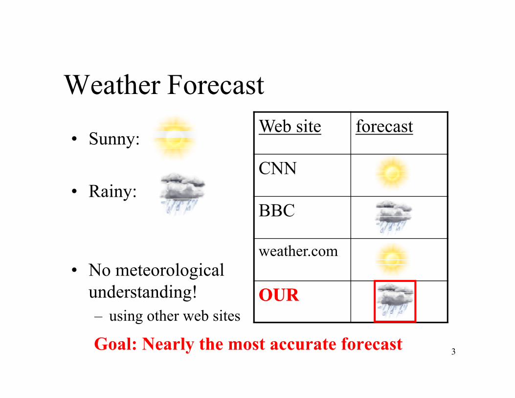
Weather Forecast
• Sunny:
• Rainy:
forecastWeb site
CNN
3
• Rainy:
• No meteorological understanding!– using other web sites
BBC
weather.com
OUROUR
Goal: Nearly the most accurate forecast
Route selection
Goal:
Fastest route
4
Challenge:
Partial Information
Rock-Paper-Scissors
5
(1,-1)(-1,1)(0, 0)
(-1,1)(0, 0)(1,-1)
(0, 0)(1,-1)(-1,1)
Rock-Paper-Scissors
• Play multiple times– a repeated zero-sum game
• How should you “learn” to play the game?!
(1,-1)(-1,1)(0, 0)
(-1,1)(0, 0)(1,-1)
(0, 0)(1,-1)(-1,1)
6
• How should you “learn” to play the game?! – How can you know if you are doing “well”
– Highly opponent dependent
– In retrospect we should always win …
Rock-Paper-Scissors
• The (1-shot) zero-sum game has a value– Each player has a mixed strategy that can enforce
the value
• Alternative 1: Compute the minimax strategy
(1,-1)(-1,1)(0, 0)
(-1,1)(0, 0)(1,-1)
(0, 0)(1,-1)(-1,1)
7
• Alternative 1: Compute the minimax strategy– Value V= 0– Strategy = (⅓, ⅓, ⅓)
• Drawback: payoff will always be the value V– Even if the opponent is “weak” (always plays )
Rock-Paper-Scissors
• Alternative 2: Model the opponent– Finite Automata
• Optimize our play given the opponent model.
(1,-1)(-1,1)(0, 0)
(-1,1)(0, 0)(1,-1)
(0, 0)(1,-1)(-1,1)
8
• Optimize our play given the opponent model.
• Drawbacks: – What is the “right” opponent model.
– What happens if the assumption is wrong.
Rock-Paper-Scissors
• Alternative 3: Online setting– Adjust to the opponent play
– No need to know the entire game in advance
(1,-1)(-1,1)(0, 0)
(-1,1)(0, 0)(1,-1)
(0, 0)(1,-1)(-1,1)
9
– No need to know the entire game in advance
– Payoff can be more than the game’s value V
• Conceptually:– Have a set of comparison class of strategies.
– Compare performance in hindsight
Rock-Paper-Scissors
• Comparison Class H:– Example : A={ , , }
– Other plausible strategies: • Play what you opponent played last time
(1,-1)(-1,1)(0, 0)
(-1,1)(0, 0)(1,-1)
(0, 0)(1,-1)(-1,1)
10
• Play what you opponent played last time
• Play what will beat your opponent previous play
• Goal:
Online payoff near the best strategy in the class H
• Tradeoff:– The larger the class H, the difference grows.
Rock-Paper-Scissors: Regret
• Consider A={ , , }– All the pure strategies
• Zero-sum game:
11
Given any mixed strategy σ of the opponent,
there exists a pure strategy a∊ A
whose expected payoff is at least V
• Corollary:For any sequence of actions (of the opponent)
We have some action whose average value is V
Rock-Paper-Scissors: Regret
payoffopponentwe
-1
1
payoffopponentplay
1
0
12
1
0
0
-1
-1
Average payoff -1/3
0
1
1
-1
New average payoff 1/3
Rock-Paper-Scissors: Regret
• More formally:After T games,
Û = our average payoff,
U(h) = the payoff if we play using h
13
U(h) = the payoff if we play using h
regret(h) = U(h)- Û
• Claim:
If for every a∊A we have regret(a) ≤ ε, then Û ≥ V- ε
• External regret: maxh∊H regret(h)
14[Blum & M] and [Cesa-Bianchi, M & Stoltz]
Regret Minimization: Setting
• Online decision making problem (single agent)
• At each time, the agent:– selects an action
15
– observes the loss/gain
• Goal: minimize loss (or maximize gain)
• Environment model:– stochastic versus adversarial
• Performance measure:– optimality versus regret
Regret Minimization: Model
• Actions A={1, … ,N}• Number time steps: t { 1, … , T}• At time step t:
– The agent selects a distribution p t over A
16
– The agent selects a distribution pit over A
– Environment returns costs cit [0,1]
– Online loss: lt = Σi cit pi
t
• Cumulative loss : Lonline = Σt lt
• Information Models:– Full information: observes every action’s cost – Partial information: observes only it own cost
Stochastic Environment
• Costs: cit are i.i.d. random variables
– Assuming an oblivious opponent
• Tradeoff: Exploration versus Exploitation
17
• Tradeoff: Exploration versus Exploitation
• Approximate solution:– sample each action O(logT) times
– select the best observed action
• Gittin’s Index– Simple optimal selection rule
• under some Bayesian assumptions
Competitive Analysis
• Costs: cit are generated adversarially,
– might depend on the online algorithm decisions• in line with our game theory applications
• Online Competitive Analysis:
18
• Online Competitive Analysis:– Strategy class = any dynamic policy
– too permissive • Always wins rock-paper-scissors
• Performance measure:– compare to the best strategy in a class of strategies
External Regret
• Static class– Best fixed solution
• Compares to a single best strategy (in H)
• The class H is fixed beforehand.
19
• The class H is fixed beforehand.– optimization is done with respect to H
• Assume H=A– Best action: Lbest = MINi {Σt ci
t }
– External Regret = Lonline – Lbest
• Normalized regret is divided by T
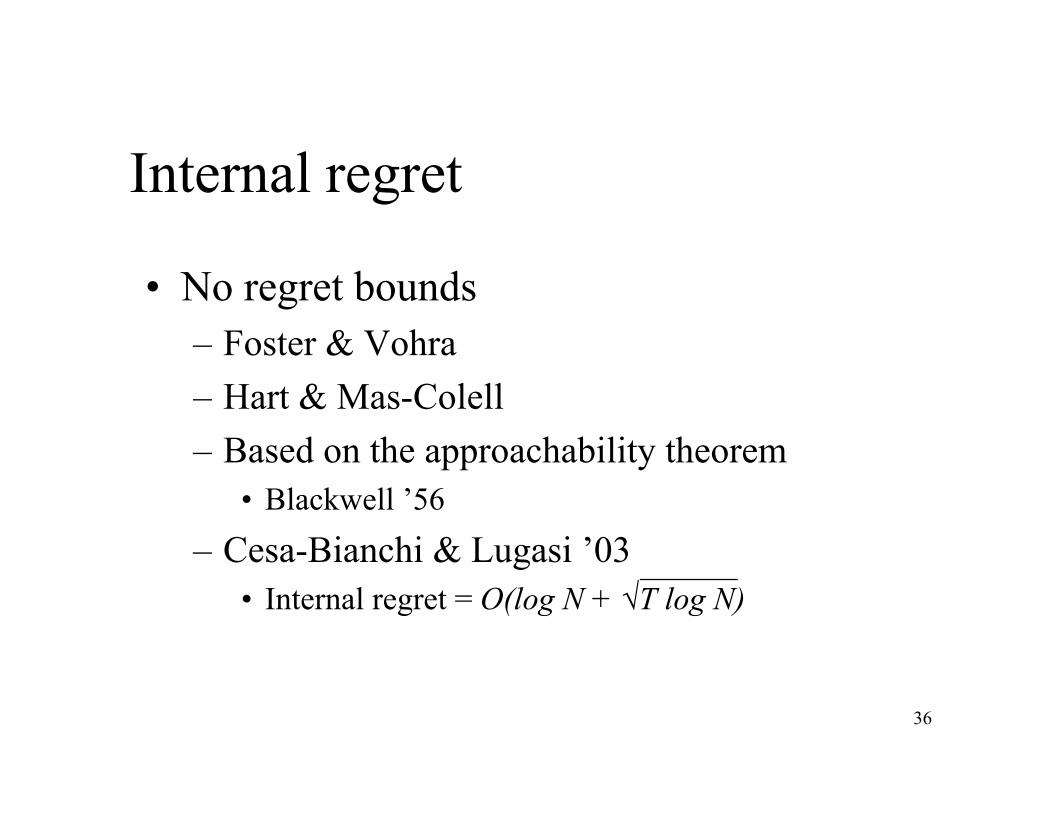
External regret: Bounds
• Average external regret goes to zero– No regret
– Hannan [1957]
20
– Hannan [1957]
• Explicit bounds– Littstone & Warmuth ‘94
– CFHHSW ‘97
– External regret = O(√Tlog N)
External Regret: Greedy
• Simple Greedy:– Go with the best action so
far.
• For simplicity loss is {0,1}
21
• For simplicity loss is {0,1}
• Loss can be N times the best action– holds for any deterministic
online algorithm
External Regret: Randomized Greedy
• Randomized Greedy:– Go with a random best
action.
• Loss is ln(N) times the
22
• Loss is ln(N) times the best action
• Analysis: When the bestbest increases
from k to k+1 expected loss is
1/N + 1/(N-1) + … ≈ ln(N)
External Regret: PROD Algorithm
• Regret is √Tlog N
• PROD Algorithm:– plays sub-best actions
– Uses exponential weights
FtWt
(1-η)
23
– Uses exponential weights
wa = (1-η)La
– Normalize weights
• Analysis:– Wt= weights of all actions at time t
– Ft= fraction of weight of actions with loss 1 at time t
• Also, expected loss: LON = ∑ Ft
Wt+1 = Wt (1-ηFt)
Wt+1
External Regret: Bounds Derivation
• Bounding WT
• Lower bound:WT > (1-η)Lmin
• Combined bound:(1-η)Lmin ≤ W1 exp{-η LON }
• Taking logarithms:
24
W > (1-η)Lmin
• Upper bound:WT = W1 Πt (1-ηFt)
≤ W1 Πt exp{-ηFt }
= W1 exp{-η LON }using 1-x ≤ e-x
Lminlog(1- η) ≤ log(W1) -ηLON
• Final bound:
LON≤ Lmin+ ηLmin+log(N)/η
• Optimizing the bound:η = √log(N)/Lmin
LON≤ Lmin+2√ Lmin log(N)
External Regret: Summary
• We showed a bound of 2√Lmin log N
• More refined bounds
√Q log N where Q = Σ (ct )2
25
√Q log N where Q = Σt (ctbest )2
• More elaborate notions of regret …
External Regret: Summary
• How surprising are the results …– Near optimal result in online adversarial setting
• very rear …
26
• very rear …
– Lower bound: stochastic model• stochastic assumption do not help …
– Models an “improved” greedy
– An “automatic” optimization methodology• Find the best fixed setting of parameters
27
Internal Regret
• Game theory applications:– Avoiding dominated actions
– Correlated equilibrium
28
– Correlated equilibrium
• Reduction from External Regret [Blum & M]
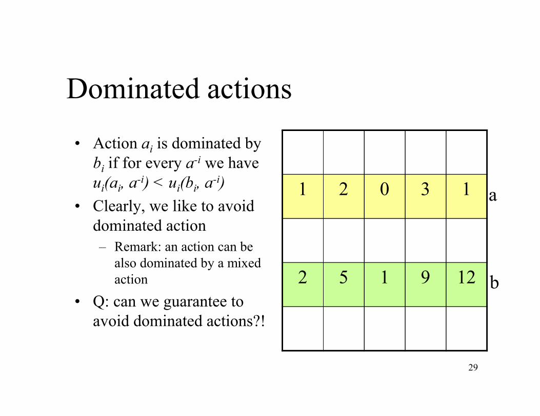
Dominated actions
• Action ai is dominated by bi if for every a-i we have ui(ai, a-i) < ui(bi, a-i)
• Clearly, we like to avoid 13021 a
29
• Clearly, we like to avoid dominated action– Remark: an action can be
also dominated by a mixed action
• Q: can we guarantee to avoid dominated actions?!
129152 b
Dominated Actions & Internal Regret
• How can we test it?!– in retrospect
• ai is dominates bi
– Every time we played ai
Internal Regret (ab)
Modified
Payoff (ab)
Our
Payoff
our actions
2-1=121a
b
30
– Every time we played ai
we do better with bi
• Define internal regret– swapping a pair of actions
• No internal regret
no dominated actions
b
c
5-2=352a
d
9-3=693a
b
d
1-0=110a
Dominated actions & swap regret
• Swap regret – An action sequence σ = σ1, …, σt
– Modification function F:A A
– A modified sequence
σ(F)σ
ba
cb
cc
31
– A modified sequence
σ(F) = F(σ1), …, F(σt)
• Swap_regret =
maxF V(σ (F)) - V(σ )
• Theorem: If Swap_regret < R then in at most R/ε steps we play ε-dominated actions.
cc
ba
bd
ba
cb
bd
ba
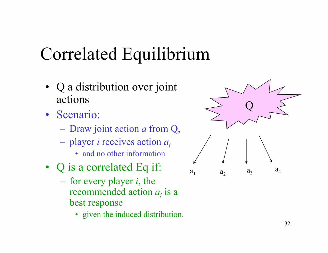
Correlated Equilibrium
• Q a distribution over joint actions
• Scenario: – Draw joint action a from Q,
Q
32
– Draw joint action a from Q,– player i receives action ai
• and no other information
• Q is a correlated Eq if:– for every player i, the
recommended action ai is a best response
• given the induced distribution.
a1 a2a3
a4
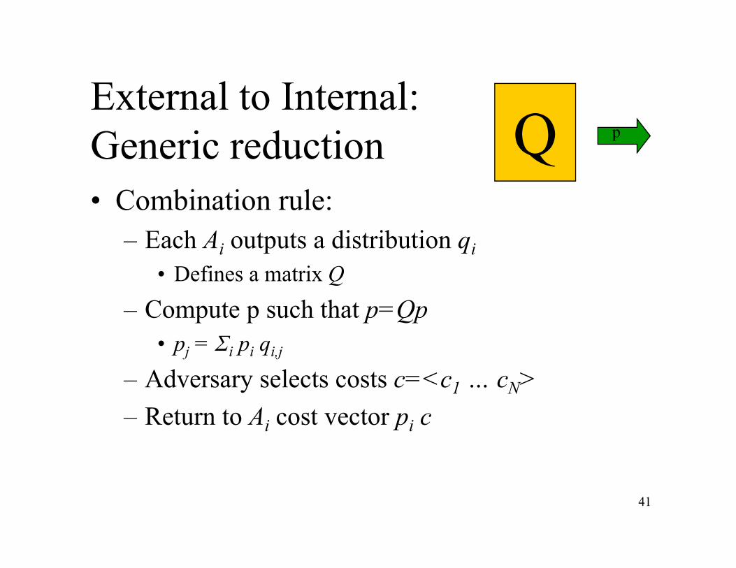
Swap Regret & Correlated Eq.
• Correlated Eq NO Swap regret
• Repeated game setting
• Assume swap_regret ≤ ε
33
• Assume swap_regret ≤ ε– Consider the empirical distribution
• A distribution Q over joint actions
– For every player it is ε best response
– Empirical history is an ε correlated Eq.
Internal/Swap Regret
• Comparison is based on online’s decisions.– depends on the actions of the online algorithm– modify a single decision (consistently)
34
• Each time action A was done do action B
• Comparison class is not well define in advanced.
• Scope:– Stronger then External Regret– Weaker then competitive analysis.
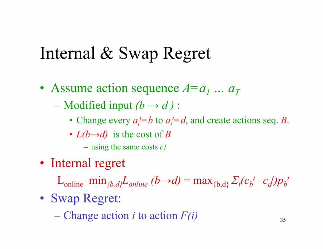
Internal & Swap Regret
• Assume action sequence A=a1 … aT
– Modified input (b → d ) :• Change every ai
t=b to ait=d, and create actions seq. B.
35
• Change every ai =b to ai =d, and create actions seq. B.
• L(b→d) is the cost of B– using the same costs ci