Regular Random Field Solutions for Stochastic Evolution ...antoni/media/phd thesis antoni.pdf ·...

.

Regular Random Field Solutions

for Stochastic Evolution Equations

Zur Erlangung des akademischen Grades eines

DOKTORS DER NATURWISSENSCHAFTEN

von der Fakultat fur Mathematik des

Karlsruher Instituts fur Technologie (KIT)

genehmigte

DISSERTATION

von

Markus Antoni

aus Karlsruhe

Tag der mundlichen Prufung: 18. Januar 2017

Referent: Prof. Dr. Lutz Weis

Korreferenten: Priv.-Doz. Dr. Peer Christian Kunstmann

Prof. Dr. Mark Christiaan Veraar

.

”Imagination is more important than knowledge.

For knowledge is limited, whereas imagination

embraces the entire world.”

- Albert Einstein, 1931

Abstract

In this thesis we investigate stochastic evolution equations of the form

dX(t) +AX(t) dt = F (t,X(t)) dt+∞∑n=1

Bn(t,X(t)) dβn(t)

for random fields X : Ω × [0, T ] × U → R, where [0, T ] is a time interval, (Ω,F ,P) a

measure space representing the randomness of the system, and U is typically a domain in

Rd (or again a measure space). More precisely, we concentrate on the parabolic situation

where A is the generator of an analytic semigroup on Lp(U). We look for mild solutions

so that X(ω, ·, ·) has values in Lp(U ;Lq[0, T ]) for almost all ω ∈ Ω under appropriate

Lipschitz and linear growth conditions on the nonlinearities F and Bn, n ∈ N. Compared

to the classical semigroup approach, which gives X(ω, ·, ·) ∈ Lq([0, T ];Lp(U)), the order of

integration is reversed. We show that this new approach together with a strong Doob and

Burkholder-Davis-Gundy inequality leads to strong regularity results in particular for the

time variable of the random field X(ω, t, u), e.g. pointwise Holder estimates for the paths

t 7→ X(ω, t, u), P-almost surely. For less-optimal regularity estimates we only need the

relatively mild assumption that the resolvents of A extend uniformly to Lp(U ;Lq[0, T ]).

However, in the maximal regularity case the difficulty of the reversed order of integration

in time and space makes extended functional calculi results necessary. As a consequence,

we obtain suitable estimates for deterministic and stochastic convolutions. Using Sobolev

embedding theorems, we obtain solutions in Lr(Ω;Lp(U ;Cα[0, T ])). In several applications

where A is an elliptic operator on a domain in Rd we show that for concrete examples of

stochastic partial differential equations our theory leads to stronger results as known in

the literature.

.

Acknowledgment

First of all I would like to thank my supervisor Lutz Weis for accepting me as his PhD

student and for introducing me in the theory of stochastic evolution equations. Thank

you, Lutz, for the possibility to participate in several conferences and schools, and for

supporting me both on a professional and personal level. I would also like to express my

gratitude to Peer Kunstmann and Mark Veraar for co-examining this thesis. Thank you

also for reading very carefully an earlier draft of this manuscript.

While working on this thesis, I had the pleasure to participate at several summer and

winter schools. Many thanks go to Zdzislaw Brzezniak, David Elworthy, and Utpal Manna

for the extraordinary experience of the Indo-UK workshop on SPDE’s and Applications in

Bangalore, India. Thank you, David and Zdzislaw, also for the wonderful trip to Mysore.

I would also like to thank the CIME board and Franco Flandoli, Martin Hairer, and

Massimiliano Gubinelli for giving me a grant to participate at the CIME-EMS Summer

School on Singular Random Dynamics in Cetraro, Italy. Thank you for the both instructive

and relaxing time in Calabria.

Over the last years, I received great support from my colleagues at the Institute of Analysis

at KIT. Thank you very much for the more than pleasant working atmosphere. Many

thanks go to Johannes Eilinghoff, Luca Hornung, Fabian Hornung, and Sebastian Schwarz

for many helpful comments and suggestions on a first draft of this thesis.

I also want to thank the board of the Department of Mathematics, most importantly Anke

Vennen, for their patience and kindness when unexpected incidents affected the last stages

of my thesis.

At this point, I also want to thank my dear friends Caro, Eva, Jessi, Lena, Alex, Alex,

Raphi, and Sebastian for being there when someone was needed. Many thanks also go to

my family for supporting me in every aspects throughout my studies. Finally, I would like

to thank Nelly and Steve. There are no words to describe the joy you brought to my life.

Markus Antoni, December 21, 2016

Contents

Introduction 1

Notational Conventions 11

1 Stochastic Integration in Mixed Lp Spaces 15

1.1 Basic Theory . . . . . . . . . . . . . . . . . . . . . . . . . . . . . . . . . . . . . . . . 15

1.2 Stopping Times and Localization . . . . . . . . . . . . . . . . . . . . . . . . . . . . . 31

1.3 Ito Processes and Ito’s Formula . . . . . . . . . . . . . . . . . . . . . . . . . . . . . . 48

1.4 Stochastic Integration in Sobolev and Besov Spaces . . . . . . . . . . . . . . . . . . . 60

2 Functional Analytic Operator Properties 67

2.1 Rq-boundedness and Rq-sectorial Operators . . . . . . . . . . . . . . . . . . . . . . . 67

2.2 H∞ and RH∞ Calculus . . . . . . . . . . . . . . . . . . . . . . . . . . . . . . . . . . 72

2.3 Rq-bounded H∞ Calculus . . . . . . . . . . . . . . . . . . . . . . . . . . . . . . . . . 75

2.4 Extension Properties . . . . . . . . . . . . . . . . . . . . . . . . . . . . . . . . . . . . 81

2.5 `q Interpolation Method . . . . . . . . . . . . . . . . . . . . . . . . . . . . . . . . . . 86

3 Stochastic Evolution Equations 97

3.1 Motivation . . . . . . . . . . . . . . . . . . . . . . . . . . . . . . . . . . . . . . . . . 97

3.2 Orbit Maps . . . . . . . . . . . . . . . . . . . . . . . . . . . . . . . . . . . . . . . . . 100

3.3 Deterministic Convolutions . . . . . . . . . . . . . . . . . . . . . . . . . . . . . . . . 111

3.4 Stochastic Convolutions . . . . . . . . . . . . . . . . . . . . . . . . . . . . . . . . . . 122

3.5 Existence and Uniqueness Results . . . . . . . . . . . . . . . . . . . . . . . . . . . . . 136

3.5.1 Lipschitz Notions . . . . . . . . . . . . . . . . . . . . . . . . . . . . . . . . . . 136

3.5.2 The Globally Lipschitz Case . . . . . . . . . . . . . . . . . . . . . . . . . . . . 137

3.5.3 The Time-dependent Case . . . . . . . . . . . . . . . . . . . . . . . . . . . . . 151

3.5.4 The Locally Lipschitz Case . . . . . . . . . . . . . . . . . . . . . . . . . . . . 154

4 Applications to Stochastic Partial Differential Equations 163

4.1 Bounded Generators . . . . . . . . . . . . . . . . . . . . . . . . . . . . . . . . . . . . 163

4.2 Stochastic Heat Equation . . . . . . . . . . . . . . . . . . . . . . . . . . . . . . . . . 165

4.3 Parabolic Equations on Rd . . . . . . . . . . . . . . . . . . . . . . . . . . . . . . . . 169

4.4 Second Order Parabolic Equations on Domains . . . . . . . . . . . . . . . . . . . . . 174

4.5 The Deterministic Case . . . . . . . . . . . . . . . . . . . . . . . . . . . . . . . . . . 178

Bibliography 181

Introduction

A historic sketch

The theory of stochastic (ordinary) differential equations started with the works of Ito in

1946 (cf. [47, 48]). His short paper [47] of four pages already contained many of the main

ideas future researchers would apply in generalizing his results. The Ito stochastic calculus

was born and it inspired the field of stochastic analysis in a fruitful way. Around 30 years

later, researchers looked beyond stochastic odinary differential equtations to stochastic

partial differential equations. In the fields of physics, biology, or control theory many

models were best described by stochastic evolution partial differential equations. A vivid

example was described by John B. Walsh in [86]:

”The general problem is this. Suppose one is given a physical system governed by a partial

differential equation. Suppose that the system is then perturbed randomly, perhaps by some

sort of a white noise. How does it evolve in time? Think for example of a guitar carelessly

left outdoors. If u(x, t) is the position of one of the strings at the point x and time t, then

in calm air u(x, t) would satisfy the wave equation ∂ttu = ∂xxu. However, if a sandstorm

should blow up, the string would be bombarded by a succession of sand grains. Let W (x, t)

represent the intensity of the bombardment at the point x and time t. The number of

grains hitting the string at a given point and time will be largely independent of the number

hitting at another point and time, so that, after subtracting a mean intensity, W may be

approximated by a white noise, and the final equation is

∂ttu(x, t) = ∂xxu(x, t) + W (x, t)

where W is a white noise in both time and space, or, in other words, a two-parameter

white noise. One peculiarity of this equation - not surprising in view of the behavior of

ordinary stochastic differential equations - is that none of the partial derivatives in it exist.

However, one may rewrite it as an integral equation, and then show that in this form there

is a solution which is a continuous, though non-differentiable, function.

Similar models were applied to other equations in physics, biology, or most notably mathe-

matical finance. As the terminology suggests, the theory of stochastic partial differential

equations lies in the intersection of two fields: stochastic processes and partial differential

equations. Therefore, several approaches to these equations emerged. In particular for

2 Introduction

filtering equations (see e.g. [51]), the stochastic evolution equation can be regarded as an

’ordinary’ Ito equation

dX(t) = A(t,X(t)) dt+B(t,X(t)) dβ(t)

for processes X taking values in a function space. Depending on the dimension of this

space we could interpret this equation as a (finite or infinite) system of one-dimensional

ordinary stochastic differential equations. An introduction to this approach can be found

in [70]. There, the focus lies on deducing a counterpart to the scalar-valued Ito theory

for the function space-valued case. One should remark that by considering an infinite

set of independent Brownian motions β = (βn)n∈N, this also covers equations driven by

space-time white noise (see [54, Section 8.3]).

Another famous approach is that of Walsh [86]. He considered the solution of stochastic

partial differential equations as random variables, or more precisely, as random fields,

because the solution depends on more than one independent variable. The focus of this

theory lies on scalar-valued techniques and measures on infinite dimensional function spaces

regarding both space and time (see also [38, 69]).

As the title of this thesis suggests, we will somehow mix these approaches to create a new

one. More precisely, we will investigate the stochastic evolution equation

dX(t) +AX(t) dt = F (t,X(t)) dt+

∞∑n=1

Bn(t,X(t)) dβn(t), X(0) = x0 ∈ Lp(U),

in Lp spaces for p ∈ (1,∞), still thinking of the solution X as a random field, i.e. a function

X : Ω× [0, T ]× U → R, and concentrate on the regularity of the process X(t, u).

Before explaining this in more detail, we give a short historical background on the develop-

ment of the theory of stochastic evolution equations. Early on, many of Ito’s results could

be generalized to the Hilbert space case using the fact that the norm comes from an inner

product (see [22, 20]). In particular, the Ito isometry is still valid in the way we would

expect it:

(1) E∥∥∥∫ T

0φ(s) dβ(s)

∥∥∥2

H= E

∫ T

0‖φ(s)‖2H ds

for any Hilbert space (H, ‖ · ‖H) and each adapted process φ : Ω × [0, T ] → H. Having a

well-defined stochastic integral is the starting point of a reasonable theory. However, in

this situation examples of stochastic evolution equations arose with very low regularity.

One famous result is the heat equation on Rd with a stochastic disturbance of gradient

type, more precisely

dX(t) = 12∆X(t) +

d∑n=1

∂xnX(t) dβn(t), X(0) = x0.

Introduction 3

Using the calculus of Ito, we can verify that for each x0 ∈W 1,2(Rd) the function

X(t, u) = x0(u+ βt), t ∈ [0, T ], u ∈ Rd,

is the unique (weak or mild) solution in L2([0, T ]×Rd), but, in general, X is not continuous

for d ≥ 2. Therefore, better Sobolev embedding theorems for large p points towards an

Lp theory for p 6= 2 and turn our attention to a Banach space-valued approach. However,

already in the construction of a stochastic integral difficulties appear which were not present

in the Hilbert space case. It turns out that L2([0, T ];E), where E is a general Banach

space, does not lead to two-sided estimates in (1). This means that L2([0, T ];E) does not

characterize the space of stochastically integrable functions. However, assuming additional

geometric properties of E, one gets at least one-sided estimates. For the case of stochastic

partial differential equations in M-type 2 Banach spaces, where the latter include all Lp

spaces for p ≥ 2, this was done by Brzezniak in [12] (see also [10, 30]). Regarding stochastic

integration theory in general Banach spaces, van Neerven and Weis characterized in [84]

the space of reasonable integrands via γ-radonifying operators. Intuitively speaking, since

L2([0, T ];E) does not do the job, they considered the space with reversed order of norms

’E(L2[0, T ])’, which is of course not defined in general. However, in the case of an Lp space

this turns out to be the right choice. The generalization of the ’square function norm’ in

’E(L2[0, T ])’ finally leads to the space of γ-radonifying operators γ(L2[0, T ];E). In [80]

van Neerven, Veraar, and Weis extended this to processes with values in a UMD Banach

space via a decoupling technique. These results were then used in a sequence of papers (see

[81, 83, 82]) to study stochastic evolution equations and their regularity in UMD spaces.

As indicated above, one can avoid γ-radonifying operators in the special case of an Lp(U)

space E, since γ(L2[0, T ];E) is isomorphic to the Bochner space Lp(U ;L2[0, T ]). The

stochastic integration theory was then investigated in [3], where the author tries to exploit

the structural advantages one has compared to the abstract setting of UMD spaces. One

of the main results in [3] is a stronger version of Doob’s maximal inequality stating that

E∥∥ N

maxn=1|Mn|

∥∥rLp≤ CE‖MN‖rLp

for an Lp-valued Lr martingale (Mn)Nn=1, p, r ∈ (1,∞). This leads to a stronger version of

the Burkholder-Davis-Gundy inequality for stochastic integrals:

E∥∥∥ supt∈[0,T ]

∣∣∣ ∫ t

0f(s) dβ(s)

∣∣∣ ∥∥∥rLp

h E∥∥∥(∫ T

0|f(s)|2 ds

)1/2 ∥∥∥rLp.

This then in turn gives rise to the question if such stronger regularity properties do not only

hold for stochastic Ito integrals in Lp spaces, but also for solutions of stochastic evolution

equations. This is the topic of this thesis.

4 Introduction

Our approach in a nutshell

In many results regarding regularity of stochastic evolution equations of the form

dX(t) +AX(t) dt = F (t,X(t)) dt+∞∑n=1

Bn(t,X(t)) dβn(t), X(0) = x0,

where −A is supposed to be the generator of an analytic semigroup (e−tA)t≥0, the solution

is almost surely an element of spaces like

Lq([0, T ];E), W σ,q([0, T ];E), or C([0, T ];E) etc.

(see [21, 81, 82] and the references therein). A typical way to deal with existence and

uniqueness for these equations is to consider mild solutions X, which are defined as func-

tions satisfying a fixed point equation such as

X(t) = e−tAx0 +

∫ t

0e−(t−s)AF (s,X(s)) ds+

∞∑n=1

∫ t

0e−(t−s)ABn(s,X(s)) dβn(s),

where the spaces mentioned above serve as fixed point spaces. In order to get for such

evolution equations with E = Lp(U) better regularity estimates in time, it is of advantage

(as suggested in the motivation above) to interchange the order of integration and choose

the spaces

Lp(U ;Lq[0, T ]), Lp(U ;W σ,q[0, T ]), or Lp(U ;C[0, T ])

as fixed point spaces. Since the norm with respect to time is now inside of the space-norm,

we get pointwise for each u ∈ U knowledge about the temporal behavior of the solution

process t 7→ X(t, u). In particular, in regard of continuity results, these stated regularity

results are stronger than what we have known before. In order to apply Banach’s fixed

point theorem in Lr(Ω;Lp(U ;Lq[0, T ])), it is necessary to investigate the following three

maps in this space:

1) the orbit map t 7→ e−tAx, x ∈ Lp(U);

2) the deterministic convolution t 7→∫ t

0 e−(t−s)Aφ(s) ds, φ ∈ Lp(U ;Lq[0, T ]);

3) the stochastic convolution t 7→∑∞

n=1

∫ t0 e−(t−s)Aφn(s) dβn(s), φ ∈ Lp(U ;Lq([0, T ]; `2)).

Using estimates of these maps, existence and uniqueness of mild solutions can be proven.

Once this is done, we turn to the study of more involved regularity results. However, even

in the case of orbit maps as in 1) one should notice that the usual estimates for analytic

semigroups used in the Banach space-valued case are not applicable now since we first have

to estimate with respect to time and then with respect to the space variable in U . This

brings up the question: Is there a way to bypass this obstacle?

Introduction 5

We make the following observation: Since −A is the generator of an analytic semigroup,

we have the representation

e−tAx =1

2πi

∫Γe−tλR(λ,A)x dλ

for each fixed t ∈ [0, T ] and x ∈ Lp(U). Here, Γ = ∂(Σα∪B(0, δ)) for a suitable angle α and

radius δ > 0 (see e.g. [59, Illustration 9.9]). In particular, the product structure inside of

the complex line integral makes estimates in Lp(U ;Lq[0, T ]) accessible since we can handle

time and space separately. In the case of convolutions this is completely different. Here,

e−(t−s)Aφ(s) =1

2πi

∫Γe−(t−s)λR(λ,A)φ(s) dλ

for a function φ : [0, T ] → Lp(U) and every fixed s ∈ [0, t]. The separation of time and

space is no longer existent which makes additional requirements for the resolvents of A

necessary. In order to figure out these properties, observe that

e−(t−s)λR(λ,A)φ(s) = R(λ,A)(e−(t−s)λφ(s)

).

Since we want to apply an Lp(U ;Lq[0, T ]) norm to this integral, it is quite natural to assume

that the resolvents should extend to Lp(U ;Lq[0, T ]) having similar norm estimates as before

(by this we mean that the set λR(λ,A) : λ ∈ Σα′ is still bounded in Lp(U ;Lq[0, T ])). For

simple functions f =∑N

n=1 1[tn−1,tn]xn ∈ Lp(U ;Lq[0, T ]), where 0 = t0 < . . . < tN = T

with tn − tn−1 = δ and (xn)Nn=1 ⊆ Lp(U), such a condition reads as

‖λR(λ,A)f‖Lp(U ;Lq [0,T ]) = δ∥∥∥( N∑

n=1

∣∣λR(λ,A)xn∣∣q)1/q ∥∥∥

Lp(U)

≤ Cδ∥∥∥( N∑

n=1

|xn|q)1/q ∥∥∥

Lp(U)= C‖f‖Lp(U ;Lq [0,T ]).

This leads us to the notion of `q- and Rq-sectorial operators. The second terminology was

first introduced by Weis in [87], and was further elaborated in [57, 79]. Estimating the

convolution terms in 2) and 3) now reduces to the estimation of the ’scalar’ convolutions

∫ t

0e−(t−s)λφ(s) ds and

∞∑n=1

∫ t

0e−(t−s)λφn(s) dβn(s),

provided that the complex line integral still converges (which will always be the case in

this setting). However, in order to investigate further regularity properties, this will not

suffice. We are also interested in estimates of

Aα∫ t

0e−(t−s)Aφ(s) ds and Aβ

∞∑n=1

∫ t

0e−(t−s)Aφn(s) dβn(s)

6 Introduction

for certain values of α and β. If A is `q-sectorial, we obtain estimates of the form

E∥∥∥Aα ∫ t

0e−(t−s)Aφ(s) ds

∥∥∥rLp(U ;Lq [0,T ])

≤ CT (1−α)rE‖φ‖rLp(U ;Lq [0,T ]),

E∥∥∥Aβ ∞∑

n=1

∫ t


∥∥∥rLp(U ;Lq [0,T ])

≤ CT (1/2−β)rE‖φ‖rLp(U ;Lq([0,T ];`2)),

for α < 1 and β < 1/2. Note that the restriction for β is forced by the L2[0, T ] norm in the

Ito isomorphism. The borderline cases α = 1 and β = 1/2 are in general false. Therefore,

we again need to impose additional assumptions on A, namely that the extension of A to

Lp(U ;Lq[0, T ]) has a bounded H∞ calculus.

This concept was introduced by McIntosh in [65] and gives an answer to the question

whether the functional calculus for sectorial operators A is bounded for functions f ∈ H∞.

Following the ideas of the Dunford calculus, this calculus is defined by

ϕ(A) :=1

2πi

∫∂Σω

ϕ(λ)R(λ,A) dλ,

where ϕ ∈ H∞0 , i.e. ϕ is a bounded and holomorphic function decaying polynomially to

0 as λ tends to 0 and to ∞. For these functions the expression above is well-defined as

a bounded operator since the integral is absolutely convergent. However, for functions

f ∈ H∞ this leads, in general, only to unbounded operators. Thus, a sectorial operator

A is said to have a bounded H∞ calculus if f(A) defines a bounded operator for each

f ∈ H∞.

Assuming that the extension of A has a bounded H∞ calculus on Lp(U ;Lq[0, T ]), we can

also treat the cases α = 1 and β = 1/2 by applying the following trick: We define the

analytic families of bounded operators

(Kλφ)(t) :=

∫ t

0λe−(t−s)λφ(s) ds, λ ∈ Σω, φ ∈ Lr(Ω;Lp(U ;Lq[0, T ])),

(Lλφ)(t) :=

∞∑n=1

∫ t

0λ

1/2e−(t−s)λφn(s) dβn(s), λ ∈ Σω, φ ∈ Lr(Ω;Lp(U ;Lq([0, T ]; `2))).

It is tempting to plug in A for λ in these formulas and hope to obtain operators KA

and LA which are still bounded on Lr(Ω;Lp(U ;Lq[0, T ])) and Lr(Ω;Lp(U ;Lq([0, T ]; `2))),

respectively. This procedure can indeed be justified by the methods of the H∞ calculus.

It requires certain randomization properties of the families (Kλ)λ∈Σω and (Lλ)λ∈Σω , and

the notion of an operator-valued functional calculus which will be explained in Section 2.2.

Writing out the boundedness of KA and LA leads to

E∥∥∥A∫ t


∥∥∥rLp(U ;Lq [0,T ])

≤ CE‖φ‖rLp(U ;Lq [0,T ]),

E∥∥∥A1/2

∞∑n=1

∫ t


∥∥∥rLp(U ;Lq [0,T ])

≤ CE‖φ‖rLp(U ;Lq([0,T ];`2)).

Introduction 7

This case is often considered as the maximal or optimal regularity case. Furthermore, we

also consider some ’regularity swapping’ results. More precisely, we show that we can give

up space regularity (which is encoded in the domains of the fractional powers of A) to

obtain more time regularity, i.e.

E∥∥∥A1−σ

∫ t


∥∥∥rLp(U ;Wσ,q [0,T ])

≤ CE‖φ‖rLp(U ;Lq [0,T ]), σ ∈ [0, 1),

E∥∥∥A1/2−σ

∞∑n=1

∫ t


∥∥∥rLp(U ;Wσ,q [0,T ])

≤ CE‖φ‖rLp(U ;Lq([0,T ];`2)), σ ∈ [0, 1/2).

The very important question as to which operators A have such an extension with a

bounded H∞ calculus is treated in Chapter 2. It is shown that many of the common

partial differential operators considered in applications do have this property.

These estimates are at the heart of our regularity theory. They also enable us to apply Ba-

nach’s fixed point theorem to get unique mild solutions in Lr(Ω;Lp(U ;Lq[0, T ])), assuming

certain Lipschitz conditions on F and B = (Bn)n∈N. We emphasize that the regularity

with respect to time benefits from the ’swapping mechanism’. As a consequence, we get

those strong results announced in the beginning. For a complete presentation of this ap-

proach we refer to Chapter 3.

Outline of this thesis

The thesis is organized as follows. In Chapter 1 we lay the foundation of the stochastic

integration theory in mixed Lp spaces. This is a continuation of [3], where the case of one

Lp space was considered. Although in the subsequent chapters no mixed Lp spaces explic-

itly appear in the main results, we will be reliant on these results in proofs of Section 3.4.

In Section 1.1 we start with the investigation of the stochastic integral for integrable pro-

cesses in Lp(U ;Lq(V )) with respect to one Brownian motion, where (U,Σ, µ) and (V,Ξ, ν)

are σ-finite measure spaces. Besides giving meaning to the expression∫ T

0 f(s) dβ(s) for

adapted processes f ∈ Lr(Ω;Lp(U ;Lq(V ;L2[0, T ]))) and deducing many properties of this

integral, one of the main results of this section includes an extension of the stronger ver-

sions of Doob’s maximal inequality and the Burkholder-Davis-Gundy inequality for mixed

Lp spaces. In contrast to [3] the latter now also includes the case r = 1. In Section 1.2 we

proceed in a classical way by extending the stochastic integral to processes without inte-

grability assumptions with respect to Ω. This is done by a localization argument involving

stopping time techniques. In particular, the Burkholder-Davis-Gundy inequality for r = 1

will lead to a general version of the stochastic Fubini theorem under minimal assumptions

on the process considered. In Section 1.3 we extend the results both of Section 1.1 and

1.2 to a stochastic integral with respect to an infinite sequence of independent Brownian

8 Introduction

motions, i.e. to an integral of the form

∫ t

0b(s) dβ(s) =

∞∑n=1

∫ t

0bn(s) dβn(s),

and formulate an appropriate version of Ito’s formula. In the final Section 1.4 we briefly

illustrate how we can use the stochastic integration theory developed for mixed Lp spaces

to obtain a stochastic integration theory in Sobolev and Besov spaces.

In Chapter 2 we shortly leave the stochastic territory and turn to some spectral theory

which will be important for Chapter 3. Section 2.1 provides a systematic introduction to

the concepts of Rq-boundedness and Rq-sectoriality. In Section 2.2 we will continue with a

short overview of the bounded H∞ and RH∞ calculus. Based on these ideas, Section 2.3

is devoted solely to the concept of an Rq-bounded H∞ calculus. Here we will use a result

of Kunstmann and Ullmann (cf. [58]) to collect several examples of differential operators

in divergence and non-divergence form having such a functional calculus. In Section 2.4

we establish the important connection between A having an Rq-bounded H∞ calculus and

having an extension on Lp(U ;Lq[0, T ]) with a bounded H∞ calculus. Finally, in Section 2.5

we introduce a new family of interpolation spaces obtained by the `q interpolation method.

As it turns out, these spaces are suitable for estimating orbit maps in Lp(U ;Lq[0, T ]).

Therefore, this section is closely connected to Section 3.2.

In Chapter 3 we will use the techniques announced and explained in the previous section

to treat stochastic evolution equations in Lp spaces. After a short motivation in Section

3.1, Section 3.2 provides a systematic treatment of the orbit map t 7→ e−tAx in the spaces

Lp(U ;Lq[0, T ]) and Lp(U ;W σ,q[0, T ]). In Sections 3.3 and 3.4 we turn to the study of

deterministic and stochastic convolutions, respectively. Here, many results of the previous

chapters come together to produce some of the main results of this thesis. In Section 3.5

we apply the tools of the previous three sections in a fixed point argument to obtain unique

mild solutions of abstract stochastic evolution equations in Lp spaces, i.e. equations of the

form

dX(t) +AX(t) dt = F (t,X(t)) dt+B(t,X(t)) dβ(t), X(0) = x0.

Here, we will assume global Lipschitz and linear growth conditions for F and B adjusted to

the fixed point space Lr(Ω;Lp(U ;Lq[0, T ])). Moreover, the connection to strong and weak

solutions is considered. Subsequently, we treat the non-autonomous and locally Lipschitz

case in Subsections 3.5.3 and 3.5.4.

In the final Chapter 4 we will apply the abstract theory to several stochastic partial

differential equations. Here, we highly benefit from the fact that many differential operators

have an Rq-bounded H∞ calculus for all q ∈ (1,∞). In cases where the domain of the

Introduction 9

operator coincides with a Sobolev space, we show that our regularity results imply Holder

regularity both in space and time. This will be compared to existing results in the literature

and reveals that in many situations our theory leads to stronger regularity results, which

then give a new insight into such equations. As one example, we consider the stochastic

heat equation

dX(t, u)− κ∆pX(t, u) dt = f(t, u,X(t, u)) dt+∞∑n=1

bn(t, u,X(t, u)) dβn(t),

X(t, u) = 0, u ∈ ∂U, t ∈ [0, T ],

X(0, u) = x0(u), u ∈ U.

In this example we already see how our theory improves the results of others. On the whole

range of r, p ∈ (1,∞) and for each q ∈ (2,∞) and γ ∈ [0, 1/2) we obtain the regularity result

X ∈ LrF(Ω;H2(γ−σ),p(U ;Cσ−1/q[0, T ])), σ ∈ (1/q, γ].

This means that even the path t 7→ X(t, u) is α-Holder continuous for almost all u ∈ Uand each α ∈ (0, 1/2).

Notational Conventions

In this introductory section we want to fix some notions and expressions used throughout

this thesis.

Miscellaneous

• If not otherwise stated, the number T > 0 always stands for a fixed finite time, and

N ∈ N for a fixed arbitrary integer.

• If a ≤ C(q) b for non-negative numbers a and b and a constant C(q) > 0 depending

only on the variable q, we write a .q b. Additionally, we write a hq b if a .q b and

b .q a.

• For real numbers x and y, we define x ∨ y := maxx, y and x ∧ y := minx, y.

Probabilistic setting

• Let (Ω,F ,P) always be a complete probability space equipped with a normal filtration

F := (Ft)t≥0, i.e. F is right-continuous and F0 contains all P-null sets.

• Let (β(t))t≥0 be a Brownian motion adapted to this filtration in the following way

1) β(t) is Ft-measurable for all t ≥ 0;

2) β(t)− β(s) is independent of Fs for all s < t.

As an example, we may choose the Brownian filtration Fβ = (Fβt )t≥0 given by

Fβt := σ(β(s) : s ≤ t

), t ≥ 0.

• By (βn)n∈N we denote a sequence of independent Brownian motions such that each

βn is adapted to F in the way described above.

• We call a random variable r : Ω→ −1, 1 satisfying

P(r = 1) = P(r = −1) = 12

a Rademacher (random) variable.

12 Notational Conventions

• A random variable γ : Ω→ R will be called standard Gaussian if its distribution has

density

fγ : R→ R, fγ(t) =1√2π

exp(−1

2 t2),

with respect to the Lebesgue measure on R.

Normed spaces and linear operators

• For two normed spaces (E, ‖ · ‖E) and (F, ‖ · ‖F ), we denote by B(E,F ) the set of all

linear and bounded operators T : E → F equipped with the norm

‖T‖ := sup‖x‖E≤1

‖Tx‖F = sup‖x‖E=1

‖Tx‖F = sup‖x‖E 6=1

‖Tx‖F‖x‖E

.

If E = F , then we let B(E) := B(E,E). In the case F = K, we define E′ := B(E,K),

where K ∈ R,C. For x′ ∈ E′ we use the notation

〈x, x′〉 := x′(x), x ∈ E.

• We call a Banach space (E, ‖ · ‖E) a UMD space, if for some (equivalently for all)

r ∈ (1,∞) there exists a real constant C = C(r, E) such that for all E-valued Lr

martingales (Mn)Nn=1 and any sequence of signs (εn)Nn=1 we have

E∥∥∥ N∑n=1

εn(Mn −Mn−1)∥∥∥rE≤ CE

∥∥∥ N∑n=1

(Mn −Mn−1)∥∥∥rE

= E‖MN‖rE .

The expression UMD is an abbreviation for unconditional martingale differences.

Important examples of UMD spaces are Hilbert spaces and Lp spaces for p ∈ (1,∞).

Function spaces

• If not otherwise stated, (U,Σ, µ) and (V,Ξ, ν) are always σ-finite measure spaces.

For p ∈ [1,∞) and any Banach space E we denote by Lp(U ;E) the space of all

(equivalence classes of) strongly measurable functions f : U → E such that

‖f‖Lp(U,E) :=(∫

U‖f(u)‖pE dµ(u)

)1/p<∞.

For p = ∞ we let L∞(U ;E) be the space of all (equivalence classes of) strongly

measurable functions f : U → E for which we have a number r ≥ 0 such that µ(u ∈

U : ‖f(u)‖E > r)

= 0. Then we endow L∞(U ;E) with the norm

‖f‖L∞(U ;E) := infr ≥ 0: µ

(u ∈ U : ‖f(u)‖E > r

)= 0.

Notational Conventions 13

• If (Un,Σn, µn), n ∈ 1, . . . , N, is a sequence of σ-finite measure spaces and E =

Lp1(U1;Lp2(U2; . . . LpN (UN )) is a mixed Lp space, then for any Banach space F we

let

E(F ) := Lp1(U1;Lp2(U2; . . . LpN (UN ;F )),

i.e. F represents the innermost norm in the norm of E(F ).

• For any r ∈ [1,∞] we define the Holder conjugate of r by r′ := rr−1 (with 1′ := ∞

and ∞′ := 1). Moreover, for 1 ≤ r < ∞, we identify the duality space Lr(U)′ with

the space Lr′(U) via Tg(f) := T (f) =

∫U fg dµ for any T ∈ Lr(U)′. Thus, by

〈f, g〉 := 〈f, Tg〉 = Tg(f) =

∫Ufg dµ

we denote the duality pairing of the elements f ∈ Lr(U) and g ∈ Lr′(U).

• For any function f ∈ Lp(U) we introduce the notion

‖f‖Lp(U) := ‖f(t)‖Lp(t)

(U).

In the presence of a mixed Lp space norm this terminology helps us to maintain an

overview which norm is taken with respect to which variable.

Chapter 1

Stochastic Integration in Mixed Lp

Spaces

In this chapter, we develop the stochastic integration theory in mixed Lp spaces E. We

closely follow the approach of [3]. More precisely, we start to define a stochastic integral

first for integrable adapted processes f ∈ Lr(Ω;E) with respect to one Brownian motion

(β(t))t∈[0,T ]. This will be further extended to measurable adapted processes f ∈ L0(Ω;E).

Both of these integrals will then be generalized to an integral with respect to an infi-

nite sequence of independent Brownian motions. Central part in every section is the Ito

isomorphism. Once this is available, properties of stochastic integrals will follow. Many

underlying concepts of this chapter were first introduced in [80, 84].

1.1 Basic Theory

In this section, we discuss the stochastic integration theory for processes with values in

mixed Lp spaces like Lp(U ;Lq(V )) for p, q ∈ (1,∞) and σ-finite measure spaces (U,Σ, µ)

and (V,Ξ, ν). Mostly, this will be an enhancement of the Lp(U)-valued case, which was

presented in more detail in [3].

In order to develop a meaningful integration theory, the first task is to figure out the correct

space of integrands. Before turning to general processes f : Ω× [0, T ]→ Lp(U ;Lq(V )) we

start with the simplest case and observe first ’step processes’.

DEFINITION 1.1.1. Let p, q ∈ (1,∞). A function φ : Ω × [0, T ] → Lp(U ;Lq(V )) is

called an adapted step process with respect to a filtration F = (Ft)t∈[0,T ] if it is of the form

f(ω, t) =N∑n=1

1(tn−1,tn](t)

Kn∑k=1

1Ak,n(ω)xk,n, (ω, t) ∈ Ω× [0, T ],

where 0 = t0 < . . . < tN = T , x1,n, . . . , xKn,n ∈ Lp(U ;Lq(V )), and A1,n, . . . , AKn,n ∈ Ftn−1

for all n ∈ 1, . . . , N.

16 Stochastic Integration in Mixed Lp Spaces

REMARK 1.1.2. In many proofs, we will abbreviate the ’stochastic’ sums in the defi-

nition above as

vn(ω) :=

Kn∑k=1

1Ak,n(ω)xk,n, ω ∈ Ω.

So vn : Ω → Lp(U ;Lq(V )) becomes an Ftn−1-measurable simple process satisfying vn ∈Lr(Ω;Lp(U ;Lq(V ))) for any r ∈ (1,∞). Also, we can think of the step process f =∑N

n=1 1(tn−1,tn]vn as a step function with values in Lr(Ω;Lp(U ;Lq(V ))). We should always

think about these sums in this way because it makes the presentation of many results

less complicated. The reason why we have chosen the sums as we did in Definition 1.1.1

is simply the fact that these simple processes are dense in Lr(Ω;Lp(U ;Lq(V ))) for every

r ∈ (1,∞).

For these basic processes we can define a stochastic integral very similar to the scalar case.

DEFINITION 1.1.3. Let f be an adapted step process with respect to the filtration

F as in Definition 1.1.1. Then we define the stochastic integral of f with respect to the

Brownian motion (β(t))t∈[0,T ] by

∫ T

0f dβ(ω) :=

N∑n=1

Kn∑k=1

1Ak,n(ω)xk,n(β(ω, tn)− β(ω, tn−1)

)=

N∑n=1

vn(ω)(β(ω, tn)− β(ω, tn−1)

).

In order to find the correct space of integrands, we first need the following lemma about

Gaussian sums in mixed Lp spaces.

LEMMA 1.1.4 (Kahane). Let p, q, r ∈ [1,∞), (xn)Nn=1 ⊆ Lp(U ;Lq(V )), (rn)Nn=1 be a

sequence of independent Rademacher variables, and (γn)Nn=1 be a sequence of independent

standard Gaussian variables. Then

E∥∥∥ N∑n=1

rnxn

∥∥∥rLp(U ;Lq(V ))

hC

∥∥∥( N∑n=1

|xn|2)1/2 ∥∥∥r

Lp(U ;Lq(V ))

and

E∥∥∥ N∑n=1

γnxn


hC′

∥∥∥( N∑n=1

|xn|2)1/2 ∥∥∥r

Lp(U ;Lq(V )),

where C and C ′ only depend on the maximum of p, q and r.

1.1 Basic Theory 17

The statement of this lemma can be deduced as in [3, Theorem 1.4] using the result for

R-valued Gaussian and Rademacher sums and the p∨q concavity of the space Lp(U ;Lq(V ))

(or Minkowski’s integral inequality twice). We leave the easy calculations to the reader.

If a step process f were independent of Ω, i.e. if it were just a step function f : [0, T ] →Lp(U ;Lq(V )), f =

∑Nn=1 1(tn−1,tn]xn, then the stochastic integral of f would be nothing

more than a Gaussian sum as in the previous lemma. Indeed, for any partition 0 = t0 <

. . . < tN = T , the random variables

γn :=1√

tn − tn−1

(β(tn)− β(tn−1)

), n ∈ 1, . . . , N,

define a sequence of independent standard Gaussian variables and

∫ T

0f dβ =

N∑n=1

γn√tn − tn−1xn.

Kahane’s inequality now leads to the estimate

E∥∥∥∫ T

0f dβ


hC

∥∥∥( N∑n=1

(tn − tn−1)|xn|2)1/2 ∥∥∥r

Lp(U ;Lq(V ))

=∥∥∥(∫ T

0|f(t)|2 dt

)1/2 ∥∥∥rLp(U ;Lq(V ))

.

Using the decoupling property of the UMD space Lp(U ;Lq(V )) (see [3, Theorem 2.23 and

Corollary 2.24]) we get the following result for step processes f : Ω× [0, T ]→ Lp(U ;Lq(V ))

(see [3, Lemma 3.18]).

PROPOSITION 1.1.5 (Ito isomorphism for step processes). For p, q, r ∈ (1,∞)

and every adapted step process f : Ω× [0, T ]→ Lp(U ;Lq(V )) we have

E∥∥∥∫ T

0f dβ


hp,q,r E∥∥∥(∫ T

0|f(t)|2 dt

)1/2 ∥∥∥rLp(U ;Lq(V ))

.

In this proposition we can see that the space for reasonable integrands is at most isomorphic

to

Lr(Ω;Lp(U ;Lq(V ;L2[0, T ]))),

i.e. not a space of Lp(U ;Lq(V ))-valued processes! For the moment, this may be unusual

and we should always be aware of this surprising fact. Although it is a little bit incorrect,

we will still call an Lp(U ;Lq(V ;L2[0, T ]))-valued ’random variable’ a process to signify the

time-dependence.


REMARK 1.1.6. If we did not have any adaptedness assumptions on our step processes

with respect to a filtration, then the space above would indeed be the correct one. But by

taking the closure of all adapted step processes in Lr(Ω;Lp(U ;Lq(V ;L2[0, T ]))) we only get

a closed subspace of it. We recall that a function f : Ω× [0, T ]→ Lp(U ;Lq(V )) is adapted

to a filtration F if f(t) : Ω → Lp(U ;Lq(V )) is strongly Ft-measurable for all t ∈ [0, T ].

For a process f ∈ Lr(Ω;Lp(U ;Lq(V ;L2[0, T ]))) we can not define adaptedness in this way,

since in general (u, v) 7→ f(u, v, t) /∈ Lp(U ;Lq(V )) for any fixed t ∈ [0, T ]. To bypass this

problem we note that at least 〈f, h〉 ∈ Lp(U ;Lq(V )) for every h ∈ L2[0, T ].

This then leads to the following definition of adaptedness.

DEFINITION 1.1.7. Let p, q, r ∈ (1,∞) and let f ∈ Lr(Ω;Lp(U ;Lq(V ;L2[0, T ]))).

Then we call f an adapted Lr process with respect to a filtration F if

〈f,1[0,t]〉L2 =

∫ t

0f(s) ds : Ω→ Lp(U ;Lq(V ))

is strongly Ft-measurable for every t ∈ [0, T ]. We denote by LrF(Ω;Lp(U ;Lq(V ;L2[0, T ])))

the closed subspace of Lr(Ω;Lp(U ;Lq(V ;L2[0, T ]))) of all F-adapted elements.

REMARK 1.1.8. If we assume that a function f : Ω × [0, T ] × U × V → R is (A ⊗B[0,T ] ⊗ Σ ⊗ Ξ)-measurable such that additionally f(t, u, v) : Ω → R is Ft-measurable for

all t ∈ [0, T ] and

E∥∥∥(∫ T

0|f(t)|2 dt

)1/2 ∥∥∥rLp(U ;Lq(V ))

<∞,(+)

then 〈f,1[0,t]〉L2 : Ω → Lp(U ;Lq(V )) is well-defined for any t ∈ [0, T ] and by Fubini’s

theorem

〈〈f,1[0,t]〉L2 , g〉Lp(U ;Lq(V )) =

∫[0,t]×U×V

f(s, ·)g d(s⊗ µ⊗ ν)

is Ft-measurable. Thus, the Pettis measurability theorem yields the strong measurability

of 〈f,1[0,t]〉L2 . This means that measurable functions which are adapted to a filtration Fin the classical way and fulfill (+) are elements of LrF(Ω;Lp(U ;Lq(V ;L2[0, T ]))).

Moreover, if we define the linear space

DF := f : Ω× [0, T ]→ Lp(U ;Lq(V )) : f is an adapted step process,

then we have the following density result.

PROPOSITION 1.1.9. Let p, q, r ∈ (1,∞). Then the closure of DF with respect to the

norm of Lr(Ω;Lp(U ;Lq(V ;L2[0, T ]))) is equal to LrF(Ω;Lp(U ;Lq(V ;L2[0, T ]))).

1.1 Basic Theory 19

PROOF. 1) We start with some preliminary remarks. For δ > 0 we define the shift

operator

Sδ : L2[0, T ]→ L2[0, T ], (Sδh)(t) :=

h(t− δ), for t ∈ (δ, T ],

0, for t ∈ [0, δ].

Then ‖Sδh− h‖L2[0,T ] → 0 as δ → 0. Now let f ∈ Lr(Ω;Lp(U ;Lq(V ;L2[0, T ]))). Then, by

the dominated convergence theorem (using the pointwise estimate ‖Sδf‖L2[0,T ] ≤ ‖f‖L2[0,T ])

we get

‖Sδf − f‖Lr(Ω;Lp(U ;Lq(V ;L2[0,T ]))) → 0 as δ → 0.

Moreover, forN ∈ N, we let PN be the orthogonal projection on lin1(0, TN

], . . . ,1((N−1) TN,T ].

Then ‖PNh− h‖L2[0,T ] → 0 as N →∞ and each h ∈ L2[0, T ]. Similar to the first case, the

dominated convergence theorem yields the convergence

‖PNf − f‖Lr(Ω;Lp(U ;Lq(V ;L2[0,T ]))) → 0 as N →∞

for any f ∈ Lr(Ω;Lp(U ;Lq(V ;L2[0, T ]))).

2) Now let f ∈ LrF(Ω;Lp(U ;Lq(V ;L2[0, T ]))), and set tn := n TN for n ∈ 0, 1, . . . , N. Then

we define

gN,δ(ω, t) := (PNSδf)(ω, t) =N∑n=1

NT

∫ tn

tn−1

(Sδf(ω))(s) ds 1(tn−1,tn](t)

=N∑n=1

NT

∫ (tn−δ)∨0

(tn−1−δ)∨0f(ω, s) ds 1(tn−1,tn](t).

Let ε > 0. First, choose δε > 0 so small that

‖f − Sδεf‖Lr(Ω;Lp(U ;Lq(V ;L2[0,T ]))) <ε

3.

Then, take N(1)ε ∈ N such that

‖Sδεf − PNSδεf‖Lr(Ω;Lp(U ;Lq(V ;L2[0,T ]))) <ε

3for N ≥ N (1)

ε .

Next, take N(2)ε ∈ N such that T

N(2)ε

< δε. Now fix any N ≥ Nε := maxN (1)ε , N

(2)ε , then

tn − δε < tn−1 for n = 1, . . . , N , i.e. the random variable

Xn(ω) :=

∫ tn

tn−1

(Sδεf(ω))(s) ds =

∫ (tn−δε)∨0

(tn−1−δε)∨0f(ω, s) ds

is strongly Ftn−1-measurable, by definition. As a consequence, the random variables Xn


are elements of Lr(Ω,Ftn−1 ;Lp(U ;Lq(V ))), n ∈ 1, . . . , N. Then, however, we can choose

Ftn−1-measurable simple random variables Yn : Ω→ Lp(U ;Lq(V )) such that

‖Yn −Xn‖Lr(Ω;Lp(U ;Lq(V ))) <ε

3N(NT )1/2, n ∈ 1, . . . , N.

Finally, define fN :=∑N

n=1 1(tn−1,tn]NT Yn. By construction, fN is an adapted step process

satisfying

‖gN,δε − fN‖Lr(Ω;Lp(U ;Lq(V ;L2[0,T ]))) ≤N∑n=1

NT ‖1(tn−1,tn]‖L2[0,T ]‖Yn −Xn‖Lr(Ω;Lp(U ;Lq(V )))

=N∑n=1

(NT

)1/2‖Yn −Xn‖Lr(Ω;Lp(U ;Lq(V ))) <ε

3.

Collecting all estimates, we obtain for N ≥ Nε

‖f − fN‖Lr(Ω;Lp(U ;Lq(V ;L2[0,T ]))) < ε.

REMARK 1.1.10. If we take a closer look at the previous proof, we see that the con-

structed sequence (fN )N∈N of adapted step processes also converges almost surely and in

L1(Ω;Lp(U ;Lq(V ;L2[0, T ]))) to f . In particular, this implies that limN→∞ fN = f in

Lp(U ;Lq(V ;L2[0, T ])) in probability.

Using Proposition 1.1.9, we finally obtain the following extension to Proposition 1.1.5.

DEFINITION/THEROEM 1.1.11 (Ito isomorphism for adapted Lr processes).

For every p, q, r ∈ (1,∞) the stochastic integral defined in Definition 1.1.3 extends uniquely

to a bounded linear operator

ILr : LrF(Ω;Lp(U ;Lq(V ;L2[0, T ])))→ Lr(Ω,FT ;Lp(U ;Lq(V ))),

which is an isomorphism onto its range and satisfies

E∥∥ILr(f)

∥∥rLp(U ;Lq(V ))


0|f(t)|2 dt

)1/2 ∥∥∥rLp(U ;Lq(V ))

.

For a process f ∈ LrF(Ω;Lp(U ;Lq(V ;L2[0, T ]))) we then define the stochastic integral of f

by ∫ T

0f dβ := ILr(f)

and say that f is Lr-stochastically integrable.

1.1 Basic Theory 21

REMARK 1.1.12. Observe that the map ILr depends on the Brownian motion and

the chosen filtration we fixed in the beginning. For example, if we choose the Brownian

filtration Fβ we get representation results for Lp(U ;Lq(V ))-valued random variables X as

in the scalar case (see [3, Theorem 3.27]), i.e.

X = EX +

∫ T

0f dβ

for a unique f ∈ LrFβ (Ω;Lp(U ;Lq(V ;L2[0, T ]))). The map ILr then leads to an isomorphism

of Banach spaces

LrFβ (Ω;Lp(U ;Lq(V ;L2[0, T ]))) ' Lr0(Ω,FβT ;Lp(U ;Lq(V ))),

where Lr0(Ω,FβT ;Lp(U ;Lq(V ))) is the closed subspace of Lr(Ω,FβT ;Lp(U ;Lq(V ))) consisting

of all elements with mean 0.

Having now finished the construction process of the stochastic integral for general processes

f ∈ LrF(Ω;Lp(U ;Lq(V ;L2[0, T ]))), we collect some more or less elementary properties of it.

PROPOSITION 1.1.13 (Properties of the Ito integral). Let p, q, r ∈ (1,∞) and

f, g ∈ LrF(Ω;Lp(U ;Lq(V ;L2[0, T ]))). Then the following properties hold:

a) The stochastic integral is linear, i.e. for a, b ∈ R we have∫ T

0af + bg dβ = a

∫ T

0f dβ + b

∫ T

0g dβ.

b)∫ T

0 f dβ is FT -measurable and the expected value satisfies E∫ T

0 f dβ = 0.

c) For S ∈ B(Lp(U ;Lq(V ))

), let SL

2be the bounded extension of S on the space

Lp(U ;Lq(V ;L2[0, T ])) (see Remark 2.4.1). Then, SL2f ∈ LrF(Ω;Lp(U ;Lq(V ;L2[0, T ])))

and ∫ T

0SL

2f dβ = S

∫ T

0f dβ.

d) For every s, t ∈ [0, T ] with s < t it holds that∫ t

sf dβ =

∫ T

01[s,t]f dβ.

e) There exists a µ-null set Nµ ∈ Σ such that f(u) is Lp∧r-stochastically integrable, i.e.

f(u) ∈ Lp∧rF (Ω;Lq(V ;L2[0, T ])), and∫ T

0f(u) dβ =

(∫ T

0f dβ

)(u) for each u ∈ U \Nµ.


f) There exists a µ ⊗ ν-null set N ∈ Σ ⊗ Ξ such that f(u, v) is Lp∧q∧r-stochastically

integrable, i.e. f(u, v) ∈ Lp∧q∧rF (Ω;L2[0, T ]), and∫ T

0f(u, v) dβ =

(∫ T

0f dβ

)(u, v) for each (u, v) ∈ (U × V ) \N .

PROOF. a) is trivial. For adapted step processes the proof of b) for the Lp case can be

found in [3, Proposition 3.17] and can be done for the mixed Lp case in the same way. The

general case then follows by approximation. For part d) see [3, Corollary 3.25].

c) If f is an adapted step process, then Sf is obviously an adapted step process, too, and∫ T

0Sf dβ = S

∫ T

0f dβ.

Now let f ∈ LrF(Ω;Lp(U ;Lq(V ;L2[0, T ]))). Then there exists a sequence of adapted step

processes (fn)n∈N such that

‖f − fn‖LrF(Ω;Lp(U ;Lq(V ;L2[0,T ]))) → 0 as n→∞.

Since SL2

is continuous from Lp(U ;Lq(V ;L2[0, T ])) to Lp(U ;Lq(V ;L2[0, T ])) we immedi-

ately obtain

‖SL2f−Sfn‖LrF(Ω;Lp(U ;Lq(V ;L2[0,T ])))

= ‖SL2(f−fn)‖

LrF(Ω;Lp(U ;Lq(V ;L2[0,T ])))→ 0 as n→∞.

Thus, SL2f ∈ LrF(Ω;Lp(U ;Lq(V ;L2[0, T ]))) and∫ T

0SL

2f dβ = lim

n→∞

∫ T

0Sfn dβ = lim

n→∞S

∫ T

0fn dβ = S

∫ T

0f dβ

using Theorem 1.1.11, the estimate for adapted step processes, and the continuity of S.

e) If f is an adapted step process, then by definition

(∫ T

0f dβ

)(ω, u) =

N∑n=1

vn(ω, u)(β(ω, tn)− β(ω, tn−1)

)=(∫ T

0f(u) dβ

)(ω)

for all ω ∈ Ω and u ∈ U . Moreover, by Minkowski’s integral inequality (p ≥ r) or Holder’s

inequality (p < r) we have

f ∈ Lr(Ω;Lp(U ;Lq(V ;L2[0, T ]))) ⊆ Lp(U ;Lp∧r(Ω;Lq(V ;L2[0, T ])))

and there exists a sequence (fn)n∈N of adapted step processes such that

‖fn − f‖Lp(U ;Lp∧r(Ω;Lq(V ;L2[0,T ]))) ≤ ‖fn − f‖Lr(Ω;Lp(U ;Lq(V ;L2[0,T ]))) → 0

1.1 Basic Theory 23

as n→∞. In any case, there exists a subsequence (fnk)k∈N and a µ-null set N0 ∈ Σ such

that

‖fnk(u)− f(u)‖Lp∧r(Ω;Lq(V ;L2[0,T ])) → 0 as k →∞

for every u /∈ N0. In particular, f(u) is adapted to the filtration F, i.e. f(u) ∈ Lp∧rF (Ω;Lq(V ;L2[0, T ]))

for every u /∈ N0. As a consequence of this pointwise convergence we obtain

∥∥∥∫ T

0fnk(u) dβ −

∫ T

0f(u) dβ

∥∥∥Lp∧r(Ω;Lq(V ))

→ 0 (k →∞)

by Theorem 1.1.11. The same argument as above yields a µ-null set N1 ∈ Σ such that

∥∥∥(∫ T

0fnkj dβ

)(u)−

(∫ T

0f dβ

)(u)∥∥∥Lp∧r(Ω;Lq(V ))

→ 0 (j →∞)

for every u /∈ N1. Combining now the estimate for adapted step processes with these

convergence results finally leads to

(∫ T

0f dβ

)(u) =

∫ T

0f(u) dβ in Lp∧r(Ω;Lq(V ))

for every u ∈ U \ (N0 ∪N1).

f) The proof here is done in nearly the same way as e). First, observe that, without loss

of generality, we can assume that µ(U), ν(V ) <∞. Then by Holder’s and/or Minkowski’s

inequality

Lr(Ω;Lp(U ;Lq(V ;L2[0, T ]))) ⊆ Lp∧q(U × V ;Lp∧q∧r(Ω;L2[0, T ]))

with corresponding norm estimates, i.e. we can follow the lines of the proof of e).

REMARK 1.1.14. .

a) In part c) of the previous proposition we also could have considered a bounded

operator mapping from one mixed Lp space to another. More precisely, if p, q ∈ (1,∞)

and (U , Σ, µ) and (V , Ξ, ν) are σ-finite measure spaces, operators like

S ∈ B(Lp(U ;Lq(V )), Lp(U ;Lq(V ))

)or S ∈ B

(Lp(U ;Lq(V )), Lp(U)

)or other combinations can be considered.

b) If T : Lp(U ;Lq(V ))→ C is linear and bounded, then the Riesz representation theorem

gives a g ∈ Lp′(U ;Lq′(V )) such that

Tf =

∫U×V

fg d(µ⊗ ν), f ∈ Lp(U ;Lq(V )).


For every Hilbert space H we also have the extension TH : Lp(U ;Lq(V ;H)) → H

which is now again given by the function g above, i.e.

THf =

∫U×V

fg d(µ⊗ ν), f ∈ Lp(U ;Lq(V ;H)),

where now the integral takes values in H. This can be seen directly by computing

THf for f =∑N

n=1 fn⊗hn ∈ Lp(U ;Lq(V ))⊗H and finally using that these functions

are dense in Lp(U ;Lq(V ;H)). In particular, we get

⟨∫ T

0f dβ, g

⟩Lp(U ;Lq(V ))

=

∫ T

0〈f, g〉L2

Lp(U ;Lq(V )) dβ,

where 〈f, g〉L2

Lp(U ;Lq(V )) :=∫U×V fg d(µ⊗ ν) is now L2[0, T ]-valued.

c) If f ∈ LrF(Ω;Lp(U ;Lq(V ;L2[0, T ]))) such that (u, v) 7→ f(u, v, t) ∈ Lp(U ;Lq(V ))

almost surely for each t ∈ [0, T ], then in Proposition 1.1.13 c) we have (SL2f)(t) =

S(f(t)) and the assertion there reads as∫ T

0Sf dβ = S

∫ T

0f dβ.

In particular, we have for every g ∈ Lp′(U ;Lq′(V ))

⟨∫ T

0f dβ, g

⟩Lp(U ;Lq(V ))

=

∫ T

0〈f, g〉Lp(U ;Lq(V )) dβ.

d) In part e) and f) of Proposition 1.1.13 we have seen how the Lp(U ;Lq(V ))-valued

integral behaves in comparison to the Lq(V )-valued and R-valued case. In the future

we will also be interested in the connection to the Lp(U)-valued integral. Here, the

question is if there might exist a ν-null set Nν such that f(v) ∈ LrF(Ω;Lp(U ;L2[0, T ]))

for some r ∈ (1,∞) and v /∈ Nν . In general, the answer here is no. Nevertheless,

there still exist positive results. E.g. if q ≥ p, then Lp(U ;Lq(V )) ⊆ Lq(V ;Lp(U)) by

Minkowski’s inequality which leads to

Lr(Ω;Lp(U ;Lq(V ;L2[0, T ]))) ⊆ Lq(V ;Lq∧r(Ω;Lp(U ;L2[0, T ])))

and we can continue as in the proof of part e).

e) Another way to get the same result exists if we have more knowledge about the

process f . For example, if we assume that f ∈ LrF(Ω;Lp(U ;Lq(V ;L2[0, T ]))) such

that f(v) ∈ LrF(Ω;Lp(U ;L2[0, T ])) for some r ∈ (1,∞) and ν-almost every v ∈ V ,

then we have ∫ T

0f(v) dβ =

(∫ T

0f dβ

)(v) for ν-almost every v ∈ V .

1.1 Basic Theory 25

This follows from Proposition 1.1.13 e) and f), since we can find a ν-nullset Nν and

for each v /∈ Nν and µ-null set Nµ,v such that for each fixed v /∈ Nν we have

(∫ T

0f(v) dβ

)(u) =

∫ T

0f(u, v) dβ =

(∫ T

0f dβ

)(u, v)

for u /∈ Nµ,v, where equality holds in Lr(Ω) for r = r ∧ r ∧ p ∧ q. This implies that∫ T0 f(v) dβ =

(∫ T0 f dβ

)(v) for v /∈ Nν with equality in Lr(Ω;Lp(U)).

A basic tool in the deterministic integration theory is to interchange the order of integration.

In the next theorem we will show under which condition we can interchange a stochastic

integral and a Lebesgue integral. Note that this condition is quite strong. In the next

section, we will see a beautiful generalization of this result using localization techniques.

THEOREM 1.1.15 (Stochastic Fubini theorem I). Let p, q, r ∈ (1,∞), (K,K, θ) be

a σ-finite measure space, and let f ∈ L1(K;LrF(Ω;Lp(U ;Lq(V ;L2[0, T ])))). Then∫K

∫ T

0f(x, s) dβ(s) dθ(x) =

∫ T

0

∫Kf(x, s) dθ(x) dβ(s).

PROOF. By assumption, f(x) ∈ LrF(Ω;Lp(U ;Lq(V ;L2[0, T ]))) for almost every x ∈ Kand by Theorem 1.1.11

x 7→∫ T

0f(x, s) dβ(s) ∈ L1(K;Lr(Ω;Lp(U ;Lq(V )))).

By Minkowski’s integral inequality (and Fubini’s theorem for adaptedness) we also have∫K f(x) dθ(x) ∈ LrF(Ω;Lp(U ;Lq(V ;L2[0, T ]))). Now the estimate trivially follows from the

continuity of the stochastic integral operator, i.e.∫K

∫ T

0f(x, s) dβ(s) dθ(x) =

∫KILrf(x) dθ(x) = ILr

∫Kf(x) dθ(x)

=

∫ T

0

∫Kf(x, s) dθ(x) dβ(s).

In the last part of this section we want to collect properties of the stochastic integral process

t 7→∫ t

0 f dβ. For this reason we will need maximal inequalities for our stochastic integral.

In order to get these estimates we will use maximal inequalities arising from martingale

theory.

THEOREM 1.1.16 (Strong Doob inequality). Let p, q, r ∈ (1,∞) and (Mn)Nn=1 be

an Lp(U ;Lq(V ))-valued Lr martingale with respect to F. Then we have

E∥∥ N

maxn=1|Mn|


.p,q,r E‖MN‖rLp(U ;Lq(V )).


PROOF. The Lq(V )-valued case was treated in [3, Section 2.2]. To extend this to the

Lp(U ;Lq(V ))-valued case we proceed ’inductively’ and very similarly to the Lq(V )-valued

case. The proof of this estimate consists of two steps. The first one is a reduction procedure

showing that it suffices to proof the estimate for a special class of martingales, so called

Haar martingales. The second step is then to show the estimate for these martingales.

1) The reduction process itself consists of three steps and can be done in exactly the same

way for the Lp(U ;Lq(V ))-valued case as for the Lq(V )-valued case (cf. [3, Section 2.2.1]).

In the first step we show that we can limit ourselves to divisible probability spaces (Ω,F ,P),

where divisible means that for all A ∈ F and s ∈ (0, 1) we can find sets A1, A2 ∈ F such

that A = A1 ∪A2 and

P(A1) = sP(A), P(A2) = (1− s)P(A).

The second and third step consist of reducing the assumptions on our filtration (Fn)Nn=1

which will lead to a special structure of the considered martingale. We first look at dyadic

σ-algebras (Fn)Nn=1, i.e. each σ-algebra Fn is generated by 2mn disjoints sets of measure

2−mn for some integer mn ∈ N. In the final step we reduce this further to the class of

Haar filtrations. This is a filtration (Fn)Nn=1 where F1 = ∅,Ω and for n ∈ N each Fn is

created from Fn−1 by dividing precisely one atom of Fn−1 of maximal measure into two

sets of equal measure. By construction, each Fn is then generated by n atoms of measure

2−k−1 or 2−k, where k is the unique integer such that 2k−1 < n ≤ 2k. The main advantage

of a Haar martingale (Mn)Nn=1 (i.e. a martingale with respect to a Haar filtration) is that

‖Mn+1 −Mn‖Lp(U ;Lq(V )) is Fn-measurable. This predictability condition will imply that a

special martingale transform is again a martingale.

2) By the reduction procedure it is sufficient to consider an Lp(U ;Lq(V ))-valued Lr mar-

tingale (Mn)Nn=1 with respect to a Haar filtration (Fn)Nn=1. Then we define

M∗(ω) :=N

maxn=1‖Mn(ω)‖Lp(U ;Lq(V )), M∗(ω) :=

∥∥ Nmaxn=1|Mn(ω)|

∥∥Lp(U ;Lq(V ))

.

For the moment let (Vn)Nn=1 be an arbitrary Lp(U ;Lq(V ))-valued Lp martingale. Then

(Vn(u))Nn=1 is an Lq(V )-valued martingale for µ-almost every u ∈ U . Thus, by the strong

Doob inequality for the Lq(V )-valued case, we obtain

E∥∥ N

maxn=1|Vn(u)|

∥∥pLq(V )

≤ cpp,qE‖VN (u)‖pLq(V ).

Then, by Fubini’s theorem

λpP(V ∗ > λ

)≤ E(V ∗)p =

∫UE∥∥ N

maxn=1|Vn(u)|

∥∥pLq(V )

dµ(u)

≤ cpp,q∫UE‖VN (u)‖pLq(V ) = E‖VN‖pLp(U ;Lq(V ))

1.1 Basic Theory 27

for each λ > 0. This weak estimate plays a central role in the proof of the following

good-λ-inequality: For all δ > 0, β > 2δ + 1, and all λ > 0 we have

P(M∗ > βλ,M∗ ≤ δλ

)≤ α(δ)pP

(M∗ > λ

),

where α(δ) := cp,q4δ

β−2δ−1 → 0 as δ → 0. This estimate is the heart of the proof of the

strong Doob inequality and can be shown in the same way as for the Lq(V )-valued case (see

[3, Lemma 2.19]). The main idea is to construct a martingale transform (Vn)Nn=1, which

is again a martingale since we work with a Haar filtration, and using the estimate above.

Note that until this point everything we have proved is independent of r. In the final step

we bring this back into play. Using

P(M∗ > βλ

)≤ P

(M∗ > βλ, M∗ ≤ δλ

)+ P(M∗ > δλ)

≤ α(δ)pP(M∗ > λ

)+ P(M∗ > δλ),

we obtain by Doob’s inequality

E|M∗|r =

∫ ∞0

rλr−1P(M∗ > λ

)dλ

= βr∫ ∞

0rλr−1P

(M∗ > βλ

)dλ

≤ α(δ)pβr∫ ∞

0rλr−1P

(M∗ > λ

)dλ+ βr

∫ ∞0

rλr−1P(M∗ > δλ) dλ

= α(δ)pβrE|M∗|r +βr

δrE|M∗|r

≤ α(δ)pβrE|M∗|r +βr

δr

( r

r − 1

)rE‖MN‖rLp(U ;Lq(V )).

Since limδ→0 α(δ) = 0, we may take δ > 0 small enough such that α(δ)pβr < 1. By recalling

that (Mn)Nn=1 is an Lr martingale, we note that E|M∗|r <∞. Then we get

E|M∗|r ≤βr(

rr−1

)r(1− α(δ)pβr)δr

E‖MN‖rLp(U ;Lq(V )).

Using similar techniques we also obtain the following stronger version of the Burkholder-

Davis-Gundy inequality.

THEOREM 1.1.17 (Strong Burkholder-Davis-Gundy inequality). Let p, q ∈ (1,∞),

r ∈ [1,∞), and (Mn)Nn=1 be an Lp(U ;Lq(V ))-valued Lr martingale with respect to F. Then

we have

E∥∥ Nmaxn=1|Mn|


hp,q,r E∥∥∥( N∑

n=1

∣∣Mn −Mn−1

∣∣2)1/2 ∥∥∥rLp(U ;Lq(V ))

.


PROOF. For the case r ∈ (1,∞) this estimate is a consequence of the strong Doob

inequality. In fact, using Kahane’s inequality for Rademacher sums as well as the UMD

property of the space Lp(U ;Lq(V )), we obtain

E∥∥∥( N∑

n=1

∣∣Mn −Mn−1

∣∣2)1/2 ∥∥∥rLp(U ;Lq(V ))

hp,q,r EE∥∥∥ N∑n=1

rn(Mn −Mn−1)∥∥∥rLp(U ;Lq(V ))

hp,q,r EE∥∥∥ N∑n=1

(Mn −Mn−1)∥∥∥rLp(U ;Lq(V ))

= E‖MN‖rLp(U ;Lq(V )),

and Theorem 1.1.16 yields the claim. So we only have to take a closer look on the case

r = 1. Here we will proceed similarly to the proof of Theorem 1.1.16.

1) The reduction to Haar martingales can be done almost exactly as in the previous proof.

Only in the transition from dyadic filtrations to Haar filtrations we have to be a little bit

more careful. In this case we have to examine the structure of Haar martingales more

closely in order to prove the statement.

2) Having finished the reduction procedure, we let (Mn)Nn=1 be an Lp(U ;Lq(V ))-valued

Lr martingale with respect to a Haar filtration (Fn)Nn=1. Similar to the proof of Theorem

1.1.16 we obtain for M∗ and M∗ the same good-λ-inequality as before, i.e.

P(M∗ > βλ,M∗ ≤ δλ

)≤ α(δ)pP

(M∗ > λ

)for all δ > 0, β > 2δ + 1, and all λ > 0, where α(δ) := cp,q

4δβ−2δ−1 . Note that up to

now everything was independent of r. In the proof of Theorem 1.1.16 this inequality and

Doob’s maximal inequality yielded the claim. In the case r = 1 Doob’s inequality is no

longer available and we replace it with the Burkholder-Davis-Gundy inequality, i.e. we use

E Nmaxn=1‖Mn‖rLp(U ;Lq(V )) hp,q,r E

∥∥∥( N∑n=1

∣∣Mn −Mn−1

∣∣2)1/2 ∥∥∥rLp(U ;Lq(V ))

,

where this is true for any r ∈ [1,∞) (see [67, Poposition 5.36]). Using this, we then obtain

E|M∗| =∫ ∞

0P(M∗ > λ

)dλ = β

∫ ∞0

P(M∗ > βλ

)dλ

≤ α(δ)pβ

∫ ∞0

P(M∗ > λ

)dλ+ β

∫ ∞0

P(M∗ > δλ) dλ

= α(δ)pβE|M∗|r +β

δE|M∗|

≤ α(δ)pβE|M∗|r +β

δcp,q,1E

∥∥∥( N∑n=1

∣∣Mn −Mn−1

∣∣2)1/2 ∥∥∥Lp(U ;Lq(V ))

.

1.1 Basic Theory 29

Again, we choose δ > 0 small enough such that α(δ)pβ < 1. We then finally get

E|M∗| ≤ βcp,q,1(1− α(δ)pβ)δ

E∥∥∥( N∑

n=1

∣∣Mn −Mn−1

∣∣2)1/2 ∥∥∥Lp(U ;Lq(V ))

.

Having these inequalities at hand, we obtain the following regularity results for the stochas-

tic integral process t 7→∫ t

0 f dβ.

THEOREM 1.1.18 (Properties of the integral process). Let p, q, r ∈ (1,∞) and

f ∈ LrF(Ω;Lp(U ;Lq(V ;L2[0, T ]))). Then the following properties hold:

a) Martingale property. The integral process (∫ t

0 f dβ)t∈[0,T ] is an Lr martingale with

respect to the filtration F.

b) Continuity. The integral process (∫ t

0 f dβ)t∈[0,T ] has a continuous version satisfying

the maximal inequality

E∥∥∥ supt∈[0,T ]

∣∣∣∫ t

0f dβ

∣∣∣ ∥∥∥rLp(U ;Lq(V ))

.p,q,r E∥∥∥∫ T

0f dβ


.

c) Burkholder-Davis-Gundy inequality. As a consequence of b) and Theorem

1.1.11 we have

E∥∥∥ supt∈[0,T ]

∣∣∣∫ t

0f dβ

∣∣∣ ∥∥∥rLp(U ;Lq(V ))


0|f(t)|2 dt

)1/2 ∥∥∥rLp(U ;Lq(V ))

.

Moreover, this estimate also holds in the case r = 1. In particular, the process

X(t) :=∫ t

0 f dβ, t ∈ [0, T ], is again Lr-stochastically integrable satisfying

E∥∥∥(∫ T

0

∣∣X(t)∣∣2 dt

)1/2 ∥∥∥rLp(U ;Lq(V ))

.p,q,r T1/2E

∥∥∥(∫ T

0|f(t)|2 dt

)1/2 ∥∥∥rLp(U ;Lq(V ))

.

PROOF. For the proofs of a) and b) see Proposition 3.30 and Theorem 3.31 in [3], and

observe that the Lp(U ;Lq(V ))-valued case can be treated in the exact same way, now using

Theorem 1.1.16 for part b) instead of the Strong Doob inequality for the Lq(V )-valued case.

The first part of c) is an easy consequence of b) and Ito’s isomorphism, and the last part

follows by an application of Holder’s inequality. So the only thing left to prove is the

Burkholder-Davis-Gundy inequality in the case r = 1. We first do this for an adapted step

process f =∑N

n=1 1(tn−1,tn]vn, where 0 = t0 < . . . < tN = T and vn are Ftn−1-measurable

simple random variables in L1(Ω;Lp(U ;Lq(V ))), n ∈ 1, . . . , N. Before turning to the

estimate, we add an important remark. On the product space (Ω × Ω,F ⊗ F ,P ⊗ P) we

define the processes

β(1)t (ω, ω′) := βt(ω), β

(2)t (ω, ω′) := βt(ω

′), t ∈ [0, T ].


Then β(1) and β(2) are Brownian motions adapted to the filtrations

F (1)t := Ft ⊗ ∅,Ω, F (2)

t := ∅,Ω ⊗ Ft, t ∈ [0, T ],

and β(1) is an independent copy of β(2), in particular it is independent of σ(F (2)t , t ∈ [0, T ]).

We also identify the predictable sequence (vn)Nn=1 with the random variables vn(ω, ω′) =

vn(ω), n ∈ 1, . . . , N. Then by [19, Proposition 2 and Example 1] we have

E∥∥∥ N∑n=1

vn(β(tn)− β(tn−1)

) ∥∥∥Lp(U ;Lq(V ))

= EE′∥∥∥ N∑n=1

vn(β(1)(tn)− β(1)(tn−1)

) ∥∥∥Lp(U ;Lq(V ))

hp,q,1 EE′∥∥∥ N∑n=1

vn(β(2)(tn)− β(2)(tn−1)

) ∥∥∥Lp(U ;Lq(V ))

,

since Lp(U ;Lq(V )) is a UMD space. Observe that in the last line of this estimate the

random variables vn and the process β(2) actually live on different probability spaces. This

decoupling plays an important role in this proof.

We let X(t) :=∫ t

0 f dβ, t ∈ [0, T ]. By a), Xn := X(tn), n ∈ 1, . . . , N, is a martingale

with respect to the filtraion Fn := Ftn , n ∈ 1, . . . , N. Moreover, we have

Xn −Xn−1 = vn(β(tn)− β(tn−1)

),

and γ′n := 1√tn−tn−1

(β(2)(tn)− β(2)(tn−1)

), n ∈ 1, . . . , N, defines a sequence of indepen-

dent standard Gaussian variables. Now the strong Burkholder-Davis-Gundy inequality,

Kahane’s inequality for Rademacher sums, and the decoupling property above lead to

E∥∥ Nmaxn=1|Xn|

∥∥Lp(U ;Lq(V ))

hp,q,1 E∥∥∥( N∑

n=1

∣∣Xn −Xn−1

∣∣2)1/2 ∥∥∥Lp(U ;Lq(V ))

= E∥∥∥( N∑

n=1

∣∣vn(β(tn)− β(tn−1))∣∣2)1/2 ∥∥∥

Lp(U ;Lq(V ))

hp,q,1 EE∥∥∥ N∑n=1

rnvn(β(tn)− β(tn−1)

) ∥∥∥Lp(U ;Lq(V ))

hp,q,1 EEE′∥∥∥ N∑n=1

rnvn(β(2)(tn)− β(2)(tn−1)

) ∥∥∥Lp(U ;Lq(V ))

= EEE′∥∥∥ N∑n=1

rnvn(tn − tn−1)1/2γ′n

∥∥∥Lp(U ;Lq(V ))

hp,q,1 EE∥∥∥( N∑

n=1

∣∣rnvn∣∣2(tn − tn−1))1/2 ∥∥∥

Lp(U ;Lq(V ))

= E∥∥∥(∫ T

0|f |2 dt

)1/2 ∥∥∥Lp(U ;Lq(V ))

.

1.2 Stopping Times and Localization 31

Now let 0 = s0 < . . . < sM = T be any partition of [0, T ]. Then, by the estimate above,

E∥∥ Mmaxm=1|X(sm)|

∥∥Lp(U ;Lq(V ))

hp,q,1 E∥∥∥(∫ T

0|f |2 dt

)1/2 ∥∥∥Lp(U ;Lq(V ))

.

The pathwise continuity and the monotone convergence theorem now imply

E∥∥ supt∈[0,T ]

|X(t)|∥∥Lp(U ;Lq(V ))

hp,q,1 E∥∥∥(∫ T

0|f |2 dt

)1/2 ∥∥∥Lp(U ;Lq(V ))

.

Finally, let f ∈ L1F(Ω;Lp(U ;Lq(V ;L2[0, T ]))) ⊆ L0

F(Ω;Lp(U ;Lq(V ;L2[0, T ]))). In the next

section we will see that the stochastic integral X of f is well-defined as an element of

L0F(Ω;Lp(U ;Lq(V ;C[0, T ]))). By Remark 1.1.10 we can find a sequence (fn)n∈N of adapted

step processes converging to f in L1F(Ω;Lp(U ;Lq(V ;L2[0, T ]))). Therefore, by the estimate

above, the sequence (∫ (·)

0 fn dβ)n∈N is a Cauchy sequence in L1(Ω;Lp(U ;Lq(V ;C[0, T ]))),

and the limit X equals X almost surely. Hence, we arrive at

E∥∥ supt∈[0,T ]

|X(t)|∥∥Lp(U ;Lq(V ))

= limn→∞

E∥∥∥ supt∈[0,T ]

∣∣∣∫ t

0fn dβ

∣∣∣ ∥∥∥Lp(U ;Lq(V ))

hp,q,1 limn→∞

E∥∥∥(∫ T

0|fn|2 dt

)1/2 ∥∥∥Lp(U ;Lq(V ))

= E∥∥∥(∫ T

0|f |2 dt

)1/2 ∥∥∥Lp(U ;Lq(V ))

.

We want to stress that these results are much stronger than in the usual Banach space set-

ting: here the supremum can be taken pointwise for each (u, v) ∈ U × V . Basically, these

results were the starting point for a new regularity theory for stochastic evolution equations.

1.2 Stopping Times and Localization

The Ito integral itself has beautiful properties and many estimates from the scalar stochastic

integration theory can be generalized to the Lp(U) or Lp(U ;Lq(V ))-valued setting without

getting too technical. One of the main problems of this integral (both in the scalar and

vector-valued case) is the strong integrability condition we demand on our ’stochastically

integrable’ functions f . The thing is that even many continuous functions do not fulfill

this property. The usual way to bypass this problem is to stop those ’bad’ processes when

they get ’too big’ and somehow try to define a stochastic integral in this localized way.

As motivated above we cannot avoid stopping times in this construction procedure.

DEFINITION 1.2.1. Let I ⊆ [0,∞). A random variable τ : Ω → I ∪ ∞ is called a

stopping time with respect to a filtration (Gi)i∈I if

τ ≤ i ∈ Gi for all i ∈ I.


In a first step we want to investigate how stopping times behave in the integral we already

know. Although the following proposition seems very natural, it is highly nontrivial to

prove (see [3, Proposition 3.35] for the Lp-valued case and note that the proof can be done

in exactly the same way for the mixed case).

PROPOSITION 1.2.2 (Ito integral and stopping times I). Let p, q, r ∈ (1,∞) and

f ∈ LrF(Ω;Lp(U ;Lq(V ;L2[0, T ]))). Then for every stopping time τ : Ω→ [0, T ] with respect

to F we have 1[0,τ ]f ∈ LrF(Ω;Lp(U ;Lq(V ;L2[0, T ]))), and for the continuous version of the

integral process it holds that∫ τ

0f dβ =

∫ T

01[0,τ ]f dβ almost surely.

In the theory of stochastic integration, especially in the context of stochastic convolutions,

we are also interested in the way how stopping times behave in integral maps of the form

J : [0, T ]→ Lr(Ω;Lp(U ;Lq(V ))), J(t) :=

∫ t

0f(t) dβ =

∫ t

0f(t, s) dβ(s),

where f : [0, T ]×Ω→ Lp(U ;Lq(V ;L2[0, T ])) has the property that f(t) is Lr-stochastically

integrable for each t ∈ [0, T ] and some p, q, r ∈ (1,∞). In this situation it seems natural

to write

J(t ∧ τ) =

∫ t∧τ

0f(t ∧ τ) dβ =

∫ t∧τ

0f(t ∧ τ, s) dβ(s)

for a stopping time τ : Ω → [0, T ]. However, the expression on the right-hand side is

meaningless since the integrand is in general not adapted, and therefore the stochastic

integral is not well-defined. To cope with this inconvenience we consider the process Jτ

defined by

Jτ (t) :=

∫ t

01[0,τ ]f(t) dβ =

∫ t

01[0,τ ](s)f(t, s) dβ(s).

PROPOSITION 1.2.3 (Ito integral and stopping times II). Let p, q, r ∈ (1,∞) and

τ : Ω→ [0, T ] be a stopping time with respect to F. Let f : [0, T ]→ LrF(Ω;Lp(U ;Lq(V ;L2[0, T ])))

be such that

i) t 7→ f(t) : [0, T ]→ Lr(Ω;Lp(U ;Lq(V ;L2[0, T ]))) is continuous and

ii) J and Jτ have continuous versions.

Then the processes J and Jτ defined above satisfy almost surely

J(t ∧ τ) = Jτ (t ∧ τ) for t ∈ [0, T ].


In particular, we almost surely have

1[0,τ ](t)

∫ t

0f(t, s) dβ(s) = 1[0,τ ](t)

∫ t

01[0,τ ](s)f(t, s) dβ(s).

PROOF. By the previous proposition, 1[0,τ ]f(t) ∈ LrF(Ω;Lp(U ;Lq(V ;L2[0, T ]))), so J(t)

and Jτ (t) are well-defined for each t ∈ [0, T ]. Thus, let us turn to the interesting part

of proving the stated equality. We first prove it for a finitely-valued stopping time. Let

0 = t0 < . . . < tN = T be a partition of the interval [0, T ] and τ0 : Ω → t0, . . . , tN be a

stopping time. For any fixed t ∈ [0, T ] and n ∈ 0, . . . , N we either have t ≥ tn or t < tn.

In the first case we obtain

J(t ∧ tn) =

∫ tn

0f(tn) dβ =

∫ tn

01[0,tn]f(tn) dβ =

∫ t∧tn

01[0,tn]f(t ∧ tn) dβ = Jtn(t ∧ tn),

and in the second case we have

J(t ∧ tn) =

∫ t

0f(t) dβ =

∫ t

01[0,tn]f(t) dβ =

∫ t∧tn

01[0,tn]f(t ∧ tn) dβ = Jtn(t ∧ tn).

Observe that by Proposition 1.2.2

Jτ0(t) =N∑n=0

1τ0=tnJtn(t) for all t ∈ [0, T ].

This leads to

J(t ∧ τ0) =N∑n=1

1τ0=tnJ(t ∧ tn) =N∑n=1

1τ0=tnJtn(t ∧ tn) = Jτ0(t ∧ τ0).

Consider now for each k ∈ N the time steps tn,k := nT2k

, n = 1, . . . , 2k, and the sequence of

stopping times (τk)k∈N constructed by

τk(ω) := mint ∈ t0,k, . . . , t2k,k : t ≥ τ(ω)

, k ∈ N.

Then limk→∞ τk = τ almost surely and τk(ω) ≥ τk+1(ω) ≥ τ(ω) for all k ∈ N, ω ∈ Ω.

Next, for k ∈ N, define the real-valued functions hk : [0, T ]→ R by

hk(t) := ‖1[0,τk]f(t)− 1[0,τ ]f(t)‖Lr(Ω;Lp(U ;Lq(V ;L2[0,T ])))

= ‖1(τ,τk]f(t)‖Lr(Ω;Lp(U ;Lq(V ;L2[0,T ]))).

Then hk is continuous by assumption (i), and limk→∞ hk(t) = 0 for each fixed t ∈ [0, T ] by

the dominated convergence theorem. Since the map δ 7→ ‖1[0,δ]f‖Lr(Ω;Lp(U ;Lq(V ;L2[0,T ]))) is

monotonically increasing, we have hk(t) ≥ hk+1(t) for all k ∈ N and any t ∈ [0, T ]. Dini’s


theorem now yields the uniform convergence of the sequence (hk)k∈N, i.e.,

limk→∞

supt′∈[0,T ]

‖1[0,τk]f(t′)− 1[0,τ ]f(t′)‖Lr(Ω;Lp(U ;Lq(V ;L2[0,T ]))) = 0.

As a consequence, we obtain for t ∈ [0, T ]

limk→∞

‖Jτk(t ∧ τk)− Jτ (t ∧ τk)‖Lr(Ω;Lp(U ;Lq(V )))

≤ limk→∞

supt′∈[0,T ]

‖Jτk(t′)− Jτ (t′)‖Lr(Ω;Lp(U ;Lq(V )))

hp,q,r limk→∞

supt′∈[0,T ]

‖1[0,τk]f(t′)− 1[0,τ ]f(t′)‖Lr(Ω;Lp(U ;Lq(V ;L2[0,T ]))) = 0.

Finally, using this and the continuity of Jτ together with the dominated convergence the-

orem, we obtain

‖Jτk(t ∧ τk)− Jτ (t ∧ τ)‖Lr(Ω;Lp(U ;Lq(V )))

≤ ‖Jτk(t ∧ τk)− Jτ (t ∧ τk)‖Lr(Ω;Lp(U ;Lq(V ))) + ‖Jτ (t ∧ τk)− Jτ (t ∧ τ)‖Lr(Ω;Lp(U ;Lq(V )))

which converges to 0 as k → ∞. The claim now follows from the continuity of J and the

already proven equality for each finitely-valued stopping time τk.

REMARK 1.2.4. .

a) In general, we do not have continuous versions of J and Jτ . In [14], Brzezniak et al.

have proved that the class of continuous functions f : R→ R with period 1 such that

the stochastic convolution t 7→∫ t

0 f(t−s) dβ(s), t ∈ [0, 1], does not have a continuous

version is of the second Baire category.

b) However, there are many situations where J and Jτ have continuous (or even α-Holder

continuous) versions. For example, if A is the generator of an analytic semigroup on

L2(U), then the stochastic convolution t 7→∫ t

0 e(t−s)A dβ(s) has a version with α-

Holder continuous paths for α < 1/2 (see [21, Theorems 5.14, 5.20 and 5.22]). In

case A is the generator of a contraction semigroup, and φ ∈ LpF(Ω;L2(U × [0, T ])),

the stochastic convolution t 7→∫ t

0 e(t−s)Aφ(s) dβ(s) has a continuous version (see

[21, Theorem 6.10], and [21, Propositions 6.13 and 7.3] for the case of an analytic

generator and different integrability conditions for φ). See also the appendix of [13].

c) If J has a continuous version, then by assumption i) and the Burkholder-Davis-Gundy

inequality Jτ also has a continuous version.

d) In case A is `q- or Rq-sectorial on Lp(U) and φ ∈ LrF(Ω;Lp(U ;Lq[0, T ])) for some

q > 2, the function f : [0, T ] → LrF(Ω;Lp(U ;L2[0, T ])), f(t) = 1[0,t]e−(t−(·))Aφ, is

continuous. See Definition 2.1.8 and Remark 3.2.4 d).


The natural, but surprisingly non-trivial fact presented in Proposition 1.2.2 allows us to

enhance the stochastic integral to processes f : [0, T ]×Ω→ Lp(U ;Lq(V )) which only satisfy

the condition f(ω) ∈ Lp(U ;Lq(V ;L2[0, T ])) for P-almost all ω ∈ Ω, i.e.,

P(f ∈ Lp(U ;Lq(V ;L2[0, T ]))

)= 1.

Since the enhancement process is rather technical, we give a short sketch of it. In the

mixed Lp space setting the idea is basically the same as in the scalar case: We want to

stop the process f such that the stopped process 1[0,τ ]f : [0, T ] × Ω → Lp(U ;Lq(V )) is

Lr-stochastically integrable for some r ∈ (1,∞). More precisely, we do not only want to

do this with one, but with an increasing sequence of stopping times in order to get a ’good’

approximation of f . The preferred localizing sequence (τn)n∈N is of course

τn(ω) := T ∧ inft ∈ [0, T ] : ‖1[0,t]f(ω)‖Lp(U ;Lq(V ;L2[0,T ])) ≥ n, ω ∈ Ω,

having the properties 1[0,τn]f ∈ LrF(Ω;Lp(U ;Lq(V ;L2[0, T ]))) for each n ∈ N as well as

limn→∞ τn = T almost surely. The principle idea is now to just define the localized stochas-

tic integral as ∫ T

0f dβ := lim

n→∞

∫ T

01[0,τn]f dβ,

where the convergence holds almost surely in Lp(U ;Lq(V )). However, we still have to

clarify how this limit is actually defined. In Section 1.1 this was done via Ito’s isomor-

phism. Since this is no longer available, we would like to have a localized analogue of

that granting the well-definedness of the localized stochastic integral. Replacing the space

LrF(Ω;Lp(U ;Lq(V ;L2[0, T ]))) of integrable functions with the vector space of strongly mea-

surable functions f : Ω → Lp(U ;Lq(V ;L2[0, T ])) leads to the search of a suitable metric.

Since almost sure convergence fails to coincide with any metric, we have to consider a close

relative of that convergence which does the job.

DEFINITION/PROPOSITION 1.2.5. For any Banach space F we denote by L0(Ω;F )

the vector space of all equivalence classes of strongly measurable functions on (Ω,F ,P) with

values in F which are identical almost surely. Together with the metric

dP : L0(Ω;F )× L0(Ω;F )→ [0,∞), dP(X,Y ) := E(‖X − Y ‖F ∧ 1)

L0(Ω;F ) turns into a complete metric space, and convergence with respect to this metric

coincides with convergence in probability (for this statement we refer to [50, Chapter 3], see

also [31, Theorems 9.2.2 and 9.2.3] or [3, Proposition 3.37]). For F = Lp(U ;Lq(V ;L2[0, T ]))

we let L0F(Ω;Lp(U ;Lq(V ;L2[0, T ]))) be the subspace of L0(Ω;Lp(U ;Lq(V ;L2[0, T ]))) con-

sisting of all elements which are adapted to the filtration F.


One of the disadvantages of this enhancement process is the loss of the Ito isomorphism,

but a somewhat weaker Ito-isomorphism-type estimate still holds. The first step is to prove

it for processes in LrF(Ω;Lp(U ;Lq(V ;L2[0, T ]))), r ∈ (1,∞).

LEMMA 1.2.6. Let p, q, r ∈ (1,∞) and f ∈ LrF(Ω;Lp(U ;Lq(V ;L2[0, T ]))). Then for

each δ > 0 and ε > 0 we have for the continuous version of∫ t

0 f dβ the estimates

P(∥∥∥ sup

t∈[0,T ]

∣∣∣ ∫ t

0f dβ

∣∣∣ ∥∥∥Lp(U ;Lq(V ))

> ε

)≤ Crδr

εr+ P

(‖f‖Lp(U ;Lq(V ;L2[0,T ])) ≥ δ

)and

P(‖f‖Lp(U ;Lq(V ;L2[0,T ])) > ε

)≤ Crδr

εr+ P

(∥∥∥ supt∈[0,T ]

∣∣∣ ∫ t

0f dβ

∣∣∣ ∥∥∥Lp(U ;Lq(V ))

≥ δ),

where C > 0 is the constant appearing in the Ito isomorphism.

If we carefully take a look on the estimates above we can interpret these inequalities as an

extension of the Burkholder-Davis-Gundy inequality from Theorem 1.1.18 for ’L0-norms’.

PROOF. The proof closely follows the lines of [3, Lemma 3.36]. Since we will face this

type of proof again later, we include the details. By Proposition 1.2.2 and the Burkholder-

Davis-Gundy inequality, there exists a constant C > 0 such that

E∥∥∥ supt∈[0,τ ]

∣∣∣ ∫ t

0f dβ

∣∣∣ ∥∥∥rLp(U ;Lq(V ))

= E∥∥∥ supt∈[0,T ]

∣∣∣ ∫ t∧τ

0f dβ

∣∣∣ ∥∥∥rLp(U ;Lq(V ))

hC E‖1[0,τ ]f‖rLp(U ;Lq(V ;L2[0,T ]))

for each stopping time τ : Ω → [0, T ] with respect to F. For δ, ε > 0 fixed we define the

stopping times

τ (1) := T ∧ inft ∈ [0, T ] :

∥∥∥ sups∈[0,t]

∣∣∣ ∫ s

0f dβ

∣∣∣ ∥∥∥Lp(U ;Lq(V ))

≥ ε,

τ (2) := T ∧ inft ∈ [0, T ] : ‖1[0,t]f‖Lp(U ;Lq(V ;L2[0,T ])) ≥ δ

.

Now take τ := τ (1) ∧ τ (2). Then τ is a stopping time with respect to F and

E∥∥∥ supt∈[0,T ]

∣∣∣ ∫ t∧τ

0f dβ

∣∣∣ ∥∥∥rLp(U ;Lq(V ))

≤ εr, E‖1[0,τ ]f‖rLp(U ;Lq(V ;L2[0,T ])) ≤ δr,

since t 7→ 1[0,t]f and t 7→ sups∈[0,t]

∣∣∫ s0 f dβ

∣∣ have continuous paths starting at zero. Now

observe that∥∥∥ supt∈[0,τ (1)]

∣∣∣ ∫ t

0f dβ

∣∣∣ ∥∥∥Lp(U ;Lq(V ))

< ε

⊆∥∥∥ sup

t∈[0,T ]

∣∣∣∫ t

0f dβ

∣∣∣ ∥∥∥Lp(U ;Lq(V ))

≤ ε


by the definition of τ (1), and on the set∥∥∥ supt∈[0,T ]

∣∣∣∫ t

0f dβ

∣∣∣ ∥∥∥Lp(U ;Lq(V ))

> ε,∥∥ supt∈[0,T ]

1[0,t]|f |∥∥Lp(U ;Lq(V ;L2[0,T ]))

< δ

we have τ (2) = T and therefore τ = τ (1). Together with Markov’s inequality this leads to

P(∥∥∥ sup

t∈[0,T ]

∣∣∣∫ t

0f dβ

∣∣∣ ∥∥∥Lp(U ;Lq(V ))

> ε,∥∥ supt∈[0,T ]

1[0,t]|f |∥∥Lp(U ;Lq(V ;L2[0,T ]))

< δ

)≤ P

(∥∥∥ supt∈[0,τ ]

∣∣∣ ∫ t

0f dβ

∣∣∣ ∥∥∥Lp(U ;Lq(V ))

≥ ε)≤ 1

εrE∥∥∥ supt∈[0,τ ]

∣∣∣ ∫ t

0f dβ

∣∣∣ ∥∥∥rLp(U ;Lq(V ))

≤ Cr 1εrE‖1[0,τ ]f‖rLp(U ;Lq(V ;L2[0,T ])) ≤ C

r δr

εr .

Using this estimate, we finally obtain

P(∥∥∥ sup

t∈[0,T ]

∣∣∣∫ t

0f dβ

∣∣∣ ∥∥∥Lp(U ;Lq(V ))

> ε)≤ Cr δrεr + P

(∥∥ supt∈[0,T ]

1[0,t]|f |∥∥Lp(U ;Lq(V ;L2[0,T ]))

≥ δ)

= Cr δr

εr + P(‖f‖Lp(U ;Lq(V ;L2[0,T ])) ≥ δ

),

where the last equality follows from the fact that

‖f(ω)‖Lp(U ;Lq(V ;L2[0,T ])) = ‖ supt∈[0,T ]

1[0,t]|f(ω)|‖Lp(U ;Lq(V ;L2[0,T ]))

for each ω ∈ Ω. The second stated inequality is shown in exactly the same way by inter-

changing the two processes.

As mentioned above, for the general case we need a sequence of stopping times to extend

Lemma 1.2.6.

DEFINITION 1.2.7. Let p, q ∈ (1,∞), f ∈ L0F(Ω;Lp(U ;Lq(V ;L2[0, T ]))) and (τn)n∈N

be a sequence of stopping times with respect to F and with values in [0, T ]. Then we call

the sequence (τn)n∈N a localizing sequence for f if

a) for all ω ∈ Ω there exists an index N(ω) ∈ N such that τn(ω) = T for all n ≥ N(ω),

and

b) 1[0,τn]f ∈ LrF(Ω;Lp(U ;Lq(V ;L2[0, T ]))) for all n ∈ N and some r ∈ (1,∞).

REMARK 1.2.8. For every f ∈ L0F(Ω;Lp(U ;Lq(V ;L2[0, T ]))) a localizing sequence (τn)n∈N

is given by

τn(ω) := T ∧ inft ∈ [0, T ] : ‖1[0,t]f(ω)‖Lp(U ;Lq(V ;L2[0,T ])) ≥ n, ω ∈ Ω.

Let us prove this assertion. We first remark that τn is a stopping time with respect to


F for all n ∈ N. To see that, note that the function t 7→ ‖1[0,t]f(ω)‖Lp(U ;Lq(V ;L2[0,T ])) is

continuous and increasing for each ω ∈ Ω, leading to

τn < t = ‖1[0,t]f‖Lp(U ;Lq(V ;L2[0,T ])) > n ∈ Ft, t ∈ [0, T ],

and by the usual conditions of F this is equivalent to τn ≤ t ∈ Ft, t ∈ [0, T ]. Additionally,

for any fixed ω ∈ Ω and each t ∈ [0, T ] we have

‖1[0,t]f(ω)‖Lp(U ;Lq(V ;L2[0,T ])) ≤ ‖f(ω)‖Lp(U ;Lq(V ;L2[0,T ])) <∞.

Therefore, there exists an integer N(ω) ∈ N such that

supt∈[0,T ]

‖1[0,t]f(ω)‖Lp(U ;Lq(V ;L2[0,T ])) ≤ N(ω).

But this just means that τn(ω) = T for n ≥ N(ω). Moreover, we have the estimate

E‖1[0,τn]f‖rLp(U ;Lq(V ;L2[0,T ])) ≤ nr

for any r ∈ (1,∞) which combined with the fact that 1[0,τn]f is adapted to F (see Propo-

sition 1.2.2) concludes the proof.

Using localizing sequences we can extend the results from Lemma 1.2.6 to measurable

processes f ∈ L0F(Ω;Lp(U ;Lq(V ;L2[0, T ]))).

THEOREM 1.2.9 (Ito homeomorphism). Let p, q, r ∈ (1,∞). Then the Ito isomor-

phism ILr : LrF(Ω;Lp(U ;Lq(V ;L2[0, T ]))) → Lr(Ω;Lp(U ;Lq(V ))) has a unique extension

to a linear mapping

IL0 : L0F(Ω;Lp(U ;Lq(V ;L2[0, T ])))→ L0

F(Ω;Lp(U ;Lq(V ;C[0, T ])))

which is a homeomorphism onto its closed range. Moreover, the estimates from Lemma

1.2.6 extend to arbitrary processes f ∈ L0F(Ω;Lp(U ;Lq(V ;L2[0, T ]))).

PROOF. Let f ∈ L0F(Ω;Lp(U ;Lq(V ;L2[0, T ]))) and (τn)n∈N be a localizing sequence for

f . Then fn := 1[0,τn]f ∈ LrF(Ω;Lp(U ;Lq(V ;L2[0, T ]))) for some r ∈ (1,∞) and by Theorem

1.1.18 there exists a version of ILr(fn) =∫ (·)

0 fn dβ such that∫ (·)

0fn dβ ∈ LrF(Ω;Lp(U ;Lq(V ;C[0, T ]))) ⊆ L0

F(Ω;Lp(U ;Lq(V ;C[0, T ])))

for all n ∈ N. Since limn→∞ fn = f almost surely in Lp(U ;Lq(V ;L2[0, T ])), the sequence

(fn)n∈N is ’Cauchy in probability’ and by Lemma 1.2.6 we deduce that (ILr(fn))n∈N is a


Cauchy sequence in L0(Ω;Lp(U ;Lq(V ;C[0, T ]))). Since this is a complete metric space,

there exists a limit X ∈ L0(Ω;Lp(U ;Lq(V ;C[0, T ]))). Now define

IL0(f) := X = limn→∞

ILr(fn) = limn→∞

∫ (·)

0fn dβ in L0(Ω;Lp(U ;Lq(V ;C[0, T ]))).

Then IL0 is well-defined and linear. To extend the estimates from Lemma 1.2.6, note that

the convergence in L0(Ω;Lp(U ;Lq(V ;L2[0, T ]))) and L0(Ω;Lp(U ;Lq(V ;C[0, T ]))) implies

that

limn→∞

P(‖ILr(fn)− IL0(f)‖Lp(U ;Lq(V ;C[0,T ])) ≥ ρ

)= 0

and

limn→∞

P(‖fn − f‖Lp(U ;Lq(V ;L2[0,T ])) ≥ ρ

)= 0

for each ρ > 0. Now let ε, δ > 0 and (ρk)k∈N ⊆ (0, 12(ε ∧ δ)) be a decreasing null sequence.

Then by Lemma 1.2.6

P(∥∥ supt∈[0,T ]

|IL0(f)(t)|∥∥Lp(U ;Lq(V ))

> ε)

≤ P(‖ILr(fn)− IL0(f)‖Lp(U ;Lq(V ;C[0,T ])) ≥ ρk

)+ P

(‖ILr(fn)‖Lp(U ;Lq(V ;C[0,T ])) ≥ ε− ρk

)≤ P

(‖ILr(fn)− IL0(f)‖Lp(U ;Lq(V ;C[0,T ]))) ≥ ρk

)+ Cr

(δ − ρk)r

(ε− ρk)r

+ P(‖fn‖Lp(U ;Lq(V ;L2[0,T ])) ≥ δ − ρk

)≤ P

(‖ILr(fn)− IL0(f)‖Lp(U ;Lq(V ;C[0,T ])) ≥ ρk

)+ P

(‖fn − f‖Lp(U ;Lq(V ;L2[0,T ])) ≥ ρk

)+ Cr

(δ − ρk)r

(ε− ρk)r+ P

(‖f‖Lp(U ;Lq(V ;L2[0,T ])) ≥ δ − 2ρk

).

If we take the limit n→∞ in this estimate for each k ∈ N, we obtain

P(∥∥ supt∈[0,T ]

|IL0(f)(t)|∥∥Lp(U ;Lq(V ))

> ε)≤ Cr (δ − ρk)r

(ε− ρk)r+ P

(‖f‖Lp(U ;Lq(V ;L2[0,T ])) ≥ δ − 2ρk

).

Using now the σ-continuity of the probability measure P, we arrive at

P(∥∥ supt∈[0,T ]

|IL0(f)(t)|∥∥Lp(U ;Lq(V ))

> ε)≤ Cr δ

r

εr+ P

(‖f‖Lp(U ;Lq(V ;L2[0,T ])) ≥ δ

)by letting k → ∞. The other inequality in Lemma 1.2.6 can be extended in exactly the

same way by interchanging the two processes. From this we infer that IL0 is continuous

and has a continuous inverse. This also shows that the mapping IL0 has a closed range in

L0(Ω;Lp(U ;Lq(V ;C[0, T ]))).


Similar to the integrable case we can now define the localized stochastic integral as the

limit of stochastic integrals we already know.

DEFINITION 1.2.10. Let p, q, r ∈ (1,∞), f ∈ L0F(Ω;Lp(U ;Lq(V ;L2[0, T ]))), and let

(fn)n∈N ⊆ LrF(Ω;Lp(U ;Lq(V ;L2[0, T ]))) be an approximating sequence for f . Then we

define the stochastic integral of f by∫ (·)

0f dβ :=

∫ (·)

0f(s) dβ(s) := IL0(f) = lim

n→∞ILr(fn),

where convergence holds in L0(Ω;Lp(U ;Lq(V ;C[0, T ]))). In this case, we call f L0-

stochastically integrable.

REMARK 1.2.11. .

a) The L0-stochastic integral is well-defined in the sense that it is independent of the

approximating sequence. Moreover, the localized integral has by definition continuous

paths and is again L0-stochastically integrable.

b) If f ∈ LrF(Ω;Lp(U ;Lq(V ;L2[0, T ]))) for some r ∈ (1,∞), then the integral process

which arises from the Ito integral coincides almost surely with the localized integral

process. From that point of view, the localized integral provides a true enhancement

of the Ito integral.

c) The new stochastic integral is in general no longer a martingale, but as in the scalar

case a local martingale (see Theorem 1.2.15 below).

d) If we take a closer look on the proof of Theorem 1.2.9, we see that∫ T

0f dβ = lim

n→∞

∫ T

01[0,τn]f dβ in probability,

where the Ito homeomorphism guarantees that this limit actually exists. This also

implies that∫ T

0 f dβ = limk→∞∫ T

0 1[0,τnk ]f dβ almost surely for an appropriate sub-

sequence as was indicated in the motivation. In order to just define the stochastic

integral we also could have imitated the proof often appearing in the scalar-valued

case via a sequential consistency of the sequence(∫ T

0 1[0,τn]f dβ)n∈N, with the disad-

vantage of not having the Ito homeomorphism.

We finally collect some properties of the new integral, where we mostly try to extend the

results we already know from the Ito integral.

PROPOSITION 1.2.12 (Properties of the localized integral). Let p, q ∈ (1,∞) and

f, g ∈ L0F(Ω;Lp(U ;Lq(V ;L2[0, T ]))). Then the following properties hold:


a) The stochastic integral is linear, i.e. for a, b ∈ R we have∫ (·)

0af + bg dβ = a

∫ (·)

0f dβ + b

∫ (·)

0g dβ.

b) The process(∫ t

0 f dβ)t∈[0,T ]

is adapted to F.


), let SL


Lp(U ;Lq(V ;L2[0, T ])) (see Remark 2.4.1). Then, SL2f ∈ L0

F(Ω;Lp(U ;Lq(V ;L2[0, T ])))

and ∫ t

0SL

2f dβ = S

∫ t

0f dβ for all t ∈ [0, T ].


sf dβ =

∫ T

01[s,t]f dβ.

e) There exists a µ-null set Nµ ∈ Σ such that f(u) is L0-stochastically integrable, i.e.

f(u) ∈ L0F(Ω;Lq(V ;L2[0, T ])), and∫ (·)

0f(u) dβ =

(∫ (·)

0f dβ


f) There exists a µ⊗ν-null setN ∈ Σ⊗Ξ such that f(u, v) is L0-stochastically integrable,

i.e. f(u, v) ∈ L0F(Ω;L2[0, T ]), and∫ (·)

0f(u, v) dβ =

(∫ (·)

0f dβ

)(u, v) for each (u, v) ∈ (U × V ) \N .

PROOF. a) and b) follow immediately from the definition.

c) Since SL2

is bounded, it follows that SL2f ∈ L0

F(Ω;Lp(U ;Lq(V ;L2[0, T ]))). Now take

an approximating sequence (fn)n∈N ⊆ LrF(Ω;Lp(U ;Lq(V ;L2[0, T ]))) for some r ∈ (1,∞).

Then by Proposition 1.1.13 c) it holds that∫ t

0SL

2fn dβ = S

∫ t

0fn dβ.

The boundedness of SL2

also implies that

E(‖SL2

fn − SL2f‖Lp(U ;Lq(V ;L2[0,T ])) ∧ 1

)≤(‖S‖ ∨ 1

)E(‖fn − f‖Lp(U ;Lq(V ;L2[0,T ])) ∧ 1

)→ 0

as n → ∞, i.e. limn→∞ SL2fn = SL

2f in L0

F(Ω;Lp(U ;Lq(V ;L2[0, T ]))). Similarly we


obtain

limn→∞

S

∫ t

0fn dβ = S

∫ t

0f dβ in L0

F(Ω;Lp(U ;Lq(V ))).

The Ito homeomorphism then yields∫ t

0SL

2f dβ = lim

n→∞

∫ t

0SL

2fn dβ = lim

n→∞S

∫ t

0fn dβ = S

∫ t

0f dβ

with convergence in L0F(Ω;Lp(U ;Lq(V ))).

d) This property follows from Proposition 1.1.13 d) and approximation.

e) Let (fn)n∈N ⊆ LrF(Ω;Lp(U ;Lq(V ;L2[0, T ]))) be an approximating sequence for f for

some r ∈ (1,∞). We first want to show that limk→∞ fnk(u) = f(u) in L0(Ω;Lq(V ;L2[0, T ]))

for µ-almost every u ∈ U and an appropriate subsequence (fnk)k∈N. This then also im-

plies the assertion about the adaptedness of f(u). In order to do that, we can assume that

µ(U) <∞ using the σ-finiteness of (U,Σ, µ). Since limn→∞ fn = f in Lp(U ;Lq(V ;L2[0, T ]))

in probability we obtain by Proposition 1.2.5∥∥E(‖fn − f‖Lq(V ;L2[0,T ]) ∧ 1)∥∥Lp(U)

≤ E∥∥‖fn − f‖Lq(V ;L2[0,T ]) ∧ 1

∥∥Lp(U)

≤ E(‖fn − f‖Lp(U ;Lq(V ;L2[0,T ])) ∧ µ(U)

1/p)

= µ(U)1/pE

(‖µ(U)−

1/p(fn − f)‖Lp(U ;Lq(V ;L2[0,T ])) ∧ 1)→ 0 as n→∞,

using the fact that the integral of the minimum of two functions is less or equal than

the minimum of the integrals of these functions. Therefore, we can choose a subsequence

(fnk)k∈N which converges µ-almost everywhere to f in L0(Ω;Lq(V ;L2[0, T ])). Similarly to

above we may choose another subsequence (fnkj )j∈N such that

limj→∞

(∫ t

0fnkj dβ

)(u) =

(∫ t

0f dβ

)(u) in L0(Ω;Lq(V ))

for µ-almost every u ∈ U . Using now Proposition 1.1.13 for every fnkj , we obtain the

desired result.

f) The proof here is done similarly to part e). Assuming that µ(U), ν(V ) <∞ we deduce

that for C := µ(U)1/p∧qν(V )1/p∧q

∥∥E(‖fn − f‖L2[0,T ] ∧ 1)∥∥Lp∧q(U×V )

≤ C E(‖ 1C (fn − f)‖Lp∧q(U×V ;L2[0,T ]) ∧ 1

)≤ C E

(‖ 1C (fn − f)‖Lp(U ;Lq(V ;L2[0,T ])) ∧ 1

)→ 0 as n→∞.

Now the proof can be finished as in e).


REMARK 1.2.13. .

a) Observe that every property from Proposition 1.1.13 still holds except for the estimate

of the expected value. The reason for that is that we can not assume that this even

exists because of the missing integrability condition of f with respect to Ω.

b) With the same arguments, the results of Remark 1.1.14 a)-e) are still valid for the

case r = 0.

The behavior of stopping times in stochastic integrals we proved in the beginning of this

section enabled us to enlarge the class of possible integrands. In the next step we want

to extend these results to the localized case. For this purpose, let J and Jτ be defined as

before Proposition 1.2.3.

PROPOSITION 1.2.14 (Localized integral and stopping times). Let p, q ∈ (1,∞)

and τ : Ω→ [0, T ] be a stopping time with respect to F.

a) Let f ∈ L0F(Ω;Lp(U ;Lq(V ;L2[0, T ]))). Then 1[0,τ ]f ∈ L0

F(Ω;Lp(U ;Lq(V ;L2[0, T ])))

and for every t ∈ [0, T ] it holds that∫ t∧τ

0f dβ =

∫ t

01[0,τ ]f dβ almost surely.

b) Let f : [0, T ]→ L0F(Ω;Lp(U ;Lq(V ;L2[0, T ]))) be such that

i) t 7→ f(t) : [0, T ]→ L0(Ω;Lp(U ;Lq(V ;L2[0, T ]))) is continuous and


Then the processes J and Jτ satisfy almost surely

J(t ∧ τ) = Jτ (t ∧ τ) for t ∈ [0, T ].


1[0,τ ](t)

∫ t

0f(t, s) dβ(s) = 1[0,τ ](t)

∫ t

01[0,τ ](s)f(t, s) dβ(s).

PROOF. The proof of a) can be done as in [3, Proposition 3.43]. To prove b) we define

for n ∈ N the stopping time

τn(ω) := T ∧ infs ∈ [0, T ] : sup

t∈[0,T ]‖1[0,s]f(t, ω)‖Lp(U ;Lq(V ;L2[0,T ])) ≥ n

, ω ∈ Ω.

Then (τn)n∈N is a localizing sequence for each f(t), t ∈ [0, T ]. In particular, for fn(t) :=

1[0,τn]f(t), we have E‖fn(t)‖rLp(U ;Lq(V ;L2[0,T ])) ≤ nr <∞ as well as

limn→∞

fn(t) = f(t) and limn→∞

1[0,τ ]fn(t) = 1[0,τ ]f(t) in L0(Ω;Lp(U ;Lq(V ;L2[0, T ])))


for all t ∈ [0, T ]. The Ito homeomorphism implies that

limn→∞

∫ t

0fn(t) dβ =

∫ t

0f(t) dβ and lim

n→∞

∫ t

01[0,τ ]fn(t) dβ =

∫ t

01[0,τ ]f(t) dβ

both in L0(Ω;Lp(U ;Lq(V ))) and for each t ∈ [0, T ]. It remains to show that fn fulfills

the requirements of Proposition 1.2.3. Let n ∈ N be fixed. Above, we have seen that

fn : [0, T ]→ LrF(Ω;Lp(U ;Lq(V ;L2[0, T ]))) for some r ∈ (1,∞). Moreover, by the definition

of the localizing sequence, we have for every ω ∈ Ω

supt∈[0,T ]

‖fn(t, ω)‖Lp(U ;Lq(V ;L2[0,T ])) ≤ n,

which is integrable with respect to Ω. Now let (hk)k∈N ⊂ R be a null sequence. Then, by

the continuity assumption of f we can choose a subsequence (hkj )j∈N such that

fn(t+ hkj )→ fn(t) almost surely in Lp(U ;Lq(V ;L2[0, T ])) as j →∞.

Now the dominated convergence theorem yields the continuity of fn. Since τ ∧ τn is also

a stopping time, the assumption about the continuous versions follows from the continuity

of J , part a), b) i), and the Ito homeomorphism. This concludes the proof.

Having these results, we can show nearly the same properties for the localized stochastic

integral process as we did for the Ito integral process.

THEOREM 1.2.15 (Properties of the localized integral process). Let p, q ∈ (1,∞),

r ∈ [1,∞), and f ∈ L0F(Ω;Lp(U ;Lq(V ;L2[0, T ]))). Then the following properties hold:

a) Local martingale property. The integral process (∫ t

0 f dβ)t∈[0,T ] is a local martin-

gale with respect to the filtration F.

b) Continuity and Burkholder-Davis-Gundy inequality. The integral process

(∫ t

0 f dβ)t∈[0,T ] is almost surely continuous satisfying the maximal inequality

E∥∥∥ supt∈[0,T ]

∣∣∣∫ t

0f dβ

∣∣∣ ∥∥∥rLp(U ;Lq(V ))


0|f(t)|2 dt

)1/2 ∥∥∥rLp(U ;Lq(V ))

,

where this is understood in the sense that the left-hand side is finite if and only if the

right-hand side is finite. If one of these cases holds, then the process X(t) :=∫ t

0 f dβ,

t ∈ [0, T ], is again Lr-stochastically integrable satisfying

E∥∥∥(∫ T

0

∣∣X(t)∣∣2 dt

)1/2 ∥∥∥rLp(U ;Lq(V ))

.p,r T1/2E

∥∥∥(∫ T

0|f(t)|2 dt

)1/2 ∥∥∥rLp(U ;Lq(V ))

.


PROOF. a) Let (τn)n∈N be the localizing sequence from Remark 1.2.8. Then τn is a

stopping time with respect to F, τn ≤ τn+1 and limn→∞ τn = T almost surely. Moreover,

by Proposition 1.2.14 a) and Theorem 1.1.18 a) the process∫ t∧τn

0f dβ =

∫ t

01[0,τn]f dβ, t ∈ [0, T ],

is a martingale with respect to F. Therefore, (∫ t

0 f dβ)t∈[0,T ] is a local martingale with

respect to F.

b) The continuity assumption follows by definition. Assume first that the right-hand side

is finite. Then the assertion is trivial and follows from Theorem 1.1.18 c). If the left-hand

side is finite, we let (τn)n∈N be a localizing sequence for f , and define

fn := 1[0,τn]f ∈ LrF(Ω;Lp(U ;Lq(V ;L2[0, T ]))).

Then limn→∞ fn = f almost surely. Thus, Fatou’s lemma, Theorem 1.1.18 c), and Propo-

sition 1.2.14 a) yield

E∥∥∥(∫ T

0|f |2 dt

) 12∥∥∥rLp(U ;Lq(V ))

≤ lim infn→∞

E∥∥∥(∫ T

0|fn|2 dt

) 12∥∥∥rLp(U ;Lq(V ))

hp,q,r limn→∞

E∥∥∥ supt∈[0,T ]

∣∣∣∫ t

01[0,τn]f dβ

∣∣∣ ∥∥∥rLp(U ;Lq(V ))

= limn→∞

E∥∥∥ supt∈[0,T ]

∣∣∣∫ t∧τn

0f dβ

∣∣∣ ∥∥∥rLp(U ;Lq(V ))

≤ E∥∥∥ supt∈[0,T ]

∣∣∣∫ t

0f dβ

∣∣∣ ∥∥∥rLp(U ;Lq(V ))

.

This shows that f ∈ LrF(Ω;Lp(U ;Lq(V ;L2[0, T ]))), and the result again follows from The-

orem 1.1.18 c).

In the last part of this section we want to give a beautiful generalization of the stochastic

Fubini Theorem 1.1.15. We closely follow the proof of [85], where this was elaborated for the

scalar-valued case and for stochastic integrals with respect to continuous semimartingales.

THEOREM 1.2.16 (Stochastic Fubini theorem II). Let p, q ∈ (1,∞), (K,K, θ) be

a σ-finite measure space, and f : K × Ω → Lp(U ;Lq(V ;L2[0, T ])) be strongly measurable

such that

f(·, ω) ∈ L1(K;Lp(U ;Lq(V ;L2[0, T ]))) for P-almost all ω ∈ Ω,

f(x, ·) ∈ L0F(Ω;Lp(U ;Lq(V ;L2[0, T ]))) for θ-almost all x ∈ K.

Then the following assertions hold:


a) For θ-almost all x ∈ K, f(x, ·) is L0-stochastically integrable, the process

ξ(x, ω, t) :=(∫ t

0f(x, s) dβ(s)

)(ω)

is measurable, and almost surely,∫K

∥∥ supt∈[0,T ]

|ξ(x, t)|∥∥Lp(U ;Lq(V ))

dθ(x) <∞.

b) For almost all (ω, t, u, v) ∈ Ω × [0, T ] × U × V the function x 7→ f(x, ω, t, u, v) is

integrable and the process

η(ω, t) :=

∫Kf(x, ω, t) dθ(x)

is L0-stochastically integrable.

c) Almost surely, we have∫Kξ(x, t) dθ(x) =

∫ t

0η(s) dβ(s), t ∈ [0, T ].

PROOF. a) By assumption, f(x, ·) is stochastically integrable for almost all x ∈ K, i.e. ξ

is well-defined. To show the additional property of ξ, we first assume that f ∈ L1(K)⊗DF

(in particular, Theorem 1.1.15 is valid for such f). Then by Fubini’s theorem and the

strong Burkholder-Davis-Gundy inequality for r = 1 we obtain

E(∫

K

∥∥ supt∈[0,T ]

|ξ(t)|∥∥Lp(U ;Lq(V ))

dθ)

=

∫KE∥∥ supt∈[0,T ]

|ξ(t)|∥∥Lp(U ;Lq(V ))

dθ

≤ Cp,q∫KE‖f‖Lp(U ;Lq(V ;L2[0,T ])) dθ

= Cp,qE(∫

K‖f‖Lp(U ;Lq(V ;L2[0,T ])) dθ

)for some constant Cp,q > 0. In particular, we have

E∫K

∥∥ξ(τ)∥∥Lp(U ;Lq(V ))

dθ ≤ Cp,qE(∫

K‖1[0,τ ]f‖Lp(U ;Lq(V ;L2[0,T ])) dθ

)by Proposition 1.2.2 for any stopping time τ : Ω→ [0, T ]. Applying now the same technique

as in the proof of Lemma 1.2.6 (just replace the processes∥∥sups∈[0,t]

∣∣∫ s0 f dβ

∣∣∥∥Lp(U ;Lq(V ))

by

‖ sups∈[0,t] |ξ(s)|‖L1(K;Lp(U ;Lq(V ))) and ‖1[0,t]f‖Lp(U ;Lq(V ;L2[0,T ])) by ‖1[0,t]f‖L1(K;Lp(U ;Lq(V ;L2[0,T ]))))

we arrive at

P(∫

K

∥∥ supt∈[0,T ]

|ξ(t)|∥∥Lp(U ;Lq(V ))

dθ > ε)≤ Cp,qδ

ε+ P

(‖f‖L1(K;Lp(U ;Lq(V ;L2[0,T ]))) ≥ δ

)


for any ε, δ > 0. Now take any f as stated in the Theorem. By Remark 1.1.10 we

can find a sequence (fn)n∈N ⊆ L1(K) ⊗ DF such that almost surely limn→∞ fn = f in

L1(K;Lp(U ;Lq(V ;L2[0, T ]))), in particular the sequence also converges in probability to

f . Define

ξn(x, ω, t) :=(∫ t

0fn(x, s) dβ(s)

)(ω), n ∈ N.

By the remark above, (ξn)n∈N is a Cauchy sequence in L0(Ω;L1(K;Lp(U ;Lq(V ;C[0, T ])))),

i.e. there exists a limit ξ in this space. By considering a sufficient subsequence, we obtain

on the one hand limk→∞ fnk(x) = f(x) in Lp(U ;Lq(V ;L2[0, T ])) almost surely and for

almost all x ∈ K, which implies

limk→∞

∫ (·)

0fnk(x) dβ =

∫ (·)

0f(x) dβ = ξ(x, ·)

in Lp(U ;Lq(V ;C[0, T ])) by Ito’s homeomorphism. On the other hand,

limk→∞

∫ (·)

0fnk(x) dβ = lim

k→∞ξnk(x, ·) = ξ(x, ·)

in Lp(U ;Lq(V ;C[0, T ])) almost surely and for almost all x ∈ K. This implies that ξ(x, ·) =

ξ(x, ·) in Lp(U ;Lq(V ;C[0, T ])). In particular, ξ has the property stated in the Theorem

and

limn→∞

∫Kξn dθ =

∫Kξ dθ in L0(Ω;Lp(U ;Lq(V ;C[0, T ]))).

b) The first statement follows by the triangle inequality. By the same argument, η ∈L0F(Ω;Lp(U ;Lq(V ;L2[0, T ]))), i.e. η is L0-stochastically integrable.

c) It remains to prove the integral equality. Let (fn)n∈N be the approximating sequence of

part a) and define

ηn(ω, t) :=

∫Kfn(x, ω, t) dθ(x), n ∈ N.

Then

‖ηn − η‖Lp(U ;Lq(V ;L2[0,T ])) ≤ ‖fn − f‖L1(K;Lp(U ;Lq(V ;L2[0,T ]))),

which converges to 0 almost surely as n→∞. By the Ito homeomorphism we obtain

limn→∞

∫ (·)

0ηn dβ =

∫ (·)

0η dβ in L0(Ω;Lp(U ;Lq(V ;C[0, T ]))).

Now the statement follows since∫ t

0 ηn dβ =∫K ξn(t) dθ by Theorem 1.1.15.


1.3 Ito Processes and Ito’s Formula

In the previous two sections we have already familiarized ourselves with the stochastic

integration theory with respect to a single Brownian motion. In this section we will extend

the theory given there to a ’stochastic integral’ with respect to an independent family of

Brownian motions. The main motivation for doing this is to have a more general approach

when applying this theory to stochastic partial differential equations of the form

dX(t) = F (t,X(t)) dt+∞∑n=1

Bn(t,X(t)) dβn(t), X(0) = X0,

which is defined as the integral equation

X(t) = X(0) +

∫ t

0F (s,X(s)) ds+

∞∑n=1

∫ t

0Bn(s,X(s)) dβn(s).

Here and in the following we will assume that (βn(t))t∈[0,T ], n ∈ N, is a sequence of

independent Brownian motions adapted to F, i.e. each βn(t) is Ft-measurable and βn(t)−βn(s) is independent of Fs for t > s and n ∈ N.

To get solutions in spaces like Lr(Ω;Lp(U ;Lq[0, T ])) or in Lr(Ω;Lp(U ;C[0, T ])) the minimal

requirements will be

f := F (·, X(·)) ∈ Lr(Ω;Lp(U ;L1[0, T ])),

bn := Bn(·, X(·)) ∈ LrF(Ω;Lp(U ;L2[0, T ])), n ∈ N,

and the series∑∞

n=1

∫ t0 bn dβn should converge in one of the spaces above. This is the

reason why we want to study processes of the form

X(t) = X(0) +

∫ t

0f(s) ds+

∞∑n=1

∫ t

0bn(s) dβn(s)

where we assume that f ∈ LrF(Ω;Lp(U ;L1[0, T ])) and bn ∈ LrF(Ω;Lp(U ;L2[0, T ])) for every

n ∈ N.

DEFINITION 1.3.1. Let p, q, r ∈ (1,∞) and let X0 ∈ Lr(Ω,F0;Lp(U ;Lq(V ))), f ∈LrF(Ω;Lp(U ;Lq(V ;L1[0, T ]))), and bn ∈ LrF(Ω;Lp(U ;Lq(V ;L2[0, T ]))) for every n ∈ N. If

the series

X(t) = X0 +

∫ t

0f(s) ds+

∞∑n=1

∫ t

0bn dβn, t ∈ [0, T ],

converges in Lr(Ω;Lp(U ;Lq(V ))), then X : Ω × [0, T ] → Lp(U ;Lq(V )) is called an Lr Ito

process with respect to F and (βn)n∈N. The integral∫ t

0 f(s) ds is called the deterministic

part and∑∞

n=1

∫ t0 bn dβn the stochastic part of the Ito process X.

1.3 Ito Processes and Ito’s Formula 49

REMARK 1.3.2. For b := (bn)n∈N and β := (βn)n∈N as in the previous definition we

will often use the shorthand notation

∫ t

0b dβ :=

∞∑n=1

∫ t

0bn dβn

or symbolically

bdβ :=

∞∑n=1

bn dβn and dX = f dt+ b dβ.

The interesting question here is of course under which condition the series in the stochastic

part of an Ito process converges. The answer to that is given in the following theorem.

THEOREM 1.3.3 (Ito isomorphism for Ito processes). Let p, q, r ∈ (1,∞), t ∈[0, T ], and bn ∈ LrF(Ω;Lp(U ;Lq(V ;L2[0, T ]))) for every n ∈ N. Then the series

∫ t

0b dβ =

∞∑n=1

∫ t

0bn dβn

converges in Lr(Ω,Ft;Lp(U ;Lq(V ))) if and only if b ∈ LrF(Ω;Lp(U ;Lq(V ;L2([0, t]×N)))),

i.e.

E∥∥∥(∫ t

0

∞∑n=1

|bn(s)|2 ds)1/2 ∥∥∥r

Lp(U ;Lq(V ))= E

∥∥∥(∫ t

0‖b(s)‖2`2 ds

)1/2 ∥∥∥rLp(U ;Lq(V ))

<∞.

In this case we have

E∥∥∥∫ t

0b dβ


hp,q,r E∥∥∥(∫ t

0‖b(s)‖2`2 ds

)1/2 ∥∥∥rLp(U ;Lq(V ))

.

For the proof of this theorem we need an ’Ito isomorphism’ for finite sums. This is the

content of the next lemma. The proof can be done exactly as in [3, Lemma 4.3], where the

Lp(U)-valued case is treated. We only need the UMD property of the space Lp(U ;Lq(V ))

and Kahane’s inequalities for Gaussian sums.

LEMMA 1.3.4. Let p, q, r ∈ (1,∞) and (bn)Nn=1 ⊆ LrF(Ω;Lp(U ;Lq(V ;L2[0, T ]))). Then

it holds

E∥∥∥ N∑n=1

∫ t

0bn dβn


hp,q,r E∥∥∥(∫ t

0

N∑n=1

|bn|2 dt)1/2 ∥∥∥r

Lp(U ;Lq(V ))

for each t ∈ [0, T ].


PROOF (of Theorem 1.3.3). If b ∈ LrF(Ω;Lp(U ;Lq(V ;L2([0, T ]× N)))), then each bn

is Lr-stochastically integrable, i.e. the random variables

XN (t) :=

N∑n=1

∫ t

0bn dβn, N ∈ N, t ∈ [0, T ],

are well-defined. By Lemma 1.3.4, the sequence (XN (t))N∈N is a Cauchy sequence in

Lr(Ω,Ft;Lp(U ;Lq(V ))), which gives the desired convergence result. Another application

of Lemma 1.3.4 and the dominated convergence theorem lead to

E∥∥∥∫ t

0b dβ


= limN→∞

E∥∥∥ N∑n=1

∫ t

0bn dβn


hp,q,r limN→∞

E∥∥∥(∫ t

0

N∑n=1

|bn|2 dt)1/2 ∥∥∥r

Lp(U ;Lq(V ))

= E∥∥∥(∫ t

0‖b(s)‖2`2 ds

)1/2 ∥∥∥rLp(U ;Lq(V ))

.

Now assume the converse. In this case we have

limN→∞

E∥∥∥ N∑n=1

∫ t

0bn dβn


= E∥∥∥∫ t

0b dβ


<∞.

An application of Fatou’s lemma and Lemma 1.3.4 then yields

E∥∥∥(∫ t

0‖b(s)‖2`2 ds

)1/2 ∥∥∥rLp(U ;Lq(V ))

≤ lim infN→∞

E∥∥∥(∫ t

0

N∑n=1

|bn(s)|2 ds)1/2 ∥∥∥r

Lp(U ;Lq(V ))

hp,q,r lim infN→∞

E∥∥∥ N∑n=1

∫ t

0bn dβn


= E∥∥∥∫ t

0b dβ


<∞.

As a consequence of this theorem, the correct assumptions in Definition 1.3.1 for an Ito

process dX = f dt+ b dβ to be well-defined are

f ∈ LrF(Ω;Lp(U ;Lq(V ;L1[0, T ]))) and b ∈ LrF(Ω;Lp(U ;Lq(V ;L2([0, T ]× N)))).

In other words, if we say that dX = f dt+ b dβ is an Lr Ito process we will always assume

these conditions.

The following properties of the stochastic part of an Ito process are now mostly immediate

consequences of Proposition 1.1.13 and Theorem 1.3.3.


PROPOSITION 1.3.5 (Properties of Lr Ito processes). Let p, q, r ∈ (1,∞), t ∈[0, T ], and b, c ∈ LrF(Ω;Lp(U ;Lq(V ;L2([0, T ]× N)))). Then the following properties hold:

a) For a, b ∈ R we have

(ab+ bc) dβ = a(b dβ) + b(c dβ).

b) b dβ is adapted to F and

E∫ t

0b dβ = 0.


), let SL


Lp(U ;Lq(V ;L2([0, T ]× N))). Then, SL2b ∈ LrF(Ω;Lp(U ;Lq(V ;L2([0, T ]× N)))) and∫ t

0SL

2b dβ = S

∫ t

0b dβ.


sb dβ =

∫ T

01[s,t]b dβ.

e) There exists a µ-null set Nµ ∈ Σ such that b(u) ∈ Lp∧rF (Ω;Lq(V ;L2([0, T ]×N))), and∫ t

0b(u) dβ =

(∫ t

0b dβ


f) There exists a µ⊗ ν-null set N ∈ Σ⊗ Ξ such that b(u, v) ∈ Lp∧q∧rF (Ω;L2[0, T ]), and∫ t

0b(u, v) dβ =

(∫ t

0b dβ

)(u, v) for each (u, v) ∈ (U × V ) \N .

PROOF. a) The linearity follows from the convergence in Theorem 1.3.3 and the linearity

of the Ito integral.

b) Adaptedness follows from Theorem 1.3.3. Moreover, since E∑N

n=1

∫ t0 bn dβn = 0 by

Proposition 1.1.13 b), we obtain

∥∥∥E∫ t

0b dβ

∥∥∥Lp(U ;Lq(V ))

=∥∥∥E∫ t

0b dβ − E

N∑n=1

∫ t

0bn dβn

∥∥∥Lp(U ;Lq(V ))

≤(E∥∥∥∫ t

0b dβ −

N∑n=1

∫ t

0bn dβn


)1/r→ 0 as N →∞,

which implies the claim.


c) For finite sums we have

N∑n=1

∫ t

0SL

2bn dβn = S

N∑n=1

∫ t

0bn dβn

by Proposition 1.1.13 c). Moreover, we trivially have SL2b ∈ LrF(Ω;Lp(U ;Lq(V ;L2([0, T ]×

N)))). Hence, Theorem 1.3.3 and the continuity of S imply

∫ t

0SL

2b dβ = lim

N→∞

N∑n=1

∫ t

0SL

2bn dβn = lim

N→∞S

N∑n=1

∫ t

0bn dβn = S

∫ t

0b dβ,

where the limits take place in Lr(Ω;Lp(U ;Lq(V ))).

For the proof of d) and e), note that the estimates for finite sums again follow from

Proposition 1.1.13 d) and e). Then the proof can be concluded in the same way as in the

proof of this proposition by approximation and Theorem 1.3.3.

REMARK 1.3.6. If we compare Proposition 1.1.13 and Proposition 1.3.5 we see that

we transferred every property from there to the Ito process case. The only additional

thing we actually needed was the convergence of the series in the stochastic part of the Ito

process. As long as the property we demand of the Ito process gets not destroyed by this

convergence, everything carries over. In particular, the statements of Remark 1.1.14 still

hold true.

Similar to the Ito integral process, the stochastic part of an Ito process has some useful

regularity properties which we collect in the next theorem.

THEOREM 1.3.7 (More properties of Lr Ito processes). Let p, q, r ∈ (1,∞) and

b ∈ LrF(Ω;Lp(U ;Lq(V ;L2([0, T ]× N)))). Then the following properties hold:

a) Martingale property. The Ito process b dβ is a martingale with respect to the

filtration F.

b) Continuity. The Ito process b dβ has a continuous version satisfying the maximal

inequality

E∥∥∥ supt∈[0,T ]

∣∣∣∫ t

0b dβ

∣∣∣ ∥∥∥rLp(U ;Lq(V ))

.p,q,r E∥∥∥∫ T

0b dβ


.

c) Burkholder-Davis-Gundy inequality. As a consequence of b) and Theorem 1.3.3

we have

E∥∥∥ supt∈[0,T ]

∣∣∣∫ t

0b dβ

∣∣∣ ∥∥∥rLp(U ;Lq(V ))


0‖b(t)‖2`2 dt

)1/2 ∥∥∥rLp(U ;Lq(V ))

.


Moreover, this estimate also holds true for r = 1. In particular, the Ito process

X(t) :=∫ t

0 b dβ, t ∈ [0, T ], is again Lr-stochastically integrable satisfying

E∥∥∥(∫ T

0

∣∣X(t)∣∣2 dt

)1/2 ∥∥∥rLp(U ;Lq(V ))

.p,q,r T1/2E

∥∥∥(∫ T

0‖b(t)‖2`2 dt

)1/2 ∥∥∥rLp(U ;Lq(V ))

.

PROOF. For the proof of a) and b) we can proceed analogously to [3, Proposition 4.5].

In this case the martingale property carries over since the conditional expectation operator

is continuous in Lr(Ω;Lp(U ;Lq(V ))). However, once we have a), part b) follows in the

same way as in Theorem 1.1.18 using the strong Doob inequality.

c) For the case r ∈ (1,∞) there is nothing left to prove. If r = 1, we proceed similarly to

the proof of Theorem 1.1.18 c). We can use the same decoupling technique to show that

E∥∥∥ supt∈[0,T ]

∣∣∣ N∑n=1

∫ t

0bn dβn

∣∣∣ ∥∥∥Lp(U ;Lq(V ))

hp,q,1 E∥∥∥(∫ T

0

N∑n=1

|bn|2 dt)1/2 ∥∥∥

Lp(U ;Lq(V )),

first for adapted step processes and then for arbitrary bn ∈ LrF(Ω;Lp(U ;Lq(V ;L2[0, T ])))

by approximation. Especially for the first part, the independence of the Brownian motions

is important (see also the proof of [3, Lemma 4.3]).

Here again, we have to anticipate some results for the localized case. Since b is an element

of L1F(Ω;Lp(U ;Lq(V ;L2([0, T ]×N)))) we will see that

∫ (·)0 b dβ is well-defined, at least as an

element of L0(Ω;Lp(U ;Lq(V ;C[0, T ]))). Additionally, by the estimate above, the sequence(∑Nn=1

∫ (·)0 bn dβn

)N∈N is a Cauchy sequence in L1(Ω;Lp(U ;Lq(V ;C[0, T ]))). Hence, there

exists a limit X ∈ L1(Ω;Lp(U ;Lq(V ;C[0, T ]))), and by considering subsequences we can

easily verify that X(t) almost surely coincides with∫ t

0 b dβ. This finally leads to

E∥∥∥ supt∈[0,T ]

∣∣∣∫ t

0b dβ

∣∣∣ ∥∥∥Lp(U ;Lq(V ))

= limN→∞

E∥∥∥ supt∈[0,T ]

∣∣∣ N∑n=1

∫ t

0bn dβn

∣∣∣ ∥∥∥Lp(U ;Lq(V ))

hp,q,1 limN→∞

E∥∥∥(∫ T

0

N∑n=1

|bn|2 dt)1/2 ∥∥∥

Lp(U ;Lq(V ))

= E∥∥∥(∫ T

0‖b‖2`2 dt

)1/2 ∥∥∥Lp(U ;Lq(V ))

.

Analogously to Section 1.2, we want to extend Ito processes to the localized case, i.e. we

want to get rid of the integrability condition with respect to Ω. In particular in regard to

an Lp(U ;Lq(V ))-valued analogue of Ito’s formula this is of huge interest.

DEFINITION 1.3.8. Let p, q ∈ (1,∞) and let X0 ∈ L0(Ω,F0;Lp(U ;Lq(V ))), f ∈L0F(Ω;Lp(U ;Lq(V ;L1[0, T ]))), and b ∈ L0

F(Ω;Lp(U ;Lq(V ;L2([0, T ] × N)))). Then we call


the process X : Ω× [0, T ]→ Lp(U ;Lq(V )) given by

X(t) = X0 +

∫ t

0f(s) ds+

∞∑n=1

∫ t

0bn dβn = X0 +

∫ t

0f(s) ds+

∫ t

0b dβ

an L0 Ito process with respect to F and (βn)n∈N.

Looking at the first half of this section it should not be a big surprise that this definition

is indeed well-defined. Similar to Lr Ito processes, this follows from an extension of the

Ito homeomorphism. However, in this case we have to be careful since we now work in

a metric space. One problem in this setting is that in general summation is no longer

continuous and in many cases not even defined. In our case, the space L0F(Ω;E) (where

E is any Banach space appearing here) is a vector space and, luckily, the metric on it is

translation invariant. These two facts suffice to obtain the following result.

THEOREM 1.3.9 (Ito homeomorphism for Ito processes). Let p, q ∈ (1,∞) and

let b ∈ L0F(Ω;Lp(U ;Lq(V ;L2([0, T ] × N)))). Then the process b dβ is well-defined as an

element of L0F(Ω;Lp(U ;Lq(V ;C[0, T ]))). Moreover, we have for all δ > 0 and ε > 0 the

estimates

P(∥∥∥ sup

t∈[0,T ]

∣∣∣∫ t

0b dβ

∣∣∣ ∥∥∥Lp(U ;Lq(V ))


(‖b‖Lp(U ;Lq(V ;L2([0,T ]×N))) ≥ δ

)and

P(‖b‖Lp(U ;Lq(V ;L2([0,T ]×N))) > ε

)≤ Cr δrεr + P

(∥∥∥ supt∈[0,T ]

∣∣∣∫ t

0b dβ

∣∣∣ ∥∥∥Lp(U ;Lq(V ))

≥ δ)

for some r ∈ (1,∞) and the constant C > 0 appearing in Theorem 1.3.3.

REMARK 1.3.10. .

a) Observe that the statement of Proposition 1.2.2 about stopping times in Ito integrals

carries over to the Lr Ito process case without any problems. Indeed, for any stopping

time τ : Ω→ [0, T ] with respect to F and some b ∈ LrF(Ω;Lp(U ;Lq(V ;L2([0, T ]×N))))

we of course have 1[0,τ ]b ∈ LrF(Ω;Lp(U ;Lq(V ;L2([0, T ]×N)))), and Proposition 1.2.2

almost surely implies

∫ τ

0b dβ =

∞∑n=1

∫ τ

0bn dβn =

∞∑n=1

∫ T

01[0,τ ]bn dβn =

∫ T

01[0,τ ]b dβ.

b) Part a) and Theorem 1.3.7 can now be used to show that

E∥∥∥ supt∈[0,τ ]

∫ t

0b dβ


hC E‖1[0,τ ]b‖rLp(U ;Lq(V ;L2([0,T ]×N)))


for some constant C > 0 and r ∈ (1,∞). This fact extends Lemma 1.2.6 for processes

b ∈ LrF(Ω;Lp(U ;Lq(V ;L2([0, T ]×N)))) using the same stopping time argument as in

the proof of this lemma. This means we obtain for all δ > 0 and ε > 0 the estimates

P(∥∥∥ sup

t∈[0,T ]

∣∣∣∫ t

0b dβ

∣∣∣ ∥∥∥Lp(U ;Lq(V ))


(‖b‖Lp(U ;Lq(V ;L2([0,T ]×N))) ≥ δ

)and

P(‖b‖Lp(U ;Lq(V ;L2([0,T ]×N))) > ε

)≤ Cr δrεr + P

(∥∥∥ supt∈[0,T ]

∣∣∣∫ t

0b dβ

∣∣∣ ∥∥∥Lp(U ;Lq(V ))

≥ δ).

PROOF (of Theorem 1.3.9). For each n ∈ N let (τn,k)k∈N be a localizing sequence for

bn ∈ L0F(Ω;Lp(U ;Lq(V ;L2[0, T ]))). Then bn,k := 1[0,τn,k]bn ∈ LrF(Ω;Lp(U ;Lq(V ;L2[0, T ])))

for some r ∈ (1,∞), and limk→∞ bn,k = bn in L0F(Ω;Lp(U ;Lq(V ;L2[0, T ]))) for all n ∈ N.

By Theorem 1.2.9 we have

limk→∞

∫ ·0bn,k dβn =

∫ ·0bn dβn in L0

F(Ω;Lp(U ;Lq(V ;C[0, T ]))),

and since the metric of L0F(Ω;Lp(U ;Lq(V ;C[0, T ]))) is translation-invariant, we obtain

limk→∞

N∑n=1

∫ ·0bn,k dβn =

N∑n=1

∫ ·0bn dβn in L0

F(Ω;Lp(U ;Lq(V ;C[0, T ])))

for each N ∈ N. Using now Remark 1.3.10 b) similarly to the proof of Theorem 1.2.9, we

arrive at

P(∥∥∥ N∑

n=1

∫ ·0bn dβn

∥∥∥Lp(U ;Lq(V ;C[0,T ]))


(‖(bn)Nn=1‖Lp(U ;Lq(V ;L2([0,T ]×N))) ≥ δ

)and

P(‖(bn)Nn=1‖Lp(U ;Lq(V ;L2([0,T ]×N))) ≥ δ

)≤ Cr δrεr + P

(∥∥∥ N∑n=1

∫ ·0bn dβn

∥∥∥Lp(U ;Lq(V ;C[0,T ]))

> ε)

for each ε > 0 and δ > 0. Using now the assumption b ∈ L0F(Ω;Lp(U ;Lq(V ;L2([0, T ] ×

N)))), we see that

limM,N→∞

P(‖(bn)Nn=M‖Lp(U ;Lq(V ;L2([0,T ]×N))) ≥ δ

)= 0.

Thus, by the previous estimate,(∑N

n=1

∫ ·0 bn dβn

)N∈N is a Cauchy sequence in the space

L0F(Ω;Lp(U ;Lq(V ;C[0, T ]))). By the completeness of this space we now obtain the conver-

gence of the series and the well-definedness of the process b dβ. The extension of Remark

1.3.10 b) to b dβ follows by a limiting argument similar to the proof of Theorem 1.2.9.


Using this Theorem together with Proposition 1.2.12, we can derive the following list of

properties by arguing similarly to the proof of Proposition 1.3.5.

PROPOSITION 1.3.11 (Properties of L0 Ito processes). Let p, q ∈ (1,∞), t ∈ [0, T ],

and b, c ∈ L0F(Ω;Lp(U ;Lq(V ;L2([0, T ]× N)))). Then the following properties hold:

a) For a, b ∈ R we have

(ab+ bc) dβ = a(b dβ) + b(cdβ).

b) b dβ is adapted to F.


), let SL


Lp(U ;Lq(V ;L2([0, T ]× N))). Then, SL2b ∈ L0

F(Ω;Lp(U ;Lq(V ;L2([0, T ]× N)))) and∫ t

0SL

2b dβ = S

∫ t

0b dβ.


sb dβ =

∫ T

01[s,t]b dβ.

e) There exists a µ-null set Nµ ∈ Σ such that b(u) ∈ L0F(Ω;Lq(V ;L2([0, T ]× N))), and∫ t

0b(u) dβ =

(∫ t

0b dβ


f) There exists a µ⊗ ν-null set N ∈ Σ⊗ Ξ such that b(u, v) ∈ L0F(Ω;L2[0, T ]), and∫ t

0b(u, v) dβ =

(∫ t

0b dβ

)(u, v) for each (u, v) ∈ (U × V ) \N .

REMARK 1.3.12. As for the localized Ito integral, we generally can not say anything

about the expected value of∫ t

0 b dβ. However, the results of Remark 1.1.14 adjusted to

the Ito process setting in the obvious way are still valid.

In Section 1.2 we proved several results regarding the behavior of stopping times in stochas-

tic integrals. Later, when dealing with existence and uniqueness results for stochastic evo-

lution equations, Ito processes like∫ t

0 b(t) dβ appear. Especially in the uniqueness part

for measurable initial values, we rely on these results since we will apply stopping times.

Let us recall (and slightly modify) the definition of J and Jτ from the previous section.

For any function b : [0, T ] → L0F(Ω;Lp(U ;Lq(V ;L2([0, T ] × N)))) and any stopping time


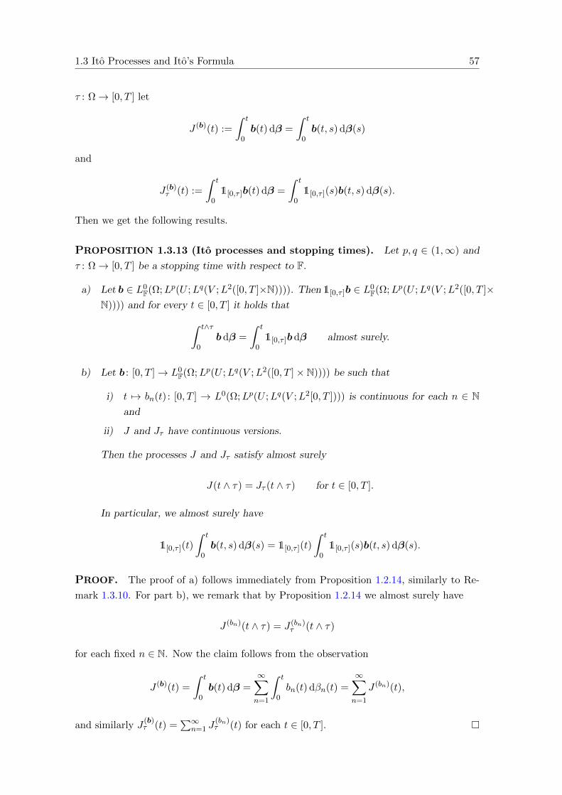
τ : Ω→ [0, T ] let

J (b)(t) :=

∫ t

0b(t) dβ =

∫ t

0b(t, s) dβ(s)

and

J (b)τ (t) :=

∫ t

01[0,τ ]b(t) dβ =

∫ t

01[0,τ ](s)b(t, s) dβ(s).

Then we get the following results.

PROPOSITION 1.3.13 (Ito processes and stopping times). Let p, q ∈ (1,∞) and

τ : Ω→ [0, T ] be a stopping time with respect to F.

a) Let b ∈ L0F(Ω;Lp(U ;Lq(V ;L2([0, T ]×N)))). Then 1[0,τ ]b ∈ L0

F(Ω;Lp(U ;Lq(V ;L2([0, T ]×N)))) and for every t ∈ [0, T ] it holds that∫ t∧τ

0b dβ =

∫ t

01[0,τ ]b dβ almost surely.

b) Let b : [0, T ]→ L0F(Ω;Lp(U ;Lq(V ;L2([0, T ]× N)))) be such that

i) t 7→ bn(t) : [0, T ] → L0(Ω;Lp(U ;Lq(V ;L2[0, T ]))) is continuous for each n ∈ Nand


Then the processes J and Jτ satisfy almost surely

J(t ∧ τ) = Jτ (t ∧ τ) for t ∈ [0, T ].


1[0,τ ](t)

∫ t

0b(t, s) dβ(s) = 1[0,τ ](t)

∫ t

01[0,τ ](s)b(t, s) dβ(s).

PROOF. The proof of a) follows immediately from Proposition 1.2.14, similarly to Re-

mark 1.3.10. For part b), we remark that by Proposition 1.2.14 we almost surely have

J (bn)(t ∧ τ) = J (bn)τ (t ∧ τ)

for each fixed n ∈ N. Now the claim follows from the observation

J (b)(t) =

∫ t

0b(t) dβ =

∞∑n=1

∫ t

0bn(t) dβn(t) =

∞∑n=1

J (bn)(t),

and similarly J(b)τ (t) =

∑∞n=1 J

(bn)τ (t) for each t ∈ [0, T ].


In the same manner as before, we turn to regularity properties of the localized Ito process.

THEOREM 1.3.14 (More properties of L0 Ito processes). Let p, q ∈ (1,∞), r ∈[1,∞), and b ∈ L0

F(Ω;Lp(U ;Lq(V ;L2([0, T ]× N)))). Then the following properties hold:

a) Local martingale property. The Ito process b dβ is a local martingale with respect

to the filtration F.

b) Continuity and Burkholder-Davis-Gundy inequality. The Ito process b dβ is

almost surely continuous satisfying the maximal inequality

E∥∥∥ supt∈[0,T ]

∣∣∣∫ t

0b dβ

∣∣∣ ∥∥∥rLp(U ;Lq(V ))


0‖b(t)‖2`2 dt

)1/2 ∥∥∥rLp(U ;Lq(V ))

,

where this is understood in the sense that the left-hand side is finite if and only if

the right-hand side is finite. If one of these cases hold, then the Ito process X(t) :=∫ t0 b dβ is again Lr-stochastically integrable satisfying

E∥∥∥(∫ T

0

∣∣X(t)∣∣2 dt

)1/2 ∥∥∥rLp(U ;Lq(V ))

.p,q,r T1/2E

∥∥∥(∫ T

0‖b(t)‖2`2 dt

)1/2 ∥∥∥rLp(U ;Lq(V ))

.

PROOF. Let (τk)k∈N be defined by

τk(ω) := T ∧ inft ∈ [0, T ] : ‖1[0,t]b(ω)‖Lp(U ;Lq(V ;L2([0,T ]×N))) ≥ k

, ω ∈ Ω.

As in Remark 1.2.8 we can show that τk is a stopping time with respect to F satisfying τk ≤τk+1, limk→∞ τk = T almost surely, and bk := 1[0,τk]b ∈ LrF(Ω;Lp(U ;Lq(V ;L2([0, T ]×N))))

for each k ∈ N and some r ∈ (1,∞).

Now the proof of a) and b) can be done by following the lines of the proof of Theorem

1.2.15, using Theorem 1.3.7 c) and Proposition 1.3.13 a).

With very little effort we can now even prove a generalization of the stochastic Fubini

Theorem 1.2.16.

THEOREM 1.3.15 (Stochastic Fubini theorem for Ito processes). Let p, q ∈ (1,∞),

(K,K, θ) be a σ-finite measure space, and b : K × Ω → Lp(U ;Lq(V ;L2([0, T ] × N))) be

strongly measurable such that

b(·, ω) ∈ L1(K;Lp(U ;Lq(V ;L2([0, T ]× N)))) for P-almost all ω ∈ Ω,

b(x, ·) ∈ L0F(Ω;Lp(U ;Lq(V ;L2([0, T ]× N)))) for θ-almost all x ∈ K.

Then the following assertions hold:


a) For θ-almost all x ∈ K, b(x, ·) dβ is an L0-Ito process and

ξ(x, ω, t) :=(∫ t

0b(x, s) dβ(s)

)(ω)

is measurable satisfying almost surely∫K

∥∥ supt∈[0,T ]

|ξ(x, t)|∥∥Lp(U ;Lq(V ))

dθ(x) <∞.

b) For almost all (ω, t, u, v) ∈ Ω × [0, T ] × U × V the functions x 7→ bn(x, ω, t, u, v) are

integrable for all n ∈ N and for

η(ω, t) :=

∫Kb(x, ω, t) dθ(x)

the process η dβ is an L0-Ito process.

c) Almost surely, we have∫Kξ(x, t) dθ(x) =

∫ t

0η(s) dβ(s), t ∈ [0, T ].

PROOF. By using the strong Burkholder-Davis-Gundy inequality from Theorem 1.3.7,

part a) can be shown in the same way as in the proof of Theorem 1.2.16. The statements

of b) and c) follow in the same way.

As already announced earlier, we finally show Ito’s formula, which can be thought of

as a counterpart of the chain rule in stochastic calculus. More precisely, we want to

determine a ’Taylor expansion’ of the process Φ(·, X) : Ω × [0, T ] → Lp(U ;Lq(V )), where

Φ: [0, T ] × Lp(U ;Lq(V )) → Lp(U ;Lq(V )) is a sufficiently differentiable function, X is an

L0 Ito process and (U , Σ, µ) and (V , Ξ, ν) are σ-finite measure spaces.

THEOREM 1.3.16 (Ito’s formula). Let p, q, p, q ∈ (1,∞), Φ: [0, T ]×Lp(U ;Lq(V ))→Lp(U ;Lq(V )) be an element of C1,2

([0, T ] × Lp(U ;Lq(V ));Lp(U ;Lq(V ))

), (βn)n∈N be a

sequence of independent Brownian motions, and X be an Lp(U ;Lq(V ))-valued Ito process

given by dX = f dt + b dβ. Further, let b ∈ L0(Ω;L2([0, T ] × N;Lp(U ;Lq(V )))). Then,

almost surely for all t ∈ [0, T ] we have

Φ(t,X(t)

)= Φ

(0, X(0)

)+

∫ t

0∂tΦ(s,X(s)

)ds+

∫ t

0D2Φ

(s,X(s)

)f(s) ds

+∞∑n=1

∫ t

0D2Φ

(s,X(s)

)bn(s) dβn(s)

+1

2

∫ t

0

∞∑n=1

(D2

2Φ(s,X(s)

)bn(s)

)bn(s) ds.


For the proof of this statement see [15, Theorem 2.4] or [3, Theorem 4.16]. As an immediate

consequence of this formula, we obtain the following product rule for Ito processes. For

the proof we refer to [15, Corollary 2.6] (see also [3, Corollary 4.18]).

COROLLARY 1.3.17 (Product rule). Let p, q ∈ (1,∞), X be an Lp(U ;Lq(V ))-valued

and Y be an Lp′(U ;Lq

′(V ))-valued Ito process given by dX = f dt + b dβ and dY =

g dt + cdβ, respectively. Let X and Y satisfy the assumptions of Theorem 1.3.16. Then,

almost surely for all t ∈ [0, T ] we have

〈X(t), Y (t)〉 = 〈X(0), Y (0)〉+

∫ t

0〈X(s), g(s)〉+ 〈f(s), Y (s)〉 ds

+∞∑n=1

∫ t

0〈X(s), cn(s)〉+ 〈bn(s), Y (s)〉dβn(s)

+

∫ t

0

∞∑n=1

〈bn(s), cn(s)〉ds.

1.4 Stochastic Integration in Sobolev and Besov Spaces

When taking a closer look at Sections 1.1, 1.2, and 1.3, it is straightforward to show the

same results for other mixed Lp spaces like

E = Lp1(U1;Lp2(U2; . . . LpN (UN )) . . .)

by induction. The key to everything is the integrability condition

b ∈ LrF(Ω;E(L2([0, T ]× N)))

for some r ∈ 0 ∩ (1,∞) and with the L2([0, T ]×N) norm inside of the norm in E. This

is the reason that makes stochastic integration theory in Lp spaces or more generally in

Banach spaces not as easy as deterministic integration theory.

Employing these results, we can treat the stochastic integration theory in (mixed) Sobolev

and Besov spaces very easily. We do not want to consider this in too much detail here.

However, we want to give an overview of how the integration theory in mixed Lp spaces

can be used to characterize the integration theory in such spaces. Let U ⊆ Rd be an open

set (with possibly non-smooth boundary), s > 0 and p ∈ [1,∞). For the case s ∈ (0, 1) we

recall that a function f ∈ Lp(U) is in the Sobolev-Slobodeckij space W s,p(U) if and only if

the function dW s,p [f ] given by

dW s,p [f ](x, y) :=1

|x− y|d/p+s(f(x)− f(y)

)

1.4 Stochastic Integration in Sobolev and Besov Spaces 61

is an element of Lp(U × U), and W s,p(U) is a Banach space with respect to the norm

‖f‖W s,p(U) =(‖f‖pLp(U) + ‖dW s,p [f ]‖pLp(U×U)

)1/p.

In the case of a Banach space-valued Sobolev space W s,p(U ;E) the norms are given by

‖f‖W s,p(U ;E) =(‖f‖pLp(U ;E) + ‖dW s,p [f ]‖pLp(U×U ;E)

)1/p.

If s ∈ N, the space W s,p(U) is of course the usual Sobolev space, i.e. the space of all

functions f ∈ Lp(U) having Lp-integrable weak derivatives up to order s; in other words,

Dαf exists in the weak sense and Dαf ∈ Lp(U) for all |α| ≤ s. If s > 1, then we can find

an integer m ∈ N and σ ∈ (0, 1) such that s = m+ σ. Here a function f ∈ Wm,p(U) is in

W s,p(U) if and only if Dαf ∈W σ,p(U) for each α ∈ Nd0 satisfying |α| = m. In this case we

have the norm

‖f‖W s,p(U) =(‖f‖pWm,p(U) +

∑|α|=m

‖Dαf‖pWσ,p(U)

)1/p.

The first thing we want to know is the correct space of integrands. Looking at the previous

sections, it is no surprise that it is given by LrF(Ω;W s,p(U ;L2([0, T ] × N))), again with

the L2([0, T ] × N) norm inside of the Sobolev norm. To prove that, we first consider

the case s ∈ (0, 1). If we want to estimate the integral∫ T

0 b dβ for ’W s,p(U)-valued’ b

we have to estimate it in the Lp(U) norm and dW s,p [∫ T

0 b dβ] in the Lp(U × U) norm.

Observe that the stochastic integral is well-defined since W s,p(U) ⊆ Lp(U). In view of

dW s,p [b] = (dW s,p [bn])n∈N ∈ LrF(Ω;Lp(U × U ;L2([0, T ]× N))), Proposition 1.3.11 e) yields

dW s,p

[∫ T

0b dβ

]=

∫ T

0dW s,p [b] dβ.

Using the Ito isomorphism for the Lp case we obtain the following Ito isomorphism for

Sobolev spaces:

E∥∥∥∫ T

0b dβ

∥∥∥rW s,p(U)

hp,r E∥∥∥∫ T

0b dβ

∥∥∥rLp(U)

+ E∥∥∥∫ T

0dW s,p [b] dβ

∥∥∥rLp(U×U)

hp,r E‖b‖rLp(U ;L2([0,T ]×N)) + E‖dW s,p [b]‖rLp(U×U ;L2([0,T ]×N))

hp,r E(‖b‖p

Lp(U ;L2([0,T ]×N))+ ‖dW s,p [b]‖p

Lp(U×U ;L2([0,T ]×N))

)r/p= E‖b‖rW s,p(U ;L2([0,T ]×N)).

One interesting fact is that the constants appearing here are independent of s. In the case

s ∈ N or s > 1, we can see very similarly that the same Ito isomorphism holds. Here we

additionally use that

Dα

∫ T

0b dβ =

∫ T

0Dαb dβ


for any multi-index α ∈ Nd0. To see this, we use Proposition 1.3.11 c) and obtain for any

φ ∈ C∞c (U)∫U

∫ T

0b dβ Dαφ dx =

⟨∫ T

0b db, Dαφ

⟩Lp(U)

=

∫ T

0〈b, Dαφ〉L2

Lp(U) dβ

= (−1)|α|∫ T

0〈Dαb, φ〉L2

Lp(U) dβ = (−1)|α|∫U

∫ T

0Dαb dβ φ dx.

Now the theory goes through without any problems. As a first result we obtain:

PROPOSITION 1.4.1 (Properties of the Sobolev space-valued integral). Let s >

0, p ∈ (1,∞), r ∈ 0 ∪ (1,∞), and b, b ∈ LrF(Ω;W s,p(U ;L2([0, T ] × N))). Then the fol-

lowing properties hold:

a) The stochastic integral is linear, i.e. for a, b ∈ R we have∫ T

0ab+ bb dβ = a

∫ T

0b dβ + b

∫ T

0b dβ.

b)∫ T

0 b dβ is FT -measurable and, if r ∈ (1,∞), the expected value satisfies E∫ T

0 b dβ =

0.

c) For S ∈ B(W s,p(U)

), let SL

2be the bounded extension of S on W s,p(U ;L2([0, T ]×

N)). Then, SL2b ∈ LrF(Ω;W s,p(U ;L2([0, T ]× N))) and∫ T

0SL

2b dβ = S

∫ T

0b dβ.


sb dβ =

∫ T

01[s,t]b dβ.

e) There exists a null set N ∈ BU such that b(u) ∈ Lp∧rF (Ω;L2[0, T ]), and∫ T

0b(u) dβ =

(∫ T

0b dβ

)(u) for each u ∈ U \N .

The next step is to investigate the Sobolev space-valued integral process t 7→∫ t

0 b dβ. One

crucial property we needed in that part of the theory is the martingale property and the

strong Doob and Burkholder-Davis-Gundy inequalities. In order to extend the results from

the Lp-valued case, we have to carefully check if the differences and derivatives appearing

in the Sobolev norms do not destroy any martingale structure. For this reason we need to

prove the following lemma.


LEMMA 1.4.2. Let s > 0, p, r ∈ [1,∞), and (Mn)Nn=1 be a W s,p(U)-valued Lr martin-

gale with respect to the filtration (Fn)Nn=1.

a) If s ∈ (0, 1), then (dW s,p [Mn])Nn=1 is an Lp(U ×U)-valued Lr martingale with respect

to (Fn)Nn=1.

b) If s ∈ N, then (DαMn)Nn=1 is an Lp(U)-valued Lr martingale with respect to (Fn)Nn=1

for any α ∈ Nd0 with |α| ≤ s. In particular, (Mn)Nn=1 is an Lp(U)-valued Lr martingale.

PROOF. The strong measurability of dW s,p [Mn] and DαMn with respect to Fn is trivial.

Also, the integrability condition follows immediately from the assumption. Hence, the only

thing left to check is the projection property. In the following let n > m.

a) Since E[Mn|Fm] = Mm in W s,p(U) almost surely, we obtain that E[Mn|Fm] = Mm in

Lp(U) and dW s,p

[E[Mn|Fm]

]= dW s,p [Mm] in Lp(U × U) almost surely. The result now

follows from

dW s,p

[E[Mn|Fm]

](x, y) = E

[dW s,p [Mn]

∣∣Fm](x, y)

for almost every (x, y) ∈ U × U .

b) By assumption we have DαE[Mn|Fm] = DαMm in Lp(U) almost surely. Additionally,

for A ∈ Fm and φ ∈ C∞c (U) we have⟨∫ADαMn dP, φ

⟩Lp

=

∫A〈DαMn, φ〉Lp dP = (−1)|α|

∫A〈Mn, D

αφ〉Lp dP

= (−1)|α|⟨∫

AE[Mn|Fm] dP, Dαφ

⟩Lp

=⟨∫

ADαE[Mn|Fm] dP, φ

⟩Lp,

where we used that Mn,E[Mn|Fm] ∈ W s,p(U). Thus, E[DαMn|Fm] = DαE[Mn|Fm] =

DαMm almost surely.

As a consequence we obtain, among other results, the following version of Doob’s maximal

inequality.

THEOREM 1.4.3 (Strong Doob inequality, II). Let s > 0, p, r ∈ (1,∞), and (Mn)Nn=1

be an W s,p(U)-valued Lr martingale with respect to the filtration (Fn)Nn=1. Then we have

E∥∥(Mn)Nn=1

∥∥rW s,p(U ;`∞)

.p,r E‖MN‖rW s,p(U).

In particular, E∥∥ N

maxn=1|Mn|

∥∥rW s,p(U)

.p,r E‖MN‖rW s,p(U).


PROOF. We first take a look at the case s ∈ (0, 1). Lemma 1.4.2 yields that (dW s,p [Mn])Nn=1

and (Mn)Nn=1 are Lp-valued Lr martingales with respect to (Fn)Nn=1. The Strong Doob in-

equality now leads to

E∥∥(Mn)Nn=1

∥∥rW s,p(U ;`∞)

hp,r E∥∥ N

maxn=1|Mn|

∥∥rLp(U)

+ E∥∥ N

maxn=1|dW s,p [Mn]|

∥∥rLp(U×U)

.p,r E‖MN‖rLp(U) + E‖dW s,p [MN ]‖rLp(U×U)

hp,r E‖MN‖rW s,p(U).

The case s ≥ 1 now follows in the same way using that (DαMn)Nn=1 and (if s /∈ N)

(dW s,p [DαMn])Nn=1 are Lp-valued Lr martingales with respect to (Fn)Nn=1 by the previous

lemma.

With nearly the same methods we obtain:

THEOREM 1.4.4 (Strong Burkholder-Davis-Gundy inequality, II). Let s > 0,

p ∈ (1,∞), r ∈ [1,∞), and (Mn)Nn=1 be an W s,p(U)-valued Lr martingale with respect to

the filtration (Fn)Nn=1. Then we have

E∥∥(Mn)Nn=1

∥∥rW s,p(U ;`∞)

hp,r E‖(Mn −Mn−1)Nn=1‖rW s,p(U ;`2).

In particular, E∥∥ Nmaxn=1|Mn|

∥∥rW s,p(U)

hp,r E‖(Mn −Mn−1)Nn=1‖rW s,p(U ;`2).

These maximal inequalities were the heart of the regularity results for stochastic integrals.

Analogously to the previous sections, these results may now be used to obtain corresponding

properties for the Sobolev space-valued integral process. Alternatively, we can also use the

results of the Lp-valued case.

THEOREM 1.4.5 (Properties of the integral processes). Let s > 0, p ∈ (1,∞),

r ∈ 0 ∪ (1,∞), and b ∈ LrF(Ω;W s,p(U ;L2([0, T ] × N))). Then the following properties

hold:

1) In the case r ∈ (1,∞):

a) Martingale property. The Ito process b dβ is a martingale with respect to

the filtration F.

b) Continuity. The Ito process b dβ has a continuous version satisfying the max-

imal inequality

E∥∥∥ t 7→ ∫ t

0b dβ

∥∥∥rW s,p(U ;C[0,T ])

.p,r E∥∥∥∫ T

0b dβ

∥∥∥rW s,p(U)

.

In particular, E∥∥supt∈[0,T ]

∣∣∫ t0 b dβ

∣∣∥∥rW s,p(U)

.p,r E∥∥∫ T

0 bdβ∥∥rW s,p(U)

.


c) Burkholder-Davis-Gundy inequality. As a consequence of b) and the Ito

isomorphism we have

E∥∥∥ t 7→ ∫ t

0b dβ

∥∥∥rW s,p(U ;C[0,T ])

hp,r E‖b‖rW s,p(U ;L2([0,T ]×N)),

where this also holds for r = 1. In particular, the process X(t) :=∫ t

0 b dβ,

t ∈ [0, T ], is again Lr-stochastically integrable satisfying

E‖X‖rW s,p(U ;L2[0,T ]) .p,r T1/2E‖b‖rW s,p(U ;L2([0,T ]×N)).

2) In the case r = 0:

a) Local martingale property. The Ito process b dβ is a local martingale with

respect to the filtration F.

b) Continuity and Burkholder-Gundy inequality. The Ito process b dβ is

almost surely continuous satisfying the maximal inequality

E∥∥∥ t 7→ ∫ t

0b dβ

∥∥∥rW s,p(U ;C[0,T ])

hp,r E‖b‖rW s,p(U ;L2([0,T ]×N)).

where this is understood in the sense that the left-hand side is finite if and only

if the right-hand side is finite. If one of these cases holds, then the process

X(t) :=∫ t

0 b dβ is again Lr-stochastically integrable satisfying

E‖X‖rW s,p(U ;L2[0,T ]) .p,r T1/2E‖b‖rW s,p(U ;L2([0,T ]×N)).

PROOF. These results follow by applying the results of Theorems 1.3.7 and 1.3.14 to b

(as an element of Lp(U ;L2([0, T ]×N))) and dW s,p [b] separately, similarly to the calculations

of the Ito isomorphism above.

At this point we conclude the discussion about Sobolev space-valued stochastic integration

theory, and turn to the case of Besov spaces. Here we define for l ∈ N0 and h ∈ Rd the set

Uh,l :=

l⋂j=0

x ∈ U : x+ jh ∈ U ⊆ U

and the difference operator

(∆lhf)(x) := f(x+ lh)− f(x+ (l − 1)h).

Let s > 0 and p, q ∈ (1,∞). Choose k, l ∈ N0 such that k < s and l > s − k (e.g. if

s ∈ R+ \ N, then we could take k = [s] < s and l = 1, and if s ∈ N then k = s − 1 and


l = 2 would suffice). Then we define the function dBs,pq [f ] by

dBs,pq [f ](h, x) := 1Uh,l(x)|h|−d/q−(s−k)(∆lhf)(x).

Therewith we define the space Bs,pq (U) as the set of all functions f ∈ Lp(U) such that

dBs,pq [Dαf ] ∈ Lq(Rd;Lp(U)) for each α ∈ Nd0 with |α| ≤ k. Then Bs,pq (U) is a Banach space

with respect to the norm

‖f‖Bs,pq (U) =(‖f‖pLp(U) +

∑|α|≤k

‖dBs,pq [Dαf ]‖pLq(Rd;Lp(U))

)1/p.

We now get exactly the same results for Besov spaces as for Sobolev spaces by replacing

dW s,p [·] with dBs,pq [·] and Lp(U × U) by the mixed Lp space Lq(Rd;Lp(U)).

As a consequence of the remark given in the beginning of this section, we can also extend

this theory to mixed Besov and/or Sobolev spaces. The only thing we have to remind

ourselves of is that the L2([0, T ]×N) norm is always inside of the mixed space in order to

have a well-defined stochastic integral.

This theory is now perfect to study time regularity for stochastic convolutions. Until this

point we have only discussed regularity of the stochastic integral process

t 7→∫ t

0b(s) dβ(s)

of Lp-valued processes f . As in the deterministic case, integrals of the form

t 7→∫ t

0e−(t−s)Ab(s) dβ(s)

will appear in the formulation of mild solutions for stochastic evolution equations, where

(−A) is the generator of an analytic semigroup. Since

t 7→∫ t

0e−(t−s)Ab(s) dβ(s) =

∫ T

01[0,t](s)e

−(t−s)Ab(s) dβ(s)

by Proposition 1.4.1, investigating regularity of stochastic convolutions in Lp(U ;Lq[0, T ])

or Lp(U ;W s,q[0, T ]) reduces to the estimation of the function

1[0,t](s)e−(t−s)Ab(s)

in Lp(U ;Lq(t)([0, T ];L2(s)[0, T ])) or Lp(U ;W s,q

(t) ([0, T ];L2(s)[0, T ])), respectively.

Chapter 2

Functional Analytic Operator

Properties

In Chapter 3 we want to use functional calculi results to deduce regularity properties of

deterministic and stochastic convolutions. These in turn will lead to new regularity results

for stochastic evolution equations. In the following sections we introduce several notions

which appear in this context. The basic question here is: How can we define the expression

f(A) for a linear operator A and some function f? And which conditions do we have to

impose on A or f to get nice properties of f(A)?

2.1 Rq-boundedness and Rq-sectorial Operators

In this section we concentrate on basic notions coming into focus when dealing with func-

tional calculi results. To give a short motivation, we recall Cauchy’s integral formula for

holomorphic functions f , stating that

f(λ) =1

2πi

∫Γ

f(z)

z − λdz,

where Γ is a closed path around the singularity λ. If we ’plug in’ an operator A in this

equation, we would end up with

f(A) =1

2πi

∫Γf(z)R(z,A) dz,

where now Γ should circumvent the ’singularity’ of R(z,A), i.e. the spectrum σ(A). Of

course, this is just a motivation. In the next section we will give a reasonable definition of

this idea. However, this already indicates the necessity of some characteristic features the

resolvent function of A should have.

68 Functional Analytic Operator Properties

Before turning to that, we start with a special randomization property for a set of bounded

operators.

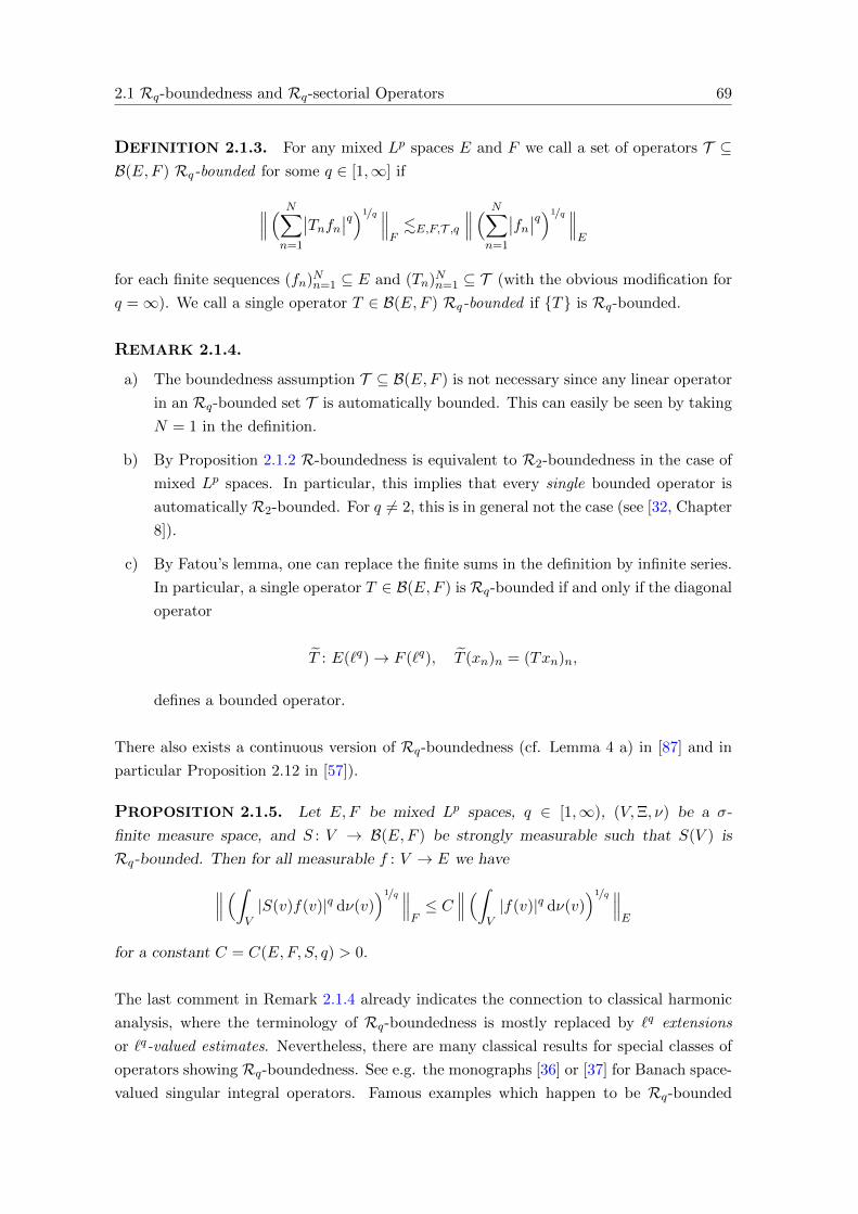
DEFINITION 2.1.1. For any Banach spaces E and F we call a set of operators T ⊆B(E,F ) R-bounded if

E∥∥∥ N∑n=1

rnTnxn

∥∥∥F.E,F,T E

∥∥∥ N∑n=1

rnxn

∥∥∥E

for each finite sequences (xn)Nn=1 ⊆ E, (Tn)Nn=1 ⊆ T , and each Rademacher sequence

(rn)Nn=1 on some probability space (Ω, F , P).

R-boundedness is a generalization of a square function estimate. In the special case of a

mixed Lp space E, like E = Lr(Ω;Lp(U ;Lq(V ))), this is particularly obvious since we have

here the following characterization.

PROPOSITION 2.1.2. Let E and F be two mixed Lp spaces. Then T ⊆ B(E,F ) is

R-bounded if and only if

∥∥∥( N∑n=1

∣∣Tnfn∣∣2)1/2 ∥∥∥F.E,F,T

∥∥∥( N∑n=1

∣∣fn∣∣2)1/2 ∥∥∥E

for each (fn)Nn=1 ⊆ E and (Tn)Nn=1 ⊂ T .

PROOF. This is a consequence of the special form Kahane’s inequality has in this par-

ticular case. Let G ∈ E,F. Using the estimate for K-valued Rademacher sums, i.e.

E∣∣∣ N∑n=1

αnrn

∣∣∣p hp

( N∑n=1

|αn|2)p/2

for any p ∈ [1,∞) and (αn)Nn=1 ⊆ K, as well as the q-concavity of the space G for some

q ∈ [1,∞), we obtain

E∥∥∥ N∑n=1

rngn

∥∥∥Gh∥∥∥( N∑

n=1

∣∣gn∣∣2)1/2 ∥∥∥G

for any sequence (gn)Nn=1 ⊆ G.

In his paper [87] Lutz Weis extended the concept of R-boundedness and introduced the

notion of Rq-boundedness in the special case of Lp spaces. In [79] this was elaborated in

detail in the setting of Banach function spaces (see also [57]).

2.1 Rq-boundedness and Rq-sectorial Operators 69

DEFINITION 2.1.3. For any mixed Lp spaces E and F we call a set of operators T ⊆B(E,F ) Rq-bounded for some q ∈ [1,∞] if

∥∥∥( N∑n=1

∣∣Tnfn∣∣q)1/q ∥∥∥F.E,F,T ,q

∥∥∥( N∑n=1

∣∣fn∣∣q)1/q ∥∥∥E

for each finite sequences (fn)Nn=1 ⊆ E and (Tn)Nn=1 ⊆ T (with the obvious modification for

q =∞). We call a single operator T ∈ B(E,F ) Rq-bounded if T is Rq-bounded.

REMARK 2.1.4. .

a) The boundedness assumption T ⊆ B(E,F ) is not necessary since any linear operator

in an Rq-bounded set T is automatically bounded. This can easily be seen by taking

N = 1 in the definition.

b) By Proposition 2.1.2 R-boundedness is equivalent to R2-boundedness in the case of

mixed Lp spaces. In particular, this implies that every single bounded operator is

automaticallyR2-bounded. For q 6= 2, this is in general not the case (see [32, Chapter

8]).

c) By Fatou’s lemma, one can replace the finite sums in the definition by infinite series.

In particular, a single operator T ∈ B(E,F ) is Rq-bounded if and only if the diagonal

operator

T : E(`q)→ F (`q), T (xn)n = (Txn)n,

defines a bounded operator.

There also exists a continuous version of Rq-boundedness (cf. Lemma 4 a) in [87] and in

particular Proposition 2.12 in [57]).

PROPOSITION 2.1.5. Let E,F be mixed Lp spaces, q ∈ [1,∞), (V,Ξ, ν) be a σ-

finite measure space, and S : V → B(E,F ) be strongly measurable such that S(V ) is

Rq-bounded. Then for all measurable f : V → E we have∥∥∥(∫V|S(v)f(v)|q dν(v)

)1/q ∥∥∥F≤ C

∥∥∥(∫V|f(v)|q dν(v)

)1/q ∥∥∥E

for a constant C = C(E,F, S, q) > 0.

The last comment in Remark 2.1.4 already indicates the connection to classical harmonic

analysis, where the terminology of Rq-boundedness is mostly replaced by `q extensions

or `q-valued estimates. Nevertheless, there are many classical results for special classes of

operators showing Rq-boundedness. See e.g. the monographs [36] or [37] for Banach space-

valued singular integral operators. Famous examples which happen to be Rq-bounded


include the Hilbert transform and the Riesz transform on Lp for p, q ∈ (1,∞) (see [11]

or [39, Corollary 5.6.3]). Another famous result is the Fefferman-Stein-inequality for the

(uncentered) Hardy-Littlewood maximal function

(Mf)(x) := supB3x

1

|B|

∫B|f |dµ, f ∈ Lqloc(R

d), x ∈ Rd,

where the supremum is taken over all balls B ⊆ Rd containing x. Here, |B| denotes the

Lebesgue measure of B. For the proof of the following result see [35] or [39, Theorem 5.6.6].

THEOREM 2.1.6 (Fefferman-Stein). Let p, q ∈ (1,∞). Then the Hardy-Littlewood

maximal operator M is Rq-bounded on Lp(Rd).

REMARK 2.1.7. This result is also true if we replace Rd by a metric measure space

(U, d, µ) of homogeneous type (cf. [40]), i.e. (U, d) is a metric space and µ is a σ-finite

regular Borel measure on U with the doubling property which in turn means that there

exists a constant C ≥ 1 such that

µ(B(x, 2r)) ≤ Cµ(B(x, r)) x ∈ U, r > 0,

where B(x, r) denotes the ball with center x and radius r.

With the concepts of R-boundedness and Rq-boundedness we can now focus on some

notions for resolvents as indicated in the beginning. For this purpose we need open sectors

in C, which we abbreviate as

Σσ := z ∈ C \ 0 : |arg(z)| < σ, σ ∈ (0, π],

and Σ0 := (0,∞).

DEFINITION 2.1.8. Let E be a Banach space and let A : D(A) ⊆ E → E be a closed

linear operator.

a) A is called a sectorial operator of angle α ∈ [0, π) if its spectrum σ(A) is contained

in the closed sector Σα and there exists a constant Cα > 0 such that

‖λR(λ,A)‖B(E) ≤ Cα for all λ ∈ C \ Σα.

The infimum over all such α is denoted by ω(A).

b) A is called anR-sectorial operator of angle α ∈ [0, π) if its spectrum σ(A) is contained

in the closed sector Σα and the set λR(λ,A) : λ ∈ C \ Σα is R-bounded, i.e. there

2.1 Rq-boundedness and Rq-sectorial Operators 71

exists a constant Cα > 0 such that

E∥∥∥ N∑n=1

rnλnR(λn, A)xn

∥∥∥E≤ Cα E

∥∥∥ N∑n=1

rnxn

∥∥∥E

for each finite sequence (λn)Nn=1 ⊆ C \ Σα, (xn)Nn=1 ⊆ E, and each Rademacher

sequence (rn)Nn=1 on some probability space (Ω, F , P). In this case, we denote by

ωR(A) the infimum over all such α.

c) Let E be a mixed Lp space and q ∈ [1,∞]. Then we call A an `q-sectorial operator

of angle α ∈ [0, π) if its spectrum σ(A) is contained in the closed sector Σα and there

exists a constant Cα > 0 such that

∥∥∥( N∑n=1

∣∣λR(λ,A)xn∣∣q)1/q ∥∥∥

E≤ Cα

∥∥∥( N∑n=1

|xn|q)1/q ∥∥∥

Efor all λ ∈ C \ Σα

and each finite sequence (xn)Nn=1 ⊆ E (with the obvious modification for q = ∞).

The infimum over all such α is denoted by ω`q(A).

d) Let E be a mixed Lp space and q ∈ [1,∞]. Then we call A an Rq-sectorial operator

of angle α ∈ [0, π) if its spectrum σ(A) is contained in the closed sector Σα and the

set λR(λ,A) : λ ∈ C \ Σα is Rq-bounded, i.e. there exists a constant Cα > 0 such

that

∥∥∥( N∑n=1

∣∣λnR(λn, A)xn∣∣q)1/q ∥∥∥

E≤ Cα

∥∥∥( N∑n=1

|xn|q)1/q ∥∥∥

E

for each finite sequence (λn)Nn=1 ⊆ C \ Σα and (xn)Nn=1 ⊆ E (with the obvious modi-

fication for q =∞). The infimum over all such α is denoted by ωRq(A).

REMARK 2.1.9. .

a) In the case of mixed Lp spaces, Proposition 2.1.2 directly yields that R-sectoriality

is equivalent to R2-sectoriality.

b) The difference between part c) and d) is the following: If A is and `q-sectorial op-

erator, then every single operator set λR(λ,A), λ ∈ Σα, is Rq-bounded with a

uniform constant Cα. In particular, every Rq-sectorial operator is `q-sectorial.

Remark 2.1.4 already indicates the connection to a diagonal operator (see [57, Proposition

3.2]). Looking closely at the proof of this statement, one sees that we only need `q-

sectoriality to get the following result.


PROPOSITION 2.1.10. Let q ∈ [1,∞], E be a mixed Lp space, and A be `q-sectorial.

Then we define

D(A) := (xn)n∈N ∈ E(`q) : xn ∈ D(A) for all n ∈ N and (Axn)n∈N ∈ E(`q)

and Ax = (Axn)n∈N, for x ∈ D(A). Then A is a sectorial operator with ω(A) ≤ ω`q(A)

and

R(λ, A)x = (R(λ,A)xn)n∈N for λ /∈ Σω`q (A) and x ∈ E(`q).

In Section 2.3 we will see more results on the connection of these notions.

2.2 H∞ and RH∞ Calculus

Using the terminology of the previous section, we can define a functional calculus for

sectorial operators. In this section we will always assume that A : D(A)→ E is a sectorial

operator on some Banach space E with dense domain and dense range. By the sectoriality,

A is then already injective (cf. [43, Proposition 2.11]). This assumption is not really

restrictive, since we mostly work in Lp spaces for p ∈ (1,∞), i.e in the reflexive case. In

this situation A always has dense domain, and the injectivity is equivalent to A having

dense range.

Let in the following be α ∈ (ω(A), π]. For functions f : Σα → C we define the norm

‖f‖∞,α := supλ∈Σα

|f(λ)|

and the space

H∞(Σα) :=f : Σα → C : f is analytic and ‖f‖∞,α <∞

,

as well as

H∞0 (Σα) :=f ∈ H∞(Σα) : sup

λ∈Σα

(|λ|ε ∨ |λ|−ε

)|f(λ)| <∞ for some ε > 0

,

Now let σ ∈ (ω(A), α). Then we define the path

Γ(σ) :=λ ∈ C : λ = γ(t) = |t|e−isign(t)σ, t ∈ R

.

As indicated in the beginning of the previous section, we define for functions ϕ ∈ H∞0 (Σα)

the expression ϕ(A) as the integral

ϕ(A) :=1

2πi

∫Γ(σ)

ϕ(λ)R(λ,A) dλ,

2.2 H∞ and RH∞ Calculus 73

which is well-defined as a Bochner integral in B(E) since ‖ϕ(γ(·))R(γ(·), A)‖B(E) is inte-

grable in R. Note that the algebra homomorphism

ϕ 7→ ϕ(A) : H∞0 (Σα)→ B(E)

is independent of σ ∈ (ω(A), α) by Cauchy’s integral formula. Following [59], we can extend

this functional calculus to functions f ∈ H∞(Σα) and even larger classes of functions (for

more details in this direction see e.g. [43, Section 2.2]). However, without any additional

assumptions on A, these extended functional calculi only yield closed operators.

One of the most important features of this calculus is the following convergence property

(see [43, Proposition 5.1.4]).

PROPOSITION 2.2.1. Let (fn)n≥1 ⊆ H∞(Σα) with the following properties

a) ∃ f0(λ) := limn→∞ fn(λ) for all λ ∈ Σα;

b) supn∈N ‖fn‖∞,α <∞;

c) fn(A) ∈ B(E) for all n ∈ N and M := supn∈N ‖fn(A)‖ <∞.

Then f0 ∈ H∞(Σα) and f0(A) ∈ B(E), satisfying ‖f0(A)‖ ≤M . Moreover,

limn→∞

fn(A)x = f0(A)x, x ∈ E.

Now let us proceed to the definition of a bounded H∞(Σα) calculus.

DEFINITION 2.2.2. Let α ∈ (ω(A), π]. Then A has a bounded H∞(Σα) calculus if

there is a constant Cα <∞ such that

‖f(A)‖ ≤ Cα‖f‖∞,α for all f ∈ H∞(Σα).

In this case we define

ωH∞(A) := infα ∈ (ω(A), π] : A has a bounded H∞(Σα) calculus.

Following [59, Remark 9.11] or [43, Proposition 5.3.4], the convergence property and the

closed graph theorem imply a slightly different characterization of a bounded H∞ calculus.

COROLLARY 2.2.3. The operator A has a bounded H∞(Σα) calculus if and only if

there is a constant Cα > 0 such that

‖ϕ(A)‖ ≤ Cα‖ϕ‖∞,α for all ϕ ∈ H∞0 (Σα).


In [52] the authors extended this calculus to operator-valued functions with R-bounded

range, the so called RH∞-functional calculus. Under some geometric assumptions on the

underlying Banach space they proved that this calculus is again R-bounded. The following

notions are taken from [52] and [59, Chapter 12]. We denote by

A := B ∈ B(E) : B commutes with the resolvents of A,

and for α ∈ (ω(A), π] the set

RH∞(Σα) := F : Σα → A : F is analytic and F (Σα) is R-bounded

as well as

RH∞0 (Σα) := F ∈ RH∞(Σα) : supλ∈Σα

(|λ|ε ∨ |λ|−ε

)‖F (λ)‖ <∞ for some ε > 0.

In the same way as above we can define for σ ∈ (ω(A), α) and F ∈ RH∞0 (Σα) the integral

F (A) :=1

2πi

∫Γ(σ)

F (λ)R(λ,A) dλ

as a Bochner integral in B(E). The mapping

ΦA : RH∞0 (Σα)→ B(E)

defines a functional calculus which can be extended to

ΦA : RH∞(Σα′)→ B(E)

for some α′ > α if A has a bounded H∞(Σα) calculus (see [52, Theorem 4.4] or [59,

Theorem 12.7]). If E has additional geometric properties, namely Pisier’s property (α),

this can be used to self-improve the H∞ calculus.

DEFINITION 2.2.4. Let (rn)n≥1 and (rn)n≥1 be two independent Rademacher sequences.

Then E has property (α) if there is a constant C <∞ such that for all N ∈ N, (αj,k)Nj,k=1 ⊆

+1,−1, and all (xj,k)Nj,k=1 ⊆ E we have

EE∥∥∥ N∑j,k=1

αj,krj rkxj,k

∥∥∥E≤ CEE

∥∥∥ N∑j,k=1

rj rkxj,k

∥∥∥E.

As an example, q-concave Banach function spaces possess this property. Therefore, espe-

cially Lp spaces do have the property (α). Putting these facts together, we obtain the

following remarkable result (see [52, Theorem 5.3 and Corollary 5.4] or [59, Theorem 12.8

and Remark 12.10]).

2.3 Rq-bounded H∞ Calculus 75

COROLLARY 2.2.5. Assume that E has property (α) and A has a bounded H∞(Σα)

calculus. Then for each α′ > α it holds that

f(A) : ‖f‖∞,α′ ≤ 1 is R-bounded,

i.e. A has an R-bounded H∞(Σα′) calculus. Moreover, also the set

F (A) : F ∈ RH∞(Σα′), ‖F‖RH∞(Σα′ )≤ 1

is R-bounded, i.e. A even has an R-bounded RH∞(Σα′) calculus.

In particular, if A has a bounded H∞(Σα) calculus, then A is R-sectorial with ωR(A) ≤ωH∞(A) (for this assertion see also [52], where this was proved under much weaker condi-

tions on E).

Looking now at the previous section again, we have seen that in mixed Lp spaces, R-

boundedness is equivalent to R2-boundedness. Therefore, it is quite natural to ask which

operators have an Rq-bounded H∞(Σα) calculus for some q ∈ [1,∞]. This is the content

of the next section.

2.3 Rq-bounded H∞ Calculus

In the following let E be any mixed Lp space with exponents p ∈ [1,∞) and A : D(A)→ E

be a sectorial operator.

DEFINITION 2.3.1. Let α ∈ (ω(A), π]. Then A has an Rq-bounded H∞(Σα) calculus

if the set

f(A) : f ∈ H∞(Σα), ‖f‖∞,α ≤ 1

is Rq-bounded, which is equivalent to the existence of a constant C > 0 such that

∥∥∥( N∑n=1

∣∣fn(A)xn∣∣q)1/q ∥∥∥

E≤ C N

maxn=1‖fn‖∞,α

∥∥∥( N∑n=1

|xn|q)1/q ∥∥∥

E

is valid for each sequence (fn)Nn=1 ⊆ H∞(Σα) and (xn)Nn=1 ⊆ E. In this case, we define

ωR∞q (A) := infα ∈ (ω(A), π] : A has an Rq-bounded H∞(Σα) calculus.

REMARK 2.3.2. Trivially, any sectorial operator with an Rq-bounded H∞-calculus has

automatically a bounded H∞ calculus. In the special case of q = 2 the converse was proven

in Corollary 2.2.5. Moreover, if A has an Rq-bounded H∞-calculus, then A is also Rq-sectorial with ωRq(A) ≤ ωR∞q (A).


Analogously to Section 2.1 we emphasize the connection between A and its diagonal oper-

ator A as defined in Proposition 2.1.10. The next result is taken from [57, Lemma 3.20].

LEMMA 2.3.3. Let q ∈ [1,∞], A be an Rq-sectorial operator, and α ∈ (ωRq(A), π].

Then the following conditions are equivalent:

a) For each f ∈ H∞(Σα) the operator f(A) is Rq-bounded.

b) The diagonal operator A has a bounded H∞(Σα) calculus in E(`q).

In [57, Theorem 3.21] it was also proven that the statement a) in the previous lemma, i.e.

theRq-boundedness of each single operator f(A), already implies anRq-bounded H∞(Σα′)

calculus for all α′ > α.

THEOREM 2.3.4. Let q ∈ [1,∞], A be anRq-sectorial operator, and α, α′ ∈ (ωRq(A), π].

Consider the following assertions:

a) A has an Rq-bounded H∞(Σα′) calculus.

b) For each f ∈ H∞(Σα) the operator f(A) is Rq-bounded.

c) For each ϕ ∈ H∞0 (Σα) the operator ϕ(A) is Rq-bounded, and there is a constant

C > 0, independent of ϕ, such that

∥∥∥( N∑n=1

∣∣ϕ(A)xn∣∣q)1/q ∥∥∥

E≤ C‖ϕ‖∞,α

∥∥∥( N∑n=1

|xn|q)1/q ∥∥∥

E

for each (xn)Nn=1 ⊆ E.

Then a)⇒ c)⇒ b) if α ≥ α′ and b)⇒ a) if α′ > α.

Combining Lemma 2.3.3 and Theorem 2.3.4 (and slightly neglecting the angles) we see

that A has an Rq-bounded H∞ calculus on E if and only if the diagonal operator A has

a bounded H∞ calculus on E(`q). Since this extension result is quite important for our

purposes, we will return to this property again in the next section.

The standard example of an operator having an Rq-bounded H∞ calculus is the Laplace

operator on Rd (see [57, Proposition 3.22]).

EXAMPLE 2.3.5. Let d,m ∈ N and p, q ∈ (1,∞). Then the Laplace operator A :=

(−∆)m has an Rq-bounded H∞ calculus in Lp(Rd) with ωR∞q (A) = 0.

Actually, many operators have an Rq-bounded H∞ calculus. For some elliptic operators in

divergence and non-divergence form as well as Schrodinger operators with singular poten-

tials this was elaborated in [58]. To establish this property the authors used (generalized)


Gaussian estimates of the corresponding operators. Below we will recall and expand the

existing list using the same tools they did. To formulate the main result we have to in-

troduce some notions. Let in the following be (U, d) be a metric space and µ be a σ-finite

regular Borel measure on U such that (U, d, µ) is a space of homogeneous type in the sense

of Coifman and Weiss (see [17], [18]), i.e. there exists a constant C ≥ 1 such that

µ(B(x, 2r)) ≤ Cµ(B(x, r)), x ∈ U, r > 0,

where B(x, r) denotes the ball with center x and radius r. This then implies the existence

of constants D > 0 and CD ≥ 1 such that

µ(B(x, λr)) ≤ CDλDµ(B(x, r)), x ∈ U, r > 0, λ ≥ 1.

We also define the annulus

Ak(x, r) := B(x, (k + 1)r) \B(x, kr), x ∈ U, r > 0, k ∈ N.

The main result then reads as follows (see [58, Theorem 2.3]).

THEOREM 2.3.6. Let 1 ≤ p0 < 2 < p1 ≤ ∞ and ω0 ∈ (0, π/2). Let A be a sectorial

operator in L2(U) such that A has a bounded H∞ calculus in L2(U) with ωH∞(A) ≤ ω0.

Assume that the generated semigroup T (λ) := e−λA satisfies the following weighted norm

estimates for each θ > ω0:

∥∥1Ak(x,|λ|1/m)T (λ)1B(x,|λ|1/m)

∥∥B(Lp0 (U),Lp1 (U))

≤ Cθµ(B(x, |λ|1/m))1p1− 1p0 (1 + k)−κθ ,∥∥1B(x,|λ|1/m)T (λ)1Ak(x,|λ|1/m)

∥∥B(Lp0 (U),Lp1 (U))

≤ Cθµ(B(x, |λ|1/m))1p1− 1p0 (1 + k)−κθ ,

for all x ∈ U , k ∈ N0, λ ∈ Σπ/2−θ, and some constants m > 0, κθ > max 1p0

+ Dp′1, 1p′1

+ Dp0

and Cθ > 0. Then for all p, q ∈ (p0, p1) and α > ω0 the operator A has an Rq-bounded

H∞(Σα) calculus in Lp(U).

This statement should be understood in the way that the semigroup T induces a consistent

C0-semigroup Tp on Lp(U) with generator (−Ap) and for all q ∈ (p0, p1) the operator Ap

has an Rq-bounded H∞ calculus with ωR∞q (A) ≤ ω0.

REMARK 2.3.7. .

a) The assertion of Theorem 2.3.6 is still true if we replace L2(U) by a general Lp(U)

space where 1 ≤ p0 < p < p1 ≤ ∞ (see [58, Remark 2.4]).

b) Note that the off-diagonal estimates of Theorem 2.3.6 are equivalent to classical

pointwise kernel estimates if the operators T (t) are integral operators with operator-

valued kernels and p0 := 1, p1 :=∞ (see [58, Lemma 2.2] and [59, Lemma 8.5]).


In the next part of this section we collect examples of operators having an Rq-bounded H∞

calculus. More precisely, we consider elliptic operators in divergence and non-divergence

form. Some of these cases were already mentioned in [58].

Example A: Elliptic operators in divergence form

Let U ⊆ Rd be an arbitrary open set. Then we shall consider elliptic operators in divergence

form given formally by

Af :=∑

|α|,|β|≤m

(−1)|α|Dα(aα,βD

βf),

with coefficients aα,β ∈ L∞(U,C). Since we want to apply Theorem 2.3.6, we have to

check two properties. Firstly that there is a realization of A in L2(U) having a bounded

H∞ calculus, and secondly that the semigroup generated by this realization satisfies the

off-diagonal estimates of Theorem 2.3.6.

We define the realization A2 of the operator A in L2(U) as the operator associated to the

form

a(f, g) :=

∫U

∑|α|,|β|≤m

aα,β(x)Dβf(x)Dαg(x) dx.

The natural domain V of this form of course depends on U and the boundary conditions.

Here, we will consider two different situations:

1) U ⊆ Rd is an arbitrary domain and we impose Dirichlet boundary conditions on A:

Here we take V := Wm,20 (U).

2) U ⊆ Rd is an arbitrary domain and we consider Neumann boundary conditions for

A: Then we let V := Wm,2(U).

In all situations we assume that the form a is sectorial, i.e. there exists an ω ∈ [0, π/2) such

that

|Im a(f, f)| ≤ tan(ω)Re a(f, f) for f ∈ V .

Moreover, we require the following ellipticity condition/Garding’s inequality for a to hold:

Re a(f, f) ≥ α0

∥∥(−∆)m/2f

∥∥2

L2(U)for f ∈ V

and some α0 > 0. Note that in the case of m = 1 both of these conditions are a consequence

of the following uniform strong ellipticity condition:

Re

d∑j,k=1

aej ,ek(x)ξjξk ≥ α0|ξ|2, for all ξ ∈ Cd and x ∈ U .


With these assumptions the operator A2 associated to the form a is sectorial and has a

bounded H∞ calculus with ωH∞(A2) ≤ α0 (see [59, Chapter 11]). To show the off-diagonal

estimates we make the following distinctions:

a) Let U ⊆ Rd be an arbitrary domain, m = 1, and consider A with Dirichlet boundary

conditions. If the coefficients (aα,β)|α|,|β|≤1 are real-valued, then by [23, Theorem

6.1] the semigroup generated by A2 has a kernel kt which satisfies classical Gaussian

bounds, i.e. there exist ω1 ≥ 0, ω2 > 0 such that for all ε ∈ (0, 1] there is a constant

Cε > 0 satisfying

|kt(x, y)| ≤ Cεt−d/2eω1(1+ε)t exp

(− |x− y|2

4tω2(1 + ε)

)for all x, y ∈ U , t > 0.

Therefore, the operator ω1(1 + ε) + A2 has an Rq-bounded H∞ calculus on Lp(U)

for all p, q ∈ (1,∞). If we do not have any lower order terms (i.e. if aα,β = 0 for

|α| + |β| < 2), then we can set ω1 = 0. In the symmetric case without lower order

coefficients this can also be found in [24, Corollary 3.2.8]. In [4] similar results where

shown under stronger conditions. However, in the case (aα,β)|α|,|β|=1 ⊆W 1,∞(U) the

authors included complex-valued lower order terms.

b) Let U ⊆ Rd be a (bounded or unbounded) domain satisfying an interior cone condi-

tion (see [1, Definition 4.6]), let m = 1, and assume Neumann boundary conditions.

In the case of real-valued coefficients (aα,β)|α|,|β|≤1 [23, Theorem 6.1] implies the same

Gaussian estimate as in a), with the difference that we have to take ω1 = α0 in the

absence of lower order terms (for this case see also [24, Theorem 3.2.9]). In partic-

ular, the operator ω1(1 + ε) + A2 has an Rq-bounded H∞ calculus on Lp(U) for all

p, q ∈ (1,∞).

Note that in [23] also the time-dependent case and Robin boundary conditions were studied.

For complex-valued coefficients the situation is very different.

c) Consider first U = Rd, m = 1, and let (aα,β)|α|,|β|≤1 be complex-valued. In dimension

d = 1 and d = 2 Theorems 2.36 and 3.11 in [6] imply the existence of constants

C, β, ω1 > 0 such that the kernel kt of the semigroup of A2 satisfies

|kt(x, y)| ≤ Ct−d/2eω1t exp(−β|x− y|

2

t

)for all x, y ∈ Rd, t > 0.

According to [6, Theorems 2.21 and 3.5], we can choose ω1 = 0 if we do not have

any lower order terms. This means that ω1 + A2 has an Rq-bounded H∞ calculus

on Lp(U) for all p, q ∈ (1,∞). For d ≥ 3 there are examples of operators failing

to have pointwise Gaussian bounds (see [44, Corollary 2.19]). In this case there are

only positive results if we have additional assumptions on the coefficients. Moreover,

even in the absence of lower order terms we have to consider ν + A for some ν > 0

to obtain Gaussian estimates. This was done in [5, Theorem 4.8] for uniformly


continuous coefficients (aα,β)|α|,|β|≤1. In this case, ν + A2 has an Rq-bounded H∞

calculus on Lp(U) for all p, q ∈ (1,∞).

d) In [8] similar results as in c) were obtained by considering Lipschitz domains U ⊆ Rd

where the Lipschitz constant is small enough (see [8, Theorem 7]). If the Lipschitz

constant is too large, A might fail to have Gaussian bounds even in the case of

constant coefficients (see [8, Proposition 6]).

e) Let U ⊆ Rd be an arbitrary domain, m = 1, and let (aα,β)|α|,|β|≤1 be complex-

valued. Consider A with Dirichlet boundary conditions. In this case we get Gaussian

estimates for A under further assumptions on the imaginary part of the coefficients.

More precisely, if

d∑j=1

DjIm aek,ej ∈ L∞(U) and Im (aek,ej + aej ,ek) = 0 for 1 ≤ j, k ≤ d,

then the semigroup of A2 is given by a kernel kt which satisfies the Gaussian bound

|kt(x, y)| ≤ Ct−d/2eδ1t exp(−|x− y|

2

4δ2t

)for all x, y ∈ U , t > 0,

and some constants δ1, δ2 > 0 (see [66, Theorem 6.10]), i.e. δ1+A2 has anRq-bounded

H∞ calculus on Lp(U) for all p, q ∈ (1,∞).

f) Let U ⊆ Rd be a domain having the extension property (i.e. there exists a bounded

linear operator P : W 1,2(U)→W 1,2(Rd) such that Pf is an extension of f from U to

Rd), m = 1, and let (aα,β)|α|,|β|≤1 be complex-valued. Consider now A with Neumann

boundary conditions. Under the same assumption on the coefficients as in part e)

[66, Theorem 6.10] implies the same Gaussian bound, leading also to an Rq-bounded

H∞ calculus of δ1 +A2 on Lp(U) for all p, q ∈ (1,∞).

g) In the general case m ∈ N we make the following distinction: If d ≤ 2m then we

define p1 := ∞, and if d > 2m we let p1 := 2dd−2m . Then by [59, Remark 8.23] (see

also [25], [27], and [7]) we obtain a ν ≥ 0 such that the semigroup T generated by

−(ν +A2) in L2(Rd) satisfies Gaussian bounds of the form

∥∥1B(x,|λ|1/2m)T (λ)1B(y,|λ|1/2m)

∥∥B(Lp0 (U),Lp1 (U))

≤ C|λ|−d

2m (1p1− 1p0

)exp(−b( |x−y|2m

|λ|) 1

2m−1

)for all λ ∈ Σδ, for some constants C, b, δ > 0, and for p0 := p′1. In particular, the

estimates of Theorem 2.3.6 hold for all κθ > 0 and some θ ∈ (0, π/2). This then

implies that ν+A2 has an Rq-bounded H∞ calculus on Lp(Rd) for all p, q ∈ (p0, p1).

In [26] it is shown that the range for p here is optimal. More precisely, for each

p /∈ [p0, p1] we can find an operator A of the form above such that the generated

semigroup does not extend to Lp(Rd).

2.4 Extension Properties 81

Example B: Elliptic operators in non-divergence form

We only consider the case U = Rd. Let m ∈ N, D(Ap) := W 2m,p(Rd), and Ap be the

realization in Lp(Rd) of the elliptic differential operator

Af :=∑|α|≤2m

aαDαf,

where aα ∈ L∞(Rd,C) for each |α| ≤ 2m. As in the case of elliptic operators in divergence

form, we first have to check that Ap has a boundedH∞ calculus and then that the generated

semigroup satisfies (generalized) Gaussian estimates. For this purpose we assume that there

exist σ ∈ (0, π/2) and δ > 0 such that

∑|α|=2m

aα(x)ξα ∈ Σσ and∣∣∣ ∑|α|=2m

aα(x)ξα∣∣∣ ≥ δ|ξ|2m

for all x, ξ ∈ Rd. To proceed further, we will make the following distinction:

a) Assume that the coefficients of the principal part are bounded and uniformly con-

tinuous, i.e. aα ∈ BUC(Rd,C) for |α| = 2m. Then [33, Theorem 6.1] implies that

ν + A2 has a bounded H∞ calculus for some ν ≥ 0. Moreover, by [55, Theorem

6.1] there exists an ν ∈ (0, π/2) such that −(ν +A2) generates an analytic semigroup

(T (z))z∈Σω satisfying the estimates of Theorem 2.3.6 for any p0 > 1 and p1 :=∞.

b) Let m = 1, aα = 0 for |α| < 2 and for |α| = 2 let aα be of vanishing mean oscillation,

i.e. aα ∈ VMO(Rd,C). Then by [34] there is a ν ≥ 0 such that ν+A2 has a bounded

H∞ calculus. And by [55, Section 6.1] (here we do not need the restriction m = 1 and

aα = 0 for |α| < 2) there is an ω ∈ (0, π/2) such that −(ν +A2) generates an analytic

semigroup (T (z))z∈Σω satisfying the estimates of Theorem 2.3.6 for any p0 > 1 and

p1 :=∞.

In both cases Theorem 2.3.6 yields that ν + A has an Rq-bounded H∞ calculus for all

p, q ∈ (p0,∞).

2.4 Extension Properties

In this section we deal with the problem of extending a bounded or unbounded operator

A on Lp(U) to the Banach space-valued Lp space Lp(U ;E) for some Banach space E.

In the following let p, q ∈ [1,∞) and E be a Banach space. For any function f : U → Cand any x ∈ E we define the function

f ⊗ x : U → E by (f ⊗ x)(u) = f(u)x.


For any linear subspace Dp ⊆ Lp(U) we let

Dp ⊗ E := N∑n=1

fn ⊗ xn : (fn)Nn=1 ⊆ Dp, (xn)Nn=1 ⊆ E,N ∈ N.

Note that Dp ⊗ E is dense in Lp(U ;E) if Dp is dense in Lp(U).

For any closed linear operator T : D(T ) ⊆ Lp(U)→ Lq(V ) we now define

T ⊗ IE : D(T )⊗ E → Lq(V ;E), (T ⊗ IE)( N∑n=1

fn ⊗ xn)

=

N∑n=1

Tfn ⊗ xn.

In the special case of T ∈ B(Lp(U), Lq(V )) we want to know if T ⊗ IE can be extended to

a bounded operator in B(Lp(U ;E);Lq(V ;E)). In general this is not the case. A prominent

example is the Hilbert transform, which is bounded on Lp(R), but only has a vector-valued

bounded extension on Lp(R;E) if E is a UMD space. For more counterexamples see [60,

Theorem 6.1 and 6.2].

On the other hand, there are a few notable positive results.

REMARK 2.4.1. .

a) If T ∈ B(Lp(U)) and E = Lp(V ), then T ⊗ IE always has a bounded extension on

Lp(U ;Lp(V )) by Fubini’s theorem.

b) If T ∈ B(Lp(U), Lq(V )) is positive (i.e. Tf ≥ 0 almost everywhere if f ≥ 0 almost

everywhere), then T ⊗IE always extends to a bounded linear operator from Lp(U ;E)

to Lq(V ;E) for every Banach space E (see [39, Proposition 5.5.10]).

c) If E is a Hilbert space, then every bounded operator T ∈ B(Lp(U), Lq(V )) extends

to a bounded operator from Lp(U ;E) to Lq(V ;E) (see [39, Theorem 5.5.1]).

Next we will turn to the definition of an E-valued extension of a closed linear operator

A : D(A) ⊆ Lp(U)→ Lp(U). In this setting, we define for f, g ∈ Lp(U ;E)

f ∈ D(AE) with AEf = g ⇐⇒ 〈f, x′〉 ∈ D(A) and A〈f, x′〉 = 〈g, x′〉 ∀x′ ∈ E′.

Then AE is well-defined, and moreover we have the following properties:

PROPOSITION 2.4.2. The following assertions are true:

a) The operator AE is closed and A⊗ IE ⊆ AE , i.e. A⊗ IE is closable.

b) If A is densely defined, then AE is also densely defined.


c) Let λ ∈ C, then

λ ∈ ρ(AE) ⇐⇒ λ ∈ ρ(A) and R(λ,A)E ∈ B(Lp(U ;X)),

and in this case R(λ,A)E = R(λ,A)⊗ IE = R(λ,AE).

d) If ρ(AE) 6= ∅, then AE = A⊗ IE . In particular, if D ⊆ D(A) is a core for A, then

D ⊗ E is a core for AE .

e) If E := Lq(V ) and f : V → D(A) satisfies f,Af ∈ Lp(U ;Lq(V )), then f ∈ D(AE)

and (AEf)(v) = Af(v) for almost every v ∈ V .

PROOF. For the proof of a)-d) see [78, Propositions 5.1.2 and 5.2.1]. To show e), take

any h ∈ Lq′(V ). Then

〈f, h〉 =

∫Vf(v)h(v) dν(v) ∈ D(A),

since A is closed, i.e. f ∈ D(AE). Moreover,

〈AEf, h〉 = A〈f, h〉 = A

∫Vf(v)h(v) dν(v) =

∫VAf(v)h(v) dν(v) = 〈Af, h〉,

which implies the claim.

REMARK 2.4.3. If we define the set

D := f : V → D(A) : f,Af ∈ Lp(U ;Lq(V )),

then Proposition 2.4.2 e) implies that D ⊆ D(ALq). Moreover, since D(A) ⊗ Lq(V ) ⊆ D,

part d) of Proposition 2.4.2 yields that D is a core for ALq. In the case that q ≥ p we even

obtain

D = D(ALq).

In fact, since q ≥ p, we know by Minkowski’s integral inequality that

Lp(U ;Lq(V )) ⊆ Lq(V ;Lp(U)).

Hence, each function f ∈ D(ALq) is actually a function f : V → Lp(U) such that f ∈

Lp(U ;Lq(V )). Since D is a core for ALq, the closedness of A finally yields f(v) ∈ D(A)

and Af(v) = ALqf(v) for ν-almost every v ∈ V , which means that f ∈ D.

For the special case that A is sectorial, Proposition 2.4.2 implies that AE is densely defined,


and if AE is also sectorial, then part c) yields for σ > ω(A) ∨ ω(AE) the identity

ϕ(AE) = ϕ(A)⊗ IE = ϕ(A)E for ϕ ∈ H∞0 (Σσ).

A proof of this result for a larger class of functions ϕ can be found in [78, Theorem 5.2.2].

If we additionally assume that A is `q-sectorial and E = `q, then Remark 3.2.4 in [79] says

that A`q

= A, where A is the diagonal operator from Proposition 2.1.10. Note that the

assumption of Rq-sectoriality in [79] can be weakened to `q-sectoriality. Using the same

proposition we derive that A`q

is a sectorial extension of A on Lp(U ; `q). Now Proposition

2.4.2 immediately yields the following results (see also [79, Corollary 3.2.5]).

COROLLARY 2.4.4. Let A be an `q-sectorial operator on Lp(U). Then we have

a) A = A⊗ I`q .

b) If λ /∈ Σω`q (A), then R(λ, A) = R(λ,A)⊗ I`q = R(λ,A).

c) For σ > ω`q(A) and f ∈ H∞0 (Σσ) we have f(A) = f(A)⊗ I`q = f(A).

The main result of this section is now the following generalization of this corollary to the

space Lq(V ).

THEOREM 2.4.5. Let A : D(A) ⊆ Lp(U)→ Lp(U) be a closed operator.

a) If A is `q-sectorial, then the extension ALq

on Lp(U ;Lq(V )) is sectorial with ω(ALq) ≤

ω`q(A).

b) If A has an Rq-bounded H∞(Σα) calculus on Lp(U) for some α ∈ (ωR∞q (A), π], then

the extension ALq

has a bounded H∞(Σα′) calculus on Lp(U ;Lq(V )) for each α′ ≥ α.

PROOF. a) Let f =∑N

n=1 1Anxn ∈ Lp(U ;Lq(V )), where xn ∈ Lp(U) and An ∈ Ξ are

pairwise disjoint with finite measure. Such functions are dense in Lp(U ;Lq(V )), and for

these functions we obtain

‖λR(λ,A)Lqf‖Lp(U ;Lq(V )) =

∥∥∥ N∑n=1

1AnλR(λ,A)xn

∥∥∥Lp(U ;Lq(V ))

=∥∥∥( N∑

n=1

ν(An)∣∣λR(λ,A)xn

∣∣q)1/q ∥∥∥Lp(U)

≤ C∥∥∥( N∑

n=1

ν(An)|xn|q)1/q ∥∥∥

Lp(U)= C‖f‖Lp(U ;Lq(V )).

This means that R(λ,A)Lq ∈ B

(Lp(U ;Lq(V ))

). Now Proposition 2.4.2 implies that ρ(A) =

ρ(ALq) and R(λ,AL

q) = R(λ,A)L

q. The estimate above finally concludes the proof of a).


b) By part a), ALq

is sectorial. The remark after Proposition 2.4.2 then leads to

ϕ(ALq) = ϕ(A)L

qfor each ϕ ∈ H∞0 (Σα).

Applying this in the same manner as in part a), we obtain for simple functions f the

estimate

∥∥ϕ(ALq)f∥∥Lp(U ;Lq(V ))

=∥∥∥( N∑

n=1

ν(An)∣∣ϕ(A)xn

∣∣q)1/q ∥∥∥Lp(U)

≤ C‖ϕ‖∞,α∥∥∥( N∑

n=1

ν(An)|xn|q)1/q ∥∥∥

Lp(U)

= C‖ϕ‖∞,α‖f‖Lp(U ;Lq(V )).

REMARK 2.4.6. Similar to Proposition 2.4.2 e) we obtain for any function g : V →Lp(U) satisfying g ∈ Lp(U ;Lq(V )) the identity

(f(AL

q)g)(t) = f(A)g(t)

for each f ∈ H∞(Σα).

EXAMPLE 2.4.7. Let β ∈ Nd0, U ⊆ Rd be open, A = Dβ be a differential operator of

order k = |β| with domain D(A) = W k,p(U), and B = Dβ be the vector-valued differential

operator of order k with domain D(B) = W k,p(U ;E) (please note that these operators are

in general not closed). Then B = AE , in particular D(AE) = W k,p(U ;E).

In fact, if f ∈ D(B), then g := Bf = Dβf ∈ Lp(U ;E) and 〈f, x′〉 ∈W k,p(U). Moreover,∫U〈g, x′〉φ du =

⟨∫Ugφdu, x′

⟩=⟨

(−1)|β|∫UfDβφ du, x′

⟩= (−1)|β|

∫U〈f, x′〉Dβφ du.

for each φ ∈ C∞c (U) and x′ ∈ E′. Hence, A〈f, x′〉 = Dβ〈f, x′〉 = 〈g, x′〉 for each x′ ∈ E′,and f ∈ D(AE). Conversely, assume that f ∈ D(AE). Then for any x′ ∈ E′ we have

〈f, x′〉 ∈W k,p(U) and 〈AEf, x′〉 = A〈f, x′〉. Therefore,⟨∫UAEfφdu, x′

⟩=

∫U〈AEf, x′〉φ du =

∫UDβ〈f, x′〉φ du

= (−1)|β|∫U〈f, x′〉Dβφ du

=⟨

(−1)|β|∫UfDβφ du, x′

⟩.

Since this holds for each x′ ∈ E′, we infer that f ∈ D(B) and AEf = Dβf = Bf .


2.5 `q Interpolation Method

In the subsequent chapter we will be faced with the question about the ’correct’ space

of initial values for stochastic evolution equations, and in this context real interpolation

spaces come into focus in a natural way. In our setting, we will need a new family of

interpolation spaces obtained by the so called `q interpolation method first introduced

by Kunstmann in [56] for closed subspaces of Banach function spaces. In this section

we concentrate on the `q interpolation of an Lp space and the domain D(A) of a closed

operator A : D(A) ⊆ Lp(U)→ Lp(U).

Let in the following

Lq∗(a, b) := Lq((a, b), dtt ) and Lq∗ = Lq∗(0,∞)

for 0 ≤ a < b ≤ ∞, q ∈ [1,∞).

DEFINITION 2.5.1. Let θ ∈ (0, 1), p, q ∈ [1,∞), and A : D(A) ⊆ Lp(U)→ Lp(U) be a

closed operator. Then we let

‖x‖θ,`q := ‖x‖(Lp(U),D(A))θ,`q

:= inf‖t−θu(t)‖Lp(U ;Lq∗(t))

+ ‖t1−θv(t)‖Lp(U ;Lq∗(t))+ ‖t1−θAv(t)‖Lp(U ;Lq∗(t))

:

:=x = u(t) + v(t), t ≥ 0, u(t) ∈ Lp(U), v(t) ∈ D(A)

for x ∈ Lp(U) and define

(Lp(U), D(A))θ,`q := x ∈ Lp(U) : ‖x‖θ,`q <∞.

REMARK 2.5.2. .

a) It is now straightforward to show that (Lp(U), D(A))θ,`q is a Banach space (see also

[56, Proposition 2.10]).

b) In the definition above we may replace the half-line (0,∞) by any interval (0, T ),

T > 0. To see this, let

‖x‖(0,T )θ,`q := ‖x‖(0,T )

(Lp(U),D(A))θ,`q

:= inf‖t−θu(t)‖Lp(U ;Lq∗(t)(0,T )) + ‖t1−θv(t)‖Lp(U ;Lq∗(t)(0,T )) + ‖t1−θAv(t)‖Lp(U ;Lq∗(t)(0,T )) :

:=x = u(t) + v(t), t ∈ (0, T ), u(t) ∈ Lp(U), v(t) ∈ D(A)

First observe that

1 =(θq(bθq − aθq)(ab)−θq

)1/q(∫ b

at−θq−1 dt

)1/q

2.5 `q Interpolation Method 87

for 0 < a < b <∞. For any T > 0 this then leads to

‖x‖Lp(U) = infx=a+b

‖a‖Lp(U) = Cθ,qT−θ inf

x=a+b

∥∥∥(∫ T

T/2t−θq−1 dt

)1/qa∥∥∥Lp(U)

≤ Cθ,qT−θ‖x‖(0,T )θ,`q ,

where Cθ,q := (θq(2θq − 1))1/q. Using this inequality, we arrive at

‖x‖(0,T )θ,`q ≤ ‖x‖

(0,∞)θ,`q ≤ ‖x‖(0,T )

θ,`q + ‖t−θ‖Lq∗(t)(0,T )‖x‖Lp(U)

≤(1 + (2θq − 1)

1/qT−2θ)‖x‖(0,T )

θ,`q ,

i.e. ‖ · ‖(0,T )θ,`q is an equivalent norm in (Lp(U), D(A))θ,`q .

To obtain a different characterization of these spaces, we define

Vθ,`q([0, T ], D(A)) :=w : [0, T ]→ D(A) : w ∈ Lp(U ;W 1,q[0, T ]) and [w]θ,`q <∞

,

where

[w]θ,`q := ‖t1−θw′(t)‖Lp(U ;Lq∗,(t)(0,T ))+‖t1−θw(t)‖Lp(U ;Lq∗,(t)(0,T ))+‖t1−θAw(t)‖Lp(U ;Lq∗,(t)(0,T )).

With these notions we let

‖x‖Trθ,`q := ‖x‖Tr

(Lp(U),D(A))θ,`q:= inf

w,w(0)=x[w]θ,`q ,

and define

(Lp(U), D(A))Trθ,`q := x ∈ Lp(U) : ∃w ∈ Vθ,`q([0, T ], D(A)) with w(0) = x.

With these notion we obtain the following connection between `q interpolation theory and

trace theory.

PROPOSITION 2.5.3 (Trace method). Let θ ∈ (0, 1), p, q ∈ [1,∞), and A : D(A) ⊆Lp(U)→ Lp(U) be a closed operator. Then

(Lp(U), D(A))θ,`q = (Lp(U), D(A))Trθ,`q

with equivalent norms. More precisely, we have

‖ · ‖Trθ,`q ≤ 4(1 + 2θ )‖ · ‖θ,`q ≤ 4

θ (1 + 2θ )‖ · ‖Trθ,`q .

PROOF. Here we closely follow the lines of Proposition 1.13 in [63].


First let x ∈ (Lp(U), D(A))Trθ,`q and w ∈ Vθ,`q([0, T ], D(A)) satisfying w(0) = x. Then

x = x− w(t) + w(t) = −∫ t

0w′(s) ds+ w(t), t ∈ [0, T ].

By Remark 2.5.2 and Hardy’s inequality (see e.g. [63, Corollary A.13]) we obtain

‖x‖θ,`q .θ,q,T∥∥∥ t1−θ 1

t

∫ t

0w′(s) ds

∥∥∥Lp(U,Lq∗(t)(0,T ))

+∥∥t1−θw(t)

∥∥Lp(U ;Lq∗(t)(0,T ))

+∥∥t1−θAw(t)

∥∥Lp(U ;Lq∗(t)(0,T ))

≤ 1θ‖t

1−θw′(t)‖Lp(U ;Lq∗,(t)(0,T )) +∥∥t1−θw(t)

∥∥Lp(U ;Lq∗(t)(0,T ))

+ ‖t1−θAw(t)‖Lp(U ;Lq∗,(t)(0,T )).

Taking now the infimum over all such w ∈ Vθ,`q([0, T ], D(A)) we arrive at

‖x‖θ,`q ≤ 1θ‖x‖

Trθ,`q .

Now let x ∈ (Lp(U), D(A))θ,`q . For t ≥ 0 and x ∈ Lp(U) we define the function

K(t, x, u) := infx=a+b,a∈Lp,b∈D(A)

|a(u)|+ |tb(u)|+ |t(Ab)(u)|, u ∈ U.

Then, by definition,

‖t−θK(t, x)‖Lp(U ;Lq∗(t)(0,T )) ≤ ‖x‖θ,`q .

Now choose for each n ∈ N elements an ∈ Lp(U) and bn ∈ D(A) such that an + bn = x and

|an(u)|+ 1n |bn(u)|+ 1

n |Abn(u)| ≤ 2K( 1n , x, u).

Since

t−θK(t, x, u) ≤ (θq)1/q‖t−θK(t, x, u)‖Lq∗(t) and lim

t→0t−θK(t, x, u) = 0

by [63, (1.7)], it holds that limn→∞ |an(u)| = 0. Now define

v(t, u) :=∞∑n=1

bn+1(u)1( 1n+1

, 1n

](t) =∞∑n=1

(x(u)− an+1(u)

)1( 1

n+1, 1n

](t) and

w(t, u) :=1

t

∫ t

0v(s, u) ds = x− 1

t

∫ t

0

∞∑n=1

an+1(u)1( 1n+1

, 1n

](s) ds.

Then

limn→∞

|x(u)− v( 1n , u)| = lim

n→∞|an+1(u)| = 0,


which means that v(0) = w(0) = x. Moreover, by [63, (1.26) and (1.27)]

|t1−θw′(t, u)| ≤ 4t−θK(t, x, u) and |t1−θv(t, u)|+ |t1−θAv(t, u)| ≤ 4t−θK(t, x, u).

These estimates and Hardy’s inequality imply that

‖x‖Trθ,`q ≤ ‖t1−θw′(t)‖Lp(U ;Lq∗,(t)(0,T )) + ‖t1−θw(t)‖Lp(U ;Lq∗,(t)(0,T )) + ‖t1−θAw(t)‖Lp(U ;Lq∗,(t)(0,T ))

≤ ‖t1−θw′(t)‖Lp(U ;Lq∗,(t)(0,T )) + 1θ‖t

1−θv(t)‖Lp(U ;Lq∗,(t)(0,T )) + 1θ‖t

1−θAv(t)‖Lp(U ;Lq∗,(t)(0,T ))

≤ 4(1 + 2θ )‖t−θK(t, x)‖Lp(U ;Lq∗(t)(0,T ))

≤ 4(1 + 2θ )‖x‖θ,`q .

In the case of an Rq-sectorial operator we have the following additional results.

THEOREM 2.5.4. Let θ ∈ (0, 1), p, q ∈ [1,∞), α ≥ 0, and A be an Rq-sectorial opera-

tor. We let

X1θ,`q ,α :=

x ∈ Lp(U) : [x]1θ,`q ,α :=

∥∥t(1−θ)αAαe−tAx∥∥Lp(U ;Lq∗(t))

<∞,

X2θ,`q ,α :=

x ∈ Lp(U) : [x]2θ,`q ,α :=

∥∥λθα[A(λ+A)−1]αx∥∥Lp(U ;Lq∗(λ)

)<∞

,

X3θ,`q :=

x ∈ Lp(U) : [x]3θ,`q :=

∥∥t−θ(e−tAx− x)∥∥Lp(U ;Lq∗(t))

<∞.

Then

(Lp(U), D(Aα))θ,`q = X1θ,`q ,α = X2

θ,`q ,α,

and ‖ · ‖(Lp(U),D(Aα))θ,`q , ‖ · ‖1θ,`q ,α := ‖ · ‖Lp(U) + [·]1θ,`q ,α, and ‖ · ‖2θ,`q ,α := ‖ · ‖Lp(U) + [·]2θ,`q ,αare equivalent norms.

Additionally, if α = 1, we have

(Lp(U), D(A))θ,`q = X3θ,`q ,

and ‖ · ‖(Lp(U),D(A))θ,`q and ‖ · ‖3θ,`q := ‖ · ‖Lp(U) + [·]3θ,`q are equivalent.

REMARK 2.5.5. .

a) For sectorial operators A and interchanged Lp and Lq∗ norms these results are well-

known (see e.g. [53, 42] or [64, Section 11.3]). Since we first apply the norm with

respect to time and then with respect to space, the assumption of sectoriality is now

replaced by Rq-sectoriality. The latter property deals with this new situation in order

to obtain the results we would expect from the reversed situation.

b) In the definition of [·]1θ,`q ,α we can replace Lq∗ by Lq∗(0, T ) for any T > 0. In fact,


using Rq-boundedness of the set (tA)αe−tA : t > 0 (see Corollary 3.7 in [57]) we

obtain by Proposition 2.1.5

[x]1θ,`q ,α ≤∥∥t(1−θ)αAαe−tAx∥∥

Lp(U ;Lq∗(t)(0,T ))+∥∥t(1−θ)αAαe−tAx∥∥

Lp(U ;Lq∗(t)(T,∞))

.∥∥t(1−θ)αAαe−tAx∥∥

Lp(U ;Lq∗(t)(0,T ))+ ‖t−θαx‖Lp(U ;Lq∗(t)(T,∞))

=∥∥t(1−θ)αAαe−tAx∥∥

Lp(U ;Lq∗(t)(0,T ))+ (θαq)−

1/qT−αθ‖x‖Lp(U).

This implies that

X1θ,`q ,α =

x ∈ Lp(U) : [x]1θ,`q ,α,T :=

∥∥t(1−θ)αAαe−tAx∥∥Lp(U ;Lq∗(t)(0,T ))

<∞

and ‖ · ‖1θ,`q ,α and ‖ · ‖1θ,`q ,α,T := ‖ · ‖Lp(U) + [·]1θ,`q ,α,T are equivalent norms. Similarly

we obtain

X2θ,`q ,α =

x ∈ Lp(U) : [x]2θ,`q ,α,T :=


(T,∞))<∞

,

X3θ,`q =

x ∈ Lp(U) : [x]3θ,`q ,T :=

∥∥t−θ(e−tAx− x)∥∥Lp(U ;Lq∗(t)(0,T ))

<∞,

with corresponding equivalent norms.

PROOF (of Theorem 2.5.4). We show that

(Lp(U), D(Aα))θ,`q ⊆ X1θ,`q ,α ⊆ X2

θ,`q ,α ⊆ (Lp(U), D(Aα))θ,`q .

First let x ∈ (Lp(U), D(Aα))θ,`q , and u(t) ∈ Lp(U) and v(t) ∈ D(A) such that x =

u(t) + v(t) for all t ≥ 0. Then we also have x = u(t1/α) + v(t1/α), t ≥ 0. Moreover, since A

is Rq-sectorial, Corollary 3.7 in [57] implies the Rq-boundedness of the set

tβAβe−tA : t > 0, β ≥ 0.

Therefore, by Proposition 2.1.5 we obtain constants C0 > 0 and Cα > 0 such that∥∥t(1−θ)αAαe−tAx∥∥Lp(U ;Lq∗(t))

≤∥∥t−θαtαAαe−tAu(t)

∥∥Lp(U ;Lq∗(t))

+∥∥t(1−θ)αAαe−tAv(t)


≤ Cα∥∥t−θαu(t)


+ C0

∥∥t(1−θ)αAαv(t)∥∥Lp(U ;Lq∗(t))

= Cαα−1/q‖t−θu(t

1/α)‖Lp(U ;Lq∗(t))+ C0α

−1/q‖t1−θAαv(t1/α)‖Lp(U ;Lq∗(t))

.

Taking now the infimum over all such u and v, we arrive at

[x]1θ,`q ,α =∥∥t(1−θ)αAαe−tAx∥∥

Lp(U ;Lq∗(t))≤ (Cα ∨ C0)α−

1/q‖x‖(Lp(U),D(Aα))θ,`q .


Now let x ∈ X1θ,`q ,α. We use the representation

[A(λ+A)−1

]αx =

1

Γ(α)

∫ ∞0

tα−1e−tλAαe−tAx dt.

Additionally, observe that∫ ∞0

λθαtα−1e−tλAαe−tAx dt =

∫ ∞0

[(tλ)θαe−tλ

][t(1−θ)αAαe−tAx

] dt

t

=

∫ ∞0

(sθαe−s

)[(sλ

)(1−θ)αAαe−

sλAx] ds

s.

Applying norms on both sides and using triangle inequality lead to

[x]2θ,`q ,α =∥∥λθα[A(λ+A)−1

]αx∥∥Lp(U ;Lq∗(λ)

)

=1

Γ(α)

∥∥∥∫ ∞0

λθαtα−1e−tλAαe−tAx dt∥∥∥Lp(U ;Lq∗(t))

≤ 1

Γ(α)

∫ ∞0

sθαe−s∥∥( s

λ

)(1−θ)αAαe−

sλAx∥∥Lp(U ;Lq∗(λ)

)

ds

s

=1

Γ(α)

∫ ∞0

sθα−1e−s ds∥∥µ(1−θ)αAαe−µAx

∥∥Lp(U ;Lq∗(µ)

)

=Γ(θα)

Γ(α)

∥∥µ(1−θ)αAαe−µAx∥∥Lp(U ;Lq∗(µ)

)=

Γ(θα)

Γ(α)[x]1θ,`q ,α,

which is finite by assumption.

In the next step, we assume that x ∈ X2θ,`q ,α. We first remark that∥∥λθα[A(λ+A)−1

]αx∥∥Lp(U ;Lq∗(λ)

)=∥∥t(1−θ)α[A(1 + tA)−1

]αx∥∥Lp(U ;Lq∗(t))

.

Let

w(t) := (1 + t1/αA)−αx, t ≥ 0.

Then w(0) = x and w′(t) = −t1/α−1A(1 + t1/αA)−α−1x. Proposition 2.5.3 and Proposition

2.1.5 (together with Corollary 3.7 in [57], similarly as in the first part) imply that

‖x‖(Lp(U),D(Aα))θ,`q

. ‖t1−θw′(t)‖Lp(U ;Lq∗,(t)(0,T )) + ‖t1−θw(t)‖Lp(U ;Lq∗,(t)(0,T )) + ‖t1−θAαw(t)‖Lp(U ;Lq∗,(t)(0,T ))

= α1/q∥∥(t1−αA1−α(1 + tA)−1

)(t(1−θ)α

[A(1 + tA)−1

]αx)∥∥Lp(U ;Lq∗(t)(0,T ))

+ α1/q∥∥t(1−θ)α[(1 + tA)−1

]αx∥∥Lp(U ;Lq∗(t)(0,T ))

+ α1/q∥∥t(1−θ)α[A(1 + tA)−1

]αx∥∥Lp(U ;Lq∗(t)(0,T ))

≤ α1/q(1 + Cα)∥∥t(1−θ)α[A(1 + tA)−1

]αx∥∥Lp(U ;Lq∗(t))

+ C ′α,T ‖t(1−θ)α‖Lq∗(t)(0,T )‖x‖Lp(U).

= α1/q(1 + Cα)


)+ C ′α,T

((1− θ)αq

)−1/qT (1−θ)α‖x‖Lp(U).


To prove the last part of this proposition, we will show that X1θ,`q ,1 ⊆ X3

θ,`q ⊆ X2θ,`q ,1. For

the moment assume that x ∈ X1θ,`q ,1. Then on U we have

∥∥t−θ(e−tAx− x)∥∥qLq∗(t)

=

∫ ∞0

∣∣∣t−θ ∫ t

0Ae−sA ds

∣∣∣q dt

t

=

∫R

∣∣∣∫ s

−∞e−θ(s−v)e(1−θ)vAe−e

vAx dv∣∣∣q ds

=∥∥∥∫ s

−∞e−θ(s−v)e(1−θ)vAe−e

vAx dv∥∥∥qLq

(s)(R).

Now Young’s inequality yields∥∥t−θ(e−tAx− x)∥∥Lq∗(t)

≤ ‖e−θ(·)‖L1(0,∞)

∥∥e(1−θ)(·)Ae−e(·)Ax

∥∥Lq(R)

=1

θ

∥∥t1−θAe−tAx∥∥Lq∗(t)

.

Applying Lp norms on both sides leads to [x]3θ,`q ≤1θ [x]1θ,`q ,1.

Finally, we assume that x ∈ X3θ,`q . Using that

A(λ+A)−1 = x− λ(λ+A)−1x =

∫ ∞0

λe−λt(x− e−tAx) dt,

we derive∥∥λθA(λ+A)−1x∥∥Lp(U ;Lq∗(λ)

)=∥∥∥∫ ∞

0λθ+1e−λt(e−tAx− x) dt

∥∥∥Lp(U ;Lq∗(λ)

)

=∥∥∥∫ ∞

0sθe−s

((sλ

)−θ(e−

sλAx− x

))ds∥∥∥Lp(U ;Lq∗(λ)

)

≤∫ ∞

0sθe−s

∥∥( sλ

)−θ(e−

sλAx− x

)∥∥Lp(U ;Lq∗(λ)

)ds

=

∫ ∞0

sθe−s ds∥∥µ−θ(e−µAx− x)


)

= Γ(θ + 1)∥∥µ−θ(e−µAx− x)


),

i.e. [x]2θ,`q ,1 ≤ Γ(θ + 1)[x]3θ,`q .

The q-power function norms appearing in the previous proposition were already investi-

gated by Kunstmann and Ullmann in [57]. As an application of their results we obtain

that these spaces are in fact intermediate spaces in the classical sense.

PROPOSITION 2.5.6. Let θ ∈ (0, 1), p, q1, q2 ∈ [1,∞) with q1 ≤ q2, and A be an Rq1-

and Rq2-sectorial operator. Then

(Lp(U), D(A))θ,1 → (Lp(U), D(A))θ,`q1 → (Lp(U), D(A))θ,`q2 → (Lp(U), D(A))θ,∞.


PROOF. By Theorem 2.5.4 and [57, Proposition 4.2] (see also [57, Example 3.13]) we

have

‖x‖θ,`q1 h ‖x‖Lp(U) +∥∥t(1−θ)Ae−tAx∥∥

Lp(U ;Lq1∗(t))

h ‖x‖Lp(U) +∥∥∥(∑

j∈Z

∣∣2(1−θ)jAe−2jAx∣∣q1)1/q1

∥∥∥Lp(U)

.

Using that

‖x‖θ,r h ‖x‖Lp(U) +∥∥2(1−θ)jAe−2jA

∥∥`r(j)

(Z;Lp(U)), r ∈ [1,∞],

(see e.g. the proof of [57, Proposition 4.16]) and `1 → `q1 → `q2 → `∞, we obtain

‖x‖θ,∞ . ‖x‖Lp(U) +∥∥supj∈Z|2(1−θ)jAe−2jA|

∥∥Lp(U)

≤ ‖x‖Lp(U) +∥∥∥(∑

j∈Z

∣∣2(1−θ)jAe−2jAx∣∣q1)1/q1

∥∥∥Lp(U)

≤ ‖x‖Lp(U) +∥∥∥(∑

j∈Z

∣∣2(1−θ)jAe−2jAx∣∣q2)1/q2

∥∥∥Lp(U)

≤ ‖x‖Lp(U) +∥∥∥∑j∈Z

∣∣2(1−θ)jAe−2jAx∣∣ ∥∥∥

Lp(U). ‖x‖θ,1.

In the proof of the preceding proposition we can see why it is reasonable to call the spaces

(Lp(U), D(A))θ,`q `q interpolation spaces. Another interesting application is the following.

PROPOSITION 2.5.7. Let θ ∈ (0, 1), α > θ, p, q ∈ [1,∞), and A be an Rq-sectorial

operator. Then

(Lp(U), D(Aα))θ/α,`q = (Lp(U), D(A))θ,`q .

PROOF. Since α > θ, [57, Proposition 4.2] implies that

∥∥t−θ(tA)αe−tAx∥∥Lp(U ;Lq∗(t))

h∥∥t−θtAe−tAx∥∥

Lp(U ;Lq∗(t)).

Now the result follows from Theorem 2.5.4, because

‖x‖(Lp(U),D(Aα))θ/α,`qh ‖x‖Lp(U) +

∥∥t(1−θ/α)αAαe−tAx∥∥Lp(U ;Lq∗(t))

= ‖x‖Lp(U) +∥∥t−θ(tA)αe−tAx


h ‖x‖Lp(U) +∥∥t−θtAe−tAx∥∥

Lp(U ;Lq∗(t))

= ‖x‖Lp(U) +∥∥t(1−θ)Ae−tAx∥∥

Lp(U ;Lq∗(t))h ‖x‖(Lp(U),D(A))θ,`q .


If we interchange the Lp and Lq∗ norm in the definition of the `q interpolation spaces,

we get the usual real interpolation spaces as we have seen in the proof of Proposition

2.5.6. If we take as an example the Laplace operator A = (−∆) on Lp(Rd), then the real

interpolation space (Lp(Rd), D(A))θ,q is the Besov space B2θ,pq (Rd) (see e.g. [63, Example

1.10]). To characterize the spaces (Lp(Rd), D(A))θ,`q in this particular case, we would

expect to obtain those spaces we get by interchanging the Lp and Lq norm in the definition

of the Besov space norm, and this turns our attention to Triebel-Lizorkin spaces.

EXAMPLE 2.5.8. We first give a short introduction of Triebel-Lizorkin spaces. There

are, of course, many ways to characterize them (see e.g. [76]). Analogously as for Besov

spaces in Section 1.4 we will define them via differences (see [76, Section 2.5.10]). Let s > 0

and M > s. We let

dF s,pq [f ](h, x) := dBs,pq [f ](h, x) = |h|−d/q−s(∆Mh f)(x),

where we have chosen k = 0 in the definition of dBs,pq [f ] (see Section 1.4). Then F s,pq :=

F s,pq (Rd) is the set of all functions f ∈ Lp(Rd) such that dF s,pq [f ] ∈ Lp(Rd;Lq(Rd)), and

F s,pq is a Banach space with respect to the norm

‖f‖F s,pq := ‖f‖Lp(Rd) + ‖dF s,pq [f ]‖Lp(Rd;Lq(Rd)).

Moreover, we let F s,pq be the homogeneous counterpart of F s,pq , i.e. the completion of F s,pq

with respect to the norm

‖f‖F s,pq := ‖dF s,pq [f ]‖Lp(Rd;Lq(Rd)).

a) Let θ ∈ (0, 1) and A = (−∆) on Lp(Rd) with D(A) = W 2,p(Rd). Then by [75,

Corollary 1 in Section 3.3] we have

‖f‖F 2θ,pq

h∥∥t(1−θ)Ae−tAf∥∥

Lp(U ;Lq∗(t)).

Hence, by Theorem 2.5.4 we obtain

(Lp(U), D(A))θ,`q = F 2θ,pq .

b) Let m ∈ N, A = (−∆)m, and D(A) = W 2m,p(Rd). Then Theorem 2.5.4 and [57,

Proposition 4.13] show that

(Lp(U), D(A))θ,`q = X1θ,`q ,1 = F 2mθ,p

q .

c) Similarly, if m ∈ N, D(Ap) = W 2m,p(Rd), and Ap is the realization of an elliptic

differential operator A in non-divergence form as considered in Example B of Section


2.3, then

(Lp(U), D(Ap))θ,`q = F 2mθ,pq .

The equality X1θ,`q ,1 = F 2mθ,p

q was also shown in Theorem 3.6.3 of [79].

d) In [79, Section 3.6.2] Ullmann also treated elliptic differential operators A of second

order in divergence form. If A2 is the operator associated to the form of A, then he

proved that

X1θ,`q ,1 = F 2θ,p

q .

This also follows from part a) and Theorem 2.5.4, since

(Lp(U), D(A2))θ,`q = (Lp(U), D(−∆))θ,`q = F 2θ,pq .

To have a more sophisticated formulation of the next result we introduce a new space. Let

here A : D(A) ⊆ Lp(U)→ Lp(U) be a closed operator. Then we define

D(A;Lq[0, T ]) := v : [0, T ]→ D(A) : v,Av ∈ Lp(U ;Lq[0, T ])

and equip it with the norm

‖v‖D(A;Lq [0,T ]) := ‖v‖Lp(U ;Lq [0,T ]) + ‖Av‖Lp(U ;Lq [0,T ]), v ∈ D(A;Lq[0, T ]).

THEOREM 2.5.9. Let p, q ∈ [1,∞), α ∈ (1/q, 1+1/q), and A be anRq-sectorial operator.

Then we have the continuous embedding

D(Aα, Lq[0, T ]) ∩ Lp(U ;Wα,q[0, T ]) → C([0, T ]; (Lp(U), D(A))α−1/q,`q

).

PROOF. Let v ∈ D(Aα, Lq[0, T ])∩Lp(U ;Wα,q[0, T ]). Central to this proof is the repre-

sentation

v(0) = t−1

∫ t

0v(τ) dτ −

∫ t

0τ−2

∫ τ

0

(v(τ)− v(µ)

)dµ dτ.

Then

∥∥t1−α+1/qAe−tAv(0)∥∥Lp(U ;Lq∗(t)(0,T ))

≤∥∥∥ t−αAe−tA ∫ t

0v(τ) dτ

∥∥∥Lp(U ;Lq

(t)(0,T ))

+∥∥∥ t1−αAe−tA ∫ t

0τ−2

∫ τ

0

(v(τ)− v(µ)

)dµ dτ

∥∥∥Lp(U ;Lq

(t)(0,T ))


We estimate the first summand. Using Proposition 2.1.5 and Corollary 3.7 in [57], as well

as Hardy’s inequality we obtain∥∥∥ t−αAe−tA ∫ t

0v(τ) dτ

∥∥∥Lp(U ;Lq

(t)(0,T ))

=∥∥∥ (tA)1−αe−tAt−1

∫ t

0Aαv(τ) dτ

∥∥∥Lp(U ;Lq

(t)(0,T ))

.∥∥∥ t−1

∫ t

0Aαv(τ) dτ

∥∥∥Lp(U ;Lq

(t)(0,T ))

=∥∥∥ t−1+1/q

∫ t

0τAαv(τ)

dτ

τ

∥∥∥Lp(U ;Lq∗(t)(0,T ))

≤ 1

1− 1/q

∥∥s−1+1/q+1Aαv(s)∥∥Lp(U ;Lq∗(s)(0,T ))

=1

1− 1/q‖Aαv‖Lp(U ;Lq [0,T ]).

For the second summand we first remark that

‖dWα,q [v]‖qLq([0,T ]×[0,T ]) = 2

∫ T

0

∫ s

0

|v(t)− v(s)|q

(s− t)αq+1dtds.

Then we again use Proposition 2.1.5 together with Corollary 3.7 of [57] and Hardy’s in-

equality, as well as Holder’s inequality to get∥∥∥ t1−αAe−tA ∫ t

0τ−2

∫ τ

0

(v(τ)− v(µ)

)dµdτ

∥∥∥Lp(U ;Lq

(t)(0,T ))

=∥∥∥ t−α(tA)e−tA

∫ t

0τ−2

∫ τ

0

(v(τ)− v(µ)

)dµdτ

∥∥∥Lp(U ;Lq

(t)(0,T ))

.∥∥∥ t−α ∫ t

0τ−2

∫ τ

0

(v(τ)− v(µ)

)dµ dτ

∥∥∥Lp(U ;Lq

(t)(0,T ))

=∥∥∥ t−α+1/q

∫ t

0τ−1

∫ τ

0

(v(τ)− v(µ)

)dµ

dτ

τ

∥∥∥Lp(U ;Lq∗(t)(0,T ))

≤ 1

α− 1/q

∥∥∥ s−α+1/q−1

∫ s

0

(v(s)− v(µ)

)dµ∥∥∥Lp(U ;Lq∗(s)(0,T ))

=1

α− 1/q

∥∥∥(∫ T

0s−(1+α)q

∣∣∣∫ s

0

(v(s)− v(µ)

)dµ∣∣∣q ds

)1/q ∥∥∥Lp(U)

≤ 1

α− 1/q

∥∥∥(∫ T

0s−αq−1

∫ s

0

∣∣v(s)− v(µ)∣∣q dµ ds

)1/q ∥∥∥Lp(U)

≤ 1

α− 1/q‖v‖Lp(U ;Wα,q [0,T ]).

Now Theorem 2.5.4, Remark 2.5.5 b), and Sobolev’s embedding theorem imply

‖v(0)‖α−1/q,`q . ‖Aαv‖Lp(U ;Lq [0,T ]) + ‖v‖Lp(U ;Wα,q [0,T ]).

The claim now follows by the strong continuity of the translation group.

Chapter 3

Stochastic Evolution Equations

In this chapter we are concerned with ’abstract’ results regarding stochastic evolution

equations in Lp spaces with an emphasis on existence, uniqueness, and regularity of their

solutions. Here, we pursue a completely new approach by interchanging the usual order of

integration. Since we want to apply a fixed point argument, we first study mild solutions,

i.e. functions of the form

X(t) = e−tAx0 +

∫ t


∫ t

0e−(t−s)AB(s,X(s)) dβ(s).

Therefore, we study orbit maps, deterministic convolutions, and stochastic convolutions.

In the final section, we apply these results via a fixed point argument. As a consequence,

existence, uniqueness, and regularity results follow.

3.1 Motivation

To motivate the study of stochastic evolution equations we present some examples arising

from from physics or other applied sciences.

Stochastic population growth

Assume that X(t, u) models the population of a species in a random environment on an

island U ⊆ R2 with finite resources. Then the competition between the members of that

species will limit the population growth. Modeling this scenario leads to the following

reaction diffusion equation

∂tX(t, u) = ν∆X(t, u) +X(t, u)(αW (t, u)− βX(t, u)

),

∂νX|∂U = 0,

X(0, u) = x0(u),

wher α, β ≥ 0 and W (t, u) is a white noise.

98 Stochastic Evolution Equations

Turbulence

Let X(t, u) be the concentration of a substance, ν be the diffusion coefficient and V =

(Vn)3n=1 be the random turbulent velocity field. Then the mixing of the substance forced

through the turbulence in a domain U ⊂ R3 can be described as

∂tX(t, u) = ν∆X(t, u)−3∑

n=1

Vn(ω, t, u)∂nX(t, u) + q(t, u),

∂νX|∂U = 0,

X(0, u) = x0(u),

where q is given. If the random field V fluctuates rapidly, it may be approximated by a

Gaussian white noise.

In both examples, the white noise could be modeled as

W (t, u) =

d∑n=1

hn(u)βn(t), u ∈ U, t ∈ [0, T ],

where (β1, . . . , βn) is an Rd-valued Brownian motion. For more examples, see e.g. [16, 21].

Motivated by these examples, we want to investigate ’abstract’ stochastic evolution equa-

tions in Lp spaces, i.e. equations of the form

(3.1) dX(t) +AX(t) dt = F (t,X(t)) dt+B(t,X(t)) dβ(t), X0 = x0,

which is the shorthand notation for the integral equation

X(t) +

∫ t

0AX(s) ds = x0 +

∫ t

0F (s,X(s)) ds+

∞∑n=1

∫ t


Here, (−A) is the generator of an analytic semigroup (e−tA)t≥0 on some space Lp(U) and

F : Ω × [0, T ] × Lp(U) → Lp(U) and B : Ω × [0, T ] × N × Lp(U) → Lp(U) are functions

defined in such a way that at least everything in (3.1) is well-defined. In this case, we

can choose a number ν ≥ 0 such that the semigroup generated by −Aν := −(ν + A) is

uniformly exponentially stable and 0 ∈ ρ(Aν). In particular, the fractional powers Aγν ,

γ ∈ R, are well-defined and the space

Dγ := D(Aγν)

is a Banach space with respect to the norm ‖x‖Dγ := ‖Aγνx‖Lp(U). Up to an equivalent

norm, this definition is independent of ν. In this context, we use the following notions for

solutions.

3.1 Motivation 99

DEFINITION 3.1.1. Let γ ≥ 0, r ∈ 0 ∪ (1,∞) and p, q ∈ (1,∞).

1) We call a process X : Ω× [0, T ]→ Dγ a strong (r, p, q) solution of (3.1) with respect

to the filtration F if

a) X is measurable and AγνX ∈ LrF(Ω;Lp(U ;Lq[0, T ]));

b) almost surely, X ∈ D(A), AX ∈ Lp(U ;L1[0, T ]), and F (·, X(·)) ∈ Lp(U ;L1[0, T ]),

and B(·, X(·)) ∈ L0F(Ω;Lp(U ;L2([0, T ] × N))), i.e. everything in (3.1) is well-

defined;

c) almost surely, X solves the equation

X(t) +

∫ t

0AX(s) ds = x0 +

∫ t

0F (s,X(s)) ds+

∞∑n=1

∫ t


2) We call a process X : Ω × [0, T ] → Dγ a weak (r, p, q) solution of (3.1) with respect



b) 〈F (·, X(·)), ψ〉 ∈ L1[0, T ] almost surely, and 〈B(·, X(·)), ψ〉 ∈ L0F(Ω;L2([0, T ] ×

N)) for each ψ ∈ D(A′);

c) almost surely and for all ψ ∈ D(A′), X solves the equation

〈X(t), ψ〉+

∫ t

0〈X(s), A′ψ〉 ds = x0 +

∫ t

0〈F (s,X(s)), ψ〉 ds

+

∞∑n=1

∫ t

0〈Bn(s,X(s)), ψ〉L2

dβn(s).

3) We call a process X : Ω × [0, T ] → Dγ a mild (r, p, q) solution of (3.1) with respect



b) e−(t−(·))AF (·, X(·)) ∈ Lp(U ;L1[0, t]) almost surely and e−(t−(·))AB(·, X(·)) ∈L0F(Ω;Lp(U ;L2([0, t]× N))) for every t ∈ [0, T ];

c) almost surely, X solves the equation

X(t) = e−tAx0 +

∫ t


∞∑n=1

∫ t

0e−(t−s)ABn(s,X(s)) dβn(s).

REMARK 3.1.2. .

a) Looking at the assumptions in the definition of solutions, we see that we do not

consider the deterministic integrals as Lp(U)-valued Bochner integrals. Instead we

assume that the integrands are integrable for almost every u ∈ U . The integrals are

then still elements of Lp(U).


b) One should also notice, that in the case of a mild and weak solutions we do not

assume that X ∈ D(A). In some situations this will be true, but in general it is not

reasonable to assume that.

We will see in Section 3.5 that under some assumptions on the operator A and the nonlin-

earities F and B these definitions are equivalent. This is the reason why we have a huge

interest in estimates for deterministic and stochastic convolutions (see Sections 3.3 and

3.4). Before turning to that we investigate the regularity of the orbit map t 7→ e−tAx0 for

suitable generators (−A) and initial values x0 ∈ Lp(U).

3.2 Orbit Maps

We start with a lemma, which also implies well-definedness results for deterministic and

stochastic convolutions. At the moment this does not seem to be relevant for orbit maps.

However, this already includes some ideas and problems of this approach.

LEMMA 3.2.1. Let p, q ∈ (1,∞), q ∈ (1, q), and A : D(A) ⊆ Lp(U) → Lp(U) be `q-

sectorial of angle ω`q(A) < π/2 with 0 ∈ ρ(A). Then for any β < q−qqq we have

‖Aβe−(·)Aφ(·)‖Lp(U ;Lq([0,T ];`2)) ≤ CTq−qqq−β‖φ‖Lp(U ;Lq([0,T ];`2)),

for φ ∈ Lp(U ;Lq([0, T ]; `2)), where C = C(β) and limβ→ q−q

qqC(β) =∞. In particular,

‖e−(t−s)Aφ(s)‖Lp(U ;Lq

(s)([0,t];`2))

≤ CTq−qqq ‖φ‖Lp(U ;Lq([0,t];`2))

for each φ ∈ Lp(U ;Lq([0, t]; `2)).

PROOF. First let φ ∈ Lp(U ;Lq[0, T ]) and β > 0. For θ ∈ (ω`q(A), π/2) we define the

path Γ(θ) := γ(ρ) := |ρ|e−isign(ρ)θ : ρ ∈ R = ∂Σθ. Then, by the functional calculus for

sectorial operators we have

Aβe−tAφ(t) =1

2πi

∫Γ(θ)

λβe−tλR(λ,A)φ(t) dλ, t ∈ [0, T ],

where the representation is independent of θ. Now observe that for each λ ∈ Γ(θ) we have

Reλ = cos(θ)|λ|. For r ∈ [1,∞) we therefore obtain

‖e−(·)Reλ‖Lr[0,T ] =( 1

rReλ(1− e−TrReλ)

)1/r≤(T ∧ 1

rReλ

)1/r=(T ∧ 1

r cos(θ)|λ|

)1/r.

Now choose r such that 1q = 1

r + 1q (i.e. r = qq

q−q ). Holder’s inequality and the `q-sectoriality

3.2 Orbit Maps 101

then lead to∥∥λβe−(·)λR(λ,A)φ∥∥Lp(U ;Lq [0,T ])

≤ Cθ|λ|β‖e−(·)λ‖Lr[0,T ]‖R(λ,A)φ‖Lp(U ;Lq [0,T ])

≤ Cθ|λ|β−1(T ∧ 1

r cos(θ)|λ|

)1/r‖φ‖Lp(U ;Lq [0,T ]).

Hence, we have

‖Aβe−(·)Aφ(·)‖Lp(U ;Lq [0,T ]) ≤2Cθ2π

∫ ∞0

ρβ−1(T ∧ 1

r cos(θ)ρ

)1/rdρ ‖φ‖Lp(U ;Lq [0,T ])

=Cθπ

(∫ 1r cos(θ)T

0ρβ−1T

1/r dρ+1

r1/r cos(θ)1/r

∫ ∞1

r cos(θ)T

ρβ−1/r−1 dρ

)‖φ‖Lp(U ;Lq [0,T ])

=Cθ

π(r cos(θ))β1

β(1− rβ)T

1/r−β‖φ‖Lp(U ;Lq [0,T ]).

If β = 0, we have to add a circle around 0 in the path Γ(θ) (see also Example 9.8 in [59]).

Here we take Γ′(θ) := ∂(Σθ ∪B(0, 1

T )). Similar calculations as above then lead to

‖e−(·)Aφ(·)‖Lp(U ;Lq [0,T ])

≤(2Cθ

2π

∫ ∞1/T

(1

r cos(θ)ρ

)1/rρ−1 dρ+

Cθ2π

∫ 2π−θ

θ

(1

r cos(θ) 1T

)1/rdα)‖φ‖Lp(U ;Lq [0,T ])

=( Cθr1/r cos(θ)1/r

r

πT

1/r +Cθ

r1/r cos(θ)1/r

2π − 2θ

2πT

1/r)‖φ‖Lp(U ;Lq [0,T ])

≤ Cθr1/r cos(θ)1/r

(rπ + 1

)T

1/r‖φ‖Lp(U ;Lq [0,T ]).

For the general case φ ∈ Lp(U ;Lq([0, T ]; `2)), we use Kahane’s inequality and the estimate

above to deduce

‖Aβe−(·)Aφ‖Lp(U ;Lq([0,T ];`2)) =∥∥∥(∑

n≥1

∣∣Aβe−(·)Aφn∣∣2)1/2 ∥∥∥

Lp(U ;Lq [0,T ])

hp,q E∥∥∥∑n≥1

rnAβe−(·)Aφn

∥∥∥Lp(U ;Lq [0,T ])

.C T1/r−βE

∥∥∥∑n≥1

rnφn

∥∥∥Lp(U ;Lq [0,T ])

hp,q T1/r−β‖φ‖Lp(U ;Lq([0,T ];`2)),

where (rn)n∈N is a Rademacher sequence on some probability space (Ω, F , P). Since r =qqq−q , the claim follows.

REMARK 3.2.2. If we assume that A is `q-sectorial in the previous lemma, then we

obtain the same result by interchanging the application of Holder’s inequality and the

estimate of the `q-sectoriality.


If we assume Rq-sectoriality of A instead of `q-sectoriality, we obtain the following result.

LEMMA 3.2.3. Let p, q ∈ [1,∞), β ≥ 0, t ∈ [0, T ] be fixed, and A : D(A) ⊆ Lp(U) →Lp(U) be Rq-sectorial of angle ωRq(A) < π/2 with 0 ∈ ρ(A). Then there exists a constant

C > 0 such that

‖(·A)βe−(·)Aφ‖Lp(U ;Lq([0,T ];`2)) ≤ C‖φ‖Lp(U ;Lq([0,T ];`2))

for φ ∈ Lp(U ;Lq([0, t]; `2)). In particular,

‖e−(t−s)Aφ(s)‖Lp(U ;Lq(s)

([0,t];`2)) ≤ C‖φ‖Lp(U ;Lq([0,t];`2))

for each φ ∈ Lp(U ;Lq([0, t]; `2)).

PROOF. Let φ ∈ Lp(U ;Lq[0, T ]). The general case follows by an application of Kahane’s

inequality as in Lemma 3.2.1. By Corollary 3.7 of [57], the Rq-sectoriality of A implies the

Rq-boundedness of the set (sA)βe−sA : s > 0. Therefore, also the set (sA)βe−sA : s ∈[0, T ] isRq-bounded as a subset of the first one. By Proposition 2.1.5 we obtain a constant

C > 0 such that

∥∥∥(∫ T

0

∣∣(sA)βe−sAφ(s)∣∣q ds

)1/q ∥∥∥Lp(U)

≤ C∥∥∥(∫ T

0

∣∣φ(s)∣∣q ds

)1/q ∥∥∥Lp(U)

.

REMARK 3.2.4. .

a) A comparison of Lemma 3.2.1 and Lemma 3.2.3 shows that Rq-sectoriality might be

needed if one wants to stay on the same function space.

b) Note that the assumption 0 ∈ ρ(A) is only required such that the fractional powers

of A are well-defined. For any result without these fractional powers we can ignore

this assumption.

c) In particular, ifA is `q-sectorial and q > 2, then for any φ ∈ LrF(Ω;Lp(U ;Lq([0, t]; `2)))

the process

s 7→ e−(t−s)Aφ(s), s ∈ [0, t],

is deterministically and stochastically integrable, since, by Holder’s inequality, we

have∥∥e−(t−s)Aφ(s)∥∥Lr(Ω;Lp(U ;L1

(s)([0,t];`2)))

≤ T 1−1/q∥∥e−(t−s)Aφ(s)

∥∥Lr(Ω;Lp(U ;Lq

(s)([0,t];`2)))

≤ CTT 1−1/q‖φ‖Lr(Ω;Lp(U ;Lq([0,t];`2)))

3.2 Orbit Maps 103

and∥∥e−(t−s)Aφ(s)∥∥Lr(Ω;Lp(U ;L2

(s)([0,t]×N)))

≤ T 1/2−1/q∥∥e−(t−s)Aφ(s)


(s)([0,t];`2)))

≤ CTT1/2−1/q‖φ‖Lr(Ω;Lp(U ;Lq([0,t];`2))),

where 2 ≤ q < q and CT is the constant from Lemma 3.2.1. If A happens to

be R2-sectorial (i.e. R-sectorial), then we obtain a similar result also for φ ∈LrF(Ω;Lp(U ;L2([0, t]; `2))).

d) IfA is `q-sectorial and q > 2, then the function f : [0, T ]→ LrF(Ω;Lp(U ;L2([0, T ]; `2))),

f(t) = 1(0,t]e−(t−(·))Aφ, is continuous for any φ ∈ LrF(Ω;Lp(U ;Lq([0, T ]; `2))). Let us

prove this. For any s, t ∈ [0, T ], s < t, we have for 2 ≤ q < q

‖f(t)− f(s)‖Lr(Ω;Lp(U ;L2([0,T ];`2)))

=∥∥1(s,t]e

−(t−(·))Aφ+ 1(0,s]

(e−(t−(·))A − e−(s−(·))A)φ∥∥

Lr(Ω;Lp(U ;L2([0,T ];`2)))

≤ T 1/2−1/q‖e−(t−(·))A(1(s,t]φ)‖Lr(Ω;Lp(U ;Lq([0,t];`2)))

+ T1/2−1/q

∥∥e−(s−(·))A(e−(t−s)A − I)φ∥∥Lr(Ω;Lp(U ;Lq([0,s];`2)))

≤ T 1/2−1/qC‖1(s,t]φ‖Lr(Ω;Lp(U ;Lq([0,t];`2)))

+ T1/2−1/qC

∥∥(e−(t−s)A − I)φ∥∥Lr(Ω;Lp(U ;Lq([0,s];`2)))

.

Now, if s → t, the first part converges to 0 by the dominated convergence the-

orem. Since the semigroup e−tA can be extended to a strongly continuous semi-

group on Lp(U ;Lq([0, T ]; `2)), the second summand also converges to 0 for s → t.

This proves the claim. As in part b), R2-sectoriality of A would include the case

φ ∈ LrF(Ω;Lp(U ;L2([0, T ]; `2))).

After this short excursion, we turn to the actual topic of this section and start to investigate

the orbit map t 7→ e−tAx, x ∈ Lp(U). We start with an elementary observation using the

same technique as in Lemma 3.2.1.

PROPOSITION 3.2.5. Let p, q ∈ [1,∞), β ∈ [0, 1/q), and A : D(A) ⊆ Lp(U) → Lp(U)

be sectorial of angle ω(A) < π/2 with 0 ∈ ρ(A). Then there exists a constant C > 0 such

that

‖Aβe−(·)Ax0‖Lp(U ;Lq [0,T ]) ≤ CT1/q−β‖x0‖Lp(U)

for x0 ∈ Lp(U).


PROOF. Observe that∥∥λβe−(·)λR(λ,A)x0

∥∥Lp(U ;Lq [0,T ])

= |λ|β‖R(λ,A)x0‖Lp(U)‖e−(·)λ‖Lq [0,T ]

≤ Cθ|λ|β−1(T ∧ 1

q cos(θ)|λ|

)1/q‖x0‖Lp(U).

Now the result can be deduced in the same way as in Lemma 3.2.1.

As indicated in the beginning of Section 2.5, `q interpolation spaces will play an impor-

tant role in connection with initial values for stochastic evolution equations, and by the

reformulation as a fixed point equation also for orbit maps. The key result is Theorem

2.5.4.

LEMMA 3.2.6. Let p, q ∈ [1,∞), 1/q < α < β < γ, and A : D(A) ⊆ Lp(U) → Lp(U)

be Rq-sectorial of angle ωRq(A) < π/2 with 0 ∈ ρ(A). Then there exists a constant C > 0

such that

‖Aα−1/qx0‖Lp(U) ≤ C(Tα−1/q + Tα−β)‖x0‖2β−1/q,`q ,1,T

for each x0 ∈ (Lp(U), D(A))β−1/q,`q and

[x0]11−1/βq,`q ,β,T = ‖Aβe−(·)Ax0‖Lp(U ;Lq [0,T ]) ≤ CT γ−β‖Aγ−1/qx0‖Lp(U)

for x0 ∈ D(Aγ−1/q). In particular, we have

‖x0‖Lp(U) + ‖Aα−1/qx0‖Lp(U) . ‖x0‖Lp(U) + ‖Aβe−(·)Ax0‖Lp(U ;Lq [0,T ]) h ‖x0‖β−1/q,`q

. ‖x0‖Lp(U) + ‖Aγ−1/qx0‖Lp(U).

PROOF. To show the first result we use the representation formula

Aα−1/qx0 =

sin(π(α− 1/q))

πA

∫ ∞0

λα−1/q−1(λ+A)−1x0 dλ.

Then, by the sectoriality of A and Holder’s inequality we have

‖Aα−1/qx0‖Lp(U)

.α,q∥∥∥∫ T

0λα−

1/qA(λ+A)−1x0dλ

λ

∥∥∥Lp(U)

+∥∥∥∫ ∞

Tλα−βλβ−

1/qA(λ+A)−1x0dλ

λ

∥∥∥Lp(U)

.∫ T

0λα−

1/q−1 dλ ‖x0‖Lp(U) + ‖λα−β‖Lq′∗(λ)

(T,∞)

∥∥λβ−1/qA(λ+A)−1x0

∥∥Lp(U ;Lq∗(λ)

(T,∞))

=1

α− 1/qTα−

1/q‖x0‖Lp(U) +1

((β − α)q′)1/q′Tα−β[x0]2β−1/q,`q ,1,T .

The second estimate follows from the definition of [·]11−1/βq,`q ,β,T and Proposition 3.2.5.

3.2 Orbit Maps 105

Finally, the last assertion follows from the estimates above, Proposition 2.5.7, and Theorem

2.5.4.

The next result is an immediate consequence of Lemma 3.2.6.

COROLLARY 3.2.7. Let p, q ∈ [1,∞), 0 < α < β < γ < 1, and A : D(A) ⊆ Lp(U) →Lp(U) be Rq-sectorial of angle ωRq(A) < π/2 with 0 ∈ ρ(A). Then

D(Aγ) → (Lp(U), D(A))β,`q → D(Aα).

REMARK 3.2.8. Corollary 3.2.7 can also be deduced by using results of Section 2.5 and

real interpolation theory. Applying [63, Proposition 1.3], Proposition 2.5.6, Proposition

2.5.7, again Proposition 2.5.6, [63, Proposition 1.4] and [63, Proposition 4.7] we obtain

D(Aγ) → (Lp(U), D(Aγ))β/γ,1 → (Lp(U), D(Aγ))β/γ,`q → (Lp(U), D(A))β,`q

→ (Lp(U), D(A))β,∞ → (Lp(U), D(A))α,1 → D(Aα).

In Lemma 3.2.6 we are also interested in the case β = γ which corresponds to β = 1/q in

Proposition 3.2.5. Unfortunately, this is, generally, not correct. To bypass this problem, we

need to assume more on the operator A. However, even if we assume that A is Rq-sectorial

in Proposition 3.2.5, then Lemma 3.2.3 leads to

‖Aβe−(·)Ax0‖Lp(U ;Lq [0,T ]) = ‖(tA)βe−tA(t−βx0)‖Lp(U ;Lq(t)

[0,T ])

≤ C‖t−βx0‖Lp(U ;Lq(t)

[0,T ])

=C

(1− βq)1/qT

1/q−β‖x0‖Lp(U)

for β < 1/q. This suggests that we have to assume even more.

THEOREM 3.2.9. Let p ∈ [1,∞), q ∈ [2,∞), and let A : D(A) ⊆ Lp(U)→ Lp(U) have

an Rq-bounded H∞(Σα) calculus of angle α ∈ (ωR∞q (A), π/2) with 0 ∈ ρ(A). Then there

exists a constant C > 0 such that

‖A1/qe−(·)Ax0‖Lp(U ;Lq [0,T ]) ≤ C‖x0‖Lp(U)

for x0 ∈ Lp(U). In particular, if β ∈ R,

‖Aβe−(·)Ax0‖Lp(U ;Lq [0,T ]) ≤ C‖Aβ−1/qx0‖Lp(U)

for x0 ∈ D(Aβ−1/q).


PROOF. Let ν ∈ (α, π/2) and define the multiplication operator

Mλ : Lp(U)→ Lp(U ;Lq[0, T ]), (Mλx)(t) := λ1/qe−tλx,

for λ ∈ Σν . Then

‖λ1/qe−(·)λ‖Lq [0,T ] = |λ|1/q(

1qReλ −

1qReλe

−TqReλ)1/q

≤ 1q1/q

( |λ|Reλ

)1/q ≤ 1(q cos(ν))1/q

=: C

for each λ ∈ Σν . Using this, we want to show that Mλ : λ ∈ Σν is R-bounded. For this

purpose, let (λn)Nn=1 ⊆ Σν , (xn)Nn=1 ⊆ Lp(U), and let (rn)Nn=1 be a Rademacher sequence

on some probability space (Ω, F , P). Then

E∥∥∥ N∑n=1

rnMλnxn

∥∥∥Lp(U ;Lq [0,T ])

hp,q

∥∥∥( N∑n=1

|Mλnxn|2)1/2 ∥∥∥

Lp(U ;Lq [0,T ])

≤∥∥∥( N∑

n=1

‖Mλnxn‖2Lq [0,T ]

)1/2 ∥∥∥Lp(U)

.C∥∥∥( N∑

n=1

|xn|2)1/2 ∥∥∥

Lp(U)

hp E∥∥∥ N∑n=1

rnxn

∥∥∥Lp(U)

.

Now define the operator Mλ,J : Lp(U ;Lq[0, T ]) → Lp(U ;Lq[0, T ]) by Mλ,Jφ := MλJφ,

where

J : Lp(U ;Lq[0, T ])→ Lp(U), Jφ =1

T

∫ T

0φ(t) dt.

Since, by Holder’s inequality,

‖Jφ‖Lp(U) ≤ T−1/q‖φ‖Lp(U ;Lq [0,T ]),

it is easy to see that the operator family Mλ,J : λ ∈ Σν is R-bounded on Lp(U ;Lq[0, T ])

with constant CT−1/q. Moreover, by Theorem 2.4.5 the operator A has an extension ALq

on Lp(U ;Lq[0, T ]) such that ALq

has a bounded H∞(Σα) calculus on Lp(U ;Lq[0, T ]). Since

each operator Mλ,J obviously commutes with R(λ,ALq), Theorem 4.4 of [52] implies that

(+) φ 7→ 1

2πi

∫∂Σα′

R(λ,ALq)Mλ,Jφ dλ

defines a bounded operator on Lp(U ;Lq[0, T ]) for α′ ∈ (α, ν). For any x0 ∈ Lp(U) let

φ = 1[0,T ]x0. Then Jφ = x0 and ‖φ‖Lp(U ;Lq [0,T ]) = T 1/q‖x0‖Lp(U). Using the boundedness

3.2 Orbit Maps 107

of (+), this leads to∥∥∥ 1

2πi

∫∂Σα′

R(λ,ALq)Mλx0 dλ

∥∥∥Lp(U ;Lq [0,T ])

=∥∥∥ 1

2πi

∫∂Σα′

R(λ,ALq)Mλ,Jφ dλ

∥∥∥Lp(U ;Lq [0,T ])

≤ CT−1/q‖φ‖Lp(U ;Lq [0,T ]) = C‖x0‖Lp(U).

Observe that A is by definition also sectorial, and that t 7→ ft(λ) := λ1/qe−tλ ∈ H∞0 (Σν)

for t > 0. For t fixed, the functional calculus for sectorial operators implies

A1/qe−tAx0 =

1

2πi

∫∂Σα′

ft(λ)R(λ,A)x0 dλ =1

2πi

∫∂Σα′

R(λ,A)(Mλx0)(t) dλ.

Together with the boundedness result above this concludes the proof.

COROLLARY 3.2.10. Let p ∈ [1,∞), q ∈ (1,∞), β ∈ (0, 1), and let A : D(A) ⊆Lp(U) → Lp(U) have an Rq-bounded H∞(Σα) calculus of angle α ∈ (ωR∞q (A), π/2) with

0 ∈ ρ(A). Then

D(Aβ) → (Lp(U), D(A))β,`q , if q ≥ 2,

and

(Lp(U), D(A))β,`q → D(Aβ), if q ≤ 2.

PROOF. The first embedding follows from Theorem 3.2.9. To show the second estimate

we use a duality argument. First observe that A′ : D(A′) ⊆ Lp′(U) → Lp

′(U) has an Rq′-

bounded H∞ calculus and that Theorem 3.2.9 also holds for T =∞ because the constant

C is independent of T . Then for any y ∈ Lp′(U) Holder’s inequality and Theorem 3.2.9

imply∣∣∣⟨∫ ∞0

Ae−tAx0 dt, y⟩Lp(U)

∣∣∣ =∣∣∣∫ ∞

0

⟨A

1/qe−12tAx0, (A

′)1/q′e−

12tA′y

⟩Lp(U)

dt∣∣∣

≤ 2

∫U

∫ ∞0

∣∣A1/qe−tAx0(A′)1/q′e−tA

′y∣∣ dtdµ

≤ 2‖A1/qe−(·)Ax0‖Lp(U ;Lq [0,∞))‖(A′)1/q′e−(·)A′y‖Lp′ (U ;Lq′ [0,∞))

≤ 2C‖A1/qe−(·)Ax0‖Lp(U ;Lq [0,∞))‖y‖Lp′ (U).

Now we use that x0 =∫∞

0 Ae−tAx0 dt to obtain

‖x0‖Lp(U) ≤ 2C‖A1/qe−(·)Ax0‖Lp(U ;Lq [0,∞)).

This concludes the proof.


For the rest of this section we want to study Sobolev regularity in time. Again we start

with an elementary estimate using a similar approach as in Proposition 3.2.5.

PROPOSITION 3.2.11. Let p, q ∈ [1,∞), σ ∈ (0, 1), β ∈ R such that 0 ≤ β + σ < 1/q,

and A : D(A) ⊆ Lp(U) → Lp(U) be sectorial of angle ω(A) < π/2 with 0 ∈ ρ(A). Then

there exists a constant C > 0 such that

‖Aβe−(·)Ax0‖Lp(U ;Wσ,q [0,T ]) ≤ C(T1/q−β + T

1/q−β−σ)‖x0‖Lp(U)

for x0 ∈ Lp(U).

PROOF. We first prove it for β ≥ 0. If we take any t ∈ [0, T ], then the functional

calculus for sectorial operators implies

Aβe−tAx0 =1

2πi

∫∂Σα′

λβe−tλR(λ,A)x0 dλ,

for some α′ ∈ (ω(A), π/2), in particular,

dWσ,q

[Aβe−(·)Ax0

](h, t) =

1

2πi

∫∂Σα′

λβdWσ,q [e−(·)λ](h, t)R(λ,A)x0 dλ.

Therefore, we first compute ‖dWσ,q [e−(·)λ]‖Lq [0,T ]2 . Since

dWσ,q [e−(·)λ](h, t) = 1[0,T−h](t)1

h1/q+σe−tλ(e−hλ − 1),

we have

‖dWσ,q [e−(·)λ]‖Lq [0,T ]2 ≤ ‖e−(·)λ‖Lq [0,T ]

∥∥ 1h1/q+σ

(e−hλ − 1)∥∥Lq

(h)[0,T ]

We take c = cq,α′ := max2, 1q cos(α′). Using that |e−hλ − 1| ≤ c ∧ |hλ|, we estimate

∫ T

0

1

h1+σq|e−hλ − 1|q dh ≤

∫ T∧ c|λ|

0h(1−σ)q−1|λ|q dh+

∫ T

T∧ c|λ|

h−σq−1cq dh

=1

(1− σ)q|λ|q(T ∧ c

|λ|)(1−σ)q +

cq

σq

((T ∧ c

|λ|)−σq − T−σq

).

Moreover, we have

‖e−(·)λ‖qLq [0,T ] =(

1qReλ −

1qReλe

−TReλq)≤ (T ∧ 1

qReλ) = (T ∧ 1q cos(α′)|λ|) ≤ (T ∧ c

|λ|),

where we used that Reλ = cos(α′)|λ| if λ ∈ ∂Σα′ . For |λ| ≥ cT the calculations above yield

‖dWσ,q [e−(·)λ]‖Lq [0,T ]2 ≤c1+1/q

((1− σ)σq)1/q|λ|σ−1/q.

3.2 Orbit Maps 109

And for |λ| ≤ cT we obtain

‖dWσ,q [e−(·)λ]‖Lq [0,T ]2 ≤c

((1− σ)q)1/qT

1/q−σ.

Using the parametrization ∂Σα′ = |ρ|e−isign(t)α′ : ρ ∈ R we finally get

‖dWσ,p

[Aβe−(·)Ax0

]‖Lp(U ;Lq [0,T ]2)

.α′,σ,q2

2πT

1/q−σ∫ c/T

0ρβ−1‖x0‖Lp(U) dρ+

2

2π

∫ ∞c/T

ρβ+σ−1/q−1‖x0‖Lp(U) dρ

=( cβπβ

T1/q−β−σ +

cβ+σ−1/q

1/q − β − σT

1/q−β−σ)‖x0‖Lp(U).

Together with Proposition 3.2.5 this leads to the claim.

If β < 0 we cannot use the representation formula of the functional calculus. Instead we

define the paths

Γ1(R, θ) := λ ∈ C : λ = γ1(ρ) = −ρeiθ, ρ ∈ (−∞,−R),

Γ2(R, θ) := λ ∈ C : λ = γ2(ϕ) = Re−iϕ, ϕ ∈ (−θ, θ),

Γ3(R, θ) := λ ∈ C : λ = γ3(ρ) = ρe−iθ, ρ ∈ (R,∞),

and Γ(R, θ) := Γ1(R, θ) + Γ2(R, θ) + Γ3(R, θ). Then, by Example 9.8 in [59] we have

e−tAx0 =1

2πi

∫Γ(R,θ)

e−tλR(λ,A)x0 dλ, t > 0,

as long as R is small enough. Moreover, the representation is independent of R and

θ ∈ (ω(A), π/2). We choose R = εT , for ε > 0 sufficiently small. Then

Aβe−tAx0 =1

Γ(−β)

∫ ∞0

s−β−1e−sAe−tAx0 ds

=1

Γ(−β)

∫ ∞0

s−β−1 1

2πi

∫Γ( εT,θ)e−(s+t)λR(λ,A)x0 dλ ds,

and

dWσ,q

[Aβe−(·)Ax0

](h, t)

=1

Γ(−β)

∫ ∞0

s−β−1 1

2πi

∫Γ( εT,θ)e−sλdWσ,q [e−(·)λ](h, t)R(λ,A)x0 dλ ds.

Using the same computation as above as well as

1

Γ(−β)

∫ ∞0

s−β−1e−sReλ ds = (Reλ)β = cos(arg(λ))β|λ|β,


we arrive at

‖dWσ,q

[Aβe−(·)Ax0

]‖Lp(U ;Lq [0,T ]2) .θ

2

2π

∫ ∞εT

ρβ−1‖dWσ,q [e−(·)γ1(ρ)]‖Lq [0,T ]2 dρ ‖x0‖Lp(U)

+1

2π

∫ θ

−θ

(εT

)β−1‖dWσ,q [e−(·)γ2(ϕ)]‖Lq [0,T ]2εT dϕ ‖x0‖Lp(U)

.σ,q1

π

∫ ∞εT

ρβ+σ−1/q−1 dρ ‖x0‖Lp(U) +1

2π

∫ θ

−θεβT

1/q−σ−β dϕ ‖x0‖Lp(U)

≤( 1

π

εβ+σ−1/q

1/q − β − σ+ εβ

)T

1/q−σ−β‖x0‖Lp(U).

If we assume slightly more on the operator A than sectoriality, we obtain stronger results

similar to Lemma 3.2.6. In the following we will say that a sectorial operator A has

bounded imaginary powers or property BIP, if Ait, t ∈ R, are bounded operators and there

are constants c, ω > 0 such that

‖Ait‖ ≤ ceω|t|, t ∈ R.

Operators having this property are, for example, operators with a bounded H∞ functional

calculus.

PROPOSITION 3.2.12. Let p, q ∈ [1,∞), β > 1/q, σ ∈ (0, 1), and A : D(A) ⊆ Lp(U)→Lp(U) be Rq-sectorial of angle ωRq(A) < π/2 with 0 ∈ ρ(A) and such that AL

qhas BIP.

Then

‖Aβ−σe−(·)Ax0‖Lp(U ;Wσ,q [0,T ]) . ‖Aβe−(·)Ax0‖Lp(U ;Lq [0,T ]) . ‖x0‖β−1/q,`q

for each x0 ∈ (Lp(U), D(A))β−1/q,`q .

PROOF. On Lp(U ;Lq[0, T ]) we define B = ddt with D(B) = Lp(U ;W 1,q[0, T ]. Then B

has property BIP (this follows e.g. from [63, Proposition 4.23]). Now [68, Theorem 2.1],

the mixed derivative theorem due to Sobolevskiı (see [73]), and Remark 2.4.6 imply

‖Aβ−σe−(·)Ax0‖Lp(U ;Wσ,q [0,T ]) = ‖A1−σBσ(Aβ−1e−(·)Ax0

)‖Lp(U ;Lq [0,T ])

≤ C‖Aβe−(·)Ax0 +Aβ−1Be−(·)Ax0‖Lp(U ;Lq [0,T ])

≤ 2C‖Aβe−(·)Ax0‖Lp(U ;Lq [0,T ]).

The final estimate follows from Lemma 3.2.6.

As a consequence of Proposition 3.2.12 and Theorem 3.2.9 we obtain even stronger results

assuming an Rq-bounded H∞ calculus.

3.3 Deterministic Convolutions 111

THEOREM 3.2.13. Let p ∈ [1,∞), q ∈ [2,∞), β ≥ 1/q, σ ∈ (0, 1), and let A : D(A) ⊆Lp(U) → Lp(U) have an Rq-bounded H∞(Σα) calculus of angle α ∈ (ωRq(A), π/2) with

0 ∈ ρ(A). Then

‖Aβ−σe−(·)Ax0‖Lp(U ;Wσ,q [0,T ]) . ‖Aβe−(·)Ax0‖Lp(U ;Lq [0,T ]) . ‖Aβ−1/qx0‖Lp(U)

for each x0 ∈ D(Aβ−1/q).

PROOF. Since ALq

has a bounded H∞ calculus by Theorem 2.4.5, ALq

also has property

BIP. Therefore, the first estimate follows from Proposition 3.2.12, and the second one from

Theorem 3.2.9.

3.3 Deterministic Convolutions

We start with a more or less easy result, but this already indicates the problems we face

by giving strong estimates for convolution terms.

PROPOSITION 3.3.1. Let p, q, r ∈ [1,∞) and β ∈ [0, 1). Let A : D(A) ⊆ Lp(U) →Lp(U) be `q-sectorial of angle ω`q(A) < π/2 with 0 ∈ ρ(A), and φ : Ω × [0, T ] → Lp(U) be

such that φ ∈ LrF(Ω;Lp(U ;Lq[0, T ])). Then the convolution process

Φ(t) :=

∫ t

0e−(t−s)Aφ(s) ds, t ∈ [0, T ],

is well-defined, takes values in D(Aβ) almost surely and

E‖AβΦ‖rLp(U ;Lq [0,T ]) ≤ CrT (1−β)rE‖φ‖rLp(U ;Lq [0,T ]),

where C = C(β) and limβ→1C(β) =∞.

PROOF. We define for θ ∈ (ω`q(A), π/2) the path Γ(θ) := γ(ρ) := |ρ|e−isign(ρ)θ : ρ ∈R = ∂Σθ. We only show the case β ∈ (0, 1). For β = 0 we proceed similarly to Lemma

3.2.1 by using the path Γ′(θ) := ∂(Σθ∪B(0, 1

T ))

instead of Γ(θ). By the functional calculus

for sectorial operators we have

Aβe−(t−s)Aφ(s) =1

2πi

∫Γ(θ)

λβe−(t−s)λR(λ,A)φ(s) dλ, s ∈ [0, t],

where the representation is independent of θ. Now observe that for each λ ∈ Γ(θ) we have

Reλ = cos(θ)|λ| and therefore

‖e−(·)Reλ‖L1[0,T ] =1

Reλ(1− e−TReλ) ≤ T ∧ 1

Reλ= T ∧ 1

cos(θ)|λ|.


We also have∣∣∣ ∫ t

0Aβe−(t−s)Aφ(s) ds

∣∣∣ =∣∣∣ ∫ t

0

1

2πi

∫Γ(θ)

λβe−(t−s)λR(λ,A)φ(s) dλ ds∣∣∣

≤∫ t

0

2

2π

∫ ∞0|γ(ρ)|βe−(t−s)Re γ(ρ)

∣∣R(γ(ρ), A)φ(s)∣∣ dρ ds

=1

π

∫ ∞0

∫ t

0|γ(ρ)|βe−(t−s)Re γ(ρ)

∣∣R(γ(ρ), A)φ(s)∣∣dsdρ.

By Young’s inequality we thus arrive at∥∥∥∫ t


∥∥∥Lq

(t)[0,T ]

=∥∥∥∫ t

0

1

2πi

∫Γ(θ)

λβe−(t−s)λR(λ,A)φ(s) dλ ds∥∥∥Lq

(t)[0,T ]

≤ 1

π

∫ ∞0

ρβ∥∥e−(·)Re γ(ρ)

∥∥L1[0,T ]

∥∥R(γ(ρ), A)φ∥∥Lq [0,T ]

dρ

≤ 1

π

∫ ∞0

ρβ(T ∧ 1

cos(θ)ρ

)∥∥R(γ(ρ), A)φ∥∥Lq [0,T ]

dρ.

Using now the `q-sectoriality of A, we obtain∥∥∥∫ t


∥∥∥Lp(U ;Lq

(t)[0,T ])

=∥∥∥∫ t

0

1

2πi

∫Γ(θ)

λβe−(t−s)λR(λ,A)φ(s) dλds∥∥∥Lp(U ;Lq

(t)[0,T ])

≤(Cθπ

∫ 1T cos θ

0ρβ−1T dρ+

Cθπ cos(θ)

∫ ∞1

T cos θ

ρβ−2 dρ)‖φ‖Lp(U ;Lq [0,T ])

=Cθ

π cos(θ)β1

(1− β)βT 1−β‖φ‖Lp(U ;Lq [0,T ]).

Applying these estimates pointwise for each ω ∈ Ω we finally obtain a constant C = C(β)

such that

E‖AβΦ‖rLp(U ;Lq [0,T ]) ≤ CrT (1−β)rE‖φ‖rLp(U ;Lq [0,T ]).

In a similar way we deduce a Sobolev regularity result.

PROPOSITION 3.3.2. Let p, q, r ∈ [1,∞) and α, β ∈ [0, 1) such that α + β < 1. Let

A : D(A) ⊆ Lp(U) → Lp(U) be `q-sectorial of angle ω`q(A) < π/2 with 0 ∈ ρ(A), and

φ : Ω × [0, T ] → Lp(U) be such that φ ∈ LrF(Ω;Lp(U ;Lq[0, T ])). Then the convolution

process Φ of Proposition 3.3.1 has the following property:

E‖AβΦ‖rLp(U ;Wα,q [0,T ]) ≤ Cr(T 1−β + T 1−α−β)rE‖φ‖rLp(U ;Lq [0,T ]),

where C = C(α, β) > 0 and limα+β→1C(α, β) =∞.


PROOF. We use the same path Γ(θ) for some θ ∈ (ω`q(A), π/2) as in the proof of Propo-

sition 3.3.1. In particular, we have the same formula for Aβe−(t−s)Aφ(s). For the moment

let ψ ∈ Lq[0, T ] be arbitrary (later it will be replaced by R(λ,A)φ). Then

dWα,q

[∫ t

0e−(t−s)λψ(s) ds

]=

1

h1/q+α

(∫ t+h

0e−(t+h−s)λψ(s) ds−

∫ t


)=

1

h1/q+α

(∫ t+h

te−(t+h−s)λψ(s) ds+

∫ t

0

(e−(t+h−s)λ − e−(t−s)λ)ψ(s) ds

)=

1

h1/q+α

(e−hλ

∫R1[−h,0](t− s)e−(t−s)λ1[0,T ](s)ψ(s) ds+ (e−hλ − 1)

∫ t


).

An application of Young’s inequality therefore gives∥∥∥dWα,q

[∫ t


]∥∥∥Lq

(t)[0,T ]

≤ 1

h1/q+α

(e−hReλ‖e−(·)λ‖L1[−h,0] + |e−hλ − 1|‖e−(·)λ‖L1[0,T ]

)‖ψ‖Lq [0,T ]

=1

h1/q+α

1

Reλ

((1− e−hReλ) + |e−hλ − 1|(1− e−TReλ)

)‖ψ‖Lq [0,T ].

If we set c := max2, 1cos(θ), we use

1Reλ(1− e−hReλ) ≤ h ∧ c

|λ| , |e−hλ − 1| ≤ |hλ| ∧ c, 1Reλ(1− e−TReλ) ≤ c

|λ| ∧ T,

for λ ∈ Γ(θ) to estimate the following integrals:∫ T

0

1Reλq (1− e−hReλ)qh−1−αq dh ≤

∫ c|λ|∧T

0hq−1−αq dh+

∫ T

c|λ|∧T

cq

|λ|qh−1−αq dh

=1

(1− α)q

(c|λ| ∧ T

)(1−α)q+

1

αq

cq

|λ|q((

c|λ| ∧ T

)−αq − T−αq),and similarly∫ T

0|e−hλ − 1|q 1

Reλq (1− e−TReλ)qh−1−αq dh

≤(c|λ| ∧ T

)q(∫ c|λ|∧T

0hq−1−αq|λ|q dh+

∫ T

c|λ|∧T

cqh−1−αq dh)

=1

(1− α)q

(c|λ| ∧ T

)(2−α)q|λ|q +cq

αq

((c|λ| ∧ T

)(1−α)q −(c|λ| ∧ T

)qT−αq

).

With these calculations we obtain for T ≤ c|λ| the estimate

∥∥∥dWα,q

[∫ t


]∥∥∥Lq [0,T ]2

≤ (1 + c)c1−α

((1− α)q)1/q

(Tc

)1−α‖ψ‖Lq [0,T ],


and for T ≥ c|λ|∥∥∥dWα,q

[∫ t


]∥∥∥Lq [0,T ]2

≤ (1 + c)c1−α

((1− α)αq)1/q|λ|−(1−α)‖ψ‖Lq [0,T ].

Here we finish our preliminary calculations. Since

dWα,q [AβΦ] =1

2πi

∫Γ(θ)

λβdWα,q

[∫ t

0e−(t−s)λR(λ,A)φ(s) ds

]dλ,

the work above yields a constant Cα such that

‖dWα,q [AβΦ]‖Lp(U ;Lq [0,T ]2) ≤2

2π

∫ ∞0

Cαρβ(Tc ∧

1ρ

)1−α‖R(γ(ρ), A)φ‖Lp(U ;Lq [0,T ]) dρ

≤ CαCθπ

(∫ c/T

0cα−1T 1−αρβ−1 dρ+

∫ ∞c/T

ρα+β−2 dρ)‖φ‖Lp(U ;Lq [0,T ])

=CαCθc1−α−βπ

(1β + 1

1−(α+β)

)T 1−α−β‖φ‖Lp(U ;Lq [0,T ]).

Finally, applying this pointwise for each ω ∈ Ω and using Proposition 3.3.1 we can choose

a constant C = C(α, β) > 0 such that

‖AβΦ‖Lr(Ω;Lp(U ;Wα,q [0,T ])) ≤ ‖AβΦ‖Lr(Ω;Lp(U ;Lq [0,T ])) + ‖dWα,q [AβΦ]‖Lr(U ;Lp(U ;Lq [0,T ]2))

≤ C(T 1−β + T 1−α−β)‖φ‖Lr(Ω;Lp(U ;Lq [0,T ])).

Using Sobolev embedding results (see e.g. [72, Corollary 26]), we obtain:

COROLLARY 3.3.3 (Holder regularity). Assume the assumptions of the previous

proposition and let α ∈ (1/q, 1), then there exists a constant C = C(α, β) > 0 such that

E‖AβΦ‖rLp(U ;Cα−1/q [0,T ])

≤ Cr(T 1−β + T 1−α−β)rE‖φ‖rLp(U ;Lq [0,T ]).

The next result is a consequence of Theorem 2.5.9.

COROLLARY 3.3.4. In addition to the assumptions of the previous corollary, we as-

sume that A is Rq-sectorial. Then there exists a constant C = C(α, β) > 0 such that

E‖AβΦ‖rC([0,T ];(Lp(U),D(A))α−1/q)≤ Cr(T 1−β + T 1−α−β)rE‖φ‖rLp(U ;Lq [0,T ]).

PROOF. Since α+ β < 1, Theorem 2.5.9, Proposition 3.3.1 and 3.3.2 imply

E‖AβΦ‖rC([0,T ];(Lp(U),D(A))α−1/q). E‖AβΦ‖rLp(U ;Wα,q [0,T ]) + E‖Aα+βΦ‖rLp(U ;Lq [0,T ])

. (T 1−β + T 1−α−β)rE‖φ‖rLp(U ;Lq [0,T ]).


To obtain stronger estimates for deterministic convolutions (i.e. the borderline cases β = 1

or α+ β = 1, respectively) we therefore have to approach in a different way. In doing this,

the following lemma will play the central role.

LEMMA 3.3.5. Let q ∈ (1,∞), σ ∈ (0, 1), and (δn)∞n=1 ⊆ (0,∞). Then the following

assertions hold:

a) The operator

Aδ : Lq([0, T ]; `2)→ Lq([0, T ]; `2), (Aδf)(t, n) =1

δn

∫ t

(t−δn)∨0fn ds

is well-defined and

‖Aδf‖Lq([0,T ];`2) .q ‖f‖Lq([0,T ];`2).

b) Let q ≥ 2. The operator Bσδ : Lq([0, T ]; `2)→ Lq([0, T ]2; `2) given by

(Bσδ f)(h, t, n) = 1[0,T−h](t)

1

δ1−σn

1

h1/q+σ

∫ T

0

∣∣1[(t+h−δn)∨0,t+h] − 1[(t−δn)∨0,t]

∣∣fn ds

is well-defined and

‖Bσδ f‖Lq([0,T ]2;`2) .q,σ ‖f‖Lq([0,T ];`2).

PROOF. Let us start with a small remark. If we define by

M : Lq(R)→ Lq(R), Mg(t) := supB3t

1

|B|

∫Bg(s) ds,

the Hardy-Littlewood maximal operator, then M is bounded (see e.g. [74, Theorem 4.1]).

By Theorem 2.1.6, M is also R2-bounded which implies that M has a bounded extension

on Lq(R; `2), q ∈ (1,∞). Using this powerful tool, there is nearly nothing to prove.

a) We have for any f ∈ Lq([0, T ]; `2)

‖Aδf‖Lq([0,T ];`2) =∥∥∥( ∞∑

n=1

∣∣∣ 1

δn

∫ t

(t−δn)∨0fn ds

∣∣∣2)1/2 ∥∥∥Lq [0,T ]

≤ 2∥∥∥( ∞∑

n=1

(supIδ3t

1

2δ

∫Iδ

1[0,T ]|fn| ds)2)1/2 ∥∥∥

Lq(R)

= 2‖M(1[0,T ]f)‖Lq(R;`2) ≤ 2Cq‖f‖Lq([0,T ];`2),

for some constant Cq > 0 only depending on q. Here, the supremum is taken over all

intervals Iδ of length 2δ containig t.


b) In this case we first observe that

∣∣1[t+h−δn,t+h] − 1[t−δn,t]∣∣ =

1[t+h−δn,t+h] + 1[t−δn,t], if h > δn,

1[t−δn,t−δn+h] + 1[t,t+h], if h ≤ δn.

Using this, we obtain pointwise on [0, T ]2 × N

∣∣(Bσδ f)(h, t, n)

∣∣ ≤ 1

δ1−σn

1[0,δn](h)1

h1/q+σ

(∫ t−δn+h

t−δn|fn(s)|ds+

∫ t+h

t|fn(s)|ds

)+

1

δ1−σn

1[δn,T ](h)1

h1/q+σ

(∫ t+h

t+h−δn|fn(s)|ds+

∫ t

t−δn|fn(s)|ds

)≤ 4δ−1+σ

n 1[0,δn](h)h1−1/q−σ(M |fn|)(t) + 4δσn1[δn,T ](h)h−1/q−σ(M |fn|)(t).

Applying now the Lq[0, T ] norm with respect to h, we have

‖(Bσδ f)(·, t, n)‖Lq [0,T ] ≤ 4δ−1+σ

n (M |fn|)(t)(∫ δn

0hq−1−σq dh

)1/q+ 4δσn(M |fn|)(t)

(∫ T

δn

h−1−σq dh)1/q

≤ 4

((1− σ)q)1/q(M |fn|)(t) +

4

(σq)1/q(M |fn|)(t).

We now use the same argument for M as in the first case. This finally leads to

‖Bσδ f‖Lq([0,T ]2;`2) ≤

∥∥‖(Bσδ f)(h, ·, ·)‖Lq

(h)[0,T ]

∥∥Lq([0,T ];`2)

≤( 4

((1− σ)q)1/q+

4

(σq)1/q

)‖M |fn|‖Lq([0,T ];`2)

≤ Cq( 4

((1− σ)q)1/q+

4

(σq)1/q

)‖f‖Lq([0,T ];`2).

The next step is now to use these bounded operators to show an R-boundedness result for

the following (deterministic) operator families

(Dδφ)(t) :=1

δ

∫ t

(t−δ)∨0φ ds, t ∈ [0, T ], δ > 0,

(Dσδ φ)(h, t) := 1[0,T−h](t)δ

σ 1

h1/q+σ

((Dδφ)(t+ h)− (Dδφ)(t)

), (h, t) ∈ [0, T ]2, δ > 0,

where σ ∈ (0, 1).

PROPOSITION 3.3.6. For q ∈ (1,∞), p, r ∈ [1,∞), and σ ∈ (0, 1) the following asser-

tions hold:

a) The operator family (Dδ)δ>0 is R-bounded on LrF(Ω;Lp(U ;Lq[0, T ])).

b) For q ≥ 2, the operator family (Dσδ )δ>0 is R-bounded from LrF(Ω;Lp(U ;Lq[0, T ])) to

LrF(Ω;Lp(U ;Lq[0, T ]2)).


PROOF. Let (δn)Nn=1 ⊆ (0,∞), (φn)Nn=1 ⊆ LrF(Ω;Lp(U ;Lq[0, T ])), (Ω, F , P) be a proba-

bility space, and (rn)Nn=1 be a Rademacher sequence defined on this space.

a) Applying Lemma 3.3.5 a), we arrive at

E∥∥∥ N∑n=1

rnDδnφn

∥∥∥Lr(Ω;Lp(U ;Lq [0,T ]))

hp,q,r

∥∥∥( N∑n=1

∣∣Dδnφn∣∣2)1/2 ∥∥∥

Lr(Ω;Lp(U ;Lq [0,T ]))

=∥∥Aδ(φn)Nn=1

∥∥Lr(Ω;Lp(U ;Lq([0,T ];`2)))

.q∥∥(φn)Nn=1

∥∥Lr(Ω;Lp(U ;Lq([0,T ];`2)))

=∥∥∥( N∑

n=1

|φn|2)1/2 ∥∥∥


hp,q,r E∥∥∥ N∑n=1

rnφn

∥∥∥Lr(Ω;Lp(U ;Lq [0,T ]))

b) Using now Lemma 3.3.5 b) we obtain

E∥∥∥ N∑n=1

rnDσδnφn

∥∥∥Lr(Ω;Lp(U ;Lq [0,T ]2))

hp,q,r

∥∥∥( N∑n=1

∣∣Dσδnφn

∣∣2)1/2 ∥∥∥Lr(Ω;Lp(U ;Lq [0,T ]2))

≤∥∥Bσ

δ (φn)Nn=1

∥∥Lr(Ω;Lp(U ;Lq([0,T ]2;`2)))

.q,σ∥∥(φn)Nn=1

∥∥Lr(Ω;Lp(U ;Lq([0,T ];`2)))

=∥∥∥( N∑

n=1

|φn|2)1/2 ∥∥∥



rnφn

∥∥∥Lr(Ω;Lp(U ;Lq [0,T ]))

Using this proposition we can use functional calculi results to deduce estimates for deter-

ministic convolutions. We first prove it for the scalar-valued case. For this purpose we

define for σ ∈ [0, 1) the set

Aσ :=f : [0,∞)→ C : f is abs. continuous, lim

t→∞f(t) = 0, and

∫ ∞0

t1−σ|f ′(t)| dt ≤ 1.

In particular, we have f(t) = −∫∞t f ′(s) ds for each f ∈ Aσ.

PROPOSITION 3.3.7 (The scalar-valued case). Let q ∈ (1,∞), p, r ∈ [1,∞), and

σ ∈ (0, 1). Then we have:

a) The operator family (Cdet(f))f∈A0 given by

[Cdet(f)φ

](t) :=

∫ t

0f(t− s)φ(s) ds, t ∈ [0, T ],

is R-bounded on LrF(Ω;Lp(U ;Lq[0, T ])).


b) Let q ≥ 2. The operator family (Cσdet(f))f∈Aσ given by

[Cσdet(f)φ

](h, t) := 1[0,T−h](t)

1

h1/q+σ

([Cdet(f)φ

](t+h)−

[Cdet(f)φ

](t)), (h, t) ∈ [0, T ]2,

is R-bounded from LrF(Ω;Lp(U ;Lq[0, T ])) to LrF(Ω;Lp(U ;Lq[0, T ]2)).

PROOF. By Proposition 3.3.6 the maps δ 7→ Dδ : (0,∞) → B(LrF(Ω;Lp(U ;Lq[0, T ]))

)and δ 7→ Dσ

δ : (0,∞) → B(LrF(Ω;Lp(U ;Lq[0, T ])), LrF(Ω;Lp(U ;Lq[0, T ]2))

)have an R-

bounded range. Corollary 2.14 of [59] now implies that the operator families Th : ‖h‖L1 ≤1 and T σh : ‖h‖L1 ≤ 1 defined by

Thφ :=

∫ ∞0

h(δ)Dδφ dδ, φ ∈ LrF(Ω;Lp(U ;Lq[0, T ])),

T σh φ :=

∫ ∞0

h(δ)Dσδ φ dδ, φ ∈ LrF(Ω;Lp(U ;Lq[0, T ])),

for h ∈ L1(0,∞) are also R-bounded. The results a) and b) finally follow from the obser-

vations

[Cdet(f)φ

](t) = −

∫ t

0

∫ ∞t−s

f ′(δ)φ(s) dδ ds

= −∫ ∞

0f ′(δ)

∫ t

(t−δ)∨0φ(s) dsdδ

= −∫ ∞

0δf ′(δ)(Dδφ)(t) dδ,

and similarly

[Cσdet(f)φ

](h, t) = 1[0,T−h](t)

1

h1/q+σ

([Cdet(f)φ

](t+ h)−

[Cdet(f)φ

](t))

= −1[0,T−h](t)1

h1/q+σ

∫ ∞0

f ′(δ)(∫ t+h

(t+h−δ)∨0φ(s) ds−

∫ t

(t−δ)∨0φ(s) ds

)dδ

= −∫ ∞

0δ1−σf ′(δ)(Dσ

δ φ)(h, t) dδ.

COROLLARY 3.3.8. Let q ∈ (1,∞), p, r ∈ [1,∞), and ν ∈ (0, π/2). For σ ∈ [0, 1) and

µ ∈ Σν we define the function

fσµ : [0,∞)→ C, fσµ (t) := µ1−σe−µt.

Then cos(ν)2−σ

Γ(2−σ) fσµ ∈ Aσ. As a consequence, the set Kµ := Cdet(f

0µ) : µ ∈ Σν is R-bounded

on LrF(Ω;Lp(U ;Lq[0, T ])), and for σ ∈ (0, 1) and q ≥ 2 the set Kσµ := Cσdet(f

σµ ) : µ ∈ Σν

is R-bounded from LrF(Ω;Lp(U ;Lq[0, T ])) to LrF(Ω;Lp(U ;Lq[0, T ]2)).


PROOF. Since Reµ > 0 for µ ∈ Σν , we have

|fσµ (t)| = |µ|1−σe−tReµ → 0 for t→∞.

Moreover, ∫ ∞0

t1−σ∣∣ d

dtfσµ (t)

∣∣ dt =

∫ ∞0

t1−σ|µ|2−σe−tReµ dt

≤ 1

cos(ν)2−σ

∫ ∞0

(tReµ)1−σReµ e−tReµ dt

=1

cos(ν)2−σ

∫ ∞0

s1−σe−s ds =Γ(2− σ)

cos(ν)2−σ ,

where we used that Reµ = cos(arg(µ))|µ| ≥ cos(ν)|µ| in the second line. This implies the

first claim. The R-boundedness results finally follow from Proposition 3.3.7.

To extend these results to the operator-valued case (i.e. if the function f in Proposition

3.3.7 is replaced by a semigroup), we need the assumption that A has an Rq-bounded H∞

calculus.

THEOREM 3.3.9 (Deterministic maximal regularity). Let q ∈ (1,∞), p, r ∈ [1,∞),

and σ ∈ (0, 1). Let A : D(A) ⊆ Lp(U) → Lp(U) have an Rq-bounded H∞(Σα) cal-

culus of angle α < π/2 with 0 ∈ ρ(A), and let φ : Ω × [0, T ] → Lp(U) be such that

φ ∈ LrF(Ω;Lp(U ;Lq[0, T ])). Then the process

Φ(t) :=

∫ t

0e−(t−s)Aφ(s) ds, t ∈ [0, T ],

is well-defined, takes values in D(A) almost surely, and

E‖AΦ‖rLp(U ;Lq [0,T ]) .p,q,r E‖φ‖rLp(U ;Lq [0,T ]).

Moreover, for q ≥ 2, we have the following Sobolev regularity result

E‖A1−σΦ‖rLp(U ;Wσ,q [0,T ]) .p,q,r,σ (1 + T σ)r E‖φ‖rLp(U ;Lq [0,T ]).

PROOF. By Theorem 2.4.5 the extension ALq

of A has a bounded H∞ calculus, and by

Corollary 3.3.8 the function µ 7→ Kµ is analytic on Σν , ν ∈ (α, π/2), has an R-bounded

range, and obviously commutes with R(µ,ALq). By Theorem 4.4 of [52] the map

φ 7→ 1

2πi

∫∂Σα′

R(µ,ALq)Kµφ dµ

defines a bounded operator on LrF(Ω;Lp(U ;Lq[0, T ])) for α′ ∈ (α, ν). For the moment let


φ(ω) =∑N

n=1 vn(ω)⊗ ψn(ω) ∈ Lp(U)⊗ Lq[0, T ]. Then, by Fubini’s theorem, we obtain

1

2πi

∫∂Σα′

R(µ,ALq)Kµφ dµ =

1

2πi

N∑n=1

∫∂Σα′

KµψnR(µ,A)vn dµ

=1

2πi

N∑n=1

∫∂Σα′

∫ t

0µe−µ(t−s)ψn(s)R(µ,A)vn dsdµ

=N∑n=1

∫ t

0ψn(s)

1

2πi

∫∂Σα′

µe−µ(t−s)R(µ,A)vn dµ ds

=

∫ t

0

N∑n=1

ψn(s)Ae−(t−s)Avn ds

=

∫ t

0Ae−(t−s)A(φ(s)

)ds.

Using the boundedness result we get

E∥∥∥ t 7→ ∫ t

0Ae−(t−s)A(φ(s)

)ds∥∥∥rLp(U ;Lq [0,T ])

.p,q,r E‖φ‖rLp(U ;Lq [0,T ])

The general case then follows by approximation and the convergence property of the RH∞

functional calculus.

For the second part of the theorem, we remark that A can also be extended to an operator

ALq

on Lp(U ;Lq[0, T ]2) such that ALq

has a bounded H∞(Σα) calculus. Moreover, we

define on this space the following operator

(Bσµψ)(h, t) := (Kσ

µJψ)(h, t), ψ ∈ LrF(Ω;Lp(U ;Lq[0, T ]2)),

where (Jψ)(s) := 1T

∫ T0 ψ(τ, s) dτ . Observe that Jψ ∈ Lr(Ω;Lp(U ;Lq[0, T ])) for ψ ∈

LrF(Ω;Lp(U ;Lq[0, T ]2)), since by Holder’s inequality we have

‖Jψ‖Lr(Ω;Lp(U ;Lq [0,T ])) ≤ T−1/q‖ψ‖Lr(Ω;Lp(U ;Lq [0,T ]2)).

Then, by Corollary 3.3.8 there exists a constant C > 0 such that

E∥∥∥ N∑n=1

rnBσµnψn

∥∥∥Lr(Ω;Lp(U ;Lq [0,T ]2))

= E∥∥∥ N∑n=1

rnKσµnJψn

∥∥∥Lr(Ω;Lp(U ;Lq [0,T ]2))

≤ C E∥∥∥ N∑n=1

rnJψn

∥∥∥Lr(Ω;Lp(U ;Lq [0,T ]))

≤ CT−1/q E∥∥∥ N∑n=1

rnψn

∥∥∥Lr(Ω;Lp(U ;Lq [0,T ]2))

,

for each finite sequences (µn)Nn=1 ⊆ Σν , (ψn)Nn=1 ⊆ LrF(Ω;Lp(U ;Lq[0, T ]2)), and each

Rademacher sequence (rn)Nn=1. In other words, the set Bσµ : µ ∈ Σν is also R-bounded.


Again, by Theorem 4.4 of [52] the linear map

ψ 7→ 1

2πi

∫∂Σα′

R(µ,ALq)Bσ

µψ dµ

defines a bounded operator on LrF(Ω;Lp(U ;Lq[0, T ]2)). Now take φ ∈ LrF(Ω;Lp(U ;Lq[0, T ]))

such that φ(ω) ∈ Lp(U) ⊗ Lq[0, T ], and let ψ(τ, s) := 1[0,T ](τ)φ(s). Then, of course,

ψ ∈ LrF(Ω;Lp(U ;Lq[0, T ]2)) and (Jψ)(s) = φ(s). Looking at the equality proven in the

first case, we see that the operators Bσµ , µ ∈ Σν , have been chosen in such a way that

dWσ,q [A1−σU ] =1

2πi

∫∂Σα′

R(µ,ALq)Bσ

µψ dµ

Using now the boundedness result as well as Proposition 3.3.1 we arrive at

‖A1−σΦ‖Lr(Ω;Lp(U ;Wσ,q [0,T ])) ≤ ‖A1−σΦ‖Lr(Ω;Lp(U ;Lq [0,T ])) + ‖dWσ,q [A1−σΦ]‖Lr(Ω;Lp(U ;Lq [0,T ]2))

= ‖A1−σΦ‖Lr(Ω;Lp(U ;Lq [0,T ])) +∥∥∥ 1

2πi

∫∂Σα′

R(µ,ALq)Bσ

µψ dµ∥∥∥Lr(Ω;Lp(U ;Lq [0,T ]2))

.p,q,r,σ Tσ‖φ‖Lr(Ω;Lp(U ;Lq [0,T ])) + T−

1/q‖ψ‖Lr(Ω;Lp(U ;Lq [0,T ]2))

= (1 + T σ)‖φ‖Lr(Ω;Lp(U ;Lq [0,T ])),

The general case again follows by approximation.

As in Corollary 3.3.3 we can apply Sobolev’s embedding theorem to obtain:

COROLLARY 3.3.10 (Holder regularity). Under the assumptions of the previous

theorem, we obtain for each α ∈ (1/q, 1), q ∈ [2,∞), a constant C = C(p, q, r, α) > 0

such that

E‖A1−αΦ‖rLp(U ;Cα−1/q [0,T ])

≤ Cr(1 + Tα)rE‖φ‖rLp(U ;Lq [0,T ]).

By replacing Proposition 3.3.1 and 3.3.2 with the results of Theorem 3.3.9 in the proof of

Corollary 3.3.4 we get the following result.

COROLLARY 3.3.11. Under the assumptions of Theorem 3.3.9, we obtain for each

α ∈ (1/q, 1], q ∈ [2,∞), a constant C = C(p, q, r, α) > 0 such that

E‖A1−αΦ‖rC([0,T ];(Lp(U),D(A))α−1/q)≤ Cr(1 + Tα)rE‖φ‖rLp(U ;Lq [0,T ]).

REMARK 3.3.12. The results concerning Sobolev regularity (especially the second part

of Theorem 3.3.9) might also be true for q ∈ (1, 2). The problem lies in the R-boundedness

of certain multiplication operators. Following [41, Satz 4.4.4], this could be further ob-

served. Since we do not need the case q ∈ (1, 2) in the following part, we do not pursue

this any further.


3.4 Stochastic Convolutions

By investigating the time regularity of stochastic evolution equations we started to study

stochastic convolutions first. The ideas for the proofs in the previous section actually arose

from the stochastic part. Here we saw how we should compare these two convolutions and

that they are nearly the same. For easier reading we of course wanted to start with the

more common Lebesgue integral. The case of the stochastic convolution is now very similar

to the proofs of the previous section, but the reader should be aware of the fact that we

started with this part and transferred it to deterministic convolutions much later.

We start to prove regularity results assuming only `q-sectoriality of the operator A. One

advantage is that we can familiarize with the stochastic convolution and recognize the

differences to the deterministic case. The basis of the following result is the Ito isomorphism

for mixed Lp spaces.

PROPOSITION 3.4.1. Let p, r ∈ (1,∞), q ∈ (2,∞), and β ∈ [0, 1/2). Let A : D(A) ⊆Lp(U)→ Lp(U) be `q-sectorial of angle ω`q(A) < π/2 with 0 ∈ ρ(A), and φn : Ω× [0, T ]→Lp(U), n ∈ N, be such that φ = (φn)n∈N ∈ LrF(Ω;Lp(U ;Lq([0, T ]; `2))). Then the convolu-

tion process

Ψ(t) :=

∫ t

0e−(t−s)Aφ(s) dβ(s), t ∈ [0, T ],

is well-defined, takes values in D(Aβ) almost surely and

E‖AβΨ‖rLp(U ;Lq [0,T ]) ≤ CrT (1/2−β)rE‖φ‖rLp(U ;Lq([0,T ];`2)),

where C = C(p, q, r, β) and limβ→1/2 C(p, q, r, β) =∞.

REMARK 3.4.2. In comparison to Proposition 3.3.1 we see that two changes have been

made. More precisely, we have the restrictions q > 2 and β < 1/2. If we assume that

A is Rq-sectorial, the previous results would stay true even for q ≥ 2 by Remark 3.2.4.

However, if q ∈ (1, 2) the stochastic integral is no longer well-defined by Ito’s isomorphism.

This makes the requirement for q ≥ 2 necessary. In return, this condition is responsible

that we can only assume β < 1/2 as we will see in the proof.

PROOF (of Proposition 3.4.1). By Remark 3.2.4 the process Ψ(t) is well-defined for

each fixed t ∈ [0, T ]. Moreover, by Ito’s isomorphism for mixed Lp spaces (see Theorem

1.3.3) we have

E‖AβΨ‖rLp(U ;Lq [0,T ]) = E∥∥∥∫ T

01[0,t](s)A

βe−(t−s)Aφ(s) dβ(s)∥∥∥rLp(U ;Lq

(t)[0,T ])

hp,q,r E∥∥1[0,t](s)A

βe−(t−s)Aφ(s)∥∥rLp(U ;Lq

(t)([0,T ];L2

(s)([0,T ]×N)))

.

3.4 Stochastic Convolutions 123

We now want to take a closer look on the innermost norm, i.e. the L2([0, T ] × N) norm

with respect to s and n. Assume that β > 0 (the case β = 0 can then be shown in the same

way as in Lemma 3.2.1). We define for θ ∈ (ω`q(A), π/2) the path Γ(θ) as in Proposition

3.3.1, and recall that by the functional calculus for sectorial operators we have

Aβe−(t−s)Aφn(s) =1

2πi

∫Γ(θ)

λβe−(t−s)λR(λ,A)φn(s) dλ, s ∈ [0, t], n ∈ N,

where the representation is independent of θ. By Minkowski’s inequality we deduce that

∥∥1[0,t](s)Aβe−(t−s)Aφ(s)

∥∥L2

(s)([0,T ]×N)

=( ∞∑n=1

∫ t

0|Aβe−(t−s)Aφn(s)|2 ds

)1/2

≤ 2

2π

∫ ∞0|γ(ρ)|β

( ∞∑n=1

∫ t

0e−2(t−s)Re γ(ρ)

∣∣R(γ(ρ), A)φn(s)∣∣2 ds

)1/2dρ

=1

π

∫ ∞0|γ(ρ)|β

(∫ t


∞∑n=1

∣∣R(γ(ρ), A)φn(s)∣∣2 ds

)1/2dρ.

Now we apply Minkowski’s inequality again for the Lq[0, T ] norm and then Young’s in-

equality to obtain∥∥1[0,t](s)Aβe−(t−s)Aφ(s)

∥∥Lq

(t)([0,T ];L2

(s)([0,T ]×N))

≤ 1

π

∫ ∞0|γ(ρ)|β

∥∥∥∫ t


∞∑n=1

∣∣R(γ(ρ), A)φn(s)∣∣2 ds

∥∥∥1/2

Lq/2(t)

[0,T ]dρ

≤ 1

π

∫ ∞0|γ(ρ)|β

∥∥e−2(·)Re γ(ρ)∥∥1/2

L1[0,T ]

∥∥∥ ∞∑n=1

∣∣R(γ(ρ), A)φn∣∣2 ∥∥∥1/2

Lq/2[0,T ]dρ

=1

π

∫ ∞0|γ(ρ)|β

∥∥e−2(·)Re γ(ρ)∥∥1/2

L1[0,T ]

∥∥R(γ(ρ), A)φ∥∥Lq([0,T ];`2)

dρ.

Next, we apply the Lr(Ω;Lp(U)) norm on both sides. But first we make two remarks.

1) Note that A can be extended to a sectorial operator on Lp(U ;Lq[0, T ]) by Theorem

2.4.5. Since `2 is a Hilbert space, we can extend it again to a sectorial operator on

Lp(U ;Lq([0, T ]; `2)).

2) We compute∥∥e−2(·)Re γ(ρ)∥∥1/2

L1[0,T ]=(

12Re γ(ρ)(1− e−2TRe γ(ρ))

)1/2 ≤ 1(2Re γ(ρ))1/2

∧ T 1/2.

Applying these remarks we obtain∥∥1[0,t](s)Aβe−(t−s)Aφ(s)


(t)([0,T ];L2

(s)([0,T ]×N))))

≤ Cθπ

∫ ∞0|γ(ρ)|β−1

((2Re γ(ρ))−

1/2 ∧ T 1/2)

dρ ‖φ‖Lr(Ω;Lp(U ;Lq([0,T ];`2)))

=Cθπ

(∫ 12 cos(θ)T

0ρβ−1T

1/2 dρ+

∫ ∞1

2 cos(θ)T

1√2 cos(θ)

ρβ−3/2 dρ

)‖φ‖Lr(Ω;Lp(U ;Lq([0,T ];`2)))

=Cθ

(2 cos(θ))βπ

1

2β(1/2− β)T

1/2−β‖φ‖Lr(Ω;Lp(U ;Lq([0,T ];`2))).


Together with the estimate in the beginning, we obtain a constant C = C(p, q, r, β) > 0

such that

‖AβΨ‖Lr(Ω;Lp(U ;Lq [0,T ])) hp,q,r

∥∥1[0,t](s)Aβe−(t−s)Aφ(s)


(t)([0,T ];L2

(s)([0,T ]×N))))

≤ CT 1/2−β‖φ‖Lr(Ω;Lp(U ;Lq([0,T ];`2))).

Of course, we also want to study the case of a Sobolev norm instead of an Lq norm. If we

compare the results of Proposition 3.3.1 and 3.4.1, and take again a look on Proposition

3.3.2 it is no surprise that in the case of stochastic convolutions the restriction on α and β

will be α+ β < 1/2.

PROPOSITION 3.4.3. Let p, r ∈ (1,∞), q ∈ (2,∞), and α, β ∈ [0, 1/2) such that

α + β < 1/2. Let A : D(A) ⊆ Lp(U) → Lp(U) be `q-sectorial of angle ω`q(A) < π/2

with 0 ∈ ρ(A), and φn : Ω × [0, T ] → Lp(U), n ∈ N, be such that φ = (φn)n∈N ∈LrF(Ω;Lp(U ;Lq([0, T ]; `2))). Then the convolution process Ψ of Proposition 3.4.1 has the

following property:

E‖AβΨ‖rLp(U ;Wα,q [0,T ]) ≤ Cr(T

1/2−β + T1/2−α−β)rE‖φ‖rLp(U ;Lq([0,T ];`2)),

where C = C(p, q, r, α, β) > 0 and limα+β→1C(p, q, r, α, β) =∞.

PROOF. Let Γ(θ) be the path of Proposition 3.3.1 for some θ ∈ (ωRq(A), π/2). Then

dWα,q [AβΨ] =

∫ T

0dWα,q

[1[0,t](s)A

βe−(t−s)Aφ(s)]

dβ(s)

=

∫ T

0

1

2πi

∫Γ(θ)

λβdWα,q

[1[0,t](s)e

−(t−s)λR(λ,A)φ(s)]

dλ dβ(s).

For the moment imagine to take the Lr(Ω;Lp(U ;Lq[0, T ]2)) norm on both sides, then

apply the Ito isomorphism and Minkowski’s inequality on the last term. It will be natural

to estimate the term

∥∥dWα,q

[1[0,(·)](s)e

−((·)−s)λR(λ,A)φ(s)](h, t)


(h,t)([0,T ]2;L2

(s)([0,T ]×N))))

.

To keep this calculation simple, we let ψ := R(λ,A)φ ∈ Lr(Ω;Lp(U ;Lq([0, T ]; `2))). Let

us start with the innermost norm:∥∥1[0,t+h](s)e−(t+h−s)λψ(s)− 1[0,t](s)e

−(t−s)λψ(s)∥∥2

L2(s)

([0,T ]×N)

=

∞∑n=1

∫ T

0

∣∣1[0,t+h](s)e−(t+h−s)λ − 1[0,t](s)e

−(t−s)λ∣∣2|ψn(s)|2 ds

≤∫ T

0

(|1[0,t+h](s)− 1[0,t](s)|e−(t+h−s)Reλ + 1[0,t](s)

∣∣e−(t+h−s)λ − e−(t−s)λ∣∣)2( ∞∑n=1

|ψn(s)|2)

ds


=

∫ t+h

te−2(t+h−s)Reλ‖ψ(s)‖2`2 ds+

∫ t

0e−2(t−s)Reλ|e−hλ − 1|2‖ψ(s)‖2`2 ds

= e−2hReλ

∫ T

01[−h,0](t− s)e−2(t−s)Reλ‖ψ(s)‖2`2 ds

+ |e−hλ − 1|2∫ t

0e−2(t−s)Reλ‖ψ(s)‖2`2 ds.

An application of Young’s inequality now leads to∥∥1[0,t+h](s)e−(t+h−s)λψ(s)− 1[0,t](s)e

−(t−s)λψ(s)∥∥2

Lq(t)

([0,T ];L2(s)

([0,T ]×N))

≤∥∥∥ e−2hReλ

∫ T

01[−h,0](t− s)e−2(t−s)Reλ‖ψ(s)‖2`2 ds

∥∥∥Lq/2(t)

[0,T ]

+∥∥∥ |e−hλ − 1|2

∫ t

0e−2(t−s)Reλ‖ψ(s)‖2`2 ds

∥∥∥Lq/2(t)

[0,T ]

≤ e−2hReλ‖e−2(·)Reλ‖L1[−h,0]

∥∥‖ψ(s)‖2`2∥∥Lq/2[0,T ]

+ |e−hλ − 1|2‖e−2(·)Reλ‖L1[0,T ]

∥∥‖ψ(s)‖2`2∥∥Lq/2[0,T ]

=(

12Reλ

(1− e−2hReλ

)+ 1

2Reλ |e−hλ − 1|2

(1− e−2TReλ

))‖ψ‖2Lq([0,T ];`2).

In the next step we apply the second Lq[0, T ] norm with respect to h. For this purpose we

use c := max2, 12 cos(θ), and

12Reλ(1− e−2hReλ) ≤ c

|λ| ∧ h, |e−hλ − 1| ≤ |hλ| ∧ c, 12Reλ(1− e−2TReλ) ≤ c

|λ| ∧ T,

for λ ∈ Γ(θ). Then we obtain∥∥dWα,q

[1[0,(·)](s)e

−((·)−s)λψ(s)](h, t)

∥∥2

Lq(h,t)

([0,T ]2;L2(s)

([0,T ]×N))

≤∥∥∥h−1/q−α

(1

2Reλ

(1− e−2hReλ

)+ 1

2Reλ |e−hλ − 1|2

(1− e−2TReλ

))1/2 ∥∥∥2

Lq(h)

[0,T ]‖ψ‖2Lq([0,T ];`2)

=∥∥∥h−2/q−2α

(1

2Reλ

(1− e−2hReλ

)+ 1

2Reλ |e−hλ − 1|2

(1− e−2TReλ

))∥∥∥Lq/2(h)

[0,T ]‖ψ‖2Lq([0,T ];`2)

≤∥∥h−2/q−2α

(( c|λ| ∧ h) + (|hλ|2 ∧ c2)( c

|λ| ∧ T ))∥∥Lq/2(h)

[0,T ]‖ψ‖2Lq([0,T ];`2)

≤( 1

(1/2− α)q

(c|λ| ∧ T

)(1/2−α)q+

1

αq

cq/2

|λ|q/2((

c|λ| ∧ T

)−αq − T−αq))2/q‖ψ‖2Lq([0,T ];`2)

+( 1

(1− α)q|λ|q(c|λ| ∧ T

)(3/2−α)q+cq

αq

((c|λ| ∧ T

)(1/2−α)q −(c|λ| ∧ T

)q/2T−αq

))2/q‖ψ‖2Lq([0,T ];`2).


In the last inequality we used the computations

∥∥h−2/q−2α(c|λ| ∧ h

)∥∥Lq/2(h)

[0,T ]=(∫ c

|λ|∧T

0hq/2−1−αq dh+

∫ T

c|λ|∧T

cq/2

|λ|q/2h−1−αq dh

)2/q

=( 1

(1/2− α)q

(c|λ| ∧ T

)(1/2−α)q+

1

αq

cq/2

|λ|q/2((

c|λ| ∧ T

)−αq − T−αq))2/q

and∥∥h−2/q−2α(|hλ|2 ∧ c2

)(c|λ| ∧ T

)∥∥Lq/2(h)

[0,T ]

=(c|λ| ∧ T

)(∫ c|λ|∧T

0|λ|qhq−1−αq dh+

∫ T

c|λ|∧T

cqh−1−αq dh)2/q

=( 1

(1− α)q|λ|q(c|λ| ∧ T

)(3/2−α)q+cq

αq

((c|λ| ∧ T

)(1/2−α)q −(c|λ| ∧ T

)q/2T−αq

))2/q.

Since this looks a little bit overwhelming, we consider the cases T ≤ c|λ| and T ≥ c

|λ|separately. If T ≤ c

|λ| , then

∥∥dWα,q

[1[0,(·)](s)e

−((·)−s)λψ(s)]∥∥Lq([0,T ]2;L2

(s)([0,T ]×N))

≤ 1 + c

((1/2− α)q)1/qT

1/2−α‖ψ‖Lq([0,T ];`2),

and if T ≥ c|λ| we have

∥∥dWα,q

[1[0,(·)](s)e

−((·)−s)λψ(s)]∥∥Lq([0,T ]2;L2

(s)([0,T ]×N))

≤ 1 + c

((1/2− α)2αq)1/q

(c|λ|)1/2−α‖ψ‖Lq([0,T ];`2).

Now we can go back to the beginning. By using Ito’s isomorphism, Minkowski’s inequality

as well as the calculations above and the sectoriality of A in Lp(U ;Lq([0, T ]; `2)) we find

constants Cα,q > 0 and Cθ > 0 such that

‖dWα,q [AβΨ]‖Lr(Ω;Lp(U ;Lq [0,T ]2))

hp,q,r

∥∥∥ 1

2πi

∫Γ(θ)

λβdWα,q

[1[0,(·)](s)e

−((·)−s)λR(λ,A)φ(s)]

dλ∥∥∥Lr(Ω;Lp(U ;Lq([0,T ]2;L2

(s)([0,T ]×N))))

≤ 2Cα,q2π

∫ ∞0

ρβ(T ∧ cρ)

1/2−α‖R(γ(ρ), A)φ‖Lr(Ω;Lp(U ;Lq([0,T ];`2))) dρ

≤ Cα,qCθπ

(∫ c/T

0ρβ−1T

1/2−α dρ+

∫ ∞c/T

c1/2−αρβ+α−3/2 dρ

)‖φ‖Lr(Ω;Lp(U ;Lq([0,T ];`2)))

=Cα,qCθc

β

π

( 1

β+

11/2− α− β

)T

1/2−α−β‖φ‖Lr(Ω;Lp(U ;Lq([0,T ];`2))).

Together with Proposition 3.4.1 the claim follows for β > 0. If β = 0 take Γ′(θ) =

∂(Σθ ∪B(0, 1

T ))

instead of Γ(θ) and proceed similarly to Lemma 3.2.1.


Using Sobolev embedding results, we obtain:

COROLLARY 3.4.4 (Holder regularity). Under the assumptions of the previous propo-

sition, we obtain for each α ∈ (1/q, 1/2) a constant C = C(r, p, q, α, β) > 0 such that

E‖AβΨ‖rLp(U ;Cα−1/q [0,T ])

≤ Cr(T 1/2−β + T1/2−α−β)rE‖φ‖rLp(U ;Lq([0,T ];`2)).

Similarly as in Corollary 3.3.4, Propositions 3.4.1 and 3.4.3 together with Theorem 2.5.9

imply the following result.

COROLLARY 3.4.5. In addition to the assumptions of the previous corollary, we as-

sume that A is Rq-sectorial. Then there exists a constant C = C(r, p, q, α, β) > 0 such

that

E‖AβΨ‖rC([0,T ];(Lp(U),D(A))α−1/q)≤ Cr(T 1/2−β + T

1/2−α−β)rE‖φ‖rLp(U ;Lq([0,T ];`2)).

As in the case of deterministic convolutions we want to improve these results for the cases

β = 1/2 and α+ β = 1/2, respectively. By comparing Proposition 3.3.1 and 3.4.1 as well as

Proposition 3.3.2 and 3.4.3 we see that the methods used there are very similar. Roughly

speaking, the L1 norm in time of the deterministic case is replaced by an L2 norm in time

in the stochastic setting. So the strategy to prove maximal regularity results will be again

quite similar. Central to everything is the following lemma.

LEMMA 3.4.6. Let q ∈ [1,∞), σ ∈ (0, 1), and (δn)∞n=1 ⊆ (0,∞). Then the following

assertions hold:

a) The operator

Aδ : Lq([0, T ]; `1)→ Lq([0, T ]; `1), (Aδf)(t, n) =1

δn

∫ t

(t−δn)∨0fn ds

is well-defined and

‖Aδf‖Lq([0,T ];`1) .q ‖f‖Lq([0,T ];`1).

b) The operator Bσδ : Lq([0, T ]; `1)→ Lq([0, T ]2; `1) given by

(Bσδ f)(h, t, n) = 1[0,T−h](t)

1

δ1−σn

1

h1/q+σ

∫ T

0

∣∣1[(t+h−δn)∨0,t+h] − 1[(t−δn)∨0,t]

∣∣fn ds

is well-defined and

‖Bσδ f‖Lq([0,T ]2;`1) .q,σ ‖f‖Lq([0,T ];`1).


PROOF. To simplify the notion we will assume that any function defined on the interval

[0, T ] is actually defined on R with the value 0 outside of [0, T ].

We start with the much simpler proof of a). It also gives some hint how to proceed in part

b). Let g ∈ Lq′([0, T ]; `∞). Then with Fubini’s theorem

〈Aδf, g〉 =

∫ T

0

∞∑n=1

1

δn

∫ t

t−δnfn(s) ds gn(t) dt

=

∫ T

0

∞∑n=1

1

δn

∫ s+δn

sgn(t) dt fn(s) ds

= 〈f,A′δg〉,

where A′δ : Lq′([0, T ]; `∞)→ Lq

′([0, T ]; `∞) is given by

(A′δg)(s, n) =1

δn

∫ s+δn

sgn(t) dt.

To conclude the proof of a), it certainly suffices to check the boundedness of A′δ. So, let

g ∈ Lq′([0, T ]; `∞), then we obtain for each fixed s ∈ [0, T ]

supn∈N|(A′δg)(s, n)| ≤ sup

n∈N

1

δn

∫ s+δn

s|gn(t)|dt ≤ 2 sup

δ>0

1

2δ

∫ s+δ

s−δsupn∈N|gn(t)|dt.

Using that supn∈N |gn| ∈ Lq′(R) as well as the boundedness of the Hardy-Littlewood max-

imal operator, we obtain a constant Cq > 0 such that

‖A′δg‖Lq′ ([0,T ];`∞) ≤ 2∥∥∥ supδ>0

1

2δ

∫ s+δ

s−δsupn∈N|gn| dt

∥∥∥Lq′ (R)

≤ 2Cq∥∥supn∈N|gn|∥∥Lq′ (R)

= 2Cq‖g‖Lq′ ([0,T ];`∞).

b) Similar to the proof above we show the boundedness of the adjoint operator

(Bσδ )′ : Lq

′([0, T ]2; `∞)→ Lq

′([0, T ]; `∞),

which is given by

[(Bσδ )′g](s, n) =

1

δ1−σn

∫ T

0

1

h1/q+σ

∫ T

0

∣∣1[s−h,s−h+δn](t)− 1[s,s+δn](t)∣∣gn(h, t) dt dh.

Observe that

∣∣1[s−h,s−h+δn] − 1[s,s+δn]

∣∣ =

1[s−h,s] + 1[s−h+δn,s+δn], if h ≤ δn,1[s−h,s−h+δn] + 1[s,s+δn], if h > δn,

such that in any case the intervals appearing on the right-hand side have the length h∧ δn.


Using this we obtain

∣∣[(Bσδ )′g](s, n)

∣∣ ≤ 1

δ1−σn

∫ δn

0

1

h1/q+σ

(∫ s

s−h|gn(h, t)| dt+

∫ s+δn

s−h+δn

|gn(h, t)|dt)

dh

+1

δ1−σn

∫ T

δn

1

h1/q+σ

(∫ s−h+δn

s−h|gn(h, t)|dt+

∫ s+δn

s|gn(h, t)| dt

)dh

=: B1(s, n) +B2(s, n).

We estimate each summand separately. First we remark that∫ s

s−h|gn(h, t)| dt+

∫ s+δn

s−h+δn

|gn(h, t)|dt

≤ 2h supε>0

1

2ε

∫ s+ε

s−ε‖g(h, t)‖`∞ dt+ 2h sup

ε>0

1

2ε

∫ s+δn+ε

s+δn−ε‖g(h, t)‖`∞ ds

≤ 4h supIε3s

1

2ε

∫Iε

‖g(h, t)‖`∞ dt,

where the supremum in the last line is taken over all intervals Iε ⊂ R of length 2ε containing

s. With this estimate Holder’s inequality leads to

B1(s, n) =1

δ1−σn

∫ δn

0h1−1/q−σ

(1

h

∫ s

s−h|gn(h, t)|dt+

1

h

∫ s+δn

s−h+δn

|gn(h, t)|dt)

dh

≤ 1

δ1−σn

(∫ δn

0h(1−σ)q−1 dh

)1/q ∥∥∥4 supIε3s

1

2ε

∫Iε

‖g(·, t)‖`∞ dt∥∥∥Lq′ [0,T ]

= 4(

1(1−σ)q

)1/q∥∥∥supIε3s

1

2ε

∫Iε

‖g(·, t)‖`∞ dt∥∥∥Lq′ [0,T ]

.

Similarly we estimate the second summand. Using that∫ s−h+δn

s−h|gn(h, t)| dt+

∫ s+δn

s|gn(h, t)|dt ≤ 4δn sup

Iε3s

1

2ε

∫Iε

‖g(h, t)‖`∞ dt,

and Holder’s inequality, we obtain

B2(s, n) ≤ 4δσn

(∫ T

δn

h−1−σq dh)1/q∥∥∥sup

Iε3s

1

2ε

∫Iε

‖g(·, t)‖`∞ dt∥∥∥Lq′ [0,T ]

= 4δσn(

1σq δ−σqn − 1

σqT−σq)1/q

∥∥∥supIε3s

1

2ε

∫Iε

‖g(·, t)‖`∞ dt∥∥∥Lq′ [0,T ]

≤ 4(

1σq

)1/q∥∥∥supIε3s

1

2ε

∫Iε

‖g(·, t)‖`∞ dt∥∥∥Lq′ [0,T ]

.

In both cases the right-hand side is now independent of n. We set Cq,σ := 4(

1σq

)1/q+

4(

1(1−σ)q

)1/q.


Then Fubini’s theorem and the boundedness of the Hardy-Littlewood maximal operator

yield

‖(Bσδ )′g‖Lq′ ([0,T ];`∞) ≤ Cq,σ

∥∥∥supIε3s

1

2ε

∫Iε

‖g(h, t)‖`∞ dt∥∥∥Lq′

(h,s)[0,T ]2

= Cq,σ

∥∥∥∥∥∥supIε3s

1

2ε

∫Iε

‖g(·, t)‖`∞ dt∥∥∥Lq′

(s)[0,T ]

∥∥∥Lq′

(h)[0,T ]

≤ CqCq,σ‖g‖Lq′ ([0,T ]2;`∞),

which proves the desired estimate.

As a first step we want to prove an R-boundedness result for the following (stochastic)

operator families

(Sδφ)(t) :=1

δ1/2

∫ t

(t−δ)∨0φdβ, t ∈ [0, T ], δ > 0,

(Sσδ φ)(h, t) := 1[0,T−h](t)δσ

h1/q+σ

((Sδφ)(t+ h)− (Sδφ)(t)

), (h, t) ∈ [0, T ]2, δ > 0,

where σ ∈ [0, 1/2). Apart from the stochastic integral as one difference to the deterministic

case, we also notice that the exponent of the fraction in front of it has changed from 1 to

1/2 and from 1 − σ to 1/2 − σ, respectively. This coincides with the changes made in the

previous results.

PROPOSITION 3.4.7. For q ∈ [2,∞), p, r ∈ (1,∞), and σ ∈ (0, 1/2) the following

assertions hold:

a) The set (Sδ)δ>0 isR-bounded from LrF(Ω;Lp(U ;Lq([0, T ]; `2))) to LrF(Ω;Lp(U ;Lq[0, T ])).

b) The set (Sσδ )δ>0 isR-bounded from LrF(Ω;Lp(U ;Lq([0, T ]; `2))) to LrF(Ω;Lp(U ;Lq[0, T ]2)).

PROOF. Let (δn)Nn=1 ⊆ (0,∞), (φn)Nn=1 ⊆ LrF(Ω;Lp(U ;Lq([0, T ]; `2))), and (rn)Nn=1 be a

Rademacher sequence defined on some probability space (Ω, F , P).

a) Define ψn(ω, s, t, u) := 1

δ1/2n

1[(t−δn)∨0,t](s)φn(ω, s, u). Then by Proposition 1.3.5 d) and

Ito’s isomorphism for mixed Lp spaces (see Theorem 1.3.3) we have

E∥∥∥ N∑n=1

rnSδnφn

∥∥∥Lr(Ω;Lp(U ;Lq [0,T ]))

= E∥∥∥∫ T

0

N∑n=1

rnψn dβ∥∥∥Lr(Ω;Lp(U ;Lq [0,T ]))


rnψn

∥∥∥Lr(Ω;Lp(U ;Lq([0,T ];L2([0,T ]×N))))

.


An application of Kahane’s inequality and Lemma 3.4.6 now leads to

E∥∥∥ N∑n=1

rnψn

∥∥∥Lr(Ω;Lp(U ;Lq([0,T ];L2([0,T ]×N))))

hp,q,r

∥∥∥( N∑n=1

|ψn|2)1/2 ∥∥∥

Lr(Ω;Lp(U ;Lq([0,T ];L2([0,T ]×N))))

=∥∥∥( N∑

n=1

1

δn

∫ t

(t−δn)∨0‖φn‖2`2 ds

)1/2 ∥∥∥Lr(Ω;Lp(U ;Lq [0,T ]))

=∥∥∥∥∥Aδ(‖φn‖2`2)Nn=1

∥∥1/2

Lq/2([0,T ];`1)

∥∥∥Lr(Ω;Lp(U))

.q∥∥∥∥∥∥ N∑

n=1

‖φn‖2`2∥∥∥1/2

Lq/2[0,T ]


=∥∥∥( N∑

n=1

|φn|2)1/2 ∥∥∥

Lr(Ω;Lp(U ;Lq([0,T ];`2)))


rnφn

∥∥∥Lr(Ω;Lp(U ;Lq([0,T ];`2)))

.

b) As in part a) we obtain by Ito’s isomorphism

E∥∥∥ N∑n=1

rnSσδnφn

∥∥∥Lr(Ω;Lp(U ;Lq [0,T ]2))

= E∥∥∥∫ T

0

N∑n=1

rn1

δ1/2−σn

dWσ,q [1[(t−δn)∨0,t]]φn dβ∥∥∥Lr(Ω;Lp(U ;Lq [0,T ]2))


rn1

δ1/2−σn

dWσ,q [1[(t−δn)∨0,t]]φn

∥∥∥Lr(Ω;Lp(U ;Lq([0,T ]2;L2([0,T ]×N))))

.

By Kahane’s inequality and Lemma 3.4.6 b) we finally arrive at

E∥∥∥ N∑n=1

rn1

δ1/2−σn

dWσ,q [1[(t−δn)∨0,t]]φn

∥∥∥Lr(Ω;Lp(U ;Lq([0,T ]2;L2([0,T ]×N))))

hp,q,r

∥∥∥( N∑n=1

1

h2/q+2σ

1

δ1−2σn

∣∣1[(t+h−δn)∨0,t+h] − 1[(t−δn)∨0,t]

∣∣‖φn‖2`2)1/2 ∥∥∥Lr(Ω;Lp(U ;Lq

(h,t)([0,T ]2;L2

(s)[0,T ])))

=∥∥∥∥∥B2σ

δ (‖φn‖2`2)Nn=1

∥∥1/2

Lq/2([0,T ]2;`1)


.q,σ∥∥∥∥∥∥ N∑

n=1

‖φn‖2`2∥∥∥1/2

Lq/2[0,T ]


=∥∥∥( N∑

n=1

|φn|2)1/2 ∥∥∥

Lr(Ω;Lp(U ;Lq([0,T ];`2)))


rnφn

∥∥∥Lr(Ω;Lp(U ;Lq([0,T ];`2)))

.


As in the previous section we first prove an R-boundedness result for the scalar-valued

convolution. Here we need the set

Bσ :=f : [0,∞)→ C : f is abs. continuous, lim

t→∞f(t) = 0 and

∫ ∞0

t1/2−σ|f ′(t)|dt ≤ 1

,

where σ ∈ [0, 1/2). In particular, we again have f(t) = −∫∞t f ′(s) ds for each f ∈ Bσ.

PROPOSITION 3.4.8 (The scalar-valued case). Let q ∈ [2,∞), p, r ∈ (1,∞), and

σ ∈ [0, 1/2). Then we have

a) The operator family (Cstoch(f))f∈B0 given by

[Cstoch(f)φ

](t) :=

∫ t

0f(t− s)φ(s) dβ(s), t ∈ [0, T ],

is R-bounded from LrF(Ω;Lp(U ;Lq([0, T ]; `2))) to LrF(Ω;Lp(U ;Lq[0, T ])).

b) The operator family (Cσstoch(f))f∈Bσ given by

[Cσstoch(f)φ

](h, t) := dWσ,q [Cstoch(f)φ](h, t), (h, t) ∈ [0, T ]2

is R-bounded from LrF(Ω;Lp(U ;Lq([0, T ]; `2))) to LrF(Ω;Lp(U ;Lq[0, T ]2)).

PROOF. By Proposition 3.4.7 the maps δ 7→ Sδ and δ 7→ Sσδ have an R-bounded

range. Corollary 2.14 of [59] now implies that the operator families Th : ‖h‖L1 ≤ 1and T σh : ‖h‖L1 ≤ 1 defined by

Thφ :=

∫ ∞0

h(δ)Sδφdδ, φ ∈ LrF(Ω;Lp(U ;Lq([0, T ]; `2))),

T σhφ :=

∫ ∞0

h(δ)Sσδ φdδ, φ ∈ LrF(Ω;Lp(U ;Lq([0, T ]; `2))),

for h ∈ L1(0,∞) are also R-bounded. The results finally follow from

[Cstoch(f)φ

](t) = −

∫ t

0

∫ ∞t−s

f ′(δ)φ(s) dδ dβ(s)

= −∫ ∞

0f ′(δ)

∫ t

(t−δ)∨0φ(s) dβ(s) dδ

= −∫ ∞

0δ

1/2f ′(δ)(Sδφ)(t) dδ,

and in the same way we can show that

[Cσstoch(f)φ

](h, t) = −

∫ ∞0

δ1/2−σf ′(δ)(Sσδ φ)(h, t) dδ.


COROLLARY 3.4.9. Let q ∈ [2,∞), p, r ∈ (1,∞), and ν ∈ (0, π/2). For σ ∈ [0, 1/2) and

µ ∈ Σν we define the function

gσµ : [0,∞)→ C, gσµ(t) := µ1/2−σe−µt.

Then cos(ν)3/2−σ

Γ(3/2−σ) gσµ ∈ Bσ. As a consequence, the set Lµ := Cstoch(g0

µ) : µ ∈ Σν is R-

bounded from LrF(Ω;Lp(U ;Lq([0, T ]; `2))) to LrF(Ω;Lp(U ;Lq[0, T ])), and for σ ∈ (0, 1/2)

the set Lσµ := Cσstoch(gσµ) : µ ∈ Σν is R-bounded from LrF(Ω;Lp(U ;Lq([0, T ]; `2))) to

LrF(Ω;Lp(U ;Lq[0, T ]2)).

PROOF. Since Reµ > 0 for µ ∈ Σν , we have

|gσµ(t)| = |µ|1/2−σe−tReµ → 0 for t→∞.

Moreover, ∫ ∞0

t1/2−σ∣∣ d

dtgσµ(t)

∣∣dt =

∫ ∞0

t1/2−σ|µ|3/2−σe−tReµ dt

≤ 1

cos(ν)3/2−σ

∫ ∞0

(tReµ)1/2−σReµ e−tReµ dt

=1

cos(ν)3/2−σ

∫ ∞0

s1/2−σe−s ds =

Γ(3/2− σ)

cos(ν)3/2−σ ,

where we used that Reµ = cos(arg(µ))|µ| ≥ cos(ν)|µ| in the second line. This implies the

first claim. The R-boundedness results finally follow from Proposition 3.4.8.

In the final step we extend these results to the operator-valued case.

THEOREM 3.4.10 (Stochastic maximal regularity). Let q ∈ [2,∞), p, r ∈ (1,∞),

and σ ∈ (0, 1/2). Let A : D(A) ⊆ Lp(U) → Lp(U) have an Rq-bounded H∞(Σα) calculus

of angle α ∈ (0, π/2) with 0 ∈ ρ(A), and let φn : Ω × [0, T ] → Lp(U), n ∈ N, be such that

φ ∈ LrF(Ω;Lp(U ;Lq([0, T ]; `2))). Then the process

Ψ(t) :=

∫ t

0e−(t−s)Aφ(s) dβ(s), t ∈ [0, T ],

is well-defined, takes values in D(A1/2) almost surely, and

E‖A1/2Ψ‖rLp(U ;Lq [0,T ]) .p,q,r E‖φ‖rLp(U ;Lq([0,T ];`2)).

Moreover, we have the following Sobolev regularity result

E‖A1/2−σΨ‖rLp(U ;Wσ,q [0,T ]) .p,q,r,σ E‖φ‖rLp(U ;Lq([0,T ];`2)).


PROOF. By Theorem 2.4.5 the extension ALq

of A has a bounded H∞ calculus on

Lp(U ;Lq[0, T ]). And since `2 is a Hilbert space, we can extend ALq

one more time to

an operator ALq(`2) which also has a bounded H∞ calculus (see Remark 2.4.1, and [60,

Proposition 5.1, Theorem 5.2] as well as [61, Theorem 4] for more information on this topic).

By Corollary 3.4.9 the function µ 7→ Lµ is analytic on Σν , ν ∈ (α, π/2), and R-bounded

from LrF(Ω;Lp(U ;Lq([0, T ]; `2))) to LrF(Ω;Lp(U ;Lq[0, T ])). To view this as an R-bounded

operator family on the space LrF(Ω;Lp(U ;Lq([0, T ]; `2))) we define

Lµφ := (Lµφ, 0, 0, . . .) ∈ LrF(Ω;Lp(U ;Lq([0, T ]; `2))).

Obviously, Lµ : µ ∈ Σν is now R-bounded on LrF(Ω;Lp(U ;Lq([0, T ]; `2))) and commutes

with R(µ,ALq(`2)). By Theorem 4.4 of [52] the linear map

φ 7→ 1

2πi

∫∂Σα′

R(µ,ALq(`2))Lµφdµ

defines a well-defined and bounded operator on LrF(Ω;Lp(U ;Lq([0, T ]; `2))) for α′ ∈ (α, ν).

Then by Theorem 4.5 of [52] the operator

φ 7→ 1

2πi

∫∂Σα′

R(µ,ALq(`2))Lµφdµ

is also well-defined and bounded from LrF(Ω;Lp(U ;Lq([0, T ]; `2))) to LrF(Ω;Lp(U ;Lq[0, T ])).

By the stochastic Fubini theorem we obtain

1

2πi

∫∂Σα′

R(µ,ALq(`2))Lµφdµ =

1

2πi

∫∂Σα′

∫ t

0µ

1/2e−µ(t−s)R(µ,A)φ(s) dβ(s) dµ

=

∫ t

0

1

2πi

∫∂Σα′

µ1/2e−µ(t−s)R(µ,A)φ(s) dµ dβ(s)

=

∫ t

0A

1/2e−(t−s)Aφ(s) dβ(s).

Using the boundedness result we get

E∥∥∥ t 7→ ∫ t

0A

1/2e−(t−s)Aφ(s) dβ(s)∥∥∥rLp(U ;Lq [0,T ])

.p,q,r E‖φ‖rLp(U ;Lq([0,T ];`2))

For the second part of the theorem, we remark that, by assumption, A can also be ex-

tended to an operator ALq(`2) on Lp(U ;Lq([0, T ]2; `2)) such that AL

q(`2) has a bounded

H∞ calculus. Moreover, we define on this space the following operator

(Mσµψ)(t, h) := (LσµJψ)(h, t), ψ ∈ LrF(Ω;Lp(U ;Lq([0, T ]2; `2))),

where (Jψ)n(s) := 1T

∫ T0 ψn(τ, s) dτ , s ∈ [0, T ], n ∈ N. Observe that Jψ ∈ Lr(Ω;Lp(U ;Lq([0, T ]; `2)))


since by Holder’s inequality we have

‖Jψ‖Lr(Ω;Lp(U ;Lq([0,T ];`2))) ≤ T−1/q‖ψ‖Lr(Ω;Lp(U ;Lq([0,T ]2;`2))).

Then, by Corollary 3.4.9 there exists a constant C > 0 such that

E∥∥∥ N∑n=1

rnMσµnψn

∥∥∥Lr(Ω;Lp(U ;Lq [0,T ]2))

= E∥∥∥ N∑n=1

rnLσµnJψn

∥∥∥Lr(Ω;Lp(U ;Lq [0,T ]2))

≤ C E∥∥∥ N∑n=1

rnJψn

∥∥∥Lr(Ω;Lp(U ;Lq([0,T ];`2)))

≤ CT−1/q E∥∥∥ N∑n=1

rnψn

∥∥∥Lr(Ω;Lp(U ;Lq([0,T ]2;`2)))

,

for each finite sequences (µn)Nn=1 ⊆ Σν , (ψn)Nn=1 ⊆ LrF(Ω;Lp(U ;Lq([0, T ]2; `2))), and each

Rademacher sequence (rn)Nn=1. In other words, the set Mσµ : µ ∈ Σν is also R-bounded

from LrF(Ω;Lp(U ;Lq([0, T ]2; `2))) to LrF(Ω;Lp(U ;Lq[0, T ]2)). Again, by Theorem 4.4 of [52]

and a similar argument as in the first case the linear map

ψ 7→ 1

2πi

∫∂Σα′

R(µ,ALq(`2))Mσ

µψ dµ

defines a bounded operator from LrF(Ω;Lp(U ;Lq([0, T ]2; `2))) to LrF(Ω;Lp(U ;Lq[0, T ]2)).

Now take any φ ∈ LrF(Ω;Lp(U ;Lq([0, T ]; `2))), and let ψ(τ, s) := 1[0,T ](τ)φ(s). Then, of

course, we see that ψ ∈ LrF(Ω;Lp(U ;Lq([0, T ]2; `2))) and (Jψ)(s) = φ(s). By the definition

of the operators Mσµ , µ ∈ Σν , and the equality proven above we obtain

dWσ,q [A1/2−σΨ] =

1

2πi

∫∂Σα′

R(µ,ALq(`2))Mσ

µψ dµ

Using now the boundedness result as well as Proposition 3.4.1 we arrive at

‖A1/2−σΨ‖Lr(Ω;Lp(U ;Wσ,q [0,T ])) ≤ ‖A1/2−σΨ‖Lr(Ω;Lp(U ;Lq [0,T ])) + ‖dWσ,q [A

1/2−σΨ]‖Lr(Ω;Lp(U ;Lq [0,T ]2))

= ‖A1/2−σΨ‖Lr(Ω;Lp(U ;Lq [0,T ])) +∥∥∥ 1

2πi

∫∂Σα′

R(µ,ALq(`2))Mσ

µψ dµ∥∥∥Lr(Ω;Lp(U ;Lq [0,T ]2))

.p,q,r,σ Tσ‖φ‖Lr(Ω;Lp(U ;Lq([0,T ];`2))) + T−

1/q‖ψ‖Lr(Ω;Lp(U ;Lq([0,T ]2;`2)))

= (1 + T σ)‖φ‖Lr(Ω;Lp(U ;Lq([0,T ];`2))).

In [83, Theorem 1.1 and 1.2] the authors investigate stochastic maximal regularity in the

space Lq(Ω× [0, T ];Lp(U)) for p ∈ [2,∞) and q ∈ (2,∞) (where q = 2 is allowed if p = 2).

In these spaces they obtain the corresponding result to Theorem 3.4.10 and present a

counterexample for the case q = 2 (see Section 6 in [83]), which means that maximal

regularity results in these spaces seem to have some unexpected limits. In our approach

we can include all values p ∈ (1,∞) and q ≥ 2.


Similar to the previous cases, an application of Sobolev’s embedding theorem yields the

following result:

COROLLARY 3.4.11 (Holder regularity). Under the assumptions of the previous

theorem, we obtain for each α ∈ (1/q, 1/2) a constant C = C(p, q, r, α) > 0 such that

E‖A1/2−αΨ‖rLp(U ;Cα−1/q [0,T ])

≤ Cr(1 + Tα)rE‖φ‖rLp(U ;Lq([0,T ];`2)),

If we apply the results of Theorem 3.4.10 closely following the proof of Corollary 3.3.4 we

obtain:

COROLLARY 3.4.12. Under the assumptions of Theorem 3.4.10, we obtain for each

α ∈ (1/q, 1/2) a constant C = C(p, q, r, α) > 0 such that

E‖A1/2−αΨ‖rC([0,T ];(Lp(U),D(A))α−1/q)≤ Cr(1 + Tα)rE‖φ‖rLp(U ;Lq([0,T ];`2)).

3.5 Existence and Uniqueness Results

The previous three sections form the basis to investigate the existence and uniqueness as

well as the regularity of solutions for stochastic evolution equations in Lp spaces. Before

turning to that, we first give a short introduction of the Lipschitz notions we will need in

this context.

3.5.1 Lipschitz Notions

This section is devoted to some preliminary notions which appear in the following sections

of this chapter. In the usual theory of stochastic evolution equations in Banach spaces one

assumes Lipschitz continuity of the nonlinearities involved (see (3.1)). The reason for that

is the application of fixed point arguments in the proof of existence and uniqueness of mild

solutions. In our case we need a different type of Lipschitz continuity.

DEFINITION 3.5.1. Let p, q ∈ [1,∞].

a) We call a function B : [0, T ]× N× Lp(U)→ Lp(U) Lq-Lipschitz continuous if

∥∥B(·, φ(·))−B

(·, ψ(·)

)∥∥Lp(U ;Lq([0,T ];`2))

≤ L‖φ− ψ‖Lp(U ;Lq [0,T ])

for some constant L > 0 and all φ, ψ : [0, T ]→ Lp(U) satisfying φ, ψ ∈ Lp(U ;Lq[0, T ]).

3.5 Existence and Uniqueness Results 137

b) We call a function B : [0, T ]×N×Lp(U)→ Lp(U) locally Lq-Lipschitz continuous if

for each R > 0 there exists a constant LR > 0 such that

∥∥B(·, φ(·))−B

(·, ψ(·)

)∥∥Lp(U ;Lq([0,T ];`2))

≤ LR‖φ− ψ‖Lp(U ;Lq [0,T ])

for all φ, ψ : [0, T ]→ Lp(U) satisfying ‖φ‖Lp(U ;Lq [0,T ]), ‖ψ‖Lp(U ;Lq [0,T ]) ≤ R.

REMARK 3.5.2. By Fubini’s theorem every (locally) Lipschitz continuous functionB : Lp(U)→Lp(U) is (locally) Lp-Lipschitz continuous.

EXAMPLE 3.5.3 (Nemytskii maps). Let b : R → R be Lipschitz continous, and de-

fine

B : Lp(U ;Lq[0, T ])→ Lp(U ;Lq[0, T ]) by B(φ)(u, t) := b(φ(u, t)).

Then B is Lq-Lipschitz continuous with the same Lipschitz constant as b. This easily

follows by estimating B pointwise and by the monotonicity of the norms involved.

3.5.2 The Globally Lipschitz Case

Let us shortly recall the considered equation in this subsection. On the space Lp(U) we

want to investigate the equation

(3.2) dX(t) +AX(t) dt = F (t,X(t)) dt+B(t,X(t)) dβ(t), X(0) = x0,

and analyze the existence and uniqueness of solutions as well as their regularity. To do

this we will assume the following hypothesis for the operator A, the nonlinearities F and

B, and the random initial value x0. For this we introduce the abbreviation

D`q

A (θ) := (Lp(U), D(A))θ,`q , θ ∈ (0, 1).

HYPOTHESIS 3.5.4. Let r ∈ 0 ∪ (1,∞), p ∈ (1,∞), q ∈ [2,∞), and γ, γF , γB ∈ R.

(HA) Assumption on the operator A: The linear operator A : D(A) ⊆ Lp(U)→ Lp(U)

is closed and there exists a ν > 0 such that Aν := ν + A has an Rq-bounded H∞(Σα)

calculus for some α ∈ (0, π/2) with 0 ∈ ρ(Aν).

(HF) Assumption on the nonlinearity F : The function F : Ω × [0, T ] × D(Aγν) →D(A−γFν ) is strongly measurable and

a) for all t ∈ [0, T ] and x ∈ D(Aγν) the random variable ω 7→ F (ω, t, x) is strongly

Ft-measurable;


b) there exist constants LF , LF , CF ≥ 0 such that for all ω ∈ Ω and φ, ψ : [0, T ] →D(Aγν) satisfying Aγνφ,A

γνψ ∈ Lp(U ;Lq[0, T ]),∥∥A−γFν

(F (ω, ·, φ)− F (ω, ·, ψ)

)∥∥Lp(U ;Lq [0,T ])

≤ LF∥∥Aγν(φ− ψ)

∥∥Lp(U ;Lq [0,T ])

+ LF∥∥A−γFν (φ− ψ)

∥∥Lp(U ;Lq [0,T ])

and

‖A−γFν F (ω, ·, φ)‖Lp(U ;Lq [0,T ]) ≤ CF (1 + ‖Aγνφ‖Lp(U ;Lq [0,T ])).

(HB) Assumption on the nonlinearity B: The function B : Ω× [0, T ]×N×D(Aγν)→D(A−γBν ) is strongly measurable and

a) for all t ∈ [0, T ], n ∈ N, and x ∈ D(Aγν) the random variable ω 7→ Bn(ω, t, x) is

strongly Ft-measurable;

b) there exist constants LB, LB, CB ≥ 0 such that for all ω ∈ Ω and φ, ψ : [0, T ] →D(Aγν) satisfying Aγνφ,A

γνψ ∈ Lp(U ;Lq[0, T ]),∥∥A−γBν

(B(ω, ·, φ)−B(ω, ·, ψ)

)∥∥Lp(U ;Lq([0,T ];`2))

≤ LB∥∥Aγν(φ− ψ)

∥∥Lp(U ;Lq [0,T ])

+ LB∥∥A−γBν (φ− ψ)

∥∥Lp(U ;Lq [0,T ])

and

‖A−γBν B(ω, ·, φ)‖Lp(U ;Lq([0,T ];`2)) ≤ CB(1 + ‖Aγνφ‖Lp(U ;Lq [0,T ])).

(Hx0) Assumption on the initial value x0: The initial value x0 : Ω→ D`q

Aν(γ − 1/q) is

strongly F0-measurable.

REMARK 3.5.5. .

a) Assuming this hypothesis and certain values of γ, γF , γB we note that the definition

of strong, weak, and mild (r, p, q) solutions we made in Section 3.1 thins down a little

bit. If γ ≥ 1, then γF ≤ 0, and (HF) implies that

‖F (·, X(·))‖Lp(U ;L1[0,T ]) ≤ T 1−1/q‖F (·, X(·))‖Lp(U ;Lq [0,T ])

= T 1−1/q‖AγFν A−γFν F (·, X(·))‖Lp(U ;Lq [0,T ])

≤ CT 1−1/q‖A−γFν F (·, X(·))‖Lp(U ;Lq [0,T ])

≤ CCFT 1−1/q(1 + ‖AγνX‖Lp(U ;Lq [0,T ]))

which means that F (·, X(·)) ∈ Lp(U ;L1[0, T ]) almost surely. Similarly, one shows

that B(·, X(·)) ∈ L0F(Ω;Lp(U ;L2([0, T ] × N))). Moreover, AX ∈ Lp(U ;L1[0, T ])

almost surely since A has a closed extension on Lp(U ;Lq[0, T ]).


For weak solutions, we assume that γF , γB ≤ 1. Then

∥∥〈F (·, X(·)), ψ〉∥∥L1[0,T ]

=

∫ T

0

∣∣〈A−γFν F (t,X(t)), (AγFν )′ψ〉∣∣dt

≤∫U

(∫ T

0|A−γFν F (t,X(t))|dt

)|(AγF )′ψ| dµ

≤∥∥∥∫ T

0|A−γFν F (t,X(t))|dt

∥∥∥Lp(U)

‖(AγF )′ψ‖Lp′ (U)

≤ T 1−1/q‖A−γFν F (·, X(·))‖Lp(U ;Lq [0,T ])‖(AγF )′ψ‖Lp′ (U)

≤ CFT 1−1/q(1 + ‖AγνX‖Lp(U ;Lq [0,T ]))‖(AγF )′ψ‖Lp′ (U)

for each ψ ∈ D(A′), i.e. 〈F (·, X(·)), ψ〉 ∈ L1[0, T ] almost surely. In the same way, it

follows that 〈B(·, X(·)), ψ〉 ∈ L0F(Ω;L2([0, T ]× N)) for each ψ ∈ D(A′).

For mild solutions and γF , γB ≤ 0 we obtain∥∥e−(t−(·))AF (·, X(·))∥∥Lp(U ;L1[0,t])

=∥∥e(t−(·))νe−(t−(·))AνF (·, X(·))

∥∥Lp(U ;L1[0,t])

≤ CeνT∥∥e−(t−(·))AνA−γFν F (·, X(·))

∥∥Lp(U ;L1[0,t])

≤ CCT eνT ‖A−γFν F (·, X(·))‖Lp(U ;Lq [0,T ])

≤ CCTCF eνT (1 + ‖AγνX‖Lp(U ;Lq [0,T ]))

by Remark 3.2.4. Similarly, we have e−(t−(·))AB(·, X(·)) ∈ L0F(Ω : Lp(U ;L2([0, t]×N))

for every t ∈ [0, T ].

b) Observe that

−AX(t) + F (t,X(t)) = −(ν +A)X(t) +(νX(t) + F (t,X(t))

).

Moreover, the function Fν defined by

Fν(t,X(t)) := νX(t) + F (t,X(t))

satisfies assumption (HF) if and only F satisfies (HF) with slightly modified Lipschitz

and linear growth constants. Therefore, in the following we may replace A and F by

ν + A and Fν and assume, without loss of generality, that ν = 0 and 0 ∈ ρ(A) in

(HA).

PROPOSITION 3.5.6. a) If Hypothesis 3.5.4 is satisfied for some γ ≥ 1, a process

X : Ω× [0, T ]→ D(Aγ) is a strong (r, p, q) solution of (3.2) if and only if it is a mild

(r, p, q) solution of (3.2).

b) If Hypothesis 3.5.4 is satisfied for some γF , γB ≤ 0, a process X : Ω× [0, T ]→ D(Aγ)

is a weak (r, p, q) solution of (3.2) if and only if it is a mild (r, p, q) solution of (3.2).


PROOF. a) Let X be a mild (r, p, q) solution. Then by Theorems 3.3.9 and 3.4.10 the

process X takes values in D(A) almost surely. Therefore, we have

x0 −∫ t

0AX(s) + F (s,X(s)) ds+

∫ t

0B(s,X(s)) dβ(s)

= x0 −∫ t

0A[e−sAx0 +

∫ s

0e−(s−τ)AF (τ,X(τ)) dτ +

∫ s

0e−(s−τ)AB(τ,X(τ)) dβ(τ)

]+ F (s,X(s)) ds+

∫ t

0B(s,X(s)) dβ(s)

= x0 −∫ t

0Ae−sAx0 ds−

∫ t

0

∫ s

0Ae−(s−τ)AF (τ,X(τ)) dτ ds

−∫ t

0

∫ s

0Ae−(s−τ)AB(τ,X(τ)) dβ(τ) ds+

∫ t

0F (s,X(s)) ds+

∫ t

0B(s,X(s)) dβ(s)

= e−tAx0 −∫ t

0

∫ t

τAe−(s−τ)AF (τ,X(τ)) dsdτ +

∫ t

0F (s,X(s)) ds

−∫ t

0

∫ t

τAe−(s−τ)AB(τ,X(τ)) dsdβ(τ) +

∫ t

0B(s,X(s)) dβ(s)

= e−tAx0 +

∫ t

0e−(t−τ)AF (τ,X(τ)) dτ +

∫ t

0e−(t−τ)AB(τ,X(τ)) dβ(τ) = X(t),

i.e. X(t), t ∈ [0, T ], is a strong (r, p, q) solution.

Now assume the converse. For any fixed g ∈ D(A′) we define the function

f : [0, t]× Lp(U)→ C as f(s, x) = 〈x, e−(t−s)A′g〉.

Then f ∈ C1,2([0, t]× Lp(U)) and

∂sf(s, x) = 〈x,A′e−(t−s)A′g〉, ∂xf(s, x) = 〈·, e−(t−s)A′g〉, ∂2xf(s, x) = 0.

By Ito’s formula we obtain for the Ito process X

f(t,X(t))− f(0, X(0)) =

∫ t

0∂sf(s,X(s)) ds+

∫ t

0∂xf(s,X(s)) dX(s).

In other words

〈X(t), g〉 − 〈e−tAx0, g〉 =

∫ t

0〈X(s), A′e−(t−s)A′g〉+

∫ t

0〈−AX(s) + F (s,X(s)), e−(t−s)A′g〉 ds

+

∫ t

0〈B(s,X(s)), e−(t−s)A′g〉 dβ(s)

=

∫ t

0〈e−(t−s)AF (s,X(s)), g〉 ds+

∫ t

0〈e−(t−s)AB(s,X(s)), g〉dβ(s).

And therefore,

X(t) = e−tAx0 +

∫ t


∫ t

0e−(t−s)AB(s,X(s)) dβ(s),

i.e. X(t), t ∈ [0, T ], is a mild (r, p, q) solution.


b) Let X be a mild (r, p, q) solution. Then we use the identities

e−tA′ψ = −

∫ t

0A′e−sA

′ψ ds+ ψ,

e−(t−s)A′ψ = −∫ t

sA′e−(r−s)A′ψ dr + ψ,

for ψ ∈ D(A′). Then we obtain by the deterministic and stochastic Fubini theorem

〈X(t), ψ〉 = 〈e−tAx0, ψ〉+

∫ t

0〈e−(t−s)AF (s,X(s)), ψ〉 ds+

∫ t

0〈e−(t−s)AB(s,X(s)), ψ〉L2

dβ(s)

= 〈x0, ψ〉 −∫ t

0〈x0, A

′e−sA′ψ〉ds

+

∫ t

0〈F (s,X(s)), ψ〉ds−

∫ t

0

∫ t

s〈F (s,X(s)), A′e−(r−s)A′ψ〉 dr ds

+

∫ t

0〈B(s,X(s)), ψ〉L2

dβ(s)−∫ t

0

∫ t

s〈B(s,X(s)), A′e−(r−s)A′ψ〉L2

dr dβ(s)

= 〈x0, ψ〉 −∫ t

0〈e−sAx0, A

′ψ〉 ds

+

∫ t

0〈F (s,X(s)), ψ〉 ds−

∫ t

0

⟨∫ r

0e−(r−s)AF (s,X(s)) ds,A′ψ

⟩dr

+

∫ t

0〈B(s,X(s)), ψ〉L2

dβ(s)−∫ t

0

⟨∫ r

0e−(r−s)AB(s,X(s)) dβ(s), A′ψ

⟩dr

= 〈x0, ψ〉 −∫ t

0〈X(s), A′ψ〉 ds+

∫ t

0〈F (s,X(s)), ψ〉ds+

∫ t

0〈B(s,X(s)), ψ〉L2

dβ(s),

which means that X is a weak (r, p, q) solution.

Let X be a weak (r, p, q) solution and z ∈ C1([0, T ];D(A′)) of the form

z(t) = ϕ(t)ψ, ϕ ∈ C1[0, T ], ψ ∈ D(A′).

Using that ϕ(t) = ϕ(0) +∫ t

0 ϕ′(s) ds, we obtain by Ito’s formula (see Corollary 1.3.17)

〈X(t), z(t)〉 = ϕ(t)〈X(t), ψ〉

= ϕ(0)〈X(0), ψ〉+

∫ t

0

(〈F (s,X(s)), ψ〉 − 〈X(s), A′ψ〉

)ϕ(s) + ϕ′(s)〈X(s), ψ〉 ds

+

∫ t

0〈B(s,X(s)), ψ〉ϕ(s) dβ(s)

= 〈X(0), z(0)〉+

∫ t

0〈X(s), z′(s)−A′z(s)〉+ 〈F (s,X(s)), z(s)〉 ds

+

∫ t

0〈B(s,X(s)), z(s)〉 dβ(s)

Since linear combinations of such functions are dense in C1([0, T ];D(A′)), this equality also


holds for general z ∈ C1([0, T ];D(A′)). Now take

z(s) := e−(t−s)A′ψ, ψ ∈ D(A′).

Then z′(s) = A′z(s) and the identity above is equivalent to

〈X(t), z(t)〉 = 〈X(0), z(0)〉+

∫ t

0〈F (s,X(s)), z(s)〉 ds+

∫ t

0〈B(s,X(s)), z(s)〉dβ(s),

which in turn is

〈X(t), ψ〉 = 〈e−tAx0, ψ〉+∫ t

0〈e−(t−s)AF (s,X(s)), ψ〉ds+

∫ t

0〈e−(t−s)AB(s,X(s)), ψ〉L2

dβ(s).

This implies that X is a mild (r, p, q) solution.

To prepare the next results, let us denote by Kdet > 0 and K(σ)det > 0, as well as Kstoch > 0

and K(σ)stoch > 0 the constants from Theorems 3.3.9 and 3.4.10 (where the index σ refers

to the Sobolev estimates). By proceeding as in Remark 3.5.5 one should note that these

constants depend on ν, in general.

THEOREM 3.5.7 (Existence and Uniqueness). Let Hypothesis 3.5.4 be satisfied,

and γF , γB ≤ 0 such that γ + γF ∈ [0, 1] and γ + γB ∈ [0, 1/2]. If the Lipschitz constants

LF and LB satisfy

LFKdet + LBKstoch < 1,

in the case of γ + γF = 1 or γ + γB = 1/2, then the following assertions hold true:

a) If x0 ∈ Lr(Ω,F0;D`q

Aν(γ − 1/q)), then (3.2) has a unique mild (r, p, q) solution X

satisfying the a-priori estimate

‖AγνX‖Lr(Ω;Lp(U ;Lq [0,T ])) ≤ C(1 + ‖x0‖Lr(Ω;D`qAν

(γ−1/q))).

b) If x0 ∈ L0(Ω,F0;D`q

Aν(γ − 1/q)), then (3.2) has a unique mild (0, p, q) solution X

satisfying AγνX ∈ L0F(Ω;Lp(U ;Lq[0, T ])).

PROOF. We split the proof in two parts, one for the maximal regularity case γ+γF = 1

and γ + γB = 1/2 and the other, if one of these conditions is not satisfied. As indicated in

Remark 3.5.5 we will assume, without loss of generality, that ν = 0. Moreover, we assume

that LF = LB = 0, since it follows from a combination of part I and II below.

I.1) We start with the seemingly ’easier’ case of maximal regularity. The proof here is a

little bit shorter, but we need some smallness assumption on our constants. Moreover, we


should not forget, that the hard work in this case was done in the previous sections. So let

γ + γF = 1 and γ + γB = 1/2 and set θ := LFKdet + LBKstoch ∈ [0, 1). Then we define the

operators

L(X)(t) := e−tAx0 +

∫ t


∫ t

0e−(t−s)AB(s,X(s)) dβ(s) and

Lγ(Y )(t) := Aγe−tAx0 +Aγ∫ t

0e−(t−s)AF (s,A−γY (s)) ds+

∫ t

0e−(t−s)AB(s,A−γY (s)) dβ(s).

We will now show that Lγ is a well-defined contraction on the fixed point space E :=

LrF(Ω;Lp(U ;Lq[0, T ])). If Y is the unique fixed point of Lγ , then X := A−γY is the unique

fixed point of L, making X the unique mild (r, p, q) solution of (3.2).

By Proposition 3.2.12, Theorem 3.3.9 and Theorem 3.4.10, and our assumptions we have∥∥Aγe−(·)Ax0

∥∥E≤ C‖x0‖Lr(Ω;D`

qA (γ−1/q)),∥∥∥Aγ ∫ (·)

0e−((·)−s)AF (s,A−γY (s)) ds

∥∥∥E≤ Kdet‖A−γFF (·, A−γY (·))‖E

≤ KdetCF (1 + ‖Y ‖E),∥∥∥Aγ ∫ (·)

0e−((·)−s)AB(s,A−γY (s)) dβ(s)

∥∥∥E≤ Kstoch‖A−γBB(·, A−γY (·))‖E(`2)

≤ KstochCB(1 + ‖Y ‖E),

for some constant C > 0 and any Y ∈ E, so Lγ : E → E is well-defined. It is also a

contraction since by Theorems 3.3.9 and 3.4.10, and the Lipschitz properties of F and B

we have

‖Lγ(Y )− Lγ(Z)‖E ≤ Kdet

∥∥A−γF (F (·, A−γY )− F (·, A−γZ))∥∥E

+Kstoch

∥∥A−γB(B(·, A−γY )−B(·, A−γZ))∥∥E(`2)

≤ KdetLF ‖Y − Z‖E +KstochLB‖Y − Z‖E= θ‖Y − Z‖E .

By the Banach fixed point theorem, Lγ has a unique fixed point Y ∈ E, and as stated

above X := A−γY is the unique mild (r, p, q) solution we were looking for. To obtain the

a-priori estimate we use the contractivity of Lγ . Then

‖AγX‖E = ‖Y ‖E = ‖Lγ(Y )‖E ≤ ‖Lγ(Y )− Lγ(0)‖E + ‖Lγ(0)‖E≤ θ‖Y ‖E + C‖x0‖Lr(Ω;D`

qA (γ−1/q)) +KdetCF +KstochCB

= θ‖AγX‖E + C(1 + ‖x0‖Lr(Ω;D`qA (γ−1/q))).

Since θ ∈ [0, 1), this is equivalent to

‖AγX‖E ≤C

1− θ(1 + ‖x0‖Lr(Ω;D`

qA (γ−1/q))).


I.2) Now let x0 ∈ L0(Ω,F0;D`q

A (γ − 1/q)), and define the set

Γn := ‖x0‖Lr(Ω;D`qA (γ−1/q)) ≤ n, n ∈ N,

as well as x0,n := 1Γnx0 ∈ Lr(Ω,F0;D`q

A (γ − 1/q)). By the first step we obtain a unique

mild (r, p, q) solution Xn of (3.2) such that Yn := AγXn ∈ E. Since Γm ∈ F0 we obtain for

m ≤ n∥∥1Γm(Ym − Yn)∥∥E

=∥∥1Γm

(Lγ(Ym)− Lγ(Yn)

)∥∥E

=∥∥1Γm

(Lγ(1ΓmYm)− Lγ(1ΓmYn)

)∥∥E

≤∥∥Lγ(1ΓmYm)− Lγ(1ΓmYn)

∥∥E

≤ θ∥∥1Γm(Ym − Yn)

∥∥E.

Hence, Ym = Yn (and Xm = Xn) on Γm for m ≤ n. Now we define

X := Xn on Γn.

Then X is well-defined and X = L(X) almost surely. Moreover, X ∈ D(Aγ) almost surely

and satisfies AγX ∈ L0F(Ω;Lp(U ;Lq[0, T ])). This proves the existence of a mild (0, p, q)

solution. It remains to prove its uniqueness. So let X and Z be two solutions for the same

initial value x0. Then we define the stopping times

τXn (ω) := T ∧ inft ∈ [0, T ] : ‖1[0,t]A

γX(ω)‖Lp(U ;Lq [0,T ]) ≥ n,

τZn (ω) := T ∧ inft ∈ [0, T ] : ‖1[0,t]A

γZ(ω)‖Lp(U ;Lq [0,T ]) ≥ n

and τn := τXn ∧ τZn . Then it suffices to show that the processes

Un := 1[0,τn]AγX and Vn := 1[0,τn]A

γZ

are equal almost surely for each n ∈ N. By Proposition 1.3.13 we have

Un(t) = 1[0,τn](t)AγX(t) = 1[0,τn](t)A

γL(X)(t)

= 1[0,τn](t)Aγe−tAx0 + 1[0,τn](t)A

γ

∫ t

01[0,τn](s)e

−(t−s)AF (s,A−γUn(s)) ds

+ 1[0,τn](t)

∫ t

01[0,τn](s)e

−(t−s)AB(s,A−γUn(s)) dβ(s),

and similarly for Vn. This implies that

‖Un − Vn‖E ≤ Kdet

∥∥1[0,τn]A−γF

(F (·, A−γUn)− F (·, A−γVn)

)∥∥E

+Kstoch

∥∥1[0,τn]A−γB

(B(·, A−γUn)−B(·, A−γVn)

)∥∥E(`2)

≤ θ‖Un − Vn‖E .

Since θ < 1, this yields Un = Vn almost surely.


II.1) If γ + γF < 1 or γ + γB < 1/2 we get similar estimates as in the first case. Here

we have the opportunity that the parameter T is still in play. (However, observe that if

one of the parameter sums satisfies γ + γF = 1 or γ + γB = 1/2, then we still need the

smallness assumption on LFKdet +LBKstoch, where these constants now might depend on

T ). Therefore, we only consider the case γ + γF < 1 and γ + γB < 1/2 here. Let L and Lγ

be the same mappings as in I.1), but this time we define as the fixed point space

Eκ := LrF(Ω;Lp(U ;Lq[0, κ])), κ ∈ [0, T ].

Then, of course, Lγ : Eκ → Eκ is still well-defined by Proposition 3.2.12, and Propositions

3.3.1 and 3.4.1. And by these results we also obtain constants cdet, cstoch > 0 such that

‖Lγ(Y )− Lγ(Z)‖Eκ ≤ cdetκ1−γ−γF

∥∥A−γF (F (·, A−γY )− F (·, A−γZ))∥∥Eκ

+ cstochκ1/2−γ−γB

∥∥A−γB(B(·, A−γY )−B(·, A−γZ))∥∥Eκ(`2)

≤ cdetLFκ1−γ−γF ‖Y − Z‖Eκ + cstochLBκ

1/2−γ−γB‖Y − Z‖Eκ= θ(κ)‖Y − Z‖Eκ ,

where θ(κ) := cdetLFκ1−γ−γF + cstochLBκ

1/2−γ−γB . In this case, we can choose κ ∈ [0, T ]

small enough such that θ(κ) < 1, or in other words Lγ : Eκ → Eκ is a contraction. Then

we get a unique fixed point Y1 ∈ Eκ, and X1 := A−γY1 is the unique mild (r, p, q) solution

of (3.2) on [0, κ]. Restricted on this interval the first part of this proof can now be repeated

in the exact same way giving us for one thing the a-priori estimate

‖AγX1‖Eκ ≤ C(κ)(1 + ‖x0‖Lr(Ω;D`qA (γ−1/q))),

and AγX1 ∈ L0F(Ω;Lp(U ;Lq[0, κ])) constructed as in part I.2) is the unique mild (0, p, q)

solution if x0 ∈ L0(Ω,F0;D`q

A (γ − 1/q)). Before we continue, we want to remark that the

constant C(κ) of the a-priori estimate, derived as in the first part, depends on the Lipschitz

constants LF and LB. For later reference, we want to point out that this is not necessary

in this case. By Proposition 3.2.12, and Propositions 3.3.1 and 3.4.1 we obtain a constant

C > 0 such that

‖AγX‖Eκ = ‖Lγ(AγX)‖Eκ≤ C‖x0‖Lr(Ω;D`

qA (γ−1/q)) +

(KdetCFκ

1−γ−γF +KstochCBκ1/2−γ−γB

)(1 + ‖AγX‖Eκ)

= C‖x0‖Lr(Ω;D`qA (γ−1/q)) + c(κ) + c(κ)‖AγX‖Eκ .

We may choose κ even a little bit smaller as above, such that

c(κ) := KdetCFκ1−γ−γF +KstochCBκ

1/2−γ−γB < 1.


Then the estimate above leads to

‖AγX‖Eκ ≤C ∨ c(κ)

1− c(κ)(1 + ‖x0‖Lr(Ω;D`

qA (γ−1/q))).

II.2) In the next step, we extend the solutions found in II.1) on some interval [0, κ] to the

next interval [κ, 2κ]. If we continue to do this procedure finitely many times, we will finally

get a solution on the whole interval [0, T ]. Let x0,κ := X1(κ) ∈ L0(Ω,Fκ;D`q

A (γ− 1/q)) and

define

F κ(s, φ(s)) := F (s+ κ, φ(s)), Bκ(s, φ(s)) := B(s+ κ, φ(s)),

as well as

βκ(s) = (βκn(s))n∈N := (βn(s+ κ)− βn(κ))n∈N.

Then F κ and Bκ still satisfy (HF) and (HB) on [0, κ] with the same constants as before.

Also, βκ is a sequence of independent Brownian motions adapted to the filtration Fκ =

(Fκt )t≥0 := (Ft+κ)t≥0. If we replace x0 by x0,κ, F by F κ, B by Bκ, β by βκ, and F by Fκ

in our fixed point operators L and Lγ we can construct an (r, p, q) solution X on [0, κ] as

before. Then we define

X2(t) := X1(t) for t ∈ [0, κ],

X2(t) := X(t− κ) for t ∈ [κ, 2κ].

The process X2 is then an element of E2κ, which also satisfies X2(t) = X1(t) = L(X1)(t) =

L(X2)(t) for t ∈ [0, κ] and

X2(t) = X(t− κ) = L(X)(t− κ)

= e−(t−κ)Ax0,κ +

∫ t−κ

0e−(t−κ−s)AF κ(s, X(s)) ds+

∫ t−κ

0e−(t−κ−s)ABκ(s, X(s)) dβκ(s)

= e−(t−κ)Ae−κAx0 + e−(t−κ)A

∫ κ

0e−(κ−s)AF (s,X1(s)) ds

+ e−(t−κ)A

∫ κ

0e−(κ−s)AB(s,X1(s)) dβ(s) +

∫ t

κe(t−s)AF (s, X(s− κ)) ds

+

∫ t

κe−(t−s)AB(s, X(s− κ)) dβ(s)

= e−tAx0 +

∫ κ

0e−(t−s)AF (s,X2(s)) ds+

∫ κ

0e−(t−s)AB(s,X2(s)) dβ(s)

+

∫ t

κe−(t−s)AF (s,X2(s)) ds+

∫ t

κe−(t−s)AB(s,X2(s)) dβ(s)

= L(X2)(t), t ∈ [κ, 2κ],


i.e. X2 is a mild (0, p, q) solution on [0, 2κ]. Iterating this till we reach [0, T ] we get a mild

(0, p, q) solution X. In the next part of the proof we will show that this solution is indeed

unique. So let Z ∈ L0F(Ω;Lp(U ;Lq[0, T ])) be another solution. By the uniqueness result

on [0, κ] we have X|[0,κ] = Z|[0,κ], in particular X(κ) = Z(κ) almost surely. By uniqueness

on the interval [κ, 2κ] we then obtain that the mild solutions X|[κ,2κ] and Z|[κ,2κ] are equal

almost surely. Again, iterating this finitely many times, we get X = Z on [0, T ]. It remains

to check the a-priori estimate in this case for the whole interval. We recall that by II.1) we

have

‖AγX‖Eκ ≤ C(κ)(1 + ‖x0‖Lr(Ω;D`qA (γ−1/q))).

In the following theorem we will show that

‖X‖Lr(Ω;C([0,T ];D`qA (γ−1/q))) ≤ C(1 + ‖x0‖Lr(Ω;D`

qA (γ−1/q))),

in particular,

‖X(κ)‖Lr(Ω;D`qA (γ−1/q)) ≤ C(1 + ‖x0‖Lr(Ω;D`

qA (γ−1/q))).

Using X(κ) as the new initial value for X on [κ, 2κ], we obtain in the same way

‖AγX‖E2κ ≤ C(1 + ‖X(κ)‖Lr(Ω;D`qA (γ−1/q))) ≤ C(1 + ‖x0‖Lr(Ω;D`

qA (γ−1/q))).

Repeating this till we arrive at the interval [0, T ], this implies the claim.

REMARK 3.5.8. .

a) In the case γ ≥ 1, in particular in the very important case γ = 1, Proposition 3.5.6

and Theorem 3.5.7 imply that (3.2) has a unique strong (r, p, q) solution X satisfying

the estimates of Theorem 3.5.7.

b) We want to remark, that in the case of γ + γF < 1 and γ + γB < 1/2, `q-sectoriality

and a stronger assumption on the initial value (e.g. x0 ∈ D(Aγν) almost surely) would

suffice to obtain similar results.

Now that we have found our solution we want to prove higher regularity properties. Here

we benefit highly from the ’regularity swapping results’ we proved for deterministic and

stochastic convolutions.

THEOREM 3.5.9 (Regularity). Under the assumptions of the previous theorem the

mild (r, p, q) solution X of (3.2) satisfies the following regularity properties:

Aγ−σν X ∈ L0F(Ω;Lp(U ;W σ,q[0, T ])), σ ∈ [0, 1/2), σ ≤ γ.


In particular,

X ∈ L0F(Ω;C([0, T ];D`q

Aν (γ − 1/q))),

and if q > 2 we have

Aγ−σν X ∈ L0F(Ω;Lp(U ;Cσ−

1/q[0, T ])), σ ∈ (1/q, 1/2), σ ≤ γ.

If x0 ∈ Lr(Ω,F0;D`q

Aν(γ − 1/q)) for some r ∈ (1,∞), we find a constant C > 0 such that

‖Aγ−σν X‖Lr(Ω;Lp(U ;Wσ,q [0,T ])) ≤ C(1 + ‖x0‖Lr(Ω;D`qAν

(γ−1/q))), σ ∈ [0, 1/2), σ ≤ γ,

‖X‖Lr(Ω;C([0,T ];D`qAν

(γ−1/q))) ≤ C(1 + ‖x0‖Lr(Ω;D`qAν

(γ−1/q))),

‖Aγ−σν X‖Lr(Ω;Lp(U ;Cσ−1/q [0,T ])) ≤ C(1 + ‖x0‖Lr(Ω;D`qAν

(γ−1/q))), σ ∈ (1/q, 1/2), σ ≤ γ, q > 2.

Moreover, in the case of γ+γF < 1 and γ+γB < 1/2 let εγ := (1−γ−γF )∧ (1/2−γ−γB).

Then we have for each ε ∈ [0, εγ) and x0 ∈ L0(Ω,F0;D`q

Aν(γ + ε− 1/q)) the estimate

Aγ+ε−σν X ∈ L0

F(Ω;Lp(U ;W σ,q[0, T ])), σ ∈ [0, 1/2), σ ≤ γ + ε.

In particular,

X ∈ L0F(Ω;C([0, T ];D`q

Aν (γ + ε− 1/q))),

Aγ+ε−σν X ∈ L0

F(Ω;Lp(U ;Cσ−1/q[0, T ])), σ ∈ (1/q, 1/2), σ ≤ γ + ε, q > 2.

And if x0 ∈ Lr(Ω,F0;D`q

Aν(γ + ε− 1/q)) for some r ∈ (1,∞) we have for σ ≤ γ + ε

‖Aγ+ε−σν X‖Lr(Ω;Lp(U ;Wσ,q [0,T ])) ≤ CT (1 + ‖x0‖Lr(Ω;D`

qAν

(γ+ε−1/q))), σ ∈ [0, 1/2),

‖X‖Lr(Ω;C([0,T ];D`qAν

(γ+ε−1/q))) ≤ CT (1 + ‖x0‖Lr(Ω;D`qAν

(γ+ε−1/q))),

‖Aγ+ε−σν X‖Lr(Ω;Lp(U ;Cσ−1/q [0,T ])) ≤ CT (1 + ‖x0‖Lr(Ω;D`

qAν

(γ+ε−1/q))), σ ∈ (1/q, 1/2), q > 2.

PROOF. Without loss of generality let ν = 0, and let X be the unique mild (r, p, q)

solution of (3.2). Then by Proposition 3.2.12, 3.3.9, 3.4.10 and the a-priori estimate of the

previous theorem the following estimates hold

‖Aγ−σX‖Lr(Ω;Lp(U ;Wσ,q [0,T ])) = ‖Aγ−σL(X)‖Lr(Ω;Lp(U ;Wσ,q [0,T ]))

≤ C‖x0‖Lr(Ω;D`qA (γ−1/q)) +K

(σ)detCF (1 + ‖AγX‖Lr(Ω;Lp(U ;Lq [0,T ])))

+K(σ)stochCB(1 + ‖AγX‖Lr(Ω;Lp(U ;Lq [0,T ])))

≤ C(1 + ‖x0‖Lr(Ω;D`qA (γ−1/q))).


Now if γ + γF < 1 and γ + γB < 1/2, choose any ε ∈ [0, εγ). Then similar calculations as

above using Proposition 3.2.12, and Propositions 3.3.2 and 3.4.3 lead to

‖Aγ+ε−σX‖Lr(Ω;Lp(U ;Wσ,q [0,T ])) = ‖Aγ+ε−σL(X)‖Lr(Ω;Lp(U ;Wσ,q [0,T ]))

≤ C‖x0‖Lr(Ω;D`qA (γ+ε−1/q)) + c

(σ)detCFT

1−γ−γF−ε(1 + ‖AγX‖Lr(Ω;Lp(U ;Lq [0,T ])))

+ c(σ)stochCBT

1/2−γ−γB−ε(1 + ‖AγX‖Lr(Ω;Lp(U ;Lq [0,T ])))

≤ CT (1 + ‖x0‖Lr(Ω;D`qA (γ+ε−1/q))).

If γ < 1/2, Theorem 2.5.9 implies that

‖X‖Lr(Ω;C([0,T ];D`qA (γ−1/q))) . ‖A

γX‖Lr(Ω;Lp(U ;Lq [0,T ])) + ‖X‖Lr(Ω;Lp(U ;W γ,q [0,T ]))

≤ C(1 + ‖x0‖Lr(Ω;D`qA (γ−1/q))).

If γ ≥ 1/2 we use ‖·‖D`qA (γ−1/q) h ‖Aγ−β ·‖D`qA (β−1/q) for some β < 1/2 and the same argument

as above. The Holder regularity results are a direct consequence of the Sobolev regularity

and the appropriate Sobolev embedding. The first statements for the cases r = 0 follow

by applying these estimates to X on each set Γn as in the previous proof.

REMARK 3.5.10. .

a) As a consequence, if γ + γF < 1 and γ + γB < 1/2, besides losing the smallness

condition on our constants we also get some additional regularity for our solutions.

More precisely, for each ε ∈ [0, εγ ∧ (1/2− 1/q)) we obtain

‖Aγ−1/qν X‖Lr(Ω;Lp(U ;Cε[0,T ])) ≤ CT (1 + ‖x0‖Lr(Ω;D`

qAν

(γ+ε−1/q))).

Observe that this is always possible if q > 2.

b) In general, we cannot assume this type of continuity for the case q = 2. On L2(Rd)consider the equation

dX(t) = 12∆X(t) dt+

d∑n=1

∂nX(t) dβn(t), X(0) = x0.

For x0 ∈W 1,2(Rd), the function

X(t, u) = x0(u+ β(t)), t ∈ [0, T ], u ∈ U,

is the (unique) weak solution of this equation. To see this, let ϕ ∈ D(12∆) = W 2,2(Rd).

Then, by Ito’s formula

ϕ(u− β(t)) = ϕ(u)−d∑

n=1

∫ t

0∂nϕ(u− β(s)) dβn(s) + 1

2

∫ t

0∆ϕ(u− β(s)) ds.


Therefore,

〈X(t), ϕ〉 =

∫Rdx0(u)ϕ(u− β(t)) du

= 〈x0, ϕ〉 −d∑

n=1

∫ t

0〈x0, ∂nϕ(· − β(s))〉 dβn(s) + 1

2

∫ t

0〈x0, (∆ϕ)(· − β(s))〉ds

= 〈x0, ϕ〉+d∑

n=1

∫ t

0〈∂nX(s), ϕ〉 dβn(s) + 1

2

∫ t

0〈X(s),∆ϕ〉 ds.

Moreover, in this situation one actually knows thatKstoch = 1√2

(see [82, Section 5.3]).

Therefore, we can apply Theorem 3.5.7 to this equation for γ = 1/2 and γB = 0. Note

that (−∆) fulfills assumption (HA) of Hypothesis 3.5.4 by Section 2.3. In particular,

this implies that our solution is unique. However, for d ≥ 2 the function X is in

general not continuous.

Finally, we collect results regarding continuous dependence of the initial values.

THEOREM 3.5.11 (Continuous dependence of data). Under the assumptions of The-

orem 3.5.7, we find a constant C > 0 such that for all x0, y0 ∈ Lr(Ω,F0;D`q

A (γ − 1/q)) and

the corresponding solutions X and Y the following statements hold

‖Aγν(X − Y )‖Lr(Ω;Lp(U ;Lq [0,T ])) ≤ C‖x0 − y0‖Lr(Ω;D`qAν

(γ−1/q)),

‖Aγ−σν (X − Y )‖Lr(Ω;Lp(U ;Wσ,q [0,T ])) ≤ C‖x0 − y0‖Lr(Ω;D`qAν

(γ−1/q)), σ ∈ [0, 1/2),

‖X − Y ‖Lr(Ω;C([0,T ];D`qAν

(γ−1/q))) ≤ C‖x0 − y0‖Lr(Ω;D`qAν

(γ−1/q)),

‖Aγ−σν (X − Y )‖Lr(Ω;Lp(U ;Cσ−1/q [0,T ])) ≤ C‖x0 − y0‖Lr(Ω;D`qAν

(γ−1/q)), σ ∈ (1/q, 1/2),

for σ ≤ γ and q > 2 in the last estimate.

PROOF. Without loss of generality, let ν = 0. By Theorem 3.5.7 and Theorem 3.2.9 we

obtain for L = Lu0 in the first case

‖Aγ(X − Y )‖Lr(Ω;Lp(U ;Lq [0,T ])) = ‖Aγ(L(X)− L(Y )) +Aγe−(·)A(u0 − v0)‖Lr(Ω;Lp(U ;Lq [0,T ]))

≤ θ‖Aγ(X − Y )‖Lr(Ω;Lp(U ;Lq [0,T ])) + C‖x0 − y0‖Lr(Ω;D`qA (γ−1/q)),

which is equivalent to

‖Aγ(X − Y )‖Lr(Ω;Lp(U ;Lq [0,T ])) ≤C

1− θ‖x0 − y0‖Lr(Ω;D`

qA (γ−1/q)).

In the second case we proceed similarly as in the previous theorem. By Proposition 3.2.12

and Theorems 3.3.9, 3.4.10 and the first result we have


‖Aγ−σ(X − Y )‖Lr(Ω;Lp(U ;Wσ,q [0,T ]))

= ‖Aγ−σ(L(X)− L(Y )) +Aγ−σe−(·)A(u0 − v0)‖Lr(Ω;Lp(U ;Wσ,q [0,T ]))

≤ Cσ‖Aγ(X − Y )‖Lr(Ω;Lp(U ;Lq [0,T ])) + C‖x0 − y0‖Lr(Ω;D`qA (γ−1/q))

≤ C‖x0 − y0‖Lr(Ω;D`qA (γ−1/q)).

The last statements finally follow from the second one and Theorem 2.5.9 or Sobolev’s

embedding theorem, respectively.

REMARK 3.5.12. In many applications it happens that the operator A will depend on

ω ∈ Ω. In this case, one has to adjust the assumption of A in Hypothesis 3.5.4 appropriately.

More precisely, we will assume that

(HA(ω)) Assumption on the operator A: Each operator A(ω) : D ⊆ Lp(U)→ Lp(U),

defined on the same domain D(A(ω)) = D is closed. The operator function A : Ω →B(D,Lp(U)) is strongly F0-measurable and there exists a ν > 0 such that for each ω ∈ Ω

the operator ν + A(ω) has an Rq-bounded H∞(Σα) calculus for some α ∈ (0, π/2), where

α and ν are independent of ω ∈ Ω. Moreover, there is a constant C > 0 (independent of

ω ∈ Ω) such that

‖f(ν +A(ω))‖B(Lp(U ;Lq [0,T ])) ≤ C‖f‖∞,α for all f ∈ H∞(Σα).

Since the Rq-bounded H∞ calculus is ’independent’ of ω ∈ Ω, the relevant Theorems 2.5.9,

3.3.9, and 3.4.10, as well as Propositions 3.3.1, 3.3.2, 3.4.1, and 3.4.3 all remain true in this

case. Therefore, the results of Theorems 3.5.7, 3.5.9, and 3.5.11 follow in exactly the same

way.

3.5.3 The Time-dependent Case

In this subsection we consider the stochastic partial differential equation

(3.3) dXt +A(t)Xt dt = F (t,Xt) dt+B(t,Xt) dβt, X0 = x0.

The difference to (3.2) is that we consider instead of the operator A the operator family

(A(t))t∈[0,T ]. In this case we will assume the following hypothesis.

HYPOTHESIS 3.5.13. Let r ∈ 0 ∪ (1,∞), p ∈ (1,∞), q ∈ [2,∞), and γ, γF , γB ∈ R.

Let (HF), (HB) and (Hx0) from Hypothesis 3.5.4 be satisfied. Instead of (HA) we assume

(HA(t)) Assumptions on the operator A: The mapA : Ω×[0, T ]→ B(D(A(0)), Lp(U))

is strongly measurable and adapted to F. Each operator A(ω, t) : D(A(0)) → Lp(U), de-

fined on the same domain, is closed, invertible (i.e. 0 ∈ ρ(A(t, ω))) and has an Rq-bounded


H∞(Σα) calculus for some α ∈ (0, π/2), where α is independent of ω and t. There is a

constant C > 0 (independent of ω and t) such that

‖f(A(ω, t))‖B(Lp(U ;Lq [0,T ])) ≤ C‖f‖∞,α for all f ∈ H∞(Σα).

Moreover, we assume the following continuity property: Let 0 = t0 < . . . < tN = T

such that for all ε > 0 there is a δ > 0 such that for all ω ∈ Ω, n ∈ 1, . . . , N and all

s, t ∈ [tn−1, tn] and φ : Ω× [0, T ]→ D(A(0)γ) satisfying A(0)γφ ∈ Lp(U ;Lq[0, T ]) we have

for |t− s| < δ the estimate∥∥A(0)−γF(A(·)φ(·)−A(s)φ(·)

)∥∥Lp(U ;Lq [s,t])

< ε‖A(0)γφ‖Lp(U ;Lq [s,t]).

In this setting it is not possible to define a mild solution of (3.3) since the evolution family

e−sA(t) of A(t) becomes Ft-measurable and therefore e−sA(t)B(s,X(s)) is no longer Fs-measurable for s ∈ [0, T ]. Due to this loss of adaptedness we would need an anticipating

integral, which we do not consider here (see [62] for more information in this direction).

But we can extend the definition of a strong solution to this case.

DEFINITION 3.5.14. Let Hypothesis 3.5.13 be satisfied. Then we call a process X : Ω×[0, T ]→ D(A(0)γ) a strong (r, p, q) solution of (3.3) with respect to the filtration F if

a) X is measurable, X ∈ D(A(0)) almost surely, and A(0)γX ∈ LrF(Ω;Lp(U ;Lq[0, T ]));

b) X solves the equation (3.3) almost surely, i.e.

X(t) +

∫ t

0A(s)X(s) ds = x0 +

∫ t

0F (s,X(s)) ds+

∫ t

0B(s,X(s)) dβ(s).

In the statement of the main result in this section we need the following constants

KΩ×[0,T ]det := sup

(ω,t)∈Ω×[0,T ]Kdet(ω, t) and K

Ω×[0,T ]stoch := sup

(ω,t)∈Ω×[0,T ]Kstoch(ω, t).

where the constants Kdet(ω, t) and Kstoch(ω, t) are from Theorems 3.3.9 and 3.4.10 with

respect to A(ω, t) for any fixed (ω, t) ∈ Ω × [0, T ]. Then KΩ×[0,T ]det and K

Ω×[0,T ]stoch are finite

since we assumed that the constants appearing in the H∞ calculus were uniform with

respect to (ω, t) ∈ Ω× [0, T ].

THEOREM 3.5.15. Let Hypothesis 3.5.13 be satisfied, and γ ≥ 1, γF , γB ∈ R such

that γ + γF ∈ [0, 1] and γ + γB ∈ [0, 1/2]. If the constants KΩ×[0,T ]det and K

Ω×[0,T ]stoch and the

Lipschitz constants LF and LB satisfy

LFKΩ×[0,T ]det + LBK

Ω×[0,T ]stoch < 1,

in the case of γ+ γF = 1 or γ+ γB = 1/2, then the assertions of Theorems 3.5.7, 3.5.9, and

3.5.11 remain true for (3.3).


PROOF. Let θ := LFKΩ×[0,T ]det + LBK

Ω×[0,T ]stoch ∈ [0, 1), and for ε :=

12

(1−θ)K

Ω×[0,T ]det

we choose a

δ > 0 such that for all n ∈ 1, . . . , N, all s, t ∈ [tn−1, tn], and all φ : Ω× [0, T ]→ D(A(0)γ)

satisfying A(0)γφ ∈ Lp(U ;Lq[0, T ]) we have∥∥A(0)−γF(A(·)φ(·)−A(s)φ(·)

)∥∥Lp(U ;Lq [s,t])

< ε‖A(0)γφ‖Lp(U ;Lq [s,t]).

if |t − s| < δ. Then fix 0 = s0 < . . . < sM = T such that t0, . . . , tN is a subset of

s0, . . . , sM and |sm − sm−1| < δ for each m ∈ 1, . . . ,M. On [0, s1] we define the map

FA,0 : Ω× [0, T ]×D(A(0)γ)→ D(A(0)−γF ) by

FA,0(t, φ(t)) := F (t, φ(t))−A(t)φ(t) +A(0)φ(t).

Then∥∥A(0)−γF(FA,0(·, φ)− FA,0(·, ψ)

)∥∥Lp(U ;Lq [0,s1])

≤∥∥A(0)−γF

(F (·, φ)− F (·, ψ)

)∥∥Lp(U ;Lq [0,s1])

+∥∥A(0)−γF

(A(·)−A(0)

)(φ− ψ)

∥∥Lp(U ;Lq [0,s1])

≤ LF ‖A(0)γ(φ− ψ)‖Lp(U ;Lq [0,s1]) + ε‖A(0)γ(φ− ψ)‖Lp(U ;Lq [0,s1])

= (LF + ε)‖A(0)γ(φ− ψ)‖Lp(U ;Lq [0,s1]),

i.e. the map FA,0 satisfies hypothesis (HF) with F replaced by FA,0 and LF replaced by

LFA,0 := LF + ε. Since LFA,0 satisfies

LFA,0KΩ×[0,T ]det + LBK

Ω×[0,T ]stoch = θ + εK

Ω×[0,T ]det = 1

2(θ + 1) < 1,

we can now apply Theorem 3.5.7 to this case (with a particular attention to Remark 3.5.8

and Remark 3.5.12), and get a unique strong (r, p, q) solution X on [0, s1] of (3.2) satisfying

A(0)γX ∈ LrF(Ω;Lp(U ;Lq[0, s1])), i.e.

X(t) +

∫ t

0A(0)X(s) ds = x0 +

∫ t

0FA,0(s,X(s)) ds+

∫ t

0B(s,X(s)) dβ(s),

which is equivalent to

X(t) +

∫ t

0A(s)X(s) ds = x0 +

∫ t

0F (s,X(s)) ds+

∫ t

0B(s,X(s)) dβ(s),

i.e. X is the unique strong (r, p, q) solution of (3.3) on [0, s1]. Additionally, all the state-

ments of Theorems 3.5.9 and 3.5.11 remain true for X on the interval [0, s1].

Now we continue by induction. If the statements of Theorem 3.5.7, 3.5.9, and 3.5.11 are

true for equation (3.3) on the interval [0, sm] for some m ∈ 1, . . . ,M−1, then we consider

the problem

dY (t) +A(sm)Y (t) dt = F smA,m(t, Y (t)) dt+Bsm(t, Y (t)) dβsmt , Y (0) = X(sm),


on the interval [0, sm+1 − sm], where F smA,m(t, φ) := F (t + sm, φ) − A(t + sm)φ + A(sm)φ,

Bsm(s, φ) = B(s+ sm, φ), and βsm is the family of shifted Brownian motions adapted to

the shifted filtration Fsm as considered in the proof of part II.2) of Theorem 3.5.7. Exactly

as before, we get a unique strong (r, p, q) solution Y ∈ LrF(Ω;Lp(U ;Lq[0, sm+1 − sm])) of

(3.3) having all the properties of Theorem 3.5.7, 3.5.9, and 3.5.11. Then we extend the

solution X on [0, sm] to the interval [0, sm+1] by taking

X(t) := Y (t− sm), t ∈ [sm, sm+1].

X is then an element of LrF(Ω;Lp(U ;Lq[0, sm+1])). Calculations similarly to the the proof

of Theorem 3.5.7 and above, and the induction hypothesis imply that X is a strong (r, p, q)

solution of (3.3) on [0, sm+1]. Also the results of Theorems 3.5.9 and 3.5.11 are now true

on the interval [0, sm] and [sm, sm+1], and by the triangle inequality also on [0, sm+1]. We

continue by showing that X is also the unique solution of (3.3) on [0, sm+1]. For this let

Z ∈ LrF(Ω;Lp(U ;Lq[0, sm+1])) be another strong (r, p, q) solution of (3.3). The induction

hypothesis then implies that X = Z in LrF(Ω;Lp(U ;Lq[0, sm])), especially X(sm) = Z(sm).

Since Z is a strong solution, one can now easily show that

Z(t) = Z(sm)−∫ t

sm

A(s)Z(s) ds+

∫ t

sm

F (s, Z(s)) ds+

∫ t

sm

B(s, Z(s)) dβ(s),

i.e. Z is a strong solution on [sm, sm+1] of (3.3) with initial value Z(sm) = X(sm). Since

the solution is also unique on [sm, sm+1] by the construction process above, we obtain

X = Z in LrF(Ω;Lp(U ;Lq[sm, sm+1])). Together with the uniqueness on [0, sm] this implies

X = Z on LrF(Ω;Lp(U ;Lq[0, sm+1])).

3.5.4 The Locally Lipschitz Case

In this subsection we extend the results of the global Lipschitz case to the case where the

nonlinearities F and B only satisfy local Lipschitz conditions. Therefore, we change the

assumptions of Hypothesis 3.5.4 to the following

HYPOTHESIS 3.5.16. Let r ∈ 0 ∪ (1,∞), p ∈ (1,∞), q ∈ [2,∞), ε > 0, and

γ, γF , γB ∈ R. Let (HA(ω)) and (Hx0) from Hypothesis 3.5.4 and Remark 3.5.12 be

satisfied. Assumption (HF) and (HB) are replaced by

(HF)loc Assumptions on the nonlinearity F : The function F : Ω× [0, T ]×D(Aγν)→D(A−γFν ) given by F = F1 + F2 is strongly measurable. Moreover,

a) for all t ∈ [0, T ] and x ∈ D(Aγν) the random variable ω 7→ F1(ω, t, x) is strongly

Ft-measurable;


b) (globally Lipschitz part) there are constants LF1 , LF1 , CF1 ≥ 0 such that for all

ω ∈ Ω and φ, ψ : [0, T ]→ D(Aγν) satisfying Aγνφ,Aγνψ ∈ Lp(U ;Lq[0, T ]),∥∥A−γFν

(F1(ω, ·, φ)− F1(ω, ·, ψ)

)∥∥Lp(U ;Lq [0,T ])

≤ LF1

∥∥Aγν(φ− ψ)∥∥Lp(U ;Lq [0,T ])

+ LF1

∥∥A−γFν (φ− ψ)∥∥Lp(U ;Lq [0,T ])

and

‖A−γFν F (ω, ·, φ)‖Lp(U ;Lq [0,T ]) ≤ CF1(1 + ‖Aγνφ‖Lp(U ;Lq [0,T ])).

c) for all t ∈ [0, T ] and x ∈ D(Aγν) the random variable ω 7→ F2(ω, t, x) is strongly

Ft-measurable;

d) (locally Lipschitz part) for all R > 0 there is a constant LF2,R > 0 such that for all

ω ∈ Ω and φ, ψ : [0, T ]→ D(Aγν) satisfying ‖Aγνφ‖Lp(U ;Lq [0,T ]), ‖Aγνψ‖Lp(U ;Lq [0,T ]) ≤ R

it holds that

∥∥A−γF+εν

(F2(ω, ·, φ)− F2(ω, ·, ψ)

)∥∥Lp(U ;Lq [0,T ])

≤ LF2,R‖Aγν(φ− ψ)‖Lp(U ;Lq [0,T ]).

Moreover, we assume that there is a constant CF2,0 > 0 such that for all ω ∈ Ω we

have

‖A−γF+εν F2(ω, ·, 0)‖Lp(U ;Lq [0,T ]) ≤ CF2,0.

(HB)loc Assumptions on the nonlinearity B: The function B : Ω × [0, T ] × N ×D(Aγν)→ D(A−γBν ) given by B = B1 +B2 is strongly measurable. Moreover,

a) for all t ∈ [0, T ] and x ∈ D(Aγν) the random variable ω 7→ B1(ω, t, x) is strongly

Ft-measurable;

b) (globally Lipschitz part) there are constants LB1 , LB1 , CB1 ≥ 0 such that for all

ω ∈ Ω and φ, ψ : [0, T ]→ D(Aγν) satisfying Aγνφ,Aγνψ ∈ Lp(U ;Lq[0, T ]) we have∥∥A−γBν

(B1(ω, ·, φ)−B1(ω, ·, ψ)

)∥∥Lp(U ;Lq([0,T ];`2))

≤ LB1

∥∥Aγν(φ− ψ)∥∥Lp(U ;Lq [0,T ])

+ LB1

∥∥A−γBν (φ− ψ)∥∥Lp(U ;Lq [0,T ])

and

‖A−γBν B(ω, ·, φ)‖Lp(U ;Lq([0,T ];`2)) ≤ CB1(1 + ‖Aγνφ‖Lp(U ;Lq [0,T ])).

c) for all t ∈ [0, T ] and x ∈ D(Aγν) the random variable ω 7→ B2(ω, t, x) is strongly

Ft-measurable;


d) (locally Lipschitz part) for all R > 0 there is a constant LB2,R > 0 such that for all

ω ∈ Ω and φ, ψ : [0, T ]→ D(Aγν) satisfying ‖Aγνφ‖Lp(U ;Lq [0,T ]), ‖Aγνψ‖Lp(U ;Lq [0,T ]) ≤ R

it holds that

∥∥A−γB+εν

(B2(ω, ·, φ)−B2(ω, ·, ψ)

)∥∥Lp(U ;Lq [0,T ])

≤ LB2,R‖Aγν(φ− ψ)‖Lp(U ;Lq [0,T ]).

Moreover, we assume that there is a constant CB2,0 > 0 such that for all ω ∈ Ω we

have

‖A−γB+εν B2(ω, ·, 0)‖Lp(U ;Lq [0,T ]) ≤ CB2,0.

REMARK 3.5.17. We note that we assume here F and B to be a little bit more regular

in the locally Lipschitz case. The reason for that is that we can not assume any smallness

condition for KdetLF,R + KstochLB,R and simultaneously let R → ∞. In most cases this

will be not reasonable. We need another parameter making this constant small enough.

As we know from the deterministic case, locally Lipschitz conditions do, in general, not

lead to global solutions, i.e. there is the possibility that the solution might only exist on

some limited time interval. In the case of stochastic evolution equations this explosion time

will depend on each ω ∈ Ω. Therefore, we introduce the following notion. If τ : Ω→ [0, T ]

is a stopping time, then

Ω× [0, τ) := (ω, t) ∈ Ω× [0, T ] : t ∈ [0, τ(ω)),

and similarly

Ω× [0, τ ] := (ω, t) ∈ Ω× [0, T ] : t ∈ [0, τ(ω)].

This leads to the following definition of local solutions.

DEFINITION 3.5.18. Let Hypothesis 3.5.16 be satisfied and τ : Ω → [0, T ] be a stop-

ping time.

a) We call a process X : Ω × [0, τ) → D(Aγν) a local mild (r, p, q) solution of (3.2) with

respect to the filtration F if there exists a sequence of increasing stopping times

τn : Ω→ [0, T ], n ∈ N, with limn→∞ τn = τ almost surely, such that

1) X is measurable and 1[0,τn]AγνX ∈ LrF(Ω;Lp(U ;Lq[0, T ]));

2) X solves the equation

X(t) = e−tAx0 +

∫ t


∫ t

0e−(t−s)AB(s,X(s)) dβ(s)

almost surely on [0, τn] for each n ∈ N.


b) We call a process X : Ω × [0, τ) → D(Aγν) a local strong (r, p, q) solution of (3.2)

with respect to the filtration F if there exists a sequence of increasing stopping times

τn : Ω→ [0, T ], n ∈ N, with limn→∞ τn = τ almost surely, such that

1) X is measurable, X(t) ∈ D(A) almost surely, and 1[0,τn]AγνX ∈ LrF(Ω;Lp(U ;Lq[0, T ]));

2) X solves the equation (3.2) almost surely on [0, τn] for each n ∈ N.

c) We call a local solution X : Ω×[0, τ)→ D(Aγν) maximal on [0, T ] if for every stopping

time τ ′ : Ω → [0, T ] and every other local solution V : Ω × [0, τ ′) → D(Aγν) we have

τ ≥ τ ′ and U = V on [0, τ ′).

d) We call a local solution X : Ω × [0, τ) → D(Aγν) a global solution if τ = T almost

surely and AγνX ∈ LrF(Ω;Lp(U ;Lq[0, T ])).

e) We say that τ is an explosion time if for almost all ω ∈ Ω with τ(ω) < T we have

lim supt→τ(ω)

‖1[0,t]AγνX‖Lp(U ;Lq [0,T ]) =∞.

We should remark that τ(ω) = T is an explosion time by definition. However, in this

case the blow up condition does not have to be true.

Motivated by this definition, we define the space LrF(Ω;Lp(U ;Lq[0, τ))) as the space of

functions φ ∈ LrF(Ω;Lp(U ;Lq[0, T ])) for which we have an increasing sequence of stop-

ping times τn : Ω → [0, T ], n ∈ N, with limn→∞ τn = τ almost surely and 1[0,τn]φ ∈LrF(Ω;Lp(U ;Lq[0, T ])). Similarly, we make the same definition for spaces like

LrF(Ω;Lp(U ;W σ,q[0, τ))) and LrF(Ω;Lp(U ;Ca[0, τ))).

Note that, if τn(ω) = T for almost all ω ∈ Ω and n large enough, then

LrF(Ω;Lp(U ;Lq[0, τ))) = LrF(Ω;Lp(U ;Lq[0, T ])).

In the following we will only consider local and global mild (r, p, q) solutions. It can be

shown similarly to Proposition 3.5.6 that mild and strong solutions are still equivalent if

we assume γ ≥ 1. In this situation we have the following result.

THEOREM 3.5.19. Let Hypothesis 3.5.16 be satisfied and let γF , γB ≤ 0 such that

γ + γF ∈ [0, 1] and γ + γB ∈ [0, 1/2]. Further assume that

LF1Kdet + LB1Kstoch < 1,

Then the following assertions hold true:


a) If x0 ∈ L0(Ω,F0;D`q

Aν(γ − 1/q)) then (3.2) has a unique maximal local mild (0, p, q)

solution (X(t))t∈[0,τ) satisfying

AγνX ∈ L0F(Ω;Lp(U ;Lq[0, τ))).

b) If additionally to a) we assume that F2 and B2 satisfy linear growth conditions, i.e.

‖A−γF+εν F2(ω, ·, φ)‖Lp(U ;Lq [0,T ]) ≤ CF2(1 + ‖Aγνφ‖Lp(U ;Lq [0,T ])),

‖A−γB+εν B2(ω, ·, φ)‖Lp(U ;Lq([0,T ];`2)) ≤ CB2(1 + ‖Aγνφ‖Lp(U ;Lq [0,T ])),

for some constants CF2 , CB2 > 0 independent of ω ∈ Ω, then the solution X in a) is

a global mild (0, p, q) solution.

c) If additionally to a) and b) we have x0 ∈ Lr(Ω,F0;D`q

Aν(γ− 1/q)) for some r ∈ (1,∞),

then the global solution X of b) satisfies

AγνX ∈ LrF(Ω;Lp(U ;Lq[0, T ]))

and

‖AγνX‖Lr(Ω;Lp(U ;Lq [0,T ])) ≤ C(1 + ‖x0‖Lr(Ω;D`qAν

(γ−1/q))).

Before turning to the proof of the theorem we will show the following lemma about local

uniqueness.

LEMMA 3.5.20. Under the assumptions of Theorem 3.5.19 let X1 : Ω× [0, τ1)→ D(Aγν)

and X2 : Ω × [0, τ2) → D(Aγν) be local mild (0, p, q) solutions of (3.2) with initial values

x0,1 and x0,2. Then on the set Ω0 := x0,1 = x0,2 we almost surely have

X1|[0,τ1∧τ2) = X2|[0,τ1∧τ2).

Moreover, if τ1 is an explosion time for X1 then almost surely on Ω0 we have τ1 ≥ τ2. If

both τ1 and τ2 are explosion times for X1 and X2, respectively, then almost surely on Ω0

we have τ1 = τ2 and X1 = X2.

PROOF. This is a light modification of [71, Lemma 5.3] (see also [81, Lemma 8.2]).

Let (τ1,n)n∈N and (τ2,n)n∈N be the sequences of increasing stopping times for τ1 and τ2,

respectively, as required in the definition. Then define

ρ1,n := τ1,n ∧ inft ∈ [0, T ] : ‖1[0,t]A

γνX1‖Lp(U ;Lq [0,T ]) ≥ n

,

ρ2,n := τ2,n ∧ inft ∈ [0, T ] : ‖1[0,t]A

γνX2‖Lp(U ;Lq [0,T ]) ≥ n

,

and ρn := ρ1,n ∧ ρ2,n, n ∈ N.


Let n be fixed for a while. Since the set Ω0 is F0 measurable and ρn is adapted to F, we

have by Proposition 1.3.13∥∥1Ω0×[0,ρn]Aγν(X1 −X2)

∥∥Lr(Ω;Lp(U ;Lq [0,T ]))

=∥∥1Ω0×[0,ρn]L

γ(1Ω0×[0,ρn] A

γν(X1 −X2)

)∥∥Lr(Ω;Lp(U ;Lq [0,T ]))

≤∥∥Lγ(1Ω0×[0,ρn] A

γν(X1 −X2)

)∥∥Lr(Ω;Lp(U ;Lq [0,T ]))

≤ C(n, T )∥∥1Ω0×[0,ρn] A

γν(X1 −X2)

∥∥Lr(Ω;Lp(U ;Lq [0,T ]))

for some constant C(n, T ) having the property limT→0C(n, T ) < 1 (see the proof of Theo-

rem 3.5.19 below). For T ′ small enough, we obtain that 1Ω0×[0,ρn]AγνX1 = 1Ω0×[0,ρn]A

γνX2

in LrF(Ω;Lp(U ;Lq[0, T ′])). Similar as in the proof of Theorem 3.5.7 we can extend this

equality to the whole interval [0, T ] by induction. Therefore, we obtain

1Ω0X1(t) = 1Ω0X2(t)

almost surely on the set t ≤ ρn for arbitrary n ∈ N. By passing n→∞ we finally get

1Ω0X1(t) = 1Ω0X2(t)

on the set t < τ1 ∧ τ2.

Now let τ1 be an explosion time and assume that τ1(ω) < τ2(ω) for some ω ∈ Ω0. Then

we can find an integer n ∈ N such that τ1(ω) < ρ2,n(ω), but X1(ω, t) = X2(ω, t) for

0 ≤ t ≤ ρ1,n+1(ω) ≤ τ1(ω). This implies

n+ 1 =∥∥1[0,ρn+1]A

γνX1(ω)‖Lp(U ;Lq [0,T ]) =

∥∥1[0,µn+1]AγνX2(ω)‖Lp(U ;Lq [0,T ])

≤∥∥1[0,ρ2,n]A

γνX2(ω)‖Lp(U ;Lq [0,T ]) = n,

which is a contradiction. If both stopping times are explosion times, we obtain by the

previous part that τ1 = τ2 almost surely on Ω0. Therefore, X1 = X2 on Ω0.

PROOF (of Theorem 3.5.19). Without loss of generality, we assume that ν = 0.

Moreover, for the sake of simplicity, we only consider the case F = F2 and B = B2. The

general case then follows as a combination of this case and Theorem 3.5.7. The following

proof contains ideas of [71].

a) Let E := Lp(U ;Lq[0, T ]). We start with a small observation. For N ∈ N we define the

function

RN (φ) :=

φ, if ‖Aγφ‖E ≤ N,Nφ

‖Aγφ‖E , if ‖Aγφ‖E > N.

Then, for ‖Aγφ‖E , ‖Aγψ‖E ≤ N we trivially have ‖Aγ(RN (φ)−RN (ψ))‖E = ‖Aγ(φ−ψ)‖E .


If ‖Aγφ‖E ≤ N and ‖Aγψ‖E > N we use that

Aγ(RN (φ)−RN (ψ)) = Aγ(φ− ψ) +(1− N

‖Aγψ‖E

)Aγψ

to obtain

‖Aγ(RN (φ)−RN (ψ))‖E ≤ ‖Aγ(φ− ψ)‖E +∥∥(1− N

‖Aγψ‖E

)Aγψ

∥∥E

= ‖Aγ(φ− ψ)‖E + ‖Aγψ‖E −N

≤ 2‖Aγ(φ− ψ)‖E .

Finally, in the case that ‖Aγφ‖E > N and ‖Aγψ‖E > N we have

RN (φ)−RN (ψ) =N

‖Aγφ‖E(φ− ψ) +

N

‖Aγφ‖Eψ − N

‖Aγψ‖Eψ

=N

‖Aγφ‖E(φ− ψ) +

N(‖Aγψ‖E − ‖Aγφ‖E)

‖Aγφ‖E‖Aγψ‖Eψ.

This then leads to

‖Aγ(RN (φ)−RN (ψ))‖E ≤ ‖Aγ(φ− ψ)‖E +∣∣‖Aγψ‖E − ‖Aγφ‖E∣∣

≤ 2‖Aγ(φ− ψ)‖E .

Therefore, we obtain in any case ‖Aγ(RN (φ)− RN (ψ))‖E ≤ 2‖Aγ(φ− ψ)‖E . Having this

at hand, we define the functions

FN (ω, t, φ) := F (ω, t, RN (φ)) and BN (ω, t, φ) := B(ω, t, RN (φ)).

By assumptions (HF)loc and (HB)loc we then obtain∥∥A−γF+ε(FN (ω, ·, φ)− FN (ω, ·, ψ)

)∥∥E≤ LF,N‖Aγ(RN (φ)−RN (ψ))‖E≤ 2LF,N‖Aγ(φ− ψ)‖E ,

and similarly

‖A−γF+εFN (ω, ·, φ)‖E ≤∥∥A−γF+ε

(FN (ω, ·, φ)− FN (ω, ·, 0)

)∥∥E

+ ‖A−γF+εFN (ω, ·, 0)‖E≤ 2LF,N‖Aγφ‖E + CF,0,

≤ CF,N (1 + ‖Aγφ‖E)

with no restriction on the norms of Aγφ or Aγψ. Similar results hold for BN in place

of FN . Hence, FN and BN satisfy the assumptions (HF) and (HB) of Hypothesis 3.5.4

with Lipschitz constants LF = 2LF,N , LB = 2LB,N , linear growth constants CF = CF,N ,

CB = CB,N , and γF = γF − ε, γB = γB − ε. Note that γ + γF < 1 and γ + γB < 1/2, so

we do not need any smallness assumption on our constants. By Theorem 3.5.7 it follows


that there exists a unique mild (0, p, q) solution XN of the modified equation (3.2) (with

nonlinearities FN and BN ) satisfying

AγXN ∈ L0F(Ω;Lp(U ;Lq[0, T ])).

In particular, XN is a solution of the original equation (3.2) on the restricted interval

[0, τN ], where

τN (ω) := T ∧ inft ∈ [0, T ] : ‖1[0,t]AγXN (ω)‖E ≥ N, ω ∈ Ω.

By Lemma 3.5.20 we then have XN = XM on [0, τN ∧ τM ] for M ≤ N . In particular,

τM ≤ τN . Since (τN (ω))N∈N is a bounded and increasing sequence, we can define

τ(ω) := limN→∞

τN (ω), ω ∈ Ω,

and X(ω, t) := XN (ω, t) for t ∈ [0, τN (ω)]. By definition, AγX ∈ L0F(Ω;Lp(U ;Lq[0, τ))),

and X is a local mild (0, p, q) solution. Uniqueness follows in the same way as in the proof

of Theorem 3.5.7, part I.2). X is also maximal, since τ is an explosion time. In fact, if

τ(ω) < T , then

lim supt→τ(ω)

‖1[0,t]AγX(ω)‖E ≥ lim sup

n→∞‖1[0,τn(ω)]A

γX(ω)‖ ≤ lim supn→∞

n =∞.

b) We define for any fixed δ > 0 the set

Ωδ := ‖x0‖D`qA (γ−1/q) ≤ δ,

and x0,δ := 1Ωδx0, which is an element of LrF(Ω,F0;D`q

Aν(γ − 1/q)) for some r ∈ (1,∞).

Similar as above, we obtain for each δ > 0 a local mild (r, p, q) solution Xδ satisfying

AγXδ ∈ LrF(Ω;Lp(U ;Lq[0, τ δ))) for some stopping time τ δ. On the set Ωδ, the uniqueness

of the solution X found in a) implies that Xδ = X and τ δ = τ almost surely. Moreover,

since we additionally assume linear growth conditions, the definition of FN and BN implies

supN∈N‖A−γF+εFN (ω, ·, φ)‖E ≤ CF (1 + ‖Aγφ‖E),

supN∈N‖A−γB+εBN (ω, ·, φ)‖E ≤ CB(1 + ‖Aγφ‖E).

Now observe that in the case of γF + γ < 1 and γB + γ < 1/2 the constant C of the

a-priori estimate can be chosen independent of the Lipschitz constants. In particular, by

the property above, it is independent of N . Then we obtain for (τN )n∈N as in a)

P(τN < T × Ωδ) = P(‖AγXN‖E ≥ N × Ωδ

)≤ N−rE‖1ΩδA

γXN‖rE≤ N−rCr(1 + ‖x0,δ‖Lr(Ω;D`

qA (γ−1/q)))

r → 0 as N →∞.


This implies

P(τ < T × Ωδ) = P( limn→∞

τn < T × Ωδ) = P(supn∈N

τn < T × Ωδ)

= P(⋂n∈Nτn < T × Ωδ

)= lim

n→∞P(τn < T × Ωδ) = 0,

i.e. τ = T almost surely on each set Ωδ. This implies that X is a global solution.

c) Moreover, if we have x0 ∈ Lr(Ω,F0;D`q

A (γ− 1/q)), then we do not need any construction

involving the sets Ωδ in part b). Then, the same a-priori estimate applied to each XN and

Fatou’s lemma yield

‖AγX‖Lr(Ω;E) ≤ lim infN→∞

‖AγXN‖Lr(Ω;E) ≤ C(1 + ‖x0‖Lr(Ω;D`qA (γ−1/q))).

REMARK 3.5.21. By restricting the solutionX of the previous theorem on each interval

1[0,τN ], N ∈ N, it immediately follows that the regularity results of Theorem 3.5.9 stay true

for r = 0 up to the random time τ . In particular, under the assumptions of b) (r = 0)

and/or c) (r ∈ (1,∞)) we obtain the corresponding results of Theorem 3.5.9 on the whole

time interval [0, T ].

Chapter 4

Applications to Stochastic Partial

Differential Equations

In this chapter we apply the theory developed in Chapter 3 to stochastic PDE’s. In

contrast to existing results, we achieve stronger regularity results with respect to time

simply because the corresponding norms are now inside of the other norms. Although

the assumptions we made in the abstract theory might be more restrictive than usual, we

will see that in many concrete cases they still hold. The following examples are chosen to

illustrate different aspects of our regularity theory. Other combinations of nonlinearities

and operators are of course possible. We also would like to point out that the theory

we developed is quite new. Since we change the ’space-time’ order of the usual regularity

theory, we do not have the extensive research basis of the existing literature, which connects

the abstract theory to partial differential equations. Nevertheless, this also means that

there is still a lot of potential for further research.

4.1 Bounded Generators

Let us start with the case of a bounded generatorA on Lp(U), where (U,Σ, µ) is an arbitrary

σ-finite measure space. Even in this case we have to make some additional assumptions on

A. We consider the equation

(4.1) dX(t) +AX(t) dt = F (t,X(t)) dt+B(t,X(t)) dβ(t), X0 = x0,

with the following assumptions for A, F , B, and x0.

HYPOTHESIS 4.1.1. Let r ∈ 0 ∪ (1,∞), p ∈ (1,∞), and q ∈ [2,∞).

(HA) Assumptions on the operator: The linear operator A : Lp(U) → Lp(U) is

bounded and has a bounded extension ALq ∈ B

(Lp(U ;Lq[0, T ])

).

164 Applications to Stochastic Partial Differential Equations

(HF) Assumptions on the nonlinearity F : The function F : Ω × [0, T ] × Lp(U) →Lp(U) is strongly measurable, adapted to F, and is Lq-Lipschitz continuous and of linear

growth, i.e. there exist constants LF , CF ≥ 0 such that for all ω ∈ Ω and φ, ψ : [0, T ] →Lp(U) satisfying φ, ψ ∈ Lp(U ;Lq[0, T ]), we have

∥∥F (ω, ·, φ)− F (ω, ·, ψ)∥∥Lp(U ;Lq [0,T ])

≤ LF∥∥φ− ψ∥∥

Lp(U ;Lq [0,T ])

and

‖F (ω, ·, φ)‖Lp(U ;Lq [0,T ]) ≤ CF (1 + ‖φ‖Lp(U ;Lq [0,T ])).

(HB) Assumptions on the nonlinearity B: The function B : Ω× [0, T ]×N×Lp(U)→Lp(U) is strongly measurable, adapted to F, and is also Lq-Lipschitz continuous and

of linear growth, i.e. there exist constants LB, CB ≥ 0 such that for all ω ∈ Ω and

φ, ψ : [0, T ]→ Lp(U) satisfying φ, ψ ∈ Lp(U ;Lq[0, T ]),

∥∥B(ω, ·, φ)−B(ω, ·, ψ)∥∥Lp(U ;Lq([0,T ];`2))

≤ LB∥∥φ− ψ∥∥

Lp(U ;Lq [0,T ])

and

‖B(ω, ·, φ)‖Lp(U ;Lq([0,T ];`2)) ≤ CB(1 + ‖φ‖Lp(U ;Lq [0,T ])).

(Hx0) Assumptions on the initial value x0: The initial value x0 : Ω → Lp(U) is


Then we obtain the following results.

THEOREM 4.1.2. Under the assumptions of Hypothesis 4.1.1, we obtain for each x0 ∈Lr(Ω,F0;Lp(U)) a unique strong and mild (r, p, q) solution X : Ω× [0, T ]→ Lp(U) of (4.1)

in LrF(Ω;Lp(U ;Lq[0, T ])). Moreover, X has a version satisfying

X ∈ LrF(Ω;Lp(U ;W σ,q[0, T ])), σ ∈ [0, 1/2),

X ∈ LrF(Ω;Lp(U ;Cσ−1/q[0, T ])), σ ∈ [1/q, 1/2), if q > 2,

with corresponding a-priori estimates

‖X‖Lr(Ω;Lp(U ;Wσ,q [0,T ])) ≤ C(1 + ‖x0‖Lr(Ω;Lp(U))), σ ∈ [0, 1/2),

‖X‖Lr(Ω;Lp(U ;Cσ−1/q [0,T ])) ≤ C(1 + ‖x0‖Lr(Ω;Lp(U))), σ ∈ [1/q, 1/2),

in the case r ∈ (1,∞).

4.2 Stochastic Heat Equation 165

PROOF. Since ALq

is bounded, we have D(An) = Lp(U) for all n ∈ N, and the function

F : Ω× [0, T ]× Lp(U)→ Lp(U), F (ω, t, φ) = −ALqφ+ F (ω, t, φ),

is Lq Lipschitz continuous. In particular, F and B satisfy assumptions (HF) and (HB) of

Hypothesis 3.5.4. Therefore, it suffices to consider the case A = 0, which clearly satisfies

Hypothesis (HA). Since we can choose γ ∈ R as large as we want to, Theorems 3.5.7, 3.5.9,

and 3.5.11 (see also Proposition 3.5.6 and Remark 3.5.8), imply the stated results.

REMARK 4.1.3. There are several situations where A has a bounded extension for

every space Lq[0, T ], e.g. for q ∈ [2,∞) (or in a larger interval). One important example

is the case of a positive operator A. Here, A always has a bounded extension ALq

(see

also Remark 2.4.1). Since we can choose q arbitrarily large, this leads to solutions in

LrF(Ω;Lp(U ;Cλ[0, T ])) for all λ ∈ [0, 1/2). Another example is the Hilbert transform H on

Lp(R), which has a vector-valued bounded extension HE if and only if E is a UMD space.

In particular, this includes every Lq[0, T ] space for q ∈ (1,∞).

4.2 Stochastic Heat Equation

Let U ⊆ Rd be an open domain. Then we consider the stochastic heat equation with

Dirichlet boundary conditions

dX(t, u)− κ∆pX(t, u) dt = f(t, u,X(t, u)) dt+∞∑n=1


X(t, u) = 0, u ∈ ∂U, t ∈ [0, T ],(4.2)

X(0, u) = x0(u), u ∈ U.

for some thermal diffusivity κ > 0. On the space Lp(U) for some p ∈ (1,∞) we let ∆p be

the Dirichlet Laplacian with domain D(∆p). If, e.g., U is a bounded domain with bound-

ary ∂U ∈ C2, then we can identify D(∆p) = W 1,p0 (U) ∩W 2,p(U) (cf. [20, (A.44)]). In this

situation we make the following assumptions about f , bn, n ∈ N, and x0.

HYPOTHESIS 4.2.1. Let r ∈ 0 ∪ (1,∞), p ∈ (1,∞), and q ∈ (2,∞).

(Hfb) Assumptions on the nonlinearities f, bn: The functions f, bn : Ω× [0, T ]×U ×R → R, n ∈ N, are measurable, adapted to F, and are globally Lipschitz continuous, i.e.

there exist constants Lf , Lbn ≥ 0 such that for all ω ∈ Ω, t ∈ [0, T ], u ∈ U , and x, y ∈ R


we have

|f(ω, t, u, x)− f(ω, t, u, y)| ≤ Lf |x− y|,

|bn(ω, t, u, x)− bn(ω, t, u, y)| ≤ Lbn |x− y|.

Moreover,

Lb :=( ∞∑n=1

L2bn

)1/2<∞,

and

‖f(ω, t, u, 0)‖Lp(u)

(U ;Lq(t)

[0,T ]) ≤ Cf ,

‖b(ω, t, u, 0)‖Lp(u)

(U ;Lq(t)

([0,T ];`2)) ≤ Cb,

for all ω ∈ Ω and constants Cf , Cb ≥ 0 independent of ω.

(Hx0) Assumptions on the initial value x0: The initial value x0 : Ω → Lp(U) is


Under these assumptions the abstract regularity theory of Section 3.5 leads to the following

results.

THEOREM 4.2.2. Let Hypothesis 4.2.1 be satisfied, U be an open domain in Rd, and

η ∈ [0, 1/2). For x0 ∈ Lr(Ω,F0;D`q

(−∆p)(η− 1/q)) there exists a unique mild (r, p, q) solution

X : Ω× [0, T ]→ D((−∆p)η) of (4.2) in LrF(Ω;Lp(U ;Lq[0, T ])) satisfying

(−∆p)η−σX ∈ LrF(Ω;Lp(U ;W σ,q[0, T ])), σ ∈ [0, η],

X ∈ LrF(Ω;C([0, T ];D`q

(−∆p)(η − 1/q))),

(−∆p)η−σX ∈ LrF(Ω;Lp(U ;Cσ−

1/q[0, T ])), σ ∈ (1/q, η],

and having the following a-priori estimates

‖(−∆p)η−σX‖Lr(Ω;Lp(U ;Wσ,q [0,T ])) ≤ C(1 + ‖x0‖Lr(Ω;D`

q

(−∆p)(η−1/q))), σ ∈ [0, η],

‖X‖Lr(Ω;C([0,T ];D`q

(−∆p)(η−1/q))) ≤ C(1 + ‖x0‖Lr(Ω;D`

q

(−∆p)(η−1/q))),

‖(−∆p)η−σX‖Lr(Ω;Lp(U ;Cσ−1/q [0,T ])) ≤ C(1 + ‖x0‖Lr(Ω;D`

q

(−∆p)(η−1/q))), σ ∈ (1/q, η],

in the case r ∈ (1,∞).

PROOF. We check the assumptions of Hypothesis 3.5.4. By Section 2.3, the Dirichlet

Laplacian −∆p has an Rq-bounded H∞ calculus in Lp(U) for all p, q ∈ (1,∞). This

implies (HA). To model f and bn, n ∈ N, we define for ω ∈ Ω, t ∈ [0, T ], u ∈ U , and

4.2 Stochastic Heat Equation 167

φ ∈ Lp(U ;Lq[0, T ])

F (ω, t, φ(t))(u) := f(ω, t, u, φ(t)),

B(ω, t, n, φ(t))(u) := bn(ω, t, u, φ(t)), n ∈ N.

Then the pointwise estimates of Hypothesis 4.2.1 imply

‖F (·, φ)− F (·, ψ)‖Lp(U ;Lq [0,T ]) ≤ Lf‖φ− ψ‖Lp(U ;Lq [0,T ]),

‖B(·, φ)−B(·, ψ)‖Lp(U ;Lq([0,T ];`2)) ≤∥∥∥( ∞∑

n=1

L2bn

∣∣φ− ψ∣∣2)1/2 ∥∥∥Lp(U ;Lq [0,T ])

= Lb‖φ− ψ‖Lp(U ;Lq [0,T ]),

as well as

‖F (·, φ)‖Lp(U ;Lq [0,T ]) ≤ ‖F (·, φ)− F (·, 0)‖Lp(U ;Lq [0,T ]) + ‖F (·, 0)‖Lp(U ;Lq [0,T ])

≤ Lf‖φ‖Lp(U ;Lq [0,T ]) + Cf

≤ (Lf ∨ Cf )(1 + ‖φ‖Lp(U ;Lq [0,T ])

),

‖B(·, φ)‖Lp(U ;Lq [0,T ]) ≤ ‖B(·, φ)−B(·, 0)‖Lp(U ;Lq([0,T ];`2)) + ‖B(·, 0)‖Lp(U ;Lq([0,T ];`2))

≤ Lb‖φ‖Lp(U ;Lq [0,T ]) + Cb

≤ (Lb ∨ Cb)(1 + ‖φ‖Lp(U ;Lq [0,T ])

),

for all φ, ψ ∈ Lp(U ;Lq[0, T ]). These calculations finally show (HF) and (HB) for γF =

γB = γ = 0. Now the claim follows from Theorems 3.5.7 and 3.5.9, where in the latter we

may choose ε = η.

REMARK 4.2.3. .

a) If we assume that the Lipschitz constants Lf and Lb are small enough, we can also

include the maximal regularity case η = 1/2 by Theorem 3.5.7.

b) Assuming that U ⊆ Rd satisfies an interior cone condition (see [1, Definition 4.6]),

Example A b) of Section 2.3 implies that the Laplace operator with Neumann bound-

ary conditions has an Rq-bounded H∞ calculus. Therefore, the results of Theorem

4.2.2 also hold for the Neumann Laplacian.

c) If U ⊆ Rd is bounded domain with C2 boundary, then the estimates imply that

X ∈ LrF(Ω;H2(η−σ),p(U ;W σ,q[0, T ])), σ ∈ [0, η],

where Hα,p(U ;Lq[0, T ]), α > 0, are the Bessel potential spaces (cf. [76]). To see this,

observe that (−∆Lqp ) has property BIP, which yields

D((−∆Lq

p )η−σ) = [Lp(U ;Lq[0, T ]), D(−∆Lq

p )]η−σ


by [77, Theorem 1.15.3]. Now Example 2.4.7 and [46, Theorem 5.93] further lead to

∥∥(−∆Lq

p )η−σf∥∥Lp(U ;Lq [0,T ])

h ‖f‖H2(η−σ),p(U ;Lq [0,T ]), f ∈ H2(η−σ),p(U ;Lq[0, T ]).

We conclude with a comparison to other results in the literature.

DISCUSSION 4.2.4. In [49], Jentzen and Rockner considered the same equation (4.2)

in the Hilbert space setting L2(U) for U = (0, 1)d, and assuming a particular structure of

the functions bn, n ∈ N (see equation (32) in [49]). More precisely, they assumed that

bn(ω, t, u, x) =√µnb(u, x)gn(u), ω ∈ Ω, t ∈ [0, T ], u ∈ U, x ∈ R,

for a globally Lipschitz function b : U×R→ R (in both variables), and sequences (µn)n∈N ⊆[0,∞), (gn)n∈N ⊆ L2(U) satisfying

supn∈N‖gn‖C(U) <∞ and

∑n∈N

µn‖gn‖2Cδ(U) <∞, δ ∈ (0, 1].

As a result they obtain for each initial value x0 ∈ C2(U) ( D((−∆p)η−1/q) ⊆ D`q

(−∆p)(η−1/q)

a unique mild solution X satisfying

X ∈ Cσ([0, T ];Lr(Ω;W 2(η−σ),2(U))), σ ∈ [0, η ∧ 1/2],

for r ≥ 2 and η ∈ [0, 3∧(2δ+2)4 ). This means that the regularity of the coefficients (gn)n∈N

improves the regularity in space, at least for δ ∈ (0, 1/2].

In our case, we obtain for a bounded domain U ⊆ Rd with C2 boundary and δ = 0 (or,

more generally, coefficients in L∞(U)) the estimate

X ∈ LrF(Ω;H2(η−σ),p(U ;Cσ[0, T ])), σ ∈ [0, η],

for η ∈ [0, 1/2), p ∈ (1,∞), and r ∈ (1,∞) by choosing q sufficiently large. This means that

our theory leads to pointwise Holder continuity. More precisely, for allmost every (fixed)

point in space, the path t 7→ X(t, u) is Holder continuous. Besides having a stronger

estimate on a general domain U and for a larger class of initial values, we also include the

cases r ∈ (1, 2) and p 6= 2. Note that Jentzen and Rockner can consider the borderline case

σ = 1/2 because the Holder regularity is true for the moments of the solution X and not

the solution itself (see also Remark 6.5 in [9]).

4.3 Parabolic Equations on Rd 169

4.3 Parabolic Equations on Rd

In this section we consider on U = Rd the equation

dX(t, u) +A(u)X(t, u) dt = f(t, u,X(t, u)) dt+

∞∑n=1


X(0, u) = x0(u), u ∈ Rd,

(4.3)

where

A(ω, u) =∑|α|≤2m

aα(ω, u)Dα

is an elliptic differential operator of order 2m in non-divergence form, m ∈ N, and with

bounded coefficients aα ∈ L∞(Ω×Rd,C) for |α| ≤ 2m. Let Ap be the realization of ν +Ain Lp(Rd) with domain D(Ap) = W 2m,p(Rd). The spectral shift ν > 0 will be introduced

later to guarantee that Ap has an Rq-bounded H∞ calculus. Then we make the following

additional assumptions about the nonlinearities f and bn, and the initial value x0.


(Ha) Assumptions on the coefficients: Let aα : Ω×Rd → C be F0⊗BRd-measurable.

Furthermore, let

aα ∈ L∞(Ω;BUC(Rd)), |α| = 2m,

aα ∈ L∞(Ω× Rd), |α| < 2m,

satisfying

max|α|=2m

‖aα(ω, ·)‖C(h) := max|α|=2m

‖aα(ω, ·)‖∞ + supu6=v

|aα(ω, u)− aα(ω, v)|h(|u− v|)

≤M, ω ∈ Ω,

where M > 0 is independent of ω ∈ Ω and h : R+ → R+ is a modulus of continuity. That

is, an increasing function which is continuous in 0 with h(0) = 0 and h(t) > 0, and satisfies

h(2t) ≤ ch(t), t > 0 (see [2, Section 4]). As an example, this assumption is satisfied if the

coefficiants aα, |α| = 2m, are Holder continuous with uniform Holder norm independent of

ω ∈ Ω. We also assume that ∫ 1

0t−1h(t)

1/3 dt <∞,

and there exist an angle σ ∈ (0, π/2) and δ > 0 such that for all ω ∈ Ω

∑|α|=2m

aα(ω, u)ξα ∈ Σσ and∣∣∣ ∑|α|=2m

aα(ω, u)ξα∣∣∣ ≥ δ|ξ|2m

for all u, ξ ∈ Rd.


(Hf) Assumptions on the nonlinearity f : The function f : Ω×[0, T ]×Rd×W 2m,p(Rd)→Lp(Rd) is measurable and adapted, and there exist constants Lf , Cf ≥ 0 such that for all

ω ∈ Ω and φ, ψ : [0, T ]→W 2m,p(Rd) satisfying φ, ψ ∈W 2m,p(Rd;Lq[0, T ]) we have∥∥f(ω, ·, φ)− f(ω, ·, ψ)∥∥Lp(Rd;Lq [0,T ])

≤ Lf∥∥φ− ψ∥∥

W 2m,p(Rd;Lq [0,T ])

and

‖f(ω, ·, φ)‖Lp(Rd;Lq [0,T ]) ≤ CF (1 + ‖φ‖W 2m,p(Rd;Lq [0,T ])).

(Hb) Assumptions on the nonlinearities bn: The function bn : Ω × [0, T ] × Rd ×W 2m,p(Rd) → Wm,p(Rd) is measurable and adapted for each n ∈ N, and for b := (bn)n∈N

there exist constants Lb, Cb ≥ 0 such that for all φ, ψ : [0, T ] → W 2m,p(Rd) satisfying

φ, ψ ∈W 2m,p(Rd;Lq[0, T ]) we have∥∥b(ω, ·, φ)− b(ω, ·, ψ)∥∥Wm,p(Rd;Lq([0,T ];`2))

≤ Lb∥∥φ− ψ∥∥

W 2m,p(Rd;Lq [0,T ])

and

‖b(ω, ·, φ)‖Wm,p(Rd;Lq([0,T ];`2)) ≤ Cb(1 + ‖φ‖W 2m,p(Rd;Lq [0,T ])).

(Hx0) Assumptions on the initial value x0: Let x0 : Ω→ F2m−2m/q,pq (Rd) be strongly

F0-measurable.

Since the nonlinearity f is allowed to lose regularity of order 1 and b of order 1/2, this is

an example of the maximal regularity case. In particular, for m = 1, this setting includes

nonlinearities b of gradient type. As a consequence of the abstract theory of Chapter 3 we

have the following results.

THEOREM 4.3.2. Assume Hypothesis 4.3.1 and

LfKdet + LbKstoch < 1.

Then for each initial value x0 ∈ Lr(Ω,F0;F2m−2m/q,pq (Rd)) equation (4.3) has a unique

mild and strong (r, p, q) solution X : Ω × [0, T ] → W 2m,p(Rd) in LrF(Ω;Lp(U ;Lq[0, T ])).

Additionally, the solution X satisfies

X ∈ LrF(Ω;H2m(1−σ)(Rd;W σ,q[0, T ])), σ ∈ [0, 1/2).

In particular

X ∈ LrF(Ω;C([0, T ];F 2m−2m/q,pq (Rd))),

X ∈ LrF(Ω;H2m(1−σ)(Rd;Cσ−1/q[0, T ])), σ ∈ (1/q, 1/2), if q > 2.


Moreover, if r ∈ (1,∞), the solution X has the properties

‖X‖Lr(Ω;H2m(1−σ)(Rd;Wσ,q [0,T ])) ≤ C(1 + ‖x0‖Lr(Ω;F

2m−2m/q,pq (Rd))

), σ ∈ [0, 1/2),

‖X‖Lr(Ω;C([0,T ];F

2m−2m/q,pq (Rd)))

≤ C(1 + ‖x0‖Lr(Ω;F

2m−2m/q,pq (Rd))

),

‖X‖Lr(Ω;H2m(1−σ)(Rd;Cσ−1/q [0,T ])) ≤ C(1 + ‖x0‖Lr(Ω;F

2m−2m/q,pq (Rd))

), σ ∈ (1/q, 1/2), q > 2.

PROOF. We check the conditions of Hypothesis 3.5.4. By Example B of Section 2.3

there exist values p0 ∈ (1, p ∧ q) and ν ≥ 0 such that the differential operator ν + A in

non-divergence form has an Rq-bounded H∞ calculus for all p, q ∈ (p0,∞). In particular,

this is true for p = p and q = q. The coefficiants of A are chosen in such a way that the

constants of the Rq-bounded H∞ calculus are independent of ω ∈ Ω (see [56, Theorem

3.1] and in particular [2, Theorem 9.6]). Moreover, by Example 2.4.7 we have D(ALq

p ) =

W 2m,p(Rd;Lq[0, T ]). Hence, [77, Theorem 1.15.3] and [46, Theorem 5.93] imply

D((ALq

p )θ) = [Lp(Rd;Lq[0, T ]), D(ALq

p )]θ = [Lp(Rd;Lq[0, T ]),W 2m,p(Rd;Lq[0, T ])]θ

= H2mθ,p(Rd;Lq[0, T ]).

We also have Hk,p(Rd;Lq[0, T ]) = W k,p(Rd;Lq[0, T ]), k ∈ N (see [46]), in particular it

holds that D((ALq

p )1/2) = Wm,p(Rd;Lq[0, T ]). By Example 2.4.7 we additionally get

D`q

Ap(1− 1/q) = F 2m−2m/q,pq (Rd).

With these results in mind we define F : Ω× [0, T ]×D(Ap)→ Lp(Rd) and B : Ω× [0, T ]×N×D(Ap)→ D(A

1/2p ) by

F (ω, t, x)(u) := f(ω, t, u, x) and B(ω, t, n, x)(u) := bn(ω, t, u, x)

for each ω ∈ Ω, t ∈ [0, T ], u ∈ Rd, and x ∈ D(Ap). Then F and B clearly satisfy

assumptions (HF) and (HB) for γ = 1, γF = 0, and γB = −1/2. Thus, the results finally

follow from Theorems 3.5.7 and 3.5.9.

REMARK 4.3.3. .

a) For m = 1, coefficients independent of Ω, and without lower order terms, we also

could have assumed that

aα ∈ VMO(Rd), |α| = 2.

In this case, Example B of Section 2.3 implies that we can choose p0 ∈ (1, p ∧ q)and ν ≥ 0 such that ν + A also has an Rq-bounded H∞ calculus on Lp(Rd) for all

p, q ∈ (p0,∞).


b) Instead of elliptic operators in non-divergence form, also operators in divergence form

could have been considered. In this case, the assumptions on the coefficients can be

further weakened (see also Section 2.3 and 4.4).

With a slight modification of Hypothesis 4.3.1 the non-autonomous case can also be treated.

More precisely, we consider the equation

dX(t, u) +A(t, u)X(t, u) dt = f(t, u,X(t, u)) dt+

∞∑n=1


X(0, u) = x0(u), u ∈ Rd,

(4.4)

for the differential operator

A(ω, t, u) =∑|α|≤2m

aα(ω, t, u)Dα

with time-dependent coefficients aα, |α| ≤ 2m, m ∈ N. In this case we have to change (Ha)

of Hypothesis 4.3.1 to the following:

(Ha(t)) Assumptions on the coefficients: Let aα : Ω× [0, T ]×Rd → C be measurable

and adapted, and let

aα ∈ L∞(Ω;BUC(Rd;C[0, T ])), |α| = 2m,

aα ∈ L∞(Ω× Rd;C[0, T ]), |α| < 2m.

satisfying

max|α|=2m

‖aα(ω, t, ·)‖C(h) ≤M, ω ∈ Ω, t ∈ [0, T ],

where M > 0 is independent of (ω, t) ∈ Ω × [0, T ] and h : R+ → R+ is a modulus of

continuity with ∫ 1

0t−1h(t)

1/3 dt <∞.

We also assume that there exist σ ∈ (0, π/2) and δ > 0 such that for all ω ∈ Ω and all

t ∈ [0, T ]

∑|α|=2m

aα(ω, t, u)ξα ∈ Σσ and∣∣∣ ∑|α|=2m

aα(ω, t, u)ξα∣∣∣ ≥ δ|ξ|2m

for all u, ξ ∈ Rd.

Then the realization Ap(t) of ν+A(t) in Lp(U) with time-independent domain D(Ap(t)) =

W 2m,p(Rd) has the same properties as the operator Ap in Theorem 4.3.2 for each fixed


t ∈ [0, T ]. In particular, Ap(t) has an Rq-bounded H∞ calculus on Lp(Rd) for each p, q ∈(1,∞) and the constants of the Rq-boundend H∞ calculus are independent of ω ∈ Ω and

t ∈ [0, T ]. To apply Theorem 3.5.15 instead of Theorem 3.5.7 we still have to show a

continuity property of Ap(·). For this purpose let ε > 0. By assumption, the function

a : [0, T ]→ C, a(t) =∑|α|≤2m

aα(ω, t, u)z =∑|α|≤2m

aα(ω, t, u)

ν + aα(ω, 0, u)(ν + aα(ω, 0, u))z,

is uniformly continuous for each fixed ω ∈ Ω, u ∈ Rd, and z ∈ C. Hence, we can find an

η > 0 (independent of ω ∈ Ω, u ∈ Rd, and z ∈ C) such that for s, t ∈ [0, T ] with |t− s| < η

we obtain

|a(t)− a(s)| =∣∣∣ ∑|α|≤2m

aα(ω, t, u)− aα(ω, s, u)

ν + aα(ω, 0, u)(ν + aα(ω, 0, u))z

∣∣∣< ε∣∣∣ ∑|α|≤2m

(ν + aα(ω, 0, u))z∣∣∣.

This immediately implies the desired continuity, more precisely, for each s, t ∈ [0, T ] with

|t− s| < η and each φ : [0, T ]→ D(Ap(0)) we have

∥∥Ap(·)φ(·)−Ap(s)φ(·)∥∥Lp(Rd;Lq [s,t])

< ε‖Ap(0)φ‖Lp(Rd;Lq [0,T ]).

Then, (HA(t)) of Hypothesis 3.5.13 is satisfied, and by Theorem 3.5.15 we obtain a unique

strong (r, p, q) solution X : Ω × [0, T ] → W 2m,p(Rd), having the same properties as in

Theorem 4.3.2.

DISCUSSION 4.3.4. The same problem (4.4) was considered by van Neerven, Veraar,

and Weis in [82, Section 6] (see also [54, Theorem 5.1]). Basically, they assumed the

same assumptions for the differential operator A, but slightly different Lipschitz and linear

growth conditions of the nonlinearities f and b. In contrast to our theory, they choose

Lipschitz conditions with respect to the space norm only and with t ∈ [0, T ] fixed. Both

in [82] and here, these conditions were chosen to fit the respective abstract theory. In [82,

Theorem 6.3] the authors obtain a strong solution X : Ω× [0, T ]→W 2m,p(Rd) such that

X ∈ LqF(Ω× [0, T ];W 2m,p(Rd)).

Moreover, the solution has trajectories in C([0, T ];B2m(1−1/q),pq (Rd)) for r = q ∈ 0∪(2,∞)

and p ≥ 2. In our situation, we obtain a strong (r, p, q) solution X : Ω×[0, T ]→W 2m,p(Rd)satisfying

X ∈ LrF(Ω;W 2m,p(Rd;Lq[0, T ]))

for all q ∈ [2,∞) and p, r ∈ (1,∞) without any relation of r and q. Without that connection


of the exponents r and q, we can choose q larger to open more possibilities for the time

regularity. In particular, we also have the continuity properties

X ∈ LrF(Ω;C([0, T ];F 2m(1−1/q),pq (Rd)))

X ∈ LrF(Ω;H2m(1−σ)(Rd;Cσ−1/q[0, T ])), for σ ∈ (1/q, 1/2), q > 2.

The latter is stronger than the one above, since we have pointwise Holder regularity. How-

ever, we also had to assume more restrictive Lipschitz and linear growth conditions.

4.4 Second Order Parabolic Equations on Domains

In this part we investigate regularity properties of second order elliptic equations on an

open domain U ⊆ Rd with Dirichlet boundary conditions. In contrast to the examples

above, we also include the locally Lipschitz case. More precisely, we consider the problem

dX(t, u) +A(u)X(t, u) dt = f(t, u,X(t, u),∇X(t, u)) dt

+

∞∑n=1

bn(t, u,X(t, u),∇X(t, u)) dβn(t),

X(t, u) = 0, u ∈ ∂U, t ∈ [0, T ],

X(0, u) = x0(u), u ∈ U.

(4.5)

Here, A(ω, u) is a second order differential operator in divergence form, formally given by

A(ω, u) = −d∑

i,j=1

Di(ai,j(ω, u)Dj) +d∑i=1

ai(ω, u)Di + a0(ω, u),

see also Section 2.3. To apply the abstract theory of Chapter 3 we will make the following

assumptions.


(Ha) Assumptions on the coefficients: Let aα : Ω × U → R be F0 ⊗ BU -measurable.

Furthermore, let

ai,j , ai, a0 ∈ L∞(Ω× U,R), i, j ∈ 1, . . . , d,

and assume that the principal part of A satisfies the uniform strong ellipticity condition

d∑i,j=1

ai,j(ω, u)ξiξj ≥ α0|ξ|2 for all ξ ∈ Rd, u ∈ U, ω ∈ Ω.

4.4 Second Order Parabolic Equations on Domains 175

Denote by Ap the realization of A in Lp(U), where the domain is given by

D(Ap) = W 2,pD (U) := f ∈W 2,p(U) : f = 0 on ∂U

assuming that the boundary of U is smooth.

(Hf) Assumptions on the nonlinearity f : The function f = f1 + f2, where f1 : Ω ×[0, T ] × U × R × Rd → R and f2 : Ω × [0, T ] × U × R → R, is measurable and adapted.

Moreover, f1 is globally Lipschitz continuous and of linear growth, i.e. there exist constants

Lf1 , Cf1 ≥ 0 such that∣∣f1(ω, t, u, x, v)− f1(ω, t, u, y, w)∣∣ ≤ Lf1

(|x− y|+ |v − w|

)and ∥∥f1(ω, ·, ··, φ)

∥∥Lp(U ;Lq [0,T ])

≤ Cf1(1 + ‖φ‖Lp(U ;Lq [0,T ]))

for all ω ∈ Ω, t ∈ [0, T ], u ∈ U , x, y ∈ R, v, w ∈ Rd, and φ ∈ Lp(U ;Lq[0, T ]). Regarding

f2 we assume a local Lipschitz condition as well as boundedness at 0. That means, there

exists a constant Cf2 ≥ 0, and for each R > 0 there is a constant Lf2,R ≥ 0 such that∣∣f2(ω, t, u, x)− f2(ω, t, u, y)∣∣ ≤ Lf2,R|x− y|

and ∥∥f2(ω, ·, ··, 0)∥∥Lp(U ;Lq [0,T ])

≤ Cf2

for all ω ∈ Ω, t ∈ [0, T ], u ∈ U , and x, y ∈ R satisfying |x|, |y| ≤ R.

(Hb) Assumptions on the nonlinearities bn: For each n ∈ N let bn = bn,1 +bn,2, where

bn,1 : Ω × [0, T ] × U × R × Rd → R and bn,2 : Ω × [0, T ] × U × R → R are measurable and

adapted. We also assume that bn,1 is globally Lipschitz continuous and of linear growth,

i.e. there exist constants Lbn,1 , Cbn,1 ≥ 0 such that∣∣bn,1(ω, t, u, x, v)− bn,1(ω, t, u, y, w)∣∣ ≤ Lbn,1(|x− y|+ |v − w|)

and ∥∥bn,1(ω, ·, ··, φ)∥∥Lp(U ;Lq [0,T ])

≤ Cbn,1(1 + ‖φ‖Lp(U ;Lq [0,T ]))

for all ω ∈ Ω, t ∈ [0, T ], u ∈ U , x, y ∈ R, v, w ∈ Rd, and φ ∈ Lp(U ;Lq[0, T ]). The function

bn,2 is assumed to be locally Lipschitz continuous and bounded in 0, i.e. there exists a

constant Cbn,2 ≥ 0, and for each R > 0 there is a constant Lbn,2,R ≥ 0 such that∣∣bn,2(ω, t, u, x)− bn,2(ω, t, u, y)∣∣ ≤ Lbn,2,R|x− y|


and ∥∥bn,2(ω, ·, ··, 0)∥∥Lp(U ;Lq [0,T ])

≤ Cbn,2

for all ω ∈ Ω, t ∈ [0, T ], u ∈ U , and x, y ∈ R satisfying |x|, |y| ≤ R. For the sequences

(Lbn,1)n∈N, (Cbn,1)n∈N, (Lbn,2,R)n∈N, and (Cbn,2)n∈N we assume that

Lb1 :=( ∞∑n=1

|Lbn,1 |2)1/2

<∞, Cb1 :=( ∞∑n=1

|Cbn,1 |2)1/2

<∞,

Lb2,R :=( ∞∑n=1

|Lbn,2,R|2)1/2

<∞, Cb2 :=( ∞∑n=1

|Cbn,2 |2)1/2

<∞.

(Hx0) Assumptions on the initial value x0: Let x0 : Ω → W 1,pD (U) be strongly F0-

measurable.

Then we obtain the following result.

THEOREM 4.4.2. Under the assumption of Hypothesis 4.4.1 and

Lf1Kdet + Lb1Kstoch < 1,

we obtain for each x0 ∈ L0(Ω,F0;W 1,pD (U)) a unique maximal local mild (0, p, q) solution

X : Ω× [0, τ)→W 1,p(U) for (4.5) in L0F(Ω;Lp(U ;Lq[0, τ))). Moreover, we have:

1) If we additionally assume that f2 and b2 = (bn,2)n∈N satisfy the linear growth condi-

tions ∥∥f2(ω, ·, ··, φ)‖Lp(U ;Lq [0,T ]) ≤ Cf2(1 + ‖φ‖Lp(U ;Lq [0,T ])),∥∥b2(ω, ·, ··, φ)‖Lp(U ;Lq([0,T ];`2)) ≤ Cb2(1 + ‖φ‖Lp(U ;Lq [0,T ]))

for all φ ∈ Lp(U ;Lq[0, T ]) and some constants Cf2 , Cb2 > 0 independent of ω ∈ Ω,

then the solution X above is a global mild (0, p, q) solution.

2) If, in addition to that, we have x0 ∈ Lr(Ω,F0;W 1,pD (U)) for some r ∈ (1,∞), then

the global solution X of part 1) satisfies

X ∈ LrF(Ω;W 1,pD (U ;Lq[0, T ]))

and

‖X‖Lr(Ω;W 1,p(U ;Lq [0,T ])) ≤ C(1 + ‖x0‖Lr(Ω;W 1,p(U))).

PROOF. We want to apply Theorem 3.5.19 and therefore have to check the condi-

tions of Hypothesis 3.5.16. The assumption on Ap is fulfilled by Section 2.3, see Ex-

4.4 Second Order Parabolic Equations on Domains 177

ample A. Note that the constants of the Rq-bounded H∞ calculus only depend on α0 and

max‖ai,j‖∞, ‖ai‖∞, ‖a0‖∞ : i, j ∈ 1, . . . , d. Moreover, we have by Example 2.4.7, [77,

Theorem 1.15.3], and [46, Theorem 5.93]

D((ALq

p )1/2) = [Lp(U ;Lq[0, T ]),W 2,p

D (U ;Lq[0, T ])]1/2 = W 1,pD (U ;Lq[0, T ]).

To model the nonlinearities f and bn, we let

F (ω, t, φ)(u) := F1(ω, t, φ)(u) + F2(ω, t, φ)(u)

:= f1(ω, t, u, φ,∇φ) + f2(ω, t, u, φ)

and

B(ω, t, n, φ)(u) := B1(ω, t, n, φ)(u) +B2(ω, t, n, φ)(u)

:= bn,1(ω, t, u, φ,∇φ) + bn,2(ω, t, u, φ)

for ω ∈ Ω, t ∈ [0, T ], u ∈ U , n ∈ N, and φ : [0, T ]→W 1,p(U). Then the remark above and

the assumptions of f1 and f2 lead to∥∥F1(ω, ·, φ)− F1(ω, ·, ψ)∥∥Lp(U ;Lq [0,T ])

. Lf1

(‖φ− ψ‖Lp(U ;Lq [0,T ]) + ‖A1/2

p (φ− ψ)‖Lp(U ;Lq [0,T ])

),∥∥F2(ω, ·, φ)− F2(ω, ·, ψ)

∥∥Lp(U ;Lq [0,T ])

≤ Lf2,R‖φ− ψ‖Lp(U ;Lq [0,T ]),

and

‖F1(ω, ·, φ)‖Lp(U ;Lq [0,T ]) ≤ Cf1(1 + ‖φ‖Lp(U ;Lq [0,T ]),

‖F2(ω, ·, 0)‖Lp(U ;Lq [0,T ]) ≤ Cf2 .

Therefore, (HF)loc is satisfied for γ = 1/2 and γF = 0. In almost the same way we can

verify (HB)loc for B and γB = 0. Finally, since x0 ∈ W 1,pD (U) almost surely, Corollary

3.2.10 implies that

x0 ∈ D(A1/2p ) → D`q

Ap(1/2− 1/q)

Hence, the claim follows from Theorem 3.5.19.

We finally compare these results to already existing results in the literature.

DISCUSSION 4.4.3. Similar equations to (4.5) have been considered by many authors

(see e.g. [9, 29, 28, 45, 81, 82]). In [9] Beck and Flandoli investigated the regularity of

weak solutions of

dX(t) = div(a(u, t)DX(t)

)dt+

N∑n=1

bn(DX(t)) dβn(t), X(0) = x0,


on a regular and bounded domain U ⊆ Rd. They assumed globally Lipschitz conti-

nuity of b = (bn)Nn=1 with a sufficiently small Lipschitz constant and coefficients a ∈L∞([0, T ];C1(U ;Rd×d)). For each x0 ∈ W 1,p(U), p > d, and every weak solution X,

it was proved that X ∈ Cα(U × [0, T ]) for some α > 0 with probability 1 (see [9, Theorem

1.4]). Existence and uniqueness results were not considered. In the non-autonomous case,

the results of Theorem 4.4.2 lead to a solution X : Ω× [0, T ]→W 1,pD (U) such that

X ∈ L0F(Ω;H1−2σ(U ;W σ,q[0, T ])), σ ∈ [0, 1/2).

If we choose σ ∈ (1/q, 1/2) and p > d1−2σ and use Sobolev’s embedding theorem, we obtain

X ∈ L0F(Ω;C1−2σ−d/p(U ;Cσ−

1/q[0, T ])) ⊆ L0F(Ω;Cα(U × [0, T ])),

where α = (1− 2σ− d/p)∧ (σ− 1/q) > 0. Therefore, we arrive at the same regularity result

as Beck and Flandoli. In particular, since this result is an implication of our theory, this

means that the stated regularity of X is indeed sharper.

We also want to emphasize that there are some limits of our theory. In [28] Denis, Matoussi,

and Stoica considered equation (4.5) in L∞(U) for an arbitrary open domain U ⊆ Rd of

finite measure and initial values x0 ∈ L∞(U). This particular case can not be treated using

our results since L∞(U) is not a UMD space.

4.5 The Deterministic Case

In this section we shortly summarize the case if there are no stochastic terms in the abstract

setting, i.e. if B = 0. In this case we also get new results for the equation

(4.6) X ′(t) +AX(t) = F (t,X(t)), X(0) = x0.

Assuming the same assumptions as in Hypothesis 3.5.4 for the operator A and the nonlin-

earity F , we obtain in the same way as in Section 3.5.2 the following theorem.

THEOREM 4.5.1 (Deterministic case). Let p, q ∈ (1,∞). Let (HA) and (HF) of

Hypothesis 3.5.4 be satisfied, and γF ≤ 0 such that γ + γF ∈ [0, 1]. In the case γ + γF = 1

we additionally assume that LFKdet < 1. Then the following assertions hold true:

a) Existence and uniquenes: If x0 ∈ D`q

A (γ − 1/q), then (4.6) has a unique mild

solution X satisfying the a-priori estimate

‖AγX‖Lp(U ;Lq [0,T ]) ≤ C(1 + ‖x0‖D`qA (γ−1/q)).

4.5 The Deterministic Case 179

b) Regularity I: For q ≥ 2 the mild solution of a) has the following properties:

Aγ−σX ∈ Lp(U ;W σ,q[0, T ]), σ ∈ [0, 1), σ ≤ γ.

In particular,

X ∈ C([0, T ];D`q

A (γ − 1/q)),

Aγ−σX ∈ Lp(U ;Cσ−1/q[0, T ]), σ ∈ (1/q, 1), σ ≤ γ.

In addition to a) we have the following a-priori estimates

‖Aγ−σX‖Lp(U ;Wσ,q [0,T ]) ≤ C(1 + ‖x0‖D`qA (γ−1/q)), σ ∈ [0, 1), σ ≤ γ,

‖X‖C([0,T ];D`qA (γ−1/q)) ≤ C(1 + ‖x0‖D`qA (γ−1/q)),

‖Aγ−σX‖Lp(U ;Cσ−1/q [0,T ]) ≤ C(1 + ‖x0‖D`qA (γ−1/q)), σ ∈ (1/q, 1), σ ≤ γ.

c) Regularity II: If γ + γF < 1, we have for each ε ∈ [0, 1 − γ − γF ) and x0 ∈D`q

A (γ + ε− 1/q)

Aγ+ε−σX ∈ Lp(U ;W σ,q[0, T ]), σ ∈ [0, 1), σ ≤ γ + ε,

X ∈ C([0, T ];D`q

A (γ + ε− 1/q)),

and

Aγ+ε−σX ∈ Lp(U ;Cσ−1/q[0, T ]), σ ∈ (1/q, 1), σ ≤ γ + ε.

satisfying

‖Aγ+ε−σX‖Lp(U ;Wσ,q [0,T ]) ≤ CT (1 + ‖x0‖D`qA (γ+ε−1/q)), σ ∈ [0, 1), σ ≤ γ + ε,

‖X‖C([0,T ];D`qA (γ+ε−1/q)) ≤ CT (1 + ‖x0‖D`qA (γ+ε−1/q)),

‖Aγ+ε−σX‖Lp(U ;Cσ−1/q [0,T ]) ≤ CT (1 + ‖x0‖D`qA (γ+ε−1/q)), σ ∈ (1/q, 1), σ ≤ γ + ε.

d) Continuous dependence of data: For initial values x0, y0 ∈ D`q

A (γ − 1/q) and the

corresponding solutions X and Y we have

‖Aγ(X − Y )‖Lp(U ;Lq [0,T ]) ≤ C‖x0 − y0‖D`qA (γ−1/q),

‖Aγ−σ(X − Y )‖Lp(U ;Wσ,q [0,T ]) ≤ C‖x0 − y0‖D`qA (γ−1/q), σ ∈ [0, 1), σ ≤ γ,

‖X − Y ‖C([0,T ];D`qA (γ−1/q)) ≤ C‖x0 − y0‖D`qA (γ−1/q),

‖Aγ−σ(X − Y )‖Lp(U ;Cσ−1/q [0,T ]) ≤ C‖x0 − y0‖D`qA (γ−1/q), σ ∈ (1/q, 1), σ ≤ γ.

Similarly, we obtain the corresponding versions for the time-dependent and locally Lipschitz


case, and if γ ≥ 1 we obtain strong solutions. One should note that the restrictions in the

regularity theorems for values of σ, i.e. σ < 1/2 (see e.g. Theorem 3.5.9), is only attributed

to the properties of the stochastic convolution, not the deterministic one. This improves

all regularity results to the case σ < 1. In particular, we obtain a new regularity theory

for deterministic evolution equations in Lp spaces with stronger results regarding time

regularity.

Bibliography

[1] Robert A. Adams and John J. F. Fournier. Sobolev spaces, volume 140 of Pure and

Applied Mathematics (Amsterdam). Elsevier/Academic Press, Amsterdam, second

edition, 2003.

[2] Herbert Amann, Matthias Hieber, and Gieri Simonett. Bounded H∞-calculus for

elliptic operators. Differential Integral Equations, 7(3-4):613–653, 1994.

[3] Markus Antoni. Stochastic Integration in Lp Spaces. Diploma thesis, Karlsruhe

Institute of Technology, Karlsruhe, 2012.

[4] Wolfgang Arendt and A. F. M. ter Elst. Gaussian estimates for second order elliptic

operators with boundary conditions. J. Operator Theory, 38(1):87–130, 1997.

[5] Pascal Auscher. Regularity theorems and heat kernel for elliptic operators. J. London

Math. Soc. (2), 54(2):284–296, 1996.

[6] Pascal Auscher, Alan McIntosh, and Philippe Tchamitchian. Heat kernels of second

order complex elliptic operators and applications. J. Funct. Anal., 152(1):22–73,

1998.

[7] Pascal Auscher and Philippe Tchamitchian. Square root problem for divergence

operators and related topics. Asterisque, (249):viii+172, 1998.

[8] Pascal Auscher and Philippe Tchamitchian. Gaussian estimates for second order

elliptic divergence operators on Lipschitz and C1 domains. In Evolution equations

and their applications in physical and life sciences (Bad Herrenalb, 1998), volume

215 of Lecture Notes in Pure and Appl. Math., pages 15–32. Dekker, New York, 2001.

[9] Lisa Beck and Franco Flandoli. A regularity theorem for quasilinear parabolic systems

under random perturbations. J. Evol. Equ., 13(4):829–874, 2013.

[10] Yana I. Belopol′skaya and Yuriı L. Daletskiı. Ito equations and differential geometry.

Uspekhi Mat. Nauk, 37(3(225)):95–142, 224, 1982.

[11] Ralph P. Boas and Salomon Bochner. On a Theorem of M. Riesz for Fourier Series.

J. London Math. Soc., S1-14(1):62.

182 BIBLIOGRAPHY

[12] Zdzislaw Brzezniak. Stochastic partial differential equations in M-type 2 Banach

spaces. Potential Anal., 4(1):1–45, 1995.

[13] Zdzislaw Brzezniak, Bohdan Maslowski, and Jan Seidler. Stochastic nonlinear beam

equations. Probab. Theory Related Fields, 132(1):119–149, 2005.

[14] Zdzislaw Brzezniak, Szymon Peszat, and Jerzy Zabczyk. Continuity of stochastic

convolutions. Czechoslovak Math. J., 51(126)(4):679–684, 2001.

[15] Zdzislaw Brzezniak, Jan M. A. M. van Neerven, Mark C. Veraar, and Lutz Weis. Ito’s

formula in UMD Banach spaces and regularity of solutions of the Zakai equation. J.

Differential Equations, 245(1):30–58, 2008.

[16] Pao-Liu Chow. Stochastic partial differential equations. Advances in Applied Math-

ematics. CRC Press, Boca Raton, FL, second edition, 2015.

[17] Ronald R. Coifman and Guido Weiss. Analyse harmonique non-commutative sur

certains espaces homogenes. Lecture Notes in Mathematics, Vol. 242. Springer-Verlag,

Berlin-New York, 1971. Etude de certaines integrales singulieres.

[18] Ronald R. Coifman and Guido Weiss. Extensions of Hardy spaces and their use in

analysis. Bull. Amer. Math. Soc., 83(4):569–645, 1977.

[19] Sonja Cox and Mark C. Veraar. Some remarks on tangent martingale difference

sequences in L1-spaces. Electron. Comm. Probab., 12:421–433, 2007.

[20] Giuseppe Da Prato and Jerzy Zabczyk. Stochastic equations in infinite dimensions,

volume 44 of Encyclopedia of Mathematics and its Applications. Cambridge Univer-

sity Press, Cambridge, 1992.

[21] Giuseppe Da Prato and Jerzy Zabczyk. Stochastic equations in infinite dimensions,

volume 44 of Encyclopedia of Mathematics and its Applications. Cambridge Univer-

sity Press, Cambridge, 1992.

[22] Yuriı L. Daletskiı. Differential equations with functional derivatives and stochastic

equations for generalized random processes. Dokl. Akad. Nauk SSSR, 166:1035–1038,

1966.

[23] Daniel Daners. Heat kernel estimates for operators with boundary conditions. Math.

Nachr., 217:13–41, 2000.

[24] Edward B. Davies. Heat kernels and spectral theory, volume 92 of Cambridge Tracts

in Mathematics. Cambridge University Press, Cambridge, 1989.

[25] Edward B. Davies. Uniformly elliptic operators with measurable coefficients. J.

Funct. Anal., 132(1):141–169, 1995.

BIBLIOGRAPHY 183

[26] Edward B. Davies. Limits on Lp regularity of self-adjoint elliptic operators. J.

Differential Equations, 135(1):83–102, 1997.

[27] Edward B. Davies. Lp spectral theory of higher-order elliptic differential operators.

Bull. London Math. Soc., 29(5):513–546, 1997.

[28] Laurent Denis, Anis Matoussi, and Lucretiu Stoica. Lp estimates for the uniform

norm of solutions of quasilinear SPDE’s. Probab. Theory Related Fields, 133(4):437–

463, 2005.

[29] Laurent Denis and Lucretiu Stoica. A general analytical result for non-linear SPDE’s

and applications. Electron. J. Probab., 9:no. 23, 674–709 (electronic), 2004.

[30] Egbert Dettweiler. Stochastic integration relative to Brownian motion on a general

Banach space. Doga Mat., 15(2):58–97, 1991.

[31] Richard M. Dudley. Real analysis and probability, volume 74 of Cambridge Studies

in Advanced Mathematics. Cambridge University Press, Cambridge, 2002. Revised

reprint of the 1989 original.

[32] Javier Duoandikoetxea. Fourier analysis, volume 29 of Graduate Studies in Math-

ematics. American Mathematical Society, Providence, RI, 2001. Translated and

revised from the 1995 Spanish original by David Cruz-Uribe.

[33] Xuan T. Duong and Gieri Simonett. H∞-calculus for elliptic operators with nons-

mooth coefficients. Differential Integral Equations, 10(2):201–217, 1997.

[34] Xuan T. Duong and Li X. Yan. Bounded holomorphic functional calculus for non-

divergence form differential operators. Differential Integral Equations, 15(6):709–730,

2002.

[35] Charles Fefferman and Elias M. Stein. Some maximal inequalities. Amer. J. Math.,

93:107–115, 1971.

[36] Jose Garcıa-Cuerva. Factorization of operators and weighted norm inequalities. In

Nonlinear analysis, function spaces and applications, Vol. 4 (Roudnice nad Labem,

1990), volume 119 of Teubner-Texte Math., pages 5–41. Teubner, Leipzig, 1990.

[37] Jose Garcıa-Cuerva and Jose L. Rubio de Francia. Weighted norm inequalities and

related topics, volume 116 of North-Holland Mathematics Studies. North-Holland

Publishing Co., Amsterdam, 1985. Notas de Matematica [Mathematical Notes], 104.

[38] James Glimm and David Sharp. Stochastic partial differential equations: selected

applications in continuum physics. In Stochastic partial differential equations: six

perspectives, volume 64 of Math. Surveys Monogr., pages 3–44. Amer. Math. Soc.,

Providence, RI, 1999.

184 BIBLIOGRAPHY

[39] Loukas Grafakos. Classical Fourier analysis, volume 249 of Graduate Texts in Math-

ematics. Springer, New York, third edition, 2014.

[40] Loukas Grafakos, Liguang Liu, and Dachun Yang. Vector-valued singular integrals

and maximal functions on spaces of homogeneous type. Math. Scand., 104(2):296–

310, 2009.

[41] Bernhard H. Haak. Kontrolltheorie in Banachraeumen und quadratische Abschaet-

zungen. PhD thesis, Universitaet Karlsruhe, 2004.

[42] Markus Haase. A functional calculus description of real interpolation spaces for

sectorial operators. Studia Math., 171(2):177–195, 2005.

[43] Markus Haase. The functional calculus for sectorial operators, volume 169 of Operator

Theory: Advances and Applications. Birkhauser Verlag, Basel, 2006.

[44] Steve Hofmann, Svitlana Mayboroda, and Alan McIntosh. Second order elliptic

operators with complex bounded measurable coefficients in Lp, Sobolev and Hardy

spaces. Ann. Sci. Ec. Norm. Super. (4), 44(5):723–800, 2011.

[45] Martina Hofmanova. Strong solutions of semilinear stochastic partial differential

equations. NoDEA Nonlinear Differential Equations Appl., 20(3):757–778, 2013.

[46] Tuomas Hytonen, Jan van Neerven, Mark Veraar, and Lutz Weis. Analysis in Banach

spaces. Vol. I. Martingales and Littlewood-Paley theory, volume 63 of Ergebnisse

der Mathematik und ihrer Grenzgebiete. 3. Folge. A Series of Modern Surveys in

Mathematics [Results in Mathematics and Related Areas. 3rd Series. A Series of

Modern Surveys in Mathematics]. Springer, Cham, 2016.

[47] Kiyosi Ito. On a stochastic integral equation. Proc. Japan Acad., 22(nos. 1-4):32–35,

1946.

[48] Kiyosi Ito. On stochastic differential equations. Mem. Amer. Math. Soc., No. 4:51,

1951.

[49] Arnulf Jentzen and Michael Rockner. Regularity analysis for stochastic partial dif-

ferential equations with nonlinear multiplicative trace class noise. J. Differential

Equations, 252(1):114–136, 2012.

[50] Olav Kallenberg. Foundations of modern probability. Probability and its Applications

(New York). Springer-Verlag, New York, 1997.

[51] Gopinath Kallianpur. Stochastic filtering theory, volume 13 of Applications of Math-

ematics. Springer-Verlag, New York-Berlin, 1980.

[52] Nigel J. Kalton and Lutz Weis. The H∞-calculus and sums of closed operators.

Math. Ann., 321(2):319–345, 2001.

BIBLIOGRAPHY 185

[53] Hikosaburo Komatsu. Fractional powers of operators. II. Interpolation spaces. Pacific

J. Math., 21:89–111, 1967.

[54] Nicolai V. Krylov. An analytic approach to SPDEs. In Stochastic partial differential

equations: six perspectives, volume 64 of Math. Surveys Monogr., pages 185–242.

Amer. Math. Soc., Providence, RI, 1999.

[55] Peer C. Kunstmann. On maximal regularity of type Lp-Lq under minimal assump-

tions for elliptic non-divergence operators. J. Funct. Anal., 255(10):2732–2759, 2008.

[56] Peer C. Kunstmann. A new interpolation approach to spaces of Triebel-Lizorkin

type. Illinois J. Math., 59(1):1–19, 2015.

[57] Peer C. Kunstmann and Alexander Ullmann. Rs-sectorial operators and generalized

Triebel-Lizorkin spaces. J. Fourier Anal. Appl., 20(1):135–185, 2014.

[58] Peer C. Kunstmann and Alexander Ullmann. Rs-bounded H∞-calculus for sectorial

operators via generalized Gaussian estimates. Math. Nachr., 288(11-12):1371–1387,

2015.

[59] Peer C. Kunstmann and Lutz Weis. Maximal Lp-regularity for parabolic equa-

tions, Fourier multiplier theorems and H∞-functional calculus. In Functional an-

alytic methods for evolution equations, volume 1855 of Lecture Notes in Math., pages

65–311. Springer, Berlin, 2004.

[60] Florence Lancien, Gilles Lancien, and Christian Le Merdy. A joint functional calculus

for sectorial operators with commuting resolvents. Proc. London Math. Soc. (3),

77(2):387–414, 1998.

[61] Gilles Lancien and Christian Le Merdy. A generalized H∞ functional calculus for

operators on subspaces of Lp and application to maximal regularity. Illinois J. Math.,

42(3):470–480, 1998.

[62] Jorge A. Leon and David Nualart. Stochastic evolution equations with random gen-

erators. Ann. Probab., 26(1):149–186, 1998.

[63] Alessandra Lunardi. Interpolation theory. Appunti. Scuola Normale Superiore di

Pisa (Nuova Serie). [Lecture Notes. Scuola Normale Superiore di Pisa (New Series)].

Edizioni della Normale, Pisa, second edition, 2009.

[64] Celso Martı nez Carracedo and Miguel Sanz Alix. The theory of fractional pow-

ers of operators, volume 187 of North-Holland Mathematics Studies. North-Holland

Publishing Co., Amsterdam, 2001.

[65] Alan McIntosh. Operators which have an H∞ functional calculus. In Miniconference

on operator theory and partial differential equations (North Ryde, 1986), volume 14

186 BIBLIOGRAPHY

of Proc. Centre Math. Anal. Austral. Nat. Univ., pages 210–231. Austral. Nat. Univ.,

Canberra, 1986.

[66] El Maati Ouhabaz. Analysis of heat equations on domains, volume 31 of London

Mathematical Society Monographs Series. Princeton University Press, Princeton,

NJ, 2005.

[67] Gilles Pisier. Martingales in Banach Spaces. Cambridge University Press, Cambridge,

2016.

[68] Jan Pruss. Maximal regularity for abstract parabolic problems with inhomogeneous

boundary data in Lp-spaces. In Proceedings of EQUADIFF, 10 (Prague, 2001),

volume 127, pages 311–327, 2002.

[69] Yuriı A. Rozanov. Random fields and stochastic partial differential equations, volume

438 of Mathematics and its Applications. Kluwer Academic Publishers, Dordrecht,

1998. Translated and revised from the 1995 Russian original.

[70] Boris L. Rozovskiı. Stochastic evolution systems, volume 35 of Mathematics and its

Applications (Soviet Series). Kluwer Academic Publishers Group, Dordrecht, 1990.

Linear theory and applications to nonlinear filtering, Translated from the Russian by

A. Yarkho.

[71] Jan Seidler. Da Prato-Zabczyk’s maximal inequality revisited. I. Math. Bohem.,

118(1):67–106, 1993.

[72] Jacques Simon. Sobolev, Besov and Nikol′skiı fractional spaces: imbeddings and

comparisons for vector valued spaces on an interval. Ann. Mat. Pura Appl. (4),

157:117–148, 1990.

[73] Pavel E. Sobolevskiı. Fractional powers of coercively positive sums of operators. Dokl.

Akad. Nauk SSSR, 225(6):1271–1274, 1975.

[74] Elias M. Stein and Rami Shakarchi. Functional analysis, volume 4 of Princeton

Lectures in Analysis. Princeton University Press, Princeton, NJ, 2011. Introduction

to further topics in analysis.

[75] Hans Triebel. Characterizations of Besov-Hardy-Sobolev spaces via harmonic func-

tions, temperatures, and related means. J. Approx. Theory, 35(3):275–297, 1982.

[76] Hans Triebel. Theory of function spaces, volume 78 of Monographs in Mathematics.

Birkhauser Verlag, Basel, 1983.

[77] Hans Triebel. Interpolation theory, function spaces, differential operators. Johann

Ambrosius Barth, Heidelberg, second edition, 1995.

[78] Marcus Uiterdijk. Functional Calculi for Closed Linear Operators. PhD thesis, Delft

University Press, 1998.

BIBLIOGRAPHY 187

[79] Alexander Ullmann. Maximal functions, functional calculus, and generalized Triebel-

Lizorkin spaces for sectorial operators. PhD thesis, Karlsruhe Institute of Technology,

2010.

[80] Jan M. A. M. van Neerven, Mark C. Veraar, and Lutz Weis. Stochastic integration

in UMD Banach spaces. Ann. Probab., 35(4):1438–1478, 2007.

[81] Jan M. A. M. van Neerven, Mark C. Veraar, and Lutz Weis. Stochastic evolution

equations in UMD Banach spaces. J. Funct. Anal., 255(4):940–993, 2008.

[82] Jan M. A. M. van Neerven, Mark C. Veraar, and Lutz Weis. Maximal Lp-regularity

for stochastic evolution equations. SIAM J. Math. Anal., 44(3):1372–1414, 2012.

[83] Jan M. A. M. van Neerven, Mark C. Veraar, and Lutz Weis. Stochastic maximal

Lp-regularity. Ann. Probab., 40(2):788–812, 2012.

[84] Jan M. A. M. van Neerven and Lutz Weis. Stochastic integration of functions with

values in a Banach space. Studia Math., 166(2):131–170, 2005.

[85] Mark C. Veraar. The stochastic Fubini theorem revisited. Stochastics, 84(4):543–551,

2012.

[86] John B. Walsh. An introduction to stochastic partial differential equations. In Ecole

d’ete de probabilites de Saint-Flour, XIV—1984, volume 1180 of Lecture Notes in

Math., pages 265–439. Springer, Berlin, 1986.

[87] Lutz Weis. A new approach to maximal Lp-regularity. In Evolution equations and

their applications in physical and life sciences (Bad Herrenalb, 1998), volume 215 of

Lecture Notes in Pure and Appl. Math., pages 195–214. Dekker, New York, 2001.

Date post:	25-Apr-2020
Category:	Documents
Upload:	others
View:	2 times
Download:	0 times

Regular Random Field Solutions for Stochastic Evolution ...antoni/media/phd thesis antoni.pdf ·...

Documents