Regularity of Euler Equations for a Class of Three-Dimensional Initial Data A. Mahalov, B. Nicolaenko and C. Bardos, F. Golse Dedicated to V. A. Solonnikov with admiration Abstract. The 3D incompressible Euler Equations with initial data character- ized by uniformly large vorticity are investigated. We prove existence on long time intervals of regular solutions to the 3D incompressible Euler Equations for a class of large initial data in bounded cylindrical domains. There are no conditional assumptions on the properties of solutions at later times, nor are the global solutions close to some 2D manifold. The approach is based on fast singular oscillating limits, nonlinear averaging and cancelation of oscillations in the nonlinear interactions for the vorticity field. With nonlinear averag- ing methods in the context of almost periodic functions, resonance conditions and a nonstandard small divisor problem, we obtain fully 3D limit resonant Euler equations. We establish the global regularity of the latter without any restriction on the size of 3D initial data and bootstrap this into the regularity on arbitrary large time intervals of the solutions of 3D Euler Equations with weakly aligned uniformly large vorticity at t = 0. 1. Introduction and main results The long-time solvability of the 3D Cauchy problem for the Euler Equations is an outstanding problem of applied analysis. At issue is the possible blow-up of vorticity in finite times [7]. Whereas local regularity and long-time regularity for small 3D initial data are well known ([32], [33], [16], [9]), there is a dearth of results for large 3D initial data without conditional assumptions on the properties of solutions at later times. Solutions in a 2D axisymmetric geometry have been constructed in [19]. Received by the editors February 25, 2004. 1991 Mathematics Subject Classification. Primary 35Q35; Secondary 76B03. Key words and phrases. Three-dimensional Euler equations, vorticity, fast singular oscillating limits, conservation laws. .
Transcript
Regularity of Euler Equations for a Class ofThree-Dimensional Initial Data
A. Mahalov, B. Nicolaenko and C. Bardos, F. Golse
Dedicated to V. A. Solonnikov with admiration
Abstract. The 3D incompressible Euler Equations with initial data character-ized by uniformly large vorticity are investigated. We prove existence on longtime intervals of regular solutions to the 3D incompressible Euler Equationsfor a class of large initial data in bounded cylindrical domains. There are noconditional assumptions on the properties of solutions at later times, nor arethe global solutions close to some 2D manifold. The approach is based on fastsingular oscillating limits, nonlinear averaging and cancelation of oscillationsin the nonlinear interactions for the vorticity field. With nonlinear averag-ing methods in the context of almost periodic functions, resonance conditionsand a nonstandard small divisor problem, we obtain fully 3D limit resonantEuler equations. We establish the global regularity of the latter without anyrestriction on the size of 3D initial data and bootstrap this into the regularityon arbitrary large time intervals of the solutions of 3D Euler Equations withweakly aligned uniformly large vorticity at t = 0.
1. Introduction and main results
The long-time solvability of the 3D Cauchy problem for the Euler Equations isan outstanding problem of applied analysis. At issue is the possible blow-up ofvorticity in finite times [7]. Whereas local regularity and long-time regularity forsmall 3D initial data are well known ([32], [33], [16], [9]), there is a dearth ofresults for large 3D initial data without conditional assumptions on the propertiesof solutions at later times. Solutions in a 2D axisymmetric geometry have beenconstructed in [19].
Received by the editors February 25, 2004.1991 Mathematics Subject Classification. Primary 35Q35; Secondary 76B03.Key words and phrases. Three-dimensional Euler equations, vorticity, fast singular oscillatinglimits, conservation laws..
2 A. Mahalov, B. Nicolaenko and C. Bardos, F. Golse
We study initial value problem for the three-dimensional Euler equationswith initial data characterized by uniformly large vorticity:
∂tV + (V · ∇)V = −∇p, ∇ ·V = 0,(1.1)
V(t, y)|t=0 = V(0) = V0(y) +Ω2e3 × y(1.2)
where y = (y1, y2, y3), V(t, y) = (V1, V2, V3) is the velocity field and p is the pres-sure. In Eqs. (1.1) e3 denotes the vertical unit vector and Ω is a constant parameter.The field V0(y) depends on three variables y1, y2 and y3. Since curl(Ω
2 e3×y) = Ωe3,the vorticity vector at initial time t = 0 is
(1.3) curlV(0, y) = curlV0(y) + Ωe3,
and the initial vorticity has a large component weakly aligned along e3, whenΩ >> 1. These are fully three-dimensional large initial data with large initial 3Dvortex stretching.
2 = R2.Without loss of generality, we can assume that R = 1. Eqs. (1.1) are consideredwith periodic boundary conditions in y3
(1.6) V(y1, y2, y3) = V(y1, y2, y3 + 2π/α)
and vanishing normal component of velocity on Γ
(1.7) V ·N = V ·N = 0 on Γ;
where N is the normal vector to Γ. From the invariance of 3D Euler equationsunder the symmetry y3 → −y3, V1 → V1, V2 → V2, V3 → −V3, all results inthis paper extend to cylindrical domains bounded by two horizontal plates. Thenthe boundary conditions in the vertical direction are zero flux on the verticalboundaries (zero vertical velocity on the plates). One only needs to restrict vectorfields to be even in y3 for V1, V2 and odd in y3 for V3.
We choose V0(y) in L2(C). We introduce V(t, y) such that
For the vorticity field ω = curlV Eqs. (1.1) become
∂
∂tω + V · ∇ω = ω · ∇V,(1.9)
ω(0, y) = curlV0(y) + Ωe3,(1.10)
and the initial condition induces large initial vortex stretching.
Regularity of Euler Equations 3
We present a simple case of results obtained in our joint work with C. Bar-dos and F. Golse [6] , where the initial value problem is solved in more gen-eral functional spaces. We establish regularity for arbitrarily large finite timesfor the 3D Euler solutions for Ω large, but finite. Our solutions are not close inany sense to those of the 2D or “quasi 2D” Euler and they are characterizedby fast oscillations in the e3 direction, together with a large vortex stretchingterm ω(t, y) · ∇V(t, y) = ω1
∂V1∂y1
+ ω2∂V2∂y2
+ ω3∂V3∂y3
, t ≥ 0 with leading componentΩ ∂∂y3
V3(t, y) >> 1. There are no assumptions on oscillations in y1, y2 for oursolutions (nor for the initial condition V0(y)).
Our approach is entirely based on fast singular oscillating limits of Eqs. (1.9)-(1.10), nonlinear averaging and cancelation of oscillations in the nonlinear interac-tions for the vorticity field for large Ω. This has been developed in [3], [4], [5] and[24] for the cases of periodic lattice domains and the infinite space R3. Throughthe canonical transformation (1.17)-(1.18) in both the field V(t, y) and the spacecoordinate y = (y1, y2, y3) for every Ω (not necessary large) we map every solutionV(t, y) of Eqs. (1.1) one-to-one to a solution U(t, x), x = (x1, x2, x3) of
∂tU + (U · ∇x)U + Ωe3 ×U = −∇x(p− Ω2
4|xh|2), ∇x ·U = 0,(1.11)
U(t, x)|t=0 = U(0, x) = V0(x),(1.12)
where x = y at t = 0 and xh = (x1, x2). For Ω >> 1 the nearly singular initialvalue problem (1.1)-(1.2) (that is with large initial vorticity and vortex stretching)is mapped into the problem (1.11)-(1.12) with the nearly singular Coriolis operatorterm restricted to solenoidal fields:
(1.13)1εe3 ×U, ∇ ·U = 0, ε = 1/Ω << 1.
As detailed in Section 2, the linear part of Eq. (1.11) is the Poincare-Sobolevnonlocal wave equations ([2], [12], [25], [29]):
(1.14) ∂tΦ + Ωe3 ×Φ = −∇π, ∇ ·Φ = 0.
Interactions between the Poincare waves generated by the quadratic nonlinearityin Eq. (1.11) are ruled by resonance conditions and a small divisor problem in thelimit Ω → ∞. With nonlinear averaging methods in the context of Banach spacevalued almost periodic functions we obtain fully 3D limit resonant Euler equations.We establish the global regularity of the latter without any restriction on the sizeof 3D initial data and bootstrap this into the global regularity of Eqs. (1.11)-(1.12)for Ω large but finite. Then by the canonical transformation (1.17)-(1.18) of thefield V (which is an isometry on curl-based generalizations of Sobolev spaces) weestablish the long-time regularity of Eqs. (1.1)-(1.2) for large finite Ω, on arbitrarilyfinite large time intervals.
4 A. Mahalov, B. Nicolaenko and C. Bardos, F. Golse
Our results crucially use the algebra of the curl operator with boundaryconditions, for the fast singular oscillating limits of ω = curlU(t, x):
(1.15) ∂tω + U · ∇ω = ω · ∇U + Ω∂
∂x3U.
For this we rely on deep properties of curl−1, extending the early pioneering resultsof O.A. Ladyzhenskaya, V.A. Solonnikov and co-workers which were obtained inthe context of Maxwell’s equations and magneto-hydrodynamics ([18], [21], [10],[11], [30]). There are three foremost issues with the analysis of (1.1)-(1.2), (1.11)-(1.15) for large parameter Ω. First, the nature of their fast singular oscillating limitequations as Ω → +∞ and the global regularity of their solutions (3D resonantlimit Euler equations). Second, the strong convergence of solutions of (1.11)-(1.12)to those of the limit equations; and, finally, bootstrapping from analysis of thefirst two questions the long-time regularity of solutions of (1.1)-(1.2) for Ω largebut finite.
We now detail the canonical transformation between the original vector fieldV(t, y) and the vector field U(t, x). Let J be the matrix such that Ja = e3 × a forany vector field a. Then
(1.16) J =
0 −1 01 0 00 0 0
, Υ(t) ≡ eΩJt/2 =
cos(Ωt2 ) − sin(Ωt
2 ) 0sin(Ωt
2 ) cos(Ωt2 ) 0
0 0 1
.
For any fixed parameter Ω (not necessary large) we introduce the followingfundamental transformation:
(1.17) V(t, y) = e+ΩJt/2U(t, e−ΩJt/2y) +Ω2
Jy, x = e−ΩJt/2y.
The transformation (1.17) is invertible:
(1.18) U(t, x) = e−ΩJt/2V(t, e+ΩJt/2x)− Ω2
Jx, y = e+ΩJt/2x.
The transformations (1.17)-(1.18) establish one-to-one correspondence betweensolenoidal vector fields V(t, y) and U(t, x). We note that for t = 0 x = y andtherefore V0(y) = V0(x). Let x = (xh, x3) where xh = (x1, x2), |xh|2 = x2
1 + x22
and similarly for y. We have:
Lemma 1.1. The following identities hold for the vector fields V(t, y) and U(t, x)and pressure p:
Dt are the corre-sponding Lagrangian derivatives, JU = e3 ×U.
Regularity of Euler Equations 5
Lemma 1.1 establishes that the transformation (1.17)-(1.18) is canonical for (1.1)-(1.2). From the property 1 of Lemma 1.1 it follows that ∇x · U(t, x) = 0 since∇y ·V(t, y) = 0. Now using 2-4 in the above Lemma 1.1 and the fact that Υ(t) isunitary we can express each term in (1.1) in x and t variables to obtain the equa-tions for U(t, x) (1.11)-(1.15). Under the transformation (1.17)-(1.18) Eqs. (1.1)-(1.2) turn into Euler system (1.11)-(1.12) with an additional Coriolis term Ωe3×Uand modified initial data and pressure. The systems Eqs. (1.1)-(1.2) and (1.11)-(1.12) are equivalent for every Ω (not necessary large) and the pair of transfor-mations (1.17)-(1.18) establishes one-to-one correspondence between their fullythree-dimensional solutions.
Remark 1.2. The canonical transformation (1.17)-(1.18) preserves the boundaryconditions (1.7) which are transformed into
(1.19) U ·N = 0, on Γ.
Using elementary identities (U · ∇)U = curlU × U +∇( |U|2
2 ) on divergencefree vector fields, Eqs. (1.11) can be rewritten in the form
∂tU + (curlU + Ωe3)×U = −∇(p− Ω2
4|xh|2 +
|U|22
),(1.20)
∇ ·U = 0, U(t, x)|t=0 = U(0) = V0(x).(1.21)
Remark 1.3. For large Ω the initial value condition (1.2) can be interpreted asweak alignment of the initial vorticity at t = 0; in the distributional sense, forevery test function φ(y) ∈ C∞0 (R3) we have:
with Ω ≥ Ω1 (Ω1 is defined in Theorem 1.4, Ω1 >> 1).
The fast singular oscillating limits of Eqs. (1.20)-(1.21) are investigated asΩ → +∞, after further transformation of Eqs. (1.20)-(1.21) with the Poincarepropagator. The latter is the unitary group solution E(−Ωt)Φ(0) = Φ(t) in L2(C)(E(0) = Id is the identity) to the linear Poincare wave problem ([25], [12], [29]):
(1.23) ∂tΦ + ΩJΦ = −∇π, ∇ ·Φ = 0,
or, equivalently,
(1.24) ∂tΦ + ΩPJPΦ = 0
where P is the Leray projection on divergence free vector fields; the solutionsE(−Ωt)Φ(0) are called Poincare waves. Eqs. (1.23) give rise to a unitary groupof transformations E(−Ωt) on a space of square-integrable divergence-free vectorfields L2(C). The spectrum of the generator of the group of motions, that is thespectrum of the skew-hermitian zero order pseudo-differential operator PJP is[−i, i]. In the case of cylindrical domains considered in this paper the eigenvalues
6 A. Mahalov, B. Nicolaenko and C. Bardos, F. Golse
(point spectrum) of the operator PJP are dense in [−i, i]. The operator PJP hasnorm one. Since PJP is bounded on L2(C), the solutions to (1.24) with initialcondition Φ(0) is given by
(1.25) Φ(t) = E(−Ωt)Φ(0) =+∞∑
j=0
(−Ωt)j
j!(−PJP)j Φ(0).
Applying to Eqs. (1.11)-(1.12) (equivalently, Eqs. (1.20)-(1.21)) the Lerayprojection P onto divergence free vector fields, we obtain for U = P U
∂tU + ΩPJPU = B(U,U),(1.26)
U|t=0 = U(0) = V0
where
(1.27) B(U,U) = −P(U · ∇U) = P(U× curlU).
The proofs of regularity rely on the analysis of the dispersion relations forPoincare waves [25], [12] (solutions to Eqs. (1.23)-(1.24)). The resonance conditionfor the interactions generated by the Euler quadratic nonlinearity in the limitΩ→ +∞ takes the form (see [3] and Sections 2, 3 below):
(1.28) ± k3√β(k1,k2,k3)2
α2 + k23
± m3√β(m1,m2,m3)2
α2 +m23
± n3√β(n1,n2,n3)2
α2 + n23
= 0
with the convolution conditions n3 = k3+m3, n2 = k2+m2. Here m = (m1,m2,m3)
are three-dimensional wave vectors. The integers m1, m2 and m3 are for the radial,azimuthal and axial directions, respectively. Similarly, for k and n. Eqs. (1.28) aretrivially satisfied for k3 = m3 = n3 = 0 which correspond to pure two-dimensionalinteractions (dependence on x1, x2 and no dependence on x3 in physical space).The nonlinear interactions with k3m3n3 = 0, k2
3 + m23 + n2
3 6= 0 correspond totwo-wave resonances and the interactions with k3m3n3 6= 0 correspond to strictthree-wave resonances. The quantities β are related to zeros of certain expressionsinvolving Bessel functions (see Eq. (2.27)).
We outline the structure of the fast oscillating limit equations obtained fromEqs. (1.26) in the limit Ω→ +∞:
∂tw = B(w,w),(1.29)
w|t=0 = w(0) = U(0) = V0.
Details are given in Sections 2 and 3.We denote the orthogonal decomposition w = w + w⊥ where w(t, x1, x2) is
the barotropic projection (vertical averaging),
(1.30) w(t, x1, x2) =1
2πα
∫ 2πα
0
w(t, x1, x2, x3)dx3
and the orthogonal field w⊥(t, x1, x2, x3) verifies w⊥ = 0. Then
(1.31) w = w + w⊥.
Regularity of Euler Equations 7
Eqs. (1.29) conserve both energy and helicity. These equations are genuinely three-dimensional since they include all 3D modes but with wave-number interactionsrestricted in B(w,w). We have (see below in Sections 2 and 3)
where B2D corresponds to pure 2D interactions (k3 = m3 = n3 = 0), BII is the‘catalytic’ operator (k3 = 0, m3n3 6= 0 or m3 = 0, k3n3 6= 0). The above impliesk3m3n3 6= 0 for interactions given by BIII. Such interactions are called strict 3-waveinteractions.
Since B(w,w)= B(w,w) the solutions w(t, x1, x2, x3) = (w1, w2, w3) of thelimit equations (1.29) split into an equation for w(t, x1, x2) which decouples andan equation for w⊥(t, x1, x2, x3) with its coefficients depending on w. The fieldw(t, x1, x2) satisfies the 2D-3C Euler equations (three components and dependenceon two variables x1, x2). Specifically,
∂tw + (w · ∇)w = −∇hq, ∇h · w = 0(1.34)
w|t=0 = w(0) = U(0)
where ∇h denotes the gradient in horizontal variables x1, x2. The componentw⊥(t, x1, x2, x3) (orthogonal to w, that is with zero vertical average) satisfies limitequations
∂tw⊥ = BII(w,w⊥) + BIII(w⊥,w⊥)(1.35)
w⊥|t=0 = w⊥(0) = U⊥(0) = U(0)−U(0).
For w(t, x1, x2) we have the usual conservation laws and global existence theoremsfor 2D Euler ([32], [33]).
For the generic case of no strict 3 wave resonances BIII = 0. In this case wehave global regularity of the limit resonant equations and long time regularity ofthe 3D Euler equations (1.11)-(1.12) for Ω large. The set of parameters α whereBIII = 0 has full Lebesgue measure. In such cases, global regularity of the limitresonant equations and long time regularity of the 3D Euler equations (1.11)-(1.12) is proven using the new 3D conservation laws for BII (see Section 3) andthe convergence Theorem 4.6 in section 4. More precisely, BIII 6= 0 for a countablediscrete set of parameters α. We now state our main existence theorem. For thecylinder, denote by h the height and R the radius. We denote by Hs
σ(C) the usualSobolev spaces of solenoidal vector fields in the cylinder C, s ≥ 0.
Theorem 1.4. Consider the initial value problem for the 3D Euler equations (1.1)-(1.2) with curlV(0, y) = Ωe3 + curl V0(y) and V0(y) ∈ Hs
σ(C), s ≥ 4. Letcurlj V0(y) · N = 0 on Γ, 0 ≤ j ≤ s. Let ||V0||Hs
σ(C) ≤ Ms. Let h/R /∈ K∗where K∗ is a countable set. Let Tm > 0 fixed, arbitrary large. Then there exists
8 A. Mahalov, B. Nicolaenko and C. Bardos, F. Golse
Ω1(h/R,Ms, Tm) such that for every fixed Ω ≥ Ω1 there exists a unique regularsolution of Eqs. (1.1)-(1.2) for 0 ≤ t < Tm:
(1.36) ||V(t, y)||Hsσ(C) ≤ Ms(h/R,Ms, Tm).
Moreover, curlj V(t, y) · N = 0 on Γ, 0 ≤ j ≤ s. For Ms fixed, Tm → +∞ as1/Ω1 → 0. Alternatively, we can take arbitrary large but bounded sets of initialdata: Ms → +∞ if 1/Ω1 → 0, Tm fixed.
The above theorem establishes a class of genuinely 3D solutions of Eulerequations which are regular on long time intervals even though the initial vorticityand the vortex stretching term are large.
2. Poincare-Sobolev equations in cylindrical domains
In this section we consider the eigenvalue problem for the Poincare-Sobolev equa-tions in the cylinder C ([2], [25], [12], [29]):
∂tΦ + ΩPJPΦ = 0, ∇ ·Φ = 0,(2.1)
The operator PJP is skew-symmetric with respect to the L2 inner product.From the fundamental identity
curlPJP = − ∂
∂x3P,(2.2)
the Poincare problem is equivalent to the nonlocal wave operator (the Poincare-Sobolev equation), [29] and [2]:
∂2
∂t2curl2Φ− Ω2 ∂
2
∂x23
PΦ = 0;(2.3)
its properties have been extensively investigated by the school of Sobolev (seereferences in [2], [17], [26]) for various domain geometries.
Theorem 2.1. ([17]). PJP is a bounded skew-adjoint zero-order nonlocal operatorwith a dense spectrum on [−i,+i].
This spectrum can be purely continuous on [−i,+i] in the case of resonantdomains which are ergodically filled by the characteristics of Eqs. (2.3) ([2]). Thesituation is simpler in periodic domains T3, where PJP does commute with thecurl operator, hence with curl2α = (−∆)α on solenoidal fields, and E(−Ωt) =exp(−ΩPJPt) preserves all Sobolev norms ([3], [4]).
In the cylindrical domains with boundary conditions ((1.7), (1.19)), the struc-ture of PJP and E(−Ωt) is much more complex, as curl does not commute withthe operator PJP (but does commute with P), whereas the operators ∇ and−∆ do not commute with P. The Helmholtz projection U→ PU is such that (i)divPU = 0 and (ii) PU·N = 0 on Γ. The Weyl-Helmholtz decomposition theoremfor L2(D) where D is a bounded domain, now involves harmonic distributions:
Regularity of Euler Equations 9
Theorem 2.2. Every vector field U ∈ L2(D) admits a unique decomposition:
(2.4) U = PU +∇πH +∇π0,
where ∇πH and ∇π0 ∈ L2(D) and
∆π0 = divU, π0 = 0 on ∂D(2.5)
∆πH = 0,∂πH∂N
= U ·N− ∂π0
∂Non ∂D, in H−1/2(∂D).(2.6)
Note that the set of harmonic distributions such that ∂πH∂N = 0 on ∂D, reduces to
0, hence the uniqueness of PU.To construct the eigenfunctions and eigenvalues of PJP and E(−Ωt), we
need to invert curl in the Poincare-Sobolev equation (2.3) subject to the boundarycondition (1.19). This is where the potential theoretical result on curl inversionby O.A. Ladyzhenskaya and V. A. Solonnikov are needed in an essential way ([18],[10], [11], [21]). V.A. Solonnikov in [30] has further demonstrated that in boundedgeometries the curl operator is an overdetermined elliptic system on solenoidalfields and does not admit any simple maximal self-adjoint extension. Nevertheless,two different potential theoretic inverses can be constructed for curl with differentdomains and ranges.
Recall the lemma for integration by parts for the curl operator
Lemma 2.3. For U, V ∈ H1(D)∫
D
curlU ·Vdx =∫
D
U · curlVdx+∫
∂D
(N×U ·V)dS,(2.7)
where the determinant in the boundary integral is taken in the sense N ×U andN×V ∈ H1/2(∂D), and U, V ∈ H1/2(∂D) ([10], [14]).
Lemma 2.4. ([21]). For U,V ∈ J0 ∩ J1 and such that curlU ·N = curlV ·N = 0on ∂D, the operator curl is symmetric:
(2.8)∫
D
curlU ·V dx =∫
D
U · curlV dx.
To briefly review the results in [18], [21], [10], [11] we introduce the notationsof Ladyzhenskaya, where D is a bounded domain with boundary ∂D:
J = ClosU ∈ C∞(D), divU = 0 in || · ||L2 ,J ≡ H0σ;(2.9)
J1 = U ∈ H1(D), divU = 0 ≡ H1σ(D);(2.10)
J0 = ClosU ∈ C∞(D), divU = 0,U ·N = 0 on ∂D in || · ||L2(2.11)J0
1,τ = ClosU ∈ C∞(D), divU = 0,U×N = 0 on ∂D in || · ||H1(D).(2.12)
Theorem 2.5. J01,τ (D) is dense in J(D).
Theorem 2.6. For every V ∈ J0(D), there exists a unique Ψ ∈ J01,τ (D) such that
V = curlΨ and for some C1, C2 > 0:
(2.13) C1||V||L2 ≤ ||Ψ||H1 ≤ C2||V||L2 .
10 A. Mahalov, B. Nicolaenko and C. Bardos, F. Golse
Theorem 2.7. For every W ∈ J(D) there exists a unique Φ ∈ J0(D)∩H1(D) suchthat W = curlΦ and for some C3, C4 > 0:
(2.14) C3||W||L2 ≤ ||Φ||H1 ≤ C4||W||L2 .
Theorem 2.6 implies the existence of a bounded operator curl−1 with domainJ0, range J0
1,τ ; and similarly Theorem 2.7 defines curl−1 with domain J, range J0∩H1. Note that Theorem 2.7 implies the Poincare inequality ||Φ||L2 ≤ C4||W||L2 .Theorem 2.7 has been rederived by C. Bardos (see discussion in [14]) using non-potential theoretic methods of K. Friedrichs [15].
Theorem 2.8. ([21], [2]). When restricted to the domain:
(2.15) D(curl) = curl−1J0,
where the vector potential curl−1 is taken as in Theorem 2.7, the operator curl isself-adjoint, invertible and with a compact inverse in J0.
Theorem 2.8 is a straightforward corollary of Theorem 2.7, with the remarkthat J0 is a closed subspace of J.
Remark 2.9. D(curl) is a closed proper subspace of J1 ∩ J0. In fact,
(2.16) J0 ∩ J1 = curl−1J0⊕
curl−1(∇πH),
where curl−1 is again taken in the sense of Theorem 2.7. Theorem 2.8 has beenrediscovered in many publications from the mid-seventies on. Note that whereasthe eigenfunctions of curl are complete in J0, they are not complete in J0 ∩ J1,only in D(curl) ⊂ H1(D).
We now explicit the common eigenfunctions to PJP and curl in the cylinder.In cylindrical coordinates (r, φ, z) we have Φ = (Φr,Φφ,Φz) and Eqs. (2.1) takethe form
∂tΦr − ΩΦφ = −∂p∂r, ∂tΦφ + ΩΦr = −1
r
∂p
∂φ, ∂tΦz = −∂p
∂z,(2.17)
1r
∂
∂r(rΦr) +
1r
∂Φφ∂φ
+∂Φz∂z
= 0.(2.18)
The vector field Φ is 2π/α periodic in z and it satisfies Φr|r=R = 0 on Γ.Applying curl operator to Eqs. (1.23) and using divergence free condition,
we obtain
∂tcurlΦ = Ω∂zΦ.(2.19)
From Eqs. (2.19) we obtain Poincare-Sobolev equations
∂2
∂t2(curl2Φ)− Ω2 ∂
2
∂z2(Φ) = 0.(2.20)
Eqs. (2.20) is a system of equations for three components of Φ. For the verticalcomponent Φz we have the following scalar equation
∂2
∂t2∆Φz + Ω2 ∂
2
∂z2Φz = 0.(2.21)
Regularity of Euler Equations 11
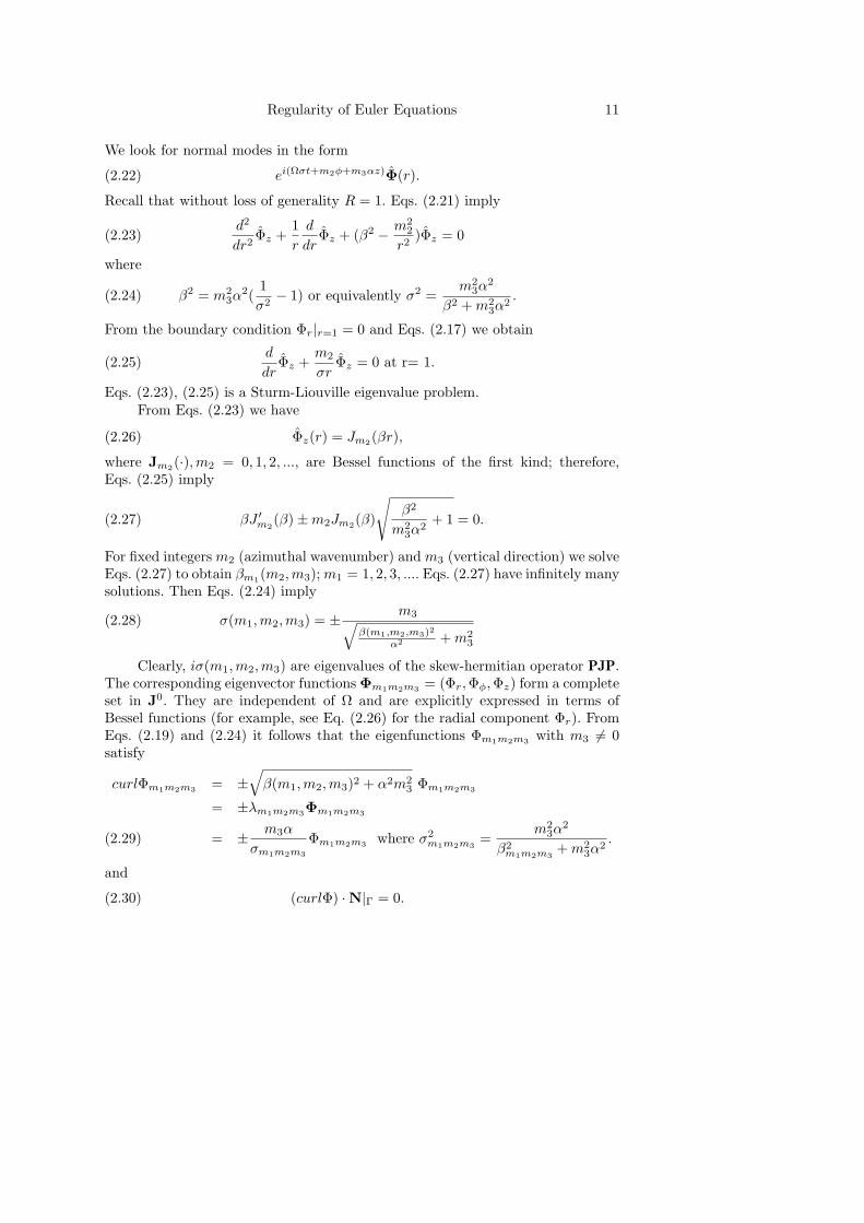
We look for normal modes in the form
ei(Ωσt+m2φ+m3αz)Φ(r).(2.22)
Recall that without loss of generality R = 1. Eqs. (2.21) imply
d2
dr2Φz +
1r
d
drΦz + (β2 − m2
2
r2)Φz = 0(2.23)
where
β2 = m23α
2(1σ2− 1) or equivalently σ2 =
m23α
2
β2 +m23α
2.(2.24)
From the boundary condition Φr|r=1 = 0 and Eqs. (2.17) we obtain
d
drΦz +
m2
σrΦz = 0 at r= 1.(2.25)
Eqs. (2.23), (2.25) is a Sturm-Liouville eigenvalue problem.From Eqs. (2.23) we have
Φz(r) = Jm2(βr),(2.26)
where Jm2(·),m2 = 0, 1, 2, ..., are Bessel functions of the first kind; therefore,Eqs. (2.25) imply
(2.27) βJ ′m2(β)±m2Jm2(β)
√β2
m23α
2+ 1 = 0.
For fixed integers m2 (azimuthal wavenumber) and m3 (vertical direction) we solveEqs. (2.27) to obtain βm1(m2,m3); m1 = 1, 2, 3, .... Eqs. (2.27) have infinitely manysolutions. Then Eqs. (2.24) imply
σ(m1,m2,m3) = ± m3√β(m1,m2,m3)2
α2 +m23
(2.28)
Clearly, iσ(m1,m2,m3) are eigenvalues of the skew-hermitian operator PJP.The corresponding eigenvector functions Φm1m2m3 = (Φr,Φφ,Φz) form a completeset in J0. They are independent of Ω and are explicitly expressed in terms ofBessel functions (for example, see Eq. (2.26) for the radial component Φr). FromEqs. (2.19) and (2.24) it follows that the eigenfunctions Φm1m2m3 with m3 6= 0satisfy
curlΦm1m2m3 = ±√β(m1,m2,m3)2 + α2m2
3 Φm1m2m3
= ±λm1m2m3Φm1m2m3
= ± m3α
σm1m2m3
Φm1m2m3 where σ2m1m2m3
=m2
3α2
β2m1m2m3
+m23α
2.(2.29)
and
(curlΦ) ·N|Γ = 0.(2.30)
12 A. Mahalov, B. Nicolaenko and C. Bardos, F. Golse
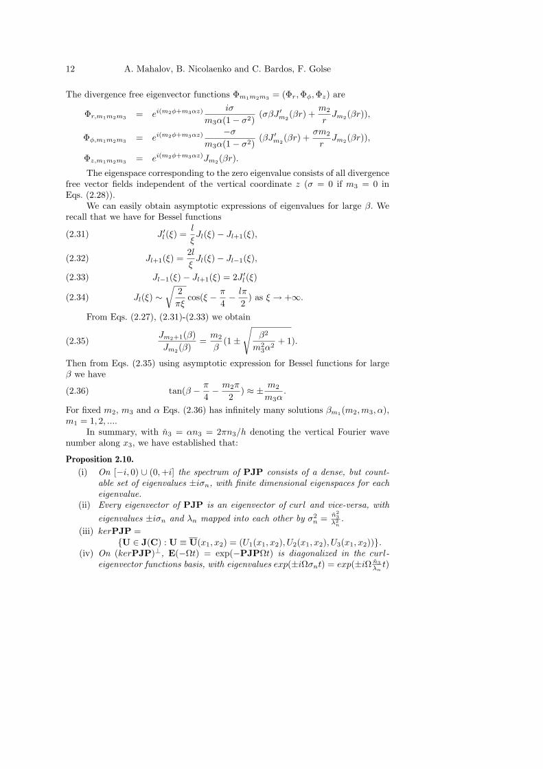
The divergence free eigenvector functions Φm1m2m3 = (Φr,Φφ,Φz) are
Φr,m1m2m3 = ei(m2φ+m3αz)iσ
m3α(1− σ2)(σβJ ′m2
(βr) +m2
rJm2(βr)),
Φφ,m1m2m3 = ei(m2φ+m3αz)−σ
m3α(1− σ2)(βJ ′m2
(βr) +σm2
rJm2(βr)),
Φz,m1m2m3 = ei(m2φ+m3αz)Jm2(βr).
The eigenspace corresponding to the zero eigenvalue consists of all divergencefree vector fields independent of the vertical coordinate z (σ = 0 if m3 = 0 inEqs. (2.28)).
We can easily obtain asymptotic expressions of eigenvalues for large β. Werecall that we have for Bessel functions
J ′l (ξ) =l
ξJl(ξ)− Jl+1(ξ),(2.31)
Jl+1(ξ) =2lξJl(ξ)− Jl−1(ξ),(2.32)
Jl−1(ξ)− Jl+1(ξ) = 2J ′l (ξ)(2.33)
Jl(ξ) ∼√
2πξ
cos(ξ − π
4− lπ
2) as ξ → +∞.(2.34)
From Eqs. (2.27), (2.31)-(2.33) we obtain
(2.35)Jm2+1(β)Jm2(β)
=m2
β(1±
√β2
m23α
2+ 1).
Then from Eqs. (2.35) using asymptotic expression for Bessel functions for largeβ we have
(2.36) tan(β − π
4− m2π
2) ≈ ± m2
m3α.
For fixed m2, m3 and α Eqs. (2.36) has infinitely many solutions βm1(m2,m3, α),m1 = 1, 2, ....
In summary, with n3 = αn3 = 2πn3/h denoting the vertical Fourier wavenumber along x3, we have established that:
Proposition 2.10.
(i) On [−i, 0) ∪ (0,+i] the spectrum of PJP consists of a dense, but count-able set of eigenvalues ±iσn, with finite dimensional eigenspaces for eacheigenvalue.
(ii) Every eigenvector of PJP is an eigenvector of curl and vice-versa, witheigenvalues ±iσn and λn mapped into each other by σ2
n = n23
λ2n
.(iii) kerPJP =
U ∈ J(C) : U ≡ U(x1, x2) = (U1(x1, x2), U2(x1, x2), U3(x1, x2)).(iv) On (kerPJP)⊥, E(−Ωt) = exp(−PJPΩt) is diagonalized in the curl-
eigenvector functions basis, with eigenvalues exp(±iΩσnt) = exp(±iΩ n3λnt)
Regularity of Euler Equations 13
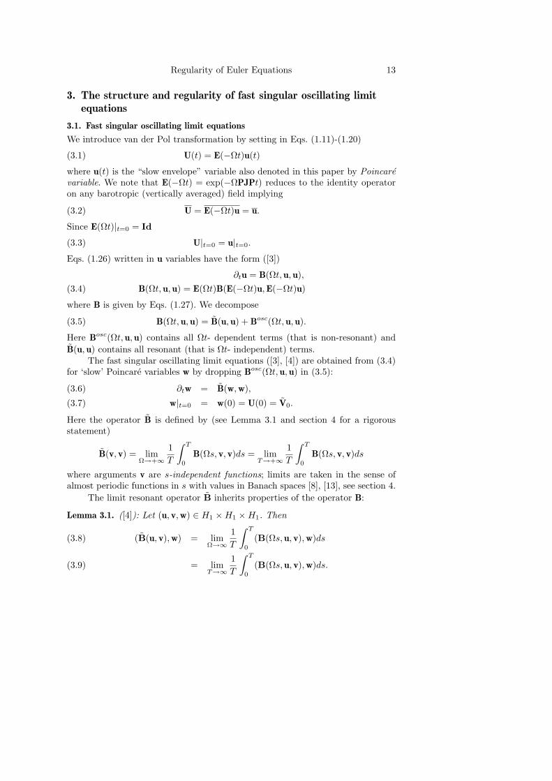
3. The structure and regularity of fast singular oscillating limitequations
3.1. Fast singular oscillating limit equations
We introduce van der Pol transformation by setting in Eqs. (1.11)-(1.20)
U(t) = E(−Ωt)u(t)(3.1)
where u(t) is the “slow envelope” variable also denoted in this paper by Poincarevariable. We note that E(−Ωt) = exp(−ΩPJPt) reduces to the identity operatoron any barotropic (vertically averaged) field implying
U = E(−Ωt)u = u.(3.2)
Since E(Ωt)|t=0 = Id
U|t=0 = u|t=0.(3.3)
Eqs. (1.26) written in u variables have the form ([3])
Here Bosc(Ωt, u, u) contains all Ωt- dependent terms (that is non-resonant) andB(u, u) contains all resonant (that is Ωt- independent) terms.
The fast singular oscillating limit equations ([3], [4]) are obtained from (3.4)for ‘slow’ Poincare variables w by dropping Bosc(Ωt, u, u) in (3.5):
∂tw = B(w,w),(3.6)
w|t=0 = w(0) = U(0) = V0.(3.7)
Here the operator B is defined by (see Lemma 3.1 and section 4 for a rigorousstatement)
B(v, v) = limΩ→+∞
1T
∫ T
0
B(Ωs, v, v)ds = limT→+∞
1T
∫ T
0
B(Ωs, v, v)ds
where arguments v are s-independent functions; limits are taken in the sense ofalmost periodic functions in s with values in Banach spaces [8], [13], see section 4.
The limit resonant operator B inherits properties of the operator B:
Lemma 3.1. ([4]): Let (u, v,w) ∈ H1 ×H1 ×H1. Then
(B(u, v),w) = limΩ→∞
1T
∫ T
0
(B(Ωs, u, v),w)ds(3.8)
= limT→∞
1T
∫ T
0
(B(Ωs,u, v),w)ds.(3.9)
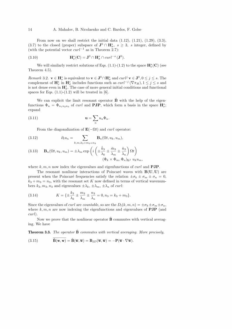
14 A. Mahalov, B. Nicolaenko and C. Bardos, F. Golse
From now on we shall restrict the initial data (1.12), (1.21), (1.29), (3.3),(3.7) to the closed (proper) subspace of J0 ∩ Hs
σ, s ≥ 3, s integer, defined by(with the potential vector curl−1 as in Theorem 2.7):
(3.10) Hsν(C) = J0 ∩Hs
σ ∩ curl−s (J0).
We will similarly restrict solutions of Eqs. (1.1)-(1.2) to the space Hsν(C) (see
Theorem 4.5).
Remark 3.2. v ∈ Hsν is equivalent to v ∈ J0∩Hs
σ and curlj v ∈ J0, 0 ≤ j ≤ s. Thecomplement of Hs
ν in Hsσ includes functions such as curl−j (∇πH), 1 ≤ j ≤ s and
is not dense even in H1σ. The case of more general initial conditions and functional
spaces for Eqs. (1.1)-(1.2) will be treated in [6].
We can explicit the limit resonant operator B with the help of the eigen-functions Φn = Φn1n2n3 of curl and PJP, which form a basis in the space Hs
ν ;expand
(3.11) u =∑n
unΦn.
From the diagonalization of E(−Ωt) and curl operator:
∂tun =∑
k,m,k3+m3=n3
Bn(Ωt, uk, um),(3.12)
Bn(Ωt, uk, um) = ±λm exp(i
(± k3
λk± m3
λm± n3
λn
)Ωt)
(3.13)
(Φk × Φm,Φn)L2 ukum,
where k,m, n now index the eigenvalues and eigenfunctions of curl and PJP.The resonant nonlinear interactions of Poincare waves with B(U,U) are
present when the Poincare frequencies satisfy the relation ±σk ± σm ± σn = 0,k3 +m3 = n3, with the resonant set K now defined in terms of vertical wavenum-bers k3,m3, n3 and eigenvalues ±λk, ±λm, ±λn of curl:
K = ± k3
λk± m3
λm± n3
λn= 0, n3 = k3 +m3.(3.14)
Since the eigenvalues of curl are countable, so are the Dl(k,m, n) = ±σk±σm±σn,where k,m, n are now indexing the eigenfunctions and eigenvalues of PJP (andcurl).
Now we prove that the nonlinear operator B commutes with vertical averag-ing. We have
Theorem 3.3. The operator B commutes with vertical averaging. More precisely,
B(w,w) = B(w,w) = B2D(w,w) = −P(w · ∇w).(3.15)
Regularity of Euler Equations 15
Proof: Let w = w + w⊥ where the orthogonal field w⊥ verifies w⊥ = 0. Clearly,
B(w,w) = B(w,w) + B(w⊥,w⊥)(3.16)
since w⊥ = 0. Thus, the theorem will be proven if we show that
B(w⊥,w⊥) = 0, w⊥ = 0.(3.17)
In the limit Ω→ +∞ interactions in the bilinear term B are restricted to theresonant manifold
(3.18) ± k3α√β(k1,k2,k3)2+k2
3α2± m3α√
β(m1,m2,m3)2+m23α
2± n3α√
β(n1,n2,k3)2+n23α
2= 0
and we have n3 = k3 + m3, n2 = k2 + m2. Now vertical averaging in Eqs. (3.17)implies n3 = 0, k3 + m3 = 0. Then from Eqs. (3.18) we obtain β(k1, k2, k3)2 =β(m1,m2,m3)2. We use eigenvector functions Φm1m2m3(r, φ, z) to represent phys-ical fields w⊥(r, φ, z), w⊥ = 0:
w⊥ =∑
m1m2m3
w⊥m1m2m3Φm1m2m3(r, φ, z).(3.19)
We recall from Eqs. (2.29) that Φm1m2m3(r, φ, z), m3 6= 0 are eigenvector functionsof curl. Then we obtain
B(w⊥,w⊥)n= Pn
∑
k3+m3=0,β2k=β2
m
w⊥k1k2k3Φk1k2k3(r, φ, z)× curl w⊥m1m2m3
Φm1m2m3(r, φ, z)
= ±Pn∑
k3+m3=0,β2k=β2
m
w⊥k1k2k3Φk1k2k3(r, φ, z)×
√β(m1,m2,m3)2 + α2m2
3 w⊥m1m2m3
Φm1m2m3(r, φ, z)
= ±Pn∑
k3+m3=0,β2k=β2
m
(β(k1, k2, k3)2 + α2k23)1/4(β(m1,m2,m3)2 + α2m2
3)1/4
w⊥k1k2k3Φk1k2k3(r, φ, z)× w⊥m1m2m3
Φm1m2m3(r, φ, z)= 0.
Clearly, the last sum is identically zero (it changes sign if we interchange indices kand m in the summation). Then we obtain Eqs. (3.17). Theorem 3.3 is proven.
3.2. Strict 3-wave resonances
In this section we show that for all values of α, except a countable set, the resonantsets lie in k3m3n3 = 0. This is generic case of no strict 3-wave resonances.
In the case of strict 3-wave resonances we have k3m3n3 6= 0 and Eqs. (3.18)become
(3.20) ± 1√β2k1
(k2,k3α)
k23α
2 + 1± 1√
β2m1
(m2,m3α)
m23α
2 + 1± 1√
β2n1
(n2,n3α)
n23α
2 + 1= 0.
16 A. Mahalov, B. Nicolaenko and C. Bardos, F. Golse
We also have convolutions in the azimuthal φ and the axial z directions implyingn3 = k3 + m3, n2 = k2 + m2. We recall that for every pair of integers k2 and k3
the quantities βk1(k2, k3α) are found from the equation
βJk2′(β)± k2Jk2(β)
√β2k1
(k2, k3α)k2
3α2
+ 1 = 0.(3.21)
For every pair of integers k2 and k3, Eqs. (3.21) have a countable number ofsolutions denoted by β(k1, k2, k3α); k1 = 1, 2, 3.... Similarly, for β(m1,m2,m3α)and β(n1, n2, n3α).
Eqs. (3.20) can be written in the form
± 1√X± 1√
Y± 1√
Z= 0(3.22)
where
β2(k1, k2, k3α)k2
3α2
+ 1 = X ↔(βJk2
′(β)k2Jk2(β)
)2
= X,(3.23)
with similar expressions for Y and Z.Substituting Eqs. (3.21) in Eqs. (3.20) we obtain
In Eqs. (3.24) k2, m2, n2, k3, m3, n3 ∈ Z and k1,m1, n1 = 1, 2, 3, .... Also,n2 = k2 +m2 and n3 = k3 +m3. In fact, we can think of Eqs. (3.24) as a countableset of nonlinear equations for α. Clearly, for every fixed kj ,mj , nj Eq. (3.24) hasat most a countable number of solutions α. Thus, we have a countable numberof equations and each equation has at most a countable number of solutions α.Therefore, the set of parameters α’s for which strict 3-wave resonances can occuris countable.
Proposition 3.4. The set K∗ of parameters α’s for which strict 3-wave resonancescan occur is countable.
3.3. Regularity of fast singular oscillating limit equations
In the generic case of no strict 3-wave resonances BIII = 0 and the limit Eulerequations (1.35) become
where w(t) satisfies 2D Euler equations with vertically averaged initial data w|t = 0
= w(0) = U(0). Eqs. (3.25) for w⊥(t) are solved with periodic boundary conditionsin the third coordinate and w⊥ ·N|Γ = 0. We also have curlw⊥ ·N|Γ = 0.
Eqs, (3.25) possess new 3D conservation laws:
Regularity of Euler Equations 17
Theorem 3.5. Let w(t) be a solution of 2D-3C Euler Eqs. (1.34). Then for everyw⊥(t) solution of Eqs. (3.25) with initial data w⊥(0) we have:
||∂3w⊥(t)||2 = ||∂3w⊥(0)||2,(3.26)
where ∂3 denotes the partial derivative with respect to x3.
Proof: Applying ∂3 to Eqs. (3.25) and using skew-symmetry property
(BII(w, ∂3w⊥), ∂3w⊥) = 0
we obtain
(3.27)d
dt||∂3w⊥||2 = 0.
Moreover, for the initial data and solutions in the function space Hsν , we have
further conservation laws:
Theorem 3.6. Let w⊥(t) be solutions of the limit equations (3.25) in Hsν . We have,
for 0 ≤ j ≤ s, j even:
(3.28) ||curlj w⊥(t)||2 = ||curlj w⊥(0)||2.Proof: Proceed as in the proof of Theorem 3.3, but with k3 = n3 (and m3 = 0) orwith m3 = n3 (and k3 = 0), together with λ2
k = λ2n, β
2k = β2
n (resp. λ2m = λ2
n, β2m =
β2n). Note that expansion along the eigenfunctions of curl and PJP requires their
completeness at least in H1ν , cf. Remark 3.2.
Remark 3.7. Note that 2D-3C Euler equations only admit conservation of energyand enstrophy. The above conservation laws (3.26)-(3.28) ensure global regularityof the limit Euler equations (3.25).
Theorem 3.8. Let h/R /∈ K∗. Let ||w(0)||Hsν≤ Ms, s ≥ 1. Let T1 > 0 fixed, arbi-
trary large. Then there exists a unique regular solution w(t) of the limit resonant3D Euler equations (3.6)-(3.7), for 0 ≤ t ≤ T1:
(3.29) ||w(t)||Hsν≤ Ms(h/R,Ms, T1).
4. Long time regularity for finite large Ω
Two major obstacles in extending the fast singular oscillating limit methods de-veloped in [3]-[5] from the periodic lattice case to the cylinder (as well as otheraxisymmetric domains) are that: (i) PJP is not skew-symmetric with respect tothe inner product of classical Sobolev spaces Hs
σ(C), s ≥ 1; (ii) E(Ωt) is not anisometry in these spaces (∇ does not commute with PJP and E(Ωt)). Item (i)implies that a priori estimates of Eqs. (1.11)-(1.12) in Sobolev spaces are 1/ε = Ωdependent; and (ii) that estimates for u(t, x), the Poincare slow variable (van derPol transformation of U(t, x), Eq.(3.1)) are not invariant for the physical variableU(t, x). That invariance was used in an essential way in the convergence proofsof [3]-[5] (periodic case). The resolution of the above requires the introduction
18 A. Mahalov, B. Nicolaenko and C. Bardos, F. Golse
of Hilbert spaces with the metric based on the operator curl-norms, with normsequivalent to that of Hs
σ(C), s integer, s ≥ 1.As before (cf. Eq. 3.10), we restrict ourselves to initial data and solutions in
the spaces (s ≥ 3):
(4.1) Hsν(C) = J0 ∩Hs
σ ∩ curl−s(J0),
such that v ∈ Hsν implies curlj v ·N = 0 on Γ, 0 ≤ j ≤ s (cf., Remark 3.2). More
general functional spaces dense in H1σ will be treated in [6].
Lemma 4.1. Let v ∈ Hsν , s ≥ 1. Then there exist constants C1, C2 > 0 such that:
(4.2) C1||v||Hsσ≤ ||v||Hs
ν≤ C2||v||Hs
σ,
where
(4.3) ||v||2Hsν
= ||v||2L2+ ||curlsv||2L2
.
Proof: Iterated applications of Theorem 2.7 and 2.8, we have equivalence of the“curl-norms” with the usual Sobolev space norms. From now on, we designate by ||v||s the curl-norm of v defined in Eq. 4.3, and by< u,v >s the corresponding inner product of u,v in Hs
ν . We have the:
Lemma 4.2. Let u,v ∈ Hsν , s ≥ 0; then we have skew-symmetry in the curl-norms:
(4.4) < PJPu,v >s= − < u,PJPv >s
and
(4.5) < PJPu,u >s= 0.
Proof: Obvious for s = 0; we outline the case s = 1:
(curlPJPu, curlv)L2 =(−∂u∂z, curlv
)
L2
=(
u, curl∂v∂z
)
L2
=(curlu,
∂v∂z
)
L2
= −(curlu, curlPJPv)L2 ,
since both u,v, ∂u∂z ,
∂v∂z satisfies the conditions of Lemma 2.4. The cases s > 1
follows a similar proof.
Remark 4.3. The all important Lemmas 4.1, 4.2 allow for local estimates of solu-tions to the 3D Euler equations (1.11)-(1.12) which are 1/ε = Ω independent.
Corollary 4.4. The Poincare-Sobolev unitary operator E(Ωt) is an isometry on thecurl spaces Hs
ν , s ≥ 0; in particular,
(4.6) ||U||s = ||u||s,where U(t) = E(−Ωt)u(t).
Regularity of Euler Equations 19
To establish long time regularity of the 3D Euler equations Eqs. (1.20)-(1.21)on 0 ≤ t ≤ TM , TM fixed, arbitrary large, we first establish convergence in Hs
ν
(as Ω → ∞) of the solution to that of the limit resonant equations (1.34)-(3.25)on the interval [0, Ts], where Ts is some local time of existence of (1.20)-(1.21).We only consider the case of “catalytic resonances”, h/R /∈ K∗. With the helpof the long time existence of solutions to the limit resonant equations on [0, TM ],cf. Theorem 3.8, we extend local regularity on [0, Ts] to long-time regularity on[0, TM ] by partitioning [0, TM ] into subintervals of length Ts and bootstrappingestimates.
Theorem 4.5. Let U(0) ∈ Hβν , β ≥ 3 and ||U(0)||β ≤ M0β, where the β-norm is
the curl-norm (4.3). Then:(i) there exists Tβ > 0 such that there exists a unique regular solution of the
3D Euler equations on 0 ≤ t ≤ Tβ which satisfies
(4.7) ||U(t)||2β ≤M2β , 0 ≤ t ≤ Tβ ;
moreover Mβ , Tβ do not depend on Ω, but only on M0β , h/R.(ii) For every α such that β ≥ α ≥ 3, there exists a constant C(β) such that
(4.8) ||U(t)||2β ≤(||U(0)||2β
)exp
((C(β)
∫ Tβ
0
||V(τ)||α dτ)
+ Tβ
),
where α can be fixed independently of β.
Proof: (i) is proven by a straightforward adaptation of the proof of Kato [16] inR3 to the cylinder C, replacing the usual Sobolev spaces by the spaces Hβ
ν . Kato’smethod is a vanishing viscosity limit via local existence for the Navier-Stokesequations (the latter via fixed-point construction, not a Galerkin approximation).That estimates are uniform in Ω stems from Lemma 4.1 and 4.2. (ii) can thenbe derived exactly as in Theorem 4.1 of [3], replacing Fourier methods by curleigenvector function expansions.
We now proceed to estimate the error between solutions u(t) of Eqs. (3.4)-(3.5) with finite large Ω
Recall that E(Ωt) is an isometry on the curl spaces Hsν spaces. Therefore, estimates
for norms of r(t) yield estimates for the norms of the error
R(t) = E(−Ωt)(u(t)−w(t)) = U(t)−E(−Ωt)w(t).(4.14)
20 A. Mahalov, B. Nicolaenko and C. Bardos, F. Golse
The equation for the error r(t) is
r(t) =∫ t
0
(B(u, r) + B(r,w) + Bosc(Ωs, u(s), u(s))
)ds,(4.15)
where
Boscn (Ωt,u(t), u(t)) =∑
l,k3+m3=n3,non−resonantk2+m2=n2
exp(iΩtDl(k,m, n))uk(t)um(t)
(curlΦk × Φm,Φn).(4.16)
We have
Theorem 4.6. Assume that the regular solution U(t) of Eq. (1.11), (1.20) withinitial condition ||U(0)||s ≤Ms0 exists on 0 ≤ t ≤ Ts, for some Ts (not necessarysmall), with ||U(t)||s ≤ Ms(Ms0, Ts, h/R). Then under conditions α ≥ 3, s−α ≥ 1we have
(4.17) ||r(t)||α ≤ δ(Ω), ∀t ∈ [0, Ts],
where δ(Ω) → 0 as Ω → +∞; Ts is independent from Ω; δ(Ω) depends on Ms0,Ts, α, s, and h/R.
Recall that PJP is skew-symmetric under inner product in the curl-norm spaces,therefore, local small time existence for (3.4)-(3.5) is independent of Ω.
To prove this convergence result we notice that the first two terms insidethe integral on the right hand side of (4.15) are linear in r and we only need toshow that the contribution of Bosc can be made arbitrary small as ε = 1/Ω → 0.From (4.16) note that Boscn (τ/ε, u(t), u(t)) is an almost periodic function of τ withvalues in L∞(t; Hα
ν ) since the set Dl(k,m, n) = ±σk ± σm ± σn is countable. Weneed the following lemma for almost periodic functions with values in Banachspaces ([6], [8], [13], [27]).
Lemma 4.7. ([6], [27]). Let f(t, τ) ∈ AP (R;C0(t; E)) be almost periodic functionsof the variable τ , with values in C0(t; E), t ∈ [0, T0], E is a Hilbert space. Let
f(t, τ) ∼∑
j∈Jfj(t) exp(iωjτ),(4.18)
in the sense of Banach space valued almost periodic functions in τ , fj(t) ∈ C0(t; E),over the (countable) set J of frequencies. If
sup0≤t≤T0 ||f(t, τ)||E ≤Mf , and if |ωj | ≥ η > 0 on J(4.19)
then:
E− limε→0
∫ T
0
f(t, t/ε)dt = 0;(4.20)
the limit also converges uniformly on 0 ≤ T ≤ T0 provided ||f(t2, τ)−f(t1, τ)||E ≤c|t2 − t1|, uniformly on [0, T0].
Regularity of Euler Equations 21
To apply Lemma 4.7 to Bosc(Ωt, u(t), u(t)) one needs |ωj | = |σk±σm±σn| > ηuniformly in k,m, n, For this, define πRu (similarly πRw) the projection of u ontothe curl eigenvector functions with |λk|, |λm|, |λn| ≤ R, with:
(4.21) ||u− πRu||Hαν≤MsR
α−s, s > α.
Then | ± σk ± σm ± σn| > η(R) for πRu in Eq. (4.16), which controls the smalldivisor estimate ([1]). Bosc(Ωt,u(t), u(t)) is decomposed as
Bosc(Ωt, u, u) = πRBosc(Ωt, πRu, πRu) + πRBosc(Ωt,u, (I − πR)u) +(4.22)πRBosc(Ωt, (I − πR)u,u) + (I − πR)Bosc(Ωt, u, u).
Finally, apply Lemma 4.7 to the integral
(4.23)∫ t
0
πRBosc(Ωs, πRu(s), πRu(s))ds, with E = Hαν ,
and use (4.21) to bound the error terms involving (I − πR). This completes theoutline of the proof of the local convergence Theorem 4.6, with details followingalong the proof of Theorem 6.3, p 139-140 in [3], albeit curl eigenvector functionsreplacing Fourier modes.
Remark 4.8. In Theorem 4.6 u(t) converges strongly to w(t). The original U(t)also converges strongly to E(−Ωt)w(t). But U(t) has no strong limit in Hs
ν asΩ→∞, hence the singular nature of the fast oscillating limit.
From the global regularity Theorem 3.8 for the 3D resonant Euler equationsand Theorem 4.6 we bootstrap long-time regularity for Eqs.(1.11)-(1.12) for Ωlarge but finite.Proof of Theorem 1.4: We complete in some detail the proof of Theorem 1.4, asthe bootstrapping arguments are rather different from the usual classical procedurefor Navier-Stokes equations [20]. Let Tm fixed, arbitrary large. Let ||V0(y)||s =||U0(x)||s ≤ Ms0, s ≥ 4. From Theorem 3.8, with ||w(0)||α = ||U0||α ≤ Mα0 ≤Ms0, for some fixed α ≥ 3, s− α ≥ 1, there exists Mα such that:
(4.24) ||w(t)||α ≤ Mα(Ms0, TM , h/R) on 0 ≤ t ≤ Tm,for the solution of the resonant 3D Euler equations. We need the:
Corollary 4.9. Let ||U(t1)||α ≤ Rα at some t1 ≥ 0, α ≥ 3, Rα > 0 given. Thenthere exists Tα(Rα, h/R) such that
22 A. Mahalov, B. Nicolaenko and C. Bardos, F. Golse
Proof: First, apply Theorem 4.5 with α = β to derive Eqs. (4.25). Then apply (ii)in Theorem 4.5 with β = s.
We now choose, with Mα given by Eqs. (4.24):
(4.27) Rα = 3Mα,
hence Tα = Tα(Ms0, Tm, α, h/R). Let Qα = 4C(s)Rα + 1. We define:
(4.28) M2s = M2
s0 expQα(Tm + Tα),
and we shall demonstrate that:
(4.29) ||U(t)||2s ≤ M2s on 0 ≤ t ≤ Tm,
by choosing Ω large enough to make the error δ(Ω) (in Theorem 4.6) uniformlysmall on the sequence of intervals [0, Tα], [Tα, 2Tα], ..., [nTα, (n + 1)Tα], wherenTα ≤ Tm < (n + 1)Tα. We apply Theorem 4.6 on the global interval [0, Tm],assuming a priori the estimate (4.29) (which will be shown self-consistent underbootstrapping); we choose such large Ω that δ(Ω) is so small and the assertion ofTheorem 4.6 holds with Ts ≡ Tm, and for Ω ≥ Ω1, the constant δ(Ω) satisfies:
(4.30) δ(Ω) ≤ Rα/2 for Ω ≥ Ω1(Ms, Tm, α, s, h/R);
equivalently, Ω1 depends only on Ms0, Tm, α, s, h/R. Hence, for 0 ≤ t ≤ Tm:
(4.31) ||U(t)||α ≤ ||U(t)−E(−Ωt)w(t)||α + ||w(t)||α ≤ Rα/2 +Rα/3 ≤ Rα.We now apply Corollary 4.9 on [0, Tα], with the choice of Rα in Eqs. (4.27):
(4.32) ||U(Tα)||2s ≤M2s0 exp(QαTα).
From the uniform estimate (4.31) for ||U(t)||α, valid at t = Tα, we apply againCorollary 4.9 on [Tα, 2Tα]:
(4.33) ||U(t)||2s ≤M2s0 exp(QαTα) exp(QαTα);
and repeating the argument on the interval [kTα, (k + 1)Tα], k ≤ n:
(4.34) ||U(t)||2s ≤M2s0 exp(kQαTα) exp(QαTα),
since ||U(kTα)||α ≤ Rα. Completing the bootstrapping, the maximal estimate for||U(t)||2s occurs on [nTα, Tm]:
||U(t)||2s ≤ M2s0 exp(nQαTα) exp(Qα(Tm − nTα))
≤ M2s ,
which corroborates the self-consistency of the choice ||U(t)||s ≤ Ms in the ap-plication of Theorem 4.6 for a uniform δ(Ω). The proof of Theorem 1.4 is thencompleted with the canonical transformation (1.17)-(1.18) between V(t, y) andU(t, x) and its isometry properties. Remark 4.10. The case h/R ∈ K∗ includes the quadratic resonant opera-tor BIII(w⊥,w⊥) in Eqs. (1.35). We have not found new conservation laws forthe latter besides energy and helicity. A most interesting issue is the possibility ofsingularity and blow-up for the full resonant Euler equations (1.35). Partial results
Regularity of Euler Equations 23
in the periodic lattice geometry are derived in [5], where (1.35) is demonstratedto be equivalent to a countable sequence of uncoupled finite dimension dynamicalsystems, in the generic case.
References
[1] V.I. Arnold (1965), Small denominators. I. Mappings of the circumference onto itself,Amer. Math. Soc. Transl. Ser. 2, 46, p. 213-284.
[2] V.I. Arnold and B.A. Khesin (1997), Topological Methods in Hydrodynamics, Ap-plied Mathematical Sciences, 125, Springer.
[3] A. Babin, A. Mahalov, and B. Nicolaenko (1997), Global regularity and integrabilityof 3D Euler and Navier-Stokes equations for uniformly rotating fluids, AsymptoticAnalysis, 15, p. 103–150.
[4] A. Babin, A. Mahalov and B. Nicolaenko (1999), Global regularity of 3D rotatingNavier-Stokes equations for resonant domains, Indiana Univ. Math. J., 48, No. 3, p.1133-1176.
[5] A. Babin, A. Mahalov and B. Nicolaenko (2001), 3D Navier-Stokes and Euler equa-tions with initial data characterized by uniformly large vorticity, Indiana Univ. Math.J., 50, p. 1-35.
[6] C. Bardos, F. Golse, A. Mahalov and B. Nicolaenko (2004), Long-time regularity of3D Euler equations with initial data characterized by uniformly large vorticity incylindrical domains, to appear.
[7] J.T. Beale, T. Kato and A. Majda (1984), Remarks on the breakdown of smoothsolutions for the 3D Euler equations, Commun. Math. Phys., 94, p. 61-66.
[8] A.S. Besicovitch (1954), Almost Periodic Functions, Dover, New York.
[9] J.P. Bourguignon and H. Brezis (1974), Remark on the Euler equations, J. Func.Anal., 15, p. 341-363.
[10] E.B. Bykhovskii (1957), Solutions of problems of mixed type of the Maxwell’s equa-tions for ideally conducting boundaries, Vestnik Leningrad Univ., 13, p. 50-66.
[11] E.B. Bykhovskii and N.V. Smirnov (1960), On orthogonal expansions in spaces ofsquare integrable vector functions and operators of vector analysis, Trudy Math.Inst. V.A. Steklov, Special Volume on Mathematical Problems in Hydrodynamicsand Magnetohydrodynamics, 59, p. 5-36.
[12] E. Cartan (1922), Sur les petites oscillations d’une masse fluid, Bull. Sci. Math., 46,p. 317-352 and p. 356-369.
[13] C. Corduneanu (1968), Almost periodic Functions, Wiley-Interscience, New York.
[14] G. Duvaut and J.L. Lions (1976), The Inequalities in Mechanics and Physics,Springer-Verlag.
[15] K. Friedrichs (1955), Differential forms on Riemannian manifolds, Comm. Pure Appl.Math, 8, No. 2.
[16] T. Kato (1972), Nonstationary flows of viscous and ideal fluids in R3, J. Func. Anal.,9, p. 296-305.
24 A. Mahalov, B. Nicolaenko and C. Bardos, F. Golse
[17] N.D. Kopachevsky and S.G. Krein (2001), Operator Approach to Linear Problemsof Hydrodynamics, Operator Theory: Advances and Applications, 128, BirkhauserVerlag.
[18] O.A. Ladyzhenskaya ed. (1960), Trudy Math. Inst. V.A. Steklov, Special Volume onMathematical Problems in Hydrodynamics and Magnetohydrodynamics, 59.
[19] O.A. Ladyzhenskaya (1968), On the unique global solvability of the 3D Cauchyproblem for the Navier-Stokes equations under conditions of axisymmetry, Bound-ary Value problems of Math. Phys. and Related Problems No. 2, Zapiski SeminarovLOMI, 7, p. 155-177.
[20] O.A. Ladyzhenskaya (1969), The Mathematical Theory of Viscous IncompressibleFlow, 2nd ed., Gordon and Breach, New York.
[21] O.A. Ladyzhenskaya and V.A. Solonnikov (1960), Solution of some nonstationaryproblems of magnetohydrodynamics for viscous incompressible fluids, Trudy Math.Inst. V.A. Steklov, Special Volume on Mathematical Problems in Hydrodynamics andMagnetohydrodynamics, 59, p. 115-173.
[22] J. Leray (1934), Sur le mouvement d’un liquide visqueux emplissant l’espace, ActaMath., 63, p. 193-248.
[23] A. Mahalov, S. Leibovich and E.S. Titi (1990), Invariant helical subspaces for theNavier–Stokes Equations, Arch. for Rational Mech. and Anal., 112, No. 3, p. 193–222.
[24] A. Mahalov and B. Nicolaenko (2003), Global solvability of the three-dimensionalNavier-Stokes equations with uniformly large initial vorticity, Russian Math. Sur-veys, 58:2, p287-318.
[25] H. Poincare (1910), Sur la precession des corps deformables, Bull. Astronomique, 27,p. 321-356.
[26] J.V. Ralston (1973), On stationary modes in inviscid rotating fluids, J. Math. Anal.and Appl., 44, p. 366-383.
[27] S. Schochet (1994), Resonant nonlinear geometric optics for weak solutions of con-servation laws, J. Diff. Eq., 113, p. 473-503.
[28] S. Schochet (1994), Fast singular limits of hyperbolic PDE’s, J. Diff. Eq., 114, p.476-512.
[29] S. L. Sobolev (1954), Ob odnoi novoi zadache matematicheskoi fiziki, IzvestiiaAkademii Nauk SSSR, Ser. Matematicheskaia, 18, No. 1, p. 3–50.
[30] V.A. Solonnikov (1972), Overdetermined elliptic boundary value problems, Bound-ary Value problems of Math. Phys. and Related Problems No. 5, Zapiski SeminarovLOMI, 21, p. 112-158.
[31] E.M. Stein (1970), Singular integrals and differentiability properties of functions,Princeton University Press.
[32] W. Wolibner (1933), Un theoreme sur l’existence du mouvement plan d’un fluideparfait, homogene et incompressible,pendant un temps infiniment long, Mat. Z., 37,p. 698-726.
[33] V.I. Yudovich (1963), Non stationary flow of an ideal incompressible liquid, Zb. Vych.Mat., 3, p. 1032-1066
Regularity of Euler Equations 25
Acknowledgment
We would like to thank Professors V.I. Arnold, C. Foias, A. Fursikov, O.A. La-dyzhenskaya, H.K. Moffatt, Ya. Sinai and V.A. Solonnikov for the very useful dis-cussions. V.A. Solonnikov has been most helpful in bringing to our attention theearlier work of his and his colleagues on magnetohydrodynamics. We acknowledgethe support of the AFOSR grant F49620-02-10026.
Department of Mathematics and Statistics, Arizona State University, Tempe, AZ85287-1804, USAE-mail address: [email protected], [email protected]
U.M.R. of Mathematics, University of Paris-7, 75251 Paris Cedex-05, and Labo-ratoire J.L. Lions, University of Paris-6, FranceE-mail address: [email protected], [email protected]