Regularization and Simulation of Constrained Partial Differential Equations vorgelegt von Diplom-Mathematiker Robert Altmann aus Berlin Von der Fakult¨at II - Mathematik und Naturwissenschaften der Technischen Universit¨at Berlin zur Erlangung des akademischen Grades Doktor der Naturwissenschaften Dr. rer. nat genehmigte Dissertation Promotionsausschuss: Vorsitzende: Prof. Dr. Noemi Kurt Berichter: Prof. Dr. Volker Mehrmann Berichterin: Prof. Dr. Caren Tischendorf Berichter: Prof. Dr. Alexander Ostermann Tag der wissenschaftlichen Aussprache: 29. 05. 2015 Berlin 2015
Transcript
Regularization and Simulation ofConstrained Partial Differential Equations
vorgelegt vonDiplom-Mathematiker
Robert Altmannaus Berlin
Von der Fakultat II - Mathematik und Naturwissenschaftender Technischen Universitat Berlin
zur Erlangung des akademischen GradesDoktor der Naturwissenschaften
Dr. rer. nat
genehmigte Dissertation
Promotionsausschuss:
Vorsitzende: Prof. Dr. Noemi Kurt
Berichter: Prof. Dr. Volker Mehrmann
Berichterin: Prof. Dr. Caren Tischendorf
Berichter: Prof. Dr. Alexander Ostermann
Tag der wissenschaftlichen Aussprache: 29. 05. 2015
Die vorliegende Arbeit beschaftigt sich mit der Regularisierung von differentiell-alge-braischen Gleichungen (DAEs) abstrakter Funktionen. Diese sogenannten Operator DAEssind Operatorgleichungen, die die Struktur differentiell-algebraischer Gleichungen verall-gemeinern. Sie bieten eine alternative Formulierung partieller Differentialgleichungen, diegewissen Nebenbedingungen genugen mussen. Die vorgestellte Regularisierung verbessertdie Sensibilitat der Operator DAEs gegenuber Storungen und resultiert in gut gestelltenSystemen bei der Ortsdiskretisierung.
Operator DAEs sind hervorragend geeignet zur Modellierung physikalischer Systeme.Anwendungsbereiche findet man in der Stromungsmechanik, der Kontinuumsmechaniksowie im Bereich des Elektromagnetismus. Im Allgemeinen fuhren gekoppelte Systeme,die aus mehreren Subsystemen bestehen, oft auf diese Art von Gleichungen. Die For-mulierung physikalischer Systeme als Operator DAE steht im direkten Zusammenhangzur schwachen Formulierung von partiellen Differentialgleichungen. Als Verallgemeinerungvon DAEs kann auch die Nebenbedingung selbst einen Differentialoperator beinhaltenwie zum Beispiel bei den Navier-Stokes Gleichungen, die durch die Divergenzfreiheit re-stringiert sind. Es handelt sich also um DAEs, die allgemein in einem Banachraumdefiniert sind. Eine weitere Charakterisierung ist gegeben durch die Eigenschaft, dasseine Semidiskretisierung im Ort auf eine DAE im ursprunglichen Sinne fuhrt. Darausresultieren auch die Stabilitatsprobleme wie die hohe Sensibilitat gegenuber Storungensowie die Notwendigkeit konsistenter Anfangsdaten.
Die Regularisierung folgt den Ideen der Indexreduktion fur DAEs. Dabei sucht maneine aquivalente Operatorgleichung, die bessere numerische Eigenschaften aufweist. Indieser Arbeit wird speziell die Methode minimal extension betrachtet, die sich hervorra-gend fur semi-expliziete Systeme eignet. Dies fuhrt dann auf ein vergroßertes System, daim Regularisierungsprozess neue Variablen eingefuhrt werden. Dabei ist zu erkennen, dasssich der Index der semidiskreten Systeme verringert. In der Stromungsmechanik erhaltman DAEs vom Index 1 statt Index 2 und im Bereich der Kontinuumsmechanik reduziertsich der Index sogar von 3 auf 1.
Diskretisiert man die Operatorgleichungen zuerst in der Zeit statt im Ort, so erhaltman eine Folge von stationaren partiellen Differentialgleichungen. Der letzte Teil derArbeit analysiert die Konvergenz dieser Zeitdiskretisierung. Dabei ist zu beobachten,dass sich die einzelnen Variablen unterschiedlich verhalten. Der Lagrange Multiplikator,beziehungsweise der Druck im Bereich der Stromungsmechanik, benotigt starkere Reg-ularitatsannahmen, um die Konvergenz zu garantieren. Desweiteren wird der Einflussvon kleinen Storungen untersucht. Auch hierbei zeigt sich der Vorteil der prasentiertenRegularisierung in Bezug auf die besseren Stabilitatseigenschaften verglichen mit dem ur-sprunglichen System.
v
Abstract
This thesis is devoted to the regularization of differential-algebraic equations in theabstract setting (operator DAEs) and the resulting positive impact on the correspondingsemi-discrete systems and on the sensitivity to perturbations. The possibility of a mod-ularized modeling and the maintenance of the physical structure of a dynamical systemmake operator DAEs convenient form the modeling point of view. They appear in allfields of applications such as fluid dynamics, elastodynamics, electromagnetics, as well asin multi-physics applications were different system types are coupled.
From a mathematical point of view, operator DAEs are constrained PDEs, written inthe weak formulation. Therein, the constraint may itself be a differential equation such asin the Navier-Stokes equations where the velocity of a Newtonian fluid is constrained to bedivergence-free. On the other hand, operator DAEs generalize the notion of DAEs to theinfinite-dimensional setting, including abstract functions which map into a Banach space.Thus, a spatial discretization leads to a DAE in the classical sense. This also implies thattypical stability issues known from the theory of DAEs such as the high sensitivity toperturbations also translate to the operator case.
The regularization of an operator DAE follows the concept of an index reduction fora DAE. Hence, an equivalent system is sought-after which has better properties from anumerical point of view. The presented regularization lifts the index reduction technique ofminimal extension for semi-explicit DAEs to the abstract setting and leads to an extendedoperator DAE. A spatial discretization of the regularized system then leads to a DAE oflower index compared to the semi-discrete system arising from the original operator DAE.For flow equations we obtain a reduction from index 2 to index 1 whereas the applicationsfrom the field of elastodynamics yield a reduction from index 3 to index 1.
The last part of this thesis deals with the convergence of time discretization schemesapplied to the regularized operator DAEs. Therein, we observe a qualitative difference fordifferent variables. More precisely, we show that the Lagrange multiplier needs strongerregularity assumptions on the given data in order to guarantee the convergence to the exactsolution of the operator DAE. Furthermore, the influence of perturbations in the right-hand sides of the system is analysed for the semi-discrete as well as for the continuoussetting. This analysis shows the advantage of the presented regularization in terms ofstability.
vii
Published Papers
Several results of this theis were already published in preprints or journal publications.We give a short overview and indicate in which parts of the thesis the results have beenused.
• [Alt13a] Index reduction for operator differential-algebraic equations in elasto-dynamics. Z. Angew. Math. Mech. (ZAMM), 93(9):648–664, 2013.This paper introduces the idea of a regularization of operator DAEs as theyappear in applications of elatodynamics. The procedure is based on the indexreduction technique of minimal extension for semi-explicit DAEs. The results areused in Sections 7 and 9.
• [Alt13b] Modeling Flexible Multibody Systems by Moving Dirichlet BoundaryConditions. Proceedings of Multibody Dynamics 2013 - ECCOMAS ThematicConference (Zagreb, Croatia)This proceedings contribution includes an example of an operator DAE includinga coupling of an elastic body and a mass-spring-damper system. This example isonly mentioned in the beginning of Section 7.
• [Alt14] Moving Dirichlet Boundary Conditions. ESAIM Math. Model. Numer.Anal. (M2AN), 48(6):1859–1876, 2014Problems were the part of the boundary, on which Dirichlet boundary conditionsare prescribed, is time-dependent may be formulated as an operator DAE. Thisis mentioned in Section 5.1.
• [AH13] Finite element decomposition and minimal extension for flow equations.Preprint 2013–11, Technische Universitat Berlin, 2013, accepted for publicationin ESAIM Math. Model. Numer. Anal. (M2AN) (with Jan Heiland)This paper is devoted to the stable approximation of the pressure variable in fluidflow applications. For this, a regularization of the corresponding operator DAEis combined with a decomposition of finite element spaces. The results of thispaper are mainly used within Section 8.
• [AH14] Regularization of constrained PDEs of semi-explicit structure. Preprint2014–05, Technische Universitat Berlin, 2014. (with Jan Heiland)This preprint provides a general framework for the regularization of semi-explicitoperator DAEs of first order. In particular, this includes flow equations such asthe (Navier-) Stokes equations. The results are used in Sections 6 and 8.
1. Introduction
With an increasing importance of automatic modeling, differential-algebraic equations(DAEs) register an increase in popularity. DAEs allow a quick and facile modeling proce-dure with a smaller need of system simplifications and exploit the system structure andsparsity [CM99]. In particular, they enable modularized modeling of several uni-physicscomponents.
Nowadays, many models contain partial differential equations (PDEs). A coupling ofsystems then leads to a mixture of DAEs and PDEs which are called partial differential-algebraic equations (PDAEs) or, formulated in a weak functional analytic setting, operatoror abstract DAEs. This approach follows the paradigm to include all available informationto the system rather than implicitly eliminate variables. Thus, all variables remain aphysically valid part of the system, also throughout the discretization process.
However, the simplicity of modeling shifts the difficulties to the mathematical part,i.e., to the analysis and simulation of such systems. DAEs suffer from instabilities, drift-offphenomena, and ill-posedness [GM86, KM06, Ria08, LMT13]. Note that the ques-tion of stability is of special importance if one considers applications including uncertaincomponents, parameters, or inputs from other subsystems including themselves numericalerrors.
The aim of this thesis is to regularize a specific class of PDAEs in the sense thatthese instabilities are reduced. Furthermore, the regularization increases the potentialof adaptive methods for the simulation of constrained PDEs and is independent of thediscretization scheme. The connection between the presented regularization on operatorlevel and the index reduction for DAEs is illustrated in the following scheme.
operator DAE ofhigh-index type
operator DAE ofindex-1 type
DAE of high index DAE of index 1
regularization
of operator DAEs
index reduction
for DAEs
spatialdiscretization
spatialdiscretization
Applications
Typical fields of applications which are modeled by DAEs are multibody systems such asproblems in robotics [ESF98] as well as electrical circuit networks in which a (typicallylarge) number of devices is coupled and constrained by Kirchhoff’s laws [Tis96]. Anotherapplication comes from path control in which a specific part of a mechanical system issupposed to follow a prescribed trajectory. This typically leads to DAEs of very highindex [BK04]. Note that the index measures, loosely speaking, the distance of a DAEfrom an ODE and thus, provides a measure of difficulty.
However, there are several applications for which the framework of DAEs is too re-strictive. This is the case if the involved physical properties are described by PDEs.The Navier-Stokes equations illustrate a typical example as they consist, besides the dy-namics, of an equation describing the conservation of mass, namely the incompressibility[Tem77, EM13]. For levitated droplet problems, in which one considers the effect of
2
the surface tension on a fluid interface, the coupling condition even contains the pressurevariable [BKZ92, EGR10]. Multibody systems including flexible components are alsodescribed by PDAEs [Sim00, Sim13]. Further examples are the modeling of chemicalkinetics [KPSG85] or the gas transfer in pipeline networks [GJH+13]. Also applicationsin chemical engineering such as a non-reacting gas ignition or a superconductive coil oftenlead to PDAEs [CM99]. In general, one can say that multi-physics models which arisefrom a coupling of different components often lead to PDAEs [EM13].
Operator DAEs
The large range of applications calls for a good understanding of the resulting systems.However, the analysis of PDAEs in the general form is still far from complete [EM13].This includes results on their well-posedness as well as a classification as it exists for DAEsin form of the index-concept [Tis03, LMT13].
An essential property used in this thesis is the possibility to formulate PDEs as ODEsin Banach spaces which we refer to as operator or abstract ODEs. Here we distinguishtwo approaches: the semigroup approach [Paz83] and the generalized formulation basedon evolution triples which is used in this thesis. The use of generalized solutions providesthe possibility to formulate problems from mathematical physics in an elegant functionalanalytic way [Zei90a, Ch. 19]. We consider here the generalized formulation since itappears naturally from the weak formulation of PDEs and allows for more general right-hand sides. The formulation as operator ODE is based on four principles [Zei90a, Ch. 23],namely
• to treat time and space variables in a different way,
• to use different spaces for the solution and its derivatives,
• to use generalized derivatives in time, and
• to search for solutions in appropriate Sobolev-Bochner spaces.
Following this framework, we may formulate constrained PDEs as operator DAEs. Oneadvantage of the formulation is the resulting structure which retains the DAE structurealthough the problem is formulated in a Banach space. This facilitates the exploration ofthe interaction of DAE and operator theory.
As mentioned above, there exists no general theory for the existence and uniqueness ofsolutions. Since the systems of interest generalize DAEs as well as PDEs, we cannot expecta unified solution theory [LMT13]. For coupled systems, one difficulty may already arisein the modeling part when it is not specified which components require initial or boundaryconditions. Note, however, that this problem does not appear within this thesis, as weonly consider semi-explicit systems. The solvability of semi-linear PDAEs with nonlinearmonotone operators, which are intended to study coupled systems as in circuit simulations,were analyzed in [Mat12], see also [Gun01].
Another open challenge is the missing index concept for general PDAEs, as this ismuch more complex than for DAEs. Recall that even in the DAE case there exist severalnonequivalent notions of the index [Meh13]. However, first steps in this direction havebeen done as there exist classifications for particularly structured systems. An extension ofthe tractability index to a class of PDAEs, which is based on linearizations, was introducedin [LMT01, Tis03]. A generalization of the perturbation index for linear systems is givenin [CM99]. Note that the involved perturbations are not restricted to the time variable,see also [LSEL99, RA05].
1. Introduction 3
Contents
This thesis is divided into four parts. An introduction to several aspects from DAE theoryand functional analysis is given in Part A. Since the thesis deals with constrained time-dependent PDEs and its formulation as operator DAEs, we have to analyse the interactionof these two topics. DAEs are characterized by its high sensitivity to perturbations andthe resulting lack of robustness which carries over to the abstract setting. For the formula-tion of DAEs in an abstract setting, we need to introduce the concepts of Bochner spacesand Gelfand triples which provide the right spaces for the generalized formulation. Fur-thermore, we have to discuss the meaning of initial conditions and consistency conditionsas they appear in the finite-dimensional setting. Finally, we recall basic discretizationschemes in time and space which are needed for the simulation of time-dependent PDEs.
Part B is devoted to the regularization of constrained time-dependent PDEs of semi-explicit structure. This kind of remodeling approach goes along with the pattern of thoughtof maintaining all constraints within the system equations and even adds the so-calledhidden constraints. Within the procedure, no variable transformation is needed such thatthe original physical meaning of the variables is preserved. The key for the presentedregularization is the formulation of the system equations as operator DAE which allowsto translate methods from the theory of DAEs to the abstract setting.
In Part C we analyse the positive effects of the regularization process in terms of theDAEs which result from a spatial discretization. We first consider the method of lines inwhich one discretizes in space first. A comparison of the DAEs arising from the originaland regularized operator equation shows a decrease of the index and thus, an improvementin terms of stability. Because of this, we may consider the regularization procedure as anindex reduction on operator level.
Discretizing the operator DAE first in time, i.e., following the Rothe method, we obtaina stationary PDE in every time step. Although this blurs the original DAE structure(because of the missing time dependence), the positive impact of the regularization fromPart B is still apparent. These effects are analyzed in the final Part D. Furthermore, weprove the convergence of the Euler method for the semi-discretized operator DAE. Notethat this corresponds to the limit case where the stationary PDEs of each time step aresolved exactly. The analysis of the limiting case is important to anticipate problems whichmay appear for very small discretization parameters and helps to design discretizationschemes which preserve properties from the continuous equations.
Acknowledgments
This thesis was developed in the scope of the ERC Advanced Grant ”Modeling, Simulationand Control of Multi-Physics Systems” MODSIMCONMP. Additionally, I would like tothank the Berlin Mathematical School BMS for their support during the last years.
I would like to thank Prof. Volker Mehrmann for the possibility to work in his group,his supervision, and the provided freedom in the choice of the research directions. Fur-thermore, I want to thank Jan for his support and cooperation and Anne for the goodatmosphere in the office.
Part
A
Preliminaries
The analysis, discretization, and simulation of constrained time-dependent PDEs re-quires the knowledge of different areas of numerical mathematics. For the formulationof such constrained PDEs in a weak sense, which is advantageous for the regularizationas well as the simulation, we need several functional analytic concepts. This includes,in particular, the notion of Sobolev and Bochner spaces but also of Gelfand triples andNemytskii mappings. On the other hand, semi-discretizations in space lead to DAEs. Asa result, for an understanding of the occuring instabilities for such systems it is helpful toaccess the theory of DAEs. Well-known results such as the necessity of consistent initialvalues and the appearance of derivatives of the right-hand side in the solution also apply tothe infinite-dimensional case. One may also observe the loss of convergence for low-orderschemes applied to constrained PDEs.
Finally, speaking about discretizations, we have to deal with discretization schemes intime and space which lead to stable approximations. Here, we have to consider instabilitiesdue to the differential-algebraic structure as well as instabilities due to the saddle pointstructure which occurs in the considered models. For this, we analyse stable mixed finiteelement schemes and time integration schemes which are suitable for DAEs.
This introductory part is organized as follows. In Section 2 we briefly review thecharacteristics of DAEs including the concept of the differentiation index and the cor-responding stability problems. Driven by applications in fluid dynamics and structuralmechanics, we do not consider the most general case and restrict ourselves to DAEs ofsemi-explicit structure. For such systems, special regularization techniques can be appliedwhich form the basis of the reformulation of the operator DAEs in Part B.
For the analysis of time-dependent PDEs several functional analytic tools are needed.Weak formulations are stated in Sobolev spaces and the time-dependence additionallyleads to so-called abstract functions. Within Section 3, we collect the necessary tools for
6 Part A: Preliminaries
the analysis performed in this thesis including the integral notion for abstract functions.Using these functional analytic concepts, we can formulate time-dependent PDEs in theform of abstract differential equations in Section 4. Thus, we obtain ODEs and DAEs inan abstract setting of Banach spaces which are equivalent to time-dependent PDEs in theweak sense.
Section 5 closes the introductory part with a short overview of some discretizationmethods. This includes some basic finite element spaces, which we will use to discretizethe problem in the space variables, as well as time integration schemes. Of special interestfor the simulation of time-dependent PDEs is the interplay between spatial and temporaldiscretization. Here we distinguish between the method of lines and the Rothe method.
2. Differential-algebraic Equations (DAEs)
A convenient way of modeling, which allows modularized coupling, is provided bydifferential-algebraic equations (DAEs). For this, different systems may be coupled throughthe introduction of algebraic constraints which classify the type of connection. On theother side, this kind of modeling leads to systems which may cause difficulties for numer-ical simulation. DAEs are known for their stability issues since the solution needs besidesintegration also a numerical differentiation which may be an ill-posed problem.
In the first part of this section the notion of the index, which classifies DAEs, is intro-duced. Since we are interested in a special kind of systems, we focus on semi-explicit DAEsof first and second order. Typical examples with this structure are the semi-discretizedNavier-Stokes equations and systems arising in (flexible) multibody dynamics. Second,problems arising from a high index are analyzed and index reduction methods are in-troduced. These methods provide a unified way to deal with DAEs of arbitrary highindex - at least theoretically. Aim of an index reduction is to find an equivalent systemwith better stability properties which is beneficial for numerical simulations. Usually, theindex-reduced systems can be treated similarly to stiff ODEs and thus, can be handled bywell-analyzed methods. A summary of differences between DAEs and ODEs can be foundin [Pet82].
2.1. Index Concepts. The index of a DAE is supposed to classify the difficulty ofsolving a given system. Nevertheless, there are several concepts which may lead to differentindices. In the applications of interest we only have square systems such that we focus onthe so-called differentiation index. Further notions are then shortly discussed afterwards.For a more detailed introduction, we refer to the monographs [BCP96, KM06, Meh13].
The most general form of a DAE of first order is given by
F (t, x, x) = 0, x(t0) = x0.(2.1)
In particular, we will consider semi-explicit systems of the form
u = f(u, p), 0 = g(u)(2.2)
or, of second order,
u = f(u, u, λ), 0 = g(u).(2.3)
The best-known example of the form (2.2) is given by the semi-discrete Navier-Stokesequations. Examples of type (2.3) appear in mechanical systems such as multibody systemsas well as semi-discretized elastodynamics.
2. Differential-algebraic Equations (DAEs) 7
2.1.1. Differentiation Index. As introductory example we consider the linear DAE0 −1 0
. . .. . .
0 −1
0
x+ x = f
with a smooth right-hand side f : [0, T ] → Rn and some (consistent) initial condition forx(0) ∈ Rn. This system is easily solvable and yields, via recursion, the solution formula
xn = fn,
xn−1 = fn−1 + xn = fn−1 + fn,
...
x1 = f1 + x2 =n∑k=1
f(k−1)k .
From this example we see that derivatives of the right-hand side may appear in the so-lution. Thus, small perturbations of f may lead to large errors, since the derivative ofa small perturbation does not need to be small itself. Because of this instability, thenumber of required derivatives can be seen as a measure for the difficulty of solving theproblem numerically. This motivates the definition of the differentiation index (d-index)[HW96, Chap. VII.1]. The d-index νd of a DAE (2.1) is the minimal number of analyticaldifferentiations of the DAE,
F (t, x, x) = 0,dF (t, x, x)
dt= 0, . . . ,
dνdF (t, x, x)
dtνd= 0,(2.4)
which allows to extract algebraically from the equations in (2.4) an explicit ODE forx(t). This resulting ODE is the so-called underlying ODE. For a precise definition of thedifferentiation index, we refer to [BCP96, Def. 2.2.2].
Remark 2.1. With additional information about the structure of the DAE, it is suf-ficient to consider differentiations of a part of (2.1). In particular, this is the case forsystems of semi-explicit form.
For the semi-explicit DAEs (2.2) and (2.3) the d-index can be determined in an easymanner. We formulate these results in form of two lemmata [HW96, Ch. VII.1]. Forthe second-order case we consider a more specific case as it appears in the modeling ofmechanical systems.
Lemma 2.2 (d-index for semi-explicit DAEs of first order). The semi-explicit DAE(2.2) has d-index 2 if the matrix gufp with gu = ∂g/∂u and fp = ∂f/∂p is invertible.
Lemma 2.3 (d-index for mechanical systems). Consider the semi-explicit DAE of sec-ond order,
M(q)q = f(q, q)−GT (q)λ,
0 = g(q).
If M(q) is positive definite and the Jacobian G(q) := ∂g/∂q is of full row rank, then thissystem is of d-index 3.
Proof. The proof is based on the fact that the matrix GM−1GT is non-singular.Details are given in [HW96, Ch. VII.1].
8 Part A: Preliminaries
2.1.2. Further Index Concepts. Although the d-index is sufficient for the purpose ofthis thesis, we give a short overview of further notions. The perturbation index measuresthe effects of perturbations of the right-hand side [HLR89]. This approach is similar tothe differentiation index but may lead to different indices in special cases. For an examplewe refer to page 460 in [HW96]. Note, however, that the perturbation index does notdistinguish between the single components of the system. For semi-explicit systems one canobserve that the differential variables are more robust to perturbations than the algebraicones.
If the system is not square or underdetermined, one needs a more general concept.One possibility is given by the strangeness index [KM06, Ch. 3], which is closely relatedto the differentiation index. An analysis of the strangeness index for (2.2) in terms ofthe semi-discrete Navier-Stokes equations is given in [Wei97]. Therein the strangenessindex was chosen because the differentiation index may not be defined if the divergenceoperator is discretized in such a way that gu is not of full rank. This may happen if thenon-uniqueness of the pressure variable is reflected within the discretization.
Further definitions of other index concepts such as the tractability or structural indexcan be found in [LMT13, Meh13]. For the applications considered in this thesis, allthese concepts are essentially equivalent. In the following, we refer to the d-index simplyas index.
2.2. High-index DAEs. The numerical integration of DAEs with index 1 worksessentially as for stiff ODEs [HW96, Ch. VI.1]. Even for DAEs of index 2 the convergenceof classical Runge-Kutta schemes is often preserved. However, the order of convergencemay be limited by two [Arn98a].
For DAEs of higher index, i.e., with index νd ≥ 2, the situation turns out to be worseand may lead to numerical instabilities due to the occurrence of derivatives of the right-hand side. As a consequence, a direct treatment is not advisable as also the iterationmatrix is very ill-conditioned [BCP96, Ch. 5.4]. In general, the application of standardnumerical methods (for ODEs) to high-index problems may lead to a reduction of theconvergence order or even a loss of convergence [Meh13]. For the implicit Euler schemeand two Runge-Kutta methods with 2 and 3 stages a survey of the convergence orders forDAEs is given in Table 2.1.
Table 2.1. Order of convergence of different time integration schemes forODEs and DAEs, cf. [KM06, Ch. 5.2].
ODE index 1 index 2 index 3 index 4 index 5
Implicit Euler order 1 order 1 order 1 - - -
Radau IIa (s=2) order 3 order 3 order 2 order 1 - -
Radau IIa (s=3) order 5 order 5 order 3 order 2 order 1 -
Before we deal with methods to decrease the index of a DAE, we show how the conceptof modularized coupling may lead to DAEs of arbitrary high index. We illustrate this bymeans of an example in which we couple two subsystems. Consider the two DAEs of index2, [
1 0
0 0
][x1
x2
]=
[0 1
1 0
][x1
x2
]+
[0
f
],
[1 0
0 0
][y1
y2
]=
[0 1
1 0
][y1
y2
]+
[0
g
].
Coupling the two systems via g = −x2, we obtain a DAE of index 4 since the solutioninvolves the third derivative of the right-hand side f . This difficulty should be in mind
2. Differential-algebraic Equations (DAEs) 9
when using automatic modeling, in particular for multi-physics systems, where differenttypes of models are coupled. Because of this it is advisable to couple systems which areitself at most of index 1. Note, however, that this may lead to high-index DAEs as well.
The numerical problems arising from high-index DAEs motivate the idea of an indexreduction. For this, the given system is modified to a system of lower index which has thesame solution set. Several strategies are introduced in the next subsection.
2.3. Index Reduction Techniques. A common approach for the reduction of theindex of a general nonlinear DAE
F (t, x, x) = 0, x(t0) = x0
is given by the derivative array approach [KM06, Ch. 6.2]. Since this approach does notassume any structure of the given system, the method works for all DAEs, which satisfy acertain hypothesis, cf. [KM06, Hyp. 3.48]. Within this procedure, one has to differentiateall equations (νd− 1) times and to find suitable projections to extract the differential andalgebraic equations. For large systems of high index the derivative array becomes verylarge and may cause memory problems. This holds especially for systems coming from thesemi-discretization of PDEs such as for flexible multibody systems.
The complexity can be reduced if additional information about the structure of thesystem is available. This is the case for semi-explicit DAEs as systems (2.2) or (2.3).Then, it suffices to build up a reduced derivative array. In Section 2.3.2 we discuss avariant where no projection matrices are needed. Instead, so-called dummy variables areintroduced which extend the system. Nevertheless, the systems dimension remains ofmoderate size for many applications. Such an approach was introduced in [MS93] andlater extended in [KM04]. This method is of particular interest as it is the base of theregularization of the operator DAEs in Part B.
2.3.1. Index Reduction by Differentiation. Before introducing the method of minimalextension in the next subsection, we study the simplest index reduction technique of all.Consider a DAE of semi-explicit structure, e.g., a DAE of second order
M(q)q = f(q, q)−GT (q)λ,(2.5a)
0 = g(q).(2.5b)
We assume that the DAE fulfills all assumptions of Lemma 2.3 such that it is of index
3. If the constraint 0 = g(q) is replaced by its second derivative 0 = d2
dt2g(q), we obtain a
DAE of index 1.Although the DAE is now suitable for numerical integration, we observe a so-called
drift-off. This means that the constraint 0 = g(q) is violated independent of the usedstep size. The magnitude of the drift-off is analyzed in [HW96, Th. VII.2.1]. A detailedillustration of this phenomenon by means of the mathematical pendulum for differentformulations and solvers can be found in [Ste06, Ex. 5.3.1].
2.3.2. Minimal Extension. In this subsection we apply the index reduction technique ofminimal extension [KM04] to a constrained multibody system, see also [KM06, Ch. 6.4].Consider again the system (2.5) with symmetric and positive definite mass matrix M(q) ∈Rn,n and the Jacobian of the constraint G(q) = ∂g/∂q ∈ Rm,n, which is assumed to be offull row rank with m ≤ n. From Lemma 2.3 we know that this system represents a DAEof index 3. Since G(q) is of full row rank, there exists an orthogonal matrix Q ∈ Rn,n suchthat G(q)Q has the block structure
G(q)Q =[G1 G2
]
10 Part A: Preliminaries
with an invertible matrix G2 ∈ Rm,m. Note that the choice of Q is not unique and thatwe assume Q to be independent of time which may restrict to length of the computationaltime interval. The matrix Q then allows to partition the position variable q into[
q1
q2
]:= QT q.
Thereby, the new variables are of size q1 ∈ Rn−m and q2 ∈ Rm, consistent with the splittingof G(q). Since we can identify the equations which have to be differentiated, namely thealgebraic constraint, we consider the reduced derivative array. For this, we add to theoriginal system the two derivatives of the constraint, i.e.,
0 = G(q)q + gt(q) and 0 = G(q)q + z(q, q)
with z(q, q) = 2Gt(q)q + gtt(q) + ∂G(q)/∂q(q, q). These equations are called the hiddenconstraints. To avoid the expensive search for projectors, we introduce two dummy vari-ables p2 := q2 and r2 := q2. Thus, we apply an extension instead of projecting the systemto its original size. With the variables q1, q2, p2, r2, and λ, the extended system is thensquare. Replacing every occurrence of q2 and q2 by its corresponding dummy variable, weobtain the overall system
M(q)Q
[q1
r2
]= f(q1, q2, q1, p2)−GT (q1, q2)λ,
0 = g(q1, q2),
0 =[G1 G2
] [q1
p2
]+ gt(q1, q2),
0 =[G1 G2
] [q1
r2
]+ z(q1, q2, q1, p2).
The proof that the resulting DAE is of index 1 is given in [KM06, Th. 6.12]. It is basedon the implicit function theorem and the structure of G(q)Q which allows to write q2, p2,and r2 in terms of q1 and its derivatives. Then, the DAE reduces to a quasi-linear ODEfor q1 and an algebraic equation for λ.
Note that the dimension of the overall system has been increased by twice the numberof constraints. Thus, for most applications the system is still of moderate size. The diffi-culty of this method is to find a suitable transformation Q. For time-dependent constraintsit may happen that the matrix Q has to be adapted over time in order to guarantee thefull rank property of the block G2.
On the other hand, there are several applications where Q can be chosen as the identitymatrix if a suitable reordering of the variables is assumed. In this case, the needed variabletransformation is just a permutation and thus, all variables keep their physical meaning.
3. Functional Analytic Tools 11
3. Functional Analytic Tools
This section gives a summary of functional analytic tools which are needed to formulateconstrained dynamical systems as operator DAEs, i.e., as DAEs on an abstract level.Starting from the definition of distributions, we introduce the concept of Sobolev spaceswhich is needed for the weak formulation of PDEs. In the analysis of PDEs, these spaceshave proven to be more suitable than the classical Ck spaces of continuously differentiablefunctions.
For the notion of abstract differential equations, we consider so-called abstract func-tions, i.e., functions of the form
f : [0, T ]→ X
with a real Banach space X and a bounded time interval [0, T ]. We introduce Bochnerintegrals in Section 3.2, which allow to integrate abstract functions, and the correspondingfunction spaces which generalize the concept of Lebesgue spaces. A further important toolfor abstract differential equations is the notion of Gelfand triples as well as the generaliza-tion of distributions. This then leads to Sobolev-Bochner spaces for which we summarizeseveral properties in Section 3.3.
3.1. Fundamentals. Within this section, Ω ⊂ Rd always denotes a domain, i.e., Ωis open, connected, and bounded. Furthermore, the domain is assumed to be non-empty.The boundary of Ω, namely ∂Ω, can be classified in terms of smoothness.
Definition 3.1 (Ck-boundary [RR04, Def. 7.9]). A domain Ω ⊂ Rd has a Ck-boundary, k ≥ 1, if for every point x ∈ ∂Ω there exists a neighborhood Nx such thatNx ∩ ∂Ω is a Ck-surface. Furthermore, Nx ∩ Ω has to be ’on one side’ of Nx ∩ ∂Ω.
Definition 3.2 (Lipschitz boundary [RR04, Def. 7.10]). The boundary of a domainΩ ⊂ Rd is called Lipschitz if for every point x ∈ ∂Ω there exists a neighborhood Nx suchthat Nx ∩ ∂Ω is the graph of a uniformly Lipschitz continuous function. Furthermore,Nx ∩ Ω has to be ’on one side’ of Nx ∩ ∂Ω.
Remark 3.3 (Polygonal domains). For simulations which rely on finite element dis-cretizations and thus, triangulations of the domain Ω, polygonal domains play a specialrole. If two neighboring boundary edges touch each other only at nodes and each boundarynode is the end of exactly two boundary edges, then the polygonal domain has a boundaryof Lipschitz type. In particular, this excludes domains with crack.
3.1.1. Dual Operators and Riesz Representation Theorem. In this subsection we recallsome basic properties of operators between Banach spaces such as the existence of adual operator. For Hilbert spaces we obtain the so-called adjoint operator due to therepresentation theorem of Riesz. This subsection is based on the two chapters [Yos80,Ch. VII] and [RR04, Ch. 8.4].
Consider two real Banach spaces X and Y and a linear operator A : D(A) ⊂ X → Y ,where D(A) denotes the domain of A. The range R(A) then denotes the subspace of Y ,given by
R(A) := y ∈ Y | there exists an element x ∈ D(A) with y = Ax.
The null space or kernel of the operator A is the subspace of X which is defined byker(A) := x ∈ X | Ax = 0. As in the finite-dimensional case, linear operators areinvertible if and only if its kernel contains only the zero element. The inverse operator isthen also linear [RR04, Th. 8.3].
12 Part A: Preliminaries
For a given operator A : D(A) ⊂ X → Y we want to define a mapping between thethe dual spaces of Y and X, which generalizes the transpose of a matrix. The dual space,namely X∗, contains all linear functionals on X, i.e., linear bounded mappings from X toR. Given such a functional w ∈ X∗, the action on an element x ∈ X is defined by theduality pairing, 〈w, x〉X∗,X := w(x).
Definition 3.4 (Dual operator [Yos80, Def. VII.1.1]). Consider a linear operatorA : D(A) ⊂ X → Y , where D(A) is dense in X. Let D(A∗) denote the following subset ofY ∗: An element v ∈ Y ∗ satisfies v ∈ D(A∗) if there exists an element w ∈ X∗ such thatfor all x ∈ D(A) it holds that
〈v,Ax〉Y ∗,Y = 〈w, x〉X∗,X .This defines the mapping A∗ : D(A∗) ⊂ Y ∗ → X∗ given by A∗v := w. The operator A∗ iscalled the dual operator of A.
The dual of a linear operator is linear and satisfies for x ∈ D(A) and v ∈ D(A∗),
〈v,Ax〉Y ∗,Y = 〈A∗v, x〉X∗,X .Furthermore, if A is linear and continuous, then D(A∗) = Y ∗ and A∗ is linear and contin-uous as well [Yos80, Th. VII.1.2].
We now consider the situation for Hilbert spaces H which are isometric to their dualspace. In particular, the following theorem provides a representation of functionals in H∗
by elements in H.
Theorem 3.5 (Riesz representation theorem [RR04, Th. 6.52]). Let H be a Hilbertspace with inner product (·, ·)H . Then, there exists an invertible and isometric mappingJ : H∗ → H such that
〈h, x〉H∗,H = (Jh, x)Hfor all h ∈ H∗ and x ∈ H. This operator is called the Riesz mapping.
Remark 3.6 (Embedding H → H∗). The inverse of the Riesz mapping, J−1 : H →H∗, which maps an element x ∈ H to the functional (x, ·)H , characterizes one possiblecontinuous embedding H → H∗. A second possibility will be introduced in Section 3.3.1below by means of a Gelfand triple.
The combination of the dual operator and the Riesz mapping yields the so-calledadjoint operator (or Hilbert adjoint) of A. For two Hilbert spaces H1, H2 and A : H1 → H2,the adjoint operator Aad := JH1A
∗J−1H2
: H2 → H1 satisfies
(Aady, x)H1 = 〈A∗J−1H2y, x〉H∗1 ,H1 = 〈J−1
H2y,Ax〉H∗2 ,H2 = (y,Ax)H2
for all x ∈ H1 and y ∈ H2.
3.1.2. Test Functions and Distributions. To generalize the concept of derivatives, whichis necessary for the later analysis of differential equations, we have to introduce so-calledtest functions. For a domain Ω ⊂ Rd, these are smooth functions which have a compactsupport in Ω. The set of all test functions is denoted by D(Ω) := C∞0 (Ω). We say thata sequence of test functions Φn, n ∈ N, converges in D(Ω) to a function Φ ∈ D(Ω) if allderivatives of Φn converge uniformly to those of Φ. Several properties of test functionscan be found in [RR04, Ch. 5.1]. The latter definition allows to introduce distributionsas the generalization of a function.
Definition 3.7 (Distribution [RR04, Def. 5.8]). A linear mapping Φ 7→ (f,Φ), whichmaps from D(Ω) to R, is called a distribution if it is continuous, i.e., the convergence of asequence Φn → Φ in D(Ω) implies (f,Φn)→ (f,Φ).
3. Functional Analytic Tools 13
We remark that a continuous function f can be identified with a distribution due to
(f,Φ) :=
∫Ωf(x)Φ(x) dx.
The set of distributions also includes the Dirac delta function which is no function in theclassical sense. Since the definition of distributions is based on smooth functions, we candefine derivatives of arbitrary order.
Definition 3.8 (Generalized derivative [RR04, Ch. 5.2]). The derivative with respectto the multi-index α of a distribution f is defined by(
Dαf,Φ)
:= (−1)|α|(f,DαΦ
).
Remark 3.9. The derivative of a distribution is again a distribution. Furthermore,the definition coincides with the classical derivative for functions f ∈ C1(Ω) due to theintegration by parts formula.
The generalization of the derivative permits to define weak solutions of differentialequations. For this approach, mainly used for PDEs, the equation of interest is multipliedby a test function and then, the integration by parts formula is applied. Pushing some orall derivatives to the test function, we obtain the notion of weak solutions which may beof lower regularity than stated in the original formulation. In the following subsection, weuse the notion of distributions to define Sobolev spaces.
3.1.3. Sobolev Spaces. This subsection is devoted to a short summary of Sobolev spacesand corresponding embedding results. These spaces are based on generalized derivativesfrom the previous subsection and the Lebesgue spaces Lp(Ω). The given definitions andresults of this subsection can be found in standard text books on functional or numericalanalysis, e.g., in [AF03, Tar07] or [RR04, Ch. 7].
Definition 3.10 (Sobolev space W k,p(Ω)). Consider a domain Ω ⊂ Rd and any integerk ≥ 0 and 0 ≤ p ≤ ∞. Then, the Sobolev space W k,p(Ω) contains all distributionsu ∈ Lp(Ω) which have (generalized) derivatives Dαu ∈ Lp(Ω) for all multi-indices α withlength |α| := α1 + · · ·+ αd ≤ k.
Let ‖ · ‖p and ‖ · ‖∞ denote the norms of Lp(Ω) and L∞(Ω), respectively. Then, the
space W k,p(Ω) is a Banach space equipped with the norm
‖u‖k,p :=( ∑|α|≤k
‖Dαu‖pp)1/p
(3.1)
for p <∞, and otherwise
‖u‖k,∞ := max|α|≤k
‖Dαu‖∞.
In the special case p = 2, we obtain a Hilbert space and write Hk(Ω) := W k,2(Ω). Forthis, we equip the space with the inner product
(u, v)Hk(Ω) :=∑|α|≤k
(Dαu,Dαv
)L2(Ω)
=∑|α|≤k
∫ΩDαuDαv dx.
Note that for k = 0 we obtain the Lebesgue space H0(Ω) = L2(Ω). Since Sobolev spacesare based on Lebesgue spaces, we obtain the likewise result concerning separability andreflexivity of W k,p(Ω).
14 Part A: Preliminaries
Theorem 3.11 (Separability and reflexivity). For p < ∞ the spaces W k,p(Ω) areseparable. Furthermore, W k,p(Ω) is reflexive if 1 < p <∞.
Most of the proofs for elements of Sobolev spaces are based on density arguments. Herewe only state that C∞(Ω)∩Hk(Ω) is dense in Hk(Ω), see [RR04, Lem. 7.48]. Furthermore,one is interested in embeddings of Sobolev spaces into each other as well as the questionwhich Sobolev spaces are embedded in the space of continuous functions C(Ω) or evencontinuously differentiable functions (in the classical sense). Two negative examples aregiven by H1(Ω) 6⊂ Lp(Ω) for p > 6, see [Tar07, Lem. 8.1], and H1(Ω) 6⊂ C(Ω) for d ≥ 2.
Theorem 3.12 (Sobolev embedding I [Ste08, Th.2.5]). Consider a domain Ω ⊂ Rdwith Lipschitz boundary and p > 1. Then, for all parameters s > d/p we obtain thecontinuous embedding W s,p(Ω) → C(Ω).
Theorem 3.13 (Sobolev embedding II [BS08, Sect.1.4]). Consider a domain Ω ⊂ Rd,non-negative integers k ≤ m, and real numbers 1 ≤ p ≤ q ≤ ∞. Then, we obtain thecontinuous embedding Wm,q(Ω) →W k,p(Ω).
It is also possible to define Sobolev spaces W s,p(Ω) with s ∈ R, so-called broken Sobolevspaces [AF03]. We will only consider the special case of s = 1/2. For this exponent weobtain the space of traces as introduced in the following subsection.
3.1.4. Traces. As mentioned in the previous subsection, functions in Sobolev spacesare not necessarily continuous. This leads to the question whether Sobolev functions canbe ’restricted’ to surfaces of measure zero, in particular on the boundary of a domainΩ, the so-called trace. This property is crucial to enforce Dirichlet boundary conditionsfor PDEs. The presented results are taken from [Tar07, Ch. 13], [BF91, Ch. III.1], and[Ste08, Ch. 2].
For continuous functions in C(Ω) the restriction to the boundary ∂Ω is well-defined.This restriction defines a linear operator which can be continuously extended to functionsin H1(Ω). Note that the extension itself is not the restriction to the boundary, since thisis not defined as ∂Ω is of measure zero [Tar07, Ch. 13]. The proof of the well-posednessof the extension is given in [Ste08, Th. 2.21] and motivates the following definition.
Definition 3.14 (Trace operator). Consider a domain Ω ⊂ Rd with Lipschitz bound-ary. Then, the extension of the restriction operator on ∂Ω defines a linear and boundedoperator γ : H1(Ω)→ H1/2(∂Ω), the so-called trace operator.
Theorem 3.15 (Inverse trace theorem [Ste08, Th. 2.22]). The trace operator fromDefinition 3.14 has a continuous right inverse, meaning that there exists a bounded operatorE : H1/2(∂Ω)→ H1(Ω) with γEw = w for all w ∈ H1/2(∂Ω).
Remark 3.16. Justified by Theorem 3.15, Definition 3.14 also defines H1/2(∂Ω) asthe trace space of H1(Ω), i.e., the range of γ. Thus, a function defined on the boundary
satisfies w ∈ H1/2(∂Ω) if and only if there exists a Sobolev function v ∈ H1(Ω) with
γv = w. Note that the space H1/2(∂Ω) is a Hilbert space [BF91, Ch. III.1].
Remark 3.16 motivates the definition of a norm for the trace space with the help ofthe H1(Ω)-norm. For this, we may define
‖w‖H1/2(∂Ω) := infv∈H1(Ω),γv=w
‖v‖1,2.
An equivalent norm can be defined by the solution of a corresponding Dirichlet problem[BF91, Ch. III.1]. The norm then reads
‖w‖H1/2(∂Ω) := ‖w‖1,2
3. Functional Analytic Tools 15
where w ∈ H1(Ω) is the unique (weak) solution of
−∆w + w = 0 in Ω,(3.2a)
w = w on ∂Ω.(3.2b)
We neglect the straightforward proof that this defines a norm on H1/2(∂Ω) but show that‖w‖H1/2(∂Ω) = 0 implies w = 0. For this, we deduce from ‖w‖H1/2(∂Ω) = 0 that w has
to vanish on Ω because ‖ · ‖1,2 forms a norm. As solution of the corresponding Dirichletproblem, we finally get 0 = w on ∂Ω in the sense of traces.
Analogously, an inner product in H1/2(∂Ω) is given by
(v, w)H1/2(∂Ω) := (v, w)H1(Ω).
Therein, v and w again denote the solution of the corresponding homogeneous Dirichletproblem (3.2) with boundary conditions v and w, respectively.
The space of traces is also defined for non-empty subsets (in the (d − 1)-dimensional
measure) of the boundary Γ ⊂ ∂Ω, namely H1/2(Γ). It can be defined by the closure ofall test functions D(Γ) → D(∂Ω) with respect to the norm ‖ · ‖H1/2(∂Ω). A norm is given
by
‖w‖H1/2(Γ) := infv∈H1(Ω),γv|Γ=w
‖v‖1,2.
Remark 3.17. Clearly, test functions in D(Γ) can be extended by zero to the entire
boundary ∂Ω. However, one has to be aware of the fact that a function in H1/2(Γ) can
not always be extended by zero to a function in H1/2(∂Ω), see [BF91, Ch. III.1].
Within this thesis, we often omit to write the trace operator explicitly, i.e., we writeu instead of γu. Since we have defined the trace operator by a density argument, theoperator γ is analogously defined for functions in W 1,p(Ω). Embedding theorems forSobolev spaces then imply that the product of two traces is also well-defined [Tar07,Lem. 13.3]. An important subspace of W 1,p(Ω) is defined by the kernel of γ.
Definition 3.18 (W 1,p0 (Ω) and H1
0 (Ω)). Let the boundary of the domain Ω be Lips-
chitz and p > 1. Then, the subspace W 1,p0 (Ω) is defined as the kernel of γ in W 1,p(Ω). In
particular, H10 (Ω) denotes the subspace of u ∈ H1(Ω) with γu = 0.
Remark 3.19. An alternative to Definition 3.18 is given by the closure of D(Ω) withrespect to the norm ‖ · ‖k,p from (3.1), cf. [Tar07, Def. 6.6]. This then leads, more
generally, to the subspaces W k,p0 (Ω) and Hk
0 (Ω) of W k,p(Ω) and Hk(Ω), respectively.
Remark 3.20. The weak solution w ∈ H1(Ω) of the Dirichlet problem (3.2) is orthog-onal to H1
0 (Ω) w.r.t. the inner product of H1(Ω). Thus, w equals the unique element inH1
0 (Ω)⊥ which has the trace γw = w.
Remark 3.21. Similarly to Definition 3.18, H1Γ(Ω) denotes the subspace of H1(Ω)
with all functions that vanish along Γ ⊂ ∂Ω in the sense of traces. This definition requiresthat Γ is of positive surface measure.
3.1.5. Poincare Inequality and Negative Norms. A peculiarity of the Sobolev norms(3.1) is the mixture of different units due to the involved derivatives. For some subspacesV ⊂ W 1,p(Ω) it is possible to avoid the ‖u‖p term within the norm [Tar07, Ch. 10].Within this subsection we assume Ω to be framed by a Lipschitz boundary.
16 Part A: Preliminaries
We say that a subspace V of W 1,p(Ω) satisfies a Poincare inequality if there exists aconstant c > 0 such that
‖u‖p ≤ c ‖∇u‖pfor all u ∈ V . Such an inequality then implies that the norms ‖ · ‖1,p and ‖∇ · ‖p areequivalent on V . Obviously, the Poincare inequality cannot hold for subspaces that containthe constant function 1.
Lemma 3.22 (Poincare inequality [Tar07, Lem. 10.2]). Let Ω ⊂ Rd be a domain with
Lebesgue measure |Ω|. Then, the space W 1,p0 (Ω) satisfies a Poincare inequality of the form
‖u‖p ≤ c(p)|Ω|1/d‖∇u‖pfor all u ∈W 1,p
0 (Ω).
Remark 3.23. This result can be generalized for functions which do not vanish alongthe entire boundary, i.e., the Poincare inequality is also valid for functions in H1
Remark 3.24. Lemma 3.22 remains valid for Sobolev spaces of higher order [RR04,Rem. 7.33]. For 1 < p <∞ there exists a constant c = c(k, p, d,Ω) > 0 such that
‖u‖pk,p ≤ c∑|α|=k
‖Dαu‖pp
for all u ∈W k,p0 (Ω).
Functions of subspaces which satisfy a Poincare inequality do not necessarily vanishalong the boundary. Consider the inequality
‖u‖1,p ≤ c(‖∇u‖p +
∣∣ ∫Ωudx
∣∣).(3.3)
which is valid for all u ∈ W 1,p(Ω) if Ω has a Lipschitz boundary [Rou05, Ch. 1.4]. Thisimplies a Poincare inequality also for the subspace of W 1,p(Ω) with vanishing mean value.Note that the integral term in (3.3) may be replaced by any other W 1,p(Ω)-continuousseminorm (i.e., a seminorm | · | which satisfies | · | ≤ c ‖ · ‖1,p) which does not vanish forthe constant function 1. A particular result for convex Lipschitz domains is given by thefollowing lemma.
Lemma 3.25 (Payne–Weinberger [PW60]). Let Ω ⊂ R2 be a convex Lipschitz domainwith diameter diam(Ω). Then, every function u ∈ H1(Ω) with integral mean u =
∫Ω u dx
satisfies
‖u− u‖2 ≤diam(Ω)
π‖∇u‖2.(3.4)
We close this subsection with the introduction of negative norms and the correspondingSobolev spaces of negative order.
Definition 3.26 (H−k(Ω)). The space H−k(Ω) is defined as the dual space of Hk0 (Ω).
Since the space H−k(Ω) is defined by duality, the norm is given by
‖f‖−k,2 := ‖f‖H−k(Ω) := supv∈Hk
0 (Ω)
〈f, v〉‖v‖k,2
.
3. Functional Analytic Tools 17
3.1.6. Weak Convergence and Compactness. A fundamental property of infinite-dimen-sional normed spaces is that the closed unit ball is not compact [Ruz04, Th. A.8.1]. Asa consequence, bounded sequences do not need to have a convergent subsequence. Here,we mean strong convergence in X or convergence in norms, i.e., xn → x if and only if
‖xn − x‖X → 0 as n→∞.In order to retain this compactness property, we have to switch over to weaker topologieswhich leads to the notion of weak convergence. The results of this subsection are importantfor the convergence proofs in Part D of this thesis. All definitions and results from thissubsection can be found in [Alt92, Ch. 5] and [Ruz04, App. A.8]. Furthermore, in whatfollows X always denotes a Banach space.
Definition 3.27 (Weak convergence). A sequence (xn) ⊂ X is weakly convergent tox ∈ X if and only if for all functionals f ∈ X∗ is holds that
〈f, xn〉 → 〈f, x〉 as n→∞.In this case, we write xn x.
Because of the involved functionals, the definition can be seen as the generalizationof the convergence in all coordinates in the finite-dimensional setting. At this point wenote that the weak limit is unique and that a weakly convergent sequence is bounded. Forsequences in a dual space, we define a second kind of weak convergence.
Definition 3.28 (Weak∗ convergence). A sequence (fn) ⊂ X∗ is weak∗ convergent tof ∈ X∗ if and only if for all x ∈ X is holds that
〈fn, x〉 → 〈f, x〉 as n→∞.
In this case, we write fn∗− f .
Remark 3.29. The two definitions above provide two different kinds of weak conver-gence for sequences in the dual space X∗. If X is a reflexive Banach space, then these twonotions coincide.
In terms of the introduced weak topologies, we state the following compactness results.The first result is based on the theorem of Banach-Alaoglu [Zei86, App.] which statesthat the closed unit ball B = f ∈ X∗ | ‖f‖X∗ ≤ 1 ⊆ X∗ is compact with respect to theweak∗ topology.
Theorem 3.30 (Weak∗ compactness). Let X be a separable Banach space. Then,every bounded sequence in X∗ has a weak∗ convergent subsequence.
For a reflexive Banach space this leads to the following theorem.
Theorem 3.31 (Weak compactness [Alt92, Th. 5.7]). Let X be a reflexive Banachspace. Then, every bounded sequence in X has a weakly convergent subsequence.
3.2. Bochner Spaces. This subsection is devoted to the definition of an integralfor abstract functions, i.e., for functions with values in a Banach space X, the so-calledBochner integral. The presented results are based on [Emm04, Ch. 7.1].
As in the theory of Lebesgue measures, we first consider simple functions, i.e., functionswhich take only a finite number of values uii=1,...,n ⊂ X. Thus, for Lebesgue measurablesets Aii=1,...,n ⊆ [0, T ] with characteristic functions χAi , a simple function u : [0, T ]→ Xhas the form u(t) =
∑ni=1 ui χAi(t). The integral of a simple function is then defined as∫ T
0u(t) dt :=
n∑i=1
uiµ(Ai).
18 Part A: Preliminaries
Therein, we have used the Lebesgue measure µ. Note that the integral is again an elementof the Banach space X. Measurable functions are then defined as point-wise limits ofsimple functions.
Definition 3.32 (Bochner measurability [Emm04, Def. 7.1.9]). A function u : [0, T ]→X is called Bochner measurable if there exists a sequence (un) of simple functions suchthat un(t)→ u(t) for a.e. t ∈ [0, T ] as n→∞.
Remark 3.33. The convergence of the sequence (un) in Definition 3.32 is requiredto hold strongly in X. The concept of weak Bochner measurability is not consideredhere, since it coincides with the strong measurability for separable Banach spaces X. Allapplications throughout this thesis work on separable spaces.
As in the theory of Lebesgue, the next step is to introduce the notion of integrability.
Definition 3.34 (Bochner integrability [Emm04, Def. 7.1.14]). Consider a Bochnermeasurable function u : [0, T ]→ X and a sequence of simple functions (un) with un(t)→u(t). Then, u is called Bochner integrable if for every ε > 0 there exists a number nε ∈ Nsuch that for all n,m > nε it holds that∫ T
0‖un − um‖X dt < ε.
For Bochner integrable functions, the integral over a Lebesgue measurable set A ⊆[0, T ] with the corresponding characteristic function χA is defined via∫
Au(t) dt := lim
n→∞
∫ T
0un(t)χA(t) dt.
Note that the Bochner integral is a generalization of the Lebesgue integral since theycoincide in the case X = R. The strong connection between these two concepts is presentedin the following result.
Proposition 3.35. Let X be a separable Banach space. Then u is Bochner measurableif and only if 〈f, u(·)〉X∗,X is Lebesgue measurable for every functional f ∈ X∗. Further-more, a Bochner measurable function u is Bochner integrable if and only if ‖u(·)‖X isLebesgue integrable.
Proof. This result goes back to Pettis and can be found in [Rou05, Th. 1.34].
Given the relatedness of Bochner and Lebesgue integrability, it is no surprise that theBochner integral adopts several properties from the theory of Lebesgue integrals. Someproperties are summarized in the following proposition.
Proposition 3.36 (Properties of the Bochner integral [Emm04, Th. 7.1.15]). Let Xand Y be Banach spaces and let u : [0, T ] → X be a Bochner integrable function. Then,for any Lebesgue measurable set A ⊆ [0, T ] and functional f ∈ X∗ it holds that∥∥∥∫
Au(t) dt
∥∥∥X≤∫A‖u(t)‖X dt,
⟨f,
∫Au(t) dt
⟩X∗,X
=
∫A〈f, u(t)〉X∗,X dt.
For a linear, continuous operator K : X → Y , the map Ku(·) is Bochner integrable and
K∫Au(t) dt =
∫AKu(t) dt.
Remark 3.37. The latter proposition shows that Bochner integrals are fully definedby the action of linear functionals on the integrand.
3. Functional Analytic Tools 19
In the sequel we utilize the notion C([0, T ];X) for abstract functions with valuesin X which are continuous in [0, T ]. Accordingly, AC([0, T ];X) denotes the space ofabsolutely continuous functions with values in X. With this, the Bochner integral ofabstract functions allows to introduce the concept of primitives. For a Bochner integrablefunction u : [0, T ]→ X we define the absolutely continuous function u ∈ AC([0, T ];X) by
u(t) :=
∫ t
0u(s) ds.
The proof for u ∈ AC([0, T ];X) and the fact that u is a.e. differentiable (in the classicalsense) is shown in [Emm04, Th. 7.1.19]. The converse, i.e., the Bochner integrability ofderivatives of absolutely continuous functions, only applies if X is reflexive, see [Rou05,Th. 1.39].
Collecting functions which coincide a.e. in equivalence classes, we obtain the notionof Bochner spaces.
Definition 3.38 (Bochner spaces Lp(0, T ;X)). For p ≥ 1 the linear space Lp(0, T ;X)is called Bochner space and contains the equivalence classes of Bochner integrable functionsu : [0, T ]→ X which satisfy
‖u‖Lp(0,T ;X) :=(∫ T
0‖u(t)‖pX dt
)1/p<∞
if p <∞ and ‖u‖L∞(0,T ;X) := ess supt ‖u(t)‖X <∞ in the case p =∞.
As for Lebesgue integrable functions, we may also define the space L1loc(0, T ;X) as
the space of functions which are Bochner integrable on every compact subset of ]0, T [. Anumber of properties of the Bochner spaces Lp(0, T ;X) are summarized in the followingproposition.
Proposition 3.39 (Properties of Bochner spaces [Emm04, Th. 7.1.23]). Let X andY be Banach spaces with X → Y , i.e., X is continuously embedded in Y , and H a Hilbertspace. Then,
(a) with ‖u‖Lp(0,T ;X) from Definition 3.38, Lp(0, T ;X) forms a Banach space,
(b) if X is separable, then so is Lp(0, T ;X) for all 1 ≤ p <∞,
(c) if X is reflexive or X∗ separable, then Lp(0, T ;X) is reflexive for all 1 < p <∞,
(d) L2(0, T ;H) is a Hilbert space, and
(e) if 1 ≤ q ≤ p ≤ ∞, then Lp(0, T ;X) → Lq(0, T ;Y ).
We close this subsection with a characterization of the dual space of Lp(0, T ;X).
Proposition 3.40 (Dual of Bochner spaces and Holder inequality). Consider 1 < p <∞ with conjugate exponent p′ = p/(p− 1). If Lp(0, T ;X) is reflexive, then its dual space
can be identified with the space Lp′(0, T ;X∗). The corresponding dual pairing is given by⟨
f, x⟩
:=
∫ T
0
⟨f(t), x(t)
⟩X∗,X
dt.
Furthermore, the Holder inequality holds, i.e., for x ∈ Lp(0, T ;X) and f ∈ Lp′(0, T ;X∗)we have ∫ T
0
⟨f(t), x(t)
⟩X∗,X
dt ≤ ‖f‖Lp′ (0,T ;X∗)‖x‖Lp (0,T ;X).
Proof. The first part of the claim is stated in [Emm04, Th. 7.1.23]. A proof of theHolder inequality can be found in [GGZ74, Ch. IV.2].
20 Part A: Preliminaries
3.3. Sobolev-Bochner Spaces. In this subsection, we discuss the interaction ofSobolev and Bochner spaces. This is of special relevance for the formulation of abstractdifferential equations which involves (generalized) derivatives of Bochner integrable func-tions. For this, we have to introduce Gelfand triples which then leads to certain embed-dings for Sobolev-Bochner spaces.
3.3.1. Gelfand Triples. For the formulation of abstract ODEs in Section 4 it is benefi-cial to use different Sobolev spaces for the solution u and its derivative u. In fact, a thirdspace is needed to provide suitable initial conditions. A formalism, which has proven itsworth, is the so-called Gelfand or evolution triple.
This subsection is based on the two chapters [Emm04, Ch. 8.1] and [Wlo87, Ch. 17.1].
Definition 3.41 (Gelfand triple [Emm04, Def. 8.1.7]). Consider a real, separable,and reflexive Banach space V and a real, separable Hilbert space H. If V is continuouslyand densely embedded in H, then the spaces V , H, V ∗ form a Gelfand triple. The spaceH is called the pivot.
A Gelfand triple is often written in the form Vd−→ H ∼= H∗
d−→ V ∗ which indicates the
resulting continuous and dense embedding H∗ → V ∗. This notion requires a justificationwhich we provide in the following. The equivalence of the Hilbert spaces H and H∗ isgiven by the Riesz representation theorem, see Theorem 3.5. Furthermore, the continuousembedding V → H implies the existence of a constant c > 0 with ‖v‖H ≤ c‖v‖V . Therein,‖ · ‖V and ‖ · ‖H denote the norms in V and H, respectively. Consider a functional f ∈ H∗which is, due to V → H, also a linear functional on V , i.e., f ∈ V ∗. We show that thisembedding H∗ → V ∗, characterized by the Gelfand triple, is continuous,
‖f‖V ∗ = supv∈V
〈f, v〉‖v‖V
≤ c · supv∈V
〈f, v〉‖v‖H
≤ c · supv∈H
〈f, v〉‖v‖H
= c ‖f‖H∗ .
Note that H∗ is dense in V ∗ because V → H is assumed to be dense and V reflexive.Another consequence of the Gelfand triple concerns the duality pairing 〈·, ·〉V ∗,V . Be-
cause of H ∼= H∗ → V ∗, the duality pairing of V , V ∗ is the continuous extension of theinner product in H, namely (·, ·)H . Thus, for h ∈ H and v ∈ V , we obtain
〈h, v〉V ∗,V = (h, v)H .
For a functional f ∈ V ∗ there exists a sequence (hn) ⊂ H such that J∗hn → f in V ∗ withthe Riesz mapping J . Thus, for v ∈ V is holds that
〈f, v〉V ∗,V := limn→∞
(hn, v)H .
Remark 3.42. Consider the case where also V is a Hilbert space. We emphasize thefact that the embedding V → V ∗ from Theorem 3.5 does not coincide with the embeddinggiven by the Gelfand triple V , H, V ∗. For u, v ∈ V we obtain the two different cases
Riesz: 〈v, u〉V ∗,V = (v, u)V ,
Gelfand: 〈v, u〉V ∗,V = (v, u)H .
Example 3.43. An example of a Gelfand triple which is used within this thesis is
H10 (Ω), L2(Ω), H−1(Ω). But also the more general Sobolev spaces W k,p
0 (Ω) lead to Gelfandtriples with the pivot space L2(Ω), see [Zei90a, Ex. 23.12].
Remark 3.44 (Poincare-Friedrich inequality). As mentioned before, the embeddingV → H implies an inequality of the form ‖v‖H ≤ c‖v‖V . This inequality is called thePoincare-Friedrich inequality, cf. Section 3.1.5 which includes the special case for theGelfand triple of Example 3.43.
3. Functional Analytic Tools 21
3.3.2. Definition and Embeddings. This subsection is devoted to a special class ofBochner spaces which occur in the analysis of abstract differential equations. For this,we have to combine the concept of Bochner spaces with Gelfand triples from the previoussubsection. The results are taken from [Rou05, Ch. 7] and [Emm04, Ch. 8.1].
Similar to Definition 3.8, generalized derivatives can be defined for abstract functionsby shifting the derivatives to the test function. This means that u ∈ L1
loc(0, T ;X) is calledthe generalized derivative of u ∈ L1
loc(0, T ;X) if for all Φ ∈ C∞0 (0, T ) it holds that∫ T
0u(t)Φ(t) dt = −
∫ T
0u(t)Φ(t) dt.
Consider two Sobolev spaces V1 and V2 with V1 → V2. We define the Sobolev-Bochnerspace
W 1;p,q(0, T ;V1, V2) :=v ∈ Lp(0, T ;V1)
∣∣ v ∈ Lq(0, T ;V2).
Note that the occurring derivative should be understood in the generalized sense. Togetherwith the norm
the space W 1;p,q(0, T ;V1, V2) is again a Banach space. For abstract differential equationsof second order in time, we define in a similar manner
W 2;p,q,r(0, T ;V1, V2, V3) :=v ∈ Lp(0, T ;V1)
∣∣ v ∈ Lq(0, T ;V2), v ∈ Lr(0, T ;V3).
Because of the assumed embedding V1 → V2, we obtain the following result.
Lemma 3.45 (Embedding for general Sobolev-Bochner spaces). Consider exponentsp, q ≥ 1 and continuously embedded Banach spaces V1 → V2. Then, there exists a contin-uous embedding W 1;p,q(0, T ;V1, V2) → C([0, T ];V2). Furthermore, C1([0, T ];V1) is densein W 1;p,q(0, T ;V1, V2).
Proof. The proof can be found in [Rou05, Lem. 7.1 and Lem. 7.2].
The application of Lemma 3.45 with V = V1 = V2 and p = q yields the embedding
W 1;p(0, T ;V ) := W 1;p,p(0, T ;V, V ) → C([0, T ];V ).(3.5)
In particular, we have H1(0, T ;V ) := W 1;2(0, T ;V ) → C([0, T ];V ). Yet another specialcase, which is important in the theory of abstract ODEs, is given by V2 = V ∗1 . If theembedding V1 → V ∗1 is given by a Gelfand triple with pivot space H, then we obtain asimilar embedding result as in Lemma 3.45 but in a stronger topology.
Lemma 3.46 (Embedding with Gelfand triple [Rou05, Lem. 7.3]). Consider a Gelfandtriple V , H, V ∗ and conjugate exponents p ≥ p′, i.e., 1/p+1/p′ = 1. Then, the embedding
W 1;p,p′(0, T ;V, V ∗) → C([0, T ];H) is continuous. Furthermore, the integration by parts
formula holds for all u, v ∈W 1;p,p′(0, T ;V, V ∗) and 0 ≤ t1 ≤ t2 ≤ T , i.e.,(u(t2), v(t2)
)H−(u(t1), v(t1)
)H
=
∫ t2
t1
⟨u(t), v(t)
⟩V ∗,V
+⟨v(t), u(t)
⟩V ∗,V
dt.
The next result is concerned with derivatives of functions which lie in a certain sub-space. Recall that a closed subspace W of a Banach space V does not necessarily have topossess a complement, i.e., a closed subspace Z with V = W ⊕Z [Mos06]. Subspaces forwhich such a complement exists are called complemented.
Lemma 3.47. Consider a complemented subspace W of a Banach space V and aBochner integrable function v ∈ Lp(0, T ;W ). Then, the existence of the time derivativev ∈ Lp(0, T ;V ) implies that v ∈ Lp(0, T ;W ).
22 Part A: Preliminaries
Proof. Since W is complemented, there exists a projection P : V →W , cf. [Zei90a,Ch. 21.12]. By assumption, it holds that (id−P )v(t) = 0 for a.e. t ∈ [0, T ] with iddenoting the identity. Since the time derivative of v exists - at least in a generalized sense- we may write (id−P )v(t) = 0, which finally implies for a.e. t ∈ [0, T ],
v(t) = P v(t) ∈W.
Finally, we close this section with one existence result of a complemented subspace.This particular situation will be faced in Section 6.
Lemma 3.48. Let A : V →W denote a linear and continuous operator with real Banachspaces V and W . Assume there exists a closed subspace of V , namely V2, such thatA2 := A|V2 : V2 →W is bijective. Then, the kernel of A satisfies V = kerA⊕ V2.
Proof. We show that P := A−12 A : V → V2 is a projection on V2. For v ∈ V we
have Pv ∈ V2. In addition, for v ∈ V2 we know that Av = A2v since A2 is defined as therestriction of A to the subspace V2. With this, we obtain
Pv = A−12 Av = A−1
2 A2v = v.
Thus, P defines a projection which also implies that (id−P ) is a projection and
V = (id−P )V ⊕ V2.
It remains to show that kerA = (id−P )V . The application of A to v − Pv yields
A(v − Pv) = Av −A2A−12 Av = Av −Av = 0.
On the other hand, if v ∈ kerA and thus, Pv = 0, then its unique decomposition is givenby
v = (v − Pv) + Pv = v + 0,
i.e., kerA ⊂ (id−P )V . Note that since kerA and V2 are closed subspaces, the projectionP is even continuous.
4. Abstract Differential Equations 23
4. Abstract Differential Equations
With the functional analytic background of the previous section, we are able to formu-late the generalization of classical differential equations in an abstract framework. Thus,we consider differential equations for abstract functions of the form
u+Ku = F , u(0) = g.
Instead of ODEs, where we search for a solution u ∈ C1([0, T ],Rn), we search here for asolution u : [0, T ]→ V with a separable and reflexive Banach space V . The restriction toseparable and reflexive Banach spaces is reasonable in view of the considered applicationswithin this thesis. More precisely, we search for solutions u ∈ W 1,p,q(0, T ;V, V ∗) whichcorresponds to weak solutions in the context of PDEs. However, several notions andconcepts of solutions exist as we will shortly discuss in the beginning of Section 4.2.Afterwards, we discuss precisely the meaning of initial conditions for such problems.
In Section 4.3 we then introduce abstract or operator DAEs, the corresponding gen-eralization of DAEs to the abstract framework. In preparation for this, we introduce firstthe notion of Nemytskii mappings which deals with the extension of operators to Bochnerspaces.
4.1. Nemytskii Mapping. To obtain well-defined operator differential equations,we need to extend possibly nonlinear operators K(t) : V → V ∗ to operators defined forabstract functions of the Bochner space Lp(0, T ;V ). More precisely, we are interested forwhich parameters 1 ≤ q, p < ∞ such an operator K induces a bounded operator of theform
K : Lp(0, T ;V )→ Lq(0, T ;V ∗)
by (Ku)(t) := K(t, u(t)). This extension is called a Nemytskii map, cf. [Rou05, Ch. 1.3].The question of boundedness is answered in the following theorem.
Theorem 4.1 (Nemytskii map [Rou05, Th. 1.43]). Consider an operator K : [0, T ]×V → V ∗ which satisfies the properties
(a) K(t, ·) : V → V ∗ is continuous for a.e. t ∈ [0, T ],
(b) K(·, v) : [0, T ]→ V ∗ is measurable for all v, and
(c) ‖K(t, v)‖V ∗ ≤ κ(t) + c‖v‖p/qV for some κ ∈ Lq(0, T ).
Then, the mapping defined via K(v)(t) := K(t, v(t)) is continuous as a map from Lp(0, T ;V )to Lq(0, T ;V ∗), where 1 ≤ p <∞ and 1 ≤ q ≤ ∞.
In the remainder of this thesis, we do not distinguish between these two notions of anoperator K and its corresponding Nemytskii map.
We give several examples which are of interest for miscellaneous applications. Ofspecial interest is the case when the exponents 1 < p, q < ∞ are conjugated, i.e, 1/p +1/q = 1. This is a basic assumption in the analysis of nonlinear evolution equations usingmonotonicity arguments [Rou05, Ch. 2 and Ch. 8]. The first example indicates that fornonlinear operators even the uniformly boundedness of K(t) : V → V ∗ is not sufficient toobtain the conjugacy of the time exponents [Emm04, Ch. 8.2].
Example 4.2 (Navier-Stokes operator). Consider the nonlinear operator which arisesin the weak formulation of the Navier-Stokes equations,
K : V → V ∗, 〈Ku,w〉V ∗,V :=
∫Ω
(u · ∇
)u · w dx.
24 Part A: Preliminaries
Then, K : V → V ∗ is bounded independently of t, cf. [Tem77, Lem. II.1.1], but, in thethree-dimensional case, it is only bounded as an operator K : L2(0, T ;V )∩L∞(0, T ;H)→L4/3(0, T ;V ∗), see e.g. [Rou05, Ch. 8.8.4].
Second, we give a positive example which leads to a bounded Nemytskii mapping withconjugate exponents.
Example 4.3 (p-Laplacian). For the p-Laplacian, i.e.,
K : V → V ∗, 〈Ku, v〉V ∗,V :=
∫Ω|∇u|p−2∇u · ∇v dx,
we take the Sobolev space V = W 1,p0 (Ω). This then induces an operator K : Lp
(0, T ;V )→
Lp′(0, T ;V ∗) with 1/p+ 1/p′ = 1, see [Ruz04, Ch. 3.3.6].
Finally, we give a corollary of Theorem 4.1 which applies for instance to linear operatorsthat are uniformly bounded with respect to time.
Corollary 4.4. Consider any 1 ≤ p < ∞ and an operator K : [0, T ] × V → V ∗
which is measurable for fixed v ∈ V and uniformly bounded in the sense that there existsa constant CK such that ‖K(t)v‖V ∗ ≤ CK‖v‖V for all v ∈ V and a.e. t ∈ [0, T ]. Then,(Kv)(t) := K(v(t)) defines a continuous operator from Lp(0, T ;V ) to Lp(0, T ;V ∗).
Proof. The application of Theorem 4.1 with p = q and γ = 0 yields the result.
Example 4.5 (Linear elasticity). In the case of linear isotropic material laws, i.e.,
K : V → V ∗, 〈Ku, v〉V ∗,V :=
∫Ω
(2µε(u) + λ trace ε(u)I2×2
): ε(v) dx
with ε(u) denoting the symmetric gradient, µ, λ the Lame constants [BS08, Ch. 11], andA : B :=
∑i,j AijBij the inner product for matrices considered as vectors, we use as ansatz
space V = H1(Ω). This setting then induces the bounded operator K : L2(0, T ;V ) →L2(0, T ;V ∗).
4.2. Operator ODEs. The generalization of an ODE, which allows solutions in func-tion spaces, is called abstract ODE, abstract Cauchy problem, or evolution equation. How-ever, not all of these notions are equivalent since they consider the differential equation indifferent function spaces with different regularity assumptions. Consistent with classicalODEs, the abstract Cauchy problem considers the equation
u+Ku = Fin a Banach space V . This means that the operator K maps from its domain D(K) ⊂ V toV and that the right-hand side satisfies F : [0, T ]→ V . Then, a classical solution satisfiesu ∈ C1([0, T ];V ) and the corresponding initial condition reads u(0) = g ∈ V . For thisapproach to the problem, there exists a generalization of the theorem of Picard-Lindelof[Emm04, Th. 7.2.3] for the local existence of solutions. This approach is closely relatedto semigroups and often deals with unbounded operators K, see [Paz83, Ch. 4]. Also inthis framework weaker notions of solutions are used such as mild solutions.
Following the concept of weak formulations in the theory of PDEs, it seems morenatural to consider operators of the form K : V → V ∗ and right-hand sides F : [0, T ] →V ∗. This leads to the theory of weak solutions which we use within this thesis. For anintroduction we refer to the book chapters [Wlo87, Ch. 26], [Emm04, Ch. 8], or [Rou05,Ch. 8.1]. The interrelation between the classical and weak solution concept is discussed in[Zei90a, Ch. 23]. Because of the weakened regularity assumptions, one important issue is
4. Abstract Differential Equations 25
the well-posedness of the initial condition and the question in which space this conditionhas to be posed.
Remark 4.6. One has to be careful with the different terminology in PDE and operatortheory. A strong solution of an operator ODE corresponds to a weak solution of thecorresponding time-dependent PDE. Going further, weak solutions of operator equationscorrespond to very weak solutions of the equivalent PDEs [Rou05, Ch. 8.1].
4.2.1. First-order Equations. This subsection is devoted to the formulation of semi-linear parabolic PDEs as operator equations. The operator equation corresponds to theweak formulation of the PDE in time and space and has the form
u+Ku = F , u(0) = g.(4.1)
Note that this formulation equals an ODE in an abstract setting, since we assume theequation to hold in a Banach space. Thus, equation (4.1) is called an abstract or operatorODE. In addition, a discretization of the Banach space by finite elements would lead toan ODE in the common sense. In order to make this formulation reasonable, one hasto specify the search space for the solution u and in which space the system should beunderstood. Considering also the weak form in time, the meaning of the initial conditionhas to be clarified as well.
The solution should satisfy u(t) ∈ V for a.e. t ∈ [0, T ] for some separable and reflexiveBanach space V . Thus, we consider u to be an element of the Bochner space Lp(0, T ;V )with 1 ≤ p. Further, we assume the operator K to satisfy K : Lp(0, T ;V )→ Lq(0, T ;V ∗),cf. the previous subsection on Nemytskii maps. For the right-hand side we assume F ∈Lq(0, T ;V ∗) such that it is sufficient for the (weak) time-derivative of u to take values inthe dual space V ∗. Thus, in the given model it is natural to search for a solution in thespace
u ∈W 1;p,q(0, T ;V, V ∗).
It remains to find a reasonable interpretation of the initial condition. For this, we assumea Gelfand triple V , H, V ∗. Lemma 3.46 then implies for q ≥ p/(p−1) that u is embeddedin the space C([0, T ], H) such that the initial condition is well-posed for g ∈ H.
Remark 4.7 (Regularity of initial data). If the prescribed initial data satisfies g ∈ V ,then we obtain ‖u(0)−g‖H = 0. Because of the embedding V → H as part of the Gelfandtriple V , H, V ∗, this implies ‖u(0)− g‖V = 0. Thus, the triangle inequality yields
‖u(0)‖V ≤ ‖u(0)− g‖V + ‖g‖V = ‖g‖V <∞.As a result, the additional regularity of the initial data translates to u(0) ∈ V .
As mentioned above, the operator ODE corresponds to a PDE in weak form. Forthis, we need to consider the PDE multiplied by test functions in V . The correspondingcomposition in the operator form is to state equation (4.1) in the dual space V ∗. Insummary, the abstract ODE has the form:
For given data F ∈ Lq(0, T ;V ∗) and g ∈ H find u ∈ W 1;p,q(0, T ;V, V ∗) such that fora.e. t ∈ [0, T ] it holds that
u(t) +Ku(t) = F(t) in V ∗(4.2)
with initial condition u(0) = g ∈ H.Note that equation (4.2) should be understood pointwise in L1, i.e., equation (4.2)
means that for all v ∈ V and φ ∈ C∞0 (0, T ) it holds that∫ T
0
⟨u(t), v
⟩V ∗,V
φ(t) + 〈Ku(t), v〉V ∗,V φ(t) dt =
∫ T
0
⟨F(t), v
⟩V ∗,V
φ(t) dt.
26 Part A: Preliminaries
As an example, we formulate the heat equation in this abstract notion.
Example 4.8 (Heat equation). The heat equation on a domain Ω is given by
u−∆u = f in Ω, u = 0 on ∂Ω, u(0) = g.
For the weak formulation we consider the spaces V = H10 (Ω), H = L2(Ω) and define the
operator K : V → V ∗, which arises from the integration by parts formula, by 〈Ku, v〉 :=∫Ω∇u · ∇v dx. If we understand this system also weakly in time, then we obtain the
operator ODE (4.2) with the initial condition stated in the space H.
Similarly, the concepts of this subsection can be applied to second-order PDEs as theyappear e.g. in the dynamics of elastic media. Nevertheless, the spaces have to be adaptedin this case.
4.2.2. Second-order Equations. We close the discussion on operator ODEs with theformulation of hyperbolic PDEs in operator form. This includes applications such as thewave equation as well as elastodynamics which are considered in detail in Section 7.1. Asin the previous subsection, the operator formulation is based on a Gelfand triple V , H,V ∗, see also [Wlo87, Ch. 29] and [LM72, Ch. 3.8].
In this subsection we consider K to be an operator of the form K : L2(0, T ;V ) →L2(0, T ;V ∗). With a right-hand side F ∈ L2(0, T ;V ∗) and initial data g and h, we mayconsider the operator ODE of second order. Without damping term, this system has theform
u(t) +Ku(t) = F(t) in V ∗(4.3a)
with initial conditions
u(0) = g, u(0) = h.(4.3b)
A suitable ansatz space for u is given by W 2;2,2,2(0, T ;V,H, V ∗), i.e., we search for u ∈L2(0, T ;V ) with derivatives in H and second derivatives in V ∗. As for first-order systemsin Section 4.2.1, we have to discuss reasonable spaces for the initial conditions. With theembedding result from Lemma 3.46 we can only assure
u ∈ C([0, T ], H), u ∈ C([0, T ], V ∗).
This would call for initial conditions in H and V ∗, respectively. However, with moreregular data F ∈ L2(0, T ;H) we even obtain continuity of u in V and of u in H, see[LM72, Ch. 3, Th. 8.1]. In this case, it is reasonable to state initial conditions g ∈ V andh ∈ H.
Several existence and uniqueness results are known for operator ODEs of second orderfor different assumptions on the included operators and right-hand sides. These alsoinclude an additional viscous damping term of the form Du(t). Note that a damping termmay need an adjustment of the ansatz space as shown in Section 7. Existence results canbe found, e.g., in the monographs [LS65], [GGZ74, Ch. 7], [Zei90b, Ch. 33], or [Rou05,Part II]. More recent results can be found in [ET10a] and the references therein. Forlinear equations of second order, the analysis can be found in [Fat85, Ch. 2]. An exampleof a linear system is given by the wave equation.
Example 4.9 (Wave equation). The wave equation with homogeneous boundary con-ditions in a domain Ω is given by
u−∆u = f in Ω, u(0) = g, u(0) = h.
4. Abstract Differential Equations 27
As for the heat equation in Example 4.8, we consider the Gelfand triple with V = H10 (Ω)
and pivot space H = L2(Ω). The weak form of the wave equation is then given by equation(4.3) if we define K as for the heat equation by 〈Ku, v〉 :=
∫Ω∇u · ∇v dx.
Equation 4.3 is just one prototype of a hyperbolic PDE which shows that the conceptof Gelfand triples is also valuable for second-order operator equations. The inclusion ofa damping term Du requires small adjustments as shown in the case of elastodynamicsin Section 7.1. This is the case if the damping operator is of the form D : V → V ∗ suchthat u ∈ L2(0, T ;H) is not sufficient. Then, we search for a solution within the Sobolev-Bochner space W 2;2,2,2(0, T ;V, V, V ∗). In this case, initial conditions with data g ∈ V andh ∈ H are required also for F ∈ L2(0, T ;V ∗).
4.3. Operator DAEs. As ODEs lead to DAEs when adding an algebraic constraint,we can obtain abstract DAEs in a similar way. In the abstract setting, the role of thealgebraic constraint may itself be a differential equation but without time derivatives.Alternatively, abstract DAEs may be characterized by the fact that a semi-discretizationin space leads to a DAE. Note that the dimension of the resulting DAE depends on thelevel of discretization and may be very large.
In Section 6 we will consider systems of semi-explicit structure which generalize theDAE (2.2) to the abstract setting. For this, consider a system of the form
u(t) + Ku(t) + B∗λ(t) = F(t) in V ∗,(4.4a)
Bu(t) = G(t) in Q∗(4.4b)
which should hold a.e. in [0, T ] with initial condition
u(0) = g ∈ H.(4.4c)
Here, V and Q denote reflexive and separable Banach spaces. For the right-hand sideswe assume F ∈ Lq(0, T ;V ∗) and G ∈ W 1;p(0, T ;Q∗). Because of the constraint (4.4b),which does not involve any time derivative, this system generalizes the notion of a semi-explicit DAE. Note that the parts of the solution u(t) and λ(t) are still part of an infinite-dimensional Banach space instead of being a vector in Rn. As already mentioned, a spatialdiscretization of this system would lead to a semi-explicit DAE in the usual sense. Thismotivates to call system (4.4) an abstract DAE or, as we often refer to, an operator DAE .
The operators K and B should be Nemytskii mappings of the form
K : Lp(0, T ;V )→ Lq(0, T ;V ∗), B : Lp(0, T ;V )→ Lp(0, T ;Q∗).
As for abstract ODEs above, we have to discuss the meaning of the initial condition ifwe assume a solution to satisfy u ∈W 1;p,q(0, T ;V, V ∗) with conjugate exponents p and q,i.e., p ≥ 2 and 1 = 1/p + 1/q. As mentioned in Section 4.2.1, the initial condition (4.4c)is meaningful if we assume an underlying Gelfand triple V , H, V ∗. From the theory ofDAEs it is known that initial conditions have to satisfy a consistency condition. Also inthe abstract setting one directly obtains by equation (4.4b) that
Bu(0) = G(0).
Note that G(0) ∈ Q∗ is well-defined, since G ∈W 1;p(0, T ;Q∗) → C([0, T ];Q∗) by Lemma 3.45.We emphasize that the operator B on the left-hand side is not applicable for u(0) ∈ H.However, Bu may be evaluated at t = 0. The equality shows that the initial data g cannotbe chosen arbitrarily as for (abstract) ODEs. An exact characterization of admissibleinitial data is given in Section 6, using the therein performed regularization. Consistentinitial conditions for operator DAEs are also discussed in [EM13].
28 Part A: Preliminaries
Remark 4.10. If the solution is sufficiently smooth, then it also has to satisfy thehidden constraint d
dtBu|t=0 = G(0).
As discussed already for abstract ODEs, the operator formulation corresponds to weaksolutions of PDEs in time and space with time derivatives understood in a generalizedsense. This remains valid for the here considered constrained PDEs. Hence, all operatorequations of this subsection should be understood pointwise in L1 as before.
For the convergence of the Lagrange multipliers in Part D of this thesis, we will relyon a weaker notion of solutions. For this, we note that λ is the (generalized) derivative of
its primitive λ. As in [EM13] we then ask the pair (u, λ) to solve instead of (4.4a) theequation∫ T
0−⟨u(t), v
⟩V ∗,V
φ(t) +⟨Ku(t), v
⟩V ∗,V
φ(t)−⟨B∗λ(t), v
⟩V ∗,V
φ(t) dt
=
∫ T
0
⟨F(t), v
⟩V ∗,V
φ(t) dt
for all v ∈ V and φ ∈ C∞0 (0, T ). In this case, we say that (u, λ) solves system (4.4) in theweak distributional sense. Note that this formulation does not require u ∈ Lq(0, T ;V ∗)anymore.
In order to analyse applications of elastodynamics, we also consider second-order op-erator DAEs of semi-explicit structure. The here assumed structure generalizes the DAEof the form (2.5) to the infinite-dimensional case. Thus, we consider operator DAEs of theform
u(t) + Du(t) + Ku(t) + B∗λ(t) = F(t) in V ∗,(4.5a)
Bu(t) = G(t) in Q∗(4.5b)
which should hold for a.e. t ∈ [0, T ]. Furthermore, we assume given initial conditions ofthe form u(0) = g ∈ V and u(0) = h ∈ H. For this particular problem class, we searchfor solutions in W 2;2,2,2(0, T ;V, V, V ∗). Thus, the embeddings of Section 3.3.2 ensure thatthe initial conditions are meaningful, see also the discussion for operator ODEs above.
As for the equations of first order, there exist consistency conditions for the initialdata g and h because of the constraint (4.5b). Obviously, g has to satisfy Bg = G(0). Thismeans that only a part of g can be chosen arbitrarily. A detailed characterization of theadmissible initial data is subject of Section 7. With more regular initial data of the formh ∈ V , we additionally obtain the constraint Bh = G(0).
5. Discretization Schemes 29
5. Discretization Schemes
For the simulation of time-dependent PDEs or its equivalent formulation as operatorODEs or DAEs, we need discretizations in time and space. Because of the special roleof time we do not consider space-time schemes like the space-time finite element method[HH90]. Instead, we consider the approach of discretizing in space and time separately.This leads to the two possibilities of discretizing first in space (method of lines) or first intime (Rothe method).
For the spatial discretization we consider the finite element method for which we intro-duce common ansatz spaces. Special emphasis is placed on the discretization and stabilityof saddle point problems, so-called mixed methods. Such systems are of importance forthe consideration of operator DAEs where the constraints are enforced by the Lagrangianmethod. For simplicity, we restrict the subsection on finite elements to two-dimensionaldomains Ω ⊂ R2. Note, however, that most of the presented schemes and results are alsovalid for three space dimensions, if we consider triangulations out of tetrahedra.
For the time integration we restrict ourselves to the implicit Euler method. Thus, forsecond-order systems we consider the scheme which results from the Euler discretizationto the corresponding first-order system. We shortly discuss the convergence properties ofthese methods when applied to DAEs. For this, we assume a semi-explicit structure ofthe system which is given for all the applications within this thesis.
Up to now, we have worked with Banach spaces V and H. In order to distinguishthe infinite dimensional spaces from their approximation spaces, we use curly letters suchas V, H, or Q for the general Banach spaces and Vh, Hh, or Qh for its finite-dimensionalcounterpart.
5.1. Spatial Discretization. For the discretization in the space variable, we con-sider finite elements. For this, an infinite-dimensional ansatz or search space V is ap-proximated by a finite-dimensional space Vh. We distinguish conforming (Vh ⊂ V) andnonconforming methods (Vh 6⊂ V). Both approaches are of interest and will be consideredin this section but also in the applications discussed in Section 6.3.
In general, the finite element spaces and resulting ansatz functions are based on atriangulation T of the domain Ω. We always assume that the given domain Ω ⊂ R2 is apolygonal Lipschitz domain such that there exists a triangulation with
⋃T∈T T = Ω. In the
three-dimensional case we would accordingly assume a polyhedral domain. Furthermore,we only consider regular triangulations in the sense of Ciarlet [Cia78], i.e., we excludehanging nodes. To avoid degenerate meshes, we also assume the mesh to be shape regularwhich means that the proportion of the diameter of each triangle and the radius of itsinterior sphere is bounded [Bra07, Ch. II.5].
In the sequel, we use the following notation: N denotes the set of nodes (or vertices)of the triangulation T and E the set of edges. The next subsection introduces commonfinite element spaces which will be used within this thesis. This includes the piecewiselinear hat-functions as well as edge-bubble functions. After this, we shortly summarizehow these spaces are used to approximate solutions of PDEs and analyse the stability ofsuch methods for saddle point problems.
Further results on the history and convergence results of finite element methods canbe found in the monographs [Bra07, BS08].
5.1.1. Finite Element Spaces. All considered finite element schemes are based on piece-wise polynomials. Here, piecewise should be understood with respect to the given trian-gulation T , i.e., the approximation space Vh consists of functions whose restriction to asingle triangle is a polynomial. The space of piecewise polynomials of degree k is denoted
30 Part A: Preliminaries
P0(T )
CR(T )S1(T )
Figure 5.1. Illustration of the finite element spaces P0(T ) (top), S1(T )(left), and CR(T ) (right) in two space dimensions.
by Pk(T ). If the functions are in addition globally continuous, we write
Sk(T ) := Pk(T ) ∩ C(Ω) ⊂ H1(Ω).
In order to approximate the space H10 (Ω) we introduce the discrete space with zero bound-
ary conditions, namely Sk,0(T ).In the linear case k = 1, the canonical basis functions are given by the usual nodal
basis functions, also called hat-functions. An illustration of the space S1(T ) is given inFigure 5.1. These functions are node-oriented and have the value one at a certain nodeand vanish at any other node [Bra07, Ch. II]. We denote these functions by ϕi where theindex i corresponds to a node of the triangulation. The dimension of S1(T ) equals thenumber of nodes of T , whereas the dimension of S1,0(T ) equals the number of interiornodes.
Remark 5.1. Nodal basis functions can also be defined on a tetrahedron [Fla00,Ch. 4.5]. Thus, the space S1(T ) can be defined in the same manner also for three-dimensional problems.
Another important function class are the so-called edge-bubble functions [Ver96, Ch. 1].For an edge E ∈ E the edge-bubble function ψE is defined as the (scaled) product of thetwo nodal basis functions associated to the endpoints of E. These functions are quitepopular because of their local support which equals the two triangles which share theedge E. Furthermore, their use has proven to be beneficial for stabilization purposes, cf.Section 5.1.3. Note that the space of edge-bubble functions B2(T ) is a subset of S2(T ).
A variant of the typical edge-bubble function was introduced by Bernardi and Raugel[BR85], see also [GR86, Ch. II]. For an interior edge E ∈ Eint, the corresponding basisfunction is given by
ΥE := ϕ1ϕ2νE ∈ R2.(5.1)
Therein, ϕ1 and ϕ2 denote the two hat-functions corresponding to the vertices of the edgeE and νE equals the outer normal vector on E. For an illustration of the basis function werefer to Figure 5.2. These functions are used to construct a stable discretization schemefor saddle point problems, see Section 5.1.3 below.
Remark 5.2. In three space dimensions, the outer normal vector is not well-definedalong edges. Thus, we have to consider bubble functions w.r.t. faces instead. They are
5. Discretization Schemes 31
E
v1
v2
Figure 5.2. Illustration of the vector-valued basis function ΥE = ϕ1ϕ2νE .
defined as the product of the three corresponding nodal basis functions and the outernormal vector of the face [BR85].
Piecewise polynomials can be used in a discontinuous manner as well. Such a non-conforming approximation space was introduced by Crouzeix and Raviart [CR73] and isdefined by
CR(T ) := P1(T ) ∩ C(mid(E) | E ∈ E) 6⊂ H1(Ω).
Thus, the space contains all piecewise linear functions which are continuous only at themidpoints of edges, cf. Figure 5.1. The degrees of freedom are hence the values taken in themidpoints of edges in E . Because of this, we call the space CR(T ) edge-oriented. PossibleDirichlet boundary conditions are introduced by setting the values at the midpoints ofboundary edges to zero. This space is then denoted by CR0(T ). The Crouzeix-Raviartbasis function corresponding to an edge E is denoted by φE . It takes the value one in themidpoint of E and vanishes in any other midpoint.
Remark 5.3. On tetrahedra, the analogon is defined by piecewise affine functionswhich have a patch condition along the faces, cf. [CR73].
5.1.2. Finite Element Discretization. The finite-dimensional spaces introduced in theprevious subsection can be used to achieve approximations of solutions of PDEs. We startwith an elliptic problem in weak form, i.e., we look for u ∈ V such that for all test functionsv ∈ V it holds that
a(u, v) = 〈f, v〉.(5.2)
Therein, a denotes a bounded and coercive bilinear form and f a linear functional in V∗.Solving for example the Laplace problem with homogeneous Dirichlet boundary conditionsin a domain Ω, −∆u = f , we would set V = H1
0 (Ω) and a(u, v) := (∇u,∇v)L2(Ω).Let Vh denote a finite element space, e.g. from Section 5.1.1, which approximates the
space V. The finite element approximation is then obtained by replacing (5.2) by thefinite-dimensional problem: find uh ∈ Vh such that for all vh ∈ Vh it holds that
a(uh, vh) = 〈f, vh〉.(5.3)
An equivalent formulation is given in terms of the coefficients of uh w.r.t. a basis of Vh.Let x = [xi] denote the coefficient vector of uh, i.e., for a given basis ϕii=1,...,n of Vh wehave uh =
∑ni=1 xiϕi. Then, (5.3) is equivalent to the linear system
Kx = b
with the stiffness matrix [Kij ] := [a(ϕi, ϕj)] and the right-hand side given by [bi] :=[〈f, ϕi〉].
Working with operators instead of bilinear forms, i.e., assuming an equation of theform Ku = F in V∗ in place of (5.2), we can rewrite this equivalently in the form: find
32 Part A: Preliminaries
u ∈ V such that for all test functions v ∈ V it holds that 〈Ku, v〉 = 〈F , v〉. Then, thestiffness matrix reads accordingly [Kij ] := [〈Kϕi, ϕj〉]. In the case of a nonlinear operatorK, the stiffness matrix has to be replaced by a nonlinear function K : Rn → Rn. The k-thcomponent of this function is then given by
K(q)k :=⟨K(∑n
i=1qiϕi
), ϕk⟩.
In the case of a nonconforming discretization scheme, one has to assure that theinvolved operators are defined for the basis functions ϕi. Note that this is not automaticallygiven since Vh 6⊂ V. For this, it may be necessary to generalize the application of theoperator to a piecewise (w.r.t. the triangulation T ) application of it. This is normallysufficient since we work with piecewise polynomials and thus, piecewise smooth functions.
With regard to the operator DAEs analyzed in Part B, we also consider problems witha saddle point structure: find functions u ∈ V and p ∈ Q such that for all test functionsv ∈ V and q ∈ Q it holds that
a(u, v) + b(v, p) = 〈f, v〉,(5.4a)
b(u, q) = 〈g, q〉.(5.4b)
An example is given by the Stokes equation, describing the steady state motion of anincompressible viscous fluid,
−∆u+∇p = f, ∇ · u = 0.
Therein, u denotes the velocity of the fluid and the scalar variable p indicates the pressure.In this case, the weak formulation works with the bilinear forms a(u, v) := (∇u,∇v)L2(Ω)
and b(v, p) := −(∇ · v, p)L2(Ω). The corresponding Sobolev spaces are V = [H10 (Ω)]d and
Q = L2(Ω)/R.The discretization of (5.4) by finite elements then needs two discrete spaces Vh and Qh.
These methods are often called mixed methods, see [BS08, Ch. 12] for an introduction.The resulting linear system has the form[
K BT
B
][x
y
]=
[b1
b2
].
Therein, x and y denote the coefficient vectors of the finite element approximations uh andph w.r.t a given basis ϕii=1,...,n of Vh and ψii=1,...,m of Qh, respectively. The matrixB corresponds to the bilinear form b, i.e., [Bij ] = [b(ϕj , ψi)]. Besides the coercivity of thebilinear form a in the nullspace of B, the well-posedness of the discrete problem requiresa stability condition of b of the form
infqh∈Qh
supvh∈Vh
b(vh, qh)
‖vh‖V‖qh‖Q= βdisc > 0.(5.5)
Thereby, the bound βdisc should be independent of discretization parameters like themesh size. This crucial property is called the discrete inf-sup condition, also called theLadyzhenskaya-Babuska-Brezzi condition. It is especially related to the stability of thepressure variable ph [BF91, Ch. VI.3]. Nowadays, this condition provides the right math-ematical tool to analyse and prevent instabilities in the simulation of saddle point problems[Bra07, Chap. III.7]. Within this thesis, we are interested in two particular cases for thebilinear form b which appear in the applications of elastodynamics and fluid dynamics.The detailed analysis of these two cases is subject of the following subsection.
5. Discretization Schemes 33
5.1.3. Stability for Saddle Point Problems. The first part of this subsection is devotedto the case where the bilinear form b corresponds to the trace operator of Definition 3.14.This particular case is of interest in the field of elastodynamics when there are constraintsalong a boundary part Γ ⊂ ∂Ω, cf. Section 7.1.2 below. For this, consider the Sobolevspaces
V := [H1(Ω)]r, Q∗ := [H1/2(Γ)]r
and the bilinear form b : V ×Q → R, which is densely defined by
b(v, q) :=
∫Γv · q dx.(5.6)
Note that the integral of v ∈ V over the boundary involves the trace operator γ of Sec-tion 3.1.4. The parameter r typically equals 1 (e.g. for the wave equation) or the dimensionof the domain d (e.g. for applications in elastodynamics).
We give a particular example of a stable discretization. For the ansatz space Vh wechoose the piecewise linear hat-functions in r dimensions. In order to ensure stability, thisspace has to be enriched by a certain number of edge-bubble functions. Let BΓ(T ) denotethe subspace of B2(T ) which contains all edge-bubble functions corresponding to edgesalong Γ. Then, we set
Vh := [S1,0(T )]r ⊕ [BΓ(T )]r.
On the other hand, the space Q is approximated by piecewise constant functions along Γ,i.e.,
Qh := [P0(T )|Γ]r.
Note that functions in Qh are discontinuous but satisfy Qh ⊂ Q.
Lemma 5.4 (Discrete inf-sup condition). With the finite-dimensional spaces Vh andQh, the bilinear form b from (5.6) satisfies a discrete inf-sup condition, i.e., there existsa positive constant βdisc, independent of the mesh size of T , which satisfies (5.5).
Proof. This stability result is a special case of [Lip04, Th. 2.3.7] and is true for d = 2as well as d = 3.
Remark 5.5. The work of [Lip04] contains the more general stability result for Qh =[Sk(T )|Γ]r. In this case, Vh has to contain all products of edge-bubble functions withpiecewise polynomials of degree k.
Remark 5.6 (Time-dependent Dirichlet boundary). For d = 2 the proposed discretiza-tion scheme Vh, Qh remains stable if the boundary part Γ changes (smoothly) with time.The needed adjustments and assumptions can be found in [Alt14]. A possible applica-tion are flexible multibody systems where the boundary conditions are used to model thecoupling. A movement of two connected domains then leads to time-dependent Dirichletboundaries.
Remark 5.7 (Mortar elements). An alternative scheme can be adapted from the nu-merical analysis of contact problems, the so-called mortar methods [BMP93, Woh99,BBBCM00]. These elements were originally introduced to enforce weak continuity con-ditions in domain decomposition methods. The discrete ansatz space for the Lagrangemultipliers are piecewise polynomials which are globally continuous on the boundary seg-ment. However, the polynomial degree differs, depending on whether the edge is at theboundary of the segment or not.
34 Part A: Preliminaries
The second example appears in the simulation of fluids dynamics, as already mentionedin the previous subsection. For the Stokes or Navier-Stokes equations, which we considerin Section 6.3, the bilinear form b corresponds to the divergence operator. With the spaces
V := [H10 (Ω)]2, Q∗ := L2(Ω)/R,
for the two-dimensional case, we define the bilinear form b : V ×Q → R by
b(v, q) :=
∫Ω∇ · v q dx.
Because of the wide range of applications, several stable schemes are known for this bilinearform, see [GR86, Ch. II] or [GS00, Ch. 3]. A negative example in the sense of stabilityis given by the scheme Vh = [S1,0(T )]2 with Qh = P0(T )/R, see [BF91, Ex. VI.3.1].
In [BR85] the ansatz space [S1,0(T )]2 has been enriched by the variant of edge-bubblefunctions introduced in (5.1). Thus, the fluxes through interior edges yield additionaldegrees of freedom and serve as stabilization. This leads to the mixed scheme with spaces
The proof of the corresponding inf-sup condition can be found in [BR85].A stable scheme of lowest order is given by the nonconforming Crouzeix-Raviart ele-
ment combined with a piecewise constant pressure approximation [CR73, BM11],
Vh =[
CR0(T )]2, Qh = P0(T )/R.(5.8)
Thus, the piecewise linear ansatz is unstable in the conforming case and stable usingdiscontinuities. It turns out that it is sufficient to consider the nonconforming ansatzin a single component. Thus, also the mixture of continuous and discontinuous velocitycomponents, namely Vh = S1,0(T ) × CR0(T ), leads to a stable discretization scheme[KS95].
Finally, we mention the popular schemes of Taylor-Hood type [TH73]. Therein, thevelocities are approximated by polynomials of one degree higher than the pressure. TheTaylor-Hood element of lowest order is given by
Vh =[S2,0(T )
]2, Qh = S1(T )/R.
One reason of the popularity is the continuity of the pressure ansatz which yields a morenatural model. On the other hand, this scheme using at least second order polynomials isquite expensive, especially if one considers three-dimensional simulations of fluid flows.
5.2. Time Integration. This subsection is devoted to the temporal discretizationmethods used within this thesis. Using ODE methods for the discretization of DAEs callsfor special care. Because of the numerical instabilities mentioned in Section 2, even simplelinear DAE systems may not be integrated accurately by ODE methods [LP86]. However,index-1 systems can be solved without great difficulties whereas codes with automatic stepsize adaptation often fail for high-index DAEs [GP84, KM06]. This is certainly the bestargument for index reduction techniques, cf. Section 2.3.
Examples from applications often provide a special structure which is advantageousfor the numerical integration. In particular, we consider here semi-explicit systems asequations (2.2) and (2.3). For the temporal discretization, we simply consider the implicitEuler scheme but other schemes could be employed as well [KM06, Ch. 5].
5. Discretization Schemes 35
5.2.1. Implicit Euler Scheme. Consider a semi-explicit DAE of first order
u = f(u, p), 0 = g(u).(5.9)
We assume this system to be of index at most 2, cf. Lemma 2.2. The discretization bythe backward or implicit Euler scheme with step size τ then reads
un − un−1 = τf(un, pn), 0 = g(un).
It is shown in [LP86] that this scheme converges for systems which come e.g. fromapplications such as fluid dynamics. However, the analysis assumes a certain accuracy insolving the resulting (nonlinear) systems in every time step. This is necessary because ofthe high sensitivity of DAEs w.r.t. perturbations. More precisely, it is assumed that thedifferential equation in (5.9) is solved up to order O(τ) and the algebraic equation evenup to order O(τ2). A more detailed analysis, which does not rely on these assumptions, isgiven in [Arn98b, Ch. 2]. Therein, the different behavior of the differential variable u andalgebraic variable p is stressed which shows that the index of a DAE provides no sharpestimates of the error of the single variables. For systems in Hessenberg form such as (5.9),the differential variable u is more robust to perturbations than its algebraic counterpartp.
In summary, numerical ODE methods may be applied to semi-explicit DAEs (5.9) ofindex up to 2 if the resulting algebraic systems are solved accurately enough. This countsfor errors of iterative solvers as well as errors due to Newton iterations. Results on theimplicit Euler scheme applied to operator DAEs of semi-explicit structure are subject ofSection 10.
Also schemes of higher order such as BDF or Runge-Kutta schemes can be applied toDAEs [Arn93, Ost93]. However, these schemes are not used within this thesis.
5.2.2. Schemes for Second-order Systems. In this subsection we consider second-orderDAEs of the form
u = f(u, u, λ), 0 = g(u).(5.10)
The applications in view of second-order systems are mainly problems from elastodynamicsor multibody dynamics. For such systems the Newmark scheme [New59, GC01] as wellas further developments like the HHT [HHT77] or the generalized-α methods [CH93,AB07] are widely used. The two latter methods include numerical dissipation, i.e., anartificial loss of energy, in order to damp the high-frequency modes of the system, whichoften results from a finite element discretization [YPR98]. This is advantageous if oneis interested only in the low-frequency response of a system. The Newmark scheme isof second order for ODEs but does not converge for the index-3 DAEs (5.10). Moreprecisely, it is the Lagrange multiplier λ which does not converge. For systems fromstructural dynamics, the deformation u is not affected and still converges although onehas to pay attention to the badly conditioned iteration matrix.
The Newmark scheme may also be applied to the index-1 DAEs which result froman index reduction. In this case, we regain the convergence of the method. AlthoughNewmark-type schemes are popular, we do not consider them here since they are notsuitable for the convergence of operator equations [EST13].
For the analysis of the Rothe method applied to second-order operator DAEs in Sec-tion 11, we consider the scheme which corresponds to the implicit Euler method applied tothe equivalent first-order system. We only consider equidistant time steps with step sizeτ . Let un denote the approximation of u at time tn = nτ . For the temporal discretization
36 Part A: Preliminaries
we then replace the derivatives u and u at time tn by
u→ un − un−1
τ=: Dun, u→ un − 2un−1 + un−2
τ2=: D2un.
The convergence of this scheme for index-3 DAEs arising from multibody dynamics isdiscussed in [LP86]. We emphasize that the analysis used therein assumes the constraintto be solved with high accuracy, namely up to the order of O(τ3).
Note that we obtain the Stormer-Verlet scheme if u is replaced by un−1 instead of un.Also this scheme is used regularly in the analysis of second-order operator equations butis not considered within this thesis.
5.3. Discretization of Time-dependent PDEs. In Section 4 we have seen how tomodel time-dependent PDEs with the help of operator ODEs or, in the constrained case,operator DAEs. The subject of this section is the discretization of such systems in orderto obtain appropriate simulations and approximate solutions. For this, we combine thetechniques of Sections 5.1 and 5.2.
Since dynamical systems represent evolution problems, the time variable plays a specialrole which should result in a special treatment [Emm04, Ch. 6]. This also explains theconsideration of abstract functions in the modeling part. One considers two main principles[Rou05, Ch. 8]:
(1) One possibility is to maintain the time as a continuous variable and use a dis-cretization of Galerkin type (e.g. finite elements of Section 5.1). This ansatz iscalled the method of lines [Hol07, Ch. 3.4].
(2) The second ansatz is to discretize in time which leads to a stationary PDE inevery time step. For this, a time discretization scheme such as in Section 5.2is formally applied to the abstract differential equation. This method is oftenreferred to as the Rothe method or the reverse method of lines [Rot30].
We discuss these two approaches in the following two subsections. Because of thementioned significance of the time variable, we do not discuss methods such as space-timefinite elements. An introduction of this approach by means of second-order systems canbe found in [HH90], see also the more recent paper on parabolic problems [NS11].
5.3.1. Method of Lines. Applying the finite element method (or any other discretiza-tion scheme) to system (4.2), we obtain an ODE where t is the only remaining variable.Accordingly, the finite element method applied to system (4.4) leads to a DAE. Note thatthe size of the resulting systems may be arbitrary large and depends on the discretizationlevel and the corresponding mesh size. However, using suitable basis functions with localsupport, we obtain sparse matrices in the ODE or DAE.
This ansatz can also be characterized in the following way: Approximate the solutionu ∈ L2(0, T ;V) by a function uh ∈ L2(0, T ;Vh) of the form
uh(x, t) =n∑i=1
qi(t)ϕi(x).
Therein, ϕii=1,...,n denotes a basis of the finite-dimensional space Vh and qi ∈ L2(0, T ).A justification of this ansatz is subject of the following lemma which shows that functionsof this form are dense in L2(0, T ;V) if Vh is an appropriate approximation space of V. Bythis we mean that the union of Vh over all mesh sizes is dense in V, i.e.,⋃
h
VhV
= V.(5.11)
5. Discretization Schemes 37
For the following result, we restrict ourselves to the conforming case, i.e., Vh ⊂ V. Nev-ertheless, analogous approximation properties also hold for nonconforming finite elementschemes [BS08, Ch. 10.3].
Lemma 5.8. Consider a real Banach space V and a sequence of finite-dimensionalapproximation spaces Vh which satisfy property (5.11). Then, the union
⋃h L
2(0, T ;Vh) isdense in L2(0, T ;V).
Proof. Consider ε > 0, an arbitrary function u ∈ L2(0, T ;V), and an equidistantpartition 0 = t0 < t1 < · · · < tn = T with step size τ . We define the piecewise constantfunction
uτ (t) :=1
τ
∫ tj
tj−1
u(t) dt ∈ V for t ∈]tj−1, tj ].
Following the proof of Theorem 4.2.5 in [Emm01], we yield the convergence uτ → u inL2(0, T ;V) as τ → 0. Hence, there exists a certain step size τε with a correspondingpartition of [0, T ] such that
‖u− uτε‖L2(0,T ;V) < ε/2.
With ujτε := uτε |]tj−1,tj ] ∈ V and the characteristic function χj := χ]tj−1,tj ], we can writeuτε in the form
uτε(t, x) =
nε∑j=1
χj(t)ujτε(x).
Note that the partition of [0, T ] and the step size τε is fixed such that we have a finitenumber of subintervals. Since Vh is assumed to be an approximation space of V in thesense of (5.11), a sufficient fine triangulation yields for all j = 1, . . . , nε approximations
ujh,τε ∈ Vh which satisfy the bound∥∥ujτε − ujh,τε∥∥V < ε
2T−1/2.
Combining all the above estimates, we note that uh(t, x) :=∑nε
Lemma 5.8 shows that the ansatz of the method of lines is reasonable. In Part C ofthis thesis, we will analyse the index of the semi-discrete DAEs resulting from the methodof lines applied to constrained operator equations of first and second order.
5.3.2. Rothe Method. Within the Rothe method, which goes back to Rothe [Rot30],one discretizes in time first. Thus, time integration schemes are formally applied to theabstract differential equation which then leads to a (stationary) PDE which has to besolved in each time step. In general, this method is favored by the finite element communitysince adaptive finite elements are easily applicable. The method of Rothe may also be usedto prove the existence of solutions of operator ODEs, see e.g. [Rou05, Th. 8.9]. In somecases, this may require higher order schemes in time, cf. [Emm01].
38 Part A: Preliminaries
We have seen in Section 4 that the right-hand sides of operator equations are notalways assumed to be continuous. Thus, function evaluations of the right-hand side asused for the discretization of ODEs are not well-defined. In this case, F(tn) may bereplaced by an integral mean over one time step or any other local regularization suchas the Clement quasi-interpolant [Cle75]. In this introductory subsection, we summarizeconvergence results for two kinds of discretizations of the right-hand side which are usedwithin this thesis.
Consider a Bochner integrable function F ∈ L2(0, T ;V) with a real Banach space Vand an equidistant partition 0 = t0 < t1 < · · · < tn = T of [0, T ]. As in Lemma 5.8 wecompute the Bochner integrals over one time step τ ,
F j :=1
τ
∫ tj
tj−1
F(t) dt ∈ V.
Recall that this is well-defined for F ∈ L2(0, T ;V). Therewith, we define the piecewiseconstant function Fτ : [0, T ]→ V by
Fτ (t) := F j for t ∈]tj−1, tj ](5.12)
and a continuous extension in t = 0. An easy calculation shows that Fτ ∈ L2(0, T ;V),
‖Fτ‖2L2(0,T ;V) = τn∑j=1
‖F j‖2V ≤n∑j=1
∫ tj
tj−1
‖F(t)‖2V dt = ‖F‖2L2(0,T ;V).(5.13)
One important property of Fτ , which we need within the convergence analysis of Part D,is the strong convergence to F as τ → 0.
Lemma 5.9 (Limit of Fτ ). Consider F ∈ L2(0, T ;V) with its approximation Fτ asdefined in (5.12) and let A : V → W denote a linear and bounded operator between the realBanach spaces V and W. Then, AFτ → AF in L2(0, T ;W) as τ → 0.
Proof. The proof of the strong convergence Fτ → F in L2(0, T ;V) as τ → 0 is givenin [Tem77, Ch. III, Lem. 4.9]. This then implies for τ → 0,
‖AFτ −AF‖2L2(0,T ;W) =
∫ T
0‖A(Fτ (t)−F(t)
)‖2W dt ≤ C2
A‖Fτ −F‖2L2(0,T ;V) → 0.
For continuous functions G ∈ C([0, T ];Q) function evaluations are well-defined. In thiscase, we may define
Gτ (t) := G(tj) for t ∈]tj−1, tj ].(5.14)
Again we consider a continuous extension at t = 0. This then leads to the followingconvergence result.
Lemma 5.10 (Limit of Gτ ). Consider G ∈ C([0, T ];Q) with its approximation Gτ asdefined in (5.14) and let A : Q → R denote a linear and bounded operator between the realBanach spaces Q and R. Then, AGτ → AG in L2(0, T ;R) as τ → 0.
Proof. To prove the strong convergence Gτ → G in L2(0, T ;Q), we estimate
‖Gτ − G‖2L2(0,T ;Q) =n∑j=1
∫ tj
tj−1
‖Gτ (t)− G(t)‖2Q dt ≤n∑j=1
τ maxt∈[tj−1,tj ]
‖G(tj)− G(t)‖2Q.
5. Discretization Schemes 39
For an arbitrary ε > 0 the (uniform) continuity of G then implies that for a sufficientlysmall step size τ , it holds that
‖Gτ − G‖2L2(0,T ;Q) ≤n∑j=1
τε2 = Tε2.
The application of a linear and bounded operator does not influence the convergence.
In Parts B and D we often deal with Bochner integrable functions of the form G ∈W 1,p(0, T ;Q). In this case, we propose to discretize G by means of function evaluations
as in (5.14) and G by the integral means as in (5.12). This approach has the nice prop-erty that the discrete derivative (in terms of the implicit Euler scheme) of Gj equals theapproximation of the derivative, i.e.,
DGj :=Gj − Gj−1
τ= Gj .
The application of a nonlinear function to a convergent sequence requires a specialtreatment. In view of Section 10.5 below, we consider one particular result for tracefunctions.
Lemma 5.11. Consider a Lipschitz domain Ω ⊂ Rd and a strongly converging sequenceGτ with Gτ → G in L2(0, T ;H1/2(∂Ω)). If f : R → R is Lipschitz continuous, then also
f(Gτ )→ f(G) in L2(0, T ;H1/2(∂Ω)).
Proof. For the proof we consider the norm of H1/2(∂Ω) given in [Wlo87, Ch. 4.2],i.e.,
‖u‖21/2 := ‖u‖2L2(∂Ω) + I1/2(u) := ‖u‖2L2(∂Ω) +
∫∂Ω
∫∂Ω
|u(x)− u(y)||x− y|d
dx dy.
The Lipschitz continuity of f with constant CLip yields
‖fGτ − fG‖L2(∂Ω) ≤ CLip‖Gτ − G‖L2(∂Ω).
Thus, it remains to show that∫ T
0 I1/2(fGτ − fG) dt tends to zero as well when τ → 0.For this, consider an arbitrary ε > 0. With δ > 0, which we fix below, we split the doubleintegral into
I1/2(fGτ − fG) = I<δ + I≥δ
:=
∫∂Ω
∫x∈∂Ω,|x−y|<δ
|fGτ (x)− fG(x)− fGτ (y)− fG(y)||x− y|d
dx dy
+
∫∂Ω
∫x∈∂Ω,|x−y|≥δ
|fGτ (x)− fG(x)− fGτ (y)− fG(y)||x− y|d
dx dy.
For the first integral we use the triangle inequality in the numerator and the Lipschitzcontinuity of f . This yields
I<δ ≤ CLip
∫∂Ω
∫x∈∂Ω,|x−y|<δ
|Gτ (x)− Gτ (y)||x− y|d
+|G(x)− G(y)||x− y|d
dx dy
Since Gτ , G ∈ H1/2(∂Ω), both fractions are integrable over ∂Ω × ∂Ω by the definitionof the norm. Furthermore, the integration domain tends to zero as δ → 0. Thus, by
40 Part A: Preliminaries
[Bog07, Th. 2.5.7], there exists a δ such that∫ T
0 I<δ dt ≤ ε/2. For the second integral,the Lipschitz continuity and the lower bound of |x− y| leads to the estimate
I≥δ ≤CLip
δd
∫∂Ω
∫x∈∂Ω,|x−y|≥δ
|Gτ (x)− G(x)|+ |Gτ (y)− G(y)|dx dy
≤ 2|∂Ω|CLip
δd
∫∂Ω|Gτ (x)− G(x)|dx.
Therein, |∂Ω| denotes the (d − 1)-dimensional measure of the boundary. Finally, theCauchy-Schwarz inequality implies
I≥δ ≤ C(δ)‖Gτ − G‖L2(∂Ω)
with a constant C(δ) which depends on δ and the boundary. The strong convergence of
Gτ then ensures∫ T
0 I≥δ dt ≤ ε/2 for a sufficiently small step size τ .
Part
B
Regularization of Operator DAEs
Within this part, a general framework for the regularization of constrained time-dependent PDEs is presented. We consider systems which can be written as semi-explicitand semi-linear operator DAEs of first or second order. Semi-explicit means that theequation which constrains the dynamics is explicitly given whereas semi-linear means thatthe time-derivative of the solution appears only linearly. The assumed structure is generalenough to include several major applications from the fields of fluid dynamics as well aselastodynamics. In particular, we discuss the (linearized) Navier-Stokes equations, thetwo-phase Stefan problem, and flexible multibody systems. More generally, we consideroperator DAEs which appear by the incorporation of a constraint via a Lagrange multi-plier.
The main idea is to translate regularization techniques from the theory of DAEs tothe infinite dimensional case. More precisely, we introduce a regularization process whichis influenced by the index reduction technique of minimal extension. Here we use the factthat the system is assumed to be of semi-explicit structure. Note that this adoption isenabled by the formulation of the constrained PDE as operator DAE. By this we maintainthe typical DAE structure although the system is stated in a Banach space formulationand we can translate the known results to the abstract framework.
We will call the presented procedure a regularization or index reduction on operatorlevel. The reason for that, and thus, the justification of the reformulation, is discussedin detail in the two subsequent parts of this thesis. In Part C we analyse the beneficialeffect on the spatial-discretized system whereas Part D investigates the impact on theconvergence and stability of the temporal discretization.
This part is partitioned into two sections dealing with first- and second-order operatorDAEs. In Section 6, we consider semi-explicit operator DAEs of first order as they appearwithin the Lagrangian method. Thus, we consider systems where the constraint is enforced
42 Part B: Regularization of Operator DAEs
by the insertion of a Lagrange multiplier which leads to an operator DAE of saddle pointstructure. We gather assumptions on the constraint - of linear and nonlinear type - whichallow a regularization in the sense described above. The section ends with a discussionof particular examples which fit in the given framework. This includes the Navier-Stokesequations, an example from PDE constrained optimization, and the regularized Stefanproblem.
Second-order equations coming from the field of elastodynamics are subject of Sec-tion 7. Therein, we focus on a particular case with the constraint given by Dirichletboundary conditions. For this example, existence and uniqueness results as well as thecontinuous dependency of the solution on the data are analysed for a particular problemincluding a nonlinear damping term.
6. Regularization of First-order Operator DAEs
This section is devoted to the regularization of first-order operator DAEs of semi-explicit structure. More precisely, we consider an operator ODE as introduced in Sec-tion 4.2,
u(t) +K(t)u(t) = F(t),
stated in the dual space of a real, separable, and reflexive Banach space V which is con-strained by an equation
B(t)u(t) = G(t).
Therein, the constraint is formulated in the dual space of a second real, separable, andreflexive Banach space Q. We further introduce the separable Hilbert space H which isassumed to form a Gelfand triple V → H ∼= H∗ → V∗, see Section 3.3.1. The space H isof special importance for the incorporation of the initial condition. The application of theLagrangian method [Ste08, Ch. 4.1.2] then leads to an operator DAE as in Section 4.3.The overall problem has the form:
Find abstract functions u : [0, T ]→ V and λ : [0, T ]→ Q such that
u(t) + Ku(t) +(∂B∂u
(u))∗λ(t) = F(t) in V∗,(6.1a)
Bu(t) = G(t) in Q∗(6.1b)
holds for a.e. t ∈ [0, T ] with initial condition
u(0) = g ∈ H.(6.1c)
Note that the constraint in enforced by the Lagrange multiplier λ which is applied to thedual operator of the Frechet derivative of B, i.e.,⟨(∂B
∂u(u))∗λ(t), v
⟩V∗,V
:=⟨λ(t),
∂B∂u
(u)v⟩Q,Q∗
.
Recall that this system forms an operator DAE since equation (6.1b) generalizes an alge-braic constraint in the DAE framework. Obviously, the system is semi-linear and semi-explicit in terms of the given constraint.
As discussed in Section 4, the choice of suitable ansatz spaces for a solution (u, λ)is crucial. The right Sobolev-Bochner spaces with the embeddings given in Section 3.3then also provide an adequate meaning of the initial condition (6.1c). As in the finite-dimensional case, the initial condition has to satisfy a consistency condition as we discussbelow. For the right-hand sides we assume that F ∈ Lq(0, T ;V∗) and G ∈W 1;p(0, T ;Q∗).Note that due to the semi-explicit structure of system (6.1), we do not need generalizedderivatives of F . This corresponds to the finite-dimensional case. The discussion on
6. Regularization of First-order Operator DAEs 43
Nemytskii maps in Section 4.1 leads to the assumption that the operator K extends to themap K : Lp(0, T ;V)→ Lq(0, T ;V∗) with 1 < q ≤ p <∞. Note that for the regularizationwe do not require the boundedness of the operator. Furthermore, we assume p ≥ 2 whichis typical for applications.
The proper search space for the solution u turns out to be W 1;p,q(0, T ;V,V∗). However,we need to guarantee the well-posedness of the initial condition (6.1c).
Remark 6.1. In the case q ≥ p′ with the conjugate exponent p′ = 1−1/p, Lemma 3.46implies the regularity u ∈ C([0, T ],H). Thus, the initial condition (6.1c) is well-posed.However, since the analysis below is also valid for smaller exponents, we refrain from arestriction of the exponent.
For the regularization of operator DAEs we consider two cases. In Section 6.1 weanalyse the case of linear constraints, i.e., the operator B is linear in u. However, we allowthe constraint operator to be time-dependent. Nonlinear operators B are then subject ofSection 6.2. Therein, we restrict ourselves to the time-independent case.
The results of this section are published within Sections 3 and 5 of [AH14].
6.1. Linear Constraints. Consider the operator DAE (6.1) with a linear constraintoperator B(t) : V → Q∗. The linearity then implies that the Frechet derivative of B isequal to itself. Thus, the operator DAE is simply given by
u(t) + Ku(t) + B∗(t)λ(t) = F(t) in V∗,(6.2a)
B(t)u(t) = G(t) in Q∗(6.2b)
with a (consistent) initial condition as is (6.1c).
6.1.1. Assumptions on B. The regularization of the operator DAE (6.2) requires sev-eral properties of the constraint operator B. We summarize these requirements in thefollowing assumption.
Assumption 6.2 (Properties of B [AH14]). The constraint operator B(t) : V → Q∗satisfies the following conditions:
(a) B(t) is linear and uniformly bounded; B(·)v is measurable for all v ∈ V,
(b) VB := kerB(t) is independent of the time t,
(c) there exists a uniformly bounded right inverse of B(t), i.e., there exists a uniformlybounded operator E(t) : Q∗ → V such that for all q ∈ Q∗ and a.e. t ∈ [0, T ] itholds that
B(t)E(t)q = q,
(d) the range of the right inverse Vc := range E(t) is independent of time t, and
(e) the time derivatives B(t) : V → Q∗ and E(t) : Q∗ → V are uniformly bounded.
Remark 6.3. In the time-invariant case B(t) ≡ B, Assumption 6.2 reduces to thepoints (a) and (c). The continuity constants of B and E are denoted by CB and CE ,respectively.
Remark 6.4. In the finite-dimensional case, it would be sufficient to assume that therange of the right-inverse has a constant rank, i.e., the spaces may change with time.Accordingly, one may think of a time-dependent Riesz basis of V which then defines time-dependent subspaces VB and Vc. However, this is excluded here, since it requires anextension of the theory of Sobolev-Bochner spaces.
44 Part B: Regularization of Operator DAEs
Lemma 6.5 (Induced operators). Let B(t) : V → Q∗ satisfy Assumption 6.2 with thepointwise right inverse E(t). Then, these operators induce the Nemytskii mappings
B : Lp(0, T ;V)→ Lp(0, T ;Q∗) and E : Lp(0, T ;Q∗)→ Lp(0, T ;Vc),where E is the right inverse of B.
Proof. The fact that B maps into the space Lp(0, T ;Q∗) can be proved similar to theresult in Corollary 4.4 and follows by the uniform boundedness of B(t). For this, consideran arbitrary v ∈ Lp(0, T ;V) and let p′ denote the conjugate exponent of p. Then, every
q ∈ Lp′(0, T ;Q) satisfies due to Holders inequality, cf. see Section 3.2,⟨Bv, q
Thus, Bv is bounded for all q ∈ Lp′(0, T ;Q) which implies that Bv is itself an element ofthe dual space, namely Lp(0, T ;Q∗). Since also E(t) is assumed to be uniformly bounded,we similarly obtain that the operator E maps functions from Lp(0, T ;Q∗) to Lp(0, T ;Vc).
Next, we show that B is surjective. For this, consider an arbitrarily element q ∈Lp(0, T ;Q∗), i.e., ∫ T
0‖q(t)‖pQ∗ dt <∞.
In particular, q(t) ∈ Q∗ for a.e. t ∈ [0, T ] which implies that E(t) is applicable and
v(t) := E(t)q(t) ∈ Vc.
Because of Assumption 6.2, v(t) satisfies B(t)v(t) = q(t) and it only remains to prove thatv ∈ Lp(0, T ;V). This then implies Bv = q and thus, q is in the range of B. Because of theuniform boundedness of E(t), we have the estimate∫ T
0‖v(t)‖pV dt =
∫ T
0‖E(t)q(t)‖pV dt ≤ CpE
∫ T
0‖q(t)‖pQ∗ dt <∞.
Note that the choice of the right inverse E (and therefore also Vc) in Assumption 6.2is not unique. For a Hilbert space V the canonical choice for the complement space iscertainly the orthogonal complement of the kernel VB. We proceed with a collection ofproperties of the right-inverse.
Lemma 6.6 (Properties of E [AH14]). Let B(t) satisfy Assumption 6.2. Then, theright inverse E(t) : Q∗ → Vc ⊂ V is linear and one-to-one. Furthermore, Vc = range E(t)is a subspace of V and the operator E(t)B(t) : V → V, restricted to Vc, equals the identity.
Proof. The linearity of E(t) follows from the linearity of the operator B(t) [RR04,Ch. 8.1.2]. For the one-to-one relation, consider q1, q2 ∈ Q∗ with E(t)q1 = E(t)q2. Then,the application of B(t) yields q1 = B(t)E(t)q1 = B(t)E(t)q2 = q2.
The linearity of E(t) implies that Vc is a subspace of V. Finally, for v ∈ Vc and fixedt ∈ [0, T ] there exists an element q ∈ Q∗ with E(t)q = v. Then, Assumption 6.2 implies
v = E(t)q = E(t)(B(t)E(t)q
)= E(t)B(t)v.
In particular, Lemma 6.6 implies that E(t)B(t) : V → V is a projection onto Vc for a.e.t ∈ [0, T ]. As a result, the operator B(t) defines an isomorphism as operator B(t) : Vc →Q∗. Equivalently, by [Bra07, Lem. III.4.2], the dual operator
B∗(t) : Q →f ∈ V∗ | 〈f, v0〉 = 0 for all v0 ∈ VB
⊆ V∗
6. Regularization of First-order Operator DAEs 45
defines an isomorphism. A third equivalence is given by the well-known stability conceptof the inf-sup condition, i.e., there exists a positive constant β > 0 such that
infq∈Q
supv∈V
〈B(t)v, q〉‖v‖V‖q‖Q
≥ β > 0.
Since B(t) and E(t) are assumed to be uniformly bounded, also the inf-sup constant β isindependent of time. Note that the existence of a uniform inf-sup constant implies theexistence of a right inverse E(t) but not point (d) of Assumption 6.2, i.e., the range of E(t)is not necessarily time-independent.
Another implication of Assumption 6.2 is the resulting decomposition of Lp(0, T ;V).This decomposition is necessary for the splitting of the variable u into an ’differential’ and’algebraic’ part within the index reduction procedure of Section 6.1.2.
Lemma 6.7 (Decomposition of Lp(0, T ;V) [AH14]). Consider the subspaces VB andVc of V from Assumption 6.2. Then, we have the decomposition
Lp(0, T ;V) = Lp(0, T ;VB)⊕ Lp(0, T ;Vc).
Proof. For given v ∈ Lp(0, T ;V), we define r := Bv ∈ Lp(0, T ;Q∗), cf. Lemma 6.5.Then, a decomposition of v ∈ Lp(0, T ;V) is given by
v = v0 + vc :=(v − Er
)+ Er.(6.3)
Obviously, vc = Er ∈ Lp(0, T ;Vc) and v0 ∈ Lp(0, T ;VB) follows from Assumption 6.2 byBv0 = Bv − BEBv = 0. We show that the decomposition in (6.3) is unique. For this,consider v0, w0 ∈ Lp(0, T ;VB) and vc, wc ∈ Lp(0, T ;Vc) with v = v0 + vc = w0 + wc. Theapplication of B yields Bvc = Bwc. Furthermore, there exist rv, rw ∈ Lp(0, T ;Q∗) suchthat vc = Erv and wc = Erw. By Assumption 6.2 we then obtain
rv − rw = BErv − BErw = Bvc − Bwc = 0.
Thus, it holds that vc = Erv = Erw = wc and finally also v0 = w0.
6.1.2. Regularization. As mentioned in the introduction of this section, the aim is aregularization of the operator DAE (6.2). The justification of this reformulation and theverification that this procedure is in fact an index reduction will be given in Section 8.2.Therein, the semi-discretization is performed which leads to a DAE of lower index.
The presented regularization is an adaptation of the index reduction technique ofminimal extension [KM04], see also Section 2.3.2. In the sequel, we assume that theoperator B satisfies Assumption 6.2.
As explained in Section 2, it is well-known from DAE theory that the existence ofderivatives of the right-hand side are necessary for the solvability of a DAE. Since theoperator DAE (6.2) results under semi-discretization in a DAE of index 2 (see Section 8.2),it can be expected that derivatives of the right-hand side are essential. Because of thesemi-explicit structure of the operator DAE, only the derivative of G is necessary and weassume G ∈W 1;p(0, T ;Q∗).
Consider the time derivative of the constraint (6.2b), which is formally given by
Bu+ Bu = G.
In terms of the theory of DAEs, this is the hidden constraint of the operator DAE (6.2).At this point we assume sufficient regularity of the solution, namely u ∈ Lp(0, T ;V). Wewill discover that this condition may be relaxed, since for the differential part of u it issufficient to have a derivative in the dual space V∗.
46 Part B: Regularization of Operator DAEs
In order to split the variable u, we apply the decomposition of Lp(0, T ;V) into Lp(0, T ;VB)and Lp(0, T ;Vc) from Lemma 6.7. Thus, we define u1 ∈ Lp(0, T ;VB) and u2 ∈ Lp(0, T ;Vc)uniquely such that u = u1 + u2. Assuming that also u1 and u2 are differentiable in time,we can reduce the constraint (6.2b) and its derivative to
Bu2 = G and Bu2 + Bu2 = G.
Note that we make use of Lemma 3.47 at this point which implies that u2 ∈ Lp(0, T ;Vc)and thus, the decomposition of u is given by u = u1 + u2. The reduction of the constraintthen causes that the operator B is only applied to the derivative of u2. The assumedregularity of G implies with Assumption 6.2, Lemma 6.6, and equation (6.2b) that u2 ∈W 1;p(0, T ;Vc). For the derivative of u1 it is sufficient to have u1 ∈ Lq(0, T ;V∗).
Following the procedure of minimal extension, we add an additional variable v2 :=u2 ∈ Lp(0, T ;Vc). Since this variable is normally not of interest, it is often called adummy variable. Note that the invertibility of B(t) on Vc from Lemma 6.6 correspondsto the full rank property of the Jacobian in the finite-dimensional case. This explains thechoice of the new variable. Finally, we obtain again a balanced number of variables andequations.
Replacing all appearances of u2 by v2, we note that in the resulting operator DAE u2 isnot differentiated anymore. Thus, the initial condition only concerns u1. This correspondsto the fact that the initial condition (6.1c) has to satisfy a consistency condition, seeSection 4.3. The initial condition for u1 can be chosen arbitrarily in the closure of VB inH, see the discussion in Remark 6.9. The initial data for u2 is fixed by the right-hand sideG.
With these preparations, we are able to formulate the regularized operator DAE cor-responding to (6.2). For this we neglect to write the time-dependence of B. Given right-hand sides F ∈ Lq(0, T ;V∗), G ∈ W 1;p(0, T ;Q∗) and initial data g ∈ H, find functions
u1 ∈W 1;p,q(0, T ;VB,V∗), u2, v2 ∈ Lp(0, T ;Vc), and λ ∈ Lp′(0, T ;Q) such that
u1(t) + v2(t) + K(u1(t) + u2(t)
)+ B∗λ(t) = F(t) in V∗,(6.4a)
Bu2(t) = G(t) in Q∗,(6.4b)
Bv2(t) + Bu2(t) = G(t) in Q∗(6.4c)
holds for a.e. t ∈ [0, T ] with initial condition
u1(0) = g − EG(0) ∈ H.(6.4d)
The well-posedness of the initial condition (6.4d) is again guaranteed by the embeddingdue to the underlying Gelfand triple and the fact that G(0) ∈ Q∗ is well-defined. The latteris true, since W 1;p(0, T ;Q∗) is continuously embedded in C([0, T ],Q∗), see Section 3.3.2.Note that this does not imply that there exists a solution of system (6.4) for every initialdata g ∈ H, cf. Remark 6.9 below. The following theorem shows that the original system(6.2) and the regularized system (6.4) are equivalent.
Theorem 6.8 (Equivalence of the reformulation [AH14]). Consider exponents 1 <q ≤ p <∞ and p′ with 1/p′+ 1/p = 1. Assume that F ∈ Lq(0, T ;V∗), G ∈W 1;p(0, T ;Q∗),and g ∈ H as well as the operator B satisfying Assumption 6.2. Then, the operatorDAE (6.2) has a solution (u, λ) with u ∈ W 1;p,q(0, T ;V,V∗), and λ ∈ Lp
′(0, T ;Q) if
and only if system (6.4) has a solution (u1, u2, v2, λ) with u1 ∈ W 1;p,q(0, T ;VB,V∗), u2,
v2 ∈ Lp(0, T ;Vc), and λ ∈ Lp′(0, T ;Q). Furthermore, it holds that u = u1 + u2 and
u2 = v2.
6. Regularization of First-order Operator DAEs 47
Proof. Since Q is separable, the dual space of Lp′(0, T ;Q) can be identified with
Lp(0, T ;Q∗), cf. Proposition 3.40. Thus, Lp′(0, T ;Q) is a suitable space for the Lagrange
multiplier λ. Let (u, λ) be a solution of (6.2). We define
u1 := u− EBu ∈ Lp(0, T ;VB) and u2 := EBu ∈ Lp(0, T ;Vc).
With (6.2b), we obtain u2 = EG and thus, by the regularity of G and Assumption 6.2,u2 ∈ Lp(0, T ;Vc). With v2 := u2 the quadruple (u1, u2, v2, λ) satisfies equations (6.4a-c).The initial condition (6.4d) is satisfied because of
u1(0) = u(0)− u2(0) = g − EG(0).
For the reverse direction consider a solution of (6.4), namely (u1, u2, v2, λ). Then,u := u1 + u2 ∈ Lp(0, T ;V) and because of the regularity of G, equation (6.4b), and the
boundedness of B and B, it holds that u = u1 + u2 ∈ Lq(0, T ;V∗). We show that u2 = v2.Equation (6.4c) and the time derivative of equation (6.4b) yield
Bv2 + Bu2 = G =d
dt
(Bu2
)= Bu2 + Bu2.
Note that u2 ∈ Lp(0, T ;Vc), as shown in the first part of the proof. The invertibility of Bon Vc (see Lemma 6.6) then gives u2 = v2. Thus, the pair (u, λ) satisfies equations (6.2a)and (6.2b). For the initial condition (6.1c), we obtain
u(0) = u1(0) + u2(0) = g − EG(0) + EG(0) = g.
Remark 6.9 (Consistent initial data). One conclusion of Theorem 6.8 is that notevery initial data g ∈ H may lead to a solution to (6.2). More precisely, it provides thenecessary condition that g can be decomposed into g = g0 + EG(0) with EG(0) ∈ Vc andg0 is in the closure of VB in H. Thus, we suggest to write the initial condition (6.4d) inthe form
u1(0) = g0 ∈ VBH.(6.5)
Note that this provides no further restriction and goes along with the theory for abstractODEs in Section 4.2 since the operator equation (6.4) contains no constraint for u1. Tosee this, we consider the Gelfand triple corresponding to the kernel of B, namely
VB → HB ∼= H∗B → V∗B.
Since a dense embedding is required, HB has to equal the closure of VB in H, i.e.,
HB := VBH
. Thus, u1 ∈ Lp(0, T ;VB) with u1 ∈ Lq(0, T ;V∗) → Lq(0, T ;V∗B) impliesu1 ∈ C([0, T ];HB) for q ≥ p/(p − 1) such that the initial condition (6.5) is indeed well-posed.
Example 6.10. If the operator B equals the divergence operator and V = [H10 (Ω)]d,
then VB denotes the space of divergence-free functions in V. In this case, the closure ofVB w.r.t. H = [L2(Ω)]d is a proper subspace of H, cf. [Tem77, Ch. 1, Thm. 1.4],
VBH
=v ∈ H | ∇ · v = 0, v · ν∂Ω = 0
6= H.
Note that the closure is even a subspace of H(div,Ω) = v ∈ H | ∇ · v ∈ L2(Ω). Thus,the initial value g0 cannot be chosen arbitrarily in H.
Example 6.11. If B equals the trace operator from Section 3.1.4, i.e., B : V = H1(Ω)→H1/2(Ω), then we have VB = H1
0 (Ω). Since the closure of H10 (Ω) in H = L2(Ω) equals H
itself, the initial data only has to satisfy g0 ∈ H.
48 Part B: Regularization of Operator DAEs
Remark 6.12. The presented regularization is not the only possibility to obtain anoperator DAE of index-1 type (in the sense of Section 8 below). Similar results can beobtained by including the hidden constraint with an additional Lagrange multiplier. Thisapproach, which is influenced by the GGL-formulation [GGL85], needs no splitting of thevariable u and maintains the saddle point structure. However, one has to require higherregularity assumptions on the solution. A regularization based on the Baumgarte stabiliza-tion [Bau72] is not recommended, since it strongly depends on the included parameter.Thus, a bad choice may lead to arbitrary inaccurate approximations [Ost91, ACPR95].
6.1.3. Influence of Perturbations. As mentioned in the introduction, we do not definean index for operator DAEs. However, the index concept for PDAEs from [LMT01], seealso [LMT13, Ch. 12], is defined for the operator DAEs (6.2) and (6.4) if formulated in astronger setting. Within this classification, the regularized operator DAE (6.4) is of index 1which is not the case of the original system (6.2). This already provides a characterizationof the behavior of the solution w.r.t. perturbations of the right-hand sides. Nevertheless,we analyse the influence of perturbations in detail within this subsection for the casep = q = 2. For this, we compare the exact solution (u, λ) with the solution of theperturbed problem
˙u + Ku + B∗λ = F + δ in V∗,(6.6a)
Bu = G + θ in Q∗.(6.6b)
Here, (u, λ) denotes the solution if we include perturbations δ ∈ L2(0, T ;V∗) and θ ∈W 1;2(0, T ;Q∗). For the regularized equations, the perturbed problem has the form
˙u1 + v2 + K(u1 + u2) + B∗λ = F + δ in V∗,(6.7a)
Bu2 = G + θ in Q∗,(6.7b)
Bv2 + Bu2 = G + ξ in Q∗.(6.7c)
For this system, we consider perturbations of the form δ ∈ L2(0, T ;V∗) and θ, ξ ∈L2(0, T ;Q∗) and the solution is denoted by (u1, u2, v2, λ). The initial condition is givenby u1(0) = u1(0) − e1,0, i.e., e1,0 contains the initial error. Because of Theorem 6.8, itis sufficient to consider the regularized system (6.7). Within the perturbation analysis ofsystem (6.6) a splitting of u as in the regularization process would be necessary. This thenleads to the equation
Bv2 + Bu2 = G + θ.
Thus, the corresponding stability result for the original operator DAE follows if we replaceξ by θ. Although the operator K was not of great importance for the regularization pro-cess, we restrict the following analysis to linear, symmetric, on VB coercive, and boundedoperators, i.e, for u ∈ VB and v, w ∈ V we assume
k1‖u‖2V ≤ 〈Ku, u〉 and 〈Kv, w〉 ≤ k2‖v‖V‖w‖V .
To simplify notation, we introduce the norms ‖ · ‖ := ‖ · ‖V and | · | := ‖ · ‖H. By Cemb wedenote the continuity constant of the embedding V → H. Furthermore, we introduce theerrors
e1 := u1 − u1, e2 := u2 − u2, ev := v2 − v2, eλ := λ− λ.The errors e2 and ev can be easily estimated. Because e2 ∈ Vc, the continuity of theright-inverse of B directly implies with equations (6.4b) and (6.7b) that
Therein, CE and CB denote the continuity constants of E and B, respectively. With thesetwo estimates, we can derive an estimate for the error in the dynamic part u1. For this,we test the difference of equations (6.7a) and (6.4a) with e1 ∈ VB. Thus, the term withthe Lagrange multiplier vanishes and we obtain
〈e1, e1〉+ 〈ev, e1〉+ 〈K(e1 + e2), e1〉 = 〈δ, e1〉.With this and the properties of K, we obtain the estimate
With Young’s inequality [Eva98, App. B], we further obtain
d
dt|e1|2 + k1‖e1‖2 ≤
3
k1
[‖δ‖2V∗ + C4
emb‖ev‖2 + k22‖e2‖2
].
Integration over the interval [0, t] for t ≤ T leads to
|e1(t)|2−|e1(0)|2 +k1‖e1‖2L2(0,t;V) ≤3
k1
[‖δ‖2L2(0,T ;V∗) +C4
emb‖ev‖2L2(0,T ;V) +k22‖e2‖2L2(0,T ;V)
].
Note that this estimate holds for all t ∈ [0, T ]. Thus, maximizing over t and inserting theestimates of e2 and ev, we obtain the following result.
Theorem 6.13. Consider the perturbed problem (6.7) with a linear, symmetric, co-ercive, and bounded operator K, B satisfying Assumption 6.2, and perturbations δ ∈L2(0, T ;V∗) and θ, ξ ∈ L2(0, T ;Q∗). With e1 := u1 − u1, where u1 denotes the solu-tion of the unperturbed problem, the solution u1 then satisfies the estimate
Remark 6.14. Note that the errors in u1, u2, and v2 behave as in the operator ODEcase, since we have a linear dependence on the perturbations. However, this is only truefor the regularized system (6.4). For the original formulation (6.2) we have to insert ξ = θ.Thus, the error also depends on the derivative of the perturbation θ which leads to possibleinstabilities known from high-index DAEs, cf. Section 2. If the perturbation is not smoothenough, one may even obtain useless results.
Remark 6.15. In the finite-dimensional setting, we obtain a continuous dependenceof the error e1 on θ also for the index-2 case if the constraint is linear [Arn98b, Ch. 2,Th. 3]. This does not work in the analysis of the operator equation. Here, we can only
get rid of the θ-term if we integrate by parts which generates derivatives of e1. However,the assumed regularity is not sufficient to bound this term such that we only manage toobtain an estimate involving θ.
In this weak setting of the evolution equations, it is not possible to gain similar es-timates for eλ. Estimates of the error in the Lagrange multiplier are only possible if weconsider the primitive of eλ or assume more regular data such that δ ∈ L2(0, T ;H∗) ande1,0 ∈ V, cf. Section 10.
We summarize the regularization of first-order operator DAEs with a linear constraintoperator B in the following table. As before, we consider the Gelfand triples V → H → V∗
and VB → HB → V∗B with HB = VBH
. Furthermore, we use the abbreviations L2(V∗) :=
50 Part B: Regularization of Operator DAEs
L2(0, T ;V∗) and L2(Q∗) := L2(0, T ;Q∗) and write a . b for the existence of a positiveconstant c ∈ R such that a ≤ cb.
original formulation regularized formulation
system of equations operator DAE (6.2) operator DAE (6.4)
u ∈W 1;p,q(0, T ;V,V∗), u1 ∈W 1;p,q(0, T ;VB,V∗),solution spaces λ ∈ Lp′(0, T ;Q) u2, v2 ∈ Lp(0, T ;Vc),
λ ∈ Lp′(0, T ;Q)
initial condition and u(0) = g ∈ H u1(0) = g0 ∈ HBconsistency g = g0 + B−G(0), g0 ∈ HBspatial discretization leads to DAE of index 2, leads to DAE of index 1,
6.2. Nonlinear Constraints. The regularization from the previous subsection isalso applicable to nonlinear constraint operators B : V → Q∗. Clearly, the assumptions onthe operator have to be adapted accordingly. In order to focus on the changes due to thenonlinearity, we restrict ourselves to the time-independent case.
We denote the Frechet derivative of B at v ∈ V by
Cv :=∂B∂u
(v) : V → Q∗.
The operator DAE (6.1) then reads
u(t) + Ku(t) + C∗uλ(t) = F(t) in V∗,(6.8a)
Bu(t) = G(t) in Q∗(6.8b)
for a.e. t ∈ [0, T ] with the initial condition
u(0) = g ∈ H.(6.8c)
Throughout this section, we suppose that there exists a solution of the constrained system(6.8) which satisfies u ∈ W 1;p,q(0, T ;V,V∗) and λ ∈ Lp′(0, T ;Q). This includes the exis-tence of the Frechet derivative Cu along the solution u. As in the linear case, the existenceof a solution requires higher derivatives of the right-hand side G.
6.2.1. Assumptions on B. Similar to the linear case, we gather properties of the op-erator B which allow a reformulation of system (6.8). Once again the aim is to obtain anequivalent but regularized formulation of the given operator DAE in terms of the semi-discretized system. For this, we assume that the constraint manifold is smooth in a certainsense and can be characterized by an implicit function.
Assumption 6.16 (Properties of B [AH14]). Consider a function u ∈ Lp(0, T ;V) thatsatisfies Bu = G in Q∗ for a.e. t ∈ [0, T ]. There exists a splitting of V into subspaces V1
and V2, i.e., V = V1 ⊕ V2, and a neighborhood U(t) ⊆ V around u(t) such that
(a) u = u1 + u2 with u1 ∈ Lp(0, T ;V1), u2 ∈ Lp(0, T ;V2),
(b) the Frechet derivative ∂B∂u exists in U(t),
6. Regularization of First-order Operator DAEs 51
(c) C2,u := ∂B∂u2
(u) : V2 → Q∗ is a homeomorphism, and
(d) ∂B∂u2
(·) is continuous in u.
Remark 6.17. Later we use the fact that Cuv = C2,uv for v ∈ V2. This follows fromthe definition of the Frechet derivative which implies that for all w ∈ V it holds that
B(u+ w)− B(u) = Cuw + o(‖w‖).
In particular, this equation is satisfied for all v ∈ V2 which then equals the definition ofC2,u. The uniqueness of the Frechet derivative finally yields the claim.
Remark 6.18. The splitting of V into V1 and V2 only depends on the operator B. Thus,the spaces V1 and V2 are independent of the right-hand side G and also independent oftime. Note that this independence may restrict the length of the considered time interval,in order to guarantee point (c) of Assumption 6.16. For a longer time horizon or a time-dependent constraint operator B(t) an update of the decomposition may be necessary. Inthis case, V has to be split again and the ansatz space for the differential part u1 changes.
Assumption 6.16 allows the application of the implicit function theorem for operators.Let B satisfy this assumption for a function u ∈ Lp(0, T ;V) which thus decomposes intou = u1 + u2 with u1 ∈ Lp(0, T ;V1) and u2 ∈ Lp(0, T ;V2). The implicit function theorem[Ruz04, Ch. 2.2] then implies the existence of a mapping η(t) : V1 → V2, the so-calledimplicit function, and a neighborhood U1 ⊆ V1 around u1 such that
B(v1 + η(v1)) = G in Q∗
for all v1 ∈ U1. Thus, the constraint manifold given by (6.8b) can be locally describedby the function η. Note that for the existence of the implicit function, point (b) of As-sumption 6.16 can be weakened that only the Frechet derivative with respect to u2 exists.Nevertheless, the additional regularity ensures the Frechet differentiability of η in a neigh-borhood of u1 [Ruz04, Cor. 2.15]. This property is needed to ensure the differentiabilityof η in time as shown in the following lemma.
Lemma 6.19 (Time derivative of η). Consider B, G, and u1 from Assumption 6.16with u1 ∈ Lp(0, T ;V1). Furthermore, let η(t) : U1 ⊆ V1 → V2 denote the implicit functiondefined above. Then, the function η(·, u1(·)) : [0, T ]→ V2 is a.e. differentiable in time.
Proof. Note that η depends implicitly on time, since it depends on the right-hand sideG. We want to apply the implicit function theorem to the operator B : V1×V2×Q∗ → Q∗,given by
B(u1, u2,G) := B(u1 + u2)− G.Obviously, B(u1, u2,G) = 0 is equivalent to (u1, u2) being a solution of B(u1 + u2) = G.Because of Assumption 6.16, the implicit function theorem for operators [Ruz04, Ch. 2.2]also applies to the operator B. Thus, there exists a Frechet differentiable mapping
η : V1 ×Q∗ → V2
which maps the pair (u1,G) to u2 such that B(u1, u2) = G. In contrast to η, the dependenceon G is explicitly included in the implicit function such that η is independent of t. Byassumption, it holds that u1 ∈ V1 and G ∈ Q∗ for a.e. t ∈ [0, T ]. Thus, we may calculate
d
dtη(u1) =
d
dtη(u1,G) =
∂η
∂u1u1 +
∂η
∂GG ∈ V2.
52 Part B: Regularization of Operator DAEs
Before we consider the regularized equations, we discuss the extensions of B and Cuto Bochner integrable functions. Since the Frechet derivative Cu is linear, a sufficientcondition to obtain a bounded operator of the form
Cu : Lp(0, T ;V)→ Lp(0, T ;Q∗)is the uniform boundedness of Cu, cf. the proof of Lemma 6.5. Note that Assumption 6.16only implies the pointwise continuity of the operator C2,u and thus, with the help ofLemma 3.48, also for Cu. A uniform continuity constant may be assumed in addition. Forthe nonlinear operator B, Assumption 6.16 allows to perform the regularization processgiven in the next subsection. However, to make equation (6.8b) reasonable in Lp(0, T ;Q∗),we need a Nemytskii map of the form
B : Lp(0, T ;V)→ Lp(0, T ;Q∗).A sufficient condition is given in Theorem 4.1 which is satisfied if, e.g., B is uniformlyLipschitz continuous.
6.2.2. Regularization. The regularization of the operator DAE (6.8) requires, as in thelinear case of Section 6.1.2, the derivative of the constraint. With the Frechet derivativeof B, namely Cu, the derivative of (6.8b) has the form
G(t) =d
dt
(Bu(t)
)=∂B∂u
(u)u(t) = Cuu(t).
With the linearity of the Frechet derivative [Zei86, Ch. 4.2] and the decomposition V =V1 ⊕ V2 from Assumption 6.16, we may also write, due to Remark 6.17,
Cuu = Cuu1 + C2,uu2 = G(t).
Note that this calls for additional regularity of the form u1, u2 ∈ Lp(0, T ;V). Assumingthis regularity, we actually obtain by Lemma 3.47 that u2 takes values in V2. Thus, wemay define v2 := u2 ∈ Lp(0, T ;V2).
With the additional (hidden) constraint and the new variable v2, the extended operator
DAE reads as follows: Find u1 ∈W 1;p(0, T ;V1), u2, v2 ∈ Lp(0, T ;V2), and λ ∈ Lp′(0, T ;Q)such that
u1(t) + v2(t) + K(u1(t) + u2(t)
)+ C∗uλ(t) = F(t) in V∗,(6.9a)
B(u1(t) + u2(t)
)= G(t) in Q∗,(6.9b)
Cuu1(t) + C2,uv2(t) = G(t) in Q∗(6.9c)
for a.e. t ∈ [0, T ] with the nonlinear initial condition
u1(0) = g − η(u1(0)) ∈ V1.(6.9d)
Note that the assumed regularity u1 ∈W 1;p(0, T ;V1) → C([0, T ],V1) calls for initial datain V1 instead of H in (6.8c). In the example of Section 6.3.3 below, the term Cuu1(t)vanishes and it is sufficient to consider u1 ∈W 1;p,q(0, T ;V1,V∗) and thus, u1(0) ∈ H.
Remark 6.20 (Regularity). If the operator B can be defined in a weaker sense, e.g.,for functions in H, then the regularity assumption on u1 may be weakened. For thiscase, equation (6.9c) has to be understood in a weaker topology. As illustrative example- although it is linear - consider the divergence operator div : [H1
0 (Ω)]d → L20(Ω) which is
also bounded as operator div : [L2(Ω)]d → H−1(Ω), cf. [Hei14, Sect. 3.2].
It remains to compare the extended system (6.9) with the original operator DAE (6.8).We show that the the two systems are basically equivalent. Nevertheless, one has to beaware of the additional smoothness assumptions on u1.
6. Regularization of First-order Operator DAEs 53
Theorem 6.21 (Equivalence of reformulation [AH14]). Consider F ∈ Lq(0, T ;V∗),G ∈ W 1;p(0, T ;Q∗), g ∈ V, and let B satisfy Assumption 6.16 for all u ∈ Lp(0, T ;V) that
satisfy Bu = G in Q∗. Then, there exists a solution (u, λ) ∈ Lp(0, T ;V) × Lp′(0, T ;Q)of (6.8) with additional smoothness u ∈ Lp(0, T ;V) if and only if (6.9) has a solution
(u1, u2, v2, λ) with u1 ∈ W 1;p(0, T ;V1), u2, v2 ∈ Lp(0, T ;V2), and λ ∈ Lp′(0, T ;Q). Fur-thermore, we obtain the relations u = u1 + u2 and u2 = v2.
Proof. Let (u, λ) be a solution of system (6.8) with initial condition u(0) = g. As-sumption 6.16, Lemma 3.47, and the additional regularity of u allow for a decompositionu = u1 + u2 with u1 ∈ W 1;p(0, T ;V1) and u2 ∈ W 1;p(0, T ;V2). Then, the construction ofthe quadruple (u1, u2, v2, λ) from this subsection with v2 := u2 shows that it satisfies equa-tions (6.9a)-(6.9c). Furthermore, we calculate u1(0)+η(u1(0)) = u1(0)+u2(0) = u(0) = g,which is the initial condition in (6.9d).
On the other hand, if (u1, u2, v2, λ) is a solution of (6.9), we first define u := u1 +u2 ∈Lp(0, T ;V). Because of (6.9b), Assumption 6.16 is satisfied for this function u. From theconstruction of u1, u2 in this subsection we see that u = u1+u2 is exactly the decompositiongiven by point (a) of Assumption 6.16. It remains to show that u2 is time differentiablein the generalized sense and v2 = u2. This then implies u1, u2 ∈ W 1;p(0, T ;V) and thus,the pair (u, λ) solves system (6.8).
By the implicit function theorem for operators [Ruz04, Ch. 2.2], we may locally writeu2 = η(u1). Since η is differentiable in time by Lemma 6.19, we obtain u2 ∈ V2 for a.e.t ∈ [0, T ]. Equation (6.9c) and the time derivative of (6.9b) yield
Cuu1 + C2,uu2 = Cuu1 + C2,uv2.
Since u2, v2 ∈ V2, part (c) of Assumption 6.16 implies u2 = v2 ∈ Lp(0, T ;V2).
Theorem 6.21 provides a necessary condition on the initial data in (6.8c), cf. the endof Section 6.1.2. Note that the additional regularity u ∈ Lp(0, T ;V) requires initial datag ∈ V.
6.2.3. Influence of Perturbations. As for linear constraints in Section 6.1.3 we analysethe effect of perturbations in the right-hand sides on the solution behavior. We againrestrict the analysis to linear, symmetric, coercive in V1, and bounded operators K andtake Assumption 6.16 as given. Furthermore, we assume the inverse of C2,u to be uniformlybounded.
Let (u1, u2, v2, λ) denote the solution of the regularized system (6.9). As before, weconsider perturbations δ ∈ L2(0, T ;V∗) and θ, ξ ∈ L2(0, T ;Q∗) which yield a perturbed
solution (u1, u2, v2, λ). The errors
e1 := u1 − u1, e2 := u2 − u2, ev := v2 − v2, eλ := λ− λ
satisfy the system
e1 + ev + K(e1 + e2
)+ C∗ueλ = δ in V∗,(6.10a)
B(u1 + u2
)− B
(u1 + u2
)= θ in Q∗,(6.10b)
Cue1 + C2,uev = ξ in Q∗.(6.10c)
The initial error is denoted by e1,0 := u1(0) − u1(0). For the following computations wehave to assume that u1 and u2 are ’close enough’ to u1 and u2, respectively. By this wemean that there exist neighborhoods U1 ⊂ V1 and U2 ⊂ V2 with u1, u1 ∈ U1 and u2,u2 ∈ U2 such that the corresponding implicit functions η : U1 → U2 and η : U1 → U2, cf.
54 Part B: Regularization of Operator DAEs
[Ruz04, Ch. 2.2], satisfy
B(u1 + η(u1)
)= B
(u1 + η(u1)
)= G, B
(u1 + η(u1)
)= B
(u1 + η(u1)
)= G + θ.(6.11)
Furthermore, we assume that the space V1 from Assumption 6.16 equals the kernel of Cu,cf. Lemma 3.48. Exactly as in the linear case, we may test equation (6.10a) by e1 whichresults in the estimate
d
dt|e1|2 + k1‖e1‖2 ≤
3
k1
(‖δ‖2V∗ + C4
emb‖ev‖2 + k22‖e2‖2
).(6.12)
Thus, it remains to find estimates of the errors e2 and ev. Since C2,u is a homeomorphismand its inverse is assumed to be uniformly bounded, there exists a positive constant c ∈ Rwith
‖ev‖ ≤ c ‖C2,uev‖Q∗ = c ‖Cue1 + C2,uev‖Q∗ = c ‖ξ‖Q∗ .By equation (6.11) and the definition of the Frechet derivative, we obtain
θ = B(u1 + η(u1)
)− B
(u1 + η(u1)
)= Cu
(u1 − u1 + u2 − u2
)+ o(‖e‖) = C2,u
(e2
)+ o(‖e‖).
Therein, we have used the abbreviation e := e1 + e2. Note that we benefit from the factthat e1 ∈ V1 = ker Cu and e2 ∈ V2. Furthermore, Remark 6.18 ensures that the spacesV1 and V2 are independent of the perturbation θ. Thus, we obtain up to a term of ordero(‖e‖) the estimate
‖e2‖ = ‖u2 − u2‖ = ‖η(u1)− η(u1)‖ ≤ c ‖C2,u
(η(u1)− η(u1)
)‖Q∗ ≈ ‖θ‖Q∗ .
Integrating equation (6.12) over the interval [0, t] for t ≤ T and using the gained estimatesof this subsection, we obtain the following result.
Theorem 6.22. Consider the solution (u1, u2, v2, λ) of the regularized system (6.9)with a linear, coercive, and bounded operator K. Let B satisfy Assumption 6.16 and letδ ∈ L2(0, T ;V∗) and θ, ξ ∈ L2(0, T ;Q∗) denote perturbations of the right-hand side. With
e1 := u1−u1 and e2 := u2−u2, the solution of the perturbed problem (u1, u2, v2, λ) satisfies,up to a term of order o(‖e1 + e2‖2L2(0,T ;V)), the estimate
Remark 6.23. Results for the original system (6.8) are again obtained by setting
ξ = θ. Thus, the error in u1 is very sensitive to perturbations of the right-hand side G.
6.3. Applications. In the previous subsections, we have provided a framework toregularize semi-explicit operator DAEs with linear as well as nonlinear constraints. Weclose the section on first-order problems with three applications which fit into the givenframework and satisfy the postulated assumptions.
First, we consider the Navier-Stokes equations (or any linearized version) which containa constraint on the divergence of the velocity. This gives an example for a linear constraint.As second example, we show that there are applications for which the divergence constraintis not homogeneous, i.e., we have a constraint of the form ∇ · u = G 6= 0. For this, weconsider an optimal control problem, constrained by the Navier-Stokes equations, wherethe pressure appears in the cost functional. Finally, we consider the Stefan problem ina regularized version. This two phase flow example is constrained at the boundary in anonlinear manner and provides an application of the framework of Section 6.2.
6. Regularization of First-order Operator DAEs 55
6.3.1. Navier-Stokes Equations. Consider a domain Ω ⊂ Rd with sufficiently smoothboundary. The evolution of a velocity field u(t) : Ω→ Rd and the pressure p(t) : Ω→ R ofan incompressible flow of a Newtonian fluid is described by the Navier-Stokes equations[Tem77]. Given initial data u0, a volume force β, and a viscosity constant ν involvingthe Reynolds number, the equations of motion read
u+ (u · ∇)u− ν∆u+∇p = β in Ω× [0, T ],
div u = 0 in Ω× [0, T ],
u = 0 on ∂Ω× [0, T ],
u(·, 0) = u0.
For the weak formulation, the commonly used spaces are V := [H10 (Ω)]d, H := [L2(Ω)]d,
andQ := L2(Ω)/R. This already includes the homogeneous Dirichlet boundary conditions.Obviously, the dynamics are constrained by the incompressibility. Thus, the constraintoperator has the form B = div : V → Q∗ and the system can be written in the weak formas
u(t) + Ku(t) − B∗p(t) = F(t) in V∗,(6.13a)
Bu(t) = 0 in Q∗(6.13b)
with initial condition u(0) = u0 ∈ H. Therein, the operator K : V → V∗ is defined via⟨Ku, v
⟩:=
∫Ω
(u · ∇)u · v dx+ ν
∫Ω∇u · ∇v dx.
Note that linearizations of the Navier-Stokes equations such as the Stokes or Oseen equa-tions lead to the same structure. In the Stokes equations, Ku corresponds to −ν∆uwhereas the Oseen equations include the term (u∞ ·∇)u−ν∆u with a given characteristicvelocity u∞. In this case, the unknown u describes the ’disturbance velocity’. Also theEuler equations may be modeled in the form of system (6.13).
In the nonlinear case and without any further assumptions, the operator K(t) onlyextends to K : L2(0, T ;V)→ L1(0, T ;V∗), cf. [Tem77, Lem. III.3.1]. This loss of regularitycauses the main difficulties in the existence theory for the Navier-Stokes equations. Forfurther remarks and results on the existence of a (unique) solution to the Navier-Stokesequations, we refer to [Tem77, Ch. III], [Tar06, Ch. 25], and [HR90]. Nevertheless, thishas no influence on the regularization process presented in this section.
The operator DAE (6.13) has the structure of system (6.2) when the pressure p isinterpreted as Lagrange multiplier to couple the incompressibility to the state equations.We show that Assumption 6.2 is satisfied. Clearly, B is linear and bounded. Furthermore,the space V allows the Helmholtz decomposition into divergence-free functions VB = v ∈V | div v = 0 and its orthogonal complement Vc := V⊥VB . Then, the divergence operatorrestricted to Vc yields an isomorphism such that there exists a continuous right inverse ofB [Tar06, Lem. I.4.1].
With regard to Remark 6.9 we emphasize that the closure of VB in H is a propersubspace of H. Consequently, the initial data of the dynamic part of u (the divergence-free part) cannot be chosen arbitrarily in H, see also Example 6.10.
The benefits of the possible regularization of (6.13) are presented in Section 8.4.Therein, we also discuss the implementation of the regularized equations in practical sim-ulations. Furthermore, we analyse the influence of the regularization with regard to thestability of the Rothe method in Section 10. Note that the framework of the previoussection also allows an inhomogeneity in the constraint (6.13b). Such an inhomogeneity
56 Part B: Regularization of Operator DAEs
may appear within optimal control problems within the dual equations, as discussed inthe following subsection.
6.3.2. Optimal Control of Fluid Flows. As a second example, we consider an optimalcontrol problem where the minimization is constrained by the Navier-Stokes equations.For an introduction to PDE constrained optimization, we refer to [Tro09]. Minimizationproblems have a large variety of applications in the field of fluid dynamics such as findingoptimal inputs in order to decrease the drag or increase the mixture of two fluids [Hin00].Many numerical methods for the Navier-Stokes equations are tailored for the particularcase of a vanishing divergence. Also in the analytical setting one often works in thespace of divergence-free functions. The here presented regularization is not affected by aninhomogeneity in the constraint.
The following example presents an application where one is interested in solving aNavier-Stokes system with an inhomogeneous constraint on the divergence. Thus, wediscuss an example of the form (6.2) with G 6= 0. Since the control variable is traditionallydenoted by u, we denote the velocity in this example by y. Then, the optimal controlproblem has the form: Find an input u which minimizes the cost functional
J(y, p, u) := α
∫ T
0
∫ΩV (y,∇y, p) dx dt
subject to
y − ν∇y + (y · ∇)y +∇p = βBu in Ω× [0, T ],
−∇ · y = 0 in Ω× [0, T ]
with homogeneous Dirichlet boundary condition y = 0 on ∂Ω and initial condition y(0) =y0. The parameters α and β are assumed to be real and positive and B is a controlextension operator. Following the general approach in [Hin00, App. A], we obtain thecorresponding optimality system with dual variables z and q,
y − ν∇y + (y · ∇)y +∇p = βBu in Ω× [0, T ],(6.14a)
−∇ · y = 0 in Ω× [0, T ],(6.14b)
−z − ν∇z − (y · ∇)z + (∇y)T z +∇q = −α(V1 −∇ · V2) in Ω× [0, T ],(6.14c)
−∇ · z = −αV3 in Ω× [0, T ].(6.14d)
Therein, Vi denotes the i-th partial derivative of V (y,∇y, p) in the cost functional. Inaddition, we have the boundary conditions y = z = 0 on ∂Ω and the initial conditionsy(0) = y0 and z(T ) = 0. Equations (6.14c) and (6.14d) then form a system of linearNavier-Stokes type for the dual variables z and q. However, the constraint is given by−∇ · z = −αV3 6= 0, i.e., G 6= 0 in the abstract setting, if the cost functional depends onthe pressure.
6.3.3. Regularized Stefan Problem. We close this section with an example of an opera-tor DAE with a nonlinear constraint which fits the framework of Section 6.2. For this, weconsider the governing equations of a change of phase (e.g. water and ice), the so-calledStefan problem [Fri68, And04]. This problem includes a free boundary at the transitionof the two phases. However, since we deal with the weak formulation of the problem, theexplicit condition at the free boundary vanishes.
For the formulation as operator DAE, we use the enthalpy formulation as stated in[DPVY13]. In contrast to the temperature, the enthalpy jumps at the free boundarywhere the phase changes and contains all the information on the state of the material.More precisely, we consider the regularized version with an enthalpy-temperature function
6. Regularization of First-order Operator DAEs 57
β which satisfies the following conditions. First, we assume that β : R → R is strictlymonotonically increasing and continuously differentiable with β′ ≥ ε > 0. Second, we stateas in [DPVY13] that there exist constants c, C > 0 such that sign(s)β(s) ≥ c|s|−C. Forthe formulation as operator DAE we additionally assume that the derivative β′ is Lipschitzcontinuous. Furthermore, we have to assume for the solution u of the regularized Stefanproblem that 1/β′(γu) ∈ Q∗ for a.e. t ∈ [0, T ]. Recall that γ denotes the trace operatorfrom Section 3.1.4. A sufficient condition would be the Lipschitz continuity of the inverseof β′.
The governing equations of the Stefan problem then have the form: Find the enthalpyu : [0, T ]→ V which satisfies the system
u−∇ ·(∇β(u)
)= f in Ω× [0, T ],(6.15a)
β(u) = g on ∂Ω× [0, T ](6.15b)
with initial condition
u(0) = u0.(6.15c)
For the operator formulation, we pass to the weak formulation in which we search foru ∈W 1;2,2(0, T ;V,V∗). Furthermore, we regard the nonlinear boundary condition (6.15b)as constraint on u, which we enforce weakly by the Lagrangian method.
Remark 6.24. The one-to-one property of β implies the existence of an inverse suchthat equation (6.15b) can be written in the form u = β−1(g). In this case, the boundaryconstraint is linear. Nevertheless, assuming that β−1 is not given in explicit form, we wouldrely on some kind of Newton method for the boundary values. In the finite-dimensionalcase, i.e., in the case of DAEs, it is well-known that small perturbations in the constraintsmay lead to crucial instabilities, see the discussion in [Arn98b, Ch. 2.1]. Because ofthis, convergence proofs normally assume that the error in the constraint (and thus, theNewton error) is maximal of size O(τ2) where τ equals the time step size. Because of this,we prefer to handle the nonlinear boundary condition (6.15b) with the help of a Lagrangemultiplier.
For the formulation of system (6.15) as operator DAE, we define the spaces
V := H1(Ω), VB := H10 (Ω), Vc := [H1
0 (Ω)]⊥V , Q∗ := H1/2(∂Ω).
The constraint operator B : V → Q∗ has the form Bu := β(γu), i.e., for q ∈ L2(∂Ω) wehave ⟨
Bu, q⟩Q∗,Q =
∫∂Ωβ(u)q dx.
Its Frechet derivative at some u ∈ V is given by the linear map
Cu :=∂B∂u
(u) : V → Q∗, v 7→ β′(γu) · γv.
Note that this is well-defined, since β′ is assumed to be Lipschitz continuous and thus,β′(γu) ∈ Q∗. With the operator B, the constraint (6.15b) has the weak form Bu = G inQ∗ with right-hand side G ∈ H1(0, T ;Q∗) densely defined by⟨
G(t), q⟩Q∗,Q :=
∫∂Ωg(t)q dx
58 Part B: Regularization of Operator DAEs
for all q ∈ L2(∂Ω) and a.e. t ∈ [0, T ]. Note that this requires a certain regularity of thegiven right-hand side g. This notion allows to formulate system (6.15) as operator DAE,
u + Ku + C∗uλ = F in V∗,(6.16a)
Bu = G in Q∗(6.16b)
with initial condition as in (6.15c).
Remark 6.25. For sufficiently regular data and a consistent initial value, system (6.15)has a unique weak solution u ∈ W 1;2,2(0, T ;V,V∗B), see [DPVY13]. The properties ofthe constraint operator B and its Frechet derivative then imply the unique solvabilityof the corresponding operator DAE (6.16) for F ∈ L2(0, T ;V∗). The solution satisfiesu ∈W 1;2,2(0, T ;V,V∗) and λ ∈ L2(0, T ;Q).
We claim that system (6.16) fits the framework of Section 6.2 for nonlinear constraints.For this, we show that Assumption 6.16 is satisfied. The splitting of V is given by thetrace-free functions V1 := VB and its orthogonal complement V2 := Vc. Furthermore,the Frechet derivative Cu exists for all u ∈ V and is also continuous in u, since the traceoperator is continuous and β is continuously differentiable. It remains to check whetherthe Frechet derivative
C2,u :=∂B∂u2
(u) : Vc → Q∗, v 7→ β′(γu) · γv,
gives a homeomorphism along the solution of the Stefan problem. For this, the key prop-erty is the fact that the trace operator is a homeomorphism as mapping from Vc to Q∗,see Lemma 7.1 below. We denote the continuity constant by Ctr and estimate
‖C2,uv‖Q∗ ≤ ‖β′(γu)‖Q∗Ctr‖v‖.Note that ‖β′(γu)‖Q∗ is finite for u ∈ V because of the Lipschitz continuity of β′. Finally,the boundedness of the inverse operator follows from the inverse trace theorem [Ste08,Th. 2.22] and the assumption that 1/β′(γu) ∈ Q∗. In summary, we have shown that thetheory and regularization procedure of Section 6.2 is applicable to the regularized Stefanproblem (6.15) if we formulate the boundary condition as nonlinear constraint.
7. Regularization of Second-order Operator DAEs 59
7. Regularization of Second-order Operator DAEs
This section is devoted to the regularization of second-order operator DAEs. Againwe consider dynamical systems of semi-explicit structure but here, the equations are ofindex-3 type. By this we mean that a suitable semi-discretization leads to DAEs of index3 as shown in Section 9 below.
Nevertheless, we can apply similar techniques and follow the same ideas as in Sec-tion 6 with regard to the inclusion of dummy variables. Note that we do not considerthe general case here. Instead we focus on a particular application from elastodynamicswhere the constraints are given on the boundary, i.e., the constraint operator equals thetrace operator γ from Section 3.1.4. Such systems arise in the field of flexible multibodydynamics [Sha97, GC01, Bau10, Sim13], where deformable bodies are coupled as inthe theory of multibody systems [RS88]. Common examples are given by the slider crankmechanism [Sim96] or the pantograph and catenary system [AS00].
Note that the considered approach also fits to a more general coupling of a flexiblebody with any other dynamical system as long as the coupling is modeled by Dirichletboundary conditions. Thus, the presented framework may be used to model multi-physicsapplications, i.e., the coupling of systems including different kinds of physics such aschemical reactions, fluid flows, or electromagnetics. A simple model of a flexible bodycoupled with a mass-spring-damper system is given in [Alt13b].
The results of this section are published within Sections 2 and 4 of [Alt13a]. Thetherein used notation was adapted to the notation presented in Part A.
7.1. Equations of Motion in Elastodynamics. Before we formulate the equationsof motion in the abstract setting as operator DAE, we review the governing equations forelastic media. Within this section, Ω ⊂ Rd denotes a domain with Lipschitz boundary,cf. Section 3. Furthermore, ΓD ⊆ ∂Ω denotes the Dirichlet boundary and ΓN = ∂Ω \ ΓD
the Neumann boundary. Note that we do not consider the pure Neumann problem, i.e.,ΓN = ∂Ω, since this would exclude the considered coupling throughout the boundary. Inthis case, the coupling takes place through the velocities which requires a different model.
7.1.1. Principle of Virtual Work. The equations of elastodynamics describe the evolu-tion of a deformable body under the influence of applied forces based on Cauchy’s theorem[Cia88, Ch. 2]. We consider the theory of linear elasticity for homogeneous and isotropicmaterials, i.e., we assume small deformations only. Note that the regularization performedin Section 7.2 can also be applied to the nonlinear case. However, the existence and unique-ness results of this section as well as the analysis performed in Section 11 is restricted tothe linear case.
The deformation of the domain Ω is described by the time-dependent displacementfield u(t) : Ω→ Rd with t ∈ [0, T ]. We define the linearized strain tensor ε(u) ∈ Rd×dsym by
ε(u) :=1
2
[∇u+ (∇u)T
].
Furthermore, Hooke’s law [Sad10, Ch. 4.2] states that the stress tensor σ(u) ∈ Rd×dsym
depends linearly on the strain tensor and the material constants λ and µ, the so-calledLame parameters,
σ(u) := λ trace ε(u)Id + 2µε(u).
Therein, Id denotes the d× d identity matrix. Let ρ ∈ R>0 denote the constant density ofthe material and n the outer normal vector along the boundary. Then, the corresponding
60 Part B: Regularization of Operator DAEs
initial-boundary value problem in strong form with prescribed Dirichlet data uD andapplied forces β and τ reads
ρu− div(σ(u)) = β in Ω,(7.1a)
u = uD on ΓD ⊆ ∂Ω,(7.1b)
σ(u) · n = τ on ΓN = ∂Ω \ ΓD.(7.1c)
with initial conditions
u(0) = g, u(0) = h.(7.1d)
For the formulation in operator form, we need the weak formulation which is obtainedby the introduction of test functions and integration by parts. This then leads to theso-called principle of virtual work (in the reference configuration). With the notation ofSection 3.1.3 for Sobolev spaces, we set
V :=[H1(Ω)
]d, VB :=
[H1
ΓD(Ω)]d, H :=
[L2(Ω)
]d.
We denote the norms in V and H by ‖·‖ := ‖·‖V and | · | := ‖·‖H. With the inner productfor matrices, A : B := trace(ABT ) =
∑i,j AijBij , we define the symmetric bilinear form
a(u, v) :=
∫Ωσ(u) : ε(v) dx.
This then defines a linear operator K : V → V∗, given by
〈Ku, v〉V∗,V := a(u, v).(7.2)
By Korn’s inequality [BS08, Ch. 11.2], a is a coercive and bounded bilinear form on VB ifΓD has positive measure, i.e., if we are not in the pure Neumann case. Since ε(·) vanishesfor constant functions, a cannot be coercive on the entire space V. Obviously, the operatorK inherits the properties of the bilinear form a.
The weak form (in terms of the space variable) of system (7.1) with homogeneousDirichlet boundary conditions uD = 0 has the form: Find u(t) ∈ VB such that for allt ∈ [0, T ] it holds that
(ρu, v)L2(Ω) + a(u, v) = (β, v)L2(Ω) + (τ, v)L2(ΓN) for all v ∈ VB.(7.3)
Note that the Dirichlet boundary condition on u is taken into account by the fact that wesearch u(t) within the space VB. Thus, we also assume the initial data to satisfy g ∈ VBand h ∈ VB. The inclusion of inhomogeneous Dirichlet boundary conditions is part ofSection 7.1.2.
Before discussing the inclusion of Dirichlet boundary conditions in detail, we shortlyreview the concept of damping or dissipation. In many applications one has to includedissipation such as friction to the mathematical model in order to obtain reasonable re-sults. Often viscous damping [Hug87, Ch. 7.2] is considered which corresponds to ageneralization of Hooke’s law.
The popular generalization of the mass proportional and stiffness proportional damp-ing is called Rayleigh damping [CP03, Ch. 12]. This concept combines frequency depen-dent and independent damping and is widespread in modeling internal structural damping.Let ζ1, ζ2 ≥ 0 be two real parameters. The first parameter ζ1 regularizes the frequencydependent damping such that the stress tensor does not depend linearly on the straintensor ε(u) anymore. The linear proportionality of the damping and the response frequen-cies implies that the stiffness proportional damping acts stronger on the higher modes
7. Regularization of Second-order Operator DAEs 61
of the structure. Unfortunately, this quite common approach has no physical justifica-tion [Wil98, Ch. 19]. The second parameter ζ2 characterizes the frequency independentdamping. In combination, the Rayleigh damping is given by the bilinear form
d(u, v) := ζ1a(u, v) + ζ2(ρu, v)L2(Ω).
Within this section we allow more general nonlinear damping terms. For this, considera mapping d : V × V → R which is linear only in the second component. Based on thismapping, a nonlinear damping operator D : V → V∗ is defined by
〈Du, v〉V∗,V := d(u, v).(7.4)
Further assumptions will be given in Section 7.3 when the existence and uniqueness ofsolutions is analyzed.
7.1.2. Dirichlet Boundary Conditions. It remains to include the inhomogeneous Dirich-let boundary conditions which are prescribed on ΓD ⊆ ∂Ω. Since we exclude the pureNeumann case, we assume that ΓD has positive measure. Following the work of [Sim00],we incorporate the boundary conditions in a weak form, i.e., with the help of Lagrangemultipliers. This then leads to a dynamic saddle point problem.
In text books on numerical analysis of PDEs, one often assumes homogeneous bound-ary data, since the inhomogeneities may be included in the right-hand side. However, thisapproach requires the construction of a function in H1(Ω) with the given Dirichlet data. Asecond drawback arises if ΓD is time-dependent, i.e., the position of the constraint changeswith time. Then, also the ansatz space for the solution would be time-dependent.
According to Section 3.1.4 the Sobolev space V has a well-defined trace on ΓD. Wedefine the space Q by its dual space,
Q∗ := [H1/2(ΓD)]d.
Recall that Q∗ is a Hilbert space. Furthermore, the spaces Q∗, [L2(ΓD)]d, Q form aGelfand triple such that the dual pairing 〈·, ·〉Q,Q∗ is densely defined for q ∈ [L2(ΓD)]d andϑ ∈ Q∗ by
〈q, ϑ〉Q,Q∗ :=
∫ΓD
q · ϑ dx.(7.5)
Based on this duality pairing, we introduce the bilinear form b : V ×Q → R by
b(u, q) := 〈q, u〉Q,Q∗ .(7.6)
We emphasize that this definition involves the trace operator γ from Section 3.1.4. Then,the classical form of the boundary condition u(·, t) = uD(·, t) on ΓD for all t ∈ [0, T ] turnsinto
b(u(t), q) =⟨q, uD(t)
⟩Q,Q∗ ,
for all q ∈ Q and a.e. t ∈ [0, T ]. A subtle but important property of b is the inf-supcondition, which is discussed within Lemma 7.1 below. Since b involves the boundaryconstraint, its analysis is a main part of the existence theory of solutions [Bra07, Ch. 3].The bilinear form b defines the operator B : V → Q∗, given by
〈q,Bu〉Q,Q∗ := b(u, q).(7.7)
According to Section 3.1.1, the dual operator B∗ : Q → V∗ satisfies
〈B∗q, u〉V∗,V := 〈q,Bu〉Q,Q∗ = b(u, q).(7.8)
We summarize important properties of these two operators (or rather the bilinear form b)in the following lemma. Therein, we consider the orthogonal decomposition V = VB ⊕Vc,
62 Part B: Regularization of Operator DAEs
i.e., Vc = (VB)⊥V . However, as for the systems of first order in Section 6 the orthogonalcomplement could be replaced by any other complement of VB. Furthermore, we introducethe polar set or annihilator of VB, namely
VoB :=
f ∈ V∗ | 〈f, v〉 = 0 for all v ∈ VB
⊂ V∗.(7.9)
This set should not be mixed up with the dual V∗B which contains all linear and boundedfunctionals defined on VB und thus satisfies V∗ ⊂ V∗B.
Lemma 7.1 (Properties of B and B∗ [Alt13a]). Let ΓD have positive measure andconsider the decomposition V = VB ⊕ Vc. Then, the following assertions hold,
(a) B vanishes on VB,
(b) B satisfies the inf-sup condition, i.e., there exists a constant β > 0 with
infq∈Q
supv∈V
〈Bv, q〉‖v‖ ‖q‖Q
= β > 0,
(c) B restricted to Vc is an isomorphism,
(d) B∗ : Q → VoB defines an isomorphism,
(e) β‖v‖ ≤ ‖Bv‖Q∗ for all v ∈ Vc,(f) d
dt(Bu) = Bu for all u ∈ H1(0, T ;V).
Proof. (a) As for first-order systems, VB is expected to be the kernel of B. We showthis be a density argument. Consider an arbitrary v ∈ VB and q ∈ [L2(ΓD)]d. Since vvanishes on ΓD,
〈q,Bv〉Q,Q∗ = b(v, q) =
∫ΓD
v · q dx = 0.
For the general case consider q ∈ Q. Since [L2(ΓD)]d is densely embedded in Q, thereexists a sequence qn ⊂ [L2(ΓD)]d with qn → q in Q as n→∞. Thus,
〈q,Bv〉Q,Q∗ = limn→∞
〈qn,Bv〉Q,Q∗ = limn→∞
0 = 0.
(b) The proof of the inf-sup condition can be found in [Ste08, Lemma 4.7] and is aconsequence of Theorem 3.15.(c) The assertion follows with the help of [Bra07, Ch. III, Th. 3.6]. It requires thecontinuity of b, which follows by the trace theorem [Ste08, Th. 2.21], the inf-sup conditionfrom (b), and a non-degeneration condition of the form: for every v ∈ Vc, v 6= 0 thereexists an element q ∈ Q such that b(v, q) 6= 0. To show the latter, assume there exists av ∈ Vc such that b(v, q) vanishes for all q ∈ Q. Thus, v has trace zero on ΓD and hencev ∈ VB ∩ Vc = 0.(d) The claim that B∗ : Q∗ → Vo
B is an isomorphism is equivalent to part (c), cf. [Bra07,Ch. III, Lem. 4.2].(e) Since B∗ is an isomorphism, b also fulfills an inf-sup condition of the form
infv∈Vc
supq∈Q
b(v, q)
‖v‖ ‖q‖Q= β > 0.
Thus, for all v ∈ Vc the following chain of inequalities holds,
β‖v‖ ≤ supq∈Q
b(v, q)
‖q‖Q≤ sup
q∈Q
‖Bv‖Q∗‖q‖Q‖q‖Q
= ‖Bv‖Q∗ .
7. Regularization of Second-order Operator DAEs 63
(f) For every q ∈ Q, the functional B∗q is bounded and thus,
d
dt
⟨q,Bu(t)
⟩Q,Q∗ =
d
dt
⟨B∗q, u(t)
⟩V∗,V =
⟨B∗q, u(t)
⟩V∗,V =
⟨q,Bu(t)
⟩Q,Q∗ .
7.1.3. Formulation as Operator DAE. With the preparations from the previous twosubsections, we are able to state system (7.1) with damping and inhomogeneous boundaryconditions in a weak form. First, we consider the weak formulation only in terms of thespace variable. For this, we introduce a Lagrange multiplier λ which has to be an elementof the space Q. The problem then reads: Determine u(t) ∈ V and λ(t) ∈ Q such that forall t ∈ [0, T ] and all test functions v ∈ V and q ∈ Q it holds that
b(u, q) = 〈q, uD〉Q,Q∗ .Remark 7.2. In contrast to the homogeneous case, where we search for u ∈ VB, the
Lagrange multiplier method extends the search space to V. In view of this, the Sobolevspace V is also used as test space in the first equation.
In the following, we derive the corresponding formulation with operators includingtime derivatives which are viewed in the generalized sense of Section 3.1.2. In addition,we have to discuss the Sobolev-Bochner spaces in which we search for solutions (u, λ). Forthe right-hand sides, we introduce two linear functionals. With the Dirichlet data uD wedefine G ∈ L2(0, T ;Q∗) by ⟨
G(t), q⟩
:=⟨q, uD(t)
⟩Q,Q∗ .(7.10)
As discussed in Section 4.3, we will need G ∈ H2(0, T ;Q∗), i.e., sufficiently smooth bound-ary data uD. The applied forces β and the possible Neumann data τ are combined withinthe functional F ∈ L2(0, T ;V∗), which is defined by⟨
F(t), v⟩
:=⟨β(t), v
⟩V∗,V +
(τ(t), v
)L2(ΓN)
.
Finally, we introduce the operatorM : V∗ → V∗ which includes the density ρ of the givenmaterial. Recall that due to the Gelfand triple V, H, V∗ the embeddings from Section 3.3.1imply for u ∈ H and v ∈ V, that
〈Mu, v〉V∗,V := 〈ρu, v〉V∗,V = (ρu, v)H.(7.11)
Otherwise, the action ofMu is defined as the continuous extension of this map. To ensurethat the introduced operators are defined for the solution, we assume that the deformationvariable satisfies u ∈ H1(0, T ;V) with derivative u ∈ L2(0, T ;V∗), i.e., we search foru ∈ W 2;2,2,2(0, T ;V,V,V∗). Note that u ∈ L2(0, T ;H) is not sufficient because of thedamping term. As search space for the Lagrange multiplier we consider λ ∈ L2(0, T ;Q).Thus, the dynamic saddle point problem of elastodynamics in operator form reads: Findu and λ such that
Mu(t) +Du(t) + Ku(t) + B∗λ(t) = F(t) in V∗,(7.12a)
Bu(t) = G(t) in Q∗(7.12b)
is satisfied for a.e. t ∈ [0, T ] with initial conditions
u(0) = g ∈ V, u(0) = h ∈ H.(7.12c)
Remark 7.3 (Initial conditions). The assumed regularity of the solution implies u ∈C([0, T ];V) and u ∈ C([0, T ];H), see Section 3.3.2. Thus, the initial conditions are well-posed for g ∈ V and h ∈ H. We discuss the consistency of the initial data in Remark 7.4below.
64 Part B: Regularization of Operator DAEs
7.2. Extension and Regularization. With the operator DAE (7.12) at hand, thissection is devoted to the regularization of this system which corresponds to an indexreduction in finite dimensions. In Section 9 we will see that a finite element discretizationof (7.12) leads to a DAE of index 3 whereas the reformulated system results in a DAEof index 1. Since the regularization follows the same ideas as for the first order systemsin Section 6.1, we keep this part short. As before, the reformulation is motivated by theindex reduction technique of minimal extension, see Section 2.3.2.
As a first step, we add the first two time derivatives of the constraint (7.12b). Accord-ing to Lemma 7.1 (f), these hidden constraints are given by
Bu = G and Bu = G.For this to make sense, we require G ∈ H2(0, T ;Q∗). A sufficient condition is that theboundary values satisfy uD ∈ H2(0, T ;Q∗) or, equivalently, there exists a function v ∈H2(0, T ;V) with uD = γv. Thereby, γ denotes the trace operator from Section 3.1.4. Theextended operator DAE reads
Obviously, this system is equivalent to system (7.12a)-(7.12b) under the regularity assump-tion that G ∈ H2(0, T ;Q∗) and u ∈ H2(0, T ;V). We show that the latter requirement canbe relaxed as in the first-order case. According to Lemma 7.1 we split the deformation uinto
u = u1 + u2 with u1(t) ∈ VB, u2(t) ∈ Vc.This then implies Bu = Bu2. Furthermore, Lemma 3.47 yields Bu = Bu2 and Bu = Bu2.
The second step is to introduce new variables. For this, we define the two dummy vari-ables v2 := u2 ∈ L2(0, T ;Vc) and w2 := u2 ∈ L2(0, T ;Vc) which yield the two constraints
Bv2 = G and Bw2 = G.Note that because of Lemma 7.1 (b) the three constraints already fix the variables u2,v2, and w2 in terms of G and its derivatives. Thus, the equation u2 = v2 is redundantand does not have to be added to the system. The same applies for w2. Replacing allappearances of u2 and u2, we obtain the regularized operator DAE:
Find u1 ∈W 2;2,2,2(0, T ;VB,VB,V∗) as well as u2, v2, w2 ∈ L2(0, T ;Vc) and the multi-plier λ ∈ L2(0, T ;Q) such that
M(u1 + w2) + D(u1 + v2) + K(u1 + u2) + B∗λ = F in V∗,(7.14a)
Bu2 = G in Q∗,(7.14b)
Bv2 = G in Q∗,(7.14c)
Bw2 = G in Q∗,(7.14d)
is satisfied for a.e. t ∈ [0, T ] with with initial conditions
u1(0) = g0 ∈ VB, u1(0) = h0 ∈ H.(7.14e)
Remark 7.4 (Consistent initial conditions). Similar to Remark 6.9 concerning first-order systems, the reformulation of the operator DAE provides necessary conditions forthe initial data. As discussed in Section 4.3, the initial data in (7.12c) has to satisfyBg = G(0). Thus, we obtain the decomposition g = g0 + B−G(0) with g0 ∈ VB and
7. Regularization of Second-order Operator DAEs 65
B− denoting a right-inverse of B. For h we have, similarly to the first-order case, thedecomposition h = h0 + B−G(0) with h0 ∈ H, cf. Example 6.11. For more regular datah ∈ V we obtain the same decomposition with h0 ∈ VB.
Remark 7.5. Since u1 is by definition in the kernel of B, we may add Bu1 to equation(7.14b). Assuming sufficient regularity, we may also add the vanishing terms Bu1 and Bu1
to equations (7.14c) and (7.14d), respectively. This will be used for the semi-discretizationin Section 9 and is necessary because of the application of nonconforming finite elements.
7.3. Existence Results and Well-posedness. For the operator DAEs of first orderin Section 6 we have stated results on the equivalence of the original and reformulatedsystems. Analogous results apply for the equations of this section. Since we deal here witha more specific situation where we focus on elastodynamics, we prefer to state an explicitexistence result instead. Thus, we study a precise problem class with nonlinear dampingterm for which we prove the well-posedness. To show the existence and uniqueness ofa solution of the regularized operator DAE (7.14), we start with the homogeneous case,i.e., with G(t) ≡ 0. We then show the existence of a unique Lagrange multiplier andthe remaining variables. Finally, we show that the solution depends continuously on thedata, i.e., on the initial values, the data of the right-hand side and the nonlinearity of thedamping term.
Further existence results for different assumptions were discussed in Section 4.2.2.
7.3.1. Homogeneous Problem. The starting point for the existence and uniqueness ofsolutions of the operator DAE (7.14) is the homogeneous problem with uD = 0. Thus, weconsider the following problem: Given initial values g ∈ VB, h ∈ H and a right-hand sideF ∈ L2(0, T ;V∗), determine a function u ∈ H1(0, T ;VB) with u ∈ L2(0, T ;V∗) such thatfor a.e. t ∈ [0, T ] it holds that
Mu(t) +Du(t) +Ku(t) = F(t) in V∗B(7.15)
and u satisfies the initial conditions u(0) = g0 and u(0) = h0. Recall that equation (7.15)stated in the weaker space V∗B means that it has to be tested only by functions in VB andnot for all v ∈ V.
As stated in Section 7.1.1 we deal with linear elastodynamics with the operator Kdefined in (7.2). Thus, we assume the existence of a positive constant k2 such that for allu, v ∈ V it holds that
a(u, v) = 〈Ku, v〉V∗,V ≤ k2‖u‖‖v‖.
Furthermore, K is coercive with constant k1 on VB. The operator M involves the densityof the material and is defined in (7.11). It remains to specify the assumptions on thedamping operator D introduced in (7.4). In the following, we assume strong monotonicityand Lipschitz continuity, i.e., we assume that there exist constants d1, d2 > 0 and d0 ≥ 0such that for all u, v, w ∈ V it holds that
d1‖u− v‖2 ≤⟨(D + d0 id)u− (D + d0 id)v, u− v
⟩V∗,V(7.16a)
and
‖Du−Dv‖V∗ ≤ d2‖u− v‖.(7.16b)
Note that the identity map id is used in terms of the embedding V → V∗ given by theGelfand triple V, H, V∗, i.e., 〈idu, v〉V∗,V = (u, v)H. The existence of a unique solutionunder the given assumptions is matter of the following theorem.
66 Part B: Regularization of Operator DAEs
Theorem 7.6 (Homogeneous problem [Alt13a]). Consider initial data g0 ∈ VB, h0 ∈H and F ∈ L2(0, T ;V∗). Then, there exists a unique solution u ∈ H1(0, T ;VB) of equation(7.15) with initial conditions u(0) = g0 and u(0) = h0. Furthermore, the second timederivative satisfies u ∈ L2(0, T ;V∗).
Proof. Since M is just a multiplication by a constant, this theorem is a specialcase of a theorem in [GGZ74, Ch. 7]. The proof makes use of Korn’s inequality for theoperator K as well as the given properties of D which imply that the operator (D+ d0 id)is continuous, monotone, and coercive. The condition h ∈ H is justified by Remark 7.3.The regularity of u follows from the assumed regularity of the right-hand side F .
Remark 7.7. Theorem 7.6 can be extended to nonlinear elastodynamics. For detailsand assumptions on a possibly nonlinear elasticity operator K we refer to [GGZ74, Ch. 7].Note that a nonlinear operator is necessary if we model large deformations for which theassumption that the stress depends linearly on the strain is not reasonable.
Remark 7.8. The corresponding existence result for the damping-free case, i.e., D ≡ 0,can be found in [Zei90a, Ch. 24].
7.3.2. Existence of the Lagrange Multiplier. The inclusion of arbitrary Dirichlet datadoes not include further difficulties. As usual, the general case can be reduced to thehomogeneous case from the previous subsection.
Theorem 7.9 (Non-homogeneous problem [Alt13a]). Let the Dirichlet data on ΓD begiven by uD ∈W 2;2,2,2(0, T ;V,V,V∗). Furthermore, assume that g ∈ V with g = uD(0) onΓD, h ∈ H, and F ∈ L2(0, T ;V∗). Then, there exists a unique solution u ∈ H1(0, T ;V) of
Mu(t) +Du(t) +Ku(t) = F(t) in V∗B(7.17)
with u(t) = uD(t) on ΓD for a.e. t ∈ [0, T ] and initial conditions u(0) = g and u(0) = h.Furthermore, the second time derivative satisfies u ∈ L2(0, T,V∗).
Proof. Instead of finding u as stated in the theorem, we consider the equivalentproblem: Find w = u− uD ∈ H1(0, T ;VB) such that
Mw(t) + Dw(t) +Kw(t) = F(t)−MuD(t)−KuD(t) in V∗B(7.18a)
with initial conditions
w(0) = g − uD(0) ∈ VB,(7.18b)
w(0) = h− uD(0) ∈ H.(7.18c)
Therein, D denotes the operator defined by Dw := D(w + uD). It is easy to see that Dis Lipschitz continuous and strongly monotone with the same constants as D. Thus, weapply Theorem 7.6 to equation (7.18) which states the existence of a unique solution w andhence the unique solvability of the original problem (7.17). Note that the special choiceof the initial data in (7.18b)-(7.18c) implies that u satisfies the posed initial conditions.In addition, we obtain w ∈ L2(0, T ;V∗) and thus, the claimed regularity for u and itsderivatives.
In view of of the formulation as operator DAE, we follow [Sim00] and show that fora solution u ∈ L2(0, T ;V) of the non-homogeneous operator ODE (7.17) there exists aunique Lagrange multiplier λ ∈ L2(0, T ;Q).
7. Regularization of Second-order Operator DAEs 67
Theorem 7.10 (Existence of the Lagrange multiplier [Alt13a]). Let g, h, F , and uDbe as in Theorem 7.9 and G as defined in (7.10). Furthermore, let u ∈ H1(0, T ;V) denotethe unique solution from Theorem 7.9. Then, there exists a unique Lagrange multiplierλ ∈ L2(0, T ;Q) such that (u, λ) is a solution of system (7.12).
Proof. Note that u fulfills the desired Dirichlet boundary condition u = uD along ΓD
and thus (7.12b). Since B∗λ vanishes for functions in VB, the given solution u of (7.17)satisfies
Mu(t) +Du(t) +Ku(t) + B∗λ(t) = F(t) in V∗B.In order to guarantee equation (7.12a) in V∗, λ has to satisfy
B∗λ(t) = F(t)−Mu(t)−Du(t)−Ku(t) in (Vc)∗.The functional on the right-hand side vanishes for all test functions in VB and thus, is anelement of Vo
B. As a result, Lemma 7.1 (d) implies that this equation has a unique solutionλ ∈ L2(0, T ;Q). Thus, the pair (u, λ) solves system (7.12).
7.3.3. Well-posedness of the Saddle Point Problem. At the end of this section, we statethe main result, namely the well-posedness of the operator DAE (7.14).
Theorem 7.11 (Well-posedness [Alt13a]). Consider F ∈ L2(0, T ;V∗), G from (7.10)with Dirichlet data uD ∈ H2(0, T ;V), and initial data g0 ∈ VB, h0 ∈ H. Then, prob-lem (7.14) is well-posed in the following sense. First, there exists a unique solution(u1, u2, v2, w2, λ) with u1 ∈ W 2;2,2,2(0, T ;VB,VB,V∗), u2, v2, w2 ∈ L2(0, T ;Vc), and λ ∈L2(0, T ;Q). Second, the map(
g0, h0,D(0),F ,G)7→(u1, u2, v2, w2, u1 +Du1 + B∗λ
)is a linear and continuous map of the form
VB ×H× V∗ × L2(0, T ;V∗)×H2(0, T ;Q∗)→C([0, T ],V) ∩ C1([0, T ],H)× L2(0, T ;Vc)3 × L2(0, T ;V∗).
Proof. Note that uD ∈ H2(0, T ;V) and the trace theorem implies G ∈ H2(0, T ;Q∗),
Uniqueness: Assume that (u1, u2, v2, w2, λ) and (U1, U2, V2,W2,Λ) are two solutions ofproblem (7.14). Equation (7.14b) provides B(u2 − U2) = 0 in Q∗. Using the isomorphismfrom Lemma 7.1 b), we obtain u2 = U2. With the same arguments, we achieve v2 = V2
and w2 = W2. With the differences e := u1 − U1 and µ := λ− Λ, equation (7.14a) reads
Me+ De+Ke+ B∗µ = 0 in V∗
with the operator D(e) := D(e + U1 + v2) − D(U1 + v2) and initial conditions e(0) = 0
and e(0) = 0. Obviously, D is Lipschitz continuous and strongly monotone with the sameconstants as D such that Theorem 7.6 is applicable. Thus, testing only with functionsin VB, we obtain by Theorem 7.6 that e = 0. Since D(0) = 0, it remains the equationb(µ, v) = 0 for all v ∈ Vc which implies µ = 0.
Existence: Let P be the projection onto VB, i.e., P : V → VB. Further, let (u, λ) denotethe solution from Theorem 7.10 with initial data u(0) = g0 +B−G(0) = g0 + (id−P)uD(0)
and u(0) = h0 +B−G(0). This then implies that u1 := Pu satisfies u1 ∈ C([0, T ],VB) withu1 ∈W 1;2,2(0, T ;VB,V∗). With the help of Lemma 7.1, we define
u2 := (id−P)u = B−G, v2 := u2 = B−G, w2 := u2 = B−G.
68 Part B: Regularization of Operator DAEs
The regularity of G, namely G, G, G ∈ L2(0, T ;Q∗), implies that u2, v2, w2 ∈ L2(0, T ;Vc).Obviously, the tuple (u1, u2, v2, w2, λ) satisfies equations (7.14a)-(7.14d). The initial valuessatisfy
For an estimate of u1, we test equation (7.14a) with u1(t) ∈ VB. We omit the explicittime-dependence and obtain
1
2
d
dt
[ρ|u1|2 + a(u1, u1)
]+⟨D(u1 + v2)−Dv2, u1
⟩= 〈F , u1〉 − (ρw2, u1)H −
⟨Dv2, u1
⟩− a(u2, u1)
= 〈F , u1〉 − (ρw2, u1)H −⟨Dv2 −D(0), u1
⟩−⟨D(0), u1
⟩− a(u2, u1).
Recall that d2 and k2 denote the continuity constants of D and K, respectively, and d0,d1 the monotonicity constants of D. With η(t) := ρ|u1(t)|2 + a(u1(t), u1(t)), the strongmonotonicity of D, and the Cauchy-Schwarz inequality we obtain the estimate
Thus, by the absolute continuity of η and Gronwall’s lemma [Eva98, App. B] we obtainthat η is bounded by
η(t) ≤ (1 + 2d0/ρ)et(η(0) + c
∫ t
0ξ(s) ds
).
7. Regularization of Second-order Operator DAEs 69
The initial value of η is given by the initial values in (7.14e),
η(0) = ρ|h0|2 + a(g0, g0) ≤ ρ|h0|2 + k2‖g0‖2.The integral term can be bounded with the help of (7.19). Therewith, the existence of apositive constant c follows such that for all t ∈ [0, T ] it holds that
≤ ‖F(t)‖V∗ + ρ|w2(t)|+ k2‖u1(t) + u2(t)‖+ d2‖v2(t)‖.Thus, by integration over the interval [0, T ], Young’s inequality, and the estimates for u1,u2, v2, and w2 from above, we obtain a positive constant c with
7.4. Influence of Perturbations. As for the operator DAEs of first order, we dis-cuss the influence of small perturbations in the right-hand side on the solution behavior.We only consider the regularized system (7.14). The results for the original formulation(7.12) then follow as in Section 6.1.3 and include derivatives of the perturbations. Let
(u1, u2, v2, w2, λ) denote the solution of the perturbed problem
M(¨u1 + w2) + D( ˙u1 + v2) + K(u1 + u2) + B∗λ = F + δ in V∗,(7.20a)
Bu2 = G + θ in Q∗,(7.20b)
Bv2 = G + ξ in Q∗,(7.20c)
Bw2 = G + ϑ in Q∗.(7.20d)
Therein, the perturbations satisfy δ ∈ L2(0, T ;V∗) and θ, ξ, ϑ ∈ L2(0, T ;Q∗). Fur-
thermore, we have perturbed initial data of the form u1(0) = u1(0) + e1,0 and ˙u1(0) =u1(0) + e1,0.
Theorem 7.12. Consider the perturbed problem (7.20) with operators M, D, K, and
B as described in the previous subsections. Then, the solution (u1, u2, v2, w2, λ) satisfieswith e1 := u1 − u1 the stability estimate
Furthermore, the L2(0, T ;V) errors of u2 − u2, v2 − v2, and w2 − w2 are bounded by theL2(0, T ;Q∗) norm of θ, ξ, and ϑ, respectively.
Proof. We consider the difference of systems (7.20) and (7.14) which yields an oper-ator DAE for the errors. The bounds for e2 := u2 − u2, ev := v2 − v2, and ew := w2 − w2
are obvious because of Lemma 7.1 (c). We proceed as in the proof of Theorem 7.11, i.e.,we test the first equation of the system by e1 and use the Gronwall lemma. Testing thedifference of equation (7.20a) and (7.14a) by e1, we obtain
ρd
dt|e1|2 +
d
dt|K1/2e1|2 + 2
⟨D( ˙u1 + v2)−D(u1 + v2), e1
⟩= 2⟨δ − ρew −Ke2, e1
⟩.(7.21)
Considering the damping term, by the properties given in (7.16) we get
Note that we have used the orthogonality of VB and Vc in the last step which implies‖e1 + ev‖2 = ‖e1‖2 + ‖ev‖2. For the right-hand side of equation (7.21) we estimate by theCauchy-Schwarz inequality,
2⟨δ − ρew −Ke2, e1
⟩≤ 2‖δ‖V∗‖e1‖+ ρC2
emb‖ew‖‖e1‖+ 2k2‖e2‖‖e1‖.Therewith, equation (7.21) turns into
An application of Young’s inequality then yields with a generic constant c,
ρd
dt|e1|2 +
d
dt|K1/2e1|2 ≤ 4d0|e1|2 + c
[‖δ‖V∗ + ‖e2‖2 + ‖ev‖2 + ‖ew‖2
]≤ 4d0|e1|2 + c
[‖δ‖2V∗ + ‖θ‖2Q∗ + ‖ξ‖2Q∗ + ‖ϑ‖2Q∗
].
The Gronwall lemma [Eva98, App. B] and maximizing over t ∈ [0, T ] then gives the claim,
since k1‖e1‖2 ≤ |K1/2e1|2.
The corresponding result for the original formulation (7.12) shows that the error in
u1 depends on δ and θ but also on the derivatives θ and θ. Thus, the operator DAEin its original formulation is much more sensitive with regard to perturbations than theregularized system. This result corresponds to the findings of Section 9 where we showthat a spatial discretization of the regularized system leads to a DAE of lower index. Note,however, that in the finite-dimensional case with corresponding Hessenberg structure theerror of the differential variable can be bounded in terms of the initial error, δ, θ, and θ,i.e., without the second derivative of θ, see [Arn98b, Ch. 2.3].
As in the section on first-order systems, we give a short overview of the properties ofthe regularized formulation in form of a table. Recall that we consider the Gelfand tripleV → H → V∗ with V denoting the Sobolev space H1(Ω) in d components. Since thekernel of the constraint operator B equals the space H1
ΓD(Ω), which is dense in L2(Ω), we
obtain VBH
= H. In the following, we use the abbreviations L2(V∗) := L2(0, T ;V∗) andL2(Q∗) := L2(0, T ;Q∗).
7. Regularization of Second-order Operator DAEs 71
original formulation regularized formulation
system of equations operator DAE (7.12) operator DAE (7.14)
u ∈W 2;2,2,2(0, T ;V,V,V∗), u1 ∈W 2;2,2,2(0, T ;VB,VB,V∗),solution spaces λ ∈ L2(0, T ;Q) u2, v2, w2 ∈ L2(0, T ;Vc),
λ ∈ L2(0, T ;Q)
initial conditions and u(0) = g ∈ V, u(0) = h ∈ H u1(0) = g0 ∈ VB,
consistency g = g0 + B−G(0), g0 ∈ VB u1(0) = h0 ∈ Hspatial discretization leads to DAE of index 3, leads to DAE of index 1,
7.5. Applications in Flexible Multibody Dynamics. In contrast to the first-order case in Section 6, we have considered in this section the reformulation of operatorDAEs of second order for a specific case. More precisely, we have regarded the dynamicsof an elastic body which is constrained at the boundary which is modeled in terms ofDirichlet boundary conditions. As mentioned before, the regularization also applies fordifferent choices of the damping and stiffness operators. Even the trace operator could bereplaced by some other constraint operator, cf. Section 6.
In this last subsection of Part B, we discuss further applications and extensions wherethe here presented methods apply directly. For this, we remove the restriction of a singlebody and consider flexible multibody systems [GC01, Bau10].
Multibody systems in which we allow the single parts to be deformable are called flexi-ble multibody systems. These systems can be formulated as abstract differential equationsand are currently very popular because of the wide range of applications. These modelsare necessary, since the traditional design of machines with a maximization of stiffnessavoids elastic vibrations but leads to a drastic increase of mass and thus, of costs. Mod-ern mechanisms need lightweight designs and thus, include bodies where the deformationcannot be neglected anymore. As a result, accurate and meaningful simulations needto include the vibrations and thus, model the systems in the form of flexible multibodysystems [SHD11].
The presented model of a deformable body can be extended to flexible multibodysystems if the coupling can be expressed in terms of Dirichlet boundary conditions. In thiscase, the coupled system can be written in the same structure as a single body constrainedby Dirichlet boundary conditions [Alt13b]. Thus, the presented regularization techniquefrom Section 7.2 also applies for flexible multibody systems of this form.
Example 7.13 (Slider crank mechanism). One popular benchmark example for multi-body systems is the slider crank mechanism [JPD93, Sim96]. The simplest model con-sists of two rods connected by a revolute joint (also called pin joint). As usual, the discretemodel equations yield a DAE of index 3. A possible extension of this model adds flexi-bility to the system. For this, we replace one rigid rod by a flexible body, cf. [Sim06]or [Sim13, Ch. 8.2]. An illustration is given in Figure 7.1, in which the rod on the right(red) is modeled as a deformable body. Details on the modeling part, following the floating
72 Part B: Regularization of Operator DAEs
x
y
Γ0
Figure 7.1. Illustration of the slider crank mechanism from Example 7.13with a rigid rod (left) and a flexible rod (right).
reference approach, are given in [Sim06]. This then leads to a PDE with a constraint atthe joint of the two rods, i.e., an operator DAE. The constraint may either be modeled byan inequality or by a nonlinear equation which - in the strong form - reads(
x+ u(x, t))T (
x+ u(x, t))
= r2.(7.22)
Therein, the function u denotes the deformation along the boundary Γ0 (where it is con-nected to the rigid rod, see Figure 7.1) and r equals the constant radius of the pin. Thus,the constraint (7.22) guarantees that the boundary Γ0 of the flexible rod stays in shape of acircle of radius r. Assuming small deformations, we may neglect the quadratic term. SincexTx = r2 on the boundary, the linearization of equation (7.22) is given by u(x, t)Tx = 0.In the weak form, this constraint is given by⟨
Bu, q⟩
:=
∫Γ0
q(uTx
)dx = 0
for all test functions q ∈ Q. For the formulation of the problem as operator DAE, itremains to find appropriate function spaces V, VB, H, and Q. For this, we set
V :=[H1(Ω)
]2, VB :=
[H1
Γ0(Ω)]2, H :=
[L2(Ω)
]2, Q∗ := H1/2(Γ0).
Note that space Q has only one component whereas the space V is defined in two spacedimensions.
Part
C
The Method of Lines
This part is devoted to justify the presented regularization of operator DAEs in Part B.We analyse the resulting benefits in the spatial discretized system which is in fact a DAE.Loosely speeking, we show that the performed reformulation is an index reduction inthe abstract setting. Recall that we have not defined any index concept for operatorequations such that one has to be cautious with the terminology. However, applying thefinite element method within the method of lines as described in Section 5.3, we obtaina DAE for which the (differentiation) index is well-defined. We show that the DAEsresulting from the semi-discretization of the regularized operator DAEs turn out to beof index 1, whereas the semi-discretization of the original equations are of index 2 or 3,respectively. Thus, the reformulation on operator level positively effects the structure ofthe semi-discretized system.
As we have called for a splitting of the ansatz space in the regularization process, wealso need a splitting of the finite-dimensional approximation space. This will mostly resultin nonconforming discretization schemes, since we need to approximate the (orthogonal)complement of the kernel of the constraint operator.
Similiar as before, this part is divided into sections on first- and second-order systems.In Section 8, we discuss the regularized first-order operator DAEs from Section 6. Againwe analyse the cases of linear and nonlinear constraints separately and discuss neededassumptions on the discretization. Afterwards, we focus on the particular example offlow equations, which includes the Navier-Stokes equations. For this, we provide specificalgorithms which provide the needed splitting of the finite element space. As a numericalexample we consider the Navier-Stokes equations within a cylinder wake. The performedregularization allows for reliable simulation results also for relatively large errors withinthe iterative solver routine solving the resulting algebraic systems.
74 Part C: The Method of Lines
The justification of the regularization for second-order operator DAEs is subject ofSection 9. Recall that we consider here the case of elastodynamics with linear constraintsalong the boundary. For such systems, spatial discretizations normally lead to DAEs ofindex 3 which have the same structure as in multibody dynamics. On the other hand,the regularized operator DAE yields a DAE of index 1. Finally, we comment on the com-mutativity of semi-discretization and index reduction for suitable discretization schemes.
8. The Method of Lines for First-order Systems
In this section we determine the index of the semi-discretized systems correspondingto the operator DAE (6.1) and its regularized versions (6.4) and (6.9). This then showsone of the achieved benefits resulting from the regularization process. For the example offlow equations, as introduced in Section 6.3.1, we provide more details for the applicationof the proposed method in practice. In particular, we discuss how to find a regular blockof the constraint matrix which corresponds to a splitting of the finite element space. Forthis, we consider two specific finite element schemes used in computational fluid dynamics.
The results of this section are published within Section 4 of [AH14] as well as in[AH13].
8.1. Preliminaries and Notation. In preparation for the index determination ofthe semi-discretized systems which occur by the method of lines, we recall the operatorequations of the previous part. In Section 6 we have considered the original system (6.1)which (in the linear case) has the form
u(t) + Ku(t) + B∗(t)λ(t) = F(t) in V∗,(8.1a)
B(t)u(t) = G(t) in Q∗.(8.1b)
Recall that in the case of nonlinear constraints we have to replace B∗ in equation (8.1a)by the dual operator of its Frechet derivative along u, namely Cu. For linear constraints,the proposed regularization results in system (6.4) which has the form
u1(t) + v2(t) + K(u1(t) + u2(t)
)+ B∗λ(t) = F(t) in V∗,(8.2a)
Bu2(t) = G(t) in Q∗,(8.2b)
Bv2(t) + Bu2(t) = G(t) in Q∗.(8.2c)
In the nonlinear case, we have obtained the reformulated operator DAE (6.9), i.e.,
u1(t) + v2(t) + K(u1(t) + u2(t)
)+ C∗uλ(t) = F(t) in V∗,(8.3a)
B(u1(t) + u2(t)
)= G(t) in Q∗,(8.3b)
Cuu1(t)+ C2,uv2(t) = G(t) in Q∗.(8.3c)
For the discretization in space, we consider finite element discretizations as described inSection 5.1. For the finite element spaces we use the following notation. The finite-dimensional spaces V1h, V2h, and Qh approximate the Sobolev spaces V1, V2, and Q,respectively. In the linear case, we use the notion V1 = VB and V2 = Vc. We emphasizethat we do not assume the finite element spaces to be subspaces of the correspondingcontinuous space, i.e., we allow nonconforming discretization schemes. Furthermore, weset Vh = V1h ⊕ V2h as approximation space of V. The dimensions of the finite elementspaces are given by
dimVh = n, dimV1h = n−m, dimV2h = dimQh = m.
8. The Method of Lines for First-order Systems 75
Given appropriate basis functions, we represent the discrete approximations of u1, u2, v2,and λ by the corresponding coefficient vectors q1 ∈ Rn−m, q2, p2 ∈ Rm, and µ ∈ Rm,respectively. Furthermore, we denote by q ∈ Rn the vector q = [qT1 , q
T2 ]T .
Accordingly, the basis functions allow to obtain the finite-dimensional representation ofthe operators K and B as well as the right-hand sides F and G, see Section 5.1. We denotethe finite-dimensional representations by K : Rn → Rn, B : Rn → Rm, f : [0, T ] → Rn,and g : [0, T ] → Rm, respectively. The mass matrix, which corresponds to the identityoperator, is denoted by M ∈ Rn,n.
Remark 8.1. The definition of the discrete operators requires that the continuousoperators can be applied to the basis functions of the discrete spaces. Since we allownonconforming discretizations, this is not automatically satisfied and has to be assumed.Usually, this is no restriction for the standard finite element spaces, since the basis func-tions are piecewise smooth (w.r.t. the triangulation T ) such that a piecewise applicationof the operators is possible.
A reasonable assumption on the resulting mass matrix M ∈ Rn,n is the positive defi-niteness. In the linear constraint case, where B is a (time-dependent) m × n matrix, weassume that it is continuously differentiable which corresponds to Assumption 6.2. Asdiscussed in Section 5.1.3, the given saddle point structure requires stability conditions.Thus, we assume B to satisfy an inf-sup condition of the form: There exists a constantβdisc > 0, independent of h and time t, such that
infqh∈Qh
supvh∈Vh
〈Bvh, qh〉‖vh‖V‖qh‖Q
= βdisc > 0.
Note that for the results of the following sections it is sufficient to assume a full rankproperty of B. However, we strongly encourage to use discretization schemes satisfyingthe stronger stability condition to ensure stable approximations of the Lagrange multiplierλ w.r.t. the discretization parameter h, see also the discussion in [Bra07, Chap. III.7].
We emphasize that there are two possible representations of B which we do not dis-tinguish in the sequel. First, the matrix representation used above,
B : Rn → Rm,⟨B(q), ej
⟩:=⟨B(
∑n
i=1qiϕi), ψj
⟩.
Therein, ej denotes the j-th cananical basis vector in Rn. Second, B can be the discreteoperator acting on the discrete functions instead of the coefficients,
B : Vh → Q∗h,⟨Bvh, qh
⟩:=⟨Bvh, qh
⟩.(8.4)
In the case of nonlinear constraints, we state the above assumptions including the discreteinf-sup condition on the Jacobian of the constraint operator.
8.2. Linear Constraints. In the case of a linear constraint operator B(t), the semi-discretization of system (8.1) by finite elements as described above leads to the DAE
Mq + K(q) + BT (t)µ = f,(8.5a)
B(t)q = g.(8.5b)
Therein, q = [qi] ∈ Rn denotes the coefficient vector corresponding to the finite elementdiscretization of u and µ = [µi] ∈ Rm corresponds to the approximation of λ. Furthermore,we obtain an initial condition for q(0) ∈ Rn. We show that this DAE has index 2 with thehelp of Lemma 2.2. For this, it is sufficient that the matrix BM−1BT is invertible, whichdirectly follows from the properties of M and B.
76 Part C: The Method of Lines
It remains to determine the index of the DAE which results form a spatial discretizationof the regularized operator DAE (8.2). Here we consider two cases. First, the case ofconforming discretizations for which we have V1h ⊂ V1 = VB, V2h ⊂ V2 = Vc, and Qh ⊂ Q.Second, the more general case where we do not state these assumptions, namely thenonconforming ansatz.
Remark 8.2. Conforming finite element schemes are naturally more convenient for theanalysis, since properties of the continuous spaces are transferred to the discrete setting.However, the necessary splitting of V into V1 and V2 demands for approximation spacesof rather complicated subspaces. Thus, the used discretization schemes are in general ofnonconforming type. Note that Vh = V1h ⊕ V2h still may satisfy Vh ⊂ V. For an examplewe refer to Section 8.4 below where the splitting is performed for flow equations.
8.2.1. Conforming Discretization. The assumption V1h ⊂ V1 implies that the basisfunctions of V1h vanish under the action of B. Thus, the matrix B(t) has the blockstructure B(t) = [0 B2(t)]. Because of the full rank property of B and the dimensions ofV2h and Qh, the matrix B2(t) is square and invertible. The semi-discrete analogue to theoperator DAE (8.2) then reads
M
[q1
p2
]+ K(q1, q2) +
[0
BT2 (t)
]µ = f,(8.6a)
B2(t)q2 = g,(8.6b)
B2(t)p2 = g − B2(t)q2.(8.6c)
We postpone the proof that this system is of index 1 to the more general case in Lemma 8.3below.
As a result, we have seen in Theorem 6.8 that the operator DAEs (8.1) and (8.2) areequivalent but result in DAEs of different index. The semi-discretization of the regularizedoperator equation leads to a DAE of index 1 rather than index 2 as for the original formu-lation. This fact explains why we call the procedure from Part B an index reduction onoperator level. The resulting benefits of the regularized operator DAE (8.2) are stronglyrelated to the general advantages of a low-index formulation. Recall that the index quan-tifies the level of difficulty of the numerical simulation due to instabilities resulting fromhidden constraints and needed differentiation steps.
8.2.2. Nonconforming Discretization. As mentioned before, V1h ⊂ V1 may not be areasonable assumption for the discretization scheme. In this case, we loose the propertykerB 6⊂ kerB, cf. [GR86, Ch. 3]. Clearly, this also affects the structure of the matrixB such that we do not obtain a zero-block as in the conforming case. Instead, we assumew.l.o.g. that the matrix B has the block structure
B(t) =[B1(t) B2(t)
]with a non-singular block B2(t). Note that this is no restriction, since the full rankproperty of B implies the existence of a regular block. Thus, the discrete spaces V1h andV2h can be chosen such that the matrix B has the given block structure. As a result,we obtain the same structural benefits as before in the conforming case. We consider theDAE resulting from a nonconforming discretization of system (8.2). For this, we add thevanishing terms Bu1 and Bu1 to the constraints again, cf. Remark 7.5. The resulting
8. The Method of Lines for First-order Systems 77
semi-discrete system has the form
M
[q1
p2
]+ K(q1, q2) + BT (t)µ = f,(8.7a)
B2(t)q2 = g −B1(t)q1,(8.7b)
B2(t)p2 = g −B1(t)q1 − B1(t)q1 − B2(t)q2.(8.7c)
We show that this DAE (and thus, also system (8.6)) is of index 1.
Lemma 8.3 (Index-1 DAE [AH14]). For a positive definite mass matrix M and acontinuously differentiable constraint matrix B with a non-singular block B2, the DAEs(8.6) and (8.7) are of index 1.
Proof. Similar to the proof of [KM06, Th. 6.12], we show that (8.7) is of index 1.The property then follows for system (8.6) as well because it is a special case.
Since the matrix B2(t) is of full rank, equations (8.7b) and (8.7c) yield direct expres-sions of q2 and p2 in terms of q1 and q1. Furthermore, a multiplication of (8.7a) from theleft by BM−1 provides a formula for µ in terms of q1. Here we use the assumptions onM and B which imply that the matrix BM−1BT is invertible. Finally, inserting all theseexpressions into equation (8.7a), we obtain an ODE in q1. Thus, we can solve system (8.7)without any further differentiation steps.
Remark 8.4 (Commutativity). The presented regularization process of Section 6 fol-lowed by a finite element discretization is equivalent to the traditional approach of firstdiscretizing and then performing the index reduction. Thus, an application of minimalextension to the DAE (8.5) leads to the index-1 DAE (8.7), assuming that correspondingdiscretization schemes are used. For this, assume that the DAE (8.5) results from thediscretization scheme Vh = V1h⊕ V2h, Qh. The assumption on the structure of the matrixB, namely the invertibility of the B2 block, then implies that the splitting q = [qT1 , q
T2 ]T
according to Vh = V1h ⊕ V2h satisfies the conditions from Section 2.3.2. Thus, minimalextension with the dummy variable p2 := q2 yields the index-1 DAE (8.7).
8.3. Nonlinear Constraints. As mentioned before, the assumed properties of Bnow pass to the Jacobian of the constraint. For this, we prefer to work with the discreteoperator B in the form of (8.4). Similar to the assumptions on the nonlinear constraintoperator in Assumption 6.16 for the regularization of the operator DAE, we formulatesufficient assumptions on B which ensure that the semi-discretized system is of index 1.Also here the assumptions are strongly connected to the implicit function theorem.
Assumption 8.5 (Properties of B [AH14]). Consider uh ∈ Vh such that 〈Buh, ψj〉 =〈G, ψj〉 for j = 1, . . . ,m. We assume that
(a) there exist subspaces V1h and V2h with Vh = V1h ⊕ V2h, uh = uh,1 + uh,2,
(b) B is continuously differentiable in a neighborhood of uh,
(c) the matrix corresponding to ∂B/∂uh,2(uh) is invertible.
Remark 8.6. In view of Assumption 8.5 with the splitting Vh = V1h ⊕ V2h, we mayassume an appropriate ordering of the basis ϕii=1,...,n of Vh which implies a decomposi-tion of the coefficient vector q. More precisely, the coefficient vector q ∈ Rn decomposesinto q = [qT1 , q
T2 ]T with uh,1 =
∑n−mi=1 q1iϕi ∈ V1h and uh,2 =
∑mi=1 q2iϕn−m+i ∈ V2h.
To simplify notation, we introduce C as the Jacobian of B, i.e., C := ∂B/∂uh(uh).Note that the discretization of the Frechet derivative ∂B/∂u(·) : V → (V → Q∗) equals the
78 Part C: The Method of Lines
Jacobian of the discrete operator B. The spatial discretization of system (6.8) then leadsto the system
Mq + K(q) + CTµ = f,(8.8a)
B(q) = g.(8.8b)
Following Lemma 2.2, we note that the invertibility of CM−1CT , which follows from thefull rank property of the Jacobian, implies that the DAE (8.8) is of index 2. The samediscretization scheme with the splitting Vh = V1h ⊕ V2h from Assumption 8.5 and basisfunctions as described in Remark 8.6 is applied to system (8.3) and yields
M
[q1
p2
]+ K(q1, q2) + CTµ = f,(8.9a)
B(q1, q2) = g,(8.9b)
C
[q1
p2
]= g.(8.9c)
It remains to show that this DAE has index 1. This then justifies the regularizationprocedure of Part B also for the case with nonlinear constraints.
Lemma 8.7 (Index-1 DAE [AH14]). Let M be positive definite and the nonlinearfunction B satisfy Assumption 8.5 along uh which corresponds to the solution q of (8.9).Then, the DAE (8.9) is of index 1.
Proof. Assumption 8.5 implies that the Jacobian C has the block structure
C =[C1 C2
]with an invertible matrix C2. Because of the implicit function theorem, locally we obtainfrom (8.9b-c) expressions for q2 and p2 in terms of q1 and q1. Furthermore, a multiplicationof CM−1 from the left to (8.9a) yields an equation for µ in terms of q1 and the right-handside g. Here we use the full rank property of C which implies that CM−1CT is non-singular. Finally, we have algebraic equations for q2, p2, and µ and an ODE for q1 withoutthe application of any differentiation steps.
8.4. Application to Flow Equations. The dynamics of incompressible flows arecharacterized by the Navier-Stokes equations or a corresponding linearized version suchas the Stokes or Oseen equations, cf. Section 6.3.1. In any case, a spatial discretizationby finite elements as described in the first part of this section leads to a DAE of the form
Mq +K(q) +BT p = f, Bq = 0.(8.10)
Due to the large interest in industrial applications, there exist several approaches in thefield of computational fluid dynamics which can be roughly grouped in
• penalty methods [HV95, She95],
• pressure correction or projection methods [GS00], and
• methods using divergence-free discretization schemes.
A summary of those methods can also be found in [Wei96]. All these methods pay specialattention to the treatment of the pressure variable. In fact, all these approaches try toavoid the instabilities coming form the index-2 structure of the given problem. Recall thatflow equations have a saddle point structure and the pressure takes the role of the Lagrangemultiplier, cf. Section 5.1.3. The first two methods decouple the velocity and pressurevariable. Although this decoupling seems to be computationally beneficial because of the
8. The Method of Lines for First-order Systems 79
splitting into smaller subsystems, the computation of the pressure from the velocity isill-conditioned, since it involves a multiplication by the discrete divergence operator. Thisincludes a factor h−1 where h denotes the spatial mesh parameter. Particularly, this ansatzis unfeasible if the coupling conditions include the pressure variable as, e.g., in levitateddroplet problems in which one considers the effect of the surface tension on a fluid interface[BKZ92, EGR10].
The idea of penalty methods is to replace the discrete divergence constraint by Bq =−λ−1p with a penalty parameter λ 1. Note that this penalization reduces the indexof the DAE (8.10) to one and yields an ODE for the velocity, namely Mq + K(q) −λBTBq = f . To gain an approximation of the pressure, one can use the so-called pressurePoisson equation including the calculated velocity [SH90]. The main disadvantages of thisapproach are the degenerating condition number of the resulting algebraic system and thedifficulties for small velocities [HV95]. Furthermore, the method requires a suitable valuefor the (heuristic) penalty parameter λ [She95].
Projection methods are based on a guess for the pressure which is used to computean approximate velocity update q by equation (8.10). This step needs to be performedin every time step. Then, one splits q in a discrete divergence-free component and acomplement which results in an incomplete decoupling [Wei97]. Furthermore, this ansatzcalls for boundary conditions for the pressure which are unphysical [GS00].
From a theoretical point of view, a complete decoupling by the use of divergence-free elements is optimal, since the DAE (8.10) automatically turns to an ODE. Hence,the discretization scheme would work on the subspace of divergence-free functions andyield an approximation which satisfies the algebraic constraint a priori. However, thesemethods are only rarely used because of the high computational costs. In order to avoidexpensive computations, one may also use quasi divergence-free elements, see e.g. [MS06].Unfortunately, this ansatz only reduces the size of the algebraic system but does not changethe high-index structure of the DAE. Furthermore, divergence-free methods are restrictedto constraints with a homogeneous right-hand side.
Within this thesis, we propose to combine the index-1 formulation of the flow equationswith a decomposition of the finite element space used for the velocity approximation. Thismethod does not depend on any heuristic parameter and requires no unfeasible boundaryconditions for the pressure, since the equations are not decoupled. Thus, the pressurevariable p remains part of the system. Furthermore, this approach is consistent with theinfinite-dimensional setting in the sense that it has a valid representation on operator level[AH13]. Hence, there is no restriction on the size of the time steps.
Recall that the index reduction procedure (in the finite- as well as in the infinite-dimensional setting) adds the so-called hidden constraint Bq = 0 to the system whichreduces instabilities. This gains particularly robustness w.r.t. perturbations in the right-hand side as they may appear due to the inexact solution of the algebraic equations. Inaddition, we stress the fact that the method does not rely on the vanishing divergence andallows for constraints of the form Bq = g 6= 0, see Section 6.3.2 for an example.
Throughout this section, we assume the computational domain Ω ⊂ R2 to be con-nected with Lipschitz boundary. As in Section 5.1, we concentrate on the two-dimensionalcase but comment on the extension to three space dimensions. Let T denote a regulartriangulation and E the set of edges, including the interior edges Eint. A number of stablediscretization schemes in the sense of a discrete inf-sup condition were already discussedin Section 5.1.3. Here, we focus on two examples for which we illustrate how to find therequired decomposition of Vh which satisfies the properties stated in Section 8.2.
80 Part C: The Method of Lines
The general advance is to take a stable discretization scheme Vh, Qh and constructthe subspaces V1h and V2h of Vh. In other words, the task is to find a regular block in thematrix B which equals the discrete divergence operator. Note that the direct approachusing a QR decomposition is not applicable for large systems, since it does not benefit fromthe sparsity of B. Instead of such an algebraic approach, we aim to find suitable subspacesbased on the geometry given by the triangulation T . Since the divergence constraint isnot local (as e.g. a constraint on the boundary) the subspace V2h cannot be read offdirectly. Since we exclude divergence-free elements in this discussion, the decompositionof Vh directly leads to discretizations of nonconforming nature.
As discussed in Section 8.2, we desire a splitting of Vh such that the resulting constraintmatrix B has the block structure B = [B1 B2]. Therein, the square block B2 correspondsto the subspace V2h and is required to be non-singular. The aim of the following subsectionsis to find such a decomposition for specific discretization schemes used in computationalfluid dynamics. This then guarantees the applicability of Lemma 8.3 and thus, the index-1 property of the resulting DAE. As shown in [AH13] this allows to apply half-explicitdiscretization schemes, i.e., to discretize the differential part of the system with an explicitscheme.
8.4.1. Decomposition for Crouzeix-Raviart Elements. The mixed scheme of Crouzeixand Raviart introduced in (5.8) of Section 5.1.3 is the most popular scheme of nonconform-ing type. This low-order scheme turns out to provide an efficient tool in computationalfluid dynamics [BM11]. Recall that the ansatz functions of CR0(T ) are edge-oriented, i.e.,the degrees of freedom are located on the edges rather than to the nodes of the triangula-tion. The basis functions in two dimensions are of the form [φE , 0]T and [0, φE ]T whereφE denotes a Crouzeix-Raviart basis function. Since we consider the space P0(T )/R forthe pressure approximation, we choose one triangle, namely T0 ∈ T , where the pressure isfixed. This compensates the fact that the governing equations only determine the pressureup to a constant.
We define a mapping ι : T \ T0 → Eint which will provide a suitable way to findproper basis functions which then span the space V2h. More precisely, the basis functionsof interest are the functions corresponding to the edges in the range of ι. The definitionof ι is part of the following algorithm, see also the illustration shown in Figure 8.1.
Algorithm 8.8 (Mapping ι [AH13]). Step 1: Choose any T ∈ T \T0 which sharesan edge with T0 and denote this edge by E := T0 ∩ T ∈ Eint. Then, define ι(T ) := E andTR := T \ T0, T. If TR = ∅, then stop.Step 2: If T from the previous step has an edge-neighbour in TR, then continue with Step2a. Otherwise, go to Step 2b.
Step 2a: Select such a neighbouring triangle S ∈ TR and set E := T ∩ S ∈ Eint.Furthermore, set ι(S) := E and TR := TR \ S. If TR = ∅, then stop. Otherwise, returnto Step 2 with T := S.
Step 2b: Reset T ∈ T \ TR such that there exists an edge-neighbour in TR and return toStep 2.
Remark 8.9. We show that Algorithm 8.8 terminates in a finite number of steps.Step 2a always reduces the (finite) set of triangles TR by one and Step 2b is realizable,since TR 6= ∅ and the domain Ω is assumed to be connected with Lipschitz boundary.
Algorithm 8.8 provides besides the mapping ι also an order of the triangles in T . Forthis, we number consecutively the triangles by their first appearance in the algorithm andobtain Tjj=1,...,|T |−1.
8. The Method of Lines for First-order Systems 81
T0
T1T2
T3T4
T5
E1E2
E3
E4
E5
Figure 8.1. Illustration of Algorithm 8.8, ι(Ti) = Ei for i = 1, . . . , 5. Step2b of the algorithm is applied once to reset T := T0.
Consider an edge E ∈ range(ι) ⊂ Eint with corresponding Crouzeix-Raviart basisfunction φE . The construction given in Algorithm 8.8 then implies that T = ι−1(E) ⊂suppφE and thus, φE |T is not constant. As a result, ∇φE |T 6= 0 which means that either∂xφE |T or ∂yφE |T does not vanish. In other words, the divergence of the ansatz function[φE , 0]T or [0, φE ]T is constant but nonzero. Let ΦE denote one of these two functionswith div(ΦE |T ) 6= 0. Repeating this procedure for all edges in range(ι), we gain the ansatzspace
V2h := spanΦE | E ∈ range(ι).(8.11)
The span of the remaining basis functions of Vh defines the subspace V1h such that we havefound a decomposition of the discrete space Vh. It remains to show that this decompositionsatisfies the requested properties.
Lemma 8.10 (Decomposition for Crouzeix-Raviart [AH13]). The discretization schemeVh, Qh from (5.8) with the decomposition Vh = V1h ⊕ V2h defined in (8.11) yields the re-quired block structure of B, i.e., B = [B1 B2] with a non-singular matrix B2.
Proof. The matrix B2 ∈ Rm,m corresponds to the discrete space V2h and is definedby
B2,ij =
∫Ωχi div Φj dx =
∫Ti
div Φj dx.
Therein, Φjj=1,...,m denote the basis functions of V2h and χii=1,...,m the basis functionsof Qh, i.e., χi = 1 on the triangle Ti and zero elsewhere. Since div Φi 6= 0 on Ti byconstruction, the diagonal entries of B2 are nonzero. Furthermore, every column can onlyhave two entries because of the support of edge-bubble functions. By the construction ofAlgorithm 8.8, the second entry can only be above the diagonal and thus, B2 is uppertriangular and non-singular.
Lemma 8.10 shows that the regularization performed in Section 6.1 together with thesplitting of Vh given by Algorithm 8.8 yields a stable numerical scheme. The proposedsplitting is used in the numerical example in Section 8.4.4 below.
Remark 8.11 (Condition number). The condition number of the matrix B2 obtainedby Algorithm 8.8 and Lemma 8.10 scales as h−1 where h denotes the mesh size. For auniform mesh of the unit square where Algorithm 8.8 runs without reset, i.e., without
82 Part C: The Method of Lines
entering step 2b, the matrix B2 has the structure
B2 =
h h
. . .. . .
. . . h
h
, B2BT2 = h
h 1
1. . .
. . .
. . .. . . 1
1 h
.The eigenvalues of h−1B2B
T2 are given by
λj = h+ 2 cos(jπh2/2
), j = 1, . . . , n = 2h−2 − 1.
Hence, a rough estimate of the condition number yields
condB2 =λmax
λmin≈ h+ 2
h≈ 2
h.
Note, however, that a degeneration of the mesh may lead to large deviations.
Remark 8.12 (Outflow boundary conditions). For flow problems that have an outflowwith homogeneous Neumann or do nothing boundary conditions, the pressure must not befixed on T0. In this case, Algorithm 8.8 defines V2h if one starts with a T0 that shares anedge E0 with the outflow boundary. Then, the inclusion of χ0 leads to a block B2 ∈ Rm,m−1
that is in Hessenberg form with the last column missing and with nonzero entries on thesubdiagonal. Adding the basis funciton ΦE0 to V2h, for which div(ΦE0 |T0) 6= 0, we adda column that is zero except from the first row’s entry and that makes B2 square andinvertible.
Remark 8.13 (Extension to three space dimensions). As discussed in Section 5.1, thefinite element spaces Vh and Qh of this subsection have a straightforward analogue inthree space dimensions [CR73]. Also Algorithm 8.8 can easily be adapted by the use oftetrahedra and faces in place of triangles and edges. Hence, the given results also applyto three-dimensional simulations.
8.4.2. Decomposition for Bernardi-Raugel Elements. As second example we considera mixed scheme of conforming type with a continuous approximation of the velocity. Thediscrete spaces Vh, Qh of Bernardi-Raugel were introduced in (5.7) of Section 5.1.1. Recallthat the space Vh is composed by hat-functions and vector-valued edge-bubble functionsof the form ΥE := ϕ1ϕ2νE . For the decomposition of Vh we propose to span V2h by anumber of edge-bubble functions. For this, we make again use of Algorithm 8.8 and theresulting map ι : T \ T0 → Eint. We define the subspace
V2h = spanΥE | E ∈ range(ι).(8.12)
The complement V1h is defined as the span of the remaining basis functions of Vh. Weshow that this decomposition fulfills the desired properties.
Lemma 8.14 (Decomposition for Bernardi-Raugel [AH13]). The discretization schemeVh, Qh from (5.7) with the given decomposition Vh = V1h ⊕ V2h defined in (8.12) yieldsthe required block structure of B, i.e., B = [B1 B2] with a non-singular matrix B2.
Proof. Note that the structure of B2 is as in Lemma 8.10. Thus, it remains to showthat the integral of div ΥE for ΥE ∈ V2h does not vanish. By definition of ΥE , it holdsthat
div ΥE = ∇(ϕ1ϕ2) · νE = ϕ1∇ϕ2 · νE + ϕ2∇ϕ1 · νE .
8. The Method of Lines for First-order Systems 83
Hence, for a triangle T with edge E,∫T
div ΥE dx = ∇ϕ2 · νE∫Tϕ1 dx+∇ϕ1 · νE
∫Tϕ2 dx
=|T |3
(∇ϕ2 +∇ϕ1
)· νE .
Let [xi, yi]T , i = 1, 2, denote the coordinates of the nodes corresponding to ϕ1 and ϕ2,
respectively. W.l.o.g, we assume that the third node is located in [0, 0]T . Then, theouter normal vector for E is, up to a constant, given by νE = [y1 − y2, x2 − x1]T . Thehat-functions are defined by
ϕ1(x, y) =1
d
(y2x− x2y
), ϕ2(x, y) =
1
d
(− y1x+ x1y
)with d = x1y2 − x2y1 6= 0, since the triangle is part of a regular triangulation. Thus, weobtain (
∇ϕ2 +∇ϕ1
)· νE = −1
d
((x1 − x2)2 + (y1 − y2)2
)6= 0
and therefore the claim∫T div ΥE dx 6= 0.
Remark 8.15 (Extension to three space dimensions). In Section 5.1 we have discussedthe extension of the Bernardi-Raugel elements to the three-dimensional case [BR85]. Asin Lemma 8.14, one can show that the integral of the divergence of the basis functionsdoes not vanish on certain tetrahedra. The full-rank property of B2 then follows as in thetwo-dimensional case.
8.4.3. Further Elements. In Section 5.1.3 we also mentioned the Taylor-Hood approachwith continuous pressure approximation and higher order velocity fields. At this point webriefly review the decomposition for this scheme and refer to the details given in Section 3.5of [AH13].
The decomposition is based on the idea of macro elements, i.e., the triangulation isgrouped into sub-triangulations. Each macro element contains exactly one interior nodewith all its adjacent triangles. Then, a special algorithm defines a mapping : N \v0 →Eint, where v0 denotes the node where the pressure is fixed, similar to the triangle T0 in theprevious sections. Edge-bubble functions corresponding to the range of are chosen to spanthe subspace V2h. The particular choice depends on the angles between the underlyingedge and the axis of the coordinate system.
The proposed methods based on a splitting of the discrete velocity space Vh also workwith triangulations T containing quadrilaterals. For this, consider a partition of Ω intoconvex quadrilaterals. The here presented schemes of Taylor-Hood type and Bernardi-Raugel have a direct analogon for such cases, see [GR86, Ch. II.3]. The analogue ofthe discontinuous approach of Crouzeix-Raviart was introduced by Rannacher and Turek[RT92] and is given by
Vh = [Q1,0(T )]2, Qh = P0(T )/R.
Therein, Q1,0 denotes the nonconforming space of piecewise polynomials of partial degree1 which are globally continuous. This space has one degree of freedom per interior edgebut is, in contrast to the Crouzeix-Raviart element, not piecewise affine. Nevertheless, thedecomposition of Vh works exactly as in the triangular case with the help of Algorithm 8.8.Note that this nonconforming scheme was found superior over comparable conformingelements in terms of stability, accuracy, and efficiency [Tur99, Ch. 3.1.1]. The main reasonfor this is the given robustness of the discrete inf-sup constant against mesh deformations.
84 Part C: The Method of Lines
For more complicated schemes or discretizations of higher order the search of a goodsubspace V2h may be very complex. In this case, one may favor to find a splitting of Vhin an algebraic manner e.g. by methods discussed in [GOS+10].
8.4.4. Numerical Example. We consider the Navier-Stokes equations for the simulationof a cylinder wake as illustrated in Figure 8.2. We refer to Section 6.3.1 for the systemequations. As boundary conditions we set no-slip conditions at the walls, a parabola asthe inflow profile at the left boundary, and do-nothing conditions at the outflow at theright. We consider the flow at Reynolds number Re = 60, calculated with the cylinderdiameter and the peak inflow velocity. We consider the time evolution of the flow in thetime interval [0, 0.2], starting with the steady-state Stokes solution.
0 2.20
0.15
0.25
0.41
Figure 8.2. Illustration of the cylinder wake with Reynolds number Re =60 at time t = 0.2, started at the steady-state Stokes solution.
For the spatial discretization, we use Crouzeix-Raviart elements from Section 5.1.1 ona nonuniform mesh with about 15000 velocity nodes and 5000 pressure nodes. We employAlgorithm 8.8 with the modification proposed in Remark 8.12 to compute the splittingVh = V1h ⊕ V2h that we need for the index-1 formulation.
To account for the included stiffness in the system equations, we consider an implicit-explicit Euler scheme for the discretization which treats the linear diffusion implicitly andthe nonlinear convection explicitly. We compute the approximation error for various timestep sizes and for various accuracy levels tol for the iterative solution of the resultinglinear systems. Since there is no analytical solution, we take the result of solving thespatial discretized Navier-Stokes equations with the implicit trapezoidal rule with directsolves and with step size τ = 0.2 · 2−11 ≈ 10−4 as the reference solution.
The results of the numerical investigation are illustrated in Figure 8.3. They clearlyshow the improvements of the index-1 formulation (right) for the pressure approximation.However, since for the cylinder wake the velocity is not discretely divergence free, i.e.due to a non-vanishing right-hand side, the poor pressure approximation directly affectsthe velocity approximation. As predicted by the theoretical considerations in [AH13], inthe index-2 formulation, a numerical error in the algebraic constraints leads to a lineargrowth in the pressure error with decreasing time step sizes τ . A smaller residual inthe continuity equation only postpones this instability. In the index-1 formulation, thissystematic instability is not observed and we obtain the expected linear convergence withrespect to the time discretization for the velocity and the pressure approximation. Abreakdown due to the algebraic error is only observed for a rough tolerance for the linearsolver.
The code used for the numerical investigations is available from the github account[Hei15]. The finite element implementation uses FEniCS, Version 1.3.0 [LORW12] andthe linear systems are solved with Krypy [Gau14].
Figure 8.3. The evolution of the errors in the velocity (top) and the pres-sure (middle) or residuals of the constraint (bottom) of the index-2 (left)and index-1 (right) formulation for varying time discretization parameterτ and tol for the cylinder wake. The additional data points for the index-1case are calculated for the much rougher tolerance tol = 3.9 ·10−3. The ad-ditional data points in the index-2 plots are the results for exact solutionsof the algebraic equations.
86 Part C: The Method of Lines
9. The Method of Lines for Second-order Systems
Similar to the previous section, we show that the regularization presented in Section 7can be interpreted as an index reduction on operator level. For this, we show that aspatial discretization of system (7.14) by finite elements leads to a DAE of index 1 ratherthan index 3 as for the original system (7.12). Furthermore, an appropriate choice ofthe finite element spaces results in the commutativity of semi-discretization and indexreduction. Thus, the suggested reformulation of the operator DAE is eligible for adaptivesimulations, since it allows to modify the triangulation as well as the discrete ansatz spaces.In contrast to the original formulation, changes of the spatial discretization scheme do notcall for another index reduction step afterwards.
The results of this section are part of [Alt13a].
9.1. Recap and Notation. In this subsection we recall the operator equations whichwe want to discretize in space and recapitulate the most important properties of theapplied finite element schemes. The dynamics of elastic media from Section 7.1.3 lead tothe operator DAE (7.12) which has the form
Mu(t) +Du(t) + Ku(t) + B∗λ(t) = F(t) in V∗,(9.1a)
Bu(t) = G(t) in Q∗.(9.1b)
The regularization procedure of Section 7.2 then results in the extended system (7.14). Asmentioned in Remark 7.5, we do not change the system if we include the vanishing termsBu1 and its derivatives. Since we allow nonconforming discretization schemes for whichthe discretization of u1 may not vanish under the action of B, we add these terms here.Hence, assuming sufficient regularity of u1, we consider the operator DAE
M(u1 + w2) + D(u1 + v2) + K(u1 + u2) + B∗λ = F in V∗,(9.2a)
B(u1 + u2) = G in Q∗,(9.2b)
B(u1 + v2) = G in Q∗,(9.2c)
B(u1 + w2) = G in Q∗.(9.2d)
As before, the finite element method based on a triangulation T is used for the spatialdiscretization, see Section 5.1. This then leads to finite-dimensional approximation spacesof V, its subspaces VB and Vc, as well as of Q. As in the previous section, theses spacesare denoted by Vh = V1h ⊕ V2h and Qh. Thereby, V1h denotes the approximation space ofV1 := VB and V2h of V2 := Vc. Recall that we do not assume the finite-dimensional spacesto be subspaces of its continuous analogue. The dimensions are given by
dimVh = n, dimV1h = n−m, dimV2h = dimQh = m.
In the sequel, we always assume that the discretization scheme satisfies a discrete inf-supcondition, see Section 5.1.3. An example of a stable scheme is given in Lemma 5.4.
The spatial discretization turns the operator DAEs (9.1) and (9.2) into semi-explicit(nonlinear) DAEs in terms of the coefficient vectors w.r.t. a given basis. Let M ∈ Rn,nbe the resulting mass matrix, D : Rn → Rn the discrete damping function, K ∈ Rn,n thestiffness matrix, and B ∈ Rm,n the constraint matrix, cf. Section 5.1.2. Since the densityρ is assumed to be positive and the discretization scheme is stable, M is positive definiteand B is of full rank. The discretized right-hand sides are denoted by f , g, g, and g.
9. The Method of Lines for Second-order Systems 87
9.2. Determination of the Index. First, we analyse the index of the DAE comingfrom the spatial discretization of system (9.1). Let q = [qi] ∈ Rn denote the coefficientvector of the finite element approximation of u and µ = [µi] ∈ Rm the correspondingvector for λ. Then, the semi-discrete problem can be written in the form
Mq(t) + D(q(t)) + Kq(t) + BTµ(t) = f(t),(9.3a)
Bq(t) = g(t).(9.3b)
In addition, the initial conditions for u and u provide initial conditions for q and q.Regardless of the damping and stiffness terms, this DAE is of index 3. Note that theDAE has the typical structure of a constrained multibody system because of the positivedefiniteness of M and the full rank property of B, cf. Lemma 2.3.
The index-3 property can also be seen by a double differentiation of the algebraicconstraint, namely Bq = g. Replacing the algebraic constraint by this derivative, we canwrite the DAE in the form[
M BT
B 0
][q
µ
]=
[f −D(q)−Kq
g
].
The properties of M and B then imply that the matrix on the left-hand side is invertible.Thus, the system decouples in an algebraic equation for µ and an ODE in q. One additionaldifferentiation then provides an ODE for q and µ. Thus, the DAE is of index 3 accordingto Section 2.
Second, we analyse the DAE resulting from a spatial discretization of system (9.2).At this point we need the finite-dimensional approximations V1h and V2h of the spaces VBand Vc, respectively.
Example 9.1. Consider the stable scheme from Section 5.1.3, i.e., Vh contains thehat functions and edge-bubble functions at the boundary and Qh is given by piecewiseconstant functions along the boundary,
Vh = [S1,0(T )]2 ⊕ [BΓ(T )]2, Qh = [P0(T )|Γ]2.
Then, one possible splitting of Vh is given by V1h := [S1,0(T )]2 and V2h := [BΓ(T )]2.Since the space BΓ(T ) contains one edge-bubble function per boundary edge, we havedimV2h = dimQh. We emphasize that neither V1h is a subspace of VB nor V2h is asubspace of Vc. Thus, we obtain a nonconforming finite element scheme although Vh ⊂ V.
As already mentioned in the previous section, the discretizations of the subspacesVB and Vc are often of nonconforming type. This may seem contradictory at first butprovides numerical benefits as we reduce the index of the DAE and thus, avoid singularities.Furthermore, the splitting appears naturally in the sense that uh ∈ Vh is equivalent to theexistence of u1,h ∈ V1h and u2,h ∈ V2h with uh = u1,h + u2,h.
In Section 9.3 we show that this splitting (of the deformation variable) corresponds tothe needed splitting in the minimal extension procedure. Although we do not assume thatV2h ⊂ Vc, we still need that V2h approximates Vc sufficiently well. To be precise, we assumethat the matrix B has the corresponding block structure B = [B1 B2] with an invertiblematrix B2 ∈ Rm,m. This property is crucial to guarantee that the semi-discretization leadsto a DAE of index 1.
Given appropriate basis functions, we represent the discrete approximations of u1, u2,v2, w2, and λ by the corresponding coefficient vectors q1 ∈ Rn−m, q2, p2, r2 ∈ Rm, andµ ∈ Rm, respectively. Then, the discrete variational formulation is equivalent to the DAE
88 Part C: The Method of Lines
M
[q1
r2
]+D
([q1
p2
])+K
[q1
q2
]+BTµ = f,(9.4a)
B
[q1
q2
]= g,(9.4b)
B
[q1
p2
]= g,(9.4c)
B
[q1
r2
]= g.(9.4d)
We postpone the proof that the DAE (9.4) has index 1 to the following subsection. Therein,we show that this DAE equals the system one obtains by the application of minimalextension to the DAE (9.3) which is known to be of index 1. This then justifies theregularization presented in Section 7 as well as calling this procedure an index reductionon operator level.
9.3. Commutativity. We apply the index reduction method of minimal extensionfrom Section 2.3.2 to the DAE (9.3). The aim of this subsection is to show that this leadsto the DAE (9.4) which we have obtained from the spatial discretization of the regularizedoperator DAE. This then shows that regularization (respectively index reduction) andspatial discretization commute if we use assortative finite elements schemes.
Following the procedure of Section 2.3.2, we need to find a transformation of variablesin order to find a regular block of the constraint matrix B. This choice is not unique butwith regard to the previous subsection there is a canonical selection. If we assume thatthe basis functions of Vh are sorted such that the first n−m functions form a basis of V1h
and the last m a basis of V2h, then the last m columns of B are linearly independent.Thus, the partition of variables is simply given by qT = [qT1 qT2 ] with q1 ∈ Rn−m and
q2 ∈ Rm. Next, we add the two hidden constraints corresponding to equation (9.3b), i.e.,
Bq = g, Bq = g
and introduce the dummy variables p2 := q2 and r2 := q2. Replacing all appearances ofq2 and q2, we finally arrive at system (9.4). Thus, the DAE is of index 1, cf. [KM06,Th. 6.12]. Clearly, the index reduction of the index-3 DAE and the semi-discretization ofthe regularized operator DAE only coincide if the underlying bases are equal. This thenshows that the order of semi-discretization and index reduction are permutable as shownin the commutative diagram in Figure 9.1.
The commutativity of semi-discretization and regularization provides benefits for theadaptive simulation in the field of elastodynamics or any other physical problem for whichthe regularization of Part B is applicable. In a conventional simulation with the method oflines one would first discretize the operator DAE (9.1) in space which leads to the index-3DAE (9.3). In order to obtain reasonable results, an index reduction (e.g. by minimalextension) would be advisable before starting the time integration. Then, every time someerror estimator calls on refining the triangulation for the spatial discretization, the indexreduction has to be repeated. In contrast, using the regularized operator equation (9.2),we obtain an index-1 DAE for any (suitable) spatial discretization. Thus, the change ofthe triangulation during the simulation does not call for additional regularization steps.Clearly, these lines also apply for the systems of first order analysed in Section 8.
9. The Method of Lines for Second-order Systems 89
operator DAE (9.1)(index-3 type)
operator DAE (9.2)(index-1 type)
index-3 DAE (9.3) index-1 DAE (9.4)
regularization
from Section 7
index reduction by
minimal extension [KM04]
semi-discretizationby finite elements
(nonconforming)semi-discretizationby finite elements
Figure 9.1. Commutative diagram showing the reversibility of semi-discretization and index reduction.
The gained potential for adaptivity is of special interest for the simulation of multi-physics systems arising from modern automatic modelling tools. Therein, one module ofthe big network could be an elasticity model as discussed in this section.
Part
D
The Rothe Method
This part deals with the application of the Rothe method to the regularized operatorDAEs from Part B, i.e., we discretize the operator equations in time. We restrict ourselvesto first-order time integration schemes. Note that high-order schemes may not pay off whenthe spatial error dominates. In particular, this is the case in the dynamics of elastic media[LS09].
We emphasize that the method of lines and the Rothe method are equivalent for linearproblems when corresponding discretizations are used. Nevertheless, the inversion of theorder of time and space discretization simplifies the insertion of adaptive strategies in space[SB98, CDD+14]. Discretizing in time first, we obtain in each time step a stationaryPDE which allows to use adaptive procedures. In particular, the underlying triangulationmay be changed easily from time step to time step. Clearly, this includes new challengessuch as mesh interpolations which is not topic of this thesis.
The application of the Rothe method for abstract ODEs is discussed is several papers.In this thesis, we mostly rely on the works [Emm01, EM13] for first-order systems aswell as [ET10a, Rou05] for the applications of second order. The papers [LO93, LO95]discuss the application of Runge-Kutta methods to parabolic equations. However, theseworks mainly work in the framework of semigroups and not in the here presented settingwith Gelfand triples. This then leads - due to the stronger regularity assumptions - tostronger results than presented here.
In this part, we mainly focus on the convergence of time discretization schemes ap-plied to the regularized operator DAEs of Part B. For this, the general strategy is toconstruct bounded sequences which approximate the solution of the operator DAE andthen use compactness results in the underlying Bochner spaces. Recall the two resultsfrom Section 3.1.6 for a reflexive and separable Banach space V:
(a) If (un) is a bounded sequence in Lp(0, T ;V) and 1 < p <∞, then there exists anelement u ∈ Lp(0, T ;V) and a subsequence which satisfies un′ u in Lp(0, T ;V).
92 Part D: The Rothe Method
(b) If (un) is a bounded sequence in L∞(0, T ;V), then there exists an element u ∈L∞(0, T ;V) and a subsequence which satisfies un′
∗− u in L∞(0, T ;V).
The second step of the Rothe method, the spatial discrization, is then included as aperturbation of the right-hand side. For this, we analyse the influence of perturbationsfor first- as well as for second-order systems.
We emphasize the fact that even the convergence of the Euler scheme without anyspatial error is of practical importance. This then corresponds to the limit case as themesh parameter h tends to zero. Results on the convergence then show the consistency ofthe discretization scheme to the infinite-dimensional setting and develop a better under-standing of the scheme.
We maintain the organization of the previous two parts and start with the analysis offirst-order systems before we consider the case of elastodynamics. In Section 10 we applythe Euler discretization in time whose convergence we then prove. For this, we concentrateon the linear case and show which techniques from the analysis of operator ODEs can bepreserved. Here we use the regularization of Part B and the splitting of the variable u.Because of the semi-explicit structure of the equations, this splitting then leads to theexpected results for u. However, the analysis will also show qualitative differences in thevariable u and the Lagrange multiplier λ. Finally, we consider the example of a two-phaseflow from Section 6.3.3 which includes a nonlinear constraint operator.
The section on second-order operator DAEs is again specialized to applications inelastodynamics. Thus, Section 11 is based on the (regularized) equations from Section 7.We then analyse the convergence of the time integration scheme from Section 5.2.2.
10. Convergence for First-order Systems
This section is devoted to the convergence analysis of the implicit Euler method appliedto the first-order operator DAEs discussed in Section 6. The temporal discretization thenleads to a stationary PDE which has to be solved in every time step. In order to obtainconvergence results for the Rothe method, we then include spatial errors as perturbationsto the system.
In Sections 10.1-10.4 we focus on the purely linear case, i.e., with a linear constraintoperator B as well as a linear operator K. For this case, we show the convergence of theEuler scheme and comment on the influence of perturbations in the right-hand sides. Thisthen shows the advantage of the regularization performed in Part B. Finally, we commentin Section 10.5 on the nonlinear case by means of the two-phase flow example.
10.1. Setting. Before we apply the temporal discretization to the operator DAE, werecall the system equations and summarize the assumptions on the operators used in thissection. We restrict the analysis to the linear case with p = q = 2, i.e., we consider linearoperators K and B. Furthermore, we assume these operators to be independent of time.The time-dependence could be included if the assumptions below hold uniformly in time.We consider these restrictions in order to focus on the differential-algebraic structurewithin the convergence proof. The inclusion of nonlinear operators is then subject ofSection 10.5 as well as Section 11 for second-order systems.
The original linear operator DAE (6.1) from Section 6 has the form
u(t) + Ku(t) + B∗λ(t) = F(t) in V∗,(10.1a)
Bu(t) = G(t) in Q∗(10.1b)
10. Convergence for First-order Systems 93
with a consistent initial condition u(0) = g ∈ H and an underlying Gelfand triple V, H,V∗. As in Part B, VB denotes the kernel of the constraint operator B and Vc a complementin V on which B is invertible.
If the right-hand side of the constraint vanishes, i.e., G = 0, then the operator DAE(10.1) reduces to an operator ODE on the kernel of the constraint operator B, i.e., onthe space VB. A typical example are the (Navier)-Stokes equations as already discussedin Section 6.3. In this case, standard methods for the convergence of time discretizationschemes of operator ODEs can be applied as e.g. in [Emm01].
The regularized formulation presented in Section 6 allows to perform the convergenceanalysis similarly also in the non-homogeneous case. Recall that the regularized system(6.4) is given by
u1(t) + v2(t) + K(u1(t) + u2(t)
)+ B∗λ(t) = F(t) in V∗,(10.2a)
Bu2(t) = G(t) in Q∗,(10.2b)
Bv2(t) = G(t) in Q∗(10.2c)
with initial condition u1(0) = g0 ∈ VBH
. The desired solution of system (10.2) shouldsatisfy u1 ∈W 1;2,2(0, T ;VB,V∗), u2, v2 ∈ L2(0, T ;Vc), and λ ∈ L2(0, T ;Q).
We retain the notion from Section 6 and use the following abbreviations for the innerproduct in H and the norms in H and V, namely
(u, v) := (u, v)H, |u| := ‖u‖H, ‖u‖ := ‖u‖V .
The constant of the continuous embedding V → H, which is implied by the Gelfandstructure, is given by Cemb, i.e, | · | ≤ Cemb‖ · ‖. The setting with the Gelfand triple impliesfor the kernel VB that
VB ⊂ V ⊂ H = H∗ ⊂ V∗ ⊂ V∗B := (VB)∗.
Recall that the polar set VoB ⊂ V∗, see its definition in (7.9), should be distinguished from
the dual space V∗B.For the right-hand sides we assume F ∈ L2(0, T ;V∗) and G ∈ H1(0, T ;Q∗) as discussed
in Section 6. As mentioned before, we consider the case with a linear and symmetricoperator K : V → V∗ which is assumed to be positive on VB and continuous, i.e., thereexist positive constants k1, k2 ∈ R such that for all u ∈ VB and v, w ∈ V it holds that
k1‖u‖2 ≤ 〈Ku, u〉, 〈Kv, w〉 ≤ k2‖v‖‖w‖.
Remark 10.1. The given assumptions on the operator K already imply that VB isa Hilbert space. In many applications, (·, ·) + 〈K·, ·〉 defines an inner product in V. Inthis case, we may assume that the splitting V = VB ⊕ Vc is orthogonal w.r.t. this innerproduct. This then allows to prove stronger convergence results for more regular data, cf.Theorem 10.10.
The operator B is assumed to be independent of time and to satisfy Assumption 6.2,i.e., B is linear, continuous, and there exists a continuous right-inverse B− : Q∗ → Vc withcontinuity constant CB− := ‖B−‖. Recall that this also implies that B satisfies an inf-supcondition with a constant βinf > 0 according to [Bra07, Lem. III.4.2].
In the following subsection, we apply the Euler scheme to system (10.2). The analysis isthen separately performed for the variable in the kernel of B (namely u1) and the remainingvariables u2, v2, and λ. Note that the latter variables correspond to the algebraic variablesin the finite-dimensional DAE case.
94 Part D: The Rothe Method
10.2. Temporal Discretization. We denote the discrete approximation of u1, u2,
v2, and λ at time tj = jτ by uj1, uj2, vj2, and λj , respectively. Hence, we consider thepartition 0 = t0 < t1 < · · · < tn = T of the interval [0, T ] with equidistant time step sizeτ . For the application of the implicit Euler scheme to system (10.2) we have to replace
the temporal derivative u1 by the discrete derivative Duj1 := (uj1 − uj−11 )/τ . This then
leads to the semi-discrete equations which have to be solved for all time steps, i.e., forj = 1, . . . , n.
We consider first the discretization of the constraints (10.2b) and (10.2c). Therein, we
have to find uj2 ∈ Vc and vj2 ∈ Vc such that for all test functions q ∈ Q it holds that
〈Buj2, q〉 = 〈Gj , q〉, 〈Bvj2, q〉 = 〈Gj , q〉.(10.3)
Since there exists a right-inverse of the operator B on Vc, we may also write uj2 = B−Gj
and vj2 = B−Gj . Recall that Gj cannot be the function evaluation of G at time tj , sincethis is not well-defined. Instead, we use integral means over a time interval as introducedin Section 5.3.2.
Second, we consider the discretization of equation (10.2a). If this equation is onlytested with functions in the kernel VB, then we obtain the following problem: Given
uj−11 ∈ H, search for uj1 ∈ VB such that for all v ∈ VB it holds that
Note that F is not continuous such that F j again cannot equal a function evaluation attime tj . The piecewise constant approximations of F , G, and G are denoted by Fτ , Gτ , and
Gτ , respectively. The precise definition is given in (5.12). We emphasize once more that
Gτ does not denote the derivative of Gτ . In the sequel we assume these approximations tosatisfy
Fτ → F in L2(0, T ;V∗), Gτ → G, Gτ → G in L2(0, T ;Q∗).Furthermore, we assume Fτ , Gτ , and Gτ to be continuous in t = 0. In order to obtain
equation (10.4), we have applied the explicit formulae for uj2 and vj2 given by (10.3).Finally, the equation for the discrete Lagrange multiplier is given by the discretization of(10.2a) with test functions in the complement space Vc. The task is then to find λj ∈ Qsuch that for all v ∈ Vc we have
Before we use the discrete approximations to construct global approximations in L2(0, T ;V)and L2(0, T ;Q), we need to discuss the solvability of the equations (10.4) and (10.5). After-wards, we have to find a priori bounds of the approximations in order to extract convergingsubsequences. The final task is then to show that the resulting limits are (in some sense)solutions of the operator DAE (10.2).
10.2.1. Existence of Solutions. We have already discussed the solvability of the equa-tions in (10.3) due to the existence of a right-inverse of the operator B. Next, we comment
on the solvability of (10.4) to ensure the existence of the sequence uj1. With the bilinearform c : V × V → R, given by
c(u, v) :=1
τ(u, v) + 〈Ku, v〉,
and the functional F ∈ V∗,
〈F, v〉 := 〈F j , v〉 − (B−Gj , v)− 〈KB−Gj , v〉+1
τ(uj−1
1 , v),
10. Convergence for First-order Systems 95
equation (10.4) can be written as c(uj1, v) = F (v) for all v ∈ VB. The unique solvability of(10.4) then follows by the Lax-Milgram lemma [Eva98, Sect. 6.2.1]. The needed propertiesof the bilinear form c such as the coercivity on VB follow directly from the assumptionson K.
It remains to show that equation (10.5) obtains a unique solution λj . Obviously, theright-hand side defines a functional in V∗. Equation (10.4) even implies that the right-hand side vanishes for all functions in VB. Thus, the functional is an element of the polarset Vo
B on which the operator B∗ is invertible [Bra07, Ch. III, Lem. 4.2].
10.2.2. A Priori Estimates. This subsection provides stability or a priori bounds of the
discrete approximations defined above. Since the equation for uj1 comes essentially froman operator ODE, the given proofs follow the lines of the stability results in [Emm01,Ch. 4], see also [Tem77, Ch. III.4]. Amongst others, we will make use of the equality
2(Duj , uj) = D|uj |2 + τ |Duj |2.(10.6)
This identity of the discrete derivative follows by a simple calculation and can also befound in [Emm01, Lem. 3.2.2].
Recall that u01 is given and represents the approximation of u1 at time t = 0, i.e., the
initial data g0. However, we do not assume that u01 and g0 coincide at this point. In order
to obtain a prioi estimates of the approximation of the differential variable, namely uj1,
we test equation (10.4) by uj1 ∈ VB. Since the Lagrange multiplier is not present in thisequation, we can maintain most of the techniques used for operator ODEs. This thenleads to the following result.
Lemma 10.2 (Stability I). Assume F ∈ L2(0, T ;V∗B) and G ∈ H1(0, T ;Q∗). Then,
the approximations uj1 ∈ VB given by the Euler scheme (10.4) with u01 ∈ H satisfy for all
1 ≤ k ≤ n the estimate
|uk1|2 + τ2k∑j=1
|Duj1|2 + τk1
k∑j=1
‖uj1‖2 ≤M2(10.7)
with constant M2 := |u01|2 + 3
(‖F‖2L2(0,T ;V∗B) + C2
B−(C4emb + k2
2)‖G‖2H1(0,T ;Q∗))/k1.
Proof. Using as test function v = uj1 ∈ VB, j ≥ 1, in the Euler scheme (10.4), weobtain
Thus, with Young’s inequality and Lemma 10.2, the summation over j yields
τ
n∑j=1
‖Duj1‖2V∗B≤ 4‖F‖2L2(0,T ;V∗B) + 4C2
B−(C4emb + k2
2)‖G‖2H1(0,T ;Q∗) + 4τk22
n∑j=1
‖uj1‖2
(10.7)
≤ 4k1
3M2 +
4k22
k1M2.
Remark 10.4. Assume that (·, ·) + 〈K·, ·〉 defines an inner product in V with whichthe decomposition V = VB ⊕ Vc is orthogonal. If we assume more regularity of the givendata in the form of F ∈ L2(0, T ;H∗) and u0
1 ∈ VB, then we even obtain the estimate
τn∑j=1
|Duj1|2 ≤M2
reg
(‖u0
1‖, ‖F‖L2(0,T ;H∗)).
This estimate can be obtained by testing equation (10.4) by Duj1 ∈ VB. Note that thisequals the result in Lemma 10.3 but in a stronger norm. We will see in the sequel thatthis difference is crucial in view of the Lagrange multiplier.
10. Convergence for First-order Systems 97
10.3. Global Approximations and Convergence. The stability estimates of theprevious subsection are the basis for the proof of convergence of the Euler scheme. Withthis, we can prove that the global approximations of u1, u2, v2, and λ, which we definewithin this subsection, are uniformly bounded.
10.3.1. Definition of U1,τ , U2,τ , and V2,τ . With the discrete approximations given bythe Euler scheme (10.3)-(10.5) we define piecewise constant and piecewise linear functions
on the interval [0, T ]. Given uj1, j = 1, . . . , n, we define U1,τ , U1,τ : [0, T ]→ VB by
U1,τ (t) :=
u0
1 if t = 0,
uj1 if t ∈]tj−1, tj ], U1,τ (t) :=
u0
1 if t = 0,
uj1 + (t− tj)Duj1 if t ∈]tj−1, tj ].(10.10)
One aim of this section is to show that the sequences U1,τ and U1,τ converge to the solutionof the operator equation (10.2) as τ → 0. For this, we have to show the uniform bound-edness of the sequences in order to obtain a converging subsequence, see also [Emm01,Ch. 4].
Lemma 10.5 (Boundedness of U1,τ and U1,τ ). Assume F ∈ L2(0, T ;V∗B), G ∈ H1(0, T ;Q∗),and u0
1 ∈ VB. Then, the sequences U1,τ and U1,τ are uniformly bounded in L∞(0, T ;H)
and L2(0, T ;VB). Furthermore, the sequence of derivatives˙U1,τ is bounded in L2(0, T ;V∗B).
Proof. The boundedness in L∞(0, T ;H) and L2(0, T ;VB) follows directly from (10.7)together with u0
1 ∈ VB. The details can be found in [Emm01, Lem. 4.2.1]. The bounded-
ness of˙U1,τ follows from the second stability estimate (10.9), namely,∥∥ ˙
U1,τ
∥∥2
L2(0,T ;V∗B)=
n∑j=1
∫ tj
tj−1
‖Duj1‖2V∗B
dt = τ
n∑j=1
‖Duj1‖2V∗B≤ cM2.
With the shown boundedness of U1,τ and U1,τ in Lemma 10.5, by Theorem 3.31 weobtain that there exist weakly convergent subsequences in L2(0, T ;VB). Furthermore, theestimate (10.7) implies that∥∥U1,τ − U1,τ
∥∥2
L2(0,T ;H)≤ τ
n∑j=1
∣∣uj1 − uj−11
∣∣2 ≤ τM2 → 0.
Thus, the limits coincide in L2(0, T ;H) and the continuous embedding V → H impliesthat the same is true for the limit in L2(0, T ;VB). We denote the joined limit of U1,τ and
U1,τ by U1, i.e., U1,τ , U1,τ U1 in L2(0, T ;VB). Note that the result is true for the entiresequence, since the considered linear operator DAE has a unique solution.
Next, we consider the approximations of u2 and v2. For this, similar as before, wedefine the piecewise constant functions
U2,τ (t) := uj2 if t ∈]tj−1, tj ], V2,τ (t) := vj2 if t ∈]tj−1, tj ](10.11)
with a continuous extension in t = 0. Note that this definition implies that U2,τ = B−Gτand V2,τ = B−Gτ . Thus, with the help of Lemma 5.9, we obtain that
U2,τ → U2 := B−G, V2,τ → V2 := B−G in L2(0, T ;Vc).
The embedding H1(0, T ;Q∗) → C([0, T ];Q∗) implies additionally that U2 satisfies theconsistency condition U2(0) = B−G(0). In the case of sufficiently regular data, for which
G(0) is well-defined in Q∗, we also obtain the consistency condition corresponding to the
hidden constraint, i.e., V2(0) = B−G(0).
98 Part D: The Rothe Method
10.3.2. Definition of Λτ . As global approximation of the Lagrange multiplier we defineΛτ : ]0, T ]→ Q by
Λτ (t) := λj if t ∈]tj−1, tj ].(10.12)
Therein, λj denote the discrete approximations of the Lagrange multiplier from equa-tion (10.5). The desired boundedness of Λτ in L2(0, T ;Q) requires a uniform upper boundof
‖Λτ‖2L2(0,T ;Q) =
∫ T
0‖Λτ (t)‖2Q dt = τ
n∑j=1
‖λj‖2Q.
With the inf-sup condition of the operator B, by equation (10.5), we can estimate
Thus, we can only show the boundedness of Λτ if we find an estimate of τ∑n
j=1 ‖Duj1‖2V∗ .
This, however, is problematic since the Lemmata 10.2 and 10.3 only provide estimates of
τ2∑n
j=1 |Duj1|2 and τ
∑nj=1 ‖Du
j1‖2V∗B . As a consequence, we are not be able to show the
convergence of Λτ to the solution of the operator DAE (10.2).
Remark 10.6. The lack of convergence of the Lagrange multiplier is a regularityproblem. In the finite-dimensional setting, this difficulty does not occur, since all normsare equivalent. In addition, the application of B requires a certain regularity whereas inthe discrete setting the discrete analogon of B equals a matrix whose application is alwayspossible. Note that the additional regularity assumptions in Remark 10.4 would suffice toprove the boundedness of the sequence of Lagrange multipliers and thus, the existence ofa weak limit Λ ∈ L2(0, T ;Q).
One possible way out, without assuming more regular right-hand sides, is to considersolutions of (10.2) in the weak distributional sense, see Section 4.3. We follow [EM13]
and show the convergence (of the primitive) to the tuple (u1, u2, v2, λ) which solves the
operator DAE in a weaker sense. For this, we define the primitive Λτ ∈ AC([0, T ];Q) by
Λτ (t) :=
∫ t
0Λτ (s) ds.(10.13)
The formulation of (10.5) with the primitive has the advantage that the problematic term
including Duj1 drops out. First, we consider an equivalent form of equation (10.5) in termsof U1,τ , U2,τ , V2,τ , and Λτ , namely
Therein, Fτ , Gτ , ˜Gτ , and U1,τ denote the primitives of Fτ , Gτ , Gτ , and U1,τ , respectively.Furthermore, the term c(v), which occurs because of the integration step, is constant intime and equals c(v) = (u0
1, v). In contrast to the Lagrange multiplier Λτ , we can prove
an a priori bound of the primitive Λτ independent of the step size τ .
Lemma 10.7 (Boundedness of Λτ ). Assume F ∈ L2(0, T ;V∗), G ∈ H1(0, T ;Q∗), and
u01 ∈ VB. Then, the sequence Λτ is bounded in C([0, T ];Q).
10. Convergence for First-order Systems 99
Proof. We make use of the inf-sup condition of the operator B and, by equation(10.15), we obtain the estimate
βinf‖Λτ‖C([0,T ];Q) = βinf maxt∈[0,T ]
‖Λτ (t)‖Q
≤ maxt∈[0,T ]
supv∈V
〈B∗Λτ (t), v〉‖v‖
(10.15)
≤ maxt∈[0,T ]
[‖Fτ (t)‖V∗ + Cemb|B− ˜Gτ (t)|+ k2‖B−Gτ (t)‖
+ Cemb|U1,τ (t)|+ k2‖U1,τ (t)‖+ Cemb|u01|].
The properties of the Bochner integral from Section 3.2 and the Cauchy-Schwarz inequalityyield, together with Lemma 10.2, the estimates
maxt∈[0,T ]
‖Fτ (t)‖V∗ ≤∫ T
0‖Fτ (t)‖V∗ dt
(5.13)
≤ T 1/2‖F‖L2(0,T ;V∗),
maxt∈[0,T ]
|B− ˜Gτ (t)| ≤ CembCB− maxt∈[0,T ]
‖ ˜Gτ (t)‖Q∗(5.13)
≤ CembCB−T 1/2‖G‖L2(0,T ;Q∗),
maxt∈[0,T ]
‖B−Gτ (t)‖V ≤ CB−
∫ T
0‖Gτ (t)‖Q∗ dt
(5.13)
≤ CB−T 1/2‖G‖L2(0,T ;Q∗),
maxt∈[0,T ]
|U1,τ (t)| ≤ maxj|uj1|
(10.7)
≤ M,
maxt∈[0,T ]
‖U1,τ (t)‖ ≤∫ T
0‖U1,τ (t)‖ dt ≤ τn1/2
( n∑j=1
‖uj1‖2)1/2 (10.7)
≤ T 1/2k−1/21 M.
Thus, ‖Λτ‖C([0,T ];Q) is uniformly bounded in terms of T , the initial data, and the right-hand sides.
A direct consequence of Lemma 10.7 is the existence of a weak limit Λ of a subsequenceof Λτ , i.e.,
Λτ Λ in Lp(0, T ;Q)
for all 1 < p < ∞. In the following subsection we analyse in which sense the obtainedlimits U1, U2, V2, and Λ solve the operator DAE (10.2).
10.3.3. Convergence Results. In the subsections above we have only assumed u01 to be
bounded. In order to show that the obtained limits solve the operator DAE (10.2), weassume in the sequel that u0
1 = g0 ∈ VB. Note that this assumption could be weakened
to u01 → g0 in VB as τ → 0. Since Gτ → G and Gτ → G in L2(0, T ;Q∗) as shown in
Section 5.3.2, we know that the limits U2 and V2 solve equations (10.2b) and (10.2c). Thefollowing result is devoted to the behavior of the limit U1.
Theorem 10.8. Assume F ∈ L2(0, T ;V∗B), G ∈ H1(0, T ;Q∗), and u01 = g0 ∈ VB.
Then, the weak limit U1 ∈ L2(0, T ;VB) of the sequence U1,τ solves equation (10.2a) in V∗B,i.e., for test functions in VB. Furthermore, U1 has a generalized derivative which satisfiesU1 ∈ L2(0, T ;V∗B).
Proof. As in [Emm01, Ch. 4], we consider equation (10.4) in terms of the globalapproximations, for which we know the existence of (weak) limits. Thus, for test functions
In order to show that U1 solves the operator DAE, we advance to the limit τ → 0. Forthis, we consider the integral formulation with Φ ∈ C∞0 (0, T ) and integrate by parts,∫ T
0−(U1,τ , v
)Φ(t) +
⟨KU1,τ , v
⟩Φ(t) dt
=
∫ T
0
⟨Fτ , v
⟩Φ(t)−
(B−Gτ , v
)Φ(t)−
⟨KB−Gτ , v
⟩Φ(t) dt.
With the limit functions U2 and V2 from Section 10.3.1 and the convergence of Fτ shownin Section 5.3.2, the right-hand side converges for τ → 0 to∫ T
0
⟨Fτ , v
⟩Φ(t)−
(B−Gτ , v
)Φ(t)−
⟨KB−Gτ , v
⟩Φ(t) dt
−→∫ T
0
⟨F , v
⟩Φ(t)−
(V2, v
)Φ(t)−
⟨KU2, v
⟩Φ(t) dt.
Furthermore, the weak convergence of U1,τ and U1,τ in L2(0, T ;VB) is sufficient to obtain∫ T
0−(U1,τ , v
)Φ +
⟨KU1,τ , v
⟩Φ dt −→
∫ T
0−(U1, v
)Φ +
⟨KU1, v
⟩Φ dt.
As a result, the obtained limit U1 ∈ L2(0, T ;VB) satisfies
for all v ∈ VB. Next, we show that U1 has a generalized derivative. From the definition
of U1,τ in (10.10) we know that its time derivative equals Duj1 for t ∈]tj−1, tj [. Further,
recall that ddt U1,τ is bounded in L2(0, T ;V∗B) due to Lemma 10.5. Thus, there exists a
subsequence which weakly converges to a limit V1 ∈ L2(0, T ;V∗B). For every Φ ∈ C∞0 (0, T )and v ∈ VB this limit satisfies the equality∫ T
0
⟨U1(t), v
⟩Φ(t) dt = lim
τ→0
∫ T
0
⟨U1,τ (t), v
⟩Φ(t) dt
= limτ→0−∫ T
0
⟨ ˙U1,τ (t), v
⟩Φ(t) dt = −
∫ T
0
⟨V1(t), v
⟩Φ(t) dt.
This shows that U1 = V1 ∈ L2(0, T ;V∗B) in the generalized sense. As a result, U1 solvesequation (10.2a) if tested only with functions in VB. Finally, we have to check whether U1
satisfies the stated initial condition U1(0) = u01 = g0 ∈ VB. Since U1 ∈W 1;2,2(0, T ;VB,V∗B)
and U1,τ U1 as well as ddt U1,τ U1 = V1, for Φ ∈ C1([0, T ]) with Φ(T ) = 0 and
arbitrary v ∈ VB, we derive that
0 = limτ→0
∫ T
0
⟨ ˙U1,τ − U1, v
⟩Φ dt
= limτ→0−∫ T
0
⟨U1,τ − U1, v
⟩Φ dt−
(U1,τ (0)− U1(0), v
)Φ(0)
= −(g0 − U1(0), v
)Φ(0).
10. Convergence for First-order Systems 101
Since VB is dense in HB := VBH
, this implies U1(0) = g0 in HB. Finally, the injectivity ofthe embedding VB → HB yields U1(0) = g0 also in VB.
It remains to analyse in which sense Λ from Section 10.3.2 solves the operator DAE.We show that this only holds in the weak distributional sense, see Section 4.3 for the usedterminology.
Theorem 10.9. Assume F ∈ L2(0, T ;V∗), G ∈ H1(0, T ;Q∗), and u01 = g0 ∈ VB.
Then, for any sequence of step sizes with τ → 0 the sequence Λτ converges weakly to Λ inL2(0, T ;Q) such that (U1, U2, V2, Λ) solves system (10.2) in the weak distributional sense.
Proof. We have already seen that the boundedness of the sequence Λτ shown inLemma 10.7 implies the existence of a weak limit Λ in Lp(0, T ;Q). Thus, for all Φ ∈C∞0 (0, T ) and v ∈ V, we obtain that∫ T
0
⟨B∗Λτ , v
⟩Φ dt →
∫ T
0
⟨B∗Λ, v
⟩Φ dt.
Considering equation (10.14) and test functions Φ ∈ C∞0 (0, T ), we obtain by the integra-tion by parts formula
−∫ T
0
⟨B∗Λτ , v
⟩Φ dt =
∫ T
0
[⟨Fτ , v
⟩−(B−Gτ , v
)−⟨KB−Gτ , v
⟩−⟨KU1,τ , v
⟩]Φ+(U1,τ , v
)Φ dt.
Since we already know that U2 = B−G and V2 = B−G, we may pass to the limit as in theproof of Theorem 10.8 and obtain the equation
∫ T
0−(U1, v
)Φ +
(V2, v
)Φ +
⟨K(U1 + U2), v
⟩Φ−
⟨B∗Λ, v
⟩Φ dt =
∫ T
0
⟨F , v
⟩Φ dt.
(10.17)
From Theorem 10.8 we know that U1 satisfies the initial condition such that (U1, U2, V2, Λ)by (10.17) solves the operator DAE (10.2) in the weak distributional sense defined inSection 4.3.
Summarizing the above, we have seen that the approximations of u1, u2, and v2 givenby the implicit Euler scheme converge weakly to the solution of the regularized operatorDAE (10.2) whereas for the Lagrange multiplier we only obtain the convergence in aweaker sense, namely in the weak distributional sense. To obtain the convergence of thesequence Λτ one may either use a time discretization of higher order or assume a higherregularity of the given data. For completeness we state the following result with additionalregularity assumptions as in Remark 10.4. Since the argumentation for the convergenceis as before, merely with stronger norms, we leave out the proof.
Theorem 10.10 (Convergence for additional regularity). Let the decomposition V =VB⊕Vc be orthogonal w.r.t. the inner product (·, ·) + 〈K·, ·〉 and assume F ∈ L2(0, T ;H∗),G ∈ H1(0, T ;Q∗), and u0
1 = g0 ∈ VB. Then, the (weak) limits U1 ∈ L2(0, T ;VB), U2,V2 ∈ L2(0, T ;Vc), and Λ ∈ L2(0, T ;Q) solve the regularized operator DAE (10.2). In
addition, we have U1 ∈ L2(0, T ;H).
To obtain conclusions on the convergence of the Rothe method, we have to include spa-tial discretization errors as well. For this, these errors may be interpreted as perturbationsof the right-hand sides.
102 Part D: The Rothe Method
10.4. Influence of Perturbations. In this subsection we consider the semi-discreteversion of system (10.2) with additional perturbations in the right-hand sides. We showthat these perturbations can then be interpreted as the errors coming from a spatialdiscretization. Note that we still assume the operators to satisfy the assumptions from
Section 10.1. The differences of the exact and perturbed solution (uj1, uj2, v
j2, λ
j), namely,
ej1 := uj1 − uj1 ∈ VB, ej2 := uj2 − u
j2 ∈ V
c, ejv := vj2 − vj2 ∈ V
c, ejλ := λj − λj ∈ Q
satisfy the equations
Dej1 + ejv + K(ej1 + ej2
)+ B∗ejλ = δj in V∗,(10.18a)
Bej2 = θj in Q∗,(10.18b)
Bejv = ξj in Q∗.(10.18c)
Therein, we assume perturbations δj ∈ H∗ and θj , ξj ∈ Q∗. We analyse the positive effectsof the regularization from Part B in terms of perturbations. Furthermore, we assume thespaces VB and Vc to be orthogonal w.r.t. the inner product defined by (·, ·) + 〈K·, ·〉.This property is needed to obtain an estimate of the Lagrange multiplier in terms of theperturbations. For the remaining variables it is sufficient to assume δj ∈ V∗.
Remark 10.11. If we assume that the perturbations are of the same order of magnitudefor each time step, i.e., δj ≈ δ ∈ H∗, θj ≈ θ ∈ Q∗, and ξj ≈ ξ ∈ Q∗ for all j = 1, . . . , n,then we may summarize, e.g.,
τ
n∑j=1
‖δj‖V∗ ≈ τn‖δ‖V∗ = T‖δ‖V∗ .
Remark 10.12 (Index-2 formulation). If we consider the index-2 type formulationinstead of the regularized operator DAE, then equation (10.18c) has to be replaced by
BDej2 = Dθj . Thus, the perturbation ξj has to be replaced by the discrete derivative ofθj which then leads to an additional 1/τ term in the error estimates.
10.4.1. Error Analysis. By equations (10.18b) and (10.18c) we directly obtain theestimates
‖ej2‖ ≤ CB−‖θj‖Q∗ , ‖ejv‖ ≤ CB−‖ξj‖Q∗ .(10.19)
With the same calculation as in Lemma 10.2, i.e., testing equation (10.18a) by ej1, weobtain for k = 1, . . . , n the estimate
|ek1|2 + τ2k∑j=1
|Dej1|2 + τk1
k∑j=1
‖ej1‖2
≤ |e01|2 +
3τ
k1
k∑j=1
(‖δj‖2V∗ + k2
2C2B−‖θj‖2Q∗ + C2
B−C4emb‖ξj‖2Q∗
).(10.20)
Since we have assumed δ ∈ H∗, cf. Remark 10.4, we obtain an additional result if we test
(10.18a) by Dej1, namely
|Dej1|2 + 〈Kej1, De
j1〉 = 〈δj , Dej1〉 − (ejv, De
j1) + (ej2, De
j1).
Note that we have used here the assumed orthogonality of VB and Vc w.r.t. (·, ·) + 〈K·, ·〉.Using the equality 2〈Kej1, De
Combining this estimate with the results in (10.19) and (10.21), we obtain with a genericconstant, which we express with the relation symbol ., that
τβ2inf
k∑j=1
‖ejλ‖2Q
(10.19)
. τk∑j=1
(‖δj‖2V∗ + ‖θj‖2Q∗ + ‖ξj‖2Q∗
)+ τ
k∑j=1
(‖ej1‖
2 + |Dej1|2)
(10.21)
. ‖e01‖2 + τ
k∑j=1
(‖δj‖2H∗ + ‖θj‖2Q∗ + ‖ξj‖2Q∗
).(10.22)
We summarize the results of this section in a theorem. For this, we define similarly as inSection 10.3 piecewise constant functions E1, E2, Ev : [0, T ]→ V and Eλ : [0, T ]→ Q by
Theorem 10.13. Consider system (10.18) where the operators K and B satisfy theassumptions stated in Section 10.1 and with perturbations δj ∈ H∗ and θj, ξj ∈ Q∗ whichare all of the same order of magnitude as in Remark 10.11. Furthermore, let VB and Vc beorthogonal w.r.t. the inner product (·, ·) + 〈K·, ·〉 and let the initial error satisfy e0
1 ∈ VB.Then, E1, E2, Ev, and Eλ from (10.23) satisfy
The result for Ev follows accordingly. The two estimates for E1 are implied by (10.20),
‖E1‖2L2(0,T ;V) = τn∑j=1
‖ej1‖2 . |e0
1|2 + τn∑j=1
(‖δj‖2V∗ + ‖θj‖2Q∗ + ‖ξj‖2Q∗
)and (10.21),
‖E1‖2L∞(0,T ;V) = maxk‖ek1‖2 . ‖e0
1‖2 + τn∑j=1
(‖δj‖2H∗ + ‖θj‖2Q∗ + ‖ξj‖2Q∗
).
Finally, by (10.22), we gain the result for the Lagrange multiplier in the same manner.
10.4.2. Spatial Discretization as Perturbation. In Theorem 10.13 we have shown thatthe convergence of the semi-discrete solution is maintained when the perturbations tendto zero as τ → 0. In order to solve the semi-discrete equations (10.3)-(10.5), we need aspatial discretization which again produces numerical errors. In the sequel we show thatthis discretization error can be seen as perturbation of the semi-discrete system.
Remark 10.14. We emphasize that we have not proven any order of convergencefor the Euler discretization. Thus, we cannot provide specific requirements on the neededaccuracy of the spatial discretization. This, however, is essential for efficient computationsto ensure that the discretization in space is neither too fine, i.e., too expensive, nor toocoarse.
Let (uj1, uj2, v
j2, λ
j) denote the (exact in space) solution of the semi-discretized operatorDAE as discussed in Section 10.2. Solving the PDEs by a conform finite element scheme,
we obtain fully discrete approximations (uj1,h, uj2,h, v
j2,h, λ
jh). Thereby, the index h denotes
that we have applied a discretization scheme based on a triangulation with mesh parameterh. These approximations are given by the discrete variational problem(
Duj1,h, vh)+
(vj2,h, vh
)+⟨K(uj1,h + uj2,h
), vh⟩
+⟨B∗λjh, vh
⟩=⟨F j , vh
⟩,⟨
Buj2,h, qh⟩
=⟨Gj , qh
⟩,⟨
Bvj2,h, qh⟩
=⟨Gj , qh
⟩for all discrete test functions vh ∈ Vh ⊂ V and qh ∈ Qh ⊂ Q. For the error analysis of thespatial discretization error, one often looks at the residuals which are given as functionalsof the form⟨
Resj1, v⟩
:=⟨F j , v
⟩−(Duj1,h, v
)−(vj2,h, v
)−⟨K(uj1,h + uj2,h
), v⟩−⟨B∗λjh, v
⟩(10.24a)
=(Dej1, v
)+(ejv, v
)+⟨K(ej1 + ej2
), v⟩
+⟨B∗ejλ, v
⟩,⟨
Resj2, q⟩
:=⟨Gj , q
⟩−⟨Buj2,h, q
⟩=⟨Bej2, q
⟩,(10.24b) ⟨
Resjv, q⟩
:=⟨Gj , q
⟩−⟨Bvj2,h, q
⟩=⟨Bejv, q
⟩.(10.24c)
Therein, we use the abbreviations ej1 := uj1 − uj1,h, ej2 := uj2 − u
j2,h, ejv := vj2 − v
j2,h, and
ejλ := λj − λjh. Note that the residuals vanish on the discrete test spaces, which is alsoknown as the Galerkin orthogonality.
Considering the definition of the residuals in (10.24), we note that they may be in-terpreted as the perturbations δj , θj and ξj from the beginning of Section 10.4. From
this definition, we directly see that Resj1 ∈ V∗ as well as Resj2, Resjv ∈ Q∗. Thus, we may
apply the results from Section 10.4.1 for the errors ej1, ej2, and ejv. However, in order toobtain the corresponding results for the Lagrange multiplier from Theorem 10.13, we need
10. Convergence for First-order Systems 105
Resj1 ∈ H∗. This assumption is certainly not given for all kinds of discretizations but maybe reached with an appropriate discretization scheme of higher order.
Remark 10.15. For spatial discretizations of nonconforming type, i.e., Vh 6⊂ V, we
may have ej1 := uj1 − uj1,h 6∈ VB. In this case, the achieved perturbation results from the
previous subsection are not applicable and a different treatment is necessary.
10.5. Nonlinear Constraints. In this final section on first-order systems, we con-sider the operator DAEs from Section 6.2 with a nonlinear constraint operator B. To showgeneral results on the convergence of the Euler scheme for this case, one would need spe-cific assumptions on the constraint operator such as weak-weak continuity or the strongconvergence of U1,τ in the energy norm. However, it is not clear whether these assumptionsare reasonable or realistic in applications. In order to stay within a reasonable framework,we consider here the example of the regularized Stefan problem from Section 6.3.3.
The equations of motion are given in system (6.15). Written as operator DAE withthe spaces
V := H1(Ω), H := L2(Ω), V1 := H10 (Ω), V2 :=
[H1
0 (Ω)]⊥V , Q∗ := H1/2(∂Ω),
we obtain system (6.16) which has the form
u + Ku + C∗uλ = F in V∗,(10.25a)
Bu = G in Q∗.(10.25b)
According to Section 6.2 and equation (6.9), the regularized operator DAE has the form
u1 + v2 + K(u1 + u2) + C∗uλ = F in V∗,(10.26a)
Bu2 = G in Q∗,(10.26b)
C2,uv2 = G in Q∗(10.26c)
with initial condition
u1(0) = g0 ∈ V1.(10.26d)
The solution (u1, u2, v2, λ) should satisfy u1 ∈ W 1;2,2(0, T ;V1;V∗), u2, v2 ∈ L2(0, T ;V2),and λ ∈ L2(0, T ;Q). Note that we have needed u1 ∈ H1(0, T ;V1) in the general case ofSection 6.2. This is not necessary here, since the nonlinear constraint operator B vanisheson V1 such that u1 ∈ L2(0, T ;V∗) is sufficient. However, we stay with the assumption thatthe initial data g0 is given in V1. The included operators B : V → Q∗ and K : V → V∗ aregiven by ⟨
Bu, q⟩Q∗,Q =
∫∂Ωβ(u)q dx,
⟨Ku, v
⟩V∗,V =
∫Ω∇β(u) · ∇v dx.(10.27)
The nonlinear enthalpy-temperature function β : R→ R was assumed to be strictly mono-tonically increasing and continuously differentiable with β′ ≥ ε > 0. Furthermore, thereexist positive constants c and C such that sign(s)β(s) ≥ c|s| −C. As a result, the inverseof β satisfies ∣∣β−1(s)
∣∣ ≤ c−1|s|+ c−1C(10.28)
and ∣∣β−1(x)− β−1(y)∣∣ ≤ max
ξ∈R
1
β′(β−1(ξ))|x− y| ≤ 1
ε|x− y|.(10.29)
As in Section 6.3.3 we need some additional assumptions for the analysis of the Eulerscheme. We assume that β′ and β−1 are Lipschitz continuous and a bound of the form
106 Part D: The Rothe Method
‖1/β′(γu)‖Q∗ ≤ Cβγ for a.e. t ∈ [0, T ] and u denoting the solution of the Stefan problem.These assumptions on the enthalpy-temperature function imply several properties of theoperator B and its Frechet derivative Cu : V → Q∗,
Cu :=∂B∂u
(u) : V → Q∗, Cuv := β′(γu) · γv.
Recall that γ denotes the trace operator from Section 3.1.4. The restriction of Cu to thesubspace V2 is again denoted by C2,u.
Lemma 10.16. Consider the operator B : V → Q∗, its Frechet derivative Cu : V → Q∗,as well as K : V → V∗ from (10.27) with the enthalpy-temperature function β. Furthermore,let UM ⊂ V denote the ball with functions satisfying ‖u‖L∞(Ω) ≤ M and M large enoughsuch that the solution of the regularized Stefan problem (10.25) satisfies u(t) ∈ UM for a.e.t ∈ [0, T ]. Then,
(a) the Frechet derivative Cu is continuous with constant Ctr‖β′(γu)‖Q∗,(b) along the solution of the Stefan problem u, the operator C2,u has a continuous
inverse, i.e., there exists a constant CC2inv such that ‖C2,u−1q‖ ≤ CC2inv‖q‖Q∗,
(c) the operator K is monotone and positive on V1, i.e., we have k1‖u‖2 ≤ 〈Ku, u〉for all u ∈ V1, and
(d) there exists a constant k2 > 0 such that for all u ∈ UM and v, w ∈ V it holds that∫Ωβ′(u)∇v · ∇w dx ≤ k2‖v‖‖w‖.
In particular, the operator K is continuous in UM with constant k2.
Proof. (a) Since u ∈ V implies β′(γu) ∈ Q∗ by the assumed Lipschitz continuity ofβ′, for v ∈ V we obtain
‖Cuv‖Q∗ = ‖β′(γu) · γv‖Q∗ ≤ ‖β′(γu)‖Q∗‖γv‖Q∗ ≤ ‖β′(γu)‖Q∗Ctr‖v‖.(b) The inverse of C2,u is given by q 7→ γ−1
(1
β′(γu)q)
where γ−1 : Q∗ → V2 denotes the
inverse trace operator, cf. Section 3.1.4. This operator is linear and from the continuityof the inverse trace operator, cf. Theorem 3.15, we obtain
(c) The monotonicity of the operator K follows from the (strict) monotonicity of β. Forthis, we may define w ∈ V pointwise by u or v such that⟨
Ku−Kv, u− v⟩
=
∫Ωβ′(u)∇u · ∇(u− v)− β′(v)∇v · ∇(u− v) dx
≥∫
Ωβ′(w)∇(u− v) · ∇(u− v) dx
≥ ε∣∣∇(u− v)
∣∣2 ≥ 0.
Also the positivity on V1 follows from the strict monotonicity of β, namely⟨Ku, u
⟩=
∫Ω∇β(u) · ∇u dx =
∫Ωβ′(u)∇u · ∇u dx ≥ ε|∇u|2.
For u ∈ V1 the term |∇u| is bounded (up to a constant) from below by ‖u‖. Thus, thereexists a positive constant k1 such that the right-hand side is bounded by k1‖u‖2.(d) By the definition of the set UM we obtain∫
Ωβ′(u)∇v · ∇w dx ≤ ‖β′(u)‖L∞(Ω)‖v‖‖w‖.
10. Convergence for First-order Systems 107
Thus, the claim follows with k2 := β′(M) <∞.
10.5.1. Temporal Discretization. For the discretization we consider again the regular-ized version of the operator DAE (10.25). Thus, we apply the implicit Euler scheme to
system (10.26), where we search for approximations uj1, uj2, vj2, and λj of u1, u2, v2, andλ at time t = tj , respectively. Throughout this section, we assume that the discrete ap-
proximation is close enough to the exact solution in the sense that uj1 + uj2 ∈ UM with theset UM introduced in Lemma 10.16. Furthermore, we have to assume that
‖1/β′(γuj2)‖Q∗ = ‖1/β′(β−1(Gj))‖Q∗(10.30)
is uniformly bounded, i.e., the property from Lemma 10.16 (b) also applies along the
discrete solution uj1 + uj2.The semi-discrete system for one time step of the Stefan problem has the form
Duj1 + vj2 + K(uj1 + uj2) + C∗ujλj = F j in V∗,(10.31a)
Buj2 = Gj in Q∗,(10.31b)
C2,ujvj2 = Gj in Q∗.(10.31c)
Note that we write Cuj and C2,uj for the Frechet derivative of B at uj1 +uj2 for the purposeof notation. The unique solvability of system (10.31) and thus, the existence of a discreteapproximation is shown in the following lemma.
Lemma 10.17. With the assumptions introduced in this subsection, system (10.31) has
a unique solution (uj1, uj2, v
j2, λ
j) for each time step j = 1, . . . , n.
Proof. Equation (10.31b) is uniquely solvable, since β is injective and the traceoperator is invertible as operator from V2 to Q∗. The invertibility of C2,uj leads to a
unique solution vj2. Next, consider equation (10.31a) restricted to test functions in V1.With the operator A : V1 → V∗1 ,⟨
Au, v⟩
:=1
τ
(u, v)
+⟨K(u+ uj2
), v⟩
we may write this equation in the form Auj1 = F j := F j − vj2 + uj−11 /τ . The continuity
assumptions on K imply that A is hemicontinuous. Furthermore, A is strongly monotonebecause of Lemma 10.16 (c) and the fact that |∇ · | is equivalent to ‖ · ‖ for functionsin V1. This also implies the coercivity of the operator, cf. [GGZ74, Ch. III, Rem. 1.4].Finally, the Browder-Minty theorem [GGZ74, Ch. III, Th. 2.1] yields the existence of
a solution uj1. The uniqueness follows again from the strong monotonicity of A. If weconsider equation (10.31a) tested by functions in V2, we obtain a unique solution λj againby the invertibility of C2,uj .
To obtain an estimate of uj2 we consider equation (10.31b). Let |∂Ω| denote the (d−1)-dimensional measure of the boundary. Then, the Lipschitz continuity of β−1 and properties(10.28) and (10.29) yield the estimate
‖uj2‖(10.31b)
≤ CinvTr
∥∥β−1Gj∥∥Q∗
(10.28),(10.29)
≤ c(‖Gj‖Q∗ + |∂Ω|1/2
).
Note that c denotes here a generic constant and that the proof of this estimate uses thedefinition of the Q∗-norm as given in Lemma 5.11. By the second constraint (10.31c) andLemma 10.16 (b) for the discrete solution, we calculate
‖vj2‖ ≤∥∥C2,uj
−1Gj∥∥ ≤ CC2inv‖Gj‖Q∗ .
108 Part D: The Rothe Method
Note that we have used here that the discrete solution is closed enough to the exactsolution in the sense that (10.30) is uniformly bounded.
To obtain a stability estimate of uj1 we proceed similarly as in the linear case in
Section 10.2.2 and test equation (10.31a) by uj1. Note that in this example the operator Kis nonlinear such that slight modifications are necessary as shown in the following lemma.
Lemma 10.18. Assume F ∈ L2(0, T ;V∗1 ), G ∈ H1(0, T ;Q∗), u01 ∈ H, and the operators
B and K from (10.27). Furthermore, let the discrete approximation satisfy uj1 + uj2 ∈ UMfor all j = 1, . . . , n with the set UM introduced in Lemma 10.16. Then, there exists apositive constant c such that for all 1 ≤ k ≤ n it holds that
Proof. Since we mainly follow the lines of the proof of Lemma 10.2, we only stress
the differences compared to the linear case. Applying the test function v = uj1 ∈ V1, j ≥ 1in equation (10.31a), we obtain(
Duj1, uj1
)+⟨K(uj1 + uj2), uj1
⟩=⟨F j , uj1
⟩−(vj2, u
j1
).
Although the operator K is nonlinear, we may split⟨K(uj1 + uj2), uj1
⟩=
∫Ωβ′(uj1 + uj2)∇uj1 · ∇u
j1 dx+
∫Ωβ′(uj1 + uj2)∇uj2 · ∇u
j1 dx.
As in Lemma 10.16 (c), a lower bound of the first term is given by k1‖uj1‖2. For the second
term we apply Lemma 10.16 (d) which yields an upper bound of the form k2‖uj2‖‖uj1‖.
Thus, we obtain the overall estimate
D|uj1|2 + τ |Duj1|
2 + 2k1‖uj1‖2 ≤ 2‖F j‖V∗1 ‖u
j1‖+ 2C2
emb‖vj2‖‖u
j1‖+ 2k2‖uj2‖‖u
j1‖.
Up to the constants, this estimate is as in the linear case. Thus, we may again sum overj = 1, . . . , k and use the Cauchy-Schwarz inequality which then finally leads to a constantc > 0 such that
Note that we have used here the estimates of uj2 and vj2 from the beginning of this subsec-tion as well as property (5.13) for the right-hand sides.
Remark 10.19. Analog to Lemma 10.3 in the linear case, with the same assumptions
as in Lemma 10.18, we obtain the boundedness of τ∑n
j=1 ‖Duj1‖2V∗1 .
10.5.2. Convergence Results. We define the global approximations U1,τ , U1,τ : [0, T ]→V1 and U2,τ , V2,τ : [0, T ] → V2 as before in Section 10.3.1 and Λτ : [0, T ] → Q as in
Section 10.3.2. Furthermore, Fτ : [0, T ] → V∗ and Gτ , Gτ : [0, T ] → Q∗ are defined as in
Section 10.2, i.e., as piecewise constant approximations of F , G, and G, respectively.Then, system (10.31) can then be expressed in the form
˙U1,τ + V2,τ + K
(U1,τ + U2,τ
)+ C∗UτΛτ = Fτ in V∗,(10.32a)
BU2,τ = Gτ in Q∗,(10.32b)
C2,UτV2,τ = Gτ in Q∗.(10.32c)
10. Convergence for First-order Systems 109
Again we use the short notation CUτ and C2,Uτ for the Frechet derivative of B in U1,τ +U2,τ .As a first result, we show that U2,τ and V2,τ converge to the solution of the constraint(10.26b) and its derivative, respectively.
Theorem 10.20. Assume G ∈ H1(0, T ;Q∗) and U2,τ , V2,τ given by equations (10.32b)and (10.32c), respectively. Then, U2,τ → U2 and V2,τ → V2 in L2(0, T ;V2) where U2
and V2 solve the equations BU2 = G and C2,U2V2 = G in Q∗, i.e., equations (10.26b) and(10.26c).
Proof. By the definition of the operator B and the approximation of the right-handside Gτ , we have
BU2,τ = β(γU2,τ
)= Gτ → G in L2(0, T ;Q∗).
It follows from Lemma 5.11 that also β−1Gτ → β−1G in L2(0, T ;Q∗). The linearity of theinverse trace operator then gives U2,τ = γ−1(β−1Gτ ) → U2 := γ−1(β−1G) in L2(0, T ;V2).For the second claim we have by assumption
Using the continuity of the inverse of C2,U2 from Lemma 10.16 (b), we obtain∥∥V2,τ − V2
∥∥L2(0,T ;V)
≤ CC2inv
∥∥C2,U2V2,τ − C2,U2V2
∥∥L2(0,T ;Q∗).
The triangle inequality then leads to∥∥V2,τ − V2
∥∥L2(0,T ;V)
.∥∥C2,U2V2,τ − C2,U2,τV2,τ
∥∥L2(0,T ;Q∗) +
∥∥C2,U2,τV2,τ − C2,U2V2
∥∥L2(0,T ;Q∗)
=∥∥(C2,U2 − C2,U2,τ )V2,τ
∥∥L2(0,T ;Q∗) +
∥∥Gτ − G∥∥L2(0,T ;Q∗).
The second term tends to zero as τ → 0, since Gτ → G in L2(0, T ;Q∗). For the first termwe estimate the operator norm of C2,U2 − C2,U2,τ by the continuity of the trace operator,
supv∈V
1
‖v‖∥∥C2,U2v − C2,U2,τ v
∥∥Q∗ ≤ Ctr‖β′(γU2)− β′(γU2,τ )‖Q∗ .
Thus, the strong convergence U2,τ → U2 and Lemma 5.11 together imply that V2,τ → V2
in L2(0, T ;V2).
In the remaining part of this subsection we analyse the limiting behavior of U1,τ
and U1,τ . As in the linear case, we show that there exists a common limit functionU1 ∈ L2(0, T ;V). Because of the nonlinearity of the operator K, the challenge is then toshow that K(U1,τ +U2,τ ) converges to K(U1 +U2). For this, we follow the procedure usedin the proof of [ET10b, Th. 5.1].
By the stability estimate of Lemma 10.18 we obtain the boundedness of the sequencesU1,τ and U1,τ in L∞(0, T ;H). The same lemma also implies the boundedness of U1,τ in
L2(0, T ;V1). Note that U1,τ is only bounded in L2(0, T ;V1) if we assume additionally thatu0
1 ∈ V1. The uniform boundedness and Theorem 3.31 then imply the existence of weaklyconverging subsequences. By the estimate∥∥U1,τ − U1,τ
∥∥2
L2(0,T ;H)≤ τ
n∑j=1
∣∣uj1 − uj−11
∣∣2 ≤ τM2 → 0.
we conclude as in Section 10.3.1 that that limits of U1,τ and U1,τ coincide. Therein, Mdenotes the upper bound from Lemma 10.18. Assuming u0
1 ∈ V1, we have
U1,τ , U1,τ U1 in L2(0, T,V1).
110 Part D: The Rothe Method
At the end of this section we will show that the limit U1 solves the operator DAE (10.26).Since the solution is unique according to Remark 6.25, we do not need the restriction tosubsequences. Also the derivatives d
dt U1,τ are uniformly bounded in L2(0, T ;V∗1 ) by thestability estimate in Remark 10.19. Thus, there exists a weak limit which we denote byV1 ∈ L2(0, T ;V∗1 ). Exactly as in Theorem 10.8 one can show that V1 equals the derivative
of U1 in the generalized sense, i.e., U1 = V1 ∈ L2(0, T ;V∗1 ).In the following calculation we mainly need two equations. First, the semi-discrete
system given by the Euler scheme, i.e., equation (10.32a), tested by functions in V1,
˙U1,τ + V2,τ +K
(U1,τ + U2,τ
)= Fτ in V∗1 .(10.33)
Second, we consider the limiting equation for τ → 0. Note that Lemma 10.16 (c) impliesthat K(U1,τ +U2,τ ) is bounded in L2(0, T ;V∗) such that there exists a weak limit a whichsatisfies (up to a subsequence) K(U1,τ +U2,τ ) a in L2(0, T ;V∗). The resulting equationthen reads
U1 + V2 + a = F in V∗1 .(10.34)
Using equations (10.33) and (10.34) as well as the integration by parts formula, we obtainthe following lemma.
Lemma 10.21. Consider the assumptions from Lemma 10.18 with u01 ∈ V1 in addition.
Then, it holds that U1(0) = u01 and lim infτ→0〈 ˙
U1,τ , U1,τ 〉 ≥ 〈U1, U1〉.
Proof. We omit to give the proof here, since it can be found in the proof of [ET10b,Th. 5.1]. However, the details can also be found in the proof of Lemma 7.1 where a similarresult for the second-order case is given.
With this result and the convergence of U2,τ and V2,τ from Theorem 10.20, we are ableto state the following convergence theorem.
Theorem 10.22. Assume F ∈ L2(0, T ;V∗1 ), G ∈ H1(0, T ;Q∗), u01 = g0 ∈ V1, as well
as uj1 + uj2 ∈ UM with the set UM introduced in Lemma 10.16. Then, the weak limita ∈ L2(0, T ;V∗) equals K(U1 + U2) and thus, U1, U2, and V2 solve equation (10.26a) in
V∗1 , i.e., they satisfy U1 +V2 +K(U1 +U2) = F for all test functions in V1 and U1(0) = g0.
Proof. We make use of the monotonicity of the operator K, see Lemma 10.16 (c),which means that 〈K(U1,τ + U2,τ ) − Kw,U1,τ + U2,τ − w〉 ≥ 0 for any w ∈ L2(0, T ;V).With this, by equation (10.33) tested by U1,τ , we obtain that
0 ≥⟨ ˙U1,τ + V2,τ −Fτ , U1,τ
⟩+⟨K(U1,τ + U2,τ
), w − U2,τ
⟩+⟨Kw,U1,τ + U2,τ − w
⟩.
The application of the limes inferior then yields the estimate
0 ≥⟨U1 + V2 −F , U1
⟩+⟨a,w − U2
⟩+⟨Kw,U1 + U2 − w
⟩(10.34)
=⟨a,w − U1 − U2
⟩+⟨Kw,U1 + U2 − w
⟩.
Note that we have used the strong convergence of U2,τ , V2,τ , and Fτ as well as Lemma 10.21.Following the so-called Minty trick [RR04, Lem. 10.47], we first set w := U1 + U2 + svwith s ∈]0, 1] and an arbitrary function v ∈ L2(0, T ;V). This then gives the estimate
s⟨K(U1 + U2 + sv
), v⟩≥ s
⟨a, v⟩.
Dividing by s and making the same ansatz for w := U1 + U2 − sv, we obtain⟨K(U1 + U2 + sv
), v⟩≥⟨a, v⟩,
⟨K(U1 + U2 − sv
), v⟩≤⟨a, v⟩.
10. Convergence for First-order Systems 111
In the limit s → 0, we then conclude that a = K(U1 + U2), since v was arbitrary. Thus,the limiting equation (10.34) turns into
U1 + V2 +K(U1 + U2) = F in V∗1 .Finally, U1 satisfies the initial condition due to U1(0) = u0
1 = g0, see Lemma 10.21.
Remark 10.23 (Lagrange Multiplier). As in the linear case, we are not able to boundthe approximation of the Lagrange multiplier independently of the step size. Due to thenonlinearity we cannot even prove the convergence in the weak distributional sense. Thereason for this is the dependence of C∗u on the solution of the operator DAE and hence,
the dependence on time. Thus, one may only prove the convergence of∫ T
0 C∗UΛ dt.
10.5.3. Influence of Perturbations. Let (uj1, uj2, v
j2, λ
j) denote the solution of a per-turbed problem with perturbations δj ∈ H∗ and θj , ξj ∈ Q∗ of the right-hand sides.Then, the differences
The impact of these perturbations is analyzed in the following theorem. Therein, we useagain the abbreviation a . b for the existence of a positive constant c ∈ R such thata ≤ cb.
Theorem 10.24. Consider perturbations δj ∈ H∗ and θj, ξj ∈ Q∗ which are of thesame magnitude, i.e., δj ≈ δ, θj ≈ θ, and ξj ≈ ξ for all j = 1, . . . , n. Furthermore,
assume τ ≤ 1/2. Then, for all 1 ≤ k ≤ n it holds up to a term of order o(maxj ‖ej2‖) that
‖ek2‖ . ‖θ‖Q∗, ‖ekv‖ . ‖ξ‖Q∗, and
|ek1|2 + τ2k∑j=1
|Dej1|2 . 4T |e0
1|2 + T4T[‖δ‖2H∗ + ‖θ‖2Q∗ + ‖ξ‖2Q∗
].
Proof. We start with the estimates of ej2 and ejv. By Lemma 10.16 (b) and (10.35c)
we directly obtain that ‖ejv‖ ≤ CC2inv‖ξj‖Q∗ . For an estimate of ej2 we proceed as inSection 6.2.3, i.e., we use the definition of the Frechet derivative. Therewith, we get
‖ej2‖ ≤ CC2inv
∥∥C2,uej2
∥∥Q∗ ≈ CC2inv
∥∥B(uj2)− B(uj2)∥∥Q∗ = CC2inv‖θj‖Q∗
up to a term of order o(‖ej2‖). Next, we test equation (10.35a) by ej1 which leads to
2(Dej1, e
j1
)+ 2⟨K(uj1 + uj2)−K(uj1 + uj2), ej1
⟩= 2⟨δj , ej1
⟩− 2(ejv, e
j1
).(10.36)
By (10.6) we can write the first term as 2(Dej1, ej1) = D|ej1|2 + τ |Dej1|2. The second term
is bounded from below by Lemma 10.16,⟨K(uj1 + uj2)−K(uj1 + uj2), ej1
⟩=⟨K(uj1 + uj2)−K(uj1 + uj2), ej1 + ej2
⟩−⟨K(uj1 + uj2)−K(uj1 + uj2), ej2
⟩≥ ε∣∣∇(ej1 + ej2)
∣∣2 − k2
∣∣∇(ej1 + ej2)∣∣‖ej2‖.
112 Part D: The Rothe Method
Thus, by Young’s inequality, we can bound this term from below by − 14εk
22‖e
j2‖2. In
summary, equation (10.36), together with the Cauchy-Schwarz inequality, leads to theestimate
D|ej1|2 + τ |Dej1|
2 ≤ 1
2εk2
2‖ej2‖
2 + 2‖δj‖H∗ |ej1|+ 2Cemb‖ejv‖|ej1|.
Another application of Young’s inequality and a multiplication by τ then yields the exis-tence of a positive constant c such that
|ej1|2 − |ej−1
1 |2 + τ2|Dej1|2 ≤ τc
(‖δj‖2H∗ + ‖ej2‖
2 + ‖ejv‖2)
+ τ |ej1|2.(10.37)
With aj := (1− τ)j , we estimate
aj |ej1|2 − aj−1|ej−1
1 |2 + τ2aj−1|Dej1|2 = aj−1
((1− τ)|ej1|
2 − |ej−11 |2 + τ2|Dej1|
2)
(10.37)
≤ aj−1τc(‖δj‖2H∗ + ‖ej2‖
2 + ‖ejv‖2).
Because of the assumption 0 < τ < 1, the coefficients satisfy 0 < aj < 1 as well as aj > ak
for j < k. Thus, the summation of the latter estimate yields
ak|ek1|2 − |e01|2 + τ2
k∑j=1
aj−1|Dej1|2 ≤ τc
k∑j=1
(‖δj‖2H∗ + ‖ej2‖
2 + ‖ejv‖2).
Finally, a division by ak and the assumptions on the perturbations yield (up to terms ofhigher order)
|ek1|2 + τ2k∑j=1
|Dej1|2 ≤ a−k|e0
1|2 + a−kcT[‖δ‖2H∗ + ‖θ‖2Q∗ + ‖ξ‖2Q∗
].
It remains to show that a−k ≤ 4T . For this, note that τ ≤ 1/2 implies n ≥ 2T and thatthe monotonicity of the sequence (1 + x/n)n for n > −x gives
Note that Theorem 10.24 does not include any statement about the influence of theperturbation on the Lagrange multiplier. As discussed in Remark 10.23, this is causedby the included nonlinearity. Furthermore, we have assumed δj ∈ H∗ in contrast to thelinear case in which δj ∈ V∗ has been sufficient, cf. Section 10.4.1.
11. Convergence for Second-order Systems 113
11. Convergence for Second-order Systems
In the simulation of flexible multibody systems the Rothe method has not establisheditself yet [LS09]. Instead, the method of lines is preferred which leads to very largeDAEs. However, discretizing in time first allows adaptive procedures, especially in thespace variable, since the underlying grid may be changed easily from time step to timestep. The practical application of the Rothe method in view of flexible multibody dynamicsis discussed in [LS09]. Therein, the same operator DAE as in Section 7 is used but withoutthe damping term and only in its original form of index-3 type.
Within this section, we analyse the convergence of the Rothe method for the second-order operator DAEs introduced in Section 7. For the temporal discretization we restrictourselves to the implicit method introduced in Section 5.2.2. Note that high-order schemesin time often do not pay off, since the spatial error dominates.
For the a priori estimates and the resulting convergence proofs, we apply the standardtechniques as used in [ET10a] for abstract ODEs of second order. For this, we constructpiecewise constant and linear (in time) approximations of the variables of interest. The apriori estimates then show the boundedness of the approximation independent of the stepsize such that a weakly convergent subsequence can be extracted.
11.1. Setting and Discretization. We retain the setting and notion from Section 7,i.e., we consider the Sobolev spaces
V :=[H1(Ω)
]d, VB :=
[H1
ΓD(Ω)]d, H :=
[L2(Ω)
]d, Q∗ := [H1/2(ΓD)]d
and use for the inner product in H and the norms in H and V the abbreviations
(u, v) := (u, v)H, |u| := ‖u‖H, ‖u‖ := ‖u‖V .Throughout this section, we only consider equidistant time steps with step size τ .
Furthermore, uj denotes the approximation of u at time tj = jτ . For the discretizationwe use the scheme introduced in the end of Section 5.2.2, i.e., we replace u and u by thediscrete derivatives u(tj) ≈ Duj and u(tj) ≈ D2uj . Recall that this scheme is based onthe Euler scheme and is fully implicit. Applied to the regularized operator DAE (7.14),the first equation turns to
ρ
τ2
(uj1 − 2uj−1
1 + uj−21
)+ ρwj2 +D
(1
τuj1 −
1
τuj−1
1 + vj2)
+K(uj1 + uj2
)+ B∗λj = F j .
(11.1a)
This equation has to be solved for j = 2, . . . , n and is still stated in the dual space of Vand thus, equals a PDE in the weak formulation. The three constraints (7.14b)-(7.14d)result in
Buj2 = Gj , Bvj2 = Gj , Bwj2 = Gj in Q∗.(11.1b)
As discussed in Section 5.3.2, the definition of the right-hand sides F j , Gj , Gj , and Gj hasto be clarified, since we only assume F ∈ L2(0, T ;V∗) and G ∈ H2(0, T ;Q∗). Furthermore,
we define the piecewise constant approximations Fτ , Gτ , Gτ , and Gτ as in (5.12) for which
we assume that Fτ → F in L2(0, T ;V∗) as well as Gτ → G, Gτ → G and Gτ → G inL2(0, T ;Q∗).
Remark 11.1 (Special case G ≡ 0). Consider the case where G vanishes on [0, T ] and
thus, uj2 = vj2 = wj2 = 0. Then, the problem reduces to an operator ODE and (11.1a)reads
ρ
τ2
(uj1 − 2uj−1
1 + uj−21
)+D
(1
τuj1 −
1
τuj−1
1
)+Kuj1 = F j
114 Part D: The Rothe Method
with test functions in VB.
In this section on second-order operator DAEs, we remain with the given frameworkon linear elasticity with nonlinear damping term as discussed in Section 7. Thus, weconsider a linear and symmetric stiffness operator K : V → V∗. The operator is assumedto be positive on VB and bounded, i.e., there exist positive constants k1 and k2 such thatfor all u ∈ VB and v, w ∈ V it holds that
Note that the symmetry of the operator implies that we may write 〈Ku, u〉 = |K1/2u|2.The nonlinear damping operator D : V → V∗ is assumed to be Lipschitz continuous andstrongly monotone, i.e., there exist constants d0, d1, and d2 such that for all u, v ∈ V itholds that
Furthermore, we may assume w.l.o.g. D(0) = 0, see [ET10a, p. 181], and thus,
‖Du‖V∗ ≤ d2‖u‖, d1‖u‖2 − d0|u|2 ≤ 〈Du, u〉V∗,V .
Remark 11.2. Because of the continuous embedding V → H, we have | · | ≤ Cemb‖ · ‖.In the case d0C
2emb < d1, we can write
〈Du, u〉V∗,V ≥ d1‖u‖2 − d0|u|2 ≥(d1 − d0C
2emb
)‖u‖2.
Thus, we may assume either d0 = 0 or d0C2emb ≥ d1.
Before we derive stability results for the discrete approximations, we have to discussthe solvability of the semi-discrete system (11.1).
Lemma 11.3. With the assumptions introduced in this subsection, system (11.1) has a
unique solution (uj1, uj2, v
j2, w
j2, λ
j) for each time step j = 2, . . . , n if the step size satisfiesτ < ρ/d0.
Proof. The invertibility of the trace operator for functions in Vc implies that the
equations in (11.1b) give unique approximations uj2, vj2, and wj2. Consider equation (11.1a)restricted to test functions in VB. We define the operator A : VB → V∗B and the functional
F j ∈ V∗ by
Au :=ρ
τ2u+D
(u− uj−11
τ+ vj2
)+Ku, F j := F j +
ρ
τ2
(2uj−1
1 − uj−21
)− ρwj2 −Ku
j2.
Then, equation (11.1a) can be written in the form Auj1 = F j in V∗B. The operator A iscontinuous and for the monotonicity we obtain by (11.2) and (11.3),⟨
Au−Av, u− v⟩≥ ρ
τ2|u− v|2 +
d1
τ‖u− v‖2 − d0
τ|u− v|2 + k1‖u− v‖2
=(d1/τ + k1
)‖u− v‖2 +
(ρ/τ2 − d0/τ
)|u− v|2.
This shows 〈Au − Av, u − v〉 ≥ k1‖u − v‖2 for τ < ρ/d0 and thus, the existence of a
solution uj1 ∈ VB due to the Browder-Minty theorem [GGZ74, Ch. III, Th. 2.1]. Thestrong monotonicity of A also implies the uniqueness of the solution. Finally, the uniquesolvability for λj follows from Lemma 7.1 (d).
11. Convergence for Second-order Systems 115
11.2. Stability and Convergence. As for first-order systems, we use the approxi-mations from system (11.1) to define global approximations and show the uniform bound-edness. In order to avoid too long terms for the discrete derivative, we use the abbreviation
vj1 := Duj1 =uj1 − u
j−11
τ.
Furthermore, we assume u11 and v1
1 to be the fixed initial data of the semi-discrete solution,i.e., approximations of the initial data u1(0) = g0 and u1(0) = h0. Clearly, this also definesu0
1 which - in the limit - coincides with u11.
In the sequel we will take several times advantage of the equality
2(a− b)a = a2 − b2 + (a− b)2.(11.4)
11.2.1. Stability Estimate. As in Section 10, we need a stability estimate which is givenin the following lemma. Note that this includes a step size restriction due to the nonlineardamping term.
Lemma 11.4 (Stability). Assume right-hand sides F ∈ L2(0, T ;V∗), G ∈ H2(0, T ;Q∗)and initial approximations u1
1 ∈ VB, v11 ∈ H. Let the approximations uj1, uj2, vj2, and wj2
be given by the semi-discrete system (11.1) and let the step size satisfy τ < ρ/8d0. Then,there exists a constant c > 0 such that for all k ≥ 2 it holds that
ρ∣∣vk1 ∣∣2 + ρ
k∑j=2
∣∣vj1 − vj−11
∣∣2 + τd1
k∑j=2
∥∥vj1∥∥2+ k1
∥∥uk1∥∥2 ≤ c 28d0T/ρM2(11.5)
with the constant
M2 = |v11|2 + ‖u1
1‖2 + ‖F‖2L2(0,T ;V∗) + ‖G‖2H2(0,T ;Q∗).
Proof. Equation (11.1b) directly leads to the estimates
The rest of the proof mainly follows the ideas of the proof of [ET10a, Th. 1] although adifferent time discretization scheme is used. We consider the case d0 > 0. The proof withd0 = 0 works in the same manner but with less difficulties. In the semi-discrete setting we
test equation (11.1a) with the discrete derivative vj1 ∈ VB, j ≥ 2. This leads to
ρ⟨Dvj1, v
j1
⟩+⟨D(vj1 + vj2
), vj1⟩
+⟨Kuj1, v
j1
⟩=⟨F j , vj1
⟩− ρ⟨wj2, v
j1
⟩−⟨Kuj2, v
j1
⟩.(11.7)
For the terms on the left-hand side, we estimate separately
ρ⟨Dvj1, v
j1
⟩=ρ
τ
⟨vj1 − v
j−11 , vj1
⟩ (11.4)=
ρ
2τ
[∣∣vj1∣∣2 − ∣∣vj−11
∣∣2 +∣∣vj1 − vj−1
1
∣∣2],for the damping term⟨
D(vj1 + vj2
), vj1⟩
=⟨D(vj1 + vj2
)−Dvj2, v
j1
⟩+⟨Dvj2, v
j1
⟩(11.3)
≥ d1‖vj1‖2 − d0|vj1|
2 − d2‖vj1‖‖vj2‖
≥ d1‖vj1‖2 − d0|vj1|
2 − d1
6‖vj1‖
2 − 3d22
2d1‖vj2‖
2,
and finally for the stiffness term⟨Kuj1, v
j1
⟩=
1
τ
⟨Kuj1, u
j1 − u
j−11
⟩ (11.4)
≥ 1
2τ
∣∣K1/2uj1∣∣2 − 1
2τ
∣∣K1/2uj−11
∣∣2.
116 Part D: The Rothe Method
For the right-hand side of (11.7) we obtain with the Cauchy-Schwarz inequality, followedby an application of Youngs inequality,
⟨F j , vj1
⟩−ρ⟨wj2, v
j1
⟩−⟨Kuj2, v
j1
⟩≤ ‖F j‖V∗‖vj1‖+ ρ|wj2||v
j1|+ k2‖uj2‖‖v
j1‖
≤ 3
2d1‖F j‖2V∗ +
d1
6‖vj1‖
2 +ρ2
4d0|wj2|
2 + d0|vj1|2 +
3k22
2d1‖uj2‖
2 +d1
6‖vj1‖
2.
Summarizing, we multiply (11.7) by 2τ and use the above estimates to obtain
ρ[|vj1|
2 − |vj−11 |2 + |vj1 − v
j−11 |2
]+ τd1‖vj1‖
2 − 4τd0|vj1|2 +
∣∣K1/2uj1∣∣2 − ∣∣K1/2uj−1
1
∣∣2≤ τ
[3
d1‖F j‖2∗ +
3k22
d1‖uj2‖
2 +3d2
2
d1‖vj2‖
2 +ρ2
2d0|wj2|
2
].
(11.8)
With the estimates of uj2, vj2, and wj2 from equation (11.6) we can bound the right-hand
side of the latter estimate by cτ(‖F j‖2V∗ + ‖Gj‖2Q∗ + ‖Gj‖2Q∗ + ‖Gj‖2Q∗). Therein, c > 0denotes a generic constant which depends on CB− , ρ, d0, d1, d2, and k2.
Before we sum over j and make benefit of several telescope sums, we have to deal with
the term 4τd0|vj1|2 on the left-hand side of (11.8). For this, we use arguments which areused to prove discrete versions of the Gronwall lemma [Emm99]. With κ := 4d0/ρ andaj := (1− κτ)j , we estimate
ρ[aj |vj1|
2 − aj−1|vj−11 |2 + aj−1|vj1 − v
j−11 |2
]+ τd1a
j−1‖vj1‖2 + aj
∣∣K1/2uj1∣∣2 − aj−1
∣∣K1/2uj−11
∣∣2= aj−1
[ρ(1− κτ)|vj1|
2 − ρ|vj−11 |2 + ρ|vj1 − v
j−11 |2 + τd1‖vj1‖
2
+ (1− κτ)∣∣K1/2uj1
∣∣2 − ∣∣K1/2uj−11
∣∣2]≤ aj−1
[ρ|vj1|
2 − ρ|vj−11 |2 + ρ|vj1 − v
j−11 |2 + τd1‖vj1‖
2 − 4τd0|vj1|2
+∣∣K1/2uj1
∣∣2 − ∣∣K1/2uj−11
∣∣2](11.8)
≤ aj−1τc(‖F j‖2V∗ + ‖Gj‖2Q∗ + ‖Gj‖2Q∗ + ‖Gj‖2Q∗
).
Note that we have used the fact that, due to the assumption on the step size τ , 0 < aj < 1for all j ≥ 1 and κ ≥ 0. The summation of this estimate for j = 2, . . . , k then yields
ρak∣∣vk1 ∣∣2 + ρ
k∑j=2
aj−1∣∣vj1 − vj−1
1
∣∣2 + τd1
k∑j=2
aj−1‖vj1‖2 + ak
∣∣K1/2uk1∣∣2
≤ ρa1∣∣v1
1
∣∣2 + a1∣∣K1/2u1
1
∣∣2 + τc
k∑j=2
aj−1(‖F j‖2V∗ + ‖Gj‖2Q∗ + ‖Gj‖2Q∗ + ‖Gj‖2Q∗
).
11. Convergence for Second-order Systems 117
Finally, we divide by ak and use the estimates aj > ak for j < k and a−k ≤ 4κT , cf. theproof of Theorem 10.24. This then leads to the final result
ρ∣∣vk1 ∣∣2 + ρ
k∑j=2
∣∣vj1 − vj−11
∣∣2 + τd1
k∑j=2
∥∥vj1∥∥2+ k1
∥∥uk1∥∥2
≤ 4κTρ∣∣v1
1
∣∣2 + k2
∥∥u11
∥∥2+ τc
k∑j=2
(‖F j‖2V∗ + ‖Gj‖2Q∗ + ‖Gj‖2Q∗ + ‖Gj‖2Q∗
).
11.2.2. Definition of Global Approximations. In this section, we define the global ap-proximations of u1, u2, v2, and w2. First, we define U1,τ , U1,τ : [0, T ]→ VB by
U1,τ (t) := uj1, U1,τ (t) := uj1 + (t− tj)vj1if t ∈ ]tj−1, tj ] for j ≥ 2 with U1,τ ≡ U1,τ ≡ u1
1 on [0, t1]. By the stability estimate
(11.5) of Lemma 11.4 we directly obtain the boundedness of U1,τ and U1,τ in L∞(0, T ;VB)
uniformly in τ . Thus, there exists an element U1 ∈ L∞(0, T ;VB) with U1,τ , U1,τ∗− U1 in
L∞(0, T ;VB) as well as U1,τ , U1,τ U1 in L2(0, T ;VB). Note that the limits of the twosequences coincide, again because of Lemma 11.4, since∥∥U1,τ − U1,τ
∥∥2
L2(0,T ;H)=
n∑j=1
∫ tj
tj−1
∣∣(t− tj)Duj1∣∣2 dt ≤n∑j=1
τ3∣∣vj1∣∣2 ≤ cτ2M2 → 0.
In an analogous way, we define the piecewise constant functions U2,τ , V2,τ , W2,τ : [0, T ]→Vc. We set
U2,τ (t) := uj2, V2,τ (t) := vj2, W2,τ (t) := wj2if t ∈ ]tj−1, tj [ for j ≥ 1 with a continuous extension in t = 0. By equation (11.1b) we
have BU2,τ = Gτ , BV2,τ = Gτ , and BW2,τ = Gτ . Thus, Lemma 5.9 implies that
U2,τ → U2, V2,τ → V2, W2,τ →W2 in L2(0, T,V)
where U2, V2, and W2 solve the equations BU2 = G, BV2 = G, and BW2 = G, respectively.This means nothing else than the (strong) convergence of U2,τ , V2,τ , and W2,τ to thesolutions of (7.14b)-(7.14d).
Finally, we define two approximations of the velocity in form of a piecewise constantand a piecewise linear approximation, namely
V1,τ (t) := vj1, V1,τ (t) := vj1 + (t− tj)Dvj1if t ∈ ]tj−1, tj ] for j ≥ 2 with V1,τ ≡ V1,τ ≡ v1
1 on [0, t1]. An illustration can be seen inFigure 11.1. For the piecewise constant approximation, by Lemma 11.4, we obtain the
t1 t2 t3
V1,τ
V1,τ
Figure 11.1. Illustration of the global approximations V1,τ and V1,τ of u1.
118 Part D: The Rothe Method
estimate
‖V1,τ‖2L2(0,T ;V) =
∫ T
0‖V1,τ (t)‖2 dt = τ
n∑j=1
∥∥vj1∥∥2(11.5)
≤ τ‖v11‖2 + cM2.
Thus, for v11 ∈ V we have found a uniform bound which implies the existence of V1 ∈
L2(0, T ;VB) with V1,τ V1 in L2(0, T ;VB). In the same manner we obtain a bound ofthe piecewise linear approximation, since∥∥V1,τ
∥∥2
L2(0,T ;V)= τ‖v1
1‖2 +n∑j=2
∫ tj
tj−1
∥∥vj1 + (t− tj)Dvj1∥∥2
dt ≤ 4τn∑j=1
∥∥vj1∥∥2.
As before, we show that V1,τ and V1,τ have the same limit V1. For this, by Lemma 11.4we calculate that∥∥V1,τ − V1,τ
∥∥2
L2(0,T ;H)=
n∑j=1
∫ tj
tj−1
∣∣V1,τ (t)− V1,τ (t)∣∣2 dt ≤ τ
n∑j=2
∣∣vj1 − vj−11
∣∣2 ≤ τcM2 → 0.
The agreement of the limits in L2(0, T ;V) then follows from the assumed embeddingV → H due to the Gelfand triple. In the following we show that the limit function V1
equals the derivative of U1 in the generalized sense. For this, we use the limits U1,τ U1
and V1,τ V1 in L2(0, T ;VB). Note, however, that ddt U1,τ = V1,τ a.e. but not in the
interval [0, τ ]. Applying the integration by parts formula with an arbitrary functionalf ∈ V∗B and Φ ∈ C∞0 (0, T ), we may write∫ T
0
⟨f, U1
⟩Φ dt = lim
τ→0
∫ T
0
⟨f, U1,τ
⟩Φ dt = − lim
τ→0
∫ T
0
⟨f,
˙U1,τ
⟩Φ dt
= − limτ→0
∫ T
0
⟨f, V1,τ
⟩Φ dt−
∫ τ
0
⟨f, v1
1
⟩Φ dt = −
∫ T
0
⟨f, V1
⟩Φ dt.
Note that the integral over [0, τ ] vanishes in the limit, since the integrand is bounded in-dependently of the step size. As a result, the limit function U1 has a generalized derivativeand U1 = V1 ∈ L2(0, T ;VB).
Finally, we mention that also D(V1,τ + V2,τ ) gives a uniformly bounded sequence inL2(0, T ;V∗) due to the continuity of the damping operator D. Thus, there exists a weaklimit a ∈ L2(0, T ;V∗) with
D(V1,τ + V2,τ ) a in L2(0, T ;V∗).
One aim of the next subsection is to show that a equals D(V1 +V2). Before we pass to thelimit and analyse the behavior of the (weak) limits, we summarize the convergence resultsof this subsection:
Assume right-hand sides F ∈ L2(0, T ;V∗), G ∈ H2(0, T ;Q∗) and initial approximationsu1
1, v11 ∈ VB. Then, we have
U1,τ , U1,τ U1, V1,τ , V1,τ V1 in L2(0, T ;VB),(11.9a)
U2,τ → U2 = B−G, V2,τ → V2 = B−G, W2,τ →W2 = B−G in L2(0, T ;Vc),(11.9b)
D(V1,τ + V2,τ ) a in L2(0, T ;V∗).(11.9c)
11. Convergence for Second-order Systems 119
11.2.3. Passing to the Limit. In order to pass to the limit for τ → 0 it is beneficial torewrite the semi-discretized equation (11.1a) in terms of the global approximations fromSection 11.2.2. The space of test functions is still restricted to the space VB in order toremove the Lagrange multiplier from the system. The semi-discrete system has the form
ρ( ˙V1,τ +W2,τ
)+D
(V1,τ + V2,τ
)+K
(U1,τ + U2,τ
)= Fτ(11.10)
for a.e. t ∈]τ, T ]. Writing equation (11.10) in its actual meaning with test functions v ∈ VBand Φ ∈ C∞0 (0, T ), cf. Section 4, and applying the integration by parts formula once, weget
∫ T
0−⟨ρV1,τ , v
⟩Φ +
⟨ρW2,τ , v
⟩Φ +
⟨D(V1,τ + V2,τ
), v⟩Φ +
⟨K(U1,τ + U2,τ
), v⟩Φ dt
=
∫ T
0
⟨Fτ , v
⟩Φ dt.
Passing to the limit for τ → 0, we then obtain by the achievements of the previoussubsection, see the summary in (11.9), that
∫ T
0
⟨ρV1, v
⟩Φ dt =
∫ T
0
⟨ρW2 + a+K
(U1 + U2
)−F , v
⟩Φ dt.
Recall that a denotes the weak limit of D(V1,τ + V2,τ ) in L2(0, T ;V∗). This implies that
V1 has a generalized derivative V1 ∈ L2(0, T ;V∗B) which satisfies the equation
ρV1 + ρW2 + a+K(U1 + U2) = F in V∗B.(11.11)
The remaining part of this section is devoted to that proof that the weak limits U1, U2,V2, and W2 solve the operator DAE (7.14a) in V∗B. With equation (11.11) at hand, itremains to show that a equals D(V1 +V2). In order to show this, we give two preparatorylemmata.
Lemma 11.5. At the final point in time, the sequence V1,τ satisfies V1,τ (T ) V1(T )in H. Furthermore, we obtain the estimate
lim infτ→0
⟨ ˙V1,τ , V1,τ
⟩≥⟨V1, V1
⟩.
Proof. The proof follows the ideas of the proof of [ET10b, Th. 5.1] adapted to the
given operator equation. First we show that V1,τ (T ) V1(T ) in H as well as V1,τ (0) =
V1(0). Because of the stability estimate in Lemma 11.4, the final approximation V1,τ (T ) =vn1 is uniformly bounded in H. Thus, there exists a weak limit ξ ∈ H which satisfies
vn1 = V1,τ (T ) ξ in H.
120 Part D: The Rothe Method
Through the integration by parts formula and with w ∈ VB and Φ ∈ C1([0, T ];R), weobtain
ρ(V1(T ), w
)Φ(T )− ρ
(V1(0), w
)Φ(0)
=⟨ρV1, wΦ
⟩+⟨ρV1, wΦ
⟩(11.11)
=⟨F − ρW2 − a−K(U1 + U2), wΦ
⟩+⟨ρV1, wΦ
⟩(11.10)
=⟨F − Fτ , wΦ
⟩− ρ⟨W2 −W2,τ , wΦ
⟩−⟨a−D(V1,τ + V2,τ ), wΦ
⟩−⟨K(U1 + U2)−K(U1,τ + U2,τ ), wΦ
⟩+⟨ρV1, wΦ
⟩+⟨ρ
˙V1,τ , wΦ
⟩=
⟨F − Fτ , wΦ
⟩− ρ⟨W2 −W2,τ , wΦ
⟩−⟨a−D(V1,τ + V2,τ ), wΦ
⟩−⟨K(U1 + U2)−K(U1,τ + U2,τ ), wΦ
⟩+ ρ⟨V1 − V1,τ , wΦ
⟩+ ρ(V1,τ (T ), w
)Φ(T )− ρ
(V1,τ (0), w
)Φ(0)
→ ρ(ξ, w
)Φ(T )− ρ
(v1
1, w)Φ(0).
Thus, we have vn1 = V1,τ (T ) ξ = V1(T ) in H and V (0) = v11. Note that at this point we
need that the embedding VB → H is dense. A direct consequence of the weak convergenceis that |V1(T )| ≤ lim infτ→0 |vn1 |. With the calculation
⟨ ˙V1,τ , V1,τ
⟩=
n∑j=1
⟨vj1 − v
j−11 , vj1
⟩≥ −1
2
n∑j=1
(∣∣vj−11
∣∣2 − ∣∣vj1∣∣2) =1
2|vn1 |2 −
1
2|v1
1|2
we finally conclude
lim infτ→0
⟨ ˙V1,τ , V1,τ
⟩≥ 1
2lim infτ→0
(|vn1 |2 − |v1
1|2)≥ 1
2
∣∣V1(T )∣∣2 − 1
2
∣∣V1(0)∣∣2 =
⟨V1, V1
⟩.
Remark 11.6. The fact that V1,τ (T ) V1(T ) in H and V1,τ (0) = V1(0), as shownin Lemma 11.5, implies with the integration by parts formula that for w ∈ VB and Φ ∈C2([0, T ];R) it holds that
limτ→0
⟨ ˙V1,τ , wΦ
⟩= lim
τ→0−⟨V1,τ , wΦ
⟩+(V1,τ (T ), w
)Φ(T )−
(V1,τ (0), w
)Φ(0)
= −⟨V1, wΦ
⟩+(V1(T ), w
)Φ(T )−
(V1(0), w
)Φ(0) =
⟨V1, wΦ
⟩.
The following lemma contains a similar result as in Lemma 11.5 for the stiffness oper-ator K.
Lemma 11.7. The sequences U1,τ , U2,τ , and V1,τ satisfy the estimate
lim infτ→0
⟨K(U1,τ + U2,τ ), V1,τ
⟩≥⟨K(U1 + U2), V1
⟩.
Proof. Because of the linearity of K and the strong convergence of U2,τ it is suffi-cient to analyse the limes inferior of 〈KU1,τ , V1,τ 〉 and show that lim infτ→0〈KU1,τ , V1,τ 〉 ≥〈KU1, V1〉. For this, we proceed as in the proof of Lemma 11.5.
Lemma 11.4 implies the boundedness of U1,τ (T ) = un1 in V such that there exists
an element ξ ∈ VB with U1,τ (T ) ξ in VB. We show that K1/2ξ = K1/2U1(T ) and
K1/2u11 = K1/2U1(0). Using the limit equation (11.11) and the semi-discrete equation
11. Convergence for Second-order Systems 121
(11.10) with test functions w ∈ VB and Φ ∈ C2([0, T ];R), we obtain⟨KU1(T ),w
⟩Φ(T )−
⟨KU1(0), w
⟩Φ(0)
=⟨KU1, wΦ
⟩+⟨KU1, wΦ
⟩(11.11)
=⟨KU1, wΦ
⟩+⟨F − ρW2 − a−KU2 − ρV1, wΦ
⟩(11.10)
=⟨F − Fτ , wΦ
⟩− ρ⟨W2 −W2,τ , wΦ
⟩−⟨a−D(V1,τ + V2,τ ), wΦ
⟩−⟨KU2 −KU2,τ , wΦ
⟩− ρ⟨V1 − ˙
V1,τ , wΦ⟩
+⟨KU1, wΦ
⟩+⟨KU1,τ , wΦ
⟩.
Passing to the limit with τ → 0, we make use of Remark 11.6 which implies that the termincluding V1 vanishes. In addition, we use the fact that, passing to the limit, we mayreplace U1,τ by U1,τ since they have the same weak limit. Thus, another application ofthe integration by parts formula then leads to⟨
KU1(T ), w⟩Φ(T )−
⟨KU1(0), w
⟩Φ(0) =
⟨Kξ, w
⟩Φ(T )−
⟨Ku1
1, w⟩Φ(0).
Since 〈K·, ·〉 defines an inner product in VB, we conclude that U1(T ) = ξ and U1(0) = u11 in
VB. As a result, we obtain K1/2un1 K1/2ξ = K1/2U1(T ) in H and K1/2u11 = K1/2U1(0).
Since U1,τ and V1,τ are both piecewise linear, as in the proof of Lemma 11.5, we maycalculate that⟨
KU1,τ , V1,τ
⟩=
n∑j=1
⟨Kuj1, u
j1 − u
j−11
⟩≥ 1
2
⟨Kun1 , un1
⟩− 1
2
⟨Ku1
1, u11
⟩+ τ⟨Ku1
1, v11
⟩=
1
2
∣∣K1/2un1∣∣2 − 1
2
∣∣K1/2u01
∣∣2 + τ⟨Ku1
1, v11
⟩.
Note that the term τ〈Ku11, v
11〉 vanishes as τ → 0, since u1
1 and v11 are fixed. By the
property |K1/2U1(T )| ≤ lim infτ→0 |K1/2un1 | we finally summarize the partial results to
lim infτ→0
⟨KU1,τ , V1,τ
⟩≥ lim inf
τ→0
1
2
∣∣K1/2un1∣∣2 − 1
2
∣∣K1/2u11
∣∣2≥ 1
2
∣∣K1/2U1(T )∣∣2 − 1
2
∣∣K1/2U1(0)∣∣2 =
⟨KU1, U1
⟩=⟨KU1, V1
⟩.
With the previous two lemmata we are now able to prove that the limit of the dampingterm equals the damping operator applied to the limit functions.
Theorem 11.8. Assume right-hand sides F ∈ L2(0, T ;V∗), G ∈ H2(0, T ;Q∗) andinitial approximations u1
1 = g0, v11 = h0 ∈ VB. Then, we have a = D(V1 + V2) and thus,
the (weak) limits U1, U2, V2, and W2 solve the operator DAE (7.14a) for test functionsv ∈ VB.
Proof. Again we follow the ideas of [ET10b, Th. 5.1] where a first-order system isanalyzed. We consider the semi-discrete equation (11.10) tested by V1,τ and subtract theterm 〈D(V1,τ + V2,τ ) − Dw, V1,τ + V2,τ − w〉 with w ∈ L2(0, T ;V), which is non-negativebecause of the monotonicity of the damping operator. This then leads to
0 ≥⟨ρ
˙V1,τ , V1,τ
⟩+⟨ρW2,τ , V1,τ
⟩+⟨K(U1,τ + U2,τ
), V1,τ
⟩−⟨Fτ , V1,τ
⟩+⟨D(V1,τ + V2,τ
), w − V2,τ
⟩+⟨Dw, V1,τ + V2,τ − w
⟩.
122 Part D: The Rothe Method
The application of the limes inferior on both sides in combination with Lemmata 11.5 and11.7 then leads to
0 ≥⟨ρV1, V1
⟩+⟨ρW2, V1
⟩+⟨K(U1 + U2), V1
⟩−⟨F , V1
⟩+⟨a,w − V2
⟩+⟨Dw, V1 + V2 − w
⟩.
Note that we have used the fact that the sequences V2,τ and W2,τ converge strongly inL2(0, T ;V) and that a equals the weak limit of D(V1,τ +V2,τ ). Rearranging the terms andapplying the limit equation (11.11), we then obtain⟨
Dw,w − V1 − V2
⟩≥
⟨ρV1 + ρW2 +K(U1 + U2)−F , V1
⟩+⟨a,w − V2
⟩(11.11)
= −⟨a, V1
⟩+⟨a,w − V2
⟩=
⟨a,w − V1 − V2
⟩.
Following again the Minty trick as in the proof of Theorem 10.22, i.e., choosing w :=V1 + V2 + sv with an arbitrary function v ∈ L2(0, T ;V) and different signs for s, we
conclude that a = D(V1 + V2). Thus, with V1 = U1 the limit equation (11.11) turns to
ρU1 + ρW2 +D(U1 + V2) +K(U1 + U2) = F in V∗B.
It remains to check whether U1 satisfies the initial conditions. Note that U1(0) = V1(0) =v1
1 = h0 was shown within the proof of Lemma 11.7, whereas U1(0) = u11 = g0 was proved
in Lemma 11.5.
11.2.4. Lagrange Multiplier. In this subsection we analyse the limiting behavior of theLagrange multiplier. Recall that the approximation of the Lagrange multiplier, namelyλj , is given by equation (11.1a), i.e.,
ρDvj1 + ρwj2 +D(vj1 + vj2
)+K
(uj1 + uj2
)+ B∗λj = F j in V∗.
In terms of the global approximations from Section 11.2.2 and with Λτ (t) := λj for t ∈]tj−1, tj ], this equation can be written in the form
ρ( ˙V1,τ +W2,τ
)+D
(V1,τ + V2,τ
)+K
(U1,τ + U2,τ
)+ B∗Λτ = Fτ in V∗.(11.12)
As in Section 10 for first-order systems, we are not able to find a uniform bound of Λτin L2(0, T ;Q). This is caused by the missing upper bound of τ
∑nj=1 ‖Dv
j1‖2V∗ . Hence,
we show that the primitive of Λτ , namely Λτ , converges to the solution of the consideredoperator DAE in a weaker sense.
In order to obtain an equation for Λτ , we have to integrate equation (11.12) over theinterval [0, t]. For an arbitrary test function v ∈ V, this then leads to the equation⟨
ρ(V1,τ + W2,τ
), v⟩
+⟨D, v
⟩+⟨K(U1,τ + U2,τ
), v⟩
+⟨B∗Λτ , v
⟩=⟨Fτ , v
⟩+⟨ρv1
1, v⟩
with Fτ , U1,τ , U2,τ , and W2,τ denoting the primitives of Fτ , U1,τ , U2,τ , and W2,τ , respec-tively, and ⟨
D(t), v⟩
:=
∫ t
0
⟨D(V1,τ (s) + V2,τ (s)
), v⟩
ds.
Note that the term ρv11 = ρV1,τ (0) is independent of time and occurs due to the integration
of˙V 1,τ .
As for first-order systems, we are now able to bound Λτ in C([0, T ];Q). Because of
(5.13), Fτ is bounded in L2(0, T ;V∗) which implies that its primitive Fτ is uniformly
11. Convergence for Second-order Systems 123
bounded in C([0, T ];V∗). Furthermore, we have shown in Section 11.2.2 the boundedness
of U1,τ , U2,τ , and W2,τ in L2(0, T ;V). Thus, the primitives U1,τ , U2,τ , and W2,τ arebounded in C([0, T ];V). With the Cauchy-Schwarz inequality, we calculate
maxt∈[0,T ]
∣∣⟨D(t), v⟩∣∣ (11.3)
≤ d2
∫ T
0‖V1,τ (s) + V2,τ (s)‖‖v‖ ds ≤ d2T
1/2‖V1,τ + V2,τ‖L2(0,T ;V)‖v‖.
The boundedness of V1,τ +V2,τ in L2(0, T ;V) was already shown in Section 11.2.2. Finally,the estimate
maxt∈[0,T ]
|V1,τ (t)| ≤ maxj|vj1|
(11.5)
≤ ce2d0T/ρM
shows with the inf-sup constant β from Lemma 7.1 the boundedness of
∥∥Λτ∥∥C([0,T ];Q)
≤ 1
βmaxt∈[0,T ]
supv∈V
⟨B∗Λτ (t), v
⟩‖v‖
.
As a result, there exists a limit function Λ ∈ Lp(0, T ;Q) such that
Λτ Λ in Lp(0, T ;Q)
for all 1 < p <∞. This then leads to the following convergence result.
Theorem 11.9. Assume right-hand sides F ∈ L2(0, T ;V∗), G ∈ H2(0, T ;Q∗) and
initial data u11 = g0, v1
1 = h0 ∈ VB. Then, the weak limit Λ of the sequence Λτ inL2(0, T ;Q) solves together with U1, U2, V2, and W2 system (7.14) in the weak distributionalsense, meaning that for all v ∈ V and Φ ∈ C∞0 (0, T ) it holds that∫ T
0−ρ⟨U1, v
⟩Φ +
⟨ρW2 +D
(U1 + V2
)+K
(U1 + U2
)−F , v
⟩Φ−
⟨B∗Λ, v
⟩Φ dt = 0
as well as BU2 = G, BV2 = G, and BW2 = G. Furthermore, U1 satisfies the initialconditions U1(0) = g0 and U1(0) = h0.
Proof. Considering once more equation (11.12) and integrating by parts, for all v ∈ Vand Φ ∈ C∞0 (0, T ) we obtain∫ T
0−ρ⟨V1,τ , v
⟩Φ+
⟨ρW2,τ +D
(V1,τ +V2,τ
)+K
(U1,τ +U2,τ
)−Fτ , v
⟩Φ−
⟨B∗Λτ , v
⟩Φ dt = 0
By the weak convergence of Λτ , we conclude that∫ T
0
⟨B∗Λτ , v
⟩Φ dt →
∫ T
0
⟨B∗Λ, v
⟩Φ dt.
The convergence of all the remaining terms - also for test functions v ∈ V - as well as thesatisfaction of the initial conditions was already shown in Theorem 11.8.
In summary, we could prove the strong convergence of u2, v2, and w2, the weakconvergence of the differential variable u1, and the convergence in the weak distributionalsense of the Lagrange multiplier λ. This result emphasizes that the Lagrange multiplierbehaves qualitatively different than the deformation variables.
124 Part D: The Rothe Method
11.3. Influence of Perturbations. As for first-order systems in Section 10.4, weanalyse in this subsection the influence of perturbations in the right-hand sides. For this,we consider δj ∈ V∗ as well as θj , ξj , ϑj ∈ Q∗. As before, we indicate the solution of theperturbed problem by ·. The differences of the exact and perturbed solution are denotedby
ej1 := uj1 − uj1, ej2 := uj2 − u
j2, ejv := vj2 − v
j2, ejw := wj2 − w
j2.
The initial errors in u11 and v1
1 are denoted by e11 and e1
1, respectively. Considering onlytest functions in VB, these errors then satisfy the equation
ρDDej1 + ρejw +D(vj1 + vj2
)−D
(vj1 + vj2
)+K
(ej1 + ej2
)= δj .(11.13a)
Furthermore, ej2, ejv, and ejw satisfy in Q∗ the equations
From equation (11.13a) we obtain an estimate of the resulting error ej1. For this, we may
follow again the lines of Lemma 11.4 and test the equation by Dej1. The only differencetakes place is the estimate of the damping term for which we obtain here⟨D(vj1+vj2
)−D
(vj1 + vj2
), Dej1
⟩=
⟨D(vj1 + vj2
)−D
(vj1 + vj2
), Dej1 + ejv
⟩−⟨D(vj1 + vj2
)−D
(vj1 + vj2
), ejv⟩
(11.3)
≥ d1
∥∥Dej1 + ejv∥∥2 − d0
∣∣Dej1 + ejv∣∣2 − d2
∥∥Dej1 + ejv∥∥∥∥ejv∥∥.
Following the remaining parts of the proof of Lemma 11.4, for k ≥ 2 we then yield anestimate of the form
ρ∣∣Dek1∣∣2 + ρ
k∑j=2
∣∣Dej1 −Dej−11
∣∣2 + τd1
k∑j=2
∥∥Dej1 + ejv∥∥2
+ k1
∥∥ek1∥∥2 ≤ ce4d0T/ρM2e .
Note that the calculation includes a restriction on the step size. The constant Me thenincludes the initial errors as well as the perturbations. More precisely, assuming pertur-bations of comparable magnitude as in Remark 10.11, we have
M2e = |e1
1|2 + ‖e11‖2 + T
[‖δ‖2V∗B + ‖θ‖2Q∗ + ‖ξ‖2Q∗ + ‖ϑ‖2Q∗
].(11.14)
Summarizing the estimates of this subsection, we obtain the following theorem.
Theorem 11.10. Consider system (11.1) with the operators K, D, and B from Sec-tion 11.1 and perturbations δj ∈ V∗ and θj, ξj, ϑj ∈ Q∗ which are all of the same orderof magnitude. With the constant Me from (11.14) and a sufficiently small step size τ theerrors ek1, ek2, ekv, and ekw then satisfy
‖ek1‖2 + ‖ek2‖2 + ‖ekv‖2 + ‖ekw‖2 ≤ ce4d0T/ρM2e .
As already seen in the previous sections, estimates of the Lagrange multiplier are moreinvolved. Only in the linear case of first-order systems in Section 10.4 we were able tobound the error in the Lagrange multiplier in terms of the perturbations. For this, we have
assumed δ ∈ H∗ and an orthogonality which ensures that Dej1 only appeares in the weakernorm of the space H instead of V. Such an assumption seems unfeasible here because ofthe nonlinear damping operator. As a consequence, we are not able to provide comparableresults for the present nonlinear case.
12. Summary and Outlook
Within this thesis we have introduced a regularization technique for semi-explicit op-erator DAEs as they appear in the dynamics of fluid flows or elastodynamics. We haveshown that this reformulation does not change the solution set and that it can be seen asan index reduction (as known for DAEs) on operator level. Besides the well-posedness ofthe resulting operator DAE, the advantages of the regularization in terms of the numericalsimulation have been displayed in detail.
Following the method of lines, i.e., discretizing in space first, we have obtained a DAEwhich is of lower index compared to the DAE we would get from the spatial discretiza-tion of the original equations. As known from the theory of DAEs, a lower index impliesmore robustness in terms of perturbations. The numerical example stresses the obtainedrobustness of the regularized system as we could gain a stable approximation of the pres-sure variable with relatively large errors within an iterative solver routine. Finally, wehave observed that a semi-discretization of the regularized operator DAE leads to thesame index-1 DAE as an application of minimal extension to the DAE resulting from theoriginal operator DAE. Thus, the use of the regularization process facilitates the imple-mentation of adaptive schemes as the index remains one, independent of the underlyingfinite element mesh. This means that an adaptation of the mesh does not call for anotherindex reduction step.
Applying the method of Rothe, i.e., discretizing in time first, we have obtained asequence of stationary PDEs which have to be solved in every time step. Due to the absenceof the time-dependence, the underlying DAE structure looses its visibility. Nevertheless,the regularized operator equations are less sensible to perturbations in the right-hand sides.Note that this is of enormous practical importance, since spatial discretization errors maybe interpreted as such perturbations. Furthermore, we have proved the convergence of theEuler scheme for first-order operator DAEs in the linear case. For a second-order system,as it appears in the dynamics of elastic media including a nonlinear damping term, wehave proved the convergence of an analogous time integration scheme.
As the field of operator DAEs is wide and still not well-understood in several aspects,there remain many open problems. Linked to this thesis, the regularization procedure maybe extended to further applications such as electromagnetics or generalized to a largerclass of systems. In particular, this may contain coupled systems which maintain thesemi-explicit structure if the coupling is realized with the help of the Lagrangian method.Since the system structure has been crucial for the regularization process, more generalsystems may call for different strategies.
Also in the analysis of temporal discretization schemes for operator DAEs there existsa great potential for improvements. One may apply other discretization schemes such asRunge-Kutta schemes in order to obtain the convergence of the Lagrange multiplier notonly in the weak distributional sense. Furthermore, it would be preferable to detect theorder of convergence of the discretization scheme in order to implement efficient simulationtools. For this, the accuracy of the spatial discretization has to be adjusted to the estimatederror of the temporal discretization.
Bibliography
[AF03] R. A. Adams and J. J. F. Fournier. Sobolev Spaces. Elsevier, Amsterdam, second edition,2003.
[Alt92] H. W. Alt. Lineare Funktionalanalysis. Springer-Verlag, Heidelberg, second edition, 1992.[Alt13a] R. Altmann. Index reduction for operator differential-algebraic equations in elastodynamics.
Z. Angew. Math. Mech. (ZAMM), 93(9):648–664, 2013.[Alt13b] R. Altmann. Modeling flexible multibody systems by moving Dirichlet boundary conditions.
In Proceedings of Multibody Dynamics 2013 - ECCOMAS Thematic Conference (Zagreb,Croatia), 2013.
[AH13] R. Altmann and J. Heiland. Finite element decomposition and minimal extension for flowequations. Preprint 2013–11, Technische Universitat Berlin, Germany, 2013. accepted forpublication in M2AN.
[AH14] R. Altmann and J. Heiland. Regularization of constrained PDEs of semi-explicit structure.Preprint 2014–05, Technische Universitat Berlin, Germany, 2014.
[And04] D. Andreucci. Lecture notes on the Stefan problem. Lecture notes, Universita da Roma LaSapienza, Italy, 2004.
[Arn93] M. Arnold. Stability of numerical methods for differential-algebraic equations of higher index.Appl. Numer. Math., 13(1-3):5–14, 1993.
[Arn98a] M. Arnold. Half-explicit Runge-Kutta methods with explicit stages for differential-algebraicsystems of index 2. BIT, 38(3):415–438, 1998.
[Arn98b] M. Arnold. Zur Theorie und zur numerischen Losung von Anfangswertproblemen furdifferentiell-algebraische Systeme von hoherem Index. VDI Verlag, Dusseldorf, 1998.
[AB07] M. Arnold and O. Bruls. Convergence of the generalized-α scheme for constrained mechanicalsystems. Multibody Syst. Dyn., 18(2):185–202, 2007.
[AS00] M. Arnold and B. Simeon. Pantograph and catenary dynamics: A benchmark problem andits numerical solution. Appl. Numer. Math., 34(4):345–362, 2000.
[ACPR95] U. M. Ascher, H. Chin, L. R. Petzold, and S. Reich. Stabilization of constrained mechanicalsystems with DAEs and invariant manifolds. Mech. Structures Mach., 23(2):135–157, 1995.
[Bau10] O. A. Bauchau. Flexible Multibody Dynamics. Solid Mechanics and Its Applications. Springer-Verlag, 2010.
[Bau72] J. Baumgarte. Stabilization of constraints and integrals of motion in dynamical systems.Comput. Methods Appl. Mech. Engrg., 1:1–16, 1972.
[BM11] R. Becker and S. Mao. Quasi-optimality of adaptive nonconforming finite element methodsfor the Stokes equations. SIAM J. Numer. Anal., 49(3):970–991, 2011.
[BBBCM00] F. Ben Belgacem, C. Bernardi, N. Chorfi, and Y. Maday. Inf-sup conditions for the mortarspectral element discretization of the Stokes problem. Numer. Math., 85(2):257–281, 2000.
[BMP93] C. Bernardi, Y. Maday, and A. T. Patera. Domain decomposition by the mortar elementmethod. In Asymptotic and numerical methods for partial differential equations with criticalparameters (Beaune, 1992), pages 269–286. Kluwer Acad. Publ., Dordrecht, 1993.
[BR85] C. Bernardi and G. Raugel. Analysis of some finite elements for the Stokes problem. Math.Comp., 44(169):71–79, 1985.
[BK04] W. Blajer and K. Ko lodziejczyk. A geometric approach to solving problems of control con-straints: theory and a DAE framework. Multibody Syst. Dyn., 11(4):343–364, 2004.
[Bog07] V. I. Bogachev. Measure Theory Vol. 1. Springer-Verlag, Berlin, 2007.[BKZ92] J. U. Brackbill, D. B. Kothe, and C. Zemach. A continuum method for modeling surface
tension. J. Comput. Phys., 100(2):335–354, 1992.
127
128
[Bra07] D. Braess. Finite Elements - Theory, Fast Solvers, and Applications in Solid Mechanics.Cambridge University Press, New York, third edition, 2007.
[BCP96] K.E. Brenan, S.L. Campbell, and L. R. Petzold. Numerical solution of initial-value problemsin differential-algebraic equations. Society for Industrial and Applied Mathematics (SIAM),Philadelphia, PA, 1996.
[BS08] S. C. Brenner and L. R. Scott. The Mathematical Theory of Finite Element Methods. Springer-Verlag, New York, third edition, 2008.
[BF91] F. Brezzi and M. Fortin. Mixed and Hybrid Finite Element Methods. Springer-Verlag, NewYork, 1991.
[CM99] S. L. Campbell and W. Marszalek. The index of an infinite-dimensional implicit system. Math.Comput. Model. Dyn. Syst., 5(1):18–42, 1999.
[CH93] J. Chung and G. M. Hulbert. A time integration algorithm for structural dynamics withimproved numerical dissipation: the generalized-α method. Trans. ASME J. Appl. Mech.,60(2):371–375, 1993.
[Cia78] P. G. Ciarlet. The Finite Element Method for Elliptic Problems. North-Holland, Amsterdam,1978.
[Cia88] P. G. Ciarlet. Mathematical Elasticity, Vol. 1. North-Holland, Amsterdam, 1988.[CDD+14] P. A. Cioica, S. Dahlke, N. Dhring, U. Friedrich, S. Kinzel, F. Lindner, T. Raasch, K. Rit-
ter, and R. L Schilling. Convergence analysis of spatially adaptive Rothe methods. Found.Comput. Math., 14(5):863–912, 2014.
[Cle75] P. Clement. Approximation by finite element functions using local regularization. RAIROAnal. Numer., 9(2):77–84, 1975.
[CP03] R. W. Clough and J. Penzien. Dynamics of Structures. McGraw-Hill, third edition, 2003.[CR73] M. Crouzeix and P.-A. Raviart. Conforming and nonconforming finite element methods for
solving the stationary Stokes equations. I. Rev. Franc. Automat. Inform. Rech. Operat., 7(R-3):33–75, 1973.
[DPVY13] D. A. Di Pietro, M. Vohralık, and S. Yousef. Adaptive regularization, linearization, anddiscretization and a posteriori error control for the two-phase Stefan problem. Math. Comp.,2013.
[ESF98] E. Eich-Soellner and C. Fuhrer. Numerical methods in multibody dynamics. B. G. Teubner,Stuttgart, 1998.
[Emm99] E. Emmrich. Discrete versions of Gronwall’s lemma and their application to the numericalanalysis of parabolic problems. Preprint 637, Technische Universitat Berlin, Germany, 1999.
[Emm01] E. Emmrich. Analysis von Zeitdiskretisierungen des inkompressiblen Navier-Stokes-Problems.Cuvillier, Gottingen, 2001.
[Emm04] E. Emmrich. Gewohnliche und Operator-Differentialgleichungen: Eine Integrierte Einfuhrungin Randwertprobleme und Evolutionsgleichnugen fur Studierende. Vieweg, Wiesbaden, 2004.
[EM13] E. Emmrich and V. Mehrmann. Operator differential-algebraic equations arising in fluid dy-namics. Comput. Methods Appl. Math., 13(4):443–470, 2013.
[EST13] E. Emmrich, D. Siska, and M. Thalhammer. On a full discretisation for nonlinear second-orderevolution equations with monotone damping: construction, convergence, and error estimates.Technical report, University of Liverpool, 2013.
[ET10a] E. Emmrich and M. Thalhammer. Convergence of a time discretisation for doubly nonlinearevolution equations of second order. Found. Comput. Math., 10(2):171–190, 2010.
[ET10b] E. Emmrich and M. Thalhammer. Stiffly accurate Runge-Kutta methods for nonlinear evo-lution problems governed by a monotone operator. Math. Comp., 79(270):785–806, 2010.
[EGR10] P. Esser, J. Grande, and A. Reusken. An extended finite element method applied to levitateddroplet problems. Internat. J. Numer. Methods Engrg., 84(7):757–773, 2010.
[Eva98] L. C. Evans. Partial Differential Equations. American Mathematical Society (AMS), Provi-dence, second edition, 1998.
[Fat85] H. O. Fattorini. Second order linear differential equations in Banach spaces. North-Holland,Amsterdam, 1985.
[Fla00] J. E. Flaherty. Finite Element Analysis. Lecture Notes, Math 6860, Rensselaer PolytechnicInstitute, 2000.
[Fri68] A. Friedman. The Stefan problem in several space variables. Trans. Amer. Math. Soc., 133:51–87, 1968.
[GGZ74] H. Gajewski, K. Groger, and K. Zacharias. Nichtlineare Operatorgleichungen undOperatordifferential-Gleichungen. Akademie-Verlag, 1974.
129
[Gau14] A. Gaul. Krypy. Iterative Solvers for Linear Systems. Public Git Repository, Commit:110a1fb756fb, https://github.com/andrenarchy/krypy, 2014.
[GGL85] C. W. Gear, G. K. Gupta, and B. Leimkuhler. Automatic integration of Euler-Lagrangeequations with constraints. J. Comput. Appl. Math., 12-13:77–90, 1985.
[GP84] C. W. Gear and L. R. Petzold. ODE methods for the solution of differential/algebraic systems.SIAM J. Numer. Anal., 21(4):716–728, 1984.
[GC01] M. Geradin and A. Cardona. Flexible Multibody Dynamics: A Finite Element Approach. JohnWiley, Chichester, 2001.
[GR86] V. Girault and P.-A. Raviart. Finite Element Methods for Navier-Stokes Equations. Springer-Verlag, Berlin, 1986.
[GOS+10] S. A. Goreinov, I. V. Oseledets, D. V. Savostyanov, E. E. Tyrtyshnikov, and N. L. Zama-rashkin. How to find a good submatrix. In Matrix methods: theory, algorithms and applica-tions, pages 247–256. World Sci. Publ., Hackensack, 2010.
[GS00] P. M. Gresho and R. L. Sani. Incompressible Flow and the Finite Element Method. Vol. 2:Isothermal Laminar Flow. Wiley, Chichester, 2000.
[GM86] E. Griepentrog and R. Marz. Differential-algebraic equations and their numerical treatment.BSB B. G. Teubner Verlagsgesellschaft, Leipzig, 1986.
[GJH+13] S. Grundel, L. Jansen, N. Hornung, T. Clees, C. Tischendorf, and P. Benner. Model or-der reduction of differential algebraic equations arising from the simulation of gas transportnetworks. Preprint MPIMD/13-09, Max Planck Institute Magdeburg, Germany, 2013.
[Gun01] M. Gunther. Partielle differential-algebraische Systeme in der numerischen Zeitbereichsanal-yse elektrischer Schaltungen. VDI-Verlag, Dusseldorf, 2001.
[HLR89] E. Hairer, C. Lubich, and M. Roche. The numerical solution of differential-algebraic systemsby Runge-Kutta methods. Springer-Verlag, Berlin, 1989.
[HW96] E. Hairer and G. Wanner. Solving Ordinary Differential Equations II: Stiff and Differential-Algebraic Problems. Springer-Verlag, Berlin, second edition, 1996.
[Hei14] J. Heiland. Decoupling, Semi-discretization, and Optimal Control of Semi-linear Semi-explicitIndex-2 Abstract Differential-Algebraic Equations and Application in Optimal Flow Control.PhD thesis, Technische Universitat Berlin, 2014.
[Hei15] J. Heiland. TayHoodMinExtForFlowEqns. Solution of Time-dependent 2D Nonviscous Flowwith Nonconforming Minimal Extension. Public Git Repository, Commit: 8eb641f21d,https://github.com/highlando/TayHoodMinExtForFlowEqns, 2015.
[HV95] J. C. Heinrich and C. A. Vionnet. The penalty method for the Navier-Stokes equations. Arch.Comput. Method E., 2:51–65, 1995.
[HR90] J. G. Heywood and R. Rannacher. Finite-element approximation of the nonstationary Navier-Stokes problem. IV: Error analysis for second-order time discretization. SIAM J. Numer.Anal., 27(2):353–384, 1990.
[HHT77] H. M. Hilber, T. J. R. Hughes, and R. L. Taylor. Improved numerical dissipation for timeintegration algorithms in structural dynamics. Earthquake Eng. Struc., 5(3):283–292, 1977.
[Hin00] M. Hinze. Optimal and instantaneous control of the instationary Navier-Stokes equations.Habilitationsschrift, Technische Universitat Berlin, Institut fur Mathematik, 2000.
[Hol07] M. H. Holmes. Introduction to Numerical Methods in Differential Equations. Springer-Verlag,New York, 2007.
[Hug87] T. J. R. Hughes. The Finite Element Method: Linear Static and Dynamic Finite ElementAnalysis. Dover Publications, 1987.
[HH90] G. M. Hulbert and T. J. R. Hughes. Space-time finite element methods for second-orderhyperbolic equations. Comput. Methods Appl. Mech. Engrg., 84(3):327–348, 1990.
[JPD93] M. Jahnke, K. Popp, and B. Dirr. Approximate analysis of flexible parts in multibody sys-tems using the finite element method. In W. Schiehlen, editor, Advanced Multibody SystemDynamics, pages 237–256. Kluwer Academic Publishers, Stuttgart, 1993.
[KPSG85] R. J. Kee, L. R. Petzold, M. D. Smooke, and J. F. Grcar. Implicit methods in combustionand chemical kinetics modeling. In J. U. Brackbill and B. I. Cohen, editors, Multiple TimeScales, pages 113–144. Academic Press, Orlando, 1985.
[KS95] R. Kouhia and R. Stenberg. A linear nonconforming finite element method for nearly in-compressible elasticity and Stokes flow. Comput. Methods Appl. Mech. Engrg, 124:195–212,1995.
[KM04] P. Kunkel and V. Mehrmann. Index reduction for differential-algebraic equations by minimalextension. Z. Angew. Math. Mech. (ZAMM), 84(9):579–597, 2004.
130
[KM06] P. Kunkel and V. Mehrmann. Differential-Algebraic Equations: Analysis and Numerical So-lution. European Mathematical Society (EMS), Zurich, 2006.
[LMT01] R. Lamour, R. Marz, and C. Tischendorf. PDAEs and further mixed systems as abstractdifferential algebraic systems. Preprint 2001–11, Humboldt-Universitat zu Berlin, Germany,2001.
[LMT13] R. Lamour, R. Marz, and C. Tischendorf. Differential-algebraic equations: a projector basedanalysis. Springer-Verlag, Heidelberg, 2013.
[LM72] J.-L. Lions and E. Magenes. Non-Homogeneous Boundary Value Problems and ApplicationsI. Springer-Verlag, New York, 1972.
[LS65] J.-L. Lions and W. A. Strauss. Some non-linear evolution equations. Bull. Soc. Math. France,93:43–96, 1965.
[Lip04] M. K. Lipinski. A posteriori Fehlerschatzer fur Sattelpunktsformulierungen nicht-homogenerRandwertprobleme. PhD thesis, Ruhr Universitat Bochum, 2004.
[LORW12] A. Logg, K. B. Ølgaard, M. Rognes, and G. N. Wells. FFC: the FEniCS form compiler. InA. Logg, K.-A. Mardal, and G. Wells, editors, Automated Solution of Differential Equationsby the Finite Element Method, pages 227–238. Springer-Verlag, Berlin, 2012.
[LP86] P. Lotstedt and L. R. Petzold. Numerical solution of nonlinear differential equations withalgebraic constraints. I. Convergence results for backward differentiation formulas. Math.Comp., 46(174):491–516, 1986.
[LO93] C. Lubich and A. Ostermann. Runge-Kutta methods for parabolic equations and convolutionquadrature. Math. Comp., 60(201):105–131, 1993.
[LO95] C. Lubich and A. Ostermann. Runge-Kutta approximation of quasi-linear parabolic equa-tions. Math. Comp., 64(210):601–627, 1995.
[LSEL99] W. Lucht, K. Strehmel, and C. Eichler-Liebenow. Indexes and special discretization methodsfor linear partial differential algebraic equations. BIT, 39(3):484–512, 1999.
[LS09] C. Lunk and B. Simeon. The reverse method of lines in flexible multibody dynamics. In Multi-body dynamics, volume 12 of Comput. Methods Appl. Sci., pages 95–118. Springer-Verlag,Berlin, 2009.
[Mat12] M. Matthes. Numerical Analysis of Nonlinear Partial Differential-Algebraic Equations: ACoupled and an Abstract Systems Approach. PhD thesis, Universitat zu Koln, 2012.
[MS06] G. Matthies and F. Schieweck. A multigrid method for incompressible flow problems usingquasi divergence free functions. SIAM J. Sci. Comput., 28(1):141–171, 2006.
[MS93] S. E. Mattsson and G. Soderlind. Index reduction in differential-algebraic equations usingdummy derivatives. SIAM J. Sci. Comput., 14(3):677–692, 1993.
[Meh13] V. Mehrmann. Index concepts for differential-algebraic equations. In T. Chan, W.J. Cook,E. Hairer, J. Hastad, A. Iserles, H.P. Langtangen, C. Le Bris, P.L. Lions, C. Lubich, A.J.Majda, J. McLaughlin, R.M. Nieminen, J. Oden, P. Souganidis, and A. Tveito, editors,Encyclopedia of Applied and Computational Mathematics. Springer-Verlag, Berlin, 2013.
[Mos06] M. S. Moslehian. A survey on the complemented subspace problem. Trends in Mathematics,9(1):91–98, 2006.
[NS11] M. Neumuller and O. Steinbach. Refinement of flexible space-time finite element meshes anddiscontinuous Galerkin methods. Comput. Vis. Sci., 14(5):189–205, 2011.
[New59] N. M. Newmark. A method of computation for structural dynamics. Proceedings of A.S.C.E.,3, 1959.
[Ost93] A. Ostermann. A class of half-explicit Runge-Kutta methods for differential-algebraic systemsof index 3. Appl. Numer. Math., 13(1-3):165–179, 1993.
[Ost91] G.-P. Ostermeyer. On Baumgarte stabilization for differential algebraic equations. In E. Haugand R. Deyo, editors, Real-Time Integration Methods for Mechanical System Simulation,volume 69 of NATO ASI Series, pages 193–207. Springer-Verlag, Heidelberg, 1991.
[PW60] L. E. Payne and H. F. Weinberger. An optimal Poincare inequality for convex domains. Arch.Rational Mech. Anal., 5:286–292, 1960.
[Paz83] A. Pazy. Semigroups of Linear Operators and Applications to Partial Differential Equations,volume 44 of Applied Math. Sciences. Springer-Verlag, New York, 1983.
[Pet82] L. R. Petzold. Differential–algebraic equations are not ODEs. SIAM J. Sci. Statist. Comput.,3(3):367–384, 1982.
[RA05] J. Rang and L. Angermann. Perturbation index of linear partial differential-algebraic equa-tions. Appl. Numer. Math., 53(2-4):437–456, 2005.
131
[RT92] R. Rannacher and S. Turek. Simple nonconforming quadrilateral Stokes element. Numer.Meth. Part. D. E., 8(2):97–111, 1992.
[RR04] M. Renardy and R. C. Rogers. An Introduction to Partial Differential Equations. Springer-Verlag, New York, second edition, 2004.
[Ria08] R. Riaza. Differential-algebraic systems. World Scientific Publishing Co. Pte. Ltd., Hacken-sack, 2008.
[RS88] R. E. Roberson and R. Schwertassek. Dynamics of multibody systems. Springer-Verlag, Berlin,1988.
[Rot30] E. Rothe. Zweidimensionale parabolische Randwertaufgaben als Grenzfall eindimensionalerRandwertaufgaben. Math. Ann., 102(1):650–670, 1930.
[Rou05] T. Roubıcek. Nonlinear Partial Differential Equations with Applications. Birkhauser Verlag,Basel, 2005.
[Ruz04] M. Ruzicka. Nichtlineare Funktionalanalysis: Eine Einfuhrung. Springer-Verlag, London,2004.
[Sad10] M. H. Sadd. Elasticity: Theory, Applications, and Numerics. Elsevier Science, Amsterdam,2010.
[SB98] M. Schemann and F. A. Bornemann. An adaptive Rothe method for the wave equation.Computing and Visualization in Science, 1(3):137–144, 1998.
[SHD11] R. Seifried, A. Held, and F. Dietmann. Analysis of feed-forward control design approachesfor flexible multibody systems. Journal of System Design and Dynamics, 5(3):429–440, 2011.
[Sha97] A. A. Shabana. Flexible multibody dynamics: review of past and recent developments. Multi-body Syst. Dyn., 1(2):189–222, 1997.
[She95] J. Shen. On error estimates of the penalty method for unsteady Navier-Stokes equations.SIAM J. Numer. Anal., 32(2):386–403, 1995.
[Sim96] B. Simeon. Modelling a flexible slider crank mechanism by a mixed system of DAEs andPDEs. Math. Comp. Model. Dyn., 2:1–18, 1996.
[Sim00] B. Simeon. Numerische Simulation Gekoppelter Systeme von Partiellen und Differential-algebraischen Gleichungen der Mehrkorperdynamik. VDI Verlag, Dusseldorf, 2000.
[Sim06] B. Simeon. On Lagrange multipliers in flexible multibody dynamics. Comput. Method. Appl.M., 195(50–51):6993–7005, 2006.
[Sim13] B. Simeon. Computational flexible multibody dynamics. A differential-algebraic approach.Differential-Algebraic Equations Forum. Springer-Verlag, Berlin, 2013.
[SH90] J. L. Sohn and J. C. Heinrich. A Poisson equation formulation for pressure calculations inpenalty finite element models for viscous incompressible flows. Int. J. Numer. Meth. Eng.,30(2):349–361, 1990.
[Ste08] O. Steinbach. Numerical Approximation Methods for Elliptic Boundary Value Problems: Fi-nite and Boundary Elements. Springer-Verlag, New York, 2008.
[Ste06] A. Steinbrecher. Numerical Solution of Quasi-Linear Differential-Algebraic Equations andIndustrial Simulation of Multibody Systems. PhD thesis, Technische Universitat Berlin, 2006.
[Tar06] L. Tartar. An Introduction to Navier-Stokes Equation and Oceanography. Springer-Verlag,Berlin, 2006.
[Tar07] L. Tartar. An Introduction to Sobolev Spaces and Interpolation Spaces. Springer-Verlag,Berlin, 2007.
[TH73] C. Taylor and P. Hood. A numerical solution of the Navier-Stokes equations using the finiteelement technique. Internat. J. Comput. & Fluids, 1(1):73–100, 1973.
[Tem77] R. Temam. Navier-Stokes Equations. Theory and Numerical Analysis. North-Holland, Ams-terdam, 1977.
[Tis96] C. Tischendorf. Solution of index-2 differential algebraic equations and its application in cir-cuit simulation. PhD thesis, Humboldt-Universitat zu Berlin, 1996.
[Tis03] C. Tischendorf. Coupled systems of differential algebraic and partial differential equationsin circuit and device simulation. Modeling and numerical analysis. Habilitationsschrift,Humboldt-Universitat zu Berlin, 2003.
[Tur99] S. Turek. Efficient Solvers for Incompressible Flow Problems. An Algorithmic and Computa-tional Approach. Springer-Verlag, Berlin, 1999.
[Ver96] R. Verfurth. A Review of A Posteriori Error Estimation and Adaptive Mesh-Refinement Tech-niques. Wiley-Teubner, Stuttgart, 1996.
132
[Wei96] J. Weickert. Navier-Stokes equations as a differential-algebraic system. Preprint SFB393/96-08, Technische Universitat Chemnitz-Zwickau, 1996.
[Wei97] J. Weickert. Applications of the Theory of Differential-Algebraic Equations to Partial Differ-ential Equations of Fluid Dynamics. PhD thesis, Technische Universitat Chemnitz-Zwickau,Chemnitz, 1997.
[Wil98] E. L. Wilson. Three Dimensional Static and Dynamic Analysis of Structures: A Physical Ap-proach with Emphasis on Earthquake Engineering. Computers and Structures Inc., Berkeley,1998.
[Wlo87] J. Wloka. Partial Differential Equations. Cambridge University Press, Cambridge, 1987.[Woh99] B. I. Wohlmuth. Hierarchical a posteriori error estimators for mortar finite element methods
with Lagrange multipliers. SIAM J. Numer. Anal., 36(5):1636–1658 (electronic), 1999.[YPR98] J. Yen, L. R. Petzold, and S. Raha. A time integration algorithm for flexible mechanism
dynamics: The DAE α-method. Comput. Method. Appl. M., 158(3–4):341–355, 1998.[Yos80] K. Yosida. Functional analysis. Springer-Verlag, Berlin, sixth edition, 1980.[Zei86] E. Zeidler. Nonlinear Functional Analysis and its Applications I: Fixed–Point Theorems.
Springer-Verlag, New York, 1986.[Zei90a] E. Zeidler. Nonlinear Functional Analysis and its Applications IIa: Linear Monotone Opera-
tors. Springer-Verlag, New York, 1990.[Zei90b] E. Zeidler. Nonlinear Functional Analysis and its Applications IIb: Nonlinear Monotone Op-
erators. Springer-Verlag, New York, 1990.
Index
AC([0, T ];X), 19C([0, T ];X), 19
Ck-boundary, 11VB, 43VoB, 62HB, 47
abstract Cauchy problem, 24abstract DAE, 27abstract function, 11abstract ODE, 25adjoint operator, 12annihilator, see also polar set
backward Euler scheme, see also implicit Eulerscheme
BochnerL1
loc(0, T ;X), 19Lp(0, T ;X), 19integrable, 18measurable, 18space, 19


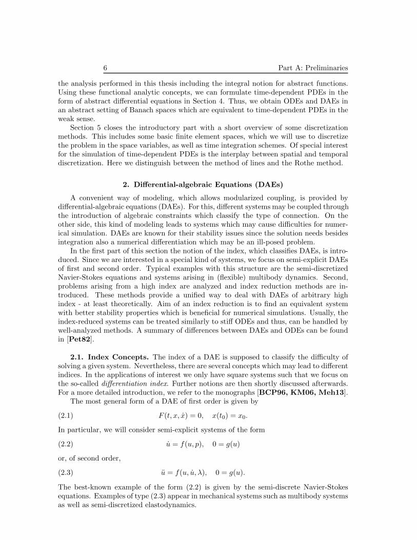
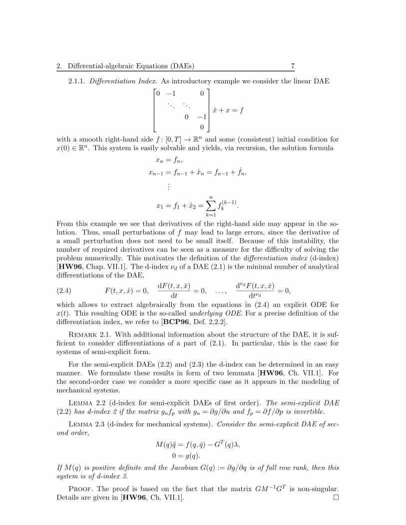
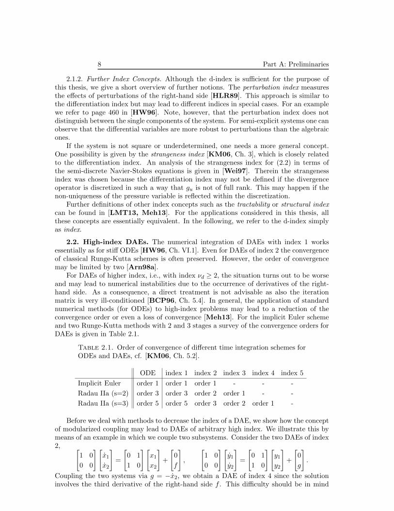
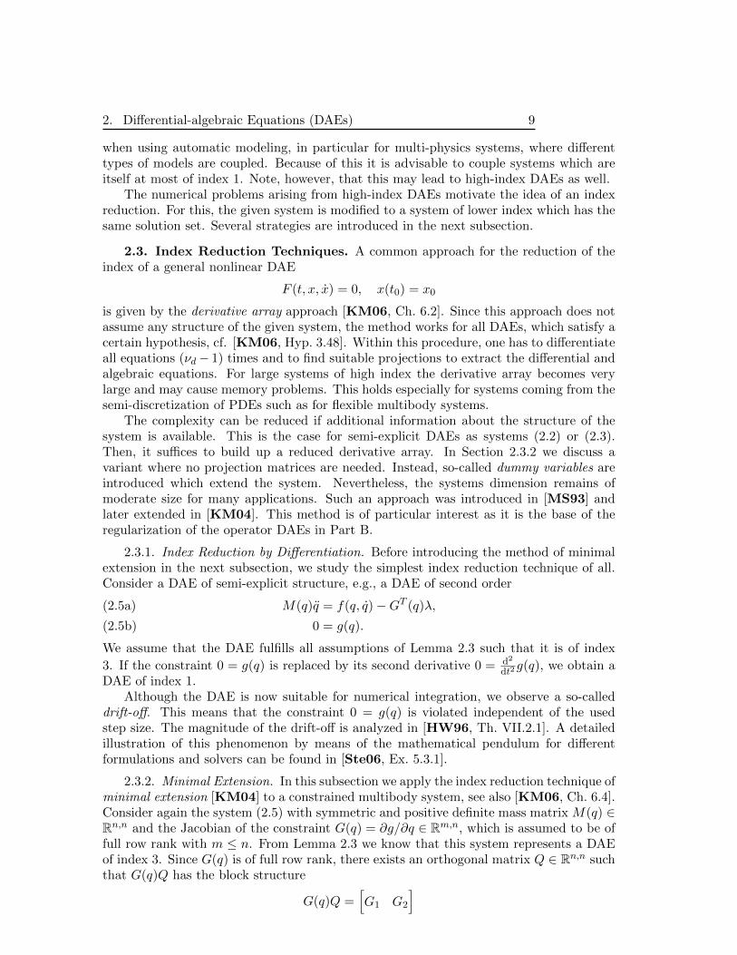
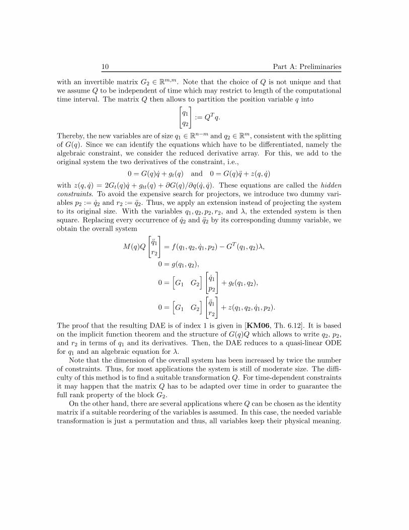
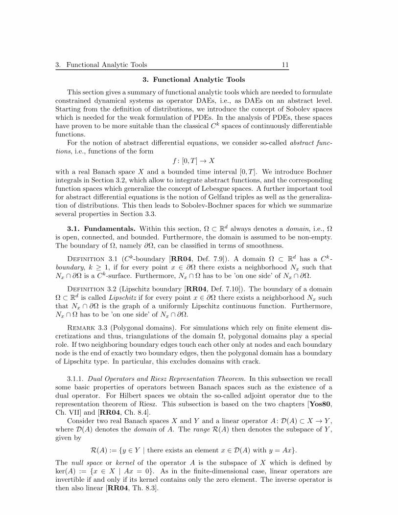
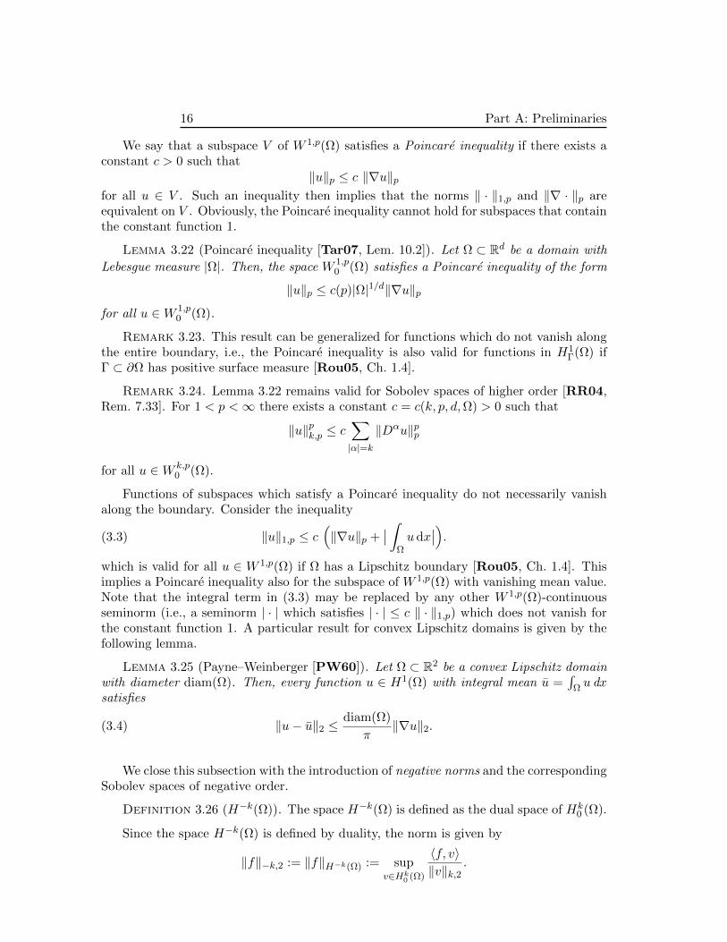
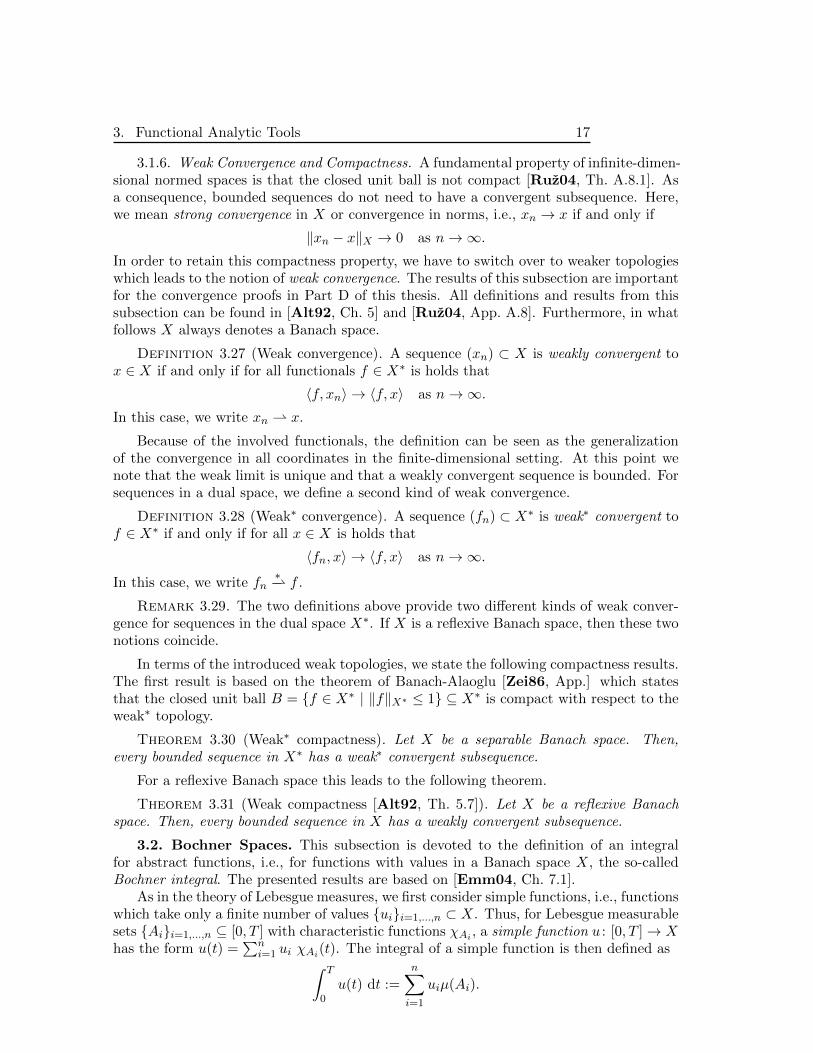
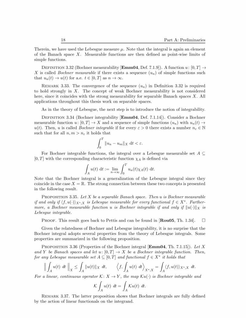
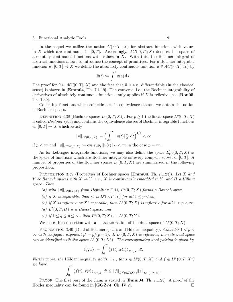
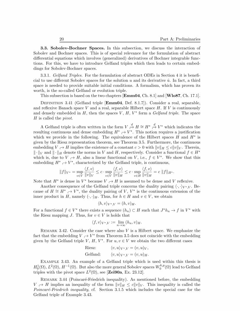
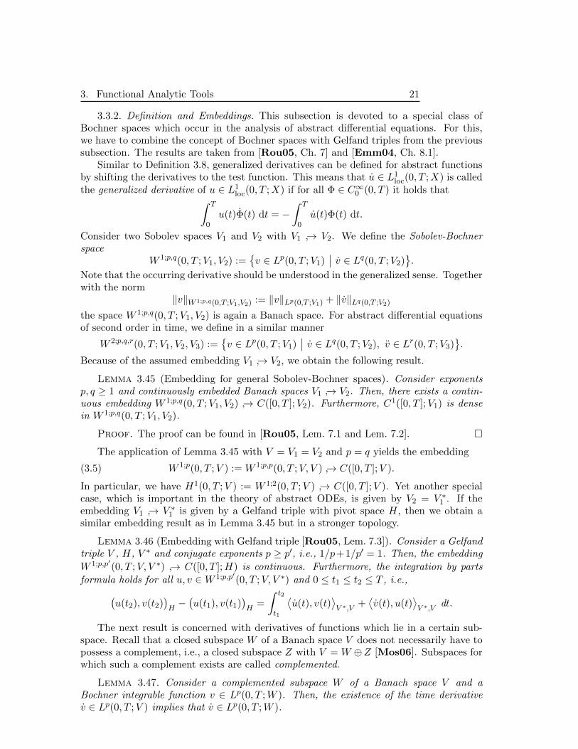
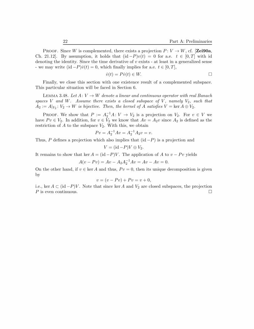
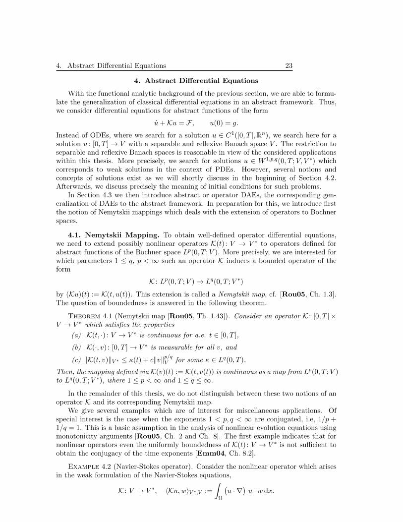

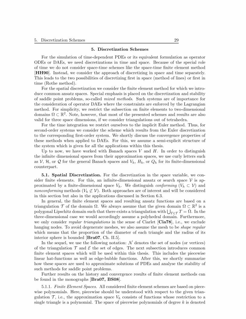
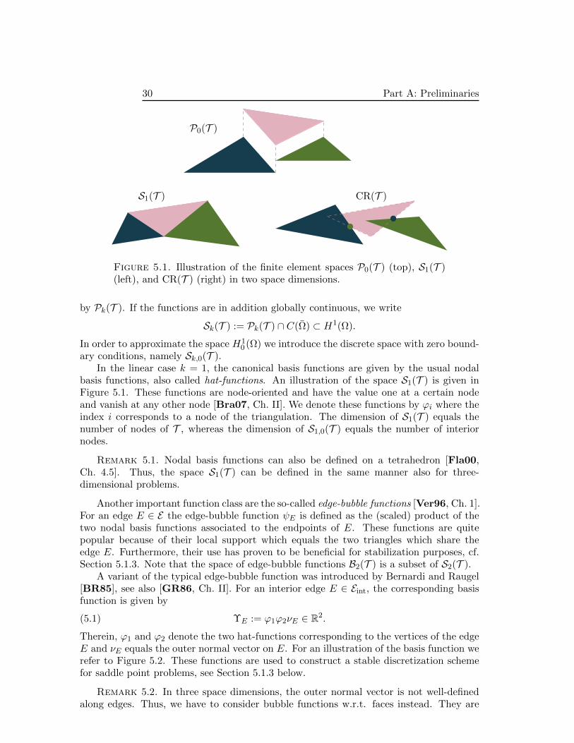
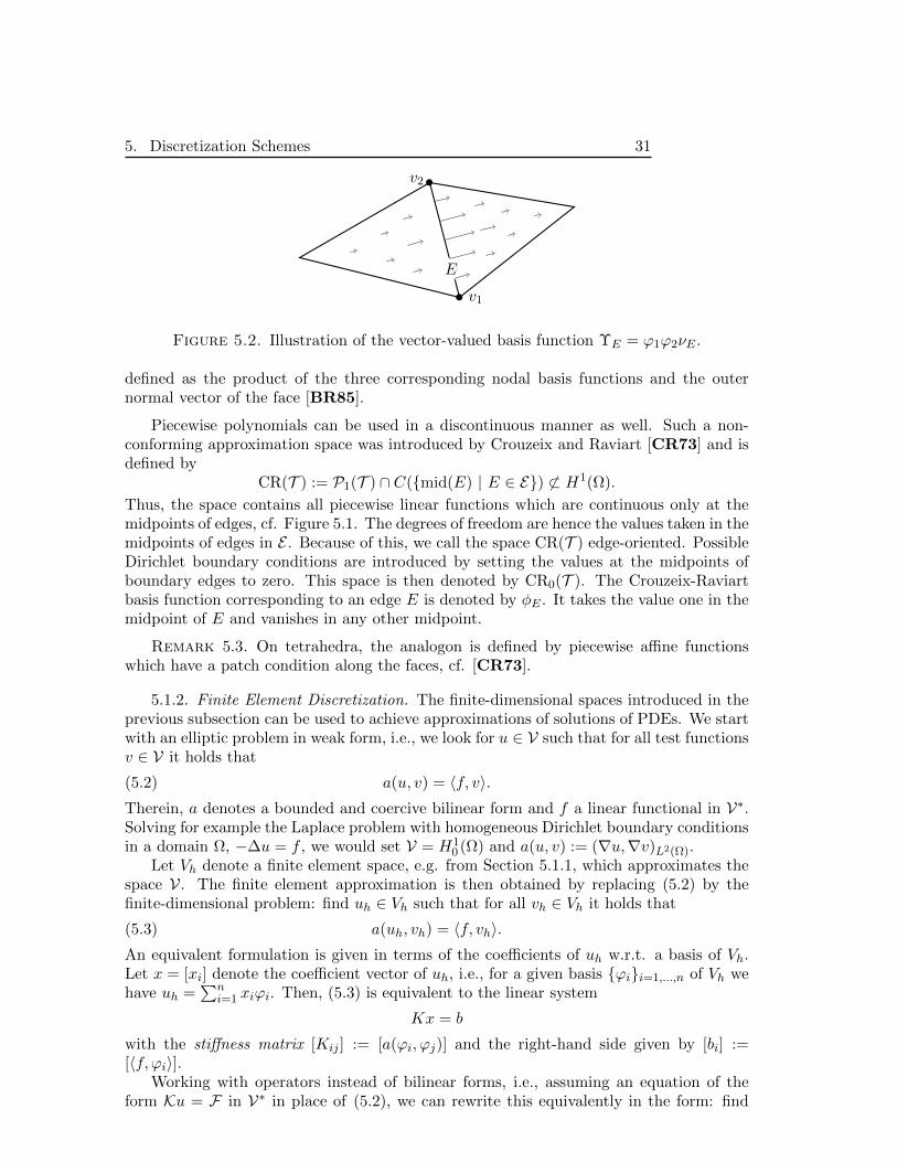
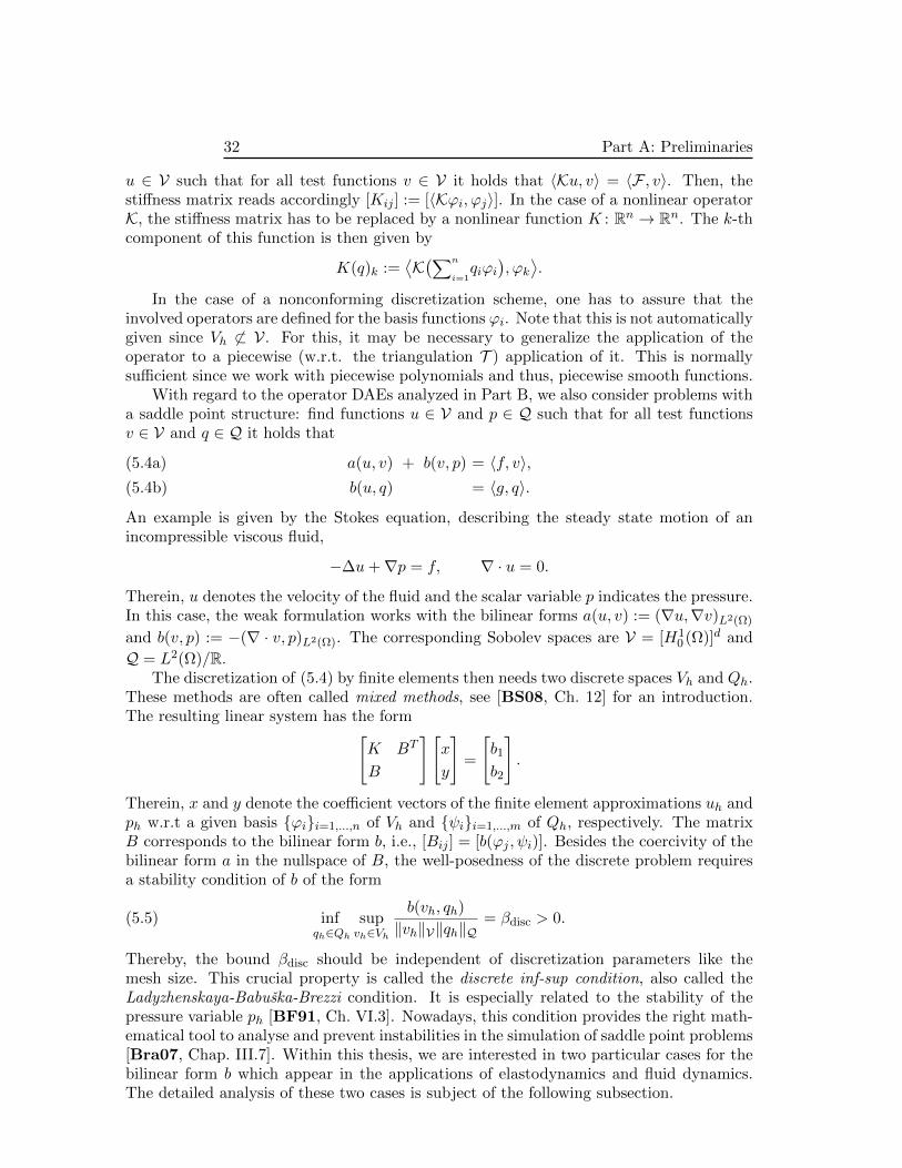
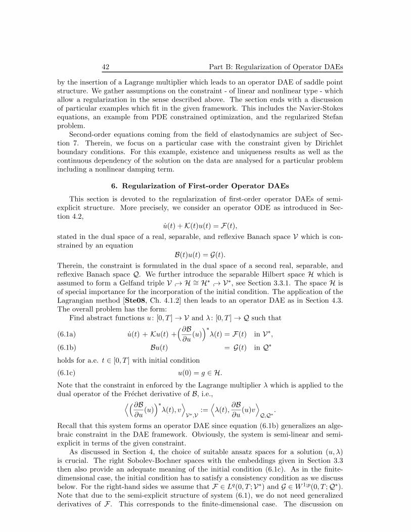
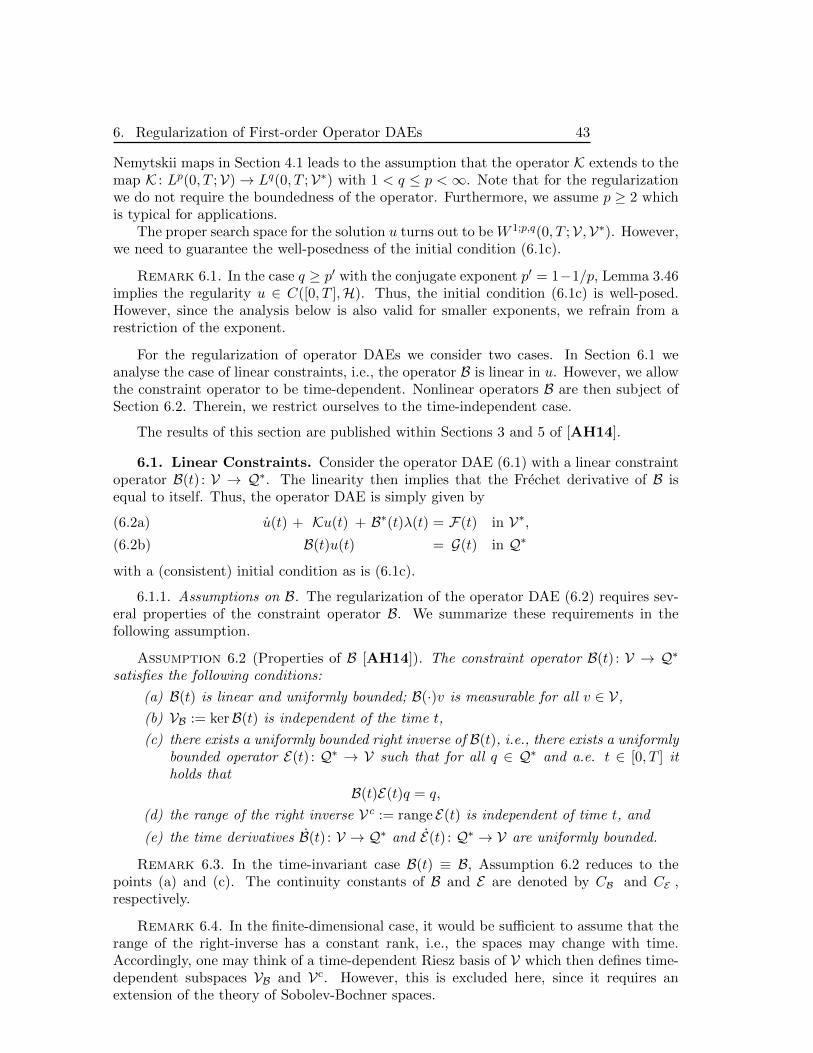
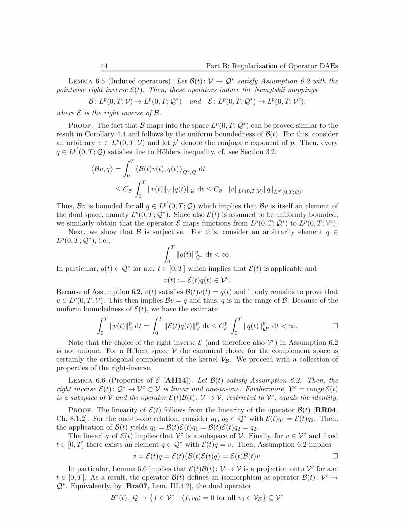
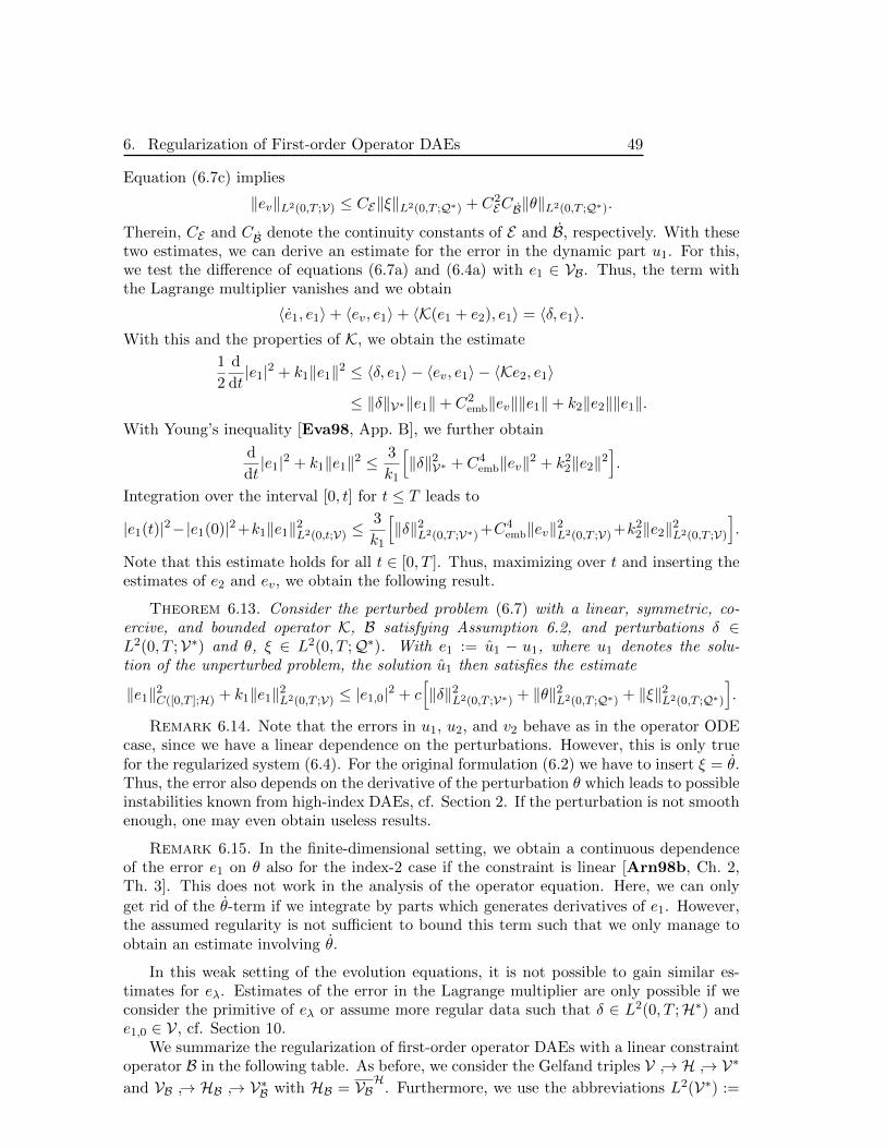
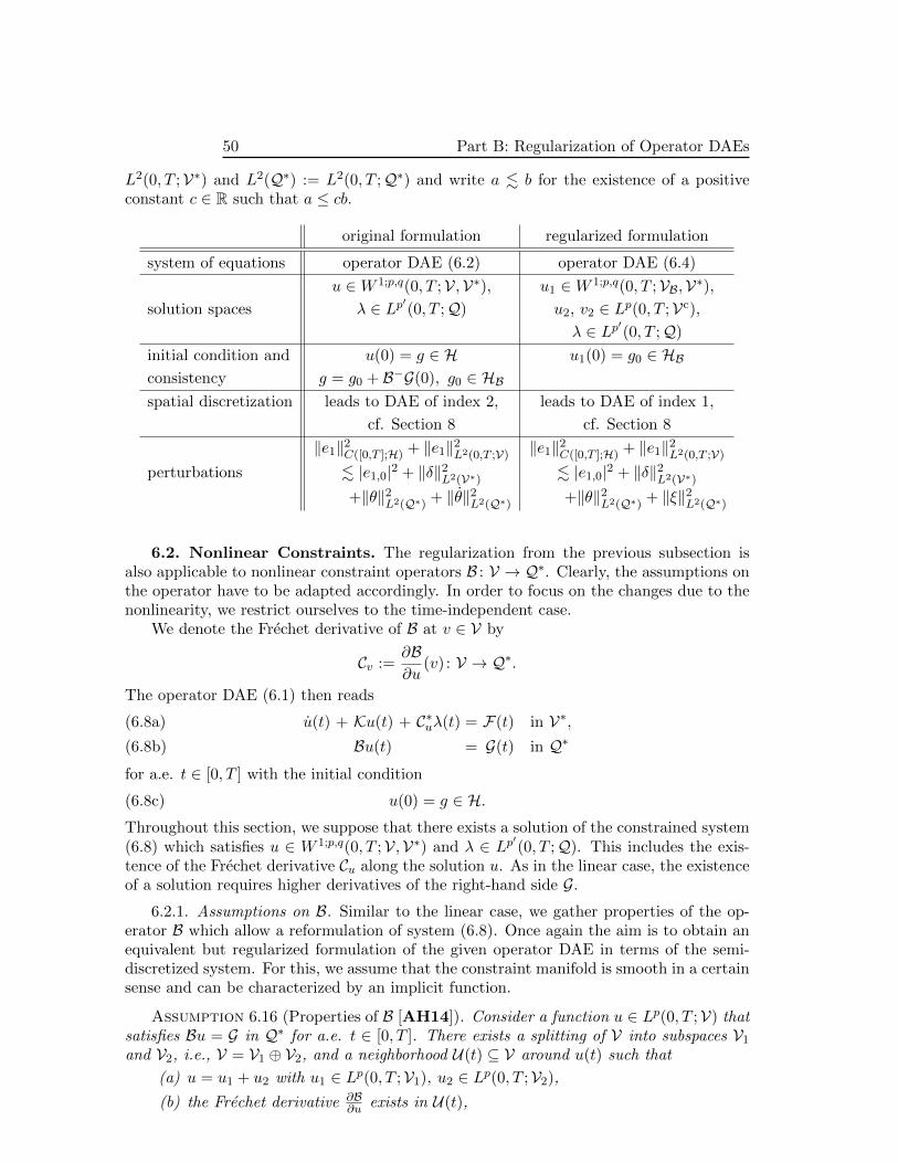
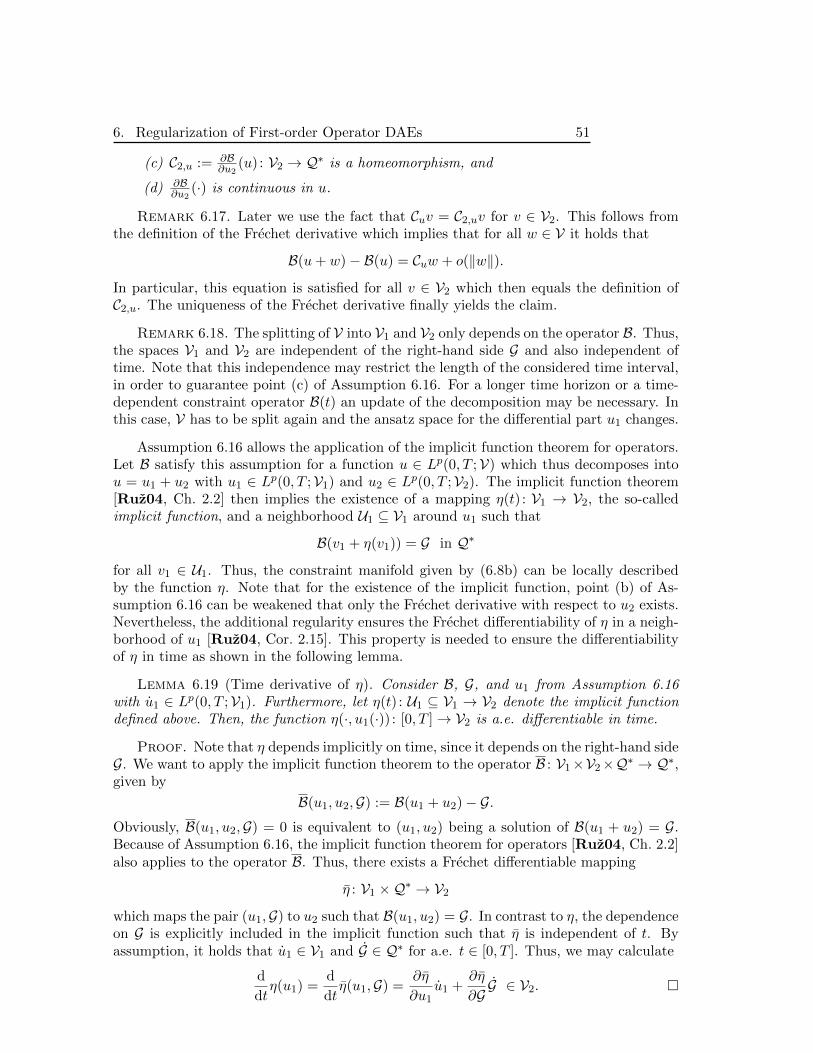
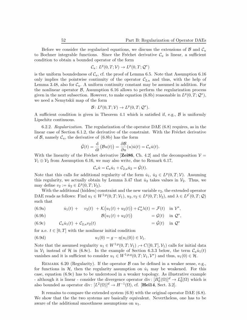
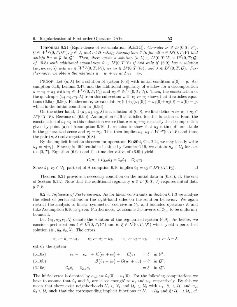
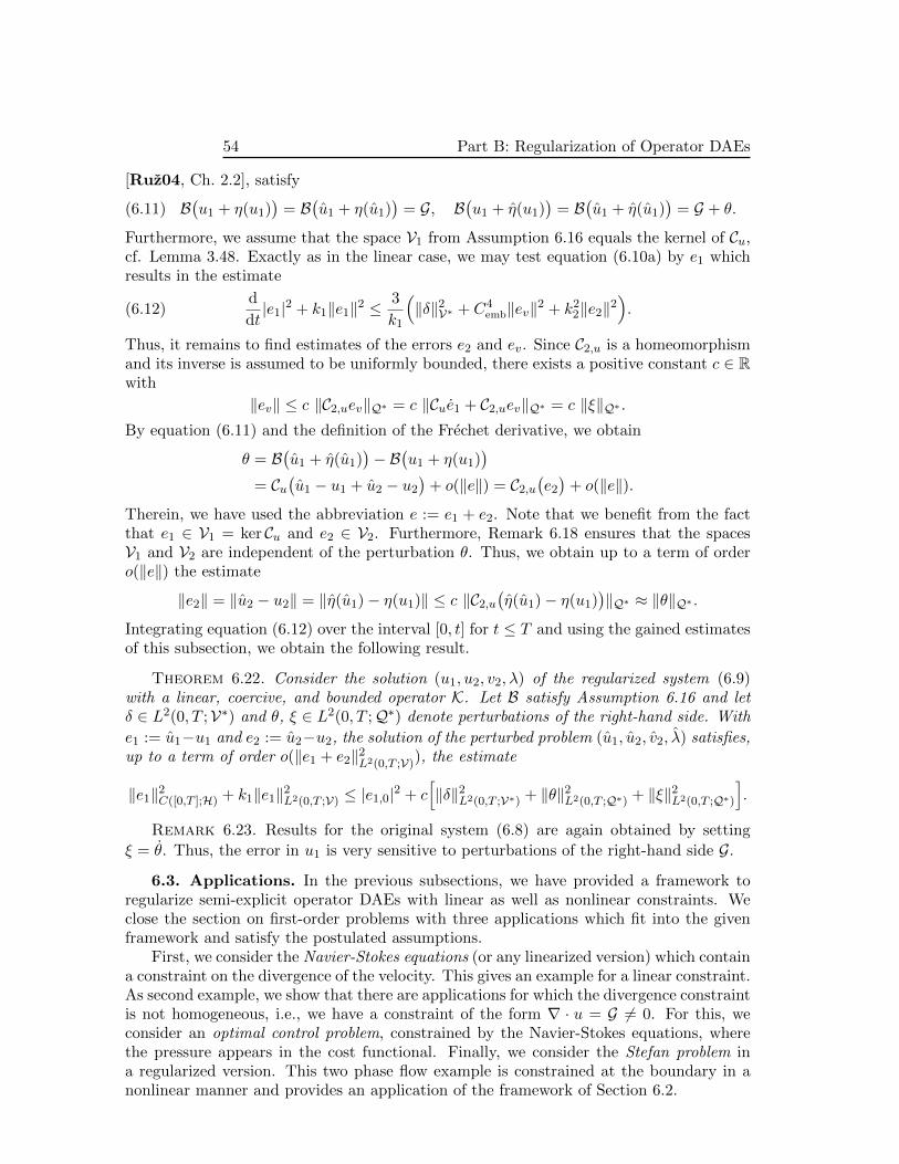
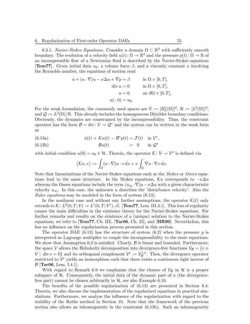
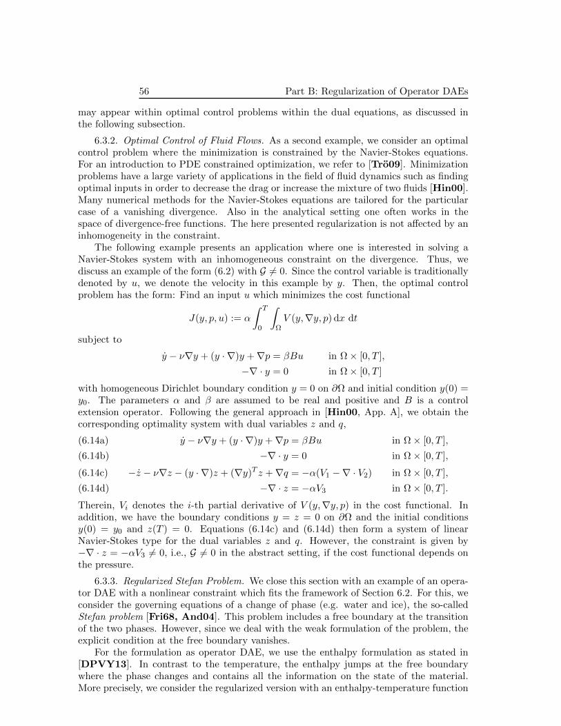
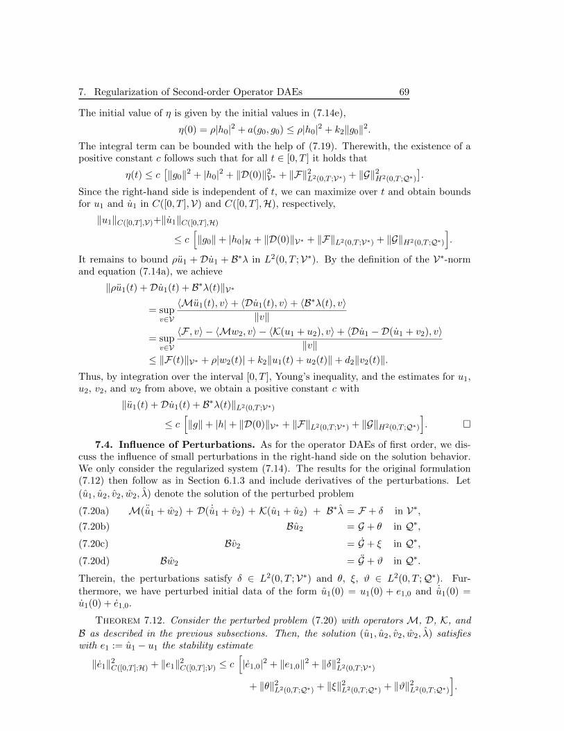
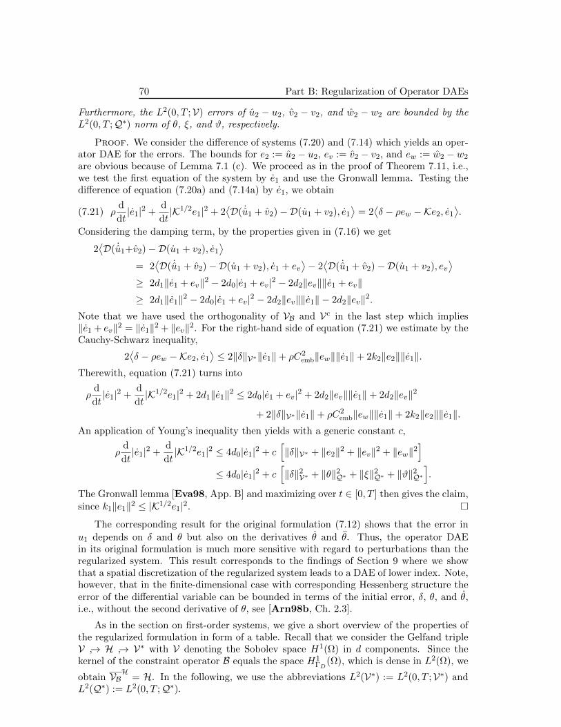
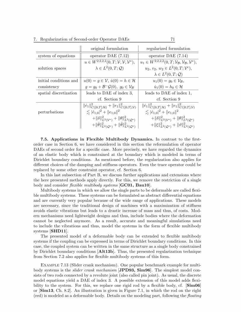
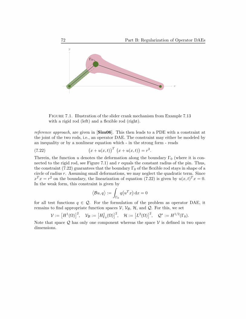
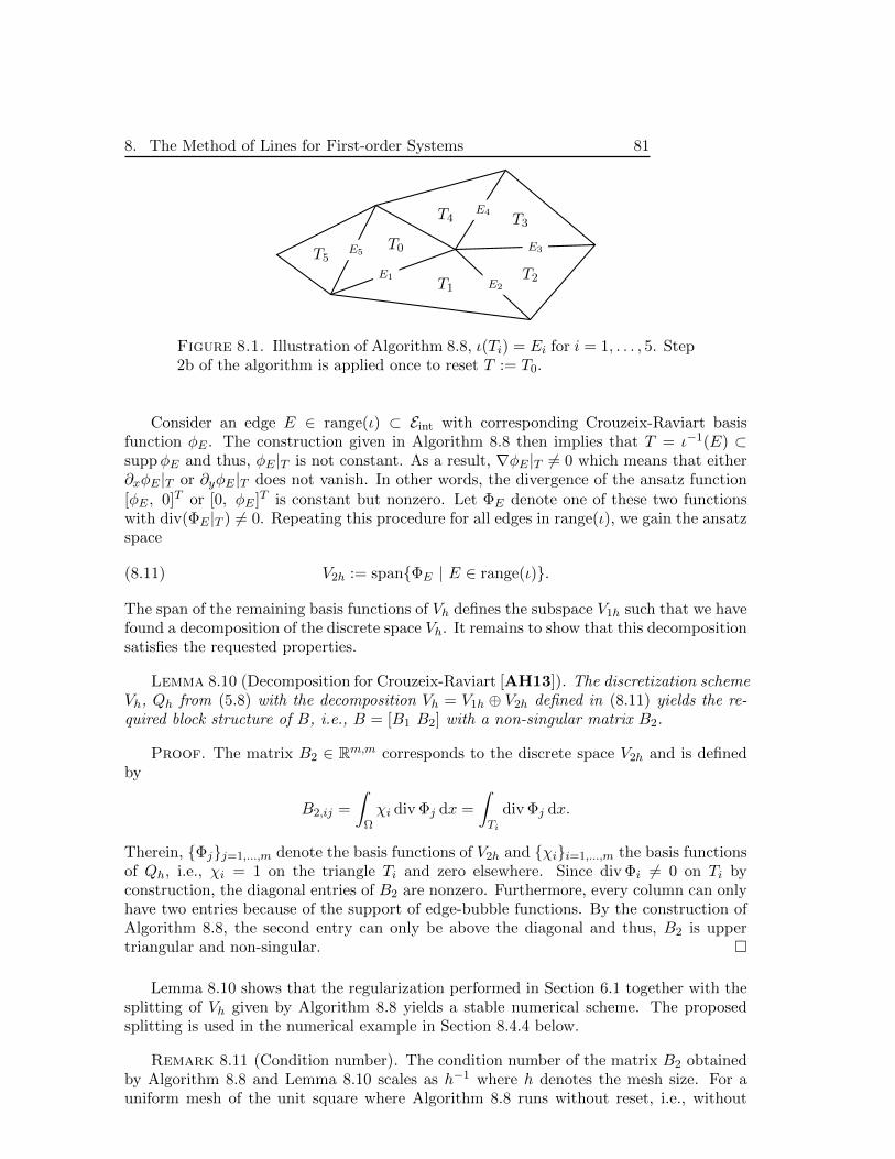
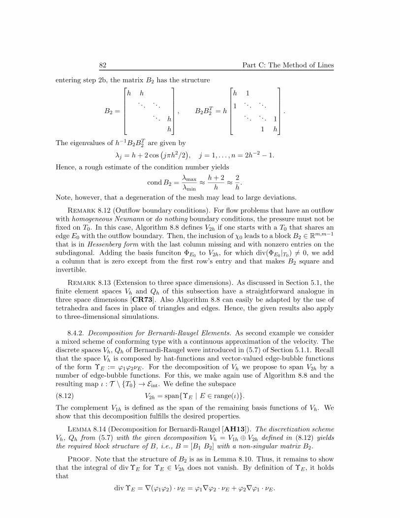
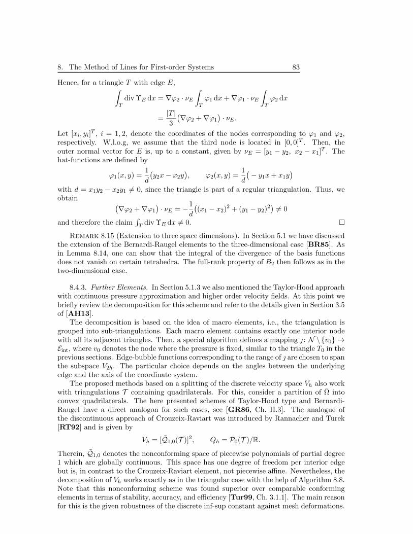
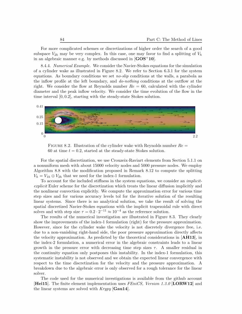
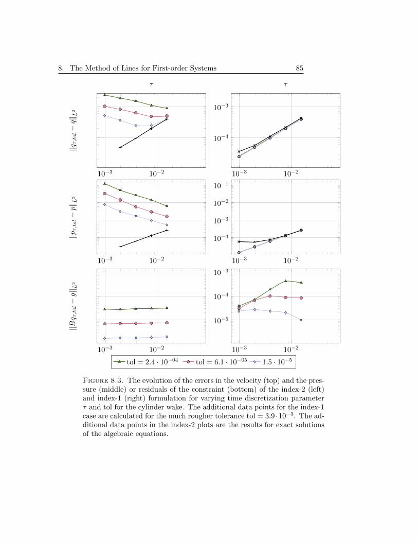
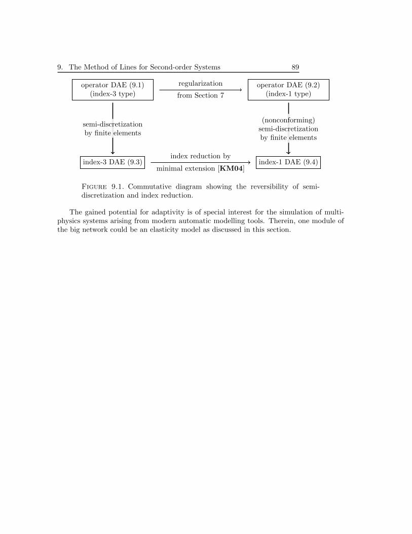

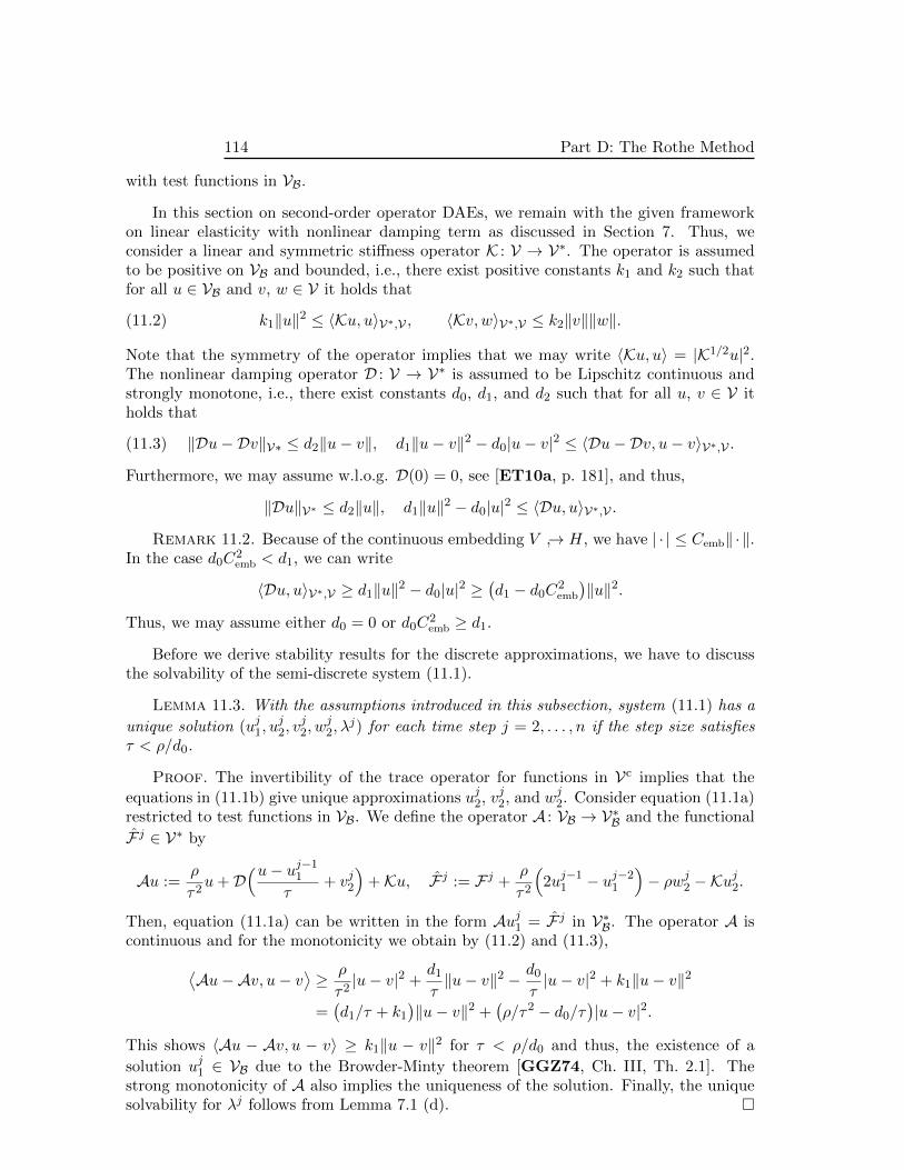
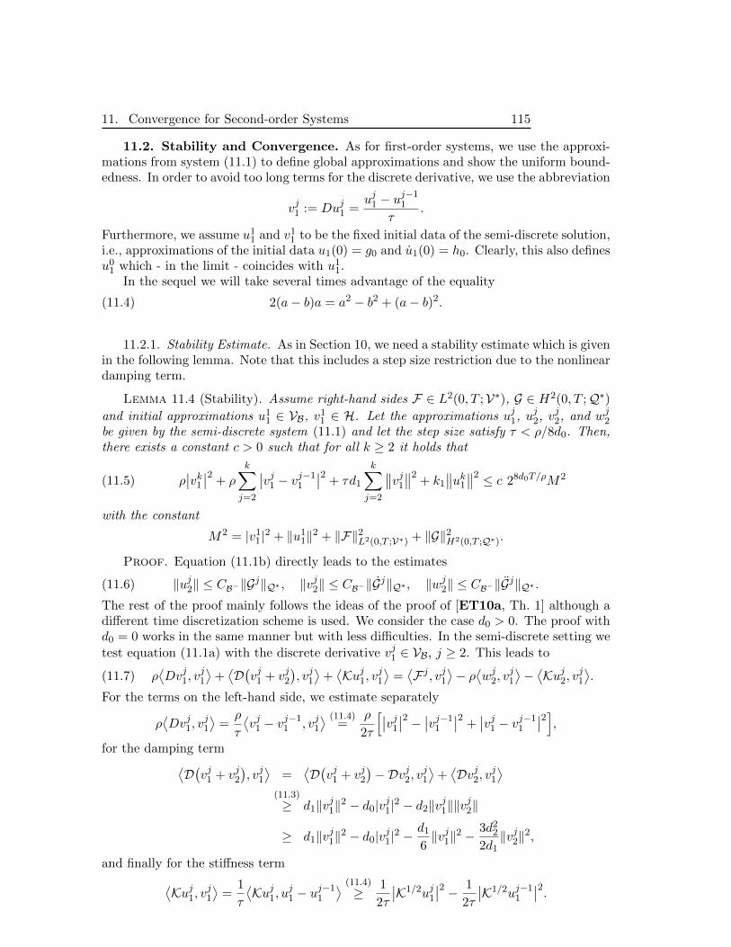
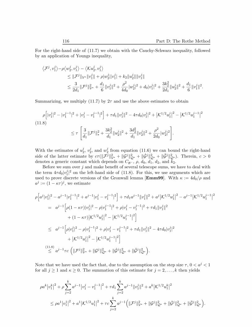
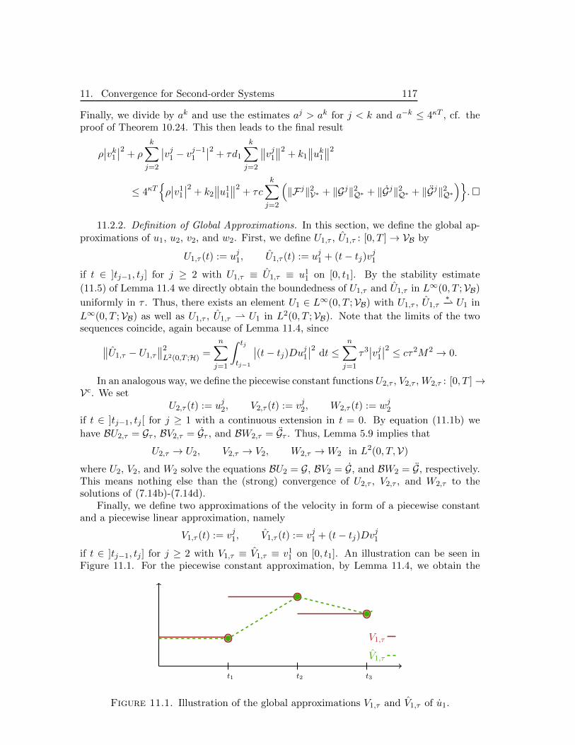


![Damping with Varying Regularization in Optimal ...constrained optimal control problem can be appreciated from the examples in [18]. Compared with those earlier works, we analyze a](https://static.documents.pub/doc/80x56/60e9b3367910de4f325a1059/damping-with-varying-regularization-in-optimal-constrained-optimal-control-problem.jpg)


![WCDA Regularization for 3D Quantitative Microwave Tomography · WCDA Regularization for 3D Quantitative Microwave Tomography 2 problem is also ill-posed [11] and regularization is](https://static.documents.pub/doc/80x56/5e3abb0a2129886ec2199ead/wcda-regularization-for-3d-quantitative-microwave-tomography-wcda-regularization.jpg)


