INTRODUCTION THE MAIN STABLE . . . THE NUMERICAL . . . SOME APPLYING . . . CONCLUSIONS AND . . . THE APPENDIX Home Page Title Page Page 1 of 107 Go Back Full Screen Close Quit Regularization of Numerical Differentiation: Methods and Applications Xiao Tingyan Hebei University of Techlonogy ty [email protected]Joint Work with Zhang Hua Shanghai University [email protected]
Transcript
INTRODUCTION
THE MAIN STABLE . . .
THE NUMERICAL . . .
SOME APPLYING . . .
CONCLUSIONS AND . . .
THE APPENDIX
Home Page
Title Page
JJ II
J I
Page 1 of 107
Go Back
Full Screen
Close
Quit
Regularization of NumericalDifferentiation:
Methods and Applications
Xiao TingyanHebei University of Techlonogyty [email protected] Work with Zhang Hua
• 1.1 Numerical Differentiation is a Long-Standing Issue
To support the above point of view we gatherthe each year’s numbers of papers, as completeas possible, which deal with at least two termsof the ”words”:
– Numerical Differentiation(/Derivative);and by hand-identifying
– Experimental ( Noisy/ Non-Exact ) Data;– Stable Method ( /Scheme );Regularization;and from the following database:elservier; EiVillage; CESJ; Springer Link; IEEE.
The situation goes as the figures shown in thenext page.
INTRODUCTION
THE MAIN STABLE . . .
THE NUMERICAL . . .
SOME APPLYING . . .
CONCLUSIONS AND . . .
THE APPENDIX
Home Page
Title Page
JJ II
J I
Page 4 of 107
Go Back
Full Screen
Close
Quit
• 1.1 Numerical Differentiation is a Long-Standing Issue
Figure 1-1: The Growth Trends of the Papers About NumericalDifferentiation
INTRODUCTION
THE MAIN STABLE . . .
THE NUMERICAL . . .
SOME APPLYING . . .
CONCLUSIONS AND . . .
THE APPENDIX
Home Page
Title Page
JJ II
J I
Page 5 of 107
Go Back
Full Screen
Close
Quit
Figure 1-2: The Growth Trends of the Papers About NumericalDifferentiation
INTRODUCTION
THE MAIN STABLE . . .
THE NUMERICAL . . .
SOME APPLYING . . .
CONCLUSIONS AND . . .
THE APPENDIX
Home Page
Title Page
JJ II
J I
Page 6 of 107
Go Back
Full Screen
Close
Quit
• 1.2 A Short List of the Titles of Applicationsof Numerical Differentiation (ND)
– The Inversion of Failure Rate from Approximate Failure Data(in Reliability Analysis);
– Recovering the Local Volatility of Underlying Assets (inFinance);
– The Estimation of Parameters in New Product (/Technology)Diffusion Model (inTechnological Forecasting)¶
– The Determination of Source (/Coefficients)Term inHeat ConductProblem;
– The Numerical Inversion ofAbel Transform (inPhysics)¶
– The Parameter Identification of Differentiation Operator¶
– The Linear Viscoelastic Stress-Strain Analysis from ExperimentalData (inViscous Elastic Mechanics);
– The Image Edge(/Corner) Detection (inImage Processing);
– Calculating Vorticity from Observational Wind (inMeteorology);
– Many Similar Problems, Many Others ......We Will Discuss SeveralRepresentative Examples in Some Details in§4.
INTRODUCTION
THE MAIN STABLE . . .
THE NUMERICAL . . .
SOME APPLYING . . .
CONCLUSIONS AND . . .
THE APPENDIX
Home Page
Title Page
JJ II
J I
Page 7 of 107
Go Back
Full Screen
Close
Quit
• 1.3 The Basic Formulations of NumericalDifferentiation
Given a tabulated functiony(∆) = y0, y1, ..., yn, which are thesampled values at the points of the grid∆ = 0 = x0 < x1 <
... < xn = 1, of an ideal and (piecewise) smooth functiony(x) on[0, 1], and a positiveδ called ’noise level’.
– Statement 1 (inForm of Discrete Discrepancy): Suppose
1. for a givenδ: |yi − y(xi)| ≤ δ, for i = 1, 2, ..., n− 1;2. y0 = y(0) andyn = y(1).
The task is to find a smooth approximationf (k)(x) of y(k)(x), k =
1, 2, from the given data(y(∆), δ), with some guaranteed accuracy.
– Statement 2 (inForm of Continuous Discrepancy): Suppose
1. yi = yδ(xi), i = 0, 1, 2, ..., n, whereyδ(x) ∈ L2[0, 1] is formallythe approximate version ofy(x);
2. for a givenδ: ‖yδ(x)− y(x)‖µ ≤ δ, µ = L2[0, 1] or µ = ∞.
The task is to find the approximation ofy(k)(∆), k = 1, 2 from thegiven data(y(∆), δ) and theyδ(x) with some guaranteed accuracy.
INTRODUCTION
THE MAIN STABLE . . .
THE NUMERICAL . . .
SOME APPLYING . . .
CONCLUSIONS AND . . .
THE APPENDIX
Home Page
Title Page
JJ II
J I
Page 8 of 107
Go Back
Full Screen
Close
Quit
• 1.4 The Basic Features of NumericalDifferentiation
– Numerical Differentiation is A Typical Inverse Problemwhich can beformulated in the first kind of integral equations:
– It Encompasses Many Subtleties and Pitfallsbecause of the nature ofill-posedness. (Non-solvability, Non-stability⇒ Ill-Posed.)
– The OperatorA is Positive; the Structure is Simple; the Singular Systemsare Easy to Obtain.
– The Degree of Ill-Posedness of Discrete Matrixes is Moderate, as shownin the following figure.⇒ Easy to Understand, Considerably Easyto Solve, Difficulties Still Exist.
INTRODUCTION
THE MAIN STABLE . . .
THE NUMERICAL . . .
SOME APPLYING . . .
CONCLUSIONS AND . . .
THE APPENDIX
Home Page
Title Page
JJ II
J I
Page 9 of 107
Go Back
Full Screen
Close
Quit
Figure 1-3:The Condition of the Discrete MatrixesCompared to Hilbert Matrix
The Condition ofA(1st) andA(2nd) are Much Less Than Hilbert Matrix;
The Condition ofA(1st) is Less Than the Condition ofA(2nd) !
INTRODUCTION
THE MAIN STABLE . . .
THE NUMERICAL . . .
SOME APPLYING . . .
CONCLUSIONS AND . . .
THE APPENDIX
Home Page
Title Page
JJ II
J I
Page 10 of 107
Go Back
Full Screen
Close
Quit
• 1.5 The Basic Ideas to Construct the StableNumerical Schemes (SNS)
– The Development of Stable Numerical Schemes of ND
∗ Parallel to the Development of Regularization Theory;∗ Derived Mainly from Regularization Theory;∗ Practical Application of Various Regularization methods.⇓
– Basic Idea of ConstructingSNSas in the Regularization Methods:Find a Good Approximation of the Original Ill-Posed Problem
From a Family of the Neighbored Well-Posed Problems
By Imposing Some Possible and Reasonable Constraints.
– Some Relevant Problems to Consider:
1. How to Construct Approximate ’Well-Posed Problem’ ?(Approximate Method? Optimization ? Discrete/Continuous ?)
2. How Does Neighbor Mean ? (Solution/Data Space, Metric)3. How to Impose the Constrains ? (y(x) ∈ H(?); ‖y(x)‖ ≤?;‖Aφ− yδ‖ ≤ δ? )
4. How to Control the Degree of the Proximity ?(Control / Regularization Parameter )
INTRODUCTION
THE MAIN STABLE . . .
THE NUMERICAL . . .
SOME APPLYING . . .
CONCLUSIONS AND . . .
THE APPENDIX
Home Page
Title Page
JJ II
J I
Page 11 of 107
Go Back
Full Screen
Close
Quit
• 1.6 The Ways of Constructing the NeighboredWell-Posed Problem
Suppose the precise datay(x) ∈ H(1)(H(2)), yδ ∈ L2[0, 1] isapproximately known with a noise levelδ > 0: ‖y − yδ‖ ≤ δ.
– Construct an integral operatorDh such thatDhyδ(x) ≈ y(k)(x):
Dhyδ(x) =
1
hk
∫ 1
−1
ψk(t)yδ(x + th)dt (k = 1, 2) (1.3)
with a appreciate step-sizeh > 0 and a selected polynomialψk(t).
– Construct a MollifierJλ, a convolution operator given by
Jλyδ(x) := yδ ∗Kλ =
∫ ∞
−∞Kλ(x− s)yδ(s)ds (1.4)
such thatJλy(x) be a smooth and’Identity Approximation’,i.e.,
limλ→0+
∫ ∞
−∞Kλ(x− s)y(s)ds = y(x),∀y ∈ H(k) (1.5)
and (Jλyδ(x))(k) =
∫ ∞
−∞(Kλ(x− s))(k)yδ(s)ds (1.6)
It can choose a kernelKλ with λ = λ that make(Jλyδ(x))(k) ≈ y(k).
INTRODUCTION
THE MAIN STABLE . . .
THE NUMERICAL . . .
SOME APPLYING . . .
CONCLUSIONS AND . . .
THE APPENDIX
Home Page
Title Page
JJ II
J I
Page 12 of 107
Go Back
Full Screen
Close
Quit
• 1.6 The Ways of Constructing the NeighboredWell-Posed Problem(Continued)
By a ’good’α, this is neighboredwell-posed problemto (1.1).
– Find a min-norm Least Square Solutionamong the set of feasiblesolutionsFδ := φ|‖Aφ− yδ‖ ≤ δ; φ ∈ H(k):
φ = arg infφ∈Fδ
Ω[φ], Ω[φ] = ‖φ‖2H(k); k = 0, 1, 2 (1.8)
which can be changed into a unconstrained optimization problemby Method of Lagrange Multiplier:
infφ∈H(k)
(‖Aφ− yδ‖2 + αΩ[φ]), (α > 0) (1.9)
( Ω[φ]...... Penalty Term / Stabilizer )Taking a satisfied value ofα > 0, this well-posed problem is closedto the problem: infφ∈H(k) ‖Aφ− yδ‖2 (Least-Square Problem).
INTRODUCTION
THE MAIN STABLE . . .
THE NUMERICAL . . .
SOME APPLYING . . .
CONCLUSIONS AND . . .
THE APPENDIX
Home Page
Title Page
JJ II
J I
Page 13 of 107
Go Back
Full Screen
Close
Quit
• 1.6 The Ways of Constructing the NeighboredWell-Posed Problem(Continued)
– Give another set of feasible solutions:( denotingyi = yδ(xi))
FD,δ := φ | 1
n− 1
n−1∑i=1
(φ(xi)− yi)2 ≤ δ2; φ are spline functions
infφ∈FD,δ
1
n− 1
n−1∑i=1
(φ(xi)− yi)2 + αΩ[φ] (1.10)
’Discrepancy Term’in a discrete format; may take other form.
( Why not‖Aφ− yδ‖∞ ≤ δ ? More difficult to deal with ! )
– Take another stabilizerwhenφ ∈ BV [0, 1] and parameterβ > 0:
Ω[φ] = ‖φ‖BV =
∫ 1
0
|φ′(x)|dx⇒ Ωβ[φ] =
∫ 1
0
√|φ′(x)|2 + βdx
(1.11)
infφ∈BV [0,1]
(‖Aφ− yδ‖2 + αΩβ[φ]), (α, β > 0) (1.12)
Whenα, β are taken suitably,(1.12) is closed to problem:
infφ∈BV [0,1]
‖Aφ− yδ‖2
INTRODUCTION
THE MAIN STABLE . . .
THE NUMERICAL . . .
SOME APPLYING . . .
CONCLUSIONS AND . . .
THE APPENDIX
Home Page
Title Page
JJ II
J I
Page 14 of 107
Go Back
Full Screen
Close
Quit
2 THE MAIN STABLE SCHEMESThere are plenty of schemes devoted toStabilized/
Let C0(I) denote the set of continuous functions over the intervalI = [0, 1] with ‖φ‖∞,I = infx∈I |φ(x)| < ∞. Supporty ∈ H2[0, 1]and its observed versionyδ ∈ C0(I), ‖yδ − y‖∞,I ≤ δ.
∗ Outline of the Steps of MBR:1. Introduce a Gaussian kernelKλ with a ’blurring radius’,λ:
Kλ(x) = exp(−x2/λ2)/λπ (2.2.7)
We notice that (1)Kλ ∈ C∞ falls to nearly0 outside a few radiifrom its center (≈ 3λ); (2) it is positive and has total integral1.
2. Make a Continuation ofy, yδ Into Iλ = [−3λ, 1+3λ] such that(1) they decay smoothly to0 in [−3λ, 0]
⋃[1, 1 + 3λ]; (2) they are
0 in R− Iλ. This can be done by definingyδ(x) = yδ(0) exp x2
[(3λ)2−x2], −3λ ≤ x ≤ 0,
yδ(x) = yδ(1) exp (x−1)2
[(x−1)2−(3λ)2], 1 ≤ x ≤ 1 + 3λ.(2.2.8)
So
Jλf(x) = (Kλ ∗ f) =
∫∞−∞Kλ(x− s)f(s)ds
∼=∫ x+3λ
x−3λ Kλ(x− s)f(s)ds, f = y, yδ (2.2.9)
3. Make the Differentiating Operation:Forf = y, yδ we have
(Jλf)′(x) = (Kλ ∗ f)
′(x) = (K
′
λ ∗ f)(x) (2.2.10)
4. Choose a Suitableλ being a Regularization Parameter
(2.2.11)We observe that the error estimate is minimized by choosingλ = λ = [2δ/3M2
√π]1/2, this results in
‖(Kλ ∗ yδ)′ − y
′‖∞ ≤ 2√
6M2
π4
√δ ⇒ ‖(Kλ ∗ yδ)
′ − y′‖∞ = O(
√δ)
(2.2.12)
∗ The Posterior Strategies for Choosingλ: There existsλ = λ suchthat ‖Jλy
δ − yδ‖ = δ (2.2.13)When data error levelδ is not known, theGCV Criterior also holds.
∗ The Numerical Implementation of MBR: The NumericalScheme ofMBR Can Refer to [3].Many applied examples areincluded in that book. Moreover, a group of programs forMBRis also Provided by Murio (1993).
– The Euler Equation of Variational Problem(1.9) is
(A∗A+ αΩ′)φ(s) = A∗yδ(s) := g(s) (2.3.2)
where
A∗Aφ =
∫ 10
∫ 10 H(x− s)H(x− ξ)dx
φ(ξ)dξ,
g(s) =∫ 1
0 H(x− s)yδ(x)dx(2.3.3)
and αΩ′[φ] =
αφ(s), if ‖Ω‖ = ‖φ‖2
L2;α(φ(s)− φ′′(s)), if ‖Ω‖ = ‖Ω‖2
H(2,2)
(2.3.4)
The later case of(2.3.4) coupled with a boundary condition:φ′(1)h(1)−φ′(0)h(0) = 0, which holds when(1) φ′(1) = φ′(0) = 0 or (2) h(1) =h(0) = 0 hereh(s) is admissible function in the variational problem.
– If condition (1) comes out, the original problem can be solved sta-bly and easily; this will be shown in§2.5. So we can mainly discuss(2.3.4) with condition(2).
1. ∃α = α(δ) such that‖B[ψδα(δ)]− gδ‖ = Cδγ, (2.4.10)
2. ‖φδα(δ) − y′′‖ = O(δmin(1−γ,γ/2)). So the optimal convergence rate
‖φδα(δ) − y′′‖ = O(δ(1/3)) is obtained forγ = 2/3.
– Computational Considerations:
1. In (2.4.7) we can take(yδ)′(0) ≈ −yδ(0)α + 1
α2
∫ 10 exp(−s√
α)yδ(s)ds;
2. A Further Simplification to(2.4.7)− (2.4.8) Givesψδ
α(x) ≈ 12α√
α
∫ 10 (exp(−|x−s|√
α) +Kα(x, s))yδ(s)ds−
− 1αy
δ(x)− 1√α(yδ)′(0) exp(−x√
α),
where Kα(x, s) = exp(−x−s√α
)− exp(x+s−2√α
).
(2.4.11)
– The Discrepancy Equation(2.4.4), (2.4.10) Must Be Solved in aDiscrete Wayif gδ(xi), i = 0, 1, 2, ......, n are merely known; andin this case the integral values in(2.4.6), (2.4.11) must be approx-imated by some quadrature formulae.
h,2, a 2 × (n + 1) order-matrix. Combine the above twoequations, we get
Ahφh := [Ah,1;Ah,2]φh = yδh := [yδ
h,1; yδh,2]. (2.5.5)
INTRODUCTION
THE MAIN STABLE . . .
THE NUMERICAL . . .
SOME APPLYING . . .
CONCLUSIONS AND . . .
THE APPENDIX
Home Page
Title Page
JJ II
J I
Page 26 of 107
Go Back
Full Screen
Close
Quit
• 2.5 Discrete Regularization Methods(cont.)
– Two Class of Discrete Schemes:Collocation and Galerkin MethodC.2 for (1.2) we adopt Galerkin Method with Orthogonal base function,by using[Ah, b] = deriv2(n, example), we can obtain an × n-ordermatrix corresponding to the second order derivative.C.3 for (1.2) we can also employ Collocation Method; on the grid∆ =0 = x0 < x1 < ... < xn−1 < xn = 1 with the kernel(1.3) we have
(xi − 1)
∫ xi
0sφ(s)ds+ xi
∫ 1
xi
(s− 1)φ(s)ds = yδ(xi) (2.5.6)
Supposehi = xi+1 − xi = h = const., by usingTrapezoid Formula,we get a(n− 1)× (n− 1)-order linear equationAhφh = yδ
For C.2 andC.3, φ(x0), φ(xn) are not included inφh !!
INTRODUCTION
THE MAIN STABLE . . .
THE NUMERICAL . . .
SOME APPLYING . . .
CONCLUSIONS AND . . .
THE APPENDIX
Home Page
Title Page
JJ II
J I
Page 27 of 107
Go Back
Full Screen
Close
Quit
• 2.5 Discrete Regularization Methods(cont.)The regularized solution can be obtained by calling M-functions inRegularization Tool (by Hansen); which provides
– Various Strategies of Implementing Regularization1. DSVD Computes a damped SVD/GSVD solution;2. TSVD Computes the truncated SVD solution;3. MTSVD Computes the modified TSVD solution;4. TGSVD Computes the truncated GSVD solution;5. TIKHONOV Computes the Tikhonov regularized solution
– Various Rules of Choosing Regularization parameter1. Discrep Discrepancy Principle (whenδ is known)2. L-corner L-Curve Criterion (whenδ is not known)3. GCV GCV-Criterion (whenδ is not known)4. Quasiopt Quasi-Optimal Rule (whenδ is not known)
– It Needs a Combination of”Strategies” and ”Rules”which De-pends on the Actual Conditions.
– Of course,Any Other Continuous Regularization Schemes Must BeReduced to Some Discrete Form at Last !
INTRODUCTION
THE MAIN STABLE . . .
THE NUMERICAL . . .
SOME APPLYING . . .
CONCLUSIONS AND . . .
THE APPENDIX
Home Page
Title Page
JJ II
J I
Page 28 of 107
Go Back
Full Screen
Close
Quit
• 2.6 Semi-Discrete Tikhonov Regularization– The Methods May Include Following Steps:
1. Preestablish a Concrete Set of Feasible Solution, for example
Pk[0, 1] = φ(x)|φ(x) is cubic spline or k-order spline, k ∈ N
2. Set Up a Discrete Constraints for the Feasible Solution:1
3. Formulate and Solve the Un-constraint Optimal Problem:
infφ∈FD,δ
1
n− 1
n−1∑i=1
(φ(xi)− yi)2 + α‖φ(k)‖2
(2.6.3)
then solve it by using(a) Interpolating Conditions:φ(xi) = yδ(xi) := yi, i = 0, 1, 2, ..., n;(b) Connecting Conditions:φ(k)(xi−) = φ(l)(xi+), i = 1, 2, ..., n −
1; l = 1, 2, ..., k;
(c) Optimality Condition:∂(the Obj.func)∂(the variables)= 0. Some other condi-
tions also need to be imposed.4. Compute the First /Second Derivative of the Spline Polynomial
∗ Wang & Wei (2005) Generalized SDTR to the Case:First OrderDerivative; Scattered Data in 2D-Space;
∗ Wei & Hon (2007) Generalized SDTR By UsingRadial Ba-sis Functionto the Case: First and Second Order Deriva-tive; Scattered Data in 1D, 2D-Space;
∗ Nakamura et. al(2008) Generalized SDTR to the Case:SecondOrder Derivative; Scattered Data in 2D-Space.We would not go into details here. The interested readers can refer tothe papers inThe Appendix of this lecture.
– Some Remarks on the SDTR:1. Question: Takingα = δ2 is a Good, but Non-Optimal Strategy !
∗ Does a Better Way for Choosingα Exist ? If So, the Accuracyof Reconstruction of the Derivative May be Improved !
∗ One of the Answers: A Hopeful Way is to EmployExtrapolated Regularization MethodThat Will be Discussed in§ 2.7.
2. The Virtues and Drawbacks ofSDTR: Specially Suitable for∗ Calculating First & Second Derivatives Simultaneously;∗ Scattered Data Both in 1D & 2D;∗ But Consume Larger Computing Cost & Larger Memory !
INTRODUCTION
THE MAIN STABLE . . .
THE NUMERICAL . . .
SOME APPLYING . . .
CONCLUSIONS AND . . .
THE APPENDIX
Home Page
Title Page
JJ II
J I
Page 33 of 107
Go Back
Full Screen
Close
Quit
• 2.7 Filter-Based Regularization Method(FBR)Basic Assumptions About the Linear, Compact Operator Equation:
(Aφ)(x) :=
∫ 1
0K(x, s)φ(s)ds A : X → Y (2.7.1)
– (A1) ‖yδ − y‖ ≤ δ, 0 < δ ≤ δ0, for givenδ0 > 0;
– (A2) A is Linear, compact, injective, andy ∈ R(A), y 6= 0, yδ 6= 0;
– (A3) φ ∈ SE := φ ∈ Xσ : ‖φ‖σ ≤ E, σ ≥ 1, E > 0, where
Xσ =
φ ∈ X :∞∑
j=1
µ−2σj |(φ, uj)|2 <∞, ‖φ‖σ =
(∑µ−2σ
j |(φ, uj|2)1/2
(2.7.2)and(µj, uj, vj)j∈N is a singular system ofA.
The Singular System of Anti-Differentiation Operators:
µj, uj, vj =
2
(2j−1)π ,√
2 cos(2j−12 πt),
√2 sin(2j−1
2 πt), j ∈ N, forA in (1.1),
1(πj)2 ,
√2 sin(jπt),
√2 sin(jπt), j ∈ N, forA in (1.2).
(2.7.3)It provides us with a good chance to construct aFilter-Based Regu-larization Method (FBR)for computing the derivatives of the first andsecond order.
INTRODUCTION
THE MAIN STABLE . . .
THE NUMERICAL . . .
SOME APPLYING . . .
CONCLUSIONS AND . . .
THE APPENDIX
Home Page
Title Page
JJ II
J I
Page 34 of 107
Go Back
Full Screen
Close
Quit
• 2.7 Filter-Based Regularization Method(cont.)
An Optimal Regularization Algorithm Based on SVD:
– The General Filter-Based Tikhonov Regularization
φα(x) = (αE + A∗A)−1A∗y =∞∑
j=1
[q(α, µj)/µj](y, vj)uj, (2.7.4)
where the functionq(α, µ) = µ2/(α + µ2), α > 0, 0 < µ < ‖A‖,is a(Tikhonov-Type) Regularizing Filter.
– By Introducing a New Regularizing Filter(G.Li et al.,A[35],(2005))
qσ(α, µ) = µσ/(α+ µσ), σ ≥ 1 (2.7.5)
and inserting(2.8.5) into (2.8.4), let yδ 7→ y we can definite a newregularized approximation:
φσ,δα (x) =
∞∑j=1
[qσ(α, µj)/µj](yδ, vj)uj, α > 0, σ ≥ 1 (2.7.6)
– Asymptotic Convergence Order ofFBR-Regularized SolutionUnder assumptions ofA1− A3, if taking regularizing parameter
α = α∗(δ) = (1/σ)σ
1+σ (δ/E)σ
1+σ then (2.7.7)
limδ→0
φσ,δα∗ = φT ; ‖φσ,δ
α∗ − φT‖ ≤ C(E, σ)δσ/(1+σ) (2.7.8)
thus ‖φσ,δα∗ − φT‖ = O(δσ/(1+σ)) (2.7.9)
INTRODUCTION
THE MAIN STABLE . . .
THE NUMERICAL . . .
SOME APPLYING . . .
CONCLUSIONS AND . . .
THE APPENDIX
Home Page
Title Page
JJ II
J I
Page 35 of 107
Go Back
Full Screen
Close
Quit
• 2.7 Filter-Based Regularization Method(cont.)
The Merits and Drawbacks of FBR:
– From(2.7.9) we can see that the more largerσ is, the more accuratethe FBR’s approximation will be; whereσ characterizes the degreeof smoothness ofφT ;
– The singular system is known analytically which is of great benefitfor numerical implementation;
– It may be useful for computing the first and second derivatives atx = 0 andx = 1 which is important in some cases; but
– The acceptance ofα∗ depends on unknown parameters:σ andE; itdoes not give a practical rule for cutting the remainder of(2.7.6);
– If yδ is given in a discrete way, we didn’t know which is cheaperin the computing costs by discrete calculation of(2.7.6) and byTSVD/DSVD?
INTRODUCTION
THE MAIN STABLE . . .
THE NUMERICAL . . .
SOME APPLYING . . .
CONCLUSIONS AND . . .
THE APPENDIX
Home Page
Title Page
JJ II
J I
Page 36 of 107
Go Back
Full Screen
Close
Quit
• 2.8 Wavelet-Based Regularization Method– Background of Wavelet-Based Regularization∗ Tikhonov had discussedRegularization in Frequency Domain
for the first kind of convolution equation (A[9],1977):
(2.8.1)where K(ω),Z(ω),U(ω) are the integral transform ofk, z, uresp. Obviously, the right-hand equation of(2.8.1) is ill-posedin L2(R); R := (−∞,∞). (IT ∈ FT, LT, MT,...)
∗ To suppress the perturbation ofhigh-frequency-error, Tikhonovpresented the idea ofstabilizing factorbeing ahigh-frequencyfilter in the terminology of signal processing.
∗ Project methodshave been employedas a regularization strat-egyin which various class of functions can be served as the baseof finite-dimensional subspace; in which the wavelet functionswould be involved naturally, since they possess the property ofmulti-scale and high-resolution.
∗ Forf (x) ∈ Ck(R)⋂Hk(R), we have
f (k)(x) =1
2√π
∫ ∞
−∞(iξ)kf(ξ) exp(iξx)dξ (2.8.2)
INTRODUCTION
THE MAIN STABLE . . .
THE NUMERICAL . . .
SOME APPLYING . . .
CONCLUSIONS AND . . .
THE APPENDIX
Home Page
Title Page
JJ II
J I
Page 37 of 107
Go Back
Full Screen
Close
Quit
• 2.8 Wavelet-Based Regularization Method(cont.)
– Background of Wavelet-Based Regularization(cont.)in (2.8.2), f (ξ) is theFourier Transformof f (x); for its mea-sured version:fδ(x) ∈ L2(R), the inversion formula(2.8.2) doesnot hold !
∗ Then Suppress High-Frequency Error + Projection Method +Suitable Waveletwould bea Good Combining Strategyto dealwith Ill-Posed Equation(2.8.2) !
– Meyer Wavelet and Its major Properties(summarized by Fu et al.)(P1) Let φ(x), ψ(x) beMeyer Scaling& Wavelet Function⇒
supp φ = [−4π/3, 4π/3],
supp ψ = [−8π/3,−2π/3]⋃
[2π/3, 8π/3].(2.8.3)
(P2) ψjk(x) = 2j/2ψ(2j − k), j, k ∈ Z constitute an orthonormalbasis ofL2(R) and we have
supp ψjk(ξ) = [−8π2j
3,−2π2j
3]⋃
[2π2j
3,8π2j
3], k ∈ Z (2.8.4)
(P3) The Multi-Resolution Analysis (MRA)Vjj∈Z of MeyerWavelet is generalized by
Vj = φjk : k ∈ Z, φjk := 2j/2φ(2jx− k), j, k ∈ Z,supp φjk(ξ) = [−4π2j/3, 4π2j/3], k ∈ Z
(2.8.5)
INTRODUCTION
THE MAIN STABLE . . .
THE NUMERICAL . . .
SOME APPLYING . . .
CONCLUSIONS AND . . .
THE APPENDIX
Home Page
Title Page
JJ II
J I
Page 38 of 107
Go Back
Full Screen
Close
Quit
• 2.8 Wavelet-Based Regularization Method(cont.)
– Meyer Wavelet and Its major Properties(cont.)(P4) The orthogonal projection of a functiong ∈ L2(R) on spaceVj and wavelet spaceWj, (Vj+1 = Vj +Wj) are given by
PJg :=∑k∈Z
(g, φjk)φjk; QJg :=∑k∈Z
(g, ψjk)ψjk (2.8.6)
(P5) Further we have following projection formulae:PJg(ξ) = 0, for |ξ| > 4π2J/3;
Qjg(ξ) = 0, for j > J, |ξ| < 4π2j/3;((I − PJ)g)(ξ) = QJg(ξ), for |ξ| ≥ 4π2J/3.
(2.8.7)
– Wave-Based Regularization (WBR) for ND(Fu et al.,2010)Let y(x) ∈ Ck(R)
⋂Hk(R) be the exact data andyδ ∈ L2(R) be
the noise data with‖y − yδ‖ ≤ δ (noise level).(S1) Denotingy(k) = Dky(x) and defining its approximation as
Dk,jyδ(x) = Dk(Pjy
δ(x)) = DkPjyδ(x) (2.8.8)
where integerJ is a regularization parameter to be determined properly.(S2) The stability and error estimate: Supposey(x) ∈ Hp(R) with‖y‖p ≤ E for somep > k. If taking J∗ = [log2(E/δ)
1/p] + 1, then
‖Dky(x)−Dk,J∗yδ(x)‖ ≤ CEkpδ1−k
p ; C > 0 is a constant. (2.8.9)
INTRODUCTION
THE MAIN STABLE . . .
THE NUMERICAL . . .
SOME APPLYING . . .
CONCLUSIONS AND . . .
THE APPENDIX
Home Page
Title Page
JJ II
J I
Page 39 of 107
Go Back
Full Screen
Close
Quit
• 2.8 Wavelet-Based Regularization Method(cont.)
– Wave-Based Regularization (WBR) for ND(cont.)(S3) A practical setting of parameterJ : a prior boundE is usuallyunknown, the concession would be made to takeE = 1 resultingJ∗∗ = [log2(1/δ)
1/p]+1. By this time the estimation(2.8.9) becomes
‖Dky(x)−Dk,J∗∗yδ(x)‖ ≤ cEδ1−kp ; c > 0 is a constant. (2.8.10)
thus ‖Dky(x)−Dk,J∗∗yδ(x)‖ = O(δ1−k/p) (2.8.11)
– Remark 1 Taking (k, p) = (1, 2), (2, 3) ⇒ O(δ1/2), O(δ1/3),resp.,these results agreed with the above answers byLavrentievTikhonov Regularizationin §2.4. And, the larger the prior pa-rameterp is, the faster of the speed of theWBR’s approximationDk,J∗∗y
δ converging toy(k) will be. This is one of its merits.– Remark 2 Another advantage ofWBR is its universality in com-
puting schemes: the difference of acquiring the first and secondderivatives is only to change the indexk, which makes a great dealof good to the programming.
– Remark 3 In many practical applications we often encounter thetabulated data sety(∆), to which the discrete version ofWBR isneeded and more useful. As the authors said, the discrete imple-mentation ofWBR ”needs more workload”. We are looking for-ward their good news !
INTRODUCTION
THE MAIN STABLE . . .
THE NUMERICAL . . .
SOME APPLYING . . .
CONCLUSIONS AND . . .
THE APPENDIX
Home Page
Title Page
JJ II
J I
Page 40 of 107
Go Back
Full Screen
Close
Quit
• 2.9 Total Variation Regularization(TVR)– The Total Variation Modelhas been introduced by ROF in 1993
as a regularization approach capable of handing properly edgesand removing noise in a given image. This model has proven tobe successful in a wide range of applications. Butthe choice ofregularization parameter has not been in orderas inConventionalTikhonov Regularization (CTR).
– The Application ofTVR to ND May Start From Chartrand(Los Alamos national Laboratory) in A[40],2005in a paper entitled”Numerical Differentiation of Noisy, Non-smooth Data”Although the numerical test fory(x) = |x− 1/2| is successful, butit seems to lake a complete theoretical and numerical analysis.
– The Difference Between CTR & TVR Let’s Consider
(Aφ)(x) :=
∫ 1
0k(x, s)φ(s)ds = yδ(x), A : F −→ U, (2.9.1)
whereF, U denote solution space & data space resp.. For ND-problem, we usually assumeU = L2[0, 1]; F = H(k,2)[0, 1], (k =1, or 2) in CTV or F = BV [0, 1] in TVR, the space of functions ofbounded variation. The Cost Functional inCTR andTVR are
MαCTR[φ, yδ] = ‖Aφ− yδ‖2
L2 + α‖φ‖2Hk; φ ∈ F = Hk,2 yδ ∈ U,
l l l l lMα
TV R[φ, yδ] = ‖Aφ− yδ‖2L2 + α‖φ′‖L1; φ ∈ F = BV, yδ ∈ U.
(2.9.2)
INTRODUCTION
THE MAIN STABLE . . .
THE NUMERICAL . . .
SOME APPLYING . . .
CONCLUSIONS AND . . .
THE APPENDIX
Home Page
Title Page
JJ II
J I
Page 41 of 107
Go Back
Full Screen
Close
Quit
• 2.9 Total Variation Regularization(TVR)(cont.)
– The Difference Between CTR & TVR:(cont.)In (2.9.2) Relevant Stabilizer / Penalty Term Are Different:
α‖φ‖2H(k) = α
∫ 10 |φ
(k)(x)|2dx, for CTR,
α‖φ‖BV [0,1] = α∫ 1
0 |φ′(x)|dx, for TVR, (2.9.3)
φ ∈ BV [0, 1] meansφ′(x) may not exit at a contable set.
So by minimizingMαCTR, M
αTV R,CTR is forcing smoothness; yet
use ofTVR accomplishes two things:It suppresses noise, as a noisyfunction will have a large total variation.It also does not suppressjump discontinuities, unlike typical regularization.
– In My View TV-Regularization is One of the Reifications & FurtherDevelopmentsof General Theory (in Metric Space) of TikhonovRegularization. Hence,Some Important Conclusions in TikhonovRegularization Still Hold for TVR( in BV[0,1], a Banach Space ):
1. ∀yδ ∈ L2[0, 1], TV-regularized solution exits and stably;2. α = α(δ) = δ2 must be admissible: since‖Aφ− yδ‖ ≤ δ ⇒
MαTV R[φδ
α, yδ] ≤ α(δ)[
δ2
α(δ)+ ‖φT‖BV ] ≤ α(δ)[1 + E] (2.9.4)
3. Some authors advocated availability ofL- curve and GCV rules.
So the numerical realization ofTVR could be well grounded.
INTRODUCTION
THE MAIN STABLE . . .
THE NUMERICAL . . .
SOME APPLYING . . .
CONCLUSIONS AND . . .
THE APPENDIX
Home Page
Title Page
JJ II
J I
Page 42 of 107
Go Back
Full Screen
Close
Quit
• 2.9 Total Variation Regularization(TVR)(cont.)
– The Numerical Implementation of TVR:After the Discretization of Minimizing Problem
φδα = arg
inf
φ∈BV [0,1]Mα
TV R[φ, yδ]
(2.9.5)
is finished,(2.9.5) ⇒ Optimizing Problem inRnc ⊂ Rn:
φδ,hα = arg
min
φh∈Rnc
Mα,hTV R[φh, yδ,h]
(2.9.6)
For any fixedα > 0, this can be done by several effective methods[8], for example1. Steepest Descent Method for Total Variation-Penalized LS;2. Newton’s Method for TV-Penalized Least Squares;3. Lagged Diffusivity Fixed Point Method for TV-Penalized LS;4. Primal-Dual Newton’s Method for TV-Penalized Least Squares
Minimization;5. A Newly Provided M-file inRegularization ToolBased on
Barrier Methodcan help us to realize the 1D-ND problem:
x = TV reg(A, b, lambda); (lambda is parameterα) (2.9.7)
Butλ =? He employs Discrepancy Principleto selectλ, but why ?
INTRODUCTION
THE MAIN STABLE . . .
THE NUMERICAL . . .
SOME APPLYING . . .
CONCLUSIONS AND . . .
THE APPENDIX
Home Page
Title Page
JJ II
J I
Page 43 of 107
Go Back
Full Screen
Close
Quit
3 THE NUMERICAL COMPARISONS• We Compare the Performance of Some Stabilized Schemes of NDin§2. One of the measures of numerical performance is relative errornorm: eMr = ‖φδα,M − φT‖/‖φT‖, M ∈ RDM,MBR, T iV R, ....For example, we may have ,eTV Rr = ‖φδα,TV R − φT‖/‖φT‖ .
• Some Typical Cases & Typical Examples to Be ConsideredDo a comprehensive Numerical Comparisons is a huge task, it remainsto be done in future. In this time we are restricted to following cases:
1. Discrete Regularization vs. Semi-Discrete Regularization;
2. Mollifier-Based Regularization vs. Discrete Regularization;
3. Lavrentiev Regularization vs. Tikhonov Regularization;
4. Filter-Based Regularization vs. TSVD, DSVD;
5. TV-Regularization vs. Conventional Tikhonov Regularization.and some typical examples that scattered in the ND-references:
where rand generates the uniform distributed random numbers in[0, 1]; randn generates the normal distributed random numbers withmean zero, variance one and standard deviation one.
• About the Operating Environment & ND-Tool
– The numerical tests are made under theMATLAB 6.5language en-vironment and on the Micro-Computer ofLenovo;
– The most of the above numerical schemes are programmed by usand based on the corresponding M-files inRegularization Tool (byHansen)and a group ofMollifier-Routines (by Murio). For somenewly presented method, we are just to directly compare the resultsbetweenTheirs(shown in their papers) andOurs(by running ourown programs for the other ND-schemes).
The Result Comparisons are Showing by Ta-bles & Figures as Below.
INTRODUCTION
THE MAIN STABLE . . .
THE NUMERICAL . . .
SOME APPLYING . . .
CONCLUSIONS AND . . .
THE APPENDIX
Home Page
Title Page
JJ II
J I
Page 46 of 107
Go Back
Full Screen
Close
Quit
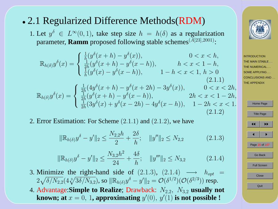
• 3.1 Numerical Comparisons: DRM vs. SDRM– We Start the Comparisons by TakingE10, E8, E14to test
DRM (with discrete schemec3) andSDRM (in the case ofLu & Wang);
– For short, we denote them asDRM-c3,SDRM-LW;
– The noisy perturbed-type is(3.0)− P1 for high frequency,(3.0)−P2 for random;
– Pay attention that these are the problems of reconstructing the sec-ond derivatives, which are more difficult than the problem of re-constructing the first derivatives;
– Combining the relevant rule of determining regularization parame-ter(DP,GCV,LC Q-opt), we may writeDRM −DP,DRM − LC,orDRM −OPT ); their meanings are self-evident.
INTRODUCTION
THE MAIN STABLE . . .
THE NUMERICAL . . .
SOME APPLYING . . .
CONCLUSIONS AND . . .
THE APPENDIX
Home Page
Title Page
JJ II
J I
Page 47 of 107
Go Back
Full Screen
Close
Quit
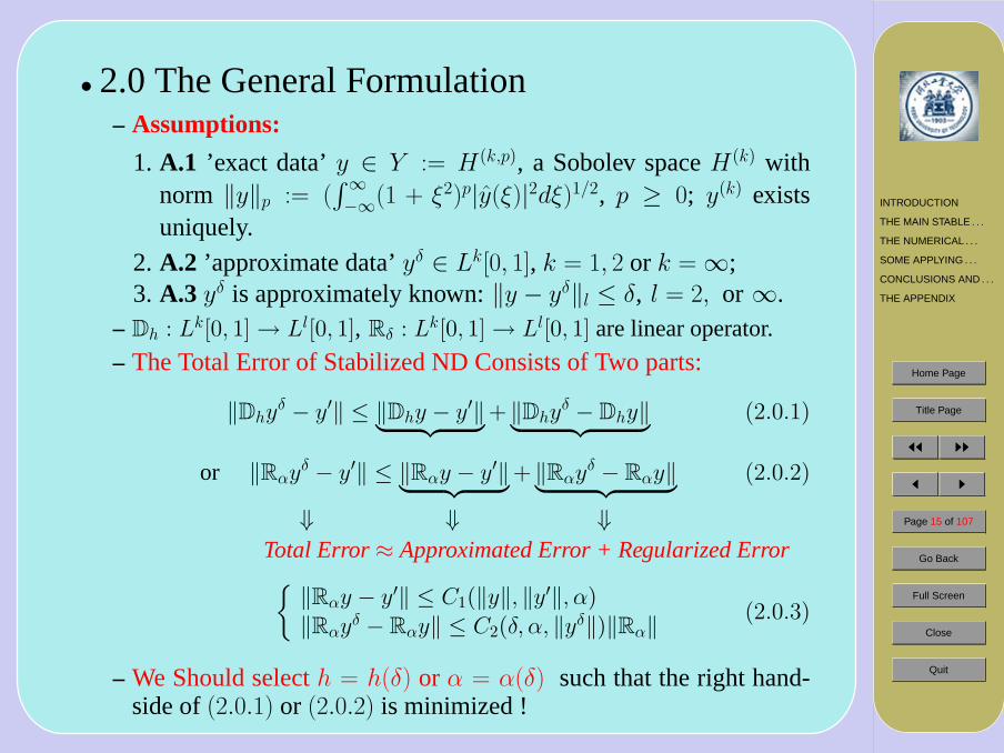
• 3.1 Numerical Comparisons:DRM vs.SDRMFigure 3-1-1: The DRM(DP) vs. SDRM for Computing Second
Derivatives of E10
Both of two methods work better when data level is small and SDRMis much better !!
INTRODUCTION
THE MAIN STABLE . . .
THE NUMERICAL . . .
SOME APPLYING . . .
CONCLUSIONS AND . . .
THE APPENDIX
Home Page
Title Page
JJ II
J I
Page 48 of 107
Go Back
Full Screen
Close
Quit
• 3.1 Numerical Comparisons:DRM vs.SDRMFigure 3-1-2: The DRM(DP) vs. SDRM for Computing Second
Derivatives of E10
INTRODUCTION
THE MAIN STABLE . . .
THE NUMERICAL . . .
SOME APPLYING . . .
CONCLUSIONS AND . . .
THE APPENDIX
Home Page
Title Page
JJ II
J I
Page 49 of 107
Go Back
Full Screen
Close
Quit
• 3.1 Numerical Comparisons:DRM vs.SDRMFigure 3-1-3: The DRM(DP) vs. SDRM for Computing Second
Derivatives of E10
Both of two methods do right job but DRM is more worse at the endsof the interval[−3, 3] !
INTRODUCTION
THE MAIN STABLE . . .
THE NUMERICAL . . .
SOME APPLYING . . .
CONCLUSIONS AND . . .
THE APPENDIX
Home Page
Title Page
JJ II
J I
Page 50 of 107
Go Back
Full Screen
Close
Quit
• 3.1 Numerical Comparisons:DRM vs.SDRMFigure 3-1-4: The DRM(DP) vs. SDRM for Computing Second
Derivatives of E8
For the oscillation function, both of two methods work well whenerror levelτ is very small !
INTRODUCTION
THE MAIN STABLE . . .
THE NUMERICAL . . .
SOME APPLYING . . .
CONCLUSIONS AND . . .
THE APPENDIX
Home Page
Title Page
JJ II
J I
Page 51 of 107
Go Back
Full Screen
Close
Quit
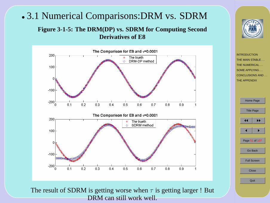
• 3.1 Numerical Comparisons:DRM vs. SDRMFigure 3-1-5: The DRM(DP) vs. SDRM for Computing Second
Derivatives of E8
The result of SDRM is getting worse whenτ is getting larger ! ButDRM can still work well.
INTRODUCTION
THE MAIN STABLE . . .
THE NUMERICAL . . .
SOME APPLYING . . .
CONCLUSIONS AND . . .
THE APPENDIX
Home Page
Title Page
JJ II
J I
Page 52 of 107
Go Back
Full Screen
Close
Quit
• 3.1 Numerical Comparisons:DRM vs. SDRMFigure 3-1-6: The DRM(DP) vs. SDRM for Computing Second
Derivatives of E8
The SDRM does not work whenτ = 0.001 ! So SDRM seems to benot suitable for the oscillation function !
INTRODUCTION
THE MAIN STABLE . . .
THE NUMERICAL . . .
SOME APPLYING . . .
CONCLUSIONS AND . . .
THE APPENDIX
Home Page
Title Page
JJ II
J I
Page 53 of 107
Go Back
Full Screen
Close
Quit
• 3.1 Numerical Comparisons:DRM vs.SDRMTable 3-1-1: The Performance Comparisons Between DRM & SDRM
• 3.1 Numerical Comparisons:DRM vs.SDRM– From Figure 3-1-1—3-1-6 and Table 3-1-1, we can see that
1. For the function being a polynomial, SDRM is the best one tocompute the approximated derivatives; but it shown a bad per-formance in the other cases;
2. DRM-DP can work robustly. Namely, it has wide adaptability;3. Sometimes, DRM-OPT works very well, for example, it is very
effective forE8 !
INTRODUCTION
THE MAIN STABLE . . .
THE NUMERICAL . . .
SOME APPLYING . . .
CONCLUSIONS AND . . .
THE APPENDIX
Home Page
Title Page
JJ II
J I
Page 55 of 107
Go Back
Full Screen
Close
Quit
• 3.2 Numerical Comparisons: MBR vs. DRM– We useE3, E4,E7to compare MBR with DRM
DRM (with discrete scheme (1.1)) andMBR (in the case ofMurio (1993)
– The noisy perturbed-type is(3.0)− P2 for random;
– We use the TSVD method to solve the disturbed equationAx = bδ.
INTRODUCTION
THE MAIN STABLE . . .
THE NUMERICAL . . .
SOME APPLYING . . .
CONCLUSIONS AND . . .
THE APPENDIX
Home Page
Title Page
JJ II
J I
Page 56 of 107
Go Back
Full Screen
Close
Quit
Figure 3-2-1: The MBR vs. DRM for Computing the first derivatives of E3
Here and in the following pages of this section,e denotes the relativeerror‖y′ − y′δ‖/‖y′‖. We can see that DRM does not work well when
δ = 0.05But in the next page we will show that the two method both work well
when theδ becomes small enough.
INTRODUCTION
THE MAIN STABLE . . .
THE NUMERICAL . . .
SOME APPLYING . . .
CONCLUSIONS AND . . .
THE APPENDIX
Home Page
Title Page
JJ II
J I
Page 57 of 107
Go Back
Full Screen
Close
Quit
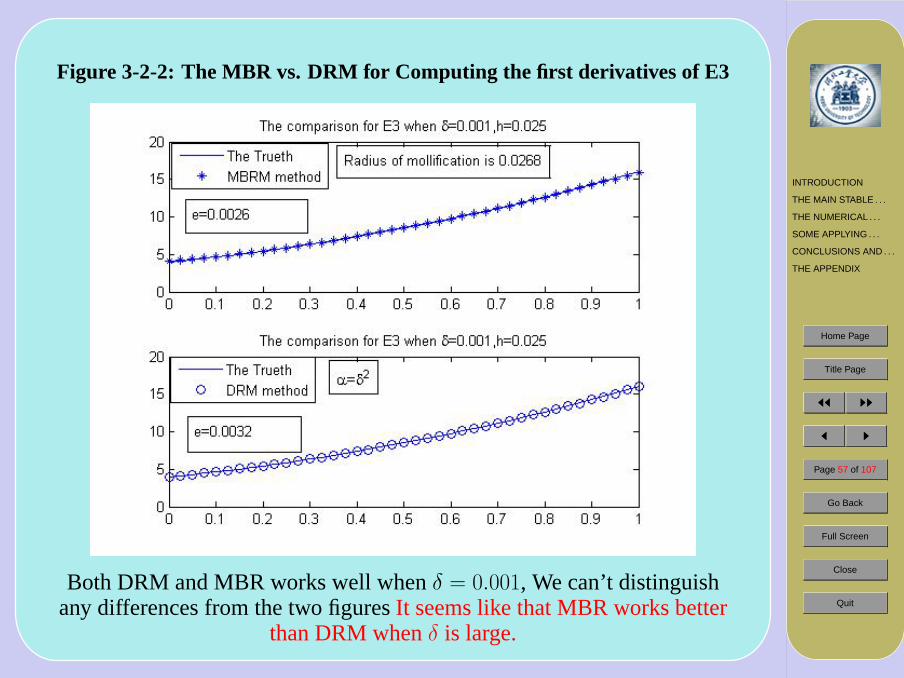
Figure 3-2-2: The MBR vs. DRM for Computing the first derivatives of E3
Both DRM and MBR works well whenδ = 0.001, We can’t distinguishany differences from the two figuresIt seems like that MBR works better
than DRM whenδ is large.
INTRODUCTION
THE MAIN STABLE . . .
THE NUMERICAL . . .
SOME APPLYING . . .
CONCLUSIONS AND . . .
THE APPENDIX
Home Page
Title Page
JJ II
J I
Page 58 of 107
Go Back
Full Screen
Close
Quit
Figure 3-2-3: The MBR vs. DRM for Computing the first derivatives of E4
We can see that DRM works badly when the steph is too small.It sounds that MBR is more accurately whenh is small, the next figure
further verifies this guess.
INTRODUCTION
THE MAIN STABLE . . .
THE NUMERICAL . . .
SOME APPLYING . . .
CONCLUSIONS AND . . .
THE APPENDIX
Home Page
Title Page
JJ II
J I
Page 59 of 107
Go Back
Full Screen
Close
Quit
Figure 3-2-4: The MBR vs. DRM for Computing the first derivatives of E4
From the above figure, we see that DRM works well again whenh is nottoo small But can we therefore say thath andδ have less impact in MBRthan in DRM ?? Please watch the next comprehensive comparison about
these two method with differenth andδ
INTRODUCTION
THE MAIN STABLE . . .
THE NUMERICAL . . .
SOME APPLYING . . .
CONCLUSIONS AND . . .
THE APPENDIX
Home Page
Title Page
JJ II
J I
Page 60 of 107
Go Back
Full Screen
Close
Quit
Figure 3-2-5: The MBR vs. DRM for Computing the first derivatives of E7
We find that when the noise levelδ is small, both MBR and DRM works well,but if δ is big, then how about the results?
INTRODUCTION
THE MAIN STABLE . . .
THE NUMERICAL . . .
SOME APPLYING . . .
CONCLUSIONS AND . . .
THE APPENDIX
Home Page
Title Page
JJ II
J I
Page 61 of 107
Go Back
Full Screen
Close
Quit
Figure 3-2-6: The MBR vs. DRM for Computing the first derivatives of E7
When the noise levelδ is big, e.g. 0.1, DRM can’t reconstruct satisfyingderivative, but the result of MBR is some how good compared to DRM.Moreover, we can see that aroundx = 0.5, MBR does not work as well.
INTRODUCTION
THE MAIN STABLE . . .
THE NUMERICAL . . .
SOME APPLYING . . .
CONCLUSIONS AND . . .
THE APPENDIX
Home Page
Title Page
JJ II
J I
Page 62 of 107
Go Back
Full Screen
Close
Quit
• 3.2 Numerical Comparisons: MBR vs. DRMFrom the above comparisons about MBR and DRM , we can obtainthe following Preliminary results:
– When the noise levelδ is relative large, MBR seems works betterthan DRM;
– However, whenδ becomes small, DRM may work better thanMBR;
– The above two conclusions are merely derived from the test of E3,E4 and E7; for other examples, we didn’t known whether the con-clusions are right or not; as a matter of fact,there may be no such amethod that is always suitable for all cases;
– Although MBR is not always superior to DRM, butMBR’s functionagainst the big noise is very attractive !.
INTRODUCTION
THE MAIN STABLE . . .
THE NUMERICAL . . .
SOME APPLYING . . .
CONCLUSIONS AND . . .
THE APPENDIX
Home Page
Title Page
JJ II
J I
Page 63 of 107
Go Back
Full Screen
Close
Quit
• 3.3 Numerical Comparisons: LRM vs. DRM– We Start the Comparisons by TakingE8 to test
LRM (see Liu etc.)DRM (see (1.2))
– The tested functions are:
– (1) y = sin(πx) + δsin(kπx), for high frequency distribution.
– (2)y = sin(kπx) + δrand(1, n), for random distribution.
– We also use the TSVD method to solve the disturbed equationAx = bδ.
INTRODUCTION
THE MAIN STABLE . . .
THE NUMERICAL . . .
SOME APPLYING . . .
CONCLUSIONS AND . . .
THE APPENDIX
Home Page
Title Page
JJ II
J I
Page 64 of 107
Go Back
Full Screen
Close
Quit
Figure 3-3-1: The LRM vs. DRM for Computing second Derivatives ofE8(function (1))
Here and in the following pages,e denotes the relative error‖y′′ − y′′δ‖/‖y′′‖. We can see that DRM works well
INTRODUCTION
THE MAIN STABLE . . .
THE NUMERICAL . . .
SOME APPLYING . . .
CONCLUSIONS AND . . .
THE APPENDIX
Home Page
Title Page
JJ II
J I
Page 65 of 107
Go Back
Full Screen
Close
Quit
Figure 3-3-2: The LRM vs. DRM for Computing second Derivatives of E8function (2)
Apparently,the computed solution of DRM stay closely to the truth,nevertheless the LRM doesn’t especially around the corners.
INTRODUCTION
THE MAIN STABLE . . .
THE NUMERICAL . . .
SOME APPLYING . . .
CONCLUSIONS AND . . .
THE APPENDIX
Home Page
Title Page
JJ II
J I
Page 66 of 107
Go Back
Full Screen
Close
Quit
Figure 3-3-3: The LRM vs. DRM for Computing second Derivatives of E8function (2)
We can see that the result of DRM is more accurately than that of LRM.
INTRODUCTION
THE MAIN STABLE . . .
THE NUMERICAL . . .
SOME APPLYING . . .
CONCLUSIONS AND . . .
THE APPENDIX
Home Page
Title Page
JJ II
J I
Page 67 of 107
Go Back
Full Screen
Close
Quit
Figure 3-3-4: The LRM vs. DRM for Computing second Derivatives of E8function (2)
It also shows that DRM works well.
INTRODUCTION
THE MAIN STABLE . . .
THE NUMERICAL . . .
SOME APPLYING . . .
CONCLUSIONS AND . . .
THE APPENDIX
Home Page
Title Page
JJ II
J I
Page 68 of 107
Go Back
Full Screen
Close
Quit
• 3.6 Numerical Comparisons: TVR vs. DRMFigure 3-6-1: The TVR vs. DRM-DP (Spline )for Non-Smooth
Function
Exceptx = 1/2, TVR inverses the derivatives very well even theτ israther large ! But DRM-DP does not work so well.
INTRODUCTION
THE MAIN STABLE . . .
THE NUMERICAL . . .
SOME APPLYING . . .
CONCLUSIONS AND . . .
THE APPENDIX
Home Page
Title Page
JJ II
J I
Page 69 of 107
Go Back
Full Screen
Close
Quit
• 3.6 Numerical Comparisons: TVR vs. DRM(cont.)
Figure 3-6-2: The TVR vs. DRM-DP (Midpoint)for NSF
The TVR works much well than the DRM-DP(midpoint)! For discretescheme of Tik-DP, the midpoint quadrature is worse than the spline
quadrature.
INTRODUCTION
THE MAIN STABLE . . .
THE NUMERICAL . . .
SOME APPLYING . . .
CONCLUSIONS AND . . .
THE APPENDIX
Home Page
Title Page
JJ II
J I
Page 70 of 107
Go Back
Full Screen
Close
Quit
• 3.6 Numerical Comparisons: TVR vs. DRM(cont.)
Figure 3-6-3: The TVR vs. DRM-DP(Spline )for Smooth Function
The result of DRM-DP is not as good as TVRwhenτ is a middle size of0.01 !
INTRODUCTION
THE MAIN STABLE . . .
THE NUMERICAL . . .
SOME APPLYING . . .
CONCLUSIONS AND . . .
THE APPENDIX
Home Page
Title Page
JJ II
J I
Page 71 of 107
Go Back
Full Screen
Close
Quit
• 3.6 Numerical Comparisons:TVR vs. DRM(cont.)
Figure 3-6-4: The TVR vs. DRM-DP (Midpoint )for Smooth Function
Whenτ = 0.001, the result of TVR is still better than DRM-DP’sresults.
INTRODUCTION
THE MAIN STABLE . . .
THE NUMERICAL . . .
SOME APPLYING . . .
CONCLUSIONS AND . . .
THE APPENDIX
Home Page
Title Page
JJ II
J I
Page 72 of 107
Go Back
Full Screen
Close
Quit
• 3.6 Numerical Comparisons: TVR vs. DRM(cont.)
Table 3-6-1: The Performance Comparisons Between DRM-DP &TVR for Smooth Functions
From Figure 3-6-1—3-6.4 and Table 3-6-1, we can see that
1. Even for the smooth problem, TVR can work well as DRM-DPdoes; and for the tested examples, the former is much better thanthe later. This seems to conform to the theoretical analysis;
2. The computational cost of TVR is double or three times of DRM.So we can suggest that if necessary the reconstruction of firstderivatives by using TVR is recommendable even for the smoothfunctions !
INTRODUCTION
THE MAIN STABLE . . .
THE NUMERICAL . . .
SOME APPLYING . . .
CONCLUSIONS AND . . .
THE APPENDIX
Home Page
Title Page
JJ II
J I
Page 73 of 107
Go Back
Full Screen
Close
Quit
4 SOME APPLYING EXAMPLESAs mentioned in§1, there are plenty of practical ap-plications of ND; we try to give some representativeexamples:1. Some Simple and Direct Applied Problem;
2. Some Inverse Problems in Heat Conduct equation;
3. The Parameter Estimation in New Product Diffusion Model;
4. The Identification of Sturm-Liouvill Operator;
5. The Numerical Inversion of Abel Transform;
6. The Linear Viscoelastic Stress-Strain Analysis.
The goal is to show in some details that1. How a Practical Problem Can Be Changed Directly to a ND-Problem;
2. How a ND-Process Can Be Embedded Into a Practical Problem as itsOne of the Sub-Problems.
INTRODUCTION
THE MAIN STABLE . . .
THE NUMERICAL . . .
SOME APPLYING . . .
CONCLUSIONS AND . . .
THE APPENDIX
Home Page
Title Page
JJ II
J I
Page 74 of 107
Go Back
Full Screen
Close
Quit
• 4.1 Some Simple and Direct Applied Problems– The Problem of Finding the Heat Capacitycp (A[26],2003) of a gas as
a function of temperatureT . Experimentally, one measured heatcontentqi := q(Ti), i = 1, 2, ...,m, while the heat capacitycp :=
cp(Ti) must obey the following physical relations:∫ T
T0
cp(τ )dτ = q(Ti), i = 1, 2, ...,m. (4.1.1)
Obviously, findingcp(Ti) from q(Ti) is a numerical differentialproblem.
– From the Recording of Courses in Navigation One Select the Di-rection of a Ship(A[26],2003) by the maximum of a certain univa-lent curve. This direction can be obtained by differentiation of thiscurve.
– Determine the Velocity and Accelerated Velocity of a Moving Bodyfrom the trip recorders at a finite number of observing points; thisis undoubtedly a first and second order-numerical differential prob-lem.
– In a Word, Things like This are too Numerous to Mention; they areclosely related to the calculation of ”change rate”, ”change rate ofthe change rate” by observations (noisy data).
INTRODUCTION
THE MAIN STABLE . . .
THE NUMERICAL . . .
SOME APPLYING . . .
CONCLUSIONS AND . . .
THE APPENDIX
Home Page
Title Page
JJ II
J I
Page 75 of 107
Go Back
Full Screen
Close
Quit
• 4.2 The Inverse Heat Conduct Problems(IHCP)– The Presentation of the Forward Problem
Consider a general type of heat conduction problem:
ut(x, t) = uxx(x, t) + f (x, t) x > 0, t ∈ (0, T ), [1]
u(x, 0) = g(x), x > 0, [2]
u(0, t) = ϕ(t), t ∈ (0, T ), [3]
ux(0, t) = ψ(t), t ∈ (0, T ), [4]
g(0) = ϕ(0) = 0, [5]
(4.2.1)
whereu(x, t), f (x, t) denote the temperature distribution, sourceterm respectively. Supposeϕ, ψ ∈ L2[0, T ], g ∈ L2[0,∞), andsupp g ∈ [0, L] is a compact set. The forward problem is:
Given the control equation (4.2.1)-[1], initial and boundary con-ditions (4.2.1)[2]-(4.2.1)-[5] (i.e.,f (x, t), g(x), ϕ(t), ψ(t) are as-sumed to be known), determine the temperature function ofu(x, t).The analytical formula ofu(x, t) exits whenf (x, t) has some spe-cific the structure. For example, iff (x, t) = f (t), we have
u(x, t) =∫ t
0 f (τ )dτ − 2∫ t
0 k(x, t− τ )ψ(τ )dτ+
+∫ +∞
0 g(ξ)[k(x− ξ, t) + k(x + ξ, t)]dξ(4.2.2)
whereK(x, t) = exp(−x2/4t)/√πt.
INTRODUCTION
THE MAIN STABLE . . .
THE NUMERICAL . . .
SOME APPLYING . . .
CONCLUSIONS AND . . .
THE APPENDIX
Home Page
Title Page
JJ II
J I
Page 76 of 107
Go Back
Full Screen
Close
Quit
• 4.2 The Inverse Heat Conduct Problems(IHCP)– The Formulation & Transform of the Source Identification
Inserting the conditions [2]-[5] into the expression (4.2.4) gives∫ t
0f(τ)dτ = ϕ(t)+
1√π
∫ t
0
ψ(τ)√t− τ
dτ− 1√π t
∫ +∞
0g(ξ) exp
(−ξ2/4t
)dξ
Define(Af )(t) :=∫ t
0 f (τ )dτ, t ∈ [0, T ], and write the r.h.s of theabove formula asF (t) ⇒ Af = F (t), t ∈ [0, T ] (4.2.5)this is a special problem ofIdentification of Source Term (IST), atypical ND of first order problem.This problem is solved by Wang & ZhengA[22],2000] employingTiVR and by Xiao et. al(A[57],2008) recently, employingLRM .
– Another Problem of IST f(x, t) = a(t)x and some other modifica-tions⇒ a parabolic equation of the form:
ut(x, t) = uxx(x, t) + a(t)x, x > 0, 0 < t < T, [1]u(x, 0) = 0, x < 0, [2]u(0, t) = f(t), f(0) = 0, 0 < t < T, [3]−ux(0, t) = g(t), g(t) > 0 0 < t < T, [4]
(4.2.6)
wheref (t), g(t) are assumed to be known and strictly increasingfunctions. We want to find unknown functionsu(x, t) anda(t) tosatisfy the above equationsof (4.2.6)[1]-(4.2.6)[4]. So this is aninverse problem.
INTRODUCTION
THE MAIN STABLE . . .
THE NUMERICAL . . .
SOME APPLYING . . .
CONCLUSIONS AND . . .
THE APPENDIX
Home Page
Title Page
JJ II
J I
Page 77 of 107
Go Back
Full Screen
Close
Quit
• 4.2 The Inverse Heat Conduct Problems(IHCP)– Another Problem of IST(cont.)
Assume that [1]-[4] has a solutionu(x, t), then it can be shown that
u(x, t) = 2
∫ t
0K(x, t− τ)g(τ) exp(θ(t)− θ(τ))dτ, (4.2.7)
hereK(x, t) = exp(−x2/4t) and θ(t) =∫ t
0 a(τ)dτ (4.2.8)
Let x → 0 in (4.2.8) and using boundary condition [3] we obtainan integral equation fory(t) := exp(−θ(t))∫ t
0
g(τ)√t− τ
y(τ)dτ =√πf(t)y(t) (4.2.9)
which is stably solvable fory(t) since (4.2.9) is aVolterra Equation ofthe second kind, a well-posed problem.
After y(t) is gotten,we meet the Numerical Differentiation again:∫ t
0
a(τ )dτ = − ln y(t) (4.2.10)
This problem is solved by Li & Zheng([6],1997).
– The Third Problem of IHCP: Determining the Conductivitya(t):
ut(x, t) = a(t)uxx(x, t), 0 < x < 1; 0 < t < T (4.2.11)
We would not go into details here. The interested readers can referto [6].
INTRODUCTION
THE MAIN STABLE . . .
THE NUMERICAL . . .
SOME APPLYING . . .
CONCLUSIONS AND . . .
THE APPENDIX
Home Page
Title Page
JJ II
J I
Page 78 of 107
Go Back
Full Screen
Close
Quit
• 4.3 The Parameter Estimation in New ProductDiffusion Model
– An Improved Diffusion Model of New ProductHow to describe the time-varying characteristics of the diffusion ofa new product(/technology) and to estimate the model parameters,have been a important content inManagement Science and Mar-keting Research. Among the numerous product-diffusion models,a representative one is anImproved Diffusion Model proposed byJones & Ritz:([7],1991) S ′(t) = [c+ b(S(t)− S0)](S
∗ − S(t)) b, c > 0 (4.3.1)R′(t) = a[pS(t)−R(t)], a, p > 0 (4.3.2)S(0) = S0, R(0) = 0 (4.3.3)
∗ S(t)....the cumulative number of retailers who have adopted the prod-uct at timet;
∗ S∗.....the maximum number of retailers who would adopt the product;∗ R(t)....the cumulative number of consumers who have adopted the
product at timet;∗ R∗.....the cumulative potential; and∗ S0.....the initial distribution level for the product.
The parameters,a, b, c, p in the model have to be estimated on thebasis of given datati, Si, Ri, i=1,2,...,m.
INTRODUCTION
THE MAIN STABLE . . .
THE NUMERICAL . . .
SOME APPLYING . . .
CONCLUSIONS AND . . .
THE APPENDIX
Home Page
Title Page
JJ II
J I
Page 79 of 107
Go Back
Full Screen
Close
Quit
• 4.3 The Parameter Estimation in New ProductDiffusion Model(cont.)
– The Exiting Methods for Estimating the Model ParametersDenoteSi = S(ti), Ri = R(ti). ξi, ηi are the approximations ofS ′(ti), R
′(ti) respectively, then we haveξi ≈ c(S∗ − Si) + b(Si − S0)(S
∗ General Difference Approximation+Least Square EstimateWithout loss of generality, consider the estimation ofc, b. LetξDi = ∆Si/∆ti = Si+1 − Si (∆ti = 1), based on
c(S∗ − Si) + b(Si − S0)(S∗ − Si) = ξD
i , i = 1, 2, ...,m− 1 (4.3.6)The linear least squares estimation ofc, b can be obtained; butas well-known, these estimates are not stable.
∗ Levenberg-Marquadrat Method based on Analytical Solution:Given the initial conditionS(0) = S0, S
∗ (a prior estimate bythe experts), eq.(4.3.1) can be explicitly solved:
S(t) = S0 + (S∗ − S0)1− exp(−ct)1 + b exp(−ct)
, b, c > 0 (4.3.7)
then parametersb, c can be obtained by LM-method being a reg-ularized strategy; but the limitation is obvious !
INTRODUCTION
THE MAIN STABLE . . .
THE NUMERICAL . . .
SOME APPLYING . . .
CONCLUSIONS AND . . .
THE APPENDIX
Home Page
Title Page
JJ II
J I
Page 80 of 107
Go Back
Full Screen
Close
Quit
• 4.3 The Parameter Estimation in New ProductDiffusion Model(cont.)
– An Improved Estimation Method Using Stabilized ND(Xu & Xiao)(A[33],2005)
Firstly, we get a stabilized approximationξRi , ηRi of ξi, ηi; then by
them we replaceξDi , ηDi in (4.3.6):
c(S∗ − Si) + b(Si − S0)(S∗ − Si) = ξR
i , i = 1, 2, ...,m− 1 (4.3.7)
resulting an over-determined linear equations. Finally we obtain aRegularized Least Squares Estimates (RLSE)by OLS.
We can also construct an implicit difference equations:
0.5∗c[(S∗−Si+(S∗−Si+1)]+b(Si−S0)(S∗−Si) = ξR
i , i = 2, 3, ...,m−1(4.3.8)
Repeat the above process, obtain a new regularized estimates ofb, c. For short, the estimates based on(4.3.7) and(4.3.8) are abbre-viated toRLSE-1, RLSE-2respectively.The Schemes RLSE-1 & RLSE-2 have been tested by a group ofsampled data from [4] and compared with OLS-method and LM-method. It demonstrates that RLSE-1, RLSE-2 are quite effective;we will show it in the next slide.
INTRODUCTION
THE MAIN STABLE . . .
THE NUMERICAL . . .
SOME APPLYING . . .
CONCLUSIONS AND . . .
THE APPENDIX
Home Page
Title Page
JJ II
J I
Page 81 of 107
Go Back
Full Screen
Close
Quit
• 4.3 The Parameter Estimation in New ProductDiffusion Model(cont.)
Table 4.3.2 The Fitted Errors by Several MethodsThe Fitted Error RLSE-1 RLSE-2 LM-method OLS-method
‖Sh − Shf‖2 3.0182 2.5018 3.4431 4.6384
‖Sh − Shf‖2/‖Sh‖2 0.1427 0.1183 0.1628 0.2194
INTRODUCTION
THE MAIN STABLE . . .
THE NUMERICAL . . .
SOME APPLYING . . .
CONCLUSIONS AND . . .
THE APPENDIX
Home Page
Title Page
JJ II
J I
Page 82 of 107
Go Back
Full Screen
Close
Quit
• 4.4 Parameter Identification of Sturm-LiouvilleOperator
– Formulation of the Operator identificationThe distribution parameter identification of Sturm-Liouville oper-ator is an important applied filed in inverse problems,which seeksk(x) or k(u(x)) in the following operator equations:
L(k) := ddx(k(x) d
dxu(x)) = f(x), (linear case)k(0) d
dxu(0) = c = const.(4.4.1)
L(k) := d
dx(k(u(x)) ddxu(x)) = f(x), (non-linear case)
k(u(0)) ddxu(0) = c = const.
(4.4.2)
from a set of discrete solutions:u(xi) and relevant boundary con-ditions. We further suppose thatu(x) ∈ C1[0, 1], f (x) ∈ C[0, 1]and constantc are known.
If there exists a compact setK ⊂ I = [0, 1] such thatinfK|dudx| >0, then it can be proven that the inversion formulas([3],1993)
L−1 = k(x) = (∫ x
0 f(t)dt+ c)/(dudx), (linear case) (4.4.3)
L−1 = k(u(x)) = (∫ x
0 f(t)dt+ c)/(dudx), (non-linear case) (4.4.4)
hold. This is grounded to the identification ofk(x), k(u(x)).
INTRODUCTION
THE MAIN STABLE . . .
THE NUMERICAL . . .
SOME APPLYING . . .
CONCLUSIONS AND . . .
THE APPENDIX
Home Page
Title Page
JJ II
J I
Page 83 of 107
Go Back
Full Screen
Close
Quit
• 4.4 Parameter Identification of Sturm-LiouvilleOperator(cont.)
– The Numerical Identifying SchemesEven the inversion formulas are known, there exist two main diffi-culties to estimatek(x) or k(u(x)):1. u(x) is approximately known asuδ : ‖u − uδ‖ ≤ δ anduδ(xi)mi=1 is merely a finite-subset ofuδ(x), infinite set;
2. It involves an unstable numerical differentiation processto thenoisy data ofuδ(xi)mi=1.
So the combination of a stable numerical differentiation process bya DRM anda numerical integration might be aConservative Strategy.In paper A[32] a stabilized identifying scheme is proposed:1. Employing DRM-c3-DP(A[32],2005) to obtain the stable approxi-
mation :yhα(δ) = (yhα(δ),1, ..., y
hα(δ),m)T of d
dxuδ(xi)mi=1 ;
2. Employing adaptive Newton-Cotes formula to computeF (xi) =
∫ xi
0 f (t)dt := Fh(xi) + ei, i = 1, 2, ...,m;3. Constructing the approximation ofk(xi), i = 1, 2...,m by
kF,hα(δ)(xi) :=
F (xi) + c
yhα(δ),i
≈ kFh,hα(δ) (xi) :=
Fh(xi) + c
yhα(δ),i
(4.4.5)
INTRODUCTION
THE MAIN STABLE . . .
THE NUMERICAL . . .
SOME APPLYING . . .
CONCLUSIONS AND . . .
THE APPENDIX
Home Page
Title Page
JJ II
J I
Page 84 of 107
Go Back
Full Screen
Close
Quit
• 4.4 Parameter Identification of Sturm-LiouvilleOperator(cont.)
– The Error Estimates and Numerical ExperimentBased on the above discussions and interpolation theory A[32]Proved the following theorem:∗ Theorem Assume u(x) ∈ C2[0, 1], y(x) = u′(x), uδ ∈C[0, 1]; 0 < λ ≤ min‖y(x)‖, ‖yhα(δ)‖ ≤ C1, then when‖uh − uhδ‖ ≤ δ < ‖uhδ‖, ‖u(x)− uδ(x)‖ ≤ δ < ‖uδ‖, we have
‖k(x)− kFh,hα(δ) (x)‖ ≤ c1
√δ + c2
√α(δ) + c3h (4.4.6)
herec1, c2, c3 are constants.∗ Two Testing Examples:
From the above table we can see that1. Both of two schemes work well and they are all numerically sta-
ble;2. For theExample-1and sameδ, the scheme we described (a kind
of DRM) is better than WBM;3. For theExample-2and sameδ, the scheme we described (a kind
of DRM) is worse than WBM.
INTRODUCTION
THE MAIN STABLE . . .
THE NUMERICAL . . .
SOME APPLYING . . .
CONCLUSIONS AND . . .
THE APPENDIX
Home Page
Title Page
JJ II
J I
Page 86 of 107
Go Back
Full Screen
Close
Quit
• 4.5 The Numerical Inversion of Abel Transform– The Abel Transform with the inversion Formula
Abel transform has many applications in various filed. A typicalAT is of the form:
(Tε)(x) := 2
∫ R
x
ε(r)rdr√r2 − x2
= y(x), x ∈ [0, R], y(R) = 0 (4.5.1)
wherey(x) ∈ H1(0, R), ε(r) ∈ C[0, R] is to be determined. Undercertain conditions the theoretical inversion formula is given by
T−1y = ε(r) =1
π
∫ R
r
y′(x)dx√x2 − r2
, r ∈ [0, R] (4.5.2)
Be cause(4.5.1) has weakly singular kernel and as the approxima-tion of y(x), yδ(x) ∈ L2[0, R], hence the solving process of(4.5.1)or (4.5.2) is ill-posed, and some regularization techniques must beemployed to get its stable numerical solution.Many efforts have been devoted to this end in which two kinds ofmethods are employed:1. The method which directly solve the first kind of Abel equation
(4.5.1) by one of some regularization methods;2. The method which firstly deals with the numerical differentia-
tion by stable numerical technique then computes the integral of(4.5.2) by some quadrature techniques.
INTRODUCTION
THE MAIN STABLE . . .
THE NUMERICAL . . .
SOME APPLYING . . .
CONCLUSIONS AND . . .
THE APPENDIX
Home Page
Title Page
JJ II
J I
Page 87 of 107
Go Back
Full Screen
Close
Quit
• 4.5 The Numerical Inversion of Abel Transform– A Numerical Inversion Scheme Based on Stabilized ND
Xiao et.al (A[21],2000) presented a numerical inversion scheme tosolve(4.5.2) which includes following steps:Step 1 Inputyhδ = (yδ,0, yδ,1..., yδ,n)
T , δ and control constantε > 0;
Step 2Find ddxy
hδ = (y
′δ,0, y
′δ,1, ..., y
′δ,n)
T by using DRM-c3-DP⇒
Step 3 Construct the Hermite Interpolationyhδ (x)(formally);
The above Table says that the DRM-c3-DP is much better than themethod by Pu Xiaoyun and both of them are of about the sameability when error level is small (δ = 0.1%).Remark 1 When y′(x) is not smooth the DRM-c3 method willwork at a discount greatly. Cheng JunA[],2006 presented an effec-tive method based on SDRM which can solve more general-type ofAbel equation.Remark 2 Obviously, if substituting TVR scheme in theStep 2ofabove scheme to deal with ND,we will also get an effective way tosolve Abel equation under the non-smooth case.
INTRODUCTION
THE MAIN STABLE . . .
THE NUMERICAL . . .
SOME APPLYING . . .
CONCLUSIONS AND . . .
THE APPENDIX
Home Page
Title Page
JJ II
J I
Page 90 of 107
Go Back
Full Screen
Close
Quit
• 4.6 The Linear Viscoelastic Stress Analysis– The Background and Presentation of the Problem
Visco-elasticity is the property of material that exhibit both viscousand elastic characteristics when undergoing deformation. In orderto construct a mathematical model for material, the material param-eters have to be determined.Moreover, after the material parameters are obtained we can anal-ysis the stress from the experimental data of the strain, or from thestress to compute the strain.For linear viscoelastic material the above mechanical qualities arelinked together in a so-calledConstitutive Equation:(A[53],2007)
σ(t) =
∫ t
0G(t− τ)ε(τ)dτ (4.6.1)
whereσ is the stress,t is time,ε is the strain andG(t) is the relax-ation modulus. Alternatively theε(t) can be written as
ε(t) =
∫ t
0J(t− τ)σ(τ)dτ (4.6.2)
whereJ(t) is the creep compliance.
INTRODUCTION
THE MAIN STABLE . . .
THE NUMERICAL . . .
SOME APPLYING . . .
CONCLUSIONS AND . . .
THE APPENDIX
Home Page
Title Page
JJ II
J I
Page 91 of 107
Go Back
Full Screen
Close
Quit
• 4.6 The Linear Viscoelastic Stress Analysis– The Strategies to Perform the Stress-Strain Analysis
Another Important Mechanical Basis is: for a typical linear vis-coelastic experiment, only eitherG(t) or J(t) can be determineddirectly. After such an experiment, the unknown linear viscoelasticmaterial can be determined with anInter-conversion Method.Actually, by performing LT to (4.6.1-2) & then the ILT we have
t =
∫ t
0G(t− τ)J(τ)dτ =
∫ t
0G(τ)J(t− τ)dτ (4.6.3)
After G(t) or J(t) is known experimentally, the other one can beobtained by solving the above convolution equation andthis can bedone by Tikhonov Regularization(A[53],2007).Formally, there existTwo Regularization Strategiesfor the stress-strain analysis: the method with ND and the method without ND:
5 CONCLUSIONS AND SUGGESTIONSFrom the above discussions and numerical experi-ments on the tested examples we can conclude that• If yδ ∈ L2[0, 1], y(x) is smooth and the suitableα value is determined
– The asymptotic convergence order of most of the regularizedND-schemes isO(δ1/2) for first-ND andO(δ1/3) for second-ND;FBR,MBR, and SDRM are even higher;
– So most of the schemes usually work well when the error levelδ isor below the middle size, for exampleδ ≤ 0.01;
– When error levelδ is rather large,δ ∈ [0.05, 0.1], MBR and SDRMcan work well but LRM, DRM sometimes do not work well or evendo not work;
– Under some of the same error level (even it is small), RDM, DRMand MBR can work well for oscillation functions but LRM, SDRMcan not;
– SDRM,MBR, FBR and WBR are suitable for both first and second-ND;but the other scheme is only suitable for some one of them;
– In a word,there may be no such a scheme that is always suitablefor all cases.
• If yδ, y ∈ BV [0, 1], TVR works well but the others can not. Even forthe smooth case TVR can works mostly better than the others.
INTRODUCTION
THE MAIN STABLE . . .
THE NUMERICAL . . .
SOME APPLYING . . .
CONCLUSIONS AND . . .
THE APPENDIX
Home Page
Title Page
JJ II
J I
Page 93 of 107
Go Back
Full Screen
Close
Quit
Roughly speaking, there are still some problems tobe explored and solved:• Many effective schemes for ND are less effective at the two sides of
the interval;
• Some schemes are moderately well at the sides but they usuallyrequire small-error level;
• The choice rule ofα for TVR is not well settled; at same time, theselection ofα = δ2 for SDRM may need and can be to improve.For the former, there are some work undergoing[1,2] and for thelater ETR might be a strong candidate(A[69,70],2010);
• For fixed δ and steph, how choose an appreciate scheme ? Sinceα = α(δ, h) actually, a reasonable collocation or design of the sam-pling points is needed for this purpose.
• After all, the differences among the above analysis and practi-cal applications may have potential impact on the choice of theschemes. A reasonable selection depends on the knowledge aboutthe theoretical bases of the methods and thephysical background of the practical problems;we should pay attention to both of them !
INTRODUCTION
THE MAIN STABLE . . .
THE NUMERICAL . . .
SOME APPLYING . . .
CONCLUSIONS AND . . .
THE APPENDIX
Home Page
Title Page
JJ II
J I
Page 94 of 107
Go Back
Full Screen
Close
Quit
• 5 Conclutions and Suggestions(cont.)
Table 5-1: The Improvement of the Regu. Solution by ETR forE13,E14
The Bibliography About StabilizedNumerical Differentiation
[1] T. F. Dolgopolova and V. K. Ivanov., Numerical Differentiation, Comp.Math. and Math. Physics, 6(3)(1966): 570-576.
[2] A. G. Ramm., On Numerical Differentiation, Mathem, Izvestija vuzov, 11(1968):131-135 (in Russian).
[3] V. V. Vasin., Regularization of Numerical Differentiation Problem, Mathem.Zap. Uralskii Univ., 7(2)(1969):29-33(in Russian).
[4] T. F. Dolgopolova., Finite Dimensional Regularization in the Case of Nu-merical Differentiation of Periodic Functions., Ural. Gos. Univ.Mat. Zap.7(4)(1970):27-33.
[6] A. G. Ramm., Simplified Optimal Differentiators, Radiotech. I. Electron.,17 (1972):1325-1328.
INTRODUCTION
THE MAIN STABLE . . .
THE NUMERICAL . . .
SOME APPLYING . . .
CONCLUSIONS AND . . .
THE APPENDIX
Home Page
Title Page
JJ II
J I
Page 97 of 107
Go Back
Full Screen
Close
Quit
[7] V.V. Vasin., The Stable Evaluation of a Derivative in the space C(−∞, ∞ ) ,USSR Computational Mathematics& Mathematical Physics,Vol. 13 (1973):16-24.
[8] R.S., Anderssen and P. Bloomfied, Numerical Differentiation Proceduresfor Non-exact Data, Numerisch Mathematik, Vol. 22(1974): 157-182.
[9] A.N. Tikhonov and V.Y. Arsenin, Solutions of Ill-Posed Problems, JohnWiley and Sons, New York,1977.
[10] A. G. Ramm., Estimates of the Derivatives of Random Functions, J. Math.Anal.,102(1984): 244-250.
[11] J. T. King and D. A. Murio., Numerical Differentiation by Finite-Dimensional Regularization., IMA Journal of Numerical Analysis, Vol. 6(1986): 65-85.
[12] D. Terzopoulos, Regularization of Inverse Visual Involving Disconti-nuities, IEEE Transaction on Pattern Analysis& Machine Intelligence, Vol.PAMI-8(4)(1986):413-424.
[13] Yu. V. Egorov and V. A. Kondat’ev., On a Problem of Numerical Differen-tiation, Vestnik Moskov, Uni. Ser. I mat. Mekh. 3(1989):
INTRODUCTION
THE MAIN STABLE . . .
THE NUMERICAL . . .
SOME APPLYING . . .
CONCLUSIONS AND . . .
THE APPENDIX
Home Page
Title Page
JJ II
J I
Page 98 of 107
Go Back
Full Screen
Close
Quit
[14] A.M. Taratorin, S. Sideman, Constrained Regularized Differentia-tion, IEEE Transactions on Pattern Analysis and Machine Intelligence,16(1)(1994):88-92.
[15] I. Knowles and R. Wallace, A Variational Method for Numerical Differen-tiation, Num. Math. 70(1995): 91-110.
[16] R.Qu., A New Approach to Numerical Differentiation and Regularization,Math. Comp. Modeling, 24(1996):55-68.
[18] D.A. Murio et al., Discrete Mollification and Automatic Numerical Differ-entiation, Computers. Math. Appl.§35(4)(1998):1-16.
[19] H.Q. Yang and Y.S. Li, The Stable Approximation Method of Approxi-mately Specified Functions (in Chinese), Progress in Natural Science,10£12¤£2000¤µ1088-1093.
[20] S. Diop, J. W. Grizzle and F. Chaplais, On Numerical DifferentiationAlgorithms for Nonlinear Estimation, the Proceedings of the IEEE Conferenceon Decision and Control, Sydney, Australia ,2000.
INTRODUCTION
THE MAIN STABLE . . .
THE NUMERICAL . . .
SOME APPLYING . . .
CONCLUSIONS AND . . .
THE APPENDIX
Home Page
Title Page
JJ II
J I
Page 99 of 107
Go Back
Full Screen
Close
Quit
[21] T.Y. Xiao & J. L. Song, A Discrete Regularization Method for the Numer-ical Inversion of Abel Transform, Chinese Journal of Computational Physics,17(6)(2000):602-610.
[22] P. Wang and K. W. Zheng, Determination of Conductivity in Heat Equa-tion, Internat J. Math.& Math. Sci., 24(9)(2000): 589-594.
[23] A. G. Ramm and A. B. Smirnova., On Stable Numerical Differentiation,Mathematics of Computation, 70(2001):1131-1153.
[24] M. Hanke and O. Scherzer., Inverse Problems Light: Numerical Differen-tiation, Amer. Math. Monthly. 6 (2001): 512-522.
[25] Y.B.Wang, X.Z. Jia and J. Cheng., A Numerical Differentiation Methodand its Application to Reconstruction of discontinuity, Inverse Problems,18(2002):1461-1476.
[26] A. G. Ramm and A. Smirnova, Stable Numerical Differentiation: When isPossible ?,J. KSIAM,7(1)(2003):47-61.
[27] X.Z. Jia, et al., The Numerical Differentiation of Scattered Data and ItsError Estimate(in Chinese), Numerical Mathematics, A Journal of ChineseUniversities,25£1¤£2003¤µ81-90.
INTRODUCTION
THE MAIN STABLE . . .
THE NUMERICAL . . .
SOME APPLYING . . .
CONCLUSIONS AND . . .
THE APPENDIX
Home Page
Title Page
JJ II
J I
Page 100 of 107
Go Back
Full Screen
Close
Quit
[28] S. LU and Y.B. Wang, The Numerical Differentiation of First and SecondOrder with Tikhonov Regularization (in Chinese), Numerical Mathematics, AJournal of Chinese Universities,§26(1)(2004):62-74.
[29] S. Lu and Y.B. Wang., First and Second Order Numerical Differentiationwith Tikhonov Regularization, Selected Publications of Chinese Universities:Mathematics Vol. 1(2004):106-116.
[30] S. IBRIR and S. DOIP, A Numerical Procedure for Filtering and Effi-cient High Order Signal Differentiation, Int. J. Appl. Math. Comput. Sci.,4(2)(2004):201-208.
[31] G.F. Yang, et al., Numerical Differentiation of Periodic Functions andIts Applications§Journal of Fudan University£Natural Science¤(in Chi-nese)§43£3¤£2004¤µ315-322.
[32]Z.F. Cheng and T.Y. Xiao, Discrete Regularization method for ParameterIdentification of Sturm-Liouville Operator (in Chinese), Numerical Mathemat-ics, a Journal of Chinese Universities§27(2005): 324-328.
[33] W. Xu and T.Y. Xiao, A Stable Algorithm for the Parameter Estimationof a New Product Diffusion Model( in Chinese), Numerical Mathematics, aJournal of Chinese Universities§27(2005):350-353.
INTRODUCTION
THE MAIN STABLE . . .
THE NUMERICAL . . .
SOME APPLYING . . .
CONCLUSIONS AND . . .
THE APPENDIX
Home Page
Title Page
JJ II
J I
Page 101 of 107
Go Back
Full Screen
Close
Quit
[34] X.J. Luo and C.N. He, A Stable High Accuracy Approximate Differ-entiation of Approximately Specified Functions, Numerical Computing andComputer Applications§26(4)£2005¤µ269-277.(in Chinese)
[35] G.S. Li and X. P. Fan, An Optimal Regularization Algorithm Based onSingular Value Decomposition, Journal of Information and ComputationalScience, 2(4)(2005):705-714.
[36] T.Wei and Y.C. Hon., Numerical Derivatives from One-Dimensional Scat-tered Data, Journal of Physics: Conference Series 12(2005):171-179.
[37] Y. B. Wang and T. Wei, numerical differentiation for two dimensionalscattered data, J. Math. Anal. Appl., 312(2005):121-137.
[38] T. Wei, Y. C. Hon and Y. B. Wang, Reconstruction of Numerical Deriva-tives from Scattered Noisy Data, Inverse Problems, 21(2005):657-672.
[39] A. G. Ramm, Inequality for the Derivatives and Stable Differentiationof Piecewise-Smooth Discontinuous Functions, Mathematical Inequality andApplications, 8(1)(2005):169-172.
INTRODUCTION
THE MAIN STABLE . . .
THE NUMERICAL . . .
SOME APPLYING . . .
CONCLUSIONS AND . . .
THE APPENDIX
Home Page
Title Page
JJ II
J I
Page 102 of 107
Go Back
Full Screen
Close
Quit
[40] R. Chartrand, Numerical Differentiation of noisy, non-smooth dada,(2005),Los. Alamos National. Laboratory, 2005.
[41] Y.B. Wang, Numerical Differentiation and Its Applications, PhD Thesis ofFudanUniversity,2005..
[42] Y.B Wang, Y.C. Hon, and J. Cheng, Reconstruction of High Order Deriva-tives from Input Data, Journal of Inverse and Ill-posed Problems, 14(2)(2006):205-218.
[43] S. Ahn, U. J. Choi and A. G. Ramm, A Scheme for Stable NumericalDifferentiation, J.Comp.Appl.Math., 186(2)(2006):325-334.
[44] X.Q. Wan and Y.B. Wang§A Local Property of Regularized Solutions forNumerical Differentiation (in Chinese)§Journal of Fudan University£NaturalScience¤§45£2¤£2006¤µ185-190.
[45] Y.Z. Ye and L. Yi, Recovering the Local Volatility of Underlying Assets(in Chinese)§Appl. Math. J. Chinese Univ. Ser A,21£1¤£2006¤µ1-8.
[46] S. Lu and S. V. Pereverzev, Numerical Differentiation: From a Viewpointof Regularization Theory, Mathematics of Computation, 75(256)(2006):1853-1870.
INTRODUCTION
THE MAIN STABLE . . .
THE NUMERICAL . . .
SOME APPLYING . . .
CONCLUSIONS AND . . .
THE APPENDIX
Home Page
Title Page
JJ II
J I
Page 103 of 107
Go Back
Full Screen
Close
Quit
[47] A. G. Ramm, Finding Discontinuities of Piecewise-Smooth Functions,Journal of Inequality in Pure and Applied Mathematics, 7(2)(2006):1-7.
[48] Z. Qian, C.L. Fu and X.L. Feng., A Modified Method for High Or-der Numerical Differentiation, Applied Mathematics and Computation 182(2006):1191-1200.
[49] T. Wei and Y. C. Hon, Numerical differentiation by radial basis functionsapproximation, Advances in Computational Mathematics, 27(3)(2007): 247-272.
[50] K. Ahnert and M. Abel, Numerical Differentiation of ExperimentalData: Local Versus Global Methods, Computer Physics Communications,177(2007):764-774.
[51] H. Zhang§A MATLAB Package for One Dimensional Numerical Differ-entiation,§MA Thesis of Hebei University of Technology£2007¤.
[52] Z.Y. Zhao, CTSVD Method and Numerical Differentiation§PhD Thesisof Shanghai University (2007¤.
INTRODUCTION
THE MAIN STABLE . . .
THE NUMERICAL . . .
SOME APPLYING . . .
CONCLUSIONS AND . . .
THE APPENDIX
Home Page
Title Page
JJ II
J I
Page 104 of 107
Go Back
Full Screen
Close
Quit
[53]J. Sovari& M. Malinen, Numerical Inter-conversion Between Linear Vis-coelastic Material Functions with Regularization, International Journal of Solidand Structures, 44(3-4)(2007):1291-1303.[54]X.W. Huang, et al., An Integral Method for the Numerical Differentiationof High Order, Journal of Mathematics£in Chinese¤, 28(4)(2008): 431-434.
[55]Z.Y. Zhao and G.Q. He, Reconstruction of High Order Derivatives Us-ing Mollification Method (in Chinese), Applied Mathematics and Mechanics,29(6)(2008):696-704.
[56] G. Nakamura, S. Z. Wang and Y. B. Wang, Numerical Differentiation forthe Second Order Derivatives of Functions of Two Variables, J. Comp. Appl.Math.,212(2)(2008): 341-358.
[57] T.Y. Xiao and J.L. Zhang, A Stable and Fast Algorithm for Identifyingthe Source Term in Heat Conduct Problem (in Chinese)§Chinese Journal ofComputational Physics, 25(3)(2008): 335-343 .
INTRODUCTION
THE MAIN STABLE . . .
THE NUMERICAL . . .
SOME APPLYING . . .
CONCLUSIONS AND . . .
THE APPENDIX
Home Page
Title Page
JJ II
J I
Page 105 of 107
Go Back
Full Screen
Close
Quit
[58] Q.F. Cai, et al., A New Method for Calculating Vorticity, Acta Phys. Sin.57£6¤£2008¤µ3912-3919.
[59] Yu Chen , Jianguo Huang and Weimin Han, Function reconstruction fromnoisy local averages, Inverse Problems, 24(2)(2008).
[60] M.X. Wang, T.Y. Xiao and K.F. Xiao, A New Algorithm for Identifyingthe Parameters In Grey Dynamic Model (in Chinese), Journal of Highway andTransportation Research and Development, 5(5)(2009): 222-225 .
[61] E. I. Sakalauskas, Galerkin-Tikhonov regularization in the numericaldifferentiation problem, Curent Applied Physics, 9(6)(2009): 1463-1466.
[62] X.H. Lu and C.S. Wu, A Numerical Differentiation Method Based on In-tegral Equation (in Chinese), Journal of Mathematics§29£4¤(2009¤:477-482.
[63] W.Y. Choi, A new method for stable numerical differentiation, CurrentApplied Physics,9(6)(2009):1431-1466.
[64] Z. Y. Zhao at al., A New Mollification Method for Numerical Differentia-tion of 2D Periodic Functions, International Joint Conference on ComputationalSciences and Optimization, vol.1(2009):205-207.
INTRODUCTION
THE MAIN STABLE . . .
THE NUMERICAL . . .
SOME APPLYING . . .
CONCLUSIONS AND . . .
THE APPENDIX
Home Page
Title Page
JJ II
J I
Page 106 of 107
Go Back
Full Screen
Close
Quit
[65] Huilin Xu and Jijun Liu, Stable numerical differentiation for the secondorder Derivatives, Advances In Computational Mathematics (2009), 1019-7168(Print) 1572-9044.
[66] J. J. Stickel, Data smoothing and numerical differentiation by a regulariza-tion method, Computers and Chemical Engineering, 34(2010):467-475.
[67] F. F. Dou, C. L. Fu and Y. J. Ma, A wavelet-Galerkin method forhigh order numerical differentiation, Applied Mathematics and Computation,215(10)(2010):3702-3712.
[68] C.L. Fu, X.L.Feng and Z.Qian., Wavelets and high Order NumericalDifferentiation, Applied Mathematical Modeling£in press¤(2010).
[69] H. Zhang and Q.Yan, Some Improvements on the Algorithms of SecondOrder Numerical Differentiation with the Comparison Study (in Chinese),Journal of Hebei University of Technology, (2010) (accepted).
[70] G.Z. Su, et al., The Extrapolated Tikhonov Regularization Schemes forNumerical Differentiation (in Chinese), (2010) (submitted)