15
© Manfred Huber 2015 1 Machine Learning Regularization, Sparsity, and Learning Complexity

© Manfred Huber 2015 1
Machine Learning
Regularization, Sparsity, and Learning Complexity

© Manfred Huber 2015 2
Regularization n Bias vs. Variance tradeoff arises in all learning
n Simpler hypothesis classes will result usually in higher bias
n They can not represent the data precisely
n More complex hypothesis classes will result usually in higher variance
n Complex models lead to overfitting to the training set
n Without knowledge of correct hypothesis class for problem and data, regularization is usually used to “disincentivize” complex solutions

© Manfred Huber 2015 3
Regularization n Regularization adds a term to performance
function that punishes complex hypotheses n Complexity can be represented in terms of
multiple functions of the parameters n Size of the parameters: usually as norm n Number of parameters used: ideally as but
often as norm n Total error: usually as norm n Frequency of use of a parameter: usually as KL
divergence (mutual information)
!2!0
!1!1

© Manfred Huber 2015 4
Regularization n Regularization introduces a tradeoff problem
between performance function and regularization term
n Determining the correct tradeoff C is part of a model selection problem for learning algorithm
n Choice affects the learning results and depends on the quality requirements
n E.g. in SVMs this is often solved using a grid search n Search over possible parameters until the best tradeoff is found
n Learning with regularization might require different optimization technique
E = Performance!+!C *Regularization

© Manfred Huber 2015 5
Regularization n Use of regularization terms allows use of
most traditional optimization approaches n Use of regularization does not allow
traditional optimization n is a step function and not differentiable
n No gradient ascent/descent, no closed loop solution n Usually requires search methods (mostly combinatorial)
making it intractable
n Use of regularization is complex n is not continuously differentiable
n Can use line search techniques
!2
!0
!1!1
!0

© Manfred Huber 2015 6
Sparsity n Sparsity as a measure of complexity can
achieve additional properties n Sparsity in terms of using few features to
represent a data point can be seen as increasing the likelihood of causality in feature learning
n Sparse coders
n Sparsity in terms of frequency of parameter use can be can be used to yield representative features in neural networks
n Sparse autoencoder networks
Ek,!,u,D = x(i) ! ! j (x(i) )ujj=1
k"
2+C *S(!(x(i) ))#
$%
&'(
i"

© Manfred Huber 2015 7
Sparsity n would be the most obvious sparsity term
n Optimization generally intractable
n Under certain circumstances regularization can yield the same solution at a lower cost n E.g. for a performance function and a good
choice of C yields sparsity n Can perform optimization using sign search
n Perform line search along gradient within the boundaries where parameters do not change sign ( has derivative)
n Check neighboring segments for gradient away from boundary
!0
!1
!2!1
!1

© Manfred Huber 2015 8
Sparsity n Including regularization / sparsity into feature
learning facilitates overcomplete basis n Learning of linearly dependent basis vectors
© Manfred Huber 2015 9
Learning Complexity n Learning complexity hasmultiple factors
n Computational complexity of the learning algorithm to learn from D
n Sample complexity indicating the required amount of data to learn
n Sample complexity determines how much data is needed to learn the best hypothesis n Size of hypothesis space changes sample
complexity n Simpler hypothesis spaces have lower sample complexity
© Manfred Huber 2015 10
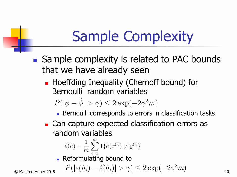
Sample Complexity n Sample complexity is related to PAC bounds
that we have already seen n Hoeffding Inequality (Chernoff bound) for
Bernoulli random variables
n Bernoulli corresponds to errors in classification tasks
n Can capture expected classification errors as random variables
n Reformulating bound to
3
generalization error that we care about, but most learning algorithms fit theirmodels to the training set. Why should doing well on the training set tell usanything about generalization error? Specifically, can we relate error on thetraining set to generalization error? Third and finally, are there conditionsunder which we can actually prove that learning algorithms will work well?
We start with two simple but very useful lemmas.
Lemma. (The union bound). Let A1, A2, . . . , Ak be k di!erent events (thatmay not be independent). Then
P (A1 ! · · · !Ak) " P (A1) + . . .+ P (Ak).
In probability theory, the union bound is usually stated as an axiom(and thus we won’t try to prove it), but it also makes intuitive sense: Theprobability of any one of k events happening is at most the sums of theprobabilities of the k di!erent events.
Lemma. (Hoe!ding inequality) Let Z1, . . . , Zm be m independent and iden-tically distributed (iid) random variables drawn from a Bernoulli(!) distri-bution. I.e., P (Zi = 1) = !, and P (Zi = 0) = 1# !. Let ! = (1/m)
!mi=1 Zi
be the mean of these random variables, and let any " > 0 be fixed. Then
P (|!# !| > ") " 2 exp(#2"2m)
This lemma (which in learning theory is also called theCherno! bound)says that if we take !—the average of m Bernoulli(!) random variables—tobe our estimate of !, then the probability of our being far from the true valueis small, so long as m is large. Another way of saying this is that if you havea biased coin whose chance of landing on heads is !, then if you toss it mtimes and calculate the fraction of times that it came up heads, that will bea good estimate of ! with high probability (if m is large).
Using just these two lemmas, we will be able to prove some of the deepestand most important results in learning theory.
To simplify our exposition, let’s restrict our attention to binary classifica-tion in which the labels are y $ {0, 1}. Everything we’ll say here generalizesto other, including regression and multi-class classification, problems.
We assume we are given a training set S = {(x(i), y(i)); i = 1, . . . , m}of size m, where the training examples (x(i), y(i)) are drawn iid from someprobability distribution D. For a hypothesis h, we define the training error(also called the empirical risk or empirical error in learning theory) tobe
#(h) =1
m
m"
i=1
1{h(x(i)) %= y(i)}.
5
3 The case of finite HLet’s start by considering a learning problem in which we have a finite hy-pothesis class H = {h1, . . . , hk} consisting of k hypotheses. Thus, H is just aset of k functions mapping from X to {0, 1}, and empirical risk minimizationselects h to be whichever of these k functions has the smallest training error.
We would like to give guarantees on the generalization error of h. Ourstrategy for doing so will be in two parts: First, we will show that !(h) is areliable estimate of !(h) for all h. Second, we will show that this implies anupper-bound on the generalization error of h.
Take any one, fixed, hi ! H. Consider a Bernoulli random variable Zwhose distribution is defined as follows. We’re going to sample (x, y) " D.Then, we set Z = 1{hi(x) #= y}. I.e., we’re going to draw one example,and let Z indicate whether hi misclassifies it. Similarly, we also define Zj =1{hi(x(j)) #= y(j)}. Since our training set was drawn iid from D, Z and theZj’s have the same distribution.
We see that the misclassification probability on a randomly drawn example—that is, !(h)—is exactly the expected value of Z (and Zj). Moreover, thetraining error can be written
!(hi) =1
m
m!
j=1
Zj .
Thus, !(hi) is exactly the mean of the m random variables Zj that are drawniid from a Bernoulli distribution with mean !(hi). Hence, we can apply theHoe!ding inequality, and obtain
P (|!(hi)$ !(hi)| > ") % 2 exp($2"2m).
This shows that, for our particular hi, training error will be close togeneralization error with high probability, assuming m is large. But wedon’t just want to guarantee that !(hi) will be close to !(hi) (with highprobability) for just only one particular hi. We want to prove that this willbe true for simultaneously for all h ! H. To do so, let Ai denote the eventthat |!(hi) $ !(hi)| > ". We’ve already show that, for any particular Ai, itholds true that P (Ai) % 2 exp($2"2m). Thus, using the union bound, we

© Manfred Huber 2015 11
Sample Complexity n For a hypothesis space with k elements the
likelihood that A has a larger error is
n This leads to
5
3 The case of finite HLet’s start by considering a learning problem in which we have a finite hy-pothesis class H = {h1, . . . , hk} consisting of k hypotheses. Thus, H is just aset of k functions mapping from X to {0, 1}, and empirical risk minimizationselects h to be whichever of these k functions has the smallest training error.
We would like to give guarantees on the generalization error of h. Ourstrategy for doing so will be in two parts: First, we will show that !(h) is areliable estimate of !(h) for all h. Second, we will show that this implies anupper-bound on the generalization error of h.
Take any one, fixed, hi ! H. Consider a Bernoulli random variable Zwhose distribution is defined as follows. We’re going to sample (x, y) " D.Then, we set Z = 1{hi(x) #= y}. I.e., we’re going to draw one example,and let Z indicate whether hi misclassifies it. Similarly, we also define Zj =1{hi(x(j)) #= y(j)}. Since our training set was drawn iid from D, Z and theZj’s have the same distribution.
We see that the misclassification probability on a randomly drawn example—that is, !(h)—is exactly the expected value of Z (and Zj). Moreover, thetraining error can be written
!(hi) =1
m
m!
j=1
Zj .
Thus, !(hi) is exactly the mean of the m random variables Zj that are drawniid from a Bernoulli distribution with mean !(hi). Hence, we can apply theHoe!ding inequality, and obtain
P (|!(hi)$ !(hi)| > ") % 2 exp($2"2m).
This shows that, for our particular hi, training error will be close togeneralization error with high probability, assuming m is large. But wedon’t just want to guarantee that !(hi) will be close to !(hi) (with highprobability) for just only one particular hi. We want to prove that this willbe true for simultaneously for all h ! H. To do so, let Ai denote the eventthat |!(hi) $ !(hi)| > ". We’ve already show that, for any particular Ai, itholds true that P (Ai) % 2 exp($2"2m). Thus, using the union bound, we
6
have that
P (!h " H.|!(hi)# !(hi)| > ") = P (A1 $ · · · $Ak)
%k
!
i=1
P (Ai)
%k
!
i=1
2 exp(#2"2m)
= 2k exp(#2"2m)
If we subtract both sides from 1, we find that
P (¬!h " H.|!(hi)# !(hi)| > ") = P (&h " H.|!(hi)# !(hi)| % ")
' 1# 2k exp(#2"2m)
(The “¬” symbol means “not.”) So, with probability at least 1#2k exp(#2"2m),we have that !(h) will be within " of !(h) for all h " H. This is called a uni-form convergence result, because this is a bound that holds simultaneouslyfor all (as opposed to just one) h " H.
In the discussion above, what we did was, for particular values of m and", give a bound on the probability that for some h " H, |!(h)# !(h)| > ".There are three quantities of interest here: m, ", and the probability of error;we can bound either one in terms of the other two.
For instance, we can ask the following question: Given " and some # > 0,how large must m be before we can guarantee that with probability at least1 # #, training error will be within " of generalization error? By setting# = 2k exp(#2"2m) and solving for m, [you should convince yourself this isthe right thing to do!], we find that if
m '1
2"2log
2k
#,
then with probability at least 1 # #, we have that |!(h) # !(h)| % " for allh " H. (Equivalently, this shows that the probability that |!(h)# !(h)| > "for some h " H is at most #.) This bound tells us how many trainingexamples we need in order make a guarantee. The training set size m thata certain method or algorithm requires in order to achieve a certain level ofperformance is also called the algorithm’s sample complexity.
The key property of the bound above is that the number of trainingexamples needed to make this guarantee is only logarithmic in k, the numberof hypotheses in H. This will be important later.
© Manfred Huber 2015 12
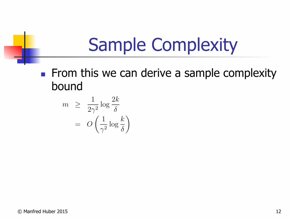
Sample Complexity n From this we can derive a sample complexity
bound
8
can only decrease (since we’d then be taking a min over a larger set of func-tions). Hence, by learning using a larger hypothesis class, our “bias” canonly decrease. However, if k increases, then the second 2
!· term would also
increase. This increase corresponds to our “variance” increasing when we usea larger hypothesis class.
By holding ! and " fixed and solving for m like we did before, we canalso obtain the following sample complexity bound:
Corollary. Let |H| = k, and let any ", ! be fixed. Then for #(h) "minh!H #(h) + 2! to hold with probability at least 1# ", it su!ces that
m $1
2!2log
2k
"
= O
!
1
!2log
k
"
"
,
4 The case of infinite HWe have proved some useful theorems for the case of finite hypothesis classes.But many hypothesis classes, including any parameterized by real numbers(as in linear classification) actually contain an infinite number of functions.Can we prove similar results for this setting?
Let’s start by going through something that is not the “right” argument.Better and more general arguments exist, but this will be useful for honingour intuitions about the domain.
Suppose we have an H that is parameterized by d real numbers. Since weare using a computer to represent real numbers, and IEEE double-precisionfloating point (double’s in C) uses 64 bits to represent a floating point num-ber, this means that our learning algorithm, assuming we’re using double-precision floating point, is parameterized by 64d bits. Thus, our hypothesisclass really consists of at most k = 264d di"erent hypotheses. From the Corol-lary at the end of the previous section, we therefore find that, to guarantee#(h) " #(h") + 2!, with to hold with probability at least 1 # ", it su!ces
that m $ O#
1!2 log
264d
"
$
= O#
d!2 log
1"
$
= O!,"(d). (The !, " subscripts are
to indicate that the last big-O is hiding constants that may depend on ! and".) Thus, the number of training examples needed is at most linear in theparameters of the model.
The fact that we relied on 64-bit floating point makes this argument notentirely satisfying, but the conclusion is nonetheless roughly correct: If whatwe’re going to do is try to minimize training error, then in order to learn
© Manfred Huber 2015 13
Sample Complexity n In infinite hypothesis spaces we need to
address this slightly differently n Sample complexity depends on complexity of
hypothesis space n Complexity of hypothesis space is measured in
terms of the Vapnik-Chervonenkis dimension n VC dimension measures the largest set of elements that
the hypothesis space can shatter n Shattering implies that it can correctly represent any binary label
assignment to the elements of the set
© Manfred Huber 2015 14
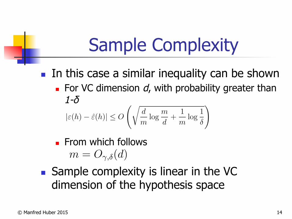
Sample Complexity n In this case a similar inequality can be shown
n For VC dimension d, with probability greater than 1-δ
n From which follows
n Sample complexity is linear in the VC dimension of the hypothesis space
11
Theorem. Let H be given, and let d = VC(H). Then with probability atleast 1! !, we have that for all h " H,
|"(h)! "(h)| # O
!
"
d
mlog
m
d+
1
mlog
1
!
#
.
Thus, with probability at least 1! !, we also have that:
"(h) # "(h!) +O
!
"
d
mlog
m
d+
1
mlog
1
!
#
.
In other words, if a hypothesis class has finite VC dimension, then uniformconvergence occurs as m becomes large. As before, this allows us to give abound on "(h) in terms of "(h!). We also have the following corollary:
Corollary. For |"(h) ! "(h)| # # to hold for all h " H (and hence "(h) #"(h!) + 2#) with probability at least 1! !, it su!ces that m = O!,"(d).
In other words, the number of training examples needed to learn “well”using H is linear in the VC dimension of H. It turns out that, for “most”hypothesis classes, the VC dimension (assuming a “reasonable” parameter-ization) is also roughly linear in the number of parameters. Putting thesetogether, we conclude that (for an algorithm that tries to minimize trainingerror) the number of training examples needed is usually roughly linear inthe number of parameters of H.
© Manfred Huber 2015 15
Regularization and Sample Complexity
n Regularization is an important tool to address overfitting and the Bias / Variance Tradeoff n Regularization is aimed at establishing a
preference for “simpler” hypotheses n Different regularization terms represent different
interpretations of “simple” and achieve different results n Choice of regularization term also influences complexity
of the required optimization
n Learning complexity derives from both computational and sample complexity n Sample complexity measures how many samples
are required to learn a near-optimal hypotheis


