Journal of Electroanalytical Chemistry 722-723 (2014) 68–77

Contents lists available at ScienceDirect

Journal of Electroanalytical Chemistry

journal homepage: www.elsevier .com/locate / je lechem

Regulation of interfacial chemistry by coupled reaction–diffusionprocesses in the electrolyte: A stiff solution dynamics modelfor corrosion and passivity of metals

http://dx.doi.org/10.1016/j.jelechem.2014.03.0141572-6657/� 2014 Elsevier B.V. All rights reserved.

⇑ Corresponding author. Tel.: +91 4565 241480; fax: +91 4565 227779.E-mail address: boscoemmanuel@yahoo.co.in (B. Emmanuel).

Infant G. Bosco a,b, Ivan S. Cole a, Bosco Emmanuel c,⇑a CSIRO Materials Science and Engineering, Clayton, 3169 Victoria, Australiab Institute for Frontier Materials, Deakin University, Burwood, 3125 Victoria, Australiac CSIR-CECRI, Modelling and Simulation, Karaikudi, 630006 Tamil Nadu, India

a r t i c l e i n f o

Article history:Received 20 November 2013Received in revised form 28 February 2014Accepted 10 March 2014Available online 17 March 2014

Keywords:ModellingStiff dynamicsCorrosionPassivityReaction–diffusion processes

a b s t r a c t

In this paper we advance a stiff solution dynamics [SSD] model to study the regulation of local chemistrynear a corroding metal by reaction and diffusion processes in the electrolyte. Using this model we com-pute the detailed space–time dynamics of the concentrations of metal ions, its hydroxy complexes, H+

and OH� ions near the corroding metal. The time for the onset of passivity for Fe and Zn is presentedfor free corrosion condition, different impressed currents and initial pH values. The theory advanced pro-vides much physical insight into corrosion and passivity of metals and motivate spectro-electrochemicalstudies.

� 2014 Elsevier B.V. All rights reserved.

1. Introduction

As early as 1972 Pickering and Frankenthal [1] modelled local-ised corrosion of iron and steel by considering the diffusion andmigration of metal ions and hydrogen ions in artificial pits. Galveleand co-workers extended this model to include solution processessuch as metal ion hydrolysis and self-hydrolysis of water and stud-ied their role in passivity breakdown [2,3]. These are steady statemodels involving a known constant current due to metal dissolu-tion at the bottom of the pit. While chemical reactions such asthe metal ion hydrolysis leading to H+ generation in the pit andself-hydrolysis of water are recognised, the cathodic reactions likeoxygen reduction or hydrogen evolution and the consequentchanges in the solution pH are not considered by these authors.Though these models have led to much useful insights into theconditions under which passivity sets in, two limitations of thesemodels should be noted:

(1) These models describe only the steady state and conse-quently cannot capture the time-dependent changes in thepit solution leading to eventual passivity or pitting. For this

reason, they cannot predict properties such as the time forpassivity. Importantly passivity may set in before the steadystate is reached.

(2) Only the anodic metal dissolution can be included in their mod-els and the cathodic counter reactions like oxygen reduction:

O2 þ 2H2Oþ 4e ! 4OH� ð1Þ

cannot be included. The reason for the inability of these models toinclude any cathodic counter reaction can be traced to the fact thatGalvele’s model is based on the steady state ‘‘atom’’ fluxes and noton the ‘‘species’’ fluxes. For electrode reactions such as (1) wherethe reactant species as well as the product species are in the solu-tion, the corresponding atom fluxes at the electrode surface turnsout to be zero. For example, in the oxygen reduction reaction above,four hydrogen atoms and four oxygen atoms enter as part of thereactants (O2 and 2H2O) and the identical numbers leave as theproduct (4OH�). Though reaction (1) leads to a flux of OH� ionsgoing into the solution, Galvele’s model which is based on atomfluxes cannot describe this flux. It can capture only the metal ionflux arising from the anodic dissolution of the metal:

M!Mnþ þ ne ð2Þ

Here the metal M is a part of the electrode, while the metal ion is inthe solution. Hence there is a non-zero metal atom flux at themetal/solution interface.

Nomenclature

Ci(x, t) concentration of i-th species in the electrolyte, mol/dm3

K1, K2 and K3 stability constants of reactions in the electrolyteDi diffusion coefficient of i-th species, dm2/sRi reaction rate of i-th chemical reaction, mol/(dm3 s)kif forward rate constant of i-th reaction in the electrolytekib backward rate constant of i-th reaction in the electro-

lyteLM(x, t), LH(x, t), and LO(x, t) linear combinations of concentra-

tions, mol/dm3

Fs flux of the species s, mol/(dm2 s)I impressed current density, A/dm2

F Faraday, C/molD the common diffusion coefficient, dm2/sx, t space and time variable, dm, ms to daysl thickness of the thin electrolyte film or the diffusion

layer in RDE experiment, dm

I.G. Bosco et al. / Journal of Electroanalytical Chemistry 722-723 (2014) 68–77 69

It is clear that for a complete understanding of the passivityphenomenon, the species fluxes (e.g. OH� and H+) at the electrodesurface arising from the cathodic counter reactions such as oxygenreduction and hydrogen evolution should also be included in themodel besides the metal ion flux. The proposed SSD model is aimedat achieving this goal and provides a new theoretical methodologyfor describing the time-dependent changes in the solution compo-sition leading to passivity or pitting. Unlike the earlier modelswhich are applicable only to the impressed current condition thepresent model is applicable to both the free corrosion conditionand the impressed current situation.

A typical corrosion scenario involves a metal or alloy surfacegenerating a flux of metal ions and hydroxyl ions or consuminghydrogen ions. The metal ions diffuse into the solution, hydrolysewater generating H+ which in turn modify the self hydrolysis equi-librium of water (H+ + OH� = H2O) and react with a host of otherions such as hydroxyl, chloride, bicarbonate and sulphate depend-ing on the composition of the corrosive medium. When the con-centration of hydroxy, chloro-hydroxy and other metalcomplexes exceed certain solubility limits passive layers may de-posit on the metal. This will decide between passivity and pittingwhen these processes take place inside pits, cracks or other voidspresent in bare or coated metals. On uniform metallic surfaces,general corrosion or passivity will be the result. Precipitation andstrong bonding of the precipitate to the corroding metal leadingto a compact, non-porous layer will be ideal for corrosion controland self-repair. On the other hand, if the corrosion products areloosely adherent to the metal surface, soft and porous or if theyprecipitate in the solution, passivity will not set in. Therefore thequestion of if and when the solubility thresholds are exceeded be-come important. In fact Cole and Muster [4] undertook an experi-mental scanning electron microscope/focussed ion beam andin situ Raman study of oxide growth on zinc under seawater drop-lets. In the in situ Raman they observed rapid (within minutes)growth in the Zn–O bond vibration and somewhat slower growthin sulphate and carbonate bond vibrations (probably associatedwith gordiate and hydrozincite). The focused ion beam sectionsdemonstrated that solid solution growth of the oxide initially dom-inated with the growth of a high porous crystalline phase (gordiateor simonkolleite) or precipitation of crystalline phase from solutionoccurring after some time (around 30 min). The present model isaimed at capturing, in such situations, the solution dynamics lead-ing to passivity or pitting.

In the present work we consider two different geometries:semi-infinite and finite. For corrosion in bulk electrolytes thesemi-infinite geometry will be appropriate while the finite geome-try will be useful for a metal covered with a thin electrolyte layer[5] or a porous oxide layer [6] and for the Rotating Disc Electrode[7]. However detailed results are presented only for the semi-infi-nite geometry and work on the other two geometries is in progress[8].

In Section 2, we formulate the detailed mathematical modelwith its assumptions and approximations clearly spelt out andthe analytical solutions of the model for the space–time depen-dence of the various species concentrations are presented in Sec-tion 3. Results, based on this model, for the time evolution of thesurface concentration of the metal-ion complexes which candeposit and passivate the metal are presented and discussed inSection 4 for free corrosion condition, different impressed currentsand initial pH values for iron and zinc. Typical concentration-ver-sus-distance profiles are also provided for all the species. Conclu-sions and future perspectives are in Section 5.

2. The SSD model framework and the assumptions

The model starts with known fluxes of metal ions and hydroxylor hydrogen ions at the metal/electrolyte interface. For free corro-sion condition the current densities associated with these fluxesbalance one another so that there is no net current through the sys-tem whereas for the case of impressed current/potential thesefluxes will be such as to produce a net current through the system.We report on both these cases. Without loss of generality we treathere the case where oxygen reduction is the cathodic reactionwhile the case of hydrogen evolution will be taken up in the futurework. Thus we have metal ions and hydroxyl ions coming into thesolution where they diffuse and undergo solution reactions whichare, in the simplest case, the following hydrolysis reactions involv-ing the metal ion M2+ and the self-hydrolysis reaction of water.

M2þ þH2O() ðMOHÞþ þHþ ð3ÞðMOHÞþ þH2O()MðOHÞ2 þHþ ð4ÞH2O() Hþ þ OH� ð5Þ

M2+ may be any divalent metal ion such as Fe2+, Zn2+ and Mg2+. Forthe trivalent metal ions Al3+ and Fe3+, there will be one more hydro-lysis step. After labelling the species M2+, H2O, (MOH)+, H+, M(OH)2

and OH� respectively by the numerals 1, 2, 3, 4, 5 and 6, the stabilityconstants may be written as

K1 ¼C3C4

C1C2ð6Þ

K2 ¼C3C4

C1C2ð7Þ

K3 ¼C4C6

C2ð8Þ

where Ci is the concentration of the ith species in the reactions(3)–(5) above.

The species 1–6 diffuse in the solution and while diffusing theyalso undergo chemical reactions. In addition, some of these specieswill be generated or consumed at the electrode surface by

70 I.G. Bosco et al. / Journal of Electroanalytical Chemistry 722-723 (2014) 68–77

corrosion reactions and their influence on the chemical reactions inthe electrolyte will enter through appropriate boundary conditionsfor the reaction–diffusion equations for the species 1–6:

@C1

@t¼ D1

@2C1

@x2

!� R1 ð9Þ

@C2

@t¼ D2

@2C2

@x2

!� ðR1 þ R2 þ R3Þ ð10Þ

@C3

@t¼ D3

@2C3

@x2

!þ R1 � R2 ð11Þ

@C4

@t¼ D4

@2C4

@x2

!þ ðR1 þ R2 þ R3Þ ð12Þ

@C5

@t¼ D5

@2C5

@x2

!þ R2 ð13Þ

@C6

@t¼ D6

@2C6

@x2

!þ R3 ð14Þ

where R1, R2 and R3 are the three chemical reaction rates corre-sponding to the reactions (3)–(5):

R1 ¼ k1f C1C2 � k1bC3C4 ð15ÞR2 ¼ k2f C2C3 � k2bC4C5 ð16ÞR3 ¼ k3f C2 � k3bC4C6 ð17Þ

Now we make the important assumption that the diffusioncoefficients of the species are the same. This approximation willbe good if the species have nearly equal diffusion coefficientsand if not it will provide lower and upper bounds for the spaceand time dependent concentrations of the species by choosingthe lowest or the highest of the diffusion coefficients as the com-mon diffusion coefficient. This approximation is well known inElectrochemistry. Besides Electrochemistry it has been used byseveral investigators in the field of bioengineering. These workershave argued that a diffusion potential gradient [9] develops whichenhances the transport of the faster ions and this reduces the dif-ferences in the diffusivities of the individual species. This approx-imation is further justified by the fact that the transport due toreaction–diffusion coupling is much more significant that causedby the differences in the individual diffusivities. Let us denotethe common diffusion by D.

The second assumption we make is that the chemical reactionstake place on much faster time scales than the diffusion of speciesand hence we propose to apply the equilibrium constraints (6)–(8)for the species concentrations. This assumption can be justified onthe basis that hydrolysis reactions are very rapid [10] and equilib-rium will be achieved within microseconds in comparison with thediffusion process which takes typically 10 s to have its influenceover a distance of 100 lm. [Besides we neglect poly-nuclear spe-cies as their concentrations will be low compared to the mononu-clear species and their formation is a much slower process [11]].Indeed what are known about these reactions are their equilibriumconstants and not the individual forward and backward rate con-stants. Such problems with widely varying time scales are termed‘‘stiff’’ in the mathematical literature and hence the name ‘‘StiffSolution Dynamics’’ for the present model. This stiffness impliesthat, at every space and time point, we may equilibrate the speciesby subjecting the species concentrations to the equilibrium con-straints (6)–(8) before the concentrations begin to change due todiffusion. However, when we apply this equilibrium, we must en-sure that the concentration of each atom (constituting the species)at every space–time point is the same before and after the equili-bration step, as every chemical reaction is only a rearrangementof atoms among the reactant and product species which conserve

the number of atoms of each kind. Now for the species concentra-tion C1(x, t), C2(x, t), C3(x, t), C4(x, t), C5(x, t) and C6(x, t), the corre-sponding atom concentrations for the atoms of M, H and O aregiven by the following linear combinations. These linear combina-tions need to include only those species involved in the solutionreactions. The dissolved O2 concentration in the oxygen reductionreaction or the dissolved H2 concentration in the hydrogen evolu-tion reaction, even if included, does not alter the final result in aself-consistent calculation.

LMðx; tÞ ¼ C1ðx; tÞ þ C3ðx; tÞ þ C5ðx; tÞ ð18ÞLHðx; tÞ ¼ 2C2ðx; tÞ þ C3ðx; tÞ þ C4ðx; tÞ þ 2C5ðx; tÞ þ C6ðx; tÞ ð19ÞLOðx; tÞ ¼ C2ðx; tÞ þ C3ðx; tÞ þ 2C5ðx; tÞ þ C6ðx; tÞ ð20Þ

We now come to an interesting stage in our development: ifwe use the above linear combinations in the reaction–diffusion Eqs.(9)–(14), we find that the three linear combinations LM(x, t), LH(x, t)and LO(x, t) satisfy the following diffusion-only equations where thereaction terms have completely disappeared.

@LMðx; tÞ@t

¼ D@2LMðx; tÞ

@x2

!ð21Þ

@LHðx; tÞ@t

¼ D@2LHðx; tÞ

@x2

!ð22Þ

@LOðx; tÞ@t

¼ D@2LOðx; tÞ

@x2

!ð23Þ

Though the above three partial differential equations (PDE’s)are identical, their initial and boundary conditions will all be differ-ent. Therefore the solutions LM(x, t), LH(x, t) and LO(x, t) will be quitedifferent from one another. The initial condition will be deter-mined by the initial composition of the electrolyte whereas theboundary conditions on the metal depend on the corrosion reac-tions taking place and the participation or non-participation ofthe species.

It is to be emphasised that the solution of the PDE’s (21)–(23)for the linear combinations (of species concentrations) LM(x, t),LH(x, t) and LO(x, t) are exact even in the presence of chemical reac-tions (3)–(5). However, these linear combinations do not as yetpossess any information about the chemical reactions and applyirrespective of whether these chemical reactions are in equilibriumor kinetically driven. Once chemical equilibrium is assumed, wehave the following six equations for the six species concentrations:

LMðx; tÞ ¼ C1ðx; tÞ þ C3ðx; tÞ þ C5ðx; tÞ ð24ÞLHðx; tÞ ¼ 2C2ðx; tÞ þ C3ðx; tÞ þ C4ðx; tÞ þ 2C5ðx; tÞ þ C6ðx; tÞ ð25ÞLOðx; tÞ ¼ C2ðx; tÞ þ C3ðx; tÞ þ 2C5ðx; tÞ þ C6ðx; tÞ ð26Þ

K1 ¼C3ðx; tÞC4ðx; tÞC1ðx; tÞC2ðx; tÞ

ð27Þ

K2 ¼C4ðx; tÞC5ðx; tÞC2ðx; tÞC3ðx; tÞ

ð28Þ

K3 ¼C4ðx; tÞC6ðx; tÞ

C2ðx; tÞð29Þ

The RHS of Eqs. (24)–(26) are known by solving the set of thethree PDE’s (21)–(23). K1, K2 and K3 are known equilibrium con-stants. It is to be noted that the time and space dependence ofthe species concentrations arise from the time and space depen-dence of the linear combinations LM(x, t), LH(x, t) and LO(x, t).

3. Analytic solutions for the reaction diffusion model

To solve the PDE’S (21)–(23), we need to prescribe the initialand boundary conditions on LM(x, t), LH(x, t) and LO(x, t).

I.G. Bosco et al. / Journal of Electroanalytical Chemistry 722-723 (2014) 68–77 71

Initial conditions:

LMðx;0Þ ¼ LM;0 ð30Þ

LHðx;0Þ ¼ LH;0 ð31Þ

LOðx;0Þ ¼ LO;0 ð32Þ

where LM,0, LH,0 and LO,0 may be found from the initial concentra-tions of the solution species using the Eqs. (24)–(26).

Boundary condition at the electrode surface at x = 0:

� D@LM

@x

� �¼ FM2þ ¼ F1 ð33Þ

� D@LH

@x

� �¼ 0 ð34Þ

� D@LO

@x

� �¼ FOH�

2¼ F6

2ð35Þ

These conditions follow from the Eqs. (24)–(26) and the stoichi-ometry of the oxygen reduction reaction:

O2 þ 2H2Oþ 4e! 4OH�

Further for free corrosion condition with zero net current,F1 ¼ F6

2 . For an impressed current experiment FM2þ , FOH� and the im-pressed current density I are related by

2FFM2þ � FFOH� ¼ I ð36Þ

which means that FOH� may be known from I and the metal ion fluxFM2þ . Here F is the Faraday.

For boundary conditions at x =1, we should consider the spe-cific experimental situation at hand. We consider 3 possible situa-tions in this paper: (I) Diffusion and Reaction in the semi-infinitemedium, (II) Diffusion and Reaction in a finite diffusion layer asin the Rotating Disc Electrode (RDE) and (III) Diffusion and Reac-tion in a thin electrolyte layer on the corroding metal. The bound-ary conditions and hence the solutions are different in each one ofthese cases. We outline the method of solution for Case (I) belowand state the modifications necessary for Cases (II) and (III) to-wards the end of this section. Detailed results are presented belowfor Fe and Zn for Case (I) only and the results for Case (II) and Case(III) will be reported elsewhere [8].

Case (I). For diffusion and reactions in the semi-infinite mediumthe boundary conditions at x =1 follow easily from the initialconditions:

LMð1; tÞ ¼ LM;0 ð37Þ

LHð1; tÞ ¼ LH;0 ð38Þ

LOð1; tÞ ¼ LO;0 ð39Þ

Using the method of Laplace transformation, the solutions toEqs. (21)–(23) can easily be obtained and they are:

LMðx; tÞ ¼ LM;0 þ F1 2

ffiffiffiffiffiffiffit

pD

rexp � x2

4Dt

� �� x

Derfc

x

2ffiffiffiffiffiffiDtp

� �" #ð40Þ

LHðx; tÞ ¼ LH;0 ð41Þ

LOðx; tÞ ¼ LO;0 þF6

22

ffiffiffiffiffiffiffit

pD

rexp � x2

4Dt

� �� x

Derfc

x

2ffiffiffiffiffiffiDtp

� �" #ð42Þ

Now the RHS of Eqs. (24)–(26) are known for every space–timepoint and hence the 6 Eqs. (24)–(29) may be solved for the 6 spe-cies concentrations with their time and space dependences in-cluded through Eqs. (40)–(42). We sketch the method of solutionbelow:

Solving Eqs. 24, 27, and 28 for C1(x, t), C3(x, t) and C5(x, t) weobtain:

C1ðx; tÞ ¼LMðx; tÞ

1þ Aðx; tÞ þ Aðx; tÞBðx; tÞ ð43Þ

C3ðx; tÞ ¼LMðx; tÞAðx; tÞ

ð1þ Aðx; tÞ þ Aðx; tÞBðx; tÞÞ ð44Þ

C5ðx; tÞ ¼LMðx; tÞAðx; tÞBðx; tÞ

ð1þ Aðx; tÞ þ Aðx; tÞBðx; tÞÞ ð45Þ

where

Aðx; tÞ ¼ K1C2ðx; tÞC4ðx; tÞ

¼ K1C6ðx; tÞK3

¼ pC6ðx; tÞ ð46Þ

and

Bðx; tÞ ¼ K2C2ðx; tÞC4ðx; tÞ

¼ K2C6ðx; tÞK3

¼ qC6ðx; tÞ ð47Þ

Thus we have expressed C1(x, t), C3(x, t) and C5(x, t) in terms ofC6(x, t).

Subtraction of Eq. (26) from Eq. (25) results in

C2ðx; tÞ þ C4ðx; tÞ ¼ LH � LO ð48Þ

Use Eq. (29) in Eq. (48) to obtain

C2ðx; tÞ ¼C6ðx; tÞðLH � LOÞ

K3 þ C6ðx; tÞð49Þ

Substitute this in Eq. (26), C3(x, t) and C5(x, t) from Eqs. (44) and(45) to obtain:

a4C46 þ a3C3

6 þ a2C26 þ a1C6 þ a0 ¼ 0 ð50Þ

where

a0 ¼ �K3L0 ð51Þa1 ¼ LH � 2L0 þ K3ð1þ pLM � pL0Þ ð52Þa2 ¼ 1þ pðLH � 2L0 þ LM þ 2qK3LM � qK3L0 þ K3Þ ð53Þ

a3 ¼ pq LH � 2L0 þ 2LM þ K3 þ1q

� �ð54Þ

a4 ¼ pq ð55ÞEq. (50) is a quartic equation. Though in principle we can track the po-sitive real root of this quartic equation, it will be quite messy andhence we have taken the simpler alternative of numerically comput-ing the solution of Eq. (50) by using the ‘‘fsolve’’ command in MAPLE.

For the experimental Cases (II) and (III) all the preceding math-ematical steps remain the same except the expressions for LM(x, t),LH(x, t) and LO(x, t) which are modified as under.

Case (II). For the RDE experiment, the following boundary condi-tions hold at x = l where l is the thickness of the diffusion layer thatcan be controlled by the speed of rotation of the RDE.

LMðl; tÞ ¼ LM;0 ð56ÞLHðl; tÞ ¼ LH;0 ð57ÞLOðl; tÞ ¼ LO;0 ð58Þ

For this Case and Case (III), the solutions can be found from onedimensional Greens functions [12] and some identities for trigono-metric series [13]. The solutions for Case (II) are:

LMðx; tÞ ¼ LM;0 þF1ðl� xÞ

D� 8F1l

p2D

X1n¼0

cosð2nþ1Þpx

2l

� �exp � p2Dtð2nþ1Þ2

4l2

� �ð2nþ 1Þ2

ð59ÞLHðx; tÞ ¼ LH;0 ð60Þ

LOðx; tÞ ¼ LO;0 þF6ðl� xÞ

2D� 4F6l

p2D

X1n¼0

cosð2nþ1Þpx

2l

� �exp � p2Dtð2nþ1Þ2

4l2

� �ð2nþ 1Þ2

ð61Þ

Fig. 1a. [Fe2+] versus time. Note that it rises from zero sharply and becomes steadywithin a short time. [Concentration unit used in all the figures is mol/dm3.]

Fig. 1b. [Fe (OH)+] versus time. The rise is gradual.

Fig. 1c. [Fe (OH)2] versus time.

72 I.G. Bosco et al. / Journal of Electroanalytical Chemistry 722-723 (2014) 68–77

For the thin layer experiment, Case (III), the following boundaryconditions hold at x = l where l is the thickness of the thin electro-lyte layer on the corroding metal.

@LMðx; tÞ@x

¼ 0 ð62Þ

@LHðx; tÞ@x

¼ 0 ð63Þ

@LOðx; tÞ@x

¼ 0 ð64Þ

The solutions for Case (III) are:

LMðx; tÞ ¼ LM;0 þF1t

lþ F1l

Dx2

2l2 �xlþ 1

3

� �� 2F1l

p2D

X1m¼1

cos mpxl

exp � p2m2Dt

l2

h ih im2 ð65Þ

LHðx; tÞ ¼ LH;0 ð66Þ

LOðx; tÞ ¼ LO;0 þF6t2lþ F6l

2Dx2

2� x

lþ 1

3

� �� F6l

p2D

X1m¼1

cos mpxl

exp � p2 m2 Dt

l2

h i� �m2 ð67Þ

This completes the solution process.

4. Results and discussion

The framework we developed here does not yet take account ofmigration in an electrical field. Hence the model, in its presentstate of development, is applicable to two experimental situations:(A) the free corrosion condition where there is no current or poten-tial gradients (except of course in the double layer region) in thesolution and (B) the impressed current or potential experimentwhere the solution has enough supporting electrolyte and only dif-fusion of species under consideration is important. In the conclud-ing section, we briefly point out how the present model can easilyincorporate convection besides diffusion and reaction.

In this paper we report the results for iron and zinc. The theoryand computations for Mg shall proceed along similar lines whereasAl will need one more hydrolysis step as it generates trivalent Alions in the solution. Though we are in this paper concerned withthe initial precipitation of ferrous hydroxide this will be eventuallyoxidised to ferric oxide or magnetite or lose a water molecule toform FeO, the ferrous oxide. Another possibility which we are notpresently considering is the formation ferric hydroxide whichmay lead to ferric oxide upon removal of two water molecules. Thispossibility which again needs the third hydrolysis step is to betaken up in later work. For the purposes of this paper we needthe equilibrium constants of the first and second hydrolysis stepsK1 and K2. K1 is reported by Sillen and Martell [14] and Gravanoand Galvele [3]. As we need K2 also, we used the cumulative orgross constants b1 and b2 reported by Sillen and Martell [14] forthe reaction of hydroxyl ions with the metal ions and computedK1 and K2. The constants calculated thus are 1.8 � 10�11 and1.8 � 10�9.9 for the zinc system and 10�5.92 and 182 � 10�18.91 forthe iron system. The equilibrium constant for the self-hydrolysisof water is 1.8 � 10�16 mol/(dm)3. The solubility products of fer-rous hydroxide and zinc hydroxide are respectively 4.87 � 10�17

and 4.5 � 10�17 in the appropriate units.Fig. 1a–1h show the time dependence of the concentrations of

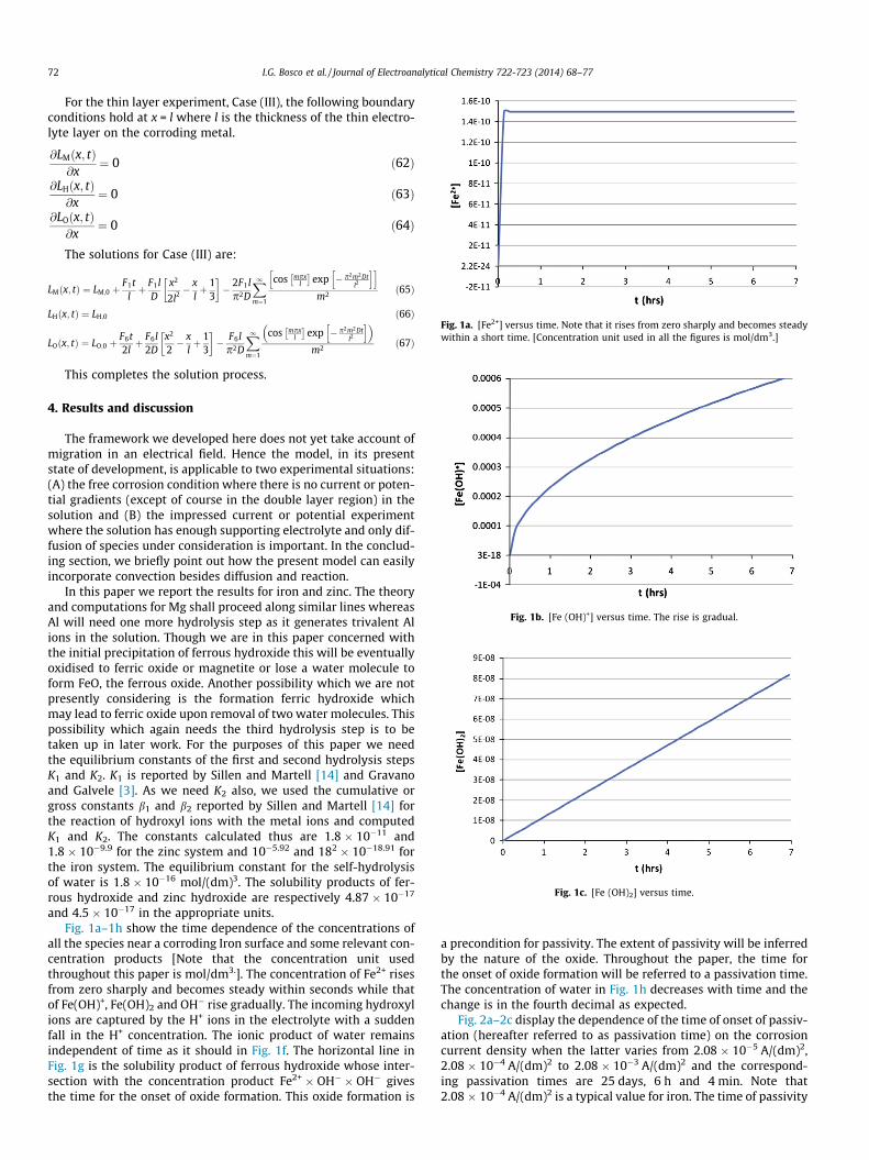
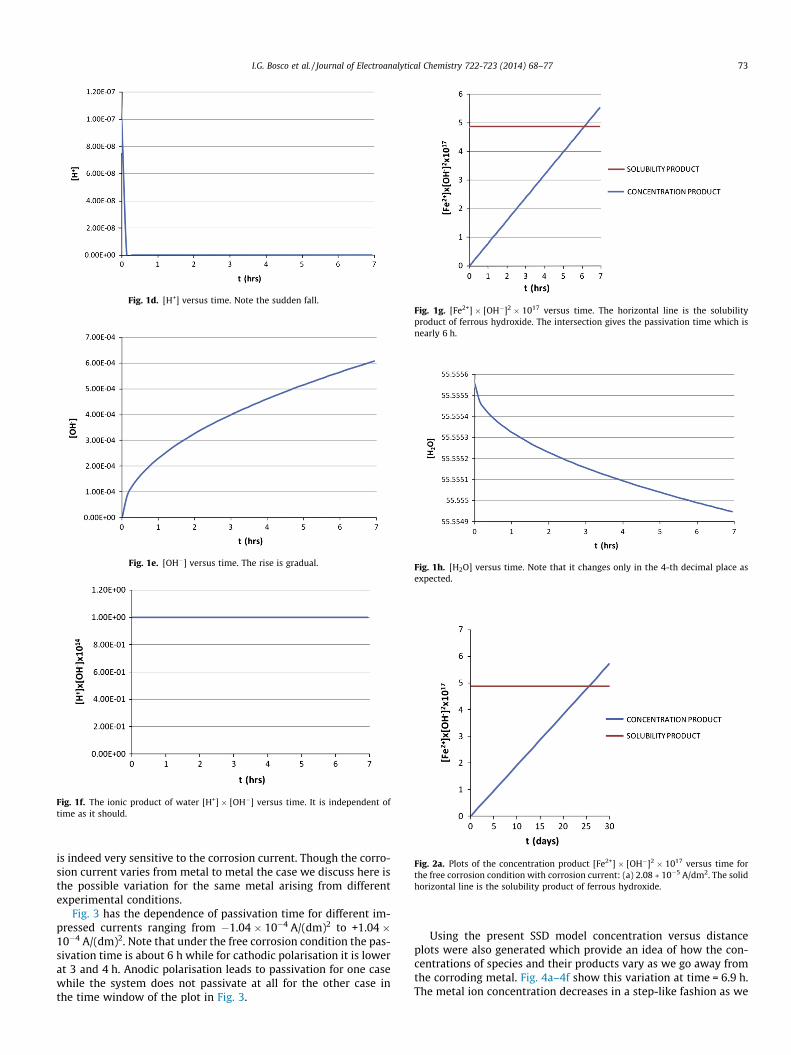
all the species near a corroding Iron surface and some relevant con-centration products [Note that the concentration unit usedthroughout this paper is mol/dm3.]. The concentration of Fe2+ risesfrom zero sharply and becomes steady within seconds while thatof Fe(OH)+, Fe(OH)2 and OH� rise gradually. The incoming hydroxylions are captured by the H+ ions in the electrolyte with a suddenfall in the H+ concentration. The ionic product of water remainsindependent of time as it should in Fig. 1f. The horizontal line inFig. 1g is the solubility product of ferrous hydroxide whose inter-section with the concentration product Fe2+ � OH� � OH� givesthe time for the onset of oxide formation. This oxide formation is

a precondition for passivity. The extent of passivity will be inferredby the nature of the oxide. Throughout the paper, the time forthe onset of oxide formation will be referred to a passivation time.The concentration of water in Fig. 1h decreases with time and thechange is in the fourth decimal as expected.

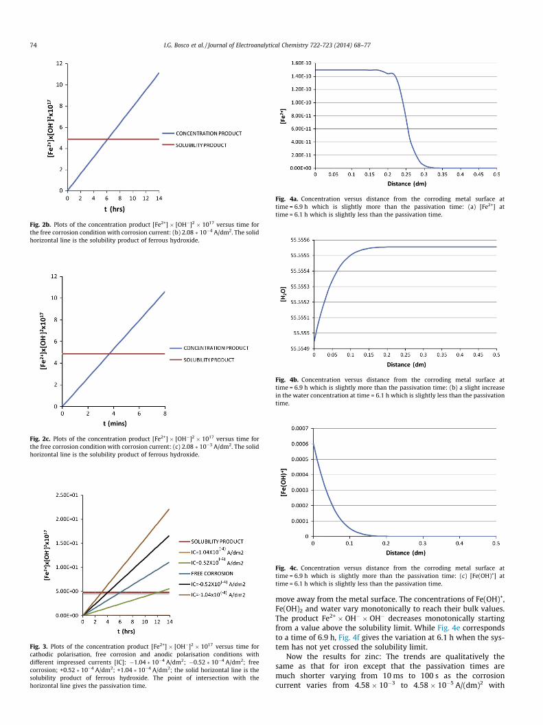
Fig. 2a–2c display the dependence of the time of onset of passiv-ation (hereafter referred to as passivation time) on the corrosioncurrent density when the latter varies from 2.08 � 10�5 A/(dm)2,2.08 � 10�4 A/(dm)2 to 2.08 � 10�3 A/(dm)2 and the correspond-ing passivation times are 25 days, 6 h and 4 min. Note that2.08 � 10�4 A/(dm)2 is a typical value for iron. The time of passivity

Fig. 1d. [H+] versus time. Note the sudden fall.

Fig. 1e. [OH�] versus time. The rise is gradual.

Fig. 1f. The ionic product of water [H+] � [OH�] versus time. It is independent oftime as it should.

Fig. 1g. [Fe2+] � [OH�]2 � 1017 versus time. The horizontal line is the solubilityproduct of ferrous hydroxide. The intersection gives the passivation time which isnearly 6 h.

Fig. 1h. [H2O] versus time. Note that it changes only in the 4-th decimal place asexpected.

Fig. 2a. Plots of the concentration product [Fe2+] � [OH�]2 � 1017 versus time forthe free corrosion condition with corrosion current: (a) 2.08 � 10�5 A/dm2. The solidhorizontal line is the solubility product of ferrous hydroxide.

I.G. Bosco et al. / Journal of Electroanalytical Chemistry 722-723 (2014) 68–77 73

is indeed very sensitive to the corrosion current. Though the corro-sion current varies from metal to metal the case we discuss here isthe possible variation for the same metal arising from differentexperimental conditions.

Fig. 3 has the dependence of passivation time for different im-pressed currents ranging from �1.04 � 10�4 A/(dm)2 to +1.04 �10�4 A/(dm)2. Note that under the free corrosion condition the pas-sivation time is about 6 h while for cathodic polarisation it is lowerat 3 and 4 h. Anodic polarisation leads to passivation for one casewhile the system does not passivate at all for the other case inthe time window of the plot in Fig. 3.

Using the present SSD model concentration versus distanceplots were also generated which provide an idea of how the con-centrations of species and their products vary as we go away fromthe corroding metal. Fig. 4a–4f show this variation at time = 6.9 h.The metal ion concentration decreases in a step-like fashion as we

Fig. 2b. Plots of the concentration product [Fe2+] � [OH�]2 � 1017 versus time forthe free corrosion condition with corrosion current: (b) 2.08 � 10�4 A/dm2. The solidhorizontal line is the solubility product of ferrous hydroxide.

Fig. 2c. Plots of the concentration product [Fe2+] � [OH�]2 � 1017 versus time forthe free corrosion condition with corrosion current: (c) 2.08 � 10�3 A/dm2. The solidhorizontal line is the solubility product of ferrous hydroxide.

Fig. 3. Plots of the concentration product [Fe2+] � [OH�]2 � 1017 versus time forcathodic polarisation, free corrosion and anodic polarisation conditions withdifferent impressed currents [IC]: �1.04 � 10�4 A/dm2; �0.52 � 10�4 A/dm2; freecorrosion; +0.52 � 10�4 A/dm2; +1.04 � 10�4 A/dm2; the solid horizontal line is thesolubility product of ferrous hydroxide. The point of intersection with thehorizontal line gives the passivation time.

Fig. 4a. Concentration versus distance from the corroding metal surface attime = 6.9 h which is slightly more than the passivation time: (a) [Fe2+] attime = 6.1 h which is slightly less than the passivation time.

Fig. 4b. Concentration versus distance from the corroding metal surface attime = 6.9 h which is slightly more than the passivation time: (b) a slight increasein the water concentration at time = 6.1 h which is slightly less than the passivationtime.

Fig. 4c. Concentration versus distance from the corroding metal surface attime = 6.9 h which is slightly more than the passivation time: (c) [Fe(OH)+] attime = 6.1 h which is slightly less than the passivation time.

74 I.G. Bosco et al. / Journal of Electroanalytical Chemistry 722-723 (2014) 68–77

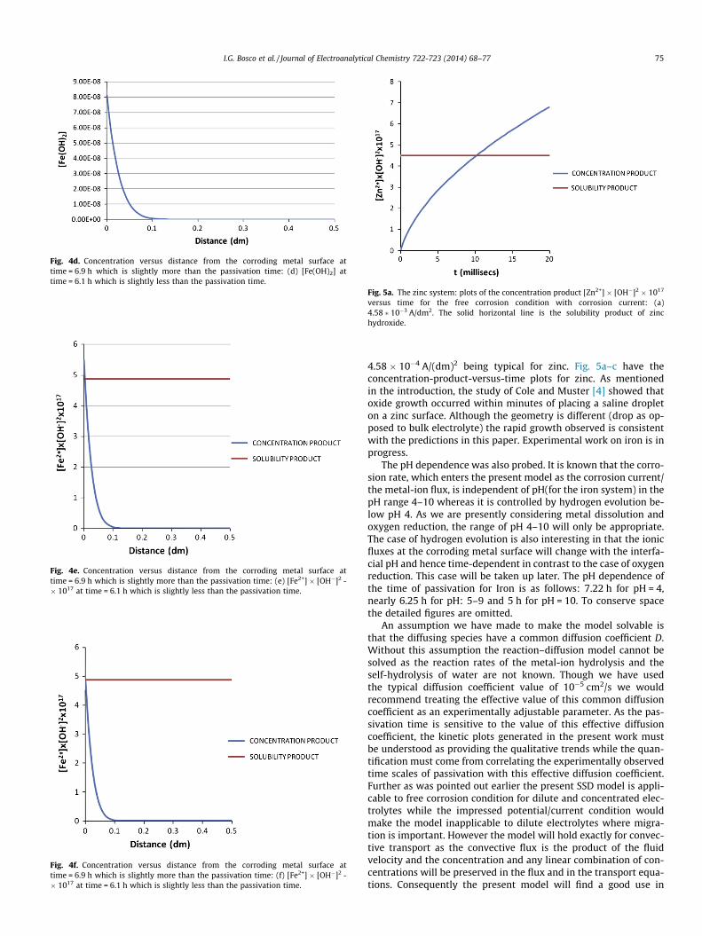
move away from the metal surface. The concentrations of Fe(OH)+,Fe(OH)2 and water vary monotonically to reach their bulk values.The product Fe2+ � OH� � OH� decreases monotonically startingfrom a value above the solubility limit. While Fig. 4e correspondsto a time of 6.9 h, Fig. 4f gives the variation at 6.1 h when the sys-tem has not yet crossed the solubility limit.

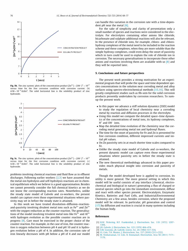
Now the results for zinc: The trends are qualitatively thesame as that for iron except that the passivation times aremuch shorter varying from 10 ms to 100 s as the corrosioncurrent varies from 4.58 � 10�3 to 4.58 � 10�5 A/(dm)2 with

Fig. 4d. Concentration versus distance from the corroding metal surface attime = 6.9 h which is slightly more than the passivation time: (d) [Fe(OH)2] attime = 6.1 h which is slightly less than the passivation time.

Fig. 4e. Concentration versus distance from the corroding metal surface attime = 6.9 h which is slightly more than the passivation time: (e) [Fe2+] � [OH�]2 -� 1017 at time = 6.1 h which is slightly less than the passivation time.

Fig. 4f. Concentration versus distance from the corroding metal surface attime = 6.9 h which is slightly more than the passivation time: (f) [Fe2+] � [OH�]2 -� 1017 at time = 6.1 h which is slightly less than the passivation time.

Fig. 5a. The zinc system: plots of the concentration product [Zn2+] � [OH�]2 � 1017

versus time for the free corrosion condition with corrosion current: (a)4.58 � 10�3 A/dm2. The solid horizontal line is the solubility product of zinchydroxide.

I.G. Bosco et al. / Journal of Electroanalytical Chemistry 722-723 (2014) 68–77 75

4.58 � 10�4 A/(dm)2 being typical for zinc. Fig. 5a–c have theconcentration-product-versus-time plots for zinc. As mentionedin the introduction, the study of Cole and Muster [4] showed thatoxide growth occurred within minutes of placing a saline dropleton a zinc surface. Although the geometry is different (drop as op-posed to bulk electrolyte) the rapid growth observed is consistentwith the predictions in this paper. Experimental work on iron is inprogress.

The pH dependence was also probed. It is known that the corro-sion rate, which enters the present model as the corrosion current/the metal-ion flux, is independent of pH(for the iron system) in thepH range 4–10 whereas it is controlled by hydrogen evolution be-low pH 4. As we are presently considering metal dissolution andoxygen reduction, the range of pH 4–10 will only be appropriate.The case of hydrogen evolution is also interesting in that the ionicfluxes at the corroding metal surface will change with the interfa-cial pH and hence time-dependent in contrast to the case of oxygenreduction. This case will be taken up later. The pH dependence ofthe time of passivation for Iron is as follows: 7.22 h for pH = 4,nearly 6.25 h for pH: 5–9 and 5 h for pH = 10. To conserve spacethe detailed figures are omitted.

An assumption we have made to make the model solvable isthat the diffusing species have a common diffusion coefficient D.Without this assumption the reaction–diffusion model cannot besolved as the reaction rates of the metal-ion hydrolysis and theself-hydrolysis of water are not known. Though we have usedthe typical diffusion coefficient value of 10�5 cm2/s we wouldrecommend treating the effective value of this common diffusioncoefficient as an experimentally adjustable parameter. As the pas-sivation time is sensitive to the value of this effective diffusioncoefficient, the kinetic plots generated in the present work mustbe understood as providing the qualitative trends while the quan-tification must come from correlating the experimentally observedtime scales of passivation with this effective diffusion coefficient.Further as was pointed out earlier the present SSD model is appli-cable to free corrosion condition for dilute and concentrated elec-trolytes while the impressed potential/current condition wouldmake the model inapplicable to dilute electrolytes where migra-tion is important. However the model will hold exactly for convec-tive transport as the convective flux is the product of the fluidvelocity and the concentration and any linear combination of con-centrations will be preserved in the flux and in the transport equa-tions. Consequently the present model will find a good use in

Fig. 5b. The zinc system: plots of the concentration product [Zn2+] � [OH�]2 � 1017

versus time for the free corrosion condition with corrosion current: (b)4.58 � 10�4 A/dm2. The solid horizontal line is the solubility product of zinchydroxide.

Fig. 5c. The zinc system: plots of the concentration product [Zn2+] � [OH�]2 � 1017

versus time for the free corrosion condition with corrosion current: (c)4.58 � 10�5 A/dm2. The solid horizontal line is the solubility product of zinchydroxide.

76 I.G. Bosco et al. / Journal of Electroanalytical Chemistry 722-723 (2014) 68–77

problems involving chemical reactions and fluid flow as in effluentdischarges. Following earlier workers [2,3] we have assumed thatthe metal-ion hydrolysis and self-hydrolysis reactions are in chem-ical equilibrium which we believe is a good approximation. Besideswe cannot presently consider the full chemical kinetics as we donot know the corresponding reaction rates. Nonetheless, unlikethe steady state model of Galvele and co-workers, the presentmodel can capture even those experimental situations where pas-sivity may set in before the steady state is attained.

In this work we have treated dissolution–diffusion–reaction-and-passivity involving divalent metal ions such as Fe2+ and Zn2+

with the oxygen reduction as the counter reaction. The generalisa-tions of the model involving trivalent metal ions like Fe3+ and Al3+

with hydrogen evolution as the possible counter reaction are inprogress [8]. Care must be exercised in the proper choice of thecounter reaction. For example, in the case of iron, the counter reac-tion is oxygen reduction between pH 4 and pH 10 and it is hydro-gen evolution below a pH of 4. In addition, the corrosion rate ofiron linearly decreases with pH below a pH of 4 and our model

can handle this variation in the corrosion rate with a time-depen-dent pH near the metal [8].

For the sake of simplicity and clarity of presentation only asmall number of species and reactions were considered in the elec-trolyte. For electrolytes containing other anions like chloride,bicarbonate and sulphate additional reactions will also be relevant.In the presence of chloride ions, for example, chloro- and chloro-hydroxy complexes of the metal need to be included in the reactionscheme and these complexes, when they are more soluble than thesimple hydroxy complexes, could even delay the onset of passivitywhich in turn could be used to explain the role of chloride ion incorrosion. The necessary generalisations to incorporate these otheranions and reactions involving them are available with us [8] andthey will be reported later.

5. Conclusions and future perspectives

The present work provides a strong motivation for an experi-mental program that will probe the space and time dependent spe-cies concentrations in the solution near corroding metal and alloysurfaces using spectro-electrochemical methods [15,16]. This willgreatly compliment studies such as fib-sem for the solid corrosionproducts presently undertaken by corrosion researchers. To sum-up the present work:

� In this paper we advance a stiff solution dynamics [SSD] modelto study the regulation of local chemistry near a corrodingmetal by reaction and diffusion processes in the electrolyte.� Using this model we compute the detailed space–time dynam-

ics of the concentrations of metal ions, its hydroxy complexes,H+ and OH� ions.� Map the detailed time evolution of the chemistry near the cor-

roding metal generating metal ion and hydroxyl fluxes.� The time for the onset of passivity for Fe and Zn is presented for

free corrosion condition, different impressed currents and ini-tial pH values.� On Zn passivity sets in at much shorter time scales compared to

Fe.� Unlike the steady state model of Galvele and co-workers, the

present dynamic model can capture even those experimentalsituations where passivity sets in before the steady state isattained.� The new theoretical methodology advanced in this paper pro-

vides much physical insight into corrosion and passivity ofmetals.

Though the model developed here is applied to corrosion, itsutility is more general. The more general setting in which thismodel will be useful consists of any interface (chemical, electro-chemical and biological in nature) generating a flux of charged orneutral species which go into the immediate environment, diffuseand react with other species present. Electrocatalysis, EnzymaticKinetics, Batteries and Fuel Cells, and Industrial/EnvironmentalChemistry are a few areas, besides corrosion, where the proposedmodel will be relevant. In particular, pH generation and control[17] by diffusion and reaction is crucial in many systems includingthe human body.

References

[1] H.W. Pickering, R.P. Frankenthal, J. Electrochem. Soc. 119 (1972) 1297–1304.

[2] J.R. Galvele, J. Electrochem. Soc. 123 (1976) 464–474.[3] S.M. Gravano, J.R. Galvele, Corros. Sci. 24 (1984) 517–534.[4] I.S. Cole, T.H. Muster, J. Electrochem. Soc. 157 (2010) C213–C222.[5] M. Venkatraman, I.S. Cole, B. Emmanuel, Electrochim. Acta 56 (2011) 7171–

7179.

I.G. Bosco et al. / Journal of Electroanalytical Chemistry 722-723 (2014) 68–77 77

[6] M. Venkatraman, I.S. Cole, B. Emmanuel, Electrochim. Acta 56 (2011) 8192–8203.

[7] V.G. Levich, Physicochemical Hydrodynamics, Prentice Hall, New Jersey, 1962.[8] B. Emmanuel, Unpublished results.[9] E. Ruckenstein, S. Varanasi, Chem. Eng. Sci. 39 (1984) 1185–1200.

[10] C.F. Baes, R.E. Mesmer, The Hydrolysis of Cations, John Wiley, New York,1976.

[11] J.P. Hunt, Metal Ions in Aqueous Solution, Benjamin, New York, 1963.

[12] J.V. Beck, K.D. Cole, A. Haji-Sheikh, B. Litkouhi, Heat Conduction Using Green’sFunctions, Taylor & Francis, New York, 1992.

[13] I.S. Gradshteyn, I.M. Ryzhik, Tables of Integrals, Series and Products, AcademicPress, Sydney, 1980.

[14] L.G. Sillen, A.E. Martell, Stability Constants of Metal-ion Complexes, ChemicalSociety, London, 1964.

[15] R. Pruiksma, R.L. McCreery, Anal. Chem. 51 (1979) 2253–2257.[16] C.C. Jan, R.L. McCreery, Anal. Chem. 58 (1986) 2771–2777.[17] G. Chen, R.L. Fournier, S. Varanasi, Biotechnol. Bioeng. 57 (1998) 394–407.