University of Hamburg MIN Faculty Department of Informatics Reinforcement Learning (2) Reinforcement Learning (2) Algorithmic Learning 64-360, Part II Norman Hendrich University of Hamburg MIN Faculty, Dept. of Informatics Vogt-K¨ olln-Str. 30, D-22527 Hamburg [email protected]26/06/2013 N. Hendrich 1
Transcript
University of Hamburg
MIN Faculty
Department of Informatics
Reinforcement Learning (2)
Reinforcement Learning (2)Algorithmic Learning 64-360, Part II
Norman Hendrich
University of HamburgMIN Faculty, Dept. of Informatics
Dynamic ProgrammingAsynchronous Dynamic ProgrammingMonte-Carlo MethodsTemporal-Difference Learning: Q-Learning and SARSAAcceleration of LearningApplications in RoboticsGrasping with RL: Parallel GripperGrasping mit RL: Barrett-Hand
N. Hendrich 2
University of Hamburg
MIN Faculty
Department of Informatics
Examples: Matlab Reinforcement Learning (2)
Three classical RL examples: Matlab demos
I pole-balancing cart
I underpowered mountain-car
I robot inverse-kinematics
I those are all toy problemsI small state-spacesI simplified environment models (e.g., no realistic physics)I but intuitive interpretation and visualization
I the learning-rules (Q, SARSA) will be explained later
Demos from Jose Antonio Martin, Madrid: http://www.dacya.ucm.es/jam/download.htm
N. Hendrich 3
University of Hamburg
MIN Faculty
Department of Informatics
Examples: Matlab Reinforcement Learning (2)
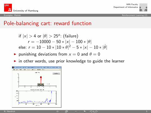
Pole-balancing cart
I balance a pole against gravity
I simplest version is 1D: pole on cart on tracksI 1D-balancing already requires 4 DOF:
I x : position of the cart (should be near origin)I x : velocity of the cartI θ: angle of the pole (zero assumed to be upright)I θ: angular velocity of the pole
I simplified physics, discretization of state-spaceI model as an episodic task
I cart position |x | > xmax terminates the taskI pole falling down |θ| > θmax terminates the task
else: r = 10− 10 ∗ |10 ∗ θ|2 − 5 ∗ |x | − 10 ∗ |θ|I punishing deviations from x = 0 and θ = 0
I in other words, use prior knowledge to guide the learner
N. Hendrich 5
University of Hamburg
MIN Faculty
Department of Informatics
Examples: Matlab Reinforcement Learning (2)
Pole-balancing cart: videos
Many related problems:
I pole-balancing in 2DI decouple into two 4-DOF problemsI don’t try 8-DOF
I inverse pendulumI multi-joint inverse-pendulumI acrobotI . . .
In theory, all those problems could be modelled analytically, usingthe corresponding differential-equations for the system. But inpractice, this is impossible due to modelling errors, e.g. unknownmass and inertia of the moving parts.
N. Hendrich 6
University of Hamburg
MIN Faculty
Department of Informatics
Examples: Matlab Reinforcement Learning (2)
Mountain-car
I underpowered car should climb a mountain-slope
I simplified physics model
I actions are full-throttle a ∈ {−1, 0,+1}I but constant a = +1 is not sufficient to reach the summit
I car must go backwards first a bit or even oscillate to buildsufficient momentum to climb the mountain
I simple example of problems where the agent cannot reach thegoal directly, but must explore intermediate solutions that seemcounterintuitive
I typical example of delayed reward
N. Hendrich 7
University of Hamburg
MIN Faculty
Department of Informatics
Examples: Matlab Reinforcement Learning (2)
Mountain-car
Details: Sutton and Barto, chapter 8.10
N. Hendrich 8
University of Hamburg
MIN Faculty
Department of Informatics
Examples: Matlab Reinforcement Learning (2)
Mountain-car: Matlab demo reward function
I +100 reward for reaching the mountain-summit
I −1 reward for every timestep without reaching the summit
I every episode is terminated after 1000 timesteps
N. Hendrich 9
University of Hamburg
MIN Faculty
Department of Informatics
Examples: Matlab Reinforcement Learning (2)
Inverse-Kinematics: planar robot
N. Hendrich 10
University of Hamburg
MIN Faculty
Department of Informatics
Examples: Matlab Reinforcement Learning (2)
Inverse-Kinematics: planar robot
I planar three-link robot (2D)
I try to reach given position (x , y) position
I need to calculate joint-angles {θ1, θ2, θ3}I actions are joint-movements ∆θi ∈ {−1, 0,+1}
Note:
I calculating (x , y) for given (θ1, θ2, θ3) is straightforward,
I but inverse-kinematics is much harder
I in general, no analytical solutions possible
I especially with high-DOF systems:humans, animals, humanoid robots: 70-DOF+
N. Hendrich 11
University of Hamburg
MIN Faculty
Department of Informatics
Dynamic Programming Reinforcement Learning (2)
Dynamic Programming
I overview of classical solution methods for MDPs, calleddynamic programming
I based on the Bellman-equations
I also, the main theory behind RL
I demonstration of the application of DP — examples forcalculating value functions and optimal policies
I discussion about the effectiveness and usefulness of DP
Details: Sutton and Barto, chapter 4
N. Hendrich 12
University of Hamburg
MIN Faculty
Department of Informatics
Dynamic Programming Reinforcement Learning (2)
Dynamic Programming for model-based learning
Dynamic Programming is a collection of approaches that can beused if a perfect model of the MDP’s is available: We assume theMarkov property, and Pa
ss′ and Rass′ are known.
In order to calculate the optimal policy, the Bellman-Equations areembedded into an update function that approximates the desiredvalue function V .Three steps:
1. Policy Evaluation
2. Policy Improvement
3. Policy Iteration
N. Hendrich 13
University of Hamburg
MIN Faculty
Department of Informatics
Dynamic Programming Reinforcement Learning (2)
Policy Evaluation (1)
Policy Evaluation: Calculate the state-value function V π for agiven policy π.
State-value function for policy π:
V π(s) = Eπ {Rt |st = s} = Eπ
{ ∞∑k=0
γk rt+k+1 | st = s
}
Bellman-Equation for V π:
V π(s) =∑a
π(s, a)∑s′
Pass′ [R
ass′ + γV π(s ′)]
– a system of |S | linear equationsN. Hendrich 14
University of Hamburg
MIN Faculty
Department of Informatics
Dynamic Programming Reinforcement Learning (2)
Policy Evaluation (2)
Policy Evaluation is a process of calculating the value-functionV π(s) for an arbitrary policy π .Based on the Bellman equation, an update rule can be createdthat calculates the approximated value-function V0,V1,V2,V3, . . .
Vk+1(s) =∑a
π(s, a)∑s′
Pass′ [R
ass′ + γVk(s ′)] ∀s ∈ S
Based on the k-th approximation Vk for each state s, the(k + 1)-th approximation Vk+1 is calculated iteratively. The oldvalue of s is replaced by an updated one that has been calculatedwith the iteration rule based on the old values.It can be shown that the sequence of the iterated value-functions{Vk} converges to V π, if k →∞.
N. Hendrich 15
University of Hamburg
MIN Faculty
Department of Informatics
Dynamic Programming Reinforcement Learning (2)
Iterative Policy Evaluation
Input π, the policy to evaluateInitialize V (s) = 0, for all s ∈ SRepeat
∆← 0For every s ∈ S :
v ← V (s)V (s)←
∑aπ(s, a)
∑s′
Pass′ [R
ass′ + γVk(s ′)]
∆← max(∆, |v − V (s)|)
until ∆ < θ (a small positive real number)Output V ≈ V π
N. Hendrich 16
University of Hamburg
MIN Faculty
Department of Informatics
Dynamic Programming Reinforcement Learning (2)
Iterative Policy Evaluation
Note: this algorithm is conceptually very simple, butcomputationally very expensive. It requires a full sweep across allactions a for all states s in the state-space S :
I typically, exponential in the number of dimensions of (s, a);all states and actions are tested many times
I requires full knowledge of the dynamics of the environment,Pass′ and Ra
ss′ are required
I the algorithm only terminates if the change in V (s) is smallerthan ∆, even if the policy π is still suboptimal
I better algorithms try to reduce the number of policy-evaluationsteps, or try to bypass this step entirely
N. Hendrich 17
University of Hamburg
MIN Faculty
Department of Informatics
Dynamic Programming Reinforcement Learning (2)
Example: another gridworld
I agent moves across the grid: a ∈ {up, down, left, right}I non-terminal states: 1, 2, . . . , 14
I one terminal state: {0, 15} (shaded: one state, but two squares)
I therefore: an episodic task, undiscounted (γ = 1)
I actions that would take the agent from the grid leave the stateunchanged
I the reward is −1 until the terminal state is reached
N. Hendrich 18
University of Hamburg
MIN Faculty
Department of Informatics
Dynamic Programming Reinforcement Learning (2)
Iterative Policy Evaluation for the gridworld (1)
left: Vk(s) for the random policy π (random moves)
right: moves according to the greedy policy Vk(s)
N. Hendrich 19
University of Hamburg
MIN Faculty
Department of Informatics
Dynamic Programming Reinforcement Learning (2)
Iterative Policy Evaluation for the gridworld (2)
In this example: the greedy policy for Vk(s) is optimal for k ≥ 3.
N. Hendrich 20
University of Hamburg
MIN Faculty
Department of Informatics
Dynamic Programming Reinforcement Learning (2)
Policy Improvement (1)
We now consider the action value function Qπ(s, a), when action ais chosen in state s, and afterwards Policy π is pursued:
Qπ(s, a) =∑s′
Pass′ [R
ass′ + γV π(s ′)]
In each state we look for the action that maximizes the actionvalue function.Hence a greedy policy π′ for a given value function V π isgenerated:
π′(s) = arg maxa
Qπ(s, a)
= arg maxa
∑s′
Pass′ [R
ass′ + γV π(s ′)]
N. Hendrich 21
University of Hamburg
MIN Faculty
Department of Informatics
Dynamic Programming Reinforcement Learning (2)
Policy Improvement (2)
Suppose we have calculated V π for a deterministic policy π.Would it be better to choose an action a 6= π(s) for a given state?If a is chosen in state s, the value is:
Qπ(s, a) = Eπ{rr+1 + γV π(st+1)|st = s, at = a}=
∑s′
Pass′ [R
ass′ + γV π(s ′)]
It is better to switch to action a in state s, if and only if
Qπ(s, a) > V π(s)
N. Hendrich 22
University of Hamburg
MIN Faculty
Department of Informatics
Dynamic Programming Reinforcement Learning (2)
Policy Improvement (3)
Perform this for all states, to get a new policy π, that is greedy interms of V π:
π′(s) = argmax
aQπ(s, a)
= argmaxa
∑s′
Pass′ [R
ass′ + γV π(s ′)]
Then V π′ ≥ V π
N. Hendrich 23
University of Hamburg
MIN Faculty
Department of Informatics
Dynamic Programming Reinforcement Learning (2)
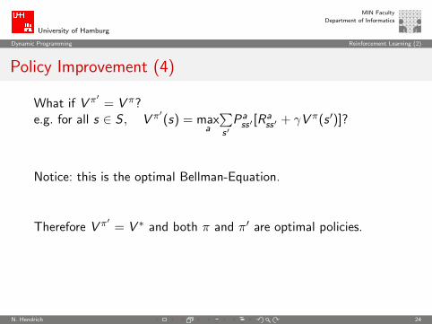
Policy Improvement (4)
What if V π′= V π?
e.g. for all s ∈ S , V π′(s) = max
a
∑s′
Pass′ [R
ass′ + γV π(s ′)]?
Notice: this is the optimal Bellman-Equation.
Therefore V π′= V ∗ and both π and π′ are optimal policies.
N. Hendrich 24
University of Hamburg
MIN Faculty
Department of Informatics
Dynamic Programming Reinforcement Learning (2)
Iterative Methods
V0 → V1 → . . .→ Vk → Vk+1 → . . .→ V π
⇑ an “iteration”
An iteration comprises one backup-operation for each state.
A full-policy evaluation-backup:
Vk+1(s)←∑a
π(s, a)∑s′
Pass′ [R
ass′ + γVk(s ′)]
N. Hendrich 25
University of Hamburg
MIN Faculty
Department of Informatics
Dynamic Programming Reinforcement Learning (2)
Policy Iteration (1)
If Policy Improvement and Policy Evaluation are performed in turn,this means that the policy π is improved with a fixed valuefunction V π, and then the corresponding value function V π′
iscalculated based on the improved policy π′.Afterwards again policy improvement is used, to get an even betterpolicy π′′, and so forth . . . :
π0PE−→ V π0
PI−→ π1PE−→ V π1
PI−→ π2PE−→ V π2 · · · PI−→ π∗
PE−→ V ∗
HerePI−→ stands for performing policy improvement and
1. initializationV (s) ∈ < and π(s) ∈ A(s) arbitrarily for all s ∈ S
2. policy-evaluationRepeat
∆← 0for every s ∈ S :
v ← V (s)
V (s)←∑aπ(s, a)
∑s′
Pπ(s)ss′ [R
π(s)ss′ + γV (s ′)]
∆← max(∆, |v − V (s)|)until ∆ < θ (a small real positive number)
N. Hendrich 28
University of Hamburg
MIN Faculty
Department of Informatics
Dynamic Programming Reinforcement Learning (2)
Policy Iteration (4)
3. policy-improvement
policy-stable ← truefor every s ∈ S :
b ← π(s)π(s)← arg max
a
∑s′
Pass′ [R
ass′ + γV (s ′)]
if b 6= π(s), then policy-stable ← falseIf policy-stable, then stop; else goto 2
Note: this algorithm converges to the optimal value-function V ∗(s)and the optimal policy π∗ (but may take a long time).
N. Hendrich 29
University of Hamburg
MIN Faculty
Department of Informatics
Dynamic Programming Reinforcement Learning (2)
Example: Jack’s car rental
Jack manages two locations for a car rental company. Every daysome number of customers arrive at each location to rent cars.
If Jack has a car available, he rents it out and is credited by $10 bythe company. If he is out of cars at that location, then the businessis lost. Cars become available for renting the day after they arereturned. To help ensure that cars are available where they areneeded, Jack can move them between the two locations overnight,at a cost of $2 per car moved.
N. Hendrich 30
University of Hamburg
MIN Faculty
Department of Informatics
Dynamic Programming Reinforcement Learning (2)
Jack’s car rental (2)
We assume that the number of cars requested and returned at eachlocation are Poisson random variables, meaning that the probabilitythat the number is n is λn
n! e−λ, where λ is the expected number.
I note: Poisson-probabilities are hard to handle analytically
I assume λ is 3 and 4 for car rental requests,
and λ is 3 and 2 for car returns
at Jack’s first and second locations
I also assume there are n < 20 cars
I a maximum of m < 5 cars can be moved between the twolocations overnight
I discount rate s γ = 0.9, time-steps are days.
N. Hendrich 31
University of Hamburg
MIN Faculty
Department of Informatics
Dynamic Programming Reinforcement Learning (2)
Jack’s car rental (3)cars moved from 1 to 2: Policies π0 up to π4 and value function V4(s)
N. Hendrich 32
University of Hamburg
MIN Faculty
Department of Informatics
Dynamic Programming Reinforcement Learning (2)
Value Iteration
A method to improve convergence speed. In policy-evaluation, weuse the full policy-evaluation backup:
Vk+1(s)←∑a
π(s, a)∑s′
Pass′ [R
ass′ + γVk(s ′)]
Instead, the full value-iteration backup is:
Vk+1(s)← maxa
∑s′
Pass′ [R
ass′ + γVk(s ′)]
N. Hendrich 33
University of Hamburg
MIN Faculty
Department of Informatics
Dynamic Programming Reinforcement Learning (2)
Value Iteration
Initialize V arbitrarily, e.g. V (s) = 0, for all s ∈ Srepeat
∆← 0For every s ∈ S :
v ← V (s)V (s)← max
a
∑s′
Pass′ [R
ass′ + γV (s ′)]
∆← max(∆, |v − V (s)|)until ∆ < θ (a small positive real number)
Output is a deterministic policy π withπ(s) = arg max
a
∑s′
Pass′ [R
ass′ + γV (s ′)]
N. Hendrich 34
University of Hamburg
MIN Faculty
Department of Informatics
Dynamic Programming Reinforcement Learning (2)
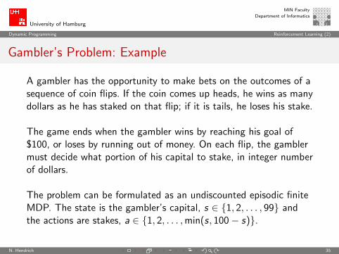
Gambler’s Problem: Example
A gambler has the opportunity to make bets on the outcomes of asequence of coin flips. If the coin comes up heads, he wins as manydollars as he has staked on that flip; if it is tails, he loses his stake.
The game ends when the gambler wins by reaching his goal of$100, or loses by running out of money. On each flip, the gamblermust decide what portion of his capital to stake, in integer numberof dollars.
The problem can be formulated as an undiscounted episodic finiteMDP. The state is the gambler’s capital, s ∈ {1, 2, . . . , 99} andthe actions are stakes, a ∈ {1, 2, . . . ,min(s, 100− s)}.
N. Hendrich 35
University of Hamburg
MIN Faculty
Department of Informatics
Dynamic Programming Reinforcement Learning (2)
Gambler’s Problem (2)
The reward is zero on all transitions except those on which thegambler reaches his goal, when it is +1. The state-value functionthen gives the probability of winning from each state. A policy is amapping from levels of capital to stakes. The optimal policymaximizes the probability of reaching the goal (winning $100).
Let p denote the probability of the coin coming up heads. If p isknown, then the entire problem is known and it can be solved, forinstance by value-iteration. The next figure shows the change inthe value function Vp=0.4(s) over successive sweeps of valueiteration, and the final policy found, for the case of p = 0.4.
N. Hendrich 36
University of Hamburg
MIN Faculty
Department of Informatics
Dynamic Programming Reinforcement Learning (2)
Gambler’s Problem (3)Estimates of the value function V (s) for p = 0.4
N. Hendrich 37
University of Hamburg
MIN Faculty
Department of Informatics
Dynamic Programming Reinforcement Learning (2)
Optimal policy for p = 0.4
I Why would this be a good policy?
I e.g, for s = 50 betting all on one flip, but nor for s = 51
I finding an optimal policy is polynomial in the number of statess ∈ S
I unfortunately, the number of states is often extremely high;typically grows exponentially with the number ofstate-variables: Bellman’s curse of dimensionality
I in practice, the classical DP can be applied to problems with afew million states
I the asynchronous DP can be applied to larger problems and isalso suitable for parallel computation
I it is surprisingly easy to find MDPs, where DP methods cannot be applied
I Policy Evaluation: complete backups without maximum
I Policy Improvement: form a greedy policy, even if only locally
I Policy Iteration: alternate the above two processes
I Value Iteration: use backups with maximum
I Complete Backups (over the full state-space S)
I Generalized Policy Iteration (GPI)
I Asynchronous DP: a method to avoid complete backups
N. Hendrich 42
University of Hamburg
MIN Faculty
Department of Informatics
Monte-Carlo Methods Reinforcement Learning (2)
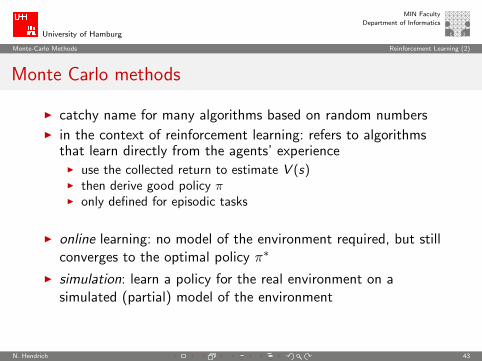
Monte Carlo methods
I catchy name for many algorithms based on random numbersI in the context of reinforcement learning: refers to algorithms
that learn directly from the agents’ experienceI use the collected return to estimate V (s)I then derive good policy πI only defined for episodic tasks
I online learning: no model of the environment required, but stillconverges to the optimal policy π∗
I simulation: learn a policy for the real environment on asimulated (partial) model of the environment
N. Hendrich 43
University of Hamburg
MIN Faculty
Department of Informatics
Monte-Carlo Methods Reinforcement Learning (2)
Monte Carlo methods: basic idea
I given: MDP, initial policy π
I goal: learn V π(s)
I run a (large) number of episodes,
I record all states si visited by the agent,
I record the final return Rt collected at the end of each episode
I for all states si visited during one episode, update V (si ) basedon the return collected in that episode
I this converges for all states that are visited ”often”
N. Hendrich 44
University of Hamburg
MIN Faculty
Department of Informatics
Monte-Carlo Methods Reinforcement Learning (2)
First-visit and Every-visit Monte Carlo
Two ways to update V π(s) from an episode trace:I first-visit MC: update V π(si ) only for the first time that state
si is visited by the learnerI every-visit MC: update V π(si ) every time that state si is visited.
I first-visit MC convergence: each return is an independent,identically distributed estimate of V π(s). By the law of largenumbers the sequence of averages converges to the expectedvalue. The standard deviation of the error falls as 1/
√n, where
n is the number of returns averaged.I both algorithms converge asymptotically
N. Hendrich 45
University of Hamburg
MIN Faculty
Department of Informatics
Monte-Carlo Methods Reinforcement Learning (2)
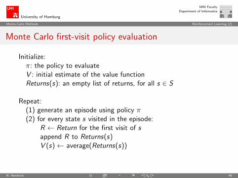
Monte Carlo first-visit policy evaluation
Initialize:π: the policy to evaluateV : initial estimate of the value functionReturns(s): an empty list of returns, for all s ∈ S
Repeat:(1) generate an episode using policy π(2) for every state s visited in the episode:
R ← Return for the first visit of sappend R to Returns(s)V (s)← average(Returns(s))
N. Hendrich 46
University of Hamburg
MIN Faculty
Department of Informatics
Monte-Carlo Methods Reinforcement Learning (2)
Example: playing Blackjack
Goal: obtain cards whose sum is as large as possible, but notexceeding 21. Face cards count as 10, an ace can count either as 1or 11. Here, considering a single player vs. the dealer.
Game begins with two cards dealt to both dealer and player. Oneof the dealer’s cards is faceup, the other is facedown. Player canask for additional cards (hit) or stop (stick), and loses (goes bust)when the sum is over 21. Then it is the dealer’s turn, who has afixed strategy: dealer sticks on any sum of 17 or greater, and hitsotherwise. If the dealer goes bust, then the player wins; otherwisethe outcome is determined by whose final sum is closer to 21.
N. Hendrich 47
University of Hamburg
MIN Faculty
Department of Informatics
Monte-Carlo Methods Reinforcement Learning (2)
Modeling Blackjack
Model as an episodic finite MDP; each game is one episode. Allrewards within a game are zero, no discount (γ = 1). Assume thatcards are dealt from an infinite deck, so no need to keep track ofcards already dealt.I states:
I sum of current cards (12 .. 21)I visible cards of the dealer (ace .. 10)I player has useable ace (1 or 11)I total number of states is 200.
I reward: +1 for winning, 0 for draw, -1 for losing
I return: same as reward
I actions: hit or stick
N. Hendrich 48
University of Hamburg
MIN Faculty
Department of Informatics
Monte-Carlo Methods Reinforcement Learning (2)
Solving Blackjack
I example policy π is: stick if sum is 20 or 21,otherwise hit (i.e., ask for another card)
I simulate many blackjack games using the policy, and averagethe returns following each state
I this uses random numbers for the card generation
I states never recur in the task, so no difference betweenfirst-visit and every-visit MC
I next slide shows the estimated value-function V (s) after 10000and 500000 episodes. Separate functions are shown for whetherthe player holds an useable ace or not.
N. Hendrich 49
University of Hamburg
MIN Faculty
Department of Informatics
Monte-Carlo Methods Reinforcement Learning (2)
Solving Blackjack: V π(s)
Approximated state-value functions V (s) for the policy that sticks only on 20 or 21. Not the best policy. . .
N. Hendrich 50
University of Hamburg
MIN Faculty
Department of Informatics
Monte-Carlo Methods Reinforcement Learning (2)
Solving Blackjack: V π(s)
Think about the estimated function:
I why is the ”useable-ace” function more noisy?
I why are the values higher for the useable-ace case?
I how to explain the basic shape of the value function?
I why does the function drop-off on the left?
I . . .
N. Hendrich 51
University of Hamburg
MIN Faculty
Department of Informatics
Monte-Carlo Methods Reinforcement Learning (2)
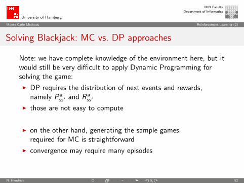
Solving Blackjack: MC vs. DP approaches
Note: we have complete knowledge of the environment here, but itwould still be very difficult to apply Dynamic Programming forsolving the game:
I DP requires the distribution of next events and rewards,namely Pa
ss′ and Rass′
I those are not easy to compute
I on the other hand, generating the sample gamesrequired for MC is straightforward
I convergence may require many episodes
N. Hendrich 52
University of Hamburg
MIN Faculty
Department of Informatics
Monte-Carlo Methods Reinforcement Learning (2)
Monte Carlo backup diagram
I consists of the whole episode from thestart-state to the goal-state
I exactly one action considered in each state,namely, the action actually taken
I no bootstrapping: estimates for one statedo not depend on other estimates
I time required to estimate the value of V (s)for a given state s does not dependon the number of states
I option to learn V (s) only for those statesthat seem interesting
N. Hendrich 53
University of Hamburg
MIN Faculty
Department of Informatics
Monte-Carlo Methods Reinforcement Learning (2)
Monte Carlo estimation of action values
When a model of the MDP is available:
I estimate V π(s) for initial policy π
I use greedification to find better policy
I but: this requires a look-ahead one step to find the action thatleads to the best combination of reward and next state
Without a model:
I state values V (s) are not enough: we don’t know Pass′ or Ra
ss′
I instead, consider Q(s, a) for all actions to find a better policy
I need MC method to estimate Qπ(s, a)
N. Hendrich 54
University of Hamburg
MIN Faculty
Department of Informatics
Monte-Carlo Methods Reinforcement Learning (2)
Monte Carlo estimation of Qπ(s, a)
I Qπ(s, a): the expected return when starting in state s, takingaction a, and thereafter following policy π
I the Monte Carlo method is essentially unchanged:I create and update data-structure for Q(s, a)I first-visit: average the returns following the first time in each
episode that s was visited and a was selectedI every-fisit: average the returns following every visit to a state s
and taking action aI again, convergence can be shown if every state-action pair is
sampled ”often”
I but one major complication: for a deterministic policy π, manyactions a may not be taken at all, and the MC estimates forthose (s, a) pairs will not improve
I need to maintain exploration
N. Hendrich 55
University of Hamburg
MIN Faculty
Department of Informatics
Monte-Carlo Methods Reinforcement Learning (2)
Monte Carlo exploring starts
I start each episode using a given (s, a) pair
— instead of starting in state s and taking a according to thecurrent policy
I ensure that all possible (s, a) pairs are used as the startingstate with a probability p(s, a) > 0
I the Qπ(s, a) estimate will then converge
I using non-deterministic policies may be easier and quicker
I e.g., using a ε-greedy policy will also guarantee that all (s, a)pairs are visited often
N. Hendrich 56
University of Hamburg
MIN Faculty
Department of Informatics
Monte-Carlo Methods Reinforcement Learning (2)
Monte Carlo control: improving the policy
I estimate Qπ(s, a) using (one or many) MC episodes
I from time to time, update policy π using greedification
π0E−→ Qπ
0I−→ π1
E−→ Qπ1
I−→ π2 . . .I−→ π∗
E−→ Q∗
N. Hendrich 57
University of Hamburg
MIN Faculty
Department of Informatics
Monte-Carlo Methods Reinforcement Learning (2)
Monte Carlo first-visit with exploring starts
Initialize for all s ∈ S , a ∈ A(s):π: the policy to evaluateQ(s, a): initial estimate of the value functionReturns(s, a): an empty list of returns, for all pairs (s, a)
Repeat:(1) generate an episode using exploring starts and policy π(2) for every pair (s, a) visited in the episode:
R ← Return for the first visit of (s, a)append R to Returns(s, a)Q(s, a)← average(Returns(s, a))
(3) for every s visited in the episode:π(s)← arg max
aQ(s, a)
N. Hendrich 58
University of Hamburg
MIN Faculty
Department of Informatics
Monte-Carlo Methods Reinforcement Learning (2)
Solving Blackjack: Optimal policy
I remember: this policy is for fresh-cards in every game
I state-space is much more complex without card replacementN. Hendrich 59
University of Hamburg
MIN Faculty
Department of Informatics
Monte-Carlo Methods Reinforcement Learning (2)
Monte Carlo: summary
I our third approach to estimate V (s) or Q(s, a)I several advantages over DP methods:
I no model of the environment requiredI learning directly from interaction with the environmentI option to learn only parts of the state-spaceI less sensitive should the Markov property be violated
I using a deterministic policy may fail to learnI need to maintain exploration
I exploring startsI non-deterministic policies, e.g. ε-greedy
I no bootstrapping
N. Hendrich 60
University of Hamburg
MIN Faculty
Department of Informatics
Monte-Carlo Methods Reinforcement Learning (2)
Intermission: labyrinth task
G
S
G
S
S
G
I learner should find way from start-state S to goal-state G
I actions are {up, down, left, right}I agent cannot move into walls (or outside world)
I first challenge is to design an appropriate reward-function
N. Hendrich 61
University of Hamburg
MIN Faculty
Department of Informatics
Monte-Carlo Methods Reinforcement Learning (2)
Intermission: labyrinth task
I another gridworld-style example
I represent V (s) as 1D- or 2D-array
I actions {up, down, left, right} implemented as
∆x = ±1,∆y = ±1 (2D)
∆x = ±1,∆y = ±n (1D)
optionally, add extra grid-cells for the outer walls
explicit representation of actions using switch statement
I problem can be either easy or very (exponentially) harddepending on the number of obstacles
I compare RL with planning algorithms (e.g. A∗)
I can random action-selection work on difficult labyrinths?
N. Hendrich 62
University of Hamburg
MIN Faculty
Department of Informatics
Monte-Carlo Methods Reinforcement Learning (2)
Intermission: gridworld example code
Example C-code for estimation of V (s) for a gridworld:
I V (s) implemented as 2D-array W matrix
I code keeps separate array V ′(s) for updated values
I V (s)← V ′(s) after each sweep through all states
I action-selection and reward calculation coded explicitly using aswitch-statement
Temporal-Difference Learning: Q-Learning and SARSA Reinforcement Learning (2)
Temporal-Difference Learning
I TD-Learning
I Q-Function
I Q-Learning algorithm
I Convergence
I Example: GridWorld
I SARSA
N. Hendrich 64
University of Hamburg
MIN Faculty
Department of Informatics
Temporal-Difference Learning: Q-Learning and SARSA Reinforcement Learning (2)
Temporal-Difference Learning
One of the key ideas for solving MDPs:
I learn from raw experience without a model of the environment
I update estimates for V (s) or Q(s, a) based on other learnedestimates
I i.e., bootstrapping estimates
I combination of Monte Carlo and DP algorithms
I TD(λ) interpolates between MC and DP
I algorithms can be extended to non-discrete state-spaces
N. Hendrich 65
University of Hamburg
MIN Faculty
Department of Informatics
Temporal-Difference Learning: Q-Learning and SARSA Reinforcement Learning (2)
Temporal-Difference Learning: TD Prediction
I MC methods wait until episode ends before updating VI the MC update uses the actual return Rt received by the agent:
V (st)← V (st) + α[Rt − V (st)
]I TD methods only wait one time-step, updating using the
observed immediate reward rt+1 and the estimate V (st+1).I the simplest method, TD(0) uses:
V (st)← V (st) + α[rt+1 + γV (st+1)− V (st))
]I basically, MC udpate is Rt while TD update is rt+1 − γVt(st+1)
N. Hendrich 66
University of Hamburg
MIN Faculty
Department of Informatics
Temporal-Difference Learning: Q-Learning and SARSA Reinforcement Learning (2)
TD Learning: TD Prediction
Reminder (definition of Return, and Bellman-Equation):
V π(s) = Eπ{Rt |st = s} (1)
= Eπ{ ∞∑k=0
γrt+k+1
∣∣∣ st = s}
(2)
= Eπ{
rt+1 + γ
∞∑k=0
γrt+k+2
∣∣∣ st = s}
(3)
= Eπ{
rt+1 + γV π(st+1)∣∣∣ st = s
}(4)
I Monte Carlo algorithms use (1)
I Dynamic Programming uses (4)N. Hendrich 67
University of Hamburg
MIN Faculty
Department of Informatics
Temporal-Difference Learning: Q-Learning and SARSA Reinforcement Learning (2)
The Q-Function
We define the Q-function as follows:
Qπ(s, a) ≡ r(s, a) + γV π(δ(s, a))
π∗ can be written as
π∗(s) = arg maxa
Q∗(s, a)
I.e.: The optimal policy can be learned, as Q is learned, even ifreward distribution r and dynamics δ are unknown.
N. Hendrich 68
University of Hamburg
MIN Faculty
Department of Informatics
Temporal-Difference Learning: Q-Learning and SARSA Reinforcement Learning (2)
Q-Learning Algorithm (1)
Q∗ and V ∗ are closely related:
V ∗(s) = maxa′
Q∗(s, a′)
This allows the re-definition of Q(s, a):
Q(s, a) ≡ r(s, a) + γmaxa′
Q(δ(s, a), a′)
This recursive definition of Q is the basis for an algorithm thatapproximates Q iteratively.
N. Hendrich 69
University of Hamburg
MIN Faculty
Department of Informatics
Temporal-Difference Learning: Q-Learning and SARSA Reinforcement Learning (2)
Q-Learning Algorithm (2)
Let Q the current approximation for Q. Let s ′ be the new stateafter execution of the chosen action and let r be the obtainedreward.Based on the recursive definition of Q the iteration-rule can bewritten as:
Q(s, a) ≡ r(s, a) + γmaxa′
Q(δ(s, a), a′)
⇒:
Q(s, a)← r + γmaxa′
Q(s ′, a′)
N. Hendrich 70
University of Hamburg
MIN Faculty
Department of Informatics
Temporal-Difference Learning: Q-Learning and SARSA Reinforcement Learning (2)
Q-Learning Algorithm (3)
The algorithm:
1. Initialize all table entries of Q to 0.
2. Determine the current state s.
3. LoopI Choose action a and execute it.I Obtain reward r .I Determine new state s ′.I Q(s, a)← r + γmaxa′ Q(s ′, a′)I s ← s ′.
Endloop
N. Hendrich 71
University of Hamburg
MIN Faculty
Department of Informatics
Temporal-Difference Learning: Q-Learning and SARSA Reinforcement Learning (2)
Convergence of Q-Learning
Theorem: If the following conditions are met:
I |r(s, a)| <∞,∀s, a
I 0 ≤ γ < 1
I Every (s, a)-pair is visited infinitely often
Then Q converges to the optimal Q∗-function.
N. Hendrich 72
University of Hamburg
MIN Faculty
Department of Informatics
Temporal-Difference Learning: Q-Learning and SARSA Reinforcement Learning (2)
Continuous Systems
The Q function of very large or continuous state spaces cannot berepresented by an explicit table.Instead function-approximation-algorithms are used, e.g a neuralnetwork or B-splines.The neural network uses the output of the Q-learning algorithm astraining examples.Convergence is then no longer guaranteed!
N. Hendrich 73
University of Hamburg
MIN Faculty
Department of Informatics
Temporal-Difference Learning: Q-Learning and SARSA Reinforcement Learning (2)
Example: GridWorld (1)
given: m × n-Grid
I S = {(x , y)|x ∈ {1, · · · ,m}, y ∈ {1, · · · , n}}I A = {up, down, left, right}
I r(s, a) =
{100, if δ(s, a) = Goalstate
0, else.
I δ(s, a) determines the following state based on the directiongiven with a.
N. Hendrich 74
University of Hamburg
MIN Faculty
Department of Informatics
Temporal-Difference Learning: Q-Learning and SARSA Reinforcement Learning (2)
Example: GridWorld (2)
Example of a path through a state space:
The numbers on the arrows show the current values of Q.
N. Hendrich 75
University of Hamburg
MIN Faculty
Department of Informatics
Temporal-Difference Learning: Q-Learning and SARSA Reinforcement Learning (2)
Example: GridWorld (3)
Progression of the Q-values:
Q(S11, up) = r + γmaxa′
Q(s ′, a′) = 0 + 0.9 ∗ 100 = 90
Q(S10, right) = 0 + 0.9 ∗ 90 = 81
. . .
N. Hendrich 76
University of Hamburg
MIN Faculty
Department of Informatics
Temporal-Difference Learning: Q-Learning and SARSA Reinforcement Learning (2)
SARSA: On-policy learning
iterative estimation of the Q(s, a) function:
I state s, chose action a according to current policy
I check reward r , enter state s ′
I select next action a′ also according to current policy
I update
Qt+1(s, a)← Qt(s, a) + α[rt+1 + γQ(s ′, a′)− Q(s, a)
]I quintuple (s, a, r , s ′, a′): SARSA
N. Hendrich 77
University of Hamburg
MIN Faculty
Department of Informatics
Temporal-Difference Learning: Q-Learning and SARSA Reinforcement Learning (2)
SARSA: the algorithm
Initialize Q(s, a) arbitrarily (e.g. zeros)Repeat (for each episode):
Initialize sChoose a from s using policy derived from Q (e.g. ε-greedy)Repeat (for each step of episode):
Take action a, observe r , s ′
Choose a′ from s ′ using policy derived from Q (e.g. ε-greedy)Qt+1(s, a)← Qt(s, a) + α
[rt+1 + γQ(s ′, a′)− Q(s, a)
]s ← s ′; a← a′;
until s is terminal
N. Hendrich 78
University of Hamburg
MIN Faculty
Department of Informatics
Temporal-Difference Learning: Q-Learning and SARSA Reinforcement Learning (2)
SARSA vs. Q-learning
I SARSA: select a′ according to current policy
Qt+1(s, a) = Qt(s, a) + α
[rt+1 + γQt(s ′, a′)− Qt(s, a)
]I Q-learning:
Qt+1(s, a) = Qt(s, a) + α
[rt+1 + γmax
a′Qt(s ′, a′)− Qt(s, a)
]
learning rate α, 0 < α < 1
discount factor γ, 0 ≤ γ < 1
N. Hendrich 79
University of Hamburg
MIN Faculty
Department of Informatics
Temporal-Difference Learning: Q-Learning and SARSA Reinforcement Learning (2)
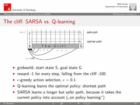
The cliff: SARSA vs. Q-learning
I gridworld, start state S, goal state G
I reward -1 for every step, falling from the cliff -100
I ε-greedy action selection, ε = 0.1
I Q-learning learns the optimal policy: shortest path
I SARSA learns a longer but safer path, because it takes thecurrent policy into account (
”on policy learning“)
N. Hendrich 80
University of Hamburg
MIN Faculty
Department of Informatics
Temporal-Difference Learning: Q-Learning and SARSA Reinforcement Learning (2)
The cliff: SARSA vs. Q-learning
I ε-greedy action selection, ε = 0.1
I therefore, risk of taking an explorative step off the cliff
N. Hendrich 81
University of Hamburg
MIN Faculty
Department of Informatics
Temporal-Difference Learning: Q-Learning and SARSA Reinforcement Learning (2)
Q-Learning - open questions
I often not met: Markov assumption, visibility of states
I continuous state-action spaces
I generalization concerning the state and action
I compromise between “exploration” and “exploitation”
I generalization of automatic evaluation
N. Hendrich 82
University of Hamburg
MIN Faculty
Department of Informatics
Temporal-Difference Learning: Q-Learning and SARSA Reinforcement Learning (2)
Backup diagrams: summary
I policy-evaluation, TD(0), SARSAI value-iteration, Q-learning
N. Hendrich 83
University of Hamburg
MIN Faculty
Department of Informatics
Temporal-Difference Learning: Q-Learning and SARSA Reinforcement Learning (2)
Ad-hoc Exploration-Strategies
I Too extensive “exploration” means, that the agent is acting aimlesslyin the usually very large state space even after a long learning period.Also areas are investigated, that are not relevant for the solution ofthe task.
I Too early “exploitation” of the learned approximation of theQ-function probably causes that a sub-optimal, i.e. longer paththrough the state space, that has been found by occasion establishesand the optimal solution will not be found.
There are:
I “greedy strategies”
I “randomized strategies”
I “interval-based techniques”
N. Hendrich 84
University of Hamburg
MIN Faculty
Department of Informatics
Acceleration of Learning Reinforcement Learning (2)
Acceleration of Learning
Some ad-hoc methods:
I Experience Replay
I Backstep Punishment
I Reward Distance Reduction
I Learner-Cascade
N. Hendrich 85
University of Hamburg
MIN Faculty
Department of Informatics
Acceleration of Learning Reinforcement Learning (2)
Experience Replay (1)
A path through the state space is considered as finished as soon asG is reached.Now assume that during the Q-learning the path is repeatedlychosen.
Often new learning steps are much more cost- and time-consumingthan internal repetitions of previously stored Learning steps. Forthese reasons it makes sense to store the learning steps and repeatthem internally. This method is called Experience Replay.
N. Hendrich 86
University of Hamburg
MIN Faculty
Department of Informatics
Acceleration of Learning Reinforcement Learning (2)
Experience Replay (2)
An experience e is a tuple
e = (s, s ′, a, r)
with s, s ′ ∈ S , a ∈ A, r ∈ IR. e represents a learning step, i.e. astate of transition, where s the initial state, s ′ the goal state, a theaction, which led to the state transition, and r the reinforcementsignal that is obtained.
A learning path is a series e1 . . . eLk of experiences (Lk is the lengthof the k-th learning path).
N. Hendrich 87
University of Hamburg
MIN Faculty
Department of Informatics
Acceleration of Learning Reinforcement Learning (2)
Experience Replay (3)
The ER-Algorithm:
for k = 1 to Nfor i = Lk down to 1
update( ei from series k)end for
end for
N. Hendrich 88
University of Hamburg
MIN Faculty
Department of Informatics
Acceleration of Learning Reinforcement Learning (2)
Experience Replay (4)
Advantages:
I Internal repetitions of stored learning steps usually cause farless cost than new learning steps.
I Internally a learning path can be used in the reverse direction,thus the information is spread faster.
I If learning paths cross, they can “learn form each other”, i.e.exchange information. Experience Replay makes this exchangeregardless of the order in which the learning path was firstlyexecuted.
N. Hendrich 89
University of Hamburg
MIN Faculty
Department of Informatics
Acceleration of Learning Reinforcement Learning (2)
Experience Replay - Example
Progression of the Q-values when the learning path is repeatedlyrun through:
N. Hendrich 90
University of Hamburg
MIN Faculty
Department of Informatics
Acceleration of Learning Reinforcement Learning (2)
Backstep Punishment
Usually an exploration strategy is needed, that ensures a straightforwardmovement of agents through the state space.Therefore backsteps should be avoided.An useful method seems to be, that in case the agent chooses abackstep, the agent may carry out this step but an artificial, negativereinforcement-signal is generated.Compromise between the “dead-end avoidance” and “fast learning”.
In context of a goal-oriented learning an extended reward function couldlook as follows:
rBP =
100 if transition to goal state
−1 if backstep
0 else
N. Hendrich 91
University of Hamburg
MIN Faculty
Department of Informatics
Acceleration of Learning Reinforcement Learning (2)
Reward Distance Reduction
The reward function could perform a more intelligent assessment of theactions. This presupposes knowledge of the structure of the state space.
If the encoding of the target state is known, then it can be a be goodstrategy to reduce the Euclidean distance between the current state andthe target state.The reward functions can be extended the way that actions that reducethe Euclidean distance to the target state, get a higher reward. (rewarddistance reduction, RDR):
rRDR =
100 if ~s ′ = ~sg
50 if |~s ′ −~sg | < |~s −~sg |0 else
where ~s, ~s ′ and ~sg are the vectors that encode the current state, the
following state, and the goal state.N. Hendrich 92
University of Hamburg
MIN Faculty
Department of Informatics
Acceleration of Learning Reinforcement Learning (2)
Learner-Cascade
The accuracy of positioning depends on how fine the state space isdivided.On the other hand the number of states increases with increasingfineness of the discretization and therefore also the effort oflearning increases.
Before the learning procedure a trade-off between effort andaccuracy of positioning has to be chosen.
N. Hendrich 93
University of Hamburg
MIN Faculty
Department of Informatics
Acceleration of Learning Reinforcement Learning (2)
Learner-Cascade - Variable Discretization
An example state space without discretization (a) with variablediscretization (b)
a) b)
This requires knowledge of the structure of the state space.
N. Hendrich 94
University of Hamburg
MIN Faculty
Department of Informatics
Acceleration of Learning Reinforcement Learning (2)
Learner-Cascade - n-Stage Learner-Cascade
Divisions of the state space of a four-stage learner cascade:
1. learner: 2. learner:
3. learner: 4. learner:
N. Hendrich 95
University of Hamburg
MIN Faculty
Department of Informatics
Acceleration of Learning Reinforcement Learning (2)
Q-Learning: Summary
I Q-Function
I Q-Learning algorithm
I convergence
I acceleration of learning
I examples
N. Hendrich 96
University of Hamburg
MIN Faculty
Department of Informatics
Applications in Robotics Reinforcement Learning (2)
Path Planning with Policy Iteration (1)
Policy iteration is used to find a path between start- andgoal-configuration.The following sets need to be defined to solve the problem.
I The state space S is the discrete configuration space, i.e. everycombination of joint angles (θ1, θ2, . . . , θDim) is exactly one state ofthe set S except the target configuration
I The set A(s) of all possible actions for a state s includes thetransitions to neighbor-configurations in the K-space, so one or morejoint angles differ by ±Dis. Only actions a in A(s) are included, thatdo not lead to K-obstacles and do not exceed the limits of theK-space
N. Hendrich 97
University of Hamburg
MIN Faculty
Department of Informatics
Applications in Robotics Reinforcement Learning (2)
Path Planning with Policy Iteration (2)
I Let Rass′ be the reward function:
Rass′ = Reward not in goal ∀s ∈ S , a ∈ A(s), s ′ ∈ S and
Rass′ = Reward in goal ∀s ∈ S , a ∈ A(s), s ′ = st .
Only if the target state is reached a different reward value isgenerated. For all other states there is the same reward.
I Let the policy π(s, a) be deterministic, i.e. there is exactly onea with π(s, a) = 1
I A threshold Θ needs to be chosen, where the policy evaluationterminates
I For the problem the Infinite-Horizon Discounted Model is thebest choice, therefore γ needs to be set accordingly.
N. Hendrich 98
University of Hamburg
MIN Faculty
Department of Informatics
Applications in Robotics Reinforcement Learning (2)
2-Joint Robot
The found sequence of motion for the 2-joint robot (left to right, top to
bottom):
N. Hendrich 99
University of Hamburg
MIN Faculty
Department of Informatics
Grasping with RL: Parallel Gripper Reinforcement Learning (2)
Grasping with RL: Partition of DOFs
Normally a robot arm needs six DOFs to grasp an object from anyposition and orientation.To grasp virtually planar objects, we suppose that the gripper isperpendicular to the table and its weight is known.There still remain three DOFs to control the robot arm: parallel tothe table-plane (x , y) and the rotation around the axisperpendicular to the table(θ).
N. Hendrich 100
University of Hamburg
MIN Faculty
Department of Informatics
Grasping with RL: Parallel Gripper Reinforcement Learning (2)
Grasping with RL: Partition of DOFs (2)
Control of x , y , θ. The pre-processed images will be centered forthe detection of the rotation.
N. Hendrich 101
University of Hamburg
MIN Faculty
Department of Informatics
Grasping with RL: Parallel Gripper Reinforcement Learning (2)
Grasping with RL: Partition of DOFs (3)
To achieve a small state space, learning will be distributed to twolearners:one for the translational movement on the plane,the other one for the rotational movement.The translation-learner can choose four actions (two in x- and two iny -direction).The rotation-learner can choose two actions (rotationclockwise/counterclockwise).The partition has advantages compared to a monolithic learner:
I The state space is much smaller.
I The state-encoding is designed the way that the state-vectors containonly the relevant information for the corresponding learner.
N. Hendrich 102
University of Hamburg
MIN Faculty
Department of Informatics
Grasping with RL: Parallel Gripper Reinforcement Learning (2)
Grasping with RL: Partition of DOFs (4)
In practice, the two learners will be used alternatingly. Firstly thetranslation-learner will be run in long learning-steps, until it has reachedthe goal defined in its state-encoding.Then the translation-learner is replaced by the rotation-learner, which isalso used in long learning-steps until it reaches its goal.
At this time it can happen, that the translation-learner is disturbed by
the rotation-learner. Therefore the translation-learner is activated once
again. The procedure is repeated, until both learners reach their goal
state. This state is the common goal state.
N. Hendrich 103
University of Hamburg
MIN Faculty
Department of Informatics
Grasping with RL: Parallel Gripper Reinforcement Learning (2)
Grasping with RL: Partition of DOFs (5)
(a) (b) (c)
(d) (e) (f)
Position and orientation-control with 6 DOFs in four steps.
N. Hendrich 104
University of Hamburg
MIN Faculty
Department of Informatics
Grasping with RL: Parallel Gripper Reinforcement Learning (2)
Grasping with RL: Partition of DOFs (6)
To use all six DOFs, additional learners need to be introduced.
1. The first learner has two DOFs and its task is that the objectcan be looked upon from a defined perspective. For a planetable this typically means, that the gripper is positionedperpendicularly to the surface of the table (a → b).
2. Apply the x/y learner (b → c).
3. Apply the θ rotation learner(c → d).
4. The last learner controls the height and corrects thez-coordinate (d → e).
N. Hendrich 105
University of Hamburg
MIN Faculty
Department of Informatics
Grasping with RL: Parallel Gripper Reinforcement Learning (2)
Visually Guided Grasping using Self-Evaluative Learning
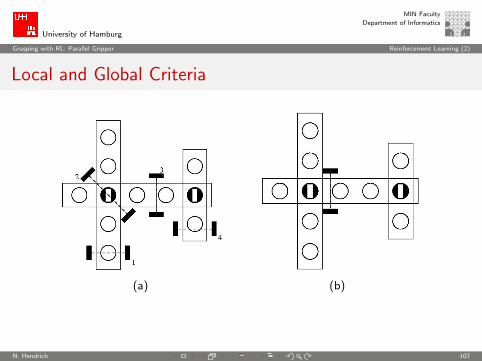
Grip is optimal with respect to local criteria:
I The fingers of the gripper can enclose the object at thegripping point
I No slip occurs between the fingers and object
Grip is optimal with respect to global criteria:
I No or minimal torque on fingers
I Object does not slip out of the gripper
I The grasp is stable, i.e. the object is held rigidly between thefingers
N. Hendrich 106
University of Hamburg
MIN Faculty
Department of Informatics
Grasping with RL: Parallel Gripper Reinforcement Learning (2)
Local and Global Criteria
(a) (b)
N. Hendrich 107
University of Hamburg
MIN Faculty
Department of Informatics
Grasping with RL: Parallel Gripper Reinforcement Learning (2)
Two approachesOne learner:
I The states consist of a set of m + n local and global properties:s = (fl1 , . . . , flm , fg1 , . . . , fgn).
I The learner tries to map them to actions a = (x , y , φ), where x and yare translational components in x- and y -direction and φ is therotational component around the approach vector of the gripper.
Two learners:
I The states for the first learner only supply the local propertiess = (fl1 , . . . , flm).
I The learner tries to map them to actions, that only consist of arotational component a = (φ).
I The second learner tries to map states of global propertiess = (fg1 , . . . , fgn) to actions concerning the translational componenta = (x , y).
N. Hendrich 108
University of Hamburg
MIN Faculty
Department of Informatics
Grasping with RL: Parallel Gripper Reinforcement Learning (2)
Setup
I Two-component learning system:
1. orientation learner 2. position learner
operates on local criteria operates on global criteria
equal for every object different for each new object
I Use of Multimodal sensors:I CameraI Force / torque sensor
I Both learners work together in the perception-action cycle.
N. Hendrich 109
University of Hamburg
MIN Faculty
Department of Informatics
Grasping with RL: Parallel Gripper Reinforcement Learning (2)
State Encoding
θ
L D COA
θ
θ θ
2 1
3 4
The orientation Lerner uses length L as well as the anglesΘ1, . . . ,Θ4, while the position learner uses the distance D betweenthe center of the gripper-line and the optical center of gravity ofthe object.
N. Hendrich 110
University of Hamburg
MIN Faculty
Department of Informatics
Grasping with RL: Parallel Gripper Reinforcement Learning (2)
Measures for Self-Evaluation in the Orientation Learner
Visual feedback of the grasp success:Friction results in rotation or misalignment of the object.
N. Hendrich 111
University of Hamburg
MIN Faculty
Department of Informatics
Grasping with RL: Parallel Gripper Reinforcement Learning (2)
Measures for Self-Evaluation in the Position Learner (1)
Feedback using force torque sensor:Unstable grasp – analyzed by force measurement
N. Hendrich 112
University of Hamburg
MIN Faculty
Department of Informatics
Grasping with RL: Parallel Gripper Reinforcement Learning (2)
Measures for Self-Evaluation in the Position Learner (2)
Suboptimal grasp – analyzed by torques
N. Hendrich 113
University of Hamburg
MIN Faculty
Department of Informatics
Grasping with RL: Parallel Gripper Reinforcement Learning (2)
The Problem of Hidden States
Examples for incomplete state information:
a) b) c) d)
N. Hendrich 114
University of Hamburg
MIN Faculty
Department of Informatics
Grasping mit RL: Barrett-Hand Reinforcement Learning (2)
Grasping mit RL: Barrett-Hand
I learn to grasp everyday objects with artificial robot hand
I reinforcement-learning process based on simulation
I find as many suitable grasps as possible
I support arbitrary type of objectsI efficiency
I memory usageI found grasps/episodes
N. Hendrich 115
University of Hamburg
MIN Faculty
Department of Informatics
Grasping mit RL: Barrett-Hand Reinforcement Learning (2)
BarretHand BH-262
I 3-finger robotic hand
I open/close each finger independently
I variable spread angle
I optical encoder
I force measurement
N. Hendrich 116
University of Hamburg
MIN Faculty
Department of Informatics
Grasping mit RL: Barrett-Hand Reinforcement Learning (2)
Applied model
States:
I pose of gripper to object
I spread angle of hand
I grasp tried yet
Actions:
I translation (x-axis, negative y-axis, z-axis)
I rotation(roll-axis, yaw-axis, pitch-axis)
I alteration of spread-angle
I grasp-execution
N. Hendrich 117
University of Hamburg
MIN Faculty
Department of Informatics
Grasping mit RL: Barrett-Hand Reinforcement Learning (2)
Applied model (cont.)
Action-Selection:
I ε-greedy (highest rated, with probability ε random)
Reward-Function:
I reward for grasps depend on stability
I stability is evaluated by wrench-space-calculation (GWS)(introduced 1992 by Ferrari and Canny)
I small negative reward if grasp unstable
I big negative reward if object is missed
r(s, a) =
−100 if number of contact points < 2−1 if GWS(g) = 0GWS(g) otherwise
N. Hendrich 118
University of Hamburg
MIN Faculty
Department of Informatics
Grasping mit RL: Barrett-Hand Reinforcement Learning (2)
Learning Strategy
Problem: The state-space is extremely large
I TD-(λ)-algorithm
I learning in episodesI episode ends
I after fixed number of stepsI after grasp trial
I Q-table built dynamically
I states are only included if they occur
N. Hendrich 119
University of Hamburg
MIN Faculty
Department of Informatics
Grasping mit RL: Barrett-Hand Reinforcement Learning (2)
Automatic Value Cutoff
Problem: There exist many terminal states (grasp can be executedevery time)
I instable grasps are tried several times
I agent gets stuck in local minimum
I not all grasps are found
=⇒ No learning at the end of an episode - waste of computingtimeThis can not simply be solved by adapting RL-parameters.
N. Hendrich 120
University of Hamburg
MIN Faculty
Department of Informatics
Grasping mit RL: Barrett-Hand Reinforcement Learning (2)
Automatic Value Cutoff (cont.)
Automatic Value Cutoff: remove actions
I leading to instable grasps (if reward negative)
I that have been evaluated sufficiently
Q(s, a)←
Q(s, a) + α
[r + γQ(s
′, a
′)− Q(s, a)
]if 0 ≤ Q(s, a) < r ∗ β
remove Q(s, a) from Q otherwise
with 0 ≤ β ≤ 1. (we had good results with β = 0.95)
N. Hendrich 121
University of Hamburg
MIN Faculty
Department of Informatics
Grasping mit RL: Barrett-Hand Reinforcement Learning (2)
Automatic Value Cutoff vs. no Cutoff
0
10
20
30
40
50
60
70
0 200 400 600 800 1000 1200 1400
Gri
ffe
Episode
Box 1 − NCOBox 1 − CO
Box 2 − NCOBox 2 − CO
Cylinder − NCOCylinder − COBanana − NCOBanana − CO
N. Hendrich 122
University of Hamburg
MIN Faculty
Department of Informatics
Grasping mit RL: Barrett-Hand Reinforcement Learning (2)
Reinforcement Learning vs. Brute Force: Mug
0
100
200
300
400
500
600
0 5000 10000 15000 20000
Gra
sps
Episodes
Mug top − BFMug top − RL
Mug side − BFMug side − RL
N. Hendrich 123
University of Hamburg
MIN Faculty
Department of Informatics
Grasping mit RL: Barrett-Hand Reinforcement Learning (2)
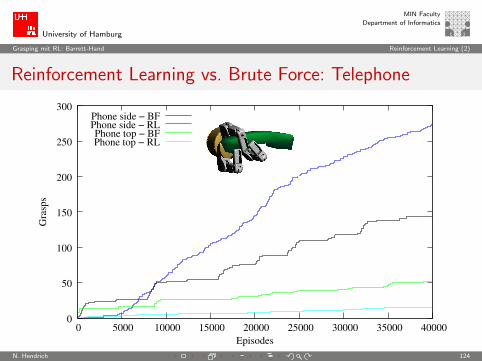
Reinforcement Learning vs. Brute Force: Telephone
0
50
100
150
200
250
300
0 5000 10000 15000 20000 25000 30000 35000 40000
Gra
sps
Episodes
Phone side − BFPhone side − RLPhone top − BFPhone top − RL
N. Hendrich 124
University of Hamburg
MIN Faculty
Department of Informatics
Grasping mit RL: Barrett-Hand Reinforcement Learning (2)
Experimental Results
Testing some grasps with the service robot TASER:
N. Hendrich 125
University of Hamburg
MIN Faculty
Department of Informatics
Grasping mit RL: Barrett-Hand Reinforcement Learning (2)