Reinforcement Learning and Optimal ControlASU, CSE 691...

Reinforcement Learning and Optimal Control

ASU, CSE 691, Winter 2019

Dimitri P. [email protected]

Lecture 11

Bertsekas Reinforcement Learning 1 / 26

Outline

1 Introduction to Aggregation

2 Aggregation with Representative States: A Form of Discretization

3 Aggregation with Representative Features

4 Examples of Feature-Based Aggregation

5 What is the Aggregate Problem and How Do We Solve It?


Aggregation within the Approximation in Value Space Framework

Approximations: Replace E{·} with nominal values (certainty equiv-alent control)

minuk,µk+1,...,µk+ℓ−1

E

!gk(xk, uk, wk) +

k+ℓ−1"

m=k+1

gk

#xm, µm(xm), wm

$+ Jk+ℓ(xk+ℓ)

%

First ℓ Steps “Future”Nonlinear Ay(x) + b φ1(x, v) φ2(x, v) φm(x, v) r x Initial

Selective Depth Lookahead Tree σ(ξ) ξ 1 0 -1 Encoding y(x)

Linear Layer Parameter v = (A, b) Sigmoidal Layer Linear WeightingCost Approximation r′φ(x, v)

Feature Extraction Features: Material Balance, uk = µdk

#xk(Ik)

$

Mobility, Safety, etc Weighting of Features Score Position EvaluatorStates xk+1 States xk+2

State xk Feature Vector φk(xk) Approximator r′kφk(xk)

x0 xk im−1 im . . . (0, 0) (N, −N) (N, 0) i (N, N) −N 0 g(i) I N − 2N i

s i1 im−1 im . . . (0, 0) (N, −N) (N, 0) i (N, N) −N 0 g(i) I N − 2 Ni

u1k u2

k u3k u4

k Selective Depth Adaptive Simulation Tree Projections ofLeafs of the Tree

p(j1) p(j2) p(j3) p(j4)

Neighbors of im Projections of Neighbors of im

State x Feature Vector φ(x) Approximator φ(x)′r

ℓ Stages Riccati Equation Iterates P P0 P1 P2 γ2 − 1 γ2PP+1

1

Approximations:

Replace E{·} with nominal values

(certainty equivalent control)


E

!gk(xk, uk, wk) +

k+ℓ−1"

m=k+1

gk

#xm, µm(xm), wm

$+ Jk+ℓ(xk+ℓ)

%





#xk(Ik)

$





u1k u2

k u3k u4


p(j1) p(j2) p(j3) p(j4)


State x Feature Vector φ(x) Approximator φ(x)′r

1

Approximations: Computation of Jk+ℓ:

DP minimization Replace E{·} with nominal values

(certainty equivalent control)

Limited simulation (Monte Carlo tree search)

Simple choices Parametric approximation Problem approximation

Rollout


E

!gk(xk, uk, wk) +

k+ℓ−1"

m=k+1

gk

#xm, µm(xm), wm

$+ Jk+ℓ(xk+ℓ)

%





#xk(Ik)

$





u1k u2

k u3k u4


p(j1) p(j2) p(j3) p(j4)

1

Approximations: Computation of Jk+ℓ: (Could be approximate)

DP minimization Replace E{·} with nominal values

(certainty equivalent control) Computation of Jk+1:



Rollout

minuk

E!

gk(xk, uk, wk) + Jk+1(xk+1)"


E

#gk(xk, uk, wk) +

k+ℓ−1$

m=k+1

gk

%xm, µm(xm), wm

&+ Jk+ℓ(xk+ℓ)

'

First ℓ Steps “Future” First StepNonlinear Ay(x) + b φ1(x, v) φ2(x, v) φm(x, v) r x Initial




%xk(Ik)

&





u1k u2

k u3k u4


1


Approximate minimization Replace E{·} with nominal values




Rollout

minuk

E!



E

#gk(xk, uk, wk) +

k+ℓ−1$

m=k+1

gk

%xm, µm(xm), wm

&+ Jk+ℓ(xk+ℓ)

'





%xk(Ik)

&





u1k u2

k u3k u4


1


Approximate minimization Replace E{·} with nominal values




Rollout Model Predictive Control

minuk

E!



E

#gk(xk, uk, wk) +

k+ℓ−1$

m=k+1

gk

%xm, µm(xm), wm

&+ Jk+ℓ(xk+ℓ)

'





%xk(Ik)

&





u1k u2

k u3k u4


1

s t j1 j2 j` j`�1 j1

Nodes j 2 A(j`) Path Pj , Length Lj · · ·

Aggregation

Is di + aij < UPPER � hj?

�jf = 1 if j 2 If x0 a 0 1 2 t b C Destination

J(xk) ! 0 for all p-stable ⇡ from x0 with x0 2 X and ⇡ 2 Pp,x0 Wp+ = {J 2 J | J+ J} Wp+ from

within Wp+

Prob. u Prob. 1 � u Cost 1 Cost 1 �pu

J(1) = min�c, a + J(2)

J(2) = b + J(1)

J⇤ Jµ Jµ0 Jµ00Jµ0 Jµ1 Jµ2 Jµ3 Jµ0

f(x; ✓k) f(x; ✓k+1) xk F (xk) F (x) xk+1 F (xk+1) xk+2 x⇤ = F (x⇤) Fµk(x) Fµk+1

(x)

Improper policy µ

Proper policy µ

1

s t j1 j2 j` j`�1 j1


Aggregation Adaptive simulation Monte-Carlo Tree Search




within Wp+


J(1) = min�c, a + J(2)

J(2) = b + J(1)



(x)

Improper policy µ

Proper policy µ

1

s t j1 j2 j` j`�1 j1


Aggregation Adaptive simulation Monte-Carlo Tree Search (certainty equivalence)




within Wp+


J(1) = min�c, a + J(2)

J(2) = b + J(1)



(x)

Improper policy µ

Proper policy µ

1

Monte Carlo tree search

Node Subset S1 SN Aggr. States Stage 1 Stage 2 Stage 3 Stage N �1

Candidate (m+2)-Solutions (u1, . . . , um, um+1, um+2) (m+2)-Solution

Set of States (u1) Set of States (u1, u2) Set of States (u1, u2, u3)

Run the Heuristics From Each Candidate (m+2)-Solution (u1, . . . , um, um+1)

Set of States (u1) Set of States (u1, u2)

Set of States u = (u1, . . . , uN ) Current m-Solution (u1, . . . , um)

Cost G(u) Heuristic N -Solutions u = (u1, . . . , uN�1)

Candidate (m + 1)-Solutions (u1, . . . , um, um+1)

Cost G(u) Heuristic N -Solutions

Piecewise Constant Aggregate Problem Approximation

Artificial Start State End State


Feature Vector F (i) Aggregate Cost Approximation Cost Jµ

�F (i)

�

R1 R2 R3 R` Rq�1 Rq r⇤q�1 r⇤3 Cost Jµ

�F (i)

�

I1 I2 I3 I` Iq�1 Iq r⇤2 r⇤3 Cost Jµ

�F (i)

�

Aggregate States Scoring Function V (i) J⇤(i) 0 n n� 1 State i Cost

function Jµ(i)I1 ... Iq I2 g(i, u, j)...

TD(1) Approximation TD(0) Approximation V1(i) and V0(i)

Aggregate Problem Approximation TD(0) Approximation V1(i) andV0(i)

�jf =

⇢1 if j 2 If

0 if j /2 If

1 10 20 30 40 50 I1 I2 I3 i J1(i)

(May Involve a Neural Network) (May Involve Aggregation)

dì = 0 if i /2 I`

�j ¯ = 1 if j 2 I¯

pff (u) =nX

i=1

dfi

nX

j=1

pij(u)�jf

1

minu∈U(i)

!nj=1 pij(u)

"g(i, u, j) + J(j)

#Computation of J :

Cost 0 Cost g(i, u, j) Monte Carlo tree search

Node Subset S1 SN Aggr. States Stage 1 Stage 2 Stage 3 Stage N −1






Cost G(u) Heuristic N -Solutions u = (u1, . . . , uN−1)







"F (i)

#

R1 R2 R3 Rℓ Rq−1 Rq r∗q−1 r∗

3 Cost Jµ

"F (i)

#

I1 I2 I3 Iℓ Iq−1 Iq r∗2 r∗

3 Cost Jµ

"F (i)

#

Aggregate States Scoring Function V (i) J∗(i) 0 n n − 1 State i Cost




φjf =

$1 if j ∈ If

0 if j /∈ If

1 10 20 30 40 50 I1 I2 I3 i J1(i)


dℓi = 0 if i /∈ Iℓ

φjℓ = 1 if j ∈ Iℓ

pff(u) =

n%

i=1

dfi

n%

j=1

pij(u)φjf

1

minu∈U(i)

!nj=1 pij(u)

"g(i, u, j) + J(j)

#Computation of J :

Cost 0 Cost g(i, u, j) Monte Carlo tree search First Step “Future”














"F (i)

#


3 Cost Jµ

"F (i)

#


3 Cost Jµ

"F (i)

#





φjf =

$1 if j ∈ If

0 if j /∈ If

1 10 20 30 40 50 I1 I2 I3 i J1(i)




pff(u) =

n%

i=1

dfi

n%

j=1

pij(u)φjf

1

minu∈U(i)

!nj=1 pij(u)

"g(i, u, j) + J(j)

#Computation of J :

Cost 0 Cost g(i, u, j) Monte Carlo tree search First Step “Future”














"F (i)

#


3 Cost Jµ

"F (i)

#


3 Cost Jµ

"F (i)

#





φjf =

$1 if j ∈ If

0 if j /∈ If

1 10 20 30 40 50 I1 I2 I3 i J1(i)




pff(u) =

n%

i=1

dfi

n%

j=1

pij(u)φjf

1

⇡/4 Sample State xsk Sample Control us

k Sample Next State xsk+1 Sample Transition Cost gs

k Simulator

Approximate PI Range of Weighted Projections

Sample Q-Factor �sk = gs

k + Jk+1(xsk+1) Jk+1

Policy Q-Factor Evaluation Evaluate Q-Factor Qµ of Current policy µ Width (✏ + 2↵�)/(1 � ↵)

Random Transition xk+1 = fk(xk, uk, wk) Random Cost gk(xk, uk, wk)

Control v (j, v) Cost = 0 State-Control Pairs Transitions under policy µ Evaluate Cost Function

Variable Length Rollout Selective Depth Rollout Policy µ Adaptive Simulation Terminal Cost Function

Limited Rollout Selective Depth Adaptive Simulation Policy µ Approximation J

u Qk(xk, u) Qk(xk, u) uk uk Qk(xk, u) � Qk(xk, u)

x0 xk x1k+1 x2

k+1 x3k+1 x4

k+1 States xN Base Heuristic ik States ik+1 States ik+2

Initial State 15 1 5 18 4 19 9 21 25 8 12 13 c(0) c(k) c(k + 1) c(N � 1) Parking Spaces

Stage 1 Stage 2 Stage 3 Stage N N � 1 c(N) c(N � 1) k k + 1

Heuristic Cost Heuristic “Future” System xk+1 = fk(xk, uk, wk) xk Observations

Belief State pk Controller µk Control uk = µk(pk) . . . Q-Factors Current State xk

x0 x1 xk xN x0N x00

N uk u0k u00

k xk+1 x0k+1 x00

k+1

Initial State x0 s Terminal State t Length = 1

x0 a 0 1 2 t b C Destination


within Wp+


J(1) = min�c, a + J(2)

J(2) = b + J(1)

1

minu2U(i)

nX

j=1

pij(u)�g(i, u, j) + ↵J(j)

�

⇡/4 Sample State xsk Sample Control us


k Simulator

Critic Actor Approximate PI Range of Weighted Projections

Sample Q-Factor �sk = gs


Policy Q-Factor Evaluation Evaluate Q-Factor Qµ of Current policy µ Width (✏ + 2↵�)/(1 � ↵)





u Qk(xk, u) Qk(xk, u) uk uk Qk(xk, u) � Qk(xk, u)

x0 xk x1k+1 x2

k+1 x3k+1 x4


Initial State 15 1 5 18 4 19 9 21 25 8 12 13 c(0) c(k) c(k + 1) c(N � 1) Parking Spaces

Stage 1 Stage 2 Stage 3 Stage N N � 1 c(N) c(N � 1) k k + 1



x0 x1 xk xN x0N x00

N uk u0k u00

k xk+1 x0k+1 x00

k+1




within Wp+

1

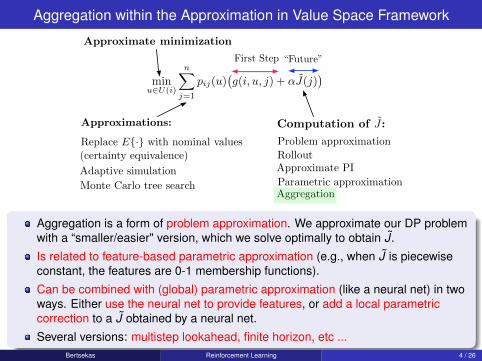
Aggregation is a form of problem approximation. We approximate our DP problemwith a “smaller/easier" version, which we solve optimally to obtain J.

Is related to feature-based parametric approximation (e.g., when J is piecewiseconstant, the features are 0-1 membership functions).

Can be combined with (global) parametric approximation (like a neural net) in twoways. Either use the neural net to provide features, or add a local parametriccorrection to a J obtained by a neural net.

Several versions: multistep lookahead, finite horizon, etc ...Bertsekas Reinforcement Learning 4 / 26

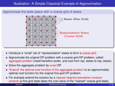
Illustration: A Simple Classical Example of Approximation

Approximate the state space with a coarse grid of states minu∈U(i)

n!

j=1

pij(u)"g(i, u, j) + αJ(j)

#

π/4 Sample State xsk Sample Control us


k Simulator

Representative States Critic Actor Approximate PI Range of Weighted Projections

Sample Q-Factor βsk = gs


Policy Q-Factor Evaluation Evaluate Q-Factor Qµ of Current policy µ Width (ϵ + 2αδ)/(1 − α)





u Qk(xk, u) Qk(xk, u) uk uk Qk(xk, u) − Qk(xk, u)

x0 xk x1k+1 x2

k+1 x3k+1 x4


Initial State 15 1 5 18 4 19 9 21 25 8 12 13 c(0) c(k) c(k + 1) c(N − 1) Parking Spaces

Stage 1 Stage 2 Stage 3 Stage N N − 1 c(N) c(N − 1) k k + 1



x0 x1 xk xN x′N x′′

N uk u′k u′′

k xk+1 x′k+1 x′′

k+1



J(xk) → 0 for all p-stable π from x0 with x0 ∈ X and π ∈ Pp,x0 Wp+ = {J ∈ J | J+ ≤ J} Wp+ from

within Wp+

1

minu∈U(i)

n!

j=1


#



k Simulator

Representative States (Coarse Grid) Critic Actor Approximate PI

Range of Weighted Projections States (Fine Grid)









x0 xk x1k+1 x2

k+1 x3k+1 x4







N uk u′k u′′

k xk+1 x′k+1 x′′

k+1



1

minu∈U(i)

n!

j=1


#



k Simulator











x0 xk x1k+1 x2

k+1 x3k+1 x4







N uk u′k u′′

k xk+1 x′k+1 x′′

k+1



1

Introduce a “small" set of “representative" states to form a coarse grid.

Approximate the original DP problem with a coarse-grid DP problem, calledaggregate problem (need transition probs. and cost from rep. states to rep. states).

Solve the aggregate problem by exact DP.

“Extend" the optimal cost function of the aggregate problem to an approximatelyoptimal cost function for the original fine-grid DP problem.

For example extend the solution by a nearest neighbor/piecewise constantscheme (a fine grid state takes the cost value of the “nearest" coarse grid state).


Approximate the Problem by “Projecting" it onto Representative States

x j1 j2 j3 y1 y2 y3

⇤ |⇥| (1 � ⇤)|⇥| l(1 � ⇤)⇥| ⇤⇥ O A B C |1 � ⇤⇥|Asynchronous Initial state x Initial state f(x, u,w) TimeVk: k-stages optimal cost vector with terminal cost function J

TJ J0

Vk+1: (k + 1)-stages optimal cost vector with terminal cost functionJ

Direct Method: Projection of cost vector Jµ �Jµ n t pnn(u) pin(u)pni(u) pjn(u) pnj(u)

Indirect Method: Solving a projected form of Bellman’s equation

Projection on S. Solution of projected equation ⇥r = �T(�)µ (⇥r)

Tµ(⇥r) ⇥r = �T(�)µ (⇥r)

�Jµ n t pnn(u) pin(u) pni(u) pjn(u) pnj(u)

J TJ �TJ J T J �T J

Value Iterate T (⇥rk) = g + �P⇥rk Projection on S ⇥rk ⇥rk+1

Solution of Jµ = �Tµ(Jµ) ⇤ = 0 ⇤ = 1 0 < ⇤ < 1

Route to Queue 2h�(n) ⇤� ⇤µ ⇤ hµ,�(n) = (⇤µ � ⇤)Nµ(n)n � 1 �(n � 1) Cost = 1 Cost = 2 u = 2 Cost = -10 µ�(i + 1) µ µ p

1 0 ⌅j(u), pjk(u) ⌅k(u), pki(u) J�(p) µ1 µ2

Simulation error Solution of Jµ = WTµ(Jµ) Bias �Jµ Slope Jµ =⇥rµ

Transition diagram and costs under policy {µ⇥, µ⇥, . . .} M q(µ)

c + Ez

⇤J�

�pf0(z)

pf0(z) + (1 � p)f1(z)

⇥⌅

Cost = 0 Cost = �1

⇥i(u)pij(u)⇥

⇥j(u)pjk(u)⇥

⇥k(u)pki(u)⇥

J(2) = g(2, u2) + �p21(u2)J(1) + �p22(u2)J(2)

J(2) = g(2, u1) + �p21(u1)J(1) + �p22(u1)J(2)

1

x j1 j2 j3 y1 y2 y3


TJ J0





Tµ(⇥r) ⇥r = �T(�)µ (⇥r)









c + Ez

⇤J�

�pf0(z)

pf0(z) + (1 � p)f1(z)

⇥⌅


⇥i(u)pij(u)⇥

⇥j(u)pjk(u)⇥

⇥k(u)pki(u)⇥

J(2) = g(2, u2) + �p21(u2)J(1) + �p22(u2)J(2)

J(2) = g(2, u1) + �p21(u1)J(1) + �p22(u1)J(2)

1

x j1 j2 j3 y1 y2 y3


TJ J0





Tµ(⇥r) ⇥r = �T(�)µ (⇥r)









c + Ez

⇤J�

�pf0(z)

pf0(z) + (1 � p)f1(z)

⇥⌅


⇥i(u)pij(u)⇥

⇥j(u)pjk(u)⇥

⇥k(u)pki(u)⇥

J(2) = g(2, u2) + �p21(u2)J(1) + �p22(u2)J(2)

J(2) = g(2, u1) + �p21(u1)J(1) + �p22(u1)J(2)

1

x j1 j2 j3 y1 y2 y3


TJ J0





Tµ(⇥r) ⇥r = �T(�)µ (⇥r)









c + Ez

⇤J�

�pf0(z)

pf0(z) + (1 � p)f1(z)

⇥⌅


⇥i(u)pij(u)⇥

⇥j(u)pjk(u)⇥

⇥k(u)pki(u)⇥

J(2) = g(2, u2) + �p21(u2)J(1) + �p22(u2)J(2)

J(2) = g(2, u1) + �p21(u1)J(1) + �p22(u1)J(2)

1

x j1 j2 j3 y1 y2 y3


TJ J0





Tµ(⇥r) ⇥r = �T(�)µ (⇥r)









c + Ez

⇤J�

�pf0(z)

pf0(z) + (1 � p)f1(z)

⇥⌅


⇥i(u)pij(u)⇥

⇥j(u)pjk(u)⇥

⇥k(u)pki(u)⇥

J(2) = g(2, u2) + �p21(u2)J(1) + �p22(u2)J(2)

J(2) = g(2, u1) + �p21(u1)J(1) + �p22(u1)J(2)

1

x j1 j2 j3 y1 y2 y3


TJ J0





Tµ(⇥r) ⇥r = �T(�)µ (⇥r)









c + Ez

⇤J�

�pf0(z)

pf0(z) + (1 � p)f1(z)

⇥⌅


⇥i(u)pij(u)⇥

⇥j(u)pjk(u)⇥

⇥k(u)pki(u)⇥

J(2) = g(2, u2) + �p21(u2)J(1) + �p22(u2)J(2)

J(2) = g(2, u1) + �p21(u1)J(1) + �p22(u1)J(2)

1

minu∈U(i)

n!

j=1


#



k Simulator











x0 xk x1k+1 x2

k+1 x3k+1 x4







N uk u′k u′′

k xk+1 x′k+1 x′′

k+1



1

minu∈U(i)

n!

j=1


#



k Simulator


Range of Weighted Projections States (Fine Grid) Original State Space









x0 xk x1k+1 x2

k+1 x3k+1 x4







N uk u′k u′′

k xk+1 x′k+1 x′′

k+1



1

minu∈U(i)

n!

j=1


#



k Simulator





x pxj1(u) pxj2(u) pxj3(u)







x0 xk x1k+1 x2

k+1 x3k+1 x4







N uk u′k u′′

k xk+1 x′k+1 x′′

k+1


1

minu∈U(i)

n!

j=1


#



k Simulator












x0 xk x1k+1 x2

k+1 x3k+1 x4







N uk u′k u′′

k xk+1 x′k+1 x′′

k+1


1

minu∈U(i)

n!

j=1


#



k Simulator












x0 xk x1k+1 x2

k+1 x3k+1 x4







N uk u′k u′′

k xk+1 x′k+1 x′′

k+1


1

minu∈U(i)

n!

j=1


#



k Simulator





x pxj1(u) pxj2(u) pxj3(u) φj1y1 φj1y2 φj1y3







x0 xk x1k+1 x2

k+1 x3k+1 x4







N uk u′k u′′

k xk+1 x′k+1 x′′

k+1


1

minu∈U(i)

n!

j=1


#



k Simulator












x0 xk x1k+1 x2

k+1 x3k+1 x4







N uk u′k u′′

k xk+1 x′k+1 x′′

k+1


1

minu∈U(i)

n!

j=1


#



k Simulator












x0 xk x1k+1 x2

k+1 x3k+1 x4







N uk u′k u′′

k xk+1 x′k+1 x′′

k+1


1

minu∈U(i)

n!

j=1


#



k Simulator

Representative States x (Coarse Grid) Critic Actor Approximate PI











x0 xk x1k+1 x2

k+1 x3k+1 x4







N uk u′k u′′

k xk+1 x′k+1 x′′

k+1


1

minu∈U(i)

n!

j=1


#i = x Ix



k Simulator

Representative States x (Coarse Grid) Critic Actor Approximate PI Aggregate Problem

pxy(u) =n!

i=1

pxj(u)φjy g(x, u) =n!

j=1

pxj(u)g(x, u, j)

Range of Weighted Projections Original States States (Fine Grid) Original State Space

dxi = 0 for i /∈ Ix φjy = 1 for j ∈ Iy

x pxj1(u) pxj2(u) pxj3(u) φj1y1 φj1y2 φj1y3 φjy Aggregation Probabilities Relate to


Random Transition xk+1 = fk(xk, uk, wk) Random Cost gk(xk, uk, wk) Representative Features





x0 xk x1k+1 x2

k+1 x3k+1 x4






1

minu∈U(i)

n!

j=1


#i = x Ix



k Simulator


pxy(u) =n!

i=1


j=1

pxj(u)g(x, u, j)



x pxj1(u) pxj2(u) pxj3(u) φj1y1 φj1y2 φj1y3 φjy with Aggregation Probabilities Relate to







x0 xk x1k+1 x2

k+1 x3k+1 x4






1

S1 S2 S3 Sℓ Sm−1 Sm

Sx1 Sxℓ Sxm x1 xℓ xm r∗x1 r∗

xℓ r∗xm Footprint Sets J(i) J(j) =

!y∈A φjyr∗

y

minu∈U(i)

n"

j=1

pij(u)#g(i, u, j) + αJ(j)

$i = x Ix



k Simulator


pxy(u) =

n"

i=1

pxj(u)φjy g(x, u) =

n"

j=1

pxj(u)g(x, u, j)

Range of Weighted Projections J∗(i) Original States States (Fine Grid) Original State Space

dxi = 0 for i /∈ Ix φjy = 1 for j ∈ Iy φjy = 0 or 1 for all j and y Each j connects to a single x

x pxj1(u) pxj2(u) pxj3(u) φj1y1 φj1y2 φj1y3 φjy with Aggregation Probabilities Relate to Rm r∗m−1 r∗

m







x0 xk x1k+1 x2

k+1 x3k+1 x4




1




!y∈A φjyr∗

y

minu∈U(i)

n"

j=1


$i = x Ix



k Simulator


pxy(u) =

n"

i=1


n"

j=1

pxj(u)g(x, u, j)




m







x0 xk x1k+1 x2

k+1 x3k+1 x4




1




!y∈A φjyr∗

y

minu∈U(i)

n"

j=1


$i = x Ix



k Simulator


pxy(u) =

n"

i=1


n"

j=1

pxj(u)g(x, u, j)

Range of Weighted Projections J∗(i) Original States to States (Fine Grid) Original State Space



m







x0 xk x1k+1 x2

k+1 x3k+1 x4




1

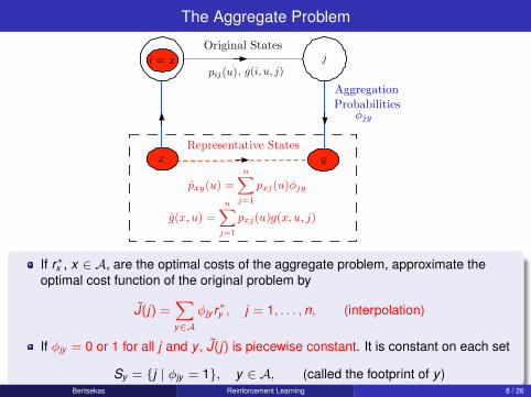
Introduce a finite subset of “representative states" A ⊂ {1, . . . , n}. We denotethem by x and y .

Original system states j are related to rep. states y ∈ A with aggregationprobabilities φjy (“weights" satisfying φjy ≥ 0,

∑y∈A φjy = 1).

Aggregation probabilities express “similarity" or “proximity" of original to rep.states.

Aggregate dynamics: Transition probabilities between rep. states x , y

pxy (u) =n∑

i=1

pxj(u)φjy

Expected cost at rep. state x under control u:

g(x , u) =n∑

j=1

pxj(u)g(x , u, j)


The Aggregate Problem

376 Approximate Dynamic Programming Chap. 6

soft aggregation, we allow the aggregate states/subsets to overlap, with thedisaggregation probabilities dxi quantifying the “degree of membership” ofi in the aggregate state/subset x. Other important aggregation possibilitiesinclude various discretization schemes (see Examples 6.3.12-6.3.13 of Vol.I).

Given the disaggregation and aggregation probabilities, dxi and φjy ,and the original transition probabilities pij(u), we define an aggregate sys-tem where state transitions occur as follows:

(i) From aggregate state x, generate original system state i according todxi.

(ii) Generate a transition from i to j according to pij(u), with costg(i, u, j).

(iii) From state j, generate aggregate state y according to φjy .

Then, the transition probability from aggregate state x to aggregate state yunder control u, and the corresponding expected transition cost, are givenby

pxy(u) =

n!

i=1

dxi

n!

j=1

pij(u)φjy , g(x, u) =

n!

i=1

dxi

n!

j=1

pij(u)g(i, u, j).

These transition probabilities and costs define the aggregate problem. Af-ter solving for the Q-factors Q(x, u), x ∈ S, u ∈ U , of the aggregateproblem using one of our algorithms, the Q-factors of the original problemare approximated by

Q(j, u) =!

y∈S

φjyQ(y, u), j = 1, . . . , n, u ∈ U, (6.91)

We recognize this as an approximate representation Q of the Q-factors ofthe original problem in terms of basis functions. There is a basis functionfor each aggregate state y ∈ S (the vector {φjy | j = 1, . . . , n}), and thecorresponding coefficients that weigh the basis functions are the Q-factorsof the aggregate problem Q(y, u), y ∈ S, u ∈ U .

Let us now apply Q-learning to the aggregate problem. We generatean infinitely long sequence of pairs {(xk, uk)} ⊂ S × U according to someprobabilistic mechanism. For each (xk, uk), we generate an original systemstate ik according to the disaggregation probabilities dxki, and then a suc-cessor state jk according to probabilities pikj(uk). We finally generate anaggregate system state yk using the aggregation probabilities φjky. Thenthe Q-factor of (xk, uk) is updated using a stepsize γk > 0 while all otherQ-factors are left unchanged [cf. Eqs. (6.78)-(6.80)]:

Qk+1(x, u) = (1 − γk)Qk(x, u) + γk(FkQk)(x, u), ∀ (x, u), (6.92)








pxy(u) =

n!

i=1

dxi

n!

j=1


n!

i=1

dxi

n!

j=1

pij(u)g(i, u, j).


Q(j, u) =!

y∈S

φjyQ(y, u), j = 1, . . . , n, u ∈ U, (6.91)











pxy(u) =

n!

i=1

dxi

n!

j=1


n!

i=1

dxi

n!

j=1

pij(u)g(i, u, j).


Q(j, u) =!

y∈S

φjyQ(y, u), j = 1, . . . , n, u ∈ U, (6.91)











pxy(u) =

n!

i=1

dxi

n!

j=1


n!

i=1

dxi

n!

j=1

pij(u)g(i, u, j).


Q(j, u) =!

y∈S

φjyQ(y, u), j = 1, . . . , n, u ∈ U, (6.91)




g(x, u) =

n⌥

i=1

dxi

n⌥

j=1

pij(u)g(i, u, j)

, g(i, u, j)Matrix D Matrix ⇥ y1 y2 y3 System Space State i µ(i, r) µ(·, r) Policy

Qµ(i, u, r) Jµ(i, r) G(r) Transition Matrix P (r) Controller Control

Evaluate Approximate Cost Steady-State Distribution ⌅(r) AverageCost ⇥(r)

⇧j1y1 ⇧j1y2 ⇧j1y3 j1 j2 j3 y1 y2 y3 Original State Space

⇥ =

�⇧⇧⇧⇧⇧⇧⇧⇧⇧⇧⇧⇤

1 0 0 01 0 0 00 1 0 01 0 0 01 0 0 00 1 0 00 0 1 00 0 1 00 0 0 1

⇥⌃⌃⌃⌃⌃⌃⌃⌃⌃⌃⌃⌅

1 2 3 4 5 6 7 8 9 x1 x2 x3 x4

⇤ |�| (1 � ⇤)|�| l(1 � ⇤)�| ⇤� O A B C |1 � ⇤�|Asynchronous Initial state Decision µ(i) x Initial state f(x, u,w)

TimeVk: k-stages optimal cost vector with terminal cost function J

TJ J0





Tµ(⇥r) ⇥r = �T(�)µ (⇥r)


1

minu∈U(i)

n!

j=1


#



k Simulator


pxy(u) =n!

i=1


j=1

pxj(u)g(x, u, j)











x0 xk x1k+1 x2

k+1 x3k+1 x4






1

minu∈U(i)

n!

j=1


#i = x



k Simulator


pxy(u) =n!

i=1


j=1

pxj(u)g(x, u, j)











x0 xk x1k+1 x2

k+1 x3k+1 x4






1

minu∈U(i)

n!

j=1


#i = x



k Simulator


pxy(u) =n!

i=1


j=1

pxj(u)g(x, u, j)











x0 xk x1k+1 x2

k+1 x3k+1 x4






1

minu∈U(i)

n!

j=1


#i = x



k Simulator


pxy(u) =n!

i=1


j=1

pxj(u)g(x, u, j)











x0 xk x1k+1 x2

k+1 x3k+1 x4






1

minu∈U(i)

n!

j=1


#i = x



k Simulator


pxy(u) =n!

i=1


j=1

pxj(u)g(x, u, j)




x pxj1(u) pxj2(u) pxj3(u) φj1y1 φj1y2 φj1y3 φjy Aggregation Probabilities







x0 xk x1k+1 x2

k+1 x3k+1 x4






1

minu∈U(i)

n!

j=1


#i = x



k Simulator


pxy(u) =n!

i=1


j=1

pxj(u)g(x, u, j)











x0 xk x1k+1 x2

k+1 x3k+1 x4






1

minu∈U(i)

n!

j=1


#i = x



k Simulator


pxy(u) =n!

i=1


j=1

pxj(u)g(x, u, j)











x0 xk x1k+1 x2

k+1 x3k+1 x4






1




!y∈A φjyr∗

y

minu∈U(i)

n"

j=1


$i = x Ix



k Simulator


pxy(u) =

n"

j=1


n"

j=1

pxj(u)g(x, u, j)




m







x0 xk x1k+1 x2

k+1 x3k+1 x4




1

If r∗x , x ∈ A, are the optimal costs of the aggregate problem, approximate theoptimal cost function of the original problem by

J(j) =∑y∈A

φjy r∗y , j = 1, . . . , n, (interpolation)

If φjy = 0 or 1 for all j and y , J(j) is piecewise constant. It is constant on each set

Sy = {j | φjy = 1}, y ∈ A, (called the footprint of y )Bertsekas Reinforcement Learning 8 / 26

The Piecewise Constant Case (φjy = 0 or 1 for all j , y )

J(x, r) =Pm

`=1 r`�`(x) x S1 S` Sm . . .

↵N�3 ↵N�2 · · · 1 � C

L0

· · · � �N�3 �N�2 � · · · � C

L1

L0L1

L0 + L1

1 � 1C I + AN�1(p) ↵N�1 0 I 1 p C JN�1(p) L0

L0+L1

↵N�2 ↵N�3 0 I 1 p C C + AN�2(p) C + AN�3(p)

(1 � p)C I + AN�1(p) ↵N�1 0 I 1 p C

(1�p)L0 pL1 L R R 1 t Delay Actuator Estimator System Measure-ment

Accept f1 Accept f2 Continue Terminate Instruction Accept

L L R R 1 t 1 � t r 1 � r µk E{xk | Ik} �k�1

Lk uk wk xk vk zk uk�1 µk E{xk | Ik} �k�1

xk+1 = Akxk + Bkuk + wk zk = Ckxk + vk

uk wk xk vk zk uk�1 µk Pxk | IkG

xk+1 = fk(xk, uk, wk) zk = hk(xk, uk�1, vk)

µk Delay Actuator Estimator System Measurement

State Transition Inspection

P P 2/3 3/4 1/3 1 1/4 B G

x ↵k Jk(xk) E{Jk+1(�x + ⇠k)} xN�1 ⇠ �xN�1 + ⇠ ↵N�1 ↵2


1

J(x, r) =Pm

`=1 r`�`(x) x S1 S` Sm . . .

↵N�3 ↵N�2 · · · 1 � C

L0

· · · � �N�3 �N�2 � · · · � C

L1

L0L1

L0 + L1

1 � 1C I + AN�1(p) ↵N�1 0 I 1 p C JN�1(p) L0

L0+L1

↵N�2 ↵N�3 0 I 1 p C C + AN�2(p) C + AN�3(p)

(1 � p)C I + AN�1(p) ↵N�1 0 I 1 p C










P P 2/3 3/4 1/3 1 1/4 B G



1

J(x, r) =Pm

`=1 r`�`(x) x S1 S` Sm . . .

↵N�3 ↵N�2 · · · 1 � C

L0

· · · � �N�3 �N�2 � · · · � C

L1

L0L1

L0 + L1

1 � 1C I + AN�1(p) ↵N�1 0 I 1 p C JN�1(p) L0

L0+L1

↵N�2 ↵N�3 0 I 1 p C C + AN�2(p) C + AN�3(p)

(1 � p)C I + AN�1(p) ↵N�1 0 I 1 p C










P P 2/3 3/4 1/3 1 1/4 B G



1

Sx1 Sxℓ Sxm x1 xℓ xm r∗1 r∗

ℓ r∗m J(j) =

!y∈A φjyr∗

y

minu∈U(i)

n"

j=1


$i = x Ix



k Simulator


pxy(u) =

n"

i=1


n"

j=1

pxj(u)g(x, u, j)










x0 xk x1k+1 x2

k+1 x3k+1 x4





1


ℓ r∗m J(j) =

!y∈A φjyr∗

y

minu∈U(i)

n"

j=1


$i = x Ix



k Simulator


pxy(u) =

n"

i=1


n"

j=1

pxj(u)g(x, u, j)










x0 xk x1k+1 x2

k+1 x3k+1 x4





1


ℓ r∗m J(j) =

!y∈A φjyr∗

y

minu∈U(i)

n"

j=1


$i = x Ix



k Simulator


pxy(u) =

n"

i=1


n"

j=1

pxj(u)g(x, u, j)










x0 xk x1k+1 x2

k+1 x3k+1 x4





1


ℓ r∗m J(j) =

!y∈A φjyr∗

y

minu∈U(i)

n"

j=1


$i = x Ix



k Simulator


pxy(u) =

n"

i=1


n"

j=1

pxj(u)g(x, u, j)










x0 xk x1k+1 x2

k+1 x3k+1 x4





1


ℓ r∗m J(j) =

!y∈A φjyr∗

y

minu∈U(i)

n"

j=1


$i = x Ix



k Simulator


pxy(u) =

n"

i=1


n"

j=1

pxj(u)g(x, u, j)










x0 xk x1k+1 x2

k+1 x3k+1 x4





1


ℓ r∗m J(j) =

!y∈A φjyr∗

y

minu∈U(i)

n"

j=1


$i = x Ix



k Simulator


pxy(u) =

n"

i=1


n"

j=1

pxj(u)g(x, u, j)










x0 xk x1k+1 x2

k+1 x3k+1 x4





1


ℓ r∗m J(j) =

!y∈A φjyr∗

y

minu∈U(i)

n"

j=1


$i = x Ix



k Simulator


pxy(u) =

n"

i=1


n"

j=1

pxj(u)g(x, u, j)










x0 xk x1k+1 x2

k+1 x3k+1 x4





1


ℓ r∗m J(j) =

!y∈A φjyr∗

y

minu∈U(i)

n"

j=1


$i = x Ix



k Simulator


pxy(u) =

n"

i=1


n"

j=1

pxj(u)g(x, u, j)

Range of Weighted Projections J∗(j) Original States States (Fine Grid) Original State Space









x0 xk x1k+1 x2

k+1 x3k+1 x4





1


ℓ r∗m J(j) =

!y∈A φjyr∗

y

minu∈U(i)

n"

j=1


$i = x Ix



k Simulator


pxy(u) =

n"

i=1


n"

j=1

pxj(u)g(x, u, j)










x0 xk x1k+1 x2

k+1 x3k+1 x4





1


ℓ r∗m Footprint Sets J(j) =

!y∈A φjyr∗

y

minu∈U(i)

n"

j=1


$i = x Ix



k Simulator


pxy(u) =

n"

i=1


n"

j=1

pxj(u)g(x, u, j)










x0 xk x1k+1 x2

k+1 x3k+1 x4





1



!y∈A φjyr∗

y

minu∈U(i)

n"

j=1


$i = x Ix



k Simulator


pxy(u) =

n"

i=1


n"

j=1

pxj(u)g(x, u, j)


dxi = 0 for i /∈ Ix φjy = 1 for j ∈ Iy φjy = 0 or 1 for all j, y








x0 xk x1k+1 x2

k+1 x3k+1 x4





1



!y∈A φjyr∗

y

minu∈U(i)

n"

j=1


$i = x Ix



k Simulator


pxy(u) =

n"

i=1


n"

j=1

pxj(u)g(x, u, j)


dxi = 0 for i /∈ Ix φjy = 1 for j ∈ Iy φjy = 0 or 1 for all j and y








x0 xk x1k+1 x2

k+1 x3k+1 x4





1


xℓ r∗xm Footprint Sets J(j) =

!y∈A φjyr∗

y

minu∈U(i)

n"

j=1


$i = x Ix



k Simulator


pxy(u) =

n"

i=1


n"

j=1

pxj(u)g(x, u, j)










x0 xk x1k+1 x2

k+1 x3k+1 x4





1



!y∈A φjyr∗

y

minu∈U(i)

n"

j=1


$i = x Ix



k Simulator


pxy(u) =

n"

i=1


n"

j=1

pxj(u)g(x, u, j)










x0 xk x1k+1 x2

k+1 x3k+1 x4





1



!y∈A φjyr∗

y

minu∈U(i)

n"

j=1


$i = x Ix



k Simulator


pxy(u) =

n"

i=1


n"

j=1

pxj(u)g(x, u, j)










x0 xk x1k+1 x2

k+1 x3k+1 x4





1



!y∈A φjyr∗

y

minu∈U(i)

n"

j=1


$i = x Ix



k Simulator


pxy(u) =

n"

i=1


n"

j=1

pxj(u)g(x, u, j)










x0 xk x1k+1 x2

k+1 x3k+1 x4





1



!y∈A φjyr∗

y

minu∈U(i)

n"

j=1


$i = x Ix



k Simulator


pxy(u) =

n"

i=1


n"

j=1

pxj(u)g(x, u, j)










x0 xk x1k+1 x2

k+1 x3k+1 x4





1

The approximate cost function J =∑

y∈A φjy r∗y is constant within Sy = {j | φjy = 1}.

Approximation error for the piecewise constant case (φjy = 0 or 1 for all j , y )

Consider the footprint setsSy = {j | φjy = 1}, y ∈ A

The (J∗ − J) error is small if J∗ varies little within each Sy . In particular,∣∣J∗(j)− J(j)∣∣ ≤ ε

1− α, j ∈ Sy , y ∈ A,

where ε = maxy∈A maxi,j∈Sy

∣∣J∗(i)− J∗(j)∣∣ is the max variation of J∗ within the Sy .


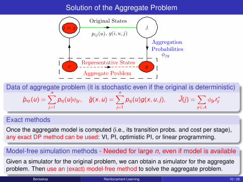
Solution of the Aggregate Problem








pxy(u) =

n!

i=1

dxi

n!

j=1


n!

i=1

dxi

n!

j=1

pij(u)g(i, u, j).


Q(j, u) =!

y∈S

φjyQ(y, u), j = 1, . . . , n, u ∈ U, (6.91)











pxy(u) =

n!

i=1

dxi

n!

j=1


n!

i=1

dxi

n!

j=1

pij(u)g(i, u, j).


Q(j, u) =!

y∈S

φjyQ(y, u), j = 1, . . . , n, u ∈ U, (6.91)











pxy(u) =

n!

i=1

dxi

n!

j=1


n!

i=1

dxi

n!

j=1

pij(u)g(i, u, j).


Q(j, u) =!

y∈S

φjyQ(y, u), j = 1, . . . , n, u ∈ U, (6.91)











pxy(u) =

n!

i=1

dxi

n!

j=1


n!

i=1

dxi

n!

j=1

pij(u)g(i, u, j).


Q(j, u) =!

y∈S

φjyQ(y, u), j = 1, . . . , n, u ∈ U, (6.91)




g(x, u) =n⌥

i=1

dxi

n⌥

j=1

pij(u)g(i, u, j)





⇥ =

�⇧⇧⇧⇧⇧⇧⇧⇧⇧⇧⇧⇤

1 0 0 01 0 0 00 1 0 01 0 0 01 0 0 00 1 0 00 0 1 00 0 1 00 0 0 1

⇥⌃⌃⌃⌃⌃⌃⌃⌃⌃⌃⌃⌅

1 2 3 4 5 6 7 8 9 x1 x2 x3 x4



TJ J0





Tµ(⇥r) ⇥r = �T(�)µ (⇥r)


1

minu∈U(i)

n!

j=1


#i = x



k Simulator


pxy(u) =n!

i=1


j=1

pxj(u)g(x, u, j)











x0 xk x1k+1 x2

k+1 x3k+1 x4






1

minu∈U(i)

n!

j=1


#i = x



k Simulator


pxy(u) =n!

i=1


j=1

pxj(u)g(x, u, j)











x0 xk x1k+1 x2

k+1 x3k+1 x4






1

minu∈U(i)

n!

j=1


#i = x



k Simulator


pxy(u) =n!

i=1


j=1

pxj(u)g(x, u, j)











x0 xk x1k+1 x2

k+1 x3k+1 x4






1

minu∈U(i)

n!

j=1


#i = x



k Simulator


pxy(u) =n!

i=1


j=1

pxj(u)g(x, u, j)











x0 xk x1k+1 x2

k+1 x3k+1 x4






1

minu∈U(i)

n!

j=1


#i = x



k Simulator


pxy(u) =n!

i=1


j=1

pxj(u)g(x, u, j)











x0 xk x1k+1 x2

k+1 x3k+1 x4






1

minu∈U(i)

n!

j=1


#i = x



k Simulator


pxy(u) =n!

i=1


j=1

pxj(u)g(x, u, j)











x0 xk x1k+1 x2

k+1 x3k+1 x4






1

minu∈U(i)

n!

j=1


#i = x Ix



k Simulator


pxy(u) =n!

i=1


j=1

pxj(u)g(x, u, j)










x0 xk x1k+1 x2

k+1 x3k+1 x4






1

Data of aggregate problem (it is stochastic even if the original is deterministic)

pxy (u) =n∑

j=1

pxj(u)φjy , g(x , u) =n∑

j=1

pxj(u)g(x , u, j), J(j) =∑y∈A

φjy r∗y

Exact methodsOnce the aggregate model is computed (i.e., its transition probs. and cost per stage),any exact DP method can be used: VI, PI, optimistic PI, or linear programming.

Model-free simulation methods - Needed for large n, even if model is availableGiven a simulator for the original problem, we can obtain a simulator for the aggregateproblem. Then use an (exact) model-free method to solve the aggregate problem.


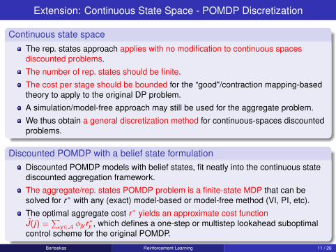
Extension: Continuous State Space - POMDP Discretization

Continuous state spaceThe rep. states approach applies with no modification to continuous spacesdiscounted problems.

The number of rep. states should be finite.

The cost per stage should be bounded for the “good"/contraction mapping-basedtheory to apply to the original DP problem.

A simulation/model-free approach may still be used for the aggregate problem.

We thus obtain a general discretization method for continuous-spaces discountedproblems.

Discounted POMDP with a belief state formulationDiscounted POMDP models with belief states, fit neatly into the continuous statediscounted aggregation framework.

The aggregate/rep. states POMDP problem is a finite-state MDP that can besolved for r∗ with any (exact) model-based or model-free method (VI, PI, etc).

The optimal aggregate cost r∗ yields an approximate cost functionJ(j) =

∑y∈A φjy r∗y , which defines a one-step or multistep lookahead suboptimal

control scheme for the original POMDP.


A Challenge Question - Think for Five Mins

A A

B B

Travel speed1 m/sec

1000 m 1000 m

Discretizing Continuous MotionA self-driving car wants to drive from A to B through obstacles. Find the fastestroute.

Car speed is 1 m/sec in any direction.

We discretize the space with a fine square grid; restrict directions of motion tohorizontal and vertical.

We take the discretized shortest path solution as an approximation to thecontinuous shortest path solution.

Is this a good approximation?Bertsekas Reinforcement Learning 12 / 26

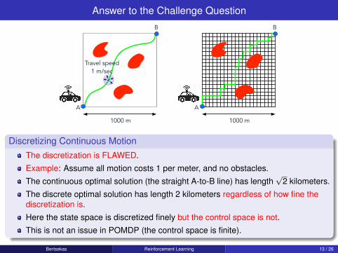
Answer to the Challenge Question

A A

B B

Travel speed1 m/sec

1000 m 1000 m

Discretizing Continuous MotionThe discretization is FLAWED.

Example: Assume all motion costs 1 per meter, and no obstacles.

The continuous optimal solution (the straight A-to-B line) has length√

2 kilometers.

The discrete optimal solution has length 2 kilometers regardless of how fine thediscretization is.

Here the state space is discretized finely but the control space is not.

This is not an issue in POMDP (the control space is finite).


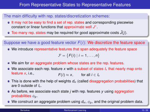
From Representative States to Representative Features

The main difficulty with rep. states/discretization schemes:It may not be easy to find a set of rep. states and corresponding piecewiseconstant or linear functions that approximate well J∗.

Too many rep. states may be required for good approximate costs J(j).

Suppose we have a good feature vector F (i): We discretize the feature space

We introduce representative features that span adequately the feature space

F ={

F (i) | i = 1, . . . , n}

We aim for an aggregate problem whose states are the rep. features.

We associate each rep. feature x with a subset of states Ix that nearly map ontofeature x , i.e., F (i) ≈ x , for all i ∈ Ix

This is done with the help of weights dxi (called disaggregation probabilities) thatare 0 outside of Ix .

As before, we associate each state j with rep. features y using aggregationprobabilities φjy .

We construct an aggregate problem using dxi , φjy , and the original problem data.


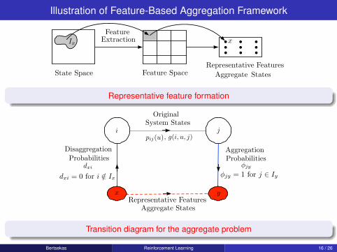
Illustration of Feature-Based Aggregation Framework

Special States Aggregate States Features n t pnn(u) pin(u) pni(u)pjn(u) pnj(u)

State i Feature Extraction Mapping Feature Vector ⇧(i) Linear CostApproximator ⇧(i)⇥r

Route to Queue 2 1 2 3 4 5 6 7 8 9





c + Ez

⇧J�

⇤pf0(z)

pf0(z) + (1 � p)f1(z)

⌅⌃


⇥i(u)pij(u)⇥

⇥j(u)pjk(u)⇥

⇥k(u)pki(u)⇥

J(2) = g(2, u2) + �p21(u2)J(1) + �p22(u2)J(2)

J(2) = g(2, u1) + �p21(u1)J(1) + �p22(u1)J(2)

J(1) = g(1, u2) + �p11(u2)J(1) + �p12(u2)J(2)

J� =�J�(1), J�(2)

⇥

1 � ⇥j(u)⇥ 1 � ⇥i(u)

⇥ 1 � ⇥k(u)⇥

1 � µi

µµi

µ

Cost = 2⇥� J0

R + g(1) + �

n⌥

j=1

p1jJ�(j)

1



Route to Queue 2 1 2 3 4 5 6 7 8 9





c + Ez

⇧J�

⇤pf0(z)

pf0(z) + (1 � p)f1(z)

⌅⌃


⇥i(u)pij(u)⇥

⇥j(u)pjk(u)⇥

⇥k(u)pki(u)⇥

J(2) = g(2, u2) + �p21(u2)J(1) + �p22(u2)J(2)

J(2) = g(2, u1) + �p21(u1)J(1) + �p22(u1)J(2)

J(1) = g(1, u2) + �p11(u2)J(1) + �p12(u2)J(2)

J� =�J�(1), J�(2)

⇥

1 � ⇥j(u)⇥ 1 � ⇥i(u)

⇥ 1 � ⇥k(u)⇥

1 � µi

µµi

µ

Cost = 2⇥� J0

R + g(1) + �

n⌥

j=1

p1jJ�(j)

1



Route to Queue 2 1 2 3 4 5 6 7 8 9





c + Ez

⇧J�

⇤pf0(z)

pf0(z) + (1 � p)f1(z)

⌅⌃


⇥i(u)pij(u)⇥

⇥j(u)pjk(u)⇥

⇥k(u)pki(u)⇥

J(2) = g(2, u2) + �p21(u2)J(1) + �p22(u2)J(2)

J(2) = g(2, u1) + �p21(u1)J(1) + �p22(u1)J(2)

J(1) = g(1, u2) + �p11(u2)J(1) + �p12(u2)J(2)

J� =�J�(1), J�(2)

⇥

1 � ⇥j(u)⇥ 1 � ⇥i(u)

⇥ 1 � ⇥k(u)⇥

1 � µi

µµi

µ

Cost = 2⇥� J0

R + g(1) + �

n⌥

j=1

p1jJ�(j)

1

State Space Feature Space

Nullspace Component Sequence Orthogonal Component Full Iterate

xk = (C′kΣ−1Ck + βkI)−1(C′

kΣ−1dk + βkx)

Tµ0J Jµ0 = Tµ0Jµ0 Markov Chain P

Cost = 2αϵ rk+1 = arg minr∈ℜs

m!

t=1

Nt−1!

τ=0

"φ(iτ,t)′r − cτ,t(rk)

#2

µℓ

µ1 − µℓ

µ

Estimated Cost φ(iτ,t)′r Simulated Cost cτ,t(rk)

Transition probabilities for the uniform version

Πx∗

µℓ

µ1 − µℓ

µ

t . . . 0 m + i0 it1 = i it2 = i it3 = i it4 = i

wt1,m bit1+m wt2,m bit2+m wt3,m bit3+m wt4,m bit4+m

(Amb)(i) = limk→∞

$kt=0 δ(it = i)wt,mbit+m$k

t=0 δ(it = i)

Simulation Sequence {i0, i1, . . .}

Generated by Row Sampling Using P

S: Subspace spanned by basis vectors

D: Set of differential cost vectors Subspace S∗

1

State Space Feature Space

Nullspace Component Sequence Orthogonal Component Full Iterate

xk = (C′kΣ−1Ck + βkI)−1(C′

kΣ−1dk + βkx)

Tµ0J Jµ0 = Tµ0Jµ0 Markov Chain P


m!

t=1

Nt−1!

τ=0

"φ(iτ,t)′r − cτ,t(rk)

#2

µℓ

µ1 − µℓ

µ

Estimated Cost φ(iτ,t)′r Simulated Cost cτ,t(rk)

Transition probabilities for the uniform version

Πx∗

µℓ

µ1 − µℓ

µ

t . . . 0 m + i0 it1 = i it2 = i it3 = i it4 = i

wt1,m bit1+m wt2,m bit2+m wt3,m bit3+m wt4,m bit4+m

(Amb)(i) = limk→∞

$kt=0 δ(it = i)wt,mbit+m$k

t=0 δ(it = i)

Simulation Sequence {i0, i1, . . .}

Generated by Row Sampling Using P

S: Subspace spanned by basis vectors

D: Set of differential cost vectors Subspace S∗

1

minu∈U(i)

n!

j=1


#i = x



k Simulator


pxy(u) =n!

i=1


j=1

pxj(u)g(x, u, j)











x0 xk x1k+1 x2

k+1 x3k+1 x4






1

minu∈U(i)

n!

j=1


#i = x



k Simulator


pxy(u) =n!

i=1


j=1

pxj(u)g(x, u, j)











x0 xk x1k+1 x2

k+1 x3k+1 x4






1

minu∈U(i)

n!

j=1


#i = x Ix



k Simulator


pxy(u) =n!

i=1


j=1

pxj(u)g(x, u, j)











x0 xk x1k+1 x2

k+1 x3k+1 x4






1

Representative feature formation








pxy(u) =

n!

i=1

dxi

n!

j=1


n!

i=1

dxi

n!

j=1

pij(u)g(i, u, j).


Q(j, u) =!

y∈S

φjyQ(y, u), j = 1, . . . , n, u ∈ U, (6.91)











pxy(u) =

n!

i=1

dxi

n!

j=1


n!

i=1

dxi

n!

j=1

pij(u)g(i, u, j).


Q(j, u) =!

y∈S

φjyQ(y, u), j = 1, . . . , n, u ∈ U, (6.91)











pxy(u) =

n!

i=1

dxi

n!

j=1


n!

i=1

dxi

n!

j=1

pij(u)g(i, u, j).


Q(j, u) =!

y∈S

φjyQ(y, u), j = 1, . . . , n, u ∈ U, (6.91)











pxy(u) =

n!

i=1

dxi

n!

j=1


n!

i=1

dxi

n!

j=1

pij(u)g(i, u, j).


Q(j, u) =!

y∈S

φjyQ(y, u), j = 1, . . . , n, u ∈ U, (6.91)











pxy(u) =

n!

i=1

dxi

n!

j=1


n!

i=1

dxi

n!

j=1

pij(u)g(i, u, j).


Q(j, u) =!

y∈S

φjyQ(y, u), j = 1, . . . , n, u ∈ U, (6.91)











pxy(u) =

n!

i=1

dxi

n!

j=1


n!

i=1

dxi

n!

j=1

pij(u)g(i, u, j).


Q(j, u) =!

y∈S

φjyQ(y, u), j = 1, . . . , n, u ∈ U, (6.91)




f�2,Xk

(��)

x1 x2 x3 x4 Slope: xk+1 Slope: xi, i ⇥ k

f�(�)

Constant � f�1 (�) f�

2 (��) F ⇤2,k(��)F ⇤

k (�)

�(g(x), f(x)) | x ⌅ X

M =�(u, w) | there exists x ⌅ X

Original System States Aggregate States

F (x) H(y) y h(y)

supz2Z

infx2X

⇥(x, z) ⇥ supz2Z

infx2X

⇥(x, z) = q⇤ = p(0) ⇥ p(0) = w⇤ = infx2X

supz2Z

⇥(x, z)

Shapley-Folkman Theorem: Let S = S1 + · · · + Sm with Si ⇤ ⇧n,i = 1, . . . ,mIf s ⌅ conv(S) then s = s1 + · · · + sm wheresi ⌅ conv(Si) for all i = 1, . . . ,m,si ⌅ Si for at least m � n � 1 indices i.

The sum of a large number of convex sets is almost convexNonconvexity of the sum is caused by a small number (n + 1) of sets

f(x) = (cl )f(x)

q⇤ = (cl )p(0) ⇥ p(0) = w⇤

Duality Gap DecompositionConvex and concave part can be estimated separatelyq is closed and concaveMin Common ProblemMax Crossing ProblemWeak Duality q⇤ ⇥ w⇤

minimize w

subject to (0, w) ⌅ M,

1

f�2,Xk

(��)


f�(�)


2 (��) F ⇤2,k(��)F ⇤

k (�)

�(g(x), f(x)) | x ⌅ X



F (x) H(y) y h(y)

supz2Z

infx2X


infx2X

⇥(x, z) = q⇤ = p(0) ⇥ p(0) = w⇤ = infx2X

supz2Z

⇥(x, z)



f(x) = (cl )f(x)

q⇤ = (cl )p(0) ⇥ p(0) = w⇤


minimize w


1

f�2,Xk

(��)


f�(�)


2 (��) F ⇤2,k(��)F ⇤

k (�)

�(g(x), f(x)) | x ⌅ X



F (x) H(y) y h(y)

supz2Z

infx2X


infx2X

⇥(x, z) = q⇤ = p(0) ⇥ p(0) = w⇤ = infx2X

supz2Z

⇥(x, z)



f(x) = (cl )f(x)

q⇤ = (cl )p(0) ⇥ p(0) = w⇤


minimize w


1

f�2,Xk

(��)


f�(�)


2 (��) F ⇤2,k(��)F ⇤

k (�)

�(g(x), f(x)) | x ⌅ X


Original System States Aggregate StatesAggregation ProbabilitiesDisaggregation Probabilities

F (x) H(y) y h(y)

supz2Z

infx2X


infx2X

⇥(x, z) = q⇤ = p(0) ⇥ p(0) = w⇤ = infx2X

supz2Z

⇥(x, z)



f(x) = (cl )f(x)

q⇤ = (cl )p(0) ⇥ p(0) = w⇤


minimize w


1

f�2,Xk

(��)


f�(�)


2 (��) F ⇤2,k(��)F ⇤

k (�)

�(g(x), f(x)) | x ⌅ X



F (x) H(y) y h(y)

supz2Z

infx2X


infx2X

⇥(x, z) = q⇤ = p(0) ⇥ p(0) = w⇤ = infx2X

supz2Z

⇥(x, z)



f(x) = (cl )f(x)

q⇤ = (cl )p(0) ⇥ p(0) = w⇤


minimize w


1

f�2,Xk

(��)


f�(�)


2 (��) F ⇤2,k(��)F ⇤

k (�)

�(g(x), f(x)) | x ⌅ X



F (x) H(y) y h(y)

supz2Z

infx2X


infx2X

⇥(x, z) = q⇤ = p(0) ⇥ p(0) = w⇤ = infx2X

supz2Z

⇥(x, z)



f(x) = (cl )f(x)

q⇤ = (cl )p(0) ⇥ p(0) = w⇤


minimize w


1

f�2,Xk

(��)


f�(�)


2 (��) F ⇤2,k(��)F ⇤

k (�)

�(g(x), f(x)) | x ⌅ X



F (x) H(y) y h(y)

supz2Z

infx2X


infx2X

⇥(x, z) = q⇤ = p(0) ⇥ p(0) = w⇤ = infx2X

supz2Z

⇥(x, z)



f(x) = (cl )f(x)

q⇤ = (cl )p(0) ⇥ p(0) = w⇤


minimize w


1

minu∈U(i)

n!

j=1


#i = x Ix



k Simulator


pxy(u) =n!

i=1


j=1

pxj(u)g(x, u, j)











x0 xk x1k+1 x2

k+1 x3k+1 x4






1

minu∈U(i)

n!

j=1


#i = x Ix



k Simulator


pxy(u) =n!

i=1


j=1

pxj(u)g(x, u, j)


dxi = 0 for i /∈ Ix φiy = 1 for ∈ Iy








x0 xk x1k+1 x2

k+1 x3k+1 x4






1

minu∈U(i)

n!

j=1


#i = x Ix



k Simulator


pxy(u) =n!

i=1


j=1

pxj(u)g(x, u, j)










x0 xk x1k+1 x2

k+1 x3k+1 x4






1








pxy(u) =

n!

i=1

dxi

n!

j=1


n!

i=1

dxi

n!

j=1

pij(u)g(i, u, j).


Q(j, u) =!

y∈S

φjyQ(y, u), j = 1, . . . , n, u ∈ U, (6.91)




g(x, u) =n⌥

i=1

dxi

n⌥

j=1

pij(u)g(i, u, j)





⇥ =

�⇧⇧⇧⇧⇧⇧⇧⇧⇧⇧⇧⇤

1 0 0 01 0 0 00 1 0 01 0 0 01 0 0 00 1 0 00 0 1 00 0 1 00 0 0 1

⇥⌃⌃⌃⌃⌃⌃⌃⌃⌃⌃⌃⌅

1 2 3 4 5 6 7 8 9 x1 x2 x3 x4



TJ J0





Tµ(⇥r) ⇥r = �T(�)µ (⇥r)


1

Transition diagram for the aggregate problem


Working Break: Feature Formation Methods in Aggregation








pxy(u) =

n!

i=1

dxi

n!

j=1


n!

i=1

dxi

n!

j=1

pij(u)g(i, u, j).


Q(j, u) =!

y∈S

φjyQ(y, u), j = 1, . . . , n, u ∈ U, (6.91)











pxy(u) =

n!

i=1

dxi

n!

j=1


n!

i=1

dxi

n!

j=1

pij(u)g(i, u, j).


Q(j, u) =!

y∈S

φjyQ(y, u), j = 1, . . . , n, u ∈ U, (6.91)











pxy(u) =

n!

i=1

dxi

n!

j=1


n!

i=1

dxi

n!

j=1

pij(u)g(i, u, j).


Q(j, u) =!

y∈S

φjyQ(y, u), j = 1, . . . , n, u ∈ U, (6.91)











pxy(u) =

n!

i=1

dxi

n!

j=1


n!

i=1

dxi

n!

j=1

pij(u)g(i, u, j).


Q(j, u) =!

y∈S

φjyQ(y, u), j = 1, . . . , n, u ∈ U, (6.91)











pxy(u) =

n!

i=1

dxi

n!

j=1


n!

i=1

dxi

n!

j=1

pij(u)g(i, u, j).


Q(j, u) =!

y∈S

φjyQ(y, u), j = 1, . . . , n, u ∈ U, (6.91)











pxy(u) =

n!

i=1

dxi

n!

j=1


n!

i=1

dxi

n!

j=1

pij(u)g(i, u, j).


Q(j, u) =!

y∈S

φjyQ(y, u), j = 1, . . . , n, u ∈ U, (6.91)




f�2,Xk

(��)


f�(�)


2 (��) F ⇤2,k(��)F ⇤

k (�)

�(g(x), f(x)) | x ⌅ X



F (x) H(y) y h(y)

supz2Z

infx2X


infx2X

⇥(x, z) = q⇤ = p(0) ⇥ p(0) = w⇤ = infx2X

supz2Z

⇥(x, z)



f(x) = (cl )f(x)

q⇤ = (cl )p(0) ⇥ p(0) = w⇤


minimize w


1

f�2,Xk

(��)


f�(�)


2 (��) F ⇤2,k(��)F ⇤

k (�)

�(g(x), f(x)) | x ⌅ X



F (x) H(y) y h(y)

supz2Z

infx2X


infx2X

⇥(x, z) = q⇤ = p(0) ⇥ p(0) = w⇤ = infx2X

supz2Z

⇥(x, z)



f(x) = (cl )f(x)

q⇤ = (cl )p(0) ⇥ p(0) = w⇤


minimize w


1

f�2,Xk

(��)


f�(�)


2 (��) F ⇤2,k(��)F ⇤

k (�)

�(g(x), f(x)) | x ⌅ X



F (x) H(y) y h(y)

supz2Z

infx2X


infx2X

⇥(x, z) = q⇤ = p(0) ⇥ p(0) = w⇤ = infx2X

supz2Z

⇥(x, z)



f(x) = (cl )f(x)

q⇤ = (cl )p(0) ⇥ p(0) = w⇤


minimize w


1

f�2,Xk

(��)


f�(�)


2 (��) F ⇤2,k(��)F ⇤

k (�)

�(g(x), f(x)) | x ⌅ X



F (x) H(y) y h(y)

supz2Z

infx2X


infx2X

⇥(x, z) = q⇤ = p(0) ⇥ p(0) = w⇤ = infx2X

supz2Z

⇥(x, z)



f(x) = (cl )f(x)

q⇤ = (cl )p(0) ⇥ p(0) = w⇤


minimize w


1

f�2,Xk

(��)


f�(�)


2 (��) F ⇤2,k(��)F ⇤

k (�)

�(g(x), f(x)) | x ⌅ X



F (x) H(y) y h(y)

supz2Z

infx2X


infx2X

⇥(x, z) = q⇤ = p(0) ⇥ p(0) = w⇤ = infx2X

supz2Z

⇥(x, z)



f(x) = (cl )f(x)

q⇤ = (cl )p(0) ⇥ p(0) = w⇤


minimize w


1

f�2,Xk

(��)


f�(�)


2 (��) F ⇤2,k(��)F ⇤

k (�)

�(g(x), f(x)) | x ⌅ X



F (x) H(y) y h(y)

supz2Z

infx2X


infx2X

⇥(x, z) = q⇤ = p(0) ⇥ p(0) = w⇤ = infx2X

supz2Z

⇥(x, z)



f(x) = (cl )f(x)

q⇤ = (cl )p(0) ⇥ p(0) = w⇤


minimize w


1

f�2,Xk

(��)


f�(�)


2 (��) F ⇤2,k(��)F ⇤

k (�)

�(g(x), f(x)) | x ⌅ X

M =�(u,w) | there exists x ⌅ X


F (x) H(y) y h(y)

supz2Z

infx2X


infx2X

⇥(x, z) = q⇤ = p(0) ⇥ p(0) = w⇤ = infx2X

supz2Z

⇥(x, z)



f(x) = (cl )f(x)

q⇤ = (cl )p(0) ⇥ p(0) = w⇤


minimize w


1

minu∈U(i)

n!

j=1


#i = x Ix



k Simulator


pxy(u) =n!

i=1


j=1

pxj(u)g(x, u, j)











x0 xk x1k+1 x2

k+1 x3k+1 x4






1

minu∈U(i)

n!

j=1


#i = x Ix



k Simulator


pxy(u) =n!

i=1


j=1

pxj(u)g(x, u, j)










x0 xk x1k+1 x2

k+1 x3k+1 x4






1

minu∈U(i)

n!

j=1


#i = x Ix



k Simulator


pxy(u) =n!

i=1


j=1

pxj(u)g(x, u, j)










x0 xk x1k+1 x2

k+1 x3k+1 x4






1








pxy(u) =

n!

i=1

dxi

n!

j=1


n!

i=1

dxi

n!

j=1

pij(u)g(i, u, j).


Q(j, u) =!

y∈S

φjyQ(y, u), j = 1, . . . , n, u ∈ U, (6.91)




g(x, u) =n⌥

i=1

dxi

n⌥

j=1

pij(u)g(i, u, j)





⇥ =

�⇧⇧⇧⇧⇧⇧⇧⇧⇧⇧⇧⇤

1 0 0 01 0 0 00 1 0 01 0 0 01 0 0 00 1 0 00 0 1 00 0 1 00 0 0 1

⇥⌃⌃⌃⌃⌃⌃⌃⌃⌃⌃⌃⌅

1 2 3 4 5 6 7 8 9 x1 x2 x3 x4



TJ J0





Tµ(⇥r) ⇥r = �T(�)µ (⇥r)


1

Question 1: Why is the rep. states model a special case of the rep. features model?

Assume the following general principle for feature-based aggregation:

Choose features so that states i with similar features F (i) have similar J∗(i), i.e., J∗(i)changes little within each of the “footprint" sets Ix = {i | dxi > 0} and Sy = {j | φjy > 0}.

Question 2: Can you think of examples of useful features for aggregation schemes?


Feature Formation Using Scoring Functions

�jf =

⇢1 if j 2 If

0 if j /2 If

1 10 20 30 40 50 I1 I2 I3 i

dfi = 0 if i /2 If

pff (u) =nX

i=1

dfi

nX

j=1

pij(u)�jf

g(f, u) =

nX

i=1

dfi

nX

j=1

pij(u)g(i, u, j)

Representative Feature States Feature Space F F (j) �jf1 �jf2 �jf3

�jf4

f1 f2 f3 f4 f5 f6 f7

Disaggregation Sets If Aggregate Optimization Feature States

Neural Network Features Approximate Cost Jµ Policy ImprovementSampling

Neural Network Features Approximate Cost Jµ Policy Improvement

F = {f1, f2, f3, f4, f5, f6, f7}

Representative Features States dfi f f with Aggregation ProblemOptimization

Current Policy µ Approximately Improved Policy µ µ

Tµ�r �r = ⇧Tµ�r

Generate “Improved” Policy µ

State Space Feature Space Subspace J = {�r | s 2 <s} Ps`=1 F`(i, v)r`

r = (r1, . . . , rs)

State i y(i) Ay(i) + b Fs(i, v) F1(i, v) F2(i, v) Linear Weighting ofFeatures

1

Aggregate Problem Approximation


�F (i)

�

Aggregate States Scoring Function V (i)

0 n n � 1 State i Cost function Jµ(i)I1 ... Iq I2 g(i, u, j)



�jf =

⇢1 if j 2 If

0 if j /2 If

1 10 20 30 40 50 I1 I2 I3 i J1(i)


dì = 0 if i /2 I`

�j ¯ = 1 if j 2 I¯

pff (u) =

nX

i=1

dfi

nX

j=1

pij(u)�jf

g(f, u) =nX

i=1

dfi

nX

j=1

pij(u)g(i, u, j)


�jf4

f1 f2 f3 f4 f5 f6 f7




F = {f1, f2, f3, f4, f5, f6, f7}

1



!F (i)

"

Aggregate States Scoring Function V (i) J∗(i) 0 n n − 1 State i Costfunction Jµ(i)I1 ... Iq I2 g(i, u, j)



φjf =

#1 if j ∈ If

0 if j /∈ If

1 10 20 30 40 50 I1 I2 I3 i J1(i)




pff(u) =

n$

i=1

dfi

n$

j=1

pij(u)φjf

g(f, u) =

n$

i=1

dfi

n$

j=1

pij(u)g(i, u, j)

Representative Feature States Feature Space F F (j) φjf1 φjf2 φjf3

φjf4

i1 i2 iℓ . . . iq




F = {f1, f2, f3, f4, f5, f6, f7}

1



!F (i)

"




φjf =

#1 if j ∈ If

0 if j /∈ If

1 10 20 30 40 50 I1 I2 I3 i J1(i)




pff(u) =

n$

i=1

dfi

n$

j=1

pij(u)φjf

g(f, u) =

n$

i=1

dfi

n$

j=1

pij(u)g(i, u, j)


φjf4

i1 i2 iℓ . . . iq




F = {f1, f2, f3, f4, f5, f6, f7}

1



!F (i)

"




φjf =

#1 if j ∈ If

0 if j /∈ If

1 10 20 30 40 50 I1 I2 I3 i J1(i)




pff(u) =

n$

i=1

dfi

n$

j=1

pij(u)φjf

g(f, u) =

n$

i=1

dfi

n$

j=1

pij(u)g(i, u, j)


φjf4

i1 i2 iℓ r∗1 r∗

q r∗ℓ . . . iq




F = {f1, f2, f3, f4, f5, f6, f7}

1



!F (i)

"




φjf =

#1 if j ∈ If

0 if j /∈ If

1 10 20 30 40 50 I1 I2 I3 i J1(i)




pff(u) =

n$

i=1

dfi

n$

j=1

pij(u)φjf

g(f, u) =

n$

i=1

dfi

n$

j=1

pij(u)g(i, u, j)


φjf4


q r∗ℓ . . . iq




F = {f1, f2, f3, f4, f5, f6, f7}

1



!F (i)

"

R1 R2 Rℓ Rq Cost Jµ

!F (i)

"




φjf =

#1 if j ∈ If

0 if j /∈ If

1 10 20 30 40 50 I1 I2 I3 i J1(i)




pff(u) =

n$

i=1

dfi

n$

j=1

pij(u)φjf

g(f, u) =

n$

i=1

dfi

n$

j=1

pij(u)g(i, u, j)


φjf4


q r∗ℓ . . . iq




F = {f1, f2, f3, f4, f5, f6, f7}

1



!F (i)

"

R1 R2 Rℓ Rq Cost Jµ

!F (i)

"




φjf =

#1 if j ∈ If

0 if j /∈ If

1 10 20 30 40 50 I1 I2 I3 i J1(i)




pff(u) =

n$

i=1

dfi

n$

j=1

pij(u)φjf

g(f, u) =

n$

i=1

dfi

n$

j=1

pij(u)g(i, u, j)


φjf4


q r∗ℓ . . . iq




F = {f1, f2, f3, f4, f5, f6, f7}

1



!F (i)

"

R1 R2 Rℓ Rq r∗2 Cost Jµ

!F (i)

"




φjf =

#1 if j ∈ If

0 if j /∈ If

1 10 20 30 40 50 I1 I2 I3 i J1(i)




pff(u) =

n$

i=1

dfi

n$

j=1

pij(u)φjf

g(f, u) =

n$

i=1

dfi

n$

j=1

pij(u)g(i, u, j)


φjf4


q r∗ℓ . . . iq




F = {f1, f2, f3, f4, f5, f6, f7}

1



!F (i)

"

R1 R2 Rℓ Rq r∗2 r∗

3 Cost Jµ

!F (i)

"




φjf =

#1 if j ∈ If

0 if j /∈ If

1 10 20 30 40 50 I1 I2 I3 i J1(i)




pff(u) =

n$

i=1

dfi

n$

j=1

pij(u)φjf

g(f, u) =

n$

i=1

dfi

n$

j=1

pij(u)g(i, u, j)


φjf4


q r∗ℓ . . . iq




F = {f1, f2, f3, f4, f5, f6, f7}

1



!F (i)

"

R1 R2 R3 Rℓ Rq−1 Rq r∗2 r∗

3 Cost Jµ

!F (i)

"


3 Cost Jµ

!F (i)

"





φjf =

#1 if j ∈ If

0 if j /∈ If

1 10 20 30 40 50 I1 I2 I3 i J1(i)




pff(u) =

n$

i=1

dfi

n$

j=1

pij(u)φjf

g(f, u) =

n$

i=1

dfi

n$

j=1

pij(u)g(i, u, j)


φjf4


q r∗ℓ . . . iq




1



!y∈A φjyr∗

y

minu∈U(i)

n"

j=1


$i = x Ix



k Simulator


pxy(u) =

n"

i=1


n"

j=1

pxj(u)g(x, u, j)




m







x0 xk x1k+1 x2

k+1 x3k+1 x4





1



!y∈A φjyr∗

y

minu∈U(i)

n"

j=1


$i = x Ix



k Simulator


pxy(u) =

n"

i=1


n"

j=1

pxj(u)g(x, u, j)




m







x0 xk x1k+1 x2

k+1 x3k+1 x4





1



!y∈A φjyr∗

y

minu∈U(i)

n"

j=1


$i = x Ix



k Simulator


pxy(u) =

n"

i=1


n"

j=1

pxj(u)g(x, u, j)




m







x0 xk x1k+1 x2

k+1 x3k+1 x4





1



!y∈A φjyr∗

y

minu∈U(i)

n"

j=1


$i = x Ix



k Simulator


pxy(u) =

n"

i=1


n"

j=1

pxj(u)g(x, u, j)




m







x0 xk x1k+1 x2

k+1 x3k+1 x4





1



!y∈A φjyr∗

y

minu∈U(i)

n"

j=1


$i = x Ix



k Simulator


pxy(u) =

n"

i=1


n"

j=1

pxj(u)g(x, u, j)




m







x0 xk x1k+1 x2

k+1 x3k+1 x4





1




!y∈A φjyr∗

y

minu∈U(i)

n"

j=1


$i = x Ix



k Simulator


pxy(u) =

n"

i=1


n"

j=1

pxj(u)g(x, u, j)




m







x0 xk x1k+1 x2

k+1 x3k+1 x4




1




!y∈A φjyr∗

y

minu∈U(i)

n"

j=1


$i = x Ix



k Simulator


pxy(u) =

n"

i=1


n"

j=1

pxj(u)g(x, u, j)




m







x0 xk x1k+1 x2

k+1 x3k+1 x4




1




!y∈A φjyr∗

y

minu∈U(i)

n"

j=1


$i = x Ix



k Simulator


pxy(u) =

n"

i=1


n"

j=1

pxj(u)g(x, u, j)




m







x0 xk x1k+1 x2

k+1 x3k+1 x4




1




!y∈A φjyr∗

y

minu∈U(i)

n"

j=1


$i = x Ix



k Simulator


pxy(u) =

n"

i=1


n"

j=1

pxj(u)g(x, u, j)




m







x0 xk x1k+1 x2

k+1 x3k+1 x4




1




!y∈A φjyr∗

y

minu∈U(i)

n"

j=1


$i = x Ix



k Simulator


pxy(u) =

n"

i=1


n"

j=1

pxj(u)g(x, u, j)




m







x0 xk x1k+1 x2

k+1 x3k+1 x4




1




!y∈A φjyr∗

y

minu∈U(i)

n"

j=1


$i = x Ix



k Simulator


pxy(u) =

n"

i=1


n"

j=1

pxj(u)g(x, u, j)




m







x0 xk x1k+1 x2

k+1 x3k+1 x4




1

Idea: Suppose that we have a scoring function V (i) with V (i) ≈ J∗(i). Then grouptogether states with similar score.

We partition the range of values of V into m disjoint intervals R1, . . . ,Rm.

We define a feature vector F (i) according to

F (i) = `, all i such that V (i) ∈ R`, ` = 1, . . . ,m

Defines a partition of the state space into the footprints S` = I` ={

i | F (i) = `}

.


Examples of Scoring Functions

Cost functions of heuristics or policies.

Approximate cost functions produced by neural networks.

Let the scoring function be the cost function Jµ of a policy µ

Let’s compare with rollout:

Rollout uses as cost approximation J = Jµ.

Score-based aggregation uses Jµ as scoring function to form features. Theresulting J is a “nonlinear function of Jµ" that aims to approximate J∗.

If the scoring function quantization were so fine as to have a single feature valueper interval R`, we would have J = J∗ (much better than rollout).

Score-based aggregation can be viewed as a more sophisticated form of rollout.

Score-based aggregation is more computation-intensive, less suitable for on-lineimplementation.

It is possible to use multiple scoring functions to generate more complex feature maps.


Feature Formation Using Neural Networks

. . .. . . . . .

Selective Depth Lookahead Tree �(⇠) ⇠ 1 0 -1 Encoding


�xk(Ik)

�


State xk Feature Vector �k(xk) Approximator r0k�k(xk)

x0 xk im�1 im . . . (0, 0) (N,�N) (N, 0) i (N, N) �N 0 g(i) I N � 2N i

s i1 im�1 im . . . (0, 0) (N,�N) (N, 0) i (N, N) �N 0 g(i) I N � 2 Ni

u1k u2

k u3k u4


p(j1) p(j2) p(j3) p(j4)


State x Feature Vector �(x) Approximator �(x)0r

` Stages Riccati Equation Iterates P P0 P1 P2 �2 � 1 �2PP+1

Cost of Period k Stock Ordered at Period k Inventory Systemr(uk) + cuk xk+1 = xk + u + k � wk

Stock at Period k +1 Initial State A C AB AC CA CD ABC

ACB ACD CAB CAD CDA

SA SB CAB CAC CCA CCD CBC CCB CCD

CAB CAD CDA CCD CBD CDB CAB

Do not Repair Repair 1 2 n�1 n p11 p12 p1n p1(n�1) p2(n�1)

...

1

Selective Depth Lookahead Tree �(⇠) ⇠ 1 0 -1 Encoding y(x)

Linear Layer Parameter v = (A, b) Sigmoidal Layer Linear WeightingCost Approximation


�xk(Ik)

�





u1k u2

k u3k u4


p(j1) p(j2) p(j3) p(j4)






ACB ACD CAB CAD CDA


1


Linear Layer Parameter v = (A, b) Sigmoidal Layer Linear WeightingCost Approximation


�xk(Ik)

�





u1k u2

k u3k u4


p(j1) p(j2) p(j3) p(j4)






ACB ACD CAB CAD CDA


1


Linear Layer Parameter v = (A, b) Sigmoidal Layer Linear WeightingCost Approximation �(x, v)0r


�xk(Ik)

�





u1k u2

k u3k u4


p(j1) p(j2) p(j3) p(j4)






ACB ACD CAB CAD CDA


1




�xk(Ik)

�





u1k u2

k u3k u4


p(j1) p(j2) p(j3) p(j4)






ACB ACD CAB CAD CDA


1




�xk(Ik)

�





u1k u2

k u3k u4


p(j1) p(j2) p(j3) p(j4)






ACB ACD CAB CAD CDA


1




�xk(Ik)

�





u1k u2

k u3k u4


p(j1) p(j2) p(j3) p(j4)






ACB ACD CAB CAD CDA


1




�xk(Ik)

�





u1k u2

k u3k u4


p(j1) p(j2) p(j3) p(j4)






ACB ACD CAB CAD CDA


1




�xk(Ik)

�





u1k u2

k u3k u4


p(j1) p(j2) p(j3) p(j4)






ACB ACD CAB CAD CDA


1




�xk(Ik)

�





u1k u2

k u3k u4


p(j1) p(j2) p(j3) p(j4)






ACB ACD CAB CAD CDA


1




�xk(Ik)

�





u1k u2

k u3k u4


p(j1) p(j2) p(j3) p(j4)






ACB ACD CAB CAD CDA


1

Ay(x) + b �1(x, v) �2(x, v) �m(x, v) r




�xk(Ik)

�





u1k u2

k u3k u4


p(j1) p(j2) p(j3) p(j4)






ACB ACD CAB CAD CDA

1

Ay(x) + b �1(x, v) �2(x, v) �m(x, v) r




�xk(Ik)

�





u1k u2

k u3k u4


p(j1) p(j2) p(j3) p(j4)






ACB ACD CAB CAD CDA

1

Nonlinear Ay(x) + b �1(x, v) �2(x, v) �m(x, v) r x Initial


Linear Layer Parameter v = (A, b) Sigmoidal Layer Linear WeightingCost Approximation r0�(x, v)


�xk(Ik)

�





u1k u2

k u3k u4


p(j1) p(j2) p(j3) p(j4)






ACB ACD CAB CAD CDA

1

FEATURES


State i y(i) Ay(i) + b φ1(i, v) φm(i, v) φ2(i, v) J(i, v) = r′φ(i, v)



!y∈A φjyr∗

y

minu∈U(i)

n"

j=1


$i = x Ix



k Simulator


pxy(u) =

n"

j=1


n"

j=1

pxj(u)g(x, u, j)




m







x0 xk x1k+1 x2

k+1 x3k+1 x4



1





!y∈A φjyr∗

y

minu∈U(i)

n"

j=1


$i = x Ix



k Simulator


pxy(u) =

n"

j=1


n"

j=1

pxj(u)g(x, u, j)




m







x0 xk x1k+1 x2

k+1 x3k+1 x4



1





!y∈A φjyr∗

y

minu∈U(i)

n"

j=1


$i = x Ix



k Simulator


pxy(u) =

n"

j=1


n"

j=1

pxj(u)g(x, u, j)




m







x0 xk x1k+1 x2

k+1 x3k+1 x4



1





!y∈A φjyr∗

y

minu∈U(i)

n"

j=1


$i = x Ix



k Simulator


pxy(u) =

n"

j=1


n"

j=1

pxj(u)g(x, u, j)




m







x0 xk x1k+1 x2

k+1 x3k+1 x4



1





!y∈A φjyr∗

y

minu∈U(i)

n"

j=1


$i = x Ix



k Simulator


pxy(u) =

n"

j=1


n"

j=1

pxj(u)g(x, u, j)




m







x0 xk x1k+1 x2

k+1 x3k+1 x4



1





!y∈A φjyr∗

y

minu∈U(i)

n"

j=1


$i = x Ix



k Simulator


pxy(u) =

n"

j=1


n"

j=1

pxj(u)g(x, u, j)




m







x0 xk x1k+1 x2

k+1 x3k+1 x4



1





!y∈A φjyr∗

y

minu∈U(i)

n"

j=1


$i = x Ix



k Simulator


pxy(u) =

n"

j=1


n"

j=1

pxj(u)g(x, u, j)




m







x0 xk x1k+1 x2

k+1 x3k+1 x4



1

Suppose we have trained a NN that provides an approximation J(i) = r ′φ(i , v)

Features from the NN can be used to define rep. features.

Training of the NN yields lots of state-feature pairs.

Rep. features and footprint sets of states can be obtained from the NN training setdata, perhaps supplemented with additional (state,feature) pair data.

NN features may be supplemented by handcrafted features.

Feature-based aggregation yields a nonlinear function J of the features thatapproximates J∗ (not J).


Policy Iteration with Neural Nets, and Feature-Based Aggregation

φjf =

!1 if j ∈ If

0 if j /∈ If

dfi = 0 if i /∈ If

pff(u) =

n"

i=1

dfi

n"

j=1

pij(u)φjf

g(f, u) =n"

i=1

dfi

n"

j=1

pij(u)g(i, u, j)

Representative Features Feature Space F F (j) φjf1 φjf2 φjf3 φjf4

f1 f2 f3 f4 f5 f6 f7



F = {f1, f2, f3, f4, f5, f6, f7}

Representative Feature States dfi f f with Aggregation

Current Policy µ Improved Policy µµ

TµΦr Φr = ΠTµΦr


State Space Feature Space Subspace J = {Φr | s ∈ ℜs} #sℓ=1 Fℓ(i, v)rℓ

r = (r1, . . . , rs)



m"

t=1

Nt−1"

τ=0

$φ(iτ,t)′r − cτ,t(rk)

%2

µℓ

µ1 − µℓ

µ

1

φjf =

!1 if j ∈ If

0 if j /∈ If


pff(u) =

n"

i=1

dfi

n"

j=1

pij(u)φjf

g(f, u) =n"

i=1

dfi

n"

j=1

pij(u)g(i, u, j)


f1 f2 f3 f4 f5 f6 f7



F = {f1, f2, f3, f4, f5, f6, f7}






r = (r1, . . . , rs)



m"

t=1

Nt−1"

τ=0


%2

µℓ

µ1 − µℓ

µ

1

φjf =

!1 if j ∈ If

0 if j /∈ If


pff(u) =

n"

i=1

dfi

n"

j=1

pij(u)φjf

g(f, u) =n"

i=1

dfi

n"

j=1

pij(u)g(i, u, j)


f1 f2 f3 f4 f5 f6 f7



F = {f1, f2, f3, f4, f5, f6, f7}






r = (r1, . . . , rs)



m"

t=1

Nt−1"

τ=0


%2

µℓ

µ1 − µℓ

µ

1

φjf =

!1 if j ∈ If

0 if j /∈ If


pff(u) =

n"

i=1

dfi

n"

j=1

pij(u)φjf

g(f, u) =n"

i=1

dfi

n"

j=1

pij(u)g(i, u, j)


f1 f2 f3 f4 f5 f6 f7



F = {f1, f2, f3, f4, f5, f6, f7}


Current Policy µ Approximately Improved Policy µµ




r = (r1, . . . , rs)



m"

t=1

Nt−1"

τ=0


%2

µℓ

µ1 − µℓ

µ

1

φjf =

!1 if j ∈ If

0 if j /∈ If


pff(u) =

n"

i=1

dfi

n"

j=1

pij(u)φjf

g(f, u) =n"

i=1

dfi

n"

j=1

pij(u)g(i, u, j)


f1 f2 f3 f4 f5 f6 f7



F = {f1, f2, f3, f4, f5, f6, f7}






r = (r1, . . . , rs)



m"

t=1

Nt−1"

τ=0


%2

µℓ

µ1 − µℓ

µ

1

φjf =

!1 if j ∈ If

0 if j /∈ If


pff(u) =

n"

i=1

dfi

n"

j=1

pij(u)φjf

g(f, u) =n"

i=1

dfi

n"

j=1

pij(u)g(i, u, j)


f1 f2 f3 f4 f5 f6 f7



F = {f1, f2, f3, f4, f5, f6, f7}






r = (r1, . . . , rs)



m"

t=1

Nt−1"

τ=0


%2

µℓ

µ1 − µℓ

µ

1

φjf =

!1 if j ∈ If

0 if j /∈ If


pff(u) =

n"

i=1

dfi

n"

j=1

pij(u)φjf

g(f, u) =n"

i=1

dfi

n"

j=1

pij(u)g(i, u, j)


f1 f2 f3 f4 f5 f6 f7



F = {f1, f2, f3, f4, f5, f6, f7}






r = (r1, . . . , rs)



m"

t=1

Nt−1"

τ=0


%2

µℓ

µ1 − µℓ

µ

1

φjf =

!1 if j ∈ If

0 if j /∈ If


pff(u) =

n"

i=1

dfi

n"

j=1

pij(u)φjf

g(f, u) =

n"

i=1

dfi

n"

j=1

pij(u)g(i, u, j)


f1 f2 f3 f4 f5 f6 f7

Disaggregation Sets If



F = {f1, f2, f3, f4, f5, f6, f7}Representative Features States dfi f f with Aggregation Problem

Optimization





r = (r1, . . . , rs)



m"

t=1

Nt−1"

τ=0


%2

1

φjf =

!1 if j ∈ If

0 if j /∈ If


pff(u) =

n"

i=1

dfi

n"

j=1

pij(u)φjf

g(f, u) =

n"

i=1

dfi

n"

j=1

pij(u)g(i, u, j)


f1 f2 f3 f4 f5 f6 f7





Optimization





r = (r1, . . . , rs)



m"

t=1

Nt−1"

τ=0


%2

1

�jf =

⇢1 if j 2 If

0 if j /2 If

1 10 20 30 40 50 I1 I2 I3 i J1(i)

dfi = 0 if i /2 If

pff (u) =nX

i=1

dfi

nX

j=1

pij(u)�jf

g(f, u) =

nX

i=1

dfi

nX

j=1

pij(u)g(i, u, j)


�jf4

f1 f2 f3 f4 f5 f6 f7




F = {f1, f2, f3, f4, f5, f6, f7}






r = (r1, . . . , rs)


1

Feature Vector F (i) S` S¯ Sets I` k Stages j1 j2 jk�1 jk

Aggregate States S` S¯ Sets I` k Stages j1 j2 jk�1 jk




�jf =

⇢1 if j 2 If

0 if j /2 If

1 10 20 30 40 50 I1 I2 I3 i J1(i)


dì = 0 if i /2 I`

�j ¯ = 1 if j 2 I¯

pff (u) =

nX

i=1

dfi

nX

j=1

pij(u)�jf

g(f, u) =

nX

i=1

dfi

nX

j=1

pij(u)g(i, u, j)


�jf4

f1 f2 f3 f4 f5 f6 f7





Optimization

1

Feature Vector F (i) Approximate Cost Jµ

�F (i)

�





�jf =

⇢1 if j 2 If

0 if j /2 If

1 10 20 30 40 50 I1 I2 I3 i J1(i)


dì = 0 if i /2 I`

�j ¯ = 1 if j 2 I¯

pff (u) =

nX

i=1

dfi

nX

j=1

pij(u)�jf

g(f, u) =

nX

i=1

dfi

nX

j=1

pij(u)g(i, u, j)


�jf4

f1 f2 f3 f4 f5 f6 f7





Optimization

1

Tail problem approximation u1k u2

k u3k u4

k u5k Constraint Relaxation

U U1 U2

AlphaZero (Google-Deep Mind) Plays much better than all computer programs F (i)

Plays different! Approximate Value Function Player Features Mapping

At State xk Current state x0 ... MCTS Lookahead Minimization Cost-to-go Approximation

Empty schedule LOOKAHEAD MINIMIZATION ROLLOUT States xk+2

minuk ,µk+1,...,µk+ℓ−1

E!gk(xk, uk, wk) +

k+ℓ−1"

m=k+1

gk

#xm, µm(xm), wm

$+ Jk+ℓ(xk+ℓ)

%

Subspace S = {Φr | r ∈ ℜs} x∗ x

Rollout: Simulation with fixed policy Parametric approximation at the end Monte Carlo tree search

T (λ)(x) = T (x) x = P (c)(x)

x − T (x) y − T (y) ∇f(x) x − P (c)(x) xk xk+1 xk+2 Slope = −1

c

T (λ)(x) = T (x) x = P (c)(x)

Extrapolation by a Factor of 2 T (λ) = P (c) · T = T · P (c)

Extrapolation Formula T (λ) = P (c) · T = T · P (c)

Multistep Extrapolation T (λ) = P (c) · T = T · P (c)

1

φjf =

!1 if j ∈ If

0 if j /∈ If


pff(u) =

n"

i=1

dfi

n"

j=1

pij(u)φjf

g(f, u) =n"

i=1

dfi

n"

j=1

pij(u)g(i, u, j)


f1 f2 f3 f4 f5 f6 f7



F = {f1, f2, f3, f4, f5, f6, f7}






r = (r1, . . . , rs)



m"

t=1

Nt−1"

τ=0


%2

µℓ

µ1 − µℓ

µ

1

φjf =

!1 if j ∈ If

0 if j /∈ If


pff(u) =

n"

i=1

dfi

n"

j=1

pij(u)φjf

g(f, u) =n"

i=1

dfi

n"

j=1

pij(u)g(i, u, j)


f1 f2 f3 f4 f5 f6 f7



F = {f1, f2, f3, f4, f5, f6, f7}






r = (r1, . . . , rs)



m"

t=1

Nt−1"

τ=0


%2

µℓ

µ1 − µℓ

µ

1

φjf =

!1 if j ∈ If

0 if j /∈ If


pff(u) =

n"

i=1

dfi

n"

j=1

pij(u)φjf

g(f, u) =n"

i=1

dfi

n"

j=1

pij(u)g(i, u, j)


f1 f2 f3 f4 f5 f6 f7



F = {f1, f2, f3, f4, f5, f6, f7}






r = (r1, . . . , rs)



m"

t=1

Nt−1"

τ=0


%2

µℓ

µ1 − µℓ

µ

1

φjf =

!1 if j ∈ If

0 if j /∈ If


pff(u) =

n"

i=1

dfi

n"

j=1

pij(u)φjf

g(f, u) =n"

i=1

dfi

n"

j=1

pij(u)g(i, u, j)


f1 f2 f3 f4 f5 f6 f7



F = {f1, f2, f3, f4, f5, f6, f7}






r = (r1, . . . , rs)



m"

t=1

Nt−1"

τ=0


%2

µℓ

µ1 − µℓ

µ

1

φjf =

!1 if j ∈ If

0 if j /∈ If


pff(u) =

n"

i=1

dfi

n"

j=1

pij(u)φjf

g(f, u) =

n"

i=1

dfi

n"

j=1

pij(u)g(i, u, j)


f1 f2 f3 f4 f5 f6 f7



F = {f1, f2, f3, f4, f5, f6, f7}






r = (r1, . . . , rs)



m"

t=1

Nt−1"

τ=0


%2

µℓ

µ1 − µℓ

µ

1

φjf =

!1 if j ∈ If

0 if j /∈ If


pff(u) =

n"

i=1

dfi

n"

j=1

pij(u)φjf

g(f, u) =

n"

i=1

dfi

n"

j=1

pij(u)g(i, u, j)


f1 f2 f3 f4 f5 f6 f7





Optimization





r = (r1, . . . , rs)



m"

t=1

Nt−1"

τ=0


%2

1

φjf =

!1 if j ∈ If

0 if j /∈ If


pff(u) =

n"

i=1

dfi

n"

j=1

pij(u)φjf

g(f, u) =

n"

i=1

dfi

n"

j=1

pij(u)g(i, u, j)


f1 f2 f3 f4 f5 f6 f7





Optimization





r = (r1, . . . , rs)



m"

t=1

Nt−1"

τ=0


%2

1

φjf =

!1 if j ∈ If

0 if j /∈ If


pff(u) =

n"

i=1

dfi

n"

j=1

pij(u)φjf

g(f, u) =

n"

i=1

dfi

n"

j=1

pij(u)g(i, u, j)


f1 f2 f3 f4 f5 f6 f7





Optimization





r = (r1, . . . , rs)



m"

t=1

Nt−1"

τ=0


%2

1

φjf =

!1 if j ∈ If

0 if j /∈ If


pff(u) =

n"

i=1

dfi

n"

j=1

pij(u)φjf

g(f, u) =

n"

i=1

dfi

n"

j=1

pij(u)g(i, u, j)


f1 f2 f3 f4 f5 f6 f7

Disaggregation Sets If Aggregate Optimization




Optimization





r = (r1, . . . , rs)



m"

t=1

Nt−1"

τ=0


%2

1

�jf =

⇢1 if j 2 If

0 if j /2 If

1 10 20 30 40 50 I1 I2 I3 i J1(i)

dfi = 0 if i /2 If

pff (u) =

nX

i=1

dfi

nX

j=1

pij(u)�jf

g(f, u) =

nX

i=1

dfi

nX

j=1

pij(u)g(i, u, j)


�jf4

f1 f2 f3 f4 f5 f6 f7




F = {f1, f2, f3, f4, f5, f6, f7}






r = (r1, . . . , rs)


1

�jf =

⇢1 if j 2 If

0 if j /2 If

1 10 20 30 40 50 I1 I2 I3 i J1(i)


dfi = 0 if i /2 If

pff (u) =

nX

i=1

dfi

nX

j=1

pij(u)�jf

g(f, u) =

nX

i=1

dfi

nX

j=1

pij(u)g(i, u, j)


�jf4

f1 f2 f3 f4 f5 f6 f7





Optimization





r = (r1, . . . , rs) Direct Method: Projecting the


1

Aggregate States Sℓ Sℓ Sets Iℓ

0 n n − 1 State i Cost function Jµ(i)I1 ... Iq I2



φjf =

!1 if j ∈ If

0 if j /∈ If

1 10 20 30 40 50 I1 I2 I3 i J1(i)




pff(u) =

n"

i=1

dfi

n"

j=1

pij(u)φjf

g(f, u) =

n"

i=1

dfi

n"

j=1

pij(u)g(i, u, j)


φjf4

f1 f2 f3 f4 f5 f6 f7





Optimization


1

Aggregate States Sℓ Sℓ Sets Iℓ

0 n n − 1 State i Cost function Jµ(i)I1 ... Iq I2



φjf =

!1 if j ∈ If

0 if j /∈ If

1 10 20 30 40 50 I1 I2 I3 i J1(i)




pff(u) =

n"

i=1

dfi

n"

j=1

pij(u)φjf

g(f, u) =

n"

i=1

dfi

n"

j=1

pij(u)g(i, u, j)


φjf4

f1 f2 f3 f4 f5 f6 f7





Optimization


1


�F (i)

�





�jf =

⇢1 if j 2 If

0 if j /2 If

1 10 20 30 40 50 I1 I2 I3 i J1(i)


dì = 0 if i /2 I`

�j ¯ = 1 if j 2 I¯

pff (u) =

nX

i=1

dfi

nX

j=1

pij(u)�jf

g(f, u) =

nX

i=1

dfi

nX

j=1

pij(u)g(i, u, j)


�jf4

f1 f2 f3 f4 f5 f6 f7





Optimization

1


�F (i)

�





�jf =

⇢1 if j 2 If

0 if j /2 If

1 10 20 30 40 50 I1 I2 I3 i J1(i)


dì = 0 if i /2 I`

�j ¯ = 1 if j 2 I¯

pff (u) =

nX

i=1

dfi

nX

j=1

pij(u)�jf

g(f, u) =

nX

i=1

dfi

nX

j=1

pij(u)g(i, u, j)


�jf4

f1 f2 f3 f4 f5 f6 f7





Optimization

1

Several options for implementation of mixed NN/aggregation-based PIThe NN-based feature construction process may be performed multiple times,each time followed by an aggregate problem solution that constructs a new policy.

Alternatively: The NN training and feature construction may be done only oncewith some “good" policy.

After each cycle of NN-based feature formation, we may add problem-specifichandcrafted features, and/or features from previous cycles.

Note: Deep NNs may produce fewer and more sophisticated final features


A Simple Version of the Aggregate Problem








pxy(u) =

n!

i=1

dxi

n!

j=1


n!

i=1

dxi

n!

j=1

pij(u)g(i, u, j).


Q(j, u) =!

y∈S

φjyQ(y, u), j = 1, . . . , n, u ∈ U, (6.91)











pxy(u) =

n!

i=1

dxi

n!

j=1


n!

i=1

dxi

n!

j=1

pij(u)g(i, u, j).


Q(j, u) =!

y∈S

φjyQ(y, u), j = 1, . . . , n, u ∈ U, (6.91)











pxy(u) =

n!

i=1

dxi

n!

j=1


n!

i=1

dxi

n!

j=1

pij(u)g(i, u, j).


Q(j, u) =!

y∈S

φjyQ(y, u), j = 1, . . . , n, u ∈ U, (6.91)











pxy(u) =

n!

i=1

dxi

n!

j=1


n!

i=1

dxi

n!

j=1

pij(u)g(i, u, j).


Q(j, u) =!

y∈S

φjyQ(y, u), j = 1, . . . , n, u ∈ U, (6.91)











pxy(u) =

n!

i=1

dxi

n!

j=1


n!

i=1

dxi

n!

j=1

pij(u)g(i, u, j).


Q(j, u) =!

y∈S

φjyQ(y, u), j = 1, . . . , n, u ∈ U, (6.91)











pxy(u) =

n!

i=1

dxi

n!

j=1


n!

i=1

dxi

n!

j=1

pij(u)g(i, u, j).


Q(j, u) =!

y∈S

φjyQ(y, u), j = 1, . . . , n, u ∈ U, (6.91)




f�2,Xk

(��)


f�(�)


2 (��) F ⇤2,k(��)F ⇤

k (�)

�(g(x), f(x)) | x ⌅ X



F (x) H(y) y h(y)

supz2Z

infx2X


infx2X

⇥(x, z) = q⇤ = p(0) ⇥ p(0) = w⇤ = infx2X

supz2Z

⇥(x, z)



f(x) = (cl )f(x)

q⇤ = (cl )p(0) ⇥ p(0) = w⇤


minimize w


1

f�2,Xk

(��)


f�(�)


2 (��) F ⇤2,k(��)F ⇤

k (�)

�(g(x), f(x)) | x ⌅ X



F (x) H(y) y h(y)

supz2Z

infx2X


infx2X

⇥(x, z) = q⇤ = p(0) ⇥ p(0) = w⇤ = infx2X

supz2Z

⇥(x, z)



f(x) = (cl )f(x)

q⇤ = (cl )p(0) ⇥ p(0) = w⇤


minimize w


1

f�2,Xk

(��)


f�(�)


2 (��) F ⇤2,k(��)F ⇤

k (�)

�(g(x), f(x)) | x ⌅ X



F (x) H(y) y h(y)

supz2Z

infx2X


infx2X

⇥(x, z) = q⇤ = p(0) ⇥ p(0) = w⇤ = infx2X

supz2Z

⇥(x, z)



f(x) = (cl )f(x)

q⇤ = (cl )p(0) ⇥ p(0) = w⇤


minimize w


1

f�2,Xk

(��)


f�(�)


2 (��) F ⇤2,k(��)F ⇤

k (�)

�(g(x), f(x)) | x ⌅ X



F (x) H(y) y h(y)

supz2Z

infx2X


infx2X

⇥(x, z) = q⇤ = p(0) ⇥ p(0) = w⇤ = infx2X

supz2Z

⇥(x, z)



f(x) = (cl )f(x)

q⇤ = (cl )p(0) ⇥ p(0) = w⇤


minimize w


1

f�2,Xk

(��)


f�(�)


2 (��) F ⇤2,k(��)F ⇤

k (�)

�(g(x), f(x)) | x ⌅ X



F (x) H(y) y h(y)

supz2Z

infx2X


infx2X

⇥(x, z) = q⇤ = p(0) ⇥ p(0) = w⇤ = infx2X

supz2Z

⇥(x, z)



f(x) = (cl )f(x)

q⇤ = (cl )p(0) ⇥ p(0) = w⇤


minimize w


1

f�2,Xk

(��)


f�(�)


2 (��) F ⇤2,k(��)F ⇤

k (�)

�(g(x), f(x)) | x ⌅ X



F (x) H(y) y h(y)

supz2Z

infx2X


infx2X

⇥(x, z) = q⇤ = p(0) ⇥ p(0) = w⇤ = infx2X

supz2Z

⇥(x, z)



f(x) = (cl )f(x)

q⇤ = (cl )p(0) ⇥ p(0) = w⇤


minimize w


1

f�2,Xk

(��)


f�(�)


2 (��) F ⇤2,k(��)F ⇤

k (�)

�(g(x), f(x)) | x ⌅ X



F (x) H(y) y h(y)

supz2Z

infx2X


infx2X

⇥(x, z) = q⇤ = p(0) ⇥ p(0) = w⇤ = infx2X

supz2Z

⇥(x, z)



f(x) = (cl )f(x)

q⇤ = (cl )p(0) ⇥ p(0) = w⇤


minimize w


1

minu∈U(i)

n!

j=1


#i = x Ix



k Simulator


pxy(u) =n!

i=1


j=1

pxj(u)g(x, u, j)











x0 xk x1k+1 x2

k+1 x3k+1 x4






1

minu∈U(i)

n!

j=1


#i = x Ix



k Simulator


pxy(u) =n!

i=1


j=1

pxj(u)g(x, u, j)










x0 xk x1k+1 x2

k+1 x3k+1 x4






1

minu∈U(i)

n!

j=1


#i = x Ix



k Simulator


pxy(u) =n!

i=1


j=1

pxj(u)g(x, u, j)










x0 xk x1k+1 x2

k+1 x3k+1 x4






1








pxy(u) =

n!

i=1

dxi

n!

j=1


n!

i=1

dxi

n!

j=1

pij(u)g(i, u, j).


Q(j, u) =!

y∈S

φjyQ(y, u), j = 1, . . . , n, u ∈ U, (6.91)




g(x, u) =n⌥

i=1

dxi

n⌥

j=1

pij(u)g(i, u, j)





⇥ =

�⇧⇧⇧⇧⇧⇧⇧⇧⇧⇧⇧⇤

1 0 0 01 0 0 00 1 0 01 0 0 01 0 0 00 1 0 00 0 1 00 0 1 00 0 0 1

⇥⌃⌃⌃⌃⌃⌃⌃⌃⌃⌃⌃⌅

1 2 3 4 5 6 7 8 9 x1 x2 x3 x4



TJ J0





Tµ(⇥r) ⇥r = �T(�)µ (⇥r)


1

Patterned after the simpler rep. states model.

Aggregate dynamics and costsAggregate dynamics: Transition probabilities between rep. features x , y

pxy (u) =∑i∈Ix

dxi

n∑j=1

pij(u)φjy

Expected cost per stage:

g(x , u) =∑i∈Ix

dxi

n∑j=1

pxj(u)g(x , u, j)


The Flaw of the Simple Version of the Aggregate Problem








pxy(u) =

n!

i=1

dxi

n!

j=1


n!

i=1

dxi

n!

j=1

pij(u)g(i, u, j).


Q(j, u) =!

y∈S

φjyQ(y, u), j = 1, . . . , n, u ∈ U, (6.91)











pxy(u) =

n!

i=1

dxi

n!

j=1


n!

i=1

dxi

n!

j=1

pij(u)g(i, u, j).


Q(j, u) =!

y∈S

φjyQ(y, u), j = 1, . . . , n, u ∈ U, (6.91)











pxy(u) =

n!

i=1

dxi

n!

j=1


n!

i=1

dxi

n!

j=1

pij(u)g(i, u, j).


Q(j, u) =!

y∈S

φjyQ(y, u), j = 1, . . . , n, u ∈ U, (6.91)











pxy(u) =

n!

i=1

dxi

n!

j=1


n!

i=1

dxi

n!

j=1

pij(u)g(i, u, j).


Q(j, u) =!

y∈S

φjyQ(y, u), j = 1, . . . , n, u ∈ U, (6.91)











pxy(u) =

n!

i=1

dxi

n!

j=1


n!

i=1

dxi

n!

j=1

pij(u)g(i, u, j).


Q(j, u) =!

y∈S

φjyQ(y, u), j = 1, . . . , n, u ∈ U, (6.91)











pxy(u) =

n!

i=1

dxi

n!

j=1


n!

i=1

dxi

n!

j=1

pij(u)g(i, u, j).


Q(j, u) =!

y∈S

φjyQ(y, u), j = 1, . . . , n, u ∈ U, (6.91)




f�2,Xk

(��)


f�(�)


2 (��) F ⇤2,k(��)F ⇤

k (�)

�(g(x), f(x)) | x ⌅ X



F (x) H(y) y h(y)

supz2Z

infx2X


infx2X

⇥(x, z) = q⇤ = p(0) ⇥ p(0) = w⇤ = infx2X

supz2Z

⇥(x, z)



f(x) = (cl )f(x)

q⇤ = (cl )p(0) ⇥ p(0) = w⇤


minimize w


1

f�2,Xk

(��)


f�(�)


2 (��) F ⇤2,k(��)F ⇤

k (�)

�(g(x), f(x)) | x ⌅ X



F (x) H(y) y h(y)

supz2Z

infx2X


infx2X

⇥(x, z) = q⇤ = p(0) ⇥ p(0) = w⇤ = infx2X

supz2Z

⇥(x, z)



f(x) = (cl )f(x)

q⇤ = (cl )p(0) ⇥ p(0) = w⇤


minimize w


1

f�2,Xk

(��)


f�(�)


2 (��) F ⇤2,k(��)F ⇤

k (�)

�(g(x), f(x)) | x ⌅ X



F (x) H(y) y h(y)

supz2Z

infx2X


infx2X

⇥(x, z) = q⇤ = p(0) ⇥ p(0) = w⇤ = infx2X

supz2Z

⇥(x, z)



f(x) = (cl )f(x)

q⇤ = (cl )p(0) ⇥ p(0) = w⇤


minimize w


1

f�2,Xk

(��)


f�(�)


2 (��) F ⇤2,k(��)F ⇤

k (�)

�(g(x), f(x)) | x ⌅ X



F (x) H(y) y h(y)

supz2Z

infx2X


infx2X

⇥(x, z) = q⇤ = p(0) ⇥ p(0) = w⇤ = infx2X

supz2Z

⇥(x, z)



f(x) = (cl )f(x)

q⇤ = (cl )p(0) ⇥ p(0) = w⇤


minimize w


1

f�2,Xk

(��)


f�(�)


2 (��) F ⇤2,k(��)F ⇤

k (�)

�(g(x), f(x)) | x ⌅ X



F (x) H(y) y h(y)

supz2Z

infx2X


infx2X

⇥(x, z) = q⇤ = p(0) ⇥ p(0) = w⇤ = infx2X

supz2Z

⇥(x, z)



f(x) = (cl )f(x)

q⇤ = (cl )p(0) ⇥ p(0) = w⇤


minimize w


1

f�2,Xk

(��)


f�(�)


2 (��) F ⇤2,k(��)F ⇤

k (�)

�(g(x), f(x)) | x ⌅ X



F (x) H(y) y h(y)

supz2Z

infx2X


infx2X

⇥(x, z) = q⇤ = p(0) ⇥ p(0) = w⇤ = infx2X

supz2Z

⇥(x, z)



f(x) = (cl )f(x)

q⇤ = (cl )p(0) ⇥ p(0) = w⇤


minimize w


1

f�2,Xk

(��)


f�(�)


2 (��) F ⇤2,k(��)F ⇤

k (�)

�(g(x), f(x)) | x ⌅ X



F (x) H(y) y h(y)

supz2Z

infx2X


infx2X

⇥(x, z) = q⇤ = p(0) ⇥ p(0) = w⇤ = infx2X

supz2Z

⇥(x, z)



f(x) = (cl )f(x)

q⇤ = (cl )p(0) ⇥ p(0) = w⇤


minimize w


1

minu∈U(i)

n!

j=1


#i = x Ix



k Simulator


pxy(u) =n!

i=1


j=1

pxj(u)g(x, u, j)











x0 xk x1k+1 x2

k+1 x3k+1 x4






1

minu∈U(i)

n!

j=1


#i = x Ix



k Simulator


pxy(u) =n!

i=1


j=1

pxj(u)g(x, u, j)










x0 xk x1k+1 x2

k+1 x3k+1 x4






1

minu∈U(i)

n!

j=1


#i = x Ix



k Simulator


pxy(u) =n!

i=1


j=1

pxj(u)g(x, u, j)










x0 xk x1k+1 x2

k+1 x3k+1 x4






1








pxy(u) =

n!

i=1

dxi

n!

j=1


n!

i=1

dxi

n!

j=1

pij(u)g(i, u, j).


Q(j, u) =!

y∈S

φjyQ(y, u), j = 1, . . . , n, u ∈ U, (6.91)




g(x, u) =n⌥

i=1

dxi

n⌥

j=1

pij(u)g(i, u, j)





⇥ =

�⇧⇧⇧⇧⇧⇧⇧⇧⇧⇧⇧⇤

1 0 0 01 0 0 00 1 0 01 0 0 01 0 0 00 1 0 00 0 1 00 0 1 00 0 0 1

⇥⌃⌃⌃⌃⌃⌃⌃⌃⌃⌃⌃⌅

1 2 3 4 5 6 7 8 9 x1 x2 x3 x4



TJ J0





Tµ(⇥r) ⇥r = �T(�)µ (⇥r)


1

There is an implicit assumption in the aggregate dynamics and cost formulas

pxy (u) =∑i∈Ix

dxi

n∑j=1

pij(u)φjy , g(x , u) =∑i∈Ix

dxi

n∑j=1

pxj(u)g(x , u, j)

For a given rep. feature x , the same control u is applied at all states i in the footprint Ix .

So the simple aggregate problem is legitimate, but the approximation J of J∗ may notbe very good. We will address this issue in the next lecture.


About the Next Lecture

We will continue approximation in value space by aggregation. We will cover:A more sophisticated aggregate problem formulation.

Aggregate problem solution methods.

Variants of aggregation.

CHECK MY WEBSITE FOR READING MATERIAL

PLEASE DOWNLOAD THE LATEST VERSIONS FROM MY WEBSITE


Date post:	08-Oct-2020
Category:	Documents
Upload:	others
View:	2 times
Download:	0 times

Reinforcement Learning and Optimal ControlASU, CSE 691...

Documents