University of Alberta Reinforcement Learning and Simulation-Based Search in Computer Go by David Silver A thesis submitted to the Faculty of Graduate Studies and Research in partial fulfillment of the requirements for the degree of Doctor of Philosophy Department of Computing Science c David Silver Fall 2009 Edmonton, Alberta Permission is hereby granted to the University of Alberta Libraries to reproduce single copies of this thesis and to lend or sell such copies for private, scholarly or scientific research purposes only. Where the thesis is converted to, or otherwise made available in digital form, the University of Alberta will advise potential users of the thesis of these terms. The author reserves all other publication and other rights in association with the copyright in the thesis and, except as herein before provided, neither the thesis nor any substantial portion thereof may be printed or otherwise reproduced in any material form whatsoever without the author’s prior written permission.
Transcript
University of Alberta
Reinforcement Learning and Simulation-Based Search in Computer Go
by
David Silver
A thesis submitted to the Faculty of Graduate Studies and Researchin partial fulfillment of the requirements for the degree of
Permission is hereby granted to the University of Alberta Libraries to reproduce single copies of this thesis and to lend orsell such copies for private, scholarly or scientific research purposes only. Where the thesis is converted to, or otherwise
made available in digital form, the University of Alberta will advise potential users of the thesis of these terms.
The author reserves all other publication and other rights in association with the copyright in the thesis and, except as hereinbefore provided, neither the thesis nor any substantial portion thereof may be printed or otherwise reproduced in any
material form whatsoever without the author’s prior written permission.
Examining Committee
Richard Sutton, Department of Computing Science, University of Alberta
Martin Muller, Department of Computing Science, University of Alberta
Csaba Szepesvari, Department of Computing Science, University of Alberta
Jonathan Schaeffer, Department of Computing Science, University of Alberta
Petr Musilek, Electrical and Computer Engineering, University of Alberta
Andrew Ng, Computer Science, Stanford University
Abstract
Learning and planning are two fundamental problems in artificial intelligence. The learning prob-
lem can be tackled by reinforcement learning methods, such as temporal-difference learning, which
update a value function from real experience, and use function approximation to generalise across
states. The planning problem can be tackled by simulation-based search methods, such as Monte-
Carlo tree search, which update a value function from simulated experience, but treat each state in-
dividually. We introduce a new method, temporal-difference search, that combines elements of both
reinforcement learning and simulation-based search methods. In this new method the value func-
tion is updated from simulated experience, but it uses function approximation to efficiently gener-
alise across states. We also introduce the Dyna-2 architecture, which combines temporal-difference
learning with temporal-difference search. Whereas temporal-difference learning acquires general
domain knowledge from its past experience, temporal-difference search acquires local knowledge
that is specialised to the agent’s current state, by simulating future experience. Dyna-2 combines
both forms of knowledge together.
We apply our algorithms to the game of 9 × 9 Go. Using temporal-difference learning, with
a million binary features matching simple patterns of stones, and using no prior knowledge except
the grid structure of the board, we learnt a fast and effective evaluation function. Using temporal-
difference search with the same representation produced a dramatic improvement: without any ex-
plicit search tree, and with equivalent domain knowledge, it achieved better performance than a
vanilla Monte-Carlo tree search. When combined together using the Dyna-2 architecture, our pro-
gram outperformed all handcrafted, traditional search, and traditional machine learning programs
on the 9× 9 Computer Go Server.
We also use our framework to extend the Monte-Carlo tree search algorithm. By forming a rapid
generalisation over subtrees of the search space, and incorporating heuristic pattern knowledge that
was learnt or handcrafted offline, we were able to significantly improve the performance of the Go
program MoGo. Using these enhancements, MoGo became the first 9 × 9 Go program to achieve
human master level.
Acknowledgements
The following document uses the first person plural to indicate the collaborative nature of much of
this work. In particular, Rich Sutton has been a constant source of inspiration and wisdom. Martin
Muller has provided invaluable advice on many topics, and his formidable Go expertise has time
and again proven to be priceless. I’d also like to thank Gerry Tesauro for his keen insights and many
constructive suggestions.
The results presented in this thesis were generated using the computer Go programs RLGO and
Mogo. I developed the RLGO program on top of the SmartGo library, which was written by Markus
Enzenberger and Martin Muller. I would like to acknowledge contributions to RLGO from numerous
individuals, including Anna Koop and Leah Hackman. In addition I’d like to thank the members of
the Computer Go mailing list for their feedback and ideas.
The Mogo progam was originally developed by Sylvain Gelly and Yizao Wang at the University
of South Paris, with research contributions from Remi Munos and Olivier Teytaud. The heuristic
MC–RAVE algorithm described in Chapter 8 was developed in collaboration with Sylvain Gelly,
who should receive most of the credit for developing it into a practical and effective technique. Sub-
sequent work on Mogo, including massive parallelisation and a number of other improvements, has
been led by Olivier Teytaud and his team at the University of South Paris, but includes contributions
from Computer Go researchers around the globe.
I’d like to thank Jessica Meserve for her enormous depths of patience, love and support that have
gone well beyond reasonable expectations. Finally, I’d like to thank Elodie Silver for bringing joy
and balance to my life. Writing this thesis has never been a burden, when I know I can return home
then the task is a Markov decision-making process (MDP) (Puterman, 1994). The current obser-
vation st summarises all previous experience and is described as the Markov state. If a task is
fully observable then the agent receives a Markov state st at every time-step; otherwise the task is
described as partially observable. This thesis is concerned primarily with fully observable tasks;
unless otherwise specified all states s are assumed to be Markov. It is also primarily concerned with
MDPs in which both the state space S and the action space A are finite.
The dynamics of an MDP, from any state s and for any action a, are determined by transition
probabilities, Pass′ , specifying the distribution over the next state s′. A reward function,Rass′ , spec-
ifies the expected reward for a given state transition,
Pass′ = Pr(st+1 = s′|st = s, at = a) (2.2)
Rass′ = E[rt+1|st = s, st+1 = s′, at = a]. (2.3)
9
Model-based reinforcement learning methods, such as dynamic programming, assume that the
dynamics of the MDP are known. Model-free reinforcement learning methods, such as Monte-Carlo
evaluation or temporal-difference learning, learn directly from experience and do not assume any
knowledge of the environment’s dynamics.
In episodic (finite horizon) tasks there is a distinguished terminal state. The return Rt =∑Tk=t rk is the total reward accumulated in that episode from time t until reaching the terminal
state at time T . For example, the reward function for a game could be rt = 0 at every move t < T ,
and rT = z at the end of the game, where z is the final score or outcome; the return would then
simply be the score for that game.1
The agent’s action-selection behaviour can be described by a policy, π(s, a), that maps a state s
to a probability distribution over actions, π(s, a) = Pr(at = a|st = s).
2.3 Value-Based Reinforcement Learning
Many successful examples of reinforcement learning use a value function to summarise the long-
term consequences of a particular decision-making policy (Abbeel et al., 2007; Tesauro, 1994; Scha-
effer et al., 2001; Singh and Bertsekas, 1997; Ernst et al., 2005).
The value function V π(s) is the expected return from state s when following policy π. The
action value function Qπ(s, a) is the expected return after selecting action a in state s and then
following policy π,
V π(s) = Eπ[Rt|st = s] (2.4)
Qπ(s, a) = Eπ[Rt|st = s, at = a]. (2.5)
where Eπ indicates the expectation over episodes of experience generated with policy π.
The optimal value function V ∗(s) is the unique value function that maximises the value of every
state, V ∗(s) = maxπ
V π(s)∀s ∈ S and Q∗(s, a) = maxπ
Qπ(s, a)∀s ∈ S, a ∈ A. An optimal
policy π∗(s, a) is a policy that maximises the action value function from every state in the MDP,
π∗(s, a) = argmaxπ
Qπ(s, a).
Value-based reinforcement learning algorithms use an iterative cycle of policy evaluation and
policy improvement. During policy evaluation, a value function V (s) ≈ V π(s) or Q(s, a) ≈Qπ(s, a) is estimated for the agent’s current policy. This value function can then be used to improve
the policy, for example by selecting actions greedily with respect to the new value function. The
improved policy is then evaluated, and so on, in a cyclic process that lies at the heart of value-based
reinforcement learning (Sutton and Barto, 1998).
1In continuing (infinite horizon) tasks, it is common to discount the future rewards. For clarity of presentation, we restrictour attention to episodic tasks with no discounting.
10
The value function is updated by an appropriate backup operator. In model-based reinforcement
learning algorithms such as value iteration, the value function is updated by a full backup, which
uses the model to perform a full-width lookahead over all possible actions and all possible state
transitions. In model-free reinforcement learning algorithms such as Monte-Carlo evaluation and
temporal-difference learning, the value function is updated by a sample backup. At each time-step a
single action is sampled from the agent’s policy, and a single state transition and reward are sampled
from the environment. The value function is then updated from this sampled experience.
2.3.1 Dynamic Programming
An important property of the optimal value function is that it maximises the expected value following
from any action. This recursive property is known as the Bellman equation (Bellman, 1957),
V ∗(s) = maxa∈A
∑s′∈SPass′ [Rass′ + V ∗(s′)]∀s ∈ S (2.6)
Dynamic programming can be used to iteratively update the value function, so as to satisfy the
Bellman equation. The value iteration algorithm updates the value function using a full backup
based directly on the Bellman equation, which we call an expectimax backup,
V (s)← maxa∈A
∑s′∈SPass′ [Rass′ + V (s′)] (2.7)
If all states are updated by expectimax backups infinitely many times, value iteration converges
on the optimal value function (Bertsekas, 2007).
2.3.2 Monte-Carlo Evaluation
Monte-Carlo evaluation provides a particularly simple, model-free method for policy evaluation
(Sutton and Barto, 1998). The value function for each state s is estimated by the average return from
all episodes that visited state s,
V (s) =1
N(s)
N(s)∑i=1
Ri(s), (2.8)
where Ri(s) is the return following the ith visit to s, and N(s) counts the total number of visits
to state s. Monte-Carlo evaluation can equivalently be implemented by a sample backup, called a
Monte-Carlo backup, that is applied incrementally at each time-step t,
N(st)← N(st) + 1 (2.9)
V (st)← V (st) +1
N(st)(Rt − V (st)), (2.10)
11
where N(s) and V (s) are initialised to zero.
At each time-step, Monte-Carlo evaluation updates the value of the current state towards the
return. However, this return depends on the action and state transitions that were sampled in every
subsequent state, which may be a very noisy signal. In general, Monte-Carlo provides an unbiased,
but high variance estimate of the true value function V π(s).
2.3.3 Temporal Difference Learning
Bootstrapping is a general method for reducing the variance of an estimate, by updating a guess from
a guess. Temporal-difference learning is a model-free method for policy evaluation that bootstraps
the value function from subsequent estimates of the value function.
In the TD(0) algorithm, the value function is bootstrapped from the very next time-step. Rather
than waiting until the complete return has been observed, the value function of the next state is
used to approximate the expected return. The TD-error δt = rt+1 + V (st+1)− V (st) is measured
between the value at state st, and the value at the subsequent state st+1, plus any reward rt+1
accumulated along the way. For example, if the agent thinks that Black is winning in position st, but
that White is winning in the next position st+1, then this inconsistency generates a TD-error. The
TD(0) algorithm adjusts the value function so as to correct the TD-error and make it more consistent
with the subsequent value,
δt = rt+1 + V (st+1)− V (st) (2.11)
∆V (st) = αδt (2.12)
where α is a step-size parameter controlling the learning rate.
2.3.4 TD(λ)
The idea of the TD(λ) algorithm is to bootstrap the value of a state from the subsequent values
many steps into the future. The parameter λ determines the temporal span over which bootstrapping
occurs. At one extreme, TD(0) bootstraps the value of a state only from its immediate successor.
At the other extreme, TD(1) updates the value of a state from the final return; it is equivalent to
Monte-Carlo evaluation.
To implement TD(λ) incrementally, an eligibility trace e(s) is maintained for each state. The
eligibility trace represents the total credit that should be assigned to a state for any subsequent
errors in evaluation. It combines a recency heuristic with a frequency heuristic: states which are
visited most frequently and most recently are given the greatest eligibility (Sutton, 1984). The
eligibility trace is incremented each time the state is visited, and decayed by a constant parameter
λ at every time-step (Equation 2.13). Every time a difference is seen between the predicted value
12
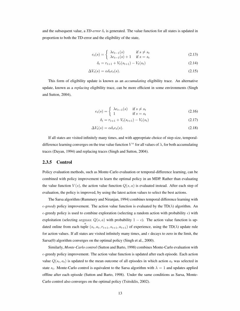
and the subsequent value, a TD-error δt is generated. The value function for all states is updated in
proportion to both the TD-error and the eligibility of the state,
et(s) ={λet−1(s) if s 6= stλet−1(s) + 1 if s = st
(2.13)
δt = rt+1 + Vt(st+1)− Vt(st) (2.14)
∆Vt(s) = αδtet(s). (2.15)
This form of eligibility update is known as an accumulating eligibility trace. An alternative
update, known as a replacing eligibility trace, can be more efficient in some environments (Singh
and Sutton, 2004),
et(s) ={λet−1(s) if s 6= st1 if s = st
(2.16)
δt = rt+1 + Vt(st+1)− Vt(st) (2.17)
∆Vt(s) = αδtet(s). (2.18)
If all states are visited infinitely many times, and with appropriate choice of step-size, temporal-
difference learning converges on the true value function V π for all values of λ, for both accumulating
traces (Dayan, 1994) and replacing traces (Singh and Sutton, 2004).
2.3.5 Control
Policy evaluation methods, such as Monte-Carlo evaluation or temporal-difference learning, can be
combined with policy improvement to learn the optimal policy in an MDP. Rather than evaluating
the value function V (s), the action value function Q(s, a) is evaluated instead. After each step of
evaluation, the policy is improved, by using the latest action values to select the best actions.
The Sarsa algorithm (Rummery and Niranjan, 1994) combines temporal difference learning with
ε-greedy policy improvement. The action value function is evaluated by the TD(λ) algorithm. An
ε-greedy policy is used to combine exploration (selecting a random action with probability ε) with
exploitation (selecting argmaxa
Q(s, a) with probability 1 − ε). The action value function is up-
dated online from each tuple (st, at, rt+1, st+1, at+1) of experience, using the TD(λ) update rule
for action values. If all states are visited infinitely many times, and ε decays to zero in the limit, the
Sarsa(0) algorithm converges on the optimal policy (Singh et al., 2000).
Similarly, Monte-Carlo control (Sutton and Barto, 1998) combines Monte-Carlo evaluation with
ε-greedy policy improvement. The action value function is updated after each episode. Each action
value Q(st, at) is updated to the mean outcome of all episodes in which action at was selected in
state st. Monte-Carlo control is equivalent to the Sarsa algorithm with λ = 1 and updates applied
offline after each episode (Sutton and Barto, 1998). Under the same conditions as Sarsa, Monte-
Carlo control also converges on the optimal policy (Tsitsiklis, 2002).
13
2.3.6 Value Function Approximation
In large environments, it is not possible or practical to learn a value for each individual state. In
this case, it is necessary to represent the state more compactly, by using some set of features φ(s)
of the state s. The value function can then be approximated by a function of the features and
parameters θ. For example, a set of binary features φ(s) ∈ {0, 1}n can be used to abstract the state
space, where each binary feature φi(s) identifies a particular property of the state. A common and
successful methodology (Sutton, 1996) is to use a linear combination of features and parameters to
approximate the value function, V (s) = φ(s) · θ.
We refer to the case when no value function approximation is used, in other words when each
state has a distinct value, as table lookup. Linear function approximation includes table lookup as
one possible representation. In this special case, we define a table lookup feature, Is′, to match each
individual state s′ ∈ S,
Is′(s) =
{1 if s = s′
0 otherwise.(2.19)
The feature vector consists of one table lookup feature for each state, φi(s) = Isi(s). A state s
is then represented by a unit vector of size |S| with a one in the sth component and zeros elsewhere.
The value of state s is represented by the sth parameter, V (s) = θs.
2.3.7 Linear Monte-Carlo Evaluation
When the value function is approximated by a parameterised function of features, errors could be
attributed to any or all of those features. Gradient descent provides a principled approach to this
problem of credit assignment: the parameters are updated in the direction that minimises the mean-
squared error.
Monte-Carlo evaluation can be generalised to use value function approximation. The parameters
are adjusted so as to reduce the mean-squared error between the estimated value and the actual re-
turn. When linear function approximation is used, Monte-Carlo evaluation has a particularly simple
form. The parameters are updated by stochastic gradient descent (Widrow and Stearns, 1985), with
a step-size of α,
∆θ = −α2∇θ(Rt − V (st))2 (2.20)
= α(Rt − V (st))∇θV (st) (2.21)
= α(Rt − V (st))φ(st) (2.22)
If table lookup features are used, and the step-size varies according to the schedule αt = 1N(st)
,
then linear Monte-Carlo evaluation is equivalent to incremental Monte-Carlo evaluation (see Section
2.3.2),
14
∆V (s) = (∆θ) · φ(s) (2.23)
= αt(Rt − V (st))φ(st) · φ(s) (2.24)
=1
N(st)(Rt − V (st))I(st) · I(s) (2.25)
=1
N(s)(Rt − V (s)) (2.26)
2.3.8 Linear Temporal-Difference Learning
The gradient descent method of the previous section can be extended to temporal difference learning.
The key idea is to replace the target, Rt, in Equation 2.21, with the estimated value at the next time-
step, rt+1 + V (st+1) (Sutton, 1984). It is important to note that this introduces bias, and it is no
longer a true gradient descent algorithm. Nevertheless, the analogy with gradient descent methods
provides a useful intuition for understanding the algorithm.
Temporal-difference learning with linear function approximation is a particularly simple case
(Sutton and Barto, 1998). The parameters are updated in proportion to the TD-error and the feature
value,
∆θ = (rt+1 + V (st+1)− V (st))∇θV (st) (2.27)
= αδtφ(st). (2.28)
The linear TD(λ) algorithm is defined similarly (Sutton, 1988). Using accumulating traces, the
weights are updated in proportion to the TD-error and the eligibility trace,
et = λet−1 + φ(s) (2.29)
∆θ = αδtet. (2.30)
If the agent’s experience is generated from its own policy, a case known as on-policy learn-
ing, linear temporal-difference learning converges to a value function that has a mean-squared error
within (1 − γλ)/(1 − γ) of the best possible approximation (Tsitsiklis and Roy, 1997), where γ is
a discount factor in continuing environments, or a horizon dependent constant in episodic environ-
ments.
The linear Sarsa algorithm combines linear temporal-difference learning with the Sarsa algo-
rithm, by updating an action value function and using an epsilon-greedy policy to select actions.
The complete linear Sarsa(λ) algorithm is shown in Algorithm 1. Although there are no guarantees
of convergence, on-policy linear Sarsa chatters without divergence (Gordon, 1996).
15
Algorithm 1 Sarsa(λ)
1: procedure SARSA(λ)2: θ ← 0 . Clear weights3: loop4: s← s0 . Start new episode in initial state5: e← 0 . Clear eligibility trace6: a← ε-greedy action from state s7: while s is not terminal do8: Execute a, observe reward r and next state s′
9: a′ ← ε-greedy action from state s′
10: δ ← r +Q(s′, a′)−Q(s, a) . Calculate TD-error11: θ ← θ + αδe . Update weights12: e← λe+ φ(s, a) . Update eligibility trace13: s← s′, a← a′
14: end while15: end loop16: end procedure
2.4 Policy Gradient Reinforcement Learning
Instead of updating a value function, the idea of policy gradient reinforcement learning is to directly
update the parameters of the agent’s policy by gradient ascent, so as to maximise the agent’s aver-
age reward per time-step. Policy gradient methods are typically higher variance and therefore less
efficient than value-based approaches, but they have three significant advantages. First, they are
able to directly learn mixed strategies that are a stochastic balance of different actions. Second, they
have better convergence properties than value-based methods: they are guaranteed to converge on a
policy that is at least locally optimal. Finally, they are able to learn a parameterised policy even in
problems with continuous action spaces.
The REINFORCE algorithm (Williams, 1992) updates the parameters of the agent’s policy by
stochastic gradient ascent. Given a differentiable policy πp(s, a) that is parameterised by a vector of
adjustable weights p, the REINFORCE algorithm updates those weights at every time-step t,
∆p = β(Rt − b(st)) log∇pπp(st, at) (2.31)
where β is a step-size parameter and b is a reinforcement baseline that does not depend on the current
action at.
Policy gradient algorithms (Sutton et al., 2000) extend this approach to use the action value
function in place of the actual return,
∆p = β(Qπ(st, at)− b(st)) log∇pπp(st, at) (2.32)
Actor-critic algorithms combine the advantages of policy gradient methods with the efficiency
of value-based reinforcement learning. They consist of two components: an actor that updates the
16
agent’s policy, and a critic that updates the action value function. When value function approxi-
mation is used, care must be taken to ensure that the critic’s parameters θ are compatible with the
actor’s parameters p. The compatibility requirement is that∇θQθ(s, a) = ∇p log πp(s, a).
2.5 Exploration and Exploitation
The ε-greedy policy used in the Sarsa algorithm provides one simple approach to balancing explo-
ration with exploitation. However, more sophisticated strategies are also possible. We mention two
of the most common approaches here.
First, exploration can be skewed towards more highly valued states, for example by using a
softmax policy,
π(s, a) =eQ(s,a)/τ∑b eQ(s,b)/τ
(2.33)
where τ is a parameter controlling the temperature (level of stochasticity) in the policy.
A second approach is to apply the principle of optimism in the face of uncertainty, for example
by adding a bonus to the value function that is largest in the most uncertain states. The UCB1
algorithm (Auer et al., 2002) follows this principle, by maximising an upper confidence bound on
the value function,
Q⊕(s, a) = Q(s, a) +
√2 logN(s)N(s, a)
(2.34)
π(s, a) = argmaxb
Q⊕(s, b) (2.35)
where N(s) counts the number of visits to state s, and N(s, a) counts the number of times that
action a has been selected from state s.
17
Chapter 3
Search and Planning
3.1 Introduction
Planning and search have been widely applied, in a variety of different forms, across much of ar-
tificial intelligence. We adopt the definition of planning typically used in reinforcement learning
(Sutton and Barto, 1998), and the definition of search that is often used in two-player games (Scha-
effer, 2000).
Planning is the process of computation by which the agent updates its action selection policy
π(s, a). The agent is given some amount of thinking time in which to plan. During this time it has
no interaction with the environment, but can perform many steps of internal computation. The result
of planning is a new policy, which can then be used to select actions in any state s in the problem.
Search refers to the process of computation that is used to select an action from a particular
root state s0. A search algorithm can be used for planning, by executing a search from the agent’s
current state st, an approach that is sometimes referred to as real-time search (Korf, 1990). Rather
than providing a complete policy over all states, this provides a partial policy for the current state st
and its successors. By focusing on the current state, real-time search methods can be considerably
more efficient than general planning methods.
3.2 Planning
Most planning methods use a model of the environment. This model can either be solved directly,
by applying model-based reinforcement learning methods, or indirectly, by sampling the model and
Most search algorithms construct a search tree from a root state s0, where each node of the tree
corresponds to a descendent state of s0. The nodes of the search tree are traversed in a particular
order. Leaf nodes may be expanded by the search algorithm, to add their successors into the search
tree. Interior nodes are evaluated by a backup of the values in the search tree. Table 3.1 summarises
the traversal and backup strategies of several well-known search algorithms.
3.3.1 Full-Width Search
A full-width search considers all possible actions and all successor states from each internal node
of the search tree. A fixed-depth search expands nodes of the search tree exhaustively up to some
fixed depth. A variable-depth search uses a selective expansion criterion to decide which leaf nodes
should be developed. The tree may be traversed in a depth-first, breadth-first, or best-first order,
where the latter utilises a heuristic function to guide the search towards the most promising states
(Russell and Norvig, 1995).
Full-width search can be applied to MDPs, so as to find the sequence of actions that leads to
the maximum expected return from the current state. Full-width search can also be applied in deter-
ministic environments, to find the sequence of actions with minimum cost. It can also be applied in
two-player games, to find the optimal minimax move sequence under alternating play. In each case,
heuristic search algorithms operate in a very similar manner. Leaf nodes are evaluated by the heuris-
tic function, and interior nodes are evaluated by a full backup that updates each parent value from
all of its children: an expectimax backup in MDPs, a max backup in deterministic environments, or
a minimax backup in two-player games.
This very general framework can be used to categorise a number of well-known search algo-
rithms: for example A* (Hart et al., 1968) is a best-first search with max backups; expectimax
search (Davies et al., 1998) is a depth-first search with expectimax backups; and alpha-beta (Knuth
and Moore, 1975) is a depth-first search with minimax backups.
A value function (see Chapter 2) can be used as a heuristic function. In this approach, leaf nodes
are evaluated by estimating the expected return or outcome from that node (Davies et al., 1998).
20
3.3.2 Sample-Based Search
In sample-based search, instead of considering all possible successors, the next state and reward
is sampled from a generative model. These samples are typically used to construct a tree, and the
value of each interior node is updated by an appropriate backup operation. Random sampling in
this manner breaks the curse of dimensionality (Rust, 1997). In environments with large branching
factors or stochastic dynamics, sample-based search can be much more effective than full-width
search.
Sparse lookahead (Kearns et al., 2002) is a depth-first approach to sample-based search. A state s
is expanded by executing each action a, and samplingC successor states from the model, to generate
a total of |A|C children. Each child is expanded recursively in depth-first order, and then evaluated
by a sample max backup,
V (s)← maxa∈A
1C
C∑i=1
V (child(s, a, i)) (3.1)
where child(s, a, i) denotes the ith child of state s for action a. Leaf nodes at maximum depthD are
evaluated by a fixed value function. Finally, the action with maximum evaluation at the root node
s0 is selected. Given sufficient depth D and breadth C, this approach will generate a near-optimal
policy for any MDP.
Sparse lookahead can be extended to use a more informed exploration policy. Rather than uni-
formly sampling each action C times, the UCB1 algorithm (see Chapter 2) can be used to select the
next action to sample (Chang et al., 2005). This ensures that the best actions are tried most often,
but that actions with high uncertainty are also explored.
3.3.3 Simulation-Based Search
The basic idea of simulation-based search is to sequentially sample episodes of experience, without
backtracking, that start from the root state s0. At each step t of simulation, an action at is selected
according to a simulation policy, and a new state st+1 and reward rt+1 is generated by the model.
After every simulation, the values of states or actions are updated from the simulated experience.
Simulation-based search algorithms can be used to selectively construct a search tree. Each
simulation starts from the root of the search tree, and the best action is selected at each step according
to the current values in the search tree. We refer to this approach as simulation-based tree search.
After each simulation, every visited state is added to the search tree, and the values of these states are
backed up through the search tree, for example by a sample max backup (Peret and Garcia, 2004).
Unlike sparse lookahead, which expands nodes in a depth-first order, simulation-based tree search
is sequentially best-first: it selects the best child at each step of a sequential simulation. This allows
the search to continually refocus its attention, each simulation, on the highest value regions of the
state space. As the simulations progress, the values in the search tree become more accurate and the
21
simulation policy becomes better informed, in a cycle of policy improvement (see Chapter 2).
3.3.4 Monte-Carlo Simulation
Monte-Carlo simulation is a very simple simulation-based search algorithm for evaluating candidate
actions from a root position s0. The search proceeds by simulating complete episodes from s0 until
termination, using a fixed simulation policy. The action-values Q(s0, a) are estimated by the mean
outcome of all simulations with candidate action a.1
In its most basic form, Monte-Carlo simulation is only used to evaluate actions, but not to
improve the simulation policy. However, the basic algorithm can be extended by progressively
favouring the most successful actions, or by progressively pruning away the least successful actions
(Billings et al., 1999; Bouzy and Helmstetter, 2003)
In some problems, such as backgammon (Tesauro and Galperin, 1996), Scrabble (Sheppard,
2002), Amazons (Lorentz, 2008) and Lines of Action (Winands and Y. Bjornsson, 2009), it is possi-
ble to construct an accurate approximation to the value function. In these cases it can be beneficial to
stop simulation before the end of the episode, and bootstrap from the estimated value at the time of
stopping. This approach, known as truncated Monte-Carlo simulation, provides faster simulations
with lower variance evaluations. In more challenging problems, such as Go (Bouzy and Helmstetter,
2003), it is hard to construct an accurate global approximation to the value function. In this case
truncating simulations increases the evaluation bias more than it reduces the evaluation variance,
and it is better to simulate until termination.
3.3.5 Monte-Carlo Tree Search
Monte-Carlo tree search (MCTS) is a simulation-based tree search algorithm that uses Monte-Carlo
simulation to evaluate the nodes of a search tree T (Coulom, 2006). There is one node, n(s),
corresponding to each state s in the search tree. Each node contains a total count for the state, N(s),
and a value Q(s, a) and count N(s, a) for each action a ∈ A.
Simulations start from the root state s0, and are divided into two stages. When state st is rep-
resented in the search tree, st ∈ T , a tree policy is used to select actions. Otherwise, a default
policy is used to roll out simulations to completion. The simplest version of the algorithm, which
we call greedy MCTS, uses a greedy tree policy during the first stage, which selects the action with
the highest value, argmaxa
Q(st, a); and a uniform random default policy during the second stage.
After each simulation s0, a0, s1, a1, ..., sT with returnR, each node in the search tree, {n(st)|st ∈T }, is updated. The counts are incremented, and the value is updated to the mean return (see Section
2.3.2),1In deterministic single-agent domains, the max outcome is sometimes used instead, e.g. nested Monte-Carlo search
(Cazenave, 2009).
22
N(st)← N(st) + 1 (3.2)
N(st, at)← N(st, at) + 1 (3.3)
Q(st, at)← Q(st, at) +R−Q(st, at)N(st, at)
, (3.4)
In addition, each visited node is added to the search tree. Alternatively, to reduce memory re-
quirements, just one new node can be added to the search tree, for the first state that is not represented
in the tree. Figure 3.1 illustrates several steps of the MCTS algorithm.
3.3.6 UCT
The UCT algorithm (Kocsis and Szepesvari, 2006) is a Monte-Carlo tree search that treats each
state of the search tree as a multi-armed bandit.2 The tree policy selects actions by using the UCB1
algorithm (see Chapter 2). The action value is augmented by an exploration bonus that is highest for
rarely visited state-action pairs, and the tree policy selects the action a∗ maximising the augmented
value,
Q⊕(s, a) = Q(s, a) + c
√2 logN(s)N(s, a)
(3.5)
a∗ = argmaxa
Q⊕(s, a) (3.6)
where c is a scalar exploration constant. Pseudocode for the UCT algorithm is given in Algorithm
2.
UCT is proven to converge in MDPs with finite horizon T , rewards in the interval [0, 1], and
an exploration constant c = T . As the number of simulations N grows to infinity, the root values
converge in probability to the optimal values, ∀a ∈ A, plimn→∞
Q(s0, a) = Q∗(s0, a). Furthermore,
the bias of the root values, E[Q(s0, a)−Q∗(s0, a)], isO(log(n)/n), and the probability of selecting
a suboptimal action, Pr(argmaxa∈A
Q(s0, a) 6= argmaxa∈A
Q∗(s0, a)), converges to zero at a polynomial
rate.
The performance of UCT can often be significantly improved by incorporating domain knowl-
edge into the default policy (Gelly et al., 2006). The UCT algorithm, using a carefully chosen default
policy, has outperformed previous approaches to search in a variety of challenging games, including
Go (Gelly et al., 2006), General Game Playing (Finnsson and Bjornsson, 2008), Amazons (Lorentz,
2008), Lines of Action (Winands and Y. Bjornsson, 2009), multi-player card games (Schafer, 2008;
Sturtevant, 2008), and real-time strategy games (Balla and Fern, 2009). Much additional research
in Monte-Carlo tree search has been developed in the context of computer Go, and is discussed in
more detail in the next chapter.2In fact, the search tree is not a true multi-armed bandit, as there is no real cost to exploration during planning. In addition
the simulation policy continues to change as the search tree is updated, which means that the payoff is non-stationary.
23
Algorithm 2 UCTprocedure UCTSEARCH(s0)
while time remaining do{s0, ..., sT }, R = SIMULATE(s0)BACKUP({s0, ..., sT }, R)
procedure BACKUP({s0, ..., sT }, R)for t = 0 to T − 1 do
N(st) += 1N(st, at) += 1Q(st, at) += R−Q(st,at)
N(st,at)
end forend procedure
procedure NEWNODE(s)N(s) = 0for all a ∈ A do
N(s, a) = 0Q(s, a) =∞
end forT .Insert(s)
end procedure
24
New node in the tree
Node stored in the tree
State visited but not stored
Terminal outcome
Current simulation
Previous simulation
Figure 3.1: Five simulations of Monte-Carlo tree search.
25
Chapter 4
Computer Go
4.1 The Challenge of Go
For many years, computer chess was considered to be “the drosophila of AI”,1 and a “grand chal-
lenge task” (McCarthy, 1997). It provided a sandbox for new ideas, a straightforward performance
comparison between algorithms, and measurable progress against human capabilities. With the
dominance of alpha-beta search programs over human players now conclusive in chess (McClain,
2006), many researchers have sought out a new challenge. Computer Go has emerged as the “new
drosophila of AI” (McCarthy, 1997), a “task par excellence” (Harmon, 2003), and “a grand chal-
lenge task for our generation” (Mechner, 1998).
In the last few years, a new paradigm for AI has been developed in computer Go. This approach,
based on Monte-Carlo simulation, has provided dramatic progress and led to the first master-level
programs (Gelly and Silver, 2007; Coulom, 2007). Unlike alpha-beta search, these algorithms are
still in their infancy, and the arena is still wide open to new ideas. In addition, this new approach
to search requires little or no human knowledge in order to produce good results. Although this
paradigm has been pioneered in computer Go, it is not specific to Go, and the core concept of
simulation-based search is widely applicable. Ultimately, the study of computer Go may illuminate
a path towards high performance AI in a wide variety of challenging domains.
4.2 The Rules of Go
The game of Go is usually played on a 19× 19 grid, with 13× 13 and 9× 9 as popular alternatives.
Black and White play alternately, placing a single stone on an intersection of the grid. Stones cannot
be moved once played, but may be captured. Sets of adjacent, connected stones of one colour are
known as blocks. The empty intersections adjacent to a block are called its liberties. If a block is
reduced to zero liberties by the opponent, it is captured and removed from the board (Figure 4.1a,
A). Stones with just one remaining liberty are said to be in atari. Playing a stone with zero liberties
is illegal (Figure 4.1a, B), unless it also reduces an opponent block to zero liberties. In this case the
1Drosophila is the fruit fly, the most extensively studied organism in genetics research.
26
r u les
A
A
B
B
C
C
D
D
E
E
F
F
G
G
H
H
J
J
1 1
2 2
3 3
4 4
5 5
6 6
7 7
8 8
9 9
B
A
B
A
D C
A
B lack to play
e yes
A
A
B
B
C
C
D
D
E
E
F
F
G
G
H
H
J
J
1 1
2 2
3 3
4 4
5 5
6 6
7 7
8 8
9 9
E
E
E
E
F
F
Black to play
G
G
G
G
H
H
G
H
G
H
H
G
H
H
territory
A
A
B
B
C
C
D
D
E
E
F
F
G
G
H
H
J
J
1 1
2 2
3 3
4 4
5 5
6 6
7 7
8 8
9 9
B*
B
B*
b
b
b
w
W*
W
B*
B*
B*
B*
b
w
w
w
W
b
B*
B*
b
b
w
w
W
W
b
b
b
B
b
w
W
W
W
B
B
b
B
b
b
w
W
W
B
B
B
B
B
b
w
W
W
B
B
B
B
b
w
w
W
W
B
B
B
B
b
w
W
W
W
B
B
B
B
b
w
W
W
W
Black to playFigure 4.1: a) The White stones are in atari and can be captured by playing at the points markedA. It is illegal for Black to play at B, as the stone would have no liberties. Black may, however,play at C to capture the stone at D. White cannot recapture immediately by playing at D; as thiswould repeat the position - it is a ko. b) The points marked E are eyes for Black. The black groupson the left can never be captured by White, they are alive. The points marked F are false eyes: theblack stones on the right will eventually be captured by White and are dead. c) Groups of looselyconnected white stones (G) and black stones (H). d) A final position. Dead stones (B∗,W∗) areremoved from the board. All surrounded intersections (B,W ) and all remaining stones (b, w) arecounted for each player. If komi is 6.5 then Black wins by 8.5 points in this example.
30 kyu 1 kyu 1 dan 7 dan 1 dan 9 dan
Beginner Master Professional
Figure 4.2: Performance ranks in Go, in increasing order of strength from left to right.
opponent block is captured, and the player’s stone remains on the board (Figure 4.1a, C). Finally,
repeating a previous board position is illegal. A situation in which a repeat could otherwise occur is
known as ko (Figure 4.1a, D).
A connected set of empty intersections that is wholly enclosed by stones of one colour is known
as an eye. One natural consequence of the rules is that a block with two eyes can never be captured
by the opponent (Figure 4.1b, E). Blocks which cannot be captured are described as alive; blocks
which will certainly be captured are described as dead (Figure 4.1b, F ). A loosely connected set of
stones is described as a group (Figure 4.1c, G,H). Determining the life and death status of a group
is a fundamental aspect of Go strategy.
The game ends when both players pass. Dead blocks are removed from the board (Figure 4.1d,
B∗,W∗). In Chinese rules, all alive stones, and all intersections that are enclosed by a player, are
counted as a point of territory for that player (Figure 4.1d, B,W ).2 Black always plays first in Go;
White receives compensation, known as komi, for playing second. The winner is the player with the
greatest territory, after adding komi for White.
27
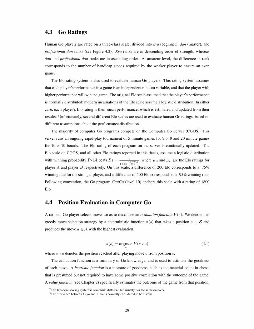
4.3 Go Ratings
Human Go players are rated on a three-class scale, divided into kyu (beginner), dan (master), and
professional dan ranks (see Figure 4.2). Kyu ranks are in descending order of strength, whereas
dan and professional dan ranks are in ascending order. At amateur level, the difference in rank
corresponds to the number of handicap stones required by the weaker player to ensure an even
game.3
The Elo rating system is also used to evaluate human Go players. This rating system assumes
that each player’s performance in a game is an independent random variable, and that the player with
higher performance will win the game. The original Elo scale assumed that the player’s performance
is normally distributed; modern incarnations of the Elo scale assume a logistic distribution. In either
case, each player’s Elo rating is their mean performance, which is estimated and updated from their
results. Unfortunately, several different Elo scales are used to evaluate human Go ratings, based on
different assumptions about the performance distribution.
The majority of computer Go programs compete on the Computer Go Server (CGOS). This
server runs an ongoing rapid-play tournament of 5 minute games for 9 × 9 and 20 minute games
for 19 × 19 boards. The Elo rating of each program on the server is continually updated. The
Elo scale on CGOS, and all other Elo ratings reported in this thesis, assume a logistic distribution
with winning probability Pr(A beats B) = 1
1+10µB−µA
400, where µA and µB are the Elo ratings for
player A and player B respectively. On this scale, a difference of 200 Elo corresponds to a 75%
winning rate for the stronger player, and a difference of 500 Elo corresponds to a 95% winning rate.
Following convention, the Go program GnuGo (level 10) anchors this scale with a rating of 1800
Elo.
4.4 Position Evaluation in Computer Go
A rational Go player selects moves so as to maximise an evaluation function V (s). We denote this
greedy move selection strategy by a deterministic function π(s) that takes a position s ∈ S and
produces the move a ∈ A with the highest evaluation,
π(s) = argmaxa
V (s ◦ a) (4.1)
where s ◦ a denotes the position reached after playing move a from position s.
The evaluation function is a summary of Go knowledge, and is used to estimate the goodness
of each move. A heuristic function is a measure of goodness, such as the material count in chess,
that is presumed but not required to have some positive correlation with the outcome of the game.
A value function (see Chapter 2) specifically estimates the outcome of the game from that position,
2The Japanese scoring system is somewhat different, but usually has the same outcome.3The difference between 1 kyu and 1 dan is normally considered to be 1 stone.
28
V (s) ≈ V ∗(s), where V ∗(s) denotes the optimal (minimax) value of position s. A static evaluation
function is stored in memory, whereas a dynamic evaluation function is computed by a process of
search from the current position s.
4.5 Static Evaluation in Computer Go
Constructing an evaluation function for Go is a challenging task. First, as we have already seen, the
state space is enormous. Second, the evaluation function can be highly volatile: changing a single
stone can transform a position from lost to won or vice versa. Third, interactions between stones
may extend across the whole board, making it difficult to decompose the global evaluation into local
features.
A static evaluation function cannot usually store a separate value for each distinct position s. In-
stead, it is represented by features φ(s) of the position s, and some number of adjustable parameters
θ. For example, a position can be evaluated by a neural network that uses features of the position as
its inputs (Schraudolph et al., 1994; Enzenberger, 1996; Dahl, 1999; Enzenberger, 2003).
4.5.1 Symmetry
The Go board has a high degree of symmetry. It has eight-fold rotational and reflectional symmetry,
and it has colour symmetry: if all stone colours are inverted, the colour to play is swapped, and komi
is reversed, then the position is exactly equivalent. This suggests that the evaluation function should
be invariant to rotational, reflectional and colour inversion symmetries. When considering the status
of a particular intersection, the Go board also exhibits translational symmetry: a local configuration
of stones in one part of the board has similar properties to the same configuration of stones in another
part of the board, subject to edge effects.
Schraudolph et al. (1994) exploit these symmetries in a convolutional neural network. The net-
work predicts the final territory status of a particular target intersection. It receives one input from
each intersection (−1, 0 or +1 for White, Empty and Black respectively) in a local region around the
target, contains a fixed number of hidden nodes, and outputs the predicted territory for the target in-
tersection. The global position is evaluated by summing the territory predictions for all intersections
on the board. Weights are shared between rotationally and reflectionally symmetric patterns of input
features,4 and between all target intersections. In addition, the input features, squashing function
and bias weights are all antisymmetric, and on each alternate move the sign of the bias weight is
flipped, so that network evaluation is invariant to colour inversion.
A further symmetry of the Go board is that stones within the same block will live or die together
as a unit, sometimes described as the common fate property (Graepel et al., 2001). One way to make
use of this invariance (Enzenberger, 1996; Graepel et al., 2001) is to treat each complete block or
4Surprisingly this impeded learning in practice (Schraudolph et al., 2000).
29
empty intersection as a unit, and to represent the board by a common fate graph containing a node
for each unit and an edge between each pair of adjacent units.
4.5.2 Handcrafted Heuristics
In many other classic games, handcrafted heuristic functions have proven highly effective. Basic
heuristics such as material count and mobility, which provide reasonable estimates of goodness in
checkers, chess and Othello (Schaeffer, 2000), are next to worthless in Go. Stronger heuristics have
proven surprisingly hard to design, despite several decades of endeavour (Muller, 2002).
Until recently, most Go programs incorporated very large quantities of expert knowledge, in a
pattern database containing many thousands of manually inputted patterns, each describing a rule of
thumb that is known by expert Go players. Traditional Go programs used these databases to recom-
mend expert moves in commonly recognised situations, typically in conjunction with local or global
alpha-beta search algorithms. In addition, they can be used to encode knowledge about connections,
eyes, opening sequences, or promising search extensions. The pattern database accounts for a large
part of the development effort in a traditional Go program, sometimes requiring many man-years of
effort from expert Go players.
However, pattern databases are hindered by the knowledge acquisition bottleneck: expert Go
knowledge is hard to interpret, represent, and maintain. The more patterns in the database, the harder
it becomes to predict the effect of a new pattern on the overall playing strength of the program.
4.5.3 Temporal Difference Learning
Reinforcement learning can be used to estimate a value function that predicts the eventual outcome
of the game. The learning program can be rewarded by the score at the end of the game, or by
a reward of 1 if Black wins and 0 if White wins. Surprisingly, the less informative binary signal
has proven more successful (Coulom, 2006), as it encourages the agent to favour risky moves when
behind, and calm moves when ahead. Expert Go players will frequently play to minimise the uncer-
tainty in a position once they judge that they are ahead in score; this behaviour cannot be replicated
by simply maximising the expected score. Despite this shortcoming, the final score is widely used
as a reward signal (Schraudolph et al., 1994; Enzenberger, 1996; Dahl, 1999; Enzenberger, 2003).
Schraudolph et al. (1994) exploit the symmetries of the Go board (see Section 4.5.1) to predict
the final territory at an intersection. They train their multilayer perceptron using TD(0), using a re-
ward signal corresponding to the final territory value of the intersection. The network outperformed
a commercial Go program, The Many Faces of Go, when set to a low playing level in 9×9 Go, after
just 3,000 self-play training games.
Dahl’s Honte (1999) and Enzenberger’s NeuroGo III (2003) use a similar approach to predict-
ing the final territory. However, both programs learn intermediate features that are used to input
additional knowledge into the territory evaluation network. Honte has one intermediate network to
30
predict local moves and a second network to evaluate the life and death status of groups. NeuroGo III
uses intermediate networks to evaluate connectivity and eyes. Both programs achieved single-digit
kyu ranks; NeuroGo won the silver medal at the 2003 9× 9 Computer Go Olympiad.
Although a complete game of Go typically contains hundreds of moves, only a small number
of moves are played within a given local region. Enzenberger (2003) suggests for this reason that
TD(0) is a natural choice of algorithm. Indeed, TD(0) has been used almost exclusively in rein-
forcement learning approaches to position evaluation in Go (Schraudolph et al., 1994; Enzenberger,
1996; Dahl, 1999; Enzenberger, 2003; Runarsson and Lucas, 2005; Mayer, 2007), perhaps because
of its simplicity and its proven efficacy in games such as backgammon (Tesauro, 1994).
4.5.4 Comparison Training
If we assume that expert Go players are rational, then it is reasonable to infer the expert’s evaluation
function Vexpert by observing their move selection decisions. For each expert move a, rational
move selection tells us that Vexpert(s ◦ a) ≥ Vexpert(s ◦ b) for any legal move b. This can be
used to generate an error metric for training an evaluation function V (s), in an approach known as
comparison training (Tesauro, 1988). The expert move a is compared to another move b, randomly
selected; if the non-expert move evaluates higher than the expert move then an error is generated.
Van der Werf et al. (2002) use comparison training to learn the weights of a multilayer per-
ceptron, using local board features as inputs. Following Enderton (1991), they compute an error
function E of the form,
E(s, a, b) ={
[V (s ◦ a) + ε− V (s ◦ b)]2 if V (s ◦ a) + ε > V (s ◦ a)0 otherwise, (4.2)
where ε is a positive control parameter used to avoid trivial solutions. The trained network was
able to predict expert moves with 37% accuracy on an independent test set; the authors estimate its
strength to be at strong kyu level for the task of local move prediction. The learnt evaluation function
was used in the Go program Magog, which won the bronze medal in the 2004 9 × 9 Computer Go
Olympiad.
4.5.5 Evolutionary Methods
A common approach is to apply evolutionary methods to learn a heuristic evaluation function, for
example by applying genetic algorithms to the weights of a multilayer perceptron. The fitness of
a heuristic is typically measured by running a tournament and counting the total number of wins.
These approaches have two major sources of inefficiency. First, they only learn from the result
of the game, and do not exploit the sequence of positions and moves used to achieve the result.
Second, many games must be run in order to produce fitness values with reasonable discrimination.
Runarsson and Lucas compare temporal difference learning with coevolutionary learning, using a
basic state representation. They find that TD(0) both learns faster and achieves greater performance
31
in most cases (Runarsson and Lucas, 2005). Evolutionary methods have not yet, to our knowledge,
produced a competitive Go program.
4.6 Dynamic Evaluation in Computer Go
An alternative method of position evaluation is to construct a search tree from the root position, and
dynamically update the evaluation of the nodes in the search tree.
4.6.1 Alpha-Beta Search
Despite the challenging search space, and the difficulty of constructing a static evaluation function,
alpha-beta search has been used extensively in computer Go. One of the strongest traditional pro-
grams, The Many Faces of Go5, uses a global alpha-beta search to select moves. Each position is
evaluated by extensive handcrafted knowledge in combination with local alpha-beta searches to de-
termine the status of individual blocks and groups. The program GnuGo6 uses handcrafted databases
of pattern knowledge and specialised search routines to determine local subgoals such as capture,
connection, and eye formation. The local status of each subgoal is used to estimate the overall
benefit of each legal move.
However, even determining the status of individual blocks can be a challenging problem. In ad-
dition, the local searches are not usually independent, and the search trees can overlap significantly.
Finally, the global evaluation often depends on more subtle factors than can be represented by simple
local subgoals (Muller, 2001).
4.6.2 Monte Carlo Simulation
In contrast to traditional search methods, Monte-Carlo simulation does not require a static evaluation
function. This makes it an appealing choice for Go, where as we have seen, position evaluation is
particularly challenging.
The first Monte-Carlo Go program, Gobble (Bruegmann, 1993), simulated many games of self-
play from the current position s. It combined Monte-Carlo evaluation with two novel ideas: the
all-moves-as-first heuristic, and ordered simulation. The all-moves-as-first heuristic assumes that
the value of a move is not significantly affected by changes elsewhere on the board. The value of
playing move a immediately is estimated by the average outcome of all simulations in which move
a is played at any time (see Chapter 8 for an exact definition). Gobble also used ordered simulation
to sort all moves according to their estimated value. This ordering is randomly perturbed according
to an annealing schedule that cools down with additional simulations. Each simulation plays out all
moves in the prescribed order. Gobble itself played weakly, with an estimated rating of around 25
Bouzy and Helmstetter developed the first competitive Go programs based on Monte-Carlo sim-
ulation (Bouzy and Helmstetter, 2003). Their basic framework simulates many games of self-play
from the current position s, for each candidate action a, using a uniform random simulation policy;
the value of a is estimated by the average outcome of these simulations. The only domain knowledge
is to prohibit moves within eyes; this ensures that games terminate within a reasonable timeframe.
Bouzy and Helmstetter also investigated a number of extensions to Monte-Carlo simulation, several
of which are precursors to the more sophisticated algorithms used now:
1. Progressive pruning is a technique in which statistically inferior moves are removed from
consideration (Bouzy, 2005b).
2. The all-moves-as-first heuristic, described above.
3. The temperature heuristic uses a softmax simulation policy to bias the random moves towards
the strongest evaluations. The softmax policy selects moves with a probability π(s, a) =eV (s◦a)/τP
b∈legal eV (s◦b)/τ , where τ is a constant temperature parameter controlling the overall level of
randomness.7
4. The minimax enhancement constructs a full width search tree, and separately evaluates each
node of the search tree by Monte-Carlo simulation. Selective search enhancements were also
tried (Bouzy, 2004).
Bouzy also tracked statistics about the final territory status of each intersection after each simu-
lation (Bouzy, 2006). This information is used to influence the simulations towards disputed regions
of the board, by avoiding playing on intersections which are consistently one player’s territory.
Bouzy also incorporated pattern knowledge into the simulation player (Bouzy, 2005a). Using these
enhancements his program Indigo won the bronze medal at the 2004 and 2006 19 × 19 Computer
Go Olympiads.
It is surprising that a Monte-Carlo technique, originally developed for stochastic games such
as backgammon (Tesauro and Galperin, 1996), Poker (Billings et al., 1999) and Scrabble (Shep-
pard, 2002) should succeed in Go. Why should an evaluation that is based on random play provide
any useful information in the precise, deterministic game of Go? The answer, perhaps, is that
Monte-Carlo methods successfully manage the uncertainty in the evaluation. A random simulation
policy generates a broad distribution of simulated games, representing many possible futures and
the uncertainty in what may happen next. As the search proceeds and more information is accrued,
the simulation policy becomes more refined, and the distribution of simulated games narrows. In
contrast, deterministic play represents perfect confidence in the future: there is only one possible
continuation. If this confidence is misplaced, then predictions based on deterministic play will be
unreliable and misleading.
7Gradually reducing the temperature, as in simulated annealing, was not beneficial.
33
4.6.3 Monte-Carlo Tree Search
Within just three years of their introduction, Monte-Carlo tree search algorithms have revolutionised
computer Go, leading to the first strong programs that are competitive with human master players.
Work in this field is ongoing; in this section we outline some of the key developments.
Monte-Carlo tree search, as described in Chapter 3, was first introduced in the Go program
Crazy Stone (Coulom, 2006). The true value of each move is assumed to have a Gaussian distribu-
tion centred on the current value estimate, Qπ(s, a) ∼ N (Q(s, a), σ2(s, a)). During the first stage
of simulation, the tree policy selects each move according to its probability of being better than the
current best move, π(s, a) ≈ Pr(∀b,Qπ(s, a) > Q(s, b)). During the second stage of simulation,
the default policy selects moves with a probability proportional to an urgency value encoding do-
main specific knowledge. In addition, Crazy Stone used a hybrid backup to update values in the tree,
which is intermediate between a minimax backup and a expected value backup. Using these tech-
niques, Crazy Stone exceeded 1800 Elo on CGOS, achieving equivalent performance to traditional
Go programs such as GnuGo and The Many Faces of Go. Crazy Stone won the gold medal at the
2006 9× 9 Computer Go Olympiad.
The Go program MoGo introduced the UCT algorithm (see Chapter 3) to computer Go (Gelly
et al., 2006; Wang and Gelly, 2007). MoGo treats each position in the search tree as a multi-armed
bandit. There is one arm of the bandit for each legal move, and the payoff from an arm is the
outcome of a simulation starting with that move. During the first stage of simulation, the tree policy
selects moves using the UCB1 algorithm. During the second stage of simulation, MoGo uses a
default policy based on specialised domain knowledge. Unlike the enormous pattern databases used
in traditional Go programs, MoGo’s patterns are extremely simple. Rather than suggesting the best
move in any situation, these patterns are intended to produce local sequences of plausible moves.
They can be summarised by four prioritised rules following an opponent move a:
1. If a put some of our stones into atari, play a saving move at random.
2. Otherwise, if one of the 8 intersections surrounding a matches a simple pattern for cutting or
hane, randomly play one.
3. Otherwise, if any opponent stone can be captured, play a capturing move at random.
4. Otherwise play a random move.
Using these patterns in the UCT algorithm, MoGo significantly outperformed all previous 9× 9 Go
programs, exceeding 2100 Elo on the Computer Go Server.
The UCT algorithm in MoGo was subsequently replaced by the heuristic MC–RAVE algorithm
(Gelly and Silver, 2007) (see Chapter 8). In 9× 9 Go MoGo reached 2500 Elo on CGOS, achieved
dan-level play on the Kiseido Go Server, and defeated a human professional in an even game for
34
the first time (Gelly and Silver, 2008). These enhancements also enabled MoGo to perform well on
larger boards, winning the gold medal at the 2007 19× 19 Computer Go Olympiad.
The default policy used by MoGo is handcrafted. In contrast, a subsequent version of Crazy
Stone uses supervised learning to train the pattern weights for its default policy (Coulom, 2007).
The relative strength of patterns is estimated by assigning them Elo ratings, much like a tournament
between games players. In this approach, the pattern selected by a human player is considered
to have won against all alternative patterns. In general, multiple patterns may match a particular
move, in which case this team of patterns is considered to have won against alternative teams. The
strength of a team is estimated by the product of the individual pattern strengths. The probability
of each team winning is assumed to be proportional to that team’s strength, using a generalised
Bradley-Terry model (Hunter, 2004). Given a data set of expert moves, the maximum likelihood
pattern strengths can be efficiently approximated by the minorisation-maximisation algorithm. This
algorithm was used to learn a default policy, by training the strengths of simple 3 × 3 patterns
and simple features such as capture, self-atari, extension, and contiguity to the previous move. A
more complicated set of 17,000 patterns, harvested from the data set, was also trained and used to
progressively widen the search tree. Crazy Stone achieved a rating of 1 kyu at 19 × 19 Go against
human players on the Kiseido Go Server.
The Zen program has combined ideas from both MoGo and Crazy Stone, using more sophis-
ticated domain knowledge. Zen has achieved a 1 dan rating, on full-size boards, against human
players on the Kiseido Go Server.
Monte-Carlo tree search can be parallelised much more effectively than traditional search tech-
niques (Chaslot et al., 2008c). Recent work on MoGo has focused on full size 19 × 19 Go, using
massive parallelisation (Gelly et al., 2008) and incorporating additional expert knowledge into the
search tree. A version of MoGo running on 800 processors defeated a 9-dan professional player
with 7 stones handicap. The latest version of Crazy Stone and a new, Monte-Carlo version of The
Many Faces of Go have also achieved impressive victories against professional players on full size
boards. Most recently, the program Fuego (Muller and Enzenberger, 2009), based on a parallelised
version of heuristic MC–RAVE, defeated a 9-dan professional player in an even 9 × 9 game, and
defeated a 6-dan amateur player with 4 stones handicap on a full size board.8
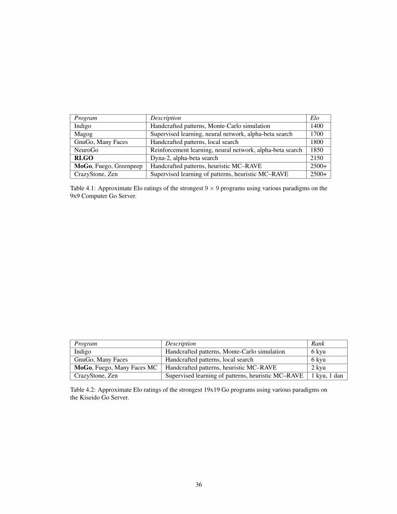
4.7 Summary
We provide a summary of the current state of the art in computer Go, based on ratings from the
Computer Go Server (see Table 4.1) and the Kiseido Go Server (see Table 4.2). The Go programs
to which this thesis has directly contributed are highlighted in bold.9
8Nick Wedd maintains a website of all human versus computer challenge matches: http://www.computer-go.info/h-c/index.html.
9Many of the top Go programs, including Crazystone, Fuego, Greenpeep, Zen, and the Monte-Carlo version of The ManyFaces of Go, now use variants of the RAVE and heuristic UCT algorithms (see Chapter 8).
35
Program Description EloIndigo Handcrafted patterns, Monte-Carlo simulation 1400Magog Supervised learning, neural network, alpha-beta search 1700GnuGo, Many Faces Handcrafted patterns, local search 1800NeuroGo Reinforcement learning, neural network, alpha-beta search 1850RLGO Dyna-2, alpha-beta search 2150MoGo, Fuego, Greenpeep Handcrafted patterns, heuristic MC–RAVE 2500+CrazyStone, Zen Supervised learning of patterns, heuristic MC–RAVE 2500+
Table 4.1: Approximate Elo ratings of the strongest 9× 9 programs using various paradigms on the9x9 Computer Go Server.
Program Description RankIndigo Handcrafted patterns, Monte-Carlo simulation 6 kyuGnuGo, Many Faces Handcrafted patterns, local search 6 kyuMoGo, Fuego, Many Faces MC Handcrafted patterns, heuristic MC–RAVE 2 kyuCrazyStone, Zen Supervised learning of patterns, heuristic MC–RAVE 1 kyu, 1 dan
Table 4.2: Approximate Elo ratings of the strongest 19x19 Go programs using various paradigms onthe Kiseido Go Server.
36
Part II
Temporal Difference Learning andSearch
37
Chapter 5
Temporal Difference Learning withLocal Shape Features
5.1 Introduction
A number of notable successes in artificial intelligence have followed a straightforward strategy:
the state is represented by many simple features; states are evaluated by a weighted sum of those
features, in a high-performance search algorithm; and weights are trained by temporal-difference
learning. In two-player games as varied as chess, checkers, Othello, backgammon and Scrabble,
programs based on variants of this strategy have exceeded human levels of performance.
• In each game, the position is broken down into a large number of features. These are usu-
ally binary features that recognise a small, local pattern or configuration within the position:
material, pawn structure and king safety in chess (Campbell et al., 2002); material and mobil-
ity terms in checkers (Schaeffer et al., 1992); configurations of discs in Othello (Buro, 1999);
checker counts in backgammon (Tesauro, 1994); and single, duplicate and triplicate letter rack
leaves in Scrabble (Sheppard, 2002).
• The position is evaluated by a linear combination of these features with weights indicating
their value. Backgammon provides a notable exception: TD-Gammon evaluates positions
with a non-linear combination of features, using a multi-layer perceptron.1 Linear evaluation
functions are fast to compute; easy to interpret, modify and debug; are effective over a wide
class of applications; and they have good convergence properties in many learning algorithms.
• Weights are trained from games of self-play, by temporal-difference or Monte-Carlo learn-
ing. The world champion checkers program Chinook was hand-tuned by experts over 5 years.
When weights were trained instead by self-play using temporal difference learning, the pro-
gram equalled the performance of the original version (Schaeffer et al., 2001). A related ap-
proach attained master level play in chess (Veness et al., 2009). TD-Gammon achieved world1In fact, Tesauro notes that evaluating positions by a linear combination of backgammon features is a “surprisingly strong
strategy” (Tesauro, 1994).
38
class backgammon performance after training by temporal-difference learning and self-play
(Tesauro, 1994). Games of self-play were also used to train the weights of the world champion
Othello and Scrabble programs, using least squares regression and a domain specific solution
respectively (Buro, 1999; Sheppard, 2002).2
• A linear evaluation function is combined with a suitable search algorithm to produce a high-
performance game playing program. Alpha-beta search variants have proven particularly ef-
fective in chess, checkers, Othello and backgammon (Campbell et al., 2002; Schaeffer et al.,
1992; Buro, 1999; Tesauro, 1994), whereas Monte-Carlo simulation has been most successful
in Scrabble and backgammon (Sheppard, 2002; Tesauro and Galperin, 1996).
In contrast to these games, the ancient oriental game of Go has proven to be particularly chal-
lenging. Handcrafted and machine-learnt evaluation functions have so far been unable to achieve
good performance (Muller, 2002). It has often been speculated that position evaluation in Go is
uniquely difficult for computers because of its intuitive nature, and requires an altogether different
approach from other games.
In this chapter, we return to the strategy that has been so successful in other domains, and apply
it to Go. We systematically investigate a representation of Go knowledge. This representation
uses features based on simple local 1 × 1 to 3 × 3 patterns. We evaluate positions using a linear
combination of these features, and learn weights by temporal-difference learning and self-play. This
approach requires no prior domain knowledge beyond the grid structure of the board, and could in
principle be used to automatically construct an evaluation function for many other games. Finally,
we apply our evaluation function in a basic alpha-beta search algorithm, and test its performance on
the Computer Go Server.
5.2 Shape Knowledge in Go
The concept of shape is extremely important in Go. A good shape uses local stones efficiently to
maximise tactical advantage (Matthews, 2003). Professional players analyse positions using a large
vocabulary of shapes, such as joseki (corner patterns) and tesuji (tactical patterns). The joseki at the
bottom left of Figure 5.1a is specific to the white stone on the 4-4 intersection,3 whereas the tesuji
at the top-right could be used at any location. Shape knowledge may be represented at different
scales, with more specific shapes able to specialise the knowledge provided by more general shapes
(Figure 5.1b). Many Go proverbs exist to describe shape knowledge, for example “ponnuki is worth
30 points”, “the one-point jump is never bad” and “hane at the head of two stones” (Figure 5.1c).
Commercial computer Go programs rely heavily on the use of pattern databases to represent
shape knowledge (Muller, 2002). Many man-years have been devoted to hand-encoding profes-
2Sheppard reports that temporal-difference learning performed poorly, due to insufficient exploration (Sheppard, 2002).3Intersections are indexed inwards from the corners, starting at 1-1 for the corner intersection itself.
39
A
B
E
E
E
E
E
E
C
E
E
E
D
D
F
F
F
D
D
F
F
F
F
F
F
shapes
A
A
B
B
C
C
D
D
E
E
F
F
G
G
H
H
J
J
1 1
2 2
3 3
4 4
5 5
6 6
7 7
8 8
9 9
I
I
I
G
G
G
I
I
I
G
G
G
I
I
I
G
G
G
J
J
J
H
H
H
J
J
J
H
H
H
J
J
J
H
H
H
Black to play
Figure 5.1: a) The pattern of stones near A forms a common joseki that is specific to the 4-4 in-tersection. Black B captures the white stone using a tesuji that can occur at any location. b) Ingeneral a stone on the 3-3 intersection (C) helps secure a corner. If it is surrounded then the corneris insecure (D), although with sufficient support it will survive (E). However, the same shape closerto the corner is unlikely to survive (F ). c) Go players describe positions using a large vocabulary ofshapes, such as the one-point jump (G), hane (H), net (I) and turn (J).
sional expertise in the form of local pattern rules. Each pattern recommends a move to be played
whenever a specific configuration of stones is encountered on the board. The configuration can also
include additional features, such as requirements on the liberties or strength of a particular stone.
Unfortunately, pattern databases suffer from the knowledge acquisition bottleneck: expert shape
knowledge is hard to quantify and encode, and the interactions between different patterns may lead
to unpredictable behaviour.
Prior work on learning shape knowledge has focused on predicting expert moves by supervised
learning (Stoutamire, 1991; van der Werf et al., 2002; Stern et al., 2006). This approach has achieved
a 30–40% success rate in predicting the move selected by a human player, across a large data-set of
human expert games. However, it has not led directly to strong play in practice, perhaps due to its
focus on mimicking rather than understanding a position by evaluating its long-term consequences.
A second approach has been to train a multi-layer perceptron, using temporal-difference learning
by self-play (Schraudolph et al., 1994). The networks implicitly contain some representation of local
shape, and utilise weight sharing to exploit the natural symmetries of the Go board. This approach
has led to stronger Go playing programs, such as Dahl’s Honte (Dahl, 1999) and Enzenberger’s
NeuroGo (Enzenberger, 2003) (see Chapter 4). However, these networks utilise a great deal of
sophisticated Go knowledge in the network architecture and input features. Furthermore, knowledge
learnt in this form cannot be manually interpreted or modified in the manner of pattern databases.
5.3 Local Shape Features
We introduce a much simpler approach for representing shape knowledge, which requires no prior
knowledge of the game, except for the basic grid structure of the board.
A state in the game of Go, s ∈ {·, ◦, •}N×N , consists of a state variable for each intersection of
40
a size N ×N board, with three possible values for empty, black and white stones respectively.4 We
define a local shape to be a specific configuration of state variables within some square region of the
board. We exhaustively enumerate all possible local shapes within all possible square regions up to
size m×m. The local shape feature φi(s) has value 1 in position s if the board exactly matches the
ith local shape, and value 0 otherwise.
The local shape features are combined into a large feature vector φ(s). This feature vector is
very sparse: exactly one local shape is matched in each square region of the board; all other local
shape features have value 0.
A vector of weights θ indicates the value of each local shape feature. The value V (s) of a position
s is estimated by a linear combination of features and their corresponding weights, squashed into
the range [0, 1] by a logistic function σ(x) = 11+e−x ,
V (s) = σ(φ(s) · θ) (5.1)
5.4 Weight Sharing
We use weight sharing to exploit the symmetries of the Go board (Schraudolph et al., 1994). We
define an equivalence relationship over local shapes, such that all rotationally and reflectionally
symmetric local shapes are placed in the same equivalence class. In addition, each equivalence class
includes inversions of the local shape, in which all black and white stones are flipped to the opposite
colour.
The local shape with the smallest index j within the equivalence class is considered to be the
canonical example of that class. Every local shape feature φi in the equivalence class shares the
weight θj of the canonical example, but the sign may differ. If the local shape feature has been
inverted from the canonical example, then it uses negative weight sharing, θi = −θj , otherwise
it uses positive weight sharing, θi = θj . In certain equivalence classes (for example empty local
shapes), an inverted shape is identical to an uninverted shape, so that either positive or negative
weight sharing could be used, θi = θj = −θj ⇒ θi = θj = 0. We describe these local shapes as
neutral, and assume that they are equally advantageous to both sides. All neutral local shapes are
removed from the representation (Figure 5.3 provides one example).
The rotational, reflectional and inversion symmetries define the vector of location dependent
weights θLD. The vector of location independent weights θLI also incorporates translation sym-
metry: all local shapes that have the same configuration, regardless of its location on the board, are
included in the same equivalence class. Figure 5.2 shows some examples of both types of weight
sharing.
For each size of square up to 3 × 3, all local shape features are exhaustively enumerated, us-
ing both location dependent and location independent weights. This provides a hierarchy of local
4Technically the state also includes the full board history, so as to avoid repetitions (known as ko).
41
0.209 0.155 -0.047
-0.209 -0.155 0.047
0.209 -0.155 0.047
-0.209 0.155 0.047
0.268 0.171 -0.039
-0.268 -0.171 0.039
0.268 -0.171 0.039
-0.268 0.171 0.039
θLD θLI
Location Dependent Location Independent
Figure 5.2: Examples of location dependent and location independent weight sharing.
42
Local shape features Total features Unique weights Max active features1× 1 Location Independent 243 1 811× 1 Location Dependent 15 812× 2 Location Independent 5184 8 642× 2 Location Dependent 344 643× 3 Location Independent 964467 1418 493× 3 Location Dependent 61876 49Total 969894 63303 388
Table 5.1: Number of local shape features of different sizes in 9× 9 Go.
shape features, from very general configurations that occur many times each game, to specific con-
figurations that are rarely seen in actual play. Smaller local shape features are more general than
larger ones, and location independent weights are more general than location dependent weights.
The more general features and weights provide no additional information, but may offer a useful
abstraction for rapid learning. Table 5.1 shows, for 9 × 9 Go, the total number of local shape fea-
tures of each size; the total number of distinct equivalence classes, and therefore the total number of
unique weights; and the maximum number of active features (features with value of 1) in the feature
vector.
5.5 Learning Algorithm
Our objective is to win games of Go. This goal can be expressed by a binary reward function, which
gives a reward of r = 1 if Black wins and r = 0 if White wins, with no intermediate rewards. The
value function V π(s) is defined to be the expected total reward from board position swhen following
policy π. This value function is Black’s winning probability from state s (see Appendix A). Black
seeks to maximise his winning probability, while White seeks to minimise it. We approximate the
value function by a linear combination of local shape features and both location dependent and
location independent weights (see Figure 5.3),
V (s) = σ(φ(s).θLI + φ(s).θLD
)(5.2)
We measure the TD-error between the current value V (st), and the value after both player and
opponent have made a move, V (st+2). In this approach, which we refer to as a two-ply update,
the value is updated between successive moves with the same colour to play. The current player
is viewed as the agent, and his opponent is viewed as part of the environment. We contrast this
approach to a one-ply update, used in prior work such as TD-Gammon (Tesauro, 1994) and NeuroGo
(Enzenberger, 2003), that measures the TD-error between Black and White moves.
We update both location dependent and location independent weights by logistic temporal-
difference learning (see Appendix A). For each feature φi, the shared value for the corresponding
weights θLIi and θLDi is updated. This can lead to the same shared weight being updated many times
43
Σ V
φ(s,a) θLD θLI
+ +
- -
+
-
-
+
+
+
+
-
-
-
+
+
Figure 5.3: Evaluating an example 9 × 9 Go position using local shape features. The first columnshows several local shape features. The dark lines indicate local shape features that are active in theexample position, and the grey lines indicate local shape features that are inactive in the exampleposition. The second and third columns show the canonical example of each local shape feature,within the location dependent and location independent equivalence classes respectively. The sixthlocal shape feature is neutral when using location independent weight sharing; this weight is as-sumed to be zero and does not contribute to the evaluation. The weights of the canonical examplesare combined together for each active feature (indicated by blue lines for location dependent, andred lines for location independent weight sharing). Finally, the linear combination of weights issquashed into a value function that estimates Black’s probability of winning in this position.
44
in a single time-step.5
It is well-known that temporal-difference learning, much like the LMS algorithm in supervised
learning, is sensitive to the choice of learning rate (Singh and Dayan, 1998). If the features are scaled
up or down in value, or if more or less features are included in the feature vector, then the learning
rate needs to change correspondingly in magnitude. To address this issue, we divide the step-size by
the total number of currently active features, ||φ(st)||2 =∑ni=1 φ(st)2. As in the NLMS algorithm,
(Haykin, 1996), this normalises the update by the total signal power of the features,
∆θLD = ∆θLI = αφ(st)||φ(st)||2 (V (st+2)− V (st)) (5.3)
As in the Sarsa algorithm (see Chapter 2) the policy is updated after every move t, by using
an ε-greedy policy. With probability 1 − ε the player selects the move that maximises (Black) or
minimises (White) the value function a = argmaxa′
V (s ◦ a′). With probability ε the player selects a
move with uniform random probability. The learning update is applied whether or not an exploratory
move is selected.
Because the local shape features are sparse, only a small subset of features need be evaluated and
updated. This leads to an an efficient O(k) implementation, where k is the total number of active
features. This requires just a few hundred operations, rather than evaluating or updating a million
components of the full feature vector.
The basic algorithm is described in pseudocode in Algorithm 5. This implementation incremen-
tally maintains two sparse sets FLI(s) and FLD(s). Each sparse set contains the canonical index i
and weight sharing sign d for each active feature in position s.
5.6 Training
We initialise all weights to zero, so that rarely encountered features do not initially contribute to the
evaluation. We train the weights by executing a million games of self-play, in 9× 9 Go. Both Black
and White select moves using an ε-greedy policy over the same value function V (s). The same
weights are used by both players, and updated after both Black and White moves by Equation 5.3.
All games begin from the empty board position, and terminate when both players pass. To
prevent games from continuing for an excessive number of moves, we prohibit moves within single-
point eyes, and only allow the pass move when no other legal moves are available. In addition, any
game that exceeds 1,000 moves (which occasionally happens when multiple ko situations occur)
is declared a draw, and both players are given a reward of r = 0.5. Games which successfully
terminate are scored by Chinese rules, assuming that all stones are alive, and using a komi of 7.5.
5An equivalent state representation would be to have one feature φi(s) for each equivalence class i, where φi(s) countsthe number of occurrences of equivalence class i in position s.
45
Algorithm 3 TD(0) Self-Play with Binary Features and Weight Sharing
procedure TD(0)-SELFPLAYwhile time available do
board.Initialise()SELFPLAY(board)
end whileboard.SetPosition(s0)return ε-GREEDY(board, 0)
end procedure
procedure SELFPLAY(board)t = 0V0,F0 = EVAL(board)while not board.Terminal() do
at = ε-GREEDY(board, ε)board.P lay(at)t++Vt,FLIt ,FLDt , k = EVAL(board)if t ≥ 2 then
δ = Vt − Vt−2
for all (i, d) ∈ FLIt−2 doθLI [i] += α
k δdend forfor all (i, d) ∈ FLDt−2 do
θLD[i] += αk δd
end forend if
end whileend procedure
procedure EVAL(board)if board.Terminal() then
return board.BlackWins(), ∅, ∅, 0end ifFLI = board.GetActiveLI()FLD = board.GetActiveLD()v = 0k = 0for all (i, d) ∈ FLI do
v += dθLI [i]k ++
end forfor all (i, d) ∈ FLD do
v += dθLD[i]k ++
end forV = 1
1+e−v
return V,FLI ,FLD, kend procedure
procedure ε-GREEDY(board, ε)if Bernoulli(ε) = 1 then
return Uniform(board.Legal())end ifblack = board.BlackToP lay()a∗ = PassV ∗ = black ? 0 : 1for all a ∈ board.Legal() do
board.P lay(a)V = EVAL(board)if (black and V ≥ V ∗)or (not black and V ≤ V ∗)
V ∗ = Va∗ = a
end ifboard.Undo()
end forreturn a∗
end procedure
46
5.7 A Case Study in 9× 9 Computer Go
We implemented the learning algorithm and training procedure described above in our computer Go
program RLGO 1.0.
5.7.1 Computational Performance
On a 2 Ghz processor, using the default parameters and Algorithm 5, RLGO evaluates approximately
500,000 positions per second. RLGO uses a number of algorithmic optimisations in order to effi-
ciently and incrementally update the value function. Nevertheless, the dominant computational cost
in RLGO is position evaluation during ε-greedy move selection. The temporal-difference learning
update itself is relatively inexpensive, and consumes around 15% of the overall computation time.
5.7.2 Experimental Setup
In this case study we compare learning curves for RLGO 1.0, using a variety of parameter choices.
This requires some means to evaluate the performance of our program for thousands of different
combinations of parameters and weights. Measuring performance online against human or com-
puter opposition is only feasible for a small number of programs. Measuring performance against
a standardised computer opponent, such as GnuGo, is only useful if the opponent is of a similar
standard to the program. When Go programs differ in strength by many orders of magnitude, this
leads to a large number of matches in which the result is an uninformative whitewash. Furthermore,
we would prefer to measure performance robustly against a variety of different opponents.
In each experiment, after training RLGO for a million games with several different parameter
settings, we ran a tournament between multiple versions of RLGO. Each version used the weights
learnt after training from N games with a particular parameter setting. Each tournament included
a variety of different N , for a number of different parameter settings. In addition, we included the
program GnuGo 3.7.10 (level 10) in every tournament, to anchor the absolute performance between
different tournaments. Each tournament consisted of at least 1,000 games for each version of RLGO.
After all matches were complete, the results were analysed by the bayeselo program to establish an
Elo rating for every program. Each figure indicates error bars corresponding to 95% confidence
intervals over these Elo ratings.
Unless otherwise specified, we used default parameter settings of α = 0.1 and ε = 0.1. All local
shape features were used for all square regions from 1 × 1 up to 3 × 3, using both location depen-
dent and location independent weight sharing. The logistic temporal-difference learning algorithm
was used, with two-ply updates (see Equation 5.3). During tournament testing games, moves were
selected by a simple one-ply maximisation (Black) or minimisation (White) of the value function,
a = argmaxa′
V (s ◦ a′), with no random exploration.
Due to limitations on computational resources, just one training run was executed for each pa-
rameter setting. However, Figure 5.4 demonstrates that our learning algorithm is remarkably consis-
47
0
200
400
600
800
1000
1200
1400
100 1000 10000 100000 1e+06
Elo
rat
ing
Training games
Control: Multiple Runs
Figure 5.4: Multiple runs using the default learning algorithm and local shape features.
tent, producing very similar performance over the same timescale in 8 different training runs with the
same parameters. Thus the conclusions that we draw from single training runs, while not definitive,
are very likely to be repeatable.6
5.7.3 Local Shape Features in 9× 9 Go
Perhaps the single most important property of local shape features is their huge range of generality.
To assess this range, we counted the number of times that each equivalence class of feature occurs
during training, and plotted a histogram for each size of local shape and for each type of weight
sharing (see Figure 5.5). Each histogram forms a characteristic curve in log-log space. The most
general class, the location independent 1 × 1 feature representing the material value of a stone,
occurred billions of times during training. At the other end of the spectrum, there were tens of
thousands of location dependent 3 × 3 features that occurred just a few thousand times, and 2,000
that were never seen at all. In total, each class of feature occurred approximately the same amount
overall, but these occurrences were distributed in very different ways. Our learning algorithm must
cope with this varied data: high-powered signals from small numbers of general features, and low-
powered signals from a large number of specific features.
We ran several experiments to analyse how different combinations of local shape features affect
6The error bars in each figure correspond to variance in the Elo rating for the tested program, and do not indicate thevariance over repeated runs.
Figure 5.5: Histogram of feature occurrences during a training run of 1 million games.
0
200
400
600
800
1000
1200
100 1000 10000 100000 1e+06
Elo
rat
ing
Training games
Local Shapes of Single Size
Size=1x1Size=2x2Size=3x3
Figure 5.6: Learning curve for one size of local shape feature: 1× 1, 2× 2 and 3× 3.
49
0
200
400
600
800
1000
1200
1400
100 1000 10000 100000 1e+06
Elo
rat
ing
Training games
Local Shapes of Cumulative Sizes
MaxSize=1x1MaxSize=2x2MaxSize=3x3
(a) Cumulative sizes: 1× 1; 1× 1 and 2× 2; and 1× 1, 2× 2 and 3× 3
0
200
400
600
800
1000
1200
1400
100 1000 10000 100000 1e+06
Elo
rat
ing
Training games
Local Shape Features of Anti-Cumulative Size
MinSize=1MinSize=2MinSize=3
(b) Anti-cumulative sizes: 1× 1, 2× 2 and 3× 3; 1× 1 and 2× 2; and 3× 3
Figure 5.7: Learning curves for cumulative and anti-cumulative sizes of local shape feature.
50
0
200
400
600
800
1000
1200
1400
100 1000 10000 100000 1e+06
Elo
rat
ing
Training games
Weight Sharing
NoneLDLI
LD and LI
Figure 5.8: Learning curves for different weight sharing rules
the learning rate and performance of RLGO 1.0. In our first experiment, we used a single size of
square region (see Figure 5.6). The 1 × 1 local shape features, unsurprisingly, performed poorly.
The 2 × 2 local shape features learnt very rapidly, but their representational capacity was saturated
at around 1000 Elo after approximately 2,000 training games. Surprisingly, performance appeared
to decrease after this point, although this may be an artifact of a single training run. The 3× 3 local
shape features learnt very slowly, but exceeded the performance of the 2 × 2 features after around
100,000 training games.
In our next experiment, we combined multiple sizes of square region (see Figure 5.7). Using
all features up to 3× 3 effectively combined the rapid learning of the 2× 2 features with the better
representational capacity of the 3× 3 features; the final performance was better than for any single
shape set, reaching 1200 Elo, and apparently still improving slowly. In comparison, the 3×3 features
alone learnt much more slowly at first, taking more than ten times longer to reach 1100 Elo, although
the final rate of improvement may be greater. We conclude that a redundant representation, in which
the same information is represented at multiple levels of generality, confers a significant advantage
for at least a million training games.
In our final experiment with local shape features, we compared a variety of different weight
sharing schemes (see Figure 5.8). Without any weight sharing, learning was very slow, eventually
achieving 1000 Elo after a million training games. Location dependent weight sharing provided an
intermediate rate of learning, and location independent weights provided the fastest learning. The
51
eventual performance of the location independent weights was equivalent to the location dependent
weights, and combining both types of weight sharing together offered no additional benefits. This
suggests that the additional knowledge offered by location dependent shapes, for example patterns
that are specific to edge or corner situations, was either not useful or not successfully learnt within
the training time of these experiments.
5.7.4 Weight Evolution
Figure 5.9 shows the evolution of several feature weights during a single training run. Among the
location independent 2 × 2 features, the efficient turn and hane shapes were quickly identified as
the best, and the inefficient dumpling as the worst. The location dependent 1 × 1 features quickly
established the value of stones in central board locations over edge locations. The 3 × 3 weights
took several thousand games to move away from zero, but appeared to have stabilised towards the
end of training.
Figure 5.10 shows how the mean cross-entropy TD-error (see Appendix A) decreases with train-
ing. In addition, the mean squared error between the value function and the final outcome is also
plotted. Both error measures show a similar downward trend that gradually flattens out with addi-
tional training.
5.7.5 Logistic Temporal-Difference Learning
In Figure 5.11 we compare our logistic temporal-difference learning algorithm to linear temporal-
difference learning algorithm, for a variety of different step-sizes α. In the latter approach, the value
function is represented directly by a linear combination of features, with no logistic function; the
weight update equation is otherwise identical to Equation 5.3.
Logistic temporal-difference learning is considerably more robust to the choice of step-size. It
achieved good performance across three orders of magnitude of step-size, and improved particularly
quickly with an aggressive learning rate. With a large step-size, the value function steps up or down
the logistic function in giant strides. This effect can be visualised by zooming out of the logistic
function until it looks much like a step function. In contrast, linear temporal-difference learning was
very sensitive to the choice of step-size, and diverged when the step-size was too large.
Logistic temporal-difference learning also achieved better eventual performance. This suggests
that, much like logistic regression for supervised learning (Jordan, 1995), the logistic representation
is better suited to representing probabilistic value functions. However, the performance of logistic
temporal-difference learning, which minimises a cross-entropy objective, was almost identical to
the performance of non-linear temporal-difference learning (see Appendix A), which minimises a
mean-squared error objective.
52
-0.2
-0.15
-0.1
-0.05
0
0.05
0.1
0.15
10 100 1000 10000 100000 1e+06
Wei
ght
Training games
Weight Evolution for 1x1 Location Dependent Shape Features
-0.1
-0.05
0
0.05
0.1
0.15
0.2
0.25
0.3
0.35
0.4
10 100 1000 10000 100000 1e+06
Wei
ght
Training games
Weight Evolution for 2x2 Location Independent Shape Features
-0.3
-0.2
-0.1
0
0.1
0.2
0.3
0.4
10 100 1000 10000 100000 1e+06
Wei
ght
Training games
Weight Evolution for 3x3 Location Independent Shape Features
Figure 5.9: Evolution of weights for several different local shape features during training.
53
0.3
0.35
0.4
0.45
0.5
0.55
0.6
0.65
0.7
100 1000 10000 100000 1e+06
Err
or
Training games
Error Reduction During Training
Cross EntropyRMSE
Figure 5.10: Reduction of cross entropy TD-error during training (red) and root mean squared errorwith respect to the actual outcomes (green).
5.7.6 Self-Play
When training from self-play, temporal-difference learning can use either one-ply or two-ply updates
(see Section 5.5). We compare the performance of these two updates in Figure 5.12. Surprisingly,
one-ply updates, which were so effective in TD-Gammon, performed very poorly in RLGO. This is
due to our more simplistic representation: RLGO does not differentiate the colour to play. Because of
this, whenever a player places down a stone, the value function is improved for that player. This leads
to a large TD-error corresponding to the current player’s advantage, which cannot ever be corrected.
This error signal overwhelms the information about the relative strength of the move, compared to
other possible moves. By using two-ply updates, this problem can be avoided altogether.7
Figure 5.13 compares the performance of different exploration rates ε. As might be expected,
the performance decreases with increasing levels of exploration. However, without any exploration
learning was much less stable, and ε > 0 was required for robust learning. This is particularly
important when training from self-play: without exploration the games are perfectly deterministic,
and the learning process may become locked into local, degenerate solutions.
54
0
200
400
600
800
1000
1200
1400
100 1000 10000 100000 1e+06
Elo
rat
ing
Training games
Linear TD
Alpha=0.001Alpha=0.003
Alpha=0.01Alpha=0.03
Alpha=0.1Alpha=0.3Alpha=1.0
0
200
400
600
800
1000
1200
1400
100 1000 10000 100000 1e+06
Elo
rat
ing
Training games
Logistic TD
Alpha=0.001Alpha=0.003
Alpha=0.01Alpha=0.03
Alpha=0.1Alpha=0.3Alpha=1.0
Figure 5.11: Comparison of linear (top) and logistic-linear (bottom) temporal-difference learning.Linear temporal-differencing learning diverged for step-sizes of α ≥ 0.1.
55
0
200
400
600
800
1000
1200
1400
100 1000 10000 100000 1e+06
Elo
rat
ing
Training games
Temporal Difference
1-ply2-ply
Figure 5.12: Learning curves for one-ply and two-ply updates.
Figure 5.14: Learning curves for different values of λ, using accumulating traces (top) and replacingtraces (bottom).
57
5.7.7 Logistic TD(λ)
The logistic temporal-difference learning algorithm can be extended to incorporate a λ parameter
that determines the time-span of the temporal difference. When λ = 1, learning updates are based
on the final outcome of the complete game, which is equivalent to logistic Monte-Carlo (see Ap-
pendix A). When λ = 0, learning updates are based on a one-step temporal difference, which is
equivalent to the basic logistic temporal-difference learning update. We implement logistic TD(λ)
by maintaining a vector of eligibility traces z that measures the credit assigned to each feature dur-
ing learning (see Chapter 2), and is initialised to zero at the start of each game. We consider two
eligibility update equations, based on accumulating and replacing eligibility traces,
zt+1 ← λzt +φ(st)||φ(st)||2 using accumulating traces (5.4)
zt+1 ← (1− φ(st))λzt +φ(st)||φ(st)||2 using replacing traces (5.5)
∆θt = α(V (st+2)− V (st))zt (5.6)
We compared the performance of logistic TD(λ) for different settings of λ. High values of λ,
especially λ = 1, performed substantially worse with accumulating traces. With replacing traces,
high values of λ were initially beneficial, but the performance dropped off with more learning,
suggesting that the high variance of the updates was less stable in the long run. The difference
between lower values of λ, with either type of eligibility trace, was not significant.
5.7.8 Extended Representations in 9× 9 Go
Local shape features are sufficient to represent a wide variety of intuitive Go knowledge. However,
this representation of state is very simplistic: it does not represent which colour is to play, and it
does not differentiate different stages of the game.
In our first experiment, we extend the local shape features so as to represent the colour to play.
Three vectors of local shape features are used: φB(s) only match local shapes when Black is to
play, φW (s) only match local shapes when White is to play, and φBW (s) matches local shapes
when either colour is to play. We append these feature vectors together in three combinations:
1. [φBW (s)] is our basic representation, and does not differentiate the colour to play.
2. [φB(s);φW (s)] differentiates the colour to play.
3. [φB(s);φW (s);φBW (s)] combines features that differentiate colour to play with features that
do not.7Mayer also reports an advantage to two-ply TD(0) when using a simple multi-layer perceptron architecture (Mayer,
2007).
58
0
200
400
600
800
1000
1200
1400
100 1000 10000 100000 1e+06
Elo
rat
ing
Training games
Local
NormalToPlay
Normal and ToPlay
Figure 5.15: Extending the representation by differentiating the colour to play.
0
200
400
600
800
1000
1200
1400
100 1000 10000 100000 1e+06
Elo
rat
ing
Training games
Stages of the Game
Length=1Length=2Length=4Length=8
Length=16Length=32Length=64
Figure 5.16: Extending the representation by differentiating the stage of the game. Stages are definedto have a variety of different lengths, measured in number of moves.
Table 5.2: Performance of full width, fixed depth, alpha-beta search, using the learnt weights as anevaluation function. Weights were trained using default settings for 1 million training games. Eloratings were established by a tournament amongst several players using the same weights. Eachplayer selected moves by an alpha-beta search of the specified depth.
Figure 5.15 compares the performance of these three approaches, showing no significant differ-
ences.
In our second experiment, we extend the local shape features so as to represent the stage of the
game. Each local shape feature φQ(st) only matches local shapes when the current move t is within
the Qth stage of the game. Each stage of the game lasts for T moves, and the Qth stage lasts from
moveQT until (Q+1)T . We consider a variety of different timescales T for the stages of the game,
and analyse their performance in Figure 5.16.
Surprisingly, differentiating the stage of the game was strictly detrimental. The more stages that
are used, the slower learning proceeds. The additional representational capacity did not offer any
benefits within a million training games.
These experiments suggest that a richer representation does not necessarily lead to better overall
performance. There is a complex interplay between the representation, the learning algorithm, and
the training data. Our basic representation already spans a wide range of levels of detail (see Figure
5.5). Ideally, a richer representation would help rather than hinder early learning, and would also
help asymptotic performance. In order to achieve this goal, it may be necessary to dynamically adapt
the representation, or to dynamically adapt the learning rate for each individual feature. It may also
be important to balance exploration and exploitation so as to ensure that uncertain and significant
features are explored more frequently.
5.7.9 Alpha-Beta Search
To complete our study of position evaluation in 9 × 9 Go, we used the learnt value function V (s)
as a heuristic function to evaluate the leaf positions in a fixed-depth alpha-beta search. We ran a
tournament between several versions of RLGO 1.0, including GnuGo as a benchmark player, using
an alpha-beta search of various fixed depths; the results are shown in Figure 5.2.
Alpha-beta search tournaments with the same program often exaggerate the performance differ-
ences between depths. To gain some additional insight into the performance of our program, RLGO
played online in tournament conditions against a variety of different opponents on the Computer Go
Server. The Elo rating established by RLGO 1.0 is shown in Table 5.3.
60
Search depth Elo rating on CGOS1 10505 1350
Table 5.3: Elo ratings established by RLGO 1.0 on the first version of the Computer Go Server(2006).
5.8 Discussion
The approach used by RLGO represents a departure from the search methods used in many previous
computer Go programs (see Chapter 4). Programs such as The Many Faces of Go and GnuGo
favour a heavyweight, knowledge intensive evaluation function, which can typically evaluate a few
hundred positions with a shallow global search. In contrast, RLGO 1.0 combines a fast, lightweight
evaluation function with a deeper, global search that evaluates millions of positions. Using a naive,
fixed-depth alpha-beta search, RLGO 1.0 was not able to compete with the heavyweight knowledge
used in previous approaches. However, a fast, simple evaluation function can be exploited in many
ways. Later in this thesis we explore other search algorithms that can utilise a lightweight evaluation
function much more effectively (see Chapters 6, 7 and 8).
The knowledge learnt using local shape features represents a broad library of common-sense Go
intuitions. Figure 5.17 displays the weights with the highest absolute magnitude within each class,
after training for a million games. The 1× 1 shapes encode the basic material value of a stone. The
2 × 2 shapes measure the value of connecting and cutting; they encourage efficient shapes such as
the turn, and discourage inefficient shapes such as the empty triangle. The 3 × 3 shapes represent
several ways to split the opponent’s stones, and three different ways to form two eyes in the corner.
However, the whole is greater than the sum of its parts. Weights are learnt for tens of thousands
of shapes, and RLGO 1.0 exhibits global behaviours beyond the scope of any single shape, such as
territory building and control of the corners. Its principal weakness is its myopic view of the board;
it will frequently play moves that look beneficial locally but miss the overall direction of the game,
for example adding stones to a group that has no hope of survival (see Figure 5.18). By themselves,
local shape features have no knowledge of the global context.
Context could be represented by a more sophisticated set of features, for example by incorpo-
rating the rich variety of Go concepts that have proven useful in other programs (see Chapter 4).
However, the quality of additional information needs to be weighted against its cost of computation,
especially in the context of online search. Furthermore, as we saw in Section 5.7.8, a richer repre-
sentation does not necessarily lead to better overall performance. It may not be feasible to generate
enough training data to justify the additional complexity. Furthermore, a fixed learning rate and ex-
ploration rate may be inadequate for a very large, diverse set of features (see Chapter 10 for further
discussion of this issue).
In Go, the number of possible contexts is vast, and it may be futile to attempt to learn a single
Figure 5.17: The top 20 shapes in each set from 1 × 1 to 3 × 3, location independent and locationdependent, with the greatest absolute weight after training on a 9 × 9 board. One example of eachset is shown, chosen to have a positive weight.
62
Figure 5.18: a) A game on the first version of the Computer Go Server (2006) between RLGO 1.0(white) and DingBat-3.2 (rated at 1577 Elo). RLGO plays a nice opening and develops a big lead.Moves 48 and 50 make good eye shape locally, but for the wrong group. DingBat takes away theeyes from the group at the bottom with move 51 and goes on to win. b) A game between RLGO1.0 (white) and the search based Liberty-1.0 (rated at 1110 Elo). RLGO plays good attacking shapefrom moves 24-37. It then extends from the wrong group, but returns later to make two safe eyeswith 50 and 62 and ensure the win.
evaluation function that is appropriate for all contexts, regardless of the richness of the representa-
tion. In the next chapter, we develop a new paradigm for combining temporal-difference learning
and search. In this approach, the evaluation function is re-learnt in every position, specialising to
the current context.
Endnotes
An early version of temporal-difference learning with local shape features, using RLGO 1.0, was published in
IJCAI (Silver et al., 2007). The evaluation methodology and results presented in this chapter supersede the
results presented in that paper. I wrote the program RLGO using the SmartGame library for computer Go, by
Martin Muller and Markus Enzenberger.
63
Chapter 6
Temporal-Difference Search
6.1 Introduction
Temporal-difference learning (Sutton, 1988) has proven remarkably successful in a wide variety
of domains. In two-player games it has been used by the world champion backgammon program
TD-Gammon (Tesauro, 1994), a version of the world champion checkers program Chinook (Scha-
effer et al., 2001), the master-level chess program Bodo (Veness et al., 2009), and the strongest
machine learnt evaluation function in Go (Enzenberger, 2003). In every case, an evaluation function
was learnt offline, by training from thousands of games of self-play, and no further learning was
performed online during actual play.
In this chapter we develop a very different paradigm for temporal-difference learning. In this
approach, learning takes place online, so as to find the best evaluation function for the current state.
Rather than training a very general evaluation function offline over many weeks or months, the agent
trains a much more specific evaluation function online, in a matter of seconds or minutes.
In a two-player game G, the current position st defines a new game, G′t, that is specific to this
position. In the subgame G′t, the rules are the same, but the game always starts from position st.
It may be substantially easier to solve or perform well in the subgame G′t, than to solve or perform
well in the original game G: the search space is reduced and a much smaller class of positions will
typically be encountered. The subgame can have very different properties to the original game:
certain patterns or features will be successful in this particular situation, which may not in general
be a good idea. The idea of temporal-difference search is to apply temporal-difference learning to
G′t, using subgames of self-play that start from the current position st.
Temporal-difference search can also be applied to any MDP M, assuming that a generative
model ofM is provided, or can be learnt from experience. The current state st defines a sub-MDP
M′t that is identical toM except that the initial state is st. Again, the sub-MDPM′t may be much
easier to solve or approximate than the full MDPM. Temporal-difference search applies temporal-
difference learning to M′t, by generating episodes of experience that start from the current state
st.
64
Rather than trying to learn a policy that covers every possible eventuality, temporal-difference
search focuses on the subproblem that arises from the current state: how to perform well now. Life
is full of such situations: you don’t need to know how to climb every mountain in the world; but
you’d better have a good plan for the one you are scaling right now.
6.2 Temporality
The nature of experience is that there is a special moment called now. The past is gone, the future
is yet to arrive, and the agent’s goal is to select the best action in the subproblem it faces right now.
We refer to this concept as temporality.
Traditional machine learning, including much of supervised and unsupervised learning, often
ignores temporality. Many current machine learning algorithms can be characterised by the search
for a single, static, optimal solution. Once found, it is presumed that this solution no longer needs
be changed. This is epitomised by the training phase / testing phase dichotomy, which assumes that
all learning should be completed before the system is ever used in practice.
In reinforcement learning, time is explicit in the problem description: there is a temporal se-
quence of states, actions and rewards. However, even in reinforcement learning, temporality is
frequently ignored. Batch methods optimise the agent’s performance over all time-steps, and explic-
itly seek the best single value function, or single policy, over all of the agent’s experience. Online
methods, such as temporal-difference learning, are often applied offline in a separate training phase,
with no further learning taking place during testing.
Sometimes, a single, static solution is sufficient to produce exceptional results. For example,
when temporal-difference learning was used in the world’s best backgammon player TD-Gammon
(Tesauro, 1994), the objective was to find a single, static, high-quality evaluation function. When
reinforcement learning was applied to helicopter flight (Ng et al., 2004), the search for the best
policy was conducted in simulation and no further learning took place during actual flight.
However, if the environment can change over time, and the agent does not have sufficient re-
sources to learn about all possible environments, then no single, stationary solution can ever be
enough. Rather, the agent’s solution must be continually be updated so as to perform well in the
environment as it is now. When the environment changes, mistakes will be made and, if learning
does not continue, they will be repeated again and again.
Temporality can be equally important in stationary problems. In very large environments, the
agent encounters different regions of the state space at different times. In this case, it may be ad-
vantageous for the agent to adapt to the temporally local environment – the specific part of the state
space it finds itself encountering right now. Usually, the agent has limited learning resources com-
pared to the complexity of the problem, for example a fixed set of parameters for value function
approximation, or a limited memory model of the environment. In this case, the agent can perform
better by adapting those resources to its current subproblem, rather than by spreading those same re-
65
sources thinly across the entire problem. Simple examples of such environments have been provided
by Koop (2007) and Sutton et al. (2007).
6.3 Temporality and Search
Real-time search algorithms (Korf, 1990) exploit temporality by executing a search from the agent’s
current state st. They construct a search tree that is local to the current state st, so that both memory
and computation are focused on the current state and its successors. The agent searches for as
much computation time as is available, selects the best action from the search tree, and proceeds
to the next state. Real-time search algorithms can reuse computation from previous time-steps,
by retaining memory between searches: open and closed lists in learning real-time A* (Korf, 1990),
transposition tables in alpha-beta search (Schaeffer, 2000), and a value function in real-time dynamic
programming (Barto et al., 1995).
However, full-width heuristic search algorithms such as A* and alpha-beta utilise a static eval-
uation function at the leaves of the search tree. Although the search tree is temporally local, the
evaluation function is not. In large or non-stationary problems with limited memory, the agent can
perform better by specialising its evaluation function to the current subproblem, rather than using a
weak heuristic that covers all possibilities.
6.4 Simulation-Based Search
Simulation-based search (see Chapter 3) is a new approach to real-time search that dynamically
adapts its evaluation function. At every time-step st the agent simulates episodes of experience that
start from the current state st. Each simulation samples experience from the agent’s own policy
and from a model of the environment. This samples from the distribution of future experience
that would be encountered if the model was correct. By learning from this distribution of future
experience, rather than the distribution of all possible experience, the agent exploits the temporality
of the environment.1 It can focus its limited resources on what is likely to happen from now onwards,
rather than learning about all possible eventualities.
In an MDP, simulation-based search requires a generative model of the environment: a black
box process for sampling a state transition from Pass′ and a reward from Rass′ . The effectiveness of
simulation-based search depends on the accuracy of the model, and learning a model can in general
be a challenging problem. In this thesis we sidestep the model learning problem and assume that an
accurate model is provided.
Two-player zero sum games provide an important special case. In these games, the opponent’s
behaviour can be modelled by the agent’s own policy. As the agent’s policy improves, so the model1In non-ergodic environments, such as episodic tasks, this distribution can be very different. However, even in ergodic
environments, the short-term distribution of experience, generated by discounting or by truncating the simulations after asmall number of steps, can be very different from the stationary distribution. This local transient in the problem can beexploited by an appropriately specialised policy.
66
of the opponent also improves. In addition, we assume that the rules of the game are known. By
combining the rules of the game with our model of the opponent’s behaviour, we can generate
complete two-ply state transitions for each possible action. We refer to this state transition model
as a self-play model. In addition, the rules of the game can be used to generate rewards: a terminal
outcome (e.g. winning, drawing or losing), with no intermediate rewards.
By simulating experience from now, using a model of the environment, the agent creates a new
reinforcement learning problem that starts from the current state st. At every computational step u
the agent receives a state su from the model, executes an action au according to its current policy
πu(s, a), and then receives a reward ru+1 from the model. The idea of simulation-based search is to
learn a policy that maximises the total future reward, in this simulation of the environment. Unlike
other sample-based planning methods, such as Dyna (Sutton, 1990), simulation-based search seeks
the specific policy that maximises expected total reward in the agent’s current subproblem.
6.5 Beyond Monte-Carlo Tree Search
Monte-Carlo tree search is the best-known example of a simulation-based search algorithm. It has
outperformed previous search algorithms in a variety of challenging problems (see Chapter 3). How-
ever, Monte-Carlo tree search is unable to generalise online between related states, and its value esti-
mates have high variance. We introduce a new framework for simulation-based search that addresses
these two issues with two new ideas.
In Monte-Carlo tree search, states are represented individually. The search tree is based on table
lookup, where each node stores the value of one state. However, unlike table lookup, only some
states are stored in the search tree. Once all states have been added, Monte-Carlo tree search is
equivalent to Monte-Carlo control using table lookup (see Chapter 2), applied to the subproblem
starting from st.
Just like table lookup, Monte-Carlo tree search cannot generalise online between related states.
Our first idea is to approximate the value function by a linear combination of features, instead of
using a search tree. In this approach, the outcome from a single position can be used to update the
value function for a large number of similar states. This can lead to a much more efficient search
given the same number of simulations. However, the approximate values will not usually be able
to represent the optimal values, and unless the features can represent all possible states, asymptotic
performance will be reduced.
Furthermore, Monte-Carlo methods must wait many time-steps until the final outcome of the
simulation is known. This outcome depends on all of the agent’s decisions, and on the environ-
ment’s uncertain responses to those decisions, throughout the simulation. In our framework, we use
temporal-difference learning instead of Monte-Carlo evaluation, so that the value function can boot-
strap from subsequent values. In reinforcement learning, bootstrapping often provides a substantial
reduction in variance and an improvement in performance. Our second idea is to apply bootstrapping
67
to simulation-based search.
6.6 Temporal-Difference Search
Algorithm 4 Linear TD Search1: θ ← 0 . Initialise parameters2: procedure SEARCH(s0)3: while time available do4: e← 0 . Clear eligibility trace5: s← s06: a← ε-greedy(s;Q)7: while s is not terminal do8: s′ ∼ Pass′ . Sample state transition9: r ← Rass′ . Sample reward
Temporal-difference search is a simulation-based search algorithm in which the value function
is updated online, from simulated experience, by temporal-difference learning. Each search begins
from a root state s0. The agent simulates many episodes of experience from s0, by sampling from its
current policy πu(s, a), and from a transition model Pass′ and reward modelRass′ , until each episode
terminates.
Instead of using a search tree, the agent approximates the value function by using features φ(s, a)
and adjustable parameters θu, using a linear combination Qu(s, a) = φ(s, a) · θu. After every step
u of simulation, the agent updates the parameters by temporal-difference learning, using the TD(λ)
algorithm.
The first time a search is performed from s0, the parameters are initialised to zero. For a subse-
quent search from s′0, the parameter values are reused, so that the value function computed by the
last search is used as the initial value function for the next search.
The agent selects actions by using an ε-greedy policy πu(s, a) that with probability 1 − ε max-
imises the current value function Qu(s, a), and with probability ε selects a random action. As in the
Sarsa algorithm, this interleaves policy evaluation with policy improvement, with the aim of finding
the policy that maximises expected total reward from s0, given the current model of the environment.
Temporal-difference search applies the Sarsa(λ) algorithm to the sub-MDP that starts from the
state s0, and thus has the same convergence properties as Sarsa(λ), i.e. continued chattering but no
68
divergence (Gordon, 1996) (see Chapter 2). We note that other online, incremental reinforcement
learning algorithms could be used in place of Sarsa(λ), for example policy gradient or actor-critic
methods (see Chapter 2), if guaranteed convergence were required. However, the computational
simplicity of Sarsa are highly desirable during online search.
6.7 Temporal-Difference Search and Monte-Carlo Search
Temporal-difference search provides a spectrum of different algorithms. At one end of the spectrum,
we can set λ = 1 to give Monte-Carlo search algorithms, or alternatively we can set λ < 1 to
bootstrap from successive values. We can use table lookup features, or we can generalise between
states by using abstract features.
In order to reproduce Monte-Carlo tree search, we use λ = 1 to backup values directly from the
final return, without bootstrapping (see Chapter 2). We use one table lookup feature IS,A for each
state S and each action A,
IS,A(s, a) =
{1 if s = S and a = A
0 otherwise.(6.1)
We also use a step-size schedule of α(s, a) = 1/N(s, a), where N(s, a) counts the number of
times that action a has been taken from state s. This computes the mean return of all simulations
in which action a was taken from state s, in an analogous fashion to Monte-Carlo evaluation (see
Chapter 2). Finally, in order to grow the search tree incrementally, in each simulation we add one
new feature IS,A for every action A, for the first visited state S that is not already represented by
table lookup features.
6.8 Temporal-Difference Search in Computer Go
As we saw in Chapter 5, local shape features provide a simple but effective representation for some
intuitive Go knowledge. The value of each shape can be learnt offline, using temporal-difference
learning and training by self-play, to provide general knowledge about the game of Go. However,
the value function learnt in this way is rather myopic: each square region of the board is evaluated
independently, without any knowledge of the global context.
Local shape features can also be used during temporal-difference search. Although the features
themselves are very simple, temporal-difference search is able to learn the value of each feature in
the current board context. This can significantly increase the representational power of local shape
features: a shape may be bad in general, but good in the current situation. By training from simulated
experience, starting from the current state, the agent can focus on what works well now.
Local shape features provide a simple but powerful form of generalisation between similar po-
sitions. Unlike Monte-Carlo tree search, which evaluates each state independently, the value θi of a
69
local shape φi is reused in a large class of related positions {s : φi(s) = 1} in which that particu-
lar shape occurs. This enables temporal-difference search to learn an effective value function from
fewer simulations than is possible with Monte-Carlo tree search.
In Chapter 5 we were able to exploit the symmetries of the Go board by using weight sharing.
However, by starting our simulations from the current position, we break these symmetries. The
vast majority of Go positions are asymmetric, so that for example the value of playing in the top-
left corner will be significantly different to playing in the bottom-right corner. Thus, we do not
utilise any form of weight-sharing during temporal-difference search. However, local shape features
that consist entirely of empty intersections are assumed to be neutral and are removed from the
representation.2
We apply the temporal-difference search algorithm to 9 × 9 computer Go using 1 × 1 to 3 × 3
local shape features. We use a self-play model, an ε-greedy policy, and default parameters of λ = 0,
α = 0.1, and ε = 0.1. We use a binary reward function at the end of the game: r = 1 if Black
wins and r = 0 otherwise. We modify the basic temporal-difference search algorithm to exploit
the probabilistic nature of the value function, by using logistic temporal-difference learning (see
Appendix A). As in Chapter 5 we normalise the step-size by the total number of active features
||φ(s)||2, and use a two-ply temporal-difference update,
V (s) = σ(φ(s).θ) (6.2)
∆θ = αφ(st)||φ(st)||2 (V (st+2)− V (st)) (6.3)
where σ(x) = 11+e−x is the logistic function.
Once each temporal-difference search is complete, moves are selected greedily so as to maximise
(Black) or minimise (White) the value function, a = argmaxb
V (s ◦ b). The basic algorithm is
described in pseudocode in Algorithm 5. This implementation incrementally maintains a sparse set
F , which contains the indices of all active features in the current position, F(s) = {i|φi(s) = 1}.
6.9 Experiments in 9× 9 Go
We implemented the temporal-difference search algorithm in our Go program RLGO 2.4. We ran a
tournament between different versions of RLGO, for a variety of different parameter settings, and a
variety of different simulations per move (i.e. varying the search effort). In addition, we included two
benchmark programs in each tournament, described below. Each Swiss-style tournament3 consisted
of at least 200 games for each version of RLGO. After all matches were complete, the results were
analysed by the bayeselo program (Coulom, 2008) to establish an Elo rating for every program.
Following convention, GnuGo was assigned an anchor rating of 1800 Elo in all cases.
2If empty shapes are used, then the algorithm is less effective in opening positions, as the majority of credit is assigned tofeatures corresponding to open space.
3Matches were randomly selected with a bias towards programs with a similar number of wins.
70
Algorithm 5 TD Search with TD(0) and Binary Features
procedure TD(0)-SEARCH(s0)board.Initialise()while time available do
TD Search (Fuego default policy)TD Search (no default policy)
Figure 6.1: Comparison of temporal-difference search and vanilla UCT.
0
200
400
600
800
1000
1200
1400
1600
1800
10 100 1000 10000
Elo
rat
ing
Training games
Switching policy to Fuego default policy
SwitchTime=1SwitchTime=2SwitchTime=4SwitchTime=8
SwitchTime=16SwitchTime=32SwitchTime=64
Figure 6.2: Performance of temporal-difference search when switching to the Fuego default policy.The number of moves at which the switch occurred was varied between 1 and 64.
72
encoded by the handcrafted default policy is more effective in positions far from the root.
We also compared the performance of temporal-difference search against the vanilla UCT im-
plementation in Fuego 0.1. We considered two variants of each program, with and without a hand-
crafted default policy. The same default policy from Fuego was used in both programs. When using
the default policy, the temporal-difference search algorithm switched to the Fuego default policy
after T = 6 moves. When not using the default policy, the ε-greedy policy was used throughout all
simulations. The results are shown in Figure 6.1.
The basic temporal-difference search algorithm, which utilises minimal domain knowledge based
only on the grid structure of the board, significantly outperformed vanilla UCT with a random de-
fault policy. When using the Fuego default policy, temporal-difference search again outperformed
vanilla UCT, although the difference was not significant beyond 2,000 simulations per move.
In our subsequent experiments, we switched to the Fuego default policy after T = 6 moves. This
had the additional benefit of increasing the speed of our program5 by an order of magnitude, from
around 200 simulations/move to 2,000 simulations/move on a 2.4 GHz processor. For comparison,
the vanilla UCT implementation in Fuego 0.1 executed around 6,000 simulations/move.
6.9.2 Local Shape Features
The local shape features that we use in our experiments are quite naive: the majority of shapes and
tactics described in Go textbooks span considerably larger regions of the board than 3 × 3 squares.
When used in a traditional reinforcement learning context, the local shape features achieved a rating
of around 1200 Elo (see Chapter 5). However, when the same representation was used in temporal-
difference search, combining the 1 × 1 and 2 × 2 local shape features achieved a rating of almost
1700 Elo with just 10,000 simulations per move, more than vanilla UCT with an equivalent number
of simulations (Figure 6.3).
The importance of temporality is aptly demonstrated by the 1 × 1 features. Using temporal-
difference learning, a static evaluation function based only on these features achieved a rating of
just 200 Elo (see Chapter 5). However, when the feature weights are adapted dynamically, these
simple features are often sufficient to identify the critical moves in the current position. Temporal-
difference search increased the performance of the 1 × 1 features to 1200 Elo, a similar level of
performance to temporal-difference learning with a million 1× 1 to 3× 3 features.
Surprisingly, including the more detailed 3 × 3 features provided no statistically significant
improvement. However, we recall from Figure 5.7, when using the standard paradigm of temporal-
difference learning, that there was an initial period of rapid 2 × 2 learning, followed by a slower
period of 3 × 3 learning. Furthermore we recall that, without weight sharing, this transition took
place after many thousands of simulations. This suggests that our temporal-difference search results
5An ε-greedy search must evaluate all legal moves with probability 1 − ε. However, a simple rule-based default policy(see Chapter 4) can select a move just by pattern matching.
73
0
200
400
600
800
1000
1200
1400
1600
1800
10 100 1000 10000
Elo
rat
ing
Simulations per move
TD Search with Cumulative Sizes of Local Shape Feature
MaxSize=1x1MaxSize=2x2MaxSize=3x3
(a) Cumulative sizes: 1× 1; 1× 1 and 2× 2; and 1× 1, 2× 2 and 3× 3
0
200
400
600
800
1000
1200
1400
1600
1800
10 100 1000 10000
Elo
rat
ing
Simulations per move
TD Search with Anti-Cumulative Sizes of Local Shape Feature
MinSize=1x1MinSize=2x2MinSize=3x3
(b) Anti-cumulative sizes: 1× 1, 2× 2 and 3× 3; 1× 1 and 2× 2; and 3× 3
Figure 6.3: Performance of temporal-difference search with cumulative and anti-cumulative sizes oflocal shape feature.
74
correspond to the steep region of the learning curve, and that the rate of improvement is likely to
flatten out with additional simulations.
6.9.3 Parameter Study
In our next experiment we varied the step-size parameter α (Figure 6.4, top). The results clearly
show that an aggressive learning rate is most effective across a wide range of simulations per move,
but the rating improvement for the most aggressive learning rates flattened out with additional com-
putation. The rating improvement for α = 1 flattened out after 1,000 simulations per move, while
the rating improvement for α = 0.1 and α = 0.3 appeared to flatten out after 5,000 simulations per
move.
We also evaluated the effect of the exploration rate ε (Figure 6.4, bottom). As in logistic
temporal-difference learning (Figure 5.11), the algorithm performed poorly with either no exploratory
moves (ε = 0), or with only exploratory moves (ε = 1). The difference between intermediate values
of ε was not significant.
6.9.4 TD(λ) Search
We extend the temporal-difference search algorithm to utilise eligibility traces, using the accumulat-
ing and replacing traces from Chapter 5. We study the effect of the temporal-difference parameter λ
in Figure 6.5. With accumulating traces, bootstrapping (λ < 1) provided a significant performance
benefit. With replacing traces, λ = 1 performed well for the first 2,000 simulations per move, but
its performance dropped off for 5000 or more simulations per move, when bootstrapping again gave
better results.
Previous work in simulation-based search has largely been restricted to Monte-Carlo methods
(Tesauro and Galperin, 1996; Kocsis and Szepesvari, 2006; Gelly et al., 2006; Gelly and Silver,
2007; Coulom, 2007). Our results suggest that generalising these approaches to temporal- difference
learning methods may provide significant benefits when value function approximation is used.
6.9.5 Temporality
Successive positions are strongly correlated in the game of Go. Each position changes incrementally,
by just one new stone at every non-capturing move. Groups and fights develop, providing specific
shapes and tactics that may persist for a significant proportion of the game, but are unique to this
game and are unlikely to ever be repeated in this combination. We conducted two experiments to
disrupt this temporal coherence, so as to gain some insight into its effect on temporal-difference
search.
In our first experiment, we selected moves according to an old value function from a previous
search. At move number t, the agent selects the move that maximises the value function that it
computed at move number t − k, for some move gap 0 ≤ k < t. The results, shown in Figure 6.6,
Figure 6.5: Performance of TD(λ) search for different values of λ, using accumulating traces (top)and replacing traces (bottom).
77
1000
1100
1200
1300
1400
1500
1600
1700
1800
0 2 4 6 8 10 12 14 16
Elo
rat
ing
Delay in Evaluation (number of moves)
Temporal-Difference Search with Delayed Evaluation
Figure 6.6: Performance of temporal-difference search with 10,000 simulations/move, when theresults of the latest search are only used after some additional number of moves have elapsed.
indicate the rate at which the global context changes. The value function computed by the search
is highly specialised to the current situation. When it was applied to the position that arose just 6
moves later, the performance of RLGO, using 10,000 simulations per move, dropped from 1700 to
1200 Elo, the same level of performance that was achieved by standard temporal-difference learning
(see Chapter 5). This also explains why it is beneficial to switch to a handcrafted default policy after
around 6 moves (see Figure 6.2).
In our second experiment, instead of reusing the weights from the last search, we reset the
weights θ to zero at the beginning of every search, so as to disrupt any transfer of knowledge between
successive moves. The results are shown in Figure 6.7. Resetting the weights dramatically reduced
the performance of our program by between 400–800 Elo. This suggests that a very important aspect
of temporal-difference search is its ability to accumulate knowledge over several successive, highly
related positions.
6.9.6 Board Sizes
In our final experiment, we compared the performance of temporal-difference search with vanilla
UCT, on board sizes from 5 × 5 up to 15 × 15. As before, the same default policy was used in
both cases, beyond the search tree for vanilla UCT, and after T = 6 moves for temporal-difference
search. The results are shown in Figure 6.8.
78
0
200
400
600
800
1000
1200
1400
1600
1800
100 1000 10000
Elo
rat
ing
Simulations per move
Temporal-Difference Search with Weight Resetting
Reuse previousReset to zero
Figure 6.7: Comparison of temporal-difference search when the weights are reset to zero at the startof each search, to when the weights are reused from the previous search.
In 5 × 5 Go, vanilla UCT was able to play near-perfect Go, and significantly outperformed the
approximate evaluation used by temporal-difference search. In 7 × 7 Go, the results were incon-
clusive, with both programs performing similarly with 10,000 simulations per move. However, on
larger board sizes, temporal-difference search outperformed vanilla UCT by a margin that increased
with larger board sizes. In 15 × 15 Go, using 10,000 simulations per move, temporal-difference
search outperformed vanilla UCT by 500 ± 200 Elo. This suggests that the importance of general-
ising between states increases with larger search spaces.
These experiments used the same default parameters from the 9× 9 experiments. It is likely that
both temporal-difference search and vanilla UCT could be improved by retuning the parameters to
the different board sizes.
6.10 An Illustrative Example
We provide an example of temporal-difference search with local shape features, using a real 9×9 Go
position taken from a game between two professional human players (see Figure 6.9a). This position
is in many ways a typical, messy middle-game Go position, consisting of several overlapping and
unresolved fights.
We executed the temporal-difference search algorithm (see Algorithm 5) for a million training
games, using this example position as the root state s0. The final evaluation of each move V (s ◦ a),
79
0
200
400
600
800
1000
1200
1400
1600
1800
2000
100 1000 10000
Elo
rat
ing
Simulations per move
TD Search in 5 x 5 Go
TD SearchVanilla UCT
GnuGo 0
200
400
600
800
1000
1200
1400
1600
1800
2000
100 1000 10000E
lo r
atin
gSimulations per move
TD Search in 7 x 7 Go
TD SearchVanilla UCT
GnuGo
0
200
400
600
800
1000
1200
1400
1600
1800
2000
100 1000 10000
Elo
rat
ing
Simulations per move
TD Search in 9 x 9 Go
TD SearchVanilla UCT
GnuGo 0
200
400
600
800
1000
1200
1400
1600
1800
2000
100 1000 10000
Elo
rat
ing
Simulations per move
TD Search in 11 x 11 Go
TD SearchVanilla UCT
GnuGo
0
200
400
600
800
1000
1200
1400
1600
1800
2000
100 1000 10000
Elo
rat
ing
Simulations per move
TD Search in 13 x 13 Go
TD SearchVanilla UCT
GnuGo 0
200
400
600
800
1000
1200
1400
1600
1800
2000
100 1000 10000
Elo
rat
ing
Simulations per move
TD Search in 15 x 15 Go
TD SearchVanilla UCT
GnuGo
Figure 6.8: Comparison of temporal-difference search and vanilla UCT with different board sizes.
80
example-position
A
A
B
B
C
C
D
D
E
E
F
F
G
G
H
H
J
J
1 1
2 2
3 3
4 4
5 5
6 6
7 7
8 8
9 9
B
A
C
D
C
C
D
D
Black to play
Figure 6.9: (Left) A 9×9 Go position (Black to move) from a game between two 5-dan professionalplayers. The position contains several overlapping fights. White A can be captured, but still has thepotential to cause trouble. Black B is caught in a ladder, but local continuations will influence blackC, which is struggling to survive in the bottom-right. White D is rather weak, and is attempting tosurvive on the right of the board, in an overlapping battle with black C. The move played by Blackis highlighted with a grey square. (Right) The final evaluation of each legal move after executing atemporal-difference search with a million simulations. The size of the square is proportional to theevaluation.
for each legal move a, is shown in Figure 6.9b. The move selected by the professional player was
evaluated highest, although extending from Black B was evaluated almost as highly.
6.10.1 Combining Local Search Trees
In the game of Go, the global position can often be approximately decomposed into a set of lo-
cal regions. Traditional computer Go programs exploit this property, by applying full-width search
algorithms to the local positions, and then combining the local results into a global evaluation func-
tion (see Chapter 4). In contrast, Monte-Carlo tree search constructs a global search tree, which can
duplicate the work of these local searches exponentially many times (see Figure 6.10).
Local shape features provide a simple mechanism for decomposing the global position into over-
lapping 1× 1 to 3× 3 local regions. All possible local shape features are enumerated, providing an
exhaustive local search tree within each region. Temporal-difference search estimates the value of
each local position in each local search tree. This value indicates the contribution of this local posi-
tion, over all simulations, towards Black winning. The global position is then evaluated by summing
the current value of each local search tree.
Like traditional computer Go programs, local shape features decompose the board into local
search trees. Like Monte-Carlo tree search, temporal-difference search evaluates positions dynam-
ically, from the outcomes of simulations. Temporal-difference search with local shape features
combines these approaches, by reusing local search trees in a simulation-based search.
81
B
A
C
D
C
C
D
D
T 1
T 2
T 3
T 4
φ1
φ2
φ3
φ4
φ5
φ6
φ7
φ8
φ9
φ10
φ11
φ12
100100100100
θ1
θ4
θ7
θ10
(1)
1
Σ V
T 1
T 2
T 3
T 4
φ1
φ2
φ3
φ4
φ5
φ6
φ7
φ8
φ9
φ10
φ11
φ12
100100100100
θ1
θ4
θ7
θ10
(1)
1
Figure 6.10: (Top) Monte-Carlo tree search constructs a global search tree that duplicates local sub-trees. In this position, the global search tree includes several subtrees in which the same moves areplayed in the blue region. After each move in the red, green and yellow regions, the blue region is re-searched, resulting in an exponential number of duplicated subtrees. (Bottom) Temporal-differencesearch constructs multiple, overlapping, local search trees. Four 3×3 regions are illustrated in blue,red, green and yellow. The set of possible local shape features in each region forms an exhaustivelocal search tree for each region. The global value is estimated by summing the value of each localshape feature, and squashing into [0, 1] with a logistic function.
Figure 6.11: The values of local shape features after executing a temporal-difference search fromthe example position in Figure 6.9. Out of approximately one million features, the top 20 1 × 1,2× 2, and 3× 3 local shape features are shown, measured by absolute weight.
6.10.2 Values of Local Shape Features
After executing a temporal-difference search in the example position for a million simulations, we
identified the 1× 1, 2× 2 and 3× 3 local shape features with highest absolute weights (see Figure
6.11).
The 1 × 1 local shape features give a coarse, first order estimate of the value of each move.
In addition, the 1 × 1 local shape features corresponding to existing stones represent the value of
keeping those stones alive. The value of keeping a multi-stone block alive is indicated by the total
value of the 1× 1 local shape features for each stone in the block.
The 2×2 local shape features were able to represent simple tactical knowledge about the example
position. Several of the highest valued 2×2 weights were for local shapes that cut, block or surround
Black’s weak group C. Several other highly valued 2 × 2 shapes represent the fight for eye-space
in the top-right corner. The empty triangle is normally considered a bad or inefficient shape, and
received a low weight with temporal-difference learning (see Chapter 5). However, using temporal-
difference search in the example position, a White empty triangle in the top-right corner of the board,
securing an important eye for White D, was among the highest valued 2× 2 shapes.
The local search tree corresponding to the green region in Figure 6.10, and overlapping search
83
trees in neighbouring 3 × 3 regions, were evaluated highly by temporal-difference search. 9 of the
top 10 3×3 local shape features correspond to the life-and-death tactics of BlackB. The other local
shape feature in the top 10 connects White’s weak stone A to the strong group on the bottom-left.
6.11 Conclusion
Reinforcement learning is often considered a slow procedure. Outstanding examples of success
have, in the past, learnt a value function from months of offline computation. However, this does
not need to be the case. Many reinforcement learning methods, such as Monte-Carlo learning and
temporal-difference learning, are fast, incremental, and scalable. When such a reinforcement learn-
ing algorithm is applied to experience simulated from the current state, it produces a high perfor-
mance search algorithm.
Monte-Carlo search algorithms, such as UCT, have recently received much attention. However,
this is just one example of a simulation-based search algorithm. There is a spectrum of algorithms
that vary from table lookup to highly abstracted state representations, and from Monte-Carlo learn-
ing to temporal-difference learning. Value function approximation can provide rapid generalisation
in large domains, and bootstrapping can be advantageous in the presence of function approximation.
By varying these dimensions in the temporal-difference search algorithm, we have achieved better
search efficiency per simulation, in 9×9 Go, than a vanilla UCT search. Furthermore, the advantage
of temporal-difference search increased with larger board sizes.
In addition, temporal-difference search offers two potential benefits over Monte-Carlo tree search.
First, search knowledge from previous time-steps can be generalised to the current search, simply
by using the previous value function to initialise the new search. Unlike Monte-Carlo tree search,
this provides an initial value estimate for all positions. Second, simulations never exit the agent’s
knowledge-base. The value function approximation covers all positions encountered during simu-
lation, so that an ε-greedy policy can be used to guide each simulation right up until it terminates,
without any requirement for handcrafting a distinct default policy. However, in practice we have
found that a handcrafted default policy still provides significant performance benefits.
The UCT algorithm retains several advantages over temporal-difference search. It is faster, sim-
pler, and given unlimited time and memory algorithms it will converge on the optimal policy. In
many ways our initial implementation of temporal-difference search is more naive: it uses straight-
forward features, a simplistic epsilon-greedy exploration strategy, a non-adaptive step-size, and a
constant policy switching time. The promising results of this basic strategy suggest that the full
spectrum of simulation-based methods, not just Monte-Carlo and table lookup, merit further inves-
tigation.
Endnotes
Several aspects of temporality, such as tracking and temporal coherence, were introduced by Anna Koop and
84
Rich Sutton (Sutton et al., 2007; Koop, 2007). We explored the idea of tracking in computer Go in our ICML
paper (Sutton et al., 2007), using an early version of temporal-difference search applied to 5×5 Go. Temporal-
difference search is a component of the Dyna-2 algorithm (see Chapter 7). Although the Dyna-2 algorithm was
published in ICML (Silver et al., 2008), this is the first time that temporal-difference search has been explicitly
identified and investigated. All of the results in this chapter are new material.
85
Chapter 7
Dyna-2: Integrating Long andShort-Term Memories
7.1 Introduction
In many problems, learning and search must be combined together in order to achieve good per-
formance. Learning algorithms extract knowledge, from the complete history of training data, that
applies very generally throughout the domain. Search algorithms both use and extend this knowl-
edge, so as to evaluate local states more accurately. Learning and search often interact in a complex
and surprising fashion, and the most successful approaches integrate both processes together (Scha-
effer, 2000; Furnkranz, 2001).
In computer Go, the most successful learning methods have used reinforcement learning algo-
rithms to extract domain knowledge from games of self-play (Schraudolph et al., 1994; Enzenberger,
1996; Dahl, 1999; Enzenberger, 2003; Silver et al., 2007). The value of a position is approximated
by a multi-layer perceptron, or a linear combination of binary features, that forms a compact rep-
resentation of the state space. Temporal-difference learning is used to update the value function,
slowly accumulating knowledge from the complete history of experience.
The most successful search methods in computer Go are simulation based, for example using
the Monte-Carlo tree search algorithm (see Chapter 4). This algorithm begins each new move with-
out any domain knowledge, but rapidly learns the values of positions in a temporary search tree.
Each state in the tree is explicitly represented, and the value of each state is learnt by Monte-Carlo
simulation, from games of self-play that start from the current position.
In this chapter we develop a unified architecture, Dyna-2, that combines both reinforcement
learning and simulation-based search. Like the Dyna architecture (Sutton, 1990), the agent updates
a value function both from real experience, and from simulated experience that is sampled from
a model of the environment. The new idea is to maintain two separate memories: a long-term
memory that is learnt from real experience; and a short-term memory that is used during search, and
is updated from simulated experience. Both memories use linear function approximation to form a
86
compact representation of the state space, and both memories are updated by temporal-difference
learning.
7.2 Long and Short-Term Memories
Domain knowledge contains many general rules, but even more special cases. A grandmaster chess
player once said, “I spent the first half of my career learning the principles for playing strong chess
and the second half learning when to violate them” (Schaeffer, 1997). Long and short-term memo-
ries can be used to represent both aspects of knowledge.
We define a memory M = (φ, θ) to be a vector of features φ, and a vector of corresponding
parameters θ. The feature vector φ(s, a) compactly represents the state s and action a, and provides
an abstraction of the state and action space. The parameter vector θ is used to approximate the value
function, by forming a linear combination φ(s, a) · θ of the features and parameters in M .
In our architecture, the agent maintains two distinct memories: a long-term memory M = (φ, θ)
and a short-term memory M = (φ, θ).1 The agent also maintains two distinct approximations
to the value function. The long-term value function, Q(s, a), uses only the long-term memory to
approximate the true value function Qπ(s, a). The short-term value function, Q(s, a), uses both
memories to approximate the true value function, by forming a linear combination of both feature
vectors with both parameter vectors,
Q(s, a) = φ(s, a) · θ (7.1)
Q(s, a) = φ(s, a) · θ + φ(s, a) · θ (7.2)
The long-term memory is used to represent general knowledge about the domain, i.e. knowledge
that is independent of the agent’s current state. For example, in chess the long-term memory could
know that a bishop is worth 3.5 pawns. The short-term memory is used to represent local knowledge
about the domain, i.e. knowledge that is specific to the agent’s current region of the state space. The
short-term memory is used to correct the long-term value function, representing adjustments that
provide a more accurate local approximation to the true value function. For example, in a closed
endgame position, the short-term memory could know that the black bishop is worth 1 pawn less
than usual. These corrections may actually hurt the global approximation to the value function, but
if the agent continually adjusts its short-term memory to match its current state, then the overall
quality of approximation can be significantly improved.
87
Real experience(Learning)
Simulated experience(Search)
Long-term memory(never forgotten)
Short-term memory(discarded after each real game)
Long-term value function
Q(s, a) = φ(s, a)T θ + φ(s, a)T θQ(s, a) = φ(s, a)T θ
22: procedure SEARCH(s)23: while time available do24: e← 0 . Clear eligibility trace25: a← ε-greedy(s;Q)26: while s is not terminal do27: s′ ∼ Pass′ . Sample state transition28: r ← Rass′ . Sample reward29: a′ ← ε-greedy(s′;Q)30: δ ← r +Q(s′, a′)−Q(s, a) . TD-error31: θ ← θ + αδe . Update weights32: e← λe+ φ . Update eligibility trace33: s← s′, a← a′
34: end while35: end while36: end procedure
89
7.3 Dyna-2
The core idea of Dyna-2 is to combine temporal-difference learning with temporal-difference search,
using long and short-term memories. The long-term memory is updated from real experience, and
the short-term memory is updated from simulated experience, in both cases using the TD(λ) algo-
rithm. We denote short-term parameters with a bar x, and long-term parameters with no bar x.
At the beginning of each real episode, the contents of the short-term memory are cleared, θ = 0.
At each real time-step t, before selecting its action at, the agent executes a simulation-based search.
Many simulations are launched, each starting from the agent’s current state st. After each step of
computation u, the agent updates the weights of its short-term memory from its simulated experience
(su, au, ru+1, su+1, au+1), using the TD(λ) algorithm. The TD-error is computed from the short-
term value function, δu = ru+1 + Q(su+1, au+1) − Q(su, au). Actions are selected using an
ε-greedy policy that maximises the short-term value function au = argmaxb
Q(su, b). This search
procedure continues for as much computation time as is available.
When the search is complete, the short-term value function represents the agent’s best local
approximation to the optimal value function. The agent then selects a real action at using an ε-greedy
policy that maximises the short-term value function at = argmaxb
Q(st, b). After each time-step, the
agent updates its long-term value function from its real experience (st, at, rt+1, st+1, at+1), again
using the TD(λ) algorithm. This time, the TD-error is computed from the long-term value function,
δt = rt+1 + Q(st+1, at+1) − Q(st, at). In addition, the agent uses its real experience to update
its state transition model Pass′ and its reward model Rass′ . The complete algorithm is illustrated in
Figure 7.1 and described in pseudocode in Algorithm 6.
The Dyna-2 architecture learns from both the past and the future. The long-term memory is
updated from the agent’s actual past experience. The short-term memory is updated from sample
episodes of what could happen in the future. Combining both memories together provides a much
richer representation than is possible with a single memory.
A particular instance of Dyna-2 must specify learning parameters: a set of features φ for the
long-term memory; a temporal-difference parameter λ; an exploration rate ε and a learning rate α.
Similarly, it must specify the equivalent search parameters: a set of features φ for the short-term
memory; a temporal-difference parameter λ; an exploration rate ε and a learning rate α.
The Dyna-2 architecture subsumes a large family of learning and search algorithms. If there is
no short-term memory, φ = ∅, then the search procedure has no effect and may be skipped. This
results in the linear Sarsa algorithm (see Chapter 2). If there is no long-term memory, φ = ∅, then
Dyna-2 reduces to the temporal-difference search algorithm. As we saw in Chapter 6, this algorithm
itself subsumes a variety of simulation-based search algorithms such as Monte-Carlo tree search.
1These names are suggestive of each memory’s function, but are not related to biological long and short-term memorysystems. There is also no relationship to the Long Short-Term Memory algorithm for training recurrent neural networks(Hochreiter and Schmidhuber, 1997).
90
b
a
b
a
Figure 7.2: a) A 1× 1 local shape feature with a central black stone. This feature acquires a strongpositive value in the long-term memory. b) In this position, move b is the winning move. Using only1×1 local shape features, the long-term memory suggests that move a should be played. The short-term memory will quickly learn to correct this misevaluation, reducing the value of a and increasingthe value of b. c) A 3 × 3 local shape feature making two eyes in the corner. This feature acquiresa positive value in the long-term memory. d) Black to play, using Chinese rules, move a is now thewinning move. Using 3× 3 features, the long-term memory suggests move b, believing this to be agood shape in general. However, the short-term memory quickly realises that move b is redundantin this context (black already has two eyes) and learns to play the winning move at a.
Finally, we note that real experience may be accumulated offline prior to execution. Dyna-2 may
be executed on any suitable training environment (e.g. a helicopter simulator) before it is applied to
real data (e.g. a real helicopter). The agent’s long-term memory is learnt offline during a preliminary
training phase. When the agent is placed into the real environment, it uses its short-term memory to
adjust to the current state. Even if the agent’s model is inaccurate, each simulation begins from its
true current state, which means that the simulations are usually fairly accurate for at least the first
few steps. This allows the agent to dynamically correct at least some of the misconceptions in the
long-term memory.
7.4 Dyna-2 in Computer Go
We have already seen that local shape features can be used with temporal-difference learning, to
learn general Go knowledge (see Chapter 5). We have also seen that local shape features can be used
with temporal-difference search, to learn the value of shapes in the current situation (see Chapter 6).
The Dyna-2 architecture lets us combine the advantages of both approaches, by using local shape
features in both the long and short-term memories.
Figure 7.2 gives a very simple illustration of long and short-term memories in 5 × 5 Go. It is
usually bad for Black to play on the corner intersection, and so long-term memory learns a negative
weight for this feature. However, Figure 7.2 shows a position in which the corner intersection is
the most important point on the board for Black: it makes two eyes and allows the Black stones to
live. By learning about the particular distribution of states arising from this position, the short-term
memory learns a large positive weight for the corner feature, correcting the long-term memory.
In general, it may be desirable for the long and short-term memories to utilise different features,
which are best suited to representing either general or local knowledge. In our computer Go ex-
periments, we focus our attention on the simpler case where both vectors of features are identical,
91
Long and Short-Term: 1x1,2x2,3x3Long and Short-Term: 1x1,2x2 Long and Short-Term: 1x1Short-Term: 1x1,2x2,3x3Short-Term: 1x1,2x2 Short-Term: 1x1Long-Term: 1x1,2x2,3x3Long-Term: 1x1,2x2Long-Term: 1x1Vanilla UCT
Win
ning
Per
cent
age
vs. G
nuG
o
Figure 7.3: Winning rate of RLGO 2.4 against GnuGo 3.7.10 (level 0) in 9 × 9 Go, for differentnumbers of simulations per move. Local shape features were used in either the long-term memory(dotted lines), the short-term memory (dashed lines), or both memories (solid lines). The long-term memory was trained in a separate offline phase from 100,000 games of self-play. Local shapefeatures varied in size from 1 × 1 up to 3 × 3. Each point represents the winning percentage over1,000 games.
φ = φ. In this special case, the Dyna-2 algorithm can be implemented somewhat more efficiently,
using just one memory during search. At the start of each real game, the contents of the short-term
memory are initialised to the contents of the long-term memory, θ = θ. Subsequent searches then
proceed using only the short-term memory, just as in temporal-difference search.
We applied Dyna-2 to 9 × 9 computer Go using 1 × 1 to 3 × 3 local shape features. We used
a self-play model, and default parameters of λ = 0, α = 0.1, and ε = 0.1. Just as in Algorithm 5,
we utilised logistic temporal-difference learning (see Appendix A) with normalised step-sizes and
two-ply updates,
V (s) = σ(φ(s).θ) (7.3)
∆θ = αφ(su)||φ(su)||2 (V (su+2)− V (su)) (7.4)
where σ(x) = 11+e−x is the logistic function. Pseudocode for the Dyna-2 algorithm, using binary
features, is given in Algorithm 7.
An ε-greedy simulation policy was used for the first T = 10 moves of each simulation; the
92
Algorithm 7 Dyna-2 with TD(0) and Binary Features
procedure DYNA2-SEARCH(st, θ)if t = 0 then
θ = θend ifboard.Initialise()while time available do
return board.BlackWins(), ∅, 0end ifF = board.GetActiveFeatures()v = 0k = 0for all i ∈ F do
v += θ[i]k ++
end forV = 1
1+e−v
return V ,F , kend procedure
procedure SELFPLAY(board, st)board.SetPosition(st)u = 0V 0,F0 = EVAL(board)while not board.Terminal() do
if u ≤ T thenau = ε-GREEDY(board, ε)
elseau = DEFAULTPOLICY(board)
end ifboard.P lay(au)u++V u,Fu, ku = EVAL(board)if t ≥ 2 then
δ = V u − V u−2
for all i ∈ Fu−2 doθ[i] += α
kuδ
end forend if
end whileend procedure
93
Search algorithm Memory Elo rating on CGOSAlpha-beta Long-term 1350Dyna-2 Long and short-term 2030Dyna-2 + alpha-beta Long and short-term 2130
Table 7.1: The Elo ratings established by RLGO 2.4 on the Computer Go Server (October 2007).
Fuego 0.1 default policy was used for the remainder of each simulation. We use weight sharing to
exploit symmetries in the long-term memory, but we do not use any weight sharing in the short-term
memory. Local shape features consisting of entirely empty intersections were ignored. The long-
term memory was trained from 100,000 games of self-play, and was not adjusted further during
actual play. After each temporal-difference search was completed, the actual move to play was
selected by a simple one-ply maximisation (Black) or minimisation (White) of the value function,
a = argmaxa′
V (s◦a′), with no random exploration. We implemented this algorithm in our program
RLGO 2.4, which executed almost 2,000 simulations per second on a 3 GHz processor.
We compared our algorithm to the vanilla UCT implementation from the Fuego 0.1 program
(Muller and Enzenberger, 2009), as described in Section 6.9. Both RLGO and vanilla UCT used
an identical default policy. We separately evaluated both RLGO and vanilla UCT by running 1,000
game matches against GnuGo 3.7.10 (level 0).2
We compared the performance of several different variants of our algorithm. First, we evaluated
the performance of the long-term memory by itself, φ = ∅, which is equivalent to the temporal-
difference learning algorithm developed in Chapter 5. Second, we evaluated the performance of
the short-term memory by itself, φ = ∅, which is equivalent to the temporal-difference search
algorithm developed in Chapter 6. Finally, we evaluated the performance of both long and short-
term memories, making use of the full Dyna-2 algorithm. In each case we compared the performance
of local shape features of different sizes (see Figure 7.3).
Using only a long-term memory, RLGO 2.4 was only able to achieve a winning rate of around
5% against GnuGo. Using only the short-term memory, RLGO achieved better performance per
simulation than vanilla UCT, by a small margin, for up to 20,000 simulations per move. RLGO
outperformed GnuGo with 5,000 or more simulations. Using both memories, RLGO achieved sig-
nificantly better performance per move than vanilla UCT, by a wide margin for few simulations
per move and by a smaller but significant margin for 20,000 simulations per move. Using both
memories, it outperformed GnuGo with just 2,000 or more simulations.
7.5 Dyna-2 and Heuristic Search
In games such as chess, checkers and Othello, human world-champion level play has been exceeded,
by combining a heuristic evaluation function with alpha-beta search. The heuristic function is a
2GnuGo plays significantly faster at level 0 than at its default level 10, so that results can be collected from many moregames. Level 0 is approximately 150 Elo weaker than level 10.
94
Long and Short-Term: 1 plyLong and Short-Term: 2 plyLong and Short-Term: 3 plyLong and Short-Term: 4 plyLong and Short-Term: 5 plyLong and Short-Term: 6 plyLong-Term: 1 plyLong-Term: 2 plyLong-Term: 3 plyLong-Term: 4 plyLong-Term: 5 plyLong-Term: 6 plyVanilla UCT
Win
ning
Per
cent
age
vs. G
nuG
o
Figure 7.4: Winning rate of RLGO 2.4 against GnuGo 3.7.10 (level 0) in 9 × 9 Go, using a hybridsearch based on both Dyna-2 and alpha-beta. A full-width α-β search is used for move selection,using a value function based on either the long-term memory alone (dotted lines), or both long andshort-term memories (solid lines). Using only the long-term memory corresponds to a traditionalalpha-beta search. Using both memories, but only a 1-ply search, corresponds to the Dyna-2 al-gorithm. The long-term memory was trained offline from 100,000 games of self-play. Each pointrepresents the winning percentage over 1,000 games.
95
linear combination of binary features, and can be learnt offline by temporal-difference learning and
self-play (Baxter et al., 2000; Schaeffer et al., 2001; Buro, 1999). In Chapter 5, we saw how this
approach could be applied to Go, by using local shape features.
In this chapter we have developed a significantly more accurate approximation of the value
function, by combining long and short-term memories, using both temporal-difference learning and
temporal-difference search. Can this more accurate value function be successfully used in a tradi-
tional alpha-beta search?
We describe this approach, in which a simulation-based search is followed by a traditional
search, as a hybrid search. We extended the Dyna-2 implementation in Algorithm 7 into a hybrid
search, by performing an alpha-beta search after each temporal-difference search. As in Dyna-2,
after the simulation-based search is complete, the agent selects a real move to play. However, in-
stead of directly maximising the short-term value function, an alpha-beta search is used to find the
best move in the depth d minimax tree, where the leaves of the tree are evaluated according to the
short-term value function Q(s, a).
The hybrid algorithm can also be viewed as an extension to alpha-beta search, in which the
evaluation function is dynamically updated. At the beginning of the game, the evaluation function is
set to the contents of the long-term memory. Before each alpha-beta search, the evaluation function
is re-trained by a temporal-difference search. The alpha-beta search then proceeds as usual, but
using the updated evaluation function.
We compared the performance of the hybrid search algorithm to a traditional search algorithm.
In the traditional search, the long-term memory Q(s, a) is used as a heuristic function to evaluate
leaf positions, as in Chapter 5. The results are shown in Figure 7.3.
Dyna-2 outperformed traditional search by a wide margin. Using only 200 simulations per move,
RLGO exceeded the performance of a full-width 6-ply search. For comparison, a 5-ply search took
approximately the same computation time as 1,000 simulations. When combined with alpha-beta in
the hybrid search algorithm, the results were even better. Alpha-beta provided a substantial perfor-
mance boost of around 15-20% against GnuGo, which remained approximately constant throughout
the tested range of simulations per move. With 5,000 simulations per move, the hybrid algorithm
achieved a winning rate of almost 80% against GnuGo. These results suggest that the benefits of
alpha-beta search are largely complementary to the simulation-based search.
Finally, we implemented a high-performance version of our hybrid search algorithm in RLGO
2.4. In this tournament version, time was dynamically allocated, approximately evenly between the
two search algorithms, using an exponentially decaying time control. We extended the temporal-
difference search to use multiple processors, by sharing the long and short-term memories between
processes, and to use pondering, by simulating additional games of self-play during the opponent’s
thinking time. We extended the alpha-beta search to use several well-known extensions: itera-
RLGO competed on the 9 × 9 Computer Go Server, which uses 5 minute time controls, for several
hundred games in total. The ratings established by RLGO are shown in Table 7.1.
Using only an alpha-beta search, based on the long-term memory alone, RLGO established a
rating of 1350 Elo. Using Dyna-2, using both long and short-term memories, but no alpha-beta
search, RLGO established a rating of 2030 Elo. Using the hybrid search algorithm, including Dyna-
2 and also an alpha-beta search, RLGO established a rating of 2130 Elo.
For comparison, the highest previous rating achieved by any handcrafted, traditional search or
traditional machine learning program was around 1850 Elo (see Chapter 4). These previous pro-
grams incorporated a great deal of sophisticated handcrafted knowledge about the game of Go,
whereas the handcrafted Go knowledge in RLGO is minimal. RLGO’s performance on CGOS
is comparable to or exceeds the performance of many vanilla UCT programs, but is significantly
weaker than the strongest programs, which are based on extensions to Monte-Carlo tree search such
as those described in the following chapter.
If we view the hybrid search as an extension to alpha-beta, then we see that dynamically updating
the evaluation function offers dramatic benefits, improving the performance of RLGO by 800 Elo.
If we view the hybrid search as an extension to Dyna-2, then the performance improves by a more
modest, but still significant 100 Elo.
7.6 Conclusion
Learning algorithms accumulate general knowledge about the full problem from real experience
within the environment. Search algorithms accumulate specialised knowledge about the local sub-
problem, using a model of the environment. The Dyna-2 algorithm provides a principled approach
to learning and search that effectively combines both forms of knowledge.
Dyna-2 can significantly improve the performance of temporal-difference search. However, the
improvement is greatest with limited computation time. Asymptotically, the advantage of the long-
term memory is reduced or removed, and the limitations introduced by approximating the value
function still apply (see Chapter 6).
In the game of Go, the consequences of a particular move or shape may not become apparent for
tens or even hundreds of moves. In a traditional, limited depth search these consequences remain
beyond the horizon, and will only be recognised if explicitly represented by the evaluation function.
In contrast, Dyna-2 only uses the long-term memory as an initial guide, and learns to identify the
consequences of particular patterns in its short-term memory. However, it lacks the precise global
lookahead required to navigate the full-board fights that can often engulf a 9× 9 board. The hybrid
search successfully combines the deep knowledge of Dyna-2 with the precise lookahead of a full-
width search. Using this approach, RLGO was able to outperform traditional 9× 9 Go programs by
a wide margin.
97
Endnotes
A version of this chapter was previously published in ICML (Silver et al., 2008). I wrote the program RLGO
2.4 using the SmartGame library for computer Go, by Martin Muller and Markus Enzenberger.
98
Part III
Monte-Carlo Tree Search
99
Chapter 8
Heuristic MC–RAVE
8.1 Introduction
Simulation-based search has revolutionised computer Go (see Chapter 4) and many other challeng-
ing domains (see Chapter 3). As we have seen in previous chapters, simulation-based search can
be significantly enhanced: both by generalising between different states, using a short-term mem-
ory; and by incorporating general knowledge about the domain, using a long-term memory. In this
chapter we apply these two ideas specifically to Monte-Carlo tree search.
Our first extension, the RAVE algorithm, uses a very simple generalisation between the nodes
of each subtree. The value of each position st and move a is estimated using the all-moves-as-first
heuristic (see Chapter 3), by averaging the outcome of all simulations in which a was played at
any time u ≥ t. The RAVE algorithm forms a very fast and rough estimate of the value; whereas
normal Monte-Carlo is slower but more accurate. The MC–RAVE algorithm combines these two
value estimates in a principled fashion, so as to minimise the mean squared error.
Our second extension, heuristic Monte-Carlo tree search, uses a heuristic function as a long-
term memory. This heuristic is used to initialise the values of new positions in the search tree. As
in Chapter 5, we use a heuristic function that has been learnt by temporal-difference learning and
self-play; however, in general any heuristic can be provided to the algorithm.
We applied our algorithms in the program MoGo, achieving a dramatic improvement to its per-
formance. The resulting program became the first program to achieve dan-level at 9× 9 Go.
8.2 Monte-Carlo Simulation and All-Moves-As-First
In a two-player game, we define the true action value function Qπ(s, a) to be the expected outcome
z after playing move a in position s, and then following policy π for both players until termination,
Qπ(s, a) = Eπ[z|st = s, at = a] (8.1)
Monte-Carlo simulation provides a simple method for estimating Qπ(s, a). N(s) complete
100
games are simulated by self-play with policy π from position s. The Monte-Carlo value (MC value)
Q(s, a) is the mean outcome of all simulations in which move a was selected in position s,
Q(s, a) =1
N(s, a)
N(s)∑i=1
Ii(s, a)zi, (8.2)
where zi is the outcome of the ith simulation; Ii(s, a) is an indicator function returning 1 if move
a was selected in position s at any step during the ith simulation, and 0 otherwise; and N(s, a) =∑N(s)i=1 Ii(s, a) counts the total number of simulations in which move a was selected in position s.
In incremental games such as computer Go, the value of a move is often unaffected by moves
played elsewhere on the board. The underlying idea of the all-moves-as-first (AMAF) heuristic
(Bruegmann, 1993) (see Chapter 4) is to have one general value for each move, regardless of when
it is played. We define the true AMAF value function Qπ(s, a) to be the expected outcome z
from position s, when following policy π for both players, given that move a was selected at some
subsequent time,
Qπ(s, a) = Eπ[z|st = s,∃u ≥ t s.t. au = a] (8.3)
The true AMAF value function provides a biased estimate of the true action value function. The
level of bias, B(s, a), depends on the particular state s and action a,
Qπ(s, a) = Qπ(s, a) + B(s, a) (8.4)
Monte-Carlo simulation can be used to approximate Qπ(s, a). The all-moves-as-first value
Q(s, a) is the mean outcome of all simulations in which move a is selected at any time after s
is encountered,
Q(s, a) =1
N(s, a)
N(s)∑i=1
Ii(s, a)zi, (8.5)
where Ii(s, a) is an indicator function returning 1 if position s was encountered at any step t of
the ith simulation, and move a was selected at any step u >= t, or 0 otherwise; and N(s, a) =∑N(s)i=1 Ii(s, a) counts the total number of simulations used to estimate the AMAF value. Note that
Black moves and White moves are considered to be distinct actions, even if they are played at the
same intersection.
In order to select the best move with reasonable accuracy, Monte-Carlo simulation requires many
simulations from every candidate move. The AMAF heuristic provides orders of magnitude more
information: every move will typically have been tried on several occasions, after just a handful of
simulations. If the value of a move really is unaffected, at least approximately, by moves played
elsewhere, then this can result in a much faster rough estimate of the value.
101
Figure 8.1: An example of using the RAVE algorithm to estimate the value of black c3. Several sim-ulations have already been performed and are shown in the search tree. During the next simulation,black uses RAVE to select his next move to play, first from the solid red node in the left diagram,and then from the solid red node in the right diagram. The AMAF values for Black c3 are shownfor the subtree beneath the solid red node. (Left) Black c3 has been played once, and resulted in aloss; its Monte-Carlo value is 0/1. Black c3 has been played 5 times in the subtree beneath the rednode, resulting in 3 wins and two losses; its AMAF value is 3/5. (Right) Black c3 has been playedonce, and resulted in a win; its Monte-Carlo value is 1/1. It has been played 3 times in the subtree,resulting in 2 wins and one loss; its AMAF value is 2/3.
8.3 Rapid Action Value Estimation (RAVE)
Monte-Carlo tree search learns a unique value for each node in the search tree, and cannot generalise
between related positions. The RAVE algorithm provides a simple way to share knowledge between
related nodes in the search tree, resulting in a rapid, but biased value estimate.
The RAVE algorithm combines Monte-Carlo tree search with the all-moves-as-first heuristic.
Instead of computing the MC value (Equation 8.2) of each node of the search-tree, (s, a) ∈ T , the
AMAF value (Equation 8.5) of each node is computed.
Every position in the search tree, s ∈ T , is the root of a subtree τ(s) ⊆ S. If a simulation visits
position st at step t, then all subsequent positions visited in that simulation, su such that u ≥ t, are
in the subtree of st, su ∈ τ(st). This includes all positions su /∈ T visited by the default policy in
the second stage of simulation.
102
The basic idea of RAVE is to generalise over subtrees. The assumption is that the value of move
a will be similar from all positions within subtree τ(s). Thus, the value of a is estimated from all
simulations starting from s, regardless of exactly when a is played.
When the AMAF values are used to select a move at in position st, the most specific sub-
tree is used, τ(st). The move with maximum AMAF value over this subtree is selected, a =
argmaxb
Q(st, b). In our experiments, combining value estimates from more general subtrees did
not confer any advantage, although this remains an interesting direction for future work.
RAVE is closely related to the history heuristic in alpha-beta search (Schaeffer, 1989). During
the depth-first traversal of the search tree, the history heuristic remembers the success1 of each move
at various depths; the most successful moves are tried first in subsequent positions. RAVE is similar,
but because the search is not developed in a depth-first manner, it must explicitly store a separate
value for each subtree. In addition, RAVE takes account of the success of all moves in the simulation,
including moves made by the default policy.
8.4 MC–RAVE
The RAVE algorithm learns very quickly, but it is often wrong. The principal assumption of RAVE,
that a particular move has the same value across an entire subtree, is frequently violated. There are
many situations, for example during tactical battles, in which nearby changes can completely change
the value of a move: sometimes rendering it redundant; sometimes making it even more vital. Even
distant moves can significantly affect the value of a move, for example playing a ladder-breaker in
one corner can radically alter the value of playing a ladder in the opposite corner.
The MC–RAVE algorithm overcomes this issue, by combining the rapid learning of the RAVE
algorithm with the accuracy and convergence guarantees of Monte-Carlo tree search.
There is one node n(s) for each state s in the search tree. Each node contains a total countN(s),
and for each a ∈ A, an MC value Q(s, a), AMAF value Q(s, a), MC count N(s, a), and AMAF
count N(s, a).
To estimate the overall value of move a in position s, we use a weighted sum Q?(s, a) of the
MC value Q(s, a) and the AMAF value Q(s, a),
Q?(s, a) = (1− β(s, a))Q(s, a) + β(s, a)Q(s, a) (8.6)
where β(s, a) is a weighting parameter for state s and action a. It is a function of the statistics for
(s, a) stored in node n(s), and provides a schedule for combining the MC and AMAF values. When
only a few simulations have been seen, we weight the AMAF value more highly, β(s, a) ≈ 1. When
many simulations have been seen, we weight the Monte-Carlo value more highly, β(s, a) ≈ 0.
As with Monte-Carlo tree search, each simulation is divided into two stages. During the first
1A successful move in alpha-beta either causes a cut-off, or has the best minimax value.
103
stage, for positions within the search tree, st ∈ T , moves are selected greedily, so as to maximise
the combined MC and AMAF value, a = argmaxb
Q?(st, b). During the second stage of simulation,
for positions beyond the search tree, st /∈ T , moves are selected by a default policy.
After each simulation s0, a0, s1, a1, ..., sT with outcome z, both the MC and AMAF values are
updated. For every position st in the simulation that is represented in the search tree, st ∈ T , the
values and counts of the corresponding node n(st) are updated,
N(st)← N(st) + 1 (8.7)
N(st, at)← N(st, at) + 1 (8.8)
Q(st, at)← Q(st, at) +z −Q(st, at)N(st, at)
(8.9)
In addition, the AMAF value is updated for every subtree. For every position st in the simulation
that is represented in the tree, st ∈ T , and for every subsequent move of the simulation au, such
that u ≥ t, the AMAF value of (st, au) is updated according to the simulation outcome z,
N(st, au)← N(st, au) + 1 (8.10)
Q(st, au)← Q(st, au) +z − Q(st, au)N(st, au)
(8.11)
If the same move is played multiple times during a simulation, then this update is only performed
the first time. Moves which are illegal in st are ignored.
8.4.1 UCT–RAVE
The tree policy in the MC–RAVE algorithm can be extended to incorporate an exploration term,
based on the UCB1 algorithm (see Chapter 1),
Q⊕? (s, a) = Q?(s, a) + c
√logN(s)N(s, a)
, (8.12)
Moves are selected during the first stage of simulation to maximise the augmented value, a =
argmaxb
Q⊕? (s, b). We call this algorithm UCT–RAVE.2
If the schedule decreases to zero in all nodes, ∀s ∈ T , a ∈ A, limN→∞
β(s, a) = 0, then the
asymptotic behaviour of UCT–RAVE is equivalent to UCT. The asymptotic convergence proper-
ties of UCT (see Chapter 3) therefore also apply to UCT–RAVE. We now describe two different
schedules which have this property.
8.4.2 Heuristic Schedule
One possible schedule for MC–RAVE uses an equivalence parameter k,2The original UCT-RAVE algorithm also included the RAVE count in the exploration term (Gelly and Silver, 2007).
However, it is hard to justify explicit RAVE exploration: many actions will be evaluated by AMAF, regardless of whichaction is actually selected at time t.
104
Combining Online and Offline Knowledge in UCT
0.2
0.25
0.3
0.35
0.4
0.45
0.5
0.55
0.6
0.65
0.7
1 10 100 1000 10000
k
UCTMC-RAVE
Win
nin
gra
teagain
stG
nuG
o3.7
.10
Figure 4. Winning rate of UCTRAV E(πMoGo) with 3000simulations per move against GnuGo 3.7.10 (level 8), fordifferent settings of the equivalence parameter k. The barsindicate the standard error. Each point of the plot is anaverage over 2300 complete games.
Q⊕RAV E(s, a) = QRAV E(s, a) + c
√log m(s)m(s, a)
β(s, a) =
√k
3n(s) + k
Q⊕UR(s, a) = β(s, a)Q⊕RAV E(s, a)+ (1− β(s, a))Q⊕UCT (s, a)
πUR(s) = argmaxa
Q⊕UR(s, a)
where m(s) =∑
a m(s, a). The equivalence parameterk controls the number of episodes of experience whenboth estimates are given equal weight.
We tested the new algorithm UCTRAV E(πMoGo), us-ing the default policy πMoGo, for different settings ofthe equivalence parameter k. For each setting, weplayed a 2300 game match against GnuGo 3.7.10 (level8). The results are shown in Figure 4, and compared tothe UCT (πMoGo) algorithm with 3000 simulations permove. The winning rate using UCTRAV E varies be-tween 50% and 60%, compared to 24% without rapidestimation. Maximum performance is achieved withan equivalence parameter of 1000 or more. This in-dicates that the rapid action value estimate is worthabout the same as several thousand episodes of UCTsimulation.
7. UCT with Prior Knowledge
The UCT algorithm estimates the value of each stateby Monte-Carlo simulation. However, in many caseswe have prior knowledge about the likely value of a
state. We introduce a simple method to utilise offlineknowledge, which increases the learning rate of UCTwithout biasing its asymptotic value estimates.
We modify UCT to incorporate an existing value func-tion Qprior(s, a). When a new state and action (s, a)is added to the UCT representation T , we initialise itsvalue according to our prior knowledge,
n(s, a) ← nprior(s, a)QUCT (s, a) ← Qprior(s, a)
The number nprior estimates the equivalent experiencecontained in the prior value function. This indicatesthe number of episodes that UCT would require toachieve an estimate of similar accuracy. After initial-isation, the value function is updated using the nor-mal UCT update (see equations 1 and 2). We de-note the new UCT algorithm using default policy πby UCT (π, Qprior).
A similar modification can be made to the UCTRAV E
algorithm, by initialising the rapid estimates accordingto prior knowledge,
m(s, a) ← mprior(s, a)QRAV E(s, a) ← Qprior(s, a)
We compare several methods for generating priorknowledge in 9 × 9 Go. First, we use an even-gameheuristic, Qeven(s, a) = 0.5, to indicate that most posi-tions encountered on-policy are likely to be close. Sec-ond, we use a grandfather heuristic, Qgrand(st, a) =QUCT (st−2, a), to indicate that the value with playerP to play is usually similar to the value of the last statewith P to play. Third, we use a handcrafted heuristicQMoGo(s, a). This heuristic was designed such thatgreedy action selection would produce the best knowndefault policy πMoGo(s, a). Finally, we use the linearcombination of binary features, QRLGO(s, a), learnedoffline by TD(λ) (see section 4).
For each source of prior knowledge, we assign an equiv-alent experience mprior(s, a) = Meq, for various con-stant values of Meq. We played 2300 games betweenUCTRAV E(πMoGo, Qprior) and GnuGo 3.7.10 (level 8),alternating colours between each game. The UCT al-gorithms sampled 3000 episodes of experience at eachmove (see Figure 5), rather than a fixed time per move.In fact the algorithms have comparable execution time(Table 4).
The value function learned offline, QRLGO, outper-forms all the other heuristics and increases the winningrate of the UCTRAV E algorithm from 60% to 69%.
Figure 8.2: Winning rate of MC–RAVE with 3,000 simulations per move against GnuGo 3.7.10(level 10), for different settings of the equivalence parameter k. The bars indicate the standard error.Each point of the plot is an average over 2300 complete games.
β(s, a) =
√k
3N(s) + k(8.13)
where k specifies the number of simulations at which the Monte-Carlo value and the AMAF value
should be given equal weight, β(s, a) = 12 ,
12
=
√k
3N(s) + k(8.14)
14
=k
3N(s) + k(8.15)
k = N(s) (8.16)
We tested MC–RAVE in the Go program MoGo, using the heuristic schedule in Equation (8.13)
and the default policy described in (Gelly et al., 2006), for different settings of the equivalence
parameter k. For each setting, we played a 2300 game match against GnuGo 3.7.10 (level 10). The
results are shown in Figure 8.2, and compared to Monte-Carlo tree search, using 3,000 simulations
per move for both algorithms. The winning rate using MC–RAVE varied between 50% and 60%,
compared to 24% without RAVE. Maximum performance is achieved with an equivalence parameter
of 1,000 or more, indicating that the rapid action value estimate is more reliable than standard Monte-
Carlo simulation until several thousand simulations have been executed from position s.
8.4.3 Minimum MSE Schedule
The schedule presented in Equation 8.13 is somewhat heuristic in nature. We now develop a more
principled schedule, which selects β(s, a) so as to minimise the mean squared error in the combined
estimate Q?(s, a).
105
Assumptions
To derive our schedule, we make a simplified statistical model of MC–RAVE. Our first assumption
is that the policy π is held constant. Under this assumption, the outcome of each Monte-Carlo
simulation, when playing move a from position s, is an independent and identically distributed
(i.i.d.) Bernoulli random variable. Furthermore, the outcome of each AMAF simulation, when
playing move a at any time following position s, is also an i.i.d. Bernoulli random variable,
Pr(z = 1|st = s, at = a) = Qπ(s, a) (8.17)
Pr(z = 0|st = s, at = a) = 1−Qπ(s, a) (8.18)
Pr(z = 1|st = s,∃u ≥ t s.t. au = a) = Qπ(s, a) (8.19)
Pr(z = 0|st = s,∃u ≥ t s.t. au = a) = 1− Qπ(s, a) (8.20)
It follows that the total number of wins, after N(s, a) simulations in which move a was played
from position s, is binomially distributed. Similarly, the total number of wins, after N(s, a) simula-
tions in which move a was played at any time following position s, is binomially distributed,
N(s, a)Q(s, a) ∼ Binomial(N(s, a), Qπ(s, a)) (8.21)
N(s, a)Q(s, a) ∼ Binomial(N(s, a), Qπ(s, a)) (8.22)
Our second assumption is that these two distributions are independent, so that the MC and
AMAF values are uncorrelated. In fact, the same simulations used to compute the MC value are
also used to compute the AMAF value, which means that the values are certainly correlated. Fur-
thermore, as the tree develops over time, the simulation policy changes. This means that outcomes
are not i.i.d. and that the total number of wins is not in fact binomially distributed. Nevertheless,
we believe that these simplifications do not significantly affect the performance of the schedule in
practice.
Derivation
To simplify our notation, we consider a single position s and move a. We denote the number of
Monte-Carlo simulations by n = N(s, a) and the number of simulations used to compute the AMAF
value by n = N(s, a), and abbreviate the schedule by β = β(s, a). We denote the estimated mean,
bias (with respect to Qπ(s, a)) and variance of the MC, AMAF and combined values respectively
by µ, µ, µ?; b, b, b? and σ2, σ2, σ2?, and the mean squared error of the combined value by e2?,
106
µ = Q(s, a) (8.23)
µ = Q(s, a) (8.24)
µ? = Q?(s, a) (8.25)
b = Qπ(s, a)−Qπ(s, a) = 0 (8.26)
b = Qπ(s, a)−Qπ(s, a) = B(s, a) (8.27)
b? = Qπ? (s, a)−Qπ(s, a) (8.28)
σ2 = E[(Q(s, a)−Qπ(s, a))2|N(s, a) = n] (8.29)
σ2 = E[(Q(s, a)− Qπ(s, a))2|N(s, a) = n] (8.30)
σ2? = E[(Q?(s, a)−Qπ? (s, a))2|N(s, a) = n, N(s, a) = n] (8.31)
e2? = E[(Q?(s, a)−Qπ(s, a))2|N(s, a) = n, N(s, a) = n] (8.32)
We start by decomposing the mean squared error of the combined value into the bias and variance
of the MC and AMAF values respectively, making use of our second assumption that these values
are independently distributed,
e2? = σ2? + b2? (8.33)
= (1− β)2σ2 + β2σ2 + (βb+ (1− β)b)2 (8.34)
= (1− β)2σ2 + β2σ2 + β2b2 (8.35)
Differentiating with respect to β and setting to zero,
0 = 2βσ2 − 2(1− β)σ2 + 2βb2 (8.36)
β =σ2
σ2 + σ2 + b2(8.37)
We now make use of our first assumption that the MC and AMAF values are binomially dis-
tributed, and estimate their variance,
σ2 =Qπ(s, a)(1−Qπ(s, a))
N(s, a)≈ µ?(1− µ?)
n(8.38)
σ2 =Qπ(s, a)(1− Qπ(s, a))
N(s, a)≈ µ?(1− µ?)
n(8.39)
β =n
n+ n+ nnb2/µ?(1− µ?)(8.40)
In roughly even positions, µ? ≈ 12 , we can further simplify the schedule,
107
β =n
n+ n+ 4nnb2(8.41)
This equation still includes one unknown constant: the RAVE bias b. This can either be evaluated
empirically (by testing the performance of the algorithm with various constant values of b), or by
machine learning (by learning to predict the error between the AMAF value and the MC value, after
many simulations). The former method is simple and effective; but the latter method could allow
different biases to be identified for different types of position.
Results
We compared the performance of MC–RAVE using the minimum MSE schedule, using the ap-
proximation in Equation 8.41, to the heuristic schedule in Equation 8.13. For the minimum MSE
schedule, we first identified the best constant RAVE bias in empirical tests. On a 9 × 9 board, the
performance of MoGo using the minimum MSE schedule increased by around 70 Elo. On a 19×19
board, the improvement was substantially larger.
8.5 Heuristic Prior Knowledge
We now introduce our second extension to Monte-Carlo tree search, heuristic MCTS. If a particular
position s and move a is rarely encountered during simulation, then its Monte-Carlo value estimate
is highly uncertain and very unreliable. Furthermore, because the search tree branches exponentially,
the vast majority of nodes in the tree are only experienced rarely. The situation at the leaf nodes is
worst of all: by definition each leaf node has been visited only once (otherwise a child node would
have been added).
In order to reduce the uncertainty for rarely encountered positions, we incorporate prior knowl-
edge by using a heuristic evaluation function H(s, a) and a heuristic confidence function C(s, a).
When a node is first added to the search tree, it is initialised according to the heuristic function,
Q(s, a) = H(s, a) and N(s, a) = C(s, a). The confidence in the heuristic function is measured in
terms of equivalent experience: the number of simulations that would be required in order to achieve
a Monte-Carlo value of similar accuracy to the heuristic value.3 After initialisation, the value and
count are updated as usual, using standard Monte-Carlo simulation.
8.6 Heuristic MC–RAVE
The heuristic Monte-Carlo tree search algorithm can be combined with the MC–RAVE algorithm,
described in pseudocode in Algorithm 8. When a new node n(s) is added to the tree, and for all
actions a ∈ A, we initialise both the MC and AMAF values to the heuristic evaluation function, and
initialise both counts to heuristic confidence functions C and C respectively,
3This is equivalent to a beta prior when binary outcomes are used.
Local Shape FeaturesHandcrafted HeuristicGrandfather HeuristicEven Game Heuristic
No Heuristic
M
Figure 5. Winning rate of UCTRAV E(πMoGo) with 3000 simulations per move against GnuGo 3.7.10 (level 8), usingdifferent prior knowledge as initialisation. The bars indicate the standard error. Each point of the plot is an average over2300 complete games.
ences. International Computer Chess AssociationJournal, 21, 84–99.
Bruegmann, B. (1993). Monte-Carlo Go.
Buro, M. (1999). From simple features to sophisticatedevaluation functions. 1st International Conferenceon Computers and Games (pp. 126–145).
Coulom, R. (2006). Efficient selectivity and backup op-erators in monte-carlo tree search. 5th InternationalConference on Computer and Games, 2006-05-29.Turin, Italy.
Enzenberger, M. (2003). Evaluation in Go by a neuralnetwork using soft segmentation. 10th Advances inComputer Games Conference (pp. 97–108).
Gelly, S., Wang, Y., Munos, R., & Teytaud, O. (2006).Modification of UCT with patterns in Monte-CarloGo (Technical Report 6062). INRIA.
Kocsis, L., & Szepesvari, C. (2006). Bandit basedMonte-Carlo planning. 15th European Conferenceon Machine Learning (pp. 282–293).
Schaeffer, J., Hlynka, M., & Jussila, V. (2001). Tempo-ral difference learning applied to a high-performancegame-playing program. 17th International JointConference on Artificial Intelligence (pp. 529–534).
Schraudolph, N., Dayan, P., & Sejnowski, T. (1994).Temporal difference learning of position evaluationin the game of Go. Advances in Neural InformationProcessing Systems 6 (pp. 817–824). San Francisco:Morgan Kaufmann.
Silver, D., Sutton, R., & Muller, M. (2007). Reinforce-ment learning of local shape in the game of Go. 20thInternational Joint Conference on Artificial Intelli-gence (pp. 1053–1058).
Sutton, R. (1988). Learning to predict by the methodof temporal differences. Machine Learning, 3, 9–44.
Sutton, R. (1990). Integrated architectures for learn-ing, planning, and reacting based on approximatingdynamic programming. 7th International Confer-ence on Machine Learning (pp. 216–224).
Sutton, R. (1996). Generalization in reinforcementlearning: Successful examples using sparse coarsecoding. Advances in Neural Information ProcessingSystems 8 (pp. 1038–1044).
Sutton, R., & Barto, A. (1998). Reinforcement learn-ing: An introduction. Cambridge, MA: MIT Press.
Wang, Y., & Gelly, S. (2007). Modifications ofuct and sequence-like simulations for monte-carlogo. IEEE Symposium on Computational Intelligenceand Games, Honolulu, Hawaii (pp. 175–182).
Figure 8.3: Winning rate of MoGo, using the heuristic MC–RAVE algorithm, with 3,000 simulationsper move against GnuGo 3.7.10 (level 10). Four different forms of heuristic function were used (seetext). The bars indicate the standard error. Each point of the plot is an average over 2300 completegames.
110
Q(s, a)← H(s, a) (8.42)
N(s, a)← C(s, a) (8.43)
Q(s, a)← H(s, a) (8.44)
N(s, a)← C(s, a) (8.45)
N(s)←∑a∈A
N(s, a) (8.46)
We compare four heuristic evaluation functions in 9 × 9 Go, using the heuristic MC–RAVE
algorithm in the program MoGo.
1. The even-game heuristic, Qeven(s, a) = 0.5, makes the assumption that most positions en-
countered between strong players are likely to be close.
2. The grandfather heuristic, Qgrand(st, a) = Q(st−2, a), sets the value of each node in the tree
to the value of its grandfather. This assumes that the value of a Black move is usually similar
to the value of that move, last time Black was to play.
3. The handcrafted heuristic, Qmogo(s, a), is based on the pattern-based rules that were success-
fully used in MoGo’s default policy. The heuristic was designed such that moves matching a
“good” pattern were assigned a value of 1, moves matching a “bad” pattern were given value
0, and all other moves were assigned a value of 0.5. The good and bad patterns were identi-
cal to those used in MoGo, such that selecting moves greedily according to the heuristic, and
breaking ties randomly, would exactly produce the default policy πmogo.
4. The local shape heuristic, Qrlgo(s, a), is computed from a linear combination of local shape
features. This heuristic is learnt offline by temporal difference learning, from games of self-
play, exactly as described in Chapter 5.
For each heuristic evaluation function, we assign a heuristic confidence C(s, a) = M , for vari-
ous constant values of equivalent experienceM . We played 2300 games between MoGo and GnuGo
3.7.10 (level 10). The MC–RAVE algorithm executed 3,000 simulations per move (see Figure 8.3).
The value function learnt from local shape features, Qrlgo, outperformed all the other heuristics
and increased the winning rate of MoGo from 60% to 69%. Maximum performance was achieved
using an equivalent experience of M = 50, which indicates that Qrlgo is worth about as much as
50 simulations using all-moves-as-first. It seems likely that these results could be further improved
by varying the heuristic confidence according to the particular position, based on the variance of the
heuristic evaluation function.
111
8.7 Exploration and Exploitation
The performance of Monte-Carlo tree search is greatly improved by carefully balancing exploration
with exploitation. The UCT algorithm significantly outperforms a greedy tree policy in computer Go
(Gelly et al., 2006). Surprisingly, this result does not appear to extend to the heuristic UCT–RAVE
algorithm: the optimal exploration rate in our experiments was zero, i.e. greedy MC–RAVE with no
exploration in the tree policy.
We believe that the explanation lies in the nature of the RAVE algorithm. Even if a move
a is not selected immediately from position s, it will often be played at some later point in the
simulation. This greatly reduces the need for explicit exploration, because the values for all moves
are continually updated, regardless of the initial move selection.
However, we were only able to run thorough tests with tens of thousands of simulations per
move. It is possible that exploration again becomes important when MC–RAVE is scaled up to
millions of simulations of move. At this point a substantial number of nodes will be dominated by
MC values rather than RAVE values, so that exploration at these nodes should be beneficial.
8.8 Soft Pruning
Computer Go has a large branching factor and several pruning techniques, such as selective search
and progressive widening (see Chapter 4), have been developed to reduce the size of the search
space. Heuristic MCTS and MC–RAVE can be viewed as soft pruning techniques that focus on
the highest valued regions of the search space without permanently cutting off any branches of the
search tree.
A heuristic function provides a principled way to use prior knowledge to reduce the effective
branching factor. Moves favoured by the heuristic function will be initialised with a high value,
and tried much more often than moves with a low heuristic value. However, if the heuristic evalu-
ation function is incorrect, then the initial value will drop off at a rate determined by the heuristic
confidence function, and other moves will then be explored.
The MC–RAVE algorithm also significantly reduces the effective branching factor. RAVE forms
a fast, rough estimate of the value of each move. Moves with high RAVE values will quickly become
favoured over moves with low RAVE values, which are soft pruned from the search tree. However,
the RAVE values are only used initially, so that MC–RAVE never cuts branches permanently from
the search tree.
Heuristic MC–RAVE can often be wrong. The heuristic evaluation function can be inaccurate,
and/or the RAVE estimate can be misleading. In this case, heuristic MC–RAVE will prioritise the
wrong moves, and the best moves can be soft pruned and not tried again for many simulations. There
are no guarantees that these algorithms will help performance. However, in practice they help more
than they hurt, and on average over many positions, they provide a very significant performance
Table 8.1: Winning rate of MoGo against GnuGo 3.7.10 (level 10) when the number of simulationsper move is increased. MoGo competed on CGOS, using heuristic MC–RAVE, in February 2007.The asterisked version used on CGOS modifies the simulations/move according to the availabletime, from 300, 000 games in the opening to 20, 000.
advantage.
8.9 Performance of MoGo
Our two extensions to MCTS, heuristic MCTS and MC–RAVE, increased the winning rate of MoGo
against GnuGo, from 24% for UCT, up to 69% using heuristic MC–RAVE. However, these results
were based on executing just 3,000 simulations per move, using the heuristic schedule in Equation
8.13. When the number of simulations was increased, the overall performance of MoGo improved
correspondingly. Table 8.1 shows how the performance of heuristic MC–RAVE scales with addi-
tional computation.
The 2007 release version of MoGo used the heuristic MC–RAVE algorithm, the minimum MSE
schedule in Equation 8.41, and an improved, handcrafted heuristic function.4 The scalability of the
release version is shown in Figure 8.4, based on the results of a combined study over many thousands
of computer hours (Dailey, 2008). This version of MoGo became the first program to achieve dan-
strength at 9× 9 Go; the first program to beat a professional human player at 9× 9 Go; the highest
rated program on the Computer Go Server for both 9×9 and 19×19 Go; and the gold medal winner
at the 2007 Computer Go Olympiad.
8.10 Survey of Subsequent Work on MoGo
The results in the previous section were achieved by MoGo in 2007. We briefly survey subsequent
work on MoGo by other researchers.
The heuristic function of MoGo was substantially enhanced (Chaslot et al., 2008a), by initialis-
ing H(s, a), C(s, a), and C(s, a) to hand-tuned values based on handcrafted rules and patterns. In
addition, the handcrafted playout policy was modified to increase the diversity of playouts, by play-
ing in empty regions of the board; and to fix a known issue with life-and-death, by playing in the
key point of simple dead shapes, known as nakade. Using 100,000 playouts, the improved version
of MoGo achieved a winning rate of 55% on 9 × 9 boards, and 53% on 19 × 19 boards, against
the 2007 release version of MoGo. A larger winning rate of 66% was achieved when running much
4RLGO was not used in the release version.
113
Figure 8.4: Scalability of MoGo (2007 release version), reproduced with thanks from (Dailey, 2008).The x-axis represents successive doublings of computation. Elo ratings were computed from a largetournament, consisting of several thousand games for each player, for each program with differentlevels of computation. a) Scalability of MoGo and the UCT program Fatman in 9 × 9 Go. MoGouses 2x+5 simulations per move; Fatman uses 2x+9. b) Scalability of MoGo and another MC–RAVE program Leela in 13 × 13 Go, in a tournament among each program with different levels ofcomputation. MoGo and Leela both use 2x+8 simulations per move.
114
longer 9× 9 games.
MoGo was also modified by massively parallelising the MC–RAVE algorithm to run on a cluster
(Gelly et al., 2008). In order to avoid huge communication overheads, memory was only shared
between the shallowest nodes in the search tree. The massively parallel version of MoGo Titan was
run on 800 processors of Huygens, the Dutch national supercomputer. MoGo Titan defeated a 9-dan
professional player, Jun-Xun Zhou, in 19× 19 Go with 7 stones handicap.
8.11 Heuristics and RAVE in Dyna-2
In this section we show that the two extensions to Monte-Carlo tree search are special cases of
the Dyna-2 architecture (see Chapter 7). We make this connection explicit in order to underline
the similarities between the algorithms described in this chapter, and the ideas we have explored
in previous chapters. We view the Dyna-2 architecture as a common framework for understanding
and improving simulation-based search algorithms, even if the special cases used in MoGo can be
implemented in a more direct and efficient manner.
8.11.1 Heuristic Monte-Carlo Tree Search in Dyna-2
Heuristic Monte-Carlo tree search can be exactly implemented by the Dyna-2 algorithm, by using
different feature vectors in the long and short-term memories. The long-term memory is used to rep-
resent the heuristic evaluation function. For example, the heuristic evaluation function Qrlgo(s, a)
was learnt by using local shape features in the long-term memory. The short-term memory in Dyna-
2 contains the search tree. We use table lookup features, IS,A that match action A in position S (see
Chapter 6),
IS,A(s, a) =
{1 if s = S and a = A;0 otherwise.
(8.47)
The short-term memory uses a state-action feature for every node in the search tree, φi(s, a) =
ITi(s, a), where Ti denotes the ith node added to the search tree. The search tree is grown incre-
mentally in the usual way, by adding the first new position and action in each simulation.
The temporal difference parameter is set to λ = 1 so as to replicate Monte-Carlo evaluation.5
The step-size schedule is set according to the heuristic confidence function C(s, a),
α(s, a) =1
C(s, a) +N(s, a). (8.48)
5In our experiments with Monte-Carlo tree search, where each state of the search tree is represented individually, boot-strapping slightly reduced performance. When the state is approximated by multiple features, bootstrapping was alwaysbeneficial.
115
8.11.2 RAVE in Dyna-2
A very similar algorithm to RAVE can be implemented by extending the Dyna-2 architecture to use
features of the history and not just of the current state.
We define a history ht to be a sequence of states and actions ht = s0a0...stat, including the
current action at. We define a RAVE feature IS,A(h) that matches move A in the subtree τ(S). This
binary feature has value 1 iff S occurs in the history and A matches the current action at,
IS,A(s0a0...stat) =
{1 if at = A and ∃i s.t. si = S;0 otherwise.
(8.49)
To implement RAVE in Dyna-2, we use a short-term memory consisting of one RAVE feature
for every node in the search tree, φi(s, a) = ITi(s, a). This set of features provides the same
abstraction over the search tree as the RAVE algorithm, by generalising over the same move within
each subtree. We again set the temporal difference parameter to λ = 1.
The RAVE algorithm used in MoGo makes two additional simplifications, compared to using
RAVE features in Dyna-2. First, the value of each RAVE feature is estimated independently. In
Dyna-2 the credit for each win or loss is shared among the RAVE features for all subtrees visited
during that simulation, by linear or logistic regression. Second, MoGo selects moves using only the
most specific subtree, whereas in Dyna-2 the evaluation function takes account of subtrees of all
levels.
In principle it could be advantageous to combine RAVE features from all levels of the tree, either
during learning or during move selection. However, in our experiments with MoGo, combining value
estimates from multiple subtrees did not confer any advantage.
8.12 Conclusions
We have presented two extensions to the Monte-Carlo tree search algorithm. First, we have pro-
vided a principled framework for incorporating heuristic knowledge into Monte-Carlo tree search,
by initialising the nodes of the search trees to appropriate values and counts.
Second, and perhaps most importantly, we have introduced a method for generalising between
related states, by sharing values between subtrees of the search tree. In large problems, such as
19×19 Go, this allows the enormous search space to be searched efficiently, and provides a dramatic
reduction in variance. However, this generalisation comes at a cost: the introduction of bias to the
value estimates. The minimum MSE schedule for MC–RAVE provides a principled approach to
balancing bias and variance.
Using the MC–RAVE algorithm, MoGo was able to beat human professional players for the first
time, both in even games on 9 × 9 boards, and in 7 stone handicap games on 19 × 19 boards. The
scalability of MoGo suggests that further successes may be achievable with additional computational
power.
116
Endnotes
The original version of MoGo was programmed by Sylvain Gelly and Yizao Wang (Gelly et al., 2006). Sylvain
Gelly devised and implemented the original MC–RAVE algorithm, using the schedule described in Equation
8.13. I developed the theory for MC–RAVE and the minimum MSE schedule, which was implemented in
MoGo by Sylvain Gelly, but has not previously been published. I also devised the heuristic MCTS algorithm,
in collaboration with Sylvain Gelly, and implemented an interface to RLGO 1.0 so that it could provide an
initial heuristic for MoGo. I collaborated with Sylvain Gelly, providing him with numerous bad and occasional
good ideas for MoGo, until the completion of his Ph.D. in August 2007. RLGO was not used in any tournament
version of MoGo, and I have made no contribution to the subsequent development of MoGo. I did not contribute
to the scalability study for MoGo, which was collated by several members of the computer Go mailing list
(Dailey, 2008). The majority of algorithms and results in this chapter have been previously published in ICML
(Gelly and Silver, 2007), AAAI (Gelly and Silver, 2008), and Sylvain Gelly’s Ph.D. thesis (Gelly, 2007).
117
Chapter 9
Monte-Carlo Simulation Balancing
9.1 Introduction
The performance of Monte-Carlo search is primarily determined by the quality of the simulation
policy. However, a policy that always plays strong moves does not necessarily produce the diverse,
well-balanced simulations that are desirable for a Monte-Carlo player. In this chapter we introduce a
new paradigm for learning a simulation policy, which explicitly optimises a Monte-Carlo objective.
Broadly speaking, two approaches have previously been taken to improving the simulation pol-
icy. The first approach is to directly construct a strong simulation policy that performs well by itself,
either by hand (Billings et al., 1999), reinforcement learning (Tesauro and Galperin, 1996; Gelly and
Silver, 2007), or supervised learning (Coulom, 2007). Unfortunately, a stronger simulation policy
can actually lead to a weaker Monte-Carlo search (Gelly and Silver, 2007). One consequence is
that human expertise, which typically provides domain knowledge for maximising strength, can be
particularly misleading in this context.
The second approach to learning a simulation policy is by trial and error, adjusting parameters
and testing for improvements in the performance of the Monte-Carlo player, either by hand (Gelly
et al., 2006), or by hill-climbing (Chaslot et al., 2008b). However, each parameter evaluation typ-
ically requires many complete games, thousands of positions, and millions of simulations to be
executed. Furthermore, hill-climbing methods do note scale well with increasing dimensionality,
and fare poorly with complex policy parameterisations.
Handcrafting an effective simulation policy has proven to be particularly problematic in Go.
Most of the top Go programs utilise a small number of simple patterns and rules, based largely on
the default policy used in Mogo (Gelly et al., 2006). Adding further Go knowledge without breaking
Mogo’s “magic formula” has proven to be surprisingly difficult.
We take a new approach to learning a simulation policy. We define an objective function, which
we call balance, that explicitly measures the performance of a simulation policy for Monte-Carlo
evaluation. We introduce two new algorithms that optimise the balance of a simulation policy by
gradient descent. These algorithms require very little computation for each parameter update, and
118
are able to learn expressive simulation policies with hundreds of parameters.
We begin with an investigation of simulation policies in 9 × 9 Go, and demonstrate the para-
doxical result that a stronger simulation policy can lead to a weaker Monte-Carlo search. We then
introduce our new simulation balancing algorithms, and evaluate them in 5 × 5 and 6 × 6 Go.
We compare them to reinforcement learning and supervised learning algorithms for maximising
strength, and to a well-known simulation policy for this domain, handcrafted by trial and error. The
simulation policy learnt by our new algorithms significantly outperforms prior approaches.
9.2 Learning a Simulation Policy in 9× 9 Go
In Chapter 5, we learnt an evaluation function for the game of Go, by reinforcement learning and
self-play. In the previous chapter, we successfully applied this evaluation function in the search
tree of a Monte-Carlo tree search. It is natural to suppose that this same evaluation function, which
provides a fast, simple heuristic for playing reasonable Go, might be successfully applied to the
default policy of a Monte-Carlo search.
9.2.1 Stochastic Simulation Policies
In a deterministic domain, Monte-Carlo simulation requires a stochastic simulation policy. If there is
insufficient diversity in the simulations, then averaging over many simulations provides no additional
benefit. We consider three different approaches for generating a stochastic simulation policy from
the learnt evaluation function Qrlgo.
First, we consider an ε-greedy policy,
πε(s, a) =
{1− ε + ε
|A(s)| if a = argmaxa′
Qrlgo(s, a′)
ε|A(s)| otherwise
Second, we consider a greedy policy, where the evaluation function has been corrupted by Gaus-
sian noise η(s, a) ∼ N(0, σ2),
πσ(s, a) =
{1 if a = argmax
a′Qrlgo(s, a
′) + η(s, a′)
0 otherwise
Third, we select moves using a softmax distribution with an explicit temperature parameter τ
controlling the level of stochasticity,
πτ (s, a) =eQrlgo(s,a)/τ∑a′ e
Qrlgo(s,a′)/τ
9.2.2 Strength of Simulation Policies
We compared the performance of each class of simulation policy πε, πσ , and πτ , with MoGo’s
default policy πmogo, and the uniform random policy πrandom. Figure 9.1 assesses the strength
119
0
0.2
0.4
0.6
0.8
1
0 0.2 0.4 0.6 0.8 1
πεπσπτ
ε, σ2 , τ
2
win
ning
rate
agai
nst
πran
dom
1
0
0.1
0.2
0.3
0.4
0.5
0.6
0.7
0.8
0.9
1
0 0.2 0.4 0.6 0.8 1
πεπσπτ
ε, σ2 , τ
2
win
ning
rate
agai
nst
πM
oG
o
2
Figure 9.1: The relative strengths of each class of default policy, against the random policy πrandom(top) and against a handcrafted policy πmogo (bottom). The x axis represents the degree of random-ness in each policy.
120
0.3
0.35
0.4
0.45
0.5
0.55
0.6
0 0.2 0.4 0.6 0.8 1
ε, σ2 , τ
2
MSE
over
labe
led
posi
tion
s
πrandomπMoGo
πεπσπτ
3
Figure 9.2: The MSE of each policy π when Monte Carlo simulation is used to evaluate a test suiteof 200 hand-labelled positions. The x axis indicates the degree of randomness in the policy.
of each policy, directly as a Go player, in a round-robin tournament of 6,000 games between each
pair of policies. Without randomisation, the policies based on Qrlgo were by far the strongest, and
outperformed both the random policy πrandom and MoGo’s handcrafted policy πmogo by a margin
of over 90%. As the level of randomisation increased, the policies degenerated towards the random
policy πrandom.
9.2.3 Accuracy of Simulation Policies in Monte-Carlo Simulation
In general, a good simulation policy for Monte-Carlo tree search is one that can evaluate each posi-
tion accurately, when using Monte-Carlo simulation with no search tree. We measured the perfor-
mance of Monte-Carlo simulation on a test suite of 200 mid to late-game positions, each of which
was hand-labelled as a win or loss by a human expert. 1,000 simulations were played from each test
position using each simulation policy. A Monte-Carlo value was estimated by the mean outcome of
these simulations. For each simulation policy, we measured the mean-squared error (MSE) between
the Monte-Carlo value and the hand-labelled value (see Figure 9.2).1
A stronger and appropriately randomised simulation policy achieved a lower MSE than uniform
random simulations. However, if the default policy was too deterministic, then Monte-Carlo simu-
lation failed to provide any benefits and the MSE increased dramatically. If the default policy was
too random, then it became equivalent to the random policy πrandom.
Surprisingly, the accuracy of πε, πσ and πτ never come close to the accuracy of the handcrafted
policy πmogo, despite the fact that these policies were much stronger Go players. To verify that
the default policies based on Qrlgo were indeed stronger in our particular suite of test positions, we
1During the development of MoGo, the MSE on this test suite was usually a good indicator of overall playing strength.
Table 9.1: Winning rate of the basic UCT algorithm in MoGo against GnuGo 3.7.10 (level 0), given5,000 simulations per move, using different default policies. The numbers after the ± correspond tothe standard error from several thousand complete games. πσ was used with σ = 0.15.
re-ran the round-robin tournament, starting from each of these positions in turn, and found that the
relative strengths of the default policies remained very similar. We also compared the performance of
a complete Monte-Carlo tree search, using the program MoGo and plugging in the simulation policy
that minimised MSE as a default policy (see Table 9.1). Again, despite being significantly stronger
than πmogo, the simulation policy based on Qrlgo performed much worse overall, performing no
better than the uniform random policy.
From these results, we conclude that the spread of outcomes produced by the simulation policy
is more important than its strength. Each policy has its own bias, leading it to a particular distri-
bution of simulations. If this distribution is skewed away from the minimax value, then the overall
performance can be significantly poorer. In the next section, we develop this intuition into a formal
objective function for simulation policies.
9.3 Strength and Balance
We consider deterministic two-player games of finite length with a terminal outcome or score z ∈ R.
During simulation, move a is selected in state s according to a stochastic simulation policy πp(s, a)
with parameter vector p, that is used to select moves for both players. The goal is to find the
parameter vector p∗ that maximises the overall playing strength of a player based on Monte-Carlo
search. Our approach is to make the Monte-Carlo evaluations in the search as accurate as possible,
by minimising the mean squared error between the estimated values V (s) = 1N
∑Ni=1 zi and the
minimax values V ∗(s).
When the number of simulations N is large, the mean squared error is dominated by the bias of
the simulation policy with respect to the minimax value, V ∗(s) − Eπp [z|s], and the variance of the
estimate (i.e. the error caused by only seeing a finite number of simulations) can be ignored. Our
objective is to minimise the mean squared bias, averaged over the distribution of states ρ(s) that are
evaluated during Monte-Carlo search.
p∗ = argminp
Eρ[(V ∗(s)− Eπp [z|s])2] (9.1)
where Eρ denotes the expectation over the distribution of actual states ρ(s), and Eπp denotes the
expectation over simulations with policy πp.
122
-10
-5
0
5
10
0 10 20 30 40 50 60 70 80 90 100
Min
imax
val
ue
Time steps
SimulationsMean
Monte-Carlo value
-10
-5
0
5
10
0 10 20 30 40 50 60 70 80 90 100
Min
imax
val
ue
Time steps
SimulationsMean
Monte-Carlo value
Figure 9.3: Monte-Carlo simulation in an artificial two-player game. 30 simulations of 100 timesteps were executed from an initial state with minimax value 0. Each player selects moves imper-fectly during simulation, with an error that is exponentially distributed with respect to the minimaxvalue, with rate parameters λ1 and λ2 respectively. a) The simulation players are strong but imbal-anced: λ1 = 10, λ2 = 5, b) the simulation players are weak but balanced: λ1 = 2, λ2 = 2. TheMonte-Carlo value of the weak, balanced simulation players is significantly more accurate.
123
In real-world domains, knowledge of the true minimax values is not available. In practice, we
use the values V ∗(s) computed by deep Monte-Carlo tree searches, which converge on the minimax
value in the limit (Kocsis and Szepesvari, 2006), as an approximation V ∗(s) ≈ V ∗(s).
At every time-step t, each player’s move incurs some error δt = V ∗(st+1)−V ∗(st) with respect
to the minimax value V ∗(st). We will describe a policy with a small error as strong, and a policy
with a small expected error as balanced. Intuitively, a strong policy makes few mistakes, whereas a
balanced policy allows many mistakes, as long as they cancel each other out on average. Formally,
we define the strength J(p) and k-step imbalance Bk(p) of a policy πp,
J(p) = Eρ[Eπp
[δ2t |st = s
]](9.2)
Bk(p) = Eρ
Eπp
k−1∑j=0
δt+j |st = s
2 (9.3)
= Eρ[(
Eπp [V ∗(st+k)− V ∗(st)|st = s])2]
We consider two choices of k in this paper. The two-step imbalance B2(p) is specifically appro-
priate to two-player games. It allows errors by one player, as long as they are on average cancelled
out by the other player’s error on the next move. The full imbalanceB∞ allows errors to be commit-
ted at any time, as long as they cancel out by the time the game is finished. It is exactly equivalent
to the mean squared bias that we are aiming to optimise in Equation 9.1,
B∞(p) = Eρ[(
Eπp [V ∗(sT )− V ∗(s)|st = s])2]
= Eρ[(
Eπp [z|st = s]− V ∗(s))2] (9.4)
where sT is the terminal state with outcome z. Thus, while the direct performance of a policy
is largely determined by its strength, the performance of a policy in Monte-Carlo simulation is
determined by its full imbalance.
If the simulation policy is optimal, Eπp [z|s] = V ∗(s), then perfect balance is achieved,B∞(p) =
0. This suggests that optimising the strength of the simulation policy, so that individual moves be-
come closer to optimal, may be sufficient to achieve balance. However, even small errors can rapidly
accumulate over the course of long simulations if they are not well-balanced. It is more important to
maintain a diverse spread of simulations, which have an average value that is close to optimal, than
for the individual moves or simulations to be low in error. Figure 9.3 shows a simple scenario in
which the error of each player is i.i.d and exponentially distributed with rate parameters λ1 and λ2
respectively. A weak, balanced simulation policy (λ1 = 2, λ2 = 2) provides a much more accurate
Monte-Carlo evaluation than a strong, imbalanced simulation policy (λ1 = 10, λ2 = 5).
In large domains it is not usually possible to achieve perfect strength or perfect balance, and
some approximation is required. Our hypothesis is that very different approximations will result
124
from optimising balance as opposed to optimising strength, and that optimising balance will lead to
significantly better Monte-Carlo performance.
To test this hypothesis, we implement two algorithms that maximise the strength of the simula-
tion policy, using softmax regression and reinforcement learning respectively. We then develop two
new algorithms that minimise the imbalance of the simulation policy by gradient descent. Finally,
we compare the performance of these algorithms in 5× 5 and 6× 6 Go.
9.4 Softmax Policy
We use a softmax policy to parameterise the simulation policy,
πp(s, a) =eφ(s,a)·p∑b eφ(s,b)·p (9.5)
where φ(s, a) is a vector of features for state s and action a, and p is a corresponding parameter
vector indicating the preference of the policy for each feature.
The softmax policy can represent a wide range of stochasticity in different positions, ranging
from near deterministic policies with large preference disparities, to uniformly random policies with
equal preferences. The level of stochasticity is very significant in Monte-Carlo simulation: if the
policy is too deterministic then there is no diversity and Monte-Carlo simulation cannot improve
the policy; if the policy is too random then the overall accuracy of the simulations is diminished.
Existing paradigms for machine learning, such as reinforcement learning and supervised learning,
do not explicitly control this stochasticity. One of the motivations for simulation balancing is to tune
the level of stochasticity to a suitable level in each position.
We will need the gradient of the log of the softmax policy, with respect to the policy parameters,
∇p log πp(s, a) = ∇p log eφ(s,a)·p −∇p log
(∑b
eφ(s,b)·p)
= ∇p (φ(s, a) · p)− ∇p∑b eφ(s,b)·p∑
b eφ(s,b)·p
= φ(s, a)−∑b φ(s, b)eφ(s,b)·p∑
b eφ(s,b)·p
= φ(s, a)−∑b
πp(s, b)φ(s, b) (9.6)
which is the difference between the observed feature vector and the expected feature vector. We
denote this gradient by ψp(s, a).
Finally, we note that if binary features are used, then the parameters of the softmax policy are
equal to the log of the ratings in a generalised Bradley-Terry model, as used in the Go program
Crazystone (Coulom, 2007).
125
9.5 Optimising Strength
We consider two algorithms for optimising the strength of a simulation policy, by supervised learn-
ing and reinforcement learning respectively.
9.5.1 Softmax Regression
Our first algorithm optimises the strength of the simulation policy by softmax regression. The aim
of the algorithm is simple: to find a simulation policy that behaves as closely as possible to a given
expert policy µ(s, a).
We consider a data-set of L training examples (sl, a∗l ) of actions a∗l selected by expert policy µ
in positions sl. The softmax regression algorithm finds parameters maximising the likelihood, L(p),
that the simulation policy πp(s, a) produces the actions a∗l . This is achieved by gradient ascent of
the log likelihood,
L(p) =L∏l=1
πp(sl, a∗l )
logL(p) =L∑l=1
log πp(sl, a∗l )
∇p logL(p) =L∑l=1
∇p log πp(sl, a∗l )
=L∑l=1
ψp(sl, a∗l ) (9.7)
This leads to a stochastic gradient ascent algorithm, in which each training example (sl, a∗l ) is
used to update the policy parameters, with step-size α,
∆p = αψp(sl, a∗l ) (9.8)
Softmax regression is a convex optimisation algorithm and is guaranteed to converge to the max-
imum likelihood solution. We note that this algorithm provides an alternative approach to finding
the maximum likelihood ratings in a generalised Bradley-Terry model (Coulom, 2007).
9.5.2 Policy Gradient Reinforcement Learning
Our second algorithm optimises the strength of the simulation policy by reinforcement learning.
The objective is to maximise the expected cumulative reward from start state s. Policy gradient
algorithms adjust the policy parameters p by gradient ascent, so as to find a local maximum for this
objective.
We define X (s) to be the set of possible games ξ = (s1, a1, ..., sT , aT ) of states and actions,
starting from s1 = s. The policy gradient can then be expressed as an expectation over game
126
outcomes z(ξ),
Eπp [z|s] =∑
ξ∈X (s)
Pr(ξ)z(ξ)
∇pEπp [z|s] =∑
ξ∈X (s)
∇p(πp(s1, a1)...πp(sT , aT ))z(ξ)
=∑
ξ∈X (s)
πp(s1, a1)...πp(sT , aT )
(∇pπp(s1, a1)πp(s1, a1)
+ ...+∇pπp(sT , aT )πp(sT , aT )
)z(ξ)
= Eπp
[z
T∑t=1
∇p log πp(st, at)
]
= Eπp
[z
T∑t=1
ψp(st, at)
](9.9)
The policy parameters are updated by stochastic gradient ascent with step-size α, after each
game, leading to a REINFORCE algorithm (Williams, 1992),
∆p =αz
T
T∑t=1
ψp(st, at) (9.10)
9.6 Optimising Balance
We now introduce two algorithms for minimising the full imbalance and two-step imbalance of
a simulation policy. Both algorithms learn from V ∗(s), an approximation to the minimax value
function constructed by deep Monte-Carlo search.
9.6.1 Policy Gradient Simulation Balancing
Our first simulation balancing algorithm minimises the full imbalance B∞ of the simulation policy,
by gradient descent. The gradient breaks down into two terms. The bias, b(s), indicates the direction
in which we need to adjust the mean outcome from state s: e.g. does black need to win more or less
frequently, in order to match the minimax value? The policy gradient, g(s), indicates how the mean
outcome from state s can be adjusted, e.g. how can the policy be modified, so as to make black win
more frequently?
b(s) = V ∗(s)− Eπp [z|s]g(s) = ∇pEπp [z|s]
B∞(p) = Eρ[b(s)2
]∇pB∞(p) = −2Eρ [b(s)g(s)] (9.11)
127
We estimate the bias, b(s), by sampling M simulations XM (s) from state s,
b(s) = V ∗(s)− 1M
∑ξ∈XM (s)
z(ξ) (9.12)
We estimate the policy gradient, g(s), by sampling N additional simulations XN (s) from state
s and using Equation 9.9,
g(s) =∑
ξ∈XN (s)
z(ξ)NT
T∑t=1
ψp(st, at) (9.13)
In general b(s) and g(s) are correlated, and we need two independent samples to form an unbi-
ased estimate of their product. The size of these samples should be large enough to ensure that the
bias (the error due to the simulation policy) dominates the variance (the error due to finite sample
size).
The two estimates provide a simple stochastic gradient descent update, ∆p = αb(s)g(s). The
full procedure is described in pseudocode in Algorithm 9.
Algorithm 9 Policy Gradient Simulation Balancingp← 0for all s1 ∈ training set do
V ← 0for i = 1 to M do
simulate (s1, a1, ..., sT , aT ; z) using πpV ← V + z
Mend forg ← 0for j = 1 to N do
simulate (s1, a1, ..., sT , aT ; z) using πpg ← g + z
NT
∑Tt=1 ψp(st, at)
end forp← p+ α(V ∗(s1)− V )g
end for
9.6.2 Two-Step Simulation Balancing
Our second simulation balancing algorithm minimises the two-step imbalance B2 of the simulation
policy, by gradient descent. The gradient can again be expressed as a product of two terms. The
two-step bias, b2(s), indicates whether black needs to win more or less games, to achieve balance
between time t and time t+ 2. The two-step policy gradient, g2(s), indicates the direction in which
the parameters should be adjusted, in order for black to improve his evaluation at time t+ 2.
128
b2(s) = V ∗(s)− Eπp [V ∗(st+2)|st = s]
g2(s) = ∇pEπp [V ∗(st+2)|st = s]
B2(p) = Eρ[b2(s)2
]∇pB2(p) = −2Eρ [b2(s)g2(s)] (9.14)
The two-step policy gradient can be derived by applying the product rule,
g2(s) = ∇pEπp [V ∗(st+2)|st = s]
= ∇p∑a
∑b
πp(st, a)πp(st+1, b)V ∗(st+2)
=∑a
∑b
πp(st, a)πp(st+1, b)V ∗(st+2)(∇pπp(st, a)πp(st, a)
Figure 9.5: Monte-Carlo evaluation accuracy of different simulation policies in 5 × 5 Go (top) and6×6 Go (bottom). Each point is the mean squared error over 1,000 positions, between Monte-Carlovalues from 100 simulations, and deep rollouts using the Go program Fuego.
131
the search are used to approximate the optimal value V ∗(s) ≈ V ∗(s). For the two-step simulation
balancing algorithm, a complete tree of depth 2 was also constructed from each position in the data-
set, and each leaf position evaluated by a further 2,000 simulations. These leaf evaluations are used
in the two-step simulation balancing algorithm, to approximate the optimal value after each possible
move and response.
We parameterise the softmax policy (Equation 9.5) with 1 × 1 and 2 × 2 local shape features,
using location dependent and location independent weight sharing (see Chapter 5). This represen-
tation includes 107 unique parameters for the simulation policy, each indicating a preference for a
particular pattern.
9.7.1 Balance of Shapes
We trained the simulation policy using 100,000 training games of 5 × 5 Go, starting with initial
weights of zero. The weights learnt by each algorithm are shown in Figure 9.4. All four algorithms
converged on a stable solution. They quickly learnt to prefer capturing moves, represented by a
positive preference for the location independent 1 × 1 feature, and to prefer central board inter-
sections over edge and corner intersections, represented by the location dependent 2 × 2 features.
Furthermore, all four algorithms learnt patterns that correspond to basic Go knowledge: e.g. the
turn shape attained the highest preference, and the dumpling and empty triangle shapes attained the
lowest preference.
In our experiments, the policy gradient reinforcement learning algorithm found the most de-
terministic policy, with a wide spectrum of weights. The softmax regression algorithm converged
particularly quickly, to a moderate level of determinism. The two simulation balancing algorithms
found remarkably similar solutions, with the turn shape highly favoured, the dumpling shape highly
disfavoured, and a stochastic balance of preferences over other shapes.
9.7.2 Mean Squared Error
We measured the accuracy of the simulation policies every 1,000 training games by selecting 1,000
random positions from an independent test-set, and performing a Monte-Carlo evaluation from 100
simulations. The mean squared error (MSE) of the Monte-Carlo values, compared to the deep search
values, is shown in Figure 9.5, for 5× 5 and 6× 6 Go.
All four algorithms significantly reduced the evaluation error compared to the uniform random
policy. The simulation balancing algorithms achieved the lowest error, with less than half the MSE
of the uniform random policy. The reinforcement learning algorithm initially reduced the MSE, but
then bounced after 20,000 steps and started to increase the evaluation error. This suggests that the
simulation policy became too deterministic, specialising to weights that achieve maximum strength,
rather than maintaining a good balance. The softmax regression algorithm quickly learnt to reduce
the error, but then converged on a solution with significantly higher MSE than the simulation bal-
Table 9.2: Elo rating of simulation policies in 5× 5 Go and 6× 6 Go tournaments. The first columnshows the performance of the simulation policy when used directly. The second column shows theperformance of a simple Monte-Carlo search using the simulation policy. Each program played aminimum of 8,000 games, and Bayesian Elo ratings were computed from the results, with a 95%confidence interval of approximately +/-10 points.
ancing algorithms. Given a source of expert evaluations, this suggests that simulation balancing
can make more effective use of this knowledge, in the context of Monte-Carlo simulation, than a
supervised learning approach.
9.7.3 Performance in Monte-Carlo Search
In our final experiment, we measured the performance of each learnt simulation policy in a Monte-
Carlo search algorithm. We ran a tournament between players based on each simulation policy,
consisting of at least 5,000 matches for every player. Two players were included for each simulation
policy: the first played moves directly according to the simulation policy; the second used the simu-
lation policy in a Monte-Carlo search algorithm. Our search algorithm was intentionally simplistic:
for every legal move a, we simulated 100 games starting with a, and selected the move with the
greatest number of wins. We included two simulation policies for the policy gradient reinforcement
learning algorithm, firstly using the parameters that maximised performance (100k games of train-
ing), and secondly using the parameters that minimised MSE (20k and 10k games of training in 5×5
and 6× 6 Go respectively). The results are shown in Table 9.2.
When the simulation policies were used directly, policy gradient RL (100k) was by far the
strongest, around 200 Elo points stronger than simulation balancing. However, when used as a
Monte-Carlo policy, simulation balancing was much stronger, 200 Elo points above policy gradient
RL (100k), and almost 300 Elo stronger than softmax regression.
The two simulation balancing algorithms achieved similar performance in 5× 5 Go, suggesting
that it suffices to balance the errors from consecutive moves, and that there is little to be gained by
balancing complete simulations. However, in the more complex game of 6 × 6 Go, Monte-Carlo
simulation balancing performed significantly better than two-step simulation balancing.
Finally, we compared the performance of our Monte-Carlo search to GnuGo, a deterministic Go
program with sophisticated, handcrafted knowledge and specialised search algorithms. Using the
strength to GnuGo. In addition, we compared the performance of the Fuego simulation policy,
which is based on the well-known MoGo patterns (see Chapter 4) and handcrafted for Monte-Carlo
search on larger boards. Surprisingly, the Fuego simulation policy performed poorly, suggesting that
handcrafted patterns do not generalise well to smaller board sizes.
9.8 Conclusions
In this chapter we have presented a new paradigm for simulation balancing in Monte-Carlo search.
Unlike supervised learning and reinforcement learning approaches, our algorithms can balance the
level of stochasticity to an appropriate level for Monte-Carlo search. They are able to exploit deep
search values more effectively than supervised learning methods, and they maximise a more relevant
objective function than reinforcement learning methods. Unlike hill-climbing or handcrafted trial
and error, our algorithms are based on an analytical gradient based only on the current position,
allowing parameters to be updated with minimal computation. Finally, we have demonstrated that
our algorithms outperform prior methods in small board Go.
We are currently investigating methods for scaling up the simulation balancing paradigm both
to larger domains, using actor-critic methods to reduce the variance of the policy gradient estimate;
and to more sophisticated Monte-Carlo search algorithms, such as UCT (Kocsis and Szepesvari,
2006). In complex domains, the quality of the minimax approximation V ∗(s) can affect the overall
solution. One natural idea is to use the learnt simulation policy in Monte-Carlo search, and generate
new deep search values, in an iterative cycle.
One advantage of softmax regression over simulation balancing is that it optimises a convex
objective function. This suggests that the two methods could be combined: first using softmax
regression to find a global optimum, and then applying simulation balancing to find a local, balanced
optimum.
For clarity of presentation we have focused on deterministic two-player games with terminal
outcomes. However, all of our algorithms generalise directly to stochastic environments and inter-
mediate rewards.
Endnotes
The experiments with MoGo were performed in collaboration with Sylvain Gelly, and were previously pub-
lished in ICML (Gelly and Silver, 2007). I developed the Monte-Carlo simulation balancing theory and algo-
rithms while visiting IBM Watson, with the help and supervision of Gerry Tesauro, and was supported in part
under the DARPA GALE project, contract No. HR0011-08-C-0110. This work was previously published in
ICML (Silver and Tesauro, 2009).
134
135
Chapter 10
Discussion
In this thesis we have used the game of Go as a case study for reinforcement learning and simulation-
based search. However, the basic framework that we have developed is widely applicable, and many
avenues remain to be explored, both within Go, and in other applications.
In this chapter we discuss several directions for future work. In particular, we mention many
of the ideas that we tried that were not successful in Go. Perhaps this may help other researchers
to avoid the same pitfalls, but perhaps also these ideas may prove to be useful in other guises or in
other applications. These ideas are presented without detailed results or experimental methodology,
and the conclusions that we draw should be considered tentative.
10.1 Representation
Temporal-difference search provides a framework for generalisation in simulation-based search.
State abstraction is used to compress the state into features, and the value function is approximated
in terms of these features.
Clearly, the choice of features has a large effect on the performance of the algorithm. So far,
we have primarily analysed one choice of representation in one application, by using local shape
features in Go. However, temporal-difference search can be applied to any MDP, and local shape
features are only one of many possible representations.
Local shape features have several important properties: they can be incrementally and efficiently
computed, they provide a rich, multi-level state abstraction at several levels of detail, and they cor-
respond to frequently occurring patterns of state variables. We now consider several other classes of
representation that have similar properties.
10.1.1 Incremental Representations
Local shape features provide a static representation based on a fixed vector of features. In Chapter 6
we saw that, in large problems with limited memory, a dynamic value function can be more effective
than a static value function. Similarly, a dynamic representation can in principle be more effective
136
than a static representation, by specialising the representation to the subproblem occurring now.
Monte-Carlo tree search uses a simple mechanism for updating the representation dynamically.
It adds the first new state encountered in each simulation into the representation. This same idea
can be applied more generally. The first new pattern to occur in each simulation can be added into
the representation as a new feature. We refer to this approach as an incremental representation.
This simple mechanism ensures that the set of features continually grows to cover the situations that
actually occur during simulations.1
10.1.2 Incremental Representations of Local Shape
Local shape features can be extended into an incremental representation. The board can be parti-
tioned into overlapping regions of any shape or size. A binary feature matches a local configuration
of stones and empty intersections within one of these regions. One new feature is added to each
region in each simulation, for the first new configuration encountered within that region. Just as
Monte-Carlo tree search incrementally grows a global search tree, this procedure incrementally
grows multiple local search trees.
We consider three types of incremental representation, based on three different shapes of region,
1. Incremental shape features are a direct extension of local shape features. Each simulation,
one new shape is added to the representation, for each square region of the board. Growing
the representation incrementally allows larger shapes to be used. We have experimented with
1× 1 to 5× 5 incremental shape features.
2. Block features match local configurations within an irregularly shaped region. Several regions
are used, one for each block of stones on the board. Each region adapts to the shape of one
block, and includes all intersections within Manhattan distance d of that block. We have
experimented with block features of Manhattan distance d = 0 to 3.
3. Table lookup features match full board positions (see Chapter 6), with one new position added
in each simulation, just like Monte-Carlo tree search. Table lookup features are also equivalent
to 9× 9 incremental shape features.
We used these incremental representations in temporal-difference search (see Chapter 6). Sur-
prisingly, none of the incremental representations performed as well as the naive 1×1 to 3×3 local
shape features. Incremental shape features were most effective when 1 × 1 to 3 × 3 features were
used. However, incremental shape features take many simulations to build up their representation,
and perform slightly worse than the equivalent sizes of local shape feature. Cumulatively including
incremental shape features of 4 × 4 and 5 × 5 was strictly detrimental. Block features performed
1We assume that there is enough memory to store one feature per simulation. Otherwise it is also necessary to prune theleast frequently used features.
137
worse than incremental shape features, and table lookup features performed worst of all. Combining
table lookup features with local shape features was no better than local shape features alone.
10.1.3 Sequence Features
Binary features can in general specify any configuration of stones in the state. They can also spec-
ify any configuration of actions in the history. Unlike local shape features, which match spatially
contiguous moves that may be played at any time, sequence features match temporally contiguous
moves that may be played at any location. They generalise between histories that include common
sequences of actions. We define a sequence feature IA1...Aτ (h) to be a binary feature of the history
h that matches a sequence of τ actions from A1 to Aτ . The binary feature is on iff the specified
sequence has occurred at any point within the history,
IA1...Aτ (s1a1...stat) =
{1 if ∃i s.t. ∀j ∈ [1, τ ], ai+j = Aj ;0 otherwise.
(10.1)
Each simulation, one new sequence of each length τ is added into the representation. We have
experimented with sequence features of length τ = 1 to 8. Initial results suggest that the perfor-
mance of temporal-difference search with sequence features is a little worse than with local shape
features. However, sequence features can be computed particularly efficiently. In simulation-based
search, they may allow the principal variation discovered in one part of the search tree to be gener-
alised immediately to other parts of the search tree.
10.1.4 Generalisations of RAVE
Local shape features perform well in temporal-difference search (see Chapter 6), and the RAVE al-
gorithm performs well in Monte-Carlo tree search (see Chapter 8). Extended RAVE features attempt
to combine their advantages together, so that the value of local shape features can be specialised to
each subtree.
We have investigated two complementary mechanisms for generalising RAVE features to use
local shape features (or other underlying features). First, we propose binary features Isφ(h) that
are on iff s occurs in the history and the local shape feature φ matches the current state and action.
Second, we propose features Iφa(h) that are on iff φ matches any state in the history, and a matches
the current action,
Isφ(s1a1...stat) =
{1 if φ(st, at) = 1 and ∃i s.t. si = s;0 otherwise.
(10.2)
Iφa(s1a1...stat) =
{1 if at = a and ∃i s.t. φ(si, ai) = 1;0 otherwise.
(10.3)
We have not investigated extended RAVE features in any depth, and they provide an interesting
avenue for further investigation.
138
10.2 Combining Dyna-2 with Heuristic MC–RAVE
In this thesis we have developed two separate approaches to computer Go based on the Dyna-2
framework. The first approach uses local shape features and temporal-difference search, and was
implemented in the program RLGO. The second approach uses the RAVE algorithm and heuristic
Monte-Carlo tree search, and was implemented in the program MoGo. Although the approach used
in MoGo is significantly stronger, it is natural to wonder whether the local shape knowledge acquired
by temporal-difference search could be combined with the search tree knowledge acquired by MC–
RAVE, to further enhance its performance. We briefly consider three different ideas for combining
these two approaches together.
The first idea is to combine the two approaches into a hybrid search. Just as we combined
temporal-difference search with alpha-beta search in Chapter 7, the idea would be to execute two
consecutive searches. A temporal-difference search would compute a value function that is spe-
cialised to the current subproblem. Just as in the heuristic MC–RAVE algorithm (see Chapter 8),
the value function would then be used as a heuristic function to initialise new nodes in the search
tree. Unfortunately, this approach does not appear to work well in practice. This is almost certainly
due to the temporality of the short-term memory. In Chapter 6 we saw that the dynamic evaluation
function learnt by temporal-difference learning is specialised to positions occurring up to 6 moves
in the future; beyond this point it is no better than a static evaluation function learnt by temporal-
difference learning. However, MC–RAVE programs such as MoGo routinely search to depths of 10
or more moves, where this dynamic evaluation function is no more effective than the local shape
heuristic described in Chapter 8.
Another idea is to use the learnt value function as a simulation policy. Unfortunately, as we
saw in Chapter 9, even though this provides an objectively stronger simulation policy, it does not
improve the performance of the overall program.
Rather than incorporating local shape knowledge into MC–RAVE, an alternative idea is to incor-
porate search tree knowledge into the Dyna-2 framework. As described in Chapter 6, table lookup
features provide the same representation in Dyna-2 as the search tree provides in Monte-Carlo tree
search. Similarly, as described in Chapter 8, RAVE features provide the same representation as the
search tree in the RAVE algorithm. A natural idea, then, is to combine these features together, along
with local shape features or any of the richer representations described above. If temporal-difference
search could adapt to this wide array of features effectively, this might be a very effective approach
for combining these different sources of knowledge together.
10.2.1 Interpolation Versus Regression
It is perhaps worth highlighting one key difference between the MC–RAVE algorithm and the Dyna-
2 architecture. In MC–RAVE, each statistic is computed independently: the MC value is assumed
to be independent from the RAVE value. This idea has subsequently been generalised to incorpo-
139
rate additional values, each estimated independently, for example in the programs Greenpeep and
Fuego (Muller and Enzenberger, 2009). In Dyna-2, values are not assumed to be independent, and
are combined together additively or multiplicatively, using linear or logistic regression.2 However,
as representations become more sophisticated, combining together many elements of overlapping
knowledge, a linear or logistic-linear combination may become preferable.
To illustrate why this might be the case, consider an example from the game of chess, in which
Black is ahead by a knight and a bishop. One could estimate the winning probability when Black
is ahead by a knight (say 0.7), and independently estimate the winning probability when Black is
ahead by a bishop (say 0.8). But a weighted average of these two estimates (say 0.75) would badly
underestimate the real winning probability. Instead, a linear evaluation function additively combines
the evidence from each feature. In a typical chess program, evidence is accumulated from thousands
of overlapping features for material balance, pawn structure and king safety. Naively interpolating
between separate value estimates for each feature would provide a very poor evaluation function.
10.3 Adaptive Temporal-Difference Search
In Chapter 5, we saw that enhancing local shape features with additional features does not necessar-
ily produce better performance in temporal-difference learning. In Chapter 6, we saw that the 2× 2
local shape features perform surprisingly well in temporal-difference search, and little advantage is
gained by using the richer 3 × 3 features. We have also tried numerous other features based on Go
specific knowledge such as liberties, capture, atari, and locality to the previous move, all of which
have proven useful in traditional machine learning approaches to Go (see 4). In each case we could
produce no significant advantage by incorporating these features.
In practice, we conclude that the naive application of temporal-difference learning and temporal-
difference search does not fully exploit a rich representation. To realise the potential of these meth-
ods, we believe that two key issues must be addressed. First, the algorithm must adapt its learning
rate appropriately to a wide array of features occurring at very different frequencies and levels of
generality. Second, the algorithm must adapt its exploration rate so as to improve the policy as
efficiently as possible.
10.3.1 Learning Rate Adaptation
Features can occur with a frequency that varies by many orders of magnitude (see Figure 5.5).
Without adaptation, the most frequent features provide an overpowering signal that can swamp the
rarer and more specific features. To solve this problem, each feature needs a distinct step-size, which
reduces over time as the uncertainty in the feature weight diminishes. One possibility is to use a fixed
step-size schedule that decays with the number of occurrences of that feature (see George and Powell
2The logistic function is linear at its centre, but exponential at its tail. Hence logistic regression combines evidenceadditively for even positions, but multiplicatively for one-sided positions.
140
(2006) for a survey). A second possibility is to estimate the variance of the feature weights, and to
set the step-sizes in proportion to the variance, for example by using a Kalman filter (Kalman, 1960).
A third possibility is to adapt the step-size by gradient descent (Sutton, 1992).
We have investigated a number of these possibilities. A diagonalised approximation to the ex-
tended Kalman filter significantly boosted performance for up to 5,000 simulations, and was used
in the tournament version of RLGO 2.4. However, subsequent experiments suggest that this algo-
rithm actually hurt performance with more simulations. We have not so far found an approach that
works as robustly and effectively, across many different board sizes, representations and levels of
computation, as a constant step-size, normalised by the number of active features (see Chapters 5
and 6).
10.3.2 Exploration Rate Adaptation
A rich set of features is only effective when sufficient data is experienced to justify the complexity
of the representation. However, in reinforcement learning problems the agent is able to control the
experience that it sees. It can choose to explore the most significant parts of its state space, so as to
learn detailed knowledge about those regions, and intentionally forsake the less significant parts of
the state space. Efficient exploration is a crucial aspect of high-performance reinforcement learning.
Perhaps the most successful and widely used principle is optimism in the face of uncertainty
(see Chapter 2). The UCT algorithm applies this principle to a table lookup representation, and has
achieved great success in several challenging games (see Chapter 3). A natural idea is to generalise
this principle to a linear combination of features.
One approach is to track the variance of the features, and to add an exploration bonus that is
proportional to the total variance of the value function (Auer, 2002). Another simple idea is to
replace the count N(s, a) in the UCT algorithm with a virtual count that is based on the number of
occurrences of each feature matching state s and action a.
Other approaches to exploration are also possible, for example decaying the exploration rate
according to a fixed schedule, using a softmax policy, or applying policy gradient methods (see
Chapter 2). Rather than exploring randomly with probability ε, it is also possible to use a handcrafted
default policy with some probability ε′; this provided a small performance improvement in 9 × 9
Go (at least for low numbers of simulations per move) and was used in the tournament version of
RLGO 2.4. However, in our experiments nothing has performed as robustly and effectively, over
many different contexts, as a naive ε-greedy exploration policy with constant ε.
10.4 Second Order Reinforcement Learning
Simulation-based search can be viewed as reinforcement learning applied to simulated experience.
A large number of reinforcement learning algorithms could be applied to simulation-based search. In
141
this thesis we have focused on first order methods, in particular Monte-Carlo search and temporal-
difference learning. However, the effectiveness of simulation-based search is determined in large
part by the efficiency of the reinforcement learning algorithm, and it is natural to wonder if second
order reinforcement learning methods could be more effective.
Unlike the traditional paradigm of reinforcement learning, experience is cheap and plentiful
during simulation-based search. The quantity of learning that takes place is determined by the com-
putational efficiency of the reinforcement learning algorithm, while the quality of the learning is
determined by its data efficiency. We desire reinforcement learning algorithms that achieve the
best combined computational and data efficiency. First order algorithms, such as TD(0), are com-
putationally efficient, requiring just O(n) computation per time-step for n features. Second order
algorithms, such as least-squares temporal-difference learning (LSTD) (Bradtke and Barto, 1996),
are generally more data efficient, but are also more computationally expensive, requiring O(n2)
computation per time-step.
In our application, simulations were fast to generate. Furthermore, using a million local shape
features, or any of the feature rich representations discussed above, a cost ofO(n2) is simply infeasi-
ble. For both these reasons, we have focused on first order methods. However, in other applications
such as robotic simulators, where it can be more expensive to simulate experience, second order
methods may prove to be desirable.
10.5 Beyond Go
Reinforcement learning has been successful across a broad variety of fields and applications (Sut-
ton and Barto, 1998). Simulation-based search, which applies reinforcement learning to simulated
experience, may prove to be equally widely applicable. We briefly consider some of the key issues
that must be addressed in order to apply this approach to other settings.
10.5.1 Generative Models
In zero sum, two-player games such as Go, a self-play model can be used to simulate experience
(see Chapter 3). To apply simulation-based search algorithms to more general MDPs, other forms
of generative model are required.
In many problems, the environment is fully specified as part of the problem. For example, in
classical planning, the consequence of each action is deterministic and known, and the challenge is to
identify a sequence of actions that achieves a particular goal. Applying stochastic methods to these
deterministic problems may seem counter-intuitive. However, as in computer Go, simulation-based
search may prove to be an effective method for breaking the curse of dimensionality (Rust, 1997),
and managing the uncertainty of the agent’s own policy (see Chapter 3). Recently, Monte-Carlo
search has achieved promising results in classical planning (Nakhost and Muller, 2009), suggesting
that the full spectrum of simulation-based search algorithms may be worth investigating.
142
Stochastic simulators are widely used in applications from robotics to finance (Asmussen and
Glynn, 2007). Sample-based planning methods can use a stochastic simulator as a black-box, to
provide a generative model of the environment.
In general, learning an accurate model of an MDP can be a very challenging problem. Never-
theless, there have been several successful examples of model learning in real-world applications,
such as robotic helicopter flight (Abbeel et al., 2007). Such models are often based on parametric
probability distributions, which can be sampled efficiently, and used to simulate experience.
In summary, there are many applications in which experience can be simulated. The question
then is how to make the most effective use of this simulated experience. By generating simulations
from the current state, and applying reinforcement learning to the simulated experience, the agent
can focus on the subproblem it is facing right now. This broad concept could be equally applied to
robotic motion-planning, financial decision-making, or classical planning.
10.5.2 Features
In computer Go, we have primarily used three representations of state: table lookup, local shape
features, and subtree features based on RAVE. In some problems, a Monte-Carlo tree search using a
simple search tree based on table lookup may be sufficient to achieve good performance. However,
as in Go, many real-world problems have an enormous state space and a large branching factor. In
these problems, it may also be advantageous to generalise between related states by using features to
abstract over the state space. Furthermore, when state abstraction is used, bootstrapping is usually
beneficial (see Chapters 2, 5 and 6). In this case, temporal-difference search may provide better
performance.
Local shape features can be generalised to other environments, by considering all possible con-
figurations of overlapping subsets of state variables. For example, in a classical planning problem
there are typically many state variables, each denoting the logical status of one atomic element of
state (e.g. “door=open” or “box=empty”). We may have some prior knowledge of the problem,
suggesting that subsets of state variables are related (e.g. the state of several boxes). Temporal-
difference search would then learn to evaluate the state in terms of these configurations (e.g. the
value of having three adjacent boxes empty). Similarly, in a robotics application, the various sensor
inputs could be combined together in different combinations, or partitioned into overlapping tiles
(Sutton, 1996).
The state abstraction used by RAVE may be more problematic to apply more widely. The key
assumption of RAVE, based on the all-moves-as-first heuristic (see Chapter 4), is that the value of an
action remains approximately consistent over several time-steps. However, this assumption depends
strongly on the underlying representation of state and actions. For example, in a maze or gridworld,
the agent’s actions can be expressed either objectively (north, east, south, west) or subjectively
(forward, right, backward, left). In the first case, actions are likely to retain similar values through
143
neighbouring regions of the grid; in the second case, the value of an action will change each time the
agent turns to face a new direction. The extended RAVE features suggested above may provide one
solution to this problem, by generalising over consistent features within each subtree, rather than
generalising over specific actions.
10.5.3 Simulation Policy
In our experiments (see Chapter 6), and in other successful applications of simulation-based search
(see Chapter 3), performance can be significantly improved by incorporating domain knowledge
into the default simulation policy. However, in many applications domain knowledge is unavailable,
or is problematic to acquire and encode.
Reinforcement learning provides a natural approach for automatically learning a default policy.
However, at least in Go, naively learning a strong default policy does not necessarily lead to a
stronger overall search (see Chapter 9). But does this observation apply beyond Go? In stochastic
games such as backgammon (Tesauro and Galperin, 1996) and Scrabble (Sheppard, 2002), a stronger
simulation policy has directly led to a stronger overall search. In these games, the randomness
inherent to the environment automatically provides diversity, and simulation balancing does not
appear to be required. Furthermore, the oscillations in value that we observed in Figure 9.3 are a
property of two-player games, and should not occur in single-agent MDPs. For these reasons, it
may well be the case that a good default policy can be learnt directly by reinforcement learning, for
example using policy gradient algorithms (see Chapter 9).
Unlike Monte-Carlo tree search, temporal-difference search does not require a separate default
policy (see Chapter 6). In stochastic, single-agent MDPs, the single simulation policy used by
temporal-difference search may perhaps be more effective than a distinct default policy.
10.5.4 Extending the Envelope
We began this thesis by suggesting that computer Go is the best case for AI (see Chapter 1). It is
deterministic, it has a discrete state space, a discrete action space, and it is fully observable. We
briefly consider how each of these restrictions might be addressed in future work.
Although Go is deterministic, reinforcement learning and simulation-based search are ideally
suited to stochastic environments. Indeed, stochastic environments may actually help simulation-
based search methods, by providing a rich diversity of simulations. Although stochastic environ-
ments may increase the total branching factor of a search tree, the effective branching factor may
still be small. For example, if the transition probabilities are concentrated, then a simulation-based
search will visit a small number of states much more frequently, regardless of the number of states
in the tail distribution.
In continuous state spaces, table lookup methods such as Monte-Carlo tree search cannot be
directly applied. However, the state space can be discretised so that table lookup can be applied.
144
Alternatively, the state space can be abstracted by an appropriate set of features, and function ap-
proximation can be applied, for example using temporal-difference search. In high dimensional
problems, the curse of dimensionality may be problematic, so that a discretisation or other state
abstraction may require very large numbers of features. However, we note that the difficulty of
simulation-based search is not necessarily determined by the size of the state space. At each time-
step t the agent faces a subproblem starting from time t. If the transitions from st are concentrated
along narrow regions of the state space, then only a small fraction of the state space need be consid-
ered, and the curse of dimensionality is circumvented (Rust, 1997).
Continuous action spaces could in principle be addressed by using policy gradient methods
(see Chapter 2) instead of value-based reinforcement learning algorithms. The temporal-difference
search algorithm could be extended to use an actor-critic algorithm, using an appropriately parame-
terised policy, and using temporal-difference learning to evaluate the policy.
It may also be possible to apply simulation-based search to partially observable environments.
For example, a simple recurrent network could be used to approximate the value function. The
network would receive observations at each time-step as inputs, and output the value. The weights of
the network could be updated from real experience by temporal-difference learning. Alternatively,
given a generative model of the environment, the weights of the network could be trained from
simulated experience, starting from the current state. Finally, as in the Dyna-2 architecture, two sets
of weights could be combined together.
10.6 Conclusions
10.6.1 The Future of Computer Go
For the last 30 years, computer Go programs have evaluated positions by using handcrafted heuris-
tics that are based on human expert knowledge of shapes, patterns and rules. However, professional
Go players often play moves according to intuitive feelings that are hard to express or quantify. Pre-
cisely encoding their knowledge into machine-understandable rules has proven to be a dead-end: a
classic example of the knowledge acquisition bottleneck. Furthermore, traditional search algorithms,
which are based on these handcrafted heuristics, cannot cope with the enormous search space and
branching factor in the game of Go, and are unable to make effective use of additional computa-
tion time. This approach has led to Go programs that are at best comparable to weak amateur-level
humans.
In contrast, simulation-based search requires no human knowledge in order to understand a posi-
tion. Instead, positions are evaluated from the outcome of thousands of simulated games of self-play
from that position. These simulated games are progressively refined to prioritise the selection of
positions with promising evaluations. Over the course of many simulations, attention is focused se-
lectively on narrow regions of the search space that are correlated with successful outcomes. Unlike
145
traditional search algorithms, this approach scales well with additional computation time.
On the Computer Go Server, using 9 × 9, 13 × 13 and 19 × 19 board sizes, traditional search
programs are rated at around 1800 Elo, whereas Monte-Carlo programs, enhanced by RAVE and
heuristic knowledge, are rated at around 2500 Elo using standard hardware3 (see Table 4.1). On
the Kiseido Go Server, on full-size boards against human opposition, traditional search programs
have reached 5-6 Kyu, whereas the best Monte-Carlo programs are rated at 1-dan using standard
hardware (see Table 4.2). The top programs are now competitive with top human professionals at
9× 9 Go, and are winning handicap games against top human professionals at 19× 19 Go.
In the Go program Mogo, every doubling in computation power led to an increase in playing
strength of approximately 100 Elo points in 13× 13 Go (see Figure 8.4), and perhaps even more in
19 × 19 Go. If this trend continues then Moore’s law alone may be enough to achieve a computer
world champion. However, computer Go research is more active than ever. Simulation-based search
is in its infancy, and we can expect exciting new developments over the coming years, so that the
inevitable supremacy of computers in Go may arrive sooner than predicted.
10.6.2 The Future of Sequential Decision-Making
In this thesis we have demonstrated that an agent can both learn and plan effectively using rein-
forcement learning algorithms. We have developed the temporal-difference learning algorithm into
a high performance search algorithm (see Chapter 6). We have combined both long and short-term
memories together, so as to represent both general knowledge about the whole environment, and
specialised knowledge about the current situation (see Chapter 7. We have applied these methods to
Monte-Carlo tree search, so as to incorporate prior knowledge, and to provide a rapid generalisation
between subtrees (see Chapter 8).
The heuristic MC-RAVE algorithm has proven particular successful in computer Go. While
this particular algorithm exploits Go specific properties, such as the all-moves-as-first heuristic, our
general framework for reinforcement learning and simulation-based search is applicable to a much
wider range of applications. The key contributions of this thesis are to combine simulation-based
search with state abstraction, with bootstrapping, and with long-term learning. Each of these ideas is
very general: given an appropriate model and state representation, they could be applied to any MDP.
The Dyna-2 algorithm brings all of these ideas together, providing a general-purpose framework for
learning and search in large environments.
In real-world planning and decision-making problems, most actions have long-term consequences,
leading to enormous search-spaces that are intractable to traditional search algorithms. Furthermore,
also just like Go, in many of these problems, expert knowledge is hard to encode, or even unavail-
able. Simulation-based search offers a hope for new progress in these formidable problems. Three
years ago, it was widely believed that dan-strength Go programs were far off in the future; now they
3A difference of 700 Elo corresponds to a 99% winning rate.
146
are a reality. But perhaps the revolution is just beginning: a revolution in how computers learn, plan
and act in challenging environments.
147
Bibliography
Abbeel, P., Coates, A., Quigley, M., and Ng, A. Y. (2007). An application of reinforcement learning
to aerobatic helicopter flight. In Advances in Neural Information Processing Systems 19, pages
1–8.
Asmussen, S. and Glynn, P. (2007). Stochastic Simulation: Algorithms and Analysis. Springer.
Auer, P. (2002). Using confidence bounds for exploitation-exploration trade-offs. Journal of Ma-
chine Learning Research, 3:397–422.
Auer, P., Cesa-Bianchi, N., and Fischer, P. (2002). Finite-time analysis of the multi-armed bandit
problem. Machine Learning, 47(2–3):235–256.
Balla, R. and Fern, A. (2009). UCT for tactical assault planning in real-time strategy games. In 21st
International Joint Conference on Artificial Intelligence.
Barto, A. G., Bradtke, S. J., and Singh, S. P. (1995). Learning to act using real-time dynamic