Proceedings of the Project Review, Geo-Mathematical Imaging Group (Purdue University, West Lafayette IN),Vol. 1 (2008) pp. 221-238.

RELATING CAPILLARY PRESSURE TO INTERFACIAL AREAS

LAURA J. PYRAK-NOLTE∗, DAVID D. NOLTE† , DAIQUAN CHEN‡ , AND NICHOLAS J. GIORDANO§

Abstract. Experiments were performed on transparent two-dimensional micro-fluidic porous systems to investi-gate the relationships among capillary pressure and the interfacial areas per volume among two fluid phases and onesolid phase. Capillary pressures were calculated from the observed interfacial curvature of the wetting – non-wettinginterface, and these correlated closely to externally measured values of applied pressure. For each applied capillarypressure, the system established mechanical equilibrium characterized by stationary interfaces, uniform curvaturesacross the model, and random surface normals. To study the relationships among capillary pressure and the interfa-cial areas, we compare the curvature-based capillary pressure to the differential change in interfacial areas per volumeas a function of wetting-phase saturation. The differential pressure contributions calculated from the experimentalmeasurements are found to be nearly independent of the measured capillary pressure. These results suggest thatother contributions to the capillary pressure must be significant when imbibition and drainage processes result insaturation gradients.

1. Introduction. The distribution of two immiscible fluid phases in a porous medium is pred-icated on the Young-Laplace equation which relates capillary pressure, pc, to the geometry of thefluid-fluid interface through the interfacial tension between the two immiscible fluid phases

(1.1) pc = γwn

(

1

R1

+1

R2

)

= γwnK

where γwn is the interfacial tension (also referred to as surface tension) between the wetting, w,and non-wetting, n, phases and K is the mean curvature of the interfaces based on the principalradii of curvature of the surface, R1 and R2. Whether a fluid is a wetting phase or a non-wettingphase is determined by the cohesive and adhesive forces among the fluid phases and the solid. Theequilibrium contact angle is defined as the angle between the solid surface and the tangent to theliquid surface at the line of contact with the solid (Barnes & Gentle, 2005). A wetting-phase fluidexhibits a contact angle that is less than 90o and tends to spread out and to wet the solid. Whentwo immiscible fluids are present, one fluid wets the surface, tending to displace the other fluid fromthe surface. In equilibrium, the forces among the fluids and the solid are balanced and produce acurved interface between the two fluid phases. A curved interface between two fluids indicates that apressure difference exists across the interface, and this pressure difference is balanced by the surfacetension forces. This pressure difference is referred to as the capillary pressure. At equilibrium, pceq

is defined by

(1.2) pceq = pn − pw

as the pressure difference between the wetting-phase pressure, pw, and the non-wetting-phase pres-sure, pn.

Equation (1.1) is a pore-scale description that is often used in theoretical analyses and porenetwork modeling to distribute two immiscible fluid phases within the network (Wilkinson, 1986;Ioannidis et al., 1991; Dullien, 1992; Reeves & Celia, 1996; Held & Celia, 2001). Equation (1.2),on the other hand, is a macroscopic relationship used in laboratory experiments on soil and rockcores to relate measurements of the non-wetting and wetting phase fluid pressures to concurrentmeasurements of saturation, S. For multiphase flow, a macroscopic capillary pressure–saturation

∗Department of Physics, Purdue University, West Lafayette, Indiana 47907, Department of Earth and AtmosphericSciences, Purdue University, West Lafayette, Indiana 47907 (ljpn@physics.purdue.edu).

†Department of Physics, Purdue University, West Lafayette, Indiana 47907 (nolte@physics.purdue.edu).‡Department of Earth and Atmospheric Sciences, Purdue University, West Lafayette, Indiana 47907, currently at

Petroleum Abstracts, The University of Tulsa, Tulsa, OK 74104.§Department of Physics, Purdue University, West Lafayette, Indiana 47907 (giordano@purdue.edu).

221

222 L. J. PYRAK-NOLTE, D. D. NOLTE, D CHEN, AND N. J. GIORDANO

relationship provides one of the constitutive relationships (Bear & Verruijt, 1987) used to couple flowequations (e.g., modified Darcy’s Law) for each fluid phase in a porous medium. This constitutiverelationship is

(1.3) pn − pw = pceq = f(S)

While this constitutive relationship is appealing, such descriptions of multiphase flow are notbased on fundamental fluid dynamics, and are known to fail in many cases (Bear, 1972; Dullien, 1992;van Genabeek & Rothman, 1996; Muccino et al., 1998). In general, knowledge of the saturation ofeach phase is not sufficient to describe the state of the system. Numerous experimental investigationshave shown that pceq is not a single-valued function of saturation, but has a hysteretic relationshipwith the imbibition history of the system (Collins, 1961; Morrow, 1965; Topp, 1969; Colonna et al.,1972; Bear, 1979; Lenhard, 1992; Dullien, 1992). Hence, capillary pressure cannot be determinedsimply from saturation or vice-versa.

In the past few decades, several investigators (Rapoport & Leas, 1951; Gvirtzman, 1991; Brad-ford, S. A. and F. J. Leij, 1997; Gray & Hassanizadeh, 1989, 1989, 1998; Hassanizedah & Gray, 1990;Powers et al., 1991; Reeves & Celia, 1996; Deinert et al., 2005) have recognized that an accuratedescription of multiphase flow in a porous medium must account for the thermodynamics and thegeometry of the interfaces between the fluids (and between the fluids and the solid phase). In thatwork, the physics of the interfaces enters as an interfacial area per volume, which, when combinedwith capillary pressure and saturation, is hypothesized (Hassanizadeh & Gray , 1990 & 1993; Muc-cino et al., 1998) to lead to a unique description of the thermodynamic energy state. Cheng (2002),Cheng et al. (2004) and Chen et al. (2007) showed experimentally that the capillary-dominatedinterfacial area per volume does lift the ambiguity in the hysteretic relationship between capillarypressure and saturation. While saturation provides a description of the relative amounts of thefluids, interfacial area per volume between the wetting and non-wetting phase provides a partialdescription of the spatial distribution of the fluids.

Thermodynamically-based theoretical studies have proposed relationships among capillary pres-sure, pc, saturation and interfacial areas of the interfaces between phases when multiple fluids arepresent in a porous medium (Morrow, 1970; Kalaydjian, 1987; Hassanizadeh & Gray, 1990 & 1993;Deinert et al., 2005). In their 1993 paper, Hassanizadeh & Gray proposed that capillary pressure,pc, in thermodynamic equilibrium under uniform phase distribution, is related to interfacial areasper volume by

(1.4) pc = −swρw ∂Aw

∂sw− snρn ∂An

∂sw−

∑

αβ

γαβ

φ

(

∂aαβ

∂sw

)

∣

∣

∣

∣

∣

T,φ,Γαβ ,Aαβ

where γαβ is the interfacial tension between phases α and β, aαβ is the interfacial area per volumebetween phases α and β, Aα is the Helmholtz free energy of phase α per unit mass of phase α, ρα

is the mass of phase α per unit volume of α phase, φ, is the porosity, and sw is the saturation of thewetting phase. The phases are represented by w for the wetting phase, n for the non-wetting phaseand s for the solid phase. The porosity is represented by φ. The first and second terms in equation(1.4) explicitly include the dependence of the free energy on saturation, which would apply to thecase of saturation gradients across the system. There is no term for free energy associated withthe solid phase because it does not depend on saturation. Because of the fundamental presence ofsaturation gradients during the physical process of imbibition and drainage in a porous medium,these free energy terms may be anticipated to make important contributions.

Expanding the last term of equation (1.4) gives the differential pressure contributions:

(1.5)∑

αβ

γαβ

φ

(

∂aαβ

∂sw

)

∣

∣

∣

∣

∣

T,φ,Γαβ ,Aαβ

=1

φ

[

γwn ∂awn

∂sw+ γns ∂ans

∂sw+ γws ∂aws

∂sw

]

CAPILLARY PRESSURE AND INTERFACIAL AREAS 223

Equation (1.5) is derived from the change in free energy of the interfaces caused by a change inwetting phase saturation and indicates that capillary pressure is a function not only of saturation butalso depends on the interfacial area per volume between the fluid phases and between each fluid phaseand the solid. Equation (1.5) requires each partial derivative to be taken at a constant temperature,T, medium porosity, interfacial mass density, Γ

αβ , and Helmholtz free energy of interface αβ perunit mass of interface αβ, Aαβ . Only at equilibrium will equation (1.4) be equal to pn – pw (equation(1.2)). The first term in equation (1.5) is the same as that proposed by Kalaydjian (1987) to beequal to pc. In their study, Deinert et al. (2005) proposed a subset of the terms in equation (1.5)to be equal to pc by defining the system to be confined to the wetting fluid and thus eliminatedthe term associated with the interfacial area between the non-wetting phase and the solid. Theseconsiderations raise important questions about the role played by the terms in equation (1.5), aboutthe relative magnitude of the individual contributions of the individual terms in equation (1.4), andhow or whether these are related to pc.

To date, the applicability of the relationships among capillary pressure, saturation and interfa-cial area per volume (such as that given by equation 1.5) has not been tested via laboratory datathat directly images interfaces between phases. In this paper, we use the results from imbibitionand drainage experiments performed on two-dimensional micro-models to investigate the ability tocalculate capillary pressure from measurements of interfacial area per volume and saturation. Theseexperiments measure interfacial area, saturation and interfacial curvature with sufficient accuracyto explore the applicability of equations (1.4) and (1.5).

2. Experimental Details. Measuring pore-scale and sub-pore-scale features requires mea-surement techniques that can probe interfacial area and pore geometry from the length scale of thepore to the length scale of a representative volume of the porous medium. Experimental methodsthat have been used to acquire measurements of interfacial area per volume on natural and syn-thetic samples include synchrotron-based x-ray micro-tomography (Culligan et al., 2004 & 2006),photoluminescent volumetric imaging (Montemagno & Gray, 1995) and interfacial tracers (Saripalliet al., 1997; Annable et al., 1998; Kim et al, 1999a&b; Anwar et al., 2000; Rao et al., 2000; Shaeferet al., 2000; Costanza-Robinson et al., 2002; Chen & Kibbey, 2006) In this study, we use transparenttwo-dimensional micro-models to quantify fluid and interfacial distributions to investigate the ro-bustness of capillary pressure calculations from interfacial information. The admitted disadvantageof using micro-models is that they are inherently two-dimensional systems. However, these are theonly systems that enable direct visualization and quantification of interfaces with such high reso-lution. A general review of two-dimensional micro-models is given in Giordano and Cheng (2001).The details of our experimental approach can be found in Cheng (2002), Cheng et al. (2004), Chen(2006) and Chen et al. (2007). A general review of other techniques for producing micro-modelsis given by Giordano and Cheng (2001). A detailed description of the procedures for performingoptical lithography is given in the manufacturer’s manual (Shipley, 1982) and by Thompson, Willsonand Bowden (1994). Below, we present a brief description of the experimental method to aid in theunderstanding of the results.

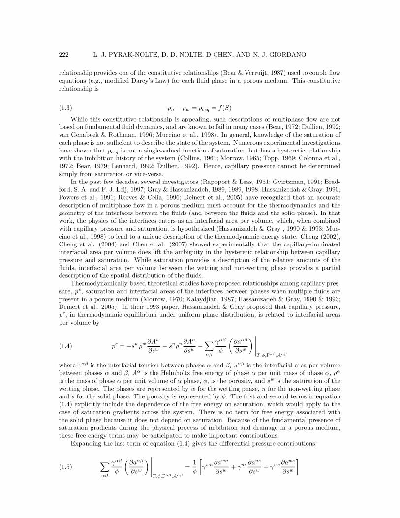
The micro-models used in this investigation were constructed using optical lithography. Apore-structure pattern is transferred under vis-UV illumination from a transparent mask to a photo-sensitive polymer layer called a photoresist. The thickness of the photoresist layer determines thedepth of the flow channels. When a region of the photoresist is exposed to a sufficiently largeintegrated intensity of blue light, a photochemical reaction within the photoresist makes the regionsoluble in a developer solution. The unexposed photoresist is not soluble, so after development thephotoresist layer contains a negative image of the original light pattern. For the micro-models inthis study, we used Shipley photoresist types 1805 and 1827 with their standard developer (Shipley,1982). The micro-models were fabricated with pore networks covering a 600 µm x 600 µm area. Thepore structure for the micro-models was generated using a standard random continuum percolationconstruction (Nolte & Pyrak-Nolte, 1991). Table 2.1 lists the name, the porosity and the depth(aperture) of the flow channels of the two micro-models shown in Figure 1. Model S70 has a 2

224 L. J. PYRAK-NOLTE, D. D. NOLTE, D CHEN, AND N. J. GIORDANO

Sample Name Aperture Porosity Number of Images Analyzed

S70 2.0 µm 62.3% 196

S1dc 1.0 µm 70.3% 411Table 2.1

The name, size, porosity and number of images analyzed of the micro-models used in this study.

(a) S70 - Aperture 2 microns (b) S1dc - Aperture 1 micron

Fig. 1. Digital images of micro-models (a) S70 and (b) S1dc. In the images, nitrogen is white, and photoresist(solid) is dark gray.

micron aperture, while model S1dc has a 1 micron aperture. The entrance pressure between thesetwo micro-models differs by a corresponding factor of two. The two different apertures of 1 micronfor model S1dc and 2 microns for model S70 test for aperture-dependent systematics in the data.

A pressure system was used for introducing two fluid phases into the micro-models. The systemenables the simultaneous measurements of pressure and optical characterization of the geometries ofthe three phases (two fluid, one solid) within the sample. The apparatus contains a pressure sensor(Omega PX5500C1-050GV) to monitor the inlet pressure, and a video camera that is interfaced toan optical microscope to image the two-phase displacement experiments. The outlet is exposed toatmospheric pressure.

To perform a measurement on a micro-model, the micro-model is initially saturated with de-cane, a wetting fluid, which is inserted from the outlet side. A second fluid, nitrogen gas, is thenintroduced from the inlet. The initially decane-saturated micro-models are invaded with nitrogenby the incremental application of pressure. After each pressure increment, the system is allowed toreach mechanical equilibrium (typically 3 to 5 minutes) in which the interfaces are fully stationary,and the inlet pressure is recorded. Then the saturation and distribution of each phase are digitallyimaged by a CCD camera through the microscope. The camera is a Qimaging Retiga EX with an ar-ray of 1360 x 1036 pixels that have a pixel-size 6.45 microns by 6.45 microns with 12-bit digitizationand FireWire (IEEE-1394) transfer. The microscope is an Olympus microscope with a 16x objectiveand is illuminated with a white light source through a red filter. The resulting digital images have apixel resolution of 0.6 microns. All measurements are conducted at room temperature (temperaturestability better than 0.5 degree Celsius during a measurement), with the apparatus located within

CAPILLARY PRESSURE AND INTERFACIAL AREAS 225

Sample Name Xpos, Ypos Min Val Max Val

S70 700, 10 115 255

S1dc 700, 10 75 255Table 3.1

The sample name and IDL parameters used in the SEARCH2D command to analyze the mask for samples S70and S1dc.

a clean-bench environment. Sample S70 was sent through several imbibition and drainage scanningcycles under a total of 196 pressures. Sample S1dc was similarly subjected to scanning cycles under411 different pressures. An image was captured and analyzed for each pressure. An archive of theimages used in this study have been placed on a website for downloading (see Pyrak-Nolte, 2007).

3. Analysis. To determine capillary pressure from either equation (1.1) or equation (1.5)requires the identification of each phase (decane, nitrogen, solid) and all the interfaces betweenthe phases. Image analysis programs are coded in the IDL language to extract phase saturation,interfacial area per volume (IAV), and curvature of the interfaces from each image. In the analysis,each grayscale image is separated into three separate images, i.e., one binary image representingeach phase. The individual phase images are used to determine the saturation of the micro-modelfor each phase. The fraction of the micro-model composed of photoresist (i.e., the solid portion ofthe micro-model where no flow occurs) is constant for all drainage-imbibition cycles. Nitrogen anddecane saturations of the pore space are calculated as a fraction of total pore space.

A mask was used to separate grayscale images into three separate phase images. The mask wasa grayscale image of the micro-model filled only with nitrogen. A two-dimensional search algorithm(command SEARCH2D in IDL) was used to find the connected pore space in the model and todetermine the regions of photoresist. The SEARCH2D command starts at a specified location (Xpos,

Ypos) within the array and finds all data that fall within a specified intensity range (Min Val ≤ data≤ Max Val) and are connected. Table 3.1 list the values of Xpos, Ypos, Min val, and Max Val usedin the analysis of the masks for samples S70 and S1dc. For both S1dc and S70, the DIAGONALkeyword is used to have the algorithm search all surrounding data points that shared commoncorners. This analysis results in the generation of a new mask that is a binary image with regionsrepresenting pore space set equal to one and those regions representing photoresist set equal tozero.

An autocorrelation method was used to align and register the new mask with each image fromthe drainage and imbibition experiments to ensure that the same region of the micro-model isanalyzed for all images After alignment, the grayscale images for each saturation, originally 1520pixels by 1180 pixels, were cropped to 1000 pixels by 1000 pixels. The SEARCH2D algorithmwas then performed on each cropped grayscale image (for each pressure value) to determine theconnected nitrogen phase. The connected nitrogen phase was set to a value of 255 and a new imagewas created. By multiplying the new image by the new mask and searching for all values equalto 255, the phase image for nitrogen is determined. The IDL DILATE command was used on thenitrogen image to algorithmically determine the boundary between nitrogen and the other phasesbecause of optical refraction effects at the interfaces between nitrogen and the other two phases.. A3 x 3 structure array (with all elements equal to 1) was defined and applied to the nitrogen imagethrough the DILATE command. Without this step, the nitrogen phase did not match the originalimage because of an apparent rim around the nitrogen phase caused by the diffraction of light fromthe nitrogen interfaces, or possibly caused by the hidden curvature. The rim around the nitrogenphase can be seen in Figure 2f which is an enlargement of a portion (300 pixels by 300 pixels) ofimage 94 shown in Figure 2a for sample S70.

Using the IDL WHERE command, the location of the photoresist in the mask is determinedand those location in the new image are set equal to zero. The phase image for photoresist is definedas the pixels in the new image equal to zero. Regions not equal to 0 or 255 are then defined to

226 L. J. PYRAK-NOLTE, D. D. NOLTE, D CHEN, AND N. J. GIORDANO

(a) Image (b) Photoresist (c) Decane

(d) Nitrogen (e) Composite (f) Portion of Raw Image

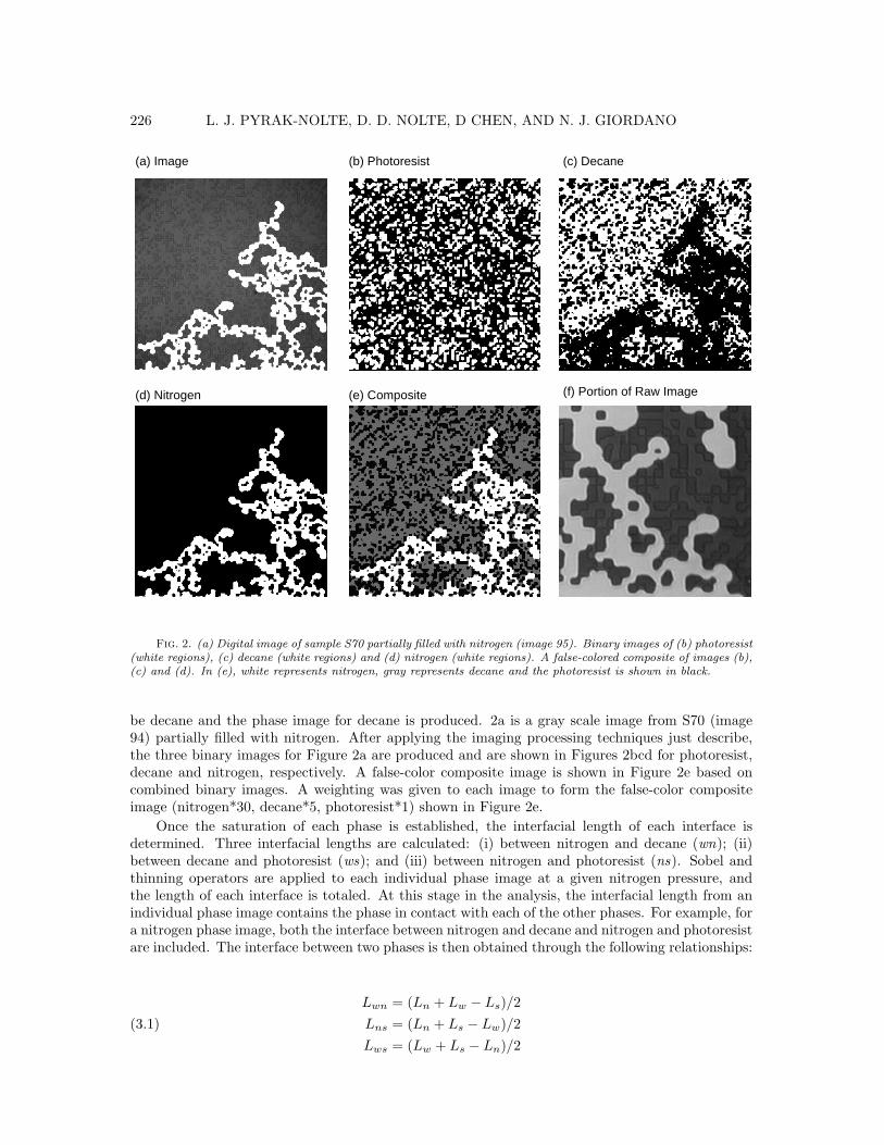
Fig. 2. (a) Digital image of sample S70 partially filled with nitrogen (image 95). Binary images of (b) photoresist(white regions), (c) decane (white regions) and (d) nitrogen (white regions). A false-colored composite of images (b),(c) and (d). In (e), white represents nitrogen, gray represents decane and the photoresist is shown in black.

be decane and the phase image for decane is produced. 2a is a gray scale image from S70 (image94) partially filled with nitrogen. After applying the imaging processing techniques just describe,the three binary images for Figure 2a are produced and are shown in Figures 2bcd for photoresist,decane and nitrogen, respectively. A false-color composite image is shown in Figure 2e based oncombined binary images. A weighting was given to each image to form the false-color compositeimage (nitrogen*30, decane*5, photoresist*1) shown in Figure 2e.

Once the saturation of each phase is established, the interfacial length of each interface isdetermined. Three interfacial lengths are calculated: (i) between nitrogen and decane (wn); (ii)between decane and photoresist (ws); and (iii) between nitrogen and photoresist (ns). Sobel andthinning operators are applied to each individual phase image at a given nitrogen pressure, andthe length of each interface is totaled. At this stage in the analysis, the interfacial length from anindividual phase image contains the phase in contact with each of the other phases. For example, fora nitrogen phase image, both the interface between nitrogen and decane and nitrogen and photoresistare included. The interface between two phases is then obtained through the following relationships:

Lwn = (Ln + Lw − Ls)/2

Lns = (Ln + Ls − Lw)/2(3.1)

Lws = (Lw + Ls − Ln)/2

CAPILLARY PRESSURE AND INTERFACIAL AREAS 227

where is Ln is the total length of the nitrogen interface, and Lw and Ls are the total lengths of thedecane and photoresist interfaces, respectively. Lwn is the length of the interface between nitrogenand decane. Lns is the length of the interface between nitrogen and photoresist. Lws is the lengthof the interface between decane and photoresist. In this study, we calculate interfacial length perarea (ILA) because the hidden curvature associated with the aperture cannot be obtained from thetwo-dimensional image (although we estimate its contributions in equation (3.3) below). Thoughwe calculate ILA, we will refer to it as either interfacial area per volume (IAV) or by the term aαβ ,where α and β give the phases (w for wetting phase, n for non-wetting phase or s for solid) betweenwhich the interface occurs. The interfacial area per volume is found by dividing Lwn by the totalarea of the micro-model (600 microns by 600 microns) giving units of inverse length.

Chen (2006) and Chen et al. (2007) determined the error in IAV and saturation by applyingthe analysis technique to circles of known radii and squares with known perimeters and areas. Forcircles with radii greater than or equal to 4 pixels (2.4 microns), the numerically determined valuesof IAV were less than 10% of that calculated from 2πr. This is caused by the pixelation of thecircle, i.e., a circle made up of small squares. For the same set of circles, the calculated area ofthe circle vs. number of pixels were within 2.5% for circles with radii greater than or equal to 4pixels. For circles with radii between 1 pixel and 4 pixels the error in area and IAV range from-20% to 3%, respectively. For the squares, the relative error between the estimated and the knownperimeter of the squares is the largest (-30% to -10%) when the edge length is less than 4 pixelsbut decreases quickly ( ∼ 5% at 6 pixels) as the perimeter increases. Other methods exist fordetermining interfacial areas (e.g. Dalla et al., Mclure et al, 2006; Prodanovic et al., 2006) thatmight reduce the error, but at this time we chose the simplest analysis method. An archive of theimages used in this study have been placed on a website for downloading so other researchers caninvestigate these issues (see Pyrak-Nolte, 2007).

The error caused by the hidden curvature along the z-axis cannot be measured directly, but canbe estimated based on the known contact angle of decane on photoresist in nitrogen. The total areaof an interface with two principle radii R1 ≪ R2 is given by

(3.2) A = 4R1R2

(π

2− θc

)2

where θc is the contact angle. The relative error in this area, caused by a systematic in the hiddencontact curvature that cannot be measured directly, is

(3.3)∆A

A=

4πR1R2∆θc

π2R1R2

=4

π∆θc

which is independent of the radii. For decane on photoresist in air, the contact angle is θc = 0.08rad. Assuming an error no larger than the contact angle itself (100% change in contact angle), thisleads to a maximum error in the calculated interfacial area of about 13%. This is a worst-case value,and practical values of the error are likely to be smaller. Therefore, the hidden curvature in thetwo-dimensional micro-models is not a large source of error and is no larger than the pixel errors.

We adapted a level set method (Sethian, 1985) to calculate capillary pressure using the curvatureof the interface between the wetting and non-wetting phases from the images. The curvature of aninterface is obtained from the image using

(3.4) K =Φ

2yΦxx − 2ΦxΦyΦxy + Φ

2xΦyy

(

Φ2x + Φ2

y

)3/2

where K is the curvature of the interface, Φi is the derivative of the image with respect to i wherei is either x or y, Φii is the second derivative of the image with respect to ii, where ii can be xx, yy

228 L. J. PYRAK-NOLTE, D. D. NOLTE, D CHEN, AND N. J. GIORDANO

or xy. The derivatives of the two-dimensional images are taken using a kernel method. The kernels(as used in IDL) are defined as

Φx = [−0.5, 0, 0.5]

Φy = transpose[Φx]

Φxx = [1.0,−2.0, 1.0](3.5)

Φyy = transpose[Φxx]

Φxy =

0.25 0 −0.25

0 0 0

0.25 0 −0.25

Because of discontinuities in the image densities, the level-set analysis is performed on the phaseimages convolved with a 19-pixel Gaussian blur of the image. This provides a gray scale or gradientat each interface to allow derivatives to be taken, after which these images are convolved withthe kernel. Once the curvature is computed, a mask of the interface relevant to each phase isapplied. We use the curvature of only the capillary-dominated interfaces to assess the capillarypressure. The MOMENT command in IDL is used to compute the average curvature for an image.The MOMENT command calculates the mean value based on the values of curvature along eachinterface, i.e. only the values for pixels representing the wetting-nonwetting interfaces in an image.The most-probable curvature is calculated from the histogram of curvatures for a single image withthe value of curvature from the peak of the distribution representing the mode of the curvature.

Computation of the normals to the interfaces was also performed. The calculation of the normalsbegins by using the equation:

nx =Φx

√

Φ2x + Φ2

y

(3.6)

ny =Φy

√

Φ2x + Φ2

y

and then applying the convolution

nxx = Image ∗ nxnx

nyy = Image ∗ nyny(3.7)

nxy = Image ∗ nxny

where nxx, nyy and nxy are the normals to the interfaces, and “image” refers to the two-dimensionalimage of the interface between two phases.

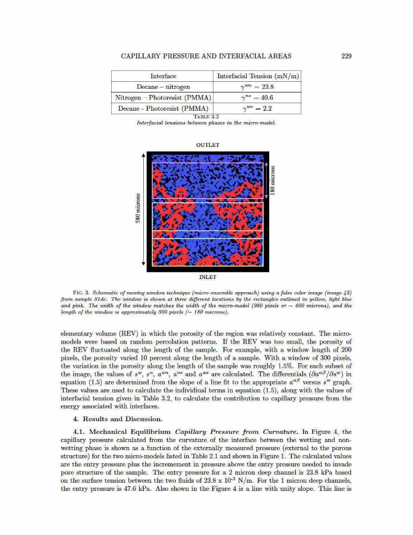
Equation (1.5) requires the calculation of the differential of the interfacial area with respect tosaturation at constant energy. In laboratory experiments, it is difficult to ensure that the condition ofconstant energy is met. In the micro-model experiments, each image is in mechanical equilibrium ata constant pressure, but different images with the same measured capillary pressure, but differentsaturations, do not have equal free energy because of the hysteresis in the pc – sw relationship.Therefore, the three partial derivatives in equation (1.5) must be evaluated from a single image ofthe micro-model at a given pc. To accomplish this, we used a “micro-ensemble” approach (Figure3), in which values of sw and awn are calculated from a single image based on subsets of the image.A window 980 pixels wide by 300 pixels in length is moved in 1 pixel increments from the inlet tothe outlet of the sample (a distance of 680 pixels out of 980 pixels). We choose a representative

230 L. J. PYRAK-NOLTE, D. D. NOLTE, D CHEN, AND N. J. GIORDANO

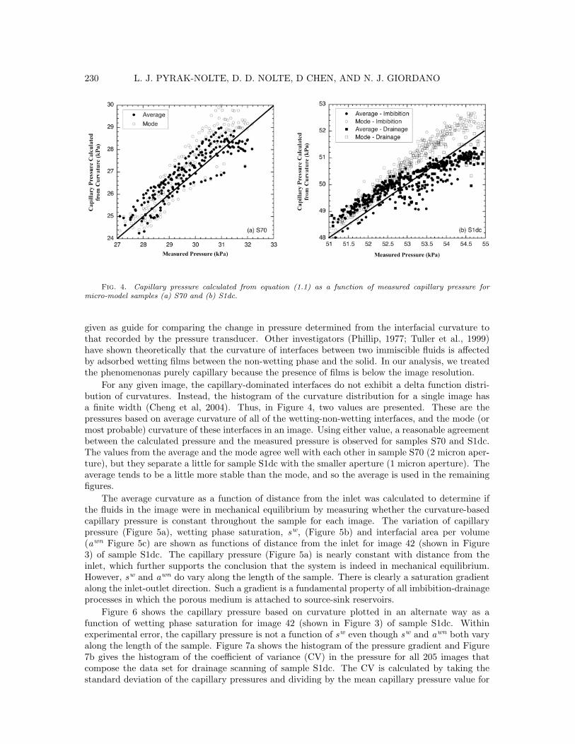
Fig. 4. Capillary pressure calculated from equation (1.1) as a function of measured capillary pressure formicro-model samples (a) S70 and (b) S1dc.

given as guide for comparing the change in pressure determined from the interfacial curvature tothat recorded by the pressure transducer. Other investigators (Phillip, 1977; Tuller et al., 1999)have shown theoretically that the curvature of interfaces between two immiscible fluids is affectedby adsorbed wetting films between the non-wetting phase and the solid. In our analysis, we treatedthe phenomenonas purely capillary because the presence of films is below the image resolution.

For any given image, the capillary-dominated interfaces do not exhibit a delta function distri-bution of curvatures. Instead, the histogram of the curvature distribution for a single image hasa finite width (Cheng et al, 2004). Thus, in Figure 4, two values are presented. These are thepressures based on average curvature of all of the wetting-non-wetting interfaces, and the mode (ormost probable) curvature of these interfaces in an image. Using either value, a reasonable agreementbetween the calculated pressure and the measured pressure is observed for samples S70 and S1dc.The values from the average and the mode agree well with each other in sample S70 (2 micron aper-ture), but they separate a little for sample S1dc with the smaller aperture (1 micron aperture). Theaverage tends to be a little more stable than the mode, and so the average is used in the remainingfigures.

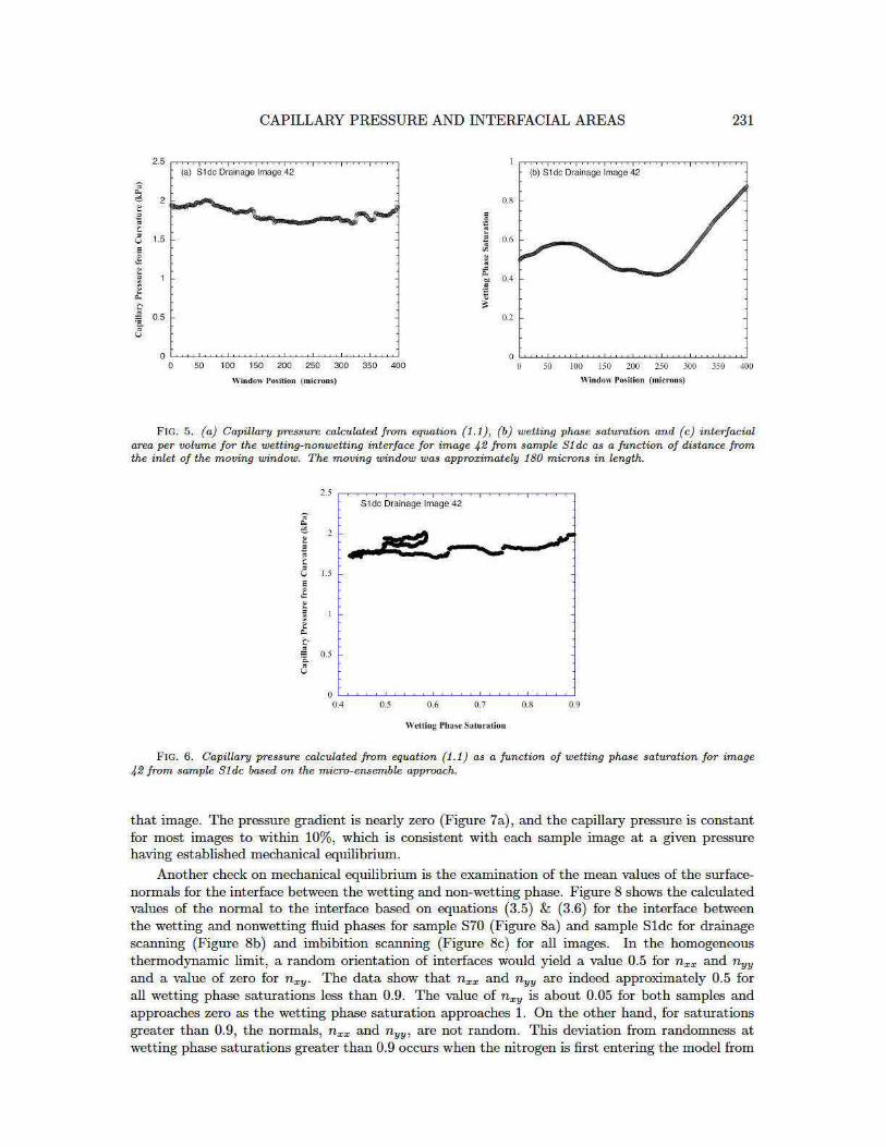
The average curvature as a function of distance from the inlet was calculated to determine ifthe fluids in the image were in mechanical equilibrium by measuring whether the curvature-basedcapillary pressure is constant throughout the sample for each image. The variation of capillarypressure (Figure 5a), wetting phase saturation, sw, (Figure 5b) and interfacial area per volume(awn Figure 5c) are shown as functions of distance from the inlet for image 42 (shown in Figure3) of sample S1dc. The capillary pressure (Figure 5a) is nearly constant with distance from theinlet, which further supports the conclusion that the system is indeed in mechanical equilibrium.However, sw and awn do vary along the length of the sample. There is clearly a saturation gradientalong the inlet-outlet direction. Such a gradient is a fundamental property of all imbibition-drainageprocesses in which the porous medium is attached to source-sink reservoirs.

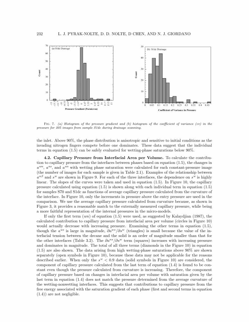
Figure 6 shows the capillary pressure based on curvature plotted in an alternate way as afunction of wetting phase saturation for image 42 (shown in Figure 3) of sample S1dc. Withinexperimental error, the capillary pressure is not a function of sw even though sw and awn both varyalong the length of the sample. Figure 7a shows the histogram of the pressure gradient and Figure7b gives the histogram of the coefficient of variance (CV) in the pressure for all 205 images thatcompose the data set for drainage scanning of sample S1dc. The CV is calculated by taking thestandard deviation of the capillary pressures and dividing by the mean capillary pressure value for

232 L. J. PYRAK-NOLTE, D. D. NOLTE, D CHEN, AND N. J. GIORDANO

Fig. 7. (a) Histogram of the pressure gradient and (b) histogram of the coefficient of variance (cv) in thepressure for 205 images from sample S1dc during drainage scanning.

the inlet. Above 90%, the phase distribution is anisotropic and sensitive to initial conditions as theinvading nitrogen fingers compete before one dominates. These data suggest that the individualterms in equation (1.5) can be safely evaluated for wetting-phase saturations below 90%.

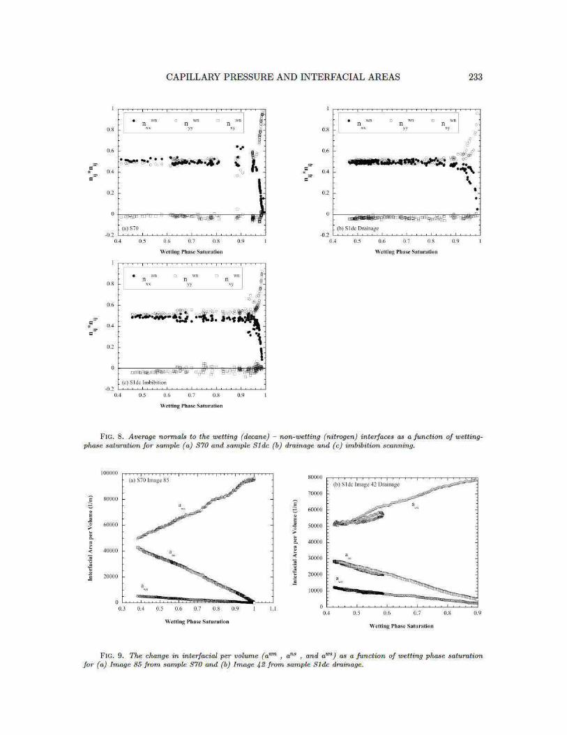
4.2. Capillary Pressure from Interfacial Area per Volume. To calculate the contribu-tion to capillary pressure from the interfaces between phases based on equation (1.5), the changes inawn, ans, and aws with wetting phase saturation were calculated for each constant-pressure image(the number of images for each sample is given in Table 2.1). Examples of the relationship betweenaαβ and sw are shown in Figure 9. For each of the three interfaces, the dependence on sw is highlylinear. The slopes of the curves were taken and used in equation (1.5). In Figure 10, the capillarypressure calculated using equation (1.5) is shown along with each individual term in equation (1.5)for samples S70 and S1dc as functions of average capillary pressure calculated from the curvature ofthe interface. In Figure 10, only the increments in pressure above the entry pressure are used in thecomparison. We use the average capillary pressure calculated from curvature because, as shown inFigure 3, it provides a reasonable match to the externally measured capillary pressure, while beinga more faithful representation of the internal pressures in the micro-models.

If only the first term (wn) of equation (1.5) were used, as suggested by Kalaydjian (1987), thecalculated contribution to capillary pressure from interfacial area per volume (circles in Figure 10)would actually decrease with increasing pressure. Examining the other terms in equation (1.5),though the aws is large in magnitude, ∂aws/∂sw (triangles) is small because the value of the in-terfacial tension between the decane and the solid is an order of magnitude smaller than that forthe other interfaces (Table 3.2). The ∂ans/∂sw term (squares) increases with increasing pressureand dominates in magnitude. The total of all three terms (diamonds in the Figure 10) in equation(1.5) are also shown. The data arising from high wetting-phase saturations above 90% are shownseparately (open symbols in Figure 10), because these data may not be applicable for the reasonsdescribed earlier. When only the sw < 0.9 data (solid symbols in Figure 10) are considered, thecomponent of capillary pressure calculated from the last term of equation (1.4) is found to be con-stant even though the pressure calculated from curvature is increasing. Therefore, the componentof capillary pressure based on changes in interfacial area per volume with saturation given by thelast term in equation (1.4) does not match the pressure determined from the average curvature ofthe wetting-nonwetting interfaces. This suggests that contributions to capillary pressure from thefree energy associated with the saturation gradient of each phase (first and second terms in equation(1.4)) are not negligible.

234 L. J. PYRAK-NOLTE, D. D. NOLTE, D CHEN, AND N. J. GIORDANO

Fig. 10. The capillary pressure based on equation (1.5) as a function of capillary pressure determined fromcurvature for samples (a) S70 and (b) S1dc from drainage scans. Shown in the graphs are the contributions from eachterm in equation (1.5) indicated by the interface (WN: wetting -nonwetting interface, WS: wetting -solid interface,NS: nonwetting-solid interface). The total represents the sum of all of the terms divided by the porosity as given byequation (1.5). The open symbols present the value of the term for wetting-phase saturations greater than ninetypercent.

4.3. Saturation Gradients. From the data showing the uniform curvature distributions andphase isotropy for each image, combined with the interface stability (they are not moving), we con-clude that the micromodels at each pressure are in mechanical equilibrium, However, from Figures5 (a) & (b), it is clear that the phase distribution is not homogenous either in terms of amount(sw) or distribution (awn) at a given pressure. These saturation gradients likely cause the contri-butions from the first two terms of equation (1.4) to dominate the calculation of capillary pressure,thereby producing the difference between the curvature-based pressure of equation (1.1) and theterms associated with the interfaces in equation (1.5).

From our data set, we cannot obtain all parameters used to determine contributions to capillarypressure from the change in Helmholtz free energy of a phase with saturation as given by equation(1.4). But we can plot the difference between equation (1.1) and equation (1.5) to obtain a residualcontribution to the capillary pressure that is a consequence of the saturation gradient. This differenceis shown in Fig. 11 as a function of the curvature-based capillary pressure. We identify this differenceas the saturation gradient contribution, and tentatively assign it to the explicit free-energy terms inequation (1.4). The free energy contribution takes on negative values at low pressure, and decreasesin magnitude toward zero under higher pressures. At pressures approaching breakthrough, the free-energy contribution vanishes. It is interesting to note that the phase distribution across the sampleis most nearly homogeneous just prior to breakthrough. This observation lends plausibility to theinterpretation of the free-energy contribution arising from the saturation gradient.

5. Conclusions. We have performed an experimental study using transparent two-dimensionalmicromodels that enable the visualization of interfacial areas during imbibition and drainage. Thesedata provide a direct means to compare experimentally-measured capillary pressure, determined ei-ther by local curvature or by external pressure measurements, to thermodynamic expressions involv-ing the differential change of interfacial areas, also measured experimentally, relative to changingsaturation. The mechanical equilibrium of the system is verified using several different measures,including the establishment of stationary phase fronts prior to data acquisition, the existence ofnear-zero pressure gradients across the sample for a given applied external pressure, the agreementbetween the pressure calculated from curvature and the pressure measured externally, and the van-

236 L. J. PYRAK-NOLTE, D. D. NOLTE, D CHEN, AND N. J. GIORDANO

duction, water wells, the study of cores in the laboratory, and micromodel experiments. In all theseexamples, the invading phase enters the micro-model from an inlet port attached to a reservoirand drains into an outlet reservoir. The inlet reservoir is a part of the equilibrium system, andthe porous medium cannot be isolated from it as a closed system. This situation is fundamentallydifferent than equilibrium bulk phase distributions in closed systems, in which pores of appropriateapertures are occupied homogeneously. Therefore, imbibition and drainage represent a class of openphysical processes which are inhomogeneous because of the communication of the porous mediumwith the reservoirs that impose inlet-outlet asymmetry on the system.

In conclusion, two-dimensional micromodels provide valuable experimental insight into the re-lationships among capillary pressure and the phase interfaces within a porous medium. In thesesystems, mechanical equilibrium is established easily and verified experimentally. The presenceof a saturation gradient at each applied pressure is likely a fundamental aspect of imbibition anddrainage for systems in close communication with a reservoir. Future experimental studies needto move into three dimensions to establish whether these results are a consequence of the lowereddimensionality, or are fundamental to systems of any dimensionality.

Acknowledgments. The authors wish to acknowledge Rossman Giese for the calculation ofinterfacial tension values used in this paper. This material is based upon work supported by theNational Science Foundation under Grant No. 0509759.

REFERENCES

[1] Annable, M.D., Jawitz, J.W., Rao, P.S.C., Dai, D.P., Kim, H., Wood, A.L., Field evaluation of interfacialand partitioning tracers for characterization of effective NAPL-water contact areas. Ground Water, 36(3):p. 495-503, 1998.

[2] Anwar, A.H.M.F., Bettahar, M., Matsubayashi, U., A method for determining ar-water interfacial area invariably saturated porous media. Journal of Contaminant Hydrology, 43: 129-146, 2000.

[3] Barnes, G. T. and I. R. Gentle, Interfacial Science, Oxford University Press, Oxford, 2005.[4] Bear, J., Dynamics of Fluids in Porous Media, Mineola, New York: Dover, 1972.[5] Bear, J., Hydraulics of Groundwater, New York, McGraw-Hill, 1979.[6] Bear, J. and A. Verruijt, Modeling Groundwater Flow and Pollution, Dordrecht, The Netherlands, D. Reidel

Pub. Co., 1987.[7] Bradford, S.A., and F. J. Leij, Estimating interfacial areas for multi-fluid soil systems. Journal of Contam-

inant Hydrology, 27:83-105, 1997.[8] Chen, D., Experimental investigation of interfacial geometry associated with multiphase flow within a porous

medium, Ph.D. Thesis, Department of Earth and Atmospheric Sciences, Purdue University, West Lafayette,Indiana, 2006.

[9] Chen, D., Pyrak-Nolte, L. J., Griffin, J. and N. J. Giordano, Measurement of interfacial area per volumefor drainage and imbibition, accepted for publication in Water Resources Research, 2007.

[10] Chen, L. and T. C. G. Kibbey, Measurement of air-water interfacial area for multiple hysteretic drainagecurves in an unsaturated fine sand, Langmuir, 22, 6874-6880, 2006.

[11] Cheng, J., Fluid flow in ultra-small structures, Ph.D. Thesis, Department of Physics, Purdue University, WestLafayette, Indiana, 2002.

[12] Cheng J.-T., Pyrak-Nolte, L. J., Nolte, D. D. and N. J. Giordano, Linking pressure and saturation throughinterfacial areas in porous media, Geophys. Res. Let., 31, L08502, doi:10.1029/2003GL019282, 2004.

[13] Collins, R. E., Flow of Fluids through Porous Materials, New York, Reinhold Pub. Corp., 1961.[14] Colonna, J., Brissaud, F. and Millet, J.L., Evolution of capillary and relative permeability hysteresis. Soc.

Pet. Eng. J., 12: 28-38, 1972.[15] Costanza-Robinson, M.S., and M. L. Brusseau, Air-water interfacial areas in unsaturated soils: Evaluation

of interfacial domains. Water Resources Research, 2002. 38(10): p. 1195 doi: 10.1029/2001WR000738,2002.

[16] Culligan, K.A., D. Wildenschild, B.S.B. Christensen, W.G. Gray, and M.L. Rivers, Pore-scale char-acteristics of multiphase flow in porous media: A synchrotron-based CMT comparison of air-water andoil-water experiments, Advances in Water Resources. 29(2), 227-238, 2006.

[17] Culligan, K.A., D. Wildenschild, B.S.B. Christensen, W.G. Gray, A.F.B. Tompson, Interfacial areameasurements for unsaturated flow through a porous medium. Water Resources Research. 40(12), Art. No.W12413, Dec 22, 2004.

[18] Dalla, E., Hilpert , M. and C. T. Miller, Computation of the interfacial area for two-fluid porous mediumsystems, Journal of Contaminant Hydrology 56, 25– 48, 2002.

CAPILLARY PRESSURE AND INTERFACIAL AREAS 237

[19] Deinert, M.R., Parlange, J.-Y. and K. B. Cady, Simplified thermodynamic model for equilibrium capillarypressure in a fractal porous medium, Physical Review E, 041203, 2005.

[20] Dullien, F. A. L., Porous Media: Fluid Transport and Pore Structure, 2nd Edition, Academic Press, 1992.[21] Giordano, N. and J.T. Cheng, Microfluid mechanics: progress and opportunities. Journal of Physics-

Condensed Matter, 13(15): p. R271-R295, 2001.[22] Gray, W.G. and S.M. Hassanizadeh, Averaging theorems and averaged equations for transport of interface

properties in multiphase systems. International Journal of Multiphase Flow, 15(1): p. 81-95, 1989.[23] Gray, W.G. and S.M. Hassanizadeh, Unsaturated flow theory including interfacial phenomena. Water Re-

sources Research, 27(8): p. 1855-1863, 1991.[24] Gray, W.G. and S.M. Hassanizadeh, Macroscale continuum mechanics for multiphase porous-media flow

including phases, interfaces, common lines and common points. Advances in Water Resources, 21(4): p.261-281, 1998.

[25] Gray, W. G, Tompson, A. F.B. and W. E. Soll, Closure conditions for two-fluid flow in porous media,Transport in Porous Media, 47:29-65, 2002.

[26] Gray, W. G. and C. T. Miller, Thermodynamically constrained averaging theory approach for moeling flowand transport phenomena in porous media systems: 3. Single-fluid-phase flow, Advances in Water Re-sources, 29:1745-1765, 2006.

[27] Gvirtzman, H. and Roberts, P.V., Pore-scale spatial analysis of two immiscible fluids in porous media. WaterResources Research, 27: 1165-1176, 1991.

[28] Hassanizadeh, S.M. and W.G. Gray, Mechanics and thermodynamics of multiphase flow in porous-mediaincluding interphase boundaries, Advances in Water Resources, 13(4): 169-186, 1990.

[29] Hassanizadeh, S.M. and W.G. Gray, Thermodynamic basis of capillary pressure in porous media, WaterResources Research, 29(10), 3389-3405, 1993.

[30] Hassanizadeh, S.M. , Celia, M. A. and H. K. Dahle, Dynamic effect in the capillary pressure–saturationrelationship and its impacts on unsaturated flow, Vadose Zone Journal 1:38–57, 2002.

[31] Held, R. J. and M. A. Celia, Modeling support of functional relationships between capillary pressure, satura-tion, interfacial area and common lines, Advances in Water Resources, 24, p325-343, 2001.

[32] Ioannidis, M. A., Chatzis, I. and A. C. Payatakes, A mercury porosimeter for investigating capillary phe-nomena and microdisplacement mechanisms in capillary networks, Journal of Colloid and Interface Science,vol. 143(1):22-36, 1991.

[33] Kalaydjian, F. A., A macroscopic description of multiphase flow involving space-time evolution of fluid/fluidinterfaces, Transport in Porous Media, 537-552, 1987.

[34] Kim, H., Rao, P.S.C., Annable, M.D., Consistency of the interfacial tracer technique: experimental evalua-tion. Journal of Contaminant Hydrology, 40:79-94, 1999a.

[35] Kim, H., Rao, P.S.C., Annable, M.D., 1999b, Gaseous tracer technique for estimating air-water interfacialareas and interface mobility, Soil Sci. Soc. Am. J. 63:1554–1560, 199b.

[36] Lenhard, R. J., Measurement and modeling of three-phase saturation-pressure hysteresis, Journal of Contam-inant Hydrology, 9, 243-269, 1992.

[37] McClure J.E., Adalsteinsson, D., Pan C, Gray, W.G. and C.T. Miller, Approximation of interfacialproperties in multiphase porous medium systems, Advances in Water Resources 30, 354–365, 2007.

[38] Montemagno, C.D. and W.G. Gray, Photoluminescent volumetric imaging - a technique for the explorationof multiphase flow and transport in porous-media. Geophysical Research Letters, 22(4):425-428, 1995.

[39] Morrow, N. R., Physics and thermodynamics of capillary action in porous media, in Flow through PorousMedia, American Chemical Society, Washington, D. C. , 104-128, 1970.

[40] Muccino, J.C., W.G. Gray, and L.A. Ferrand, Toward an improved understanding of multiphase flow inporous media. Reviews of Geophysics, 36(3):401-422, 1998.

[41] Nolte, D.D. and L.J. Pyrak-Nolte, Stratified Continuum Percolation - Scaling Geometry of HierarchicalCascades. Physical Review A, 44(10):6320-6333, 1991.

[42] Philip, J. R., Unitary approach to capillary condensation and adsorption, J. Chem. Phys., 66(11), 5069-5075,1977

[43] Powers, S.E., Loureiro, C. O., Abriola, L. M. and W.. J. Weber, Jr., Theoretical study of the significanceof nonequilibrium dissolution of nonaqueous phase liquids in subsurface systems. Water Resources Research,27(4): p. 463-477, 1991.

[44] Prodanovic, M., W.B. Lindquist , and R.S. Seright, Porous structure and fluid partitioning in polyethylenecores from 3D X-ray microtomographic imaging, Journal of Colloid and Interface Science 298, 282–297,2006.

[45] Pyrak-Nolte, L. J., Giordano, N. J. and D. D. Nolte, Experimental investigation of relative permeabiliyupscaling from the Micro-scale to the macro-scale, Final Report , DOE Award: DE-AC26-99BC15207,OSTI ID: 833410, DOI 10.2172/833410, 2004.

[46] Pyrak-Nolte, L. J., 2007, URL of website with original data: http://www.physics.purdue.edu/rockphys/DataImages/

[47] Rao, P.S.C., Annable, M.D., Kim, H., NAPL source zone characterization and remediation technology per-formance assessment: recent developments and applications of tracer techniques. Journal of ContaminantHydrology, 45: p. 63-78, 2000.

[48] Rapoport, L.A., and W. J. Leas, Relative permeability to liquid in liquid-gas systems. Petroleum Transaction.

238 L. J. PYRAK-NOLTE, D. D. NOLTE, D CHEN, AND N. J. GIORDANO

192: p. 83-98, 1951.[49] Reeves, P. C. and M. A. Celia, A functional relationship between capillary pressure, saturation, and in-

terfacial area as revealed by a pore-scale network model, Water Resources Research, vol. 32, no. 8, pages2345-2358, 1996.

[50] Saripalli, K.P., Kim, H., Rao, P.S.C., Annable, M.D., Measurement of specific fluid-fluid interfacial areasof immiscible fluids in porous media. Environmental Science and Technology, 31(3): p. 932-926, 1997.

[51] Schaefer, C.E., DiCarolo, D.A., Blunt, M.J., Determination of water-oil interfacial area during 3-phasegravity drainage in porous media. Journal of Colloid and Interface Science, 221: p. 308-312, 2000.

[52] Shipley Microelectronic Product Guide, Shipley Co., Newton, MA, 1982.[53] Sethian, J. A., Curvature and the evolution of fronts, Communications of Mathematical Physics, 101, 4,

487-499, 1985.[54] Thompson, L.F., C.G. Willson, and M.J. Bowden, Introduction to Microlithography, 2nd edition, American

Chemical Society, Washington, DC, 1994.[55] Topp, G.C., Soil-water hysteresis measured in a sandy loam and compared with the hysteretic domain model.

Soil Sci. Soc. Am. Proc., 33: 645-651, 1969.[56] Tuller, M., Or, D. and L. M. Dudley, Adsorption and capillary condensation in porous media: Liquid

retention and interfacial configurations in angular porous media, Water Resources Research, vol 35, no. 7,pages 1949-1964, July 1999.

[57] van Genabeek, O., and D. H. Rothman, Macroscopic manifestations of microscopic flows through porousmedia: Phenomenology from simulation. Annual Review of Earth and Planetary Sciences, 24: p. 63-87,1996.

[58] Wilkinson, D., Percolation effects in immiscible displacement, Physical Review A., vol. 34, no. 2, p1380-1391,1986.